Identiﬁcation of Regeneration Times in MCMC … · · 2010-04-13Identiﬁcation of Regeneration...

Identification of Regeneration Times in MCMC Simulation, withApplication to Adaptive Schemes

Anthony E. Brockwell and Joseph B. Kadane

December 13, 2002

Abstract

Regeneration is a useful tool in Markov chain Monte Carlo simulation, since it can be used toside-step the burn-in problem and to construct better estimates of the variance of parameter estimatesthemselves. It also provides a simple way to introduce adaptive behaviour into a Markov chain, andto use parallel processors to build a single chain. Regeneration is often difficult to take advantage of,since for most chains, no recurrent proper atom exists, and it is not always easy to use Nummelin’ssplitting method to identify regeneration times. This paper describes a constructive method for gen-erating a Markov chain with a specified target distribution and identifying regeneration times. As aspecial case of the method, an algorithm which can be “wrapped” around an existing Markov transi-tion kernel is given. In addition, a specific rule for adapting the transition kernel at regeneration timesis introduced, which gradually replaces the original transition kernel with an independence-samplingMetropolis-Hastings kernel using a mixture normal approximation to the target density as its proposaldensity. Computational gains for the regenerative adaptive algorithm are demonstrated in examples.

Keywords: regenerative simulation, adaptive Markov chain Monte Carlo, splitting, atoms, burn-in, mix-ture approximations, parallel processing

1 Introduction

Markov chain Monte Carlo (MCMC) methods have become popular in the last decade as a tool forexploring properties of distributions which are known only up to a constant of proportionality. The basicidea is to construct an ergodic Markov chain whose limiting distribution is the same as the distributionof interest � (called the target distribution). Further details, as well as information about various aspectsof implementation, are given in a variety of sources, including Tierney (1994), Gilks et al. (1996), andRobert and Casella (1999). Development of the underlying probabilistic theory of Markov chains takingvalues in a general state-space can be found in Revuz (1975), Nummelin (1984), and Meyn and Tweedie(1993).

There are several important problems associated with standard methods of constructing Markov chains forMonte Carlo simulation. The first is a convergence problem, sometimes known as the “burn-in problem”.One does not generally know how long it takes before the chain is (by some measure) sufficiently close

1

to its limiting distribution. A standard approach to dealing with this is simply to discard some initialportion of the chain, labelling it as a “burn-in” component of the chain. However, without the ability tostart the chain with a “perfect sample” from the target distribution, the problem, although reduced, stillremains. A second problem is the inherent correlation between successive elements of the chain, whichmakes it difficult to estimate the variance of the Monte Carlo estimates. One widely-adopted method forestimating this variance is the batch-means method, which relies on division of the Markov chain intoequal-length segments, but as pointed out by Glynn and Iglehart (1990), batch-means estimates are notconsistent for the true normalized variance. A related problem is that that the chain might “mix” poorly.Even if the chain starts in exactly the limiting distribution, it may take a long time for the chain to exploreall interesting parts of the state-space, particularly when the correlation between successive elements ofthe chain is high. A fourth problem is the simple computational burden required to carry out MCMCsimulation. Errors in integrals approximated by MCMC simulation are approximately proportional to theinverse of the square root of the length of the chain. These are an order of magnitude larger than errors inother standard methods for numerical integration, and hence Markov chains need to be relatively long togive accurate estimates of integrals.

Regenerative simulation provides a means of dealing with all of these problems. As discussed in Craneand Iglehart (1975a), Crane and Iglehart (1975b), Crane and Lemoine (1977), Ripley (1987), and morerecently in Mykland et al. (1995), Jones and Hobert (2001),and Robert and Casella (1999), regenerativesimulation can be used to avoid the burn-in problem and to get consistent estimates of the variance ofestimators themselves. Gilks et al. (1998) show how regeneration can be used to introduce so-called“adaptive” schemes into MCMC simulation. These schemes allow parameters of the transition kernel tobe modified as the chain is being generated, to improve mixing properties. Mykland et al. (1995) hintat the possibility of using regeneration to “parallelize” generation of a Markov chain. Constructing aMarkov chain on parallel processors can give dramatic improvements in speed. (See, e.g. Geyer, 1992,for discussion of the relative merits of constructing a single long chain rather than multiple short chains.)

Loosely speaking, a regenerative process “starts again” probabilistically at each of a set of random stop-ping times, called regeneration times. If regeneration times can be identified in an ergodic Markov chain,then tours of the chain between these times are (on an appropriate probability space) independent andidentically distributed (i.i.d.) entities. Thus if a fixed number of tours is generated for the purpose ofMCMC simulation (this is typically done by starting the chain in its regenerative state and stopping it at aregeneration time), it makes no sense to discard any initial tours, or indeed, any part of the first tour, sinceproperties of the “clipped” tour would be different from properties of the other un-clipped tours. In thissense, the problem of burn-in is avoided. In addition, since the tours are i.i.d, when estimating the expec-tation of an arbitrary function of a parameter, the variance of the estimator itself can easily be estimated,and furthermore, there is no need for the tours to be generated on a single processor - they can be gener-ated separately on different processors and then “patched together” in any order which doesn’t depend onthe contents of the tours themselves. Once a mechanism for generating tours is in place, results of Gilkset al. (1998) establish that parameters (which could be, for instance, variances of proposal distributionsused in a Metropolis-Hastings chain) can be modified at each regeneration time, without disrupting con-sistency of MCMC estimators. This procedure, carried out carefully, can significantly improve mixing ofthe chain.

Although every ergodic Markov chain is regenerative (this follows from Theorem 5.2.3 of Meyn andTweedie, 1993), identification of regeneration times in a Markov chain is generally a difficult problem(unless the chain takes values in a finite state-space). Mykland et al. (1995) give an ingenious method,

2

based on the splitting technique of Nummelin (1978) for identifying regeneration times in a large classof Markov chains (including chains generated by the standard algorithms for MCMC simulation). Theirmethod relies on establishing a so-called “minorization condition”, which is essentially a decompositionof the transition kernel of the chain into two components, one of which does not depend on the currentstate of the chain.

In this paper, we present an alternative way of identifying regeneration times, which relies on constructinga Markov chain on an enlarged state-space, and does not require checking of minorization conditions oranalysis of the transition kernel of the chain. The procedure is to modify the initial target distribution �

by mixing it with a point mass concentrated on an “artificial atom” � which is outside the state-space�

.It is then a straightforward matter (for instance, using the Metropolis-Hastings Algorithm) to construct aMarkov chain with the new target distribution. For this chain, the state � is Harris-recurrent (i.e. withprobability one, it occurs infinitely many times). By the Markov property, the times at which the newchain hits � are regeneration times. On the face of it, this might not seem particularly useful, since thenew chain doesn’t have the desired target distribution. However, to recover an ergodic chain with limitingdistribution � , it is sufficient simply to delete every occurrence of the state � from the new chain. Thepoints immediately after the (deleted) occurrences of the state � are then regeneration times in a Markovchain with limiting distribution � . This makes identification of regeneration times trivial. Møller andNicholls (2001) use a generalized form of this mixed target distribution for purposes of perfect-sampling.They do not, however address applications in regenerative simulation or parallel processing.

In addition to presenting this “constructive” method for identification of regeneration times, we describehow an existing transition kernel can be embedded into a new kernel for which identification of regen-eration times is trivial. This is described in terms of our state-space augmentation approach, but theembedding can also be thought of as effectively adding an independence-sampler in between each appli-cation of the original kernel (Mykland et al., 1995, also advocate this idea at the end of their Section 4),and provides a simple way to make the transition from standard to regenerative MCMC simulation. Wealso describe an easily-implemented adaptive algorithm which progressively replaces an original kernel,with an independence sampler for which the proposal distribution is constructed as a crude mixture ap-proximation to the target distribution. In terms of mixing, the adaptive algorithm typically outperformsnon-adaptive algorithms, and also represents a refinement of some of the adaptive techniques describedin Gilks et al. (1998). This idea is also quite similar to that used by Chauveau and Vandekerkhove (2002),but avoids problems associated with construction of a histogram to represent a current approximation tothe target distribution.

Section 2 introduces our method for constructing a regenerative chain. Section 3 gives more explicitdetails on how it can be used for purposes of regenerative and adaptive simulation. A potentially adaptivealgorithm is given for estimating the expectation of a function of an unknown parameter as well as thevariance of the estimator itself, and a specific adaptation mechanism is described. In Section 4, we presentexamples of application of the method. Theoretical results are given in Appendix A.

3

2 The Method

We propose the following method for constructing a Markov chain and identifying regeneration times.

The main idea is to enlarge the state-space from�

to��

��where � is a new state called the artificial atom. Then it is possible (as described in Subsection 3.2) toconstruct a Markov chain �� with �� and with limiting distribution

�� "!$# � � �&%(' # � �"!*) � #,+ ' -�. � � # � (1)

defined on appropriate subsets ! of� �

, where ' is some constant in the interval � � �� # . The new limitingdistribution � �� is a mixture distribution which assigns mass ' to the new state � and mass � �&%/' # to theoriginal distribution � .

Next let 0�1 �324# � 2 � ��5� denote the 2 th time after time zero that the chain �,�6� hits the state � , with0 1 � � # ��

, so that

0�1 �324# ��798;: �5<(=>0�1 �32 %>� #@? �A � �B�C� 2 � ��D�� (2)

and define the tours FE��G�H�� to be the segments of the chain between the hitting times, that is

JI � � � �K0�1 �32 %*� #ML �@N*0�1 �324# �C� 2 � ��O� (3)

Once the Markov chain ��6� has been generated, the next step is to recover a regenerative chain withlimiting distribution � . This can be done quite simply. Define the chain �OPM� �Q� �R� �� to beexactly the chain ��6� , with every occurrence of the state � removed. Noting that the state � occursexactly once at the end of each tour I , �OPS�6� can be constructed by stringing together the tours I whoselength is larger than one, after removing the last element (which is equal to � ) from each one. Tours P Iof �OPT�6� are then defined by their correspondence to the truncated tours of ��U� . We denote by V I the timeat which the �32W+ � # th tour of �OP��6� begins, for 2 �X� �� (with the convention that V�� is equal tozero), so we can then write the tour lengths as Y I

� V I %ZV I�[ E � 2� ��O�

The following result, proved in Appendix A, establishes the validity of this procedure.

Theorem 2.1 Suppose that �� @� �\� ��]� is an ergodic Markov chain taking values in� �

with � �

� and limiting distribution � �� given by (1). Let the process �OP��6� be constructed from ��6� inthe manner described above. Then �OP�� is an ergodic Markov chain taking values in

�with limiting

distribution � . Furthermore, the times V I � 2�^� �� are regeneration times for the chain. In other

words, the Markov chains �OP�� [`_5a �S�� V�bU�6V�b + ��]�C�Sc�d �

are identically distributed, and given anyV�b and non-negative integers e and � , P@f and PS� are independent if e L Vgb L � .

3 Simulation Algorithms

In this section, we briefly review the technique of estimation using regenerative simulation, as discussedin Crane and Lemoine (1977) and, more recently, by others. We also explicitly state regenerative and

4

adaptive MCMC simulation algorithms based on the construction we have introduced.

3.1 Estimating Functionals of the Target Distribution

One is often interested primarily in estimating

�� # � ��g#

for some integrable function�? �� Let tours P I , tour lengths Y I , and cumulative tour lengths V I

of the Markov chain �OP � � with limiting distribution � be as defined in the previous section. Also let

�I� _�� [ E�� _��

�� PS� # � (4)

and assume that�I and Y I have finite variances. Then by the strong law of large numbers, the ratio

estimator ��W�� I � E � I� �I � E Y I

�� I � E � IV I

(5)

converges almost surely to �� , and it follows from the central limit theorem that ! � ��"� % �#� # convergesto a N � � �%$gH # distribution.

One way of estimating $ H is as follows. Let & I �'�I % �� Y I , so that �(& I � is an i.i.d. sequence of random

variables, and define )& �9� ! [ E � �I � E & I , )Y � � ! [ E � �

I � E Y I , and *,+ �'- Y E . Then- � ! � �� % �#� # H # � ! - � )& �/. )Y � # H (6)0 ! - � )& �/. *1+ # H� �* H + Var � & E # 0 �$ H� �

where �$ H� � ! [ E � �I � E � � I %

��"� Y I # H)Y H � (7)

When��2 # is a vector-valued function, we estimate the covariance matrix of ! � �� % �� # by replacing

the term � � I %��"� Y I # H in (7) with � � I %

��"� Y I # � � I %��"� Y I # _ .

In the preceding argument, in order to avoid dealing with the ratio of random variables in (6), )Y iseffectively treated as the constant *3+ . Hence to limit the error in the approximation, it is desirable for thecoefficient of variation 4 � of )Y to be small. Mykland et al. (1995) suggest that the estimator should notbe used if the coefficient is larger than 0.01. The coefficient of variation 4 � depends on the distribution ofthe tour lengths Y I , which is usually not known. However, it may be estimated by�4 � �

��I � E � Y I

. V � %*� . ! # H � (8)

Furthermore, noting that 4 � (apart from some random variation) is proportional to ! [ E , if we have

�4 � � =5 , then approximately ! H � ! E � �4 � � 5 [ E % � # additional tours are required to ensure that 4 � �76 �98 is less than5 .5

3.2 Constructing a Chain with Limiting Distribution � ��In this section we give two methods which can be used to construct a chain with limiting distribution � �� .(recall the definition (1)).

3.2.1 Metropolis-Hastings

One of the most obvious ways to construct � � � is simply to use the standard Metropolis-Hastings Al-gorithm, making appropriate modifications to densities so that they are defined on

� �instead of only on

�.

Assume that the measure � has a density (not necessarily with respect to Lebesgue measure), which, forthe sake of simplicity, we will also denote by � . In order to allow for the usual case where the densityis known only to within a constant of proportionality, we will assume that the density integrates to anunknown constant

�.

Define the density�� # �� # � ��

<��

on� �

, where < is some positive constant, and let � � � � 2 # denote a family of proposal distributions on� �

, satisfying the property that for each � , � �� # = �for all ��

and � � �B� !$# = �for all sets !

such that � �"!J# = �. Also define the acceptance probabilities� E � � � P # ��798;:�� P # �� P��G � #

� � � � # �� P #�� P � ��

We introduce the parameter � so that we can use adaptive methods for modifying the proposal distributionas the chain runs; this is described in the next subsection. Then the standard Metropolis-Hastings Algo-rithm using proposal density �� 2 � 2 # , acceptance probabilities � E �2 � 2 # , and target density � � , generates aMarkov chain with limiting distribution � �� , ' � < � � + < # [ E , on the augmented space

�. (Note that ' is

always strictly between�

and � ,as required, in spite of the fact that�

is not known.)

3.2.2 A Hybrid Kernel

An alternative method for constructing � � � is to build a hybrid kernel around an existing transitionkernel.

Suppose that a kernel �� 2 � 2 # is given for an ergodic Markov chain with limiting distribution � , forinstance, a Metropolis-Hastings or Gibbs sampling chain. The hybrid kernel consists of two compo-nents. The first component leaves the state at � if it is already � , otherwise it updates the state using the

� -invariant kernel �� 2 � 2 # . (Again, � is a parameter which will enable us to use adaptive methods as de-scribed in the next section.) The second component is a Metropolis-Hastings step, in which the proposalis � if the current state is in

�, and is drawn from a “re-entry proposal distribution” � on

�if the current

state is � . It is not difficult to verify that each of these components has invariant distribution � �� (for some' � � � �� # ), and that the hybrid kernel inherits properties of irreducibility, aperiodicity, etc. from �� 2 � 2 # .

6

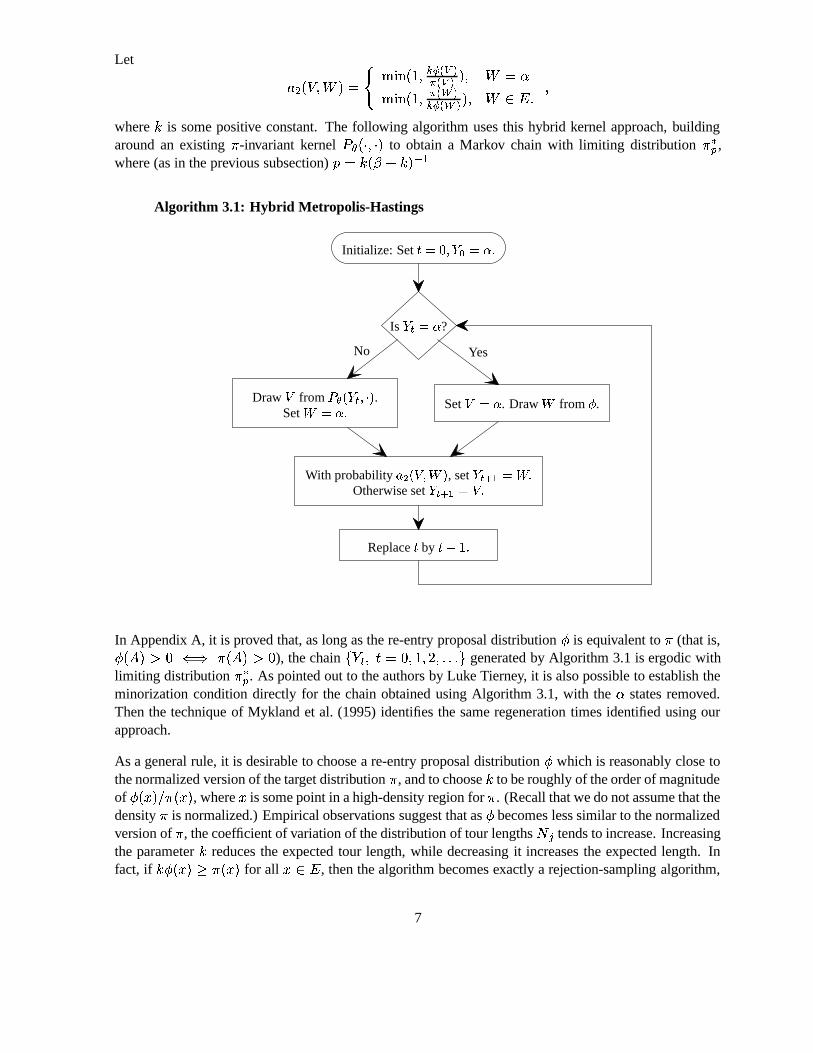
Let � H � &S�� # �� 7 8;: � �� A�� # � � �

�7 8;: � �� A�� # ��

where < is some positive constant. The following algorithm uses this hybrid kernel approach, buildingaround an existing � -invariant kernel � �2 � 2 # to obtain a Markov chain with limiting distribution � �� ,where (as in the previous subsection) ' � < � � + < # [ E

Algorithm 3.1: Hybrid Metropolis-Hastings

Is �� ?

With probability �� "!$# , set � �&%(' �)!+*Otherwise set �,�&%('-�.��*

Replace / by /10324*

Initialize: Set / ��5� 6�,78�.� *

Set �9�.� . Draw ! from : .

Yes

Draw � from ;=<4��> @?A# .Set !B��*

No

In Appendix A, it is proved that, as long as the re-entry proposal distribution � is equivalent to � (that is,� �"!$# = �DCFE� �"!$# = �

), the chain � � �S� � � �� generated by Algorithm 3.1 is ergodic withlimiting distribution � �� . As pointed out to the authors by Luke Tierney, it is also possible to establish theminorization condition directly for the chain obtained using Algorithm 3.1, with the � states removed.Then the technique of Mykland et al. (1995) identifies the same regeneration times identified using ourapproach.

As a general rule, it is desirable to choose a re-entry proposal distribution � which is reasonably close tothe normalized version of the target distribution � , and to choose < to be roughly of the order of magnitudeof � ��g# . � ��# , where � is some point in a high-density region for � . (Recall that we do not assume that thedensity � is normalized.) Empirical observations suggest that as � becomes less similar to the normalizedversion of � , the coefficient of variation of the distribution of tour lengths Y I tends to increase. Increasingthe parameter < reduces the expected tour length, while decreasing it increases the expected length. Infact, if < � ��# d � ��# for all � � �

, then the algorithm becomes exactly a rejection-sampling algorithm,

7

yielding a chain which alternates between � and�

, in which the non- � values are i.i.d. draws from thetarget distribution.

In practice, a small segment of a chain generated using the original kernel � �2 � 2 # can be used to determine� and < . In many cases, � can be taken to be a mixture normal approximation to the distribution of theelements of the initial segment, obtained, for instance, using the method described later in this section.The constant < can then be selected to be approximately the average value of � , evaluated over theelements of the initial segment (recall that � is not normalized), divided by the average value of thedensity � , evaluated over a number of draws from � itself.

Algorithm 3.1 is particularly useful since it provides a simple means of wrapping up an existing MCMCalgorithm for sampling from � to yield a Markov chain with limiting distribution � �� . However, it isimportant to note that Algorithm 3.1 does not necessarily improve mixing of the underlying kernel � �2 � 2 # .If � �2 � 2 # mixes badly, then the resulting chain �g�6� is also likely to mix badly.

3.3 Adaptive Modification of the Kernel

Implementation of MCMC sampling schemes typically requires a significant amount of effort to be de-voted to design of a transition kernel in order to ensure that the chain is well-mixing. This design pro-cedure can include the selection of an appropriate parameterization of the quantities of interest, as wellas potential parameters of proposal distributions in a Metropolis-Hastings chain. It is tempting to con-struct algorithms which modify these design parameters automatically as the chain runs. However, evenif for each fixed set of parameter values the kernel has the correct limiting distribution, introduction ofself-tuning can alter the limiting distribution of the process (which will not necessarily be Markovian anymore). Gelfand and Sahu (1994) give an interesting example where this problem occurs. Fortunately,however, there is a simple way around this problem. Gilks et al. (1998) have shown that if the Markovchain is regenerative, then one can modify design parameters at each regeneration time, and estimatorsare still well-behaved. In particular, Theorems 1 and 2 of Gilks et al. (1998) establish that under thisself-tuning scheme, if some technical conditions are satisfied, then (recall the definitions (5) and (7))

��"�is MSE-consistent for � � , and the quantity! � �

I � E � � I % �� Y I # HV H� (9)

converges in probability to $ H . It is relatively straightforward to show that the difference between

�$ H� andthe expression in (9) converges to zero, and hence that

�$TH� is consistent for $,H .Thus in Algorithm 3.1, the kernel parameter � can be changed every time the chain hits the state � , basedon an analysis of the past behaviour of the chain. Even though the process itself is no longer (necessarily)Markovian, it consists of a sequence of tours which, in isolation, are each Markovian, and the estimates��"�

and

�$gH� still have the desired consistency properties.

We now state an algorithm, based on the ideas presented in the previous sections, which estimates theexpection (with respect to the probability measure � ) of a “function of interest”

��2 # , and allows for

adaptive modification of a tuning parameter � . Given a desired number of tours � = �, the following

algorithm uses our method to construct a regenerative chain, an estimate

��of �

��g# � ��# , and an

estimate of the variance of

�� itself.

8

Intuitively, the algorithm works as follows. It repeatedly generates tours of a Markov chain �T�6� withlimiting distribution � �� . Tours of length one (that is, tours which consist only of the state � ) are thrownout. Remaining tours are truncated just before they hit � so as to become tours of a chain �OP&�6� withlimiting distribution � . The sum over each tour of the function of interest, evaluated at the chain’s state,is recorded, as is the length of the tour. At the end of the � th tour, the tuning parameter �� 6 E can bechosen based on analysis of past history of the chain. Once a total of � tours have been generated, thealgorithm terminates, and equations (5) and (7) can be used to obtain the desired estimates.

Algorithm 3.2:

Initialize: Set � 7 �.� �� $2� / �35� � 7 �35�*Choose some tuning parameter ��' .

Draw � �&% ' from � <� � � � ��# *Replace t by t+1.

Is �,�=�.� ?

Is �,�=�.� ?

Set � �$24 �� (� �,� # *

Draw � �&% ' from � <� � � � ��# *Replace t by t+1.

Replace � by � 0� (� �,� # *Replace n by n+1.

No

�� . Replace m by m+1.

Is �� ?

Yes

Yes

Terminate and computedesired estimates.

No

Choose � � ,based on analysis of� ' �*@*@*@ 6� � *

No

Yes

Set � ��( �� ' 0��

Most of Algorithm 3.2 is easily implemented. The only complicated part, obtaining draws from a kernel� �� 2 � 2 # with invariant distribution � �� , can be carried out using the basic Metropolis-Hastings Algorithmappropriately modified as described in Section 3.2.1, or Algorithm 3.1. Some consideration should begiven also to the method by which the kernel parameter �� is updated, although in the simplest case, onecan construct a non-adaptive chain by fixing � � � � � for all � .

It might be tempting to use an alternative approach, stopping the procedure at a fixed time and discardingthe last incomplete tour. However, this would not be a valid approach. It would introduce bias since the

9

discarded tour is more likely to be a long tour than a short tour, and different length tours typically havedifferent probabilistic properties.

On a final note, before using the variance estimate computed in Step 9 of Algorithm 3.2, the estimate

�4 �(recall its definition (8)) of the coefficient of variation should be checked. The variance estimate shouldnot be considered reliable if

�4 � is too large. Furthermore, it is important to keep in mind that even thoughAlgorithm 3.2 side-steps the burn-in problem in the sense that there is no point in removing any initialportion of the chain, it is still possible that after stopping generation of the chain, not all of the importantareas of the state-space have been explored.

3.4 An Adaptation Rule

Algorithm 3.2 allows for adaptation through selection (at the end of the � th tour) of the parameter � � 6 E ,which determines the form of the kernel

� � � � �2 � 2 # used in the � � + � # th tour. In this section we describeone method of doing this when the state space

�is ��

, based on the concept that an independence samplerwith a proposal distribution closely matching the target distribution is near-optimal in terms of mixing.(There are, of course, many other possible ways of adapting parameters of a Markov chain; some of theseare discussed briefly in Gilks et al., 1998)

Our approach is to start with a kernel� � �2 � 2 # , and as time goes by, to transform it progressively into an

independence-sampling kernel which uses a normal mixture approximation to the target distribution asits proposal distribution. The mixture approximation itself is updated at the end of each tour, based onthe contents of the tour itself.

We use a simple recursive update procedure, described by Titterington (1984), to compute our mixtureapproximations. The update rule is as follows. Given a multivariate normal mixture

� ��b � E �,b N � *gbU��@b # �

for which the parameters � b ��* b �� b �Jc � ��O� are unknown, and an infinite sequence of draws E �G H �� from

� � , parameter estimates

�� A b �

�* � A b �� A b can be updated sequentially, once after each

draw, by the formulae�* � A 6 E b �* � A�b +�

� A b<�

�� A b �� A 6 E % �* � A b #�

� � A 6 E b �� A b +

� A b<�

�� A b� �� A 6 E % �* Ab # �� A 6 E % �* � A b # _ %

�� A b� �

�� A 6 E b

�� A b + < [ E �

� A b %�

�� A b # �

where � A b �

��Ab � �� A 6 E�� * � A b �

�� A�b # with � �b � E b � � , � �2 � 2 � 2 # denoting the multivariate normal den-

sity. As Titterington (1984) points out, there is no guarantee of consistency of these sequentially updatedestimators, but for our purposes, since the mixture approximation is to be used to generate proposals,we only require a crude approximation to the target distribution, and consistency is not necessary forour adaptive method. Better methods for constructing mixture approximations have been widely studied

10

(see, e.g. McLachlan and Peel, 2000), but the vast majority of these methods cannot be implementedsequentially, which prevents them from being useful in the procedure we propose.

We now state the full adaptive procedure to be used in Algorithm 3.2. Let the adaptive parameters bedefined by � � � �� # , where, for each � , � � is a constant in the interval � � �� # and

� � is a set ofweights, mean vectors, and covariance matrices, defining a normal mixture distribution. We denote thedensity of the mixture distribution by

� � �2 # .Let � �� !$# � � ��% �`# � � �� !$#,+�� !$# �where �� !J# is an independence-sampling Metropolis-Hastings kernel, in which the proposals havedensity

� �2 # , that is,

�� !$# � - . ��g# � � � ��`# � � % � �� `# ��+ �.� �� # �� `#��

with � �� # � 798;: � �� `# � ��g# � � ��# � ��`# # [ E # . Thus the kernel� �2 � 2 # is a mixture of the original

kernel� � �2 � 2 # and the independence-sampling Metropolis-Hastings kernel.

To initialize the adaptive parameters, let � E��

, and let�E be some initial normal mixture approximation

to � .

At the end of the � th tour ( � � �� ), set

� � 6 E � 7 �� % � �� % � � #�� # �where the constants � and � are in the interval

� � �� . In addition, calculate the parameters of� � 6 E by

starting with the mixture distribution� � and updating it sequentially using the rules given above, once

for each element of the � th tour.

The first of these two updates increases the relative contribution of the independence sampler in� � � � �2 � 2 # , to a “maximal” proportional contribution of � . Choosing � � � allows the kernel to be(as time increases to infinity) completely replaced by the independence sampler. Choosing � L � ensuresthat some of the original kernel

� � �2 � 2 # is always retained, and guards against the possibility of buildingan independence sampler based on the potentially false belief that all important parts of the space havealready been explored. The second update simply refines the normal mixture approximation to the targetdistribution.

Under ideal circumstances, this procedure for adapting � will gradually replace the original kernel withan independence sampling Metropolis-Hastings kernel, whose proposal density

� � becomes close to thetrue target density as � increases.

In some cases (particularly when the state-space�

is high-dimensional), it can be impractical to con-struct approximations to the target distribution on the entire state-space. However, if the original kernel� � �2 � 2 # consists of Metropolis-Hastings block-updates for subspaces of

�, it often makes sense to use

the same basic idea, but to restrict approximations to the appropriate conditional target densities on thesubspaces, and progressively replace the original block-update rules with Metropolis-Hastings indepen-dence sampling steps whose proposals are the respective conditional approximations. If conditional targetdensities are difficult to approximate, a slightly less optimal approach is to use the respective marginaltarget densities.

11

� �� `� � �� ;�� D�� D�� ;�� D� �� D � �� D� ��D�� `�� D �� O� ��

Table 1: The dugong data set used in Section 4.1.

3.5 Comments on Parallel Processing

Algorithm 3.2 generates � independent tours, possibly updating the kernel parameter � after each touris completed. Hence it lends itself readily to parallel processing implementations.

In the non-adaptive case (i.e. where � � � �5�O� � � �� ), it is clear that tours can be generated onseparate processors, and combined to obtain the desired estimates. There is a potential trap, however.Stopping at a fixed time and discarded incomplete tours leads to bias in favor of shorter tours. Allcurrently-running tours must be allowed to run to completion before the algorithm is terminated. Inthe adaptive case, there is a further complication. Each processor can certainly carry out some kind ofadaptive scheme based on only its own generated tours. (It is not hard to see that this is like a single largeadaptive scheme in which adaptation at each time point depends only on a subset of previously-observedtours.) However, it is not clear that processors should be allowed to adapt their kernels based on resultscoming in from other processors, since in this case, a processor would be likely to observe short toursarriving before long tours.

4 Examples

To examine the performance of Algorithm 3.2 we apply to it two problems. As a measure of the mixingquality of Markov chains obtained, we compute the sample precision per iteration (SPPI) of our estimates,which we define to be �

�$ H� ! # [ E , where ! is the length of the chain generated and

�$ H� is the estimate ofthe variance of the estimator given by (7). Assuming that computational cost to obtain an iteration isroughly invariant, precision per iteration is a direct measure of the computational efficiency of an MCMCsimulation. Since this quantity is a random variable itself, we generate multiple realizations of Markovchains, and show box-plots of the resulting SPPI values across the different realizations.

4.1 Dugongs

First we consider a data set used in Ratkowsky (1983), which has also been considered in Carlin andGelfand (1991). Length ( ) and age (

�) measurements were made of 27 specimens of a particular

species of sea cows (dugongs), captured near Townsville, Queensland. The data are shown in Table 1.

12

As discussed in Ratkowsky (1983), a frequently-used model for such a data set is

b � N � *,b �G0 [ E # (10)* b �� % �� a (11)

for the data, where� b and b are the age and length of the c th dugong, respectively, and � = �

,� = �

,� � � � �� # , and 0 = �are unknown model parameters. We assign the (relatively uninformative) priors

� � N � � �� #� � N � � �� #� � U � � �� #0 � Ga � � � � � �� # �

Our object is to determine the posterior mean of �� # , �� # , �� . � � % � # # , and 0 [ E .A Markov chain with the posterior as its limiting distribution can be constructed by computing full-conditional distributions and updating each of the four parameters in turn. The parameters � ,

�and 0

have conjugate priors for the likelihood (11). Hence they can be updated by sampling directly from theirrespective full-conditional distributions. The parameter

�does not have a conjugate prior. However, it

can be updated by using a single Metropolis-Hastings step whose target density is proportional to the full-conditional density of

�. As our proposal distribution for the

�-update, we choose a uniform distribution

on the interval� � �� # .

We simulate using two methods. In the first we simply embed this kernel into Algorithm 3.1 to obtaina regenerative Markov chain, and we use the tours of the resulting chain to compute estimates of theposterior means, along with their (estimated) standard errors. The re-entry proposal distribution � isconstructed by running the original chain for 1000 iterations, and using these iterations to construct anormal approximation to the target density, using the update rules described in Section 3.4. The constant< is chosen so that �� < # is equal to the average log-target density over the 1000 iterations, minus theaverage log-density of � �2 # over 1000 draws, minus a constant which is chosen (experimentally) to adjustthe distribution of the tour-lengths. After the initial 1000 iterations, the transition kernel is fixed.

Next we use Algorithm 3.2, with the adaptation rule described in Section 3.4. Sampling from the full-conditional is retained for �� and 0 , but the uniform proposals for the

�-update are gradually replaced

with independent proposals coming from the conditional distribution of�

in a two-component mixturenormal approximation to the marginal target density of the full parameter vector. The re-entry proposaldistribution and the constant < are the same as chosen for the non-adaptive method.

Table 2 gives posterior means obtained using these two methods, along with their standard errors, esti-mated using both the batch-means method and the regenerative method. Figure 1 contains box plots of theSPPI, over 1000 separate regenerative chains, each one consisting of 1000 tours, in both the non-adaptiveand adaptive case.

The difference between standard errors estimated using the batch-means method and using the regener-ative approach is noticeable, but not very large. In this case, the batch-means method appears to consis-tently under-estimate the variance.

The improvement in SPPI due to use of the adaptive algorithm is clearly quite substantial. Roughly

13

Parameter EstimatesNon-adaptive Adaptive

Function Post. Mean (Batch SE, Regen. SE) Post. Mean (Batch SE, Regen. SE)�� # 0.97819 (0.00076, 0.00103) 0.97928 (0.00041, 0.00048)�� # -0.02208 (0.00053, 0.00066) -0.02123 (0.00054, 0.00066)logit � � # 1.88223 (0.00805, 0.01078) 1.89209 (0.00484, 0.00623)0 [ E 0.00903 (0.00002, 0.00002) 0.00905 (0.00002, 0.00003)

Table 2: Posterior means, along with batch-means and regenerative standarderror estimates, from (1) a non-adaptive chain (1000 tours, total length 261139)and (2) an adaptive chain (1000 tours, total length 263143).

speaking, it appears that one iteration of the adaptive chain is worth two to five iterations of the non-adaptive chain.

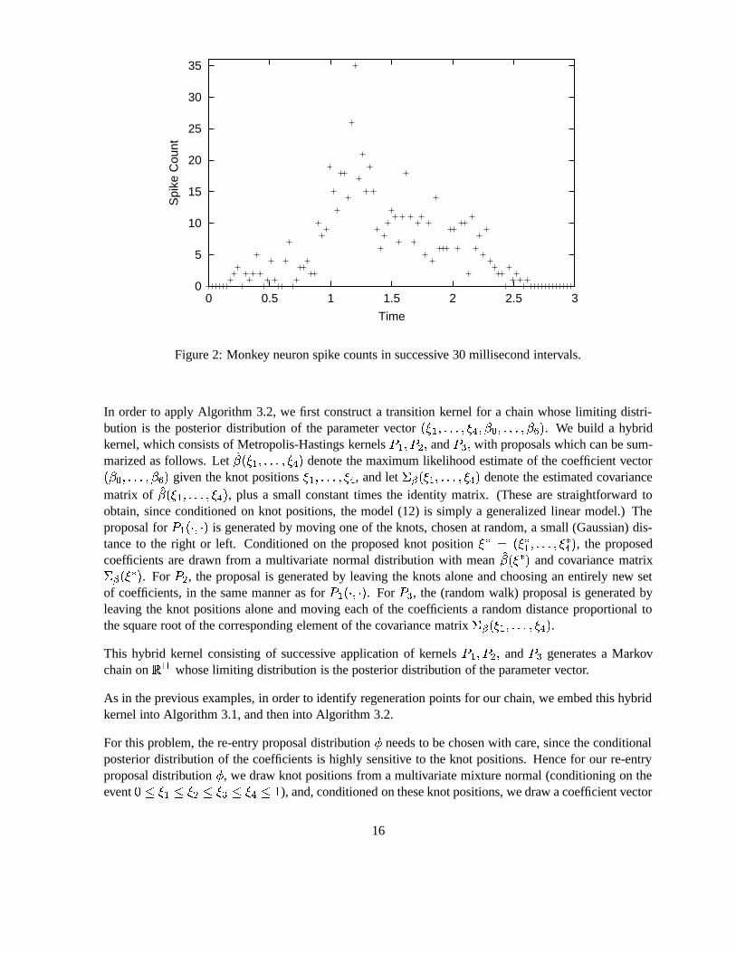
4.2 Monkeys and Free-Knot Splines

We next consider a more complicated problem. Ventura et al. (2002) describe experiments in which amacaque monkey watches images appear on a screen. The monkey is trained to move its eyes in responseto certain visual cues, and an electrode measures numbers of “neuron-spikes” occurring in a neuron in themonkey’s supplementary eye field. (The supplementary eye field is thought to be involved in generatingeye movements in response to stimuli.)

Figure 2 shows the number of spikes � A observed in time intervals� � � � D <�� D � < + � # # � < �

� ��O� � , for one such task.

We assume that the observations � � �� are Poisson with a time-varying rate, and can be modelledby

�A � � �2 # � Pn �� < . � # # �%$ H # � (12)

where� �2 # is a cubic spline function with four knots, that is,

� ��g# � � � + � E �9+ � H � H + � �� % � E # 6+ � �� % � H # 6 + �� % � # 6 + �� % � # 6 � � � � � �� where ��# 6 � 7 �� # � The knot positions

�E ��

� � � � �� and the coefficients� �� are not

known. Our object is to determine the posterior distributions of� � < . � # � < � � �� , as well as the

posterior distribution of�� 7 �� g# , which corresponds to the time at which the firing rate reaches its

maximum.

We adopt a Bayesian approach, assigning a Dirichlet( D��D��D��D��D ) prior distribution to the gaps betweenthe knots, that is, to the vector � � E �

�H %�E �� % � H �

� % � ��,% � # _ . The coefficients�I are assigned (the

relatively uninformative) independent normal priors with mean zero and variance � � E H . The likelihoodfor the model is easily computed from (12).

14

Non−Adaptive Adaptive

010

2030

40

SPPIs of Log(Alpha)


05

1015

2025

30

SPPIs of Log(Beta)


0.0

0.1

0.2

0.3

0.4

SPPIs of Logit(Lambda)


010

000

3000

0SPPIs of Inv(Tau)

Figure 1: Sample precision per iteration (SPPI) for each of the four parametersin the Dugong problem, for both non-adaptive and adaptive chains generatedusing Algorithm 3.2. SPPIs are evaluated for 1000 non-adaptive and 1000adaptive chains, each consisting of exactly 1000 tours, with length approxi-mately equal to 250000.

15

0

5

10

15

20

25

30

35

0 0.5 1 1.5 2 2.5 3

Spi

ke C

ount

Time

Figure 2: Monkey neuron spike counts in successive 30 millisecond intervals.

In order to apply Algorithm 3.2, we first construct a transition kernel for a chain whose limiting distri-bution is the posterior distribution of the parameter vector � � E ��

� � � �� # . We build a hybridkernel, which consists of Metropolis-Hastings kernels � E � � H � and � � with proposals which can be sum-marized as follows. Let

�� E ��5� � # denote the maximum likelihood estimate of the coefficient vector� � �� # given the knot positions

�E ��

� , and let �� E ��

� # denote the estimated covariancematrix of

�� E �� # , plus a small constant times the identity matrix. (These are straightforward toobtain, since conditioned on knot positions, the model (12) is simply a generalized linear model.) Theproposal for � E �2 � 2 # is generated by moving one of the knots, chosen at random, a small (Gaussian) dis-tance to the right or left. Conditioned on the proposed knot position

� � � � � �E �� # , the proposed

coefficients are drawn from a multivariate normal distribution with mean

�� # and covariance matrix�� # . For � H , the proposal is generated by leaving the knots alone and choosing an entirely new setof coefficients, in the same manner as for � E �2 � 2 # . For � , the (random walk) proposal is generated byleaving the knot positions alone and moving each of the coefficients a random distance proportional tothe square root of the corresponding element of the covariance matrix �� E ��

� # .This hybrid kernel consisting of successive application of kernels � E � � H � and � generates a Markovchain on

E E whose limiting distribution is the posterior distribution of the parameter vector.

As in the previous examples, in order to identify regeneration points for our chain, we embed this hybridkernel into Algorithm 3.1, and then into Algorithm 3.2.

For this problem, the re-entry proposal distribution � needs to be chosen with care, since the conditionalposterior distribution of the coefficients is highly sensitive to the knot positions. Hence for our re-entryproposal distribution � , we draw knot positions from a multivariate mixture normal (conditioning on theevent

� N � E N�H N

� N � N � ), and, conditioned on these knot positions, we draw a coefficient vector

16

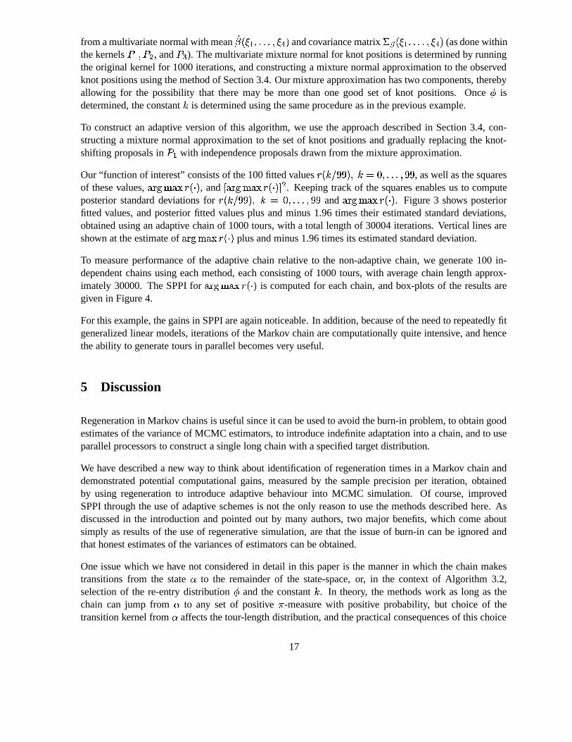
from a multivariate normal with mean

�� E �� # and covariance matrix � � � � E �� # (as done within

the kernels � E � � H � and � ). The multivariate mixture normal for knot positions is determined by runningthe original kernel for 1000 iterations, and constructing a mixture normal approximation to the observedknot positions using the method of Section 3.4. Our mixture approximation has two components, therebyallowing for the possibility that there may be more than one good set of knot positions. Once � isdetermined, the constant < is determined using the same procedure as in the previous example.

To construct an adaptive version of this algorithm, we use the approach described in Section 3.4, con-structing a mixture normal approximation to the set of knot positions and gradually replacing the knot-shifting proposals in � E with independence proposals drawn from the mixture approximation.

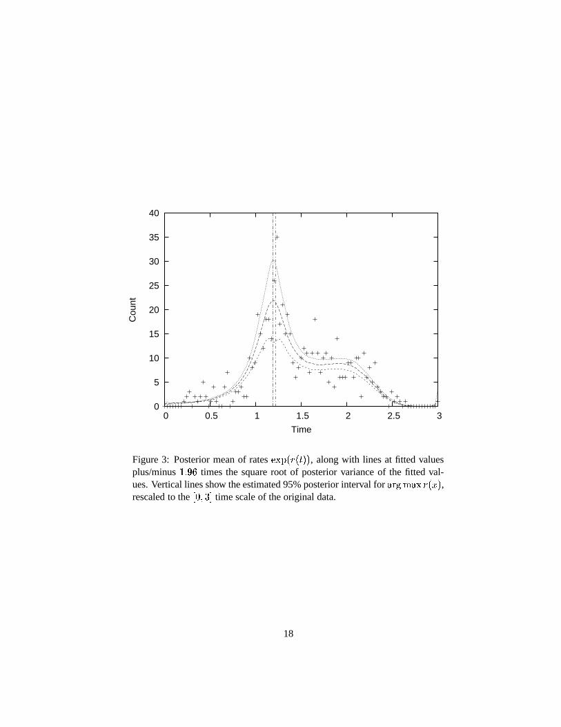
Our “function of interest” consists of the 100 fitted values� � < . � # �S< �� , as well as the squares

of these values,�� 7 �� 2 # , and

� �� 7 �� 2 # H . Keeping track of the squares enables us to computeposterior standard deviations for

� � < . � # �J< � � �� and�� 7 �� 2 # . Figure 3 shows posterior

fitted values, and posterior fitted values plus and minus 1.96 times their estimated standard deviations,obtained using an adaptive chain of 1000 tours, with a total length of 30004 iterations. Vertical lines areshown at the estimate of

�� 7 �� 2 # plus and minus 1.96 times its estimated standard deviation.

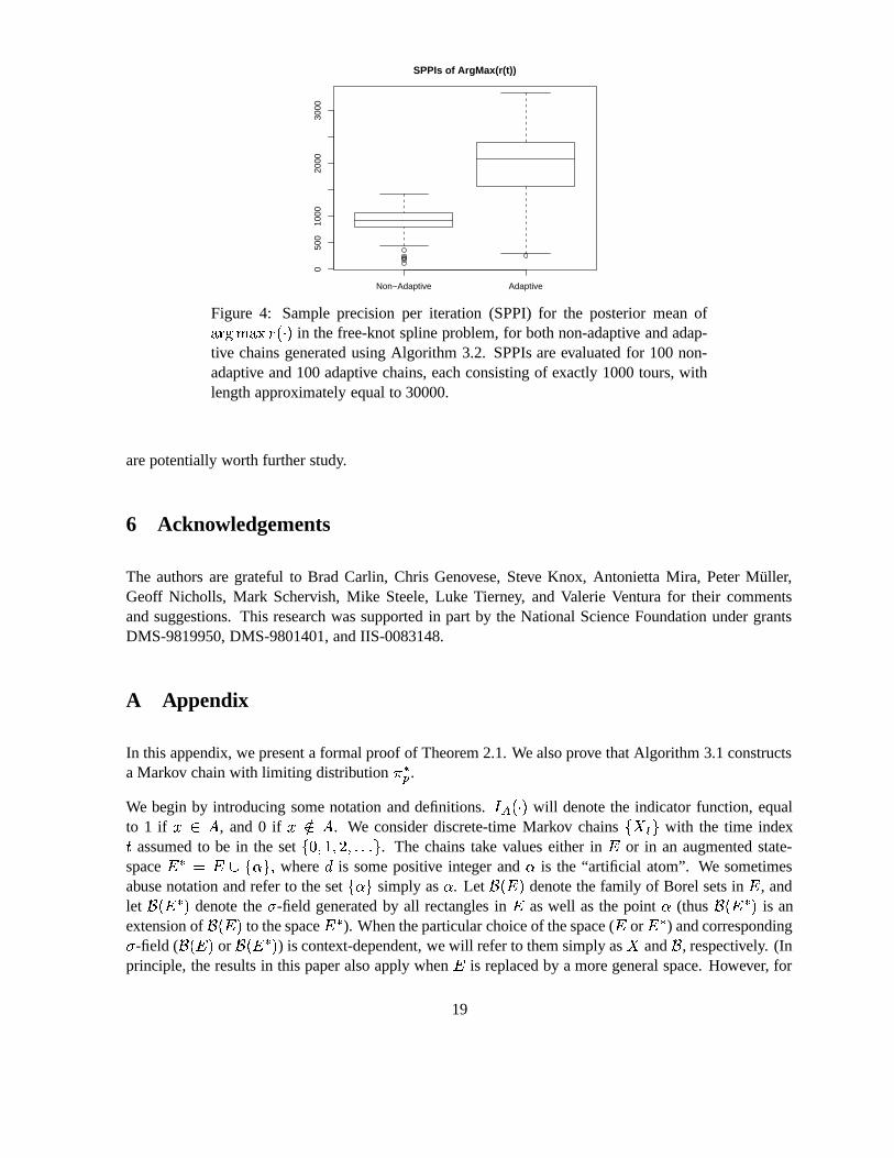
To measure performance of the adaptive chain relative to the non-adaptive chain, we generate 100 in-dependent chains using each method, each consisting of 1000 tours, with average chain length approx-imately 30000. The SPPI for

�� 7 �� 2 # is computed for each chain, and box-plots of the results aregiven in Figure 4.

For this example, the gains in SPPI are again noticeable. In addition, because of the need to repeatedly fitgeneralized linear models, iterations of the Markov chain are computationally quite intensive, and hencethe ability to generate tours in parallel becomes very useful.

5 Discussion

Regeneration in Markov chains is useful since it can be used to avoid the burn-in problem, to obtain goodestimates of the variance of MCMC estimators, to introduce indefinite adaptation into a chain, and to useparallel processors to construct a single long chain with a specified target distribution.

We have described a new way to think about identification of regeneration times in a Markov chain anddemonstrated potential computational gains, measured by the sample precision per iteration, obtainedby using regeneration to introduce adaptive behaviour into MCMC simulation. Of course, improvedSPPI through the use of adaptive schemes is not the only reason to use the methods described here. Asdiscussed in the introduction and pointed out by many authors, two major benefits, which come aboutsimply as results of the use of regenerative simulation, are that the issue of burn-in can be ignored andthat honest estimates of the variances of estimators can be obtained.

One issue which we have not considered in detail in this paper is the manner in which the chain makestransitions from the state � to the remainder of the state-space, or, in the context of Algorithm 3.2,selection of the re-entry distribution � and the constant < . In theory, the methods work as long as thechain can jump from � to any set of positive � -measure with positive probability, but choice of thetransition kernel from � affects the tour-length distribution, and the practical consequences of this choice

17

0

5

10

15

20

25

30

35

40

0 0.5 1 1.5 2 2.5 3

Cou

nt

Time

Figure 3: Posterior mean of rates � �� # # , along with lines at fitted valuesplus/minus �� times the square root of posterior variance of the fitted val-ues. Vertical lines show the estimated 95% posterior interval for

�� 7 �� g# ,rescaled to the

� � ��D time scale of the original data.

18


050

010

0020

0030

00

SPPIs of ArgMax(r(t))

Figure 4: Sample precision per iteration (SPPI) for the posterior mean of�� 7 �� 2 # in the free-knot spline problem, for both non-adaptive and adap-tive chains generated using Algorithm 3.2. SPPIs are evaluated for 100 non-adaptive and 100 adaptive chains, each consisting of exactly 1000 tours, withlength approximately equal to 30000.

are potentially worth further study.

6 Acknowledgements

The authors are grateful to Brad Carlin, Chris Genovese, Steve Knox, Antonietta Mira, Peter Muller,Geoff Nicholls, Mark Schervish, Mike Steele, Luke Tierney, and Valerie Ventura for their commentsand suggestions. This research was supported in part by the National Science Foundation under grantsDMS-9819950, DMS-9801401, and IIS-0083148.

A Appendix

In this appendix, we present a formal proof of Theorem 2.1. We also prove that Algorithm 3.1 constructsa Markov chain with limiting distribution � �� .

We begin by introducing some notation and definitions. -�. �2 # will denote the indicator function, equalto 1 if � � ! , and 0 if � .�^! . We consider discrete-time Markov chains � � �G� with the time index� assumed to be in the set � � ��"� . The chains take values either in

�or in an augmented state-

space� � � � � � �S�C� where is some positive integer and � is the “artificial atom”. We sometimes

abuse notation and refer to the set � �B� simply as � . Let� � � # denote the family of Borel sets in

�, and

let� � � � # denote the $ -field generated by all rectangles in

�as well as the point � (thus

� � � � # is anextension of

� � � # to the space� �

). When the particular choice of the space (�

or� �

) and corresponding$ -field (� � � # or

� � � � # ) is context-dependent, we will refer to them simply as�

and�

, respectively. (Inprinciple, the results in this paper also apply when

�is replaced by a more general space. However, for

19

the sake of simplicity, and since most chains of interest take values in a space which can be mapped to�

,we do not present explicit versions of our results which apply for more general spaces.)

The transition probability kernel of a Markov chain � � � �,� �� taking values in�

is a function� �� !$# � Pr� � � 6 E �/! � � � � � � � � � � ! � � � The < -step transition probability kernels are defined

by � A �� !$# � Pr� � � 6 A � ! � � � � � . The notation � � ��9# is used to denote the conditional probability

of the event � , given the initial condition� � � � for the chain � � �6� with transition probability kernel� �2 � 2 # .

The chain � � �6� is said to be irreducible (or � -irreducible) if there exists a measure � on�

with � � � # = �such that � �"!$# = � E ��

A � E � �� !$# =�

for all � � � � (13)

A � -irreducible chain � � � � is said to have a v-cycle if there exist sets � E �� such that� �� Wb 6 E # � �� WbU��c � ��5� % �� E #

� � for � � � � � and � � � � �b � E �Wb #��B# � �.

If the largest for which a -cycle occurs is equal to one, then the chain is said to be aperiodic. The firstreturn time for a set ! � �

is0�. � 798;: �� d � ? � � �/! � (14)

and the occupation time (after time zero) is defined to be � . � � �� E -�. � � � # � A set ! � �is said to

be Harris recurrent if � � �� . �� # � � for all � � ! � and the Markov chain � � �6� is said to be Harrisrecurrent if it is � -irreducible and every set ! with � �"!$# = �

is Harris recurrent. A set � � �is said to

be uniformly accessible from ! � �if there exists ��= �

such that8;:�� . � � � 0�� L # d��

The chain � � �6� is said to be ergodic if there exists a probability measure � on�

such that

� 8]7�� 2 # % � �2 # � ��

for all � � � � (15)

where� 2 � is the total variation norm defined for signed measures on

�by

� * � �� . �� * �"!J# %8;: � . �!� * �"!$# � If this is the case, then the probability measure � is called the limiting distribution of thechain.

A.1 Incorporating the Artificial Atom

Recall that the space� �

includes the artificial atom � as well as every element of�

. As introduced in (1),� �� denotes the probability measure

��"!J# � � ��%(' # � �"!*) � #,+ '�-�. � � # � ! � � � � � # � (16)

where ' is some constant in the interval � � �� # . Let �,� � � � � ��]� be an ergodic Markov chaintaking values in

� �with initial value ��

� , whose limiting distribution is � �� . Let the hitting times0�1 �324# and the tours I be as defined by (2) and (3), respectively. The tour lengths are given by

� I� 0�1 �324# % 0�1 �32 %>� # � 2 � ��5� (17)

and the elements of a tour I are referred to as IA � #"%$ � I�[ E 6 A � < � ��5� � I �The following result shows that � is a proper Harris recurrent atom for the chain. Hence the chain �T�6�is regenerative with regeneration times �0 1 �324# � 2 �� .

20

Theorem A.1 Let �� R� �� be an ergodic Markov chain taking values in� �

with initialcondition �� and limiting distribution � �� given by (16). Let the tours and their lengths be as definedin (3) and (17). Then

1. � is a Harris recurrent state for the chain, and with probability one, the tour lengths � � I � 2�

�� are all finite, and

2.- � � I � ' [ E��

Proof of Theorem A.1: To prove the first part, note (c.f. (14)) that � � � 0�� L # d � � �� # for every! . Also, � � �� # � � �� # � ' as ! � , regardless of � . Thus � �S� is uniformly accessible from the

state-space� �

. It then follows from Theorem 9.1.3(ii) of Meyn and Tweedie (1993) that� � �� # � �for all � � � �

, and hence that � is Harris recurrent and with probability one, the tour lengths are allfinite. The second part of the result is a direct consequence of Kac’s Theorem (see Kac, 1947; Meyn andTweedie, 1993, Theorem 10.2.2).

�

A.2 Removing the Artificial Atom

Next let �OPB�6� be the sequence derived from ��6� as described in Section 2. Formally, its construction canbe described as follows. Let e E

��798;: ��c@d � ? � bT= �O� , and define

e I��798]: � 2 =>e I�[ E ? � I = �O�C�

(Thus �5e I � is the set of indices of tours of ��6� whose length is strictly greater than one.) Then the toursP I can be written as

P@I � � f �A �T< � �� f � %*�O�C� (18)

and their corresponding lengths areY I

� � f � %*�� (19)

for 2 � ��O� The cumulative tour lengths are then V I� � I b � E Y I � 2 � ��5� with V � � �

.Finally, �OPS�6� is the sequence obtained by concatenating the tours P E�� P H5�� together in sequence. (It isnot difficult to verify that the sequence �OP �6� is exactly the sequence ��6� with every occurrence of thestate � removed.)

We are now in a position to prove Theorem 2.1.

Proof of Theorem 2.1: The proof consists of three main parts. First it is shown that �OP��6� is a Markovchain, and its transition probability kernel is derived. Next it is shown that it has invariant distribution � ,and finally it is shown that the chain is ergodic, and that the times V I are regeneration times.

To see that �OPS�6� is a Markov chain, note that P�� " , where 0 is the stopping time defined to be the� -th time that ��A � is not equal to � . Also define the function

� . �2 � 2 �� # to be equal to one if its secondnon- � argument is in the set ! , and zero otherwise. Then

� . � " �G " 6 E �G " 6 H �� # � - . � P � 6 E # � ! � � �

21

By the strong Markov property (which every discrete-time Markov chain satisfies),- � � . � " �G " 6 E �� # � " �G " [ E ��5�G � � - 1�� . � ��G E �� # � (20)

The term on the right of (20) only depends on " � PS� . The term on the left is equal toPr� PT� 6 E �/! � PT� �G " [ E ��G�� Thus PS� 6 E � PT� is independent of " [ E �G " [ H ��G�� , and since

�OP � [ E � P � [ H �� P � �� " [ E �G " [ H ��5�G � �C�

it follows thatPr� PT� 6 E � ! � PS� � PT� [ E �� PB�

�Pr� PS� 6 E �/! � PT� �

which establishes that �OPB�6� is a Markov chain.

Now let � �� !J# denote the transition probability kernel of �,�6� and define

�� "!J# � � �"!*) � # � ! � � � � � # � (21)

Let ! be some set in� � � � # , and let ! � � !() � �B� . Consider the probability

� �� !$# that P � 6 E �/! giventhat PT� � � . By construction, PB� 6 E can never be equal to � , so

� �� # � �and

� �� !$# � � �� ! � # .Also, PS� is equal to gf for some e/d � . So PS� 6 E will be in ! � if and only if gf 6 E �*! � , or �f 6 E � �

and �f 6 H � ! � , or �f 6 E � �f 6 H � � and �f 6 � ! � , �� Since these events are mutually exclusive, thetransition probability kernel for �OP��6� is

� �� !$# � � �� ! � # � Pr �3PT� 6 E �/! � � PT� � �� ! � # + � �� #

��I �� # I�� ! � #

� � �� ! � # + � �� # � � �� ! � #��% � � �� # � (22)

Now (c.f. (16) and (21)) � � ��# � � �&%F' # [ E � � ��g# %(' -�� # � Hence, using (22),�� !J# � � ��# � � � �� ! � # � � ��g# � � � �� ! � # � � ��#,+ � � �� # � � �� ! � #�&% � � �� # � � ��#

� � ��%(' # [ E� � �� ! � # �

�� # % ' � ��%(' # [ E � � �� ! � #+ � � �� ! � #��% � � �� #�� %(' # [ E

� � �� # ��,��g# %(' � � %(' # [ E � � �B� � #�� (23)

Since � �� is the invariant distribution of the chain with kernel � �2 � 2 # , we know that� � �� !$# �� g# � �

�� "!$#for ! � � � � � # . Making use of this result, along with the fact that � �� # � ' , equation (23) becomes� �� !$# � � ��# � � ��%(' # [ E �

��"! � # %(' � ��%(' # [ E � � �B� ! � #+ � � �� ! � #� % � � �� #

� � ��%(' # [ E �� # % ' � � %(' # [ E � � �� #

� � ��%(' # [ E �� "! � # � � ��%(' # [ E � ��% ' # � � �"!J# � � � �"!$# �

22

which applies for all ! � � � � � # . This means that � � is the invariant distribution of the chain �OP@�6� .Since �OPS�6� can never hit the point � , it can also be regarded as a chain taking values in

�with invariant

distribution � .

Next it is necessary to show that �OP��6� is ergodic. First, note that from (22),� �� !$# d � �� !J# for any ! � � � � # (24)

(because ! � � � � # implies that ! � ! � ). Since � �"!J# = � E� �� "!$# = �

, and � �� "!$# = � E� �A � E � �� !$# = �

, it follows that � �"!$# = �+E � �A � E � �� !$# = �for all ! � � � � # and all � � �

.Thus �OP � � is � -irreducible. Aperiodicity of �OP � � also follows from (24), as does the property that everyHarris recurrent set ! for ��6� with �

.��! must be a Harris recurrent set for �OP��6� . Hence the chain�OPT�6� is Harris recurrent. Then since �OP��6� is irreducible, aperiodic and positive Harris, it follows from theAperiodic Ergodic Theorem (see, e.g., Meyn and Tweedie, 1993, Theorem 13.0.1) that it is ergodic, andhence that the invariant distribution � is also the limiting distribution.

Finally, it follows directly from the strong Markov property that the times ��VSb6� c � � �� areregeneration times for the chain �OP �6� . �

A.3 Analysis of Algorithm 3.1

Next we establish that Algorithm 3.1 does indeed generate a Markov chain with limiting distribution � �� .

Theorem A.2 Suppose that � has density�� 2 # with respect to some measure � , where

�is an unknown

constant, and let � denote a re-entry density with respect to � , satisfying the property that� ��# = �� # = � � � � � �Let � �2 � 2 # be the kernel of an ergodic Markov chain with limiting distribution � , and let ' � be some arbi-trary positive constant. Then Algorithm 3.1 generates an ergodic Markov chain with limiting distribution

� �� , where ' � � ' � � � + � ' � # [ E �Proof: Let � E �2 � 2 # represent the extension of � �2 � 2 # given by

� E �� !J# � � � �� !*) � # � � � �

- . � � # � � � ��for � � � �

and ! � � � � � # . Let � H �2 � 2 # be the kernel

� H �� !J# �� -�. � � # �� &% � � �� # � � ��`#K+ � . � �� # � � � # � � � ��

- . ��g# � ��% � �� # + - . � � # � �� # � � � � �where � �2 � 2 # is the function defined in Step 4 of the algorithm. Thus � E represents the operation carriedout in Step 2 of the algorithm � H represents the operation carried out in Steps 3 and 4 of the algorithm,and the transition probability kernel for the chain � �U� generated by Algorithm 3.1 can then be written as

� �� !J# � � � H�� E # �� !$# � � � E �� # � H �� !$# �23

It is not too difficult to show that for every � � � � �� , � �� is an invariant distribution for � E �2 � 2 # . Also,� �� is an invariant distribution for � H �2 � 2 # . It follows directly that � �� is also an invariant distribution for� �2 � 2 # , and hence that the Markov chain �g�U� is positive recurrent.

Furthermore, since� �� # � �

�� E �� # � H �� # , � H �� # = �for all ��

, and � E �� # � � ,by basic properties of integrals, � �� # = � � � � � � � (25)

Also, by the Chapman-Kolmogorov equations,

� I �� !$# � �/� � I�[ E �� # � �� !J# d � I�[ E �� # � � �� !J# (26)

for 2 � ��D�� , and since � E � �� !J# � -�. � � # ,� � �� !J# � � H � �� !$# �

Since for any � � � � � # , � � � # = ��E � H � �� # = �, and � is equivalent to � , it follows that � � � # =� E � � �� # = �

. In conjunction with the property (25) and the definition (1), it follows that

��"!$# = � E � � �B� !$# = � � ! � � � � � # � (27)

Substituting this result in turn into the inequality (26), with 2 � � , and using (25), we have

�� "!$# = � E � H �� !$# = � � � � � � � ! � � � � � # �

An inductive argument using inequality (26) with 2 � D�� `�� shows that, more generally,

�� "!J# = � E � I �� !$# = � � � � � � � ! � � � � � # � 2 � ��D�� (28)

This establishes that the Markov chain � � � is � �� -irreducible and aperiodic. Since it also has invariantdistribution � �� , it is positive, and thus (see, e.g. Meyn and Tweedie, 1993, Theorem 9.0.1) the space

� �can be decomposed as

� � � � � Y , where � �� Y # � �, Y is transient, and the chain restricted to

�is

Harris recurrent. To show that ��6� is Harris recurrent, it suffices to show that� � � 0�� L # � � for all� � Y . Let �

�W� � � � 0�� = ! # for ! � �� , so that

� E� �

�

� �� `# �� H

� ��

��

� �� # � �� # �and so on. Similarly, let ' � � � � � 0�� = ! # for ! � ��O� Then since

� �� !$# N � �� !J# when!��

�, it follows that �

� N ' � for ! � ��O� Next, since � �2 � 2 # is assumed to be ergodic withlimiting distribution � , it is (by definition) Harris recurrent. Furthermore, since � �� # � � , � � � # must bepositive, so � 8]7"�� ' �(� � � � 0�� # �^�

. Hence� � � 0�� # � � 8;7 �� N � 8;7 �� ' �(� �

,so � �6� is Harris recurrent.

Finally, since � � � is irreducible, aperiodic, and Harris recurrent with invariant distribution � �� , it isergodic with � �� as the limiting distribution.

�

24

References

B.P. Carlin and A.E. Gelfand. An iterative Monte Carlo method for nonconjugate Bayesian analysis.Statistics and Computing, 1:119–128, 1991.

D. Chauveau and P. Vandekerkhove. Improving convergence of the Hastings-Metropolis algorithm withan adaptive proposal. Scandinavian Journal of Statistics, 29(1), 2002.

M.A. Crane and D.L. Iglehart. Simulating stable stochasting systems, I: General multi-server queues.Journal of the Association of Computing Machinery, 21:103–113, 1975a.

M.A. Crane and D.L. Iglehart. Simulating stable stochasting systems, II: Markov chains. Journal of theAssociation of Computing Machinery, 21:114–123, 1975b.

M.A. Crane and A.J. Lemoine. An Introduction to the Regenerative Method for Simulation Analysis,volume 4 of Lecture Notes in Control and Information Sciences. Springer, 1977.

A. E. Gelfand and S. K. Sahu. On Markov chain Monte Carlo acceleration. Journal of Computationaland Graphical Statistics, 3:261–276, 1994.

C. Geyer. Practical Markov chain Monte Carlo. Statistical Science, 7(4):473–483, 1992.

R. Gilks, G.O. Roberts, and S.K. Sahu. Adaptive Markov chain Monte Carlo through regeneration.Journal of the American Statistical Association, 93(443):1045–1054, 1998.

W.R. Gilks, S. Richardson, and D.J.Spiegelhalter. Markov Chain Monte Carlo in Practice. CRC Press,1996.

P.W. Glynn and D.L. Iglehart. Simulation output analysis using standardized time series. Math. Oper.Research, 15:1–16, 1990.

G.L. Jones and J.P. Hobert. Honest exploration of intractable probability distributions via Markov chainMonte Carlo. Statistical Science, 16(4):312–334, 2001.

M. Kac. On the notion of recurrence in discrete stochastic processes. Bulletin of the American Mathe-matical Society, 53:1002–1010, 1947.

G. McLachlan and D. Peel. Finite Mixture Models. Wiley, 2000.

S.P. Meyn and R.L. Tweedie. Markov Chains and Stochastic Stability. Springer, 1993.

J. Møller and G.K. Nicholls. Perfect simulation for sample-based inference. Statistics and Computing,To appear, 2001.

P. Mykland, L. Tierney, and B. Yu. Regeneration in Markov chain samplers. Journal of the AmericanStatistical Association, 90:233–241, 1995.

E. Nummelin. A splitting technique for Harris recurrent Markov chains. Zeitschrift fur Wahrschein-lichkeitstheorie und Vervandte Gebiete, 43:309–318, 1978.

E. Nummelin. General Irreducible Markov Chains and Non-Negative Operators. Cambridge UniversityPress, Cambridge, 1984.

25

D.A. Ratkowsky. Nonlinear Regression Modeling. Dekker, 1983.

D. Revuz. Markov Chains. North-Holland, 1975.

B.D. Ripley. Stochastic Simulation. Wiley, 1987.

C.P. Robert and G. Casella. Monte Carlo Statistical Methods. Springer, New York, 1999.

L. Tierney. Markov chains for exploring posterior distributions. The Annals of Statistics, 22:1701–1728,1994.

D.M. Titterington. Recursive parameter estimation using incomplete data. Journal of the Royal StatisticalSociety, Series B (Methodological), 46:257–267, 1984.

V. Ventura, R. Carta, R.E. Kass, C.R. Olson, and S.N. Gettner. Statistical analysis of temporal evolutionin single-neuron firing rates. Biostatistics, 1(3):1–20, 2002.

26

Identiﬁcation of Regeneration Times in MCMC … · · 2010-04-13Identiﬁcation of Regeneration...

Documents

Transcript of Identiﬁcation of Regeneration Times in MCMC … · · 2010-04-13Identiﬁcation of Regeneration...