I. The influence of forest management activities on …lhill/AnnualReport2010.pdf · The influence...

1

I. The influence of forest management activities on the population viability of Appalachian Jacob’s ladder A. Introduction The main research objective is to examine how various ecological factors and forest management practices affect the future population viability of rare plant Appalachian Jacob’s ladder (Polemonium vanbruntiae). This study uses a combination of field experimentation and ecological modeling to determine how forest management practices affect the population viability and extinction risk of Appalachian Jacob’s ladder (AJL). This year, 2010, marks the third year of data collection on the survival, reproduction, and growth of ~450 clonal fragments of AJL under 5 management regimes (white-tailed deer herbivory, canopy-cover, invasive species, road maintenance, and purplestem aster). To date, there as been no timber harvesting adjacent to GMNF populations of AJL, but the experimental cutting in 2007 at site FR has enabled me to determine what affect canopy-cover has on AJL persistence. Because I now have data on 2 annual transitions (i.e., growth, survival, and reproduction from 2008-2009 and 2009-2010), I can model population growth and make predictions about the future risk of extinction. However, the more annual transitions I have, the more realistic predictions will be about the future persistence of these populations under different management scenarios. Two more years of funding would make for a rigorous analysis of a perennial plant (Menges, 2000). Table 1 outlines the ongoing field experiments in 8 natural populations of AJL in the GMNF. Also see the previous annual reports (2008 and 2009) for a detailed explanation of the field experiments, method of data collection, and sample size within each population. B. Data collection As of September 2010, I have collected annual data on the vital rates (survivorship, growth, and fertility) for all mapped plants for 3 years (2008-2010) and 2 annual transitions (2008-2009 and 2009-2010) with the help of field assistants. In the field, my field assistants and I annually reassess each plant in each of the thirty 0.5m2 grids to determine the number of plants that survived, and we map any new plants in each grid (Figure 1). Post-flowering, in mid-August, we collect growth data including height, number of leaves, and number of ramets/genet, and fertility data (i.e., number of fruits). During each annual census, we also record evidence of white-tailed deer herbivory, evidenced as a straight cut to the stem (Knight 2004). In most cases, deer tracks or nearby scat provided supplementary evidence that browsing was caused by deer. C. Matrix population model parameterization I highly recommend the book Quantitative Conservation Biology by William Morris and Daniel Doak (cited in references), which is a highly readable guide to matrix population modeling. That said, I hope the following description is understandable and straightforward. Calculation of population vectors for model simulations— The estimation of population vectors is necessary for the models to predict future population growth and probability of extinction. The population vector n0 equals to the initial number of individuals in each life history stage in the population, and the sum of the vector equals the total population size (Morris and Doak 2002). To estimate population vectors, I calculated the average number of small, medium and large genets in each 0.5m2 grid at each site under each experimental treatment (browse/no browse,

2

Phalaris/no Phalaris, sun/shade, road/no road). Then, I estimated total small, medium and large genets in the population by multiplying the average by the total population area (m2) (Table 2). I have not been following the fates of individual seeds and seedlings in the current analysis. Therefore, I used the results from my 2004-2008 demographic study (Hill Bermingham 2010) to estimate population vector values for seeds and seedlings for all population vectors in the current GMNF study. From my previous demographic analysis of AJL (Hill Bermingham, 2010), I used the “forest site” population vectors as an estimate for the browse/no browse, sun/shade, and no road/road seed and seedling densities, because sites FR, NBE, and BBD are forest sites. I also used the “meadow site” population vectors as an estimate for the Phalaris/no Phalaris seed and seedling densities because site BBC is a meadow site. I included a copy of the 2010 publication for clarity, if needed. Estimation of vital rates and calculation of matrix elements— In any demographic study, the vital rates (i.e., survival, growth, and fertility) are the basic biological components of the model. These vital rates are used to calculate the matrix elements that compose the transition matrix models (Morris and Doak 2002). I use capital letters throughout this report to refer to matrix elements, whereas lower case letters refer to vital rates. sj represents the survival rate for stage class j, which is the expected proportion of individuals in a certain stage class at time t that are still alive at time t + 1. gij refers to growth rate, or the probability an individual in stage class j at time t makes the transition to stage class i at time t+1 given survival. fj is the fertility rate for stage class j. In this analysis, fertility is the average number of sexually-produced offspring (i.e., seed set) of small, medium and large genets (Table 3). In stage-based matrix models, Pij represents the product of 2 vital rates: sj, the probability that an individual in stage class j at time t survives to time t +1, and gij, the probability that a survivor from stage j transitions to class i (Morris and Doak 2002). Fij, the reproduction term in the model, combines both fertility (i.e, seed production) and survival of offspring (Morris and Doak 2002). Pj refers to persistence, which can be represented by stasis, regression, or growth (Caswell 2001). The model presented in Table 4 outlines the calculation of matrix elements for AJL. The transition probabilities through the various life history stages can be represented with a life cycle graph (Figure 2). Genets producing flowering stalks can contribute to the seed bank or directly to seedling production. To calculate the fecundity matrix element (F1,5) for small (1-2 ramets/genet), medium (3-4 ramets/genet), and large (5+ ramets/genet) genet contributions to the seed bank, I multiplied the mean number of seeds/fruit by the mean number of fruits to estimate seed production. We counted number of fruits and number of seeds per fruit in the laboratory in 2008 for each population and each experimental treatment. In 2009 and 2010, we just counted number of fruits in the field and extrapolated number of seeds from the 2008 estimates. I then multiplied this value by the probability of seed surviving the overwinter period (s1) by the probability that a seed will not germinate (1 – g21) but will remain viable in the seed bank (g11). To calculate the fecundity matrix elements (F2,5) for small, medium, and large genet contributions to seedlings, I multiplied annual seed production by the probability of seedling survival (s2) by the probability of germinating (g21) and not remaining in the seed bank (1 – g11). To parameterize seed bank survival, germination rate, and seedling-to-small genet transitions for each transition matrix, I used estimates from 9 natural P. vanbruntiae populations containing a total of 31 seed grids in a previous 4-year demographic study (Hill Bermingham,

3

2010). For matrix element (P1,1), seed bank survival, I multiplied the probability that the seed survives the winter in the soil (s1) by the probability that a seed does not germinate (1 – g21) by the probability that the seed will remain viable in the seed bank (g11). A seed in the seed bank will become a seedling at the next census (P2,1) if the seed survives the winter in the soil (s1), germinates the following spring (g21), and does not remain in the seed bank (1 – g11). Because a seedling cannot remain a seedling for more than 1 year, there are only 2 fates: death or progression to the small genet stage (P3,2). Therefore, P3,2 is the number of seedlings that survive (s2), and those that survive always advance to the small genet stage (i.e., g32 = 1). If a small genet survives, it can remain small-sized in year t + 1 (P3,3), transition to the medium genet stage (P4,3), or transition to the large genet stage (P5,4). If a medium genet survives, it can remain medium-sized in year t + 1 (P4,4), transition to the large genet stage (P5,4), or regress back to a small genet (P4,3). A large genet can regress to the small genet stage (P3,5), regress to the medium genet stage (P4,5), or remain large (P5,5). C. Matrix population model simulations I performed matrix model simulations in MATLAB v.7.5. I analyzed each population matrix for each transition interval (2008-2009, 2009-2010) to calculate the stochastic growth rates (λs), and cumulative probability of extinction. I performed all analyses and simulations for 9 transition matrices (i.e., sun vs. shade, browse vs. no browse, Phalaris vs. no Phalaris, road vs. no road, and sun/no browse). The transition matrices containing vital rates are included in Appendix I. Estimation of the population growth rate (λ) —The transition matrix condenses the contribution of each stage class at one census to all stage classes at the next census, which is the underlying mechanism by which matrix population models can project the number of individuals in each stage class as an estimate of future population growth (Morris and Doak 2002). Let A represent the transition matrix containing matrix elements aij, which define life history stage transitions from stage j to stage i. Vector n(t) is a column vector containing the total number of individuals in the population in each life history stage at time t (Caswell 2001). Matrix A is multiplied by vector n(t) in order to project population growth by a single time step (i.e., n(t + 1)): Equation 1

)()()1( tntAtn !=+ Equation 1 is iterated to solve for the dominant eigenvalue, λ, which represents the population growth rate. In the simplest deterministic model with only one matrix, over time the population eventually converges to an asymptote, grows at a fixed growth rate (λ) and has a constant proportion of individuals in each life-history stage (Caswell 2001). Analysis of population growth rate is as follows: λ > 1 implies an increasing population, λ = 1 implies a stable population, and λ < 1 implies a decreasing population. I performed the deterministic analysis for all transition matrices in Appendix I. It is most realistic to determine a population’s growth rate in a variable environment rather than a constant one. In these more realistic stochastic models, population dynamics are simulated by sampling one of each possible matrices over each time step where each matrix has a

4

constant probability of sampling (Morris and Doak 2002). A first-order Markov chain describes environmental variability. The result of the stochastic simulations is a stationary distribution of population structures to which all initial populations converge (Caswell 2001). In addition, estimating the log population growth rate over a long sequence of years yields the best projection of long-term population growth (Caswell 2001). One common way to project long-term population growth is to link environmental stochasticity to the matrix elements, which are functions of the vital rates (Morris and Doak 2002). To do this, I used a simulation to estimate stochastic log growth rate (λs). Each matrix was drawn at random with equal probability for each time interval in order to calculate n(t +1) from n(t) and projected for 50,000 time intervals. I set the number of years of simulated population growth at a high level in order to gain a reasonably accurate λs (Caswell 2001). Additionally, the simulation used the total population density in successive years to calculate the arithmetic mean and variance of all simulated population growth increments to generate an estimate of log λS (Morris and Doak 2002). Calculating probability of extinction— Calculating population growth under stochastic conditions allows the calculation of risk of population extinction (Caswell 2001). However, it is mathematically impossible for a simulated population to ever reach true 0, so it is necessary to define a quasi-extinction threshold (Ginzburg et al. 1982, Morris and Doak 2002). I set the quasi-extinction threshold to 10 genets and the probability of extinction in 50 years over 5000 iterations. If the population was not expected to go extinct in 50 years, I re-ran the analysis and set the probability of extinction to 150 years. To measure extinction risk, I ran a simulation using the cumulative distribution function (CDF), which estimates the probability that the population hits the quasi-extinction threshold at any given point from the present time to the future date specified in the simulation. D. Results Life history transitions for AJL— A persistent seed bank exists in AJL populations (Fig 2), although seed bank survival is quite low, and previous studies have shown that seeds in the seed bank do not contribute significantly to future population growth. Approximately 1% of seeds remain viable in the soil from year 1 to year 2 (Hill Bermingham, 2010). The remaining seeds either die or became seedlings. Seedlings either transition to the next stage (small genets) or die. Small genets will either remain small, transition to the medium genet stage, or die. Medium genets will either regress back to small genets, remain medium genets, transition to the large genet stage, or die. Lastly, large genets will either regress back to small or medium genets, remain large genets, or die. Model simulation results— The simulations indicate that AJL genets under under a closed-canopy, in close proximity to the road, in competition with reed canarygrass (Phalaris arundinacea), and browsed by white-tailed deer have the highest probability of extinction in the near future. The sites that are being managed for white-tailed deer browsing all have stochastic population growth rate (λS) less than 1, implying that we should expect declines in AJL genets even with the exclusion of white-tailed deer (Figure 3). However, the stochastic population growth rate (λS) for browsed genets is significantly lower (λS = 0.73 or a decline of 0.315 genets/genets/year) compared to unbrowsed genets (λS = 0.96 or a decline of 0.037

5

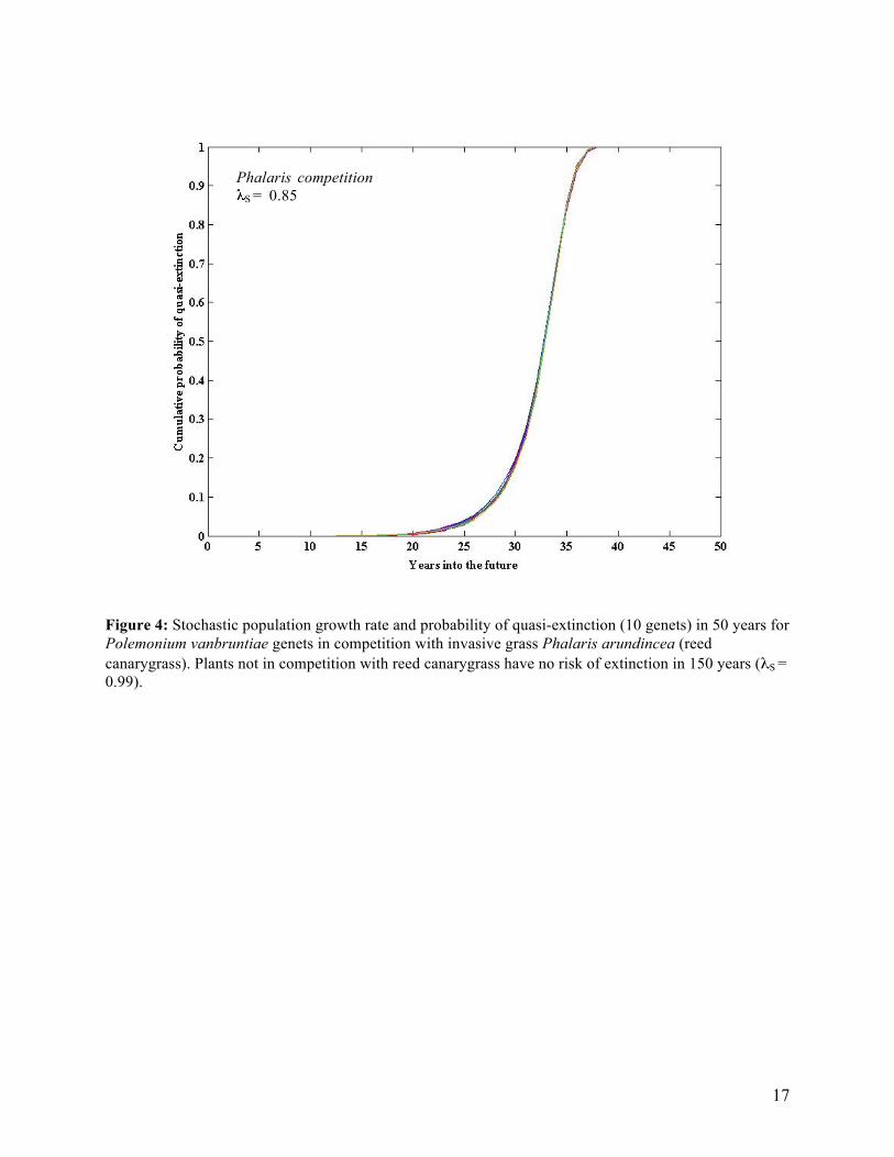
genets/genets/year). The probability of quasi-extinction to 10 genets in 50 years is certain in 17 years under white-tailed deer browsing whereas there is only a 12% probability of extinction in 100 years with no browsing (Table 5). The sites that are being managed for invasive grass Phalaris arundinacea (reed canarygrass, RCG) also have stochastic population growth rates (λS) less than 1, but populations of plants in competition with RCG are significantly more prone to extinction (Figure 4). Populations of genets in competition with RCG have a significantly lower growth rate compared to populations with no RCG (λS = 0.99 no RCG; λS = 0.85 with RCG). These stochastic growth rates translate into a decline of 0.17 genets/genets/year (with RCG) and a decline of only 0.01 genets/genet/year (no RCG). The probability of quasi-extinction to 10 genets in 50 years is certain in 43 years when AJL is in competition with RCG. There is no risk of extinction in populations with no RCG (Table 5). The population of plants under an open-canopy at site FR has the highest population growth rate in this study (λS = 1.43); therefore, canopy-cover is significantly adding to the decline of AJL populations (Figure 5). The stochastic population growth rate (λS) for genets under a closed canopy is significantly lower (λS = 0.95 or a decline of 0.05 genets/genets/year) compared to genets under an open canopy (λS = 0.1.43 or an increase of 0.36 genets/genets/year). There is a 100% probability of quasi-extinction to 10 genets in 79 years under a closed canopy, but extinction can be completely subverted if the woody vegetation is removed from AJL populations (Table 5). There is a significant “proximity to road” effect as plants nearby the road are predicted to decline in the future, whereas plants not effected by roads are expected to increase in the future. The “road” factor is a correlation between road management impacts (i.e, mowing, grading, etc.) and AJL population persistence. Proximity to road significantly decreases the population growth rate of AJL, as the stochastic population growth rate (λS) for genets close to the road is 0.80, whereas λS = 1.19 for genets not impacted by road management (Figure 6). The stochastic growth rates translate into a decline of 0.2284 genets/genets/year (road impacts) and an increase of 0.1703 genets/genet/year (no road impacts). There is a 98% probability of quasi-extinction to 10 genets in 50 years for genets impacted by the road and no risk of extinction for genets not impacted by road management (Table 5). The North Branch susbpopulation F site is being analyzed for a purplestem aster effect In other words, what is the effect on AJL population persistence if purplestem aster, Symphyotrichum puniceum, is removed? As of August 2010, this site has only 9 remaining genets in the 2 grids (1 grid with aster, 1 without), although the original sample included 23 AJL genets. Four small genets existed in the grid where asters are removed from the roots at the beginning of the experiment in 2008. As of August 2010, only 1 AJL remains alive in the “no aster” grid (a 75% decline over 2 years). As of 2008, we mapped 18 small genets and 1 medium-sized genet in the “with aster” grid. As of August 2010, only 8 remain alive in the “with aster” grid (a 58% decline over 2 years). The small sample size and uneven distribution of life-history stages (95% of genets are small, only 1 medium-sized genet is represented) makes the population matrix model unfit for the simulations. However, the precipitous rate of decline is obvious in the numbers collected from 2008-2010. Although prediction modeling was impossible with the current life history model due to the small sample size at site NBF, the picture is clear; the population is experiencing rapid declines and is sure to be extinct in the near future. Other small AJL subpopulations have gone extinct, including Blue Banks subpopulations A and B along the Natural Turnpike, and this seems to be the case for site NBF. However, I would pinpoint the

6

major source of decline as an extremely small population confounded by limited sunlight due to dense canopy cover, rather than competition with the purplestem aster. The study allows me to analyze the impact of both excluding deer and opening the canopy, as there are plants at site FR under both treatments (i.e., deer exclusion/open-canopy). This population includes 38 genets followed for 2 annual transitions. Out of 38 genets, 32 survived to 2010, which translates into an 84% survival rate. Together, these 2 management strategies increase the population growth rate most significantly (λS = 1.51 or an increase of 0.4115 genets/genet/year), pinpointing canopy-opening plus deer exclusion as the best management strategy for AJL. Conclusions: The implications of this study are stark – the major threats to Appalachian Jacob’s ladder (Polemonium vanbruntiae) are, in order of significance, canopy-cover, road management practices, invasive species, and white-tailed deer herbivory. In addition, there is less than 50 years to circumvent extinction of populations existing under these scenarios. I demonstrate that a multi-faceted approach (i.e., opening the canopy and excluding deer) is the best management strategy for increasing population growth rates and avoiding certain extinction. However, I must express caution, because this study only includes 2 annual transitions. Thus, the study only gives us a glimpse into the long-term trends of AJL populations. Studies have shown that population viability analyses are best informed with 5+ years of data (Menges, 2000). Two more years of funding from the USDA Forest Service would accomplish this goal of a 5-year study on population dynamics of AJL under various management scenarios. However, I also cannot hesitate to recommend that management begin promptly under the extinction scenarios presented in these models. Management recommendations: Canopy-opening— Canopy-cover has the most significant impact on AJL populations. Selective cutting has already occurred at one-half of site FR in 2007 under the auspices of Diane Burbank. I recommend cutting the remaining one-half of the population at site FR, as the results indicate an extremely positive effect on population growth while eliminating any risk of extinction. Canopy cover is certainly impacting other AJL sites within the GMNF, including site NBF, so I recommend selectively cutting here as well. I also suggest surveying all known GMNF populations of AJL in 2011 for canopy-cover effects, as this is a straightforward, one-time management regime that will have lasting, positive effects on future persistence of AJL. Road impacts— I recommend working more closely with the GMNF and Ripton town road crews to minimize road impacts to AJL populations. Signage would be perhaps a noticeable means of alerting crews to the presence of AJL along the forest roads. It is difficult to pinpoint which road management practices are causing the declines, so I also recommend introducing new plants to areas within the population that are not impacted by road (e.g., experimental “no road” grids are placed ~4 m from roadside). I recommend either gathering seeds from natural populations or experimenting with taking clones of AJL, and raising plants in a greenhouse or nursery, because medium and large genets have the highest survival rate, whereas seedlings and small genets exhibit high mortality. After 2+ years of growth in the greenhouse or nursery, volunteers can transplant these plants into the field under the supervision of the GMNF. Perhaps the New England Wildflower Society would be willing to raise plants to facilitate this planting

7

effort, or I can raise plants if I can secure funding to rent greenhouse space. In addition, seeds should be gathered from natural populations of AJL at a regular interval for safe keeping in the seed bank at the NEWFS to provide a buffer if AJL populations do go extinct, as predicted. Reed canarygrass (Phalaris arundinacea)— The model predictions indicate that reed canarygrass (Phalaris arundinacea) is significantly, negatively impacting populations of AJL, and is, in fact, a major force of extinction. Reed canarygrass is an aggressive wetland invader that decreases native species diversity and exacerbates extinction risk of rare plants (Green and Galatowitsch 2002). The spread of invasives can have severe implications for the diversity of natural communities, such as those harboring AJL. It is well known that native species may face much higher extinction rates when competing with invasive grasses (Williams and Crone 2006). Invasive species removal is a major focus of the GMNF, but the focus has been on invasive species other than RCG. I recommend shifting the focus toward removing RCG, especially at roadside sites BBC and BBD along the Natural Turnpike (FR 54). RCG eradication methods— RCG responds variably to herbicides, but it is unknown what effect herbicides would have on AJL and other native plants in these populations. That said, Glyphosate, Amitrol, Dalapon, and Paraquat have all been tried on RCG with some success, and maximum control depends on the timing of application (Apfelbaum and Sams 1987). However, reed canarygrass can recolonize an herbicide-treated area from seed bank recruitment (White et al. 1993). Mechanical removal also shows limited success as rapid regrowth occurs from rhizomes and seeds that remain in the soil even after tillers are mechanically removed. Cutting back plants at ground level and covering them with opaque black plastic can reduce, but not eliminate populations (Apfelbaum and Sams 1987). Mowing may be a valuable control method, since it removes seed heads before seed maturation and exposes the ground to light, which promotes the growth of native species, but it would be problematic to mow only RCG within AJL populations. However, studies in Wisconsin indicated that twice-yearly mowings (in early to mid-June and early October) led to increased numbers of native species in comparison to reed canarygrass-infested plots that were not mowed (Gillespie and Murn 1992). White-tailed deer herbivory— White-tailed deer repeatedly browse AJL at sites BBG, FR, and NBL, and browsing has significant negative effects on future population growth. Therefore, I recommend erecting deer-exclusion fences to exclude deer from the whole AJL population to remove the browsing pressure. Some sites will be much more conducive to deer-exclusion fencing. For example, all AJL plants at sites FR and BBG occur in a discrete area, so this clumped spatial distribution will facilitate fencing while translating into a big positive impact on AJL persistence. However, AJL is sporadic at site NBL, which is also a large site, so I anticipate difficulties and a significant amount of money to fence the entire NBL population. Therefore, I recommend using smaller fences to exclude deer from significantly large clumps of AJL at this site. Management recommendations summary

• Remove reed canarygrass mechanically on an annual basis while minimizing new introductions

• Protect whole populations from deer by erecting fencing (sites especially conducive to fencing include FR and BBG)

8

• Selectively cut woody vegetation to open the canopy, especially at sites FR, NBF, and other sites not included in this analysis (e.g., Abbey Pond, other North Branch subpopulations, etc.)

o canopy-opening and deer exclusion can be effectively combined at site FR • Introduce new 2+ year old individuals at existing sites, especially roadside populations,

while searching for new reintroduction sites Note: I would like to be informed of any management that will take place within AJL sites beforehand so I can plan my field work and data analysis accordingly. I would also like to be of assistance implementing the management regimes that the Forest Service would like to pursue. II. Predictive habitat modeling - A spatial analysis indicating potential locations of new populations of Appalachian Jacob’s ladder based on habitat characteristics A. Introduction The purpose of the GIS analysis is to locate suitable habitat areas for AJL within the Green Mountain National Forest (GMNF) based on several parameters. The map will serve as a template for which to search for undiscovered populations of this rare plant within the north-half region of the GMNF. To do this, I created a habitat suitability model using ArcGIS (v. 9.3) with various habitat parameters in order to locate areas within the GMNF where AJL is most likely to occur. B. Habitat model parameterization Data Layers The following data files were acquired from various sources for use in this analysis:

• The projected coordinate system is NAD 1983 State Plane for all data layers • VermontElevationDEM_DEM24 is a raster dataset containing elevation for the State of

Vermont. These data were downloaded from VCGI website. • WaterWetlands_VSWI contains NWI maps used by the State of Vermont Agency of

Natural resources. Nearly 66% of the wetlands were hand digitized from RF 24000 scale NWI mylars. The remainder of the state was scanned from RF 24000 or RF 25000 scale mylars. Mylars were created by transferring wetland polygon boundaries from RF 62500 scale NWI mylars to RF 24000 scale base maps. These data were also downloaded from VCGI website.

• GeologicSurficial_Surficial62K shows surficial geology features for the state of Vermont and were downloaded from VCGI website.

• GMNF Management boundaries (ENVIRON_MAREA2004_POLY layer) contained all land within the Green Mountain National Forest and were downloaded from VCGI website.TOURISM_GMNFTRAILS_ROUTE_ROAD was used to map the existing Forest Roads within the GMNF for orientation.

• BOUNDARY_CNTYBNDS_POLY was downloaded from VCGI website and used to map VT counties for orientation.

9

• Existing Polemonium vanbruntiae population shapfiles were provided by Jodi Shippee at the State of Vermont Nongame and Natural Heritage Program.

GIS Analysis To begin, the GMNF management area layer from ENVIRON_MAREA2004_POLY layer was used as my basemap. This was used throughout the analysis to clip data to the study area within the north half region of the Green Mountain National Forest (GMNF). I added the roads and trails layer and labeled these features for orientation. I then added the county map layer, clipped this layer to the GMNF and labeled the VT counties for orientation purposes. I began the analysis with elevation by adding the raster elevation layer to ArcMap. Optimal elevation for AJL is between 1000' and 2000,’ so I utilized the raster calculator in the Spatial Analyst toolbar to query elevation > 1000' and < 2000.' I then reclassified these data, removing all the “0's” from the output and converted “raster to feature” to convert into polygons. I saved this as the “elev_reclassify” layer. I then clipped the layer using ‘GMNF.’ This created a layer named ‘Optimal_Elevation_Clip.’ I then added the layer “Geologic_SURFICIAL62K_poly” and selected by attribute for swamp/peat/muck AND till, because P. vanbruntiae grows exclusively in swampy area with muck and peat soils and also in areas of glacial till. I only selected rows with the following till type: “till mantling the bedrock and reflecting the topography of the underlying bedrock surface. Thicker in the valleys and thinner in the uplands. On many exposed uplands postglacial erosion has left only rubble and scattered boulders on bedrock.” I saved the selection as a layer file, then clipped this layer to the GMNF north-half and named it ‘Muck_Till_Clip’. Next, I added the layer ‘WaterWetlands_VSWI” which contains all significant Vermont wetlands, many of which occur within the north-half GMNF. I clipped this layer to ‘GMNF’ and renamed it ‘Wetlands_Clip’. I then added the shapefile containing x-y coordinate points for all existing AJL populations in the GMNF from the State of Vermont. There is evidence that P. vanbruntiae displays a clumped spatial distribution as plants are dispersal limited and all GMNF populations occur within ~10km of one another. Therefore, this layer is useful for predicting where new populations may occur within the GMNF. After these steps were accomplished, an intersect command was used to intersect ‘Optimal_Elevation_Clip’, ‘Muck_Till_Clip’, and ‘Wetlands_Clip’ layers. This created a layer (‘Intersect_OEC_MTC_WC’) that displayed areas of the northhalf GMNF where all of these features occur concurrently. I then designated conservation priorities for these areas based on the areas of potential sites by selecting by attribute (area) and created new layers for 13 sites that had the largest total area. See the annual report from 2009 for maps of all 13 priority sites. More effort needs to be given to the GIS spatial modeling component of this cooperative contract agreement. It was assumed that volunteers would assess these priority sites in 2010, but this work did not get completed by the end of the field season. It is necessary to field check the model, as I am fairly confident that we will have to make changes to the habitat model to further refine our ability to pinpoint areas of new, undiscovered populations. Visiting the 13 priority sites will help me to determine whether the model needs to be refined, and, if so, how. Pending funding or volunteer efforts, I plan to field check the 13 priority sites in summer 2011 and the model will be refined based on the findings in the field.

10

References Apfelbaum, S.I. and C.E. Sams. 1987. Ecology and control of reed canarygrass (Phalaris

arundinacea L.). Natural Areas Journal, 7: 69-74. Caswell, H. 2001. Matrix population models: Construction, analysis, and interpretation, 2nd

edition. Sinauer, Sunderland, Massachusetts. Gillespie, J. and T. Murn. 1992. Mowing controls reed canarygrass, releases native wetland

plants (Wisconsin). Restoration and Management Notes, 10: 93-94. Ginzburg, L.R., Slobodkin, L.B., Johnson, K., Bindman, A.G. 1982. Quasiextinction

probabilities as a measure of impact on population growth. Risk Analysis 2, 171-181. Green and Galatowitsch. 2002. Effects of Phalaris arundinacea and nitrate-N addition on the

establishment of wetland plant communities. Journal of Applied Ecology, 39: 134-144. Knight, T.M. 2004. The effects of herbivory and pollen limitation on a declining population of

Trillium grandiflorum. Ecological Applications, 14, 915–928. Menges, E.S. 2000. Population viability analyses in plants: challenges and opportunities. Trends

in Ecology and Evolution, 15 (2): 251-56. Morris W.F. and Doak D.F. 2002. Quantitative Conservation Biology: Theory and Practice of

Population Viability Analysis. Sinauer, Sunderland, Massachusetts. White, D.J., E. Haber, and C. Keddy. 1993. Invasive plants of natural habitats in Canada.

Canadian Wildlife Service, Ottawa, ON.

Williams J.L. and Crone E.E. 2006. The impact of invasive grasses on the population growth of Anemone patens, a long-lived native forb. Ecology, 87, 3200–3208.

11

Table 1: Appalachian Jacob’s ladder experimental site locations and site abbreviations within the Green Mountain National Forest Appalachian Jacob’s ladder site and location Site abbreviation Management influence Blue Banks Brook subpopulation C, along FR 54, Lincoln

BBC forest road maintenance, invasive reed canarygrass*

Blue Banks Brook subpopulation D, along FR 54, Lincoln

BBD forest road maintenance, invasive reed canarygrass*

Blue Banks Brook subpopulation E, along FR 54, Lincoln

BBE small site, continued monitoring

**Blue Banks Brook subpopulation G, behind Spruce Lodge, FR 54, Lincoln

BBG white-tailed deer herbivory, potential timber-harvesting

North Branch River subpopulation F, intersection of FR 235 & Lincoln-Ripton Rd., Ripton

NBF purple-stem aster competition

North Branch River subpopulation E, along the Lincoln-Ripton Rd., Ripton

NBE roadside mowing and grading (town-maintained highway)

North Branch River subpopulation L, in wetland hikeable from FR 235A, Ripton

NBL white-tailed deer herbivory

Forest Rd. 233 reintroduction site, in wet swale off FR 233, Ripton

FR canopy-cover, white-tailed deer herbivory

* Phalaris arundinacea ** site located on non-GMNF land

Table 2: Population vectors used to parameterize model simulations

Site(s) Treatment Population vector n0 Initial population size (# genets)*

NBE, BBD, BBC Road [745; 21877; 368; 29; 33] 23052 NBE, BBD, BBC No road [745; 21877; 521; 83; 61] 23287 FR, NBL, BBG Browse [96; 1116; 122; 58; 43] 1435 FR, NBL, BBG No browse [96; 1116; 154; 52; 37] 1455 BBC/BBD Phalaris/no

Phalaris [745; 21877; 209; 21; 5] 22857

FR Open canopy [96; 1116; 100; 60; 62] 1434 FR Closed canopy [96; 1116; 108; 57; 57] 1434 * includes an estimate of seeds in the seed bank and seedlings

12

Table 3: Description and abbreviations for P. vanbruntiae vital rates. Stages: 1 = seed; 2 = seedling; 3 = small genet (1-2 ramets); 4 = medium genet (3-4 ramets); 5 = large genet (5+ ramets).

Vital rate abbreviations

Vital rate description

s1 Seeds surviving the 8-month overwinter period in the soil

s2 Seedling survival

s3 Small genet survival

s4 Medium genet survival

s5 Large genet survival

g11 Seeds that do not germinate and remain viable in the seed bank

g21 Proportion of seeds that survived the winter in the soil and germinated

g32 Seedling-to-small genet transition given winter seedling survival

g33 Survival and stasis of small genets

g43 Small genet to medium genet transition

g53 Small genet to large genet transition, skipping the medium genet stage

g44 Survival and stasis of medium genets

g54 Growth from a medium to large genet

g45 Regression of large genets to the medium genet stage

g35 Regression of large genets to the small genet stage

g45 Regression of large genets to medium genet stage

g55 Survival and stasis of large genets

f3 + f4 + f6 Average seed set of small, medium, and large genets

13

Table 4: Matrix population model parameters and equations for the calculation of matrix elements from the underlying survival (sj), growth (gij), and fertility (fj) rates. The subscripts represent placement of the matrix element in the matrix, represented by row, column (i.e., F1,5 is the fecundity value in row 1, column 5).

Seed

Seedling

Small genet

Medium

genet

Large genet

Seed

P1,1 = s1 ×

(1 – g21) × g11

0

0

0

F1,5 =

(f3 + f4 + f5) × s1 × (1 – g21) × g11

Seedling

P2,1 =

s2 × g21 × (1 - g11)

0

0

0

F2,5 =

(f3 + f4 + f5) × s2 × g21 ×

(1 - g11)

Small genet 0

P3,2 =

s2 × g32

P3,3 =

s3 × g33

P3,4 =

s4 × g34

P3,5 =

s5 × g53

Medium

genet

0

0

P4,3 =

s3 × g43

P4,4 =

s4 × g44

P5,4 =

s5 × g54

Large genet

0

0

P5,3 =

s3 × g53

P4,5 =

s4 × g54

P5,5 =

s5 × g55

14

Table 5: Stochastic population growth rates and probability of extinction for all AJL sites under management in the Green Mountain National Forest. Populations with growth rates less than 1 are generally prone to extinction in the near future.

Site Treatment Stochastic population growth rate (λS)

Probability of extinction in 50 years

NBE, BBD, BBC Road 0.80 98% NBE, BBD, BBC No road 1.19 0% FR, NBL, BBG Browse 0.73 100% FR, NBL, BBG No browse 0.96 12% (in 100 years) BBC/BBD Phalaris 0.85 100% BBC/BBD No Phalaris 0.99 0% FR Open canopy 1.43 0% FR Closed canopy 0.95 100% (in 100 years)

15

Figure 2: Life cycle of Polemonium vanbruntiae genets. Self-loops represent survival and stasis, double-arrows represent either growth or regression in life history stage. Arrows pointing to the seed and seedling stage represent fertility (i.e., contributing seeds to the seed bank or seeds that germinate and become seedlings).

Figure 1: All ramets within the 0.5m2 experiment grids are mapped with x-y coordinates. Green circles represent individual ramets. The 3 green circles enclosed in the red circle indicate that a physical connection was detected among these 3 ramets, and so they are considered a genet (i.e., clonal fragment).

16

Figure 3: Stochastic population growth rate (λS) and probability of quasi-extinction (10 genets) in 100 and 50 years, respectively for Polemonium vanbruntiae genets (A) protected from white-tailed deer browsing (Odocoileus virginianus), and (B) browsed by deer.

A

B

No browse λS = 0.96

Browse λS = 0.73

17

Figure 4: Stochastic population growth rate and probability of quasi-extinction (10 genets) in 50 years for Polemonium vanbruntiae genets in competition with invasive grass Phalaris arundincea (reed canarygrass). Plants not in competition with reed canarygrass have no risk of extinction in 150 years (λS = 0.99).

Phalaris competition S = 0.85

18

Figure 5: Stochastic population growth rate and probability of quasi-extinction (10 genets) in 50 years for Polemonium vanbruntiae genets under a closed canopy (i.e., shade). Plants under an experimentally opened canopy (i.e., sun) have no risk of extinction in 150 years (λS = 1.43).

Closed-canopy λS = 0.95

Closed canopy λS = 0.95

19

Figure 6: Stochastic population growth rate and probability of quasi-extinction (10 genets) in 50 years for Polemonium vanbruntiae genets impacted by forest road management (i.e., mowing, grading, culverts, etc.). Genets not influenced by forest road management have no risk of extinction in 150 years (λS = 1.19).

Road impacts λS = 0.80

20

Appendix I (A) Sun/no browse transition matrices

2008-2009 Seed Seedling Small genet Medium genet Large genet

Seed 0.004 0 0 0 0.131 Seedling 0.144 0 0 0 17.27

Small genet 0 0.471 0.352 0 0 Medium

genet 0 0

0.175 0.495 0 Large genet 0 0 0.070 0.331 1

2009-2010

Seed Seedling Small genet Medium genet Large genet Seed 0.004 0 0 0 0.143

Seedling 0.144 0 0 0 18.87 Small genet 0 0.471 0.54 0.455 0

Medium genet

0 0 0.18 0.273 0.545

Large genet 0 0 0.09 0.273 0.455

21

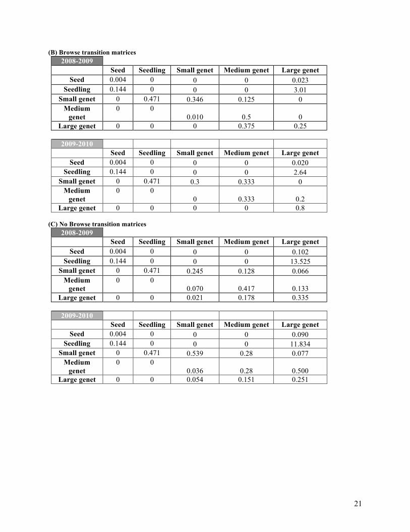
(B) Browse transition matrices 2008-2009


Seedling 0.144 0 0 0 3.01 Small genet 0 0.471 0.346 0.125 0

Medium genet

0 0 0.010 0.5 0

Large genet 0 0 0 0.375 0.25


Seed 0.004 0 0 0 0.020 Seedling 0.144 0 0 0 2.64

Small genet 0 0.471 0.3 0.333 0 Medium

genet 0 0

0 0.333 0.2 Large genet 0 0 0 0 0.8

(C) No Browse transition matrices


Seed 0.004 0 0 0 0.102 Seedling 0.144 0 0 0 13.525

Small genet 0 0.471 0.245 0.128 0.066 Medium

genet 0 0

0.070 0.417 0.133 Large genet 0 0 0.021 0.178 0.335

2009-2010


Seedling 0.144 0 0 0 11.834 Small genet 0 0.471 0.539 0.28 0.077

Medium genet

0 0 0.036 0.28 0.500

Large genet 0 0 0.054 0.151 0.251

22

(D) Sun (open-canopy) transition matrices 2008-2009


Seedling 0.144 0 0 0 17.265 Small genet 0 0.471 0.286 0 0.000

Medium genet

0 0 0.143 0.424 0.000

Large genet 0 0 0.057 0.424 1.000


Seed 0.004 0 0 0 0.143 Seedling 0.144 0 0 0 18.867


genet 0 0

0.182 0.164 0.411 Large genet 0 0 0.091 0.164 0.478

(E) Shade (closed-canopy) transition matrices


Seed 0.004 0 0 0 0.044 Seedling 0.144 0 0 0 5.764


genet 0 0

0.045 0.538 0.222 Large genet 0 0 0.045 0.033 0.667

2009-2010



Medium genet

0 0 0.000 0.250 0.375

Large genet 0 0 0.083 0.250 0.625

23

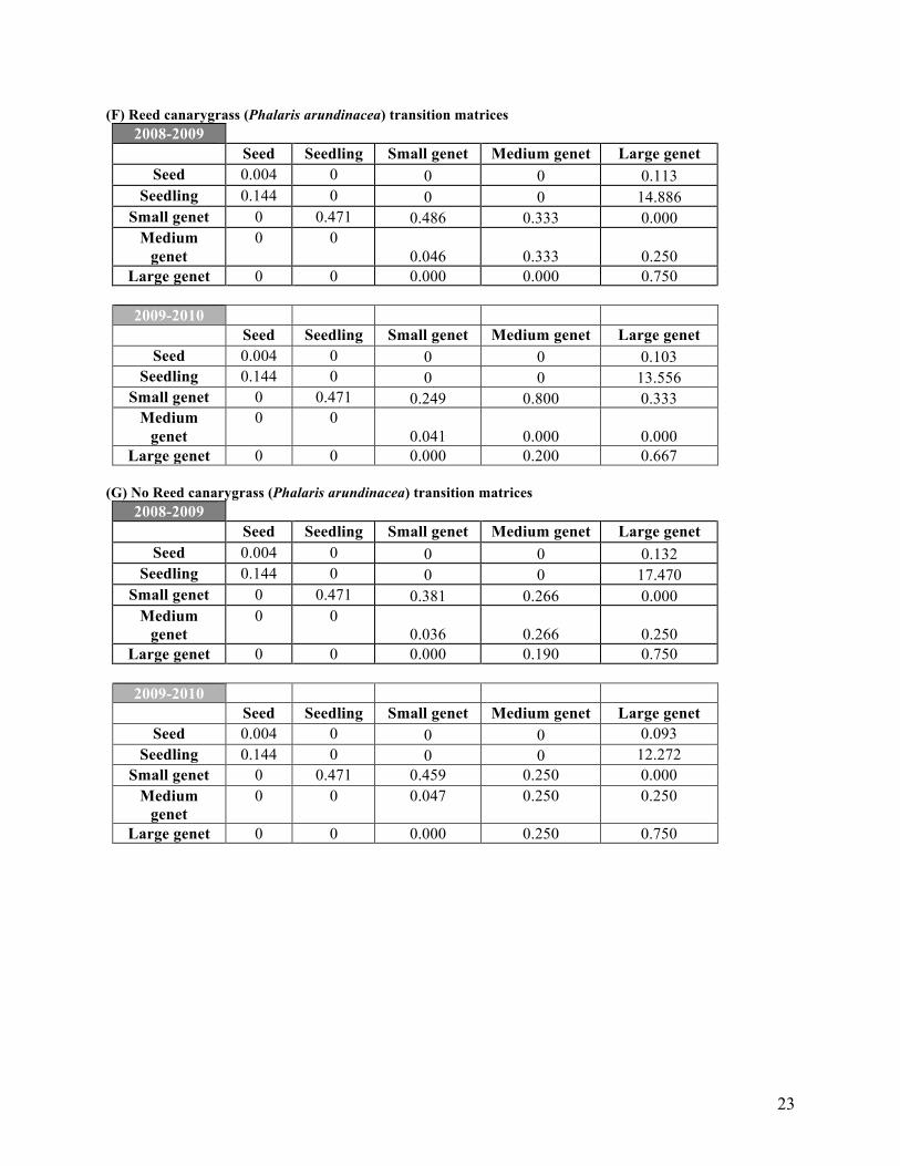
(F) Reed canarygrass (Phalaris arundinacea) transition matrices 2008-2009



Medium genet

0 0 0.046 0.333 0.250

Large genet 0 0 0.000 0.000 0.750


Seed 0.004 0 0 0 0.103 Seedling 0.144 0 0 0 13.556


genet 0 0

0.041 0.000 0.000 Large genet 0 0 0.000 0.200 0.667

(G) No Reed canarygrass (Phalaris arundinacea) transition matrices


Seed 0.004 0 0 0 0.132 Seedling 0.144 0 0 0 17.470


genet 0 0

0.036 0.266 0.250 Large genet 0 0 0.000 0.190 0.750

2009-2010



Medium genet

0 0 0.047 0.250 0.250

Large genet 0 0 0.000 0.250 0.750

24

(H) No road transition matrices 2008-2009



Medium genet

0 0 0.040 0.250 0.333

Large genet 0 0 0.000 0.500 0.667


Seed 0.004 0 0 0 0.141 Seedling 0.144 0 0 0 18.645


genet 0 0

0.051 0.250 0.250 Large genet 0 0 0.051 0.250 0.750

(I) Road transition matrices


Seed 0.004 0 0 0 0.126 Seedling 0.144 0 0 0 16.682


genet 0 0

0.028 0.245 0.000 Large genet 0 0 0.019 0.320 0.747

2009-2010



Medium genet

0 0 0.017 0.222 0.167

Large genet 0 0 0.000 0.000 0.120

I. The influence of forest management activities on …lhill/AnnualReport2010.pdf · The influence...

Documents

Transcript of I. The influence of forest management activities on …lhill/AnnualReport2010.pdf · The influence...