I N L Credit Risk Calibration E based on CDS Spreads B...
41
SFB 649 Discussion Paper 2014-026 Credit Risk Calibration based on CDS Spreads Shih-Kang Chao* Wolfgang Karl Härdle* Hien Pham-Thu* * Humboldt-Universität zu Berlin, Germany This research was supported by the Deutsche Forschungsgemeinschaft through the SFB 649 "Economic Risk". http://sfb649.wiwi.hu-berlin.de ISSN 1860-5664 SFB 649, Humboldt-Universität zu Berlin Spandauer Straße 1, D-10178 Berlin SFB 6 4 9 E C O N O M I C R I S K B E R L I N
Transcript of I N L Credit Risk Calibration E based on CDS Spreads B...

S F
B XXX
E
C O
N O
M I
C
R I
S K
B
E R
L I
N
SFB 649 Discussion Paper 2014-026
Credit Risk Calibration based on CDS Spreads
Shih-Kang Chao* Wolfgang Karl Härdle*
Hien Pham-Thu*
* Humboldt-Universität zu Berlin, Germany
This research was supported by the Deutsche
Forschungsgemeinschaft through the SFB 649 "Economic Risk".
http://sfb649.wiwi.hu-berlin.de
ISSN 1860-5664
SFB 649, Humboldt-Universität zu Berlin Spandauer Straße 1, D-10178 Berlin
SFB
6
4 9
E
C O
N O
M I
C
R I
S K
B
E R
L I
N
Credit Risk Calibration based on CDS Spreads∗
Shih-Kang Chao†, Wolfgang Karl Hardle‡§, Hien Pham-Thu¶,
May 9, 2014
Abstract
As observed in the financial crisis, CDS spreads tend to increase simutaneously as
a reaction to common shocks. Focusing on the spillover effects triggered by extreme
events, we propose a credit risk analysis tool by applying credit default swap spread
returns to the concept of 4CoVaR suggested by Adrian and Brunnermeier (2011).
The interconnection and mutual impact on credit spreads are investigated based on
CDS spreads of the biggest derivative dealers in the market. By including factors
identified as determinants of CDS spreads to the set of explanatory variables such as
equity return and equity volatility and implementing the variable selection technique
least absolute shrinkage and selection operator (LASSO), the results demonstrate an
improved performance in CDS spread VaR calculation. The enhancement is more
significant in pre-crisis period but both methodologies tend to overestimate risk in
turbulent period. Further, non-linear effects between CDS spreads in extreme events
are captured by the introduction of a partial linear model in the CoVaR calculation.
JEL: G12, G13, G23
Keywords: CDS, VaR, CoVaR, stressed VaR, Central Counterparty, Quantile Regression
∗Financial support from the Deutsche Forschungsgemeinschaft (DFG) via SFB 649 ”Economic Risk”and International Research Training Group (IRTG) 1792 are gratefully acknowledged.†Ladislaus von Bortkiewicz Chair of Statistics, C.A.S.E. - Center for applied Statistics and Eco-
nomics, Humboldt-Universitat zu Berlin, Unter den Linden 6, 10099 Berlin, Germany. Email: [email protected]‡Ladislaus von Bortkiewicz Chair of Statistics, C.A.S.E. - Center for applied Statistics and Economics,
Humboldt-Universitat zu Berlin, Unter den Linden 6, 10099 Berlin, Germany. Email: [email protected]§School of Business, Singapore Management University, 50 Stamford Road, Singapore 178899, Sin-
gapore.¶Ladislaus von Bortkiewicz Chair of Statistics, C.A.S.E. - Center for applied Statistics and Eco-
nomics, Humboldt-Universitat zu Berlin, Unter den Linden 6, 10099 Berlin, Germany. Email: [email protected]
1

1. Introduction
Nowaday derivatives are standard elements of the financial market and cover a wide
variety of products. There are listed derivatives such as exchange traded futures and
options but also over-the-counter (OTC) products such as forwards or swaps traded
bilaterally by financial institutions, fund managers, and corporate treasurers. The flex-
ibility of OTC derivatives in the area of hedging and risk management, price discovery
and enhancement of liquidity is one of the reasons for the fast growth of these prod-
ucts in the market (Acharya et al. (2009)). Since the financial crisis unfolded several
vulnerabilities in OTC trading (lack of transparency, interconnectedness and change in
counterparty credit risk) regulators advocate for the clearing of OTC derivative trans-
actions through central counterparties. This has been legally established in the Dodd-
Frank Wall Street Reform and Consumer Protection Act of 2010 for the United States
of America (SEC (2010)) and regulatory adopted by the European Parliament and The
Council (ESMA (2013)). The Basel Committee supports this attempt by offering in-
centives for centrally cleared OTC derivative transactions through counterparty credit
risk reforms under Basel III framework (BIS (2011)). The main objective of these acts
are to centrally control the counterparty credit risk of those trades and to anticipate
systemic risk mitigation. This regulation is facing two main challenges. One is the
implementation of standardized contractual terms and operational processes. A legal
standardisation is important for netting and effective risk management whereas opera-
tional standardisation of trade terms is vital for setting initial and variation margins.
The second challenge is an appropriate counterparty credit risk allocation for an ade-
quate risk controlling. A mapping of risk contribution to individual counterparties has
two main enhancements. Firstly, it provides further information how the default or dis-
tress of one bank impacts the system. Secondly, it reduces the incentive for risk-seeking
behavior and fosters effective risk monitoring.
The recent financial crisis and its aftermath disclose the boost in interconnectedness
within financial market participants. High correlation among financial firms can usually
be explained by simultaneous response to common risk factors. Moreover, in stressed
period market participants are engaged progressively in ”flight to quality” when market
participants are forced to reduce risk and invest in securities with good credit ratings.
Further, the increased trading of derivatives contributes to the high sensitivity to coun-
terparty credit risk in the financial industry. Thus, mutual impacts play an important
role within the system. As a consequence, monitoring of individual risk is not suffi-
cient and systemic risk contribution needs to be considered. The interconnection and
2

externality effects of financial institutions have already been examined by Acharya et al.
(2010), Adrian and Brunnermeier (2011), Hautsch et al. (2013), Brownlees and En-
gle (2010) or Dullmann and Sosinska (2007), Upper and Worm (2004) with focus on
the German banking sector. Further, the Basel Committee on Banking Supervision in-
cluded supplementary methodology in December 2011 to identify systemically important
banks (Global Systemically Important Banks (G-SIBs)). The assessment methodology is
based on five categories: size, interconnectedness, substituability, cross-border activity,
and complexity of the bank.
In this paper we propose a macro-prudential view from a central counterparty’s
perspective. This research is focused on the measurement of spillover effects of credit
risk by using credit default swaps spreads as a proxy for credit risk. The scope of our
work is the analysis of counterparty credit risk effects of a distressed counterparty on
other market members. This requires the study of ’tail events’ given that one of the
market participants is in stress. Quantitatively speaking this falls into the category of
VaR (value at risk) and more precisely conditional value at risk. Therefore, we employ
CoVaR of Adrian and Brunnermeier (2011). It denotes the maximum loss in time t+ d
which will only be exceeded under a confidence level of τ , where 0 < τ < 1. This measure
is expressed statistically by the τ -quantile of the conditional distribution of returns
VaRτt+d = inf {x ∈ R : P(Xt+d ≤ x | Ft) ≥ τ} , (1)
where Ft is the information set up to time t.
The CoVaR is defined as the VaR of an institution j conditional on an event of
institution i denoted by C(Xi).
Pr{Xj ≤ CoVaRj|C(Xi)
τ | C(Xi)}
= τ. (2)
Subsequently, the systemic contribution of each institution is determined by the delta
CoVaR (4CoVaR) level conditional on the median state of the institution and the status
where the institution is under distress
4 CoVaRj|iτ = CoVaRj|Xi=VaRiτ
τ −CoVaRj|Xi=Medianτ (3)
This quantity exhibits the marginal contribution of individual financial institutions to
the remainder within the system. The benefit in applying 4CoVaR measure is versatile.
The main advantage lies in its ability to reflect the effect of the distress of one individual
3

institution on another firm based on the stand-alone risk level. In addition, 4CoVaR
is effective for the identification of systemically relevant counterparties. This measure
reflects the concept of the ”stressed VaR” proposed by Basel Committee to supplement
the VaR framework - a risk measure of stand-alone risk under extreme and volatile mar-
ket conditions.
In order to capture credit risk properly we add further variables which are identi-
fied to have major impact on CDS spreads including variables at firm level. Since this
inclusion greatly inflates the number of variables, multicollinearity or strong correlation
between covariates might cause inadequate error in the estimation results of the regres-
sion. Therefore, we apply least absolute shrinkage and selection operator (LASSO) as a
simple variable selection technique to overcome this problem. As the proposed method
generates less exceedance in backtesting our method improves the performance in the
VaR prediction in comparison to the earlier methodology.
Corresponding to Espinosa et al. (2013) we discover that the most relevant coeffi-
cients for CDS spreads VaR are the VIX and the liquidity spread. The LASSO technique
reveals that CDS spread returns can be mostly solely described by the covariate VIX.
This could result from the fact that market volatility have a high impact on the remain-
ing variables as the CDS spread returns are described by more coefficients when VIX is
excluded from the set of explanatory variables. In contrast to Breitenfellner and Wagner
(2012) we find a predominant negative influence of stock market volatitlity on spread
changes relative to stock market return. The influence increases during the crisis. This
result goes along with the findings from Alexander and Kaeck (2008) for crisis period.
The 4CoVaR from our research reveals that the effect of distress varies between banks
and there are institutions which have a higher effects on their counterparties and there-
fore can be considered as more systemic relevant than others.
The remainder of the paper is organised as follows. The next section introduces the
structure and risk management of a central counterparty. Section 2 provides a short
discussion about the application of CDS spreads in credit risk predictions. Thereafter,
the methodology is introduced and data are described. An empirical anaylsis is given in
section 5. Section 6 concludes and presents further remarks.
4
2. Concept of Central Counterparty
The OTC derivatives market is facing many changes. One of these major changes
is the mandatory clearing of standardized OTC derivatives via central clearing counter-
party (CCP). Standardized OTC derivatives offer pre-determined terms in legal and op-
erational specifications which are provided by the ISDA master agreement ISDA (2013).
A CCP can be seen as a counterparty which interposes itself between the initial counter-
parties of the derivative contract and takes the position as a seller to the original buyer
and the position of a buyer to the original seller. The original bilateral relationship
between the counterparties is then withdrawn. The main benefit of this new structure
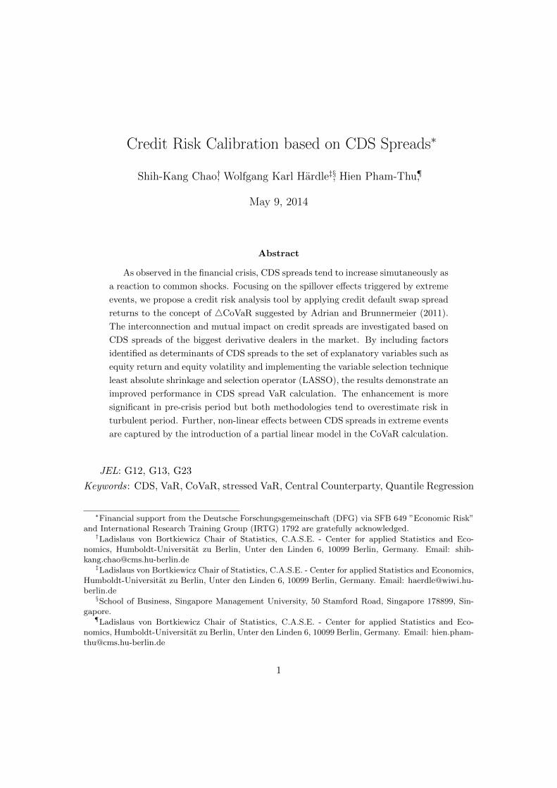
lies in the reduction of the total exposure. In the example shown in figure 1, the total
exposure amounts to 760 without netting. The total exposure is reduced from 760 to
420 in case netting effects are taken into account. Herein, the long and short position
between two counterparties are offset. Multilateral netting further reduces the total ex-
posure of the trades from 420 to 180. It is important to note that the exposure reduces
or increases when there are more than one CCPs which clear different classes of OTC
derivatives (Duffie et al. (2010), Duffie and Zhu (2011), Cont and Kokholm (2013)).
Due to the replacement of the original contract by two new contracts, the posi-
tions with opposite direction are automatically offset and CCP barely faces less market
risk. However, the CCP internalizes counterparty credit risk from its clearing members.
When a counterparty defaults, the CCP has to unwind the defaulted position. In case
replacement costs exceed the deposit collateral the remaining losses are then mutualized
to their clearing members.
Figure 1: Market structure of OTC derivatives market with and without central clearingcounterparty
Currently, CCPs rely on different risk management mechanism such as stringent
membership access, initial margin, variation margin and default fund contribution. Ini-
5

tial margins are deposits required by opening new position and cover the extreme changes
of potential future exposures whereas variation margin is needed to cover daily changes
in mark-to-market value. Default fund contribution is an additional deposit where each
clearing member has to contribute. It represents further buffer in case the occurred losses
exceed the variation and initial margins. However, there still exists a lack of standard in
the risk management mechanism of a CCP (Duffie et al. (2010)). There is a necessity in a
distinct credit risk mapping in the calculation of the default fund contribution based on
the severeness of the spillover effects. As the default fund covers the loss from extreme
events, there is a need to find a stressed risk measure reflecting severe changes in the
credit spreads. Default funds’ relevant losses occur when a counterparty defaults and
losses are not fully covered by deposit collateral. Further, a CCP needs to consider the
mark-to-market changes of derivative trades initiated by distressed derivative dealers.
An application of our work is the identification of credit risk contribution of individual
clearing members to the central clearing counterparty (CCP).
To understand the challenges a CCP faces in the real world, we refer to the insur-
ance corporation American International Group (AIG) as an example. This monoline
was struggling from significant losses in securities lending businesses, mark-to-market
losses on CDS and associated margin calls as a consequence of excessive CDS selling.
Due to lack in liquidity and downgrade by the major rating agencies, AIG could not
fulfill all collateral requirements. In order to avoid spill-over effects caused by AIG’s
bankruptcy, the company was bailed out by the US government. AIG is an example
worth mentioning because it could not fullfil the collateral requirements resulting from
mark-to-market changes in derivatives among other circumstances. As a consequence,
the question arises whether a central counterparty can prevent financial market partici-
pants from such excessive CDS selling and manage the risks implied by distressed market
environment? By offering clearing and settlement procedures, the CCP would be highly
sensitive to counterparty credit risk due to changes in market value and therefore de-
pends on accurate future exposure simulation methods. Therefore, the central clearing
counterparty should put emphasis on the identification of risks triggered by default of a
clearing member and take precautionary measures.
Further discussion of the structure and the risk of central counterparty is to be found
in Pirrong (2011). Economical analysis on the reduction of counterparty credit risk by
introducing a unique CCP is given in Duffie and Zhu (2011). Duffie and Zhu show that
counterparty credit risk can diminish in case there is an unique existing CCP but also
6

point out that multiple CCP might decrease netting opportunities and increase risk.
Arora et al. (2012) support and complement the results provided by Duffie and Zhu
(2011).
3. Data
3.1. Credit Default Swaps Spread and its determinants
Until recently, many papers have been published referring to the evaluation of coun-
terparty risk by using CDS spreads as a proxi for credit risk. A credit default swap
(CDS) is an insurance contract on debt of a reference entity. The buyer of the CDS
receives a payment in case the reference entity defaults and makes a fixed payment (usu-
ally quarterly) to the CDS seller as long as default has not been occurred. The spread
on the reference entity is expressed as a fair premium based on the expected loss given
default and the probability default.
Towards credit risk assessment by rating, CDS spreads are more benificial as they
are traded market indicators for credit risk and react quickly to market events. Further,
they directly reflect the market’s perception of credit risk (Longstaff et al. (2007)) and
express the implied price of risk on the reference entity to a certain extent. This is
illustrated by the soaring CDS spread of AIG during the financial crisis in 2. Another
example is Bear Stearns which was in financial distress from mid February until mid
March in 2008. In mid February, the spread of a CDS on Bear Stearns’ senior unsecured
debt with 5 year maturity was located at 100 basis points. In mid March, it rose to
almost 250 basis points. When the crisis by Bear Stearns was solved through its sale to
JP Morgan Chase arranged by the Fed, the spreads reverted within a month to its mid-
February levels. This example taken from Acharya and Subrahmanyam (2008) shows
the impacts of distress and new information on CDS spreads movements. In addition,
it also reveals the relevant impact of liquidity risk. The scarcity of CDS seller could
also lead to high CDS spreads which automatically increases the concentration on the
market. CDS spreads not only reflect the credit risk of the underlying entity, but also
include the credit risk of the counterparty providing the protection.
Our research raises the question how to forecast CDS spreads and how to quantify
the effect of correlation within a portfolio of CDS. By using the macro variables observed
in the market, we are able to analyse the effect of market development on the change
of CDS spreads for individual counterparty. It is obvious that counterparties which
7

Figure 2: AIG bid-ask level
show high systemic importance and high dependence to market movements in its CDS
spread should meet higher capital requirements than others, which is also applied by
the standard regulatory tools such as supervision and risk-based capital requirements in
Duffie (2010). Since the group of derivative dealers and especially CDS dealers is small,
it increases the interconnectedness on the dealer market and could lead to a rise in re-
placement costs in case a dealer defaults and other market participants have to amend
the derivative trade. Therefore, CoVaR would not only give an credit risk overview of
one counterparties to the remaining counterparty of the portfolio. Furthermore, it also
provides the basis for the overall credit risk effect on replacement cost of a derivative
contract. This effect is illustrated in the high bid-ask spreads of CDS derivatives and
IRS during and after the financial crisis of the distressed firm. The credit risk from
financial institutions are not only determined by their fundametals but also affected by
spillover effects created by the condition of the macroeconomics and conditions of other
system relevant financial institutions on the market.
3.2. Data selection
The CDS data are obtained from Bloomberg and cover the period from September
12, 2002 to December 31, 2011. The data set is divided into two periods which are
considered as pre-crisis and crisis. The shock event is marked by the default of Lehman
on September 16, 2008. CDS spreads of fourteen biggest derivative dealers in the market
are included, which contain Bank of America (BoA), Barclays (BARC), BNP Paribas
8

(BNP), Citigroup (Citi), Credit Suisse (CS), Deutsche Bank (DB), Goldman Sachs (GS),
HSBC (HSBC), J.P. Morgan (JPM), Morgan Stanley (MS), Royal Bank of Schottland
(RBS), Societe Generale (SG), UBS, and Lehman Brothers. In addition, we add the
monoline AIG to the variable set to capture extreme high spread development. Until
the shock event in 2008, the majority of the financial institutions receive an AA rating
from Standard and Poor’s (S&P). However, the CDS spreads show significant movement
after Lehman’s default in September 2008. At the end of 2008 and the beginning of
2009, AA-rated banks were downgraded to A level except for Barclays, BNP and HSBC.
In the late post shock period, all financial institutions are rated on an A level by S&P.
The overall sample contains 2208 observations for all institutions except for Lehman and
a descriptive statistic overview of CDS spread level and CDS spread log returns is given
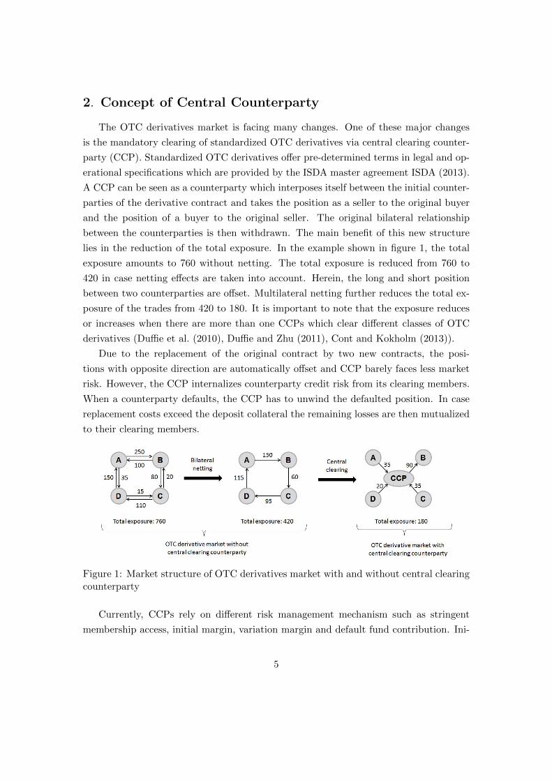
in table 1 and 2. The spread curves of selected representative institutions are shown in
Figure 3.
010
0020
0030
0040
00
Date
CD
S s
prea
d
Citi
BoA
Barclay
RBS
Lehman
AIG
12.09.2002 25.01.2004 08.06.2005 21.10.2006 04.03.2008 17.07.2009 29.11.2010
Figure 3: CDS spreads of the representative 5 global financial institutions and one globalinsurance company
As CDS spread determinants we considered in total 37 independent variables. The
panel data covers 7 state variables suggested by Adrian and Brunnermeier (2011). It
includes the VIX for implied volatility of the stock market reported by Chicago Board
Options Exchange. The short term liquidity spread which is measured by the differ-
ence between the three-month repo rate and three-month bill rate. The change in the
three-month Treasury bill rate from the Federal Reserve Board is also included as its
9

Table 1: Descriptive statistics of CDS spreads in basis point
Mean Std. Dev Skewness Kurtosis Min Median Max Autocorr
CITI 104,795 121,726 1,748 3,498 7,438 34,709 665,532 0,996BOA 87,620 95,516 1,586 2,397 8,003 32,167 483,064 0,997BARCLAYS 65,094 68,200 0,991 -0,066 5,594 23,209 278,637 0,997BNP 50,618 59,424 2,168 5,560 5,375 23,268 359,586 0,997CS 62,647 52,799 0,978 0,215 8,397 45,509 263,295 0,996DB 59,720 53,089 1,087 0,762 9,550 38,035 311,601 0,996GS 95,775 89,719 1,561 2,116 18,750 53,750 545,143 0,993HSBC 45,008 41,161 0,996 0,114 4,937 25,000 183,530 0,997JPM 61,303 43,124 0,979 0,291 11,450 46,492 232,301 0,995MS 123,375 138,067 2,521 10,767 17,833 55,488 1239,997 0,984RBS 83,709 94,375 1,124 0,474 3,964 23,750 395,937 0,998SG 64,678 78,502 2,124 5,274 5,964 24,317 440,265 0,997UBS 63,464 70,687 1,316 1,337 4,500 21,125 361,675 0,997LEHMAN 59,429 71,726 3,411 13,356 18,821 34,402 641,911 0,991AIG 279,207 500,674 3,096 11,119 8,156 42,667 3758,987 0,992
Table 2: Descriptive statistics of CDS spread log returns. Mean and median of CDSspread returns of all financial institution are almost at zero and therefore are not shownin the table.
Std. Dev Skewness Kurtosis Min Max Autocorr.
CITI 0.023 0.871 27.203 -0.174 0.286 0.032BOA 0.023 0.579 14.454 -0.182 0.247 0.008BARCLAYS 0.021 1.045 24.028 -0.155 0.270 0.115BNP 0.021 0.160 17.017 -0.192 0.214 0.117CS 0.019 0.172 17.983 -0.168 0.182 0.065DB 0.020 0.682 22.554 -0.156 0.252 0.143GS 0.020 -0.040 28.865 -0.248 0.219 0.222HSBC 0.019 -0.294 13.582 -0.147 0.151 0.067JPM 0.019 0.453 15.169 -0.138 0.213 0.117MS 0.023 4.678 118.434 -0.255 0.475 -0.006RBS 0.024 1.884 87.755 -0.368 0.376 -0.072SG 0.020 -0.209 21.404 -0.223 0.187 0.129UBS 0.020 0.439 20.372 -0.153 0.218 0.090LEHMAN 0.019 -2.040 30.336 -0.226 0.148 0.138AIG 0.024 1.106 61.673 -0.253 0.402 0.237
10

rate is significant in explaining the tails of financial sector market-valued asset returns.
The risk-free interest rate is also a component of the structural model (Merton (1974))
which decreases the likelihood of default as it gets higher. We assume that interest rate
and credit spread reveal a negative relationship, since in a macroeconomic context, a
high level of interest rate is usually found in an economy with high growth where default
rarely occurs. In our research, we consider the three month treasury bill as the risk
free interest rate referring to Adrian and Brunnermeier (2011). Several fixed-income
factors that capture the time variation in tails of asset returns are further included such
as change in slope of the yield curve, where an increase in the slope of the yield curve
indicates an improvement in economic growth. Another factor is the change in credit
spreads between BAA-rated bonds and treasury rate (both instruments with maturity
of 10 years), which reflects default premium based on market risk. A rise suggests a high
default premium and therefore implies an increase in market risk. In accordance with
Galil et al. (2013) daily equity market returns (CRSP) as determinant of CDS spreads is
also included in addition to daily real estate sector excess return over the market return.
Following the structure model rationale stock returns and stock volatility returns are
components in the spread calculation. Variables such as asset growth, asset volatility
and leverage have a direct impact on credit spreads as the model assumes that they
are the key driving factors for bankcruptcy. As a consequence, we include financial
institution’s individual equity return as a proxy for the change in firm value. A high
equity return increases firm value which leads to reduction in the spread level of the
financial institution. It is also obvious to assume that stock return and credit spread
expose a negative relationship. Refer to Galil et al. (2013) change in leverage is not
statistically significant as a determinant for CDS spread and is therefore excluded from
the set of explanatory variables. However, as change in leverage is highly correlated with
stock return this factor is considered through equity return to a certain extent.
4. Methodology
4.1. Quantile regression
For the calculation of value at risk (VaR), we apply the quantile regression proposed
by Koenker and Bassett (1978), which reveals the relationship between the predictive
variables and a specific quantile of the response variables. By considering the CDS
spreads movements in quantile, we capture the risk and variability of the credit spreads
of the constituents under extreme scenario. Denote Xi as the CDS spread return of
11

institution i with i = 1, ..., N , where N is the number of financial institutions (FIs)
considered in our sample. Referring to Adrian and Brunnermeier (2011), the predicted
quantiles of the CDS spread return is modeled through a linear equation as the following:
Xi,t = αi + γ>i Mt−1 + εi,t, (4)
where the vector Mt represents state variables, αi describes the intercept and transposed
vector γ>i outlines the parameters respective to Mt. εi,t is independent in i and t with
τ quantile equal to 0. Again with linear modeling paradigm as equation (4), if we
are interested in the CDS spread returns of Xj , we can form a linear function of state
variables Mt and another CDS spread returns Xi (j 6= i) so that
Xj,t = αj|i + βj|iXi,t + γ>j|iMt−1 + εj,t. (5)
Recent findings have questioned the linear relationship between returns of financial
institutions (Chao et al. (2014)). Since the linearity relation between institutions’ CDS
spread returns is not evident nor justified by any economic theory, a partial linear model
has been chosen to model the relationship between the input and output variables.
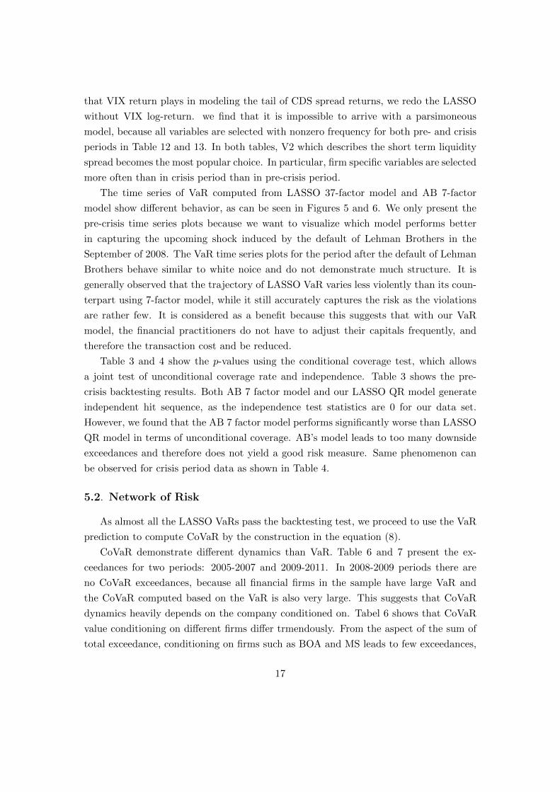
Figure 4 demonstrates the non-linearity between the CDS spreads returns especially in
extreme events from different institutions as the linear function is not lying within the
confidence bands of the nonparametric curve, which is constructed in Song et al. (2012).
PLM approach has the virtue of allowing more flexibility in the model while avoiding
the curse of dimensionality. Given scalar response variable Xj,t and explanatory scalar
variable Xi,t and state variables vector Mt, the PLM is defined as
Xj,t = f(Xi,t) + β>Mt + εj,t (6)
where f is an unknown nonparametric function to be estimated, and β> is a transposed
coefficient vector. A detailed explanation about the estimation procedure can be found
in Song et al. (2012). The idea behind the fitting procedure is first finding a reasonable
estimate of β for β, and then regressing the residual Xj,t−β>Mt on Xi,t via local linear
quantile smoothing (Detailed algorithm description is explained in the PLM appendix).
Following by the parameter estimation, the VaR of institution i and the CoVaR of j
conditional on the V aR event of institution i are given by
V aRi,t = αi + γ>i Mt−1, (7)
CoV aRj|i,t = αj|i + fj|i(V aRi,t
)+ γ>j|iMt−1. (8)
12

●
●
●●
●
●
●
●
●●●●
●● ●
●● ●
●
●
●●●●
●●
●
●●●●●
●
●
●
● ● ●●
●
●
●
●●●
●
●●
●
●
●
●●
●●●
●● ●
●● ●●
●● ●
●●●
●
●●●
● ●
●●
●●
●●
●
●●
●●●●
●
●●●●●●
●
●
●●●
●●
●●
●
● ●●●
● ●
●
●
●●
●
●
●
●●
●●
●
●
●
●●
●
●
●●
●
●●
●
●
● ●●
●●
● ●
●
●
●
●●
●
●
●
●●●●
●
●
●
●●
●
●●
●
●
●●
●
●●
●●
●
●●
●
●
●
●
●
●
●●●
● ●●●●
● ●● ●
●
●
●
●●
●●
●●
●●●
●●
●
●●
●● ●
●
●
●
●
●
●
●
●●●●
●●●
●●
●
●●● ●●
●
●
●●●
●
●● ●
●
●
● ●●
●●●●● ●●●
●●●
●
●●
●●●
●●●●●●●
● ●●●
●●●
●●●●
● ●●●●
●
●●
●
●
●●●●
●●
●●●
●●●
●
●●
●●
●
●● ● ●●
●
●●
●●
●
●●
●
●
●
●
●
●
●
●
●●
●
●●●●
●
●
●
●● ●
●●
● ●●
●●●●●
●●●
●●●
●
●●●
●
●
● ●●
●●●
● ●
●
●
●●●●●
●
●
●●
●
●
●● ●●
●
●●● ●
●
●●
●●●
●
●●● ●●●●
●
●●● ●●●●
●
●●● ●
●
●
●●
●●
●
●
●●
●
●●●●●●●●●●
●●●
●
●●
●●●
●●●
●●●●●●● ●●
●●●●●
●●
●
●
●●●
●
●
●● ●
●●●
● ●●●
●
●
●
●
●●
●
●●● ●
●●●
●●●
●●●●
● ● ●●
●
●
●
●●●●
●
●
●●
●
● ●
●●
●●
●
●
●
●●●
●●●
●
●●
●
●●●
●
●
●
●
●●●
●
●
●●●
●
●● ●●
●
●
●●●
●●●
●●
●
●
●●
●●
●
●●
●●●
●●●
●
●
●●●●● ●●●
●●
●●
●●●
●
●
●
●
●●
●●
●
●
●●
● ●●●
●
●●
●● ●
●
●●
●
●
●
●
●●
●
●●
●●
●
●
●
●
●
●
●
●
●
●
●
●●● ●
●
●
●●●●
●
●
● ●●●
● ●
● ●●
●
●●
●●
●●
●
●●●●●● ●
● ●●●
●
●
● ●
●●
● ●●●●
●
●
●
●●●● ●●●
● ●
●
●
●
●●●
●●●●
● ●
●
●
●
●
●●
●●
●●●
●●
●
●● ●
●
●● ●●
●
●
● ●
●
●
●●●●●●
●●●●
● ●●
●●●●
●●● ●●
●●●●
●
● ●
●● ●●●●
●
●●
●●
●
●●
●
●
●
●
●
●●
●●
●●
●●●
●
● ●●●●
● ●●
●●
●● ●
●● ●
●●
●
●●
● ●
●
●●
●
●●●●
●●
●
●●
●
●
●
●
●
●●●
●●
●●●
●
●
●
●
●
●● ●●●
●●
●
● ●●
●
●
●●
●
●
●●
●
●
● ●
●
●●●
●
●
●
●●
●●
●●
●
●
●
●●●
●
● ●
●
●
●
●
●
●●
●●●
●
●
●
●●
●
● ●
●●●
●
●●
●
●
●●
●
●
●●
●
●● ●
●●●
●
●
●
●
●●● ●●● ●
●●
●
●
●
●●
●
●●●
●●
●
●●
● ●●
●●
●
●
●
●
●●
●
●
●● ●
●●●
●● ●
●●
●
●
● ●●
●
● ●●
●
●
●●
●
●●
●
●
●
●
● ●
●
●
●
● ●●
●
●●
●
● ●
●
●
●
●●●●● ●
●
● ●●
●
●
●●
●
●
●●●
●
●
●
● ●●●●● ●●●●●
●
●
●
●
●●
●●
●
●●
●
●
●
●
●
●
●
●
●
●
●●
●
●
●
●
●
●
●
●●
●
●
●
● ●●
●
●●
●
●
●
●
●
●
●●
●
●
●● ●
●●
●
●
●
●
●
●●
●
●
●
●
●
●
●
●
●
●●●
●
●● ●●
●
●●
● ●●
●
●
●● ●
●●
●●●●
●
●●●
●
●
●
●
● ●●
●
●●
●
●●
●
●
●
●
●
●
●
●
●
●
● ●
●
●
●
●
●
●
●
●●
●●
●
●
● ●
●
●●●
● ●●●
●
●
●
●●
●
●
●
●
●●
●
● ●
●●
●
●
●
●
●
●
●
●
●
●
●●
●
●
●
●
●
●
●
●
●
●
●
●●
●
●
●
●● ●
●
●
●
●
●
●●
●
●●
●●
●
●● ●
●
●●
●
●
●
●
●●●
●
●●
●
●
●
●●
●●
●
●
●
●
●●
●
●
●
●
●
●
●
●
●
●
●
●
●
●
●
●● ●
●
●
●●
●
●●
●
●
●
●
●
●●
● ●●●●
●●
●●
●● ●
●
● ●
●
●
●
●
●●
●●
●
●
●
●●
●
●
●
●
●
●●
●
●●
●
●
●
●
●
●●●
●
●●
−0.1 0.0 0.1
−0.
20.
00.
2
GS CDS Spreads Returns
LE
HM
AN
CD
S S
prea
ds R
etur
ns
●
●
●●
●
●
●
●
● ●● ●
●●●
●● ●
●
●
● ●● ●
●●
●
● ●● ●●
●
●
●
●● ●●
●
●
●
●●●
●
●●
●
●
●
●●
●● ●
●●●
●●●
●●
● ●● ●●
●
●●
●●●
●●
● ●
●●
●
●●
●●● ●
●
●●●●
●●
●
●
●●●
●●
●●
●
●●●●
●●
●
●
●●
●
●
●
●●
● ●
●
●
●
● ●
●
●
●●
●
●●
●
●
●●●
●●
●●
●
●
●
●●
●
●
●
● ●●●
●
●
●
●●
●
●●
●
●
●●
●
●●
●●
●
●●
●
●
●
●
●
●
●●
●● ●●
● ●●● ●●
●
●
●
●●
●●
●●●●
●
●●
●
●●
●● ●
●
●
●
●
●
●
●
●● ●●
●● ●●
●
●
●●● ●●●
●
●● ●
●
●●●
●
●
● ●●
●●●● ●●
●●● ●
●●
●●
●●●●●●
●●●●
●●●
●●
● ●●●
●●
● ●● ●
●●
●●
●
●
●●● ●
●●
●●●
● ●●
●
●●
● ●
●
●● ●●●
●
●●
●●
●
●●
●
●
●
●
●
●
●
●
●●
●
●●● ●●
●
●
●●●
●●
● ●●
●● ●●●●●
●●●
●
●
●●●
●
●
● ●●
●●●
●●
●
●
●●●●●
●
●
●●
●
●
●●●●
●
●●● ●
●
●●●●
●
●
●●●● ●●●
●
●●● ●●●●
●
●●● ●
●
●
●●
●●
●
●
●●
●
●●
●● ●
●●
●●●
●●●
●
●●
●●●
●●
●
●●●●●●●●●
●●●●●
●●
●
●
●● ●
●
●
●● ●
●●
●
●● ●●
●
●
●
●
●●
●
●●
●●●●
●● ●
●●●
●●
● ●●●
●
●
●
●●● ●
●
●
●●
●
● ●
● ●
●●
●
●
●
●●●
●●●
●
●●
●
●●●
●
●
●
●
●●●
●
●
●●●
●
●● ●●
●
●
●●●
●●●
●●
●
●
●●●●
●
●●
●●●
●●●
●
●
●●●●●●●
●●
●
●●
●●●
●
●
●
●
●●
●●
●
●
●●
●●●●
●
● ●
●● ●
●
●●
●
●
●
●
●●
●
●●
●●
●
●
●
●
●
●
●
●
●
●
●
●●●●
●
●
●●●●
●
●
●●●●
● ●
● ●●
●
●●●●
●●
●
●●●●● ● ●
●●●●
●
●
● ●
●●
● ●● ●●
●
●
●
●●●●●●●
● ●
●
●
●
●●●
●●● ●
●●
●
●
●
●
●●
●●
●● ●
●●
●
●●●
●
● ●●●
●
●
●●
●
●
●●● ●●
●●
●●●●●
●
●●●●
●●● ●
●
● ●●●
●
●●
● ●●●●●
●
●●
●●
●
●●
●
●
●
●
●
●●
●●
●●
●●●
●
●●●● ●
●●●
●●
● ●●
●●●
●●
●
● ●
●●
●
●●
●
●● ●
●●
●●
●●
●
●
●
●
●
●●●
●●
●●●
●
●
●
●
●
●●●● ●
●●
●
●●●
●
●
● ●
●
●
●●
●
●
● ●
●
●●
●
●
●
●
●●●
●●
●
●
●
●
●●●
●
●●
●
●
●
●
●
●●
●●●
●
●
●
●●
●
● ●
●●●
●
●●●
●
●●
●
●
●●
●
●● ●
●●●
●
●
●
●
●●● ●●●●
●●
●
●
●
●●
●
●●●
●●
●
●●
●●●
●●
●
●
●
●
●●
●
●
●● ●
●● ●
●●●
●●
●
●
●● ●
●
●●●
●
●
●●
●
●●
●
●
●
●
● ●
●
●
●
●●●
●
●●
●
● ●
●
●
●
● ●● ●● ●
●
● ●●
●
●
●●
●
●
● ●●
●
●
●
● ●●●● ●●●●
●●
●
●
●
●
●●
●●
●
● ●
●
●
●
●
●
●
●
●
●
●
●●
●
●
●
●
●
●
●
●●
●
●
●
●●●
●
● ●
●
●
●
●
●
●
●●
●
●
●●●●●
●
●
●
●
●
● ●
●
●
●
●
●
●
●
●
●
●●●
●
●●●●
●
● ●
●●●
●
●
●●●
●●
●● ●●
●
●● ●
●
●
●
●
●●●
●
●●
●
●●
●
●
●
●
●
●
●
●
●
●
● ●
●
●
●
●
●
●
●
●●
●●
●
●
● ●
●
● ●●
●●● ●
●
●
●
●●
●
●
●
●
●●
●
●●
●●
●
●
●
●
●
●
●
●
●
●
●●
●
●
●
●
●
●
●
●
●
●
●
●●
●
●
●
●● ●
●
●
●
●
●
●●
●
●●
●●
●
●● ●
●
●●
●
●
●
●
●●●
●
●●
●
●
●
●●
●●
●
●
●
●
●●
●
●
●
●
●
●
●
●
●
●
●
●
●
●
●
●●●
●
●
●●
●
●●
●
●
●
●
●
●●
● ●● ●●
●●
●●
●●●
●
● ●
●
●
●
●
●●●
●●
●
●
●●
●
●
●
●
●
●●
●
●●
●
●
●
●
●
●●●
●
●●
−0.1 0.0 0.1
−0.
20.
00.
2
Citi CDS Spreads Returns
LEH
MA
N C
DS
Spr
eads
Ret
urns
●●
●● ●●
●●
●● ●●
●
●
●
●
●
●●●
●
● ●●●
●
●●●
●●
●
●
●●●
●
●●●
●
●
●
●●
●●
● ●
●
●
●
●●
●●
●●
●
●● ●●
●● ●●
●
●
●●
●
●●●
●
●●
●
●
●
●
●
●●
●●●
●
●
●
●●
●●
●
●●
●
●
●
●
●
●
●
●
●●
●● ●
●●●
●●
●● ●●
●●●
●
●●
●
●
●●●●
●
●
●●
●
●
●
●
●
●
●
●●
●●
●● ●● ●
●● ●
●
●● ●●
●●●
●
●
●
●
●●
●
●●
●
●●
●●
●
● ●● ●●●
●
●●
●●●
●●
●●
●● ●●
●●●
●
●
●
●
●●
●
●
●
●
●●●
●●
●
●
●
●
●
●●●● ●
●●●
●●●●
●●●
●●●
● ●●●
●
●
●●
●●●
●
●●●
●●
●●
●
●●
●
●
●● ●●
●●●●
●
●●
●●
●●
●●●
●
●● ●●
●●
●
●●●
●
●
●
●●●
●●● ●● ●
●●●
●●
●
●
●
●
●
●●
●
●●
●
●
●● ●
●
●●● ●
●
●
●
●
● ●
●
●
●●●
●
●
●
●
●
● ●●
●
●
● ●●●●
●●● ●
●
●
●
●
●●●●
●●
●●
●●●
●●●
●
●
●
●●
● ●●
● ●
●●
●● ●●●
● ●●
●
●
●
●●
●● ●● ●● ●●
●●●
●●
● ●●
●●●
●●● ●●●●
●●●
●●●●
●●
●●●● ●●●
●●
●
●
●
● ●
●●
●●
●
●
●
●●●●
●●● ●● ●●●●●●●
●●
●
●●
●●
●●
●● ●●● ●●
●●
●
● ● ● ●●●
●
● ●●●●
●
●
●
●
●
●
●
●
●
●
●
●
●●●
●
●
●
●
●●
●
●
●
●●
● ●●
●
●●●
●●●
●●●●
●●●●●●●●
●●
●●●
●
●●● ●
●● ●● ●● ●
●●● ●●
●●
●●
●●●●
●●●
●
●●
●●●
●●●
●
●●● ●
●
●●●
●
●
●
●
● ●
●
●
●
●
●
●
●
●
●
●
●
●
●●
●
●●●●
●
●
●●
●
●
●●
●
●●
●●
● ●● ●●
●●
●● ●
● ●
●●
●●
●
●
●
●●●
●
●●
●●
●●●● ●●
●● ●●●
●●
●●
●
●●
●●
●
●
●
●●
●●
●●● ●●
●●●
●●●
● ●●
●
●
●● ●●●●
●●●
●●
●
●●
●
●●
● ●●
●
●●
●●
●●
●●
●
●
●
●
●
●
●●●
●
●●
●●
●●●●●
●●●
●
●●
●●
●
●●
●
●
●
●
●
●
●● ●●●
●
●●
●●
●
●● ●
●● ●
●
●●
●
●
●●
●● ●● ●●
●●●● ●
●●● ●●
●●●
●●●
●
●
●●
●
●●
●
●●●●
●
●
●
●
● ●●●
●
●
●●●
●
●● ●●●
●
●●●●
●
●●
●
●
●●● ●●
●
●
●● ●●●● ●●●
●●
●
●●●
●
●
●
●
●●
●
●●●●
●● ●● ● ●● ●●
●●●●
●●
● ●●●
●●●
● ●●
●
●●
●●●
●● ●
●
●●● ●
●●●
●●
●●
●
●●●
●
●●●
●●●●
●
●●
●●●
● ●●
● ●●●
●
●
●●●
●●●
● ●●●●
●●
●
●
●●
●
●
●
●
●●●
● ●●
●
●
●
●
●
●●
●●●
●
●●
●
●
●
●
●
●●
●
●
●
●●
●
●
●●
●
●
●
●
●●
●
●
●
●●●
●
●
●
●
●
●
●
●
●
●
●●
●
●
●●
●
● ●
●●●
●●
●
●
●
●
●●●
●
●●●●
●
●
●
●
●
●
●
●●●
●
●
●
●
●
●
●●
●●
●●
●
●
●
●●
●
●
●
●
●
●
●
●
●
●●
●
●
●●●●
●●
●●
●
●
●●
●
●
●
●
● ●
●
●●
●
●●●
●●●
●●
●●
●
●●●
●●
●●
●● ●
●●
●
●●
●●
●
●
●
●
●
●
●
●
●●● ●●
●
●
●
●
● ●●
●●
●
●
●
●
●
●
●
●
●
●●
●●
●
●●
●
● ●●●
●
●
●
●
●
●
●
●
●
●●
●
●●
●
●
●● ●
●
●
● ●
●
●
●
●
●
●
●
●
●
● ●●
●
●
●●
●●
●
●
●●
●
●
●
●
●
●●
●●
●●
●
●
●
●●
●
●
●
●
●●
● ●
●
●●●
●
●
●
●
●
●●
●●
●
●
●
●
●
●
●●
●
●●
●
●
●
●
●
●
●●
●
●
●
●
●●
●
●
●
●
●●
●
● ●
●
●
●
●
●
● ●● ●●
●
●
●
●
●
● ●●●
●
●
●●
●
●●
●●●
●
●
●●
●●
●
●
●●●
●
●●●●
●●
●
● ●●
● ●●●●● ●
●
●●
●
●
●●
●
●●
●
●
●
●
−0.1 0.0 0.1
−0.
20.
00.
2
GS CDS Spreads Returns
AIG
CD
S S
prea
ds R
etur
ns
●●
●●●●
●●
●● ●●
●
●
●
●
●
●● ●
●
● ●●●
●
●●●
●●●
●
●●●
●
●●●
●
●
●
●●
●●
● ●
●
●
●
●●
●●
●●●
●●●●
●●● ●
●
●
●●
●
● ●●
●
●●●
●
●
●
●
● ●
●●●
●
●
●
●●
●●
●
●●
●
●
●
●
●
●
●
●
●●
●●●
●● ●
●●
● ●●●
●●●
●
● ●
●
●
●●
●●●
●
●●
●
●
●
●
●
●
●
●●
●●
●● ●● ●
●●●
●
●● ●●
●● ●
●
●
●
●
● ●
●
●●
●
●●
●●
●
● ●● ●●●
●
●●
●●
●●
●● ●
●●●●
●● ●
●
●
●
●
●●
●
●
●
●
●● ●
● ●
●
●
●
●
●
●●●● ●
●●
●●●
●●●●
●●
●●
● ●●●
●
●
●●
●●●
●
●●●●
●●
●
●
●●
●
●
●● ●●
●●●●
●
●●
●●
●●
●●●
●
●● ●●
●●
●
●●
●
●
●
●
●●●
●●● ●●●
●●●
●●
●
●
●
●
●
●●
●
●●
●
●
●● ●
●
●●● ●
●
●
●
●
● ●
●
●
●●●●
●
●
●
●
● ●●
●
●
● ●●●●
●●●●
●
●
●
●
●●●●
● ●
● ●
●●●
●●
●
●
●
●
●●
● ●●
●●
●●
●●●●●●●
●
●
●
●
●●
●● ●●●
●●●
●●●
●●●●●
●●●
●●●● ●●
●●●
●●●
●●
●●
●● ●● ●● ●
●●
●
●
●
●●
●●
●●
●
●
●
●●●●
●●●●● ●●●●
● ●●●
●●
●●
●●
●●●● ● ●●●
●
●●
●
● ● ●●● ●
●
●●●●●
●
●
●
●
●
●
●
●
●
●
●
●
●●●
●
●
●
●
●●
●
●
●
●●● ●
●
●
●●●
●●●
●● ●●●●●● ●●
●●
●●
●●●
●
●●● ●
●●●● ●● ●
●●●●
●●
●●
●●●●●
●●●
●
●●
●●●
●●●
●
●●●●●
●●●
●
●
●
●
●●
●
●
●
●
●
●
●
●
●
●
●
●
●●
●
●●●
●
●
●
●●
●
●
●●
●
●●
●●
● ●● ●●
●●
●●●
● ●
●●
●●
●
●
●
●●●
●
●●
●●
●● ●●●●
●●●●
●●
●● ●
●
●●
●●
●
●
●
●●
●●
●● ●●●
●●●
●●●
● ●●
●
●
●●●●●●●●
●●
●●
●●
●
●●
●● ●
●
●●
●●
●●
●●
●
●
●
●
●
●
● ●●
●
●●
●●
●● ●● ●●●●
●
●●
●●
●
●●
●
●
●
●
●
●
●●●●●
●
●●
● ●
●
●●●
●● ●●
●●
●
●
●●
●● ●● ●●
●●●● ●
●●●●●●●
●●●
●●
●
●●
●
●●
●
●●● ●
●
●
●
●
● ●●●
●
●
●●●
●
●●●●●
●
●●● ●
●
●●
●
●
●●● ●●
●
●
●●●●●● ●●●● ●
●
●●●
●
●
●
●
●●
●
●●●●●● ●● ●● ●●●
●● ●
●
●●● ●●
●●
●●● ●●
●
●●●●
●●
●●
●
●●●●
●●●
●●
●●
●
●●●
●
●●●●●●●
●
●●
●●●●●●
●● ●●
●
●
●●●
●●●
● ●●●
●●●
●
●
●●
●
●
●
●
●●●
● ●●
●
●
●
●
●
●●
●●●
●
●●●
●
●
●
●
●●
●
●
●
●●
●
●
●●
●
●
●
●
●●
●
●
●
●● ●
●
●
●
●
●
●
●
●
●
●
●●
●
●
●●
●
● ●
●●●
●●
●
●
●
●
●●●●
●●●●●
●
●
●
●
●
●
●●●
●
●
●
●
●
●
●●
●●
●●
●
●
●
●●
●
●
●
●
●
●
●
●
●
●●
●
●
●●●●
●●
●●
●
●
●●
●
●
●
●
●●
●
●●
●
●●●
●●●
●●
●●
●
●●●
●●
●●●●●
●●
●
●●
●●
●
●
●
●
●
●
●
●
●●●●●
●
●
●
●
●●●
●●
●
●
●
●
●
●
●
●
●
●●
●●
●
●●
●
● ●●●
●
●
●
●
●
●
●
●
●
●●
●
●●
●
●
●● ●
●
●
● ●
●
●
●
●
●
●
●
●
●
● ● ●
●
●
●●
●●
●
●
●●
●
●
●
●
●
●●
●●
●●
●
●
●
●●
●
●
●
●
● ●
● ●
●
● ●●
●
●
●
●
●
●●
●●
●
●
●
●
●
●
●●
●
●●
●
●
●
●
●
●
●●
●
●
●
●
●●
●
●
●
●
●●
●
● ●
●
●
●
●
●
● ●●●●
●
●
●
●
●
● ●●●
●
●
●●
●
●●
●●●
●
●
●●
●●
●
●
●●●
●
●● ● ●
●●
●
● ●●
● ●●●
● ●●
●
●●
●
●
●●
●
●●●
●
●
●
−0.2 −0.1 0.0 0.1
−0.
20.
00.
2
Lehman CDS Spreads Returns
AIG
CD
S S
prea
ds R
etur
ns
Figure 4: Quantile regression at 0.01 level on CDS spread return. The blue line shows thepartial linear quantile regression function. The four dashed lines express the asymptotic(magenta) and bootstrap (red) confidence bands at 95% confidence level.
13

This construction follows from Adrian and Brunnermeier (2011). The algorithm to
estimate fj|i(·) is proposed by Song et al. (2012), and is described in detail in the
appendix.
4.2. Least Absolute Shrinkage and Selection Operator for Quantile Re-
gression
Since Chao et al. (2014) show unsatisfactory backtesting results regarding VaR val-
ues, we apply a different way to compute the individual VaR in our paper. First, we
apply the linear Least Absolute Shrinkage and Selection Operator (LASSO) technique
in order to find variables with significant effect on CDS spread returns. The LASSO
variable selection method has been introduced by Tibshirani (1996). It is widely known
that LASSO outperforms ridge regression in terms of shrinkage effect. For the typical
case described by Tibshirani (1996), the loss function for LASSO can be viewed as con-
strained versions of the ordinary least squares (OLS) regression loss function, which can
also be presented in the Lagrange form as
Llasso(β1, ..., βp) = ‖Y −Xβ‖22, s.t.‖β‖`1 ≤ t1,
where Y ∈ Rn the dependent variable, X ∈ Rnp the independent variable and β ∈ Rp
denotes the coefficients. The LASSO penalty can also be applied to quantile regression
analysis. One is referred to Koenker (2005) for more details. The loss function reads:
Llasso(β) =n∑i=1
ρτ
(Yi −X>i β
)+ λn
p∑j=1
|βj |, (9)
where ρτ (u) = {τ − 1(u ≤ 0)}u and 0 ≤ τ ≤ 1 is a given constant.
In our empirical analysis, we use 37 variables for Xi, as mentioned in Section 3.2.
In the section of empirical findings, we will see that the coefficients associated to many
of the independent variable are shrunk to zero as the result of LASSO. To choose the
penalty parameter λn, we apply the generalized approximate cross-validation (GACV)
of Yuan (2006) and Li et al. (2007).
4.3. Backtesting
For check of accuracy of the out-of-sample VaR estimation we compare the actual
CDS spread returns to the calculated VaR (model VaR). Following Christoffersen (1998),
14

the hit sequence is defined as
It(τ) =
{1, if Xt < VaRτ
t
0, otherwise.
The probability of getting x exceedance from T observations is therefore
f(x | T, π) =
(T
x
)πx(1− π)T−x
where π is the probability of an exceedance for a given confidence level. As the VaR is
calculated under a 1%-quantile, this leads to an expectation of one exceedance every 100
days. The unconditional coverage test introduced by Kupiec(Kupiec (1995)) explores
the frequency of the violations over specific time interval (proportion of failure (POF)).
The null hypothesis for the Kupiec test is represented by
H0 : π = π0 =x
T.
The test statistic is calculated as
LRPOF = 2 log
[(1− π1− π
)T−I(π)( ππ
)I(π)]π =
1
TI(τ)
I(τ) =T∑t=1
It(τ)
In case the value of the test statistic LRPOF exceeds the critical value of the χ2 distri-
bution with onedegree of freedom, the null hypothesis is to be rejected and the model
is considered as inaccurate. We expect the VaR to be in line with the confidence level.
A failure of the unconditional coverage leads to the conclusion that the VaR does not
measure the risk accurately.
However, it is not only important to test the sequence of exceedance but also look at
the clustering of violations. The conditional coverage test suggested by Christoffersen
(Christoffersen (1998)) includes a seperate statistic for the detection of exceedance’s
independence. We assume that the calculated value accurately reflects the change in
market condition when the exceedance is independent from the previous state. This
means no effect on current exceedance whether there was a violation the day before,
15

It−1 = 1, or no violation has occured, It−1 = 0. Let Tij be the total number of event
(It−1, It) = (j, i) in the data for i, j ∈ {0, 1}. Denote the probability of observing a
violation condition on the state i ∈ {0, 1} by
πi =Ti1
Ti0 + Ti1.
The unconditional probability for violation is
π =T01 + T11
T00 + T01 + T10 + T11.
The test statistic of independence is denoted by
LRind = 2 log
((1− π)(T00+T10)π(T01+T11)
(1− π0)T00πT100 (1− π1)T10πT111
).
Under the hypothesis that the method for VaR estimation is accurate, the sequence of
violations should statisfy the unconditional coverage property as well as the independence
property. Therefore, as suggested in Christoffersen (1998), we consider the ”conditional
coverage” test statistic:
LRCC = LRPOF + LRind
exceeds the critical value given by χ2 distribution with two degrees of freedom. The
rejection of the test indicates an inaccurate coverage, clustered violations or both.
5. Empirical results
5.1. Variables that drive the tails
Our regression analysis confirms the relationship between the tail of CDS spread
return and the market volatility, approximated by VIX returns. Interestingly, the effect
of firm specific volatility is not as strong as volatility of the market indicated by the
VIX index. By LASSO, we observe from Tables 10 and 11 that the CDS spread return
is almost described by the VIX log-returns, S&P500 log-returns and the change in daily
real estate sector return in excess to the market return, in which VIX plays the dominant
role.
It is surprising to see that the firm specific variables are so underselected. For some
CDS spreads, such as Citi in pre-crisis period, and CITI, DB, GS, JPM, MS and UBS in
crisis period, firm specific variables are not selected at all. To check for the important role
16
that VIX return plays in modeling the tail of CDS spread returns, we redo the LASSO
without VIX log-return. we find that it is impossible to arrive with a parsimoneous
model, because all variables are selected with nonzero frequency for both pre- and crisis
periods in Table 12 and 13. In both tables, V2 which describes the short term liquidity
spread becomes the most popular choice. In particular, firm specific variables are selected
more often than in crisis period than in pre-crisis period.
The time series of VaR computed from LASSO 37-factor model and AB 7-factor
model show different behavior, as can be seen in Figures 5 and 6. We only present the
pre-crisis time series plots because we want to visualize which model performs better
in capturing the upcoming shock induced by the default of Lehman Brothers in the
September of 2008. The VaR time series plots for the period after the default of Lehman
Brothers behave similar to white noice and do not demonstrate much structure. It is
generally observed that the trajectory of LASSO VaR varies less violently than its coun-
terpart using 7-factor model, while it still accurately captures the risk as the violations
are rather few. It is considered as a benefit because this suggests that with our VaR
model, the financial practitioners do not have to adjust their capitals frequently, and
therefore the transaction cost and be reduced.
Table 3 and 4 show the p-values using the conditional coverage test, which allows
a joint test of unconditional coverage rate and independence. Table 3 shows the pre-
crisis backtesting results. Both AB 7 factor model and our LASSO QR model generate
independent hit sequence, as the independence test statistics are 0 for our data set.
However, we found that the AB 7 factor model performs significantly worse than LASSO
QR model in terms of unconditional coverage. AB’s model leads to too many downside
exceedances and therefore does not yield a good risk measure. Same phenomenon can
be observed for crisis period data as shown in Table 4.
5.2. Network of Risk
As almost all the LASSO VaRs pass the backtesting test, we proceed to use the VaR
prediction to compute CoVaR by the construction in the equation (8).
CoVaR demonstrate different dynamics than VaR. Table 6 and 7 present the ex-
ceedances for two periods: 2005-2007 and 2009-2011. In 2008-2009 periods there are
no CoVaR exceedances, because all financial firms in the sample have large VaR and
the CoVaR computed based on the VaR is also very large. This suggests that CoVaR
dynamics heavily depends on the company conditioned on. Tabel 6 shows that CoVaR
value conditioning on different firms differ trmendously. From the aspect of the sum of
total exceedance, conditioning on firms such as BOA and MS leads to few exceedances,
17

while conditioning on firms such as SG, UBS, CS, AIG leads to many exceedances.
The exceedance time series of CoVaR shown in Figure 7 demonstrate strong clustering
phenomenon. In the pairs of AIG on JPM, AIG on MS and Citi on BOA, the exceedances
accumulate in certain periods. In the crisis period, few exceedances are observed, but
the CoVaR seems to over-estimate the risk in the sense that the estimated CoVaRs are
far below the realizations of returns.
The idea of ∆CoVaR calibration on credit risk and intergration of state variables as
well as firm-specific variables have been applied on the model suggested by Adrian and
Brunnermeier (2011). Our results show that the 4CoVaR results from the period until
Lehman’s default reveals different effects on financial institutions from different regions.
As shown in Table 9, for the US financial institutions, the 4CoVaR effect is high when
the distressed counterparty is a US financial institution. The same can be observed
for European based financial institutions. This shows that the 4CoVaR captures the
spillover effect owing to the geological closeness, as we would expect.
Given the VaR obtained from the last section based on 37 variables for pre-crisis
period and crisis period, we are able to compute the CoV aR with (8) using partial
linear model at levels τ = 1% and 50%. The ∆CoV aR can therefore be obtained by the
difference of the two CoVaRs.
The mean and the maximum of the estimated ∆CoV aRs are summarized in Table 8
for pre-crisis period and Table 9. Comparing the two tables, the CoVaRs of crisis period
are in general greater than that of the pre-crisis period in terms of absolute value. In
pre-crisis period, among the 15 financial institutions, BoA, Barc, RBS and JPM are the
ones which introduce the most risk to the market, while AIG and HSBC contribute the
fewest. RBS’s high risk contribution reflects its risk seeking business model before the
crisis. AIG’s low risk contribution may be due to its nature as an insurance company,
but ∆CoVaR seems to underestimate AIG’s potential impact to the market due to its
gigantic CDS position before the crisis. However, it is interesting to note that after LEH
defaults, SG, DB and GS become largest risk contributors, while AIG, Citi, Barc and
MS contribute the fewest. Among the smallest risk contributors in the crisis period, the
first ones are the ones which suffer the greatest hit of the crisis, while MS shifted its
business orientation to a more conservative ground after the crisis.
In order to visualize the risk contribution defined by ∆CoVaR, we make the network
plots. We focus on the data in 3 periods: 2005-2007 (first pre-crisis period), 2007-
2008 (eve of crisis) and 2008-2011 (crisis), as shown in Figures 8, 9 and 10. In these
figures, the nodes represent the financial institutions, the edges represent the amount
of risk contribution and the arrows show the direction of risk contribution. The thicker
18

the edge, the larger the ∆CoVaR in absolute value and therefore the larger the risk
contribution.
It can be seen in Figure 8 for the period 2005-2007 that several financial institutions
are connected through risk contribution. RBS contributes much risk to BARC, which
could be due to their geographic closeness; moreover it is obvious that RBS also con-
tribute risk to HSBC, SG and CS. JPM and LEH contribute much risk to AIG, while
AIG seemingly conveys not too much risk to the others, except BOA. BOA transmits
much risk to CITI and GS.
For the period 2007-2008, the relationship between these firms varies. The risk
contribution to AIG becomes prominent. RBS still contribute risk to BARC and SG,
but the contribution to HSBC becomes less obvious. BOA still conveys much risk to
CITI. At this moment, although the international financial market looks interconnected,
but regional effect actually plays a big role.
We then proceed to the last network figure for crisis periof depicted in Figure 10.
The boundaries of region crash and firms from different regions can contribute significant
risk to each other, while the firms in the same region remain very much connected. SG
contribute much risk to JPM, BOA and GS. It is also interesting to note that the direction
of risk contribution can also change. BOA contributes risk to CITI in pre-crisis period,
but in crisis it is the other way around. SG is mainly a risk receiver before the crisis, but
it changes its role to a risk contributor for this period. This could result from European
debt crisis in 2011, during which the fear of bankrupcy for SG drives its CDS spread
higher and thus introduce huge amount of uncertainty into the global financial market.
19

−0.3
−0.2
−0.1
0.0
0.1
0.2
Date
CD
S s
prea
d re
turn
s
02.10.2003 25.03.2005 16.09.2006 09.03.2008
(a) Citi-LASSO37−0
.3−0
.2−0
.10.
00.
10.
2
Date
CD
S s
prea
d re
turn
s
02.10.2003 25.03.2005 16.09.2006 09.03.2008
(b) Citi-AB7
−0.3
−0.2
−0.1
0.0
0.1
0.2
Date
CD
S s
prea
d re
turn
s
02.10.2003 25.03.2005 16.09.2006 09.03.2008
(c) BOA-LASSO37
−0.3
−0.2
−0.1
0.0
0.1
0.2
Date
CD
S s
prea
d re
turn
s
02.10.2003 25.03.2005 16.09.2006 09.03.2008
(d) BOA-AB7
−0.3
−0.2
−0.1
0.0
0.1
0.2
Date
CD
S s
prea
d re
turn
s
02.10.2003 25.03.2005 16.09.2006 09.03.2008
(e) Barclays-LASSO37
−0.3
−0.2
−0.1
0.0
0.1
0.2
Date
CD
S s
prea
d re
turn
s
02.10.2003 25.03.2005 16.09.2006 09.03.2008
(f) Barclays-AB7−0
.3−0
.2−0
.10.
00.
10.
2
DateC
DS
spr
ead
retu
rns
02.10.2003 25.03.2005 16.09.2006 09.03.2008
(g) BNP-LASSO37
−0.3
−0.2
−0.1
0.0
0.1
0.2
Date
CD
S s
prea
d re
turn
s
02.10.2003 25.03.2005 16.09.2006 09.03.2008
(h) BNP-AB7
−0
.3−
0.2
−0
.10
.00
.10
.2
Date
CD
S s
pre
ad
re
turn
s
02.10.2003 25.03.2005 16.09.2006 09.03.2008
(i) Credit Suisse-LASSO37
−0.3
−0.2
−0.1
0.0
0.1
0.2
Date
CD
S s
prea
d re
turn
s
02.10.2003 25.03.2005 16.09.2006 09.03.2008
(j) Credit Suisse-AB7
−0.3
−0.2
−0.1
0.0
0.1
0.2
Date
CD
S s
prea
d re
turn
s
02.10.2003 25.03.2005 16.09.2006 09.03.2008
(k) DB-LASSO37
−0.3
−0.2
−0.1
0.0
0.1
0.2
Date
CD
S s
prea
d re
turn
s
02.10.2003 25.03.2005 16.09.2006 09.03.2008
(l) DB-AB7
−0.3
−0.2
−0.1
0.0
0.1
0.2
Date
CD
S s
prea
d re
turn
s
02.10.2003 25.03.2005 16.09.2006 09.03.2008
(m) GS-LASSO37
−0.3
−0.2
−0.1
0.0
0.1
0.2
Date
CD
S s
prea
d re
turn
s
02.10.2003 25.03.2005 16.09.2006 09.03.2008
(n) GS-AB7
−0.3
−0.2
−0.1
0.0
0.1
0.2
Date
CD
S s
prea
d re
turn
s
02.10.2003 25.03.2005 16.09.2006 09.03.2008
(o) HSBC-LASSO37
−0.3
−0.2
−0.1
0.0
0.1
0.2
Date
CD
S s
prea
d re
turn
s
02.10.2003 25.03.2005 16.09.2006 09.03.2008
(p) HSBC-AB7
Figure 5: First part: The plots VaR from LASSO 37 factors model and AB 7 factormodel in pre-crisis period Sep. 2002-Sep. 2008.
20
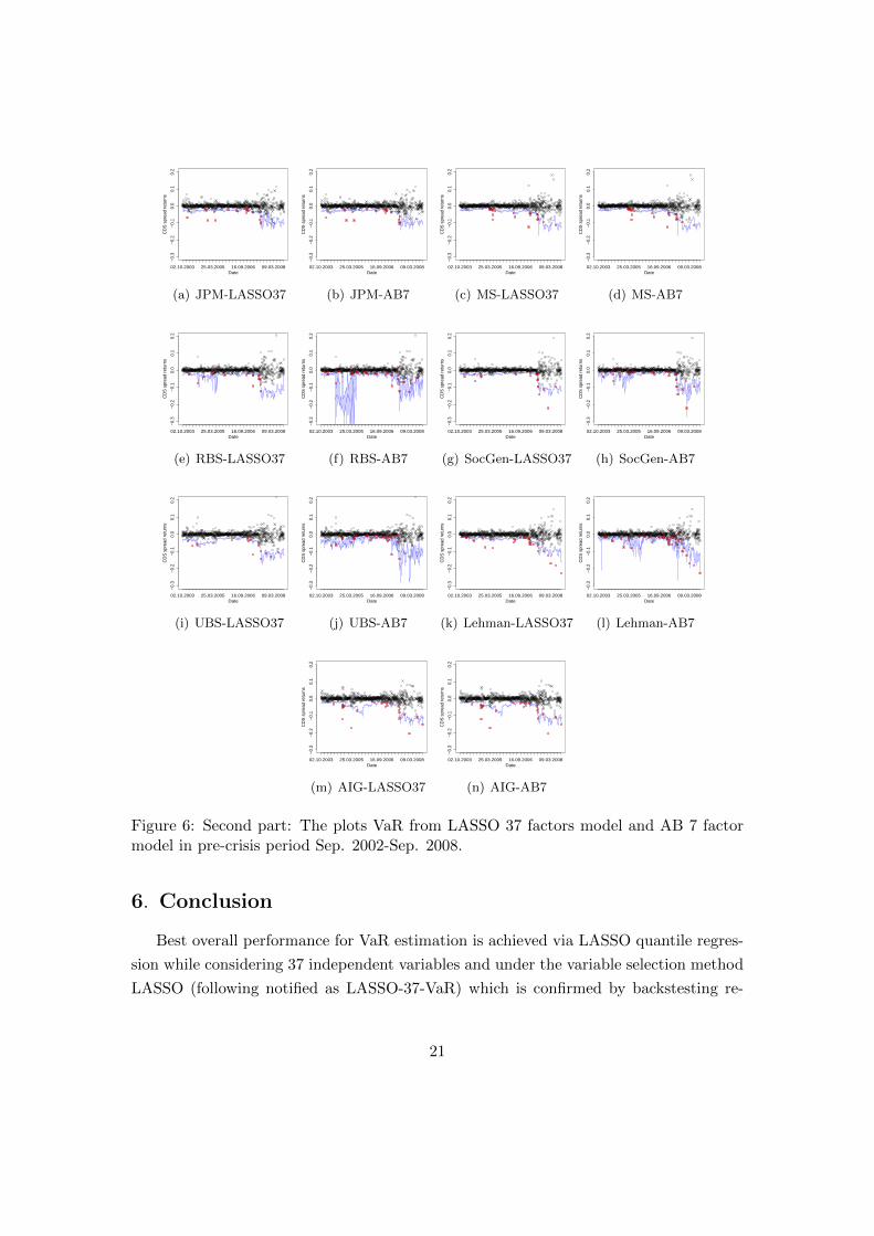
−0.3
−0.2
−0.1
0.0
0.1
0.2
Date
CD
S s
prea
d re
turn
s
02.10.2003 25.03.2005 16.09.2006 09.03.2008
(a) JPM-LASSO37−0
.3−0
.2−0
.10.
00.
10.
2
Date
CD
S s
prea
d re
turn
s
02.10.2003 25.03.2005 16.09.2006 09.03.2008
(b) JPM-AB7
−0.3
−0.2
−0.1
0.0
0.1
0.2
Date
CD
S s
prea
d re
turn
s
02.10.2003 25.03.2005 16.09.2006 09.03.2008
(c) MS-LASSO37
−0.3
−0.2
−0.1
0.0
0.1
0.2
Date
CD
S s
prea
d re
turn
s
02.10.2003 25.03.2005 16.09.2006 09.03.2008
(d) MS-AB7
−0.3
−0.2
−0.1
0.0
0.1
0.2
Date
CD
S s
prea
d re
turn
s
02.10.2003 25.03.2005 16.09.2006 09.03.2008
(e) RBS-LASSO37
−0.3
−0.2
−0.1
0.0
0.1
0.2
Date
CD
S s
prea
d re
turn
s
02.10.2003 25.03.2005 16.09.2006 09.03.2008
(f) RBS-AB7−0
.3−0
.2−0
.10.
00.
10.
2
DateC
DS
spr
ead
retu
rns
02.10.2003 25.03.2005 16.09.2006 09.03.2008
(g) SocGen-LASSO37
−0.3
−0.2
−0.1
0.0
0.1
0.2
Date
CD
S s
prea
d re
turn
s
02.10.2003 25.03.2005 16.09.2006 09.03.2008
(h) SocGen-AB7
−0.3
−0.2
−0.1
0.0
0.1
0.2
Date
CD
S s
prea
d re
turn
s
02.10.2003 25.03.2005 16.09.2006 09.03.2008
(i) UBS-LASSO37
−0.3
−0.2
−0.1
0.0
0.1
0.2
Date
CD
S s
prea
d re
turn
s
02.10.2003 25.03.2005 16.09.2006 09.03.2008
(j) UBS-AB7
−0.3
−0.2
−0.1
0.0
0.1
0.2
Date
CD
S s
prea
d re
turn
s
02.10.2003 25.03.2005 16.09.2006 09.03.2008
(k) Lehman-LASSO37
−0.3
−0.2
−0.1
0.0
0.1
0.2
Date
CD
S s
prea
d re
turn
s
02.10.2003 25.03.2005 16.09.2006 09.03.2008
(l) Lehman-AB7
−0.3
−0.2
−0.1
0.0
0.1
0.2
Date
CD
S s
prea
d re
turn
s
02.10.2003 25.03.2005 16.09.2006 09.03.2008
(m) AIG-LASSO37
−0.3
−0.2
−0.1
0.0
0.1
0.2
Date
CD
S s
prea
d re
turn
s
02.10.2003 25.03.2005 16.09.2006 09.03.2008
(n) AIG-AB7
Figure 6: Second part: The plots VaR from LASSO 37 factors model and AB 7 factormodel in pre-crisis period Sep. 2002-Sep. 2008.
6. Conclusion
Best overall performance for VaR estimation is achieved via LASSO quantile regres-
sion while considering 37 independent variables and under the variable selection method
LASSO (following notified as LASSO-37-VaR) which is confirmed by backstesting re-
21

sults. The calculated VaR also shows a good performance during the crisis period and
is able cover certain extreme CDS spreads drops. However, these VaR overestimate the
risk during the crisis period whereas VaR simulated via standard quantile regression by
using 7 state variables suggested by (Adrian and Brunnermeier, 2011) shows a lower
VaR level. On the other hand, LASSO-37-VaR show a more accurate and stable VaR es-
timation during the pre-crisis and crisis period. VaR simulated under the assumptionof
Adrian and Brunnermeier tends to over-estimate CDS spread returns in calm period.
Based on our findings, the calculated4CoVaR can be used as a basis for risk weights
which described the change between normal circumstances and a stressed VaR. As a
consequence, risk contribution can be charged based on idiosyncratic risk and further on
the spillover effects given by the risk weight. A valuable question of how counterparty
credit risk affects the pricing of CDS contracts could also be investigated based on the
overall effects of one distressed institution on CDS spreads of other market players. In
addition, this approach provides the possibility to measure spread widening effect from
derivative dealer on spread level from reference entities. Effect of extreme CDS spreads
of bid dealers on spread level of reference entitiy when it comes to CDS spread central
clearing.
22

7. Appendix
PLM Fitting
For the PLM estimation, we adopt the algorithm described in Song et al. (2012).
Given data {(Xt, Yt)}Tt=1 bivariate and {Mt}Tt=1 multivariate random variables. The
PLM is:
Yt = f(Xt) + β>Mt + εt.
Suppose the support of Xt is bounded in [0, 1] for simplicity. Let an denote an
increasing sequence of positive integers and set bn = a−1n . For each n = 1, 2, ..., dividing
the interval [0, 1] into an subintervals Ii, i = 1, ..., an with equal length bn. On each Ii,
f(·) can approximately be taken as a constant.
The PLM estimation procedure is:
1. Inside each partition Ii, a linear quantile regression is performed to get βi, then
their weighted mean gives β. Formally, let ρτ (·) be the check function. f1, ..., fanare constants, then
β = argminβ
minf1,...,fan
T∑t=1
ρτ
{Yt − β>Mt −
an∑i=1
fi1(Xt ∈ Ii)
}
2. Perform the local linear quantile estimates of f(·) from {(Xt, Yt − β>Mt)}Tt=1.
23

−0.3
−0.2
−0.1
0.0
0.1
0.2
0.3
Date
CD
S s
prea
d re
turn
s
02.10.2003 25.03.2005 16.09.2006 09.03.2008
(a) Pre-crisis: AIG on JPM
−0.3
−0.2
−0.1
0.0
0.1
0.2
0.3
Date
CD
S s
prea
d re
turn
s
02.10.2003 25.03.2005 16.09.2006 09.03.2008
(b) Pre-crisis: AIG on MS
−0.3
−0.2
−0.1
0.0
0.1
0.2
0.3
Date
CD
S s
prea
d re
turn
s
02.10.2003 25.03.2005 16.09.2006 09.03.2008
(c) Pre-crisis: Citi on BOA
−0.4
−0.2
0.0
0.2
0.4
Date
CD
S s
prea
d re
turn
s
22.09.2009 20.05.2010 15.01.2011 12.09.2011
(d) Crisis: BOA on GS
−0.4
−0.2
0.0
0.2
0.4
Date
CD
S s
prea
d re
turn
s
22.09.2009 20.05.2010 15.01.2011 12.09.2011
(e) Crisis: BOA on SG
−0.4
−0.2
0.0
0.2
0.4
Date
CD
S s
prea
d re
turn
s
22.09.2009 20.05.2010 15.01.2011 12.09.2011
(f) Crisis: BNP on SG
Figure 7: The plots for the time series of CoVaR.
24

CITIBOA
BARC
BNP
CS
DB
GS
HSBCJPM
MS
RBS
SG
UBS
LEH
AIG
Figure 8: 4CoVaR network: average 4CoVaR between FIs from 2005 to 2007.
CITIBOA
BARC
BNP
CS
DB
GS
HSBCJPM
MS
RBS
SG
UBS
LEH
AIG
Figure 9: 4CoVaR network: average 4CoVaR between FIs from 2007 to 2008.
25

CITIBOA
BARC
BNP
CS
DB
GSHSBC
JPM
MS
RBS
SG
UBS
AIG
Figure 10: 4CoVaR network: average 4CoVaR between FIs within the crisis period.
26

Table 3: Backtesting results for LASSO-QR VaR and AB’s 7 factor model for data inpre-crisis periods.
LASSO-QR VaR AB 7 Factor
Fin. Firms LRPOF LRcond p-value LRPOF LRcond p-valueCITI 3.22 0 0.20 38.69 0 < 0.001***BOA 5.27 0 0.07 41.17 0 < 0.001***BARC 1.01 0 0.60 17.22 0 < 0.001***BNP 4.19 0 0.12 27.17 0 < 0.001***CS 1.01 0 0.60 59.9 0 < 0.001***DB 7.73 0 0.02* 62.76 0 < 0.001***GS 13.73 0 0.001** 57.08 0 < 0.001***HSBC 3.22 0 0.20 46.27 0 < 0.001***JPM 4.19 0 0.12 93.73 0 < 0.001***MS 5.27 0 0.07 103.77 0 < 0.001***RBS 3.22 0 0.20 43.7 0 < 0.001***SG 6.45 0 0.04* 22.99 0 < 0.001***UBS 1.62 0 0.44 33.91 0 < 0.001***LEH 27.17 0 < 0.001*** 51.58 0 < 0.001***AIG 12.11 0 0.002** 93.73 0 < 0.001***
Table 4: Backtesting results for LASSO-QR VaR and AB’s 7 factor model for data incrisis periods.
LASSO-QR VaR AB 7 Factor
Fin. Firms LRPOF LR p-value LRPOF LRcond p-valueCITI 1.75 0 0.42 30.67 0 < 0.001***BOA 0.07 0 0.97 10.88 0 < 0.001***BARC 8.95 0 0.01* 33.6 0 < 0.001***BNP 10.88 0 0.004** 39.72 0 < 0.001***CS 1.75 0 0.42 25.09 0 < 0.001***DB 0.91 0 0.63 42.9 0 < 0.001***GS 5.54 0 0.06 17.47 0 < 0.001***HSBC 2.81 0 0.24 19.9 0 < 0.001***JPM 0.27 0 0.97 8.95 0 < 0.001***MS 8.95 0 0.01* 25.09 0 < 0.001***RBS 0.32 0 0.85 17.47 0 < 0.001***SG 4.09 0 0.13 63.54 0 < 0.001***UBS 17.47 0 < 0.001*** 17.47 0 < 0.001***AIG 0.07 0 0.97 36.62 0 < 0.001***
27

Table 5: The variables used for predicting VaR
Index Variable
V1 VIXV2 Short term liquidity spreadV3 3 months Treasury Bill rateV4 Slope of the yield curveV5 Credit spread between 10 years BAA-rated bonds and Treasury Bond rateV6 S&P500 index log-returnV7 Dow Jones US Real Estate IndexV8 CITIGROUP equityV9 BANK of AMERICA equityV10 BARCLAYS equityV11 BNP PARIBAS equityV12 CREDIT SUISSE equityV13 DEUTSCHE BANKV14 GOLDMAN SACHSV15 HSBCV16 JP MORGAN equityV17 MORGAN STANLEY equityV18 ROYAL BANK of SCOTLAND equityV19 SOCIETE GENERALE equityV20 UBS equityV21 LEHMAN BROTHERS equityV22 AIG equityV23 CITIGROUP equity volatilityV24 BANK of AMERICA equity volatilityV25 BARCLAYS equity volatilityV26 BNP PARIBAS equity volatilityV27 CREDIT SUISSE equity volatilityV28 DEUTSCHE BANKV29 GOLDMAN SACHSV30 HSBCV31 JP MORGAN equity volatilityV32 MORGAN STANLEY equity volatilityV33 ROYAL BANK of SCOTLAND equity volatilityV34 SOCIETE GENERALE equity volatilityV35 UBS equity volatilityV36 LEHMAN BROTHERS equity volatilityV37 AIG equity volatility
28

Tab
le6:
Th
eex
ceed
ance
sof
CoV
aRin
pre
-cri
sis
per
iod
.
VaR
Input
Citi
BoA
BARC
BNP
CS
DB
GS
HSBC
JPM
MS
RBS
SG
UBS
LEH
AIG
sum
Citi
-60
68
53
67
142
35
120
24
36
37
104
93
64
84
987
BoA
7-
17
29
12
65
86
42
19
15
25
23
14
30
26
403
BARC
186
54
-27
21
147
190
33
27
150
32
14
28
114
163
1000
BNP
188
86
20
-21
180
209
32
44
159
29
21
34
137
153
1125
CS
119
83
83
52
-73
116
111
31
17
69
71
91
159
115
1071
DB
79
116
29
39
16
-99
56
44
57
33
42
61
59
146
797
GS
20
82
53
23
57
77
-76
13
22
61
149
55
42
74
784
HSBC
109
91
918
11
114
90
-23
66
14
520
41
120
622
JPM
21
61
17
50
11
69
55
37
-44
111
24
123
50
85
737
MS
20
51
79
29
34
41
31
40
18
-41
36
65
19
61
545
RBS
173
160
12
139
21
29
213
10
19
173
-5
26
148
122
1077
SG
171
117
27
28
33
188
193
49
45
157
59
-66
155
149
1266
UBS
245
120
952
30
147
157
45
34
64
47
144
-172
249
1270
LEH
43
37
26
72
47
92
124
48
12
107
69
13
40
-60
747
AIG
82
54
108
53
77
116
62
94
26
46
92
98
139
100
-1065
Tab
le7:
Th
eex
ceed
ance
sof
CoV
aRin
cris
isp
erio
d.
VaR
Input
Citi
BoA
BARC
BNP
CS
DB
GS
HSBC
JPM
MS
RBS
SG
UBS
AIG
sum
Citi
-2
415
49
63
05
512
61
72
BoA
1-
50
03
14
03
12
17
137
BARC
42
-8
24
10
32
61
66
151
BNP
42
4-
34
12
43
60
53
248
CS
36
38
-5
16
312
50
55
169
DB
74
49
2-
84
36
23
41
50
GS
31
10
84
3-
60
33
513
258
HSBC
10
51
82
210
-0
62
54
045
JPM
10
02
01
22
-2
02
91
21
MS
63
19
24
14
13
11
95
-4
19
13
2136
RBS
34
02
12
13
10
45
9-
73
29
85
SG
11
15
22
91
05
0-
30
29
UBS
99
15
13
712
24
631
11
312
-1
144
AIG
24
35
11
20
12
711
54
73
13
44
19
9-
308
29

Tab
le8:4
CoV
aRes
tim
ated
inth
ep
re-c
risi
sp
erio
d.
Th
eu
pp
erta
ble
ind
icat
esan
over
vie
wof
aver
age4
CoV
aR
,w
her
eas
the
low
erta
ble
show
sth
em
axim
um
neg
ativ
eeff
ects
on4
CoV
aR.
Citi
BoA
BARC
BNP
CS
DB
GS
HSBC
JPM
MS
RBS
SG
UBS
LEH
AIG
sum
Citi
--0.04
-0.03
-0.02
-0.03
-0.02
-0.03
-0.01
-0.03
-0.03
-0.03
-0.02
-0.03
-0.04
-0.04
-0.41
BoA
-0.07
--0.04
-0.04
-0.02
-0.03
-0.05
-0.04
-0.05
-0.04
-0.04
-0.05
-0.04
-0.04
-0.04
-0.58
BARC
-0.01
-0.04
--0.05
-0.05
-0.05
-0.03
-0.06
-0.04
-0.03
-0.07
-0.06
-0.07
-0.03
-0.03
-0.61
BNP
0.00
-0.01
-0.05
--0.03
-0.03
-0.02
-0.04
-0.02
-0.02
-0.05
-0.04
-0.05
-0.02
-0.01
-0.38
CS
-0.01
-0.02
-0.04
-0.03
--0.04
-0.03
-0.04
-0.02
-0.02
-0.03
-0.02
-0.04
-0.02
-0.02
-0.38
DB
0.00
-0.01
-0.05
-0.03
-0.04
--0.03
-0.03
-0.03
-0.03
-0.04
-0.02
-0.04
-0.01
-0.02
-0.37
GS
-0.05
-0.04
-0.02
-0.03
-0.03
-0.02
--0.03
-0.04
-0.04
-0.03
-0.03
-0.02
-0.03
-0.04
-0.46
HSBC
0.00
-0.01
-0.04
-0.03
-0.03
-0.02
-0.01
--0.02
-0.01
-0.05
-0.03
-0.04
-0.02
-0.02
-0.32
JPM
-0.05
-0.05
-0.03
-0.03
-0.05
-0.03
-0.04
-0.04
--0.03
-0.03
-0.04
-0.03
-0.03
-0.04
-0.52
MS
-0.04
-0.03
-0.03
-0.02
-0.03
-0.03
-0.05
-0.03
-0.03
--0.03
-0.04
-0.02
-0.03
-0.05
-0.43
RBS
-0.03
-0.02
-0.12
-0.04
-0.05
-0.07
-0.02
-0.09
-0.04
-0.02
--0.09
-0.15
-0.03
-0.02
-0.78
SG
0.00
-0.01
-0.04
-0.03
-0.02
-0.02
-0.01
-0.03
-0.01
-0.01
-0.04
--0.04
-0.01
-0.01
-0.28
UBS
0.00
-0.02
-0.05
-0.04
-0.05
-0.05
-0.02
-0.05
-0.02
-0.03
-0.06
-0.03
--0.01
-0.01
-0.43
LEH
-0.04
-0.04
-0.03
-0.03
-0.03
-0.03
-0.04
-0.02
-0.04
-0.03
-0.03
-0.03
-0.04
--0.04
-0.46
AIG
-0.02
-0.02
-0.01
-0.03
-0.02
-0.02
-0.03
-0.01
-0.03
-0.02
-0.02
-0.02
-0.03
-0.02
--0.28
Citi
BoA
BARC
BNP
CS
DB
GS
HSBC
JPM
MS
RBS
SG
UBS
LEH
AIG
Citi
0.00
-0.37
-0.23
-0.25
-0.28
-0.27
-0.35
-0.20
-0.32
-0.27
-0.34
-0.32
-0.49
-0.42
-0.45
BoA
-0.52
0.00
-0.33
-0.32
-0.20
-0.26
-0.29
-0.35
-0.27
-0.21
-0.50
-0.39
-0.37
-0.33
-0.43
BARC
-0.42
-0.29
0.00
-0.48
-0.51
-0.35
-0.42
-0.33
-0.35
-0.30
-0.46
-0.38
-0.55
-0.58
-0.52
BNP
-0.33
-0.15
-0.31
0.00
-0.24
-0.21
-0.30
-0.24
-0.17
-0.18
-0.41
-0.22
-0.27
-0.38
-0.29
CS
-0.29
-0.13
-0.28
-0.29
0.00
-0.23
-0.20
-0.24
-0.15
-0.15
-0.18
-0.21
-0.19
-0.30
-0.29
DB
-0.23
-0.22
-0.52
-0.26
-0.34
0.00
-0.16
-0.50
-0.21
-0.24
-0.52
-0.28
-0.37
-0.29
-0.50
GS
-0.27
-0.28
-0.29
-0.27
-0.36
-0.22
0.00
-0.26
-0.22
-0.27
-0.61
-0.29
-0.27
-0.34
-0.28
HSBC
-0.33
-0.19
-0.31
-0.44
-0.31
-0.26
-0.32
0.00
-0.22
-0.20
-0.35
-0.25
-0.42
-0.41
-0.35
JPM
-0.29
-0.25
-0.20
-0.31
-0.31
-0.23
-0.24
-0.27
0.00
-0.46
-0.50
-0.32
-0.31
-0.45
-0.26
MS
-0.27
-0.25
-0.50
-0.37
-0.31
-0.36
-0.37
-0.33
-0.23
0.00
-0.56
-0.56
-0.32
-0.27
-0.47
RBS
-0.32
-0.35
-1.67
-0.39
-0.60
-0.80
-0.16
-0.71
-0.55
-0.22
0.00
-0.93
-1.11
-0.46
-0.46
SG
-0.19
-0.10
-0.23
-0.25
-0.20
-0.16
-0.18
-0.21
-0.14
-0.33
-0.32
0.00
-0.24
-0.25
-0.22
UBS
-0.41
-0.25
-0.31
-0.48
-0.51
-0.28
-0.24
-0.27
-0.22
-0.27
-0.39
-0.40
0.00
-0.52
-0.37
LEH
-0.35
-0.29
-0.26
-0.21
-0.24
-0.32
-0.30
-0.36
-0.25
-0.29
-0.27
-0.21
-0.28
0.00
-0.32
AIG
-0.34
-0.32
-0.36
-0.25
-0.26
-0.21
-0.28
-0.27
-0.21
-0.27
-0.52
-0.25
-0.36
-0.36
0.00
30

Tab
le9:4
CoV
aRes
tim
ated
inth
ecr
isis
per
iod
.T
he
up
per
tab
lein
dic
ates
anov
ervie
wof
aver
age4
CoV
aR,
wh
erea
sth
elo
wer
tab
lesh
ows
the
max
imu
mn
egat
ive
effec
tson4
CoV
aR.
Citi
BoA
BARC
BNP
CS
DB
GS
HSBC
JPM
MS
RBS
SG
UBS
AIG
sum
Citi
--0.16
-0.07
-0.09
-0.09
-0.05
-0.15
-0.12
-0.15
-0.11
-0.07
-0.08
-0.06
-0.11
-1.32
BoA
-0.19
--0.14
-0.17
-0.14
-0.13
-0.20
-0.13
-0.19
-0.18
-0.13
-0.16
-0.07
-0.11
-1.96
BARC
-0.11
-0.15
--0.13
-0.12
-0.10
-0.12
-0.13
-0.12
-0.08
-0.14
-0.13
-0.08
-0.10
-1.51
BNP
-0.12
-0.18
-0.13
--0.15
-0.12
-0.10
-0.17
-0.16
-0.11
-0.18
-0.21
-0.12
-0.19
-1.94
CS
-0.13
-0.17
-0.11
-0.13
--0.10
-0.12
-0.16
-0.16
-0.10
-0.17
-0.17
-0.10
-0.12
-1.74
DB
-0.15
-0.16
-0.13
-0.16
-0.16
--0.19
-0.19
-0.18
-0.17
-0.20
-0.20
-0.11
-0.16
-2.16
GS
-0.21
-0.20
-0.13
-0.17
-0.20
-0.15
--0.19
-0.22
-0.18
-0.14
-0.17
-0.07
-0.14
-2.16
HSBC
-0.13
-0.17
-0.13
-0.14
-0.16
-0.13
-0.14
--0.19
-0.09
-0.17
-0.18
-0.11
-0.15
-1.89
JPM
-0.17
-0.18
-0.09
-0.12
-0.14
-0.12
-0.17
-0.16
--0.17
-0.14
-0.15
-0.06
-0.13
-1.80
MS
-0.11
-0.13
-0.07
-0.09
-0.11
-0.08
-0.17
-0.13
-0.14
--0.10
-0.11
-0.06
-0.13
-1.42
RBS
-0.10
-0.17
-0.12
-0.15
-0.19
-0.16
-0.17
-0.13
-0.12
-0.12
--0.14
-0.09
-0.16
-1.80
SG
-0.15
-0.25
-0.13
-0.16
-0.16
-0.14
-0.21
-0.18
-0.24
-0.18
-0.22
--0.12
-0.17
-2.31
UBS
-0.10
-0.16
-0.10
-0.14
-0.13
-0.10
-0.12
-0.17
-0.12
-0.10
-0.15
-0.17
--0.11
-1.68
AIG
-0.01
-0.03
-0.05
-0.02
-0.06
-0.06
-0.04
-0.02
-0.03
-0.04
-0.05
-0.04
-0.05
--0.49
Citi
BoA
BARC
BNP
CS
DB
GS
HSBC
JPM
MS
RBS
SG
UBS
AIG
Citi
--0.79
-0.97
-0.38
-0.60
-0.79
-1.03
-0.58
-1.55
-1.36
-1.06
-0.51
-0.48
-1.24
BoA
-0.84
--0.55
-0.54
-0.42
-0.58
-0.83
-0.57
-0.58
-1.19
-0.45
-0.65
-0.34
-0.56
BARC
-1.72
-0.78
--0.44
-1.07
-0.58
-0.90
-0.48
-0.46
-0.42
-0.95
-0.47
-0.42
-0.74
BNP
-0.63
-0.88
-0.48
--0.50
-0.45
-0.48
-0.49
-0.73
-0.76
-0.64
-0.81
-0.72
-0.78
CS
-1.19
-1.09
-0.47
-1.13
--0.39
-1.31
-0.58
-1.18
-0.61
-0.75
-0.67
-0.35
-0.90
DB
-1.41
-0.82
-0.97
-1.63
-0.58
--1.60
-1.57
-1.52
-1.32
-0.74
-2.19
-1.94
-1.35
GS
-0.90
-1.18
-0.63
-0.63
-1.25
-1.09
--1.22
-0.73
-1.99
-1.51
-0.94
-0.76
-1.66
HSBC
-0.73
-0.83
-0.60
-0.34
-0.62
-0.65
-0.75
--0.65
-0.38
-0.62
-0.76
-0.44
-0.75
JPM
-0.58
-0.54
-0.34
-0.45
-0.44
-0.42
-0.55
-0.72
--1.07
-0.44
-0.61
-0.34
-0.77
MS
-1.26
-0.94
-0.83
-0.45
-1.16
-1.05
-0.95
-0.68
-0.89
--1.40
-1.14
-0.74
-2.31
RBS
-0.69
-0.67
-0.39
-0.40
-0.50
-0.52
-0.81
-0.53
-0.55
-0.47
--0.61
-0.40
-0.64
SG
-0.89
-1.02
-0.38
-0.54
-0.75
-0.44
-0.90
-0.49
-0.79
-0.71
-0.63
--0.46
-0.54
UBS
-0.51
-1.00
-0.39
-0.40
-0.61
-0.51
-0.57
-0.62
-0.47
-0.81
-0.56
-0.75
--1.30
AIG
-0.61
-0.41
-0.65
-0.27
-1.15
-0.71
-0.37
-0.39
-0.49
-0.58
-0.78
-0.31
-0.72
-
31
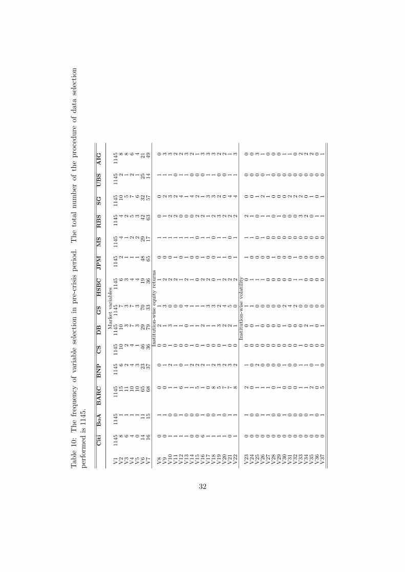
Tab
le10
:T
he
freq
uen
cyof
vari
able
sele
ctio
nin
pre
-cri
sis
per
iod
.T
he
tota
lnu
mb
erof
the
pro
ced
ure
ofd
ata
sele
ctio
np
erfo
rmed
is11
45.
Citi
BoA
BARC
BNP
CS
DB
GS
HSBC
JPM
MS
RBS
SG
UBS
AIG
Market
variables
V1
1145
1145
1145
1145
1145
1145
1145
1145
1145
1145
1145
1145
1145
1145
V2
81
15
610
10
76
24
410
28
V3
61
11
22
33
31
12
51
8V4
41
10
44
77
41
25
72
6V5
01
10
31
33
41
23
61
4V6
14
11
65
23
46
29
70
19
48
29
42
32
25
21
V7
16
15
68
37
36
79
33
36
65
17
63
57
14
49
Institution-w
iseeq
uityretu
rns
V8
01
00
02
11
01
00
10
V9
01
01
01
32
01
12
13
V10
10
12
13
02
01
23
13
V11
10
11
01
02
11
22
02
V12
11
60
01
01
01
04
12
V13
10
11
00
42
11
01
13
V14
00
12
11
11
01
04
02
V15
00
52
01
10
00
22
01
V16
61
12
12
12
11
21
03
V17
10
01
01
32
01
13
13
V18
10
82
01
30
00
23
13
V19
11
53
03
21
11
32
02
V20
10
72
12
42
11
20
02
V21
01
73
02
52
00
24
11
V22
11
82
01
02
11
24
13
Institution-w
isevolatility
V23
01
21
00
10
11
20
00
V24
00
00
00
11
01
10
00
V25
00
12
01
01
00
01
03
V26
01
10
00
01
01
12
01
V27
01
10
00
00
00
11
10
V28
00
00
00
00
10
00
00
V29
00
10
00
00
00
10
00
V30
01
01
01
20
00
00
01
V31
00
00
00
40
00
02
01
V32
00
00
00
21
10
02
00
V33
00
11
10
01
00
32
02
V34
00
11
02
00
00
20
02
V35
01
20
01
00
00
01
02
V36
00
01
00
00
00
10
00
V37
01
50
01
00
00
11
01
32

Tab
le11
:T
he
freq
uen
cyof
vari
able
sele
ctio
nin
cris
isp
erio
d.
Th
eto
tal
nu
mb
erof
the
pro
ced
ure
ofd
ata
sele
ctio
np
erfo
rmed
is56
1.
Citi
BoA
BARC
BNP
CS
DB
GS
HSBC
JPM
MS
RBS
SG
UBS
AIG
Market
variables
V1
561
561
561
561
561
561
561
561
561
561
561
561
561
561
V2
22
35
11
13
11
22
21
V3
01
14
10
03
10
22
01
V4
32
111
10
03
11
32
12
V5
22
24
10
03
11
22
11
V6
87
83
30
25
49
16
140
52
23
65
51
51
18
74
V7
77
87
24
42
26
19
117
28
89
144
34
61
961
Institution-w
iseeq
uityretu
rns
V8
11
13
10
01
01
21
01
V9
00
15
10
03
11
11
01
V10
10
13
10
03
01
22
00
V11
11
12
10
02
00
22
00
V12
01
02
10
01
01
21
01
V13
00
12
10
00
01
02
01
V14
01
01
10
02
00
01
01
V15
01
04
10
02
01
01
01
V16
01
01
10
00
00
12
00
V17
01
12
00
01
01
21
00
V18
10
04
10
03
01
02
01
V19
10
12
10
02
01
21
00
V20
20
00
00
01
01
22
00
V22
11
13
00
02
01
21
01
Institution-w
isevolatility
V23
01
00
10
01
00
00
00
V24
00
00
10
00
00
01
00
V25
00
00
00
01
00
00
01
V26
00
00
00
01
00
10
01
V27
01
02
00
01
00
00
00
V28
00
01
00
01
00
01
01
V29
00
00
00
01
00
11
00
V30
00
00
00
02
00
01
00
V31
00
00
00
00
00
00
00
V32
00
00
00
00
00
00
00
V33
00
00
10
01
00
00
00
V34
00
00
10
01
00
00
01
V35
00
00
00
01
00
01
00
V37
00
00
00
00
00
01
00
33

Tab
le12
:T
he
freq
uen
cyof
vari
able
sele
ctio
nin
pre
-cri
sis
per
iod
excl
ud
ing
VIX
.T
he
tota
lnu
mb
erof
the
pro
ced
ure
of
data
sele
ctio
np
erfo
rmed
is11
45.
Citi
BoA
BARC
BNP
CS
DB
GS
HSBC
JPM
MS
RBS
SG
UBS
AIG
Market
variables
V2
1145
1145
1145
1145
1145
1145
1145
1145
1145
1145
1145
1145
1145
1145
V3
148
120
92
173
123
164
159
128
190
258
61
128
204
124
V4
132
113
95
164
122
141
181
121
168
187
55
135
179
114
V5
105
101
65
141
94
119
142
98
150
158
51
109
160
102
V6
287
272
300
355
271
323
439
273
443
507
276
265
472
262
V7
302
415
236
379
322
282
481
281
472
612
272
266
480
303
Institution-w
iseeq
uityretu
rns
V8
60
65
45
88
70
96
72
95
97
104
15
60
106
87
V9
61
87
54
123
64
107
85
85
111
118
39
94
128
86
V10
64
79
60
89
75
96
86
75
117
109
30
102
121
89
V11
77
71
46
104
79
69
85
66
93
115
33
96
119
84
V12
101
90
60
113
81
96
86
76
100
126
35
106
132
70
V13
96
90
50
98
70
98
89
77
109
125
28
108
115
98
V14
86
68
47
112
70
97
66
85
119
115
32
100
104
86
V15
94
71
46
126
83
88
92
89
111
128
28
97
130
104
V16
100
84
65
114
75
93
98
74
113
115
36
86
97
98
V17
93
71
48
128
74
107
93
77
120
129
34
100
133
91
V18
74
66
55
125
72
101
81
74
121
118
38
104
110
73
V19
88
77
56
87
57
88
88
82
84
105
35
99
116
74
V20
90
97
55
119
82
78
96
86
128
121
33
92
124
69
V21
87
86
44
117
56
97
96
65
115
146
35
73
128
92
V22
79
85
56
115
79
118
99
90
126
141
29
94
120
94
Institution-w
isevolatility
V23
72
63
40
67
77
85
81
71
82
133
24
51
93
87
V24
59
76
34
99
64
97
91
52
100
112
24
63
80
94
V25
66
76
29
91
68
83
89
35
100
135
28
93
103
87
V26
64
71
36
122
68
65
75
55
64
119
27
100
95
78
V27
86
85
54
83
73
100
65
61
96
94
34
26
115
87
V28
91
75
36
90
60
102
78
46
113
128
19
90
91
84
V29
87
64
29
52
49
54
48
27
88
84
23
82
30
31
V30
81
55
58
130
75
102
86
88
112
114
27
85
117
95
V31
21
34
15
97
63
45
48
44
88
96
10
78
99
95
V32
65
52
19
63
34
50
50
42
52
70
17
88
58
43
V33
61
36
38
53
56
56
63
40
78
71
21
77
48
69
V34
62
68
51
84
42
82
66
51
91
124
34
89
104
61
V35
65
58
40
63
62
86
85
68
120
141
31
52
129
65
V36
48
67
31
53
60
61
70
45
94
78
14
22
103
63
V37
67
76
41
102
74
99
67
85
58
95
19
29
86
57
34
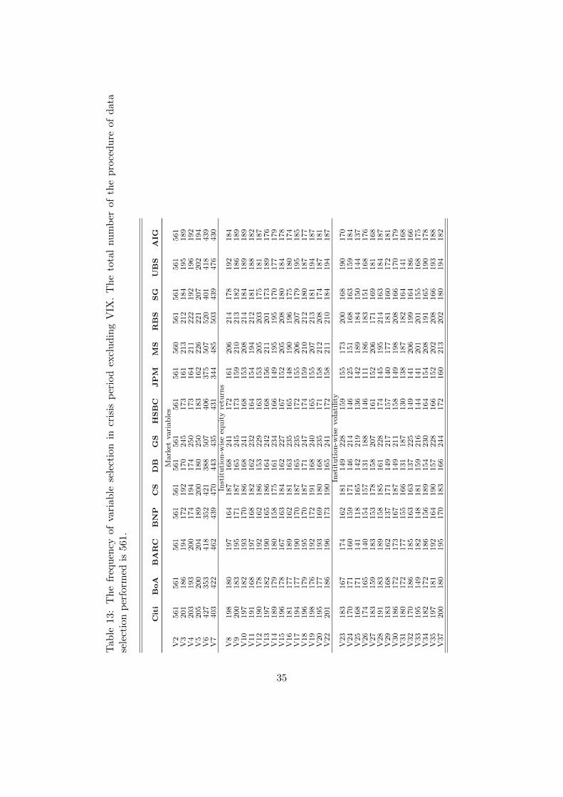
Tab
le13
:T
he
freq
uen
cyof
vari
able
sele
ctio
nin
cris
isp
erio
dex
clu
din
gV
IX.
Th
eto
tal
nu
mb
erof
the
pro
ced
ure
of
data
sele
ctio
np
erfo
rmed
is56
1.
Citi
BoA
BARC
BNP
CS
DB
GS
HSBC
JPM
MS
RBS
SG
UBS
AIG
Market
variables
V2
561
561
561
561
561
561
561
561
561
560
561
561
561
561
V3
201
186
194
172
192
170
245
173
161
213
212
184
195
189
V4
203
193
200
174
194
174
250
173
164
211
222
192
196
192
V5
205
200
204
189
200
180
250
183
162
226
221
207
202
194
V6
427
353
418
352
421
388
507
406
375
507
520
401
418
439
V7
403
422
462
439
470
443
435
431
344
485
503
439
476
430
Institution-w
iseeq
uityretu
rns
V8
198
180
197
164
187
168
241
172
161
206
214
178
192
184
V9
200
183
195
171
187
165
245
173
159
210
213
182
186
189
V10
197
182
193
170
186
168
241
168
153
208
214
184
189
189
V11
191
168
197
168
182
162
232
164
154
194
212
181
188
182
V12
190
178
192
162
186
153
229
163
153
205
203
175
181
187
V13
197
182
190
165
186
164
242
168
156
211
201
173
189
176
V14
189
179
180
158
175
161
234
166
149
195
195
170
177
179
V15
196
178
167
163
184
162
227
167
152
205
208
180
184
178
V16
181
177
189
162
181
163
235
165
148
190
196
175
180
174
V17
194
177
190
170
187
165
235
172
155
206
207
179
195
185
V18
196
179
195
170
187
171
247
174
159
210
212
180
187
177
V19
198
176
192
172
191
168
240
165
155
207
213
181
194
187
V20
195
177
193
169
180
168
235
171
158
212
208
174
187
181
V22
201
186
196
173
190
165
241
172
158
211
210
184
194
187
Institution-w
isevolatility
V23
183
167
174
162
181
149
228
159
155
173
200
168
190
170
V24
170
171
160
159
171
146
214
146
125
151
168
163
159
184
V25
168
171
141
118
165
142
219
136
142
189
184
150
144
137
V26
174
165
140
154
157
131
188
146
111
186
183
151
168
176
V27
183
159
183
153
178
158
207
161
152
206
171
169
181
168
V28
191
183
189
158
185
161
228
174
145
195
214
163
184
187
V29
183
168
162
137
171
149
217
157
140
177
181
160
172
181
V30
186
172
173
167
187
149
211
158
149
198
208
166
170
179
V31
180
172
177
155
166
131
187
130
138
187
182
164
141
168
V32
170
186
185
163
163
137
225
149
141
206
199
164
186
166
V33
195
149
182
148
181
159
216
144
141
201
201
155
168
175
V34
182
172
186
156
189
154
230
164
154
208
191
165
190
178
V35
197
181
192
164
190
157
228
166
152
202
208
166
193
188
V37
200
180
195
170
183
166
244
172
160
213
202
180
194
182
35

References
Acharya, V., Engle, R., Figlewski, S., Lynch, A. and Subrahmanyam, M. (2009). Cen-
tralized Clearing for Credit Derivatives, Wiley, chapter 11, pp. 251–268.
Acharya, V. V., Pedersen, L. H., Philippon, T. and Richardson, M. (2010). Measuring
systemic risk, Working Paper 10-02, Federal Reserve Bank of Cleveland.
Acharya, V. V. and Subrahmanyam, M. G. (2008). Time to lift the veil.
Adrian, T. and Brunnermeier, M. K. (2011). CoVaR, Staff Reports 348, Federal Reserve
Bank of New York.
Alexander, C. and Kaeck, A. (2008). Regime dependent determinants of credit default
swap spreads, Journal of Banking and Finance 32: 1008–1021.
Arora, N., Gandhi, P. and Longstaff, F. A. (2012). Counterparty credit risk and the
credit default swap market, Journal of Financial Economics 103: 280–293.
BIS (2011). Basel iii: A global regulatory framework for more resilient banks and banking
systems, Basel Committee on Banking Supervision .
Breitenfellner, B. and Wagner, N. (2012). Explaining aggregate credit default swap
spreads, International Review of Financial Analysis 22: 18–29.
Brownlees, C. T. and Engle, R. (2010). Volatility, correlation and tails for systemic risk
measurement, Working paper, NYU Stern School of Business.
Chao, S.-K., Hardle, W. and Wang, W. (2014). Quantile regression in risk calibration, in
C.-F. Lee (ed.), Handbook of Financial Econometric and Statistics, Springer-Verlag,
chapter 54.
Christoffersen, P. F. (1998). Evaluating interval forecasts, International Economic Re-
view 39(4): 841–862.
Cont, R. and Kokholm, T. (2013). Central clearing of otc derivatives: bilateral vs
multilateral netting.
URL: arXiv:1304.5065
36

Duffie, D. (2010). How Big Banks Fail And What to do About It Darrell Duffie, Princeton
University Press.
Duffie, D., Li, A. and Lubke, T. (2010). Policy perspectives on OTC derivatives market
infrastructure, Staff Reports 424, Federal Reserve Bank of New York.
Duffie, D. and Zhu, H. (2011). Does a central clearing counterparty reduce counterparty
risk?, Review of Asset Pricing Studies 1(1): 74–95.
Dullmann and Sosinska (2007). Credit default swap prices as risk indicators of listed
german banks, Financial Markets and Portfolio Management 21(3): 269–292.
ESMA (2013). The clearing obligation under emir, Discussion Paper .
Espinosa, G., Rubia, A., Valderrama, L. and Anton, M. (2013). Good for one, bad for
all: Determinants of individual versus systemic risk, Journal of Financial Stability
9: 287–299.
Galil, K., Shapir, O. M., Amiran, D. and Ben-Zion, U. (2013).
The determinants of cds spreads, Journal of Banking & Finance
http://dx.doi.org/10.1016/j.jbankfin.2013.12.005.
Hautsch, N., Schaumburg, J. and Schienle, M. (2013). Financial network systemic risk
contributions, Submitted to the Review of Finance (2011-072).
ISDA (2013). Non-cleared otc derivatives: Their importance to the global economy, The
International Swaps and Derivatives Association, Inc. .
Koenker, R. (2005). Quantile Regression, Cambridge University Press.
Koenker, R. and Bassett, G. S. (1978). Regression quantiles, Econometrica 46: 33–50.
Kupiec, P. (1995). Techniques for verifying the accuracy of risk management models,
Journal of Derivatives 3: 73–84.
Li, Y., Lui, Y. and Zhu, J. (2007). Quantile regression in reproducing kernel hilbert
spaces, J. Am. Stat. Assoc. 102(477): 255–268.
URL: http://dx.doi.org/10.1198/016214506000000979
Longstaff, F. A., Pan, J., Pedersen, L. and Singleton, K. (2007). How sovereign is
37

sovereign credit risk?, NBER Working Paper 13658.
Merton, R. C. (1974). The pricing of corporate debt: The risk structure of interest rates,
Journal of Finance 29 (2): 449¡V470.
Pirrong, C. (2011). The economics of central clearing: Theory and practice, Discussion
Paper 1, International Swaps and Derivatives Association.
SEC (2010). Dodd-frank wall street reform and consumer protection act, United States
Securities and Exchange Commission (SEC) .
Song, S., Hardle, W. and Ritov, Y. (2012). Partial linear quantile regression and boot-
strap confidence bands, Journal of Multivariate Analysis 107: 244–262.
Tibshirani, R. (1996). Regression shrinkage and selection via the Lasso, Journal of the
Royal Statistical Society, Series B 58: 267–288.
Upper, C. and Worm, A. (2004). Estimating bilateral exposures in the german interbank
market: Is there a danger of contagion?, European Economic Review 48: 827–849.
Yuan, M. (2006). GACV for quantile smoothing splines, Computational Statistics &
Data Analysis 50: 813–829.
38

SFB 649 Discussion Paper Series 2014
For a complete list of Discussion Papers published by the SFB 649,
please visit http://sfb649.wiwi.hu-berlin.de.
001 "Principal Component Analysis in an Asymmetric Norm" by Ngoc Mai
Tran, Maria Osipenko and Wolfgang Karl Härdle, January 2014.
002 "A Simultaneous Confidence Corridor for Varying Coefficient Regression
with Sparse Functional Data" by Lijie Gu, Li Wang, Wolfgang Karl Härdle
and Lijian Yang, January 2014.
003 "An Extended Single Index Model with Missing Response at Random" by
Qihua Wang, Tao Zhang, Wolfgang Karl Härdle, January 2014.
004 "Structural Vector Autoregressive Analysis in a Data Rich Environment:
A Survey" by Helmut Lütkepohl, January 2014.
005 "Functional stable limit theorems for efficient spectral covolatility
estimators" by Randolf Altmeyer and Markus Bibinger, January 2014.
006 "A consistent two-factor model for pricing temperature derivatives" by
Andreas Groll, Brenda López-Cabrera and Thilo Meyer-Brandis, January
2014.
007 "Confidence Bands for Impulse Responses: Bonferroni versus Wald" by
Helmut Lütkepohl, Anna Staszewska-Bystrova and Peter Winker, January
2014.
008 "Simultaneous Confidence Corridors and Variable Selection for
Generalized Additive Models" by Shuzhuan Zheng, Rong Liu, Lijian Yang
and Wolfgang Karl Härdle, January 2014.
009 "Structural Vector Autoregressions: Checking Identifying Long-run
Restrictions via Heteroskedasticity" by Helmut Lütkepohl and Anton
Velinov, January 2014.
010 "Efficient Iterative Maximum Likelihood Estimation of High-
Parameterized Time Series Models" by Nikolaus Hautsch, Ostap Okhrin
and Alexander Ristig, January 2014.
011 "Fiscal Devaluation in a Monetary Union" by Philipp Engler, Giovanni
Ganelli, Juha Tervala and Simon Voigts, January 2014.
012 "Nonparametric Estimates for Conditional Quantiles of Time Series" by
Jürgen Franke, Peter Mwita and Weining Wang, January 2014.
013 "Product Market Deregulation and Employment Outcomes: Evidence
from the German Retail Sector" by Charlotte Senftleben-König, January
2014.
014 "Estimation procedures for exchangeable Marshall copulas with
hydrological application" by Fabrizio Durante and Ostap Okhrin, January
2014.
015 "Ladislaus von Bortkiewicz - statistician, economist, and a European
intellectual" by Wolfgang Karl Härdle and Annette B. Vogt, February
2014.
016 "An Application of Principal Component Analysis on Multivariate Time-
Stationary Spatio-Temporal Data" by Stephan Stahlschmidt, Wolfgang
Karl Härdle and Helmut Thome, February 2014.
017 "The composition of government spending and the multiplier at the Zero
Lower Bound" by Julien Albertini, Arthur Poirier and Jordan Roulleau-
Pasdeloup, February 2014.
018 "Interacting Product and Labor Market Regulation and the Impact of
Immigration on Native Wages" by Susanne Prantl and Alexandra Spitz-
Oener, February 2014.
SFB 649, Spandauer Straße 1, D-10178 Berlin
http://sfb649.wiwi.hu-berlin.de
This research was supported by the Deutsche
Forschungsgemeinschaft through the SFB 649 "Economic Risk".
SFB 649, Spandauer Straße 1, D-10178 Berlin
http://sfb649.wiwi.hu-berlin.de
This research was supported by the Deutsche
Forschungsgemeinschaft through the SFB 649 "Economic Risk".

SFB 649, Spandauer Straße 1, D-10178 Berlin
http://sfb649.wiwi.hu-berlin.de
This research was supported by the Deutsche
Forschungsgemeinschaft through the SFB 649 "Economic Risk".
SFB 649 Discussion Paper Series 2014
For a complete list of Discussion Papers published by the SFB 649, please visit http://sfb649.wiwi.hu-berlin.de.
019 "Unemployment benefits extensions at the zero lower bound on nominal
interest rate" by Julien Albertini and Arthur Poirier, February 2014.
020 "Modelling spatio-temporal variability of temperature" by Xiaofeng Cao,
Ostap Okhrin, Martin Odening and Matthias Ritter, February 2014.
021 "Do Maternal Health Problems Influence Child's Worrying Status?
Evidence from British Cohort Study" by Xianhua Dai, Wolfgang Karl
Härdle and Keming Yu, February 2014.
022 "Nonparametric Test for a Constant Beta over a Fixed Time Interval" by
Markus Reiß, Viktor Todorov and George Tauchen, February 2014.
023 "Inflation Expectations Spillovers between the United States and Euro
Area" by Aleksei Netšunajev and Lars Winkelmann, March 2014.
024 "Peer Effects and Students’ Self-Control" by Berno Buechel, Lydia
Mechtenberg and Julia Petersen, April 2014.
025 "Is there a demand for multi-year crop insurance?" by Maria Osipenko,
Zhiwei Shen and Martin Odening, April 2014.
026 "Credit Risk Calibration based on CDS Spreads" by Shih-Kang Chao,
Wolfgang Karl Härdle and Hien Pham-Thu, May 2014.