I Atmospheric Effects on I- Laser Propagation · PDF fileAbsorption coefficient of nitrous...

I

NASA

I

Technical Paper 1357

- I -

Atmospheric Effects on ’ - CO, .~ Laser Propagation ’

L ~ A N COPY: RETURN 1 ‘kWL TECHNICAL LlBRl

KIRTLAND AFB, N. M

S . S . R. Murty .and J. W. Bilbro

NOVEMBER

,’ . I -

, -

https://ntrs.nasa.gov/search.jsp?R=19790005436 2018-05-07T06:40:31+00:00Z

NASA Technical, Paper 1357

Atmospheric Effects on CO, Laser Propagation

S . S . R. Murty Alabama ACM University Normal, Alabama

and J. W. Bilbro George C. Marshall Space Flight Center Marshall Space Flight Center, Alabama

National Aeronautics and Space Administration

Scientific and Technical Information Office

TECH LIBRARY KAFB, NY

1978

ACtiNOWLEDGMENTS

The authors gratefully acknowledge the assistance provided by those who aided in the preparation of this report. In particular, appreciation is expressed to Mr . R. M. Huffaker of the Wave Propagation Laboratory, NOAA, Boulder, Colorado, for his efforts in the initiation of this work and to Mr . C. 0. Jones of NASA/MSFC for his discussions and critique of our efforts. Additionally, the authors acknowledge Dr. L. Z. Kennedy (LASL, Los Alamos, New Mexico) , Dr. T. R. Lawrence (NOAA, Boulder, Colorado), Dr. Alex Thomson (Physical Dynamics, Berkely, California), M r . H. B. Jeffreys (Teledyne Brown, Huntsville, Alabama), and Dr. J. L. Randal, Mr . F. W . Wagnon, Mr . E. A . Weaver, Mr . J. A. Dunkin, and M r . R. W. George, all of NASA/MSFC.

TABLE OF CONTENTS

Page

I . INTRODUCTION ............................... 1

II . ABSORPTION LOSSES ........................... 2

A . Absorption Coefficient ....................... 2 B . Absorption by Carbon Dioxide .................. 7 C . Absorption by Water Vapor .................... 10 D . Absorption by Nitrous Oxide ................... 27 E . Comparison with AFCRL Calculations ............. 27 F . Absorption Losses for Edwards AFB 1973

Flight Test ............................... 27 G . Lase r s with Low Transmission Loss .............. 36

IU . TURBULENCE LOSSES ........................... 43

A . Parameters of Atmospheric Turbulence . . . . . . . . . . . . 43

C . Effect of Atmospheric Turbulence on Laser Beams .... 50 D . Effect of Turbulence on Heterodyne Systems ......... 63 E . Signal-to-Noise Ratio Loss .................... 64

B . Optical Properties of the Turbulent Eddies .......... 45

IV . AEROSOL EFFECTS ............................ 78

A . Calculation of the Aerosol Backscatter and

B . Performance of the MSFC Pulsed Laser System Extinction Coefficients ....................... 79

at Ground Level ............................ 81

V . CONCLUDING REMARKS ......................... 90

REFERENCES ...................................... 91

iii

.

L I ST OF ILLUSTkATIONS

Figure Title P age

1. Near-infrared solar spectrum, spectra of various atmospheric gases and operating frequencies of H F , DF, and CO, lasers ........................ 3

2. Variation of two-way transmission loss with altitude for P and R lines of CO, laser i n AFCRL Midlatitude Summer Hazy Atmosphere ...................... 5

3. Absorption coefficient of carbon dioxide at T = 300 K ..... 8

4. Absorption coefficient of carbon dioxide at T = 200 K ..... 9

5. Absorption coefficient of carbon dioxide at v = 947.738 cm-’ ............................... 11

6. Absorption coefficient of carbon dioxide at v = 945.976 cm” ............................... 12

7. Absorption coefficient of carbon dioxide at v = 944.190 cm-I ............................... 13

8. Absorption coefficient of carbon dioxide at I, = 942.38 cm-’ ................................ 14

9. Absorption coefficient of carbon dioxide at v = 940.544 cm-I ............................... 15

10. Continuum absorption coefficient of water at different temperatures ......................... 16

11. Absorption coefficient of water vapor continuum for 1 pr-cm at 10.6 p m . ........................ 19

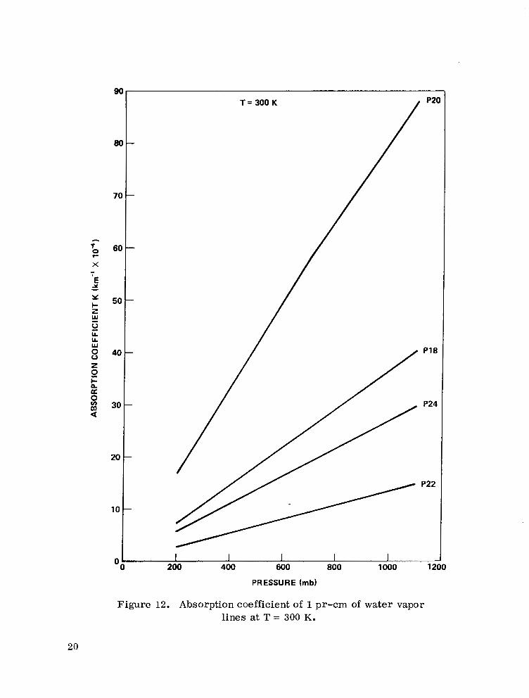
12. Absorption coefficient of 1 pr-cm of water vapor lines at T = 300 K ............................ 20

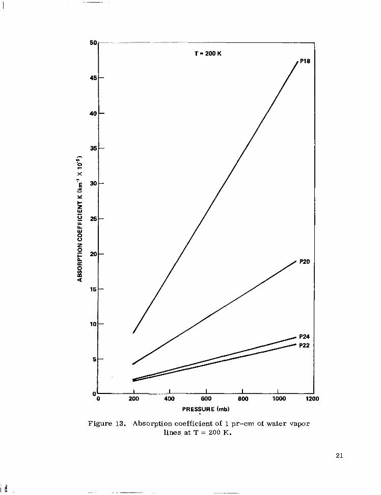
13. Absorption coefficient of 1 pr-cm of water vapor lines at T = 200 K ............................. 21

iv

"

LIST OF ILLUSTRATIONS (Continued)

Figure Title Page

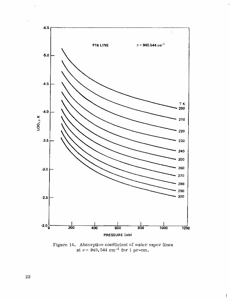
14. Absorption coefficient of water vapor lines at u = 940.544 cm" for 1 pr-cm . . . . . . . . . . . . . . . . . . . . . . . 22

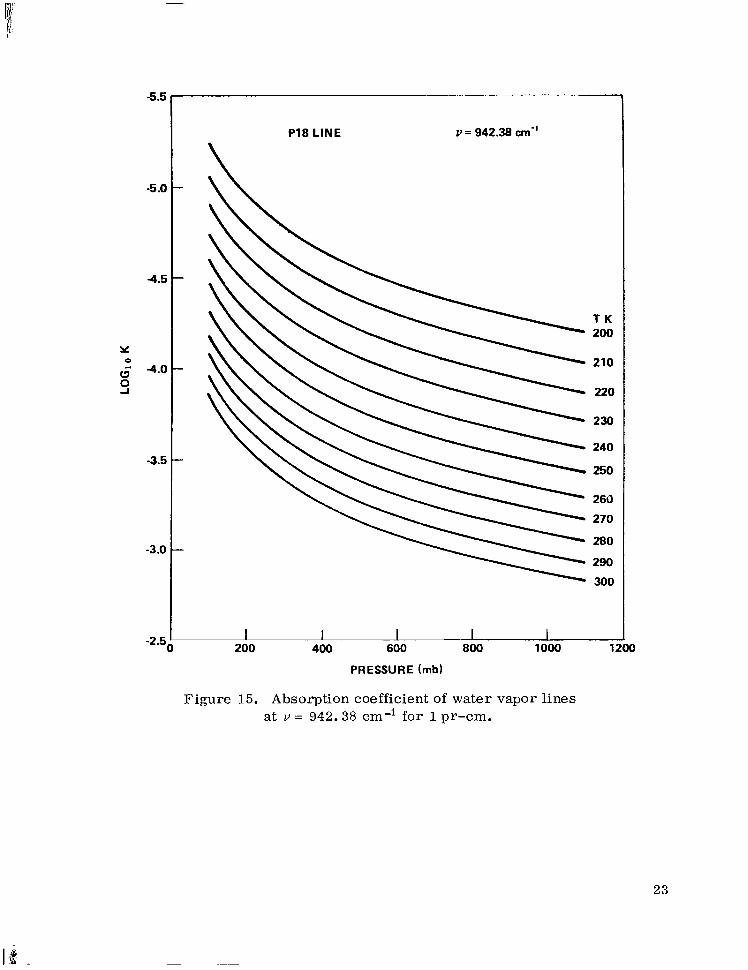
15. Absorption coefficient of water vapor lines at u = 942.38 cm-I for 1 pr-cm . . . . . . . . . . . . . . . . . . . . . . . . 23

16. Absorption coefficient of water vapor lines at u = 944.19 cm" for 1 pr-cm . . . . . . . . . . . . . . . . . . . . . . . . 24

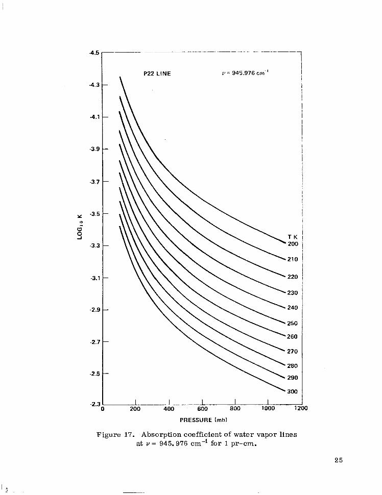
17. Absorption coefficient of water vapor lines at v = 945.976 cm'l for 1 pr-cm . . . . . . . . . . . . . . . . . . . . . . . 25

18. Absorption coefficient of water vapor lines at u = 947.738 cm-' for 1 pr-cm . . . . . . . . . . . . . . . . . . . . . , . 26

19. Absorption coefficient of nitrous oxide lines at T = 300 K . . 28

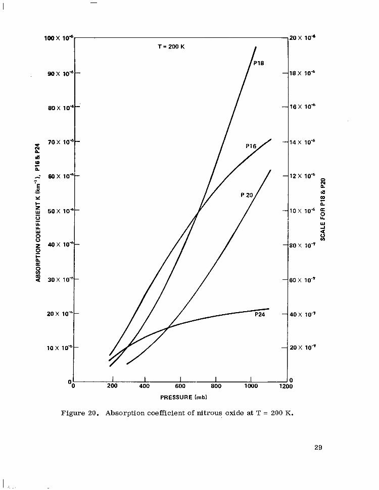
20. Absorption coefficient of nitrous oxide at T = 200 K . . . . . . 29

21. Absorption coefficient of nitrous oxide lines at u = 940.544 cm-I . . . . . . . . . . . . . . . . . . . . . . . . . . . . . 30

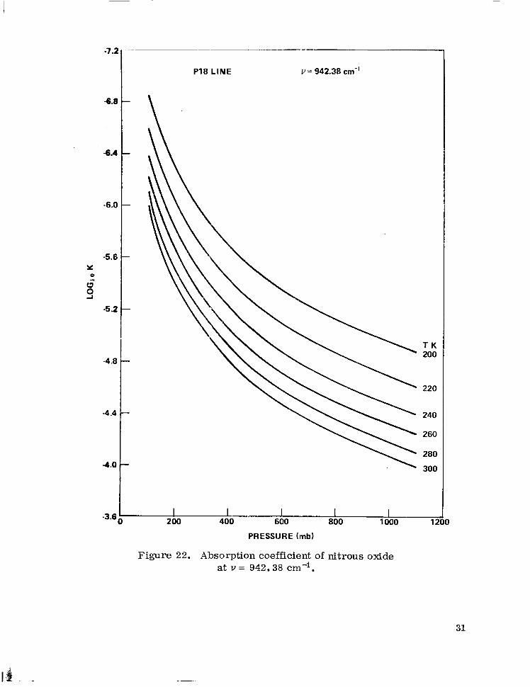
22. Absorption coefficient of nitrous oxide at v = 942.38 cm-I . . . . . . . . . . . . . . . . . . . . . . . . . . . . . . . . 31

23. Absorption coefficient of nitrous oxide lines at v = 944.19 cm-I . . . . . . . . . . . . . . . . . . . . . . . . . . . . . . . . 32

24 Absorption coefficient of nitrous oxide lines at v = 945.976 cm-I . . . . . . . . . . . . . . . . . . . . . . . . . . . . . . . 33

25. Absorption coefficient of nitrous oxide lines at u = 947.738 cm" . . . . . . . . . . . . . . . . . . . . . . . . . . . . . . . 34

26. Total transmission loss at the P lines for flight B8, Run 18, 1/19/1973 at Edwards AFB . . . . . . . . . . . . . . . . 39

27. Comparison of measured and theoretical S/N values . . . . . 40

V

I 1 1 1 I

L IST OF ILLUSTRATIONS (Concluded)

Figure Title Page

28. Performance of C 0 2 , H F , and DF laser Doppler systems against ground target at 15 deg inclination in AFCRL Midlatitude Summer Atmosphere .................. 41

29. Three-dimensional turbulence spectrum models for index-of-refraction fluctuation .................... 46

30. Saturation of the variance of log-amplitude fluctuations of a spherical wave propagating through a homogeneous turbulence path .............................. 57

31. Theoretical curves of the log-amplitude covariance function in weak to strong turbulence. . . . . . . . . . . . . . . . 60-

32. Comparison of measured and theoretical S/N values ..... 74

33. Atmospheric attenuation at 10.6 pm . . . . . . . . . . . . . . . . 76

34. S /N ratio as a function of aperture at fixed range L ...... 83

35. Optimum value of aperture as a function of range . . . . . . . 85

36. Maximum range of MSFC Pulsed Laser Doppler System for horizontal path at sea level . . . . . . . . . . . . . . . . . . . . 86

37. Maximum ground range of MSFC system . . . . . . . . . . . . . 87

38. Atmospheric molecular absorption coefficient as a function of relative humidity and temperature at sea level for h = 10.59 p m . ...................... 89

vi

LIST OF TABLES

Table Title Page

1. Transmission Losses ........................... 4

2. Comparison with the Results of McClatchey and Selby ..... 35

3. Calculation of Absorption Coefficient for Flight B8, Run 18, 1/19/1973, Edwards AFB .................. 37

4.

5.

6.

7.

8.

9.

10.

Molecular Absorption Coefficient of P Lines and Aerosol Attenuation per Kilometer .................. 38

Round-Trip Horizontal Transmission Loss for Infrared Lasers Over 40 km Range ........................ 42

Comparison of Losses at CO, and DF Laser Wavelengths Over a 20 km Horizontal Path at 2.5 km and 5 lm Altitudes ................................... 75

Signal Loss in Atmospheric Propagation at 10.6 pm Due to Absorption, Scattering, and Coherence Degradation for a Two-way Horizontal Path of 20 km at Each Altitude . . . . . 77

Backscatter and Extinction Coefficients at 10.59 pm for N = 100 particles/cm3 for Several Distributions . . . . . . . . . 80

AFCRL Model of Aerosol Number Density Variation with Altitude ................................. 82

The Range at Which S/N Reaches a Maximum Due to Aerosols Having Haze C Size Distribution . . . . . . . . . . . . . 82

vii

ATMOSPHERIC EFFECTS ON C02 LASEI? PROPAGATION

1. INTRODUCTION

The Marshall Space Flight Center (MSFC) has been involved in the development of CO, Laser Doppler Velocimeter Systems for atmospheric measurement since the late 1960's. The shorter range continuous wave (CW) system development has led to a variety of applications, including measurement of the following: aircraft wake vortices [ 11 , dust devils [ 21 , smokestack emissions [ 31 , and wind profiles [ 41. The development of a pulsed system has resulted in measurement programs for clear air turbulence (CAT) [ 51 and severe s torm research [ 61.

Accompanying the development of these systems w a s an increased interest in the overall effects resulting from the characteristics of the transmission path. This report deals with several of the losses associated with the transmission path including absorption, scattering, and turbulence.

The bulk of the work has appeared earlier in the form of two NASA Technical Memoranda, "Atmospheric Transmission of CO, Lase r Radiation With Application to Lase r Doppler Systems" [ 7 ] , and "Laser Doppler Systems in Atmospheric Turbulence" 181. This work has been combined with an examination of the propagation effects of aerosols in an attempt to more clearly define carbon dioxide transmission losses in an atmospheric path.

Section II of this report discusses transmission losses by addressing those losses attributed to absorption, particularly absorption by carbon dioxide water vapor, and nitrous oxide. In addition, absorption losses are calculated for a 1973 flight test of the system at Edwards A i r Force Base. A brief comparison of hydrogen fluoride ( H F ) and deuterium fluoride ( D F ) lasers with CO, lasers is also provided. Section 111 is a discussion of turbulence effects, including turbulence parameters and optical effects, and their effects on laser beam propagation and coherent heterodyne systems. It concludes with the calculation of the signal-to-noise equation. Section IV is involved with aerosol effects on the backscatter and extinction coefficients and their relation to the signal-to-noise ratio. The performance of the MSFC Pulsed Laser System at ground level is also discussed. The conclusions of this study are presented in Section V.

'I

1 1 . ABSORPTION LOSSES

Transmission losses are characterized as l inear o r nonlinear to dis- tinguish between laser power independent and dependent processes. In this section we examine the linear, power independent losses attributed to molecular gases and aerosols.

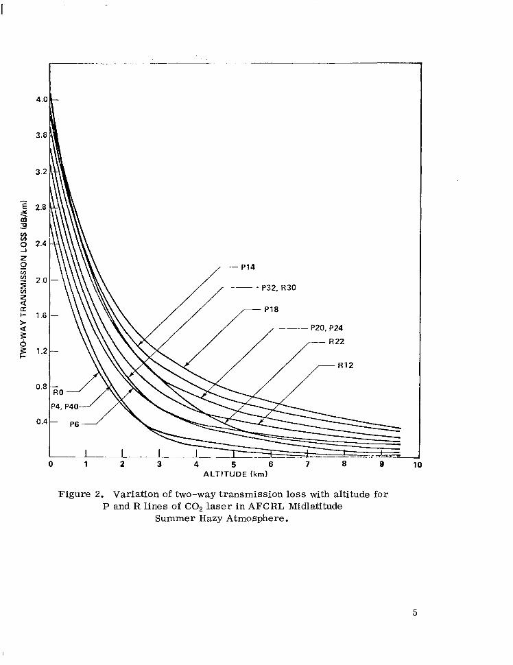
An atmospheric window is defined as a spectral region over which the absorption of a particular wavelength by the permanent atmospheric gases is relatively weak. Although none of the windows are completely transparent because of molecular absorption and particulate scattering, selection of a window is mandatory for long-range propagation. The atmospheric windows i n the infrared wavelengths lie between strong bands of carbon dioxide and water vapor, the two major absorbing gases of infrared. Figure 1 shows a low resolution absorption spectrum ( 1 to 15 pm) of solar radiation at ground level [ 91. In addition, the spectra of various atmospheric gases are displayed as obtained from laboratory measurements. The operating wavelength regions of H F , DF , and CO, lasers are indicated in the figure. The gases indicated (with the excep- tion of ozone and water vapor) are generally uniformly mixed. It should be noted that within the infrared region relatively narrow line widths can be obtained with CO, lasers. These lines are typically 2 x pm o r 60 MHz, while the absorption lines of the atmospheric gases are several orders of magnitude wider. The transmission losses for several CO, lines are shown in Table 1. These values were obtained for a 10 lun horizontal roundtrip path at an altitude of 3 . 5 km. While the P40 and RO lines have the least transmission loss, practical considerations involving availability of equipment have necessi- tated the choice of 10.6 p m for operation of the MSFC system. McClatchey and and Selby [ 101 have calculated the atmospheric transmission in the 10.6 pm region for a set of standard atmospheric conditions. Their results a re shown in Figure 2 as round trip losses for several P and R lines using the A i r Force Cambridge Research Laboratories (AFCRL) Midlatitude Summer Hazy Atmosphere.

A. Absorption Coefficient Since atmospheric conditions are variable and deviations from the stan-

dard models can result in l a rge e r rors , a more accurate indication of absorption loss can be obtained using the prevailing atmospheric conditions for a given experiment. This can be accomplished by providing an absorption coefficient for each of the molecules relevant to CO, laser radiation as a function of pressure

2

HF DF LASER LASER

0

100 0

100 0

i=

a 3 0

0 w I 5 100

k - 0

a

3 d

100 0

100 0

1 00 0

100

cot LASER

co

1 1 I 1 I

cH4

SOLAR SPECTRUM

900 800

11 12 13 14 15 fl++ 'Io0-

Figure 1. Near-infrared solar spectrum, spectra of various atmospheric gases and operating frequencies of HF , DF,

and CO, lasers.

3

TABLE 1. TRANSMISSION LOSSES

Laser Line

P 4 0

P32

P20

P18

P 14

P 6

P4

RO

R12

R22

R30

Wavelength (pm)

10.81

10.72

10.59

10.57

10.53

10.46

10.44

10.40

10.30

10.23

10.18

-

Loss (dB) ~~

~ .~ - "

2.15

5.00

7.85

10.40

9.23

4.64

3.58

2.20

6.80

6.30

4.60 . _ ~ _ . .- ~~ "~

and temperature. The absorption coefficient as a function of frequency is assumed to be described by the Lorentz relation

K ( v ) = Sa!

n[ ( v - vo)2 + a21 ,

where

v = the resonant frequency ( c m l ) 0

S = the line intensity per absorbing molecule (cml/molecules cm-2)

a = the Lorentz line width parameter (cm-l) .

The validity of equation (1) in describing the correct line shape in the wings is in doubt, especially for carbon dioxide and water. In the first case, the wings are overpredicted, while in the latter, they are underestimated.

4

I

0 1 2 3 4 5 6 7 8 9 ALTITUDE (km)

Figure 2. Variation of two-way transmission loss with altitude for P and R lines of CO, laser in AFCRL Midlatitude

Summer Hazy Atmosphere.

5

The line intensity, S , i n equation (1) is independent of pressure but not temperature; i.e.,

where

T = the ambient temperature

T = the standard temperature (296 K) S

Q = the vibrational partition function V

Q = the rotational partition function r

E" = the energy of the lower state of the transition (cm-I) .

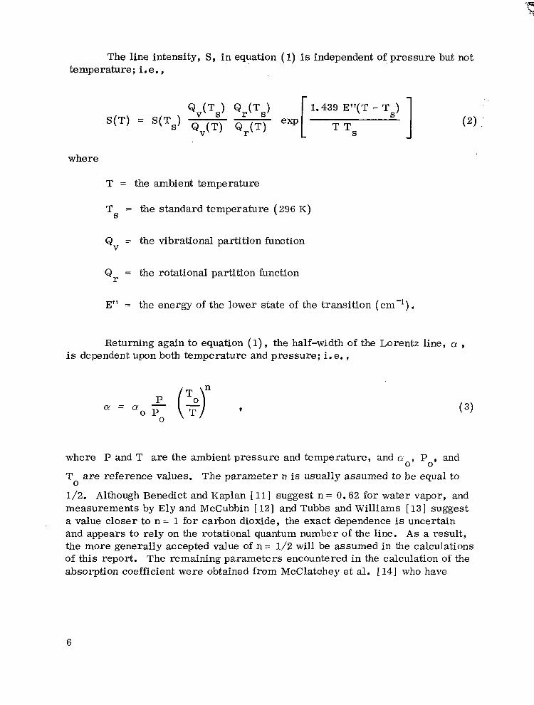
Returning again to equation (1) , the half-width of the Lorentz line, (Y , is dependent upon both temperature and pressure; i. e.,

O P 2 (g , 0

where P and T are the ambient pressure and temperature, and Q 9 Po' and

T are reference values. The parameter n is usually assumed to be equal to

1/2. Although Benedict and Kaplan [ 111 suggest n = 0.62 for water vapor, and measurements by Ely and McCubbin [ 121 and Tubbs and Williams [ 131 suggest a value closer to n = 1 for carbon dioxide, the exact dependence is uncertain and appears to rely on the rotational quantum number of the line. A s a result, the more generally accepted value of n = 1/2 will be assumed in the calculations of this report. The remaining parameters encountered in the calculation of the absorption coefficient were obtained from McClatchey et al. [ 141 who have

0

6

The particular molecules which are active in the 10 pm region of the infrared are: methane, CH,; ethylene, C2H4; nitrous oxide, N20; ammonia, NH,; ozone, 0,; nitric acid, HNO,; carbon dioxide, CO,; and water, H20. Among these molecules, carbon dioxide and water vapor are the major atmospheric attenuators at the C 0 2 laser line frequencies. The primary reason for this is that the atmospheric concentrations of the trace gases and pollutants are too low to have any significant effect. This is illustrated by the following simple estimate: A t the center of the absorption line, the absorption coefficient is given by K = S / m per molecule. For a concentration of 1 ppm, the number of molecules in a 1 km path is approximately For S = an no1 = 0.1, one obtains K = lom4 c h m , where c is the number of ppm. Most trace gases have a concentration, c, of unity or less. For example, ozone has a concentration of 0.02 ppm at sea level and 0.2 ppm at 25 km. Nitrous oxide, in turn, has a concentration of 0.28 ppm. Consequently, it is apparent that these effects will be very small compared to those of carbon dioxide and water. It should be noted, however, that at altitudes above 12 km, ozone absorption may become more important (particularly at the R-lines) . Because of the small effect of the trace gases, calculations in this report are primarily restricted to carbon dioxide, water vapor, and nitrous oxide. The calculations for nitrous oxide are performed to indicate the level of trace gas contributions to the overall absorption. It should be remembered that in addition to molecular absorption, scattering and absorption due to aerosols must be considered.

B. Absorption by Carbon Dioxide The absorption coefficient at the center of P20 laser line by the atmos-

pheric carbon dioxide has been calculated by Yin and Ling [ 151 who have provided polynomial fits to the absorption coefficient as a function of altitude for two model atmospheres. The wings of neighboring lines also contribute to the absorption at any laser line frequency. In this work, lines within 2~20 cm-I are assumed to contribute to the absorption. A concentration of 330 ppm of carbon dioxide in the atmosphere is assumed. The effect of including the wings of the neighboring lines is approximately an increase of 3 to 5 percent at the P20 line. Since the CO, laser operates efficiently around the P20 line, the absorption coefficients for P16, P18, P20, P22, and P24 lines are calculated for temperatures and pressures of interest in the lower atmosphere. The effect of temperature on the absorption coefficient may be seen from Figures 3 and 4. The absorption coefficients for P16, P18, and P20 lines are approximately the same

7

o.la

0.095

0.03

1 - 3 0.085

Y z - 0 k a g 0.08 0

U

0.075

0.07

T = 300 K

”“ ” / p24 u I-

PRESSURE (mb)

Figure 3 . Absorption coefficient of carbon dioxide at T = 300 K.

8

O.OO!

O.OOE

0.004

E Y - 0.004 Y

h

0.0028

" . - . . . . .~

T 200 K "" ""

P16

"""" I

-. .. "" " P20

PRESSURE (mb)

Figure 4. Absorption coefficient of carbon dioxide at T = 200 K.

9

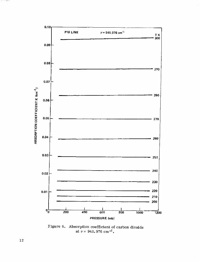
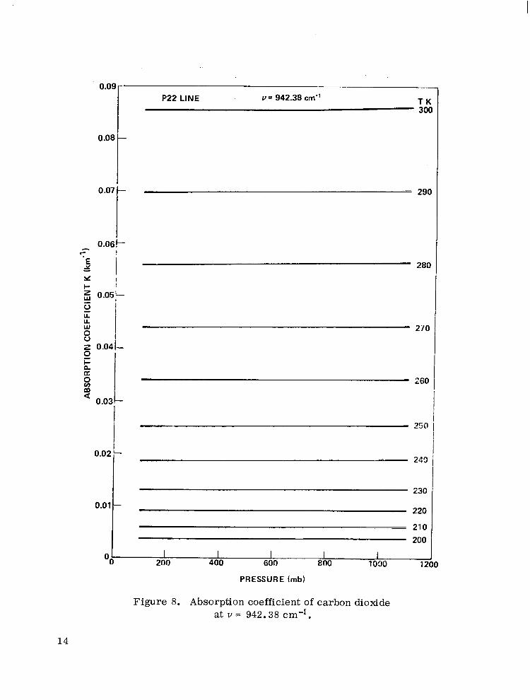
at 300 K and they separate out at 200 K. The absorption coefficients are almost independent of pressure and the slight pressure dependence comes from the line wings as the absorption at the line center is independent of pressure. Figures 5 through 9 give the absorption coefficient at the individual laser lines for pressures f rom 100 to 1100 mb and temperatures from 200 to 300 K.

C. Absorption by Water Vapor Many weak absorption lines of water vapor occur in the 10 pm region.

On the basis of these lines, there should be an almost complete transparency in this region for reasonable atmospheric water content. However, measurements of heat radiation of the sky yield higher values of total radiation than expected due to the rotational lines of water vapor. To explain the observed higher emissions, Elsasser [ 161 in 1938 postulated the existence of a water vapor continuum in the 8 to 14 pm atmospheric window and beyond. This continuum was believed to be due to the wings of strong lines located in the bands on either side of the window. The existence of this continuum has now been well established as a result of several experiments in solar spectrum observation and laboratory measurements [ 17-22]. However, the theory based on usual line shapes has still not been successful in explaining experimental observations; consequently, calculations have to be based on available experimental results.

McCoy, Rensch, and Long I221 measured the absorption of the water vapor equation and suggested the empirical equation

where p is the partial pressure of water vapor and P is the total pressure, both in torr. This equation solves the problem of pressure dependence and is valid at room temperature. This relation has been widely used to estimate water vapor absorption.

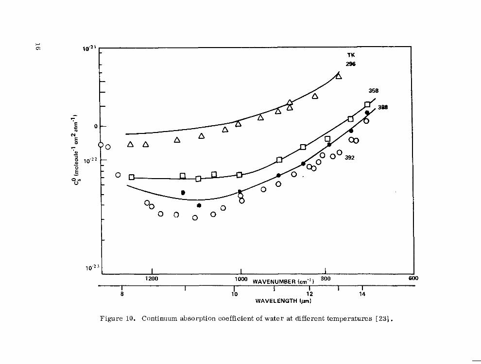
Burch [23] measured the continuum absorption coefficient for pure water vapor at three temperatures and his resul ts are shown in Figure 10. The points marked are revised values and a re 10 to 15 percent less than the solid curves obtained in earlier measurements [ 241. The rapid decrease in the absorption coefficient with increasing temperature is a prominent feature of these results. This trend was predicted by Varanasi, Chow, and Penner [25] as being a result of the association of water molecules due to hydrogen bonding (dimerization).

10

P16 LINE Y = 947.738 cm" T K 300

0.07 I 270

250

~~ 240

230

0.03 -

0.02 -

0.01 -

OO I I i I 1 200 400 600 800 lo00 l i

"- 210

2oa

PRESSURE (mb)

Figure 5. Absorption coefficient of carbon dioxide at v = 947.738 cm".

11

0.1

0.0

0.0

0 .o

0.Of

O.Ot

0.04

0.03

0.02

0.01 I

P18 LINE v = 945.976 cm“ T k 30C

280

261

25E

240

230

220

210 200

200 4 00 GOO 800 1000 1i

PRESSURE (mb)

Figure 6. Absorption coefficient of carbon dioxide

I J

io0

at v = 945.976 cm”.

1 2

0.09

0.08

0.07

0.06

0.05

0.04

0.03

0.02

0.01

280

270

260

250

240

- 230

220

= 210

200

" " ~. ~ ~

J

PRESSURE (rnb)

Figure 7. Absorption coefficient of carbon dioxide at v = 944.190 cm-I.

13

0.09

0.08

0.07

0.02 i

0.01 L

P22 LINE u = 942.38 crn" T K 3oc

~ 290

280

270

~ 2 6C

- 223

230

- 220

OO 200 400 600 800 1030 12 I I I I I

21 0 200 "

PRESSURE (mb)

J 100

Figure 8. Absorption coefficient of carbon dioxide at v = 942.38 crn-',

14

0.08

0.07

0.06

0.05

0.04

0.03

0.02

0.01

0

T K- 300

P24 LINE Y = 940.544 cm"

290

280

270

260

"Y

210 200 .. . . - . . . . .

PRESSURE (rnb)

Figure 9. Absorption coefficient of carbon dioxide at v = 940.544 cm'l.

15

I- t

0

TK 296

/ 358

I I I 1200 low WAVENUMBER (crn-1)

I I 1 I I I 800 600

I 8 10 12 14

WAVELENGTH ( p n )

Figure 10. Continuum absorption coefficient of water at d i f fe ren t t empera tures [ 231.

For atmospheric transmission studies, we are interested in temperatures less than 296 K. Since no data are available at low temperatures, an empirical extrapolation suggested by Burch is used in this work:

Cso ( T ) = Cso (296) (y) where C ' is the absorption coefficient (molecule" cm2 atm"') and T is to be

determined from the experimental values. A t 10.6 pm, we find that T = 5.300 for T = 358 K and T = 5.25 for T = 392 K. T appears to decrease slightly with temperature. These T values are for temperatures above room temperature; no laboratory measurements are available for temperatures below room temperature. One value of the absorption coefficient at T = 283 K is 10 gm" cm2 atm-* from Figure 8 of Bignell's [ 2 1 J paper from the solar spectrum observations. The magnitude of the e r r o r is unknown here. This value corresponds to T = 5.1 at T = 283 K. Thus, the value of T appears to remain approximately 5 even below T = 296 K. We assume T = 5.25 in this work.

S

There is also the effect of foreign gas broadening on the continuum absorption. The results of McCoy, Rensch, and Long [ 2 2 ] give C O r 0.005 C,"

at room temperature. The continuum absorption coefficient is given by K = Cu where u is the absorber thickness expressed in molecules cm-' and C is given by

B

c = Cs"p + CBOP

where p is the partial pressure of water vapor and P is the total pressure, both in atmospheres. The partial pressure of water vapor may be obtained from

where w is the number of gm-cm-2/lun of water vapor. The water vapor is usually expressed in units of precipitable centimeters (pr-cm) which is the Same as gm-cm'2. The absorber thickness u is given by

17

!

22 7.18 X p molecdes/cm2 . u = 3.34x 10 w = T ( 8)

The continuum absorption may be written as follows after combining equation (5) with equation (8) :

1.58 X 105 ( 2 3 5.25 K = -

T p(p + 0.005 P) km” .

W e used C; = 2.2 x molecules-‘ cm2 atm-l at 10.6 hm. Equation (9) is

used in this work to calculate the water vapor continuum absorption coefficient for all C02 laser lines shown in Figure 11.

Recently the temperature

McClatchy and D’Agali [ 261 gave the following expression for variation of C (v,T) in the 8 to 14 pm continuum:

S

= Cs( ~ ~ 2 9 6 ) exp [ 1800 (; - - - 2:6)]

where

Cs( u, 296) = 4.18 + 5578 exp (-7.87 x u ) ( 11)

and C ( u , T ) = 0.002 C ( u , T) . The unit of C ( u , T ) and C (u ,T) is (pr-cm) -i

atm-I. For temperatures within *15O of 296 K, the power law variation in equation (5) and the exponential variation in equation (10) yield absorption coefficients within 11 percent of each other. However, the exponential dependence has better theoretical justification and equation (10) is preferable for the water vapor continuum.

N S S N

In addition to the continuum, rotational lines of water vapor absorb in the 10.6 pm region. Line-by-line calculation is performed for lines which a r e within h20 cm-I from the laser line. The line parameters tabulated by McClatchy et al. are used in these calculations. The effects of varying the pressure and the temperature are shown in Figures 12 through 18.

18

1.1

1 .a

0.1

0.5

0 .i

0.t

0.5

0.4

0.3

0.2

0.1

PRESSURE (mb)

Figure 11. Absorption coefficient of water vapor continuum for 1 pr-cm at 10.6 pm.

19

w

8(

7(

6t

5c

40

30

m

10

0

T = 300 K T = 300 K P2C

P18

P24

P22

1 I I I I . "" ~

200 400 600 800 1000 121

PRESSURE (mb)

Figure 12. Absorption coefficient of 1 pr-cm of water vapor lines at T = 300 K.

20

T = 200 K P18

P20

P24 P22

PRESSURE (mb)

Figure 13. Absorption coefficient of 1 pr-cm of water vapor lines at T = 200 K.

21

-5.5

-5.0

-4.5

-4.0 Y c - 0 2

-3.5

-3.0

-2.5

-2.0

P16 LINE L' = 940.544 crn"

T K 200

210

220

230

240

250

260

270

280

290 300

I 1 I I 1 200 400 600 800 1000 121

PRESSURE (rnb)

Figure 14. Absorption coefficient of water vapor lines at v = 940.544 cm-l for 1 pr-cm.

22

-5.5

-5.0

4 . 5

Y

4 . 0 0

s

-3.5

-3.0

-2.5

P18 LINE v = 942.38 cm"

T K 200

210

220

230

240

250

26i)

270

280

290

300

1 I 200 400 600 800 1 O W 1;

~ ~.

PRESSURE (mb)

Figure 15. Absorption coefficient of water vapor l ines at u = 942.38 cm-I for 1 pr-cm.

23

-5 .c

-4.5

-4 .a

Y

Q - -3.5 0

s

-3.0

-2.5

P20 LINE V = 944.19 cm"

PRESSURE (mb)

Figure 16. Absorption coefficient of water vapor lines at v = 944.19 cm-* for 1 pr-cm.

24

-4.5

-4.3

-4.1

-3.9

-3.7

y -3.5

2 0 -

0

-3.3

-3.1

-2.9

-2.7

-2.5

-2.2 0

\ P22 LINE

1 1

i 1' = 945.976 cm" 1

1

I 1 ~~~ ~ 1 200 400 600 800 1000 1201

PRESSURE (mh)

D

Figure 17. Absorption coefficient of water vapor lines at v = 945.976 cm-' for 1 pr-cm.

25

-3.6

-3.4

-3.2

-3.0

-2.8

Y -2.6

0

W 0 J

-2.4

-2.2

-2.0

-1.8

-1.6

PRESSURE (mb)

Figure 18. Absorption coefficient of water vapor lines at v = 947.738 c.rn-I for 1 pr-cm.

26

D. Absorption by Nitrous Oxide Nitrous oxide has several lines in the 10 pm region. The absorption due

to these lines at the laser line frequencies is obtained by a line-to-line calculation assuming that lines within &20 cm-l contribute. The concentration of nitrous oxide is assumed to be 0.28 ppm. The results are shown in Figures 19 to 25 for various pressures and temperatures. It may be seen that the absorption of nitrous oxide is approximately two orders of magnitude less than that of carbon dioxide.

E. Comparison with AFCRL Calculat ions The present calculations are compared in Table 2 with those of McClatchey

and Selby [ 101 for the AFCRL Standard Atmospheric Models at sea level. Our results have been within &20 percent of AFCRL calculations.

F. Absorption Losses for Edwards AFB 1973 Fl ight Test

The 1973 flight test of the MSFC Pulsed Laser Doppler System occurred aboard the NASA CU990, Galileo I. The particular test in consideration involved the descent of the airplane against the uniform target of Roger's Dry Lake on Edwards AFB. During this test, the atmospheric temperature, dew point, and altitude were measured along the flight path in addition to .the particle concentration and laser system signal-to-noise (S/N) ratio. The data from this test are used to calculate the transmission loss for five P lines and assess the effect on the S/N. A detailed derivation of the S/N, including the effects turbulence, is discussed in a later section. In this case, the simplified expression for the S/N is given by

E o ' q q q d2 d S a . S/N =

16 h v [L2 + ( g)2] The parameters involved for this calculation are as follows [27] :

27

b 30

v) m a

1 T = 300 K

0 0

20 -

10 -

0 0 200 400 600 800 1000 1

PRESSURE (mb)

90

80

70

60

z - X

50 L d

n a 0

0 N

40

A w

0 v)

a

30

20

IO

I 1

Figure 19. Absorption. coefficient of nitrous oxide lines at T = 300 K.

28

1oox lo'

9ox 10-

8 0 X 1 0

7 0 X 1 0 A n a8 (0

n " 60 x 10'

F

- 'E Y

Y + 50X 10' w

0 u. U

0

0

a 0 v)

2 30X 10-

4ox 10-

E

20 x lo'(

10 x 10"

0 200 400 600 800 1000

PRESSURE (mb)

2ox 104

1 8 X 10"

16X lo-'

1 4 X

12x 10-6 8 n d E n

l o x 10" = B a 5: ul A

BO Y 10-7

60 X 10"

40 x 10-7

20 x 10-9

D 3

Figure 20. Absorption coefficient of nitrous oxide at T = 200 K.

29

I :

I I l l 1 I I I l l II I I I I1 I

-5.1

-5.1

-5.4

-5.:

-5 .I

4.1 Y

0 0 - s

-4.4

4 . 4

4.1

4.c

-3.13

-3.6

\ P16 LINE v .= 940.544 cm"

T U 200

220

240

260

280

300

PRESSURE (mb)

Figure 21. Absorption coefficient of nitrous oxide lines at u = 940.544 cm-*.

30

P18 LINE v -- 942.38 crn"

T K 200

220

240

260

280

300 -4.0 -

-3.60- 200 I I 1 1 400 600 800 1000 12

PRESSURE (mb)

0

Figure 22. Absorption coefficient of nitrous oxide at v = 942.38 cm-'.

31

-7.i

-6.1

-6.4

-6.C

-5.m Y

0 0 - s

-5.2

4.8

-4.4

4.0

-3.6

P20 LINE Y = 944.1 9 an”

T K 200

220

240

260

280

300

I 1 1 I I 200 400 600 800 1000 12(

PRESSURE (mb)

Figure 23. Absorption coefficient of nitrous oxide lines at v = 944.19 c3n-l.

32

I

*.e

-6.2

-5 .E

-5.4

Y

j -5.0 3

2

4 . 6

-4.2

-3.8

-3.4

\ P22 LINE v = 945.976 cm”

1 1 1 200 400 600 800 1000 1200

PRESSURE (mb)

Figure 24. Absorption coefficient of nitrous oxide lines at I, = 945.976 cmA.

33

-3.6

-3.2

P24 LINE Y = 947.738 cm"

PRESSURE (mb)

Figure 25. Absorption coefficient of nitrous oxide lines at v = 947.738 cm-'.

34

.. . . ..... . . . . . . . . .

T K m

220

240

260

280

300

J r o a

TABLE 2. COMPARISON WITH THE RESULTS OF McCLATCHEY AND SELBY

~ ..

Midlatitude Summer

Midlatitude Winter

~-

Trop icd Subarctic Summer

Present "

~-

5FCRL ~~~

0.3527

0.4146

0.3852

0.3867

0.3815

~"

AFCRL . .

0.5722

0.6346

0.6094

0.6058

0.6029 ~~

AFCRL

0.1953

0.2548

0.2238

0.229

0.2223

AFCRL Present

0.07466 0.08775

0.1223

0.0795 0.09554

0.084 0.1021

0.08964 0.09575

0.0907

Present

0.5481

0.4972

0.5051

0.4842

0.4796

~

-

Present

0.3728

0.3377

0.3419

0.3266

0.3216

0.2274

0.2065

0.2078

0.1973

0.1921

Symbol

S/N E 0'

L d

77, 'd

3 hv

Value Parameter

Signal-to-Noise Power Ratio Laser Pulse Energy Modified Target Cross-section Target Range Aperture Diameter System Efficiency Detector Quantum Efficiency Atmospheric Transmission Wavelength Energy per Photon

12 m J 0.05 sr-'

10 in. 0.05 0.25

1.06 x lom5 m 1.9 x J

The atmospheric transmission loss 7 is calculated from a

77, = exp 1 2 K (L) dL . 0

The range is converted into altitude by the relation

H = 1.97 kft + L sin 7" . ( 14)

35

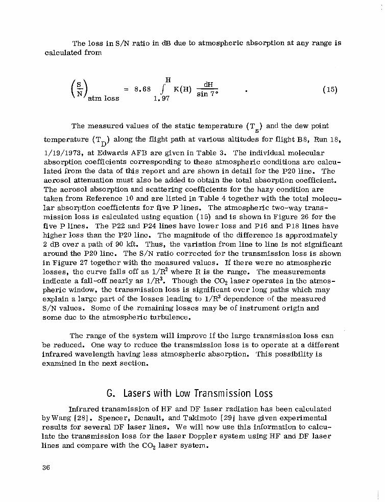
The loss in S/N ratio in dB due to atmospheric absorption at any range is calculated from

The measured values of the static temperature (T ) and the dew point S

temperature (T ) along the flight path at various altitudes for flight B8, Run 18,

1/19/1973, at Edwards AFB are given in Table 3. The individual molecular absorption coefficients corresponding to these atmospheric conditions are calculated from the data of this report and a re shown in detail for the P20 line. The aerosol attenuation must also be added to obtain the total absorption coefficient. The aerosol absorption and scattering coefficients for the hazy condition are taken from Reference 10 and are listed in Table 4 together with the total molecular absorption coefficients for five P lines. The atmospheric two-way transmission loss is calculated using equation (15) and is shown in Figure 26 for the five P lines. The P22 and P24 lines have lower loss and P16 and P18 lines have higher loss than the P20 line. The magnitude of the difference is approximately 2 dB over a path of 90 kft. Thus, the variation from line to line is not significant around the P20 line. The S/N ratio corrected for the transmission loss is shown in Figure 27 together with the measured values. If there were no atmospheric losses, the curve falls off as 1/R2 where R is the range. The measurements indicate a fall-off nearly as l/R3. Though the C 0 2 laser operates in the atmospheric window, the transmission loss is significant over long paths which may explain a large part of the losses leading to l/R3 dependence of the measured S/N values. Some of the remaining losses may be of instrument origin and some due to the atmospheric turbulence.

D

The range of the system will improve i f the large transmission loss can be reduced. One way to reduce the transmission loss is to operate at a different infrared wavelength having less atmospheric absorption. This possibility is examined in the next section.

G. Lasers with Low Transmission Loss Infrared transmission of H F and DF laser radiation has been calculated

by Wang [28]. Spencer, Denault, and Takimoto [ 291 have given experimental results for several DF laser lines. W e will now use this information to calculate the transmission loss for the laser Doppler system using H F and DF laser lines and compare with the C 0 2 laser system.

36

H (kft)

2.39

3.00

4.00

5.03

5.98

6.98

8. Ob 8.99

10.00

11.03

12.02

12.96

14.00

14.99

16.01

TABLE 3. CALCULATION OF ABSORPTION COEFFICIENT FOR FLIGHT B8, RUN 18, 1/19/1973, EDWARDS AFB

Ts" C

-0.6

-3.6

-8.6

-10.5

-9.9

-12.3

-13.5

-15.0

- 16.4

-17.3

-18.5

-19.5

-19.8

-20.7

-21.3

T " C 0

-7.9

-9.4

-9.9

-11.1

-13.8

-15.3

-16.6

-19.0

-20.8

-25.9

-27.4

-34.2

-45.0

-42.3

-40.6

0.05187

0.04821

0.0424

0.0404

0.04105

0.03852

0.03729

0.03579

0.03444

0.03358

0.03246

0.03156

0.03128

0.03048

0.02997

KP20 HZ0

Continuum

0.02773

0.02633

0.0309

0.0291

0.02016

0.01877

0.0168

0.01346

0.0115

0.0068

0.00568

0.00267

0.00075

0.001044

0.00127

KP20 HZ0

Lines

0.000983

0.000818

7.1 X

6.08 X

4.75 x 10'1

3.95x 10-4

3.37 X 10-4

2.61 X 10-4

2.13 X

1.29 X 10'~

1.07 X

5 X

2 X 10-5

2 X 10'~

2.4 X

KP20 n20 i kml

5 X 10-5

3.9 X

3.5 X 10'~

3.3 X 10'~

2 . 9 ' ~

2.6 X 10'~

2.4 X 10'~

2.1 X

1.9 X 10-5

1.6 X 10'~

1.5 X 10'~

1.3 X

1.2 X

9.5 x 10-6

1.8 X

0.08063

0.0754

0.07405

0.070 14

0.0617

0.05771

0.05445

0.04953

0.04617

0.04053

0.03826

0.0343

0.03205

0.03156

0.03127

w al

TABLE 4. MOLECULAR ABSORPTION COEFFICIENT OF P LINES AND AEROSOL ATTENUATION PER KILOMETER

I

H (kft)

2.39

3.00

4.00

5.03

5.98

6.98

8.00

' 8.99

10.00

11.03

12.02

12.96

14.00

14.99

16.01

K (P16)

0.08803

0.08227

0.08081

0.07634

0.06717

0.06278

0.05894

0.05386

0.05024

0.04378

0.04167

0.03736

0.03487

0.03438

0.03409

K (P18)

0.08171

0.07658

0.07 542

0.07143

0.06303

0.05903

0.05578

0.0508

0.04751

0.04157

0.0396

0.03563

0.03339

0.03288

0.03258

K (P20)

0.08063

0.0754

0.07405

0.07014

0.0617

0.05771

0.05445

0.04953

0.04617

0.04053

0.03826

0.0343

0.03205

0.03156

0.03127

K (P22)

0.07512

0.07032

0.06963

0.06585

0.05747

0.05374

0.05062

0.04588

0.04267

0.03686

0.035

0.03125

0.029

0.02854

0.02829

K (P24)

0.07062

0.06603

0.06572

0.06207

0.05363

0.05007

0.04703

0.0442

0.0393

0.03352

0.03175

0.02796

0.02579

0.02542

0.02521

K + u a a

(aerosol)

0.0248

0.02075

0.0153

0.0114

0.0085

0.0057

0.0036

0.0026

0.002

0.0017

0.0013

0.001

0.00072

0.00053

0.00039

20

18

16

14

1

m - Q

12 (3 z 0 2 E 10

a

v)

v) z K c

5 8

6

4

2

P16

0 20 40 60 80 100 120 RANGE (kftl

Figure 26. Total transmission loss at the P lines for flight B8, Run 18, 1/19/1973 at Edwards AFB.

39

~

48 -

44-

40 -

36 -

32 - &

m - 28 - z v)

U

\

24 -

20 -

16 -

12 -

FLT 88,1/19/73, RUN 18 EDWARDS AFB 0

0 0

0 10 20 30 40 50 60 70 80 90

SLANT RANGE (kft)

Figure 27. Comparison of measured and theoretical S /N values.

The performances of C02, H F , and DF laser Doppler systems looking down at a ground target from 5 km altitude at an inclination of 15 deg in AFCRL Midlatitude Summer Atmosphere are shown in Figure 28. The curves without atmospheric effects are calculated for the same values of the parameters assuming that the backscatter coefficient varies as 1/h2 [ 301. The C 0 2 laser experiences a loss which is 16 dB higher than that for DF laser for a slant range of 20 km.

40

I -

20 -

15 -

10 -

5 -

- 0

WITH TRANSMISSION LOSS

I 1 I 5 10 15

SLANT RANGE (km)

Figure 28. Performance of C 0 2 , H F , and DF laser Doppler systems against ground target at 15 deg inclination in AFCRL Midlatitude

Summer Atmosphere.

41

The round-trip transmission losses for horizontal transmission over a range of 40 k m at altitudes of 5 km and 10 km are given in Table 5.

The DF laser has the least loss. A s the altitude increases, the magnitude of the loss reduces. At 10 km altitude,. HF, DF, and CO lasers have approximately the same loss. While DF laser is much better than the COz l a s e r for transmission through the atmosphere, due to the longer wavelength the C02 laser system has a larger coherence diameter which may be an important consideration for an operating system.

TABLE 5. ROUND-TRIP HORIZONTAL TRANSMISSION LOSS FOR INFRARED LASERS OVER 40 km RANGE

Loss in dB

Laser, Line, and Wavelength H = 1 O k m H = 5 k m

C 0 2 , P20, 10.6 pm 19

0.45 3.5 CO, Ps(5) , 5.07 pm

0.45 1 DF, P2(8), 3.8pm

0.6 4 H F , P2(8) , 2.91 pm

7

42

1 1 1 . TURBULENCE LOSSES

The atmospheric turbulence resulting from random temperature fluctuations causes a variety of optical effects: twinkling (variation of image bright- ness), quivering (displacement of image from normal position) , tremor disk (smearing of the diffraction image), dancing (continuous movement of a star image about a mean point), wandering (slow oscillatory motions of the image with a period of approximately 1 minute and angular excursions of a few seconds of arc) , pulsation or breathing (fairly rapid change of size of the image), boiling (time-varying nonuniform illumination in a larger spot image), and image dis- tortion [ 311. In the case of the laser beam, the turbulence effects are broadly categorized as beam wander, spot dancing, beam spread, and scintillations. These effects are caused by the temporal and spatial fluctuations of the direction, phase, and intensity of the wavefront. A description of the atmospheric inhomogeneities causing these effects is givenin this section.

A. Parameters of Atmospheric Turbulence

The optical effects of interest are produced by the variations of refractive index along the path of the beam. The changes in the refractive index are caused by the fluctuations of temperature which arise in turbulent mixing of various thermal layers. It is found that the temperature fluctuations obey the same spectral law as the velocity fluctuations. In analogy with the velocity turbulence, the atmosphere may be imagined to consist of a large number of eddies with varying dimensions and refractive indicies. For isotropic turbulence, the velocity spectrum 9 (x) (where the wavenumber fi = 27r/P , P being the size of a turbulent eddy) contains the information about the turbulence. $,(E) is intuitively interpreted as the amount of energy in the turbulent eddies

of size L . The kinetic energy of turbulence is assumed to be introduced through eddy scale sizes larger than the "outer scale" of turbulence, Lo, corresponding

to a spatial wavenumber x = 27r/L0. A s the wavenumber increases beyond x 0 0' the turbulence tends to become isotropic and homogeneous. Experiments have

confirmed the predictions of Kolmogorov's theory of "11/3 K dependence for the three-dimensional spectrum up to wavenumber E related to the inner scale of

turbulence L o by x = 5. 92/P0. The spectrum in the dissipation region for

which the scale s izes are smaller than P or wavenumbers greater thanx 0 m

V

m

m

43

. . .. - . .. _ _ " . . .. "

is steeper than K . The spatial wavenumber region between the inner scale I and the outer scale L obeying the Kolmogorov theory of a spectral slope of

-11/3 is known as the inertial subrange. I is of the order of several milli- meters and L several meters.

--11/3

0 0

0 0

A t optical wavelengths the refractive index may be related to the 'temperature through the relation

ni = n - 1 = T

where

n = refractive index

P = pressure (mb)

T = temperature (K)

h = wavelength (pm) .

The refractive index structure constant C is a measure of the strength of

atmospheric turbulence and is defined as the mean-square difference in the refractive index at two points divided by the separation distance r raised to the 2/3 power, i.e.,

n

The temperature structure constant, C 2 , is similarly defined for tem- T

perature fluctuations. Thus, C may be determined from temperature measure-

ments alone from the following relation: n

44

Typical temperature variations of approximately 1 K resulting in refractive index variations of a few ppm will cause significant effects on optical radiation fields propagating through the atmosphere. C! is measured in units of

11

( meters)-zh and var ies f rom or more for strong turbulence to o r less for weak turbulence.

Assuming that the form of the temperature spectrum and the refractive index spectrum is the same as that of the velocity spectrum, Tatarski [ 321 gave the following form for the refractive index spectrum:

(X) = 0.033 C i K -iih e q ( 3 ) n

where E I = 5.92. This spectrum has a singularity at x = 0. Physically, m O

the singularity implies that the energy per unit volume becomes unbounded as the eddy size increases. This singularity is avoided by using the modified von Karman spectrum [ 331 :

which gives a bounded variation for E < 27r/Lo. The three-dimensional refractive index spectrum models according to equations (19) and (20) are shown in Figure 29. Deviations from these models occur i f the turbulence is not homogeneous. Deviations have been observed in measurements over paths close to the ground and under conditions of weak turbulence [ 331.

B. Optical Properties of the Turbulent Eddies A qualitative description of the effect of the optical inhomogeneities on

the wavefront is sometimes helpful. A s a plane wavefront passes through a region of relatively lower refractive index, the wavefront will advance as the speed of light is higher. When passing +rough a region of higher refractive index, the wavefront is slowed down. Thus, the refractive inhomogeneities of

45

,/ S I NAGTUi TY

\ \ \ \ \ ’\/ MODEL

TATARSKI

\ \ \ \ \ \ MODIFIED

VON KARMAN MODEL

P = 5/3 FOR KOLMOGOROV I MODEL I I

I \

\ / R - P - z

INPUT I RANGE 1

I - I I

I I I I I

DISSIPATION REGION

I

I I I I

I I

KO ‘ m c

K‘= SPATIAL WAVENUMBER

g = 2 r / f WHERE k?= SIZE OF TURBULENCE EDDY; go = 27r/L0, TYPICALLY Lo = 1 - 100 m;

gm = 2r/L0, TYPICALLY % = 1 - 3 m m

Figure 29. Three-dimensional turbulence spectrum models for index-of-refraction fluctuation.

46

the atmosphere deform the wavefronts. Portions of the wavefront may be convex or concave in the direction of propagation, The concave portions converge while the convex portions diverge. Thus, it is possible for the intensity to build up in some areas. Since the inhomogeneities are random and moving, the bright and the dark areas move randomly. This point of view has been developed by the optical astronomers [ 311.

In general, the optics of the turbulent atmosphere may be described in terms of a collection of weak, moving, three-dimensional, gaseous lenses of varying scale sizes bounded by the inner scale 1, and the outer scale L,, of the turbulence. From equation (17) , it may be seen that the refractive index fluctuations associated with any scale size P increases as the size of the eddy increases:

An eddy of radius P can act as a lens with a focal length f = R/ni, where R is the radius of lens curvature. This is approximated from equation (21) as

P ni

f " M P 2/3 c;

Turbulence as it naturally occurs can consist of eddies of hot and cold air. Eddies cooler than the ambient air have a higher index of refraction. In this case, nl is positive and the lens is convergent. If the eddy consists of warmer air, the index of refraction is lower (giving negative nl) and the lens is divergent. Typical values in the atmosphere are C N I ni 1 - and I a few centimeters. Thus, the focal length of the atmospheric lenses is f N 10 km.

n

The turbulent eddies cause diffraction and refraction of the optical wavefront, and it is instructive to consider these two effects separately. Each eddy of size P bends as a ray bundle individually and has a diffraction pattern of approximate width, h L / P , where L is the distance from the eddy to the receiver. The diffraction effects are negligible i f h L / I <> and this is the geometric optics regime. But, if hL/P >> P , the diffraction pattern entirely determines the intensity distribution of the receiver. Thus, the distance L

beyond which the diffraction effects are important may be defined by L N P2/A. d

d

47

The refractive bending of rays by an eddy of s ize P depends on the refractive index of the eddy and may be calculated by Snell’s law to give be - 6n. 6n is zero on the average. The mean square angular fluctuation for one eddy is <( 68)2> - <( 6n)2>.

Over a path length L, let the beam traverse L/P eddies. Since the deflections are uncorrelated from one eddy to another, they add up as mean squares and the total mean square deflection is

The effect of refraction is to change the cross-section of the beam from P 2 to (1 7 LO )2. The amplitudes of the wave before and after refraction are related as r

~~a~ = ( A + A A ) ~ (a Ler)z

The fractional amplitude change is then given by

A A L A P r

x = - - - e

The variance of the amplitude fluctuation is then given by

The particular scale size 1 which contributes predominantly to the amplitude fluctuation depends on the path length; i.e., different eddies are more effective at different path lengths in producing amplitude fluctuations. This point has been discussed by Tatarski [ 341 and De Wolf [ 351 as follows.

48

There are no diffraction effects in equation ( 2 6 ) . Diffraction effects are

negligible i f the path length Ls is shor t o r Ls << I /A in the geometric optics

regime. Since I (inner scale length) is the smallest eddy size, the diffraction

by eddies of all s izes is negligible in this case. The smallest eddies then have the largest contribution. Equation (26) then becomes

2 0

0

2 3 -7/3 Y

<x"> - c L I 0

for L << - S h n s O

For path lengths L greater than L such that L >> I o / h , the eddies 2 I S' I

with sizes greater than I ( 1 > I ) have negligible diffraction, while eddies with

sizes smaller than I (1 < I ) diffract the rays where I I

1 1

The diffraction pattern entirely determines the intensity distribution and the refraction is negligible for the small eddies of size I << I ; i.e., these eddies

simply scatter the energy, not focusing the rays, and have little effect on the amplitude fluctuations. Geometric optics results may still be applied i f the eddies of size 1 < P are excluded. Then the smallest eddy size contributing

significantly to the amplitude fluctuation is I and P = I is substituted in equation (26) :

I

I

P I

This is also the result obtained by the Rytov approximation. Equation (10) has been interpreted by Tatarski [ 9 ] as the result of the application of geometrical optics to a medium from which all eddies of scale s izes less than have been removed.

49

Young [ 361 obtained equation (28) on considering an aperture of Fresnel- zone size while calculating the normalized variance o r the total modulation power obtained with a circular aperture using geometric optics. He observed that ray optics gave the correct parametric dependence because very little power

is contributed by the range of spatial frequencies greater than (AL) which a r e i n the wave optics regime. Thus, weak scintillation may be thought of as aperture filtering with a Fresnel-zone size aperture which filters out spatial fre-

quencies higher than (AL) .

-I/2

A related view developed by radio astronomers is the phase screen concept. Immediately after passing through a layer of inhomogeneities, only the phase is affected and the intensity remains constant. A s the distorted wavefront propagates further, the relative phases will be changed due to different directions of propagation and in this way, the amplitude fluctuations develop. This concept has been applied by Lee and Harp 1371 to wave propagation by dividing the three- dimensional refractive field of the medium into thin slabs perpendicular to the direction of propagation. The effects of the refractive inhomogeneities on the propagation of laser beams in the atmosphere is discussed in the following section.

C. Effect of Atmospheric Turbulence on Laser Beams A qualitative description of the effects based on the relative sizes of the

beam and the refractive inhomogeneity is given first, followed by the results of Rytov approximation on the wave equation.

If the scale size of the inhomogeneity is much larger than the diameter of the laser beam, the entire beam is bent away from the line-of-sight and results in beam wander o r beam steering. The center of the beam executes a two-dimensional random walk in the receiver plane and, for isotropic turbulence, the displacement of the beam from the line-of-sight will be Raleigh-distributed [ 381. Inhomogeneities of the size of the beam diameter act as weak lenses on the whole o r par ts of the beam with a small amount of steering and spreading. When the inhomogeneities are much smaller than the beam diameter, small portions of the beam are independently diffracted and refracted and the phase front becomes corrugated. The propagation of the distorted phase front causes constructive interference over some parts of the receiver and destructive interference over others, leading to alternate bright and dark areas. Since the atmosphere is seldom stationary, the locations of the bright and dark regions change continually and give the pattern of "boiling." Thus, the turbulence causes

50

the received field to scintillate in time and space. Since the atmosphere consists of inhomogeneities of all s izes in motion, the laser beam experiences fluctuations of beam size (spreading), beam position (steering o r wander), and intensity distribution within the beam (scintillation) simultaneously. The relative importance of these effects depends on the path length, strength of turbulence, and the wavelength of the laser radiation. The variance of irradiance reflects the deviations from the mean due to beam wander, broadening, and scintillations. Estimates of these effects for finite beams are discussed as follows.

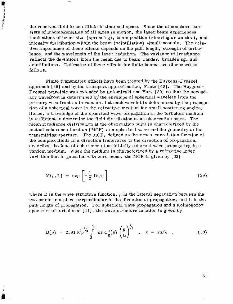
Finite transmitter effects have been treated by the Huygens-Fresnel approach [ 391 and by the transport approximation, Fante [ 401. The Huygens- Fresnel principle was extended by Lutomirski and Yura [ 391 so that the second- a r y wavefront is determined by the envelope of spherical wavelets from the primary wavefront as i n vacuum, but each wavelet is determined by the propagation of a spherical wave in the refractive medium for small scattering angles. Hence, a knowledge of the spherical wave propagation in the turbulent medium is sufficient to determine the field distribution at an observation point. The mean irradiance distribution at the observation point is characterized by the mutual coherence function ( M C F ) of a spherical wave and the geometry of the transmitting aperture. The MCF, defined a s the cross-correlation function of the complex fields in a direction transverse to the direction of propagation, describes the loss of coherence of an initially coherent wave propagating in a random medium. When the medium is characterized by a refractive index variation that is gaussian with zero mean, the MCF is given by [ 321

where D is the wave s t ructure function, p is the lateral separation between the two points in a plane perpendicular to the direction of propagation, and L is the path length of propagation. For spherical wave propagation and a Kolmogorov spectrum of turbulence [ 4 1 ] , the wave structure function is given by

51

For constant C n’

~ ( p ) = 1.089 k2C:Lp %

Equation (29) may be written as

where

L -3/5

Po = [ 1.455 k2 d s C 2 ( s ) (:)%I . 0

n

For constant C , n

P O = [ O . 545 k2LC 2 ] n

-3/5

(33)

(34)

po is the lateral separation such that the MCF becomes equal to l / e and is called the lateral coherence length. If d > po where d is the diameter of the aperture, the turbulence along the path of the beam reduces the lateral coherence between different elements of the aperture and effectively transforms it into a partially coherent radiator of dimension, po, which decreases with increasing distance from the aperture [ 381. But i f d < po, the entire aperture behaves l ike a coherent radiator. Thus, the resulting field distribution is characterist ic of a coherent aperture with a diameter d equal to the smaller of po and d. Yura

[42] showed that if L >> kd d the beam properties may be approximated by

those of a spherical wave and i f L << kd d the beam properties may be approximated by those of a plane wave.

eff

eff’

eff’

In the absence of turbulence, a gaussian laser beam will have a far-field angular spread e = 2h/7rd. When turbulence is present along the path, the scattering of the beam by the moving turbulent eddies causes additional spreading which is greater than 8 under some conditions.

52

The spreading of the beam consists of the deflection of the beam as a whole by the eddies larger than the beam diameter d and by the broadening of the beam due eddies smaller than d. The separation of the beam spread into the two components of wander and broadening is usually based on the length of the time of observation. If V is the transverse wind-velocity component, the turbulence eddies are interacting with the beam in time intervals of order A t d/V. For times much longer than A t , the received spot will be fully spread due to wander and broadening. The total spot size, viewed on a time scale T >> At, is called the long-term spot size and the beam radius of long- term spread is denoted by p If a picture with an exposure time much less

than A t were taken of the beam, a laser spot of radius p broadened by the small

eddies at some distance p normal to the line-of-sight would be observed. p is

the radius of beam-centroidal motion.

L'

S

C C

The concepts of the beam spread just discussed apply only i f the beam is intact. When the beam wander effect is removed, the atmospheric spreading of the beam at the receiver is the short-term beam spread; however, when the turbulence along the path is strong, the beam breaks up into multiple patches and there is not much wander. Kerr and Dunphy [43 ] found experimentally at near field that the focused beam broke up at the receiver into a proliferation of transmitter-diffraction-scale patches, when there is either transmitter mis- adjustment o r strong turbulence. Reidt and HEhn [44] observed in recent experiments that the focused beam at 0 . 6 3 pm was broken into several spots of characteristic length 2hL/7rd which is the free-space diffraction-limited focused radius. They verified also the inverse variation of the patch size with the diameter of the beam, that is, the increase in patch size with decreasing beam diameter o r vice versa.

The beam will be quivering while remaining intact as long as the turbu-

where d is lence is relatively weak and the path is not too long or , more precisely, if L < LCR where L is the critical range defined by L

the smaller of po and d [20] . CR CR = di f f eff

Quantitatively, the spreading of the beam depends on the lateral coherence length po. If the beam diameter d is much smaller than po, the effect of turbulence on the beam is negligible and the beam diameter in the far field will be that due to diffraction, namely, 2hL/nd. However, i f the initial beam diameter is greater than the lateral coherence length po, the beam diameter in the far field is given by 2hL/7rp0 [45]. That is, the beam behavior is characterist ic of an aperture of diameter po instead of d. The turbulence alo'ng the path t ransforms the aperture into a partially coherent radiator. For the initial field distribution of gaussian form given by

53

P .

where F is the radius of the curvature, the long-term beam radius is obtained as [46]

e;> = m+Q 4L2 d2 (1 - $ ) 2 + k2po2 4L2

When the turbulence is strong, the beam will be broken up and for this case Klyatskin and Kon [47] found that the wander of the center-of-gravity of the beam may be obtained from

2 for constant C , L >> kpo (far-field case), and d >> p Taking the ratio of

equations (37) and ( 3 6 ) and observing that the last t e r m on the left-hand side of equation ( 3 6 ) is dominhnt for strong turbulence, we obtain

n 0'

Since L >> kp then G><< (p:), which means that the motion of the beam

centroid is negligible compared with the beam spread when the beam breaks up into multiple patches. It is not possible to tell how many patches will form, but

the bright patches will be in a zone with mean square radius p [48].

0

2 L

For ranges less than the critical range, tracking laser transmitters have been proposed and discussed [49,50] to compensate the beam wander which is a relatively low-frequency phenomenon of the order of 0.5 Hz. For L < L the beam centroidal motion is given approximately by [ 511 C R'

54

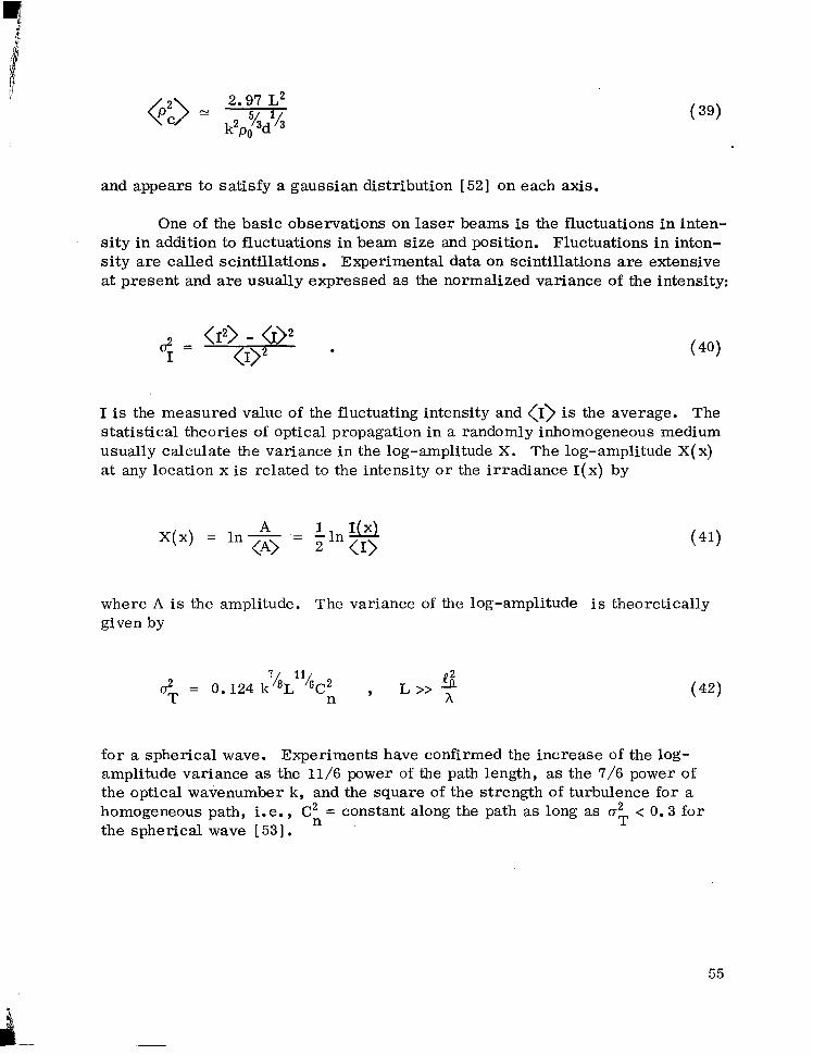
and appears to satisfy a gaussian distribution [52 ] on each axis.

One of the basic observations on laser beams is the fluctuations in intensity in addition to fluctuations in beam size and position. Fluctuations in inten- s i ty are called scintillations. Experimental data on scintillations are extensive at present and are usually expressed as the normalized variance of the intensity:

I is the measured value of the fluctuating intensity and is the average. The statistical theories of optical propagation in a randomly inhomogeneous medium usually calculate the variance in the log-amplitude X. The log-amplitude X(x) at any location x is related to the intensity o r the irradiance I ( x ) by

A 1 1 0 X ( x ) = In- - <A) - T I n 

where A is the amplitude. The variance of the log-amplitude is theoretically given by

for a spherical wave. Experiments have confirmed the increase of the log- amplitude variance as the 11/6 power of the path length, as the 7/6 power of the optical wavenumber k, and the square of the strength of turbulence for a homogeneous path, i. e. , C2 = constant along the path as long as u2 < 0.3 for the spherical wave [ 531.

n T

55

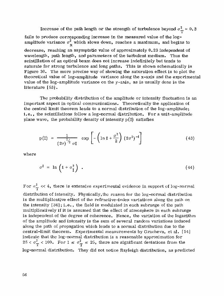
Increase’ of the path length o r the strength of turbulence beyond CT’ = 0 . 3 T

fails to produce corresponding increase in the measured value of the log- amplitude variance CT’ which slows down, reaches a maximum, and begins to

decrease, reaching an asymptotic value of approximately 0.23 independent of wavelength, path length, and parameters of the turbulent medium. Thus the scintillation of an optical beam does not increase indefinitely but tends to saturate for strong turbulence and long paths. This is shown schematically in Figure 30. The more precise way of showing the saturation effect is to plot the theoretical value of log-amplitude variance along the x-axis and the experimental value of the log-amplitude variance on the y-axis, as is usually done in the l i terature [ 531.

x

The probability distribution of the amplitude o r intensity fluctuation is an important aspect in optical communications. Theoretically the application of the central limit theorem leads to a normal distribution of the log-amplitude; i.e. , the scintillations follow a log-normal distribution. F o r a unit-amplitude plane wave, the probability density of intensity p(1) satisfies

where

F o r a2 << 4, there is extensive experimental evidence in support of log-normal

distribution of intensity. Physically, the reason for the log-normal distribution is the multiplicative effect of the refractive-index variations along the path on the intensity [ 341 ; i.e. , the field is modulated in each subrange of the path multiplicatively i f it is assumed that the effect of atmosphere in each subrange is independent of the degree of coherence. Hence, the variation of the logarithm of the amplitude and intensity is the sum of several random variations induced along the path of propagation which leads to a normal distribution due to the central-limit theorem. Experimental measurements by Gracheva, et al. [ 541 indicate that the log-normal distribution is a reasonable approximation for 25 < a2 < 100. F o r 1 5 o2 < 25, there are significant deviations from the

T

T T - log-normal distribution. They did not notice Rayleigh distribution, as predicted

56

/

(PATH LENGTH) 11/6

Figure 30. Saturation of the variance of log-amplitude fluctuations of a spherical wave propagating through a homogeneous ( C2 n = const. ) turbulence path.

by de Wolf [ 551 for large values of 0;. Physically, Rayleigh distribution

results when the field at the receiver is the sum of a large number of independently scattered fields. The physical model of de Wolf 1351 attributes the Rayleigh distribution to the multiple scattering by off-axis eddies which are large in strong turbulence.

In addition to temporal variation, the received field exhibits a spatially varying intensity after propagation through turbulence. The spatial structure of scintillations is usually studied by the covariance of the logarithm of the amplitude fluctuations. A correlation length may be defined in several ways. One definition is the value of separation for which the spatial covariance function goes to zero for the first time. The correlation length provides a measure of the separation between two points over which the scintillations are correlated. The concept of the correlation length has been useful for some applications. For example, the theoretical calculation of the log-amplitude variance is usually based on a point detector. In practice, a collector aperture of diameter less than the correlation length is treated as a point detector for comparison of theory and experiment. Another use of the correlation length is in understanding the aperture averaging effect which is discussed later. The intensity covariance function is usually measured and is related to the log-amplitude covariance as [56]

where the separation is p = I x - x' 1 , the covariance of log-amplitude is

and the covariance of intensity is

C,(P) = <[ I (x) - ] [I(x') -]> . (47)

The intensity and the log-amplitude correlation distances may be seen to be the same from equation (45) but the curves differ greatly. For plane or spherical wave propagation, C (p) has the form X

58

. ..

where f is a function which depends on the mode of propagation. The first zero

of f is the correlation length and is approximately 0.76 (AL) for a plane wave

and 1.8 (AL)Ih for a spherical wave based on the perturbation theory of Tatarski.

Experiments confirm a correlation length of the order of (AI,)% when there is no saturation scintillations.

I/

The classical method of reducing the fluctuations in the received power has been to increase the size of the receiving optics. The reduction of the fluctuations in the received power, when the diameter of the receiving aperture is increased, is called aperture averaging. The physical reasoning is that large apertures tend to average over the statistically independent portions of the scintillation pattern [ 561. The diameter of an independent patch is usually imagined to be of the order of the correlation length. Thus for weak scintilla-

tions, the size of the patch is of the order of the Fresnel length (AL)lh. Experi- ments [ 571 show that the correlation length decreases as the turbulence gets stronger. Moreover, the covariance curve develops a progressively higher correlation tail and aperture averaging deteriorates as the turbulence strength increases. Figure 31 illustrates the covariance function for several a2 T'

To summarize, the phenomenon of saturation of optical scintillation may be characterized by the following experimental observations:

1) There is a physical breakup of the beam into multiple patches when the turbulence is strong.

2) The variance of the log-amplitude reaches a maximum instead of increasing indefinitely and then decreases to an asymptotic value of approximately 0 . 2 3 independent of the wavelength of the optical radiation and parameters of the turbulent medium as the path length, or the strength of turbulence, o r both are increased.

3) The spatial covariance function of log-amplitude decays progressively faster but maintains a progressively higher tail as a function of the detector spacing with increasing turbulence strength and path length.

59

0.8

0.6

c

1 Q

u X

0.4

0.2

Figure 31. Theoretical curves of the log-amplitude covariance function in weak to strong turbulence [35] .

4) Aperture averaging becomes progressively less effective for a given size of the aperture as the turbulence strength and the path length are increased.

There were several theoretical attempts to explain the saturation phenomenon in the past but it is only in recent years that the theory is able to account for all the observed effects. Since the saturation effect is observed under conditions of strong turbulence, a working definition is needed for the conditions specified as weak or strong turbulence. The turbulence is called "weak" i f the theoretical variance of log-amplitude

7 o2 = 0.124 k /6 L ?hC2 T n (49)

60

satisfies the inequality a2 < 0.3 . The turbulence is called "strong" if a2 > 0.3.

Thus the specification of the turbulence conditions involves not just the refractive- index structure constant C2 but a combination of the wavelength of radiation, path length, and C2. n

T T

n

One of the earlier attempts to physically explain saturation is that by Young [58] . When stellar scintillation is observed with small apertures, the total modulation power first increases with zenith angle and then decreases. Young suggested that the smearing o r blurring of the details of the wavefront distortions caused by the intervening atmospheric turbulence is responsible for the observed saturation of astronomical scintillation. The blurring effect is produced by the small-scale fluctuations in the wavefront which change rapidly due to the short lifetime of the small eddies. Thus, a shadow pattern produced by a high layer in the atmosphere becomes smeared or washed out by the intervening turbulence as it propagates down through the atmosphere.

Clifford, Ochs, and Lawrence [59] give a detailed description of the smearing process in the scintillation pattern in strong turbulence. The wavefront develops small-scale and large-scale distortions while passing through the turbulent medium. When such a distorted wave is incident on a Fresnel-zone- s ize eddy, the small-scale distortions reduce the resolving power of the eddy while distortions larger than the eddy merely tilt the diffraction pattern of the eddy. The small scale distortions may be expected to change in detail several times during the lifetime of the larger eddies due to the shorter lifetimes of small eddies. These fluctuations of the small-scale distortions of the wavefront cause the smearing of the diffraction pattern of the Fresnel-size eddy, thus making it less effective as a producer of scintillation. Scintillations remain bounded and do not build up indefinitely due to the smearing by the small-scale eddies.

The smearing effect of strong turbulence is incorporated into the first- order analysis by means of a spectral-filter function which filters out higher spatial frequencies. The spectral filter function is given by the normalized two-dimensional Fourier transform of the short-term average of the irradiance profile of an optical beam propagating through turbulence. The filter function turns out to be the short-term modulation transfer function ( M T F ) . It is assumed that the log-amplitude covariance of a spherical wave for strong turbulence is given by the first-order log-amplitude covariance whose spatial frequency spectrum has been modified by multiplication with the spectral filter function (or the short-term MTF) . The log-amplitude covariance thus calculated agrees well with the experiments and is shown in Figure 31.

61

From this covariance function, Clifford and Yura [60] obtained the following asymptotic behavior for the log-amplitude variance:

where a is a constant found from experiments. F o r Q = 0.7, which is obtained from the strong scintillation data, c2 tends to 0.23 for large values of 0’

X T’

The perturbation theory of Tatarski [ 32,341 implicitly assumes that the initial coherence is maintained along the propagation path and eddies having scale s izes of the order of the Fresnel length are most effective in producing scintillation. However, as the wave travels through the medium, the transverse spatial coherence decreases continuously and the wave becomes partially coherent. A s was previously noted, the spreading of a beam of initial diameter d i n a turbulent medium is characterist ic of an aperture of diameter po (the lateral coherence length) and not of diameter d. The radiator has become partially coherent in the presence of turbulence. Incorporating the loss of coherence of a radiator in the turbulent medium into the analysis, Yura [ 611 obtained the saturation of scintillations and the behavior of the amplitude covariance. He showed also that in the strong turbulence regime, the amplitude correlation length is equal to the lateral coherence length and C2 increase. The turbulent

eddies most effective in producing scintillations in the saturation regime are those that have scale sizes of the order of the lateral coherence length and not the Fresnel length.

n

- The asymptotic log-amplitude variance behavior of (0’ ) 2’5 has been

T predicted also by Fante [ 621 and Gochelashvily and Shishov [ 631 from approximate solutions to the equation satisfied by the fourth moment of the field.

The physical theories [ 59,60,61] and the approximate solutions [ 62,631 have been able to predict the observed behavior of the covariance function, namely, a rapid fall-off followed by a slow decay resulting in a long tail. These curves indicate that there are small-scale and large-scale structures in the scintillation pattern for strong turbulence. The correlation in strong turbulence is over a transverse separation of the order of

6 2

i A s o2 increases, the lateral coherence length and the amplitude correlation

length decrease. The diameter of the detector must be smaller than po for point detector performance in strong turbulence.

T

The aperture averaging which produced a reduction in scintillation noise became less effective for a given aperture of the receiver as the turbulence increased. This effect is due to the presence of large-scale scintillations at the receiver as o2 increased. T

Another quantity of interest is the temporal frequency spectrum of intensity fluctuations observed at-a fixed point. The width of the frequency spectrum

is of the order of V/(AL) for weak turbulence where V is the velocity component normal to the beam. This is typically 10 to 100 Hz. For the case of strong turbulence, the width of the frequency spectrum is of the order V/po

which is approximately 100 to 1000 Hz. In fact, the peak of the spectrum occurs

at approximately V/( AL)lh for o2 < 1 and at approximately V/po for uT > 1.

I/

2 T

In addition to the shifting of the peak of the spectrum to higher frequencies, there is a broadening of the spectrum and the maximum value of the spectrum decreases for increasing a2 These features of the spectrum have been quali-

tatively observed in the experiments. Finally, to obtain all of the temporal information of the scintillation in the strong turbulence regime, it may be necessary to use an electronic bandwidth of the order of V/p,. Otherwise, the

use of a smaller electronic bandwidth may result in an apparent decrease of the log-amplitude variance for increasing values of a2

T'

T'

D. Effect of Turbulence on Heterodyne Systems In a heterodyne receiver, the incoming wave which is usually weal; is

combined with a reference wave on the photodetector surface. Coherent detection results from the square-law response of the photodetector to the incident radiation. The squaring operation of the photodetector produces a current at the intermediate freqxency which contains the signal-modulation information.

The heterodyne detection of an atmospherically distorted wavefront has been the subject of several studies [64,65]. The various effects of atmospheric turbulence on the laser beam are related to the image behavior in a heterodyne system. Comparison of the expression for the optical power density due to a

63

laser transmitter at a point scme distance L away from the transmitter and the expression for the S/N ratio of a heteradyne receiver detecting a signal from a point source at a distance L shows that they have identical functional dependence on the turbulence parameters. Thus, the telescope performance measured in te rms of the coherence diameter remains the same whether i t is used as par t of a transmitter or as par t of a heterodyne receiver for propagation in a turbulent atmosphere [ 661. In simple terms, the reciprocity between the transmitter and receiver indicates that the average target illumination is related to the power received by the heterodyne receiver. Furthermore, beam wander and beam spread in the target illumination system are related respectively to image dancing and spread in the heterodyne receiver. Thus, the beam-image reciprocity implies the familiar effects of turbulence on the beam propagation in the analysis of the heterodyne detection.

Fried [64] considered the amplitude and phase fluctuations and found that for an atmospherically distorted plane wave and a plane-wave local oscillator there is an upper limit to the achievable S/N no matter how large the detector aperture. The aperture diameter for the near-peak value of S/N is of the order of the lateral coherence diameter. This aperture size has the virtue of avoiding large signal power fluctuations and variance which would result for larger collection apertures. Moreland and Collins [ 651 tried to determine the possibility of increasing S/N by properly shaping the local oscillator beam and came to the conclusion that, though the optimum location oscillator shape differs significantly from that of a plane wave, the increase of average S/N over the plane-wave case is negligible.

E. Signal-to-Noise Ratio Loss The wave function at a distance L from the transmitting telescope of

radius R may be written by the Fresnel diffraction theory in the absence of turbulence along the path as [ 67,68,69]

64

1 where

A' = number of photons transmitted per second

"9

r" = vector in the plane of the transmitting lens

d

r = vector in the plane at distance L from the transmitter and normal to the optic axis

h = wavelength of laser radiation

w = angular frequency

t = time.

Equation (51) may be integrated by completing the square and the result is

where

and

7rR2 p = - hL

L f

[ = -

( 53)

(54)

65

The effect of the atmospheric turbulence along the path of propagation is to produce random variations of phase and intensity. These random variations are introduced into the analysis by multiplying equation (51) with

X( r , r") is the perturbation of logarithm of amplitude, equation (41) , and S( y,?"') is the perturbation of phase between the point ff at the transmitter and the range point y. Thus, the outgoing wave function at a distance L with the effect of turbulence is given by

"

The transmitted wave is assumed to be backscattered by a diffuse target of scattering particles. Considering a single particle, the incoming wave is scattered by the particle as a spherical wave, and the scattered wave function at a point 7' i n the plane of the receiving lens for a coaxial system is given by

where

CT' = backscattering coefficient of the particle

Am = 2 u V/c = Doppler shift due to the velocity component V of the moving particle along the optic axis

X( r , r') = perturbation of the log-amplitude "

S( r , r?) = perturbation of phase, between the range point and the - 4

point y? at the receiver.

66

p The local oscillator reference wave function which is added to the

i received wave function is assumed a plane wave with gaussian amplitude variation which may be written as

where cy is a constant and the arbitrary phase factor is assumed to be zero.

The total signal photo-current is given by the real par t of

where W (r ' ) is the apodization or transmission function €or the receiver aperture and is assumed equal to unity over the width of the reference beam.

Substituting equations ( 5 7 ) , ( 5 8 ) , and (59) into equation (60) gives the signal current as the real part .of

where

r 1

The photo-current due to a single scatterer may be written as

67

J L 1

+ S( r, r") d-F' d?' - - 1 '

The signal power is proportional to i2 and S

68

If the signal power is averaged over a period longer than 1/ (2Aw), then

where Re denotes the real part. The point 7"' lies on the receiver aperture and rrtrc lies on the transmitting aperture. -

The expected value of the signal power is obtained by taking the ensemble average of i2 as given by

S

- - + X( r , r f f v ) + X( r, rvv) + X( "

For this report it is assumed that the outgoing and incoming paths are statistically independent. ( A more accurate treatment assuming gaussian distributed random variables will be described in a later report.) This assumption allows the following:

69

where D( r) is the wave structure function. Kolmogorov theory of isotropic turbulence gives a 5/3-power variation for the wave structure function:

D ( r ) = 2 ( t r

where r is proportional to the coherence radius an$ has the value a

r = 0.088 h L v 5 - Y 5 - Y 5 , for plane wave a n

r = 0.1586 h Y 5 L -3/5c-6/5 , for spherical wave . a n

It will be appropriate to use r for a spherical wave for the wave originating at the range point;

a

To simplify the calculations, the structure function is approximated as

D ( r ) = 2(,)2 and the plane-wave value of r is used for both ways to give z conservative estimate.

a

70

The expected value of i2 becomes S

t

- " -c r' 2 + p 2 + r' 1t2 + rcrr?2

R2

Performing the integrations approximately, the expected value of the S/N ratio for a single scatterer is obtained as [67 ]

where a = ( R / r ) and T is the pulse duration. Integrating equation (73) over a

plane normal to the axis at the range L, the S/N ratio due to a plane target (dropping the angle brackets) is obtained:

a

In the absence of the turbulence effects, a = 0 and thus the S/N is reduced by the ratio

71

due to turbulence. If the system is focused to infinity, then

7?R4 L ~ ( 1 + a2) + - L 2 + -

A2 P = 7?R4 A2

Thus, the calculation of the loss of power due to turbulence reduces to the calculation of a = R/r and P. a

The wave structure function for a plane wave is given by

D(r) = 2.91 (F)2 r' C2 dL . Path n (77)

For a propagation path which is inclined at an angle e' with respect to the horizontal

h = H + L s i n e ' ( 7 8 )

where h is any altitude above sea level and H is the altitude of the scattering surface above sea level. Fo r flights at Edwards AFB, the dry lake is approximately 600 m above sea level. The strength of turbulence is assumed to vary as

2 2 - 1/3 h' C = CnO(h') exp - - n

h O

2 2 where C is a constant, h' = h - H, and H = 3200 m. The value of C nO 0 no ' obtained from earlier measurements of Huffnagel and Stanley [ 701, is 4.2 x lomi4 . We use H = 600 m and assume that equation (79) is valid from h = 10 m. Sub- stituting equation (79) into equation (77) , the structure function may be written as

72

where I(P) is the incomplete gamma function given by

and Pi and 1, are dimensionless lower and upper altitudes. From equation (80)

-3/5

a nO 2 h

For the flight tests, 8 = 7 O and h = 10.6 pm. Using these values, r becomes a

-3/5 r a = 5.8 x lo-'' [C:o ( 1(12) - 1(11))] .

The optics diameter is taken as 25.4 cm and this gives R = 0.127 m; therefore,

a = - = 2.19 x l o8 [1(12) - 1(11)] R 3/5 6/5 r no a

The incomplete gamma functions may be obtained from the Pearson Tables [ 711.

The calculations are made for the flight tests between 600 m and 4000 m

altitude and for C = 4.2 x The calculated S/N values shown in Figure 2 no

32 also include the transmission loss.

73

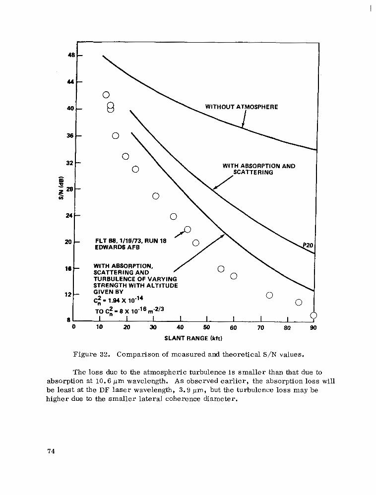
TO C: = 8 X 10-1 1 I I 1 1 1 I

0 10 20 30 40 50 60 70 80 90 SLANT RANGE (kft)

Figure 32. Comparison of measured and theoretical S/N values.

The loss due to the atmospheric turbulence is smaller than that due to absorption at 10.6 pm wavelength. A s observed earlier, the absorption loss will be least at the DF laser wavelength, 3.9 pm, but the turbulence loss may be higher due to the smaller lateral coherence diameter.

74

~

A comparison of the losses due to absorption and turbulence over a 20 km horizontal path at altitudes of 2.5 km and 5 km is given in Table 6 at CO, and DF laser wavelengths using the same optic size. Due to the smaller coherence diameter at DF wavelength, the optics diameter should be less than that at C 0 2 wavelength. By using the same optics size for both, the turbulence losses have been overestimated for the DF laser. Even so, the total loss of DF system is approximately 15 dB less than for CO, system at 2.5 km. A t 5 km altitude, the magnitude of the losses has dropped and there is an improvement of only 5 dB using the DF system. For altitudes below 5 km, the DF system is s e e n t o give less total loss due to the atmosphere.

TABLE 6. COMPARISON OF LOSSES AT CO, AND DF LASER WAVELENGTHS OVER A 20 km HORIZONTAL PATH

A T 2.5 km AND 5 km ALTITUDES

Altitude . ". " ~~

2.5 km

5 km

Absorption Loss ( d B )

24

1.75

9.6

0.46

Turbulence Loss (dB)

2.6

9.05

0.37

4.9

Total Loss ( dB)

26.6

10.8

10.0

5.4

Since the atmospheric conditions are constantly changing, it is desirable to estimate the maximum and minimum attenuation of the CO, laser radiation that may be expected due to the atmospheric propagation. The upper limit on the attenuation is estimated using the AFCRL Midlatitude Summer Hazy Atmos- phere and an exponential variation with altitude of the turbulence strength with

Cno = 4.2 x 10 m2/3. The lower limit on the attenuation is estimated using

AFCRL Midlatitude Winter Clear Atmosphere and an exponential variation with

altitude of the turbulence strength with Cno = 4.2 x 10 m . The results

for a two-way horizontal path of 20 km range at each altitude up to 10 km altitude are shown in Figure 33. The difference in the upper and lower limits of attenuation is considerable near sea level mainly because of the differences in the temperature, humidity, and aerosol concentration. The breakup of the attenuation into the transmission part and turbulence part zit each altitude is given i n Table 7.

2 -14

2 -15 -2/3

75

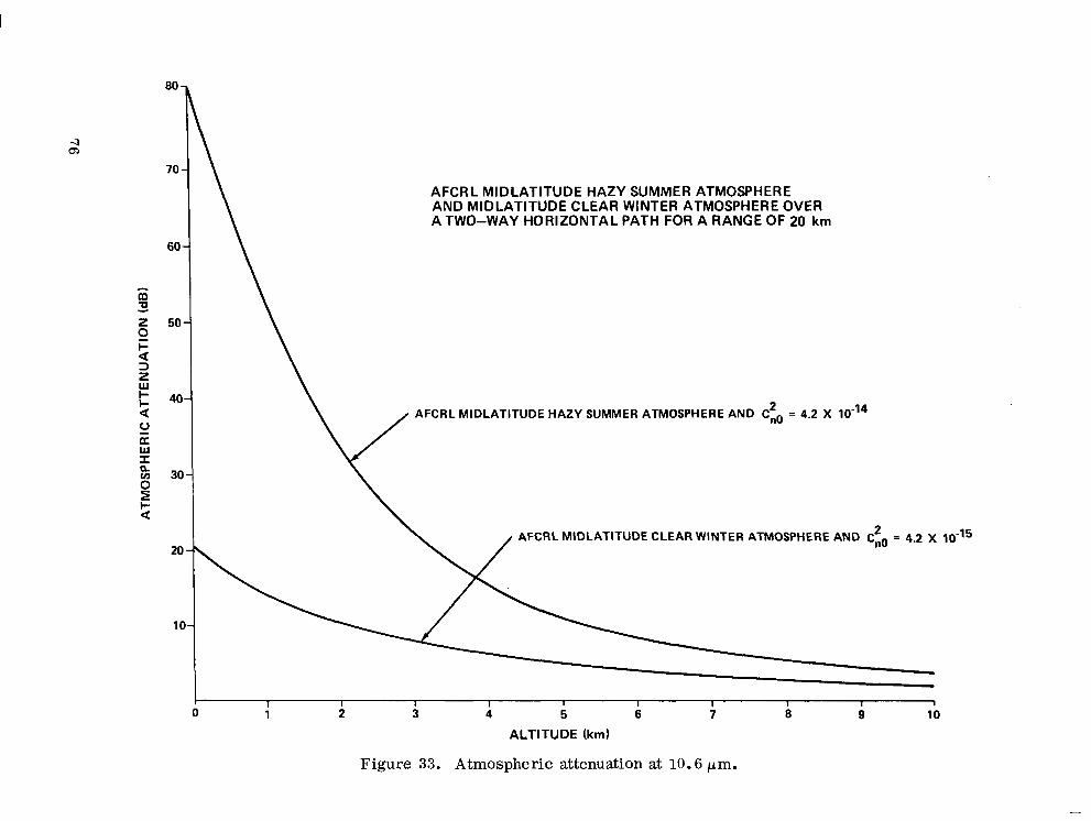
1

70 -

60 -

m

z a

'0 - Z 50-

+ 3 z W E 40. a 0 K W I 0 30

I- B a

20

10

AFCRL MIDLATITUDE HAZY SUMMER ATMOSPHERE AND MIDLATITUDE CLEAR WINTER ATMOSPHERE OVER A TWO-WAY HORIZONTAL PATH FOR A RANGE OF 20 km

I I 1 2

1 3

I I

4 I

5 6 I I 7 8 9 10

1 1

ALTITUDE (km)

Figure 33. Atmospheric attenuation at 10.6 pm.

I

TABLE 7. SIGNAL LOSS IN ATMOSPHERIC PROPAGATION A T 10.6 p m DUE TO ABSORPTION, SCATTERING, AND

HORIZONTAL PATH OF 20 km A T EACH ALTITUDE

COHERENCE DEGRADATION FOR A TWO-WAY

Altitude

10.0 m 2.5 km 5.0 km 7.5 km

10.0 km

AFCRL Midlatitude Summer Hazy Atmosphere 2

and Cno = 4.2 x 10 - 14

10 m 2 km 4 km 7 km

10 km

~ ~

Absorption and Scattering Loss

Turbulence Loss

(dB) ( d B ) ~ ~ ~~

68.0 24.6

13.0 2.6

9.6 0.34 5.8 1.05

0.12 3 . 5 3 I AFCRL Midlatitude Winter Clear Atmosphere

21 and Cno = 4.2 x 10

-15

I 17.3

0 . 3 10.5 3.4

6.5 3 . 5 1.8

- - -

81.0 27.2 10.65 6.14 3.65

20.7 10.8 6.5 3. 5 1.8

77

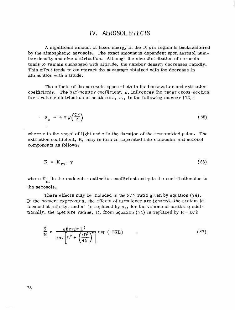
IV. AEROSOL EFFECTS

A significant amount of laser energy in the 10 p m region is backscattered by the atmospheric aerosols. The exact amount is dependent upon aerosol number density and size distribution. Although the size distribution of aerosols tends to remain unchanged with altitude, the number density decreases rapidly. This effect tends to counteract the advantage obtained with the decrease in attenuation with altitude.

The effects of the aerosols appear both in the backscatter and extinction coefficients. The backscatter coefficient, p, influences the radar cross-section for a volume distribution of scat terers , uo, i n the following manner [ 721 :

u 0 = 4 .p(?)

where c is the speed of light and T is the duration of the transmitted pulse. The extinction coefficient, K, may in turn be separated into molecular and aerosol components as follows:

where K is the molecular extinction coefficient and y is the contribution due to

the aerosols . m

These effects may be included in the S/N ratio given by equation (74) . In the present expression, the effects of turbulence are ignored, the system is focused at infinity, and IT’ is replaced by uo, for the volume of scat ters ; additionally, the aperture radius, R, from equation (74) is replaced by R = D/2

78

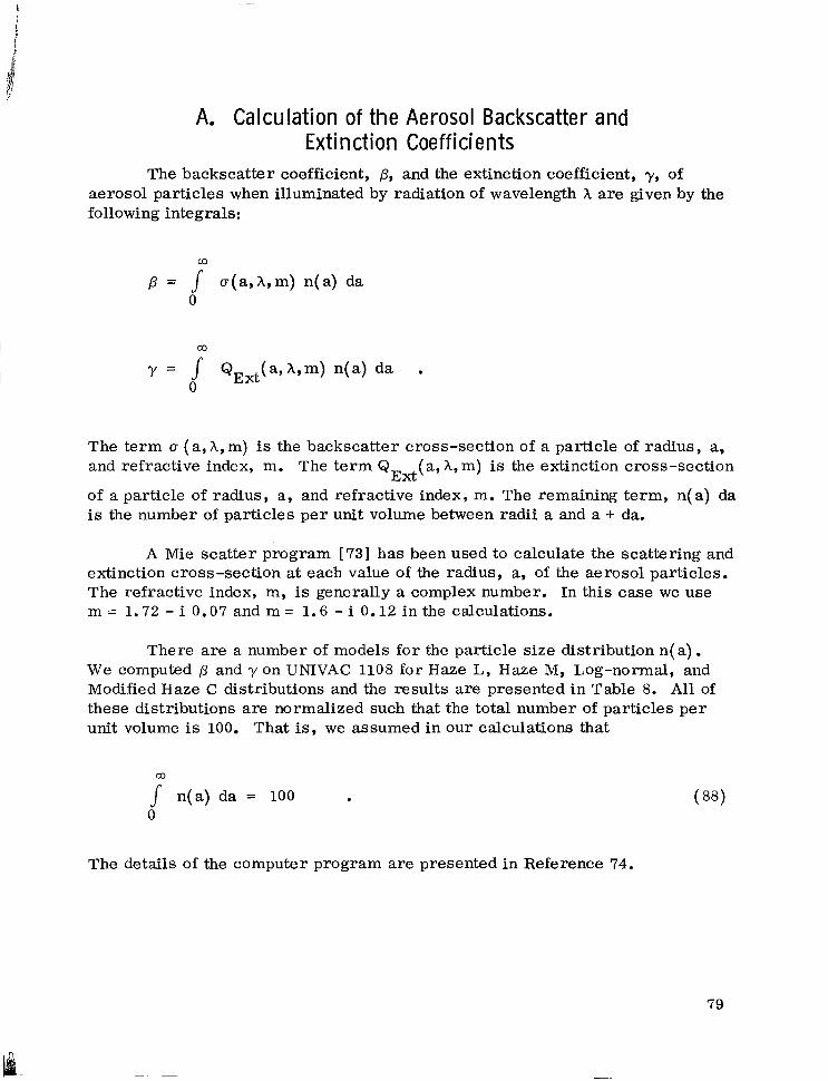
A. Calculat ion of the Aerosol Backscatter and Extinction Coefficients

The backscatter coefficient, p, and the extinction coefficient, y , of aerosol particles when illuminated by radiation of wavelength h are given by the following integrals:

m

p = 1 u(a,A,m) .(a) da 0

The term 0 (a, A, m) is the backscatter cross-section of a particle of radius, a, and refractive index, m. The term Q (a, A, m) is the extinction cross-section

Ext of a particle of radius, a, and refractive index, m. The remaining term, n( a) da is the number of particles per unit volume between radii a and a + da.

A Mie scatter program [73 ] has been used to calculate the scattering and extinction cross-section at each value of the radius, a, of the aerosol particles. The refractive index, m, is generally a complex number. In this case we use m = 1.72 - i 0.07 and m = 1 .6 - i 0.12 i n the calculations.

There are a number of models for the particle size distribution n( a). W e computed p and y on UNIVAC 1108 for Haze L, H a z e M, Log-normal, and Modified Haze C distributions and the results are presented in Table 8. Al l of these distributions are normalized such that the total number of particles per unit volume is 100. That is, we assumed in our calculations that

m 1 n( a) da = 100 0

The details of the computer program are presented in Reference 74.

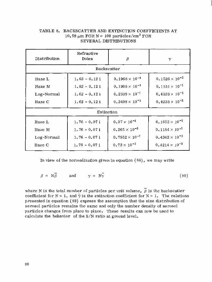
TABLE 8. BACKSCATTER AND EXTINCTION COEFFICIENTS AT 10.59 p m FOR N = 100 particles/cm3 FOR

SEVERAL DISTRIBUTIONS

Refractive Distribution Y P Index

Haze L

Haze M

Log-Normal

Haze C

Haze L

Haze M

Log-Normal

Haze C

Backscatter

1.62 - 0.12 i

0.3408 x 1.62 - 0.12 i

0.2339 x loe7 1.62 - 0.12 i

0.1905 x 1.62 - 0.12 i

0.1968 x

Extinction

1.76 - 0.07 i

0.73 X 1.76 - 0.07 i

0.7952 x 1.76 - 0.07 i

0.265 x 1.76 - 0.07 i

0.27 X

I I

0.1526 x

0.1151 x lo-' 0.4533 x

0.4233 x

0.1053 X

0.1164 X lo-' 0.4342 x

0.4214 x

In view of the normalization given in equation ( 8 8 ) , we may write

p = NF and y = Ny

where N is the total number of particles per unit volume, is the backscatter coefficient for N = 1, and is the extinction coefficient for N = 1. The relations presented in equation (89) express the assumption that the size distribution of aerosol particles remains the same and only the number density of aerosol particles changes from place to place. These results can now be used to calculate the behavior of the S/N ratio at ground level.

80

I' B. Performance of t he MSFC Pulsed Laser System at Ground Level

The dependence of the S/N ratio on aerosol particles is contained in the .expression p exp (-2KL) which, using equation (89) , may be written as

A = pexp(-2KL) = NPexpE -2(K + Ny) L J . m (90)

If there are more aerosols in the atmosphere, N j : , iarge and we get more backscattered energy. However, aerosol extinction increases with N exponentially. Thus, it is not advantageous to have a very hazy atmosphere. The optimum value of the number density of aerosols for a given range may be found by differentiating equation (90) with respect to N and setting it equal to zero. The resul t is

F o r modified Haze C distribution, we have 7 = 0.42 x 10-5/km. For example, we get N = 1.185 x 104/cm3 for a range of 10 km. Using the altitude distribu-

tion of aerosol number densities given by the AFCRL model [ 751 (Taale 9), the values of the range at which the S/N ratio reaches a maximum value due to the aerosols in the lower atmosphere are presented in Table 1.0. It may be observed that the optimum range at ground level in hazy atmosphere is limited to approximately 9 km due to the large number of aerosols. A s the altitude increases, aerosols do not pose any limitations on the S/N ratio due to the rapid decrease in their number density.

opt

W e now consider the maximum possible ground range. Examination of equation (87) reveals that there is an optimum optics diameter for each range which maximizes the S/N ratio. Figure 34 illustrates the dependence of the S /N ratio on the diameter. Differentiation of equation (87) with respect to the diameter D and setting equal to zero results in the following relation:

7TD2 L = opt 4h

81

TABLE 9. AFCRL MODEL OF AEROSOL NUMBER DENSITY VARIATION WITH ALTITUDE

C l e a r A t m o s p h e r e (particles/cm3)

1.244 X l o3

5.371 x l o 2

2.256 x lo2

1.192 x l o 2

8.987 x 10

Hazy Atmosphere (particles/cm3)

1.378 x l o 4

5.03 X l o 3

1.844 x lo3

6.731 x lo2

2.453 x l o 2

8.987 x 10 ~~

TABLE 10. THE RANGE AT WHICH S/N REACHES A MAXIMUM DUE T O AEROSOLS HAVING HAZE C SIZE DISTRIBUTION

C l e a r A t m o s p h e r e ( L - km)

41.9 ~

95.3

220.6

525

9 94

1319 . ..

~~ ~~

Hazy Atmosphere ( L - km)

8.6

23.6

64.3

186

483

1319 ~-

82

30

20

10

L (km) 4

10

20

q = O . O 5 E = 10mJ ~ = 2 p s p = NO ATMOSPHERIC ATTENUATION

\ u/- LOCUS OF (S/N) MAX

\

I. " I I I I I 1 0 4 8 12 16 20 24 28 D (in.)

Figure 34. S/N ratio as a function of aperture at fixed range L.

83

Equation (90) is presented in numerical form in Figure 35. The corresponding S/N ratio is given by

(S/N) max is the maximum value of the S/N ratio obtained by using the optimum

di,ameter of the optics. Any laser system with fixed optics cannot have a S/N ratio value higher thanthat of equation ( 9 3 ) . Thus, it forms an upper limit to the S/N ratio.

Using equation (91), we obtain the ground range as follows, assuming that the minimum detectable S/N ratio is 10 dB. Taking the logarithm of both sides of the equation and with (S/N)max= 10 dB, we obtain the relation between

the extinction coefficient K in units of dB/km and the maximum range L - m'

r 1

K = - Pog 77EChp7 - 1 5

Lm 4hvLm

Setting the minimum detectable S/N equal to zero, we obtain:

5 ~ E c A P T

m K = - log

L 4hvLm

(94)

(95)

The situation of equation (95) is not practical but is presented here for the purpose of comparison.

A t present, for the MSFC Laser System 7) = 0.05, E = 10 mJ, and T = 2 x s. The backscatter coefficient is left as a parameter varying between lom8 to 10m6/m. Based on these parameters, the maximum ground range obtained from equation (94) is presented in Figures 36 and 37.

It may be observed from Figure 37 that the ground range is quite sensitive to the attenuation. A major component of the atmospheric attenuation is the

84

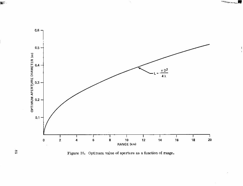
0.6

0.5

a: W

0.4 E 5 n

a

a W n

5 0.2 E - k 0

0.1

0

4h

2 4 6 8 10 12 RANGE (kml

14 16 18 20

Figure 35. Optimum value of aperture as a function of range.

20

18

16

14

12 Y

w (3 z fI 10 E 3 E X

1 8

- a

- a

6

4

2

0

\\ q = 0.05 E = 10 rnJ A = 1 0 . 5 9 ~ rn

LOSS DUE TO TURBULENCE IS IGNORED

1 2 3 ATTENUATION K (dB/km)

Figure 36. Maximum range of MSFC Pulsed Laser Doppler System for horizontal path at sea level.

86

2C

18

16

14

12 Y

w a Z

[r 10 5 5 3

x a ~8

- a

-

6

4

2

0

Figure 37. Maximum ground range of MSFC system.

87

molecular absorption. The total atmospheric attenuation consists of the molecular absorption, aerosol absorption, and scattering. Aerosol absorption and scattering amount to approximately 10 percent of the total attenuation at sea level and drops off rapidly with attitude. Therefore, molecular absorption alone gives a fairly good picture of the attenuation being experienced by the laser beam. Molecular absorption is extremely sensitive to the temperature and relative humidity. Using the results calculated in Section II, the molecular absorption is presented in Figure 38 as a function of temperature and relative humidity. This figure is useful in determining the attenuation rapidly when the temperature and humidity are known at the time of field test.

The contribution of atmospheric turbulence discussed in Section III is usually in the range of 15 percent ( o r less) of the total atmospheric attenuation. In the calculation of the ground range, the turbulence effect may be included, but its effect on the ground range is not noticeable.

88

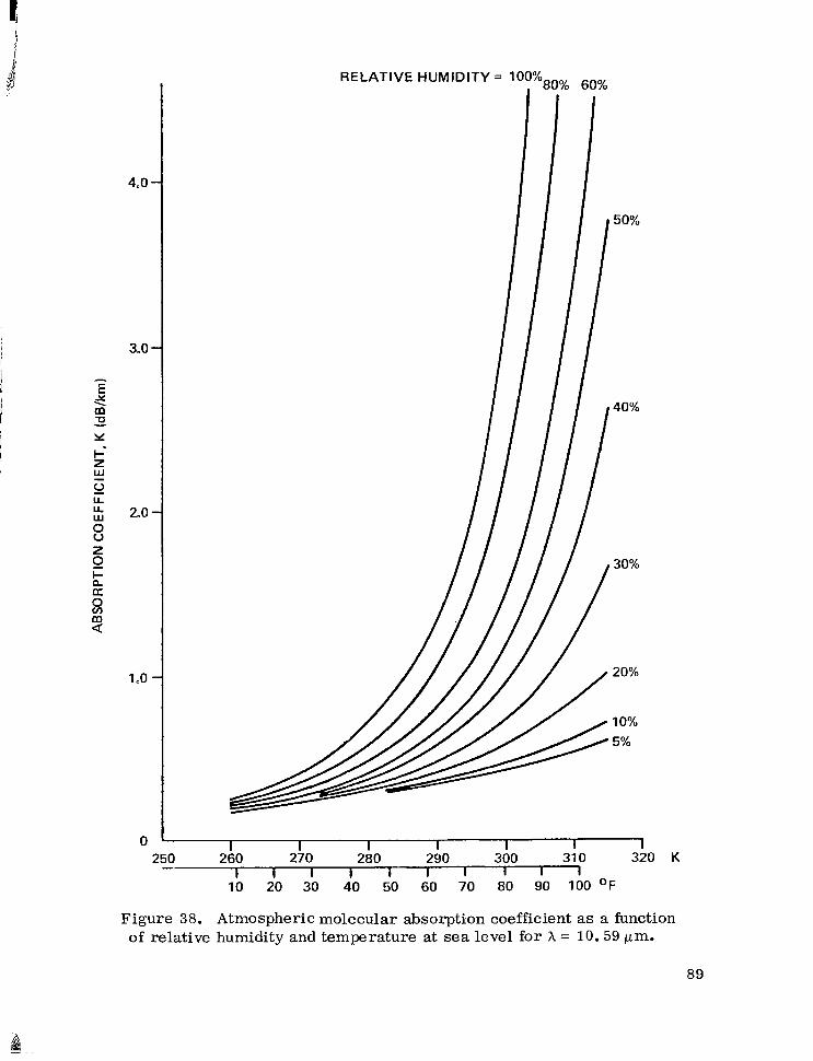
4.0

3.0

2.0

1.0

RELATIVE HUMIDITY = 60%

-

-

-

-

0 I 1 I 1 I I 1

I I 1 1 I I I I I 1 250 260 270 280 290 300 31 0 320 K -

10 20 30 40 50 60 70 80 90 100 OF

Figure 38. Atmospheric molecular absorption coefficient as a function of relative humidity and temperature at sea level for h = 10.59 pm.

89

V. CONCLUDING REMARKS

This report has discussed some of the various losses associated with the transmission of C02 laser radiation through the atmosphere, in particular molecular absorption, turbulence, and aerosol absorption and scattering. Additionally, calculations have been performed for selected data from test flights of the MSFC Pulsed Laser Doppler System.

Specifically, the atmospheric transmission loss was calculated for five P lines (P16, P18, P20, P22, and P24) of the CO, laser using the January 1973 flight test conditions. It was found that the transmission loss was approximately 7 percent higher for P16 lines and 10 percent lower for P24 lines compared to the P20 line. Thus, the variation of the transmission loss is not very significant around the P20 line which is the usual range of efficient operation of the C 0 2 laser. The P40 line o r RO line have better transmission, but it may not be possible to operate on these lines. Also, the attenuation of the COz laser radiation due to absorption, scattering, and turbulence of the atmosphere is estimated for the January 1973 flight test conditions. The theoretical values of S/N, including the atmospheric attenuation, compare favorably with the flight test results.

Molecular absorption was calculated for carbon dioxide, water vapor, and nitrous oxide for varying pressures and temperatures as a function of several P lines.

The effects of atmospheric turbulence are analyzed and included in the expression for the S/N ratio along with aerosol effects relative to backscatter and extinction.

The upper and lower limits on the atmospheric attenuation at each altitude up to 10 km are provided in graph form for a two-way horizontal path of 20 km range. These calculations are based on the curre.ntly accepted models of atmospheric pressure, temperature, humidity, aerosol concentration, and turbulence strength. These results are expected to be useful in the interpreta- tion of the future test results at several altitudes using the Pulsed COz L a s e r Doppler System.

90

.. .

. .

REFEkEN CES

1.

2.

3.

4.

5.

6.

7.

8.

9.

. .

Huffaker, Robert M., Jeffreys, Harold, B., Weaver, Edwin A., and '

Bilbro, James W. : Development of a Laser Doppler System for the- Detection, Tracking, and Measurement of Aircraft Wake Vortices. '

FAA Final Report, FAA-RD-74-213, NASA T M X-66868, March, 1975.

Bilbro, James W., Jeffreys, Harold, B., Kaufman, John W. , and Weaver, Edwin A. : Laser Doppler Measurements of Dust Devils. NASA TN D-8429, November, 1976.

Miller, C. R. and Sonnenschein, C. M. : Remote Measurement of Power Plant Smoke Stack Effluent Velocity. Raytheon Co. Final Report, Environmental Protection Agency, August, 1975.

Bilbro, J. W., Jeffreys, H. B., Weaver, E. A. , Huffaker, M. : Laser Doppler Velocimeter Wake Vortex Tests. FAA Final Report, FAA-RD-76-11, NASA TM X-64988, March, 1976.

Weaver, E. A., Bilbro, J. W., Dunkin, J. A., Jeffreys, H. B. : Laser Doppler Technology Applied to Atmospheric Environmental Problems. NASA Technical Report, NASA SP-416, 1976.

Bilbro, James W. and Vaughan, William W. : Wind Field Measurement in the Nonprecipitous Regions Surrounding Severe Storms by an Airborne Pulsed Doppler Lidar System. Submitted for publication.

Murty, S. S. R. : Atmospheric Transmission of CO, Laser Radiation with Application to Laser Doppler Systems. NASA TM X-64987, November, 1975.

Murty, S. S. R. : Laser Doppler Systems in Atmospheric Turbulence. NASA T M X-73354, November, 1976.

Howard, J. N., King, J. I. F., and Gast, P. R. : Thermal Radiation, Handbook of Geophysics. Chapter 16, United States Air Force, Geophysics Research Directorate, the Macmillan Company, New York, 1960.

91

REFERENCES (Cont inued)

10.

15.

16.

17.

18.

Benedict, W. S. and Kaplan, L. D. : Calculation of Line Widths in H20-N2 Collisions. Journal of Chemical Physics, vol. 30, 1959, p. 388.

Ely, R. and McCubbin, T. K. : The Temperature Dependence of the Self-Broadened Half-Width of the P-20 Line in the 001-100 Band of CO,. Applied Optics, vol. 9, no. 5, 1970, p. 1230.

Tubbs, L. D. and Williams, D. : Broadening of Infrared Absorption Lines at Reduced Temperatures: Carbon Dioxide. J. Optical Society of America, vol. 62, 1972, p. 284.

McClatchey, R. A. , Benedict, W. S. , Clough, S. A. , Burch, D. E. , Calfee, R. F. , Fox, K. , Rothman, L. S. , and Garing, J. S. : AFCRL Atmospheric Absorption Line Parameter Compilation, AFCRL-TR-73- 0096, Air Force Cambridge Research Laboratories, Bedford, Massachusetts, January 26, 1973.

Yin, P. K. L. and Long, R. K. : Atmospheric Absorption at the Line Center of P( 20) C02 Laser Radiation. Applied Optics, vol. 8, August, 1968, p. 1551.

Elsasser, W. M. : Note on Atmospheric Absorption Caused by the Rotational Water Band. Physical Review, vol. 53, 1938, p. 768.

Yates, H. W. and Taylor, J. H. : Infrared Transmission of the Atmos- phere. NRL Report 5453, 1960.

Anthony, R. : Atmospheric Absorption of Solar Infrared Radiation. Physical Review, vol. 85, 1952, p. 674.

92

REFERENCES (Continued)

19.

20.

21.

22.

23.

24.

25.

26.

27.

28.

5

Roach, W. T. and Goody, R. W. : Absorption and Emission in the Atmospheric Window from 770 to 1250 cm". Quarterly J. Royal Meteorological Society, vol. 3 4 , 1958, p. 319.

Bignell, K. J. , Saiedy, F., and Sheppard, P. A. : On the Infrared Con- tinuum. J. Optical Society of America, vol. 53, 1963, p. 466.

Bignell, K. J. : The Water-Vapor Infrared Continuum. Quarterly J. Royal Meteorological Society, vol. 96, 1970, p. 390.

McCoy, J. H. , Rensch, D. B., and Long, R. K. : Water Vapor Con- tinuum Absorption of Carbon Dioxide Laser Radiation Near 10 p. Applied Optics, vol. 8, 1969, p. 1471.

Burch, D. E. : Radiative Properties of the Atmospheric Windows. Preprints of Conference on Atmospheric Radiation, American Meteorolo- gical Society, August, 1972, p. 61.

Burch, D. E. : Private Communication, August, 1975.

Varanasi, P. , Chou, S. , and Penner, S . S . : Absorption Coefficients for Water Vapor in the 600-1000 cm-I Region. J. Quantitative Spectro- scopy and Radiative Transfer, vol. 8, 1968, p. 1537.

Kawachi, D. A. : Data Analysis of the January 1973 Clear Air Turbulence Laser Flight Tests, Report No. ER 74-4140, Raytheon Company, Equip- ment Division, Sudbury, Massachusetts, December, 1973.

Wang, J. Y. : Infrared Atmospheric Transmission of Laser Radiation. Applied Optics, vol. 13, 1974. PO 56.

93


29.

30.

31.

32.

33.

34.

35.

36.

37.

38.

Spencer, D. J., Denault, G . C . , and Takimoto, H. H. : Atmospheric Gas Absorption at DF Laser Wavelength. Applied Optics, vol. 13, 1974, p. 2855.

Rensch, D. B. and Long, R. K. : Comparative Studies of Extinction and Backscattering by Aerosols, Fog and Rain at 10.6 p and 0.63 p. Applied Optics, vol. 9, 1970, p. 1563.

Meyer-Arendt, J. R. and Emmanuel, C. B. : Optical Scintillation; A Survey of Literature. National Bureau of Standards, Technical Note 225, April 5, 1965.

Tatarski, V. I. : Wave Propagation in a Turbulent Medium. McGraw- Hill Company, New York, 1961.

Kerr , J. R. : Experiments on Turbulence Characteristics and Multi- wavelength Scintillation Phenomena. J. of the Optical Society of America, vol. 62, September, 1972, p. 1040.

Tatarski, V. I. : The Effects of the Turbulent Atmosphere on Wave Propagation. U. S. Department of Commerce, National Technical Information Service, Springfield, Virginia, 1971.

De Wolf, D. A. : Waves in Turbulent Air: A Phenomenological Model. Proceedings of the IEEE, vol. 57, April, 1969, p. 375.

Young, A. T. : Aperture Filtering and Saturation of Scintillation. J. Optical Society of America, vol. 60, February, 1970, p. 248.

Lee, R. W. and Harp, J. C. : Weak Scattering in Random Media, with Applications to Remote Probing. Proceedings of the IEEE, April, 1969, p. 375.

Davis, J. I. : Consideration of Atmospheric Turbulence in Laser System Design. Applied Optics, vol. 5, January, 1966.

94


39. Lutomirski, R. F. and Yura, H. T. : Propagation of a Finite Optical Beam in an Inhomogeneous Medium. Applied Optics, vol. 10, July, 1971, p. 1652.

40. Fante, R. : Mutual Coherence Function and Frequency Spectrum of a Laser Beam Propagating Through Atmospheric Turbulence. J. Optical Society of America, vol. 64, May, 1974, p. 592.

41. Fried, D. L. : Limiting Resolution Looking Down Through the .Atmos- phere. J. Optical Society of America, vol. 56, October, 1966, p. 1380.

42. yura , H. T. : Mutual Coherence Function of a Finite Cross Section Optical Beam Propagating in a Turbulent Medium. Applied Optics, vol. 11, June, 1972, p. 1399.

43. Kerr, J. R.. and Dumphy, J. R. : Experimental Effects of Finite Trans- mitter Apertures on Scintillations. J. Optical Society of America, vol. 63, January, 1973, pb. 1,

44. Raidt, H. and HEhn, D. H. : Instantaneous Intensity Distribution in a Focussed Laser Beam at 0.63 m and 10.6 m Propagating through the Atmosphere. Applied Optics, vol. 14, November, 1975.

45. Yura, H. T. : Short-Term Average Optical Beam Spread in a Turbulent Medium. J. Optical Society of America, vol. 63, May, 1973, p. 567.

46. Yura, H. T. : Atmospheric Turbulence Induced Laser Beam Spread. Applied Optics, vol. 10, December, 1971, p. 2771.

47. Klyatskin, V. and Kon, A. : On the Displacement of Spatially-Bounded Light Beams in a Turbulent Medium in the Markovian-Random-Process Approximation. Radiophysics and Quantum Electronics, vol. 15, September, 1972, p. 1056.

48. Fante, Ronald L. : Electromagnetic Beam Propagation in Turbulent Media. Proceedings of the LEEE, v01. 63, December, 1975, p. 1669.

95


49.

50.

51.

52.

53.

54.

55.

56.

57.

58.

Dunphy, J. R. and Kerr, J. R. : Atmospheric Beam-Wander Cancella- tion by a Fast-Tracking Transmitter. J. Optical Society of America, vol. 64, July, 1974, p. 1015.

Sher, Lawrence: Tracking Systems Requirements for Atmospheric Steering Compensation. Applied Optics, vol. 14, November, 1975, p. 2750.

Andreev, G. A. and Gel' fer, E. I. : Angular Random Walks of the Center of Gravity of the Cross Section of a Diverging Light Beam. Radiophysics and Quantum Electronics, vol. 14, 1971, p. 1145.

Fried, D. L. : Statistics of Laser Beam Fade Induced by Pointing Jitter. Applied Optics, vol. 12, February, 1973, p. 422.

Kleen, R. H. and Ochs, G. R. : Measurements of the Wavelength Dependence of Scintillation in Strong Turbulence. J. Optical Society of America, vol. 60, December, 1970, p. 1695.

Gracheva, M., Gurvich, A., Kashkarov, S., and Pokasov, V. : Similarity Correlations and Their Experimental Verification in the Case of Strong Intensity Fluctuations of Laser Radiation. Soviet Physics JETP, vol. 40, no. 6, 1975, p. 1011.

De Wolf, D. A. : Saturation of Irradiance Fluctuations due to Turbulent Atmosphere. J. Optical Society of America, vol. 58, April, 1968, p. 461.

Fried, D. L. : Aperture Averaging of Scintillations. J. Optical Society of America, vol. 57, February, 1967, p. 169.

Dunphy, J. R. and Kerr, J. R. : Scintillation Measurements for Large Integrated Path Turbulence. J. Optical Society of America, vol. 63, August, 1973, p. 981.

Young, A. T. : Saturation of Scintillations. J. Optical Society of America, vol. 60, November, 1970, p. 1495.

96

"


59. Clifford, S. F. , Ochs, G. R. , and Lawrence, R. S. : Saturation of Optical Scintillation by Strong Turbulence. J. Optical Society of America, vol. 64, February, 1974, p. 148.

60. Clifford, S. F. and Yura, H. T. : Equivalence of Two Theories of Strong Optical Scintillation. J. Optical Society of America, vol. 64, December, 1974, p. 1641.

61. Yura, H. T. : Physical Model for Strong Optical-Amplitude Fluctuations in a Turbulent Medium. J. Optical Society of America, vol. 64, January, 1974, p. 59.

62. Fante, R. : Electric Field Spectrum and Kntensity Covariance of a Wave i n a Random Medium. Radio Science, vol. 10, January, 1975, p. 77.

64. Fried, D. L. : Optical Heterodyne Detection of an Atmospherically Distorted Signal Wave Front. Proceedings of the IEEE, vol. 55, January, 1967, p. 57.

65. Moreland, J. P. and Collins, S. A. , Jr. : Optical Heterodyne Detection of a Randomly Distorted Signal Beam. J. Optical Society Of America, vol. 59, January, 1969, p. 10.

66. Fried, D. L. and Yura, H. T. : Telescope-Performance Reciprocity for Propagation in a Turbulent Medium. J. Optical Society of America, vol. 62, April, 1972, p. 600.

67. Thomson, A. and Dorian, M. F. : Heterodyne Detection of Monochromatic Light Scattered from a Cloud of Moving Particles. Gnera l Dynamics/ Convair, San Diego, California, CDC-ERR-AN-1090, June, 1967.

68. Sonnenschein, C. H. and Horrigan, F. A. : Signal-to-Noise Relationships for Coaxial Systems that Heterodyne Backscatter from the Atmosphere. Applied Optics, vol. 10, July, 1971, p. 1600.

97

REFERENCES (Concluded)

69. Krause, M. C., Morrison, L. K., Craven, C. E. , Logan, N. A. 9 and Lawrence, T. R. : Development of Theory and Experiments to Improve Understanding of Laser DoppIer Systems. Lockheed Missiles and Space Company, Huntsville, Alabama, LMSC-HREC TR D306632, June, 1973.

70. Hufnagel, R. E. and Stanley, N. R. : Modulation Transfer Function Associated with Image Transmission Through Turbulent Media. J. Optical Society of Americg, vol. 54, January, 1964, p. 52.

71. Pearson, Karl: Tables of the Incomplete r-Function, University Press, Cambridge, England, 1957.

72. Logan, N. A. : Computer Modelizing of Laser Doppler Clear Air Turbulence System. Lockheed Missiles and Space Company, Huntsville, Alabama, LMSC-HREC D306745, February, 1973.

73. A Program for the Evaluation of the Mie Series. Appendix to the report LMSC-HREC TM D306995, Lockheed Missiles and Space Company, Huntsville, Alabama.

74. Backscatter and Extinction Coefficients Calculation. Programmed by E. Poorman, CSC, Huntsville, in preparation.

75. McClatchey, et al. : Optical Properties of the Atmosphere. Air Force Cambridge Research Laboratories, Bedford, Massachusetts, AFCRL- 720497, 1972.

98

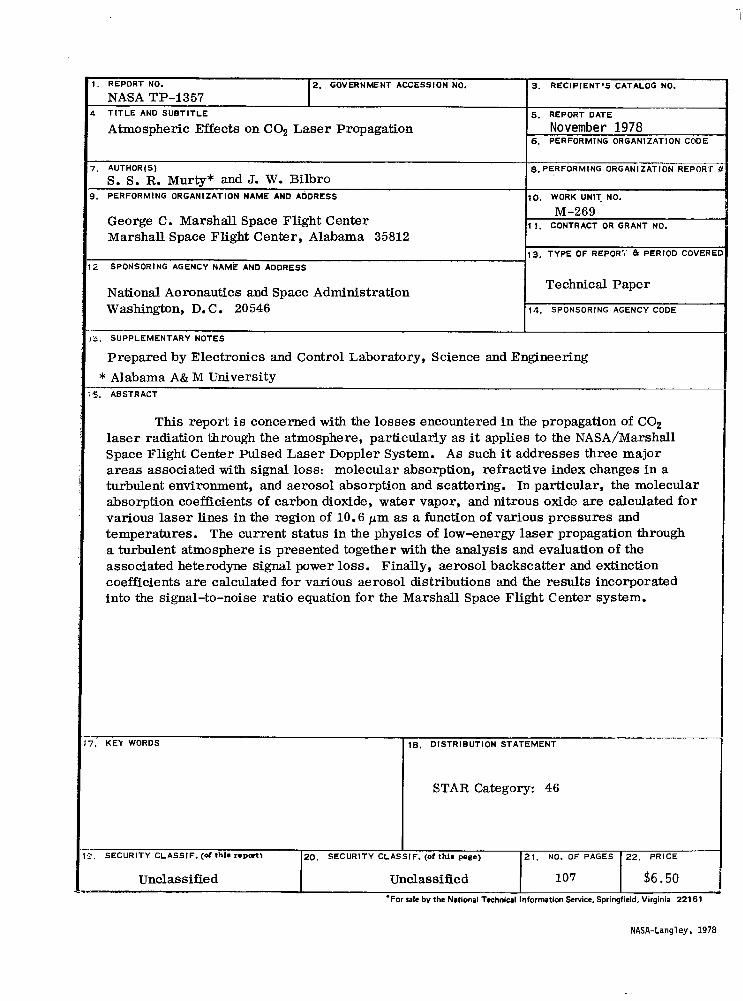
1 . REPORT NO. 3. RECIPIENT'S CATALOG NO. 2. GOVERNMENT ACCESSION NO.

NASA TP-1357 d T I T L E AND S U B T I T L E 5. REPORT DATE

I Atmospheric Effects on CO, Laser Propagation November 1978 6. PERFORMTNG ORGANIZATION CODE

7. AUTHOR(S)

S. S. R. Murty* and J. W. Bilbro 8. PERFORMING ORGANIZATION REPORT

9. PERFORMING ORGANIZATION NAME AND ADDRESS 110. WORK UNIT, NO. -~

George C. Marshall Space Flight Center Marshall Space Flight Center, Alabama 35812

"269 1 1. CONTRACT OR GRANT NO.

13. TYPE OF REPORi . PERIOD COVERE

12 SPONSORING AGENCY NAME AND ADDRESS "-1

I National Aeronautics and Space Administration Washington, D. C. 20546

Technical Paper

SUPPLEMENTARY NOTES J

Prepared by Electronics and Control Laboratory, Science and Engineering : * Alabama A& M University ! .4. ABSTRACT

This report is concerned with the losses encountered in the propagation of CO, laser radiation through the atmosphere, particularly as it applies to the NASA/Marshall Space Flight Center Pulsed Laser Doppler System. A s such it addresses three major areas associated with signal loss: molecular absorption, refractive index changes in a turbulent environment, and aerosol absorption and scattering. In particular, the molecular absorption coefficients of carbon dioxide, water vapor, and nitrous oxide are calculated for various laser lines in the region of 10.6 pm as a function of various pressures and temperatures. The current status in the physics of low-energy laser propagation through a turbulent atmosphere is presented together with the analysis and evaluation of the associated heterodyne signal power loss. Finally, aerosol backscatter and extinction coefficients are calculated for various aerosol distributions and the results incorporated into the signal-to-noise ratio equation for the Marshall Space Flight Center system.

I ' i7. KEY WORDS 18 . D ISTRIBUTION STATEMENT

I SECURITY CLASSIF. (of thim ropart)

$6.50 107 Unclassified Unclassified

22. PRICE 2 1 . NO. OF PAGES 20. SECURITY CLASSIF . (of thlm pago)

*For sale by the National Technical Information Service, Springfield, Virginia 22161

NASA-Langley. 1978

. .

,~ National Aeronautics and . . THIRD-CLASS BULK RATE

- Space Administration , . , .

Washington, D.C. 20546 -.

, -

Official Business Penalty for Private Use, $300

I .

.~ ' . . .

J 1 ' u, E,, I I U O 1 0 , . . DEPT OF THE A I S FORCE

Postage and Fees Paid, National Aeronautics and Space Administration NASA451

I Atmospheric Effects on I- Laser Propagation · PDF fileAbsorption coefficient of nitrous...

Documents

Transcript of I Atmospheric Effects on I- Laser Propagation · PDF fileAbsorption coefficient of nitrous...