Hyperspectral Image Classification Using

Orthogonal Subspace Projections: Image

Simulation and Noise Analysis

Emmett Ientilucci, Center for Imaging Science

April 23, 2001

Contents

1 Introduction 4

2 Background 42.1 Remote Sensing: An Overview . . . . . . . . . . . . . . . . . 42.2 Sensors and Imaging Spectrometers . . . . . . . . . . . . . . . 52.3 Classification Techniques and Transforms . . . . . . . . . . . 6

3 Orthogonal Subspace Projection Classification 73.1 Problem Formation . . . . . . . . . . . . . . . . . . . . . . . . 73.2 Hyperspcetral Pixel Classification . . . . . . . . . . . . . . . . 8

3.2.1 Interference Rejection by Orthogonal Subspace Pro-jection . . . . . . . . . . . . . . . . . . . . . . . . . . . 8

3.2.2 Signal-to-Noise Ratio (SNR) Maximization . . . . . . 9

4 100 Pixel Simulated Scene 104.1 Scene Overview . . . . . . . . . . . . . . . . . . . . . . . . . . 104.2 OSP Formulation and Results for One Pixel w/o Noise . . . . 124.3 OSP Results for Test Image with out Noise . . . . . . . . . . 154.4 OSP Results for Test Image with Noise . . . . . . . . . . . . 16

4.4.1 1% Gaussian Noise . . . . . . . . . . . . . . . . . . . . 164.4.2 5% Gaussian Noise . . . . . . . . . . . . . . . . . . . . 17

4.5 Classified Concrete Image: A Closer Look at Noise . . . . . . 194.5.1 Look at Effect on All Image Pixels . . . . . . . . . . . 194.5.2 Look at Effect on Pixels That Only Contain Concrete 19

1

CONTENTS 2

5 Conclusions 22

6 References 23

LIST OF FIGURES 3

List of Figures

1 Atmospheric transmission spectra showing windows availablefor earth observations. . . . . . . . . . . . . . . . . . . . . . 6

2 Test image used for OSP evaluation (400× 400). . . . . . . . 113 Test image pixels convolved down to 10× 10. . . . . . . . . . 114 Spectral signature of 3 materials or endmembers and gaussian

noise. . . . . . . . . . . . . . . . . . . . . . . . . . . . . . . . 135 Classified concrete image, a) 10× 10 and b) 400× 400 pixels. 166 Classified a) tree-leaf and b) dirt images. . . . . . . . . . . . 167 Classified concrete image with 1% noise present. . . . . . . . 178 Classified a) tree-leaf and b) dirt images with 1% noise present.

179 Classified concrete image with 5% noise present. . . . . . . . 1810 Classified a) tree-leaf and b) dirt images with 5% noise present.

1811 Normalized energy for classified concrete, as a function of

noise, on a per-pixel basis. . . . . . . . . . . . . . . . . . . . 2012 Normalized energy for classified concrete showing actual data

reflectance data points for the no-noise curve. . . . . . . . . 2013 Plot illustrating . . . . . . . . . . . . . . . . . . . . . . . . . 22

List of Tables

1 The mixture fractions of 16 selected pixels from the test im-age. . . . . . . . . . . . . . . . . . . . . . . . . . . . . . . . . 21

2 Error associated with applying 1% and 5% noise to the image. 23

1 INTRODUCTION 4

1 Introduction

Remote sensing technology is concerned with the determination of charac-teristics of physical objects through the analysis of measurement taken ata distance from these objects. One important problem in remote sensingis the characterization and classification of (spectral) measurements takenfrom various situations on the earth surface. For example, based on certainspectral measurements, we may want to classify various crops planted ina particular region, or we would like to identify one or several specific soiltypes in a region from the spectral measurements [1]. Data can be collectedin a few (multispectral) to as many as 200 (hyperspectral) spectral bands.Classification of a hyperspectral image data amounts to identifying whichpixels contain various spectrally distinct materials that have been speci-fied by the user. Classification approaches such as minimum distance tothe mean (MDM) and Gaussian maximum likelihood (GML) [2] can be ap-plied to this data as well as correlation/matched filter-type approaches suchas spectral signature matching [3] and spectral angle mapper [4]. However,these techniques have difficulty accounting for mixed pixels (pixels that con-tain multiple spectral classes). A possible solution is to use the concept oforthogonal subspace projection (OSP) [5], [6]. This can be done by finding amatrix operator that eliminate’s undesired signatures in the data and thenfinding a vector operator which maximizes the residual desired signaturesignal-to-noise ratio (SNR). This, in turn, will produce a new set of imageswhich highlight the presence of each signature of interest. At the same time,the orthogonal subspace projection technique will reduce the dimensionallyof the hyperspectral data, which maybe more appeasing to the analysts.

2 Background

2.1 Remote Sensing: An Overview

Remote sensing, for all practical purposes, is the field of study associatedwith extracting information about an object without coming into physicalcontact with it [7]. A definition such as this can include a multitude ofdisciplines such as medical imaging, astronomy, vision, sonar, and earthobservation from above via an aircraft or space satellite. For the mostpart, remote sensing is often thought of in the latter context, viewing andanalyzing earth from above.

The field of remote sensing is rather young, being about 30 years old orso. This goes back to the late 40’s and early 50’s when some of the first

2 BACKGROUND 5

satellite photographs were being recovered from V-2 launches. During thistime the satellite imaging of the earth developed hand in hand with the in-ternational space program. Following the first manmade satellite launch ofSputnik 1 on October 4, 1957, photographs and video images were acquiredby U.S. Explorer and Mercury programs and the Soviet Union’s LUNA se-ries. Just 3 years after Sputnik 1’s debut (April 1960), the U.S. initiatedits spaced-based reconnaissance program acquiring high-resolution photo-graphic images from space [8]. Today remote sensing is used in a varietyof applications such as environmental mapping, global change research, ge-ological research, wetlands mapping, assessment of trafficability, plant andmineral identification and abundance estimation, and crop analysis.

In general, remote sensing enables us to look at the earth from a differ-ent point of view. This different vantage point can aid analysts and alikein making improved decision’s or assessments. Furthermore, remote sens-ing technology enables us to view the earth through “windows” of the EMspectrum that would not otherwise be humanly possible. Figure 1 showsthe transmission spectra of the earth’s atmosphere. From this, it is clearthat there are some regions or windows in the EM spectrum that have ahigher transmission than others. These are what folks in the remote sensingcommunity term “spectral bands”. The earth can appear quite different de-pending on which band it is viewed in. Only recently have we been able tocapture a multitude of high resolution spectral bands at once. Such devicesthat seize this high resolution imagery are called imaging spectrometers.

2.2 Sensors and Imaging Spectrometers

One of the most important parts of the remote imaging system is the sen-sor. The imaging system must have some type of sensing mechanism tocapture EM radiation. These mechanisms can be analog or digital. Someimagers use film while others use CCD arrays. These instrument or sensorplatforms can be divided into those with one to ten or so spectral channels(multispectral) and those with tens to hundreds of spectral channels (hyper-spectral). The focus here is on the latter. Advances in sensor design havepaved the way for a new generation of sensors called imaging spectrometers.Imaging spectrometry has been under development since the 1970’s as ameans of identifying and mapping earth resources. As a result, hyperspec-tral data permit the expansion of detection and classification activities totargets previously unresolved in multispectral images. In spectroscopy, re-flectance variation as a function of wavelength provides a unique signature,or fingerprint, that can be used to identify materials. Imaging spectrome-

2 BACKGROUND 6

Figure 1: Atmospheric transmission spectra showing windows available forearth observations.

ters go one step further, imaging a scene with high spatial resolution andover many discrete wavelength bands so that absorption features can beassigned to distinct geographic elements such as vegetation, rock, or urbandevelopment. One such sensor is the Airborne Visible InfraRed ImagingSpectrometer (AVIRIS) which images in 224 bands from 400 to 2500nm.

2.3 Classification Techniques and Transforms

With the increased use of hyperspectral image data comes the need for moreefficient tools that can dimensionally reduce, classify, and reveal importantinformation content of the data. As previously mentioned, classificationof a hyperspectral image data amounts to identifying which pixels containvarious spectrally distinct materials that have been specified by the user.There has been numerous techniques applied to this data such as minimumdistance to the mean (MDM), Gaussian maximum likelihood (GML) [2],and correlation/matched filter-type approaches such as spectral signaturematching [3] and spectral angle mapper [4], [9]. The MDM and GML classi-fiers have difficulty accounting for mixed pixels (pixels that contain multiplespectral classes), though there have been attempts to improve this for hy-

3 ORTHOGONAL SUBSPACE PROJECTION CLASSIFICATION 7

perspectral data [10]. Correlation and match filtering techniques have thesame mixed pixel problem as well as the limitation that the output of thematched filter is nonzero and quite often large for multiple classes [5].

Various transforms can be used to reduce the dimentionality of the data.One of the more common linear transforms is the principle components(PC) transformation. It is designed to decorrelate the data and maximizethe information content in a reduced number of features. A recent improve-ment to the PC transformation is the noise-adjusted PC transformation [12].This transformation orders the new images in terms of SNR, and thus de-emphasizes noise in the resulting images [13]. While these techniques areadequate for reducing data dimentionality, they lack the ability to accentu-ate spectral signatures of interest. A possible solution to this problem is theuse of orthogonal subspace projections (OSP).

3 Orthogonal Subspace Projection Classification

3.1 Problem Formation

The idea of the orthogonal subspace projection classifier is to eliminate allunwanted or undesired spectral signatures (background) within a pixel, thenuse a matched filter to extract the desired spectral signature (endmember)present in that pixel.

To start with we formulate the problem at hand. In hyperspectral imageanalysis, the spatial coverage of each pixel, more often than not, may en-compass several different materials. Such a pixel is called a “mixed” pixel.It contains multiple spectral signatures. To start with, we formulate and de-scribe a column vector ri to represent the mixed pixel by the linear model:

ri = Mαi + ni (1)

In this treatment it should be noted that vectors are in lower case boldtypeface while matrices are in uppper case bold. As Tu et al [6] point out,let the vector ri be a `× 1 column vector and denote the ith mixed pixel ina hyperspectral image, where ` is the number of spectral bands.

Each distinct material in the mixed pixel is called an endmember (p).We assume there are p spectrally distinct endmembers in the ith mixed pixel.The column vector ri can be in digital counts (DC), radiance, or reflectancedepending on how endmembers and noise are defined.

Now assume that the matrix M, of dimension `×p, is made up of linearlyindependent columns. These columns are denoted (m1,m2, . . .mj , . . .mp)

3 ORTHOGONAL SUBSPACE PROJECTION CLASSIFICATION 8

where ` > p (overdetermined system) and mj is the spectral signature of thejth distinct material or endmember. Let αi be a p column vector given by(α1, α2, . . . αj , . . . αp)T where the jth element represents the fraction of thejth signature present in the ith mixed pixel. This is a vector of endmemberfractions.

Finally we consider additive noise. Let ni be a `×1 column vector repre-senting additive white gaussian noise with zero mean and covariance matrixσ2I , where I is an `× ` identity matrix.

In this representation we assume ri is a linear combination of p endmem-bers with the weight coefficients designated by the abundance (fraction) vec-tor αi. We can rewrite the term Mαi so as to separate the desired spectralsignatures from the undesired signatures. Simply put, we are separating thetarget from the background. For brevity we omit the subscript i represent-ing the calculation on a per pixel basis. In searching for a single spectralsignature we write:

Mα = dαp + Uγ (2)

where d is ` × 1, the desired signature of interest containing columnvector mp while αp is 1 × 1, the fraction of the desired signature. Thematrix U is composed of the remaining column vectors from M. These arethe undesired spectral signatures or background information. This is givenby U = (m1,m2, . . .mj , . . .mp−1) with dimension ` × (p − 1) where γ is acolumn vector which contains the remaining (p− 1) components (fractions)of α. That is γ = (α1, α2, . . . αj , . . . αp)T .

3.2 Hyperspcetral Pixel Classification

3.2.1 Interference Rejection by Orthogonal Subspace Projection

We can now develop an operator P which eliminates the effects of U, theundesired signatures. To do this we develop an operator that projects r ontoa subspace that is orthogonal to the columns of U. This results in a vectorthat only contains energy associated with the target d and noise n. This isdone by using a least squares optimal interference rejection operator [5], [6].The operator used is the `× ` matrix

P = (I−UU†) (3)

where U† is the pseudo inverse of U, denoted U† = (UTU)−1UT . Theoperator P maps d into a space orthogonal to the space spanned by the

3 ORTHOGONAL SUBSPACE PROJECTION CLASSIFICATION 9

uninteresting signatures in U. We now operate on the mixed pixel r fromEquation 1.

Pr = Pdαp + PUγ + Pn (4)

It should be noticed that P operating on Uγ reduces the contributionof U to zero (close to zero in real data applications). Therefore, uponrearrangement we have

Pr = Pdαp + Pn (5)

This is an optimal interference rejection process in the least squaressense.

3.2.2 Signal-to-Noise Ratio (SNR) Maximization

We now want to find an operator xT which will maximize the signal-to-noiseratio (SNR). The operator xT acting on Pr will produce a scalar.

λ =xTPdαp

2dTPTxxTPE{nnT }PTx

(6)

λ =

(αp

2

σ2

)xTPddTPTx

xTPPTx(7)

where E{} denotes the expected value. Maximization of this quotient isthe generalized eigenvector problem

PddTPTx = λ̃PPTx (8)

where λ̃ = λ(σ2/αp). The value of xT which maximizes λ̃ can be de-termined in general using techniques outlined in [14] and the idempotent(P2 = P) and symmetric (PT = P) properties of the interference rejectionoperator. As it turns out the value of xT which maximizes the SNR is

xT = kdT (9)

where k is an arbitrary scalar. This leads to an overall classificationoperator for a desired hyperspectral signature in the presence of multipleundesired signatures and white noise. This is given by the 1× `, vector

qT = dTP (10)

4 100 PIXEL SIMULATED SCENE 10

This result first nulls the interfering signatures, and then uses a matchedfilter for the desired signature to maximize the SNR. When the operator isapplied to all of the pixels in a hyperspectral scene, each `×1 pixel is reducedto a scalar which is a measure of the presence of the signature of interest.The ultimate result is to reduce the ` images that make-up the hyperspectralimage cube into a single image where pixels with high intensity indicate thepresence of the desired signature.

This operator can be easily extended to seek out k signatures of interest.The vector operator simply becomes a k× ` matrix operator which is givenby

Q = (q1,q2, . . .qi, . . .qk)T (11)

where each of the qiT = di

TPi is formed with the appropriate desiredand undesired signature vectors. In this case, the hyperspectral image cubeis reduced to k images which classify each of the signatures of interest.

4 100 Pixel Simulated Scene

4.1 Scene Overview

A sample image (10× 10) with linearly mixed pixels was created in order toverify the functionality of the OSP operator. This image or image cube con-sisted of 16 spectral bands (0.5µm to 2.0µm) and 3 endmembers or classes(concrete, tree leaf, and dirt). The endmember vectors contained reflectancevalues that were representative of the various materials. Gaussian normallydistributed noise was also added to the vectors. One data set was run with-out noise. A second data set contained noise, n(µ = 0, σ = 0.01) while athird contained noise, n(µ = 0, σ = 0.05).

The hypothetical hi-res image (400× 400) resembles a road with a treeline on both sides of it. Outside of the tree line are open areas of dirt. Oneband of the image can bee seen in Figure 2 where the darkest pixels areconcrete, the lightest pixels are dirt, and the middle shade of grey are tress.

In general, the pixel size in the final output image is a function of thedetector element size. If we wish to work with a 10× 10 image, we will haveto convolve or degrade the test scene. With this in mind, the test imagewould actually look like the one in Figure 3. This process gives us our mixedpixel test image.

4 100 PIXEL SIMULATED SCENE 11

Figure 2: Test image used for OSP evaluation (400× 400).

Figure 3: Test image pixels convolved down to 10× 10.

4 100 PIXEL SIMULATED SCENE 12

4.2 OSP Formulation and Results for One Pixel w/o Noise

We start with 3 vectors or classes, each 16 elements or bands long. Thevectors are in reflectance units and can be seen below. A graphical repre-sentation of these vector is illustrated in Figure 4 along with a curve of 5%gaussian noise.

Concrete =

0.260.300.310.310.310.310.340.340.330.320.330.340.350.340.280.27

Treeleaf =

0.070.070.110.540.550.540.560.500.490.180.190.300.320.280.050.10

Dirt =

0.070.130.190.250.300.340.380.400.420.420.440.450.460.460.400.42

We now need to define the fraction mixtures of each of the 100 pixelsin Figure 2 (on page 11) starting from left-to-right, top-to-bottom. Forexample, the model for pixel 40 (last pixel in the 4th row) might look like,

pixel40 ≡ (0.08)concrete + (0.75)treeleaf + (0.17)dirt + noise

Where noise, in this first case, is zero. Once all the pixel mixture frac-tions have been defined, we can choose a particular class spectra to extractfrom the test image. For the first image we will develop and algorithm us-ing the OSP operator to extract the material concrete from all the pixelsthroughout the test image. This same procedure will then be used to extractthe grass and dirt materials.

To start, we will develop the algorithm for one particular pixel and thenapply the same technique to the remaining pixels. For example, we assume

4 100 PIXEL SIMULATED SCENE 13

-0.1

0

0.1

0.2

0.3

0.4

0.5

0.6

0.7

0.4 0.6 0.8 1 1.2 1.4 1.6 1.8 2

Wavelength [um]

Ref

lect

ance

Concrete

Tree

Dirt

5% Gaus. Noise

Figure 4: Spectral signature of 3 materials or endmembers and gaussiannoise.

that pixel 40 is made up of some weighted linear combination of endmembersand noise.

pixel40 = Mα + noise (12)

Furthermore, we can break up Mα into desired, dαp and undesired, Uγsignatures.

pixel40 = dαp + Uγ + noise (13)

Now we assign the desired, d and undesired, U signatures to spectra.We let concrete be the vector d and tree-leaf and dirt be the column vectorsof the matrix U. However, we don’t know the fractions. We just know pixel40 is made up of some combination of d and U.

d ≡ [concrete] U ≡ [treeleaf, dirt]

We ultimately want to reduce the effects of U. To do this we needto find a projection operator P, that when operated on U, will reduce itscontribution to zero. Ultimately we want U −U = O, the null matrix. IfU were symmetric we could use the operator P = I −UU−1. This wouldyield

4 100 PIXEL SIMULATED SCENE 14

(I−UU−1)U = (I− I)U = U−U = O (14)

However, U will more than likey be asymmetric. So we need to use thepseudoinvers, U† in place of U−1.

U† = (UTU)−1UT (15)

The projection operator now becomes

P = I−UU† (16)

where I is the identity matrix

To find concrete, d, we project pixel 40 onto a subspace that is orthogonalto the columns of U using the operator P. In other words, P maps d intoa space orthogonal to the space spanned by the undesired signatures whilesimultaneously minimizing the effects of U.

If we operate on U, which contains tree-leaf and dirt, with P, we cansee that it does a good job at minimizing the effects of U.

PU =

0 00 00 00 00 00 00 00 00 00 00 00 00 00 00 00 0

If we let r1 = pixel 40 and n = noise, we have from Equation 5

Pr1 = Pdαp + Pn (17)

4 100 PIXEL SIMULATED SCENE 15

We now want to find an operator xT which will maximize the signal-to-noise ratio (SNR). The operator xT acting on Pr1 will produce a scalar. Asstated before, the value of xT which maximizes the SNR is

xT = kdT (18)

where k is an arbitrary scalar. This leads to the overall OSP operator

dTP{} (19)

For pixel 40, which has 8% concrete, 75% tree-leaf, and 17% dirt, theenergy result is

(dTP)r1 = 5.19

The output of the OSP operator is just a scalar that is proportional tothe energy we are seeking. In this case it was concrete from pixel 40.

4.3 OSP Results for Test Image with out Noise

We now wish to apply the operator image wide, so as to classify concrete,tree-leaf, and dirt, respectively. Again, the operator is applied to each pixeland a scalar is generated. The scalar is a function of the energy associatedwith the signature of interest. Some pixels in the test scene in Figure 3 arepure concrete while others are a combination of the 3 materials and potentialnoise.

The initial classification was done using concrete as the desired, d sig-nature and tree-leaf and dirt as the undesired signatures, U. The result ofthis can be seen in Figure 5 where we have up-convolved the image back to400× 400 pixels.

The abundance of concrete (the desired signature) is directly propor-tional to the brightness of the pixel. Black pixels contain no concrete whilepure white pixels are made up entirely of concrete.

Similarly, the operator was then used to classify tree-leaf and dirt. Therelationship between abundance and brightness holds true for these examplesas well. These results can be seen in Figure 6.

We see that the OSP operator has done a very good job of extracting the3 different material types from the test image. This is expected, however.If we look at pixel 40 again, we know it had 8% concrete in it. For thenoiseless case, the normalized concrete energy will correlate exactly with the

4 100 PIXEL SIMULATED SCENE 16

Figure 5: Classified concrete image, a) 10× 10 and b) 400× 400 pixels.

Figure 6: Classified a) tree-leaf and b) dirt images.

normalized concrete reflectance. Therefore, the error between the reflectanceand normalized concrete energy will be zero. This would be expected sincethe values that make up the U matrix are exactly the truth signatures in theimage. The normalization here assumes that the maximum concrete energyvalue came from a pixel that was 100% concrete.

4.4 OSP Results for Test Image with Noise

4.4.1 1% Gaussian Noise

We now look at the performance of the OSP operator in the presence ofnoise. The noise distribution added to the vector set was random gaussiandistributed noise with µ = 0 and σ = 0.01. The results of this on the test

4 100 PIXEL SIMULATED SCENE 17

Figure 7: Classified concrete image with 1% noise present.

Figure 8: Classified a) tree-leaf and b) dirt images with 1% noise present.

image can be seen in Figures 7 and 8.Noise at the 1% level has not affected the results that much. The clas-

sifications look very similar to the noise-less cases. One exception can beseen in the dirt classification of Figure 8, however. We can see that there isa little bit of uncertainty in the open dirt areas. The pixels in this regionare slightly darker than the ones in the similar, noise-less case, of Figure 6.

4.4.2 5% Gaussian Noise

In this last set of images we add noise with µ = 0 and σ = 0.05. This valueof 5% is approaching the baseline reflectance for some of the endmembers inFigure 4. In the 1.6µm to 1.8µm range, the 5% noise may actually have the

4 100 PIXEL SIMULATED SCENE 18

Figure 9: Classified concrete image with 5% noise present.

Figure 10: Classified a) tree-leaf and b) dirt images with 5% noise present.

ability to completely mix-up or distort the tree-leaf and concrete spectra.The results of this experiment can be seen in Figures 9 and 10.

It is evident from the images that noise at the 5% level has played amajor role in the classification results. As an example, some of the dirtareas have been falsely identified as concrete in Figure 9. However, evenwith noise at this level, the three classes can still be differentiated from thebackground.

4 100 PIXEL SIMULATED SCENE 19

4.5 Classified Concrete Image: A Closer Look at Noise

4.5.1 Look at Effect on All Image Pixels

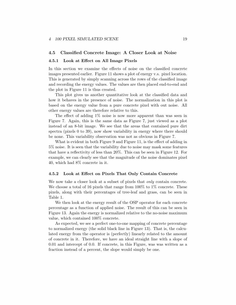
In this section we examine the effects of noise on the classified concreteimages presented earlier. Figure 11 shows a plot of energy v.s. pixel location.This is generated by simply scanning across the rows of the classified imageand recording the energy values. The values are then placed end-to-end andthe plot in Figure 11 is thus created.

This plot gives us another quantitative look at the classified data andhow it behaves in the presence of noise. The normalization in this plot isbased on the energy value from a pure concrete pixel with out noise. Allother energy values are therefore relative to this.

The effect of adding 1% noise is now more apparent than was seen inFigure 7. Again, this is the same data as Figure 7, just viewed as a plotinstead of an 8-bit image. We see that the areas that contained pure dirtspectra (pixels 0 to 39), now show variability in energy where there shouldbe none. This variability observation was not as obvious in Figure 7.

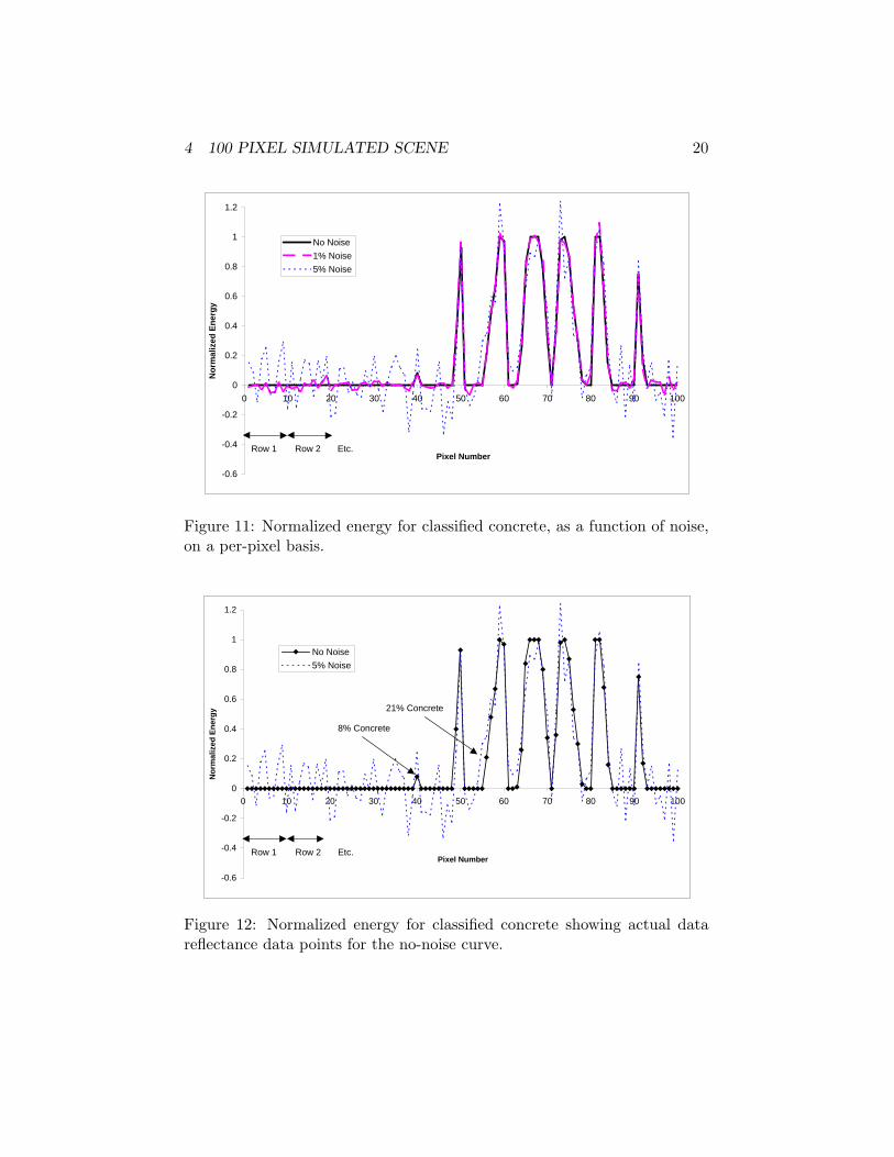
What is evident in both Figure 9 and Figure 11, is the effect of adding in5% noise. It is seen that the variability due to noise may mask some featuresthat have a reflectivity of less than 20%. This can be seen in Figure 12. Forexample, we can clearly see that the magnitude of the noise dominates pixel40, which had 8% concrete in it.

4.5.2 Look at Effect on Pixels That Only Contain Concrete

We now take a closer look at a subset of pixels that only contain concrete.We choose a total of 16 pixels that range from 100% to 1% concrete. Thesepixels, along with their percentages of tree-leaf and grass, can be seen inTable 1.

We then look at the energy result of the OSP operator for each concretepercentage as a function of applied noise. The result of this can be seen inFigure 13. Again the energy is normalized relative to the no-noise maximumvalue, which contained 100% concrete.

As expected, we see a perfect one-to-one mapping of concrete percentageto normalized energy (the solid black line in Figure 13). That is, the calcu-lated energy from the operator is (perfectly) linearly related to the amountof concrete in it. Therefore, we have an ideal straight line with a slope of0.01 and intercept of 0.0. If concrete, in this Figure, was was written as afraction instead of a percent, the slope would simply be one.

4 100 PIXEL SIMULATED SCENE 20

-0.6

-0.4

-0.2

0

0.2

0.4

0.6

0.8

1

1.2

0 10 20 30 40 50 60 70 80 90 100

Pixel Number

No

rmal

ized

En

erg

y

No Noise

1% Noise

5% Noise

Row 1 Row 2 Etc.

Figure 11: Normalized energy for classified concrete, as a function of noise,on a per-pixel basis.

-0.6

-0.4

-0.2

0

0.2

0.4

0.6

0.8

1

1.2

0 10 20 30 40 50 60 70 80 90 100

Pixel Number

No

rmal

ized

En

erg

y

No Noise

5% Noise

Row 1 Row 2 Etc.

21% Concrete

8% Concrete

Figure 12: Normalized energy for classified concrete showing actual datareflectance data points for the no-noise curve.

4 100 PIXEL SIMULATED SCENE 21

Table 1: The mixture fractions of 16 selected pixels from the test image.Pixel Number Concrete [%] Tree-leaf [%] Dirt [%]

59 100 0 050 93 0 765 84 16 069 80 0 2091 75 20 558 67 0 3376 53 27 2057 48 0 5249 40 0 6070 34 0 6664 26 22 5256 21 11 6892 17 29 5440 8 75 1778 3 48 4963 1 36 63

Once we add noise, 1% and 5%, to the pixels, we see that the energyvalues deviate significantly. As expected, the energy return with 1% noisein it, stays fairly close to the 1:1 line, but tends to deviate more at the lowerpercentages. Similarly, the energy associated with the 5% noise contributionhas the same behavior but on a larger scale.

We can see the magnitude of these errors numerically by looking atTable 2. Here we have normalized the selected concrete pixel energy’s whilesimultaneously computing a proportional error, ε using the relation

ε =|E0 −Ex|

E0100 (20)

where E0 is the energy associated with the no-noise case and Ex is eitherthe energy from the 1% or 5% noise cases. If we omit the last few error termsand compute an average error (using the 100% to 26% concrete values), wefind and average error of 6% for the 1% noise case and 17% for the morevariable 5% case.

Overall we can see that that OSP operator did a fairly good job ofextracting concrete from the other signatures in the presence of noise, withmoderate secsess at the 5% level. However, we see that the errors are fairlysignificant at percentages below 26% and extremely high at values below 8%concrete, espcially in the 5% noise case. Again, if there wasn’t any noise inthe data, the normalized concrete energy would correlate exactly with the

5 CONCLUSIONS 22

0

0.2

0.4

0.6

0.8

1

1.2

0 10 20 30 40 50 60 70 80 90 100

Concrete [%]

No

rmal

ized

En

erg

y0% noise

1% noise

5% noise

Figure 13: OSP operator result for concrete only as a function of noise.

normalized concrete percentages, thus driving the error to zero.

5 Conclusions

The OSP operator can be viewed as a combination of two linear opera-tors into a single classification operator. The first operator is an optimalinterference rejection process in the least squares sense, and the second isan optimal detector in the maximum SNR sense. This technique does notsuffer from the limitations of standard statistical classifiers and matched fil-tering/spectral signature matching techniques which are suboptimal in thepresence of multiple correlated interferers.

Though the technique is fairly robust, there are some limitations to thisapproach. You need to know the end member vectors that make up thed vector and U matrix. However, the endmembers don’t necessarily needto be identified, they can be image derived (e.g., using the pixel purityindex algorithm (PPI)). Also, if your target looks like an endmember, youmay have suppressed it in the suppression step. Since noise is assumed to beindependent, identically distributed (i.i.d), you have to work in a space wherethis is approximately true, i.e., image DC or radiance space. Transformingto reflectance space may distort noise and invalidate this approach, thoughwe did not perform any transforms for we started in reflectance space.

REFERENCES 23

Table 2: Error associated with applying 1% and 5% noise to the image.

Pixel Concrete Norm Energy Norm Energy Norm Energy 1% Noise 5% NoiseNumber [%] 0% Noise 1% Noise 5% Noise Error [%] Error [%]

59 100 1.00 1.01 1.03 0.5 3.150 93 0.93 0.93 1.03 0.0 10.265 84 0.84 0.79 0.96 5.9 13.769 80 0.80 0.85 0.85 6.3 6.791 75 0.75 0.76 0.82 1.5 9.558 67 0.67 0.69 0.81 2.7 20.476 53 0.53 0.49 0.67 7.8 27.357 48 0.48 0.45 0.53 6.4 9.549 40 0.40 0.37 0.35 8.4 11.770 34 0.34 0.36 0.50 5.6 46.964 26 0.26 0.32 0.18 21.4 30.156 21 0.21 0.24 0.20 12.9 3.192 17 0.17 0.12 0.21 27.7 21.740 8 0.08 0.07 0.28 12.5 249.079 3 0.03 0.07 0.01 148.2 82.963 1 0.01 0.07 0.24 560.4 2315.0

References

6 References

[1] Fu, K.S., Applications of Pattern Recognition, Florida: CRC Press,Inc., 1982.

[2] Swain, P., Davis, E.S., Remote Sensing: The Quantitative Approach.New York: McGraw-Hill, 1983.

[3] Mazer, A.S., Martin, M., et al., “Image processing software for imagingspectrometry data analysis,” Remote Sensing of Environment, vol. 24.no. 1, pp. 201-210, 1988.

[4] Yuhas, R.H., Goetz, A.F.H., Boardman, J.W., “Discrimination amoungsemi-arid landscape endmembers using the spectral angle mapper(SAM) algorithm,” Summaries 3rd Annual JPL Airborne GeoscienceWorkshop, Jun 1992, R.O. Green, Ed., Publ. 92-14, vol. 1, Jet Propul-sion Laboratory, Pasadena, CA, 1992, pp. 147-149.

[5] Harsanyi, J.C, Chang, C.-I, “Hyperspectral image classification and di-mensionality reduction: An orthogonal subspace projection approach”,

6 REFERENCES 24

IEEE Transactions on geoscience and remote sensing, vol. 32, pp. 779-785, July 1994.

[6] Tu, T.-M, Chen, C.-H, Chang, C.-I, “A posteriori least squares orthog-onal subspace projection approach to desired signature extraction anddetection”, IEEE Transactions on geoscience and remote sensing, vol.35, pp. 127-139, January 1997.

[7] Schott, J.R., Remote Sensing: The Image Chain Approach, New York,Oxford University Press, 1997.

[8] McDonald, R.A., “Opening the cold war sky to the public: declassifyingsatellite reconnaissance imagery.” Photogrammetric Engineering andRemote Sensing, vol. 61, no. 4, pp. 385-390, 1995.

[9] Kruse, F.A., Lefkoff, A.B., Boardman, J.W., Heidebrecht, K.B.,Shapiro, A.T., Barloon, P.J., Goetz, A.F.H., “The spectral image pro-cessing system (SIPS) interactive visualization and analysis of imagingspectrometer data.” Remote Sensing of Enviornment, vol. 44, pp. 145-163, 1993.

[10] Roger, R.E., “Sparse inverse covariance matrices and efficient maximumlikelihood classification of hyperspectral data”, International journal ofremote sensing, vol. 17, pp. 589-613, June 1995.

[11] Clark, R.N., Gallagher, A.J., Swayze, G.A., “Material absorption banddepth mapping of imaging spectrometer data using a complete bandshape least-squares fit with library reference spectra,” AVIRIS work-shop, Robert O. Green, ed., pp. 176-186. 1990.

[12] Lee, J.B., Woodyatt, A.S., Berman, M., “Enhancement of high spec-tral resolution remote sensing data by a noise-adjusted principal compo-nents transform”, IEEE Transactions on geoscience and remote sensing,vol. 28, pp. 295-304, May 1990.

[13] Green, A.A, Berman, M., Switzer, P., Craig, M.D., “A transformationfor ordering multispectral data in terms of image quality with implica-tions for noise removal”, IEEE Transactions on geoscience and remotesensing, vol. 26, pp. 65-74, January 1988.

[14] Miller, J.W.V., Farison, J.B., Shin, Y., “Spatially invariant images se-quences.” IEEE Transactions on Image Processing, vol. 1, pp. 148-161,Apr. 1992.