HYPERSONIC NONEQUILIBRIUM FLOW …oaktrust.library.tamu.edu/bitstream/handle/1969.1/ETD...HYPERSONIC...
170
HYPERSONIC NONEQUILIBRIUM FLOW SIMULATION OVER A BLUNT BODY USING BGK METHOD A Thesis by SUNNY JAIN Submitted to the Office of Graduate Studies of Texas A&M University in partial fulfillment of the requirements for the degree of MASTER OF SCIENCE December 2007 Major Subject: Aerospace Engineering
Transcript of HYPERSONIC NONEQUILIBRIUM FLOW …oaktrust.library.tamu.edu/bitstream/handle/1969.1/ETD...HYPERSONIC...
HYPERSONIC NONEQUILIBRIUM FLOW SIMULATION
OVER A BLUNT BODY USING BGK METHOD
A Thesis
by
SUNNY JAIN
Submitted to the Office of Graduate Studies of Texas A&M University
in partial fulfillment of the requirements for the degree of
MASTER OF SCIENCE
December 2007
Major Subject: Aerospace Engineering
HYPERSONIC NONEQUILIBRIUM FLOW SIMULATION OVER A
BLUNT BODY USING BGK METHOD
A Thesis
by
SUNNY JAIN
Submitted to the Office of Graduate Studies of Texas A&M University
in partial fulfillment of the requirements for the degree of
MASTER OF SCIENCE
Approved by: Chair of Committee, Sharath Girimaji Committee Members, Adonios Karpetis Prabir Daripa Head of Department, Helen L. Reed
December 2007
Major Subject: Aerospace Engineering
iii
ABSTRACT
Hypersonic Nonequilibrium Flow Simulation Over a Blunt
Body Using BGK Method. (December 2007)
Sunny Jain, B.Tech., Indian Institute of Technology, Bombay
Chair of Advisory Committee: Dr. Sharath Girimaji
There has been a continuous effort to unveil the physics of hypersonic flows both
experimentally and numerically, in order to achieve an efficient hypersonic vehicle
design. With the advent of the high speed computers, a lot of focus has been given on
research pertaining to numerical approach to understand this physics. The features of
such flows are quite different from those of subsonic, transonic and supersonic ones and
thus normal CFD methodologies fail to capture the high speed flows efficiently. Such
calculations are made even more challenging by the presence of nonequilibrium
thermodynamic and chemical effects. Thus further research in the field of
nonequilibrium thermodynamics is required for the accurate prediction of such high
enthalpy flows.
The objective of this thesis is to develop improved computational tools for
hypersonic aerodynamics accounting for non-equilibrium effects. A survey of the
fundamental theory and mathematical modeling pertaining to modeling high temperature
flow physics is presented. The computational approaches and numerical methods
pertaining to high speed flows are discussed.
In the first part of this work, the fundamental theory and mathematical modeling
iv
pertaining to modeling high temperature flow physics is presented. Continuum based
approach (Navier Stokes) and Boltzmann equation based approach (Gas Kinetic) are
discussed. It is shown mathematically that unlike the most popular continuum based
methods, Gas Kinetic method presented in this work satisfies the entropy condition.
In the second part of this work, the computational approaches and numerical
methods pertaining to high speed flows is discussed. In the continuum methods, the
Steger Warming schemes and Roe’s scheme are discussed. The kinetic approach
discussed is the Boltzmann equation with Bhatnagar Gross Krook (BGK) collision
operator.
In the third part, the results from new computational fluid dynamics code developed
are presented. A range of validation and verification test cases are presented. A
comparison of the two common reconstruction techniques: Green Gauss gradient method
and MUSCL scheme are discussed. Two of the most common failings of continuum
based methods: excessive numerical dissipation and carbuncle phenomenon techniques,
are investigated. It is found that for the blunt body problem, Boltzmann BGK method is
free of these failings.
v
ACKNOWLEDGMENTS
The completion of this thesis would not have been possible without the
contributions of many people. I would like to sincerely thank Dr. Sharath Girimaji for
his moral, financial and scientific support during the course of my graduate school. I also
thank my committee members, Dr. Prabir Daripa and Dr. Adonios Karpetis, for their
support and advice.
I extend thanks to my fellow graduate students involved in this project, Sawan
Suman, Dr. Johannes Kerimo and Gaurav Kumar. Success of this project can be
undoubtedly attributed to their help and assistance at every phase. I would also like to
thank Ben Riley and Tucker Lavin for the invaluable discussions related to this work.
Additionally, I would like to thank Dr. Jacques Richard, whose expert knowledge and
advice on computational fluid dynamics methods has been invaluable.
I would also like to thank the members of Turbulence Research Group, with whom I
had the privelege of working with. They have all helped make graduate school an
enjoyable experience for me.
Finally, I would like to thank my family for their support. I wouldn’t have even
made it to the start of graduate school without my parents, V.K. Jain and Pramila Jain.
My brother, Kapil Jain has always been there for me and has been my inspiration.
Thanks to everyone, I am very lucky to have all of you in my life.
vi
TABLE OF CONTENTS
Page
ABSTRACT……………………………………………………………………………..iii
ACKNOWLEDGMENTS………………………………………………………………..v
TABLE OF CONTENTS…………………………………………………………….......vi
LIST OF FIGURES………………………………………………………………….......ix
CHAPTER
I INTRODUCTION .....................................................................................................1
1.1 Computational Approaches ................................................................................6 1.2 Outline ................................................................................................................6
II NAVIER STOKES EQUATIONS ............................................................................8
2.1 Navier Stokes Equations ....................................................................................8 2.2 Turbulence Modeling .........................................................................................9 2.3 Statistical Turbulence Models ..........................................................................11 2.4 Reynolds Averaged Flow Equations.................................................................11
2.4.1 Reynolds Averaging ..................................................................................11 2.4.2 Reynolds Averaged Navier Stokes Equations (RANS) .............................12
2.5 Favre-Averaged Navier Stokes Equations........................................................14 2.5.1 Favre Averaging ........................................................................................14 2.5.2 Favre Averaged Navier Stokes Equations (FANS)....................................15
2.6 Eddy Viscosity..................................................................................................17 2.7 Classification of Turbulence Models................................................................20 2.8 Spalart-Allmaras Turbulence Model ................................................................20 2.9 Incompressible Model ......................................................................................21 2.10 Compressible Model ......................................................................................25 2.11 Advantages and Disadvantages of Spalart-Allmaras Model ..........................26
vii
CHAPTER Page
III BOLTZMANN GAS KINETIC SCHEMES.........................................................28
3.1 Boltzmann Equation.........................................................................................28 3.2 Modeling the Collision Term ...........................................................................32
3.2.1 Compatibility Conditions ..........................................................................34 3.2.2 Entropy Condition .....................................................................................34
3.3 Moments of Boltzmann BGK Equation ...........................................................36 3.4 Deriving Navier Stokes Equations ...................................................................40
IV HIGH TEMPERATURE FLOWS: MATHEMATICAL FORMULATIONS AND MODELS....................................................................................................48
4.1 Variables and Their Dependencies ...................................................................48 4.1.1 Conservation of Mass................................................................................48 4.1.2 Conservation of Momentum......................................................................48 4.1.3 Conservation of Energy.............................................................................48
4.2 Physics of Vibrational Nonequilibrium............................................................49 4.3 Harmonic and Anharmonic Oscillators ............................................................51 4.4 Vibrational Energy Transfer Modes .................................................................53
4.4.1 Vibrational Translational EnergyTransfer .................................................54 4.4.2 Vibrational-Vibrational-Translational Transfer .........................................54 4.4.3 Vibrational-Vibrational Transfer ...............................................................54
4.5 Vibrational Population Distribution .................................................................55 4.6 Modeling Vibrational Energy Evolution ..........................................................57
4.6.1 Multiquantum Transition Approach ..........................................................58 4.6.2 Landau- Teller Approach...........................................................................60 4.6.3 Ruffin’s Model ..........................................................................................64 4.6.4 Comparison of the Three Vibrational Models ...........................................68
4.7 Chemical Models..............................................................................................69 4.7.1 Vibration –Chemistry Coupling ................................................................71 4.7.2 Chemistry-Vibration Coupling ..................................................................72 4.7.3 Coupled Vibrational-Chemistry-Vibrational(CVCV) Modeling...............73
4.8 Transport Models..............................................................................................75
V NUMERICAL METHODS: NS, BGK AND SA MODELS..................................83
5.1 Navier Stokes Equations ..................................................................................83
viii
CHAPTER Page
5.2 Finite Volume Methods ....................................................................................85 5.3 Inviscid Fluxes .................................................................................................88
5.3.1 Steger Warming Schemes..........................................................................88 5.3.2 Roe’s Scheme ............................................................................................91
5.4 Boundary Conditions........................................................................................93 5.5 BGK Boltzmann Equation ...............................................................................96 5.6 CollisionTime...................................................................................................98
5.7 Spalart Allmaras Model................................................................................99 5.8 Boundary and Initial Conditions ................................................................100
VI RECONSTRUCTION AND LIMITERS............................................................102
6.1 Introduction ....................................................................................................102 6.2 Linear Interpolation........................................................................................102
6.2.1 MUSCL Based Scheme...........................................................................104 6.2.2 Green Gauss Reconstruction ...................................................................105
6.3 Limiters ..........................................................................................................106 6.4 TVD Schemes.................................................................................................107
6.4.1 MinMod Limiter......................................................................................110 6.4.2 Van Albada Limiter ................................................................................. 111
VII NUMERICAL ISSUES .....................................................................................112
7.1 Introduction ....................................................................................................112 7.2 CFD Solver for Nonequilibrium Flow ...........................................................112 7.3 Grid Generation..............................................................................................115 7.4 Time Integration Schemes ..............................................................................117 7.5 Spatial Differencing Schemes ........................................................................119
VIII RESULTS .........................................................................................................122
8.1 Geometric Conservation Law Test .................................................................122 8.2 Shock Tube Problem ......................................................................................124 8.3Viscous Flow over Flat Plate: BGK Scheme ..................................................128 8.4 Reconstruction Schemes: Green Gauss and MUSCL Scheme.......................131 8.5 Nonequilibrium Hypersonic Flow over Blunt Body ......................................135
ix
CHAPTER Page
IX CONCLUSIONS AND SCOPE FOR FUTURE WORK ...................................146
9.1 Conclusions ....................................................................................................146 9.2 Scope for Future Work ...................................................................................147
REFERENCES……………………………………………………………………......152
VITA………………………………………………………………………………….160
x
LIST OF FIGURES
Page
Figure 1.1: Flow field around a space shuttle reentering the earth’s atmosphere………...2 Figure 1.2: The energy levels in different modes of excitations….……………………...4
Figure 1.3: Schematic chart for the effects of nonequilibrium……..…………………….5
Figure 3.1: Summary of steps involved in derivation of Boltzmann equation………….29
Figure 3.2: Parameters used to describe a binary collision……………………………..30
Figure 3.3: Interparticle forces.…………………………………………………………32
Figure 4.1: Various processes and their interrelations for the case of hypersonic flows..50
Figure 4.2: Vibrational excitation of molecule A through single quantum transition…...51
Figure 4.3: Vibrational energy levels for Harmonic Oscillator…..…..…………………52
Figure 4.4: Vibrational energy levels for Anharmonic Oscillator………………………53
Figure 4.5: Nonequilibrium vibrational population distribution (expanding flows)........55
Figure 4.6: Nonequilibrium vibrational population distribution (post shock flows)…....56
Figure 4.7: Overview of derivation for Landau Teller model…………………………...61
Figure 4.8: Overview of derivation for Ruffin’s model…………………………………65
Figure 4.9: Comparison of the three models……………………………………………69
Figure 4.10: Classification of the chemistry models……………………………………76
Figure 5.1: Fluxes across the edges of a cell……………………………………………86
Figure 5.2: Flux across a cell interface…………………………………………………87
xi
Page
Figure 5.3: Piecewise-constant reconstruction (Riemann problem)……………………92
Figure 5.4: Layout of the ghost cell…………………………………………………….94
Figure 5.5: Boundary condition for inviscid wall………………………………………95
Figure 6.1: Left and right states of Q………………………………………………….103
Figure 6.2: Gradient at vertex 0 using values of immediate neighbors 1,2, and 3……106
Figure 6.3: Example of monotonic and non-monotonic solution……………………..107
Figure 6.4: Solution without use of limiter……………………………………………109
Figure 6.5: Solution after using limiter…….………………………………………….110
Figure 7.1: Basic Steps for a general CFD solver……………………………………..114
Figure 7.2: Timestepping limitations and the methods to eliminate it………………...118
Figure 7.3: Comparison of different Implicit methods………………………………..119
Figure 7.4: Classification of upwind schemes………………………………………...121
Figure 8.1: Mesh for the channel flow………………………………………………..123
Figure 8.2: Pressure profiles along the shock tube……….…………………………...125
Figure 8.3: Velocity profiles along the shock tube…………………………………....126
Figure 8.4: Compressive and expansive sonic points…….…………………………...127
Figure 8.5: Verification of the Crocco-Busemann relationship……………………….129
Figure 8.6: Van Driest profile using BGK scheme……………………………………130
Figure 8.7: Computational mesh for the blunt body problem…………………………131
xii
Page
Figure 8.8: Normalized temperature profiles along stagnation line…….……………..132
Figure 8.9: Contour plot for translational temperature using Green Gauss scheme…...133
Figure 8.10: Contour plot for the translational temperature using MUSCL scheme…..133
Figure 8.11: Contour plot for the translational temperature using Roe’s scheme……..136
Figure 8.12: Contour plot for the Mach number using Roe’s scheme…………………137
Figure 8.13: Contour plot for the translational temperature using Steger Warming…..138
Figure 8.14: Contour plot for the vibrational temperature using Steger Warming…….139
Figure 8.15: Contour plot for the translational temperature using BGK’s scheme……139
Figure 8.16: Contour plot for the vibrational temperature using BGK’s scheme……...140
Figure 8.17: Normalized temperature profiles along stagnation line…...……………..143
Figure 8.18: Normalized vibrational temperature profiles along stagnation line……...143
1
CHAPTER I
INTRODUCTION
The feasibility of hypersonic flight depends, to a large extent, on our ability to
understand and predict high temperature gas effects on aerodynamics. Key aerodynamic
features of hypersonic flows are generally different from those of sub- and super-sonic
flows. Over the last several decades, there have been various efforts, both computational
and experimental, to unveil hypersonic flow physics. Unlike other flow regimes,
hypersonic flight conditions are virtually impossible to replicate in ground-based
experiments. Therefore computational fluid dynamics (CFD) can be expected to play a
crucial role in the design and development of future hypersonic vehicles.
While CFD methods are mature and sophisticated for subsonic and even supersonic
flows, it is quite inadequate in its current form for hypersonic flows. This is due to the
fact that computer models of the interaction between high-temperature gas effects and
aerodynamics, in general, and turbulence, in particular, are very poor. High temperature
gas effects can be categorized into two parts: non-equilibrium thermodynamics and
air-chemistry effects. The objective of this thesis is to develop improved computational
tools for hypersonic aerodynamics accounting for non-equilibrium effects.
Shocks occur in compressible flows and are characterized by rapid spatial variations
(perhaps can be treated as a discontinuity) in velocity, pressure and temperature.
Upstream of the shock, the Mach number is high. The upstream kinetic energy is
converted in the shock to internal energy. Therefore, downstream of the shock, the
This thesis follows the format of International Journal of Numerical Methods in Fluids.
2
velocity is much lower and pressure and temperature are much higher.
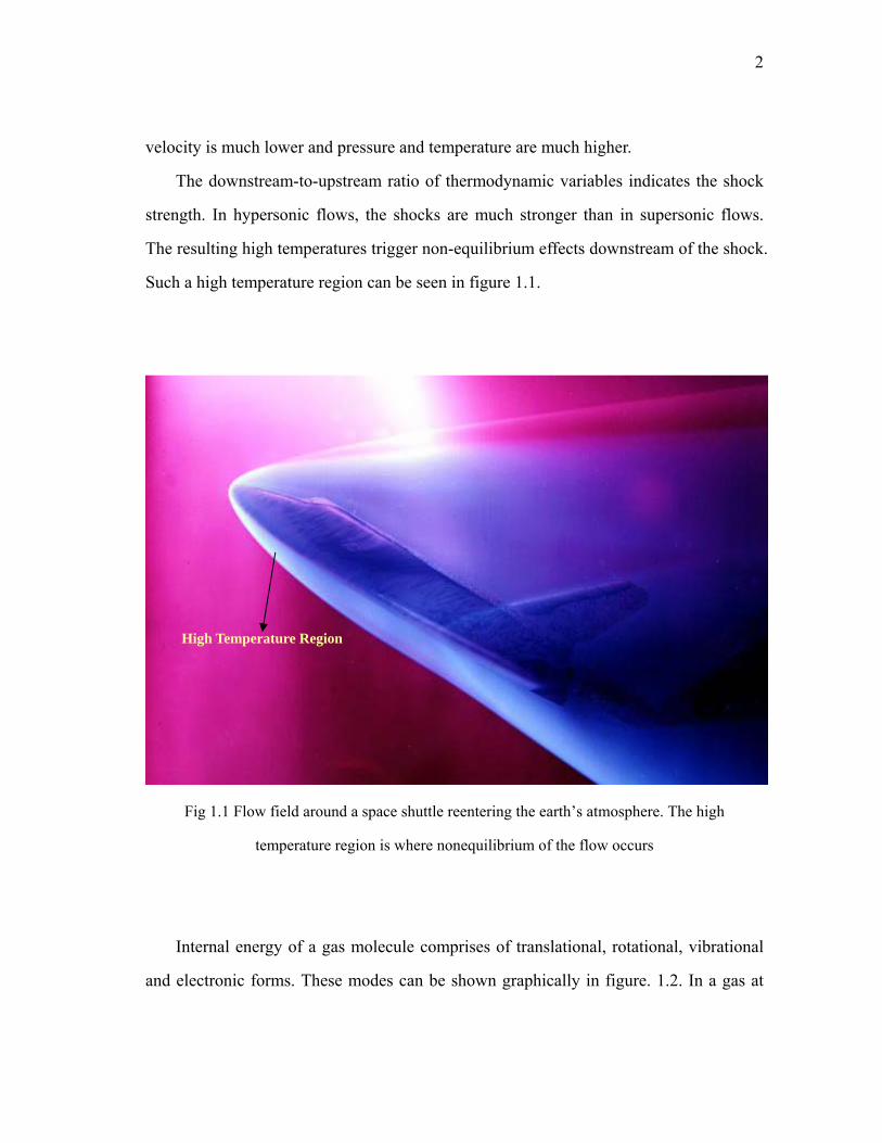
The downstream-to-upstream ratio of thermodynamic variables indicates the shock
strength. In hypersonic flows, the shocks are much stronger than in supersonic flows.
The resulting high temperatures trigger non-equilibrium effects downstream of the shock.
Such a high temperature region can be seen in figure 1.1.
Fig 1.1 Flow field around a space shuttle reentering the earth’s atmosphere. The high
temperature region is where nonequilibrium of the flow occurs
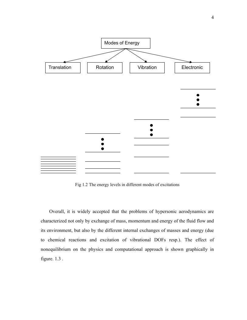
Internal energy of a gas molecule comprises of translational, rotational, vibrational
and electronic forms. These modes can be shown graphically in figure. 1.2. In a gas at
High Temperature Region
3
thermodynamic equilibrium, the total internal energy is partitioned equally between the
active forms. At high temperatures, all energy forms maybe active. As a volume of gas
passes through a shock, the various energy forms must transition from upstream
equilibrium condition to downstream equilibrium conditions. Molecular collision brings
about this transfer. However, different energy forms equilibrate at different rates. The
rate of relaxation from upstream to downstream conditions for the different energy forms
are as follows:
( ) ( ) ( ) ( )trans rot vib elecτ τ τ τ< < <
In low strength shock typical of low mach numbers, the flow transit time is larger
than the time taken for equilibration of various forms of energy from upstream
conditions to downstream distributions. As a result, in low-strength shocks, the gas on
either side of a shock can be considered to be in equilibrium and equipartition principle
is valid on the high temperature side as well.
In strong shocks that occur at high Mach numbers, the flow transit time may be
smaller than equilibrium relaxation time. In such a case, the energy form not in
equilibrium must be treated appropriately in CFD computations. In this thesis, we will
consider hypersonic flow regime in which translational and rotational modes can be
reasonably taken to be in equilibrium and electronic form is not active. Thus we will
only consider vibrational non-equilibrium.
4
Fig 1.2 The energy levels in different modes of excitations
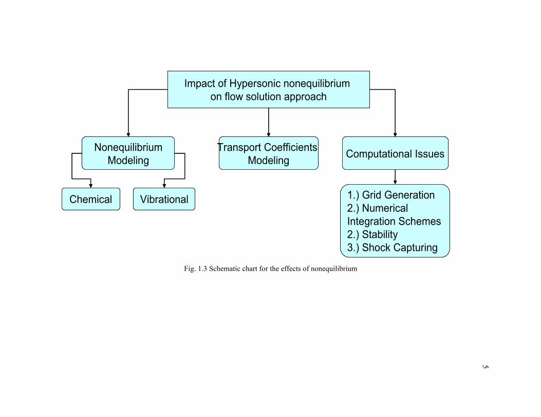
Overall, it is widely accepted that the problems of hypersonic aerodynamics are
characterized not only by exchange of mass, momentum and energy of the fluid flow and
its environment, but also by the different internal exchanges of masses and energy (due
to chemical reactions and excitation of vibrational DOFs resp.). The effect of
nonequilibrium on the physics and computational approach is shown graphically in
figure. 1.3 .
Rotation Vibration Electronic
Modes of Energy
Translation
5
Fig. 1.3 Schematic chart for the effects of nonequilibrium
Impact of Hypersonic nonequilibrium on flow solution approach
NonequilibriumModeling
Chemical Vibrational
Transport Coefficients Modeling Computational Issues
1.) Grid Generation2.) Numerical Integration Schemes2.) Stability3.) Shock Capturing
Impact of Hypersonic nonequilibrium on flow solution approach
NonequilibriumModeling
Chemical Vibrational
Transport Coefficients Modeling Computational Issues
1.) Grid Generation2.) Numerical Integration Schemes2.) Stability3.) Shock Capturing
6
1.1 Computational Approaches
The experimental modeling of hypersonic vibrational and chemical nonequilibrium
flows presents a lot of challenges. The problems arising with the wind tunnels such as
HEG (Eitelberg 1994), F4 (Eitelberg et al 1992) and LENS (Holden 1993) are widely
known. Thus for such flows, using a computational approach becomes much more
attractive.
These approaches are broadly divided into two categories:
(a) Models based on continuum or macroscopic approaches which were proposed during
the 1960’s and 1970’s [2]
(b) Models based on kinetic or microscopic approaches using Boltzmann equation,
which have been pursued during the last decade (eg. [3])
Simulation of flows with both continuum and non-continuum regions using a hybrid
approach is an area of current research. The use of information preserving methods is
one such methodology on such problems [61]. A different approach allowing
communication between a standard Navier Stokes (NS) code and Direct Simulation
Monte Carlo (DSMC) code is also being developed [6].
In this study both the approaches are considered. One of the objectives of this work
is to compare the capabilities of BGK method with that of conventional Navier Stokes
based methods for the high Mach number regime.
1.2 Outline
The thesis is divided into three parts:
Part A: Fundamental Theory and Mathematical Models
The Navier Stokes equations and the one equation Spalart Allmaras model are
described in the second chapter. The third chapter discusses the Boltzmann Gas Kinetic
Schemes and the assumptions made in deriving it. The fourth chapter corresponds to the
7
mathematical models given in literature to numerically simulate the vibrational
nonequilibrium effects, chemical nonequilibrium effects and the high temperature effects
on the transport coefficients.
Part B: Numerical Methodology
The fifth chapter discusses the numerical methodologies used to implement Navier
Stokes model, Boltzmann Gas Kinetic model and Spalart Allmaras turbulence model.
The sixth chapter presents reconstruction schemes required for increasing the accuracy
of the solvers. Chapter VII presents the CFD techniques: grid generation issues and
numerical integration schemes required to solve the Navier Stokes equations for
hypersonic flows.
Part C: Results and Conclusions
The results obtained from the Computational Fluid Dynamics (CFD) code are
presented in chapter VIII. The code is validated against standard test cases followed by
the results for nonequilibrium flow over blunt body. Finally, the conclusions and scope
for future work are presented in chapter IX
8
CHAPTER II
NAVIER STOKES EQUATIONS
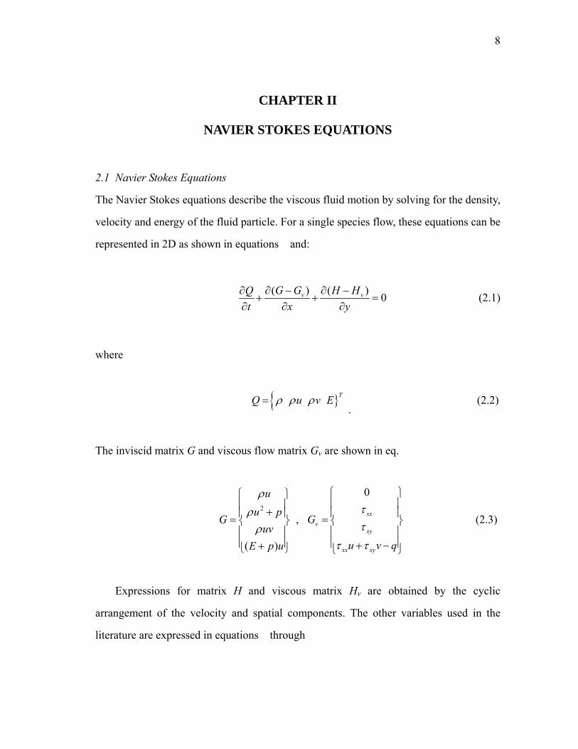
2.1 Navier Stokes Equations
The Navier Stokes equations describe the viscous fluid motion by solving for the density,
velocity and energy of the fluid particle. For a single species flow, these equations can be
represented in 2D as shown in equations and:
( ) ( ) 0v vG G H HQt x y
∂ − ∂ −∂+ + =
∂ ∂ ∂ (2.1)
where
TQ u v Eρ ρ ρ=
. (2.2)
The inviscid matrix G and viscous flow matrix Gv are shown in eq.
2
( )
uu p
Guv
E p u
ρ
ρρ
⎧ ⎫⎪ ⎪+⎪ ⎪= ⎨ ⎬⎪ ⎪⎪ ⎪+⎩ ⎭
,
0
xxv
xy
xx xy
G
u v q
ττ
τ τ
⎧ ⎫⎪ ⎪⎪ ⎪= ⎨ ⎬⎪ ⎪⎪ ⎪+ −⎩ ⎭
(2.3)
Expressions for matrix H and viscous matrix Hv are obtained by the cyclic
arrangement of the velocity and spatial components. The other variables used in the
literature are expressed in equations through
9
21
2VE C T uρ ρ= +r
(2.4)
' ' 2,3
ji kij ij
j i k
uu ux x x
τ µ δ λ λ µ⎛ ⎞∂∂ ∂
= + + = −⎜ ⎟⎜ ⎟∂ ∂ ∂⎝ ⎠ (2.5)
q Tκ= − ∇r (2.6)
P RTρ= (2.7)
In the finite volume method, the integral form of Navier Stokes equation is more
applicable and is represented as in equations and
. 0V S
QdV F dSt∂
+ =∂ ∫ ∫
r (2.8)
F Gi Hj= +r r
(2.9)
where S and V is the boundary and volume, which for 2D case is parameter and the area
of the cell.
2.2 Turbulence Modeling
Most practical engineering problems involving fluid flows are turbulent in nature. At a
very basic level, turbulence can be interpreted as a collection of eddies or vortices, of
different sizes and strengths, giving the flow a random appearance. Turbulence often
originates as instability of laminar flows when the Reynolds number becomes too high.
The instabilities are related to interaction between viscous terms and nonlinear inertia
10
terms in the equations of motion, the mechanism for which is complicated. It is very
difficult to give a precise definition of turbulence. However, one can enlist some of the
characteristics exhibited by turbulent flows [82]:
1.) Irregularity: Due to the randomness of the flow, it is impossible to use deterministic
approach to turbulence problems and one has to rely on statistical methods.
2.) Diffusivity: Turbulence amplifies the diffusivity and hence enhances the mixing of
flows as well as increases the heat transfer rates.
3.) Three-dimensional vorticity fluctuations: Turbulence is rotational and three
dimensional and is characterized by high levels of fluctuating vorticity. Therefore
vorticity dynamics plays an important role in the description of turbulent flows.
4.) Dissipation: Turbulent flows are always dissipative and the dissipation occurs at
the smaller scales or smaller eddies. Therefore turbulence requires a continuous
supply of energy for sustenance.
5.) Large Reynolds Number: As mentioned before, turbulence always occurs at high
Reynolds numbers.
The prediction of turbulence computationally becomes a challenging task because of
the presence of wide range of scales. To incorporate the physics of such a wide spectrum,
one needs to solve the fluid flow governing equations on very large grids. One also
requires an exceptionally accurate discretization method so that both large and small
scale aspects of turbulence can be captured. Such an approach is called the Direct
Numerical Simulation (DNS) of turbulence. Although DNS has been used to give
accurate prediction of turbulence in the past, it still needs tremendous amount of
computing resources. Hence, it is not feasible for most of the practical problems.
11
In an attempt to alleviate the computational burden, the approach of Large Eddy
Simulation (LES) is used. In this approach, the large energy containing scales of
turbulence are resolved or explicitly calculated, whereas the small scales of turbulence
which are more universal in nature are modeled. Although LES is more feasible
compared to DNS, both LES and DNS require enormous computing resources. With the
increase in computing power, it is expected that these approaches will gain even more
popularity.
2.3 Statistical Turbulence Models
Currently, the most popular approaches for turbulence modeling are the statistical
turbulence models. In this approach, the flow quantities are broken down into a mean
and a fluctuating part. The equations are then averaged over time thus resulting in a set
of mean flow equations. Statistics of the fluctuating field influence the mean flow
evolution. Based on the type of averaging method, two kinds of averaged equations can
be obtained. These are discussed in the next two sections.
2.4 Reynolds Averaged Flow Equations
2.4.1 Reynolds Averaging
The Reynolds Averaging method was introduced by Reynolds (1895). Here averaging
can represent ensemble, time or space average. Let F(t) be the instantaneous value of a
flow variable. The Reynolds average is defined as the following ensemble average:
( )
1
1( ) ( ),N
nN
nF t F t
N =
< > ≡ ∑ (2.9)
12
where F(n)(t) is the measurement on the nth realization. This type of averaging is most
general, but the experiment has to be replicated N times, where N should be very large.
In simulation of statistically homogenous flow in a cubic domain of side L, the
above average can be approximated using the spatial averages, which are defined as
1 2 330 0 0
1( ) ( , )L L L
LF t F x t dx dx dxL
< > ≡ ∫ ∫ ∫ (2.10)
The most commonly used definition is the time averaging. This technique is
applicable for statistically stationary flows. The average over a time interval T is defined
as
1( , ) ( , ') 't T
Tt
F x t F x t dtT
+
< > ≡ ∫ (2.11)
As T →∞ the time average approaches the ensemble average.
Thus any of the flow variables, for example, the velocity field can be broken down
into its average and fluctuating components.
( , ) ( ) '( , )i i iu x t U x u x t= +
where '( , )iu x t is the fluctuation and Ui(x,t) is the averaged part which can be defined
using any of the above definitions given in equations , and .
2.4.2 Reynolds Averaged Navier Stokes Equations (RANS)
The Navier Stokes Equations for unsteady incompressible flows are given as
13
0
( )
i
i
j i jii
j i j
ux
u uu pt x x x
τρ ρ
∂=
∂
∂ ∂∂ ∂+ = − +
∂ ∂ ∂ ∂
(2.12)
where ui, xi are velocity and position, t is time, p is pressure, ρ is density and ijτ is
viscous stress and is given in terms of strain rate tensor as:
jiij
j i
uux x
τ µ⎛ ⎞∂∂
= +⎜ ⎟⎜ ⎟∂ ∂⎝ ⎠
Averaging these equations leads to the Reynolds Averaged Navier Stokes:
' '
0
( ) ( ),
i
i
j i ji j ii
j i j
ux
u u u uu pt x x x
τ ρρ ρ
∂=
∂
∂ ∂ −∂ ∂+ = − +
∂ ∂ ∂ ∂
(2.13)
where jiij
j i
uux x
τ µ⎛ ⎞∂∂
= +⎜ ⎟⎜ ⎟∂ ∂⎝ ⎠.
The only unknown quantity in the above equations is the correlation
term ' 'turbij j iu uτ ρ= − . This term is known as the Reynolds stress tensor. Therefore the
turbulence is introduced in the mean flow equations by the presence of this new term. It
can be seen that turbijτ is a symmetric tensor and introduces six new components in the
system. The number of equations are, however still the same. Thus the system is not
closed and the correlation terms need to be modeled.
14
2.5 Favre-Averaged Navier Stokes Equations
2.5.1 Favre Averaging
In compressible flows, the density and temperature fluctuations are significant and
should be taken into account. Therefore, applying the Reynolds Averaging technique to
the compressible Navier-Stokes (NS) equations produces many new correlation terms
such as ' 'iuρ and ' 'iTρ etc. An alternative way to average the compressible NS
equations is the Favre averaging, suggested by Favre (1965).
The Favre Average for a quantity ui can be given as
( )
1
( )
1
( )N
ni
i N ni N
nN
n
uuu
ρρρ ρ
=
=
< >≡ =
< >
∑
∑% (2.14)
Similar to the Reynolds Averaging, the Favre average can be can be approximated
using spatial and time averages defined as:
Spatial averaging for statistically homogeneous flows:
1 2 30 0 0
1 2 30 0 0
L L L
ii L
i L L LL
u dx dx dxuu
dx dx dx
ρρρ
ρ
< >≡ =
< >
∫ ∫ ∫
∫ ∫ ∫%
Time averaging for statistically stationary flows:
15
'
'
t T
ii T t
i t TT
t
u dtuu
dt
ρρρ
ρ
+
+
< >≡ =
< >
∫
∫%
One can break down the instantaneous velocity component into its Favre Averaged part
and the fluctuating part, i.e, ''i i iu u u= +% . If both sides are scaled with density and
Reynolds averaging is done, the following can be obtained
''i i iu u uρ ρ ρ= +%
i.e., '' 0iuρ =
where the Reynolds average F< > is denoted by F .
2.5.2 Favre Averaged Navier Stokes Equations (FANS)
The compressible Navier Stokes Equations can be written as
( ) 0
( )( ) ,
i
i
j i jii
j i j
ut x
u uu pt x x x
ρρ
ρ τρ
∂∂+ =
∂ ∂∂ ∂∂ ∂
+ = − +∂ ∂ ∂ ∂
( ( / 2)) ( )( ( / 2)) j i i j i iji i
j j j
u h u u q ue u ut x x x
ρ τρ ∂ + ∂ ∂∂ ++ = − +
∂ ∂ ∂ ∂ (2.15)
where,
16
12 2 ,3
k kij ij ij ij ij
k k
u us sx x
τ µ λ δ µ δ⎛ ⎞∂ ∂
= + = −⎜ ⎟∂ ∂⎝ ⎠
12
jiij
j i
uusx x
⎛ ⎞∂∂= +⎜ ⎟⎜ ⎟∂ ∂⎝ ⎠
, / ,v pe C T h e p C T p RTρ ρ= = + = =
, PrPr
Pj
j j
CT hqx x
µµκκ
∂ ∂= − = − =
∂ ∂
For the averaging of equations, the above variables are decomposed as follows:
''
'i i iu u uρ ρ ρ= += +
%
'
''
p p p
h h h
= +
= +%
'
''''
j j j
e e eT T Tq q q
= +
= +
= +
%
%
Substituting these values followed by averaging the resulting equations, one can get
Favre Averaged Navier Stokes (FANS) equations:
17
'' ''
'' '''' ''
'' '' '' '' '' '' '' ''
( ) 0
( ) ( )( ) ,
( ( / 2) / 2)( ( / 2) / 2)
( / 2) ( (
i
i
j i ji j ii
j i j
j i i j i ii i i i
j
j j ji i j i i i ij i
j
ut x
u u u uu pt x x x
u h u u u u ue u u u ut x
q u h u u u u u u ux
ρρ
ρ τ ρρ
ρ ρρ ρ
ρ τ ρ τ ρ
∂∂+ =
∂ ∂
∂ ∂ −∂ ∂+ = − +
∂ ∂ ∂ ∂
∂ + +∂ + ++ =
∂ ∂
∂ − − + − ∂ −+
∂
%
% %%
%% % % %% % %
% '' ))j
jx∂
(2.16)
where,
, , ,v p jj
Tp RT e C T h C T qx
ρ κ ∂= = = = −
∂
%%% % %%
There are 26 unknowns introduced due to averaging whereas the number of
equations is still 5. Therefore, the unknown terms need to be modeled in order to close
the terms. It is remarkable that Reynolds averaging of the compressible NS equations
would have led to an even higher number of new correlations. This explains the
popularity of Favre averages for compressible flows.
2.6 Eddy Viscosity
The RANS momentum equation for incompressible flow derived in previous section can
be written as
' '( ) ( )j i ji j ii
j i j
u u u uu pt x x x
τ ρρ ρ
∂ ∂ −∂ ∂+ = − +
∂ ∂ ∂ ∂ (2.17)
18
The viscous stress is given as
jiij
j i
uux x
τ µ⎛ ⎞∂∂
= +⎜ ⎟⎜ ⎟∂ ∂⎝ ⎠
An analogy can be drawn between the correlation term ' 'j iu uρ and the viscous
stress term to get the following expression for the correlation term:
' ' jturb turb iij j i
j i
uuu ux x
τ ρ µ⎛ ⎞∂∂
= = +⎜ ⎟⎜ ⎟∂ ∂⎝ ⎠ (2.18)
Therefore the total stress term can be denoted as total viscous turbij ij ijτ τ τ= + .
Thus, the RANS equations for incompressible flows become exactly the same as
Navier Stokes equations for laminar flows by just replacing the viscosity by effective
viscosity given as eff turbµ µ µ= + . Therefore, if eddy viscosity turbµ is known, the
RANS system of equations is closed and can be solved using the same methodology as
for laminar Navier Stokes Equations.
In case of Favre averaged equations for compressible flows, making such a
substitution for viscosity does not lead to the recovery of laminar compressible NS
equations. However, the above analogy can still be applied for FANS equations if
following assumptions are made:
a) Turbulent kinetic energy is negligible compared to the mean enthalpy, i.e.
'' ''12 i ik u u eρ ρ ρ= << %
19
This assumption is reasonable for all flows below the hypersonic regime. Even in
hypersonic regime, this assumption holds well if the flow is continuously contracting
and the free stream flow had negligible turbulent kinetic energy.
b) The molecular diffusion '' ''ji iuτ and turbulent transport '' '' ''1
2 j i iu u uρ are neglected in the
energy equation. The molecular diffusion can be safely neglected since it is small when
compared to the following term:
'' '' ''ji i ji iu uτ τ<
On the other hand the turbulent transport would be negligible if assumption (a) holds true. c) It is also assumed that the heat flux term can be represented as
'' ''
Pr
turbturbj j turb
j
hq u hx
µρ ∂= = −
∂
%
where Prturb is the turbulent Prandtl number. d) The Favre averaged Reynolds Stress tensor can be represented as
'' '' 1 223 3
turb turb kij j i ij ij ij
k
uu u s kx
τ ρ µ δ ρ δ⎛ ⎞∂
= − = − −⎜ ⎟∂⎝ ⎠
The term 2 / 3ijkρ δ can be ignored on the basis of assumption (a).
Thus after making the above assumptions the Navier Stokes Equations can be
recovered from FANS equation by making the following substitutions:
20
Pr Pr Pr
eff turb
eff turb
turb
µ µ µ
µ µ µ
= +
⎛ ⎞ = +⎜ ⎟⎝ ⎠
2.7 Classification of Turbulence Models
The objective of turbulence models is to provide closure for the RANS or FANS
equations. Depending on the number of differential equations needed for closure, the
turbulence models can be classified as
(a) Zero Equation or Algebraic Models
(b) One Equation Models
(c) Two Equation Models
(d) Stress Equation Models
The models (a)-(c) are based on the eddy viscosity approximation discussed in the
last section. However the models of class (d) solve the Reynolds Stress terms directly by
solving the corresponding evolution equation (wherein the higher order terms are
required to be modeled). Currently the one equation and two equation models are
popular approaches for engineering problems involving turbulence. In this study, the
turbulence model discussed belongs to the category (b), i.e. one equation model.
2.8 Spalart-Allmaras Turbulence Model
The Spalart-Allmaras model [83] is a one equation model for turbulent viscosity for
incompressible as well as compressible flows. This model was first developed in 1992
and uses Baldwin and Barth’s [84] model as a framework. The key modification made in
Spalart-Allmaras (SA) model is the approach used for determining the near wall
semi-local term. Its formulation and coefficients were defined using dimensional
21
analysis, Galilean invariance, and selected empirical results. The empirical results used
were the 2-D mixing layers, wakes and flat plate boundary layer flows.
One of the objectives of this model was to improve upon the predictions obtained
with zero equation or algebraic mixing length models in order to develop a local model
for complex flows. It also provides a simpler alternative to two equation turbulence
models.
The model uses distance from the nearest wall in its formulation and has provision
of including a smooth laminar to turbulent transition assuming that the transition point is
known.
2.9 Incompressible Model
The eddy viscosity function tν is given in terms of eddy viscosity variable ν% and the
wall function 1vf as
1( )t vv fν χ= % (2.19)
where /χ ν ν= % .
The function 1vf is formulated such that away from the wall boundaries, its value
becomes one.
3
1 3 31
( )( )v
v
fC
χχχ
=+
(2.20)
where Cv1 = 7.1 is a constant.
The convective transport equation of the eddy viscosity is modeled as
22
( , , ) ( , ) ( ) ( )prod dest trip T difD b S v d b v d b d b vDtν= − + +
%% % % (2.21)
The terms on the RHS are as follows:
1) Production Term ( , , )prodb S v d
The eddy viscosity production term is related to the vorticity. This choice allows
good modeling of the near wall flows but is not consistent with the homogeneous
turbulence behavior. The production term is defined as
1 2
22 2
[1 ( )] ,
( )
prod b t
v
b c f S
S S fk d
χ ν
ν χ
= −
= +
% %
%
Here, S is the magnitude of the mean vorticity and fv2 is another damping function
defined as
21
( ) 11 ( )v
v
ffχχ
χ χ= −
+
k is the von Karman’s constant and its value is 0.41,
cb1 is calibration constant with value 0.1355
ft2 is related to transition modeling.
2) Destruction Term ( , )destb v d
In a boundary layer, the blocking effect of a wall is felt at a distance through the
pressure term, which acts as the main destruction term for the Reynolds shear stress.
23
Therefore the wall distance d appears directly in the expression for destruction term,
which is given as
211 22
2 2
[ ( ) ( )]( ) ,bdest w w t
cb c f r fk d
rSk d
νχ
ν
= −
=
%
%%
The role of the function fw is to provide with a better calibration in the outer region
of boundary layer, and is defined as
16 6
36 6
3
62
1( ) ( ) ,( )
( ) ( )
ww
w
w
cf r g rg r c
g r r c r r
⎡ ⎤+= ⎢ ⎥+⎣ ⎦
= + −
Here, cw2 = 0.2, cw3 = 2.0 and cw1 is given as
1 21 2
1b bw
c cck σ
+= +
3) Trip term ( )trip Tb d
The transition to turbulence is achieved due to the presence of two terms. The first
term is the function 2 ( )tf χ used in the expressions for production and destruction
terms. The function of this term is to restrict the eddy viscosity in the regions
where / 2v ν<% . Therefore if eddy viscosity is initialized to a small value in some region,
turbulence will not develop. The second term used for transition is the source term or the
trip term defined as
24
2
1
22 2 2
1 2 2
,
exp( [ ])
trip t
tt t t t t t
b f u
wf c g c d g du
= ∆
= − +∆
Here, u∆ is the norm of difference between the velocities at the transition point and the
field point being considered,
tx∆ is the grid spacing along the wall at the location of the trip,
tω is the vorticity at the wall at the transition point,
ct1 and ct2 are two calibration constants with ct1 = 1, ct2 = 2
and gt is given as
min 0.1,tt t
ugxω
⎛ ⎞∆= ⎜ ⎟∆⎝ ⎠
Near the transition point, the trip term produces a positive peak in the eddy viscosity
production overcoming the limit imposed by the function ft2 on the eddy viscosity
increase. Therefore, the turbulent region spreads from the transition point by means of
the convective terms. Once steady state is reached, turbulent flow is obtained in the
region downstream of the transition point while the upstream region remains laminar.
However, one needs to know the transition point beforehand.
4.) Diffusion terms ( )difb v%
The diffusion term is expressed as
25
22
1( ) [ .(( ) ) ( ) ]dif bb v cν ν ν νσ
= ∇ + ∇ + ∇% % %%
For numerical efficiency, these terms are rearranged as
22 2 2
22 2
1( ) .[( ) ] ( )( )
1 .[( ) ]
b b bdif
b b
c c cb v
c c
ν ν ν ν ν νσ σ σ
ν ν ν νσ σ
+= ∇ + ∇ − ∇ − ∇ ∇
+≈ ∇ + ∇ − ∇
% % % %%
% % %
The term 2 ( )( )bc ν νσ
∇ ∇ % is small and can be neglected.
The alternate form avoids discretization of the term 2( )ν∇ % , which does not easily
results in positive discrete operators.
The constant σ has value 2/3, and cb2 = 0.622.
2.10 Compressible Model
The formulation for compressible model is almost the same as the incompressible one
except for a few modifications to account for the change in density. The expression of
eddy viscosity function is modified to the following
1( )t vv fρν χ= % (2.21)
where ρ is the local mean density.
The convective transport equation of the eddy viscosity is modified to give the
following equation:
26
'( , , ) ( , ) ( ) ( )prod dest trip T difD b S v d b v d b d b vDtνρ ρ ρ ρ= − + +%
% % % (2.22)
The definitions of production, destruction and trip term are the same as for the
incompressible model. However, the diffusion term is defined as
22
1( ) [ .(( ) ) ( ) ]dif bb v cµ ρν ν ρ νσ
= ∇ + ∇ + ∇% % %%
To avoid discretization of 2( )ν∇ % , the above expression is rearranged to give
22
1( ) [ .(( ) ) .( ) ]dif bb v cµ ρν ν ρ ν ν ρν νσ
= ∇ + ∇ + ∇ ∇ − ∇% % % % % %%
In this thesis work, we use the compressible SA model. Its numerical
implementation is described next.
2.11 Advantages and Disadvantages of Spalart-Allmaras Model
The following advantages can be listed for the Spalart-Allmaras model:
1.) It does not require a finer grid near wall as required for the two-equation models.
2.) It is computationally inexpensive as well as simpler compared to the two-equation
models since only one extra equation needs to be solved.
3.) It is applicable to free shear flows as well as viscous flows past solid bodies.
4.) Gives very good predictions in 2-D mixing layers, wake flows, flat plate boundary
layer, wake region and shows improvements in the prediction of flows with adverse
pressure gradient compared to the two equation models.

27
Some of the drawbacks of the model are:
1.) The model does not give very accurate predictions for jet flows.
2.) The model only predicts the turbulent shear term ( ' 'u vρ ) but cannot predict the
turbulent kinetic energy.
3.) It is generally inadequate for more complex flows.
28
CHAPTER III
BOLTZMANN GAS KINETIC SCHEMES
3.1 Boltzmann Equation
In the continuum formulation leading to the Navier-Stokes equations, the constitutive
relations between viscous stress and velocity gradients and heat flux and temperature
gradient are taken as assumptions that can be verified by experiment. However, another
logical approach to predict the fluid flow would be by following the dynamical
trajectories of individual molecules from given initial conditions. This is only feasible in
rarefied medium especially in the free molecular regime. Direct Simulation Monte
Carlo(DSMC) is a well developed tool for such rarefied gas flows. For the problems of
our present interest, any significant volume of gas will contain molecules of the order of
Avogadro number, making the latter approach impossible to solve computationally.
Another approach would be to concentrate on the distribution function where
statistically averaged quantities are of interest rather than dealing with individual
particles. Thus we require an equation which describes the rate of change with respect to
position and time of the distribution function. The Boltzmann Equation provides us with
such a relation and it represents the time evolution of distribution function f(ci,xi,t) in one
particle phase space. To derive this equation we start with the more general Liouville
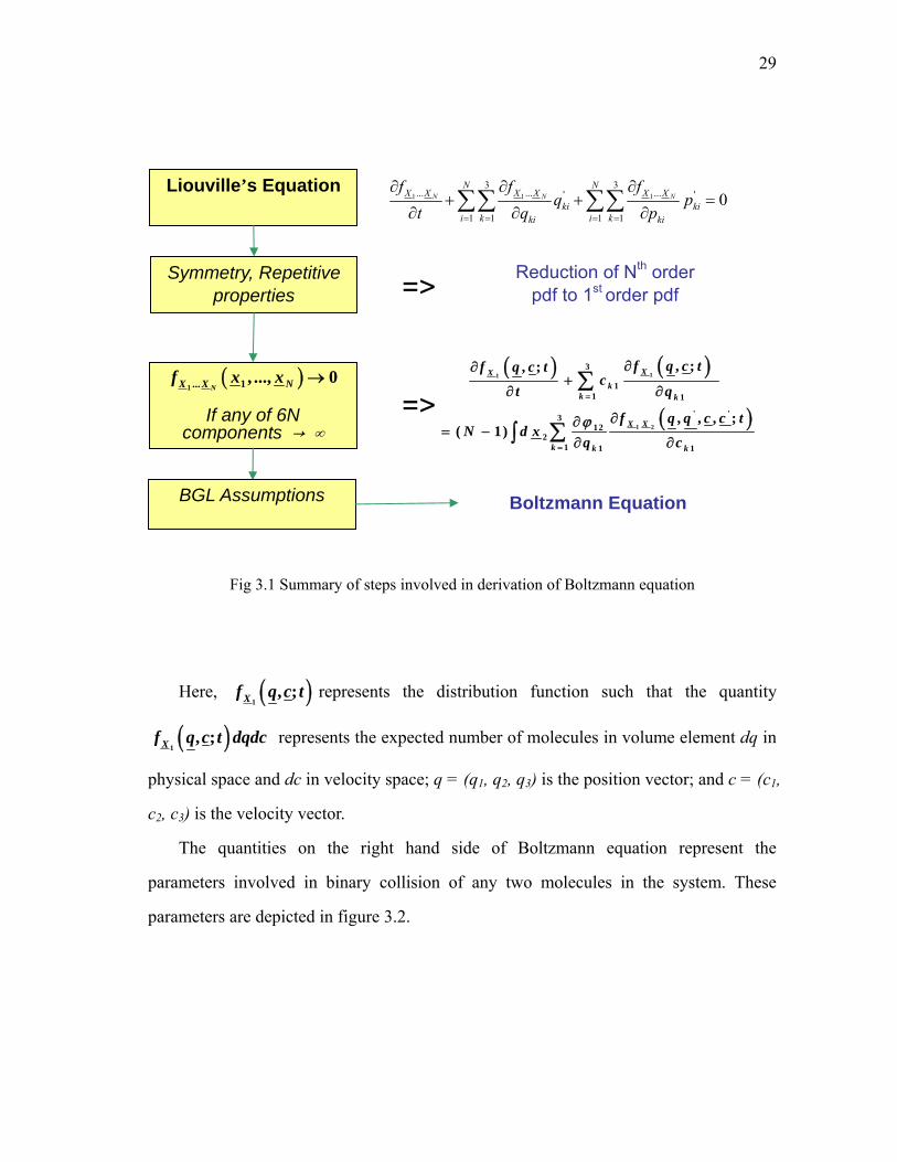
Equation. A summary of the derivation is shown in the figure. 3.1.
The Boltzmann equation in the final form can be written as
( ) ( )
( ) ( ) ( ) ( )
1
1
1 1 1 1
3
1
2 / 2 ' ' 2
0 0
, ;, ;
, , , , sin cos
X
X kk k
X X X X
f q c tf q c t c
t q
f q c f q z f q c f q z gd d d d zπ π
ψ ψ ψ ε
=
+∞
−∞
⎡ ⎤∂∂ ⎣ ⎦⎡ ⎤ + =⎣ ⎦∂ ∂
⎡ ⎤−⎣ ⎦
∑
∫ ∫ ∫
29
Fig 3.1 Summary of steps involved in derivation of Boltzmann equation
Here, ( )1, ;Xf q c t represents the distribution function such that the quantity
( )1, ;Xf q c t dqdc represents the expected number of molecules in volume element dq in
physical space and dc in velocity space; q = (q1, q2, q3) is the position vector; and c = (c1,
c2, c3) is the velocity vector.
The quantities on the right hand side of Boltzmann equation represent the
parameters involved in binary collision of any two molecules in the system. These
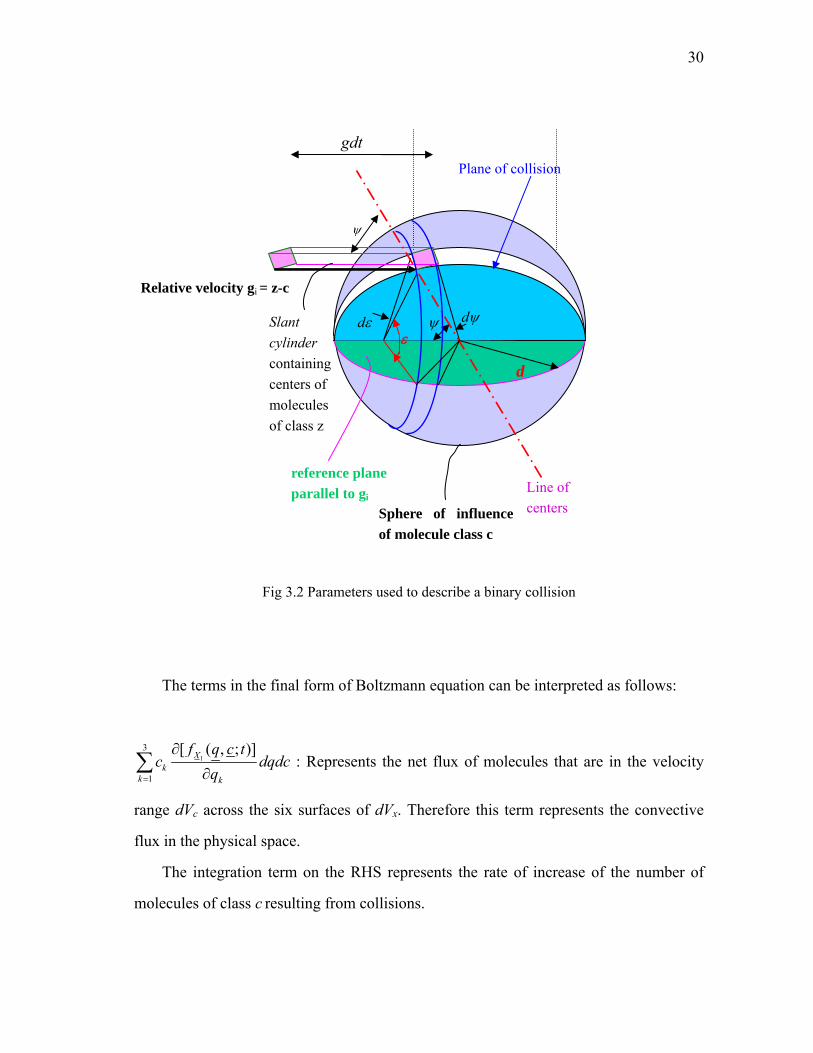
parameters are depicted in figure 3.2.
If any of 6N components → ∞
1 1 13 3
... ... ...' '
1 1 1 1
0N N NN N
X X X X X Xki ki
i k i kki ki
f f fq p
t q p= = = =
∂ ∂ ∂+ + =
∂ ∂ ∂∑∑ ∑∑
Symmetry, Repetitive properties => Reduction of Nth order
pdf to 1st order pdf
=>
BGL Assumptions
Liouville’s Equation
( ) ( )
( )
11
1 2
3
11 1
' '312
21 1 1
, ;, ;
, , , ;( 1)
XXk
k k
X X
k k k
f q c tf q c tc
t q
f q q c c tN d x
q cϕ
=
=
∂∂+
∂ ∂
∂∂= −
∂ ∂
∑
∑∫
Boltzmann Equation
( )1 1... , ..., 0
N NX Xf x x →
30
Fig 3.2 Parameters used to describe a binary collision
The terms in the final form of Boltzmann equation can be interpreted as follows:
13
1
[ ( , ; )]Xk
k k
f q c tc
q=
∂
∂∑ dqdc : Represents the net flux of molecules that are in the velocity
range dVc across the six surfaces of dVx. Therefore this term represents the convective
flux in the physical space.
The integration term on the RHS represents the rate of increase of the number of
molecules of class c resulting from collisions.
reference plane parallel to gi
Line of centers
gdt Plane of collision
d
ψ dψ ε
dε
ψ
Slant cylinder containing centers of molecules of class z
Sphere of influence of molecule class c
Relative velocity gi = z-c
31
As shown in figure 3.1, the Boltzmann Equation is only applicable to cases which
satisfy the Boltzmann gas limit (BGL), which is a set of following assumptions ([70] ):
1.) Dilute Gas Assumption :
The density is sufficiently low so that only binary collisions between the constituent
molecules need to be considered.
2.) Slow Spatial dependence of the gas properties
Due to this assumption, the collisions can be thought of as being localized in the
physical space.
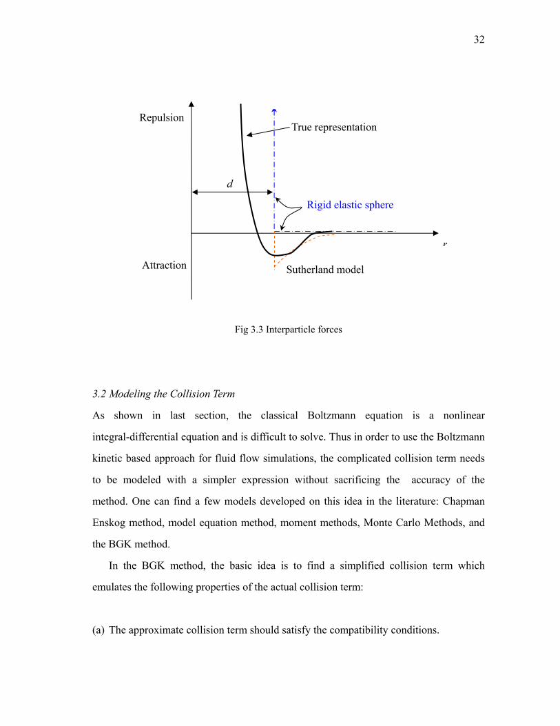
3.) Interparticle potential is sufficiently short range
As a consequence of this assumption, two molecules only interact with each other when
the distance between the molecules is equal to the sum of their radii. This effect is shown
in the figure 3.3, where the long range forces are zero for distances greater than d.
Therefore, the consequence of the first assumption is further reinforced and collisions
involving three or more molecules can be safely neglected.
32
Fig 3.3 Interparticle forces
3.2 Modeling the Collision Term
As shown in last section, the classical Boltzmann equation is a nonlinear
integral-differential equation and is difficult to solve. Thus in order to use the Boltzmann
kinetic based approach for fluid flow simulations, the complicated collision term needs
to be modeled with a simpler expression without sacrificing the accuracy of the
method. One can find a few models developed on this idea in the literature: Chapman
Enskog method, model equation method, moment methods, Monte Carlo Methods, and
the BGK method.
In the BGK method, the basic idea is to find a simplified collision term which
emulates the following properties of the actual collision term:
(a) The approximate collision term should satisfy the compatibility conditions.
r
d
Repulsion
Attraction
Rigid elastic sphere
Sutherland model
True representation
33
This property follows from the properties of elastic collisions of molecules. In a system
of N molecules, the collision is a process internal to the system and should not affect the
total mass, momentum and energy of the system.
(b) It should satisfy the entropy condition.
This follows from the second law of thermodynamics and the approximate collision term
should not violate it.
One of the important consequences of the collision term is that it should bring the
nonequilibrium distribution function closer to the equilibrium function. Also, it is
reasonable to assume that the rate at which the nonequilibrium distribution function
approaches equilibrium is proportional to the difference between them. Thus a simple
expression which emulates the above properties is:
Collision term = 1 1
( )eqX XK f f−
This was the basic idea used by P.L. Bhatnagar, E. P. Gross and M. Krook in their
1954 paper [71]. Thus the BGK - Boltzmann equation is
eq
ji
f f f fct x τ
∂ ∂ −+ =
∂ ∂ (3.1)
The constant τ is called the relaxation time and represents the average time
between two consecutive collisions for a molecule in the system. Thus during a time dt,
a fraction of /dt τ of molecules in a given small volume undergoes collision. This
quantity is constant with respect to the particle velocities but can be a function of the
local state of the particles and hence vary in time and space.
34
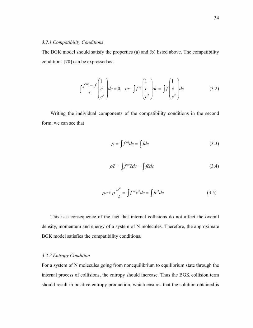
3.2.1 Compatibility Conditions
The BGK model should satisfy the properties (a) and (b) listed above. The compatibility
conditions [70] can be expressed as:
2 2 2
1 1 10,
eqeqf f c dc or f c dc f c dc
c c cτ
⎛ ⎞ ⎛ ⎞ ⎛ ⎞− ⎜ ⎟ ⎜ ⎟ ⎜ ⎟= =⎜ ⎟ ⎜ ⎟ ⎜ ⎟
⎜ ⎟ ⎜ ⎟ ⎜ ⎟⎝ ⎠ ⎝ ⎠ ⎝ ⎠
∫ ∫ ∫r r r (3.2)
Writing the individual components of the compatibility conditions in the second
form, we can see that
eqf dc fdcρ = =∫ ∫ (3.3)
eqc f cdc fcdcρ = =∫ ∫r r r (3.4)
2
2 2
2eque f c dc fc dcρ ρ+ = =∫ ∫ (3.5)
This is a consequence of the fact that internal collisions do not affect the overall
density, momentum and energy of a system of N molecules. Therefore, the approximate
BGK model satisfies the compatibility conditions.
3.2.2 Entropy Condition
For a system of N molecules going from nonequilibrium to equilibrium state through the
internal process of collisions, the entropy should increase. Thus the BGK collision term
should result in positive entropy production, which ensures that the solution obtained is
35
physical. An example of an unphysical solution is the presence of expansion shocks.
These are typically obtained in high Mach number flows which occur in the cases we are
interested in.
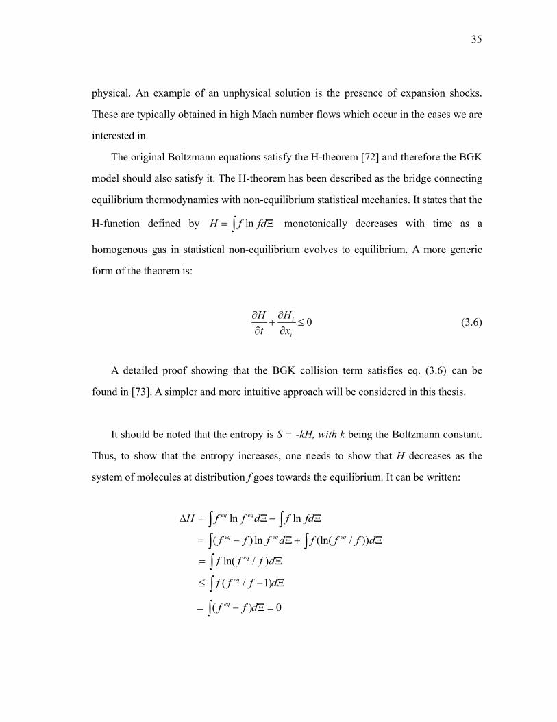
The original Boltzmann equations satisfy the H-theorem [72] and therefore the BGK
model should also satisfy it. The H-theorem has been described as the bridge connecting
equilibrium thermodynamics with non-equilibrium statistical mechanics. It states that the
H-function defined by lnH f fd= Ξ∫ monotonically decreases with time as a
homogenous gas in statistical non-equilibrium evolves to equilibrium. A more generic
form of the theorem is:
0i
i
HHt x
∂∂+ ≤
∂ ∂ (3.6)
A detailed proof showing that the BGK collision term satisfies eq. (3.6) can be
found in [73]. A simpler and more intuitive approach will be considered in this thesis.
It should be noted that the entropy is S = -kH, with k being the Boltzmann constant.
Thus, to show that the entropy increases, one needs to show that H decreases as the
system of molecules at distribution f goes towards the equilibrium. It can be written:
ln ln
( ) ln (ln( / ))
eq eq
eq eq eq
H f f d f fd
f f f d f f f d
∆ = Ξ − Ξ
= − Ξ + Ξ
∫ ∫∫ ∫
ln( / )
( / 1)
eq
eq
f f f d
f f f d
= Ξ
≤ − Ξ
∫∫
( ) 0eqf f d= − Ξ =∫
36
Thus H decreases with time for the system considered here. It should also be noted
that f →feq monotonically, implying H decreases monotonically with time. Thus the
H-theorem is satisfied and this will ensure that the system will approach to a state with
larger entropy. Hence the formation of unphysical rarefaction shocks is prevented.
3.3 Moments of Boltzmann BGK Equation
In this section, the moments of the Boltzmann BGK equation are evaluated. It will be
later shown that these moment equations represent the Navier-Stokes equations if
appropriate assumptions are made.
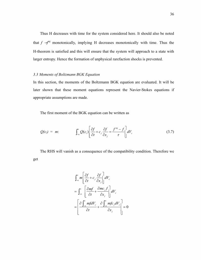
The first moment of the BGK equation can be written as
Q(ci) = m: ( )eq
i j cj
f f f fQ c c dVt x τ
∞
−∞
⎡ ⎤∂ ∂ −+ =⎢ ⎥
∂ ∂⎢ ⎥⎣ ⎦∫ (3.7)
The RHS will vanish as a consequence of the compatibility condition. Therefore we
get
0
j cj
jc
j
c j c
j
f fm c dVt x
mc fmf dVt x
mfdV mfc dV
t x
∞
−∞
∞
−∞
∞ ∞
−∞ −∞
⎡ ⎤∂ ∂+⎢ ⎥
∂ ∂⎢ ⎥⎣ ⎦⎡ ⎤∂∂
= +⎢ ⎥∂ ∂⎢ ⎥⎣ ⎦
⎡ ⎤∂ ∂⎢ ⎥= + =⎢ ⎥∂ ∂⎢ ⎥⎣ ⎦
∫
∫
∫ ∫
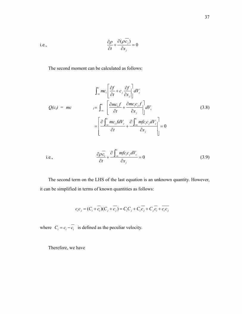
37
i.e., ( )
0j
j
ct x
ρρ ∂∂+ =
∂ ∂
The second moment can be calculated as follows:
Q(ci) = mc i
0
i j cj
i jic
j
i c i j c
j
f fmc c dVt x
mc c fmc f dVt x
mc fdV mfc c dV
t x
∞
−∞
∞
−∞
∞ ∞
−∞ −∞
⎡ ⎤∂ ∂+⎢ ⎥
∂ ∂⎢ ⎥⎣ ⎦⎡ ⎤∂∂
= +⎢ ⎥∂ ∂⎢ ⎥⎣ ⎦
⎡ ⎤∂ ∂⎢ ⎥= + =⎢ ⎥∂ ∂⎢ ⎥⎣ ⎦
∫
∫
∫ ∫
(3.8)
i.e., 0i j ci
j
mfc c dVct xρ
∞
−∞∂∂
+ =∂ ∂
∫ (3.9)
The second term on the LHS of the last equation is an unknown quantity. However,
it can be simplified in terms of known quantities as follows:
( )( )i j i i j j i j i j j i i jc c C c C c C C C c C c c c= + + = + + +
where i i iC c c= − is defined as the peculiar velocity.
Therefore, we have
38
i j c i j i j j i i j c
i j c i j j i c i j c
mfc c dV mf C C C c C c c c dV
mfC C dV mf C c C c dV mf c c dV
∞ ∞
−∞ −∞
∞ ∞ ∞
−∞ −∞ −∞
⎡ ⎤= + + +⎣ ⎦
⎡ ⎤= + + +⎣ ⎦
∫ ∫∫ ∫ ∫
The second term on the RHS vanishes because of the compatibility conditions. Thus,
we can write
i j c i j c i jmfc c dV mfC C dV c cρ∞ ∞
−∞ −∞= +∫ ∫
Defining pressure as
[ ] 2 2 2 21 1 2 2 3 3 1 2 3
1 1 1 13 3 3 3i i c
p C C f C C C C C C dV C C C Cρ ρ ρ ρ∞
−∞⎡ ⎤≡ = + + = + + =⎣ ⎦∫
(3.10)
and the stress tensor as ij i j ijC C pτ ρ δ⎡ ⎤= − −⎣ ⎦ , we can write
i j c ij
j j j
mfc c dV px x x
τ∞
−∞∂ ∂∂
= −∂ ∂ ∂
∫ ,
This gives the equation
i j iji
j i j
c cc pt x x x
ρ τρ ∂ ∂∂ ∂+ = − +
∂ ∂ ∂ ∂
The third moment of the BGK equation can be obtained as follows,
39
Q(ci) = mc2/2
2
2 2
12
1 02
j cj
c j c
j
f fmc c dVt x
mc fdV mfc c dV
t x
∞
−∞
∞ ∞
−∞ −∞
⎡ ⎤∂ ∂+⎢ ⎥
∂ ∂⎢ ⎥⎣ ⎦⎡ ⎤∂ ∂⎢ ⎥= + =⎢ ⎥∂ ∂⎢ ⎥⎣ ⎦
∫
∫ ∫
Using 2 2 2 i i ic c c C cρ ρ ρ ρ= = + and 212tre e Cρ= = , we can write the first term
of LHS as
22
1( )1 22
ice cmnc fdV
t t
ρ∞
−∞∂ +∂
=∂ ∂
∫ (3.11)
In the second term, we have the quantity 2jc c . This term can be expressed as
( )( )( )( )( )
2
2
2 2
2 2 2
2 2 2
2
2
( 2
2
)
j i i j i i i i j j
i i j j
j j j i i j
j j i i j
i j i j
c c c c c c C c C c C
c C c C c C
c c c C C C cc c C C C
c c C C C c C C
c C
= = + + +
= + + +
= + + + + +
= + + +
The highlighted terms vanish because of the properties of random variables Ci.
Therefore, we can write
40
2 2 2 2
2 2 2
1 1 1 1( )2 2 2 2
1 1 1( ) ( )2 2 2
j j j i i j
j j i ij ij
c c c c C C C c C C
c c C C C c p
ρ ρ ρ ρ ρ
ρ ρ ρ δ τ
= + + +
= + + + −
i.e.,
2 2 22
2 2
1 1 1( ) ( )2 2 2
1 1( )2 2
j j i ij ijj c
j j
j jj i ij
j j j j
c c C C C c pmnfc c dV
x x
c e c C C c p cx x x x
ρ ρ ρ δ τ
ρ ρ ρ τ
∞
−∞
⎡ ⎤∂ + + + −∂ ⎢ ⎥⎣ ⎦=∂ ∂
⎡ ⎤ ⎡ ⎤∂ + ∂⎢ ⎥ ⎢ ⎥ ⎡ ⎤ ⎡ ⎤∂ ∂⎣ ⎦ ⎣ ⎦ ⎣ ⎦ ⎣ ⎦= + + −∂ ∂ ∂ ∂
∫(3.12)
Defining 212j j cq C C fdVρ
∞
−∞
⎡ ⎤= ⎢ ⎥
⎣ ⎦∫ , we can write the second moment of the BGK
equation in the final form as
2 21 1( ) ( )2 2j
j i ijj
j j j j
e c c e c c p cqt x x x x
ρ ρ ρ ρ τ⎡ ⎤ ⎡ ⎤∂ + ∂ +⎢ ⎥ ⎢ ⎥ ⎡ ⎤ ⎡ ⎤∂ ∂∂⎣ ⎦ ⎣ ⎦ ⎣ ⎦ ⎣ ⎦+ = − − +
∂ ∂ ∂ ∂ ∂ (3.13)
3.4 Deriving Navier Stokes Equations
In the above three relations, the unknowns are p, ijτ and qj. From the above relations we
find that pressure is related to energy as
2 / 3trp e RTρ= = (3.14)
Therefore, how accurately the equations obtained represent the true physics will
41
depend on the choice of ijτ and qj. In the case of Navier-Stokes equations, these
unknowns are expressed as linear functions of the velocity and temperature gradients.
The value of the corresponding constants is determined experimentally. However, such a
linear relationship only holds for low Knudsen number or continuum cases where the
higher order terms can be neglected. Therefore to simulate high Knudsen number flows
we need to take into account higher order terms.
To show that the BGK moment equations actually recover the Navier Stoke
equations in low Knudsen number regions, the Chapman-Enskog expansion of the BGK
equation needs to be considered. Before starting the calculations, we first normalize the
BGK equation using the following scaling parameters:
Characteristic length: L
Reference speed: cr
Characteristic time: 1/ cr
Reference number density: nr
Reference f: cr-3
Reference v: vr
The scaled equation can be written as
0( )jj
nf nfc nv f ft x
ξ⎡ ⎤∂ ∂
+ = −⎢ ⎥∂ ∂⎢ ⎥⎣ ⎦
% %% % % %% % %% %
(3.15)
42
where 3, r rr
r r r
c tc x c vf fc t x c vLv L L c v
ξ = = = = = =% % % % %
It can be shown that ξ ~ Knudsen number ( r
Lλ ). Since we are working in the
continuum regime for this derivation, we haveξ << 1. Then from the above equation we
can see that 0f% is very close to f% . This allows us to expand the distribution function
around the equilibrium distribution as:
2
0 1 0 2 0
20 1 2 (1 )
f f f f
f
ξφ ξ φ
ξφ ξ φ
= + + +
= + + +
% % % % K
% K
Here 1 2, , ...φ φ are unknown quantities which are to be determined in terms of mean
flow quantities.
Substituting this expansion in the normalized Boltzmann equation and by comparing
the coefficients of ξ we get
00 01j
j
nf nfc nv ft x
φ⎡ ⎤∂ ∂
+ = −⎢ ⎥∂ ∂⎢ ⎥⎣ ⎦
% %% % %% % %% %
(3.16)
The normalized equilibrium distribution function being a Maxwellian can be expressed
as
43
%3/ 2 20
1 1( ) exp[ ( ) ]2 2
( , , )
where ( , ), ( , )
ii
i i
i i
f c cT Tfunction T c c
T T x t c c x t
π= − −
=
= =
% %% %
% % %
% % % %%
(3.17)
Therefore, we can calculate the terms in the LHS of the above equation using the
following relations:
%
%
%
%
0 0 0 0
0 0 0 0
= +
= +
j
j
j
ji i i i
nf nf nf nfn c Tt n t t tc Tnf nf nf nfn c Tx n x x xc T
∂ ∂ ∂ ∂∂ ∂ ∂+
∂ ∂ ∂ ∂ ∂∂ ∂
∂ ∂ ∂ ∂∂ ∂ ∂+
∂ ∂ ∂ ∂ ∂∂ ∂
% % % %% % % %%
% % % %%
% % % %% % % %%
% % % % %
(3.18)
where
( ) ( )
( ) ( )
0 0 0 0
2
0 0 0 0 2
=- , =
3= , = 2 2
i
i
i
i
Cnf nf nf fc T n
C Cnf nf nf nfc T T T T
∂ ∂∂ ∂
⎡ ⎤∂ ∂−⎢ ⎥∂ ∂ ⎣ ⎦
%% % % %% % %
%% %
% %% % % %% % % %
% % % %%
(3.19)
The time derivatives nt∂∂%
%,
% jct
∂∂%
and Tt
∂∂%
can be found by making use of the
continuity, momentum and energy equations:
Continuity Equation: ( ) ( )
0 =- j j
j j
c ncnt x t x
ρρ ∂ ∂∂ ∂+ = ⇒
∂ ∂ ∂ ∂
%%%
% % (3.20)
44
Momentum Equation:
i j ij iji i ij
j i j j i j
c cc c cp pn nct x x x t x x x
ρ τ τρ ∂ ∂ ∂∂ ∂ ∂∂ ∂+ = − + ⇒ = − − +
∂ ∂ ∂ ∂ ∂ ∂ ∂ ∂
% % %%%% %% % % %
(3.21)
Energy Equation:
2 2 21 1 1( ) ( )2 2 2
3 32 2
j jj i ij
j j j j
j j ij ij
j j j j
e c c e c C C c p ct x x x x
q c cT Tn c n pt x x x x
ρ ρ ρ ρ ρ τ
τ
⎡ ⎤ ⎡ ⎤ ⎡ ⎤∂ + ∂ + ∂⎢ ⎥ ⎢ ⎥ ⎢ ⎥ ⎡ ⎤ ⎡ ⎤∂ ∂⎣ ⎦ ⎣ ⎦ ⎣ ⎦ ⎣ ⎦ ⎣ ⎦+ = − − +∂ ∂ ∂ ∂ ∂
∂ ∂ ∂∂ ∂⇒ = − − − +
∂ ∂ ∂ ∂ ∂
%% % %%%% % % %
% % % % %
(3.22)
The expressions for normalized stress tensor and heat flux can be obtained as
follows
1 0
1 0
(1 )ij i j c ij
i j
nC C f dV p
n C C f dV
τ ξφ δ
ξ φ
∞
−∞
∞
−∞
⎡ ⎤= − + −⎢ ⎥
⎣ ⎦
= −
∫
∫
%% % %% % %
%% % %%
(3.23)
21 0
21 0
1 (1 )2
12
j i c
i c
q n C C f dV
n C C f dV
ξφ
ξ ξφ
∞
−∞
∞
−∞
⎡ ⎤= +⎢ ⎥
⎣ ⎦⎡ ⎤
= ⎢ ⎥⎣ ⎦
∫
∫
%% % %% %
%% % %%
(3.24)
Since we are interested in finding the coefficients of ξ in (3.15), we can neglect
ijτ% and jq% from (3.21) and (3.22), since these are first order in ξ . Therefore the time
derivative terms can be written as
45
( )=- j
j
ncnt x
∂∂∂ ∂
%%%
% %
i ij
j i
c c pn nct x x
∂ ∂ ∂≈ − −
∂ ∂ ∂
% % %%% %% % %
(3.25)
3 32 2
jj
j j
cT Tn c n pt x x
∂∂ ∂≈ − −
∂ ∂ ∂
%% %%% % %
% % %
Making the substitutions of the above derivates in (3.16), we can derive 1φ as
%
%0 0 0
1 0
1 1 1 2=- + 3
j jii i i
ji i j i j i
cnf c nf nfn p c Tn C nC p nCn x x n x x n x xnvf c T
φ⎡ ⎤⎡ ⎤ ⎡ ⎤∂⎡ ⎤∂ ∂ ∂ ∂∂ ∂ ∂ ∂
+ + + − +⎢ ⎥⎢ ⎥ ⎢ ⎥⎢ ⎥∂ ∂ ∂ ∂ ∂ ∂ ∂∂ ∂⎢ ⎥ ⎢ ⎥⎢ ⎥⎣ ⎦ ⎣ ⎦ ⎣ ⎦⎣ ⎦
% % %% % % %%% % %% % % %% % % % % % % % %% %
(3.26)
The normalized pressure can be obtained from the normalized equation of state:
kp RT nm T nkT p nTm
ρ= = = ⇒ = %% %
Substituting the above in (3.26), we get
%2 2
11 5= -
2 2 3ji j ji
i i j
C C cCC T c Cn n nnv T T x T x T x
φ⎡ ⎤∂⎡ ⎤ ∂ ∂
− ⋅ + −⎢ ⎥⎢ ⎥ ∂ ∂ ∂⎢ ⎥⎣ ⎦⎣ ⎦
% %%% %% % %
% % % %% % % % (3.27)
The expression can be written in dimensional form to give:
46
22
11 5 ln( ) 1= - ( )
2 2 3i
j i j iji j
cmC T mC C C Cv kT x kT x
ξφ δ⎡ ⎤⎡ ⎤ ∂∂
− ⋅ + −⎢ ⎥⎢ ⎥ ∂ ∂⎢ ⎥⎣ ⎦⎣ ⎦ (3.28)
Substituting the above value in expressions for ijτ% and qj, we get
1 0
1 0
(1 )
23
ij i j c ij
i j
ji kij
j i k
C C f dV p
C C f dV
cc cnkTx x x
τ ρ ξφ δ
ρ ξφ
δν
∞
−∞
∞
−∞
⎡ ⎤= − + −⎢ ⎥
⎣ ⎦
= −
⎡ ⎤∂∂ ∂= + −⎢ ⎥
∂ ∂ ∂⎢ ⎥⎣ ⎦
∫
∫ (3.29)
21 0
21 0
1 (1 )2
12
52
j j c
j c
j
q C C f dV
C C f dV
k nkT Tm v x
ρ ξφ
ξρ ξφ
∞
−∞
∞
−∞
⎡ ⎤= +⎢ ⎥
⎣ ⎦⎡ ⎤
= ⎢ ⎥⎣ ⎦
∂= −
∂
∫
∫ (3.30)
Therefore by comparison with the expressions for stress tensor and heat flux in
Navier Stokes equation, we can write
52
nkT
k nkTKm
µν
ν
=
= (3.31)

47
Thus, the BGK Boltzmann moment equations represent the Navier Stokes equation
in low Knudsen number or continuum regime, if (3.31) holds true.
48
CHAPTER IV
HIGH TEMPERATURE FLOWS: MATHEMATICAL
FORMULATIONS AND MODELS
4.1 Variables and Their Dependencies
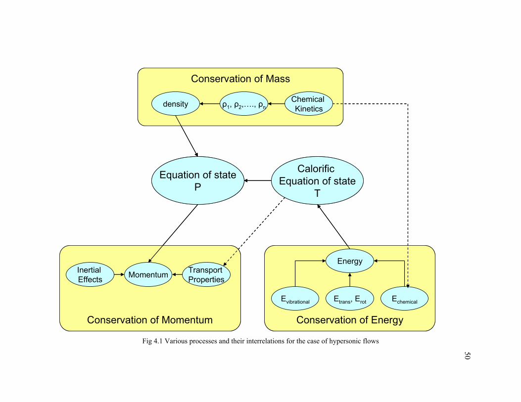
The various laws governing a high enthalpy flow and their interrelations are shown in
the figure 4.1. The various blocks can be explained as follows:
4.1.1 Conservation of Mass
At very high temperatures dissociation and chemical reactions between air components
set in. Thus conservation of mass equation needs to be written for each of the species
and will have a contribution from the kinetics of reactions. The total density needs to be
calculated by adding the individual densities. The total density is used in calculation of
pressure in the equation of state.
4.1.2 Conservation of Momentum
Throughout this work, it is assumed that momentum conservation equation can be
adequately represented by the Navier Stokes equation. The high temperature flow
physics affects the momentum equation via pressure and body force effects. Due to the
high enthalpy of the flow, the viscosity coefficient is no longer constant and becomes a
function of temperature.
4.1.3 Conservation of Energy
The total energy is conserved even as there is an active exchange between various
modes:: translational-rotational, vibrational and chemical. The translational, rotational
49
energies are obtained using the temperature, while the chemical energy is dependent on
the free energies of each of the species. However, we need to model the excited
vibrational energy mode, which is done by writing an evolution equation for it. This will
be discussed in the next section.
It is shown in figure 4.1 that all the three conservation laws are coupled through two
parameters: pressure and temperature. Comparing to compressible flows, nonequilibrium
flows have even more couplings due to temperature dependence of various transport and
chemical rate coefficients. The presence of numerous species and the enhanced
couplings due to temperature is what makes solving nonequilibrium flows expensive.
4.2 Physics of Vibrational Nonequilibrium
Vibrational excitation and relaxation processes take place by molecular collisions and
radiative interactions. A molecule in ground state must experience a large number of
collisions to become vibrationally excited. Such a process is represented as
A(n) ↔ A(n+1)
50
Fig 4.1 Various processes and their interrelations for the case of hypersonic flows
Conservation of Mass
Equation of stateP
Conservation of Momentum Conservation of Energy
Inertial Effects Momentum Transport
Properties
Etrans, Erot
Energy
EchemicalEvibrational
ρ1, ρ2,…., ρndensity Chemical Kinetics
Calorific Equation of state
T
Conservation of Mass
Equation of stateP
Conservation of Momentum Conservation of Energy
Inertial Effects Momentum Transport
Properties
Etrans, Erot
Energy
EchemicalEvibrational
ρ1, ρ2,…., ρndensity Chemical Kinetics
Calorific Equation of state
T
51
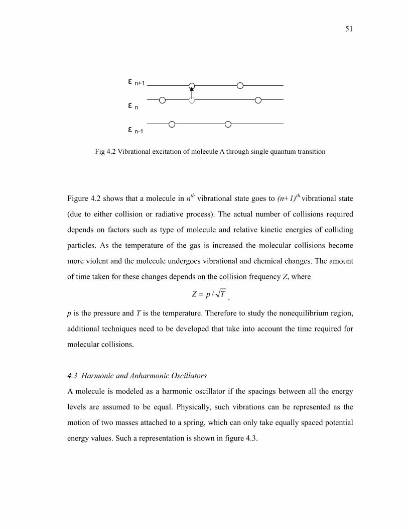
Fig 4.2 Vibrational excitation of molecule A through single quantum transition
Figure 4.2 shows that a molecule in nth vibrational state goes to (n+1)th vibrational state
(due to either collision or radiative process). The actual number of collisions required
depends on factors such as type of molecule and relative kinetic energies of colliding
particles. As the temperature of the gas is increased the molecular collisions become
more violent and the molecule undergoes vibrational and chemical changes. The amount
of time taken for these changes depends on the collision frequency Z, where
/Z p T= .
p is the pressure and T is the temperature. Therefore to study the nonequilibrium region,
additional techniques need to be developed that take into account the time required for
molecular collisions.
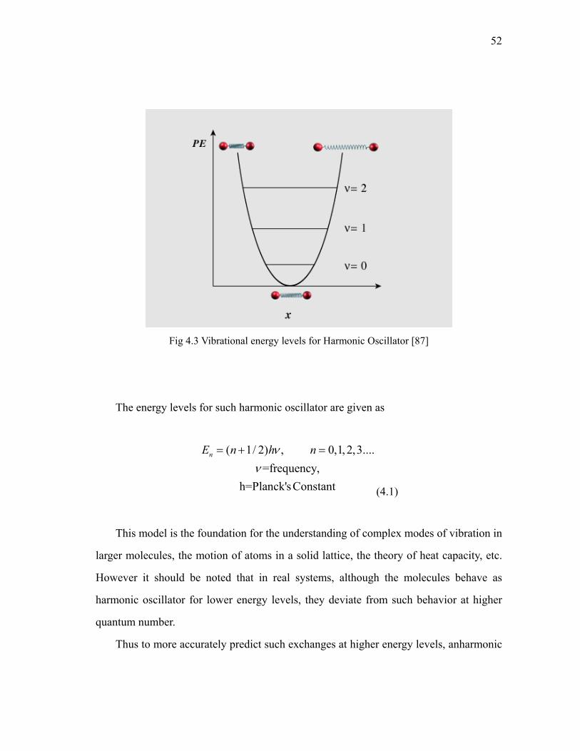
4.3 Harmonic and Anharmonic Oscillators
A molecule is modeled as a harmonic oscillator if the spacings between all the energy
levels are assumed to be equal. Physically, such vibrations can be represented as the
motion of two masses attached to a spring, which can only take equally spaced potential
energy values. Such a representation is shown in figure 4.3.
ε n-1
ε n
ε n+1
52
Fig 4.3 Vibrational energy levels for Harmonic Oscillator [87]
The energy levels for such harmonic oscillator are given as
( 1/ 2) , 0,1, 2,3....=frequency,
h=Planck's Constant
nE n h nνν
= + =
(4.1)
This model is the foundation for the understanding of complex modes of vibration in
larger molecules, the motion of atoms in a solid lattice, the theory of heat capacity, etc.
However it should be noted that in real systems, although the molecules behave as
harmonic oscillator for lower energy levels, they deviate from such behavior at higher
quantum number.
Thus to more accurately predict such exchanges at higher energy levels, anharmonic
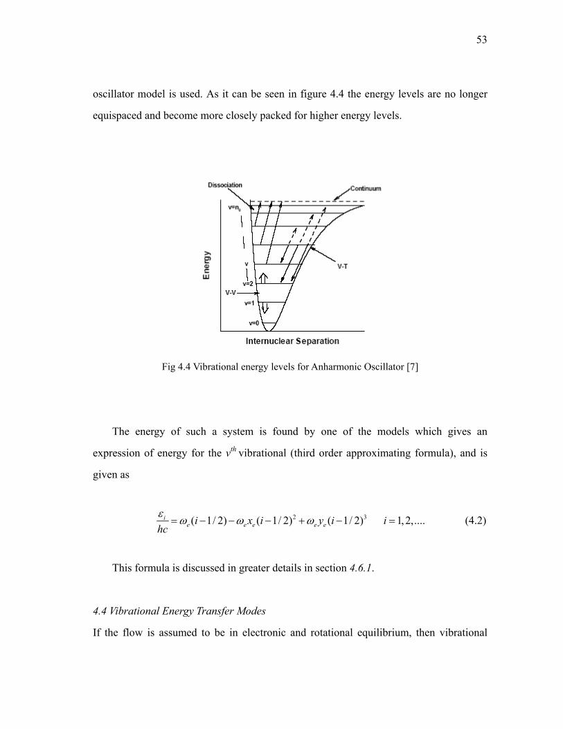
53
oscillator model is used. As it can be seen in figure 4.4 the energy levels are no longer
equispaced and become more closely packed for higher energy levels.
Fig 4.4 Vibrational energy levels for Anharmonic Oscillator [7]
The energy of such a system is found by one of the models which gives an
expression of energy for the vth vibrational (third order approximating formula), and is
given as
2 3( 1/ 2) ( 1/ 2) ( 1/ 2) 1,2,....i
e e e e ei x i y i ihcε ω ω ω= − − − + − = (4.2)
This formula is discussed in greater details in section 4.6.1.
4.4 Vibrational Energy Transfer Modes
If the flow is assumed to be in electronic and rotational equilibrium, then vibrational
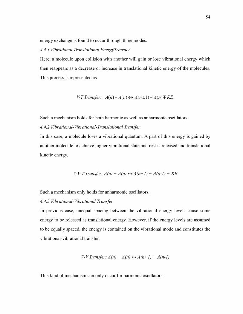
54
energy exchange is found to occur through three modes:
4.4.1 Vibrational Translational EnergyTransfer
Here, a molecule upon collision with another will gain or lose vibrational energy which
then reappears as a decrease or increase in translational kinetic energy of the molecules.
This process is represented as
V-T Transfer: ( ) ( ) ( 1) ( )A n A n A n A n KE+ ↔ ± + m
Such a mechanism holds for both harmonic as well as anharmonic oscillators.
4.4.2 Vibrational-Vibrational-Translational Transfer
In this case, a molecule loses a vibrational quantum. A part of this energy is gained by
another molecule to achieve higher vibrational state and rest is released and translational
kinetic energy.
V-V-T Transfer: A(n) + A(n) ↔ A(n+1) + A(n-1) + KE
Such a mechanism only holds for anharmonic oscillators.
4.4.3 Vibrational-Vibrational Transfer
In previous case, unequal spacing between the vibrational energy levels cause some
energy to be released as translational energy. However, if the energy levels are assumed
to be equally spaced, the energy is contained on the vibrational mode and constitutes the
vibrational-vibrational transfer.
V-V Transfer: A(n) + A(n) ↔ A(n+1) + A(n-1)
This kind of mechanism can only occur for harmonic oscillators.
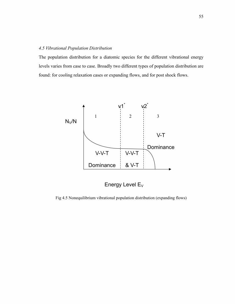
55
4.5 Vibrational Population Distribution
The population distribution for a diatomic species for the different vibrational energy
levels varies from case to case. Broadly two different types of population distribution are
found: for cooling relaxation cases or expanding flows, and for post shock flows.
Fig 4.5 Nonequilibrium vibrational population distribution (expanding flows)
Energy Level EV
v1* v2*
NV/N
V-V-T
Dominance
V-V-T
& V-T
V-T
Dominance
1 2 3
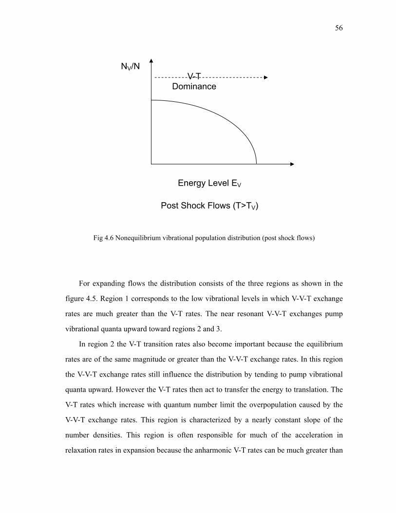
56
Fig 4.6 Nonequilibrium vibrational population distribution (post shock flows)
For expanding flows the distribution consists of the three regions as shown in the
figure 4.5. Region 1 corresponds to the low vibrational levels in which V-V-T exchange
rates are much greater than the V-T rates. The near resonant V-V-T exchanges pump
vibrational quanta upward toward regions 2 and 3.
In region 2 the V-T transition rates also become important because the equilibrium
rates are of the same magnitude or greater than the V-V-T exchange rates. In this region
the V-V-T exchange rates still influence the distribution by tending to pump vibrational
quanta upward. However the V-T rates then act to transfer the energy to translation. The
V-T rates which increase with quantum number limit the overpopulation caused by the
V-V-T exchange rates. This region is characterized by a nearly constant slope of the
number densities. This region is often responsible for much of the acceleration in
relaxation rates in expansion because the anharmonic V-T rates can be much greater than
Energy Level EV
NV/N V-T
Dominance
Post Shock Flows (T>TV)
57
those assumed by Landau Teller model.
In region 3, the V-T rates become much greater the V-V exchange rates as well as
the V-T rates at lower levels. Unlike region 2, vibrational quanta are not being pumped
into this region and are only being lost to translation mode through V-T transfer. Thus
region 3 reaches equilibrium much faster than the remainder of the vibrational levels.
Hence the distribution in this region corresponds to the Boltzmann distribution at local
translational temperature.
For the case of post shock flows, figure 4.6 shows that the V-T rates dominate the
V-V-T transition rates for all levels. The distribution is similar to the distribution of
region 3 for expanding flows.
4.6 Modeling Vibrational Energy Evolution
To write the vibrational rate equation, we need to write the net rate of change of
population of ith level. This can be written as
, ,i
j i j i j ij i j i
d k kdtρ ρ ρ
≠ ≠
= −∑ ∑ , (4.3)
where ρm represents the number of molecules in mth vibrational level, and km,n represents
the vibrational rate constant for transition from mth energy level to nth energy level. This
equation is called the master equation for vibrational relaxation. The first term on the
RHS represents the number of molecules jumping to ith level from all other energy levels,
while the second term represents the number of molecules leaving the ith level.
Corresponding equation for the rate of change of total energy of molecules in ith
level can be written as
58
,, ,
v ij i j j i j i i
j i j i
dek k
dtρ ε ρ ε
≠ ≠
= −∑ ∑. (4.4)
Based on this equation, we can write vibrational rate equation for the total vibrational
energy ev as
,, ,
v ivj i j j i j i i
i i j i i j i
dede k kdt dt
ρ ε ρ ε≠ ≠
= = −∑ ∑∑ ∑∑ , (4.5)
where εn represents the energy of nth vibrational level, and ρn represents the density of nth
vibrational level.
Further modeling of terms appearing in the above equation to obtain complete
expression of the vibration rate equation is required. The three important approaches in
this context are discussed below.
4.6.1 Multiquantum Transition Approach
In this approach we model the molecule as an Anharmonic oscillator. The vibrational
energy for ith level is represented using a result from quantum mechanics known as the
third order approximating formula, as shown in [7] and [8],
2 3( 1/ 2) ( 1/ 2) ( 1/ 2) 1,2,....i
e e e e ei x i y i ihcε ω ω ω= − − − + − = (4.6)
Here, h is the Planck’s constant; c is the speed of light; and ωe , ωexe and ωeye are the
spectroscopic constants.
Therefore, in this case there is no need of a separate vibrational rate equation as the
vibrational energy at any moment can be found by adding the energies of individual
vibrational levels. Thus,
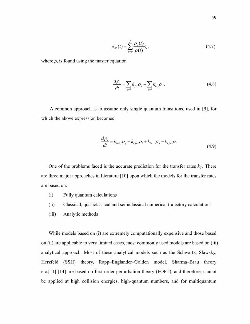
59
*
0
( )( )( )
vv
vib vv
te tt
ρ ερ=
=∑ , (4.7)
where ρv is found using the master equation
, ,i
j i j i j ij i j i
d k kdtρ ρ ρ
≠ ≠
= −∑ ∑ . (4.8)
A common approach is to assume only single quantum transitions, used in [9], for
which the above expression becomes
1, , 1 1, , 1
ii i j i i i i i j i i i
d k k k kdtρ ρ ρ ρ ρ+ + − −= − + −
(4.9)
One of the problems faced is the accurate prediction for the transfer rates kij . There
are three major approaches in literature [10] upon which the models for the transfer rates
are based on:
(i) Fully quantum calculations
(ii) Classical, quasiclassical and semiclassical numerical trajectory calculations
(iii) Analytic methods
While models based on (i) are extremely computationally expensive and those based
on (ii) are applicable to very limited cases, most commonly used models are based on (iii)
analytical approach. Most of these analytical models such as the Schwartz, Slawsky,
Herzfeld (SSH) theory, Rapp–Englander–Golden model, Sharma–Brau theory
etc.[11]-[14] are based on first-order perturbation theory (FOPT), and therefore, cannot
be applied at high collision energies, high-quantum numbers, and for multiquantum
60
processes. However, an exception is the nonperturbative forced harmonic oscillator
(FHO) model [15]–[18] which takes into account the coupling of many vibrational states
during collisions and is, therefore, applicable for such conditions.
The Multi Quantum or master equation model is the most accurate models available
to simulate the vibrational energy transfer rate. However, computational requirements
for such a model make it unpractical for fairly complicated problems. Joysula et al. [7]
solved the master equations assuming double quantum transitions only. It was found that
the results had only a minor deviation from the single quantum transition results. Thus in
most of the works based on anharmonic oscillator models, the single quantum transition
assumption has been made which has given results in good agreement with experimental
results. However, even the single quantum transition models turn out to be very
expensive and make them unsuitable for use for complex geometries.
4.6.2 Landau- Teller Approach
To reduce the complexities and the number of equations involved in the multi quantum
transition approach, simplifying assumptions are made to get an easy to use and
inexpensive model. An outline of the important steps in the derivation of this model
along with the implications of the assumptions made, are shown in figure 4.7:
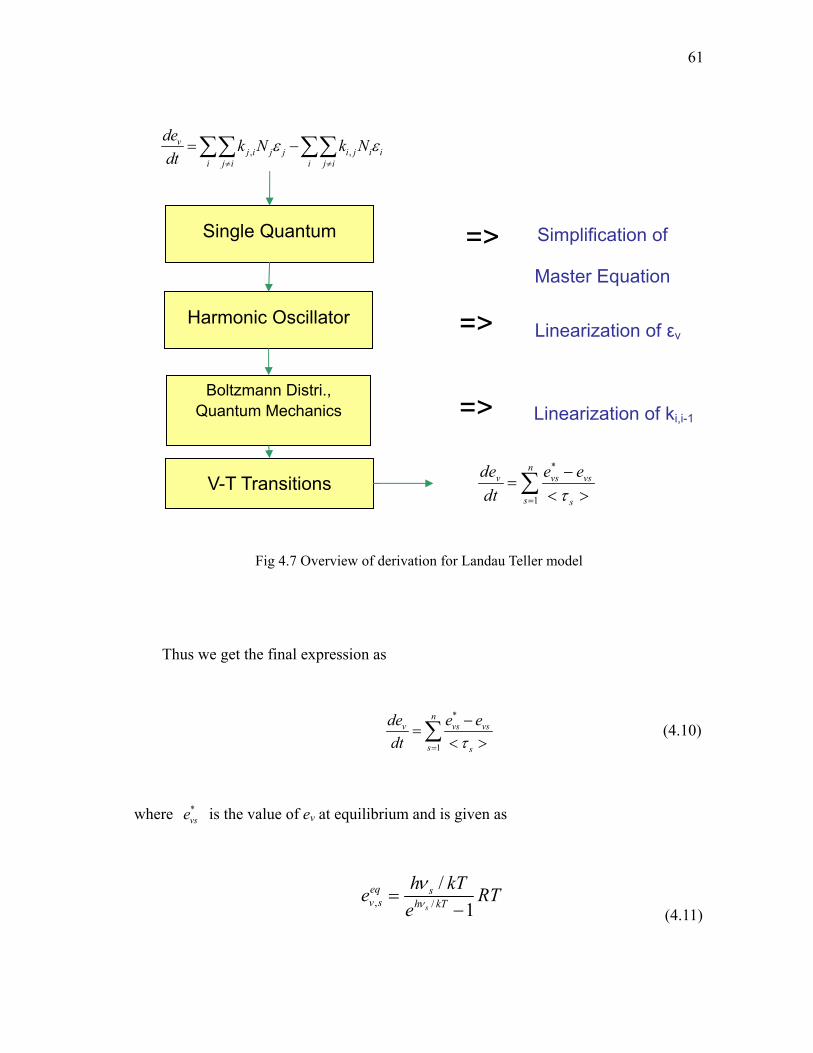
61
Fig 4.7 Overview of derivation for Landau Teller model
Thus we get the final expression as
*
1
nv vs vs
s s
de e edt τ=
−=
< >∑ (4.10)
where *vse is the value of ev at equilibrium and is given as
, /
/1s
eq sv s h kT
h kTe RTe ν
ν=
− (4.11)
, ,v
j i j j i j i ii j i i j i
de k N k Ndt
ε ε≠ ≠
= −∑∑ ∑∑
Single Quantum
Harmonic Oscillator
*
1
nv vs vs
s s
de e edt τ=
−=
< >∑
=> Simplification of
Master Equation
=> Linearization of εv
Boltzmann Distri., Quantum Mechanics
V-T Transitions
=> Linearization of ki,i-1
62
and sτ is the vibrational relaxation time. Physically the expression for vibrational rate can
be understood as follows: suppose we instantaneously excite the vibrational mode above
its equilibrium value, i.e. for t = 0
0
eqvib vibe e>
Due to molecular collisions, the excited particles will exchange this excessive
vibrational energy with the translational and rotational energies of the gas and after a
period of time evib will decrease and approach its equilibrium value. However, as the
vibrational energy decreases, it reappears in the form of translational energy and thus T
increases. And thus the equilibrium value of vibrational energy will also increase. Thus
at large times evib and eqvibe will approach the same value asymptotically.
As discussed in previous section, vibrational nonequilibrium occurs due to the
presence of very high temperatures in the flow. For example in the case of shock wave in
hypersonic flows, as p and T are suddenly changed, the equilibrium vibrational and
chemical properties will change. The fluid element will start to seek these new
equilibrium properties which require collisions between molecules and hence time.
However by this time, the flow has covered a certain distance behind the shock and
hence we get a region of vibrational nonequilibrium.
The relaxation time τ is a function of both local pressure and temperature. One of
the most commonly used model for τ is the Millikan and White [19] formula. The
following assumptions are made:
(i) The system consists of diatomic oscillators only
(ii) Only one type of collision is allowed (V-T transitions)
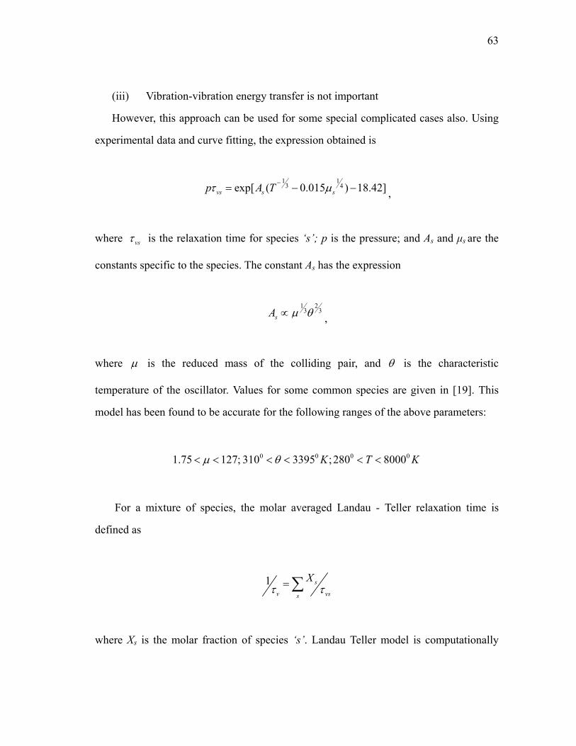
63
(iii) Vibration-vibration energy transfer is not important
However, this approach can be used for some special complicated cases also. Using
experimental data and curve fitting, the expression obtained is
1 1
3 4exp[ ( 0.015 ) 18.42]vs s sp A Tτ µ−= − − ,
where vsτ is the relaxation time for species ‘s’; p is the pressure; and As and µs are the
constants specific to the species. The constant As has the expression
1 2
3 3sA µ θ∝ ,
where µ is the reduced mass of the colliding pair, and θ is the characteristic
temperature of the oscillator. Values for some common species are given in [19]. This
model has been found to be accurate for the following ranges of the above parameters:
0 0 0 01.75 127; 310 3395 ;280 8000K T Kµ θ< < < < < <
For a mixture of species, the molar averaged Landau - Teller relaxation time is
defined as
1 s
v vss
Xτ τ=∑
where Xs is the molar fraction of species ‘s’. Landau Teller model is computationally
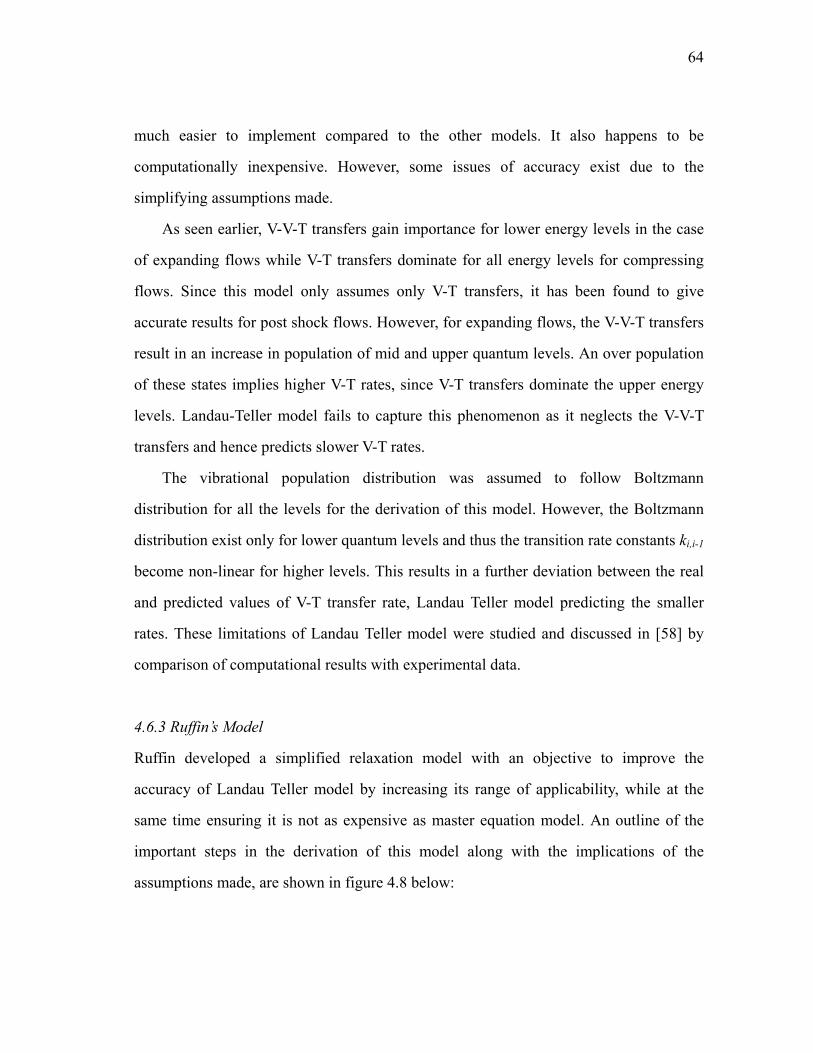
64
much easier to implement compared to the other models. It also happens to be
computationally inexpensive. However, some issues of accuracy exist due to the
simplifying assumptions made.
As seen earlier, V-V-T transfers gain importance for lower energy levels in the case
of expanding flows while V-T transfers dominate for all energy levels for compressing
flows. Since this model only assumes only V-T transfers, it has been found to give
accurate results for post shock flows. However, for expanding flows, the V-V-T transfers
result in an increase in population of mid and upper quantum levels. An over population
of these states implies higher V-T rates, since V-T transfers dominate the upper energy
levels. Landau-Teller model fails to capture this phenomenon as it neglects the V-V-T
transfers and hence predicts slower V-T rates.
The vibrational population distribution was assumed to follow Boltzmann
distribution for all the levels for the derivation of this model. However, the Boltzmann
distribution exist only for lower quantum levels and thus the transition rate constants ki,i-1
become non-linear for higher levels. This results in a further deviation between the real
and predicted values of V-T transfer rate, Landau Teller model predicting the smaller
rates. These limitations of Landau Teller model were studied and discussed in [58] by
comparison of computational results with experimental data.
4.6.3 Ruffin’s Model
Ruffin developed a simplified relaxation model with an objective to improve the
accuracy of Landau Teller model by increasing its range of applicability, while at the
same time ensuring it is not as expensive as master equation model. An outline of the
important steps in the derivation of this model along with the implications of the
assumptions made, are shown in figure 4.8 below:
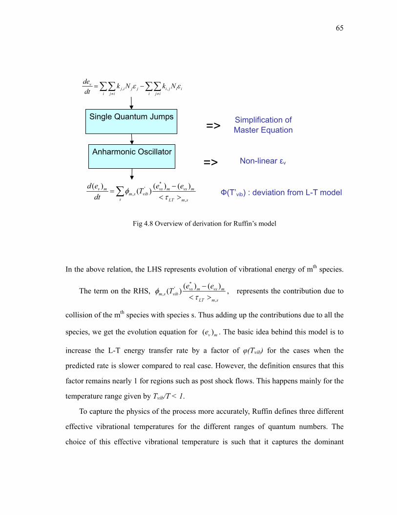
65
Fig 4.8 Overview of derivation for Ruffin’s model
In the above relation, the LHS represents evolution of vibrational energy of mth species.
The term on the RHS, *
',
,
( ) ( )( ) vs m vs mm s vib
LT m s
e eTφτ−
< >, represents the contribution due to
collision of the mth species with species s. Thus adding up the contributions due to all the
species, we get the evolution equation for ( )v me . The basic idea behind this model is to
increase the L-T energy transfer rate by a factor of φ(Tvib) for the cases when the
predicted rate is slower compared to real case. However, the definition ensures that this
factor remains nearly 1 for regions such as post shock flows. This happens mainly for the
temperature range given by Tvib/T < 1.
To capture the physics of the process more accurately, Ruffin defines three different
effective vibrational temperatures for the different ranges of quantum numbers. The
choice of this effective vibrational temperature is such that it captures the dominant
, ,v
j i j j i j i ii j i i j i
de k N k Ndt
ε ε≠ ≠
= −∑∑ ∑∑
Single Quantum Jumps
Anharmonic Oscillator
*'
,,
( ) ( ) ( )( )v m vs m vs mm s vib
s LT m s
d e e eTdt
φτ−
=< >∑
=> Simplification of Master Equation
=> Non-linear εv
Ф(T’vib) : deviation from L-T model
66
physics for that particular range.
The first such range is defined as *1ν ν≤ , where
*1ν = minimum ν for which 1, , 1, ,( ) ( )VT VV
v v m s v v m sK K+ +>
Thus for this limit, the V-V-T transfers have more dominance and the distribution is
approximated by Treanor Distribution. For the case of compression or post shock flows,
V-T transfer dominates for all quantum levels and hence *1ν = 0.
The second range is given as *2ν ν> , where the most rapid anharmonic V-T rates
dominate, where *2ν = minimum ν for which both of these conditions hold:
3
1, , 1, ,
1, , 1,0 ,
( ) 1 10 ( )
( ) 10( 1)( )
VT VVv v m s v v m s
VT VTv v m s m s
K K
K Kν+ +
+
> ×
> +
The third range, * *1 2ν ν ν< ≤ , is characterized by V-T transition rates and the
distribution can be approximated by Boltzmann distribution at effective vibrational
temperature.
Expressions for *1ν and *
2ν are obtained using curve fit methods. Data for these
curves are available in [58] and [59] for combinations on N2, CO2, CO, Ar. It should be
noted that a common value of *1ν as well as *
2ν is used when a mixture of species is
present. This common value is the molar fraction weighted average of individual species
combination values.
* *1 1 , , ,( ) ( )m m s m s m s
s s
W Wν ν=∑ ∑
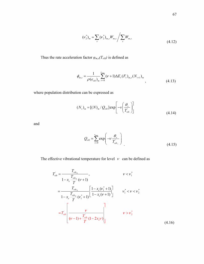
67
* *2 2 , , ,( ) ( )m m s m s m s
s sW Wν ν=∑ ∑
(4.12)
Thus the rate acceleration factor φm,s(Tvib) is defined as
max
, , 10
1 ( 1) ( ) ( )( )m s v v m s v m
vib m
E F Ne
ν
ν
φ νρ +
=
= + ∆∑, (4.13)
where population distribution can be expressed as
'( ) [( ) / ]exp v
v m m vibvib
N N Q vTθ⎡ ⎤⎛ ⎞
= −⎢ ⎥⎜ ⎟⎝ ⎠⎣ ⎦ (4.14)
and
max
'0
expv
vv
vibv vib
QTθν
=
⎛ ⎞= −⎜ ⎟⎜ ⎟
⎝ ⎠∑
. (4.15)
The effective vibrational temperature for level ν can be defined as
0
0
0
0
' *2
' *1
** *11 2
*1
'
,1 ( 1)
1 ( 1)1 ( 1)1 ( 1)
( 1) (1 2 )
vibvib
vibe
v
vibvib
ib e
vib e
e
e
TT T
xT
T xT x
TT xT
xT
ν νν
ν ν ν νν
ν ν νν
ν
ν
= <− +
⎡ ⎤− += < <⎢ ⎥−
⎡ ⎤⎢ ⎥
= >⎢ ⎥⎢ ⎥− + −⎢ ⎥⎣ ⎦
+⎣ ⎦− +
(4.16)
68
4.6.4 Comparison of the Three Vibrational Models
Ruffin [58] has shown the comparison between the three approaches to model the
vibrational energy transfer rate (figure 4.9). In this figure, Y-axis (φ) represents how
much the Ruffin’s simplified anharmonic model and other models deviate from each
other:
Model
Landau Teller
( / )( / )
de dtde dt
φ =
The value of φ is 1 for Landau Teller model by definition.
It can be seen in the figure that for heating environments (Tvib/T<1), φ is not very
different from unity. Thus the temperatures in the range 1000 K < T < 5000 K, the
Landau–Teller relaxation model is a reasonable approximation for relaxations in heating
environments such as those in postshock flows. In cooling relaxations though, Tvib/T > 1,
Landau Teller model predicts slower V-T transfer rates compared to anharmonic models.
This deviation becomes prominent for Tvib/T > 2.5.
However using the Ruffin’s simplified relaxation model, the predictions for φ are in
good agreement with the master equation results for cases where V-T energy transfer
rates dominate [60]. For extreme cases of thermal nonequilibrium(Tvib/T > 4.5), the V-V
energy transfer becomes significant. Thus the predicted energy transfer rate of the
anharmonic relaxation model is too low, but it is still more accurate than values from
Landau Teller model. Another advantage of using Ruffin’s model is that it is
computationally very inexpensive compared to the full master equation model. For
example, although L-T model takes only 1 s for this simulation, Ruffin’s simplified
anharmonic model takes almost 4 s on the same. It should be noted that full master
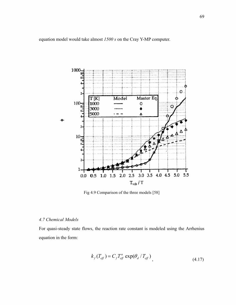
69
equation model would take almost 1500 s on the Cray Y-MP computer.
Fig 4.9 Comparison of the three models [58]
4.7 Chemical Models
For quasi-steady state flows, the reaction rate constant is modeled using the Arrhenius
equation in the form:
( ) exp( / )n
f eff f eff d effk T C T Tθ=, (4.17)
70
where Teff = Ttranslational . However for the cases when the thermodynamic state of the gas
is undergoing such rapid changes that the internal energy state does not satisfy the
quasi-steady state condition, the above equation cannot be used for Teff = Ttranslational.
Thus, a model is needed which reflects the physics of nonequilibrium flows.
The main problem consists in determining the influence of molecular vibrational
distribution on the rate of dissociation and recombination. The secondary objective is to
quantify the influence of recombination and dissociation on the vibrational energy
distribution. There are two main approaches found in literature:
(1) Physicochemical studies which allow the construction of interaction models
based on a specific and detailed approach of dissociative collisions and the
determination of statistical properties such as dissociation constants, vibrational
energy lost per dissociation etc ([35]-[39]). These models are difficult to
implement computationally, but are physically more realistic in spite of frequent
restrictive assumptions.
(2) Semi-empirical approach for building models leading to simple relations which
gives rate constants as a function of vibrational temperature ([23],[40],[41]).
These models are more attractive and useful for hypersonic flows.
For the present study, we consider models based on approach (2). To understand
these couplings, it is important to understand the primary coupling (vibration-chemistry)
and secondary coupling (chemistry-vibration) separately. Basic steps for the derivation
of the most general vibration-chemistry coupling model will be shown. This will be
followed by the determination of models which are simpler than the general model.
71
4.7.1 Vibration –Chemistry Coupling
Consider the following reactions:
( ) ( )AB v C AC w B+ +
AB C AC B+ +
The latter reaction represents the summation of the former reaction for different
combinations of v and w. Thus, we can write
( ) ( ) ( ) ( )AB
AB C AB d AC B AC dc c c f v k v c c f w k wt
∂= −
∂ ∑ ∑, (4.18)
where max max
0 0( ) ( , ) , ( ) ( , )
w v
d dw v
k v k v w k w k w v= =
= =∑ ∑.
k(v,w) represents the rate constant of the reaction in which a v-excited AB molecule
decomposes, and an AC molecule excited in the w-th state is formed. fi(v) represents the
population distribution function of the discrete vibrational states v of molecule i
However, we can also write
AB
AB C f AC B bc c c k c c kt
∂= −
∂ (4.19)
Thus comparing the above two equations, we can obtain expression for the bulk rate
constants kf and kb, if we know the distribution functions fi(v). Thus,
72
( ) ( )f AB dk f v k v=∑
( ) ( )b AC dk f w k w=∑
(4.20)
4.7.2 Chemistry-Vibration Coupling
Consider collision of molecule AB in vth vibrational state with another molecule C. This
can be represented by the reaction shown above:
( ) ( )AB v C AC w B+ + .
The total vibrational energy content of species AB is diminished by an amount that is
equal to the vibrational energy content of AB(v), represented as , ( )vib AB vε . However,
some energy also appears due to the formation of AB(w), which is represented as
, ( )vib AB wε . Thus the rate at which vibrational energy for molecule AB is produced and the
rate at which it is lost are given as
max
, , , ,0
( ) ( ) ( )v
dva AB va AB va AB AB vib AB
v f
k vG f v vk
ω ω ε=
≡ ∑& &
max max
, , , ,0 0
( , )( ) ( )v w
app AB app AB app AB vib AB ACv w b
k w vG v f wk
ω ω ε= =
≡ ∑ ∑& &
(4.21)
where the subscripts va and app represent the vanishing and appearing energies. Thus, in
general, the evolution equation of vibrational energy for molecule i will have an extra
term QC-V given as
73
, , , , ,( )C V i app ij app ij va ij va ij
j
Q G Gω ω− = −∑ & &
(4.22)
4.7.3 Coupled Vibrational-Chemistry-Vibrational(CVCV) Modeling
Based on above concepts, the CVCV model is derived after making the following
assumptions:
1.) All vibrational states of a molecular species Xi are populated according to a
Boltzmann distribution characterized by a vibrational temperature Tvib,i .
2.) The molecule Xi is an rotationless harmonic oscillator
Thus the relation for the rate constant k(v,d) can be written as
, ,( , ) exp[( ( ) / )(1/ 1/ )] ( )Evib i i vib ik v d k v T U v Aε ε α= Λ ℜ + ≤
, ,( , ) exp[ ( ) / / ] ( )Evib i i i vib ik v d k v U A T v Aε α ε α= Λ ℜ + ℜ >
where,
,* *
, , ,
exp( / ) ( )exp( / ) ( ) ( ) ( )
i
i
Dvib iDA A
vib i i vib i i vib i i
A RT Q TA RT Q U Q T Q Tα α
αα
−Λ =
− − + − (4.23)
Di and A represent the dissociation energy of molecule Xi and activation energy of the
reaction respectively. ( )vibQ Tϒ denotes the partition function given as
,
1 exp( / )( )1 exp( / )vib
vib i
TQ TT
ϒ − −ϒ ℜ=
− −Θ ℜ (4.24)
74
Ui is taken to be a measure of the extent to which the upper vibrational levels are more
reactive due to a cross section enlargement at higher excitation.
The other models can be derived from this general model by setting the different
parameters particular values. One such model given by Treanor and Marrone assumes
that only dissociation reaction takes place. This is the case when A = Di and α = 1 in the
above formulation, and is called preferential coupled vibration-dissociation-vibration
(CVDV) model [23]. Neglecting the effects of the dissociation reactions on the
vibrational energy exchange (QC-V = 0) leads us to preferential coupled
vibration-dissociation (CVD) model.
Making the assumption that dissociation occurs only from the last bound quantum
state, we obtain the ladder model [24]. The formula for rate constant becomes
[ ]1 1( , ) ( ) exp[ ( )][ ]eff eq
vibd v d v
v vib v
Z Tk T T k TT T Z T
ε= −, (4.25)
where Zvib is the vibrational partition function and εv is the energy of quantum level v.
Assuming Ui = ∞, for the above methods, we get the non-preferential CVDV [22] and
CVD [21] models. Thus dissociation is assumed to occur from all vibrationally excited
states with equal probability. For the CVD model, the rate constant is given as [20]
1 exp( / / ) exp( / ) 1( , ) ( )exp( / / ) 1 exp( / ) 1eff eq
d v d vd v d
d v
T T T T Tk T T k TT T T T
θθθ θ θ
− − + −=
− − − (4.26)
The above models are complex and not easy to implement in CFD codes. Thus a
much simpler empirical formula was given by Park [3] where Teff is modeled as
75
eff vT TT=. (4.27)
Therefore, the rate constant can be modeled as
( ) exp( / )
eff
nd d eff d eff d effk k T C T Tθ= =
(4.28)
This approach is named as the Park’s two temperature model [20]. Currently, this is
the most commonly used model for hypersonic simulations. The various models and the
corresponding assumptions are shown in figure 4.10.
4.8 Transport Models
The accurate prediction of mixture viscosity, thermal conductivity and diffusion
coefficient is a critical component in the computation of hypersonic viscous flows.
Prediction of these parameters in hypersonic nonequilibrium flows becomes a big
challenge as they deviate from the values for thermally and calorifically perfect gases.
We still do not have well established models for such cases. The early research in this
field focused on the determination of single or binary gas mixture properties based on
kinetic theory [26]-[29]. However, the subsequent work focused on curve fits or
approximations to obtain mixture viscosity, thermal conductivity and diffusion
coefficient of multi component gas mixtures [30]-[34]. Using the first approach of
models based on exact kinetic theory for the determination of transport properties can
make the problem CPU intensive. Thus curve fitting methods are preferred for
simulation of hypersonic flows.
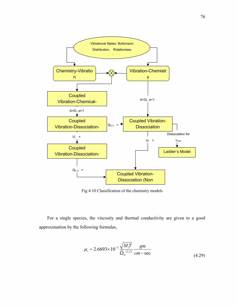
76
Fig 4.10 Classification of the chemistry models
For a single species, the viscosity and thermal conductivity are given to a good
approximation by the following formulas,
5(2,2)2.6693 10
seci
iii
M T gmcm
µ −= ×Ω − (4.29)
Ladder’s Model
Vibration-Chemistry
Chemistry-Vibration
Coupled Vibration-Dissociation-
Coupled Vibration- Dissociation (Non
Vibrational States: Boltzmann
Distribution, Rotationless
H i O ill t
A=Di, α=1
Ui =
Coupled Vibration-Chemical-
QC-V =
Ui =
A=Di, α=1
Dissociation for
vmax
QC-V = Coupled
Vibration-Dissociation- Coupled Vibration-
Dissociation
77
And
,
154 sec
itr i
i
R calKM cm Kµ
=− −
, (4.30)
,int,
52 sec
p ii iii
i i
CD calK RM R cm Kµ ρ
µ⎛ ⎞⎛ ⎞
= −⎜ ⎟⎜ ⎟ − −⎝ ⎠⎝ ⎠ (4.31)
where Ktr,i is the translational component of the thermal conductivity and Kint,i is the
component of thermal conductivity resulting from the diffusion of internal excitation
energy of the molecules, Mi is the molecular weight in gm/gm-mole, R is the universal
gas constant, Dii is the component of self diffusion, and iiΩ is average collision
cross-in range of sections for the molecules within an Armstrong. The self diffusion
component is the reciprocal Schmidt number and is related to the collision cross sections
through the relation:
3 23
(1,1)
/2.6280 10
seci
iiii
T M cmDp
−= ×Ω (4.32)
The complication in the above relations arises due to the presence of the term iiΩ ,
which brings an uncertainty in the determination of transport properties. The expression
for iiΩ further complicates the above relations. Thus it is computationally practical to
find the transport properties as a polynomial of temperature T. This polynomial is found
by curve fitting on experimental data.
Thus the expressions for the transport properties are found as,
78
3 2[ (ln ) (ln ) ln ] ,sec
i i i i iE A T B T C T Di
gme Tcm
µ µ µ µ µµ + + +=−
3 2, , , , ,[ (ln ) (ln ) ln ]
, , int, ,sec
K K K K Kf i f i f i f i f iE A T B T C T Df i tr i i
calK K K e Tcm
+ + += + =
−
2 2[ (ln ) ln ],
secD D D Dij ij ij ij
D A T B T C
ijcm atmD e T
+ + −=
(4.33)
The values of the curve fit coefficients are given in [20]. The values obtained from
the tables from the mentioned reference are for a p = 1 atm and thus needs to be
corrected depending on the pressure. This is done using the relation:
, int,
, int,
4 8/32
4 8/32
1/ 4 1/ 4
( ) ( )( )(1 ) (1 ) (1 )
ln 2.09 10 1.521000 1000
ln 2.09 10 1.521000 1000
ir i e i ei e
i ir i i
e e
K p K ppatm K atm K atm
T T
T Tp p
µµ
−
−
= = =
⎡ ⎤⎛ ⎞ ⎛ ⎞× +⎢ ⎥⎜ ⎟ ⎜ ⎟⎝ ⎠ ⎝ ⎠⎢ ⎥⎣ ⎦=
⎡ ⎤⎛ ⎞ ⎛ ⎞⎢ ⎥× +⎜ ⎟ ⎜ ⎟⎢ ⎥⎝ ⎠ ⎝ ⎠⎣ ⎦
The problem becomes more complex when a mixture of different species is present
in the flow. For such cases, the standard approaches are
(a) Wilke’s mixing formula
In this method, kinetic theory with some simplifying assumptions is used to compute the
mixture transport properties. Using this method, the mixture viscosity is expressed as
[29]
79
2
i i
i i
N sm
χ µµφ
−=∑
(4.34)
Similarly, the mixture thermal conductivity becomes,
i i
i i
Jm s K
χ κκφ
=− −∑
(4.35)
Here, фi is defined as
21/ 4
1
8 1
jij
j i
ij
i
j
MM
MM
µχµ
φ
⎡ ⎤⎛ ⎞⎢ ⎥+ ⎜ ⎟⎢ ⎥⎝ ⎠⎣ ⎦=
⎛ ⎞+⎜ ⎟⎜ ⎟
⎝ ⎠
∑
(4.36)
The multicompoment diffusion coefficient Dm is related to the binary diffusion
coefficients Dij for the diffusion of the species i into j by means of the expression
1 iim
j
j ij
D
D
χχ
−=
∑, (4.37)
where χ is the species mole fraction and M is the molecular mass.
(b) Collision Integrals
This is the most rigorous method of obtaining the mixture properties and uses an
80
approximation to Chapman-Enskog formula [20]. The total mixture viscosity under this
formulation is given as
int,
int
P ii
i
ijij
j ij
CRM R J
Sc m s K
χκ
χµ
=− −∑
∑
Defining (2)
1ij
ij
µ =∆
, the formula for the total viscosity can be rewritten as
2i
ji
j ij
N sm
χµ χµ
−=∑
∑,
where (2)ij∆ is defined as
1/ 2
(2) (1,1)283 ( )
i jij ij
A i j
M MN kT M M
ππ⎡ ⎤
∆ = Ω⎢ ⎥+⎢ ⎥⎣ ⎦ .
Curve fits for ijµ for 11 species air are available in [42]. The mixture translation
thermal conductivity thus becomes
154 i
itr
ij ji
j ij
RM J
m s K
χκ α χ
µ
⎡ ⎤⎢ ⎥⎢ ⎥=⎢ ⎥ − −⎢ ⎥⎣ ⎦
∑∑
,
81
where
2
1 0.45 2.541
1
i i
j jij
i
j
M MM M
MM
α
⎡ ⎤ ⎡ ⎤− −⎢ ⎥ ⎢ ⎥
⎢ ⎥ ⎢ ⎥⎣ ⎦ ⎣ ⎦= +⎡ ⎤+⎢ ⎥
⎢ ⎥⎣ ⎦ .
The mixture internal thermal conductivity can be written as
int,
int
P ii
i
ijij
j ij
CRM R J
Sc m s K
χκ
χµ
=− −∑
∑,
where Scij is the Schmidt number, the curve fits for which can be found in [42].
(c) Species Summation
In this method, the mixture viscosity/thermal conductivity is obtained by computing the
sum of the products of species mole fraction with each species’ viscosities/conductivities.
It is assumed that there is no interaction between the various species. Thus the mixture
viscosity is given as
2i ii
N sm
µ χ µ −=∑
And the mixture thermal conductivity becomes
82
i ii
Jm s K
κ χ κ=− −∑
83
CHAPTER V
NUMERICAL METHODS: NS, BGK AND SA MODELS
In this chapter, the numerical methods pertaining to Navier Stokes(NS) method,
Boltzmann BGK method and Spalart Allmaras(SA) turbulence model are discussed.
5.1 Navier Stokes Equations
The analytical solution of the Navier-Stokes equations is practically impossible to solve
for most of the practical flow problems barring a very few simple flows. Iterative
numerical methods have been used to solve these equations. A wide range of numerical
techniques are available to solve such kind of equations. Such techniques can be broadly
classified into the following groups based on the discretization method:
1. Finite Difference schemes [62, 63, and 64]: In this approach, the solution domain is
represented by a structured array of discrete nodes. The Navier Stokes equations are
written in terms of the nodal values by replacing the derivatives with their finite
difference approximations, obtained through Taylor series expansion about the nodal
values. Although the method tends to be very accurate, problems occur due to the finite
difference representation of the derivatives when discontinuities are present in the
solution. Additionally, the advantage of higher accuracy is lost when solving for
complex geometries. For such cases, the solution domain has to be mapped from
physical space to the computational space using Jacobians.
2. Finite Volume Schemes [65, 66]: In this approach, the solution domain is divided into
small control volumes termed as cells. The integral form of Navier Stokes is solved for
84
each of these cells. This is done by keeping an account of the net flux passing through
each cell and updating the cell properties based on this residual or net flux. A steady state
is achieved when the net flux passing through each cell becomes almost zero. The flux
passing through a cell interface is calculated based on the properties of the cells sharing
a common interface boundary.
The advantage of Finite Volume method over the finite difference method is in its
ability to handle the discontinuities in the flow field. Since the Navier Stokes equations
are solved in their integral form, it becomes easier to treat the derivatives which
otherwise are theoretically infinite. Another main advantage of the Finite Volume
methodology is the conservative nature of the approach. Since the flux being added into
one cell will be deducted from one of the neighboring cells, the scheme remains
conservative over the whole solution domain. Treatment of complex geometries becomes
simpler using this approach. However, extending the accuracy of the scheme to higher
orders is not straightforward and one needs to implement reconstruction schemes.
3. Finite Element Schemes [67]: In this approach, the solution domain is broken down
into subdomains which are termed as elements. These elements can be of arbitrary shape
and sizes. Unlike the Finite Volume scheme where the flow properties are assumed to be
constant or vary linearly in the cells, in Finite Element methodologies the solution is
assumed to take some particular functional form within an element. Therefore the
solutions obtained from Navier Stokes equations lie in such a functional domain. Finite
element methods have been used successfully to solve incompressible as well as
compressible flow problems. One of the major disadvantages of using these methods is
the computational cost. Since the Finite Element methods involve matrix inversions, the
solvers are much slower in terms of computational time when compared to FDM and
FVM solvers and needs parallelization to be used for practical purposes.
85
After comparing the pros and cons of the three methodologies listed above, it was
decided to go ahead with the Finite Volume methodology.
5.2 Finite Volume Methods
As discussed in previous section, the first step for this approach is to subdivide the
computational domain into finite volumes. This can be done in many ways, but it must
be ensured that the volumes should fill the entire domain without overlapping. In the
node centered approach there is one node in each volume and the flow properties are
solved for at this node. The node in most cases coincides with the centroid of the volume.
The volumes can have any polygon shape (triangles, quadrilaterals) in 2D and
polyhedral shapes (tetrahedrons, hexahedrons, prisms etc.) in 3D. For this study,
structured 2D grids are used and therefore the cells are almost rectangular.
The second step involves discretization of the integral form of Navier Stokes
equations for application to finite volume cells. In finite volume, the cell centre flow
properties are assumed to represent the cell average value as shown in equation (5.1),
i.e.,
1 ( , , )ctrr
Q Q x y z dVV
= ∫ (5.1)
where Vr is the volume of rth cell.
Also, the fluxes are assumed to be uniform along each cell interface. Using these
two assumptions one can simplify the integral form of Navier Stokes equation to the
equation represented in equation.
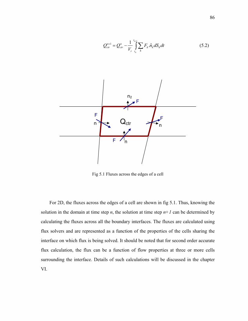
86
11 1 ˆ.
n
n
tn nctr ctr k k k
kr t
Q Q F n dS dtV
++ = − ∑∫ (5.2)
Fig 5.1 Fluxes across the edges of a cell
For 2D, the fluxes across the edges of a cell are shown in fig 5.1. Thus, knowing the
solution in the domain at time step n, the solution at time step n+1 can be determined by
calculating the fluxes across all the boundary interfaces. The fluxes are calculated using
flux solvers and are represented as a function of the properties of the cells sharing the
interface on which flux is being solved. It should be noted that for second order accurate
flux calculation, the flux can be a function of flow properties at three or more cells
surrounding the interface. Details of such calculations will be discussed in the chapter
VI.
Qctr n
n2
n
n
F
FF
F
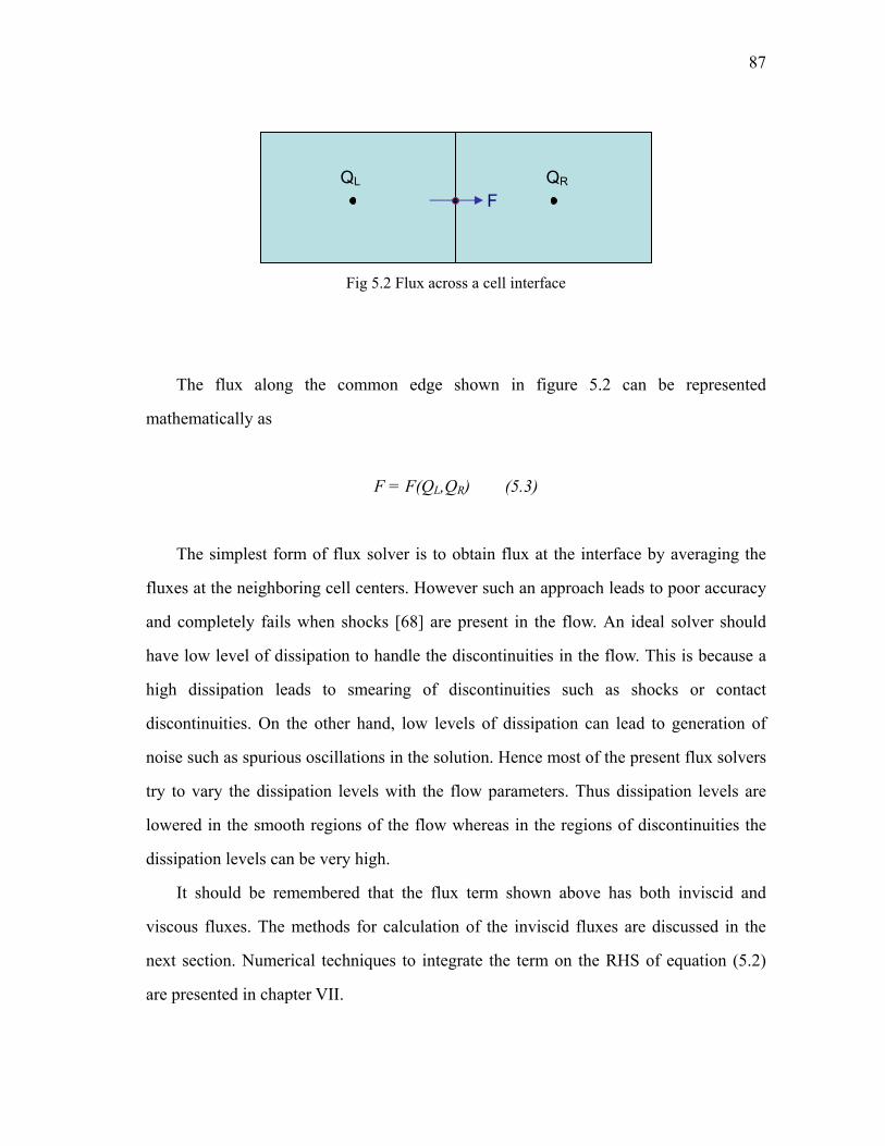
87
Fig 5.2 Flux across a cell interface
The flux along the common edge shown in figure 5.2 can be represented
mathematically as
F = F(QL,QR) (5.3)
The simplest form of flux solver is to obtain flux at the interface by averaging the
fluxes at the neighboring cell centers. However such an approach leads to poor accuracy
and completely fails when shocks [68] are present in the flow. An ideal solver should
have low level of dissipation to handle the discontinuities in the flow. This is because a
high dissipation leads to smearing of discontinuities such as shocks or contact
discontinuities. On the other hand, low levels of dissipation can lead to generation of
noise such as spurious oscillations in the solution. Hence most of the present flux solvers
try to vary the dissipation levels with the flow parameters. Thus dissipation levels are
lowered in the smooth regions of the flow whereas in the regions of discontinuities the
dissipation levels can be very high.
It should be remembered that the flux term shown above has both inviscid and
viscous fluxes. The methods for calculation of the inviscid fluxes are discussed in the
next section. Numerical techniques to integrate the term on the RHS of equation (5.2)
are presented in chapter VII.
QL QR F
88
5.3 Inviscid Fluxes
The flux solvers discussed in this section belong to the wave approach category of flux
calculation methods [69]. These wave based methods can be further categorized into two
classes: the Flux Vector Splitting method and Flux Difference Splitting method. Two
schemes, each of them belonging to one of these two classes, have been implemented in
this study.
5.3.1 Steger Warming Schemes
Steger and Warming (55) proposed the first flux vector splitting scheme, based on wave
speed splitting. The flux vector can be split as
F(U) = F+(U) + F-(U) (5.4)
where the characteristic values of df+/du are all nonnegative and the characteristic values
of df-/du are all nonpositive. In standard notation,
0, 0dF dFdU dU
+ −
≥ ≤
(5.5)
Therefore the flux is split on the basis of the direction in which it is traveling. The
flux can be written in terms of the characteristic diagonal matrix as
1dFF U AU Q Q UdU
−= = = Λ, (5.6)
where
89
1
2 1 2 3
3
0 00 0 , , ,0 0
u a u u aλ
λ λ λ λλ
Λ = = − = = + . (5.7)
Q is the eigen matrix corresponding to eigenvalues of A = dF/dU
Thus the split equation can also be written as
1 1( )F U Q Q Q Q+ − − −= Λ + Λ (5.8)
where +Λ and −Λ are based on eigenvalues split as λ λ λ+ −= + . One of many such
possible splits was proposed in [55]:
1max(0, ) ( | |)21min(0, ) ( | |)2
i i i i
i i i i
λ λ λ λ
λ λ λ λ
+
−
= = +
= = − (5.9)
Thus using the above values, F+ and F- come out to be
For 1M ≤ − :
F+ = 0
F- = F
For 1 0M− < ≤ :
90
2 2
1( )
2
2 1
F u a u au a au
ργ
γ
+
⎡ ⎤⎢ ⎥⎢ ⎥⎢ ⎥= + +⎢ ⎥⎢ ⎥+ +⎢ ⎥−⎣ ⎦
, 2 2 2
1 11 ( )
2
2 2 1
F u u u a u au u a au
γ ρργ γ
γ
−
⎡ ⎤⎡ ⎤⎢ ⎥⎢ ⎥⎢ ⎥⎢ ⎥− ⎢ ⎥= + − −⎢ ⎥⎢ ⎥⎢ ⎥⎢ ⎥⎢ ⎥ + −⎢ ⎥⎢ ⎥⎣ ⎦ −⎣ ⎦
(5.10)
For 0 1:M< ≤
2 2 2
1 11 ( )
2
2 2 1
F u u u a u au u a au
γ ρργ γ
γ
+
⎡ ⎤⎡ ⎤⎢ ⎥⎢ ⎥⎢ ⎥⎢ ⎥− ⎢ ⎥= + + +⎢ ⎥⎢ ⎥⎢ ⎥⎢ ⎥⎢ ⎥ + +⎢ ⎥⎢ ⎥⎣ ⎦ −⎣ ⎦
, 2 2
1( )
2
2 1
F u a u au a au
ργ
γ
−
⎡ ⎤⎢ ⎥⎢ ⎥⎢ ⎥= − −⎢ ⎥⎢ ⎥+ −⎢ ⎥−⎣ ⎦
(5.11)
For 1M > :
F+ = F,
F- = 0
Therefore, for supersonic right running flows, all of the waves are right running and
the flux vector splitting correctly attributes all of the flux to right running waves and
none to left running waves. Similarly, for supersonic left running flows all of the waves
are left running and the flux vector splitting correctly attributes all of the flux to left
running waves and none to right running waves. For subsonic flows, waves are both left
and right running, and the flux vector splitting correctly attributes some to left and some
to right running waves, although it should be noted that the exact physical proportions
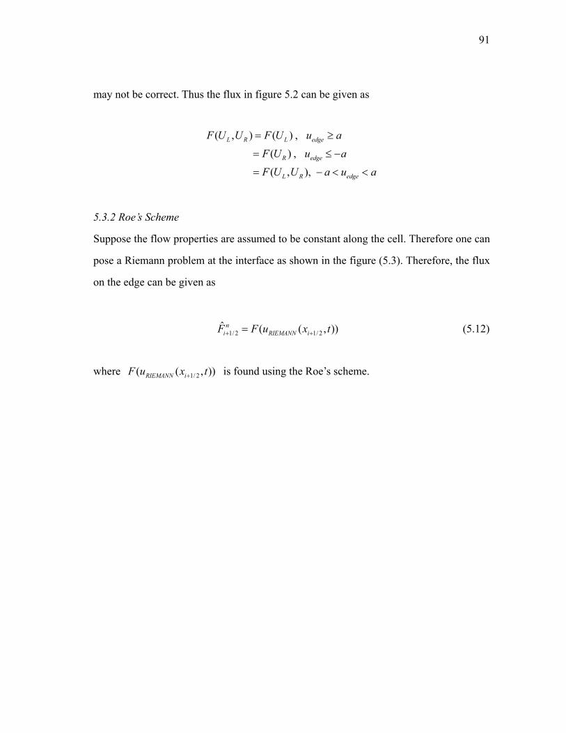
91
may not be correct. Thus the flux in figure 5.2 can be given as
( , ) ( ) ,
( ) ,
( , ),
L R L edge
R edge
L R edge
F U U F U u a
F U u a
F U U a u a
= ≥
= ≤ −
= − < <
5.3.2 Roe’s Scheme
Suppose the flow properties are assumed to be constant along the cell. Therefore one can
pose a Riemann problem at the interface as shown in the figure (5.3). Therefore, the flux
on the edge can be given as
1/ 2 1/ 2ˆ ( ( , ))ni RIEMANN iF F u x t+ += (5.12)
where 1/ 2( ( , ))RIEMANN iF u x t+ is found using the Roe’s scheme.
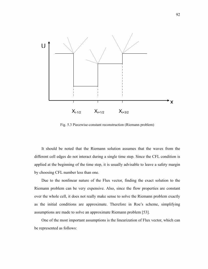
92
Fig. 5.3 Piecewise-constant reconstruction (Riemann problem)
It should be noted that the Riemann solution assumes that the waves from the
different cell edges do not interact during a single time step. Since the CFL condition is
applied at the beginning of the time step, it is usually advisable to leave a safety margin
by choosing CFL number less than one.
Due to the nonlinear nature of the Flux vector, finding the exact solution to the
Riemann problem can be very expensive. Also, since the flow properties are constant
over the whole cell, it does not really make sense to solve the Riemann problem exactly
as the initial conditions are approximate. Therefore in Roe’s scheme, simplifying
assumptions are made to solve an approximate Riemann problem [53].
One of the most important assumptions is the linearization of Flux vector, which can
be represented as follows:
Xi-1/2 Xi+1/2 Xi+3/2
U
x
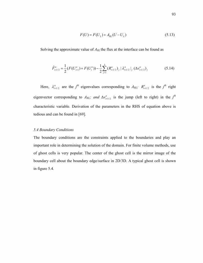
93
( ) ( ) ( )L RL LF U F U A U U= + − (5.13)
Solving the approximate value of ARL the flux at the interface can be found as
3
1/ 2 1 1/ 2 1/ 2 1/ 21
1 1ˆ ( ( ) ( )) ( ) | | ( )2 2
n n n n n ni i i i j i j i j
jF F U F U R vλ+ + + + +
=
= + − ∆∑ (5.14)
Here, 1/ 2niλ + are the jth eigenvalues corresponding to ARL; 1/ 2
niR + is the jth right
eigenvector corresponding to ARL; and 1/ 2niv +∆ is the jump (left to right) in the jth
characteristic variable. Derivation of the parameters in the RHS of equation above is
tedious and can be found in [69].
5.4 Boundary Conditions
The boundary conditions are the constraints applied to the boundaries and play an
important role in determining the solution of the domain. For finite volume methods, use
of ghost cells is very popular. The center of the ghost cell is the mirror image of the
boundary cell about the boundary edge/surface in 2D/3D. A typical ghost cell is shown
in figure 5.4.
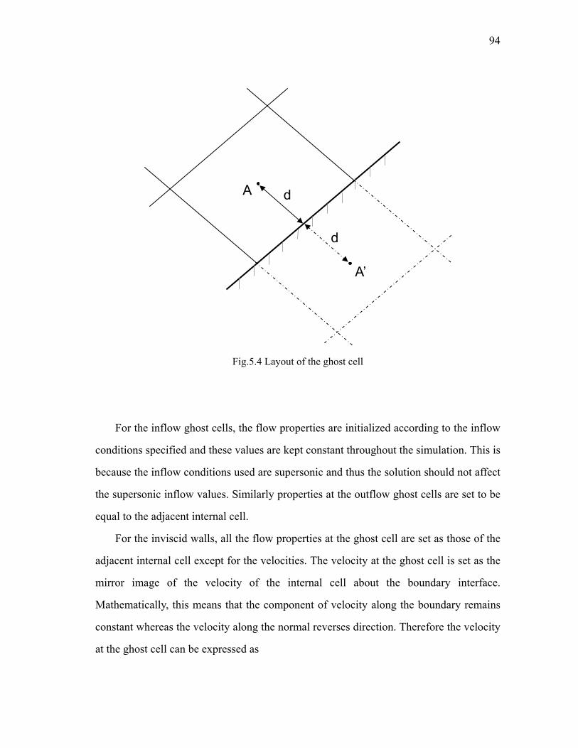
94
Fig.5.4 Layout of the ghost cell
For the inflow ghost cells, the flow properties are initialized according to the inflow
conditions specified and these values are kept constant throughout the simulation. This is
because the inflow conditions used are supersonic and thus the solution should not affect
the supersonic inflow values. Similarly properties at the outflow ghost cells are set to be
equal to the adjacent internal cell.
For the inviscid walls, all the flow properties at the ghost cell are set as those of the
adjacent internal cell except for the velocities. The velocity at the ghost cell is set as the
mirror image of the velocity of the internal cell about the boundary interface.
Mathematically, this means that the component of velocity along the boundary remains
constant whereas the velocity along the normal reverses direction. Therefore the velocity
at the ghost cell can be expressed as
d
d
A
A’
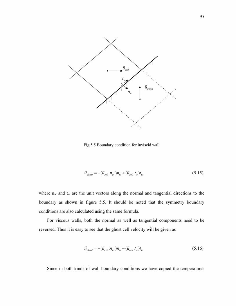
95
Fig 5.5 Boundary condition for inviscid wall
( . ) ( . )ghost cell w w cell w wu u n n u t t= − +r r r (5.15)
where nw and tw are the unit vectors along the normal and tangential directions to the
boundary as shown in figure 5.5. It should be noted that the symmetry boundary
conditions are also calculated using the same formula.
For viscous walls, both the normal as well as tangential components need to be
reversed. Thus it is easy to see that the ghost cell velocity will be given as
( . ) ( . )ghost cell w w cell w wu u n n u t t= − −r r r (5.16)
Since in both kinds of wall boundary conditions we have copied the temperatures
ghostur wn
cellur
wt
96
from the internal cell to the ghost cells, it follows that all the walls are assumed to be
adiabatic for this study. 5.5 BGK Boltzmann Equation
The exact solution of the BGK Boltzmann equation at a cell interface xj+1/2 at time t can
be written as
/ ( ') /1/ 2 0 1/ 2
0
1( , , , , ) ( ) ( ', ', , , ) 't
t t tj jf x t u v e f x ut e g x t u v dtτ τξ ξ
τ− − −
+ += − + ∫ (5.17)
where 1/ 2' ( ')jx x u t t+= − − represents the particle trajectory and f0 is the initial gas
distribution function f at the beginning of each time step (t=0). Assuming cell interface
as the origin, we can set xj+1/2 = 0 without any loss of generality.
The gas distribution function f0 which is given at the beginning of each time step can
be written in the neighborhood of a cell interface as
0
[1 ] ( ), 0[1 ] ( ), 0
l l l l l
r r r r r
g a x g a u A xf
g a x g a u A xτ
τ
⎧ + − + ≤⎪= ⎨+ − + ≥⎪⎩
(5.18)
The first part of the expression represents the equilibrium part of the distribution
function. The quantities gl and gr are the Maxwellian distributions at the left and right of
a cell interface. The slopes al and ar represent the spatial derivative of a Maxwellian and
are calculated using the slopes of the conservative variables.
The second term which is first order in τ represents the nonequilibrium part of
distribution function and is obtained from the Chapman-Enskog expansion of the BGK
97
model. Detailed formulation on the calculation of coefficients (al, Al, ar, Ar) can be found
in [74].
It should be noted that for flow simulations where the cell size cannot properly
resolve the viscous flow structure, the nonequilibrium part vanishes. An example where
this term becomes significant would be the region inside a shock. Therefore, if the cell
size is fine enough to resolve the physical shock structure, the distribution will deviate
from the Maxwellian because of the presence of this nonequilibrium term.
The second term in equation (5.17) can be evaluated using the following expression
for g:
0[1 (1 [ ]) [ ]) ]l rg g H x a x H x a x At= + − + + (5.19)
where H[x] is the Heaviside function defined as
0, 0,
[ ]1, 0.
xH x
x<⎧
= ⎨ ≥⎩ g0 is the local Maxwellian distribution function located at the cell interface. As a
consequence of the above relation it can be seen that g has different slopes for x<0 and
x>0. The details for the calculation of la , ra and A can be found in [74].
Making the substitutions from eq (5.18) and eq (5.19) into eq (5.17) we get the
expression for f as:
98
/ /1/ 2 0 0
/ /0
/
/
( , , , , ) (1 ) ( / 1 )
( ( 1 ) )( [ ] (1 [ ]))
((1 ( ) ) [ ] (1 ( ) )(1 [ ]) )( [ ] (1 [ ]) )
t tj
t t l r
t l l r r
t l l r r
f x t u v e g t e Ag
e te a H u a H u ug
e u t a H u g u t a H u ge A H u g A H u g
τ τ
τ τ
τ
τ
ξ τ τ
τ
τ τ
τ τ
− −+
− −
−
−
= − + − +
+ − + + + −
+ − + + − + −
+ − − − (5.20)
Thus the flux along x-direction can be found by integrating the above f to give:
1/ 2
2 2 2
1
( , , , , )
1 ( )2
uj
v
E
FuF
u f x t u v dvFu vF
ρ
ρ
ρ
ξ
ξ
+
⎛ ⎞⎛ ⎞ ⎜ ⎟⎜ ⎟ ⎜ ⎟⎜ ⎟ = Ξ⎜ ⎟⎜ ⎟ ⎜ ⎟⎜ ⎟ ⎜ ⎟⎜ ⎟ + +⎜ ⎟⎝ ⎠ ⎝ ⎠
∫
(5.21)
The same procedure can be repeated to calculate the flux along y-direction.
5.6 Collision Time
As derived in section 4.4, the final expression for τ comes out to be
/ Pτ µ=
This formula works well for cases when cell size is much smaller than the dissipative
length scale determined by the physical viscosity. However, in cases of shocks where the
cell sizes are usually not enough to resolve the wave structure and thus the physical
structure has to be replaced by a numerical one. Since the shock thickness is determined
by the viscosity, the effective viscosity should also be changed to account for this new
shock thickness. The additional dissipation is provided by the following term:
99
| / / || / / |
l l r r
l l r r
tp
ρ λ ρ λµτρ λ ρ λ
−= + ∆
+
It can be seen that in the smooth regions the second term on the RHS vanishes.
However, the term will have a significant value at the interface of a discontinuity such as
a shock.
It should be noted that the ratio of average collision time τ and the numerical time
step t∆ has a significant effect on the stability of the BGK method. For the cases when
/ tτ ∆ >> 1, there are effectively no collisions taking place for any particular iteration i.
Since viscous effects are a direct consequence of the collision between molecules, the
effective viscosity for the whole domain will decrease. Therefore there is a higher
chance of the solver becoming unstable since less amount of dissipation is available to
handle the discontinuities. It is therefore important to keep the ratio / tτ ∆ < 1. In Euler
cases, this ratio is maintained around 0.01-0.05 by defining the collision time as
1| / / || / / |
l l r r
l l r r
C t tρ λ ρ λτρ λ ρ λ
−= ∆ + ∆
+
5.7 Spalart Allmaras Model
The compressible Spalart Allmaras model is given as
'( , , ) ( , ) ( ) ( )prod dest trip T difD b S v d b v d b d b vDtνρ ρ ρ ρ= − + +%
% % %
Using the discretizations discussed in chapter II for the terms on the RHS, the
implicit backward Euler solution procedure [85] can be used to ensure a positive
turbulence field at each update. However, such a method requires expensive inversion of
100
a large sparse matrix in 2-D or 3-D. Therefore an approximate factorization of the
implicit operator is required although the unconditional positivity is lost. Thus a small
timestep is required so that factorization error does not ruin the positivity of the solution.
For 2-D, the conventional ADI method can be used. The equation can be written as
n n[ I M ][ I M ][ I (P D)] v (M +M +P D)]vt t t tξ η ξ ηρ ρ ρ−∆ −∆ −∆ − ∆ = ∆ − (5.22)
where Mξ and Mη are finite differences in the ξ and η coordinate directions
respectively, while Mξ and Mη are the corresponding implicit operators. For an
unsteady problem, the Alternating Direction Implicit (ADI) method can have
convergence problems and requires several sub-iterations for every timestep. A more
efficient factorization is suggested in [83]. However, for steady state problems, such
subiterations are not required and the conventional ADI method can be applied.
It should be noted that although the turbulence equations are solved implicitly, the
mean flow equations can still be updated using explicit method. Such an approach is
discussed in [86].
5.8 Boundary and Initial Conditions
The eddy viscosity variable ν% is put to zero on the no slip boundary. On the inlet
boundary /10ν ν<% is suggested in literature [83]. However, in case of a steady state
flow over smooth flat plate with no shocks present, there is no instability to induce
turbulence in the flow. Therefore, ν% of the order of 10ν has to be used to see
turbulence effects.
On the extrapolation boundaries like supersonic outflows, the Neumann condition is
used, i.e.,
101
ˆ. 0ˆ
nnνν ∂
∇ = =∂%
%
A uniform initial condition equal to the freestream value can be given.
102
CHAPTER VI
RECONSTRUCTION AND LIMITERS
6.1 Introduction
The discussion of the last chapter assumed that the flux solver is of first order accuracy.
To increase the accuracy to higher orders, reconstruction schemes are used. The
reconstruction can be achieved in two steps: interpolation and limiting. In the
interpolation step, the value of the flow variables is found at particular locations such as
a cell interface or a vertex using the values of flow properties in the surrounding cells. In
the limiter step the reconstructed values are recalculated to prevent oscillations to
develop in the solution. These reconstructed values are then used as input to the flux
solver. In an alternate postprocessing form, the reconstruction can also be applied to the
calculated flux instead of applying them to the flow properties in the preprocessing form.
However, only the former approach will be discussed here.
6.2 Linear Interpolation
In the previous chapter, it was assumed that the value at the cell center is constant
throughout the cell region, the constant value being the value at the cell center. Thus the
flowfield was approximated as a series of piecewise constant states. Such an approach is
also known as Gudonov’s first order scheme [75]. Thus the flow conditions to the
immediate left and right of the cell interface are given as
1/ 2 1/ 2 1,L Ri i i iQ Q Q Q+ + += =
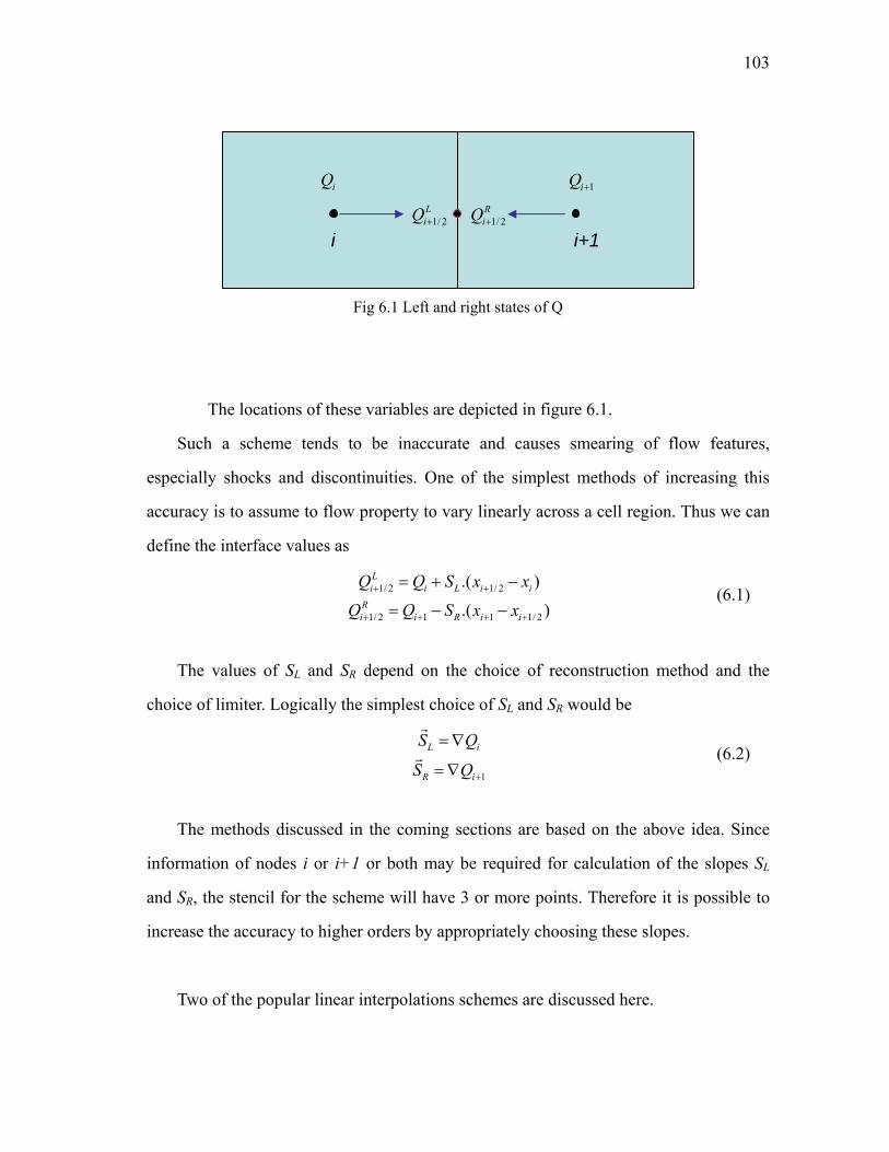
103
Fig 6.1 Left and right states of Q
The locations of these variables are depicted in figure 6.1.
Such a scheme tends to be inaccurate and causes smearing of flow features,
especially shocks and discontinuities. One of the simplest methods of increasing this
accuracy is to assume to flow property to vary linearly across a cell region. Thus we can
define the interface values as
1/ 2 1/ 2
1/ 2 1 1 1/ 2
.( )
.( )
Li i L i i
Ri i R i i
Q Q S x x
Q Q S x x+ +
+ + + +
= + −
= − − (6.1)
The values of SL and SR depend on the choice of reconstruction method and the
choice of limiter. Logically the simplest choice of SL and SR would be
1
L i
R i
S Q
S Q +
= ∇
= ∇
r
r (6.2)
The methods discussed in the coming sections are based on the above idea. Since
information of nodes i or i+1 or both may be required for calculation of the slopes SL
and SR, the stencil for the scheme will have 3 or more points. Therefore it is possible to
increase the accuracy to higher orders by appropriately choosing these slopes.
Two of the popular linear interpolations schemes are discussed here.
iQ 1iQ +
1/ 2LiQ + 1/ 2
RiQ +
i i+1
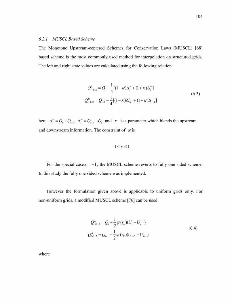
104
6.2.1 MUSCL Based Scheme
The Monotone Upstream-centered Schemes for Conservation Laws (MUSCL) [68]
based scheme is the most commonly used method for interpolation on structured grids.
The left and right state values are calculated using the following relation
1/ 2
1/ 2 1 1 1
1 [(1 ) (1 ) ]41 [(1 ) (1 ) ]4
Li i i i
Ri i i i
Q Q
Q Q
κ κ
κ κ
− ++
+ −+ + + +
= + − ∆ + + ∆
= − − ∆ + + ∆ (6.3)
here 1 1,i i i i i iQ Q Q Q− +− +∆ = − ∆ = − and κ is a parameter which blends the upstream
and downstream information. The constraint of κ is
1 1κ− ≤ ≤
For the special case 1κ = − , the MUSCL scheme reverts to fully one sided scheme.
In this study the fully one sided scheme was implemented.
However the formulation given above is applicable to uniform grids only. For
non-uniform grids, a modified MUSCL scheme [76] can be used:
1/ 2 1
1/ 2 1 2 1
1 ( )( )21 ( )( )2
Li i L i i
Ri i R i i
Q Q r U U
Q Q r U U
ψ
ψ
+ −
+ + + +
= + −
= − − (6.4)
where
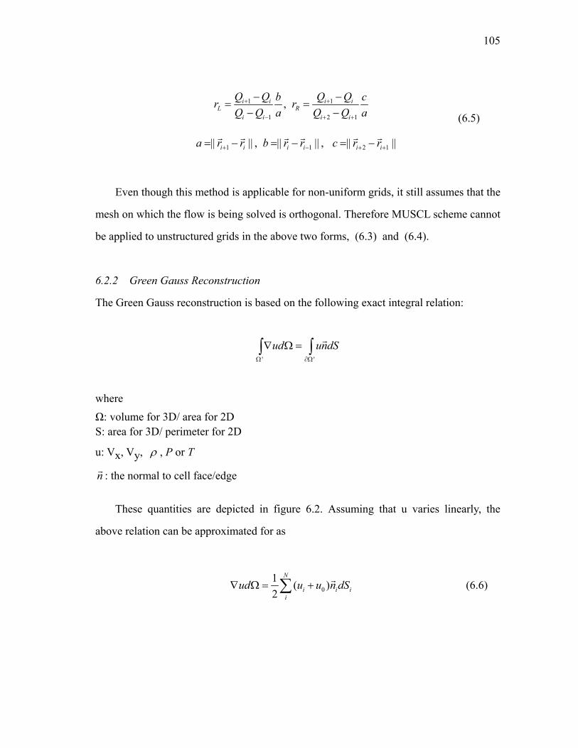
105
1 1
1 2 1
,i i i iL R
i i i i
Q Q Q Qb cr rQ Q a Q Q a
+ +
− + +
− −= =
− − (6.5)
1 1 2 1|| || , || || , || ||i i i i i ia r r b r r c r r+ − + += − = − = −r r r r r r
Even though this method is applicable for non-uniform grids, it still assumes that the
mesh on which the flow is being solved is orthogonal. Therefore MUSCL scheme cannot
be applied to unstructured grids in the above two forms, (6.3) and (6.4).
6.2.2 Green Gauss Reconstruction
The Green Gauss reconstruction is based on the following exact integral relation:
' '
ud undSΩ ∂Ω
∇ Ω =∫ ∫r
where Ω: volume for 3D/ area for 2D S: area for 3D/ perimeter for 2D
u: Vx, Vy, ρ , P or T
nr : the normal to cell face/edge
These quantities are depicted in figure 6.2. Assuming that u varies linearly, the
above relation can be approximated for as
01 ( )2
N
i i ii
ud u u n dS∇ Ω = +∑ r (6.6)
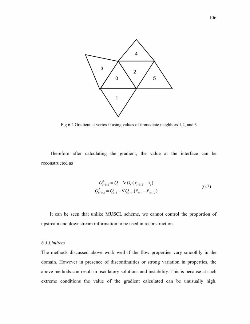
106
Fig 6.2 Gradient at vertex 0 using values of immediate neighbors 1,2, and 3
Therefore after calculating the gradient, the value at the interface can be
reconstructed as
1/ 2 1/ 2
1/ 2 1 1 1 1/ 2
.( )
.( )
Li i i i i
Ri i i i i
Q Q Q x x
Q Q Q x x+ +
+ + + + +
= +∇ −
= −∇ −
r r
r r (6.7)
It can be seen that unlike MUSCL scheme, we cannot control the proportion of
upstream and downstream information to be used in reconstruction.
6.3 Limiters
The methods discussed above work well if the flow properties vary smoothly in the
domain. However in presence of discontinuities or strong variation in properties, the
above methods can result in oscillatory solutions and instability. This is because at such
extreme conditions the value of the gradient calculated can be unusually high.
0
1
23
4
5
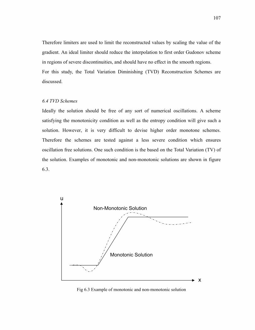
107
Therefore limiters are used to limit the reconstructed values by scaling the value of the
gradient. An ideal limiter should reduce the interpolation to first order Gudonov scheme
in regions of severe discontinuities, and should have no effect in the smooth regions.
For this study, the Total Variation Diminishing (TVD) Reconstruction Schemes are
discussed.
6.4 TVD Schemes
Ideally the solution should be free of any sort of numerical oscillations. A scheme
satisfying the monotonicity condition as well as the entropy condition will give such a
solution. However, it is very difficult to devise higher order monotone schemes.
Therefore the schemes are tested against a less severe condition which ensures
oscillation free solutions. One such condition is the based on the Total Variation (TV) of
the solution. Examples of monotonic and non-monotonic solutions are shown in figure
6.3.
Fig 6.3 Example of monotonic and non-monotonic solution
Non-Monotonic Solution
Monotonic Solution
x
u
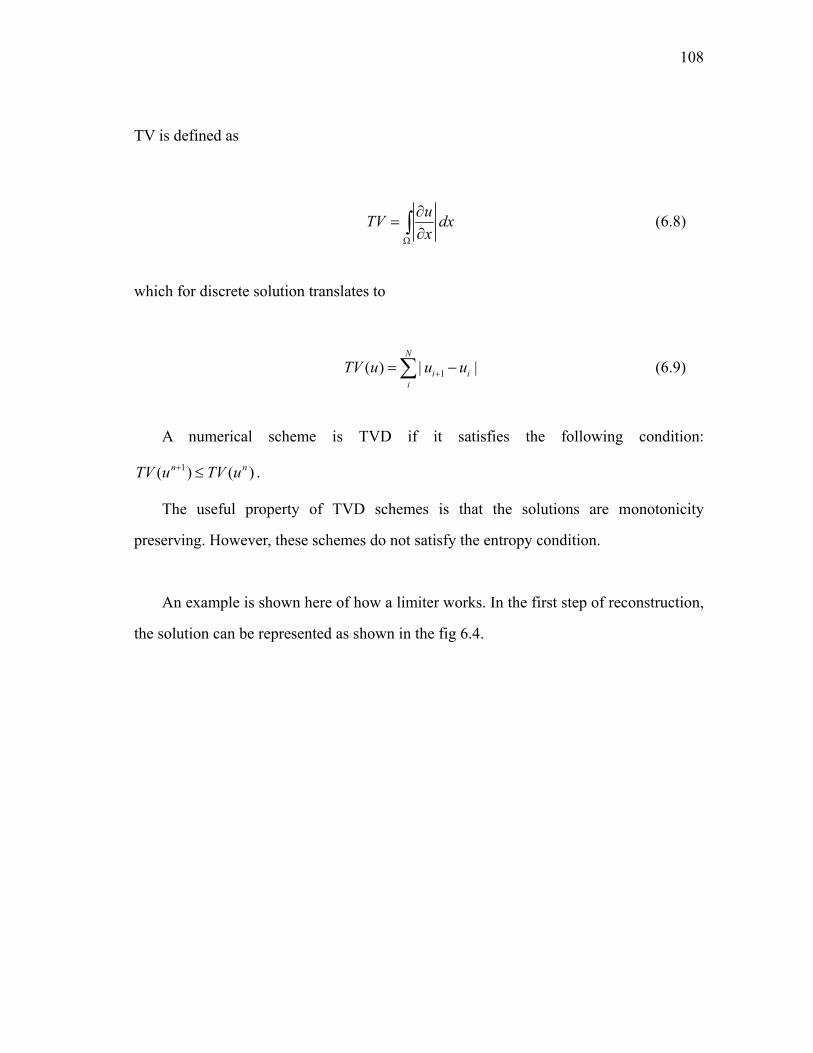
108
TV is defined as
uTV dxxΩ
∂=
∂∫ (6.8)
which for discrete solution translates to
1( ) | |N
i ii
TV u u u+= −∑ (6.9)
A numerical scheme is TVD if it satisfies the following condition:
1( ) ( )n nTV u TV u+ ≤ .
The useful property of TVD schemes is that the solutions are monotonicity
preserving. However, these schemes do not satisfy the entropy condition.
An example is shown here of how a limiter works. In the first step of reconstruction,
the solution can be represented as shown in the fig 6.4.
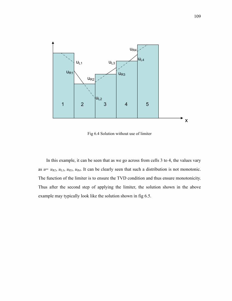
109
Fig 6.4 Solution without use of limiter
In this example, it can be seen that as we go across from cells 3 to 4, the values vary
as u= uR2, uL3, uR3, uR4. It can be clearly seen that such a distribution is not monotonic.
The function of the limiter is to ensure the TVD condition and thus ensure monotonicity.
Thus after the second step of applying the limiter, the solution shown in the above
example may typically look like the solution shown in fig 6.5.
1 2 3 4 5
uR1
uL1
uL2
uR2
uL3
uR3
uL4
uR4
x
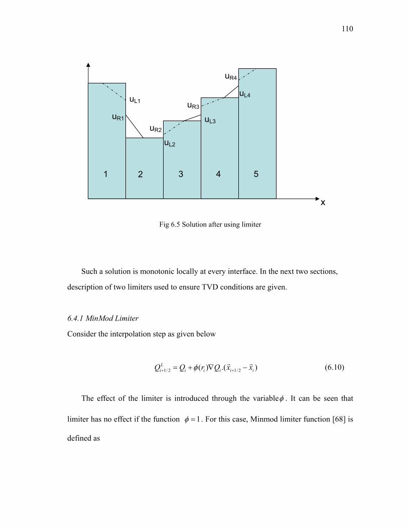
110
Fig 6.5 Solution after using limiter
Such a solution is monotonic locally at every interface. In the next two sections,
description of two limiters used to ensure TVD conditions are given.
6.4.1 MinMod Limiter
Consider the interpolation step as given below
1/ 2 1/ 2( ) .( )Li i i i i iQ Q r Q x xφ+ += + ∇ −
r r (6.10)
The effect of the limiter is introduced through the variableφ . It can be seen that
limiter has no effect if the function 1φ = . For this case, Minmod limiter function [68] is
defined as
1 2 3 4 5
uR1
uL1
uR2 uL3
uR3
uL4
uR4
uL2
x
111
( ) (1, )r m rφ =
where r is defined as /r + −= ∆ ∆ and the function m is based on the minimum-modulus
(minmod) function given as
( , ) ( , ) ( ) max0,min[| |, . ( )]m x y m y x sign x x y sign x= = (6.11)
This function returns 0 if x and y have different signs or the value of the argument
with the smallest modulus.
The minmod limiter is popular for flow problems in which strong shocks are present.
One of the disadvantages of this limiter is that it is not differentiable.
6.4.2 Van Albada Limiter
Using non-differentiable limiters can result in very slow convergence to a steady state
solution. This is because such limiters can cause temporal oscillations due to which the
residues never fall to the machine precision levels.
The Van Albada limiter [77] is a differentiable one. It is defined as
2
2( )1
r rrr
φ +=
+ (6.12)
This limiter is good for steady state smooth flows. However, one of the disadvantages is
that it can not be applied to unsteady flows.
112
CHAPTER VII
NUMERICAL ISSUES
7.1 Introduction
As mentioned in [43], a very common joke shared amongst CFD practitioners correctly
describes a perceived problem with numerical predictions: “Everyone believes
experimental results except the person who performed the experiment, and no one
believes numerical results except the person who performed the prediction.” Nowhere is
this statement more true (and more of a problem) than in hypersonic flow simulation.
The following complex features of hypersonic flows are what make their CFD
analysis a challenging task:
(a) Presence of vibrational, chemical nonequilibrium
(b) Thin shock layers (high compression)
(c) Entropy layers caused by highly swept and curved shock waves
(d) Viscous/inviscid interactions
(e) Real gas effects, including dissociation, ionization (high temperatures)
(f) Rarefaction (high altitudes)
In the next few sections, some of the common practices in CFD used to counter some
of the above mentioned problems will be discussed. The main steps involved in
developing a CFD solver are discussed in the next section.
7.2 CFD Solver for Nonequilibrium Flow
The general governing equation for single species flow in vibrational nonequilibrium can
be written as
113
( ) ( )v vcv
G G H HQ St x y
∂ − ∂ −∂+ + =
∂ ∂ ∂ (7.1)
Where,
1T
vnQ u v Eρ ρ ρ ρ= L
1 0 0 0Tcv vnS w w= & &L
The inviscid and viscous flow matrices are written as
1
2
( )
vn
u
uG
u puv
E p u
ρ
ρ
ρρ
⎧ ⎫⎪ ⎪⎪ ⎪⎪ ⎪⎪ ⎪= ⎨ ⎬
+⎪ ⎪⎪ ⎪⎪ ⎪
+⎪ ⎪⎩ ⎭
M
,
0
0
( )
vxx
xy
xx xy tx rx vx
G
u v q q q
ττ
τ τ
⎧ ⎫⎪ ⎪⎪ ⎪⎪ ⎪⎪ ⎪= ⎨ ⎬⎪ ⎪⎪ ⎪⎪ ⎪
+ − + +⎪ ⎪⎩ ⎭
M
Here,
21
2V vE C T u Eρ ρ= + +r
' ' 2,3
ji kij ij
j i k
uu ux x x
τ µ δ λ λ µ⎛ ⎞∂∂ ∂
= + + = −⎜ ⎟⎜ ⎟∂ ∂ ∂⎝ ⎠ (7.2)
, , , , , ,t r v t r v t r vq Tκ= − ∇r
P RTρ=
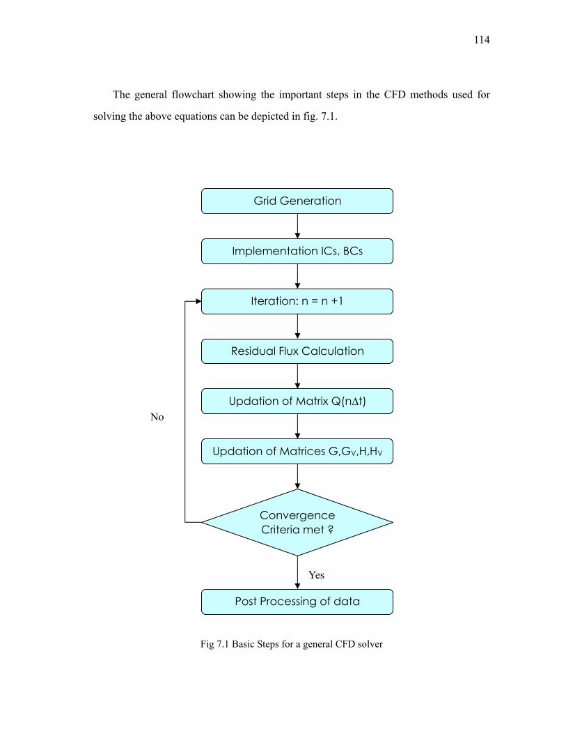
114
The general flowchart showing the important steps in the CFD methods used for
solving the above equations can be depicted in fig. 7.1.
Fig 7.1 Basic Steps for a general CFD solver
Grid Generation
Implementation ICs, BCs
Iteration: n = n +1
Residual Flux Calculation
Updation of Matrix Q(n∆t)
Updation of Matrices G,GV,H,HV
Convergence Criteria met ?
Post Processing of data
No
Yes
115
The presence of complex hypersonic flow features makes the above steps (specially
the process of grid generation, calculation of residual fluxes using differencing scheme
and updation of matrices using integration schemes) a challenging task. The approaches
found in literature for these steps will be presented in the next few sections.
7.3 Grid Generation
Grid generation has made great strides over the past decades and a number of
commercially available programs are available that do a reasonably good job of creating
grids around complex geometries. However, many of these softwares fail when creating
grids for CFD analysis of hypersonic flows due to its difficult requirements. Grid
generation for complex geometries can take anywhere from weeks to months even after
using these commercial softwares.
Grids can be categorized as body fitted and non body fitted. The body fitted grids
can be further categorized as structured and unstructured grids, while the non body fitted
grids found in literature are the Cartesian grids.
Most industry still relies on body fitted grids for the grid generation process. For
such grids, surface geometry definition and grid generation are still considered to be the
biggest bottlenecks in the CFD process. However, unstructured grids are gaining
popularity over structured grids as the process is more or less automated and requires
much less human hours. They also offer geometric flexibility and efficient refinement
capabilities which are not available in structured grids.
However even for unstructured grid generation, an initial explicit generation of
surface grid is required which calls for a high level of expertise and has been one of the
least automated steps in the numerical simulation process.
The requirement of surface grids is removed when using the non body fitted
Cartesian grids. In this case the surface grid is obtained as a byproduct when the whole
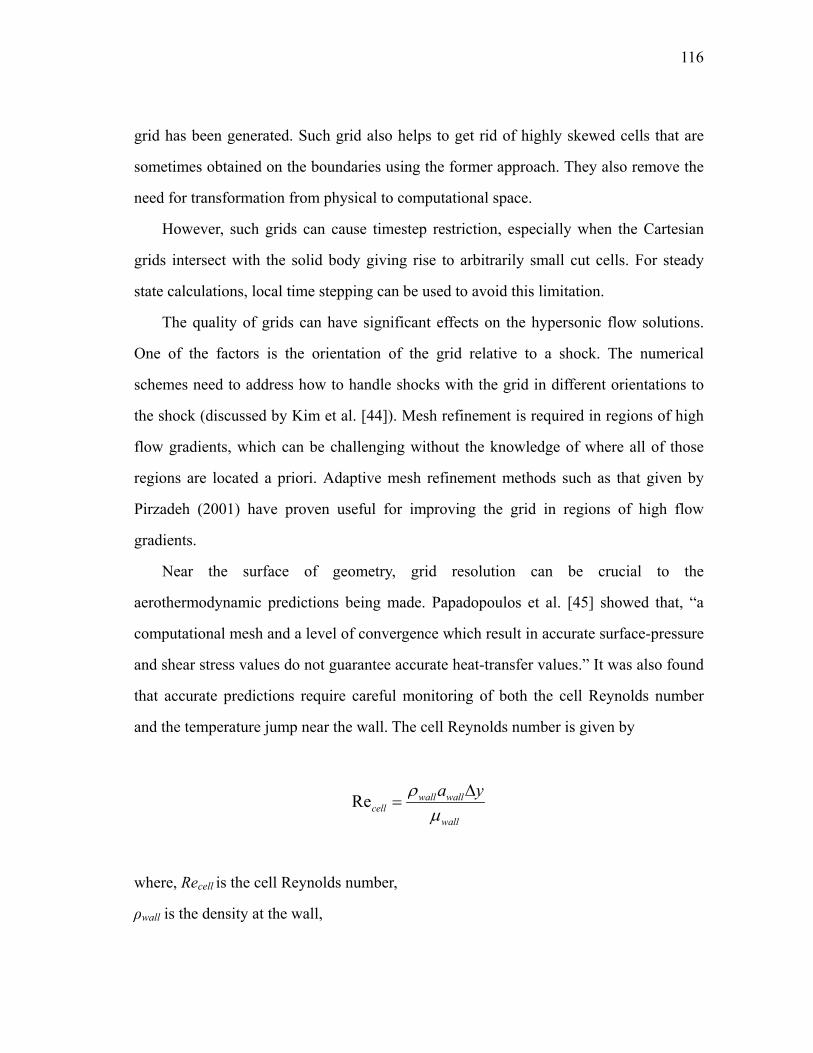
116
grid has been generated. Such grid also helps to get rid of highly skewed cells that are
sometimes obtained on the boundaries using the former approach. They also remove the
need for transformation from physical to computational space.
However, such grids can cause timestep restriction, especially when the Cartesian
grids intersect with the solid body giving rise to arbitrarily small cut cells. For steady
state calculations, local time stepping can be used to avoid this limitation.
The quality of grids can have significant effects on the hypersonic flow solutions.
One of the factors is the orientation of the grid relative to a shock. The numerical
schemes need to address how to handle shocks with the grid in different orientations to
the shock (discussed by Kim et al. [44]). Mesh refinement is required in regions of high
flow gradients, which can be challenging without the knowledge of where all of those
regions are located a priori. Adaptive mesh refinement methods such as that given by
Pirzadeh (2001) have proven useful for improving the grid in regions of high flow
gradients.
Near the surface of geometry, grid resolution can be crucial to the
aerothermodynamic predictions being made. Papadopoulos et al. [45] showed that, “a
computational mesh and a level of convergence which result in accurate surface-pressure
and shear stress values do not guarantee accurate heat-transfer values.” It was also found
that accurate predictions require careful monitoring of both the cell Reynolds number
and the temperature jump near the wall. The cell Reynolds number is given by
Re wall wallcell
wall
a yρµ
∆=
where, Recell is the cell Reynolds number,
ρwall is the density at the wall,
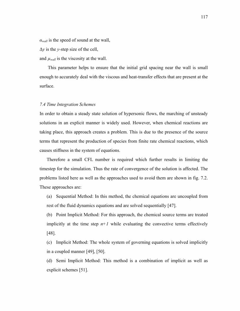
117
αwall is the speed of sound at the wall,
∆y is the y-step size of the cell,
and µwall is the viscosity at the wall.
This parameter helps to ensure that the initial grid spacing near the wall is small
enough to accurately deal with the viscous and heat-transfer effects that are present at the
surface.
7.4 Time Integration Schemes
In order to obtain a steady state solution of hypersonic flows, the marching of unsteady
solutions in an explicit manner is widely used. However, when chemical reactions are
taking place, this approach creates a problem. This is due to the presence of the source
terms that represent the production of species from finite rate chemical reactions, which
causes stiffness in the system of equations.
Therefore a small CFL number is required which further results in limiting the
timestep for the simulation. Thus the rate of convergence of the solution is affected. The
problems listed here as well as the approaches used to avoid them are shown in fig. 7.2.
These approaches are:
(a) Sequential Method: In this method, the chemical equations are uncoupled from
rest of the fluid dynamics equations and are solved sequentially [47].
(b) Point Implicit Method: For this approach, the chemical source terms are treated
implicitly at the time step n+1 while evaluating the convective terms effectively
[48].
(c) Implicit Method: The whole system of governing equations is solved implicitly
in a coupled manner [49], [50].
(d) Semi Implicit Method: This method is a combination of implicit as well as
explicit schemes [51].
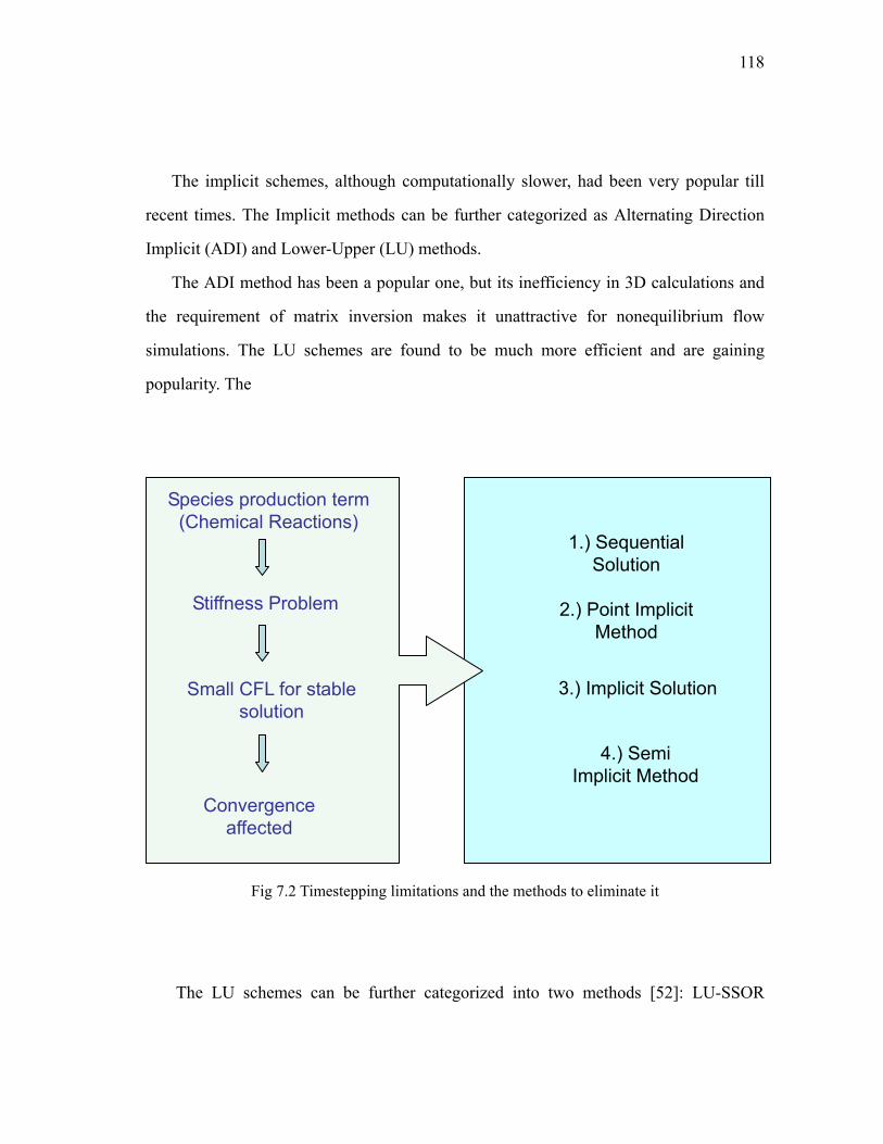
118
The implicit schemes, although computationally slower, had been very popular till
recent times. The Implicit methods can be further categorized as Alternating Direction
Implicit (ADI) and Lower-Upper (LU) methods.
The ADI method has been a popular one, but its inefficiency in 3D calculations and
the requirement of matrix inversion makes it unattractive for nonequilibrium flow
simulations. The LU schemes are found to be much more efficient and are gaining
popularity. The
Fig 7.2 Timestepping limitations and the methods to eliminate it
The LU schemes can be further categorized into two methods [52]: LU-SSOR
Species production term (Chemical Reactions)
Stiffness Problem
Small CFL for stable solution
Convergence affected
1.) Sequential Solution
2.) Point Implicit Method
3.) Implicit Solution
4.) Semi Implicit Method
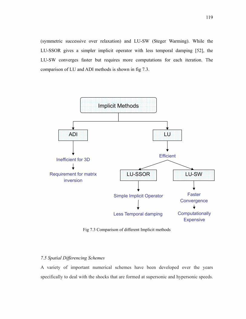
119
(symmetric successive over relaxation) and LU-SW (Steger Warming). While the
LU-SSOR gives a simpler implicit operator with less temporal damping [52], the
LU-SW converges faster but requires more computations for each iteration. The
comparison of LU and ADI methods is shown in fig 7.3.
Fig 7.3 Comparison of different Implicit methods
7.5 Spatial Differencing Schemes
A variety of important numerical schemes have been developed over the years
specifically to deal with the shocks that are formed at supersonic and hypersonic speeds.
Implicit Methods
ADI LU
LU-SSOR LU-SW
Inefficient for 3D
Requirement for matrix inversion
Efficient
Simple Implicit Operator
Less Temporal damping
Faster Convergence
Computationally Expensive
120
A majority of these methods fall into the “shock capturing” approach, where the
equations of fluid motion are solved to determine shock locations and strengths. One of
the first approaches of this kind was the explicit method of Lax & Wendroff (1960) and
the predictor-corrector scheme of MacCormack (1969).
A second method for predicting shocks is “shock fitting” approach, which was
proposed by Moretti (1974). In this method, the Rankine-Hugoniot shock relations are
used to determine shock jump conditions once the position of the shock is known. Most
of the algorithms developed over the years belong to the shock capturing category.
It is very well known that shocks cause instabilities in numerical methods and the
scheme should have the capability to take care of them. This is done either through
explicit addition of numerical dissipation or through some sort of upwind differencing.
However, the method of addition of numerical dissipation needed to dampen the shock
leads to inaccurate predictions of viscous phenomenon such as vortical flows or
boundary layers.
Therefore upwind schemes are preferred for eliminating the problem of shock
instabilities. Gudonov’s exact Reimann solver was the first scheme which was able to
capture shock waves without inducing spurious oscillations. Although Reimann Solvers
were widely used due to their robustness and high resolution of shock waves, they were
computationally very expensive.
Approximate Reimann Solvers were developed in order to make the above approach
more practical. The flux difference schemes based on this method are Roe’s scheme [53],
Osher’s scheme and the HLL scheme [54].
Another approach, known as the flux vector splitting method, is used for upwinding.
The popular schemes that fall under this category are Steger-Warming [55], Van Leer [56]
and Advection Upstream Splitting Method (AUSM) by Liou & Steffen [57].
The categorization of these upwind schemes and some advantages and

121
disadvantages are shown in the fig. 7.4.
Fig 7.4 Classification of upwind schemes
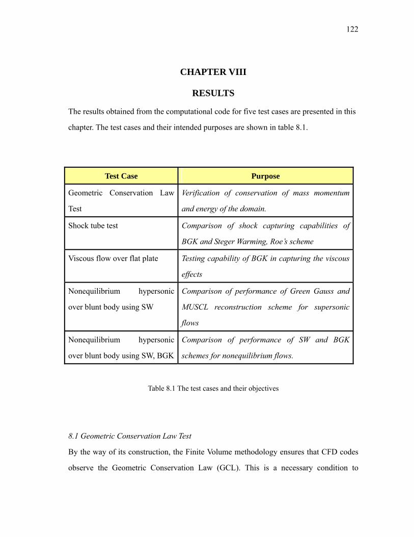
122
CHAPTER VIII
RESULTS
The results obtained from the computational code for five test cases are presented in this
chapter. The test cases and their intended purposes are shown in table 8.1.
Test Case Purpose
Geometric Conservation Law
Test
Verification of conservation of mass momentum
and energy of the domain.
Shock tube test Comparison of shock capturing capabilities of
BGK and Steger Warming, Roe’s scheme
Viscous flow over flat plate Testing capability of BGK in capturing the viscous
effects
Nonequilibrium hypersonic
over blunt body using SW
Comparison of performance of Green Gauss and
MUSCL reconstruction scheme for supersonic
flows
Nonequilibrium hypersonic
over blunt body using SW, BGK
Comparison of performance of SW and BGK
schemes for nonequilibrium flows.
Table 8.1 The test cases and their objectives
8.1 Geometric Conservation Law Test
By the way of its construction, the Finite Volume methodology ensures that CFD codes
observe the Geometric Conservation Law (GCL). This is a necessary condition to
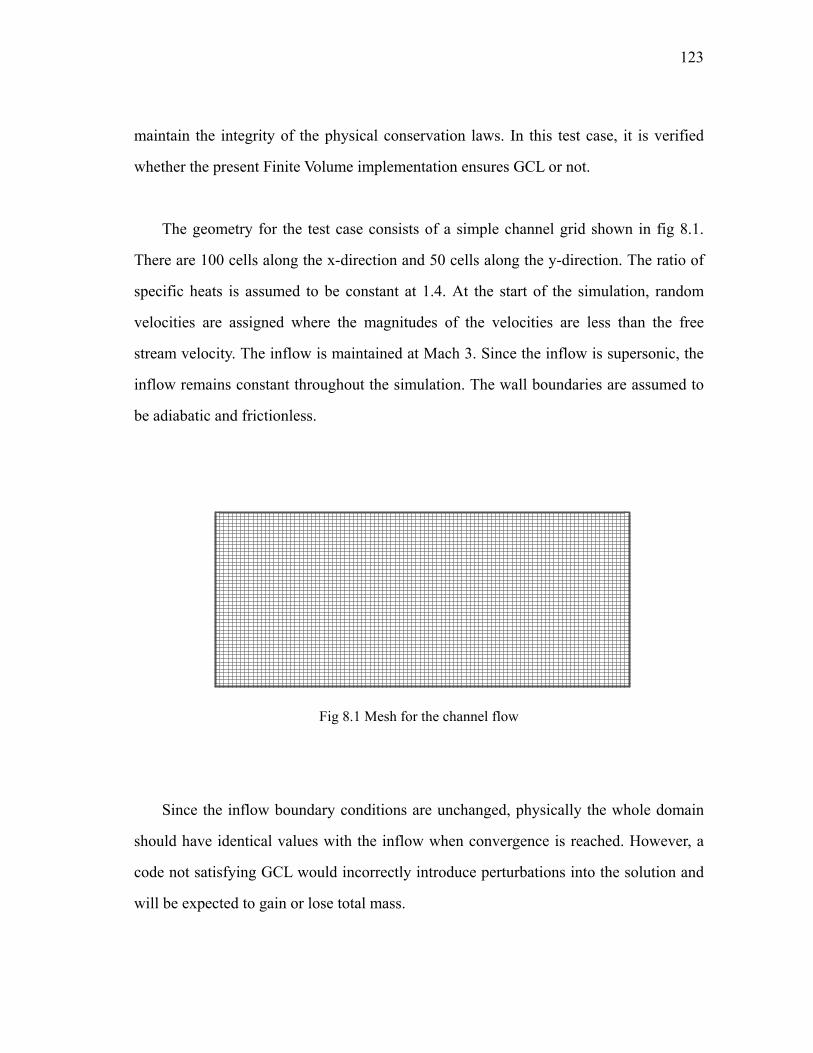
123
maintain the integrity of the physical conservation laws. In this test case, it is verified
whether the present Finite Volume implementation ensures GCL or not.
The geometry for the test case consists of a simple channel grid shown in fig 8.1.
There are 100 cells along the x-direction and 50 cells along the y-direction. The ratio of
specific heats is assumed to be constant at 1.4. At the start of the simulation, random
velocities are assigned where the magnitudes of the velocities are less than the free
stream velocity. The inflow is maintained at Mach 3. Since the inflow is supersonic, the
inflow remains constant throughout the simulation. The wall boundaries are assumed to
be adiabatic and frictionless.
Fig 8.1 Mesh for the channel flow
Since the inflow boundary conditions are unchanged, physically the whole domain
should have identical values with the inflow when convergence is reached. However, a
code not satisfying GCL would incorrectly introduce perturbations into the solution and
will be expected to gain or lose total mass.
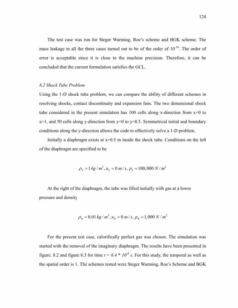
124
The test case was run for Steger Warming, Roe’s scheme and BGK scheme. The
mass leakage in all the three cases turned out to be of the order of 10-16. The order of
error is acceptable since it is close to the machine precision. Therefore, it can be
concluded that the current formulation satisfies the GCL.
8.2 Shock Tube Problem
Using the 1-D shock tube problem, we can compare the ability of different schemes in
resolving shocks, contact discontinuity and expansion fans. The two dimensional shock
tube considered in the present simulation has 100 cells along x-direction from x=0 to
x=1, and 50 cells along y-direction from y=0 to y=0.5. Symmetrical initial and boundary
conditions along the y-direction allows the code to effectively solve a 1-D problem.
Initially a diaphragm exists at x=0.5 m inside the shock tube. Conditions on the left
of the diaphragm are specified to be
3 21 / , 0 / , 100,000 /L L Lkg m u m s p N mρ = = =
At the right of the diaphragm, the tube was filled initially with gas at a lower
pressure and density
3 20.01 / , 0 / , 1,000 /R R Rkg m u m s p N mρ = = =
For the present test case, calorifically perfect gas was chosen. The simulation was
started with the removal of the imaginary diaphragm. The results have been presented in
figure. 8.2 and figure 8.3 for time t = 6.4 * 10-6 s. For this study, the temporal as well as
the spatial order is 1. The schemes tested were Steger Warming, Roe’s Scheme and BGK
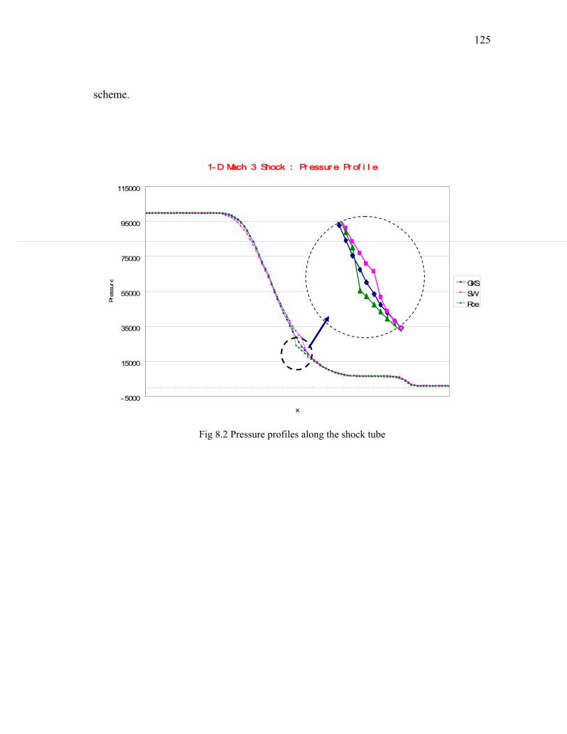
125
scheme.
Fig 8.2 Pressure profiles along the shock tube
1- D Mach 3 Shock : Pr essur e Pr of i l e
-5000
15000
35000
55000
75000
95000
115000
x
Pres
sure GKS
SWRoe
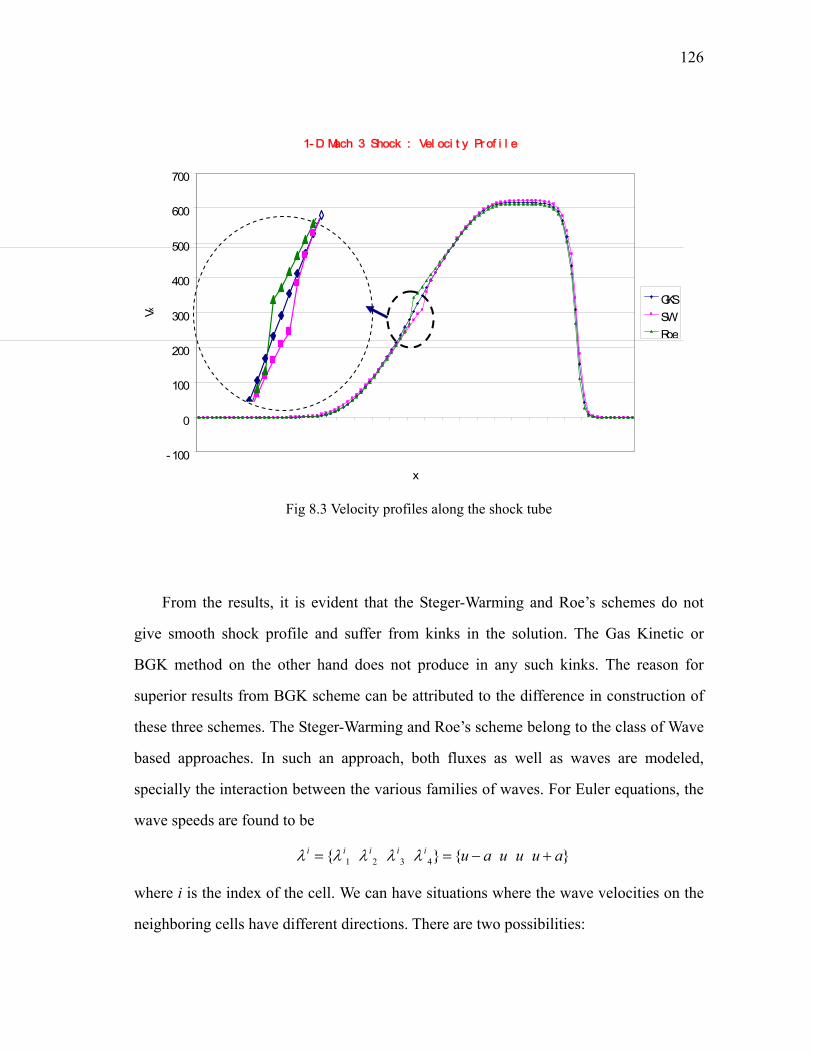
126
Fig 8.3 Velocity profiles along the shock tube
From the results, it is evident that the Steger-Warming and Roe’s schemes do not
give smooth shock profile and suffer from kinks in the solution. The Gas Kinetic or
BGK method on the other hand does not produce in any such kinks. The reason for
superior results from BGK scheme can be attributed to the difference in construction of
these three schemes. The Steger-Warming and Roe’s scheme belong to the class of Wave
based approaches. In such an approach, both fluxes as well as waves are modeled,
specially the interaction between the various families of waves. For Euler equations, the
wave speeds are found to be
1 2 3 4 i i i i i u a u u u aλ λ λ λ λ= = − +
where i is the index of the cell. We can have situations where the wave velocities on the
neighboring cells have different directions. There are two possibilities:
1- D Mach 3 Shock : Vel oci t y Pr of i l e
-100
0
100
200
300
400
500
600
700
x
Vx
GKSSWRoe
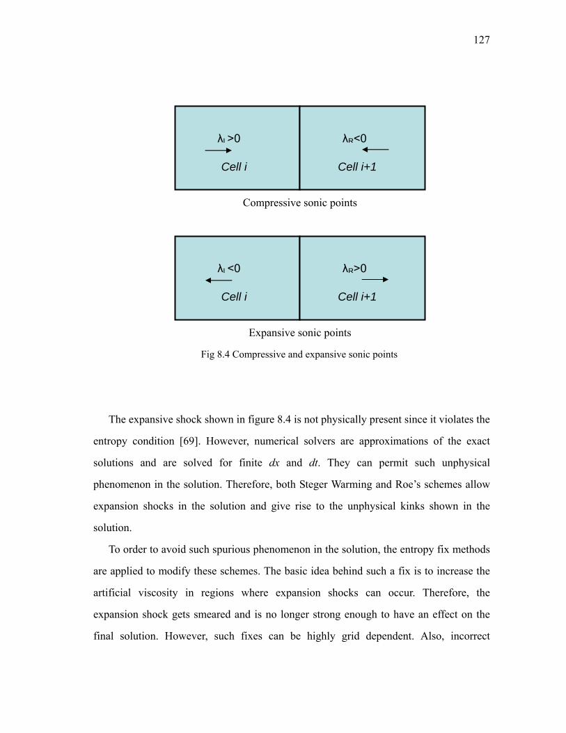
127
Compressive sonic points
Expansive sonic points
Fig 8.4 Compressive and expansive sonic points
The expansive shock shown in figure 8.4 is not physically present since it violates the
entropy condition [69]. However, numerical solvers are approximations of the exact
solutions and are solved for finite dx and dt. They can permit such unphysical
phenomenon in the solution. Therefore, both Steger Warming and Roe’s schemes allow
expansion shocks in the solution and give rise to the unphysical kinks shown in the
solution.
To order to avoid such spurious phenomenon in the solution, the entropy fix methods
are applied to modify these schemes. The basic idea behind such a fix is to increase the
artificial viscosity in regions where expansion shocks can occur. Therefore, the
expansion shock gets smeared and is no longer strong enough to have an effect on the
final solution. However, such fixes can be highly grid dependent. Also, incorrect
λL<0 λR>0
Cell i Cell i+1
λL>0 λR<0
Cell i Cell i+1
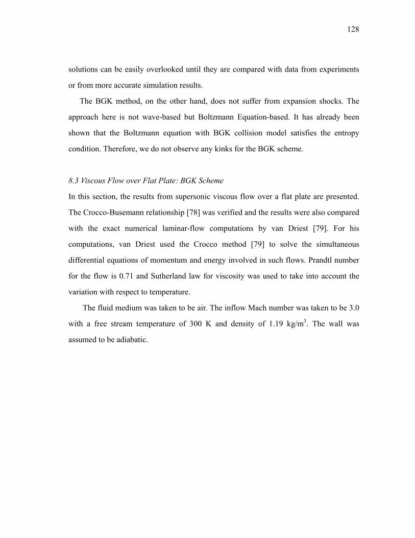
128
solutions can be easily overlooked until they are compared with data from experiments
or from more accurate simulation results.
The BGK method, on the other hand, does not suffer from expansion shocks. The
approach here is not wave-based but Boltzmann Equation-based. It has already been
shown that the Boltzmann equation with BGK collision model satisfies the entropy
condition. Therefore, we do not observe any kinks for the BGK scheme.
8.3 Viscous Flow over Flat Plate: BGK Scheme
In this section, the results from supersonic viscous flow over a flat plate are presented.
The Crocco-Busemann relationship [78] was verified and the results were also compared
with the exact numerical laminar-flow computations by van Driest [79]. For his
computations, van Driest used the Crocco method [79] to solve the simultaneous
differential equations of momentum and energy involved in such flows. Prandtl number
for the flow is 0.71 and Sutherland law for viscosity was used to take into account the
variation with respect to temperature.
The fluid medium was taken to be air. The inflow Mach number was taken to be 3.0
with a free stream temperature of 300 K and density of 1.19 kg/m3. The wall was
assumed to be adiabatic.
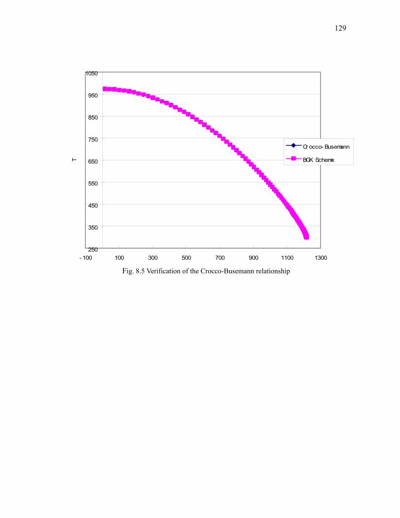
129
250
350
450
550
650
750
850
950
1050
- 100 100 300 500 700 900 1100 1300
T
Cr occo- Busemann
BGK Scheme
Fig. 8.5 Verification of the Crocco-Busemann relationship
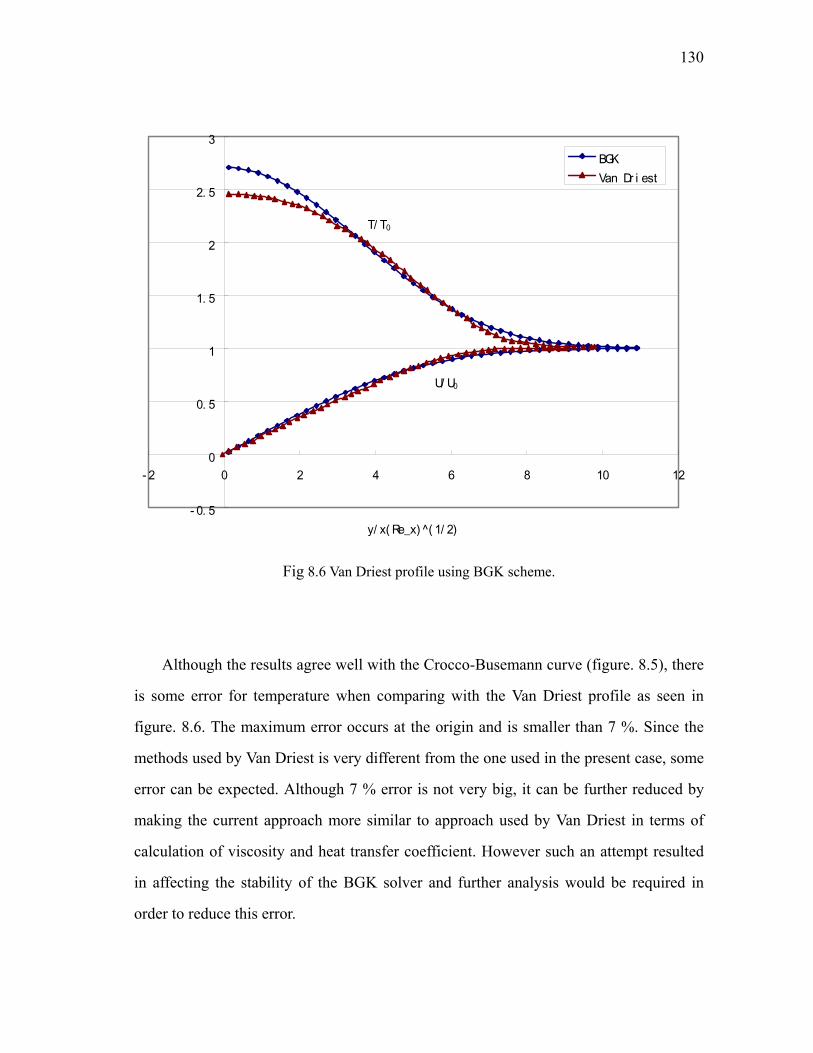
130
- 0. 5
0
0. 5
1
1. 5
2
2. 5
3
- 2 0 2 4 6 8 10 12
y/ x( Re_x) ^( 1/ 2)
BGKVan Dr i est
T/ T0
U/ U0
Fig 8.6 Van Driest profile using BGK scheme.
Although the results agree well with the Crocco-Busemann curve (figure. 8.5), there
is some error for temperature when comparing with the Van Driest profile as seen in
figure. 8.6. The maximum error occurs at the origin and is smaller than 7 %. Since the
methods used by Van Driest is very different from the one used in the present case, some
error can be expected. Although 7 % error is not very big, it can be further reduced by
making the current approach more similar to approach used by Van Driest in terms of
calculation of viscosity and heat transfer coefficient. However such an attempt resulted
in affecting the stability of the BGK solver and further analysis would be required in
order to reduce this error.
131
8.4 Reconstruction Schemes: Green Gauss and MUSCL Scheme
As discussed in Chapter VI, accuracy of the Finite Volume schemes can be increased to
higher orders using reconstruction schemes. In this study, the two popular approaches,
namely Green Gauss Reconstruction and MUSCL scheme are investigated and compared
using Steger-Warming scheme.
Inviscid flow of N2 past a flat ended cylinder of nose radius 1.0, placed in a
hypersonic uniform stream, is considered. The stream is assumed to be in thermal
nonequilibrium. A description of computational mesh along with the freestream
conditions is tabulated in the figure 8.7:
Gas M∞ T∞(K) p∞(Pa)
Nitrogen 6.5 300 50
Fig 8.7 Computational mesh for the blunt body problem
X-2 -1 0 1
0
0.5
1
1.5
2
2.5
3
160*120
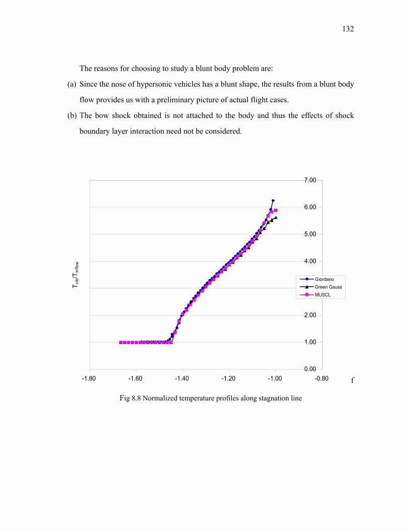
132
The reasons for choosing to study a blunt body problem are:
(a) Since the nose of hypersonic vehicles has a blunt shape, the results from a blunt body
flow provides us with a preliminary picture of actual flight cases.
(b) The bow shock obtained is not attached to the body and thus the effects of shock
boundary layer interaction need not be considered.
0.00
1.00
2.00
3.00
4.00
5.00
6.00
7.00
-1.80 -1.60 -1.40 -1.20 -1.00 -0.80
T vib/T
inflo
w
GiordanoGreen GaussMUSCL
f
Fig 8.8 Normalized temperature profiles along stagnation line
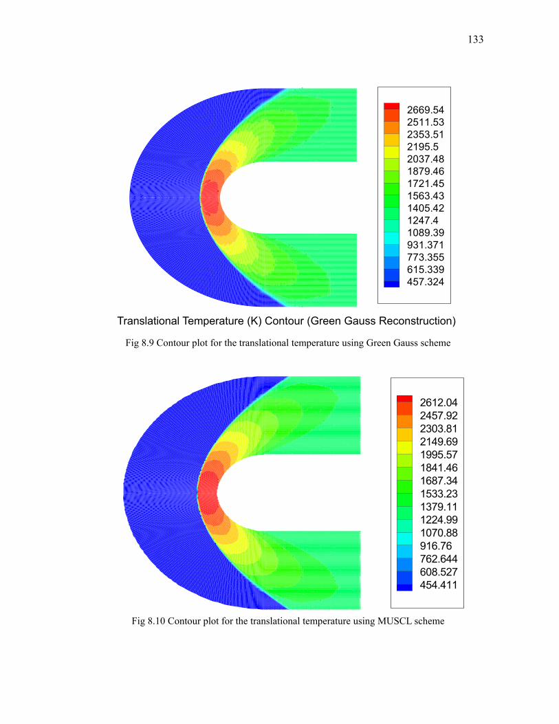
133
Fig 8.9 Contour plot for the translational temperature using Green Gauss scheme
Fig 8.10 Contour plot for the translational temperature using MUSCL scheme
2669.542511.532353.512195.52037.481879.461721.451563.431405.421247.41089.39931.371773.355615.339457.324
Translational Temperature (K) Contour (Green Gauss Reconstruction)
2612.042457.922303.812149.691995.571841.461687.341533.231379.111224.991070.88916.76762.644608.527454.411
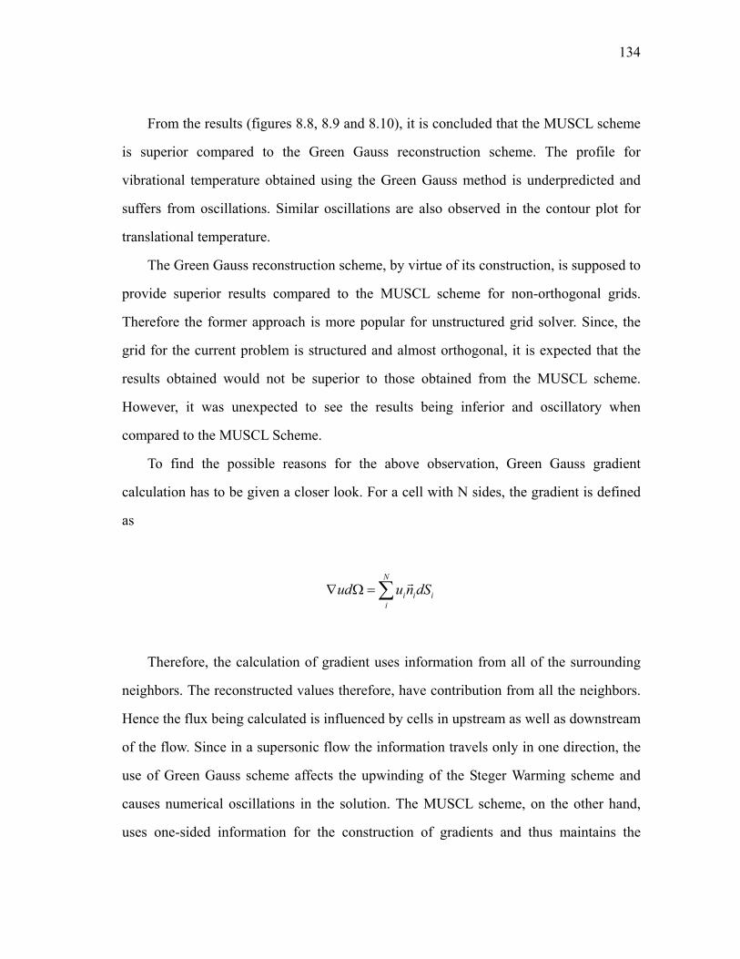
134
From the results (figures 8.8, 8.9 and 8.10), it is concluded that the MUSCL scheme
is superior compared to the Green Gauss reconstruction scheme. The profile for
vibrational temperature obtained using the Green Gauss method is underpredicted and
suffers from oscillations. Similar oscillations are also observed in the contour plot for
translational temperature.
The Green Gauss reconstruction scheme, by virtue of its construction, is supposed to
provide superior results compared to the MUSCL scheme for non-orthogonal grids.
Therefore the former approach is more popular for unstructured grid solver. Since, the
grid for the current problem is structured and almost orthogonal, it is expected that the
results obtained would not be superior to those obtained from the MUSCL scheme.
However, it was unexpected to see the results being inferior and oscillatory when
compared to the MUSCL Scheme.
To find the possible reasons for the above observation, Green Gauss gradient
calculation has to be given a closer look. For a cell with N sides, the gradient is defined
as
N
i i ii
ud u n dS∇ Ω =∑ r
Therefore, the calculation of gradient uses information from all of the surrounding
neighbors. The reconstructed values therefore, have contribution from all the neighbors.
Hence the flux being calculated is influenced by cells in upstream as well as downstream
of the flow. Since in a supersonic flow the information travels only in one direction, the
use of Green Gauss scheme affects the upwinding of the Steger Warming scheme and
causes numerical oscillations in the solution. The MUSCL scheme, on the other hand,
uses one-sided information for the construction of gradients and thus maintains the
135
upwinding nature of the scheme. Therefore, in solving high Mach number flows on
structured meshes, MUSCL scheme has clear advantages.
8.5 Nonequilibrium Hypersonic Flow over Blunt Body
In this section, the performances of the continuum based schemes (Steger Warming and
Roe’s scheme) and the Boltzmann based schemes (BGK scheme) are compared for
hypersonic nonequilibrium flows. The test case used for this purpose is the blunt body
problem. The reasons for selecting such a test case were discussed in previous section.
The test case also provides the opportunity to test the BGK scheme for any possible
failure because of the carbuncle phenomenon (described later in the section).
The grid and flow details are exactly the same as previous test case. The initial
condition in the domain is assumed to be the same as the free stream condition. The flux
is calculated using Steger Warming, Roe’s Scheme and BGK scheme. Second order
accuracy is obtained using the MUSCL scheme along with the Minmod limiter.
Iterations are carried out until steady state is reached. The vibrational nonequilibrium
physics is modeled using the Landau Teller method. The expression for the vibrational
relaxation time proposed by Millikan and White [19] is used. The specific heat ratio is
varied with temperature using the relation:
(7 / 2)(5 / 2)
vib
vib
RT eRT e
γ +=
+
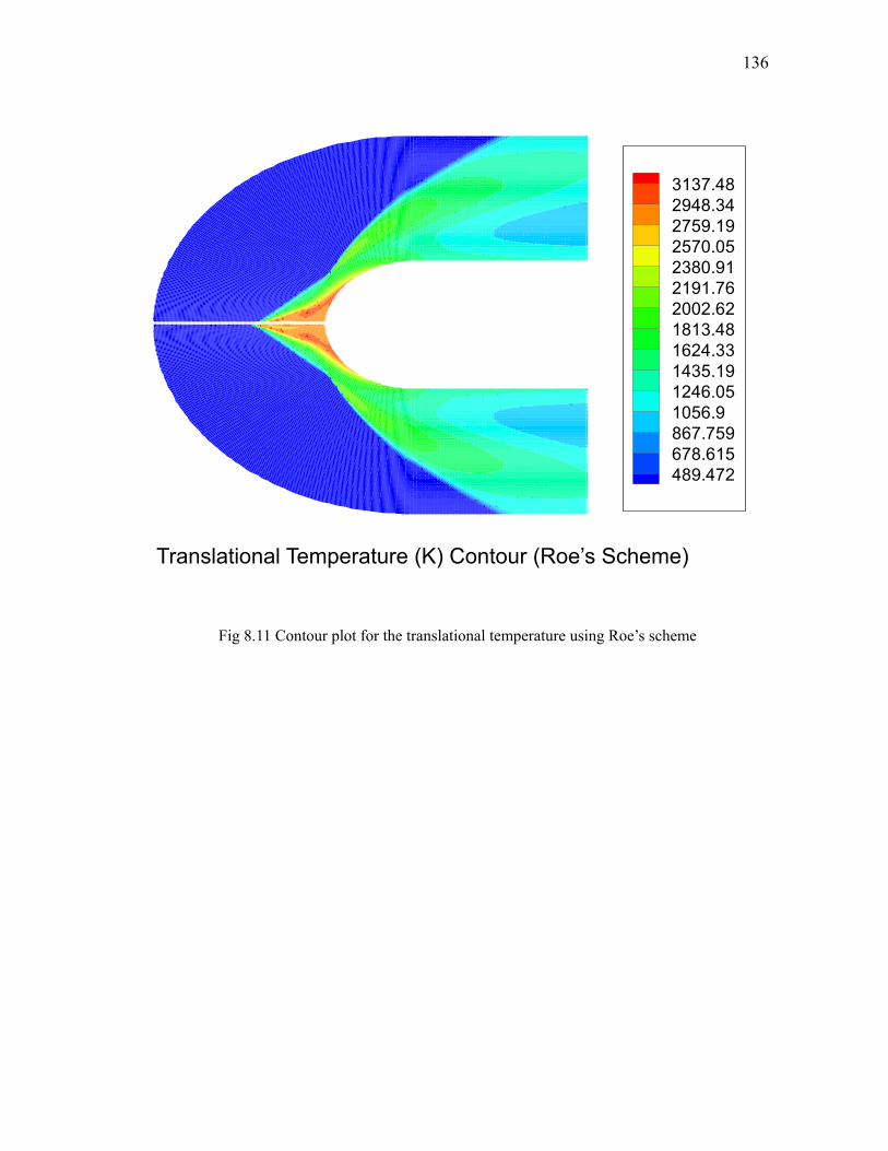
136
Fig 8.11 Contour plot for the translational temperature using Roe’s scheme
Translational Temperature (K) Contour (Roe’s Scheme)
3137.482948.342759.192570.052380.912191.762002.621813.481624.331435.191246.051056.9867.759678.615489.472
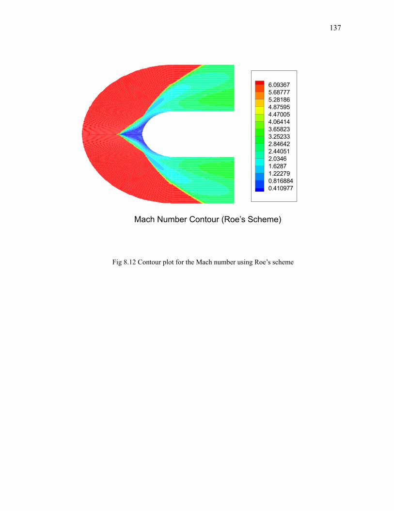
137
Fig 8.12 Contour plot for the Mach number using Roe’s scheme
6.093675.687775.281864.875954.470054.064143.658233.252332.846422.440512.03461.62871.222790.8168840.410977
Mach Number Contour (Roe’s Scheme)
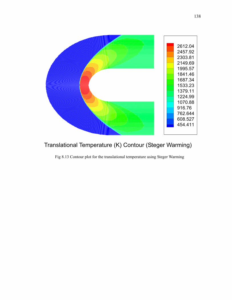
138
Fig 8.13 Contour plot for the translational temperature using Steger Warming
Translational Temperature (K) Contour (Steger Warming)
2612.042457.922303.812149.691995.571841.461687.341533.231379.111224.991070.88916.76762.644608.527454.411
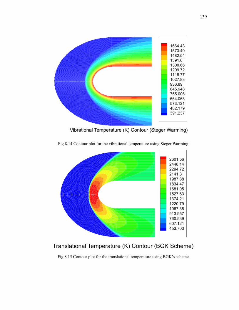
139
Fig 8.14 Contour plot for the vibrational temperature using Steger Warming
Translational Temperature (K) Contour (BGK Scheme)
Fig 8.15 Contour plot for the translational temperature using BGK’s scheme
Vibrational Temperature (K) Contour (Steger Warming)
1664.431573.491482.541391.61300.661209.721118.771027.83936.89845.948755.006664.063573.121482.179391.237
2601.562448.142294.722141.31987.881834.471681.051527.631374.211220.791067.38913.957760.539607.121453.703
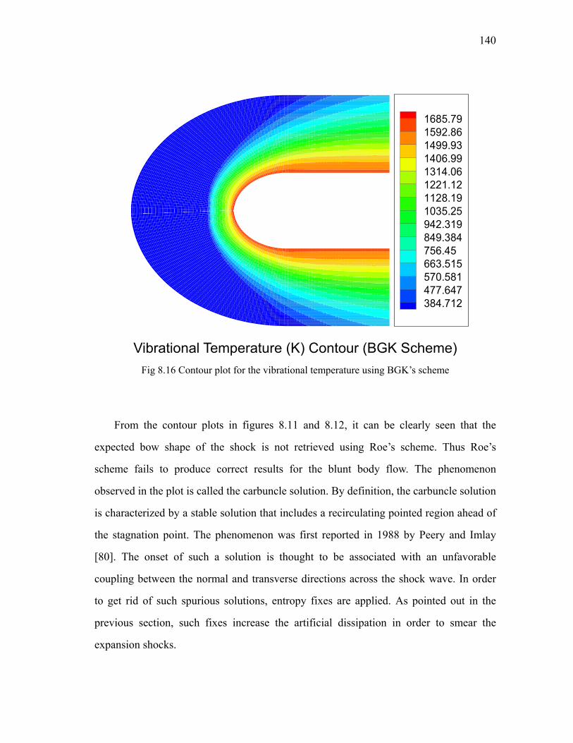
140
Vibrational Temperature (K) Contour (BGK Scheme) Fig 8.16 Contour plot for the vibrational temperature using BGK’s scheme
From the contour plots in figures 8.11 and 8.12, it can be clearly seen that the
expected bow shape of the shock is not retrieved using Roe’s scheme. Thus Roe’s
scheme fails to produce correct results for the blunt body flow. The phenomenon
observed in the plot is called the carbuncle solution. By definition, the carbuncle solution
is characterized by a stable solution that includes a recirculating pointed region ahead of
the stagnation point. The phenomenon was first reported in 1988 by Peery and Imlay
[80]. The onset of such a solution is thought to be associated with an unfavorable
coupling between the normal and transverse directions across the shock wave. In order
to get rid of such spurious solutions, entropy fixes are applied. As pointed out in the
previous section, such fixes increase the artificial dissipation in order to smear the
expansion shocks.
1685.791592.861499.931406.991314.061221.121128.191035.25942.319849.384756.45663.515570.581477.647384.712
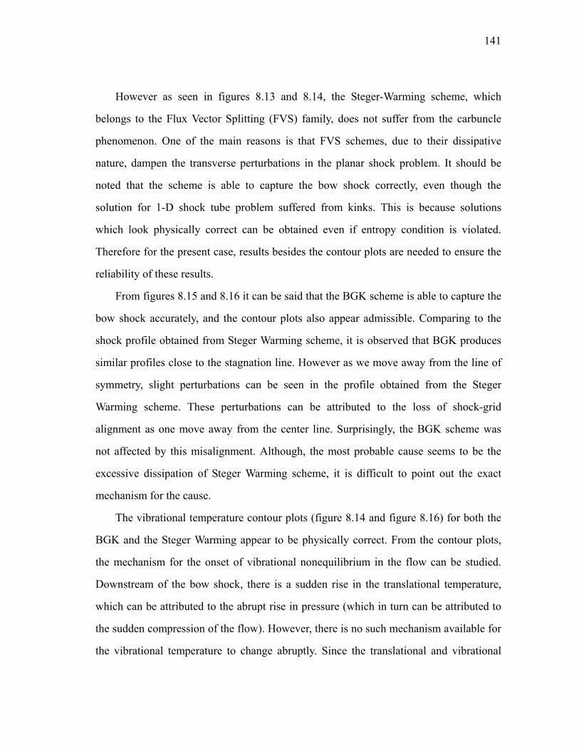
141
However as seen in figures 8.13 and 8.14, the Steger-Warming scheme, which
belongs to the Flux Vector Splitting (FVS) family, does not suffer from the carbuncle
phenomenon. One of the main reasons is that FVS schemes, due to their dissipative
nature, dampen the transverse perturbations in the planar shock problem. It should be
noted that the scheme is able to capture the bow shock correctly, even though the
solution for 1-D shock tube problem suffered from kinks. This is because solutions
which look physically correct can be obtained even if entropy condition is violated.
Therefore for the present case, results besides the contour plots are needed to ensure the
reliability of these results.
From figures 8.15 and 8.16 it can be said that the BGK scheme is able to capture the
bow shock accurately, and the contour plots also appear admissible. Comparing to the
shock profile obtained from Steger Warming scheme, it is observed that BGK produces
similar profiles close to the stagnation line. However as we move away from the line of
symmetry, slight perturbations can be seen in the profile obtained from the Steger
Warming scheme. These perturbations can be attributed to the loss of shock-grid
alignment as one move away from the center line. Surprisingly, the BGK scheme was
not affected by this misalignment. Although, the most probable cause seems to be the
excessive dissipation of Steger Warming scheme, it is difficult to point out the exact
mechanism for the cause.
The vibrational temperature contour plots (figure 8.14 and figure 8.16) for both the
BGK and the Steger Warming appear to be physically correct. From the contour plots,
the mechanism for the onset of vibrational nonequilibrium in the flow can be studied.
Downstream of the bow shock, there is a sudden rise in the translational temperature,
which can be attributed to the abrupt rise in pressure (which in turn can be attributed to
the sudden compression of the flow). However, there is no such mechanism available for
the vibrational temperature to change abruptly. Since the translational and vibrational
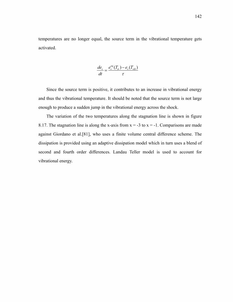
142
temperatures are no longer equal, the source term in the vibrational temperature gets
activated.
( ) ( )eqv v tr v vibde e T e T
dt τ−
=
Since the source term is positive, it contributes to an increase in vibrational energy
and thus the vibrational temperature. It should be noted that the source term is not large
enough to produce a sudden jump in the vibrational energy across the shock.
The variation of the two temperatures along the stagnation line is shown in figure
8.17. The stagnation line is along the x-axis from x = -3 to x = -1. Comparisons are made
against Giordano et al.[81], who uses a finite volume central difference scheme. The
dissipation is provided using an adaptive dissipation model which in turn uses a blend of
second and fourth order differences. Landau Teller model is used to account for
vibrational energy.
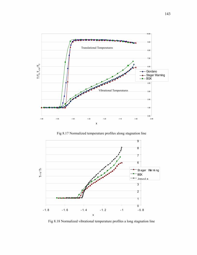
143
0.00
1.00
2.00
3.00
4.00
5.00
6.00
7.00
8.00
9.00
10.00
-1.60 -1.50 -1.40 -1.30 -1.20 -1.10 -1.00 -0.90
x
T/T 0
,Tvi
b,/T 0
GiordanoSteger WarmingBGK
Fig 8.17 Normalized temperature profiles along stagnation line
0
1
2
3
4
5
6
7
8
9
- 1. 8 - 1. 6 - 1. 4 - 1. 2 - 1 - 0. 8x
Tvib
/T0 St eger War mi ng
BGKJosyul a
Fig 8.18 Normalized vibrational temperature profiles a long stagnation line
Translational Temperatures
Vibrational Temperatures
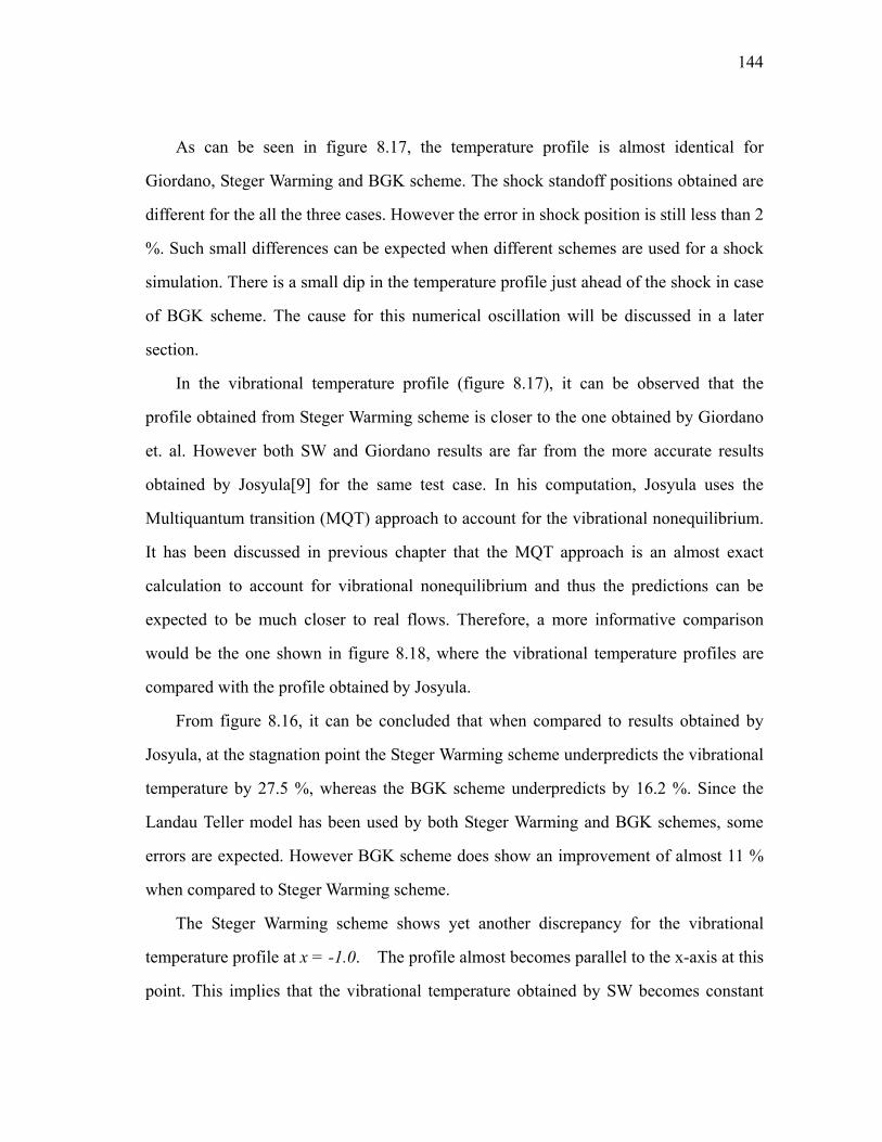
144
As can be seen in figure 8.17, the temperature profile is almost identical for
Giordano, Steger Warming and BGK scheme. The shock standoff positions obtained are
different for the all the three cases. However the error in shock position is still less than 2
%. Such small differences can be expected when different schemes are used for a shock
simulation. There is a small dip in the temperature profile just ahead of the shock in case
of BGK scheme. The cause for this numerical oscillation will be discussed in a later
section.
In the vibrational temperature profile (figure 8.17), it can be observed that the
profile obtained from Steger Warming scheme is closer to the one obtained by Giordano
et. al. However both SW and Giordano results are far from the more accurate results
obtained by Josyula[9] for the same test case. In his computation, Josyula uses the
Multiquantum transition (MQT) approach to account for the vibrational nonequilibrium.
It has been discussed in previous chapter that the MQT approach is an almost exact
calculation to account for vibrational nonequilibrium and thus the predictions can be
expected to be much closer to real flows. Therefore, a more informative comparison
would be the one shown in figure 8.18, where the vibrational temperature profiles are
compared with the profile obtained by Josyula.
From figure 8.16, it can be concluded that when compared to results obtained by
Josyula, at the stagnation point the Steger Warming scheme underpredicts the vibrational
temperature by 27.5 %, whereas the BGK scheme underpredicts by 16.2 %. Since the
Landau Teller model has been used by both Steger Warming and BGK schemes, some
errors are expected. However BGK scheme does show an improvement of almost 11 %
when compared to Steger Warming scheme.
The Steger Warming scheme shows yet another discrepancy for the vibrational
temperature profile at x = -1.0. The profile almost becomes parallel to the x-axis at this
point. This implies that the vibrational temperature obtained by SW becomes constant
145
very near to the stagnation point. This is not the case with the results obtained by Josyula
[9], where vibrational temperature keeps increasing even at the stagnation point. The
reason for this drop is again the high inherent dissipation present in the Steger Warming
scheme. The BGK scheme, on the other hand, does not show such a drop in slope and
thus once again outperforms the Steger Warming scheme.
146
CHAPTER IX
CONCLUSIONS AND SCOPE FOR FUTURE WORK
9.1 Conclusions
After a detailed literature survey and observations from the numerical results obtained
for various test cases, the following conclusions have been made.
(a) To account for vibrational nonequilibrium the Multiquantum transition or vibrational
kinetics method is the more accurate compared to Landau Teller model and Ruffin’s
model. However, due to its high computational demands, the Landau Teller(L-T) model
is more popular because of its simplicity and ease of implementation. The L-T model is
especially more popular for blunt body problems. This is because for flow over blunt
body undergoes compression. For such a case the V-T transfer dominates all the
vibrational energy levels. Hence even though the L-T model takes into account only the
V-T transfer (neglecting the V-V-T transfer), reasonable predictions can be expected
from it.
(b) To take into account another effect of nonequilibrium: on the chemical reaction rate
constants, the main approaches found in literature are those based on physiochemical
models and on semi empirical models. The most popular model used currently is the
Park’s two temperature model, which is simple and easy to implement in CFD codes.
(c) As in chemical models, two approaches can be used to model transport coefficient:
kinetic theory and curve fit based models. It was found that the curve fit models are
preferred for hypersonic flow simulations.
(d) From the results of shock tube problem, it can be concluded that the Boltzmann BGK
method has a clear advantage over the continuum based Steger Warming and Roe’s
147
schemes. The Steger Warming scheme, belonging to the Flux Vector Splitting class, and
Roe’s scheme, belonging to the Flux Difference Splitting class, may allow entropy
violating solutions and is the reason for the inaccurate results obtained. The Boltzmann
BGK always satisfies the entropy condition and hence accurately captures the shock.
(e) The Green Gauss reconstruction scheme performs poorly when compared to MUSCL
scheme when used to simulate vibrational nonequilibrium flow. It was found that the
Green Gauss scheme affects the upwinding of the scheme and thus results in oscillations
in the solution.
(f) The Boltzmann BGK scheme outperforms in Steger Warming schemes and Roe’s
schemes for the case of nonequilibrium flow over a blunt body. The Roe’s scheme
completely fails since it allows for expansion shocks in the solution. The Steger
Warming scheme, on the other hand produces poorer results due to excessive dissipation.
Although these failings can be avoided by using entropy fixes, such fixes tend to be
highly grid dependent. Since the hypersonic aircrafts have a blunt shape for the nose, the
Boltzmann BGK scheme seems to be a better option for simulating actual flight cases.
9.2 Scope for Future Work
(a) The Mutliquantum transition model to account for vibrational nonequilibrium can be
implemented so that the code can be used to solve expanding flows as well.
(b) The chemical nonequilibrium effects can be added by implementing the Park’s two
temperature model.
(c) The relation for relaxation time in the BGK model was derived assuming the
nonequilibrium distribution to be a first order expansion around the equilibrium
distribution. However a modified relaxation time can be implemented using a higher
order expansion for the nonequilibrium distribution function. This would enable the code
to be applicable to higher Knudsen number flows.

148
(d) The turbulence effects can be included using a one equation Spalart Allmaras model.
149
REFERENCES
[1] Anderson JD Jr. Hypersonic and High Temperature Gas Dynamics.
McGraw-Hill;New York, 1989.
[2] Napolitano LG. Belotserkovski OM.Computational Gasdynamics. CISM Courses and
Lectures n. 40; New York,1975.
[3] Park C. Nonequilibrium Hypersonic Aero Thermodynamics. John Wiley and Sons:
New York, 1990.
[4] Ivanov MS, Gimelshein SF. Computational Hypersonic Rarefied Flows. Annu. Rev.
Fluid Mech. 1998; 30:469–505.
[5] Leonardo CS, Boyd ID. Development of an Unstructured Navier-Stokes Solver for
Hypersonic Nonequilibrium Aerothermodynamics. 38th AIAA Thermophysics
Conference, Toronto, Canada, 6-9 June 2005.
[6] Schwartzentruber TE, Boyd ID. Detailed Analysis of a Hybrid CFD-DSMC Method
for Hypersonic Non-Equilibrium Flows. 38th AIAA Thermophysics Conference,
Toronto, Ontario Canada, 6-9 June 2005.
[7] Josyula E, Bailey WF. Multiquantum Vibrational Energy Exchanges in
Nonequilibrium Hypersonic Flows. 38th AIAA Thermophysics Conference, Toronto,
Ontario Canada, 6-9 June 2005.
[8] Josyula E, Bailey WF., Nonequilibrium Relaxation in High Speed Flows. 37th AIAA
Thermophysics Conference, Portland, Oregon, 28 June-1 July 2004.
[9] Josyula E. Computational Study of Vibrationally Relaxing Gas Past Blunt Body in
Hypersonic Flows, Journal of Thermophysics and Heat Transfers, vol. 14, 2000; pp.
18-26.
[10] Adamovich IV, Rich JW. Three-dimensional nonperturbative analytic model of
vibrational energy transfer in atom–molecule collisions. The Journal of Chemical
Physics, vol. 109, Issue 18, November 8, 1998, pp.7711-7724.
150
[11] Herzfeld KF, Litovitz TA. Absorption and Dispersion of Ultrasonic Waves.
Academic Press:. New York, 1959.
[12] Rapp D, Sharp TE. Vibrational Energy. Transfer in Molecular Collisions Involving
Large. Transition Probabilities. J. Chem. Phys, vol. 38, 1963; pp 2641.
[13] Rapp D, Golden PE. Resonant and Near Resonant Vibrational—Vibrational Energy
Transfer between Molecules in Collisions, J. Chem. Phys. vol. 40, 1964; pp 3120 .
[14] Sharma RD, Brau CA. Energy Transfer in Near-Resonant Molecular Collisions due
to Long-Range Forces, J. Chem. Phys, vol. 50, 1969; pp 924-930.
[15] Kerner EH, Note on The Forced and Damped Oscillator in Quantum Mechanics,
Can. J. Phys, vol. 36, 1958.: pp 371.
[16] Treanor CE. Vibrational Energy Transfer in High Energy Collisions, J. Chem. Phys,
vol. 43, 1965; pp 532.
[17] Zelechow A, Rapp D, Sharp TE. Vibrational-Vibrational Translational Energy
Transfer Between Two Diatomic Molecules, J. Chem. Phys, vol. 49, 1968; pp 286.
[18] Kelley JD, Vibrational Energy Transfer Processes in Collisions between Diatomic
Molecules, J. Chem. Phys. 56, 1972; pp 6108.
[19] Millikan RC, White DR. Systematics of Vibrational Relaxation, J. of Chem. Phys.,
vol. 39, 1963; pp. 3209–3213.
[20] Gupta RN, Yos JM, Thompson RA. A Review of Reaction Rates and
Thermodynamic and Transport Properties for the 11 Species Air Model for
Chemical and Thermal Nonequilibrium Calculations to 30000 K, NASA
TM-101528, 1989.
[21] Hammerling P, Teare JD, Kivel B. Theory of Radiation from Luminous Shock
Waves in Nitrogen, Physics of Fluids, vol. 2, no. (4), 1959; pp. 422–426.
[22] Treanor CE, Marrone PV. Effects of Dissociation on the Rate of Vibrational
Relaxation, Physics of Fluids, vol. 5, no. (9), 1962; pp. 1022–1026.
151
[23] Marrone PV, Treanor CE. Chemical Relaxation with Preferential Dissociation from
Excited Vibrational Levels, Physics of Fluids, vol. 6, no. (9), 1963; pp. 1215–1221.
[24] Josyula E, Bailey WF, Xu K. Nonequilibrium Relaxation in High Speed Flows, 37th
AIAA Thermophysics Conference, Portland, Oregon, 28 June - 1 July 2004.
[25] Knab O, Fruhauf HH, Messerschmid EW. Theory and Validation of the Physically
Consistent Coupled Vibration-Chemistry-Vibration Model, Journal of
Thermophysics and Heat Transfer, vol. 9, no. (2), 1995; pp. 219–226.
[26] Curtiss C, Hirschfelder JO. Transport Properties of Multicomponent Gas Mixtures,
J. Chem. Phys., vol. 17, no. (6), 1949; p. 550-555.
[27] Hirschfelder JO, Curtiss CF, Bird RB. Molecular Theory of Gases and Liquids,
John Wiley and Sons, New York, 1954.
[28] Hirschfelder JO. Heat Conductivity in Polyatomic or Electronically Excited Gases
II., J. Chem Phys., vol. 26, no. (2), 1957; pp. 282-285.
[29] Wilke CR. A Viscosity Equation for Gas Mixtures, J. Chem. Phys, vol. 18, no.(4) ,
1950; p. 517-519.
[30] Mason E, Saxena S. Approximate Formula for the Thermal Conductivity of Gas
Mixtures, Physics of Fluids, vol. 1, no. (5), 1958; pp. 361-369.
[31] Hanson C. Approximations for the Thermodynamic and Transport Properties of
High-Temperature Air, NASA TR-50, 1960.
[32] Viegas J, Howe J. Thermodynamic and Transport Property Correlation Formulas
for Equilibrium Air from 1,000 K to 15,000 K, NASA TN D-1429, 1962.
[33] Blottner F. Chemically Reacting Viscous Flow Program for Multi-Component Gas
Mixtures, Sandia Labs Report SCRR-70-754, 1971.
[34] Candler G. The Computation of Weakly Ionized Hypersonic Flows in
Thermo-Chemical Nonequilibrium, Journal of Thermophysics and Heat Transfer,
vol. 5, no.(3) , 1991; pp 266-273.
152
[35] Macheret SO, Rich JW. Nonequilibrium Dissociation Rates behind Strong Shock
Waves. Chemical Physics, vol. 174, no.(1),1993; pp 25-43.
[36] Macheret SO, Fridman AA, Adamovich IV, Rich JW, Treanor CE. Mechanisms of
Nonequilibrium Dissociation of Diatomic Molecules. Joint Thermophysics and Heat
Transfer Conference, 6th, Colorado Springs, Colorado, 20-23 June 1994.
[37] Gonzales DA, Varghese P.L. Evaluation of Simple Rate Expressions for
Vibration-Dissociation Coupling. Journal of Thermophysics and Heat Transfer, vol
8, no.(2), 1994; pp 236-243.
[38] Kiefer JH, Hadjuk JC. A Vibrational Bias Mechanism for Diatomic Dissociation :
Induction Times and Steady Rates for 02, H2 and D2 Dilute in Argon,. J. Chem. Phys,.
vol. 38, 1979; pp 329-340.
[39] Sharma SP, Huo WM., Park C. Rate Parameters for Coupled Vibration-Dissociation
in a Generalized SSH Approximation. Jour. Thermo. Heat. Transf,. vol. 6, no.(1),
1992; pp 9-21.
[40] Losev SA, Makarov VN, Pogosbekyan MJ, Shatalov OP. Thermochemical
Nonequilibrium Kinetic Models in Strong Shock Waves in Air. Joint Thermophysics
and Heat Transfer Conference, 6th, Colorado Springs, Colorado, 20-23 June 1994.
[41] Park C. Assessment of a Two-Temperature Kinetic Model for Dissociating and
Weakly Ionizing Nitrogen. AIAA and ASME, Joint Thermophysics and Heat
Transfer Conference, 4th, Boston, Massachusetts, June 2-4, 1986.
[42] Palmer G. An Assessment of Transport Property Methodologies for Hypersonic
Flows, AIAA, Aerospace Sciences Meeting & Exhibit, 35th, Reno, Nevada, Jan. 6-9,
1997.
[43] Bertin JJ, Cummings RM. Critical Hypersonic Aerothermodynamic Phenomena.
Annu. Rev. Fluid Mech. vol. 38, 2006; pp 129–57.
[44] Kim KH, Kim C, Rho OH. Methods for the Accurate Computations of Hypersonic
153
Flows: AUSMPW+ scheme. J. Comput. Phys, vol. 174, 2001; pp 38–80.
[45] Pirzadeh S. Vortical Flow Prediction Using an Adaptive Unstructured Grid Method.
RTO Applied Vehicle Technology (AVT) Panel, Loen, Norway, May 2001.
[46] Papadopoulos P, Venkatapathy E, Prabhu D, Loomis MP, Olynick D. Current
Grid-generation Strategies and Future Requirements in Hypersonic Vehicle Design,
Analysis, and Testing., Appl. Math. Model, vol. 23, 1999; pp 705–735.
[47] Ait-Ali-Yahia D, Habashi WG. Finite Element Adaptive Method for Hypersonic
Thermochemical Nonequilibrium Flows. AIAA Journal, vol. 35, no. (8), August
1997; pp 1294.
[48] Palmer G, Venkatapathy E. Comparison of Nonequilibrium Solution Algorithms
Applied to Chemically Stiff Hypersonic Flows. AIAA Journal, vol. 33, no. (7), July
1995; pp 1211-1219.
[49] Ju Y. Lower-Upper Scheme for Chemically Reacting Flow with Finite Rate
Chemistry. AIAA Journal, vol. 33, no. (7), July 1995; pp 1418-1425.
[50] Park C, Yoon S. Fully Coupled Implicit Method for Thermochemical
Nonequilibrium Air at Suborbital Flight Speeds. AIAA Computational Fluid
Dynamics Conference, 9th, Buffalo, New York; 13-15 June 1989;. pp. 440-449.
[51] Bertolazzi E. A Finite Volume Scheme for Two Dimensional Chemically Reactive
Hypersonic Flow. International Journal of Numerical Methods for Heat & Fluid
Flow, vol. 8, no. (8), 1998; pp 888-933.
[52] Tsai YLP, Hsieh KC. Comparative Study of Computational Efficiency of Two LU
Schemes for Non-Equilibrium Reacting Flows. Aerospace Sciences Meeting, 28th,
Reno, Nevada, Jan 8-11, 1990.
[53] Roe PL. Approximate Riemann Solver, Parameter Vector and Difference Schemes,
Journal of Computational Physics, vol. 43:1981: pp 357-372,
[54] Harten A, Lax PD, Leer BV. On Upstream Differencing and Godunov-type
154
Schemes for Hyperbolic Conservation Laws, SIAM Rev., vol. 25, 1983; pp 35-61.
[55] Steger JL, Warming RF. Flux Vector Splitting of the Inviscid Gas Dynamics
Equations with Application to Finite Difference Methods. Journal of Computational
Physics, vol. 40, 1981, pp 263-293.
[56] B. Van Leer. Flux-Vector Splitting for the Euler Equations, Lecture Notes in Physics,
170:507-512, 1982;.pp 507-512.
[57] Liou MS, Steffen CJ. A New Flux Splitting Scheme, Journal of Computational
Physics, vol. 107, July 1993, pp.23-39.
[58] Ruffin SM. Vibrational Energy Transfer of Diatomic Gases in Hypersonic
Expanding Flows, PhD. Dissertation, SUDDAR 635, Stanford Univ., Stanford,
California, June 1993.
[59] Ruffin SM. Prediction of Vibrational Relaxation in Hypersonic Expanding Flows
Part I : Model Development. Journal of Thermophysics and Heat Transfer, vol. 9,
no. (3), 1995; p. 432.
[60] Ruffin S M. Prediction of Vibrational Relaxation in Hypersonic Expanding Flows
Part II: Results. Journal of Thermophysics and Heat Transfer, vol. 9, no. (3), 1995;
pp. 438.
[61] Wang WL, Boyd ID. Hybrid DSMC-CFD Simulations of Hypersonic Flow over
Sharp and Blunted Bodies, 36th AIAA Thermophysics Conference, Orlando Florida,
June 23-26, 2003.
[62] Anderson JD. Computational Fluid Dynamics: The Basics with Applications,
McGraw-Hill: New York, 1995.
[63] MacCormack RW. The Effect of Viscosity in Hypervelocity Impact Cratering,
AIAA Paper, 1969; pp 354.
[64] Hirsch C. The Finite Difference Method, Numerical Computation of Internal and
External Flows, vol. 1, chap. 4, John Wiley and Sons: Chichester, United Kingdom,
155
1988, pp. 167–200.
[65] Hirsch C, Finite Volume Method and Conservative Discretizations, Numerical
Computation of Internal and External Flows, vol. 1, chap. 6, John Wiley and Sons:
Chichester, United Kingdom, 1988, pp. 237–264.
[66] Rizzi AW, Inouye M. Time-Split Finite-Volume Method for Three-Dimensional
Blunt-Body Flow, AIAA Journal, vol. 11, no. (11), Nov. 1973; pp. 1478–1485.
[67] Hirsch C. The Finite Element Method, Numerical Computation of Internal and
External Flows, vol. 1, chap. 5, John Wiley and Sons: Chichester, United Kingdom,
1988, pp. 201–236.
[68] Hirsch C. Numerical Computation of Internal and External Flows, John Wiley &
Sons: New York 1991.
[69] Laney CB. Computational Gas Dynamics. Cambridge University Press: New York
1998.
[70] Harris S. An Introduction to the Theory of the Boltzmann Equation, Dover
Publications: New York 1971.
[71] Bhatnagar PL, Gross EP, Krook M. A Model for Collision Processes in Gases. Phys.
Rev., 1954; pp. 511.
[72] Vincenti WG, Kruger CH. Introduction to Physical Gas Dynamics. John Wiley &
Sons: New York 1965.
[73] Xu K, Martinelli L, Jameson A, Gas-kinetic Finite Volume Methods, Flux-Vector
Splitting, and Artificial Diffusion. Journal of Computational Physics, vol. 120,
no.(1), Aug. 1995; p.48-65.
[74] Xu K. A Gas-Kinetic BGK Scheme for the Navier-Stokes Equations and Its
Connection with Artificial Dissipation and Godunov Method. Journal of
Computational Physics, vol. 171, no (1), 20 July 200; pp. 289-335.
[75] Godunov SK. A Difference Scheme for Numerical Computation of Discontinuous
156
Solution of Hydrodynamic Equations, Matematicheskii Sbornik, vol. 47, 1959; pp.
271–306 (in Russian).
[76] Leonardo S, Boyd I. Numerical Simulation of Weakly Ionized Hypersonic Flow for
Reentry Configurations. 9th AIAA/ASME Joint Thermophysics and Heat Transfer
Conference, San Francisco, California, 5-8 June, 2005.
[77] Choi H, Liu JG. The Reconstruction of Upwind Fluxes for Conservation Laws: Its
Behavior in Dynamics and Steady State Calculations, Journal of Computational
Physics, vol. 144, no. (2), Aug. 1998; pp. 237–256.
[78] White FM. Viscous Fluid Flow. McGraw Hill: New York 2005.
[79] Van Driest R. Investigation of Laminar Boundary Layer and Compressible Fluids
Using the Crocco. Method. Technical Note. TN. 2597, NACA, January. 1952.
[80] Peery KM , Imlay ST. Blunt Body Flow Simulations, AIAA Paper 1988; pp 2924.
[81] Belluci GD, Colonna V, Capitelli G, Armenise MI, Bruno C. Vibrationally Relaxing
Flow of N2 Past an Infinite Cylinder. Journal of Thermophysics and Heat Transfer,
vol. 11, no.(1), 1997; pp. 27-35.
[82] Tennekes H, Lumley JL. A First Course on Turbulence. IBM Univers Medium;
Boston, Massachusetts 1972.
[83] Spalart PR, Allmaras SR A One-Equation Turbulence Model for Aerodynamic
Flows. AIAA Paper, January 1992; pp 439.
[84] Baldwin BS, Barth TJ. A One-equation Turbulence Transport Model for High
Reynolds Number for Wall-Bounded Flows. NASA TM 102847, 1990.
[85] Schlichting, H. Boundary Layer Theory, McGraw-Hill: New York, 1979.
[86] Jiang YT, Damodaran M, Lee KH. High Resolution Finite Volume Computation of
Turbulence Transonic Flow Past Airfoils. AIAA Journal, vol. 35, no.(7), July 1997;
pp 1134-1142.
[87] Raman IR. http://neon.otago.ac.nz/chemlect/chem306/pca/IR_Raman/

157
Hyperphysics, Principal Component Analysis, University of Otago, New Zealand,
2007
158
VITA
Name: Sunny Jain Address: H.R. Bright Building, Rm. 631B 3141 TAMU College Station, TX 77843-3141 Education: B.Tech., Aerospace Engineering, Indian Institute of Technology Bombay,
2005 M.S., Aerospace Engineering, Texas A&M University, 2007