Hyperclique pattern discovery - Hui Xiong - Rutgers...

10618_2006_43 styleAv1.cls (2006/04/29 v1.1 LaTeX Springer document class) May 19, 2006 22:19

Data Min Knowl DiscDOI 10.1007/s10618-006-0043-9

Hyperclique pattern discovery

Hui Xiong · Pang-Ning Tan · Vipin Kumar

Received: 11 February 2004 / Accepted: 6 February 2006C© Springer Science + Business Media, LLC 2006

Abstract Existing algorithms for mining association patterns often rely on the support-based pruning strategy to prune a combinatorial search space. However, this strategy isnot effective for discovering potentially interesting patterns at low levels of support. Also,it tends to generate too many spurious patterns involving items which are from differentsupport levels and are poorly correlated. In this paper, we present a framework for mininghighly-correlated association patterns called hyperclique patterns. In this framework, an ob-jective measure called h-confidence is applied to discover hyperclique patterns. We provethat the items in a hyperclique pattern have a guaranteed level of global pairwise similarityto one another as measured by the cosine similarity (uncentered Pearson’s correlation co-efficient). Also, we show that the h-confidence measure satisfies a cross-support propertywhich can help efficiently eliminate spurious patterns involving items with substantiallydifferent support levels. Indeed, this cross-support property is not limited to h-confidenceand can be generalized to some other association measures. In addition, an algorithm calledhyperclique miner is proposed to exploit both cross-support and anti-monotone properties ofthe h-confidence measure for the efficient discovery of hyperclique patterns. Finally, our ex-perimental results show that hyperclique miner can efficiently identify hyperclique patterns,even at extremely low levels of support.

Keywords Association analysis . Hyperclique patterns . Pattern Mining

H. Xiong (�)Department of Management Science & Information Systems, Rutgers University, Ackerson Hall,180 University Avenue, Newark, NJ 07102e-mail: [email protected]

P.-N. TanDepartment of Computer Science & Engineering, Michigan State University, 3115 EngineeringBuilding, East Lansing, MI 48824-1226e-mail: [email protected]

V. KumarDepartment of Computer Science and Engineering, University of Minnesota, 4-192, EE/CSci Building,Minneapolis, MN 55455e-mail: [email protected]

Springer


Data Min Knowl Disc

1. Introduction

Many data sets have inherently skewed support distributions. For example, the frequencydistribution of English words appearing in text documents is highly skewed—while a fewof the words may appear many times, most of the words appear only a few times. Such adistribution has also been observed in other application domains, including retail data, Webclick-streams, and telecommunication data.

This paper examines the problem of mining association patterns (Agrawal et al., 1993)from data sets with skewed support distributions. Most of the algorithms developed so far relyon the support-based pruning strategy to prune the combinatorial search space. However, thisstrategy is not effective for data sets with skewed support distributions due to the followingreasons.

– If the minimum support threshold is low, we may extract too many spurious patternsinvolving items with substantially different support levels. We call such patterns as weakly-related cross-support patterns. For example, {Caviar, Milk} is a possible weakly-related cross-support pattern since the support for an expensive item such as Caviar isexpected to be much lower than the support for an inexpensive item such as Milk. Suchpatterns are spurious because they tend to be poorly correlated. Using a low minimumsupport threshold also increases the computational and memory requirements of currentstate-of-the-art algorithms considerably.

– If the minimum support threshold is high, we may miss many interesting patterns occurringat low levels of support (Hastie et al., 2001). Examples of such patterns are associationsamong rare but expensive items such as caviar and vodka, gold necklaces and earrings, orTVs and DVD players.

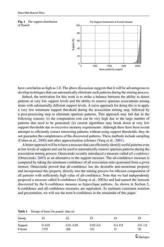
As an illustration, consider thepumsb census data set,1 which is often used as a benchmarkdata set for evaluating the computational performance of association rule mining algorithms.Figure 1 shows the skewed nature of the support distribution. Note that 81.5% of the itemshave support less than 0.01 while only 0.95% of them having support greater than 0.9.

Table 1 shows a partitioning of these items into five disjoint groups based on their supportlevels. The first group, S1, has the lowest support level (less than or equal to 0.01) but containsthe most number of items (i.e., 1735 items). In order to detect patterns involving items fromS1, we need to set the minimum support threshold to be less than 0.01. However, such alow support threshold will degrade the performance of existing algorithms considerably.For example, our experiments showed that, when applied to the pumsb data set at supportthreshold less than 0.4,2 state-of-the-art algorithms such as Apriori (Agrawal and Srikant,1994) and Charm (Zaki and Hsiao, 2002) break down due to excessive memory requirements.Even if a machine with unlimited memory is provided, such algorithms can still producea large number of weakly-related cross-support patterns when the support threshold is low.Just to give an indication of the scale, out of the 18847 frequent pairs involving items from S1and S5 at support level 0.0005, about 93% of them are cross-support patterns, i.e., containingitems from both S1 and S5. The pair wise correlations within these cross-support patternsare extremely poor because the presence of the item from S5 does not necessarily implythe presence of the item from S1. Indeed, the maximum correlation obtained from thesecross-support patterns is only 0.029377. In contrast, item pairs from S1 alone or S5 alone

1 It is available at http://www.almaden.ibm.com/ software/quest/resources.2 This is observed on Sun Ultra 10 work station with a 440 MHz CPU and 128 Mbytes of memory.

Springer


Data Min Knowl Disc

0

20

40

60

80

100

0 500 1000 1500 2000

Sup

port

(%

)

Items sorted by support

The Support Distribution of Pumsb DatasetFig. 1 The support distributionof Pumsb

have correlation as high as 1.0. The above discussion suggests that it will be advantageous todevelop techniques that can automatically eliminate such patterns during the mining process.

Indeed, the motivation for this work is to strike a balance between the ability to detectpatterns at very low support levels and the ability to remove spurious associations amongitems with substantially different support levels. A naive approach for doing this is to applya very low minimum support threshold during the association mining step, followed bya post-processing step to eliminate spurious patterns. This approach may fail due to thefollowing reasons: (i) the computation cost can be very high due to the large number ofpatterns that need to be generated; (ii) current algorithms may break down at very lowsupport thresholds due to excessive memory requirements. Although there have been recentattempts to efficiently extract interesting patterns without using support thresholds, they donot guarantee the completeness of the discovered patterns. These methods include sampling(Cohen et al., 2000) and other approximation schemes (Yang et al., 2001).

A better approach will be to have a measure that can efficiently identify useful patterns evenat low levels of support and can be used to automatically remove spurious patterns during theassociation mining process. Omiecinski recently introduced a measure called all-confidence(Omiecinski, 2003) as an alternative to the support measure. The all-confidence measure iscomputed by taking the minimum confidence of all association rules generated from a givenitemset. Omiecinski proved that all-confidence has the desirable anti-monotone propertyand incorporated this property directly into the mining process for efficient computation ofall patterns with sufficiently high value of all-confidence. Note that we had independentlyproposed a measure called h-confidence (Xiong et al., 2003a) and had named the itemsetsdiscovered by the h-confidence measure as hyperclique patterns. As shown in Section 2,h-confidence and all-confidence measures are equivalent. To maintain consistent notationand presentation, we will use the term h-confidence in the remainder of this paper.

Table 1 Groups of items for pumsb data set

Group S1 S2 S3 S4 S5

Support 0–0.01 0.01–0.05 0.05–0.4 0.4–0.9 0.9–1.0# Items 1735 206 101 51 20

Springer


Data Min Knowl Disc

1.1. Contributions

This paper extends our work (Xiong et al., 2003b) on hyperclique pattern discovery andmakes the following contributions. First, we formally define the concept of the cross-supportproperty, which helps efficiently eliminate spurious patterns involving items with substan-tially different support levels. We show that this property is not limited to h-confidence andcan be generalized to some other association measures. Also, we provide an algebraic costmodel to analyze the computation savings obtained by the cross-support property. Second,we prove that if a hyperclique pattern has an h-confidence value above the minimum h-confidence threshold, hc, then every pair of objects within the hyperclique pattern must havea cosine similarity (uncentered Pearson’s correlation coefficient3) greater than or equal tohc. Also, we show that all derived size-2 hyperclique patterns are guaranteed to be positivelycorrelated, as long as the minimum h-confidence threshold is above the maximum supportof all items in the given data set. Finally, we refine our algorithm (called hyperclique miner)that is used to discover hyperclique patterns. Our experimental results show that hypercliqueminer can efficiently identify hyperclique patterns, even at low support levels. In addition, wedemonstrate that the utilization of the cross-support property provides significant additionalpruning over that provided by the anti-monotone property of h-confidence.

1.2. Related work

Recently, there has been growing interest in developing techniques for mining associationpatterns without support constraints. For example, Wang et al. (2001) proposed the use ofuniversal-existential upward closure property of confidence to extract association rules with-out specifying the support threshold. However, this approach does not explicitly eliminatecross-support patterns. Cohen et al. (2000) have proposed using the Jaccard similarity mea-sure, sim(x, y) = P(x∩y)

P(x∪y) , to capture interesting patterns without using a minimum supportthreshold. As we show in Section 3, the Jaccard measure has the cross-support propertywhich can be used to eliminate cross-support patterns. However, the discussion in Cohenet al. (2000) focused on how to employ a combination of random sampling and hashingtechniques for efficiently finding highly-correlated pairs of items.

Many alternative techniques have also been developed to push various types of constraintsinto the mining algorithm (Bayardo et al., 1999; Grahne et al., 2000; Liu et al., 1999). Al-though these approaches may greatly reduce the number of patterns generated and improvecomputational performance by introducing additional constraints, they do not offer any spe-cific mechanism to eliminate weakly-related patterns involving items with different supportlevels.

Besides all-confidence (Omiecinski, 2003), other measures of association have beenproposed to extract interesting patterns in large data sets. For example, Brin et al. (1997)introduced the interest measure and χ2 test to discover patterns containing highly dependentitems. However, these measures do not possess the desired anti-monotone property.

The concept of closed itemsets (Pei et al., 2000; Zaki and Hsiao, 2002) and maximalitemsets (Bayardo, 1998; Burdick et al., 2001) have been developed to provide a compactpresentation of frequent patterns and of the “boundary” patterns, respectively. Algorithmsfor computing closed itemsets and maximal itemsets are often much more efficient thanthose for computing frequent patterns, especially for dense data sets, and thus may be

3 When computing Pearson’s correlation coefficient, the data mean is not subtracted.

Springer


Data Min Knowl Disc

able to work with lower support thresholds. Hence, it may appear that one could discoverclosed or maximal itemsets at low levels of support, and then perform a post-processingstep to eliminate cross-support patterns represented by these concepts. However, as shownby our experiments, for data sets with highly skewed support distributions, the number ofspurious patterns represented by maximal or closed itemsets is still very large. This makesthe computation cost of post-processing very high.

1.3. Overview

The remainder of this paper is organized as follows. Section 2 defines the concept ofhyperclique patterns and shows the equivalence between all-confidence and h-confidence.In Section 3, we introduce the concept of the cross-support property and prove that theh-confidence measure has this property. We demonstrate the relationship between the h-confidence measure and some other association measures in Section 4. Section 5 describesthe hyperclique miner algorithm. In Section 6, we present experimental results. Finally,Section 7 gives our conclusions and suggestions for future work.

2. Hyperclique pattern

In this section, we present a formal definition of hyperclique patterns and show the equiva-lence between all-confidence (Omiecinski, 2003) and h-confidence.

2.1. Hyperclique pattern definition

A hypergraph H = {V, E} consists of a set of vertices V and a set of hyperedges E. Theconcept of a hypergraph extends the conventional definition of a graph in the sense that eachhyperedge can connect more than two vertices. It also provides an elegant representation forassociation patterns, where every pattern (itemset) P can be modeled as a hypergraph witheach item i ∈ P represented as a vertex and a hyperedge connecting all the vertices of P.A hyperedge can also be weighted in terms of the magnitude of relationships among itemsin the corresponding itemset. In the following, we define a metric called h-confidence as ameasure of association for an itemset.

Definition 1. The h-confidence of an itemset P = {i1, i2, . . . , im} is defined as follows:

hcon f (P) = min{con f {i1 → i2, . . . , im}, con f {i2 → i1, i3, . . . , im},. . . , con f {im → i1, . . . , im−1}},

where conf follows from the conventional definition of association rule confidence (Agrawalet al., 1993).

Example 1. Consider an itemset P = {A, B, C}. Assume that supp({A}) = 0.1,

supp({B}) = 0.1, supp({C}) = 0.06, and supp({A, B, C}) = 0.06, where supp denotes the

Springer


Data Min Knowl Disc

support (Agrawal et al., 1993) of an itemset. Since

con f {A → B, C} = supp({A, B, C})/supp({A}) = 0.6,

con f {B → A, C} = supp({A, B, C})/supp({B}) = 0.6,

con f {C → A, B} = supp({A, B, C})/supp({C}) = 1,

therefore, hcon f (P) = min{0.6, 0.6, 1} = 0.6.

Definition 2. Given a set of items I = {i1, i2, . . . , in} and a minimum h-confidence thresholdhc, an itemset P ⊆ I is a hyperclique pattern if and only if hcon f (P) ≥ hc.

A hyperclique pattern P can be interpreted as follows: the presence of any item i ∈ Pin a transaction implies the presence of all other items P − {i} in the same transactionwith probability at least hc. This suggests that h-confidence is useful for capturing patternscontaining items which are strongly related with each other, especially when the h-confidencethreshold is sufficiently large.

Nevertheless, the hyperclique pattern mining framework may miss some interesting pat-terns too. For example, an itemset such as {A, B, C} may have very low h-confidence, andyet it may be still interesting if one of its rules, say AB → C , has very high confidence.Discovering such type of patterns is beyond the scope of this paper.

2.2. The equivalence between the all-confidence measure and the h-confidence measure

The following is a formal definition of the all-confidence measure as given in Omiecinski(2003).

Definition 3. The all-confidence measure (Omiecinski, 2003) for an itemset P ={i1, i2, . . . , im} is defined as allcon f (P) = min{{con f (A → B | ∀A, B ⊂ P, A ∪ B =P, A ∩ B = ∅}}.

Conceptually, the all-confidence measure checks every association rule extracted from agiven itemset. This is slightly different from the h-confidence measure, which examines onlyrules of the form {i} −→ P − {i}, where there is only one item on the left-hand side of therule. Despite their syntactic difference, both measures are mathematically identical to eachother, as shown in the lemma below.

Lemma 1. For an itemset P = {i1, i2, . . . , im}, hcon f (P) ≡ allcon f (P).

Proof: The confidence for any association rule A → B extracted from an itemset P is givenby con f {A → B} = supp(A∪B)

supp(A) = supp(P)supp(A) . From Definition 3, we may write allcon f (P)

= min({con f {A → B}}) = supp(P)max({supp(A)|∀A⊂P} ). From the anti-monotone property of the sup-

port measure, max({supp(A) | A ⊂ P}) = max1≤k≤m{supp({ik})}. Hence,

allcon f (P) = supp({i1, i2, . . . , im})max1≤k≤m{supp({ik})} . (1)

Springer


Data Min Knowl Disc

Also, we simplify h-confidence for an itemset P in the following way.

hcon f (P)= min{con f {i1 → i2, . . . , im}, con f {i2 → i1, i3, . . . , im}, . . . , con f {im → i1, . . . , im−1}}

= min

{supp({i1, i2, . . . , im})

supp({i1}) ,supp({i1, i2, . . . , im})

supp({i2}) , . . . ,supp({i1, i2, . . . , im})

supp({im})}

= supp({i1, . . . , im}) · min

{1

supp({i1}) ,1

supp({i2}) , . . . ,1

supp({im})}

= supp({i1, i2, . . . , im})max1≤k≤m{supp({ik})} .

The above expression is identical to Eq. (1), so Lemma 1 holds. �

2.3. Anti-monotone property of h-confidence

Omiecinski has previously shown that the all-confidence measure has the anti-monotoneproperty (Omiecinski, 2003). In other words, if the all-confidence of an itemset P is greaterthan a user-specified threshold, so is every subset of P. Since h-confidence is mathemati-cally identical to all-confidence, it is also monotonically non-increasing as the size of thehyperclique pattern increases. Such a property allows us to push the h-confidence constraintdirectly into the mining algorithm. Specifically, when searching for hyperclique patterns,the algorithm eliminates every candidate pattern of size m having at least one subset of sizem − 1 that is not a hyperclique pattern.

Besides being anti-monotone, the h-confidence measure also possesses other desirableproperties. A detailed examination of these properties is presented in the following sections.

3. The cross-support property

In this section, we describe the cross-support property of h-confidence and explain howthis property can be used to efficiently eliminate cross-support patterns. Also, we show thatthe cross-support property is not limited to h-confidence and can be generalized to someother association measures. Finally, a sufficient condition is provided for verifying whethera measure satisfies the cross-support property or not.

3.1. Illustration of the cross-support property

First, a formal definition of cross-support patterns is given as follows.

Definition 4 (Cross-support Patterns). Given a threshold t, a pattern P is a cross-supportpattern with respect to t if P contains two items x and y such that supp({x})

supp({y}) < t , where0 < t < 1.

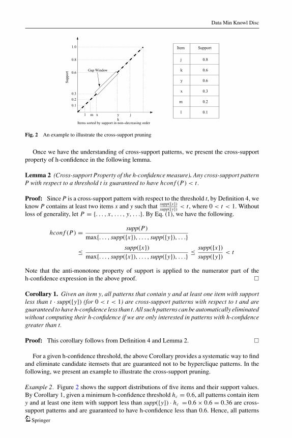
Let us consider the diagram shown in Fig. 2, which illustrates cross-support patterns ina hypothetical data set. In the figure, the horizontal axis shows items sorted by support innon-decreasing order and the vertical axis shows the corresponding support for items. Forexample, in the figure, the pattern {x, y, j} is a cross-support pattern with respect to thethreshold t = 0.6, since this pattern contains two items x and y such that supp({x})

supp({y}) = 0.30.6 =

0.5 < t = 0.6.

Springer


Data Min Knowl Disc

Gap WindowS

uppo

rt

xml y

0.1

0.2

0.3

0.6

Item Support

j

k

y

l 0.1

0.2

0.3

0.6

0.6

0.8

m

x

j

0.8

1.0

k

Fig. 2 An example to illustrate the cross-support pruning

Once we have the understanding of cross-support patterns, we present the cross-supportproperty of h-confidence in the following lemma.

Lemma 2 (Cross-support Property of the h-confidence measure). Any cross-support patternP with respect to a threshold t is guaranteed to have hcon f (P) < t .

Proof: Since P is a cross-support pattern with respect to the threshold t, by Definition 4, weknow P contains at least two items x and y such that supp({x})

supp({y}) < t , where 0 < t < 1. Withoutloss of generality, let P = {. . . , x, . . . , y, . . .}. By Eq. (1), we have the following.

hcon f (P) = supp(P)

max{. . . , supp({x}), . . . , supp({y}), . . .}

≤ supp({x})max{. . . , supp({x}), . . . , supp({y}), . . .} ≤ supp({x})

supp({y}) < t

Note that the anti-monotone property of support is applied to the numerator part of theh-confidence expression in the above proof. �

Corollary 1. Given an item y, all patterns that contain y and at least one item with supportless than t · supp({y}) (for 0 < t < 1) are cross-support patterns with respect to t and areguaranteed to have h-confidence less than t. All such patterns can be automatically eliminatedwithout computing their h-confidence if we are only interested in patterns with h-confidencegreater than t.

Proof: This corollary follows from Definition 4 and Lemma 2. �

For a given h-confidence threshold, the above Corollary provides a systematic way to findand eliminate candidate itemsets that are guaranteed not to be hyperclique patterns. In thefollowing, we present an example to illustrate the cross-support pruning.

Example 2. Figure 2 shows the support distributions of five items and their support values.By Corollary 1, given a minimum h-confidence threshold hc = 0.6, all patterns contain itemy and at least one item with support less than supp({y}) · hc = 0.6 × 0.6 = 0.36 are cross-support patterns and are guaranteed to have h-confidence less than 0.6. Hence, all patterns

Springer


Data Min Knowl Disc

containing item y and at least one of l, m, x do not need to be considered if we are onlyinterested in patterns with h-confidence greater than 0.6.

3.2. Generalization of the cross-support property

In this subsection, we generalize the cross-support property to other association measures.First, we give a generalized definition of the cross-support property.

Definition 5 (Generalized Cross-support Property). Given a measure f, for any cross-supportpattern P with respect to a threshold t, if there exists a monotone increasing function g suchthat f (P) < g(t), then the measure f has the cross-support property.

Given the h-confidence measure, for any cross-support pattern P with respect to a thresholdt, if we let the function g(l) = l, then we have hcon f (P) < g(t) = t by Lemma 2. Hence,the h-confidence measure has the cross-support property. Also, if a measure f has thecross-support property, the following theorem provides a way to automatically eliminatecross-support patterns.

Theorem 1. Given an item y, a measure f with the cross-support property, and a thresholdθ , any pattern P that contains y and at least one item x with support less than g−1(θ ) ·supp({y}) is a cross-support pattern with respect to the threshold g−1(θ ) and is guaranteedto have f (P) < θ , where g is the function to make the measure f satisfy the generalizedcross-support property.

Proof: Since supp({x}) < g−1(θ ) · supp({y}), we have supp({x})supp({y}) < g−1(θ ). By Definition 4,

the pattern P is a cross-support pattern with respect to the threshold g−1(θ ). Also, becausethe measure f has the cross-support property, by Definition 5, there exists a monotoneincreasing function g such that f (P) < g(g−1(θ )) = θ . Hence, for the given threshold θ , allsuch patterns can be automatically eliminated if we are only interested in patterns with themeasure f greater than θ . �

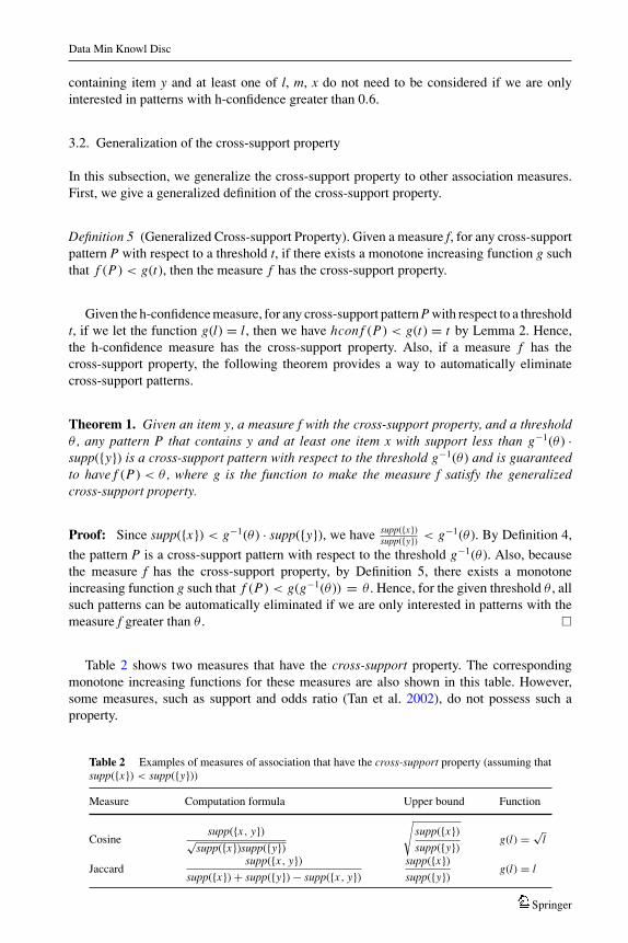
Table 2 shows two measures that have the cross-support property. The correspondingmonotone increasing functions for these measures are also shown in this table. However,some measures, such as support and odds ratio (Tan et al. 2002), do not possess such aproperty.

Table 2 Examples of measures of association that have the cross-support property (assuming thatsupp({x}) < supp({y}))

Measure Computation formula Upper bound Function

Cosinesupp({x, y})√

supp({x})supp({y})

√supp({x})supp({y}) g(l) = √

l

Jaccardsupp({x, y})

supp({x}) + supp({y}) − supp({x, y})supp({x})supp({y}) g(l) = l

Springer


Data Min Knowl Disc

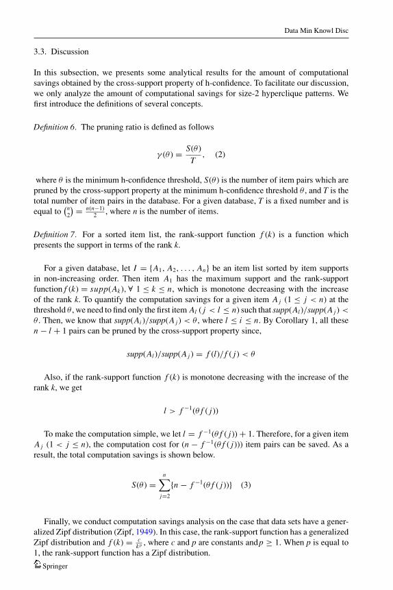
3.3. Discussion

In this subsection, we presents some analytical results for the amount of computationalsavings obtained by the cross-support property of h-confidence. To facilitate our discussion,we only analyze the amount of computational savings for size-2 hyperclique patterns. Wefirst introduce the definitions of several concepts.

Definition 6. The pruning ratio is defined as follows

γ (θ ) = S(θ )

T, (2)

where θ is the minimum h-confidence threshold, S(θ ) is the number of item pairs which arepruned by the cross-support property at the minimum h-confidence threshold θ , and T is thetotal number of item pairs in the database. For a given database, T is a fixed number and isequal to

(n2

) = n(n−1)2 , where n is the number of items.

Definition 7. For a sorted item list, the rank-support function f (k) is a function whichpresents the support in terms of the rank k.

For a given database, let I = {A1, A2, . . . , An} be an item list sorted by item supportsin non-increasing order. Then item A1 has the maximum support and the rank-supportfunction f (k) = supp(Ak),∀ 1 ≤ k ≤ n, which is monotone decreasing with the increaseof the rank k. To quantify the computation savings for a given item A j (1 ≤ j < n) at thethreshold θ , we need to find only the first item Al ( j < l ≤ n) such that supp(Al )/supp(A j ) <

θ . Then, we know that supp(Ai )/supp(A j ) < θ , where l ≤ i ≤ n. By Corollary 1, all thesen − l + 1 pairs can be pruned by the cross-support property since,

supp(Al )/supp(A j ) = f (l)/ f ( j) < θ

Also, if the rank-support function f (k) is monotone decreasing with the increase of therank k, we get

l > f −1(θ f ( j))

To make the computation simple, we let l = f −1(θ f ( j)) + 1. Therefore, for a given itemA j (1 < j ≤ n), the computation cost for (n − f −1(θ f ( j))) item pairs can be saved. As aresult, the total computation savings is shown below.

S(θ ) =n∑

j=2

{n − f −1(θ f ( j))} (3)

Finally, we conduct computation savings analysis on the case that data sets have a gener-alized Zipf distribution (Zipf, 1949). In this case, the rank-support function has a generalizedZipf distribution and f (k) = c

k p , where c and p are constants andp ≥ 1. When p is equal to1, the rank-support function has a Zipf distribution.

Springer


Data Min Knowl Disc

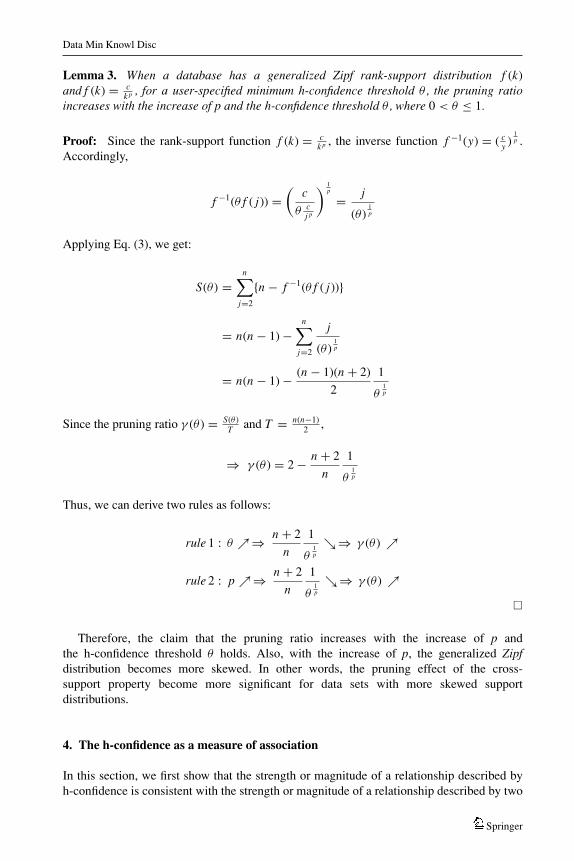
Lemma 3. When a database has a generalized Zipf rank-support distribution f (k)and f (k) = c

k p , for a user-specified minimum h-confidence threshold θ , the pruning ratioincreases with the increase of p and the h-confidence threshold θ , where 0 < θ ≤ 1.

Proof: Since the rank-support function f (k) = ck p , the inverse function f −1(y) = ( c

y )1p .

Accordingly,

f −1(θ f ( j)) =(

c

θ cj p

) 1p

= j

(θ )1p

Applying Eq. (3), we get:

S(θ ) =n∑

j=2

{n − f −1(θ f ( j))}

= n(n − 1) −n∑

j=2

j

(θ )1p

= n(n − 1) − (n − 1)(n + 2)

2

1

θ1p

Since the pruning ratio γ (θ ) = S(θ )T and T = n(n−1)

2 ,

⇒ γ (θ ) = 2 − n + 2

n

1

θ1p

Thus, we can derive two rules as follows:

rule 1 : θ ↗⇒ n + 2

n

1

θ1p

↘⇒ γ (θ ) ↗

rule 2 : p ↗⇒ n + 2

n

1

θ1p

↘⇒ γ (θ ) ↗�

Therefore, the claim that the pruning ratio increases with the increase of p andthe h-confidence threshold θ holds. Also, with the increase of p, the generalized Zipfdistribution becomes more skewed. In other words, the pruning effect of the cross-support property become more significant for data sets with more skewed supportdistributions.

4. The h-confidence as a measure of association

In this section, we first show that the strength or magnitude of a relationship described byh-confidence is consistent with the strength or magnitude of a relationship described by two

Springer


Data Min Knowl Disc

traditional association measures: the Jaccard measure (Rijsbergen, 1979) and the correlationcoefficient (Reynolds, 1977).

Given a pair of items P = {i1, i2}, the affinity between both items using these measuresis defined as follows:

jaccard(P) = supp({i1, i2})supp({i1}) + supp({i2}) − supp({i1, i2}) ,

correlation, φ(P) = supp({i1, i2}) − supp({i1})supp({i2})√supp({i1})supp({i2})(1 − supp({i1}))(1 − supp({i2}))

.

Also, we demonstrate that h-confidence is a measure of association that can be used tocapture the strength or magnitude of a relationship among several objects.

4.1. Relationship between h-confidence and Jaccard

In the following, for a size-2 hyperclique pattern P, we provide a lemma that gives a lowerbound for jaccard(P).

Lemma 4. If an item set P = {i1, i2} is a size-2 hyperclique pattern, then jaccard(P) ≥hc/2.

Proof: By Eq. (1), hcon f (P) = supp({i1,i2})max{supp({i1}),supp({i2})} . Without loss of generality, let

supp({i1}) ≥ supp({i2}). Given that P is a hyperclique pattern, hcon f (P) = supp({i1,i2})supp({i1})

≥ hc. Furthermore, since supp({i1}) ≥ supp({i2}), jaccard(P) = supp({i1,i2})supp({i1})+supp({i2})−supp({i1,i2})

≥ supp({i1,i2})2supp({i1}) ≥ hc/2. �

Lemma 4 suggests that if the h-confidence threshold hc is sufficiently high, then all size-2hyperclique patterns contain items that are strongly related with each other in terms of theJaccard measure, since the Jaccard values of these hyperclique patterns are bounded frombelow by hc/2.

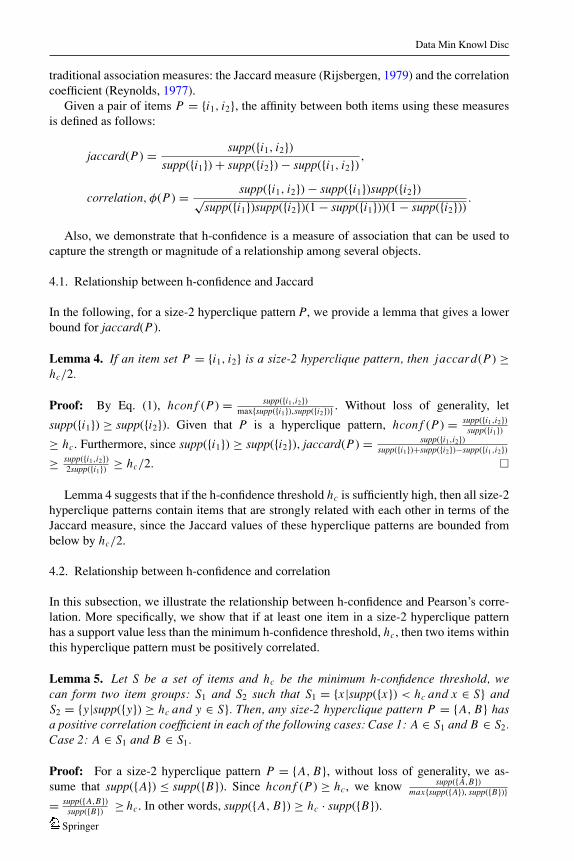
4.2. Relationship between h-confidence and correlation

In this subsection, we illustrate the relationship between h-confidence and Pearson’s corre-lation. More specifically, we show that if at least one item in a size-2 hyperclique patternhas a support value less than the minimum h-confidence threshold, hc, then two items withinthis hyperclique pattern must be positively correlated.

Lemma 5. Let S be a set of items and hc be the minimum h-confidence threshold, wecan form two item groups: S1 and S2 such that S1 = {x |supp({x}) < hc and x ∈ S} andS2 = {y|supp({y}) ≥ hc and y ∈ S}. Then, any size-2 hyperclique pattern P = {A, B} hasa positive correlation coefficient in each of the following cases: Case 1: A ∈ S1 and B ∈ S2.Case 2: A ∈ S1 and B ∈ S1.

Proof: For a size-2 hyperclique pattern P = {A, B}, without loss of generality, we as-sume that supp({A}) ≤ supp({B}). Since hcon f (P) ≥ hc, we know supp({A,B})

max{supp({A}), supp({B})}= supp({A,B})

supp({B}) ≥ hc. In other words, supp({A, B}) ≥ hc · supp({B}).Springer


Data Min Knowl Disc

b

ItemsTID

1 a

2

4

5

6

7

8

9

c, e

b

a

a, b, c, d, e

a, b

a, b

a

b, c, d

Support

0.6

0.6

0.3

0.2

0.2

Item

3

10

a

b

c

d

e d

c

b

a

a

b

d

c

a

0.1020.3560.25

edcba

0.4080.089

0.375

0.7640.764

0.102

0.102

0.667

0.333 0.167

0.667

0.5

0.1670.167

0.333

0.1670.5

edcb

Pairwise Correlation

Pairwise h confidence

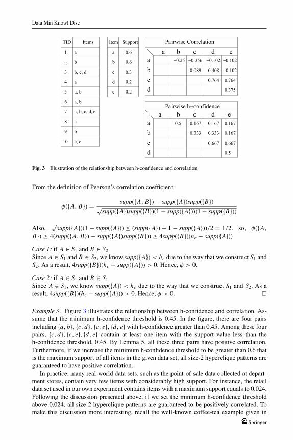
Fig. 3 Illustration of the relationship between h-confidence and correlation

From the definition of Pearson’s correlation coefficient:

φ({A, B}) = supp({A, B}) − supp({A})supp({B})√supp({A})supp({B})(1 − supp({A}))(1 − supp({B}))

Also,√

supp({A})(1 − supp({A})) ≤ (supp({A}) + 1 − supp({A}))/2 = 1/2. so, φ({A,

B}) ≥ 4(supp({A, B}) − supp({A})supp({B})) ≥ 4supp({B})(hc − supp({A}))Case 1: if A ∈ S1 and B ∈ S2

Since A ∈ S1 and B ∈ S2, we know supp({A}) < hc due to the way that we construct S1 andS2. As a result, 4supp({B})(hc − supp({A})) > 0. Hence, φ > 0.

Case 2: if A ∈ S1 and B ∈ S1

Since A ∈ S1, we know supp({A}) < hc due to the way that we construct S1 and S2. As aresult, 4supp({B})(hc − supp({A})) > 0. Hence, φ > 0. �

Example 3. Figure 3 illustrates the relationship between h-confidence and correlation. As-sume that the minimum h-confidence threshold is 0.45. In the figure, there are four pairsincluding {a, b}, {c, d}, {c, e}, {d, e} with h-confidence greater than 0.45. Among these fourpairs, {c, d}, {c, e}, {d, e} contain at least one item with the support value less than theh-confidence threshold, 0.45. By Lemma 5, all these three pairs have positive correlation.Furthermore, if we increase the minimum h-confidence threshold to be greater than 0.6 thatis the maximum support of all items in the given data set, all size-2 hyperclique patterns areguaranteed to have positive correlation.

In practice, many real-world data sets, such as the point-of-sale data collected at depart-ment stores, contain very few items with considerably high support. For instance, the retaildata set used in our own experiment contains items with a maximum support equals to 0.024.Following the discussion presented above, if we set the minimum h-confidence thresholdabove 0.024, all size-2 hyperclique patterns are guaranteed to be positively correlated. Tomake this discussion more interesting, recall the well-known coffee-tea example given in

Springer


Data Min Knowl Disc

(Brin et al., 1997). This example illustrates the drawback of using confidence as a measureof association. Even though the confidence for the rule tea → coffee may be high, bothitems are in fact negatively-correlated with each other. Hence, the confidence measure canbe misleading. Instead, with h-confidence, we may ensure that all derived size-2 patterns arepositively correlated, as long as the minimum h-confidence threshold is above the maximumsupport of all items.

4.3. H-confidence for measuring the relationship among several objects

In this subsection, we demonstrate that the h-confidence measure can be used to describe thestrength or magnitude of a relationship among several objects.

Given a pair of items P = {i1, i2}, the cosine similarity between both items is defined asfollows.

cosine(P) = supp({i1, i2})√supp({i1})supp({i2})

,

Note that the cosine similarity is also known as uncentered Pearson’s correlation coeffi-cient (when computing Pearson’s correlation coefficient, the data mean is not subtracted).For a size-2 hyperclique pattern P, we first derive a lower bound for the cosine similarity ofthe pattern P, cosine(P), in terms of the minimum h-confidence threshold hc.

Lemma 6. If an item set P = {i1, i2} is a size-2 hyperclique pattern, then cosine(P) ≥ hc.

Proof: By Eq. (1), hcon f (P) = supp({i1,i2})max{supp({i1}),supp({i2})} . Without loss of generality, let

supp({i1}) ≥ supp({i2}). Given that P is a hyperclique pattern, hcon f (P) = supp({i1,i2})supp({i1}) ≥ hc.

Since supp ({i1}) ≥ supp({i2}), cosine(P) = supp({i1,i2})√supp({i1})supp({i2}) ≥ supp({i1,i2})

supp({i1}) ≥ hc. �

Lemma 6 suggests that if the h-confidence threshold hc is sufficiently high, then all size-2hyperclique patterns contain items that are strongly related with each other in terms of thecosine measure, since the cosine values of these hyperclique patterns are bounded frombelow by hc.

For the case that hyperclique patterns have more than two objects, the following theoremguarantees that if a hyperclique pattern has an h-confidence value above the minimum h-confidence threshold, hc, then every pair of objects within the hyperclique pattern must havea cosine similarity great than or equal to hc.

Theorem 2. Given a hyperclique pattern P = {i1, i2, . . . , ik} (k > 2) at the h-confidencethreshold hc, for any size-2 itemset Q = {il , im} such that Q ⊂ P, we have cosine (Q) ≥ hc.

Proof: By the anti-monotone property of the h-confidence measure and the condition thatQ ⊂ P , we know Q is also a hyperclique pattern. Then, by Lemma 6, we know cosine(Q) ≥hc. �

Clique View. Indeed, a hyperclique pattern can be viewed as a clique, if we construct a graphin the following way. Treat each object in a hyperclique pattern as a vertex and put an edgebetween two vertices if the cosine similarity between two objects is above the h-confidencethreshold, hc. According to Theorem 2, there will be an edge between any two objects withina hyperclique pattern. As a result, a hyperclique pattern is a clique.

Springer


Data Min Knowl Disc

Viewed as cliques, hyperclique patterns have applications in many different domains.For instance, Xiong et al. (2004) show that the hyperclique pattern is the best candidate forpattern preserving clustering—a new paradigm for pattern based clustering. Also, Xionget al. (2005) describe the use of hyperclique pattern discovery for identifying functionalmodules in protein complexes.

5. Hyperclique miner algorithm

The Hyperclique Miner is an algorithm which can generate all hyperclique patterns withsupport and h-confidence above user-specified minimum support and h-confidence thresh-olds.Hyperclique MinerInput:

(1) a set F of K Boolean feature types F = { f1, f2, . . . , fK}(2) a set T of N transactions T = {t1 . . . tN }, each ti ∈ T is a record with K attributes

{i1, i2, . . . , iK } taking values in {0, 1}, where the i p (1 ≤ p ≤ K ) is the Boolean valuefor the feature type f p.

(3) A user specified minimum h-confidence threshold (hc)(4) A user specified minimum support threshold (min supp)

Output:hyperclique patterns with h-confidence > hc and support > min supp

Method:

(1) Get size-1 prevalent items(2) for the size of itemsets in (2, 3, . . . , K − 1) do(3) Generate candidate hyperclique patterns using the generalized apriori gen algorithm(4) Generate hyperclique patterns(5) end;

Explanation of the detailed steps of the algorithm

Step 1 scans the database and gets the support for every item. Items with support abovemin supp form size-1 candidate set C1. The h-confidence values for size-1 itemsets are 1.All items in the set C1 are sorted by the support values and relabeled in alphabetic order.

Step 2 to Step 4 loops through 2 to K – 1 to generate qualified hyperclique patterns of size 2or more. It stops whenever an empty candidate set of some size is generated.

Step 3 uses generalized apriori gen to generate candidate hyperclique patterns of size k fromhyperclique patterns of size k – 1. The generalized apriori gen function is an adaptation ofthe apriori gen function of the Apriori algorithm (Agrawal and Srikant, 1994). Let Ck−1

indicate the set of all hyperclique patterns of size k – 1. The function works as follows.First, in the join step, we join Ck−1 with Ck−1 and get candidate set Ck . Next in the prunestep, we delete all candidate hyperclique patterns c ∈ Ck based on two major pruningtechniques:

(a) Pruning based on anti-monotone property of h-confidence and support: If anyone of the k – 1 subsets of c does not belong to Ck−1, then c is pruned. (Recallthat this prune step is also done in apriori gen by Agrawal and Srikant because

Springer


Data Min Knowl Disc

of the anti-monotone property of support. Omiecinski (2003) also applied theanti-monotone property of all-confidence in his algorithm.)

(b) Pruning of cross-support patterns by using the cross-support property of h-confidence: By Corollary 1, for the given h-confidence threshold hc and an item y,all patterns that contain y and at least one item with support less than hc ·supp({y})are cross-support patterns and are guaranteed to have h-confidence less than t. Hence,all such patterns can be automatically eliminated.

Note that the major pruning techniques applied in this step are illustrated by Example 4.

Step 4 computes exact support and h-confidence for all candidate patterns in Ck and prunesthis candidate set using the user specified support threshold min supp and the h-confidencethreshold hc. All remaining patterns are returned as hyperclique patterns of size k.

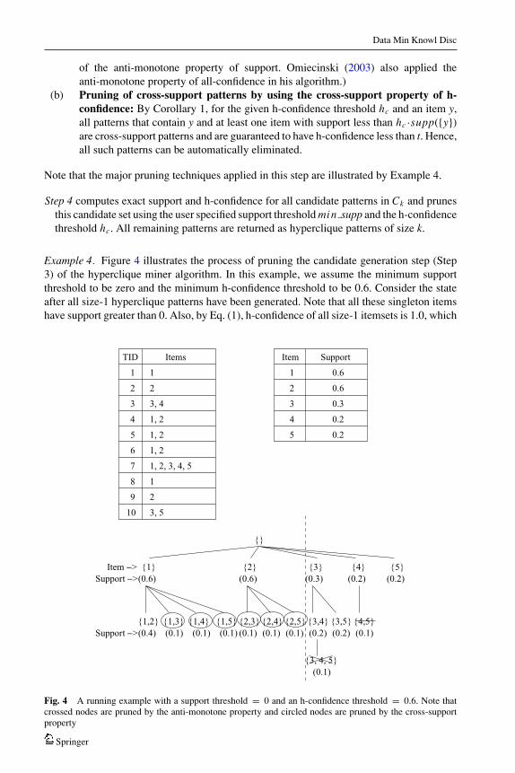
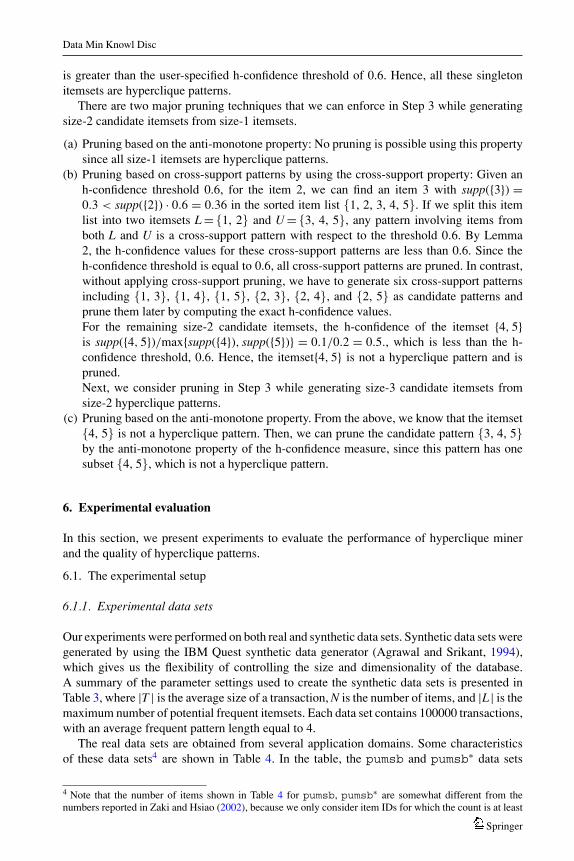
Example 4. Figure 4 illustrates the process of pruning the candidate generation step (Step3) of the hyperclique miner algorithm. In this example, we assume the minimum supportthreshold to be zero and the minimum h-confidence threshold to be 0.6. Consider the stateafter all size-1 hyperclique patterns have been generated. Note that all these singleton itemshave support greater than 0. Also, by Eq. (1), h-confidence of all size-1 itemsets is 1.0, which

Item Support

1

2

3

4

0.6

0.6

0.3

0.2

5 0.2

{}

}5{}4{}2{ {3}{1}

{3, 4, 5}(0.1)

(0.1) (0.1) (0.1) (0.2) (0.2) (0.1)(0.1)(0.1)(0.4)

(0.2) (0.2)(0.3)(0.6)(0.6)Support >Item >

TID Items

1

2

3, 4

1, 2

1, 2

1, 2

1, 2, 3, 4, 5

1

2

3, 510

9

8

7

6

5

4

3

2

1

{1,2} {1,3} {1,4} {1,5} {2,3} {2,4} {2,5} {3,4} {3,5} {4,5}(0.1)Support >

Fig. 4 A running example with a support threshold = 0 and an h-confidence threshold = 0.6. Note thatcrossed nodes are pruned by the anti-monotone property and circled nodes are pruned by the cross-supportproperty

Springer


Data Min Knowl Disc

is greater than the user-specified h-confidence threshold of 0.6. Hence, all these singletonitemsets are hyperclique patterns.

There are two major pruning techniques that we can enforce in Step 3 while generatingsize-2 candidate itemsets from size-1 itemsets.

(a) Pruning based on the anti-monotone property: No pruning is possible using this propertysince all size-1 itemsets are hyperclique patterns.

(b) Pruning based on cross-support patterns by using the cross-support property: Given anh-confidence threshold 0.6, for the item 2, we can find an item 3 with supp({3}) =0.3 < supp({2}) · 0.6 = 0.36 in the sorted item list {1, 2, 3, 4, 5}. If we split this itemlist into two itemsets L = {1, 2} and U = {3, 4, 5}, any pattern involving items fromboth L and U is a cross-support pattern with respect to the threshold 0.6. By Lemma2, the h-confidence values for these cross-support patterns are less than 0.6. Since theh-confidence threshold is equal to 0.6, all cross-support patterns are pruned. In contrast,without applying cross-support pruning, we have to generate six cross-support patternsincluding {1, 3}, {1, 4}, {1, 5}, {2, 3}, {2, 4}, and {2, 5} as candidate patterns andprune them later by computing the exact h-confidence values.For the remaining size-2 candidate itemsets, the h-confidence of the itemset {4, 5}is supp({4, 5})/max{supp({4}), supp({5})} = 0.1/0.2 = 0.5., which is less than the h-confidence threshold, 0.6. Hence, the itemset{4, 5} is not a hyperclique pattern and ispruned.Next, we consider pruning in Step 3 while generating size-3 candidate itemsets fromsize-2 hyperclique patterns.

(c) Pruning based on the anti-monotone property. From the above, we know that the itemset{4, 5} is not a hyperclique pattern. Then, we can prune the candidate pattern {3, 4, 5}by the anti-monotone property of the h-confidence measure, since this pattern has onesubset {4, 5}, which is not a hyperclique pattern.

6. Experimental evaluation

In this section, we present experiments to evaluate the performance of hyperclique minerand the quality of hyperclique patterns.

6.1. The experimental setup

6.1.1. Experimental data sets

Our experiments were performed on both real and synthetic data sets. Synthetic data sets weregenerated by using the IBM Quest synthetic data generator (Agrawal and Srikant, 1994),which gives us the flexibility of controlling the size and dimensionality of the database.A summary of the parameter settings used to create the synthetic data sets is presented inTable 3, where |T | is the average size of a transaction, N is the number of items, and |L| is themaximum number of potential frequent itemsets. Each data set contains 100000 transactions,with an average frequent pattern length equal to 4.

The real data sets are obtained from several application domains. Some characteristicsof these data sets4 are shown in Table 4. In the table, the pumsb and pumsb∗ data sets

4 Note that the number of items shown in Table 4 for pumsb, pumsb∗ are somewhat different from thenumbers reported in Zaki and Hsiao (2002), because we only consider item IDs for which the count is at least

Springer


Data Min Knowl Disc

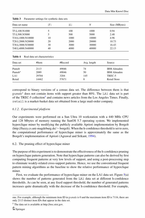
Table 3 Parameter settings for synthetic data sets

Data set name |T | |L| N Size (MBytes)

T5.L100.N1000 5 100 1000 0.94T5.L500.N5000 5 500 5000 2.48T10.L1000.N10000 10 1000 10000 4.96T20.L2000.N20000 20 2000 20000 10.73T30.L3000.N30000 30 3000 30000 16.43T40.L4000.N40000 40 4000 40000 22.13

Table 4 Real data set characteristics

Data set #Item #Record Avg. length Source

Pumsb 2113 49046 74 IBM AlmadenPumsb∗ 2089 49046 50 IBM AlmadenLA1 29704 3204 145 TREC-5Retail 14462 57671 8 Retail Store

correspond to binary versions of a census data set. The difference between them is thatpumsb∗ does not contain items with support greater than 80%. The LA1 data set is partof the TREC-5 collection5 and contains news articles from the Los Angeles Times. Finally,retail is a market-basket data set obtained from a large mail-order company.

6.1.2. Experimental platform

Our experiments were performed on a Sun Ultra 10 workstation with a 440 MHz CPUand 128 Mbytes of memory running the SunOS 5.7 operating system. We implementedhyperclique miner by modifying the publicly available Apriori implementation by Borgelt(http://fuzzy.cs.uni-magdeburg.de/ ∼ borgelt). When the h-confidence threshold is set to zero,the computational performance of hyperclique miner is approximately the same as theBorgelt’s implementation of Apriori (Agrawal and Srikant, 1994).

6.2. The pruning effect of hyperclique miner

The purpose of this experiment is to demonstrate the effectiveness of the h-confidence pruningon hyperclique pattern generation. Note that hyperclique patterns can also be derived by firstcomputing frequent patterns at very low levels of support, and using a post-processing stepto eliminate weakly-related cross-support patterns. Hence, we use the conventional frequentpattern mining algorithms as the baseline to show the relative performance of hypercliqueminer.

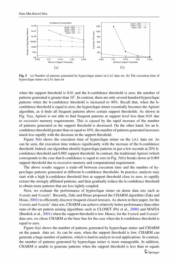
First, we evaluate the performance of hyperclique miner on the LA1 data set. Figure 5(a)shows the number of patterns generated from the LA1 data set at different h-confidencethresholds. As can be seen, at any fixed support threshold, the number of generated patternsincreases quite dramatically with the decrease of the h-confidence threshold. For example,

one. For example, although the minimum item ID in pumsb is 0 and the maximum item ID is 7116, there areonly 2113 distinct item IDs that appear in the data set.5 The data set is available at http://trec.nist.gov.

Springer


Data Min Knowl Disc

100

1000

10000

100000

1e+06

1e+07

1e+08

0.005 0.01 0.015 0.02 0.025

Num

ber

of H

yper

cliq

ue P

atte

rns

Minimum Support Thresholds

Confidence-Pruning Effect

hconf = 40%hconf = 20%hconf = 10%hconf = 0%

200

400

600

800

1000

1200

0.005 0.01 0.015 0.02 0.025

Exe

cutio

n Ti

me

(sec

)


hconf = 20%hconf = 10%hconf = 0%

)b()a(

Fig. 5 (a) Number of patterns generated by hyperclique miner on LA1 data set. (b) The execution time ofhyperclique miner on LA1 data set

when the support threshold is 0.01 and the h-confidence threshold is zero, the number ofpatterns generated is greater than 107. In contrast, there are only several hundred hypercliquepatterns when the h-confidence threshold is increased to 40%. Recall that, when the h-confidence threshold is equal to zero, the hyperclique miner essentially becomes the Apriorialgorithm, as it finds all frequent patterns above certain support thresholds. As shown inFig. 5(a), Apriori is not able to find frequent patterns at support level less than 0.01 dueto excessive memory requirements. This is caused by the rapid increase of the numberof patterns generated as the support threshold is decreased. On the other hand, for an h-confidence threshold greater than or equal to 10%, the number of patterns generated increasesmuch less rapidly with the decrease in the support threshold.

Figure 5(b) shows the execution time of hyperclique miner on the LA1 data set. Ascan be seen, the execution time reduces significantly with the increase of the h-confidencethreshold. Indeed, our algorithm identify hyperclique patterns in just a few seconds at 20% h-confidence threshold and 0.005 support threshold. In contrast, the traditional Apriori (whichcorresponds to the case that h-confidence is equal to zero in Fig. 5(b)) breaks down at 0.005support threshold due to excessive memory and computational requirement.

The above results suggest a trade-off between execution time and the number of hy-perclique patterns generated at different h-confidence thresholds. In practice, analysts maystart with a high h-confidence threshold first at support threshold close to zero, to rapidlyextract the strongly affiliated patterns, and then gradually reduce the h-confidence thresholdto obtain more patterns that are less tightly-coupled.

Next, we evaluate the performance of hyperclique miner on dense data sets such asPumsb and Pumsb∗. Recently, Zaki and Hsiao proposed the CHARM algorithm (Zaki andHsiao, 2002) to efficiently discover frequent closed itemsets. As shown in their paper, for thePumsb and Pumsb∗ data sets, CHARM can achieve relatively better performance than otherstate-of-the-art pattern mining algorithms such as CLOSET (Pei et al., 2000) and MAFIA(Burdick et al., 2001) when the support threshold is low. Hence, for the Pumsb and Pumsb∗

data sets, we chose CHARM as the base line for the case when the h-confidence threshold isequal to zero.

Figure 6(a) shows the number of patterns generated by hyperclique miner and CHARMon the pumsb data set. As can be seen, when the support threshold is low, CHARM cangenerate a huge number of patterns, which is hard to analyze in real applications. In contrast,the number of patterns generated by hyperclique miner is more manageable. In addition,CHARM is unable to generate patterns when the support threshold is less than or equals

Springer


Data Min Knowl Disc

100

1000

10000

100000

1e+06

1e+07

1e+08

0 0.05 0.1 0.15 0.2 0.25 0.3 0.35 0.4 0.45 0.5

Num

ber

of H

yper

cliq

ue P

atte

rns




CHARM

10

100

1000

0 0.05 0.1 0.15 0.2 0.25 0.3 0.35 0.4 0.45 0.5

Exe

cutio

n Ti

me

(sec

)



CHARM

)b()a(

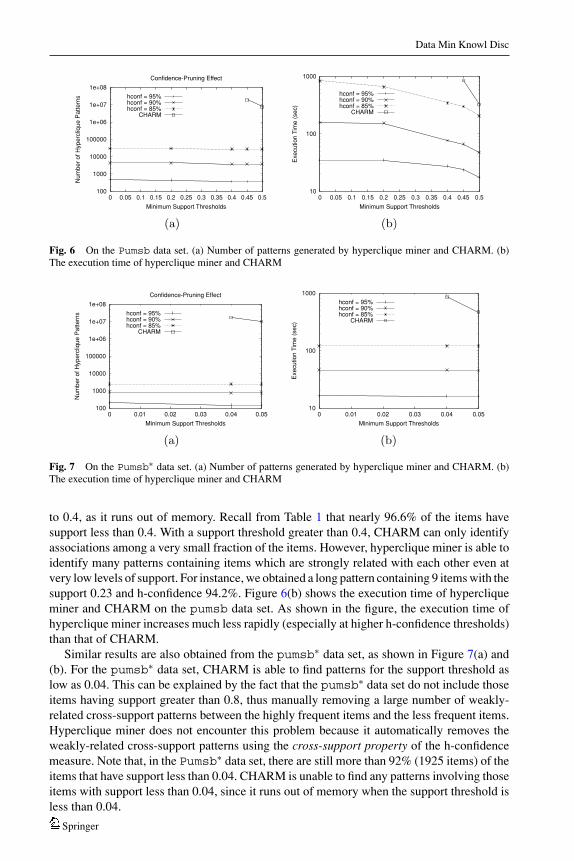
Fig. 6 On the Pumsb data set. (a) Number of patterns generated by hyperclique miner and CHARM. (b)The execution time of hyperclique miner and CHARM

100

1000

10000

100000

1e+06

1e+07

1e+08

0 0.01 0.02 0.03 0.04 0.05

Num

ber

of H

yper

cliq

ue P

atte

rns




CHARM

10

100

1000

0 0.01 0.02 0.03 0.04 0.05

Exe

cutio

n Ti

me

(sec

)



CHARM

)b()a(

Fig. 7 On the Pumsb∗ data set. (a) Number of patterns generated by hyperclique miner and CHARM. (b)The execution time of hyperclique miner and CHARM

to 0.4, as it runs out of memory. Recall from Table 1 that nearly 96.6% of the items havesupport less than 0.4. With a support threshold greater than 0.4, CHARM can only identifyassociations among a very small fraction of the items. However, hyperclique miner is able toidentify many patterns containing items which are strongly related with each other even atvery low levels of support. For instance, we obtained a long pattern containing 9 items with thesupport 0.23 and h-confidence 94.2%. Figure 6(b) shows the execution time of hypercliqueminer and CHARM on the pumsb data set. As shown in the figure, the execution time ofhyperclique miner increases much less rapidly (especially at higher h-confidence thresholds)than that of CHARM.

Similar results are also obtained from the pumsb∗ data set, as shown in Figure 7(a) and(b). For the pumsb∗ data set, CHARM is able to find patterns for the support threshold aslow as 0.04. This can be explained by the fact that the pumsb∗ data set do not include thoseitems having support greater than 0.8, thus manually removing a large number of weakly-related cross-support patterns between the highly frequent items and the less frequent items.Hyperclique miner does not encounter this problem because it automatically removes theweakly-related cross-support patterns using the cross-support property of the h-confidencemeasure. Note that, in the Pumsb∗ data set, there are still more than 92% (1925 items) of theitems that have support less than 0.04. CHARM is unable to find any patterns involving thoseitems with support less than 0.04, since it runs out of memory when the support threshold isless than 0.04.

Springer


Data Min Knowl Disc

0

10

20

30

40

50

60

70

15% 20% 25% 30% 35%

Exe

cutio

n Ti

me

(sec

)

Minimum H-confidence Thresholds

Anti-monotoneCross-support+Anti-monotone

0

500

1000

1500

2000

2500

3000

84% 86% 88% 90% 92% 94% 96% 98% 100%

Exe

cutio

n Ti

me

(sec

)

Minimum h-confidence Thresholds

Anti-monotoneCross-support+Anti-monotone

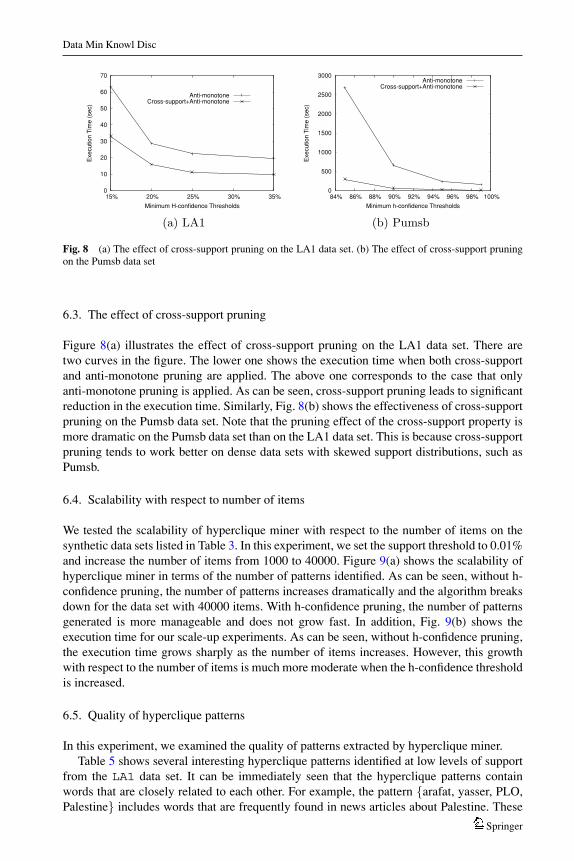
bsmuP)b(1AL)a(

Fig. 8 (a) The effect of cross-support pruning on the LA1 data set. (b) The effect of cross-support pruningon the Pumsb data set

6.3. The effect of cross-support pruning

Figure 8(a) illustrates the effect of cross-support pruning on the LA1 data set. There aretwo curves in the figure. The lower one shows the execution time when both cross-supportand anti-monotone pruning are applied. The above one corresponds to the case that onlyanti-monotone pruning is applied. As can be seen, cross-support pruning leads to significantreduction in the execution time. Similarly, Fig. 8(b) shows the effectiveness of cross-supportpruning on the Pumsb data set. Note that the pruning effect of the cross-support property ismore dramatic on the Pumsb data set than on the LA1 data set. This is because cross-supportpruning tends to work better on dense data sets with skewed support distributions, such asPumsb.

6.4. Scalability with respect to number of items

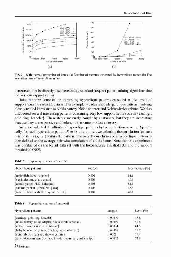
We tested the scalability of hyperclique miner with respect to the number of items on thesynthetic data sets listed in Table 3. In this experiment, we set the support threshold to 0.01%and increase the number of items from 1000 to 40000. Figure 9(a) shows the scalability ofhyperclique miner in terms of the number of patterns identified. As can be seen, without h-confidence pruning, the number of patterns increases dramatically and the algorithm breaksdown for the data set with 40000 items. With h-confidence pruning, the number of patternsgenerated is more manageable and does not grow fast. In addition, Fig. 9(b) shows theexecution time for our scale-up experiments. As can be seen, without h-confidence pruning,the execution time grows sharply as the number of items increases. However, this growthwith respect to the number of items is much more moderate when the h-confidence thresholdis increased.

6.5. Quality of hyperclique patterns

In this experiment, we examined the quality of patterns extracted by hyperclique miner.Table 5 shows several interesting hyperclique patterns identified at low levels of support

from the LA1 data set. It can be immediately seen that the hyperclique patterns containwords that are closely related to each other. For example, the pattern {arafat, yasser, PLO,Palestine} includes words that are frequently found in news articles about Palestine. These

Springer


Data Min Knowl Disc

10

100

1000

10000

100000

1e+06

1e+07

1000 5000 10000 20000 30000 40000

Num

ber

of H

yper

cliq

ue P

atte

rns

Number of attributes

hconf = 95%hconf = 80%hconf = 50%hconf = 30%hconf = 0%

0 50

200

400

600

800

1000

1200

1400

1000 5000 10000 20000 30000 40000

Exe

cutio

n Ti

me

(sec

)

Number of attributes

hconf = 95%hconf = 80%hconf = 50%hconf = 30%hconf = 0%

)b()a(

Fig. 9 With increasing number of items. (a) Number of patterns generated by hyperclique miner. (b) Theexecution time of hyperclique miner

patterns cannot be directly discovered using standard frequent pattern mining algorithms dueto their low support values.

Table 6 shows some of the interesting hyperclique patterns extracted at low levels ofsupport from theretail data set. For example, we identified a hyperclique pattern involvingclosely related items such as Nokia battery, Nokia adapter, and Nokia wireless phone. We alsodiscovered several interesting patterns containing very low support items such as {earrings,gold ring, bracelet}. These items are rarely bought by customers, but they are interestingbecause they are expensive and belong to the same product category.

We also evaluated the affinity of hyperclique patterns by the correlation measure. Specifi-cally, for each hyperclique pattern X = {x1, x2, . . . xk}, we calculate the correlation for eachpair of items (xi , x j ) within the pattern. The overall correlation of a hyperclique pattern isthen defined as the average pair wise correlation of all the items. Note that this experimentwas conducted on the Retail data set with the h-confidence threshold 0.8 and the supportthreshold 0.0005.

Table 5 Hyperclique patterns from LA1

Hyperclique patterns support h-confidence (%)

{najibullah, kabul, afghan} 0.002 54.5{steak, dessert, salad, sauce} 0.001 40.0{arafat, yasser, PLO, Palestine} 0.004 52.0{shamir, yitzhak, jerusalem, gaza} 0.002 42.9{amal, militia, hezbollah, syrian, beirut} 0.001 40.0

Table 6 Hyperclique patterns from retail

Hyperclique patterns support hconf (%)

{earrings, gold ring, bracelet} 0.00019 45.8{nokia battery, nokia adapter, nokia wireless phone} 0.00049 52.8{coffee maker, can opener, toaster} 0.00014 61.5{baby bumper pad, diaper stacker, baby crib sheet} 0.00028 72.7{skirt tub, 3pc bath set, shower curtain} 0.0026 74.4{jar cookie, canisters 3pc, box bread, soup tureen, goblets 8pc} 0.00012 77.8

Springer


Data Min Knowl Disc

0

0.1

0.2

0.3

0.4

0.5

0.6

0.7

0.8

0.9

1

0 20 40 60 80 100

Ave

rage

Cor

rela

tion

Percentile

Non-hypercliquesHypercliques

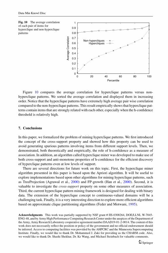
Fig. 10 The average correlationof each pair of items forhyperclique and non-hypercliquepatterns

Figure 10 compares the average correlation for hyperclique patterns versus non-hyperclique patterns. We sorted the average correlation and displayed them in increasingorder. Notice that the hyperclique patterns have extremely high average pair wise correlationcompared to the non-hyperclique patterns. This result empirically shows that hyperclique pat-terns contain items that are strongly related with each other, especially when the h-confidencethreshold is relatively high.

7. Conclusions

In this paper, we formalized the problem of mining hyperclique patterns. We first introducedthe concept of the cross-support property and showed how this property can be used toavoid generating spurious patterns involving items from different support levels. Then, wedemonstrated, both theoretically and empirically, the role of h-confidence as a measure ofassociation. In addition, an algorithm called hyperclique miner was developed to make use ofboth cross-support and anti-monotone properties of h-confidence for the efficient discoveryof hyperclique patterns even at low levels of support.

There are several directions for future work on this topic. First, the hyperclique mineralgorithm presented in this paper is based upon the Apriori algorithm. It will be useful toexplore implementations based upon other algorithms for mining hyperclique patterns, suchas TreeProjection (Agrawal et al., 2000) and FP-growth (Han et al., 2000). Second, it isvaluable to investigate the cross-support property on some other measures of association.Third, the current hyperclique pattern mining framework is designed for dealing with binarydata. The extension of the hyperclique concept to continuous-valued domains will be achallenging task. Finally, it is a very interesting direction to explore more efficient algorithmsbased on approximate clique partitioning algorithms (Feder and Motwani, 1995).

Acknowledgments This work was partially supported by NSF grant # IIS-0308264, DOE/LLNL W-7045-ENG-48, and by Army High Performance Computing Research Center under the auspices of the Department ofthe Army, Army Research Laboratory cooperative agreement number DAAD19-01-2-0014. The content of thiswork does not necessarily reflect the position or policy of the government and no official endorsement shouldbe inferred. Access to computing facilities was provided by the AHPCRC and the Minnesota SupercomputingInstitute. Finally, we would like to thank Dr. Mohammed J. Zaki for providing us the CHARM code. Also,we would like to thank Dr. Shashi Shekhar, Dr. Ke Wang, and Michael Steinbach for valuable comments.

Springer


Data Min Knowl Disc

References

Agarwal R, Aggarwal C, Prasad V (2000) A tree projection algorithm for generation of frequent itemsets.Journal of Parallel and Distributed Computing

Agrawal R, Imielinski T, Swami A (1993) Mining association rules between sets of items in large databases. In:Proceedings of the 1993 ACM SIGMOD International Conference on Management of Data. pp 207–216

Agrawal R, Srikant R (1994) Fast algorithms for mining association rules. In: Proceedings of the 20thInternational Conference on Very Large Data Bases

Bayardo R, Agrawal R, Gunopulous D (1999) Constraint-based rule mining in large, dense databases. In:Proceedings of the Int’l Conference on Data Engineering

Bayardo RJ (1998) Efficiently mining long patterns from databases. In: Proceedings of the 1998 ACMSIGMOD International Conference on Management of Data

Brin S, Motwani R, Silverstein C (1997) Beyond market baskets: Generalizing association rules to correlations.In: Proceedings of ACM SIGMOD Int’l Conference on Management of Data. pp 265–276

Burdick D, Calimlim M, Gehrke J (2001) MAFIA: A maximal frequent itemset algorithm for transactionaldatabases. In: Proceedings of the 2001 Int’l Conference on Data Engineering (ICDE)

Cohen E, Datar M, Fujiwara S, Gionis A, Indyk P, Motwani R, Ullman J, Yang C (2000) Finding interestingassociations without support pruning. In: Proceedings of the 2000 Int’l Conference on Data Engineering(ICDE). pp 489–499

Feder T, Motwani R (1995) Clique partitions, graph compression and speeding-up algorithms. Special Issuefor the STOC conference. Journal of Computer and System Sciences 51:261–272

Grahne G, Lakshmanan LVS, Wang X (2000) Efficient mining of constrained correlated sets. In: Proceedingsof the Int’l Conference on Data Engineering

Han J, Pei J, Yin Y (2000) Mining frequent patterns without candidate generation. In: Proceedings of ACMSIGMOD Int’l Conference on Management of Data

Hastie T, Tibshirani R, Friedman J (2001) The elements of statistical learning: Data mining, inference, andprediction, Springer

Liu B, Hsu W, Ma Y (1999) Mining association rules with multiple minimum supports. In: Proceedings ofthe 1999 ACM SIGKDD International Conference on Knowledge Discovery and Data Mining

Omiecinski E (2003) Alternative interest measures for mining associations. IEEE Transactions on Knowledgeand Data Engineering 15(1)

Pei J, Han J, Mao R (2000) CLOSET: An efficient algorithm for mining frequent closed itemsets. In: ACMSIGMOD Workshop on Research Issues in Data Mining and Knowledge Discovery

Reynolds HT (1977) The analysis of cross-classifications. The Free PressRijsbergen CJV (1979) Information retrieval, 2nd edn., Butterworths, LondonTan P, Kumar V, Srivastava J (2002) Selecting the right interestingness measure for association patterns. In:

Proceedings of the 1999 ACM SIGKDD International Conference on Knowledge Discovery and DataMining

Wang K, He Y, Cheung D, Chin Y (2001) Mining confident rules without support requirement. In: Proceedingsof the 2001 ACM International Conference on Information and Knowledge Management (CIKM)

Xiong H, He X, Ding C, Zhang Y, Kumar V, Holbrook S (2005) Identification of functional modules in proteincomplexes via hyperclique pattern discovery. In: Proceedings of the Pacific Symposium on Biocomputing(PSB)

Xiong H, Steinbach M, Tan P-N, Kumpar V (2004) HICAP: Hierarchial clustering with pattern preservation.In: Proceedings of 2004 SIAM Int’l Conference on Data Mining (SDM). pp 279–290

Xiong H, Tan P, Kumar V (2003a) Mining hyperclique patterns with confidence pruning. In: Technical Report03-006, January, Department of computer science, University of Minnesota, Twin Cities

Xiong H, Tan P, Kumar V (2003b) Mining strong affinity association patterns in data sets with skewed supportdistribution. In: Proceedings of the 3rd IEEE International Conference on Data Mining. pp 387–394

Yang C, Fayyad UM, Bradley PS (2001) Efficient discovery of error-tolerant frequent itemsets in high dimen-sions. In: Proceedings of the 1999 ACM SIGKDD International Conference on Knowledge Discoveryand Data Mining

Zaki M, Hsiao C-J (2002) CHARM: An efficient algorithm for closed itemset mining. In: Proceedings of2002 SIAM International Conference on Data Mining

Zipf G (1949) Human behavior and principle of least effort: An introudction to human ecology. AddisonWesley, Cambridge, Massachusetts

Springer

Hyperclique pattern discovery - Hui Xiong - Rutgers...

Documents

Transcript of Hyperclique pattern discovery - Hui Xiong - Rutgers...