Nonlinear Dyn (2012) 69:1383–1391DOI 10.1007/s11071-012-0354-x

O R I G I NA L PA P E R

Hyperchaos and hyperchaos control of the sinusoidallyforced simplified Lorenz system

Keihui Sun · Xuan Liu · Congxu Zhu · J.C. Sprott

Received: 27 February 2011 / Accepted: 29 January 2012 / Published online: 23 February 2012© Springer Science+Business Media B.V. 2012

Abstract This paper analyzes the hyperchaotic be-haviors of the newly presented simplified Lorenz sys-tem by using a sinusoidal parameter variation and hy-perchaos control of the forced system via feedback.Through dynamic simulations which include phaseportraits, Lyapunov exponents, bifurcation diagrams,and Poincaré sections, we find the sinusoidal forc-ing not only suppresses chaotic behaviors, but alsogenerates hyperchaos. The forced system also ex-hibits some typical bifurcations such as the pitch-fork, period-doubling, and tangent bifurcations. Inter-estingly, three-attractor coexisting phenomenon hap-pens at some specific parameter values. Furthermore, afeedback controller is designed for stabilizing the hy-perchaos to periodic orbits, which is useful for engi-neering applications.

K. Sun · X. Liu (�) · C. ZhuSchool of Physics Science and Technology, Central SouthUniversity, Changsha 410083, P.R. Chinae-mail: liuxuanyezi@163.com

K. Sune-mail: kehui@csu.edu.cn

C. Zhue-mail: zhucongxu@126.com

J.C. SprottDepartment of Physics, University of Wisconsin-Madison,Madison, WI 53706, USAe-mail: sprott@physics.wisc.edu

Keywords Hyperchaos · Hyperchaos control ·Sinusoidal forcing · Simplified Lorenz system ·Poincaré section

1 Introduction

A hyperchaotic system is characterized as a chaoticsystem with at least two positive Lyapunov exponents,indicating that its dynamics are expand in more thanone direction and give rise to a more complex attractor.Historically, the two most well-known hyperchaoticsystems are the hyperchaos Rössler [1] and hyper-chaos Chua’s circuit [2]. Due to the great potential intechnological application, the hyperchaos generationhas become a focal research topic [3–8]. Very recently,hyperchaos has been generated numerically and exper-imentally by adding a controller [9–13] in the general-ized Lorenz system [14], Chen system [15], Lü system[16] or a unified chaotic system [17].

Since Ott et al. [18] introduced the OGY controlmethod, researchers have increasingly interested incontrolling chaos of the nonlinear systems. Chaos con-trol, in a broader sense, is now understood for twodifferent purposes: one is to suppress the chaotic dy-namical behaviors when chaos effect is undesirable inpractice, and the other is to generate or enhance chaoswhen it is useful under some circumstances, for exam-ple, in heartbeat regulation [19], encryption [20], dig-ital communications [21], etc. The process of generat-ing or enhancing chaos is called chaotification or anti-

1384 K. Sun et al.

control of chaos. At present, generating and control-ling hyperchaos are usually achieved by state feedbackmethods [22–24] or parameter perturbations [25–28],which are identified as non-feedback control. How-ever, parameter perturbation can be more easily real-ized in practical systems and it is also more robust tonoise, because it does not require determining the sys-tem state variables and continuous tracking of the sys-tem state.

In this paper, we focus on hyperchaos and hyper-chaos control based on the newly presented simpli-fied Lorenz system [29] with a sinusoidal parameterforcing. Compared with previous references, dynam-ics of the forced system are analyzed with both fre-quency variation and amplitude variation, and the gen-erated hyperchaos is not only demonstrated by Lya-punov exponent spectrum and bifurcation diagrams,but also verified by Poincaré sections. In addition, asimple feedback controller is designed to stabilize thenonautonomous hyperchaotic system to different pe-riodic orbits. It is organized as follows: The mode ofsinusoidally forced simplified Lorenz system is pre-sented in Sect. 2. In Sect. 3, the dynamical behav-iors, including hyperchaotic behaviors, are analyzedby calculating the Lyapunov exponents, bifurcation di-agrams, and Poincaré sections. In Sect. 4, a feedbackcontroller is applied to the forced system, and someperiodic orbits are obtained from the controlled hyper-chaotic simplified Lorenz system. Finally, we summa-rize the results and indicate the future directions.

2 The sinusoidally forced simplified Lorenzsystem

The simplified Lorenz system with a single adjustableparameter c is described by⎧⎪⎨

⎪⎩

x = 10(y − x)

y = (24 − 4c)x − xz + cy

z = xy − 8z/3

(1)

where x, y and z are state variables. When the pa-rameter c ∈ (−1.59,7.75), the system is typicallychaotic. The system is ‘simplified’ in these senses that:(1) There is only one parameter c; (2) for c = 0 orc = 6, the term y or x is removed from the secondequation; (3) for c = −1, it is the conventional Lorenzsystem with the standard parameters. This system can

be reformulated in the following canonical form [14,30]:⎡

⎣x

y

z

⎤

⎦ =⎡

⎣a11 a12 0a21 a22 00 0 a33

⎤

⎦

⎡

⎣x

y

z

⎤

⎦

+ x

⎡

⎣0 0 00 0 −10 1 0

⎤

⎦

⎡

⎣x

y

z

⎤

⎦ (2)

According to the canonical-form criterion formulatedin Ref. [19], the sign of a12a21 distinguishes nonequiv-alent topologies. For the simplified Lorenz system,a12a21 > 0 when c < 6; a12a21 = 0 when c = 6; anda12a21 < 0 when c > 6. So the system includes threedifferent topological structures and has abundant dy-namic properties.

Consider a simple sinusoidal control function c =c0 sin(ωt), then c ∈ [−c0, c0]. Noticing that the func-tion c = c0 sin(ωt) is a time-varying forcing term, thethree-dimensional autonomous system (1) is changedto a three-dimensional nonautonomous system, whichis equivalent to a four-dimensional autonomous sys-tem⎧⎪⎪⎪⎪⎨

⎪⎪⎪⎪⎩

x = 10(y − x)

y = (24 − 4c0 sin(u))x − xz + c0 sin(u)y

z = xy − 8z/3

u = ω

(3)

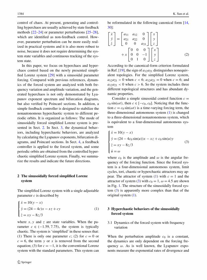
where c0 is the amplitude and ω is the angular fre-quency of the forcing function. Since the forced sys-tem is a four-dimensional autonomous system, limitcycles, tori, chaotic or hyperchaotic attractors may ap-pear. The attractor of system (1) with c = 1 and theattractor of system (3) with c0 = 1, ω = 4.5 are shownin Fig. 1. The structure of the sinusoidally forced sys-tem (3) is apparently more complex than that of theoriginal system (1).

3 Hyperchaotic behaviors of the sinusoidallyforced system

3.1 Dynamics of the forced system with frequencyvariation

When the perturbation amplitude c0 is a constant,the dynamics are only dependent on the forcing fre-quency ω. As is well known, the Lyapunov expo-nents measure the exponential rates of divergence and

Hyperchaos and hyperchaos control of the sinusoidally forced simplified Lorenz system 1385

Fig. 1 Attractors of system (1) and system (3) with different parameter. (a) System (1) with c = 1. (b) System (3) with c0 = 1,ω = 4.5

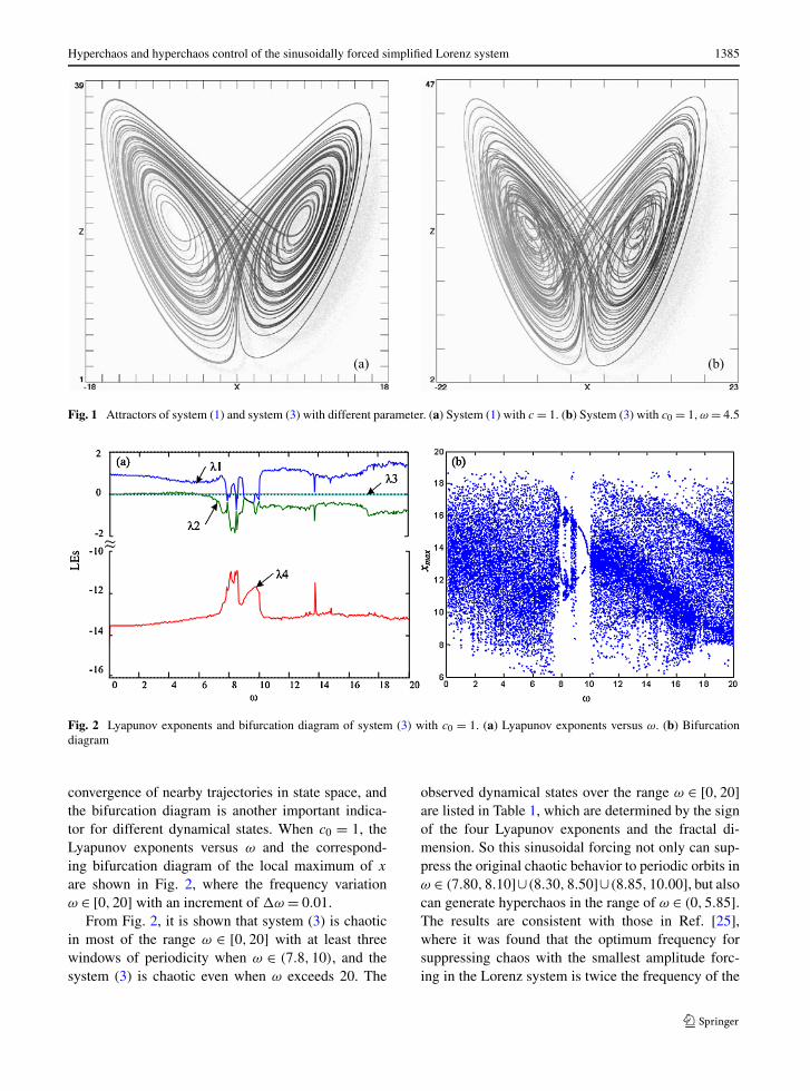
Fig. 2 Lyapunov exponents and bifurcation diagram of system (3) with c0 = 1. (a) Lyapunov exponents versus ω. (b) Bifurcationdiagram

convergence of nearby trajectories in state space, andthe bifurcation diagram is another important indica-tor for different dynamical states. When c0 = 1, theLyapunov exponents versus ω and the correspond-ing bifurcation diagram of the local maximum of x

are shown in Fig. 2, where the frequency variationω ∈ [0,20] with an increment of �ω = 0.01.

From Fig. 2, it is shown that system (3) is chaoticin most of the range ω ∈ [0,20] with at least threewindows of periodicity when ω ∈ (7.8,10), and thesystem (3) is chaotic even when ω exceeds 20. The

observed dynamical states over the range ω ∈ [0,20]are listed in Table 1, which are determined by the signof the four Lyapunov exponents and the fractal di-mension. So this sinusoidal forcing not only can sup-press the original chaotic behavior to periodic orbits inω ∈ (7.80,8.10]∪(8.30,8.50]∪(8.85,10.00], but alsocan generate hyperchaos in the range of ω ∈ (0,5.85].The results are consistent with those in Ref. [25],where it was found that the optimum frequency forsuppressing chaos with the smallest amplitude forc-ing in the Lorenz system is twice the frequency of the

1386 K. Sun et al.

Table 1 The dynamics ofsystem (3) for the differentranges of ω with c0 = 1

Range of ω Sign ofthe LE

Dimension Dynamics

(7.80,8.10] ∪ (8.30,8.50] ∪ (8.85,10.00] 0 − − − 1 periodic orbits

(5.85,7.80] ∪ (8.10,8.30] ∪ (8.50,8.85]∪ (10.00,20.00]

+ 0 − − >2 chaotic attractor

(0,5.85] + + 0 − >3 hyperchaotic attractor

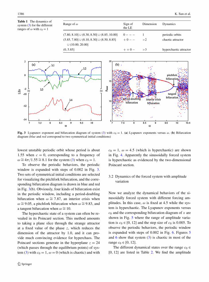
Fig. 3 Lyapunov exponent and bifurcation diagram of system (3) with c0 = 1. (a) Lyapunov exponents versus ω. (b) Bifurcationdiagram (blue and red correspond to two symmetrical initial conditions)

lowest unstable periodic orbit whose period is about1.55 when c = 0, corresponding to a frequency ofω ∼= 4π/1.55 ∼= 8.1 for the system (3) when c0 = 1.

To observe the periodic behaviors, the periodicwindow is expanded with steps of 0.002 in Fig. 3.Two sets of symmetrical initial conditions are selectedfor visualizing the pitchfork bifurcation, and the corre-sponding bifurcation diagram is drawn in blue and redin Fig. 3(b). Obviously, four kinds of bifurcation existin the periodic window, including a period-doublingbifurcation when ω ∼= 7.87, an interior crisis whenω ∼= 9.05, a pitchfork bifurcation when ω ∼= 9.83, anda tangent bifurcation when ω ∼= 10.

The hyperchaotic state of a system can often be re-vealed in its Poincaré section. This method amountsto taking a plane slice through the strange attractorat a fixed value of the phase z, which reduces thedimension of the attractor by 1.0, and it can pro-vide much convincing evidence for hyperchaos. ThePoincaré sections generate in the hyperplane z = 24(which passes through the equilibrium points) of sys-tem (3) with c0 = 1, ω = 0 (which is chaotic) and with

c0 = 1, ω = 4.5 (which is hyperchaotic) are shownin Fig. 4. Apparently the sinusoidally forced systemis hyperchaotic as evidenced by the two-dimensionalPoincaré section.

3.2 Dynamics of the forced system with amplitudevariation

Now we analyze the dynamical behaviors of the si-nusoidally forced system with different forcing am-plitudes. In this case, ω is fixed at 4.5 while the sys-tem is hyperchaotic. The Lyapunov exponents versusc0 and the corresponding bifurcation diagram of x areshown in Fig. 5 where the range of amplitude varia-tion is c0 ∈ [0,12] and the step size of c0 is 0.005. Toobserve the periodic behaviors, the periodic windowis expanded with steps of 0.002 in Fig. 6. Figures 5and 6 show that system (3) is chaotic in most of therange c0 ∈ [0,12].

The different dynamical states over the range c0 ∈[0,12] are listed in Table 2. We find the amplitude

Hyperchaos and hyperchaos control of the sinusoidally forced simplified Lorenz system 1387

Fig. 4 Poincaré sections of system (3) for different ω. (a) c0 = 1, ω = 0 (chaotic). (b) c0 = 1, ω = 4.5 (hyperchaotic)

Fig. 5 Lyapunov exponents and bifurcation diagram of system (3) with ω = 4.5. (a) Lyapunov exponents versus c0. (b) Bifurcationdiagram (blue and red correspond to two symmetrical initial conditions)

Fig. 6 Lyapunov exponent and bifurcation diagram of system (3) with ω = 4.5. (a) Lyapunov exponents versus c0 ∈ [8.88,12].(b) Bifurcation diagram (blue and red correspond to two symmetrical initial conditions)

1388 K. Sun et al.

Table 2 The dynamics ofsystem (3) for the differentranges of c0 with ω = 4.5

Range of c0 Sign ofthe LE

Dimension Dynamics

[2.76,5.00) ∪ [7.47,7.65) ∪ [8.30,8.61)

∪ [8.88,9.17) ∪ [9.26,9.41) ∪ [10.47,10.94)

∪ [11.24,12.00)

0 − − − 1 periodic orbits

[0,0.53) ∪ [1.30,2.76) ∪ [5.00,7.47) ∪ [7.65,8.30)

∪ [8.61,8.88) ∪ [9.17,9.26) ∪ [9.41,10.47)

∪ [10.94,11.24)

+ 0 − − >2 chaotic attractor

[0.53,1.30) + + 0 − >3 hyperchaoticattractor

Fig. 7 Poincaré sections of system (3) for the different c0. (a) c0 = 0, ω = 4.5 (chaotic). (b) c0 = 1.2, ω = 4.5 (hyperchaotic)

variation not only can suppress the original hyper-chaotic behavior to chaotic behavior, or to a periodicorbit, but also can preserve the hyperchaos in the rangeof c0 ∈ [0.53,1.30).

The Poincaré sections are shown in Fig. 7 fordemonstrating the existence of hyperchaos in theforced system. These sections generate in the hyper-plane z = 24 of system (3) with c0 = 0, ω = 4.5(which is chaotic) and with c0 = 1.2,ω = 4.5 (whichis hyperchaotic). Obviously the sinusoidally forcedsystem is hyperchaotic on the evidence of its two-dimensional Poincaré section.

Interestingly, the three-attractor coexisting phe-nomenon occurs in this forced system. There existthree attractors when c0 = 8.6,ω = 4.5 and c0 = 10.6,ω = 4.5, respectively. The coexisting attractors areshown in Fig. 8, denoted in green, blue and red cor-responding to different initial conditions. The initial

conditions of this first case are chosen as [x0, y0, z0,

u0] = [−15.0794,−4.1277,60.8300,2.8345], [x0, y0,

z0, u0] = [−1.1578,−0.5678,18.7900,5.2480] and[x0, y0, z0, u0] = [6.5245,7.4527,39.1987,3.8621],respectively. The initial conditions of the second caseare set to [x0, y0, z0, u0] = [5.0546,5.5616,40.7255,

4.0424], [x0, y0, z0, u0] = [−22.3068,−35.0684,

49.7511,2.5573] and [x0, y0, z0, u0] = [0.7080,

0.8707,6.0358,1.2553], respectively.

4 Hyperchaos control for the sinusoidally forcedsystem

Since chaos (or hyperchaos) may cause irregular be-haviors which is undesirable, in this section, a feed-back controller is designed to stabilize the nonau-tonomous hyperchaotic system to periodic orbits.

Hyperchaos and hyperchaos control of the sinusoidally forced simplified Lorenz system 1389

Fig. 8 Coexisting attractors of system (3) for the different c0. (a) c0 = 8.6, ω = 4.5. (b) c0 = 10.6, ω = 4.5.

Fig. 9 Lyapunov exponents and bifurcation diagram of system (5) with ω = 4.5, c0 = 1. (a) Lyapunov exponents versus k ∈ [−6,9].(b) Bifurcation diagram

Assume that the controlled hyperchaotic system isgiven by⎧⎪⎪⎪⎪⎨

⎪⎪⎪⎪⎩

x = 10(y − x) + v1

y = (24 − 4c0 sin(u))x − xz + c0 sin(u)y + v2

z = xy − 8z/3 + v3

u = ω + v4

(4)

where v1, v2, v3 and v4 are feedback control input. Tokeep it simple, we set v1 = kx, v2 = v3 = v4 = 0, sothat the controlled hyperchaotic system becomes⎧⎪⎪⎪⎪⎨

⎪⎪⎪⎪⎩

x = 10(y − x) + kx

y = (24 − 4c0 sin(u))x − xz + c0 sin(u)y

z = xy − 8z/3

u = ω

(5)

where k is the feedback coefficient, and the system pa-rameters are chosen as ω = 4.5 and c0 = 1 to ensurethat the original perturbed system is hyperchaotic.

For the hyperchaos control, one problem is howto choose the feedback coefficient k. Firstly, find therange of k by analyzing the equilibrium and stabilityof system (5) at ω = 0. Secondly, calculate the Lya-punov exponents and plot the bifurcation diagram ofsystem (5) in the nearby range. Then we can easily de-termine the feedback coefficient k required to controlthe hyperchaos to stable periodic orbits. The Lyapunovexponents versus k and the corresponding bifurcationdiagram of system (5) are shown in Fig. 9 where therange of feedback coefficient is k ∈ [−6,9] and thestep size of k is 0.005.

1390 K. Sun et al.

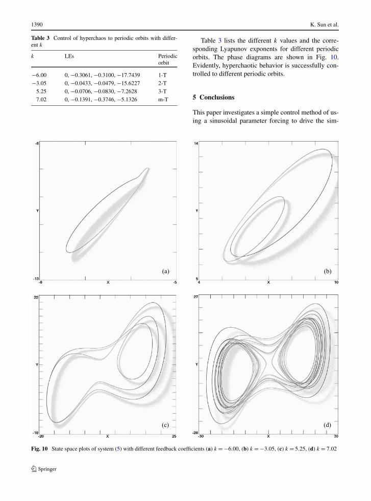
Table 3 Control of hyperchaos to periodic orbits with differ-ent k

k LEs Periodicorbit

−6.00 0, −0.3061, −0.3100, −17.7439 1-T

−3.05 0, −0.0433, −0.0479, −15.6227 2-T

5.25 0, −0.0706, −0.0830, −7.2628 3-T

7.02 0, −0.1391, −0.3746, −5.1326 m-T

Table 3 lists the different k values and the corre-sponding Lyapunov exponents for different periodicorbits. The phase diagrams are shown in Fig. 10.Evidently, hyperchaotic behavior is successfully con-trolled to different periodic orbits.

5 Conclusions

This paper investigates a simple control method of us-ing a sinusoidal parameter forcing to drive the sim-

Fig. 10 State space plots of system (5) with different feedback coefficients (a) k = −6.00, (b) k = −3.05, (c) k = 5.25, (d) k = 7.02

Hyperchaos and hyperchaos control of the sinusoidally forced simplified Lorenz system 1391

plified Lorenz system to hyperchaos. It is found thatthe sinusoidal forcing not only suppresses the originalchaotic behavior to a periodic orbit, but also generateshyperchaos in some parameter ranges. The basic prop-erties of the dynamics are analyzed by using the Lya-punov exponents, bifurcation diagrams, and Poincarésections. With both the change of frequency variationω and amplitude variation c0, the sinusoidal forcedsystem exhibits limit cycles, pitchfork bifurcations,period-doubling bifurcations, chaos, and hyperchaos.It has more complex dynamical behaviors than that ofthe original system. Furthermore, hyperchaotic statesalso can be controlled to chaos or a periodic orbit bya simple feedback control, which is desirable for engi-neering applications. Future works on this topic couldinclude its circuit implementation, as well as a theo-retical analysis of the counterpart fractional-order sys-tem.

Acknowledgements This work was supported by the Na-tional Nature Science Foundation of People’s Republic of China(Grant No. 61161006), and the National Science Foundation forPost-doctoral Scientists of People’s Republic of China (GrantNo. 20070420774). One of us (Xuan Liu) wishes to thank Prof.Guanrong Chen for discussions by E-mail.

References

1. Rössler, O.E.: An equation for hyperchaos. Phys. Lett. A72(2–3), 155–157 (1979)

2. Kapitaniak, T., Chua, L.O.: Hyperchaotic attractor of uni-directionally coupled Chua’s circuit. Int. J. Bifurc. Chaos4(2), 477–482 (1994)

3. Gao, T.G., Chen, G.R., Chen, Z.Q., Cang, S.J.: The genera-tion and circuit implementation of a new hyper-chaos basedupon Lorenz system. Phys. Lett. A 361, 78–86 (2007)

4. Wang, F.Q., Liu, C.X.: Hyperchaos evolved from the Liuchaotic system. Chin. Phys. Soc. 15(5), 963–968 (2006)

5. Niu, Y.J., Wang, X.Y., Wang, M.J., Zhang, H.G.: A new hy-perchaotic system and its circuit implementation. Commun.Nonlinear Sci. Numer. Simul. 15, 3518–3524 (2010)

6. Zheng, S., Dong, G.G., Bi, Q.S.: A new hyperchaotic sys-tem and its synchronization. Appl. Math. Comput. 215,3192–3200 (2010)

7. Zhou, X.B., Wu, Y. Li, Y., Xue, H.Q.: Adaptive control andsynchronization of a new modified hyperchaotic Lü sys-tem with uncertain parameters. Chaos Solitons Fractals 39,2477–2483 (2009)

8. Qi, G.Y., van Wyk, M.A., van Wyk, B.J., Chen, G.R.: Ona new hyperchaotic system. Phys. Lett. A 372, 124–136(2008)

9. Li, Y.X., Tang, W.K.S., Chen, G.R.: Hyperchaos evolvedfrom the generalized Lorenz equation. Int. J. Circuits Theor.Appl. 33(4), 235–251 (2005)

10. Chen, A., Lu, J., Lü, J.H., Yu, S.M.: Generating hyper-chaotic Lü attractor via state feedback control. Physica A364, 103–110 (2006)

11. Li, Y.X., Tang, W.K.S., Chen, G.R.: Generating hyperchaosvia state feedback control. Int. J. Bifurc. Chaos 15(10),3367–3375 (2005)

12. Li, Y.X., Chen, G.R., Tang, W.K.S.: Controlling a unifiedchaotic system to hyperchaotic. IEEE Trans. Circuits Syst.II, Express Briefs 52(4), 204–207 (2005)

13. Wang, G.Y., Zhang, X., Zheng, Y., Li, Y.X.: A new mod-ified hyperchaotic Lü system. Physica A 371, 260–272(2006)

14. Celikovský, S., Chen, G.R.: On a generalized Lorenzcanonical form of chaotic systems. Int. J. Bifurc. Chaos12(8), 1789–1812 (2002)

15. Chen, T., Ueta, T.: Yet another chaotic attractor. Int. J. Bi-furc. Chaos 9(7), 1465–1466 (1999)

16. Lü, J.H., Chen, G.R.: A new chaotic attractor coined. Int. J.Bifurc. Chaos 12(3), 659–661 (2002)

17. Lü, J.H., Chen, G.R., Cheng, D., Celikovský, S.: Bridge thegap between the Lorenz system and the Chen system. Int.J. Bifurc. Chaos 12(12), 2917–2928 (2002)

18. Ott, E., Grebogi, G., Yorke, J.A.: Controlling chaos. Phys.Rev. Lett. 64, 1196–1199 (1990)

19. Brandt, M.E., Chen, G.R.: Bifurcation control of two non-linear models of cardiac activity. IEEE Trans. Circuits Syst.I, Fundam. Theory Appl. 44, 1031–1034 (1997)

20. Jakimoski, G., Kocarev, L.: Chaos and cryptography: blockencryption ciphers based on chaotic maps. IEEE Trans. Cir-cuits Syst. I, Fundam. Theory Appl. 48, 163–169 (2001)

21. Kocarev, L.G., Maggio, M., Ogorzalek, M., Pecora, L.,Yao, K.: Applications of chaos in modern communicationsystems. IEEE Trans. Circuits Syst. I, Fundam. TheoryAppl. 48, 385–527 (2001)

22. Zhu, C.X.: Controlling hyperchaos in hyperchaotic Lorenzsystem using feedback controllers. Appl. Math. Comput.216, 3126–3132 (2010)

23. Dou, F.Q., Sun, J.A., Duan, W.S., Lü, K.P.: Controlling hy-perchaos in the new hyperchaotic system. Commun. Non-linear Sci. Numer. Simul. 14, 552–559 (2009)

24. Jia, Q.: Hyperchaos generated from the Lorenz chaotic sys-tem and its control. Phys. Lett. A 366, 217–222 (2007)

25. Mirus, K.A., Sprott, J.C.: Controlling chaos in low- andhigh-dimensional systems with periodic parametric pertur-bations. Phys. Rev. A 59, 5313–5324 (1999)

26. Tam, L.M., Chen, J.H., Chen, H.K., Tou, W.M.S.: Gener-ation of hyperchaos from the Chen-Lee system via sinu-soidal perturbation. Chaos Solitons Fractals 38, 826–839(2008)

27. Sun, M., Tian, L.X., Zeng, C.Y.: The energy resources sys-tem with parametric perturbations and its hyperchaos con-trol. Nonlinear Anal., Real World Appl. 10, 2620–2626(2009)

28. Wu, X.Q., Lu, J.A., Iu, H.H.C., Wong, S.C.: Suppres-sion and generation of chaos for a three-dimensional au-tonomous system using parametric perturbations. ChaosSolitons Fractals 31, 811–819 (2007)

29. Sun, K.H., Sprott, J.C.: Dynamics of a simplified Lorenzsystem. Int. J. Bifurc. Chaos 19(4), 1357–1366 (2009)

30. Vanecek, A., Celikovský, S.: Control Systems: From Lin-ear Analysis to Synthesis of Chaos. Prentice-Hall, London(1996)