893

Available at http://pvamu.edu/aam

Appl. Appl. Math.

ISSN: 1932-9466

Vol. 10, Issue 2 (December 2015), pp. 893-908

Applications and

Applied Mathematics: An International Journal

(AAM)

Hydromagnetic Flow and Heat Transfer of Eyring-Powell Fluid

over an Oscillatory Stretching Sheet with Thermal Radiation

S. U. Khan and N. Ali 1 Department of Mathematics and Statistics,

International Islamic University

Islamabad 44000, Pakistan

sk_iiu@yahoo.com

nasirali_qau@yahoo.com

Z. Abbas Department of Mathematics,

The Islamia University of Bahawalpur,

Bahawalpur 63100, Pakistan

za_qau@yahoo.com

Received: January 28, 2015; Accepted: June 2, 2015

Abstract

An analysis is carried out to investigate the magnetohydrodynamic flow and heat transfer in an

unsteady flow of Eyring-Powell fluid over an oscillatory stretching surface. The radiation effects

are also considered in energy equation. The flow is induced due to infinite elastic sheet which is

stretched periodically back and forth in its own plane. Finite difference scheme is used to solve

dimensionless partial differential equations. The effects of emerging parameters on both velocity

and temperature profiles are illustrated through graphs. The results obtained by means of finite

difference scheme are compared with earlier studies and found in excellent agreement.

Keywords: Boundary layer flow, non-Newtonian fluid, Eyring-Powell fluid, heat flow,

oscillatory stretching sheet, finite difference method

MSC 2010 No.: 76A05, 76M20, 76N20

1. Introduction The boundary layer flow and heat transfer of non-Newtonian fluids over a stretching sheet has

numerous applications in various engineering and industrial processes. Such applications include

manufacturing of plastic fluids, artificial fibers and polymeric sheets, plastic foam processing,

894 S.U. Khan et al.

crystal growing, cooling of metallic sheets in a cooling bath, extrusion of polymer sheet from a

die, heat treated materials travelling between a feed role and many others. Besides this, radiation

plays a vital role in controlling the heat transfer in the polymer processing industry. In view of all

these applications many authors studied the flow of different fluid models over stretching sheet.

Sakiadis (1961) initiated the study of boundary layer flow over a flat surface moving with a

constant velocity. Since then many researchers extended the work of Sakiadis (1961) for both

Newtonian and non-Newtonian fluids. Crane (1970) obtained the closed form solution for the

flow caused by stretching of an elastic flat sheet that moves in its own plane. Gupta and Gupta

(1977) extended the work of Crane (1970) by considering suction/blowing at the sheet surface.

Anderson et al. (1994) studied the diffusion of chemically reactive species over a moving

continuous sheet. Golra et al. (1978) discussed unsteady mass transfer in the boundary over a

continuous moving sheet. Rajagopal et al. (1984) discussed the flow of viscoelastic second

grade fluid over stretching sheet. Pop (1996) studied the unsteady flow past a stretching sheet.

Cortell et al. (2006) investigated the heat transfer in an incompressible second grade fluid past a

stretching sheet. Ariel (2001) analyzed an axisymmetric flow of second grade fluid past over a

radially stretching sheet by finding exact numerical solution. Akyildiz et al (2006) studied the

diffusion of chemically reactive species of a non-Newtonian fluid immersed in a porous medium

over a stretching sheet. Hayat and Sajid (2007) extended the problem of Ariel (2001) by

performing heat transfer analysis with help of homotopy analysis method. Some more

contributions in this regard are made by Hayat et al. (2008), Sajid et al. (2012), Nazar et al.

(2004), Ishake (2008), Ariel et al. (2006), Nazar et al. (2004), Nandeppanavar et al. (2013), Joshi

et al. (2010) and many references therein.

The literature shows that all these investigations are carried out for the case when sheet is only

stretched. However, there may arise situations where the sheet is stretched as well as oscillates

simultaneously in its own plane. To the best of our knowledge, Wang (1988) was the first who

discussed viscous flow due to oscillatory stretching surface. Siddapa et al. (1995) extended

Wang's problem for viscoelastic Walter-B fluid. Later on Abbas et al. (2009) included the

effects of heat transfer and slip effects on Wang's problem (1988) . In another work, Abbas et. al.

(2008) reported the hydromagnetic flow of viscoelastic second grade fluid over an oscillatory

stretching sheet. Zheng et al. (2013) discussed the Soret and Dufour effects on two-dimensional

flow of viscous fluid over a moving oscillatory stretching surface by using homotopy analysis

method. Recently Ali et al. (2015) investigated hydromagnetic flow and heat transfer of a Jeffrey

fluid over an oscillatory stretching sheet by using homotopy analysis method and finite

difference scheme. The literature survey indicates that no attempt is available in the literature

which deals with flow and heat transfer of Eyring-Powell fluid over an oscillatory stretching

surface with radiation effects.

The purpose of present work is to provide such an analysis. Eyring-Powell fluid model deduced

from kinetic theory of liquids rather than the empirical relation (Hayat et al. (2013)). Some

studies on flows of Eyring-Powell fluid are reported by Sirohi eta al. (1984),Hayat et al. (2012), Javed et al. (2012) and Hayat (2014).

AAM: Intern. J., Vol. 10, Issue 2 (December 2015) 895

The structure of this paper is as follows. In Section 2, we present the formulation of the problem.

Solution by finite difference method is provided in Section 3. Graphical results obtained through

finite difference scheme are shown and discussed in detail in Section 4 . Finally, the main

conclusions of the study are summarized in Section 5 .

2. Flow Analysis

Let us consider an unsteady and two-dimensional flow of incompressible Eyring-Powell fluid

over an oscillatory stretching sheet coinciding with plane 0y (Figure 1 ). In the Cartesian

coordinate system x is along the sheet and y is perpendicular to the sheet. Let wT denote the

surface temperature and T is the temperature of the fluid far away from the surface. It is

assumed that .wT T A magnetic field of magnitude 0B is applied in transverse direction to the

sheet. Using the boundary layer approximations, continuity, momentum and energy equations are

[see Hayat et al. (2014)]

Figure 1. Geometry of the problem

0,u v

x y

(1)

2 22 2

0

2 3 2

1 1,

2

Bu u u u u uu v u

t x y C y C y y

(2)

2

2,r

p

qT T T Tc u v k

t x y y y

(3)

where u and v are the velocity component along x and y directions, respectively,

represents the kinematic viscosity, is the density, and C are the fluid parameters of the

Eyring-Powell model, pc represents the specific heat, k is the thermal conductivity, is the

electrical conductivity, T is the temperature and rq is the radiative heat flux which is given by

Rosseland approximation [Raptis et al. (2004)]

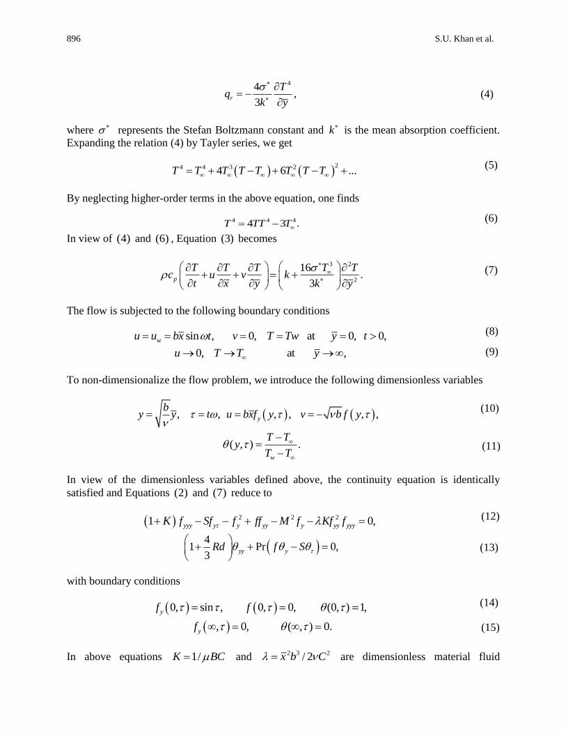
896 S.U. Khan et al.

44,

3r

Tq

k y

(4)

where represents the Stefan Boltzmann constant and k is the mean absorption coefficient.

Expanding the relation (4) by Tayler series, we get

24 4 3 24 6 ...T T T T T T T T

(5)

By neglecting higher-order terms in the above equation, one finds

4 4 44 3 .T TT T (6)

In view of (4) and (6) , Equation (3) becomes

3 2

2

16.

3p

TT T T Tc u v k

t x y k y

(7)

The flow is subjected to the following boundary conditions

sin , 0, at 0, 0,wu u bx t v T Tw y t (8)

0, at ,u T T y (9)

To non-dimensionalize the flow problem, we introduce the following dimensionless variables

, , , , , , y

by y t u bxf y v b f y

(10)

( , ) .w

T Ty

T T

(11)

In view of the dimensionless variables defined above, the continuity equation is identically

satisfied and Equations (2) and (7) reduce to

2 2 21 0,yyy y y yy y yy yyyK f Sf f ff M f Kf f (12)

4

1 Pr 0,3

yy yRd f S

(13)

with boundary conditions

0, sin , 0, 0, (0, ) 1,yf f (14)

, 0, ( , ) 0.yf (15)

In above equations 1/K BC and 2 3 2/ 2x b C are dimensionless material fluid

AAM: Intern. J., Vol. 10, Issue 2 (December 2015) 897

parameters, /S b is the ratio of the oscillation frequency of the sheet to its stretching rate,

2

0 /M B b is the Hartmann number, Pr /pc k is the Prandtl number and 34 T

Rdkk

is

the radiation parameter. According to Javed et al. (2012) equation (12) is subject to the constraint

1K .

The physical quantities of interest are the skin-friction coefficient fC and the local Nusselt

number ,xNu which are defined as

2

0

, , ,w wf x w

w w y

xq TC Nu q k

u k T T y

(16)

where w and wq are the shear stress and heat flux at wall, respectively. In view of (10) and

(11) , Equation (16) takes the following forms

1/ 2 1/ 2

0

4Re 1 , Re 1 0, ,

3 3x f yy yy x x yy

KC K f f Nu Rd

(17)

where Re /x wu x is the local Reynold number.

3. Direct numerical solution of the problem

We intend to use a finite difference scheme to solve nonlinear boundary value problem

consisting of Equations (12) and (13) with boundary conditions (14) and (15). Since, the flow is

in unbounded domain, a coordinate transformation 1/( 1)y is used to transform the semi-

infinite physical domain [0, )y to finite calculation domain [0,1] . Thus, we get

2 2 2 22 4 3 2

2 2

11, , 2 , ,y

y y y

3 3 26 5 4

3 3 26 6 .

y

In view of above transformations, Equations (12) and (13) become

22 2 3

2 2 3 2 4

2 36 1 2 6 1 1

f f f f fS K f K f K

2 3 22 3 2 2

2 12 11 10

2 3 2 26 6

f f f f f fM K K K

898 S.U. Khan et al.

2 2 33 210 9 8

3 24 24 24

f f f f fK K K

2 22 3 2 211 10 9

2 3 2 24 24 24

f f f f f f fK K K

(18)

24 3 2

2

41 2 Pr 0,

3Rd f S

(19)

0, 0 at 0,f

(20)

0, sin , 1 at 1.f

f

(21)

Equations (18) and (19) are discretized for L uniformly distributed discrete points

1 2, ,..., 0, 1L

with a space grid size of 1/ 1L and time level 1 2, ,... .t t t

Hence the discrete values 1 2, , ..., n n n

Lf f f and 1 2, , ..., n n n

L at these grid point for time

levels nt n t is the time stept can be numerically solved together with boundary

conditions at 0 0 and 11.

L

We start our simulations from a motionless velocity

field and a uniform temperature distribution equal to temperature at infinity as

, 0 0 and , 0 0.f (22)

Following Abbas et al. (2009) an implicit difference scheme is constructed for velocity f and

temperature as follows

21 1

2 216 1 2

n n n n nnf f f f f

S K ft

12 2

3 2

2 26 1 2

n n nn nf f f

K f f

21 13 2 3

4 2 12

3 2 31

n n n nf f f f

K M K

3 22 2

11 10

2 26 6

n n nf f f

K K

AAM: Intern. J., Vol. 10, Issue 2 (December 2015) 899

2 23 2

10 9

3 24 24

n n n nf f f f

K K

32 3

8 11

2 324 4

n n n nf f f f

K K

2 22 2

10 9

2 224 24

n n n nf f f f

K K

(23)

1

1 1 124 3 2

2

4Pr 1 2 Pr .

3

n nn n n

nS Rd f

t

In this way, only linear equations at new time step ( 1)n are to be solved. It should be noted

that other different choices of time differences are also possible. By using finite difference

method two systems of linear equations for 1n

if

and 1n

i

1, 2,...,i L at the time step

1n are obtained which can be solved with help of the Gaussian elimination.

4. Results and discussion

In order to discuss the effects of emerging parameters on velocity and temperature fields, the

numerical technique discussed in the previous section is implemented to solve the non-linear

partial differential Equations (12) and (13) with boundary conditions (14) and (15). In this

section, we discuss the effects of involved parameters graphically. In all the plots, the values of

K and are chosen so that the product K should be very sufficiently smaller than unity.

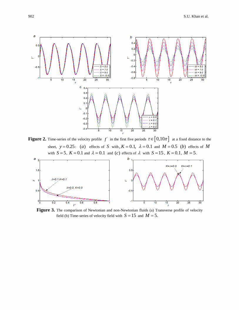
Figure 2 depicts the effects of the relative amplitude of frequency to the stretching rate S ,

Hartmann number M and fluid parameters on the time-series of the velocity component 'f

at a fixed distance 0.25y from the sheet, respectively. Figure 2( )a shows the effects of the S

on the time-series of the velocity profile 'f by keeping 0.1K , 0.1 and 0.5M fixed.

This figure shows that the amplitude of the flow motion decreases by increasing .S Furthermore,

one can easily observe that a phase shift occurs which increases for large values .S Figure 2( )b

elucidates the behavior of Hartmann number M on the time-series of the velocity component 'f .

As expected, the amplitude of the flow motion decreases by increasing Hatmann number M .

The reason is that magnetic field acts as a resistance to the flow. Figure 2( )c shows that an

increase in fluid parameter results in an increase of amplitude '.f

Figure 3(a) shows a comparison of transverse profile of velocity 'f for Newtonian and Eyring-

Powell fluids. It is evident that magnitude of velocity inside the boundary layer for Eyring-

Powell fluid is greater than the magnitude of velocity for Newtonian fluid. Similarly amplitude

of time-series of 'f for Eyring-Powell fluid is also greater than the amplitude of time-series of

'f for Newtonian fluid (Figure 3(b)).

900 S.U. Khan et al.

Figure 4 shows the influence of relative amplitude of frequency to the stretching rate S on

transverse profile of velocity 'f at four different time instants 8.5 , 9 , 9.5 and

10 . Figure 4( )a is plotted at time instant 8.5 . From this figure we see that velocity

decreases by increasing .S At time instant 9 (Figure 4( ))b the velocity 'f at the surface is

zero and for away from the surface it again approaches zero. Moreover, at this time instant it

oscillates near the wall. Figure 4( )c shows the effects of S on 'f at 9.5 . From this Figure

we note that velocity decreases from 1 at the surface to zero far away from the surface. The

effects of S on 'f at time instant 10 are similar to the effects of S on 'f at time instant

9 .

The variation of Hartmann number M on transverse profile of velocity 'f at different time

instants 8.5 , 9 , 9.5 and 10 are shown in Figure 5. Figure 5( )a shows that

an increase in Hartmann number M causes a decrease in the velocity at time instant 8.5 .

Furthermore, the boundary layer thickness is also found to decrease. It is observed from Figure

5(b) that at 9 , the velocity 'f oscillates near the surface and approaches to zero far away

from the surface. Figure 5( )c shows that at 9.5 , the velocity 'f at the surface decreases

from 1 to zero far away from the surface. Moreover, at this time instant there exists no

oscillation in the velocity '.f The velocity profile at time instant 10 is illustrated in Figure

5( ).d From this Figure one can observe that velocity oscillates near the sheet and approaches

zero far away from the surface.

Figure 6 illustrates the influence of fluid parameter on the velocity profile 'f at four

different time instants 8.5 , 9 , 9.5 and 10 . Figure 6( )a shows the variation

of fluid parameter at 8.5 . Here, we see the velocity 'f increases by increasing fluid

parameter . From Figure 6( ),b it can be seen that the velocity oscillates near the sheet before

approaching zero far away from the sheet. The effects of at time instant 9.5 are

illustrated in Figure 6( )c . An opposite trend is found in velocity at this time instant, i.e. the

velocity increases by increasing fluid parameter . The behavior of fluid parameter at time

instant 10 is shown in Figure 6( )d .

Figure 7 describes the effects of Hartmann number M relative amplitude of frequency to the

stretching rate ,S fluid parameter K and on the time-series of shear stress at the wall for the

first five periods [0,10 ]. Figure 7( )a shows the influence the variation of Hartmann

number M on the skin-friction coefficient 1/ 2Rex fC by keeping other parameters fixed. It is

clear from this Figure that the amplitude of oscillation of the skin-friction coefficient increases

by increasing Hartmann number M. From Figure 7(b), we observe that skin friction coefficient

oscillates with time and the amplitude of oscillation increases for large values of S . The effects

of fluid parameter K and are shown in Figures 7( )c and ( ),d respectively. In these Figures

an opposite trend is observed. These Figures show that the skin friction coefficient 1/ 2Rex fC

decreases monotonically by increasing the fluid parameters. The temperature profile for

different values of , Pr,S Rd and M are shown in Figure 8.

AAM: Intern. J., Vol. 10, Issue 2 (December 2015) 901

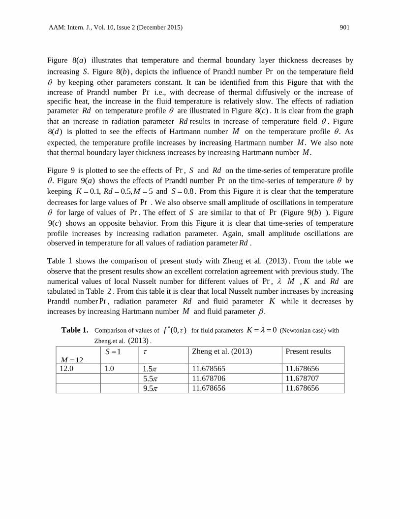
Figure 8( )a illustrates that temperature and thermal boundary layer thickness decreases by

increasing .S Figure 8( )b , depicts the influence of Prandtl number Pr on the temperature field

by keeping other parameters constant. It can be identified from this Figure that with the

increase of Prandtl number Pr i.e., with decrease of thermal diffusively or the increase of

specific heat, the increase in the fluid temperature is relatively slow. The effects of radiation

parameter Rd on temperature profile are illustrated in Figure 8( )c . It is clear from the graph

that an increase in radiation parameter Rd results in increase of temperature field . Figure

8( )d is plotted to see the effects of Hartmann number M on the temperature profile . As

expected, the temperature profile increases by increasing Hartmann number .M We also note

that thermal boundary layer thickness increases by increasing Hartmann number .M

Figure 9 is plotted to see the effects of Pr , S and Rd on the time-series of temperature profile

. Figure 9( )a shows the effects of Prandtl number Pr on the time-series of temperature by

keeping 0.1, 0.5, 5K Rd M and 0.8S . From this Figure it is clear that the temperature

decreases for large values of Pr . We also observe small amplitude of oscillations in temperature

for large of values of Pr . The effect of S are similar to that of Pr (Figure 9( )b ). Figure

9( )c shows an opposite behavior. From this Figure it is clear that time-series of temperature

profile increases by increasing radiation parameter. Again, small amplitude oscillations are

observed in temperature for all values of radiation parameter Rd .

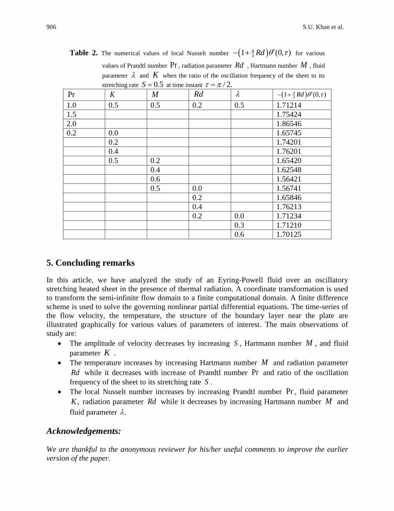
Table 1 shows the comparison of present study with Zheng et al. (2013) . From the table we

observe that the present results show an excellent correlation agreement with previous study. The

numerical values of local Nusselt number for different values of Pr , M , K and Rd are

tabulated in Table 2 . From this table it is clear that local Nusselt number increases by increasing

Prandtl number Pr , radiation parameter Rd and fluid parameter K while it decreases by

increases by increasing Hartmann number M and fluid parameter .

Table 1. Comparison of values of (0, )f for fluid parameters 0K (Newtonian case) with

Zheng.et al. (2013) .

12M 1S Zheng et al. (2013) Present results

12.0 1.0 1.5 11.678565 11.678656

5.5 11.678706 11.678707

9.5 11.678656 11.678656

902 S.U. Khan et al.

Figure 2. Time-series of the velocity profile f in the first five periods 0,10 at a fixed distance to the

sheet, 0.25y : ( )a effects of S with , 0.1,K 0.1 and 0.5M ( )b effects of M

with 5S , 0.1K and 0.1 and ( )c effects of with 15S , 0.1K , 5M .

Figure 3. The comparison of Newtonian and non-Newtonian fluids (a) Transverse profile of velocity

field (b) Time-series of velocity field with 15S and 5.M

AAM: Intern. J., Vol. 10, Issue 2 (December 2015) 903

Figure 4. Transverse profiles of the velocity field

f for the different values of S in the fifth period

8 ,10 , ( )a 8.5 , ( )b 9 , ( )c 9.5 , and ( )d 10 ,

with 0.1,K 0.1 and 1.0.M

Figure 5. Transverse profiles of the velocity field f for different values of M in the fifth period

8 ,10 , (a) 8.5 , (b) 9 , (c) 9.5 and (d) 10 with

904 S.U. Khan et al.

15,S 0.1K and 0.1.

Figure 6. Transverses profile of the velocity field f for different values of in the fifth period

8 ,10 , ( )a 8.5 , ( )b 9 , ( )c 9.5 and ( )d 10 with

15,S 0.1K and 1.M

Figure 7. Time-series of the skin friction coefficient in the first five periods 0,10 at a fixed

distance to the sheet, 0.25y : (a) effects of M with 5,S 0.1 and 0.1K

( )b effects of S with 4,M 0.1 and 0.1K , ( )c effects of K with 12S ,

0.1 , 12M and ( )d effects of with 12S , 0.1K and 12.M

AAM: Intern. J., Vol. 10, Issue 2 (December 2015) 905

Figure 8. Transverse profiles of the temperature field at 8 : (a) effects of S with 0.1,K

0.1, 5M , Pr 10, 0.5,Rd (b) effects of Pr with 0.1,K 0.1,

5M , 15,S 0.5Rd , ( )c effects of Rd of with 0.1,K 0.1, 5M ,

Pr 10 and 15S ( )d effects of M of with 0.1,K 0.1, 5Rd , Pr 10

and 15S .

Figure 9. Time-series of the temperature , 0,10 at 0.25y (a) effects of Pr with

0.1,K 0.1, 5M , 0.8,S 0.5,Rd (b) effects of S with 0.1,K

0.1, 5M ,Pr=10, 2.5Rd and (c) effects of Rd of with 0.1,K 0.1,

10M , Pr 10 and 15.S

906 S.U. Khan et al.

Table 2. The numerical values of local Nusselt number 43

1 (0, )Rd for various

values of Prandtl number Pr , radiation parameter Rd , Hartmann number M , fluid

parameter and K when the ratio of the oscillation frequency of the sheet to its

stretching rate 0.5S at time instant / 2.

Pr K M Rd 4

31 (0, )Rd

1.0 0.5 0.5 0.2 0.5 1.71214

1.5 1.75424

2.0 1.86546

0.2 0.0 1.65745

0.2 1.74201

0.4 1.76201

0.5 0.2 1.65420

0.4 1.62548

0.6 1.56421

0.5 0.0 1.56741

0.2 1.65846

0.4 1.76213

0.2 0.0 1.71234

0.3 1.71210

0.6 1.70125

5. Concluding remarks

In this article, we have analyzed the study of an Eyring-Powell fluid over an oscillatory

stretching heated sheet in the presence of thermal radiation. A coordinate transformation is used

to transform the semi-infinite flow domain to a finite computational domain. A finite difference

scheme is used to solve the governing nonlinear partial differential equations. The time-series of

the flow velocity, the temperature, the structure of the boundary layer near the plate are

illustrated graphically for various values of parameters of interest. The main observations of

study are:

The amplitude of velocity decreases by increasing S , Hartmann number M , and fluid

parameter K .

The temperature increases by increasing Hartmann number M and radiation parameter

Rd while it decreases with increase of Prandtl number Pr and ratio of the oscillation

frequency of the sheet to its stretching rate S .

The local Nusselt number increases by increasing Prandtl number Pr , fluid parameter

,K radiation parameter Rd while it decreases by increasing Hartmann number M and

fluid parameter .

Acknowledgements:

We are thankful to the anonymous reviewer for his/her useful comments to improve the earlier

version of the paper.

AAM: Intern. J., Vol. 10, Issue 2 (December 2015) 907

REFERENCES

Abbas, Z., Wang, Y., Hayat, T. Oberlack, M. (2009). Slip effects and heat transfer analysis in a

Viscous fluid over an oscillatory stretching surface. Int. J. Numer. Meth. Fluids, Vol. 59, pp.

443-458

Abbas, Z., Wang, Y., Hayat, T., Oberlack, M. (2008). Hydromagnetic flow in a viscoelastic fluid

due to the oscillatory stretching surface, Int. J. Non Lin. Mech. Vol. 43, pp. 783-793.

Akyilidiz, F. T., Bellout, H. and Vajravelu, K. (2006). Diffusion of chemical reactive species in

porous medium over a stretching sheet, J Math. Anal. Appl. (2006) pp. 322-339.

Ali, N., Khan, S.U. and Abbas, Z. (2015). Hydromagnetic flow and heat transfer of a Jeffrey-

fluid, over an oscillatory stretching surface Z. Naturforsch A. DOI 10.1515/zna-2014-0273

(In Press).

Anderson, H. I., Hansen, O. R. and Olmedal, B. (1994). Diffusion of chemically reactive species

from a stretching sheet, Int. J. Heat Mass Transf., Vol. 37, pp. 659-664.

Ariel, P.D. (2001). Axismmetric flow of a second grade fluid past a stretching sheet. Int. J. Eng.

Sci. Vol. 39, pp. 529-553.

Ariel, P.D., Hayat, T. and Asghar, S. (2006). The flow of an elastico-viscous fluid past stretching

sheet with partial slip, Acta. Mech. Vol. 187, pp. 29-35.

Cortell, R. (2006). A note on flow and heat transfer of viscoelastic fluid over a stretching sheet,

Int. J. Non-Lin. Mech. Vol. 41, pp. 78-85.

Crane, L.J. (1970). Flow past a stretching plate. Z Angew Math Phys. (ZAMP), Vol. 21, pp. 645-

647.

Gorla, R.S. R. (1978). Unsteady mass transfer in the boundary layer on continuos moving sheet

electrode, J. Electrochem. Soc. Vol. 125, pp. 865-869.

Gupta, P. S. and Gupta, A. S. (1977). Heat and mass transfer on stretching sheet with suction or

blowing, Can. J. Chem. Eng. Vol. 55, pp. 744-746.

Hayat, T. and Sajid, M. (2007). Analytic solution for axisymmetric flow and heat transfer flow of

a second grade fluid past a stretching sheet. Int. J. Heat Mass Transf., Vol. 50, pp. 75-84.

Hayat, T., Abbas, Z. and Sajid, M. (2008). Heat and mass transfer analysis on the flow of second

grade fluid in the presence of chemical reaction, Phys. Lett. A, Vol. 372, pp. 2400-2408.

Hayat, T., Asad, S., Mustafa, M. and Alsaedi, A. (2014). Radiation effects on the flow of Powell-

Eyring fluid past an unsteady inclined stretching sheet with Non-uniform heat source/sink.

PLOS ONE 9(7): e103214. doi:10.1371/journal.pone.0103214.

Hayat, T., Awais, M. and Asghar, S. (2013). Radiative effects in a three-dimensional flow of

MHD Eyring-Powell fluid, J. Egyp. Math. Society, Vol. 21, pp. 379-384.

Hayat, T., Iqbal, Z., Qasim, M.and Obaidat, S. (2012). Steady flow of an Eyring Powell fluid

over a moving surface with convective boundary conditions, Int. J. Heat Mass Transf. Vol.

55, pp. 1817-1822.

Ishake, A., Nazar, R. and Pop, I. (2008). Mixed convection stagnation point flow towards a

stretching sheet, Meccania Vol. 43, pp. 411-418.

Javed, T., Ali, N., Abbas, Z. and Sajid, M. (2012). Flow of an Eyring-Powell non-Newtonian

over a stretching sheet, Chem. Eng. Commun., Vol. 200, pp. 327-336

Joshi, N. and Kumar, M. (2010). The Combined Effect of Chemical reaction, Radiation, MHD

on Mixed Convection Heat and Mass Transfer Along a Vertical Moving Surface, Appl.

908 S.U. Khan et al.

Appl. Math. Vol. 05, Issue 2 (December 2010), pp. 534 – 543.

Nandeppanavar, M. M, Siddalingappa, M. N., Jyoti, H.,(2013). Heat Transfer of viscoelastic

fluid flow due to stretching sheet with internal heat source, Int. App. Mech. Eng. Vol. 18,

pp.739-760.

Nazar, R., Amin, N., Filip, D. and Pop, I. (2004). Stagnation point flow of a micropolar fluid

towards a stretching sheet, Int. J. Non-linear Mech. Vol. 39, pp. 1227-1235.

Nazar, R., Amin, N., Pop, I. (2004). Unsteady boundary layer flow due to stretching surface in a

rotating fluid. Mech Res Commun. Vol. 31, pp. 121-128.

Pop, I, Na, T Y. (1996). Unsteady flow past a stretching sheet. Mech. Res. Comm. Vol. 23, pp.

413-422.

Rajagopal, K. R., Na, T. Y. and Gupta, A. S. (1984). Flow of viscoelastic fluid over a stretching

sheet, Rheol. Acta. Vol. 31, pp. 213-215.

Raptis, A., Perdikis, C. and Takhar, H. S. (2004). Effect of thermal radiation on MHD flow,

Appl. Math. Comput. Vol. 153, pp. 645-649.

Sajid, M., Abbas, Z., Ali, N. and Javed, T. (2012). Stretching a surface having a layer of porous

medium in a viscous fluid, Appl. Appl. Math. Vol. 7, pp. 609 - 618.Sakiadis, B.C. (1961).

Boundary layer behavior on continuous solid surfaces, AIChE J. Vol. 7, pp. 26-28

Siddappa, B., Abel, S. and Hongunti V. (1995). Oscillatory motion of a viscoelastic fluid past a

stretching sheet, ll Nuovo Cimento D Vol. 17, pp. 53.

Sirohi, V., Timol, M.G.and Kalathia, N.L. (1984). Numerical treatment of Powell-Eyring fluid

flow past a 90 degree wedge, Reg. J. Energy Heat Mass Transf., Vol. 6, pp. 219-228.

Wang, C. Y. (1988). Nonlinear streaming due to the oscillatory stretching of a sheet in a

Viscous, Acta Mech. Vol. 72, pp. 261-268.

Zheng, L.C, Jin, X., Zhang, X. X, Zhang, J. H. (2013). Unsteady heat and mass transfer in MHD

flow over an oscillatory stretching surface with Soret and Dufour effects, Acta Mech. Sin.,

Vol. 29, pp. 667-675.