1

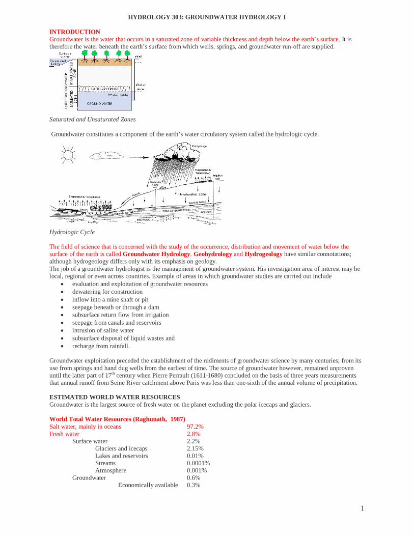
HYDROLOGY 303: GROUNDWATER HYDROLOGY I INTRODUCTION Groundwater is the water that occurs in a saturated zone of variable thickness and depth below the earth’s surface. It is therefore the water beneath the earth’s surface from which wells, springs, and groundwater run-off are supplied.

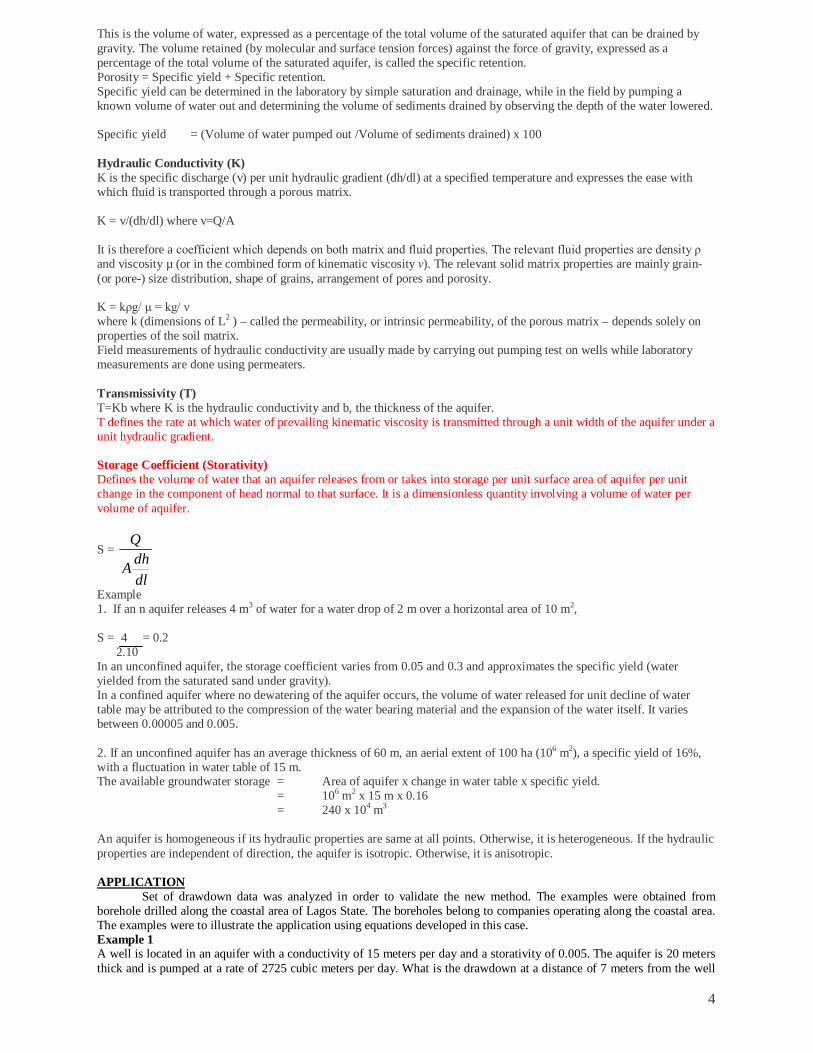
Saturated and Unsaturated Zones Groundwater constitutes a component of the earth’s water circulatory system called the hydrologic cycle.

Hydrologic Cycle The field of science that is concerned with the study of the occurrence, distribution and movement of water below the surface of the earth is called Groundwater Hydrology. Geohydrology and Hydrogeology have similar connotations; although hydrogeology differs only with its emphasis on geology. The job of a groundwater hydrologist is the management of groundwater system. His investigation area of interest may be local, regional or even across countries. Example of areas in which groundwater studies are carried out include

evaluation and exploitation of groundwater resources dewatering for construction inflow into a mine shaft or pit seepage beneath or through a dam subsurface return flow from irrigation seepage from canals and reservoirs intrusion of saline water subsurface disposal of liquid wastes and recharge from rainfall.

Groundwater exploitation preceded the establishment of the rudiments of groundwater science by many centuries; from its use from springs and hand dug wells from the earliest of time. The source of groundwater however, remained unproven until the latter part of 17th century when Pierre Perrault (1611-1680) concluded on the basis of three years measurements that annual runoff from Seine River catchment above Paris was less than one-sixth of the annual volume of precipitation. ESTIMATED WORLD WATER RESOURCES Groundwater is the largest source of fresh water on the planet excluding the polar icecaps and glaciers. World Total Water Resources (Raghunath, 1987) Salt water, mainly in oceans 97.2% Fresh water 2.8%

Surface water 2.2% Glaciers and icecaps 2.15% Lakes and reservoirs 0.01% Streams 0.0001% Atmosphere 0.001%

Groundwater 0.6% Economically available 0.3%

2

TYPES OF GROUNDWATER Meteoric - found in circulatory system of hydrologic cycle Connate - fossil interstitial water out of contact with the atmosphere for appreciable length of time. Juvenile - originates from volcanic emanations Metamorphic - associated with heat, pressure and re-crystallization that created metamorphic rocks WATER WELLS A water well is a hole or shaft, usually vertical, excavated in the earth for bringing groundwater to the surface. Many methods exist for constructing wells; selection of a particular method depends on the purpose of the well, the quantity of water required, depth to groundwater, geologic conditions and economic factors. AQUIFERS The term aquifer is traceable to its Latin origin: aqui from aqua meaning water fer from ferre meaning to bear. An aquifer is a geologic formation, or a group of formations, which contains water and permits significant amount of water to move through it under ordinary field conditions. Other terms used are groundwater reservoir (or basin) and water bearing zone (or formation). Aquifers are generally extensive and may be overlain or underlain by a confining bed. A confining bed may be an aquiclude, aquifuge or aquitard. Aquiclude: A relatively impermeable material that does not yield appreciable quantitaties of water to wells i.e. may

contain water but is incapable of transmitting significant quantities of water under ordinary field conditions e.g. clay, shale.

Aquifuge: A geologic formation neither containing nor transmitting water e.g. fresh granite, basalt. Aquitard: A poorly permeable geologic formation that transmits water at a very low rate compared to

an aquifer e.g. sandy clay. However, it may transmit appreciable water to or from adjacent aquifers where sufficiently thick and may constitute an important groundwater storage zone.

AQUIFER CLASSIFICATION Aquifers may be classed as confined, unconfined or leaky, which can be taken as a combination of the unconfined and confined. Confined Aquifer (Pressure or piezometric aquifers)

Impervious K’=0Aquifer K>K’Impervious K’=0

A confined aquifer is confined above and below by an impervious (may contain water but can’t transmit it) layer under pressure greater than the atmospheric. Therefore, in a well penetrating such an aquifer, the water level rises above the bottom of the top confining bed. The water in a confined aquifer is called confined or artesian water. Artesian water flows freely without pumping and the well producing such water is called an artesian or a free flowing well. An example of artesians well near Mariental, Namibia yields approx 300 kl/day and the one near Uitenhage yields approx 120kl/day. Unconfined Aquifer (Phreatic, Water table) An unconfined aquifer is one in which a water table (phreatic surface) serves as its upper boundary. A phreatic aquifer is directly recharged from the ground surface above it.

The water level in well taping an unconfined aquifer and the water table in the aquifer are the same. Therefore, contour maps and profiles of the water table can be prepared from the elevations of water in wells that tap the aquifer to determine the quantities of water available, their distribution and movement.

Impervious K”=0Aquifer K=K’

Water table K’

3

Leaky Aquifer (Semi-confined)

Semi-pervious K’

Aquifer K>K’Impervious K=0

A leaky aquifer is underlain or overlain by semi-pervious strata. Pumping from a well in a leaky aquifer removes water in two ways: by horizontal flow within the aquifer and by vertical leakage or seepage through the semi-confining layer into the aquifer. Aquifers that are completely confined or unconfined occur less frequently than leaky aquifers. Perched Aquifers Perched aquifers, are special kinds of phreatic aquifers occurring whenever an impervious (or semi-pervious) layer of limited extent is located between the water table of a phreatic aquifer and the ground surface, thereby making a groundwater body, separated from the main groundwater body, to be formed. Sometimes, these aquifers exist only during a relatively short part of each year as they drain to the underlying phreatic aquifer. Therefore wells taping such aquifers yield only temporary or small quantities of water.

AQUIFER PARAMETERS Porosity The spaces where groundwater occupies are known as voids, interstices, pores or pore spaces. They are fundamentally important to the study of groundwater because they serve as water conduits. Their nature is dependent on their geology. Porosity is a measure by the ration of the contained voids in a solid mass to its total volume. θ = vv/V where θ is the porosity, vv is the volume of voids and V is the total volume. The term effective porosity refers to the amount of interconnected pore space available for fluid flow and is also expressed as the ratio of the interstices to total volume. Shape, size, packing and degree of cementation affect porosity. Uniformly graded sand has a higher porosity than a less uniform, fine and coarse mixture, because in the latter, the fines occupy the voids in the coarse material. In square packing for example, the porosity is as high as 48% while in rhombic packing, it is as low as 26%. Angularity tends to increase porosity while cementation decreases porosity. Porosity can be primary (original) or secondary. Primary porosity is created at the time of origin of the rock in which they occur. In sedimentary rocks, the voids coincide with the intergrannular spaces while in igneous rocks, it results from the cooling of molten lava and may range in size from minute intercrystalline spaces to large caverns. Secondary porosity results from the actions of subsequent geological, climatic or biotic factors upon the original rock. Examples include joints, fractures, faults, solution openings and openings formed by plants and animals. Recharge and Discharge Groundwater recharge represents the portion of rainfall which reaches an aquifer. Groundwater therefore owes its existence directly or indirectly to precipitation. Artificial recharge occurs from excess irrigation seepage from canals and water purposely applied to augment groundwater supplies. Seawater can enter underground along the coasts where the hydraulic gradients slope in an inland direction. The most direct way of quantifying recharge is by examination of borehole hydrograph. This method requires that the specific yield of the aquifer is known. Another approach is to use meteorological data inputs to a recharge simulation model. Natural recharge includes stream bed percolation, deep percolation of rainfall, leakage from ponds, lakes and reservoirs. Discharge of groundwater occurs when water emerges from underground. Most natural discharge occurs as flows into the surface water bodies e.g. streams, lakes and oceans. Discharge to the ground surface appears as springs. Groundwater discharge also occurs by evaporation from within the soil and by transpiration from vegetation that has access to the water table. However, pumpage from wells constitutes the major artificial discharge of groundwater. Specific Yield

4

This is the volume of water, expressed as a percentage of the total volume of the saturated aquifer that can be drained by gravity. The volume retained (by molecular and surface tension forces) against the force of gravity, expressed as a percentage of the total volume of the saturated aquifer, is called the specific retention. Porosity = Specific yield + Specific retention. Specific yield can be determined in the laboratory by simple saturation and drainage, while in the field by pumping a known volume of water out and determining the volume of sediments drained by observing the depth of the water lowered. Specific yield = (Volume of water pumped out /Volume of sediments drained) x 100 Hydraulic Conductivity (K) K is the specific discharge (v) per unit hydraulic gradient (dh/dl) at a specified temperature and expresses the ease with which fluid is transported through a porous matrix. K = v/(dh/dl) where v=Q/A It is therefore a coefficient which depends on both matrix and fluid properties. The relevant fluid properties are density ρ and viscosity µ (or in the combined form of kinematic viscosity ν). The relevant solid matrix properties are mainly grain-(or pore-) size distribution, shape of grains, arrangement of pores and porosity. K = kρg/ μ = kg/ ν where k (dimensions of L2 ) – called the permeability, or intrinsic permeability, of the porous matrix – depends solely on properties of the soil matrix. Field measurements of hydraulic conductivity are usually made by carrying out pumping test on wells while laboratory measurements are done using permeaters. Transmissivity (T) T=Kb where K is the hydraulic conductivity and b, the thickness of the aquifer. T defines the rate at which water of prevailing kinematic viscosity is transmitted through a unit width of the aquifer under a unit hydraulic gradient. Storage Coefficient (Storativity) Defines the volume of water that an aquifer releases from or takes into storage per unit surface area of aquifer per unit change in the component of head normal to that surface. It is a dimensionless quantity involving a volume of water per volume of aquifer.

S =

dldhA

Q

Example 1. If an n aquifer releases 4 m3 of water for a water drop of 2 m over a horizontal area of 10 m2, S = 4 = 0.2 2.10 In an unconfined aquifer, the storage coefficient varies from 0.05 and 0.3 and approximates the specific yield (water yielded from the saturated sand under gravity). In a confined aquifer where no dewatering of the aquifer occurs, the volume of water released for unit decline of water table may be attributed to the compression of the water bearing material and the expansion of the water itself. It varies between 0.00005 and 0.005. 2. If an unconfined aquifer has an average thickness of 60 m, an aerial extent of 100 ha (106 m2), a specific yield of 16%, with a fluctuation in water table of 15 m. The available groundwater storage = Area of aquifer x change in water table x specific yield. = 106 m2 x 15 m x 0.16

= 240 x 104 m3 An aquifer is homogeneous if its hydraulic properties are same at all points. Otherwise, it is heterogeneous. If the hydraulic properties are independent of direction, the aquifer is isotropic. Otherwise, it is anisotropic. APPLICATION

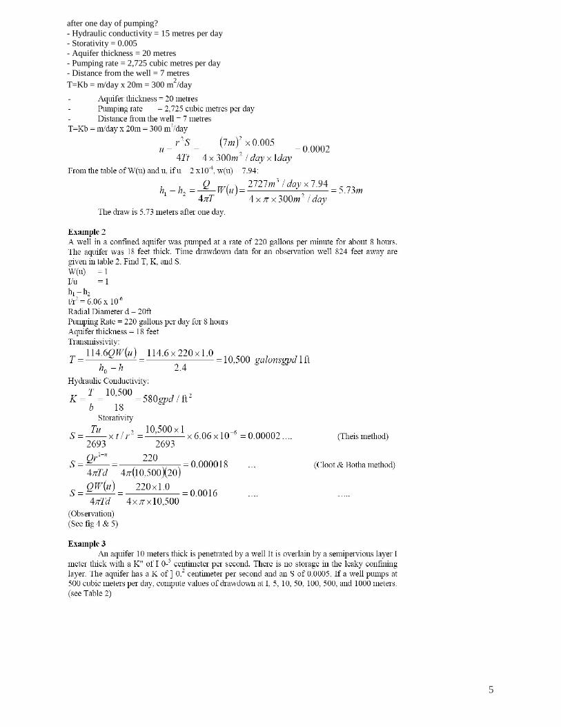
Set of drawdown data was analyzed in order to validate the new method. The examples were obtained from borehole drilled along the coastal area of Lagos State. The boreholes belong to companies operating along the coastal area. The examples were to illustrate the application using equations developed in this case. Example 1 A well is located in an aquifer with a conductivity of 15 meters per day and a storativity of 0.005. The aquifer is 20 meters thick and is pumped at a rate of 2725 cubic meters per day. What is the drawdown at a distance of 7 meters from the well

5

after one day of pumping? - Hydraulic conductivity = 15 metres per day - Storativity = 0.005 - Aquifer thickness = 20 metres - Pumping rate = 2,725 cubic metres per day - Distance from the well = 7 metres T=Kb = m/day x 20m = 300 m2/day

6

Discussion of Results:

All the three examples of drawdown data show that the new method underlying this law and the observed drawdown variations in hydraulic conductivity of the aquifer is correct. Each of the analytical solution describes the response to pumping in a very idealized representation of aquifer configurations. In the real world, aquifers are heterogeneous and isotropic: They usually vary in thickness; and they certainly do not extend to infinity. Where they are bounded, it is not by straight-line boundaries that provide perfect confinement. Aquifers are created by complex geologic processes that head to irregular stratigraphy and trendouts of both aquifers and aquitards. The Predictions that can be carried out with the analytical solution presented in this paper must be viewed as best estimates. In general, hydraulic head solutions are most applicable when the unit of study is a well.

They are less applicable on a large scale, where the unit of study is an entire aquifer. The graphical method of solution starts with the construction of reversed type curve of W(u) against I/u on logarithm paper (see fig. 4). Data from observation well located at different distances from the pumping wells were used. If there is only one observation well, then it is sufficient to plot hi - h2 as a function of t (table I). .

Using "Contouring the Water Table Map", we noticed that the contours form V's with the river and its tributaries. That's because the river is a "gaining" river. It is receiving recharge from the aquifer. The contours show that ground water is moving down the sides of the valley and into the river channel. The opposite of a gaining stream is a "losing" stream. It arises when the water table at the stream channel is lower than the stream's elevation or stage, and stream water flows downward through the channel to the water table. This is very common in dryer regions of the Southwest. In the case of a losing stream, the V will point downstream, instead of upstream. (see fig. 6)

When making a water table map, it is important that your well and stream elevations are accurate. All elevations should be referenced to a standard datum, such as mean Sea level. This means that all elevations are either above or below the standard datum (e.g., 50 feet above mean sea level datum). It's also very important to measure all of the water table elevations within a short period of time, such as one day, so that you have a "snapshot" of what's going on (Adeosun et al 2006). Because the water table rises and falls over time, you would be more accurate if readings are made before these changes occur.

Understanding how ground water flows is important when you want to know where to drill a well or a water supply, to estimate a well's recharge area, or to predict the direction of contamination is likely to take once it reaches the water table. Water table contouring can help groundwater developer to do all these things. Hence, groundwater flow through the subsurface is the whole essence of this paper and called for further investigation.

7

GEOLOGIC FORMATION AS AQUIFERS Many types of geologic formations serve as aquifers. Alluvial deposits Probably 90% of all developed aquifers consist of unconsolidated rocks, chiefly gravels and sands related to the deposits made by flowing water; washed away from one place and deposited in another. Wells located in highly permeable strata bordering streams produce large quantities of water, as infiltration from the stream augments groundwater supplies. Limestone Limestone varies widely in density, porosity and permeability depending on the degree of consolidation and development of permeable zones after deposition. Openings in limestone may range from microscopic original pores to large solution caverns forming subterranean channels sufficiently large to carry the entire flow of a stream. The term lost river has been applied to a stream that disappears completely underground in a limestone terrain. Dissolution of calcium carbonate by water causes hard groundwater to be found in limestone areas. Also by dissolving the rock, water tends to increase the pore space and permeability with time. Karst terrain, characterized by solution channels, closed depressions, subterranean drainage through sinkholes and caves are common in limestone areas. Volcanic rocks Volcanic rocks can form highly permeable aquifers; basalt flows in particular often display such characteristics. The type of openings found in basalts include: interstitial spaces at the tops of flows, cavities between adjacent beds, shrinkage cracks, lava tubes, gas vesicles, fissures resulting from faulting and cracking after rocks have cooled and holes left by the burning of trees overwhelmed by lava. An excellent example of a highly permeable volcanic rock is in Nicaragua, where a circular lake contained in an extinct crater, serves as the major municipal source and yields 75 000 m3/day. There is no surface inflow and evaporation exceeds precipitation; hence, the lake, fed entirely by groundwater acts as a large natural well.

8

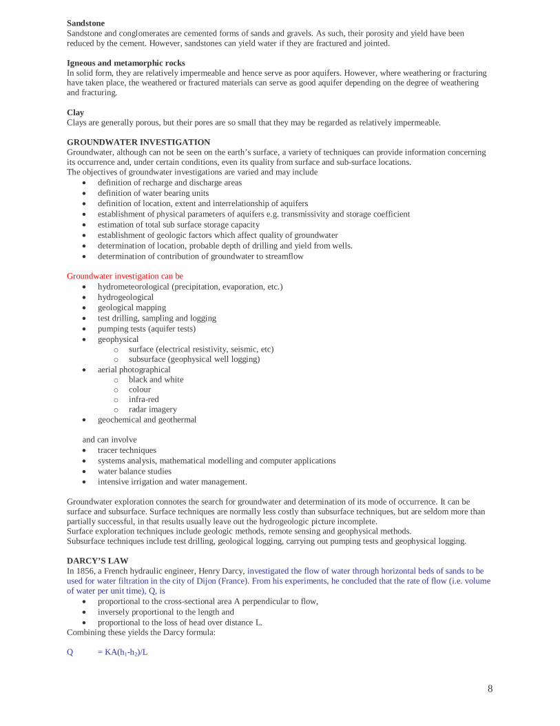
Sandstone Sandstone and conglomerates are cemented forms of sands and gravels. As such, their porosity and yield have been reduced by the cement. However, sandstones can yield water if they are fractured and jointed. Igneous and metamorphic rocks In solid form, they are relatively impermeable and hence serve as poor aquifers. However, where weathering or fracturing have taken place, the weathered or fractured materials can serve as good aquifer depending on the degree of weathering and fracturing. Clay Clays are generally porous, but their pores are so small that they may be regarded as relatively impermeable. GROUNDWATER INVESTIGATION Groundwater, although can not be seen on the earth’s surface, a variety of techniques can provide information concerning its occurrence and, under certain conditions, even its quality from surface and sub-surface locations. The objectives of groundwater investigations are varied and may include

definition of recharge and discharge areas definition of water bearing units definition of location, extent and interrelationship of aquifers establishment of physical parameters of aquifers e.g. transmissivity and storage coefficient estimation of total sub surface storage capacity establishment of geologic factors which affect quality of groundwater determination of location, probable depth of drilling and yield from wells. determination of contribution of groundwater to streamflow

Groundwater investigation can be

hydrometeorological (precipitation, evaporation, etc.) hydrogeological geological mapping test drilling, sampling and logging pumping tests (aquifer tests) geophysical

o surface (electrical resistivity, seismic, etc) o subsurface (geophysical well logging)

aerial photographical o black and white o colour o infra-red o radar imagery

geochemical and geothermal and can involve tracer techniques systems analysis, mathematical modelling and computer applications water balance studies intensive irrigation and water management.

Groundwater exploration connotes the search for groundwater and determination of its mode of occurrence. It can be surface and subsurface. Surface techniques are normally less costly than subsurface techniques, but are seldom more than partially successful, in that results usually leave out the hydrogeologic picture incomplete. Surface exploration techniques include geologic methods, remote sensing and geophysical methods. Subsurface techniques include test drilling, geological logging, carrying out pumping tests and geophysical logging. DARCY’S LAW In 1856, a French hydraulic engineer, Henry Darcy, investigated the flow of water through horizontal beds of sands to be used for water filtration in the city of Dijon (France). From his experiments, he concluded that the rate of flow (i.e. volume of water per unit time), Q, is

proportional to the cross-sectional area A perpendicular to flow, inversely proportional to the length and proportional to the loss of head over distance L.

Combining these yields the Darcy formula: Q = KA(h1-h2)/L

9

where K is the coefficient of proportionality called the hydraulic conductivity and (h1-h2)/L is called the hydraulic gradient.

v = Q/A = Kdh/dl, v is the Darcy velocity or specific discharge (Q = KA(h1-h2)/L) therefore Q/A = K(h1-h2)/L which is Kdh/dl

Darcy velocity, v, assumes that flow occurs through the entire section of the material without regard to solids and pores. However, flow is limited to the pore space only and the average interstitial velocity, va

va = A

Q

where is porosity

Darcy’s law is valid if 1 ≤ NR ≥ 10 (i.e. valid for laminar flow and not turbulent flow) NR = ρqd/ μ where NR = Reynolds number ρ = density of groundwater q = velocity (seepage or bulk) of groundwater flow. d = mean diameter of the soil grain µ = dynamic viscosity of groundwater STEADY STATE FLOW Steady flow occurs when the water level has ceased to decline as a result of equilibrium between the discharge of the pumped well and the recharge of the aquifer buy outside source. The Dupuit (1863) equation, later modified by Theim, 1906 can be used for analysing steady flow to wells. Confined Aquifers The yield from the well is Q = KiA (Darcy’s law)

= Kdxdy

(2пxb)

Rearranging and integrating with appropriate boundary conditions

Q 2

1

r

r xdx

= 2пKb 2

1

h

hdy

Q = 2пKb )ln(

)(

1

2

12

rr

hh

K =)(2 12 hhb

Q

)ln(1

2r

r

The above is referred to as the equilibrium or Theim’s equation. r1, r2 are respective distances of piezometers (observation wells) to the pumped well h2, h1 are their respective water levels. The Theim’s equation enables the K or T of an aquifer to be determined from a pumped well being monitored from at least two observation wells at different distances from the pumped well. If the drawdown in the observation wells are s1 and s2, then h2-h1 = s1-s2. The assumptions in Theim’s equation are: i. the aquifer is confined. ii. the aquifer has an infinite areal extent. iii. the aquifer is homogeneous, isotropic and of uniform thickness over the area influenced by the test. iv. prior to pumping, the piezometric surface is horizontal over the area that will be influenced by the test. v. the aquifer is pumped at a constant discharge rate.

10

vi the well penetrates the entire saturated thickness of the aquifer. vii. the flow to the well is at steady state. Unconfined Aquifers Q = KiA (Darcy’s law)

= Kdxdy

(2пxy)

Q 2

1

r

r xdx

= 2пK 2

1

h

hy dy

Q = пK )ln(

)(

1

2

21

22

rr

hh

K = )( 2

12

2 hhQ

1

2ln rr

T can be approximated from the above from

T ≈ K2

21 hh

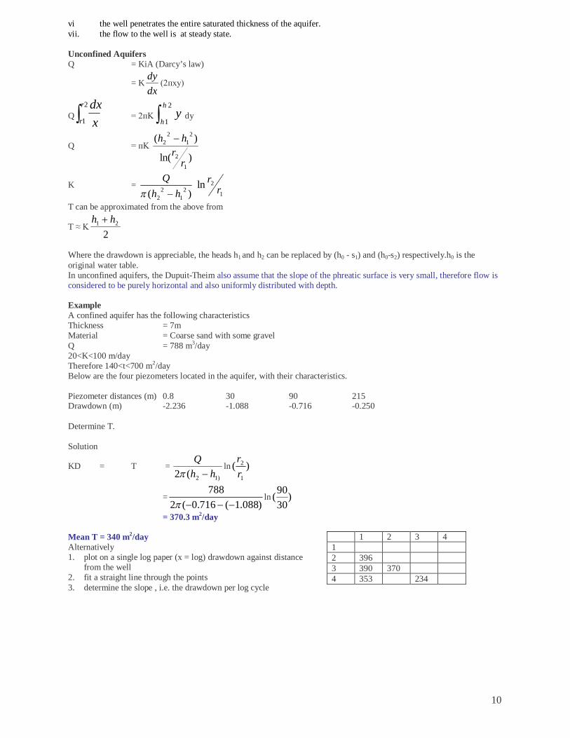
Where the drawdown is appreciable, the heads h1 and h2 can be replaced by (h0 - s1) and (h0-s2) respectively.h0 is the original water table. In unconfined aquifers, the Dupuit-Theim also assume that the slope of the phreatic surface is very small, therefore flow is considered to be purely horizontal and also uniformly distributed with depth. Example A confined aquifer has the following characteristics Thickness = 7m Material = Coarse sand with some gravel Q = 788 m3/day 20<K<100 m/day Therefore 140<t<700 m2/day Below are the four piezometers located in the aquifer, with their characteristics. Piezometer distances (m) 0.8 30 90 215 Drawdown (m) -2.236 -1.088 -0.716 -0.250 Determine T. Solution

KD = T = )12(2 hh

Q

ln )(1

2

rr

=)088.1(716.0(2

788

ln )3090(

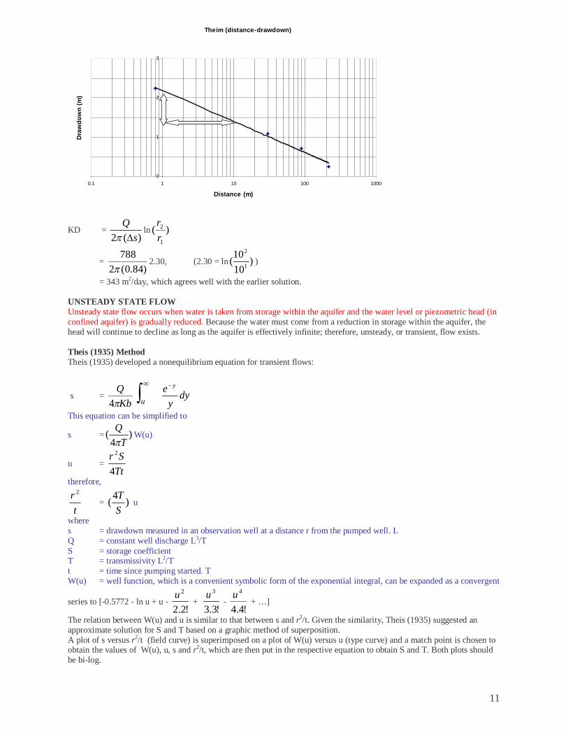
= 370.3 m2/day Mean T = 340 m2/day Alternatively 1. plot on a single log paper (x = log) drawdown against distance

from the well 2. fit a straight line through the points 3. determine the slope , i.e. the drawdown per log cycle

1 2 3 4 1 2 396 3 390 370 4 353 234

11

Theim (distance-drawdown)

0

1

2

3

0.1 1 10 100 1000

Distance (m)

Dra

wdo

wn

(m)

KD = )(2 s

Q

ln )(1

2

rr

= )84.0(2

788

2.30, (2.30 = ln )1010( 1

2

)

= 343 m2/day, which agrees well with the earlier solution. UNSTEADY STATE FLOW Unsteady state flow occurs when water is taken from storage within the aquifer and the water level or piezometric head (in confined aquifer) is gradually reduced. Because the water must come from a reduction in storage within the aquifer, the head will continue to decline as long as the aquifer is effectively infinite; therefore, unsteady, or transient, flow exists. Theis (1935) Method Theis (1935) developed a nonequilibrium equation for transient flows:

s = Kb

Q4

udy

ye y

This equation can be simplified to

s = )4

(T

Q

W(u)

u = TtSr

4

2

therefore,

tr 2

= )4(ST

u

where s = drawdown measured in an observation well at a distance r from the pumped well. L Q = constant well discharge L3/T S = storage coefficient T = transmissivity L2/T t = time since pumping started. T W(u) = well function, which is a convenient symbolic form of the exponential integral, can be expanded as a convergent

series to [-0.5772 - ln u + u - !2.2

2u +

!3.3

3u -

!4.4

4u + …]

The relation between W(u) and u is similar to that between s and r2/t. Given the similarity, Theis (1935) suggested an approximate solution for S and T based on a graphic method of superposition. A plot of s versus r2/t (field curve) is superimposed on a plot of W(u) versus u (type curve) and a match point is chosen to obtain the values of W(u), u, s and r2/t, which are then put in the respective equation to obtain S and T. Both plots should be bi-log.

12

The nonequilibiumn is widely applied in practice and is preferred over the equilibrium equation because (i) S (storage coefficient) can be determined (ii) only one observation well is required (iii) a shorter period of pumping is generally necessary and (iv) no steady state flow is required. The assumptions inherent in Theis (1935) equation are:

The aquifer is homogeneous, isotropic, of uniform thickness and has an infinite areal extent. Prior to pumping, the piezometric surface is horizontal. The aquifer is pumped at a constant discharge rate. The well penetrates the entire saturated thickness of the aquifer. The well diameter is infinitesimal so that storage within the well can be neglected Water removed from storage is discharged instantaneously with decline of head.

Cooper-Jacob’s Method For small value of u (u<0.01), the terms in the convergent series of the well function becomes negligible after the first two terms. Hence

s = )4

ln5772.0(4

2

Ttr

TQ

= SrTt

TQ

2

25.2log430.2

A plot of s versus log of t forms a straight line. Projecting the line to s = 0, where t =t0,

s = SrTt

TQ

2025.2

log430.2

then,

SrTt

2025.2

= 1 and

S = 2025.2

rTt

To obtain t, note that if t/t0 = 10, then log t/t0 = 0, therefore replacing s by s , where s is the drawdown difference per log cycle of t, then

T = sQ4

30.2

Thus the procedure is to solve for T first and then solve for S. Chow’s Method Unlike the Theis’s method, Chow’s avoids curve fitting. - Measurements of drawdown in an observation well near a pumped well are made and the observational data are plotted on semilog paper (t on the log scale) as in Cooper-Jacob’s. -Select an arbitrary point on the line, note the coordinates, t and s of the point and determine the drawdown difference per log cycle of time, s . - Then calculate the value of F(u) for the selected point. F(u) = s/ s - Knowing the value of F(u), find the corresponding values of W(u) and u from the nomogram. - then calculate T and S

T = s

Q4

W (u) and S = 4 2rtuT

CHOW nomogram u W(u) F(u) u W(u) F(u) .500E+01 .400E+01 .300E+01 .200E+01 .100E+01 .900E+00 .800E+00 .700E+00 .600E+00 .500E+00 .400E+00 .300E+00 .200E+00 .100E+00 .900E-01 .800E-01

.114E-02

.378E-02

.130E-01

.489E-01

.219E+00

.260E+00

.311E+00

.374E+00

.454E+00

.560E+00

.702E+00

.906E+00

.122E+01

.182E+01

.192E+01

.203E+01

.734E-01

.898E-01

.117E+00

.157E+00

.259E+00

.276E+00

.301E+00

.327E+00

.360E+00

.401E+00

.455E+00

.532E+00

.647E+00

.874E+00

.913E+00

.956E+00

.700E-01

.600E-01

.500E-01

.400E-01

.300E-01

.200 E-01

.100E-01

.900E-02

.800E-02

.700E-02

.600E-02

.500E-02

.400E-02

.300E-02

.200E-02

.100E-02

.215E+01

.230E+01

.247E+01

.268E+01

.296E+01

.335 E+01

.404E+01

.414E+01

.426E+01

.439E+01

.454E+01

.473E+01

.495E+01

.523E+01

.564E+01

.633E+01

.100E+01

.106E+01

.113E+01

.121E+01

.133E+01

.149 E+01

.177E+01

.182E+01

.187E+01

.192E+01

.199E+01

.207E+01

.216E+01

.228E+01

.246E+01

.275E+01

13

Recovery Test At the end of pumping, water levels in the pumping and observation well rise. This is referred to as recovery of groundwater. The drawdown below the original static water level (prior to pumping) during the recovery period is known as residual drawdown. Theis found that

s’ = residual drawdown = )log(430.2

'tt

TQ

where t’ = time since pump shut down (beginning of recovery) t = time since pumping started. A plot of residual drawdown versus log(t’/t) forms a straight line with a slope of 2.30Q/4 T, so that for △s’, the residual drawdown per log cycle of t/t’, the transmissivity becomes

T = '4

30.2sQ

S can not be determined by the recovery method. GROUNDWATER POLLUTION May be defined as the artificially induced degradation of natural groundwater quality. Most pollution stems from disposal of wastes on or into the ground and the pollutants may be of organic (e.g. chlorinated phenoxy acid herbicides), inorganic (e.g. nitrate), biological (e.g. coliform bacteria), physical (colour) and radiological (e.g. barium) types.] Methods of disposal of wastes include discharge in to the sea and streams, placement in percolation ponds, on the ground surface, (spreading or irrigation), in landfills, into disposal wells and into injection wells. Waste can be defined to be all undesirable or superfluous by-products, emissions, residues or remainders of any process or activity, whether gaseous, liquid or solid, or a combination of these. For practical reasons, material is taken to become waste when it is committed to storage (to last three months or longer) or leaves the site or enters the environment. The principal sources of pollution include Municipal – sewer leakages, liquid and solid wastes Industrial – Mining activities, tank and pipeline leakage, oil field brines, liquid wastes Agriculture – Irrigation return flows, fertilizers, pesticides, animal wastes Miscellaneous – saline water intrusion, septic tank and cesspools, roadway deicing, interchange through wells. The sources can be point (singular location), line (with a liner alignment) or diffuse (occupying extensive areas) sources. The aims of groundwater pollution investigation are varied, but may include

determination of the extent of pollution by quantifying the amount of pollutants determination of the sources of possible pollutants to the groundwater regime quantification of the contribution from different sources the study of the migration rate of the pollutants through the aquifers model the local and regional movement of pollutants through the aquifer and predict future water qualities suggestion of management strategies whereby the influence of disposal can be minimized.

Remedial measures which can be used to prevent or reduce aquifer contamination include

surface water control o increases runoff, reduces infiltration

groundwater control o seals off lateral flow in shallow aquifers

plume management o lower water table below contaminant o scavenger wells to extract leachate o injection to create hydraulic barrier

excavation o physical removal of contaminant to safe site.

The choice of which remedial measure is most appropriate or cost effective depends on : extent of contamination type of contaminant – is the contaminant “toxic or hazardous” material or a convectional pollutant. whether the material is organic or inorganic how tightly bound the contaminant is to the soil. hydrological setting

The generator of hazardous waste should be liable for damage resulting from the disposal of hazardous waste. GROUNDWATER LAW Most groundwater law falls under four major doctrines

14

absolute ownership - allows a landowner to pump groundwater under his land without bearing any responsibility to neighbouring landowners

reasonable use - waste and malicious use are prohibited and the water must be used on overlying land unless it can be used elsewhere without injuring other overlying owners.

correlative rights - the landowners over a common aquifer have an equal or correlative right to the beneficial

use of the water in the aquifer, to the full extent off their needs when the common supply is sufficient.

prior appropriation - while no one may own the water in a stream, all persons, corporations, and municipalities

have the right to use the water for beneficial purposes. The allocation of water rests upon the fundamental maxim "first in time, first in right." The first person to use water (called a "senior appropriator") acquires the right (called a "priority") to its future use as against later users (called "junior appropriators").

GROUNDWATER OCCURRENCE Effective description of groundwater occurrence in a large, geologically complex area such as Nigeria requires division and delineation of sub-areas that have uniform occurrence characteristics. Groundwater characterisation ideally entails:

ascertaining hydrogeological characteristics of groundwater occurrence; delineating hydraulic groundwater units; determining the hydraulic characteristics – transmissivity, storage coefficient etc; estimating groundwater recharge and discharge; ascertaining chemical composition and potability of groundwater; establishing the current state of and potential for development; predicting the effects of groundwater exploitation on the environment and of environmental change on

groundwater availability and quality. As the concept of interstices – open spaces that form receptacles and conduits for groundwater, their origin, shape and interconnection, is fundamental to groundwater hydrology, the types and origin of openings, therefore, may be considered to be a basis for the delineation of sub-areas. In terms of interstice origin groundwater occurrence in Nigeria can be divided into:

1. Regions consisting of primary aquifers in which groundwater occur in pores which originate contemporaneously with the genesis of the sedimentary rocks in which they occur. Primary openings in igneous and metamorphic rocks are generally of no consequence in groundwater hydrology, owing to their minute size and lack of interconnection. The patchy occurrence of narrow strips of water-bearing alluvial deposits along rivers can also be classified here, but usually since they are not extensive, are treated as components of the larger secondary water – bearing units.

2. Regions consisting mainly of secondary aquifers in which groundwater occur in secondary openings which

originate from processes that affect rocks after they were formed. The secondary openings are in terms of joints, cleavages, bedding planes, faults and pores resulting from the disintegration, decomposition and dissolution of rocks. The processes are tectonic deformation, weathering and unloading by degradation of the land surface.

WELL DESIGN Wells may be dug, bored, driven, jetted or drilled. The drilled types are commonly referred to as boreholes. A well design involves selection of dimensions (depth/length, diameter) and type of the well (mode of construction), casing, screens (material) and of completion methods. The choice of water well and method of design depends upon topography, availability of space, hydrogeology, depth of groundwater table, rainfall, climate, quantity of water required and available funds. Diameter - significantly affects cost - large enough to accommodate the proposed pump - well yield is not proportional to well diameter as can be seen from Theim’s equation. Depth - usually to the bottom of the aquifer - because ‘hard rock is intersected is not necessarily any reason to stop, as water fissures can be encountered after hard rock. - poor quality aquifers encountered can be sealed to prevent contamination of good quality water. - 300 m in some areas of the Cape, but most usually between 30 m and 80 m Screen -70 – 80% of aquifer thickness is screened - slot size is taken as 40 – 70% of the size of aquifer material

15

- material selected depends on quality of groundwater, strength requirement. The screen material should be resistant to incrustation and corrosion and should have strength to withstand the column load and collapse pressure. Principal indicators of corrosive groundwater are low pH, presence of dissolved oxygen, CO2>50 ppm, Cl >500 ppm. Principal indicators of incrusting groundwater are total hardness > 330 ppm, iron content > 2 ppm, pH > 8. Mineral and slime deposits can be removed by chlorine and acid. SURFACE WATER-GROUNDWATER INTERACTION The hydrologic processes involved in surface water groundwater interaction according to Kelbe and Germishuye (2000) can be given as evapotranspiration, precipitation, groundwater recharge, groundwater discharge, river runoff, lakes recharge/discharge (seepage), wetlands recharge/discharge (seepage), sea and oceans (river discharge and groundwater seepage). The figure below shows the principal processes involved in the interactions. However, the processes can be represented and conveniently understood in terms of groundwater recharge and discharge.

The principal processes involved in surface water – groundwater interaction. The interactions between surface water and groundwater, particularly streams, can be put into three basic categories: surface water body gaining water from inflow of groundwater, surface water body losing water to groundwater by outflow, or the surface water body disconnected from the groundwater system. These classes of surface water bodies can be referred to as gaining (effluent), losing (influent) and perched respectively.

Stream Stream Stream

The three basic categories of stream-aquifer interactions- losing, gaining and perched streams. Much of the low water flow in streams (baseflow) is derived from groundwater whose water table elevations in the vicinity of a stream are higher than the stream. The hydrologic exchange of groundwater and rivers in a landscape is controlled by

the distribution and magnitude of hydraulic conductivities, both within the channel and the associated aquifer, the relation of stream stage to the adjacent groundwater level; and geomorphology, especially in terms of the geometry and position of the stream channel within the alluvial plain.

The field of assessment of the interaction between surface water and groundwater is wide, covering hydrological, ecological, biogeochemical and geological, and involving different simulation techniques. However the methods for the hydrological consideration of the interaction between surface water and groundwater can be classified into hydrograph analyses, water budgeting, field, chemical and modelling methods. The interactions between the two components of the hydrologic system i.e. surface water and groundwater imply that the development or contamination of one commonly affects the other. The development and contamination occur in consequence of superimposition of human activities on the natural dynamic equilibrium that exists between surface water –groundwater interchange. The range of human activities that affect the interaction between surface water and groundwater include agricultural development (especially irrigation and application of chemicals to cropland), urban and industrial development (for example, discharges of sewage), drainage of land surface, groundwater pumping, construction of reservoirs, removal of natural vegetation and atmospheric discharge and deposition e.t.c. By far the most important need for the understanding of surface water –groundwater interactions is in the area of effective water resources management. It has been acknowledged that effective water resources management is best logically considered with the catchments as planning units. Therefore, assessments of surface water-groundwater interactions should be tailored along eventual considerations and understanding at basin-wide or catchment scales.

16

Naturally, this would require investigations at local scales for the necessary data collection required for adequate understanding of the interactions and the necessary tools for extrapolating results from local to basin-wide or catchment scales. References Raghunath, H. M. 1987. Groundwater. Wiley astern Limited, New Delhi. Kelbe, B. E. and Germishuyse, T. 2000. Conceptualization of the surface water – groundwater

processes in South Africa. Draft of Proceeding of a Workshop on Surface Water-Groundwater Interaction held in Pietermaritzburg, South Africa.

DATA ANALYSIS AND SYNTHESIS

In this study, all aquifer-test results compiled from published reports were verified by re-analyzing the aquifer-test data using analytical solutions appropriate to the hydrogeologic setting in which those tests were conducted. If the published results agreed to within a factor of 2, the published results were accepted. If the difference between the published data and the independent calculations exceeded a factor of 2, and no independent justification was found for using the published data, the calculated values were reported. Because of the uncertainty associated with converting specific capacity data to transmissivity values, specific capacity data were not used. Because of the low volume of geologic material samples, results from the permeameter tests were not used in the analyses discussed in this report (with the exception of the clastic confining units). Following the elimination of suspect data and the addition of newly analyzed data, statistical methods were used to evaluate the distribution of hydraulic properties in the 11 DVRFS derived HGU's. Except for wells located on the Colorado Plateau in Utah, figure 2 shows the locations of the wells and boreholes used to collect data for the estimation of hydraulic properties presented in this report. The Colorado Plateau wells are not contained in the USGS National Water Information System (NWIS) database and do not have exact locations associated with them. These wells were included in the analysis of hydraulic properties because they are completed in the sedimentary confining unit (table 1), of which data are sparse in the DVRFS. The following hydraulic parameters are the primary focus of this study because of their use in ongoing numerical flow-modeling studies. The parameters were defined by Lohman (1979, p. 6 and 8):

Hydraulic conductivity (unit length per unit time): The coefficient that describes the ability of a geologic medium to ". . . transmit in unit time a unit volume of ground water at the prevailing viscosity through a cross section of unit area, measured at right angles to the direction of flow, under a hydraulic gradient of unit change in head through unit length of flow." Hydraulic conductivity can be calculated by dividing the transmissivity by the aquifer thickness (Lohman, 1979).

Transmissivity (square unit length per unit time): ". . . The rate at which water of the prevailing kinematic viscosity is transmitted [horizontally] through a unit width of the aquifer under a unit hydraulic gradient."

Specific yield (unitless): "The ratio of (1) the volume of water which after being saturated, it [rock or soil] will yield by gravity to (2) its [rock or soil] own volume." Specific yield is virtually the same as the storativity for unconfined aquifers.

Storage Coefficient or Storativity (unitless): "The volume of water an aquifer releases from or takes into storage per unit surface area of the aquifer per unit change in head."

Methods Used to Analyze Aquifer Tests

17

Aquifer tests in unconsolidated sediments throughout the Death Valley region were analyzed by conventional methods developed for porous media (Dawson and Istok, 1991; Driscoll, 1986; Lohman, 1979). Because the consolidated sedimentary and igneous rocks of the region tend to be heavily fractured and the aquifer volume generally is large enough to permit an equivalent porous-media response to pumping, porous-media analysis methods were deemed adequate. This assumption is examined in more detail in the section "Fractured Media and Equivalent Porous Media." Once a match has been determined, a point is selected and the corresponding coordinate values for head, time, dimensionless head, and dimensionless time are selected.

Several different methods were used to analyze the data which were acquired from tests of constant-rate pumping, slug (injection and bailing), swabbing, and drill stem. Common analytical methods are briefly described below, while details can be found in the cited references. Uncommon analytical methods used in this study are cited with the aquifer-test results (app. A).

Constant-rate pumping and injection tests were analyzed by curve-fitting methods. Theoretical solutions to aquifer-test problems are represented as dimensionless curves. Data in the form of water levels or recovery are plotted as a function of elapsed time on log-log scales. These data curves are then matched to the dimensionless curves. These match-point values are then substituted into analytical equations to estimate hydraulic-property values. The Theis (1935) solution was used for aquifer tests in non-leaky confined aquifers. Residual drawdown in pumping tests and residual water-level rise in injection tests were analyzed to determine transmissivity, storativity, and, if the representative thickness of the aquifer is known, hydraulic conductivity. For this method, water-level change was plotted as a function of the log of the ratio of elapsed time since pumping or injection started to the elapsed time since pumping or injection ceased (Theis, 1935). The Theis method, as do those methods discussed below for confined aquifers, assumes that observation wells completely penetrate homogeneous, isotropic, confined aquifer of infinite extent. Curve-fitting techniques for estimating transmissivity and storativity for leaky, confined aquifers without storage in the confining unit were developed by Hantush and Jacob (1955) and Cooper (1963). Curve-fitting methods for estimating the transmissivity and storativity for leaky, confined aquifers with storage in the confining unit were developed by Hantush (1961) and Bourdet (1985). For unconfined aquifers with anisotropy but using the other assumptions previously mentioned for confined aquifer methods, Boulton (1963), Stallman (1965), and Neuman (1975) developed curve-fitting techniques to estimate transmissivity, anisotropy, and storativity. It should be noted that the Neuman (1975) method may not be appropriate for use with fractured rock. Fractured rock has a "dual-porosity" response that comes from the immediate de-watering of fractures (being the most permeable), followed by the delayed response of de-watering from the matrix. The Neuman (1975) method assumes that this delayed response is due to aquifer depressurization and dewatering. In fractured rock, the delayed response is believed to be from the exchange of water between fractures and matrix rock. Neuman analyses reported in the database are primarily from non-fractured media (e.g., alluvium). Where the Neuman (1975) method was applied to fractured volcanic rocks, the database (app. A) contains the previously published values. Because of the above-mentioned conditions, vertical anisotropy estimates for fractured rock using the Neuman method are suspect.

In fractured hydrogeologic media, fluid can be contributed to the system either from fractures or the matrix. This "dual-porosity" concept involves the exchange of water between the fractures and the matrix. Several specialized methods involving this concept have been developed, some of which were used in the published hydraulic-property estimates compiled for this report. The two methods whose results are reported in the database are by Moench (1984) and Streltsova-Adams (1978). Both methods use derived type curves for dual-porosity solutions to aquifer-test problems to match time-drawdown data from pumping and observation wells.

Straight-line fitting methods involve fitting a straight line through drawdown or residual drawdown data as a function of the log time or distance from the test well, and then substituting the slope of this line into analytical equations to estimate hydraulic-property values. Under the same assumptions applicable for the Theis (1935) solution, the slope of a straight-line fit to drawdown or recovery data

18

plotted as a function of log time the values of transmissivity and storativity can be determined (Cooper and Jacob, 1946).

In bailing tests, water is bailed repeatedly for an extended period, but some recovery of water level in well occurs as the bailer is brought to the surface, emptied, and then returned to the test interval. The average withdrawal rate, which is the total volume of water removed divided by the time that the well was bailed, does not account for drainage back to the well between bailing runs or variations in the rate of bailing. In most bailing tests, residual drawdown from bailing can be analyzed using the recovery method of Theis (1935).

In swabbing tests, a mechanical device is lowered into the well to displace water. After repeated runs, the average withdrawal rate is calculated in the same way that the average bailing rate is calculated. Residual drawdown is then analyzed using the recovery method of Theis (1935).

In slug tests, a known volume of water either is instantaneously removed from or is injected into a well, and the time history of water-level recovery to the static water level is monitored. Cooper and others (1967) developed a method for analyzing slug tests, which was later modified by Bredehoeft and Papadopulos (1980). In the solution of Cooper and others (1967), ratios of the water-level drawdown or rise to the static water level (H/H0) are plotted as a function of log time since the test was initiated. Similar to the other curve-fitting techniques previously described, the data curve is then matched to a dimensionless type curve to obtain values of hydraulic properties.

Drill-stem tests are the standard way in which hydraulic properties of potential oil and gas reservoirs are evaluated by the petroleum industry (Bredehoeft, 1965). This test measures the pressure drop as the formation fluid (such as oil) moves from an isolated section of the borehole into a drill stem lowered into the borehole. In the method of Horner (1951), fluid-pressure recovery during the second shut-in period is plotted as a function of the ratio of the time elapsed during the shut-in period and preceding flow period to the time elapsed during the shut-in period.

Statistical Analyses

Descriptive statistics, including the geometric and arithmetic means, range, and the 95-percent confidence interval (±1.96 standard deviations from the geometric mean) of the hydraulic conductivity, storage parameters, and anisotropy ratios are reported for each of the HGU's. These parameters will be used to aid in the calibration of the DVRFS transient ground-water flow model. Because hydraulic conductivity tends to be log normally distributed (Neuman, 1982), the geometric mean of the estimates is reported. The arithmetic mean also is reported. Storage parameters tend to be normally distributed (Neuman, 1982) and because of this, the arithmetic mean of the estimates is reported. Values of hydraulic conductivity derived from pumping well data, when an observation well was available, were not used in the statistical calculations to avoid bias from re-sampling the same aquifer test. For similar reasons, slug tests from intervals that overlapped each other, although present in the database (app. A), were not used in the statistical calculations.

Fractured Media and Equivalent Porous Media

Most of the analytical methods used in this work assume that an aquifer is a porous medium. However, the influence of fractures is fundamental to the flow of water in volcanic and carbonate rocks. In order to apply these aquifer-test methods to fractured rocks it is necessary to assume that the rocks are sufficiently homogeneously fractured and interconnected such that the rock being tested can be considered "an equivalent porous medium." The spacing of fractures, as well as their interconnectivity, can affect the results of an aquifer test. In areas where fractures are tightly spaced and interconnected, transmissivities generally are higher than in areas where the fractures are widely spaced and not interconnected. In a study on transmissivity in crystalline rock, slug tests using either porous or fractured media methods, provided estimates of transmissivity within an order of magnitude

19

of each other (Shapiro and Hsieh, 1998). In the cases examined here, the equivalent-porous-medium assumption cannot be ruled out because plots of drawdown or recovery of water levels in wells conform to type curves derived for porous media.

Effects of Test Scale on Determination of Hydraulic

Properties

Hydraulic-conductivity and transmissivity estimates are functions of test scale (Dagan, 1986; Neuman, 1990). As media test volume increases, more aquifer heterogeneity is encountered and influences the test results. For example, the potential exists to involve a larger network of fractures in the aquifer response to the imposed stress. In laboratory permeameter tests of core samples for determining rock matrix properties, unfractured core is needed for successful results. Because only matrix rock properties are determined from permeameter tests, the estimates generally are not useful for regional-scale ground-water flow models of fractured-rock aquifer systems. Thus, results for permeameter tests of core samples are not utilized in the descriptive statistical calculations of the hydraulic parameters (with the exception of the clastic confining units). Similarly, slug tests only examine a relatively small amount of aquifer material adjacent to the borehole. Because of this, hydraulic-property estimates from slug tests might not be representative of an entire unit. Single-well aquifer tests (including the pumping or injection well in multiple-well tests) optimally determine hydraulic properties in the near-borehole environment, but the accuracy of these tests can be decreased by inefficient borehole construction, convergence of flow lines and related head losses as water flows into or out of sections of perforated casing, and head loss as water moves between the test-interval depth and the pump-intake depth. As such, for the same set of wells transmissivity estimates derived from single-well tests tend to be less than those of multiple-well tests. Similarly, estimates of storage coefficients from single-hole tests are less reliable than those from multiple-well tests. Multiple-well aquifer tests tend to be more reliable because they manifest the influence of field-scale features, such as faults and fractures, as well as the water-transmitting properties of the rock matrix.

The hydraulic-property estimates presented in this report are based on the results of mostly field-scale tests involving wells. These tests include only a small amount of the volume of aquifer material within an HGU and thus are testing only a very small part of the HGU. The hydraulic-property estimates presented herein are intended to serve only as the basis for constraining flow estimates obtained from the simulation process. The scaling-up of these values for use in calibrating a regional ground-water flow model is problematic and is not explicitly addressed in this report.

General Limitations

General guidelines were used for selecting hydraulic-property data for compilation. These include: (1) the use of published aquifer-test results from wells in the DVRFS area. Selected unpublished data and aquifer-test results were evaluated and analyzed to fill spatial or hydrogeologic data gaps. (2) analyses of aquifer tests using methods appropriate to regional numerical ground-water flow models, and (3) analyses for each HGU should be sufficient to provide adequate spatial coverage and statistically describe variance resulting from differences in lithology, fracturing, and faulting. Based on Freund (1992), about 30 samples are a sufficient number to statistically describe parameters. Because wells and boreholes often are installed for purposes other than obtaining hydraulic-property data (such as water supply or monitoring), the above quidelines were not satisfied completely. Selected unpublished DVRFS area aquifer-test results and published data are from hydrologically similar areas.

Analytical methods used to determine the hydraulic-property estimates presented in this report rely on assumptions about the type and configuration of the aquifer. These assumptions are necessary to simplify the flow system so that mathematical equations representing ground-water flow can be solved analytically but result in some uncertainty in the computed hydraulic properties.

20

Most analytical methods assume that flow to a pumping well is derived from an aquifer of infinite extent. This assumption may not be accurate for many aquifer tests presented in this report because of faults in the study area that may act as either recharge or barrier boundaries.

The most commonly applied analytical methods for pumping tests in the study area, those of Theis (1935) and Cooper and Jacob (1946), assume radial flow to the pumping well under an axisymmetric hydraulic gradient. However, because of media heterogeneities, hydraulic gradients may vary directionally. Differing results in hydraulic-property values obtained from multiple-well aquifer tests involving multiple observation wells may arise as a result of non-radial flow occurring in a part of the flow system monitored by one or more, but not all observation wells. Disregarding a non-uniform hydraulic gradient seemingly would result in inaccurate computations of hydraulic properties, if the solutions of Theis (1935) or Cooper and Jacob (1946) are used. Only a single estimate of transmissivity and storage properties should be reported for these particular tests. To obtain these single results, the average of the property estimates could be used. Because the purpose of this report is to compile and report on estimates of hydraulic properties for use with a numerical flow model, all estimates are considered to be independent with respect to the descriptive statistics (central tendency and spread). Estimates from a pumping well are excluded when one or more observation wells were available due to inaccuracies inherent in the pumping well estimates. Several estimates from the same well (in the case of packer tests) or the same test (in the case of multiple observation wells) can give a range of values reflecting varying material properties of the unit. It is reasoned that because the statistics describe the central tendency and the spread of these parameters for a particular unit, use of most the estimates is appropriate (except where tested intervals straddle each other). One limitation to this approach is that the statistics may be biased toward the estimates obtained from multiple-well tests.

Single-well pumping or slug tests can provide estimates of storativity. These estimates, however, may vary up to an order of magnitude of the actual value (Cooper and others, 1967, p. 267). The slug-test solution of Cooper and others used in these analyses is very insensitive to storativity. Storativity values calculated from slug tests were not used in the statistical summaries of the hydraulic-property estimates and are not reported in the database.

Spatial bias could be significant for the hydraulic-property estimates compiled in this report. Wells and boreholes were drilled to meet the original goals of their respective studies, not to collect data to determine statistically representative regional-scale hydraulic properties. Most information was collected from wells clustered around Yucca Mountain and the NTS. Data were collected for studies of these areas and the number of wells decreases away from these areas. Many wells also were installed in relatively shallow formations because of the difficulties and cost associated with drilling deep wells.

Limitations Regarding Hydraulic Conductivity Estimates

To obtain hydraulic-conductivity estimates for use in the calibration of the DVRFS model, transmissivity estimates were divided by the thickness or length of the open interval of the tested or monitored well or borehole. The aquifer thickness was not used as this generally was unknown. Because most wells are open to the productive intervals, in a heterogeneous aquifer, coupled with usage of the open-interval thickness, hydraulic-conductivity estimates may be biased toward the larger values. Thus, the statistical means and variances presented here may be only representative of the hydraulic properties of the more productive zones within an HGU.

Other limitations of the hydraulic-property estimates involve the variability inherent in the hydrogeologic media. Lithologic factors, such as facies changes in sedimentary rock, welding in volcanic rocks, and degree of fracturing can cause hydraulic properties to vary greatly over relatively short distances. Variability also can be caused by sampling biases. For example, differences in the overlap between lithologic or sedimentologic bedding and the tested interval can cause estimates of hydraulic conductivity to vary. Sampling variability also can arise in fractured rocks as a result of a

21

borehole failing to penetrate rock fractures especially for vertical boreholes penetrating rocks with steeply dipping (subvertical) fractures. Because of the inherent nature of variability, longer-term aquifer tests typically will produce more representative hydraulic-property estimates (hydraulic conductivity and storativity) than shorter-term aquifer tests or tests with shorter screened intervals (such as packer tests). Because of this, a smaller statistical constraint on the parameter estimates during calibration of the DVRFS model where this condition applies.

Flow (Unsteady) in a Confined

Aquifer - Theis Method

Fetter 7.3-2 7.4-3

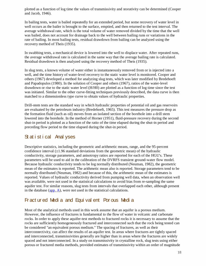
Assumptions for transient drawdown effects (C.V. Theis 1935) (1.) Aquifer is confined top and bottom.

(2.) There is no source of recharge to aquifer. (3.) The Aquifer is compressible and water is released instantaneously from the aquifer as the head is lowered. (4.) The well is pumping at a constant rate.

Theis (Non Equilibrium Equation

Replace the integral with a Taylor expansion series

Q = Constant pumping rate (L3/T),

h = Hydraulic head (L),

h0 = Hydraulic head before pumping starts (L),

h0 - h = drawdown (L),

T = Transmissivity (L2/T),

22

t = Time since pumping began (T),

r = Radial distance from pumping well (L), and

S = Aquifer storativity.

Sometimes the series is referred to as the Well function W(u).

So

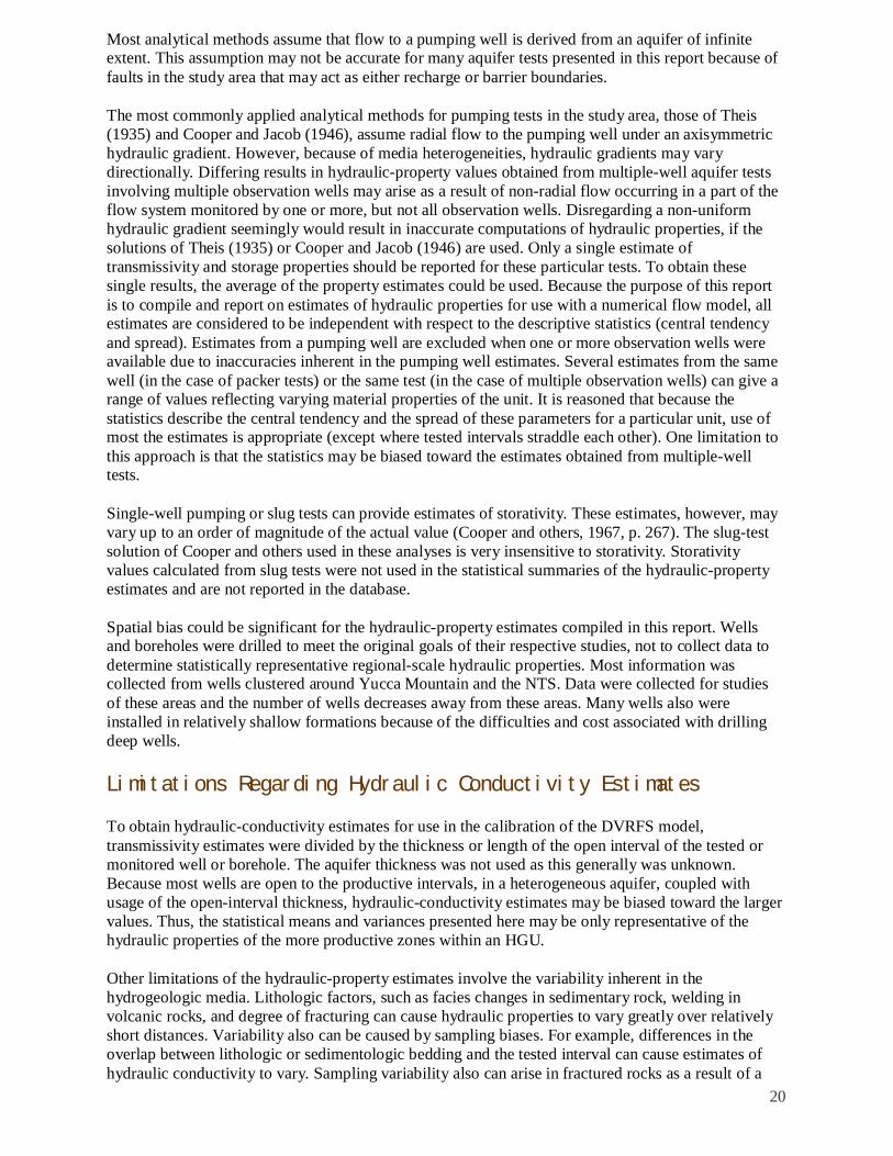
Confined aquifer system using Theis analysis

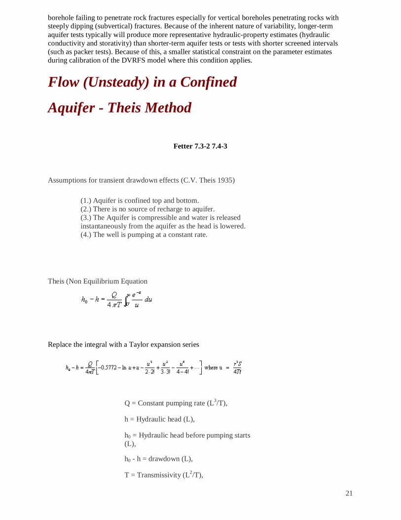
Theis Method for getting aquifer parameters from time - drawdown data.

23

Nonequilibrium - cone of depression continues to grow. Pumping well - T K if know b Observation well - T + S Rearrange Theis equation

(ft or m) = s drawdown

u = dimensionless constant

Theis Type Curve - non equilibrium type curve

W(u) vs 1) Plot s as a function of time on log-log 2) Place type curve over field data 3) Keep axes parallel 4) Overlay the two curves 5) Select match point usually pick point on field data where W(u) = 1

find s and t at this point 6) Convert minutes to days 7) Substitute values into equations

24

Values of the function W(u) for various values of u

u W(u) u W(u) u W(u) u W(u)

1 X 10-10 22.45 7 X 10-8 15.90 4 X 10-5 9.55 1 X 10-2 4.04

2 21.76 8 15.76 5 9.33 2 3.35

3 21.35 9 15.65 6 9.14 3 2.96

4 21.06 1 X 10-7 15.54 7 8.99 4 2.69

5 20.84 2 14.85 8 8.86 5 2.47

6 20.66 3 14.44 9 8.74 6 2.30

7 20.50 4 14.15 1 X 10-4 8.63 7 2.15

8 20.37 5 13.93 2 7.94 8 2.03

9 20.25 6 13.75 3 7.53 9 1.92

1 x 10-9 20.15 7 13.60 4 7.25 1 X 10-1 1.823

2 19.45 8 13.46 5 7.02 2 1.223

3 19.05 9 13.34 6 6.84 3 0.906

4 18.76 1 X 10-6 13.24 7 6.69 4 0.702

5 18.54 2 12.55 8 6.55 5 0.560

6 18.35 3 12.14 9 6.44 6 0.454

7 18.20 4 11.85 1 X 10-3 6.33 7 0.374

8 18.07 5 11.63 2 5.64 8 0.311

9 17.95 6 11.45 3 5.23 9 0.260

1 X 10-8 17.84 7 11.29 4 4.95 1 X 100 0.219

2 17.15 8 11.16 5 4.7. 2 0.049

3 16.74 9 11.04 6 4.54 3 0.013

4 16.46 1 X 10-5 10.94 7 4.39 4 0.004

5 16.23 2 10.24 8 4.26 5 0.001

6 16.05 3 9.84 9 4.14

Source: Adapted from L.K. Wenzel, Methods for Determining Permeability of Water-Bearing

Materials with Special Reference to Discharging Well Methods. U.S. Geological Survey

Water-Supply Paper 887, 1942.

Effects of well-bore storage neglects when

25

rw = radius of pumping well

r = radial distance between pumping well and observation well

Part A

Part A'

The effect of well-bore storage in the pumped well on the theoretical

time-drawdown plots of observation wells or piezometers. The dashed

curves are those of Parts A and A’ of Figure 2.12

Discharge Measuring Devices

1) Commerical water meter

2) If a tall ditch flume

3) Container - bucket, drum

4) Orifice Weir

- perfectly round hole in the center of a circular pipe,

26

fastened to end of level pipe

- place a piezometer tube 61 cm from orifice plate

- water level in piezometer represents pressure in discharge pipe

5) Open pipe flow

ENV 302 - Lectures