Hydrological Calibration in the Mount Lofty Ranges using Source Paramenter Estimation Tool (PEST)

Source hydrological calibration in the Mount Lofty Ranges using

parameter estimation tool (PEST)

eWater CRC Application Report Fleming, N.K.1, Cox, J.W.2, He, Y.3, Thomas, S.2

1 South Australian Research and Development Institute 2 University of Adelaide

3 Environment Protection Authority South Australia

Source hydrological calibration in the Mount Lofty Ranges

ii

Copyright Notice

© 2012 eWater Ltd

Legal Information

This work is copyright. You are permitted to copy and reproduce the information, in an unaltered form, for non-commercial use, provided you acknowledge the source as per the citation guide below. You must not use the information for any other purpose or in any other manner unless you have obtained the prior written consent of eWater Ltd.

While every precaution has been taken in the preparation of this document, the publisher and the authors assume no responsibility for errors or omissions, or for damages resulting from the use of information contained in this document. In no event shall the publisher and the author be liable for any loss of profit or any other commercial damage caused or alleged to have been caused directly or indirectly by this document.

Citing this document

Fleming, N.K., Cox, J.W., He, Y., Thomas, S. (2012) (eWater CRC) Source Catchment hydrological calibration in the Mount Lofty Ranges using parameter estimation tool (PEST).

Publication date: June 2012 (Version 1)

ISBN: 978-1-921543-63-0

For more information: eWater CRC UC Innovation Centre University Drive South Bruce, ACT, 2617, Australia T: 1300 5 WATER (1300 592 937) T: +61 2 6201 5834 (outside Australia) E: [email protected] www.ewater.com.au

OR

Nigel Fleming SARDI, GPO Box 397, Adelaide SA 5001 [email protected] Acknowledgements: This study was carried out with funds from the eWater CRC and in-kind support from South Australia Environment Protection Authority, South Australian Research and Development Institute and University of South Australia. The contribution of Dave Waters to reviewing this document is gratefully acknowledged.

mailto:[email protected]


iii

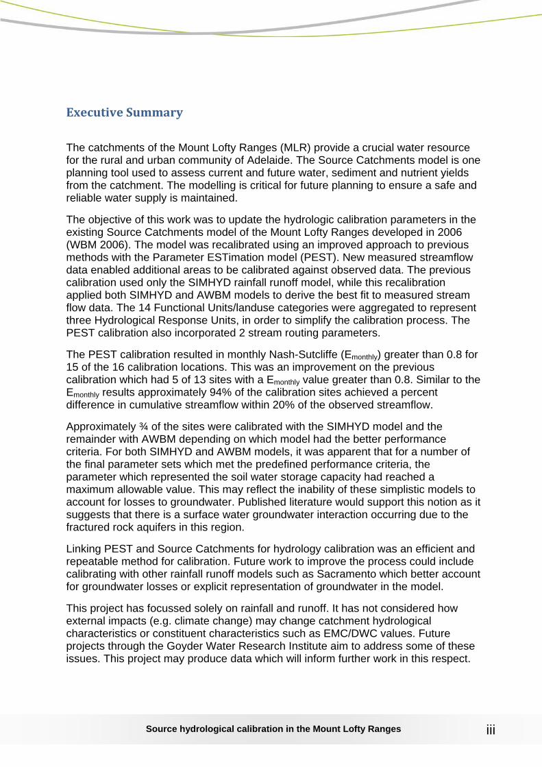
Executive Summary

The catchments of the Mount Lofty Ranges (MLR) provide a crucial water resource for the rural and urban community of Adelaide. The Source Catchments model is one planning tool used to assess current and future water, sediment and nutrient yields from the catchment. The modelling is critical for future planning to ensure a safe and reliable water supply is maintained.

The objective of this work was to update the hydrologic calibration parameters in the existing Source Catchments model of the Mount Lofty Ranges developed in 2006 (WBM 2006). The model was recalibrated using an improved approach to previous methods with the Parameter ESTimation model (PEST). New measured streamflow data enabled additional areas to be calibrated against observed data. The previous calibration used only the SIMHYD rainfall runoff model, while this recalibration applied both SIMHYD and AWBM models to derive the best fit to measured stream flow data. The 14 Functional Units/landuse categories were aggregated to represent three Hydrological Response Units, in order to simplify the calibration process. The PEST calibration also incorporated 2 stream routing parameters.

The PEST calibration resulted in monthly Nash-Sutcliffe (Emonthly) greater than 0.8 for 15 of the 16 calibration locations. This was an improvement on the previous calibration which had 5 of 13 sites with a Emonthly value greater than 0.8. Similar to the Emonthly results approximately 94% of the calibration sites achieved a percent difference in cumulative streamflow within 20% of the observed streamflow.

Approximately ¾ of the sites were calibrated with the SIMHYD model and the remainder with AWBM depending on which model had the better performance criteria. For both SIMHYD and AWBM models, it was apparent that for a number of the final parameter sets which met the predefined performance criteria, the parameter which represented the soil water storage capacity had reached a maximum allowable value. This may reflect the inability of these simplistic models to account for losses to groundwater. Published literature would support this notion as it suggests that there is a surface water groundwater interaction occurring due to the fractured rock aquifers in this region.

Linking PEST and Source Catchments for hydrology calibration was an efficient and repeatable method for calibration. Future work to improve the process could include calibrating with other rainfall runoff models such as Sacramento which better account for groundwater losses or explicit representation of groundwater in the model.

This project has focussed solely on rainfall and runoff. It has not considered how external impacts (e.g. climate change) may change catchment hydrological characteristics or constituent characteristics such as EMC/DWC values. Future projects through the Goyder Water Research Institute aim to address some of these issues. This project may produce data which will inform further work in this respect.


iv

Contents

Executive Summary ................................................................................................ iii

LIST OF FIGURES ................................................................................................... vi

LIST OF TABLES ..................................................................................................... vi

1.0 Introduction ........................................................................................................ 1

2.0 Objectives ........................................................................................................... 1

3.0 Methods .............................................................................................................. 2

3.1 Model construction ............................................................................................ 2

3.2 PEST calibration ............................................................................................... 2

3.3 Weighting of objective functions in PEST ......................................................... 2

3.4 Assessment of model Performance .................................................................. 4

3.5 Analysis of Hydrological Response Unit sets .................................................... 4

3.6 Structure of the model ...................................................................................... 7

3.7 Time period of PEST optimisation .................................................................... 9

3.8 Rainfall-runoff models used with PEST ............................................................ 9

4.0 Results .............................................................................................................. 10

4.1 Performance of PEST and RRL models ......................................................... 10

Monthly Nash-Sutcliffe comparison ................................................................... 11

Daily Nash-Sutcliffe comparison ....................................................................... 13

Total volume comparison .................................................................................. 15

4.2 PEST Calibrated Rainfall Runoff Parameters ................................................. 17

5.0 Discussion ........................................................................................................ 19

5.1 Overall calibration ........................................................................................... 19

5.2 PEST vs RRL .................................................................................................. 19

Monthly Nash-Sutcliffe ...................................................................................... 19

Daily Nash-Sutcliffe ........................................................................................... 19

Total volume comparison .................................................................................. 19

5.3 Choice of runoff models .................................................................................. 20


v

5.4 SIMHYD model parameters ............................................................................ 20

5.5 AWBM model parameters ............................................................................... 20

5.6 Use of PEST to optimise hydrological parameters .......................................... 21

6.0 Conclusions ...................................................................................................... 21

7.0 Future work ....................................................................................................... 21

6.0 References ........................................................................................................ 23

Appendix A. .......................................................................................................... 24

Appendix B. .......................................................................................................... 25

Appendix Cndix C ................................................................................................. 26

Appendix D. .......................................................................................................... 29


vi

LIST OF FIGURES Figure 1. Proportions of land use at site 5030526 (Cox Creek) in the MLR ............... 5 Figure 2. PEST and E2CL. ......................................................................................... 6 Figure 3. Map of major catchments in the MLR Source Catchments model flow gauges (nodes) and links used to calibrate models. .................................................. 8 Figure 4. Cumulative daily rainfall residual and average annual rainfall from 1970 to 2008 at the Lobethal climate station (BOM site 23726) within the Mount Lofty Ranges. ...................................................................................................................... 9 Figure 5. Monthly Nash-Sutcliffe values for hydrologic calibration of Source Catchment models in the Mount Lofty Ranges using Rainfall Runoff Library or PEST. The dashed red line indicates a Nash-Sutcliffe value of 0.6 and the solid red line a value of 0.8. .............................................................................................................. 11 Figure 6. Map of monthly Nash-Sutcliffe values by gauged catchment in the PEST-calibrated MLR model. ............................................................................................. 12 Figure 7. Daily Nash-Sutcliffe values for hydrologic calibration of Source Catchment models using PEST. The dashed red line indicates a Nash-Sutcliffe value of 0.6 and the solid red line a value of 0.8. ................................................................................ 13 Figure 8. Map of daily Nash-Sutcliffe values by gauged catchment in the PEST-calibrated MLR model. ............................................................................................. 14 Figure 9. Difference in simulated and observed total volumes of Source Catchment models in the Mount Lofty Ranges using PEST. The red line indicates zero difference – where the modelled volume equals the observed volume. ................... 15 Figure 10. Map of differences in modelled and observed total volumes by gauged catchment in the PEST-calibrated MLR model. ........................................................ 16 Figure 11. SIMHYD normalised soil moisture store coefficients for gauging stations calibrated with 3 HRU’s ............................................................................................ 18

LIST OF TABLES

Table 1. Objective functions (daily and monthly NS), simulated and observed volumes from Scott Creek catchment (gauge 5030502) following PEST optimisation of the Onkaparinga Source Catchments model. ......................................................... 3


vii


1

1.0 Introduction

The catchments of the Mount Lofty Ranges (MLR) are a crucial water resource important to the well-being of the people of Adelaide. There are seven reservoirs on rivers and streams of the MLR to harvest rainfall and supply Adelaide with drinking water. This drinking water is supplemented with water diverted from the River Murray and with desalinated water. However, water collected within the catchments is a significant component of the total supply needs of Adelaide and is the most cost effective water source.

The MLR are used for different purposes including harvesting of drinking water, agriculture, intensive horticulture, recreation, rural living, tourism, environmental conservation and urban environments. These multiple uses place pressure on the water resource and can impact on water quality. The Source Catchments suite of modelling tools is being used as a decision support tool to help prioritise and assess management of these catchments.

An existing model of the MLR (WBM, 2006) had been developed to examine major contributions of nutrients and sediments to Adelaide's water storages and key stressors to reservoir water quality and risk to water treatment capacity and performance. Proceeding this report, new data and calibration techniques became available including: 5 years of flow data, updated constituent generation data and an improved calibration methodology using the PEST parameter estimation software.Therefore an updated MLR model was developed through the eWater CRC Applications projects commencing in 2010. This document summarises the hydrological calibration component of the updated model. Two additional reports are available covering the constituent generation component (Fleming, et al. 2010) and the water quality modelling component (Thomas, et al. 2012) of the project.

This document outlines the construction of the MLR Source Catchments model, its hydrological calibration using PEST, and its utility for prediction of constituent loads.

2.0 Objectives

The objectives of this work were to:

• Improve the existing hydrological calibration of a Source Catchments model for the MLR, by incorporating the most recent stream flow data and utilising the PEST parameter estimation tool

• Compare the new calibration performance to the previous one carried out with the Rainfall Runoff Library


2

3.0 Methods

3.1 Model construction A Source Catchments model of the Mount Lofty Ranges (MLR) was developed to estimate sediment and nutrient loads in the MLR (WBM 2006). This model was calibrated with the Rainfall Runoff Library (RRL) and will be referred to as the RRL model. It was recently updated with improved EMC and DWC values (Fleming et al. 2010). However, when simulations were run to estimate constituent loads it was found that the RRL model did not accurately reflect recent hydrology. A new calibration of the model would improve this, and also include more recent hydrological data. The Parameter ESTimation tool (PEST) (Doherty, 2007), using the method applied by Ellis et al. 2009, was used for the new calibration. The PEST model was also calibrated with in-stream flow routing, which was not feasible with the RRL model.

3.2 PEST calibration PEST is a tool which adjusts model parameters until the fit between model outputs and observed data is optimised, as measured by least squares (Doherty, 2007). PEST estimates parameters sets for a model by minimising the error between observed and modelled data. The process by which PEST optimised parameters has been succinctly described by WBM (2010). Briefly, for the MLR project, there were three observed and modelled data sets – daily flow, monthly flow and flow duration. The sum of squared residuals for these three parts of the calibration were weighted and then summed to form a composite error term (phi). Phi is the term which PEST minimised through parameter adjustment.

3.3 Weighting of objective functions in PEST To undertake the PEST calibration of rainfall runoff models, objective functions were required to assess whether the calibration was improving. PEST was set to optimise three objective functions (WBM 2011)- two Nash-Sutcliffe criteria and flow exceedance values. The Nash-Sutcliffe coefficient of efficiency (Nash and Sutcliffe, 1970) describes the agreement between modelled and recorded runoff. A value of 1.0 indicates that modelled runoff is the same as recorded runoff. In general, values greater than 0.6 suggest a reasonable modelling of runoff and values greater than 0.8 suggest a good modelling of runoff (Chiew and Siriwardena, 2005).The three objective functions were:

• Nash-Sutcliffe (NS) value for the natural log of daily flow volumes. This weighted the optimisation towards day by day congruence, and was important for matching hydrographs at a daily step. Many of the subcatchments in the MLR are less than ~ 50 km2 and an entire runoff event can often occur during one day. Thus it was important to weight for optimisation of daily data.

• Nash-Sutcliffe (NS) value for monthly flow volumes. This matches flow volumes at a time interval which essentially excludes the effect of lag times. Matching of monthly flow volumes reduces error in water balances at a monthly timestep. This was chosen to have a stabilising


3

effect to counteract short-term variation.

• exceedance values for daily flow. This was chosen to align baseflow and the length of hydrograph recession.

Each of the three objective functions was weighted. This weighting determined the amount of importance assigned to optimising each objective function. Initially, weighting was in the ratio of 1 : 1 : 1 for NS daily : NS monthly : exceedance. WBM (2011) considered that generally, if the data is worth contributing to the objective function, then it is reasonable to give the data weight similar to other objective function components. However, we tested three weighting scenarios on all regions in order to fine-tune the optimisation process. For the ratio of NS daily : NS monthly : exceedance, these were:

• 1 : 1 : 1 (standard)

• 1 : 0 : 0 (NS daily only). This put all weighting on the daily flows, and was investigated for small catchments where lag times were much less than 1 day

• 0.6 : 0.3 : 0.1 (mixed weighting). This is biased towards daily flows as per the last option, but still maintained some weighting for the monthly and base flows

The weighting scenario with the best outcome in terms of NS (daily and monthly) and total volume (modelled vs observed) was selected for each region of the relevant model.

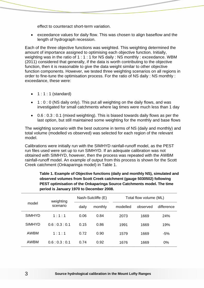
Calibrations were initially run with the SIMHYD rainfall-runoff model, as the PEST run files used were set up to run SIMHYD. If an adequate calibration was not obtained with SIMHYD, however, then the process was repeated with the AWBM rainfall-runoff model. An example of output from this process is shown for the Scott Creek catchment (Onkaparinga model) in Table 1.

Table 1. Example of Objective functions (daily and monthly NS), simulated and observed volumes from Scott Creek catchment (gauge 5030502) following PEST optimisation of the Onkaparinga Source Catchments model. The time period is January 1970 to December 2008.

model weighting scenario

Nash-Sutcliffe (E) Total flow volume (ML)

daily monthly modelled observed difference

SIMHYD 1 : 1 : 1 0.06 0.84 2073 1669 24%

SIMHYD 0.6 : 0.3 : 0.1 0.15 0.86 1991 1669 19%

AWBM 1 : 1 : 1 0.72 0.90 1579 1669 -5%

AWBM 0.6 : 0.3 : 0.1 0.74 0.92 1676 1669 0%


4

In this case the AWBM rainfall-runoff model with mixed weighting gave best results and was used in the model.

The process was simplified by calibrating one gauge at a time, and applying the resultant parameters to subcatchments draining to that gauge. Headwater gauges were calibrated first. Downstream gauges were then calibrated using either observed flow at the headwater gauge (where available) or the newly calibrated parameters for runoff generation at the headwater gauge.

3.4 Assessment of model Performance The aim of PEST calibration was to minimise a specified residual error term. For the MLR this was the sum of squared error between observed and modelled data (WBM, 2010). Performance of a calibration run against this criteria was assessed objectively by Nash-Sutcliffe efficiency criteria on daily and monthly flows (as described previously) and by percentage difference between modelled and observed total flow volumes. It is necessary, however, to “reality check” the parameters selected by PEST to determine that they are within reasonable bounds. PEST is an objective optimisation program, and any number of parameter combinations may satisfy the conditions of the objective function, as discussed by Doherty (2007). Because of this, parameter values need to be checked for congruence to “reasonable” limits.

3.5 Analysis of Hydrological Response Unit sets The number of runs needed for an iteration of PEST increases geometrically with the number of HRU’s for a given model. Thus there is a need to minimise the number of HRU’s, without compromising the fit of the model. Simplification of the model for hydrological calibration was made on the basis of grouping land uses (FU’s) which are likely to have similar hydrological characteristics, into hydrological response units (HRU’s).

PEST calibration of Source Catchments models with different numbers of HRU’s have been reported previously (Barlow, et al. (2010),WBM (2010)). However, the spatial arrangement and density of land use and geology of the MLR are quite complex and therefore warranted investigation into the number of HRU’s required to optimise calibration.


5

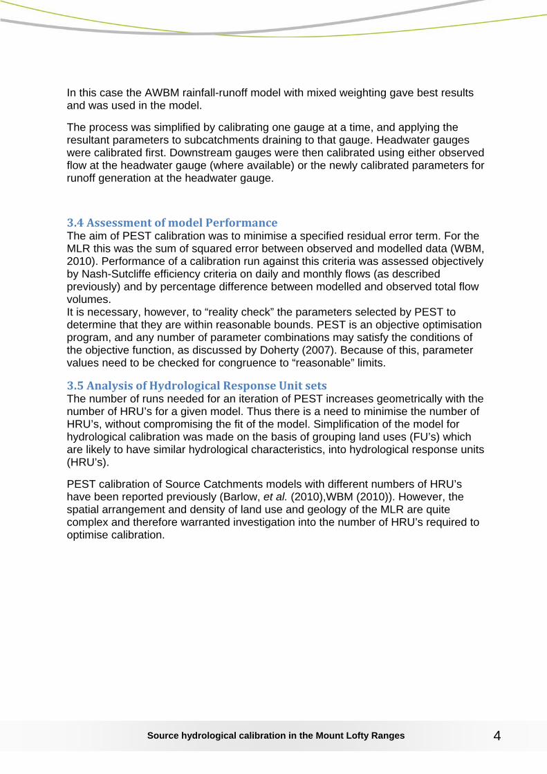
Figure 1. Proportions of land use at site 5030526 (Cox Creek) in the MLR

For example, Figure 1 highlights that the Cox Creek site had three or four major land uses, from a total of eight categories. Water quality at this site, however, was dominated by the impacts of broadscale annual horticulture.

The final combination of HRU’s was selected on a case by case basis, depending on the objective functions produced by each optimisation. In some cases, 5 HRU’s were used, in other cases 3 HRU’s.

The set of 3 HRU’s were Grazing related (shallow-rooted pasture plants), Forestry related (deep rooted perennial plants) and Residential related (mixture of pervious and impervious surfaces)

• Grazing related land uses – Grazing, Broadscale Agriculture, Dense urban, Broadscale perennial horticulture, Intensive grazing, Broadscale annual horticulture, Recreation and culture, and Intensive production

• Forestry related land uses – Conservation area and Managed forest • Residential related land uses – Rural living and Utilities

The set of 5 FU’s added Horticulture related land uses (annual and perennial) and Urban related land uses (higher proportion of impervious areas)

• Grazing related land uses – Grazing, Broadscale Agriculture, Intensive grazing, Recreation and culture, and Intensive production

• Horticulture related land uses - Broadscale perennial horticulture and Broadscale annual horticulture

• Forestry related land uses - Conservation area and Managed forest • Residential related land uses – Rural living and Utilities


6

• Urban related land uses – Dense urban

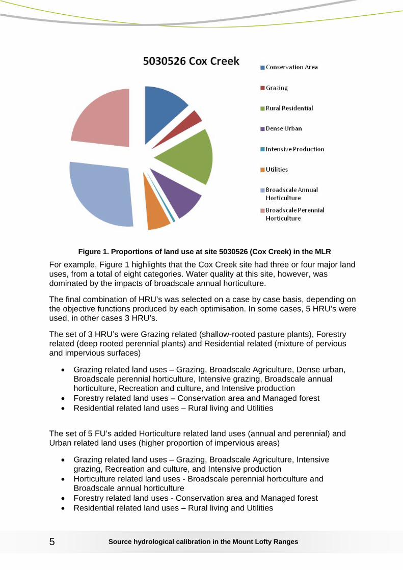
The use of PEST enabled calibration of multiple hydrological response units (HRU’s) within each hydrologic region. PEST has been shown to significantly improve calibration performance over RRL (Ellis et al. 2009). PEST works with the command line version of Source Catchments (E2 Command Line – E2CL) by running the model with many different input parameter settings. These settings and the way in which they are adjusted are specified for PEST. By comparing output from each model run to the observed data, the best model fit can be identified. Input parameter values which give the best fit are then output by PEST. The way in which PEST interacts with E2CL is shown in Figure 2.

Figure 2. PEST and E2CL.

The steps were

1) the project was loaded and run by E2CL,

2) the output was read by PEST and compared to observed data. The degree of model fit was noted, and a new set of parameter values sent to E2CL. Once this had run, the output was again examined, then compared to observed data and the results of the first run

3) improvement or loss of model fit was noted, and a new set of parameters sent to E2CL, and so on

4) repeat from 1).


7

This iterative process continued until either the target objective function was reached, or a preset maximum number of iterations was carried out.

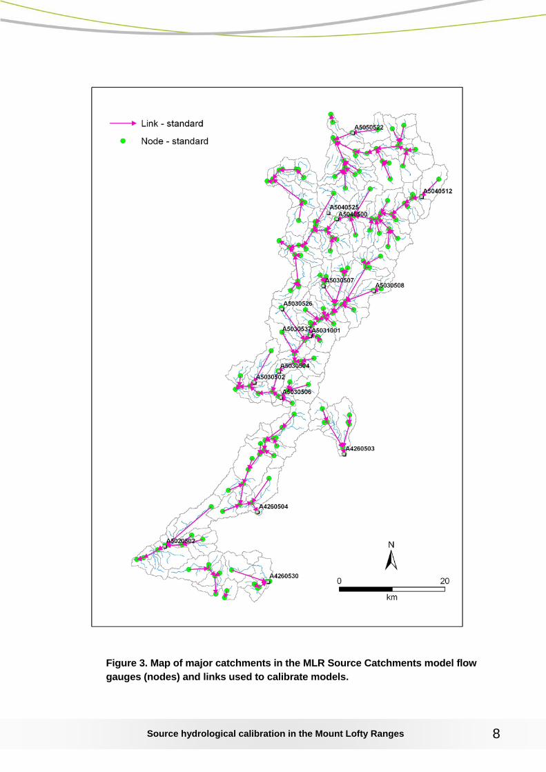
3.6 Structure of the model Initially a single model of the MLR watershed was constructed. It was intended to set up a single model in PEST with all required parameter variations which could be left to run until the optimisation was complete. However, this unearthed some practical difficulties, mainly due to the combination of large number of runs and a slow run-time. The model required 1440 runs per iteration, and would likely need 15-20 iterations for optimisation. At four minutes per run, this would be 60-80 days of run time, using parallel PEST on a 6-processor computer. A further complication was that a lot of error checking and fine tuning of the PEST files was needed during development. This was not generally apparent until a few iterations had been completed and the output examined, which was also time-consuming. As a result, seven separate smaller models were constructed for major catchments in the MLR, rather than a single larger model. The catchments were:

• Torrens • Onkaparinga • Myponga • Angas • Finniss • Currency • Victoria

The smaller models generally had a run time of around 30 seconds. They also needed fewer runs per iteration than the large model due to the smaller number of variables. Hydrologic regions in the models calibrated with RRL and PEST are shown in Figure 3.


8

Figure 3. Map of major catchments in the MLR Source Catchments model flow gauges (nodes) and links used to calibrate models.


9

Further details of hydrologic regions in the MLR models are shown in Appendix B.

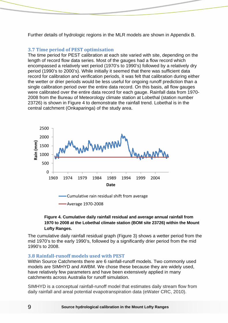
3.7 Time period of PEST optimisation The time period for PEST calibration at each site varied with site, depending on the length of record flow data series. Most of the gauges had a flow record which encompassed a relatively wet period (1970’s to 1990’s) followed by a relatively dry period (1990’s to 2000’s). While initially it seemed that there was sufficient data record for calibration and verification periods, it was felt that calibration during either the wetter or drier periods would be less useful for ongoing runoff prediction than a single calibration period over the entire data record. On this basis, all flow gauges were calibrated over the entire data record for each gauge. Rainfall data from 1970-2008 from the Bureau of Meteorology climate station at Lobethal (station number 23726) is shown in Figure 4 to demonstrate the rainfall trend. Lobethal is in the central catchment (Onkaparinga) of the study area.

Figure 4. Cumulative daily rainfall residual and average annual rainfall from 1970 to 2008 at the Lobethal climate station (BOM site 23726) within the Mount Lofty Ranges.

The cumulative daily rainfall residual graph (Figure 3) shows a wetter period from the mid 1970’s to the early 1990’s, followed by a significantly drier period from the mid 1990’s to 2008.

3.8 Rainfall-runoff models used with PEST Within Source Catchments there are 6 rainfall-runoff models. Two commonly used models are SIMHYD and AWBM. We chose these because they are widely used, have relatively few parameters and have been extensively applied in many catchments across Australia for runoff simulation.

SIMHYD is a conceptual rainfall-runoff model that estimates daily stream flow from daily rainfall and areal potential evapotranspiration data (eWater CRC, 2010).

0

500

1000

1500

2000

2500

1969 1974 1979 1984 1989 1994 1999 2004

Rain

(mm

)

Date

Cumulative rain residual shift from average

Average 1970-2008


10

SIMHYD contains three stores for interception loss, soil moisture and groundwater. The model has seven parameters, as described in the Source Catchments User Guide (eWater CRC, 2010):

• Baseflow Coefficient • Impervious Threshold • Infiltration Coefficient • Infiltration shape • Interflow Coefficient • Pervious Fraction • Rainfall Interception Store Capacity • Recharge coefficient • Soil Moisture Store Capacity

PEST was initially set up to calibrate using only the SIMHYD rainfall-runoff model. While this was generally successful, good calibrations could not be obtained with the SIMHYD model in a number of catchments. Therefore the model was recalibrated with PEST using the Australian Water Balance Model (AWBM) rainfall-runoff model and successful calibrations were achieved.

AWBM is a water balance model which relates rainfall to runoff with daily data, and calculates losses from rainfall for flood hydrograph modelling (Boughton, 2004). It contains five stores; three surface stores to simulate partial areas of runoff, a baseflow store and a surface runoff routing store (eWater CRC, 2010). The parameters in AWBM are:

• C1, C2, C3 - Surface storage capacities • A1, A2, A3 - Partial areas represented by storage areas • BFI - Baseflow index • Kbase - Daily baseflow recession constant • Ksurf - Daily surface flow recession constant

The runoff generating capacity of the AWBM can be summarised in a single parameter, the average surface storage capacity, which is calculated as

Cave = C1*A1 + C2*A2 + C3*A3

where Cave is the average surface storage capacity; Cl,C2,C3 are the capacities of the 3 surface stores, and A1,A2,A3 are the partial areas of the 3 surface stores (Boughton, 1996).

4.0 Results

4.1 Performance of PEST and RRL models The following section presents Nash-Sutcliffe values for daily and monthly flow volumes at calibrated gauges. In general, values greater than 0.6 indicate a reasonable modelling of runoff and values greater than


11

0.8 indicate a good modelling of runoff (Chiew and Siriwardena, 2005).

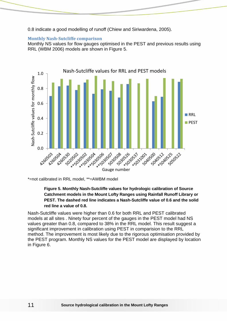
Monthly Nash-Sutcliffe comparison Monthly NS values for flow gauges optimised in the PEST and previous results using RRL (WBM 2006) models are shown in Figure 5.

*=not calibrated in RRL model, **=AWBM model

Figure 5. Monthly Nash-Sutcliffe values for hydrologic calibration of Source Catchment models in the Mount Lofty Ranges using Rainfall Runoff Library or PEST. The dashed red line indicates a Nash-Sutcliffe value of 0.6 and the solid red line a value of 0.8.

Nash-Sutcliffe values were higher than 0.6 for both RRL and PEST calibrated models at all sites . Ninety four percent of the gauges in the PEST model had NS values greater than 0.8, compared to 38% in the RRL model. This result suggest a significant improvement in calibration using PEST in comparision to the RRL method. The improvement is most likely due to the rigorous optimisation provided by the PEST program. Monthly NS values for the PEST model are displayed by location in Figure 6.

0.0

0.2

0.4

0.6

0.8

1.0

Nas

h-Su

tclif

fe v

alue

s for

mon

thly

flow

Gauge number

Nash-Sutcliffe values for RRL and PEST models

RRL

PEST


12

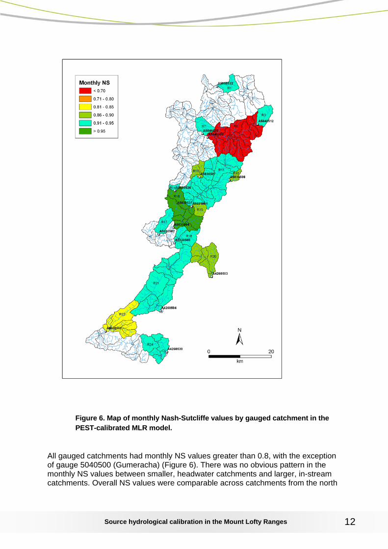
Figure 6. Map of monthly Nash-Sutcliffe values by gauged catchment in the PEST-calibrated MLR model.

All gauged catchments had monthly NS values greater than 0.8, with the exception of gauge 5040500 (Gumeracha) (Figure 6). There was no obvious pattern in the monthly NS values between smaller, headwater catchments and larger, in-stream catchments. Overall NS values were comparable across catchments from the north


13

to the south of the study area. The following chart (Figure 7) shows Nash-Sutcliffe values for daily flow of gauges optimised in the PEST model.

**=AWBM model

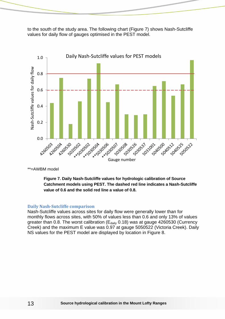
Figure 7. Daily Nash-Sutcliffe values for hydrologic calibration of Source Catchment models using PEST. The dashed red line indicates a Nash-Sutcliffe value of 0.6 and the solid red line a value of 0.8.

Daily Nash-Sutcliffe comparison Nash-Sutcliffe values across sites for daily flow were generally lower than for monthly flows across sites, with 50% of values less than 0.6 and only 13% of values greater than 0.8. The worst calibration (Edaily 0.18) was at gauge 4260530 (Currency Creek) and the maximum E value was 0.97 at gauge 5050522 (Victoria Creek). Daily NS values for the PEST model are displayed by location in Figure 8.

0.0

0.2

0.4

0.6

0.8

1.0

Nas

h-Su

tclif

fe v

alue

s for

dai

ly fl

ow

Gauge number

Daily Nash-Sutcliffe values for PEST models


14

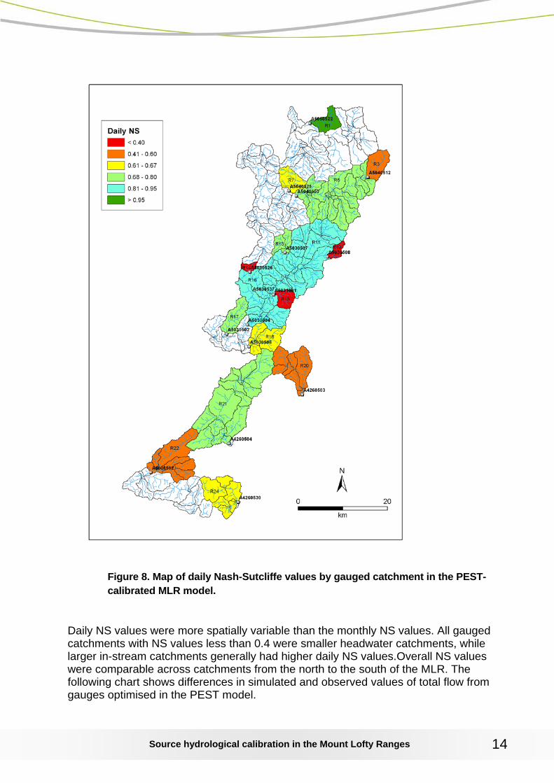
Figure 8. Map of daily Nash-Sutcliffe values by gauged catchment in the PEST-calibrated MLR model.

Daily NS values were more spatially variable than the monthly NS values. All gauged catchments with NS values less than 0.4 were smaller headwater catchments, while larger in-stream catchments generally had higher daily NS values.Overall NS values were comparable across catchments from the north to the south of the MLR. The following chart shows differences in simulated and observed values of total flow from gauges optimised in the PEST model.


15

Total volume comparison

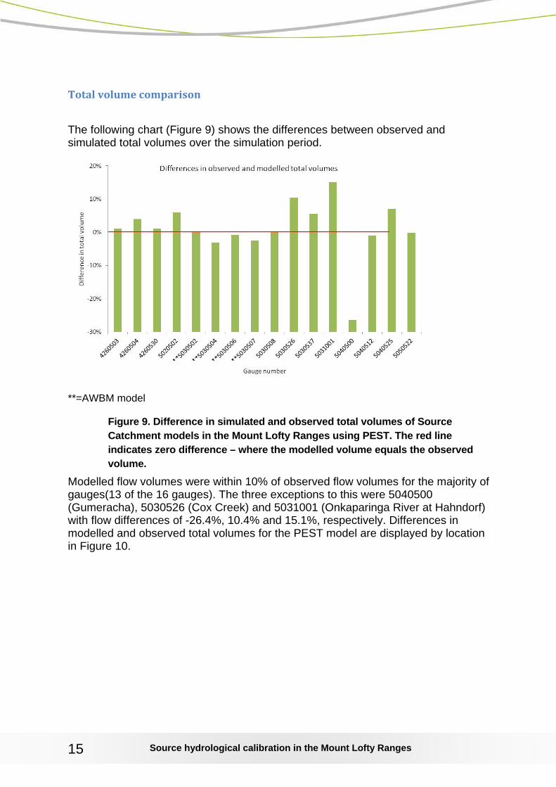
The following chart (Figure 9) shows the differences between observed and simulated total volumes over the simulation period.

**=AWBM model

Figure 9. Difference in simulated and observed total volumes of Source Catchment models in the Mount Lofty Ranges using PEST. The red line indicates zero difference – where the modelled volume equals the observed volume.

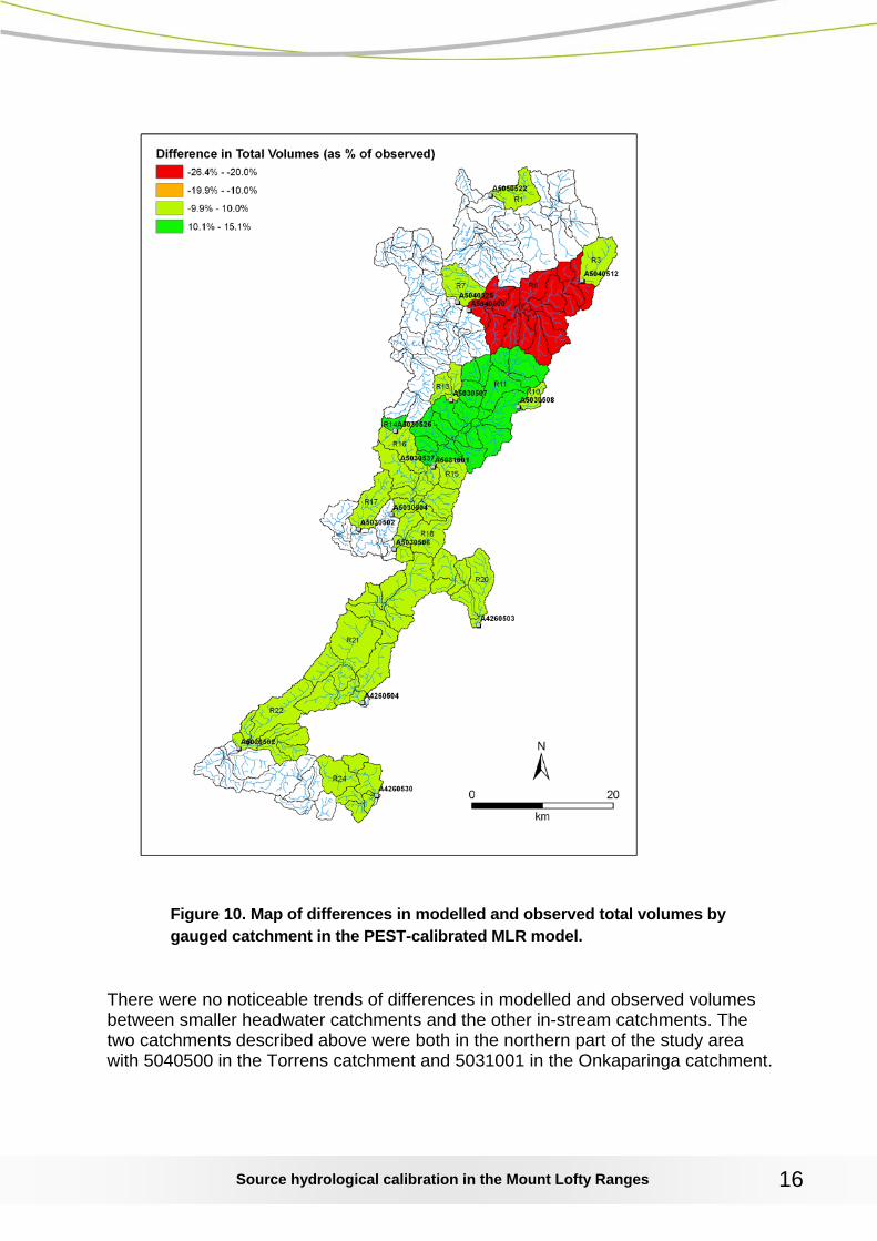
Modelled flow volumes were within 10% of observed flow volumes for the majority of gauges(13 of the 16 gauges). The three exceptions to this were 5040500 (Gumeracha), 5030526 (Cox Creek) and 5031001 (Onkaparinga River at Hahndorf) with flow differences of -26.4%, 10.4% and 15.1%, respectively. Differences in modelled and observed total volumes for the PEST model are displayed by location in Figure 10.


16

Figure 10. Map of differences in modelled and observed total volumes by gauged catchment in the PEST-calibrated MLR model.

There were no noticeable trends of differences in modelled and observed volumes between smaller headwater catchments and the other in-stream catchments. The two catchments described above were both in the northern part of the study area with 5040500 in the Torrens catchment and 5031001 in the Onkaparinga catchment.


17

4.2 PEST Calibrated Rainfall Runoff Parameters

Each rainfall runoff model has a number of parameters – 9 for SIMHYD and 8 for AWBM.The most sensitive parameter impacting on runoff will be discussed further. The SMSC parameter was found to be the most significant in terms of model sensitivity for SIMHYD by Chiew and Siriwardena (2005), while Boughton (1996) found the average surface storage capacity could summarise runoff generating capacity of the AWBM.

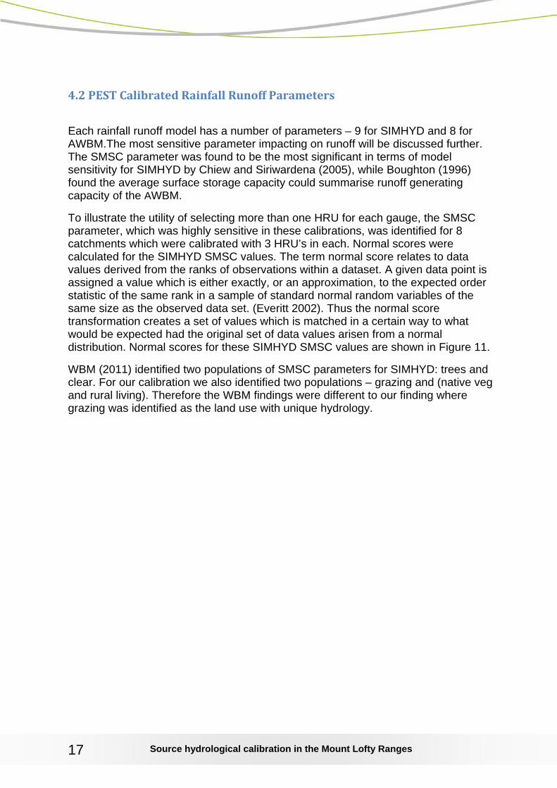
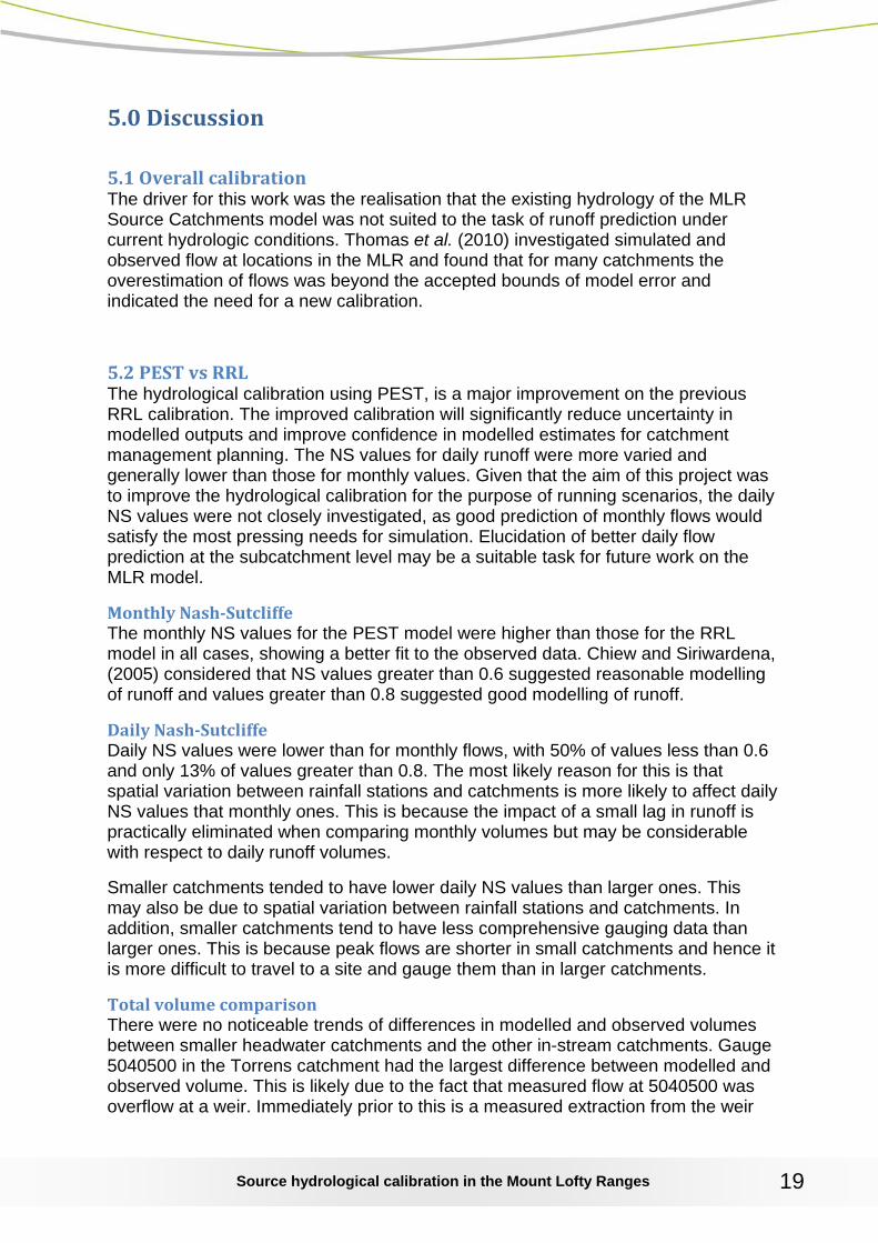
To illustrate the utility of selecting more than one HRU for each gauge, the SMSC parameter, which was highly sensitive in these calibrations, was identified for 8 catchments which were calibrated with 3 HRU’s in each. Normal scores were calculated for the SIMHYD SMSC values. The term normal score relates to data values derived from the ranks of observations within a dataset. A given data point is assigned a value which is either exactly, or an approximation, to the expected order statistic of the same rank in a sample of standard normal random variables of the same size as the observed data set. (Everitt 2002). Thus the normal score transformation creates a set of values which is matched in a certain way to what would be expected had the original set of data values arisen from a normal distribution. Normal scores for these SIMHYD SMSC values are shown in Figure 11.

WBM (2011) identified two populations of SMSC parameters for SIMHYD: trees and clear. For our calibration we also identified two populations – grazing and (native veg and rural living). Therefore the WBM findings were different to our finding where grazing was identified as the land use with unique hydrology.


18

Figure 11. SIMHYD normalised soil moisture store coefficients for gauging stations calibrated with 3 HRU’s

Figure 11 suggests there are two distinct populations, grazing and native vegetation / rural living. As the data above suggests, using more than one HRU per gauging station may capture real effects of land use. While it would be interesting to compare calibrations using 3 HRU’s with 5 HRU’s using this method; the project was not designed with this in mind. In order to clarify this aspect, PEST calibrations would need to be carried out with both 3 and 5 HRU’s for each gauging station.

A similar analysis was undertaken for the AWBM surface store of the four catchments where AWBM was used (data not presented). There was no clear difference between land uses.

It was found in one calibration that the sum of optimised values of partial areas (A1-A3) in AWBM was greater than 1. As the partial areas must sum to 1, this was an incorrect parameterisation. When these factors are entered into the AWBM rainfall-runoff model via the Source Catchments Graphical User Interface, values with a sum greater than 1 are rejected. As the parameters were optimised by PEST via the E2commandline program, this parameter check was not enforced. The optimisation was re-run with the sum of partial areas constrained to a maximum of 1, and a successful calibration obtained. This was a reminder, however, that manual checking

of hydrological parameters is a necessity when they are optimised by an objective process of iteration.

1.5

2.0

2.5

3.0

-2 -1.5 -1 -0.5 0 0.5 1 1.5 2

log

SMSC

Normal Score

Normal Scores Plot, SMSC, Mount Lofty Ranges

grazing native veg. rural living


19

5.0 Discussion

5.1 Overall calibration The driver for this work was the realisation that the existing hydrology of the MLR Source Catchments model was not suited to the task of runoff prediction under current hydrologic conditions. Thomas et al. (2010) investigated simulated and observed flow at locations in the MLR and found that for many catchments the overestimation of flows was beyond the accepted bounds of model error and indicated the need for a new calibration.

5.2 PEST vs RRL The hydrological calibration using PEST, is a major improvement on the previous RRL calibration. The improved calibration will significantly reduce uncertainty in modelled outputs and improve confidence in modelled estimates for catchment management planning. The NS values for daily runoff were more varied and generally lower than those for monthly values. Given that the aim of this project was to improve the hydrological calibration for the purpose of running scenarios, the daily NS values were not closely investigated, as good prediction of monthly flows would satisfy the most pressing needs for simulation. Elucidation of better daily flow prediction at the subcatchment level may be a suitable task for future work on the MLR model.

Monthly Nash-Sutcliffe The monthly NS values for the PEST model were higher than those for the RRL model in all cases, showing a better fit to the observed data. Chiew and Siriwardena, (2005) considered that NS values greater than 0.6 suggested reasonable modelling of runoff and values greater than 0.8 suggested good modelling of runoff.

Daily Nash-Sutcliffe Daily NS values were lower than for monthly flows, with 50% of values less than 0.6 and only 13% of values greater than 0.8. The most likely reason for this is that spatial variation between rainfall stations and catchments is more likely to affect daily NS values that monthly ones. This is because the impact of a small lag in runoff is practically eliminated when comparing monthly volumes but may be considerable with respect to daily runoff volumes.

Smaller catchments tended to have lower daily NS values than larger ones. This may also be due to spatial variation between rainfall stations and catchments. In addition, smaller catchments tend to have less comprehensive gauging data than larger ones. This is because peak flows are shorter in small catchments and hence it is more difficult to travel to a site and gauge them than in larger catchments.

Total volume comparison There were no noticeable trends of differences in modelled and observed volumes between smaller headwater catchments and the other in-stream catchments. Gauge 5040500 in the Torrens catchment had the largest difference between modelled and observed volume. This is likely due to the fact that measured flow at 5040500 was overflow at a weir. Immediately prior to this is a measured extraction from the weir


20

(gauge 5040525). Total volume at 5040500 was thus calculated from two measured flow series, and may contain the combined errors from two flow measurement data series.

5.3 Choice of runoff models Historically the SIMHYD rainfall-runoff model had been applied to predict catchment runoff in the MLR. However, it was found that some catchments did not calibrate well with SIMHYD, specifically that SIMHYD over predicted runoff. While a process-based model might be expected to capture shifts in climate sequences, SIMHYD as a lumped conceptual model does not due to its limited physical reality (Barlow et al. 2010). Despite this, the PEST parameterisation gave a reasonable prediction of flow in most of the catchments. Where the SIMHYD calibration was poor (monthly NS value of less than 0.6), the AWBM model was optimised using PEST. This was carried out at four of the 16 flow gauges, and greatly improved the hydrological calibrations, with an average monthly NS value of 0.93 for these gauges.

5.4 SIMHYD model parameters Where the SIMHYD model diverged from observed values, it was generally over-estimating runoff. This was also found by Barlow et al. (2011) in the Oven River catchment in Northern Victoria. They discussed the seven calibrated SIMHYD parameters for each sub-catchment. The values for these parameters in the MLR model are presented in Appendix C. Overestimation of surface runoff may be partly due to interactions between surface and groundwater as discussed previously, that is, loss of surface water as aquifer recharge not being accounted for in the SIMHYD nor AWBM models.

SMSC has been identified as a key hydrological parameter associated with land use. WBM (2011) combined land uses into three categories – Clear, Trees and Cropping, and determined that the hydrology of Trees was different to that of the other two categories. We also combined land uses into three categories – Grazing, Native Vegetation (including forestry) and Rural Living. These reflected the land use in the MLR, and we determined that the hydrology of Grazing was different to the other categories. Reasons for difference between the findings of WBM (2011) and this work may include the disparity between temperate grazing systems in this work and tropical grazing systems described by WBM (2011). The size of catchments in this study (up to 320 km2) was also much less than those of WBM (2011) (up to 140,000 km2),

5.5 AWBM model parameters The AWBM model was used where the SIMHYD model could not produce a suitable calibration. Values for AWBM parameters in the MLR model are presented in Appendix C. Boughton (2006) noted that the AWBM has only one parameter (average surface storage capacity) determining the amount of runoff. Average surface storage capacity is calculated from the three partial area coefficients (A1-A3) and their respective surface storage capacities (C1-C3). Values for the MLR model ranged from 93 to 395mm (Figure 11). Boughton (1996) considered that calibrated

storage values (calibrated from measured rainfall and runoff) above 200mm should be treated as potential data errors and that values greater than 300mm should be


21

treated as due to data error. It would appear that the AWBM dealt with the problem of disposing of surplus runoff water by increasing the average surface storage capacity above reasonable values. In this endeavour, it was more successful than SIMHYD and thus gave better calibrations, but was still attempting to represent a process (contribution of groundwater to streamflow) which it was not intended to cope with.

5.6 Use of PEST to optimise hydrological parameters PEST calibration improved the fit of the Source Catchments model considerably, as measured by all objective functions, and satisfied the aims of this work. However, the initial optimised parameter sets as identified by PEST were not necessarily within sensible ranges based on previous work. However, PEST does calculate multiple sets of rainfall runoff parameters which meet the defined set of objective functions. Therefore, final rainfall runoff parameter sets were chosen based on local knowledge of the area in relation to soil types and relative proportion of perviousness in the catchments. This approach is recommended for future users of PEST with Source Catchments to determine the appropriateness of parameters based on local knowledge.

6.0 Conclusions

The MLR Source Catchments model has been calibrated to a satisfactory level using PEST coupled to Source Catchments. Both the SIMHYD and AWBM rainfall-runoff models were applied to catchments within the MLR. The PEST calibration approach significantly improved runoff estimates in comparison to the previous RRL method.

The use of multiple HRU’s has resulted in improved calibration for a number of catchments. A number of the SIMHYD and AWBM model parameters calibrated to the maximum possible values. The high parameters could be attributed to the model trying to account for runoff being lost to the fractured rock aquifers which underly the study area.

7.0 Future work

The parameterisation of a matrix of all gauges with 1, 3, or 5 HRU’s and both SIMHYD and AWBM rainfall-runoff models would explicitly identify the best combination for each flow gauge. Specifically addressing surface water/groundwater interactions prior to this exercise would allow parameterisation under more “normal’ conditions.

Additional areas that could be investigated to further improve calibration include:

• Further investigation of the optimum number of HRU’s required to achieve the best calibration


22

• Spatial variation in rainfall, due to the uneven topography of the MLR. These have been shown to have a great effect on the prediction of surface runoff (Boughton, 1996). There may be value in using local rainfall data to improve the spatial resolution of rainfall inputs

• interactions between groundwater and surface water in the fractured rock environment of the MLR. The degree of groundwater interaction with surface water could be estimated by mapping the runoff coefficient of all measured catchments in relation to rainfall and topography and looking for outliers in this distribution. It could also be tested by looking for changes in groundwater levels in the vicinity of streams which are affected by surface runoff events.

• Error in measurement of water flow, due to either the accuracy of flow control and measurement devices, or unknown factors at gauged sites


23

6.0 References

Barlow, K, Weeks, A., Githui, F., Christy, B. (2010) Northern Victoria Application Project: Parameterisation tools (PEST and RRL) and Source Catchments base model of the Goulburn River between Lake Eildon and the Goulburn Weir. eWater Cooperative Research Centre Technical Report, June 2010.

Barnett, S., Banks, E.W., Love, A.J., Simmons, C.T. and Gerges, N.Z. (2010) Aquifers and groundwater, Chapter 4 In Adelaide: Water of a City. Edited by Christopher B. Daniels, Wakefield Press, Adelaide.

Boughton, W. (1996). Detecting data errors in rainfall-runoff data sets: Cooperative Research Centre for Catchment Hydrology.

Boughton, W. (2004). The Australian water balance model. Environmental Modelling & Software, 19, 943-956.

Everitt, B.S. (2002) The Cambridge Dictionary of Statistics (2nd Edition). Cambridge University Press. ISBN 052181099x

eWater CRC (2010). Source Catchments Scientific Reference Guide. Canberra: eWater Cooperative Research Centre.

Chiew, F. H. S., & Siriwardena, L. (2005). Estimation of SIMHYD parameter values for application in ungauged catchments. Paper presented at the MODSIM 2005 International Congress on Modelling and Simulation, Christchurch, New Zealand.

Doherty, J. (2007). PEST Model Independent Parameter Estimation User Manual: 5th Edition.

Ellis, R. J., Doherty, J., Searle, R. D., & Moodie, K. (2009). Applying PEST (Parameter ESTimation) to improve parameter estimation and uncertainty analysis in WaterCAST models. Paper presented at the 18th World IMACS / MODSIM Congress, 13-17 July 2009, Cairns, Australia.

Fleming, N.K., Cox, J.W., He, Y., Thomas, S. and Frizenschaf, J. (2010) Analysis of Total Suspended Sediment and Total Nutrient Concentration data in the Mount Lofty Ranges to derive event mean concentrations, eWater Cooperative Research Centre Technical Report, August 2010. ISBN 978-1-921543-32-6

Nash, J. E., & Sutcliffe, J. V. (1970). River forecasting using conceptual models. Part I: A discussion of principles. Journal of Hydrology, 10(3), 282-290.

Thomas, S., Fleming, N., & He, Y. (2010). Progress Report on the Mount Lofty Ranges Source Catchments Application Project, eWater Cooperative Research Centre Technical Report, October 2010.

WBM (2006). Mt Lofty Ranges Storage Catchments EMSS to E2 Conversion Report. WBM (2010). Tamar Estuary and Esk Rivers Catchment WaterCAST Model: Final

Report. WBM (2011). Great Barrier Reef Catchment Modelling: Parameter Sensitivity and

Uncertainty Analysis Hydrologic Model Parameterisation Methodology: WBM


24

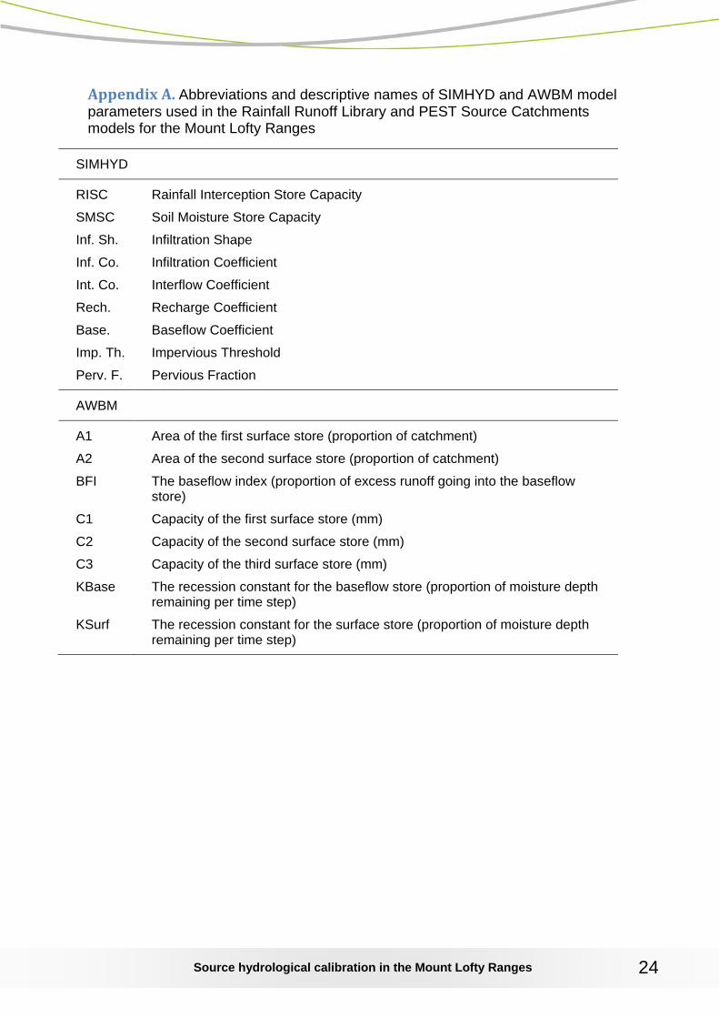
Appendix A. Abbreviations and descriptive names of SIMHYD and AWBM model parameters used in the Rainfall Runoff Library and PEST Source Catchments models for the Mount Lofty Ranges

SIMHYD

RISC Rainfall Interception Store Capacity SMSC Soil Moisture Store Capacity Inf. Sh. Infiltration Shape Inf. Co. Infiltration Coefficient Int. Co. Interflow Coefficient Rech. Recharge Coefficient Base. Baseflow Coefficient Imp. Th. Impervious Threshold Perv. F. Pervious Fraction

AWBM

A1 Area of the first surface store (proportion of catchment) A2 Area of the second surface store (proportion of catchment) BFI The baseflow index (proportion of excess runoff going into the baseflow

store) C1 Capacity of the first surface store (mm) C2 Capacity of the second surface store (mm) C3 Capacity of the third surface store (mm) KBase The recession constant for the baseflow store (proportion of moisture depth

remaining per time step) KSurf The recession constant for the surface store (proportion of moisture depth

remaining per time step)


25

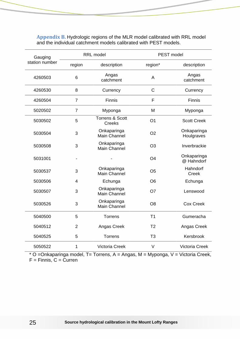
Appendix B. Hydrologic regions of the MLR model calibrated with RRL model and the individual catchment models calibrated with PEST models.

Gauging station number

RRL model PEST model

region description region* description

4260503 6 Angas catchment A Angas

catchment

4260530 8 Currency C Currency

4260504 7 Finnis F Finnis

5020502 7 Myponga M Myponga

5030502 5 Torrens & Scott Creeks O1 Scott Creek

5030504 3 Onkaparinga Main Channel O2 Onkaparinga

Houlgraves

5030508 3 Onkaparinga Main Channel O3 Inverbrackie

5031001 - - O4 Onkaparinga @ Hahndorf

5030537 3 Onkaparinga Main Channel O5 Hahndorf

Creek 5030506 4 Echunga O6 Echunga

5030507 3 Onkaparinga Main Channel O7 Lenswood

5030526 3 Onkaparinga Main Channel O8 Cox Creek

5040500 5 Torrens T1 Gumeracha

5040512 2 Angas Creek T2 Angas Creek

5040525 5 Torrens T3 Kersbrook

5050522 1 Victoria Creek V Victoria Creek

* O =Onkaparinga model, T= Torrens, A = Angas, M = Myponga, V = Victoria Creek, F = Finnis, C = Curren

Source hydrological calibration in the Mount Lofty R

anges

26

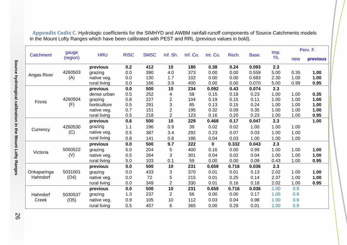
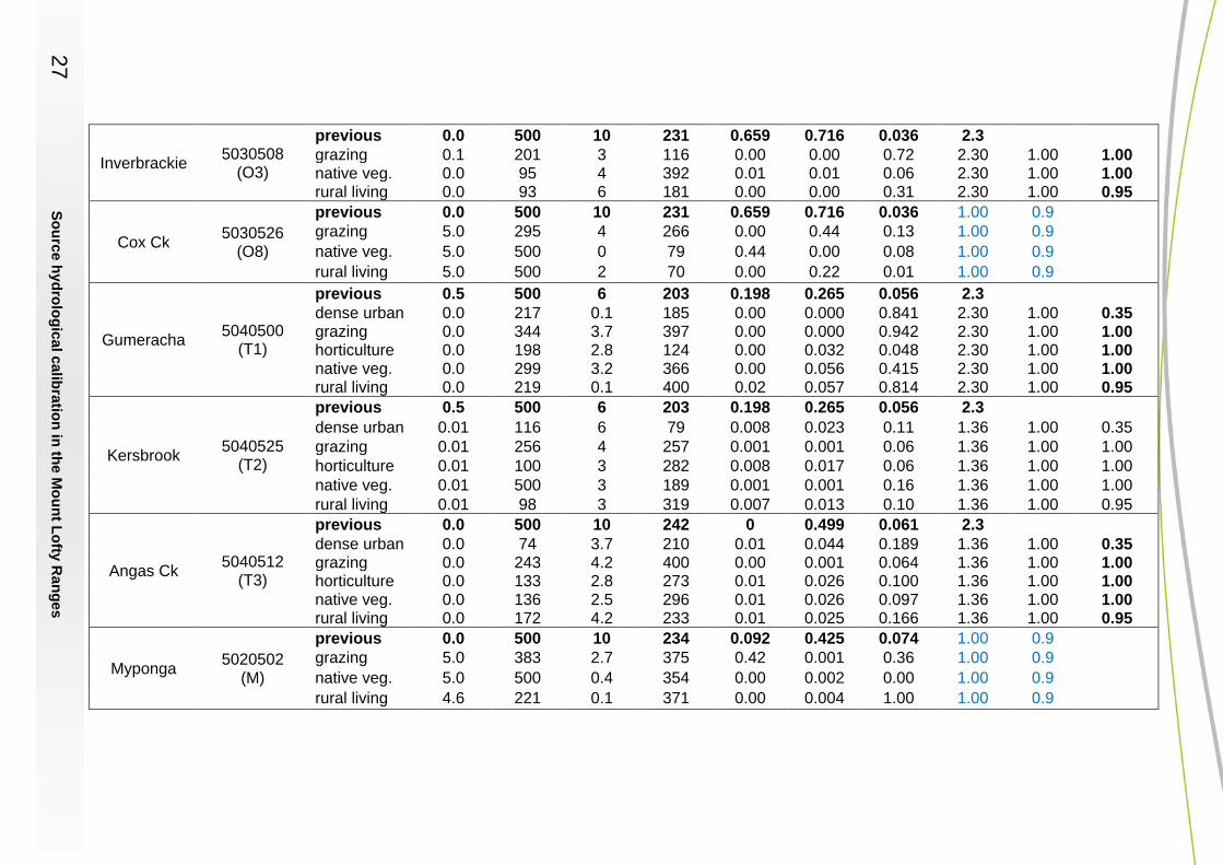
Appendix Cndix C. Hydrologic coefficients for the SIMHYD and AWBM rainfall-runoff components of Source Catchments models in the Mount Lofty Ranges which have been calibrated with PEST and RRL (previous values in bold).

Catchment gauge (region) HRU RISC SMSC Inf. Sh. Inf. Co. Int. Co. Rech. Base. Imp.

Th. Perv. F.

new previous

Angas River 4260503 (A)

previous 0.2 412 10 180 0.38 0.24 0.093 2.3 grazing 0.0 390 4.0 373 0.00 0.00 0.559 5.00 0.35 1.00 native veg. 0.0 130 1.7 102 0.00 0.00 0.683 2.30 1.00 1.00 rural living 0.0 166 3.9 400 0.00 0.00 0.070 5.00 0.99 0.95

Finnis 4260504 (F)

previous 0.0 500 10 234 0.092 0.43 0.074 2.3 dense urban 0.5 252 4 58 0.15 0.18 0.23 1.00 1.00 0.35 grazing 0.8 227 2 104 0.19 0.15 0.11 1.00 1.00 1.00 horticulture 0.5 291 3 85 0.13 0.15 0.24 1.00 1.00 1.00 native veg. 0.7 151 2 195 0.32 0.09 0.35 1.00 1.00 1.00 rural living 0.5 218 2 123 0.16 0.20 0.23 1.00 1.00 0.95

Currency 4260530 (C)

previous 0.6 500 10 229 0.468 0.17 0.047 2.3 1.00 grazing 1.1 196 0.9 39 0.02 0.02 1.00 1.00 1.00 native veg. 0.5 387 3.4 292 0.23 0.07 0.03 1.00 1.00 rural living 0.8 141 0.8 186 0.04 0.03 1.00 1.00 1.00

Victoria 5050522 (V)

previous 0.0 500 9.7 222 0 0.332 0.043 2.3 grazing 5.0 204 5 400 0.16 0.00 0.99 1.00 1.00 1.00 native veg. 0.5 264 3 301 0.04 0.02 0.04 1.00 1.00 1.00 rural living 5.0 103 0.1 59 0.00 0.00 0.09 0.43 1.00 0.95

Onkaparinga Hahndorf

5031001 (O4)

previous 0.0 500 10 231 0.659 0.716 0.036 2.3 grazing 0.0 433 3 370 0.01 0.01 0.13 2.02 1.00 1.00 native veg. 0.0 72 5 215 0.01 0.25 0.14 2.37 1.00 1.00 rural living 0.0 349 2 330 0.01 0.16 0.18 2.02 1.00 0.95

Hahndorf Creek

5030537 (O5)

previous 0.0 500 10 231 0.659 0.716 0.036 1.00 0.9 grazing 1.3 237 2 56 0.00 0.00 0.17 1.00 0.9 native veg. 0.9 105 10 112 0.03 0.04 0.98 1.00 0.9 rural living 0.5 457 6 365 0.00 0.29 0.01 1.00 0.9


anges

27

Inverbrackie 5030508 (O3)

previous 0.0 500 10 231 0.659 0.716 0.036 2.3 grazing 0.1 201 3 116 0.00 0.00 0.72 2.30 1.00 1.00 native veg. 0.0 95 4 392 0.01 0.01 0.06 2.30 1.00 1.00 rural living 0.0 93 6 181 0.00 0.00 0.31 2.30 1.00 0.95

Cox Ck 5030526 (O8)

previous 0.0 500 10 231 0.659 0.716 0.036 1.00 0.9 grazing 5.0 295 4 266 0.00 0.44 0.13 1.00 0.9 native veg. 5.0 500 0 79 0.44 0.00 0.08 1.00 0.9 rural living 5.0 500 2 70 0.00 0.22 0.01 1.00 0.9

Gumeracha 5040500 (T1)

previous 0.5 500 6 203 0.198 0.265 0.056 2.3 dense urban 0.0 217 0.1 185 0.00 0.000 0.841 2.30 1.00 0.35 grazing 0.0 344 3.7 397 0.00 0.000 0.942 2.30 1.00 1.00 horticulture 0.0 198 2.8 124 0.00 0.032 0.048 2.30 1.00 1.00 native veg. 0.0 299 3.2 366 0.00 0.056 0.415 2.30 1.00 1.00 rural living 0.0 219 0.1 400 0.02 0.057 0.814 2.30 1.00 0.95

Kersbrook 5040525 (T2)

previous 0.5 500 6 203 0.198 0.265 0.056 2.3 dense urban 0.01 116 6 79 0.008 0.023 0.11 1.36 1.00 0.35 grazing 0.01 256 4 257 0.001 0.001 0.06 1.36 1.00 1.00 horticulture 0.01 100 3 282 0.008 0.017 0.06 1.36 1.00 1.00 native veg. 0.01 500 3 189 0.001 0.001 0.16 1.36 1.00 1.00 rural living 0.01 98 3 319 0.007 0.013 0.10 1.36 1.00 0.95

Angas Ck 5040512 (T3)

previous 0.0 500 10 242 0 0.499 0.061 2.3 dense urban 0.0 74 3.7 210 0.01 0.044 0.189 1.36 1.00 0.35 grazing 0.0 243 4.2 400 0.00 0.001 0.064 1.36 1.00 1.00 horticulture 0.0 133 2.8 273 0.01 0.026 0.100 1.36 1.00 1.00 native veg. 0.0 136 2.5 296 0.01 0.026 0.097 1.36 1.00 1.00 rural living 0.0 172 4.2 233 0.01 0.025 0.166 1.36 1.00 0.95

Myponga 5020502 (M)

previous 0.0 500 10 234 0.092 0.425 0.074 1.00 0.9 grazing 5.0 383 2.7 375 0.42 0.001 0.36 1.00 0.9 native veg. 5.0 500 0.4 354 0.00 0.002 0.00 1.00 0.9 rural living 4.6 221 0.1 371 0.00 0.004 1.00 1.00 0.9


anges

28

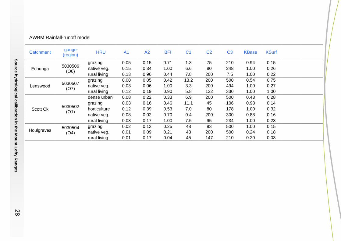
AWBM Rainfall-runoff model

Catchment gauge (region) HRU A1 A2 BFI C1 C2 C3 KBase KSurf

Echunga 5030506 (O6)

grazing 0.05 0.15 0.71 1.3 75 210 0.94 0.15 native veg. 0.15 0.34 1.00 6.6 80 248 1.00 0.26 rural living 0.13 0.96 0.44 7.8 200 7.5 1.00 0.22

Lenswood 5030507 (O7)

grazing 0.00 0.05 0.42 13.2 200 500 0.54 0.75 native veg. 0.03 0.06 1.00 3.3 200 494 1.00 0.27 rural living 0.12 0.19 0.90 5.8 132 330 1.00 1.00

Scott Ck 5030502 (O1)

dense urban 0.08 0.22 0.33 6.9 200 500 0.43 0.28 grazing 0.03 0.16 0.46 11.1 45 106 0.98 0.14 horticulture 0.12 0.39 0.53 7.0 80 178 1.00 0.32 native veg. 0.08 0.02 0.70 0.4 200 300 0.88 0.16 rural living 0.08 0.17 1.00 7.5 95 234 1.00 0.23

Houlgraves 5030504 (O4)

grazing 0.02 0.12 0.25 48 93 500 1.00 0.15 native veg. 0.01 0.09 0.21 43 200 500 0.24 0.18 rural living 0.01 0.17 0.04 45 147 210 0.20 0.03


29

Appendix D. Instruction Sheets for Use of PEST

Instruction sheets to:

• easily construct tsproc.exe input files for a regionalised model:

region_and_landuse.txt

region_list.txt

subcatchment_2_region.txt

subcatchment_2_region_short.txt

• create input files to use AWBM rainfall runoff model instead of SIMHYD (example files)

• enter hydrological parameters into a Source Catchments model with E2CL

Hydrological Calibration in the Mount Lofty Ranges using Source Paramenter Estimation Tool (PEST)

Environment

Transcript of Hydrological Calibration in the Mount Lofty Ranges using Source Paramenter Estimation Tool (PEST)