Hydrogeology and Simulation of Ground-Water Flow in the - USGS

Hydrogeology and Simulation of Ground-Water Flow in the Thick Regolith-Fractured Crystalline Rock Aquifer System of Indian Creek Basin, North Carolina

AVAILABILITY OF BOOKS AND MAPS OF THE US. GEOLOGICAL SURVEY

Instructions on ordering publications of the U.S. Geological Survey, along with prices of the last offerings, are given in the current- year issues of the monthly catalog "New Publications of the U.S. Geological Survey." Prices of available U.S. Geological Survey publica tions released prior to the current year are listed in the most recent annual "Price and Availability List." Publications that may be listed in various U.S. Geological Survey catalogs (see back inside cover) but not listed in the most recent annual "Price and Availability List" may be no longer available.

Order U.S. Geological Survey publications by mail or over the counter from the offices given below.

BY MAIL OVER THE COUNTER

Books

Professional Papers, Bulletins, Water-Supply Papers, Tech niques of Water-Resources Investigations, Circulars, publications of general interest (such as leaflets, pamphlets, booklets), single copies of Preliminary Determination of Epicenters, and some mis cellaneous reports, including some of the foregoing series that have gone out of print at the Superintendent of Documents, are obtain able by mail from

U.S. Geological Survey, Information Services Box 25286, Federal Center, Denver, CO 80225

Subscriptions to Preliminary Determination of Epicenters can be obtained ONLY from the

Superintendent of DocumentsGovernment Printing Office

Washington, DC 20402

(Check or money order must be payable to Superintendent of Documents.)

Maps

For maps, address mail orders to

U.S. Geological Survey, Information Services Box 25286, Federal Center, Denver, CO 80225

Books and Maps

Books and maps of the U.S. Geological Survey are available over the counter at the following U.S. Geological Survey Earth Sci ence Information Centers (ESIC's), all of which are authorized agents of the Superintendent of Documents:

ANCHORAGE, Alaska Rm. 101, 4230 University Dr. LAKEWOOD, Colorado Federal Center, Bldg. 810 MENLO PARK, California Bldg. 3, Rm. 3128, 345

Middlefield Rd. RESTON, Virginia USGS National Center, Rm. 1C402,

12201 Sunrise Valley Dr. SALT LAKE CITY, Utah Federal Bldg., Rm. 8105, 125

South State St. SPOKANE, Washington U.S. Post Office Bldg., Rm. 135,

West 904 Riverside Ave. WASHINGTON, D.C. Main Interior Bldg., Rm. 2650, 18th

and C Sts., NW.

Maps Only

Maps may be purchased over the counter at the following U.S. Geological Survey office:

ROLLA, Missouri 1400 Independence Rd.

Chapter C

Hydrogeology and Simulation of Ground-Water Flow in the Thick Regolith-Fractured Crystalline Rock Aquifer System of Indian Creek Basin, North Carolina

By CHARLES C. DANIEL III, DOUGLAS G. SMITH, and JO L. EIMERS

Hydrogeologic conditions, aquifer properties, and recharge rates were characterized to develop a digital ground-water flow model of a 69-square-mile watershed underlain by a thick regolith-fractured crystalline rock aquifer system.

U.S. GEOLOGICAL SURVEY WATER-SUPPLY PAPER 2341

GROUND-WATER RESOURCES OF THE PIEDMONT-BLUE RIDGE PROVINCES OF NORTH CAROLINA

U.S. DEPARTMENT OF THE INTERIOR BRUCE BABBITT, Secretary

U.S. GEOLOGICAL SURVEY Gordon P. Eaton, Director

Any use of trade, product, or firm names in this publication is for descriptive purposes only and does not imply endorsement by the U.S. Government.

For sale by theU.S. Geological SurveyInformation ServicesBox 25286, Federal CenterDenver, CO 80225

Library of Congress Cataloging in Publication Data

Daniel, Charles C.Hydrogeology and simulation of ground-water flow in the thick regolith-fractured crystalline rock aquifer system of

Indian Creek Basin, North Carolina / by Charles C. Daniel III, Douglas G. Smith, and Jo L. Eimers.p. cm. (U.S. Geological Survey water-supply paper; 2341) (Ground-water resources of the Piedmont-Blue

Ridge provinces of North Carolina ; ch. C)Includes bibliographical references.1. Hydrogeology North Carolina Indian Creek Watershed (Lincoln County) 2. Groundwater flow North Carolina

Indian Creek Watershed (Lincoln County) 3. Aquifers North Carolina Indian Creek Watershed (Lincoln County) I. Smith, Douglas G. (Douglas Gray), 1961- . II. Eimers, Jo Leslie. III. Title. IV. Series. V. Series: Ground-water resources of the Piedmont-Blue Ridge provinces of North Carolina ; ch. C. GB1025.N8G76 1989ch.C [GB1025.N8] 553.7'9'097565 s dc21[551.49'09756'782] 97-11158

CIP

ISBN 0-607-87028-1

CONTENTS

Abstract.............................................................................................................^ ClIntroduction ................................................................................................................................................................^ C2

Approach ................................................................................................................................................................. C3Purpose and Scope ................................................................................................................................................... C4Description of the Study Area .................................................................................................................................. C4Climate ........................................................................................................................................................^ C6Previous Investigations............................................................................................................................................. C6Acknowledgments.................................................................................................................................................... C7

Conceptualization of the Aquifer System........................................................................................................................... C7Hydrogeologic Framework of the Indian Creek Basin............................................................................................. C9Ground-Water Movement ........................................................................................................................................ CllCharacterization of Topographic Settings................................................................................................................. C12Conceptual Hydrogeologic Section.......................................................................................................................... C15

Hydrogeology of the Indian Creek Basin........................................................................................................................... C16Geology ............................................................................................................................................^ C16Hydrogeologic Units................................................................................................................................................. CISGeologic Belts ...................................................................................................................................^^ C19Structural Fabric and Orientation ............................................................................................................................. C21

Faults .................................................................................................................................................... C22Folds .....................................................................................................................................................^ C24

Soils.......................................................................................................................................................................... C24Ground-Water Flow System..................................................................................................................................... C26

Ground-Water Levels...................................................................................................................................... C27Base Flow ...................................................................................................................................................... C30Springs............................................................................................................................................................ C36

Water Budget ................................................................................................................................................^ C36Precipitation..................................................................................................................................^ C37Recharge-Discharge....................................................................................................................................... C37Ground-Water Storage.................................................................................................................................... C39

Variation in the Water Budget................................................................................................................................... C41Hydrogeologic Characteristics ................................................................................................................................. C42

Characteristics of Wells .................................................................................................................................. C43Well Yields by Hydrogeologic Unit and Topographic Setting........................................................................ C45Analyses of Specific-Capacity Data............................................................................................................... C46Transmissivity and Hydraulic Conductivity of Bedrock................................................................................ C54Transmissivity of Regolith.............................................................................................................................. C56Storage Coefficients and Specific Yield.......................................................................................................... C58

Water Use..........................................................................................................................................^ C58Water-Quality Characteristics................................................................................................................................... C59

Synoptic Surveys at Surface-Water Sites........................................................................................................ C61Comparison of Ground- and Surface-Water Quality...................................................................................... C61

Simulation of Ground-Water Flow ..................................................................................................................................... C66Model Selection........................................................................................................................................................ C66

Grid and Layer Design .................................................................................................................................. C66Model Boundaries........................................................................................................................................... C67

Model Input.............................................................................................................................................................. C69Topographic Settings...................................................................................................................................... C69Transmissivity and Vertical Conductance....................................................................................................... C69

Contents III

Ground-Water Recharge.................................................................................................................................. C72Stream Characteristics .................................................................................................................................... C73Ground-Water Withdrawals ............................................................................................................................ C74Starting Heads................................................................................................................................................. C74

Model Calibration .................................................................................................................................................... C75Simulated and Observed Water Levels............................................................................................................ C75

Sensitivity Analysis................................................................................................................................................... C80Method of Analysis......................................................................................................................................... C80Results..........................................................^ C80Limitations of the Model................................................................................................................................. C81

Evaluation of the Ground-Water Flow System Based on Simulations ..................................................................... C82Flow Budgets .................................................................................................................................................. C82Flow-Path and Time-of-Travel Analysis ......................................................................................................... C86

Summary and Conclusions.................................................................................................................................................. C88Selected References............................................................................................................................................................ C90Additional Tables ................................................................................................................................................................ C95

FIGURES

1.-3. Maps showing:1. The Appalachian Valleys-Piedmont Regional Aquifer-System Analysis study area and locations

of five type-area studies.............................................................................................................................. C32. Location of the Indian Creek Basin in the Piedmont physiographic province of North Carolina............. C53. Study areas of reconnaissance ground-water investigations that were sources of well data for this

study........................................................................................................................................................... C74-6. Diagrams showing:

4. The principal hydrogeologic components of a crystalline-rock terrane in which massive or foliatedcrystalline rocks are mantled by thick regolith.......................................................................................... C9

5. Conceptual variations of transition zone thickness and texture due to parent rock type........................... CIO6. Conceptual view of the ground-water flow system of the North Carolina Piedmont showing the

unsaturated zone, the water table surface, the saturated zone, and directions of ground-water flow ........ C127. Box plots showing distributions of distances between streams and wells in different topographic settings

of the North Carolina Piedmont and between streams and interstream drainage divides................................... C138. Conceptual hydrogeologic section from Piedmont stream to interstream drainage divide showing details

of average hydrogeologic conditions .................................................................................................................. C149. Schematic diagram showing relative changes in specific capacity, estimated transmissivity and hydraulic

conductivity, and inferred fracture abundance with depth in different topographic settings of the North Carolina Piedmont............................................................................................................................................... C15

10. Conceptual hydrogeologic section through the ground-water flow system of the North Carolina Piedmont..... C1611. Geologic map of the southwestern Piedmont of North Carolina showing the Indian Creek model area,

geologic belts, major plutons, and major structural features............................................................................... C1712. Hydrogeologic unit map of the southwestern Piedmont of North Carolina showing the Indian Creek

model area........................................................................................................................................................... C2013. Map showing sites where measurements of strike and dip were made on fractures and foliation planes

in the Indian Creek Basin.................................................................................................................................... C2214.-16. Contour diagrams of:

14. Poles to fracture planes in the Indian Creek Basin .................................................................................... C2315. Poles to foliation planes in the Indian Creek Basin ................................................................................... C2316. Poles to foliation planes for subregions of the Indian Creek Basin........................................................... C23

17. Beta diagram of foliation planes represented by the three maxima from the contour plots of the IndianCreek Basin shown in figure 16........................................................................................................................... C24

18. General soil associations map of parts of Burke, Catawba, Cleveland, Gaston, and Lincoln Countiesshowing the Indian Creek model area................................................................................................................. C25

19. Map showing locations of 38 observation wells in the Indian Creek Basin area used to obtain informationon natural fluctuation of ground-water levels...................................................................................................... C27

IV Contents

20-24. Hydrographs of:20. Daily average water levels from a drilled well tapping bedrock and five bored or hand-dug wells

tapping regolith in the Indian Creek Basin, June 1991 through September 1992...................................... C2821. Monthly water levels in well pair Li-120 and Li-121, located on a hilltop in the Indian Creek Basin.... C2922. Monthly water levels in well pair Li-180 and Li-179, located on a hilltop in the Indian Creek Basin.... C2923. Monthly water levels in well pair Li-198 and Li-199, located on a hilltop in the Indian Creek Basin.... C2924. Monthly average water levels in 22 bored and hand-dug wells tapping regolith and 14 drilled wells

tapping bedrock in the Indian Creek Basin, April 1991 through September 1992.................................... C3025. Map showing locations of 85 stream sites in the Indian Creek Basin where synoptic surveys of base flow

and water-quality conditions were made............................................................................................................. C3126. Modified Thiessen polygon of precipitation stations used for estimating average rainfall for the Indian

Creek Basin and model area................................................................................................................................ C3727 .-31. Graphs showing:

27. Relations of porosity and specific yield to total ground-water storage and available water in theregolith.....................................................................................................................................................^ C40

28. Variation of estimated monthly mean ground-water recharge for the Indian Creek Basin nearLaboratory, N.C., for water years 1952-90................................................................................................ C41

29. Relation of yield per foot of total depth of drilled wells to specific capacity............................................ C4730. Relation of ranks of yield per foot of total depth of drilled wells to ranks of specific capacity for data

shown in figure 29...................................................................................................................................... C4831. Relation of rank estimates of yield per foot of total depth of drilled wells to specific capacity for data

shown in figure 29...................................................................................................................................... C4932. Map showing locations of wells in the Chauga, Inner Piedmont, Kings Mountain, and Charlotte geologic

belts of the southwestern Piedmont that were the source of data used to estimate hydraulic characteristics of the five hydrogeologic units in the Indian Creek area..................................................................................... C50

33. Graph showing relation of estimated average transmissivity, in 25-foot intervals of well depth, to totalwell depth for 6-inch-diameter wells in the southwestern Piedmont.................................................................. C51

34. Graph showing relation of estimated average hydraulic conductivity, in 25-foot intervals of well depth,to total well depth for 6-inch-diameter wells in the southwestern Piedmont...................................................... C51

35. Trend surface contours showing relation between yield per foot of total well depth, total well depth, and well diameter for drilled wells that are located (A) in valleys and draws, (B) on slopes, and (C) on hills and ridges............................................................................................................................................................. C52

36.-3S. Graphs showing relation of estimated:36. (A) Yield per foot of total well depth and (B) specific capacity to total well depth of 6-inch-diameter

wells in each of three topographic settings................................................................................................ C5337. (A) Transmissivity and (B) hydraulic conductivity to depth in each of three topographic settings........... C5538. Transmissivity to depth for each foot of bedrock aquifer between 50 and 850 feet in each of three

topographic settings................................................................................................................................... C5639. Discretization of the conceptual hydrogeologic section for use in a ground-water flow model......................... C5740. Map showing locations of 23 sites on streams and 22 wells where samples were collected for chemical

analysis, Lincoln and Gaston Counties ............................................................................................................... C6041. Cation-anion diagrams comparing averages of (A) ground-water samples (all wells) to averages of

surface-water samples and (B) ground water from wells tapping regolith to wells tapping bedrock ................. C6342. Indian Creek model grid indicating the boundary of the Indian Creek model area and the area of active

cells...................................................................................................................................................................... C6743. Map showing location of no-flow and specified-flux boundaries (streams) within the Indian Creek model

area ......................................................................................................................................^ C6844. Map showing classification of cells within the Indian Creek model area based on topographic setting ............ C7045. Graph showing relation of rank estimates of water levels in wells tapping bedrock to total well depth in

each of three topographic settings....................................................................................................................... C7446. A, Index map of the Indian Creek model area showing the area of the potentiometric contours shown in

figure 46B, and B, Potentiometric contours of simulated heads in model layers 2 and 10 for part of the Indian Creek model area...................................................................................................................................... C78

47. Graph showing sensitivity of simulated heads to changes in transmissivity and vertical hydraulicconductivity........................................................................................_^ C80

Contents V

48.-51. Maps of the Indian Creek model area showing the:48. Direction of flow across the boundary between layers 1 and 2 at a depth of 50 feet below land

surface........................................................................................................................................................ C8349. Direction of flow across the boundary between layers 6 and 7 at a depth of 250 feet below land

surface........................................................................................................................................................ C8450. Direction of flow across the boundary between layers 10 and 11 at a depth of 675 feet below land

surface........................................................................................................................................................ C8551. Area of a flow-path analysis along row 97 between columns 50 and 65................................................... C86

52. Diagram of the ground-water flow paths through the 11 model layers along row 97 between columns 50and 65 ....................................................................^^ C87

TABLES

1. General hydrologic characteristics of the hydrogeologic terranes of the Piedmont and Blue Ridge physiographic provinces within the Appalachian Valleys-Piedmont Regional Aquifer-System Analysis study area............................................................................................................................................... C8

2. Classification and lithologic description of hydrogeologic units in the Indian Creek model area of thesouthwestern Piedmont of North Carolina........................................................................................................... C19

3. Geologic belts of part of the Piedmont Province of southwestern North Carolina.............................................. C214. Measurements of fracture orientation from bedrock outcrops at stream sites in the Indian Creek Basin............ C965. Measurements of foliation orientation from bedrock outcrops at stream sites in the Indian Creek Basin........... C976. General soil association, predominant soil types, occurrence, U.S. Department of Agriculture soil texture,

and permeability of soils in the Indian Creek model area.................................................................................... C267. Water-level measurements from wells in the Indian Creek Basin........................................................................ C998. Surface-water sites in the Indian Creek Basin...................................................................................................... C1039. Stream width, cross-section area, and average depth at 85 stream sites in the Indian Creek Basin,

November 26-28, 1990 ........................................................................................................................................ C3210. Results of synoptic base-flow survey of 85 stream sites within the Indian Creek Basin,

November 26-28, 1990 ........................................................................................................................................ C3411. Statistical summary of unit area discharges at sites in the Indian Creek Basin.................................................... C3612. Daily net ground-water recharge estimated by hydrograph separation of streamflow record from the

gaging station on Indian Creek near Laboratory, N.C.......................................................................................... C10713. Water budget for the Indian Creek Basin, 1952 through 1990 water years.......................................................... C3814. Water budget for the Indian Creek Basin, 1991 and 1992 water years................................................................. C3815. Statistical summary of casing depth, water-level, and estimated saturated thickness of regolith data for

drilled wells according to topographic setting compared to statistics for all wells.............................................. C4016. Well records for the Indian Creek study area....................................................................................................... Cl 1817. Average and median values of selected characteristics for drilled wells according to topographic setting

compared to statistics for all wells ....................................................................................................................... C4318. Statistical summary of depth, water-level, and well yield data for bored and hand-dug wells in different

topographic settings compared to statistics for all wells...................................................................................... C4419. Summary of yields from drilled wells according to hydrogeologic unit and topography.................................... C4520. Summary of well depths, average specific capacity, average estimated transmissivity, and average

estimated hydraulic conductivity for drilled wells in three topographic settings in the southwestern Piedmont of North Carolina................................................................................................................................. C51

21. Total, urban, and rural populations; total, urban, and rural areas; rural population density; number of wells;and rural population per well by county and for total area in the Indian Creek model area................................ C59

22. Water-quality data from a synoptic survey of selected surface-water sites in the Indian Creek Basin,August 13-15, 1991.............................................................................................................................................. C129

23. Water-quality data from a synoptic survey of selected wells in the Indian Creek Basin,August 12-14, 1991.............................................................................................................................................. C132

24. Chemical properties and characteristics of surface water at 85 stream sites in the Indian Creek Basinfrom three surveys conducted during 1990 and 1991........................................................................................... C135

VI Contents

25. Statistical summary of milliequivalents of selected cations and anions in surface water and ground waterin the Indian Creek Basin ..................................................................................................................................... C62

26. Results of analysis of variance tests on water-quality data for wells tapping regolith, wells tappingbedrock, and surface water in the Indian Creek Basin......................................................................................... C63

27. Statistical summary of milliequivalents of selected cations and anions in rain water collected near SilverHill, N.C. ............................................. C65

28. Average transmissivities in model layers 2 through 11 (bedrock layers) beneath three topographic settingsexpressed as a percentage of the maximum value of transmissivity .................................................................... C71

29. Average water levels used to compute starting heads in model layers 2 through 11 (bedrock layers)................. C7530. Summary statistics for simulated and corresponding observed heads for nine model layers............................... C7631. Sensitivity of simulated heads to changes in recharge rates................................................................................. C8132. Summary of model fluxes, including recharge to layer 1, flux within layer 1 to streams, and average flux

between model layers ........................................................................................................................................... C82

Contents VII

CONVERSION FACTORS, VERTICAL DATUM, TEMPERATURE, TRANSMISSIVITY, SPECIFIC CONDUCTANCE, DEFINITION, AND ACRONYMS

Multiply

inch (in.)foot (ft)

mile (mi)

square foot (ft )square mile (mi2)

cubic foot per second (ft3/s)cubic foot per second per square mile

By

Length2.540.30481.609

Area0.09292.590

Flow0.028320.01093

To obtain

centimetermeterkilometer

square metersquare kilometer

cubic meter per secondcubic meter per second per square kilometer

[(ft3/s)/mi2] gallon per minute (gal/min)

gallon per day (gal/d) million gallons per day (Mgal/d)

foot squared per day (ft2/d)

0.06309 liter per second0.003785 cubic meter per day0.04381 cubic meter per secondTransmissivity0.0929 meter squared per day

Sea level: In this report "sea level" refers to the National Geodetic Vertical Datum of 1929 (NGVD of 1929) A geodetic datum derived from a general adjustment of the first-order level nets of both the United States and Canada, formerly called Sea Level Datum of 1929.

Equation for temperature conversion between degrees Celsius (°C) and degrees Fahrenheit (°F):°C = 5/9 (°F - 32)

Transmissivity: The standard unit for transmissivity is cubic foot per day per square foot times foot of aquifer thickness [(ft3/d)/ft2]ft. In this report, the mathematically reduced form, foot squared per day (ft2/d), is used for convenience.

Specific conductance is given in microsiemens per centimeter at 25 degrees Celsius (|j.S/cm at 25 °C).

Definition: Water year in U.S. Geological Survey reports is the 12-month period October 1 through September 30, designated by the calendar year in which it ends.

Acronyms:ANOVA

APRASADEHNR

EUDGIS

GWSIMODFLOW

NADP RASA RMSE

TIN-OEM USGS

analysis of varianceAppalachian Valleys-Piedmont Regional Aquifer-System AnalysisNorth Carolina Department of Environment, Health, and Natural Resourcesequivalent uniform depthGeographic Information SystemGround-Water Site Inventorymodular three-dimensional finite-difference ground-water flow modelNational Atmospheric Deposition ProgramRegional Aquifer-System Analysisroot mean square errortriangulated irregular network-digital elevation mapU.S. Geological Survey

VIII Contents

Hydrogeology and Simulation of Ground-Water Flow in the Thick Regolith-Fractured Crystalline Rock Aquifer System of Indian Creek Basin, North CarolinaBy Charles C. Daniel III, Douglas G. Smith, and Jo L. Eimers

Abstract

The Indian Creek Basin in the southwestern Piedmont of North Carolina is one of five type areas studied as part of the Appalachian Valleys- Piedmont Regional Aquifer-System Analysis. Detailed studies of selected type areas were used to quantify ground-water flow characteristics in various conceptual hydrogeologic terranes. The conceptual hydrogeologic terranes are considered representative of ground-water conditions be neath large areas of the three physiographic provinces Valley and Ridge, Blue Ridge, and Piedmont that compose the Appalachian Valleys-Piedmont Regional Aquifer-System Analysis area. The Appalachian Valleys-Piedmont Regional Aquifer-System Analysis study area extends over approximately 142,000 square miles in 11 states and the District of Columbia in the Appalachian highlands of the Eastern United States. The Indian Creek type area is typical of ground-water conditions in a single hydrogeologic terrane that underlies perhaps as much as 40 percent of the Piedmont physiographic prov ince.

The hydrogeologic terrane of the Indian Creek model area is one of massive and foliated crystalline rocks mantled by thick regolith. The area lies almost entirely within the Inner Piedmont geologic belt. Five hydrogeologic units occupy major portions of the model area, but statistical tests on well yields, specific capacities, and other hydrologic characteristics show that the five

hydrogeologic units can be treated as one unit for purposes of modeling ground-water flow.

The 146-square-mile Indian Creek model area includes the Indian Creek Basin, which has a surface drainage area of about 69 square miles. The Indian Creek Basin lies in parts of Catawba, Lincoln, and Gaston Counties, North Carolina. The larger model area is based on boundary condi tions established for digital simulation of ground- water flow within the smaller Indian Creek Basin.

The ground-water flow model of the Indian Creek Basin is based on the U.S. Geological Survey's modular finite-difference ground-water flow model. The model area is divided into a uni formly spaced grid having 196 rows and 140 col umns. The grid spacing is 500 feet. The model grid is oriented to coincide with fabric elements such that rows are oriented parallel to fractures (N. 72° E.) and columns are oriented parallel to foliation (N. 18° W.). The model is discretized ver tically into 11 layers; the top layer represents the soil and saprolite of the regolith, and the lower 10 layers represent bedrock. The base of the model is 850 feet below land surface. The top bedrock layer, which is only 25 feet thick, represents the transition zone between saprolite and unweathered bedrock.

The assignment of different values of transmissivity to the bedrock according to the topo graphic setting of model cells and depth results in inherent lateral and vertical anisotropy in the model with zones of high transmissivity in bed rock coinciding with valleys and draws, and zones

Hydrogeology and Simulation of Ground-Water Flow in the Indian Creek Basin, North Carolina C1

of low transmissivity in bedrock coinciding with hills and ridges. Lateral anisotropy tends to be most pronounced in the north-northwest to south- southeast direction. Transmissivities decrease nonlinearly with depth. At 850 feet, depending on topographic setting, transmissivities have decreased to about 1 to 4 percent of the value of transmissivity immediately below the regolith- bedrock interface.

The model boundaries are, for the most part, specified-flux boundaries that coincide with streams that surround the Indian Creek Basin. The area of active model nodes within the boundaries is about 146 square miles and has about 17,400 active cells. The numerical model is designed not as a predictive tool, but as an interpretive one. The model is designed to help gain insight into flow- system dynamics. Predictive capabilities of the numerical model are limited by the constraints placed on the flow system by specified fluxes and recharge distribution.

Results of steady-state analyses that simu late long-term, average annual conditions indicate that the quantity of ground water flowing through model layers decreases with depth. In the top model layer, representing the soil and saprolite of the regolith, about 55 percent of recharge flows directly to streams, and 45 percent flows into layer 2. Lesser amounts flow into deeper layers. In the bottom model layer, the quantity of water moving in or out of the layer is about 2 percent of the max imum quantity that flows through the top layer. The quantity decreases with depth by about two orders of magnitude between layers 1 and 11, even though the bottom layer is 175 feet thick and the saturated thickness of the top layer is about 20 to 30 feet thick.

Flow-path and time-of-travel analyses show that most ground water flows through the shal lower parts of the system close to streams, and that travel times in the regolith vary from less than 10 years to as much as 20 years from time of recharge to time of discharge in streams. Travel times along flow paths through the lower layers can take decades or even centuries; travel times approaching five centuries were computed in some

areas for flow that passed through the bottom layer (675 to 850 feet below land surface).

INTRODUCTION

The Appalachian Valleys-Piedmont Regional Aquifer-System Analysis (APRASA) is one of several regional investigations conducted to assess the Nation's principal aquifer systems (Sun, 1986). The APRASA is part of the Regional Aquifer-System Analysis (RASA) program of the U.S. Geological Survey (USGS). The USGS began the RASA program in 1978, as mandated by Congress, and was given the task of "initiating a program to identify the water resources of the major aquifer systems within the United States *** and *** establish the aquifer bound aries, the quantity and quality of the water within the aquifer, and recharge characteristics of the aquifer" (Sun, 1986, p. 2).

The APRASA study area is in the Appalachian Highlands (Fenneman, 1938) of the Eastern United States. The study area covers about 142,000 mi2 in parts of Pennsylvania, New Jersey, Maryland, the District of Columbia, Delaware, West Virginia, Virginia, Tennessee, North Carolina, South Carolina, Georgia, and Alabama (fig. 1). Severe and prolonged drought, allocation of surface-water flow, and increased demands on ground-water resources have resulted in a need to evaluate ground-water resources in the Valley and Ridge, Piedmont, and Blue Ridge physiographic provinces. Rapid industrial growth and urban expansion have caused existing freshwater sup plies to be used at or near maximum capacity.

Although large amounts of ground water and surface water are currently (1993) being withdrawn throughout the Appalachian Valley and Ridge, Blue Ridge, and Piedmont Provinces, processes of recharge, discharge, storage, ground-water flow, and stream- aquifer relations within the three physiographic provinces are poorly understood. This lack of under standing is due primarily to the diverse and complex nature of the hydrogeologic system.

The APRASA study area can be subdivided into two distinct major subareas based on differences in geology and hydrologic characteristics. One subarea consists of the Valley and Ridge and the extreme west ern edge of the Blue Ridge. This area is underlain pri marily by sedimentary rocks such as sandstone, shale, and carbonate rocks. The second subarea consists of the central and eastern Blue Ridge and the Piedmont.

C2 Ground-Water Resources of the Piedmont-Blue Ridge Provinces of North Carolina

85° 80°

40°

35° -

30°

EXPLANATION

PHYSIOGRAPHIC PROVINCES WITHIN APRASA STUDY AREA

Valley and Ridge

INN Blue Ridge

I " 1 Piedmont

0 Location of type-area study in specific basin

75°

s Hopewell Pennington, N.J.

JSIEWYORK_

PENNSYLVANIA

*! Cumberland /' I Valley, Pa.

,_ Indian Creek C - / Basin, N.C. ' - s

Figure 1. The Appalachian Valleys-Piedmont Regional Aquifer-System Analysis (APRASA) study area and locations of five type-area studies.

This area is underlain primarily by crystalline rocks of metasedimentary, metaigneous, and igneous origin. Large rift basins, extending within the Piedmont crys talline rocks from New Jersey to South Carolina, have been filled with sedimentary deposits of Mesozoic age. The Indian Creek Basin in North Carolina occurs entirely within the Piedmont physiographic province.

ApproachThe fundamental approach of the APRASA has

been similar to that of other RASA studies (Sun, 1986)

in that available geologic and hydrologic data have been assembled and used to describe the regional aqui fer systems. In the APRASA study, however, the lack of regional continuity and the diverse nature of aquifers prevented the development of a regional ground-water flow model for the entire study area. Understanding the hydrogeology of the APRASA study area was complicated by the fact that the poros ity and permeability of the rocks are mostly of second ary origin and extremely variable, which obscures the distinction between aquifers and confining units.


A more useful approach than making a distinc tion between aquifers and confining units has been to divide the study area into hydrogeologic terranes on the basis of the distribution and magnitude of factors related to secondary porosity and permeability. Spe cific type areas within these terranes were then selected for detailed investigation (Swain and others, 1991, 1992). A "hydrogeologic terrane," as defined in the APRASA study, is a combination of rock type, regolith characteristics, and topographic setting that is relatively homogeneous with respect to water-yielding potential of the materials, ground-water storage, and ground-water quality. Ground-water flow within speci fied terranes has been described in terms of conceptual flow systems. The Indian Creek Basin is the type area for terranes identified as "massive or foliated crystal line rocks, thick regolith," that is described later in this report.

Two specific approaches were taken to define the hydrogeologic terranes. The first approach was to produce hydrogeologic terrane maps for the entire APRASA study area. Lithologic and hydrologic infor mation was combined with well-yield data and addi tional hydrologic data.

The second specific approach was quantification of ground-water flow characteristics within selected "type areas" that were considered representative of flow in various hydrogeologic terranes. For this approach, a flow system was conceptualized for each type of hydrogeologic terrane, and ground-water flow in selected type areas was analyzed and simulated by use of ground-water flow models. Flow models were used to improve the understanding of ground-water flow related to various hydrogeologic components and streams. Techniques used to quantify recharge, dis charge, storage, and flow within the type areas may be transferable to other areas within similar hydrogeo logic terranes.

Purpose and Scope

The purpose of this report is to describe the hydrogeologic framework and results of ground-water flow simulations in part of the southwestern Piedmont of North Carolina. Hydrogeologic information on the region is presented, including a conceptual model of the flow system and application of a finite-difference ground-water flow model based on this conceptual model. The flow model simulations are designed to characterize the complex two-part aquifer system that

underlies much of the Piedmont. Discussions include descriptions of modeling procedures and flow bound aries, and determination of aquifer properties. Model calibration strategies, steady-state conditions prior to 1991, and a sensitivity analysis are also described.

Results of the simulations are discussed with respect to changes in ground-water flow as shown by changes in the water budget, potentiometric surfaces of the model layers, and directions of ground-water flow through the aquifer system. An inventory and analysis of available ground-water and surface-water data used in support of model design are also pre sented.

Description of the Study Area

The APRASA study area in North Carolina includes the Indian Creek Basin and surrounding areas in Catawba, Cleveland, Gaston, and Lincoln Counties (fig. 2). The study area is located in the southwestern Piedmont of North Carolina approximately 30 mi north of the South Carolina State line (fig. 1).

The Indian Creek Basin (fig. 2) extends over approximately 69 mi2 in the Piedmont Province (Fenneman, 1938). The basin extends from southwest ern areas of Catawba County in a southeasterly direc tion, completely transecting western Lincoln County, to northern areas of Gaston County. The easternmost boundary of the basin is approximately 2 mi southwest of the city of Lincolnton, with the southernmost boundary extending partially into the city of Cherry ville. The Indian Creek model area, which includes the Indian Creek Basin, covers 146 mi2 and extends to surrounding rivers and streams. The larger model area is based on boundary conditions estab lished for digital simulation of ground-water flow within the smaller Indian Creek Basin.

The Indian Creek Basin lies within the Inner Piedmont belt of the western Piedmont of North Carolina. The Inner Piedmont belt is a fault-bounded stack of thrust sheets containing schists, gneisses, sparse ultramafic bodies, and granitic intrusives (Horton and McConnell, 1991). The Inner Piedmont belt in North Carolina has undergone several periods of metamorphism and intrusive activity, and is bounded to the northwest by the Brevard fault zone and by the Kings Mountain shear zone and Eufola fault to the southeast. The Inner Piedmont belt is the largest of the geologic belts in the Piedmont of North


BLUE RIDGE PIEDMONT COASTAL PLAIN

81°30'

LINCOLN COUNTY AND PHYSIOGRAPHIC PROVINCES IN NORTH CAROLINA

20' 10' 81°

35°35

35°30'

35°25'

02468 10 KILOMETERS

Figure 2. Location of the Indian Creek Basin in the Piedmont physiographic province of North Carolina.

Carolina, occupying a 50- to 60-mi-wide area across the State (Conrad and others, 1975).

Metamorphic and igneous crystalline rocks underlie most of the basin. Although most of the for mations in the area have been metamorphosed and exhibit strong directional fabrics, igneous intrasives emplaced after the last metamorphic event during the late Paleozoic Era are generally massive and less foli ated. Most of the formations in the area were subjected to uplift during the Cenozoic Era (Swain and others, 1991).

Throughout the Indian Creek Basin, bedrock is generally overlain by regolith consisting of soil, allu vium, and weathered rock material. Bedrock is gener ally exposed only in areas of rugged topography or in stream channels where erosion has removed the

regolith. In some locations, the regolith consists only of weathered material, called saprolite, which remains atop the parent rock from which it was derived (Swain and others, 1991). Thickness of the regolith in the study area ranges from 0 to more than 100 ft.

Regolith can be divided into three horizons the soil zone, saprolite, and a transition zone between saprolite and weathered bedrock. Where the regolith does not include material that has been transported, these three horizons represent stages in the breakdown of bedrock in response to weathering (Swain and others, 1991).

Topography of the study area is typical of the western Piedmont and foothills regions of North Carolina. Moderately rounded hills with long, fairly steep ridges are common. Local relief is generally


80 to 120 ft from stream bottom to drainage divides. Land-surface altitudes generally decrease across the basin in a southeasterly direction, ranging from greater than 1,340 ft near the headwaters at the northwest drainage divides to about 740 ft in the southeast at the gaging station site on Indian Creek (fig. 2). The Indian Creek stream channel produces perennial flow for about 20 mi, while dropping some 330 ft in altitude along its course. Perennial flow begins near the head waters of Indian Creek at an altitude of about 1,070 ft and continues downstream, reaching an altitude of less than 740 ft near the gaging station site. Stream chan nels of tributaries flowing into Indian Creek generally trend in a northeast or southwest direction (fig. 2).

Streamflow at the gaging station site on Indian Creek has been monitored since 1951. The 69.2-mi2 Indian Creek Basin had a mean annual discharge of 88.4 ftVs during the 40-year period from 1951 to 1991. The maximum peak flow for this period was 8,450 ftVs recorded on August 10, 1970. The highest daily mean flow at the site was 4,350 ftVs, which also occurred on August 10, 1970. Minimum flow for this 40-year period, 1.7 ft3/s, was recorded on July 21, 1986, during a period of extreme drought. The lowest daily mean flow, 2.1 ftVs, occurred on July 20 of the same year (U.S. Geological Survey, 1992).

Since 1951, streamflow data from the Indian Creek gaging station indicate that monthly mean flow generally increases in October, decreases slightly in November, then gradually increases each month until the maximum monthly mean flow occurs in March. Beginning in April, monthly mean streamflow decreases. Throughout the growing season, monthly mean flow continues to decline until reaching the minimum monthly mean flow in September (U.S. Geological Survey, 1952-92, 1964).

Climate

The climate of the Indian Creek area is moder ate and can be typed as humid-subtropical. The area is characterized by short, mild winters and long, hot, humid summers. Mean minimum January tempera tures range from 28 to 32 °F, whereas mean maximum July temperatures range from 88 to 90 °F. Average annual precipitation in the area is 44 to 48 in. Prevail ing winds are from the northeast, with a mean annual windspeed of 7 miles per hour. The average length of the freeze-free season in the area lasts approximately 210 to 230 days, with the average last date of freezing

temperature occurring between April 1 and April 11. The average first date of freezing temperature occurs between October 30 and November 9 (Kopec and Clay, 1975).

Previous Investigations

Between 1946 and 1971, 14 reconnaissance ground-water investigations were completed that pro vided information on ground-water resources in all the counties in the Piedmont and Blue Ridge Provinces of North Carolina (Daniel, 1989). Included in the 14 reports are maps that show well locations in each county and tables of well records that provide details of well construction, yield, use, topographic setting, water-bearing formation, and miscellaneous notes. Data for drilled wells finished in bedrock were com piled from these reports and statistically analyzed by Daniel (1989) to determine relations between well yield and construction, topographic setting, hydrogeologic units, lithotectonic belts, and other characteris tics. A hydrogeologic unit map of the Piedmont and Blue Ridge Provinces of North Carolina was also compiled by Daniel and Payne (1990) as part of this work. Three of these reconnaissance reports (fig. 3) provide specific information about the Indian Creek area in Burke, Catawba, Cleveland, Gaston, and Lincoln Counties.

The hydrogeology of the Piedmont and Blue Ridge Provinces of the Eastern and Southeastern United States is described by LeGrand (1967), Heath (1984), and Swain and others (1991). The hydrogeo logic framework of the Piedmont of North Carolina was described by Harned (1989) as part of a recon naissance study of ground-water quality. Details of the hydrogeologic framework, particularly the nature of the transition zone between bedrock and regolith, were refined by Harned and Daniel (1992). Ground-water recharge rates in the Piedmont and Blue Ridge of North Carolina have been estimated by Daniel and Sharpless (1983), Harned and Daniel (1987), and Daniel (1990a, 1990b). The distribution of fracture permeability with depth in fractured bedrock beneath different topographic settings in the Piedmont of North Carolina has been statistically characterized by Daniel (1992).


83 L 82U 80U

36e

35°-

BLUE RIDGE PIEDMONT

MAP NUMBER AND REFERENCE1 Sumsion and Laney, 19672 LeGrand and Mundoiff, 19523 LeGrand, 1954

- - - GENERALIZED PHYSIOGRAPHIC PROVINCE BOUNDARY

25 50 75 100 MILES

25 75 100 KILOMETERS

Figure 3. Study areas of reconnaissance ground-water investigations that were sources of well data for this study.

Acknowledgments

Many records of wells included in the well inventory were furnished by the Ground-Water Section, Division of Environmental Management, North Carolina Department of Environment, Health, and Natural Resources (DEHNR). Barbara Christian, of the DEHNR Mooresville Regional Office at the time of this study, deserves special thanks for provid ing access to and assisting with the compilation of these data.

Many residents of the study area provided access to wells so that project staff could complete inventories, collect water samples, and measure water levels. Six wells were equipped with water-level recorders, and water levels in another 32 wells were measured monthly during 1991-92. The special assistance from this group of well owners, although too numerous to recognize individually, is gratefully acknowledged.

CONCEPTUALIZATION OF THE AQUIFER SYSTEM

The hydrogeology of the APRASA study area is best described in terms of hydrogeologic terranes and

conceptual flow systems. The hydrologic characteris tics of terranes and flow systems in the Valley and Ridge, Piedmont, and Blue Ridge Provinces are dis cussed by Swain and others (1991). In summary, the APRASA study area can be considered as two distinct subareas based on differences in geology and hydrologic characteristics. One subarea consists of carbon ate rock, sandstone, and shale in the Valley and Ridge and the extreme western part of the Blue Ridge. The second subarea consists of metamorphic and igneous crystalline rocks in the Piedmont and central and east ern Blue Ridge. Because the crystalline rocks that form most of the Piedmont and Blue Ridge are so sim ilar in character, these provinces are grouped as one unit for this study. Large rift basins, extending within the Piedmont crystalline rocks from New Jersey to South Carolina, have been filled with sedimentary deposits of Mesozoic age. The hydrogeology of the Piedmont and Blue Ridge is different from that of the Valley and Ridge in that the aquifer material in the Piedmont and Blue Ridge does not have the propen sity to form large dissolution cavities.

Regolith, consisting of soil, alluvium, and weathered rock material, overlies most of the geologic units throughout both subareas. In some locations, it


includes material that has been transported and depos ited as glacial drift, colluvium, or alluvium. In other locations, the regolith consists only of material weath ered in place called residuum or saprolite, which remains atop the parent rock from which it was derived. Thickness of the regolith throughout the study area is extremely variable and ranges from 0 to more than 150 ft.

Terranes in both subareas can be distinguished primarily by rock type and secondarily by rock tex ture, regolith thickness and texture, rock structure, and topographic setting. Variability in the thickness and texture of the regolith, which can store a significant amount of ground water, in addition to variability in the secondary permeability of the bedrock, also must be considered in describing ground-water flow within the subareas.

Water-yielding characteristics of the various hydrogeologic terranes within the Piedmont and Blue Ridge Provinces (table 1) are highly dependent on the thickness of the regolith and transition zone. Because

the sedimentary rocks of the Mesozoic Basins are so distinct from the metamorphic and igneous crystalline rocks of the Piedmont and Blue Ridge, the hydrogeology of the Piedmont and Blue Ridge Provinces has been divided into two distinct groups based on dif ferences in lithology: (1) crystalline-rock terranes, which make up 86 percent of total Piedmont area, and (2) sedimentary-rock terranes of the early Mesozoic Basins, which make up 14 percent of the Piedmont. The Indian Creek Basin represents the first group.

The hydrogeologic terranes identified for the Piedmont and Blue Ridge Provinces in the APRASA study area are (1) massive or foliated crystalline rocks mantled by thick regolith, (2) massive or foliated crys talline rocks mantled by thin regolith, (3) metamor phosed carbonate rocks, and (4) sedimentary rocks of the Mesozoic Basins (table 1). These hydrogeologic terranes are thought to be associated with local or intermediate flow systems as described by Toth (1963). Local and intermediate flow systems are com monly restricted to depths shallower than 600 ft in the

Table 1. General hydrologic characteristics of the hydrogeologic terranes of the Piedmont and Blue Ridge physiographic provinces within the Appalachian Valleys-Piedmont Regional Aquifer-System Analysis (APRASA) study area[<, less than or equal to; do, ditto. Modified from Swain and others, 1991]

Hydrologic characteristics

Hydrogeologic terrane

Massive or foliated crystalline rocks, thick regolith.

Massive or foliated crystalline rocks, thinregolith.

Metamor phosed carbonate rocks.

Mesozoic sedimentary basins.

Topo graphic

relief

Low to high.

......do...

Low to moder ate.

......do...

Recharge

Precipita tion on topo graphic highs.

......do......

......do......

......do......

Type of_. . porosity Discharge *

permeability

To Intergranular streams. in regolith,

fracture.

......do..... Dissolutionopenings, some fractures.

......do..... Intergranular,some fractures.

Type of

flow

Diffuse, fracture.

Fracture...

Conduit, fracture.

Diffuse, fracture.

Depth of

flow, in feet

Shallow to intermedi ate, < 800.

Shallow (mostly) to intermedi ate, < 500.

Shallow......

Shallow (mostly) to intermedi ate, < 800.

Confined or

unconfined

Mostly uncon fined.

Uncon fined.

......do......

Mostly uncon fined.

Rego lith

storage

Large....

Small....

Small to moder ate.

Small....

Well yield

Propor tional to regolith thickness.

Low.

Variable, some very high.

Variable, decreas ing from north tosouth.

Valley and Ridge Province and 800 ft in the Piedmont and Blue Ridge Provinces. The local flow systems commonly lie between adjacent topographic divides that range from a few thousand feet to a few miles apart. The intermediate flow systems are thought to occur at depths up to 800 ft and, in places, to traverse adjacent topographic divides. The quantity of flow in the intermediate flow systems is thought to represent less than 5 percent of the total ground-water flow (Swain and others, 1992). The hydrogeologic terrane discussed in this report is more closely associated with local flow systems than with intermediate flow return systems.

Hydrogeologic Framework of the Indian Creek Basin

The Indian Creek Basin represents the hydrogeologic terrane in which massive or foliated crystal line rocks are mantled by thick regolith (table 1). An idealized sketch of the principal hydrogeologic com ponents of this terrane (fig. 4) shows (1) the unsaturated zone in the regolith, which generally contains the

SOIL __Regolith I ZONE

unsaturated<zone I water table

Regolithsaturated

zoneTRANSITION/

ZONE \

FRACTURED BEDROCK

UNWEATHERED BEDROCK

SHEET JOINT

BEDROCK STRUCTURE

Figure 4. The principal hydrogeologic components of a crystalline-rock terrane in which massive or foliated crystalline rocks are mantled by thick regolith (from Harned and Daniel, 1992).

organic layers of the surface soil, (2) the saturated zone in the regolith, (3) the lower regolith, which con tains the transition zone between regolith and bedrock, and (4) the fractured crystalline bedrock.

Collectively, the uppermost layer is regolith, which is composed of saprolite, alluvium, and soil (Daniel and Sharpless, 1983). The regolith consists of an unconsolidated or semiconsolidated mixture of clay and fragmental material ranging in grain size from silt to boulders. Because of its porosity, the regolith pro vides the bulk of the water storage within the Pied mont crystalline rock terrane (Heath, 1984).

Saprolite is the clay-rich, residual material derived from in-place, predominantly chemical, weathering of bedrock. Saprolite is often highly leached and, being granular material with principal openings between mineral grains and rock fragments, differs substantially in texture and mineral composi tion from the unweathered crystalline parent rock in which principal openings are along fractures. Because saprolite is the product of in-place weathering of the parent bedrock, some of the textural features of that bedrock are retained within the outcrops. Saprolite is usually the dominant component of the regolith; allu vial deposits are restricted to locations of active and former stream channels and river beds, and soil is generally restricted to a thin mantle on top of both the saprolite and alluvial deposits.

In the transition zone, unconsolidated material grades into bedrock. The transition zone consists of partially weathered bedrock and lesser amounts of saprolite. Particles range in size from silts and clays to large boulders of unweathered bedrock. The thickness and texture of this zone depend primarily on the tex ture and composition of the parent rock. The best defined transition zones are usually those associated with highly foliated metamorphic parent rock, whereas those of massive igneous rocks are poorly defined, with saprolite present between masses of unweathered rock (Harned and Daniel, 1992).

Variations in the thickness and texture of the transition zone may result from different parent rock types (fig. 5). The incipient planes of weakness pro duced by mineral alignment in the foliated rocks probably facilitate fracturing at the onset of weather ing, resulting in numerous rock fragments. Such planes of weakness are not present in the more mas sive rocks, and weathering tends to progress along

SOIL

SAPROLITE

TRANSITION ZONE

BEDROCK

SOIL<

SAPROLITE

INDISTINCTTRANSITION

ZONE

BEDROCK

Figure 5. Conceptual variations of transition zone thickness and texture due to parent rock type. A, Development of distinct transition zone on highly foliated schists, gneisses, and slates; B, Development of an indistinct transition zone on massive bedrock (from Harned and Daniel, 1992).

fractures such as joints. The result is a less distinct transition zone in the massive rocks.

In the Piedmont of North Carolina, 90 percent of the records for cased bedrock wells show thick nesses of 97 ft or less for the regolith (Daniel, 1989). This value is comparable to a thickness of 100 ft or less observed in the Indian Creek area and in sur rounding parts of the Chauga, Inner Piedmont, Kings Mountain, and Charlotte belts. However, the average thickness of the regolith for the entire North Carolina Piedmont was reported by Daniel (1989) to be 52 ft (average of 4,038 sites), whereas the average thickness of the regolith in the Indian Creek area was 63 ft (aver age of 736 sites). Overall, the thickness of regolith in the Indian Creek area exceeds the average thickness in the North Carolina Piedmont.

Careful augering of three wells in the central Piedmont of North Carolina indicated that the transi tion zone over a highly foliated mafic gneiss was approximately 15 ft thick (Harned and Daniel, 1992). A similar zone was found in Georgia (Stewart, 1962) and in Maryland (Nutter and Otton, 1969) where the transition zone has been described as being more permeable than the upper regolith and slightly more permeable than the soil zone. This observation is sub stantiated by reports from well drillers of so-called "first water" in drillers' logs (Nutter and Otton, 1969).

The high permeability of the transition zone is probably due to less advanced weathering in the lower regolith relative to the upper regolith. Chemical alter ation of the bedrock has progressed to the point that expansion of certain minerals causes extensive minute fracturing of the crystalline rock, yet has not pro gressed so far that the formation of clay has clogged these fractures. The presence of a zone of relatively high permeability on top of the bedrock can create a zone of concentrated flow within the ground-water system. Well drillers indicate they occasionally find water at relatively shallow depth, yet complete a dry hole after setting casing through the transition zone into unweathered bedrock. When this occurs, the ground water that is present is probably moving pri marily within the transition zone, and there is a poor connection between the regolith reservoir, the bedrock fracture system, and the well. Based on this observa tion, it can be hypothesized that the transition zone

between bedrock and saprolite is a potentially high- flow zone of ground-water movement (Harned and Daniel, 1992).

Stewart (1962) and Stewart and others (1964) tested saprolite cores from the Georgia Nuclear Labo ratory area for variables including porosity and perme ability. These data indicate that porosity, although variable, changes only slightly with depth through the saprolite profile until the transition zone is reached, where porosity begins to decrease. The highest perme ability values occurred in the soil near land surface and within the transition zone.

Ground-Water Movement

A conceptual view of the ground-water flow system for a typical area in the North Carolina Pied mont is shown in figure 6. Under natural conditions (no major ground-water withdrawals or artificial recharge), ground water in the intergranular pore spaces of the regolith and bedrock fractures is derived from infiltration of precipitation. As shown, water enters the ground-water system in the recharge areas, which generally include all the land surfaces above the lower parts of stream valleys. Following infiltration, the water slowly moves downward through the unsaturated zone to the saturated zone. Water moves verti cally and laterally through the saturated zone, discharging as seepage springs on steep slopes and as bank and channel seepage into streams, lakes, or swamps where the saturated zone is near land surface. Some ground water is returned to the atmosphere by evapotranspiration (soil moisture evaporation and plant transpiration). In the regolith, ground-water movement is primarily through intergranular flow. In the bedrock, ground-water flow is through fractures, and the flow paths from recharge areas to discharge areas are commonly more circuitous than those in the regolith.

The depth to the water table varies from place to place and from time to time depending on the topogra phy, climate, and properties of the water-bearing mate rials. However, the climate throughout the Indian Creek area is relatively uniform, and the water-bearing properties of the different bedrock lithologies and


ARROWS SHOW DIRECTION OF GROUND-WATER MOVEMENT

UNSATURATED ZONE

SHEET JOINTS

SATURATED ZONE

ZONE OF FRACTURE CONCENTRATION

TECTONIC JOINTS

Figure 6. Conceptual view of the ground-water flow system of the North Carolina Piedmont showing the unsaturated zone (lifted up), the water table surface, the saturated zone, and directions of ground-water flow (from Daniel, 1990a).

regoliths are similar. Therefore, topography probably has the greatest influence on the depth to the water table in a specific area.

In stream valleys and areas adjacent to ponds and lakes, the water table can be at or very near to land surface. On the upland flats and broad interstream divides, the water table generally ranges from a few feet to a few tens of feet beneath the surface, but on hills and rugged ridge lines, the water table can be at considerably greater depths. The depth to the water table and its relation to the saturated thickness of regolith influence the timing of recharge, the amount of water in storage, and the movement of ground water to discharge areas. The influence of topography on ground-water flow must be considered for development of ground-water flow models of this terrane.

Characterization of Topographic Settings

The topographic settings of interest to this study were grouped into three categories based on well yield (Daniel, 1989). The three categories are valleys and draws, slopes, and hills and ridges. Consideration of three other settings was necessary to refine the limits of the three major categories. The three other settings are bottom of slope, top of slope, and drainage divide. Each major and minor topographic setting was numeri cally defined by relating the setting at a number of sites to the orthogonal distance to the nearest perennial stream. These distances were subset by setting and sta tistics were generated to describe the distribution of the distance data.


Well data were related to each topographic set ting to define aquifer hydraulic and hydrogeologic characteristics. Well data included (1) depth to the static water level below land surface, (2) depth of casing in drilled wells as an approximation of regolith thickness, and (3) the topographic setting in which the well was drilled. Topographic setting was described in well records. The topographic setting of well sites described in well records is a subjective determination made by the well driller or hydrologist who visits the well site. The well sites were located on 7.5-minute topographic maps, and the orthogonal distance to the nearest perennial stream was measured. Topographic settings, distances, and well data were determined for 846 sites.

Frequency distributions for distances from perennial streams to wells in valleys and draws, at bot toms of slopes, on slopes, at tops of slopes, and on hills and ridges were determined along with a fre quency distribution for distances from streams to drainage divides. Box plots of these six distributions are shown in figure 7. For wells at bottoms of slopes,

at tops of slopes, and on hills and ridges, mean and median distances from streams are the same or nearly the same. For wells in valleys and draws, and on slopes, the mean distance is slightly greater than the median distance. The mean distance to drainage divides also is slightly greater than the median dis tance.

Although the topographic setting of well sites is a subjective determination, the results of this analysis, as shown in figure 7, are distinct because of the sys tematic increase in mean distance from stream to topo graphic setting, and these distances were used to develop a conceptual hydrogeologic section from stream to drainage divide (fig. 8). The total relief of the section is 200 ft, which is typical of the south western Piedmont of North Carolina. Data on relief for each of the 846 sites were unavailable and, although somewhat subjective, were estimated based on field observation and experience.

Data on the average depth to static water level in bored and hand-dug wells tapping regolith (table 18, p. C44), the average depth to the static water level in

DRAINAGE DIVIDE

HILL AND RIDGE

TOP OF SLOPE

SLOPE

BOTTOM OF SLOPE

VALLEY AND DRAW

1.20

-r LARGEST OBSERVATION

75th PERCENTILE

MEAN

50th PERCENTILE (MEDIAN)

25th PERCENTILE

SMALLEST OBSERVATION

0.05 0.10 0.15 0.20 0.25 0.30 0.35 0.40

DISTANCE FROM STREAM, IN MILES

0.45 0.50 0.55 0.60

Figure 7. Distributions of distances between streams and wells in different topographic settings of the North Carolina Piedmont and between streams and interstream drainage divides.


Dl

0 r-

50

100

150

200

250

300

HILL AND RIDGE

HR

TS

SLOPE SL

VALLEY AND DRAW

65

EXPLANATION

MEAN DISTANCE FROM STREAM

VD VALLEY AND DRAW

BS BOTTOM OF SLOPE

SL SLOPE

TS TOP OF SLOPE

HR HILL AND RIDGE

Dl DRAINAGE DIVIDE (Mid-distance between streams)

25 MEAN DEPTH, IN FEET, TOHYDROGEOLOGIC FEATURE

0.05 0.10 0.15 0.20 0.25 DISTANCE FROM STREAM, IN MILES

0.30 0.35 0.40 0.42

Figure 8. Conceptual hydrogeologic section from Piedmont stream to interstream drainage divide showing details of average hydrogeologic conditions.

drilled wells tapping bedrock (table 15, p. C40), and the average depth of well casing in drilled wells used to estimate the thickness of regolith (table 15), were compiled to supplement the data on topographic set tings of well sites. Relational profiles based on these data define the average depths to the water table, the bedrock potentiometric surface, and the bedrock- regolith contact along the conceptual section (fig. 8). Depths to the water table and bedrock potentiometric surface are greatest beneath hills and ridges at inter stream divides and are least beneath valleys and draws. The depth of the bedrock-regolith contact is rather uniform at about 60 to 65 ft.

Boundaries for topographic settings identified in figure 8 divide the section into three physical regions comparable to the categorical subdivisions identified by Daniel (1989). The bottom-of-slope (BS) and top- of-slope (TS) positions were used to define the

boundaries of slopes. The mean distance of well loca tions from perennial streams to valleys and draws (VD) was used to establish the outer limit of valleys and draws and the boundary between valleys and draws and adjacent slopes. Similarly, the mean dis tance of well locations from perennial streams to hills and ridges was used to establish the boundary between slopes and upland areas of hills and ridges. Although the bottom-of-slope and top-of-slope positions could be better boundaries than the valley/draw and hill/ridge (HR) positions, two considerations were given to the positions selected: (1) the mean positions of the valley/draw and bottom-of-slope well locations are nearly the same, and the mean positions of top-of- slope and hill/ridge well locations are similar; there fore, the choice of one setting rather than the other would not likely be a major source of error, and (2) the topographic boundaries are not really discrete


boundaries, but typically are marked by a gentle change in slope, particularly as slopes merge into hill tops and interstream divides. Therefore, well positions clearly described as being in valleys and draws and on hills and ridges defined more definitive boundaries.

According to Stewart (1962), Daniel and Sharpless (1983), and Harned and Daniel (1992), the transition zone in similar hydrogeologic settings of the Piedmont is about 15 to 30 ft thick. Along stream channels, erosion can locally remove the saprolite and expose the partially weathered rock of the transition zone. If a transition zone having these characteristics were incorporated into figure 8, the top of the transi tion zone would approximately coincide with the water table. Whether this is coincidental or reflective of differences in hydrologic properties between the saprolite and transition zone is uncertain, but might justify further evaluation.

Conceptual Hydrogeologic Section

A conceptual hydrogeologic section for the Piedmont Province can be generated using informa tion from the topographic characterization described in the previous section, in combination with informa tion about water-yielding properties (Daniel, 1989) and the permeability distribution (Daniel, 1992) in fractured crystalline bedrock. Basic to the understand ing of ground-water flow in fractured rocks is some comprehension of fracture distribution, and perme ability, within these rocks as shown schematically in figure 9. According to Daniel (1989, 1992), the yields of wells drilled in valleys and draws are about three times greater than yields from wells on hills and ridges. Yields from wells on slopes are intermediate to those from the other two topographic settings. Based on specific-capacity data and estimates of transmissivity and hydraulic conductivity, Daniel (1992) deter mined that among the three topographic settings, transmissivity and hydraulic conductivity have essen tially the same distribution as well yield. Daniel (1992) also noted that transmissivity and conductivity decreased nonlinearly with depth; values for the three topographic settings converged at depths between 750 and 850 ft and remained nearly constant at greater depths. Based on these evaluations, the inferred frac ture abundance is greatest beneath valleys and draws, lower beneath slopes, and least beneath hills and ridges. The inferred abundance also decreases with

depth and becomes relatively constant below depths of 750 to 850 ft.

INCREASING VALUES OF SPECIFIC CAPACITY, ESTIMATED TRANSMISSIVITY AND HYDRAULIC CONDUCTIVITY, AND INFERRED FRACTURE ABUNDANCE

SBg*

LL ^ m O i <05 Q LULu z gc

TOPOGRAPHIC SETTING

HILLS AND RIDGES

SLOPES VALLEYS AND DRAWS

O 5"

Figure 9. Schematic diagram showing relative changes in specific capacity, estimated transmissivity and hydraulic conductivity, and inferred fracture abundance with depth in different topographic settings of the North Carolina Piedmont.

The conceptual hydrogeologic section that emerges from these observations is shown in figure 10. The average distance between the Piedmont streams in this example is 0.83 mi. The topography between the streams comprises, on average, 14 percent valleys and draws, 38 percent slopes, and 48 percent hills and ridges. The regolith averages about 60 to 65 ft in thick ness, although it may be partly or completely dissected by stream channels. The base of the ground-water flow system occurs about 850 ft below land surface. Below 850 ft, there are few open fractures, and little ground- water circulation occurs. Open fractures are most abundant immediately below the regolith-bedrock interface beneath valleys and draws. The number of open fractures decreases both with depth and with hor izontal distance toward the divide. To use this concep tual model in a digital ground-water flow model, aquifer coefficients had to be determined for a com plex system in which properties vary not only with depth, but areally as well. Determination of aquifer properties is discussed in the section, "Hydrogeologic Characteristics."

VALLEY AND DRAW

SLOPE

LJU

3Z c/3 <IJU DC d Q ^

? 0.10LJJ

Su 0.20

HILL AND RIDGE

REGOLITH DRAINAGE DIVIDE

SLOPE VALLEY AND DRAW

BEDROCK

~BASE OF GROUND-WATER SYSTEM

I I I0.10 0.10 0.20 0.30 0.40 0.50 0.60

DISTANCE FROM STREAM, IN MILES0.70 0.80 0.90 0.93

Figure 10. Conceptual hydrogeologic section through the ground-water flow system of the North Carolina Piedmont.

HYDROGEOLOGY OFTHE INDIAN CREEK BASIN

In previous discussion, the conceptual hydrogeologic framework of the Piedmont and the Indian Creek Basin has been described. However, to fully understand the hydrology of the Indian Creek Basin and the quantities, rates, and pathways through which water moves through the ground-water system, numer ous components and characteristics of the system must be evaluated in detail. Among these components and characteristics are local geology and geologic struc tures, soil types, and the shape and relief of the water table and other potentiometric surfaces. Other neces sary components and characteristics include the water budget of the area, which defines quantities of recharge to and discharge from the ground-water sys tem, and aquifer hydraulic characteristics, which define the storativity and transmissivity in regolith and rock units. Knowledge about water use and ground- water withdrawals facilitates an understanding of fluctuations of the ground-water levels or possible long-term water-level declines. Water-quality charac teristics can provide insights into aquifer homogene ity, or lack of homogeneity, as well as help identify general pathways through which ground water has traveled. These and other topics are discussed in fol lowing sections.

Geology

The geology of the Indian Creek Basin and sur rounding model area has been mapped in detail by Goldsmith and others (1988) and as part of the State

geologic map by Brown and Parker (1985). The model area lies almost entirely within the Inner Piedmont belt, which occurs between the Charlotte and Kings Mountain belts to the east and the Blue Ridge and Chauga belts to the west (fig. 11). The Inner Piedmont is separated from the Charlotte and Kings Mountain belts by the Kings Mountain shear zone and Eufola fault zone and from the Blue Ridge by the Brevard fault zone. Faults bounding the Inner Piedmont typi cally exhibit ductile deformation but locally, brittle faulting may be present.

Stratified rocks of the Inner Piedmont consist predominantly of thinly layered mica schist and biotite gneiss, which are interlayered with lesser amounts of hornblende gneiss, amphibolite, quartzite, and some rare calc-silicate rock and marble. Two stratigraphic suites seem to be present. A mostly mafic lower suite, consisting mainly of biotite gneiss and amphibolite with layers of mica schist and layered granitoid gneiss, structurally underlies a metasedimentary upper suite of interlayered mica schist, biotite gneiss, and minor calc-silicate rock. The lower suite is predominantly of metasedimentary origin, but appears, in part, to be of metavolcanic origin that could have been flows or tuffs. The age of the stratified rocks in the Inner Pied mont is unknown but, because they are intruded by granite that is probably as old as Cambrian, they are probably of Proterozoic age, but no younger than Cambrian.

Many large and small intrusive bodies of granite and granodiorite are scattered through the Inner Pied mont. The granitic rocks of the Toluca pluton, a gray, medium-grained biotite granite that grades into a gran odiorite, are widely distributed in the central core of

35°30' 7

20 MILES

20 KILOMETERS

EXPLANATION

DPALEOZOIC PLUTONS

PALEOZOIC GNEISSES AND SCHISTS

?---- ? BOUNDARY OF LITHOTECTONIC BELT Shown where no fault is evident; queried where uncertain

FAULTS

- - HIGH ANGLE Dashed where inferred

"»"~* ~* THRUST Dashed where inferred

FOLDS

ANTICLINE OR ANTIFORM Plunge shown where known

Upright

Overturned

SYNCLINE OR SYNFORM Plunge shown where known

f > Upright

\j > Overturned

= ~j= ZONE OF SHEARED ROCK

LITHO-TECTONIC BELTS

Figure 11. Geologic map of the southwestern Piedmont of North Carolina showing the Indian Creek model area, geologic belts, major plutons, and major structural features (from Goldsmith and others, 1988).


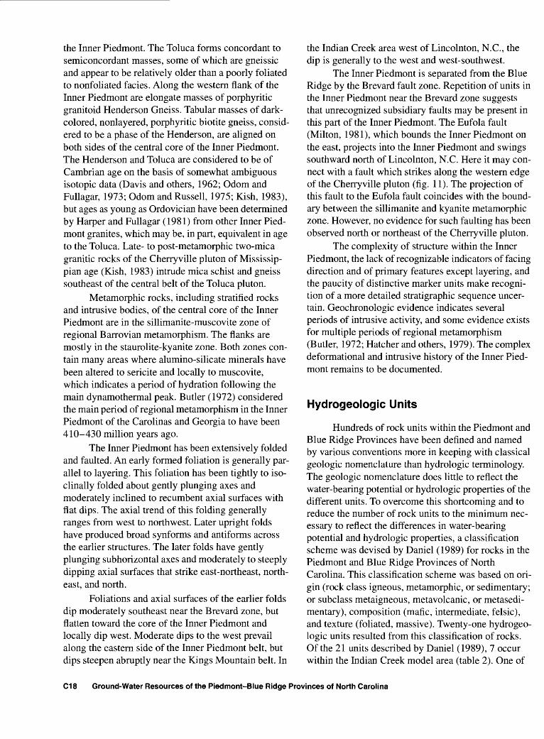
the Inner Piedmont. The Toluca forms concordant to semiconcordant masses, some of which are gneissic and appear to be relatively older than a poorly foliated to nonfoliated facies. Along the western flank of the Inner Piedmont are elongate masses of porphyritic granitoid Henderson Gneiss. Tabular masses of dark- colored, nonlayered, porphyritic biotite gneiss, consid ered to be a phase of the Henderson, are aligned on both sides of the central core of the Inner Piedmont. The Henderson and Toluca are considered to be of Cambrian age on the basis of somewhat ambiguous isotopic data (Davis and others, 1962; Odom and Fullagar, 1973; Odom and Russell, 1975; Kish, 1983), but ages as young as Ordovician have been determined by Harper and Fullagar (1981) from other Inner Pied mont granites, which may be, in part, equivalent in age to the Toluca. Late- to post-metamorphic two-mica granitic rocks of the Cherryville pluton of Mississip- pian age (Kish, 1983) intrude mica schist and gneiss southeast of the central belt of the Toluca pluton.

Metamorphic rocks, including stratified rocks and intrusive bodies, of the central core of the Inner Piedmont are in the sillimanite-muscovite zone of regional Barrovian metamorphism. The flanks are mostly in the staurolite-kyanite zone. Both zones con tain many areas where alumino-silicate minerals have been altered to sericite and locally to muscovite, which indicates a period of hydration following the main dynamothermal peak. Butler (1972) considered the main period of regional metamorphism in the Inner Piedmont of the Carolinas and Georgia to have been 410-430 million years ago.

The Inner Piedmont has been extensively folded and faulted. An early formed foliation is generally par allel to layering. This foliation has been tightly to iso- clinally folded about gently plunging axes and moderately inclined to recumbent axial surfaces with flat dips. The axial trend of this folding generally ranges from west to northwest. Later upright folds have produced broad synforms and antiforms across the earlier structures. The later folds have gently plunging subhorizontal axes and moderately to steeply dipping axial surfaces that strike east-northeast, north east, and north.

Foliations and axial surfaces of the earlier folds dip moderately southeast near the Brevard zone, but flatten toward the core of the Inner Piedmont and locally dip west. Moderate dips to the west prevail along the eastern side of the Inner Piedmont belt, but dips steepen abruptly near the Kings Mountain belt. In

the Indian Creek area west of Lincolnton, N.C., the dip is generally to the west and west-southwest.

The Inner Piedmont is separated from the Blue Ridge by the Brevard fault zone. Repetition of units in the Inner Piedmont near the Brevard zone suggests that unrecognized subsidiary faults may be present in this part of the Inner Piedmont. The Eufola fault (Milton, 1981), which bounds the Inner Piedmont on the east, projects into the Inner Piedmont and swings southward north of Lincolnton, N.C. Here it may con nect with a fault which strikes along the western edge of the Cherryville pluton (fig. 11). The projection of this fault to the Eufola fault coincides with the bound ary between the sillimanite and kyanite metamorphic zone. However, no evidence for such faulting has been observed north or northeast of the Cherryville pluton.

The complexity of structure within the Inner Piedmont, the lack of recognizable indicators effacing direction and of primary features except layering, and the paucity of distinctive marker units make recogni tion of a more detailed stratigraphic sequence uncer tain. Geochronologic evidence indicates several periods of intrusive activity, and some evidence exists for multiple periods of regional metamorphism (Butler, 1972; Hatcher and others, 1979). The complex deformational and intrusive history of the Inner Pied mont remains to be documented.

Hydrogeologic Units

Hundreds of rock units within the Piedmont and Blue Ridge Provinces have been defined and named by various conventions more in keeping with classical geologic nomenclature than hydrologic terminology. The geologic nomenclature does little to reflect the water-bearing potential or hydrologic properties of the different units. To overcome this shortcoming and to reduce the number of rock units to the minimum nec essary to reflect the differences in water-bearing potential and hydrologic properties, a classification scheme was devised by Daniel (1989) for rocks in the Piedmont and Blue Ridge Provinces of North Carolina. This classification scheme was based on ori gin (rock class igneous, metamorphic, or sedimentary; or subclass metaigneous, metavolcanic, or metasedimentary), composition (mafic, intermediate, felsic), and texture (foliated, massive). Twenty-one hydrogeologic units resulted from this classification of rocks. Of the 21 units described by Daniel (1989), 7 occur within the Indian Creek model area (table 2). One of


Table 2. Classification and lithologic description of hydrogeologic units in the Indian Creek model area of the southwestern Piedmont of North Carolina[From Daniel, 1989]

Symbol Hydrogeologic unit Lithologic description

Igneous intrusive rocks

IFI...... Igneous, felsic intrusive .. Light-colored, mostly granitic rocks, fine- to coarse-grained, some porphyritic, usually massive, locally foliated; includes granite, granodiorite, quartz diorite, quartz monzonite, alaskites.

Metamorphic rocks

MIF..... Metaigneous, felsic............

MIL.... Metaigneous, intermediate.

MIM... Metaigneous, mafic............

GNR... Gneiss, felsic.

GNM.. Gneiss, mafic.

SCH.... Schist.............

Metaigneous rocks (intrusive)

Light-colored, massive to foliated metamorphosed bodies of varying assemblages of felsic intrusive rock types; local shearing and jointing are common.

Gray to greenish-gray, medium- to coarse-grained, massive to foliated, well-jointed, metamorphosed bodies of diotitic composition.

Massive to schistose greenstone, amphibolite, metagabbro and metadiabase, may be strongly sheared and recrystallized; metamorphosed ultramafic bodies are often strongly foliated, altered to serpentine, talc, chlorite-tremolite schist and gneiss.

Metasedimentary rocks

Mainly granitic gneiss; light-colored to gray, fine- to coarse-grained rocks, usually with distinct layering and foliation, often interlayered with mafic gneisses and schists.

Mainly biotite hornblende gneiss; fine- to coarse-grained, dark-gray to green to black rock, commonly with distinct layering and foliation, often interlayered with biotite and hornblende gneisses and schists, and occasional amphibolite layers.

Schistose rocks containing primarily the micas muscovite or biotite or both, occasional sericite and chlorite schists; locally interlayered with hornblende gneiss and schist, commonly with distinct layering and foliation.

these units (SCH) is limited to a tiny area at the south east end of the Indian Creek model area where it crosses into the Kings Mountain belt (fig. 12). Another unit (GNF) occupies a small area along the northeast margin of the Indian Creek model area. Because the areas underlain by SCH and GNF are small and lie outside the surface drainage divides of the Indian Creek Basin, they were omitted from any analyses of hydrologic characteristics made during this study.

The identification of hydrogeologic units shown in table 2 is based on the hypothesis that origin, com position, and texture can be linked not only to a rock's primary porosity but also to its susceptibility to the development of secondary porosity in the form of frac tures and solution openings. The composition and tex ture of the rocks would also determine, in part, the rate and depth of weathering of these units and the water bearing properties of the resulting regolith.

Using this classification scheme and the most recent geologic maps available, Daniel and Payne (1990) compiled a hydrogeologic unit map for the Piedmont and Blue Ridge Provinces in North Carolina. Part of this map that includes the Indian Creek model area is shown in figure 12. Well location maps were related to hydrogeologic units using this

map. Hydrologic and hydraulic characteristics of each unit were then determined using well-construction, specific-capacity, and aquifer-test data.

Geologic Belts

The Piedmont and Blue Ridge have been divided into a number of northeast-trending geologic belts (Brown and Parker, 1985). Within a belt, rocks are to some degree similar to each other in general appearance, metamorphic rank, structural history, and relative abundance of igneous, metaigneous, metasedimentary, and metavolcanic rocks (Butler and Ragland, 1969). Areally, the most significant belts are the Blue Ridge, Inner Piedmont, Charlotte, Carolina slate, and Raleigh (Daniel, 1989).

The belts important to this study are the Chauga, Inner Piedmont, Kings Mountain, and Charlotte belts (fig. 11). A brief summary of the belts and the hydrogeologic units that constitute the belts is given in table 3. Hydrogeologic units present in the Indian Creek model area are common to these belts. To obtain a large enough data set with which to determine hydrologic characteristics and aquifer properties of hydrogeologic units within the Indian Creek model


35°40'81°30'

LINCOLON COUNTY

Lincolnton Laboratory

35°20'

01234 SMILES

01234 5 KILOMETERS

EXPLANATION

IGNEOUS INTRUSIVE ROCKS

| | IGNEOUS, FELSIC INTRUSIVE (IFI)

METAMORPHIC ROCKS

METAIGNEOUS ROCKS (INTRUSIVE) METASEDIMENTARY ROCKS

Q2J METAIGNEOUS, FELSIC (MIF) |//3 GNEISS, FELSIC (GNF)

E]j] METAIGNEOUS, INTERMEDIATE (Mil) Q GNEISS, MAFIC (GNM)

H METAIGNEOUS, MAFIC (MIM) 0 SCHIST (SCH)

Figure 12. Hydrogeologic unit map of the southwestern Piedmont of North Carolina showing the Indian Creek model area (from Daniel and Payne, 1990).


Table 3. Geologic belts of part of the Piedmont Province of southwestern North Carolina[GNF, gneiss, felsic; GNM, gneiss, mafic; MIF, metaigneous, felsic; SCH, schist; Mil, metaigneous, intermediate; MIM, metaigneous, mafic; IFI, igneous, felsic intrusive; MVU, metavolcanic, undifferentiated. The hydrogeologic unit MVU is not found in the Indian Creek model area. The other hydrogeologic units are described in table 2. From Daniel, 1989]

Belt BoundariesDominant

hydrogeologicunits

Chauga (includes Brevard fault Blue Ridge belt on northeast, Inner Piedmont on southeast.................. GNF, GNM.zone).

Inner Piedmont......................... Chauga and Blue Ridge belts on northwest, Kings Mountain and GNM, MIF.Charlotte belts on southeast.

Kings Mountain ....................... Inner Piedmont belt on northwest, Charlotte belt on southeast............. SCH, MIF, GNF.Charlotte................................... Kings Mountain and Inner Piedmont belts on northwest, Milton belt on Mil, MIF, MIM, IFI, MVU.

north, Gold Hill shear zone and Carolina slate belt on southwest.

area, data from wells tapping comparable hydrogeo logic units within the four belts were compiled into one data set and analyzed. The boundary between the Blue Ridge and Piedmont Provinces crosses the Chauga and Inner Piedmont belts in southwestern North Carolina. The selection of wells was restricted to the Piedmont area of these belts.

Structural Fabric and Orientation

The structural fabric and orientation of bedrock beneath the Indian Creek Basin were characterized by taking measurements of strike and dip at points of rock outcrop throughout the basin. Fractures and foliation are the principal fabric components considered to have a role in the hydrogeology of the basin. Joints are the most common form of fracture, although fracture zones of closely spaced joints and minor zones of shearing were observed. Foliation varies from simple mineral lineation to schistosity and gneissic banding. The Cherryville pluton is generally massive with sparse fracturing and only minor foliation, possibly flow banding, that seems to occur near the edges of the pluton. Relict foliation could frequently be observed in the regolith where exposed in road cuts and other excavations.

Measurements of strike and dip were compiled on fractures and foliation. Sites where measurements were made on fractures and foliation are shown in figure 13. Individual measurements of strike and dip on fractures and foliation are compiled in tables 4 and 5, respectively (p. C96-C98).

Analysis of the fabric data consisted of plotting pi diagrams (poles to planes plotted on equal-area nets) and contouring data points so that the geometry

of the fabric elements could be determined. Methods of plotting, contouring, and analysis are discussed by Billings (1972).

The contour diagram for poles to fracture planes (fig. 14) shows that most fractures are steeply dipping and strike northeast. There is some range in strikes to the northeast and an indication that many fractures dip steeply to the northwest; however, the greatest concen tration of fractures strikes N. 72° E. and is vertical.

Analysis of foliation data followed the same process used for analyzing fracture data. A contour diagram for all foliation data (fig. 15) shows that the greatest concentration of foliation planes strikes N. 18° W. and dips 27° SW. By subsetting the foliation data so that data from the northern, central, and south ern parts of the basin could be analyzed separately, a subtle variation in strike and dip is observed along strike. The division of sites into three subsets is shown in figure 16. Once the three subsets of foliation data were contoured, poles to planes for the concentration maxima were determined. A beta diagram (Billings, 1972) shows the foliation planes represented by these three maxima (fig. 17). In the northern part of the basin, foliation strikes due north and dips rather gently to the west at 16° W. In the central part of the basin, foliation has a more northwesterly strike at N. 26° W. and the dip steepens to 37° SW. In the southern part of the basin, foliation returns to a more northerly orienta tion with a strike of N. 16° W. and dip of 31 ° SW.

Because local deviation in orientation of folia tion from the regional average is minor, different parts of the basin do not need to be considered individually for hydrologic analysis. The fabric data are consistent in that the entire basin apparently lies on the southwest flank of an anticlinal fold whose axis is northeast and outside of the basin and has a strike slightly west of


81°30' 81°22'30"

35°30' -

35°22'30

CATAWBA COUNTY

LINCOLN COUNTY

EXPLANATION

- - - - BOUNDARY OF NORTH, CENTER, AND SOUTH DIVISIONS FOR ANALYSIS OF FOLIATION DATA

26i- - -..---. BASIN BOUNDARY

A STREAM SITE AND NUMBER(See tables 4, 5, and 8)

CLEVELAND COUNTY

GASTON COUNTY

6 MILES

024 6 KILOMETERS

Figure 13. Sites where measurements of strike and dip were made on fractures and foliation planes in the Indian Creek Basin. (Site locations and descriptions are listed in tables, p. C103).

north (fig. 11). The average strike of fractures (prima rily joints) at N. 72° W. is at right angles to foliation and is consistent with an extensional joint set created normal to the anticlinal axis.

It is fortuitous that the two fabric components thought to have a role in ground-water movement are oriented at right angles to each other. By orienting a model grid to coincide with the fabric components, model development is greatly simplified. The develop ment of the model grid is discussed in later sections.

Faults

A few high-angle faults have been observed in outcrop and deduced from map patterns within the

Indian Creek Basin and surrounding model area (fig. 11). A zone of closely spaced high-angle joints and fractures was observed at site 30 (fig. 13). The most intense fracturing occurs in a zone 25-30 ft wide, but less intense fracturing on either side of this zone extends the total width to 50 ft. Fractures within the zone have strikes between N. 65° E. and N. 80° E., but most are in the N. 65° E. direction. Relative move ment or displacement associated with this fracture zone could not be determined. Topographic expression of this fracture zone was poorly developed; however, a small topographic low that is barely perceptible on the topographic map may reflect this feature (U.S. Geo logical Survey, 1973). Other shear zones are


EXPLANATIONLOCATIONS OF MAXIMA AND VALUE WHERE SHOWN

21 20

Figure 14. Contour diagram of poles to fracture planes in the Indian Creek Basin.

EXPLANATION

LOCATIONS OF MAXIMA AND VALUE WHERE SHOWN

Figure 15. Contour diagram of poles to foliation planes in the Indian Creek Basin.

Figure 16. Contour diagrams of poles to foliation planes for subregions of the Indian Creek Basin. A, Northern third; B, Central third; C, Southern third.

EXPLANATION

LOCATIONS OF MAXIMA SHOWN; VALUES NOT GIVEN. CONTOUR HATCHURES INDICATE VALUES LESS THAN SURROUNDING AREA


Figure 17. Beta diagram of foliation planes represented by the three maxima from the contour plots of the Indian Creek Basin shown in figure 16.

interpreted primarily on topographic expression by alignment of stream channels, particularly alignment of tributary channels across the channel of the main stream. A recurved pattern is especially indicative of structural control. Examples of these patterns are found upstream from site 13, site 26, and sites 41 and 42 that are expressed topographically by alignment of tributary streams across Indian Creek. The channel of Indian Creek also appears in part to be controlled by a structural feature north of sites 41 and 42. The change in channel orientation of Indian Creek northeast of Cherryville, N.C., from southeast to northeast also indicates possible fracture control, although no fault ing was observed. Outcrops are sparse and poorly exposed in this reach of Indian Creek because flatten ing of the stream gradient results in submersion of the channel bottom and extensively developed flood-plain deposits. Perhaps the most extensive fault in the Indian Creek model area is a fault mapped by Goldsmith and others (1988) that bounds the western edge of the Cherryville pluton west of Lincolnton, N.C., and extends southwest at least as far as Cherryville, N.C. No evidence of brittle fracturing associated with this fault could be identified in outcrop. Evidence for this fault is based, in part, on map patterns.

Folds

The stratified metamorphic rocks of the Indian Creek model area dip gently to moderately to the west and southwest. Dips in the northern part of the area are lower than in the central and southern parts of the area. According to the tectonic map of Goldsmith and oth ers (1988), the Indian Creek model area lies between antiforms on the east and northeast and a synform (Buffalo Creek synform) on the southwest (fig. 11). The Buffalo Creek synform is truncated on the north by the Toluca pluton. Dips within the Indian Creek model area are consistent with regional folds mapped by Goldsmith and others (1988).

SoilsSoils in the Indian Creek model area have differ

ent properties and characteristics such as color, texture, size and shape of soil aggregates, kind and amount of rock fragments, distribution of plant roots, soil reaction, and other features (U.S. Department of Agriculture, 1995). Soils generally occur in patterns that result from the combined influences of climate, parent rock type, relief, and biological activities inter acting through time (U.S. Department of Agriculture, 1995). Soils with similar properties, characteristics, and arrangement of horizons within their profiles are identified and assigned to taxonomic classes. Each taxonomic class, or soil type, has a set of soil charac teristics with defined limits and is associated with a particular kind of landscape. Figure 18 shows the general types and locations of soils in the Indian Creek model area.

One property important to hydrologic study is soil permeability. Permeability indicates the ability of water to move through the soil profile. Soil permeabil ity is important in its ability to enhance or restrict the infiltration of precipitation through the soil profile. Typically within a profile, soils at depths of less than 1 ft below land surface exhibit maximum permeability. As depth increases to greater than 1 ft, permeability generally decreases. As precipitation moves down ward through the different layers within a soil profile, the layer of minimum permeability controls infiltra tion. In this manner, soil permeability can greatly affect the hydrology of an area by controlling the amount of recharge available to the ground-water sys tem.

Permeability and other properties of soils in the Indian Creek model area are published by the U.S. Department of Agriculture, Bureau of Soils and Soil


81°30'

35°35'

EXPLANATION2 SOIL ASSOCIATION

MAP NUMBER (See table 6)

Indian Creekmodel

boundary

35°25' -

01234 5 KILOMETERS

Figure 18. General soil associations map of parts of Burke, Catawba, Cleveland, Gaston, and Lincoln Counties showing the Indian Creek model area. The soil associations corresponding to the map numbers are described in table 6. (Map compiled from U.S. Department of Agriculture, 1916, 1918, 1930, 1975, 1989, 1995.)


Conservation Service (U.S. Department of Agricul ture, 1916, 1918, 1930, 1975, 1989, 1995). Table 6 summarizes the general soil associations, predominant soil types within each association, topographic occur rence, texture, and permeability of soils in the study area. When compared to the permeability of soils in the study area, estimates of net recharge (table 12, p. C107) derived from hydrograph separation were found to be much less than the permeabilities of all soils in the study area. As a result, net recharge to the ground-water system is not limited or restricted by the soils in the study area.

Ground-Water Flow SystemMovement of ground water through the ground-

water flow system is controlled by the hydraulic prop

erties of the bedrock and overlying regolith, the distri bution of these properties, and the distribution of potentiometric heads within the system. In fractured- rock aquifer systems, anisotropic conditions often are present because of nonuniform distributions of frac tures, faults, foliation, and lithologic contacts in the bedrock, and relict foliation in the overlying regolith (Harned and Daniel, 1992). If the fractured-rock aqui fer under investigation is sufficiently extensive and if the fractures have similar dimensions, have relatively uniform spacing, have distributed rather than uniform orientations, and are sufficiently abundant so as to be interconnected, then porous-media equivalence is gen erally assumed. Implicit in the criteria of fracture abundance and spacing is the factor of scale in evaluat ing porous media equivalence (Long and others,

Table 6. General soil association, predominant soil types, occurrence, U.S. Department of Agriculture soil texture, and permeability of soils in the Indian Creek model area[USDA, U.S. Department of Agriculture; <, less than; do. ditto. Modified from U.S. Department of Agriculture, 1916, 1918, 1930, 1975, 1989, 1995]

Predominant Map _ .. soil types (in

number . .. decreasing « *o\ association . * (fig. 18) order of

abundance)

1 Cecil................. Cecil, Pacolet,Hiwassee.

2 Gaston .............. Gaston, Pacolet,Cecil, Winns- boro, Hiwassee.

3 Pacolet- Pacolet, Madison. Madison, Cecil.

4 Chewacla.......... Chewacla,Congaree.

5 Georgeville- Georgeville, Tatum. Tatum.

Wedowee, Pacolet.

7 Urban land........ Pacolet, Cecil, Madison, Urban land.

Typical Topographic USDAoccurrence soil

Broad ridges, short Sandy clay loam .. side slopes.

Broad to narrow ......do...................ridges, gently sloping to steep side slopes.

Broad to narrow ......do...................ridges, gently sloping to moderately steep side slopes.

Flood plains of Silty clay loam..... major streams.

Broad to narrow Gravelly silty ridges, gently clay loam, sloping to moderately steep side slopes.

ridges, gently sloping to steep side slopes.

Uplands in urbanized ......do...................areas.

Soil permeability1 , in inches per hour

Depth below land surface

<1 foot

0.6-6.3

0.6-6.0

0.6-6.0

0.6-2.0

0.6-2.0

0.6-6.0

0.6-6.0

1 to 5 feet

0.06-2.0

0.6-2.0

0.6-2.0

0.6-2.0

0.6-2.0

0.6-2.0

0.6-2.0

'Given values of permeability do not include areas of impervious cover.

1982). Given these assumptions, analytical techniques and models developed for porous media can be applied to fractured-rock aquifer systems.

Large fracture discontinuities, such as major faults or shear zones (or solution openings such as caverns, although none are thought to be present due to the sparsity of carbonate rocks in the area), are potential sources or sinks for ground water that could preferentially conduct ground water within the ground-water system or even transfer ground water past the surface drainage divides of the basin. If this occurs, a basic assumption about the nature of the ground-water flow system that ground-water divides coincide with surface drainage divides is violated. Any water budgets, mass balance computations, or models based on this assumption would be in error.

The hydraulic properties of bedrock and regolith are discussed in a later section, "Hydrogeologic

Characteristics." Potentiometric heads in the Indian Creek area were determined by measuring water levels in wells and the water-surface altitude in streams and lakes. The determination of water levels and fluctua tions of ground-water levels are described below. In order to identify possible sources or sinks for large quantities of ground water, an investigation of base flow was made at 85 sites uniformly distributed throughout the basin. The results of this investigation also are discussed below.

Ground-Water Levels

Information about the natural fluctuation of ground-water levels was obtained from a network of 38 observation wells distributed throughout the Indian Creek Basin (fig. 19). The network consisted of 16 drilled wells tapping bedrock and 22 bored or

81°30' 81°22'30"

35°30'

35°22'30"

CATAWBA COUNTY

LINCOLN COUNTY

EXPLANATION -..-. -. BASIN BOUNDARY

APRASA OBSERVATION WELL NETWORK

Recording well and number

Li-132© Drilled well and number

Li-149Q Bored or dug we|| and number

CLEVELAND COUNTY \

...- " 'V.X

GASTON COUNTY

» Gs-257" %'--->'

\

Figure 19. Locations of 38 observation wells in the Indian Creek Basin area used to obtain information on natural fluctuation of ground-water levels. (The wells are described in table 16, p. C118.)

6 MILES

6 KILOMETERS


hand-dug wells tapping regolith. One drilled well and five bored or hand-dug wells were instrumented with recorders to obtain continuous records of water levels. Water levels in the other 32 wells were measured monthly. Monthly water-level measurements began in April 1991 and continued through September 1992. Five recorders were installed in June 1991 and the sixth was installed in July 1991. Hydrographs of water levels from the six wells equipped with recorders for

June 1991 through October 1992 are shown in figure 20. Records of monthly water-level measure ments from the 38 observation wells are given in table 7 (p. C99).

Four pairs of wells, each pair consisting of a drilled well and a bored or hand-dug well, were identi fied to compare the water level in the regolith with the water level in the bedrock at specific sites. One pair of wells, consisting of wells Li-117 and Li-118, was

15

20

25

30

LLJ O

Q

gLLJCO

LJJ LLJ

35

UJ

LLJ 40

DC LLJ

I

45

50

55

\ i i i \ \ i

Li-211 GERALDINE DELLINGER WELLDrilled well in bedrock; site on

a slope.

i i

Li-130 SANFORD YATES WELLHand-dug well in regolith; site

Gs-244 FLOYD DELLINGER WELL °" a hilltop.

Hand-dug well in regolith; site on

Li-203 JERRY REYNOLDS WELL Bored well in regolith

Li-164 HARVEY HEAVNER WELLHand-dug well in regolith; site on

a hilltop.

Cw-327 ARNOLD COOK WELL Hand-dug well in regolith; site on

JUNE JULY AUG SEPT OCT NOV DEC JAN FEB MAR APR MAY JUNE JULY AUG SEPT

1991 1992

Figure 20. Daily average water levels from a drilled well tapping bedrock and five bored or hand-dug wells tapping regolith in the Indian Creek Basin, June 1991 through September 1992. (Location of wells shown in figure 19.)


later determined to be unsuitable for this purpose because of the effects of pumping on water levels in well Li-118. Hydrographs of water levels in the other three pairs of wells (Li-120 and Li-121, Li-179 and Li-180, and Li-198 and Li-199) are shown in figures 21, 22, and 23, respectively. Elevations between pairs of wells were determined to establish a common land-surface reference for the water levels.

35

ITen 40 Q

45

55

e » ESTIMATED DATA POINT

WATER LEVEL IN DRILLED WELL Li-121

A M J J A S O 1991

N D F M A M J 1992

Figure 21 . Monthly water levels in well pair Li-120 and Li-121, located on a hilltop in the Indian Creek Basin. (Well Li-120 is a hand-dug well tapping regolith; well Li-121 is a drilled well tapping bedrock.)

35

? 40

. WATER LEVEL IN BORED WELL Li-180

A M J J A S O 1991

M A M J 1992

Figure 22. Monthly water levels in well pair Li-180 and Li-179, located on a hilltop in the Indian Creek Basin. (Well Li-180 is a bored well tapping regolith; well Li-179 is a drilled well tapping bedrock.)

35

340

45

55

WATER LEVEL IN BORED WELL Li-198

WATER LEVEL IN DRILLED WELL Li-199

A M J J A S O 1991

N D A M J J 1992

Figure 23. Monthly water levels in well pair Li-198 and Li-199, located on a hilltop in the Indian Creek Basin. (Well Li-198 is a bored well tapping regolith; well Li-199 is a drilled well tapping bedrock.)

The three pairs of wells are on uplands; how ever, wells Li-120 and Li-121 (fig. 21) are on the edge of an interstream upland at the top of a steep slope, and the other two pairs of wells are more cen trally located on interstream uplands. The difference in topographic settings may explain, in part, the greater seasonal amplitude of water-level changes in wells Li- 120 and Li-121 as compared to the other two pairs of wells. The average difference in water levels between wells Li-120 and Li-121 is 2.15 ft for the 18 months of water-level measurements. Between wells Li-179 and Li-180 (fig. 22), the average difference in water levels is 4.70 ft, and between wells Li-198 and Li-199 (fig. 23), the average difference is 17.54 ft.

To compare average conditions in the regolith with average conditions in the bedrock, monthly water-level measurements from 22 bored and hand- dug wells tapping regolith were averaged for each month, and monthly water-level measurements from 14 drilled wells tapping bedrock were averaged for each month (fig. 24). Only a few wells were measured in May and June of 1991, and the averages were omit ted because they are not representative of the entire observation-well network. Two drilled wells, Li-118


w 30

1LU 35

40

45

BORED OR HAND-DUG WELLS

A M J J A S 1991

O N D M A M J J 1992

Figure 24. Monthly average water levels in 22 bored and hand-dug wells tapping regolith and 14 drilled wells tapping bedrock in the Indian Creek Basin, April 1991 through September 1992.

and Li-146, were not included in the computation of monthly averages because of erratic water levels pro duced by pumping. The hydrographs in figure 24 represent average conditions for the entire basin for the 18 months during which water-level measurements were collected. The average difference between monthly average water levels in wells tapping regolith and in wells tapping bedrock is 8.34 ft. The minimum difference in monthly averages is 6.70 ft in July 1991; the maximum difference in monthly averages is 10.21 ft in September 1992.

The hydrographs in figures 20, 21, 22, 23, and 24 show similar patterns. Declines in water levels begin during the growing season and extend into dry fall and winter months. Rises in water levels in response to precipitation begin in late spring and extend into the summer months. During 1991-92, water levels in most wells reached seasonal high levels in July or August and seasonal low levels in February or March, although wells Li-168, Cw-327, and Li-180 reached seasonal lows in April 1992. This pat tern is somewhat atypical from the long-term seasonal pattern for this area. The long-term pattern (LeGrand, 1954) for ground-water levels is for the seasonal high to occur in late winter or early spring, typically in March or April. Once the growing season starts, ground-water levels typically follow a long decline until the growing season ends in September or Octo ber. In December or January, late fall and early winter rains cause a rise in water levels that continues until

the next growing season begins. During 1992, recov ery of ground-water levels in some wells did not begin until late February, and in others recovery did not begin until March or April. Water levels rose in response to above-average rainfall until June 1992 when heavy rain produced atypically high summer ground-water levels.

In the Indian Creek area, the decline of ground- water levels extends over a longer aggregate period during a year and is more gradual than the rise of ground-water levels. In spite of the difference between the aggregate periods of water-level rise and water- level decline, in most years recharge to the ground- water system is approximately equal to the discharge from it, so that ground-water levels at the end of the year are at about the same level as at the beginning of the year.

Base Flow

Base flow is that part of streamflow resulting from the discharge of ground water to surface-water bodies such as springs, seeps, and perennial streams. The rate of discharge can be affected by many factors including, but not limited to, aquifer hydraulic proper ties and the lateral hydraulic gradient between the water table and the spring or stream. Aquifer hydraulic properties are often assumed to be uniformly distrib uted to facilitate analytical solutions, but in nature they can vary a great deal areally and vertically within an aquifer system. In fractured-rock terranes, variability is expected because of the variety of processes that produce the secondary permeability (fractures) within these systems. Therefore, an evaluation of the perme ability distribution within the Indian Creek Basin was necessary to identify any possible exceptions to the assumption of uniformity. One means of assessing the areal uniformity of aquifer hydraulic properties is through a detailed study of base flow throughout the basin.

At a very small scale, differences in hydraulic properties between fractures and the intervening solid rock are exaggerated. As scale increases and the num ber of fractures in any unit volume of aquifer (fracture density) increases, hydraulic properties of the fractured-rock aquifer take on some semblance of porous-media equivalence. At scales contemplated for the model described in this study, highly fractured rock presumably would have porous-media equiva lence, but large features such as faults, shear zones, and solution openings would not. Large solution


openings such as caverns are not likely in the Indian Creek area, although some small carbonate (marble) bodies have been mapped in the Inner Piedmont and Kings Mountain belts (Goldsmith and others, 1988). Faults and shear zones are more likely pathways for channeling ground-water flow within the basin or across basin boundaries. Some faults and shear zones possess considerable secondary porosity, although others do not, and some have lost their porosity as a result of secondary mineralization. A detailed study of base flow, in addition to providing information on uni formity of aquifer properties, can provide information on channeling of ground water along preferential path

ways such as faults, shear zones, and solution open ings.

A detailed synoptic survey of base flow in the Indian Creek Basin was conducted during November 26 28, 1990. Discharge was measured at 85 stream sites (fig. 25; table 8, p. C103) during this period. Measurements of stream width, cross-section area, and average depth also were determined at these sites (table 9). Discharge from the basin, as measured at the gaging station near Laboratory, N.C., was about 57 ftrVs on November 27. This is nearly the same as the median discharge of 56 ftVs during the 39-year period of record from water years 1952 through 1990.

81°30' 81°22'30"

35°30' -

35°22'30"

EXPLANATION

- -"- BASIN BOUNDARY

35A STREAM SAMPLING SITE AND NUMBER

6 KILOMETERS

Figure 25. Locations of 85 stream sites in the Indian Creek Basin where synoptic surveys of base flow and water-quality conditions were made. (Measurements of strike and dip were made on fractures and foliation in the bedrock exposed at some sites [tables 4 and 5] in the stream channel. Gaging station 02143500, Indian Creek near Laboratory, N.C., is at site 85.)


Table 9. Stream width, cross-section area, and average depth at 85 stream sites in the Indian Creek Basin, November 26-28, 1990[ft, feet; ft2 , square feet]

Site number (fig. 25; table 8)

12 3 4 56 7 8 9

1011 12 13 14 1516 17 18 19 202122 23 24 2526 27 28 29 303132 33 34 3536 37 38 39 404142 43 44 4546 47 48 49 50

Width (ft)

3.3 8.9 3.0 3.0 5.01.58.2

10.0 7.7

10.77.5 1.5

15.0 1.9 2.0

20.0 9.33.4 9.7 4.4

24.0 25.0 16.5 9.6 1.8

26.0 2.6 2.9 2.0

12.63.1

24.0 17.0 29.04.54.3 3.7 3.8 9.5 6.3

34.0 4.0 2.3 1.80 9.04.3

17.0 2.9

11.5 6.0

Area (ft2)1.06 3.04

.87

.50 2.02

.22 3.03 1.78 3.00 3.063.03

.21 5.08

.66

.7410.9 3.66

.903.79

.9222.7 20.5 13.1 4.35

.1815.4

.42 1.16 .60

7.691.17

20.5 4.75

25.3 1.091.22 1.78

.97 2.962.97

23.2 .91 .38 .41

5.62.81

8.01 .61

9.482.57

Average depth (ft)

0.32 .34 .29 .16 .40.15 .37 .18 .39 .29.40 .14.34 .35 .37.54 .39 .26 .39 .21.95.82 .79 .45 .10.59 .16 .40 .30 .61.38 .85 .28 .87.24

Table 9. Stream width, cross-section area, and average depth at 85 stream sites in the Indian Creek Basin, November 26-28, 1 990 Continued[ft, feet; ft2 , square feet]

Site number Width Area Average (fig. 25; table 8) (ft) (ft2) depth (ft)

51 15.0 8.00 0.53 52 17.0 8.43 .50 53 30.0 36.7 1.23 54 4.2 1.32 .31 55 4.0 1.05 .2656 9.0 4.79 .53 57 3.0 .69 .23 58 2.3 .19 .08 59 4.9 2.29 .47 60 7.1 2.35 .3361 2.7 .52 .19 62 9.3 4.08 .44 63 10.0 2.59 .26 64 13.0 5.03 .39 65 4.5 1.04 .2366 3.5 .71 .22 67 4.9 1.06 .22 68 .80 .04 .05 69 12.0 3.77 .31 70 1.6 .16 .10071 34.0 34.3 1.01 72 51.0 200.0 3.92 73 2.5 .40 .16 74 8.6 1.81 .21 75 3.5 1.66 .4776 32.0 89.8 2.81 77 3.2 1.12 .35 78 3.6 .89 .25 79 4.7 2.87 .61 80 25.0 32.2 1.2981 1.5 .21 .14 82 8.0 2.23 .28 83 1.6 .23 .14 84 2.2 .42 .19 85 63.0 61.3 .97

.28

.48 26 in addition to being representative of median flow 31 conditions, no major storms occurred in the basin

.68

.23

.16

.23

.62

.19

.47

.21

.82

.43

1990, survey. A minor storm occurred on November 10, 16 days prior to the survey, when daily average discharge peaked at 1 12 ft3/s. Flow from this storm had entirely dissipated by the time of the survey. Accordingly, based on stream discharge and climatological records, streamflow during the survey was considered steady and due entirely to ground-water discharge.


Unit area discharges were computed to facilitate comparison of discharges at the 85 sites. Unit area dis charges were computed for the entire drainage area above the site where streamflow was measured, and as the difference between discharge at a site and any upstream site (net discharge) divided by the drainage area for the reach between the sites (intervening drain age area). When a site was the most upstream site on a stream, the intervening drainage area was simply the drainage area above the site. The net discharge compu tation was performed to isolate and enhance any local variation in base flow. Statistics for the two computa tions of unit area discharge, total drainage areas above sites, and drainage areas between sites are listed in table 10.

Drainage areas for the 85 synoptic survey sites range from 0.13 mi2 for a headwater site the most upstream site on a stream to 69.48 mi2 at the gaging station near Laboratory, N.C. Unit area discharges at these 85 sites (table 11) range from 0.070 (ft3/s)/mi2 to 1.337 (ft3/s)/mi2 and average 0.799 (ft3/s)/mi2 . Approximately 80 percent of the unit area discharges are within plus or minus one standard deviation of the mean. If these data were normally distributed, 66 percent of the data would occur within plus or minus one standard deviation. This tendency of the data to cluster about the mean is also indicated by a kurtosis of 5.035. The nature of data at the extremes is interesting because both the minimum and maximum values of unit area discharge are from headwater sites. In fact, the five lowest unit area discharges and the five highest unit area discharges are from headwater sites. Drainage areas of the five lowest unit area discharge sites range from 0.14 to 0.30 mi 2 and average 0.20 mi2 . Drainage areas related to the five highest unit area dis charge sites range from 0.38 to 0.68 mi2 and average 0.54 mi2 . Unit area discharges at the other 75 sites are between these extremes, yet many of the sites relate to larger, often much larger, drainage areas.

Inspection of topographic maps suggests that differences in extremes of base-flow discharge are due to differences in relief and depth of incision of corre sponding headwater streams. The five tributary areas with the lowest unit area discharges have modest relief, their valleys are not deeply incised, and the streamflow measurement sites are closer to drainage divides compared to the five areas with the highest unit area discharges. Stream gradients in the five high dis charge areas are also steeper than gradients in the low discharge areas. These observations suggest that

higher base flows are associated with higher relief, which could result in steeper ground-water hydraulic gradients. Assuming that the hydraulic properties of regolith and bedrock are everywhere similar in the Indian Creek Basin, differences in base flow reflect differences in ground-water gradients.

Unit area discharges at sites further downstream from headwater sites and with larger drainage areas probably reflect an averaging of the extremes. Stream gradients and relief also tend to decrease with distance downstream, and valleys and flood plains tend to broaden. This suggests that as tributary drainage areas increase and valleys and flood plains broaden, ground- water gradients decline.

Unit area discharges for intervening areas between streamflow measuring sites ranged from -0.444 to 4.497 (ft3/s)/mi2 and averaged 0.840 (ft3/s)/mi2 (table 11). No discernible pattern of discharge occurred on an areal basis or along individ ual streams to indicate preferential movement of ground water through faults or shear zones. Negative values of unit area discharge were computed for two sites on Indian Creek site 76 [-0.444 (ft3/s)/mi2] and site 80 [-0.406 (ft3/s)/mi2]. However, discharge gains in streams tributary to Indian Creek near sites 76 and 80 are positive and relatively large. The two highest intervening unit area discharges occurred at site 26 [4.497 (ft3/s)/mi2] and site 72 [2.558 (ft3/s)/mi2]. These two sites also are on Indian Creek, have above average discharge and drainage area compared to the other 83 sites, and have small intervening areas between the sites and upstream sites. Accordingly, much of the variation in intervening unit area discharge data may result from (1) errors in discharge measurements (gen erally given as plus or minus 5 percent, although it may be higher), (2) errors in determining drainage areas from topographic maps where diversion of drainage for agriculture, roadways, and urban devel opment may not always be apparent, and (3) the related mathematical computations, particularly divi sion by small values of intervening drainage area when measurement sites are close together. Even if preferential ground-water flow were taking place, evaluation of this flow probably would be hindered by variation of unit area discharge resulting from other nonhydrologic data.

Data from the synoptic survey of base flow and related unit area discharges do not indicate channeling of ground water within the basin or beneath basin boundaries through large-scale features such as faults,


Table 10. Results of synoptic base-flow survey of 85 stream sites within the Indian Creek Basin, November 26-28, 1990[ft3/s, cubic feet per second; mi2 , square miles; (ft3/s)/mi2 , cubic feet per second per square mile; *, denotes the furthest upstream site on a stream]

Site number (fig. 25)

1*23*4*5*

6*

78*

910

1112*

1314*15*

161718*

1920*

21222324*25*

2627*28*29*

30

31*

32333435*

36*37*38*

3940

4142*43*44*

45

Date (1990)

11/2611/2611/2611/2611/26

11/2611/2611/2611/2611/26

11/2611/2611/2611/2611/26

11/2611/2611/2611/2611/26

11/2611/2611/2611/2611/26

11/2611/2611/2611/2611/26

11/2711/2711/2711/2611/26

11/2711/2711/2611/2611/27

11/2711/2711/2711/2711/27

Time (hours)

10301130121010151055

11351210111512051300

11051300132514301410

12201300135014501010

14001700155016351440

14301530153015551605

11150905103515501635

11101020170017250930

08500845123513051355

Discharge (ft3/s)

0.201.14

.58

.251.15

.09

.961.082.241.36

2.45.19

3.18.33.25

4.051.62

.413.35

.58

8.2810.14.16

.66

.07

15.6.22.27.15

1.86

.3417.23.17

23.8.51

.64

.68

.311.671.00

25.9.87.09.17

2.67

Drainage area (mi2 , total

above site)

0.291.24.62.32

1.21

.131.091.252.701.44

2.66.32

3.26.38.29

4.932.00

.403.72

.68

10.6812.005.64

.86

.14

17.94.25.27.30

2.53

.4819.604.00

26.94.55

.93

.66

.461.901.44

30.521.06.18.27

3.68

Unit area discharge ([ft3/s]/mi2 , for total drainage

area)

0.690.931.922.787.950

.703

.878

.862

.828

.941

.921

.594

.976

.849

.852

.821

.8081.035.902.848

.776

.842

.738

.767

.479

.870

.8691.007.517.736

.706

.878

.792

.883

.932

.6921.030.675.877.693

.849

.826

.478

.624

.725

Intervening drainage

area (mi2 ,

for reach between

sites)0.29

.93

.62

.321.21

.13

.471.251.48.35

1.00.32.60.38.29

.65

.56

.40

.46

.68

1.981.321.92.86.14

.30

.25

.27

.30

.96

.48

.941.483.33

.55

.93

.66

.461.36.52

2.461.06.18.27

1.78

Unit area discharge ([ft3/s]/mi2, for reach between

sites)

0.6901.008.922.787.950

.703

.820

.862

.7431.136

.955

.5941.225.849.852

.826

.4641.035.371.848

.5281.375.421.767.479

4.497.869

1.007.517.739

.7061.115.886

1.029.932

.6921.030.675.855.694

.453

.826

.478

.624

.562


Table 10. Results of synoptic base-flow survey of 85 stream sites within the Indian Creek Basin, November 26-28, 1990 Continued

[ft3/s, cubic feet per second; mi2, square miles; (ft3/s)/mi2, cubic feet per second per square mile; *, denotes the furthest upstream site on a stream]

Site number (fig. 25)

46*

4748*

4950

51525354*

55

5657*58*59*

60

61*

62636465*

66*

6768*

6970*

717273*

7475*

7677*78*79*

80

81*

8283*84*

85

Date (1990)

11/2711/2711/2711/2611/27

11/2711/2711/2711/2711/27

11/2711/2711/2711/2711/27

11/2711/2711/2711/2711/28

11/2711/2711/2811/2811/27

11/2811/2811/2711/2711/28

11/2711/2711/2711/2711/27

11/2811/2811/2711/2811/27

Time (hours)

10551200113014451540

13501210113010501450

15401600090016301310

14301450172516500905

10150940080508301240

10200915132014051045

18001630083016001510

10251020160009501720

Discharge (fWs)

0.271.64

.682.741.90

4.985.53

27.4.32.63

3.68.58.04.50

2.49

.284.422.084.28

.74

.24

.51

.011.46

.18

43.148.1

.361.16.28

54.3.31.47.75

54.1

.161.79.17.15

57.2

Drainage area (mi2, total

above site)

0.511.93

.723.092.31

6.436.66

32.75.40.90

4.87.56.21.38

2.99

.305.102.545.64

.68

.38

.58

.181.64.24

50.1252.07

.461.74.28

62.97.46.58

1.1364.69

.282.52

.24

.1869.48

Unit area discharge ([ft3/s]/mi2,

for total drainage

area)

0.530.848.944.887.821

.774

.831

.836

.809

.703

.7561.025.192

1.337.834

.953

.867

.818

.7591.092

.648

.877

.070

.888

.755

.860

.924

.786

.6681.014

.862

.679

.815

.667

.836

.551

.710

.714

.826

.823

Intervening drainage

area (mi2,

for reach between

sites)0.511.42

.72

.44

.87

1.03.22

1.18.40.63

1.19.56.21.38.78

.301.821.46.20.68

.38

.37

.18

.69

.24

2.951.96.46.69.28

2.04.46.58

1.131.26

.281.11.24.18

1.86

Unit area discharge ([tfVsJ/mi2, for reach between

sites)

0.530.962.944.966

1.033

.3302.466

.531

.809

.736

.8511.025.192

1.337.658

.953

.907

.931

.1031.092

.6481.263.070

1.026.755

1.2882.558

.786

.4671.014

-.444.679.815.667

-.406

.551

.795

.714

.826

.534


Table 11 . Statistical summary of unit area discharges at sites in the Indian Creek Basin[(ft3/s)/mi2 , cubic feet per second per square mile. Discharges were measured during a synoptic low-flow survey of 85 sites. November 26-28, 1990]

Unit area discharge ([ft3/s]/mi2)

Average Standard deviation

MinimumFirst

dectileFirst

quartileMedian Third

dectileNinth .

dectile Maximum

Unit area discharge for total drainage area above site

0.799 0.173 0.070 0.624 0.714 0.826 0.878 0.953 1.337

Unit area discharge for intervening drainage area between sites 1

0.840 0.576 -0.444 0.453 0.624 0.815 0.962 1.136 4.497

'When a site is the most upstream site on a stream, the drainage area is the drainage area above the site.

shear zones, or solution openings. The narrow range of unit area discharges (by the first method described above) indicates a rather uniform contribution of ground water to streamflow throughout the Indian Creek Basin. Hydrologic explanations for areal varia tion in unit area discharge are based on local variation in topographic relief and ground-water gradients. Hydrologic properties of the aquifer materials seem to be areally uniform at the scales involved in this evalua tion.

Springs

Small springs occur throughout the Indian Creek area. Most springs occur near the outer margins of valley flats along the base of terraces or valley walls, or on near-valley slopes. Some springs are depression springs that occur where a topographic low or change in topography results in ground-water dis charge below the intersection of the water table and the land surface. Other springs, called contact springs, may be created by seepage from an area where the contact between regolith and bedrock is at or near land surface.

Some springs in the area have been developed for use as agricultural or domestic water sources. Development usually involves construction of masonry or concrete spring boxes to maintain sanitary conditions; some supplies depend on gravity flow to the point of use, whereas other springs have pumps and pressure tanks. Development of a few springs

included excavation of as much as 8 to 10 ft of soil and the installation of gravel-packed concrete casing and pump. In one instance, the developed spring provides enough flow to be used as the primary source of water for several households.

Water Budget

The water budget of the Indian Creek Basin can be expressed by the following general form of a mass balance equation:

precipitation = evaporation + transpiration + streamflow ± change in storage. (1)

Under natural conditions, precipitation represents the source of 100 percent of surface-water and ground- water supplies. Part of the precipitation is returned to the atmosphere by evaporation from soil, wet surfaces, and surface-water bodies and by transpiration by vegetation (collectively referred to as evapotranspiration).

Streamflow has two components: (1) ground- water discharge (also called base flow), and (2) surface runoff consisting of overland flow from areas that can not absorb the water as fast as it falls, and precipitation that falls directly on bodies of water. Storage has two components: (1) water stored in surface-water bodies, and (2) water stored in the ground as ground water.


Components of the water budget that are impor tant to this study are ground-water storage and recharge to and discharge from the ground-water sys tem that result in changes in ground-water storage. When net changes in ground-water storage are small over a specified time interval, ground-water recharge is roughly equal to ground-water discharge. For this discussion, components of the water budget are expressed as percentages of precipitation on an annual (water year) basis.

Precipitation

Average precipitation in the water budget was computed from a modified form of the Thiessen poly gon method (Johnstone and Cross, 1949, p. 45) for an area of southwestern North Carolina that includes the Indian Creek Basin (fig. 26). Because only one precip itation station is in the basin, additional stations in the immediate vicinity of the basin were selected for use

81°30'

35°45'

35°30'

35°15'

BURKE COUNTY

EXPLANATION MAP

NUMBER STATION

Hickory FAA AP

Casar

Lincolnton 4W

Shelby 2 NNE

Gastonia

Indian Creek Basin LINCOLN

COUNTY

5 MILES_l

5 KILOMETERS

Figure 26. Modified Thiessen polygon of precipitation stations used for estimating average rainfall for the Indian Creek Basin and model area.

in the computation to obtain a regionally representa tive value. The Thiessen method is favored over the arithmetic mean because it has the theoretical advan tage of allowing for irregularities in gage spacing by weighting the value from each gage in proportion to the area that the gage is assumed to represent.

The modified Thiessen method produced weighted monthly and annual averages (equivalent uniform depth, EUD) for the area within the large polygon (fig. 26) that includes the Indian Creek Basin. Data from five National Weather Service rainfall sta tions (fig. 26) were used to compute regional average values according to the following equation:

EUD = 0.1148 (Station 1) + 0.1719 (Station 2) + 0.4442 (Station 3) + 0.1657 (Station 4)

+ 0.1034 (Station 5). (2)

Long-term annual average precipitation from 1952 through the 1990 water years for the Indian Creek area was 48.25 in. Monthly average values are given as part of a water budget in the next section of this report.

Recharge-Discharge

The net ground-water recharge from precipi tation cannot be measured directly; however, an esti mate of the amount of precipitation that infiltrates into the ground and ultimately reaches the streams of the study area as base flow can be determined by the tech nique of hydrograph separation (Rorabaugh, 1964; Daniel, 1976; Pettyjohn and Henning, 1979; Daniel, 1990b; Rutledge, 1992). Hydrograph separation entails dividing the streamflow graph (hydrograph) into two components ground-water discharge and overland runoff and then totaling the flow deter mined to be ground-water discharge over the hydrograph period. Assuming no long-term change in ground-water storage has occurred, ground-water dis charge is equal to ground-water recharge.

The hydrograph separation method employed in this study is the local minimum method of Pettyjohn and Henning (1979) that estimates values of daily base flow (table 12, p. C107). The method is executed by a Fortran-77 computer program that reads data files of daily mean streamflow obtained from USGS records.


Because this method entails calculation of daily ground-water discharge, use of the small time scale may result in substantial errors in daily estimates because storm events last for periods longer than a day. Therefore, means for longer periods (month, year) are reported in the water-budget summaries (tables 13 and 14) that are discussed in a later section.

The Pettyjohn-Henning method belongs to a category of hydrograph separation techniques known as base-flow-record estimation (Rutledge, 1992). Results from this method include the effects of ripar ian evapotranspiration (loss of ground water to vegeta tion and evaporative losses on the flood plain) and, therefore, are usually lower than estimates produced by the hydrograph separation technique of recession-

curve-displacement (Rutledge, 1992). Estimates of ground-water recharge produced by base-flow-record estimation are sometimes called effective (or residual) ground-water recharge because the estimates represent the difference between actual recharge and losses to riparian evapotranspiration.

The recession-curve-displacement method, often referred to as the Rorabaugh or the Rorabaugh- Daniel method (Rorabaugh, 1964; Daniel, 1976), is more theoretically based compared to base-flow- record estimation, and is much less affected by riparian evapotranspiration. Disadvantages of the recession-curve-displacement method include the lengthy time required to manually apply all the steps necessary to calculate recharge for each storm event.

Table 13. Water budget for the Indian Creek Basin, 1952 through 1990 water years[Values in inches, except percent, which is the annual total expressed as percent of precipitation]

Total runoff. .............

Overland runoff .......

Evapotranspiration . . .

Oct.

3.14

1.08

.56

.52

2.06

Nov.

3.01

1.02

.67

.35

1.99

Dec.

3.83

1.56

.89

.67

2.27

Jan.

3.92

1.88

1.12

.76

2.04

Feb.

4.09

2.07

1.17

.90

2.02

Mar.

5.24

2.47

1.38

1.09

2.77

Apr.

3.73

1.87

1.24

.63

1.86

May

4.18

1.49

.99

.50

2.69

June

4.40

1.17

.74

.43

3.23

July

4.26

.91

.61

.30

3.35

Aug.

4.29

.91

.53

.38

3.38

Sept.

4.16

.76

45

.31

3.40

Annual total

48.25

17.19

10.35

6.84

31.06

Per cent

100.0

35.6

21.4

14.2

64.4

Note: Base flow during the period 1952 through 1990 water years was 60.2 percent of total runoff.

Table 14. Water budget for the Indian Creek Basin, 1991 and 1992 water years[Values in inches, except percent, which is the annual total expressed as percent of precipitation]

1991 water year

Precipitation ............

Total runoff..............

Base flow.................


Evapotranspiration ..

Oct.

11.67

4.68

1.16

3.52

6.99

Nov.

2.24

1.16

.94

.22

1.08

Dec.

3.25

1.27

1.09

.18

1.98

Jan. Feb.

4.93 1.94

2.51 1.19

1.61 1.14

.90 .05

2.42 .75

Mar.

6.67

3.16

1.55

1.61

3.51

Apr.

7.13

3.00

1.77

1.23

4.13

May

3.86

1.78

1.41

.37

2.08

June

3.15 1.19

.80

.39

1.96

July

2.84

.75

.60

.15

2.09

Aug.

7.16

1.26

.66

.60

5.90

Sept.

1.19

.48

.45

.03

.71

Annual total56.03

22.43

13.18

9.25

33.60

Per cent100.0

40.0

23.5

16.5

60.01992 water year

Precipitation............

Total runoff..............

Base flow.................


Evapotranspiration ..

Oct.

0.08

.44

.41

.03(i)

Nov.

1.34

.55

.49

.06

.79

Dec.

3.29

.71

.56

.15

2.58

Jan. Feb.

2.64 4.40

.98 1.47

.67 .64

.31 .83

1.66 2.93

Mar.

4.68

1.93 1.12

.81

2.75

Apr.

3.90

1.65 .91

.74

2.25

May

5.62

1.34

.83

.51

4.28

June

6.80

2.56 1.12

1.44

4.24

July

2.12

.70

.60

.10

1.42

Aug.

5.62

.83

.49

.34

4.79

Sept.

4.77

.59

.50

.09

4.18

Annual total

45.26

13.75

8.34

5.41

31.87

Per cent

100.0

30.4

18.4

12.0

70.4

'Evapotranspiration was not estimated because total runoff was greater than precipitation.Note: Base flow during the 1991 water year was 58.8 percent of total runoff. Base flow during the 1992 water year was 60.7 percent of total runoff.


Development and testing of a computer program to mechanically compute recession-curve-displacement (Rorabaugh-Daniel) results was begun as part of the APRASA study but was not available for this study. Streamflow data for Indian Creek at the Laboratory, N.C., gaging station began in 1951, and represent dis charge from most of the drainage included in the Indian Creek model area. The computerized Pettyjohn-Henning local minimum method was chosen to analyze the more than 30 years of this streamflow record.

Results from selected hydrograph separation techniques, including the Pettyjohn-Henning local minimum method and the Rorabaugh-Daniel method, were compared by Daniel (1990b). Results of the comparison for 161 water years of record from 16 stations in four states (Georgia, North Carolina, Pennsylvania, and Tennessee), showed that the Pettyjohn-Henning local minimum method produced results that averaged 21 percent lower than the Rorabaugh-Daniel recession-curve-displacement method. These results suggest that riparian evapotranspiration may consume, on average, 21 percent of ground-water recharge before it discharges to streams as base flow.

Knowledge of differences between estimates of ground-water recharge produced by different hydrograph separation techniques, and the magnitude of these differences, is important for the development and calibration of ground-water models. Initial esti mates of recharge to the Indian Creek Basin ground- water model were based on results from the Pettyjohn-Henning local minimum method; therefore, during model testing and calibration, increases in esti mates of recharge of up to 21 percent were considered reasonable, particularly for upland areas outside of flood plains.

Ground-Water Storage

Most ground water in the Piedmont ground- water system is stored in the regolith; the quantity stored in the bedrock is small by comparison. Ground- water levels and corresponding changes in storage vary seasonally, declining during the summer when atmospheric conditions enhance evaporation and plants transpire significant quantities of water, and rising during the winter when plants are dormant. The seasonal range of water-level change is about 6-10 ft; thus, the average saturated thickness of the regolith varies seasonally by 6 to 10 ft. However, net changes

on an annual basis are usually small, and long-term changes in ground-water storage in the study area are small or zero.

Because nearly all ground water is stored in the regolith, the quantity of water in storage can be esti mated from the saturated thickness of regolith. The depth of well casing used in drilled open-hole wells approximates the regolith thickness at a given well. By subtracting the depth to water from the depth of cas ing, an estimate of the saturated thickness of regolith is obtained. If the water level in the well is below the bottom of the casing, the saturated thickness of regolith is equal to zero. Table 15 provides a statistical summary of data on depth of well casing, depth to water, and estimated saturated thickness of regolith for wells in different topographic settings. The average depth of well casing for all wells is 63 ft. The average depth to water is greatest beneath hills and ridges and least beneath valleys and draws. Consequently, the sat urated thickness of regolith is least beneath hills and ridges (average 26.1 ft) and greatest beneath valleys and draws (average 35.6 ft).

Accordingly, the quantity of ground water avail able from storage in the Indian Creek Basin can be estimated from the following general equation:

Available ground water = average saturated thickness of regolith x average specific

yield of regolith. (3)

The specific yield to be used in the above storage computation can be derived from the relation for northeastern Georgia as shown in figure 27A (modified from Stewart, 1962). Specific yield is the ratio of the volume of water a saturated rock (or other earth material) will yield by gravity, to the total volume of rock. The distinction between porosity and specific yield is important; porosity indicates the total volume of pore space in the rock while specific yield refers to the volume of water that can be drained by gravity from the saturated rock. The two values are not equal because some water is retained within the spaces by surface tension and as a film on the rock surface. The ratio of the volume of water retained to the total volume of rock is the specific retention. Based on the average thicknesses of saturated regolith as shown in table 15 and the relations shown in figure 27B, the average quantity of available water in storage is 0.8 million gallons per acre beneath hills and ridges,


Table 15. Statistical summary of casing depth, water-level, and estimated saturated thickness of regolith data for drilled wells according to topographic setting compared to statistics for all wells[ft, feet; VD, wells in valleys and draws; SL, wells on slopes; HR, wells on hills and ridges]

Topographic setting Average First

dectileFirst

quartileThird Median ... quartile

Ninth dectile

Number of wells

Depth of well casing (ft)

VD.............

SL..............

HR.............

All wells....

59.6 62.2 65.4 63.0

21 26 3027

32 40 44 40

48 60 61 60

80 80 82 80

100 100 102 100

101 368267 736

Water level (ft below land surface)

VD.............

SL..............

HR.............

All wells....

23.9 33.1 47.0 37.0

5.115 26 15

12 203522

2032 45 35

30 40 55 47

46 50 72 60

128 307 287 722

Saturated thickness of regolith (ft)

VD.............

SL..............

HR... ..........

All wells....

35.6 30.0 26.1 29.5

0 0 0 0

10 6 04

3024 1722

58 48 44.847

77 67 62 67

82 255 192 529

A

Soil SaproliteTransition

zone

60

50

40

LU

ILU 30 ODC LU D_

20

10

Porosity ^

Specific yield

STORAGE, IN MILLIONS OF GALLONS PER ACRE g |

_L CD S.

D N) *» O5 00 O O

0able at Water table at regolith land surface

/.

T b

/^

Dial wat elow the

//

er in stor ; water t

/

x^

age able^-

/Availab

water

y

e

0 10 20 30 40 50 60 70 SATURATED THICKNESS OF REGOLITH, IN FEET

10 20 30 40 50 DEPTH, IN FEET

60 70

Figure 27. Relations of porosity and specific yield to total ground-water storage and available water in the regolith. A, Variation of porosity and specific yield with depth in the regolith (modified from Stewart, 1962); B, Total water in storage below the water table and water available by gravity drainage.


1.1 million gallons per acre beneath slopes, and1.5 million gallons per acre beneath valleys and draws.

Where a discrete transition zone is present between the saprolite and unweathered bedrock (Harned and Daniel, 1992), the relations between porosity and depth, and specific yield and depth are nonlinear. Consequently, the equation given in the pre ceding paragraph would be nonlinear, and a plot of this relation would be nonlinear as shown in figure 27B. The quantity of water available from stor age can be estimated from figure 27B. However, the water table throughout much of the basin seems to be in the saprolite, as determined from water levels in bored and hand-dug wells. Few, if any, of these wells penetrate the transition zone, the top of which is the point of refusal for most well-boring equipment. Although water levels fluctuate seasonally in these wells, few go dry, indicating that for the most part sea sonal fluctuation of the water table occurs within the saprolite. As shown in figure 27B, water available from storage in the saprolite follows a more or less lin ear part of the relation corresponding to a specific yield of about 0.20 as shown in figure 27A. Therefore, the contribution to base flow from storage can be esti mated by the linear relation:

Water from storage = 0.20 x changein water table. (4)

Based on this equation and a 6-10 ft annual variation in the water table, the quantity of water in storage can increase or decrease by 1.2-2.0 cubic feet per square foot of aquifer area (0.34-0.56 million gallons per acre) in a year's time.

Because sufficient similarities exist between the Piedmont of northeastern Georgia and the Piedmont of southwestern North Carolina, this information can be used with reasonable confidence. The depth of weath ering, lithology of the underlying bedrock, and geologic structures are similar for both areas. Further more, Daniel and Sharpless (1983) reported that de- watering of saprolite during a pumping test in a similar hydrogeologic setting in the central Piedmont of North Carolina could be explained by a specific yield of 0.20.

Variation in the Water Budget

Water budgets for the Indian Creek Basin have been computed for the period 1952 through 1990

water years (table 13) and for the 1991 and 1992 water years (table 14). The period 1952 through 1990 is the period of streamflow record from the gaging station on Indian Creek near Laboratory, N.C., that was compiled prior to this study. The budgets for the 1991 and 1992 water years correspond to the 2 years of data collec tion, including water-level measurements, that occurred during this study. The verification period for the ground-water flow model also was 1991-92. Through 1990, precipitation averaged 48.25 in. annu ally. The 1991 water year was relatively wet, with 56.03 in. of precipitation, whereas the 1992 water year was relatively dry, particularly at the beginning of the year, with 45.26 in. of precipitation. Ground-water recharge, as estimated from base flow, was 13.18 in. in 1991 and 8.34 in. in 1992. In terms of total runoff, base flow was 58.8 percent of the total in 1991 and 60.7 percent of the total in 1992. These estimates are comparable to the long-term average for the 39-year period from 1952 to 1990 during which base flow averaged 10.35 in., or 60.2 percent of total runoff. For this period, the minimum was 45.4 percent of total runoff in 1952, and the maximum was 74.4 percent in 1976.

When the components of the water budget are analyzed on a monthly basis, a pronounced pattern, or seasonality, is apparent. Higher ground-water recharge occurs during the cooler, nongrowing months of December through March, whereas lower ground- water recharge occurs at the height of the growing season during June through September (fig. 28). The seasonality in ground-water recharge is due primarily

OCT NOV DEC JAN FEB MAR APR MAY JUNE JULY AUG SEPT WATER YEAR

Figure 28. Variation of estimated monthly mean ground- water recharge for the Indian Creek Basin near Laboratory, N.C., for water years 1952-90.


to seasonal variation in evapotranspiration. Seasonal patterns in precipitation have less effect on recharge. In fact, long-term records indicate that precipitation is rather evenly distributed during the year and that the wettest months are often June and July, near the height of seasonal ground-water declines.

Hydrogeologic Characteristics

Hydrogeologic characteristics of the aquifer system in the Indian Creek area were determined from well data compiled from various sources and from published reports detailing hydrogeologic characteris tics in similar terranes elsewhere in the Piedmont. The sources of well data included site inventories by project staff, published reports, unpublished data from USGS well data files, and computerized well records in the USGS's Ground-Water Site Inventory (GWSI) data base.

Well data from the study area were compiled during a systematic field inventory that began with a 1-mi by 1-mi grid superimposed on a topographic map of the study area. Within each grid cell, an effort was made to identify and inventory at least one well for each of three topographic settings: (1) upland areas, (2) slopes, and (3) topographic lows along valleys and draws. The most complete data, by grid cell, are for wells in upland areas, which is partly attributable to the fact that most wells are found at homes and farms located at the better drained sites on hills and drainage divides. Another factor affecting data availability was the order of data collection. The collection of data dur ing the inventory was prioritized by topographic set ting such that wells in upland areas were to be collected first, and data for wells in topographic lows were to be collected last. This prioritization was based on the contingency that wells for all three settings might not be identified in the time set aside for field work, and on the knowledge that the greatest depth to the water table and the greatest seasonal fluctuation in the water table occur beneath uplands. In the advent that wells were not identified in lowlands, water levels in perennial streams, as estimated from topographic contour maps, would provide estimates of the water table.

A second phase of the well inventory was based on drillers' well completion reports filed with the North Carolina Division of Environmental Management, Ground-Water Section. Well records for the Indian Creek area were obtained from the

Mooresville, N.C., office of the Division of Environ mental Management. Useful well data included depth of casing in drilled wells, depth of bored wells, static water levels, yields, specific capacity or data from pumping tests from which specific capacity could be determined, construction characteristics, and site- location maps. Because the reports contained usable data and site-location maps, an effort was made to field check the well locations and plot the sites on USGS 7.5-minute topographic quadrangle maps. Only those wells that were field checked were included in the final inventory.

Following the location of well sites on topo graphic maps, latitudes and longitudes of well sites were determined, corresponding land-surface altitudes were estimated, and hydrogeologic units were assigned based on the hydrogeologic unit map for the Piedmont and Blue Ridge Provinces by Daniel and Payne (1990). The coding of data on GWSI forms was then completed and entered into the GWSI data base.

A third aspect of the well inventory involved checking the GWSI data base for records of wells in the Indian Creek area. The few existing records were based on data taken from published reports of ground- water studies by Legrand and Mundorff (1952), LeGrand (1954), and Sumsion and Laney (1967). These records were reviewed for completeness and were updated whenever additional information was available. Many of the GWSI sites were visited during the field inventory and located on 7.5-minute topo graphic maps for an update of land-surface altitudes (which were not available from the previous studies) and assignment of hydrogeologic units. Entry of land- surface altitudes and corrections of latitude and longi tude data were the most important updates. Including updates, data for more than 310 wells were added to the GWSI data base. Records for these wells in the Indian Creek area are listed in table 16 (p. Cl 18).

Data for drilled wells completed in bedrock throughout the Piedmont part of the Chauga and Inner Piedmont belts, the Kings Mountain belt, and the Charlotte belt were also retrieved from the GWSI data base and edited. Depth and yield data were extracted for wells that were located in the same hydrogeologic units (table 2) present in the Indian Creek Basin. In addition, a review of reports by LeGrand and Mundorff (1952), Legrand (1954), and Sumsion and Laney (1967), and files of well records and field notes indicated that specific capacities could be calculated from available test data for 336 wells in these units.


Many specific-capacity tests reported by LeGrand (1954) were of 2-hour duration or less, and most occurred in 6-in.-diameter wells.

Characteristics of Wells

Drilled wells completed in bedrock in the south western Piedmont Province of North Carolina are characterized with regard to yield, yield per foot of total well depth, specific capacity, and depth by the statistics presented in table 17. Data used for the com putation of these statistics were compiled from the GWSI data base reports by LeGrand and Mundorff (1952), LeGrand (1954), and Sumsion and Laney (1967) for the areas shown in figure 3, and combined with data about drilled wells inventoried during this study (table 16). As described in the preceding section, the data were edited so that they were limited to the Piedmont part of the Chauga and Inner Piedmont belts, the Kings Mountain belt, and the Charlotte belt

(figs. 11, 32 [p. C50]). The wells included in the data set are limited to the five hydrogeologic units present in the Indian Creek Basin.

The average and median values of depth, yield, and specific capacity for wells in each of three topo graphic settings are listed on the left half of table 17. Daniel (1989) observed that wells could be catego rized into three significantly different groups of topo graphic settings on the basis of well yield. These topographic settings are arranged in order of decreas ing average yield. The statistics of well characteristics in the three topographic settings can be compared to statistics computed for all wells in the sample. The sta tistics given in the right half of table 17 define the fre quency at which a given value of a well characteristic can be expected to occur. Similar statistics for depth of well casing, depth to static water level, and saturated thickness of regolith are presented in table 15 in the section, "Ground-Water Storage." The drilled wells

Table 17. Average and median values of selected characteristics for drilled wells according to topographic setting compared to statistics for all wells

Topographic setting

Characteristic

Average yield 1(gallons per minute)

Median yield 1(gallons per minute)

Average yield per foot

Valleys and Slopes

draws

30.0 19.3

20 11

.212 .118

Hills and

ridges

13.3

8

.083

All wells Num- ber

First First .. .. Third Ninth of Average . ... ... Median ... . ... ..

9 dectile quartile quartile dectile wells

19.3 3 5 11 24 40 1,245

1,245

.124 .019 .040 .079 .161 .272 1,242of total well depth(gallons per minute perfoot of total well depth)

Median yield per foot of totalwell depth(gallons per minute perfoot of total well depth)

Average specific capacity2(gallons per minute perfoot of drawdown)

Median specific capacity2(gallons per minute perfoot of drawdown)

Average depth(feet)

Median depth(feet)

.154

1.132

.575

.079

.531

.237

.056

.312

.165

1,242

.569 .051 .109 .235 .600 1.200 1,153

1,153

174.7

150

187.6

140

189.1

145

185.7 80 100.5 145 205 334 1,290

1,290

'Unadjusted for differences in depth and diameter.Includes 336 measurements of specific capacity and 817 estimates of specific capacity based on yield per foot of total well depth as shown

in figure 31, p. C49.


described in tables 15 and 17 range in diameter from 2 to 12 in.; however, the diameter of 62 percent of these wells range between 5.5 and 6.5 in. diameters com monly referred to as "6-in. wells."

The yield per foot of total well depth and satu rated thickness of regolith are computed characteris tics. The specific-capacity data include measured and estimated values; the method of estimating specific capacity from yield per foot of total well depth is described in the section, "Analyses of Specific- Capacity Data." The data in tables 15 and 17 indicate a pattern of generally decreasing yield, yield per foot of total well depth, specific capacity, and saturated thick ness of regolith from valleys and draws to higher topo graphic settings (slopes, hills and ridges). Conversely, the average well depth is greatest for wells on hills and ridges, and least for wells in valleys and draws. Median well depths, however, do not show any appar ent relation to topographic setting.

Bored and hand-dug wells were characterized in a manner similar to drilled wells. Bored and hand-dug wells are completed in the regolith; none were identi fied that extended into bedrock. Bored and hand-dug wells ranged in diameter from 18 to 72 in.; however,

more than 87 percent of this group of wells were 24 in. in diameter. Statistical summaries show that bored and hand-dug wells are deepest on hills and ridges and shallowest in valleys and draws (table 18). This obser vation is expected because the depth to the water table is greatest beneath hills and ridges and least in valleys and draws. Machine-bored wells can extend some dis tance below the water table, but hand-dug wells are limited to depths of 3 to 5 ft below the water table. The depths of bored and hand-dug wells probably reflect the limitations of hand excavation as well as the fact that machine boring can produce a more adequate res ervoir for storage at shallower depths in valleys and draws than beneath hills and ridges. Also, bedrock probably would be encountered at shallower depths in valleys and draws than beneath hills and ridges, thus limiting depths to which these wells can be bored or dug.

When water levels in bored and hand-dug wells (table 18) in each of the three topographic settings are compared to water levels in drilled wells (table 15) from the same three topographic settings, water levels in bored and hand-dug wells are found to be closer to

Table 18. Statistical summary of depth, water-level, and well yield data for bored and hand-dug wells in different topographic settings compared to statistics for all wells

[ft, feet; VD, wells in valleys and draws; SL, wells on slopes; HR, wells on hills and ridges; gal/min, gallons per minute]

Topo graphic setting Average

First First dectile quartile

Third Median quartile

Ninth dectile

Number of

wellsDepth of well (ft)

VD 1 ...........

SL .............

HR.............

All wells....

34.4 47.3 49.6

47.6

18.132 31.4

29.8

22.9 38.5 38.6

38.0

39 46.4 46.5

45

45 54 60

57.9

45.4 69 71

69.1

1149 76

136Water level (ft below land surface)

VD 1 ...........SL .............HR.............

All wells....

18.0 24.8 28.1

26.3

12 16 14.0

14.1

12 20 20.9

20

20 2427.8

25

21 3035

32.3

22 35 40.4

38.9

11 49 90

150Well yield (gal/min)

VD2 ...........

SL .............HR 1 ...........

All wells....

5.64.4

5.7

2 2.5

2

3 3

3

5 5

5

65

6

105.5

12

3 25 10

38

Statistics for categories having less than 15 observations should be used with caution. Statistics for categories having less than 10 observations are not given.


land surface in each of the topographic settings than water levels in drilled wells. The difference in water levels is indicative of the potential for the downward movement of ground water and ground-water recharge. As could be expected, the difference in water levels is greatest for wells on hills and ridges (average difference 18.9 ft) and least for wells in valleys and draws (average difference 5.9 ft). Although valleys and draws are generally considered discharge areas, these data indicate that not all low areas in valleys and draws are discharge areas. However, some wells were drilled in discharge areas. Four drilled wells located in valleys and draws were reported to flow, and water levels in seven wells (about 1 percent of the drilled wells for which water-level data are available) were 0 to 3 ft below land surface.

Yields of bored and hand-dug wells (table 18) are low in comparison to yields of drilled wells (table 17). The yields of bored and hand-dug wells in the Indian Creek area range from 1 to 16 gal/min, whereas yields of drilled wells range from 0 to 500 gal/min. The average yield of bored and hand-dug wells is slightly less than 6 gal/min; the average yield of drilled wells is slightly more than 19 gal/min.

Well Yields by Hydrogeologic Unit and Topographic Setting

Yields of drilled wells were compared to rock types to determine the relative yields of the different hydrogeologic units (table 19). Because yield is strongly influenced by well depth, well diameter, and

topographic setting, which can lead to a bias favoring one hydrogeologic unit over another (Daniel, 1989), a series of calculations was performed to account for the variation in well yield attributed to differences in well depth and well diameter in different topographic set tings. The equations used to perform these calcula tions are described by Daniel (1989); however, in the current study (1990-93), the data were adjusted to an average 186-ft depth and 6-in. diameter, the average for drilled wells in the Indian Creek area.

The well data show little variation in well yield between hydrogeologic units within any statistical cat egory (table 19). The most variation is for wells in val leys and draws, where the average yield from unit GNM (42.8 gal/min) is nearly twice the yield from unit IFI (21.6 gal/min), and in the first dectile, where well yields range from 0.0 gal/min from unit GNM to 6.7 gal/min from unit MIM. At yields above the first dectile, there is less variation in yield between hydrogeologic units; median yields range from 14.5 gal/min from unit GNM to 17.9 gal/min from unit MIM, and at the ninth dectile, yields range from 36.9 gal/min from unit IFI to 40.6 gal/min from unit GNM. The average yields for the five hydrogeologic units only range from 19.2 gal/min (unit Mil) to 21.8 gal/min (unit MIM). Approximately 90 percent of all wells drilled in the Indian Creek area, regardless of hydrogeologic unit, yield between 0 and 40 gal/min.

Perhaps the most notable feature of the data in table 19 is the difference in average well yields for wells in different topographic settings. The average yield of wells drilled in valleys and draws is 2.4 times

Table 19. Summary of yields from drilled wells according to hydrogeologic unit and topography

[gal/min, gallons per minute; GNM, gneiss, mafic; IFI, igneous, felsic intrusive; MIF, metaigneous, felsic; Mil, metaigneous, intermediate; MIM, metaigneous, mafic. Yield data are adjusted to account for differences in yield due to differences in well depth and diameter. The average well is 6 inches in diameter and 186 feet deep. Hydrogeologic units are described in table 2]

Hydro- geologic

unit

GNM........

IFI............

MIF..........

MIL..........

MIM.........

All types...

Mean yield by topographic setting (gal/min)

Valleys and

draws

42.8

21.6

26.9

23.5

32.7

31.0

Slopes

21.7

19.6

18.7

22.6

23.7

21.2

Hills and

ridges

13.8

14.1

14.4

12.3

13.9

13.7

Average

21.3

19.6

19.4

19.2

21.8

20.4

First dectile

0.0

1.5

2.1

5.5

6.7

.7

Yield of all wells (gal/min)

First quart! le

7.8

8.5

8.4

9.8

10.9

8.4

Median

14.5

17.2

15.9

16.6

17.9

15.9

Third quartile

26.1

26.6

25.5

22.6

29.2

25.9

Ninth dectile

40.6

36.9

39.9

39.4

37.9

39.4

Number of

wells

579

211

151

178

60

1,245


the average yield of wells located on hills and ridges. The average yield of wells on slopes is intermediate to yields from wells located in the other two topographic settings. This pattern of highest yields from wells in valleys and draws and lowest yields from wells on hills and ridges is consistent for all five hydrogeologic units. This pattern also is consistent with the findings of Daniel (1989) from a statistical analysis of drilled wells throughout the Piedmont and Blue Ridge of North Carolina.

Analysis-of-variance tests (SAS Institute, 1982a, 1982b) were made to determine whether any of the five hydrogeologic units were significantly differ ent from other units in terms of adjusted yield, yield per foot of total well depth, and specific capacity. None of the five units are statistically different (0.95 confidence level) on the basis of these three well characteristics. Therefore, project staff decided that test data from wells tapping these five units could be aggregated for the determination of aquifer hydraulic characteristics. This decision leads to an important simplification in the configuration of the ground-water flow model because multiple sets of aquifer character istics based on hydrogeologic units are unnecessary, and the model area does not have to be subdivided on the basis of hydrogeologic units.

Analysis-of-variance tests also were made to determine whether the values of yield, yield per foot of total well depth, and specific capacity were signifi cantly different based on topographic settings of wells (table 19). Well data for the three topographic settings are statistically different (0.95 confidence level). This finding indicates that statistically different aquifer hydraulic characteristics can be associated with differ ent topographic settings.

Analyses of Specific-Capacity Data

Estimates of aquifer transmissivities were calcu lated from specific-capacity data using the methods of Theis and others (1963); however, before these esti mates were made, additional specific-capacity data were incorporated in the data base through regression modeling techniques. Previous work (Daniel, 1989) had demonstrated the advantage of large data sets for characterizing hydrologic properties of fractured crys talline rocks. On the basis of this work (Daniel, 1989), specific-capacity data for wells in the Indian Creek

area were subset by topographic setting. Specific capacity also was expected to decrease nonlinearly with depth. Although 336 specific-capacity determina tions represent a substantial field effort, division of these data into three or more representative subsets based on topographic setting was expected to be diffi cult because of the large variance usually present in such data. Therefore, it was decided to first develop and test an estimator for specific capacity that was based on more readily available data such as yield and total well depth. With a valid estimator, the size of the data set (and the degrees of freedom) could be increased before attempting to relate hydraulic characteristics to topographic setting.

Three calculated variables were tested as esti mators of specific capacity: (1) the yield per foot of total well depth, (2) the yield per saturated foot of well depth, and (3) the yield per foot of open hole if the static water level is within the casing, or yield per satu rated foot if the static water level is below the bottom of the casing. The saturated thickness of a well is the difference between the total depth of the well and the depth to the static water level. The amount of open hole is the difference between the total depth of the well and the depth of casing. The first test was to determine least squares linear regressions between specific capacity as the independent variable and the three possible estimators. Regressions of specific capacity with yield per foot of total well depth and with yield per saturated foot of well depth produced similar results with coefficients of determination (r-square) of about 0.5; regression of specific capacity with yield per foot of open hole resulted in a lower coefficient of determination and was not considered in subsequent tests.

However, plots of the data and best fit lines from these least squares regressions indicated at least two undesirable characteristics of these models. As shown for the regression of yield per foot of total well depth and specific capacity in figure 29, the linear regression line (1) does not appear to correspond to the trend of the data, and (2) does not pass through the origin. This is attributed to the positive skew of the data whereby a few high values on the tail of the distribution unduly influence the regression. The least desirable character istic of this regression is that the regression line does not pass through the origin. When values of yield per foot of total well depth are less than 0.09 gal/min per


I1-o.UJD

UJ

^Oi-LL

0

0OLL

o:UJa.UJi-13 Z

DCUJa.COzo-!

OZ

BoLL

DC LLJa.D

LLJ>-

1.1

1.0

0.9

0.8

0.7

0.6

0.5

0.4

0.3

0.2

0.1

n .

'

_

.

A

.

A

A

A

A

A A AA

AAA AA A

A ABAA A A A A A

CBA A A A A C A A A A

DABA AAAA- ABB ABAA BA A B

BCBEQCAAC ABADDAAAAA AGJCDAAB B A

-BLEFAAB A ACLEC BB A A A AZt-CBB A

.2GC AR I I I I >

1

: oilf * ' A

"^

\<tf&* A "***^

A c,C-* N*>*°'

V°^'\!&>J\"

A

A 1 OBSERVATIONB 2 OBSERVATIONS, AND

SO FORTHNUMBER OF OBSERVATIONS: 336NOTE: 17 OBSERVATIONS HIDDEN

S.C. SPECIFIC CAPACITYyield/ft YIELD PER FOOT OF

TOTAL WELL DEPTHa,b,c REGRESSION COEFFICIENTS

A-

i i i < i i34567 89

SPECIFIC CAPACITY, IN GALLONS PER MINUTE PER FOOT OF DRAWDOWN

10 12

Figure 29. Relation of yield per foot of total depth of drilled wells to specific capacity. (The straight line is a least squares best fit to the raw data; the curved regression is a least squares best fit to the rank estimates of yield per foot of total well depth.)

foot of well depth, estimates of specific capacity will be less than zero. Ideally, when well yield is zero and yield per foot of total well depth is zero, the estimate of specific capacity also should be zero.

Polynomial least squares regressions were also attempted, and although some improvement over lin ear regression was observed, the results were less than desired. Again, concerns over the shape and position of the regression lines were attributed to the skew of the data. Efforts to fit a regression line through the data then turned to nonparametric statistical techniques.

Nonparametric rank correlation analyses were performed on the data according to procedures described by Iman and Conover (1983). A scatterplot of the ranks of yield per foot of total well depth versus ranks of specific capacity is shown in figure 30. The rank correlation coefficient, Spearman's rho, for this relationship is 0.837. A similar analysis for ranks of

yield per saturated foot of well depth versus ranks of specific capacity produced a rank correlation coeffi cient of 0.812. The authors then decided to use yield per foot of total well depth as the estimator for specific capacity. The higher rank correlation coefficient was one reason for this decision, but because the coeffi cients were nearly the same, another factor influenced this choice. More data are available on depths of drilled wells than on static water levels. The number of wells for which depth and static water-level data are available is even lower. Therefore, a larger number of estimates of specific capacity can be generated by using yield per foot of total well depth as a predictor than yield per saturated foot of well depth.

Rank estimates (Iman and Conover, 1983) of yield per foot of total depth for drilled wells were cal culated for the data set shown in figure 29. A scatter plot of the rank estimates of yield per foot of total well

360

330

300

§ 270

240

210

180QL Q

uj 150

120

90

60

30

A 1 OBSERVATION

B 2 OBSERVATIONS, AND SO FORTH

NUMBER OF OBSERVATIONS: 336 SPEARMAN'S RHO: r = 0.837

A A

A B

A B A A

AAAB

A A

AAA A A AA A

A A A A A A

AA AA B

A AA AAA

A

A A A

AAA A A AA

A AAA

A A

A AA

A A

AA AA

A AAA

A A B

A A A

A A AA A

A A A ABA A

A A AAA

B AAB

BB A A

A A

A A A A

A A A

AAA

A A A

B A

A

A A

A AA A AA

B

AA A

A

AAA AAA A A

AA A A AA AA A A A

AA AA A BB AA AAA

B A A AA A B AB B

ABC A A

A AA

AAA B A

A A AA I A A AAA

AAA AA

A AA A

A A

0 LAAA-

0 20 40 60 80 100 120 140 160 180 200 220 240 260 280 300 320 340

RANK FOR VARIABLE: SPECIFIC CAPACITY

360

Figure 30. Relation of ranks of yield per foot of total depth of drilled wells to ranks of specific capacity for data shown in figure 29.

depth versus specific capacity is shown in figure 31. A polynomial least squares regression was then run on these data, producing the equation

specific capacity = -0.004946 2.819076(yield/foot) + 5.871527(yield/foot) 2 (5)

and the curved regression line shown in figure 31. The coefficient of determination for this regression is 0.97. When this regression is plotted on the scatterplot of yield per foot of total well depth versus specific capacity (fig. 29), it is apparent that this regression has much more desirable characteristics than the linear regression. The polynomial regression follows the trend of the data, and just as importantly, when yield per foot of total well depth is zero, the estimate of specific capacity is nearly zero (-0.005 gal/min per foot of drawdown).

Two methods for estimating specific capacity using the above equation were considered: (1) estimates of specific capacity were determined for 6-in.-diameter wells using values of yield per foot of

total well depth from individual 6-in. wells, and (2) estimates of yield per foot of total well depth for 6-in. wells were generated from multiple regressions of well depth, well diameter, and yield per foot of total well depth similar to the regression derived by Daniel (1989, fig. 12); the estimates of yield per foot of total well depth were then used to estimate specific capac ity. Results of the first method, followed by a discus sion of results from the second method, are described below.

When records of 6-in. drilled wells retrieved according to specified geologic belts, hydrogeologic units, and yield and depth data were obtained from the GWSI data base, an additional 817 well records were added to the 336 for which specific capacity had been determined. By use of equation 5, estimates of specific capacity were calculated for these 817 drilled wells. Pumping tests of wells in the North Carolina Piedmont (Daniel and Sharpless, 1983; Daniel, 1990a) indicate that the fractured bedrock, when overlain by thick regolith, has characteristics of a semiconfined artesian aquifer. Estimates of transmissivity were computed for a total of 1,153 wells in the southwestern Piedmont


1.2

1.1

H 1.0UJ Q

nl 0.9

0.8

0.7

0.6

0.5

0.4

0.3 -

0.2 -

0.1 p-

.0^

.0-

wFK

Y6 ZA

BDP

LC

A 1 OBSERVATION

B 2 OBSERVATIONS, ANDSO FORTH

NUMBER OF OBSERVATIONS: 336 NOTE: 31 OBSERVATIONS HIDDEN

S.C. SPECIFIC CAPACITY

yield/ft YIELD PER FOOT OF TOTAL WELL DEPTH

a,b,c REGRESSION COEFFICIENTS

3456789

SPECIFIC CAPACITY, IN GALLONS PER MINUTE PER FOOT OF DRAWDOWN

10 12

Figure 31 . Relation of rank estimates of yield per foot of total depth of drilled wells to specific capacity for data shown in figure 29. (The curved regression line is based on a least squares best fit to the rank estimates of yield per foot of total well depth.)

(fig. 32) using the equation derived by Theis and others (1963) for estimating transmissivity of an arte sian aquifer from the specific capacity of a well.

The equation given by Theis and others (1963, eq. 6, p. 337) cannot be used to compute transmissiv ity directly. Instead, the equation gives a value for a term T ', which must be used with a diagram (Theis and others, 1963, fig. 99, p. 334) to estimate transmis sivity from the specific capacity. The lower the spe cific capacity, the more nearly T ' approximates transmissivity. Because 94 percent of the values of specific capacity were less than or equal to 2 gal/min per foot of drawdown, T' was assumed to be equal to transmissivity. As shown by Theis and others (1963), even if the specific capacity is four times greater (8 gal/min per foot of drawdown), T' will overesti mate transmissivity only by about 15 percent. Less than 1 percent of the known values of specific capacity from the southwestern Piedmont of North Carolina are greater than 8 gal/min per foot of drawdown. Another

assumption in the derivation of T ' by Theis and others (1963) is an aquifer storage coefficient of 0.0002; this is not an unreasonable storage coefficient for a frac tured bedrock aquifer overlain by thick clay-rich regolith.

The estimated transmissivities then were used to compute estimates of hydraulic conductivity based on the assumption that the thickness of the bedrock aqui fer tapped by any well is equal to the depth of the well. The values of specific capacity, transmissivity, and hydraulic conductivity were then subset by the topo graphic settings of the well sites similar to the divi sions used by Daniel (1989). An analysis of variance (ANOVA) determined that the subsets of these data are significantly different at 95 percent confidence. The range of well depths and averages of specific capacity, transmissivity, and hydraulic conductivity for drilled wells in valleys and draws, on slopes, and on hills and ridges are summarized in table 20. Well depths range


83° 82° 81° 80° 79°

36°

35°

VIRGINIA

COASTAL

PLAIN

25 50 75 100 MILES

25 50 75 100 KILOMETERS

83° 82°

0 25 50 75 100 KILOMETERS

35°

EXPLANATION

SAURATOWN Sauratown Mountains MTN. ANT. anticlinorium

SR Smith River allochthon Tr-DCB Davie County Triassic Basin Tr-DRB Dan River Triassic Basin Tr-SDB Sanford-Durham Triassic Basin Tr-WB Wadesboro Triassic Basin

CS Carolina slate belt ESB Eastern slate belt

- - - - PHYSIOGRAPHIC PROVINCEBOUNDARY

T ? v THRUST FAULT WITH TEETHON UPTHROWN BLOCK

WELL Site of specific capacity

data or estimate

Figure 32. Locations of wells in the Chauga, Inner Piedmont, Kings Mountain, and Charlotte geologic belts of the southwestern Piedmont that were the source of data used to estimate hydraulic characteristics of the five hydrogeologic units in the Indian Creek area.


Table 20. Summary of well depths, average specific capacity, average estimated transmissivity, and average estimated hydraulic conductivity for drilled wells in three topographic settings in the southwestern Piedmont of North Carolina[ft, feet; (gal/min)/ft, gallons per minute per foot; (gal/d)/ft, gallons per day per foot; ftVd, feet squared per day; (gal/d)/ft : , gallons per day per square foot; ft/d, feet per day; VD, valleys and draws; SL, slopes; HR, hills and ridges]

Topo graphic settingVD .......

SL .......

HR.......

Number of

wells220

530

403

Well depths (ft)

Minimum37

36

36

Maximum1,301

1,108

1,200

Specific capacity

([gal/min]/ft)1.13

.531

.312

Transmissivity

([gal/d]/ft)2,488

1,210

692

(ft2/d)332

162

92

Hydraulic conductivity1

«gal/d]/ft2)26.7

11.5

5.64

(ft/d)3.57

1.54

.75

Assumes thickness of bedrock aquifer is equal to total well depth.

from approximately 35 ft to more than 1,100 ft in all three topographic settings.

Values of transmissivity and hydraulic conduc tivity for the 6-in.-diameter wells were subset by 25-ft intervals of well depth and then averaged. Plots of the averages of transmissivity and hydraulic conductivity (figs. 33, 34) indicated nonlinear decreases in the val ues of these properties with depth. When the data were subset by topographic setting, the scatterplots sug gested three different nonlinear patterns of decreasing values. Attempts to fit least squares regressions to the three data subsets were only partly successful because of the scatter in the data due to the small numbers of observations in some 25-ft intervals at depths greater than 300 ft. In order to increase the number of obser vations for wells deeper than 300 ft and thereby improve the fit of the regressions, a different approach was applied to the problem. This is the second method for estimating specific capacity that was mentioned above and is described below.

Records of all drilled wells, regardless of diam eter, that met the criteria mentioned previously, were retrieved from the GWSI data base. These records included wells ranging in diameter from 1.25 in. to 12 in. The deepest well was a 6-in. well that was 1,301 ft deep (table 20). Values of yield per foot of total well depth were computed, the data were subset by the three topographic settings described above, and polynomial least squares regressions were run on the variables well depth, well diameter, and yield per foot of total well depth. Contour plots of the trend surfaces

DDC 700

O 500 CO

£ 400LL

z._- 300

>to 200 CO5% 100

A AVERAGE OF OBSERVATIONS WITHIN A 25-FOOT INTERVAL

NUMBER OF OBSERVATIONS: 970

AA' A A

A

0 100 200 300 400 500 600 700 800 900

TOTAL WELL DEPTH, IN FEET BELOW LAND SURFACE

Figure 33. Relation of estimated average transmissivity, in 25-foot intervals of well depth, to total well depth for 6-inch- diameter wells in the southwestern Piedmont.

16

13

I- <* LLJ L1J 11

A AVERAGE OF OBSERVATIONS WITHIN A 25-FOOT INTERVAL

NUMBER OF OBSERVATIONS: 970

A AAA A A A A A A A-£ A A

500 600100 200 300 400 500 600 700 800 90


Figure 34. Relation of estimated average hydraulic conductivity, in 25-foot intervals of well depth, to total well depth for 6-inch-diameter wells in the southwestern Piedmont.

are shown in figure 35. The equations for these three trend surfaces are:

(1) For wells in valleys and draws,

yield per foot = 0.02467 - 0.00015550 (depth)+ 0.021774 (diameter)

+ 1.071461 (diameter/depth), (6)

(2) For wells on slopes,

yield per foot = -0.0005355 - 0.000055392 (depth)+ 0.013888 (diameter)

+ 1.16168 (diameter/depth), and (7)

(3) For wells on hills and ridges,

yield per foot = 0.007569 + 0.000015870 (depth)+ 0.00015176 (diameter)

+ 1.62061 (diameter/depth). (8)

Using these three equations, estimates of yield per foot of total well depth were computed for 6-in.- diameter wells in each of the three topographic set tings. Plotting the estimates (fig. 36A) indicated that there were three curves that intersected at depths of 750 to 850 ft, and that values of yield per foot of total well depth decreased to a low, nearly constant, value. This depth generally coincides with depths at which drilled wells in the Piedmont and Blue Ridge Prov inces of North Carolina are reported (Daniel, 1989) to attain maximum total yield; at greater depths there is little additional increase in yield. Based on these find ings, the base of the ground-water flow system is placed at a depth of 850 ft below land surface. Based on the average thickness of regolith, the top of bedrock occurs about 50 ft below land surface. Therefore, for average conditions, the bedrock part of the flow sys tem lies between 50 and 850 ft below land surface. This range of depths is indicated for 6-in.-diameter wells by a solid bar on the contour plots in figure 35.

Estimates of yield per foot of total well depth in each of the three topographic settings were trans formed to estimates of specific capacity (fig. 36B) using methods previously described. Estimates of

O 8

uj «I- 6

LINE OF EQUAL WELL YIELD Interval is variable, gallons per minute per foot

WELLS IN VALLEYS AND DRAWS

B

10

O 8


WELLS ON SLOPES


100 200 300 400 500 600 700 800 900 1,0001,1001,2001,30, TOTAL WELL DEPTH, IN FEET BELOW LAND SURFACE

Figure 35. Trend surface contours showing relation between yield per foot of total well depth, total well depth, and well diameter for drilled wells that are located (A) in valleys and draws, (B) on slopes, and (C) on hills and ridges. (The bar indicates the range of values of yield per foot of total well depth used to estimate specific capacity between 50 and 850 feet below land surface.)


CD i

nY

IELD

PE

R F

OO

T, I

N G

ALL

ON

S P

ER

MIN

UT

E P

ER

FO

OT

O

F T

OT

AL

WE

LL D

EP

TH

SP

EC

IFIC

CA

PA

CIT

Y,

IN G

ALL

ON

S P

ER

MIN

UT

E P

ER

FO

OT

OF

DR

AW

DO

WN

Q

-L

-I.

-I.

-I.

I a. i (D O O

(Q < 0) 3 Q. 3 c U 5' 3 o o 0 3 Q.

$ (D ^ n i 5' 5 (D 5" Q. £5'

3 O i 3T CD 0) (0 5' o 3. 3- ff

0)

3DJ.

. CD

S a

7§ S' o

3

~h

2. £

2.CD

^'

$ E

CD_

CD

^".

-^

CD >

<

rr c

aO

^3

^*

CD3

1 Z s 8

CD

2-

o a

T3

^*

o

oC

Q

g"

0)

-

^"

fDo"

^ it D' ^ (Q

0)W

Z

!'

Q.

C^

<2 U)

CD

O.

o'

O

^3 S o_ o o §L

3 > 1 m i i O

m T3 I z Tl m

m H CD m O ^ ^ z o CO c U 3 m

***> Ol o o o Ol o ro o o r\D Ul o CO o o CO

Ul o o o Ol o Ol o o Ul

Ol o O) o

o O)

Ul o -4 o o --4

Ol o 0

0 o o CO Ol o co 1 *

I

<fl

1.

<fi

<

1.

(fi





<

x

v>







<

5

Z

OT <

> z.

1.

<fi <

f> O

z

<

^ 0

z

<

O mZ

<O

T

CO

z <

< O

T

Z V

)

< O

T

i >

i i

i i

i i

i i

i

<

OT

<

« £

§ F

S 5

CO

CO > z.

o o U 1 CO ,

_ - - - - _ - - . . - - . - . -

v>OT

<

Z Z

OT

Z

<

Z

<(/

)

Z<

V

)OT

<

<

F -

^

§"

S>

co

o

2 o

o

m

co

o ui

yield per foot of total well depth for 6-in.-diameter wells were used because the relation between specific capacity and yield per foot of total well depth had been derived using specific-capacity data collected from 6-in.-diameter wells. The diameter of open-hole wells in fractured rock has been shown (Daniel, 1989, 1992) to have considerable positive correlation to well yield and to yield per foot of total well depth. To con trol bias caused by different well diameters, only data for 6-in.-diameter wells were used in this analysis.

Transmissivity and Hydraulic Conductivity of Bedrock

Estimates of specific capacity (fig. 36B) were transformed to estimates of transmissivity (fig. 37A) using the methods of Theis and others (1963) that take into account differences in well diameter. The esti mates of transmissivity were converted to estimates of hydraulic conductivity (fig. 37B) by dividing transmis sivity by depth. Plots of transmissivity and hydraulic conductivity (fig. 37) reflect fundamental differences in well yields and hydraulic properties among differ ent topographic settings in this Piedmont terrane. The rate of decrease with depth is lowest for wells in val leys and draws and greatest for wells on hills and ridges. For wells 300 ft deep, specific yield and trans missivity have decreased nearly 90 percent beneath hills and ridges, but only 60 percent beneath valleys and draws. This suggests that open, interconnected fractures are more abundant and persist to greater depths beneath valleys and draws than beneath hills and ridges.

The plots of transmissivity and hydraulic con ductivity (fig. 37) could also be used for assigning val ues of these properties to layers in a ground-water flow model. Because these plots represent average condi tions for a region that includes but is not strictly lim ited to the Indian Creek model area, a method was conceived whereby the plots can be generalized for use in adapting a model to local conditions. By recom puting transmissivity as a percentage of the maximum value of transmissivity (for 800 ft of bedrock beneath valleys and draws), the values become relative rather than absolute. By assigning percentages of transmis sivity to a model grid according to topographic setting and depth, the hydraulic characteristics of different model layers can be assigned by simply multiplying

the percentages throughout the model grid with a cho sen value of r-maximum. Changes in transmissivity that may be required for model calibration can be made rapidly by using a different r-maximum.

Typically, hydraulic conductivity is used in ground-water flow models to compute transmissivity of the model layers in each grid cell using the thick ness of various layers assigned to the cell. This proce dure accounts for areal changes in the thickness of aquifer layers and intervening confining units. How ever, in the Indian Creek model area, the bedrock com ponent of the system is conceptually one aquifer layer with aquifer properties varying nonlinearly with depth. Lateral changes in rock properties are accounted for by assigning model cells to one of three topographic settings as described in the section, "Characterization of Topographic Settings." The non linear vertical changes in hydraulic characteristics are accounted for by creating a number of layers that are areally uniform in thickness but increase in thickness with depth. Because the thickness of individual layers remains constant across the model area, transmissivity rather than hydraulic conductivity was used in the model.

Percentages of r-maximum were computed for bedrock aquifer layers by using equations 5, 6, 7, 8, and an equation by Theis and others (1963, eq. 6, p. 337) in a computer program written for this pur pose. Transmissivity was first calculated for 1-ft inter vals of depth between 50 and 850 ft below land surface as shown in figure 38. The 1-ft estimates of transmissivity were then summed vertically for the interval between 50 and 850 ft. The total transmissiv ity beneath valleys and draws was the largest and was assigned the value as r-maximum. All 1-ft estimates of transmissivity were converted to a percentage of r-maximum. By specifying the depth of layer bound aries between 50 and 850 ft, the number of layers, thickness of layers, and percentages of r-maximum for each layer were then computed. If the number and thickness of layers needed to be changed, the layer boundaries were respecified and new percentages were calculated.

Figure 39 illustrates discretization of the con ceptual hydrogeologic section shown in figure 10 used in the ground-water flow model. Valleys and draws occupy 14 percent of the distance between the two streams, slopes occupy 38 percent of the distance, and


400

350

ill o_Q HI

< 250

OCO

Hitu 200

> 150CO CO

< 100tr

50 -

V VALLEYS AND DRAWS

S SLOPES

H HILLS AND RIDGES

S

H V

s v v s v

H S SS V V

s s vH S S S V V

8 s s s s s v v v vS S S S s vs Vs v s

HHHH VVSSSS HHHHHHHHH VVV

HHHHHHHHHHHV

B

I 4QZO oO 3 O

V VALLEYS AND DRAWS

S SLOPES

H HILLS AND RIDGES

H S VS V V

H S S V VHH SSSVVVV

HHHHSHSSVSVSV SV VVV i i i i i i H-H H H H-H H H S-H S-V H-S V-H S V H S-

0 50 100 150 200 250 300 350 400 450 500 550 600 650 700 750 800 850 900

DEPTH, IN FEET BELOW LAND SURFACE

Figure 37. Relation of estimated (A) transmissivity and (B) hydraulic conductivity to depth in each of three topographic settings.

o oLL DC LU Q_

I,DC LU 0_Q LU DC

O 3 CO

HiLU

V VALLEYS AND DRAWS

S SLOPES

H HILLS AND RIDGES

H

H

HH

VH

SV

S VSH VH SH VH SV SH

VVH

SH SV SH

VVH

SH SV

SH SV SHV

SHV SHV SHHV SSHV

SSHVVV HSHVVVV

HSHSVVVVVVVVVHSHSHHSSSVVVVVVVVVVVVVVVVVVVVVVVVVVVVV

I I I I I I HHHHHHHHHHHHHHHHHHHHHHHHHHHHHHHHHHHHHHHHHHHHHSHSHSHSHSHSHSHSHSHSHS

50 100 150 200 250 300 350 400 450 500 550 600 650 700 750 800 850

DEPTH, IN FEET BELOW LAND SURFACE

900

Figure 38. Relation of estimated transmissivity to depth for each foot of bedrock aquifer between 50 and 850 feet in each of three topographic settings.

hills and ridges occupy 48 percent. The regolith is shown as one layer, and the bedrock is shown as 10 layers. Individual bedrock layers have constant thickness across the section, but layers increase in thickness with depth because the rate of change in aquifer properties decreases with depth. Percentages of r-maximum shown in each layer correspond to the three topographic settings and are the sum for a layer of a given thickness.

Transmissivity of Regolith

Aquifer tests for bored and hand-dug wells were unavailable for the Indian Creek area. The transmissiv ity of the regolith, therefore, is computed from stream discharge (base flow) using the following equation (Rorabaugh and Simons, 1966, p. 12):

where

TS

0.933(a ) dt I cycle

(9)

T is aquifer transmissivity, S is the storage coefficient, a is the distance from the stream to the

hydrologic divide, and dt/cycle is the time for stream discharge to decline

through one log cycle.

Distance a was determined from the relation A = 2aL, where A is basin drainage area, a is average distance from stream to divide, and L is total length of streams in the basin. Measurements were taken from 1:24,000- scale topographic maps. Measured values of A and L


EXPLANATION

26 TRANSMISSIVITY OF BEDROCK AS A PERCENTAGE OF 7-MAXIMUM

T-MAXIMUM MAXIMUM 358 FEET SQUARED PERDAY BENEATH VALLEYS AND DRAWS

VD VALLEY AND DRAW BOUNDARY (See fig. 8)

HR HILL AND RIDGE BOUNDARY (See fig. 8)

DRAINAGE DIVIDE

1,050 8500 0.10 0.20 0.30 0.40 0.50 0.60 0.70 0.800.83

DISTANCE, IN MILES

Figure 39. Discretization of the conceptual hydrogeologic section for use in a ground-water flow model.


were 69.5 mi2 and 164.7 mi, respectively. The resulting value of a is 1,114 ft. Determination of dt/cycle from 37 base-flow recessions (at the gaging station on Indian Creek near Laboratory, N.C.) resulted in an average value of 64.6 days per log cycle.

By substituting these values for a and dt/cycle into the above equation, an aquifer diffusivity, 77S1, of about 17,900 ft2/d is obtained. Aquifer transmissivity can be computed from the diffusivity by substitut ing a value of S. A representative value of S for the regolith, based on specific yield, is 0.20. By substitut ing this value into TVS', the computed value of T is 3,580 ft2/d. This value probably represents an average diffusivity for the entire thick regolith-fractured bed rock aquifer system, and not just the regolith. The stor age coefficient of the bedrock is typically much lower than 0.20, and an average S for the entire regolith- bedrock system will be lower than 0.20. For similar terranes in the Piedmont physiographic province in Pennsylvania, Olmsted and Hely (1962, p. 17) com puted the average gravity yield (approximately numer ically equal to specific yield) to be about 0.07 to 0.10 based on water-table recessions in wells and base flow. Trainer and Watkins (1975, table 4) report a range of values from 0.001 to 0.022, with an average value of 0.010, for 42 tests of gravity yield in five areas of the Upper Potomac River Basin underlain by thick regolith-fractured bedrock. Substituting 0.01 for S in the diffusivity determined for the Indian Creek Basin, a T of 179 ft2/d is computed. The actual transmissivity of the regolith probably is between 3,580 and 179ft2/d.

Storage Coefficients and Specific Yield

The storage coefficient used for estimating the transmissivity of artesian aquifers from specific capac ity by the method of Theis and others (1963) is 0.0002. This is a reasonable value for fractured bedrock over lain by thick clay-rich regolith and is within the range of values reported by Trainer and Watkins (1975) from multiple-well aquifer tests of the crystalline rocks of Maryland. It is less than an order of magnitude lower than storage coefficients reported by Stewart and oth ers (1964) for schists and gneisses in the Piedmont of north central Georgia.

The storage coefficient of the regolith under water-table conditions is equal to the specific yield. Specific yields of regolith derived from schists and gneisses are reported by Stewart and others (1964) to range from 0.119 to 0.404 and to average 0.265.

Daniel and Sharpless (1983) report a specific yield of 0.20 for regolith derived from schists and gneisses in the central Piedmont of North Carolina. In both exam ples, the bedrock is texturally and compositionally similar to the mafic gneisses (GNM) in the Indian Creek area.

Water Use

Water use in the Indian Creek model area includes withdrawals from both surface- and ground- water sources for public and private water supplies, livestock, irrigation, sewage treatment, and other pur poses. Water-use data compiled by the USGS for 1990 include information for Catawba, Cleveland, Gaston, and Lincoln Counties (Terziotti and others, 1994).

Public water-supply systems in the model area supply the cities of Cherryville and Lincolnton, and the Grouse Community from surface-water sources (figs. 2, 12). The city of Cherryville withdraws water from Indian Creek for its public supply. Cherryville also returns water to Indian Creek through a wastewater-treatment facility. The city of Lincolnton withdraws surface water from South Fork Catawba River for its public supply. Lincolnton also returns water to South Fork Catawba River after treatment. The Grouse Community receives its water from the Lincoln County water system, which withdraws water from Lake Norman in eastern Lincoln County. Grouse Community has no water-treatment facilities and uses private septic systems for wastewater disposal (Geoffry Wolfe, Lincoln County Wastewater Treat ment Plant operator, oral commun., 1993).

In rural areas of Catawba, Cleveland, Gaston, and Lincoln Counties included in the Indian Creek model area, water use is generally domestic and self- supplied. The entire Indian Creek model area is pre dominantly rural with no public water-supply systems, except for those in the Cherryville, Grouse, and Lincolnton areas. As a result, water for most of the population in rural areas is supplied from ground- water sources. Single family households supplied by individual wells are the most common users of ground water in the area. However, at least one mobile home park in the study area uses a single well to supply mul tiple households. Some crop, dairy, and livestock farms, as well as small rural businesses, use wells for supplying their water needs. Wells are also used for limited irrigation during dry periods for some crops grown in the study area. Table 21 lists, for each


Table 21. Total, urban, and rural populations; total, urban, and rural areas; rural population density; number of wells; and rural population per well by county and for total area in the Indian Creek model area

[mi2, square miles. Estimates of population and wells for the Indian Creek model area were computed from data furnished by the U.S. Bureau of the Census (1992)]

County

Catawba.......

Cleveland.....

Lincoln ........

Total formodel area.

Total population

1,201

569

6,394

11,870

20,034

Urban population

0

0

2,496

1,602

4,098

Rural population

1,201

569

3,898

10,268

15,936

Total area (mi2)

16.03

7.66

26.62

95.58

145.89

Urban area (mi2)

0

0

11.33

9.44

20.77

Rural area (mi2)

16.03

7.66

15.29

86.14

125.12

Ruralpopulation

density (personsper mi2)

74.9

74.3

254.9

119.2

127.4

Wells(bored, dug, or drilled)

463

119

1,224

3,448

5,254

Ruralpopulation

perwell

2.6

4.8

3.2

3.0

3.0

county, population data, urban and rural areas, and data for wells in the Indian Creek model area.

In 1985, per capita water use for self-supplied households in North Carolina was about 60 gal/d (Treece and others, 1990). Based on the rural popula tion and number of wells listed in table 21, ground- water withdrawals in the Indian Creek model area are as follows:

[gal/d, gallons per day]

County

Catawba

Cleveland

Gaston

Lincoln

Total

Ground-water withdrawals

(gal/d)

72,060

34,140

233,880

616,080

956,160

Withdrawal by pumping of wells is not great in the Indian Creek model area. Ground-water withdraw als average 182 gal/d per well, equivalent to a pump ing rate of 0.126 gal/min. At such low rates, pumping is not expected to significantly affect ground-water levels near individual wells, and lowering of the water table during pumping near individual wells is intermit tent and of short duration, and does not affect the regional water table.

Nearly all rural homes have on-site wastewater treatment in the form of septic tanks and drain fields. Most of the ground water pumped from wells, there fore, is returned to the ground. Consumptive use of freshwater from all sources in North Carolina is less

than 6 percent (Treece and others, 1990). If the con sumptive use of ground water in the Indian Creek model area is 6 percent, then actual loss of ground water from the ground-water system by pumping is only 57,370 gal/d, or about 0.01 inch per year for the 125.12 mi2 of rural area (table 21). This amount is about 0.1 percent of annual base flow (table 13) from the Indian Creek Basin. Therefore, ground-water loss from consumptive use is not considered an important budget component in developing a ground-water flow model of the Indian Creek area.

Water-Quality Characteristics

Water-quality characteristics of surface water and ground water in the Indian Creek Basin were eval uated through collection and analysis of samples from 23 sites on streams and 22 wells located throughout the basin (fig. 40). Samples from wells included 11 samples from drilled wells and 11 samples from bored and hand-dug wells. The purpose of collecting samples from the two types of wells was to compare ground-water quality in the regolith with that in the bedrock. Samples were collected during a 4-day period in August 1991 after almost 2 months without major rainfall, and streamflow at the gaging station near Laboratory was in the lower 40 percent of recorded flows. A period of rain began during the sam pling period, but there is no indication that water qual ity was significantly affected.

Analytical data for the 23 surface-water samples and the 22 ground-water samples are given in tables 22 and 23, respectively (p. C129-C134). At mospheric contributions to water-quality conditions in


81°30'

35°30'

35°22'30"

81°22'30"

CATAWBA COUNTY

LINCOLN COUNTY

EXPLANATION _.._.._, BASIN BOUNDARY

60 T SURFACE-WATER QUALITYSITE AND NUMBER

LI-1Q4© DRILLED WELL SAMPLING

SITE AND NUMBER

Li-198 o BORED OR HAND-DUG WELL SAMPLING SITE AND NUMBER

GASTON COUNTY

CLEVELAND COUNTY\ Gs-25?" s -

6 MILES

024 6 KILOMETERS

Figure 40. Locations of 23 sites on streams and 22 wells where samples were collected for chemical analysis, Lincoln and Gaston Counties.

the Indian Creek Basin were approximated by data from a National Atmospheric Deposition Program (NADP) station, Jordan Creek near Silver Hill, N.C. This station is 115 mi east-southeast of Lincolnton. Criteria for siting NADP stations are described by the National Atmospheric Deposition Program (1984) and Robertson and Wilson (1985). Data collected in 1991 as part of the NADP are compiled in the National Atmospheric Deposition Program (1992). During 1991, a second precipitation collector was operated at the Jordan Creek station as part of a quality-assurance program. Therefore, data are available for two samples each week during 1991. Data for the 6-month period preceding the synoptic sampling of ground-water and

surface-water sites were compiled and analyzed for selected conservative cations and anions also found in surface water and ground water in the Indian Creek Basin.

The water-quality data for surface-water sites included synoptic surveys of field parameters at as many as 85 sites on three different occasions. The 85 sites are listed in table 8 (p. C103), and the field parameters specific conductance, pH, and water tem perature are given in table 24 (p. C135). Measure ments of air temperature were made during the second survey in November 1990 for comparison with water temperature.


Synoptic Surveys at Surface-Water Sites

Synoptic surveys of the 85 surface-water sites (table 24) were made twice in November 1990 and at 23 sites during August 1991. The measurements dur ing August 1991 were made as part of the sampling at surface-water and ground-water sites in the basin. Spe cific conductance is the water-quality characteristic common to these three surveys. Water temperature, air temperature, and pH were also measured during the second survey in November 1990. The principal rea son for collecting these data was to evaluate ground- water discharge and the possibility of unusual flow conditions. These data were supplementary to the base-flow survey and were another means of evaluat ing the homogeneity of the ground-water flow system.

During the three surveys, the lowest measured value of specific conductance was 28 jiS/cm at 25 °C, and the highest value was 155 |iS/cm (table 24). Only eight sites had values of 100 jJ,S/cm or greater during any of the three surveys. Five of the sites (sites 71, 72, 76, 80, and 85) are on Indian Creek downstream from the outfall of the Cherryville wastewater-treatment plant. The other three sites (sites 74, 75, and 78) are on a single tributary to Indian Creek that flows out of the urban area on the northeastern side of Cherryville. These high values reflect, to some extent, the effects of human activities. Throughout much of the basin, spe cific conductance values ranged between 40 and 60 jlS/cm. Excluding the eight sites associated with runoff from Cherryville, the average specific conduc tance during the three surveys was 49 (iS/cm, with a range from 28 to 89 jiS/cm.

Measurements of pH during the second survey (table 24) fall in a narrow range from 5.49 to 6.74. Measurements of pH at the eight sites affected by run off from Cherryville range from 5.94 to 6.53 and are not associated with either extreme. Water temperatures measured during the second survey range from 9.0 to 15.0 °C, and average 12.2 °C. Because of the narrow widths and shallow depths of many of the streams that were measured, water temperatures are less buffered from solar heating and the temperature of the air. Therefore, surface-water temperatures are more indic ative of atmospheric conditions than the temperature of ground water discharging to the streams and were not useful for evaluating the homogeneity of ground- water discharge.

Measurements of specific conductance and pH of surface water throughout the Indian Creek Basin

fall in a narrow range of values (specific conductance downstream from Cherryville being the occasional exception). There is no areal variation in surface-water (base flow) quality that might be evidence of inhomo- geneity within the ground-water flow system. These observations serve to support similar conclusions drawn from the analysis of unit discharges.

Comparison of Ground- and Surface-Water Quality

A statistical analysis of milliequivalents of selected cations and anions in surface water and ground water in the Indian Creek Basin is summarized in table 25. Data for samples from surface-water sites 72 and 85 are not included in the summary because water quality at these sites is affected by discharge from the Cherryville wastewater-treatment plant. Cation-anion diagrams (Stiff, 1951) comparing the averages of all ground-water samples to the averages of all surface-water samples are shown in figure 41 A. Comparison of the two diagrams shows surface water to be the most dilute and ground water to be the most concentrated in major dissolved constituents. In sur face and ground water, the major cation is calcium and the major anion is bicarbonate. Potassium is the least abundant cation in surface and ground water. Ground water in the Indian Creek Basin is a calcium- bicarbonate type water (Stiff, 1951). Surface water might be considered a calcium-bicarbonate type because calcium is the most abundant cation; however, calcium is not much more abundant than magnesium, sodium, or potassium and, compared to ground water, surface water is not particularly distinct as a chemical type.

Cation-anion diagrams were used to compare the averages of ground water from wells tapping regolith to wells tapping bedrock (fig. 41B). Ground water in the regolith has higher concentrations of major dissolved constituents than ground water in the bedrock. Much of the difference is due to the cation calcium and the anion bicarbonate, but ground water in the regolith also contains about twice the quantity of chloride plus fluoride and more than twice the quantity of nitrate present in ground water in the bedrock. Average concentrations of the major cations magne sium, sodium, and potassium, and the major anion sulfate, are not much different in ground water from regolith and bedrock.

An ANOVA was made on water-quality data to determine whether apparent differences in the


Table 25. Statistical summary of milliequivalents of selected cations and anions in surface water and ground water in the Indian Creek Basin[Sites at which samples were collected and individual chemical analyses are given in tables 22 and 23, respectively (p. C129-C134). Data for samples from surface-water sites 72 and 85 are not included in the summary. Samples were collected during August 1991; eight wells were resampled for nitrogen in September and November 1991]

Cations and anions

Number of samples Mean Standard

deviationMinimum value

Maximum value

Surface-water chemistryCa....................Mg...................Na........... .........K.....................Cations (sum).. HC03 .. ....... ......SO

Cl ....................F......................

N03 .................

Anions (sum) ..

21 21 21 21 21 21 21 21 21 21 21

0.18200 .13580 .10400 .06781 .48938 .25043 .07443 .09690 .00581 .04396 .47134

0.07883 .03853 .03649 .01829 .15220 .15264 .01636 .03704 .00306 .02282 .16321

0.10500 .09900 .07000 .04100 .32400 .04000 .04600 .05900 .00300 .00000 .24898

0.44400 .23000 .21700 .11800 .96100 .71900 .12100 .20600 .01300 .09282 .97698

Ground-water chemistry (All wells)

Ca....................

Mg...................

Na....................

K.....................

Cations (sum)..

HC03 ...............

S04 ..................

Cl ....................

F. .....................

N03 .................

Anions (sum) ..

22 22 22 22 22 22 22 22 22 22 22

0.76154 .25132 .22923 .06923

1.31118 .93727 .15836 .14295 .00400 .13599 1.37844

0.82352 .19930 .16242 .05042

1.04573 .79806 .26966 .18833 .00487 .18093 .95550

0.04300 .01600 .03500 .01000 .21200 .02000 .00400 .01400 .00000 .00000 .28700

3.39300 .69900 .60900 .23300

4.30400 3.25700 1.08300 .76200 .01800 .64261

3.91913Bored and hand-dug wells

Ca...... ..............

Mg...................

Na....................

K.....................

Cations (sum)..

HC03 ...............

S04 ..................

Cl ....................

F......................

NO, .................

Anions (sum) ..

11 11 11 11 11 11 11 11 11 11 11

1.04280 .29460 .23320 .07950 1.65000 1.12900 .15610 .19140 .00150 .20663

1.68413

1.01267 .26987 .16149 .07018 1.27612 1.08040 .23992 .23082 .00242 .15919 1.17219

0.16000 .01600 .03500 .01000 .23400 .12000 .00400 .02000 .00000 .00000 .42514

3.39300 .69900 .56500 .23300

4.30400 3.25700 .77000 .76200 .00700 .41413

3.91913Drilled wells

Ca....................

Mg...................

Na....................

K.....................

Cations (sum)..

HCO3 ...............

S04 ..................

Cl ....................

F......................

NO3 .................Anions (sum) ..

11 11 11 11 11 11 11 11 11 11 11

0.52717 .21525 .22592 .06067

1.02883 .77750 .16025 .10258 .00608 .07711

1.12370

0.56906 .11454 .17028 .02546 .75096 .44675 .30286 .14216 .00548 .18287 .68044

0.04300 .06400 .05200 .01900 .21200 .02000 .00900 .01400 .00000 .00000 .28700

2.19600 .42800 .60900 .10000

3.23500 1.65800 1.08300 .42300 .01800 .64261

3.10800


MILLIEQUIVALENTS PER LITERCATIONS ANIONS

1.2 1.0 0.8 0.6 0.4 0.2 0 0.2 0.4 0.6 0.8 1.0 1.2

Ca

Mg

Na

K

Ca

Mg

Na

K

Ground water

Surface water

HC03

S04

CUF

N03

HC03

S04

CUF

NO,

MILLIEQUIVALENTS PER LITERCATIONS ANIONS

1.2 1.0 0.8 0.6 0.4 0.2 0 0.2 0.4 0.6 0.8 1.0 1.2

Regolith wells

Figure 41. Cation-anion diagrams comparing averages of (A) ground-water samples (all wells) to averages of surface- water samples and (B) ground water from wells tapping regolith to wells tapping bedrock.

cation-anion diagrams were significant based on statis tical tests. Other constituents and properties were included in the ANOVA to make the evaluation as thorough as available data allowed. The results of the ANOVA are presented in table 26. Comparisons that are different at the 95-percent confidence level are indicated. The largest number of significant differ ences was found in comparisons of ground water (grouped data) to surface water. The second largest number of significant differences was in comparisons of ground water from the regolith to surface water; the number of differences was only one less than the num ber for comparisons of ground water (grouped data) with surface water. The third largest number of signifi cant differences was in comparisons of ground water

from bedrock to surface water. The fewest number of significant differences was in comparisons of ground water from the regolith to ground water from bedrock, with only nitrate, fluoride, and silica being signifi cantly different.

Table 26. Results of analysis of variance (ANOVA) tests on water-quality data for wells tapping regolith, wells tapping bedrock, and surface water in the Indian Creek Basin[GW, ground water; SW, surface water; RG, regolith; RK, bedrock. Compar isons based on Tukey's studentized range (BSD) test and Duncan's multiple range test. Means different at 95-percent confidence are indicated by an X]

Property or

constituent

Specific conductance (field) ...

Specific conductance (laboratory).

HCO3 (fixed endpoint)............

NO3 .... .....................................

Ortho P (dissolved).................

Hardness (total as CaCO3)......

Ca ...........................................

Mg ..........................................

Na................................. ..........

K................... ..........................

Cl............................................

SO

F.... ..........................................

Si ............................................

Fe.................... ........................

Mn ..........................................

Dissolved solids (sum of constituents).

Comparison Comparisons of of

grouped subgrouped data data

GW-SW

X

X

X

X

X

X

X

X

X

X

X

RG-SW RK-SW

X

X

X X

X

X

X

X

X

X X

X

X

X X

RG-RK

X

X

X

X

Further inspection of results of the ANOVA for subgrouped data shows that bicarbonate, sodium, and dissolved solids are the only constituents in ground water from the regolith and from bedrock that are dif ferent from surface water. Silica is the only constituent in ground water from bedrock that is different from ground water from the regolith and surface water. The constituents potassium, chloride, sulfate, iron, and manganese are not significantly different in any of the comparisons. The analysis shows that ground-water quality is different from surface-water quality largely


because of differences in concentrations of the cations calcium, magnesium, sodium, and silica and the anion bicarbonate. These differences in constituent concen trations translate into differences in dissolved solids (sum of constituents).

Prior to sampling, it had been hypothesized that surface-water quality would be the result of mixing ground water from the regolith with ground water from the bedrock as flow through these two parts of the ground-water system converged on discharge areas along streams and at other surface-water bodies. On the basis of theoretical considerations proposed by Toth (1963), it was anticipated that ground water from the bedrock would have the highest constituent con centrations, and ground water from the regolith would have the lowest constituent concentrations. The water quality of base flow, which is a mix of ground water from these two parts of the ground-water system, would be intermediate to these extremes. The results from the chemical analyses were completely unantici pated. Not only does base flow (surface water) have lower concentrations of constituents than ground water from either the regolith or bedrock, but ground water from bedrock has lower concentrations of con stituents than ground water from the regolith.

There are several possible explanations for the lower chemical content of base flow. These include(1) dilution by precipitation and surface runoff,(2) geochemical processes that result in demineralization of the ground water before it discharges into streams or other surface-water bodies, and (3) ground- water samples that were collected are not representa tive of the ground-water flow system that contributes to base flow. Although rain storms began during the sampling in August 1991, little surface runoff was observed by the sampling party. Thus, dilution by sur face runoff is not considered the best explanation. Per haps the most persuasive argument against the dilution theory is based on the surveys of field parameters that are summarized in table 24. Measurements of specific conductance changed very little between the three sets of measurements, and no rain was associated with the two sets of measurements in November 1990. The spe cific conductance measurements suggest that the min eralization of base flow in the Indian Creek Basin is typically low.

No evidence is available to support or refute a geochemical explanation for the lower mineralization of base flow. However, for the cation and anion abun dance to be reduced approximately 2.8 times from the

concentration of ground water to the concentration of base flow (table 25), conditions would have to be favorable for demineralization in some part of the ground-water flow system. The few detailed drilling logs available do not suggest that precipitation or sec ondary mineralization of the aquifer materials (bed rock or regolith) is occurring on a large scale in the ground-water flow system.

The third of the possible explanations is perhaps the most valid and the easiest to support given the available information. The difference between ground- water quality and surface-water quality could relate to the topographic settings of the wells that were sam pled. All of the wells that were sampled were on the interstream divides. Ground water traveling from these sites to discharge areas will have the longest flow paths and residence times. Ground water beneath hill sides and valley slopes will have shorter flow paths and residence times, and ground water beneath valleys and draws will have the shortest flow paths and resi dence times. According to Toth (1963), minerali zation of ground water will be greatest in those parts of the system with the longest flow paths and resi dence times, and lowest in those parts of the system with the shortest flow paths and residence times. According to this concept, the wells that were sampled will be among the most mineralized in the ground- water flow system. In discharge areas, admixture of less mineralized ground water from shallower regions of the flow system that are closer to the discharge areas could result in surface water that is less mineral ized than the ground water that was sampled.

In the absence of ground-water samples from shallower wells at sites closer to discharge areas, the dilution necessary to achieve observed surface-water concentrations was estimated by using rain-water chemistry as the initial composition of ground water. The rain-water chemistry in the Indian Creek area was approximated from data collected at the NADP sta tion, Jordan Creek near Silver Hill. Data were com piled for the 6-month period preceding the sampling of surface- and ground-water sites in the Indian Creek Basin. Presumably, the quality of rain water during this period is representative of recharge to the shallow parts of the ground-water flow system in the Indian Creek Basin and, within 6 months, some of the recharge to the shallow regions of the ground-water flow system would have time to travel to discharge areas. A statistical summary of milliequivalents of


selected cations and anions in rain water is presented in table 27.

In comparing ground-water quality to rain-water quality, the analyses of ground water from wells tap ping regolith and bedrock were grouped (table 25). One reason for grouping the analyses of ground water was the small number of statistically significant differ ences in average concentrations of cations and anions in ground water from the regolith and bedrock (table 27). The ratio of milliequivalents of cations in ground water (all wells) to milliequivalents of cations in surface water is 2.68. The ratio of milliequivalents of anions in ground water (all wells) to milliequiva lents of anions in surface water is 2.91 (NO3 was not included in the anion sums for this computation because of its role in biologic activity). Based on the cation and anion ratios, ground water is 2.68 to 2.91 times more concentrated than surface water (base flow). Using rain-water quality to approximate initial ground-water quality, mixing calculations were made using the sums of the cations (Ca, Mg, Na, and K) in ground water, surface water, and rain water to estimate the minimum dilution of ground water necessary to produce the surface-water cation sum. The calcula tions indicate that 1.77 volumes of rain water would have to be mixed with 1.00 volume of ground water to produce 2.77 volumes of surface water having 0.4894 milliequivalents of cations per liter. Similar computations were made using the sums of the anions SO4 and Cl that were determined in rain water. The calculations indicated that 1.13 volumes of rain water would have to be mixed with 1.00 volume of ground water to produce 2.13 volumes of surface water

having 0.1714 milliequivalents of the anions SO4 and Cl per liter. The mixing ratio for the anions is probably not as reliable as for the cations because HCO3 is not included in the anion sum. Even if it were included, many of the anions are not nearly as conservative as the cations in the hydrologic system, and the ratios would be suspect. Therefore, the dilution factor based on the cations is probably the more reliable of the two factors.

A dilution factor based on the composition of rain water is a minimum dilution factor, assuming that infiltrating rain water does not pick up additional dis solved constituents as it moves through the ground- water system. This is not likely. It is more likely that ground water that has traveled from interstream divide areas will be diluted as it enters discharge areas by ground water from shallower regions of the ground- water flow system in proportions greater than 1.77 tol.

Results of the water-quality sampling and data analysis indicate that more study of the ground-water flow system in this terrane is needed to better explain observed water-quality conditions. Ground-water quality within the regolith and bedrock at sites inter mediate to upland recharge areas and discharge areas along streams needs to be determined. One method of making this evaluation would be to construct clusters of wells of varying depths along a transect from interstream divide to stream. A sufficient number of clus ters to determine water-quality conditions and potentiometric heads in all topographic settings along the transect would be needed.

Table 27. Statistical summary of milliequivalents of selected cations and anions in rain water collected near Silver Hill, N.C.

[Duplicate samples were collected weekly during the period February 19, 1991, to August 20, 1991. The station where the samples were collected is named "Jordan Creek near Silver Hill, N.C.," and is located in Scotland County at latitude 34°58'12" N., longitude 79°31'34" W. It is one of a national network of stations operated as part of the National Atmospheric Deposition Program (1984)]

Cations and

anions

Number of

samplesMean Standard

deviationMinimum

valueMaximum

value

Rain-water chemistryCa......... ...........Mg...................Na.... ................K......................Cations (sum).. S04 ..................ClAnions (sum)...

48 48 48 48 48 48 48 48

0.00577 .00375 .01536 .00101 .02589 .04104 .01530 .05634

0.00569 .00518 .02708 .00100 .03589 .02579 .02282 .04128

0.00000 .00000 .00048 .00000 .00170 .00083 .00169 .00450

0.02345 .02477 .12041 .00445 .17091 .11576 .10212 .21788


SIMULATION OF GROUND-WATER FLOW Grid and Layer Design

A digital ground-water flow model was used to further investigate the complex ground-water flow sys tem in the Indian Creek Basin and is based on the con ceptual model of subsurface flow described in a previous section of this report. Long-term ground- water discharge to springs and streams is considered to be in equilibrium with long-term net recharge to ground water. Because storage remains nearly con stant from year to year, a steady-state approach to model analysis was considered appropriate.

Model Selection

The ground-water flow model selected for use in this investigation is a modular three-dimensional finite-difference ground-water flow model (MODFLOW) documented by McDonald and Harbaugh (1988). In both the conceptual and digital models, flow through fractured rock is simulated as flow through an equivalent porous medium. MODFLOW was selected because it is well docu mented, well supported, and has been used in other studies in the absence of a suitable model for frac tured rock to simulate flow in fractured rock using assumptions of porous-media equivalence (Long and others, 1982; P.S. Hsieh, U.S. Geological Survey, oral commun., 1990). This study provided an opportunity to test the applicability of a new conceptual model of spatial variation of transmissivity, both areal and verti cal, within a volume of fractured rock and, by compar ison to a variety of field data, to assess the suitability of MODFLOW as a simulator of flow in fractured rock.

The finite-difference solution technique re quires that the study area be subdivided into a two- dimensional grid and that the thickness of the modeled subsurface be subdivided vertically into layers. Model boundary conditions and other model input, such as transmissivity, vertical hydraulic conductivity, stream- reach characteristics, and recharge, are adjusted during model calibration. The sensitivity of model output (or response) to these adjustments is assessed. Model lim itations are primarily due to grid resolution and sparse data.

The model area is divided into a uniformly spaced rectangular grid having 196 rows and 140 col umns (fig. 42); the grid spacing is 500 ft. Each grid cell covers 250,000 ft2 . The model has 11 layers; the top of the first layer is land surface, and the bottom of the eleventh layer is 850 ft below land surface. Each layer contains 27,440 cells, and the 11 layers have a total of 301,840 cells. The model nodes are located at the center of each cell. Each input value assigned to a node is considered to be an average for the entire cell. Likewise, output values (hydraulic head and flux) are also average values for that cell.

Rows and columns parallel the average strikes of fracturing and foliation in the study area. Average strikes of foliation and fracturing in the study area are orthogonal to one another. The average strike of folia tion trends N. 18° W; columns are oriented in the same direction. The average strike of fractures trends N. 72° E.; rows are oriented in the same direction.

The modeled area covers about 146 mi2, or 17,400 active grid cells, to include natural hydrologic boundaries at streams. For the 11 layers, the number of active cells is 191,400. The area within the surface drainage boundaries of the Indian Creek Basin is 69.2 mi2 . Most field data that were collected for the evaluation of aquifer characteristics were collected within the smaller area; however, values determined through model simulations are presented for the larger area, which is called the Indian Creek model area.

The aquifer system is simulated as 11 layers. The top layer represents the soil and saprolite horizons of the regolith. The second layer, or top bedrock layer, functionally represents the transition zone between saprolite and unweathered bedrock (fig. 4). Although the transition zone is hydrogeologically considered the bottom horizon in the regolith, based on intensity of weathering, the hydraulic characteristics of the transi tion zone were determined as part of the numerical analysis to be similar to the hydraulic characteristics of the bedrock. Layers 3 through 11 represent frac tured, unweathered bedrock.

The soil and saprolite horizons, represented in the model by layer 1, are unconfined; transmissivity varies with saturated aquifer thickness. Because model results represent long-term steady-state conditions and because heads do not change from year to year, layer 1 is assigned a constant transmissivity in the model. Layers 2 through 11 also are simulated as confined aquifers with constant transmissivity.


81°30' 81°25'

35°35'

35°30'

35°25'

CATAWBA COUNTYINDIAN CREEK MODEL

Grid spacing 500 ft x 500 ft

Oriented N. 18°W.

196 rows; 140 columns; 27,440 cells

About 17,400 active cells

11 layers

BURKE COUNTY

LINCOLN COUNTY

CLEVELAND COUNTY

GASTON COUNTY

Figure 42. Indian Creek model grid indicating the boundary of the Indian Creek model area and the area of active cells.

Model Boundaries

Boundary conditions are restrictions placed on the solution to the ground-water flow equation at a given location. During simulation, boundaries may be assigned as specified-flux boundaries, no-flow bound aries across which no ground water flows, or head-

dependent flux boundaries. Boundaries for the Indian Creek model area are described in this section.

Streams within and at the edges of the Indian Creek model area (fig. 43) are simulated as specified- flux boundaries. Cells corresponding to streams were considered to only incise layer 1; therefore, lateral


35°35'

35°30'

35°25'

81°30'

BURKE COUNTY

81°25' 81°20'

EXPLANATION

NO-FLOW BOUNDARY

SPECIFIED-FLUX BOUNDARY (Streams)

CATAWBA COUNTY

LINCOLN COUNTY

CLEVELAND COUNTYGASTON COUNTY

234 SMILES

0 1 5 KILOMETERS

Figure 43. Location of no-flow and specified-flux boundaries (streams) within the Indian Creek model area.

flow to streams was simulated only from the regolith (excluding the transition zone). Vertical flow to streams was simulated from underlying bedrock lay ers, including layer 2 which represents the transition zone.

Layer 1 is almost everywhere surrounded by streams, or specified-flux (discharge) boundaries. At a few locations along the northeast, west, and southwest boundaries of the model area, gaps occur in the bounding stream coverage. These gaps (fig. 43) are


represented in layer 1 of the model as no-flow bound aries. Lateral boundaries of layers 2 through 11 were everywhere characterized as no-flow boundaries. Because virtually no ground water flows across the lower face of the modeled volume, the bottom bound ary of layer 11 is simulated as a no-flow boundary.

Ponds along streams also were simulated by specified-flux cells. Isolated ponds not associated with streams were not individually simulated. Cells con taining isolated ponds were treated like other interstream cells having potentiometric heads free to react to aquifer properties and recharge.

Model Input

Model input consists of a designation of topo graphic setting for each cell, a value of ground-water recharge, a variety of hydraulic values characterizing the regolith-bedrock system through which ground water flows, as well as values that characterize ground-water discharge to streams in the study area. Estimates of potentiometric heads also are entered for each block to initialize the simulation. These "starting heads" are used only at the beginning of the first time step in the simulation.

Topographic Settings

Input of hydraulic values and starting heads into model layers is dependent upon the topographic set ting of model cells in valleys and draws, on slopes, or on hills and ridges. Based on the conceptual model discussed previously, valleys and draws comprise about 14 percent of the area between Piedmont streams, slopes comprise about 38 percent, and hills and ridges comprise the remaining 48 percent. Model cells were classified as being in one of the three topo graphic settings based on the presence or absence of streams and a slope analysis to determine the average land-surface slope of each model cell (fig. 44).

The average land-surface slope of all cells was determined from USGS digital elevation maps of l:24,000-scale topographic quadrangles with data point spacing of 7 meters. A triangulated irregular net work-digital elevation map (TIN-DEM) was created and manipulated in a Geographic Information System (GIS) using ARC/INFO (Environmental Systems Research Institute, 1992). The model grid was super imposed on the TIN-DEM, and weighted-average

slopes were computed for each cell. Weighted aver ages were necessary to account for slope reversals that occurred within cells; otherwise, average slopes for cells containing slope reversals would be low.

Because most hydrogeologic data were col lected within the 69.2-mi2 Indian Creek Basin, includ ing additional digital mapping of stream channels, the assignment of cells to topographic settings for the entire model area was based on stream and slope data for cells within the Indian Creek Basin. Accordingly, if a stream passes through a cell, the cell is classified as a valley and draw cell. Cells assigned to valleys and draws in the Indian Creek Basin were counted and found to be 21.8 percent of the approximately 7,700 cells in the basin. This proportion is 7.9 percent higher than the 13.9 percent for valleys and draws determined using orthogonal distances to streams and was consid ered an artifact of the 500- by 500-ft cell size. Many streams in the basin are narrow (table 9), and valley bottoms are less than 500 ft wide. However, without reducing cell size, 21.8 percent was the minimum pro portion of cells that could be assigned to valleys and draws using a GIS. Thus, it was decided to reduce the percentage of cells assigned to slopes and hills/ridges equally by 3.95 percent. As a result, the percentage of cells to be assigned to slopes and hills/ridges was reduced to 33.8 and 44.4 percent, respectively.

In order to identify cells to be classified as slopes, average slopes of cells in the Indian Creek Basin were ranked in a frequency distribution. The comparison of slope and frequency indicated that the average slope of 33.8 percent of the cells was greater than 6.94 degrees and, thus, cells with average slopes greater than 6.94 degrees were classified as slopes. Cells with average slopes less than 6.94 degrees that were not already classified as valleys and draws were classified as hills and ridges. Cells classified as hills and ridges accounted for 44.4 percent of the cells within the Indian Creek Basin. When this classifica tion technique was applied to the entire 17,400 active cells in the Indian Creek model area, cells in valleys and draws accounted for 18.5 percent of the total; cells assigned to slopes were 38.8 percent; and cells on flat- topped hills and ridges were 42.6 percent of the total (fig. 44).

Transmissivity and Vertical Conductance

Aquifer transmissivity is the product of the hori zontal hydraulic conductivity of the aquifer and the


35°35'

35°30'

35°25'

81°30'

BURKE COUNTY

81°25' 81°20'

CATAWBA COUNTY

EXPLANATION

TOPOGRAPHIC SETTINGS

SYMBOL SETTING CONCEPTUAL INDIAN MODEL MODEL CREEK AREA

BASIN (percent) (percent) (percent)

Valleys and draws

Slopes

13.9

37.7 33.8

48.3 44.4Hills and

ridges

No-flow boundaryStream outside modeled area, treatedas no-flow boundary

18.5

38.3

42.6

Cells are considered slopes when the average slope computed from a triangulated integrated network is greater than 6.94 degrees

LINCOLN COUNTY

CLEVELAND COUNTY

Figure 44. Classification of cells within the Indian Creek model area based on topographic setting.

thickness of the aquifer. The thickness of the 11 aquifer layers used in the Indian Creek model is constant within each layer, although thicknesses vary by layer to facilitate discretization of aquifer proper ties with depth.

The regolith-fractured rock aquifer system in the Indian Creek model area does not contain distinct confining units. However, aquifer tests and water-level hydrographs for observation wells indicate increasing confinement with depth. Storage coefficients derived


from aquifer tests of deep regolith and bedrock wells are often in the range of 0.001 to 0.0001 (Trainer and Watkins, 1975), indicating confined artesian condi tions. In addition, water levels in wells tapping bed rock in areas of thick regolith often exhibit lunar tides and barometric effects, both indicative of confinement. Because of the lack of confining units and the neces sity to account for confined conditions, a vertical con ductance is specified in MODFLOW between vertically adjacent aquifer layers. Vertical conductance is discussed later in this section.

Model layer 1, which represents the soil and saprolite of the regolith, is assigned a constant thick ness of 50 ft throughout the model area. The transmissivity of model layer 1 was estimated from aquifer diffusivity to be 179 ft2 per day, and this value is assigned to each cell in layer 1. In the absence of detailed information about hydraulic properties of the regolith, any attempt to vary this term by topography did not appear justified.

The bedrock from 50 to 850 ft is divided into 10 layers of varying thickness; although some adja cent layers are of the same thickness, the layers tend to increase in thickness with depth. The top rock layer, model layer 2, is 25 ft thick, and the bottom rock layer, model layer 11, is 175 ft thick. This generally system atic increase in layer thickness with depth in bedrock is intended to facilitate model representation of the nonlinear decrease in bedrock transmissivity with depth (fig. 38). As discussed in the section on trans missivity and hydraulic conductivity of bedrock, hydraulic properties of the bedrock also can be varied according to topographic setting. The novel feature of this conceptual model is the treatment of spatial varia tion of transmissivity within a volume of fractured rock. Based on the transmissivity data presented in figure 38, the maximum transmissivity for 800 ft of bedrock (^-maximum) is 358 ft2 per day for rock beneath valleys and draws. Once rock layer thick nesses are chosen, the transmissivities per foot (fig. 38) can be summed for each layer and then expressed for each of the three topographic settings as a percentage of the maximum transmissivity beneath valleys and draws (table 28).

The transmissivity of 800 ft of bedrock beneath slopes is only about 73 percent of the transmissivity of bedrock beneath valleys and draws; beneath hills and ridges the percentage is even lower at approximately 67 percent of the transmissivity beneath valleys and draws (table 28). The highest percentages, and there

fore the highest transmissivities, are in the first bed rock layer, model layer 2. The difference in transmissivities between topographic settings is much less pronounced near the top of bedrock than at the bottom of bedrock; in fact, the transmissivity of model layer 2 beneath hills and ridges is slightly higher than beneath valleys and draws. The more uniform distribu tion of transmissivity between topographic settings near the top of bedrock may reflect differences in frac ture permeability with depth. Near the top of bedrock there probably is a tendency toward exfoliation joint ing coupled with fracturing associated with weather ing in the transition zone. At depth, the predominant fracturing probably is associated with high-angle jointing and faulting which, areally, is not evenly dis tributed. Because streams tend to erode into zones of weakness in bedrock, the high-angle jointing and faulting would be manifest by higher transmissivities at depth beneath valleys and draws.

Table 28. Average transmissivities in model layers 2 through 11 (bedrock layers) beneath three topographic settings expressed as a percentage of the maximum value of transmissivity[ft, feet]

Modellayer

23456789

1011Totals:

Depthto

topof

layer(ft)

5075

100150200250325425550675

Depthto

bottomof

layer(ft)

75100150200250325425550675850

Transmissivity expressed as a percentage of the maximum

value of transmissivityBeneathvalleys

anddraws

(percent)22.411.312.57.665.766.987.788.437.569.56

99.96

Beneathslopes

(percent)

20.49.79

10.05.563.874.374.604.844.345.62

73.39

Beneathhillsand

ridges(percent)

25.711.410.65.053.032.892.452.081.561.78

66.59

NOTE: The total modeled thickness of bedrock is 800 feet. The maximum transmissivity for 800 feet of bedrock is 358 feet squared per day beneath valleys and draws.

The assignment of different values of transmis sivity to the bedrock according to the topographic set ting of model cells results in an inherent anisotrophy in the model, with zones of high transmissivity in bed rock coinciding with valleys and draws, and zones of low transmissivity in bedrock coinciding with hills


and ridges. North-northwest to south-southeast trend ing valleys and draws tend to follow zones of weak ness associated with compositional layering and foliation in the gneisses and schists underlying the basin. East-northeast to west-southwest trending val leys and draws tend to follow zones of weakness asso ciated with fracturing in the bedrock. The resulting drainage pattern has linear reaches of valley and draw cells (fig. 44). Where valleys and draws tend to be par allel to one another, the intervening area tends to be occupied by more or less linear zones of slope cells adjacent to the valley and draw cells, and linear zones of hill and ridge cells midway between the valleys and draws. Locally and regionally, this linear zoning results in anisotrophic conditions, which tend to be most pronounced in the north-northwest to south- southeast direction.

The advantage of expressing transmissivities in the model layers as percentages of maximum transmissivity becomes apparent during calibration of the model. The transmissivities of each cell in 10 layers with different transmissivities beneath three topo graphic settings can be changed by using the chosen value of maximum transmissivity as a multiplier to modify the data matrices.

The vertical conductance of aquifer material is equal to the vertical hydraulic conductivity times the cross sectional area perpendicular to flow divided by the length of the flow path (McDonald and Harbaugh, 1988). For the Indian Creek model it is assumed that the vertical hydraulic conductivity is equal to the hori zontal hydraulic conductivity. Because horizontal transmissivity is equal to horizontal hydraulic conduc tivity times aquifer thickness, vertical hydraulic con ductance of the aquifer material is equal to horizontal transmissivity divided by aquifer thickness squared. Similarly, vertical hydraulic conductivity is equal to horizontal transmissivity divided by aquifer thickness.

In model layer 1, the vertical conductance is constant throughout the model area during steady-state simulations because there is no adjustment of trans missivity for topographic setting and the saturated thickness and horizontal transmissivity remain con stant. However, in model layers 2 through 11 the hori zontal transmissivities vary according to the three topographic settings, differences in layer thickness (the layers generally increase in thickness with depth), and the decline in horizontal hydraulic conductivity

with depth (fig. 37B). Therefore, the vertical conduc tance of aquifer material in each bedrock layer is equal to r-maximum times the percentage of r-maximum assigned to each bedrock layer in each of three topo graphic settings (table 28) divided by the layer thick ness squared.

Vertical hydraulic conductance between aquifer layers is a function of the vertical hydraulic conductiv ities and thicknesses of the adjacent layers. In the Indian Creek model the nodes are at the centers of model cells. Because the vertical hydraulic conduc tances are not the same in adjacent layers, the conduc tance between the nodes in adjacent layers is equivalent to the conductance of two half cells in series (McDonald and Harbaugh, 1988). That is, the vertical conductance between nodes in adjacent layers is equal to the vertical conductance of the lower half of the cell in the upper layer multiplied by the vertical conductance of the upper half of the cell in the lower layer, divided by the sum of these two terms.

Values of vertical conductance in the model are easily updated during model calibration. When hori zontal transmissivities in bedrock are modified by changing the maximum transmissivity multiplier (/"-maximum), the vertical conductivities of cells are modified simultaneously and conductances between nodes in cells are recomputed.

Ground-Water Recharge

The water budget analysis indicates that, on average, 10.35 in. of recharge (52.8 ftVs) enters the ground-water system annually. In areas of ground- water recharge, this water moves downward into underlying layers or discharges locally to nearby streams. In areas of ground-water discharge, this water is recharged and discharged quickly to nearby streams.

In the ground-water flow model, recharge is considered to be uniformly distributed to the top of the saturated zone in the regolith layer for those topo graphic settings classified as slopes and hills/ridges. Recharge was not applied to stream cells that occur in and are limited to the topographic setting classified as valleys and draws. The application of recharge only to those cells classified as slopes and hills/ridges is based on the average water-level data presented in figure 8. Beneath slopes and hills/ridges, water levels on the water table are higher than water levels on the bedrock


potentiometric surface at the same locations. Even at the outer margins of valleys and draws (near the bot tom of slopes), the water table is higher than the bed rock potentiometric surface. These data indicate a downward gradient and the potential for downward movement of ground water (recharge) in those areas classified as slopes and hills/ridges. On the other hand, valley and draw cells in the model area coincide with perennial streams which typically occur in areas of ground-water discharge.

The difference between water levels on the water table and the bedrock potentiometric surface is greatest beneath interstream divides, but the difference decreases away from divides and toward streams (fig. 8). In discharge areas, potentiometric levels in deeper parts of the flow system have an upward gradi ent and are higher than the water table. Therefore, cells classified as valleys and draws are considered to be in discharge areas. Cells in the model are 500 by 500 ft. If a valley/draw cell is centered along a stream channel, the cell will extend 250 ft on either side of the stream. By inspection of figure 8, it is apparent that this distance approximately coincides with the posi tion of the boundary between the valley/draw and slope settings.

In the Indian Creek model area, 18.5 percent of the area is occupied by valley/draw cells and the remaining 81.5 percent is occupied by slope and hill/ridge cells (fig. 44). The equivalent uniform depth of recharge for the entire land area of the Indian Creek Basin was estimated to be 10.35 in. annually. Because recharge is only applied to the 81.5 percent of the model area that is considered recharge area, the equiv alent uniform depth of recharge applied to the recharge area is 12.70 in.

Recharge in ground-water flow models is often distributed in varying amounts across the model area to account for differences in soil characteristics (Giese and others, 1991), land-surface slope, and other fac tors that may affect infiltration rates. In the Indian Creek model area, soil characteristics and land slope were thought to be the two factors that would have the most direct influence on infiltration.

Inspection of the soil map of the Indian Creek model area (fig. 18), as well as the infiltration charac teristics of the soils (table 6), indicates that distribu tion of infiltration based on soil characteristics is unwarranted. It is apparent from the soil distribution in

figure 18 that soils in the upland areas generally do not coincide with topographic settings (fig. 44) or under lying hydrogeologic units (fig. 12). Only the Chewacla silty clay loam, which occurs in flood plains of major streams, exhibits a clear association with a topo graphic setting. Furthermore, the permeability of the soils to a depth of 5 ft below land surface are the same or nearly the same for all soil associations. Of the soils within the model area, only the Chewacla silty clay loam has a lower range of permeabilities in the inter val between land surface and a depth of 1 ft. However, this soil is generally restricted to flood plains (dis charge areas) and would not be used for distribution of recharge.

Land-surface slopes can also be used to distrib ute recharge based on the assumption that less recharge will occur on slopes and hills than on flat interstream uplands where water runs off more slowly, accumulates in depressions, and thus has more time for infiltration to occur. Inspection of topographic maps of the area indicates that there is very little upland area that is flat or has low slopes. Even the upland areas classified as hills and ridges (the divide areas) have average slopes within model cells of up to about 7 degrees. Therefore, there is little justification for distributing recharge on the basis of land surface slope in the Indian Creek model area.

In summary, the existing water-level, soils, and land-surface slope data provide little justification for the uneven distribution of recharge throughout the area. Consequently, the recharge was distributed uni formly to the top of the zone of saturation, except in model areas classified as valleys and draws.

Stream Characteristics

Streams in the Indian Creek model area are sim ulated by specified-flux cells. The stream cells are lim ited to layer 1 in the area classified topographically as valleys and draws. Stream cells constitute 18.5 percent of the 17,400 active cells in layer 1. Discharge equal to the 10.35 in. of annual recharge (52.8 ftVs) is divided equally among the stream cells. Heads in stream cells are allowed to fluctuate in the model in response to recharge, discharge, and aquifer properties.


Ground-Water Withdrawals

Based on information presented in the discus sion of water use in the Indian Creek model area, loss of ground water from consumptive uses associated with individual domestic supply wells is estimated to be about 0.01 inch per year, which is about 0.1 percent of annual base flow. The average daily pumping rate of individual domestic supply wells is estimated to be 0.126 gal/min. The amount of water lost from the ground-water system through consumptive uses is minuscule; the effect of such low pumping rates on the regional water table is probably not detectable. There fore, effects of ground-water withdrawals, either locally from individual wells or regionally from all wells, are not considered in this model.

Starting Heads

Starting heads for the 10 bedrock layers were estimated on the basis of rank correlation analysis of water levels measured in 673 drilled wells for which topographic settings had been described. These data were compiled from wells from the Chauga, Inner

Piedmont, Kings Mountain, and Charlotte belts that are located in the same five hydrogeologic units that occur in the Indian Creek Basin. Wells located inside the Indian Creek model area that were selected for comparing simulated versus measured water levels were not included in this data set.

Based on results from analysis of variance tests described previously, the drilled wells were catego rized into three subsets according to topographic set ting: (1) wells in valleys and draws, (2) wells on slopes, and (3) wells on hills and ridges. All of these wells are of open-hole construction and few have cas ing that extends below the regolith-bedrock contact. Therefore, water levels represent some average head that is probably different from the head that would be determined at the bottom of wells if the wells were cased to the bottom. In spite of this complication, the data set was divided according to topographic setting, rank correlations were determined, and rank estimates of water levels based on total well depth were calcu lated. Rank estimates of water levels in wells in the three topographic settings are shown in figure 45. The water-level estimates were then divided among the 10 bedrock layers on the basis of total well depth. In

20

40

60

80

UJ

> 100

120

140

s vvvSH VVV SSH VVV SHH VVWV SHS VVVV HSSS WVV HHSSSS WVV HH SSSS WV HHH SSSSS V V HH SSSS V HH SSSS V VVVV HH SS SS VV \ HHH SSSSHHH SSSSSS

HHH SSS HHH SS HHH

HHH HHH

HHH HH

HHHH HH

HH HH

V WELLS IN VALLEYS AND DRAWS (126 wells)

S WELLS ON SLOPES (291 wells)

H WELLS ON HILLS AND RIDGES (256 wells)

V VV V

SSS S

V V

SSs

SS

HHHH

50 100 150 200 250 300 350 400 450 500 550 600 650 700 750 800 850 900


Figure 45. Relation of rank estimates of water levels in wells tapping bedrock to total well depth in each of three topographic settings.


order to keep the estimated water levels within the range of observed values, the rank estimates were compared to observed water levels in each setting. The few rank estimates for wells on hills and ridges that fell outside the range of observed values were set equal to the maximum or minimum observed value depending upon whether the rank estimates were less than the minimum or greater than the maximum value. Average water levels were finally computed for each layer in each of the three topographic settings. The results of this analysis are summarized in table 29.

Table 29. Average water levels used to compute starting heads in model layers 2 through 11 (bedrock layers)[ft, feet. Water levels in layers 2 through 11 were derived from a rank correlation analysis of measured water levels in wells in three topo graphic settings. The rank estimates of water levels were truncated at observed minimum and maximum values for each topographic setting prior to computation of means for each layer]

Model layer

23456789

1011

Depthto

top of

layer (ft)

5075

100150200250325425550675

Depthto

bottom of

layer (ft)

75100150200250325425550675850

Waterlevel

beneath valleys

and draws

(ft)5.5

10.215.822.127.333.040.047.855.563.7

Waterlevel

beneath slopes

(ft)

15.120.927.033.739.345.352.560.568.476.8

Waterlevel

beneath hills and ridges

(ft)

14.223.235.147.457.267.479.693.2

106.5117.9

Water levels in layer 1, which represents the soil and saprolite of the regolith, were set equal to levels for layer 2, which represents the transition zone at the base of the regolith. This simplified estimate of water levels in layer 1 was necessary because water-level data for bored and hand-dug wells were not available for wells outside the Indian Creek model area. Water levels in layer 1 beneath valleys and draws, slopes, and hills and ridges were set to 5.5 ft, 15.1 ft, and 14.2 ft, respectively.

Once water levels, in feet below land surface, were estimated for each layer in each of the three

topographic settings, the water-level data were assigned to cells in the model grid according to the topographic setting associated with each cell. Starting heads in layers beneath each cell were then computed by subtracting the water levels for each layer from the average land-surface altitude of the cell computed as part of the TIN-DEM analysis.

Model Calibration

Calibration of the Indian Creek ground-water flow model was a trial-and-adjustment procedure whereby model input was varied, and the resulting model output was compared to observed values. The process was repeated to minimize the difference between computed and observed values until the simu lated results agreed with observed values within some acceptable degree of accuracy. The calibrated parame ter set presented in this report is not the only set that could be used to match simulated heads with observed heads; however, one way of ensuring that the final cal ibrated data set is reasonable is to include as much information about the ground-water flow system as possible in the calibration process. To accomplish this, input data were adjusted within probable limits according to available water-level information, recharge estimates, well-log data, and hydraulic char acteristic data. Generally, calibration was considered acceptable when simulated water levels in each of the 11 model layers averaged within ±20 ft of measured values (the contour interval of topographic maps used for estimating land-surface altitude at well sites). Average differences between simulated and observed water levels for the completed model were less than 9 ft in layers 1 through 8 and less than 12 ft in layer 9. Of the 243 wells used for calibration, only two wells within the model area are open to layer 9, and none are open to layers 10 and 11.

Simulated and Observed Water Levels

A layer-by-layer summary of differences between simulated and observed water levels indicates that the average difference for 243 observation wells is slightly less than -1.5 ft (table 30). The median


Table 30. Summary statistics for simulated and corresponding observed heads for nine model layers[Ah = hs - h0 ; ft, feet; do, ditto. Water-level data were unavailable for layers 10 and 1 1 within the model area. Root mean square error (RMSI where hs is simulated head, h0 is observed head, and n is the number of data points]

Layer

1

2

3

4

5

6

7

8

9

10

11

All layers....

Lithology

Regolith....

Bedrock....

......do........

......do........

......do........

......do........

......do........

......do........

......do........

......do........

......do........

Number of

points84

55

18

27

25

16

10

6

2

0

0

243

Median Ah (ft)

-7.98

-5.21

-2.55

1.11

-6.13

-.07

-5.86

19.52

-11.96

-4.36

,, | Z(VA)2

i} = A/ '

Mean Ah (ft)

-6.62

-2.39

1.58

6.46

2.98

1.87

-.37

8.62

-11.96

-1.47

RMSE (ft)

24.64

23.17

25.55

33.44

29.43

19.10

22.87

31.48

22.78

25.52

Minimum Ah (ft)

-64.88

-51.34

-37.09

-71.61

-36.72

-43.37

-36.67

-50.33

-31.34

-71.61

Maximum Ah (ft)

43.01

51.23

42.01

97.25

68.17

38.18

50.76

37.43

7.42

97.25

difference between these water-level values is less than -4.4 ft. The negative difference between simu lated and observed values shows that, on average, the simulated heads are lower than the observed heads, and that the model slightly underestimates observed water levels. In the nine model layers for which water- level comparisons were made, the average difference ranges from 6.46 ft in layer 4 to -11.96 ft in layer 9.

A given observed head value or the observed average annual head value can be expected to differ from a spatially averaged computed head value for a node. At some places, however, minimizing the differ ences between computed and observed heads is not necessarily a calibration objective. The spatial distri bution of observed data points also is a factor in model calibration; it is difficult to reasonably calibrate a model with widely ranging head data from sites located near each other. Additionally, depending upon the location of sites within the model area, certain matches of computed and observed heads can be more important than others.

In the case of the Indian Creek model, the rela tion between topographic relief and cell dimensions can make a major contribution to differences between

simulated and observed heads. Therefore, attempts to calibrate the model to individual observed heads is probably much less satisfactory than assessing goodness-of-fit by evaluating differences between simulated and observed heads distributed over the area. For example, data in table 30 show an average difference between simulated and observed heads of -1.47 ft within a range of head differences from -71.61 to 97.25 ft. During model calibration, an assessment of head differences at individual sites indicated that the larger differences between simulated and observed heads could not be localized to specific areas of the model. Therefore, areal variation in aquifer properties did not seem to account for the larger differences between simulated and observed heads. The root mean square error (RMSE) was similar for all layers, which suggested that vertical changes in aquifer properties were not a major contributor to RMSE. When it was recognized that the RMSE for each layer and for all data pairs was about half the relief across a typical model cell, changes to model parameters during cali bration were applied globally.

Simulated water levels were entered into a contouring program (Harbaugh, 1990b) in order to


generate a potentiometric contour map of part of the Indian Creek model area (fig. 46A). The potentiometric contour map (fig. 46B) is centered on the confluence of Indian Creek and Little Indian Creek and covers an area of 9.2 mi2 that is bounded by columns 46 and 72 and rows 65 and 102. This area also includes the area of a flow-path analysis made along row 97 between columns 50 and 65 that is described later in this report. The potentiometric contours shown in figure 46B are for simulated water levels in model layers 2 and 10; these are representative of simulated water levels in the upper and lower layers of the model. All wells in the area with measured water levels are also shown with the layer that they tap indicated; the difference between the simulated head and observed head for the indicated layer is also shown. Negative differences indicate that the simulated head is lower than the observed head; positive differences indicate that the simulated head is higher than the observed head.

The potentiometric contours in figure 46B reflect the complexity and relief of the surface topography within the map area and are typical of the topographic complexity throughout the model area. Just within the area shown in figure 46B, the altitude of the potentio metric surfaces, as indicated by the potentiometric con tours, ranges from less than 910 ft beneath Indian Creek in the southern part of the map to more than 1,040 ft beneath the interstream area in the north- central part of the map. These altitudes compare, respectively, to land-surface altitudes of 860 to 880 ft at the southern end of the map, and 1,060 to 1,100 ft at the northern end of the map. Thus, simulated heads are below land surface in the interstream uplands and above land surface along the major streams. This is consistent with the potential for downward ground- water flow beneath the uplands recharge areas and upward ground-water flow beneath stream valleys discharge areas indicated by the separation and relative positions of the potentiometric contours. The potential for downward flow is readily apparent along the Indian Creek Basin drainage divide that runs approximately parallel to the right side of figure 46B. At any point along this divide, the head in layer 2 is higher than the head in layer 10. Inspection of figure 46B finds that this relation is present beneath other upland areas as well. The opposite is true along the valleys of perennial streams, especially along the

valleys of larger streams such as Indian Creek and Little Indian Creek, and the downstream valleys of trib utary streams. Along any of these valleys, the head in layer 10 is higher than the head in layer 2.

Along hill sides and valley flanks, the potentio metric contours are closer together and in some places coincident. The closeness of the potentiometric con tours indicates that beneath these settings, the direction of ground-water flow is predominantly horizontal and that ground water is moving away from the upland recharge areas toward discharge areas in the valleys.

Although the relations indicated by the potentio metric contours in figure 46B are consistent with theo retical considerations of ground-water flow, the vertical head differences between layers 2 and 10 are less than observed differences as indicated by water levels in three well pairs that were discussed previously. The average head difference between layers 2 and 10 is, on average, about 4 ft. Model layer 2 represents the transi tion zone at the base of the regolith, and layer 10 is within the bed rock. Water levels in the three well pairs, with one well tapping regolith and one well tapping bedrock, differed, on average, by as little as 2.15 ft to as much as 17.54 ft. The average head difference between layers 2 and 10 is also less than the average difference between water levels in wells tapping regolith and wells tapping bedrock. The average differ ence between monthly water-level measurements in 22 bored and hand-dug wells tapping regolith and 14 drilled wells tapping regolith was 8.34 ft during an 18-month period from 1991 to 1992. Thus, the differ ence between the heads in layers 2 and 10 is apparently low by a factor of 2 or more.

The data for wells shown in figure 46B also sug gest that simulated heads tend to be lower than observed heads beneath upland areas and higher than observed heads beneath lower topographic settings. These observations suggest that vertical hydraulic con ductivities in the model are too large and that differ ences between simulated heads could be brought into line with observed differences by reducing vertical hydraulic conductivities. In this model, vertical hydraulic conductivities in model layers are set equal to horizontal transmissivities divided by layer thick ness; changes in transmissivity resulting from a change in jT-maximum automatically result in a change in the vertical hydraulic conductivity. Refinement of the model to achieve simulated head differences that are in


81°30' 81°25' 81°20 r

35°35'

35°30'

35°25'

BURKE COUNTY/

CATAWBA COUNTY

Li-131

JL 36

980

980

EXPLANATION

NO-FLOW BOUNDARY

SPECIFIED-FLUX BOUNDARY (Streams)

AREA OF FLOW-PATH ANALYSIS SHOWN IN FIGURES 46B AND 51

WELL AND WELL NUMBER _

Model layer

Ah, (simulated head minus observed head, in feet)

SIMULATED POTENTIOMETRIC CONTOUR Shows altitude at which water would have stood in tightly cased wells in model layer 2 (fig. 46B). Contour interval 10 feet. Datum is sea level

SIMULATED POTENTIOMETRIC CONTOUR Shows altitude at which water would have stood in tightly cased wells in model layer 10 (fig. 46B). Contour interval 10 feet. Datum is sea level

PAIRED CONTOURS HAVE SAME ALTITUDE; ONLY ONE VALUE SHOWN

LINCOLN COUNTY

CLEVELAND COUNTY GASTON COUNTY

5 MILES

0 1 5 KILOMETERS\

Figure 46. A, Index map of the Indian Creek model area showing the area of the potentiometric contours shown in figure 46B.


COLUMN

59

102

Figure 46. B, Potentiometric contours of simulated heads in model layers 2 and 10 for part of the Indian Creek model area. (Explanation shown in figure 46A.)


better agreement with observed differences will require that vertical hydraulic conductivities be adjusted independently after the initial computation.

Sensitivity Analysis

Two applications of sensitivity analysis are appropriate for modeling studies. Logically, the first application is performed during model calibration to aid in data collection. If this analysis shows that the model is not sensitive to changes in certain parame ters, efforts to improve parameter estimates in the modeled area would not improve the simulation capa bility of the model. Conversely, if the initial sensitivity analysis shows that the model is sensitive to changes in a particular parameter, data-collection activities and analyses to better define or verify the parameter values in the model area could result in improved simulation capability.

A second application is performed after calibra tion to evaluate the relation between parameter vari ability and model response. This relation indicates the extent to which calibration is likely to have improved parameter estimates and may be a guide for future modeling studies. The following sections discuss this second application.

Method of Analysis

The model response investigated in the sensitiv ity analysis was hydraulic head. The parameters selected for testing were transmissivity, vertical

hydraulic conductivity, and recharge. Because trans missivity is set by two multipliers (transmissivity of regolith and maximum transmissivity of bedrock) and vertical conductance is calculated from the horizontal transmissivity for each block, transmissivity and verti cal conductance are varied simultaneously by chang ing the multipliers. The multipliers were varied by plus and minus 50 percent and plus and minus 90 percent of their calibrated values (T for model layer 1, soil and saprolite of the regolith, is 180 ft2 per day; r-maximum for bedrock beneath valleys and draws is 360 ft2 per day). Model simulations at minus 90 percent and minus 50 percent did not converge, so additional simulations at minus 25,40, and 45 percent also were performed. The model simulations at minus 25 and 40 percent converged; the simulation at minus 45 percent did not converge. The estimated annual recharge of 10.35 in. was varied by plus and minus 2.00 in. (approximately plus and minus 20 percent).

Results

Generally, the model was highly insensitive to changes in transmissivity and vertical hydraulic con ductivity (fig. 47). At minus 40 percent, the average difference between simulated and observed heads in all model layers was -0.40 ft with a RMSE of 25.28 ft. At plus 90 percent, the average difference between simulated and observed heads was -2.22 ft, and the RMSE was 26.52 ft.

Changing the annual recharge rate of 10.35 in. by plus and minus 2.00 in. also produced little change in the simulated heads. The sensitivity of simulated

Q I^OzQ 100W H

< LU 75D -,1-50CO CO" 7 QLu < 25LU LU ? Q 0

LU LU OQ >8 85 '25^ C/)Is -5°LULL yc U. /0

Q ir\r\

- £ cc** *

8 CD CD >_ £ £CD CD CDQ. Q. Q.o o m05 in ^f

CO CO CO CD CDCD---- _ ' ' -

CD CD CD

c c c II II II II U -

8 88- o oo---- -^ - - c c c

!2 2 S

"35 "35 "CD"D ~O T3 _

. o o o

-100 -50 0 50

PERCENT CHANGE IN TRANSMISSIVITY AND VERTICAL HYDRAULIC CONDUCTIVITY

100

EXPLANATION

MAXIMUM

ROOT MEANSQUARE ERROR (+)

MEAN

ROOT MEAN SQUARE ERROR (-)

MINIMUM

Figure 47. Sensitivity of simulated heads to changes in transmissivity and vertical hydraulic conductivity.

heads in model layers to changes in recharge is sum marized in table 31. At 8.35 in. of recharge, the mean difference between simulated and observed heads in 243 wells was 0.30 ft greater than at 10.35 in. of recharge. At 12.35 in. of recharge, the mean difference between simulated and observed heads was 0.31 ft less than at 10.35 in. of recharge. The difference between simulated heads and observed heads (/z5 -/z0) systemati cally decreased as recharge increased, as was expected because the simulated heads were lower, on average, than the observed heads at low annual recharge rates. However, the small change in heads in response to a large increase in recharge an average rise of 0.61 ft in simulated heads with an increase in recharge from 8.35 to 12.35 in. (a 48-percent increase) was not expected.

Limitations of the Model

Simplification of the subsurface framework is inherent in the modeling process because of the required spatial discretization. Each finite-difference cell is assigned one value for each hydraulic parame ter, which represents a spatially averaged uniform value. Simplification is apparent, for instance, when computed heads are compared to observed water lev els. Poor matches of simulated and observed water

levels at some cells can be attributed to discretization scale rather than to poor estimates of hydrologic parameters. Topographic relief and water-table gradi ents are high in the Indian Creek model area, and even with cell dimensions of 500 by 500 ft, the model grid is not fine enough to adequately reflect this variation. A comparison of the model grid to topographic maps (contour interval 20 ft) of the model area indicates that individual cells routinely cross two contour intervals and sometimes cross three or four intervals throughout much of the model area. Therefore, land-surface alti tude varies by 40 to 80 ft within many cells. If a well is located near the uphill or downhill side of a cell, the observed water level may differ from the water levels simulated at the center of the cell by 20 to 40 ft. This condition is apparently reflected in the RMSE of 25.52 ft, obtained when observed water levels in 243 wells are compared to simulated water levels. Future ground-water modeling studies of the Indian Creek area could obtain more accurate results by using a much finer model grid.

The resolution of the model grid is also not fine enough to reflect the narrow widths of draws, streams, and associated valley bottoms in discharge areas. This ineffectualness might be suspected from the narrow

Table 31. Sensitivity of simulated heads to changes in recharge rates

[Ah = hs - ha \ ft, feet; do, ditto. Summary statistics for simulated minus observed heads for nine model layers. Water-level data were unavailable for layers 10 and 11 within the model area. Root mean square error (RMSE) where hs is simulated head, h0 is observed head, and n is the number of data points]

Recharge

Layer

1

2

3

4

5

6

7

8

9

10

11

All layers....

Lithology

Regolith ...

Bedrock....

......do .......

......do .......

......do.......

......do.......

......do.......

......do.......

......do .......

......do.......

......do.......

Number of

points

84

55

18

27

25

16

10

6

2

0

0

243

8.35 inchesMean

Ah (ft)

-6.86

-2.78

1.33

6.10

2.50

1.49

-.36

8.28

-11.67

-1.77

RMSE (ft)

25.06

23.63

25.77

33.43

29.22

19.37

23.42

31.41

22.53

26.09

10.35 inchesMean

Ah (ft)

-6.62

-2.39

1.58

6.46

2.98

1.87

-.37

8.62

-11.96

-1.47

RMSE (ft)

24.64

23.17

25.55

33.44

29.43

19.10

22.87

31.48

22.78

25.52

12.35 inchesMean

Ah (ft)

-6.37

-2.01

1.84

6.81

3.45

2.25

-.38

8.96

-12.24

-1.16

RMSE (ft)

24.24

22.75

25.38

33.48

29.69

18.88

22.34

31.65

23.02

25.62


widths of streams in the Indian Creek Basin (fig. 25; table 8, p. C103). However, it is readily apparent when the percentage of model cells in valleys and draws (21.8 percent in the Indian Creek Basin and 18.5 percent in the Indian Creek model area) is com pared to the percentage for valleys and draws in the conceptual model (13.9 percent).

The simulations using the calibrated model approximate the unpumped, long-term average, ground-water flow conditions in the study area. Local adjustments to changes in ground-water withdrawal are not simulated by this model. Additionally, the model simulates only average annual conditions and does not account for seasonal changes in ground-water recharge and discharge or seasonal variability in val ues of hydraulic head. This numerical model is designed not as a predictive tool, but as an interpretive one. The model is designed to help gain insight into flow-system dynamics given the proposed conceptual model. Predictive capabilities of the numerical model are limited by the constraints placed on the flow sys tem by specified fluxes and recharge distribution.

Evaluation of the Ground-Water Flow System Based on Simulations

Model simulations were used to evaluate spe cific conditions or components of the ground-water flow system. A program written by Harbaugh (1990a) was used to analyze ground-water budgets within the Indian Creek model area. A particle-tracking program written by Pollock (1989) was used to analyze and dis play selected ground-water flow paths. Ground-water budget information and flow-path analyses are used to assess the distribution of flow within the ground-water system, and estimate the time of travel for ground- water flow from recharge areas to discharge areas.

Flow Budgets

Long-term average recharge to the ground-water system in the approximately 146-mi2 Indian Creek model area occurs at the rate of about 10.35 inches per year. The calibrated model indicates that about 55 per cent of recharge is discharged directly to streams from model layer 1 (the soil and saprolite of the regolith). Only about 30 percent of recharge passes through layer 2 (the uppermost bedrock layer, but functionally

considered the transition zone of the regolith) into deeper parts of the system. In other words, about 70 percent of recharge flows through the regolith to streams. About 90 percent of recharge flows through the system at depths less than 250 ft (the boundary between layers 6 and 7); only about 10 percent of recharge goes deeper in the bedrock. About 98 percent of recharge flows through the system at depths less than 675 ft (the boundary between layers 10 and 11); only about 2 percent flows deeper still into the bed rock.

A summary of model fluxes, including recharge to layer 1, flux within layer 1 to streams, and average fluxes between model layers is presented in table 32. The fluxes between model layers (presented in table 32 and described in the preceding paragraph) are the average fluxes across layer boundaries. That is, flow downward across a boundary in recharge areas is balanced by flow upward across the same boundary in discharge areas. Thus, the total flux across layer boundaries, regardless of direction of flow, is twice as large as the average flux between model layers (table 32).

Table 32. Summary of model fluxes, including recharge to layer 1, flux within layer 1 to streams, and average flux between model layerst(ft3/d)/mi2 , cubic feet per day per square mile]

Recharge to layer 1 (regolith)....

Flux within layer 1 to streams...

Average flux between:

Regolith and bedrock Layers 1 and 22 ...........

Bedrock layers Layers 22 and 3 ...........

Layers 4 and 5 ............

Layers 5 and 6 ............

Layers 7 and 8 ............

Layers 9 and 10..........

Layers 10 and 11 ........

Flux ([ft3/d]/

146 mi2)

9,847,850

5,417,500

4,430,350

2,964,600

2 275 250

1,584,550

1,240,950

1,022,370

791,355

571 645

369,100

207,245

Flux as percent age of

recharge1

100.0

55.0

45.0

30.1

23.1

16.1

12.6

10.4

8.0

5.8

3.7

2.1

'Daily recharge is equivalent to 2Layer 2, the top bedrock layer.

10.35 inches per year, functions as the transition zone.


The cell-by-cell vertical flow across boundaries between model layers was analyzed to identify areas in which downward and upward flows are occurring. Results of the analysis for the boundaries between

model layers 1 and 2, 6 and 7, and 10 and 11 are shown in figures 48, 49, and 50, respectively. Flow from model layer 1 into model layer 2 is equal to about 45 percent of recharge; flow from model layer 6

81°30' 81°25'

35°35'

35°30'

35°25'

BURKE COUNTY

EXPLANATION

FLOW DOWN

FLOW UP

STREAM

FLOW BETWEEN LAYERS 1 AND 2

CATAWBA COUNTY

Boundary depth: 50 feet below land surface ' Flow equal to 55 percent of recharge

is above this boundary Average flow equal to 45 percent of recharge

passes through this boundary

LINCOLN COUNTY

CLEVELAND COUNTY

Figure 48. The Indian Creek model area showing the direction of flow across the boundary between layers 1 and 2 at a depth of 50 feet below land surface.


81°30' 81°25' 81°20'

CATAWBA COUNTY

35°35'

EXPLANATION

| FLOW DOWN

Q FLOW UP

^- STREAM


Boundary depth: 250 feet below land surface Flow equal to 90 percent of recharge



LINCOLN COUNTY35°30'

35°25'

GASTON COUNTY

234 5 MILES

5 KILOMETERS


into model layer 7 is equal to about 10 percent of recharge; and flow from model layer 10 into model layer 11 is equal to about 2 percent of recharge. In figures 48-50, downward flow (recharge) is indicated by the black cells and upward flow (discharge) is indi

cated by the white cells. In figure 48, nearly all the interstream areas are indicated as recharge areas, and discharge from layer 2 upward to layer 1 is almost entirely restricted to the area beneath valleys and draws. As indicated by figures 48-50, the area where


81°30'

35°35'

35°30'

35°25 T

BURKE COUNTY

EXPLANATION

FLOW DOWN

FLOW UP

STREAM


CATAWBA COUNTY

Boundary depth: 675 feet below land surface Flow equal to 98 percent of recharge _



LINCOLN COUNTY

CLEVELAND COUNTYGASTON COUNTY


discharge is occurring increases with depth, whereas the area where recharge is occurring decreases with depth. Nonetheless, recharge areas continue to be associated with interstream areas, and discharge areas continue to be associated with valleys and draws. The

implication of these three figures regarding discharge and flow paths is that upward flow in the system con verges on the stream cells in model layer 1.

Boundaries of the Indian Creek model area are either specified-flux boundaries or no-flow boundaries.


Specified fluxes to streams total 10.35 in. annually. The fluxes are prorated so that stream cells on the outer boundary receive half the rate that stream cells inside the model area receive. Stream cells are present only in model layer 1.

Flow-Path and Time-of-Travel Analysis

Particle tracking (Pollock, 1989) can be used to show where recharge water will move after it enters the ground-water flow system. If numerous particles are distributed over the top surface of a cell and are tracked through the flow system, the combined set of path lines will delineate the area through which recharge that entered the ground-water system at that cell would flow. In combination with ground-water budget information, time-of-travel along the various path lines can be estimated.

A representative section was selected along which flow paths and time-of-travel could be analyzed (fig. 51). The section chosen is in row 97 between

columns 50 and 65 and traverses uplands southwest of Indian Creek, Indian Creek (in column 62), and the valley wall northeast of Indian Creek. An intermittent tributary to Indian Creek crosses the section in column 54. The average altitude of the cell (row 97, column 62) through which Indian Creek crosses the line of section is 815 ft. The average altitude of the cell (row 97, column 62) through which the tributary crosses the line of section is 910 ft. The flow-path analysis shows that the intermittent tributary has little effect on the flow of ground water to Indian Creek along this section.

One hundred particles were released on the sur face of the Indian Creek cell (row 97, column 62) and backtracked to determine where they would originate. The decreasing density of flow paths with depth as shown in figure 52 is generally indicative of the decreasing ground-water flux with depth as summa rized in table 32. Travel times through layer 1 range from less than 10 years over a horizontal distance of 500 to 1,000 ft to about 20 years over horizontal

81°30'

CATAWBA COUNTY

EXPLANATION

\ NO-FLOW BOUNDARY

-O SPECIFIED-FLUX BOUNDARY^ (Streams)

CZ3 AREA OF FLOW-PATH ANALYSIS

Figure 51. The Indian Creek model area showing the area of a flow-path analysis along row 97 between columns 50 and 65. (The shaded area indicates the line of section shown in figure 52. The grid spacing is 500 by 500 feet.)


50

850VERTICAL EXAGGERATION IS 10 1,000 FEET

200 METERS

300-500

Figure 52. The ground-water flow paths through the 11 model layers along row 97 between columns 50 and 65. (Representative travel times through each of the layers are given on the right side of the figure.)


distances of about 2,000 ft. Travel times increase markedly with depth. Travel times along flow paths that pass through layer 11 are on the order of 300 to 500 years over a horizontal distance of about 5,000 ft. The deepest flow path shown in figure 52 has a com puted travel time of 487 years and a total length of about 6,900 ft. Although velocities vary along the flow path as indicated by the 10-year increment marks, the average velocity along the entire flow path is about 14 ft per year, or 0.04 ft per day.

SUMMARY AND CONCLUSIONS

The Indian Creek Basin in the southwestern Piedmont of North Carolina is one of five type areas studied as part of the Appalachian Valleys-Piedmont Regional Aquifer-System Analysis (APRASA). The APRASA utilized two specific approaches to define the hydrogeologic framework of the APRASA study area. The first involved producing hydrogeologic maps for the entire study area, which covers about 142,000 mi2 in the Appalachian Highlands of the Eastern United States. The second approach involved quantification of ground-water conditions and flow characteristics through detailed studies of selected "type areas" considered representative of flow in vari ous hydrogeologic terranes. The hydrogeologic terranes have been defined on the basis of conceptual flow systems. The Indian Creek type area is typical of ground-water conditions in a single hydrogeologic terrane that underlies a large part (perhaps as much as 40 percent) of the Piedmont physiographic province.

The 146-mi2 Indian Creek model area includes the Indian Creek Basin, which has a surface drainage area of about 69 mi2 . The Indian Creek Basin lies in parts of Catawba, Lincoln, and Gaston Counties, North Carolina. The larger area is based on boundary conditions established for digital simulation of ground-water flow within the Indian Creek Basin.

The hydrogeologic terrane of the Indian Creek area is one of massive and foliated crystalline rocks mantled by thick regolith. The area lies almost entirely within the Inner Piedmont geologic belt. Seven hydrogeologic units are found in the area, but only five occupy major portions of the area. Data from wells tapping the five units show that the units are hydrolog- ically similar based on results of statistical tests on well yields, specific capacities, and other characteris tics. For purposes of modeling the ground-water flow

system, the five hydrogeologic units can be treated as one unit.

Ground-water movement is through shallow flow systems that are commonly less than 850 ft deep. Ground water flows from recharge areas on the interstream divides to discharge areas along the nearest perennial streams and adjacent flood plains. Most ground-water storage is in the regolith, which has porosities that can exceed 50 percent and specific yields of 10 to 20 percent. The porosity and specific yield of the fractured crystalline rocks is much lower and decreases with depth; below 850 ft, the specific yield of bedrock is near zero. In the Indian Creek area, 90 percent of the records for cased wells show regolith thicknesses of 100 ft or less; the average thickness is 63 ft. The average depth to the water table, based on data from bored and hand-dug wells, is about 26 ft.

Principal structural fabric components consid ered to have a role in the hydrogeology of the area are fractures and foliation. Ground water flows through fractures in the otherwise solid rock, and tends to flow most effectively parallel to relict foliation in the regolith. Joints are the most common form of fracture. Foliation varies from simple mineral lineation to schistosity and gneissic banding. The greatest concen tration of fracture planes strikes N. 72° E. and is verti cal. The greatest concentration of foliation planes strikes N. 18° W. and dips 27° SW. These two fabric elements are oriented at right angles to each other; the model grid is oriented to coincide with the fabric ele ments.

Recharge to the ground-water system is from precipitation and averages about 10.4 inches per year, but varies seasonally from a low of about 0.45 in. in September to a high of about 1.38 in. in March. The amount of ground water in storage is usually greatest in late winter and early spring and least in late summer and fall. Seasonal fluctuation of ground-water levels was determined from measurements of water levels in a network of 38 observation wells. On an annual basis, water levels in wells tapping regolith averaged 8.34 ft higher than water levels in wells tapping bedrock.

The Indian Creek area is predominantly rural, and water use is generally domestic and self-supplied from wells. Some crop, dairy, and livestock farms, as well as small rural businesses, use wells for supplying their water needs. Withdrawal of ground water by pumping of wells is not great in the Indian Creek area. Total ground-water withdrawals in the Indian Creek model area average about 0.96 Mgal/d, or 182 gal/d


per well. These low pumping rates are expected to have little effect on ground-water levels near individ ual wells and no effect on the regional water table. Water-level changes are due almost entirely to climatic effects and hydrogeologic conditions.

Synoptic base-flow surveys of streamflow and selected water-quality indicators at as many as 85 stream sites indicated that ground-water discharge is rather evenly distributed throughout the basin. There is no indication of channeling of ground-water flow along preferential pathways such as faults, shear zones, or solution openings. The narrow range of unit area discharges indicates a relatively uniform contri bution of ground water to streamflow throughout the basin. Hydrologic properties of the aquifer materials are assumed to be areally uniform at the scales employed in the ground-water flow model.

The observed quality of ground water from the regolith is not much different from the quality of ground water from the bedrock. However, ground water generally has much higher concentrations of chemical constituents particularly calcium, magne sium, sodium, silica, and bicarbonate than surface water. Based on cation and anion ratios, ground water beneath the interstream divides is 2.68 to 2.91 times more concentrated, respectively, than base flow. The low concentrations of constituents in base flow sug gest that (1) most base flow is derived from shallow regions of the ground-water system between the interstream divides and discharge areas, (2) most ground-water flow follows short flow paths, and (3) most shallow ground water has very low concen trations of chemical constituents. Mixing calculations show that at a minimum, 1 part of ground water from beneath the interstream divides would have to be diluted with 1.77 parts of ground water having a cation composition equivalent to rain water in order to obtain the same cation concentration as base flow. Inferences about ground-water flow based on chemical data are in agreement with estimates of ground-water flow and flow paths produced by the ground-water model.

Specific-capacity data obtained for more than 330 wells meeting requirements for construction, geo logic belts, and hydrogeologic units were analyzed to estimate transmissivity within the bedrock. The data were subset based on topographic settings of the wells in valleys and draws, on slopes, and on hills and ridges. At the regolith-bedrock contact, transmissivities are highest beneath valleys and draws and least

beneath hills and ridges; transmissivities beneath slopes are intermediate to the other settings. Transmis sivities decrease nonlinearly with depth along separate curves that converge at depths of about 850 ft below land surface. At 850 ft, depending upon topographic setting, transmissivities have decreased to about 1 to 4 percent of the value of transmissivity immediately below the regolith-bedrock interface. The model has 10 bedrock layers to account for the nonlinear decrease in transmissivity with depth. The model uses a unique approach to assign transmissivities to model layers. Transmissivities beneath the three topographic settings are assigned to individual layers as percent ages of the maximum transmissivity (r-maximum) which occurs in bedrock beneath valleys and draws. Changes in model transmissivities are made by select ing other values of r-maximum and using these values as a multiplier in conjunction with the percentages to generate new values of transmissivity.

The assignment of different values of transmis sivity to the bedrock according to the topographic set ting of model cells results in an inherent anisotrophy in the model, with zones of high transmissivity in bed rock coinciding with valleys and draws, and zones of low transmissivity in bedrock coinciding with hills and ridges. This tends to be most pronounced in the north-northwest to south-southeast direction.

The transmissivity of the regolith was estimated from aquifer diffusivity calculated from streamflow recession in Indian Creek. The storage coefficient of the regolith is estimated to be between 0.20 and 0.01. The storage coefficient of the bedrock is estimated to be about 0.0002.

The ground-water flow model of the Indian Creek model area is based on the USGS modular three-dimensional finite-difference ground-water flow model (MODFLOW). The model area is divided into a uniformly spaced grid with 196 rows and 140 columns. The grid spacing is 500 ft. Rows are oriented parallel to fractures (N. 72° E.), and columns are oriented parallel to foliation (N. 18° W.). The model has 11 layers; the top layer represents soil and saprolite of the regolith, and the lower 10 layers repre sent bedrock. The base of the model is 850 ft below land surface. The top bedrock layer, which is only 25 ft thick, serves as the transition zone between saprolite and unweathered bedrock. The model bound aries are, for the most part, specified-flux boundaries that coincide with streams that surround the Indian Creek Basin. Streams inside the model boundaries


also are represented by specified-flux cells. The area of active model nodes within the boundaries is about 146 mi2 and has about 17,400 active cells.

In steady-state simulations, the quantity of ground water flowing through model layers decreases with depth. In the bottom model layer, the quantity of water moving in or out of the layer is about 2 percent of the maximum quantity that flows through the top (regolith) layer. The quantity decreases with depth by about two orders of magnitude, even though the bot tom layer is 175 ft thick and the saturated thickness of the top layer is about 20 to 30 ft thick. Flow-path and time-of-travel analyses show that most ground water flows through the shallower parts of the system close to streams and that travel times in the regolith vary from less than 10 years to as much as 20 years from time of recharge to time of discharge in streams. Travel times along flow paths through the lower layers can take decades or even centuries; travel times approaching five centuries were computed in some areas for flow that passed through the bottom layer (675 to 850 ft below land surface).

Use of the modular finite-difference model MODFLOW incorporating aquifer characterization based on assumptions of porous-media equivalence produced apparently reliable estimates of ground- water circulation in the thick regolith-fractured crystalline rock aquifer system that lies beneath the Indian Creek model area. However, this numerical model is designed not as a predictive tool, but as an interpretive one. The model is designed to help gain insight into flow-system dynamics given the proposed conceptual model. Predictive capabilities of the numerical model are limited by the constraints placed on the flow system by specified fluxes and recharge distribution.

Limited geochemical data are consistent with ground-water flow predominantly through shallow parts of the ground-water system. Water from deeper regions of the flow system, as represented by samples from wells on drainage divides, has higher concentra tions of chemical constituents than base flow. Accord ing to model results, this water represents only a small fraction of base flow. The model indicates that most ground-water flow follows short, shallow flow paths and has short residence times. Although no chemical data are available for shallow ground water at lower topographic settings, the combination of short, shal low flow paths and short residence times is expected to

result in ground water with low concentrations of dissolved constituents. Combined with lesser quanti ties of ground water from deeper regions of the flow system, the resulting discharge to streams as base flow would also be expected to be low in dissolved constit uents.

Although the chemical data are consistent with model results, further model development and verifi cation are needed. Estimates of travel times and flow paths based on model calculations need to be tested in detail. Age dating and additional geochemical analy ses of ground water from all parts of the ground-water system, not just that from beneath the uplands, would help verify the model. Refinement of the model could almost certainly be achieved by use of smaller cell sizes. Because streams in the area are generally very narrow in comparison to cell sizes, the most improve ment probably could be achieved in characterizing discharge areas, flow paths, and heads beneath valley and draw topographic settings.

Vertical hydraulic conductivities in the model are set equal to horizontal transmissivity divided by layer thickness. Changes in horizontal transmissivity resulting from changes in r-maximum result in com parable changes in vertical hydraulic conductivity. Comparison of differences between simulated heads in model layers, as well as comparison of differences between simulated heads and observed heads in wells, suggest that vertical hydraulic conductivities, and the hydraulic conductances between model layers, are too large. Therefore, it is likely that additional refinement could be achieved by independently adjusting the vertical hydraulic conductivities and the hydraulic conductances that are derived from them.

SELECTED REFERENCES

Billings, M.P., 1972, Structural geology (3d ed.): Englewood Cliffs, N.J., Prentice-Hall, Inc., 606 p.

Brown, P.M., and Parker, J.M., III, comps., 1985, Geologic map of North Carolina: North Carolina Department of Natural Resources and Community Development, Division of Land Resources, Geological Survey Section, scale 1:500,000, 1 sheet.

Butler, J.R., 1972, Age of Paleozoic regional metamorphism in the Carolinas, Georgia, and Tennessee, southern Appalachians: American Journal of Science, v. 272, no. 4, p. 319-333.


Butler, J.R., and Ragland, P.C., 1969, A petrochemical survey of plutonic intrusions in the Piedmont, southeastern Appalachians, U.S.A.: Contributions to Mineralogy and Petrology, v. 24, p. 164-190.

Clay, J.W., Orr, D.M., Jr., and Stuart, A.W., eds., 1975, North Carolina atlas, portrait of a changing Southern State: Chapel Hill, The University of North Carolina Press, 331 p.

Conrad, S.G., Carpenter, PA., Ill, Wilson, W.F., 1975, Physiography, geology, and mineral resources, in Clay, J.W., Orr, D.M., Jr., and Stuart, A.W., eds., North Carolina atlas, portrait of a changing Southern State: Chapel Hill, The University of North Carolina Press, p. 112-127.

Daniel, C.C., III, 1989, Statistical analysis relating well yield to construction practices and siting of wells in the Piedmont and Blue Ridge Provinces of North Carolina: U.S. Geological Survey Water-Supply Paper 2341-A, 27 p.

1990a, Evaluation of site-selection criteria, well design, monitoring techniques, and cost analysis for a ground-water supply in Piedmont crystalline rocks, North Carolina: U.S. Geological Survey Water-Supply Paper 2341-B, 35 p.

1990b, Comparison of selected hydrograph separa tion techniques for estimating ground-water recharge from streamflow records [abs.]: Geological Society of America Abstracts with Programs, v. 22, no. 4, p. 9.

-1992, Geostatistical characterization of permeabilitydistribution in fractured crystalline rocks of the Piedmont for use in digital flow models [abs.]: Geological Society of America Abstracts with Programs, v. 24, no. 2, p. 11.

Daniel, C.C., III, and Payne, R.A., 1990, Hydrogeologic unit map of the Piedmont and Blue Ridge Provinces of North Carolina: U.S. Geological Survey Water- Resources Investigations Report 90-4035, scale 1:500,000, 1 sheet.

Daniel, C.C., III, and Sharpless, N.B., 1983, Ground-water supply potential and procedures for well-site selection in the upper Cape Fear River Basin, North Carolina: North Carolina Department of Natural Resources and Community Development, 73 p.

Daniel, J.F., 1976, Estimating evapotranspiration from streamflow records: Water Resources Research, v. 12, no. 3, p. 360-364.

Davis, G.L., Tilton, G.R., and Wetherill, G.W., 1962, Mineral ages from the Appalachian Province in North Carolina and Tennessee: Journal of Geophysical Research, v. 67, no. 5, p. 1987-1996.

Environmental Systems Research Institute, 1992,ARC/INFO user's guide ARC/INFO data model, concepts, and key terms: Redlands, Calif., Environmental Systems Research Institute, 259 p.

Fenneman, N.M., 1938, Physiography of Eastern United States: New York, McGraw-Hill, 714 p.

Fullagar, P.D., and Odum, A.L., 1973, Geochronology of Precambrian gneisses in the Blue Ridge Province of northwestern North Carolina and adjacent parts of Virginia and Tennessee: Geological Society of America Bulletin, v. 84, p. 3065-3079.

Giese, G.L., Eimers, J.L., and Coble, R.W., 1991, Simula tion of ground-water flow in the Coastal Plain aquifer system of North Carolina: U.S. Geological Survey Open-File Report 90-372, 178 p. (pending publication as Professional Paper 1404-M).

Goldsmith, Richard, Milton, D.J., and Horton, J.W., Jr.,1988, Geologic map of the Charlotte 1x2 quadrangle, North Carolina and South Carolina: U.S. Geological Survey Miscellaneous Investigations Series Map 1-1251-E, scale 1:250,000, 1 sheet, explanatory pamphlet, 7 p.

Harbaugh, A.W., 1990a, A computer program for calcula ting subregional water budgets using results from the U.S. Geological Survey modular three-dimensional finite-difference ground-water flow model: U.S. Geological Survey Open-File Report 90-392, 46 p.

1990b, A simple contouring program for gridded data: U.S. Geological Survey Open-File Report 90-144, 37 p.

Harned, D.A., 1989, The hydrogeologic framework and a reconnaissance of ground-water quality in the Piedmont Province of North Carolina, with a design for future study: U.S. Geological Survey Water-Resources Investigations Report 88-4130, 55 p.

Harned, D.A., and Daniel, C.C., III, 1987, Ground-water component of Piedmont streams Implications for ground-water supply systems and land-use planning [abs.]: Geological Society of America Abstracts with Programs, v. 19, no. 2, p. 89.

1992, The transition zone between bedrock and regolith Conduit for contamination? in Daniel, C.C., III, White, R.K., and Stone, PA., eds., Ground water in the Piedmont Proceedings of a conference on ground water in the Piedmont of the Eastern United States: Clemson, S.C., Clemson University, p. 336-348.

Harper, S.B., and Fullagar, P.O., 1981, Rb-Sr ages of granitic gneisses of the Inner Piedmont belt of northwestern North Carolina and southwestern South Carolina: Geological Society of America Bulletin, v. 92, no. 11, part I, p. 864-872.

Hatcher, R.D., Jr., Butler, J.R., Fullagar, P.O., Secor, D.T., and Snoke, A.W., 1979, Geologic synthesis of the Tennessee-Carolinas-northeast Georgia southern Appalachians, in Wones, D.R., ed., The Caledonides in the U.S.A.; International Geologic Correlation Program, Project 27, Caledonide Orogen, Proceedings: Blacksburg, Virginia Polytechnic Institute, Department of Geological Sciences Memoir 2, p. 83-90.


Heath, R.C., 1984, Ground-water regions of the United States: U.S. Geological Survey Water-Supply Paper 2242, 78 p.

Horton, J.W., Jr., and McConnell, K.I., 1991, The Western Piedmont, in Horton, J.W, Jr., Zullo, V.A., eds., The geology of the Carolinas, Carolina Geological Society Fiftieth Anniversary Volume: Knoxville, The University of Tennessee Press, p. 36-58.

Iman, R.L., and Conover, W.J., 1983, A modern approach to statistics: New York, John Wiley and Sons, Inc., 497 p.

Johnstone, Don, and Cross, W.P., 1949, Elements of applied hydrology: New York, Ronald Press Co., 276 p.

Kish, S.A., 1977, Geochronology of plutonic activity in the Inner Piedmont and Kings Mountain belt of North Carolina, in Burt, E.R., ed., Field guides for Geological Society of America, Southeastern Section Meeting, Winston-Salem, N.C.: North Carolina Geology and Mineral Resources Section, p. 144-149.

1983, A geochronological study of deformation and metamorphism in the Blue Ridge and Piedmont of the Carolinas: Chapel Hill, University of North Carolina at Chapel Hill, Ph.D. dissertation, 202 p.

Kopec, R.J., and Clay, J.W., 1975, Climate and air quality, in Clay, J.W., Orr, D.M., Jr., and Stuart, A.W, eds., North Carolina atlas, portrait of a changing Southern State: Chapel Hill, The University of North Carolina Press, p. 92-111.

LeGrand, H.E., 1954, Geology and ground water in the Statesville area, North Carolina: North Carolina Department of Conservation and Development Bulletin 68, 68 p.

1967, Ground water of the Piedmont and Blue Ridge Provinces in the Southeastern United States: U.S. Geological Survey Circular 538, 11 p.

LeGrand, H.E., and Mundorff, M.J., 1952, Geology and ground water in the Charlotte area, North Carolina: North Carolina Department of Conservation and Development Bulletin 63, 88 p.

Lloyd, O.B., Jr., and Growitz, D.J., 1977, Ground-water resources of central and southern York County, Pennsylvania: Pennsylvania Geological Survey, Fourth Series, Water Resource Report 42, 93 p.

Long, J.C.S., Remer, J.S., Wilson, C.R., and Witherspoon, PA., 1982, Porous media equivalents for networks of discontinuous fractures: Water Resources Research, v. 18, no. 3, June 1982, p. 645-658.

McDonald, M.G., and Harbaugh, A.W, 1988, A modular three-dimensional finite-difference ground-water flow model: U.S. Geological Survey Techniques of Water-Resources Investigations, book 6, chap. Al, 586 p.

Milton, D.J., 1981, The northern termination of the Kings Mountain belt, in Horton, J.W., Jr., and others, eds., Geological investigations of the Kings Mountain belt and adjacent areas in the Carolina, Carolina Geological Society, field trip guidebook, 1981: Columbia, South Carolina Geological Survey, p. 1-5.

National Atmospheric Deposition Program, 1984,Instruction manual, National Atmospheric Deposition Program/National Trends Network site selection and installation: Fort Collins, Colo., Natural Resource Ecology Laboratory, Colorado State University, 23 p.

1992, National Atmospheric DepositionProgram/National Trends Network annual data summary, precipitation chemistry in the United States, 1991: Fort Collins, Colo., Natural Resource Ecology Laboratory, Colorado State University, 475 p.

Nutter, L.J., and Otton, E.G., 1969, Ground-water occurrence in the Maryland Piedmont: Maryland Geological Survey Report of Investigations no. 10, 56 p.

Odom, A.L., and Fullagar, P.D., 1973, Geochronologic and tectonic relationships between the Inner Piedmont, Brevard Zone, and Blue Ridge belts, North Carolina: American Journal of Science, v. 273-A (Byron N. Cooper Volume), p. 133-149.

Odom, A.L., and Russell, G.S., 1975, The time of regional metamorphism of the Inner Piedmont, North Carolina, and Smith River allochthon; inference from whole- rock ages [abs.]: Geological Society of America Abstracts with Programs, v. 7, no. 4, p. 522-523.

Olmsted, F.H., and Hely, A.G., 1962, Relation between ground water and surface water in Brandy wine Creek Basin, Pennsylvania: U.S. Geological Survey Professional Paper 417-A, 21 p.

Parizek, R.R., and Parizek, K.A., 1989, Characterization of zones of fracture concentrations for hydrogeologic and geotechnical investigations: Hydrological Science and Technology, v. 5, no. 1-4, p. 20-31.

Pavich, M.J., Leo, G.W, Obermeier, S.F., and Estabrook, J.R., 1989, Investigations of the characteristics, origin, and residence time of the upland residual mantle of the Piedmont of Fairfax County, Virginia: U.S. Geological Survey Professional Paper 1352, 58 p.

Pettyjohn, W.A., and Henning, Roger, 1979, Preliminary estimate of regional effective ground-water recharge rates, related streamflow, and water quality in Ohio: Columbus, Ohio State University Water Resources Center Project Completion Report, no. 552, 333 p.

Pollock, D.W, 1989, Documentation of computer programs to compute and display pathlines using results from the U.S. Geological Survey modular three-dimensional finite-difference ground-water flow model: U.S. Geological Survey Open-File Report 89-381, 188 p.


Robertson, J.K., and Wilson, J.W., 1985, Design of the national trends network for monitoring the chemistry of atmospheric precipitation: U.S. Geological Survey Circular 964, 46 p.

Rorabaugh, M.I., 1964, Estimating changes in bank storage and ground-water contribution to streamflow: International Association of Scientific Hydrology, Publication 63, p. 432-441.

Rorabaugh, M.I., and Simons, W.D., 1966, Exploration of methods of relating ground water to surface water, Columbia River Basin Second phase: U.S. Geological Survey Open-File Report, 62 p.

Rutledge, A.T., 1992, Methods of using streamflow records for estimating total and effective recharge in the Appalachian Valley and Ridge, Piedmont, and Blue Ridge physiographic provinces, in Hotchkiss, W.R., and Johnson, A.I., eds., Regional aquifer systems of the United States Aquifers of the Southern and Eastern States: Bethesda, Md., American Water Resources Association Monograph Series no. 17, p. 59-73.

SAS Institute, Inc., 1982a, SAS user's guide Basics (1982 ed.): Gary, N.C., SAS Institute, Inc., 923 p.

1982b, SAS user's guide Statistics (1982 ed.): Gary, N.C., SAS Institute, Inc., 584 p.

Stewart, J.W, 1962, Water-yielding potential of weathered crystalline rocks at the Georgia Nuclear Laboratory, Dawson County, Georgia: U.S. Geological Survey Professional Paper 450-B, p. 106-107.

Stewart, J.W, Callahan, J.T., Carter, R.F., and others, 1964, Geologic and hydrologic investigation at the site of the Georgia Nuclear Laboratory, Dawson County, Georgia: U.S. Geological Survey Bulletin 1133-F,90p.

Stiff, H.A., Jr., 1951, The interpretation of chemical water analysis by means of patterns: Journal Petroleum Technology, v. 3, no. 10, p. 15-17.

Sumsion, C.T., and Laney, R.L., 1967, Geology andground-water resources of the Morganton area: North Carolina Department of Water Resources Ground- Water Bulletin 12, 119 p.

Sun, R.J., 1986, Regional Aquifer-System Analysisprogram of the U.S. Geological Survey Summary of projects, 1978-84: U.S. Geological Survey Circular 1002, 264 p.

Swain, L.A., Hollyday, E.F., Daniel, C.C., III, and Mesko, T.O., 1992, An overview of the Appalachian Valleys- Piedmont Regional Aquifer-System Analysis, in Hotchkiss, W.R., and Johnson, A.I., eds., Regional aquifer systems of the United States Aquifers of the Southern and Eastern States: American Water Resources Association Monograph Series no. 17, p. 43-58.

Swain, L.A., Hollyday, E.F., Daniel, C.C., III, andZapecza, O.S., 1991, Plan of study for the Regional Aquifer-System Analysis of the Appalachian Valley and Ridge, Piedmont, and Blue Ridge physiographic provinces of the Eastern and Southeastern United States, with a description of study-area geology and hydrogeology: U.S. Geological Survey Water- Resources Investigations Report 91-4066, 44 p.

Terziotti, Silvia, Schrader, T.P, and Treece, M.W, Jr., 1994, Estimated water use, by county, in North Carolina, 1990: U.S. Geological Survey Open-File Report 94-522, 102 p.

Theis, C.V, Brown, R.H., and Meyer, R.R., 1963,Estimating the transmissibility of aquifers from the specific capacity of wells, in Bentall, Ray, comp., Methods of determining permeability, transmissibility and drawdown: U.S. Geological Survey Water-Supply Paper 1536-1, p. 331-341.

Toth, Jozsef, 1963, A theoretical analysis of ground-water flow in small drainage basins: Journal of Geophysical Research, v. 68, p. 4795-4812.

Trainer, F.W, and Watkins, FA., 1975, Geohydrologic reconnaissance of the Upper Potomac River Basin: U.S. Geological Survey Water-Supply Paper 2035, 68 p.

Treece, M.W, Jr., Bales, J.D., and Moreau, D.H., 1990, North Carolina water supply and use, in National water summary 1987 Hydrologic events and water supply and use: U.S. Geological Survey Water-Supply Paper 2350, p. 393-400.

U.S. Bureau of the Census, 1992, Census of population and housing, 1990 Summary tape file 3 on CD-ROM (North Carolina) [machine-readable data files/prepared by the Bureau of the Census]: Washington, D.C.

U.S. Department of Agriculture, 1916, Soil survey of Lincoln County, North Carolina: Washington, D.C., Bureau of Soils, 34 p.

1918, Soil survey of Cleveland County, North Carolina: Washington, D.C., Bureau of Soils, 37 p.

1930, Soil survey of Burke County, North Carolina:Washington, D.C., Bureau of Chemistry and Soils, 34 p. 1975, Soil survey of Catawba County, North Carolina: Washington, D.C., Soil Conservation Service, 48 p. 1989, Soil survey of Gaston County, North Carolina: Washington, D.C., Soil Conservation Service, 121 p. 1995, Soil survey of Lincoln County, North Carolina: Washington, D.C., Soil Conservation Service, 140 p.


U.S. Department of Commerce, 1951-92, Climatological 1964, Compilation of records of surface water ofdata, North Carolina: Asheville, N.C., National the United States, October 1950 to September 1960,Climatic Data Center, National Oceanic and part ^ South Adantic slope basinS5 James Riyer toAtmospheric Administration, monthly bulletins v. 56, , . TT ^ ^, , . ,

ir.~" n~ n Savannah River: U.S. Geological Survey Water- no. 10 to v. 97, no. 9. fe J

U.S. Geological Survey, 1952-92, Water resources data, Supply Paper 1723 ' 303 p 'North Carolina: Raleigh, N.C., U.S. Geological 1973, Topographic map, Cherryville quadrangle:Survey Water-Data Reports, issued annually. U.S. Geological Survey, scale 1:24,000.


ADDITIONAL TABLES


Table 4. Measurements of fracture orientation from bedrock outcrops at stream sites in the Indian Creek Basin[Site descriptions are given in table 8, p. C103]

Site 2

Strike Dip

N. 11°E. 90°N. 20° E. 74° NW.N. 66° E. 78° NW.N. 62° E. 90°

Site 23

Strike Dip

N. 84° E. 74° SW

Site 49

Strike DipN. 74° E. 87° NW.N. 70° E. 83° SE.N. 39° E. 90°

StrikeN. 59° EN. 64° EN. 71° EN. 80° EN. 66° EN. 71° EN. 73° E

StrikeN. 72° EN. 80° EN. 56° EN. 66° E

StrikeN. 62° EN. 65° EN. 74° EN. 68° EN. 75° EN. 83° EN. 9° E.N. 15° EN. 64° EN. 62° EN. 75° EN. 82° EN. 7° E.N. 38° EN. 48° EN. 57° E

Site 9

Dip74° NW.75° NW.85° NW.79° NW84° NW.83° NW.81° NW.

Site 26

Dip74° SE.90°

82° SE.90°

Site 50

Dip85° NW.90°90°

45° NE.90°

69° NW.66° NW.63° NW.81° SE.64° SE.90°

85° SE.60° NW.77° NW.72° NW.84° SE.

Site 16 Site 20

StrikeN. 15° E.N. 79° E.N. 80° E.N. 64° E.N. 65° E.N. 80° E.N. 80° WN. 80° W.N. 68° E.N. 72° E.N. 78° E.N. 78° E.

Dip Strike Dip

9° SE. N. 70° E. 90°90° N. 58° E. 90°90° N. 53° E. 90°77° NW N. 72° E. 90°75° NW N. 45° W. 84° SW.59° NW N. 73° E. 90°84° NE. N. 30° W 90°90° N. 64° E. 77° SE.82° NW.84° NW.90°

76° NWSite 30 Site 31

StrikeN. 72° E.N. 65° E.N. 69° E.N. 83° E.N. 65° E.N. 65° E.N. 65° E.N. 18°E.N. 25° E.N. 27° E.N. 18°E.N. 18°E.N. 12° E.

Dip Strike Dip81° NW. N. 74° E. 77° SE.86° NW N. 75° E. 79° SE.82° NW.80° NW.90°

88° NW90°

65° NW74° NW87° NW77° NW.76° NW72° NW

Site 51 Site 69

StrikeN. 86° W.N. 84° W.N. 76° E.N. 23° W.N. 34° W.N. 78° E.N. 75° E.N. 32° W.

Dip Strike Dip

85° SW. N. 63° E. 68° NW.86° NE. N. 80° E. 78° SE.90° N. 83° E. 88° NW.90°

77° NE.90°

88° NW.76° NE.

Site 21

StrikeN. 17° W.N. 74° E.N. 77° E.N. 16° W.N. 72° E.N. 15° E.N. 73° E.N. 11°W.N. 80° E.N. 10° W.

Dip

74° NE.88° NW.90°90°90°90°90°

63° NE.90°

65° NE.

Site 37

StrikeN. 78° W.N. 76° E.N. 83° E.N. 51° E.N. 85° E.N. 81° E.N. 40° E.N. 38° E.

Dip

84° SW.90°

85° NW.90°90°90°

75° NW.83° NW.

Site 84

StrikeN. 65° E.N. 30° E.

Dip

66° NW.83° SE.


Table 5. Measurements of foliation orientation from bedrock outcrops at stream sites in the Indian Creek Basin[R, measurement on relict foliation in regolith. Site descriptions are given in table 8, p. C103]

Site 2Strike

N. 46° W.N. 40° W.N. 50° W.N. 45° W.N. 45° W.N. 45° W.N. 43° W.N. 48° W.N. 32° W.N. 5° E.N. 6° E.N. 25° W.N. 30° W.N. 20° W.N. 38° W.N. 35° W.N. 38° W.N. 40° W.N. 50° W.N. 52° W.

Dip

77° NE.70° NE.89° NE.77° NE.84° NE.84° NE.80° NE.78° NE.74° SW.32° NW.50° NW.32° SW.41° SW.44° SW.65° SW.52° SW.48° SW.42° SW.34° SW.34° SW.

Site 23Strike

N. 35° W.N. 20° W.N. 35° W.N. 39° W.N. 35° W.N. 38° W.N. 34° W.N. 37° W.N. 42° W.N. 37° W.N. 25° W.

Dip

40° SW.45° SW.42° SW.63° SW.44° SW.47° SW.45° SW.34° SW.32° SW.38° SW.50° SW.

Site 9Strike

N. 9° W.N. 30° E.N. 50° E.N. 25° E.DUEN.N. 35° E.N. 2° W.N. 3° W.N. 7° W.N. 14° W.N. 28° W.

Dip

25° SW.25° NW.39° NW.12° SE.29° W.14° SE.24° SW.19° SW24° SW.16° SW.39° SW.

Site 30Strike

N. 57° W.N. 60° W.N. 50° E.N. 65° E.N. 45° E.N. 10° WN. 50° WN. 50° E.N. 5° W.N. 25° E.N. 27° E.N. 29° E.N. 27° E.N. 55° E.N. 9° W.N. 50° E.N. 48° E.N. 46° E.N. 64° E.N. 63° E.

Dip

12° SW.10° SW.15° SE.15° SE.17° SE.76° SW.60° NE.65° NW.43° NE.50° SE.47° SE.42° SE.47° SE.58° SE.34° NE.40° NW.39° NW.42° NW.29° SE.28° SE.

Site 16

StrikeN. 12° E.N. 15° E.N. 14° W.N. 11°E.N. 15° W.N. 35° W.N. 5° W.N. 30° W.N. 22° W.N. 26° W.

Dip

37° NW.42° NW.55° NE.34° NW.63° NE.44° SW.41° SW.43° SW.46° SW.37° SW.

Site 31Strike

N. 15° W.N. 35° W.N. 31° W.N. 18°W.N. 14° W.N. 25° W.N. 19° W.N. 22° W.N. 17°W.N. 34° W.N. 12°W.

Dip

32° SW.34° SW.36° SW.31° SW.33° SW.38° SW.34° SW.30° SW.54° SW.55° SW.61° SW.

Site 20Strike Dip Strike

N. 65° E. 58° SE. N. 7° E.N. 30° W. 28° SW. N. 4° W.N. 55° E. 5° NW. N. 5° E.

N. 4° E.N. 10° E.N. 25° W.N. 22° W.N. 24° W.N. 25° W.N. 10° W.N. 20° W.N. 4° W.N. 24° W.N. 15° W.N. 15°W.N. 55° W.N. 23° W.N. 19° W.N. 20° W.N. 19° W.N. 22° W.N. 24° W.N. 10°° E.N. 75° W.N. 60° W.N. 77° W.N. 65° E.N. 70° E.

Site 32Strike Dip Strike

N. 34° W. 34° SW. N. 24° W.N. 44° W. 46° SW. N. 22° W.N. 46° W. 29° SW. N. 20° W.N. 40° W. 30° SW. N. 22° W.N. 50° W. 44° SW. N. 20° W.N. 38° W. 38° SW. N. 30° W.N. 5° W. 28° SW. N. 28° W.N. 6°E. 14° NW. N. 37° W.N. 15° W. 31° SW. N. 40° W.N.35°W. 39° SW. N. 38° W.

N. 30° W.N. 27° W.N. 2° W.

Site 21Dip

12°NW. R10° SW. R15°NW.8°NW.12°NW.10° SW.15° SW.24° SW.6°SW.9°SW.19° SW.16° SW.20° SW.12°° SW.12° SW.24° SW.12° SW.14° SW.8°SW.10° SW.12° SW.13° SW.12° NW.15° SW. R17° SW. R18° SW. R15° SE. R32° SE. R

Site 34Dip

13° SW.15° SW.7°SW.10° SW.8°SW.

30° SW.27° SW.37° SW.16° SW.32° SW.26° SW.14° SW.15° SW.


Table 5. Measurements of foliation orientation from bedrock outcrops at stream sites in the Indian Creek Basin Continued[R, measurement on relict foliation in regolith. Site descriptions are given in table 8, p. C103]

Site 36

StrikeN. 10°W.N. 15°W.N. 8° W.N. 10° W.N. 15°W.N. 8° W.N. 12°W.

Dip52° SW.40° SW.48° SW51° SW.31° SW.30° SW.50° SW.

Site 51

Strike

N. 3° E.N. 6° E.N. 5° W.N. 7° W.N. 5° E.N. 7° E.N. 18°W.N. 8° W.N. 14° W.N. 8° E.N. 12° E.N. 20° W.N. 17° W.N. 25° W.N. 13°W.N. 19° W.N. 22° W.N. 15°W.N. 5° E.N. 15°W.N. 15° W.N. 17°W.

Dip35° NW.27° NW.30° SW.34° SW.38° NW.36° NW.50° SW60° SW52° SW24° NW.29° NW.30° SW.44° SW.24° SW.44° SW.40° SW.38° SW.26° SW.36° NW.32° SW.34° SW.29° SW.

Site 37

StrikeN. 45° W.N. 25° E.N. 30° E.N. 50° E.N. 48° E.N. 51° E.N. 10° WN. 30° W.N. 30° WN. 48° WN. 53° WN. 50° WN. 40° WN. 40° E.N. 24° WN. 25° W.N. 14° WN. 20° WN. 20° E.N. 10° E.N. 10° E.N. 5° E.N. 25° E.N. 3° E.N. 52° WN. 57° W

Dip74° SW.58° SE.52° SE.44° NW.46° NW.47° NW.89° SW.58° SW.46° SW55° SW.68° SW.89° SW.48° SW75° SE.62° NE.65° NE.47° NE.30° NE.44° NW.36° NW.48° NW.49° NW.55° SE.36° SE.65° SW60° SW.

Site 67

StrikeN. 40° W.N. 32° WN. 10° WN. 38° W.N. 29° W.N. 53° W.N. 50° W.N. 55° W.N. 47° W.N. 85° W.N. 54° WN. 39° WN. 42° WN. 40° W.N. 39° WN. 34° W

Dip58° SW.43° SW.30° SW.50° SW.38° SW.30° SW.32° SW.29° SW.34° SW.58° SW.29° SW38° SW39° SW.32° SW.38° SW37° SW.

Site 39

StrikeN. 10° E.N. 15° E.N. 18°W.N. 35° W.N. 32° W.N. 30° W.N. 31°W.N. 34° W.N. 18° E.N. 30° W.N. 34° W.N. 10° W.N. 15°W.N. 14° W.N. 29° W.N. 18°W.

Dip36° NW.45° NW.32° SW.28° SW.27° SW.40° SW.32° SW.43° SW.22° NW.40° SW.42° SW.56° SW.32° SW.56° SW.54° SW.30° SW.

Site 69

StrikeN. 54° W.N. 55° W.N. 65° W.N. 70° E.N. 25° W.N. 68° W.N. 50° W.N. 35° W.N. 48° W.

Dip38° SW.39° SW.40° SW.30° SE.46° NE.49° SW.26° SW.64° SW.52° SW.

Site 43

StrikeN. 35° WN. 38° WN. 30° W.N. 39° W.N. 40° WN. 36° WN. 38°WN. 30° WN. 44° WN. 42° WN.41°W

Dip41° SW.32° SW.50° SW62° SW58° SW.45° SW42° SW40° SW.48° SW.53° SW.50° SW.

StrikeN. 17°W.N. 15°W.N. 14° W.N. 18°W.N. 40° W.N. 16° W.N. 12° W.N. 18°W.N. 12° W.N. 20° W.N. 21 °W.N. 20° W.N. 19° W.N. 28° W.N. 45° W.N. 27° W.N. 20° E.N. 40° W.N. 25° E.N. 27° E.N. 29° E.N. 27° E.N. 25° E.

Site 81

StrikeN. 20° WN. 28° W.N. 40° E.N. 35° E.N. 65° E.N. 60° E.N. 55° E.N. 35° E.N. 29° W.N. 32° E.N. 38° E.

Dip10° SW15° SW50° SE.45° SE.35° SE.37° SE.36° SE.38° SE.18° SW.42° SE.40° SE.

StrikeN. 6° E.N. 5° E.N. 12° E.N. 8° E.N. 10° E.N. 5° E.N. 7° E.N. 10° E.N. 12° E.N. 7° E.N. 5° E.N. 10° W.N. 17° E.N. 5° E.N. 10° E.

Site 46

Dip30° SW.30° SW.32° SW.18° SW.21° SW.40° SW.35° SW.36° SW34° SW.28° SW.32° SW.22° SW.20° SW.38° SW20° SW30° SW89° NW.21° SW54° SE.40° SE.44° SE.50° SE.54° SE.

Site 85

Dip34° NW.36° NW30° NW28° NW.27° NW.15°NW.20° NW.54° NW.50° NW.35° SE.50° NW.42° SW.50° NW.59° NW.52° NW.


Table 7. Water-level measurements from wells in the Indian Creek Basin[Cw, Catawba County; Gs, Gaston County; ft, feet; -NM-, well was not measured during the month; Li, Lincoln County]

Well

Date

04/04/91

06/26/9107/10/9107/17/9108/28/9109/19/9110/16/9111/25/9112/12/9101/23/9202/21/9203/26/9204/27/9205/19/9206/25/9207/23/9208/20/9209/24/92

Well

Date

05/08/91

07/11/91

08/27/9109/20/9110/17/9111/26/9112/13/9101/24/9202/22/9203/27/9204/27/9205/20/9206/26/9207/24/9208/21/9209/25/92

Cw-327Depth

towater

(ft)

45.98

39.90

39.48

39.54

41.03

41.97

43.22

45.22

46.09

47.79

48.87

49.73

49.92

49.73

48.73

47.33

46.20

46.13Gs-258

Depth to

water(ft)

16.00

17.30

18.85

20.60

21.07

22.61

22.91

23.74

23.65

20.88

19.91

19.48

18.61

19.39

20.53

21.22

Well Gs-244

Date

05/01/91

06/27/91

07/11/91

07/17/91

08/28/91

09/20/91

10/17/91

11/26/91

12/13/91

01/24/92

02/22/92

03/27/92

04/28/92

05/21/92

06/26/92

07/24/92

08/21/92

09/25/92Well

Date

04/10/91

07/10/91

08/26/9109/19/9110/16/9111/25/9112/12/9101/23/9202/21/9203/26/9204/27/9205/19/9206/25/9207/23/9208/20/9209/24/92

Depth to

water(ft)

27.8126.5526.3326.3226.3426.4927.1428.7029.2630.8331.6131.9331.6431.3430.5129.9029.83-NM-

Li-114Depth

towater

(ft)

58.10

52.87

52.53

53.10

53.69

55.31

55.94

57.06

58.44

59.06

60.25

60.58

60.40

59.94

58.84

58.28

Well Gs-246

Date

05/02/91

07/11/91

08/27/91

09/20/91

10/17/91

11/26/91

12/13/91

01/24/92

02/22/92

03/27/92

04/28/92

05/21/92

06/26/92

07/24/92

08/21/92

09/25/92

Depth to

water(ft)

21.18

22.0524.6125.6527.6529.6130.5932.4233.3932.1130.8129.8628.7327.8829.1630.65

Well Li-1 17

Date

04/09/91

07/10/91

08/26/9109/19/9110/16/9111/25/9112/12/9101/23/9202/21/9203/26/9204/27/9205/19/9206/25/9207/24/9208/20/9209/24/92

Depth to

water(ft)

39.54

37.03

36.87

37.13

37.59

38.48

38.82

39.59

40.45

40.87

41.28

41.32

41.00

40.51

40.28

40.27

Well Gs-254

Date

05/06/91

07/11/91

08/27/91

09/20/91

10/17/91

11/26/91

12/13/91

01/24/92

02/22/92

03/27/92

04/28/92

05/21/92

06/26/92

07/24/92

08/21/92

09/25/92

Well

Date

04/09/91

07/10/91

08/26/9109/19/9110/16/9111/25/9112/12/9101/23/9202/21/9203/26/9204/27/9205/19/9206/25/9207/24/9208/20/9209/24/92

Depth to

water(ft)

54.03

52.18

52.69

53.35

54.43

57.14

56.33

58.09

60.02

59.07

59.27

59.50

59.44

58.11

58.79

59.83

Li-118Depth

towater

(ft)

68.17

68.02

68.90

68.08

81.38

83.84

82.34

89.71

83.11

80.03

81.80

79.46

84.84

79.11

87.44

80.18

Well

Date

05/07/91

07/11/91

08/27/9109/20/9110/17/9111/26/9112/13/9101/24/9202/22/9203/27/9204/28/9205/20/9206/26/9207/24/9208/21/9209/25/92

Well

Date

04/10/91

07/10/91

08/26/9109/19/9110/16/9111/25/9112/12/9101/24/9202/22/9203/26/9204/27/9205/19/9206/25/9207/24/9208/21/9209/24/92

Gs-257Depth

towater

(ft)

21.8921.8723.1123.7224.6226.4126.5327.2927.5525.8628.2824.4823.6923.9425.0525.78

Li-120Depth

towater

(ft)

41.41

37.27

41.87

44.21

45.50

47.89

49.00

51.32

52.43

52.27

51.03

49.89

45.80

47.88

53.50

55.99


Table 7. Water-level measurements from wells in[Cw, Catawba County; Gs, Gaston County; ft, feet; -NM-, well

the Indian Creek Basin Continuedwas not measured during the month; Li, Lincoln County]

Well Li-121

Date

04/10/9107/10/9108/26/9109/19/9110/16/9111/25/9112/12/9101/24/9202/22/9203/26/9204/27/9205/19/9206/25/9207/24/9208/21/9209/24/92

Well

Date

04/17/9107/09/9108/26/9109/19/9110/17/9111/25/9112/12/9101/23/9202/21/9203/26/9204/27/92

05/19/9206/26/9207/24/9208/21/9209/24/92

Depthto

water(ft)

38.4438.3941.7642.7244.0545.8247.1749.1950.1449.3748.2947.6243.2140.9942.5344.09

Li-146Depth

towater

(ft)26.2153.3348.0077.4079.7293.8783.5083.1586.1587.9585.8685.17-NM-

78.1082.5783.86

Well

Date

04/10/9107/10/9108/26/9109/19/9110/16/9111/25/9112/12/9101/23/9202/21/9203/26/9204/27/9205/19/9206/25/9207/24/9208/20/92

09/24/92

Well

Date

04/18/9107/24/9108/26/9109/19/9110/16/9111/25/9112/12/9101/23/9202/21/9203/26/9204/27/9205/19/92

06/25/9207/24/9208/20/9209/24/92

Li-124Depth

towater

(ft)

28.97

27.68

29.53

30.1331.2233.0233.6934.3334.8833.9133.1332.4330.8430.0130.5931.86

Li-149Depth

towater

(ft)

27.04

27.43

27.86

28.1828.4629.0529.2429.7429.7729.5328.20

27.9227.6426.8727.2127.86

Well

Date

04/12/9106/27/9107/10/9107/17/9108/28/9109/19/9110/16/9111/25/9112/12/9101/23/9202/21/9203/26/9204/27/9205/19/9206/25/9207/23/92

08/20/9209/24/92

Well

Date

04/18/9107/09/9108/26/9109/19/9110/16/9111/26/9112/13/9101/24/9202/22/9203/26/9204/27/92

05/19/9206/25/9207/24/9208/21/9209/25/92

Li-130Depth

towater

(ft)21.2121.0321.4021.6422.8423.2023.9325.0725.4826.0726.2325.2324.2923.9423.1922.62

23.2124.16

Li-152Depth

towater

(ft)26.1524.1625.3225.3726.3328.6729.2830.4230.9329.9828.84

28.2027.0726.5826.9527.90

Well

Date

04/11/9107/10/9108/26/9109/19/9110/16/9111/25/9112/12/91

01/23/9202/21/9203/26/9204/27/9205/19/9206/26/9207/24/9208/21/9209/24/92

Well

Date

06/19/9108/27/9109/19/9110/16/9111/25/9112/12/9101/23/9202/21/9203/26/9204/27/9205/19/9206/25/9207/24/9208/21/9209/24/92

Li-132Depth

towater

(ft)

16.9013.8014.9916.0617.1919.0819.92

21.5422.7623.2023.5223.3722.1521.5120.5420.37

Li-154Depth

towater

(ft)15.2916.66

17.3818.6220.3721.0021.6721.7719.1218.4418.1116.65

17.3518.4119.11

Well

Date

04/16/9107/09/9108/26/9109/19/9110/16/9111/25/9112/12/91

01/23/9202/21/9203/26/9204/27/9205/19/9206/25/9207/24/9208/21/9209/24/92

Well

Date

04/19/9107/09/9108/28/9109/19/9110/16/9111/25/9112/12/9101/24/9202/21/9203/26/9204/28/9205/19/92

06/26/9207/24/9208/21/9209/24/92

Li-140Depth

towater

(ft)

25.89

24.85

26.9027.7928.7230.1230.6231.5932.3132.8032.1231.3129.7327.9327.2727.65

Li-158Depth

towater

(ft)

37.54

34.77

38.2034.9632.8332.6235.0337.5244.2640.5938.2241.04

38.03-NM-

35.0138.33


Table 7. Water-level measurements from wells in the Indian Creek Basin Continued[Cw, Catawba County; Gs, Gaston County; ft, feet; -NM-, well was not measured during the month; Li, Lincoln County]

Well

Date

04/19/91

07/09/91

08/01/91

08/28/91

09/19/91

10/16/91

11/26/91

12/12/91

01/24/92

02/22/92

03/26/92

04/27/92

05/19/92

06/26/92

07/24/92

08/21/92

09/24/92Well

Date

04/25/91

07/11/91

08/27/91

09/19/91

10/16/91

11/26/91

12/13/91

01/24/92

02/22/92

03/27/92

04/28/92

05/20/92

06/26/92

07/24/92

08/21/92

09/25/92

Li-164Depth

towater

(ft)

34.41

33.50

33.78

34.32

34.90

35.38

36.38

36.80

37.77

38.66

38.61

38.43

38.05

36.33

35.77

35.38

35.92Li-179

Depth to

water(ft)

41.61

39.37

39.77

40.62

41.07

41.71

42.72

42.94

43.26

44.11

43.92

44.10

43.33

43.29

43.19

43.33

Well

Date

04/24/91

07/09/91

08/27/91

09/19/91

10/16/91

11/26/91

12/13/91

01/24/92

02/22/92

03/27/92

04/27/92

05/19/92

06/25/92

07/24/92

08/21/92

09/25/92

Li-168Depth

towater

(ft)

13.85

14.71

14.62

15.17

16.14

17.82

18.40

19.15

18.90

16.66

16.10

15.85

15.01

15.43

16.39

17.43

Well Li-180

Date

04/25/91

07/11/91

08/27/91

09/19/91

10/16/91

11/26/91

12/13/91

01/24/92

02/22/92

03/27/92

04/28/92

05/20/92

06/26/92

07/24/92

08/21/92

09/25/92

Depth to

water(ft)

36.69

33.64

33.95

34.34

34.80

35.90

36.25

37.45

38.20

38.89

39.20

39.18

38.54

38.32

37.95

38.13

Well

Date

04/24/91

07/09/91

08/27/91

09/19/91

10/16/91

11/26/91

12/13/91

01/24/92

02/22/92

03/27/92

04/28/92

05/19/92

06/26/92

07/24/92

08/21/92

09/25/92

Well

Date

04/25/91

07/11/91

08/27/91

09/20/91

10/16/91

11/26/91

12/13/91

01/24/92

02/22/92

03/27/92

04/28/92

05/19/92

06/26/92

07/24/92

08/21/92

09/25/92

Li-171Depth

towater

(ft)

29.56

28.27

29.99

30.3731.4433.3233.9135.3635.8435.1934.0033.4132.5732.1633.3634.11

Li-183Depth

towater

(ft)

7.80

9.68

10.44

12.25

13.82

16.36

16.92

17.18

17.80

13.20

12.27

11.59

9.38

10.91

13.09

13.37

Well

Date

04/24/91

07/09/91

08/28/91

09/20/91

10/31/91

11/26/91

12/12/91

01/24/92

02/21/92

03/26/92

04/28/92

05/19/92

06/26/92

07/24/92

08/21/92

09/25/92

Well

Date

04/26/91

07/11/91

08/27/91

09/20/91

10/17/91

11/26/91

12/13/91

01/24/92

02/22/92

03/27/92

04/28/92

05/18/92

06/26/92

07/24/92

08/21/92

09/25/92

Li-172Depth

towater

(ft)

53.11

51.35

51.31-NM-

53.10-NM-

54.37

54.68

54.96

55.25

55.81

56.35

54.84

55.48

54.29

54.22

Li-192Depth

towater

(ft)

48.93

49.36

47.22

47.71

47.34

48.69

48.72

49.34

49.20

49.41

51.56

50.92

52.18

50.12

49.97

51.30

Well

Date

04/25/91

07/11/91

08/27/91

09/20/91

10/16/91

11/26/91

12/13/91

01/24/92

02/22/92

03/27/92

04/28/92

05/21/92

06/26/92

07/24/92

08/21/92

09/25/92

Li-174Depth

towater

(ft)

21.80

16.66

14.27

21.77

19.39

21.26

21.37

19.72

19.69

15.98

14.85

15.25

21.32

20.62

20.56

20.63

Well Li-194

Date

05/01/91

07/11/91

08/27/91

09/20/91

10/17/91

11/26/91

12/13/91

01/24/92

02/22/92

03/27/92

04/28/92

05/21/92

06/26/92

07/24/92

08/21/92

09/25/92

Depth to

water(ft)

43.61

43.11

44.38

46.14

45.77

45.06

48.13

46.20

48.04

46.72

45.70

46.37

45.71

44.11

46.23

45.50


Table 7. Water-level measurements from wells in the Indian Creek Basin Continued[Cw, Catawba County; Gs, Gaston County; ft, feet; -NM-, well was not measured during the month; Li, Lincoln County]

Well Li-198

Date

05/01/91

07/11/91

08/27/91

09/20/91

10/17/91

11/26/91

12/13/91

01/24/92

02/22/92

03/27/92

04/28/92

05/20/92

06/26/92

07/24/92

08/21/92

09/25/92

Well

Date

05/03/91

07/11/91

08/27/91

09/20/91

10/17/91

11/26/91

12/13/91

01/24/92

02/22/92

03/27/92

04/28/92

05/20/92

06/26/92

07/24/92

08/21/92

09/25/92

Depth to

water(ft)

39.23

38.05

38.33

38.73

39.30

40.74

41.09

42.05

42.77

43.08

42.86

42.53

41.79

41.42

41.03

41.38

Li-206

Depth to

water (ft)

19.05

20.37

21.45

22.03

22.76

23.79

24.14

24.63

24.84

23.25

22.91

22.74

21.81

22.07

22.76

23.44

Well

Date

05/01/91

07/11/91

08/27/91

09/20/91

10/17/91

11/26/91

12/13/91

01/24/92

02/22/92

03/27/92

04/28/92

05/20/92

06/26/92

07/24/92

08/21/92

09/25/92

Well

Date

05/06/91

07/11/91

08/27/91

09/19/91

10/17/91

11/26/91

12/13/91

01/24/92

02/22/92

03/27/92

04/28/92

05/20/92

06/26/92

07/24/92

08/21/92

09/25/92

Li-199

Depth to

water(ft)

57.51

55.30

55.20

55.57

55.51

57.55

58.04

59.31

59.06

59.75

59.21

58.77

58.14

58.97

58.95

59.42

Li-210

Depth to

water(ft)

26.93

27.38

29.18

29.87

30.96

32.48

33.02

33.97

34.27

33.20

32.25

31.83

31.06

30.52

31.23

31.97

Well

Date

04/26/91

07/11/91

08/27/91

09/20/91

10/17/91

11/26/91

12/13/91

01/24/92

02/22/92

03/27/92

04/28/92

05/20/92

06/26/92

07/24/92

08/21/92

09/25/92

Well

Date

06/27/91

07/11/91

07/17/91

08/28/91

09/19/91

10/17/91

11/26/91

12/13/91

01/24/92

02/22/92

03/27/92

04/28/92

05/20/92

06/26/92

07/24/92

08/21/92

09/25/92

Li-202

Depth to

water(ft)

25.57

24.93

25.55

25.67

25.92

26.51

26.80

27.58

27.96

28.16

27.70

27.45

26.91

26.43

26.29

26.45

Li-211

Depth to

water(ft)

16.65

17.15

17.40

18.78

19.60

20.70

22.04

22.41

22.77

22.66

20.83

20.15

19.85

18.80

19.25

19.98-NM-

Well Li-203

Date

05/03/91

06/28/91

07/11/91

07/17/91

08/28/91

09/20/91

10/17/91

11/26/91

12/13/91

01/24/92

02/22/92

03/27/92

04/28/92

05/21/92

06/26/92

07/24/92

08/21/92

09/25/92

Well

Date

05/03/91

07/24/91

08/27/91

09/20/91

10/17/91

11/26/91

12/13/91

01/24/92

02/22/92

03/27/92

04/28/92

05/20/92

06/26/92

07/24/92

08/21/92

09/25/92

Depth to

water(ft)

25.08

27.03

27.69

28.08

30.32

31.46

32.81

34.64

35.28

36.46

37.00

35.13

34.21

33.56

31.62

31.63

32.75-NM-

Li-213

Depth to

water(ft)

40.76

40.36

41.17

41.59

42.18

43.11

43.40

44.32

44.80

44.96

44.76

44.58

44.01

43.58

43.39

43.66


Table 8. Surface-water sites in the Indian Creek Basin[Lat, latitude; long, longitude; mi, miles; N.C., North Carolina; ft, feet]

Sitenum- _., . . x .

. Site description

(fig. 25)

1 Lat 35°33'30", long 81°28'34", Lincoln County, Hydrologic Unit 03050102, at upstream side of abandoned farm or logging road, 0.44 mi northeast of intersection of Secondary Road 1114 and Secondary Road 1108 and 0.57 mi southeast of intersection of N.C. Highway 10 and Secondary Road 1106.

2 Lat 35°33'13", long 81°27'59", Lincoln County, Hydrologic Unit 03050102, 30 ft upstream from double corrugated metal pipe culvert on Secondary Road 1108, 0.47 mi west of intersection of Secondary Road 1108 and Secondary Road 1111.

3 Lat 35°33'26", long 81°27'11", Lincoln County, Hydrologic Unit 03050102, 35 ft upstream from corrugated metal pipe culvert on Secondary Road 1108, 0.36 mi northeast of intersection of Secondary Road 1108 and Secondary Road 1111.

4 Lat 35°33'45", long 81°26'40", Lincoln County, Hydrologic Unit 03050102, 20 ft downstream from corrugated metal pipe culvert on Secondary Road 1124, 0.93 mi west of intersection of Secondary Road 1124 and Secondary Road 1002.

5 Lat 35°33'46", long 81°26'13", Lincoln County, Hydrologic Unit 03050102, at upstream side of corrugated metal pipe culvert on Secondary Road 1124, 0.49 mi west of intersection of Secondary Road 1124 and Secondary Road 1002.

6 Lat 35°33'47", long 81°25'57", Lincoln County, Hydrologic Unit 03050102, at downstream side of corrugated metal pipe culvert on Secondary Road 1124, 0.25 mi northwest of intersection of Secondary Road 1124 and Secondary Road 1002.

7 Lat 35°32'49", long 81°26'50", Lincoln County, Hydrologic Unit 03050102, 20 ft upstream from wood bridge on Secondary Road 1110, 0.33 mi northeast of intersection of Secondary Road 1110 and Secondary Road 1111.

8 Lat 35°32'03", long 81°27'41", Lincoln County, Hydrologic Unit 03050102, 100 ft upstream from corrugated metal pipe culvert on Secondary Road 1120, 0.09 mi southwest of intersection of Secondary Road 1120 and Secondary Road 1113.

9 Lat 35°32'07", long 81°27'21", Lincoln County, Hydrologic Unit 03050102, 40 ft downstream from concrete bridge on Secondary Road 1113, 0.24 mi northeast of intersection of Secondary Road 1113 and Secondary Road 1120.

10 Lat 35°32'24", long 81°26'40", Lincoln County, Hydrologic Unit 03050102, at double concrete box culvert on Secondary Road 1113, 0.31 mi northeast of intersection of Secondary Road 1113 and Secondary Road 1111.

11 Lat 35°33'06", long 81°25'51", Lincoln County, Hydrologic Unit 03050102, 10 ft downstream from wood bridge over Indian Creek on Secondary Road 1108, 0.55 mi southwest of intersection of Secondary Road 1108 and Secondary Road 1002.

12 Lat 35 031'38", long 81°27'07", Lincoln County, Hydrologic Unit 03050102, 10 ft upstream from corrugated metal pipe culvert on Secondary Road 1121, 0.42 mi southeast of intersection of Secondary Road 1121 and Secondary Road 1120.

13 Lat 35°32'44", long 81°25'17", Lincoln County, Hydrologic Unit 03050102, 50 ft downstream from wood bridge on Secondary Road 1123, 0.28 mi southwest of intersection of Secondary Road 1123 and Secondary Road 1002.

14 Lat 35°30'47", long 81°27'16", Lincoln County, Hydrologic Unit 03050102, 70 ft downstream from corrugated metal pipe culvert on Secondary Road 1111, 0.32 mi northeast of intersection of Secondary Road 1111 and N.C. Highway 27.

15 Lat 35°30'53", long 81°27'05", Lincoln County, Hydrologic Unit 03050102, 75 ft downstream from corrugated metal pipe culvert on Secondary Road 1111, 0.51 mi northeast of intersection of Secondary Road 1111 and N.C. Highway 27.

16 Lat 35°31'35", long 81°26'36", Lincoln County, Hydrologic Unit 03050102, at wood bridge on Secondary Road 1111, 0.09 mi southwest of intersection of Secondary Road 1111 and Secondary Road 1104.

17 Lat 35°31'35", long 81°26'26", Lincoln County, Hydrologic Unit 03050102, 20 ft upstream from double concrete box culvert over Little Indian Creek on Secondary Road 1104, 0.07 mi southeast of intersection of Secondary Road 1104 and Secondary Road 1111.

18 Lat 35°31'56", long 81°26'09", Lincoln County, Hydrologic Unit 03050102, 40 ft downstream from corrugated metal pipe culvert on Secondary Road 1104, 0.56 mi southwest of intersection of Secondary Road 1104 and Secondary Road 1113.

19 Lat 35°32'16", long 81°24'56", Lincoln County, Hydrologic Unit 03050102, at double concrete box culvert over Indian Creek on Secondary Road 1113, 0.31 mi southwest of intersection of Secondary Road 1113 and Secondary Road 1002.

20 Lat 35°30'14", long 81°26'19", Lincoln County, Hydrologic Unit 03050102, 100 ft downstream from bridge on N.C. Highway 27, 0.43 mi northwest of intersection of N.C. Highway 27 and Secondary Road 1127.

21 Lat 35°30'35", long 81°25'49", Lincoln County, Hydrologic Unit 03050102, at wood bridge over Little Indian Creek on Secondary Road 1127, 0.57 mi northeast of intersection of Secondary Road 1127 and N.C. Highway 27.

22 Lat 35°30'33", long 81°24'48", Lincoln County, Hydrologic Unit 03050102, 120 ft upstream from wood bridge over LittleIndian Creek on Secondary Road 1129, 0.70 mi southeast of intersection of Secondary Road 1129 and Secondary Road 1002.


Table 8. Surface-water sites in the Indian Creek Basin Continued[Lat, latitude; long, longitude; mi, miles; N.C., North Carolina; ft, feet]

Site

n"m" Site description

(fig. 25)

23 Lat 35°30'36", long 81°24'33", Lincoln County, Hydrologic Unit 03050102, at wood bridge over Indian Creek on Secondary Road 1129, 0.47 mi southeast of intersection of Secondary Road 1129 and Secondary Road 1002.

24 Lat 35°29'22", long 81°25'52", Lincoln County, Hydrologic Unit 03050102, 20 ft upstream from wood bridge on Secondary Road 1127, 0.83 mi south of intersection of Secondary Road 1127 and N.C. Highway 27.

25 Lat 35°29'33", long 81°25'20", Lincoln County, Hydrologic Unit 03050102, 30 ft downstream from corrugated metal pipe culvert on Secondary Road 1147, 0.51 mi southeast of intersection of Secondary Road 1147 and Secondary Road 1138.

26 Lat 35°30'15", long 81°24'33", Lincoln County, Hydrologic Unit 03050102, at wood bridge over Indian Creek on Secondary Road 1130, 0.68 mi northeast of intersection of Secondary Road 1130 and Secondary Road 1129.

27 Lat 35°30'14", long 81°24'27", Lincoln County, Hydrologic Unit 03050102, at double corrugated metal pipe culvert on Secondary Road 1130, 0.57 mi west of intersection of Secondary Road 1130 and Secondary Road 1002.

28 Lat 35°28'49", long 81 °26'03", Lincoln County, Hydrologic Unit 03050102, 80 ft downstream from corrugated metal pipe culvert on Secondary Road 1127, 0.38 mi northeast of intersection of Secondary Road 1127 and Secondary Road 1146.

29 Lat 35°28'51", long 81°26'02", Lincoln County, Hydrologic Unit 03050102, 60 ft downstream from corrugated metal pipe culvert on Secondary Road 1127, 0.44 mi northeast of intersection of Secondary Road 1127 and Secondary Road 1146.

30 Lat 35°28'46", long 81°25'19", Lincoln County, Hydrologic Unit 03050102, 125 ft upstream from concrete bridge on Secondary Road 1146, 0.62 mi southwest of intersection of Secondary Road 1146 and Secondary Road 1147.

31 Lat 35°28'33", long 81°2r51", Lincoln County, Hydrologic Unit 03050102, 125 ft downstream from double concrete box culvert on N.C. Highway 27, 150 ft northeast of intersection of N.C. Highway 27 and Secondary Road 1147.

32 Lat 35°29'25", long 81°24'05", Lincoln County, Hydrologic Unit 03050102, at concrete bridge over Indian Creek on N.C. Highway 27, 0.24 mi southeast of intersection of N.C. Highway 27 and Secondary Road 1147.

33 Lat 35°28'35", long 81°24'47", Lincoln County, Hydrologic Unit 03050102, at wood bridge over Little Creek on Secondary Road 1150, 1.09 mi northeast of intersection of Secondary Road 1150 and Secondary Road 1140.

34 Lat 35°27'48", long 81°23'53", Lincoln County, Hydrologic Unit 03050102, at concrete bridge over Indian Creek on Secondary Road 1140, 0.72 mi northeast of intersection of Secondary Road 1140 and Secondary Road 1159.

35 Lat 35°28'33", long 81°2r51", Lincoln County, Hydrologic Unit 03050102, 200 ft downstream from concrete box culvert on Secondary Road 1140, 0.40 mi southwest of intersection of Secondary Road 1140 and N.C. Highway 27.

36 Lat 35°26'43", long 81°25'09", Lincoln County, Hydrologic Unit 03050102, 50 ft downstream from corrugated metal pipe culvert over Mill Creek on Secondary Road 1150, 0.40 mi northeast of intersection of Secondary Road 1150 and N.C. Highway 274.

37 Lat 35°27'05", long 81°24'20", Lincoln County, Hydrologic Unit 03050102, 75 ft upstream from wood bridge on Secondary Road 1159, 0.94 mi north of intersection of Secondary Road 1159 and N.C. Highway 182.

38 Lat 35°27'24", long 81°23'15", Lincoln County, Hydrologic Unit 03050102, at downstream side of corrugated metal pipeculvert on Secondary Road 1163, 0.10 mi southeast of Secondary Road 1162 and 0.59 mi south of intersection of Secondary Road 1162 and Secondary Road 1140.

39 Lat 35°28'00", long 81 °21' 16", Lincoln County, Hydrologic Unit 03050102, 75 ft downstream from double corrugated metal pipe culvert on Secondary Road 1190, 0.97 mi northeast of intersection of Secondary Road 1190 and Secondary Road 1002.

40 Lat 35°26'11", long 81°24'43", Lincoln County, Hydrologic Unit 03050102, 50 ft upstream from double concrete box culvert over Mill Creek on N.C. Highway 182, 0.43 mi east of intersection of N.C. Highway 182 and N.C. Highway 274.

41 Lat 35°26'29", long 81°22'45", Lincoln County, Hydrologic Unit 03050102, 125 ft upstream from concrete bridge over Indian Creek on N.C. Highway 182, 0.97 mi southwest of intersection of N.C. Highway 182 and Secondary Road 1002.

42 Lat 35°26'30", long 81°22'45", Lincoln County, Hydrologic Unit 03050102, tributary to Indian Creek (site 41), left bank, 10 ft upstream from mouth, 100 ft upstream from concrete bridge over Indian Creek on N.C. Highway 182, 0.97 mi southwest of intersection of N.C. Highway 182 and Secondary Road 1002.

43 Lat 35°26'59", long 81°21 r 36", Lincoln County, Hydrologic Unit 03050102, 10 ft upstream from corrugated metal pipe culvert on N.C. Highway 182, 0.26 mi northeast of intersection of N.C. Highway 182 and Secondary Road 1002.


Table 8. Surface-water sites in the Indian Creek Basin Continued

[Lat, latitude; long, longitude; mi, miles; N.C., North Carolina; ft, feet]

Sitenum- _. . . . Site description

(fig. 25)

44 Lat 35°27'17", long 8r21'01", Lincoln County, Hydrologic Unit 03050102, upstream from corrugated metal pipe culvert on N.C. Highway 182, 0.91 mi northeast of intersection of N.C. Highway 182 and Secondary Road 1002.

45 Lat 35°27'26", long 81°20'12", Lincoln County, Hydrologic Unit 03050102, at bridge over Leonard Fork on N.C. Highway 182, 0.32 mi northeast of intersection of N.C. Highway 182 and Secondary Road 1179.

46 Lat 35°25'05", long 8T25'32", Gaston County, Hydrologic Unit 03050102, 20 ft downstream from corrugated metal pipe culvert on Secondary Road 1647, 0.42 mi east of intersection of Secondary Road 1647 and Secondary Road 1649.

47 Lat 35°25'04", long 81°24'37", Gaston County, Hydrologic Unit 03050102, above tributary, upstream from concrete bridge on N.C. Highway 274, 0.74 mi northwest of intersection of N.C. Highway 274 and Secondary Road 1638.

48 Lat 35°25'03", long 81°24'37", Gaston County, Hydrologic Unit 03050102, 30 ft above mouth, tributary to site 47, right bank, upstream from concrete bridge on N.C. Highway 274,0.74 mi northwest of intersection of N.C. Highway 274 and Secondary Road 1638.

49 Lat 35°25'19", long 81°24'04", Lincoln County, Hydrologic Unit 03050102, 20 ft downstream from wood bridge on Secondary Road 1158, 0.66 mi northeast of intersection of Secondary Road 1158 and N.C. Highway 274.

50 Lat 35°25'37", long 81°23'57", Lincoln County, Hydrologic Unit 03050102, 35 ft upstream from wood bridge over Mill Creek on Secondary Road 1158, 0.57 mi south of intersection of Secondary Road 1158 and N.C. Highway 182.

51 Lat 35°25'28", long 81°23'24", Lincoln County, Hydrologic Unit 03050102, 100 ft downstream from 30-ft half-roundcorrugated metal pipe culvert over Mill Creek on Secondary Road 1166,0.40 mi northwest of intersection of Secondary Road 1166 and Secondary Road 1168.

52 Lat 35°25'28", long 81°22'59", Lincoln County, Hydrologic Unit 03050102, 75 ft downstream from wood bridge over Mill Creek on Secondary Road 1168, 0.42 mi northeast of intersection of Secondary Road 1168 and Secondary Road 1166.

53 Lat 35°25'37", long 8F22'18", Lincoln County, Hydrologic Unit 03050102, at concrete bridge over Indian Creek on Secondary Road 1168, 0.72 mi southwest of intersection of Secondary Road 1168 and Secondary Road 1169.

54 Lat 35°25'55", long 81°21'44", Lincoln County, Hydrologic Unit 03050102, 5 ft upstream from corrugated metal pipe culvert on Secondary Road 1169, 0.43 mi southeast of intersection of Secondary Road 1169 and Secondary Road 1168.

55 Lat 35°26'29", long 81°20'23", Lincoln County, Hydrologic Unit 03050102, 250 ft downstream from private drive, 600 ft west of Secondary Road 1179, 0.96 mi northwest of intersection of Secondary Road 1179 and Secondary Road 1180.

56 Lat 35°26'25", long 81°19'54", Lincoln County, Hydrologic Unit 03050102, 25 ft upstream from wood bridge over Leonard Fork on Secondary Road 1179, 0.49 mi west of intersection of Secondary Road 1179 and Secondary Road 1180.

57 Lat 35°26'25", long 81°19'53", Lincoln County, Hydrologic Unit 03050102, tributary to Leonard Fork (site 56), 15 ft above mouth, at upstream side of wood bridge over Leonard Fork on Secondary Road 1179, 0.49 mi west of intersection of Secondary Road 1179 and Secondary Road 1180.

58 Lat 35°23'52", long 81 °24' 15", Gaston County, Hydrologic Unit 03050102, 25 ft upstream from corrugated metal pipe culvert on Secondary Road 1658, 0.64 mi northeast of intersection of Secondary Road 1658 and N.C.Highway 274.

59 Lat 35°24'21", long 81°23'H", Gaston County, Hydrologic Unit 03050102, 175 ft downstream from corrugated metal pipe culvert on Secondary Road 1641, 0.73 mi northwest of intersection of Secondary Road 1641 and N.C. Highway 274.

60 Lat 35°24'26", long 81°22'56", Gaston County, Hydrologic Unit 03050102, at downstream side of bridge over Lick Fork Creek on Secondary Road 1638, 0.09 mi southeast of intersection of Secondary Road 1638 and Secondary Road 1642.

61 Lat 35°24'43", long 8P22'57", Gaston County, Hydrologic Unit 03050102, 20 ft upstream from corrugated metal pipe culvert on Secondary Road 1642, 0.21 mi south of intersection of Secondary Road 1642 and Secondary Road 1637.

62 Lat 35°24'52", long 81°22'16", Gaston County, Hydrologic Unit 03050102, at upstream side of wood bridge over Lick Fork Creek on Secondary Road 1637, 0.44 mi northwest of intersection of Secondary Road 1637 and Secondary Road 1636.

63 Lat 35°25'59", long 81°19'50", Lincoln County, Hydrologic Unit 03050102, at wood bridge on Secondary Road 1180, 0.44 mi northeast of intersection of Secondary Road 1180 and Secondary Road 1169.

64 Lat 35°26'02", long 81° 19'46", Lincoln County, Hydrologic Unit 03050102, at wood bridge over Leonard Fork on secondary Road 1180, 0.51 mi northeast of intersection of Secondary Road 1180 and Secondary Road 1169.


Table 8. Surface-water sites in the Indian Creek Basin Continued[Lat, latitude; long, longitude; mi, miles; N.C., North Carolina; ft, feet]

Sitenum- _.. . . ..Site description

(fig. 25)

65 Lat 35°26'16", long 81°18'47", Lincoln County, Hydrologic Unit 03050102, 65 ft upstream from corrugated metal pipe culvert on Secondary Road 1178, 0.60 mi west of intersection of Secondary Road 1178 and Secondary Road 1177.

66 Lat 35°23'21", long 81°24'01", Gaston County, Hydrologic Unit 03050102, 50 ft downstream from corrugated metal pipe culvert on Secondary Road 1670, 0.37 mi north of intersection of Secondary Road 1670 and Secondary Road 1651.

67 Lat 35°23'37", long 81°23'49", Gaston County, Hydrologic Unit 03050102, 20 ft upstream from double corrugated metal pipe culvert on Secondary Road 1681, 0.70 northeast of intersection of Secondary Road 1681 and Secondary Road 1651.

68 Lat 35°23'36", long 81°23'32", Gaston County, Hydrologic, Unit 03050102, 50 ft downstream from corrugated metal pipe culvert on N.C. Highway 274, 0.36 mi southeast of intersection of N.C. Highway 274 and Secondary Road 1641.

69 Lat 35°23'26", long 81°23'24", Gaston County, Hydrologic Unit 03050102, 50 ft downstream from corrugated metal pipe culvert over Lick Fork Creek at Cherryville city limits on N.C. Highway 274, 0.80 mi northwest of intersection of N.C. Highway 274 and N.C. Highway 150.

70 Lat 35°24'39", long 81°21'42", Gaston County, Hydrologic Unit 03050102, 30 ft downstream from corrugated metal pipe culvert on Secondary Road 1636, 0.28 mi northeast of intersection of Secondary Road 1636 and Secondary Road 1637.

71 Lat 35°24'47", long 81°20'41", Gaston County, Hydrologic Unit 03050102, at downstream side of concrete bridge over Indian Creek on Secondary Road 1002, 0.55 mi north of intersection of Secondary Road 1002 and Secondary Road 1636.

72 Lat 35°25'30", long 81°19'42", Lincoln County, Hydrologic Unit 03050102, at upstream side of concrete bridge over Indian Creek on Secondary Road 1169, 0.84 mi northwest of intersection of Secondary Road 1169 and N.C. Highway 150.

73 Lat 35°24'12", long 81°21'25", Gaston County, Hydrologic Unit 03050102, 100 ft downstream from corrugated metal pipe culvert on Secondary Road 1634, 0.32 mi southwest of intersection of Secondary Road 1634 and Secondary Road 1636.

74 Lat 35°24'22", long 81°20'59", Gaston County, Hydrologic Unit 03050102, at upstream side of corrugated metal pipe culvert on Secondary Road 1636, 0.35 mi west of intersection of Secondary Road 1636 and Secondary Road 1002.

75 Lat 35°24'41", long 81°20'36", Gaston County, Hydrologic Unit 03050102, 75 ft upstream from corrugated metal pipe culvert on Secondary Road 1002, 0.43 mi north of intersection of Secondary Road 1002 and Secondary Road 1636.

76 Lat 35°25'42", long 81°18'12", Lincoln County, Hydrologic Unit 03050102, at upstream side of concrete bridge over Indian Creek on Secondary Road 1176, 0.54 mi north of intersection of Secondary Road 1176 and N.C. Highway 150.

77 Lat 35°26'08", long 81°17'32", Lincoln County, Hydrologic Unit 03050102, 100 ft downstream from corrugated metal pipe culvert on Secondary Road 1228, 0.33 mi north of intersection of Secondary Road 1228 and N.C. Highway 150.

78 Lat 35°23'42", long 81°21'12", Gaston County, Hydrologic Unit 03050102, 15 ft upstream from small concrete and stonebridge on paved private road at Club Estates Golf Course, 0.34 mi northwest of N.C. Highway 150 and 0.68 mi southwest of intersection of N.C. Highway 150 and Secondary Road 1002.

79 Lat 35°24'55", long 81°18'20", Lincoln County, Hydrologic Unit 03050102, 25 ft upstream from double corrugated metal pipe culvert on Secondary Road 1172, 0.27 mi south of intersection of Secondary Road 1172 and Secondary Road 1173.

80 Lat 35°25'47", long 81°17'24", Lincoln County, Hydrologic Unit 03050102, 75 ft upstream from wood bridge over Indian Creek on Secondary Road 1175, 0.76 mi northeast of intersection of Secondary Road 1175 and Secondary Road 1176.

81 Lat 35°24'43", long 81°17'44", Gaston County, Hydrologic Unit 03050102, 75 ft downstream from corrugated metal pipe culvert on Secondary Road 1617, 0.53 mi northeast of intersection of Secondary Road 1617 and Secondary Road 1625.

82 Lat 35°25'23", long 81°17'17", Lincoln County, Hydrologic Unit 03050102, 150 ft downstream from wood bridge on Secondary Road 1176, 0.98 mi east of intersection of Secondary Road 1176 and Secondary Road 1173.

83 Lat 35°25'47", long 81°16'53", Lincoln County, Hydrologic Unit 03050102, 125 ft downstream from concrete pipe culvert on private road, 0.17 mi southeast of Secondary Road 1175 and 0.63 mi south of intersection of Secondary Road 1175 and Secondary Road 1236.

84 Lat 35°25'07", long 81°16'52", Lincoln County, Hydrologic Unit 03050102, 5 ft upstream from wood bridge on Secondary Road 1176, 1.36 mi east of intersection of Secondary Road 1176 and Secondary Road 1173.

85 Lat 35°25'20", long 81°15'52", Lincoln County, Hydrologic Unit 03050102, 250 ft upstream from remains of Rudisill Mill dam, 0.5 mi upstream from bridge on Secondary Road 1252, 1.5 mi upstream from mouth, 1.5 mi south of Laboratory and 3.5 mi south of Lincolnton. Site of gaging station 02143500, Indian Creek near Laboratory, N.C.


Table 12. Daily net ground-water recharge estimated by hydrograph separation of streamflow record from the gaging station on Indian Creek near Laboratory, N.C.

[Water-year date: Oct. 1 = 1; Sept. 30 = 365; in., inches. Gaging station location shown in figure 2. Values determined with Pettyjohn-Henning local minimum method]

Water- year date

1

2

3

4

5

6

7

8

910

11

12

13

14

15

16

17

18

19

20

2122

23

24

25

26

27

28

29

30

31

32

33

34

35

Daily recharge for period 1952 through 1990 water years

Minimum daily value

(in.)0.00279

.00279

.00279

.00279

.00279

.00279

.00279

.00279

.00291

.00304

.00316

.00330

.00344

.00344

.00368

.00394

.00421

.00451

.00462

.00473

.00484

.00484

.00484

.00484

.00484

.00484

.00484

.00484

.00520

.00558

.00600

.00645

.00679

.00715

.00752

Mean daily value

(in.)0.01692

.01708

.01708

.01710

.01703

.01697

.01699

.01708

.01720

.01731

.01741

.01751

.01762

.01765

.01769

.01781

.01798

.01815

.01837

.01856

.01879

.01883

.01889

.01890

.01899

.01911

.01921

.01929

.01942

.01959

.01984

.02029

.02072

.02123

.02118

Maximum daily value

(in.)0.03547

.03547

.03547

.03547

.03355

.03174

.03363

.03566

.03782

.04010

.04253

.04510

.04783

.04803

.04823

.04843

.04863

.04883

.04903

.04924

.04944

.04755

.04651

.04640

.04628

.04615

.04604

.04592

.04580

.04568

.04493

.04419

.04876

.06664

.06188

Daily recharge for: 1991 1992

water year water yearDaily value (in.)

0.00967

.00967

.00967

.00967

.00967

.00967

.00967

.01047

.01129

.01229

.01331

.01441

.01561

.01691

.01832

.01984

.02148

.02327

.02520

.02729

.02956

.05060

.08664

.14833

.13337

.11991

.08545

.06610

.05374

.04622

.04246

.03816

.03547

.03386

.03278

Daily value (in.)

0.01290

.01290

.01290

.01290

.01290

.01290

.01290

.01290

.01290

.01290

.01290

.01290

.01290

.01290

.01290

.01290

.01290

.01290

.01290

.01290

.01316

.01342

.01369

.01397

.01408

.01419

.01430

.01440

.01451

.01451

.01460

.01469

.01478

.01486

.01496


Table 12. Daily net ground-water recharge estimated by hydrograph separation of streamflow record from the gaging station on Indian Creek near Laboratory, N.C. Continued

[Water-year date: Oct. 1 = 1; Sept. 30 = 365; in., inches. Gaging station location shown in figure 2. Values determined with Pettyjohn-Henning local minimum method]

Water- year date

36

37

38

39

40

41

42

43

44

45

46

47

48

49

50

51

52

53

54

55

56

57

58

59

60

61

62

63

64

65

66

67

68

69

70


Minimum daily value

(in.)0.00752

.00752

.00752

.00752

.00752

.00752

.00752

.00770

.00788

.00806

.00806

.00887

.00976

.01075

.01032

.00991

.00951

.00914

.00895

.00878

.00860

.00860

.00860

.00877

.00894

.00912

.00930

.00949

.00967

.00967

.01080

.01207

.01337

.01283

.01232

Mean daily value

(in.)0.02112

.02106

.02109

.02099

.02101

.02109

.02115

.02117

.02123

.02134

.02130

.02149

.02159

.02179

.02198

.02219

.02238

.02266

.02279

.02330

.02377

.02432

.02464

.02520

.02555

.02591

.02582

.02575

.02573

.02581

.02594

.02615

.02646

.02695

.02736

Maximum daily value

(in.)0.05747

.05337

.04956

.03977

.03868

.03804

.03741

.03680

.03655

.03610

.03567

.03719

.04172

.04681

.05252

.05892

.06610

.07417

.07127

.06848

.06581

.06324

.06077

.05840

.05611

.06288

.05839

.05422

.05035

.04676

.04482

.04407

.04407

.05249

.06251



0.03225

.03225

.03063

.03010

.03031

.03052

.03072

.03094

.03115

.03137

.03158

.03180

.03203

.03225

.03197

.03170

.03143

.03117

.03084

.03052

.03010

.02988

.02956

.02934

.02912

.02891

.02869

.02848

.02907

.02967

.03028

.03091

.03154

.03219

.03286

Daily value (in.)

0.01505

.01522

.01539

.01557

.01575

.01592

.01611

.01629

.01647

.01666

.01666

.01666

.01666

.01666

.01666

.01666

.01666

.01666

.01666

.01666

.01666

.01666

.01666

.01691

.01717

.01742

.01769

.01796

.01822

.01850

.01878

.01906

.01935

.01935

.01898


Table 12. Daily net ground-water recharge estimated by hydrograph separation of streamflow record from the gaging station on Indian Creek near Laboratory, N.C. Continued[Water-year date: Oct. 1 = 1; Sept. 30 = 365; in., inches. Gaging station location shown in figure 2. Values determined with Pettyjohn-Henning local minimum method]

Water- year date

71

72

73

74

75

76

77

78

79

80

81

82

83

84

85

86

87

88

89

90

91

92

93

94

95

96

97

98

99

100

101

102

103

104

105


Minimum daily value

(in.)0.01182

.01182

.01182

.01233

.01285

.01308

.01290

.01290

.01303

.01316

.01330

.01344

.01344

.01344

.01325

.01290

.01290

.01290

.01290

.01290

.01290

.01290

.01290

.01290

.01290

.01290

.01290

.01272

.01254

.01236

.01236

.01236

.01236

.01236

.01218

Mean daily value

(in.)0.02783

.02841

.02863

.02897

.02936

.02960

.02976

.02973

.02981

.02991

.03012

.03022

.03006

.02991

.02988

.03002

.03006

.03032

.03073

.03106

.03174

.03302

.03409

.03561

.03522

.03491

.03446

.03419

.03373

.03368

.03364

.03419

.03487

.03558

.03508

Maximum daily value

(in.)0.07446

.08868

.08605

.08350

.08103

.07863

.07630

.07404

.07185

.06718

.06889

.08061

.07509

.06995

.06516

.06070

.05654

.05482

.05536

.05536

.05643

.06861

.08458

.10426

.09320

.08332

.07448

.06658

.06311

.06537

.06772

.06805

.08785

.11340

.10303



0.03354

.03423

.03493

.03493

.03466

.03439

.03412

.03386

.03493

.03605

.03719

.03837

.03959

.04085

.04016

.03948

.03881

.03816

.03857

.03898

.03940

.03982

.04025

.04068

.04112

.04156

.04201

.04246

.04469

.04705

.04952

.05213

.05485

.05770

.06070

Daily value (in.)

0.01862

.01827

.01800

.01772

.01746

.01720

.01720

.01692

.01665

.01639

.01612

.01633

.01654

.01676

.01698

.01720

.01774

.01827

.01933

.02009

.02088

.02171

.02257

.02257

.02252

.02246

.02241

.02236

.02230

.02225

.02220

.02214

.02209

.02204

.02204



Water- year date

106

107

108

109

110

111

112

113

114

115

116

117

118

119

120

121

122

123

124

125

126

127

128

129

130

131

132

133

134

135

136

137

138

139

140


Minimum daily value

(in.)0.01200

.01182

.01200

.01218

.01236

.01288

.01341

.01397

.01397

.01418

.01439

.01461

.01483

.01505

.01505

.01468

.01432

.01397

.01397

.01604

.01658

.01607

.01559

.01652

.01751

.01856

.01903

.01901

.01869

.01836

.01805

.01774

.01827

.01881

.02064

Mean daily value

(in.)0.03468

.03446

.03419

.03464

.03519

.03615

.03663

.03755

.03864

.03993

.03990

.03939

.03889

.03821

.03781

.03749

.03781

.03841

.03915

.03958

.04024

.04122

.04101

.04090

.04109

.04138

.04145

.04132

.04124

.04109

.04174

.04187

.04222

.04216

.04229

Maximum daily value

(in.)0.09361

.08506

.06879

.07109

.08871

.11071

.10050

.09123

.08614

.09190

.08629

.08102

.07607

.06718

.06372

.06307

.06521

.08074

.09996

.09340

.08728

.09029

.08335

.07695

.07104

.06782

.08169

.07810

.07466

.07138

.08484

.10083

.11985

.10576

.09332



0.06386

.06718

.06565

.06415

.06270

.06127

.05949

.05777

.05610

.05448

.05290

.05137

.04837

.04676

.04704

.04568

.04496

.04424

.04353

.04192

.04217

.04138

.04085

.04038

.03993

.03948

.03903

.03859

.03816

.03816

.03816

.03834

.03851

.03870

.03923

Daily value (in.)

0.02176

.02148

.02121

.02094

.02068

.02042

.02050

.02057

.02065

.02072

.02080

.02087

.02095

.02103

.02111

.02119

.02126

.02134

.02142

.02150

.02122

.02095

.02069

.02042

.01987

.01933

.01881

.01881

.01916

.01952

.01989

.02051

.02116

.02184

.02253



Water- year date

141

142

143

144

145

146

147

148

149

150

151

152

153

154

155

156

157

158

159

160

161

162

163

164

165

166

167

168

169

170

171

172

173

174

175


Minimum daily value

(in.)0.02085

.02107

.02128

.02150

.02150

.02160

.02171

.02182

.02176

.02149

.02122

.02096

.02096

.02096

.02096

.02069

.02042

.02004

.01935

.01935

.01935

.01935

.02042

.02191

.02150

.02150

.02150

.02150

.02113

.02078

.02042

.02096

.02153

.02212

.02271

Mean daily value

(in.)0.04252

.04225

.04210

.04197

.04184

.04190

.04235

.04263

.04261

.04251

.04262

.04283

.04309

.04369

.04402

.04416

.04427

.04446

.04389

.04324

.04285

.04251

.04268

.04317

.04351

.04391

.04418

.04465

.04544

.04592

.04602

.04596

.04589

.04598

.04552

Maximum daily value

(in.)0.11501

.10896

.10324

.09781

.09195

.08644

.08266

.09029

.08553

.08102

.07675

.07270

.06887

.07046

.07739

.07390

.08710

.10265

.09696

.09160

.08653

.08438

.08229

.08024

.07793

.07954

.08197

.09124

.10157

.09524

.09459

.08852

.09260

.09996

.09260



0.04024

.04104

.04186

.04269

.04353

.04298

.04244

.04190

.04137

.04085

.04085

.04138

.04687

.05021

.05378

.05761

.06171

.06610

.06304

.06011

.05733

.05467

.05213

.05073

.04937

.04805

.04676

.04636

.04598

.04560

.04521

.04484

.04446

.04409

.04372

Daily value (in.)

0.02324

.02398

.02474

.02552

.02633

.02687

.02740

.02796

.02852

.02909

.02968

.03027

.03088

.03150

.03214

.03278

.03298

.03318

.03339

.03359

.03379

.03400

.03420

.03441

.03462

.03483

.03504

.03526

.03547

.03646

.03748

.03852

.03959

.04069

.04183



Water- year date

176

177

178

179

180

181

182

183

184

185

186

187

188

189

190

191

192

193

194

195

196

197

198

199

200

201

202

203

204

205

206

207

208

209

210


Minimum daily value

(in.)0.02332

.02395

.02460

.02526

.02525

.02416

.02311

.02311

.02311

.02311

.02311

.02295

.02229

.02165

.02096

.02042

.02042

.02024

.02006

.01988

.01961

.01934

.01907

.01882

.01882

.01859

.01827

.01816

.01794

.01774

.01774

.01738

.01704

.01670

.01636

Mean daily value

(in.)0.04551

.04570

.04592

.04626

.04638

.04667

.04689

.04718

.04762

.04737

.04707

.04656

.04592

.04547

.04501

.04493

.04480

.04500

.04427

.04352

.04275

.04188

.04122

.04055

.03988

.03916

.03848

.03778

.03725

.03682

.03644

.03617

.03589

.03564

.03543

Maximum daily value

(in.)0.08579

.07977

.08504

.09459

.08929

.08835

.09432

.10069

.10749

.10411

.10083

.09766

.09459

.09162

.08873

.08803

.09029

.10265

.09139

.08203

.07945

.07695

.07453

.07218

.06991

.06771

.06503

.06180

.05965

.05958

.05905

.05884

.06277

.06751

.07260



0.04335

.04299

.04459

.04624

.04796

.04973

.05157

.05349

.05547

.05752

.05965

.05855

.05746

.05640

.05536

.05396

.05260

.05127

.04998

.05237

.05486

.05748

.06022

.06309

.06610

.06569

.06528

.06487

.06447

.06407

.06367

.06327

.06288

.06145

.06005

Daily value (in.)

0.04299

.04213

.04129

.04046

.03964

.03885

.03807

.03730

.03656

.03582

.03510

.03440

.03440

.03384

.03329

.03276

.03223

.03171

.03116

.03061

.03008

.02956

.02872

.02790

.02711

.02633

.02644

.02654

.02665

.02675

.02686

.02697

.02708

.02718

.02729



Water- year date

211

212

213

214

215

216

217

218

219

220

221

222

223

224

225

226

227

228

229

230

231

232

233

234

235

236

237

238

239

240

241

242

243

244

245


Minimum daily value

(in.)0.01604

.01573

.01541

.01505

.01481

.01451

.01424

.01396

.01370

.01344

.01344

.01344

.01344

.01344

.01344

.01379

.01415

.01451

.01427

.01403

.01380

.01356

.01334

.01312

.01290

.01290

.01236

.01183

.01133

.01086

.01040

.00996

.00954

.00914

.00914

Mean daily value

(in.)0.03548

.03559

.03587

.03588

.03551

.03535

.03522

.03523

.03498

.03425

.03389

.03367

.03354

.03292

.03237

.03191

.03164

.03153

.03151

.03133

.03119

.03099

.03079

.03064

.03074

.03034

.02997

.02970

.02921

.02872

.02847

.02830

.02802

.02788

.02767

Maximum daily value

(in.)0.07807

.08396

.09029

.08384

.07822

.07298

.07102

.07846

.07545

.07255

.06976

.06708

.08008

.07349

.06745

.06190

.06587

.07689

.08975

.08051

.07363

.07113

.06872

.07383

.08653

.07685

.06825

.06664

.06461

.06265

.06075

.05890

.05711

.05538

.05370



0.05869

.05735

.05605

.05478

.05353

.05232

.05113

.04997

.04883

.04772

.04664

.04558

.04454

.04353

.04514

.04461

.04676

.05043

.05232

.05428

.05157

.04899

.04654

.04421

.04200

.03990

.03791

.03601

.03534

.03469

.03405

.03342

.03280

.03219

.03160

Daily value (in.)

0.02740

.02751

.02762

.02773

.02783

.02795

.02798

.02802

.02806

.02810

.02813

.02818

.02822

.02825

.02829

.02833

.02837

.02841

.02845

.02848

.02729

.02615

.02506

.02400

.02300

.02204

.02257

.02409

.02518

.02633

.02668

.02703

.02739

.02775

.02811


Table 12. Daily net ground-water recharge estimated by hydrograph separation of streamflow record from the gaging station on Indian Creek near Laboratory, N.C. Continued

[Water-year date: Oct. 1 = 1; Sept. 30 - 365; in., inches. Gaging station location shown in figure 2. Values determined with Pettyjohn-Henning local minimum method]

Water- year date

246

247

248

249

250

251

252

253

254

255

256

257

258

259

260

261

262

263

264

265

266

267

268

269

270

271

272

273

274

275

276

277

278

279

280


Minimum daily value

(in.)0.00914

.00870

.00829

.00790

.00752

.00770

.00788

.00806

.00746

.00691

.00639

.00591

.00591

.00550

.00513

.00477

.00444

.00414

.00392

.00371

.00352

.00333

.00316

.00279

.00284

.00269

.00268

.00267

.00266

.00265

.00264

.00263

.00262

.00262

.00261

Mean daily value

(in.)0.02730

.02715

.02696

.02681

.02667

.02664

.02615

.02571

.02529

.02491

.02437

.02389

.02364

.02347

.02335

.02337

.02343

.02341

.02345

.02343

.02343

.02336

.02311

.02274

.02236

.02206

.02181

.02158

.02129

.02111

.02076

.02053

.02035

.02014

.02003

Maximum daily value

(in.)0.05207

.05049

.04895

.04906

.05921

.07148

.06272

.05503

.04676

.04568

.04501

.04525

.04549

.04573

.04598

.04622

.04497

.04375

.04281

.04246

.04248

.04657

.05106

.04876

.04657

.04448

.04248

.04013

.03968

.03977

.03923

.03923

.03923

.03923

.03845



0.03102

.03044

.02988

.02933

.02879

.02825

.02773

.02722

.02672

.02622

.02574

.02526

.02520

.02514

.02508

.02502

.02496

.02489

.02484

.02478

.02472

.02466

.02460

.02454

.02448

.02442

.02436

.02430

.02424

.02418

.02418

.02351

.02285

.02221

.02159

Daily value (in.)

0.02848

.02976

.03110

.03249

.03395

.03547

.03626

.03707

.03790

.03874

.03961

.04049

.04139

.04232

.04326

.04423

.04521

.04622

.04509

.04399

.04192

.04138

.04085

.03801

.03537

.03292

.03063

.02944

.02829

.02719

.02613

.02511

.02414

.02320

.02229



Water- year date

281

282

283

284

285

286

287

288

289

290

291

292

293

294

295

296

297

298

299

300

301

302

303

304

305

306

307

308

309

310

311

312

313

314

315


Minimum daily value

(in.)0.00260

.00259

.00258

.00241

.00225

.00210

.00192

.00176

.00161

.00147

.00135

.00123

.00113

.00113

.00171

.00261

.00396

.00487

.00498

.00509

.00521

.00521

.00521

.00491

.00462

.00434

.00408

.00400

.00392

.00384

.00377

.00369

.00362

.00355

.00334

Mean daily value

(in.)0.02001

.02002

.01100

.01988

.01973

.01952

.01922

.01897

.01886

.01885

.01909

.01914

.01919

.01897

.01892

.01898

.01902

.01938

.01941

.01950

.01949

.01940

.01916

.01901

.01926

.01919

.01926

.01900

.01880

.01851

.01831

.01815

.01801

.01775

.01747

Maximum daily value

(in.)0.03893

.04084

.04307

.04542

.04791

.05052

.04822

.04603

.04393

.04193

.04837

.05208

.06127

.05662

.05232

.04926

.04944

.04582

.04246

.04279

.04625

.04998

.04691

.05020

.05643

.05217

.04837

.04458

.04031

.03601

.03493

.03832

.04514

.04180

.03870



0.02098

.02040

.01982

.01927

.01873

.01820

.01769

.01720

.01701

.01683

.01664

.01646

.01628

.01611

.01593

.01576

.01559

.01689

.01831

.01984

.02150

.02122

.02095

.02069

.02042

.01956

.01874

.01795

.01720

.01827

.02040

.02221

.02418

.02400

.02381

Daily value (in.)

0.02142

.02059

.01978

.01901

.01827

.01800

.01772

.01746

.01720

.01720

.01755

.01791

.01827

.01827

.01787

.01747

.01709

.01671

.01634

.01598

.01562

.01528

.01494

.01461

.01429

.01397

.01361

.01325

.01290

.01307

.01325

.01343

.01361

.01379

.01397



Water- year date

316

317

318

319

320

321

322

323

324

325

326

327

328

329

330

331

332

333

334

335

336

337

338

339

340

341

342

343

344

345

346

347

348

349

350


Minimum daily value

(in.)0.00315

.00297

.00274

.00263

.00247

.00231

.00216

.00202

.00188

.00177

.00179

.00181

.00183

.00184

.00186

.00188

.00214

.00244

.00278

.00317

.00361

.00411

.00420

.00382

.00380

.00355

.00344

.00328

.00333

.00339

.00344

.00349

.00355

.00363

.00372

Mean daily value

(in.)0.01718

.01694

.01675

.01657

.01641

.01630

.01624

.01630

.01639

.01649

.01668

.01667

.01668

.01639

.01612

.01590

.01562

.01542

.01514

.01497

.01485

.01473

.01468

.01460

.01455

.01450

.01452

.01456

.01461

.01462

.01451

.01445

.01446

.01443

.01442

Maximum daily value

(in.)0.03583

.03318

.03380

.03459

.03540

.03623

.03708

.03607

.03508

.03412

.03328

.03487

.03655

.03564

.03475

.03388

.03304

.03222

.03142

.03063

.02987

.02913

.02840

.02769

.02701

.02633

.02633

.02769

.02963

.03171

.03027

.02890

.02759

.02633

.02633



0.02362

.02344

.02325

.02307

.02289

.02271

.02253

.02236

.02219

.02201

.02184

.02167

.02150

.02150

.02107

.02064

.02022

.01982

.01942

.01903

.01865

.01827

.01791

.01755

.01720

.01720

.01675

.01631

.01588

.01546

.01505

.01487

.01468

.01450

.01432

Daily value (in.)

0.01397

.01450

.01505

.01562

.01621

.01683

.01746

.01812

.01881

.01863

.01845

.01827

.01791

.01755

.01720

.01726

.01732

.01738

.01743

.01749

.01755

.01762

.01768

.01774

.01782

.01791

.01800

.01809

.01818

.01827

.01772

.01718

.01666

.01666

.01655



Water- year date

351

352

353

354

355

356

357

358

359

360

361

362

363

364

365

Daily recharge for period 1 952 through 1 990 water years

Minimum daily value

(in.)0.00365

.00344

.00344

.00328

.00344

.00344

.00344

.00344

.00344

.00344

.00344

.00344

.00344

.00344

.00344

Mean daily value

(in.)0.01445

.01453

.01489

.01518

.01563

.01627

.01645

.01661

.01648

.01636

.01621

.01612

.01593

.01563

.01572

Maximum daily value

(in.)0.02633

.02633

.02795

.03679

.05147

.07202

.07202

.07202

.06073

.04729

.04031

.04031

.03601

.03117

.04031



0.01415

.01397

.01384

.01370

.01357

.01344

.01344

.01344

.01344

.01344

.01344

.01344

.01344

.01344

.01344

Daily value (in.)

0.01645

.01634

.01623

.01612

.01603

.01594

.01585

.01576

.01567

.01559

.01559

.01559

.01559

.01559

.01559


1 S.«a* 6 6 tf J o<' §*§i- O "^ M ^ to

*- u 1 C_y > M3 ^ ô '^

"^ ^ GJ * - Rl <t-C C

j- 'oc O o o o U ^J

^. 1 1 ?-3° <S C ^

c ta o U .2 _6 6 c

identifying number. Method of construe and surface. Altitude of land surface: esl sic intrusive igneous rock; FCMG, felsic ed or unknown; do, Do., ditto; Gs, Gast

||£|rf county prefix follow er. measured in feet b metaigneous rock; FT tawba County; , not

.s * 1 H co . 2 ^ y cCO ° S" B Q

ndian Creek study equential well number Depth of casing, and I ,L, saprolite; IMMG, ii

1/min, gallons per mini

0 ^> *QJ r/^

£5 | 'o .1 %**~ . £ e -rt CO <3 S. M r"o -^ ^* o c

o 1 -g 1 J

Table 16. Well r[Well number: U.S. G drilled; Cable, cable tc Aquifer code: MFCG,

metaigneous rock, ft, 1

II <

, .£> o>0 £ CQ. Q. *:£ 2 «

O) w

a> TJ o>"° c ° ^^

"ft 3 < O (0

lilt

£ 1-

Q 5 ^

i 0) C l_ c *" C m H ._ .« y o w .E

Z? -^Q S

<D £ Q-5

r°ii-i

c1

o*

c5

1

ij

u

f3 a U

d i d i rjOOOO OnJoOrj OhJoOO£QQQQ Q"QQE QPnQQQ S on S w

Q^'ICL: o^'''' : o. O^DOD O^^^^ ^^DO^

PCiooPCoo PC:::: : : c/5 i! :

VI 'sj" CO C^l OO C^ C^ OO C^l C^ *>O OO ^J" f^"3 SO

O vi oo oo o 1 1

VI VI f*3 1/1 C*3 1/1 Ô ^^ CO f^ T^" CO ^^ ^~<co vi cî co &\ ~^ co vi vi c^ ^sj" cî co ^^

(N (N CN CO (N (N (N

Oq q q q q ; ; -;C>lt~-t~-vOO> ^ -rtOOl -rJ-vOVO

OO ^H ^H

1 : 73 O : O i 73 0 hn U 73 : 73 ^ 0) 733 0 j -fe 3 0 j Q PQ : < Q PQ :

jJNigjMI & M §^.^S-^ -g i-i J (J ^ jal

J^^^^^ c/3p_oOo " 4^> bo [i.

^HÔ^^ OOCNV10 OÔVÔ

COCNCNcNCN CNCNCNCNCN CNCNCNCNCNOOOOO OOOOO OOOOO

oooooooooo oooooooooo oooooooooo

r-.-rt^H^HOO OOCOVO^HO> cocooooo

OOOOO OOOOO OOOOO

CN CN CN CN CN CN CO CO CO CO CO CO CO CO CO

UUUUU UUUUU UUUUU

. . . o j d jQQQfcQ QQ^fcQQ^

.S^,0.,0),0) ,°1 ,O|iU&;>iuOH

C*3 CN| VI ^> VI C*3 C*3 C*3 C^"3 C*3 1/1 C*3

^J- O *>O O "^" O viCO VI CN CO

OO O ^-i Tt ^t

VI VI VI VI VICN CN CN CN CN

CN CO CN CN CN

Tt CN VI Tj- CO CO f-

co

vico^^ vioovicNOOr--

73|O:O OO73 DJTS

: : : : O : :: : : : cs : : : : : : o : ; : : : : 3 : :

: : : : O : >,

O PQ fl nn C

r^ 1-1 M C ^.Cûj Cqj 3 JH O ' ' CH

^Pn ^"'U CS fficj-TC^H

|S |2 |o|||S^

V1V1COCOV1 OOÔCOCNO

CNCNfNCNCN CNCNCNCNCNCNCNOOOOO 0000000

oooooooooo oooooooooooooo

^^^V^^ VIV^CÔVIVI^

cococococo cococococococoOOOOO 0000000 V1V1V1V1V1 V1V1V1V1V1V1V1CO CO CO CO CO CO CO CO CO CO CO CO

COCOCOCOTt ^ ^ ^ ^ ^J" ^ ^" CO CO CO CO CO CO CO CO CO CO CO CO

1 ' ' ' ' ' UUUUU UUUUUUU

Tabl

e 16

. W

ell r

ecor

ds fo

r the

Ind

ian

Cre

ek s

tudy

are

a C

ontin

ued

[Wel

l nu

mbe

r: U

.S.

Geo

logi

cal

Surv

ey s

eque

ntia

l w

ell

num

ber

cons

istin

g of

cou

nty

pref

ix f

ollo

wed

by

iden

tifyi

ng n

umbe

r. M

etho

d of

con

stru

ctio

n: D

ug, h

and

dug;

Bor

ed, b

ucke

t aug

er;

Air

, ai

r ro

tary

dr

illed

; C

able

, ca

ble

tool

; D

epth

of

wel

l, D

epth

of

casi

ng,

and

Dep

th to

wat

er:

mea

sure

d in

fee

t bel

ow l

and

surf

ace.

Alti

tude

of

land

sur

face

: es

timat

ed f

rom

U.S

. G

eolo

gica

l Su

rvey

top

ogra

phic

map

s.

Aqu

ifer

cod

e: M

FCG

, m

afic

gne

iss;

SPR

L,

sapr

olite

; IM

MG

, int

erm

edia

te m

etai

gneo

us r

ock;

FTV

I, fe

lsic

int

rusi

ve i

gneo

us r

ock;

FC

MG

, fe

lsic

met

aign

eous

roc

k; F

LC

G,

fels

ic g

neis

s; M

FMG

, m

afic

I 'o. o (Q

(D O

O (Q a> 3 81 o' 3 a o o c 3 1 a> ft T1 i 3 ^ (D a

5' 3 O i 09 0) 52.5' z o 3 o Q) Q> 0 (O

Wel

l nu

mbe

r

Gs-

020

Gs-

022

Gs-

023

Gs-

024

Gs-

030

Gs-

031

Gs-

033

Gs-

034

Gs-

035

Gs-

036

Gs-

037

Gs-

038

Gs-

039

Gs-

040

Gs-

041

Gs-

042

Gs^

2a

Gs-

043

Gs-

044

Gs-

047

Gs-

048

Gs-

049

Gs-

050

Gs-

051

Gs-

052

Gs-

053

Gs-

054

Gs-

055

Gs-

056

Gs-

057

Lat

itude

35°2

4'36

"35

°24'

28"

35°2

4'26

"35

°24'

29"

35°2

3'01

"

35°2

3'21

"35

°22'

59"

35°2

3'18

"35

°23'

13"

35°2

3'09

"

35°2

3'09

"35

°23'

13"

35°2

3'05

"35

°23'

05"

35°2

3'05

"

35°2

3'06

"35

°23'

06"

35°2

3'06

"35

°22'

54"

35°2

2'40

"

35°2

2'40

"35

°22'

40"

35°2

2'40

"35

°22'

29"

35°2

2'29

"

35°2

2'29

"35

°22'

38"

35°2

2'37

"35

°22'

37"

35°2

2'26

"

Lon

gitu

de

81°1

5'01

"81

°16'

29"

81°1

7'09

"81

°17'

24"

81°1

8'59

"

81°1

8'42

"81

°20'

00"

81°1

9'35

"81

°21'

16"

81°2

1'39

"

81°2

1'39

"81

°21'

37"

81°2

1'56

"81

°21'

56"

81°2

1'56

"

81°2

3'00

"81

°23'

00"

81°2

2'51

"81

°22'

17"

81°2

2'49

"

81°2

2'49

"81

°22'

49"

81°2

2'49

"81

°22'

43"

81°2

2'43

"

81°2

2'43

"81

°23'

07"

81°2

3'14

"81

°23'

14"

81°2

3'21

"

Ow

ner

Car

pent

er, M

rs. M

. A...

... ..

......

......

.K

iser

, D.C

. ....

......

......

......

......

......

..D

ellin

ger,

Forr

est .

......

......

......

......

.K

iser

, W.E

......

......

. ....

......

......

......

..C

arpe

nter

, S.C

......

......

......

......

......

.

Car

pent

er, B

.H. .

......

......

......

......

....

Bea

m, C

.G. .

......

......

......

......

......

....

......

do...

......

......

......

......

......

......

.....

......

do...

......

......

......

......

......

......

.....

Car

lton

Mill

s....

......

......

......

......

.....

......

do...

......

......

......

......

......

......

.....

Car

olin

a Fr

eigh

t Car

riers

.....

......

...R

hyne

-Hau

ser C

ompa

ny ..

......

......

....

...do

......

......

......

......

......

......

......

.....

...do

.....

......

......

......

......

......

......

..

Dor

a Yar

n M

ills.

......

......

......

......

......

... do

.....

......

......

......

......

......

......

..To

wn

of C

herr

yvill

e....

......

. ....

......

......

do ..

......

......

......

......

......

......

.....

......

do...

......

......

......

......

......

......

....

......

do...

......

......

......

......

......

......

....

......

do...

......

......

......

......

......

......

....

......

do...

......

......

......

......

......

......

....

......

do ..

......

......

......

......

......

......

.....

......

do ..

......

......

......

......

......

......

.....

......

do ..

......

......

......

......

......

......

.....

......

do...

......

......

......

......

......

......

....

Nuw

ay S

pinn

ing

Com

pany

......

....

......

do ..

......

......

......

......

......

......

.....

Rhy

ne-H

ause

r Com

pany

......

......

..

Met

hod

_ t.

of

Dep

th

Deop

fth

con-

of

wel

l st

ruc-

(ft

) ca

(s'n

9 tio

n v

'G

asto

n C

ount

y

404

83.0

73

.0

105

30

90.0

94

_

197

. .. .

.

1 £

* /

225

100

458

97.0

_

1 18

_

300

170

190

200

250

46.0

300

180

200

182

177

200

200

1 ^

9.. ..

. 1 *

J £

*

143

150

210

178

118

1 SO

. . .

. .

l ~J

\J

196

80.0

Dia

m

eter

of 6 5.

625.

625.

623 3 5.

626 6 5.

62

5.62

6 8 6 6 5.62

8 6 6 5.62

5.62

5.62

5.62

5.62

5.62

5.62

5.62

5.62

5.62

Dep

th

to

wat

er

(ft)

60 30 6.51

0 75 100 90 58 90 40 41

8

Wel

l yi

eld

(gal

/ m

in)

15 40 5 5 5 10 10 6 35 30 30 15 28 20 25 10 40 50 30 30 20 20 25 25 25 25 18 12 80

Alti

tude

of

land

su

rfac

e (ft

) 820

862

905

905

922

870

865

862

910

942

942

942

945

945

945

930

930

920

960

980

980

980

980

950

950

940

940

930

930

900

-lui^j To

po

grap

hic

setti

ng

Hill

top.

...Fl

at...

......

Hill

top.

......

...do

.....

......

do...

..

Slop

e....

..H

illto

p....

......

do...

..Sl

ope.

.....

Dra

w ..

....

......

do...

.....

...do

......

......

do...

.....

...do

.....

......

do...

..

......

do...

.....

...do

.....

......

do...

..Fl

at...

......

Hill

top.

...

......

do...

.....

...do

.....

......

do...

..Sl

ope.

.....

......

do...

..

Dra

w ..

....

......

do...

.....

...do

.....

......

do...

.....

...do

.....

Aqu

ifer

code

IMM

G.

Do.

Do.

Do.

FIV

I. Do.

Do.

Do.

Do.

Do.

Do.

Do.

Do.

Do.

Do.

Do.

Do.

Do.

Do.

Do.

Do.

Do.

Do.

Do.

Do.

Do.

Do.

Do.

Do.

Do.

T3(Duc"c o

!toQto

T3ZJ"w

<D 0)

0c toT3 ^<D

.C.

.0

C/)"2oo0)

TT^

^

<6I

0)

(0H

c3 =« yO cS cSt: s sS .J ob D< S< 2E.- bO 5II*2 -2 .225^ -^ (D« ?ao ^* ^*

-§ 2 1 5 o S ^ §8 -a o oo o U ^& -0 rf G' *" U PH ^?

3 O rr o

§ ^ 2 J

J3 G 3 J^ S o -M 8 a >>Q -S .^ §C cC O O c .§ S c

| « 1 1£ u <£ O

111!°"§^l

S J3 iT "^^ *n O ^

1 J |4§ < -2? 5t bO u ^ 2

'>. V 3 GJt: 5 S 3c M S ou "OS g-§|^^2 1 a o _r g-S -B > c

I« E I o ^ 'Jf

S -2 2^ "O en i>g U 3 G& 3 S 3>~i tt c; rPG S bO ^

§ s 'B £o u u £

«S B s 5~1 CS U CS

G > .3 U^1 *-* u "^'« -g S ^R & S ifJi Q G a(n _- G

ll§"g

| ^| |

1 1 S 1ra ^ *S 'cSCO O u ir,. i-l I-l oJj

Sf s.s|Q^|s . S »>>== (X bOg > ^ n2 y u

^lll"g K &o 7a j^ O G Q iS° ... e3 iT

^ "° S J>

° u ^ So^ 3 u "7p g ^ "o

1 -"^ »C "cS O §

3 U " g^ « £ M

^^ < S

^« «

§ o^ "^

. .2 0)S -5 £ Q. a 5O W rtt ~ 0) «>

0) TJ <D T3 X O

si "C £, "S3< O (/)

= 2 "£"

> ">,S E

_£. ,_

Q_ O *^ ff"^) ** W 52^

i O)1 5 "- c^

o 8 ~~*

6*f-Q

BJ ^^

O

£ ^5a> £ Q-5

0 0 c« o o E oQ> O ** -S

1C

^

CgO

0) o3M

CoJ

0> a3

^2

J3

iic

unty Continued

Gaston Co

NH d rj d i-j J d d d d d d d _; nJ ^» Q £ Q M M Q Q Q QQQQ^*- P^PH 2 CO CO P- CO

aj o* o o o o o o o <j o* c >p o* o o

coffi::: liiico ffi > ffi i :

o o o in m CN oc ON in ô o in o CN CN oo m -^f -^f < CN i CN m CN -^f F- -<3" oc ô -rj- <ON ON ON ON O O O O ON OC ON ON OC ON ON ON

O Ô OO in^H CN ^H

OO CN CN i > OO t~~ i OO O -^f1 F- t~~ r~~ i *& v~i m 06 - < <x> ~^r in\ ^H CN CN CN CN ^ CN ^H m m in i

CN CN CN CN

CN ^1" CN CN CN CN ^H CN CN CN

CN CN O ^ ^ OO inOO O ON f- < CN > m < 06 CN

OO CN CN p -<3- ^J" OC ON inin ON o O O ON r-- ^H CN ^ m ^H 06 m oc CN "^ ro ON ON Ô ro in ^}~ C*"" ^}~ f"J ^}~ in in Ô ro

i iT3 i-OOOO : -a O : : -a

OQ ooQili Q m 1 Q < OQ

S i ! i : i : i ; ; ; ; ; i ;0 : : : : : : : : : : : : :

II I I I I i i i i§ S S E ^ u ° -^ ;> S * < '5i> ^ II | S3" S3 * °- 1 S3 S 1 * £ 1HH r j QJ QJ «- ^V. [ J| QJ pQ f^'| Q j«y» Q£ j T»H ^J^ (jiD J^ 2J^ W) C/5 ^^

C>T;T;(U 33>-^s ÛCC^-s Qjqo ^ T3T3oSS l3SSoa -5 K ffi W QQOQcoOQ QOQOQOtico OQ

O Ô ON Ô O \O ^t~ */^ C^- OO CN I*"- ' * OO O \OCN CN CN m o ' * m CN i * */") ^3" */^ m o m ommmmô >/->>/->-<3-cN i ^j-cNmcN^n oCNCNCNCNCN CNCNCNCNCN CNCNCNCNCN CNooooo ooooo ooooo ooooooooooo oooooooooc oooooooooo oo

^f i O t~~ -^f i ^ m < oo Ô i t~~ t~~ >/^ O m^'^m'î' ocNmmrn > imcNO>/^ > <cNCNcNcN-^j- lOTf-^j-TfTf mmm^m -rj-CNCNCNCNCN CNCNCNCNCN CNCNCNCNCN CN ooooo ooooo ooooo o / > / ) / ) / > / > V) v~) v~) v~) «/i v> v> v> \n v~> V)mmmmm mmmmm mmmmm m

oo ON o < m ^- /^ÔOOON o HCNm-^f v~>OOOOC-4 CNCNCNCNCN CNCNCNCNCN CN

ooooo ooooo ooooo o

i d i d i d iNH ^ O |_^ ^ H- J ^ O nJ O O O rj N^

EcOttHNHCOficO ScO

>->QOO OOOO; C jjOO

>S:i :i::E col:

B CNOCN mmoc«/->o ooooo vom-^f ooomcN ^^CNOCNCNOOONONON ONONONOOO OON p p O

I ro ro C~^* t*i ô CN

O ' i oo O oo vo

^j-CN^CN >^mCN^l--^ CNCNCNmCN

CN

CN CN 1 CN CN CN CN CN

Om^' ' o ^f-ONONô

OO-rJ-i/^ ON CNOÔ «/^vovooomm < ! «* ^^

: "O O : OOOO"O OOO :"O (L)T3 'O'O'O'OlL) 'O'O'O - <L>

VH^-V-I ::::>-i i::^ 1-1

< OQ i < i i i : OQ :::' < OQ

^ . . ..... .....

: C : : : : : : : : : : : :

; u ; ; ; ; ; ; ; i ; ; ; ;: C : : : : : : : : : : : : : O : : : : : : : : : : : :

. (U . . . : . . ..S S ^ : = ! 03 :

jj tC| 60 w 43 3 :

°- 8 ^S^^ 1 u«

1.144 «ill1: tfllEol^^l § II & S. § III -^s<uo?=3 -S <u T3 3 o OO.SB UQU< WQcoUD-l UOnSco

O C^- ' < C^- ON V^ O ^" m ON O ' * Ô Ô ^ -^ O ' < m i in in incNCNCNCNo m ' i o oot~~t~--inin inmTfTf-^j-CNCNCNCN ^H^H^H^HCN CNCNCNCNCNOOOO OOOOO OOOOO

oooooooo oooooooooo oooooooooo

C-4OONOO r-ON-^j-' if- F- F- ' ^ ^l" ^f o i in O < CN m in om-^fCNCNCNCNCNCN CNCNCNCNCN CNCNCNCNCNOOOO OOOOO OOOOO n in m in in in in «n in in in m in inmmmm mmmmm mmmmm

ôr-ooON o < CN m -^f inôr-oooNCNCNCNCN CNCNCNCNCN CNCNCNCNCN

OOOO OOOOO OOOOO

Tabl

e 16

. W

ell

reco

rds

for t

he I

ndia

n C

reek

stu

dy a

rea

Con

tinue

d[W

ell n

umbe

r: U

.S. G

eolo

gica

l Su

rvey

seq

uent

ial

wel

l nu

mbe

r co

nsis

ting

of c

ount

y pr

efix

fol

low

ed b

y id

entif

ying

num

ber.

Met

hod

of c

onst

ruct

ion:

Dug

, ha

nd d

ug;

Bor

ed, b

ucke

t aug

er;

Air

, ai

r ro

tary

dr

illed

; C

able

, ca

ble

tool

; D

epth

of

wel

l, D

epth

of

casi

ng,

and

Dep

th to

wat

er:

mea

sure

d in

fee

t be

low

lan

d su

rfac

e. A

ltit

ude

of la

nd s

urfa

ce:

estim

ated

fro

m U

.S.

Geo

logi

cal

Surv

ey t

opog

raph

ic m

aps.

A

quif

er c

ode:

MFC

G,

maf

ic g

neis

s; S

PRL

, sa

prol

ite;

IMM

G, i

nter

med

iate

met

aign

eous

roc

k; F

IVI,

fel

sic

intr

usiv

e ig

neou

s ro

ck;

FCM

G,

fels

ic m

etai

gneo

us r

ock;

FL

CG

, fe

lsic

gne

iss;

MFM

G,

maf

ic

Hydrogeology and

Simulation of

Ground-Water Flow

in

the

Indian

Creek

Basin, North

Carolina

C12

Wel

l nu

mbe

r

'

Latit

ude

Lon

gitu

de

Ow

ner

Met

hod

of

con

st

ruc

tio

n

Dep

th

of w

ell

(ft)

Dep

th

of

casi

ng

(ft)

Dia

m

eter

of

ca

sing

(in

.)

Dep

th

to

wat

er

(ft)

Wel

l yi

eld

(gal

/ m

in)

Alti

tude

of

land

su

rfac

e (ft

)

Topo

gr

aphi

c se

tting

Aqu

ifer

code

Gas

ton

Cou

nty C

onti

nued

Gs-

270

Gs-

271

Gs-

272

Gs

273

Gs-

274

Gs-

275

Gs-

276

Gs-

277

Gs-

278

Gs-

279

Gs-

280

Gs-

281

Gs-

282

Gs-

283

Gs-

284

Gs-

285

Gs-

286

35°2

3'28

" 81

°23'

49"

Wof

ford

, Jer

ry...

......

......

......

......

....

35°2

3'25

" 81

°22'

02"

Hes

ter,

Stev

e ...

......

......

......

......

......

35°2

3'55

" 81

°22'

45"

Spak

e, M

ildre

d....

......

......

......

......

..35

°23'

28"

81°2

0'53

" R

oger

s, T

.C. .

......

......

......

......

......

...35

°23'

33"

81°2

3'53

" A

bern

athy

, Dav

id...

......

......

......

....

35°2

4'.15

" 81

°22'

07"

Cro

cker

, Tom

my

......

......

......

......

...35

°24'

41"

81°2

1'57

" B

eam

, Dav

id ..

......

......

......

......

......

.35

°24'

30"

81°2

3'12

" W

hite

, Jun

ior..

......

......

......

......

......

35°2

3'26

" 81

°20'

24"

Car

olin

a Fr

eigh

t Car

riers

......

......

.35

°24'

37"

81°2

1'59

" C

lark

, Gle

nn, J

r.....

......

... ..

......

......

35°2

4'37

" 81

°22'

01"

Cla

rk, G

lenn

, Sr..

......

......

.. ...

......

..

35°2

3'59

" 81

°22'

45"

Mr.

Phill

ips

......

......

......

......

......

...35

°23'

42"

81°2

3'34

" B

lack

burn

, Mrs

. Hal

l ....

......

......

...35

°25'

03"

8F24

'33"

B

eam

, Luk

e....

......

......

......

......

......

35°2

4'28

" 81

°16'

34"

Kis

er, M

rs. D

.C...

......

......

......

......

.35

°24'

07"

81°1

7'05

" M

aune

y, M

ildre

d....

......

......

......

....

35°2

4'12

" 81

°19'

28"

Che

rry

Blo

ck C

ompa

ny ..

......

......

.

Bor

ed...

.....

......

do..

.....

......

do..

.....

Air

......

....

.. ...

...do

..

Bor

ed...

.....

......

do..

.....

......

do..

.....

Air

......

.B

ored

......

.. ...

...do

..

.....

......

do..

.....

......

do..

.....

......

do..

.....

Air

......

....

.. ...

...do

.....

.. B

ored

...

74

38.5

50

20

6 18

6 39

56

51

400 68

75 54

76

58

12

6 20

6 47

74

38.5

50

11

1 99 39

56

51

99

68

75 54

76

58

66

39

47

24

24

24 6.25

6.

25

24

25

24 6.25

24

24 24

24

24 6.25

6.

25

24

35

14

25

10

35 20

35

36

30

40

49 31

43

38

30

30

17

10 8 15 5 5 60

20 1 5 12

10

20

15

890

940

885

910

910

900

840

890

885

850

850

865

890

900

865

885

890

Slop

e....

.. Fl

at...

......

Slop

e....

.. Fl

at...

......

Slop

e....

..

Dra

w ..

....

Hill

top.

...

Slop

e....

..

Slop

e....

.. Fl

at...

......

Hill

top.

...

......

do...

..Fl

at...

......

SPR

L.

Do.

D

o.

FIV

I. Do.

SPR

L.

Do.

D

o.

FIV

I. SP

RL.

D

o.

Do.

D

o.

Do.

IM

MG

. D

o.

SPR

L.L

inco

ln C

ount

yLi

-001

L

i-00

2 L

i-00

3 L

i-00

4 L

i-00

5

Li-

006

Li-

007

Li-

008

Li-

009

Li-

010

35°3

2'45

" 81

°28'

51"

Nor

thbr

ook

Scho

ol N

umbe

r 3 ..

...35

°31'

36"

81°2

9'47

" U

pton

, D.C

......

......

......

......

......

.....

35°2

9'48

" 8P

2718

" N

orth

broo

k Sc

hool

Num

ber

2 ...

..35

°27'

33"

81°2

8'26

" Pe

eler

, Joh

n B.

.....

......

......

......

......

35°2

6'19

" 81

°25'

17"

Hea

vner

, Mar

shal

l.....

......

......

......

.

35°2

6'10

" 81

°25'

16"

Ded

mon

, Roy

L. .

......

......

......

......

.35

°26'

17"

81°2

4'21

" H

ardt

, F.L

... ..

......

......

......

......

......

..35

°32'

20"

81°2

5'47

" H

ouse

r, H

arry

......

......

......

......

......

.35

°33'

16"

81°2

5'20

" Y

ount

, Dr.

Bla

ir....

......

......

.....

......

.35

°32'

35"

81°2

4'47

" Y

ount

, J.L

... ..

......

......

......

......

......

.......

Dug

......

.....

Air

......

.D

ug...

......

.. ...

...do

..

100 24.5

12

3 80.0

19

2

120 35

34

218

130

50.0

24.5

78

.0

20.0

35

34

5.62

24

5.62

3 4 6 24

24 6 4

47

22.1

27

18 14

.4

32.3

28

.1

15 10

15 15 10 10

15

1,19

0 1,

090

1,09

0 1,

000

1,00

0

1,01

5 96

0 1,

085

1,06

5 1,

045

Hill

top.

...

Slop

e....

.. Fl

at...

......

Dra

w ..

....

......

do...

..

Hill

top.

...

......

do...

.....

...do

.....

Dra

w ..

....

Slop

e....

..

MFC

G.

SPR

L.

MFC

G.

FCM

G.

MFC

G.

Do.

SP

RL

. M

FCG

. D

o.

Do.

o O

<r- § U

t: e e ' a s °' ^ § §

'ÛU "o J c

CU HH "o

o y 3

C ^)cs '-'* 6

Q T3y SiS 03 2 Scj 'S2 S

a §=2 ow UG c

£ 3

03 CU r^

§"5

U SHH .S

o o

l|-s <! .^ I«; cu oo > C

<2 '1 c S 2 3-o03 'S'1 ^ 1?

<L>

C o o.

;-H --H t^

0) ^ S £=3 C S 00-I § s s^^ C i _ _ fll

« 6 a

S U

S1 1 a2-s § la's

(D =3

2 Io -^

§ I

« i ^'i y §° .tn

^ s U-G C. .S =S c

1 p' Q j" ^. oi 73

^ Cu w>

*= &

-o .9 8-0 dO g* 0 !^

8 S -3 6 .1O -

^ P

o ,~

R oT3 JJ 00

^ 3 '5 "2 5T e

a> o

f!

i O) 0 £ C Q- Q. £

SosT

= 2 *£*

f i_

i 0)E fc ,- .£ 7 w *- o w .±Q 0) (0 >-*

u

£ O)l"5 â o

o , o o cr; n_ C 3 -r

0)

i

o

co

0)

3

_l

= 1II

n County Continued

"o uB

J

G 6 i i cU Q Pi C-J OH [X GO

be i ;

o o <n vON \O oo N£ ON ON ON C

in om

*xt; oi

m -si- m c*

-sj- \O ^f ^£

(N f

OO eN >/m -sf -s

o inON m <N i/NO O "^ "N

: C* *T&o

3Q

43

3 |[X <o H £

m in ' i vi * i * i i i/-sf m CN coooo

OO OO OO Oi

(N ^t (N CeN en ^""^ *NCN ^D ON o< ooooin in in if

^H eN in N£oooc

J 3 J 1-

5 S ^' 8 ° ° *- 5 £ g S Q Q >

S GO S U

M §§. §!?: : : GO : DC V

> O o in in in i/Dm r- i oo N£N ON ON oo oo oo 0(

NO in o ^

3 NO4 NO <n o N£ i CN m in -

rN£

:> NO oo m -si- m if-} i i

p p c > o cs o r i- m ^ oc o

p v -) o O NO O *x|- e* o) m NO ON oo a

: 3; Q

O I

o S 5 J ^ « ? 2 -^ £? o3 <L) O t i DC «;3 fy u -; i > ^ ^ U u Pi i-J i^

35 ^ > c5 c jH | o g «3 'C jc DC pa DC ^ pa P

^ m o) ^H CNI O r<3 ON oo O ON ON oi

o ooooo

0 OO OO OO OO OO 0(

j! § cs m cs 0 -

-< (N CN (N (N (N Co ooooo > in in in in in >/

H CN m m m m e<pp ooooc

J J I-J I-J J J _

; o £j _; o 6 dddo'oj >.

: s I s s

V * ' O 4 ^ f^ 4_l '^ '^ '^ f*) *

) i t Q i < 2 O ""^ I ! O ^

> oinooin ooooo c3 OOOOOOOOOO OOOOOOOOOO O

inI- oooomoo oo o -^ o oo i/H 1 (N 1-H O

in m p 2 ^în-ôo -sj-ON >/ -i CN ^H <N mm T

4 (N5 NO > \oinmmm mômoom T

5 >r> O-i i> m 06 oo c N r- r- c

1 op~) ^^ C^ ^^ IO ^^ ^^ ^^ ^^ ^^ ^^ C N ^^ ^H ^^ TJ~ i-^ <^\ ^^) o^ ^^ ro C

i

! INN |M! s -S ; ; : ; a ;3 «»:::: § : : :

I |-5 i § ! i- IQ ^ 1 -^H C . ^ -3 ^ [J5 ^ 2 pa w £; w2 " S J -- - -- !3 M ^ g" '"^ c c 'S3 c c '«

i 2 ^2 S "3 "3 "3 iuupapi Pi Pio

5 in<N<Nmo (Noooooo i r- "i r^ ^^ ^^ ^^ ^n ^n ^^ ^^ ^^ m ^D OO OO OO Ô Ô Ô Ô ^D NO r^" N

ooooo ooooo o

3 OOOOOOOOOO OOOOOOOOOO 0

1 eN^HOfNm en en en en ^f r

^ eNeNeNeNfN fNeNeNeNeN rooooo ooooo o

> ininininin ininininin u~> mmmmm mmmmm r

-) Nor-ooo i eNm*si-inNO t en en en -^- -^- Tl-'sl-'sl-'sl-'sl- i/

J J 3 J J J J J J J J ,.

. O i O i O i H " ^ rj * r) T rj ^H ^

^ -PI ' .* r

3 i :. : : ,O ~ ': ^ =c i ; ; ; GO DC > a

^ m co en co in ^D to oo i/° iineNeN-^ r-ôoo-ê'OO4eNmfN O' ^HO

2 1

<nr-^-i i meNo^si -)ONeNo6od inONodeN^ hmmin-sf <Nm\o^H-ix

(N (N <N (N (N r

ON r- ON if5 r-' ' o ' oo en 5 in in ON eN T|- i *

ON r- ON ^r--^^mo ood m'c îninr-ON eNi^l- \i

d O : -d : -d : i C

m = < m < pa < Q

^ > S o >^ ^>>^GXlpi -rtg T3 .i

J«joS IS P3 ^ _- c c3 J WH- Pa r 3 -^ | 8 -g ^ | % & \3 11 1 S 8 -a ' S 1ol^2l>i-J Upi Ui-

' IOONO r~- T^~O'^}"'- - enin^nen in^HfNj, icDONOOONOO r-r-r-\oo(oooo ooooo

OOOOOOOOO OOOOOOOOOt

"imNO^too -^tminino n^tinmm -înin-sfe*--meNmm mmmmc ^mmmm mmmme'oooo ooooo

-> in in in in in in in in irnmmmm mmmme'

-* eN m "sj" in NO r^- oo ON c0 ____^___ ____^H^Hr

J J J I-J -J J J _ ] l_ J l_

Tabl

e 16

. W

ell

reco

rds

for

the

Indi

an C

reek

stu

dy a

rea

Con

tinue

d[W

ell

num

ber:

U.S

. G

eolo

gica

l Su

rvey

seq

uent

ial

wel

l nu

mbe

r co

nsis

ting

of c

ount

y pr

efix

fol

low

ed b

y id

entif

ying

num

ber.

Met

hod

of c

onst

ruct

ion:

Dug

, han

d du

g; B

ored

, buc

ket

auge

r; A

ir, a

ir r

otar

y dr

illed

; C

able

, cab

le t

ool;

Dep

th o

f w

ell,

Dep

th o

f cas

ing,

and

Dep

th t

o w

ater

: m

easu

red

in f

eet

belo

w l

and

surf

ace.

Alti

tude

of

land

sur

face

: es

timat

ed f

rom

U.S

. G

eolo

gica

l Su

rvey

top

ogra

phic

map

s.

Aqu

ifer

cod

e: M

FCG

, m

afic

gne

iss;

SPR

L,

sapr

olite

; IM

MG

, in

term

edia

te m

etai

gneo

us r

ock;

FIV

I, f

elsi

c in

trus

ive

igne

ous

rock

; FC

MG

, fe

lsic

met

aign

eous

roc

k; F

LC

G,

fels

ic g

neis

s; M

FMG

, m

afic

Hydrogeology and

Simulatio

n of

Ground-Water

Flow

in

the

Indian

Creek

Basin, North

Carolina

C123

Wel

l nu

mbe

rL

atit

ude

Lon

gitu

de

Ow

ner

Met

hod

of

con

st

ruc

tio

n

Dep

th

of w

ell

(ft)

Dep

th

of

casi

ng

(ft)

Dia

m

eter

of

ca

sing

(in

.)

Dep

th

to

wat

er

(ft)

Wel

l A

ltitu

de

yiel

d of

land

(g

al/

surf

ace

min

) (ft

)

Topo

gr

aphi

c se

tting

Aqu

ifer

code

Lin

coln

Cou

nty C

onti

nued

Li-

121

Li-

122

Li-

123

Li-

124

Li-

125

Li-

126

Li-

127

Li-

128

Li-

129

Li-

130

Li-

131

Li-

132

Li-

133

Li-

134

Li-

135

Li-

136

Li-

137

Li-

138

Li-

139

Li-

140

Li-

141

Li-

142

Li-

143

Li-

144

Li-

145

Li-

146

Li-

147

Li-

148

Li-

149

Li-

150

35°3

2'39

" 35

°33'

09"

35°3

2'46

" 35

°33'

25"

35°3

3'25

"

35°3

3'16

" 35

°31'

27"

35°3

1'39

" 35

°31'

49"

35°3

2'17

"

35°3

1'54

" 35

°32'

04"

35°3

2'22

" 35

°32'

39"

35°3

3'10

"

35°3

0'34

" 35

°31'

17"

35°3

0'58

" 35

°31'

43"

35°3

1'12

"

35°3

1'34

" 35

°32'

11"

35°3

0'10

" 35

°30'

19"

35°3

0'15

"

35°3

0'21

" 35

°30'

18"

35°3

0'38

" 35

°30'

50"

35°3

1'33

"

81°2

8'00

" Le

dwel

l, M

icke

y ...

......

......

......

......

81°2

6'29

" H

ouse

r, Sa

m...

......

......

......

......

......

.81

°26'

54"

Dav

is, A

be...

......

......

......

......

......

....

81°2

5'40

" K

iser

, Fitz

hugh

W. .

......

......

......

.....

81°2

5'40

" ...

...do

......

......

......

......

......

......

......

..

81°2

5'00

"

81°2

7'57

" M

iller

, Sam

my

Lee

......

......

......

.....

81°2

8'55

" Li

nger

felt,

Alie

n....

......

.....

......

......

.81

°27'

33"

Talle

nt, D

wig

ht M

. ....

......

......

......

..81

°26'

58"

Yat

es, S

anfo

rd...

......

......

......

......

....

81°2

6'11

" H

edgp

eth,

Tro

y ...

......

......

......

......

..81

°25'

27"

Hoy

le, B

ill...

......

......

......

......

......

....

81°2

4'38

" C

audl

e, R

ober

t H. .

......

......

......

......

81°2

3'12

" Sa

in, P

aul E

......

......

.. ...

......

......

......

81°2

2'51

" G

ilber

t, Pr

ue...

.....

......

......

......

......

.

81°2

7'46

" H

arbi

son,

Jim

my

E. ..

......

......

......

.81

°27'

15"

Tayl

or, D

ale.

......

......

......

......

......

...81

°27'

05"

Mos

tele

r, Le

e ...

......

......

......

......

....

81°2

5'46

" H

elm

s, W

illia

m D

. ....

......

......

......

.81

°25'

19"

Sain

, Joh

n W

. ....

......

......

......

......

...

81°2

4'25

" G

antt,

Ted

......

......

......

......

......

......

.81

°22'

35"

War

lick,

War

ren

......

......

......

......

...81

°27'

23"

Will

is, H

uber

t.....

......

......

......

......

..81

°27'

13"

Can

ipe,

Eno

ch...

......

......

......

......

...81

°26'

32"

Will

is, R

uth

H. .

......

......

......

......

....

81°2

5'53

" C

edar

Gro

ve L

uthe

ran

Chu

rch.

....

81°2

4'47

" Je

ffrie

s, Fr

edric

k....

.....

......

......

.....

81°2

4'47

" Ph

elps

, Ben

.....

......

......

......

......

.....

81°2

4'10

" G

oins

, Pau

line

M. .

......

......

......

.....

81°2

2'41

" Y

ount

. Ben

.....

......

......

......

......

......

....

Air

......

.....

Dug

.....

.....

......

do.

Bor

ed..

.....

Dug

.....

.....

......

do.

.....

......

do.

.....

......

do.

.....

Air

......

.....

Dug

.....

.....

Air

......

.....

Dug

.....

.....

Dug

.....

.....

......

do.

Bor

ed..

.....

Dug

.....

.....

Air

......

.....

Dug

.....

Bor

ed..

.....

......

do.

......

do.

.....

Air

......

.....

......

do.

.....

Dug

.....

.....

Air

......

122

173 37

.7

43.2

21

2 42

25

36

34.5

25.0

63

.9

580 43 38

.2

18.2

53

35

.4

85.2

41

.8

45.2

192 46

.4

40.3

13

0

0.25

43.2 0 25 .4

34

.5

25.0

.6

43

.7

18.2

53

.9 .55

45.2 0 1.0

6 6 24

24 6 24

24

24

24

24 24 6 24 6 24 24

24

36

24

24 6 24

24

24

24 6 6 24

24 6

38.4

37

.1

32.0

29

.0

37.8

33.5

29

.9

13.7

13

.0

21.2 7.35

16

.9

33.2

10

3 19.6

24.0

19

.2

11.2

23

.6

25.9

29.5

25

.9

21.4

15

.8

20.4

26.2

91

.4

33.7

27

.0

15.5

1,13

2

1,12

2

1,04

1

1,08

2

1,08

2

1,04

5

1,14

2

1,14

1

1,09

3

1,06

0

981

1,09

1

1,06

2

1,12

3

1,14

0

1,10

2

1,07

6

1,02

0

1,08

2

1,06

9

1,02

2

1,04

2

1,10

2

1,08

4

1,00

5

1,01

3

965

928

1,02

0

1,00

0

Hill

top.

...

......

do...

..Sl

ope.

.....

Hill

top.

...

......

do...

..

......

do...

.....

...do

.....

......

do...

.....

...do

.....

......

do...

..

Val

ley.

....

Hill

top.

...

......

do...

.....

...do

.....

......

do...

..

......

do...

.....

...do

.....

Slop

e....

.. H

illto

p....

...

...do

.....

......

do...

.....

...do

.....

......

do...

.....

...do

.....

Slop

e....

..

Hill

top.

...

......

do...

..Sl

ope.

.....

Hill

top.

...

......

do...

..

MFC

G.

Do.

SP

RL.

D

o.

MFC

G.

SPR

L.

Do.

D

o.

Do.

D

o.

Do.

M

FCG

. SP

RL

. M

FCG

. SP

RL

.

Do.

D

o.

Do.

D

o.

Do.

MFC

G.

SPR

L.

Do.

D

o.

Do.

MFC

G.

Do.

SP

RL

. D

o.

MFC

G.

o03_cc oI2CO >. o

^ "w

^02Oc CO

T3C

0

£L_

£

CO o oo0)

"0

tr>

VA^

b ^ o5 0, CO rt cS^66' 3 1 0'

fc o. S< 2 SH.^ M 51 fe °M S- '«'

3 2 22CS -^ Dsi'?u 3 .« S^-S ^_j p ts t-i a

|l86m "o H £l°Sl S ^ 2 jC LD 'a ^ -^ ° s § Jw> £ 2 >^«- !§.. w 2 oc « «5 u 2 g E c^ .« so C o 22 « S ^§ | « 4S 02^§62 g § o^ -a £ tt1 sS 531^2^

U en« "a 3 °"Xi 3 0 T3g -a a .- I<-^|

gfs' .£ J>^ <S 3 G"-i " C_ 3

' 3 3 « Sc M S oU T3

T3 c ° "^'"" es '3 ^

>~» ' * "T\ wxi > <£ o g 1 HH' &g 13 > -? 43 KH -S^? fc. §^ja^ fS -S 2 ...

"oS T3 « >^5. D 3 C

Ss s 1 t i au§ 6 2 4?0 .. D >

<8 S S §": ss D ssg> ^ « u San**'g 5 i u8 &S s" Q -s s

Pi!D _^ S ft>c g>S S.^H 1FH ^"^ W

£ 8 a"!^ o 1 a.If f|3 u , aISÎn- ?p» * ' mb b_. "5 ri

îlS o< M r « rj Cf9.«Sf.si 6 £O 2 0" "*t

« H cw 3 y .^S?fc ^' ii ^

43 43 T3 313 s 1 ° ««§ &

13 ^ '3 2^ ^ 5 cC^ T3 < E

0 cu~ -o= 0^8

, ° O)0 £ .E

O W fl>O) «"

0) -o 0)"° c ° ^»

< o w

lilt£ 4) <-vQ* O ** ±^ nj *< (0 !tQ 3

i O)E ^ _ .E "

S * g c

n)^Z *'

« o '1 £Q o

fn ^J

*- CO ^_^~ > d

J!h <^ ^^^J O

Q

£ * C 3 £

0) ° 8 « * S W

0)c

O

V o3

C O_l

V a3

5

ilc

unty Continued

Lincoln Co

..... . o . . i 2 i d ii jOOOO O rj O O 1 ®SU " 1C

g-dddd d ,j ^ d d 5^ o* U o* d ° c^^ .... O I-H """3 ^^ O ^^ *

ffi : : : : : c/5 ffi : : > ffi c/5 ffi : :

8 0C OC rO ^^lO ^^lO "^" ^D Ô ^^lO t""^ O^ ^D 0s! i~H ^^ ^ ^^ O^ ^^ ^^ ^^ O^ ^5 ^^ ^^ O^ O^ O^ ^^ ^D ^D C

1

(N

C*") Ô "^" V) Ô ^D V) f"1^1 ^D i/") ON V") Ô "^" "^" i~H t""i~^ 0s) O-J '~H i~H ro ro "^" i~H i~H OJ '~H ro i~H ro *~

"^" "^" "^" "^" "^" "^" Vs>O Ô "^" "^" "^" "^" ^^lO "^" ^ CNCNCNCNCNCN CNCNC-4 CNr

O cN^Hm^ OC^HÔ oc^c

to f"1^1 ^^"O OJ t""^1 O^ O^ *~^ ro O

^J-^HCO^ OC^Ô OC^C

<-H <N en <N ^

"O " ^ O O O : O O '"O O i ^ : : ^ C

030= : .^ : : o j -fcj O 3 -S O CQQCQ: :<!::CQ :<CQQ<; CQ

rj : O : : : : c« : C :: 45 : : : : « : C '

1 ^ ^^ 2; ô ^ g

II' 1 iiiii il 111 iio2^?5^2 °icsSi?5m So^m^ ^°f-- vo vo in in ^j~ ^J" en ^j~ vo vo in ^j~ ^J~ CN ^ * i/1CNCNCNCNCN CNCNfNCNCN CNCNCNCNCN CNCOOOOO OOOOO OOOOO OO

ococococoo oooooooooo oooooooooo oca

^HCNenmin inencNinr-4 inOenm^ enir

CNCNCNCNCN CNCNenCNCN CNCNCNCNCN CNrOOOOO OOOOO OOOOO 00inininmin inmininin ininminin inu-enenenenen enenenenen enenenenen ene*

1 1 13 3 J J J J J J J J J J J J J J _

d i d i d iJOOO M O ' ' CJ """ OOOrj 1 1iQQQ [LQ^LL^ O O O ?r o^

;OOO OOjJojj oOOOO

. . . . * * O * * O """^ ....: : : : : : K S W ffi : : : :

> o o ^ o o o> o o> o^ o^ o^ o o

1JOO^HVO vo^înoor- ooNoovor--- en f^ ON ON en ^f ^H ^~^ en r^* r^* ^H Ô H i i en CN CN in CN CN CN * * CN CN ^J" en

4CNCNCN CN CN CNCNCN CN

3 O CN Tj- Tj- Os>O O rj- r-~ in ^ in t~--

3 CN r~~ CN ^ ^ ON 5 in o in in rt in t~- in ^f in CN i>- 'CN VO ONO'd'O'^J" eninvOVO^

ri CN ^

^ O O O : O 'O : 'O : 'O O : *O

i : : : -fa : O « O 3 O = -fe O :::: <:CQ<;cq QcQ:<;cq

! -S.s i i 1 ;^ bo ...

i ' * ^tlg^gC '^ IT&> S>

I^^S 1 g .-s 1 1 1 1> 1 1 "i

^^^ ^^^^S ^^2°^°^4CNCNCN CNCNCNCNCN CNCNCNCNCÎ

OOO OOOOO OOOOO

ooooooo oooooooooo oooooooooo

i in en in ^nO'^tO^^ cN^î/ienen

-ICNCNCN CNCNCNCNCN CNCNCNCNCNOOO OOOOO OOOOO

i in in in ininminm inminininS en en en en en rn en en en en en en en

1 1 13 j j j j j j j j j j j j i-J

Tabl

e 16

. W

ell

reco

rds

for

the

Indi

an C

reek

stu

dy a

rea

Con

tinue

d[W

ell

num

ber:

U.S

. G

eolo

gica

l Su

rvey

seq

uent

ial

wel

l nu

mbe

r co

nsis

ting

of c

ount

y pr

efix

fol

low

ed b

y id

entif

ying

num

ber.

Met

hod

of c

onst

ruct

ion:

Dug

, han

d du

g; B

ored

, buc

ket

auge

r; A

ir, a

ir r

otar

y dr

illed

; C

able

, cab

le to

ol;

Dep

th o

f w

ell,

Dep

th o

f ca

sing

, and

Dep

th to

wat

er:

mea

sure

d in

fee

t be

low

lan

d su

rfac

e. A

ltitu

de o

f lan

d su

rfac

e: e

stim

ated

fro

m U

.S.

Geo

logi

cal

Surv

ey t

opog

raph

ic m

aps.

A

quif

er c

ode:

MFC

G,

maf

ic g

neis

s; S

PRL

, sa

prol

ite;

IMM

G, i

nter

med

iate

met

aign

eous

roc

k; F

IVI,

fel

sic

intr

usiv

e ig

neou

s ro

ck;

FCM

G, f

elsi

c m

etai

gneo

us r

ock;

FL

CG

, fel

sic

gnei

ss;

MFM

G,

maf

ic

Hydrogeology and

Simulation

of

Ground-Water Flow

in

the

Indian

Creek

Basin, North

Carolina

C125

Wel

l nu

mbe

rL

atitu

deL

ongi

tude

O

wne

r

Met

hod

of

con

st

ruc

ti

on

Dep

th

of w

ell

(ft)

Dep

th

of

casi

ng

(ft)

Dia

m

eter

of

ca

sing

(in

.)

Dep

th

Wel

l to

yi

eld

wat

er

(gal

/ (ft

) m

in)

Alti

tude

of

land

su

rfac

e (ft

)

Topo

gr

aphi

c se

tting

Aqu

ifer

code

Lin

coln

Cou

nty C

ontin

ued

Li-

181

Li-

182

Li-

183

Li-

184

Li-

185

Li-

186

Li-

187

Li-

188

Li-

189

Li-

190

Li-

191

Li-

192

Li-

193

Li

194

Li-

195

Li-

196

Li-

197

Li-

198

Li-

199

Li-

200

Li-

201

Li-

202

Li-

203

Li-

204

Li-

205

Li-

206

Li-

207

Li-

208

Li-

209

Li-

210

35°2

8'26

" 35

°25'

33"

35°2

6'30

" 35

°26'

11"

35°2

6'14

"

35°2

6'18

" 35

°26'

54"

35°2

7'10

" 35

°26'

58"

35°2

7'16

"

35°2

7'34

" 35

°27'

47"

35°2

5'11

" 35

°25'

11"

35°2

5'43

"

35°2

5'37

" 35

°26'

22"

35°2

6'22

" 35

°26'

23"

35°2

6'17

"

35°2

7'12

" 35

°27'

04"

35°2

5'40

" 35

°25'

23"

35°2

6'06

"

35°2

6'14

" 35

°26'

17"

35°2

6'33

" 35

°25'

00"

35°2

5'19

"

81°2

0'54

" H

eavn

er,

Jeff

.....

......

......

......

......

.81

°26'

04"

81°2

4'18

" L

eonh

ardt

, Mab

el ..

......

......

......

..81

°24'

23"

Mul

l, G

ene

......

......

......

......

......

...81

°23'

14"

Leo

nhar

dt,

Stow

e ...

......

......

......

.

81°2

3'06

" B

yers

, Sa

mue

l, Jr

......

......

......

......

8102

1'54

" B

ethp

age

Lut

hera

n C

hurc

h ...

....

81°2

1'22

" H

uss,

Roy

......

......

......

......

......

....

81°2

1'30

"

81°2

0'30

" H

eavn

er, H

oke.

......

......

......

......

...

81°1

9'58

" H

ouse

r, E

vere

tte...

......

......

......

...81

°19'

33"

Stal

lings

, G

ary.

......

......

......

......

..81

°24'

38"

81°2

3'38

" Z

ion

Hill

Chu

rch

......

......

......

.....

81°2

3'19

" B

eam

, Ish

mae

l.. ..

......

......

......

.....

81°2

3'02

" B

eam

, Jo

hn...

.... .

......

......

......

......

8102

2'04

" H

uss,

Rob

ert..

......

......

......

......

....

81°2

1'08

" H

eavn

er, A

ndre

w H

......

......

......

.81

°21'

08"

......

do...

......

......

......

......

......

......

..81

°19'

22"

Ric

hard

, Rus

sel

......

......

......

......

.

81°1

8'31

" Se

lf, D

ot ..

......

......

......

......

......

....

81°1

8'10

" T

uthe

row

,Vel

ma.

......

......

......

.....

81°2

0'54

" R

eyno

lds,

Jer

ry...

......

......

......

.....

81°2

0'36

" N

eal,

Lin

da...

......

......

......

......

.....

81°1

9'31

" W

illis

, Car

l ....

......

......

......

......

....

81°1

8'15

"

81°1

8'58

" H

eafn

er, T

omm

y....

......

......

......

..81

°17'

07"

Cha

pman

, R

ay ..

......

......

......

......

.81

°19'

16"

Dav

is,

Ken

......

......

......

......

......

...81

°18'

36"

Jeho

vah'

s W

itnes

s C

hurc

h....

.....

......

.. B

ored

.....

...do

.. ...

.....

......

do..

......

.. ...

...do

.....

.....

Dug

.....

......

.. A

ir ..

....

......

.. B

ored

.....

.....

......

do..

Dug

.....

......

.. A

ir...

...

......

.. B

ored

.....

.....

......

do..

......

do..

......

.. A

ir ..

....

......

.. D

ug...

..

......

.. A

ir...

...

......

.. ...

...do

.....

.....

Air

.....

....

.....

Bor

ed..

......

.. ...

...do

.....

.....

Dug

.....

......

.. B

ored

.....

.....

Air

......

......

.. ...

...do

..

......

do..

......

.. ...

...do

.....

.....

......

do..

......

.. ...

...do

.....

.....

Bor

ed..

32.1

25

.8

43.2

50 13

4 75 18.1

30

6 37.9

70

45

.4

365 55 63

.2

65

76.3

30

6 55 41.4

20

5 46

5 94.8

12

3 30

0 10

0 43.3

32.1

25

.8

43.2

0 75

.2

164 37.9

70

.0

45.4

46

.055 65

76

.3

85 55

41.6

41

.4

55 43.3

24

24

24

24

24 6 24

24

24 6.25

24

24

24 6 24 6 24

24 6 24 24

48

24 6 6 4 4 6 5 24

29.3

14.2

7.80

22.0

15.8

35.7

30

20.9

12.2

40.6

23.6

48.9

20.0

43.6

38.1

14.7

33.0

39.2

45

38.9

35.6

25.6

25.1

38.7

45.1

19.0

12.8

37.7

39.7

26.9

941

1,01

0 98

2 93

5 94

3

930

982

955

916

910

838

923

903

981

920

820

942

935

935

865

922

921

910

855

862

863

885

881

898

882

Hill

top

... ...

...do

.....

......

do...

..V

alle

y ...

. H

illto

p ...

Slop

e ...

.. H

illto

p ...

......

do...

..V

alle

y ...

. H

illto

p ...

Slop

e ...

.. H

illto

p ...

Val

ley

....

Hill

top

... ...

...do

.....

Val

ley

....

Hill

top

... ...

...do

.....

......

do...

.....

...do

.....

......

do...

.....

...do

.....

......

do...

..Sl

ope

.....

Hill

top

...

......

do...

..Sl

ope

.....

Hill

top

... ...

...do

.....

......

do...

..

SPR

L.

Do.

D

o.

Do.

D

o.

MFC

G.

SPR

L.

Do.

D

o.

MFC

G.

SPR

L.

Do.

D

o.

MFC

G.

SPR

L.

MFC

G.

SPR

L.

Do.

M

FCG

. SP

RL

.

Do.

D

o.

Do.

M

FCG

. D

o.

FIV

I. M

FCG

. FI

VI.

MFC

G.

SPR

L.

o

Tabl

e 16

. W

ell

reco

rds

for t

he I

ndia

n C

reek

stu

dy a

rea

Con

tinue

dN

> o>

[Wel

l nu

mbe

r: U

.S.

Geo

logi

cal

Surv

ey s

eque

ntia

l w

ell

num

ber

cons

istin

g of

cou

nty

pref

ix f

ollo

wed

by

iden

tifyi

ng n

umbe

r. M

etho

d of

con

stru

ctio

n: D

ug, h

and

dug;

Bor

ed, b

ucke

t au

ger;

Air

, air

rot

ary

drill

ed;

Cab

le, c

able

tool

; D

epth

of w

ell,

Dep

th o

f cas

ing,

and

Dep

th to

wat

er:

mea

sure

d in

fee

t bel

ow l

and

surf

ace.

Alti

tude

of l

and

surf

ace:

est

imat

ed f

rom

U.S

. G

eolo

gica

l Su

rvey

top

ogra

phic

map

s.

O

Aqu

ifer

cod

e: M

FCG

, m

afic

gne

iss;

SPR

L,

sapr

olite

; IM

MG

, int

erm

edia

te m

etai

gneo

us r

ock;

FIV

I, f

elsi

c in

trus

ive

igne

ous

rock

; FC

MG

, fel

sic

met

aign

eous

roc

k; F

LC

G,

fels

ic g

neis

s; M

FMG

, m

afic

O

m

etai

gneo

us r

ock,

ft,

feet

; in

., in

ches

; ga

l/min

, ga

llons

per

min

ute;

Cw

, Cat

awba

Cou

nty;

, n

ot r

epor

ted

or u

nkno

wn;

do,

Do.

, di

tto;

Gs,

Gas

ton

Cou

nty;

Li,

Lin

coln

Cou

nty]

Q. ! 33 (D 8 C 3 (D S 3 (D TJ

(D Q.

3 O r 03 (D 33 Q.

(0

(D TJ I 3 n o^ o a. o Q> 5 Q>

Wel

l nu

mbe

rL

atitu

de

Lon

gitu

de

Ow

ner

Met

hod

of

con

st

ruc

tio

n

Dep

th

of w

ell

(ft)

Dep

th

of

casi

ng

(ft)

Dia

m

eter

of

ca

sing

(in

.)

Dep

th

to

wat

er

(ft)

Wel

l yi

eld

(gal

/ m

in)

Alti

tude

of

land

su

rfac

e (ft

)

Top

o

grap

hic

sett

ing

Aqu

ifer

co

de

Lin

coln

Cou

nty C

onti

nued

Li-

211

Li-

212

Li-

213

Li-

214

Li-

215

Li-

216

Li-

217

Li-

218

Li-

219

Li-

220

Li-

221

Li-

222

Li-

223

Li-

224

Li-

225

Li-

226

Li-

227

Li-

228

Li-

229

Li-

230

Li-

231

Li-

232

Li-

233

Li-

234

Li-

235

Li-

236

Li-

237

Li 2

38L

i-23

9L

i-24

0

35°2

5'16

" 81

°18'

33"

Del

linge

r, G

eral

dine

.....

......

.....

35°2

4'57

" 81

°18'

21"

Pope

, Jer

ry .

......

......

......

......

....

35°2

5'08

" 81

°17'

04"

Mar

tin, B

illy

......

......

......

......

...35

°25'

08"

81°1

7'00

" Sm

ith, R

alph

O. .

......

......

......

...35

°25'

47"

81°1

6'14

" Su

lliva

n, J

essi

e R

. ....

......

......

...

35°2

5'14

" 81

°15'

52"

Mrs

. Jew

ell.

......

.....

......

......

......

35°3

3'16

" 81

°25'

06"

Paul

You

nt F

arm

s....

......

......

....

35°3

2'32

" 81

°25'

38"

Wis

e, J

imm

ie ..

.....

......

......

......

.35

°31'

40"

81°2

4'22

" W

ood,

Hal

l.....

......

......

......

......

35°3

2'58

" 81

°22'

50"

Hic

kman

, Hew

itt. .

......

......

......

.

35°3

1'09

" 81

°23'

26"

Wai

ts,

Stev

e....

......

......

......

......

.35

°33'

36"

81°2

4'30

" St

urgf

fl, D

alla

s ...

......

......

......

...35

°31'

43"

81°2

4'08

" D

eerw

ood

Subd

ivis

ion.

......

.....

35°3

2'20

" 81

°25'

43"

Ree

p, R

oy ..

......

......

......

......

.....

35°3

3'24

" 81

°29'

13"

Cra

ig, B

arba

ra...

......

......

......

....

35°3

0'30

" 81

°27'

45"

Abe

rnat

hy, R

ay ..

......

......

......

...35

°30'

29"

81°2

7'50

" Ta

ylor

, Gar

y ...

......

......

......

......

.35

°33'

47"

81°2

8'41

" N

ance

, Fre

d W

., Jr

......

......

......

.35

°30'

55"

81°2

5'50

" B

eam

, Car

l.....

......

......

......

......

.35

°33'

26"

81°2

7'39

" B

iven

s, E

vere

tte...

......

.. ...

......

..

35°3

2'31

" 81

°25'

57"

Har

key,

Ben

C...

......

......

......

....

35°3

0'51

" 81

°27'

13"

Del

ong,

Ter

ry ..

......

......

......

......

35°3

0'46

" 81

°27'

59"

Rho

m, H

azel

.....

......

......

......

....

35°3

3'44

" 81

°28'

51"

Rho

ny, D

ean.

......

......

......

......

...35

°31'

28"

81°2

6'36

" E

lmor

e, T

racy

.....

......

......

......

..

35°3

1'46

" 81

°24'

32"

Mr.

Bla

nken

ship

....

......

......

.....

35°2

9'49

" 81

°26'

48"

Sain

, Don

......

......

......

......

......

..35

°26'

30"

81°2

6'57

" Pa

rker

, C.C

......

......

.... .

......

......

.35

°29'

49"

81°2

6'08

" B

urto

n, R

.L. .

......

......

......

......

...35

°26'

18"

81°2

4'14

" A

ntho

ny, S

onny

.....

......

......

........

......

.. A

ir...

......

......

.. ...

...do

....

......

.. ...

...do

....

......

.. B

ored

.....

......

.. A

ir...

...

......

.....

......

do.

......

....

......

do.

......

....

Bor

ed..

......

.....

......

do.

Cab

le ..

......

.....

Bor

ed..

......

....

......

do.

......

.....

...

......

..

......

....

Air

......

......

....

Bor

ed..

......

....

......

do.

......

.....

......

do.

......

....

Cab

le..

......

....

Bor

ed..

......

....

Air

......

......

....

Cab

le..

......

....

Bor

ed..

......

.....

......

do .

Air

......

......

.....

Bor

ed...

......

.. ...

...do

....

......

.. ...

...do

....

......

.. A

ir...

......

......

. ...

...do

.

92.5

125

104 48.1 50

0 48 55 132 50 61.5

190

183

140 51 34 59 190 36 125

131 42 79

.520

5 58 38 60 286

163

48.1 99 48 55 21 50 61

.558 50 80 51 34 59 41 36 51 33 42 79

.542 58 38 60 40 70

6 6 6 24 6 6 6.25

24 24 6.25

24 24 6.25

6.25

6.25

24 24 24 6.25

24 6 6.25

24 24 6.25

24 24 24 6.25

6.25

16.6

15.8

40.8

32.2

32.1

44.2

50 23 26 18 25 30 12 15 35 31 24 32 15 18 27 50 25 60 35 31 20 35 10 30

3 15 3 5 80 20 3 10 2 10 20 30 2 40 5 20 20

865

805

841

829

863

770

1,05

01,

070

1,02

51,

105

940

1,01

597

51,

080

1,28

5

1,10

51,

090

1,21

51,

030

1,16

5

1,10

01,

030

1,08

51,

230

1,00

01,

025

1,06

596

01,

015

Slop

e....

..V

alle

y....

.H

illto

p....

Slop

e....

..H

illto

p....

Slop

e....

..Fl

at...

......

......

do...

..

Slop

e....

..

......

do...

.....

...do

.....

Dra

w ..

....

Hill

top.

......

...do

.....

Flat

......

...Sl

ope.

.....

......

do...

.....

...do

.....

Hill

top.

...

......

do...

..Sl

ope.

.....

......

do...

..H

illto

p....

Hill

top.

...Fl

at...

......

......

do...

..D

raw

.....

.H

illto

p....

FIV

I. Do.

Do.

SPR

L.IM

MG

.

Do.

MFC

G.

SPR

L.D

o.M

FCG

.

SPR

L.D

o.M

FCG

.D

o.D

o.

SPR

L.D

o.D

o.M

FCG

.SP

RL.

MFC

G.

Do.

SPR

L.D

o.

SPR

L.D

o.D

o.M

FCG

.M

FMG

.

Tabl

e 16

. W

ell

reco

rds

for t

he I

ndia

n C

reek

stu

dy a

rea

Con

tinue

d[W

ell

num

ber:

U.S

. G

eolo

gica

l Su

rvey

seq

uent

ial

wel

l nu

mbe

r co

nsis

ting

of c

ount

y pr

efix

fol

low

ed b

y id

entif

ying

num

ber.

Met

hod

of c

onst

ruct

ion:

Dug

, ha

nd d

ug;

Bor

ed,

buck

et a

uger

; A

ir,

air

rota

ry

drill

ed;

Cab

le,

cabl

e to

ol;

Dep

th o

f wel

l, D

epth

of

casi

ng,

and

Dep

th to

wat

er:

mea

sure

d in

fee

t be

low

lan

d su

rfac

e. A

ltitu

de o

f la

nd s

urfa

ce:

estim

ated

fro

m U

.S.

Geo

logi

cal

Surv

ey t

opog

raph

ic m

aps.

A

quif

er c

ode:

MFC

G,

maf

ic g

neis

s; S

PRL

, sa

prol

ite;

IMM

G,

inte

rmed

iate

met

aign

eous

roc

k; F

IVI,

fel

sic

intr

usiv

e ig

neou

s ro

ck;

FCM

G,

fels

ic m

etai

gneo

us r

ock;

FL

CG

, fe

lsic

gne

iss;

MFM

G,

maf

ic

Hydrogeology and

Simulation

of

Ground-Water

Flow

in

the

Indian

Creek

Basin, North

Carolina C127

Wel

l nu

mbe

rL

atitu

de

Lon

gitu

de

Ow

ner

Met

hod

of

con

st

ruc

tio

n

Dep

th

of w

ell

(ft)

Dep

th

of

casi

ng

(ft)

Dia

m

eter

of

ca

sing

(in

.)

Dep

th

to

wat

er

(ft)

Wel

l yi

eld

(gal

/ m

in)

Alti

tude

of

land

su

rfac

e (f

t)

Topo

gr

aphi

c se

tting

Aqu

ifer

co

de

Linc

oln

Cou

nty C

ontin

ued

Li-

241

Li-

242

Li-

243

Li-

244

Li-

245

Li-

246

Li-

247

Li-

248

Li-

249

Li-

250

Li-

251

Li-

252

Li-

253

Li-

254

Li-

255

Li-

256

Li-

257

Li-

258

Li-

259

Li-

260

Li-

261

Li-

262

Li-

263

Li-

264

Li-

265

Li-

266

Li-

267

Li-

268

Li-

269

Li-

270

35°2

8'33

" 81

°24'

46"

Stee

le, S

kip

......

......

......

......

......

....

35°2

7'59

" 81

°23'

29"

Bol

inge

r, B

illy

......

......

......

......

.....

35°2

7'27

" 81

°25'

11"

Bai

ley,

Cha

rles

......

......

......

......

.....

35°2

7'41

" 81

°25'

20"

Ray

fiel

d, F

orre

st ..

......

......

......

......

35°2

9'39

" 81

°27'

15"

Nor

thbr

ook

Scho

ol N

umbe

r 2

.....

35°2

6'07

" 81

°25'

16"

Jone

s, M

ary

M. .

......

......

......

......

...35

°27'

28"

81°2

0'40

" H

uss,

Jer

ry W

. ....

......

......

......

......

..35

°28'

33"

81°2

0'11

" In

gle,

Wal

ter

P....

......

......

......

......

..35

°25'

17"

81°2

0'45

" N

eal,

Don

ald.

......

......

......

......

......

.35

°26'

33"

81°2

3'44

" E

aker

, Rus

sell

......

......

......

......

......

35°2

9'58

" 81

°24'

56"

Qua

tes,

Rob

ert .

......

......

......

......

....

35°2

5'49

" 81

°23'

51"

ffio

tt, L

arry

.....

......

......

......

......

.....

35°2

7'46

" 81

°24'

15"

Car

pent

er, F

redd

ie . .

......

......

......

. ..35

°27'

10"

81°2

1'27

" H

oss,

Mar

y....

......

......

......

......

......

.35

°25'

06"

81°2

3'12

" H

ales

, Les

ter .

......

......

......

......

......

.

35°2

6'49

" 81

°23'

45"

Eak

er, J

ohn.

......

......

......

. ....

......

... ..

35°2

6'45

" 81

°23'

45"

......

do ..

......

......

......

......

......

......

.....

35°2

5'20

" 81

°20'

30"

Ree

p, B

ill...

......

......

......

......

......

....

35°2

7'11

" 81

°24'

22"

McS

wai

n, D

wig

ht...

......

......

......

...35

°26'

12"

81°2

1'20

" PW

A H

omes

(co

ntra

ctor

).....

......

..

35°2

7'42

" 81

°18'

57"

Moo

re, M

ike

......

......

......

......

......

..35

°27'

42"

81°1

8'59

" St

ory

Hom

es (

cont

ract

or)

......

......

35°2

7'41

" 81

°19'

00"

......

do ..

......

......

......

......

......

......

.....

35°2

9'36

" 81

°25'

48"

Stee

le, S

hast

a.. .

......

......

......

......

....

35°2

9'05

" 81

°19'

11"

Smith

, Her

man

H. .

......

......

......

.....

35°2

5'52

" 81

°16'

17"

Dru

m, T

omm

y....

......

......

......

......

..35

°27'

05"

81°1

6'17

"

35°2

5'44

" 81

°17'

36"

Jenk

ins,

Ter

ry...

......

......

......

......

....

35°2

9'32

" 81

°20'

20"

Hea

vner

, Cha

rles

......

......

......

......

..35

°27'

35"

81°1

6'44

" D

unca

n. F

lovd

A. .

......

......

......

.....

.....

Air

......

Bor

ed..

.....

......

do.

.....

......

do.

.....

Bor

ed..

.....

......

do.

.....

Cab

le..

Bor

ed..

.....

Air

......

.....

......

do.

.....

......

do.

.....

Cab

le..

Bor

ed..

.....

......

do.

......

do.

......

do.

.....

......

do.

.....

......

do.

.....

......

do.

.....

......

do.

......

B

ored

..

.....

Air

......

......

do.

......

...

...do

....

...

......

do.

......

...

...do

.

145 40

45

45

20

5 69

46

117 24

10

5

165

185

125 63

63 39 60 70

71 45

55

74

280 68 206

246

225

126

106

21

40 45

45

57 69

46

70

44

28 63

33

38

63

63 39 60 70

71 45

55

74

72

68 20

95

25

41

66

6 24

24

24 6.25

24

24 6.25

24

6.25

6 6 6.25

24

24 24 6.25

24

24

24 24

24

24 6.25

24 6.25

6.

25

6.25

6.

25

6.25

20

20

25

20

30 49

13 32

23

40 20 38

33

45 20 45.4

35

42

38 23

30

35

30

30 20

20

40 25

8

5 2

100 8 3 20 5 20

6 10 2 3 5 5 10 6 4 5 5 30 5 2 2 .5

10

75

965

905

945

1,03

5 1,

030

1,09

0 1,

010

905

895

905

865

905

1,05

0 93

5 91

0

895

925

870

925

955

905

910

915

1,02

0 90

5

880

775

805

805

820

Slop

e....

.. ...

...do

.....

......

do...

.....

...do

.....

Hill

top.

...

Slop

e....

.. ...

...do

.....

Hill

top.

...

Slop

e....

.. H

illto

p....

...

...do

.....

......

do...

..

Val

ley.

....

Hill

top.

...

......

do...

..Sl

ope.

.....

Hill

top.

...

Flat

......

......

...do

.....

......

do...

..Sl

ope.

.....

Hill

top.

...

......

do...

..Sl

ope.

.....

......

do...

.....

...do

.....

......

do...

..

MFM

G.

SPR

L.

Do.

D

o.

MFC

G.

SPR

L.

Do.

M

FCG

. SP

RL

. M

FMG

.

MFC

G.

MFM

G.

Do.

SP

RL

. D

o.

Do.

M

FMG

. SP

RL

. D

o.

Do.

Do.

D

o.

Do.

M

FCG

. SP

RL

.

IMM

G.

FIV

I. Do.

M

FCG

. FI

VI.

Tabl

e 16

. W

ell

reco

rds

for t

he I

ndia

n C

reek

stu

dy a

rea

Con

tinue

d[W

ell n

umbe

r: U

.S.

Geo

logi

cal

Surv

ey s

eque

ntia

l w

ell

num

ber

cons

istin

g of

cou

nty

pref

ix f

ollo

wed

by

iden

tifyi

ng n

umbe

r. M

etho

d of

con

stru

ctio

n: D

ug, h

and

dug;

Bor

ed, b

ucke

t au

ger;

Air

, ai

r ro

tary

dr

illed

; C

able

, cab

le t

ool;

Dep

th o

f w

ell.

Dep

th o

f ca

sing

, an

d D

epth

to w

ater

: m

easu

red

in f

eet b

elow

lan

d su

rfac

e. A

ltitu

de o

f la

nd s

urfa

ce:

estim

ated

fro

m U

.S.

Geo

logi

cal

Surv

ey t

opog

raph

ic m

aps.

A

quif

er c

ode:

MFC

G,

maf

ic g

neis

s; S

PRL

, sa

prol

ite;

IMM

G,

inte

rmed

iate

met

aign

eous

roc

k; F

IVI,

fel

sic

intr

usiv

e ig

neou

s ro

ck;

FCM

G,

fels

ic m

etai

gneo

us r

ock;

FL

CG

, fe

lsic

gne

iss;

MFM

G,

maf

ic

ound-Water

Resources

of

the

Piedmont-Blue

Ridge Provinces

of

North

Carolin

a

met

aign

eous

roc

k, f

t, fe

et;

in.,

inch

es;

gal/m

in,

gallo

ns p

er m

inut

e; C

w, C

ataw

ba C

ount

y; , n

ot r

epor

ted

or u

n

Wel

l nu

mbe

rL

atitu

de

Lon

gitu

de

Ow

ner

Met

hod

of

con

st

ruc

tio

n

Dep

th

of w

ell

(ft)

know

n; d

o, D

o., d

itto;

Gs.

Gas

ton

C

Dep

th

of

casi

ng

(ft)

Dia

m

eter

of

ca

sing

(in

.)

Dep

th

to

wat

er

(ft)

boun

ty; L

i, L

inco

ln C

ount

y]

Wel

l yi

eld

(gal

/ m

in)

Alti

tude

of

land

su

rfac

e (ft

)

Topo

gr

aphi

c se

tting

Aqu

ifer

code

Lin

coln

Cou

nty C

ontin

ued

Li-

271

Li-

272

Li-

273

Li-

274

Li-

275

Li-

276

Li-

277

Li-

278

Li-

279

Li-

280

Li-2

81

Li-

282

Li-

283

Li-

284

Li-

285

Li-

286

Li-

287

Li-

288

Li-

289

35°2

6'26

" 81

°18'

11"

Rhy

ne, F

redd

ie ..

......

......

......

.....

35°2

5'16

" 81

°18'

29"

Bra

ck, B

ob...

......

......

......

......

.....

35°2

7'21

" 81

°16'

18"

Hel

ms,

Mrs

. Roy

.....

......

......

.....

35°2

5'30

" 81

°19'

28"

Ave

ry, H

arry

.....

......

......

......

......

35°2

5'42

" 81

°15'

54"

Wal

lace

, Wal

ter..

......

......

......

.....

35°2

7'39

" 81

°18'

42"

Mr.

Hou

ser..

......

......

. ....

......

......

.35

°26'

51"

81°1

7'27

" Sm

ith, R

icha

rd...

......

......

......

.....

35°2

5'57

" 81

°17'

23"

Talb

ert,

Bob

.....

......

......

......

......

.35

°25'

48"

81°1

8'11

" H

uss,

Mik

e....

......

......

......

......

....

35°2

7'42

" 81

°16'

29"

Sain

, Car

l.....

......

......

......

......

.....

35°2

8'36

" 81

°18'

44"

Bill

Rile

y B

uild

ers.

......

......

......

.35

°27'

25"

81°1

8'52

" Fo

rtner

, Abe

......

......

......

......

......

35°2

7'45

" 81

°18'

05"

35°2

7'43

" 81

°18'

00"

Buf

f, Ja

ck...

......

......

......

......

......

.35

°27'

21"

81°1

8'32

" G

antt,

Mal

com

......

.....

......

......

...

35°2

6'08

" 81

°17'

34"

Gat

es, D

ale

(con

tract

or)

......

.....

35°2

7'57

" 81

°19'

34"

Sain

, Jam

es, J

r. ...

......

......

......

....

35°2

7'16

" 81

°17'

36"

Gat

es, C

raig

(co

ntra

ctor

).....

.....

35°3

2'42

" 81

°28'

52"

Ded

mon

, Roy

Lee

......

......

......

...

......

....

Bor

ed..

......

....

......

do..

......

....

Air.

......

......

....

......

do..

......

....

Bor

ed..

......

....

......

do..

......

....

Air.

......

......

....

Bor

ed..

......

....

Air.

......

......

....

......

do..

......

....

Bor

ed..

......

....

......

do..

......

do..

......

....

......

do..

......

....

......

do..

......

....

......

do..

......

....

......

do..

......

....

......

do..

......

....

Air.

......

44.5

36

20

6 28

6 46 28

185 37

12

6 16

6 26 45 52.5

40 32

63

50

10

6

44.5

36

73

21

46 28

82

37

51

21 26 45

40 52

.5

40 32

63

50

24

24 6.25

6.

2524 24

6 24 6.25

6.

25

24

24

24

24

24 24

24

24 6

23

18

30

15

21 12

20 25

45

38 16 21 22

22 17

28

26

38.1

5 15 2 1 20 1 20 1 3 16 12 3 5 5 6 6

880

865

810

785

830

840

900

795

800

840

830

890

845

870

910

785

925

882

1,18

8

Hill

top.

...

Slop

e....

.. D

raw

......

Te

rrac

e...

Slop

e....

..

Dra

w...

...

Flat

......

...Sl

ope.

.....

......

do...

..D

raw

......

Und

ulat

ing

Dra

w...

...

......

do...

..Sl

ope.

.....

Hill

top.

...

Slop

e....

.. ...

...do

.....

Flat

......

...H

illto

p....

SPR

L.

Do.

FI

VI.

MFC

G.

SPR

L.

Do.

FI

VI.

SP

RL

. FI

VI. Do.

SPR

L.

Do.

D

o.

Do.

D

o.

Do.

D

o.

Do.

M

FCG

.

(Q O

(Q «<

Q) 3 a. CO 3 c O

o 3

Q. I TJ i o

Tab

le 2

2.

Wat

er-q

ualit

y da

ta fr

om a

syn

optic

sur

vey

of s

elec

ted

surfa

ce-w

ater

site

s in

the

Ind

ian

Cre

ek B

asin

, A

ugus

t 1 3

-1 5

, 1 9

91°C

, de

gree

s C

elsi

us;

uS/c

m,

mic

rosi

emen

s pe

r ce

ntim

eter

; m

g/L

, m

illig

ram

s pe

r lit

er;

, n

ot r

epor

ted;

do,

ditt

o;

<, l

ess

than

; |ig

/L,

mic

rogr

ams

per

liter]

Su

rfa

ce-

wa

ter

site

num

ber

(fig

. 40

; ta

ble

8)

8 9 10

11

20 22

23

24

32

33 34

45

49

50 52 53

60

63

65 72 74

82

85

Dat

e

Aug

. 13

......

do...

..

......

do...

..

......

do...

..

......

do...

..

......

do...

..

......

do...

..

......

do...

..

Aug

. 14

Aug

. 13

Aug

. 14

Aug

. 13

Aug

. 14

......

do...

..

Aug

. 15

......

do...

..

Aug

. 14

Aug

. 15

......

do...

..

......

do...

..

......

do...

..

......

do...

..

......

do...

..

Tem

per

atur

e,

wate

r (°

C)

2.0

2.0

2.0

19.5

2.0

2.0

2.5

2.5

2.0

21.0 2.0

2.0

2.0

2.0

2.5

2.5

2.0

23.0

21.5

21.5

23.0

21.0

21.5

Speci

fic

con

du

c

tan

ce

(uS

/cm

)

60 37

42

47

50 46 47

57

48

62 50

60

49

42

46 53

69

61

57

89 100 74

70

Sp

eci

fic

conduc

tanc

e,

lab

(|iS

/cm

)

47

36

40

46

48 43

46

55

46

60 48

58

46

40

44 50

68

58

60

90 98 78

73

pH,

wat

er,

wh

ole

fie

ld

(sta

n

dard

u

nits

)

6.8

6.4

6.4

6.7

6.4

6.6

6.6

6.3

6.6

6.6

6.6

6.8

6.7

6.5

6.6

6.5

6.8

6.8

6.5

6.7

7.0

6.9

7.0

PH

, w

ater

, w

ho

le

lab

(sta

nd

ard

u

nits

)

6.5

6.9

6.8

6.6

6.8

7.2

6.7

6.9

7.0

6.9

6.8

6.9

7.1

7.1

6.9

6.9

7.1

6.9

7.0

6.9

7.1

7.1

6.7

Alk

alin

ity,

wat

er,

wh

ole

fixe

d

en

dp

oin

t tit

ratio

n,

field

(m

g/L

as

CaC

03)

6 6 2 2 11 9 9 10

11

11 11

16

13

10

10 11

22

18

16

20 36 23

55

Alk

alin

ity,

lab

(mg

/L a

s C

aC

03)

7.4

9.2

7.5

10

12 10 9.9

10

11

10 12

17

13 8.8

11 12

23

18

20

17 37

28

15

Bic

arb

on

at

e, w

ater

, N

itro

ge

n,

dis

solv

ed

nitr

ite,

incr

em

en-

dis

solv

ed

ta

l titr

atio

n,

(mg/

L as

fie

ld (

mg/

L N

) as

HC

O3)

6

5

5

5

13

10

10

11

12

12

12

18

15

11

10

12

26

21

20

24

43

29

66

Nitr

og

en

, n

itra

te,

Nitr

og

en

, dis

- N

O2+

N0

3, so

lve

d

dis

solv

ed

(mg/L

as

(mg/

L as

N)

N)

0.79

0

.400

.770

1.10

.570

.650

.720

1.30

.540

1.30

.610

<.0

10

.420

.270

.290

.480

.660

.430

.450

.590

.700

.480

.110

o <D

TJ

5'

Q.

O i <D

30

£

(Q

<D TJ

Tabl

e 22

. W

ater

-qua

lity

data

from

a s

ynop

tic s

urve

y of

sel

ecte

d su

rfac

e-w

ater

site

s in

the

Indi

an C

reek

Bas

in,

Aug

ust

13-1

5, 1

991

Con

tinue

d°C

, deg

rees

Cel

sius

; [i

S/cm

, mic

rosi

emen

s pe

r ce

ntim

eter

; m

g/L

, m

illig

ram

s pe

r lit

er; , n

ot r

epor

ted;

do,

ditt

o; <

, les

s th

an;

(ig/

L,

mic

rogr

ams

per

liter

]

Sur

face

- w

ater

si

te

num

ber

(fig

. 40;

ta

ble

8) 8 9 10 11 20 22 23 24 32 33 34 45 49 50 52 53 60 63 65 72 74 82 85

Dat

e

Aug

. 13

......

do...

..

......

do...

..

......

do...

..

......

do...

..

......

do...

..

......

do...

..

......

do...

..

Aug

. 14

Aug

. 13

Aug

. 14

Aug

. 13

Aug

. 14

......

do...

..

Aug

. 15

......

do...

..

Aug

. 14

Aug

. 15

......

do...

..

......

do...

..

......

do...

..

......

do...

..

......

do...

..

Pho

s-

_.

. .

Pho

s

phat

e,

. *i_

ph

orus

,T

,0'

orth°'

. .

diss

olve

d so

lved

.

(m

g/L

<m9'

Las

as P

04)

'

<0.0

10

<01

0

<.01

0

<.01

0

<.01

0

<.0

10

<.01

0

<.01

0

<.01

0

0.12

.0

40

<.01

0

<.01

0

<.01

0

<.01

0

<.01

0

<.01

0

<.01

0

<.01

0

<.01

0

.06

.020

<.0

10

<.01

0

.06

.020

Har

d

ness

, to

tal

(mg/

L as

C

aCO

3)

11 11 11 14 14 12 12 17 13 17 14 16 15 11 13 14 24 17 17 16 34 27 16

Har

d

ness

, no

n-

carb

on

ate,

dis

so

lved

, fi

eld,

(m

g/L

as

CaC

O3)

6 7 7 10 3 4 4 8 3 7 4 1 2 2 5 4 2 0 1 0 0 3 0

Cal

cium

, di

ssol

ved

(mg/

L as

C

a)

2.1

2 3

2.4

3.4

3.0

2.6

2.8

3.6

3.0

3.8

3.1

3.4

3.4

2.6

3.0

3.2

5.8

3.7

4.1

3.8

8.9

6.3

3.6

Mag

ne

sium

, di

ssol

ved

(mg/

L as

M

g)

1.3

1.2

1.2

1.4

1.5

1.4

1.3

1.9

1.4

1.9

1.5

1.8

1.5

1.2

1.3

1.5

2.2

1.9

1.7

1.7

2.8

2.8

1.6

Sod

ium

, di

s

solv

ed

< (m

g/L

as

Na)

3.0

1.6

2.0

2.0

2.1

1.9

2.0

1.8

2.2

2.1

2.2

2.3

2.0

2.0

1.6

1.9

3.4

2.2

2.9

9.6

5.0

4.0

5.5

Sodi

um,

adso

rptio

n ra

tio

0.4 .2 .3 .2 .2 .2 .2 .2 .3 .2 .3 .3 .2 .3 .2 .2 .3 .2 .3 1 .4 .3 .6

Sodi

um,

perc

ent

32 21 24 20 22 22 21 16 23 17 22 20 20 24 18 18 22 17 23 49 23 22 37

Pot

as

sium

, di

s

solv

ed

(mg/

L a

s K

)

2.4

1.6

2.1

2.8

2.1

2.2

2.8

2.9

2.4

3.7

2.2

3.4

2.2

1.9

2.6

3.2

2.1

4.6

3.5

4.0

2.7

2.2

4.1

I 5 (O o (O «< 0) Q.

to 3 c_ 0) 5" I

O

o o o> O w

Tabl

e 22

. W

ater

-qua

lity

data

from

a s

ynop

tic s

urve

y of

sel

ecte

d su

rface

-wat

er s

ites

in th

e In

dian

Cre

ek B

asin

, A

ugus

t 13

-15,

1991

Con

tinue

d°C

, deg

rees

Cel

sius

; (i

S/cm

, mic

rosi

emen

s pe

r ce

ntim

eter

; m

g/L

, mill

igra

ms

per

liter

; , n

ot r

epor

ted;

do,

ditt

o; <

, les

s th

an;

|J.g/

L, m

icro

gram

s pe

r lit

er]

Sur

face

- w

ater

si

te

num

ber

(fig

. 40;

ta

ble

8) 8 9 10 11 20 22 23 24 32

33 34

45

49

50 52 53 60

63

65 72 74 82 85

Dat

e

Aug

. 13

......

do...

..

......

do...

..

......

do...

..

......

do...

..

......

do...

..

......

do...

..

......

do...

..

Aug

. 14

Aug

. 13

Aug

. 14

Aug

. 13

Aug

. 14

......

do...

..

Aug

. 15

......

do...

..

Aug

. 14

Aug

. 15

......

do...

..

......

do...

..

......

do...

..

......

do...

..

......

do...

..

Chl

o

ride

, di

s

solv

ed

(mg/

L

asC

I)

5.6

2.3

2.6

2.4

3.5

3.2

2.7

3.8

5.6

7.3

3.1

3.2

2.7

2.3

2.1

2.9

3.0

2.7

2.8

3.6

4.2

4.2

2.8

Bro

mid

e,

diss

olve

d (m

g/L

as

Br)

<0.0

10

<.01

0

<.01

0

<.01

0

<.01

0

<.01

0

<.01

0

<.01

0

<.01

0

<.01

0

<.01

0

<.01

0

<.01

0

<.01

0

<.01

0

<.01

0

<.01

0

<.01

0

<.01

0

<.01

0

<.01

0

<.01

0

<.01

0

Fluo

- ri

de,

dis

so

lved

(m

g/L

as

F)

0.24

.06

.22

.09

.07

.08

.20

.08

.05

.09

.05

.09

.09

.06

.07

.08

.13

.12

.10

.12

.19

.11

.10

Sulfa

te,

dis

so

lved

(m

g/L

as

S0

4)

3.4

2.9

3.3

4.2

2.9

3.4

3.8

4.3

3.0

5.8

3.2

3.4

3.0

4.0

4.7

4.2

2.8

3.3

2.2

17 3.8

3 5

9.5

Silic

a,

diss

olve

d (m

g/L

as

SI0

4)

7.9 .2

0

8.9

10 9.8

9.3

10 11 11

10 11

13

12

13 11 9.7

18

12

14 11 20 90 11

Iron

, di

ssol

ved

(|ig/

L as

Fe

)

270

230

210

300

160

230

280

260

210

270

230

360

220

170

330

320

150

350

230

210

230

300

440

Man

ga

nese

, di

s

solv

ed

(|ig/

L as

M

n)

26

17 32 42 22 13 28 23 23

21 26

95

17

13 22 27 34

110

170 39 99 61 41

Alk

alin

ity,

wat

er,

diss

olve

d,

incr

emen

ta

l titr

atio

n,

f iei

d (m

g/L

as C

aCO

3)5 4 4 4 11 8 8 9 10

10 10

15

12 9 8 10 22

17

16 20 35 24 54

Solid

s,

sum

of

cons

titu

en

ts,

diss

olve

d (m

g/L) 33

17 29 34 34 32 34 41 37

47 35

40

36

34 33 35 53

43

44 66 72 62 72

Solid

s,

dis

so

lved

(t

ons

per

acre

-foo

t)

0.04

.02

.04

.05

.05

.04

.05

.06

.05

.06

.05

.05

.05

.05

.05

.05

.07

.06

.06

.09

.10

.08

.10

o a CQ

(D

Tabl

e 23

. W

ater

-qua

lity

data

from

a s

ynop

tic s

urve

y of

sel

ecte

d w

ells

in th

e In

dian

Cre

ek B

asin

, A

ugus

t 12

-14,

199

1[°

C, d

egre

es C

elsi

us;

(iS/

cm, m

icro

siem

ens

per

cent

imet

er;

mg/

L, m

illig

ram

s pe

r lit

er; , n

ot r

epor

ted;

do,

ditt

o; <

, les

s th

an;

(ig/

L, m

icro

gram

s pe

r lit

er. W

ell

Li-

121

was

sam

pled

in

Sept

embe

r 19

91;

wel

ls G

s-25

7, L

i-11

7, L

i-13

2, L

i-14

6, L

i-16

7, L

i-17

4, a

nd L

i-19

8 w

ere

resa

mpl

ed f

or n

itrog

en a

nd p

hosp

horu

s in

Nov

embe

r 19

91;

wel

l Li-

183

was

res

ampl

ed f

or

nitr

ogen

and

pho

spho

rus

in J

anua

ry 1

992]

Wel

l nu

mbe

r (f

ig. 4

0;

tabl

e 16

)

Gs-

246

Gs-

254

Gs-

257

Gs-

258

Li-

117

Li-

118

Li-

121

Li-

132

Li-

146

Li-

149

Li-

152

Li-

158

Li-

167

Li-

171

Li-

174

Li-

183

Li-

192

Li-

194

Li-

198

Li-

199

Li-

202

Li-

213

Dat

e

Aug

. 14

...

...do

.....

......

do...

..N

ov.

19

Aug

. 14

Aug

. 12

N

ov.

19

Aug

. 12

Se

pt. 2

0 A

ug.

12

Nov

. 19

Aug

. 12

N

ov.

19

Aug

. 12

A

ug.

13

Aug

. 12

Aug

. 13

N

ov.

19

Aug

. 13

...

...do

.....

Nov

. 19

Aug

. 13

Ja

n. 2

3 A

ug.

13

......

do...

.....

...do

.....

Nov

. 19

Aug

. 13

A

ug.

14

......

do...

..

Tem

per

at

ure,

w

ater

(°

C)

18.5

17

.517

.516

.0

18.5

18.0

16

.0

18.5

16

.0

19.0

16

.018

.0

15.0

19

.0

18.5

17

.517

.5

15.0

18

.0

2.0

15.5

16.0

15

.0

18.5

19

.519

.515

.518

.5

18.0

18

.0

Spec

ific

co

nduc

ta

nce

((iS

/cm

)

70

69 236

263

200

118 87

85

79

14

7 14

528

5 22

8 59

23

71 218

305 21

123

108

135

122 82

72 357

390 64

72

46

Spe

ci

fic

cond

uc

tanc

e,

lab

(uS/

cm)

79

80 285

227

118 95 83

145

320 64

26 82 249 23

113

138 90

91 396 70

80

56

pH,

wat

er,

who

le

fiel

d (s

tan

da

rd

units

)

6.3

6.9

7.8

7.6

6.9

7.3

6.4

7.2

6.5

5.4

5.1

7.4

6.5

5.6

5.8

7.1

6.3

6.8

5.8

7.2

6.8

6.1

5.7

7.2

6.8

7.5

7.3

6.8

6.5

6.7

pH,

wat

er,

who

le

lab

(sta

ndar

d un

its)

6.5

6.8

8.0

7.1

7.3

7.5

6.6

5.4

7.5

5.6

6.1

7.2

6.4

6.1

7.3

6.0

7.3

6.8

7.5

6.9

6.6

6.4

Alk

alin

ity,

wat

er,

who

le fi

xed

endp

oint

tit

ratio

n,

fiel

d (m

g/L

as

CaC

03)

23

51 128 94

N32 41 24 1 83 6 19 38 61 12

63 16 56 32 16

3 29 23

37

Alk

alin

ity

, lab

(m

g/L

as

CaC

03)

19 37 131

119 46 79 22 5.0

80 62

11 34 39 9.8

55 14 44

27 177 29

17

20

Bic

arbo

n

ate,

wat

er,

diss

olve

d in

crem

en

tal t

itrat

ion,

fie

ld (

mg/

L as

HC

O3)

29

63 159

115 39 51

29 2

103 7 24

44 73 17

76 20 68 37 195 32

27

27

Nitr

ogen

, N

itrt°g

ten

'ni

trite

, m'r

ate'

_

- oi

s-

diss

olve

d .

. .

., so

lved

(m

g/L

as

,

m

(mg/

L as

' N)

1.60

.030

<0.0

10

<.

010

<.01

0

<.01

0

1.50

<.01

0

<.01

0

<.01

0

4.50

.100

<.01

0

.020

4.

78

<.01

0

<.01

0

<.01

0

.030

<.01

0

<.01

0

1.30

4.40

1.10

Nitr

ogen

, N

02 +

N03

di

ssol

ved

(mg/

L a

s N)

0.10

0<.

050

.960

1.70

8.30

9.

00<

050

<.05

0

4.80

4.

80

<.05

0<.

050

.870

5.

10

5.30

5.80

Tabl

e 23

. W

ater

-qua

lity

data

from

a s

ynop

tic s

urve

y of

sel

ecte

d w

ells

in th

e In

dian

Cre

ek B

asin

, A

ugus

t 12

-14,

199

1 C

ontin

ued

[°C

, deg

rees

Cel

sius

; uS

/cm

, m

icro

siem

ens

per

cent

imet

er;

mg/

L,

mill

igra

ms

per

liter

; , n

ot r

epor

ted;

do,

ditt

o; <

, les

s th

an;

ug/L

, m

icro

gram

s pe

r lit

er. W

ell

Li-

121

was

sam

pled

in

Sept

embe

r 19

91;

wel

ls G

s-25

7, L

i-11

7, L

i-13

2, L

i-14

6, L

i-16

7, L

i-17

4, a

nd L

i-19

8 w

ere

resa

mpl

ed f

or n

itrog

en a

nd p

hosp

horu

s in

Nov

embe

r 19

91;

wel

l L

i-18

3 w

as r

esam

pled

for

ni

trog

en a

nd p

hosp

horu

s in

Jan

uary

199

2]

(Q O (Q «<

0) Q.

(ft 3 O o a. £>

Wel

l nu

mbe

r (f

ig. 4

0;

tabl

e 16

)

Gs-

246

Gs-

254

Gs-

257

Gs-

258

Li-

117

Li-

118

Li-

121

Li-

132

Li-

146

Li-

149

Li-

152

Li-

158

Li-

167

Li-

171

Li-

174

Li-

183

Li-

192

Li-

194

Li-

198

Li-

199

Li-

202

Li-

213

Dat

e

Aug

. 14

......

do...

.....

...do

.....

Nov

. 19

Aug

. 14

Aug

. 12

Nov

. 19

Aug

. 12

Sept

. 20

Aug

. 12

Nov

. 19

Aug

. 12

Nov

. 19

Aug

. 12

Aug

. 13

Aug

. 12

Aug

. 13

Nov

. 19

Aug

. 13

......

do...

..N

ov.

19A

ug.

13Ja

n. 2

3A

ug.

13...

...do

.....

......

do...

..N

ov.

19A

ug.

13A

ug.

14...

...do

.....

Pho

s-

Pho

s

phat

e,

phor

us,

orth

o,

orth

o,

dis-

di

s

solv

ed

solv

ed

(mg/

L

(mg/

L

as P

O4)

as P

)

<0.0

100.

15

.050

<.01

0.0

3 .0

10

<.01

0

.0

3 .0

10.1

2 .0

40

<.01

0

<.01

0

.0

3 .0

10

<.01

0

<.01

0

<.01

0

<.01

0

<.01

0_

_

.18

.060

<.01

0

<.01

0

<.01

0

<.01

0

<.01

0.1

2 .0

40.1

8 .0

60

Har

d

ness

, to

tal

(mg/

L

as

CaC

O3)

19 28 140 93 48 38 21 23 130 17 9 34 73 5 51 46 41 31 200 26 23 16

Har

d

ness

, no

n-

carb

on

ate,

dis

so

lved

, fi

eld,

(m

g/L

as

CaC

O3)

0 0 5 0 16 0 0 21 47 11 0 0 13 0 0 30 0 145 0 1 0

Cal

cium

, di

ssol

ved

(mg/

L a

s C

a)

7.4

6.1

41 25 18 13 3.9

3.5

44 3.5

3.2

9.5

22 .8

713 15 15 6.

968 7.

35.

93.

7

Mag

ne

sium

, di

ssol

ved

(mg/

L a

s M

g)

0.20 3.

18.

1

7.4

.74 1.4

2.7

3.4 5.2 2.0

.36

2.6

4.4 .78

4.5 2.1 .81

3.4

8.5

1.8

2.0

1.7

Sod

ium

, di

s

solv

ed

a (m

g/L

as

Na) 7.

75.

72.

1

9.6

4.6

5.3

4.0

14 12 3.9 .8

04.

613

1.4

4.2

3.6

1.

23.

13.

1

2.9

5.2

3.9

Sod

ium

, id

sorp

tion

ra

tio 0.8 .5 .1 .4 .3 .4 .4 1 .5 .4 .1 .3 .7 .3 .3 .2 .1 .2 .1 .2 .5 .4

Sod

ium

, pe

rcen

t

45 29 3 18 16 22 25 54 16 31 15 22 25 29 14 13 5 16 3 19 30 33

Pot

as

sium

, di

s

solv

ed

(mg/

L a

s K

)

0.73

1.4

4.0

1.4

2.3

2.2

3.6

2.9

3.5

1.4 .3

91.

69.

1

1.7

2.7

6.4

3.9

2.6

3.0

1.6

2.3 .7

5

Q Q. I 33

(D

W

O i (D

W (D

TJ 5'

Q.

O CD (D

33 E (O

(D

Tabl

e 23

. W

ater

-qua

lity

data

from

a s

ynop

tic s

urve

y of

sel

ecte

d w

ells

in th

e In

dian

Cre

ek B

asin

, A

ugus

t 12

-14,

199

1 C

ontin

ued

[°C

, deg

rees

Cel

sius

; |lS

/cm

, mic

rosi

emen

s pe

r ce

ntim

eter

; m

g/L

, m

illig

ram

s pe

r lit

er; , n

ot r

epor

ted;

do,

ditt

o; <

, les

s th

an;

|lg/L

, m

icro

gram

s pe

r lit

er. W

ell

Li-

121

was

sam

pled

in

Sept

embe

r 19

91; w

ells

Gs-

257,

Li-

117,

Li-

132,

Li-

146,

Li-

167,

Li-

174,

and

Li-

198

wer

e re

sam

pled

for

nitr

ogen

and

pho

spho

rus

in N

ovem

ber

1991

; wel

l L

i-18

3 w

as r

esam

pled

for

ni

trog

en a

nd p

hosp

horu

s in

Jan

uary

199

2]

Wel

l nu

mbe

r (f

ig. 4

0;

tabl

e 16

)

Gs-

246

Gs-

254

Gs-

257

Gs-

258

Li-

117

Li-

118

Li-

121

Li-

132

Li-

146

Li-

149

Li-

152

Li-

158

Li-

167

Li-

171

Li-

174

Li-

183

Li-

192

Li-

194

Li-

198

Li-

199

Li-

202

Li-

213

Dat

e

Aug

. 14

......

do...

.....

...do

.....

Nov

. 19

Aug

. 14

Aug

. 12

Nov

. 19

Aug

. 12

Sept

. 20

Aug

. 12

Nov

. 19

Aug

. 12

Nov

. 19

Aug

. 12

Aug

. 13

Aug

. 12

Aug

. 13

Nov

. 19

Aug

. 13

......

do...

..N

ov.

19A

ug.

13Ja

n. 2

3A

ug.

13...

...do

.....

......

do...

..N

ov.

19A

ug.

13A

ug.

14...

...do

.....

Chl

o

ride

, di

s

solv

ed

(mg/

L

asC

I)

8.1

1.1 .8

0

14 4.3

5.6

1.2

15 13 4.1 1.0 .98

27 1.

0 .50

5.2

.9

41.

1 .70

1.1

2.6

2.1

Bro

m

ide,

di

s

solv

ed

(mg/

L as

Br)

<0.0

10<.

010

.030

.030

.030

<.01

0<.

010

.32

.020

<.01

0<.

010

.030

.020

<.01

0.0

10

.080

<.01

0<.

010

.020

<.01

0<.

010

<.01

0

Fluo

- ri

de,

dis

so

lved

(m

g/L

asF

)

0.08 .1

8<.

10

<.10

<.10 .1

0.1

4.1

0 <.

10 .05

.02

.04

<.10

<.01

<.10

<.10 .1

3.1

4<.

10 .34

.13

.24

Sulf

ate,

di

s

solv

ed

(mg/

L a

s S

04)

1.0

2.0

11

.80

1.1

3.5

12.6

0 52

.37

.46

4.2

12 .9

22.

5

37 .6

412 11 1.

6 .17

.44

Silic

a,

diss

olve

d (m

g/L

as

SI04

)

5.3

38 9.8

6.4

20 29 32 7.7

23 11 6.0

44 7.5

15 36 6.8

9.1

28 8.6

19 32 27

Iron

, di

ssol

ved

(|ig/

L as

Fe

)

28 19 <3 4 14 <36,

000

340 38 29 17 3 31 11 <3 160 13

440 <3 7 13 <3

Man

ga

nese

, di

s

solv

ed

(ng/

L as

M

n) 3 4 <1 9 6 <1 222,

900 74 14 19 4 14 10 2 87 4

110 <1 3 1

<1

Alk

alin

ity,

wat

er,

diss

olve

d in

crem

en

tal t

itrat

ion,

fi

eld

(mg/

L as

CaC

O3)

24 52 130 94 32 42 24 2 84 6 20 36 60 14 62 16 56 30 160 26 22 22

Solid

s,

sum

of

cons

titu

en

ts,

diss

olve

d (m

g/L)

52 89 155

125 78 92 80 88 203 50 25 89 152 30 101 90 65 76 222 57 83 58

Solid

s,

dis

so

lved

(t

ons

per

acre

-foo

t)

0.07 .1

2.2

1

.17

.11

.13

.11

.12

.28

.07

.03

.12

.21

.04

.14

.12

.09

.10

.30

.08

.11

.08

Tabl

e 24

. C

hem

ical

pro

perti

es a

nd c

hara

cter

istic

s of

sur

face

wat

er a

t 85

stre

am s

ites

in th

e In

dian

Cre

ek B

asin

from

thre

e su

rvey

s co

nduc

ted

durin

g 19

90 a

nd 1

991

[mm

, mon

th;

dd, d

ay;

|xS/

cm, m

icro

siem

ens

per

cent

imet

er;

°C, d

egre

es C

elsi

us; , n

ot r

epor

ted.

Air

tem

pera

ture

dat

a w

ere

colle

cted

dur

ing

Surv

ey 2

]

I o (D <

D> a CO 3 o

o a o

Surv

ey 1

Site

nu

mbe

r (f

ig. 2

5) 1 2 3 4 5 6 7 8 9 10 11 12 13 14 15 16 17 18 19 20 21 22 23 24 25 26 27 28 29 30 31 32 33 34 35

Dat

e Sp

ecif

ic

1990

co

nduc

tanc

e (m

m/d

d)

(|aS/

cm)

11/6

11

/6

11/6

11

/6

11/6

11/6

11/6

11/7

11/7

11/6

11/6

11/7

11/6

11/7

11/7

11/7

11/7

11/7

11/7

11/9

11/7

11/7

11/7

11/7

11/7

11/7

11/7

11/7

11/7

11/7

11/7

11/7

11/7

11/7

11/7

40 34

28

47

32 57 32 40 35 36 43 45 42 48 52 43 40 42 43 52 44 43 44 59 57 43 48 56 79 58 43 43 54 45 39

Dat

e 19

90

(mm

/dd)

11/2

6 11

/26

11/2

6 11

/26

11/2

611

/26

11/2

611

/26

11/2

611

/26

11/2

611

/26

11/2

611

/26

11/2

611

/26

11/2

611

/26

11/2

611

/26

11/2

611

/26

11/2

611

/26

11/2

611

/26

11/2

611

/26

11/2

611

/26

11/2

711

/27

11/2

711

/26

11/2

6

Surv

ey 2

Spec

ific

T

ime

cond

ucta

nce

(hou

rs)

(nS/

cm)

1030

11

30

1210

10

15

1055

1135

1210

1115

1205

1300

1105

1300

1325

1430

1410

1220

1300

1350

1450

1010

1400

1700

1550

1635

1440

1430

1530

1530

1555

1605

1115

0905

1035

1550

1635

42

37

31

51

35 61 34 41 35 35 45 51 43 50 54 42 39 41 44 50 40 40 44 53 46 41 47 62 89 58 42 44 56 42 36

PH

(sta

ndar

d un

its)

5.78

6.

11

6.23

6.

45

6.38

6.29

5.64

6.40

6.53

6.57

5.49

6.09

5.64

6.35

6.22

6.58

6.62

6.54

5.81

6.68

6.54

5.79

5.75

6.45

5.54

6.37

6.55

6.57

6.47

6.56

5.87

5.90

5.85

6.36

6.43

Wat

er

tem

pera

ture

(°

C)

9.5

10.5

11

.5

10.5

10

.512

.010

.512

.010

.011

.5 9.5

12.0

11.0

12.0

12.0

10.5

11.5

13.5

11.0

10.0

12.0

11.0

11.0

12.0

13.5

11.5

13.5

13.0

11.5

12.5

11.5 9.0

10.0

11.0

13.0

Air

tem

pera

ture

(°

C) 18.0

18.0

20.5 22

.022

.521

.019

.0 8.9

9.5

18.5 22

.022

.0 21

.517

.013

.015

.517

.515

.0

Surv

ey 3

Dat

e Sp

ecif

ic

1991

co

nduc

tanc

e (m

m/d

d)

(|aS/

cm)

8/13

8/13

8/13

8/13 8/

13 8/

138/

138/

13 8/

148/

138/

14

60 37 42 47 50 46 47 57 48 62 50

o i o

5 Q.

0) 33 (D u>

o (D

TJ (5* Q.

O Q.

(Q

(D O 0)

Tabl

e 24

. C

hem

ical

pro

perti

es a

nd c

hara

cter

istic

s of

sur

face

wat

er a

t 85

stre

am s

ites

in th

e In

dian

Cre

ek B

asin

from

thre

e su

rvey

s co

nduc

ted

durin

g 19

90 a

nd 1

991

Con

tinue

d[m

m,

mon

th;

dd,

day;

(0,

S/cm

, mic

rosi

emen

s pe

r ce

ndm

eter

; °C

, deg

rees

Cel

sius

; , n

ot r

epor

ted.

Air

tem

pera

ture

dat

a w

ere

colle

cted

dur

ing

Surv

ey 2

]

Surv

ey 1

Site

nu

mbe

r (fi

g. 2

5)36 37 38 39 40 41 42 43 44 45 46 47 48 49 50 51 52 53 54 55 56 57 58 59 60 61 62 63 64 65 66 67 68 69 70

Dat

e Sp

ecif

ic

1990

co

nduc

tanc

e (m

m/d

d)

(|.iS

/cm

)11

/811

/811

/811

/711

/811

/811

/811

/711

/711

/711

/811

/811

/811

/811

/811

/811

/811

/811

/811

/811

/811

/811

/811

/811

/811

/811

/811

/811

/811

/711

/811

/811

/811

/811

/8

39 39 42 43 41 46 44 33 84 49 37 44 40 43 39 43 49 47 38 68 54 55 36 32 59 47 66 58 60 60 44 32 79 62 75

Dat

e 19

90

(mm

/dd)

11/2

711

/27

11/2

611

/26

11/2

711

/27

11/2

711

/27

11/2

711

/27

11/2

711

/27

11/2

711

/26

11/2

711

/27

11/2

711

/27

11/2

711

/27

11/2

711

/27

11/2

711

/27

11/2

711

/27

11/2

711

/27

11/2

711

/28

11/2

711

/27

11/2

811

/28

11/2

7

Surv

ey 2

Spec

ific

Ti

me

cond

ucta

nce

(hou

rs)

(|iS/

cm)

1110

1020

1700

1725

0930

0850

0845

1235

1305

1355

1055

1200

1130

1445

1540

1350

1210

1130

1050

1450

1540

1600

0900

1630

1310

1430

1450

1725

1650

0905

1015

0940

0805

0830

1240

42 41 60 44 45 43 33 70 47 40 41 40 47 41 45 46 43 39 70 55 60 28 37 57 46 68 60 55 62 32 81 66 71

PH

(sta

ndar

d un

its)

6.26

6.38

6.67

6.55

6.38

6.01

5.97

6.05

6.05

6.11

6.04

6.06

6.10

5.93

6.49

6.22

6.73

6.53

6.23

6.18

6.35

6.30

6.19

5.99

6.68

6.03

6.19

6.17

6.19

5.77

6.29

6.08

6.47

6.30

6.30

Wat

er

tem

pera

ture

(°

C)

11.0

10.5

12.5

12.0 9.5

10.0

10.5

14.0

14.5

12.0

11.5

12.5

11.5

13.0

12.5

12.5

12.5

11.5

14.0

14.0

13.0

14.0

11.0

13.5

14.0

14.5

14.5

13.0

13.0

14.0

11.5

12.0

13.5

13.5

13.0

Air

tem

pera

ture

(°

C)

19.0

15.0

11.0

18.5

20.0

18.5

16.0

23.0

22.5

16.0

18.5

17.0

17.0

23.0 16

.016

.018

.516

.015

.520

.020

.0

Surv

ey 3

Dat

e Sp

ecif

ic

1991

co

nduc

tanc

e (m

m/d

d)

(|iS/

cm)

8/13 8/

148/

14 8/

158/

15 8/

14 8/

15 8/

15

60 49 42 46 53 69 61 57

z

Tabl

e 24

. C

hem

ical

pro

perti

es a

nd c

hara

cter

istic

s of

sur

face

wat

er a

t 85

stre

am s

ites

in th

e In

dian

Cre

ek B

asin

from

thre

e su

rvey

s co

nduc

ted

durin

g "g

. 19

90 a

nd 1

991

Con

tinue

do (o

[m

m,

mon

th;

dd, d

ay;

|iS/c

m,

mic

rosi

emen

s pe

r ce

ntim

eter

; °C

, deg

rees

Cel

sius

; , n

ot r

epor

ted.

Air

tem

pera

ture

dat

a w

ere

colle

cted

dur

ing

Surv

ey 2

] (D

O I a

D> ff 3 I a.

5' 3

O

Surv

ey 1

Site

nu

mbe

r (fi

g. 2

5)71 72 73 74 75 76 77 78 79 80 81 82 83 84 85

Dat

e S

peci

fic

1990

co

nduc

tanc

e (m

m/d

d)

(|iS/

cm)

11/8

11/8

11/8

11/8

11/9

11/7

11/9

11/9

11/9

11/9

11/9

11/9

11/9

11/9

11/9

155

125 75 85 94 122 44 108 62 144 61 68 48 53 125

Dat

e 19

90

(mm

/dd)

11/2

811

/28

11/2

711

/27

11/2

811

/27

11/2

711

/27

11/2

711

/27

11/2

811

/28

11/2

711

/28

11/2

7

Sur

vey

2S

peci

fic

Tim

e co

nduc

tanc

e (h

ours

) (|a

S/cm

)10

2009

1513

2014

0510

4518

0016

3008

3016

0015

1010

2510

2016

0009

5017

20

141

149 71 105

112 45 104 67 94 67 70 57 55 105

PH

(sta

ndar

d un

its)

5.97

6.16

6.57

6.50

5.94

6.43

6.64

6.38

6.74

6.53

6.07

6.54

6.46

6.57

6.70

Wat

er

tem

pera

ture

(°

C)

13.0

13.0

14.0

14.0

15.0

12.5

13.0

11.0

14.5

12.5

14.0

13.5

14.0

14.0

12.0

Air

tem

pera

ture

(°

C)

19.0

18.0

12.5

18.0

12.0

20.5 19

.021

.5

Sur

vey

3D

ate

Spe

cifi

c 1 9

91

cond

ucta

nce

(mm

/dd)

(n

S/cm

)

8/

15

89

8/

15

100

8/

15

74

8/

15

70

Hydrogeology and Simulation of Ground-Water Flow in the - USGS

Documents

Transcript of Hydrogeology and Simulation of Ground-Water Flow in the - USGS