· HYDROGEOLOGIC FRAMEWORK AND DEVELOPMENT OF A THREE-DIMENSIONAL FINITE DIFFERENCE GROUNDWATER...
953
HYDROGEOLOGIC FRAMEWORK AND DEVELOPMENT OF A THREE-DIMENSIONAL FINITE DIFFERENCE GROUNDWATER FLOW MODEL OF THE SALT BASIN, NEW MEXICO AND TEXAS by André Bleu Ocean Ritchie Submitted to the Faculty of the Department of Earth and Environmental Science of the New Mexico Institute of Mining and Technology in Partial Fulfillment of the Requirements for the Degree of Master of Science in Hydrology New Mexico Institute of Mining and Technology Socorro, New Mexico July 2011
Transcript of · HYDROGEOLOGIC FRAMEWORK AND DEVELOPMENT OF A THREE-DIMENSIONAL FINITE DIFFERENCE GROUNDWATER...

HYDROGEOLOGIC FRAMEWORK AND DEVELOPMENT OF A
THREE-DIMENSIONAL FINITE DIFFERENCE GROUNDWATER
FLOW MODEL OF THE SALT BASIN, NEW MEXICO AND TEXAS
by
André Bleu Ocean Ritchie
Submitted to the Faculty of the
Department of Earth and Environmental Science of the
New Mexico Institute of Mining and Technology
in Partial Fulfillment of the
Requirements for the Degree of
Master of Science in Hydrology
New Mexico Institute of Mining and Technology
Socorro, New Mexico
July 2011
ABSTRACT
The Salt Basin groundwater system was declared by the New Mexico State
Engineer during 2000 in an attempt to regulate and control growing interest in the
groundwater resources of the basin. By declaring the boundaries of the Salt Basin
groundwater system the State Engineer took administrative control of groundwater
pumped from the basin, requiring anyone wanting to withdraw groundwater to apply for a
permit from the State to do so. In order to help guide long-term management strategies,
the goal of the study described in this thesis was to establish a conceptual model of
groundwater flow in the Salt Basin, and verify this conceptual model using groundwater
chemistry and a numerical groundwater flow model. Development of the conceptual
model involved reconstructing the tectonic forcings that have affected the basin during its
formation, and identifying the depositional environments that formed and the resultant
distribution of facies. The distribution of facies and structural features were then used to
evaluate the distribution of permeability within the basin, and conceptualize the
groundwater flow system.
A 3-D hydrogeologic framework model of the Salt Basin was constructed by
compiling information on the location and characteristics of the structural features within
the basin, compiling data from oil-and-gas exploratory wells to constrain the subsurface
distribution of the various geologic units, and compiling information on the location of
surface exposures of the various geologic units. The 3-D hydrogeologic framework

model was used to develop a 3-D finite difference groundwater flow model of the Salt
Basin groundwater system in order to test the conceptual model and quantify the
hydraulic properties of the aquifer. The groundwater flow model was constructed using
Groundwater Modeling System (GMS) version 6.5, which provides a graphical pre- and
post-processor for MODFLOW-2000, the U.S. Geological Survey’s modular
groundwater flow model. MODPATH, a post-processing program designed to use output
from steady-state or transient MODFLOW simulations to compute 3-D flow paths and
travel times for imaginary “particles” of water moving through the simulated
groundwater system, was used to estimate groundwater residence times for comparison
with groundwater ages derived from groundwater chemistry.
Two recharge distributions (water-balance based and elevation-dependent) were
tested using MODFLOW-2000 in an attempt to match observed groundwater levels from
wells throughout the Salt Basin, and radiocarbon groundwater ages from wells
predominantly in the eastern half of the New Mexico portion of the Salt Basin. Total
recharge to the groundwater flow model domain using the water-balance based recharge
distribution ranged from 160,000 m3/day (49,000 acre-feet/year) for the minimum
recharge scenario to 350,000 m3/day (110,000 acre-feet/year) for the maximum recharge
scenario, with the average recharge scenario producing 270,000 m3/day (81,000 acre-
feet/year). These values for total recharge to the Salt Basin are on the upper end of the
range of values reported in previous studies. Total recharge to the groundwater flow
model domain using the elevation-dependent recharge distribution ranged from 9,100
m3/day (2,700 acre-feet/year) for the minimum recharge scenario to 99,000 m3/day
(29,000 acre-feet/year) for the maximum recharge scenario, with the average recharge

scenario producing 50,000 m3/day (15,000 acre-feet/year). Abundant hydrogeologic
evidence suggests that these relatively low recharge values are reasonable.
Both recharge distribution models were calibrated to steady-state groundwater
levels in 378 wells throughout the Salt Basin by varying the distribution of horizontal
hydraulic conductivity within the groundwater flow model domain. In general, for both
recharge distributions, the highest permeability zones within the groundwater flow model
domain corresponded to the regions of pervasive faulting and fracturing associated with
the Otero Break, the Salt Basin graben, and to a lesser extent the subsurface Pedernal
uplift. In contrast, the Otero Mesa and Diablo Plateau regions, which have undergone
relatively little faulting and fracturing, were zones of lower permeability within the
groundwater flow model.
Both the calibrated water-balance based and elevation-dependent recharge
distribution models produced a reasonably good match to observed groundwater levels
and regional groundwater flow. However, MODPATH particle ages derived from the
average recharge scenario/minimum porosity model and the maximum recharge
scenario/minimum and average porosity models of the elevation-dependent recharge
distribution resulted in a statistically better match to radiocarbon groundwater ages, as
compared to the water-balance based recharge distribution. In general, MODPATH
particle ages derived from the water-balance based recharge distribution models ranged
from one to three orders of magnitude younger than the radiocarbon groundwater ages.
Keywords: Salt Basin; hydrogeologic framework; finite difference; MODFLOW;
MODPATH; groundwater flow model.

ii
ACKNOWLEDGMENTS
I would like to thank my advisor Fred M. Phillips, and committee members
Penelope J. Boston and John L. Wilson for their help and support throughout my tenure
at New Mexico Tech. A special thanks to Fred and Penny for giving me the opportunity
to work on this amazing project. This project was made possible through funding
provided by the New Mexico Interstate Stream Commission (ISC). Thanks to Craig
Roepke at the ISC.
I would like to thank my research partner Sophia Sigstedt for being an
enthusiastic field partner, always willing to endure dust storms, numerous flat tires, and
endless dirt roads in our quest to collect that next groundwater sample. I would also like
to recognize the field assistance provided by Jeremiah Morse and Lewis Land. I would
like to extend my gratitude to Stacy Timmons at the New Mexico Bureau of Geology &
Mineral Resources for instructing us on proper field sampling protocols, allowing us
access to the Bureau’s field equipment, and always being available to answer questions.
The prospect of organizing field campaigns was a daunting task, and it would not have
been possible without Stacy’s help. I would also like to thank Talon Newton and Ron
Broadhead at the Bureau, and Bonnie Frey and Frederick Partey at the Bureau’s
Analytical Chemistry Lab.
I would like to thank all the landowners who generously allowed us onto their
property, and sometimes into their homes, so we could collect a little water. This project

iii
would not have been possible without their assistance. I would like to thank Dan
Abercrombie at Otero County Soil and Water for providing me with an initial list of
landowners and their contact information. I would also like to thank Larry Paul at the
Lincoln National Forest Guadalupe Ranger District for allowing us to install field
equipment within the National Forest boundary. My thanks also go out to Mark Person of
New Mexico Tech, and Jim McCord and Jodi Clark of AMEC Earth & Environmental
for taking the time to provide their opinions and suggestions regarding my modeling
efforts in MODFLOW. Thanks to all the members of Fred’s research group, especially
Marty Frisbee, Shasta Marrero, and Brian Cozzens.
Finally, thanks to my friends and family. I would like to extend my love to
Vyoma Nenuji. Vyoma was a constant source of support and encouragement to keep
going and finish my thesis. Also, my thanks to Vyoma for cooking fabulous meals every
day, making me laugh, being a great stress buster, and all the small things. I would like to
extend my love to my mom and dad for always giving me the opportunity and
encouragement to pursue my goals. Last, but not least, thanks to the friends I met here in
Socorro: Jaron Andrews, Ravindra Dwivedi, Giovanni Forzieri, Giuseppe Mascaro,
Agustin Robles Morua, Carlos Aragon, Carlos Ramírez Torres, Wilhelmina, and Savni.

iv
TABLE OF CONTENTS
Page
LIST OF FIGURES ......................................................................................................... ix
LIST OF TABLES ..................................................................................................... xxviii
LIST OF APPENDIX FIGURES ............................................................................. xxxiii
LIST OF APPENDIX TABLES .................................................................................... lvi
INTRODUCTION..............................................................................................................1
CHAPTER 1: PHYSICAL AND GEOLOGICAL SETTING.......................................5
1.1: Physiographic Features........................................................................................5
1.2: Climate.................................................................................................................16
1.3: Vegetation............................................................................................................17
1.4: Geologic Setting ..................................................................................................18
CHAPTER 2: GEOLOGIC FRAMEWORK................................................................42
2.1: Previous Geologic Studies ..................................................................................42
2.2: Stratigraphy, Depositional Environments, and Facies Distributions ............45
2.2.a: Proterozoic ..................................................................................................45
2.2.b: Early Paleozoic ...........................................................................................47
2.2.c: Late Paleozoic .............................................................................................50
2.2.d: Permian .......................................................................................................53
-Basin-facies....................................................................................................55
-Shelf-margin-facies.......................................................................................59

v
-Shelf-facies.....................................................................................................62
2.2.e: Mesozoic ......................................................................................................75
2.2.f: Cenozoic.......................................................................................................76
2.3: Structure..............................................................................................................78
2.3.a: Pennsylvanian-to-Early Permian Features ...............................................79
-Huapache Thrust Zone and Monocline......................................................79
-Pedernal Uplift..............................................................................................81
-Bug Scuffle Fault ..........................................................................................83
-Unnamed Ancestral Rocky Mountain Faults.............................................83
2.3.b: Middle-to-Late Permian Features..............................................................85
-Bone Spring Flexure.....................................................................................85
-Babb and Victorio Flexures .........................................................................86
-Otero Fault ....................................................................................................87
-Bitterwell Break............................................................................................88
-Sixmile, Y-O, and Lewis Buckles ................................................................88
-Artesia-Vacuum Arch, “AV” Lineament, and Piñon Cross Folds...........89
2.3.c: Late Cretaceous Features ...........................................................................90
-McGregor Fault ............................................................................................90
-Otero Mesa and Guadalupe Ridge Folds ...................................................91
2.3.d: Cenozoic Features ......................................................................................91
-Otero Break, and Otero Mesa Folds...........................................................91
-Sacramento Canyon Fault and Related Faults ..........................................94
-Alamogordo Fault.........................................................................................95

vi
-Guadalupe and Dog Canyon Fault Zones ..................................................96
-Border Fault Zone ........................................................................................97
-Hueco Mountains Faults ..............................................................................97
-Campo Grande Fault Zone, and Arroyo Diablo Fault..............................99
-North Sierra Diablo Fault Zone, and East Sierra Diablo and East
Flat Top Mountains Faults..........................................................................100
-Southern Sierra Diablo Mountains Faults ...............................................102
-North Baylor Fault, and East Carrizo Mountains-Baylor
Mountains Fault ...........................................................................................103
-Delaware Mountains Fault Zone...............................................................103
-Unnamed Salt Basin Graben Faults .........................................................104
CHAPTER 3: HYDROGEOLOGIC FRAMEWORK...............................................136
3.1: Previous Hydrogeologic Studies ......................................................................136
3.2: 3-D Hydrogeologic Framework Model ...........................................................148
3.2.a: Subsurface Data........................................................................................149
3.2.b: Surface Data .............................................................................................151
3.2.c: 3-D Hydrogeologic Framework Solid Model Development ....................153
3.3: 2-D Hydrogeologic Cross-sections...................................................................155
3.3.a: Hand-drawn Cross-sections .....................................................................155
3.3.b: Cross-sections Through the 3-D Hydrogeologic Framework Solid
Model ...................................................................................................................159
3.4: Surface Water and Springs..............................................................................160
3.5: Groundwater.....................................................................................................161

vii
3.5.a: Distribution, Recharge, and Movement...................................................161
-Permian........................................................................................................161
-Bone Spring-Victorio Peak Aquifer....................................................162
-High Mountain, Pecos Slope, and Salt Basin Aquifers .....................163
-Diablo Plateau Aquifer.........................................................................166
-Capitan Reef Complex Aquifer ...........................................................167
-Cretaceous ...................................................................................................168
-Cenozoic.......................................................................................................169
3.5.b: Discharge ..................................................................................................170
3.5.c: Structural Controls on Groundwater Flow..............................................171
3.6: Hydraulic Properties ........................................................................................175
3.6.a: Published Values ......................................................................................175
-Specific-capacity, Hydraulic Conductivity, and Transmissivity ............175
-Storage Coefficient .....................................................................................181
3.6.b: Estimates of Transmissivity Based on 14
C Data Along Cross-
section A to A’ .....................................................................................................181
3.6.c: Estimates of Storage Coefficient Based on the Northward
Propagation of a Periodic Pumping Signal from Dell City, Texas ...................188
CHAPTER 4: 3-D FINITE DIFFERENCE GROUNDWATER FLOW
MODEL ..........................................................................................................................286
4.1: Model Development..........................................................................................287
4.1.a: Boundary and Initial Conditions .............................................................292
-Recharge Distributions...............................................................................292

viii
-Water-balance Based Recharge Distribution.....................................293
-Elevation-dependent Recharge Distribution......................................295
-Discharge .....................................................................................................300
4.1.b: Model-assigned Hydraulic Properties......................................................300
4.2: Model Calibration and MODPATH Particle-tracking Setup ......................303
4.2.a: Model Calibration .....................................................................................303
4.2.b: MODPATH Particle-tracking Setup ........................................................306
4.3: Model Results....................................................................................................310
4.3.a: MODFLOW ..............................................................................................310
4.3.b: MODPATH ...............................................................................................313
4.4: Model Discussion ..............................................................................................315
CONCLUSION ..............................................................................................................433
REFERENCES...............................................................................................................440
APPENDIX.....................................................................................................................459

ix
LIST OF FIGURES
Page
Figure 1.1: Location of Salt Basin watershed with respect to physiographic
divisions of the U.S., from Fenneman and Johnson (1946), and basins of the
Rio Grande rift, from Keller and Cather (1994)...........................................................26
Figure 1.2: Location map of Salt Basin watershed with respect to populated
places and U.S. counties of New Mexico and Texas......................................................27
Figure 1.3: Location map of northern Salt Basin watershed, after Hutchison
(2006).................................................................................................................................28
Figure 1.4: Cenozoic intrusions in the Salt Basin region .............................................29
Figure 1.5: Physiographic features of the north and northeast portions of
Otero Mesa, from Black (1973).......................................................................................30
Figure 1.6: Structural features of the north and northeast portions of Otero
Mesa, from Black (1973), Broadhead (2002), Kelley (1971), and Sharp et al.
(1993).................................................................................................................................31
Figure 1.7: Average annual temperature (1971-2000), from USDA ...........................32
Figure 1.8: Average maximum annual temperature (1971-2000), from USDA.........33
Figure 1.9: Average minimum annual temperature (1971-2000), from USDA..........34
Figure 1.10: Precipitation (cm) as a function of elevation (m) for recording
stations in and near the northern Salt Basin watershed, from Mayer and
Sharp (1998) .....................................................................................................................35

x
Figure 1.11: Average annual precipitation (1971-2000), from USDA.........................36
Figure 1.12: Level IV ecoregions within the northern Salt Basin watershed.............37
Figure 1.13: Location of the Diablo and Coahuila Platforms, from Shepard
and Walper (1982)............................................................................................................38
Figure 1.14: Location of the Diablo and Texas Arches, and the Tobosa Basin,
from Adams (1965) ..........................................................................................................39
Figure 1.15: Late-Pennsylvanian-to-Early-Permian tectonic features of the
Salt Basin region, from Ross and Ross (1985)...............................................................40
Figure 1.16: Location of the Mesozoic Chihuahua trough and Chihuahua
tectonic belt, from Haenggi (2002) .................................................................................41
Figure 2.1: Surface geology of the northern Salt Basin watershed ...........................106
Figure 2.2: Generalized stratigraphic chart of the Salt Basin region .......................112
Figure 2.3: Precambrian basement rocks of the Salt Basin region, from
Adams et al. (1993) and Denison et al. (1984)..............................................................113
Figure 2.4: Late-Precambrian-to-Early-Ordovician paleogeography of the
Salt Basin region, from Blakey (2009b) .......................................................................114
Figure 2.5: Middle-Ordovician-to-Late-Silurian paleogeography of the Salt
Basin region, from Blakey (2009b) ...............................................................................115
Figure 2.6: Early-Devonian-to-Early-Mississippian paleogeography of the
Salt Basin region, from Blakey (2009b) .......................................................................116
Figure 2.7: Early-Mississippian-to-Pennsylvanian-Morrowan
paleogeography of the Salt Basin region, from Blakey (2009a).................................117

xi
Figure 2.8: Pennsylvanian-Atokan-to-Pennsylvanian-Virgilian
paleogeography of the Salt Basin region, from Blakey (2009a).................................118
Figure 2.9: Early-Permian paleogeography of the Salt Basin region, from
Blakey (2009a) ................................................................................................................119
Figure 2.10: Early-Permian-to-Late-Permian paleogeography of the Salt
Basin region, from Blakey (2009a) ...............................................................................120
Figure 2.11: Late-Permian-to-Late-Triassic paleogeography of the Salt Basin
region, from Blakey (2009a) and Blakey (2009b)........................................................121
Figure 2.12: Early-Jurassic-to-Late-Jurassic paleogeography of the Salt
Basin region, from Blakey (2009b) ...............................................................................122
Figure 2.13: Early-Cretaceous-to-Late-Cretaceous paleogeography of the
Salt Basin region, from Blakey (2009b) .......................................................................123
Figure 2.14: Late-Cretaceous-to-Paleogene-Paleocene paleogeography of the
Salt Basin region, from Blakey (2009b) .......................................................................124
Figure 2.15: Paleogene-Eocene-to-Neogene-Miocene paleogeography of the
Salt Basin region, from Blakey (2009b) .......................................................................125
Figure 2.16: Neogene-Miocene-to-Present paleogeography of the Salt Basin
region, from Blakey (2009b)..........................................................................................126
Figure 2.17: Wolfcampian-to-Early-Leonardian facies, from King (1942) and
King (1948) .....................................................................................................................127
Figure 2.18: Late-Leonardian-to-Early-Guadalupian facies, from King
(1942) and King (1948) ..................................................................................................128

xii
Figure 2.19: Middle-Guadalupian-to-Late-Guadalupian facies, from King
(1942) and King (1948) ..................................................................................................129
Figure 2.20: Permian shelf-margin trends, from Black (1975)..................................130
Figure 2.21: Pennsylvanian-to-Early-Permian structural features of the
northern Salt Basin watershed .....................................................................................131
Figure 2.22: Mid-to-Late-Permian structural features of the northern Salt
Basin watershed .............................................................................................................132
Figure 2.23: Late-Cretaceous (Laramide) structural features of the northern
Salt Basin watershed......................................................................................................133
Figure 2.24: Late-Cretaceous (Laramide) structural features of the north and
northeast portions of Otero Mesa.................................................................................134
Figure 2.25: Cenozoic structural features of the northern Salt Basin
watershed ........................................................................................................................135
Figure 3.1: Structural zones/blocks used in 3-D hydrogeologic framework
model ...............................................................................................................................197
Figure 3.2: Land surface expression of the 3-D hydrogeologic framework
solid model ......................................................................................................................199
Figure 3.3: Elevation of the top of the Precambrian ..................................................200
Figure 3.4: Elevation of the top of the Cambrian through the Silurian ...................201
Figure 3.5: Elevation of the top of the Devonian.........................................................202
Figure 3.6: Elevation of the top of the Mississippian through the
Pennsylvanian.................................................................................................................203
Figure 3.7: Elevation of the top of Lower Abo/Pow Wow Conglomerate ................204

xiii
Figure 3.8: Elevation of the top of Hueco Limestone/Formation (or Bursum
Formation) and Wolfcamp Formation.........................................................................205
Figure 3.9: Elevation of the top of Abo Formation.....................................................206
Figure 3.10: Elevation of the top of Yeso Formation..................................................207
Figure 3.11: Elevation of the top of Bone Spring Limestone/Formation..................208
Figure 3.12: Elevation of the top of Victorio Peak Limestone/Formation and
Cutoff Shale and Wilke Ranch Formation ..................................................................209
Figure 3.13: Elevation of the top of San Andres Formation ......................................210
Figure 3.14: Elevation of the top of Delaware Mountain Group...............................211
Figure 3.15: Elevation of the top of Goat Seep
Dolomite/Limestone/Formation and Capitan Limestone/Formation .......................212
Figure 3.16: Elevation of the top of Artesia Group ....................................................213
Figure 3.17: Elevation of the top of the Cretaceous....................................................214
Figure 3.18: Elevation of the top of Cenozoic alluvium .............................................215
Figure 3.19: Thickness of the Cambrian through the Silurian..................................216
Figure 3.20: Thickness of the Devonian.......................................................................217
Figure 3.21: Thickness of the Mississippian through the Pennsylvanian.................218
Figure 3.22: Thickness of Lower Abo/Pow Wow Conglomerate...............................219
Figure 3.23: Thickness of Hueco Limestone/Formation (or Bursum
Formation) and Wolfcamp Formation.........................................................................220
Figure 3.24: Thickness of Abo Formation ...................................................................221
Figure 3.25: Thickness of Yeso Formation ..................................................................222
Figure 3.26: Thickness of Bone Spring Limestone/Formation ..................................223

xiv
Figure 3.27: Thickness of Victorio Peak Limestone/Formation and Cutoff
Shale and Wilke Ranch Formation ..............................................................................224
Figure 3.28: Thickness of San Andres Formation ......................................................225
Figure 3.29: Thickness of Delaware Mountain Group...............................................226
Figure 3.30: Thickness of Goat Seep Dolomite/Limestone/Formation and
Capitan Limestone/Formation......................................................................................227
Figure 3.31: Thickness of Artesia Group.....................................................................228
Figure 3.32: Thickness of the Cretaceous ....................................................................229
Figure 3.33: Thickness of Cenozoic alluvium..............................................................230
Figure 3.34: Land surface expression of the 3-D hydrogeologic framework
solid model clipped to the groundwater flow model boundary .................................231
Figure 3.35: Oblique views of the 3-D hydrogeologic framework solid model
clipped to the groundwater flow model boundary......................................................232
Figure 3.36: Location of the five hydrogeologic cross-sections..................................233
Figure 3.37: North-South cross-section A - A’ ............................................................234
Figure 3.38: North-South cross-section B - B’.............................................................235
Figure 3.39: West-East cross-section C - C’ ................................................................236
Figure 3.40: West-East cross-section D - D’ ................................................................237
Figure 3.41: West-East cross-section E - E’.................................................................238
Figure 3.42: Groundwater elevation contours for the Salt Basin region..................239
Figure 3.43: Depth-to-groundwater for the Salt Basin region...................................240
Figure 3.44: Locations and an oblique view of the five cross-sections within
the 3-D hydrogeologic framework solid model ...........................................................241

xv
Figure 3.45: Side views along cross-section A - A’ of the 3-D framework solid
model on left and hand-drawn cross-section on right ................................................242
Figure 3.46: Side views along cross-section B - B’ of the 3-D framework solid
model on left and hand-drawn cross-section on right ................................................243
Figure 3.47: Side views along cross-section C - C’ of the 3-D framework solid
model on left and hand-drawn cross-section on right ................................................244
Figure 3.48: Side views along cross-section D - D’ of the 3-D framework solid
model on left and hand-drawn cross-section on right ................................................245
Figure 3.49: Side views along cross-section E - E’ of the 3-D framework solid
model on left and hand-drawn cross-section on right ................................................246
Figure 3.50: Aquifers in the Salt Basin region ............................................................247
Figure 3.51: Predevelopment groundwater elevation contours, from JSAI
(2002)...............................................................................................................................248
Figure 3.52: Predevelopment groundwater elevation contours for the valley-
fill aquifer within the Salt Basin graben, from Sharp (1989) ....................................249
Figure 3.53: 14
C activity measured in groundwater versus distance along
cross-section line A - A' .................................................................................................250
Figure 3.54: [HCO3-] measured in groundwater versus distance along cross-
section line A - A' ...........................................................................................................251
Figure 3.55: [Mg2+
] measured in groundwater versus distance along cross-
section line A - A' ...........................................................................................................252
Figure 3.56: 14
C activity [A] and [A0] versus distance along cross-section line
A - A' ...............................................................................................................................253

xvi
Figure 3.57: Range of hydraulic conductivity [K] values from previous
studies and this study.....................................................................................................254
Figure 3.58: Range of transmissivity [T] values from previous studies and
this study.........................................................................................................................255
Figure 3.59: Location of the four groundwater wells in the New Mexico
portion of the Salt Basin watershed with continuous water level
measurements from 2003 to the middle of 2006, as presented in Huff and
Chace (2006), and the TWDB’s State Well Number 4807516 ...................................256
Figure 3.60: Change in groundwater levels versus time for wells H&C 1,
H&C 2, H&C 3, and H&C 4 .........................................................................................257
Figure 3.61: Change in groundwater levels versus time for wells H&C 1,
H&C 2, H&C 3, H&C 4, and 4807516 .........................................................................258
Figure 3.62: Location of maximum and minimum change in groundwater
levels used to calculate the average annual amplitude of water level
fluctuations in wells H&C 1, 2, 3, and 4, and 4807516 ...............................................259
Figure 3.63: Change in groundwater level versus time for well H&C 4...................260
Figure 3.64: Detrended change in groundwater level versus time for well
H&C 4 .............................................................................................................................261
Figure 3.65: sT/s0 calculated from water level fluctuations in 2003 at wells
H&C 1, 2, and 3, and 4807516, and in 2004 and 2005 at wells H&C 1, 2, 3,
and 4, and 4807516 versus distance from Dell City, Texas ........................................262
xvii
Figure 3.66: Average phase lag between well H&C 1 and wells H&C 2 and 3
in 2003, and well H&C 1 and wells H&C 2, 3, and 4 in 2004 and 2005 versus
distance from well H&C 1.............................................................................................263
Figure 3.67: Range of storage coefficient [S] values from previous studies and
this study.........................................................................................................................264
Figure 4.1: Locations and an oblique view of the five cross-sections within the
solid model on left and groundwater flow model on right .........................................318
Figure 4.2: Side views along cross-section A - A’ of the solid model on left
and groundwater flow model on right .........................................................................319
Figure 4.3: Side views along cross-section B - B’ of the solid model on left and
groundwater flow model on right.................................................................................320
Figure 4.4: Side views along cross-section C - C’ of the solid model on left
and groundwater flow model on right .........................................................................321
Figure 4.5: Side views along cross-section D - D’ of the solid model on left
and groundwater flow model on right .........................................................................322
Figure 4.6: Side views along cross-section E - E’ of the solid model on left and
groundwater flow model on right.................................................................................323
Figure 4.7: Locations and an oblique view of the five cross-sections within the
simplified solid model on left and groundwater flow model on right .......................324
Figure 4.8: Side views along cross-section A - A’ of the simplified solid model
on left and groundwater flow model on right..............................................................325
Figure 4.9: Side views along cross-section B - B’ of the simplified solid model
on left and groundwater flow model on right..............................................................326

xviii
Figure 4.10: Side views along cross-section C - C’ of the simplified solid
model on left and groundwater flow model on right ..................................................327
Figure 4.11: Side views along cross-section D - D’ of the simplified solid
model on left and groundwater flow model on right ..................................................328
Figure 4.12: Side views along cross-section E - E’ of the simplified solid
model on left and groundwater flow model on right ..................................................329
Figure 4.13: Distribution of hydrogeologic units within layer 1 of the
groundwater flow model grid .......................................................................................330
Figure 4.14: Distribution of hydrogeologic units within layer 2 of the
groundwater flow model grid .......................................................................................331
Figure 4.15: Distribution of hydrogeologic units within layer 3 of the
groundwater flow model grid .......................................................................................332
Figure 4.16: Distribution of hydrogeologic units within layer 4 of the
groundwater flow model grid .......................................................................................333
Figure 4.17: Distribution of hydrogeologic units within layer 5 of the
groundwater flow model grid .......................................................................................334
Figure 4.18: Distribution of hydrogeologic units within layer 6 of the
groundwater flow model grid .......................................................................................335
Figure 4.19: Groundwater flow model domain, plan view of model grid,
recharge zones derived from sub-basins delineated by JSAI (2010), and
discharge zone at Salt Flats playa.................................................................................336
Figure 4.20: Water-balance based minimum recharge rates applied to the
sub-basins within the groundwater flow model domain ............................................337

xix
Figure 4.21: Water-balance based average recharge rates applied to the sub-
basins within the groundwater flow model domain....................................................338
Figure 4.22: Water-balance based maximum recharge rates applied to the
sub-basins within the groundwater flow model domain ............................................339
Figure 4.23: Water-balance based minimum areal recharge applied to the
sub-basins within the groundwater flow model domain ............................................340
Figure 4.24: Water-balance based average areal recharge applied to the sub-
basins within the groundwater flow model domain....................................................341
Figure 4.25: Water-balance based maximum areal recharge applied to the
sub-basins within the groundwater flow model domain ............................................342
Figure 4.26: Elevation-dependent minimum recharge rates applied to the
recharge zones within the groundwater flow model domain .....................................343
Figure 4.27: Elevation-dependent average recharge rates applied to the
recharge zones within the groundwater flow model domain .....................................344
Figure 4.28: Elevation-dependent maximum recharge rates applied to the
recharge zones within the groundwater flow model domain .....................................345
Figure 4.29: Elevation-dependent minimum areal recharge applied to the
recharge zones within the groundwater flow model domain .....................................346
Figure 4.30: Elevation-dependent average areal recharge applied to the
recharge zones within the groundwater flow model domain .....................................347
Figure 4.31: Elevation-dependent maximum areal recharge applied to the
recharge zones within the groundwater flow model domain .....................................348

xx
Figure 4.32: Range of hydraulic conductivity [K] values calculated from
transmissivity [T] ...........................................................................................................349
Figure 4.33: Calibration targets within the groundwater flow model domain ........350
Figure 4.34: Location of the groundwater age wells within the MODFLOW
model domain .................................................................................................................351
Figure 4.35: Comparison of the computed hydraulic head in layer 1 for the
calibrated water-balance based minimum recharge scenario model and the
observed groundwater surface......................................................................................352
Figure 4.36: Comparison of the computed hydraulic head in layer 1 for the
calibrated water-balance based average recharge scenario model and the
observed groundwater surface......................................................................................353
Figure 4.37: Comparison of the computed hydraulic head in layer 1 for the
calibrated water-balance based maximum recharge scenario model and the
observed groundwater surface......................................................................................354
Figure 4.38: Comparison of the computed hydraulic head in layer 1 for the
calibrated elevation-dependent minimum recharge scenario model and the
observed groundwater surface......................................................................................355
Figure 4.39: Comparison of the computed hydraulic head in layer 1 for the
calibrated elevation-dependent average recharge scenario model and the
observed groundwater surface......................................................................................356
Figure 4.40: Comparison of the computed hydraulic head in layer 1 for the
calibrated elevation-dependent maximum recharge scenario model and the
observed groundwater surface......................................................................................357

xxi
Figure 4.41: Computed versus observed hydraulic head for the calibrated
water-balance based minimum recharge scenario model ..........................................358
Figure 4.42: Computed versus observed hydraulic head for the calibrated
water-balance based average recharge scenario model .............................................359
Figure 4.43: Computed versus observed hydraulic head for the calibrated
water-balance based maximum recharge scenario model .........................................360
Figure 4.44: Computed versus observed hydraulic head for the calibrated
elevation-dependent minimum recharge scenario model...........................................361
Figure 4.45: Computed versus observed hydraulic head for the calibrated
elevation-dependent average recharge scenario model ..............................................362
Figure 4.46: Computed versus observed hydraulic head for the calibrated
elevation-dependent maximum recharge scenario model ..........................................363
Figure 4.47: Residual versus observed hydraulic head for the calibrated
water-balance based minimum recharge scenario model ..........................................364
Figure 4.48: Residual versus observed hydraulic head for the calibrated
water-balance based average recharge scenario model .............................................365
Figure 4.49: Residual versus observed hydraulic head for the calibrated
water-balance based maximum recharge scenario model .........................................366
Figure 4.50: Residual versus observed hydraulic head for the calibrated
elevation-dependent minimum recharge scenario model...........................................367
Figure 4.51: Residual versus observed hydraulic head for the calibrated
elevation-dependent average recharge scenario model ..............................................368

xxii
Figure 4.52: Residual versus observed hydraulic head for the calibrated
elevation-dependent maximum recharge scenario model ..........................................369
Figure 4.53: Sum of the residuals and sum of the absolute values of the
residuals between observed and computed hydraulic head for the calibrated
water-balance based minimum, average, and maximum recharge scenario
models..............................................................................................................................370
Figure 4.54: Sum of the squares of the residuals between observed and
computed hydraulic heads for the calibrated water-balance based minimum,
average, and maximum recharge scenario models .....................................................371
Figure 4.55: Sum of the residuals and sum of the absolute values of the
residuals between observed and computed hydraulic heads for the calibrated
elevation-dependent minimum, average, and maximum recharge scenario
models..............................................................................................................................372
Figure 4.56: Sum of the squares of the residuals between observed and
computed hydraulic heads for the calibrated elevation-dependent minimum,
average, and maximum recharge scenarios models....................................................373
Figure 4.57: Horizontal hydraulic conductivity [HK] distribution in layer 1
for the calibrated water-balance based minimum recharge scenario
groundwater flow model................................................................................................374
Figure 4.63: Horizontal hydraulic conductivity [HK] distribution in layer 1
for the calibrated water-balance based average recharge scenario
groundwater flow model................................................................................................375

xxiii
Figure 4.69: Horizontal hydraulic conductivity [HK] distribution in layer 1
for the calibrated water-balance based maximum recharge scenario
groundwater flow model................................................................................................376
Figure 4.75: Horizontal hydraulic conductivity [HK] distribution in layer 1
for the calibrated elevation-dependent minimum recharge scenario
groundwater flow model................................................................................................377
Figure 4.81: Horizontal hydraulic conductivity [HK] distribution in layer 1
for the calibrated elevation-dependent average recharge scenario
groundwater flow model................................................................................................378
Figure 4.87: Horizontal hydraulic conductivity [HK] distribution in layer 1
for the calibrated elevation-dependent maximum recharge scenario
groundwater flow model................................................................................................379
Figure 4.93: Range of horizontal hydraulic conductivity [HK] values for the
calibrated water-balance based minimum recharge scenario model........................380
Figure 4.94: Range of horizontal hydraulic conductivity [HK] values for the
calibrated water-balance based average recharge scenario model ...........................381
Figure 4.95: Range of horizontal hydraulic conductivity [HK] values for the
calibrated water-balance based maximum recharge scenario model .......................382
Figure 4.96: Range of horizontal hydraulic conductivity [HK] values for the
calibrated elevation-dependent minimum recharge scenario model ........................383
Figure 4.97: Range of horizontal hydraulic conductivity [HK] values for the
calibrated elevation-dependent average recharge scenario model............................384

xxiv
Figure 4.98: Range of horizontal hydraulic conductivity [HK] values for the
calibrated elevation-dependent maximum recharge scenario model........................385
Figure 4.99: Distribution of aquifer transmissivity [T] for the calibrated
water-balance based minimum recharge scenario groundwater flow model...........386
Figure 4.100: Distribution of aquifer transmissivity [T] for the calibrated
water-balance based average recharge scenario groundwater flow model..............387
Figure 4.101: Distribution of aquifer transmissivity [T] for the calibrated
water-balance based maximum recharge scenario groundwater flow model..........388
Figure 4.102: Distribution of aquifer transmissivity [T] for the calibrated
elevation-dependent minimum recharge scenario groundwater flow model ...........389
Figure 4.103: Distribution of aquifer transmissivity [T] for the calibrated
elevation-dependent average recharge scenario groundwater flow model ..............390
Figure 4.104: Distribution of aquifer transmissivity [T] for the calibrated
elevation-dependent maximum recharge scenario groundwater flow model ..........391
Figure 4.105: Range of transmissivities [T] derived from the calibrated
water-balance based minimum, average, and maximum recharge scenario
models..............................................................................................................................392
Figure 4.106: Range of transmissivities [T] derived from the calibrated
elevation-dependent minimum, average, and maximum recharge scenario
models..............................................................................................................................393
Figure 4.107: NETPATH versus MODPATH ages for the calibrated water-
balance based minimum recharge scenario model using minimum, average,
and maximum porosities ...............................................................................................394

xxv
Figure 4.108: NETPATH versus MODPATH ages for the calibrated water-
balance based average recharge scenario model using minimum, average,
and maximum porosities ...............................................................................................395
Figure 4.109: NETPATH versus MODPATH ages for the calibrated water-
balance based maximum recharge scenario model using minimum, average,
and maximum porosities ...............................................................................................396
Figure 4.110: NETPATH versus MODPATH ages for the calibrated
elevation-dependent minimum recharge scenario model using minimum,
average, and maximum porosities ................................................................................397
Figure 4.111: NETPATH versus MODPATH ages for the calibrated
elevation-dependent average recharge scenario model using minimum,
average, and maximum porosities ................................................................................398
Figure 4.112: NETPATH versus MODPATH ages for the calibrated
elevation-dependent maximum recharge scenario model using minimum,
average, and maximum porosities ................................................................................399
Figure 4.113: MODPATH pathlines and origins of particles for the water-
balance based minimum recharge scenario using average porosity values .............400
Figure 4.114: MODPATH pathlines and origins of particles for the water-
balance based average recharge scenario using average porosity values.................401
Figure 4.115: MODPATH pathlines and origins of particles for the water-
balance based maximum recharge scenario using average porosity values.............402
Figure 4.116: MODPATH pathlines and origins of particles for the elevation-
dependent minimum recharge scenario using average porosity values....................403

xxvi
Figure 4.117: MODPATH pathlines and origins of particles for the elevation-
dependent average recharge scenario using average porosity values .......................404
Figure 4.118: MODPATH pathlines and origins of particles for the elevation-
dependent maximum recharge scenario using average porosity values ...................405
Figure 4.119: Sum of the residuals between MODPATH and NETPATH ages
for the water-balance based minimum, average, and maximum recharge
scenarios using minimum, average, and maximum porosities ..................................406
Figure 4.120: Sum of the absolute values of the residuals between
MODPATH and NETPATH ages for the water-balance based minimum,
average, and maximum recharge scenarios using minimum, average, and
maximum porosities.......................................................................................................407
Figure 4.121: Sum of the squares of the residuals between MODPATH and
NETPATH ages for the water-balance based minimum, average, and
maximum recharge scenarios using minimum, average, and maximum
porosities .........................................................................................................................408
Figure 4.122: Sum of the residuals between MODPATH and NETPATH ages
for the elevation-dependent minimum, average, and maximum recharge
scenarios using minimum, average, and maximum porosities ..................................409
Figure 4.123: Sum of the absolute values of the residuals between
MODPATH and NETPATH ages for the elevation-dependent minimum,
average, and maximum recharge scenarios using minimum, average, and
maximum porosities.......................................................................................................410

xxvii
Figure 4.124: Sum of the squares of the residuals between MODPATH and
NETPATH ages for the elevation-dependent minimum, average, and
maximum recharge scenarios using minimum, average, and maximum
porosities .........................................................................................................................411

xxviii
LIST OF TABLES
Page
Table 3.1: New Mexico oil-and-gas exploratory wells used in this study .................266
Table 3.2: Texas oil-and-gas exploratory wells used in this study ............................273
Table 3.21: Subsurface oil-and-gas exploratory wells along cross-section A -
A’ .....................................................................................................................................277
Table 3.22: Subsurface oil-and-gas exploratory wells along cross-section B -
B’......................................................................................................................................277
Table 3.23: Subsurface oil-and-gas exploratory wells along cross-section C -
C’ .....................................................................................................................................277
Table 3.24: Subsurface oil-and-gas exploratory wells along cross-section D -
D’ .....................................................................................................................................277
Table 3.25: Subsurface oil-and-gas exploratory wells along cross-section E -
E’......................................................................................................................................278
Table 3.29: Continuous parameters used in stoichiometric dedolomitization
model, and resultant 14
C activities and groundwater ages.........................................279
Table 3.30: Wellsite core analysis porosity [n] and permeability [k], and
calculated hydraulic conductivity [K] data from the Yates Petroleum
Corporation, One Tree Unit #2 (YPCOTU2) well along cross-section A - A’..........280

xxix
Table 3.31: Range of hydraulic conductivity [K] values calculated from
stoichiometric dedolomitization model groundwater ages along cross-section
A - A’ ...............................................................................................................................281
Table 3.32: Range of transmissivity [T] values calculated from stoichiometric
dedolomitization model groundwater ages along cross-section A - A’ .....................281
Table 3.33: Maximum and minimum groundwater level change, average
amplitude of water level fluctuation, and S/T values for 2003 ..................................282
Table 3.34: Maximum and minimum groundwater level change, average
amplitude of water level fluctuation, and S/T values for 2004 ..................................282
Table 3.35: Maximum and minimum groundwater level change, average
amplitude of water level fluctuation, and S/T values for 2005 ..................................283
Table 3.36: Values of sT/s0 for each year, and values of S/T calculated from
exponential trends of sT/s0 versus distance for each year ...........................................284
Table 3.37: Average annual phase lag [tL] between each well pair for each
year, and values of S/T calculated from linear trends of tL versus distance for
each year .........................................................................................................................284
Table 3.38: Values of S calculated using S/T values estimated from the
attenuation of the amplitude of the periodic water level fluctuations.......................285
Table 3.39: Values of S calculated using S/T values estimated from the phase
lag of the periodic water level fluctuations ..................................................................285
Table 3.40: Range of S values reported in the scientific literature for confined
and/or predominantly carbonate aquifers...................................................................285

xxx
Table 4.1: Water-balance based minimum, average, and maximum recharge
rates and areal recharge applied to the Salt Basin sub-basins within the 3-D
MODFLOW groundwater flow model domain...........................................................413
Table 4.2: Sacramento Mountains recharge factors from Newton et al. (2011) ......414
Table 4.3: Kreitler et al. (1987) recharge rates for Diablo Plateau from
Mayer (1995)...................................................................................................................414
Table 4.4: Elevation-dependent minimum, average, and maximum recharge
rates and areal recharge applied to the recharge zones within the 3-D
MODFLOW groundwater flow model domain in the Sacramento and
Guadalupe Mountains ...................................................................................................415
Table 4.5: Elevation-dependent minimum, average, and maximum recharge
rates and areal recharge applied to the recharge zones within the 3-D
MODFLOW groundwater flow model domain in around the Cornudas
Mountains and on the Diablo Plateau..........................................................................415
Table 4.7: Initial horizontal hydraulic conductivity [K], vertical anisotropy,
and final horizontal K assigned to each hydrogeologic unit for the calibrated
water-balance based minimum, average, and maximum recharge scenario
models..............................................................................................................................416
Table 4.8: Initial horizontal hydraulic conductivity [K], vertical anisotropy,
and final horizontal K assigned to each hydrogeologic unit for the calibrated
elevation-dependent minimum, average, and maximum recharge scenario
models..............................................................................................................................417

xxxi
Table 4.10: Minimum, average, and maximum porosity values used for
MODPATH solution ......................................................................................................418
Table 4.11: Groundwater age wells incorporated into MODPATH particle
tracking exercise.............................................................................................................419
Table 4.12: Elevations at which MODPATH particles were generated for the
calibrated water-balance based minimum, average, and maximum recharge
scenario models ..............................................................................................................420
Table 4.13: Elevations at which MODPATH particles were generated for the
calibrated elevation-dependent minimum, average, and maximum recharge
scenario models ..............................................................................................................421
Table 4.16: Residual hydraulic head statistics for the calibrated water-
balance based minimum, average, and maximum recharge scenario models..........422
Table 4.17: Residual hydraulic head statistics for the calibrated elevation-
dependent minimum, average, and maximum recharge scenario models................423
Table 4.18: Range of transmissivity [T] values derived from the calibrated
water-balance based minimum, average, and maximum recharge scenario
models..............................................................................................................................424
Table 4.19: Range of transmissivity [T] values derived from the calibrated
elevation-dependent minimum, average, and maximum recharge scenario
models..............................................................................................................................424
Table 4.20: NETPATH ages from Sigstedt (2010) and MODPATH ages from
the calibrated water-balance based minimum recharge scenario MODFLOW
solution using minimum, average, and maximum porosities.....................................425

xxxii
Table 4.21: NETPATH ages from Sigstedt (2010) and MODPATH ages from
the calibrated water-balance based average recharge scenario MODFLOW
solution using minimum, average, and maximum porosities.....................................426
Table 4.22: NETPATH ages from Sigstedt (2010) and MODPATH ages from
the calibrated water-balance based maximum recharge scenario
MODFLOW solution using minimum, average, and maximum porosities..............427
Table 4.23: NETPATH ages from Sigstedt (2010) and MODPATH ages from
the calibrated elevation-dependent minimum recharge scenario MODFLOW
solution using minimum, average, and maximum porosities.....................................428
Table 4.24: NETPATH ages from Sigstedt (2010) and MODPATH ages from
the calibrated elevation-dependent average recharge scenario MODFLOW
solution using minimum, average, and maximum porosities.....................................429
Table 4.25: NETPATH ages from Sigstedt (2010) and MODPATH ages from
the calibrated elevation-dependent maximum recharge scenario MODFLOW
solution using minimum, average, and maximum porosities.....................................430
Table 4.38: Residual age statistics for the calibrated water-balance based
minimum, average, and maximum recharge scenario MODFLOW solutions
using minimum, average, and maximum porosities ...................................................431
Table 4.39: Residual age statistics for the calibrated elevation-dependent
minimum, average, and maximum recharge scenario MODFLOW solutions
using minimum, average, and maximum porosities ...................................................432

xxxiii
LIST OF APPENDIX FIGURES
Page
Figure A-1.1: Location of Salt Basin watershed with respect to physiographic
divisions of the U.S., from Fenneman and Johnson (1946), and basins of the
Rio Grande rift, from Keller and Cather (1994).........................................................461
Figure A-1.2: Location map of Salt Basin watershed with respect to
populated places and U.S. counties of New Mexico and Texas..................................462
Figure A-1.3: Location map of northern Salt Basin watershed, after
Hutchison (2006) ............................................................................................................463
Figure A-1.4: Cenozoic intrusions in the Salt Basin region .......................................464
Figure A-1.5: Physiographic features of the north and northeast portions of
Otero Mesa, from Black (1973).....................................................................................465
Figure A-1.6: Structural features of the north and northeast portions of
Otero Mesa, from Black (1973), Broadhead (2002), Kelley (1971), and Sharp
et al. (1993)......................................................................................................................466
Figure A-1.7: Average annual temperature (1971-2000), from USDA.....................467
Figure A-1.8: Average maximum annual temperature (1971-2000), from
USDA...............................................................................................................................468
Figure A-1.9: Average minimum annual temperature (1971-2000), from
USDA...............................................................................................................................469

xxxiv
Figure A-1.10: Precipitation (cm) as a function of elevation (m) for recording
stations in and near the northern Salt Basin watershed, from Mayer and
Sharp (1998) ...................................................................................................................470
Figure A-1.11: Average annual precipitation (1971-2000), from USDA ..................471
Figure A-1.12: Level IV ecoregions within the northern Salt Basin watershed.......472
Figure A-1.13: Location of the Diablo and Coahuila Platforms, from Shepard
and Walper (1982)..........................................................................................................473
Figure A-1.14: Location of the Diablo and Texas Arches, and the Tobosa
Basin, from Adams (1965).............................................................................................474
Figure A-1.15: Late-Pennsylvanian-to-Early-Permian tectonic features of the
Salt Basin region, from Ross and Ross (1985).............................................................475
Figure A-1.16: Location of the Mesozoic Chihuahua trough and Chihuahua
tectonic belt, from Haenggi (2002) ...............................................................................476
Figure A-2.1: Surface geology of the northern Salt Basin watershed.......................478
Figure A-2.2: Generalized stratigraphic chart of the Salt Basin region...................484
Figure A-2.3: Precambrian basement rocks of the Salt Basin region, from
Adams et al. (1993) and Denison et al. (1984)..............................................................485
Figure A-2.4: Late-Precambrian-to-Early-Ordovician paleogeography of the
Salt Basin region, from Blakey (2009b) .......................................................................486
Figure A-2.5: Middle-Ordovician-to-Late-Silurian paleogeography of the
Salt Basin region, from Blakey (2009b) .......................................................................487
Figure A-2.6: Early-Devonian-to-Early-Mississippian paleogeography of the
Salt Basin region, from Blakey (2009b) .......................................................................488

xxxv
Figure A-2.7: Early-Mississippian-to-Pennsylvanian-Morrowan
paleogeography of the Salt Basin region, from Blakey (2009a).................................489
Figure A-2.8: Pennsylvanian-Atokan-to-Pennsylvanian-Virgilian
paleogeography of the Salt Basin region, from Blakey (2009a).................................490
Figure A-2.9: Early-Permian paleogeography of the Salt Basin region, from
Blakey (2009a) ................................................................................................................491
Figure A-2.10: Early-Permian-to-Late-Permian paleogeography of the Salt
Basin region, from Blakey (2009a) ...............................................................................492
Figure A-2.11: Late-Permian-to-Late-Triassic paleogeography of the Salt
Basin region, from Blakey (2009a) and Blakey (2009b) .............................................493
Figure A-2.12: Early-Jurassic-to-Late-Jurassic paleogeography of the Salt
Basin region, from Blakey (2009b) ...............................................................................494
Figure A-2.13: Early-Cretaceous-to-Late-Cretaceous paleogeography of the
Salt Basin region, from Blakey (2009b) .......................................................................495
Figure A-2.14: Late-Cretaceous-to-Paleogene-Paleocene paleogeography of
the Salt Basin region, from Blakey (2009b) .................................................................496
Figure A-2.15: Paleogene-Eocene-to-Neogene-Miocene paleogeography of the
Salt Basin region, from Blakey (2009b) .......................................................................497
Figure A-2.16: Neogene-Miocene-to-Present paleogeography of the Salt Basin
region, from Blakey (2009b)..........................................................................................498
Figure A-2.17: Wolfcampian-to-Early-Leonardian facies, from King (1942)
and King (1948) ..............................................................................................................499

xxxvi
Figure A-2.18: Late-Leonardian-to-Early-Guadalupian facies, from King
(1942) and King (1948) ..................................................................................................500
Figure A-2.19: Middle-Guadalupian-to-Late-Guadalupian facies, from King
(1942) and King (1948) ..................................................................................................501
Figure A-2.20: Permian shelf-margin trends, from Black (1975) .............................502
Figure A-2.21: Pennsylvanian-to-Early-Permian structural features of the
northern Salt Basin watershed .....................................................................................503
Figure A-2.22: Mid-to-Late-Permian structural features of the northern Salt
Basin watershed .............................................................................................................504
Figure A-2.23: Late-Cretaceous (Laramide) structural features of the
northern Salt Basin watershed .....................................................................................505
Figure A-2.24: Late-Cretaceous (Laramide) structural features of the north
and northeast portions of Otero Mesa .........................................................................506
Figure A-2.25: Cenozoic structural features of the northern Salt Basin
watershed ........................................................................................................................507
Figure A-3.1: Structural zones/blocks used in 3-D hydrogeologic framework
model ...............................................................................................................................509
Figure A-3.2: Land surface expression of the 3-D hydrogeologic framework
solid model ......................................................................................................................511
Figure A-3.3: Elevation of the top of the Precambrian ..............................................512
Figure A-3.4: Elevation of the top of the Cambrian through the Silurian ...............513
Figure A-3.5: Elevation of the top of the Devonian ....................................................514
xxxvii
Figure A-3.6: Elevation of the top of the Mississippian through the
Pennsylvanian.................................................................................................................515
Figure A-3.7: Elevation of the top of Lower Abo/Pow Wow Conglomerate ............516
Figure A-3.8: Elevation of the top of Hueco Limestone/Formation (or
Bursum Formation) and Wolfcamp Formation..........................................................517
Figure A-3.9: Elevation of the top of Abo Formation.................................................518
Figure A-3.10: Elevation of the top of Yeso Formation .............................................519
Figure A-3.11: Elevation of the top of Bone Spring Limestone/Formation..............520
Figure A-3.12: Elevation of the top of Victorio Peak Limestone/Formation
and Cutoff Shale and Wilke Ranch Formation...........................................................521
Figure A-3.13: Elevation of the top of San Andres Formation..................................522
Figure A-3.14: Elevation of the top of Delaware Mountain Group ..........................523
Figure A-3.15: Elevation of the top of Goat Seep
Dolomite/Limestone/Formation and Capitan Limestone/Formation .......................524
Figure A-3.16: Elevation of the top of Artesia Group ................................................525
Figure A-3.17: Elevation of the top of the Cretaceous ...............................................526
Figure A-3.18: Elevation of the top of Cenozoic alluvium .........................................527
Figure A-3.19: Thickness of the Cambrian through the Silurian .............................528
Figure A-3.20: Thickness of the Devonian...................................................................529
Figure A-3.21: Thickness of the Mississippian through the Pennsylvanian.............530
Figure A-3.22: Thickness of Lower Abo/Pow Wow Conglomerate ..........................531
Figure A-3.23: Thickness of Hueco Limestone/Formation (or Bursum
Formation) and Wolfcamp Formation.........................................................................532

xxxviii
Figure A-3.24: Thickness of Abo Formation...............................................................533
Figure A-3.25: Thickness of Yeso Formation..............................................................534
Figure A-3.26: Thickness of Bone Spring Limestone/Formation..............................535
Figure A-3.27: Thickness of Victorio Peak Limestone/Formation and Cutoff
Shale and Wilke Ranch Formation ..............................................................................536
Figure A-3.28: Thickness of San Andres Formation ..................................................537
Figure A-3.29: Thickness of Delaware Mountain Group...........................................538
Figure A-3.30: Thickness of Goat Seep Dolomite/Limestone/Formation and
Capitan Limestone/Formation......................................................................................539
Figure A-3.31: Thickness of Artesia Group ................................................................540
Figure A-3.32: Thickness of the Cretaceous................................................................541
Figure A-3.33: Thickness of Cenozoic alluvium..........................................................542
Figure A-3.34: Land surface expression of the 3-D hydrogeologic framework
solid model clipped to the groundwater flow model boundary .................................543
Figure A-3.35: Oblique views of the 3-D hydrogeologic framework solid
model clipped to the groundwater flow model boundary ..........................................544
Figure A-3.36: Location of the five hydrogeologic cross-sections .............................545
Figure A-3.37: North-South cross-section A - A’........................................................546
Figure A-3.38: North-South cross-section B - B’ ........................................................547
Figure A-3.39: West-East cross-section C - C’............................................................548
Figure A-3.40: West-East cross-section D - D’............................................................549
Figure A-3.41: West-East cross-section E - E’ ............................................................550
Figure A-3.42: Groundwater elevation contours for the Salt Basin region..............551
xxxix
Figure A-3.43: Depth-to-groundwater for the Salt Basin region ..............................552
Figure A-3.44: Locations and an oblique view of the five cross-sections within
the 3-D hydrogeologic framework solid model ...........................................................553
Figure A-3.45: Side views along cross-section A - A’ of the 3-D framework
solid model on left and hand-drawn cross-section on right .......................................554
Figure A-3.46: Side views along cross-section B - B’ of the 3-D framework
solid model on left and hand-drawn cross-section on right .......................................555
Figure A-3.47: Side views along cross-section C - C’ of the 3-D framework
solid model on left and hand-drawn cross-section on right .......................................556
Figure A-3.48: Side views along cross-section D - D’ of the 3-D framework
solid model on left and hand-drawn cross-section on right .......................................557
Figure A-3.49: Side views along cross-section E - E’ of the 3-D framework
solid model on left and hand-drawn cross-section on right .......................................558
Figure A-3.50: Aquifers in the Salt Basin region ........................................................559
Figure A-3.51: Predevelopment groundwater elevation contours, from JSAI
(2002)...............................................................................................................................560
Figure A-3.52: Predevelopment groundwater elevation contours for the
valley-fill aquifer within the Salt Basin graben, from Sharp (1989) .........................561
Figure A-3.53: 14
C activity measured in groundwater versus distance along
cross-section line A - A' .................................................................................................562
Figure A-3.54: [HCO3-] measured in groundwater versus distance along
cross-section line A - A' .................................................................................................563
xl
Figure A-3.55: [Mg2+
] measured in groundwater versus distance along cross-
section line A - A' ...........................................................................................................564
Figure A-3.56: 14
C activity [A] and [A0] versus distance along cross-section
line A - A' ........................................................................................................................565
Figure A-3.57: Range of hydraulic conductivity [K] values from previous
studies and this study.....................................................................................................566
Figure A-3.58: Range of transmissivity [T] values from previous studies and
this study.........................................................................................................................567
Figure A-3.59: Location of the four groundwater wells in the New Mexico
portion of the Salt Basin watershed with continuous water level
measurements from 2003 to the middle of 2006, as presented in Huff and
Chace (2006), and the TWDB’s State Well Number 4807516 ...................................568
Figure A-3.60: Change in groundwater levels versus time for wells H&C 1,
H&C 2, H&C 3, and H&C 4 .........................................................................................569
Figure A-3.61: Change in groundwater levels versus time for wells H&C 1,
H&C 2, H&C 3, H&C 4, and 4807516 .........................................................................570
Figure A-3.62: Location of maximum and minimum change in groundwater
levels used to calculate the average annual amplitude of water level
fluctuations in wells H&C 1, 2, 3, and 4, and 4807516 ...............................................571
Figure A-3.63: Change in groundwater level versus time for well H&C 4 ..............572
Figure A-3.64: Detrended change in groundwater level versus time for well
H&C 4 .............................................................................................................................573

xli
Figure A-3.65: sT/s0 calculated from water level fluctuations in 2003 at wells
H&C 1, 2, and 3, and 4807516, and in 2004 and 2005 at wells H&C 1, 2, 3,
and 4, and 4807516 versus distance from Dell City, Texas ........................................574
Figure A-3.66: Average phase lag between well H&C 1 and wells H&C 2 and
3 in 2003, and well H&C 1 and wells H&C 2, 3, and 4 in 2004 and 2005
versus distance from well H&C 1 .................................................................................575
Figure A-3.67: Range of storage coefficient [S] values from previous studies
and this study..................................................................................................................576
Figure A-4.1: Locations and an oblique view of the five cross-sections within
the solid model on left and groundwater flow model on right...................................578
Figure A-4.2: Side views along cross-section A - A’ of the solid model on left
and groundwater flow model on right .........................................................................579
Figure A-4.3: Side views along cross-section B - B’ of the solid model on left
and groundwater flow model on right .........................................................................580
Figure A-4.4: Side views along cross-section C - C’ of the solid model on left
and groundwater flow model on right .........................................................................581
Figure A-4.5: Side views along cross-section D - D’ of the solid model on left
and groundwater flow model on right .........................................................................582
Figure A-4.6: Side views along cross-section E - E’ of the solid model on left
and groundwater flow model on right .........................................................................583
Figure A-4.7: Locations and an oblique view of the five cross-sections within
the simplified solid model on left and groundwater flow model on right .................584

xlii
Figure A-4.8: Side views along cross-section A - A’ of the simplified solid
model on left and groundwater flow model on right ..................................................585
Figure A-4.9: Side views along cross-section B - B’ of the simplified solid
model on left and groundwater flow model on right ..................................................586
Figure A-4.10: Side views along cross-section C - C’ of the simplified solid
model on left and groundwater flow model on right ..................................................587
Figure A-4.11: Side views along cross-section D - D’ of the simplified solid
model on left and groundwater flow model on right ..................................................588
Figure A-4.12: Side views along cross-section E - E’ of the simplified solid
model on left and groundwater flow model on right ..................................................589
Figure A-4.13: Distribution of hydrogeologic units within layer 1 of the
groundwater flow model grid .......................................................................................590
Figure A-4.14: Distribution of hydrogeologic units within layer 2 of the
groundwater flow model grid .......................................................................................591
Figure A-4.15: Distribution of hydrogeologic units within layer 3 of the
groundwater flow model grid .......................................................................................592
Figure A-4.16: Distribution of hydrogeologic units within layer 4 of the
groundwater flow model grid .......................................................................................593
Figure A-4.17: Distribution of hydrogeologic units within layer 5 of the
groundwater flow model grid .......................................................................................594
Figure A-4.18: Distribution of hydrogeologic units within layer 6 of the
groundwater flow model grid .......................................................................................595

xliii
Figure A-4.19: Groundwater flow model domain, plan view of model grid,
recharge zones derived from sub-basins delineated by JSAI (2010), and
discharge zone at Salt Flats playa.................................................................................596
Figure A-4.20: Water-balance based minimum recharge rates applied to the
sub-basins within the groundwater flow model domain ............................................597
Figure A-4.21: Water-balance based average recharge rates applied to the
sub-basins within the groundwater flow model domain ............................................598
Figure A-4.22: Water-balance based maximum recharge rates applied to the
sub-basins within the groundwater flow model domain ............................................599
Figure A-4.23: Water-balance based minimum areal recharge applied to the
sub-basins within the groundwater flow model domain ............................................600
Figure A-4.24: Water-balance based average areal recharge applied to the
sub-basins within the groundwater flow model domain ............................................601
Figure A-4.25: Water-balance based maximum areal recharge applied to the
sub-basins within the groundwater flow model domain ............................................602
Figure A-4.26: Elevation-dependent minimum recharge rates applied to the
recharge zones within the groundwater flow model domain .....................................603
Figure A-4.27: Elevation-dependent average recharge rates applied to the
recharge zones within the groundwater flow model domain .....................................604
Figure A-4.28: Elevation-dependent maximum recharge rates applied to the
recharge zones within the groundwater flow model domain .....................................605
Figure A-4.29: Elevation-dependent minimum areal recharge applied to the
recharge zones within the groundwater flow model domain .....................................606

xliv
Figure A-4.30: Elevation-dependent average areal recharge applied to the
recharge zones within the groundwater flow model domain .....................................607
Figure A-4.31: Elevation-dependent maximum areal recharge applied to the
recharge zones within the groundwater flow model domain .....................................608
Figure A-4.32: Range of hydraulic conductivity [K] values calculated from
transmissivity [T] ...........................................................................................................609
Figure A-4.33: Calibration targets within the groundwater flow model
domain.............................................................................................................................610
Figure A-4.34: Location of the groundwater age wells within the
MODFLOW model domain ..........................................................................................611
Figure A-4.35: Comparison of the computed hydraulic head in layer 1 for the
calibrated water-balance based minimum recharge scenario model and the
observed groundwater surface......................................................................................612
Figure A-4.36: Comparison of the computed hydraulic head in layer 1 for the
calibrated water-balance based average recharge scenario model and the
observed groundwater surface......................................................................................613
Figure A-4.37: Comparison of the computed hydraulic head in layer 1 for the
calibrated water-balance based maximum recharge scenario model and the
observed groundwater surface......................................................................................614
Figure A-4.38: Comparison of the computed hydraulic head in layer 1 for the
calibrated elevation-dependent minimum recharge scenario model and the
observed groundwater surface......................................................................................615
xlv
Figure A-4.39: Comparison of the computed hydraulic head in layer 1 for the
calibrated elevation-dependent average recharge scenario model and the
observed groundwater surface......................................................................................616
Figure A-4.40: Comparison of the computed hydraulic head in layer 1 for the
calibrated elevation-dependent maximum recharge scenario model and the
observed groundwater surface......................................................................................617
Figure A-4.41: Computed versus observed hydraulic head for the calibrated
water-balance based minimum recharge scenario model ..........................................618
Figure A-4.42: Computed versus observed hydraulic head for the calibrated
water-balance based average recharge scenario model .............................................619
Figure A-4.43: Computed versus observed hydraulic head for the calibrated
water-balance based maximum recharge scenario model .........................................620
Figure A-4.44: Computed versus observed hydraulic head for the calibrated
elevation-dependent minimum recharge scenario model...........................................621
Figure A-4.45: Computed versus observed hydraulic head for the calibrated
elevation-dependent average recharge scenario model ..............................................622
Figure A-4.46: Computed versus observed hydraulic head for the calibrated
elevation-dependent maximum recharge scenario model ..........................................623
Figure A-4.47: Residual versus observed hydraulic head for the calibrated
water-balance based minimum recharge scenario model ..........................................624
Figure A-4.48: Residual versus observed hydraulic head for the calibrated
water-balance based average recharge scenario model .............................................625

xlvi
Figure A-4.49: Residual versus observed hydraulic head for the calibrated
water-balance based maximum recharge scenario model .........................................626
Figure A-4.50: Residual versus observed hydraulic head for the calibrated
elevation-dependent minimum recharge scenario model...........................................627
Figure A-4.51: Residual versus observed hydraulic head for the calibrated
elevation-dependent average recharge scenario model ..............................................628
Figure A-4.52: Residual versus observed hydraulic head for the calibrated
elevation-dependent maximum recharge scenario model ..........................................629
Figure A-4.53: Sum of the residuals and sum of the absolute values of the
residuals between observed and computed hydraulic head for the calibrated
water-balance based minimum, average, and maximum recharge scenario
models..............................................................................................................................630
Figure A-4.54: Sum of the squares of the residuals between observed and
computed hydraulic heads for the calibrated water-balance based minimum,
average, and maximum recharge scenario models .....................................................631
Figure A-4.55: Sum of the residuals and sum of the absolute values of the
residuals between observed and computed hydraulic heads for the calibrated
elevation-dependent minimum, average, and maximum recharge scenario
models..............................................................................................................................632
Figure A-4.56: Sum of the squares of the residuals between observed and
computed hydraulic heads for the calibrated elevation-dependent minimum,
average, and maximum recharge scenarios models....................................................633

xlvii
Figure A-4.57: Horizontal hydraulic conductivity [HK] distribution in layer 1
for the calibrated water-balance based minimum recharge scenario
groundwater flow model................................................................................................634
Figure A-4.58: Horizontal hydraulic conductivity [HK] distribution in layer 2
for the calibrated water-balance based minimum recharge scenario
groundwater flow model................................................................................................635
Figure A-4.59: Horizontal hydraulic conductivity [HK] distribution in layer 3
for the calibrated water-balance based minimum recharge scenario
groundwater flow model................................................................................................636
Figure A-4.60: Horizontal hydraulic conductivity [HK] distribution in layer 4
for the calibrated water-balance based minimum recharge scenario
groundwater flow model................................................................................................637
Figure A-4.61: Horizontal hydraulic conductivity [HK] distribution in layer 5
for the calibrated water-balance based minimum recharge scenario
groundwater flow model................................................................................................638
Figure A-4.62: Horizontal hydraulic conductivity [HK] distribution in layer 6
for the calibrated water-balance based minimum recharge scenario
groundwater flow model................................................................................................639
Figure A-4.63: Horizontal hydraulic conductivity [HK] distribution in layer 1
for the calibrated water-balance based average recharge scenario
groundwater flow model................................................................................................640

xlviii
Figure A-4.64: Horizontal hydraulic conductivity [HK] distribution in layer 2
for the calibrated water-balance based average recharge scenario
groundwater flow model................................................................................................641
Figure A-4.65: Horizontal hydraulic conductivity [HK] distribution in layer 3
for the calibrated water-balance based average recharge scenario
groundwater flow model................................................................................................642
Figure A-4.66: Horizontal hydraulic conductivity [HK] distribution in layer 4
for the calibrated water-balance based average recharge scenario
groundwater flow model................................................................................................643
Figure A-4.67: Horizontal hydraulic conductivity [HK] distribution in layer 5
for the calibrated water-balance based average recharge scenario
groundwater flow model................................................................................................644
Figure A-4.68: Horizontal hydraulic conductivity [HK] distribution in layer 6
for the calibrated water-balance based average recharge scenario
groundwater flow model................................................................................................645
Figure A-4.69: Horizontal hydraulic conductivity [HK] distribution in layer 1
for the calibrated water-balance based maximum recharge scenario
groundwater flow model................................................................................................646
Figure A-4.70: Horizontal hydraulic conductivity [HK] distribution in layer 2
for the calibrated water-balance based maximum recharge scenario
groundwater flow model................................................................................................647
xlix
Figure A-4.71: Horizontal hydraulic conductivity [HK] distribution in layer 3
for the calibrated water-balance based maximum recharge scenario
groundwater flow model................................................................................................648
Figure A-4.72: Horizontal hydraulic conductivity [HK] distribution in layer 4
for the calibrated water-balance based maximum recharge scenario
groundwater flow model................................................................................................649
Figure A-4.73: Horizontal hydraulic conductivity [HK] distribution in layer 5
for the calibrated water-balance based maximum recharge scenario
groundwater flow model................................................................................................650
Figure A-4.74: Horizontal hydraulic conductivity [HK] distribution in layer 6
for the calibrated water-balance based maximum recharge scenario
groundwater flow model................................................................................................651
Figure A-4.75: Horizontal hydraulic conductivity [HK] distribution in layer 1
for the calibrated elevation-dependent minimum recharge scenario
groundwater flow model................................................................................................652
Figure A-4.76: Horizontal hydraulic conductivity [HK] distribution in layer 2
for the calibrated elevation-dependent minimum recharge scenario
groundwater flow model................................................................................................653
Figure A-4.77: Horizontal hydraulic conductivity [HK] distribution in layer 3
for the calibrated elevation-dependent minimum recharge scenario
groundwater flow model................................................................................................654

l
Figure A-4.78: Horizontal hydraulic conductivity [HK] distribution in layer 4
for the calibrated elevation-dependent minimum recharge scenario
groundwater flow model................................................................................................655
Figure A-4.79: Horizontal hydraulic conductivity [HK] distribution in layer 5
for the calibrated elevation-dependent minimum recharge scenario
groundwater flow model................................................................................................656
Figure A-4.80: Horizontal hydraulic conductivity [HK] distribution in layer 6
for the calibrated elevation-dependent minimum recharge scenario
groundwater flow model................................................................................................657
Figure A-4.81: Horizontal hydraulic conductivity [HK] distribution in layer 1
for the calibrated elevation-dependent average recharge scenario
groundwater flow model................................................................................................658
Figure A-4.82: Horizontal hydraulic conductivity [HK] distribution in layer 2
for the calibrated elevation-dependent average recharge scenario
groundwater flow model................................................................................................659
Figure A-4.83: Horizontal hydraulic conductivity [HK] distribution in layer 3
for the calibrated elevation-dependent average recharge scenario
groundwater flow model................................................................................................660
Figure A-4.84: Horizontal hydraulic conductivity [HK] distribution in layer 4
for the calibrated elevation-dependent average recharge scenario
groundwater flow model................................................................................................661
li
Figure A-4.85: Horizontal hydraulic conductivity [HK] distribution in layer 5
for the calibrated elevation-dependent average recharge scenario
groundwater flow model................................................................................................662
Figure A-4.86: Horizontal hydraulic conductivity [HK] distribution in layer 6
for the calibrated elevation-dependent average recharge scenario
groundwater flow model................................................................................................663
Figure A-4.87: Horizontal hydraulic conductivity [HK] distribution in layer 1
for the calibrated elevation-dependent maximum recharge scenario
groundwater flow model................................................................................................664
Figure A-4.88: Horizontal hydraulic conductivity [HK] distribution in layer 2
for the calibrated elevation-dependent maximum recharge scenario
groundwater flow model................................................................................................665
Figure A-4.89: Horizontal hydraulic conductivity [HK] distribution in layer 3
for the calibrated elevation-dependent maximum recharge scenario
groundwater flow model................................................................................................666
Figure A-4.90: Horizontal hydraulic conductivity [HK] distribution in layer 4
for the calibrated elevation-dependent maximum recharge scenario
groundwater flow model................................................................................................667
Figure A-4.91: Horizontal hydraulic conductivity [HK] distribution in layer 5
for the calibrated elevation-dependent maximum recharge scenario
groundwater flow model................................................................................................668

lii
Figure A-4.92: Horizontal hydraulic conductivity [HK] distribution in layer 6
for the calibrated elevation-dependent maximum recharge scenario
groundwater flow model................................................................................................669
Figure A-4.93: Range of horizontal hydraulic conductivity [HK] values for
the calibrated water-balance based minimum recharge scenario model .................670
Figure A-4.94: Range of horizontal hydraulic conductivity [HK] values for
the calibrated water-balance based average recharge scenario model.....................671
Figure A-4.95: Range of horizontal hydraulic conductivity [HK] values for
the calibrated water-balance based maximum recharge scenario model.................672
Figure A-4.96: Range of horizontal hydraulic conductivity [HK] values for
the calibrated elevation-dependent minimum recharge scenario model ..................673
Figure A-4.97: Range of horizontal hydraulic conductivity [HK] values for
the calibrated elevation-dependent average recharge scenario model .....................674
Figure A-4.98: Range of horizontal hydraulic conductivity [HK] values for
the calibrated elevation-dependent maximum recharge scenario model .................675
Figure A-4.99: Distribution of aquifer transmissivity [T] for the calibrated
water-balance based minimum recharge scenario groundwater flow model...........676
Figure A-4.100: Distribution of aquifer transmissivity [T] for the calibrated
water-balance based average recharge scenario groundwater flow model..............677
Figure A-4.101: Distribution of aquifer transmissivity [T] for the calibrated
water-balance based maximum recharge scenario groundwater flow model..........678
Figure A-4.102: Distribution of aquifer transmissivity [T] for the calibrated
elevation-dependent minimum recharge scenario groundwater flow model ...........679
liii
Figure A-4.103: Distribution of aquifer transmissivity [T] for the calibrated
elevation-dependent average recharge scenario groundwater flow model ..............680
Figure A-4.104: Distribution of aquifer transmissivity [T] for the calibrated
elevation-dependent maximum recharge scenario groundwater flow model ..........681
Figure A-4.105: Range of transmissivities [T] derived from the calibrated
water-balance based minimum, average, and maximum recharge scenario
models..............................................................................................................................682
Figure A-4.106: Range of transmissivities [T] derived from the calibrated
elevation-dependent minimum, average, and maximum recharge scenario
models..............................................................................................................................683
Figure A-4.107: NETPATH versus MODPATH ages for the calibrated
water-balance based minimum recharge scenario model using minimum,
average, and maximum porosities ................................................................................684
Figure A-4.108: NETPATH versus MODPATH ages for the calibrated
water-balance based average recharge scenario model using minimum,
average, and maximum porosities ................................................................................685
Figure A-4.109: NETPATH versus MODPATH ages for the calibrated
water-balance based maximum recharge scenario model using minimum,
average, and maximum porosities ................................................................................686
Figure A-4.110: NETPATH versus MODPATH ages for the calibrated
elevation-dependent minimum recharge scenario model using minimum,
average, and maximum porosities ................................................................................687

liv
Figure A-4.111: NETPATH versus MODPATH ages for the calibrated
elevation-dependent average recharge scenario model using minimum,
average, and maximum porosities ................................................................................688
Figure A-4.112: NETPATH versus MODPATH ages for the calibrated
elevation-dependent maximum recharge scenario model using minimum,
average, and maximum porosities ................................................................................689
Figure A-4.113: MODPATH pathlines and origins of particles for the water-
balance based minimum recharge scenario using average porosity values .............690
Figure A-4.114: MODPATH pathlines and origins of particles for the water-
balance based average recharge scenario using average porosity values.................691
Figure A-4.115: MODPATH pathlines and origins of particles for the water-
balance based maximum recharge scenario using average porosity values.............692
Figure A-4.116: MODPATH pathlines and origins of particles for the
elevation-dependent minimum recharge scenario using average porosity
values...............................................................................................................................693
Figure A-4.117: MODPATH pathlines and origins of particles for the
elevation-dependent average recharge scenario using average porosity values ......694
Figure A-4.118: MODPATH pathlines and origins of particles for the
elevation-dependent maximum recharge scenario using average porosity
values...............................................................................................................................695
Figure A-4.119: Sum of the residuals between MODPATH and NETPATH
ages for the water-balance based minimum, average, and maximum recharge
scenarios using minimum, average, and maximum porosities ..................................696

lv
Figure A-4.120: Sum of the absolute values of the residuals between
MODPATH and NETPATH ages for the water-balance based minimum,
average, and maximum recharge scenarios using minimum, average, and
maximum porosities.......................................................................................................697
Figure A-4.121: Sum of the squares of the residuals between MODPATH and
NETPATH ages for the water-balance based minimum, average, and
maximum recharge scenarios using minimum, average, and maximum
porosities .........................................................................................................................698
Figure A-4.122: Sum of the residuals between MODPATH and NETPATH
ages for the elevation-dependent minimum, average, and maximum recharge
scenarios using minimum, average, and maximum porosities ..................................699
Figure A-4.123: Sum of the absolute values of the residuals between
MODPATH and NETPATH ages for the elevation-dependent minimum,
average, and maximum recharge scenarios using minimum, average, and
maximum porosities.......................................................................................................700
Figure A-4.124: Sum of the squares of the residuals between MODPATH and
NETPATH ages for the elevation-dependent minimum, average, and
maximum recharge scenarios using minimum, average, and maximum
porosities .........................................................................................................................701

lvi
LIST OF APPENDIX TABLES
Page
Table A-3.1: New Mexico oil-and-gas exploratory wells used in this study .............703
Table A-3.2: Texas oil-and-gas exploratory wells used in this study ........................710
Table A-3.3: Oil-and-gas exploratory wells used as control for the top of the
Precambrian ...................................................................................................................714
Table A-3.4: Oil-and-gas exploratory wells used as control for the top of the
Bliss Sandstone...............................................................................................................721
Table A-3.5: Oil-and-gas exploratory wells used as control for the top of the
El Paso/Ellenburger Group...........................................................................................723
Table A-3.6: Oil-and-gas exploratory wells used as control for the top of the
Montoya Group..............................................................................................................726
Table A-3.7: Oil-and-gas exploratory wells used as control for the top of the
Fusselman Formation ....................................................................................................729
Table A-3.8: Oil-and-gas exploratory wells used as control for the top of the
Devonian .........................................................................................................................733
Table A-3.9: Oil-and-gas exploratory wells used as control for the top of the
Mississippian ..................................................................................................................736
Table A-3.10: Oil-and-gas exploratory wells used as control for the top of the
Pennsylvanian.................................................................................................................741

lvii
Table A-3.11: Oil-and-gas exploratory wells used as control for the top of the
Pow Wow Conglomerate ...............................................................................................746
Table A-3.12: Oil-and-gas exploratory wells used as control for the top of the
Hueco Limestone/Formation and Wolfcamp Formation ...........................................748
Table A-3.13: Oil-and-gas exploratory wells used as control for the top of the
Abo Formation ...............................................................................................................752
Table A-3.14: Oil-and-gas exploratory wells used as control for the top of the
Yeso Formation ..............................................................................................................757
Table A-3.15: Oil-and-gas exploratory wells used as control for the top of the
Bone Spring Limestone/Formation ..............................................................................760
Table A-3.16: Oil-and-gas exploratory wells used as control for the top of the
San Andres Formation ..................................................................................................762
Table A-3.17: Oil-and-gas exploratory wells used as control for the top of the
Delaware Mountain Group ...........................................................................................766
Table A-3.18: Oil-and-gas exploratory wells used as control for the top of the
Goat Seep Dolomite/Limestone/Formation .................................................................766
Table A-3.19: Oil-and-gas exploratory wells used as control for the top of the
Capitan Limestone/Formation......................................................................................766
Table A-3.20: Oil-and-gas exploratory wells used as control for the top of the
Cenozoic alluvium..........................................................................................................767
Table A-3.21: Subsurface oil-and-gas exploratory wells along cross-section A
- A’ ...................................................................................................................................768

lviii
Table A-3.22: Subsurface oil-and-gas exploratory wells along cross-section B
- B’ ...................................................................................................................................768
Table A-3.23: Subsurface oil-and-gas exploratory wells along cross-section C
- C’ ...................................................................................................................................768
Table A-3.24: Subsurface oil-and-gas exploratory wells along cross-section D
- D’ ...................................................................................................................................768
Table A-3.25: Subsurface oil-and-gas exploratory wells along cross-section E
- E’ ...................................................................................................................................769
Table A-3.26: Groundwater surface and depth-to-groundwater control wells .......770
Table A-3.27: Published values of hydraulic conductivity [K] for the Salt
Basin region ....................................................................................................................814
Table A-3.28: Published values of transmissivity [T] for the Salt Basin region ......815
Table A-3.29: Continuous parameters used in stoichiometric
dedolomitization model, and resultant 14
C activities and groundwater ages ...........823
Table A-3.30: Wellsite core analysis porosity [n] and permeability [k], and
calculated hydraulic conductivity [K] data from the Yates Petroleum
Corporation, One Tree Unit #2 (YPCOTU2) well along cross-section A - A’..........824
Table A-3.31: Range of hydraulic conductivity [K] values calculated from
stoichiometric dedolomitization model groundwater ages along cross-section
A - A’ ...............................................................................................................................825
Table A-3.32: Range of transmissivity [T] values calculated from
stoichiometric dedolomitization model groundwater ages along cross-section
A - A’ ...............................................................................................................................825

lix
Table A-3.33: Maximum and minimum groundwater level change, average
amplitude of water level fluctuation, and S/T values for 200A-3 ..............................826
Table A-3.34: Maximum and minimum groundwater level change, average
amplitude of water level fluctuation, and S/T values for 2004 ..................................826
Table A-3.35: Maximum and minimum groundwater level change, average
amplitude of water level fluctuation, and S/T values for 2005 ..................................827
Table A-3.36: Values of sT/s0 for each year, and values of S/T calculated from
exponential trends of sT/s0 versus distance for each year ...........................................828
Table A-3.37: Average annual phase lag [tL] between each well pair for each
year, and values of S/T calculated from linear trends of tL versus distance for
each year .........................................................................................................................828
Table A-3.38: Values of S calculated using S/T values estimated from the
attenuation of the amplitude of the periodic water level fluctuations.......................829
Table A-3.39: Values of S calculated using S/T values estimated from the
phase lag of the periodic water level fluctuations .......................................................829
Table A-3.40: Range of S values reported in the scientific literature for
confined and/or predominantly carbonate aquifers ...................................................829
Table A-4.1: Water-balance based minimum, average, and maximum
recharge rates and areal recharge applied to the Salt Basin sub-basins within
the 3-D MODFLOW groundwater flow model domain .............................................831
Table A-4.2: Sacramento Mountains recharge factors from Newton et al.
(2011)...............................................................................................................................832

lx
Table A-4.3: Kreitler et al. (1987) recharge rates for Diablo Plateau from
Mayer (1995)...................................................................................................................832
Table A-4.4: Elevation-dependent minimum, average, and maximum
recharge rates and areal recharge applied to the recharge zones within the 3-
D MODFLOW groundwater flow model domain in the Sacramento and
Guadalupe Mountains ...................................................................................................833
Table A-4.5: Elevation-dependent minimum, average, and maximum
recharge rates and areal recharge applied to the recharge zones within the 3-
D MODFLOW groundwater flow model domain in around the Cornudas
Mountains and on the Diablo Plateau..........................................................................833
Table A-4.6: Hydraulic conductivity [K] values estimated from
transmissivity [T] ...........................................................................................................834
Table A-4.7: Initial horizontal hydraulic conductivity [K], vertical
anisotropy, and final horizontal K assigned to each hydrogeologic unit for
the calibrated water-balance based minimum, average, and maximum
recharge scenario models ..............................................................................................842
Table A-4.8: Initial horizontal hydraulic conductivity [K], vertical
anisotropy, and final horizontal K assigned to each hydrogeologic unit for
the calibrated elevation-dependent minimum, average, and maximum
recharge scenario models ..............................................................................................843
Table A-4.9: Calibration targets for the steady-state 3-D MODFLOW
groundwater flow model................................................................................................844

lxi
Table A-4.10: Minimum, average, and maximum porosity values used for
MODPATH solution ......................................................................................................858
Table A-4.11: Groundwater age wells incorporated into MODPATH particle
tracking exercise.............................................................................................................859
Table A-4.12: Elevations at which MODPATH particles were generated for
the calibrated water-balance based minimum, average, and maximum
recharge scenario models ..............................................................................................860
Table A-4.13: Elevations at which MODPATH particles were generated for
the calibrated elevation-dependent minimum, average, and maximum
recharge scenario models ..............................................................................................861
Table A-4.14: Mass balances for the calibrated water-balance based
minimum, average, and maximum recharge scenario models ..................................862
Table A-4.15: Mass balances for the calibrated elevation-dependent
minimum, average, and maximum recharge scenario models ..................................863
Table A-4.16: Residual hydraulic head statistics for the calibrated water-
balance based minimum, average, and maximum recharge scenario models..........864
Table A-4.17: Residual hydraulic head statistics for the calibrated elevation-
dependent minimum, average, and maximum recharge scenario models................865
Table A-4.18: Range of transmissivity [T] values derived from the calibrated
water-balance based minimum, average, and maximum recharge scenario
models..............................................................................................................................866
lxii
Table A-4.19: Range of transmissivity [T] values derived from the calibrated
elevation-dependent minimum, average, and maximum recharge scenario
models..............................................................................................................................866
Table A-4.20: NETPATH ages from Sigstedt (2010) and MODPATH ages
from the calibrated water-balance based minimum recharge scenario
MODFLOW solution using minimum, average, and maximum porosities..............867
Table A-4.21: NETPATH ages from Sigstedt (2010) and MODPATH ages
from the calibrated water-balance based average recharge scenario
MODFLOW solution using minimum, average, and maximum porosities..............868
Table A-4.22: NETPATH ages from Sigstedt (2010) and MODPATH ages
from the calibrated water-balance based maximum recharge scenario
MODFLOW solution using minimum, average, and maximum porosities..............869
Table A-4.23: NETPATH ages from Sigstedt (2010) and MODPATH ages
from the calibrated elevation-dependent minimum recharge scenario
MODFLOW solution using minimum, average, and maximum porosities..............870
Table A-4.24: NETPATH ages from Sigstedt (2010) and MODPATH ages
from the calibrated elevation-dependent average recharge scenario
MODFLOW solution using minimum, average, and maximum porosities..............871
Table A-4.25: NETPATH ages from Sigstedt (2010) and MODPATH ages
from the calibrated elevation-dependent maximum recharge scenario
MODFLOW solution using minimum, average, and maximum porosities..............872

lxiii
Table A-4.26: Standard deviation of MODPATH ages from the calibrated
water-balance based minimum recharge scenario MODFLOW solution using
minimum, average, and maximum porosities .............................................................873
Table A-4.27: Standard deviation of MODPATH ages from the calibrated
water-balance based average recharge scenario MODFLOW solution using
minimum, average, and maximum porosities .............................................................874
Table A-4.28: Standard deviation of MODPATH ages from the calibrated
water-balance based maximum recharge scenario MODFLOW solution
using minimum, average, and maximum porosities ...................................................875
Table A-4.29: Standard deviation of MODPATH ages from the calibrated
elevation-dependent minimum recharge scenario MODFLOW solution using
minimum, average, and maximum porosities .............................................................876
Table A-4.30: Standard deviation of MODPATH ages from the calibrated
elevation-dependent average recharge scenario MODFLOW solution using
minimum, average, and maximum porosities .............................................................877
Table A-4.31: Standard deviation of MODPATH ages from the calibrated
elevation-dependent maximum recharge scenario MODFLOW solution using
minimum, average, and maximum porosities .............................................................878
Table A-4.32: Residual ages (i.e. MODPATH ages minus NETPATH ages)
from the calibrated water-balance based minimum recharge scenario
MODFLOW solution using minimum, average, and maximum porosities..............879
lxiv
Table A-4.33: Residual ages (i.e. MODPATH ages minus NETPATH ages)
from the calibrated water-balance based average recharge scenario
MODFLOW solution using minimum, average, and maximum porosities..............880
Table A-4.34: Residual ages (i.e. MODPATH ages minus NETPATH ages)
from the calibrated water-balance based maximum recharge scenario
MODFLOW solution using minimum, average, and maximum porosities..............881
Table A-4.35: Residual ages (i.e. MODPATH ages minus NETPATH ages)
from the calibrated elevation-dependent minimum recharge scenario
MODFLOW solution using minimum, average, and maximum porosities..............882
Table A-4.36: Residual ages (i.e. MODPATH ages minus NETPATH ages)
from the calibrated elevation-dependent average recharge scenario
MODFLOW solution using minimum, average, and maximum porosities..............883
Table A-4.37: Residual ages (i.e. MODPATH ages minus NETPATH ages)
from the calibrated elevation-dependent maximum recharge scenario
MODFLOW solution using minimum, average, and maximum porosities..............884
Table A-4.38: Residual age statistics for the calibrated water-balance based
minimum, average, and maximum recharge scenario MODFLOW solutions
using minimum, average, and maximum porosities ...................................................885
Table A-4.39: Residual age statistics for the calibrated elevation-dependent
minimum, average, and maximum recharge scenario MODFLOW solutions
using minimum, average, and maximum porosities ...................................................886

1
INTRODUCTION
The Salt Basin is a closed drainage basin which covers an area of approximately
20,000 km2 (7,700 mi2) in southeast New Mexico and northwest Texas (Chapman, 1984).
The areal extent of the basin is largest in Texas, encompassing parts of Hudspeth,
Culberson, Jeff Davis, and Presidio Counties, but also defines an area of approximately
6,200 km2 (2,400 mi2) in Otero, Chaves, and Eddy Counties in New Mexico (Chace and
Roberts, 2004). The basin owes its current physiographic form to deformation associated
with Cenozoic Basin-and-Range extension. This extension is still active today [Goetz,
1980], and some researchers [Dickerson and Muehlberger, 1994; Keller and Cather,
1994] have included the Salt Basin as part of the Rio Grande rift.
The Salt Basin groundwater system was declared by the New Mexico State
Engineer during 2000. By declaring the boundaries of the Salt Basin groundwater system
the State Engineer took administrative control of groundwater pumped from the basin,
requiring anyone wanting to withdraw groundwater to apply for a permit from the State
to do so. Interest has arisen in the groundwater resources of the basin as a future source of
water supply for El Paso, Texas, Las Cruces, New Mexico, and Ciudad Juárez, Mexico.
Thus, long-term management of the water resources is needed. In order to help guide
long-term management strategies, the goal of the study described in this thesis was to
establish a conceptual model of groundwater flow in the Salt Basin, and verify this

2
conceptual model using groundwater chemistry and a three-dimensional (3-D) finite
difference groundwater flow model.
The development of a conceptual model of groundwater flow in the Salt Basin
was accomplished by reconstructing the tectonic forcings that affected the basin during
its formation, and identifying the depositional environments and facies distributions that
were produced as a result of these forcings. The distribution of facies and structural
features were then used to evaluate the distribution of permeability within the basin, and
conceptualize the groundwater flow system. A 3-D hydrogeologic framework model of
the Salt Basin was constructed by compiling information on the location and
characteristics of the structural features within the basin, compiling data from oil-and-gas
exploratory wells to constrain the subsurface distribution of the various geologic units,
and compiling information on the location of surface exposures of the various geologic
units. Five hydrogeologic cross-sections were assembled from this data. Finally, ArcGIS
was used to contour the top surface of each hydrogeologic unit using the available
subsurface well control and surface exposures, and the location of the structural features.
The rocks within the basin and along the bounding highlands display evidence of
a long history of tectonic instability. The tectonic history of the Salt Basin can be divided
into four main periods: a) Pennsylvanian-to-Early Permian, b) Mid-to-Late Permian, c)
Late Cretaceous, and d) Cenozoic. The collision of the southern margin of North America
with South America-Africa during the Pennsylvanian-to-Early Permian Ouachita-
Marathon orogeny resulted in the differential uplift and subsidence of the Pedernal
landmass, and Diablo and Central Basin Platforms, and the Orogrande, Delaware, and
Midland Basins, respectively (Dickerson, 1989). Mid-to-Late Permian structural features
3
outlined the margins of the subsiding Delaware Basin (Black, 1973; Dickerson, 1989;
King, 1948). East-west oriented compression during the Late Cretaceous Laramide
orogeny produced northwest trending thrust faults and northwest to westerly trending
folds in the Otero Mesa region (Black, 1973; Broadhead, 2002). Finally, Cenozoic Basin-
and-Range extension overprinted all these former structures with the formation of horst
and graben structures bounded by high-angle normal faults (Goetz, 1977).
The primary rocks exposed in the basin are Permian sedimentary rocks
(carbonates, such as limestone and dolomite, evaporites, such as gypsum, anhydrite, and
halite, sandstones, siltstones, and claystones), which are covered by a thin to locally thick
layer of Cenozoic alluvium. These Permian rocks were deposited in a shallow marine
shelf to shelf-margin transitional environment adjacent to the subsiding Delaware Basin
to the southeast. The rocks in the subsurface display a nearly continuous geologic record
from the Precambrian to the Holocene, although rocks of the Mesozoic era are largely
absent from the basin (Black, 1973). Permian carbonates are the main water-bearing units
in the Salt Basin (Huff and Chace, 2006; Newton et al., 2009). Groundwater flow within
these rocks is highly fracture- and solution-controlled (Mayer and Sharp, 1998).
The conceptual and hydrogeologic framework models were then used to aid in the
development of a numerical model of groundwater flow in the Salt Basin in order to
quantify the hydraulic properties of the aquifer system. A 3-D finite difference
groundwater flow model was constructed with MODFLOW-2000 for the northern portion
of the Salt Basin in New Mexico and Texas. Two recharge distributions (water-balance
based and elevation-dependent) were tested using the groundwater flow model in an
attempt to match observed groundwater levels from wells throughout the Salt Basin, and

4
radiocarbon groundwater ages from wells predominantly in the eastern half of the New
Mexico portion of the Salt Basin. The hydraulic properties of the Salt Basin aquifer
system were also analyzed using the northward propagation of a periodic pumping signal
from Dell City, Texas.
In addition to the conceptual, hydrogeologic framework, and numerical models
presented in this thesis, the distribution of environmental groundwater tracers in the Salt
Basin was also investigated during this study in order to elucidate sources and amounts of
recharge, groundwater flow rates, and controls on the evolution of groundwater
chemistry. Although some of the environmental tracers data is presented in this thesis, the
bulk of this data was analyzed in a separate thesis: Sigstedt (2010).

5
CHAPTER 1: PHYSICAL AND GEOLOGICAL SETTING
1.1: Physiographic Features
The Salt Basin watershed is located primarily in the Sacramento section of the
Basin and Range physiographic province, but the far southern section (basically that
portion south of the city of Van Horn, Texas) is located in the Mexican Highland section
of the Basin and Range physiographic province (Fenneman and Johnson, 1946). (Figure
1.1) The Salt Basin is a structural basin that extends in a northwest-southeast direction for
approximately 350 km (217 mi) (Goetz, 1977), covering the southeastern portion of
Otero County and the extreme southwestern corners of Chaves and Eddy Counties in
New Mexico, and the central and eastern portion of Hudspeth County, the western
section of Culberson County, and portions of Jeff Davis and Presidio Counties in Texas.
(Figure 1.2) Some researchers [Dickerson and Muehlberger, 1994; Keller and Cather,
1994] have included the Salt Basin as part of the Rio Grande rift. (Figure 1.1) The Rio
Grande rift is distinguished from the Basin and Range province by deep Miocene
grabens, synextensional volcanism, elevated heat flow, Quaternary normal faulting, and
evidence for full lithospheric rupture (Dickerson and Muehlberger, 1994).
The Salt Basin can be divided into two groundwater flow systems: a northern and
southern system. The northern Salt Basin is essentially that portion of the basin that lies
north of the Sierra Diablo (Chapman, 1984). The boundary that separates the Salt Basin
into northern and southern portions is a combination of a watershed divide due to the
6
Baylor Mountains, and a groundwater divide associated with the Babb Flexure and
Bitterwell Break (Hutchison, 2006). (Figure 1.3)
The northern Salt Basin is bounded on the north by the Sacramento Mountains
and the Peñasco Basin, on the west by the Tularosa Basin and the Hueco Mountains, on
the southwest by the southeast portion of the Hueco bolson, on the south by the Sierra
Diablo and Baylor Mountains, and on the east by the Guadalupe, Brokeoff, and Delaware
Mountains. (Figure 1.3) There are several distinct physiographic features within the
northern Salt Basin: 1) the Salt Basin graben, 2) the western escarpments of the
Guadalupe, Delaware, and Brokeoff Mountains, 3) the Otero Mesa/Diablo Plateau, 4) the
Cornudas Mountains, 5) the southern escarpment of the Sacramento Mountains, and 6)
the Sierra Diablo. (Figure 1.3)
The Salt Basin graben is an 8 to 32 km (5 to 20 mi) wide, northwest-southeast
trending Cenozoic structural feature that marks the easternmost limit of modern Basin
and Range tectonism (Goetz, 1980; Veldhuis and Keller, 1980). The graben is
asymmetric, composed of four segments, each offset to the west of its adjacent southern
segment along Paleozoic transform zones, and extends for approximately 350 km (217
mi) from southern New Mexico to west Texas as an en echelon offset of the Rio Grande
rift system (Goetz, 1977, 1980, and 1985). The blocks that form the graben floor dip, in
general, to the southwest to west, and are covered by 10 to 700 meters (33 to 2,300 feet)
of Cenozoic basin fill (Bjorklund, 1957; Gates et al., 1980; Goetz, 1980; Spirakis et al.,
1997). The blocks are being actively down-dropped to the west-southwest, have
increasing displacements to the south, and are broken by generally northwest trending,
down-to-the-north transverse structural zones which are from north to south: the Otero

7
fault, the Bitterwell Break, and the Babb and Victorio flexures (Goetz, 1980, 1985).
(Figure 2.22)
The floor of the Salt Basin graben lies at an elevation of 1,000 to 1,100 meters
(3,300 to 3,600 feet) in the far northern segment, and rises gently to the south, where it
reaches a maximum elevation of about 1,500 meters (4,900 feet) in the far southern
segment (Angle, 2001; Mayer, 1995). The portion of the northern Salt Basin graben in
New Mexico is known as Crow Flats, while the portion in Texas is known as Salt Flats
(Angle, 2001; Gates et al., 1980; Huff and Chace, 2006). The Crow Flats portion of the
graben is underlain by the large Crow Flats syncline (Black, 1976). (Figure 1.6) The
Crow Flats syncline may terminate to the north against the “AV” lineament, and narrows
to the south where it passes between the Victorio Peak anticline on the west and the
Brokeoff Mountains on the east (Black, 1976). (Figure 1.6) The location of the southern
termination of the Crow Flats syncline is unknown because it is concealed beneath
graben fill (Black, 1976). At the lowest point along the central axis of the graben lie a
series of northwest-southeast trending playa lakes or alkali flats, which encompass an
area of approximately 150 km2 (58 mi2) that serves as the natural discharge region of the
northern groundwater system (Bjorklund, 1957). (Figure 1.3) These lakes are normally
dry, but can briefly fill with water during intense periods of rainfall (Chapman, 1984).
The northern Salt Basin graben is bounded to the west by the rolling hills and
gently eastward sloping surface of the Otero Mesa/Diablo Plateau, and to the east by the
steep western escarpments of the Guadalupe, Brokeoff, and Delaware Mountains. (Figure
1.3) The graben floor rises gradually to the west, where it merges with the Otero
Mesa/Diablo Plateau at an elevation of 1,250 meters (4,100 feet) (Mayer and Sharp,

8
1998). Along the western margin of the Salt Basin graben, and just south of the New
Mexico-Texas state line lies a broad alluvial outwash plain, known as Dell Valley, which
is the site of a large irrigation district associated with the town of Dell City, Texas
(Ashworth, 2001). (Figure 1.3) The valley consists of approximately 160 km2 (62 mi2) of
irrigable land, and rises gently to the west from an elevation of approximately 1,109
meters (3,638 feet) to 1,280 meters (4,198 feet) (Ashworth, 2001).
In the northern two segments of the graben, north of the Sierra Diablo, the high
point lies along the eastern side, with the Guadalupe Mountains approximately 1,400
meters (4,600 feet) higher than the Otero Mesa/Diablo Plateau on the western side (Boyd,
1982; Goetz, 1977). However, in the southern two segments, the high point occurs along
the western side, with the Sierra Diablo approximately 180 meters (590 feet) higher than
the southern Delaware Mountains on the eastern side (Boyd, 1982; Goetz, 1977).
The steep western escarpments of the Guadalupe, Brokeoff, and Delaware
Mountains tower over the eastern margin of the Salt Basin graben, rising to a maximum
elevation of 2,667 meters (8,748 feet) at Guadalupe Peak, which is also the highest point
in Texas, and 2,610 meters (8,561 feet) in Guadalupe Mountains National Park in New
Mexico (Boyd and Kreitler, 1986b; Spirakis et al., 1997). (Figure 1.3) The Guadalupe
and Delaware Mountains are part of a larger, eastward tilted, largely late Cenozoic Basin
and Range fault block that extends from the southern end of the Delaware Mountains
north-northwestward towards the northern end of the Guadalupe Mountains in T. 19 S.,
R. 18 E (Kelley, 1971). Guadalupe Ridge is a northeastward trending spur of the
Guadalupe Mountains, which follows the trend of the Early Permian Bone Spring
flexure/monocline, and results in part from the presence of the resistant reef rocks that

9
formed around the margin of the Delaware Basin during the Permian (Hayes, 1964;
Kelley, 1971). (Figures 1.15 and 2.22) Guadalupe Ridge consists of several parallel, 40
km (25 mi) long, east-northeastward plunging folds, from north to south: Guadalupe
Ridge anticline (whose axial trace is near the crest of the Ridge), Walnut Canyon
syncline, and Reef anticline (whose southeast flank is the result of the original
sedimentary dip in the reef breccia beds of the Capitan Limestone and a Cenozoic
tectonic component of dip (Hayes, 1964; Kelley, 1971). (Figure 2.23)
The Brokeoff Mountains are a down-dropped, and heavily faulted spur of the
Guadalupe Mountains, which rise to approximately 1,830 meters (6,000 feet) in New
Mexico and trend in a more north-south direction than the Guadalupe or Delaware
Mountains (Black, 1973; Spirakis et al., 1997). The floor of the Salt Basin graben and the
western escarpments of the Guadalupe, Brokeoff, and Delaware Mountains are separated
by a series of gently westward sloping alluvial fans consisting of material derived from
the surrounding mountains (Boyd and Kreitler, 1986b). The Guadalupe, Brokeoff, and
Delaware Mountains separate the Salt Basin and the associated Basin and Range province
from the Permian Delaware Basin, a stable cratonic feature filled with greater than 6,100
meters (20,000 feet) of Paleozoic sediments, and the Pecos Valley section of the Great
Plains physiographic province to the east (Fenneman and Johnson, 1946; Sharp, 1989).
(Figures 1.1 and 1.15) The Huapache thrust zone/monocline is typically considered the
eastern boundary of the Guadalupe Mountains uplift, while the Bone Spring monocline is
considered the southern boundary of the uplift (Kelley, 1971). (Figures 2.21 and 2.22)
The Otero Mesa/Diablo Plateau rises gently to the west to an elevation of 1,500
meters (4,900 feet) along the western boundary of the Salt Basin watershed with the

10
Hueco Mountains and Tularosa Basin (Mayer and Sharp, 1998). The Otero Mesa/Diablo
Plateau is a continuous feature that encompasses approximately 4,850 km2 (1,870 mi2),
extends across the New Mexico-Texas state line, and is known as the Otero Mesa in New
Mexico and the Diablo Plateau in Texas (Mayer and Sharp, 1998). (Figure 1.3)
In the central portion of the Otero Mesa/Diablo Plateau lie a cluster of Cenozoic
intrusive bodies, known as the Cornudas Mountains, which straddle the New Mexico-
Texas state line. (Figure 1.3) The Cornudas Mountains rise more than 600 meters (2,000
feet) above the plateau surface to elevations greater than 2,100 meters (6,900 feet), and
are composed of Late Eocene to Early Oligocene alkaline intrusive rocks that form the
northern portion of the Trans-Pecos magmatic province (Mayer, 1995; McLemore and
Guilinger, 1993; Nutt and O’Neill, 1998). The Cornudas Mountains represent the
westernmost extent of alkaline magmatism in the Trans-Pecos magmatic province, with
intrusive rocks to the west, in the Hueco Mountains for example, being less alkalic to
calc-alkalic (McLemore and Guilinger, 1993). (Figure 1.4) This progressive eastward
change from calc-alkalic to alkalic igneous rocks is associated with the shallow
subduction of the Farallon plate beneath the North American plate during the Late
Cretaceous Laramide orogeny. As a result, Trans-Pecos magmatism, including that which
formed the Cornudas Mountains, is thought to be related to subduction as opposed to
continental rifting that occurred during Basin and Range extension (McLemore and
Guilinger, 1993).
Southeast of the Cornudas Mountains, on the Diablo Plateau, Cenozoic alkaline
intrusions of the Trans-Pecos magmatic province include, from northwest to southeast:
the Sierra Tinaja Pinta group, Cornudas Station, the Antelope Hill intrusives, the Sierra

11
Prieta sill, and the Marble Canyon intrusives (Barker et al., 1977; Masson, 1956). (Figure
1.4) Cenozoic intrusions are also associated with Dantes dome (centered around the
Shiloh Hills) northeast of the Cornudas Mountains on the Otero Mesa, Round Mountain
east of Dell City, Texas, and Granite Mountain in the southwest portion of the Diablo
Plateau (Ashworth, 2001; Barker et al., 1977; Black, 1973). (Figure 1.4)
The physiographic features of the north and northeast portions of Otero Mesa
were discussed extensively by Black (1973). Several distinct features include a) the Chert
Plateau, b) the Otero Hills complex, c) Jefferies Peak escarpment, d) the Sacramento
River valley, e) the Otero Flats, and f) Manual Mesa. (Figure 1.5)
The Chert Plateau is a heavily drainage-dissected, relatively flat-topped tableland,
which rises steeply from the alluvial plains bounding the western margin of Crow Flats
and slopes gently eastward from an elevation of approximately 1,460 meters (4,800 feet)
in the northwest to approximately 1,250 meters (4,100 feet) in the south (Black, 1973).
The northern limit of the Chert Plateau was arbitrarily set by Black (1973) as coinciding
with the “AV” lineament. The gently folded surface of the Chert Plateau consists of
southeast trending, gently doubly plunging, anticlines and synclines (Black, 1976). The
west flank of the western-most anticline, probably the southern extension of the
McGregor anticline, forms the east flank of the South Otero syncline of the Otero Flats,
while the east flank of the easternmost anticline forms the west flank of the Crow Flats
syncline of the Salt Basin graben (Black, 1976). (Figure 1.6) The easternmost anticline
may be continuous with the Victorio Peak anticline to the southeast, which plunges to the
south beneath valley-fill as it passes to the east of Dell City, Texas (Black, 1976; Sharp et
al., 1993). (Figure 1.6)

12
The Otero Hills, which include the Cornucopia and Collins Hills, extend north
and northwest of the Chert Plateau to the town of Piñon, New Mexico, and to the Piñon
cross folds, respectively, where they merge to the north with Jefferies Peak escarpment
and the Sacramento River valley (Black, 1973). (Figures 1.5 and 1.6) The northwest
portion of the Otero Hills is formed by a southeast trending belt of parallel, generally
southeast plunging folds 6 to 10 km (4 to 6 mi) wide and 39 km (24 mi) long known as
the Otero folds (Black, 1976). (Figure 1.6) Several major anticlines and synclines
(Prather anticline and syncline, and McGregor anticline) extend along the entire length of
the belt (Black, 1976). (Figure 1.6) The southwest flank of the McGregor anticline, and
the associated McGregor fault zone, form the northeast flank of the Otero syncline of the
Otero Flats (Black, 1976). (Figure 1.6)
North and east of the Otero folds are a series of small, generally parallel, arcuate,
northerly trending, doubly plunging anticlines and synclines known as the Fleming folds
(Black, 1976). (Figure 1.6) The Fleming folds are bound on the north by the Piñon Creek
valley and the Stevenson fault, and appear to merge to the south with the Prather anticline
(Black, 1976). (Figures 1.5 and 1.6) To the east of the Otero and Fleming folds are a 6 to
10 km (4 to 5 mi) wide and 32 km (20 mi) long belt of southwest- to southeast trending
folds known as the Cornucopia folds, which include the Cornucopia anticline and the
associated Cornucopia fault, and the Jernigan Wash syncline (Black, 1976). (Figure 1.6)
The Cornucopia folds are bound on the north by the Stevenson fault, on the east by the
Jernigan Wash anticline, and on the south by the “AV” lineament (Black, 1976). (Figure
1.6) The Fleming and Cornucopia folds are on trend with, and are probably the southern
continuation of, Kelley’s (1971) Dunken uplift and associated folds south of the

13
Stevenson fault (Black, 1976). (Figure 1.6) The Dunken uplift is a 56 km (35 mi) long, 8
to 16 km (5 to 10 mi) wide block bounded on the west by the Elk syncline and on the east
by the Dunken syncline (Kelley, 1971).
The gently undulating, northerly trending, 24 km (15 mi) long Jernigan Wash
anticline is bound on the east by The Rim of the Guadalupe Mountains, and terminates to
the south at the “AV” lineament (Black, 1976). (Figure 1.6) Jefferies Peak escarpment is
formed by the large, southeast trending, southeast plunging Sacramento anticline, which
is downfaulted to the southwest by the Sacramento Canyon fault (Black, 1973; Black,
1976). (Figures 1.5 and 1.6)
The Sacramento River valley drains an area of approximately 2,100 km2 (1,300
mi2) (Scalapino, 1950). The northwest portion of the Sacramento River valley consists of
the southeast trending, and southeast plunging Sacramento River syncline, the southeast
trending Wild Boy fault (a high-angle reverse fault), and the southeast to east trending,
and east plunging Orendorf anticline which subparallels the river (Black, 1973; Black,
1976). (Figure 1.6) The southern portion of the Sacramento River valley consists of the
Piñon cross folds and the McGregor folds (Black, 1976). (Figure 1.6) The Piñon cross
folds are a 2 to 3 km (1 to 2 mi) wide zone of closely spaced, parallel faults, joints, and
tight folds against which the McGregor, Prather, and Orendorf anticlines terminate
(Black, 1976). (Figure 1.6) Left shift is suggested by the apparent drag of the axes of
these terminated folds as they approach the Piñon cross folds (Black, 1976). The Piñon
cross folds are bound on the south by the parallel, but much gentler and open, northeast
plunging McGregor folds (Black, 1976). (Figure 1.6) The McGregor folds pass to the
south and become lost in the northern portion of Otero Flats (Black, 1976).

14
The Otero Flats are a series of low-lying (1,269 to 1,307 meters [4,162 to 4,288
feet]) dry lake beds, that were the site of Late Pleistocene lakes, which are bound on the
east and northeast by the abrupt rise of the Chert Plateau and Otero Hills, respectively,
and on the west by the Manual Mesa (Black, 1973). (Figures 1.5 and 1.6) The Otero dry
lake of Black (1973) corresponds to Lake Sacramento of Hawley (1993) and Wilkins and
Currey (1997). The topographic low occupied by the Otero dry lake is formed by the
large, asymmetric Otero syncline (Black, 1976). (Figure 1.6) To the south, the Otero
syncline is bound by the Manual Mesa along the trend of the “AV” lineament (Black,
1976). (Figures 1.5 and 1.6)
The Otero dry lake is connected by a narrow alluviated surface to the South Otero
dry lake of Black (1973), which is the site of a large internally-drained basin occupied by
Van Winkle Lake. (Figure 1.6) The topographic low occupied by the South Otero dry
lake is formed by the South Otero syncline (Black, 1976). (Figure 1.6) The South Otero
syncline may be the offset continuation of the Otero syncline south of the “AV”
lineament (Black, 1976). (Figure 1.6) The abrupt rise of the Chert Plateau and the Otero
Hills on the eastern margin of the Otero Flats is the result of a series of down-to-the-west
normal faults and intense fracturing identified by Mayer (1995) as the Otero Break.
(Figure 1.5)
Manual Mesa is the western continuation of the Chert Plateau to the east, but lies
about 120 to 150 meters (400 to 500 feet) lower than the Chert Plateau due to relative
down-dropping along the west side of the Chert Plateau (Black, 1973). (Figure 1.5) Like
the Chert Plateau, the Manual Mesa is a relatively flat-topped surface that slopes gently
to the southeast, but rises to the southwest as it encounters the intrusive complexes

15
associated with Dantes dome and the Cornudas Mountains (Black, 1973). (Figure 1.4)
Manual anticline is a gently arched, northwest trending anticline that forms a topographic
high modified by Dantes dome, and terminates to the north on the “AV” lineament and
Otero syncline (Black, 1976). (Figure 1.6) To the southwest, the Cornudas slope rises out
of a large southeast trending syncline that flanks the Manual anticline (Black, 1976).
(Figures 1.5 and 1.6) The northern boundary of Manual Mesa coincides with the western
projection of the “AV” lineament (Black, 1973). (Figure 1.5)
To the north the Otero Mesa merges into the southeastern escarpment of the
Sacramento Mountains, a Cenozoic Basin and Range uplift, which rise to an elevation of
2,750 meters (9,020 feet) at Sunspot (Mayer and Sharp, 1998). (Figure 1.3) The
Sacramento Mountains uplift is largely the result of displacement along a large fault
(Alamogordo fault) at the western base of the uplift, but a broad, gentle anticline defines
the uplift east of the fault (Kelley, 1971). (Figure 2.25)
The Sierra Diablo is located in the far southern portion of the northern Salt Basin
watershed, and its plateau-like surface rises to greater than 1,830 meters (6,000 feet)
(King, 1965). (Figure 1.3) The Sierra Diablo extends in a general north-south direction
for approximately 40 km (25 mi), and is bound on the east by the Salt Basin graben and
on the west by the Diablo Plateau (King, 1965). (Figure 1.3) The eastern escarpments of
the range are steep, dropping almost vertically 910 meters (3,000 feet) to the floor of the
Salt Basin graben, although the lower portion of the slope consists of alluvial fans (King,
1965). The western escarpment slopes more gradually downward, about 610 meters
(2,000 feet) over 16 km (10 mi), to the Diablo Plateau (King, 1965).

16
1.2: Climate
The Salt Basin has a semiarid climate typical of the desert Southwest U.S.,
characterized by long, hot, dry summers, and short, mild winters. Although summer
temperatures during the day can be hot, the night-time temperatures can be cool
(Chapman, 1984). Temperatures range from -12 to 46ºC (10 to 115ºF) (Boyd, 1982).
Based on the Parameter-elevation Regressions on Independent Slopes Model (PRISM)
[Daly et al., 1994], average annual temperatures in the northern Salt Basin over the 30
year period from 1971 to 2000 ranged from 6.1 to 17ºC (43 to 63ºF). (Figure 1.7) Using
the same model and over the same time period, average minimum annual temperatures
ranged from -9 to 1ºC (15 to 33ºF), while average maximum annual temperatures ranged
from 21 and 36ºC (69 to 97ºF). (Figures 1.8 and 1.9) Average monthly temperatures
range from -1 to 7ºC (30 to 45ºF) in January to 21 to 27ºC (70 to 81ºF) in August (Mayer,
1995).
Precipitation falls mainly during the summer (May through October) due to
intense thunderstorms associated with monsoon moisture from the Gulf of Mexico and
Pacific Ocean (Black, 1973; Boyd, 1982). Rainfall is controlled by the orographic effect
as moisture-laden air rises over the mountain ranges that surround the basin, and
therefore is highly elevation-dependent (Mayer and Sharp, 1998). (Figure 1.10)
Precipitation averages 20 to 25 cm/year (8 to 10 inches/year) in the valley floors, more
than 50 cm/year (20 inches/year) in the Guadalupe Mountains, and more than 90 cm/year
(35 inches/year) in the Sacramento Mountains (Boyd, 1982; Mayer and Sharp, 1998).
Based on PRISM, from 1971 to 2000 average annual precipitation ranged from 23 cm (9
inches) to 84 cm (33 inches). (Figure 1.11) Weather phenomenon in the form of decadal

17
droughts every 20 years are also common (Chapman, 1984). Historic periods of drought
include: 1887-1898, 1907-1918, 1930-1940, 1950-1956, and Chapman (1984) indicated
that the area was in the midst of a drought during the early 1980s.
There is also evidence for a long-term climate shift towards more arid conditions
in the region since the Pleistocene (Chapman, 1984). During cold and wet episodes of the
Last Glacial Maximum (LGM), annual temperatures in the southwest U.S. were reduced
by at least 5ºC (9ºF), and precipitation was 50 to 100% higher than the present (Menking
et al., 2004). The vegetation history in the Salt Basin region suggests that summer
temperatures were 3.5 to 5ºC (6.3 to 9ºF) lower and precipitation was at least 20% higher
than the present (Betancourt et al., 2001). Although the Salt Basin was not directly
affected by glaciation, it is likely that it was much wetter during the Pleistocene, as
evidenced by the presence of dry lake beds on Otero Mesa and in the Salt Basin graben
(Black, 1973; Hawley, 1993; Wilkins and Currey, 1997).
Relative humidity, on average, is low (Black, 1973). Westerly winds are common,
and can gust up to 90 km/hour (56 mi/hour) in early spring (Black, 1973; Boyd, 1982).
Potential evaporation rates are high, ranging from 190 cm/year (75 inches/year) at high
elevations to 250 cm/year (98 inches/year) at low elevations (Mayer and Sharp, 1998).
Therefore, while precipitation increases with elevation, temperatures and potential
evaporation decrease with increasing elevation (Mayer, 1995).
1.3: Vegetation
Agriculture and cattle ranching are the primary forms of land use in the northern
Salt Basin watershed. The Dell City area contains an extensive irrigation district, with up
to 160 km2 (62 mi2) of irrigable land (Ashworth, 2001). The principal crops, in order of

18
importance are: alfalfa, onions, wheat, cotton, corn, and sorghum (Goetz, 1977). The
primary native plant associations in the basin include the Desert Plains Association
(Lower Sonoran zone), which dominates in the southern portion, and the Mixed
Grassland Association (Lower portion of the Upper Sonoran zone), which dominates in
the higher elevations of the northwest Otero Mesa (Black, 1973). The far northwest
portion of the basin includes the Piñon-Juniper Association (upper portion of the Sonoran
zone), which shifts into the Yellow Pine Association (Transition zone) at higher
elevations (Black, 1973).
Level IV ecoregions compiled by the U.S. Environmental Protection Agency
(EPA) indicate that the Otero Mesa and Diablo Plateau primarily fall within the
Chihuahuan Desert Grasslands region. (Figure 1.12) At higher elevations in the
Sacramento and Guadalupe Mountains, and the Sierra Diablo, the level IV ecoregions
include Montane Woodlands, and Rocky Mountain Conifer Forests along the crest of the
Sacramento Mountains. These higher elevation ecoregions are separated from the Otero
Mesa/Diablo Plateau ecoregion by the Chihuahuan Desert Slopes ecoregion.
1.4: Geologic Setting
The stratigraphy and structure of the Salt Basin, and the physiographic expression
of those features, are strongly controlled by the tectonic deformation that has occurred in
the region. The rocks exposed at the surface and in subsurface well cores record a long,
and complex history of deformation in the Salt Basin region. This deformation controlled
the depositional environments that formed, and the resultant distribution of facies
throughout the region. The primary aquifer units in the Salt Basin were deposited during
the Permian in a shallow marine environment along the shelf and shelf-margin of

19
subsiding basins to the southeast (Delaware Basin) and west (Orogrande Basin). (Figure
1.15) Basin-and-Range extension during the Cenozoic produced the current
physiographic form of the Salt Basin, and resulted in the infilling of the Salt Basin graben
with alluvium and lacustrine deposits, which also serve as an aquifer in the Crow Flats,
New Mexico and Dell City, Texas regions.
A major rifting event during the Precambrian, about 1.5 Ga, along western and
southwestern North America produced a passive continental margin (Shepard and
Walper, 1982). Subsequent seafloor subduction beneath this continental margin produced
an offshore volcanic arc separated from the North American craton by a marginal basin
(Shepard and Walper, 1982). This volcanic arc formed the thick sequence of volcanics
that comprise the Carrizo Mountain Group (Shepard and Walper, 1982). (Figure 2.3)
About 1.25 Ga the rocks of this volcanic arc, as well as limestones, volcanics, and
clastics of the Allamore and Hazel Formations, were metamorphosed and thrust
northward into Trans-Pecos Texas to form the Van Horn mobile belt. The Van Horn
mobile belt would later form the positive axis of Adams’ (1965) Diablo Arch, and the
basement of the Diablo Platform, and its southern extension the Coahuila Platform
(Shepard and Walper, 1982). (Figures 1.13 and 1.14) The Streeruwitz thrust fault
separates the stable Diablo Platform to the north from the unstable Van Horn mobile belt
to the south (Goetz, 1977). (Figure 1.13) Subsequent erosion of the Van Horn orogenic
belt during the Late Precambrian reduced this area to a hilly, deeply eroded surface over
which the Late Precambrian seas advanced and deposited the Van Horn Sandstone
(Shepard and Walper, 1982).

20
In addition to this major collision event during the Grenville orogeny (1.232 to
1.116 Ga), episodic periods of folding and thrusting during the Precambrian are
suggested by the presence of various metamorphic terrains, including the 1.6 Ga Torrance
metamorphic terrain and Granite Gneiss to the north and west of the region, the 1.34 to
1.41 Ga Granite Rhyolite terrain, which includes the 1.4 Ga and older Chaves Granite
gneiss terrain, to the east of the region, and the 1.0 to 1.1 Ga Debaca-Swisher terrain and
the 1.0 Ga Franklin Mountains igneous rocks, which underlie most of the study area
(Adams et al., 1993; Black, 1973; Denison et al., 1984; Goetz, 1977). (Figure 2.3)
Episodic periods of extension also occurred during the Precambrian, as suggested by
bimodal igneous intrusions (1.215 to 1.074 Ga) found in the Central Basin Platform,
Pajarito Mountain, the Franklin Mountains, and the Van Horn uplift (Adams, 1993;
Dickerson, 1989). (Figure 2.3)
Continental rifting again affected the region during the Late Precambrian or Early
Cambrian as the North American craton was separated from the proto-Afro-South
American plate (Shepard and Walper, 1982). The Tobosa Basin, the precursor to the
Permian Basin, formed along the Delaware Aulacogen, one of the failed-rift arms
associated with this episode of rifting (Shepard and Walper, 1982). The Tobosa Basin
was flanked on the west and east by the Diablo arch and the Texas arch, respectively
(Adams, 1965). (Figure 1.14) The Paleozoic (Mid-Cambrian to Devonian) was generally
a period of little tectonic activity, with the region occupying the broad, west-northwest
trending passive margin of the southwestern North American craton (Dickerson, 1989;
Goetz, 1977; Shepard and Walper, 1982). The broad continental shelf that formed along
this passive margin consisted of a series of undulating shelf ridges and troughs
21
(Dickerson, 1989). At the start of the Late Ordovician the proto-Atlantic or Iapetus Ocean
began to close as the passive margin of the southwestern North American craton
transitioned to an active margin (Shepard and Walper, 1982).
During the Late Paleozoic (Early Pennsylvanian) uplift was renewed due to the
collision of the southern margin of North America with South America-Africa during the
Ouachita-Marathon orogeny (Dickerson, 1989; Kluth and Coney, 1981). (Figure 1.15)
Differential uplift and subsidence in the foreland of the fold and thrust front resulted in
the formation of the Diablo and Central Basin Platforms and the adjacent Orogrande (the
precursor of the Tularosa Basin), Delaware, and Midland Basins (Dickerson, 1989;
Goetz, 1977). (Figure 1.15) The Central Basin Platform was uplifted along reactivated
faults of the Delaware Aulacogen, while the Delaware and Midland Basins subsided
(Shepard and Walper, 1982). To the north, the Pedernal uplift became a dominant
structural feature and acted as a primary source of sedimentary detrital material to the
Orogrande Basin to the west and the Delaware Basin to the east during most of the
Permian (Black, 1973). The Sierra Diablo region was also uplifted and faulted during the
Pennsylvanian (King, 1948).
Uplift of the southern portion of the north-south trending Pedernal landmass was
greatest during the Late Pennsylvanian to Early Permian (Wolfcampian Stage), and cut
the study area in half (Meyer, 1968). The southeast margin of the Orogrande basin,
named the Sacramento shelf, occupied the western portion of the present Otero Mesa as
well as the region of the Hueco and Sacramento Mountains (Meyer, 1968). (Figure 1.15)
The shelf portion of the Delaware basin, known as the Northwestern shelf, occupied the
eastern portion of the study area (Meyer, 1968). (Figure 1.15) This uplift resulted in the

22
extensive folding and faulting of Precambrian through Early Permian strata, and the
localized removal of the thick sequence of Paleozoic rocks overlying the Precambrian
basement (Black, 1976; Kottlowski, 1963).
Coarse grained clastic rocks and red beds derived from the Pedernal uplift form
most of the Wolfcampian (Abo Formation) near Alamogordo, New Mexico (Kottlowski,
1963). Southward, the coarse-grained clastics are restricted mainly to the lower (Pow
Wow Conglomerate) or upper parts (Abo Formation tongues in the Hueco Formation) of
the Wolfcampian (Kottlowski, 1963). Uplift of the Diablo Platform also occurred during
the Early Wolfcampian, and resulted in the localized deposition of limestone
conglomerates and red beds that form the basal part of the Wolfcampian (Pow Wow
Conglomerate) in western-most Trans-Pecos Texas (Kottlowski, 1963). By the Late
Wolfcampian, the Pedernal uplift was almost completely buried by uppermost red beds of
the Abo Formation derived from emergent areas far to the north, and the later Permian
units (Leonardian Yeso Formation and Guadalupian San Andres Formation) were
deposited over a relatively even surface (Kottlowski, 1963).
During the Permian, down-to-the-northeast faulting propagated along several
northwest trends, which include, from north to south, Huapache monocline, the Otero
fault, the Babb flexure, and the Victorio flexure (Dickerson, 1989; Goetz, 1977, 1985).
(Figures 2.21 and 2.22) The Huapache thrust zone, the Victorio and Babb flexures, as
well as the southwest-northeast trending, down-to the-southeast Bone Spring flexure,
outlined the northwest margins of the Delaware Basin, and controlled sedimentation in
the basin and along the margins of the basin throughout the Late Paleozoic (Black, 1973;
Dickerson, 1989; King, 1948). (Figures 2.21 and 2.22) Tectonic activity stopped by the

23
end of the Permian, and regional uplift through the Late Jurassic resulted in the formation
of a broad peneplain, known as the Wichita peneplain (Goetz, 1977; McAnulty, 1976).
During the Mesozoic, extension related to the breakup of Pangea and the opening
of the Gulf of Mexico resulted in the development of the northwest trending Chihuahua
trough to the southwest of the Diablo and Coahuila Platforms (Goetz, 1977; Keller et al.,
1983; Shepard and Walper, 1982). (Figure 1.16) During the Jurassic and Cretaceous
approximately 1,830 meters (6,000 feet) of marine sediments accumulated in the
Chihuahua trough, and unconformably lapped onto Permian strata along the western edge
of the Diablo Platform (Goetz, 1977; McAnulty, 1976; Shepard and Walper, 1982).
Towards the close of the Cretaceous Period sedimentation became largely fluvial and
deltaic, and finally completely continental (Shepard and Walper, 1982). The beginning of
Laramide deformation during the Late Cretaceous brought an end to the extensional
regime, and marked a return to compressional tectonics (Black, 1973). The east-west
directed compressional stress of the Laramide orogeny thrust and folded the Mesozoic fill
of the Chihuahua trough against the stable Diablo-Coahuila Platform, resulting in the
formation of the Chihuahua tectonic belt (Goetz, 1977; Keller et al., 1983; McAnulty,
1976). (Figure 1.16) Uplift and folding, associated with Laramide compression, was
prominent throughout the Salt Basin region during the Late Cretaceous to Early
Cenozoic, resulting in northwest to westerly trending folds (Black, 1973; King and
Harder, 1985).
Late Eocene-to-Oligocene igneous activity was widespread throughout Trans-
Pecos Texas, overlapping the transition between Laramide compression and Basin and
Range extension (McLemore and Guilinger, 1993). (Figure 1.4) These igneous intrusions
24
form the core of the Cornudas Mountains and Dantes dome (Black, 1973). (Figure 1.4)
Cenozoic Basin-and-Range extension produced the current physiographic form of the
region, with the uplift of the Sacramento, Hueco, Sierra Diablo, Brokeoff, Guadalupe,
Delaware, and Apache Mountains, and the formation of broad intermontane basins
(Goetz, 1977). (Figure 1.3) Basin-and-Range extensional structures overprint all the
earlier structures, but are strongly influenced by the pre-existing structural grains
(Shepard and Walper, 1982). Continued extensional tectonic activity in the Salt Basin
graben through the present day is evidenced by the preferential alignment of Quaternary,
possibly Holocene, fault scarps, and playa lakes along the western side of the graben
(Goetz, 1980).
Goetz (1985) proposed two distinct tectonic episodes related to formation of the
Salt Basin graben. First, the Otero Mesa/Diablo Plateau was translated northward and
rotated counterclockwise between the left-lateral transtensional Rio Grande rift fault zone
and the right-lateral transtensional Salt Basin Fault System. Second, the region
experienced a stronger east-west component of Basin-and-Range extension, and the
current horst-and-graben structure developed along pre-existing fault zones.

25
FIGURES – CHAPTER 1
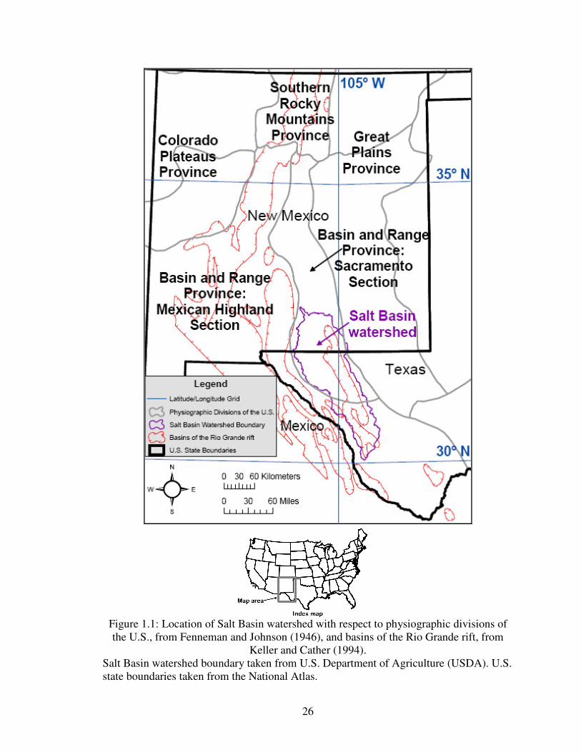
26
Figure 1.1: Location of Salt Basin watershed with respect to physiographic divisions of the U.S., from Fenneman and Johnson (1946), and basins of the Rio Grande rift, from
Keller and Cather (1994). Salt Basin watershed boundary taken from U.S. Department of Agriculture (USDA). U.S. state boundaries taken from the National Atlas.

27
Figure 1.2: Location map of Salt Basin watershed with respect to populated places and
U.S. counties of New Mexico and Texas. Location of populated places, and U.S. county boundaries taken from the National Atlas.

28
Legend
Elevation
(meters)
High : 2,955
Low : 1,032
Watershed Boundaries
Babb Flexure - Bitterwell Break
Alkali flats/playa lakes
# Mountain Peaks
U.S. County Boundaries
U.S. State Boundaries
Figure 1.3: Location map of northern Salt Basin watershed, after Hutchison (2006). Elevation taken from the National Elevation Dataset (NED) 1-arc second DEM. Watershed boundaries taken from USDA. Location of Babb Flexure - Bitterwell Break taken from Goetz (1985). Location of alkali flats/playa lakes taken from National Hydrography Dataset (NHD) for New Mexico, and from Stoeser et al. (2005) for Texas.

29
Figure 1.4: Cenozoic intrusions in the Salt Basin region.
Location of Cenozoic intrusives taken from Stoeser et al. (2005). Alkalic to Calc-Alkalic Line separates calc-alkalic magmatism to the west from alkalic magmatism to the east, from McLemore and Guilinger (1993).
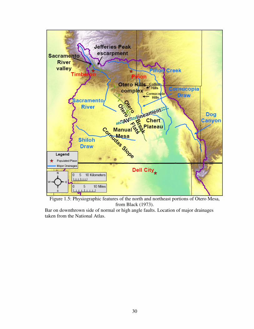
30
Figure 1.5: Physiographic features of the north and northeast portions of Otero Mesa,
from Black (1973). Bar on downthrown side of normal or high angle faults. Location of major drainages taken from the National Atlas.

31
Figure 1.6: Structural features of the north and northeast portions of Otero Mesa, from
Black (1973), Broadhead (2002), Goetz (1985), and Kelley (1971). Bar on downthrown side of normal or high angle faults. Location of Van Winkle Lake and closed topographic depressions taken from the U. S. Geological Survey’s 1:100,000-scale metric topographic map of Crow Flats, NM-TX.

32
Legend
Average Annual Temperature (1971-2000)
Median value for each area in ºC (ºF)
17 (63)
16 (61)
15 (59)
14 (57)
13 (55)
12 (53)
11 (51)
9.4 (49)
8.3 (47)
7.2 (45)
6.1 (43)
Figure 1.7: Average annual temperature (1971-2000), from USDA. Source scale: 1:250,000. Horizontal resolution: ~800 meters.

33
Legend
Average Maximum Annual Temperature (1971-2000)
Median value for each area in ºC (ºF)
36 (97)
35 (95)
34 (93)
33 (91)
32 (89)
31 (87)
29 (85)
28 (83)
27 (81)
26 (79)
25 (77)
24 (75)
23 (73)
22 (71)
21 (69)
Figure 1.8: Average maximum annual temperature (1971-2000), from USDA. Source scale: 1:250,000. Horizontal resolution: ~800 meters.

34
Legend
Average Minimum Annual Temperature (1971-2000)
Median value for each area in ºC (ºF)
1 (33)
-1 (31)
-2 (29)
-3 (27)
-4 (25)
-5 (23)
-6 (21)
-7 (19)
-8 (17)
-9 (15)
Figure 1.9: Average minimum annual temperature (1971-2000), from USDA. Source scale: 1:250,000. Horizontal resolution: ~800 meters.

35
Figure 1.10: Precipitation (cm) as a function of elevation (m) for recording stations in and
near the northern Salt Basin watershed, from Mayer and Sharp (1998). Recording stations are: AL – Alamogordo; CL – Cloudcroft; CO – Cornudas; DC – Dell City; EL – Elk; MH – Mayhill; MP – Mountain Park; OR – Orogrande; SF – Salt Flat; WS – White Sands.

36
Legend
Average Annual Precipitation (1971-2000)
Median value for each area in cm (in)
84 (33)
79 (31)
74 (29)
69 (27)
64 (25)
58 (23)
53 (21)
48 (19)
43 (17)
38 (15)
33 (13)
28 (11)
23 (9)
Figure 1.11: Average annual precipitation (1971-2000), from USDA. Mean monthly precipitation was calculated using PRISM, and then summed to produce the above map. Source scale: 1:250,000. Horizontal resolution: ~800 meters.

37
Figure 1.12: Level IV ecoregions within the northern Salt Basin watershed.
Ecoregions from the U.S. Environmental Protection Agency (EPA).

38
Figure 1.13: Location of the Diablo and Coahuila Platforms, from Shepard and Walper
(1982). Location of Steeruwitz thrust fault taken from Goetz (1977). Features formed about 1.25 Ga.
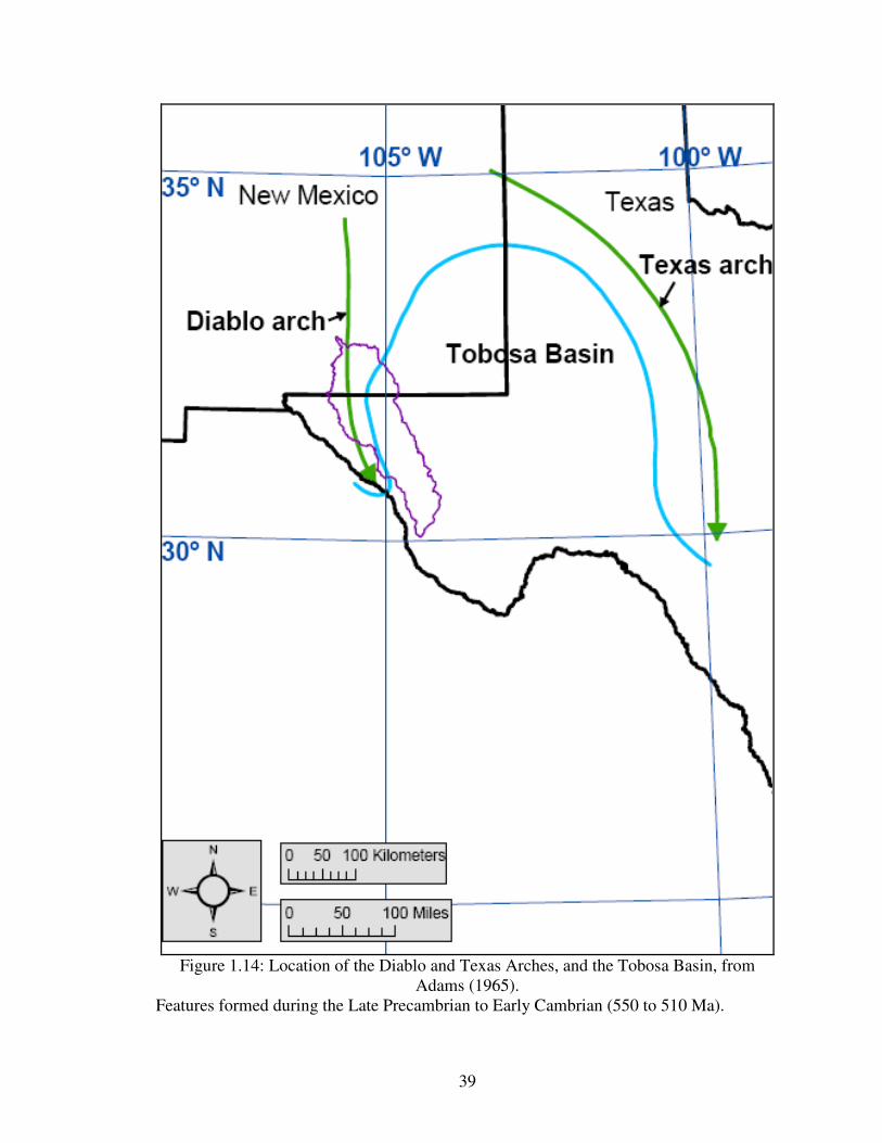
39
Figure 1.14: Location of the Diablo and Texas Arches, and the Tobosa Basin, from
Adams (1965). Features formed during the Late Precambrian to Early Cambrian (550 to 510 Ma).

40
Figure 1.15: Late-Pennsylvanian-to-Early-Permian tectonic features of the Salt Basin
region, from Ross and Ross (1985).

41
Figure 1.16: Location of the Mesozoic Chihuahua trough and Chihuahua tectonic belt,
from Haenggi (2002).
42
CHAPTER 2: GEOLOGIC FRAMEWORK
2.1: Previous Geologic Studies
Most of the earliest studies in the Salt Basin region were focused on describing
the geology of the Guadalupe Mountains (King, 1948). The first observations during the
mid-to-late-1800s were associated with the search for a suitable route for a railroad to the
Pacific coast (King, 1948). John Pope, G. G. Shumard, and B. F. Shumard were among
the most notable of these early explorers (King, 1948). H. S. Tarr of the Texas Geological
Survey was the last geologist to visit the Guadalupe Mountains, doing so in 1890, before
the turn of the century (King, 1948).
In the early 1900s important studies were conducted in the Guadalupe Mountains
by G. H. Girty and G. B. Richardson of the U.S. Geological Survey, and J. W. Beede
(Boyd, 1958; King, 1948). In the 1920s the development of oil fields in the region to the
northeast and east of the Guadalupe Mountains focused attention on the outcrops exposed
in the mountains (Boyd, 1958). A surge of papers were published on the description and
interpretation of rocks of the Guadalupe Mountains during this time period, including
work by Baker, Blanchard and Davis, Darton and Reeside, Crandall, King and King,
Lloyd, and Willis (Boyd, 1958; King, 1948).
P. B. King of U.S. Geological Survery conducted some of the most detailed and
important surveys of the stratigraphy and structure of the Salt Basin region in Texas
during the mid-1900s. King (1942) described the Permian of West Texas and

43
Southeastern New Mexico, and developed paleogeographic facies maps of the Permian
rocks deposited within the Salt Basin region. King (1948) and King (1965) thoroughly
described the stratigraphy and structure of the southern Guadalupe Mountains and the
Sierra Diablo, respectively.
Boyd (1958) studied the Permian sedimentary facies and stratigraphic
relationships of the central Guadalupe Mountains in New Mexico. Pray (1961) produced
a comprehensive account of the stratigraphy and structure of the southern Sacramento
Mountains. Kottlowski (1963) provided a regional summary of the Paleozoic and
Mesozoic strata of Southwestern and South-Central New Mexico, which included
isopach and facies maps. Hayes (1964) described the stratigraphy and structure of the
Guadalupe Mountains in New Mexico, which included a detailed description and
correlation of the Permian shelf-, shelf-margin-, and basin-facies rocks. Meyer (1968)
described the geology of Pennsylvanian and Lower Permian (Wolfcampian) rocks in
Southeastern New Mexico, which included isopach and lithofacies maps.
Kelley (1971) investigated the stratigraphy to the north, northeast, and east of the
Salt Basin region, as well as the regional structure. Kelley (1971) formally divided the
San Andres Formation into three members, in ascending order, the Rio Bonito, Bonney
Canyon, and Fourmile Draw Members. Newell et al. (1972) described the stratigraphy
and correlation of Permian shelf-, shelf-margin-, and basin-facies rocks of the Guadalupe
Mountains in New Mexico and Texas. Black (1973, 1975, and 1976) expanded on the
work of Kelley (1971) and produced the first descriptions and interpretations of the
stratigraphy and structure of the north-and-northeast portions of Otero Mesa. Foster

44
(1978) described the stratigraphy and structure of the southern Tularosa Basin, but also
included information on the western portion of Otero Mesa.
Goetz (1977, 1980, and 1985) focused on the structure and tectonics of the Salt
Basin graben in Texas. Many of the structures displayed on her tectonic sketch map
[Goetz, 1985] were incorporated into the structural maps produced for this thesis. King
and Harder (1985) studied the oil and gas potential of the Tularosa Basin, Otero Mesa,
and Salt Basin graben region in New Mexico and Texas. They described the stratigraphy
and depositional environments, produced isopach and lithofacies maps of Paleozoic
strata, and discussed the geophysics and structure of the region. Much of the subsurface
data presented in their report, in the form of oil-and-gas exploratory well logs and cross-
sections, was incorporated into this thesis.
Collins and Raney (1991 and 1997) provided a comprehensive description of the
Cenozoic structure of the Hueco bolson and the Salt Basin graben. McLemore and
Guilinger (1993), Nutt et al. (1997), and Nutt and O’Neill (1998) studied the geology and
mineral resources of the Cenozoic intrusions of the Cornudas Mountains in New Mexico.
O’Neill and Nutt (1998) mapped the geology of the Cornudas Mountains region. Their
discussion of the stratigraphic relationships around the New Mexico-Texas state line
proved invaluable in resolving the differences between the geologic maps of New Mexico
and Texas.
More recently, Broadhead (2002) investigated the subsurface structure of the Salt
Basin region in New Mexico. He identified numerous Ancestral Rocky Mountain
(Pennsylvanian-to-Permian), Laramide (Late Cretaceous-to-Early Cenozoic), and Basin-

45
and-Range (Cenozoic) structures within the Salt Basin region. His subsurface tectonic
map served as a primary reference for the structural maps produced for this thesis.
2.2: Stratigraphy, Depositional Environments, and Facies Distributions
Rocks exposed in the northern Salt Basin range from Precambrian to Quaternary.
(Figures 2.1 and 2.2) By far the predominant surface exposures consist of Permian rocks.
(Figure 2.1) Figure 2.2 presents a generalized stratigraphic chart of the geologic units in
the Salt Basin region, as well as the correlation of these units between different
geographic regions and depositional environments. Figures 2.4 through 2.16 present
paleogeographic reconstructions of the Salt Basin region from the Late Precambrian, 550
Ma, to the present, and are referenced throughout this section to illustrate the depositional
environments associated with the geologic units described herein. Figures 2.17 through
2.19 illustrate the resultant distribution of facies during the Permian, and are also
referenced throughout this section.
2.2.a: Proterozoic
There are very few exposures of Precambrian rocks in the Salt Basin, although
some do crop out on the Diablo Plateau at Pump Station Hills, in the southern Hueco
Mountains, in the southern portion of the Sierra Diablo region, and along the base of the
Sacramento Mountains escarpment south of Alamogordo, New Mexico (Denison and
Hetherington, 1969; King, 1965; Masson, 1956; Pray, 1961). Pray (1961) described the
Precambrian rocks exposed in the Sacramento Mountains as slightly metamorphosed
sedimentary rocks (largely shale, siltstone, and fine-grained quartz sandstone) intruded by
igneous sills of basic-to-intermediate composition, some of which are porphyritic. In the
Hueco Mountains the Precambrian is a red, partly micrographic perthite granite (Denison

46
and Hetherington, 1969). Masson (1956) extensively described the Precambrian rocks at
Pump Station Hills and found the dominant rock type to be a rhyolite porphyry, with
some fine micrographic granite porphyry and other rock types also present.
Oil-and-gas exploratory well cores provide the primary source of information on
the type and distribution of Precambrian rocks in the region. Precambrian rocks include
the 1.4 Ga and older Chaves Granite and Granitic Gneiss, the 1.25 Ga Carrizo Mountain
Group metamorphic rocks, the 1.0 to 1.1 Ga DeBaca-Swisher metasedimentary and
basaltic rocks, and the 1.0 Ga Franklin Mountains igneous rocks (Denison et al., 1984).
(Figure 2.3) Precambrian rocks exposed in the Sacramento Mountains and encountered in
the Southern Production Co., Cloudcroft Unit #1 (SPCCLU1) well [Figure 3.1] fall
within the DeBaca-Swisher Terrain (Denison and Hetherington, 1969; Pray, 1961).
(Figure 2.3) Precambrian rocks exposed in the southern Hueco Mountains and at Pump
Station Hills are related to the Franklin Mountains igneous rocks (Denison and
Hetherington, 1969). (Figure 2.3) In the southern portion of the Sierra Diablo region the
Precambrian is represented by the Carrizo Mountain Group, consisting of quartzite,
schist, phyllite, and marble overlain and intruded by metarhyolite and amphibolite, which
has been thrust over the thick marbles with interbedded phyllite, chert, and pyroclastic
volcanic rocks of the Allamore Formation and the overlying coarse-grained conglomerate
and sandstone of the Hazel Formation (Denison and Hetherington, 1969).
Rocks of the Chaves Granitic Terrain were covered by a varied series of later
Precambrian sediments (Black, 1973). These later sediments were eventually
metamorphosed to form the DeBaca-Swisher Terrain, which were contemporaneously or
slightly later intruded by the Franklin Mountains igneous rocks (Black, 1973). These

47
rocks were eventually deeply eroded, and the overlying Lower Paleozoic rocks were
deposited over this heavily eroded surface (Black, 1973).
2.2.b: Early Paleozoic
During the Early Paleozoic, the Salt Basin region was situated along the passive
margin of the southwestern North American craton (King and Harder, 1985). Seas spread
across the region, depositing the Cambrian-Ordovician Bliss Sandstone, Ordovician
carbonates of the El Paso and Montoya Groups (LeMone, 1969), and Silurian carbonates
of the Fusselman Formation (King and Harder, 1985). (Figures 2.4 and 2.5) In the Salt
Basin, all of these Lower Paleozoic units are exposed in the Sacramento and Hueco
Mountains, and in the Sierra Diablo region (King, 1965; King et al., 1945; Kottlowski,
1963; Pray, 1961).
The Bliss Sandstone is predominantly a quartz sandstone, partly glauconitic, with
thin interbeds and lenses of siliceous hematite, arenaceous shale, and arenaceous
limestone that records deposition in a shallow marine environment far from the shoreline
(Kottlowski, 1963). (Figures 2.4b, 2.4c, and 2.4d) In general, the Bliss Sandstone
thickens southward, but was removed from areas to the north and south due to uplift of
the Pedernal landmass and Diablo Platform, respectively, during the Pennsylvanian to
Early Permian (Kottlowski, 1963).
The El Paso Group (LeMone, 1969) is equivalent to the Ellenburger Group, which
is often indicated in subsurface oil-and-gas wells in the Permian Basin (Hayes, 1964;
Kottlowski, 1963). In the Sacramento Mountains the El Paso Group consists of dolomite,
minor sandy dolomite, and dolomitic quartz sandstones, which record deposition on a
broad open-marine shelf, in shallow, moderately turbulent water (Pray, 1961). (Figures

48
2.4d and 2.5a) In the Hueco Mountains the El Paso Group consists predominantly of thin-
bedded, mottled limestone, with thicker-bedded, dolomitic limestone near the top of the
unit (King et al., 1945). In general, the El Paso Group thickens southward due to erosion
to the north before deposition of the overlying Montoya Formation (Kottlowski, 1963).
Similar to the Bliss Sandstone, the El Paso Group was removed from the areas associated
with the uplift of the Pedernal landmass and the Diablo Platform (Kottlowski, 1963).
The Bliss and El Paso are time-transgressive units that are older to the west and
become younger to the east, due to the transgression of the Cambrian and Early
Ordovician sea from west to east (Hayes, 1964; Kottlowski, 1963; LeMone, 1969).
(Figures 2.4b through 2.5a) In actuality this transgression was not a simple, single
transgression, but a series of transgressions and regressions (LeMone, 1969).
The Montoya Group was originally deposited as a limestone, but has since been
largely irregularly dolomitized (Kottlowski, 1963). (Figure 2.5b) In the Hueco
Mountains, however, about 50% of the Montoya is limestone (Kottlowski, 1963). The
Montoya Group generally increases in thickness from north to south, the bulk of this
increase being depositional (Kottlowski, 1963). Similar to the Bliss and El Paso, the
Montoya was removed from the areas associated with the uplift of the Pedernal landmass
and the Diablo Platform (Kottlowski, 1963). Valmont Dolomite has been used by Pray
(1961) in the Sacramento Mountains to describe the distinctive upper unit of the Montoya
Group.
The Fusselman Formation is an aphanitic to coarsely crystalline, grayish brown to
dark gray, massive, light brown- to dark yellowish brown-weathering dolomite
(Kottlowski, 1963). The Fusselman thickens from north to south, due primarily to Late

49
Silurian and Early Devonian erosion to the north, but also probably depositional
thickening to the south (Kottlowski, 1963). (Figures 2.5d and 2.6a) The Fusselman
records deposition on a shallow marine shelf adjacent to the subsiding Tobosa Basin to
the southeast (McGlasson, 1969). (Figures 1.14, 2.5c, and 2.5d) The Fusselman is
unconformably overlain by Devonian strata, and a Devonian eroded edge is located just
north of Alamogordo, New Mexico in the Sacramento Mountains (Kottlowski, 1963).
The Fusselman was also removed from the area associated with the uplift of the Diablo
Platform during the Early Wolfcampian (Kottlowski, 1963).
Uplift of the Peñasco dome to the north beveled and eroded these older Paleozoic
rocks, before shallow seas again spread over the region and deposited the Devonian
Oñate and Sly Gap Formations, the Percha and Woodford Shales, and the cherty
Canutillo Formation (King and Harder, 1985; Kottlowski, 1969). (Figures 2.6a, 2.6b, and
2.6c) Similar to the Fusselman Formation, the Devonian units record deposition on a
shallow marine shelf adjacent to the subsiding Tobosa Basin to the southeast
(McGlasson, 1969). (Figures 2.6b and 2.6c) The Devonian Oñate Formation silty facies is
found throughout the Sacramento Mountains, but transitions to the gray-black Percha
Shale to the south (Kottlowski, 1963; Pray, 1961). The silty Sly Gap facies is largely
restricted to the northern and central parts of the Sacramento Mountains (Pray, 1961).
The Devonian thickens further to the south in the Hueco Mountains, where it contains an
upper shaly zone consisting mostly of soft, calcareous, silty shale and lenses of silty
limestone equivalent to the Oñate, Sly Gap and Percha to the north, and a lower zone of
cherty limestones of the Canutillo Formation (Kottlowski, 1963). The Devonian is also
exposed in the Sierra Diablo region (King, 1965).
50
The Oñate and Sly Gap Formations record deposition far from a shoreline
(Kottlowski, 1963). (Figure 2.6c) The Percha Shale is equivalent to the subsurface
Woodford Shale farther to the east (McGlasson, 1969). East of the Hueco Mountains, in
the subsurface, the Canutillo Formation becomes argillaceous and eventually grades into
the lower part of the Percha/Woodford Shale (McGlasson, 1969). The black, fissile
Percha/Woodford Shale and the cherty Canutillo Formation record deposition in
restricted, stagnant basins (Kottlowski, 1963). (Figures 2.6b and 2.6c) In general the
Devonian units thicken from north to south (Kottlowski, 1963). The Devonian units are
also characterized by a similar Late Pennsylvanian and Early Permian eroded edge to the
north in the Sacramento Mountains and to the south on the Diablo Platform as the Bliss,
El Paso, Montoya, and Fusselman (Kottlowski, 1963).
2.2.c: Late Paleozoic
During the Mississippian and Pennsylvanian, the seas extended even farther into
the North American craton, depositing a wide range of carbonates (King and Harder,
1985). (Figures 2.6d through 2.8d) Mississippian and Pennsylvanian rocks are exposed in
the Sacramento and Hueco Mountains, and in the Sierra Diablo region (King, 1965; King
et al., 1945; Kottlowski, 1963; Pray, 1961). In general, Mississippian strata thicken to the
south, due to depositional thickening to the south, and erosional thinning associated with
the Pedernal uplift to the north (Kottlowski, 1963). Mississippian strata were also
removed from the region of the Diablo Platform due to uplift during the Early
Wolfcampian (Kottlowski, 1963). Chesterian strata pinch out to the north of a line
approximately along latitude 33º N, which is likely close to the northern shoreline, due to
deposition on an inclined surface associated with pre-Chesterian deformation

51
(Kottlowski, 1969; Meyer, 1968). (Figures 2.7a, 2.7b, and 2.7c) Upper Mississippian
(Chesterian) strata (Helms Formation of south-central New Mexico and western-most
Texas, and its western equivalent the Paradise Formation) consist mainly of massive
limestones which grade abruptly southeastward into black shales of the Delaware Basin
that are considered to by equivalent to the Barnett Shale of southeast New Mexico and
west Texas (Kottlowski, 1969; Meyer, 1968).
North of latitude 33º N Mississippian rocks are Meramecian (Meyer, 1968).
Farther to the northwest the strata (Caballero and Lake Valley Formations) are mainly
Lower to Middle Mississippian (Kinderhookian to Osagean) (Kottlowski, 1963; Meyer,
1968). Most of these Lower to Middle Mississippian strata are crinoidal limestones that
formed biohermal reefs (Kottlowski, 1969). (Figures 2.6d and 2.7a) The Middle
Mississippian (Meramec) Rancheria Formation forms an anomalous dark siliceous
limestone facies that thins and abruptly grades northward from the Franklin Mountains to
near the northern limit of the Helms Formation in the southern Sacramento Mountains
(Kottlowski, 1963; Kottlowski, 1969). The Rancheria also occurs locally throughout
southeastern New Mexico, and represents deposition in a relatively deep, stagnant basin
(Kottlowski, 1969). (Figures 2.7a and 2.7b)
Late Mississippian-to-Early Pennsylvanian uplift to the north in central and
northern New Mexico tilted and eroded the older Paleozoic units such that Pennsylvanian
strata were deposited on Mississippian to Precambrian rocks from south to north
(Kottlowski, 1969; Meyer, 1968). (Figure 2.7c) In the Salt Basin, Lower Pennsylvanian
(Morrowan) beds unconformably overlie Mississippian beds with a hiatus that represents
the Early Pennsylvanian Springeran (Meyer, 1968). Early movements along the northern

52
portion of the Pedernal uplift during the Late Mississippian-to-Early Pennsylvanian
provided a source of sediment to the subsiding Orogrande and Delaware Basins to the
west and east, respectively (Kottlowski, 1963; Meyer, 1968). (Figures 2.7b, 2.7c, and
2.7d) The Pennsylvanian was marked by a major transgression that began in the
Morrowan and climaxed in the Virgilian at the close of the Pennsylvanian (Meyer, 1968).
(Figures 2.7d through 2.8d)
Like the Mississippian, the Pennsylvanian in southeastern New Mexico was a
time of carbonate deposition, with the carbonates most commonly being interbedded with
shale (Meyer, 1968). Pennsylvanian rocks in southeastern New Mexico represent a
marine sequence of two principal facies: 1) black limestones and shales, and 2) light-
colored fossiliferous limestones and variegated shales (Meyer, 1968). East of the
Pedernal uplift, Pennsylvanian sediments transgress southeast to northwest, onlapping
onto the uplift (Meyer, 1968). Upper Mississippian and Pennsylvanian strata were
deposited continuously across the southern quarter of the Pedernal uplift (Meyer, 1968).
During the Pennsylvanian, the northern three-quarters of the Pedernal uplift was never a
high mountain range, but ranged from a slight emergent feature to a shoal area at various
times and places (Meyer, 1968).
Subsurface geologists of west Texas often use Bend, Strawn, Canyon, and Cisco
for Derryan, Desmoinesian, Missourian, and Virgilian nomenclature, respectively
(Meyer, 1968). Also, the Derryan Stage is correlative with the Atokan Stage (Meyer,
1968). In the Sacramento Mountains, Pray (1961) divided the Pennsylvanian into three
major rock units in ascending order: the Gobbler, Beeman, and Holder Formations. The
Gobbler ranges in age from Morrowan to Middle Missourian, the Beeman ranges in age
53
from Middle to Upper Missourian, and the Holder is essentially Virgilian (Pray, 1961).
Another term, Magdalena (Formation or Group), has been used to refer to all of the
Pennsylvanian as well as part of the Permian below the Abo Formation (Pray, 1961).
Panther Seep Formation is another term that has been applied to Upper Pennsylvanian
(Virgilian) strata in the San Andres Mountains to the west (Kottlowski, 1963; Pray,
1961).
Uplift of the southern portion of the Pedernals during the Late Pennsylvanian
provided a large source of sediment to the Orogrande and Delaware Basins, and largely
removed the thick sections of Mississippian and Pennsylvanian strata from the region
(King and Harder, 1985; Meyer, 1968). (Figures 2.8c and 2.8d) A regression followed
during the Wolfcampian, as red beds derived from a major uplift to the northwest of the
region spread south over the Pedernal uplift and interfingered with marine deposits of the
Northwestern and Sacramento shelves (Meyer, 1968). (Figures 2.9a through 2.9d) By
Late Wolfcampian, the Pedernal landmass was almost entirely buried beneath the red-
beds of the Abo Formation (King and Harder, 1985). (Figure 2.9d)
2.2.d: Permian
In addition to encompassing the majority of surface exposures in the northern Salt
Basin watershed, Permian rocks also form the primary aquifer in the Salt Basin (Huff and
Chace, 2006). These Permian units can be divided into 3 distinct facies (shelf, shelf-
margin, and basin), similar to those presented by Nielson and Sharp (1985). The margin
of the Delaware Basin evolved from a poorly defined boundary during the Wolfcampian
to a well defined boundary fringed by the massive reef dolomites and limestones of the
Goat Seep and Capitan Formations during the Guadalupian (Hayes, 1964). (Figures 2.9a

54
through 2.11a) As depicted by Black (1975), the margin of the basin also progressed
towards the southeast during the Permian. (Figure 2.20)
Figures 2.9a through 2.11a present the paleogeographic reconstructions for the
Permian. Examination of these reconstructions reveals that the Salt Basin region was
dominated by a landmass, associated with the Diablo Platform, surrounded by a shallow
marine environment. This appears to contradict the predominantly shallow marine
environment suggested by the facies distributions displayed in Figures 2.17 through 2.19.
However, the facies distribution maps indicate a landmass over a large region of the
Texas portion of the Salt Basin during the Early Leonardian [Figure 2.17b], and over a
large region of the western portion of the Salt Basin during the Guadalupian [Figures
2.18b through 2.19b]. In addition, the location of the landmass in the paleogeographic
reconstructions corresponds closely to the location of the Diablo Platform as presented in
Shepard and Walper (1982) [Figure 1.13] and Ross and Ross (1985) [Figure 1.15].
The Early Leonardian of Figure 2.17b corresponds approximately to the Early
Permian (280 Ma) and (278 Ma) paleogeographic reconstructions of Figures 2.9d and
2.10a, which indicate a landmass a little farther to the east than is displayed in Figure
2.17b. The Early Permian (275 Ma) paleogeographic reconstruction of Figure 2.10b
indicates that the New Mexico portion of the Salt Basin was dominated by a marine
environment. This is supported by the Late Leonardian facies distribution displayed in
Figure 2.18a. The Guadalupian of Figures 2.18b through 2.19b corresponds
approximately to the Early Permian (270 Ma) and (260 Ma) paleogeographic
reconstructions of Figures 2.10c and 2.10d, which indicate a landmass a little farther to
the east than is displayed in Figures 2.18b through 2.19b.

55
Despite the apparent agreement between the paleogeographic reconstructions and
the facies distributions, it is also possible that the extent and location of the landmass in
the paleogeographic reconstructions is incorrect. For example, most of the facies
distribution figures suggest that the landmass in the reconstructions should be located a
little farther to the west. The paleogeographic reconstructions were obtained from Blakey
(2009a), who produced these maps to illustrate the regional paleogeographic evolution of
Southwestern North America. Therefore, the extent and location of the landmass within
the Salt Basin from these regional reconstructions could be slightly inaccurate, as
opposed to what a more localized paleogeographic reconstruction of the Salt Basin region
might reveal. Also, the paleogeographic reconstructions from Blakey (2009a) were
imported into ArcGIS and georeferenced using the U.S. state boundaries displayed on the
reconstructions. The Salt Basin watershed boundary was then overlaid on top of the
reconstructions. The georeferencing technique employed probably created some errors in
the exact position of the reconstructions relative to the Salt Basin watershed boundary. As
a result, all of the paleogeographic reconstructions should be viewed as an indication of
the general, rather than exact, distribution of geographic features within the Salt Basin.
-Basin-facies
Rocks of the basin-facies consist of, from oldest to youngest, the Wolfcamp
Formation [Figures 2.9a through 2.9d, and Figure 2.17a], the Leonardian Bone Spring
Limestone [Figures 2.9d, 2.10a, 2.10b, 2.17b, and 2.18a], the Guadalupian Delaware
Mountain Group [Figures 2.10c, 2.10d, 2.18b, 2.19a, and 2.19b], and the Ochoan Castile,
Salado, and Rustler Formations [Figures 2.10d and 2.11a] (Hayes, 1964).

56
Hayes (1964) proposed that the term Hueco Limestone be restricted to those
Wolfcampian units of the Northwestern shelf based on a pronounced difference in
lithology between the shelf and basin Wolfcampian units. (Figure 2.17a) Thus, he
tentatively assigned Wolfcampian rocks of the Delaware Basin to the Wolfcamp
Formation. Rocks of the Wolfcamp basin-facies are not exposed in the Guadalupe or
Sierra Diablo Mountains, and thus lithologic descriptions are based on subsurface data
(Hayes, 1964; King, 1983). In the northern portion of the Delaware Basin the Wolfcamp
Series ranges from 450 to 530 meters (1,490 to 1,750 feet) thick, and consists of about
equal amounts of gray, black, or brown shale, and fine-crystalline rarely cherty brownish
limestone, with a few thin beds of fine-grained gray micaceous and calcareous sandstone
(Hayes, 1964). (Figure 2.17a) The Wolfcamp Series lies unconformably on the middle
part of the Pennsylvanian sequence, as the upper part is missing (Hayes, 1964).
King (1983) restricted the term Bone Spring Limestone to the black limestone
facies deposited in a deep, stagnant water environment. (Figures 2.17b and 2.18a)
Outcrops of the Bone Spring Limestone are present in the southern Guadalupe
Mountains, and in the Delaware, Baylor, and Sierra Diablo Mountains (King, 1948; King,
1965). The Leonardian Bone Spring Formation consists predominantly of fine-grained,
dark-colored, arenaceous limestone in thin (generally < 1 foot thick) even beds, with
minor amounts of platy, sandy, black shale and fine-grained, buff quartz sandstone
(Newell et al., 1972). The Bone Spring Formation ranges from 600 to 760 meters (2,000
to 2,500 feet) thick near the margin of the Delaware Basin, and becomes somewhat
dolomitic as it approaches the basin margin (Newell et al., 1972). The Bone Spring
Limestone (King, 1934) has an average calcite-dolomite ratio of 79:21 (Hayes, 1964).

57
During the first half of Leonard time, the Bone Spring Limestone extended several
kilometers farther shelfward across the basin margin, but does not reach the Union Oil
Co., Federal White #1 (UNOCFW1) well in the Guadalupe Mountains (Hayes, 1964;
King, 1948). (Figures 2.17b and 3.1) Instead, the Bone Spring Limestone grades
northwestward into the lower portion of the Victorio Peak Limestone (Hayes, 1964).
(Figure 2.17b)
In the Sierra Diablo region the lower part of the Bone Spring Limestone
interfingers with tongues of lighter gray, more clastic or dolomitic shelf-margin deposits
(King, 1965). (Figures 2.17b and 2.18a) Along the Babb and Victorio flexures the Bone
Spring Limestone interfingers with thickening limestone reefs, and wedges out farther to
the south (King, 1965). In the Permian Delaware Basin margin region now occupied by
the northern portion of the Sierra Diablo Mountains the Bone Spring Limestone thins
southwestward from 268 meters (880 feet) to a few hundred feet by overlap on the
underlying Hueco Limestone and intergradation with the Victorio Peak Limestone (King,
1965). In the southern portion of the Sierra Diablo the Bone Spring thickens southward
towards the Victorio flexure from 295 meters (970 feet) to 320 meters (1,050 feet) as it
passes into the marginal facies (King, 1965).
The Guadalupian Delaware Mountain Group attains a maximum thickness of
1,220 meters (4,000 feet) in the Delaware Basin (Newell et al., 1972). The Delaware
Mountain Group consists predominantly of gray or black, to weathered buff or tan,
flaggy, thin-bedded, fine-grained quartz sandstone with a few thin beds of detrital
limestone (Newell et al., 1972). The quartz sandstones of the Delaware Mountain Group
wedge out around the margin of the basin, and are replaced by massive dolomites and
58
limestones of the Goat Seep and Capitan Formations (Newell et al., 1972). (Figures 2.19a
and 2.19b) The Delaware Mountain Group consists of three formations, in ascending
order: the Brushy Canyon, Cherry Canyon, and Bell Canyon Formations (Newell et al.,
1972). (Figures 2.18b through 2.19b)
Limestone beds of the Brushy Canyon Formation have an average calcite-
dolomite ratio of 73:27 (Hayes, 1964). The Brushy Canyon Formation wedges out
completely over the Bone Spring flexure, and has no equivalent strata on the shelf
(Newell et al., 1972). (Figure 2.18b) The Brushy Canyon Formation filled the Delaware
Basin level with sand (Newell et al., 1972). (Figure 2.18b) The lowermost sandstone
tongue of the Cherry Canyon Formation is unique in that it extends about 24 km (15
miles) shelfward, where it then grades into dolomites of the lower San Andres Formation
(Hayes, 1964; Newell et al., 1972). The lowest limestone of the Cherry Canyon
Formation, the Getaway Member, is strongly calcitic in the Delaware Basin, with an
average calcite-dolomite ratio of 80:20 (Hayes, 1964). It passes across the margin of the
basin as thick-bedded dolomite beneath the Goat Seep Formation, before grading into the
San Andres Formation on the shelf (Newell et al., 1972). The middle and upper limestone
member tongues of the Cherry Canyon Formation (South Wells and Manzanita
Members), and the five limestone member tongues of the Bell Canyon Formation (in
ascending order, Hegler, Pinery, Rader, McCombs, and Lamar) thicken towards the basin
margin where they form massive, inclined beds of reef talus before passing into the Goat
Seep and Capitan Formations, respectively (Newell et al., 1972). (Figures 2.19a and
2.19b) In the Delaware Basin the South Wells and Manzanita Members are strongly

59
dolomitic, while the Bell Canyon Formation limestone members are strongly calcitic
(Hayes, 1964).
Ochoan rocks of the Castile, Salado, and Rustler Formations are present only in
the Delaware Basin, having been removed by erosion from the margin and shelf regions
(Hayes, 1964). None of these rocks fall within the model domain, and thus will not be
discussed.
-Shelf-margin-facies
Rocks of the shelf-margin-facies consist of, from oldest to youngest, the
Wolfcamp Series [Figures 2.9a through 2.9d, and Figure 2.17a], the Leonardian Victorio
Peak Limestone and Cutoff Shale [Figures 2.9d, 2.10a, 2.10b, 2.17b, and 2.18a], and the
Guadalupian sandstone tongue of the Cherry Canyon Formation, Goat Seep Dolomite,
and Capitan Limestone [Figures 2.10c, 2.10d, 2.19a, and 2.19b] (Hayes, 1964).
The margin of the Delaware Basin was poorly defined during the Wolfcampian,
as compared to during the Leonardian and Guadalupian (Hayes, 1964). As a result, a
broad transition zone of marginal facies Wolfcamp rocks probably exists, although no
outcrops exist in the Guadalupe Mountains to confirm the position of this zone (Hayes,
1964). (Figure 2.17a) In the Guadalupe Mountains, the Union Oil Co., Federal White #1
(UNOCFW1) well [Figure 3.1] apparently penetrates the shelfward portion of this broad
transition zone as the Wolfcamp Series consists mostly of fine-crystalline light- to dark-
gray dolomite containing minor amounts of gray, brown, green, and black shale (Hayes,
1964). The basal portion of the Wolfcamp Series in the Union Oil Co., Federal White #1
well consists predominantly of light- to dark-gray limestone, suggesting that the
transition zone is located farther shelfward in the basal part of the series (Hayes, 1964).

60
In the central and northern part of the Sierra Diablo region the outcropping Wolfcamp
(Hueco Formation) is composed of a thin-bedded dolomitic limestone facies, and further
to the northeast includes marl and thin- to thick-bedded limestone (King, 1983). (Figure
2.17a) These facies formed along the margin of the Delaware Basin (King, 1983). Unlike
during the Guadalupian, no extensive reefs formed along the margin of the Delaware
Basin during the Wolfcampian (King, 1983).
The Victorio Peak Limestone is exposed in the Guadalupe and Sierra Diablo
Mountains, and on the Diablo Plateau (King, 1983; Newell et al., 1972). (Figure 2.1)
Massive, white and light-buff dolomite and limestone of the Victorio Peak Limestone
abruptly replaces black limestones of the Bone Spring Formation around the margin of
the Delaware Basin (Newell et al., 1972). (Figures 2.17b and 2.18a) The Victorio Peak
Limestone in the Guadalupe Mountains region is restricted to a narrow belt a few
kilometers wide around the basin margin (Newell et al., 1972). (Figure 2.17b) Six or
eight kilometers (four or five miles) shelfward of the basin rim, the lower and middle
portions of the Victorio Peak Limestone and the lower Bone Spring Formation grade into
the dolomite and gypsiferous shelf-facies of the Yeso Formation (Newell et al., 1972)
(Figure 2.17b) The upper portion of the Victorio Peak Limestone grades northwestward
into the basal part of the San Andres Formation (Hayes, 1964). (Figure 2.18a) In the
southern portion of the Guadalupe Mountains, King (1948) described the Victorio Peak
as a thick-bedded, gray limestone 244 meters (800 feet) thick.
In the Sierra Diablo and on the Diablo Platform the Victorio Peak Limestone
ranges from 305 to 457 meters (1,000 to 1,500 feet) thick, and, where the Bone Spring
Limestone has wedged out beneath, lies unconformably on the Hueco Limestone (King,

61
1983). Although the Victorio Peak Limestone is predominantly of the shelf-margin-
facies, it does not contain frame-building organic structures similar to those found in the
overlying Goat Seep and Capitan Limestones, and is more accurately described as a
limestone bank rather than a limestone reef (King, 1948; King, 1983). In the northeast
Sierra Diablo the Victorio Peak Limestone consists of a light-gray, thick-bedded calcitic
limestone facies, while in the southwest Sierra Diablo the Victorio Peak Limestone
consists of a thin-bedded, dolomitic limestone facies (King, 1965). King (1965)
interpreted the dolomitic limestone facies to have been deposited on a back-reef platform
area behind the low banks formed by the calcitic limestone facies.
At the north end of the Sierra Diablo and north of the Bone Spring flexure in the
Guadalupe Mountains, the Cutoff Shale, composed of a few hundred feet (30 to 91
meters [100 to 300 feet] in the Guadalupe Mountains, and 76 to 84 meters [250 to 275
feet] in the Sierra Diablo region) of thin-bedded limestone interbedded with dark
siliceous shale, sandy shale, and soft-weathering sandstone, overlies the Victorio Peak
Limestone (Hayes, 1964; King, 1965; King, 1983; Newell et al., 1972). In the Guadalupe
Mountains, the Cutoff Shale grades to the northwest over a broad transition zone into the
San Andres Formation (Hayes, 1964).
As mentioned above, in the Guadalupe Mountains 61 to 91 meters (200 to 300
feet) of the lowermost sandstone tongue of the Cherry Canyon Formation extends across
the shelf-margin where it then grades into the lower San Andres Formation of the shelf-
facies. In the Sierra Diablo region the Cherry Canyon sandstone tongue is 46 to 58 meters
(150 to 190 feet) thick, and unconformably overlies the Cutoff Shale (King, 1965).

62
In the Guadalupe Mountains the Middle Guadalupian Goat Seep Formation is a
narrow reef belt (no more than 1.5 kilometers or 1 mile wide) of predominantly massive
dolomite that is equivalent to the Queen and Grayburg Formations of the shelf-facies
Artesia Group (Newell et al., 1972). (Figure 2.19a) In the Guadalupe Mountains the Goat
Seep ranges in thickness from171 to 366 meters (560 to 1,200 feet) (King, 1948). In the
northern part of the Sierra Diablo region the Goat Seep Limestone conformably overlies
and intertongues with portions of the Cherry Canyon sandstone tongue (King, 1965).
(Figure 2.19a) In the Sierra Diablo region the Goat Seep is 61 meters (200 feet) thick,
although its upper contact is missing (King, 1965).
The Capitan Formation of massive white limestones and thin-bedded black
limestones and sandstones formed a 4 to 6 km (2.5 to 3.5 mile) wide reef zone for a
distance of about 560 to 640 kilometers (350 to 400 miles) around the rim of the
Delaware Basin during the Middle to Late Guadalupian (Newell et al., 1972). (Figure
2.19b) About 64 kilometers (40 miles) of the Capitan reef outcrops in the Guadalupe
Mountains (Newell et al., 1972). (Figure 2.1) The Capitan Limestone also outcrops in the
Patterson Hills (King, 1948). (Figure 2.1) In the southern Guadalupe Mountains the
Capitan Limestone ranges in thickness from 305 to 610 meters (1,000 to 2,000 feet)
(King, 1948).
-Shelf-facies
Rocks of the shelf-facies consist of, from oldest to youngest, the Wolfcampian
Abo Formation and Hueco Limestone, including the Pow Wow Conglomerate Member,
[Figures 2.9a through 2.9d, and Figure 2.17a], the Leonardian Yeso Formation [Figures

63
2.9d, 2.10a, 2.10b, and 2.17b], and the Guadalupian San Andres Formation and Artesia
Group [Figures 2.10c, 2.10d, 2.18a, and 2.18b] (Hayes, 1964).
The Wolfcampian was marked by a regression, during which red beds derived
from a major uplift to the northwest of the region spread southeast over the Pedernal
uplift and interfingered with the marine deposits of the Northwestern shelf (Meyer,
1968). (Figures 2.9a through 2.9d, and Figure 2.17a) The interfingering of red beds with
marine shelf limestones and shales also occurred southward in the Orogrande basin and
over the Sacramento shelf (Meyer, 1968). (Figure 2.17a) In the Guadalupe Mountains
region of the Northwestern shelf, Hayes (1964) identified two distinct members of the
Hueco Limestone. The lower member consists of medium-gray, fine-crystalline, locally
siliceous limestone interbedded with reddish-brown, greenish-gray, and gray shale and
minor amounts of fine-grained sandstone, and reaches a maximum thickness of at least
150 meters (500 feet) (Hayes, 1964). The upper member ranges in thickness from about
270 to 405 meters (880 to 1,330 feet), consists predominantly of medium-gray fine-
crystalline dolomite, subordinate greenish-gray shale, and rare grayish-red shale, and
grades northwestward into the Abo Formation (Hayes, 1964). The upper member of the
Hueco Limestone grades basinward into fine- to coarse-crystalline dolomite beds referred
to as “Abo reefs” (Hayes, 1964). Meyer (1968) noted that east of the Pedernal uplift the
overlying Yeso Formation is separated from Wolfcampian strata by another Leonardian
unit consisting of red beds and brown fine-grained anhydritic dolomite (Abo Formation
of the subsurface) that grades to the south and east into a narrow zone of white coarse-
grained dolomite (Abo Reef of the subsurface), and then into the black siltstones and
black massive limestones of the lower Bone Spring Formation. The upper member of

64
Hayes (1964) thus probably corresponds to the Abo Formation of the subsurface that
Meyer (1968) proposed be designated as the Leonardian Wichita Formation. As Hayes
(1964) writes, “Much of the Hueco Limestone is laterally equivalent to rocks of the
Wolfcamp Series of the Delaware basin, but the uppermost part is probably equivalent to
the basal part of the Bone Spring of Leonard age.”
On the Sacramento shelf, Wolfcampian rocks consist of a southward thickening
middle tongue of gray shales, limestones, and dolomites designated as the Pendejo tongue
of the Hueco Limestone by Pray (1961), surrounded by thick beds of arkose and red shale
at the base and at the top, designated as the Danley Ranch and Lee Ranch tongues of the
Abo Formation, respectively, by Bachman and Hayes (1958). Pray (1961) described the
Abo Formation in the Sacramento Mountains as a sequence of dark, reddish-brown
mudstone and arkose. The upper and lower tongues are interpreted by Pray (1961) to
represent fresh-water deposits laid down on a broad surface of little relief. (Figures 2.9a
through 2.9d) In the Sacramento Mountains the Abo Formation ranges from about 61 to
152 meters (200 to 500 feet) thick, and thickens southward along the escarpment to a
maximum of about 168 meters (550 feet) near T. 19 S. (Pray, 1961). The thickness of the
tongues of the Abo Formation is structurally controlled, and therefore deformation
initiated during the Late Pennsylvanian probably continued into the Early Permian (Pray,
1961).
The Pendejo tongue generally thins from west to east, and pinches out over the
axis of the Pedernal landmass (Black, 1973). Eastward across the Pedernal uplift only the
upper red shales are present, and the Abo Formation lies unconformably on Missourian
(Pennsylvanian) to Precambrian rocks (Kottlowski, 1963; Meyer, 1968). In the Delaware

65
and Orogrande basins, Wolfcampian rocks are conformable with the underlying Virgilian
(Pennsylvanian) (Meyer, 1968). In the southern portion of the Sacramento Mountains, the
Abo Formation lies on the Pennsylvanian with an angular unconformity (Pray, 1961).
The Abo Formation grades sharply over a short distance into the overlying, conformable
Yeso Formation, which Pray (1961) believed represented the sudden invasion of the Yeso
marine depositional environment. Black (1973) considered the basal conglomerates in the
Danley Ranch tongue to be depositionally equivalent to the Pow Wow Conglomerate
Member of the Hueco Formation mapped in the Hueco Mountains by King et al. (1945).
The terms Bursum and Laborcita Formations have been used in the northern
portion of the Sacramento Mountains to describe Lower Wolfcampian strata below the
Abo Formation (Pray, 1961). Southward from the Sacramento Mountains towards the
Hueco Mountains the Abo Formation thins and the upper red bed tongues are replaced by
the marine facies of the Hueco Formation (Kottlowski, 1963; Pray, 1961). (Figure 2.17a)
The Sun Oil Company, T.J. Pearson #1 (SOCTJP1) well [Figure 3.1] penetrated a
Wolfcampian section more than 607 meters (1,990 feet) thick, in which red beds of the
Abo Formation occur as a tongue between limestones of the Hueco Formation
(Kottlowski, 1963).
In the Hueco Mountains the Wolfcampian is represented by about 488 meters
(1,600 feet) of gray to dark-gray, thinly- to thickly-bedded limestones and shaly
limestones of the Hueco Formation (Kottlowski, 1963). In the Hueco Mountains and the
Diablo Plateau, the basal part of the Wolfcampian (limestone conglomerates and red beds
of the Pow Wow Conglomerate) lies with angular and erosional unconformity on older
Paleozoic rocks down to the Precambrian basement due to uplift of the Diablo Platform

66
during the Early Wolfcampian (Kottlowski, 1963; Pray, 1961). Along the west edge of
the Diablo Plateau, east of the Hueco Mountains, a dolomite and limestone unit that has
been correlated with the Hueco Formation locally contains Leonardian beds in the upper
part of the unit (Kottlowski, 1963). Kottlowski (1963) speculated that “either the Hueco
grades without appreciable beak up into these Leonardian beds of the Yeso Formation or
there is an unconformity between the two units which has not been recognized on the
west edge of the Diablo Plateau because of dolomitization, faulting, and burial by
alluvium.” On the Diablo Plateau and southeastward in the Sierra Diablo Mountains the
Hueco Formation thins, and is unconformably overlain by Leonardian (Bone Spring or
Victorio Peak) or Cretaceous strata (King, 1983; Kottlowski, 1963).
The thickness of the Hueco Formation in the Sierra Diablo region is highly
variable owing to overlap of its unconformable basal surface and erosion of its upper
surface before deposition of the Bone Spring Limestone (King, 1965). Along the Sierra
Diablo escarpment the Hueco ranges from less than 122 meters (400 feet) to greater than
274 meters (900 feet) thick, averaging 152 meters (500 feet) thick (King, 1965). In the
northern Sierra Diablo region the Hueco Formation ranges from more than 335 meters
(1,100 feet) at the head of Apache Canyon to a few hundred feet at the lower end of the
canyon (King, 1965). In the Baylor Mountains to the southeast the Hueco wedges out in
several places (King, 1965). In the southern and southwestern part of the Sierra Diablo
region the Hueco Formation is composed of the calcitic limestone facies found to the
west in the Hueco Mountains, which formed in an extensive shelf sea (King, 1983). In the
Sierra Diablo region, the Pow Wow is more extensive and varied, consisting of

67
varicolored, coarse to fine clastic rocks, and, except for localized wedge outs, everywhere
underlies the main body of the Hueco Limestone (King, 1965).
In the shelf area of the Guadalupe Mountains outcrops of the upper portion of the
Leonardian Yeso Formation consist predominantly of dark- to light-gray, generally
slightly fetid dolomite and dolomitic limestone, interbedded with about equal amounts of
massive, white gypsum and thin beds of nonresistant, grayish-yellow, sandy quartzose
siltstone (Hayes, 1964). (Figure 2.17b) In outcrop along the lower slopes of the Algerita
Escarpment, the percentage of gypsum and siltstone in the Yeso decreases from
northwest to southeast (Hayes, 1964). The Yeso Formation is much more gypsiferous in
areas to the north (Hayes, 1964). (Figure 2.17b) In the northern portion of the Guadalupe
Mountains escarpment a 270 meter (890 feet) measured section of the Yeso Formation
consisted of gypsum, gypsiferous siltstone, and dolomite (Kelley, 1971).
In the subsurface of the Guadalupe Mountains, the Yeso Formation ranges in
thickness from about 510 to 735 meters (1,685 to 2,410 feet), and is thinnest where the
underlying Hueco Limestone is relatively thin, and the Pennsylvanian is thin or absent
(Hayes, 1964). In these subsurface wells the Yeso Formation consists predominantly of
medium- to light-gray, fine-crystalline dolomite, interbedded with very light gray, coarse
quartzose siltstone and very fine grained sandstone, and small amounts of white to very
light gray anhydrite in the upper 61 to 76 meters (200 to 250 feet) of the formation
(Hayes, 1964). Thus, the Yeso Formation was likely impacted by the continuation of the
deformation that affected Pennsylvanian and Wolfcampian sedimentation (Hayes, 1964).
(Figures 2.9d through 2.10c) This is supported by Kelley (1971), who postulated that the
68
Pedernal uplift may have been active during deposition of the Yeso Formation, owing to
a lack of carbonate or evaporite beds in an exposure near the top of the axis.
In the Sacramento Mountains Pray (1961) described the Yeso Formation as a
heterogeneous unit of carbonate rocks, mostly limestones and some dolomite; red,
yellow, and gray shales and siltstones; evaporites, largely anhydrite and minor halite; and
yellowish, fine-grained sandstones, that displays rapid vertical and lateral variations in
lithology. Carbonate rocks, including some dolomite, become more abundant to the
south, especially in the upper part of the formation, while gypsum becomes less abundant
(Pray, 1961). “Red beds” and evaporites are most abundant in the lower and middle
portions of the formation (Pray, 1961). To the south, these “red beds” and evaporates are
confined primarily to the lower and middle portions of the formation, being replaced
largely by limestones in the upper part of the formation (Pray, 1961). In a deep
groundwater well near the town of Cloudcroft, New Mexico, and the Southern Production
Co., Cloudcroft Unit #1 (SPCCLU1) well [Figure 3.1], evaporites (anhydrite, gypsum,
and/or halite) were not reported until 283 and 287 meters (930 and 940 feet) below the
top of the Yeso, respectively (Newton et al., 2009). In two measured sections, one in the
northern and one in the southern part of the escarpment, Pray (1961) noted that limestone
increased from 25 to 45%, dolomite increased from 0.1 to 2%, and mixed gypsum and
shale and pure gypsum decreased from 47 to 9% from north to south. (Figure 2.17b)
Yellow to yellow-brown, silty, very fine- to fine-grained quartz sandstone is a minor
constituent of the Yeso Formation (2 to 9%) and occurs mainly in the upper part of the
formation as interbeds in limestone (Pray, 1961).

69
In the Sacramento Mountains escarpment, the Yeso Formation ranges in thickness
from about 365 to 550 meters (1,200 to 1,800 feet), based on measured outcrop sections
and the Southern Production Co., Cloudcroft Unit #1 (SPCCLU1) well [Figure 3.1]
(Pray, 1961). Pray (1961) also suspected that the Yeso Formation underwent similar
thickness variations over developing anticlinal and synclinal folds to those observed in
the underlying Abo Formation. Black (1973) could not prove these subsurface
relationships for the Yeso, and postulated that thickness variations in the Yeso were more
likely to be the result of solution and collapse of evaporite beds, and differential
compaction of fine-grained clastics.
On the Otero Mesa Black (1973) measured a section of the Yeso Formation in T.
24 S., R. 15 E., secs. 23 and 2 to be 331 meters (1,087 feet) thick. The Yeso Formation
records deposition on a broad marine shelf, which experienced periods of restricted
circulation and super-saline conditions (Black, 1973; Pray, 1961). (Figures 2.9d through
2.10c) Based on the presence of abundant carbonates in the upper portion of the Yeso in
the region of Dantes dome on the Otero Mesa, Black (1973) believed that the Yeso
grades from clastics into littoral and lagoonal evaporates, and finally into carbonates
towards the south. (Figure 2.17b) Black (1973) also postulated that the light-gray to
almost white limestones in the upper portion of the Yeso in the Dantes dome region were
the shelf equivalent and correlative with parts of the Victorio Peak Formation to the
southeast. (Figure 2.17b) As observed in outcrops in the Sacramento and Guadalupe
Mountains, and on the Otero Mesa, the Yeso Formation grades into the conformably
overlying San Andres Formation (Black, 1973; Hayes, 1964; Pray, 1961).

70
The Guadalupian San Andres Formation is exposed over most of the northern and
eastern portions of the Otero Mesa, along the crest and most of the eastern slope of the
Sacramento Mountains, and in the Guadalupe and Brokeoff Mountains (Black, 1973;
Hayes, 1964; Pray, 1961). (Figure 2.1) During the Guadalupian, a relative rise in sea
level occurred and the shelf to shelf-margin depositional environment gave way to the
deep water carbonates of the San Andres Formation (King and Harder, 1985). (Figures
2.10c and 2.10d)
Hayes (1964) divided the San Andres Formation of the Guadalupe Mountains into
two informal units: a lower cherty member and an upper member. In the northwestern
part of the Guadalupe Mountains the lower cherty member is predominantly dolomite and
dolomitic limestone (average calcite-dolomite ratios of carbonate rock in the member of
16:84) that contains variable amounts of rusty-weathering, light- to medium-gray chert
that is most abundant near the top of the member (Hayes, 1964). The upper part of the
lower member also tends to be more calcitic (Hayes, 1964). Farther to the southeast
towards the basin margin the lower member contains thin beds of grayish-orange-
weathering siltstone and silty claystone, and the carbonate rocks are somewhat more
calcitic (average calcite-dolomite ratios of 38:62), finer textured, and siltier (Hayes,
1964). The upper dolomitic member is distinguishable from the lower member by a
relative lack of chert (Hayes, 1964). Hayes (1964) measured a composite section of the
San Andres Formation along the base of the Algerita Escarpment in T. 24 S., R. 20 E.,
sec. 3 to be a little more than 366 meters (1,200 feet) thick. In the Guadalupe Mountains
the upper contact of the San Andres Formation with the Grayburg Formation of the
Artesia Group is locally unconformable (Hayes, 1964).

71
In the Sacramento Mountains the upper contact of the San Andres Formation
forms the present erosion surface (Pray, 1961). Pray (1961) described the San Andres
Formation in the Sacramento Mountains as a monotonous succession of limestone layers
of various shades of mostly dark colored gray and olive gray. Dolomitic beds are present,
but dolomite is uncommon in the escarpment area (Pray, 1961). In the Sacramento
Mountains the maximum thickness of San Andres noted by Pray (1961) was about 213
meters (700 feet) in the southern part of T. 16 S., R. 11 E., but the top of the formation is
missing in the Sacramento Mountains due to erosion.
Kelley (1971) divided the San Andres Formation into three members during the
process of field mapping to the north and northeast of the northern Salt Basin watershed,
in ascending order: the thick-bedded Rio Bonito, the typically thin-bedded Bonney
Canyon, and the typically evaporitic Fourmile Draw Members. The Rio Bonito Member,
and the Bonney Canyon and Fourmile Draw Members correspond to the cherty and
“noncherty” members, respectively, identified by Hayes (1964) in the Guadalupe
Mountains (Kelley, 1971). The Bonney Canyon Member, and maybe a thin lower part of
the Fourmile Draw Member, roughly corresponds to the subsurface Slaughter zone of
porosity identified to the east near Roswell, New Mexico (Kelley, 1971). In the northern
Guadalupe Mountains a pieced together outcrop section of the San Andres Formation
measured 368 meters (1,208 feet) thick (Kelley, 1971). Black (1973) projected a total
thickness of a composite San Andres section from the Otero Mesa of 258 meters (847
feet).
The Rio Bonito Member thickens to the south of about T. 15 S. at the expense of
the overlying Bonney Canyon Member (Kelley, 1971). In the northern portion of the

72
Guadalupe Mountains the Glorieta Sandstone occurs as scattered tongues in the Rio
Bonito, which become thinner, and finer grained toward the south (Kelley, 1971). Chert
is uncommon in the San Andres Formation, but becomes more abundant in the lower part
of the formation in the southern Guadalupe Mountains (Kelley, 1971). The thin-bedded
Bonney Canyon Member consists primarily of light- to medium-gray, brownish-gray,
fine-grained dolomite and limestone (Kelley, 1971). In the Guadalupe Mountains, the
Fourmile Draw Member becomes more evaporitic to the north of T. 21 S., R. 21 E. as
gypsum begins to appear (Kelley, 1971). To the south, the lower part of a shelf-margin
transition facies of the Fourmile Draw Member grades into the Cherry Canyon sandstone
tongue of the Delaware Mountain Group (Kelley, 1971).
On the Otero Mesa, the basal Rio Bonito Member consists predominantly of dark-
gray to gray limestone to the north, but becomes more dolomitic and cherty to the south
towards the shelf-margin (Black, 1973). Black (1973) believed that this may suggest a
more normal, deeper water, and less restricted shelf environment to the north than to the
south. In contrast, in areas to the north and northeast of the Salt Basin region, Kelley
(1971) found that dolomite decreases from north to south, being replaced by limestone.
South of the “AV” lineament the Rio Bonito forms the surface of the Chert Plateau and
consists predominantly of cherty dolomites and cherty dolomitic limestones (Black,
1973). Chace and Roberts (2004) report a Rio Bonito thickness of up to 244 meters (800
feet) in the southern portion of Otero Mesa. Along the eastern edge of the northern
portion of the Diablo Plateau, the lower cherty limestones of the Rio Bonito Member
grade abruptly into the predominantly cherty dolomites of the shelf-margin Victorio Peak
Formation (Black, 1973). On the basis of these relationships, Black (1973) inferred that

73
the upper Victorio Peak is equivalent to the upper portion of the Yeso and the basal
portion of the San Andres. (Figures 2.17b and 2.18a) The clean, well rounded and
frosted, very fine- to medium-grained orthoquartzites of the Glorieta Sandstone are not
found in the Rio Bonito south of the Piñon cross folds, and are replaced by a massive
carbonate facies (Black, 1973).
The typically thin- to medium-bedded, light- to medium-gray to black,
predominantly limestones or dolomitic limestones of the Bonney Canyon Member form
the predominant surface exposures north of the “AV” lineament in the Otero Hills (Black,
1973). Like the Bonney Canyon Member mapped by Kelley (1971) to the north, the
Bonney Canyon thins to the south on the Otero Mesa, and cannot be easily identified
south of T. 25 S (Black, 1973). The basal portion of the Bonney Canyon also contains
scattered oolite beds (Black, 1973). Black (1973) postulated that the occurrence of oolites
in the basal Bonney Canyon just to the north of the “AV” lineament and the observed
facies change in the Rio Bonito from limestone to dolomite across this feature indicated a
possible shelf trough of deeper water partly controlled by the lineament. The Bonney
Canyon Member was deposited in a broad, shallow shelf area to the northwest of the
shelf-margin (King and Harder, 1985).
The Fourmile Draw Member does not occur in the northern portions of the study
area, but an interval that Black (1973) believed may correspond to the carbonate facies of
Kelley (1971) does outcrop to the south, near the New Mexico-Texas border. In this area
it consists primarily of dark-brown calcareous dolomite, with calcareous sandstones and
sandy limestones (Black, 1973). The Fourmile Draw Member was deposited in a
restricted shelf environment (King and Harder, 1985).

74
The Artesia Group consists of five formations, in ascending order: the Grayburg,
Queen, Seven Rivers, Yates, and Tansill Formations (Newell et al., 1972). The Artesia
Group forms the predominant surface exposures in the southern Guadalupe Mountains
and farther to the east, and experiences a rapid facies variation northward from a
carbonate facies near the shelf-margin to a clastic and evaporitic facies on the shelf
(Kelley, 1971). (Figures 2.1, 2.19a, and 2.19b) The Middle Guadalupian (Goat Seep
Formation equivalent) shelf rocks of the Grayburg and Queen Formations outcrop in the
southernmost portion of the Guadalupe Mountains, and consist of interbedded dolomite
and sandstone (Kelley, 1971; Newell et al., 1972). (Figure 2.19a) The Grayburg
Formation is probably 122 meters (400 feet) thick or less in the northern Guadalupe
Mountains, and thickens to the southeast towards the basin margin to as much as 183
meters (600 feet) (Hayes, 1964). Measured sections of the Queen Formation range from
64 to 128 meters (210 to 421 feet) thick (Hayes, 1964).
The Upper Guadalupian (Capitan Formation equivalent) shelf rocks of the Seven
Rivers, Yates, and Tansill Formations are collectively known as the Carlsbad Group and
consist of alternating dolomite and fine-grained quartz sandstone (Newell et al., 1972).
(Figure 2.19b) The formations of the Carlsbad Group thicken to the southeast towards the
Capitan Formation of the basin margin (Hayes, 1964). In outcrop sections the thickness
of the Seven Rivers Formation ranges from 140 meters (460 feet) to possibly 183 meters
(600 feet), the Yates Formation ranges from 80 to 114 meters (262 to 375 feet), and the
incomplete (due to erosion) Tansill Formation ranges from 38 to 99 meters (123.5 to 325
feet) (Hayes, 1964).

75
2.2.e: Mesozoic
Rocks of Mesozoic age are largely absent in the Salt Basin region. Post-
Wolfcampian strata were removed from the western-most Diablo Plateau during the
Early Mesozoic (Kottlowski, 1963). (Figures 2.11b through 2.12d) Here Lower
Cretaceous conglomerates unconformably overlie the Wolfcampian Hueco Formation
(Kottlowski, 1963). Cretaceous strata have largely been removed from the region by
erosion during the Cenozoic (Kottlowski, 1963). (Figures 2.14d through 2.16d) Lower
Cretaceous strata where deposited on the western margin of the Diablo Platform as
Cretaceous seas overlapped it from the south, and scattered remnants remain on the Otero
Mesa and Diablo Plateau (Kottlowski, 1963). (Figures 2.13a, 2.13b, and 2.13c) In the
southwestern Diablo Plateau the Cretaceous rocks form a perched, confined to semi-
confined aquifer overlying the deeper regional aquifer (Kreitler et al., 1990; Mayer, 1995;
Sharp, 1989).
In the Cornudas Mountains, shales, limestones, marls, and basal sandstones of the
Washita Group crop out unconformably on the Yeso Formation (Kottlowski, 1963).
(Figure 2.13d) In the western-most Diablo Plateau the older Fredericksburg and Trinity
Groups are exposed (Kottlowski, 1963). (Figures 2.13b and 2.13c) The oldest units are
the calcareous limestone-chert-pebble conglomerate with interbedded red and brown
sandy limestone of the Campagrande Conglomerate, which unconformably overlies the
Hueco Formation, and is overlain by the coarse-grained cross-bedded sandstone with
interbedded fossiliferous limestone of the Cox Sandstone (Kottlowski, 1963). These
Trinity Group strata are overlain by the Finlay Limestone of the Fredericksburg Group on
the mesa tops (Kottlowski, 1963). To the south these Lower Cretaceous beds thicken

76
rapidly into the Chihuahua Trough, where they are overlain by younger strata of the
Fredericksburg and Washita Groups (Kottlowski, 1963).
It is likely that thick sections of the Upper Cretaceous Dakota, Mancos, and
Mesaverde Formations were deposited across the region, and now only occur in scattered
locations along the crest of the Sacramento Mountains (Kottlowski, 1963). (Figures
2.14a, 2.14b, and 2.14c) In general, Cretaceous rocks consist of limestone and chert-
pebble conglomerate, which are overlain by interbedded limestone and calcareous shale
(Mayer, 1995).
2.2.f: Cenozoic
Cenozoic rocks are present in the subsurface as intrusive bodies in the
southwestern Otero Mesa and northwestern Diablo Plateau, and are exposed in the
Cornudas Mountains, the Sierra Tinaja Pinta group, Cornudas Station, Granite Mountain,
the Antelope Hill intrusives, the Sierra Prieta sill, and the Marble Canyon intrusives
(Barker et al., 1977; Masson, 1956). (Figure 1.4) These Cenozoic laccoliths, sills, and
dikes are predominantly syenite and phonolite in composition, and intrude Precambrian
through Cretaceous strata (King and Harder, 1985; McLemore and Guilinger, 1993; Nutt
et al., 1997; Nutt and O’Neill, 1998). Also, a small nepheline-bearing trachyte intrusion
known as Round Mountain is located east of Dell City, Texas (Ashworth, 2001; Mayer,
1995). A Cenozoic intrusion is also associated with Dantes dome (centered around the
Shiloh Hills) northeast of the Cornudas Mountains on the Otero Mesa (Black, 1973).
A veneer of Quaternary bolson sediments, largely consisting of fanglomerates,
conglomerates, soft sandstones, caliche, shale, and gypsum, cover the Salt Basin region,
and range in thickness from several meters on the plateau surfaces to 700 meters (2,300

77
feet) within the Salt Basin graben (King and Harder, 1985; Spirakis et al., 1997). Gates et
al. (1980) examined electrical resistivity along several electrical-sounding profiles in the
Salt Flats region of the Salt Basin graben, and interpreted the data to indicate that the
basin-fill underlying the Salt Flats is predominantly low permeability lacustrine clay and
sand. Aeolian deposits are common along the eastern margin of the Salt Basin graben,
consisting primarily of quartz-based sheet and dune sands (Wilkins and Currey, 1999).
These dunes are largely inactive, however gypsum deflated from the playa surface forms
active gypsum-sand dunefields between the playa and the inactive dunes (Wilkins and
Currey, 1999).
Hussain et al. (1988) identified three major depostional facies in the Salt Flats
region: bajada and alluvial fan, sand flat, and sabkha dry mud flat (alkali flat). The bajada
consists of coalesced alluvial fans that occupy a 3 to 6 kilometer (2 to 4 mile) wide belt
that rises 150 to 500 meters (490 to 1,640 feet) from the floor of the Salt Basin graben to
the base of the western escarpments of the Guadalupe and Brokeoff Mountains (Hussain
et al., 1988). The bajada facies also extends outward from the escarpments of the
Delaware and Sierra Diablo Mountains toward the center of the Salt Basin graben (King,
1965). East of the Beach and Baylor Mountains, the bajada facies extends from the
mountains on both sides of the Salt Basin graben to the center of the graben (King, 1965).
Debris flow deposits are common in the proximal areas of the alluvial fans, but also are
infrequently found throughout the bajada (Hussain et al., 1988). The sand flat facies
corresponds to the quartz- and gypsum-sand dunes described above. The sand flat facies
forms a belt up to 6 kilometers (4 miles) wide between the bajada and the sabkha
78
(Hussain et al., 1988). The sabkha mud flat facies consists of a laminated sequence of
alternating gypsum and organic-rich micritic sediments (Hussain et al., 1988).
The wetter climate associated with Pleistocene glaciation also resulted in several
beach deposits along the shores of lakes in Otero Mesa and the Salt Basin graben (Black,
1973; King, 1948). (Figure 2.16c) These beach ridges consist of very coarse gravel, while
the dry lake beds are underlain by lacustrine silt and shale (Black, 1973). During the
Pleistocene, lakes occupied the Salt Basin graben region (Lake King) and the region west
of the Otero Break near the terminus of the Sacramento River (Lake Sacramento)
(Hawley, 1993; Wilkens and Currey, 1997). Lake Sacramento formed in a structural
basin and acted as a reservoir for Lake King, transmitting water collected from the
Sacramento River through the Permian units of Otero Mesa and into the valley-fill of the
Salt Basin graben (Hawley, 1993; Wilkens and Currey, 1997).
2.3: Structure
As discussed above, deformation in the Salt Basin region can be broken into four
principal periods: a) Pennsylvanian-to-Early Permian, b) Mid-to-Late Permian, c) Late
Cretaceous, and d) Cenozoic. Pennsylvanian-to-Early Permian faulting and folding is
associated with the collision of the southern margin of North America with South
America-Africa during the Ouachita-Marathon orogeny, and the resulting differential
uplift and subsidence of the Pedernal landmass, and Diablo and Central Basin Platforms,
and the Orogrande, Delaware, and Midland Basins, respectively (Dickerson, 1989). Mid-
to-Late Permian features outlined the margins of the subsiding Delaware Basin (Black,
1973; Dickerson, 1989; King, 1948). Late Cretaceous deformation during the Laramide
orogeny produced northwest trending thrust faults and northwest to westerly trending

79
folds in the Otero Mesa region (Black, 1973; Broadhead, 2002). Cenozoic Basin-and-
Range extension produced the current physiographic form of the region, with the
formation of horst-and-graben structures bounded by high-angle normal faults (Goetz,
1977).
2.3.a: Pennsylvanian-to-Early Permian Features (Figure 2.21)
-Huapache Thrust Zone and Monocline
The low east-northeastward dipping Huapache monocline defines the eastern
boundary of the northern Guadalupe Mountains in New Mexico, and is the surface
expression of the Huapache thrust zone (Hayes, 1964). Maximum dips along the
generally less than 3 km (2 mile) wide monocline range from 5º to 8º (Hayes, 1964). The
Huapache fault zone was intermittently active throughout all or most of the
Pennsylvanian, and possibly the Early Permian, and defined the eastern boundary of the
rising Pedernal uplift (Hayes, 1964). The age of the fault zone is constrained by the lack
of lithologic variation in Mississippian strata on either side of the fault, but the vertical
displacement of these units by as much as 1,200 to 1,800 meters (4,000 to 6,000 feet),
and the lack of rupture of the Guadalupian Stage San Andres Formation at the surface
(Hayes, 1964). The fault zone strikes roughly N 35º W, and the fault planes dip westward
at 45º to 85º (Hayes, 1964).
Pennsylvanian rocks show dramatic thickness variation on either side of the fault
zone (Hayes, 1964). For example, near the Bone Spring flexure, on the west or upthrown
side of the fault zone, the Union Oil Co., Federal White #1 (UNOCFW1) well
encountered a Pennsylvanian section about 450 meters (1,500 feet) thick, while on east or
downthrown side the Humble Oil & Refining Co., Huapache Oil Unit #2 (HO&RHO2)

80
well penetrated a Pennsylvanian section about 1,200 meters (3,950 feet) thick. (Figure
2.21) Vertical movement along the thrust zone was even greater to the north as indicated
by the absence of the Pennsylvanian in the Continental Oil Co., H.W. Bass #1
(COCHWB1) well, located about 23 km (14 mi) northwest of the Union Oil Co., Federal
White #1 well on the west side of the fault (Hayes, 1964). (Figure 2.21) The Tri-Service
Drilling Co., Little Dog Federal #1 (TSDLDF1) well and the Standard of Texas, Scarp
Unit #1 (SOTSCU1) well, located about 21 km (13 mi) and 30 km (19 mi) west-
northwest of the Continental Oil Co., H.W. Bass #1 well, respectively, indicate even
greater uplift as no Pennsylvanian or Mississippian rocks are present, and Wolfcampian
rocks rest on Silurian rocks (Hayes, 1964). (Figure 2.21)
Wolfcampian (Hueco and Abo Formations) and Leonardian (Yeso Formation)
rocks also show thickness variations across the fault zone, which suggests that fault
movement continued into the Early Permian (Hayes, 1964). The thrust zone may extend
southeast across the Bone Spring flexure into the Delaware Basin [Hayes, 1964], but the
hydrogeologic system was not modeled into this region. The Huapache monocline is an
east-northeastward dipping, 0.8 to 4 km (0.5 to 2.5 mi) wide fold that resulted from post-
Permian (probably Cenozoic) flexing and drape folding over the underlying Huapache
thrust zone (Hayes, 1964; Kelley, 1971). The Huapache monocline terminates to the
north against the northward trending Lewis buckle, which merges northward with the Y-
O buckle, and terminates to the south against the Guadalupe fault zone (Kelley, 1971).
The trace of the Huapache monocline was obtained from Broadhead (2002).

81
-Pedernal Uplift
The northeastern Otero Mesa is dominated structurally by the southern extension
of the buried Pedernal uplift, which trends north-south and bisects Otero Mesa (Black,
1975). The location of the main western boundary fault of the Pedernal uplift has been
indicated by several researchers to be near the Cornudas Mountains (Black, 1975; Black,
1976; King and Harder, 1985; Nutt, 1997; Broadhead, 2002). In a west-east cross-section
through the northern Cornudas Mountains, Black (1975) placed the fault 3.5 km (2 miles)
to the east of the Cornudas Mountains. However, King and Harder (1985) positioned the
fault beneath the Cornudas Mountains on their Precambrian basement structure contour
map of the Otero Mesa-Salt Basin graben area. Nutt (1997) also supported the placement
of the fault beneath or just to the west of the Cornudas Mountains based on subsurface
oil-and-gas exploratory well data, geologic mapping, and geophysical evidence.
The Hunt Oil Co., McMillan-Turner #1 (HUOCMT1) well drilled 16 km (10
miles) east of the Cornudas Mountains, and the Union Oil Co., McMillan #1
(UNOCMC1) well drilled 8 km (5 miles) northwest of the Cornudas Mountains,
encountered 295 m (970 feet) and 210 m (690 feet) thick Yeso sections, respectively,
while geologic mapping of the Cornudas Mountains by Nutt (1997) revealed a Yeso
thickness of 30 m (100 feet). (Figure 2.21) Audio-magnetoelluric (ATM) soundings
conducted across the Cornudas Mountains detected highly resistive rocks (Precambrian
crystalline basement) directly east of the Cornudas Mountains, and a layered rock
sequence (sedimentary rocks) on the west, which was interpreted to indicate a more
elevated Precambrian basement surface east of the Cornudas Mountains (Nutt, 1997).
The dramatic thinning of the Yeso Formation in the Cornudas Mountains, and the fact

82
that the Precambrian basement is 610 m (2,000 feet) deeper to the west than to the east of
the Cornudas Mountains suggests that the fault is located west of, or beneath, the
Cornudas Mountains (Nutt, 1997).
Nutt and O’Neill (1998) proposed that the alkaline intrusive rocks of the
Cornudas Mountains were emplaced along a major fault or fault system along the western
margin of the buried Pedernal uplift. Therefore, Nutt and O’Neill (1998) suggested that
the cross-section by Black (1975) be altered so that Precambrian basement lie directly
beneath the Cornudas Mountains.
Broadhead (2002) presented a subsurface structure and Permian subcrop map of
the Otero Mesa-Salt Basin graben region that also places the trace of the fault beneath the
Cornudas Mountains. (Figure 2.21) For use in the 3-D hydrogeologic framework model,
the trace of this fault presented by Broadhead (2002) was projected to the southwest into
Texas. The projection passes to the west of the Magnolia Petr. Co., U-Tex Lease #39881
#1 (MPCUTL1) well, between the Trail Mountain, Inc., University Big Iron “C45” #1
(TMUBIC1) and Trail Mountain, Inc., University Felina “D27” #1 (TMUFD27) wells to
the east and the Trail Mountain, Inc., University Sizzler D5 #1 (TMUSD51) well to the
west, which indicate down-to-the-west displacement of Precambrian through
Pennsylvanian strata, and between the Transocean Oil, Inc., 36-1 MSA Trustee, Inc.
(TO36MSA) well to the east and the Pan American Pet. Corp., Phillip F. Hass #1
(PAPPFH1) well to the west, which indicate down-to-the-west displacement of
Precambrian through Mississippian strata. (Figures 2.21 and 3.1) This projection is
justified because the western fault system of the Pedernal uplift extends southward as the
western margin of the Diablo Platform (Ross and Ross, 1985).
83
-Bug Scuffle Fault
The north-south trending, down-to-the-west fault indicated by Broadhead (2002)
just to the east of the Alamogordo fault likely is the Bug Scuffle fault mapped by Pray
(1961). (Figure 2.21) Pray (1961) mapped this fault as far south as T. 19 S., R. 11 E., but
indicated that it probably extended farther to the south. Pray (1961) described it as a long,
high-angle fault that shows evidence of strike-slip and dip-slip displacements associated
with pre-Abo Formation deformation. For the hydrogeologic framework model, the trace
of the Bug Scuffle fault was obtained from Broadhead (2002), and was projected
northward and eventually terminated with the northwest projection of the Sacramento
Canyon fault near the headwaters of the Sacramento River. (Figures 2.21, 2.25, and 3.1)
-Unnamed Ancestral Rocky Mountain Faults
Broadhead (2002) studied the subsurface structure beneath the New Mexico
portion of the Salt Basin region, and identified numerous Ancestral Rocky Mountain
structures (Pennsylvanian to Early Permian) in the form of horst-and-graben blocks
bounded by northerly to northwesterly trending high-angle normal faults. Pennsylvanian
strata and rocks of the Lower Permian Hueco Formation are present in the grabens, but
not on all the horsts (Broadhead, 2002). The Pow Wow Conglomerate unconformably
overlies Pennsylvanian and older rocks on the horst blocks, and thickens significantly
into the grabens, which suggests either syn-tectonic deposition or post-tectonic deposition
into the grabens (Broadhead, 2002). Mississippian strata overlain by Pennsylvanian
strata, and post-Wolfcampian strata show no variation in thickness across the fault zones,
and therefore are pre- and post-tectonic, respectively (Broadhead, 2002). Ancestral
Rocky Mountain structures also include anticlines and synclines in the southern

84
Sacramento Mountains, in which the Abo Formation unconformably overlies
Pennsylvanian strata (Broadhead, 2002).
The traces of the generally north-trending faults associated with the Pedernal
uplift were obtained from Broadhead (2002) for incorporation in the hydrogeologic
framework model. (Figure 2.21) In his west to east A to A’ cross-section, Broadhead
(2002) depicted these Ancestral Rocky Mountain structures as displacing Precambrian
through Pennsylvanian strata, and cutting through the Lower Permian Pow Wow
Conglomerate. Just to the north of the trace of the Otero fault, Broadhead (2002)
identified a southeasterly trending Ancestral Rocky Mountain fault that has down-to-the-
southwest displacement. This fault was projected to the southeast into Texas, where it
passes to the south of the Hunt Oil Co., Dyer #1 (HUOCDY1) well, and eventually
terminates against the western boundary fault of the Salt Basin graben. (Figures 2.21,
2.25, and 3.1) This well lacks a Devonian-through-Lower Permian (Wolfcampian)
section, which suggests that this region was impacted by the Pedernal uplift.
The locations of the west-northwest trending faults that cut through the
southwestern portion of the McGregor Range were obtained from Broadhead (2002).
(Figure 2.21) The northernmost west-northwest trending fault in this region corresponds
to the trend of the Otero fault of Goetz (1985) and Nutt (1997), and therefore these
features were connected. (Figures 2.21, 2.22, and 3.1) The western termination of the
Otero fault was chosen at its intersection with the Alamogordo fault of Cather and
Harrison (2002). (Figures 2.25 and 3.1) For the hydrogeologic framework model, the
southernmost west-northwest trending fault presented by Broadhead (2002) was extended
southeastward into Texas based on its southeasterly trend in New Mexico. The fault

85
projection passes between the Hueco Basin, University #1 (HUBAUN1) well to the north
and the California Standard of Texas, Theisen #1 (CASATT1) well to the south based on
a sense of down-to-the-north displacement of Pennsylvanian strata between the two
wells. (Figures 2.21 and 3.1) The fault then terminates against the southward projection
of the main western boundary fault of the Pedernal uplift as defined for New Mexico by
Broadhead (2002). (Figures 2.21 and 3.1)
2.3.b: Middle-to-Late Permian Features (Figure 2.22)
-Bone Spring Flexure
The Late Leonardian-to-Early Guadalupian Bone Spring flexure is a broad
southeastward dipping monocline that outlined the northwest margin of the subsiding
Delaware Basin during the Permian (Hayes, 1964; King, 1948). (Figure 2.22) The gray
Victorio Peak Limestone was deposited along the shelfward side of the southwest-
northeast trending monocline, with the black Bone Spring Limestone being deposited
predominantly south of the flexure (Hayes, 1964; King, 1948). The Bone Spring flexure
is overlain by the Guadalupian Goat Seep and Capitan reef limestones (King, 1948).
Rocks of the Guadalupian Delaware Mountain Group were derived from the uplifted
limestones of the flexure and were deposited along the sloping surface of the monocline
as it descended into the Delaware Basin (Hayes, 1964; King, 1948). Beds of the
lowermost formation of the Delaware Mountain Group, the Brushy Canyon, are nearly
horizontal, but wedge out by transgressive overlap onto the flexure (Newell et al., 1972).
The flexure had been almost completely buried by the beginning of deposition of the
middle formation of the Delaware Mountain Group, the Cherry Canyon, and had little
effect on sedimentation throughout the rest of the Guadalupian (Hayes, 1964). North of

86
the flexure, the lowermost sandstone tongue of the Cherry Canyon Formation lies
unconformably on rocks of the Bone Spring Formation (Newell et al., 1972). For the
model, the trace of the Bone Spring flexure was obtained from Goetz (1985). (Figure
2.22)
-Babb and Victorio Flexures
The east-southeast trending Babb and Victorio flexures are northeastward dipping
monoclines that also are of Permian age and outlined the northwest margin of the
Delaware Basin (King, 1948). (Figure 2.22) Similar to the Bone Spring flexure, these
flexures are also ringed by reefs through parts of their courses; however in these cases the
reefs are Leonardian (King, 1948). The Leonardian Bone Spring Limestone overlaps the
Wolfcampian Hueco Limestone along both of these flexures, and shows evidence of
conglomeritic material derived from the Hueco along the Victorio flexure (King, 1948).
Exposures on the Victorio flexure indicate that the basement rocks are flexed down to the
northeast in the same manner as the overlying younger rocks (King, 1948). Both flexures
were major down-to-the-north faults in post-Early Pennsylvanian time, experienced no
movement during deposition of the Hueco Formation, and then underwent renewed
down-to-the-north movement during the Leonardian (Muehlberger, 1980). Displacement
on the Babb and Victorio flexures are 300 m (1,000 feet) and 520 m (1,700 feet),
respectively (King, 1965). The Babb flexure and the more easterly trending Victorio
flexure cut through the blocks of the Salt Basin graben, and intersect the trend of the
Apache Mountains on the east side of the graben (Goetz, 1980). For the hydrogeologic
framework model, the trace of the Babb and Victorio flexures was obtained from Goetz
(1985). (Figure 2.22)

87
These flexures were projected northwestward past the end of the traces presented
in Goetz (1985), and terminated against the southward projection of the main western
boundary fault of the Pedernal uplift as defined for New Mexico by Broadhead (2002).
(Figures 2.21, 2.22, and 3.1) The projected western termination of the Babb flexure
passes between the Trail Mountain, Inc., University Big Iron “C45” #1 (TMUBIC1) well
to the north and the Trail Mountain, Inc., University Felina “D27” #1 (TMUFD27) well
to the south based on a sense of down-to-the-north displacement of Pennsylvanian strata
between these two wells. (Figures 2.22 and 3.1) The westward projection of the Victorio
flexure passes between the Hassle Hunt Trust, Univ. “M-49” #1 (HHUM491) well to the
north and the Hassle Hunt Trust, Mosely #1 (HAHUTM1) well to the south based on a
sense of down-to-the-north displacement of Ordovician through Silurian strata between
these two wells. (Figures 2.22 and 3.1)
-Otero Fault
The Otero fault was first described by Goetz (1985), however King (1965) had
hypothesized a northwest striking fault zone terminating at Bitterwell Mountain. (Figure
2.22) Like the Babb and Victorio flexures, the Otero fault strikes about N 60º W and
shows displacement down to the northeast (Goetz, 1985). The fault cuts through Otero
Mesa and continues southeast towards Dell City along the northeast side of the Cornudas
Mountains (Goetz, 1985). The fault passes south of Dell City where it is exposed at the
surface before reaching Salt Flat (Goetz, 1985). The fault terminates along a pair of
normal faults bounding the eastern side of the Salt Basin graben at Bitterwell Mountain
(Goetz, 1985). Total-intensity aeromagnetic and Bouguer gravity anomaly maps
presented by Nutt (1997) support the trace of the Otero fault in Goetz (1985) and suggest
88
it acted as a zone of crustal weakness in the crystalline basement that accommodated the
placement of igneous intrusions.
-Bitterwell Break
The Bitterwell Break is a prominent break in the blocks of the Salt Basin graben
that trends east-west from the Babb Flexure to the south side of Bitterwell Mountain
(Goetz, 1980). (Figure 2.22) The trend of the Bitterwell Break appears to correspond to
the trend of the North Sierra Diablo fault zone of Collins and Raney (1997). (Figure 2.25)
Like the other Paleozoic transform zones that cut the blocks of the Salt Basin graben
(Otero fault, and Babb and Victorio flexures), the Bitterwell Break shows down-to-the-
north displacement (Goetz, 1980). The Bitterwell Break is also an important
hydrogeologic feature, as it corresponds to a groundwater divide (Nielson and Sharp,
1985). Nielson and Sharp (1985) postulated that the Bitterwell Break may act as a
permeability barrier, and noted that the Victorio flexure also corresponds to a
groundwater divide. For the hydrogeologic framework model, the trace of the Bitterwell
Break was obtained from Goetz (1985), and this trend forms a portion of the southern
boundary of the 3-D finite difference (MODFLOW-2000) groundwater flow model.
-Sixmile, Y-O, and Lewis Buckles
The northeast-southwest trending faults northeast of the Salt Basin watershed are
from north to south the Sixmile and the Y-O buckles. (Figure 2.22) These features are
expressed at the surface in some places as folds and in other places as faults, and also
show evidence of right-lateral strike-slip movement (Kelley, 1971). The slightly
undulated Sixmile buckle strikes N 41º E (Kelley, 1971). The slightly curved Y-O buckle
strikes N 40º E to N 43º E, and shows reversals of the upthrown side along the fault

89
(Kelley, 1971). The buckle follows a pre-existing grain of deformation which
experienced generally down-to-the-southeast displacement during the Paleozoic (Kelley,
1971). The Y-O buckle essentially merges to the south with the Lewis buckle, which
eventually terminates against the Guadalupe fault zone (Kelley, 1971). For the
hydrogeologic framework model, the traces of these buckles were obtained from Kelley
(1971) and Broadhead (2002). (Figure 2.22)
-Artesia-Vacuum Arch, “AV” Lineament, and Piñon Cross Folds
The Artesia-Vacuum arch is a long, easterly-plunging nose that represents the
Abo reef trend (Kelley, 1971). (Figures 2.20 and 2.22) The “AV” lineament of Black
(1973) trends northeast from the northeast portion of Otero Mesa towards The Rim of the
Guadalupe Mountains, and if projected farther to the northeast coincides with the
southwest end of the Artesia-Vacuum arch. (Figure 2.22) Structural offsets of the
McGregor anticline, The Rim and probably the Guadalupe fault zone, and the Huapache
monocline suggest left-lateral movement along this feature (Black, 1973). The offsets of
the McGregor anticline, The Rim, and the Guadalupe fault zone indicate that this feature
has been active during the Cenozoic. In his C to C’ cross-section, Black (1973) depicted
the “AV” lineament as two down-to-the-southeast faults that cut Precambrian through
Leonardian (Yeso Formation) strata. Early movement along this feature during the Late
Paleozoic is suggested by the abrupt facies change in the basal Rio Bonito Member of the
San Andres Formation from predominantly limestone north of the lineament to mostly
dolomite south of the lineament, and its gross parallelism with the Bone Spring
monocline to the south (Black, 1976). It is also possible that the Piñon cross-folds

90
developed as a result of Late Paleozoic deformation, but a similar facies change is not
observed across this feature (Black, 1976). (Figure 2.22)
2.3.c: Late Cretaceous Features (Figures 2.23 and 2.24)
-McGregor Fault
The McGregor fault is a northwest trending reverse fault located to the west of the Hueco
Mountains in the Tularosa Basin-Hueco bolson that offsets Silurian to Pennsylvanian
strata, and is probably a Laramide structure (Broadhead, 2002). (Figure 2.23) U.S. Army
Corps of Engineers geothermal test well GDP 51-8 (GDP51-8) constrains the location of
this fault as gently-dipping Silurian strata overlie steeply-dipping and overturned
Mississippian strata in this well (Finger and Jacobson, 1997). (Figure 2.23) The trace of
the fault was also presented in Cather and Harrison (2002). Machette et al. (1998) also
described an unnamed structure that forms an east-west trending, down-to-the-south
monocline within the Hueco bolson, but then becomes a south-to-southeast trending,
down-to-the-west fault along the eastern edge of the bolson. This feature was first
mapped by Seager et al. (1987), and corresponds closely to the trace of the McGregor
fault presented in Cather and Harrison (2002). The McGregor fault and this unnamed
structure are likely the same feature, and are modeled as such. It is likely that this feature
extends south into Texas along the boundary between the Hueco bolson and the Hueco
Mountains, but its trace has not been defined (Machette et al., 1998). For the
hydrogeologic framework model, this fault was projected south-southwestward along the
southwestern side of the Hueco Mountains to its intersection with the northernmost
down-to-the-west normal fault bounding the Hueco graben mapped by Collins and Raney
(1991). (Figures 2.23, 2.25, and 3.1) This “fault zone” continues southeastward along the
91
southernmost down-to-the-west normal fault bounding the Hueco graben of Collins and
Raney (1991) to its intersection with the northern end of the Campo Grande fault zone
presented by Collins and Raney (1991). (Figures 2.25 and 3.1)
-Otero Mesa and Guadalupe Ridge Folds
Late Cretaceous-to-Early Cenozoic east-west oriented compressional stress
associated with the Laramide orogeny also produced northwesterly and northerly trending
folds throughout the Otero Mesa region (Black, 1975). (Figures 2.23 and 2.24) These
relatively symmetrical, gently dipping and commonly doubly plunging folds affected the
carbonate rocks of the San Andres Formation on the surface of the Otero Mesa, and likely
also affected the incompetent Yeso Formation in the subsurface (Black, 1975). These
structures include the Otero, Fleming, and Cornucopia folds, and possibly the Jernigan
Wash anticline and the Chert Plateau folds (Black, 1976). Farther to the north, the
Dunkin uplift and associated folds are also probably Laramide structures (Kelley, 1971).
Similarly, the Guadalupe Ridge folds are probably the result of Laramide compression,
and may be indirectly related to the older Bone Spring monocline (Hayes, 1964).
2.3.d: Cenozoic Features (Figure 2.25)
-Otero Break, and Otero Mesa Folds
The Otero Break, which was named by Mayer (1995), is a northwest trending
system of down-to-the-west normal faulting and intense fracturing that extends from the
southeastern Sacramento Mountains, where it defines the course of the Sacramento River,
to just north of Dell City, Texas. (Figure 2.25) The preferred fracture orientation parallels
the trend of normal faults along the Otero Break at N 20º W (Mayer and Sharp, 1998).
Mayer (1995) described this fault zone as terminating in the Sacramento Mountains

92
against the eastern bounding faults of the Tularosa Basin. The Otero Break separates the
faulted and fractured Chert Plateau, which is a southeastward structural extension of the
Sacramento Mountains, on the east from the relatively unfractured Otero Mesa on the
west (Mayer, 1995; Mayer and Sharp, 1998). The Otero Break also separates the
predominantly carbonate lithology of the San Andres Formation outcropping on the Chert
Plateau from the more heterogeneous transitional marine-terrestrial lithology of the Yeso
Formation outcropping on Otero Mesa (Mayer and Sharp, 1998). (Figure 2.1) The lack of
fracturing to the west of the Otero Break on Otero Mesa may be due in part to this
difference in lithology (Mayer and Sharp, 1998). The Otero Break roughly parallels other
major Paleozoic structural features (Huapache monocline, Babb and Victorio flexures,
and the Otero fault) and may be a reactivated Paleozoic feature (Mayer, 1995). (Figures
2.21 and 2.22)
The normal faulting and fracturing of the Otero Break are concentrated along the
axial crests and steep southwestern flanks of several asymmetrical anticlines mapped by
Black (1973). (Figures 1.6 and 2.25) The McGregor anticline extends from the Piñon
cross folds southeastward to the “AV” lineament in T. 23 S, R. 16 E, sec. 19 and 20,
where the anticline is offset 3.2 km (2 miles) to the east by the lineament (Black, 1973).
To the south of the “AV” lineament, the western-most anticline of the Chert Plateau folds
likely is the extension of the McGregor anticline (Black, 1973). The McGregor fault zone
of Black (1973), which extends along the western flank of the McGregor anticline,
consists of numerous high-angle normal faults and associated parallel joints. Black
(1973) describes encountering more than a dozen openings along these faults and joints
93
that could be descended into the subsurface, and were lined with multiple layers of calcite
cement.
Cenozoic Basin-and-Range extension produced a series of northwest trending,
deep-seated basement fault blocks that are less deformed and uplifted to the south and
east, over which the anticlines and synclines that dominate the northeast Otero Mesa
formed by drape-folding (Black, 1973; Black, 1976). (Figures 1.6 and 2.25) Large
anticlines and synclines outline these tilted fault blocks due to drape folding of the San
Andres and underlying Yeso Formations over these structures (Black, 1976). These drape
folds include the Sacramento, Orendorf, McGregor, and Prather anticlines, and the
Sacramento River, Otero, and Prather synclines (Black, 1976). The Cornucopia and
Jernigan Wash anticlines may also be the result of drape folding over eastward-tilted fault
blocks (Black, 1976).
Only the southern portion of the Otero Break south of the “AV” lineament is
shown by Broadhead (2002), and this trace is used in the hydrogeologic framework
model. (Figure 2.21) North of the “AV” lineament the trace of the Otero Break is offset
to the west of its southern segment (Black, 1973). For the model, the trace of the Otero
Break north of the “AV” lineament was obtained from Black (1976) and Schruben et al.
(1994). (Figure 2.25) The trace of this portion of the Break is not mapped by Black
(1976) or Schruben et al. (1994) northwest of the point where the Sacramento River takes
a dramatic bend from its southeast course to the south-southwest. For the model, the fault
was projected to the west along the base of the upland region that is bounded on the south
by Cenozoic alluvium, and terminated against the Alamogordo fault of Cather and
Harrison (2002). (Figures 2.25 and 3.1) The Otero Break is represented as a single fault
94
in the model, but is actually a series of en echelon, northwest trending, down-to-the-
southwest faults.
John Shomaker & Associates, Inc. [JSAI] (2002) described the structural feature
bounded by the Otero Break on the north and east as a “graben.” For the hydrogeologic
framework model, the southern and western boundary of the “graben” was taken as the
down-to-the-north Ancestral Rocky Mountain fault of Broadhead (2002) located just
south of the Otero Break. (Figures 2.21 and 3.1) The northwestern trace of this fault was
altered from Broadhead (2002) to place the fault farther to the south along the southern
edge of the Cenozoic alluvial deposits south of the Otero Break, forming a “graben”
filled with alluvium. (Figures 2.21 and 3.1) The projection of this fault also terminates
against the Alamogordo fault of Cather and Harrison (2002). (Figures 2.25 and 3.1) The
southern portions of this “graben” correspond to the Otero and South Otero synclines of
Black (1973), which have steeply-dipping northeastern flanks and more gently-dipping
southwestern flanks that rise towards the Otero Mesa. (Figures 1.6, 2.25, and 3.1) Black
(1973) noted that the southwestern boundary of the Otero syncline may be fault
controlled, and that a large structural depression exits beneath the Otero syncline.
-Sacramento Canyon Fault and Related Faults
Just north of the Otero Break, Broadhead (2002) indicated a northwest trending,
down-to-the-southwest fault. (Figure 2.21) This fault trace corresponds to the southern
end of a northwest trending fault shown by Schruben et al. (1994) that originates near the
headwaters of the Sacramento River and in general trends southeastward along its course
until the Sacramento River bends sharply to the south-southwest. (Figures 2.21 and 2.25)
The fault trace of Schruben et al. (1994) also corresponds, in general, to portions of the

95
Sacramento Canyon fault described and mapped by Black (1976). Black (1973) indicated
that the Sacramento Canyon fault dips about 80º to the southwest, and displaces the
Permian San Andres and Yeso Formations at the surface. In his cross-sections F to F’ and
G to G’ Pray (1961) indicated a series of inferred faults and a single inferred fault,
respectively, located between the Sacramento River and the Sacramento anticline that
displace the Yeso Formation and older strata. For the hydrogeologic framework model,
these faults were combined into one continuous fault that was projected slightly to the
northwest and terminated with the northern projection of the Bug Scuffle fault near the
headwaters of the Sacramento River. (Figures 2.21, 2.25, and 3.1) The Sacramento
Canyon fault, like all the other high-angle normal faults associated with the major
anticlines and folds on the Otero Mesa, is the result of Basin-and-Range extensional
tectonics (Black, 1973).
-Alamogordo Fault
The uplift of the Sacramento, Hueco, Sierra Diablo, Brokeoff, Guadalupe,
Delaware, and Apache Mountains are the result of Cenozoic Basin-and-Range extension
and associated normal faulting (Pray, 1961; King, 1965; Kelley, 1971; Black, 1975;
Brown et al., 1978). (Figure 1.3) The Sacramento uplift is separated from the Tularosa
Basin on the west by a major north to northwest trending boundary fault known as the
Alamogordo fault (Cather and Harrison, 2002). (Figure 2.25) The Alamogordo fault is a
steep, westerly dipping normal fault that exhibits a minimum offset of 2,100 m (7,000
feet) along the central portions of the escarpment, which decreases to a minimum offset
of 1,200 m (4,000 feet) to the north and south (Pray, 1961). The Sacramento uplift also
consists of a broad, gentle anticline to the east of the Alamogordo fault, which suggests

96
that the uplift may be a broken anticline (Kelley, 1971). The Sacramento anticline is
asymmetric with a steeply-dipping western flank that approaches 45º, and a gently-
dipping eastern flank of generally less than 15º (Black, 1973). For the hydrogeologic
framework model, the trace of the Sacramento anticline was obtained from Broadhead
(2002). (Figure 2.25) The trace of the Alamogordo fault was obtained from Cather and
Harrison (2002). (Figure 2.25) They extended the southern trace of the fault farther to the
south-southwest than is indicated in Machette et al. (1998).
-Guadalupe and Dog Canyon Fault Zones
The generally north-south trending Guadalupe fault zone follows along the
alluvium-covered base of the Buckhorn Escarpment of The Rim and consists of high-
angle, down-to-the-west normal faults (Black, 1973; McKnight, 1986). (Figure 2.25)
Apparent throw across the faults ranges from 600 to 1,200 m (2,000 to 4,000 feet) and
increases from north to south (Kelley, 1971; Black, 1973). At the intersection of the
“AV” lineament with the Guadalupe fault zone, The Rim of the Guadalupe Mountains
and the fault zone bend abruptly to the southeast (Black, 1973). (Figure 1.6) From this
point south the zone of faulting that continues along the Algerita Escarpment of the
Guadalupe Mountains is known as the Dog Canyon fault zone (McKnight, 1986). (Figure
2.25) To the north, the east-west trending Stevenson fault is the possible westward
extension of the Guadalupe fault zone, and exhibits high-angle, down-to-the-south
normal faulting (Kelley, 1971; Black, 1973; McKnight, 1986). (Figure 2.25) Kelley
(1971) found evidence of Quaternary movement in the form of a small Holocene fan
scarp on the northern portion of the Guadalupe fault zone in T. 20 S., R. 17 E, and
Muehlberger et al. (1978) found a second Quaternary scarp 10 km (6 mi) south. A slight

97
anticlinal crest parallels the Guadalupe Mountains escarpment just east of The Rim
(McKnight, 1986). The trace of the Stevenson fault, the Guadalupe Mountains fault zone,
and the Dog Canyon fault zone were obtained from Broadhead (2002).
-Border Fault Zone
The Brokeoff Mountains are an anticlinal horst feature separated like a spur from
the Guadalupe Mountains by the synclinal graben of Dog Canyon (McKnight, 1986).
(Figure 1.3) The Brokeoff Mountains trend generally north-south, and are bounded on the
east and west by down-to-the-east normal faults, and the down-to-the west normal faults
of the Border fault zone, respectively (McKnight, 1986). (Figure 2.25) The Border fault
zone is a north-south trending zone of down-to-the-west normal faulting that defines the
eastern edge of the Salt Basin graben south of the intersection of the “AV” lineament
with the Guadalupe fault zone (McKnight, 1986). (Figure 2.25) The Border fault zone
shows displacements of 600 to 1,200 m (2,000 to 4,000 feet) (King, 1948). The Border
fault zone also shows evidence of Quaternary displacement east of the Patterson Hills in
Texas where it strikes N 25º W to N 35º W, and dips 74º to the southwest at the surface
(Collins and Raney, 1997). The trace of the Border fault zone was obtained from
Broadhead (2002).The trace of the unnamed eastern fault was placed along the northern
and eastern base of the Brokeoff Mountains. (Figure 2.25)
-Hueco Mountains Faults
The Hueco Mountains were also uplifted during the Cenozoic. The Hueco
Mountains are bounded on the west by the Tularosa Basin-Hueco bolson (Muehlberger et
al., 1978). (Figure 1.3) Two major down-to-the-west normal faults separate the Hueco
graben from the thin veneer of basin deposits that fill the northeast portion of the Hueco

98
bolson as it rises towards the Hueco Mountains, and show Quaternary displacement
(Muehlberger et al., 1978; Collins and Raney, 1991). (Figure 2.25) These faults have
subtle surface traces with northward regional strikes that range from N 40º W – N 20º E
to N 20º W – N 10º E, and show displacements at the base of the basin-fill deposits of
1,070 m (3,500 feet) and 870 m (2,850 feet), respectively (Collins and Raney, 1991). The
Hueco Mountains are also diced by several northward trending normal faults that show
displacement down-to-the-west and east (Collins and Raney, 1991). (Figure 2.25) It is
unknown if these faults have experienced Quaternary displacement, but most of the
Quaternary fault movement has been focused along the Hueco graben boundaries and
within the Hueco bolson (Collins and Raney, 1991). Only the longest down-to-the-west
fault shown in Collins and Raney (1991) was included in the hydrogeologic framework
model. (Figure 2.25) For the model, the trace of the fault presented in Collins and Raney
(1991) was extended to the north along the east side of the Seaboard Oil Co., Trigg-
Federal #1 (SEOCTF1) well based on a sense of down-to-the-west displacement of
Precambrian strata through the Pow Wow Conglomerate compared to the Harvey E.
Yates Co., Bennett Ranch Unit #1 (HEYBRU1) and Bennett Ranch Unit 25 #1
(HEYBR25) wells to the east. (Figures 2.25 and 3.1)
Seager et al. (1987) also mapped an inferred, northerly trending, down-to-the-
west fault along the western base of the Hueco Mountains. (Figure 2.25) On their F to F’
cross-section and geologic map, Seager et al. (1987) depicted this fault displacing
Precambrian through Permian strata, and juxtaposing Pennsylvanian strata and the
Permian Hueco Formation of the Hueco Mountains with Cenozoic alluvium at the
surface. For the model, this fault was extended southeastward into Texas along the base

99
of the Hueco Mountains where it passes to the north of the Pan American Pet. Corp.,
Phillip F. Hass #1 (PAPPFH1) well. (Figures 2.25 and 3.1) The fault was placed to the
north of the Phillip F. Hass #1 well based on a sense of down-to-the-south displacement
of Precambrian through Pennsylvanian strata compared to the California Standard of
Texas, Theisen #1 (CASATT1) well to the north. (Figures 2.25 and 3.1) The fault was
then terminated against the southward projection of the main western boundary fault of
the Pedernal uplift as defined for New Mexico by Broadhead (2002). (Figures 2.21, 2.25,
and 3.1) The fault was also extended to the north where it merges with the southern end
of the Alamogordo fault as presented in Cather and Harrison (2002). (Figures 2.25 and
3.1)
-Campo Grande Fault Zone, and Arroyo Diablo Fault
The Diablo Plateau had evolved into a positive area flanking the greater subsiding
Delaware Basin to the northeast by the Early Permian (King, 1965). During the Permian,
the Diablo Plateau was the site of shallow-marine deposition of mainly carbonates, while
the Delaware Basin was the site of deep-marine deposition of black limestone and
siliceous shale (King, 1965). This positive region persisted into the Cretaceous, before
being disturbed by Cenozoic Basin and Range extension that uplifted the Hueco, Sierra
Diablo, Brokeoff, Guadalupe, Delaware, and Apache Mountains, and depressed the
Hueco and Salt Basin grabens (King, 1965; Brown et al., 1978). To the southwest, the
Diablo Plateau is separated from the southeast portion of the Hueco bolson by the Campo
Grande fault zone and the Arroyo Diablo fault, which both show Quaternary
displacement (Collins and Raney, 1997). (Figure 2.25) The Campo Grande fault zone
consists of a series of down-to-the-southwest en-echelon fault strands that strike N 25º W
100
to N 75º W and dip from 60º to 89º to the southwest (Collins and Raney, 1997). The
Campo Grande fault zone separates the thick (> 2,000 m (6,560 feet)) basin-fill deposits
of the Hueco graben from the thin (< 175 m (575 feet)) deposits that fill the northeastern
margin of the Hueco bolson as it rises towards the Diablo Plateau (Collins and Raney,
1991). From northwest to southeast, three en-echelon subsurface fault sections show
displacements on the base of the basin-fill deposits of 1,220 m (4,000 feet), 1,290 m
(4,230 feet), and 460 m (1,510 feet) (Collins and Raney, 1991). The Arroyo Diablo fault
is en echelon to the southeast segment of the Campo Grande fault zone, striking N 30º W
to N 60º W and dipping 60º to 85º to the southwest (Collins and Raney, 1997). Like the
Campo Grande fault zone, the Arroyo Diablo fault bounds the Hueco graben on the
northeast, and shows down-to-the-southwest displacement of the basin-fill deposits of
240 m (785 feet) (Collins and Raney, 1991).
-North Sierra Diablo Fault Zone, and East Sierra Diablo and East Flat Top
Mountains Faults
To the south, the Diablo Plateau is bounded by the Northwest Eagle Flat Basin
(Collins and Raney, 1997). No faults cut Cenozoic basin-fill sediments in the Northwest
Eagle Flat Basin, but surface bedrock geology, subsurface drill hole data, and seismic
reflection data suggest that the underlying Cretaceous and older rocks may be displaced
by several faults (Collins and Raney, 1997). To the east and southeast, the Diablo Plateau
is bordered by the Salt Basin graben and the Sierra Diablo Mountains, respectively (King,
1965). The Sierra Diablo Mountains and its associated down-dropped southeastern
foothills (the Baylor Mountains and Beach Mountain) are bounded on the north and east
by major normal faults along the Salt Basin graben (King, 1965). (Figures 1.3 and 2.25)
101
The North Sierra Diablo fault zone is an east-southeastward trending (N 75º W to
N 85º W) zone of primarily down-to-the-north, subparallel, interlacing normal faults that
have displacements of 300 m to 520 m (1,000 to 1,500 feet) (King, 1965; Collins and
Raney, 1997). (Figure 2.25) To the west, the North Sierra Diablo fault zone coincides
with the Babb flexure and is probably the result of renewed movement along this flexure
in the Cenozoic (King, 1965). (Figures 2.22 and 2.25) At the west and east ends of the
fault zone, north-south trending fault zones continue the displacement to the north (East
Flat Top Mountains fault) and south (East Sierra Diablo fault), respectively (King, 1965;
Collins and Raney, 1997). (Figure 2.25)
The East Sierra Diablo fault extends southward 37 km (23 mi) along the eastern
margin of the Sierra Diablo Mountains, striking N 10º W to N 20º E and dipping to the
east (Collins and Raney, 1997). (Figure 2.25) The northern portion of the fault separates
the Sierra Diablo uplift from the Salt Basin graben and has the greatest displacement,
while the southern portion of the fault separates the Sierra Diablo from the intermediate
block of the Baylor Mountains (King, 1965). The fault also shows Quaternary
displacement (Collins and Raney, 1997).
The East Flat Top Mountains fault extends northward 23 km (14 mi) from the
west end of the North Sierra Diablo fault zone to about the latitude of Salt Flat, Texas
(Collins and Raney, 1997). (Figure 2.25) This normal fault strikes N 25º W to N 5º E,
dips to the east, forms the western boundary of the Salt Basin graben, and shows
Quaternary displacement (Collins and Raney, 1997). Northward, the 19 km (12 mi) long,
N 45º W to N 60º W striking, and northeastward dipping Dell City fault of Collins and
Raney (1997) may correspond to a southeastern portion of the Otero fault of Goetz

102
(1985). The down-to-the-northeast Dell City fault also bounds the western boundary of
the Salt Basin graben, but Quaternary displacement is inconclusive (Collins and Raney,
1997). The traces of the North Sierra Diablo fault zone, and East Sierra Diablo and East
Flat Top Mountains faults were obtained from Goetz (1985).
-Southern Sierra Diablo Mountains Faults
The southern Sierra Diablo Mountains are broken by several west-northwest
trending, steeply-dipping, down-to-the-south normal faults, which are named, from north
to south, the Bat Cave fault, Cox Mountain fault, Sulphur Creek fault, Sheep Peak fault,
Circle Ranch fault zone, and South Diablo fault (King, 1965). (Figure 2.25) These faults
experienced Cenozoic movement, and are probably reactivated features along a long-
persistent, west-northwest structural grain (King, 1965). All of the faults originate near
the East Sierra Diablo fault and die out to west, with the Cox Mountain and the South
Diablo faults being the longest at 32 km (20 mi) and 48 km (30 mi), respectively (King,
1965). Unlike the other faults, the South Diablo fault does not lose its displacement of
>305 m (>1,000 feet) towards the west (King, 1965). Therefore, the South Diablo fault
was the only southern Sierra Diablo fault included in the hydrogeologic framework
model. (Figures 2.25 and 3.1) For the model, the trace of the South Diablo fault was
obtained from Goetz (1985). Similar to the Babb and Victorio flexures, the western end
of the South Diablo fault as indicated by Goetz (1985) was projected to the northwest and
terminated against the southward projection of the main western boundary fault of the
Pedernal uplift as defined for New Mexico by Broadhead (2002). (Figures 2.21, 2.25, and
3.1) The South Diablo fault was projected between the Transocean Oil, Inc., 36-1 MSA
Trustee, Inc. (TO36MSA) well to the south and the Lockhart, Roseborough & Benton,

103
Gardner & Mosely #1 (a.k.a. Western States Oil, Gardner & Moseley #1) [LR&BGM1
(WSOG&M1)] well to the northeast based on a sense of down-to-the-south displacement
of Silurian strata between the two wells. (Figures 2.25 and 3.1)
-North Baylor Fault, and East Carrizo Mountains-Baylor Mountains Fault
The Baylor Mountains are bounded on the north by the North Baylor fault, which
trends eastward and has displacement down-to-the-north (King, 1965). (Figure 2.25)
Similar to the North Sierra Diablo fault zone, the trend of the North Baylor fault
generally coincides with the east-southeastward trend of the Victorio flexure (King,
1965). (Figures 2.22 and 2.25) The eastern boundary of the Baylor and Beach Mountains
with the Wild Horse Flat sub-basin of the Salt Basin graben is formed by a 41 km (25 mi)
long, northeastward striking (N 10º E to N 40º E), and southeastward dipping normal
fault known as the East Carrizo Mountains-Baylor Mountains fault (King, 1965; Collins
and Raney, 1997). (Figure 2.25) This fault also shows Quaternary displacement (Collins
and Raney, 1997). For the hydrogeologic framework model, the trace of the North Baylor
fault was obtained from Goetz (1985), while the East Carrizo Mountains-Baylor
Mountains fault was not included in the model.
-Delaware Mountains Fault Zone
The Delaware Mountains trend generally northwest-southeast along the eastern
boundary of the Salt Basin graben. (Figure 1.3) The western flank of the Delaware
Mountains is separated from the Salt Basin graben by the N 25º W to N 45º W striking,
southwest dipping Delaware Mountains fault zone (Collins and Raney, 1997). (Figure
2.25) This 64 km (40 mi) long fault zone consists of a series of subparallel and en

104
echelon normal fault strands (Collins and Raney, 1997). The trace of the Delaware
Mountains fault zone was obtained from Goetz (1985).
-Unnamed Salt Basin Graben Faults
In their north-south cross-section G to G’, King and Harder (1985) indicated that
the Salt Basin graben was cut by two additional faults that displace Paleozoic and
Cenozoic strata. These faults are located between the E.J. Dunigan, Alpha Federal #1
(EJDALF1), Hunt Petroleum Corp., C.L. Ranch “5” #1 (HPCCL51), and Hunt Petroleum
Corp., C.L. Ranch #1 (HPCCLR1) wells (King and Harder, 1985). (Figure 2.25) No
information exists on their trends or locations, so for inclusion in the hydrogeologic
framework model they were placed half-way between each well, with east-west trends.
The eastern boundary faults of the New Mexico portion of the Salt Basin graben include
the Guadalupe and Border fault zones, and their traces were obtained from Broadhead
(2002). (Figure 2.25) The trace of the unnamed western boundary fault of the Salt Basin
graben in New Mexico was also obtained from Broadhead (2002). (Figure 2.25)

105
FIGURES – CHAPTER 2

106
Figure 2.1: Surface geology of the northern Salt Basin watershed.
Geology from Stoeser et al. (2005), with location of alkali flats/playa lakes for New Mexico taken from NHD.

107
Figure 2.1: Legend
Legend
Alkali Flats/Playa Lakes (Caf)
Cenozoic Alluvial Deposits (Cal)
Cenozoic Intrusives (Ci)
Cretaceous (K)
Jurassic (J)
Castile, Salado, and Rustler Formations (POcsr)
Artesia Group (PGag)
Capitan Limestone/Formation (PGc)
Goat Seep Dolomite/Limestone/Formation (PGgs)
Delaware Mountain Group (PGdmg)
San Andres Formation (PGsa)
Cutoff Shale (PLcs)
Victorio Peak Limestone/Formation (PLvp)
Wilke Ranch Formation [Leonardian] (PLwr)
Yeso Formation (PLy)
Bone Spring Limestone/Formation (PLbs)
Abo Formation (PWa)
Hueco Limestone/Formation / Bursum Formation (PWhb)
Lower Abo / Pow Wow Conglomerate (PWla)
Pennsylvanian (P)
Devonian - Mississippian (D-M)
Cambrian - Silurian (C-S)
Precambrian (PC)
Permian
Paleozoic
Mesozoic
Cenozoic
Proterozoic
Phanerozoic
Eon Era Period

108
Ma System Series Stage
Northwestern and Sacramento Shelves (Sacramento Mountains,
Otero Mesa/Diablo Plateau, Hueco Mountains)
Shelf Margin (Guadalupe Mountains,
Sierra Diablo)
Delaware Basin
2.588 –
Present Quaternary
In mountains and mesas, alluvium, colluvium, terrace gravels, and spring deposits; in grabens, bolson deposits, lacustrine deposits, fanglomerate,
and drifted sand.
65.5 –
2.588
Neogene Paleogene
Intrusive igneous rocks
Mesaverde Fm.
Mancos Fm.
99.6 –
65.5 Gulfian
Dakota Fm.
Washita Group
Fre
der
icksb
urg
Gro
up
Finlay Limestone
Cox Sandstone
127 –
99.6
Cretaceous
Comanchean
Tri
nit
y
Gro
up
Campagrande Cong.
Also present in the Sierra
Diablo
199.6 –
145.5 Jurassic
251 –
199.6 Triassic
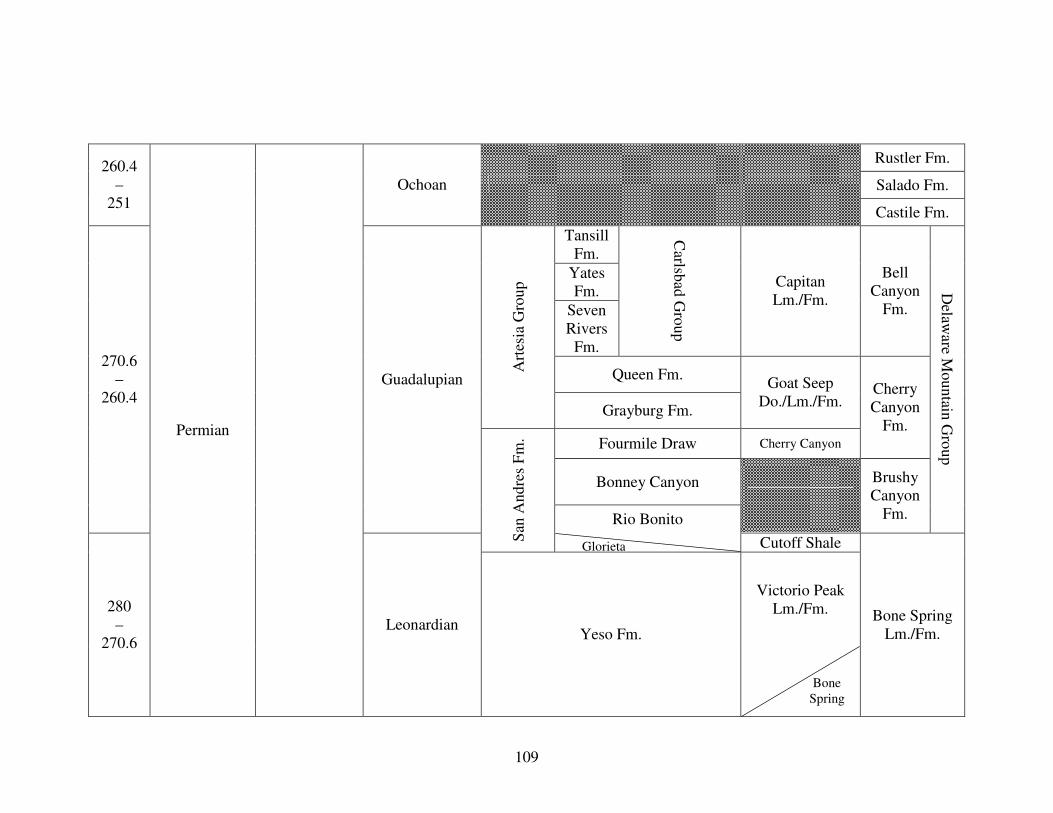
109
Rustler Fm.
Salado Fm.
260.4 –
251 Ochoan
Castile Fm.
Tansill Fm.
Yates Fm.
Seven Rivers
Fm.
Carlsb
ad G
roup
Capitan Lm./Fm.
Bell Canyon
Fm.
Queen Fm. Art
esia
Gro
up
Grayburg Fm.
Goat Seep Do./Lm./Fm.
Fourmile Draw Cherry Canyon
Cherry Canyon
Fm.
Bonney Canyon
270.6 –
260.4 Guadalupian
Rio Bonito
Brushy Canyon
Fm.
Delaw
are Mountain
Gro
up
San
Andre
s F
m.
Cutoff Shale
Victorio Peak Lm./Fm. 280
– 270.6
Permian
Leonardian Yeso Fm.
Bone Spring Lm./Fm.
Glorieta
Bone
Spring

110
Pow Wow Cong.
299 –
280 Permian
Bursum / Laborcita Fm.
Wolfcamp Series (Hueco Lm./Fm. and Pow Wow
Cong.)
Wolfcamp Fm.
305 –
299 Virgilian Holder Fm. Unnamed Cisco
Beeman Fm. 306.5 –
305 Missourian Unnamed Canyon
308 –
306.5 Desmoinesian Unnamed Strawn
311.7 –
308 Atokan/Derryan Unnamed Bend
318.1 –
311.7
Carboniferous Pennsylvanian
Morrowan
Mag
dal
ena
Fm
./G
roup
Gobbler Fm.
Unnamed?
Lee Ranch
tongue
Abo
Fm.
Danley Ranch
tongue
Pendejo
tongue Hueco
Lm./Fm.
Wolfcampian

111
333 –
318.1 Chesterian Helms Fm. Barnett Shale
340 –
333 Meramecian Rancheria Fm.
348 –
340 Osagean Lake Valley Fm.
359.2 –
348
Carboniferous Mississippian
Kinderhookian Caballero Fm.
“Mississippian Limestone”
Sly Gap Fm.
Oñate Fm. Percha Shale 385.3
– 359.2
Upper
Canutillo Fm.
Percha / Woodford Shale
397.5 –
385.3 Middle
416 –
397.5
Devonian
Lower
“Devonian”
438 –
421.3 Silurian
Niagaran Fusselman Fm.

112
Valmont Dolomite 451 –
443.7
Cincinnatian Montoya Group
Montoya Group
El Paso / Ellenburger Group 488.3
– 471.8
Ordovician
Canadian
501 –
488.3 Cambrian Croixian
Bliss Sandstone
Precambrian
Figure 2.2: Generalized stratigraphic chart of the Salt Basin region. Adapted from numerous sources, including Black (1973), Boyd (1958), Foster (1978), Hayes (1964), Kelley (1971), Kottlowski (1963), LeMone (1969), McGlasson (1969), Newell et al. (1972), and Pray (1961).

113
Figure 2.3: Precambrian basement rocks of the Salt Basin region, from Adams et al.
(1993) and Denison et al. (1984).

114
a: Late Precambrian (550 Ma)
c: Late Cambrian (500 Ma)
b: Middle Cambrian (510 Ma)
d: Early Ordovician (485 Ma)
Figure 2.4: Late-Precambrian-to-Early-Ordovician paleogeography of the Salt Basin region, from Blakey (2009b).

115
a: Middle Ordovician (470 Ma)
c: Early Silurian (430 Ma)
b: Late Ordovician (450 Ma)
d: Late Silurian (420 Ma)
Figure 2.5: Middle-Ordovician-to-Late-Silurian paleogeography of the Salt Basin region, from Blakey (2009b).

116
a: Early Devonian (400 Ma)
c: Late Devonian (360 Ma)
b: Middle Devonian (385 Ma)
d: Early Mississippian (345 Ma)
Figure 2.6: Early-Devonian-to-Early-Mississippian paleogeography of the Salt Basin region, from Blakey (2009b).
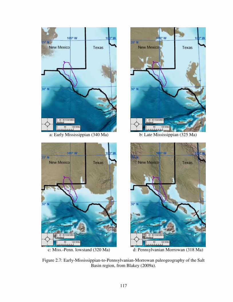
117
a: Early Mississippian (340 Ma)
c: Miss.-Penn. lowstand (320 Ma)
b: Late Mississippian (325 Ma)
d: Pennsylvanian Morrowan (318 Ma)
Figure 2.7: Early-Mississippian-to-Pennsylvanian-Morrowan paleogeography of the Salt Basin region, from Blakey (2009a).

118
a: Pennsylvanian Atokan (315 Ma)
c: Pennsylvanian Missourian (300 Ma)
b: Pennsylvanian Desmoinian (310 Ma)
d: Pennsylvanian Virgilian (295 Ma)
Figure 2.8: Pennsylvanian-Atokan-to-Pennsylvanian-Virgilian paleogeography of the Salt Basin region, from Blakey (2009a).
OrB = Orogrande Basin, DeB = Delaware Basin, MiB = Midland Basin.

119
a: Early Permian (290 Ma)
c: Early Permian (285 Ma)
b: Early Permian (287 Ma)
d: Early Permian (280 Ma)
Figure 2.9: Early-Permian paleogeography of the Salt Basin region, from Blakey (2009a). OrB = Orogrande Basin, DeB = Delaware Basin, MiB = Midland Basin.

120
a: Early Permian (278 Ma)
c: Middle Permian (270 Ma)
b: Early Permian (275 Ma)
d: Late Permian (260 Ma)
Figure 2.10: Early-Permian-to-Late-Permian paleogeography of the Salt Basin region, from Blakey (2009a).
OrB = Orogrande Basin, DeB = Delaware Basin, MiB = Midland Basin.

121
a: Late Permian (255 Ma)
c: Middle Triassic (230 Ma)
b: Early Triassic (240 Ma)
d: Late Triassic (210 Ma)
Figure 2.11: Late-Permian-to-Late-Triassic paleogeography of the Salt Basin region, from Blakey (2009a) and Blakey (2009b).
DeB = Delaware Basin, MiB = Midland Basin.

122
a: Early Jurassic (195 Ma)
c: Middle Jurassic (170 Ma)
b: Early Jurassic (180 Ma)
d: Late Jurassic (150 Ma)
Figure 2.12: Early-Jurassic-to-Late-Jurassic paleogeography of the Salt Basin region, from Blakey (2009b).

123
a: Early Cretaceous (140 Ma)
c: Early Cretaceous (115 Ma)
b: Early Cretaceous (130 Ma)
d: Late Cretaceous (100 Ma)
Figure 2.13: Early-Cretaceous-to-Late-Cretaceous paleogeography of the Salt Basin region, from Blakey (2009b).

124
a: Late Cretaceous (85 Ma)
c: Cretaceous-Paleogene (65 Ma)
b: Late Cretaceous (75 Ma)
d: Paleogene Paleocene (60 Ma)
Figure 2.14: Late-Cretaceous-to-Paleogene-Paleocene paleogeography of the Salt Basin region, from Blakey (2009b).

125
a: Paleogene Eocene (50 Ma)
c: Paleogene Oligocene (25 Ma)
b: Paleogene Eocene (40 Ma)
d: Neogene Miocene (15 Ma)
Figure 2.15: Paleogene-Eocene-to-Neogene-Miocene paleogeography of the Salt Basin region, from Blakey (2009b).

126
a: Neogene Miocene (8 Ma)
c: Quaternary Glacial (0.126 Ma)
b: Neogene Pliocene (3 Ma)
d: Present
Figure 2.16: Neogene-Miocene-to-Present paleogeography of the Salt Basin region, from Blakey (2009b).
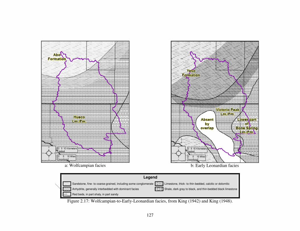
127
a: Wolfcampian facies
b: Early Leonardian facies
Legend
Sandstone, fine- to coarse-grained, including some conglomerate
Anhydrite, generally interbedded with dominant facies
Red beds, in part shaly, in part sandy
Limestone, thick- to thin-bedded, calcitic or dolomitic
Shale, dark gray to black, and thin-bedded black limestone
Figure 2.17: Wolfcampian-to-Early-Leonardian facies, from King (1942) and King (1948).

128
a: Late Leonardian facies
b: Early Guadalupian facies
Legend
Sandstone, fine- to coarse-grained, including some conglomerate
Anhydrite, generally interbedded with dominant facies
Red beds, in part shaly, in part sandy
Limestone, thick- to thin-bedded, calcitic or dolomitic
Shale, dark gray to black, and thin-bedded black limestone
Figure 2.18: Late-Leonardian-to-Early-Guadalupian facies, from King (1942) and King (1948).

129
a: Middle Guadalupian facies
b: Late Guadalupian facies
Legend
Sandstone, fine- to coarse-grained, including some conglomerate
Anhydrite, generally interbedded with dominant facies
Red beds, in part shaly, in part sandy
Limestone, thick- to thin-bedded, calcitic or dolomitic
Shale, dark gray to black, and thin-bedded black limestone
Figure 2.19: Middle-Guadalupian-to-Late-Guadalupian facies, from King (1942) and King (1948).

130
Figure 2.20: Permian shelf-margin trends, from Black (1975).

131
Figure 2.21: Pennsylvanian-to-Early-Permian structural features of the northern Salt
Basin watershed. Bar on downthrown side of normal or high angle faults, triangles on upthrown side of thrust zone. Location of structures in New Mexico taken from Broadhead (2002). Location of Diablo Platform taken from Kottlowski (1969).

132
Figure 2.22: Mid-to-Late-Permian structural features of the northern Salt Basin
watershed. Arrows indicate sense of displacement. Bar on downthrown side of Bitterwell Break. Location of structures taken from Black (1976), Goetz (1985), and Kelley (1971).

133
Figure 2.23: Late-Cretaceous (Laramide) structural features of the northern Salt Basin
watershed. Syncline and anticline symbols are the same as those used on Figure 2.22. Bar on downthrown side of McGregor fault. Location of structures taken from Black (1976), Goetz (1985), Kelley (1971), and Seager et al. (1987).
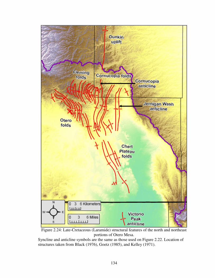
134
Figure 2.24: Late-Cretaceous (Laramide) structural features of the north and northeast
portions of Otero Mesa. Syncline and anticline symbols are the same as those used on Figure 2.22. Location of structures taken from Black (1976), Goetz (1985), and Kelley (1971).

135
Figure 2.25: Cenozoic structural features of the northern Salt Basin watershed.
Syncline and anticline symbols are the same as those used on Figure 2.22. Bar on downthrown side of normal or high angle faults. Location of structures taken from Black (1976), Broadhead (2002), Cather and Harrison (2002), Collins and Raney (1991), Goetz (1985), Pray (1961), Schruben et al. (1994), and Seager et al. (1987).

136
CHAPTER 3: HYDROGEOLOGIC FRAMEWORK
3.1: Previous Hydrogeologic Studies
The earliest studies of the groundwater system of the Salt Basin region were
conducted by Scalapino (1950) and Bjorklund (1957). Scalapino (1950) reported on the
direction of movement, quantity, and quality of groundwater in the Dell City area.
Scalapino (1950) noted that drilling in the Dell City area indicated that the region is
underlain by a limestone with large, solution-enhanced openings along joints and bedding
planes, but the distribution of these openings is erratic. Scalapino (1950) also noted that
the alluvial material within the Salt Basin graben consisted of interbedded clay and fine-
grained sand, and wells completed in this material had small yields. Scalapino (1950) was
the first researcher to hypothesize that infiltration of Sacramento River flows was the
primary source of recharge to the Dell City region. Scalapino (1950) also identified the
Salt Flats region as the primary area of natural discharge from the groundwater system,
and reported on the flow of Crow Spring.
Bjorklund (1957) conducted a similar study in the Crow Flats region of New
Mexico. Bjorklund (1957) commented on the levelness of the pieziometric surface in the
southern part of the Crow Flats area, and attributed this to the high permeability of the
water-bearing materials, especially the limestone with its many interconnected solution
channels. Bjorklund (1957) also identified a zone of perched groundwater in the far
northern portion of the Crow Flats region. Bjorklund (1957) hypothesized that recharge is
137
primarily through infiltration in the beds of ephemeral streams during flash floods.
Bjorklund (1957) estimated recharge to the groundwater system as being less than
120,000,000 m3 (100,000 acre-feet) per year based on the relationship between the
quantity of groundwater pumped for irrigation and water level fluctuations between 1948
and 1955. Bjorklund (1957) also noted that Crow Spring had stopped flowing due to
groundwater level declines associated with pumping for irrigation.
Gates et al. (1980) conducted a geophysical survey of the Salt Flats region and
used this data to estimate the thickness and lithology of the basin-fill within the Salt
Basin graben. Based on this data, Gates el al. (1980) interpreted the basin-fill lithology
as predominantly low permeability lacustrine clay and sand, saturated with saline water,
with a maximum thickness ranging from 244 meters (800 feet) in the north to 610 meters
(2,000 feet) in the south. Gates et al. (1980) also identified the lateral extent and thickness
of the Goat Seep and Capitan Limestones of the Capitan Reef Complex aquifer in the Salt
Flats region, and provided specific capacity data for the Capitan Limestone in the Beacon
Hill irrigation area. Gates et al. (1980) noted that recharge to the Capitan and Goat Seep
Limestones is concentrated primarily along outcrop areas in the Guadalupe Mountains,
Patterson Hills, and Delaware Mountains, and flows generally westward through the
Beacon Hill area towards its final discharge region at the Salt Flats.
Nielson and Sharp (1985) discussed the geological controls on the hydrogeology
of the Texas portion of the Salt Basin graben. They divided the Permian strata within the
Salt Basin graben into three aquifer systems: basin, shelf-margin, and shelf, and provided
estimates of transmissivity for each system. Nielson and Sharp (1985) also recognized the

138
existence of groundwater divides within the Salt Basin graben, and their correspondence
to structural features (Bitterwell Break and Victorio flexure).
Kreitler et al. (1990) studied the hydrogeology of the Diablo Plateau. They
identified two aquifers in the Diablo Plateau region: a deep regional aquifer, and a
shallow, locally perched, confined to semi-confined aquifer in the southwestern portion
of the Plateau. Kreitler et al. (1990) produced a potentiometric surface map for the Diablo
Plateau and Salt Basin graben regions of Texas, and concluded that groundwater flow on
the Diablo Plateau is primarily from southwest to northeast, and the underlying rocks are
locally highly transmissive. Based on the presence of tritium in nearly all wells
throughout the Plateau, Kreitler et al. (1990) concluded that the entire Plateau area
receives recharge. Kreitler et al. (1990) also analyzed soil-water chloride concentrations
and interpreted this to indicate that most recharge is concentrated within arroyos during
flash flood events.
Ashworth (1995) investigated the groundwater resources in the Dell Valley
region. Based on a comparison of irrigation pumpage and water level fluctuations,
Ashworth (1995) estimated total annual recharge to the groundwater system, including
both lateral inflow and irrigation return flow, to range from 110,000,000 to 120,000,000
m3 (90,000 to 100,000 acre-feet). Mayer (1995) analyzed the affect that regional fracture
systems have on regional groundwater flow within the Salt Basin. Mayer (1995)
constructed a two-dimensional, finite element groundwater flow model, and performed
several steady-state simulations to investigate the role of fractures in controlling regional
transmissivity, and thus regional groundwater flow. Mayer (1995) concluded that the
139
Otero Break region corresponds to a highly transmissive zone with a transmissivity
ranging from 1 to 3 orders of magnitude higher than surrounding regions.
The western and northern boundaries of Mayer’s model correspond to the surface
water divide defining the Salt Basin watershed. However, Mayer (1995) defined these
boundaries as no-flow boundaries, thus neglecting the potential for interbasin
groundwater flow from the Peñasco Basin to the north. The eastern boundary of Mayer’s
model was defined as a no-flow boundary in the north, where westward flow from the
Guadalupe Mountains and eastward flow from the Otero Mesa converge, and a constant
head boundary in the south, which corresponds to the water table at the Salt Flats. The
southern boundary corresponds to a symmetry boundary where regional flow is to the
east, parallel to the boundary, and was defined as a no-flow boundary (Mayer, 1995).
Mayer (1995) used the method described by Maxey and Eakin (1949) to estimate
the distribution and quantity of recharge above an elevation of approximately 1,675
meters (5,500 feet). The Maxey-Eakin method is an empirical technique based on a water
balance analysis of the White River Valley in eastern Nevada (Maxey and Eakin, 1949).
Below an elevation of 1,160 meters (3,800 feet) recharge from direct precipitation was
assumed to be negligible (Mayer, 1995). For the intermediate regions of the Otero
Mesa/Diablo Plateau, a composite recharge rate of 0.018 cm/year (0.0071 inches/year)
was calculated based on soil-water chloride data from the Diablo Plateau as cited by
Mayer (1995). The above techniques resulted in a total distributed recharge value of
72,000,000 m3/year (58,370 acre-feet/year).
During each model simulation, Mayer (1995) held recharge and discharge
constant and tested three configurations of transmissivity: homogeneous and isotropic,

140
heterogeneous and isotropic, and heterogeneous and anisotropic. For each configuration,
transmissivity was estimated by trial-and-error in order to best match the observed
potentiometric surface. Mayer (1995) found that the heterogeneous and isotropic case
produced the best match to the observed potentiometric surface, and adding anisotropy
did not significantly change the model output because of the coincidental alignment of
the hydraulic gradient nearly parallel to the major axis of transmissivity. Mayer (1995)
noted that the highest transmissivity zone, corresponding to the Otero Break region, had a
transmissivity (860 m2/day [9,300 ft2/day]) more than one order of magnitude less than
the highest transmissivity values that he cited from the literature for carbonate aquifers in
Texas. Based on the modeling approach taken, Mayer (1995) concluded that an equally
good match to the observed potentiometric surface could be achieved by either increasing
transmissivity and recharge, or lowering transmissivity and recharge.
Angle (2001) described the hydrogeology of the Texas portion of the Salt Basin
graben. Angle (2001) presented a basin-fill thickness map for the Salt Basin graben
modified from Gates et al. (1980). Angle (2001) also compiled transmissivity values for
the aquifers within the Salt Basin graben region. Mullican and Mace (2001) reported on
the hydrogeology of the Diablo Plateau region. They noted that the two aquifers in the
Diablo Plateau correspond to the geology, with the aquifer on the southwestern portion of
the Plateau located in Cretaceous rocks, and the underlying aquifer located in Permian
rocks that are exposed on the northern and northeastern portions of the Plateau.
John Shomaker & Associates, Inc. [JSAI] (2002) developed a three-dimensional,
finite difference groundwater flow model of the Salt Basin using MODFLOW to help
evaluate the potential for developing groundwater from deep wells within the New

141
Mexico portion of the Salt Basin. The model was calibrated to steady-state and historical-
transient conditions, but was based on limited knowledge of the hydrogeologic
framework and distribution of recharge (JSAI, 2010). The model domain was defined
primarily by the Salt Basin watershed boundary, but also included a portion of the
Peñasco Basin to the north (JSAI, 2002). The model consisted of 4 layers, each with a
variable thickness (JSAI, 2002).
Recharge was applied along the perimeter of the model domain in the form of
fully penetrating wells (JSAI, 2002). Recharge values were determined through model
calibration and comparison to known estimates of recharge (JSAI, 2002). Discharge from
the Salt Flats was simulated using the MODFLOW Evapotranspiration Package (EVT),
with the discharge region delineated by predevelopment depth-to-water less than 15
meters (50 feet) (JSAI, 2002). The steady-state model was calibrated to 1) an estimated
recharge of 67,771,000 m3/year (54,943 acre-feet/year), and 2) predevelopment
groundwater contours (JSAI, 2002). Steady-state model calibration involved adjusting
hydraulic conductivity values, slightly adjusting the specified recharge up or down for a
particular region, and changing the area and rate of evaporation (JSAI, 2002). Steady-
state calibrated inflow from the Peñasco Basin was estimated to be 9,811,000 m3/year
(7,954 acre-feet/year) (JSAI, 2002).
The distribution of hydraulic conductivity in each layer was derived from
expected values representative of the rock type of each geologic unit, and model
calibration (JSAI, 2002). JSAI (2002) estimated the hydraulic conductivity of the
Permian units in layers 1 and 2 in the Otero Break, Crow Flats, and Dell City regions to
be 30 meters/day (100 feet/day), while the surrounding units had conductivities ranging

142
from 0.02 to 3 meters/day (0.05 to 10 feet/day). In layers 3 and 4 hydraulic conductivities
ranged from 0.02 to 1.5 meters/day (0.05 to 5 feet/day), and 0.02 to 0.3 meters/day (0.05
to 1 feet/day), respectively (JSAI, 2002).
George et al. (2005) summarized the current knowledge concerning the
hydrogeology of Hudspeth County, Texas. They compiled information concerning
geology and hydrostratigraphy, water levels and groundwater flow, recharge, hydraulic
properties, discharge, and water quality for the groundwater system in the Dell Valley
region, the Diablo Plateau, and the Capitan Reef Complex. In their section on the Diablo
Plateau, George et al. (2005) noted that the Cretaceous and Permian aquifers are
vertically connected to each other. Huff and Chace (2006) summarized the current
knowledge of the hydrogeology of the New Mexico portion of the Salt Basin watershed,
and identified future study needs. Huff and Chace (2006) also presented groundwater
level changes measured nearly continuously in four wells north of Dell City, Texas over
an approximately three and a half year time period from 2003 to the middle of 2006. The
data demonstrated that groundwater level declines associated with irrigation pumping at
Dell City, Texas can propagate many miles away.
Hutchison (2008) developed three two-dimensional, finite difference groundwater
flow models of the Salt Basin using MODFLOW-2000. The purpose of Hutchison’s
study was to help El Paso Water Utilities assess the groundwater availability in the Dell
City and Diablo Farms regions for future City of El Paso water-supply development
projects. The three models included a structural geology model, a geochemistry model,
and a hybrid model of the two (Hutchison, 2008). The domain of each model was defined
by the Salt Basin watershed boundary, except in the far northwestern portion, and along

143
the western portion (Hutchison, 2008). The far northwestern portion of the Salt Basin
watershed was included in initial model simulations, but was later removed because its
protruding geometry created numerical problems (Hutchison, 2008). The western edge of
each model domain was moved to the east of the watershed boundary in order to
correspond more closely to a groundwater divide (Hutchison, 2008).
Hutchison (2008) assumed an aquifer thickness of 300 meters (1,000 feet). The
model domain boundary was defined as a no-flow boundary, except in the northwestern,
western, and southeastern portions of the domain. The general head boundary package
was used to simulate flow into the model domain in the northwestern portion of the
domain in the Sacramento Mountains (Hutchison, 2008). Outflow along the western
portion of the model domain was simulated using the drain package (Hutchison, 2008).
The possibility of outflow along the southeastern portion of the model domain, which
corresponds to the groundwater divide associated with the Bitterwell Break, was
investigated using the constant head boundary package (Hutchison, 2008). Discharge
from the Salt Flats was simulated using the evapotranspiration package (Hutchison,
2008).
The three groundwater flow models were calibrated to steady-state and historical-
transient simulations (Hutchison, 2008). Recharge was estimated using a modified
Maxey-Eakin approach in which higher elevation areas have a higher recharge rate than
lower elevation areas, and higher precipitation years have a higher recharge rate than
lower precipitation years (Hutchison, 2008). Average distributed recharge from steady-
state calibration of all three models was estimated to be 78,000,000 m3/year (63,000 acre-
feet/year) (Hutchison, 2008). Total steady-state inflow to the model domain, including

144
inflow from the Sacramento Mountains, ranged from 97,000,000 to 128,000,000 m3/year
(79,000 to 104,000 acre-feet/year) (Hutchison, 2008).
The study described in this thesis was part of a much larger multi-disciplinary
study organized by the New Mexico Interstate Stream Commission (NMISC) to obtain a
better understanding of Salt Basin groundwater system. Daniel B. Stephens & Associates,
Inc. was tasked with estimating groundwater evaporation from playas based on core
sampling and developing a watershed model to estimate recharge. John Shomaker &
Associates, Inc. was assigned the task of developing a conceptual model and updating the
groundwater flow model they developed in 2002. The U.S. Geologic Survey (USGS) was
charged with estimating stormwater runoff and potential recharge for major drainages.
INTERA was tasked with evaluating groundwater discharge from agricultural pumping
and playas using satellite image analysis.
Daniel B. Stephens & Associates, Inc. [DBS&A] (2010a) developed a basin-scale
water balance model that evaluated precipitation, evapotranspiration, and resultant
percolation through the soil column to estimate the amount and distribution of recharge
within the Salt Basin. They conceptualized recharge within the Salt Basin watershed to be
the result of four processes: mountain block recharge, mountain front recharge, local
recharge, and diffuse recharge (DBS&A, 2010a). Mountain block recharge is
concentrated primarily in higher elevation regions where precipitation is greater, the soils
are thinner, and the bedrock is exposed and permeable (DBS&A, 2010a). Mountain front
recharge is associated with the transition area between mountain block and valley floor,
where surface water can flow into thick alluvium and infiltrate into the groundwater
system (DBS&A, 2010a). Local recharge is possible along unvegetated sandy drainages

145
in the interior of the basin or where water may temporarily pond after intense rainfall
events (DBS&A, 2010a). The broad lowland areas between drainages can be the site of
diffuse recharge when soil water is not evapotranspired and is able to reach the water
table (DBS&A, 2010a). They determined water balance components for three years with
below-average, average, and above-average precipitation to provide minimum, average,
and maximum annual recharge, respectively (DBS&A, 2010a). Recharge originating in
the Salt Basin watershed was estimated to range from 46,000,000 to 100,000,000 m3/year
(37,000 to 82,000 acre-feet/year), with an average of 78,000,000 m3/year (63,000 acre-
feet/year) (DBS&A, 2010a).
DBS&A (2010b) also estimated historical playa evaporation rates within the Salt
Basin, and these rates were used to infer groundwater recharge rates. They collected core
from the Salt Basin playas and used luminescence geochronology to date the evaporative
sediments (DBS&A, 2010b). Based on the ages of the cored sediments, the
predevelopment annual discharge from the Salt Basin playas was estimated to range from
26,200,000 to 40,300,000 m3/year (21,250 to 32,700 acre-feet), with an average of
34,900,000 m3/year (28,300 acre-feet) (DBS&A, 2010b).
JSAI (2010) revised the hydrogeologic framework, and updated the groundwater
flow model they developed in 2002. They also developed a conceptual recharge model.
Groundwater recharge was conceptualized to be due to direct infiltration of precipitation
in the highlands (areal recharge) and infiltration of stormwater runoff into drainage
channels and alluvial fans (JSAI, 2010). The distribution of areal recharge was based on
the water balance model developed by DBS&A, as well as the delineation of major sub-
basins and watershed areas (JSAI, 2010). The amount of areal recharge was based on the

146
difference between potential recharge and stormwater runoff (JSAI, 2010). Potential
recharge was estimated using an empirical relationship, in which potential recharge is
some fraction of average annual precipitation, with the fraction increasing with increasing
elevation (JSAI, 2010). The amount of stormwater runoff for the Sacramento River,
Piñon Creek, Cornucopia Draw, and Big Dog Canyon sub-basins was obtained from the
study conducted by the USGS, while the amount of runoff generated in other sub-basins
was calculated using the average magnitude and annual frequency of runoff-generating
precipitation events based on data obtained from 16 weather stations in and around the
Salt Basin (JSAI, 2010). JSAI (2010) assumed that the amount of recharge associated
with the infiltration of stormwater runoff was equal to 30 percent of stormwater runoff.
The conceptual recharge model developed by JSAI (2010) resulted in an
estimated groundwater inflow from the Peñasco Basin of 7,154,000 m3/year (5,800 acre-
feet/year). Total recharge originating in the Salt Basin watershed was estimated to be
70,550,000 m3/year (57,196 acre-feet/year), which compared favorably to the amount
estimated from the calibrated steady-state groundwater flow model developed by JSAI
(2002) (JSAI, 2010). However, the distribution of recharge was different between the two
studies, with the conceptual recharge model producing larger recharge contributions from
the lower Sacramento River and Otero Mesa, Coffelt Draw, and Shiloh Draw sub-basins,
and the watershed areas that drain to Crow Flats, and smaller recharge contributions from
the sub-basins that drain the Cornudas and Hueco Mountains, and the Diablo Plateau
(JSAI, 2010).
JSAI (2010) used MODFLOW-96 to model groundwater flow in the Salt Basin of
New Mexico and Texas. The model was calibrated to steady-state and historical-transient

147
conditions (JSAI, 2010). The model grid was refined from the JSAI (2002) model to
consist of 160 rows and 160 columns with an even spacing of 805 meters (2,640 feet)
(JSAI, 2010). The model grid consisted of 4 layers, with layer 1 having a variable
thickness, layer 2 being 90 meters (300 feet) thick, layer 3 being 150 meters (500 feet)
thick, and layer 4 being 900 meters (3,000 feet) thick (JSAI, 2010). The top of layer 1
was defined as the land surface, and the bottom of layer 1 was defined based on initial
steady-state model-calibrated heads and saturated thickness based on transmissivity
(JSAI, 2010).
The model domain was defined primarily by the Salt Basin watershed boundary,
but unlike the JSAI (2002) model the Peñasco Basin was not included in the model
domain (JSAI, 2010). Instead, groundwater inflow from the Peñasco Basin was modeled
using a series of injection wells located along the northern boundary of the model domain
(JSAI, 2010). The remainder of the model domain boundary was defined as a no-flow
boundary. The Recharge Package (RCH) was used to apply areal recharge in the basin
and mountain-front recharge along arroyos (JSAI, 2010). The Evapotranspiration
Package (EVT) was used to model discharge from the Salt Flats, with the discharge
region defined by pre-development depth-to-water of 9 meters (30 feet) or less (JSAI,
2010).
The distribution of hydraulic conductivity in each layer was derived from
expected values representative of the rock type of each geologic unit (JSAI, 2010). JSAI
(2010) assigned a horizontal hydraulic conductivity value of 30 meters/day (100
feet/day), and a vertical to horizontal hydraulic conductivity ratio of 1:100 to the basin
fill units in layers 1 through 4. Permian units in layers 1 through 3 in the Otero Break,

148
Crow Flats, and Dell City regions were assigned higher horizontal hydraulic conductivity
values ranging from 15 to 30 meters/day (50 to 100 feet/day), while the surrounding
Permian units had conductivities ranging from 0.003 to 2 meters/day (0.01 to 5 feet/day)
(JSAI, 2010). Permian rocks in layer 4 were assigned lower horizontal hydraulic
conductivity values ranging from 0.003 to 0.03 meters/day (0.01 to 0.1 feet/day) (JSAI,
2010). Permian units with higher horizontal hydraulic conductivities were given a vertical
to horizontal hydraulic conductivity ratio of 1:10, while a ratio of 1:100 was used for the
lower conductivity Permian units (JSAI, 2010). Cambrian and Precambrian rocks in
layers 1 through 4 were assigned horizontal hydraulic conductivity values of 0.02
meters/day (0.05 feet/day) and 0.006 meters/day (0.02 feet/day), respectively, and a
vertical to horizontal hydraulic conductivity ratio of 1:500 (JSAI, 2010).
3.2: 3-D Hydrogeologic Framework Model
The development of a 3-D hydrogeologic framework model of the northern Salt
Basin was accomplished by:
1) reconstructing the tectonic forcings that impacted the region and the
resulting structural features that formed,
2) reconstructing the depositional environments and resultant facies
distributions during basin formation,
3) compiling data from oil-and-gas exploratory wells to constrain the
subsurface distribution of the various geologic units, and
4) compiling information on the location of surface exposures of the various
geologic units.
Items 1 and 2 were discussed in Chapters 1 and 2. Items 3 and 4 are discussed below.

149
3.2.a: Subsurface Data
Subsurface data for New Mexico was obtained from the Oil Conservation
Division online well files (http://www.emnrd.state.nm.us/OCD/OCDOnline.htm), Foster
(1978), King and Harder (1985), Finger and Jacobson (1997), scout cards and well
records from the New Mexico Subsurface Data Library at the New Mexico Bureau of
Geology and Mineral Resources, and Broadhead (2007). Subsurface data for Texas was
obtained from oil/gas well imaged records downloaded from the Railroad Commission of
Texas online Public GIS Map Viewer (http://www.rrc.state.tx.us/data/online/index.php#),
scout cards and well records obtained from the Bureau of Economic Geology’s Austin
Core Research Center on the campus of the University of Texas at Austin, King and
Harder (1985), and Veldhuis and Keller (1980). Tables 3.1 and 3.2 list all of the
subsurface control points for New Mexico and Texas, respectively, used in this study,
including the well name, a unique 7 character well I.D. used in this study, the API
number (if applicable), the UTM coordinates using the North American Datum 1983
(NAD 83) coordinate system, the well elevation in meters, the reference level for the well
elevation and the source (if applicable), the well depth in meters, and the
township/section, range/block, and section/survey of each point.
Tops of the various subsurface geologic units were compiled from these
resources. In all cases, geologic unit tops were reported as depths, in feet, from some
datum, which was not reported. To convert these depths to elevations, relative to mean
sea level, the depths were subtracted from the reported well elevations. Often, two or
more well elevations were reported from different reference levels, which included the
ground surface, kelley bushing, tubing head, derrick floor, and well head. In all cases,

150
kelley bushing, tubing head, derrick floor, or well head were chosen over the ground
surface as the datum if two or more well elevations were available. However, if only one
well elevation was reported this elevation was used as the datum, even if it was the
ground surface. If no well elevation was reported the elevation was derived from the 1-
arc second U.S. Geological Survey (USGS) National Elevation Dataset (NED) discussed
below. Tables 3.1 and 3.2 indicate the reference level of the well elevations used to
determine the elevation of the top of each geologic unit.
Next, these geologic unit tops were inserted into ArcGIS for analysis. The model
region was broken into 33 blocks, bounded by the various structural features described in
Chapter 2.2. (Figure 3.1) The top of each geologic unit (in meters above mean sea level)
was then contoured by hand separately for each block utilizing the subsurface well
control and the known sense of displacement on the bounding structural features. The
contours representing the top of the Precambrian basement were modeled after those
presented in King and Harder (1985), but were modified slightly to account for additional
subsurface data and structural displacement. Some of the subsurface well control for the
top of the Precambrian basement was obtained from Foster (1978) and Broadhead (2007),
who made projections based on isopach maps and selected geologic unit tops. Additional
Precambrian basement control points were compiled from subsurface projections based
on the depth-to-basement in neighboring wells. Table A-3.3 lists the subsurface well
control for the top of the Precambrian basement.
The tops of the overlying geologic units were then built up from these
Precambrian basement contours. Each successive geologic unit was contoured by adding
the observed thickness of the unit in the surrounding oil-and-gas wells to the preceding

151
geologic unit contours. In addition to the Precambrian basement, contours were produced
for, from bottom to top, the interval from the Bliss Sandstone to the Fusselman Formation
(the Cambrian through the Silurian), the Devonian, the Mississippian through the
Pennsylvanian, Pow Wow Conglomerate, Hueco Limestone/Formation and Wolfcamp
Formation, Abo Formation, Yeso Formation, Bone Spring Limestone/Formation,
Victorio Peak Limestone/Formation, San Andres Formation, Delaware Mountain Group,
Goat Seep Dolomite/Limestone/Formation and Capitan Limestone/Formation, Artesia
Group, the Cretaceous, and Cenozoic alluvium. These groupings were chosen such that
geologic units with similar lithologies and facies, and thus probably similar hydraulic
properties, were combined. Therefore, the resultant 16 groups represent hydrogeologic
units. The oil-and-gas exploratory wells used as control for the top of each hydrogeologic
unit are listed in Tables A-3.3 through A-3.20.
3.2.b: Surface Data
The land surface geology was modeled based on the USGS digital geologic map
of Stoeser et al. (2005), which consists of a polygon shapefile of the surface geology.
(Figure 2.1) The surface exposures of the various geologic units were modeled by using
the USGS NED at a resolution of 1-arc second downloaded from the National Map
Seamless Server (http://seamless.usgs.gov/index.php). The NED was converted to a
point shapefile in ArcGIS, and this point shapefile was clipped to the various surface
geology polygons in order to represent the elevation, relative to mean sea level, of the
outcropping units.
There are some discrepancies between the surface geologic maps of New Mexico
and Texas, especially around the Cornudas Mountains region. The Yeso and San Andres
152
Formations are mapped in New Mexico, but are not mapped in Texas. The San Andres
Formation as mapped in New Mexico is equivalent to the Victorio Peak Formation and
Leonardian limestones and dolomites of the Wilke Ranch Formation as mapped in Texas
(O’Neill and Nutt, 1998). According to Stoeser et al. (2005), the Wilke Ranch Formation,
as mapped on the Diablo Plateau, is equivalent to the Victorio Peak and Bone Spring
Limestones, and contains some beds equivalent to the Hueco Limestone. The Hueco
Limestone as mapped in Texas is equivalent to the Hueco Limestone and Yeso
Formations as mapped in New Mexico (O’Neill and Nutt, 1998).
The absence of the Yeso and San Andres Formations in Texas may be due to
complex stratigraphic relationships between the Permian units, rather than just a
difference in nomenclature between New Mexico and Texas geologists. As noted by
Black (1973), Hayes (1964), and Newell et al. (1972), the upper Yeso and lower San
Andres Formations grade laterally into the shelf-margin-facies Victorio Peak Limestone.
The absence of the Yeso Formation in Texas may be due to an abrupt pinch out to the
south, and/or an abrupt lateral gradation into the Victorio Peak Limestone (O’Neill and
Nutt, 1998). Likewise, the absence of the San Andres Formation in Texas may be due to
abrupt lateral gradation into the Victorio Peak Limestone (O’Neill and Nutt, 1998).
The digital geologic map of Stoeser et al. (2005) does not contain all of the
geologic units identified in the subsurface oil-and-gas exploratory wells, as it often lumps
several geologic units into one group. However, these surface groupings correspond very
well to the modeled subsurface hydrogeologic unit groupings discussed above. The
surface geologic groups include, from oldest to youngest, the Precambrian, the Cambrian
through the Silurian, the Devonian through the Mississippian, the Pennsylvanian, Lower
153
Abo, Hueco Limestone/Formation (or Bursum Formation), Abo Formation, Yeso
Formation, Bone Spring Limestone/Formation, Victorio Peak Limestone/Formation and
Cutoff Shale and Wilke Ranch Formation, San Andres Formation, Delaware Mountain
Group, Goat Seep Dolomite/Limestone/Formation and Capitan Limestone/Formation,
Artesia Group, the Cretaceous, Cenozoic intrusions, and Cenozoic alluvium.
3.2.c: 3-D Hydrogeologic Framework Solid Model Development
The point shapefiles representing the surface geology were combined with the
subsurface contours to model the elevation, relative to mean sea level, of the top of each
hydrogeologic unit. The Cambrian through the Silurian surface group was combined with
the subsurface contour for the interval from the Bliss Sandstone to the Fusselman
Formation. The Devonian through the Mississippian surface group was combined with
the subsurface contour for the Devonian. The Pennsylvanian surface group was combined
with the subsurface contour for the Mississippian through the Pennsylvanian. The Lower
Abo surface group was assumed to be equivalent to the Pow Wow Conglomerate contour
of the subsurface. The Victorio Peak Limestone/Formation, Cutoff Shale, and Wilke
Ranch Formation surface group was combined with the subsurface contour for the
Victorio Peak Limestone/Formation. All of the remaining surface groups were combined
with their respective subsurface contours, except for the Cenozoic intrusions. Subsurface
contours were not produced for this unit. However, the Cenozoic intrusions were
incorporated in the 3-D hydrogeologic framework model, as discussed below.
In order to create a 3-D hydrogeologic framework model, the combined surface
and subsurface data for each of the 16 hydrogeologic units were converted to raster
surfaces using ArcGIS. A raster surface consists of a grid of cells in which each cell

154
contains a value representing information, such as temperature or elevation. A raster cell
size of 500 by 500 meters (1,640 by 1,640 feet) was chosen represent the elevation of the
top of each hydrogeologic unit. The combined surface and subsurface data was mapped
to the raster surface using a spline with barriers interpolation technique. This
interpolation technique allowed the structural features [Figure 3.1] to be designated as
barriers that the spline technique would not interpolate across. As a result, the
displacement of each hydrogeologic unit across the structural features, as defined by the
hand contours of the top of each unit, was maintained during the conversion to a raster
surface.
Groundwater modeling system (GMS) version 6.5 was used to graphically display
these raster surfaces in 3-D as a solid model of all 16 hydrogeologic units. GMS was also
used to construct a 3-D finite difference groundwater flow model of the Salt Basin, which
is discussed in Chapter 4.1. A grid of cells with the same cell size and origin as the raster
surfaces was created in GMS. The GMS grid was assigned 16 layers to represent the 16
hydrogeologic units. The elevation values from the 16 raster surfaces were used to define
the elevation values of the 16 layers in the GMS grid. The land surface expression of the
resulting 3-D hydrogeologic framework solid model is displayed in Figure 3.2. The
Cenozoic intrusions were modeled as a series of vertical intrusions, extending from their
land surface outcrop locations downward, through the other 15 units, to the top of the
Precambrian. In total, 17 hydrogeologic units were incorporated into the 3-D framework
solid model, from oldest to youngest, the Precambrian, the Cambrian through the
Silurian, the Devonian, the Mississippian through the Pennsylvanian, Lower Abo/Pow
Wow Conglomerate, Hueco Limestone/Formation (or Bursum Formation) and Wolfcamp

155
Formation, Abo Formation, Yeso Formation, Bone Spring Limestone/Formation,
Victorio Peak Limestone/Formation and Cutoff Shale and Wilke Ranch Formation, San
Andres Formation, Delaware Mountain Group, Goat Seep
Dolomite/Limestone/Formation and Capitan Limestone/Formation, Artesia Group, the
Cretaceous, Cenozoic intrusions, and Cenozoic alluvium.
Figures 3.3 through 3.18 display the elevation, in meters relative to mean sea
level, of the top of the 16 hydrogeologic units, excluding the Cenozoic intrusions. Figures
3.19 through 3.33 display the thickness, in meters, of the 15 hydrogeologic units above
the Precambrian, excluding the Cenozoic intrusions. Personal computer memory
constraints prevented graphical rendering of oblique views of the full extent of the 3-D
hydrogeologic framework model displayed in Figure 3.2. However, when the full extent
of the 3-D framework model was clipped to the groundwater flow model domain [Figure
3.34], as discussed in Chapter 4, oblique views of the 3-D framework solid model were
able to be generated. Figure 3.35 presents several oblique views of the 3-D hydrogeologic
framework solid model.
3.3: 2-D Hydrogeologic Cross-sections
3.3.a: Hand-drawn Cross-sections
Before the 3-D hydrogeologic framework model was assembled, the compiled
subsurface data and surface geology of Stoeser et al. (2005) were used to construct five
hydrogeologic cross-sections through primarily the New Mexico portion of the northern
Salt Basin watershed. (Figure 3.36) Two cross-sections trend generally north-south along
the eastern portion of the Salt Basin watershed from the Peñasco Basin to the natural
discharge region at the Salt Flats (A to A’ and B to B’). (Figures 3.37 and 3.38,

156
respectively) Both of these north-south oriented cross-sections generally follow along a
groundwater flow path, and intersect groundwater wells that were sampled for
environmental tracers during this study. The remaining three cross-sections trend
generally west-east (C to C’, D to D’, and E to E’). (Figures 3.39, 3.40, and 3.41,
respectively) Control on the subsurface geology for each cross-section was provided by
the oil-and-gas exploratory wells discussed in Chapter 3.2.a. Tables 3.21 through 3.25 list
the oil-and-gas wells used to construct these cross-sections, including the well I.D. used
in this study, the distance of the well along the cross-section in meters, the well elevation
in meters, and the well depth in meters.
These cross-sections indicate the complex subsurface structure that typifies the
Salt Basin region. Ancestral Rocky Mountain structures displace Precambrian through
Pennsylvanian-to-Lower Permian strata. The overlying Middle-to-Upper Permian units
are gently folded and faulted due to Laramide compression and subsequent Cenozoic
extension. Towards the south and east, these Upper Permian units transition into shelf-
margin, and eventually basin-facies rocks deposited in the Delaware Basin. Cross-section
E to E’ indicates the presence of Cenozoic intrusions that cut Precambrian through
Permian, and locally Cretaceous, strata in the Cornudas and Hueco Mountains regions.
(Figure 3.41) Locally thin to thick deposits of Cenozoic alluvium fill the depressions or
grabens bounding uplifts associated with Basin-and-Range extension.
The groundwater surfaces displayed in these cross-sections were contoured by
hand using groundwater level data obtained from the New Mexico Office of the State
Engineer’s (NMOSE) New Mexico Water Rights Reporting System (NMWRRS) online
database (http://nmwrrs.ose.state.nm.us/nmwrrs/disclaimer.html), the Texas Water

157
Development Boards’s (TWDB) Groundwater Database (http://www.twdb.state.tx.us/
publications/reports/GroundWaterReports/GWDatabaseReports/GWdatabaserpt.htm),
and from Appendix A of the New Mexico Bureau of Geology & Mineral Resources’
Sacramento Mountains Hydrogeology Study (SMHS) Open File Report – 518
(http://geoinfo.nmt.edu/publications/openfile/details.cfml?Volume=518). Depth-to-water
measurements in these databases were converted to groundwater elevations, relative to
mean sea level, by inserting the location of these groundwater wells into ArcGIS, using
the 1-arc second NED described above in Chapter 3.2.b to define the ground surface
elevation of these wells, and then subtracting the reported depth-to-water from the ground
surface elevation. A subset of the groundwater elevation points from these databases
were used to contour the groundwater surface for the Salt Basin region. (Figure 3.42) The
cross-section lines were then overlaid on top of this groundwater surface [Figure 3.36],
and the intersections of the groundwater surface contours with each cross-section line
were used to define the groundwater surface in each cross-section. Some of the
groundwater elevation data used to construct the groundwater surface was obtained
during this study from personal communication with the owners of the groundwater
wells.
A subset of the groundwater elevation points were also used to hand-contour a
depth-to-groundwater map for the Salt Basin region. (Figure 3.43) The location of
groundwater wells in the NMOSE’s NMWRRS database are taken from Water Right
Documents, which often include only township, range, section, and, sometimes, quarter-
section locations using the Public Land Survey System (PLSS). These PLSS locations are
then converted to UTM coordinates using the NAD 83 coordinate system. Therefore,

158
sometimes several wells occupy the same coordinate location. In such cases, the well
with the greatest depth-to-water, or, if no depth-to-water measurements were available,
the greatest well depth was chosen as the groundwater elevation control point for that
coordinate location.
Groundwater wells in the TWDB’s database sometimes have multiple depth-to-
water measurements, ranging from the early 1900s to the present. For wells with multiple
depth-to-water measurements, the mean of these measurements were used as
groundwater elevation control points. In contrast, groundwater wells in the NMOSE’s
database have only one depth-to-water measurement per well. Researchers for the SMHS
have collected multiple depth-to-water measurements per well throughout the
Sacramento Mountains, but only the static depth-to-water measurements presented in
Appendix A were used as groundwater elevation control points.
Also, all of the groundwater wells in these databases were not used as
groundwater elevation control points. If neighboring wells had drastically different depth-
to-water measurements, the well with the greatest depth-to-water was chosen as a
groundwater elevation control point. The groundwater surface for the Salt Basin region
represents the regional groundwater surface, and does not include localized zones of
shallow or perched groundwater. (Figure 3.42) However, in the far southwestern portion
of the Diablo Plateau, the groundwater surface incorporates a locally perched aquifer in
the Cretaceous rocks unconformably overlying the Permian. However, as discussed
below in Chapter 3.5.a, the Cretaceous aquifer is hydraulically connected to the
underlying Permian aquifer. The depth-to-groundwater map indicates zones of shallower

159
groundwater than the overall regional trends displayed by the surrounding depth-to
groundwater polygons. (Figure 3.43)
Table A-3.26 lists all the groundwater wells used to construct the groundwater
surface and depth-to-groundwater maps for the Salt Basin region, including the
NMOSE’s NMWRRS database point of diversion (POD) number, well ID, or the
TWDB’s database state well number, the UTM coordinates using the NAD 83 coordinate
system, the ground surface elevation in meters, the elevation of the well depth in meters
(if available), the groundwater elevation in meters (if available), the aquifer that the well
obtains groundwater from (if available), the county the well is located in, whether the
well was used as a depth-to-groundwater and/or a groundwater surface control point, and
the source of the depth-to-water measurement. Groundwater wells in the TWDB’s
database contain an aquifer code that indicates the aquifer the well penetrates. The
aquifer name associated with each aquifer code is listed under the caption for Table A-
3.26.
3.3.b: Cross-sections Through the 3-D Hydrogeologic Framework Solid Model
The same cross-section trends were cut through the 3-D hydrogeologic framework
solid model. As discussed above in Chapter 3.2.c, personal computer memory constraints
prevented oblique views of the full extent of the 3-D hydrogeologic framework model
from being rendered. However, when the 3-D framework model was clipped to the
groundwater flow model domain, oblique views of, and cross-sections through the 3-D
model were able to be generated. As a result, the beginning of the A to A’ and B to B’
cross-sections derived from the 3-D hydrogeologic framework solid model are slightly
truncated, as compared to the hand-drawn cross-sections presented in Figures 3.37 and

160
3.38. In addition, both the beginning and the end of the C to C’, D to D’, and E to E’
cross-sections derived from the 3-D hydrogeologic framework solid model are slightly
truncated, as compared to the hand-drawn cross-sections presented in Figures 3.39, 3.40,
and 3.41.
The locations and an oblique view of the 5 cross-sections within the 3-D
hydrogeologic framework solid model are presented in Figure 3.44. Side views of the 3-
D framework solid model cross-sections are shown in Figures 3.45 through 3.49. In
addition, the hand-drawn cross-sections are displayed alongside the 3-D framework solid
model cross-sections in Figures 3.45 through 3.49. The 3-D hydrogeologic framework
solid model cross-sections compare favorably to the hand-drawn cross-sections, and, in
general, maintain the displacement and juxtaposition of hydrogeologic units across the
structural features.
3.4: Surface Water and Springs
The Sacramento River is the only perennial stream in the Salt Basin watershed.
(Figure 1.5) The USGS measured mean daily discharge in the Sacramento River at
streamgaging station 08492900 near Sunspot, New Mexico from 1984 to 1989, during
which time it ranged from 60 to 370 liters per second (2 to 13 cubic feet per second [cfs])
(JSAI, 2002; Huff and Chace, 2006). All of the other drainages are ephemeral and flow
only during periods of intense rainfall (Hutchison, 2006). It is believed that runoff from
the Sacramento River and Piñon Creek subwatersheds, derived from these intense rainfall
events and melting snowpack, is a major contributor to groundwater recharge in the
northern Salt Basin watershed (JSAI, 2002; Huff and Chace, 2006).

161
Springs are common in the southern Sacramento Mountains, often near, but
below, the contact between the San Andres and the underlying Yeso Formation (Newton
et al., 2009). The majority of springs discharge from the Yeso Formation at several
different stratigraphic levels, but often from fractured limestone beds immediately
overlying low permeability clay or siltstone beds (Newton et al., 2009). During this
study, a site was sampled in the upper reaches of the Piñon Creek subwatershed, just east
of Piñon, New Mexico, where the land owner had dug down 9 to 11 meters (30 to 35
feet) through yellow rock to a spring discharge above a hard, impermeable layer. Near
Timberon, New Mexico, Carissa Spring flows at an average rate of 76 liters per second
(1,200 gallons per minute [gpm]) and rapidly infiltrates into the Sacramento Canyon fault
(Finch, 2010). (Figures 1.5 and 1.6) Just south of the New Mexico-Texas border, near
Dell City, Texas, Crow Spring was reported to be flowing at a rate of 0.2 liters per second
(3 gpm) before the development of the Dell City irrigation district, but has since become
dry (Bjorklund, 1957; Scalapino, 1950).
3.5: Groundwater
3.5.a: Distribution, Recharge, and Movement
-Permian
Permian rocks can be divided into three hydrogeologic facies, corresponding
closely to the geologic facies described above (Sharp, 1989). Permian rocks of the
hydrogeologic basin-facies (Guadalupian and Ochoan Series) were deposited in a deep-
marine environment within the Delaware Basin, and have low permeability and poor
water quality (Nielson and Sharp, 1985; Sharp, 1989). Rocks of the hydrogeologic shelf-
margin-facies (Guadalupian) are highly permeable reef limestones (Goat Seep and

162
Capitan) that were deposited around the margin of the Delaware Basin (Nielson and
Sharp, 1985; Sharp, 1989). Rocks of the hydrogeologic shelf-facies (Wolfcampian to
Guadalupian) have a highly variable permeability that is strongly dependent on the
degree of fracturing in the rocks (Nielson and Sharp, 1985).
-Bone Spring-Victorio Peak Aquifer
As mentioned above, the Victorio Peak Limestone is more accurately described as
a limestone bank rather than a limestone reef, and contains strata interpreted to have been
deposited in a lagoonal or back-reef environment, separated from the basin by the
limestone banks (King, 1948; King, 1983). Also discussed above, during the first half of
the Leonardian the Bone Spring Limestone extended several kilometers farther shelfward
over the shelf margin (King, 1948). Therefore, based on the hydrogeologic facies
characteristics of Nielson and Sharp (1985), the Victorio Peak Limestone and the lower
portion of the Bone Spring Limestone fall within the hydrogeologic shelf-facies. The
fracture-dependent permeability of the Victorio Peak and Bone Spring Limestones in the
Dell City region is indicated by the more-than-one-order-of-magnitude difference in the
specific-capacity of wells drilled no more than 30 meters (100 feet) apart, the low success
rate (<50%) of wells drilled without the aid of fracture mapping as compared to the high
success rate (>90%) of wells drilled with the aid of fracture mapping, and local well
drillers reports of lost circulation (Mayer and Sharp, 1998).
The Dell Valley irrigation district is centered around Dell City, Texas just south
of the New Mexico-Texas state line in northeastern Hudspeth County (Ashworth, 2001).
(Figure 3.50) The irrigated area also extends northward into the Crow Flats region of
New Mexico in southeastern Otero County (Ashworth, 2001). (Figure 3.50) The
163
irrigation area derives groundwater from the hydrogeologic shelf-facies rocks that
comprise the Bone Spring-Victorio Peak aquifer (George et al., 2005). (Figure 3.50)
Mayer and Sharp (1998) reported a combined thickness of the Bone Spring and Victorio
Peak Limestones in the Dell City, Texas area to range from 100 meters (328 feet) to at
least 430 meters (1,410 feet). Peckham (1963) reported at least 152 meters (499 feet) of
Bone Spring Limestone, and at least 244 meters (800 feet) of Victorio Peak Limestone in
the Dell City, Texas area. The Bone Spring-Victorio Peak aquifer is believed to exist
under both unconfined and confined conditions (Bjorklund, 1957).
-High Mountain, Pecos Slope, and Salt Basin Aquifers
Groundwater flow converges on the Dell Valley region from the Diablo Plateau to
the southwest, and from the Sacramento Mountains and Otero Mesa to the northwest
(Kreitler et al., 1990; Mayer and Sharp, 1998). (Figure 3.42) The majority of groundwater
in the Dell Valley region originates as recharge in the Sacramento Mountains and along
the Sacramento River as it infiltrates into the heavily fractured Permian shelf-facies rocks
that constitute the Otero Break (Mayer, 1995; Mayer and Sharp, 1998). In the Sacramento
Mountains, snow melt in the high mountains is the primary source of recharge to the
groundwater system, although extremely wet monsoon seasons can contribute
significantly to groundwater recharge (Newton et al., 2009). Chace and Roberts (2004)
report a combined thickness of the San Andres and Yeso Formations of at least 457
meters (1,499 feet) within the northern Salt Basin watershed. Hydraulic gradients in the
northern-most portion of the northern Salt Basin watershed also suggest a component of
interbasin groundwater flow from the Peñasco Basin to the north (JSAI, 2002; Newton et
al., 2009). South Central Mountain RC&D Council, Inc. (2002) estimated the inflow

164
component from the Peñasco Basin to be 10,000,000 m3/year (8,000 acre-feet/year).
Groundwater flow modeling work by JSAI (2002) and JSAI (2010) resulted in estimates
of inflow from the Peñasco Basin of 9,811,000 m3/year (7,954 acre-feet/year) and
6,724,000 m3/year (5,451 acre-feet/year), respectively.
In the Sacramento Mountains, west of the town of Mayhill, New Mexico, the
regional groundwater system is located primarily in the Yeso Formation (Newton et al.,
2009). This high mountain aquifer system consists of several unconfined, perched
aquifers connected to each other by regional fracture networks, and probably a deeper,
continuous, locally confined, regional aquifer in the eastern portion of the high mountains
(Newton et al., 2009). (Figure 3.50) In the high mountains, groundwater is found
predominately in fractured limestone, collapse breccias formed by dissolution of gypsum
and/or limestone, and less commonly, sandstone beds within the Yeso Formation (80% of
groundwater wells with logs) (Newton et al., 2009). Other groundwater zones exist in the
underlying Abo Formation along the west face of the mountains, in shallow valley-
bottom alluvium, or spring deposits (Newton et al., 2009). East of Mayhill, groundwater
occupies a more single, continuous aquifer (Pecos slope aquifer) in both the San Andres
and Yeso Formations (Newton et al., 2009). (Figure 3.50)
Groundwater recharge to the high mountain aquifer is focused in the high
mountains where the Yeso is exposed at the surface (Newton et al., 2009). The high
mountain aquifer recharges both the Pecos slope and Salt Basin aquifers (Newton et al.,
2009). (Figure 3.50) As indicated by the discharge of springs from several different
stratigraphic levels in the Yeso Formation, groundwater flows at several levels within the
Yeso Formation (Newton et al., 2009). Abundant claystone in the upper portion of the

165
Yeso formation acts as a barrier to vertical groundwater flow (Newton et al., 2009).
Hydrogeologic cross-section C to C’ suggests that in the higher elevations in the
northwestern portion of the Otero Mesa and southeastern Sacramento Mountains
groundwater may reside in localized, shallow perched aquifers in the San Andres
Formation, which probably overlie the deeper regional aquifer in the Yeso Formation.
(Figure 3.39)
Hydraulic gradients also indicate that groundwater generally flows east- to
northeastward from the Otero Mesa towards the Dell Valley region (JSAI, 2002; Mayer,
1995). (Figure 3.42) In the western portion of the Otero Mesa shelf-facies rocks of the
Hueco and Yeso Formations are exposed (Stoeser et al., 2005). (Figure 2.1) The Hueco
Formation also outcrops on the Diablo Plateau to the south, but thins, and is
unconformably overlain by Leonardian (Bone Spring or Victorio Peak) or Cretaceous
strata southeastward towards the Sierra Diablo Mountains (King, 1983; Kottlowski, 1963;
Stoeser et al., 2005). (Figure 2.1) As discussed below, the regional Permian aquifer
beneath the Diablo Plateau encompasses rocks of the Hueco Formation. Therefore, the
Hueco Formation could be an important aquifer in the New Mexico portion of the Salt
Basin (Huff and Chace, 2006). Further, hydrogeologic cross-sections C to C’, D to D’,
and E to E’ indicate that groundwater occurs in the Hueco, Abo and Yeso Formations in
the western portion of the Otero Mesa. (Figures 3.39, 3.40, and 3.41)
Hydraulic gradients also suggest a component of groundwater flow to the west
and southwest from the Guadalupe and Brokeoff Mountains towards the Salt Basin
graben. (Figure 3.42) However, the importance of this flow system to the Salt Basin
hydrologic system has not been quantified. Depth-to-groundwater in this region ranges

166
from 230 meters (750 feet) to greater-than 300 meters (1,000 feet). (Figure 3.43)
Therefore, it is unlikely that the Guadalupe and Brokeoff Mountains contribute much
modern recharge to the Salt Basin hydrologic system.
-Diablo Plateau Aquifer
In the southwestern portion of the Diablo Plateau a regional aquifer is found in the
Permian rocks unconformably underlying the Cretaceous rocks, and extends to the
northern and northeastern portions of the Plateau where the Permian rocks are exposed at
the surface (Kreitler et al., 1990; Mullican and Mace, 2001). (Figure 3.50) The regional
Permian aquifer is primarily unconfined, although it is likely confined beneath the
Cretaceous rocks (Mullican and Mace, 2001). The regional Permian aquifer (Hueco,
Bone Spring, and Victorio Peak Formations) on the Diablo Plateau is hydraulically
connected to the Permian rocks (Bone Spring and Victorio Peak Formations) in the Dell
City region to the northeast (George et al., 2005). Groundwater flow is predominantly
from southwest to northeast (Kreitler et al., 1990).
Depths to water in the regional Permian aquifer are as great as 244 meters (800
feet), and hydraulic gradients are much lower than in the overlying shallow aquifer in the
Cretaceous rocks (George et al., 2005; Kreitler et al., 1990). (Figures 3.42 and 3.43)
Recharge is distributed over the entire area of the plateau (7,500 km2 [2,900 mi2]) based
on measurable amounts of tritium in nearly all wells within the regional aquifer (Kreitler
et al., 1990). Low chloride concentrations in arroyo soils, compared to high chloride
concentration in inter-arroyo soils suggest that most recharge is restricted to flood events
through fractures concentrated in the arroyos (Kreitler et al., 1990).

167
-Capitan Reef Complex Aquifer
In the southern Guadalupe Mountains, and extending southwestward into the
Patterson Hills and the Texas portion of the Salt Basin graben is the Capitan Reef
Complex aquifer (George et al., 2005). (Figure 3.50) This aquifer consists of the reef
rocks of the Goat Seep and Capitan Formations, as well as back-reef (near shelf-edge)
rocks of the Artesia Group (Hiss, 1980). This aquifer outcrops in the Guadalupe
Mountains and the Patterson Hills, and subcrops south of the Patterson Hills where it
supplies water to the Beacon Hill irrigation area (Gates et al., 1980). (Figure 3.50)
Recharge to this aquifer is focused where it outcrops in the Guadalupe Mountains,
Apache Mountains, and the Patterson Hills, and locally from ephemeral streamflow in
and east of the Beacon Hill irrigation area (Gates et al., 1980; George et al., 2005). Gates
et al. (1980) reported that the Goat Seep Limestone is as much as 370 meters (1,200 feet)
thick in the Salt Flats region, and that the Capitan Limestone is first encountered at
depths from 18 to 84 meters (60 to 275 feet) and extends to as much as 514 meters (1,686
feet) in the Beacon Hill area.
The Border fault zone acts as a groundwater divide between two regional
groundwater flow systems within the high permeability trend of the Capitan Reef
Complex aquifer: one that originates in the southern Guadalupe Mountains and flows to
the north and northeast towards Carlsbad, New Mexico, and one that flows south from
the recharge zone in the Patterson Hills towards the Apache Mountains (Hiss, 1980;
Standen et al., 2009; Uliana, 2001). (Figures 2.25, 3.42, and 3.50) Numerous researchers
have presented compelling hydrochemical and structural evidence that supports a
regional groundwater flow system from the Wild Horse Flat portion of the Salt Basin

168
graben eastward through the Capitan Reef Complex in the Apache Mountains to
Balmorhea Springs in the Toyah Basin (Nielson and Sharp, 1985; Sharp, 1989; Sharp,
2001; Uliana, 2000; Uliana and Sharp, 2001; Uliana et al., 2007). (Figure 3.50) Using
hydrochemical tracers, Chowdhury et al. (2004) concluded that groundwater originating
in the Capitan Reef Complex in the area west of the Delaware Mountains and in the
Apache Mountains flows southeast to Balmorhea Springs.
-Cretaceous
In the southwestern portion of the Diablo Plateau a shallow, primarily unconfined,
locally perched and confined to semi-confined aquifer is located in the Cretaceous rocks
unconformably overlying the Permian (Kreitler et al., 1990; Mullican and Mace, 2001).
(Figure 3.50) The Cretaceous aquifer is vertically connected to the underlying regional
aquifer in the Permian, and is also hydraulically connected to the Hueco bolson aquifer to
the west, the aquifer in the Quaternary deposits filling the Salt Basin graben to the east,
and the Permian rocks in the Dell City region to the northeast (George et al., 2005).
(Figure 3.50) Groundwater flows outward from a groundwater mound in the
southwestern part of the Diablo Plateau south of U.S. Highway 62-180 toward the Hueco
bolson to the southwest, the Finlay Mountains and northwest Eagle Flats to the southeast,
the Salt Basin graben to the northeast, and possibly to the north of Highway 62-180
where it then flows eastward to Dell City, Texas (Mullican and Mace, 2001). (Figure
3.42) Depths to water in the Cretaceous aquifer are generally less than 61 meters (200
feet), and hydraulic gradients are much steeper than in the underlying Permian aquifer
(George et al., 2005; Kreitler et al., 1990). (Figures 3.42 and 3.43)

169
-Cenozoic
Some wells in the Crow Flats and Dell City regions obtain water from the
alluvium and lacustrine deposits filling the Salt Basin graben (Bjorklund, 1957). The
thickness of valley-fill encountered by most wells drilled in the Crow Flats and Dell City
regions range from 7.6 to 91.4 meters (25 to 300 feet) (Bjorklund, 1957). The E.J.
Dunigan, Alpha Federal #1 (EJDALF1) well [Figure 3.1] in the Crow Flats region, just
west of the Brokeoff Mountains, penetrated 18 meters (60 feet) of basin fill. Farther to
the south in the Texas portion of the Salt Basin graben the thickness of valley-fill
increases, ranging from 152 to 610 meters (500 to 2,000 feet), with the thickest intervals
generally found in the center of the graben (Veldhuis and Keller, 1980). The maximum
thickness of the lacustrine clays and sands filling the Texas portion of the graben range
from 244 meters (800 feet) in the region north of U.S. Highway 62-180 to 610 meters
(2,000 feet) southwest of Bitter Well Mountain in the Delaware Mountains (Gates et al.,
1980).
The valley-fill aquifer in the Salt Basin graben is hydraulically connected to the
surrounding aquifer in the Dell Valley irrigation area to the west (Bjorklund, 1957).
(Figures 3.42 and 3.50) The valley-fill aquifer is unconfined (Bjorklund, 1957). During
the late 1940s (1947-1949) in the Dell City region water levels were slightly lower (0.3 to
1.5 meters [1 to 5 feet]) in the valley-fill aquifer than in the surrounding Bone Spring-
Victorio Peak aquifer, which suggests that groundwater was flowing from the Bone
Spring-Victorio Peak aquifer into the valley-fill aquifer (Bjorklund, 1957). Recharge to
the valley-fill aquifer is primarily by flash flood infiltration in the flat-bottomed canyons
and bajadas along ephemeral streams draining into the valley floor (Bjorklund, 1957). In

170
the Salt Flat region the valley-fill aquifer consists predominately of low permeability
lacustrine clay and sand saturated with saline water, and is not a good aquifer (Gates et
al., 1980).
Farther to the north in T. 21 S., R. 17 E., sec. 12 a perched saturated zone above
the regional aquifer is located in the alluvium filling Piñon Creek (Bjorklund, 1957). It is
likely that similar shallow, perched groundwater zones exist in the alluvium filling the
other ephemeral drainages in the Salt Basin. In the Sacramento Mountains, shallow,
perched zones are located in valley-bottom alluvium and spring deposits (Newton et al.,
2009).
3.5.b: Discharge
Before the development of the Dell City irrigation district the natural discharge
mechanism of the groundwater system in the northern Salt Basin was through
evaporation from the playa lakes/alkali flats situated along the center of the Salt Basin
graben (Bjorklund, 1957). Groundwater withdrawals due to pumping increased steadily
after the installation of irrigation wells in the Dell City region in 1947 and 1948, and in
the Crow Flats region in 1949 (Bjorklund, 1957). The amount of groundwater pumped
for irrigation purposes temporarily peaked in the late 1970s around 190,000,000 m3/year
(150,000 acre-feet/year) (Ashworth, 2001). Irrigation pumping declined in the 1980s to
about 120,000,000 m3/year (100,000 acre-feet/year) due to economic hardships and
government conservation programs, but increased again in the subsequent years to over
250,000,000 m3/year (200,000 acre-feet/year) in 2000 (Ashworth, 2001). Groundwater
withdrawals for irrigation have resulted in a steady decline in regional groundwater levels

171
by as much as 12 meters (40 feet) from the late 1940s to about 2000 (Huff and Chace,
2006).
In the Sacramento Mountains, groundwater discharges to springs and streams
(Newton et al., 2009). As mentioned above, prior to development of the Dell City
irrigation district, groundwater discharged from Crow Spring just to the east of Dell City
(Bjorklund, 1957). Also, as discussed above, groundwater discharges from Carissa Spring
near Timberon, New Mexico before rapidly infiltrating into the Sacramento Canyon fault
(Finch, 2010).
3.5.c: Structural Controls on Groundwater Flow
Based on hydraulic gradients and hydrochemistry, previous researchers have
ascertained that the Otero Break acts as a high permeability conduit for groundwater flow
from the Sacramento Mountains to the southeast towards the Dell Valley region (JSAI,
2002; Hutchison, 2006; Mayer, 1995; Mayer and Sharp, 1998). The region surrounding
the Otero Break is a heavily fractured zone with a strong preferred fracture orientation of
approximately N20W (Mayer and Sharp, 1998). This fracture system may act as an
interconnected pathway along which groundwater flow is focused.
Previous researchers [JSAI, 2002; Mayer, 1995; Mayer and Sharp, 1998] have
depicted a prominent trough in the groundwater surface that is not centered on the Otero
Break, but rather to the west of this feature. (Figure 3.51) The region of the groundwater
trough coincides with a plume of fresh water, as indicated by low total dissolved solids
(TDS) [≤ 500 milligrams per liter (mg/L)], that extends from the southern Sacramento
Mountains toward Dell City (Mayer and Sharp, 1998). John Shomaker & Associates, Inc.
(2010) have also measured wells in the region of the groundwater trough with TDS

172
values that range from 500 to 600 mg/L. Numerous sinkholes that drain significant
watershed areas are also located in the region of the groundwater trough parallel to the
Otero Break (JSAI, 2010). The groundwater trough is located in a region of karst terrain
thought to be characterized by very high transmissivity (JSAI, 2010).
Groundwater elevation contours produced for this study suggest an alternate
interpretation of the Otero Break. (Figure 3.42) To the northeast of the Otero Break, the
groundwater elevation contours are orthogonal to the trend of the Break, and indicate
groundwater flow to the southeast from the southern Sacramento Mountains. (Figure
3.42) Near the Otero Break, the contours bend drastically to the northwest and parallel
the trend of the Break. (Figure 3.42) This pattern can also be seen on Figure 3.51.
Therefore, an alternate hypothesis is the Otero Break acts as a barrier to groundwater
flow perpendicular to this feature, and that most of the groundwater flow in the Salt Basin
aquifer from recharge in the southern Sacramento Mountains is restricted to the region
along and to the northeast of the Break.
This hypothesis is also supported by the intense faulting and fracturing observed
on the Chert Plateau to the northeast of the Otero Break, and the relative lack of
fracturing on Otero Mesa to the southwest of the Break (Mayer and Sharp, 1998). The
faulting and fracturing on the Chert Plateau parallels the Otero Break, and it is likely that
groundwater flow is focused along these features. The prominent trough in the
groundwater surface to the west of the Otero Break could be the result of the relatively
flat topography in this region, rather than this region acting as a high permeability
conduit for groundwater flow. (Figures 3.42 and 3.51)

173
The groundwater elevation contours parallel to the Otero Break could also be
interpreted as indicating the direction of groundwater flow from recharge on the fractured
Chert Plateau to the highly transmissive karst system. However, as indicated by Mayer
and Sharp (1998), the region surrounding the Otero Break has a strong preferred fracture
orientation, which parallels the trend of the Otero Break. Therefore, focused groundwater
flow orthogonal to these fractures is unlikely.
Around the Cornudas Mountains, closed groundwater elevation contours suggest
that this may be a region of recharge. (Figure 3.42) Also, there is a steep gradient in the
groundwater elevation contours on the eastern edge of the Cornudas Mountains, along the
New Mexico-Texas state line. (Figure 3.42) This steep gradient may be the result of a
structural barrier to groundwater flow to the east of the Cornudas Mountains, possibly the
Otero fault or an elevated block of Precambrian basement associated with the Pedernal
uplift. However, cross-section E to E’, which passes through the Cornudas Mountains
region, does not indicate any structural features that could act as impediments to
groundwater flow in the Permian aquifer units. (Figure 3.41)
An alternate explanation for the groundwater mound and steep gradient associated
with the Cornudas Mountains is that the Cenozoic intrusive bodies, which form the core
of the Cornudas Mountains, act as a low permeability barrier to vertical groundwater
movement in this region. Gravity and aeromagnetic data suggest that the Cornudas
Mountains are underlain by a mass, likely syenite, that was emplaced at or just above the
level of Precambrian basement (670 meters [2,200 feet] deep) (Nutt et al., 1997).
Therefore, it is likely that the relatively impermeable igneous intrusions in the Cornudas
Mountains region cause recharge to mound and then spill over to the east towards Dell

174
City, Texas. (Figure 3.42) This hypothesis is also supported by the fact that the steep
gradient zone corresponds to the eastern margin of a broad residual gravity low that is
inferred to reflect the subsurface extent of the intrusive mass (Nutt et al., 1997).
As discussed above, a groundwater divide is associated with the Paleozoic
transform zone known as the Bitterwell Break (Nielson and Sharp, 1985). Another
groundwater divide is associated with the Victorio flexure (Nielson and Sharp, 1985).
These groundwater divides are located in the Cenozoic valley-fill aquifer within the Salt
Basin graben, and may be the result of permeability barriers formed by these structural
features (Nielson and Sharp, 1985). (Figure 3.52) South of the Bitterwell Break,
groundwater moves toward and discharges at the alkali flat just to the east of the Sierra
Diablo Mountains (Gates et al., 1980). (Figures 1.3 and 3.52) South of the Victorio
flexure, groundwater flows toward a groundwater depression associated with irrigation
pumping in Wild Horse Flat, and also eastward through the Capitan Reef Complex in the
Apache Mountains (Gates et al., 1980). (Figure 3.52) These groundwater divides may not
impact the regional groundwater flow system in the Capitan Reef Complex aquifer
underlying the valley-fill aquifer in the Salt Basin graben (Standen et al., 2009).
Hydrogeologic cross-section A to A’ suggests that the Precambrian bedrock high
associated with the Pedernal uplift and later Basin-and-Range tectonism along the
Stevenson fault may cause groundwater mounding on the upgradient side of this feature.
(Figure 3.37) Groundwater wells in the NMOSE’s NMWRRS database indicate that
groundwater levels north of the Stevenson fault are about 200 meters (660 feet) higher
than groundwater levels south of this feature (see Table A-3.26, and the difference in

175
water elevation between ST 00005, which is north of the Stevenson fault, and ST 00003,
which is south of the Stevenson fault).
Hydrogeologic cross-sections C to C’, D to D’, and E to E’ suggest that the
Guadalupe and Dog Canyon fault zones along the eastern edge of the Salt Basin may act
as barriers to groundwater flow. (Figures 3.39, 3.40, and 3.41) Groundwater wells in the
NMWRRS database indicate that groundwater levels are up to 500 meters (1,640 feet)
higher on the eastern side of these structural features. The hydraulic gradient across these
features is likely large enough to produce groundwater flow across the mountain front
and into the northern Salt Basin watershed. (Figure 3.42) As discussed above, the Border
fault zone acts as a groundwater divide between two regional groundwater flow systems
within the Capitan Reef Complex aquifer (Standen et al., 2009).
3.6: Hydraulic Properties
3.6.a: Published Values
-Specific-capacity, Hydraulic Conductivity, and Transmissivity
All of the hydraulic conductivity and transmissivity data discussed in this section
are presented in Tables A-3.27 and A-3.28, and Figures 3.57 and 3.58. Scalapino (1950)
and Bjorklund (1957) presented specific-capacity data for the Dell City, Texas and Crow
Flats, New Mexico regions, respectively. These data were analyzed by Hutchison (2006)
to estimate transmissivity, and the results are discussed below.
Peckham (1963) reported that specific-capacity values of wells in the Dell City,
Texas area completed in the Bone Spring-Victorio Peak aquifer ranged from 1.1 to 13.2
liters per second per meter of drawdown (5.2 to 63.8 gpm per foot of drawdown). In the
bolson deposits of the Salt Basin graben, Peckham (1963) reported that specific-capacity

176
values ranged from 1.9 to 6.89 liters per second per meter of drawdown (9.1 to 33.3 gpm
per foot of drawdown) in the Wild Horse Flat region, and from 2.88 to 10.1 liters per
second per meter of drawdown (13.9 to 49.0 gpm per foot of drawdown), averaging 5.2
liters per second per meter of drawdown (25 gpm per foot of drawdown), in the Lobo Flat
region.
Gates et al. (1980) presented specific-capacity data for the Capitan Limestone in
the Beacon Hill area of the Salt Basin watershed. Specific capacities ranged from 1.3 to
12 liters per second per meter of drawdown (6.5 to 58 gpm per foot of drawdown), with a
median value of 3.42 liters per second per meter of drawdown (16.5 gpm per foot of
drawdown) (Gates et al., 1980). Based on this median value of specific-capacity, Gates et
al. (1980) estimated a transmissivity of about 500 m2/day (5,400 ft2/day). Gates et al.
(1980) also referenced a transmissivity value of 1,500 m2/day (16,000 ft2/day) that was
calculated from an aquifer test in the Beacon Hill area, but stated that the well had an
above-average specific-capacity.
Hiss (1980) did not present any hydraulic property values, but did note that the
average hydraulic conductivity of Permian basin-facies strata is generally one to two
orders of magnitude less than Permian shelf-margin-facies rocks of the Capitan Reef
Complex aquifer.
White et al. (1980) presented specific-capacity data for the Salt Basin region in
Texas. Similar to Scalapino (1950) and Bjorklund (1957), these data were analyzed by
Hutchison (2006) to estimate transmissivity, and the results are discussed below.
Wasiolek (1991) presented values of transmissivity and hydraulic conductivity
calculated from aquifer tests performed on Yeso Formation strata in the Mescalero

177
Apache Indian Reservation, encompassing parts of the Rio Hondo and Peñasco Basins, to
the north of the Salt Basin region. Aquifer tests were run for an average of 48 hours (24
hours of pumping, and 24 hours of recovery), and the water level response was monitored
in four deep pumping wells and four associated piezometers. Unfractured siltstones and
gypsum beds within the Yeso Formation produced transmissivities that ranged from 0.33
to 1.7 m2/day (3.5 to 19 ft2/day). Assuming that water was contributed by the entire
screened interval, hydraulic conductivities ranged from 0.0022 to 0.011 m/day (0.0071 to
0.037 ft/day), and averaged 0.0060 m/day (0.020 ft/day). Limestone beds within the Yeso
Formation produced transmissivities that ranged from 42 to 86 m2/day (460 to 930
ft2/day), and hydraulic conductivities that ranged from 0.18 to 0.45 m/day (0.60 to 1.5
ft/day). Wasiolek (1991) interpreted this data to suggest that the hydraulic conductivity in
limestone beds in the Yeso Formation that have fracture and subsequent dissolution-
enhanced secondary permeability, is several orders of magnitude higher than the
hydraulic conductivity in unfractured siltstone and gypsum beds in the Yeso Formation.
Mayer (1995) referenced two publications that presented transmissivity values for
the Otero Mesa/Diablo Plateau aquifer based on aquifer tests. In Kreitler et al. (1987)
four data points yielded transmissivities that ranged from 0.0297 to 0.213 m2/day (0.320
to 230 ft2/day), with a median value of 0.107 m2/day (115 ft2/day) (Mayer, 1995). George
et al. (2005) also referenced this data, and indicated that these values came from Permian
rocks on the northeast portion of the Diablo Plateau. In Logan (1984) two data points
yielded transmissivities that ranged from 4,440 to 4,830 m2/day (47,800 to 52,000
ft2/day), with a median value of 4,640 m2/day (49,900 ft2/day) (Mayer, 1995).

178
Angle (2001) presented transmissivity values calculated from aquifer tests and
specific capacities for the bolson deposits filling the Salt Basin graben, shelf-margin-
facies rocks of the Capitan Reef Complex aquifer, Cretaceous rocks, basin-facies rocks of
the Delaware Mountain Group, and Cenozoic volcanics within the Salt Basin graben
region in Texas. However, the method used to calculate transmissivity from specific-
capacity was not indicated by Angle (2001). The highest transmissivities occur in those
wells completed either entirely or partially in the Capitan Reef Complex aquifer (Angle,
2001). Wells completed in Cretaceous rocks beneath the bolson deposits have higher
transmissivities than wells completed in the bolson deposits, while wells completed in
volcanic rocks have lower transmissivities than wells completed in the overlying bolson
deposits (Angle, 2001). Wells completed in basin-facies rocks of the Delaware Mountain
Group also tend to have lower transmissivities than wells completed in the overlying
bolson deposits.
Mullican and Mace (2001) used the Thomasson et al. (1960) (C = 1.2) method to
estimate transmissivity from the specific-capacity range for the Bone Spring-Victorio
Peak aquifer in the Dell City, Texas region presented by Peckham (1963). Based on this
approach, Mullican and Mace (2001) calculated that transmissivity ranged from 110 to
1,400 m2/day (1,200 to 15,000 ft2/day).
Uliana (2001) summarized published values of transmissivity for shelf-margin
and shelf-facies Permian rocks in the Texas portion of the Salt Basin watershed.
Transmissivities as high as 1,500 m2/day (16,200 ft2/day) were reported for the Capitan
Reef Complex aquifer by Reed (1965) (Uliana, 2001). Uliana (2001) presented a range of
transmissivity values for shelf-facies Permian rocks referenced from Davis and Leggat

179
(1965), and an average transmissivity value for shelf-facies Permian rocks in the Dell
City area referenced from Scalapino (1950). According to Nielson and Sharp (1985),
these transmissivity values for shelf-facies Permian rocks were estimated from specific-
capacity data, but they do not indicate the method by which transmissivity was
calculated. In Davis and Leggat (1965), transmissivity values for shelf-facies Permian
rocks ranged from 160 to 1,950 m2/day (1,720 to 21,000 ft2/day), while in Scalapino
(1950) the average transmissivity for shelf-facies Permian rocks was 3,110 m2/day
(33,500 ft2/day) (Uliana, 2001).
Some of the data presented in Uliana (2001) is suspect. First, wells 4717202 and
4717204 are listed in the TWDB groundwater database as being completed in the Salt
Bolson and Capitan Reef Complex, and the Capitan Reef Complex and Associated
Limestones, respectively, whereas in Uliana (2001) they are grouped with Permian shelf-
facies wells. Also, well 4717602 is listed in the TWDB groundwater database as being
completed in the Salt Bolson and Delaware Mountain Group, while it is grouped with
Permian shelf-facies wells in Uliana (2001). The remaining wells listed as Permian shelf-
facies wells in Uliana (2001) are completed in the Bone Spring-Victorio Peak according
to the TWDB, except for wells 4807605, 4807701, and 4816701, which could not be
found in the TWDB database.
George et al. (2005) referenced transmissivity values for the Cretaceous aquifer
on the southwest portion of the Diablo Plateau from Kreitler et al. (1987). The
transmissivity of the Cretaceous aquifer on the Diablo Plateau ranged from 460 to 620
m2/day (5,000 to 6,700 ft2/day) (George et al., 2005). These values are significantly high
compared to the range of transmissivity values reported by Kreitler et al. (1987), as

180
referenced in Mayer (1995) and George et al. (2005), for the Permian aquifer on the
northeast portion of the Diablo Plateau.
Hutchison (2006) presented estimates of transmissivity derived from specific-
capacity values for the Salt Basin region reported in Scalapino (1950), Bjorklund (1957),
and White et al. (1980). Hutchison used eight methods to estimate transmissivity from
specific-capacity, six of which are based on empirical relationships between
transmissivity and specific-capacity for carbonate aquifers throughout the U.S. as
presented in Mace (2001). The other two methods are from Gates et al. (1980); one
method is based on the assumption that the aquifer has a storage coefficient of 0.1, the
diameter of the well is 30 cm (12 inches), specific-capacity was measured after one day
of pumping, and the well is 100 percent efficient, while the other method is based on a
comparison of aquifer test and specific-capacity data from individual wells completed in
limestone or basin fill in the Salt Basin region.
Some of the wells (4709207, 4717202, 4717204, 4717218, 4717317, 4717321,
and 4717602) analyzed by Hutchison (2006) from White et al. (1980) were previously
analyzed by Davis and Leggat, as referenced in Uliana (2001), and Angle (2001).
However, only one well from Angle (2001) [4717317] had a transmissivity value that
was based on an aquifer test, rather than specific-capacity. The average values of
transmissivity for wells completed in the Bone Spring-Victorio Peak aquifer in the Dell
City region and related Permian shelf-facies rocks in the Crow Flats region ranged from
170 to 26,000 m2/day (1,900 to 280,000 ft2/day). Wells associated with the Capitan Reef
Complex had average transmissivities that ranged from 140 to 8,200 m2/day (1,500 to
88,000 ft2/day).

181
As discussed above in Chapter 3.1, the distribution of permeability within the Salt
Basin has been estimated using both 2-D and 3-D groundwater flow models. Mayer
(1995) estimated the transmissivity of the Salt Basin aquifer system to range from 0.86 to
860 m2/day (9.3 to 9,300 ft2/day), with the highest transmissivities being assigned to the
regions of greatest fracture density. Hutchison (2008) defined numerous hydraulic
conductivity zones within the Salt Basin aquifer system on the basis of structure,
geochemistry, and a hybrid of the two. Hydraulic conductivities assigned to the zones in
the three models ranged from 0.0003 to 61 meters/day (0.001 to 200 feet/day)
(Hutchison, 2008). Hutchison (2008) assumed an aquifer thickness of 300 meters (1,000
feet), and thus transmissivities ranged from 0.3 to 61,000 m2/day (1 to 200,000 ft2/day).
JSAI (2010) developed a 3-D groundwater flow model of the Salt Basin aquifer system.
The hydraulic conductivity values incorporated into the model are discussed in Chapter
3.1. Aquifer transmissivity was estimated to range from less than 9.3 to greater than
9,300 m2/day (less than 100 to greater than 100,000 ft2/day) (JSAI, 2010).
-Storage Coefficient
Wasiolek (1991) calculated a storage coefficient (S) of 0.00085 from the aquifer
test performed on the wells completed in the unfractured siltstones and gypsum beds
within the Yeso Formation.
3.6.b: Estimates of Transmissivity Based on 14
C Data Along Cross-section A to A’
Cross-section A to A’ [Figure 3.37] was chosen to model the geochemical
evolution of groundwater in the Salt Basin, because it follows a generalized groundwater
flow path along the eastern portion of the northern Salt Basin watershed, and intersects
six of the groundwater wells sampled during this study (Beech, Doll Day, Uña, Runyan,

182
Cauhape, and Harvey Lewis Well) and two wells sampled by the New Mexico Bureau of
Geology & Mineral Resources’ Sacramento Mountains Hydrogeology Study (SM-0085
and SM-0044). (Figure 3.36) In addition, three other wells sampled during this study
(Piñon Well, Evrage House, and Hammock Well) were located near, and projected to this
cross-section. (Figure 3.36)
As discussed by Sigstedt (2010) and Newton et al. (2009), data collected from the
groundwater wells along this cross-section consist of groundwater temperature, general
ion chemistry, including total dissolved solids (TDS), δ13C (‰ PDB), and 14C (pmC).
Sigstedt (2010) analyzed all of the environmental tracers data collected for this project
and concluded that the primary process controlling the geochemical evolution of
groundwater in the Salt Basin was dedolomitization. Dedolomitization is a process in
which dolomite dissolution and the concomitant precipitation of calcite is driven
irreversibly by the dissolution of gypsum (or anhydrite) (Back et al., 1983). Miller (1997)
also hypothesized that dedolomitization was one of the processes controlling groundwater
chemistry in the Cornudas Mountains region.
Morse (2010) also presented evidence that dedolomitization was the primary
control on the geochemical evolution of groundwater in the Peñasco Basin. Morse (2010)
presented a stoichiometric model of the dedolomitization process that incorporates the
change in HCO3- and Mg2+ concentration along a groundwater flow path to model the
change in 14C activity due to dedolomitization alone:
( )( )
∆+
∆−=
mMg2 mHCO
mHCO1
mHCO
mHCOC C
f3
3
f3
i3
i
14
f
14 , [1]
where

183
14Cf =
14C activity at final well (pmC),
14Ci =
14C activity at initial well (pmC),
∆mMg = change in [Mg2+
] between initial and final wells (mmoles/L),
∆mHCO3 = change in [HCO3-] between initial and final wells (mmoles/L),
mHCO3i = [HCO3-] at initial well (mmoles/L), and
mHCO3f = [HCO3-] at final well (mmoles/L).
This equation is first applied to the initial and subsequent wells along a groundwater flow
path to calculate the 14
C activity at the subsequent well. This calculated 14
C activity is
then used in the equation as the initial activity to calculate the 14
C activity at the next well
along the flow path, and so on to the last well along the flow path. The difference
between the 14
C activity calculated using the stoichiometric dedolomitization model (A0)
and the 14
C activity measured in groundwater (A) represents the depletion in 14
C activity
due to radioactive decay. Using the decay equation (Kalin, 2000):
−=
0
14
A
Aln
λ
1 Age C , [2]
where
14C Age =
14C groundwater age (years),
λ = 14
C decay constant = 0.00012 (years-1
),
A = 14
C activity measured in the groundwater (pmC), and
A0 = 14
C activity calculated using the stoichiometric dedolomitization model,
a groundwater age can be calculated. Therefore, this stoichiometric dedolomitization
model was used to calculate a 14
C groundwater age at selected groundwater wells along
the A to A’ cross-section.
184
For the purpose of modeling the evolution of Salt Basin groundwater along this
cross-section, the Daugherty and Beech wells were not included in this analysis. The
groundwater chemistry in these wells appears to be much more evolved than the
preceding (SM-0085 and SM-0044) or following (Doll Day) wells along this flow path.
The Daugherty and Beech wells may be on a shallower, more local groundwater flow
path than the regional flow path modeled with this cross-section. In addition, Piñon Well
and Hammock Well were not included in this analysis, because they were projected to the
cross-section. However, Evrage House was included as the final well along this flow
path, because it has the most evolved groundwater chemistry.
As mentioned above, the calculation of 14
C groundwater ages using the
stoichiometric dedolomitization model relies on the evolution of HCO3- and Mg
2+
concentration, as well as 14
C activity along the groundwater flow path. The groundwater
data collected along the line of cross-section displays scatter and does not necessarily
continuously evolve from sample point to sample point along the groundwater flow path.
When discrete groundwater data are used in the stoichiometric dedolomitization model,
the calculated 14
C groundwater ages sometimes get younger down the flow path. To yield
a more consistent analysis, the evolution of the 14
C activity, and the HCO3- and Mg
2+
concentrations measured in the groundwater wells along the cross-section, were modeled
as continuous functions versus distance along the cross-section. (Figures 3.53, 3.54, and
3.55) The evolution of the 14
C activity was modeled with an exponential function,
because 14
C decays exponentially, while the evolution of the HCO3- and Mg
2+
concentrations were modeled using functions that produced the highest r2 values; in this
case linear functions.

185
However, 14
C data were not available for the initial wells along the flow path
(SM-0085 and SM-0044). A good first approximation for the initial 14
C activity of
groundwater in both humid and arid climatic regions has been shown to be 85 ± 5 pmC
(Vogel, 1970). In addition, 14
C data from the Sacramento Mountains, as presented in
Newton et al. (2009) and Morse (2010), support this range of initial 14
C activity.
Therefore, the 14
C activity at the beginning of the flow path was set at 85 pmC for the
continuous exponential model of the evolution of the 14
C activity measured in
groundwater. (Figure 3.53)
The values from these continuous functions were then used in the stoichiometric
dedolomitization model to calculate the change in 14
C activity along the flow path due
only to dedolomitization, and finally to calculate the 14
C groundwater age. Figure 3.56
presents the continuous exponential model of the 14
C activity measured in groundwater
(A), and the resultant 14
C activity calculated using the stoichiometric dedolomitization
model (A0) versus distance along the cross-section. These 14
C activities are also presented
in Table 3.29, along with the HCO3- and Mg
2+ concentrations from the linear trends and
the calculated 14
C ages at each groundwater well along the cross-section. The initial 14
C
activity (14
Ci) used in the stoichiometric dedolomitization model for the first groundwater
well along the flow path (SM-0085) was taken from the continuous exponential model of
the 14
C activity measured in groundwater. However, the subsequent initial 14
C activities
(14
Ci) used in the stoichiometric dedolomitization model were those final 14
C activities
(14
Cf) calculated from the stoichiometric dedolomitization model.
The use of this stoichiometric dedolomitization model to calculate the change in
14C activity along the flow path due only to dedolomitization relies on the assumption

186
that there are no additional sources or sinks for carbon along the flow path. This
assumption is justified, because, as discussed below in Chapter 3.6.c, the Salt Basin
groundwater system is tightly confined. Therefore, there is likely very little addition of
atmospheric carbon from recharge to the groundwater system along the flow path. Also,
as discussed above, this model was applied to groundwater samples along a cross-section
that follows a generalized flow path. Thus, there is likely very little convergence of
groundwater from different flow paths, or divergence of groundwater to different flow
paths along this cross-section. The only region where this assumption may not hold
occurs near the Evrage House well, where hydraulic gradients suggest groundwater
converges from the Guadalupe and Brokeoff Mountains to the east. (Figure 3.36)
However, as mentioned above, the groundwater chemistry of the Evrage House well is
the most evolved of any well along the cross-section, and its evolution also appears to be
controlled by dedolomitization.
The seepage velocities over the intervals between successive wells along the
cross-section were calculated by dividing the distance from well to well along the cross-
section by the change in 14
C age between wells. The darcy velocity, or specific discharge,
can by calculated by multiplying the seepage velocity by the formation porosity (n). Very
little information is available on the porosity of the aquifer units in the Salt Basin.
However, one oil-and-gas exploratory well (Yates Petroleum Corporation, One Tree Unit
#2 [YPCOTU2]) along cross-section A to A’ does have some wellsite core analysis
porosity (n) and permeability (k) data for the lower portion of the Yeso Formation, the
Abo Formation, the El Paso/Ellenburger Group, the Bliss Sandstone, and the
Precambrian. (Figures 3.1 and 3.37, and Table 3.30) The Hydraulic conductivity (K)

187
values in Table 3.30 were calculated from the permeability data. In this well, the porosity
of the Permian Yeso and Abo Formations ranges from 0 to 18.3%. Excluding the zero
values of porosity for these strata, the porosity ranges from 0.1 to 18.3%, the average
porosity is 6.57%, and the median porosity is 6.95%.
The hydraulic gradient for each interval was calculated using the hand-contoured
groundwater surface and the distance between successive wells along the cross-section.
(Figures 3.36 and 3.42) The hydraulic conductivity (K) for each interval was then
calculated by dividing the darcy velocity by the hydraulic gradient. The average saturated
thickness of the Permian units was also calculated for each interval along the cross-
section using the available oil-and-gas exploratory well subsurface control. The average
saturated thickness was then multiplied by the hydraulic conductivity to estimate the
transmissivity (T) for each interval along the cross-section. Tables 3.31 and 3.32 present
the range of hydraulic conductivity and transmissivity values, respectively, for each
interval along the cross-section using the median porosity of 6.95%, the minimum
porosity of 0.1%, and the maximum porosity of 18.3% obtained from the YPCOTU2
well. These values of hydraulic conductivity and transmissivity compare favorably to the
published values presented in Tables A-3.27, A-3.28, and 3.30 for Permian shelf-facies
rocks in the Salt Basin. Figures 3.57 and 3.58 graphically compare the published range of
hydraulic conductivity and transmissivity values with the range of values calculated from
this analysis.
The large range of hydraulic conductivity and transmissivity values presented in
Figures 3.57 and 3.58 are the result of the large range of porosities (0.1 to 18.3%) used to
calculate them. A more reasonable estimate of formation-scale porosities would range

188
from 8 to 15%. The range of hydraulic conductivity and transmissivity values that result
from these more reasonable porosity values are highlighted in Figures 3.57 and 3.58.
3.6.c: Estimates of Storage Coefficient Based on the Northward Propagation of a
Periodic Pumping Signal from Dell City, Texas
Huff and Chace (2006) presented continuous water level measurements for a
three-and-a-half year time period from 2003 to the middle of 2006 from four groundwater
wells in the New Mexico portion of the Salt Basin watershed. (Figure 3.59) All four wells
show seasonal water level fluctuations that are associated with irrigation pumping near
Dell City, Texas during the summer, and an overall decline in water levels from 2003 to
the middle of 2006. The data in Huff and Chace (2006) was presented in the form of
groundwater level change versus time, and was reproduced for this study [Figure 3.60]
using a free computer software known as Plot Digitizer 2.4.1.
The wells range from 8.22 to 47.48 km (5.11 to 29.50 miles) north of Dell City,
Texas. The closest well [H&C 1] is 8.22 km (5.11 miles) north of Dell City, the next
closest [H&C 2] is 24.59 km (15.28 miles) north-northwest of Dell City, the next closest
[H&C 3] is 28.92 km (17.97 miles) north-northeast of Dell City, and the farthest [H&C 4]
is 47.48 km (29.50 miles) north of Dell City. The amplitude of the periodic water level
fluctuations associated with pumping becomes more attenuated with increasing distance
from Dell City. There is also an increasing phase lag in the arrival time of the periodic
water level fluctuation signal with increasing distance from Dell City.
The TWDB has one well in the Dell City region with continuous water level
measurements for this same time period. State well number 4807516 began daily water
level measurements in 2003, and increased to hourly water level measurements in 2006.

189
When the water level change in 4807516, relative to the first water level measurement
made in 2003 on January 15th
, versus time is plotted along with the above data [Figure
3.61] it is apparent that the periodic signal at Dell City, Texas is lagged behind the other
signals to the north. In theory, the other periodic signals farther away from the periodic
forcing at Dell City should be lagged behind the periodic signal at Dell City. There is no
hydrologic explanation for the lag of the periodic signal in 4807516 behind the wells to
the north. Therefore, well 4807516 was not included in the analysis of the phase lag of
the periodic water level fluctuation signal.
The attenuation of the amplitude and the phase lag of the periodic water level
fluctuations with increasing distance from Dell City, Texas were analyzed using an
analytical solution to a one-dimensional form of the diffusion equation as presented in
Ferris (1963):
t
s
T
S
x
s2
2
∂
∂
=
∂
∂, [3]
where
s = Water elevation (L),
x = Distance (L),
t = Time (t),
S = Storage coefficient of aquifer (-), and
T = Transmissivity of aquifer (L2/t).
Ferris (1963) assumes that the aquifer is homogeneous, has a uniform thickness, and has
a great lateral extent in the direction perpendicular to the source of the cyclic water level
fluctuations. Further, Ferris (1963) assumes that the change in water storage within the
aquifer responds instantaneously with, and at a rate proportional to, the change in

190
pressure associated with the cyclic water level fluctuations. With the following boundary
condition at x = 0:
( )00 ωtsins t)(0, s = , [4]
where
s0 = Amplitude of fluctuation at x = 0 (L),
ω = Angular frequency = 0t
π2 (t-1), and
t0 = Period of fluctuation (t),
the solution is:
−
−=
Tt
πSx
t
2ππsin
Tt
πSxexps t)(x, s
000
0 . [5]
The first part of [5] describes the exponential decay of the amplitude of a periodic signal
with increasing distance from a periodic forcing, while the second part describes the
increasing phase lag in a periodic signal with increasing distance from a periodic forcing.
The first part of [5] was used to analyze the attenuation of the amplitude of the periodic
water level fluctuations with increasing distance from Dell City:
−=
Tt
πSxexps s
0
0T , [6]
where, in terminology adapted to the given problem,
sT = Amplitude of water level fluctuation at some distance from forcing (L),
s0 = Amplitude of water level fluctuation of forcing (L),
x = Distance from forcing (L), and
t0 = Period of water level fluctuation of forcing (t).
Solving for S/T:

191
2
0
2
0
T
πx
ts
sln
T
S
= . [7]
In [6] and [7], state well 4807516 was taken as the forcing, because it is the
closest well to Dell City. The average annual amplitude of the periodic water level
fluctuation was calculated for each well. For wells H&C 1 to 3 and 4807516, the average
annual amplitude was calculated directly from Figure 3.61 by picking out the peaks
(maximum groundwater level change) and troughs (minimum groundwater level change)
of each curve. (Figure 3.62) Well H&C 4 displays a much less distinct seasonal water
level fluctuation, but a distinct decreasing trend in groundwater level over its period of
record from 2004 to 2006. In order to include this well in the analysis, a linear trend was
fit to the data [Figure 3.63], the data was detrended [Figure 3.64], and this detrended data
was used to calculate the average annual amplitude of the water level fluctuation in well
H&C 4. The locations of the maximum and minimum detrended groundwater level
change for well H&C 4 are also displayed in Figure 3.64. These values were then inserted
into [7] to calculate S/T for each year using only the data from well 4807516 and one of
the Huff and Chace (2006) wells to the north. The results are presented in Tables 3.33,
3.34, and 3.35.
A more robust method was employed which involved calculating sT/s0 from the
average annual amplitude of the water level fluctuation for each well pair (4807516 and
H&C 1 to 4) for each year (2003, 2004, or 2005). The values of sT/s0 for each well pair
were then plotted versus distance of the Huff and Chace (2006) well from Dell City,
Texas for each year. (Figure 3.65) These yearly trends were fit with exponential

192
functions, and the value inside the exponential was used to calculate S/T using a variation
of [6]:
−=
Tt
πSxexp
s
s
00
T . [8]
The values of S/T for each year calculated from this method, along with the values of
sT/s0 for each year, are presented in Table 3.36. This method assumes that the Huff and
Chace (2006) wells fall along a single line that projects outward from Dell City, Texas.
The increasing phase lag in the arrival time of the periodic water level fluctuation
signal with increasing distance from Dell City, Texas was analyzed using:
4ππ
St x t 0
L = , [9]
from Ferris (1963), where
tL = Lag in time of the occurrence of a given maximum or minimum in the water
level fluctuation (t).
Solving for S/T:
0
2
2
L
tx
4πt
T
S= . [10]
The slope of the line defined by plotting values of phase lag versus distance from the
periodic forcing can be used to solve [10] for S/T.
The phase lag between the maximum and minimum values of groundwater level
change in wells H&C 1, 2, 3, and 4 was calculated using the points indicated in Figure
3.62. As discussed above, state well 4807516 was not included in this analysis. Instead,
the phase lag was calculated between well H&C 1 and the other wells farther to the north.
The average phase lag between the maximum and minimum values of groundwater level

193
change in well H&C 1 and wells H&C 2 and 3 was calculated for each year (2003, 2004,
and 2005). As mentioned above, no groundwater level change data was available for well
H&C 4 for 2003. Therefore, the average phase lag between the maximum and minimum
values of groundwater level change in well H&C 1 and well H&C 4 was calculated for
2004 and 2005 only.
The average phase lag between well H&C 1 and wells H&C 2 and 3 in 2003, and
well H&C 1 and wells H&C 2, 3, and 4 in 2004 and 2005 was plotted versus the distance
of each well from well H&C 1. (Figure 3.66) Values of S/T were calculated from the
slope of the best fit line through the phase lag data for each year. The average annual
phase lag between each well pair (H&C 1 and H&C 2 to 4) for each year (2003, 2004, or
2005), along with the values of S/T calculated from this method, are presented in Table
3.37.
The values of S/T presented in Tables 3.36 and 3.37 were multiplied by the
median, minimum, and maximum values of transmissivity estimated from the
stoichiometric dedolomitization model presented in Chapter 3.5.b to calculate a range of
S values. The range of S values calculated fall within the typical range reported for
confined aquifers (Schwartz and Zhang, 2003). (Figure 3.67) The range of S values also
compares favorably to the value of S presented by Wasiolek (1991), and the range of S
values reported for confined, predominantly carbonate aquifers in west Texas and
southeast Oklahoma (Ryder, 1996), and western South Dakota (Greene, 1993). (Figure
3.67) Tables 3.38 through 3.40 summarize the range of S values calculated from the
above analyses and reported in the scientific literature. Figure 3.67 graphically compares
the published range of S values with the range of values calculated from these analyses.

194
The range of S values that were obtained using the range of transmissivities calculated
from the more reasonable estimate of formation-scale porosities are highlighted in Figure
3.67.
The propagation of the seasonal pumping signal up to 47.48 km (29.50 miles)
away from Dell City, and the above analyses indicates that the basin-floor Salt Basin
aquifer system is tightly confined. Hydrogeologic cross-sections compiled for this study
indicate that the groundwater surface is primarily within the Yeso Formation, especially
in the central portion of the northern Salt Basin watershed. As discussed above in Chapter
3.5.a, in the southern Sacramento Mountains groundwater also is primarily found in the
Yeso Formation (Newton et al., 2009). Groundwater flows at several different
stratigraphic levels within the Yeso Formation, locally as shallow, unconfined, perched
aquifers above a deeper, locally confined, regional aquifer (Newton et al., 2009). It is
probable that a similar situation exists in the Salt Basin, as groundwater flows from the
high mountain aquifer system in the Sacramento Mountains to the Salt Basin aquifer
system. The abundant claystone reported in the upper portion of the Yeso Formation from
driller’s logs in the Sacramento Mountains may act as confining beds within the Salt
Basin aquifer system (Newton et al., 2009; Wasiolek, 1991).
Confined conditions within the Yeso Formation are also suggested by numerous
oil-and-gas exploratory well records and groundwater well driller’s logs, which note the
subsequent rise of the groundwater surface in the hole from the level at which it was first
encountered in the Yeso. A total of 17 driller’s logs are available for groundwater wells
in the Salt Basin from the NMOSE’s NMWRRS database, most of which are for wells in
and around the town of Timberon, New Mexico. In general, these logs contain very

195
minimal descriptions of the rocks encountered, often just consisting of a color and a
single word descriptor (e.g. limestone, sandstone, siltstone, shale, clay, etc.). These logs
indicate the presence of groundwater in primarily fractured carbonate rocks, and to a
lesser extent sandstone and siltstone beds, within the Yeso Formation, fractured
carbonate rocks of the San Andres Formation, and alluvium filling ephemeral drainages.

196
FIGURES – CHAPTER 3

197
Figure 3.1: Structural zones/blocks used in 3-D hydrogeologic framework model.
Black circles indicate the location of all oil-and-gas exploratory wells used in this study as control on the subsurface geology. Oil-and-gas exploratory well key on next page.

198
Figure 3.1: Key
# Well ID
1 HO&MSL1
2 HO&MJL1
3 HO&MCL2
4 HO&MFA1
5 LAHTHO1
6 HO&MS31
7 MCOCFH1
8 MCOCGB1
9 HO&RYF1
10 JCTSA61
11 LM&SAR1
12 HO&RHY1
13 WHBDCS1
14 COCSNN1
15 JCTFA28
16 C&KSLS1
17 SPCCLU1
18 YPCDNU1
19 YPCDDU2
20 YPCDDU1
21 SE&PJT1
22 C&KLCS1
23 LO>LW
24 MAGHEF2
25 YPCLCU1
26 SOCSAV1
27 WHIBHU1
28 YPCLCU2
29 MAGBLHI
30 GOCCSU1
31 TEXIFE1
32 YPCOTU1
33 YPCDCF1
34 TO&GFC1
35 KOCFMU1
36 TEXIFF1
37 YPCOTU2
38 TEXIFG1
39 MOCMVR1
40 YPCBAYU
41 TO&GFA1
42 YPCBAVW
43 SOCPIU2
44 SOCPIU1
45 UVILCU1
46 GOCFMU1
47 PLOCEV1
# Well ID
48 TO&GFB1
49 ARCSAV1
50 ZPCF141
51 SOCTJP1
52 TRBCU1Y
53 SO>U1
54 SOTSCU1
55 LEPCFE1
56 YPCBIOF
57 TSDLDF1
58 OTOCMC1
59 BRCFEA1
60 COCHWB1
61 MOCBCU1
62 PIECF91
63 SO&GFE1
64 EPCAHU1
65 TLISTE1
66 FTUEVE1
67 EPCALI1
68 WRWETH1
69 EPCALS1
70 PRIICF1
71 EPCAMF1
72 HO&RHO2
73 CO&GCW1
74 IOCSBU1
75 CO&GAS1
76 ARCHUU9
77 SOCLCD1
78 UNOCFW1
79 HO&RHU5
80 TDCR21F
81 FTUJEV1
82 EPCAFE1
83 FWYDON1
84 FA&FTD1
85 UNOCMC1
86 UOCV7F1
87 WWWWDC1
88 TROGJA1
89 RHELLC1
90 TDM28F1
91 BOCRUS1
92 PCS28S1
93 FTUJST1
94 EJDALF1
# Well ID
95 GDP61-6
96 GDP45-5
97 GDP46-6
98 HUOCMT1
99 HEYBRU1
100 SEOCTF1
101 GDP51-8
102 EPCSPF1
103 SO&GGR1
104 HEYBR25
105 HPCCL51
106 TSTFO31
107 CODFRS1
108 MPCUTL1
109 EOGRC24
110 PAPCLA1
111 BONCOPI
112 PUOCHU1
113 HUOCDY1
114 HUBAUN1
115 TMUBIC1
116 HPCCLR1
117 TEXCLF1
118 TOTXLF1
119 PAPCEH1
120 TMUSD51
121 TXLCCF1
122 GCOCMV1
123 MPNA1HC
124 EOGKS1H
125 EOGKES2
126 CASATT1
127 DJJCHJ2
128 TMUFD27
129 BECHCT1
130 TXLCBT1
131 ARJECM1
132 TCST1BS
133 JLCECM1
134 BECJJM1
135 TERCMO2
136 TSOCCS1
137 COIDM3S
138 TMUDWL5
139 SALSUL2
140 HORMCS1
141 NARIPO1
# Well ID
142 COUL462
143 JMHCTP1
144 EOGSR47
145 A&PBOR1
146 TMUODL1
147 PHMTS27
148 FMINWW1
149 AQPVCR1
150 HHUM491
151 EOGWHD7
152 PAPPFH1
153 COMT105
154 TO36MSA
155 EPCN1MO
156 GOCMAG1
157 HAHUTM1
158LR&BGM1/
WSOG&M1
159 COSS701
160 SINCLOO
161 GOCJBS1
162 LOBG&M1
163 SOGAL1R
164 H&GJSP1
165 FADWAD1

199
Figure 3.2: Land surface expression of the 3-D hydrogeologic framework solid model.
Color-coding of hydrogeologic units corresponds to that used in Figure 2.1. Purple line indicates northern Salt Basin watershed boundary. Red line designates groundwater flow model boundary.
groundwater flow model boundary
northern Salt Basin watershed boundary

200
Figure 3.3: Elevation of the top of the Precambrian.
Elevations are in meters relative to mean sea level. Contour interval is 500 meters (1,640 feet). Black circles indicate the oil-and-gas exploratory wells used as control for the unit.
Top (m)
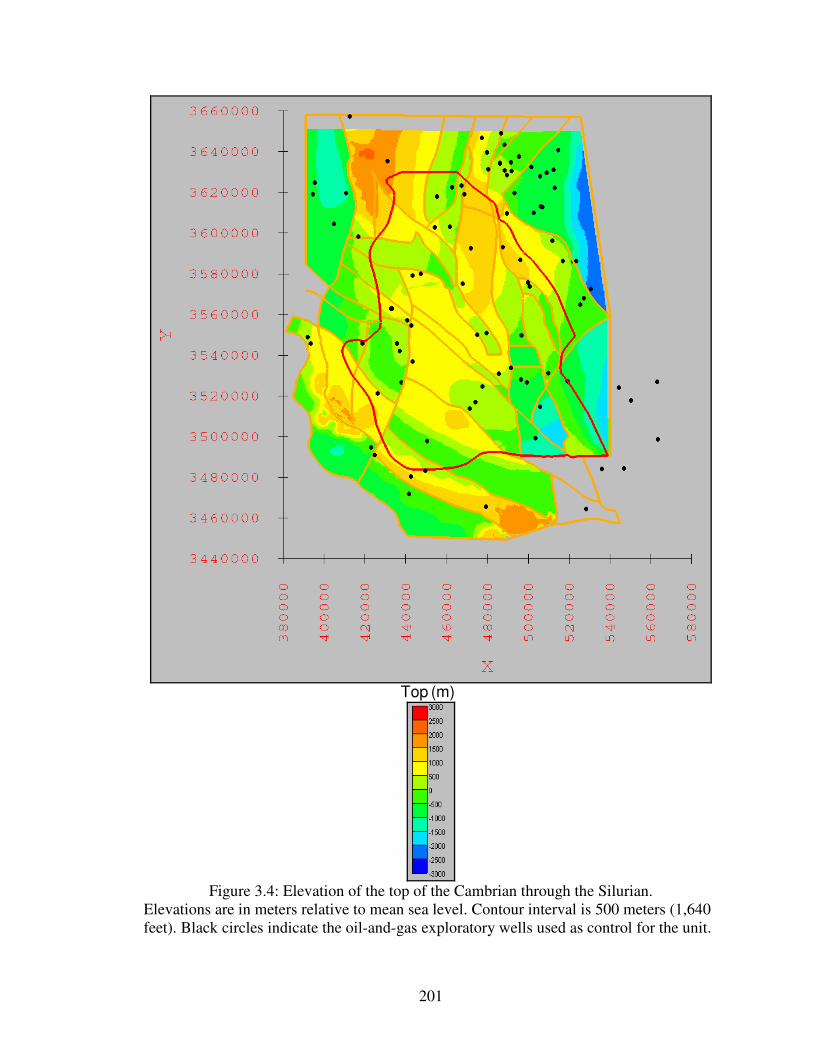
201
Figure 3.4: Elevation of the top of the Cambrian through the Silurian.
Elevations are in meters relative to mean sea level. Contour interval is 500 meters (1,640 feet). Black circles indicate the oil-and-gas exploratory wells used as control for the unit.
Top (m)

202
Figure 3.5: Elevation of the top of the Devonian.
Elevations are in meters relative to mean sea level. Contour interval is 500 meters (1,640 feet). Black circles indicate the oil-and-gas exploratory wells used as control for the unit.
Top (m)
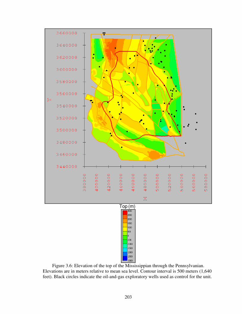
203
Figure 3.6: Elevation of the top of the Mississippian through the Pennsylvanian.
Elevations are in meters relative to mean sea level. Contour interval is 500 meters (1,640 feet). Black circles indicate the oil-and-gas exploratory wells used as control for the unit.
Top (m)

204
Figure 3.7: Elevation of the top of Lower Abo/Pow Wow Conglomerate.
Elevations are in meters relative to mean sea level. Contour interval is 500 meters (1,640 feet). Black circles indicate the oil-and-gas exploratory wells used as control for the unit.
Top (m)

205
Figure 3.8: Elevation of the top of Hueco Limestone/Formation (or Bursum Formation)
and Wolfcamp Formation. Elevations are in meters relative to mean sea level. Contour interval is 500 meters (1,640 feet). Black circles indicate the oil-and-gas exploratory wells used as control for the unit.
Top (m)

206
Figure 3.9: Elevation of the top of Abo Formation.
Elevations are in meters relative to mean sea level. Contour interval is 500 meters (1,640 feet). Black circles indicate the oil-and-gas exploratory wells used as control for the unit.
Top (m)

207
Figure 3.10: Elevation of the top of Yeso Formation.
Elevations are in meters relative to mean sea level. Contour interval is 500 meters (1,640 feet). Black circles indicate the oil-and-gas exploratory wells used as control for the unit.
Top (m)

208
Figure 3.11: Elevation of the top of Bone Spring Limestone/Formation.
Elevations are in meters relative to mean sea level. Contour interval is 500 meters (1,640 feet). Black circles indicate the oil-and-gas exploratory wells used as control for the unit.
Top (m)

209
Figure 3.12: Elevation of the top of Victorio Peak Limestone/Formation and Cutoff Shale
and Wilke Ranch Formation. Elevations are in meters relative to mean sea level. Contour interval is 500 meters (1,640 feet). Black circles indicate the oil-and-gas exploratory wells used as control for the unit.
Top (m)

210
Figure 3.13: Elevation of the top of San Andres Formation.
Elevations are in meters relative to mean sea level. Contour interval is 500 meters (1,640 feet). Black circles indicate the oil-and-gas exploratory wells used as control for the unit.
Top (m)

211
Figure 3.14: Elevation of the top of Delaware Mountain Group.
Elevations are in meters relative to mean sea level. Contour interval is 500 meters (1,640 feet). Black circles indicate the oil-and-gas exploratory wells used as control for the unit.
Top (m)

212
Figure 3.15: Elevation of the top of Goat Seep Dolomite/Limestone/Formation and
Capitan Limestone/Formation. Elevations are in meters relative to mean sea level. Contour interval is 500 meters (1,640 feet). Black circles indicate the oil-and-gas exploratory wells used as control for the unit.
Top (m)

213
Figure 3.16: Elevation of the top of Artesia Group.
Elevations are in meters relative to mean sea level. Contour interval is 500 meters (1,640 feet). Black circles indicate the oil-and-gas exploratory wells used as control for the unit.
Top (m)

214
Figure 3.17: Elevation of the top of the Cretaceous.
Elevations are in meters relative to mean sea level. Contour interval is 500 meters (1,640 feet). Black circles indicate the oil-and-gas exploratory wells used as control for the unit.
Top (m)

215
Figure 3.18: Elevation of the top of Cenozoic alluvium.
Elevations are in meters relative to mean sea level. Contour interval is 500 meters (1,640 feet). Black circles indicate the oil-and-gas exploratory wells used as control for the unit.
Top (m)

216
Figure 3.19: Thickness of the Cambrian through the Silurian.
Contour interval is 250 meters (820 feet). White color indicates unit is not present. Black circles indicate the oil-and-gas exploratory wells used as control for the unit.
Thickness (m)
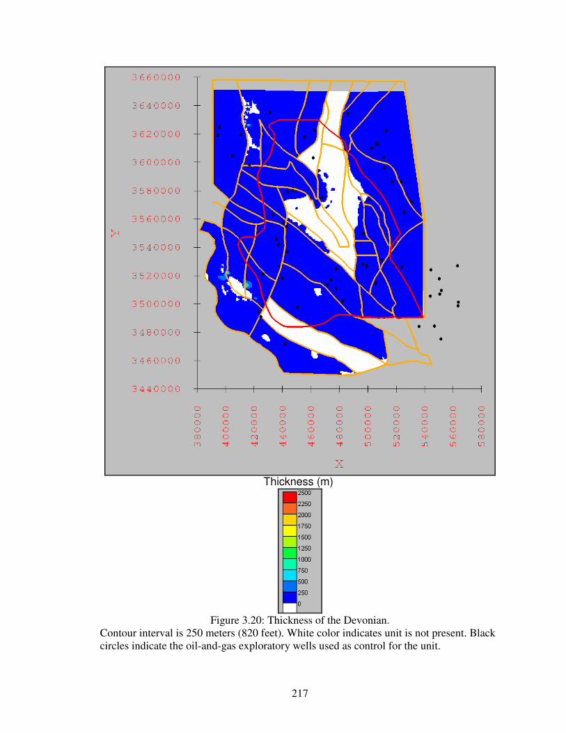
217
Figure 3.20: Thickness of the Devonian.
Contour interval is 250 meters (820 feet). White color indicates unit is not present. Black circles indicate the oil-and-gas exploratory wells used as control for the unit.
Thickness (m)

218
Figure 3.21: Thickness of the Mississippian through the Pennsylvanian.
Contour interval is 250 meters (820 feet). White color indicates unit is not present. Black circles indicate the oil-and-gas exploratory wells used as control for the unit.
Thickness (m)
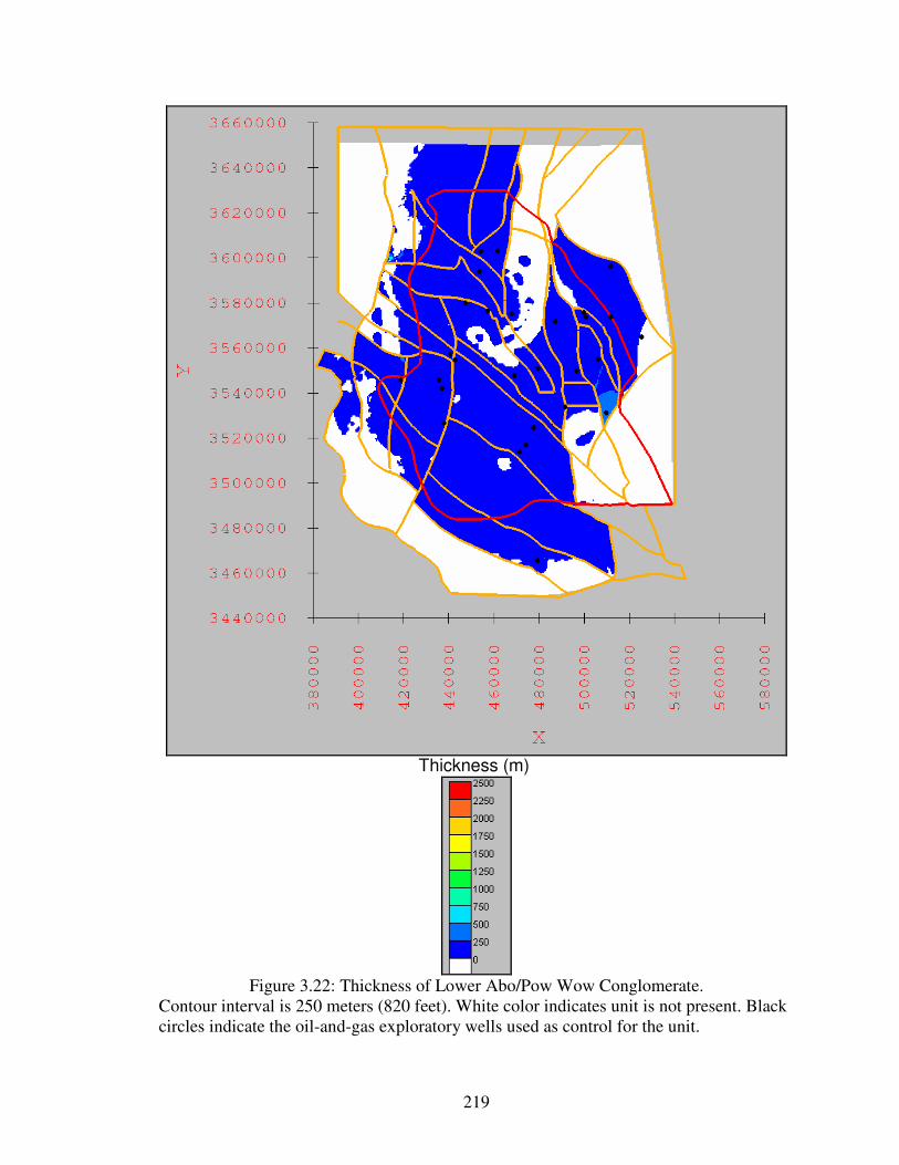
219
Figure 3.22: Thickness of Lower Abo/Pow Wow Conglomerate.
Contour interval is 250 meters (820 feet). White color indicates unit is not present. Black circles indicate the oil-and-gas exploratory wells used as control for the unit.
Thickness (m)

220
Figure 3.23: Thickness of Hueco Limestone/Formation (or Bursum Formation) and
Wolfcamp Formation. Contour interval is 250 meters (820 feet). White color indicates unit is not present. Black circles indicate the oil-and-gas exploratory wells used as control for the unit.
Thickness (m)
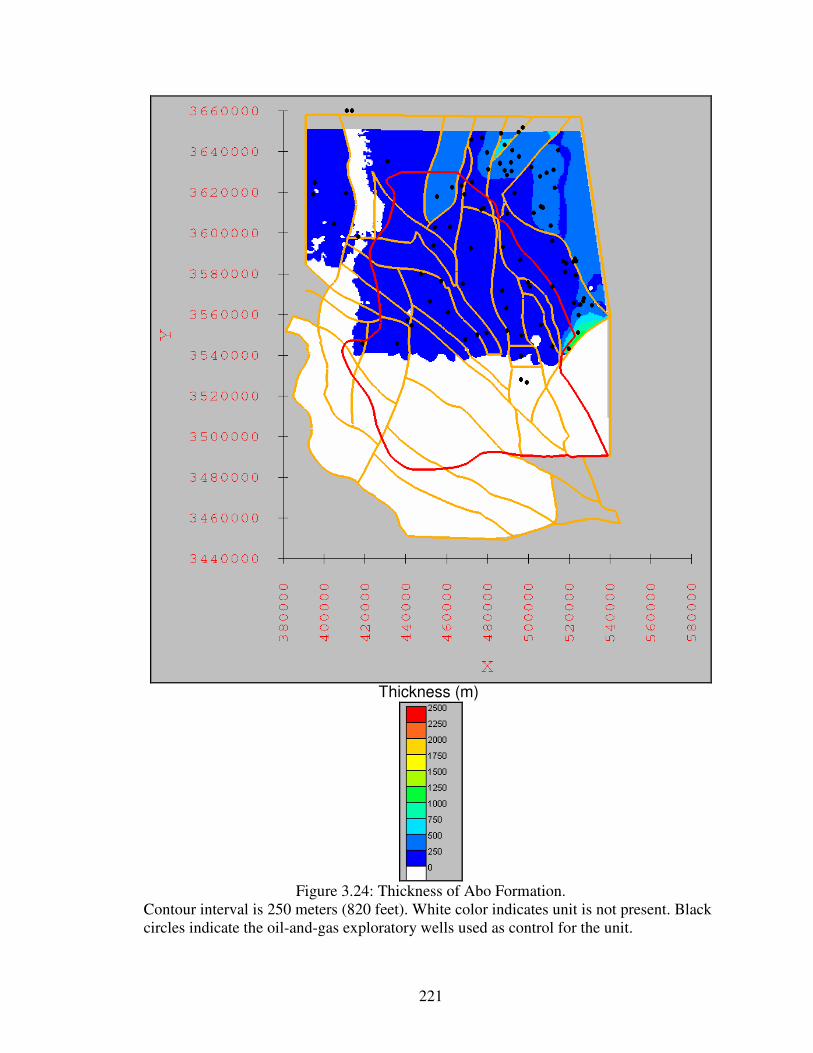
221
Figure 3.24: Thickness of Abo Formation.
Contour interval is 250 meters (820 feet). White color indicates unit is not present. Black circles indicate the oil-and-gas exploratory wells used as control for the unit.
Thickness (m)

222
Figure 3.25: Thickness of Yeso Formation.
Contour interval is 250 meters (820 feet). White color indicates unit is not present. Black circles indicate the oil-and-gas exploratory wells used as control for the unit.
Thickness (m)

223
Figure 3.26: Thickness of Bone Spring Limestone/Formation.
Contour interval is 250 meters (820 feet). White color indicates unit is not present. Black circles indicate the oil-and-gas exploratory wells used as control for the unit.
Thickness (m)

224
Figure 3.27: Thickness of Victorio Peak Limestone/Formation and Cutoff Shale and
Wilke Ranch Formation. Contour interval is 250 meters (820 feet). White color indicates unit is not present. Black circles indicate the oil-and-gas exploratory wells used as control for the unit.
Thickness (m)

225
Figure 3.28: Thickness of San Andres Formation.
Contour interval is 250 meters (820 feet). White color indicates unit is not present. Black circles indicate the oil-and-gas exploratory wells used as control for the unit.
Thickness (m)

226
Figure 3.29: Thickness of Delaware Mountain Group.
Contour interval is 250 meters (820 feet). White color indicates unit is not present. Black circles indicate the oil-and-gas exploratory wells used as control for the unit.
Thickness (m)

227
Figure 3.30: Thickness of Goat Seep Dolomite/Limestone/Formation and Capitan
Limestone/Formation. Contour interval is 250 meters (820 feet). White color indicates unit is not present. Black circles indicate the oil-and-gas exploratory wells used as control for the unit.
Thickness (m)

228
Figure 3.31: Thickness of Artesia Group.
Contour interval is 250 meters (820 feet). White color indicates unit is not present. Black circles indicate the oil-and-gas exploratory wells used as control for the unit.
Thickness (m)

229
Figure 3.32: Thickness of the Cretaceous.
Contour interval is 250 meters (820 feet). White color indicates unit is not present. Black circles indicate the oil-and-gas exploratory wells used as control for the unit.
Thickness (m)

230
Figure 3.33: Thickness of Cenozoic alluvium.
Contour interval is 250 meters (820 feet). White color indicates unit is not present. Black circles indicate the oil-and-gas exploratory wells used as control for the unit.
Thickness (m)

231
Figure 3.34: Land surface expression of the 3-D hydrogeologic framework solid model
clipped to the groundwater flow model boundary. Color-coding of hydrogeologic units corresponds to that used in Figure 2.1. Red line designates groundwater flow model boundary.
groundwater flow model boundary

232
Figure 3.35: Oblique views of the 3-D hydrogeologic framework solid model clipped to
the groundwater flow model boundary. Color-coding of hydrogeologic units corresponds to that used in Figure 2.1. Vertical exaggeration 10×.
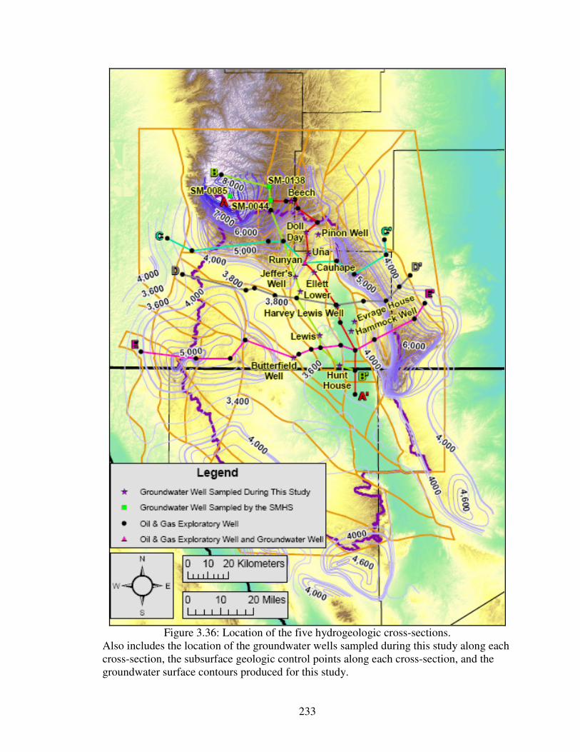
233
Figure 3.36: Location of the five hydrogeologic cross-sections.
Also includes the location of the groundwater wells sampled during this study along each cross-section, the subsurface geologic control points along each cross-section, and the groundwater surface contours produced for this study.

234
Figure 3.37: North-South cross-section A - A’.
Vertical exaggeration 23×. On all cross-sections, the light brown vertical lines are oil-and-gas exploratory well subsurface control points, the pink vertical lines are groundwater wells sampled during this study and by the SMHS, and the arrows indicate the sense of displacement on faults. Dashed lines for wells indicate that the well was projected to the line of cross-section. The groundwater surface is represented by the dark blue line. Color-coding of hydrogeologic units and unit labels corresponds to that used in Figure 2.1.

235
Figure 3.38: North-South cross-section B - B’.
Vertical exaggeration 18×.

236
Figure 3.39: West-East cross-section C - C’.
Vertical exaggeration 22×.

237
Figure 3.40: West-East cross-section D - D’.
Vertical exaggeration 18×.

238
Figure 3.41: West-East cross-section E - E’.
Vertical exaggeration 15×.

239
Figure 3.42: Groundwater elevation contours for the Salt Basin region.
Elevations are in feet above mean sea level. Contour interval is 200 feet. Hachured contours indicate groundwater depressions. The red circle and green square symbols indicate groundwater wells used as control for the contours, while the pink triangle symbols indicate groundwater wells not used as control points.

240
Figure 3.43: Depth-to-groundwater for the Salt Basin region.
Depths are in feet. Groundwater well symbology is the same as Figure 3.42. Light blue regions delineate zones of shallower groundwater than is indicated by the surrounding depth-to-groundwater polygons.

241
Figure 3.44: Locations and an oblique view of the five cross-sections within the 3-D
hydrogeologic framework solid model. Color-coding of hydrogeologic units corresponds to that used in Figure 2.1, and Figures 3.37 through 3.41. Red line designates groundwater flow model boundary. Blue lines indicate cross-sections. Vertical exaggeration 10×.
A
A’
B’
B
C C’
D’
E’
E
D
A
B C
D
E

242
Figure 3.45: Side views along cross-section A - A’ of the 3-D framework solid model on left and hand-drawn cross-section on right. Vertical exaggeration 10× on 3-D framework solid model cross-sections. Vertical exaggeration 23× on hand-drawn cross-section.
N S
Cenozoic alluvium
S N
N S
Permian
Cambrian through Silurian
Precambrian
Permian
Cambrian through Silurian
Precambrian
Mississippian through
Pennsylvanian
Devonian
Mississippian through
Pennsylvanian
Devonian
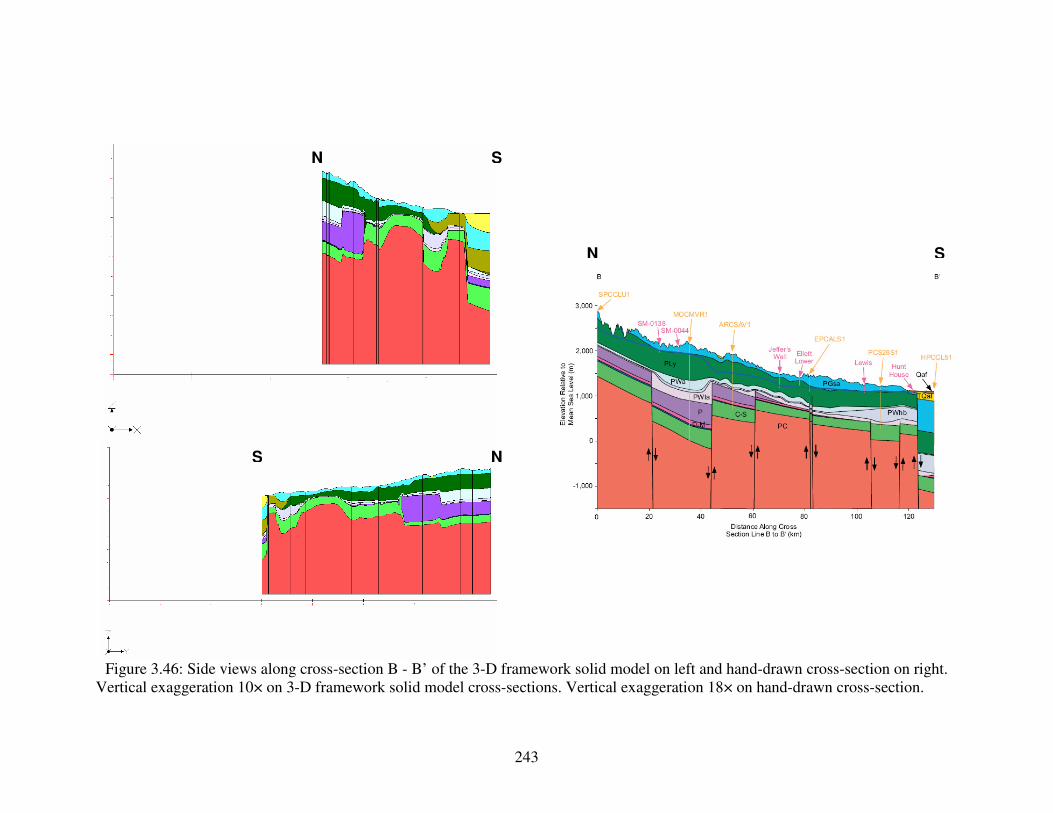
243
Figure 3.46: Side views along cross-section B - B’ of the 3-D framework solid model on left and hand-drawn cross-section on right. Vertical exaggeration 10× on 3-D framework solid model cross-sections. Vertical exaggeration 18× on hand-drawn cross-section.
N S
N S
S N

244
Figure 3.47: Side views along cross-section C - C’ of the 3-D framework solid model on left and hand-drawn cross-section on right. Vertical exaggeration 10× on 3-D framework solid model cross-section. Vertical exaggeration 22× on hand-drawn cross-section.
E W
E W

245
Figure 3.48: Side views along cross-section D - D’ of the 3-D framework solid model on left and hand-drawn cross-section on right. Vertical exaggeration 10× on 3-D framework solid model cross-section. Vertical exaggeration 18× on hand-drawn cross-section.
E W
E W
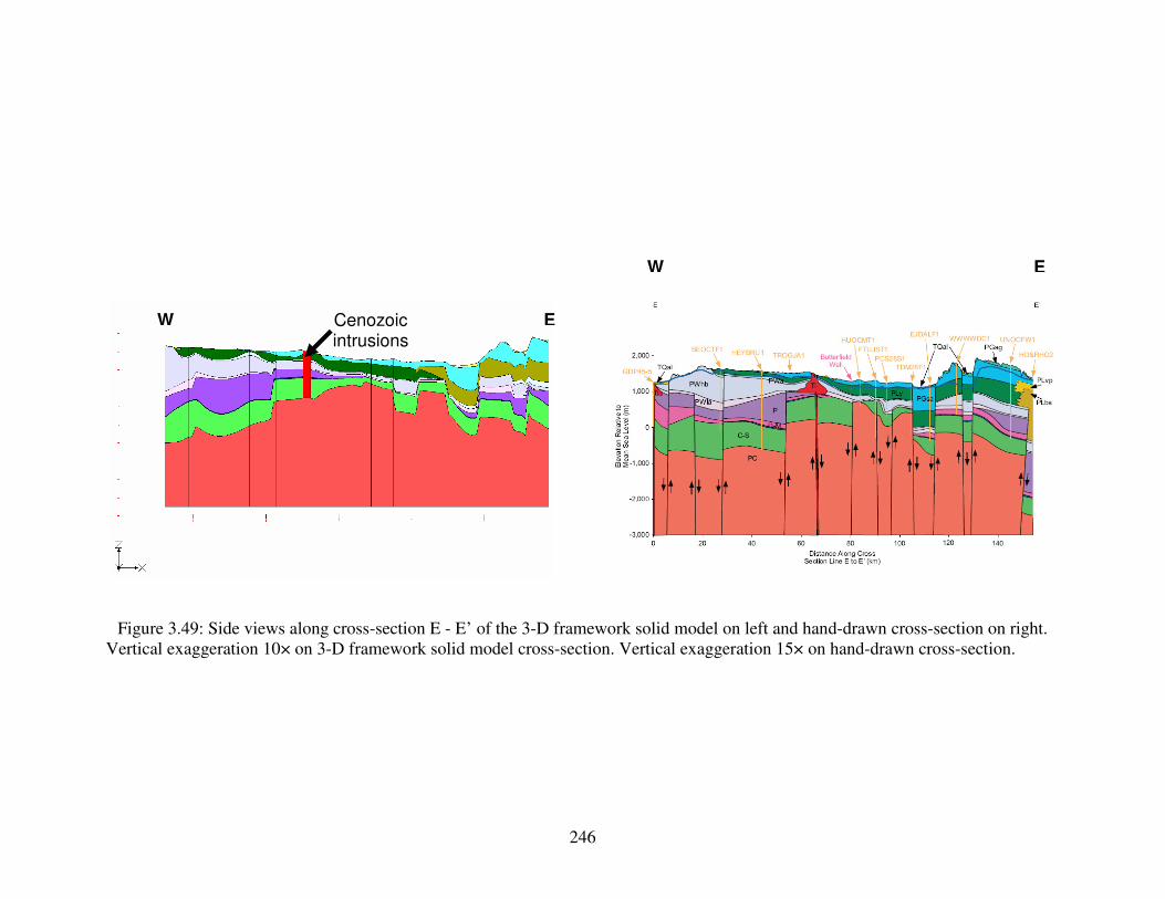
246
Figure 3.49: Side views along cross-section E - E’ of the 3-D framework solid model on left and hand-drawn cross-section on right. Vertical exaggeration 10× on 3-D framework solid model cross-section. Vertical exaggeration 15× on hand-drawn cross-section.
E W
E W
Cenozoic intrusions

247
Figure 3.50: Aquifers in the Salt Basin region.
Location of high mountain and Pecos slope aquifers from SMHS. Location of Bone Spring-Victorio Peak and Hueco bolson aquifers from TWDB. Location of Capitan Reef Complex aquifer from Uliana (2001). Location of Cretaceous aquifer from Sharp (1989).

248
Figure 3.51: Predevelopment groundwater elevation contours, from JSAI (2002).
Elevations are in feet above mean sea level. Contour interval is 200 feet.

249
Figure 3.52: Predevelopment groundwater elevation contours for the valley-fill aquifer
within the Salt Basin graben, from Sharp (1989). Elevations are in feet above mean sea level. Contour interval is 10 feet. Also illustrates the structural features associated with groundwater divides in the valley-fill aquifer.

250
A = 85.0*[exp((-1.39 E-5)*X)]
R2 = 0.813
0.0
10.0
20.0
30.0
40.0
50.0
60.0
70.0
80.0
90.0
0 20,000 40,000 60,000 80,000 100,000 120,000
Distance Along Cross Section Line A to A' [X] (meters)
14C
Ac
tiv
ity
Mea
su
red
in
Gro
un
dw
ate
r [A
] (p
mC
)
Figure 3.53: 14C activity measured in groundwater versus distance along cross-section line A - A'.
Doll Day
Uña
Cauhape
Harvey
Lewis Well Evrage
House

251
[HCO3-] = (-2.43 E-5)*(X) + 6.45
R2 = 0.784
0.0
1.0
2.0
3.0
4.0
5.0
6.0
7.0
8.0
0 20,000 40,000 60,000 80,000 100,000 120,000
Distance Along Cross Section Line A to A' [X] (meters)
[HC
O3- ]
Me
as
ure
d i
n G
rou
nd
wa
ter
(mm
ole
s/L
)
Figure 3.54: [HCO3
-] measured in groundwater versus distance along cross-section line A - A'.
Doll Day
Uña
Cauhape
Harvey
Lewis Well
Evrage
House
Runyan
SM-0044
SM-0085

252
[Mg2+
] = (2.56 E-5)*(X) + 0.285
R2 = 0.920
0.0
0.5
1.0
1.5
2.0
2.5
3.0
3.5
0 20,000 40,000 60,000 80,000 100,000 120,000
Distance Along Cross Section Line A to A' [X] (meters)
[Mg
2+]
Me
as
ure
d i
n G
rou
nd
wa
ter
(mm
ole
s/L
)
Figure 3.55: [Mg2+] measured in groundwater versus distance along cross-section line A - A'.
Doll Day
Uña
Cauhape Harvey
Lewis Well
Evrage
House
Runyan
SM-0044
SM-0085

253
A = 85.0*[exp((-1.39 E-5)*X)]
0.0
10.0
20.0
30.0
40.0
50.0
60.0
70.0
80.0
90.0
0 20,000 40,000 60,000 80,000 100,000 120,000
Distance Along Cross Section Line A to A' [X] (meters)
14C
Ac
tiv
ity
(p
mC
)
Ao
A
Figure 3.56: 14C activity [A] and [A0] versus distance along cross-section line A - A'.
SM-0044
SM-0085
Doll Day
Uña
Runyan
Cauhape
Harvey
Lewis Well Evrage
House

254
0.00000001
0.0000001
0.000001
0.00001
0.0001
0.001
0.01
0.1
1
10
100
1000K
(m
/da
y)
Figure 3.57: Range of hydraulic conductivity [K] values from previous studies and this study. Vertical axis is logarithmic scale. Squares indicate median values, and triangles indicate average values.
Wasiolek (1991):
Yeso Fm.: unfractured siltstone and
gypsum
Wasiolek (1991):
Yeso Fm.: fractured limestone
YPCOTU2 wellsite
core analysis: Yeso Fm. and Abo
Fm.
This study: 14
C groundwater ages along
cross-section A to A’
Source
median
YPCOTU2 wellsite
core analysis: Cambrian
Hutchison (2008)
JSAI (2010):
Basin-fill
JSAI (2010):
Un-fractured Permian
JSAI (2010):
Fractured Permian
JSAI (2010):
Cambrian
JSAI (2010):
Pre-cambrian
average
Sigstedt (2010):
Salt Basin average

255
0.01
0.1
1
10
100
1000
10000
100000
1000000T
(m
2/d
ay
)
Figure 3.58: Range of transmissivity [T] values from previous studies and this study. Vertical axis is logarithmic scale. Squares indicate median values, and triangles indicate average values.
This study: 14
C groundwater ages
along cross-section A to A’
Aquifer/Facies/Source
Shelf- facies
Shelf-margin-facies
Basin-facies
Cretaceous Cenozoic volcanics
Valley- fill
median
Mayer (1995)
Hutchison (2008)
JSAI (2010)
average
Compiled from numerous sources as discussed in Chapter 3.6.a

256
Figure 3.59: Location of the four groundwater wells in the New Mexico portion of the
Salt Basin watershed with continuous water level measurements from 2003 to the middle of 2006, as presented in Huff and Chace (2006), and the TWDB’s State Well Number
4807516.

257
-4
-3.5
-3
-2.5
-2
-1.5
-1
-0.5
0
0.5
1
2003 2003.5 2004 2004.5 2005 2005.5 2006 2006.5 2007
Time [t] (years)
Gro
un
dw
ate
r L
ev
el
Ch
an
ge
[∆
h]
(m)
H&C 1
H&C 2
H&C 3
H&C 4
Figure 3.60: Change in groundwater levels versus time for wells H&C 1, H&C 2, H&C 3, and H&C 4.

258
-9
-8
-7
-6
-5
-4
-3
-2
-1
0
1
2003 2003.5 2004 2004.5 2005 2005.5 2006 2006.5 2007
Time [t] (years)
Gro
un
dw
ate
r L
ev
el
Ch
an
ge
[∆
h]
(m)
H&C 1
H&C 2
H&C 3
H&C 4
4807516
Figure 3.61: Change in groundwater levels versus time for wells H&C 1, H&C 2, H&C 3, H&C 4, and 4807516.

259
-9
-8
-7
-6
-5
-4
-3
-2
-1
0
1
2003 2003.5 2004 2004.5 2005 2005.5 2006 2006.5 2007
Time [t] (years)
Gro
un
dw
ate
r L
ev
el
Ch
an
ge
[∆
h]
(m)
H&C 1
H&C 2
H&C 3
H&C 4
4807516
Figure 3.62: Location of maximum and minimum change in groundwater levels used to calculate the average annual amplitude of
water level fluctuations in wells H&C 1, 2, 3, and 4, and 4807516.
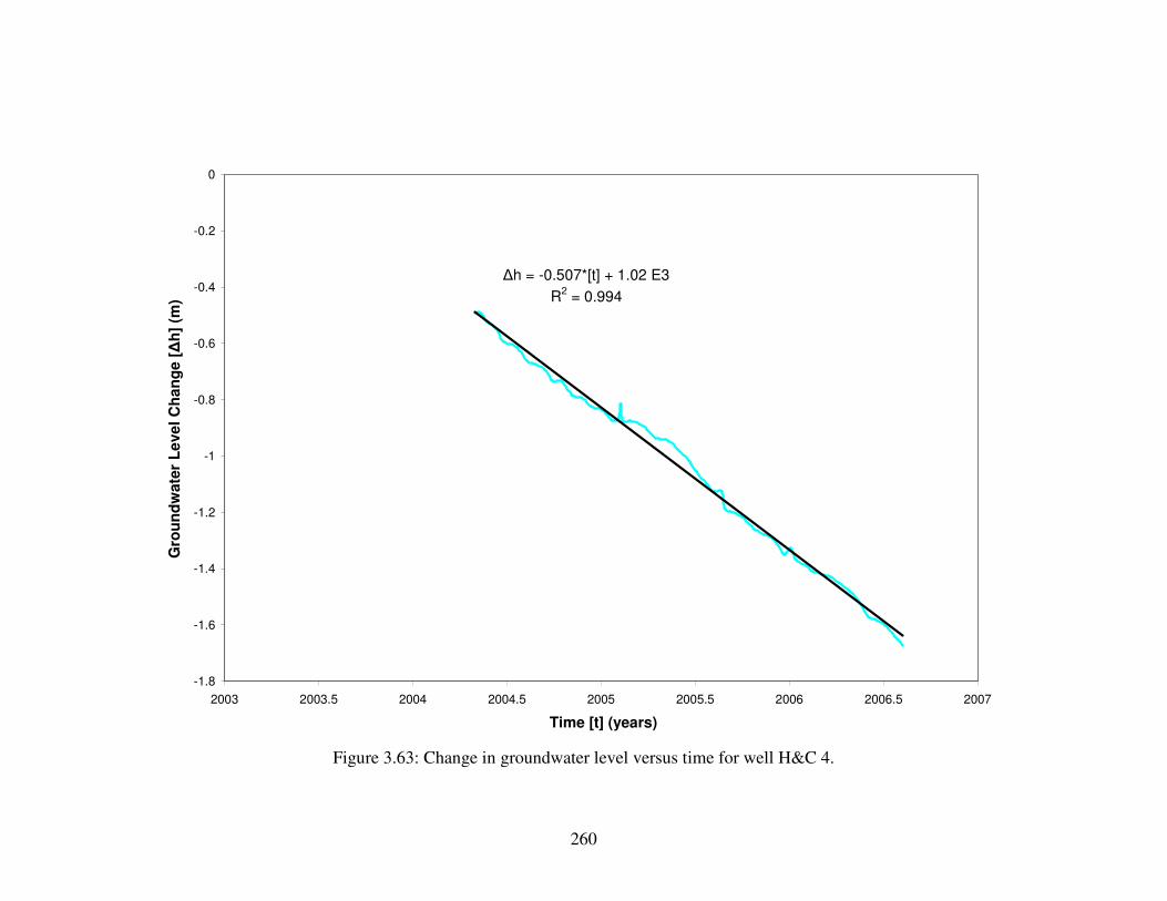
260
∆h = -0.507*[t] + 1.02 E3
R2 = 0.994
-1.8
-1.6
-1.4
-1.2
-1
-0.8
-0.6
-0.4
-0.2
0
2003 2003.5 2004 2004.5 2005 2005.5 2006 2006.5 2007
Time [t] (years)
Gro
un
dw
ate
r L
eve
l C
ha
ng
e [∆
h]
(m)
Figure 3.63: Change in groundwater level versus time for well H&C 4.

261
-0.06
-0.04
-0.02
0
0.02
0.04
0.06
0.08
2003 2003.5 2004 2004.5 2005 2005.5 2006 2006.5 2007
Time [t] (years)
De
tre
nd
ed
Gro
un
dw
ate
r L
ev
el C
ha
ng
e (
m)
Figure 3.64: Detrended change in groundwater level versus time for well H&C 4.

262
sT/s0 = 0.727*[exp((-6.99 E-5)*X)]
R2 = 0.959
sT/s0 = 1.27*[exp((-9.58 E-5)*X)]
R2 = 0.953
sT/s0 = 1.28*[exp((-9.28 E-5)*X)]
R2 = 0.957
0
0.1
0.2
0.3
0.4
0.5
0.6
0.7
0 5,000 10,000 15,000 20,000 25,000 30,000 35,000 40,000 45,000 50,000
Distance from Dell City, Texas [X] (meters)
sT/s
0
2003
2004
2005
Figure 3.65: sT/s0 calculated from water level fluctuations in 2003 at wells H&C 1, 2, and 3, and 4807516, and in 2004 and 2005 at
wells H&C 1, 2, 3, and 4, and 4807516 versus distance from Dell City, Texas.

263
tL = (3.67 E-3)*X - 40.6
R2 = 0.998
tL = (2.71 E-3)*X - 24.6
R2 = 0.999
tL = (1.95 E-3)*X - 23.7
R2 = 1
0
20
40
60
80
100
120
0 5,000 10,000 15,000 20,000 25,000 30,000 35,000 40,000 45,000
Distance from H&C 1 [X] (meters)
Av
era
ge P
ha
se
Lag
[t L
] (d
ay
s)
2003
2004
2005
Figure 3.66: Average phase lag between well H&C 1 and wells H&C 2 and 3 in 2003, and well H&C 1 and wells H&C 2, 3, and 4 in
2004 and 2005 versus distance from well H&C 1.
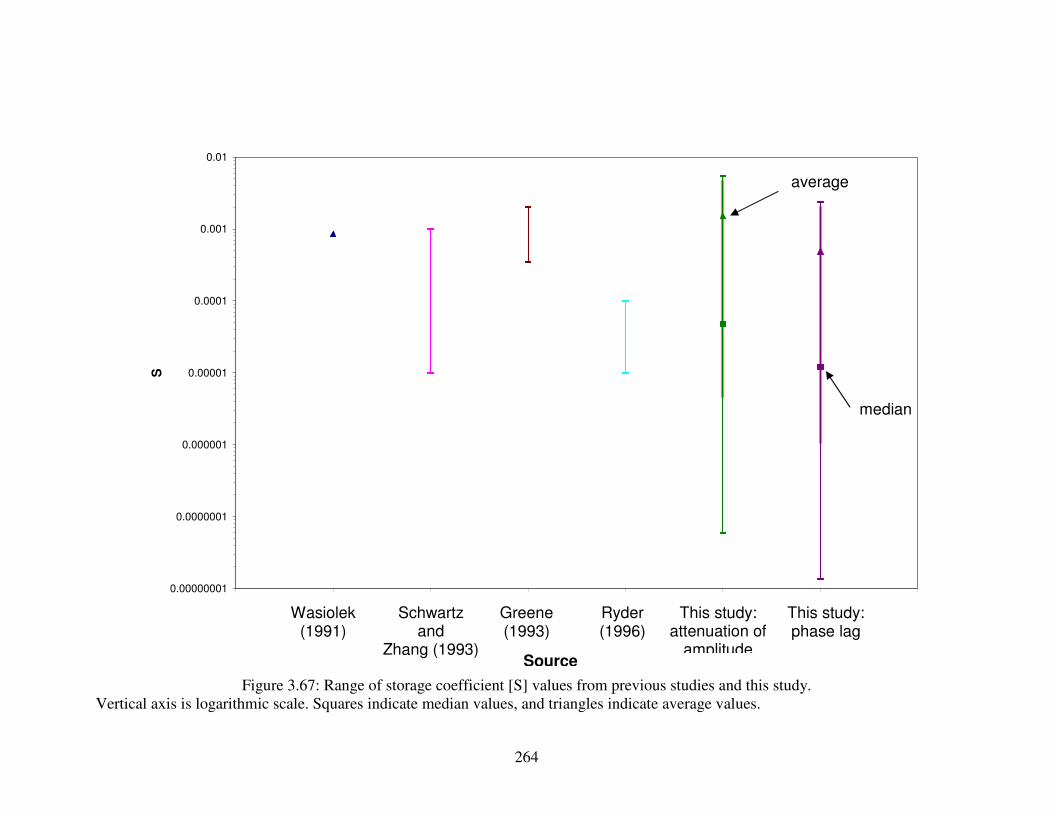
264
0.00000001
0.0000001
0.000001
0.00001
0.0001
0.001
0.01S
Figure 3.67: Range of storage coefficient [S] values from previous studies and this study. Vertical axis is logarithmic scale. Squares indicate median values, and triangles indicate average values.
Wasiolek (1991)
Schwartz and
Zhang (1993) Source
Greene (1993)
Ryder (1996)
This study: attenuation of
amplitude
This study: phase lag
median
average

265
TABLES – CHAPTER 3

266
Well Name,
LeaseWell ID API Number Easting Northing
Well
Elevation
(m)
Reference
Level
(Source)
Well
Depth
(m)
Township
(S)
Range
(E)Section
Houston Oil & Minerals Corp.,
State L.G. "1453" #1HO&MSL1 3003520013 406876 3685414 1,511 GR 3,003 12 10 5
Houston Oil & Minerals Corp.,
J.M. Lewelling #1HO&MJL1 3003520010 402778 3684425 1,440 KB 2,852 12 9 12
Houston Oil & Minerals Corp.,
Lewelling #2HO&MCL2 3003520015 399960 3684444 1,373 GR 2,892 12 9 10
Houston Oil & Minerals Corp.,
Federal "A" #1HO&MFA1 3003520009 413617 3660369 1,619 GR 1,125 14 10 24
Leland A. Hodges, Trustee,
Houston #1LAHTHO1 3003520005 411157 3660302 1,529 GR 928 14 10 23
Houston Oil & Minerals Corp.,
State 3724 #1HO&MS31 3003520011 412512 3657622 1,540 GR 1,396 14 10 36
McClellan Oil Corp.,
Flying "H" Ranch Unit Tract 3 #1MCOCFH1 3000562244 497349 3652108 1,554 GR 1,557 15 19 14
McClellan Oil Corp.,
Gragg B #1MCOCGB1 3000561993 495371 3649683 1,529 GR 1,407 15 19 27
Humble Oil & Refining Co.,
Yates Federal #1HO&RYF1 3000560015 486777 3649300 1,648 GR 1,643 15 18 26
J. Cleo Thompson,
State A-6 #1JCTSA61 3000562988 477111 3646836 1,824 GR 1,203 16 17 6
Lubbook Machine & Supply Co., Inc.,
Anderson-Randell #1LM&SAR1 3000500003 472069 3645946 1,767 TH 563 16 16 3
Humble Oil & Refining Co.,
Humble-Yates N.M. State #1HO&RHY1 3000510521 488336 3643533 1,574 DF 1,802 16 18 8
W.H. Black Drilling Co.,
Shildneck #1WHBDCS1 3000500012 514561 3641046 1,330 ? 2,137 16 20 24
Continental Oil Company,
State NN #1COCSNN1 3000560185 492051 3640997 1,538 DF 1,677 16 18 22
J. Cleo Thompson,
Federal A-28 #1JCTFA28 3000562915 479948 3639939 1,649 GR 1,481 16 17 28
C & K Petroleum, Inc.,
Singer Lake State #1C&KSLS1 3000560320 495659 3637945 1,545 KB 1,617 16 19 31
Table 3.1: New Mexico oil-and-gas exploratory wells used in this study. Key at bottom of table.
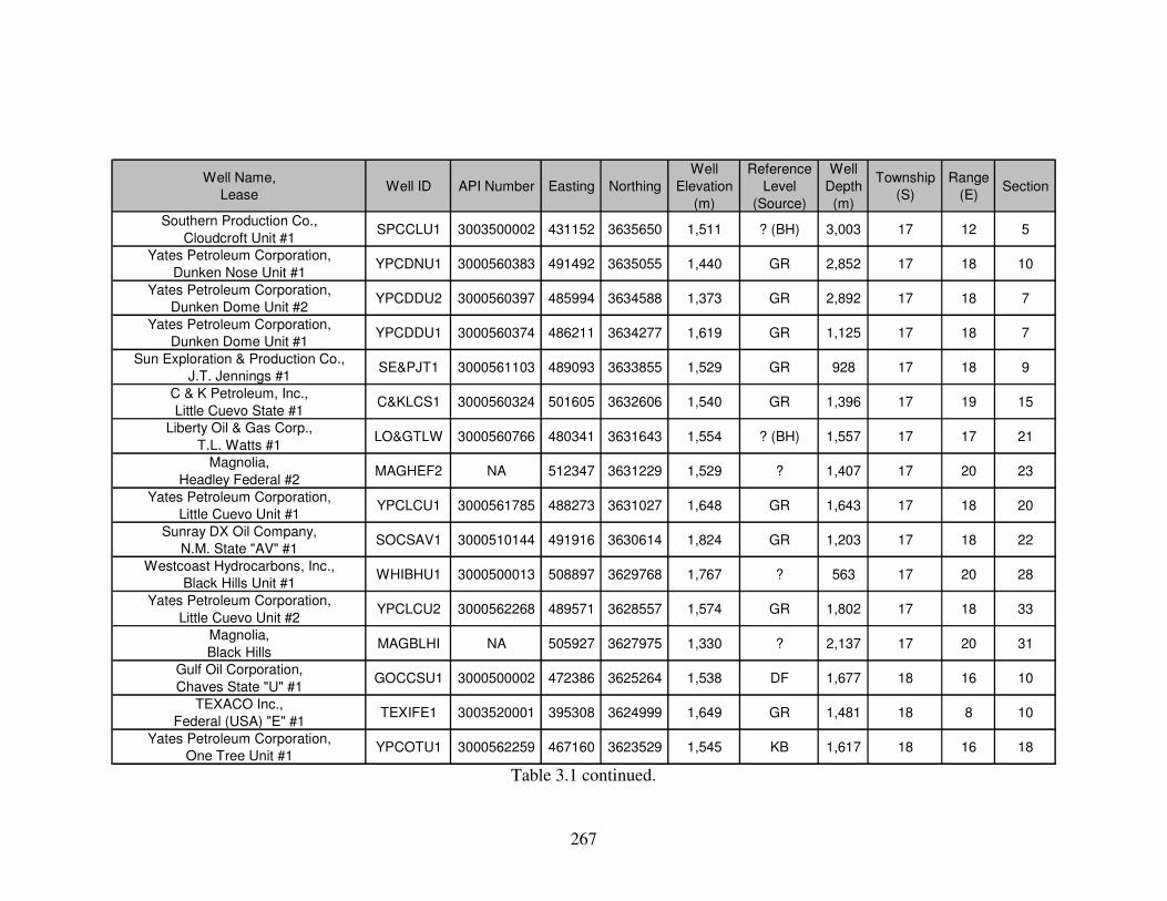
267
Well Name,
LeaseWell ID API Number Easting Northing
Well
Elevation
(m)
Reference
Level
(Source)
Well
Depth
(m)
Township
(S)
Range
(E)Section
Southern Production Co.,
Cloudcroft Unit #1SPCCLU1 3003500002 431152 3635650 1,511 ? (BH) 3,003 17 12 5
Yates Petroleum Corporation,
Dunken Nose Unit #1YPCDNU1 3000560383 491492 3635055 1,440 GR 2,852 17 18 10
Yates Petroleum Corporation,
Dunken Dome Unit #2YPCDDU2 3000560397 485994 3634588 1,373 GR 2,892 17 18 7
Yates Petroleum Corporation,
Dunken Dome Unit #1YPCDDU1 3000560374 486211 3634277 1,619 GR 1,125 17 18 7
Sun Exploration & Production Co.,
J.T. Jennings #1SE&PJT1 3000561103 489093 3633855 1,529 GR 928 17 18 9
C & K Petroleum, Inc.,
Little Cuevo State #1C&KLCS1 3000560324 501605 3632606 1,540 GR 1,396 17 19 15
Liberty Oil & Gas Corp.,
T.L. Watts #1LO>LW 3000560766 480341 3631643 1,554 ? (BH) 1,557 17 17 21
Magnolia,
Headley Federal #2MAGHEF2 NA 512347 3631229 1,529 ? 1,407 17 20 23
Yates Petroleum Corporation,
Little Cuevo Unit #1YPCLCU1 3000561785 488273 3631027 1,648 GR 1,643 17 18 20
Sunray DX Oil Company,
N.M. State "AV" #1SOCSAV1 3000510144 491916 3630614 1,824 GR 1,203 17 18 22
Westcoast Hydrocarbons, Inc.,
Black Hills Unit #1WHIBHU1 3000500013 508897 3629768 1,767 ? 563 17 20 28
Yates Petroleum Corporation,
Little Cuevo Unit #2YPCLCU2 3000562268 489571 3628557 1,574 GR 1,802 17 18 33
Magnolia,
Black HillsMAGBLHI NA 505927 3627975 1,330 ? 2,137 17 20 31
Gulf Oil Corporation,
Chaves State "U" #1GOCCSU1 3000500002 472386 3625264 1,538 DF 1,677 18 16 10
TEXACO Inc.,
Federal (USA) "E" #1TEXIFE1 3003520001 395308 3624999 1,649 GR 1,481 18 8 10
Yates Petroleum Corporation,
One Tree Unit #1YPCOTU1 3000562259 467160 3623529 1,545 KB 1,617 18 16 18
Table 3.1 continued.

268
Well Name,
LeaseWell ID API Number Easting Northing
Well
Elevation
(m)
Reference
Level
(Source)
Well
Depth
(m)
Township
(S)
Range
(E)Section
Yates Petroleum Corporation,
Dog Canyon "YF" Federal #1YPCDCF1 3003520024 462754 3622676 1,511 KB 3,003 18 15 15
Texas Oil & Gas Corp.,
Federal "C" #1TO&GFC1 3000560017 512954 3622309 1,440 GR 2,852 18 20 23
Kewanee Oil Co.,
F-M Unit #1KOCFMU1 3000500009 493140 3619927 1,373 ? 2,892 18 18 26
TEXACO Inc.,
Federal (USA) "F" #1TEXIFF1 3003520006 410790 3619951 1,619 GR 1,125 18 10 30
Yates Petroleum Corporation,
One Tree Unit #2YPCOTU2 3000562276 468582 3619170 1,529 KB 928 18 16 29
TEXACO Inc.,
Federal (USA) "G" #1TEXIFG1 3003520004 394443 3619379 1,540 GR 1,396 18 8 33
Marathon Oil Co.,
Mesa Verde Ranch #1MOCMVR1 3003520022 455326 3618246 1,554 ? (BH) 1,557 18 14 35
Yates Petroleum Corp.,
Buckhorn AYU State Com #1YPCBAYU 3000560541 506142 3613140 1,529 ? (BH) 1,407 19 20 18
Texas Oil & Gas Corp.,
Federal "A" #1TO&GFA1 3000510431 506950 3613041 1,648 KB 1,643 19 20 17
Yates Petroleum Corporation
(aka Phoenix Resources Co.),
Bullis "AVW" State Com
(aka Ranch Road) #1
YPCBAVW 3000560557 507355 3612640 1,824 GR 1,203 19 20 20
Sun Oil Co.,
Pinon Unit #2SOCPIU2 3000500007 478157 3612259 1,767 DF 563 19 17 20
Sun Oil Co.,
Pinon Unit #1SOCPIU1 3000500006 476922 3611828 1,574 DF 1,802 19 17 19
U.V. Industries, Inc.,
Long Canyon Unit #1UVILCU1 3000560411 502547 3610225 1,330 KB 2,137 19 19 26
Gulf Oil Corp.,
Federal Munson #1GOCFMU1 3000510075 489407 3609839 1,538 DF 1,677 19 18 28
Plymouth Oil Co.,
Evans (aka Federal D) #1PLOCEV1 3003500003 404731 3604561 1,649 DF 1,481 20 9 15
Table 3.1 continued.

269
Well Name,
LeaseWell ID API Number Easting Northing
Well
Elevation
(m)
Reference
Level
(Source)
Well
Depth
(m)
Township
(S)
Range
(E)Section
Texas Oil & Gas Corp.,
Federal "B" #1TO&GFB1 NA 510832 3603835 1,511 ? 3,003 20 20 15
Atlantic Refining Co.,
State "AV" #1ARCSAV1 3003510001 461443 3603143 1,440 ? (BH) 2,852 20 15 16
Zapata Petroleum Corp.,
Federal 14 #1ZPCF141 3003500006 454127 3603086 1,373 DF 2,892 20 14 14
Sun Oil Company,
T.J. Pearson #1SOCTJP1 3003500005 416750 3598464 1,619 ? 1,125 20 10 35
Terra Resources, Inc.,
Burro Canyon Unit #1-YTRBCU1Y 3003520017 511686 3596471 1,529 ? (BH) 928 21 20 2
Stanolind Oil & Gas,
Thorn Unit #1SO>U1 3003500007 453419 3593869 1,540 Topo 1,396 21 14 15
Standard of Texas,
Scarp Unit #1SOTSCU1 3003500009 487438 3593394 1,554 DF 1,557 21 18 18
Lefors Petroleum Co.,
Federal #1LEPCFE1 3003500008 471863 3592611 1,529 KB 1,407 21 16 22
Yates Petroleum Corporation,
Brainerd "IO" Federal #1YPCBIOF 3001522149 523000 3587630 1,648 KB 1,643 22 21 1
Tri-Service Drilling Co.,
Little Dog Federal #1TSDLDF1 3003520008 496060 3586992 1,824 GR 1,203 22 19 6
Otero Oil Co.,
McGregor #1OTOCMC1 3003500010 412151 3586894 1,767 ? 563 22 10 5
Brainerd Corp.
(aka Continental Oil Co.),
Federal "A"
(aka East Texas Hill Unit) #1
BRCFEA1 3001500005 523406 3586429 1,574 DF 1,802 22 21 1
Continental Oil Co.,
H.W. Bass #1COCHWB1 3001500004 516898 3586367 1,330 ? 2,137 22 21 5
Marathon Oil Company,
Box Canyon Unit #1MOCBCU1 3001510012 522193 3586059 1,538 DF 1,677 22 21 12
Pitts Energy Co.,
Federal "9" #1PIECF91 3001527563 518567 3585218 1,649 KB 1,481 22 21 9
Table 3.1 continued.

270
Well Name,
LeaseWell ID API Number Easting Northing
Well
Elevation
(m)
Reference
Level
(Source)
Well
Depth
(m)
Township
(S)
Range
(E)Section
Sinclair Oil & Gas Company,
Federal Eddy 193 #1SO&GFE1 3001500001 518145 3580901 1,511 DF 3,003 22 21 28
E.P. Campbell,
Hurley #1EPCAHU1 3003500012 447355 3580223 1,440 DF 2,852 22 14 30
Tom L. Ingram,
State "E" #1TLISTE1 3001520003 523070 3579540 1,373 GR 2,892 22 21 36
Fred Turner, Jr.,
Everett #1FTUEVE1 NA 443146 3579159 1,619 ? (BH) 1,125 22 13 34
E.P. Campbell,
Liberman State #1EPCALI1 3003500014 457361 3576570 1,529 DF 928 23 15 7
W.R. Weaver,
Thompson #1WRWETH1 3003500017 499785 3575900 1,540 DF 1,396 23 19 9
E.P. Campbell,
Lois Spanel #1EPCALS1 3003500015 467947 3575324 1,554 DF (Est.) 1,557 23 16 7
Presco, Inc.,
Indian Creek Federal #1PRIICF1 3003520030 511700 3573937 1,529 GR 1,407 23 20 14
E.P. Campbell,
McMillan Federal #1EPCAMF1 3003500018 500598 3573842 1,648 DF 1,643 23 19 15
Humble Oil & Refining Co.,
Huapache Oil Unit #2HO&RHO2 3001500013 530547 3572779 1,824 DF 1,203 23 22 23
Coral Oil & Gas Co.,
Warren #1CO&GCW1 3003500016 487264 3571960 1,767 Topo 563 23 18 19
Inexco Oil Company,
Sitting Bull Unit #1IOCSBU1 3001520752 527152 3568073 1,574 GR 1,802 24 22 4
Coral Oil & Gas Company,
Ann Spanel #1CO&GAS1 3003500021 451716 3566857 1,330 DF 2,137 24 14 9
Atlantic Refining Co.,
Huapache Unit #9ARCHUU9 3001500016 527053 3566737 1,538 DF 1,677 24 22 9
Skelly Oil Co.,
Las Cruces "D" #1SOCLCD1 3001500003 522240 3565867 1,649 DF 1,481 24 21 12
Union Oil Co.,
Federal White #1UNOCFW1 3001500019 525449 3565154 1,545 DF 1,617 24 22 17
Table 3.1 continued.

271
Well Name,
LeaseWell ID API Number Easting Northing
Well
Elevation
(m)
Reference
Level
(Source)
Well
Depth
(m)
Township
(S)
Range
(E)Section
Humble Oil & Refining Co.,
Huapache Unit #5HO&RHU5 3001500018 531153 3564735 1,511 DF 3,003 24 22 14
Threshold Development Co.,
Chiricahua R 21 Federal #1TDCR21F 3003520034 489264 3563381 1,440 GR 2,852 24 18 21
Fred Turner, Jr.
(aka Pasotero Pet. Corp.),
Evans #1
FTUJEV1 3003500020 433355 3563003 1,373 ? (BH) 2,892 24 12 22
E.P. Campbell (aka John J. Eisner),
Federal #1EPCAFE1 3003500019 432641 3562887 1,619 DF 1,125 24 12 21
Flynn, Welch, Yates,
Donahue #1FWYDON1 NA 460768 3561350 1,529 ? (Dunn) 928 24 15 28
Franklin, Aston & Fair, Inc.,
Turkey Draw Unit #1FA&FTD1 3001521378 524583 3560015 1,540 GR 1,396 24 22 31
Union Oil Co.,
McMillan #1UNOCMC1 3003500028 440825 3557266 1,554 Topo 1,557 25 13 9
Union Oil Co.,
Verse 7 Federal #1UOCV7F1 3001520591 524435 3556316 1,529 GR 1,407 25 22 7
W.W. West,
West Dog Canyon Unit #1WWWWDC1 3003520007 505979 3555044 1,648 GR 1,643 25 20 18
Transocean Oil,
G.J. Ablah #1TROGJA1 3003520018 442810 3554817 1,824 GR 1,203 25 13 15
R.H. Ernest,
Located Land Co. #1RHELLC1 3003500023 382791 3553354 1,767 USGS 563 25 7 20
Threshold Development Co.,
Mescalero 28 Federal #1TDM28F1 3003520033 489514 3552255 1,574 GR 1,802 25 18 28
Beard Oil Company,
Ridge USA #1BOCRUS1 3001522547 524447 3551405 1,330 GR 2,137 25 22 30
Pennzoil Co.,
Southland "28" State #1PCS28S1 3003520019 479573 3551070 1,538 GR 1,677 25 17 28
Fred Turner, Jr.,
State #1FTUJST1 3003500027 475070 3550274 1,649 DF 1,481 25 16 36
Table 3.1 continued.

272
Well Name,
LeaseWell ID API Number Easting Northing
Well
Elevation
(m)
Reference
Level
(Source)
Well
Depth
(m)
Township
(S)
Range
(E)Section
E.J. Dunigan,
Alpha Federal #1EJDALF1 3003520002 496594 3549815 1,511 KB 3,003 25 19 31
GDP 61-6 GDP61-6 NA 390213 3549130 1,440 WH 2,852 26 8 6
GDP 45-5 GDP45-5 NA 391837 3549102 1,373 WH 2,892 26 8 5
GDP 46-6 GDP46-6 NA 390223 3549119 1,619 WH 1,125 26 8 6
Hunt Oil Co.,
McMillan-Turner #1HUOCMT1 3003500029 469015 3547882 1,529 ? (Dunn) 928 26 16 5
Harvey E. Yates Co.,
Bennett Ranch Unit #1HEYBRU1 3003520027 435547 3545814 1,540 GR 1,396 26 12 14
Seaboard Oil Co.,
Trigg-Federal #1SEOCTF1 3003500032 418801 3545797 1,554 DF 1,557 26 11 18
GDP 51-8 GDP51-8 NA 393417 3545870 1,529 WH 1,407 26 8 16
E.P. Campbell,
Spiegel-Federal #1EPCSPF1 3003510002 511803 3544568 1,648 Topo 1,643 26 20 14
Sinclair Oil & Gas Co.,
Guadalupe Ridge Unit #1SO&GGR1 3001520176 519670 3543204 1,824 GR 1,203 26 21 22
Harvey E. Yates Co.,
Bennett Ranch Unit 25 #1HEYBR25 3003520031 437133 3542284 1,767 ? 563 26 12 25
Table 3.1 continued:
API Number Key: NA = Not applicable. Reference Level (Source) Key: GR = Ground surface, KB = Kelley bushing, TH = Tubing head, DF = Derrick floor, WH = Well head, ? = unknown if elevation is from GR, KB, TH, DF, or WH, DEM = from USGS NED, Topo = GR from topo. map, BH = from Broadhead (2007), Est. = Estimated, Dunn = from Dunn NMGS (1954), USGS = from USGS.

273
Well Name,
LeaseWell ID API Number Easting Northing
Well
Elevation
(m)
Reference
Level
(Source)
Well
Depth
(m)
Section Block Survey
Hunt Petroleum Corp.,
C.L. Ranch "5" #1HPCCL51 4222930011 496478 3539912 1,110 ? (K&H) 1,678 5 67 T-1, T&P
TEXACO, Inc.,
State of Texas "FO" "3" #1TSTFO31 4222930005 421857 3539803 1,580 ? 2,647 3 A UL
Chesapeake Operating, Inc.,
DF Ranch State 63-12 #1CODFRS1 4210932302 543327 3538510 1,211 GR 2,780 12 63 T-1, T&P
Magnolia Petr. Co.,
U-Tex Lease #39881 #1MPCUTL1 4222900015 443219 3536988 1,533 DF 1,652 19 C UL
EOG Resources, Inc.,
Rector Canyon 24 State #1EOGRC24 4210932250 544329 3534119 1,200 GR 3,024 24 63 T-1, T&P
Pan American Petroleum Corporation,
List Anderson #1PAPCLA1 NA 491521 3533849 1,108 ? (V&K) 2,021 23 68 T-1, T&P
Bonanza Co.,
PiersonBONCOPI NA 531346 3532226 1,346 ? (V&K) 2,142 26 64 T-1, T&P
Pure Oil Co.,
Hunter #1PUOCHU1 NA 509809 3531380 1,625 ? (K&H) 2,027 34 66 T-1, T&P
Hunt Oil Co.,
Dyer #1HUOCDY1 4222930007 485477 3530917 1,119 ? (K&H) 898 31 68 T-1, T&P
Hueco Basin,
University #1HUBAUN1 NA 421896 3530405 1,558 DEM 765 39 A UL
Trail Mountain, Inc.,
University Big Iron "C45" #1TMUBIC1 4222900029 440743 3529232 1,516 GR 965 45 C UL
Hunt Petroleum Corp.,
C.L. Ranch #1HPCCLR1 4222930010 496475 3528252 1,105 ? (K&H) 1,595 44 67 T-1, T&P
TEXACO Inc.,
Culberson "L" Fee #1TEXCLF1 NA 519234 3527336 1,564 ? (K&H) 2,652 45 65 T-1, T&P
Tenneco Oil Co.,
TXL Fee #1TOTXLF1 4210931401 563041 3526975 1,086 KB 4,095 1 61 T-2, T&P
Pan American Petroleum Corporation,
Ed Hammock #1PAPCEH1 NA 499124 3526693 1,110 GR 2,152 4 67 T-2, T&P
Trail Mountain, Inc.,
University Sizzler D5 #1TMUSD51 4222930227 437784 3526650 1,437 GR 1,774 5 D UL
TXL Corp.,
Culberson "C" Fee #1TXLCCF1 NA 523721 3526221 1,515 ? (V&K) 2,362 1 65 T-2, T&P
Table 3.2: Texas oil-and-gas exploratory wells used in this study. Key at bottom of table.

274
Well Name,
LeaseWell ID API Number Easting Northing
Well
Elevation
(m)
Reference
Level
(Source)
Well
Depth
(m)
Section Block Survey
General Crude Oil Company,
Merrill and Voyles et al. #1GCOCMV1 NA 477481 3524877 1,580 DF 2,647 8 69 T-2, T&P
Magnolia Petro.,
No. A-1 Homer, CowdenMPNA1HC NA 544286 3524346 1,211 ? (V&K) 2,780 12 63 T-2, T&P
EOG Resources, Inc.,
Kenney 16 State #1HEOGKS1H 4210932270 527946 3523355 1,533 GR 1,652 16 64 T-2, T&P
EOG Resources, Inc.,
Kenney 16 State #2EOGKES2 4210932269 528404 3522559 1,200 GR 3,024 16 64 T-2, T&P
California Standard of Texas,
Theisen #1CASATT1 NA 426103 3521248 1,108 ? 2,021 19 E UL
D & J Equip Co.,
J.C. Hunter, Jr. #2DJJCHJ2 NA 512403 3519886 1,346 ? (V&K) 2,142 2 120 PSL
Trail Mountain, Inc.,
University Felina "D27" #1TMUFD27 4222930006 439917 3518350 1,625 GR 2,027 27 D UL
Border Exploration Co.,
Hammack et al. CT-1BECHCT1 4222930196 505172 3518026 1,119 ? (K&H) 898 20 120 PSL
TXL Oil Corp.,
Culberson B-T Fee #1TXLCBT1 NA 550456 3517797 1,558 ? (V&K) 765 33 62 T-2, T&P
A.R. Jones Co.,
E.C. Mowry #1ARJECM1 NA 474192 3516927 1,516 DF 965 36 70 T-2, T&P
Tipperary Corp.,
ST-1 Billye SparksTCST1BS 4222930195 474281 3516816 1,105 GR 1,595 36 70 T-2, T&P
J.L. Cowley,
E.C. Mowry #1JLCECM1 NA 473079 3515907 1,564 ? 2,652 37 70 T-2, T&P
Border Exploration Co.,
J.J. McAdoo 7 #1BECJJM1 4222930200 505794 3514682 1,086 ? (K&H) 4,095 7 119 PSL
T.E. Robertson Co., Inc.,
Mowry et al. #2TERCMO2 NA 471217 3514010 1,110 DF 2,152 47 70 T-2, T&P
The Superior Oil Company,
Covington State #1TSOCCS1 4210931405 565213 3512927 1,437 GR 1,774 1 115 PSL
Chesapeake Operating, Inc.,
Dela Minerals "3" State #701COIDM3S 4210932268 566918 3512065 1,515 GR 2,362 7 114 PSL
Trail Mountain, Inc.,
University Devil Woman L5 #1TMUDWL5 4222930253 477595 3510876 1,181 GR 1,461 5 L UL
Table 3.2 continued.

275
Well Name,
LeaseWell ID API Number Easting Northing
Well
Elevation
(m)
Reference
Level
(Source)
Well
Depth
(m)
Section Block Survey
Samson Lone Star, L.L.C.,
University Lands 46-14 #2SALSUL2 4210932278 551660 3509591 1,110 KB 1,678 14 46 UL
Humble Oil & Ref. Co.,
M.C. Sibley #1HORMCS1 NA 533795 3508569 1,580 ? (V&K) 2,647 24 68 PSL
N. Amer. Royalties, Inc.,
Potter #1NARIPO1 NA 511738 3508091 1,211 ? (V&K) 2,780 31 119 PSL
Chesapeake Operating, Inc.,
University Lands 4627 #1COUL462 4210932287 550571 3507028 1,533 GR 1,652 27 46 UL
J.M. Huber Corp.,
Tom Potter #1JMHCTP1 NA 514111 3505748 1,200 ? (V&K) 3,024 2 118 PSL
EnCana Oil & Gas (USA) Inc.,
Sibley Ranch 47 State "25" #1EOGSR47 4210932251 544180 3505778 1,108 KB 2,021 25 47 PSL
Anderson & Prichard,
Bordens #1A&PBOR1 NA 521137 3505265 1,346 ? (V&K) 2,142 34 69 PSL
Trail Mountain, Inc.,
University Ooby Dooby L35 #1TMUODL1 4222930261 482251 3502319 1,625 KB 2,027 35 L UL
Petro-Hunt, L.L.C.,
Melissa Taylor State 27 #1-HPHMTS27 4210932255 563684 3501318 1,119 GR 898 27 109 PSL
Faith Minerals, Inc.,
Wesley West #1FMINWW1 4222930012 503401 3499500 1,558 GR 765 36 118 PSL
American Quasar Pet. Co.,
V.C. Rounsaville #1AQPVCR1 NA 563477 3498883 1,516 ? (V&K) 965 13 108 PSL
Hassle Hunt Trust,
Univ. "M-49" #1HHUM491 NA 450328 3497929 1,105 DF 1,595 9 M UL
EOG Resources, Inc.,
Wild Horse Draw 7 #1EOGWHD7 4210932256 536584 3497771 1,564 GR 2,652 7 106 PSL
Pan American Pet. Corp.,
Phillip F. Hass #1PAPPFH1 NA 422942 3494846 1,086 DF 4,095 14 13 PSL
Chesapeake Operating, Inc.,
Melissa Taylor State 105-3COMT105 4210932297 541293 3493028 1,110 GR 2,152 3 105 PSL
Transocean Oil, Inc.,
36-1 MSA Trustee, Inc.TO36MSA 4222930192 424652 3490962 1,437 KB 1,774 36 13 PSL
El Paso Co.,
No. 1 MontgomeryEPCN1MO NA 546957 3484390 1,515 ? (V&K) 2,362 17 100 PSL
Table 3.2 continued.

276
Well Name,
LeaseWell ID API Number Easting Northing
Well
Elevation
(m)
Reference
Level
(Source)
Well
Depth
(m)
Section Block Survey
Gulf Oil Corp.,
M.A. Grisham #1GOCMAG1 NA 535928 3484129 1,110 ? (V&K) 1,678 18 99 PSL
Hassle Hunt Trust,
Mosely #1HAHUTM1 NA 449636 3483385 1,580 GR 2,647 27 24 PSL
Lockhart, Roseborough & Benton,
Gardner & Mosely #1
or
Western States Oil,
Gardner & Moseley #1
LR&BGM1
or
WSOG&M1
NA 442367 3480668 1,211 DF 2,780 12 18 PSL
Chesapeake Operating, Inc.,
State Street State #701COSS701 4210932271 546492 3478738 1,533 GR 1,652 7 97 PSL
Sinclair,
LooneySINCLOO NA 551319 3475371 1,200 ? (V&K) 3,024 22 97 PSL
Gulf Oil Corp.,
J. Burner-State "B" #1GOCJBS1 NA 441556 3472050 1,108 DF 2,021 14 19 PSL
Lockhart Bros.,
Gardner & Mosely (Formerly Public School) #1LOBG&M1 NA 446485 3468512 1,346 ? 2,142 5 21 PSL
Stanolind Oil & Gas Co. American Land,
No. 1 RoseboroughSOGAL1R NA 444464 3467169 1,625 ? (V&K) 2,027 7 21 PSL
J.P. Hurndall & R.A. Gray,
J.S. Pierce #1H&GJSP1 NA 479266 3465692 1,119 DEM 898 8 46 PSL
Fred A. Davis West and Armour,
Davis #1FADWAD1 NA 528309 3464645 1,558 ? (V&K) 765 5 86 PSL
Table 3.2 continued:
API Number Key: NA = Not applicable. Reference Level (Source) Key: GR = Ground surface, KB = Kelley bushing, DF = Derrick floor, ? = unknown if elevation is from GR, KB, or DF, DEM = from USGS NED, K&H = from King and Harder (1985), V&K = from Veldhuis and Keller (1980).

277
Well ID Distance Along Cross Section (m) Well Elevation (m) Well Depth (m)
SPCCLU1 0 2,859 1,433
YPCDCF1 27,841 1,946 2,569
YPCOTU1 32,348 1,876 1,992
YPCOTU2 36,933 2,010 908
SOCPIU2 48,742 1,925 506
LEPCFE1 71,399 1,642 686
CO&GCW1 97,263 1,186 717
TDCR21F 106,121 1,133 1,834
EJDALF1 121,541 1,159 1,523
HPCCL51 131,444 1,110 1,678
HPCCLR1 143,104 1,105 1,595 Table 3.21: Subsurface oil-and-gas exploratory wells along cross-section A - A’.
Well ID Distance Along Cross Section (m) Well Elevation (m) Well Depth (m)
SPCCLU1 0 2,859 1,433
MOCMVR1 35,636 2,143 2,137
ARCSAV1 51,931 1,921 1,227
EPCALS1 81,521 1,408 817
PCS28S1 108,977 1,206 905
HPCCL51 129,671 1,110 1,678 Table 3.22: Subsurface oil-and-gas exploratory wells along cross-section B - B’.
Well ID Distance Along Cross Section (m) Well Elevation (m) Well Depth (m)
PLOCEV1 0 1,233 2,312
SOCTJP1 13,477 1,344 1,362
ZPCF141 51,139 2,109 1,537
ARCSAV1 58,455 1,921 1,227
LEPCFE1 73,270 1,642 686
SOTSCU1 88,865 1,628 812
TSDLDF1 99,604 1,940 1,259
TRBCU1Y 117,881 1,572 1,704
TO&GFB1 125,294 1,463 2,480 Table 3.23: Subsurface oil-and-gas exploratory wells along cross-section C - C’.
Well ID Distance Along Cross Section (m) Well Elevation (m) Well Depth (m)
OTOCMC1 0 1,295 527
FTUEVE1 31,946 1,476 1,202
EPCAHU1 36,287 1,404 742
EPCALI1 46,939 1,326 823
EPCALS1 57,597 1,408 817
CO&GCW1 77,205 1,186 717
EPCAMF1 90,671 1,319 972
PRIICF1 101,774 1,767 1,454
SO&GFE1 111,262 1,582 1,524
BRCFEA1 118,893 1,397 3,230 Table 3.24: Subsurface oil-and-gas exploratory wells along cross-section D - D’.

278
Well ID Distance Along Cross Section (m) Well Elevation (m) Well Depth (m)
GDP 45-5 0 1,255 1,207
SEOCTF1 27,166 1,618 1,707
HEYBRU1 43,911 1,554 2,156
TROGJA1 55,479 1,509 1,617
HUOCMT1 83,689 1,269 663
FTUJST1 90,199 1,317 1,583
PCS28S1 94,772 1,206 905
TDM28F1 104,784 1,219 1,409
EJDALF1 112,272 1,159 1,523
WWWWDC1 123,016 1,771 1,390
UNOCFW1 144,954 1,740 2,053
HO&RHO2 154,127 1,358 3,835 Table 3.25: Subsurface oil-and-gas exploratory wells along cross-section E - E’.

279
Groundwater
Well IDSource
Distance
Along
Cross
Section
(m)
14C Activity
from
Exponential
Trend [A]
(pmC)
[HCO3-]
from
Linear
Trend
(mmoles/L)
[Mg2+
]
from
Linear
Trend
(mmoles/L)
14C Activity
Calculated
Using
Dedolomitization
Model [A0]
(pmC)
14C Age (yr)
SM-0085 SMHS 537 84.4 6.4 0.3 NA
SM-0044 SMHS 20,294 64.1 6.0 0.8 82.3 2,067
Doll Day A&S 56,137 39.0 5.1 1.7 70.6 4,916
Uña A&S 66,705 33.6 4.8 2.0 69.9 6,049
Runyan A&S 71,399 31.5 4.7 2.1 69.8 6,572
Cauhape A&S 77,842 28.8 4.6 2.3 69.5 7,280
Harvey Lewis Well A&S 97,882 21.8 4.1 2.8 65.4 9,077
Evrage House A&S 118,245 16.4 3.6 3.3 59.9 10,694 Table 3.29: Continuous parameters used in stoichiometric dedolomitization model, and
resultant 14C activities and groundwater ages. Source Key: SMHS = New Mexico Bureau of Geology & Mineral Resources’ Sacramento Mountains Hydrogeology Study, A&S = This study.

280
Geologic Unit
Sample
Depth
(m)
n
(%)
k
(mD)
K
(m/day)
Yeso 405 1.7 NA NA
Yeso 430 18.3 NA NA
Yeso 456 0 0.01 7.E-06
Yeso 470 12 NA NA
Yeso 482 5.1 0.01 7.E-06
Yeso 488 9.9 0 0
Yeso 519 9.5 0.15 1.1E-04
Yeso 546 8.8 0.43 3.2E-04
Yeso 564 0 0 0
Yeso 581 0 0.01 7.E-06
Yeso 588 0.2 NA NA
Abo 596 0 0 0
Abo 629 NA 1.75 1.30E-03
Abo 639 0.1 NA NA
Abo 641 0 0 0
Abo 648 0.1 0.01 7.E-06
El Paso/Ellenburger 691 No visible porosity. NA NA
El Paso/Ellenburger 693 Minor porosity. NA NA
El Paso/Ellenburger 710 0.3 0.000342 2.54E-07
Bliss 823 2.5 NA NA
Precambrian 833 0 0 0
Precambrian 841 0 0 0
Precambrian 849 0 0 0
Precambrian 858 0 0 0 Table 3.30: Wellsite core analysis porosity [n] and permeability [k], and calculated
hydraulic conductivity [K] data from the Yates Petroleum Corporation, One Tree Unit #2 (YPCOTU2) well along cross-section A - A’.

281
Cross Section
Interval
K
with
n = 6.95%
(m/day)
K
with
n = 0.1%
(m/day)
K
with
n = 18.3%
(m/day)
SM-0085 to
SM-00446.38E-02 9.18E-04 1.68E-01
SM-0044 to
Doll Day1.51E-01 2.18E-03 3.98E-01
Doll Day to
Uña3.38E-01 4.86E-03 8.90E-01
Uña to
Runyan4.78E-02 6.88E-04 1.26E-01
Runyan to
Cauhape1.66E-01 2.39E-03 4.37E-01
Cauhape to
Harvey Lewis Well4.46E+00 6.42E-02 1.17E+01
Harvey Lewis Well
to Evrage House1.44E+00 2.08E-02 3.80E+00
Table 3.31: Range of hydraulic conductivity [K] values calculated from stoichiometric
dedolomitization model groundwater ages along cross-section A - A’.
Cross Section
Interval
Average
Saturated
Aquifer
Thickness
Over Each
Interval (m)
T
with
n = 6.95%
(m2/day)
T
with
n = 0.1%
(m2/day)
T
with
n = 18.3%
(m2/day)
SM-0085 to
SM-0044763 4.87E+01 7.00E-01 1.28E+02
SM-0044 to
Doll Day564 8.53E+01 1.23E+00 2.25E+02
Doll Day to
Uña142 4.78E+01 6.88E-01 1.26E+02
Uña to
Runyan152 7.26E+00 1.04E-01 1.91E+01
Runyan to
Cauhape160 2.66E+01 3.82E-01 6.99E+01
Cauhape to
Harvey Lewis Well438 1.95E+03 2.81E+01 5.14E+03
Harvey Lewis Well
to Evrage House840 1.21E+03 1.74E+01 3.19E+03
Table 3.32: Range of transmissivity [T] values calculated from stoichiometric
dedolomitization model groundwater ages along cross-section A - A’.

282
Groundwater
Well
ID/
State
Well
Number
Maximum
Groundwater
Level
Change
2003
(m)
Minimum
Groundwater
Level
Change
2003
(m)
Maximum
Groundwater
Level
Change
2004
(m)
Average Amplitude
of
Water Level
Fluctuation
2003
[s0] for 4807516
and
[sT] for H&C 1, 2, and 3
(m)
S/T
(day/m2)
4807516 5.43E-01 -7.78E+00 -1.80E-01 3.98E+00 NA
H&C 1 9.34E-02 -3.33E+00 -4.72E-01 1.57E+00 4.52E-06
H&C 2 4.08E-01 -1.14E+00 -2.28E-01 6.16E-01 1.26E-06
H&C 3 2.56E-01 -5.03E-01 7.58E-02 3.35E-01 1.40E-06
H&C 4 NA NA 1.03E-02 NA NA Table 3.33: Maximum and minimum groundwater level change, average amplitude of
water level fluctuation, and S/T values for 2003.
Groundwater
Well
ID/
State
Well
Number
Maximum
Groundwater
Level
Change
2004
(m)
Minimum
Groundwater
Level
Change
2004
(m)
Maximum
Groundwater
Level
Change
2005
(m)
Average Amplitude
of
Water Level
Fluctuation
2004
[s0] for 4807516
and
[sT] for H&C 1, 2, 3, and 4
(m)
S/T
(day/m2)
4807516 -1.80E-01 -5.87E+00 5.73E-01 3.03E+00 NA
H&C 1 -4.72E-01 -2.98E+00 -7.36E-02 1.35E+00 3.88E-06
H&C 2 -2.28E-01 -1.42E+00 -4.99E-01 5.30E-01 1.14E-06
H&C 3 7.58E-02 -5.62E-01 1.70E-01 3.42E-01 1.15E-06
H&C 4 1.03E-02 -3.71E-02 6.18E-02 3.66E-02 3.63E-06 Table 3.34: Maximum and minimum groundwater level change, average amplitude of
water level fluctuation, and S/T values for 2004.

283
Groundwater
Well
ID/
State
Well
Number
Maximum
Groundwater
Level
Change
2005
(m)
Minimum
Groundwater
Level
Change
2005
(m)
Maximum
Groundwater
Level
Change
2006
(m)
Average Amplitude
of
Water Level
Fluctuation
2005
[s0] for 4807516
and
[sT] for H&C 1, 2, 3, and 4
(m)
S/T
(day/m2)
4807516 5.73E-01 -6.46E+00 -6.10E-03 3.37E+00 NA
H&C 1 -7.36E-02 -3.12E+00 -5.07E-01 1.42E+00 4.18E-06
H&C 2 -4.99E-01 -1.99E+00 -1.19E+00 5.73E-01 1.17E-06
H&C 3 1.70E-01 -6.40E-01 -8.10E-02 3.42E-01 1.24E-06
H&C 4 6.18E-02 -2.90E-02 1.80E-02 3.45E-02 3.87E-06 Table 3.35: Maximum and minimum groundwater level change, average amplitude of
water level fluctuation, and S/T values for 2005.

284
Groundwater
Well
ID/
State
Well
Number
Distance
from
Dell City
(m)
sT/s0
2003
S/T
2003
(day/m2)
sT/s0
2004
S/T
2004
(day/m2)
sT/s0
2005
S/T
2005
(day/m2)
4807516 NA NA NA NA NA NA NA
H&C 1 8,224 3.95E-01 NA 4.45E-01 NA 4.20E-01 NA
H&C 2 24,591 1.55E-01 NA 1.75E-01 NA 1.70E-01 NA
H&C 3 28,920 8.40E-02 NA 1.13E-01 NA 1.01E-01 NA
H&C 4 47,476 NA NA 1.20E-02 NA 1.02E-02 NA
5.68E-07 1.00E-06 1.07E-06 Table 3.36: Values of sT/s0 for each year, and values of S/T calculated from exponential
trends of sT/s0 versus distance for each year.
Groundwater
Well
ID
Distance
from
H&C 1
(m)
Average
Annual
Phase Lag
between
H&C 1 and
Indicated Well
[tL] 2003
(days)
S/T
2003
(day/m2)
Average
Annual
Phase Lag
between
H&C 1 and
Indicated Well
[tL] 2004
(days)
S/T
2004
(day/m2)
Average
Annual
Phase Lag
between
H&C 1 and
Indicated Well
[tL] 2005
(days)
S/T
2005
(day/m2)
H&C 2 16,367 8 NA 19 NA 21 NA
H&C 3 20,696 17 NA 32 NA 34 NA
H&C 4 39,252 NA NA 81 NA 104 NA
1.30E-07 2.52E-07 4.65E-07 Table 3.37: Average annual phase lag [tL] between each well pair for each year, and
values of S/T calculated from linear trends of tL versus distance for each year.

285
Year
S/T from the
Attenuation of
the Amplitude
of the Periodic
Water Level
Fluctuations
(day/m2)
Median T
from 14
C
Groundwater
Ages Along
Cross Section
A to A'
(m2/day)
S
Using
Median
T
Minimum T
from 14
C
Groundwater
Ages Along
Cross Section
A to A'
(m2/day)
S
Using
Minimum
T
Maximum T
from 14
C
Groundwater
Ages Along
Cross Section
A to A'
(m2/day)
S
Using
Maximum
T
2003 5.68E-07 4.78E+01 2.72E-05 1.04E-01 5.93E-08 5.14E+03 2.92E-03
2004 1.00E-06 4.78E+01 4.79E-05 1.04E-01 1.05E-07 5.14E+03 5.15E-03
2005 1.07E-06 4.78E+01 5.10E-05 1.04E-01 1.11E-07 5.14E+03 5.48E-03 Table 3.38: Values of S calculated using S/T values estimated from the attenuation of the
amplitude of the periodic water level fluctuations.
Year
S/T from the
Phase Lag of
the Periodic
Water Level
Fluctuations
(day/m2)
Median T
from 14
C
Groundwater
Ages Along
Cross Section
A to A'
(m2/day)
S
Using
Median
T
Minimum T
from 14
C
Groundwater
Ages Along
Cross Section
A to A'
(m2/day)
S
Using
Minimum
T
Maximum T
from 14
C
Groundwater
Ages Along
Cross Section
A to A'
(m2/day)
S
Using
Maximum
T
2003 1.30E-07 4.78E+01 6.23E-06 1.04E-01 1.36E-08 5.14E+03 6.69E-04
2004 2.52E-07 4.78E+01 1.21E-05 1.04E-01 2.64E-08 5.14E+03 1.30E-03
2005 4.65E-07 4.78E+01 2.22E-05 1.04E-01 4.85E-08 5.14E+03 2.39E-03 Table 3.39: Values of S calculated using S/T values estimated from the phase lag of the
periodic water level fluctuations.
Minimum
S
Maximum
S
Average
SAquifer Source
8.5E-04
Yeso Fm.
(unfractured siltstone
and gypsum)
Wasiolek (1991)
1.0E-05 1.0E-03 NA Confined Schwartz and Zhang (2003)
3.5E-04 2.E-03 NAMadison
aquifer system Greene (1993)
1.E-05 1.E-04 NA
Confined portion
of
Edwards-Trinity
aquifer system
Ryder (1996)
Table 3.40: Range of S values reported in the scientific literature for confined and/or
predominantly carbonate aquifers.
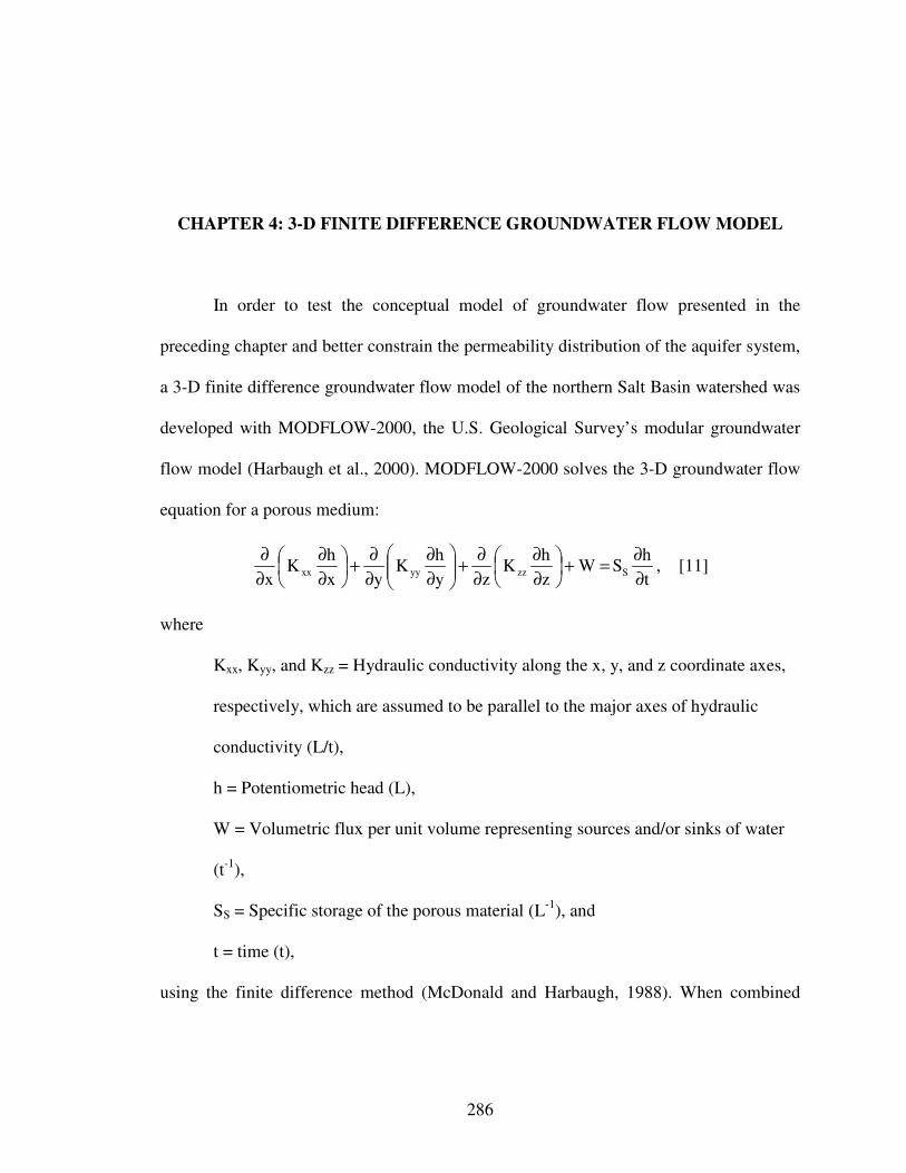
286
CHAPTER 4: 3-D FINITE DIFFERENCE GROUNDWATER FLOW MODEL
In order to test the conceptual model of groundwater flow presented in the
preceding chapter and better constrain the permeability distribution of the aquifer system,
a 3-D finite difference groundwater flow model of the northern Salt Basin watershed was
developed with MODFLOW-2000, the U.S. Geological Survey’s modular groundwater
flow model (Harbaugh et al., 2000). MODFLOW-2000 solves the 3-D groundwater flow
equation for a porous medium:
t
hS W
z
hK
z
y
hK
y
x
hK
xSzzyyxx
∂
∂=+
∂
∂
∂
∂+
∂
∂
∂
∂+
∂
∂
∂
∂, [11]
where
Kxx, Kyy, and Kzz = Hydraulic conductivity along the x, y, and z coordinate axes,
respectively, which are assumed to be parallel to the major axes of hydraulic
conductivity (L/t),
h = Potentiometric head (L),
W = Volumetric flux per unit volume representing sources and/or sinks of water
(t-1),
SS = Specific storage of the porous material (L-1), and
t = time (t),
using the finite difference method (McDonald and Harbaugh, 1988). When combined

287
with boundary and initial conditions, [11] describes transient 3-D groundwater flow in a
heterogeneous and anisotropic medium (Harbaugh et al., 2000).
4.1: Model Development
Groundwater Modeling System (GMS) provides a graphical pre- and post-
processor for MODFLOW-2000. As discussed in Chapter 3.2.c, GMS version 6.5 was
used to construct a 3-D hydrogeologic framework model of the Salt Basin. The 3-D
hydrogeologic framework solid model was used to aid in the development of a 3-D finite
difference groundwater flow model of the Salt Basin. However, for simplicity, and to
minimize model run times, only 6 hydrogeologic groupings from the framework solid
model were incorporated into the groundwater flow model, including, from oldest to
youngest, the Precambrian, the Paleozoic (the Cambrian through the Pennsylvanian), the
Permian (Lower Abo/Pow Wow Conglomerate through Artesia Group), the Cretaceous,
Cenozoic intrusions, and Cenozoic alluvium. Similar to the 17 hydrogeologic groupings
used for the 3-D hydrogeologic framework model, the 6 hydrogeologic groupings used in
the groundwater flow model were chosen such that hydrogeologic units with similar
lithologies and facies, and thus probably similar hydraulic properties, were combined.
Also, for simplicity, and to minimize model run times, a cell size of 1,000 by
1,000 meters (3,280 by 3,280 feet) was used for the 3-D MODFLOW grid, in contrast to
500 by 500 meters (1,640 by 1,640 feet) cell size used for the 3-D hydrogeologic
framework model. In order to facilitate the assignment of hydrogeologic units to the 3-D
MODFLOW grid, a simplified 3-D hydrogeologic framework solid model was created.
The simplified 3-D framework solid model consisted of the 6 hydrogeologic units listed
above, and a cell size of 1,000 by 1,000 meters (3,280 by 3,280 feet). Using the same

288
method as described in Chapter 3.2.c, a GMS grid was assigned 6 layers to represent the
6 hydrogeologic units, and the elevation values from the 6 ArcGIS raster surfaces were
used to define the elevation values of the 6 layers in the GMS grid.
However, unlike the 500 by 500 meters (1,640 by 1,640 feet) solid model,
described in Chapter 3, the cell size of the simplified solid model did not match the cell
size of the ArcGIS raster surfaces representing the elevation of the top of the
hydrogeologic units. As a result, the elevation values from the ArcGIS raster surfaces
could not be directly used to define the elevation of the 6 layers in the GMS grid. Instead,
the elevation values from the ArcGIS raster surfaces were interpolated to the GMS grid
layers using a natural neighbor interpolation scheme to create the simplified 3-D
framework solid model.
The active portion of the 3-D MODFLOW grid consisted of 6 layers, 146 rows,
130 columns, and 72,366 cells. The top of the MODFLOW grid was set at the top of the
simplified 3-D hydrogeologic framework solid model (i.e. the land surface elevation).
Layer 1 was given a variable thickness, as discussed in more detail below, while layers 2
through 6 were assigned a constant thickness of 50, 250, 500, 1,000, and 1,500 meters
(160, 820, 1,600, 3,300, and 4,900 feet), respectively. As a result, the MODFLOW grid
layers crosscut the hydrogeologic units within the 3-D framework solid model. The
simplified 3-D framework solid model was used to assign a hydrogeologic unit to each
cell within the MODFLOW model domain. The hydrogeologic unit assigned to each cell
in the MODFLOW grid was chosen as the hydrogeologic unit from the simplified 3-D
framework solid model occupying the majority of each MODFLOW cell.

289
In addition to the 6 hydrogeologic units from the 3-D framework solid model,
several other units were incorporated into the MODFLOW grid. The Cenozoic intrusive
mass postulated by Nutt et al. (1997) to exist beneath the Cornudas Mountains was
included in the groundwater flow model from layer 3 to the top of the Precambrian. The
lateral extent of this mass within the groundwater flow model domain corresponds to the
residual gravity low, as defined by the 0 mGal contour, presented in Nutt et al. (1997).
The intrusive mass was grouped with the Cenozoic intrusions hydrogeologic unit. In an
attempt to model the confined to semi-confined Cretaceous aquifer overlying the regional
Permian aquifer in the southwestern portion of the Diablo Plateau, a low permeability
confining unit was inserted in layer 2 beneath the Cretaceous hydrogeologic unit in layer
1. As a result, the MODFLOW grid consists of 7 hydrogeologic units.
The base of layer 1 was originally defined as 100 meters (330 feet) below the
groundwater surface depicted in Figure 3.42. However, initial model runs reveled that
numerous cells in layer 1 would become dry. Original versions of MODFLOW allowed
variable-head model cells to become desaturated, in which case they were converted to
no-flow cells, but did not allow them to become resaturated and converted back to
variable-head cells (McDonald et al., 1998). Variable-head cells can incorrectly become
dry during the iterative solution process (McDonald et al., 1998). MODFLOW-2000
includes an option to allow dry cells to be converted to variable-head cells (termed
“wetting”) based on the head in variable-head cells immediately below and/or
horizontally adjacent to the dry cells, but enabling this feature can lead to instability in
the convergence of the iterative solution process (McDonald et al., 1998).

290
As mentioned in the preceding paragraph, during initial model runs numerous
cells in layer 1would become dry during the solution process. The wetting capability was
enabled in subsequent model runs to allow variable-head cells that may have been
incorrectly converted to no-flow cells to become re-wetted. However, enabling the
wetting capability produced instability in the iterative solution process, and convergence
could not be achieved. Therefore, in order to ensure that variable-head cells would not
incorrectly become dry during the solution process the thickness of layer 1 was increased
so that the heads in layer 1 would not fall below the bottom of layer 1 during the solution
process. As a result, the wetting capability wasn’t needed, and the stability of the solution
was re-established. The base of layer 1 was re-defined as 100 meters (330 feet) below a
subdued version of the groundwater surface depicted in Figure 3.42, in which the
subdued groundwater surface was up to 685 meters (2,250 feet) lower than the
groundwater surface in Figure 3.42. The re-defined thickness of layer 1 ranged from 100
to 1,470 meters (330 to 4,820 feet).
Figure 4.1 presents the locations and an oblique view of the 5 cross-sections, as
discussed in Chapter 3.3, within the 3-D hydrogeologic framework solid model, and the
3-D groundwater flow model. Figures 4.2 through 4.6 compare side views of the 5 cross-
sections through the 3-D hydrogeologic framework solid model, and the 3-D groundwater
flow model. Figure 4.7 presents the locations and an oblique view of the 5 cross-sections
within the simplified 3-D hydrogeologic framework solid model, and the 3-D
groundwater flow model. Figures 4.8 through 4.12 compare side views of the 5 cross-
sections through the simplified 3-D hydrogeologic framework solid model, and the 3-D
groundwater flow model to illustrate how hydrogeologic units from the simplified solid

291
model were assigned to cells within the 6 layer groundwater flow model. Figures 4.13
through 4.18 show the distribution of the 6 hydrogeologic units from the simplified 3-D
hydrogeologic framework solid model, and the low permeability Cretaceous confining
unit, within layers 1 through 6 of the groundwater flow model grid. Faults are represented
within the 3-D groundwater flow model solely through juxtaposition of the
hydrogeologic units, as defined by the simplified 3-D framework solid model.
Model length is in meters, and time is in days. The Layer-Property Flow (LPF)
Package was used as the internal flow package. The LPF Package assumes that a node is
located at the center of each model cell (Harbaugh et al., 2000). Layer 1 was defined as
convertible, in which case cell thickness depends on the computed hydraulic head in the
cell. If the head is above the elevation of the top of the cell, the cell thickness is
calculated as the elevation of the top of the cell minus the elevation of the bottom of the
cell (Harbaugh et al., 2000). If the head is below the top of the cell, the cell thickness is
calculated as the head minus the elevation of the bottom of the cell (Harbaugh et al.,
2000). Layers 2 through 6 were set as confined, in which case cell thickness is calculated
as the elevation of the top of the cell minus the elevation of the bottom of the cell
(Harbaugh et al., 2000).
MODFLOW-2000 includes several solver packages, each of which can be used to
solve the set of simultaneous finite difference equations for head at each cell by iteration.
Initial model runs were attempted with the strongly implicit procedure (SIP) and
preconditioned Conjugate Gradient (PCG) solvers, but convergence could not be
achieved with either of these two solvers. The slice successive overrelaxtion (SOR)
solver proved to be the most stable and capable of converging. The SOR technique

292
divides the finite difference grid into vertical “slices,” and groups the node equations
from each slice into discrete sets (McDonald and Harbaugh, 1988). During every
iteration, these sets of equations are processed in turn, resulting in a new set of estimated
head values for each slice (McDonald and Harbaugh, 1988). The head change criterion
for convergence was set at 0.001 meters (0.003 feet).
4.1.a: Boundary and Initial Conditions
The domain of the 3-D solid and groundwater flow models was defined using the
groundwater surface shown in Figure 3.42. The boundary was drawn to correspond to the
groundwater divides as indicated by the groundwater surface, except in the southeastern
portion of the domain where the boundary corresponds to the groundwater divide
associated with the Bitterwell Break. Also, the northwestern portion of the domain
encompasses a part of the Peñasco Basin, as suggested by the groundwater surface. As a
result, the entire domain of the groundwater flow model is surrounded by a no-flow
boundary. (Figure 4.19) As mentioned above, the active portion of the groundwater flow
model grid consists of 6 layers, 146 rows, 130 columns, and 72,366 cells, each with a
plan view area of 1.0 km2 (0.39 mi2). (Figure 4.19) The groundwater surface depicted in
Figure 3.42 was used as the starting head for all 6 layers.
-Recharge Distributions
The Recharge (RCH) Package was used to apply areal recharge to layer 1 of the
groundwater flow model domain. Two different recharge distributions were investigated
for this modeling exercise: a water-balance based and an elevation-dependent
distribution. Each recharge distribution was hand-calibrated to steady-state groundwater
elevations in 378 wells throughout the model domain by varying the horizontal hydraulic

293
conductivity of the hydrogeologic units. More detail on the calibration process is
provided in Chapter 4.2.a. The appropriateness of the two recharge distributions was
tested by comparing radiocarbon groundwater ages from wells within the Salt Basin, as
presented in Sigstedt (2010), to MODPATH particle-tracking ages calculated from the
hand-calibrated MODFLOW solutions for each recharge distribution. The MODPARTH
particle-tracking setup is discussed in more detail in Chapter 4.2.b, and the results are
presented in Chapter 4.3.b.
-Water-balance Based Recharge Distribution
For the water-balance based recharge distribution, recharge was applied to the
sub-basins delineated by JSAI (2010). (Figure 4.19) The recharge rates applied to the
sub-basins were derived from visual inspection of the figures depicting the net infiltration
simulated by the water-balance recharge modeling conducted by DBS&A (2010a).
(Figures 4.20 through 4.25, and Table 4.1) The sub-basins delineated by JSAI (2010)
were placed over the top of the DBS&A (2010a) net infiltration figures, and a recharge
rate was selected for each sub-basin based on the average net infiltration simulated over
the entire area of each sub-basin. DBS&A (2010a) simulated net infiltration for
minimum, average, and maximum water years. Thus, three different recharge scenarios
were examined for the water-balance based recharge distribution, incorporating the
recharge rates and areal distribution of recharge derived from the DBS&A (2010a)
simulated net infiltration for the minimum, average, and maximum water years. (Figures
4.20 through 4.25, and Table 4.1)
As discussed in Chapter 3.1, DBS&A (2010a) conceptualized the recharge
mechanisms in the Salt Basin to include: mountain block recharge, mountain front

294
recharge, local recharge, and diffuse recharge. DBS&A (2010a) only estimated recharge
within the Salt Basin watershed boundary. However, the groundwater flow model domain
was defined using the groundwater surface, and thus does not correspond exactly to the
watershed boundary. For those regions of the model domain not incorporated in the
DBS&A (2010a) study, the distribution and amount of recharge was estimated to be
similar to the neighboring regions included in the DBS&A (2010a) study. For the portion
of the Peñasco Basin included in the model domain, recharge was assumed to be equal to
the subsurface flux through the eastern portion of the Salt Basin calculated by Sigstedt
(2010) using apparent groundwater ages estimated from the 14C data. Sigstedt (2010)
calculated a minimum, average, and maximum subsurface flux, and these values were
incorporated into the three recharge scenarios.
The recharge rates and areal recharge applied to the sub-basins for the minimum,
average, and maximum recharge scenarios of the water-balance based recharge
distribution are summarized in Table 4.1. Total recharge to the groundwater flow model
domain using the water-balance based recharge distribution ranged from 160,000 m3/day
(49,000 acre-feet/year) for the minimum recharge scenario to 350,000 m3/day (110,000
acre-feet/year) for the maximum recharge scenario, with the average recharge scenario
producing 270,000 m3/day (81,000 acre-feet/year). These values for total recharge to the
Salt Basin are on the upper end of the range of values reported in previous studies, as
discussed in Chapter 3.1. Figures 4.20, 4.21, and 4.22 show the distribution of recharge
rates for the minimum, average, and maximum recharge scenarios. Figures 4.23, 4.24,
and 4.25 present the distribution of areal recharge for the minimum, average, and
maximum recharge scenarios. The sub-basins contributing the most to total recharge

295
included those sub-basins encompassing the Sacramento and Guadalupe Mountains, and
the region to the southwest and northeast of the Otero Break.
One of the shortcomings of the water-balance based recharge distribution is that it
appears to overestimate recharge in the lower elevation regions of the Salt Basin. In the
DBS&A (2010a) study most recharge to the groundwater system is concentrated along
sinkholes to the southwest of the Otero Break and on the Chert Plateau and Otero Hills to
the northeast of the Otero Break, while the high mountain region of the Sacramento
Mountains contributes almost no recharge. Several sources of hydrogeologic evidence
suggest that regions to the southwest and northeast of the Otero Break receive much less
recharge than the Sacramento Mountains. Depth to the regional groundwater surface in
the region around the Otero Break ranges from 76 meters (250 feet) to greater than 300
meters (1,000 feet), while in the Sacramento Mountains depths are generally less than 76
meters (250 feet). (Figure 3.43) Tritium levels in wells to the northeast of the Otero
Break are low, ranging from 0.24 to 1.6 Tritium Units (TU), while tritium levels in wells
and springs within the Sacramento Mountains generally range from 2.97 to 10.4 TU,
indicating groundwater is typically less than 50 years old (Newton et al., 2009; Sigstedt,
2010). Also, radiocarbon groundwater ages in wells to the northeast of the Otero Break
are greater than 1,000 years old, with some ages near or greater than 10,000 years old
(Sigstedt, 2010).
-Elevation-dependent Recharge Distribution
For the elevation-dependent recharge distribution, recharge was applied to the
high mountain regions of the Sacramento and Guadalupe Mountains, as well as the
regions around the Cornudas Mountains and the southwest portion of the Diablo Plateau

296
where the depth-to-groundwater map [Figure 3.43] indicates areas of shallower
groundwater. Again, three different recharge scenarios, minimum, average, and
maximum, were examined for the elevation-dependent recharge distribution. The
recharge rates applied to the Sacramento and Guadalupe Mountains regions of the
groundwater flow model domain were derived using data presented in Newton et al.
(2011).
Based on water level, geochemistry, and stable isotope data, Newton et al. (2011)
determined that the main recharge source areas for the High Mountain, Pecos Slope, and
Salt Basin aquifer systems are located in the high mountain areas of the Sacramento
Mountains above a surface elevation of approximately 2,500 meters (8,200 feet). Using
the chloride mass balance method, Newton et al. (2011) estimated the relative recharge
rate within this area to range from 4 to 44%, with a mean value of 22%, of average
annual precipitation. (Table 4.2) The recharge factors presented in Newton et al. (2011)
were multiplied by the average annual precipitation, obtained from PRISM [Figure 1.11],
to calculate the minimum, average, and maximum recharge rates that were applied to the
Sacramento and Guadalupe Mountains regions of the groundwater flow model domain
above a surface elevation of 2,500 meters (8,200 feet).
On the Otero Mesa/Diablo Plateau recharge rates were based on soil chloride
profile data from the Diablo Plateau collected by Kreitler et al. (1987), as cited in Mayer
(1995). Kreitler et al. (1987) concluded that on the Diablo Plateau the main recharge
mechanism is through fractures in creek beds and closed depressions during occasional
flash floods (Mayer, 1995). On the basis of soil chloride profiles, Kreitler et al. (1987)
calculated recharge for creek beds and depressions to range from 0.028 to 0.457 cm/year

297
(0.011 to 0.180 inches/year), and for areas outside creek beds to range from 0.005 to
0.020 cm/year (0.002 to 0.0079 inches/year) (Mayer, 1995). (Table 4.3) The minimum
and maximum of each range were used for the minimum and maximum recharge
scenarios, respectively, while the midpoint of each range was used for the average
recharge scenario. As mentioned above, these recharge rates were applied to the region of
shallow groundwater around the Cornudas Mountains and on the southwest portion of the
Diablo Plateau. On the basis of digitized topography and stream courses, and assuming a
stream-bed width of 10 meters (33 feet), Mayer (1995) calculated creek beds and
depressions to occupy only 3% of the total area of the Otero Mesa/Diablo Plateau. Thus,
the creek bed and depression recharge rate was applied to only 3% of the area of the
Cornudas Mountains and Diablo Plateau recharge zones within the groundwater flow
model domain.
The recharge rates and areal recharge applied to the Sacramento and Guadalupe
Mountains, and Cornudas Mountains and Diablo Plateau recharge zones for the
minimum, average, and maximum recharge scenarios of the elevation-dependent
recharge distribution are summarized in Tables 4.4 and 4.5, respectively. Total recharge
to the groundwater flow model domain using the elevation-dependent recharge
distribution ranged from 9,100 m3/day (2,700 acre-feet/year) for the minimum recharge
scenario to 99,000 m3/day (29,000 acre-feet/year) for the maximum recharge scenario,
with the average recharge scenario producing 50,000 m3/day (15,000 acre-feet/year).
Figures 4.26, 4.27, and 4.28 show the distribution of recharge rates for the minimum,
average, and maximum recharge scenarios. Figures 4.29, 4.30, and 4.31 present the

298
distribution of areal recharge for the minimum, average, and maximum recharge
scenarios.
Recharge to the Sacramento Mountains recharge zone ranged from 7,400 m3/day
(2,200 acre-feet/year) for the minimum recharge scenario to 81,000 m3/day (24,000 acre-
feet/year) for the maximum recharge scenario, with the average recharge scenario
resulting in 41,000 m3/day (12,000 acre-feet/year). These values for the Sacramento
Mountains recharge zone compare favorably to the subsurface flux from the Sacramento
Mountains through the eastern portion of the Salt Basin, calculated by Sigstedt (2010)
using radiocarbon groundwater ages. Sigstedt (2010) estimated the subsurface flux to
range from 20,000 m3/day (6,000 acre-feet/year) to 37,000 m3/day (11,000 acre-
feet/year). Recharge to the Guadalupe Mountains recharge zone ranged from 1,600
m3/day (470 acre-feet/year) for the minimum recharge scenario to 17,000 m3/day (5,100
acre-feet/year) for the maximum recharge scenario, with the average recharge scenario
resulting in 8,600 m3/day (2,600 acre-feet/year). These values for the Guadalupe
Mountains recharge zone seem reasonable compared to the recharge values for the
Sacramento Mountains recharge zone.
Abundant hydrogeologic evidence exists to indicate that the Guadalupe
Mountains receive much less recharge than the Sacramento Mountains. The northern
portion of the Guadalupe Mountains (i.e. the portion that extends in a general northwest
direction from Guadalupe Ridge along the Algerita and Buckhorn Escarpments), and the
Brokeoff Mountains and Dog Canyon areas contain no springs or perennial streams
(Hayes, 1964). In contrast, the Sacramento Mountains contain numerous springs, and
several perennial streams, including the upper portions of the Sacramento River, and the

299
Rio Peñasco (Newton et al., 2009). In addition, depth to the regional groundwater surface
is generally greater than 230 meters (750 feet) in the Guadalupe Mountains, while in the
Sacramento Mountains depths are generally less than 76 meters (250 feet). (Figure 3.43)
Tritium levels in wells near the base of the Guadalupe and Brokeoff Mountains are low
(< 1 TU), while tritium levels in wells and springs within the Sacramento Mountains
generally range from 2.97 to 10.4 TU, indicating groundwater is typically less than 50
years old (Newton et al., 2009; Sigstedt, 2010). Also, radiocarbon groundwater ages
calculated by Sigstedt (2010) for wells near the base of the Guadalupe and Brokeoff
Mountains are greater than 10,000 years old. All of this evidence suggests the Guadalupe
and Brokeoff Mountains do not contribute significant recharge to the Salt Basin
groundwater system.
Recharge to the Cornudas Mountains and Diablo Plateau recharge zones ranged
from 140 m3/day (41 acre-feet/year) for the minimum recharge scenario to 1,000 m3/day
(300 acre-feet/year) for the maximum recharge scenario, with the average recharge
scenario resulting in 580 m3/day (170 acre-feet/year). Hydrogeologic evidence suggests
that these relatively low recharge values are reasonable. Sigstedt (2010) produced
groundwater chemistry contours of magnesium and sulfate concentration for the Salt
Basin in New Mexico and Texas. Although radiocarbon groundwater ages were not
obtained from the Otero Mesa/Diablo Plateau region, the groundwater chemistry
contours, along with correlations between increasing radiocarbon groundwater age and
increasing magnesium and sulfate concentrations on the eastern side of the basin, have
implications for relative fluxes on the western side of the basin (Sigstedt, 2010). In
addition, radiocarbon groundwater ages from two wells just to the east of the Cornudas
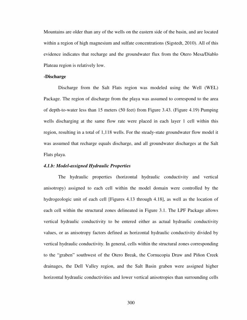
300
Mountains are older than any of the wells on the eastern side of the basin, and are located
within a region of high magnesium and sulfate concentrations (Sigstedt, 2010). All of this
evidence indicates that recharge and the groundwater flux from the Otero Mesa/Diablo
Plateau region is relatively low.
-Discharge
Discharge from the Salt Flats region was modeled using the Well (WEL)
Package. The region of discharge from the playa was assumed to correspond to the area
of depth-to-water less than 15 meters (50 feet) from Figure 3.43. (Figure 4.19) Pumping
wells discharging at the same flow rate were placed in each layer 1 cell within this
region, resulting in a total of 1,118 wells. For the steady-state groundwater flow model it
was assumed that recharge equals discharge, and all groundwater discharges at the Salt
Flats playa.
4.1.b: Model-assigned Hydraulic Properties
The hydraulic properties (horizontal hydraulic conductivity and vertical
anisotropy) assigned to each cell within the model domain were controlled by the
hydrogeologic unit of each cell [Figures 4.13 through 4.18], as well as the location of
each cell within the structural zones delineated in Figure 3.1. The LPF Package allows
vertical hydraulic conductivity to be entered either as actual hydraulic conductivity
values, or as anisotropy factors defined as horizontal hydraulic conductivity divided by
vertical hydraulic conductivity. In general, cells within the structural zones corresponding
to the “graben” southwest of the Otero Break, the Cornucopia Draw and Piñon Creek
drainages, the Dell Valley region, and the Salt Basin graben were assigned higher
horizontal hydraulic conductivities and lower vertical anisotropies than surrounding cells

301
due to the greater density of faulting and fracturing within these blocks, as discussed in
Chapter 2.
The hydraulic property data presented in Chapter 3.6 and Tables A-3.27 and A-
3.28, and displayed graphically in Figures 3.57 and 3.58, along with the permeability
distribution from previous groundwater flow modeling efforts, as discussed in Chapter
3.1, were used to guide the initial values and distribution of horizontal hydraulic
conductivity assigned to each hydrogeologic unit. The bulk of the published hydraulic
property data presented in Chapter 3 were transmissivity values estimated from specific
capacity or aquifer tests performed on wells completed in a particular aquifer or
hydrogeologic facies. In order to calculate hydraulic conductivity from this data, the
transmissivity values were divided by the saturated aquifer thickness, which was assumed
to be equal to the length of the screened and/or open interval for each well. The use of the
screened/open interval, along with the fact that most wells are open to the most
productive intervals in a heterogeneous aquifer may bias the hydraulic conductivity
estimates towards larger values. Thus, the range of hydraulic conductivity values
calculated from published transmissivity values were used to constrain the maximum
value of horizontal hydraulic conductivity assigned to each hydrogeologic unit.
The majority of the transmissivity data were obtained from wells for which
screened and open intervals were commonly available in the TWDB’s database. If a well
contained multiple screened and/or open intervals, the bottom of the deepest screened or
open interval was used as the bottom of the screened/open interval and the top of the
shallowest screened or open interval was used as the top of the screened/open interval.
For wells in which screened or open intervals were not available (i.e. wells located in

302
New Mexico, as well as some wells in Texas), the aquifer thickness was assumed to be
equal to the length from the mean water level to the bottom of the well. In situations were
no water levels were available, or well depth was not given, the aquifer thickness was
assumed to be 30 meters (98 feet), which approximately corresponds to the minimum
length of screened interval for all wells with screen data. Assuming the minimum screen
length maximizes the estimate of hydraulic conductivity, but none of the hydraulic
conductivity values estimated in this way produced the maximum estimate of hydraulic
conductivity for a particular aquifer or hydrogeologic facies. The hydraulic conductivity
values estimated from the transmissivity data are presented in Table A-4.6 and Figure
4.32.
Cenozoic alluvium in layers 1 through 3 was assigned an initial horizontal
hydraulic conductivity of 1 meters/day (3 feet/day). The Cretaceous in layer 1 was given
an initial horizontal hydraulic conductivity of 0.01 meters/day (0.03 feet/day). The
Permian in layers 1 through 5 within the structural zones associated with a high density
of faulting and fracturing was assigned an initial horizontal hydraulic conductivity
ranging from 1 to 10 meters/day (3 to 30 feet/day), while the surrounding Permian units
were assigned an initial horizontal hydraulic conductivity ranging from 0.01 to 0.1
meters/day (0.03 to 0.3 feet/day). The Permian within the higher permeability structural
zones was given a vertical anisotropy of 10, while the other units described above were
given a vertical anisotropy of 100.
The low permeability confining unit inserted in layer 2 beneath the Cretaceous
was assigned an initial horizontal hydraulic conductivity of 0.000001 meters/day
(0.000003 feet/day), and a vertical anisotropy of 1,000. The Paleozoic (Cambrian through

303
Pennsylvanian) in layers 2 through 6 was assigned an initial horizontal hydraulic
conductivity of 0.001 meters/day (0.003 feet/day). The Precambrian in layers 1 through 6
was assigned an initial horizontal hydraulic conductivity of 0.001 meters/day (0.003
feet/day). The Cenozoic intrusions in layers 1 through 5, including the Cenozoic mass in
layers 3 through 5, were given an initial horizontal hydraulic conductivity of 0.0001
meters/day (0.0003 feet/day). The Paleozoic, Precambrian, and Cenozoic intrusions were
assigned a vertical anisotropy of 1,000.
4.2: Model Calibration and MODPATH Particle-tracking Setup
4.2.a: Model Calibration
A subset of the groundwater wells used to contour the groundwater surface
displayed in Figure 3.42 (i.e. those wells within the groundwater flow model domain)
were used as calibration targets. (Figure 4.33) Both recharge distribution models were
calibrated to steady-state conditions. Model calibration involved manually varying only
the horizontal hydraulic conductivity of each hydrogeologic unit to attempt to minimize
the sum of the squares of the residuals for all groundwater well calibration points. The
range of hydraulic conductivity values presented in Figures 3.57 and 4.32, and Tables A-
3.27 and A-4.6 were used to constrain the minimum and maximum horizontal hydraulic
conductivity of each unit during model calibration.
Model calibration was achieved by manually increasing or decreasing the
horizontal hydraulic conductivity of each hydrogeologic unit from the initial value
assigned to each unit [Tables 4.7 and 4.8], through the range of possible conductivity
values for each unit [Figures 3.57 and 4.32, and Tables A-3.27 and A-4.6], until the sum
of the squares of the residuals for all calibration points was minimized or stable. If the

304
sum of the squares of the residuals became stable (i.e. unchanging) during calibration,
and remained stable through the range of possible conductivity values, the horizontal
hydraulic conductivity value associated with the initial stabilization of the sum of the
squares of the residuals was assigned to the unit being calibrated. If increasing and
decreasing the horizontal hydraulic conductivity value of a unit through the range of
possible conductivity values didn’t result in a reduction of the sum of the squares of the
residuals, the initial horizontal hydraulic conductivity value [Tables 4.7 and 4.8] was
restored to that unit. Another constraint maintained throughout the calibration process
was the horizontal hydraulic conductivity assigned to a hydrogeologic unit in the average
recharge scenario model must be greater than or equal to the conductivity assigned to the
same unit in the minimum recharge scenario model, and less than or equal to the
conductivity assigned to the same unit in the maximum recharge scenario model.
In general, calibration proceeded from the youngest to the oldest hydrogeologic
unit: Cenozoic alluvium, the Cretaceous, the low permeability Cretaceous confining, the
Permian, the Paleozoic (the Cambrian through the Pennsylvanian), and the Precambrian.
The one exception was Cenozoic intrusions, which were calibrated after the Precambrian.
For Cenozoic alluvium, the Cretaceous, the low permeability Cretaceous confining, and
the Permian hydrogeologic units, the horizontal hydraulic conductivity was varied in
increments of a quarter of an order-of-magnitude (e.g. 1 to 2.5, or 0.1 to 0.075). For the
Paleozoic hydrogeologic unit, the horizontal hydraulic conductivity was varied in
increments of a half of an order-of-magnitude (e.g. 1 to 5, or 0.1 to 0.05). For Cenozoic
intrusions and the Precambrian hydrogeologic units, the horizontal hydraulic conductivity
was varied in increments of an order-of-magnitude (e.g. 1 to 10, or 0.1 to 0.01).

305
The residual for a calibration, also referred to as an observation, point was defined
as the hydraulic head computed by the groundwater flow model minus the observed head.
If multiple water levels measurements were available for a groundwater well, the
observed head was set as the mean groundwater elevation, relative to mean sea level.
However, numerous wells, especially those located in the New Mexico portion of the
model domain, had only one water level measurement available. Refer to Chapter 3.3 for
more information on the groundwater wells used in this study.
GMS 6.5 can determine the location of an observation point within the 3-D
MODFLOW grid in several ways: 1) the user defines an elevation for the point and this
elevation is compared to the layer elevations to determine which layer the point is in, 2)
the user automatically assigns the point to a layer, or 3) the user defines a top and bottom
elevation representing the screened interval of the well and this interval is compared to
the layer elevations to determine which layer or layers the point is in. The third method
listed was used for this modeling exercise. The criteria used to define the length of the
screened interval assigned to each well was the same as that described above in Chapter
4.1.b. The groundwater wells used as calibration targets within the groundwater flow
model are displayed in Figure 4.33. Table A-4.9 lists the groundwater wells used as
calibration targets, including the row and column location of each well within the model
domain, the model layer or layers intersected by the screened interval of each well, the
top and bottom elevation of the screened interval, and the observed groundwater
elevation.
Model calibration was first performed for the minimum recharge scenario of both
the water-balance based recharge distribution and the elevation-dependent recharge

306
distribution. The quality of the calibration was assessed through several statistics,
including the sum of the residuals, the sum of the absolute values of the residuals, the
sum of the squares of the residuals, and the root-mean-square (RMS) error, as well as
visual inspection of a plot of the observed versus computed heads. In addition to the sum
of the residuals, the sum of the absolute values of the residuals, the sum of the squares of
the residuals, and the RMS error, calculated calibration statistics included the mean of the
residuals, the mean of the absolute values of the residuals, the standard deviation of the
residuals, the standard deviation of the residuals divided by the range of observed
hydraulic head, and the mean of the residuals divided by the range of observed hydraulic
head.
4.2.b: MODPATH Particle-tracking Setup
After an adequate calibration to the groundwater level observation points had
been achieved for all recharge scenarios of both recharge distributions, MODPATH was
used to simulate groundwater residence times. As mentioned in Chapter 4.1.a, the
purpose of the MODPATH particle-tracking exercise was to test the appropriateness of
the two recharge distributions. This was accomplished by comparing radiocarbon
groundwater ages from wells within the Salt Basin, as presented in Sigstedt (2010), to
MODPATH particle-tracking ages calculated from the hand-calibrated MODFLOW
solutions for each recharge distribution. Chapter 4.3.b summarizes the results of the
MODPATH particle-tracking exercise.
MODPATH is a post-processing program designed to use output from steady-
state or transient MODFLOW simulations to compute 3-D flow paths and travel times for
imaginary “particles” of water moving through the simulated groundwater system

307
(Pollock, 1994). MODPATH calculates the average linear groundwater velocity vector
field within each cell based on the intercell flow rates calculated by MODFLOW, and
uses this field to compute particle path lines (Pollock, 1994). Thus, MODPATH only
simulates advective transport, and the groundwater ages calculated using this method are
advective ages.
In order to calculate the average linear groundwater velocity within each cell,
MODPATH requires porosity values to be assigned to each hydrogeologic unit. Sigstedt
(2010) referenced porosity and depth relationships for a major west Texas oil field from
Galloway (1983). The data presented in Galloway (1983) included a plot of depth versus
average porosity for the Permian San Andres and Abo Formations, the Siluro-Devonian,
and the Ordovician. The porosity data in Galloway (1983) and the wellsite core analysis
porosity data from the Yates Petroleum Corporation, One Tree Unit #2 well [Table 3.30]
were used to assign a minimum, average, and maximum porosity value to each
MODFLOW hydrogeologic unit. The minimum, average, and maximum porosity values
were used to compute particle flow paths and travel times for the minimum, average, and
maximum recharge scenario models of both recharge distributions. Table 4.10 lists the
minimum, average, and maximum porosity values used for each hydrogeologic unit.
MODPATH can perform either forward or reverse particle tracking. Reverse
particle tracking was used for this modeling exercise, and involved generating particles in
the MODFLOW grid cells corresponding to the location of 13 of the 15 wells for which
radiocarbon groundwater ages were calculated by Sigstedt (2010) [Figure 4.34] and
tracking them backward to their origins. Particle origins refers to their position within the
MODFLOW grid when they reached the simulated groundwater surface (i.e. recharged

308
the groundwater system). Two of the radiocarbon groundwater age wells from Sigstedt
(2010), Hunt C13 and Hunt House, were not included because they are very close to, and
have similar groundwater ages to the included Hunt 8 well, and they are located in grid
cells which already contain pumping wells used to simulate discharge from the
groundwater system at the Salt Flats.
The total depths of 12 of the 13 radiocarbon groundwater age wells do not exceed
the bottom of layer 1 in the MODFLOW grid, and thus particles were generated in layer
1 for these wells. The total depth of Butterfield Well extends into layer 2 of the
MODFLOW grid, and thus particles were generated in layer 2 for this well. Table 4.11
lists the groundwater age wells used, including the NMOSE POD Number (if available),
the UTM coordinates using the NAD 83 coordinate system, the row and column location
within the MODFLOW domain, the layer location within the MODFLOW domain, the
ground surface elevation in meters derived from the 1-arc second NED discussed above
in Chapter 3.2.a, the total well depth in meters, and the elevation of the total well depth in
meters. Figure 4.34 displays the location of the groundwater age wells within the
MODFLOW model domain.
MODPATH can generate particles at a MODFLOW grid cell in several ways: 1)
on the computed groundwater surface within the cell, 2) in the interior of the cell, or 3)
on the cell faces. The vertical position of particles generated in the interior of the cell is
set at the midpoint between the computed groundwater surface within the cell and the
bottom of the cell. The computed groundwater surface within each cell varied between
the different recharge scenarios of both recharge distributions, and therefore the vertical

309
position of particles generated using methods 1) and 2) also varied between the different
models.
Using 1), 2), or 3), particles could be generated on the computed groundwater
surface within each cell, at the midpoint between the computed groundwater surface and
the bottom of each cell, or on the bottom cell face, respectively. In general, particles were
generated in two of these three positions within the MODFLOW cells in order to bound
the vertical position of the elevation, relative to mean sea level, of the total depth of the
radiocarbon groundwater age wells. However, if the elevation of the total depth of a
groundwater age well was higher than the computed groundwater surface within the
MODFLOW cell, only particles generated on the groundwater surface were deemed to
represent the pathlines of groundwater sampled at the well. If the elevation of the total
depth of a groundwater age well was located between the computed groundwater surface
and the midpoint, or the midpoint and the bottom cell face, the particles generated at the
corresponding two vertical positions which bound the elevation of the total depth of the
well were chosen to represent the potential pathlines and residence times of groundwater
sampled at the well. Tables 4.12 and 4.13 list the elevation of the total depth of each
groundwater age well as well as the elevations of the three vertical positions within each
cell for the calibrated minimum, average, and maximum recharge scenario models of the
water-balance based and elevation-dependent recharge distributions, respectively. Tables
4.12 and 4.13 also designate which vertical positions were chosen to represent the
potential pathlines and residence times of groundwater sampled at each well.
A maximum of 100 particles could be generated in the interior of the cell. As a
result, 100 particles were generated at each selected vertical position within the cells

310
corresponding to the location of the radiocarbon groundwater age wells. The mean,
median, and standard deviation of the particle travel times (i.e. ages) were calculated for
each selected vertical position within the cells. The median of the particle travel times for
each selected vertical position within the cells were used for graphical comparison to the
radiocarbon groundwater ages presented in Sigstedt (2010).
4.3: Model Results
4.3.a: MODFLOW
The mass balances for the calibrated minimum, average, and maximum recharge
scenario models of the water-balance based and elevation-dependent recharge
distributions are presented in Tables A-4.14 and A-4.15, respectively. Figures 4.35
through 4.37, and Figures 4.38 through 4.40 compare model computed heads in layer 1
for the calibrated recharge scenario models of the water-balance based and elevation-
dependent recharge distributions, respectively, to the groundwater surface depicted in
Figure 3.42. In general, model computed heads for both recharge distributions represent
the overall configuration of the groundwater surface displayed in Figure 3.42, and the
model computed heads for both recharge distributions are similar.
Plots of model computed head versus observed head at all calibration points for
the minimum, average, and maximum recharge scenario models of the water-balance
based and elevation-dependent recharge distributions are presented in Figures 4.41
through 4.43, and Figures 4.44 through 4.46, respectively. Figures 4.47 through 4.49, and
Figures 4.50 through 4.52 plot residual head versus observed head at all calibration points
for the minimum, average, and maximum recharge scenario models of the water-balance
based and elevation-dependent recharge distributions, respectively. Visual inspection of

311
Figures 4.41 through 4.52 reveal that model computed heads for both recharge
distributions provide a reasonably close match to observed heads throughout the range of
observed heads. Residual hydraulic head statistics for the calibrated recharge scenario
models of the water-balance based and elevation-dependent recharge distributions are
presented in Tables 4.16 and 4.17, respectively. Figures 4.53 and 4.54, and Figures 4.55
and 4.56 graphically compare the sum of the residuals, the sum of the absolute values of
the residuals, and the sum of the squares of the residuals between the calibrated
minimum, average, and maximum recharge scenario models of the water-balance based
and elevation-dependent recharge distributions, respectively.
Tables 4.7 and 4.8 summarize the initial horizontal hydraulic conductivity values
assigned to each hydrogeologic unit, as discussed in Chapter 4.1.b, and the final
horizontal hydraulic conductivity values for the calibrated minimum, average, and
maximum recharge scenario models of the water-balance based and elevation-dependent
recharge distributions, respectively. Tables 4.7 and 4.8 also summarize the vertical
anisotropy factors applied to each hydrogeologic unit. As mentioned in Chapter 4.2.a, the
vertical anisotropy factors were not varied during model calibration.
Figure 4.57 and Figures A-4.58 through A-4.62, Figure 4.63 and Figures A-4.64
through A-4.68, and Figure 4.69 and Figures A-4.70 through A-4.74 display the range of
horizontal hydraulic conductivities within layers 1 through 6 for the calibrated minimum,
average, and maximum recharge scenario models, respectively, of the water-balance
based recharge distribution. Figure 4.75 and Figures A-4.76 through A-4.80, Figure 4.81
and Figures A-4.82 through A-4.86, and Figure 4.87 and Figures A-4.88 through A-4.92
present the same range of horizontal hydraulic conductivities for the calibrated elevation-

312
dependent recharge distribution models. Figures 4.93 through 4.95, and Figures 4.96
through 4.98 plot the range of horizontal hydraulic conductivities assigned to each
hydrogeologic unit for the calibrated minimum, average, and maximum recharge scenario
models of the water-balance based and elevation-dependent recharge distributions,
respectively. These plots can be compared to the range of hydraulic conductivity values
from previous studies, as presented in Figure 3.57.
Horizontal hydraulic conductivities from the calibrated minimum, average, and
maximum recharge scenario models were used to derive the distribution of aquifer
transmissivity within Cenozoic alluvium and the Permian hydrogeologic units. Under the
assumption that groundwater flow is parallel to unit layering, the transmissivity of an
aquifer containing layers with different hydraulic conductivities is equal to the sum of the
transmissivities of each unit (Oosterbaan and Nijland, 1994). The transmissivity of
Cenozoic alluvium and the Permian hydrogeologic units was calculated by multiplying
the saturated thickness of each cell occupied by either Cenozoic alluvium or the Permian
unit by the hydraulic conductivity assigned to that cell. The transmissivities calculated for
a particular row and column location within the model domain were then summed over
the range of layers occupied by either Cenozoic alluvium or the Permian hydrogeologic
units to arrive at the aquifer transmissivity for that row and column location.
Figures 4.99, 4.100, and 4.101 show the distribution of aquifer transmissivity for
the calibrated minimum, average, and maximum recharge scenario models, respectively,
of the water-balance based recharge distribution. The distribution of aquifer
transmissivity for the calibrated elevation-dependent recharge distribution models are
displayed in Figures 4.102, 4.103, and 4.104. Figures 4.105 and 4.106 plot the range of

313
transmissivities derived from the calibrated minimum, average, and maximum recharge
scenario models of the water-balance based and elevation-dependent recharge
distributions, respectively. These plots can be compared to the range of transmissivity
values from previous studies, as presented in Figure 3.58. The range of transmissivities
derived from the two recharge distributions are very similar to previous estimates,
including the transmissivity values calculated using the 14C groundwater ages along
cross-section A to A’, as discussed in Chapter 3.6.b. The range of transmissivities derived
from the water-balance based and elevation-dependent recharge distributions are further
summarized in Tables 4.18 and 4.19, respectively.
As indicated by the distribution of horizontal hydraulic conductivity and
transmissivity within the groundwater flow model domain, the highest permeability zones
correspond to regions of extensive faulting and fracturing. These heavily faulted regions
include the Otero Break, the Salt Basin graben, and the subsurface Pedernal uplift. In
contrast, the Otero Mesa and Diablo Plateau regions, which have experienced relatively
little faulting and fracturing, correspond to the lowest permeability zones.
4.3.b: MODPATH
Tables 4.20 through 4.22, and Tables 4.23 through 4.25 list the median
MODPATH particle ages derived from the three calibrated recharge scenario models of
the water-balance based and elevation-dependent recharge distributions, respectively,
using the minimum, average, and maximum porosity values presented in Table 4.10.
Tables 4.20 through 4.25 also present the radiocarbon groundwater ages calculated by
Sigstedt (2010) using inverse geochemical modeling in NETPATH. Figures 4.107
through 4.109, and Figures 4.110 through 4.112 plot the NETPATH ages versus the

314
median MODPATH particle ages derived from the three calibrated recharge scenario
models of the water-balance based and elevation-dependent recharge distributions,
respectively, using minimum, average, and maximum porosities. Figures 4.113 through
4.115, and Figures 4.116 through 4.118 display the pathlines and origins of all particles
derived from the three calibrated recharge scenario models of the water-balance based
and elevation-dependent recharge distributions, respectively, using average porosity
values.
The standard deviation of the MODPATH particle ages derived from the three
calibrated recharge scenario models of the water-balance based and elevation-dependent
recharge distributions using minimum, average, and maximum porosity values are
presented in Tables A-4.26 through A-4.28, and Tables A-4.29 through A-4.31,
respectively. Tables A-4.32 through A-4.34, and Tables A-4.35 through A-4.37 list the
residual ages (i.e. the MODPATH ages minus the NETPATH ages) for the three
calibrated recharge scenario models of the water-balance based and elevation-dependent
recharge distributions, respectively, using minimum, average, and maximum porosity
values. Tables 4.38 and 4.39 present residual age statistics (i.e. the sum of the residuals,
the sum of the absolute values of the residuals, the sum of the squares of the residuals,
and the root-mean-square [RMS] error) for the three calibrated recharge scenario models
of the water-balance based and elevation-dependent recharge distributions, respectively,
using minimum, average, and maximum porosity values. These residual age statistics for
the water-balance based and elevation-dependent recharge distributions are displayed
graphically in Figures 4.119 through 4.121, and Figures 4.122 through 4.124,
respectively.

315
As can be seen in Figures 4.107 through 4.109, and Figure 4.119 (sum of
residuals), the ages derived from MODPATH using the MODFLOW solution for the
three calibrated recharge scenario models of the water-balance based recharge
distribution are generally younger than the NETPATH ages presented in Sigstedt (2010).
In contrast, Figures 4.110 through 4.112, and Figure 4.122 (sum of residuals) show that
the MODPATH ages derived from the three calibrated recharge scenario models of the
elevation-dependent recharge distribution are generally older than the NETPATH ages
presented in Sigstedt (2010). Upon initial inspection of the residual age statistics [Tables
4.38 and 4.39], MODPATH particle ages derived from the water-balance based recharge
distribution models appear to more closely match the radiocarbon groundwater ages
calculated by Sigstedt (2010). However, MODPATH particle ages derived from the
elevation-dependent recharge distribution models at the Evrage House and Collins wells
are generally over one order of magnitude larger than the particle ages at the other wells,
ranging from 390,000 to 4,600,000 years. (Figures 4.110 through 4.112, and Tables 4.23
through 4.25) If the MODPATH particle ages from the Evrage House and Collins wells
are treated as outliers, the residual age statistics indicate that MODPATH particle ages
derived from the average recharge scenario/minimum porosity model and the maximum
recharge scenario/minimum and average porosity models of the elevation-dependent
recharge distribution produce a better match to the radiocarbon groundwater ages, as
compared to the water-balance based recharge distribution. (Tables 4.38 and 4.39)
4.4: Model Discussion
Both the water-balance based and elevation-dependent recharge distribution
models produced a reasonably good match to observed groundwater levels and regional

316
groundwater flow. However, MODPATH particle ages derived from the average recharge
scenario/minimum porosity model and the maximum recharge scenario/minimum and
average porosity models of the elevation-dependent recharge distribution resulted in a
statistically better match to radiocarbon groundwater ages calculated by Sigstedt (2010),
as compared to the water-balance based recharge distribution. In general, MODPATH
particle ages derived from the water-balance based recharge distribution models ranged
from one to three orders of magnitude younger than the radiocarbon groundwater ages.
The MODFLOW solutions for the two recharge distributions tested in this thesis
illustrate the non-uniqueness of the solutions. An adequate match to observed
groundwater levels was achieved by either increasing hydraulic conductivity and
recharge, as seen in the water-balance based recharge distribution, or decreasing
hydraulic conductivity and recharge, as seen in the elevation-dependent recharge
distribution. This issue of non-uniqueness is similar to the one discussed by Mayer (1995)
concerning his modeling exercise. In addition, the MODPATH particle-tracking ages
depend upon the distribution of hydrogeologic units within the groundwater flow model,
as defined by the 3-D hydrogeologic framework model, as well as the hydraulic
conductivity and recharge values assigned to the model. Thus, it is not possible to
definitively say that the statistically better match between MODPATH particle ages
derived from the elevation-dependent recharge distribution and the radiocarbon
groundwater ages is the result of either the recharge distribution, or the distribution of
hydrogeologic units. However, abundant hydrogeologic evidence, and the statistically
better agreement between MODPATH and radiocarbon ages suggest that the elevation-
dependent recharge distribution is a better representation of recharge in the Salt Basin.

317
FIGURES – CHAPTER 4

318
Figure 4.1: Locations and an oblique view of the five cross-sections within the solid model on left and groundwater flow model on
right.
A
A’
B’
B
C C’
D’
E’
E
D
A
A’
B’
B
C C’
D’
E’
E
D
A B
C D
E
A B
C D
E

319
Figure 4.2: Side views along cross-section A - A’ of the solid model on left and groundwater flow model on right.
Vertical exaggeration 10×.
Precambrian
Permian
Cambrian through
Pennsylvanian
N S
Cenozoic alluvium
S N
N S
S N
Cenozoic alluvium
Permian
Cambrian through Silurian
Precambrian
Permian
Cambrian through Silurian
Precambrian
Mississippian through
Pennsylvanian
Devonian
Mississippian through
Pennsylvanian
Devonian

320
Figure 4.3: Side views along cross-section B - B’ of the solid model on left and groundwater flow model on right.
Vertical exaggeration 10×.
N S N S
S N S N

321
Figure 4.4: Side view along cross-section C - C’ of the solid model on left and groundwater flow model on right. Vertical exaggeration 10×.
E W E W

322
Figure 4.5: Side view along cross-section D - D’ of the solid model on left and groundwater flow model on right. Vertical exaggeration 10×.
E W E W

323
Figure 4.6: Side view along cross-section E - E’ of the solid model on left and groundwater flow model on right. Vertical exaggeration 10×.
E W E W Cenozoic intrusions
Cenozoic intrusions

324
Figure 4.7 Locations and an oblique view of the five cross-sections within the simplified solid model on left and groundwater flow
model on right.
A
A’
B’
B
C C’
D’
E’
E
D
A
A’
B’
B
C C’
D’
E’
E
D
A B
C D
E
A B
C D
E

325
Figure 4.8: Side views along cross-section A - A’ of the simplified solid model on left and groundwater flow model on right.
Vertical exaggeration 10×.
Precambrian
Permian
Cambrian through
Pennsylvanian
N S
Cenozoic alluvium
S N
N S
S N
Precambrian
Permian
Cambrian through
Pennsylvanian
Cenozoic alluvium

326
Figure 4.9: Side views along cross-section B - B’ of the simplified solid model on left and groundwater flow model on right.
Vertical exaggeration 10×.
N S N S
S N S N

327
Figure 4.10: Side view along cross-section C - C’ of the simplified solid model on left and groundwater flow model on right. Vertical exaggeration 10×.
E W E W

328
Figure 4.11: Side view along cross-section D - D’ of the simplified solid model on left and groundwater flow model on right. Vertical exaggeration 10×.
E W E W
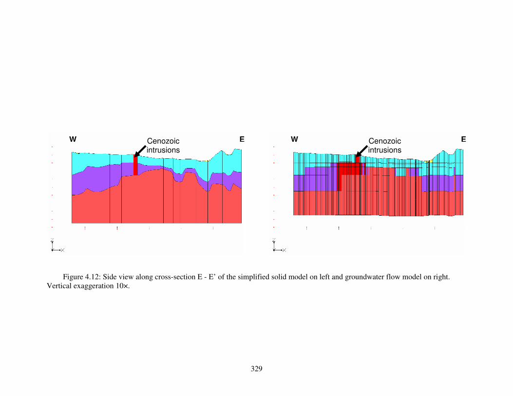
329
Figure 4.12: Side view along cross-section E - E’ of the simplified solid model on left and groundwater flow model on right. Vertical exaggeration 10×.
E W E W Cenozoic intrusions
Cenozoic intrusions

330
Figure 4.13: Distribution of hydrogeologic units within layer 1 of the groundwater flow
model grid. Axes scale is in UTM NAD83 Zone 13 North coordinates.
Permian
Cretaceous
Cenozoic alluvium
Precambrian
Cenozoic intrusions
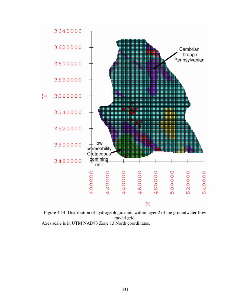
331
Figure 4.14: Distribution of hydrogeologic units within layer 2 of the groundwater flow
model grid. Axes scale is in UTM NAD83 Zone 13 North coordinates.
low permeability Cretaceous
confining unit
Cambrian through
Pennsylvanian

332
Figure 4.15: Distribution of hydrogeologic units within layer 3 of the groundwater flow
model grid. Axes scale is in UTM NAD83 Zone 13 North coordinates.
Cenozoic intrusive
mass beneath
Cornudas Mountains

333
Figure 4.16: Distribution of hydrogeologic units within layer 4 of the groundwater flow
model grid. Axes scale is in UTM NAD83 Zone 13 North coordinates.

334
Figure 4.17: Distribution of hydrogeologic units within layer 5 of the groundwater flow
model grid. Axes scale is in UTM NAD83 Zone 13 North coordinates.

335
Figure 4.18: Distribution of hydrogeologic units within layer 6 of the groundwater flow
model grid. Axes scale is in UTM NAD83 Zone 13 North coordinates.

336
Figure 4.19: Groundwater flow model domain, plan view of model grid, recharge zones
derived from sub-basins delineated by JSAI (2010), and discharge zone at Salt Flats playa.
Axes scale is in UTM NAD83 Zone 13 North coordinates. Red line along perimeter of model domain designates no-flow boundary. Areas enclosed by blue lines indicate recharge zones. Grid cells highlighted with yellow specify discharge zone.
Peñasco Basin
Diablo Plateau
Upper Sacramento
River and Upper
Piñon Creek
Lower Piñon Creek
Lower Sacramento
River and Otero Mesa
Washburn Draw
Cornudas Draw
Salt Flats
Fourmile Draw
Collins Hills
Upper Cornucopia Draw
Rim of the Guadalupes
Lower Cornucopia Draw
Guadalupe Mts.
Crow Flats
Long Canyon
Lewis Canyon
Big Dog Canyon
Brokeoff Mts.
Delaware Mts.
limestone highlands
Coffelt Draw
Shiloh Draw
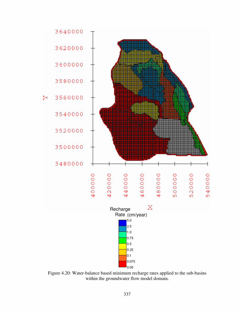
337
Figure 4.20: Water-balance based minimum recharge rates applied to the sub-basins
within the groundwater flow model domain.
Recharge Rate (cm/year)

338
Figure 4.21: Water-balance based average recharge rates applied to the sub-basins within
the groundwater flow model domain.
Recharge Rate (cm/year)

339
Figure 4.22: Water-balance based maximum recharge rates applied to the sub-basins
within the groundwater flow model domain.
Recharge Rate (cm/year)

340
Figure 4.23: Water-balance based minimum areal recharge applied to the sub-basins
within the groundwater flow model domain.
Areal Recharge (acre-feet)

341
Figure 4.24: Water-balance based average areal recharge applied to the sub-basins within
the groundwater flow model domain.
Areal Recharge (acre-feet)

342
Figure 4.25: Water-balance based maximum areal recharge applied to the sub-basins
within the groundwater flow model domain.
Areal Recharge (acre-feet)

343
Figure 4.26: Elevation-dependent minimum recharge rates applied to the recharge zones within the groundwater flow model domain.
Recharge Rate (cm/year)

344
Figure 4.27: Elevation-dependent average recharge rates applied to the recharge zones within the groundwater flow model domain.
Recharge Rate (cm/year)

345
Figure 4.28: Elevation-dependent maximum recharge rates applied to the recharge zones within the groundwater flow model domain.
Recharge Rate (cm/year)

346
Figure 4.29: Elevation-dependent minimum areal recharge applied to the recharge zones within the groundwater flow model domain.
Cornudas Mountains: 18 acre-feet
Guadalupe Mountains: 470 acre-feet
Sacramento Mountains: 2,200 acre-feet
Diablo Plateau: 24 acre-feet
Areal Recharge (acre-feet)

347
Figure 4.30: Elevation-dependent average areal recharge applied to the recharge zones within the groundwater flow model domain.
Cornudas Mountains: 60 acre-feet
Guadalupe Mountains: 2,600 acre-feet
Sacramento Mountains: 12,000 acre-feet
Diablo Plateau: 110 acre-feet
Areal Recharge (acre-feet)

348
Figure 4.31: Elevation-dependent maximum areal recharge applied to the recharge zones within the groundwater flow model domain.
Areal Recharge (acre-feet)
Cornudas Mountains: 100 acre-feet
Guadalupe Mountains: 5,100 acre-feet
Sacramento Mountains: 24,000 acre-feet
Diablo Plateau: 200 acre-feet

349
0.00000001
0.0000001
0.000001
0.00001
0.0001
0.001
0.01
0.1
1
10
100
1000K
(m
/day
)
Figure 4.32: Range of hydraulic conductivity [K] values calculated from transmissivity [T]. Vertical axis is logarithmic scale. Squares indicate median values, and triangles indicate average values.
Aquifer/Facies
Valley- fill
Cenozoic volcanics
Cretaceous Basin-facies Shelf-margin-facies
Shelf-facies
median
average
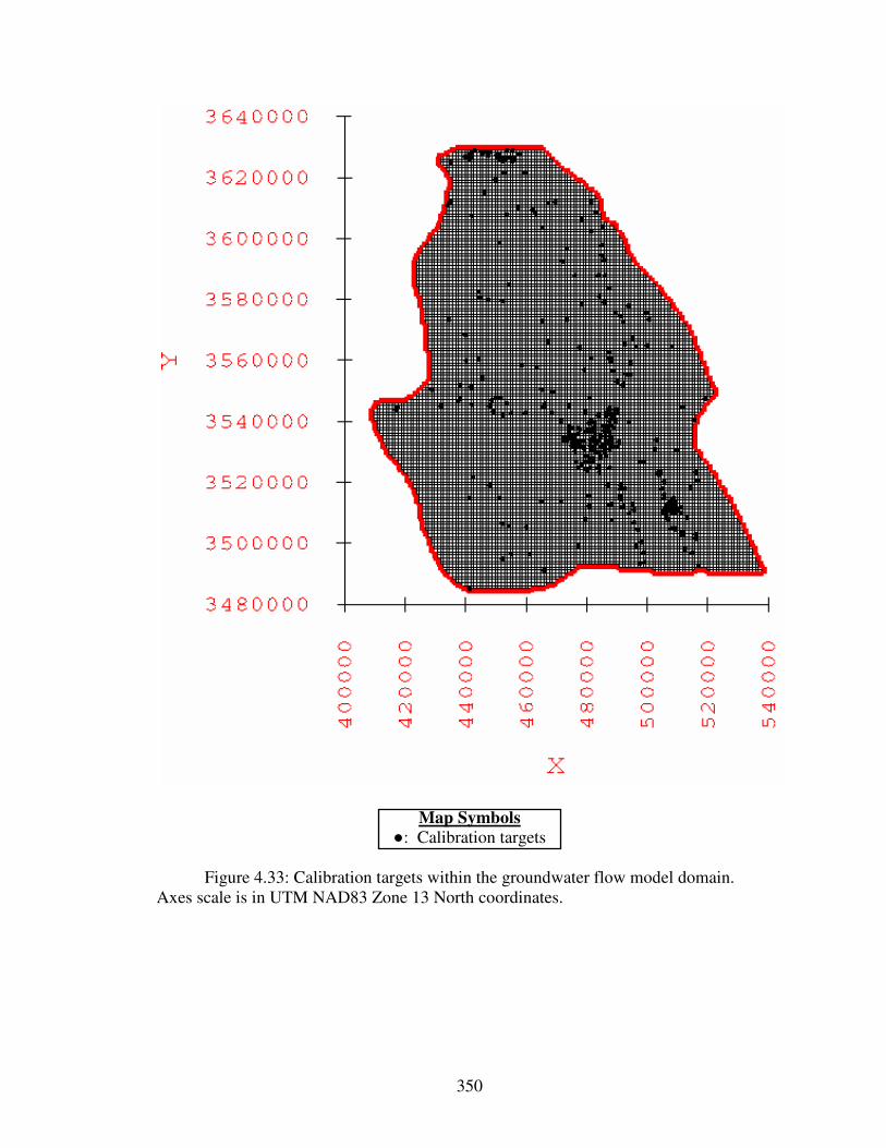
350
Map Symbols ●: Calibration targets
Figure 4.33: Calibration targets within the groundwater flow model domain.
Axes scale is in UTM NAD83 Zone 13 North coordinates.

351
Map Symbols
●: Groundwater age wells
Figure 4.34: Location of the groundwater age wells within the MODFLOW model
domain.
Doll Day
Piñon Well
Webb House
Uña
Cauhape
Harvey Lewis Well
Collins
Jeffer’s Well
Ellett Lower
Evrage House
Lewis
Butterfield Well
Hunt 8

352
Figure 4.35: Comparison of the computed hydraulic head in layer 1 for the calibrated
water-balance based minimum recharge scenario model and the observed groundwater surface.
Green lines are the model computed head contours. Purple dashed lines are the observed groundwater surface contours. Contour elevations are in meters above mean sea level. Contour interval is 200 meters.
1,400
1,400
1,400
1,800
2,200
1,800
1,400
1,400
1,800 2,200
1,400

353
Figure 4.36: Comparison of the computed hydraulic head in layer 1 for the calibrated water-balance based average recharge scenario model and the observed groundwater
surface. Green lines are the model computed head contours. Purple dashed lines are the observed groundwater surface contours. Contour elevations are in meters above mean sea level. Contour interval is 200 meters.
1,400
1,400
1,400
1,800
2,200
1,800
1,400
1,400
2,200 1,800
1,400
1,400

354
Figure 4.37: Comparison of the computed hydraulic head in layer 1 for the calibrated
water-balance based maximum recharge scenario model and the observed groundwater surface.
Green lines are the model computed head contours. Purple dashed lines are the observed groundwater surface contours. Contour elevations are in meters above mean sea level. Contour interval is 200 meters.
1,400
1,400
1,400
1,800
2,200
1,800
1,400
1,400
2,200 1,800
1,400
1,400

355
Figure 4.38: Comparison of the computed hydraulic head in layer 1 for the calibrated
elevation-dependent minimum recharge scenario model and the observed groundwater surface.
Green lines are the model computed head contours. Purple dashed lines are the observed groundwater surface contours. Contour elevations are in meters above mean sea level. Contour interval is 200 meters.
1,400
1,400
1,400
1,800
1,800
1,400
2,200
2,200
1,800

356
Figure 4.39: Comparison of the computed hydraulic head in layer 1 for the calibrated elevation-dependent average recharge scenario model and the observed groundwater
surface. Green lines are the model computed head contours. Purple dashed lines are the observed groundwater surface contours. Contour elevations are in meters above mean sea level. Contour interval is 200 meters.
1,400
1,400
1,800
2,200
1,800
1,400
2,200 1,800
1,400
1,400

357
Figure 4.40: Comparison of the computed hydraulic head in layer 1 for the calibrated
elevation-dependent maximum recharge scenario model and the observed groundwater surface.
Green lines are the model computed head contours. Purple dashed lines are the observed groundwater surface contours. Contour elevations are in meters above mean sea level. Contour interval is 200 meters.
1,400
1,400
1,400
1,800
2,200
1,800
1,400
2,200 1,800
1,400

358
1,000
1,500
2,000
2,500
3,000
1,000 1,500 2,000 2,500 3,000
Observed Head (meters)
Co
mp
ute
d H
ea
d (
me
ters
)
Figure 4.41: Computed versus observed hydraulic head for the calibrated water-balance based minimum recharge scenario model.
1:1 line
RMS Error = 61 meters

359
1,000
1,500
2,000
2,500
3,000
1,000 1,500 2,000 2,500 3,000
Observed Head (meters)
Co
mp
ute
d H
ea
d (
me
ters
)
Figure 4.42: Computed versus observed hydraulic head for the calibrated water-balance based average recharge scenario model.
1:1 line
RMS Error = 60 meters

360
1,000
1,500
2,000
2,500
3,000
1,000 1,500 2,000 2,500 3,000
Observed Head (meters)
Co
mp
ute
d H
ea
d (
me
ters
)
Figure 4.43: Computed versus observed hydraulic head for the calibrated water-balance based maximum recharge scenario model.
1:1 line
RMS Error = 59 meters

361
1,000
1,500
2,000
2,500
3,000
1,000 1,500 2,000 2,500 3,000
Observed Head (meters)
Co
mp
ute
d H
ea
d (
me
ters
)
Figure 4.44: Computed versus observed hydraulic head for the calibrated elevation-dependent minimum recharge scenario model.
1:1 line
RMS Error = 76 meters

362
1,000
1,500
2,000
2,500
3,000
1,000 1,500 2,000 2,500 3,000
Observed Head (meters)
Co
mp
ute
d H
ea
d (
me
ters
)
Figure 4.45: Computed versus observed hydraulic head for the calibrated elevation-dependent average recharge scenario model.
1:1 line
RMS Error = 78 meters

363
1,000
1,500
2,000
2,500
3,000
1,000 1,500 2,000 2,500 3,000
Observed Head (meters)
Co
mp
ute
d H
ea
d (
me
ters
)
Figure 4.46: Computed versus observed hydraulic head for the calibrated elevation-dependent maximum recharge scenario model.
1:1 line
RMS Error = 73 meters

364
-700
-600
-500
-400
-300
-200
-100
0
100
200
300
1,000 1,500 2,000 2,500 3,000
Observed Head (meters)
Re
sid
ua
l H
ea
d (
me
ters
)
Figure 4.47: Residual versus observed hydraulic head for the calibrated water-balance based minimum recharge scenario model.

365
-700
-600
-500
-400
-300
-200
-100
0
100
200
300
1,000 1,500 2,000 2,500 3,000
Observed Head (meters)
Re
sid
ua
l H
ea
d (
me
ters
)
Figure 4.48: Residual versus observed hydraulic head for the calibrated water-balance based average recharge scenario model.

366
-700
-600
-500
-400
-300
-200
-100
0
100
200
300
1,000 1,500 2,000 2,500 3,000
Observed Head (meters)
Re
sid
ua
l H
ea
d (
me
ters
)
Figure 4.49: Residual versus observed hydraulic head for the calibrated water-balance based maximum recharge scenario model.

367
-700
-600
-500
-400
-300
-200
-100
0
100
200
300
1,000 1,500 2,000 2,500 3,000
Observed Head (meters)
Re
sid
ua
l H
ea
d (
me
ters
)
Figure 4.50: Residual versus observed hydraulic head for the calibrated elevation-dependent minimum recharge scenario model.

368
-700
-600
-500
-400
-300
-200
-100
0
100
200
300
1,000 1,500 2,000 2,500 3,000
Observed Head (meters)
Re
sid
ua
l H
ea
d (
me
ters
)
Figure 4.51: Residual versus observed hydraulic head for the calibrated elevation-dependent average recharge scenario model.
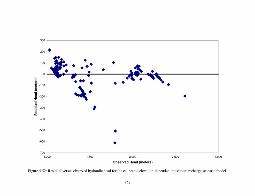
369
-700
-600
-500
-400
-300
-200
-100
0
100
200
300
1,000 1,500 2,000 2,500 3,000
Observed Head (meters)
Re
sid
ua
l H
ea
d (
me
ters
)
Figure 4.52: Residual versus observed hydraulic head for the calibrated elevation-dependent maximum recharge scenario model.

370
-2,500
0
2,500
5,000
7,500
10,000
12,500
15,000
17,500
Minimum Recharge
Scenario
Average Recharge
Scenario
Maximum Recharge
Scenario
Re
sid
ua
ls (
me
ters
)
Sum of Residuals
Sum of Absolute Values of Residuals
Figure 4.53: Sum of the residuals and sum of the absolute values of the residuals between observed and computed hydraulic heads for
the calibrated water-balance based minimum, average, and maximum recharge scenario models.

371
0
250,000
500,000
750,000
1,000,000
1,250,000
1,500,000
1,750,000
2,000,000
2,250,000
2,500,000
Minimum Recharge Scenario Average Recharge Scenario Maximum Recharge Scenario
Su
m o
f S
qu
are
d R
es
idu
als
(m
2)
Figure 4.54: Sum of the squares of the residuals between observed and computed hydraulic heads for the calibrated water-balance
based minimum, average, and maximum recharge scenario models.

372
-2,500
0
2,500
5,000
7,500
10,000
12,500
15,000
17,500
Minimum Recharge
Scenario
Average Recharge
Scenario
Maximum Recharge
Scenario
Re
sid
ua
ls (
me
ters
)
Sum of Residuals
Sum of Absolute Values of Residuals
Figure 4.55: Sum of the residuals and sum of the absolute values of the residuals between observed and computed hydraulic heads for
the calibrated elevation-dependent minimum, average, and maximum recharge scenario models.

373
0
250,000
500,000
750,000
1,000,000
1,250,000
1,500,000
1,750,000
2,000,000
2,250,000
2,500,000
Minimum Recharge Scenario Average Recharge Scenario Maximum Recharge Scenario
Su
m o
f S
qu
are
d R
es
idu
als
(m
2)
Figure 4.56: Sum of the squares of the residuals between observed and computed hydraulic heads for the calibrated elevation-
dependent minimum, average, and maximum recharge scenarios models.

374
Figure 4.57: Horizontal hydraulic conductivity [HK] distribution in layer 1 for the
calibrated water-balance based minimum recharge scenario groundwater flow model.
(m/day)

375
Figure 4.63: Horizontal hydraulic conductivity [HK] distribution in layer 1 for the
calibrated water-balance based average recharge scenario groundwater flow model.
(m/day)

376
Figure 4.69: Horizontal hydraulic conductivity [HK] distribution in layer 1 for the
calibrated water-balance based maximum recharge scenario groundwater flow model.
(m/day)

377
Figure 4.75: Horizontal hydraulic conductivity [HK] distribution in layer 1 for the
calibrated elevation-dependent minimum recharge scenario groundwater flow model.
(m/day)

378
Figure 4.81: Horizontal hydraulic conductivity [HK] distribution in layer 1 for the
calibrated elevation-dependent average recharge scenario groundwater flow model.
(m/day)
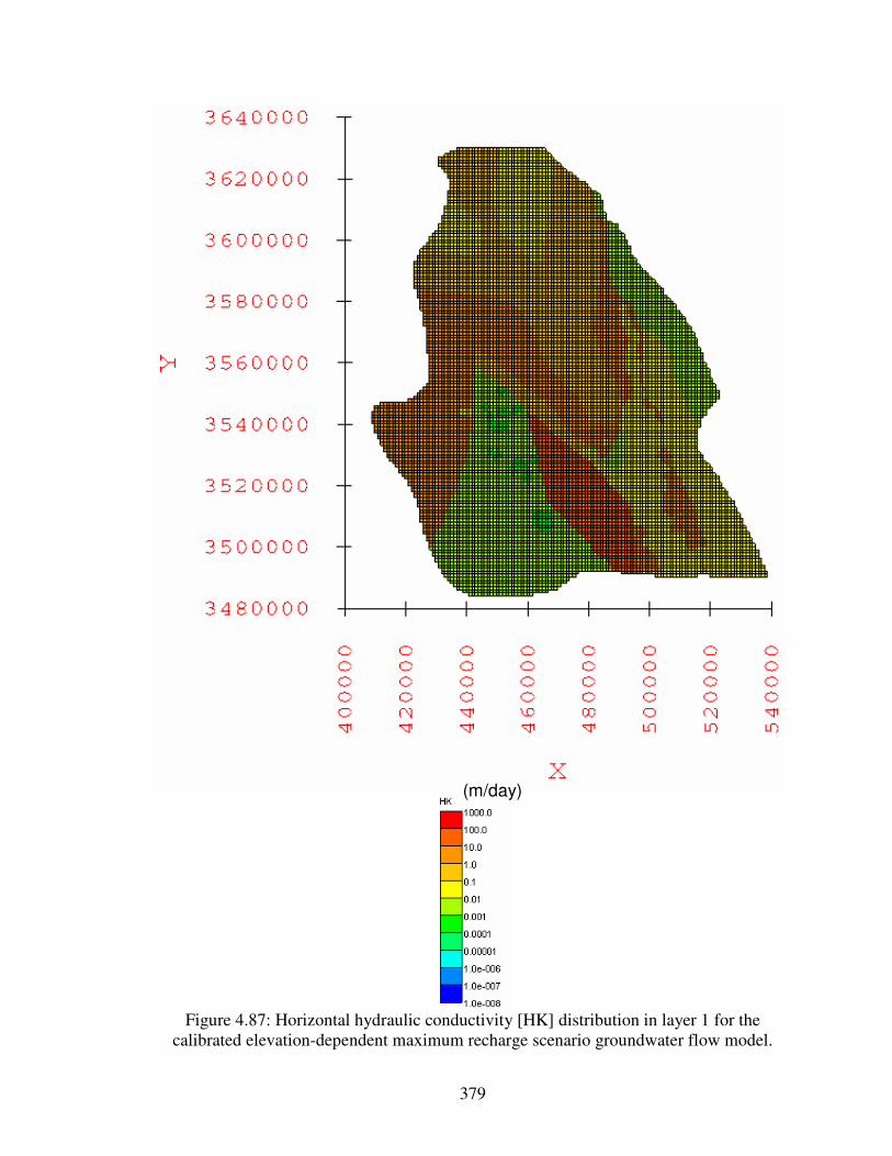
379
Figure 4.87: Horizontal hydraulic conductivity [HK] distribution in layer 1 for the
calibrated elevation-dependent maximum recharge scenario groundwater flow model.
(m/day)

380
0.00000001
0.0000001
0.000001
0.00001
0.0001
0.001
0.01
0.1
1
10
100
1000H
K (
m/d
ay
)
Figure 4.93: Range of horizontal hydraulic conductivity [HK] values for the calibrated water-balance based minimum recharge scenario model.
Hydrogeologic Unit
Cenozoic alluvium
Cenozoic intrusions
Cretaceous unfractured Permian
fractured Permian
Cambrian through
Pennsylvanian
Precambrian low permeability Cretaceous

381
0.00000001
0.0000001
0.000001
0.00001
0.0001
0.001
0.01
0.1
1
10
100
1000H
K (
m/d
ay
)
Figure 4.94: Range of horizontal hydraulic conductivity [HK] values for the calibrated water-balance based average recharge scenario model.
Cenozoic alluvium
Cenozoic intrusions
Cretaceous unfractured Permian
Hydrogeologic Unit
fractured Permian
Cambrian through
Pennsylvanian
Precambrian low permeability Cretaceous

382
0.00000001
0.0000001
0.000001
0.00001
0.0001
0.001
0.01
0.1
1
10
100
1000H
K (
m/d
ay
)
Figure 4.95: Range of horizontal hydraulic conductivity [HK] values for the calibrated water-balance based maximum recharge scenario model.
Cenozoic alluvium
Cenozoic intrusions
Cretaceous unfractured Permian
Hydrogeologic Unit
fractured Permian
Cambrian through
Pennsylvanian
Precambrian low permeability Cretaceous

383
0.00000001
0.0000001
0.000001
0.00001
0.0001
0.001
0.01
0.1
1
10
100
1000H
K (
m/d
ay
)
Figure 4.96: Range of horizontal hydraulic conductivity [HK] values for the calibrated elevation-dependent minimum recharge scenario model.
Cenozoic alluvium
Cenozoic intrusions
Cretaceous unfractured Permian
Hydrogeologic Unit
fractured Permian
Cambrian through
Pennsylvanian
Precambrian low permeability Cretaceous

384
0.00000001
0.0000001
0.000001
0.00001
0.0001
0.001
0.01
0.1
1
10
100
1000H
K (
m/d
ay
)
Figure 4.97: Range of horizontal hydraulic conductivity [HK] values for the calibrated elevation-dependent average recharge scenario model.
Cenozoic alluvium
Cenozoic intrusions
Cretaceous unfractured Permian
Hydrogeologic Unit
fractured Permian
Cambrian through
Pennsylvanian
Precambrian low permeability Cretaceous

385
0.00000001
0.0000001
0.000001
0.00001
0.0001
0.001
0.01
0.1
1
10
100
1000H
K (
m/d
ay
)
Figure 4.98: Range of horizontal hydraulic conductivity [HK] values for the calibrated elevation-dependent maximum recharge scenario model.
Cenozoic alluvium
Cenozoic intrusions
Cretaceous unfractured Permian
Hydrogeologic Unit
fractured Permian
Cambrian through
Pennsylvanian
Precambrian low permeability Cretaceous

386
Figure 4.99: Distribution of aquifer transmissivity [T] for the calibrated water-balance
based minimum recharge scenario groundwater flow model.
(m2/day) T

387
Figure 4.100: Distribution of aquifer transmissivity [T] for the calibrated water-balance
based average recharge scenario groundwater flow model.
(m2/day) T

388
Figure 4.101: Distribution of aquifer transmissivity [T] for the calibrated water-balance
based maximum recharge scenario groundwater flow model.
(m2/day) T
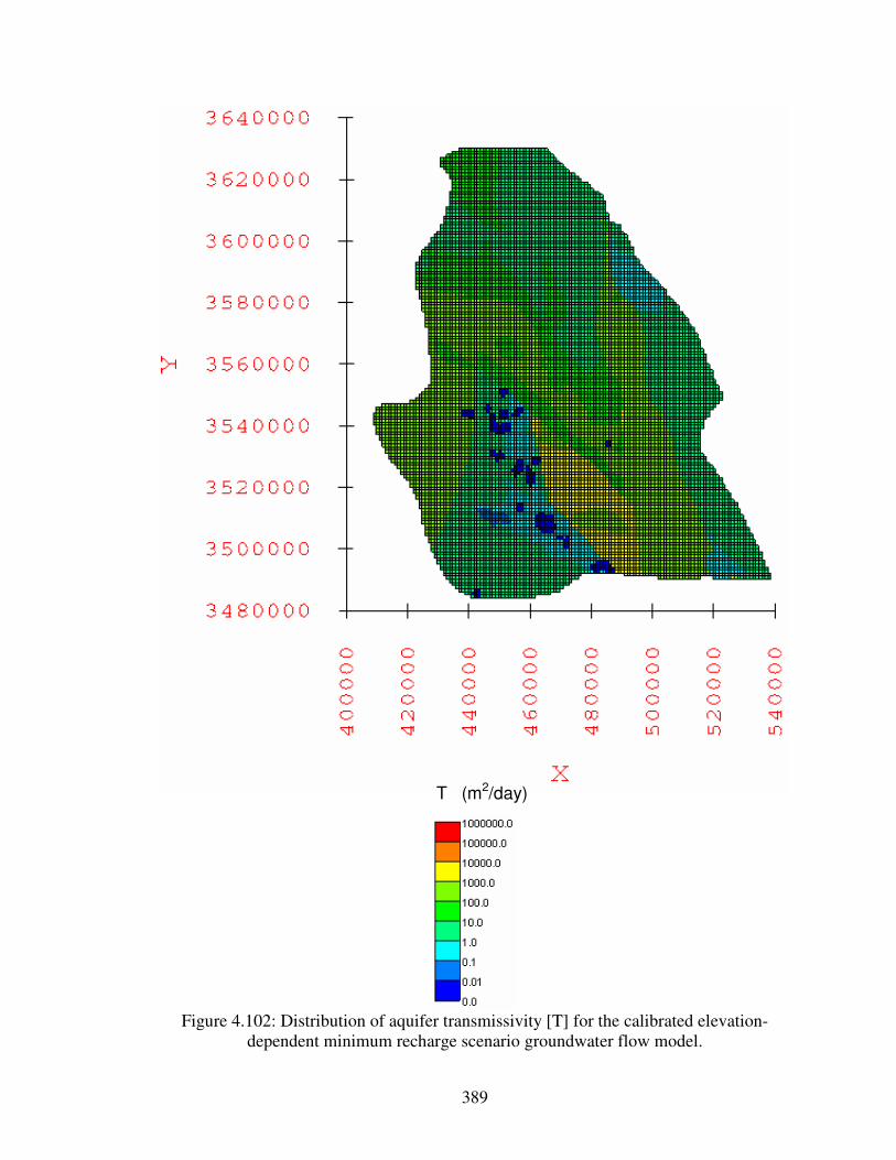
389
Figure 4.102: Distribution of aquifer transmissivity [T] for the calibrated elevation-
dependent minimum recharge scenario groundwater flow model.
(m2/day) T

390
Figure 4.103: Distribution of aquifer transmissivity [T] for the calibrated elevation-
dependent average recharge scenario groundwater flow model.
(m2/day) T

391
Figure 4.104: Distribution of aquifer transmissivity [T] for the calibrated elevation-
dependent maximum recharge scenario groundwater flow model.
(m2/day) T

392
0.01
0.1
1
10
100
1000
10000
100000
1000000T
(m
2/d
ay
)
Figure 4.105: Range of transmissivities [T] derived from the calibrated water-balance based minimum, average, and maximum recharge scenario models.
Minimum Recharge Scenario
Average Recharge Scenario
Maximum Recharge Scenario
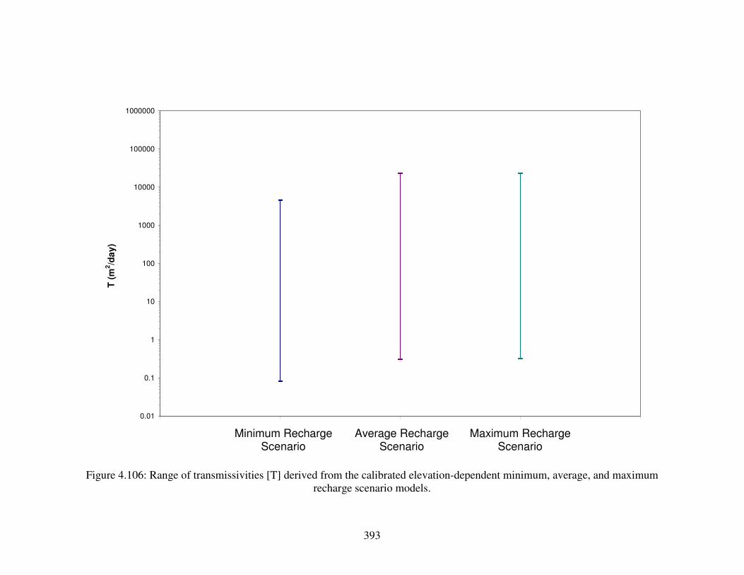
393
0.01
0.1
1
10
100
1000
10000
100000
1000000T
(m
2/d
ay
)
Figure 4.106: Range of transmissivities [T] derived from the calibrated elevation-dependent minimum, average, and maximum recharge scenario models.
Minimum Recharge Scenario
Average Recharge Scenario
Maximum Recharge Scenario

394
100
1,000
10,000
100,000
0 1 10 100 1,000 10,000 100,000 1,000,000 10,000,000
MODPATH Age (years)
NE
TP
AT
H A
ge
(y
ea
rs)
Min. n lower bound
Min. n upper bound
Avg. n lower bound
Avg. n upper bound
Max. n lower bound
Max. n upper bound
1:1 Line
Figure 4.107: NETPATH versus MODPATH ages for the calibrated water-balance based minimum recharge scenario model using
minimum, average, and maximum porosities. Vertical and horizontal axes are logarithmic scale.
RMS Error (years): Minimum Porosity = 9,800 Average porosity = 9,400
Maximum porosity = 9,900
.1

395
100
1,000
10,000
100,000
0 1 10 100 1,000 10,000 100,000 1,000,000 10,000,000
MODPATH Age (years)
NE
TP
AT
H A
ge
(y
ea
rs)
Min. n lower bound
Min. n upper bound
Avg. n lower bound
Avg. n upper bound
Max. n lower bound
Max. n upper bound
1:1 Line
Figure 4.108: NETPATH versus MODPATH ages for the calibrated water-balance based average recharge scenario model using
minimum, average, and maximum porosities. Vertical and horizontal axes are logarithmic scale.
RMS Error (years): Minimum Porosity = 9,700 Average porosity = 9,200
Maximum porosity = 9,000
.1

396
100
1,000
10,000
100,000
0 1 10 100 1,000 10,000 100,000 1,000,000 10,000,000
MODPATH Age (years)
NE
TP
AT
H A
ge
(y
ea
rs)
Min. n lower bound
Min. n upper bound
Avg. n lower bound
Avg. n upper bound
Max. n lower bound
Max. n upper bound
1:1 Line
Figure 4.109: NETPATH versus MODPATH ages for the calibrated water-balance based maximum recharge scenario model using
minimum, average, and maximum porosities. Vertical and horizontal axes are logarithmic scale.
RMS Error (years): Minimum Porosity = 9,900 Average porosity = 9,500
Maximum porosity = 9,300
.1

397
100
1,000
10,000
100,000
0 1 10 100 1,000 10,000 100,000 1,000,000 10,000,000
MODPATH Age (years)
NE
TP
AT
H A
ge
(y
ea
rs)
Min. n lower bound
Min. n upper bound
Avg. n lower bound
Avg. n upper bound
Max. n lower bound
Max. n upper bound
1:1 Line
Figure 4.110: NETPATH versus MODPATH ages for the calibrated elevation-dependent minimum recharge scenario model using
minimum, average, and maximum porosities. Vertical and horizontal axes are logarithmic scale.
.1
RMS Error (years): Minimum Porosity = 180,000 Average porosity = 450,000
Maximum porosity = 720,000
Collins outliers
RMS Error with outliers removed (years):
Minimum Porosity = 43,000 Average porosity = 120,000
Maximum porosity = 200,000

398
100
1,000
10,000
100,000
0 1 10 100 1,000 10,000 100,000 1,000,000 10,000,000
MODPATH Age (years)
NE
TP
AT
H A
ge
(y
ea
rs)
Min. n lower bound
Min. n upper bound
Avg. n lower bound
Avg. n upper bound
Max. n lower bound
Max. n upper bound
1:1 Line
Figure 4.111: NETPATH versus MODPATH ages for the calibrated elevation-dependent average recharge scenario model using
minimum, average, and maximum porosities. Vertical and horizontal axes are logarithmic scale.
.1
RMS Error (years): Minimum Porosity = 140,000 Average porosity = 360,000
Maximum porosity = 570,000
RMS Error with outliers removed (years):
Minimum Porosity = 7,600 Average porosity = 25,000
Maximum porosity = 44,000
Evrage House and Collins outliers

399
100
1,000
10,000
100,000
0 1 10 100 1,000 10,000 100,000 1,000,000 10,000,000
MODPATH Age (years)
NE
TP
AT
H A
ge
(y
ea
rs)
Min. n lower bound
Min. n upper bound
Avg. n lower bound
Avg. n upper bound
Max. n lower bound
Max. n upper bound
1:1 Line
Figure 4.112: NETPATH versus MODPATH ages for the calibrated elevation-dependent maximum recharge scenario model using
minimum, average, and maximum porosities. Vertical and horizontal axes are logarithmic scale.
.1
RMS Error (years): Minimum Porosity = 210,000 Average porosity = 690,000
Maximum porosity = 1,200,000
RMS Error with outliers removed (years):
Minimum Porosity = 6,800 Average porosity = 5,000
Maximum porosity = 9,400
Collins outliers
Evrage House outliers

400
Map Symbols
●: Particle origins
●: Groundwater age wells
Figure 4.113: MODPATH pathlines and origins of particles for the water-balance based minimum recharge scenario using average porosity values.
Upper bound
Lower bound

401
Map Symbols
●: Particle origins
●: Groundwater age wells
Figure 4.114: MODPATH pathlines and origins of particles for the water-balance based average recharge scenario using average porosity values.
Upper bound
Lower bound

402
Map Symbols
●: Particle origins
●: Groundwater age wells
Figure 4.115: MODPATH pathlines and origins of particles for the water-balance based maximum recharge scenario using average porosity values.
Upper bound
Lower bound

403
Map Symbols
●: Particle origins
●: Groundwater age wells
Figure 4.116: MODPATH pathlines and origins of particles for the elevation-dependent minimum recharge scenario using average porosity values.
Lower bound
Upper bound

404
Map Symbols
●: Particle origins
●: Groundwater age wells
Figure 4.117: MODPATH pathlines and origins of particles for the elevation-dependent average recharge scenario using average porosity values.
Upper bound
Lower bound

405
Map Symbols
●: Particle origins
●: Groundwater age wells
Figure 4.118: MODPATH pathlines and origins of particles for the elevation-dependent maximum recharge scenario using average porosity values.
Upper bound
Lower bound

406
-1,000,000
-500,000
0
500,000
1,000,000
1,500,000
2,000,000
2,500,000
3,000,000
3,500,000
4,000,000
4,500,000
5,000,000
Minimum Recharge
Scenario
Average Recharge
Scenario
Maximum Recharge
Scenario
Su
m o
f R
es
idu
als
(y
ea
rs)
Minimum Porosity
Average Porosity
Maximum Porosity
Figure 4.119: Sum of the residuals between MODPATH and NETPATH ages for the water-balance based minimum, average, and
maximum recharge scenarios using minimum, average, and maximum porosities.

407
0
500,000
1,000,000
1,500,000
2,000,000
2,500,000
3,000,000
3,500,000
4,000,000
4,500,000
5,000,000
Minimum Recharge
Scenario
Average Recharge
Scenario
Maximum Recharge
Scenario
Su
m o
f A
bs
ou
te V
alu
es
of
Re
sid
ua
ls (
ye
ars
)
Minimum Porosity
Average Porosity
Maximum Porosity
Figure 4.120: Sum of the absolute values of the residuals between MODPATH and NETPATH ages for the water-balance based
minimum, average, and maximum recharge scenarios using minimum, average, and maximum porosities.

408
0
1
10
100
1,000
10,000
100,000
1,000,000
10,000,000
100,000,000
1,000,000,000
10,000,000,000
100,000,000,000
1,000,000,000,000
Minimum Recharge
Scenario
Average Recharge
Scenario
Maximum Recharge
Scenario
Su
m o
f S
qu
are
d R
es
idu
als
(ye
ars
2)
Minimum Porosity
Average Porosity
Maximum Porosity
Figure 4.121: Sum of the squares of the residuals between MODPATH and NETPATH ages for the water-balance based minimum,
average, and maximum recharge scenarios using minimum, average, and maximum porosities. Vertical axis is logarithmic scale.

409
-1,000,000
-500,000
0
500,000
1,000,000
1,500,000
2,000,000
2,500,000
3,000,000
3,500,000
4,000,000
4,500,000
5,000,000
Minimum Recharge
Scenario
Average Recharge
Scenario
Maximum Recharge
Scenario
Su
m o
f R
es
idu
als
(y
ea
rs)
Minimum Porosity
Average Porosity
Maximum Porosity
Figure 4.122: Sum of the residuals between MODPATH and NETPATH ages for the elevation-dependent minimum, average, and
maximum recharge scenarios using minimum, average, and maximum porosities.

410
0
500,000
1,000,000
1,500,000
2,000,000
2,500,000
3,000,000
3,500,000
4,000,000
4,500,000
5,000,000
Minimum Recharge
Scenario
Average Recharge
Scenario
Maximum Recharge
Scenario
Su
m o
f A
bs
ou
te V
alu
es
of
Re
sid
ua
ls (
ye
ars
)
Minimum Porosity
Average Porosity
Maximum Porosity
Figure 4.123: Sum of the absolute values of the residuals between MODPATH and NETPATH ages for the elevation-dependent
minimum, average, and maximum recharge scenarios using minimum, average, and maximum porosities.

411
0
1
10
100
1,000
10,000
100,000
1,000,000
10,000,000
100,000,000
1,000,000,000
10,000,000,000
100,000,000,000
1,000,000,000,000
Minimum Recharge
Scenario
Average Recharge
Scenario
Maximum Recharge
Scenario
Su
m o
f S
qu
are
d R
es
idu
als
(ye
ars
2)
Minimum Porosity
Average Porosity
Maximum Porosity
Figure 4.124: Sum of the squares of the residuals between MODPATH and NETPATH ages for the elevation-dependent minimum,
average, and maximum recharge scenarios using minimum, average, and maximum porosities. Vertical axis is logarithmic scale.

412
TABLES – CHAPTER 4

413
Salt Basin Sub-basins
Delineated by JSAI (2010)
Minimum
Recharge
Rate
(cm/year)
Average
Recharge
Rate
(cm/year)
Maximum
Recharge
Rate
(cm/year)
Minimum
Recharge
(m3/day)
Average
Recharge
(m3/day)
Maximum
Recharge
(m3/day)
Minimum
Recharge
(acre-
feet/year)
Average
Recharge
(acre-
feet/year)
Maximum
Recharge
(acre-
feet/year)
Peñasco Basin 1.3 1.9 2.4 19,842 28,523 37,204 5,875 8,446 11,016
Upper Sacramento River and Upper Piñon Creek 0.5 1.0 1.2 9,637 19,275 22,166 2,854 5,707 6,564
Lower Piñon Creek 0.5 1.5 2.5 1,342 4,025 6,708 397 1,192 1,986
Collins Hills 1.0 2.5 5.0 3,970 9,925 19,850 1,176 2,939 5,878
Rim of the Guadalupes 2.0 2.8 4.0 8,542 11,746 17,085 2,529 3,478 5,059
Guadalupe Mountains 2.0 2.8 4.0 16,482 22,663 32,964 4,880 6,711 9,761
Upper Cornucopia Draw 1.0 2.5 3.5 3,888 9,720 13,607 1,151 2,878 4,029
limestone highlands 2.5 3.0 5.0 8,282 9,939 16,564 2,452 2,943 4,905
Lower Sacramento River and Otero Mesa 0.1 0.3 0.3 2,988 5,976 6,573 885 1,769 1,946
Lower Cornucopia Draw 2.5 3.0 5.0 28,064 33,676 56,127 8,310 9,972 16,620
Crow Flats 0.1 0.2 0.2 2,015 4,030 3,023 597 1,193 895
Shiloh Draw 0.1 0.2 0.2 1,655 4,413 4,965 490 1,307 1,470
Coffelt Draw 2.0 2.5 2.8 13,909 17,386 19,124 4,118 5,148 5,663
Big Dog Canyon 1.0 2.0 2.0 9,254 18,508 18,508 2,740 5,480 5,480
Long Canyon 2.0 3.0 3.3 3,559 5,339 5,784 1,054 1,581 1,713
Lewis Canyon 2.0 3.0 3.3 8,268 12,403 13,436 2,448 3,673 3,979
Brokeoff Mountains 0.8 1.5 1.5 5,709 11,417 11,417 1,690 3,381 3,381
Fourmile Draw 0.1 1.0 1.0 145 2,902 2,902 43 859 859
Cornudas Draw 0.5 1.5 1.8 6,817 20,452 23,861 2,019 6,056 7,065
Washburn Draw 0.1 0.1 0.1 348 695 695 103 206 206
Diablo Plateau 0.1 0.1 0.1 4,325 8,649 10,811 1,281 2,561 3,201
Delaware Mountains 0.8 1.5 1.5 5,647 11,294 11,294 1,672 3,344 3,344
Salt Flats 0.0 0.0 0.0 0 0 0 0 0 0
164,688 272,956 354,670 48,765 80,824 105,020Sum all sub-basins Table 4.1: Water-balance based minimum, average, and maximum recharge rates and areal recharge applied to the Salt Basin sub-
basins within the 3-D MODFLOW groundwater flow model domain.

414
Minimum
Sacramento Mountains
Recharge Factor
(%)
Average
Sacramento Mountains
Recharge Factor
(%)
Maximum
Sacramento Mountains
Recharge Factor
(%)
4 22 44 Table 4.2: Sacramento Mountains recharge factors from Newton et al. (2011).
Location
Minimum
Recharge
Rate
(cm/year)
Average
Recharge
Rate
(cm/year)
Maximum
Recharge
Rate
(cm/year)
Creek beds and depressions 0.028 0.242 0.457
Outside creek beds 0.005 0.0125 0.020 Table 4.3: Kreitler et al. (1987) recharge rates for Diablo Plateau from Mayer (1995).

415
Range of
Average Annual
Precipitation in
Figure 1.11
Polygons
(cm/year)
Median
Average Annual
Precipitation in
Figure 1.11
Polygons
(cm/year)
Minimum
Recharge
Factor
(%)
Average
Recharge
Factor
(%)
Maximum
Recharge
Factor
(%)
Minimum
Recharge
Rate
(cm/year)
Average
Recharge
Rate
(cm/year)
Maximum
Recharge
Rate
(cm/year)
Minimum
Recharge
(m3/day)
Average
Recharge
(m3/day)
Maximum
Recharge
(m3/day)
Minimum
Recharge
(acre-
feet/year)
Average
Recharge
(acre-
feet/year)
Maximum
Recharge
(acre-
feet/year)
61 to 66 64 4 22 44 2.5 14.0 27.9
66 to 71 69 4 22 44 2.7 15.1 30.2
71 to 76 74 4 22 44 2.9 16.2 32.4
76 to 81 79 4 22 44 3.1 17.3 34.67,366 40,513 81,026 2,181 11,996 23,992
61 to 66 64 4 22 44 2.5 14.0 27.9
66 to 71 69 4 22 44 2.7 15.1 30.2
71 to 76 74 4 22 44 2.9 16.2 32.41,572 8,644 17,288 465 2,560 5,119
Sum Sacramento Mountains recharge zone
Sum Guadalupe Mountains recharge zone
Table 4.4: Elevation-dependent minimum, average, and maximum recharge rates and areal recharge applied to the recharge zones within the 3-D MODFLOW groundwater flow model domain in the Sacramento and Guadalupe Mountains.
Location
Minimum
Recharge
Rate
(cm/year)
Average
Recharge
Rate
(cm/year)
Maximum
Recharge
Rate
(cm/year)
Minimum
Recharge
(m3/day)
Average
Recharge
(m3/day)
Maximum
Recharge
(m3/day)
Minimum
Recharge
(acre-
feet/year)
Average
Recharge
(acre-
feet/year)
Maximum
Recharge
(acre-
feet/year)
Creek beds and depressions 0.028 0.242 0.457
Outside creek beds 0.005 0.0125 0.02060 202 344 18 60 102
Creek beds and depressions 0.028 0.242 0.457
Outside creek beds 0.005 0.0125 0.02080 380 679 24 112 201
Sum Cornudas Mountains recharge zone
Sum Diablo Plateau recharge zone Table 4.5: Elevation-dependent minimum, average, and maximum recharge rates and areal recharge applied to the recharge zones
within the 3-D MODFLOW groundwater flow model domain in around the Cornudas Mountains and on the Diablo Plateau.

416
Hydrogeologic
Unit
Model
Layers
Initial
Horizontal
K (m/day)
Vertical
Anisotropy
Calibrated
Water-balance
Based Minimum
Recharge
Scenario
Horizontal
K (m/day)
Calibrated
Water-balance
Based Average
Recharge
Scenario
Horizontal
K (m/day)
Calibrated
Water-balance
Based Maximum
Recharge
Scenario
Horizontal
K (m/day)
Cenozoic
alluvium1, 2, and 3 1 100 10 10 10
Cenozoic intrusions 1, 2, 3, 4, and 5 0.0001 1,000 0.00001 to 0.0001 0.00001 to 0.001 0.00001 to 0.001
Cretaceous 1 0.01 100 0.005 0.0075 0.0075
Low permeability
confining unit
beneath Cretaceous
2 0.000001 1,000 0.00000001 0.00000001 0.00000001
Unfractured Permian 1, 2, 3, 4, and 5 0.01 to 0.1 100 0.005 to 0.5 0.0075 to 1 0.01 to 2.5
Fractured Permian 1, 2, 3, 4, and 5 1 to 10 10 0.025 to 25 0.025 to 250 0.025 to 250
Paleozoic
(Cambrian through
Pennslyvanian)
2, 3, 4, 5, and 6 0.001 1,000 0.00005 to 0.5 0.00005 to 0.5 0.00005 to 0.5
Precambrian 1, 2, 3, 4, 5, and 6 0.001 1,000 0.00001 to 0.01 0.00001 to 0.01 0.00001 to 0.01 Table 4.7: Initial horizontal hydraulic conductivity [K], vertical anisotropy, and final horizontal K assigned to each hydrogeologic unit
for the calibrated water-balance based minimum, average, and maximum recharge scenario models.

417
Hydrogeologic
Unit
Model
Layers
Initial
Horizontal
K (m/day)
Vertical
Anisotropy
Calibrated
Elevation-
dependent
Minimum
Recharge
Scenario
Horizontal
K (m/day)
Calibrated
Elevation-
dependent
Average
Recharge
Scenario
Horizontal
K (m/day)
Calibrated
Elevation-
dependent
Maximum
Recharge
Scenario
Horizontal
K (m/day)Cenozoic
alluvium1, 2, and 3 1 100 0.005 to 10 0.0075 to 10 0.01 to 10
Cenozoic intrusions 1, 2, 3, 4, and 5 0.0001 1,000 0.00001 to 0.1 0.00001 to 0.1 0.00001 to 0.1
Cretaceous 1 0.01 100 0.0005 0.0025 0.005
Low permeability
confining unit
beneath Cretaceous
2 0.000001 1,000 0.00000001 0.00001 0.0001
Unfractured Permian 1, 2, 3, 4, and 5 0.01 to 0.1 100 0.005 to 0.5 0.005 to 5 0.005 to 5
Fractured Permian 1, 2, 3, 4, and 5 1 to 10 10 0.0075 to 5 0.075 to 25 0.25 to 25
Paleozoic
(Cambrian through
Pennslyvanian)
2, 3, 4, 5, and 6 0.001 1,000 0.00005 to 0.1 0.00005 to 0.1 0.00005 to 0.1
Precambrian 1, 2, 3, 4, 5, and 6 0.001 1,000 0.00001 to 0.01 0.00001 to 0.01 0.00001 to 0.01 Table 4.8: Initial horizontal hydraulic conductivity [K], vertical anisotropy, and final horizontal K assigned to each hydrogeologic unit
for the calibrated elevation-dependent minimum, average, and maximum recharge scenario models.

418
Hydrogeologic
Unit
Minimum Porosity
(%)
Averge Porosity
(%)
Maximum Porosity
(%)
Cenozoic alluvium 5 12.5 20
Cenozoic intrusions 0.1 0.5 1
Cretaceous 5 12.5 20
Low permeability confining
unit beneath Cretaceous5 12.5 20
Unfractured Permian 5 12.5 20
Fractured Permian 5 12.5 20
Paleozoic (Cambrian
through Pennslyvanian)1 5.5 10
Precambrian 0.1 0.5 1 Table 4.10: Minimum, average, and maximum porosity values used for MODPATH solution.

419
Groundwater
Age Well IDPOD Number Easting Northing
Model
Row
Model
Column
Model
Layer
Ground
Surface
Elevation
(m)
Well
Depth
(m)
Elevation
of
Well
Depth
(m)
Note
Doll Day ST 00241 POD1 472590 3607544 79 44 1 1,718 475 1,243 Well depth from well owner
Piñon Well ST 00003 478550 3606619 73 45 1 1,623 335 1,287 Well depth from NMOSE
Webb House NA 465825 3606007 85 46 1 1,815 457 1,358 Well depth unkown; estimated
Uña ST 00018 473476 3596830 78 55 1 1,743 390 1,353 Well depth from NMOSE
Cauhape ST 00019 476365 3588074 75 64 1 1,447 315 1,131 Well depth from NMOSE
Jeffer's Well NA 467327 3585742 84 66 1 1,481 305 1,177 Well depth from well owner
Ellett Lower NA 469670 3578554 82 73 1 1,397 160 1,237 Well depth from well owner
Harvey Lewis Well ST 00014 487565 3571656 64 80 1 1,181 91 1,090 Well depth from NMOSE
Collins NA 499579 3568454 52 83 1 1,238 183 1,055 Well depth from well owner
Evrage House ST 00050 496187 3563804 55 88 1 1,147 61 1,086 Well depth from NMOSE
Lewis ST 00163 479239 3557196 72 94 1 1,230 154 1,076 Well depth from NMOSE
Butterfield Well ST 00044 466258 3546182 85 105 2 1,268 244 1,024 Well depth from NMOSE
Hunt 8 ST 00057 490345 3544103 61 108 1 1,114 48 1,066 Well depth from NMOSE Table 4.11: Groundwater age wells incorporated into MODPATH particle tracking exercise.
POD Number Key: NA = Not applicable.

420
Elevation
of
Computed
Groundwater
Surface (m)
Elevation
of
Midpoint
(m)
Elevation
of
Bottom
of Cell
(m)
Elevation
of
Computed
Groundwater
Surface (m)
Elevation
of
Midpoint
(m)
Elevation
of
Bottom
of Cell
(m)
Elevation
of
Computed
Groundwater
Surface (m)
Elevation
of
Midpoint
(m)
Elevation
of
Bottom
of Cell
(m)
Doll Day 1,243 1,401 1,297 1,192 1,398 1,295 1,192 1,412 1,302 1,192
Pinon Well 1,287 1,359 1,256 1,154 1,349 1,251 1,154 1,368 1,261 1,154
Webb House 1,358 1,429 1,328 1,227 1,428 1,328 1,227 1,445 1,336 1,227
Una 1,353 1,334 1,227 1,120 1,323 1,222 1,120 1,338 1,229 1,120
Cauhape 1,131 1,276 1,167 1,058 1,254 1,156 1,058 1,267 1,163 1,058
Jeffer's Well 1,177 1,301 1,201 1,101 1,272 1,186 1,101 1,276 1,189 1,101
Ellett Lower 1,237 1,269 1,173 1,077 1,231 1,154 1,077 1,230 1,154 1,077
Harvey Lewis Well 1,090 1,157 1,087 1,018 1,143 1,080 1,018 1,154 1,086 1,018
Collins 1,055 1,169 1,093 1,018 1,152 1,085 1,018 1,164 1,091 1,018
Evrage House 1,086 1,146 1,093 1,040 1,135 1,088 1,040 1,144 1,092 1,040
Lewis 1,076 1,155 1,076 997 1,139 1,068 997 1,139 1,068 997
Butterfield Well 1,024 1,031 1,006 981 1,031 1,006 981 1,031 1,006 981
Hunt 8 1,066 1,110 1,054 997 1,109 1,053 997 1,111 1,054 997
Water-balance Based
Maximum
Recharge ScenarioGroundwater
Age Well ID
Elevation
of
Well
Depth
(m)
Water-balance Based
Minimum
Recharge Scenario
Water-balance Based
Average
Recharge Scenario
Table 4.12: Elevations at which MODPATH particles were generated for the calibrated water-balance based minimum, average, and
maximum recharge scenario models. Orange highlighted rectangles indicate the vertical position of generated MODPATH particles chosen to represent the potential pathlines and residence times of groundwater sampled at each well.

421
Elevation
of
Computed
Groundwater
Surface (m)
Elevation
of
Midpoint
(m)
Elevation
of
Bottom
of Cell
(m)
Elevation
of
Computed
Groundwater
Surface (m)
Elevation
of
Midpoint
(m)
Elevation
of
Bottom
of Cell
(m)
Elevation
of
Computed
Groundwater
Surface (m)
Elevation
of
Midpoint
(m)
Elevation
of
Bottom
of Cell
(m)
Doll Day 1,243 1,462 1,327 1,192 1,464 1,328 1,192 1,454 1,323 1,192
Pinon Well 1,287 1,399 1,276 1,154 1,396 1,275 1,154 1,390 1,272 1,154
Webb House 1,358 1,491 1,359 1,227 1,495 1,361 1,227 1,483 1,355 1,227
Una 1,353 1,338 1,229 1,120 1,334 1,227 1,120 1,332 1,226 1,120
Cauhape 1,131 1,248 1,153 1,058 1,231 1,145 1,058 1,240 1,149 1,058
Jeffer's Well 1,177 1,274 1,188 1,101 1,267 1,184 1,101 1,284 1,193 1,101
Ellett Lower 1,237 1,243 1,160 1,077 1,226 1,152 1,077 1,251 1,164 1,077
Harvey Lewis Well 1,090 1,143 1,081 1,018 1,123 1,071 1,018 1,125 1,071 1,018
Collins 1,055 1,140 1,079 1,018 1,125 1,072 1,018 1,123 1,071 1,018
Evrage House 1,086 1,136 1,088 1,040 1,122 1,081 1,040 1,121 1,081 1,040
Lewis 1,076 1,149 1,073 997 1,135 1,066 997 1,142 1,070 997
Butterfield Well 1,024 1,031 1,006 981 1,031 1,006 981 1,031 1,006 981
Hunt 8 1,066 1,113 1,055 997 1,114 1,056 997 1,110 1,054 997
Elevation-dependent
Maximum
Recharge ScenarioGroundwater
Age Well ID
Elevation
of
Well
Depth
(m)
Elevation-dependent
Minimum
Recharge Scenario
Elevation-dependent
Average
Recharge Scenario
Table 4.13: Elevations at which MODPATH particles were generated for the calibrated elevation-dependent minimum, average, and
maximum recharge scenario models. Orange highlighted rectangles indicate the vertical position of generated MODPATH particles chosen to represent the potential pathlines and residence times of groundwater sampled at each well.

422
Sum Residuals (m) 44
Sum Absolute Residuals (m) 11,780
Sum Squared Residuals (m2) 1,400,350
RMS Error (m) 61
Residual Mean (m) 0.1
Absolute Residual Mean (m) 16
Residual Standard Deviation (m) 61
Minimum Observed Hydraulic Head (m) 1,029
Maximum Observed Hydraulic Head (m) 2,610
Residual Standard Deviation/Range 0.039
Residual Mean/Range 0.00007
Sum Residuals (m) -649
Sum Absolute Residuals (m) 10,793
Sum Squared Residuals (m2) 1,379,233
RMS Error (m) 60
Residual Mean (m) -2
Absolute Residual Mean (m) 13
Residual Standard Deviation (m) 60
Minimum Observed Hydraulic Head (m) 1,029
Maximum Observed Hydraulic Head (m) 2,610
Residual Standard Deviation/Range 0.038
Residual Mean/Range -0.001
Sum Residuals (m) 236
Sum Absolute Residuals (m) 10,568
Sum Squared Residuals (m2) 1,318,998
RMS Error (m) 59
Residual Mean (m) 0.6
Absolute Residual Mean (m) 14
Residual Standard Deviation (m) 59
Minimum Observed Hydraulic Head (m) 1,029
Maximum Observed Hydraulic Head (m) 2,610
Residual Standard Deviation/Range 0.037
Residual Mean/Range 0.0004
Water-balance Based Minimum Recharge Scenario
Water-balance Based Average Recharge Scenario
Water-balance Based Maximum Recharge Scenario
Table 4.16: Residual hydraulic head statistics for the calibrated water-balance based
minimum, average, and maximum recharge scenario models.

423
Sum Residuals (m) 1,364
Sum Absolute Residuals (m) 15,478
Sum Squared Residuals (m2) 2,208,280
RMS Error (m) 76
Residual Mean (m) 4
Absolute Residual Mean (m) 22
Residual Standard Deviation (m) 76
Minimum Observed Hydraulic Head (m) 1,029
Maximum Observed Hydraulic Head (m) 2,610
Residual Standard Deviation/Range 0.048
Residual Mean/Range 0.002
Sum Residuals (m) 1,621
Sum Absolute Residuals (m) 16,612
Sum Squared Residuals (m2) 2,291,432
RMS Error (m) 78
Residual Mean (m) 4
Absolute Residual Mean (m) 24
Residual Standard Deviation (m) 78
Minimum Observed Hydraulic Head (m) 1,029
Maximum Observed Hydraulic Head (m) 2,610
Residual Standard Deviation/Range 0.049
Residual Mean/Range 0.003
Sum Residuals (m) 951
Sum Absolute Residuals (m) 14,836
Sum Squared Residuals (m2) 2,018,583
RMS Error (m) 73
Residual Mean (m) 3
Absolute Residual Mean (m) 21
Residual Standard Deviation (m) 73
Minimum Observed Hydraulic Head (m) 1,029
Maximum Observed Hydraulic Head (m) 2,610
Residual Standard Deviation/Range 0.046
Residual Mean/Range 0.002
Elevation-dependent Average Recharge Scenario
Elevation-dependent Maximum Recharge Scenario
Elevation-dependent Minimum Recharge Scenario
Table 4.17: Residual hydraulic head statistics for the calibrated elevation-dependent
minimum, average, and maximum recharge scenario models.

424
Recharge Scenario Minimum T (m2/day) Maximum T (m
2/day)
Water-balance Based Minimum 0.53 23,000
Water-balance Based Average 0.80 230,000
Water-balance Based Maximum 0.68 230,000 Table 4.18: Range of transmissivity [T] values derived from the calibrated water-balance based minimum, average, and maximum
recharge scenario models.
Recharge Scenario Minimum T (m2/day) Maximum T (m
2/day)
Elevation-dependent Minimum 0.083 4,500
Elevation-dependent Average 0.31 23,000
Elevation-dependent Maximum 0.33 23,000 Table 4.19: Range of transmissivity [T] values derived from the calibrated elevation-dependent minimum, average, and maximum
recharge scenario models.

425
MODPATH
Age on
Computed
Groundwater
Surface
(years)
MODPATH
Age on
Midpoint
(years)
MODPATH
Age on
Bottom
of Cell
(years)
MODPATH
Age on
Computed
Groundwater
Surface
(years)
MODPATH
Age on
Midpoint
(years)
MODPATH
Age on
Bottom
of Cell
(years)
MODPATH
Age on
Computed
Groundwater
Surface
(years)
MODPATH
Age on
Midpoint
(years)
MODPATH
Age on
Bottom
of Cell
(years)
Doll Day 2,900 NA 1,211 5,051 NA 3,027 12,627 NA 4,844 20,203
Pinon Well 4,200 2 639 NA 5 1,599 NA 8 2,558 NA
Webb House 1,000 2 2,163 NA 5 5,409 NA 8 8,654 NA
Una 7,100 1 NA NA 3 NA NA 4 NA NA
Cauhape 8,000 NA 290 6,541 NA 726 16,351 NA 1,161 26,162
Jeffer's Well 8,200 NA 223 462 NA 558 1,155 NA 893 1,848
Ellett Lower 13,800 0 214 NA 1 535 NA 2 856 NA
Harvey Lewis Well 12,000 7 301 NA 17 753 NA 28 1,204 NA
Collins 9,700 NA 447 1,087 NA 1,116 2,719 NA 1,786 4,350
Evrage House 12,800 NA 409 543 NA 1,023 1,358 NA 1,636 2,174
Lewis 11,000 NA 231 609 NA 577 1,523 NA 924 2,437
Butterfield Well 16,100 1,758 1,870 NA 4,396 4,675 NA 7,033 7,480 NA
Hunt 8 14,100 6 1,585 NA 14 3,961 NA 23 6,338 NA
Maximum
Porosity
Water-balance Based Minimum Recharge Scenario
Groundwater
Age Well ID
NETPATH
Age
(years)
Minimum
Porosity
Average
Porosity
Table 4.20: NETPATH ages from Sigstedt (2010) and MODPATH ages from the calibrated water-balance based minimum recharge
scenario MODFLOW solution using minimum, average, and maximum porosities. Orange highlighted rectangles indicate the MODPATH ages chosen to bound the residence time of groundwater sampled at each well.

426
MODPATH
Age on
Computed
Groundwater
Surface
(years)
MODPATH
Age on
Midpoint
(years)
MODPATH
Age on
Bottom
of Cell
(years)
MODPATH
Age on
Computed
Groundwater
Surface
(years)
MODPATH
Age on
Midpoint
(years)
MODPATH
Age on
Bottom
of Cell
(years)
MODPATH
Age on
Computed
Groundwater
Surface
(years)
MODPATH
Age on
Midpoint
(years)
MODPATH
Age on
Bottom
of Cell
(years)
Doll Day 2,900 NA 772 3,631 NA 1,930 9,078 NA 3,087 14,525
Pinon Well 4,200 1 395 NA 2 989 NA 3 1,582 NA
Webb House 1,000 1 1,035 NA 3 2,588 NA 4 4,141 NA
Una 7,100 0 NA NA 1 NA NA 2 NA NA
Cauhape 8,000 NA 222 3,886 NA 554 9,716 NA 886 15,546
Jeffer's Well 8,200 NA 151 277 NA 377 692 NA 603 1,108
Ellett Lower 13,800 0 NA NA 1 NA NA 1 NA NA
Harvey Lewis Well 12,000 3 159 NA 8 397 NA 12 636 NA
Collins 9,700 NA 189 421 NA 472 1,052 NA 756 1,683
Evrage House 12,800 NA 365 368 NA 912 919 NA 1,459 1,471
Lewis 11,000 0 142 NA 1 356 NA 1 569 NA
Butterfield Well 16,100 1,483 2,462 NA 3,706 6,157 NA 5,930 9,850 NA
Hunt 8 14,100 3 1,254 NA 7 3,136 NA 11 5,017 NA
Water-balance Based Average Recharge Scenario
Groundwater
Age Well ID
NETPATH
Age
(years)
Minimum
Porosity
Average
Porosity
Maximum
Porosity
Table 4.21: NETPATH ages from Sigstedt (2010) and MODPATH ages from the calibrated water-balance based average recharge
scenario MODFLOW solution using minimum, average, and maximum porosities. Orange highlighted rectangles indicate the MODPATH ages chosen to bound the residence time of groundwater sampled at each well.

427
MODPATH
Age on
Computed
Groundwater
Surface
(years)
MODPATH
Age on
Midpoint
(years)
MODPATH
Age on
Bottom
of Cell
(years)
MODPATH
Age on
Computed
Groundwater
Surface
(years)
MODPATH
Age on
Midpoint
(years)
MODPATH
Age on
Bottom
of Cell
(years)
MODPATH
Age on
Computed
Groundwater
Surface
(years)
MODPATH
Age on
Midpoint
(years)
MODPATH
Age on
Bottom
of Cell
(years)
Doll Day 2,900 NA 686 2,776 NA 1,715 6,939 NA 2,744 11,103
Pinon Well 4,200 0 339 NA 1 848 NA 2 1,357 NA
Webb House 1,000 1 1,053 NA 2 2,633 NA 4 4,212 NA
Una 7,100 0 NA NA 1 NA NA 1 NA NA
Cauhape 8,000 NA 137 2,499 NA 342 6,248 NA 547 9,997
Jeffer's Well 8,200 NA 85 159 NA 213 397 NA 341 634
Ellett Lower 13,800 0 NA NA 0 NA NA 1 NA NA
Harvey Lewis Well 12,000 5 119 NA 11 297 NA 18 476 NA
Collins 9,700 NA 210 445 NA 524 1,112 NA 838 1,779
Evrage House 12,800 NA 254 296 NA 635 739 NA 1,016 1,182
Lewis 11,000 0 134 NA 1 334 NA 1 534 NA
Butterfield Well 16,100 801 906 NA 2,002 2,265 NA 3,203 3,624 NA
Hunt 8 14,100 4 943 NA 10 2,359 NA 15 3,774 NA
Water-balance Based Maximum Recharge Scenario
Groundwater
Age Well ID
NETPATH
Age
(years)
Minimum
Porosity
Average
Porosity
Maximum
Porosity
Table 4.22: NETPATH ages from Sigstedt (2010) and MODPATH ages from the calibrated water-balance based maximum recharge
scenario MODFLOW solution using minimum, average, and maximum porosities. Orange highlighted rectangles indicate the MODPATH ages chosen to bound the residence time of groundwater sampled at each well.

428
MODPATH
Age on
Computed
Groundwater
Surface
(years)
MODPATH
Age on
Midpoint
(years)
MODPATH
Age on
Bottom
of Cell
(years)
MODPATH
Age on
Computed
Groundwater
Surface
(years)
MODPATH
Age on
Midpoint
(years)
MODPATH
Age on
Bottom
of Cell
(years)
MODPATH
Age on
Computed
Groundwater
Surface
(years)
MODPATH
Age on
Midpoint
(years)
MODPATH
Age on
Bottom
of Cell
(years)
Doll Day 2,900 NA 29,209 31,326 NA 73,024 78,315 NA 116,838 125,304
Pinon Well 4,200 39,254 39,614 NA 98,136 99,034 NA 157,017 158,455 NA
Webb House 1,000 NA 25,841 28,442 NA 64,603 71,104 NA 103,365 113,767
Una 7,100 30,123 NA NA 75,308 NA NA 120,492 NA NA
Cauhape 8,000 NA 37,965 65,573 NA 94,912 174,911 NA 151,860 284,339
Jeffer's Well 8,200 NA 37,819 38,024 NA 94,548 95,061 NA 151,277 152,097
Ellett Lower 13,800 47,809 47,940 NA 119,524 119,850 NA 191,238 191,761 NA
Harvey Lewis Well 12,000 43,494 43,553 NA 108,736 108,882 NA 173,978 174,210 NA
Collins 9,700 NA 619,774 611,088 NA 1,552,414 1,530,378 NA 2,485,056 2,450,553
Evrage House 12,800 NA 64,322 62,917 NA 160,806 157,294 NA 257,290 251,670
Lewis 11,000 77,238 81,206 NA 193,095 203,015 NA 308,953 324,823 NA
Butterfield Well 16,100 27,025 27,276 NA 67,562 68,191 NA 108,100 109,106 NA
Hunt 8 14,100 91,061 92,916 NA 227,653 248,452 NA 364,245 406,894 NA
Maximum
Porosity
Elevation-dependent Minimum Recharge Scenario
Groundwater
Age Well ID
NETPATH
Age
(years)
Minimum
Porosity
Average
Porosity
Table 4.23: NETPATH ages from Sigstedt (2010) and MODPATH ages from the calibrated elevation-dependent minimum recharge
scenario MODFLOW solution using minimum, average, and maximum porosities. Orange highlighted rectangles indicate the MODPATH ages chosen to bound the residence time of groundwater sampled at each well.

429
MODPATH
Age on
Computed
Groundwater
Surface
(years)
MODPATH
Age on
Midpoint
(years)
MODPATH
Age on
Bottom
of Cell
(years)
MODPATH
Age on
Computed
Groundwater
Surface
(years)
MODPATH
Age on
Midpoint
(years)
MODPATH
Age on
Bottom
of Cell
(years)
MODPATH
Age on
Computed
Groundwater
Surface
(years)
MODPATH
Age on
Midpoint
(years)
MODPATH
Age on
Bottom
of Cell
(years)
Doll Day 2,900 NA 5,057 8,541 NA 12,642 21,352 NA 20,227 34,163
Pinon Well 4,200 4,558 4,688 NA 11,396 11,721 NA 18,233 18,753 NA
Webb House 1,000 NA 4,131 5,751 NA 10,328 14,376 NA 16,525 23,002
Una 7,100 4,973 NA NA 12,434 NA NA 19,894 NA NA
Cauhape 8,000 NA 6,352 8,984 NA 15,880 22,459 NA 25,408 35,935
Jeffer's Well 8,200 NA 5,721 5,776 NA 14,303 14,439 NA 22,885 23,103
Ellett Lower 13,800 7,474 NA NA 18,685 NA NA 29,896 NA NA
Harvey Lewis Well 12,000 6,924 7,281 NA 17,311 18,203 NA 27,697 29,125 NA
Collins 9,700 NA 401,260 406,635 NA 1,003,149 1,016,589 NA 1,605,040 1,626,542
Evrage House 12,800 387,340 7,445 NA 968,351 18,612 NA 1,549,362 29,780 NA
Lewis 11,000 21,646 22,039 NA 54,115 55,098 NA 86,585 88,157 NA
Butterfield Well 16,100 5,094 5,217 NA 12,736 13,043 NA 20,377 20,869 NA
Hunt 8 14,100 24,184 33,523 NA 60,459 83,808 NA 96,734 134,093 NA
Elevation-dependent Average Recharge Scenario
Groundwater
Age Well ID
NETPATH
Age
(years)
Minimum
Porosity
Average
Porosity
Maximum
Porosity
Table 4.24: NETPATH ages from Sigstedt (2010) and MODPATH ages from the calibrated elevation-dependent average recharge
scenario MODFLOW solution using minimum, average, and maximum porosities. Orange highlighted rectangles indicate the MODPATH ages chosen to bound the residence time of groundwater sampled at each well.

430
MODPATH
Age on
Computed
Groundwater
Surface
(years)
MODPATH
Age on
Midpoint
(years)
MODPATH
Age on
Bottom
of Cell
(years)
MODPATH
Age on
Computed
Groundwater
Surface
(years)
MODPATH
Age on
Midpoint
(years)
MODPATH
Age on
Bottom
of Cell
(years)
MODPATH
Age on
Computed
Groundwater
Surface
(years)
MODPATH
Age on
Midpoint
(years)
MODPATH
Age on
Bottom
of Cell
(years)
Doll Day 2,900 NA 2,446 4,669 NA 6,116 11,672 NA 9,785 18,675
Pinon Well 4,200 2,353 2,408 NA 5,882 6,020 NA 9,411 9,632 NA
Webb House 1,000 2,001 2,174 NA 5,002 5,435 NA 8,004 8,696 NA
Una 7,100 2,515 NA NA 6,287 NA NA 10,060 NA NA
Cauhape 8,000 NA 3,216 5,989 NA 8,039 14,971 NA 12,863 23,954
Jeffer's Well 8,200 NA 3,256 3,279 NA 8,140 8,197 NA 13,024 13,115
Ellett Lower 13,800 3,929 3,948 NA 9,824 9,871 NA 15,718 15,794 NA
Harvey Lewis Well 12,000 3,540 3,580 NA 8,851 8,950 NA 14,161 14,321 NA
Collins 9,700 NA 836,078 676,253 NA 2,734,009 2,107,019 NA 4,638,479 3,543,782
Evrage House 12,800 39,353 3,748 NA 98,381 9,370 NA 157,410 14,992 NA
Lewis 11,000 6,904 7,009 NA 17,259 17,522 NA 27,615 28,035 NA
Butterfield Well 16,100 2,512 2,520 NA 6,279 6,301 NA 10,046 10,081 NA
Hunt 8 14,100 7,254 7,517 NA 18,136 18,792 NA 29,017 30,067 NA
Elevation-dependent Maximum Recharge Scenario
Groundwater
Age Well ID
NETPATH
Age
(years)
Minimum
Porosity
Average
Porosity
Maximum
Porosity
Table 4.25: NETPATH ages from Sigstedt (2010) and MODPATH ages from the calibrated elevation-dependent maximum recharge
scenario MODFLOW solution using minimum, average, and maximum porosities. Orange highlighted rectangles indicate the MODPATH ages chosen to bound the residence time of groundwater sampled at each well.

431
StatisticMinimum
Porosity
Average
Porosity
Maximum
Porosity
Sum Residuals (years) -209,047 -170,567 -132,087
Sum Absolute Residuals (years) 215,675 215,796 222,213
Sum Squared Residuals (years2) 2,382,279,439 2,216,152,581 2,440,163,800
RMS Error (years) 9,762 9,415 9,880
StatisticMinimum
Porosity
Average
Porosity
Maximum
Porosity
Sum Residuals (years) -203,679 -177,848 -152,017
Sum Absolute Residuals (years) 205,212 196,812 197,014
Sum Squared Residuals (years2) 2,256,174,267 2,013,764,816 1,954,184,998
RMS Error (years) 9,696 9,160 9,024
StatisticMinimum
Porosity
Average
Porosity
Maximum
Porosity
Sum Residuals (years) -209,049 -191,273 -173,496
Sum Absolute Residuals (years) 209,155 202,616 200,321
Sum Squared Residuals (years2) 2,352,235,737 2,170,874,905 2,072,649,619
RMS Error (years) 9,900 9,511 9,293
Water-balance Based Maximum Recharge Scenario
Water-balance Based Minimum Recharge Scenario
Water-balance Based Average Recharge Scenario
Table 4.38: Residual age statistics for the calibrated water-balance based minimum, average, and maximum recharge scenario MODFLOW solutions using minimum,
average, and maximum porosities.

432
StatisticMinimum
Porosity
Average
Porosity
Maximum
Porosity
Sum Residuals (years) 894,651 2,586,717 4,281,779
Sum Absolute Residuals (years) 894,651 2,586,717 4,281,779
Sum Squared Residuals (years2) 43,034,332,815 352,316,919,807 963,202,659,626
RMS Error (years) 176,283 449,210 722,450
RMS Error with outliers removed
(years)43,256 123,766 204,642
StatisticMinimum
Porosity
Average
Porosity
Maximum
Porosity
Sum Residuals (years) 16,661 324,702 632,743
Sum Absolute Residuals (years) 120,743 337,545 632,743
Sum Squared Residuals (years2) 1,159,868,251 12,142,411,637 38,117,422,665
RMS Error (years) 140,235 356,675 573,260
RMS Error with outliers removed
(years)7,615 24,640 43,656
StatisticMinimum
Porosity
Average
Porosity
Maximum
Porosity
Sum Residuals (years) -115,734 14,416 144,565
Sum Absolute Residuals (years) 123,621 90,478 168,711
Sum Squared Residuals (years2) 1,019,805,143 553,112,221 1,934,670,863
RMS Error (years) 212,501 687,851 1,165,130
RMS Error with outliers removed
(years)6,808 5,014 9,378
Elevation-dependent Maximum Recharge Scenario
Elevation-dependent Minimum Recharge Scenario
Elevation-dependent Average Recharge Scenario
Table 4.39: Residual age statistics for the calibrated elevation-dependent minimum, average, and maximum recharge scenario MODFLOW solutions using minimum,
average, and maximum porosities.
433
CONCLUSION
The Salt Basin region experienced a long and complex geologic history. Four
main episodes of deformation from the Pennsylvanian to the Cenozoic affected the
depositional environments and resulting facies distributions of the rocks within the basin.
The collision of the southern margin of North America with South America-Africa during
the Pennsylvanian-to-Early Permian Ouachita-Marathon orogeny resulted in the
differential uplift and subsidence of the Pedernal landmass, and Diablo and Central Basin
Platforms, and the Orogrande, Delaware, and Midland Basins, respectively (Dickerson,
1989). Mid-to-Late Permian structural features outlined the margins of the subsiding
Delaware Basin (Black, 1973; Dickerson, 1989; King, 1948). East-west oriented
compression during the Late Cretaceous Laramide orogeny produced northwest trending
thrust faults and northwest to westerly trending folds in the Otero Mesa region (Black,
1973; Broadhead, 2002). Finally, Cenozoic Basin-and-Range extension overprinted all
these former structures with the formation of horst and graben structures bounded by
high-angle normal faults (Goetz, 1977).
The primary aquifer is found in Permian rocks that were deposited on a shallow
marine shelf adjacent to the Delaware Basin to the southeast. The permeability of these
rocks is highly dependent upon fracture density. Groundwater flow is concentrated in
fractures and solution channels formed in limestones and dolomites within these rocks.
The majority of the faulting and fracturing within these rocks is the result of deformation

434
associated with the Late Cretaceous Laramide orogeny and Cenozoic Basin-and-Range
extension. Interbedded, less permeable lithologies act as barriers to groundwater
movement, causing groundwater to flow at different stratigraphic levels within the same
unit.
The primary aquifer units are the San Andres and Yeso Formations, which
transition to the Victorio Peak and Bone Spring Limestones/Formations toward the
southeast. These units are hydraulically connected to each other, and to the Cenozoic
valley-fill deposits within the Salt Basin graben. Perched aquifers occur in localized
Cretaceous deposits above the regional Permian aquifer, and also in alluvial deposits
associated with ephemeral drainages. Previous studies, as well as the 3-D groundwater
flow modeling presented in this thesis, indicate that a zone of high permeability
associated with the heavily faulted and fractured Otero Break extends from the southern
Sacramento Mountains southeastward towards Dell City, Texas and the Salt Basin
graben. High permeabilities in the Permian and valley-fill aquifers extending northward
from, and surrounding, the Dell City region are also suggested by the 3-D groundwater
flow modeling results.
The range of transmissivity values calculated using 14C groundwater ages and 3-D
groundwater flow modeling vary up to more than six orders of magnitude. Transmissivity
values estimated using 14C groundwater ages along cross-section A to A’ to the northeast
of the Otero Break ranged from 0.10 to 5,100 m2/day (1.1 to 55,000 ft2/day). Using a
more reasonable range of formation-scale porosities, the transmissivity values along
cross-section A to A’ ranged from 8.4 to 4,200 m2/day (90 to 45,000 ft2/day).
Transmissivity values derived from the 3-D groundwater flow modeling ranged from

435
0.083 to 230,000 m2/day (0.89 to 2,500,000 ft2/day), with the highest transmissivity zones
concentrated around the densely faulted and fractured regions of the Otero Break, the Salt
Basin graben, and the subsurface Pedernal uplift. These transmissivities compare
favorably to the range of published transmissivity values derived from aquifer tests or
specific capacity data for groundwater wells completed in shelf-facies rocks within the
Salt Basin region.
Analysis of the northward propagation of the periodic rise and fall in groundwater
levels associated with seasonal groundwater withdrawals for irrigation near Dell City,
Texas indicates that the Salt Basin aquifer system is confined, and the fracture systems
which act as conduits for groundwater flow are highly connected. The seasonal
fluctuation in groundwater levels was recorded in four wells, the farthest being 47.48 km
(29.50 miles) away from Dell City. The values of storage coefficient estimated using the
attenuation of the amplitude of the periodic water level fluctuations and the phase lag in
the arrival time of the periodic water level fluctuations vary over a large range of up to
five orders of magnitude due to the fact that the range of transmissivity values obtained
from the 14C groundwater ages along cross-section A to A’ were used to calculate them.
Storage coefficient values calculated using the attenuation of the amplitude of the
periodic water level fluctuations ranged from 0.000000059 to 0.0055, with a median of
0.000048 and an average of 0.0015. Using the range of transmissivity values calculated
from more reasonable formation-scale porosities, the storage coefficient values obtained
using the attenuation of the amplitude ranged from 0.0000047 to 0.0045. Storage
coefficient values calculated using the phase lag in the arrival time of the periodic water
level fluctuations ranged from 0.000000014 to 0.0024, with a median of 0.000012 and an
436
average of 0.00049. Using the range of transmissivity values calculated from more
reasonable formation-scale porosities, the storage coefficient values obtained using the
phase lag ranged from 0.0000011 to 0.0020. These values encompass the range of storage
coefficient values reported in the scientific literature for confined, predominantly
carbonate aquifers in the Western United States.
Two recharge distributions (water-balance based and elevation-dependent) were
tested using MODFLOW-2000 in an attempt to match observed groundwater levels from
wells throughout the Salt Basin, and radiocarbon groundwater ages from wells
predominantly in the eastern half of the New Mexico portion of the Salt Basin. For the
water-balance based recharge distribution, recharge was applied to the sub-basins
delineated by JSAI (2010). The recharge rates applied to the sub-basins were derived
from visual inspection of the figures depicting the net infiltration simulated by the water-
balance recharge modeling conducted by DBS&A (2010a). For the elevation-dependent
recharge distribution, recharge was applied to the high mountain regions of the
Sacramento and Guadalupe Mountains above a surface elevation of 2,500 meters (8,200
feet), as well as the regions around the Cornudas Mountains and the southwest portion of
the Diablo Plateau where depth-to-groundwater is shallow. Both recharge distribution
models were calibrated to steady-state groundwater levels in 378 wells by varying the
distribution of horizontal hydraulic conductivity within the groundwater flow model
domain.
Total recharge to the groundwater flow model domain using the water-balance
based recharge distribution ranged from 160,000 m3/day (49,000 acre-feet/year) for the
minimum recharge scenario to 350,000 m3/day (110,000 acre-feet/year) for the maximum

437
recharge scenario, with the average recharge scenario producing 270,000 m3/day (81,000
acre-feet/year). These values for total recharge to the Salt Basin are on the upper end of
the range of values reported in previous studies. One of the shortcomings of the water-
balance based recharge distribution is that most recharge to the groundwater system is
concentrated along sinkholes to the southwest of the Otero Break and on the Chert
Plateau and Otero Hills to the northeast of the Otero Break, while the high mountain
region of the Sacramento Mountains contributes almost no recharge, despite abundant
hydrogeologic evidence to the contrary.
Total recharge to the groundwater flow model domain using the elevation-
dependent recharge distribution ranged from 9,100 m3/day (2,700 acre-feet/year) for the
minimum recharge scenario to 99,000 m3/day (29,000 acre-feet/year) for the maximum
recharge scenario, with the average recharge scenario producing 50,000 m3/day (15,000
acre-feet/year). Recharge to the Sacramento Mountains recharge zone ranged from 7,400
m3/day (2,200 acre-feet/year) for the minimum recharge scenario to 81,000 m3/day
(24,000 acre-feet/year) for the maximum recharge scenario, with the average recharge
scenario resulting in 41,000 m3/day (12,000 acre-feet/year). These values for the
Sacramento Mountains recharge zone compare favorably to the subsurface flux from the
Sacramento Mountains through the eastern portion of the Salt Basin, calculated by
Sigstedt (2010) using radiocarbon groundwater ages. Sigstedt (2010) estimated the
subsurface flux to range from 20,000 m3/day (6,000 acre-feet/year) to 37,000 m3/day
(11,000 acre-feet/year).
Recharge to the Guadalupe Mountains recharge zone ranged from 1,600 m3/day
(470 acre-feet/year) for the minimum recharge scenario to 17,000 m3/day (5,100 acre-

438
feet/year) for the maximum recharge scenario, with the average recharge scenario
resulting in 8,600 m3/day (2,600 acre-feet/year). These values for the Guadalupe
Mountains recharge zone seem reasonable, based on abundant hydrogeologic evidence
that indicates the Guadalupe Mountains receive much less recharge than the Sacramento
Mountains. Recharge to the Cornudas Mountains and Diablo Plateau recharge zones
ranged from 140 m3/day (41 acre-feet/year) for the minimum recharge scenario to 1,000
m3/day (300 acre-feet/year) for the maximum recharge scenario, with the average
recharge scenario resulting in 580 m3/day (170 acre-feet/year). Again, hydrogeologic
evidence suggests that these relatively low recharge values are reasonable.
Both the calibrated water-balance based and elevation-dependent recharge
distribution models produced a reasonably good match to observed groundwater levels
and regional groundwater flow. However, MODPATH particle ages derived from the
average recharge scenario/minimum porosity model and the maximum recharge
scenario/minimum and average porosity models of the elevation-dependent recharge
distribution resulted in a statistically better match to radiocarbon groundwater ages
calculated by Sigstedt (2010), as compared to the water-balance based recharge
distribution. In general, MODPATH particle ages derived from the water-balance based
recharge distribution models ranged from one to three orders of magnitude younger than
the radiocarbon groundwater ages.
The groundwater flow modeling discussed in this thesis suffers from several
issues of non-uniqueness. As illustrated by the MODFLOW solutions for the two
recharge distributions, an adequate match to observed groundwater levels was achieved
by either increasing hydraulic conductivity and recharge (water-balance based recharge

439
distribution), or decreasing hydraulic conductivity and recharge (elevation-dependent
recharge distribution). This issue of non-uniqueness is similar to the one discussed by
Mayer (1995) concerning his modeling exercise. In addition, the MODPATH particle-
tracking ages depend upon the distribution of hydrogeologic units within the groundwater
flow model, as defined by the 3-D hydrogeologic framework model, as well as the
hydraulic conductivity and recharge values assigned to the model. Thus, it is not possible
to definitively say that the statistically better match between MODPATH particle ages
derived from the elevation-dependent recharge distribution and the radiocarbon
groundwater ages is the result of either the recharge distribution, or the distribution of
hydrogeologic units. However, the abundant hydrogeologic evidence discussed in this
thesis, along with the statistically better agreement between MODPATH particle ages
derived from the elevation-dependent recharge distribution and radiocarbon groundwater
ages suggest that the elevation-dependent recharge distribution is a better representation
of recharge to the Salt Basin aquifer, as compared to the water-balance based recharge
distribution.
440
REFERENCES
Adams, J. E. (1965). Stratigraphic-Tectonic Development of Delaware Basin. American
Association of Petroleum Geologists Bulletin, 49(11), 2140-2148.
Adams, D. C., Ouimette, M. A., and Moreno, F. (1993). Middle-Late Proterozoic
Extension in the Carlsbad Region of Southeastern New Mexico and West Texas.
New Mexico Geological Society Guidebook, 44th
Field Conference, Carlsbad
Region, 137-144.
Angle, E. S. (2001). Hydrogeology of the Salt Basin. In Mace, R. E., Mullican, W. F. III,
and Angle, E. S. (Eds.), Aquifers of West Texas: Texas Water Development Board
Report, 356, 232-247.
Ashworth, J. B. (1995). Ground-Water Resources of the Bone Spring - Victorio Peak
Aquifer in the Dell Valley Area, Texas. Texas Water Development Board Report,
344, 42 p.
Ashworth, J. B. (2001). Bone Spring-Victorio Peak Aquifer of the Dell Valley Region of
Texas. In Mace, R. E., Mullican, W. F. III, and Angle, E. S. (Eds.), Aquifers of
West Texas: Texas Water Development Board Report, 356, 135-152.
Bachman, G. O., and Haves, P. T. (1958). Stratigraphy of Upper Pennsylvanian and
Lower Permian Rocks in the Sand Canyon Area, Otero County, New Mexico.
Bulletin of the Geological Society of America, 69, 689-700.

441
Back, W., Hanshaw, B. B., Plummer, L. N., Rahn, P. H., Rightmire, C. T., and Rubin, M.
(1983). Process and Rate of Dedolomitization: Mass Transfer and 14C Dating in a
Regional Carbonate Aquifer. Bulletin of the Geological Society of America, 94,
1415-1429.
Barker, D. S., Long, L. E., Hoops, G. K., and Hodges, F. N. (1977). Petrology and Rb-Sr
Isotope Geochemistry of Intrusions in the Diablo Plateau, Northern Trans-Pecos
Magmatic Province, Texas and New Mexico. Geological Society of America
Bulletin, 88(10), 1437-1446.
Betancourt, J. L., Rylander, K. A., Peñalba, C., and McVickar, J. L. (2001). Late
Quaternary Vegetation History of Rough Canyon, South-Central New Mexico,
USA. Palaeogeography, Palaeoclimatology, Palaeoecology, 165(1), 71-95.
Bjorklund, L. J. (1957). Reconnaissance of Ground-Water Conditions in the Crow Flats
Area, Otero County, New Mexico. State of New Mexico State Engineer Office
Technical Report, 8, 26 p.
Black, B. A. (1973). Geology of the Northern and Eastern Parts of the Otero Platform,
Otero and Chaves Counties, New Mexico. Dissertation, 170 p.
Black, B. A. (1975) Geology and Oil and Gas Potential of the Northeast Otero Platform
Area, New Mexico. New Mexico Geological Society Guidebook, 26th
Field
Conference, Las Cruces Country, 323-333.
Black, B. A. (1976). Tectonics of the Northern and Eastern Parts of the Otero Platform,
Otero and Chaves Counties, New Mexico. In Woodward, L. A. and Northrop, S.
A. (Eds.), Tectonics and Mineral Resources in Southwestern North America: New
Mexico Geological Society Special Publication, 61, 39-45.

442
Blakey, R. (2009a). [JPEG images and text modified from a poster session presented to
the Annual Meeting of the Geological Society of America, Salt Lake City, Oct.
2005]. Paleogeography and Tectonic Evolution of Late Paleozoic Sedimentary
Basins, Southwestern North America. Retrieved from
http://jan.ucc.nau.edu/~rcb7/garm.html.
Blakey, R. (2009b). [JPEG images that track the ancient landscapes of North America].
Paleogeography and Geologic Evolution of North America. Retrieved from
http://jan.ucc.nau.edu/~rcb7/nam.html.
Boyd, D. W. (1958). Permian Sedimentary Facies, Central Guadalupe Mountains, New
Mexico. New Mexico Institute of Mining & Technology State Bureau of Mines
and Mineral Resources Bulletin, 49, 100 p.
Boyd, F. M. (1982). Hydrogeology of the Northern Salt Basin of West Texas and New
Mexico. Thesis, 135 p.
Boyd, F. M. and Kreitler, C. W. (1986a). Hydrogeology of a Gypsum Playa, Northern
Salt Basin, Texas. Bureau of Economic Geology Report of Investigations, 158, 37
p.
Boyd, F. M. and Kreitler, C. W. (1986b). Hydrogeology of a Gypsum Playa, Northern
Salt Basin, Texas. El Paso Geological Society Guidebook, 18, 170-183.
Broadhead, R. F. (2002). Petroleum Geology of the McGregor Range, Otero County,
New Mexico. New Mexico Geological Society Guidebook, 53rd
Field Conference,
Geology of White Sands, 331-338.
Broadhead, R. F. (2007). Personal Communication.

443
Brown, L. D., Reilinger, R. E., and Hagstrum, J. R. (1978). Contemporary Uplift of the
Diablo Plateau, West Texas, From Leveling Measurements. Journal of
Geophysical Research, 83(811), 5465-5471.
Cather, S. M. and Harrison, R. W. (2002). Lower Paleozoic Isopach Maps of Southern
New Mexico and Their Implications for Laramide and Ancestral Rocky Mountain
Tectonism. New Mexico Geological Society Guidebook, 53rd
Field Conference,
Geology of White Sands, 85-101.
Chace, D. A. and Roberts, R. M. (2004). South-Central Salt Basin Groundwater
Characterization. El Paso Geological Society Field Guide Book for the Otero
Mesa Area, New Mexico, 47-61.
Chapman, J. (1984). Hydrogeochemistry of the Unsaturated Zone of a Salt Flat in
Hudspeth County, Texas. Thesis, 132 p.
Chowdhury, A. H., Ridgeway, C., and Mace, R. E.. (2004). Origin of the Waters in the
San Solomon Spring System, Trans-Pecos Texas. In Mace, R. E., Angle, E. S.,
and Mullican, W. F. III (Eds.), Aquifers of the Edwards Plateau: Texas Water
Development Board Report, 360, 315-344.
Collins, E. W. and Raney, J. A. (1991). Tertiary and Quaternary Structure and
Paleotectonics of the Hueco Basin, Trans-Pecos Texas and Chihuahua, Mexico.
Bureau of Economic Geology: Geological Circular, 91-2, 44 p.
Collins, E. W. and Raney, J. A. (1997). Quaternary Faults Within Intermontane Basins of
Northwest Trans-Pecos Texas and Chihuahua, Mexico. Bureau of Economic
Geology: Report of Investigations, 245, 59 p.

444
Daly, C., Neilson, R. P., and Phillips, D. L. (1994). A Statistical-Topographic Model for
Mapping Climatological Precipitation over Mountainous Terrain. Journal of
Applied Meteorology, 33(2), 140-158.
Daniel B. Stephens & Associates, Inc. (2010a). Recharge Modeling Study, Salt Basin of
Southeastern New Mexico. Daniel B. Stephens & Associates, Inc. Draft Report,
Prepared for New Mexico Interstate Stream Commission, 34 p.
Daniel B. Stephens & Associates, Inc. (2010b). Salt Basin Historical Playa Evaporation
Study. Daniel B. Stephens & Associates, Inc. Draft Report, Prepared for New
Mexico Interstate Stream Commission, 28 p.
Denison, R. E. and Hetherington, E. A., Jr. (1969). Basement Rocks in Far West Texas
and South-central New Mexico. In Kottlowski, F. E. and LeMone, D. V. (Eds.),
Border Stratigraphy Symposium: New Mexico Bureau of Mines and Mineral
Resources Circular, 104, 1-16.
Denison, R. E., Lidiak, E. G., Bickford, M. E., and Kisvarsanyi, E. B. (1984). Geology
and Geochronology of Precambrian Rocks in the Central Interior Region of the
United States. U.S. Geological Survey Professional Paper 1241-C, 25 p.
Dickerson, P. W. (1989). Evolution of the Delaware Basin. In Muehlberger, R. W. and
Dickerson, P. W. (Eds.), Structure and Stratigraphy of Trans-Pecos Texas;
American Geophysical Union, 28th
International Geological Congress Field Trip
Guidebook, T137, 113-124.
Dickerson, P. W. and Muehlberger, W. R. (1994). Basins in the Big Bend Segment of the
Rio Grande Rift, Trans Pecos, Texas. In Keller, G. R., and Cather, S. M. (Eds.),

445
Basins of the Rio Grande Rift-Structure, Stratigraphy, and Tectonic Setting:
Geological Society of America Special Paper, 291, 283-297.
Fenneman, N. M. and Johnson, D. W. (1946). Physical Divisions of the United States.
U.S. Geological Survey Special Map.
Ferris, J. G. (1963). Cyclic Water-Level Fluctuations as a Basis for Determining Aquifer
Transmissibility. In Bentall, R. (Compiler), Methods of Determining
Permeability, Transmissibility and Drawdown: U. S. Geological Survey Water-
Supply Paper 1536-I, 305-318.
Finch, S. T., Jr. (2010). Personal Communication.
Finger, J. T. and Jacobson, R. D. (1997). Fort Bliss Exploratory Slimholes: Drilling and
Testing. Sandia National Laboratories Report, SAND97-3075, 17 p.
Foster, R. W. (1978). Oil and Gas Evaluation of White Sands Missile Range and Fort
Bliss Military Reservation, South-central New Mexico. New Mexico Bureau of
Mines and Mineral Resources Open file report, 92, 60 p.
Gates, J. S., White, D. E., Stanley, W. D., and Ackermann, H. D. (1980). Availability of
Fresh and Slightly Saline Ground-Water in the Basins of Westernmost Texas.
Texas Department of Water Resources Report, 256, 108 p.
George, P., Mace, R. E., and Mullican, W. F. (2005). The Hydrogeology of Hudspeth
County, Texas. Texas Water Development Board Report, 364, 95 p.
Goetz, L. K. (1977). Quaternary Faulting in the Salt Basin Graben, West Texas. Thesis,
136 p.

446
Goetz, L. K. (1980). Quaternary Faulting in Salt Basin Graben, West Texas. New Mexico
Geological Society Guidebook, 31st Field Conference, Trans-Pecos Region, 83-
92.
Goetz, L. K. (1985). Salt Basin Graben: A Basin and Range Right-lateral Transtensional
Fault Zone, Some Speculations. In Dickerson, P. W. and Muehlberger, R. W.
(Eds.), Structure and Tectonics of Trans-Pecos Texas: West Texas Geological
Society Publication, 85-81, 165-168.
Greene, E. A. (1993). Hydraulic Properties of the Madison Aquifer System in the
Western Rapid City Area, South Dakota. U. S. Geological Survey Water-
Resources Investigations Report, 93-4008, 56 p.
Haenggi, W. T. (2002). Tectonic History of the Chihuahua Trough, Mexico and Adjacent
USA, Part II: Mesozoic and Cenozoic. Boletín de la Sociedad Geológica
Mexicana, 55(1), 38-94.
Harbaugh, A. W., Banta, E. R., Hill, M. C., and McDonald, M. G. (2000). MODFLOW-
2000, The U.S. Geological Survey Modular Ground-Water Model – User Guide
to Modularization Concepts and the Ground-Water Flow Process. U. S.
Geological Survey Open-File Report, 00-92, 121 p.
Hawley, J. W. (1993). Geomorphic Setting and Late Quaternary History of Pluvial-Lake
Basins in the Southern New Mexico Region. New Mexico Bureau of Mines and
Mineral Resources Open-File Report, 391, 28 p.
Hayes, P. T. (1964). Geology of the Guadalupe Mountains, New Mexico. U.S.
Geological Survey Professional Paper, 446, 68 p.

447
Hiss, W. L. (1980). Movement of Groundwater in Permian Guadalupian Aquifer
Systems, Southeastern New Mexico and Western Texas. New Mexico Geological
Society Guidebook, 31st Field Conference, Trans-Pecos Region, 85-90.
Hsieh, P. A. and Freckleton, J. R. (1993). Documentation of a Computer Program to
Simulate Horizontal-Flow Barriers Using the U.S. Geological Survey’s Modular
Three-Dimensional Finite-Difference Ground-Water Flow Model. U. S.
Geological Survey Open-File Report, 92-477, 32 p.
Huff, G. F. and Chace, D. A. (2006). Knowledge and Understanding of the Hydrogeology
of the Salt Basin in South-central New Mexico and Future Study Needs. U.S.
Geological Survey Open-File Report, 2006-1358, 17 p.
Hussain, M., Rohr, D. M., and Warren, J. K. (1988). Depositional Environments and
Facies in a Quaternary Continental Sabkha, West Texas. In Reid, S. T., Bass, R.
O., and Welch, P. (Eds.), Guadalupe Mountains Revisited, Texas and New
Mexico: West Texas Geological Society Publication, 88-84, 177-185.
Hutchison, W. R. (2006). Groundwater Management in El Paso, Texas. Dissertation, 329
p.
Hutchison, W. R. (2008). Preliminary Groundwater Flow Model, Dell City Area,
Hudspeth and Culberson Counties, Texas. El Paso Water Utilities Hydrogeology
Report, 08-01, 435 p.
John Shomaker & Associates, Inc. (2002). Hydrogeologic Framework of the Salt Basin
and Development of Three-Dimensional Ground-Water Flow Model. John
Shomaker & Associates, Inc. Final Report, Prepared for New Mexico Interstate
Stream Commission, 28 p.
448
John Shomaker & Associates, Inc. (2010). Revised Hydrogeologic Framework and
Updated Groundwater-Flow Model of the Salt Basin, New Mexico. John
Shomaker & Associates, Inc. Draft Report, Prepared for New Mexico Interstate
Stream Commission, 68 p.
Kalin, R. M. (2000). Radiocarbon Dating of Groundwater Systems. In Cook, P.G. and
Herczeg, A.L. (Eds.), Environmental Tracers in Subsurface Hydrology (111-144).
Netherlands: Springer.
Keller, G. R. and Cather, S. M. (1994). Introduction. In Keller, G. R. and Cather, S. M.
(Eds.), Basins of the Rio Grande Rift-Structure, Stratigraphy, and Tectonic
Setting: Geological Society of America Special Paper, 291, 1-3.
Keller, G. R., Veldhuis, J. H., and Powers, D. W. (1983). An Analysis of Gravity and
Magnetic Anomalies in the Diablo Plateau Area. In Meader-Roberts, S. J. (Ed.),
Geology of the Sierra Diablo and Southern Hueco Mountains West Texas:
Permian Basin Section Society of Economic Paleontologists and Mineralogists
Field Conference Guidebook, 83-22, 152-165.
Kelley, V. C. (1971). Geology of the Pecos Country, Southeastern New Mexico. New
Mexico Bureau of Mines & Mineral Resources Memoir, 24, 75 p.
King, P. B. (1942). Permian of West Texas and southeastern New Mexico. American
Association of Petroleum Geologists Bulletin, 26(4), 535-763.
King, P. B. (1948). Geology of the Southern Guadalupe Mountains, Texas. U.S.
Geological Survey Professional Paper, 215, 183 p.
King, P. B. (1965). Geology of the Sierra Diablo Region Texas. U.S. Geological Survey
Professional Paper, 480, 185 p.
449
King, P. B. (1983). Leonard and Wolfcamp Series of Sierra Diablo, Texas. In Meader-
Roberts, S. J. (Ed.), Geology of the Sierra Diablo and Southern Hueco Mountains
West Texas: Permian Basin Section Society of Economic Paleontologists and
Mineralogists Field Conference Guidebook, 83-22, 80-96.
King, P. B., King, R. E., and Knight, J. B. (1945). Geology of the Hueco Mountains, El
Paso and Hudspeth Counties, Texas. U.S. Geological Survey Oil and Gas Inv.
Prelim. Map, 36, 2 sheets.
King, W. E. and Harder, V. M. (1985). Oil and Gas Potential of the Tularosa Basin-Otero
Platform-Salt Basin Graben Area, New Mexico and Texas. New Mexico Bureau
of Mines and Mineral Resources Circular, 198, 36 p.
Kluth, C. F. and Coney, P. J. (1981). Plate Tectonics of the Ancestral Rocky Mountains.
Geology, (9), 10-15.
Kottlowski, F. E. (1963). Paleozoic and Mesozoic Strata of Southwestern and South-
Central New Mexico. New Mexico Institute of Mining & Technology State Bureau
of Mines and Mineral Resources Bulletin, 79, 100 p.
Kottlowski, F. E. (1969). Summary of Late Paleozoic in El Paso Border Region. In
Kottlowski, F. E. and LeMone, D. V. (Eds.), Border Stratigraphy Symposium;
State Bureau of Mines and Mineral Resources, New Mexico Institute of Mining
and Technology Circular, 104, 38-51.
Kreitler, C. W., Mullican, W. F., and Nativ, R. (1990). Hydrogeology of the Diablo
Plateau, Trans-Pecos Texas. In Kreitler, C. W. and Sharp, J. M., Jr. (Eds.),
Hydrology of Trans-Pecos Texas: Texas Bureau of Economic Geology
Guidebook, 25, 49-58.

450
Kreitler, C. W., Raney, J. A., Nativ, R., Collins, E. W., Mullican, W. F., III, Gustavson,
T. C., and Henry, C. D. (1987). Siting a Low-level Radioactive Waste Disposal
Facility in Texas: Geological and Hydrological Investigations of State of Texas
and the University of Texas Lands: Austin, Texas Bureau of Economic Geology,
University of Texas, Report to the Texas Low-level Radioactive Waste Disposal
Authority, 4, 330 p.
LeMone, D. V. (1969). Cambrian-Ordovician in El Paso Border Region. In Kottlowski,
F. E. and LeMone, D. V. (Eds.), Border Stratigraphy Symposium; State Bureau of
Mines and Mineral Resources, New Mexico Institute of Mining and Technology
Circular, 104, 17-25.
Mace, R. E. (2001). Estimating Transmissivity Using Specific-Capacity Data. Bureau of
Economic Geology Geological Circular, 01-2, 44 p.
Machette, M. N., Personius, S. F., Kelson, K. I., Haller, K. M., and Dart, R. L. (1998).
Map and Data for Quaternary Faults and Folds in New Mexico. U.S. Geological
Survey Open-File Report, 98-521, 443 p.
Masson, P. H. (1956). Age of Igneous Rocks at Pump Station Hills, Hudspeth County,
Texas. Bulletin of the American Association of Petroleum Geologists, 40(3), 501-
518.
Maxey, G. B. and Eakin, T. E. (1949). Ground Water in White River Valley, White Pine,
Nye, and Lincoln Counties, Nevada. State of Nevada Office of the State Engineer
Water Resources Bulletin, 8, 59 p.

451
Mayer, J. R. (1995). The Role of Fractures in Regional Groundwater Flow: Field
Evidence and Model Results from the Basin and Range of Texas and New
Mexico. Thesis, 218 p.
Mayer, J. R. and Sharp, J. M., Jr. (1995). The Role of Fractures in Regional Groundwater
Flow. In Rossmanith, H. (Ed.), Mechanics of Jointed and Faulted Rock, 375-380.
Mayer, J. R. and Sharp, J. M., Jr. (1998). Fracture Control of Regional Ground-Water
Flow in a Carbonate Aquifer in a Semi-Arid Region. GSA Bulletin, 110(2), 269–
283.
McAnulty, N. (1976). Resurgent Cauldrons and Associated Mineralization, Trans-Pecos
Texas. Tectonics and Mineral Resources in Southwestern North America: New
Mexico Geological Society Special Publication, 61, 180-186.
McDonald, M. G. and Harbaugh, A. W. (1988). A Modular Three-Dimensional Finite-
Difference Ground-Water Flow Model. Techniques of Water-Resources
Investigations of the U. S. Geological Survey, Book 6, Chapter A1, 586 p.
McDonald, M. G., Harbaugh, A. W., Orr, B. R., and Ackerman, D. J. (1998). A Method
of Converting No-Flow Cells to Variable-Head Cells for the U.S. Geological
Survey Modular Finite-Difference Ground-Water Flow Model. U. S. Geological
Survey Open-File Report, 91-536, 56 p.
McGlasson, E. H. (1969). Siluro-Devonian of West Texas and Southeastern New
Mexico. In Kottlowski, F. E. and LeMone, D. V. (Eds.), Border Stratigraphy
Symposium; State Bureau of Mines and Mineral Resources, New Mexico Institute
of Mining and Technology Circular, 104, 26-37.

452
McKnight, C. L. (1986). Descriptive Geomorphology of the Guadalupe Mountains,
South-Central New Mexico and West Texas. Baylor Geological Studies Bulletin,
43, 40 p.
McLemore, V. T. and Guilinger, J. R. (1993). Geology and Mineral Resources of the
Cornudas Mountains, Otero County, New Mexico and Hudspeth County, Texas.
New Mexico Geological Society Guidebook, 44th
Field Conference, Carlsbad
Region, 145-153.
Menking, K. M., Anderson, R. Y., Shafike, N. G., Syed, K. H., and Allen, B. D. (2004).
Wetter or Colder During the Last Glacial Maximum? Revisiting the Pluvial Lake
Question in Southwestern North America. Quaternary Research, 62(3), 280-288.
Meyer, R. F. (1968). Geology of Pennsylvanian and Wolfcampian Rocks in Southeastern
New Mexico. Dissertation, 186 p.
Miller, W. R. (1997). Environmental Geochemistry and Processes Controlling Water
Chemistry, Cornudas Mountains, New Mexico. U.S. Geological Survey Open-File
Report, 97-158, 27 p.
Morse, J. T. (2010). The Hydrogeology of the Sacramento Mountains Using
Environmental Tracers. Thesis, 120 p.
Muehlberger, W. R. (1980). Texas Lineament Revisited. New Mexico Geological Society
Guidebook, 31st Field Conference, Trans-Pecos Region, 113-121.
Muehlberger, W. R., Belcher, R. C., and Goetz, L. K. (1978). Quaternary Faulting in
Trans-Pecos Texas. Geology, 6, 337-340.
Mullican, W. F. III and Mace, R. E. (2001). The Diablo Plateau Aquifer. Aquifers of West
Texas: Texas Water Development Board Report, 356, 248-258.

453
Newell, N. D., Rigby, J. K., Fischer, A. G., Whiteman, A. J., Hickox, J. E., and Bradley,
J. S. (1972). The Permian Reef Complex of the Guadalupe Mountains Region,
Texas and New Mexico A Study in Paleoecology. Hafner Publishing Company,
Inc., New York, 236 p.
Newton, B. T., Timmons, S. S., Rawling, G., Land, L., Kludt, T., and Timmons, J. M.
(2011). Sacramento Mountains Hydrogeology Study, New Mexico Bureau of
Geology and Mineral Resources Open File Report, 538.
Newton, B. T., Timmons, S. S., Rawling, G., Partey, F., Kludt, T., Land, L., Timmons, J.
M., and Walsh, P. (2009). Sacramento Mountains Hydrogeology Study, New
Mexico Bureau of Mines and Mineral Resources: Aquifer Mapping Program
Open File Report, 518, 63 p.
Nielson, P. D. and Sharp, J. M., Jr. (1985). Tectonic Controls on the Hydrogeology of the
Salt Basin, Trans-Pecos Texas. Structure and Tectonics of Trans-Pecos Texas:
West Texas Geological Society Publication, 85-81, 231-234.
Nutt, C. J., O’Neill, J. M., Kleinkopf, M. D., Klein, D. P., Miller, W. R., Rodriquez, B.
D., and McLemore, V. T. (1997). Geology and Mineral Resources of the
Cornudas Mountains, New Mexico. U.S. Geological Survey Open-File Report,
97-282, 46 p.
Nutt, C. J. and O’Neill, J. M. (1998). Geologic Framework of Tertiary Intrusions of the
Cornudas Mountains, Southern New Mexico. In Mack, G. H., Austin, G. S., and
Barker, J. M. (Eds.), New Mexico Geological Society Guidebook, 49th
Field
Conference, Las Cruces Country II, 129-134.

454
O’Neill, J. M. and Nutt, C. J. (1998). Geologic Map of the Cornudas Mountains, New
Mexico. U.S. Geological Survey, Geologic Investigations Map GI, 2631, scale
1:24,000.
Oosterbaan, R. J. and Nijland, H. J. (1994). Chapter 12: Determining the Saturated
Hydraulic Conductivity. In Ritzema, H. P. (Ed.), Drainage Principles and
Applications, International Institute for Land Reclamation and Improvement
(ILRI) Publication 16, 38 p.
Peckham, R. C. (1963). Summary of the Ground-water Aquifers in the Rio Grande Basin.
Texas Water Commission Circular, 63-05, 18 p.
Pollock, D. W. (1994). User’s Guide for MODPATH/MODPATH-PLOT, Version 3: A
Particle Tracking Post-Processing Package for MODFLOW, the U.S. Geological
Survey Finite-Difference Ground-Water Flow Model. U. S. Geological Survey
Open-File Report, 94-464, 249 p.
Pray, L. C. (1961). Geology of the Sacramento Mountains Escarpment, Otero County,
New Mexico. New Mexico Institute of Mining & Technology State Bureau of
Mines and Mineral Resources Bulletin, 35, 144 p.
Ross, C. A. and Ross, J. R. P. (1985). Paleozoic Tectonics and Sedimentation in West
Texas, Southern New Mexico, and Southern Arizona. In Dickerson, P. W. and
Muehlberger, W. R. (Eds.), Structure and Tectonics of Trans-Pecos Texas: West
Texas Geological Society Field Conference, West Texas Geological Society
Publication 85-81, 221-230.

455
Ryder, P. D. (1996). Ground Water Atlas of the United States: Oklahoma, Texas. U.S.
Geological Survey, Hydrologic Investigations Atlas 730-E.
http://pubs.usgs.gov/ha/ha730/ch_e/index.html.
Scalapino, R. A. (1950). Development of Groundwater for Irrigation in the Dell City
Area, Hudspeth County, Texas. Texas Board of Water Engineers Bulletin, 5004,
38 p.
Schruben, P. G., Arndt, R. E., and Bawiec, W. J. (1994). Geology of the Conterminous
United States at 1:2,500,000 Scale – A Digital Representation of the 1974 P. B.
King and H. M. Beikman Map. U.S. Geological Survey Digital Data Series 11,
Release 2. http://tin.er.usgs.gov/geology/us/.
Schwartz, F. W. and Zhang, H. (2003). Fundamentals of Groundwater. New York, NY:
John Wiley & Sons, Inc.
Seager, W. R., Hawley, J. W., Kottlowski, F. E., and Kelley, S. A. (1987). Geology of
East Half of Las Cruces and Northeast El Paso 1º x 2º Sheets, New Mexico. New
Mexico Bureau of Mines & Mineral Resources Geologic Map, 57.
Sharp, J. M., Jr. (1989). Regional Ground-Water Systems in Northern Trans-Pecos Texas.
In Dickerson, P. W., and Muehlberger, W. R. (Eds.), Structure and Stratigraphy
of Trans-Pecos Texas: American Geophysical Union Field Trip Guidebook, T317,
123-130.
Sharp, J. M., Jr. (2001). Regional Groundwater Flow Systems in Trans-Pecos Texas. In
Mace, R. E., Mullican, W. F. III, and Angle, E. S. (Eds.), Aquifers of West Texas:
Texas Water Development Board Report, 356, 41-75.
456
Sharp, J. M., Jr., Mayer, J. R., and McCutcheon, E. (1993). Hydrogeologic Trends in the
Dell City Area, Hudspeth County, Texas. New Mexico Geological Society
Guidebook, 44th
Field Conference, Carlsbad Region, 327-330.
Shepard, T. M. and Walper, J. L. (1982). Tectonic Evolution of Trans-Pecos, Texas. In
Meader-Roberts, S. J. (Ed.), Geology of the Sierra Diablo and Southern Hueco
Mountains West Texas: Permian Basin Section Society of Economic
Paleontologists and Mineralogists Field Conference Guidebook, 83-22, 131-140.
Sigstedt, S. C. (2010). Environmental Tracers in Groundwater of the Salt Basin, New
Mexico, and Implications for Water Resources. Thesis, 190 p.
South Central Mountain RC&D Council, Inc. (2002). Tularosa Basin and Salt Basin
Regional Water Plan 2000-2040 Executive Summary. 33 p.
Spirakis, C. S., O’Neill, J. M., and Kleinkopf, M. D. (1997). Geology and Mineral
Resources of Salt Flats and Surrounding Area, Cienega School 7.5’ Quadrangle,
New Mexico and Texas. U.S. Geological Survey Open-File Report, 97-281, 25 p.
Standen, A., Finch, S., Williams, R., and Lee-Brand, B. (2009). Capitan Reef Complex
Structure and Stratigraphy. Texas Water Development Board, Contract Number
0804830794, 53 p.
Stoeser, D. B., Green, G. N., Morath, L. C., Heran, W. D., Wilson, A. B., Moore, D. W.,
and Van Gosen, B. S. (2007). Preliminary Integrated Geologic Map Databases for
the United States: Central States: Montana, Wyoming, Colorado, New Mexico,
North Dakota, South Dakota, Nebraska, Kansas, Oklahoma, Texas, Iowa,
Missouri, Arkansas, and Louisiana. U.S. Geological Survey Open-File Report,
2005-1351, Version 1.2. http://pubs.usgs.gov/of/2005/1351/.

457
Uliana, M. M. (2000). Delineation of Regional Groundwater Flow Paths and their
Relation to Structural Features in the Salt and Toyah Basins, Trans-Pecos Texas.
Dissertation, 215 p.
Uliana, M. M. (2001). The Geology and Hydrogeology of the Capitan Aquifer: A Brief
Overview. In Mace, R. E., Mullican, W. F. III, and Angle, E. S. (Eds.), Aquifers
of West Texas: Texas Water Development Board Report, 356, 153-166.
Uliana, M. M. and Sharp, J. M., Jr. (2001). Tracing Regional Flow Paths to Major
Springs in Trans-Pecos Texas Using Geochemical Data and Geochemical Models.
Chemical Geology, 179, 53-72.
Uliana, M. M., Banner, J. L., and Sharp, J. M., Jr. (2007). Regional Groundwater Flow
Paths in Trans-Pecos, Texas Inferred From Oxygen, Hydrogen, and Strontium
Isotopes. Journal of Hydrology, 334, 334-346.
Veldhuis, J. H. and Keller, G. R. (1980). An Integrated Geologic and Geophysical Study
of the Salt Basin Graben, West Texas. New Mexico Geological Society
Guidebook, 31st Field Conference, Trans-Pecos Region, 141-150.
Vogel, J. C. (1970). Carbon-14 Dating of Groundwater. In International Atomic Energy
Agency (Ed.), Isotope Hydrology 1970, 225-239.
Wasiolek, M. (1991). The Hydrogeology of the Permian Yeso Formation Within the
Upper Rio Hondo Basin and the Eastern Mescalero Apache Indian Reservation,
Lincoln and Otero Counties, New Mexico. New Mexico Geological Society
Guidebook, 42nd
Field Conference, Sierra Blanca, Sacramento, Capitan Ranges,
343-351.

458
White, D. E., et al. (1980). Ground-Water Data for the Salt Basin, Eagle Flat, Red Light
Draw, Green River Valley and Presidio Bolson in Westernmost Texas. Texas
Department of Water Resources Report, 259, 97 p.
Wilkins, D. E. and Currey, D. R. (1997). Timing and Extent of Late Quaternary
Paleolakes in the Trans-Pecos Closed Basin, West Texas and South-Central New
Mexico. Quaternary Research, 47(3), 306-315.
Wilkins, D. E. and Currey, D. R. (1999). Radiocarbon Chronology and d13C Analysis of
Mid- to Late-Holocene Aeolian Environments, Guadalupe Mountains National
Park, Texas, USA. The Holocene, 9(3), 363-371.

459
APPENDIX

460
FIGURES – CHAPTER 1

461
Figure A-1.1: Location of Salt Basin watershed with respect to physiographic divisions of
the U.S., from Fenneman and Johnson (1946), and basins of the Rio Grande rift, from Keller and Cather (1994).
Salt Basin watershed boundary taken from U.S. Department of Agriculture (USDA). U.S. state boundaries taken from the National Atlas.

462
Figure A-1.2: Location map of Salt Basin watershed with respect to populated places and
U.S. counties of New Mexico and Texas. Location of populated places, and U.S. county boundaries taken from the National Atlas.

463
Legend
Elevation
(meters)
High : 2,955
Low : 1,032
Watershed Boundaries
Babb Flexure - Bitterwell Break
Alkali flats/playa lakes
# Mountain Peaks
U.S. County Boundaries
U.S. State Boundaries
Figure A-1.3: Location map of northern Salt Basin watershed, after Hutchison (2006). Elevation taken from the National Elevation Dataset (NED) 1-arc second DEM. Watershed boundaries taken from USDA. Location of Babb Flexure - Bitterwell Break taken from Goetz (1985). Location of alkali flats/playa lakes taken from National Hydrography Dataset (NHD) for New Mexico, and from Stoeser et al. (2005) for Texas.

464
Figure A-1.4: Cenozoic intrusions in the Salt Basin region.
Location of Cenozoic intrusives taken from Stoeser et al. (2005). Alkalic to Calc-Alkalic Line separates calc-alkalic magmatism to the west from alkalic magmatism to the east, from McLemore and Guilinger (1993).

465
Figure A-1.5: Physiographic features of the north and northeast portions of Otero Mesa,
from Black (1973). Bar on downthrown side of normal or high angle faults. Location of major drainages taken from the National Atlas.
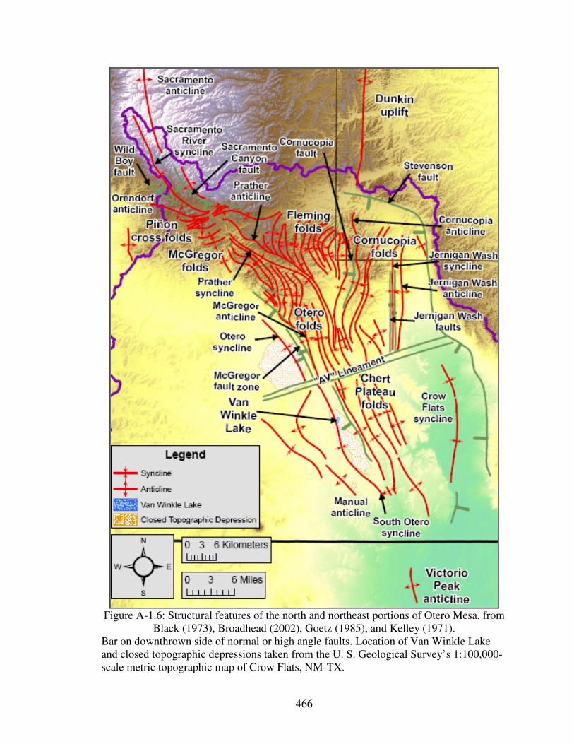
466
Figure A-1.6: Structural features of the north and northeast portions of Otero Mesa, from
Black (1973), Broadhead (2002), Goetz (1985), and Kelley (1971). Bar on downthrown side of normal or high angle faults. Location of Van Winkle Lake and closed topographic depressions taken from the U. S. Geological Survey’s 1:100,000-scale metric topographic map of Crow Flats, NM-TX.

467
Legend
Average Annual Temperature (1971-2000)
Median value for each area in ºC (ºF)
17 (63)
16 (61)
15 (59)
14 (57)
13 (55)
12 (53)
11 (51)
9.4 (49)
8.3 (47)
7.2 (45)
6.1 (43)
Figure A-1.7: Average annual temperature (1971-2000), from USDA. Source scale: 1:250,000. Horizontal resolution: ~800 meters.

468
Legend
Average Maximum Annual Temperature (1971-2000)
Median value for each area in ºC (ºF)
36 (97)
35 (95)
34 (93)
33 (91)
32 (89)
31 (87)
29 (85)
28 (83)
27 (81)
26 (79)
25 (77)
24 (75)
23 (73)
22 (71)
21 (69)
Figure A-1.8: Average maximum annual temperature (1971-2000), from USDA. Source scale: 1:250,000. Horizontal resolution: ~800 meters.

469
Legend
Average Minimum Annual Temperature (1971-2000)
Median value for each area in ºC (ºF)
1 (33)
-1 (31)
-2 (29)
-3 (27)
-4 (25)
-5 (23)
-6 (21)
-7 (19)
-8 (17)
-9 (15)
Figure A-1.9: Average minimum annual temperature (1971-2000), from USDA. Source scale: 1:250,000. Horizontal resolution: ~800 meters.

470
Figure A-1.10: Precipitation (cm) as a function of elevation (m) for recording stations in
and near the northern Salt Basin watershed, from Mayer and Sharp (1998). Recording stations are: AL – Alamogordo; CL – Cloudcroft; CO – Cornudas; DC – Dell City; EL – Elk; MH – Mayhill; MP – Mountain Park; OR – Orogrande; SF – Salt Flat; WS – White Sands.
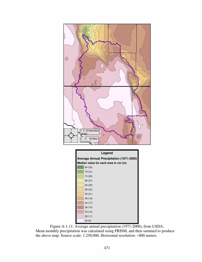
471
Legend
Average Annual Precipitation (1971-2000)
Median value for each area in cm (in)
84 (33)
79 (31)
74 (29)
69 (27)
64 (25)
58 (23)
53 (21)
48 (19)
43 (17)
38 (15)
33 (13)
28 (11)
23 (9)
Figure A-1.11: Average annual precipitation (1971-2000), from USDA. Mean monthly precipitation was calculated using PRISM, and then summed to produce the above map. Source scale: 1:250,000. Horizontal resolution: ~800 meters.

472
Figure A-1.12: Level IV ecoregions within the northern Salt Basin watershed.
Ecoregions from the U.S. Environmental Protection Agency (EPA).

473
Figure A-1.13: Location of the Diablo and Coahuila Platforms, from Shepard and Walper
(1982). Location of Steeruwitz thrust fault taken from Goetz (1977). Features formed about 1.25 Ga.

474
Figure A-1.14: Location of the Diablo and Texas Arches, and the Tobosa Basin, from
Adams (1965). Features formed during the Late Precambrian to Early Cambrian (550 to 510 Ma).

475
Figure A-1.15: Late-Pennsylvanian-to-Early-Permian tectonic features of the Salt Basin
region, from Ross and Ross (1985).

476
Figure A-1.16: Location of the Mesozoic Chihuahua trough and Chihuahua tectonic belt,
from Haenggi (2002).

477
FIGURES – CHAPTER 2

478
Figure A-2.1: Surface geology of the northern Salt Basin watershed.
Geology from Stoeser et al. (2005), with location of alkali flats/playa lakes for New Mexico taken from NHD.

479
Figure A-2.1: Legend
Legend
Alkali Flats/Playa Lakes (Caf)
Cenozoic Alluvial Deposits (Cal)
Cenozoic Intrusives (Ci)
Cretaceous (K)
Jurassic (J)
Castile, Salado, and Rustler Formations (POcsr)
Artesia Group (PGag)
Capitan Limestone/Formation (PGc)
Goat Seep Dolomite/Limestone/Formation (PGgs)
Delaware Mountain Group (PGdmg)
San Andres Formation (PGsa)
Cutoff Shale (PLcs)
Victorio Peak Limestone/Formation (PLvp)
Wilke Ranch Formation [Leonardian] (PLwr)
Yeso Formation (PLy)
Bone Spring Limestone/Formation (PLbs)
Abo Formation (PWa)
Hueco Limestone/Formation / Bursum Formation (PWhb)
Lower Abo / Pow Wow Conglomerate (PWla)
Pennsylvanian (P)
Devonian - Mississippian (D-M)
Cambrian - Silurian (C-S)
Precambrian (PC)
Permian
Paleozoic
Mesozoic
Cenozoic
Proterozoic
Phanerozoic
Eon Era Period
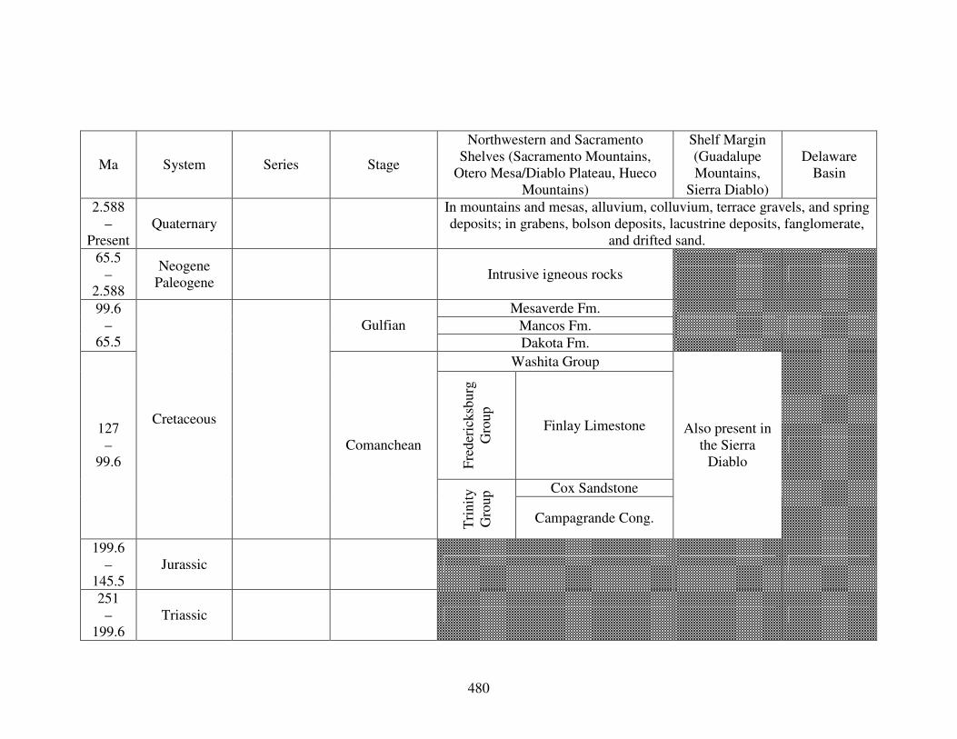
480
Ma System Series Stage
Northwestern and Sacramento Shelves (Sacramento Mountains,
Otero Mesa/Diablo Plateau, Hueco Mountains)
Shelf Margin (Guadalupe Mountains,
Sierra Diablo)
Delaware Basin
2.588 –
Present Quaternary
In mountains and mesas, alluvium, colluvium, terrace gravels, and spring deposits; in grabens, bolson deposits, lacustrine deposits, fanglomerate,
and drifted sand.
65.5 –
2.588
Neogene Paleogene
Intrusive igneous rocks
Mesaverde Fm.
Mancos Fm.
99.6 –
65.5 Gulfian
Dakota Fm.
Washita Group
Fre
der
icksb
urg
Gro
up
Finlay Limestone
Cox Sandstone
127 –
99.6
Cretaceous
Comanchean
Tri
nit
y
Gro
up
Campagrande Cong.
Also present in the Sierra
Diablo
199.6 –
145.5 Jurassic
251 –
199.6 Triassic

481
Rustler Fm.
Salado Fm.
260.4 –
251 Ochoan
Castile Fm.
Tansill Fm.
Yates Fm.
Seven Rivers
Fm.
Carlsb
ad G
roup
Capitan Lm./Fm.
Bell Canyon
Fm.
Queen Fm. Art
esia
Gro
up
Grayburg Fm.
Goat Seep Do./Lm./Fm.
Fourmile Draw Cherry Canyon
Cherry Canyon
Fm.
Bonney Canyon
270.6 –
260.4 Guadalupian
Rio Bonito
Brushy Canyon
Fm.
Delaw
are Mountain
Gro
up
San
Andre
s F
m.
Cutoff Shale
Victorio Peak Lm./Fm. 280
– 270.6
Permian
Leonardian Yeso Fm.
Bone Spring Lm./Fm.
Glorieta
Bone
Spring

482
Pow Wow Cong.
299 –
280 Permian
Bursum / Laborcita Fm.
Wolfcamp Series (Hueco Lm./Fm. and Pow Wow
Cong.)
Wolfcamp Fm.
305 –
299 Virgilian Holder Fm. Unnamed Cisco
Beeman Fm. 306.5 –
305 Missourian Unnamed Canyon
308 –
306.5 Desmoinesian Unnamed Strawn
311.7 –
308 Atokan/Derryan Unnamed Bend
318.1 –
311.7
Carboniferous Pennsylvanian
Morrowan
Mag
dal
ena
Fm
./G
roup
Gobbler Fm.
Unnamed?
Lee Ranch
tongue
Abo
Fm.
Danley Ranch
tongue
Pendejo
tongue Hueco
Lm./Fm.
Wolfcampian

483
333 –
318.1 Chesterian Helms Fm. Barnett Shale
340 –
333 Meramecian Rancheria Fm.
348 –
340 Osagean Lake Valley Fm.
359.2 –
348
Carboniferous Mississippian
Kinderhookian Caballero Fm.
“Mississippian Limestone”
Sly Gap Fm.
Oñate Fm. Percha Shale 385.3
– 359.2
Upper
Canutillo Fm.
Percha / Woodford Shale
397.5 –
385.3 Middle
416 –
397.5
Devonian
Lower
“Devonian”
438 –
421.3 Silurian
Niagaran Fusselman Fm.

484
Valmont Dolomite 451 –
443.7
Cincinnatian Montoya Group
Montoya Group
El Paso / Ellenburger Group 488.3
– 471.8
Ordovician
Canadian
501 –
488.3 Cambrian Croixian
Bliss Sandstone
Precambrian
Figure A-2.2: Generalized stratigraphic chart of the Salt Basin region. Adapted from numerous sources, including Black (1973), Boyd (1958), Foster (1978), Hayes (1964), Kelley (1971), Kottlowski (1963), LeMone (1969), McGlasson (1969), Newell et al. (1972), and Pray (1961).

485
Figure A-2.3: Precambrian basement rocks of the Salt Basin region, from Adams et al.
(1993) and Denison et al. (1984).

486
a: Late Precambrian (550 Ma)
c: Late Cambrian (500 Ma)
b: Middle Cambrian (510 Ma)
d: Early Ordovician (485 Ma)
Figure A-2.4: Late-Precambrian-to-Early-Ordovician paleogeography of the Salt Basin region, from Blakey (2009b).

487
a: Middle Ordovician (470 Ma)
c: Early Silurian (430 Ma)
b: Late Ordovician (450 Ma)
d: Late Silurian (420 Ma)
Figure A-2.5: Middle-Ordovician-to-Late-Silurian paleogeography of the Salt Basin region, from Blakey (2009b).

488
a: Early Devonian (400 Ma)
c: Late Devonian (360 Ma)
b: Middle Devonian (385 Ma)
d: Early Mississippian (345 Ma)
Figure A-2.6: Early-Devonian-to-Early-Mississippian paleogeography of the Salt Basin region, from Blakey (2009b).

489
a: Early Mississippian (340 Ma)
c: Miss.-Penn. lowstand (320 Ma)
b: Late Mississippian (325 Ma)
d: Pennsylvanian Morrowan (318 Ma)
Figure A-2.7: Early-Mississippian-to-Pennsylvanian-Morrowan paleogeography of the Salt Basin region, from Blakey (2009a).

490
a: Pennsylvanian Atokan (315 Ma)
c: Pennsylvanian Missourian (300 Ma)
b: Pennsylvanian Desmoinian (310 Ma)
d: Pennsylvanian Virgilian (295 Ma)
Figure A-2.8: Pennsylvanian-Atokan-to-Pennsylvanian-Virgilian paleogeography of the Salt Basin region, from Blakey (2009a).
OrB = Orogrande Basin, DeB = Delaware Basin, MiB = Midland Basin.
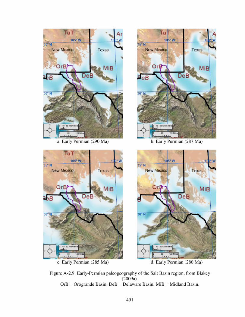
491
a: Early Permian (290 Ma)
c: Early Permian (285 Ma)
b: Early Permian (287 Ma)
d: Early Permian (280 Ma)
Figure A-2.9: Early-Permian paleogeography of the Salt Basin region, from Blakey (2009a).
OrB = Orogrande Basin, DeB = Delaware Basin, MiB = Midland Basin.

492
a: Early Permian (278 Ma)
c: Middle Permian (270 Ma)
b: Early Permian (275 Ma)
d: Late Permian (260 Ma)
Figure A-2.10: Early-Permian-to-Late-Permian paleogeography of the Salt Basin region, from Blakey (2009a).
OrB = Orogrande Basin, DeB = Delaware Basin, MiB = Midland Basin.

493
a: Late Permian (255 Ma)
c: Middle Triassic (230 Ma)
b: Early Triassic (240 Ma)
d: Late Triassic (210 Ma)
Figure A-2.11: Late-Permian-to-Late-Triassic paleogeography of the Salt Basin region, from Blakey (2009a) and Blakey (2009b).
DeB = Delaware Basin, MiB = Midland Basin.

494
a: Early Jurassic (195 Ma)
c: Middle Jurassic (170 Ma)
b: Early Jurassic (180 Ma)
d: Late Jurassic (150 Ma)
Figure A-2.12: Early-Jurassic-to-Late-Jurassic paleogeography of the Salt Basin region, from Blakey (2009b).

495
a: Early Cretaceous (140 Ma)
c: Early Cretaceous (115 Ma)
b: Early Cretaceous (130 Ma)
d: Late Cretaceous (100 Ma)
Figure A-2.13: Early-Cretaceous-to-Late-Cretaceous paleogeography of the Salt Basin region, from Blakey (2009b).

496
a: Late Cretaceous (85 Ma)
c: Cretaceous-Paleogene (65 Ma)
b: Late Cretaceous (75 Ma)
d: Paleogene Paleocene (60 Ma)
Figure A-2.14: Late-Cretaceous-to-Paleogene-Paleocene paleogeography of the Salt Basin region, from Blakey (2009b).

497
a: Paleogene Eocene (50 Ma)
c: Paleogene Oligocene (25 Ma)
b: Paleogene Eocene (40 Ma)
d: Neogene Miocene (15 Ma)
Figure A-2.15: Paleogene-Eocene-to-Neogene-Miocene paleogeography of the Salt Basin region, from Blakey (2009b).

498
a: Neogene Miocene (8 Ma)
c: Quaternary Glacial (0.126 Ma)
b: Neogene Pliocene (3 Ma)
d: Present
Figure A-2.16: Neogene-Miocene-to-Present paleogeography of the Salt Basin region, from Blakey (2009b).

499
a: Wolfcampian facies
b: Early Leonardian facies
Legend
Sandstone, fine- to coarse-grained, including some conglomerate
Anhydrite, generally interbedded with dominant facies
Red beds, in part shaly, in part sandy
Limestone, thick- to thin-bedded, calcitic or dolomitic
Shale, dark gray to black, and thin-bedded black limestone
Figure A-2.17: Wolfcampian-to-Early-Leonardian facies, from King (1942) and King (1948).

500
a: Late Leonardian facies
b: Early Guadalupian facies
Legend
Sandstone, fine- to coarse-grained, including some conglomerate
Anhydrite, generally interbedded with dominant facies
Red beds, in part shaly, in part sandy
Limestone, thick- to thin-bedded, calcitic or dolomitic
Shale, dark gray to black, and thin-bedded black limestone
Figure A-2.18: Late-Leonardian-to-Early-Guadalupian facies, from King (1942) and King (1948).

501
a: Middle Guadalupian facies
b: Late Guadalupian facies
Legend
Sandstone, fine- to coarse-grained, including some conglomerate
Anhydrite, generally interbedded with dominant facies
Red beds, in part shaly, in part sandy
Limestone, thick- to thin-bedded, calcitic or dolomitic
Shale, dark gray to black, and thin-bedded black limestone
Figure A-2.19: Middle-Guadalupian-to-Late-Guadalupian facies, from King (1942) and King (1948).

502
Figure A-2.20: Permian shelf-margin trends, from Black (1975).

503
Figure A-2.21: Pennsylvanian-to-Early-Permian structural features of the northern Salt
Basin watershed. Bar on downthrown side of normal or high angle faults, triangles on upthrown side of thrust zone. Location of structures in New Mexico taken from Broadhead (2002). Location of Diablo Platform taken from Kottlowski (1969).

504
Figure A-2.22: Mid-to-Late-Permian structural features of the northern Salt Basin
watershed. Arrows indicate sense of displacement. Bar on downthrown side of Bitterwell Break. Location of structures taken from Black (1976), Goetz (1985), and Kelley (1971).

505
Figure A-2.23: Late-Cretaceous (Laramide) structural features of the northern Salt Basin
watershed. Syncline and anticline symbols are the same as those used on Figure A-2.22. Bar on downthrown side of McGregor fault. Location of structures taken from Black (1976), Goetz (1985), Kelley (1971), and Seager et al. (1987).

506
Figure A-2.24: Late-Cretaceous (Laramide) structural features of the north and northeast
portions of Otero Mesa. Syncline and anticline symbols are the same as those used on Figure A-2.22. Location of structures taken from Black (1976), Goetz (1985), and Kelley (1971).

507
Figure A-2.25: Cenozoic structural features of the northern Salt Basin watershed.
Syncline and anticline symbols are the same as those used on Figure A-2.22. Bar on downthrown side of normal or high angle faults. Location of structures taken from Black (1976), Broadhead (2002), Cather and Harrison (2002), Collins and Raney (1991), Goetz (1985), Pray (1961), Schruben et al. (1994), and Seager et al. (1987).

508
FIGURES – CHAPTER 3

509
Figure A-3.1: Structural zones/blocks used in 3-D hydrogeologic framework model.
Black circles indicate the location of all oil-and-gas exploratory wells used in this study as control on the subsurface geology. Oil-and-gas exploratory well key on next page.

510
Figure A-3.1: Key
# Well ID
1 HO&MSL1
2 HO&MJL1
3 HO&MCL2
4 HO&MFA1
5 LAHTHO1
6 HO&MS31
7 MCOCFH1
8 MCOCGB1
9 HO&RYF1
10 JCTSA61
11 LM&SAR1
12 HO&RHY1
13 WHBDCS1
14 COCSNN1
15 JCTFA28
16 C&KSLS1
17 SPCCLU1
18 YPCDNU1
19 YPCDDU2
20 YPCDDU1
21 SE&PJT1
22 C&KLCS1
23 LO>LW
24 MAGHEF2
25 YPCLCU1
26 SOCSAV1
27 WHIBHU1
28 YPCLCU2
29 MAGBLHI
30 GOCCSU1
31 TEXIFE1
32 YPCOTU1
33 YPCDCF1
34 TO&GFC1
35 KOCFMU1
36 TEXIFF1
37 YPCOTU2
38 TEXIFG1
39 MOCMVR1
40 YPCBAYU
41 TO&GFA1
42 YPCBAVW
43 SOCPIU2
44 SOCPIU1
45 UVILCU1
46 GOCFMU1
47 PLOCEV1
# Well ID
48 TO&GFB1
49 ARCSAV1
50 ZPCF141
51 SOCTJP1
52 TRBCU1Y
53 SO>U1
54 SOTSCU1
55 LEPCFE1
56 YPCBIOF
57 TSDLDF1
58 OTOCMC1
59 BRCFEA1
60 COCHWB1
61 MOCBCU1
62 PIECF91
63 SO&GFE1
64 EPCAHU1
65 TLISTE1
66 FTUEVE1
67 EPCALI1
68 WRWETH1
69 EPCALS1
70 PRIICF1
71 EPCAMF1
72 HO&RHO2
73 CO&GCW1
74 IOCSBU1
75 CO&GAS1
76 ARCHUU9
77 SOCLCD1
78 UNOCFW1
79 HO&RHU5
80 TDCR21F
81 FTUJEV1
82 EPCAFE1
83 FWYDON1
84 FA&FTD1
85 UNOCMC1
86 UOCV7F1
87 WWWWDC1
88 TROGJA1
89 RHELLC1
90 TDM28F1
91 BOCRUS1
92 PCS28S1
93 FTUJST1
94 EJDALF1
# Well ID
95 GDP61-6
96 GDP45-5
97 GDP46-6
98 HUOCMT1
99 HEYBRU1
100 SEOCTF1
101 GDP51-8
102 EPCSPF1
103 SO&GGR1
104 HEYBR25
105 HPCCL51
106 TSTFO31
107 CODFRS1
108 MPCUTL1
109 EOGRC24
110 PAPCLA1
111 BONCOPI
112 PUOCHU1
113 HUOCDY1
114 HUBAUN1
115 TMUBIC1
116 HPCCLR1
117 TEXCLF1
118 TOTXLF1
119 PAPCEH1
120 TMUSD51
121 TXLCCF1
122 GCOCMV1
123 MPNA1HC
124 EOGKS1H
125 EOGKES2
126 CASATT1
127 DJJCHJ2
128 TMUFD27
129 BECHCT1
130 TXLCBT1
131 ARJECM1
132 TCST1BS
133 JLCECM1
134 BECJJM1
135 TERCMO2
136 TSOCCS1
137 COIDM3S
138 TMUDWL5
139 SALSUL2
140 HORMCS1
141 NARIPO1
# Well ID
142 COUL462
143 JMHCTP1
144 EOGSR47
145 A&PBOR1
146 TMUODL1
147 PHMTS27
148 FMINWW1
149 AQPVCR1
150 HHUM491
151 EOGWHD7
152 PAPPFH1
153 COMT105
154 TO36MSA
155 EPCN1MO
156 GOCMAG1
157 HAHUTM1
158LR&BGM1/
WSOG&M1
159 COSS701
160 SINCLOO
161 GOCJBS1
162 LOBG&M1
163 SOGAL1R
164 H&GJSP1
165 FADWAD1

511
Figure A-3.2: Land surface expression of the 3-D hydrogeologic framework solid model. Color-coding of hydrogeologic units corresponds to that used in Figure A-2.1. Purple line indicates northern Salt Basin watershed boundary. Red line designates groundwater flow model boundary.
groundwater flow model boundary
northern Salt Basin watershed boundary

512
Figure A-3.3: Elevation of the top of the Precambrian.
Elevations are in meters relative to mean sea level. Contour interval is 500 meters (1,640 feet). Black circles indicate the oil-and-gas exploratory wells used as control for the unit.
Top (m)

513
Figure A-3.4: Elevation of the top of the Cambrian through the Silurian.
Elevations are in meters relative to mean sea level. Contour interval is 500 meters (1,640 feet). Black circles indicate the oil-and-gas exploratory wells used as control for the unit.
Top (m)

514
Figure A-3.5: Elevation of the top of the Devonian.
Elevations are in meters relative to mean sea level. Contour interval is 500 meters (1,640 feet). Black circles indicate the oil-and-gas exploratory wells used as control for the unit.
Top (m)

515
Figure A-3.6: Elevation of the top of the Mississippian through the Pennsylvanian.
Elevations are in meters relative to mean sea level. Contour interval is 500 meters (1,640 feet). Black circles indicate the oil-and-gas exploratory wells used as control for the unit.
Top (m)

516
Figure A-3.7: Elevation of the top of Lower Abo/Pow Wow Conglomerate.
Elevations are in meters relative to mean sea level. Contour interval is 500 meters (1,640 feet). Black circles indicate the oil-and-gas exploratory wells used as control for the unit.
Top (m)

517
Figure A-3.8: Elevation of the top of Hueco Limestone/Formation (or Bursum
Formation) and Wolfcamp Formation. Elevations are in meters relative to mean sea level. Contour interval is 500 meters (1,640 feet). Black circles indicate the oil-and-gas exploratory wells used as control for the unit.
Top (m)

518
Figure A-3.9: Elevation of the top of Abo Formation.
Elevations are in meters relative to mean sea level. Contour interval is 500 meters (1,640 feet). Black circles indicate the oil-and-gas exploratory wells used as control for the unit.
Top (m)

519
Figure A-3.10: Elevation of the top of Yeso Formation.
Elevations are in meters relative to mean sea level. Contour interval is 500 meters (1,640 feet). Black circles indicate the oil-and-gas exploratory wells used as control for the unit.
Top (m)

520
Figure A-3.11: Elevation of the top of Bone Spring Limestone/Formation.
Elevations are in meters relative to mean sea level. Contour interval is 500 meters (1,640 feet). Black circles indicate the oil-and-gas exploratory wells used as control for the unit.
Top (m)

521
Figure A-3.12: Elevation of the top of Victorio Peak Limestone/Formation and Cutoff
Shale and Wilke Ranch Formation. Elevations are in meters relative to mean sea level. Contour interval is 500 meters (1,640 feet). Black circles indicate the oil-and-gas exploratory wells used as control for the unit.
Top (m)

522
Figure A-3.13: Elevation of the top of San Andres Formation.
Elevations are in meters relative to mean sea level. Contour interval is 500 meters (1,640 feet). Black circles indicate the oil-and-gas exploratory wells used as control for the unit.
Top (m)

523
Figure A-3.14: Elevation of the top of Delaware Mountain Group.
Elevations are in meters relative to mean sea level. Contour interval is 500 meters (1,640 feet). Black circles indicate the oil-and-gas exploratory wells used as control for the unit.
Top (m)

524
Figure A-3.15: Elevation of the top of Goat Seep Dolomite/Limestone/Formation and
Capitan Limestone/Formation. Elevations are in meters relative to mean sea level. Contour interval is 500 meters (1,640 feet). Black circles indicate the oil-and-gas exploratory wells used as control for the unit.
Top (m)

525
Figure A-3.16: Elevation of the top of Artesia Group.
Elevations are in meters relative to mean sea level. Contour interval is 500 meters (1,640 feet). Black circles indicate the oil-and-gas exploratory wells used as control for the unit.
Top (m)

526
Figure A-3.17: Elevation of the top of the Cretaceous.
Elevations are in meters relative to mean sea level. Contour interval is 500 meters (1,640 feet). Black circles indicate the oil-and-gas exploratory wells used as control for the unit.
Top (m)

527
Figure A-3.18: Elevation of the top of Cenozoic alluvium.
Elevations are in meters relative to mean sea level. Contour interval is 500 meters (1,640 feet). Black circles indicate the oil-and-gas exploratory wells used as control for the unit.
Top (m)
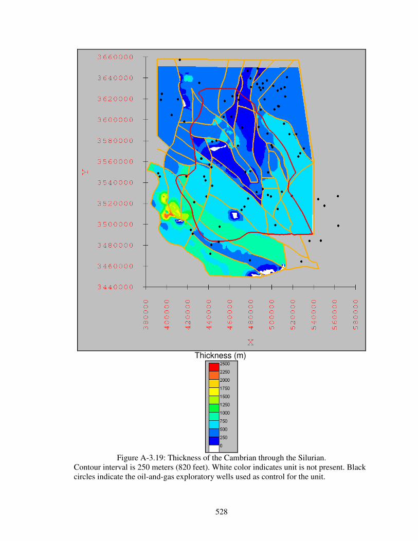
528
Figure A-3.19: Thickness of the Cambrian through the Silurian.
Contour interval is 250 meters (820 feet). White color indicates unit is not present. Black circles indicate the oil-and-gas exploratory wells used as control for the unit.
Thickness (m)

529
Figure A-3.20: Thickness of the Devonian.
Contour interval is 250 meters (820 feet). White color indicates unit is not present. Black circles indicate the oil-and-gas exploratory wells used as control for the unit.
Thickness (m)
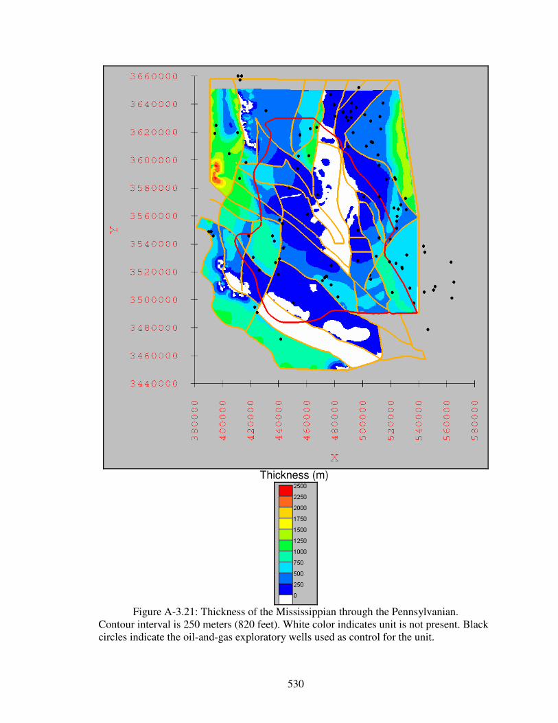
530
Figure A-3.21: Thickness of the Mississippian through the Pennsylvanian.
Contour interval is 250 meters (820 feet). White color indicates unit is not present. Black circles indicate the oil-and-gas exploratory wells used as control for the unit.
Thickness (m)

531
Figure A-3.22: Thickness of Lower Abo/Pow Wow Conglomerate.
Contour interval is 250 meters (820 feet). White color indicates unit is not present. Black circles indicate the oil-and-gas exploratory wells used as control for the unit.
Thickness (m)

532
Figure A-3.23: Thickness of Hueco Limestone/Formation (or Bursum Formation) and
Wolfcamp Formation. Contour interval is 250 meters (820 feet). White color indicates unit is not present. Black circles indicate the oil-and-gas exploratory wells used as control for the unit.
Thickness (m)

533
Figure A-3.24: Thickness of Abo Formation.
Contour interval is 250 meters (820 feet). White color indicates unit is not present. Black circles indicate the oil-and-gas exploratory wells used as control for the unit.
Thickness (m)

534
Figure A-3.25: Thickness of Yeso Formation.
Contour interval is 250 meters (820 feet). White color indicates unit is not present. Black circles indicate the oil-and-gas exploratory wells used as control for the unit.
Thickness (m)

535
Figure A-3.26: Thickness of Bone Spring Limestone/Formation.
Contour interval is 250 meters (820 feet). White color indicates unit is not present. Black circles indicate the oil-and-gas exploratory wells used as control for the unit.
Thickness (m)

536
Figure A-3.27: Thickness of Victorio Peak Limestone/Formation and Cutoff Shale and
Wilke Ranch Formation. Contour interval is 250 meters (820 feet). White color indicates unit is not present. Black circles indicate the oil-and-gas exploratory wells used as control for the unit.
Thickness (m)

537
Figure A-3.28: Thickness of San Andres Formation.
Contour interval is 250 meters (820 feet). White color indicates unit is not present. Black circles indicate the oil-and-gas exploratory wells used as control for the unit.
Thickness (m)

538
Figure A-3.29: Thickness of Delaware Mountain Group.
Contour interval is 250 meters (820 feet). White color indicates unit is not present. Black circles indicate the oil-and-gas exploratory wells used as control for the unit.
Thickness (m)

539
Figure A-3.30: Thickness of Goat Seep Dolomite/Limestone/Formation and Capitan
Limestone/Formation. Contour interval is 250 meters (820 feet). White color indicates unit is not present. Black circles indicate the oil-and-gas exploratory wells used as control for the unit.
Thickness (m)

540
Figure A-3.31: Thickness of Artesia Group.
Contour interval is 250 meters (820 feet). White color indicates unit is not present. Black circles indicate the oil-and-gas exploratory wells used as control for the unit.
Thickness (m)

541
Figure A-3.32: Thickness of the Cretaceous.
Contour interval is 250 meters (820 feet). White color indicates unit is not present. Black circles indicate the oil-and-gas exploratory wells used as control for the unit.
Thickness (m)

542
Figure A-3.33: Thickness of Cenozoic alluvium.
Contour interval is 250 meters (820 feet). White color indicates unit is not present. Black circles indicate the oil-and-gas exploratory wells used as control for the unit.
Thickness (m)

543
Figure A-3.34: Land surface expression of the 3-D hydrogeologic framework solid model
clipped to the groundwater flow model boundary. Color-coding of hydrogeologic units corresponds to that used in Figure A-2.1. Red line designates groundwater flow model boundary.
groundwater flow model boundary

544
Figure A-3.35: Oblique views of the 3-D hydrogeologic framework solid model clipped
to the groundwater flow model boundary. Color-coding of hydrogeologic units corresponds to that used in Figure A-2.1. Vertical exaggeration 10×.

545
Figure A-3.36: Location of the five hydrogeologic cross-sections.
Also includes the location of the groundwater wells sampled during this study along each cross-section, the subsurface geologic control points along each cross-section, and the groundwater surface contours produced for this study.

546
Figure A-3.37: North-South cross-section A - A’.
Vertical exaggeration 23×. On all cross-sections, the light brown vertical lines are oil-and-gas exploratory well subsurface control points, the pink vertical lines are groundwater wells sampled during this study and by the SMHS, and the arrows indicate the sense of displacement on faults. Dashed lines for wells indicate that the well was projected to the line of cross-section. The groundwater surface is represented by the dark blue line. Color-coding of hydrogeologic units and unit labels corresponds to that used in Figure A-2.1.

547
Figure A-3.38: North-South cross-section B - B’.
Vertical exaggeration 18×.

548
Figure A-3.39: West-East cross-section C - C’.
Vertical exaggeration 22×.

549
Figure A-3.40: West-East cross-section D - D’.
Vertical exaggeration 18×.

550
Figure A-3.41: West-East cross-section E - E’.
Vertical exaggeration 15×.

551
Figure A-3.42: Groundwater elevation contours for the Salt Basin region.
Elevations are in feet above mean sea level. Contour interval is 200 feet. Hachured contours indicate groundwater depressions. The red circle and green square symbols indicate groundwater wells used as control for the contours, while the pink triangle symbols indicate groundwater wells not used as control points.

552
Figure A-3.43: Depth-to-groundwater for the Salt Basin region.
Depths are in feet. Groundwater well symbology is the same as Figure A-3.42. Light blue regions delineate zones of shallower groundwater than is indicated by the surrounding depth-to-groundwater polygons.

553
Figure A-3.44: Locations and an oblique view of the five cross-sections within the 3-D
hydrogeologic framework solid model. Color-coding of hydrogeologic units corresponds to that used in Figure A-2.1, and Figures A-3.37 through A-3.41. Red line designates groundwater flow model boundary. Blue lines indicate cross-sections. Vertical exaggeration 10×.
A
A’
B’
B
C C’
D’
E’
E
D
A
B C
D
E

554
Figure A-3.45: Side views along cross-section A - A’ of the 3-D framework solid model on left and hand-drawn cross-section on right. Vertical exaggeration 10× on 3-D framework solid model cross-sections. Vertical exaggeration 23× on hand-drawn cross-section.
N S
Cenozoic alluvium
S N
N S
Permian
Cambrian through Silurian
Precambrian
Permian
Cambrian through Silurian
Precambrian
Mississippian through
Pennsylvanian
Devonian
Mississippian through
Pennsylvanian
Devonian

555
Figure A-3.46: Side views along cross-section B - B’ of the 3-D framework solid model on left and hand-drawn cross-section on right. Vertical exaggeration 10× on 3-D framework solid model cross-sections. Vertical exaggeration 18× on hand-drawn cross-section.
N S
N S
S N
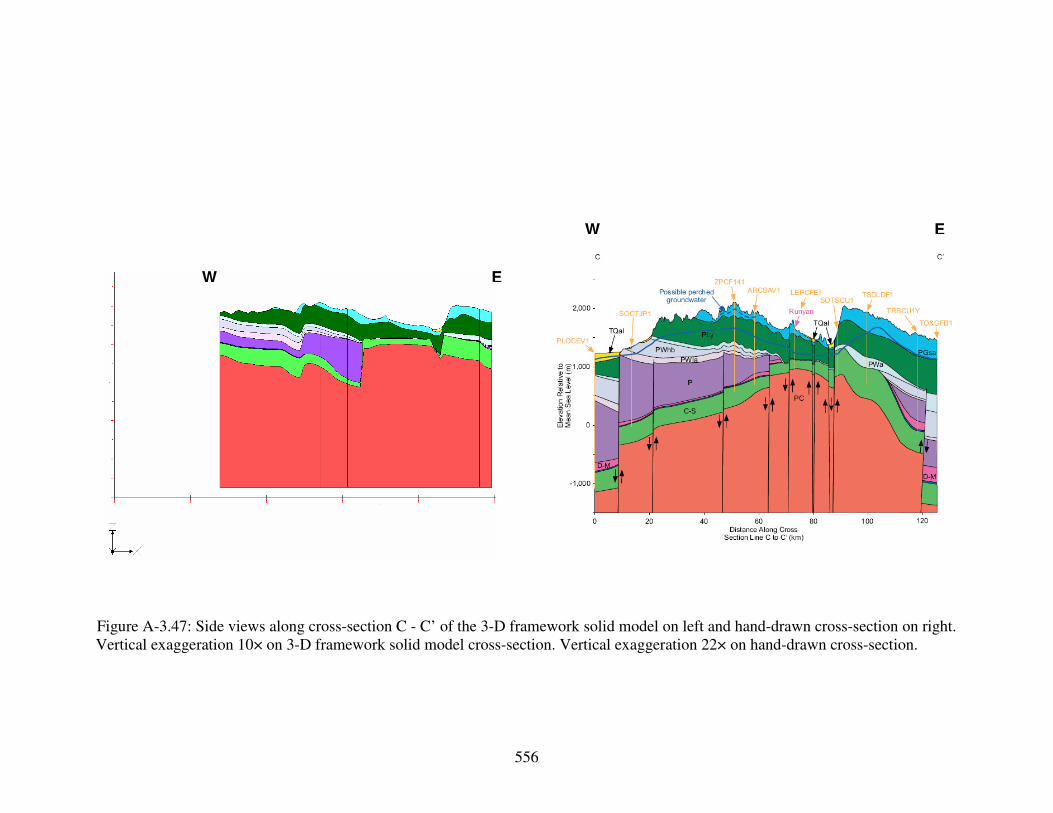
556
Figure A-3.47: Side views along cross-section C - C’ of the 3-D framework solid model on left and hand-drawn cross-section on right. Vertical exaggeration 10× on 3-D framework solid model cross-section. Vertical exaggeration 22× on hand-drawn cross-section.
E W
E W
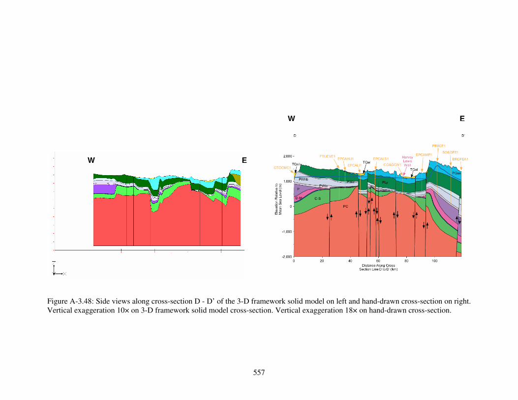
557
Figure A-3.48: Side views along cross-section D - D’ of the 3-D framework solid model on left and hand-drawn cross-section on right. Vertical exaggeration 10× on 3-D framework solid model cross-section. Vertical exaggeration 18× on hand-drawn cross-section.
E W
E W

558
Figure A-3.49: Side views along cross-section E - E’ of the 3-D framework solid model on left and hand-drawn cross-section on right. Vertical exaggeration 10× on 3-D framework solid model cross-section. Vertical exaggeration 15× on hand-drawn cross-section.
E W
E W
Cenozoic intrusions

559
Figure A-3.50: Aquifers in the Salt Basin region.
Location of high mountain and Pecos slope aquifers from SMHS. Location of Bone Spring-Victorio Peak and Hueco bolson aquifers from TWDB. Location of Capitan Reef Complex aquifer from Uliana (2001). Location of Cretaceous aquifer from Sharp (1989).
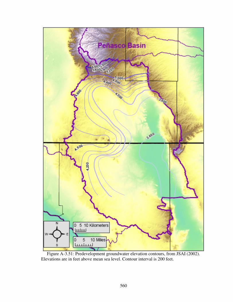
560
Figure A-3.51: Predevelopment groundwater elevation contours, from JSAI (2002).
Elevations are in feet above mean sea level. Contour interval is 200 feet.
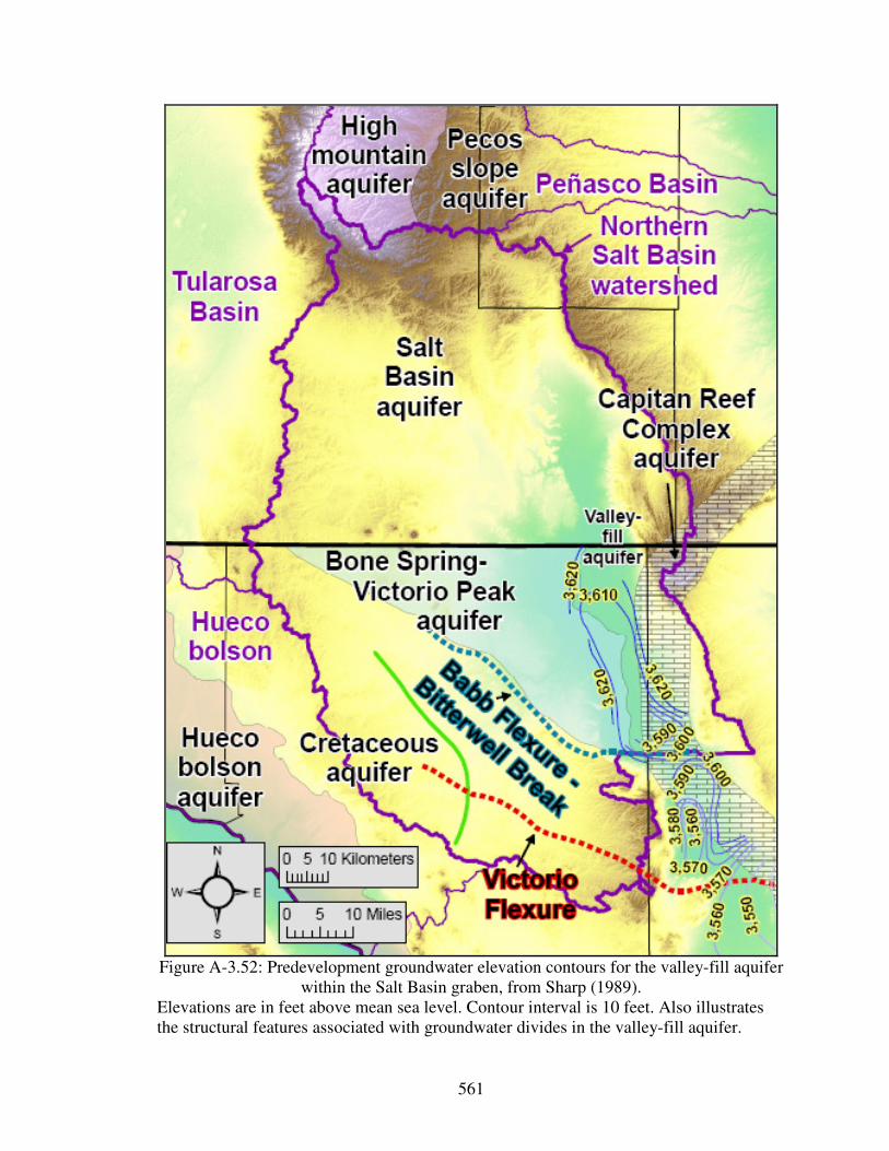
561
Figure A-3.52: Predevelopment groundwater elevation contours for the valley-fill aquifer
within the Salt Basin graben, from Sharp (1989). Elevations are in feet above mean sea level. Contour interval is 10 feet. Also illustrates the structural features associated with groundwater divides in the valley-fill aquifer.

562
A = 85.0*[exp((-1.39 E-5)*X)]
R2 = 0.813
0.0
10.0
20.0
30.0
40.0
50.0
60.0
70.0
80.0
90.0
0 20,000 40,000 60,000 80,000 100,000 120,000
Distance Along Cross Section Line A to A' [X] (meters)
14C
Ac
tiv
ity
Mea
su
red
in
Gro
un
dw
ate
r [A
] (p
mC
)
Figure A-3.53: 14C activity measured in groundwater versus distance along cross-section line A - A'.
Doll Day
Uña
Cauhape
Harvey
Lewis Well Evrage
House
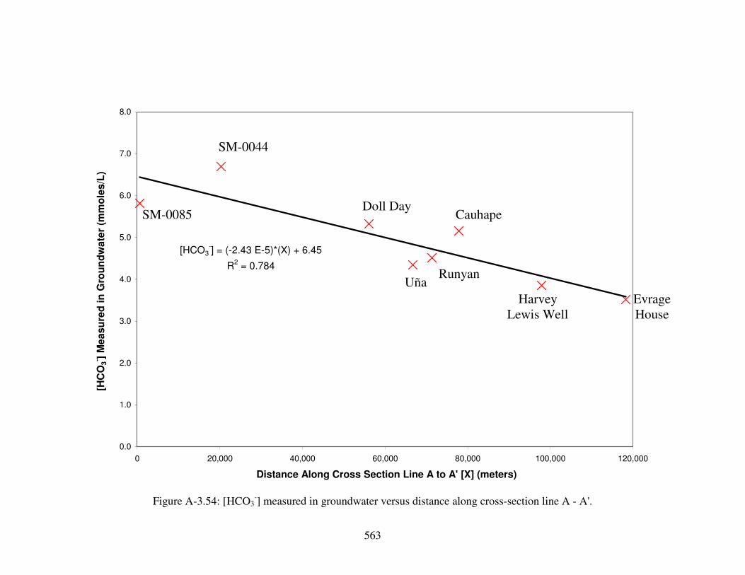
563
[HCO3-] = (-2.43 E-5)*(X) + 6.45
R2 = 0.784
0.0
1.0
2.0
3.0
4.0
5.0
6.0
7.0
8.0
0 20,000 40,000 60,000 80,000 100,000 120,000
Distance Along Cross Section Line A to A' [X] (meters)
[HC
O3
- ] M
ea
su
red
in
Gro
un
dw
ate
r (m
mo
les
/L)
Figure A-3.54: [HCO3
-] measured in groundwater versus distance along cross-section line A - A'.
Doll Day
Uña
Cauhape
Harvey
Lewis Well
Evrage
House
Runyan
SM-0044
SM-0085

564
[Mg2+
] = (2.56 E-5)*(X) + 0.285
R2 = 0.920
0.0
0.5
1.0
1.5
2.0
2.5
3.0
3.5
0 20,000 40,000 60,000 80,000 100,000 120,000
Distance Along Cross Section Line A to A' [X] (meters)
[Mg
2+]
Me
as
ure
d i
n G
rou
nd
wa
ter
(mm
ole
s/L
)
Figure A-3.55: [Mg2+] measured in groundwater versus distance along cross-section line A - A'.
Doll Day
Uña
Cauhape Harvey
Lewis Well
Evrage
House
Runyan
SM-0044
SM-0085
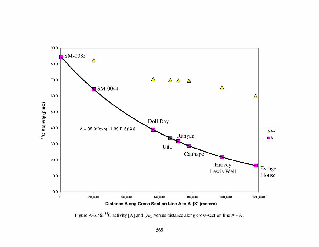
565
A = 85.0*[exp((-1.39 E-5)*X)]
0.0
10.0
20.0
30.0
40.0
50.0
60.0
70.0
80.0
90.0
0 20,000 40,000 60,000 80,000 100,000 120,000
Distance Along Cross Section Line A to A' [X] (meters)
14C
Ac
tiv
ity
(p
mC
)
Ao
A
Figure A-3.56: 14C activity [A] and [A0] versus distance along cross-section line A - A'.
SM-0044
SM-0085
Doll Day
Uña
Runyan
Cauhape
Harvey
Lewis Well Evrage
House

566
0.00000001
0.0000001
0.000001
0.00001
0.0001
0.001
0.01
0.1
1
10
100
1000K
(m
/da
y)
Figure A-3.57: Range of hydraulic conductivity [K] values from previous studies and this study. Vertical axis is logarithmic scale. Squares indicate median values, and triangles indicate average values.
Wasiolek (1991):
Yeso Fm.: unfractured siltstone and
gypsum
Wasiolek (1991):
Yeso Fm.: fractured limestone
YPCOTU2 wellsite
core analysis: Yeso Fm. and Abo
Fm.
This study: 14
C groundwater ages along
cross-section A to A’
Source
median
YPCOTU2 wellsite
core analysis: Cambrian
Hutchison (2008)
JSAI (2010):
Basin-fill
JSAI (2010):
Un-fractured Permian
JSAI (2010):
Fractured Permian
JSAI (2010):
Cambrian
JSAI (2010):
Pre-cambrian
average
Sigstedt (2010):
Salt Basin average
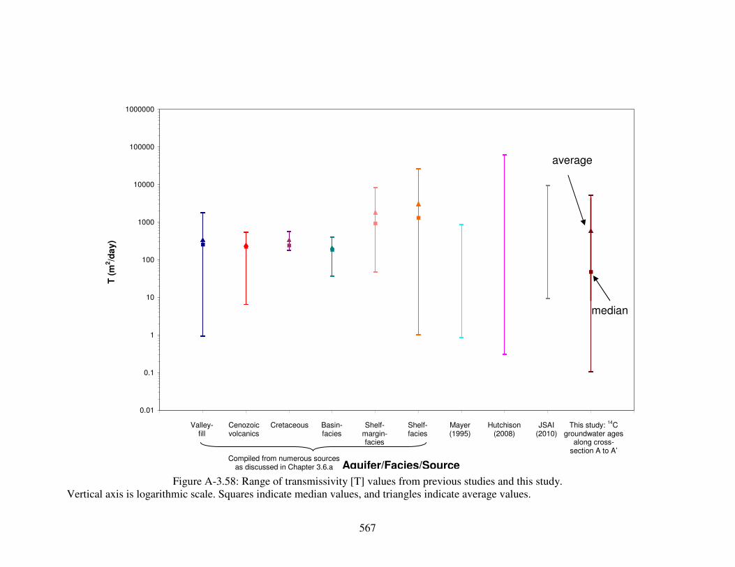
567
0.01
0.1
1
10
100
1000
10000
100000
1000000T
(m
2/d
ay
)
Figure A-3.58: Range of transmissivity [T] values from previous studies and this study. Vertical axis is logarithmic scale. Squares indicate median values, and triangles indicate average values.
This study: 14
C groundwater ages
along cross-section A to A’
Aquifer/Facies/Source
Shelf- facies
Shelf-margin-facies
Basin-facies
Cretaceous Cenozoic volcanics
Valley- fill
median
Mayer (1995)
Hutchison (2008)
JSAI (2010)
average
Compiled from numerous sources as discussed in Chapter 3.6.a

568
Figure A-3.59: Location of the four groundwater wells in the New Mexico portion of the Salt Basin watershed with continuous water level measurements from 2003 to the middle
of 2006, as presented in Huff and Chace (2006), and the TWDB’s State Well Number 4807516.

569
-4
-3.5
-3
-2.5
-2
-1.5
-1
-0.5
0
0.5
1
2003 2003.5 2004 2004.5 2005 2005.5 2006 2006.5 2007
Time [t] (years)
Gro
un
dw
ate
r L
ev
el
Ch
an
ge
[∆
h]
(m)
H&C 1
H&C 2
H&C 3
H&C 4
Figure A-3.60: Change in groundwater levels versus time for wells H&C 1, H&C 2, H&C 3, and H&C 4.

570
-9
-8
-7
-6
-5
-4
-3
-2
-1
0
1
2003 2003.5 2004 2004.5 2005 2005.5 2006 2006.5 2007
Time [t] (years)
Gro
un
dw
ate
r L
ev
el
Ch
an
ge
[∆
h]
(m)
H&C 1
H&C 2
H&C 3
H&C 4
4807516
Figure A-3.61: Change in groundwater levels versus time for wells H&C 1, H&C 2, H&C 3, H&C 4, and 4807516.

571
-9
-8
-7
-6
-5
-4
-3
-2
-1
0
1
2003 2003.5 2004 2004.5 2005 2005.5 2006 2006.5 2007
Time [t] (years)
Gro
un
dw
ate
r L
ev
el
Ch
an
ge
[∆
h]
(m)
H&C 1
H&C 2
H&C 3
H&C 4
4807516
Figure A-3.62: Location of maximum and minimum change in groundwater levels used to calculate the average annual amplitude of
water level fluctuations in wells H&C 1, 2, 3, and 4, and 4807516.

572
∆h = -0.507*[t] + 1.02 E3
R2 = 0.994
-1.8
-1.6
-1.4
-1.2
-1
-0.8
-0.6
-0.4
-0.2
0
2003 2003.5 2004 2004.5 2005 2005.5 2006 2006.5 2007
Time [t] (years)
Gro
un
dw
ate
r L
eve
l C
ha
ng
e [∆
h]
(m)
Figure A-3.63: Change in groundwater level versus time for well H&C 4.

573
-0.06
-0.04
-0.02
0
0.02
0.04
0.06
0.08
2003 2003.5 2004 2004.5 2005 2005.5 2006 2006.5 2007
Time [t] (years)
De
tre
nd
ed
Gro
un
dw
ate
r L
ev
el C
ha
ng
e (
m)
Figure A-3.64: Detrended change in groundwater level versus time for well H&C 4.

574
sT/s0 = 0.727*[exp((-6.99 E-5)*X)]
R2 = 0.959
sT/s0 = 1.27*[exp((-9.58 E-5)*X)]
R2 = 0.953
sT/s0 = 1.28*[exp((-9.28 E-5)*X)]
R2 = 0.957
0
0.1
0.2
0.3
0.4
0.5
0.6
0.7
0 5,000 10,000 15,000 20,000 25,000 30,000 35,000 40,000 45,000 50,000
Distance from Dell City, Texas [X] (meters)
sT/s
0
2003
2004
2005
Figure A-3.65: sT/s0 calculated from water level fluctuations in 2003 at wells H&C 1, 2, and 3, and 4807516, and in 2004 and 2005 at
wells H&C 1, 2, 3, and 4, and 4807516 versus distance from Dell City, Texas.

575
tL = (3.67 E-3)*X - 40.6
R2 = 0.998
tL = (2.71 E-3)*X - 24.6
R2 = 0.999
tL = (1.95 E-3)*X - 23.7
R2 = 1
0
20
40
60
80
100
120
0 5,000 10,000 15,000 20,000 25,000 30,000 35,000 40,000 45,000
Distance from H&C 1 [X] (meters)
Av
era
ge P
ha
se
Lag
[t L
] (d
ay
s)
2003
2004
2005
Figure A-3.66: Average phase lag between well H&C 1 and wells H&C 2 and 3 in 2003, and well H&C 1 and wells H&C 2, 3, and 4
in 2004 and 2005 versus distance from well H&C 1.

576
0.00000001
0.0000001
0.000001
0.00001
0.0001
0.001
0.01S
Figure A-3.67: Range of storage coefficient [S] values from previous studies and this study. Vertical axis is logarithmic scale. Squares indicate median values, and triangles indicate average values.
Wasiolek (1991)
Schwartz and
Zhang (1993) Source
Greene (1993)
Ryder (1996)
This study: attenuation of
amplitude
This study: phase lag
median
average

577
FIGURES – CHAPTER 4

578
Figure A-4.1: Locations and an oblique view of the five cross-sections within the solid model on left and groundwater flow model on
right.
A
A’
B’
B
C C’
D’
E’
E
D
A
A’
B’
B
C C’
D’
E’
E
D
A B
C D
E
A B
C D
E

579
Figure A-4.2: Side views along cross-section A - A’ of the solid model on left and groundwater flow model on right.
Vertical exaggeration 10×.
Precambrian
Permian
Cambrian through
Pennsylvanian
N S
Cenozoic alluvium
S N
N S
S N
Cenozoic alluvium
Permian
Cambrian through Silurian
Precambrian
Permian
Cambrian through Silurian
Precambrian
Mississippian through
Pennsylvanian
Devonian
Mississippian through
Pennsylvanian
Devonian

580
Figure A-4.3: Side views along cross-section B - B’ of the solid model on left and groundwater flow model on right.
Vertical exaggeration 10×.
N S N S
S N S N

581
Figure A-4.4: Side view along cross-section C - C’ of the solid model on left and groundwater flow model on right. Vertical exaggeration 10×.
E W E W

582
Figure A-4.5: Side view along cross-section D - D’ of the solid model on left and groundwater flow model on right. Vertical exaggeration 10×.
E W E W

583
Figure A-4.6: Side view along cross-section E - E’ of the solid model on left and groundwater flow model on right. Vertical exaggeration 10×.
E W E W Cenozoic intrusions
Cenozoic intrusions

584
Figure A-4.7 Locations and an oblique view of the five cross-sections within the simplified solid model on left and groundwater flow
model on right.
A
A’
B’
B
C C’
D’
E’
E
D
A
A’
B’
B
C C’
D’
E’
E
D
A B
C D
E
A B
C D
E

585
Figure A-4.8: Side views along cross-section A - A’ of the simplified solid model on left and groundwater flow model on right.
Vertical exaggeration 10×.
Precambrian
Permian
Cambrian through
Pennsylvanian
N S
Cenozoic alluvium
S N
N S
S N
Precambrian
Permian
Cambrian through
Pennsylvanian
Cenozoic alluvium

586
Figure A-4.9: Side views along cross-section B - B’ of the simplified solid model on left and groundwater flow model on right.
Vertical exaggeration 10×.
N S N S
S N S N
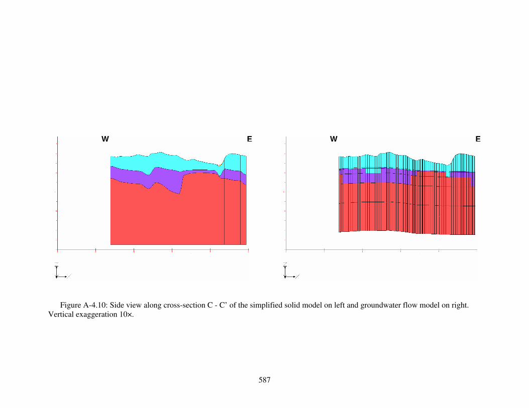
587
Figure A-4.10: Side view along cross-section C - C’ of the simplified solid model on left and groundwater flow model on right. Vertical exaggeration 10×.
E W E W

588
Figure A-4.11: Side view along cross-section D - D’ of the simplified solid model on left and groundwater flow model on right. Vertical exaggeration 10×.
E W E W

589
Figure A-4.12: Side view along cross-section E - E’ of the simplified solid model on left and groundwater flow model on right. Vertical exaggeration 10×.
E W E W Cenozoic intrusions
Cenozoic intrusions

590
Figure A-4.13: Distribution of hydrogeologic units within layer 1 of the groundwater
flow model grid. Axes scale is in UTM NAD83 Zone 13 North coordinates.
Permian
Cretaceous
Cenozoic alluvium
Precambrian

591
Figure A-4.14: Distribution of hydrogeologic units within layer 2 of the groundwater
flow model grid. Axes scale is in UTM NAD83 Zone 13 North coordinates.
low permeability Cretaceous
confining unit
Cambrian through
Pennsylvanian

592
Figure A-4.15: Distribution of hydrogeologic units within layer 3 of the groundwater
flow model grid. Axes scale is in UTM NAD83 Zone 13 North coordinates.
Cenozoic intrusive
mass beneath
Cornudas Mountains

593
Figure A-4.16: Distribution of hydrogeologic units within layer 4 of the groundwater
flow model grid. Axes scale is in UTM NAD83 Zone 13 North coordinates.

594
Figure A-4.17: Distribution of hydrogeologic units within layer 5 of the groundwater
flow model grid. Axes scale is in UTM NAD83 Zone 13 North coordinates.
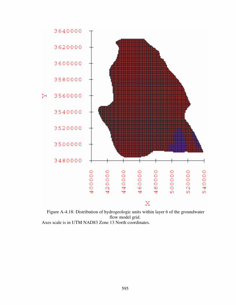
595
Figure A-4.18: Distribution of hydrogeologic units within layer 6 of the groundwater
flow model grid. Axes scale is in UTM NAD83 Zone 13 North coordinates.

596
Figure A-4.19: Groundwater flow model domain, plan view of model grid, recharge zones derived from sub-basins delineated by JSAI (2010), and discharge zone at Salt
Flats playa. Axes scale is in UTM NAD83 Zone 13 North coordinates. Red line along perimeter of model domain designates no-flow boundary. Areas enclosed by blue lines indicate recharge zones. Grid cells highlighted with yellow specify discharge zone.
Peñasco Basin
Diablo Plateau
Upper Sacramento
River and Upper
Piñon Creek
Lower Piñon Creek
Lower Sacramento
River and Otero Mesa
Washburn Draw
Cornudas Draw
Salt Flats
Fourmile Draw
Collins Hills
Upper Cornucopia Draw
Rim of the Guadalupes
Lower Cornucopia Draw
Guadalupe Mts.
Crow Flats
Long Canyon
Lewis Canyon
Big Dog Canyon
Brokeoff Mts.
Delaware Mts.
limestone highlands
Coffelt Draw
Shiloh Draw

597
Figure A-4.20: Water-balance based minimum recharge rates applied to the sub-basins
within the groundwater flow model domain.
Recharge Rate (cm/year)

598
Figure A-4.21: Water-balance based average recharge rates applied to the sub-basins
within the groundwater flow model domain.
Recharge Rate (cm/year)

599
Figure A-4.22: Water-balance based maximum recharge rates applied to the sub-basins
within the groundwater flow model domain.
Recharge Rate (cm/year)

600
Figure A-4.23: Water-balance based minimum areal recharge applied to the sub-basins
within the groundwater flow model domain.
Areal Recharge (acre-feet)

601
Figure A-4.24: Water-balance based average areal recharge applied to the sub-basins
within the groundwater flow model domain.
Areal Recharge (acre-feet)

602
Figure A-4.25: Water-balance based maximum areal recharge applied to the sub-basins
within the groundwater flow model domain.
Areal Recharge (acre-feet)

603
Figure A-4.26: Elevation-dependent minimum recharge rates applied to the recharge zones within the groundwater flow model domain.
Recharge Rate (cm/year)

604
Figure A-4.27: Elevation-dependent average recharge rates applied to the recharge zones within the groundwater flow model domain.
Recharge Rate (cm/year)
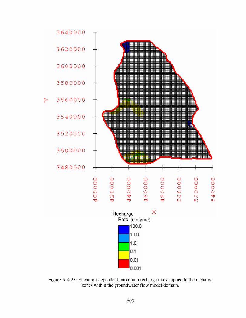
605
Figure A-4.28: Elevation-dependent maximum recharge rates applied to the recharge zones within the groundwater flow model domain.
Recharge Rate (cm/year)
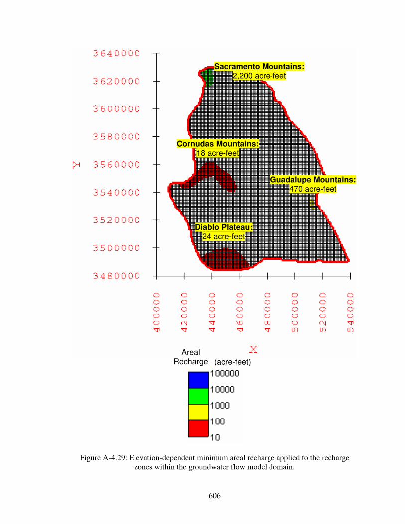
606
Figure A-4.29: Elevation-dependent minimum areal recharge applied to the recharge zones within the groundwater flow model domain.
Cornudas Mountains: 18 acre-feet
Guadalupe Mountains: 470 acre-feet
Sacramento Mountains: 2,200 acre-feet
Diablo Plateau: 24 acre-feet
Areal Recharge (acre-feet)
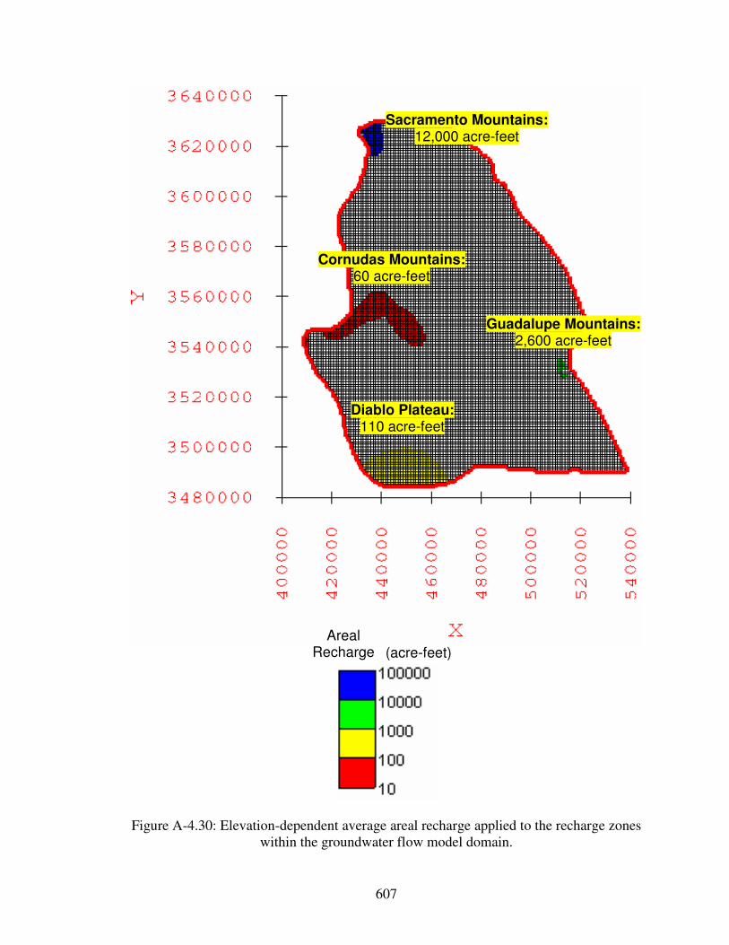
607
Figure A-4.30: Elevation-dependent average areal recharge applied to the recharge zones within the groundwater flow model domain.
Cornudas Mountains: 60 acre-feet
Guadalupe Mountains: 2,600 acre-feet
Sacramento Mountains: 12,000 acre-feet
Diablo Plateau: 110 acre-feet
Areal Recharge (acre-feet)

608
Figure A-4.31: Elevation-dependent maximum areal recharge applied to the recharge zones within the groundwater flow model domain.
Areal Recharge (acre-feet)
Cornudas Mountains: 100 acre-feet
Guadalupe Mountains: 5,100 acre-feet
Sacramento Mountains: 24,000 acre-feet
Diablo Plateau: 200 acre-feet

609
0.00000001
0.0000001
0.000001
0.00001
0.0001
0.001
0.01
0.1
1
10
100
1000K
(m
/day
)
Figure A-4.32: Range of hydraulic conductivity [K] values calculated from transmissivity [T]. Vertical axis is logarithmic scale. Squares indicate median values, and triangles indicate average values.
Aquifer/Facies
Valley- fill
Cenozoic volcanics
Cretaceous Basin-facies Shelf-margin-facies
Shelf-facies
median
average

610
Map Symbols ●: Calibration targets
Figure A-4.33: Calibration targets within the groundwater flow model domain.
Axes scale is in UTM NAD83 Zone 13 North coordinates.

611
Map Symbols
●: Groundwater age wells
Figure A-4.34: Location of the groundwater age wells within the MODFLOW model
domain.
Doll Day
Piñon Well
Webb House
Uña
Cauhape
Harvey Lewis Well
Collins
Jeffer’s Well
Ellett Lower
Evrage House
Lewis
Butterfield Well
Hunt 8

612
Figure A-4.35: Comparison of the computed hydraulic head in layer 1 for the calibrated water-balance based minimum recharge scenario model and the observed groundwater
surface. Green lines are the model computed head contours. Purple dashed lines are the observed groundwater surface contours. Contour elevations are in meters above mean sea level. Contour interval is 200 meters.
1,400
1,400
1,400
1,800
2,200
1,800
1,400
1,400
1,800 2,200
1,400

613
Figure A-4.36: Comparison of the computed hydraulic head in layer 1 for the calibrated
water-balance based average recharge scenario model and the observed groundwater surface.
Green lines are the model computed head contours. Purple dashed lines are the observed groundwater surface contours. Contour elevations are in meters above mean sea level. Contour interval is 200 meters.
1,400
1,400
1,400
1,800
2,200
1,800
1,400
1,400
2,200 1,800
1,400
1,400

614
Figure A-4.37: Comparison of the computed hydraulic head in layer 1 for the calibrated water-balance based maximum recharge scenario model and the observed groundwater
surface. Green lines are the model computed head contours. Purple dashed lines are the observed groundwater surface contours. Contour elevations are in meters above mean sea level. Contour interval is 200 meters.
1,400
1,400
1,400
1,800
2,200
1,800
1,400
1,400
2,200 1,800
1,400
1,400

615
Figure A-4.38: Comparison of the computed hydraulic head in layer 1 for the calibrated elevation-dependent minimum recharge scenario model and the observed groundwater
surface. Green lines are the model computed head contours. Purple dashed lines are the observed groundwater surface contours. Contour elevations are in meters above mean sea level. Contour interval is 200 meters.
1,400
1,400
1,400
1,800
1,800
1,400
2,200
2,200
1,800

616
Figure A-4.39: Comparison of the computed hydraulic head in layer 1 for the calibrated
elevation-dependent average recharge scenario model and the observed groundwater surface.
Green lines are the model computed head contours. Purple dashed lines are the observed groundwater surface contours. Contour elevations are in meters above mean sea level. Contour interval is 200 meters.
1,400
1,400
1,800
2,200
1,800
1,400
2,200 1,800
1,400
1,400

617
Figure A-4.40: Comparison of the computed hydraulic head in layer 1 for the calibrated elevation-dependent maximum recharge scenario model and the observed groundwater
surface. Green lines are the model computed head contours. Purple dashed lines are the observed groundwater surface contours. Contour elevations are in meters above mean sea level. Contour interval is 200 meters.
1,400
1,400
1,400
1,800
2,200
1,800
1,400
2,200 1,800
1,400

618
1,000
1,500
2,000
2,500
3,000
1,000 1,500 2,000 2,500 3,000
Observed Head (meters)
Co
mp
ute
d H
ea
d (
me
ters
)
Figure A-4.41: Computed versus observed hydraulic head for the calibrated water-balance based minimum recharge scenario model.
1:1 line
RMS Error = 61 meters

619
1,000
1,500
2,000
2,500
3,000
1,000 1,500 2,000 2,500 3,000
Observed Head (meters)
Co
mp
ute
d H
ea
d (
me
ters
)
Figure A-4.42: Computed versus observed hydraulic head for the calibrated water-balance based average recharge scenario model.
1:1 line
RMS Error = 60 meters
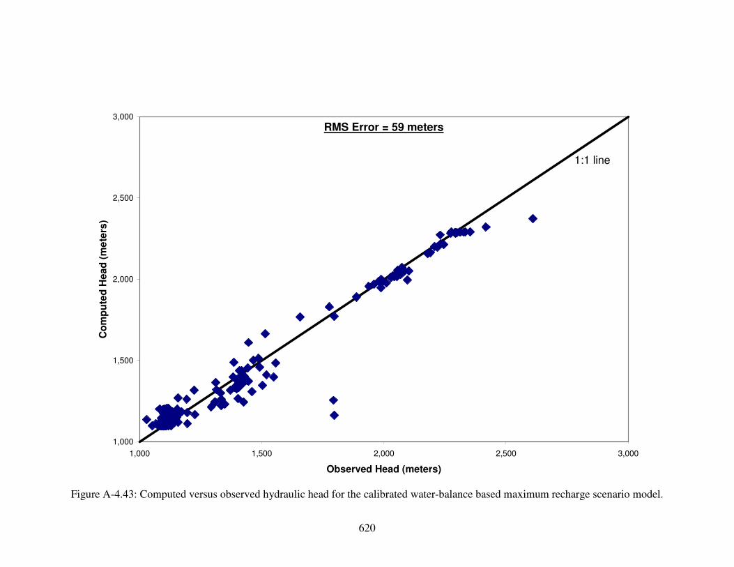
620
1,000
1,500
2,000
2,500
3,000
1,000 1,500 2,000 2,500 3,000
Observed Head (meters)
Co
mp
ute
d H
ea
d (
me
ters
)
Figure A-4.43: Computed versus observed hydraulic head for the calibrated water-balance based maximum recharge scenario model.
1:1 line
RMS Error = 59 meters

621
1,000
1,500
2,000
2,500
3,000
1,000 1,500 2,000 2,500 3,000
Observed Head (meters)
Co
mp
ute
d H
ea
d (
me
ters
)
Figure A-4.44: Computed versus observed hydraulic head for the calibrated elevation-dependent minimum recharge scenario model.
1:1 line
RMS Error = 76 meters

622
1,000
1,500
2,000
2,500
3,000
1,000 1,500 2,000 2,500 3,000
Observed Head (meters)
Co
mp
ute
d H
ea
d (
me
ters
)
Figure A-4.45: Computed versus observed hydraulic head for the calibrated elevation-dependent average recharge scenario model.
1:1 line
RMS Error = 78 meters

623
1,000
1,500
2,000
2,500
3,000
1,000 1,500 2,000 2,500 3,000
Observed Head (meters)
Co
mp
ute
d H
ea
d (
me
ters
)
Figure A-4.46: Computed versus observed hydraulic head for the calibrated elevation-dependent maximum recharge scenario model.
1:1 line
RMS Error = 73 meters

624
-700
-600
-500
-400
-300
-200
-100
0
100
200
300
1,000 1,500 2,000 2,500 3,000
Observed Head (meters)
Re
sid
ua
l H
ea
d (
me
ters
)
Figure A-4.47: Residual versus observed hydraulic head for the calibrated water-balance based minimum recharge scenario model.

625
-700
-600
-500
-400
-300
-200
-100
0
100
200
300
1,000 1,500 2,000 2,500 3,000
Observed Head (meters)
Re
sid
ua
l H
ea
d (
me
ters
)
Figure A-4.48: Residual versus observed hydraulic head for the calibrated water-balance based average recharge scenario model.

626
-700
-600
-500
-400
-300
-200
-100
0
100
200
300
1,000 1,500 2,000 2,500 3,000
Observed Head (meters)
Re
sid
ua
l H
ea
d (
me
ters
)
Figure A-4.49: Residual versus observed hydraulic head for the calibrated water-balance based maximum recharge scenario model.
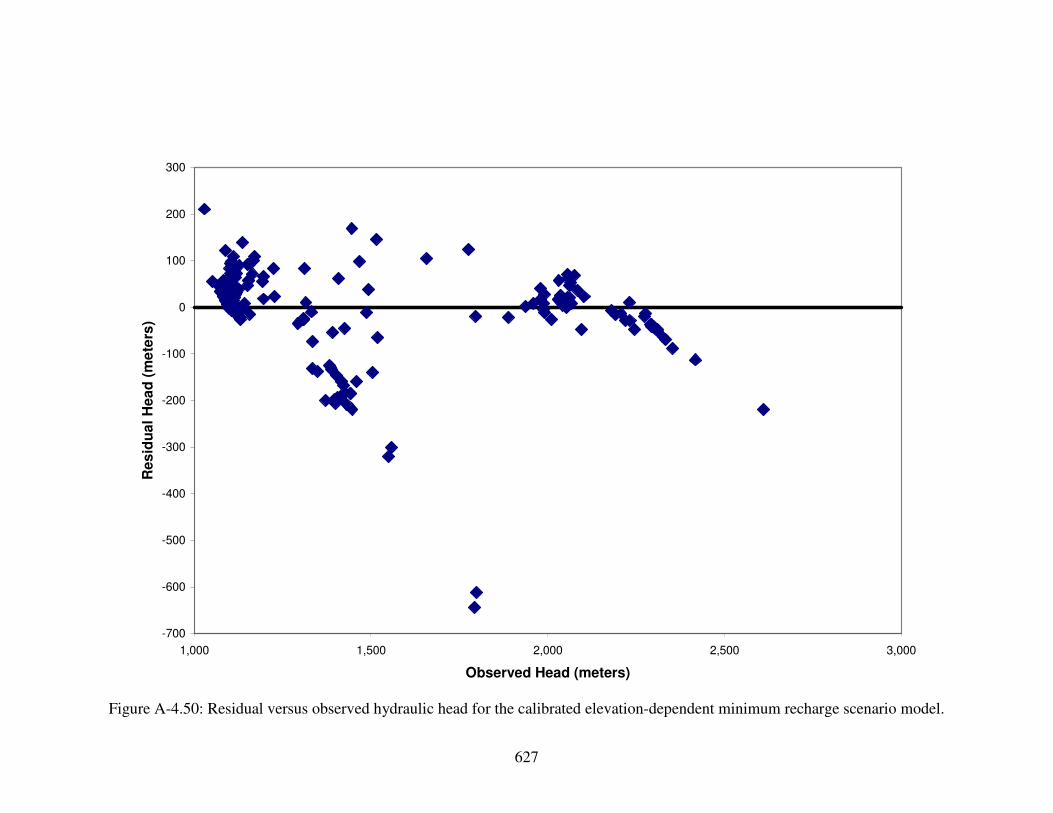
627
-700
-600
-500
-400
-300
-200
-100
0
100
200
300
1,000 1,500 2,000 2,500 3,000
Observed Head (meters)
Re
sid
ua
l H
ea
d (
me
ters
)
Figure A-4.50: Residual versus observed hydraulic head for the calibrated elevation-dependent minimum recharge scenario model.

628
-700
-600
-500
-400
-300
-200
-100
0
100
200
300
1,000 1,500 2,000 2,500 3,000
Observed Head (meters)
Re
sid
ua
l H
ea
d (
me
ters
)
Figure A-4.51: Residual versus observed hydraulic head for the calibrated elevation-dependent average recharge scenario model.

629
-700
-600
-500
-400
-300
-200
-100
0
100
200
300
1,000 1,500 2,000 2,500 3,000
Observed Head (meters)
Re
sid
ua
l H
ea
d (
me
ters
)
Figure A-4.52: Residual versus observed hydraulic head for the calibrated elevation-dependent maximum recharge scenario model.

630
-2,500
0
2,500
5,000
7,500
10,000
12,500
15,000
17,500
Minimum Recharge
Scenario
Average Recharge
Scenario
Maximum Recharge
Scenario
Re
sid
ua
ls (
me
ters
)
Sum of Residuals
Sum of Absolute Values of Residuals
Figure A-4.53: Sum of the residuals and sum of the absolute values of the residuals between observed and computed hydraulic heads
for the calibrated water-balance based minimum, average, and maximum recharge scenario models.
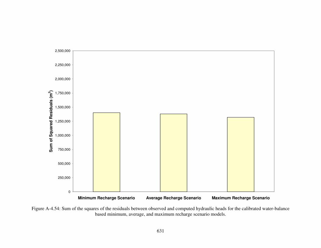
631
0
250,000
500,000
750,000
1,000,000
1,250,000
1,500,000
1,750,000
2,000,000
2,250,000
2,500,000
Minimum Recharge Scenario Average Recharge Scenario Maximum Recharge Scenario
Su
m o
f S
qu
are
d R
es
idu
als
(m
2)
Figure A-4.54: Sum of the squares of the residuals between observed and computed hydraulic heads for the calibrated water-balance
based minimum, average, and maximum recharge scenario models.

632
-2,500
0
2,500
5,000
7,500
10,000
12,500
15,000
17,500
Minimum Recharge
Scenario
Average Recharge
Scenario
Maximum Recharge
Scenario
Re
sid
ua
ls (
me
ters
)
Sum of Residuals
Sum of Absolute Values of Residuals
Figure A-4.55: Sum of the residuals and sum of the absolute values of the residuals between observed and computed hydraulic heads
for the calibrated elevation-dependent minimum, average, and maximum recharge scenario models.

633
0
250,000
500,000
750,000
1,000,000
1,250,000
1,500,000
1,750,000
2,000,000
2,250,000
2,500,000
Minimum Recharge Scenario Average Recharge Scenario Maximum Recharge Scenario
Su
m o
f S
qu
are
d R
es
idu
als
(m
2)
Figure A-4.56: Sum of the squares of the residuals between observed and computed hydraulic heads for the calibrated elevation-
dependent minimum, average, and maximum recharge scenarios models.

634
Figure A-4.57: Horizontal hydraulic conductivity [HK] distribution in layer 1 for the calibrated water-balance based minimum recharge scenario groundwater flow model.
(m/day)

635
Figure A-4.58: Horizontal hydraulic conductivity [HK] distribution in layer 2 for the calibrated water-balance based minimum recharge scenario groundwater flow model.
(m/day)

636
Figure A-4.59: Horizontal hydraulic conductivity [HK] distribution in layer 3 for the calibrated water-balance based minimum recharge scenario groundwater flow model.
(m/day)

637
Figure A-4.60: Horizontal hydraulic conductivity [HK] distribution in layer 4 for the calibrated water-balance based minimum recharge scenario groundwater flow model.
(m/day)

638
Figure A-4.61: Horizontal hydraulic conductivity [HK] distribution in layer 5 for the calibrated water-balance based minimum recharge scenario groundwater flow model.
(m/day)

639
Figure A-4.62: Horizontal hydraulic conductivity [HK] distribution in layer 6 for the calibrated water-balance based minimum recharge scenario groundwater flow model.
(m/day)

640
Figure A-4.63: Horizontal hydraulic conductivity [HK] distribution in layer 1 for the calibrated water-balance based average recharge scenario groundwater flow model.
(m/day)

641
Figure A-4.64: Horizontal hydraulic conductivity [HK] distribution in layer 2 for the calibrated water-balance based average recharge scenario groundwater flow model.
(m/day)

642
Figure A-4.65: Horizontal hydraulic conductivity [HK] distribution in layer 3 for the calibrated water-balance based average recharge scenario groundwater flow model.
(m/day)

643
Figure A-4.66: Horizontal hydraulic conductivity [HK] distribution in layer 4 for the calibrated water-balance based average recharge scenario groundwater flow model.
(m/day)

644
Figure A-4.67: Horizontal hydraulic conductivity [HK] distribution in layer 5 for the calibrated water-balance based average recharge scenario groundwater flow model.
(m/day)
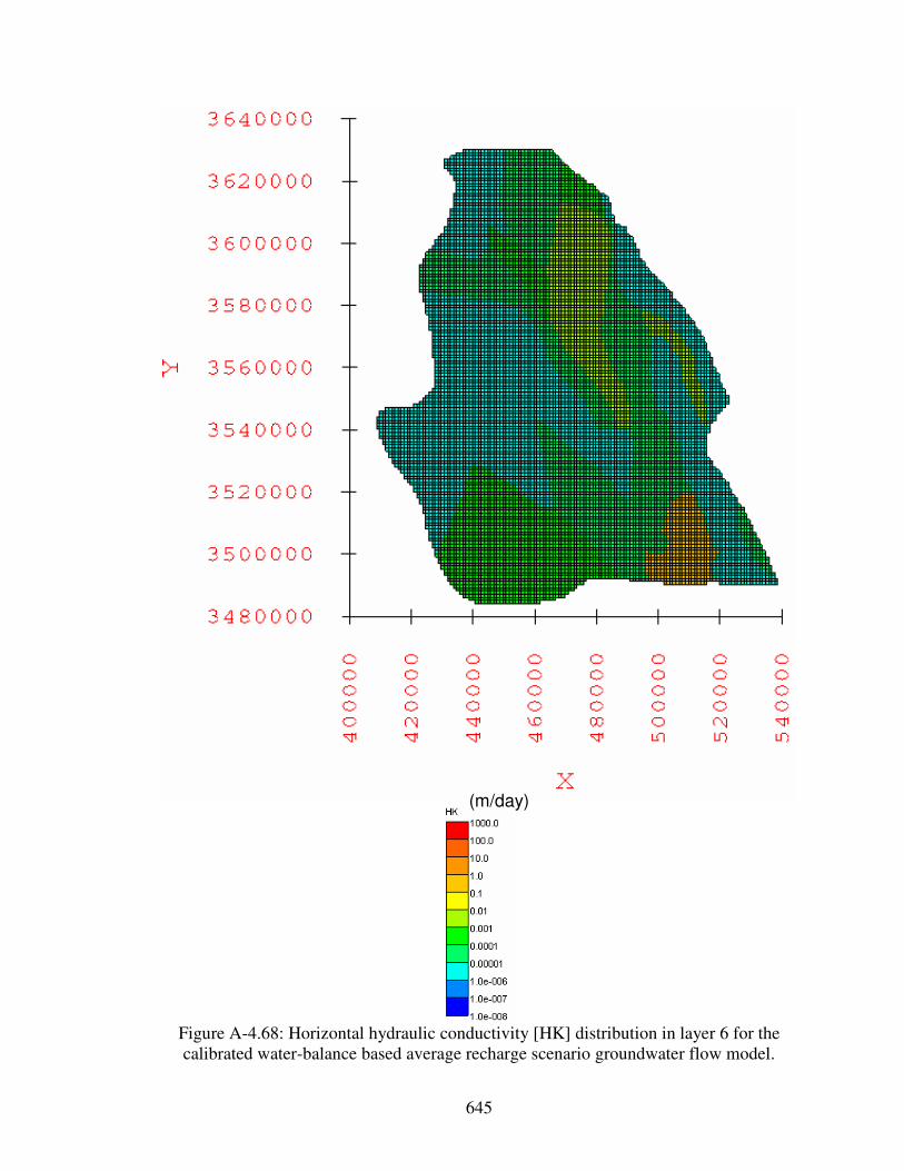
645
Figure A-4.68: Horizontal hydraulic conductivity [HK] distribution in layer 6 for the calibrated water-balance based average recharge scenario groundwater flow model.
(m/day)

646
Figure A-4.69: Horizontal hydraulic conductivity [HK] distribution in layer 1 for the calibrated water-balance based maximum recharge scenario groundwater flow model.
(m/day)

647
Figure A-4.70: Horizontal hydraulic conductivity [HK] distribution in layer 2 for the calibrated water-balance based maximum recharge scenario groundwater flow model.
(m/day)

648
Figure A-4.71: Horizontal hydraulic conductivity [HK] distribution in layer 3 for the calibrated water-balance based maximum recharge scenario groundwater flow model.
(m/day)

649
Figure A-4.72: Horizontal hydraulic conductivity [HK] distribution in layer 4 for the calibrated water-balance based maximum recharge scenario groundwater flow model.
(m/day)

650
Figure A-4.73: Horizontal hydraulic conductivity [HK] distribution in layer 5 for the calibrated water-balance based maximum recharge scenario groundwater flow model.
(m/day)

651
Figure A-4.74: Horizontal hydraulic conductivity [HK] distribution in layer 6 for the calibrated water-balance based maximum recharge scenario groundwater flow model.
(m/day)

652
Figure A-4.75: Horizontal hydraulic conductivity [HK] distribution in layer 1 for the calibrated elevation-dependent minimum recharge scenario groundwater flow model.
(m/day)

653
Figure A-4.76: Horizontal hydraulic conductivity [HK] distribution in layer 2 for the calibrated elevation-dependent minimum recharge scenario groundwater flow model.
(m/day)

654
Figure A-4.77: Horizontal hydraulic conductivity [HK] distribution in layer 3 for the calibrated elevation-dependent minimum recharge scenario groundwater flow model.
(m/day)

655
Figure A-4.78: Horizontal hydraulic conductivity [HK] distribution in layer 4 for the calibrated elevation-dependent minimum recharge scenario groundwater flow model.
(m/day)

656
Figure A-4.79: Horizontal hydraulic conductivity [HK] distribution in layer 5 for the calibrated elevation-dependent minimum recharge scenario groundwater flow model.
(m/day)

657
Figure A-4.80: Horizontal hydraulic conductivity [HK] distribution in layer 6 for the calibrated elevation-dependent minimum recharge scenario groundwater flow model.
(m/day)

658
Figure A-4.81: Horizontal hydraulic conductivity [HK] distribution in layer 1 for the calibrated elevation-dependent average recharge scenario groundwater flow model.
(m/day)

659
Figure A-4.82: Horizontal hydraulic conductivity [HK] distribution in layer 2 for the calibrated elevation-dependent average recharge scenario groundwater flow model.
(m/day)

660
Figure A-4.83: Horizontal hydraulic conductivity [HK] distribution in layer 3 for the calibrated elevation-dependent average recharge scenario groundwater flow model.
(m/day)
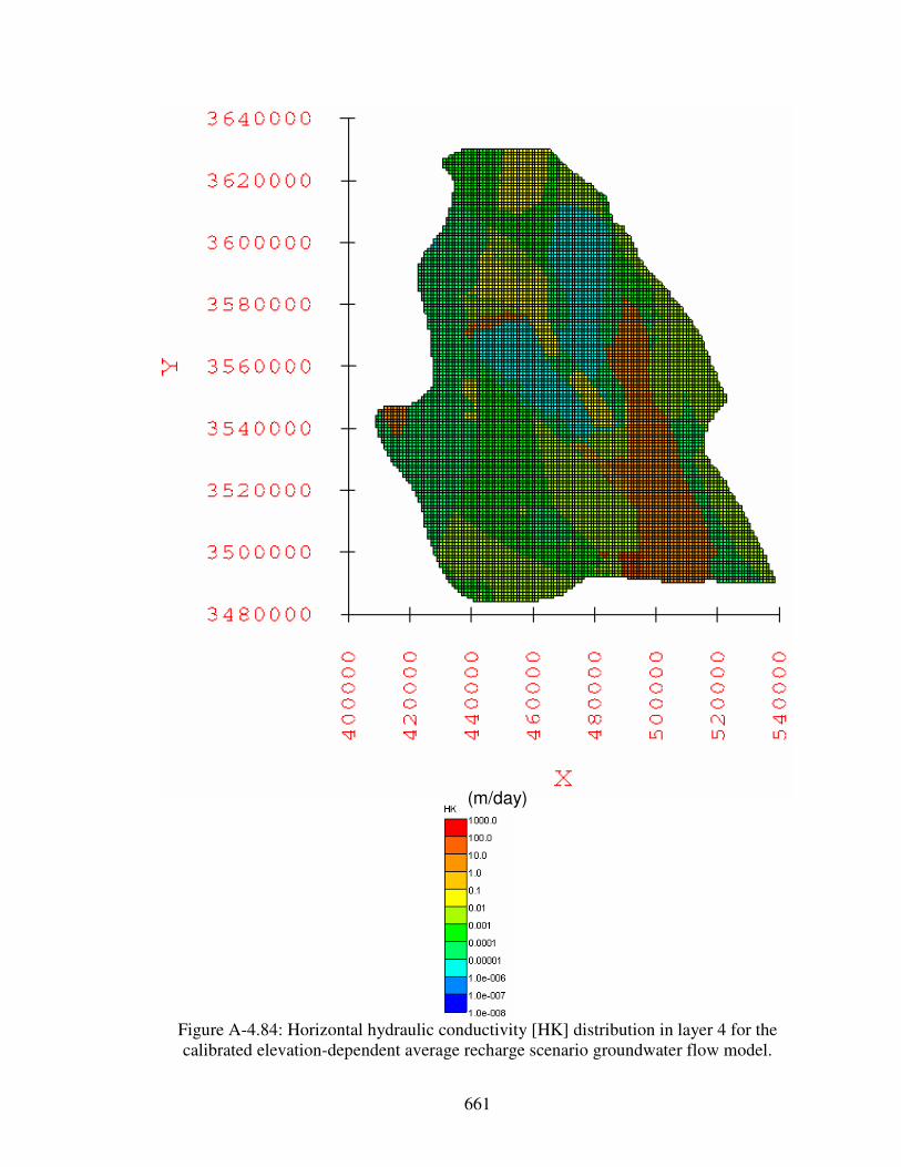
661
Figure A-4.84: Horizontal hydraulic conductivity [HK] distribution in layer 4 for the calibrated elevation-dependent average recharge scenario groundwater flow model.
(m/day)

662
Figure A-4.85: Horizontal hydraulic conductivity [HK] distribution in layer 5 for the calibrated elevation-dependent average recharge scenario groundwater flow model.
(m/day)

663
Figure A-4.86: Horizontal hydraulic conductivity [HK] distribution in layer 6 for the calibrated elevation-dependent average recharge scenario groundwater flow model.
(m/day)

664
Figure A-4.87: Horizontal hydraulic conductivity [HK] distribution in layer 1 for the calibrated elevation-dependent maximum recharge scenario groundwater flow model.
(m/day)

665
Figure A-4.88: Horizontal hydraulic conductivity [HK] distribution in layer 2 for the calibrated elevation-dependent maximum recharge scenario groundwater flow model.
(m/day)

666
Figure A-4.89: Horizontal hydraulic conductivity [HK] distribution in layer 3 for the calibrated elevation-dependent maximum recharge scenario groundwater flow model.
(m/day)

667
Figure A-4.90: Horizontal hydraulic conductivity [HK] distribution in layer 4 for the calibrated elevation-dependent maximum recharge scenario groundwater flow model.
(m/day)
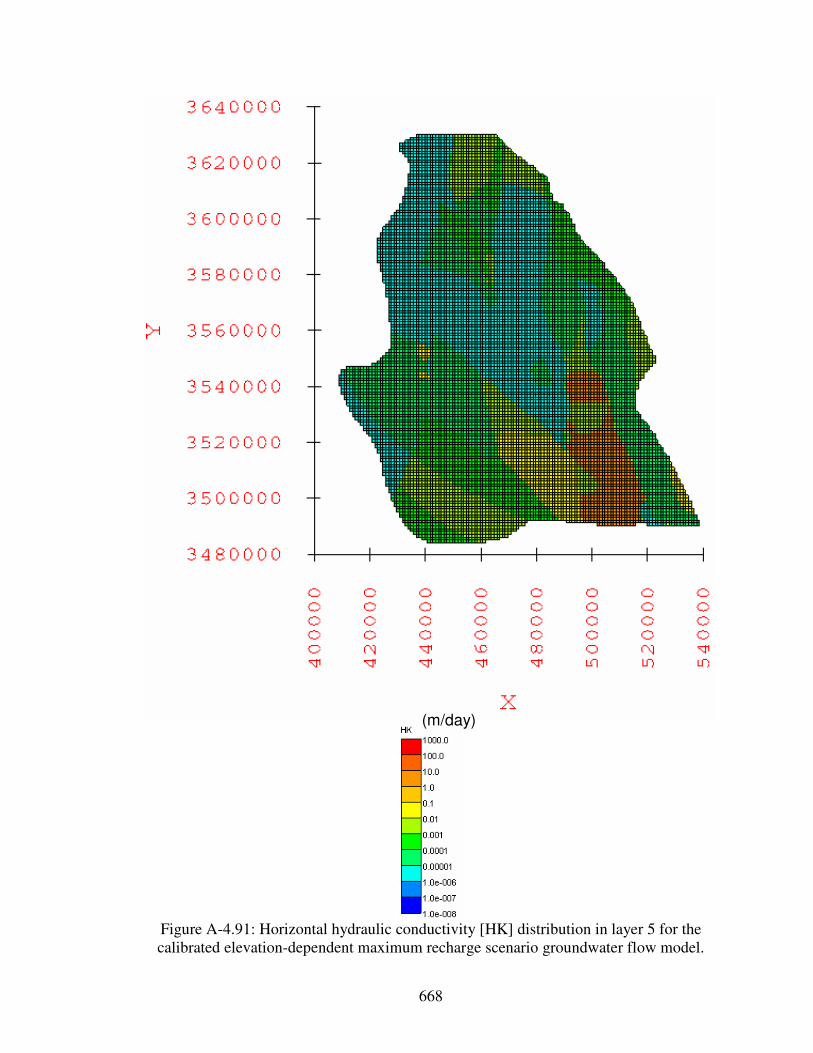
668
Figure A-4.91: Horizontal hydraulic conductivity [HK] distribution in layer 5 for the calibrated elevation-dependent maximum recharge scenario groundwater flow model.
(m/day)

669
Figure A-4.92: Horizontal hydraulic conductivity [HK] distribution in layer 6 for the calibrated elevation-dependent maximum recharge scenario groundwater flow model.
(m/day)
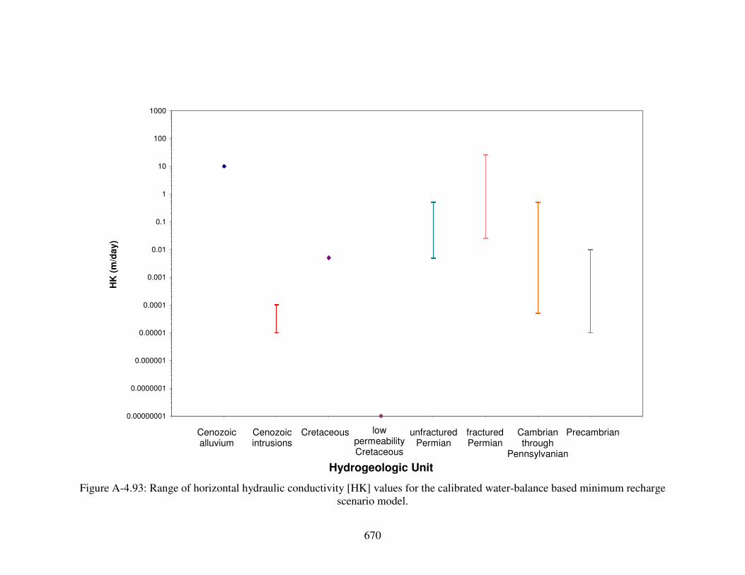
670
0.00000001
0.0000001
0.000001
0.00001
0.0001
0.001
0.01
0.1
1
10
100
1000H
K (
m/d
ay
)
Figure A-4.93: Range of horizontal hydraulic conductivity [HK] values for the calibrated water-balance based minimum recharge scenario model.
Hydrogeologic Unit
Cenozoic alluvium
Cenozoic intrusions
Cretaceous unfractured Permian
fractured Permian
Cambrian through
Pennsylvanian
Precambrian low permeability Cretaceous

671
0.00000001
0.0000001
0.000001
0.00001
0.0001
0.001
0.01
0.1
1
10
100
1000H
K (
m/d
ay
)
Figure A-4.94: Range of horizontal hydraulic conductivity [HK] values for the calibrated water-balance based average recharge scenario model.
Cenozoic alluvium
Cenozoic intrusions
Cretaceous unfractured Permian
Hydrogeologic Unit
fractured Permian
Cambrian through
Pennsylvanian
Precambrian low permeability Cretaceous

672
0.00000001
0.0000001
0.000001
0.00001
0.0001
0.001
0.01
0.1
1
10
100
1000H
K (
m/d
ay
)
Figure A-4.95: Range of horizontal hydraulic conductivity [HK] values for the calibrated water-balance based maximum recharge scenario model.
Cenozoic alluvium
Cenozoic intrusions
Cretaceous unfractured Permian
Hydrogeologic Unit
fractured Permian
Cambrian through
Pennsylvanian
Precambrian low permeability Cretaceous
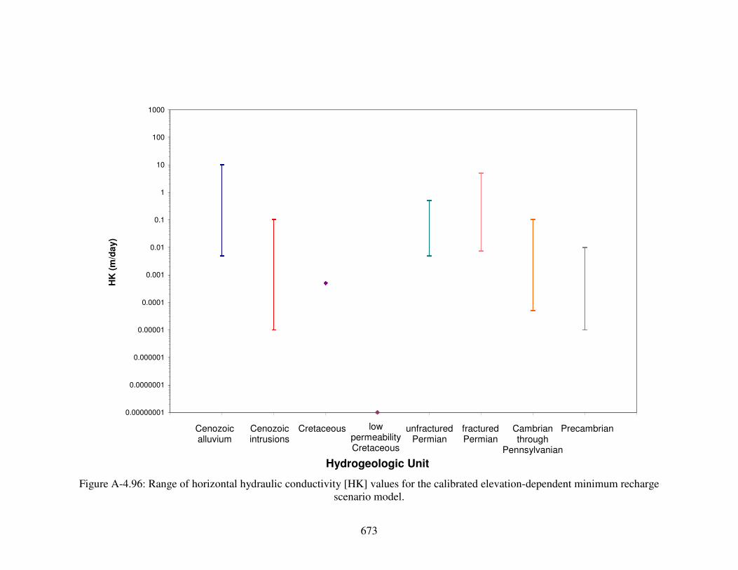
673
0.00000001
0.0000001
0.000001
0.00001
0.0001
0.001
0.01
0.1
1
10
100
1000H
K (
m/d
ay
)
Figure A-4.96: Range of horizontal hydraulic conductivity [HK] values for the calibrated elevation-dependent minimum recharge scenario model.
Cenozoic alluvium
Cenozoic intrusions
Cretaceous unfractured Permian
Hydrogeologic Unit
fractured Permian
Cambrian through
Pennsylvanian
Precambrian low permeability Cretaceous

674
0.00000001
0.0000001
0.000001
0.00001
0.0001
0.001
0.01
0.1
1
10
100
1000H
K (
m/d
ay
)
Figure A-4.97: Range of horizontal hydraulic conductivity [HK] values for the calibrated elevation-dependent average recharge scenario model.
Cenozoic alluvium
Cenozoic intrusions
Cretaceous unfractured Permian
Hydrogeologic Unit
fractured Permian
Cambrian through
Pennsylvanian
Precambrian low permeability Cretaceous
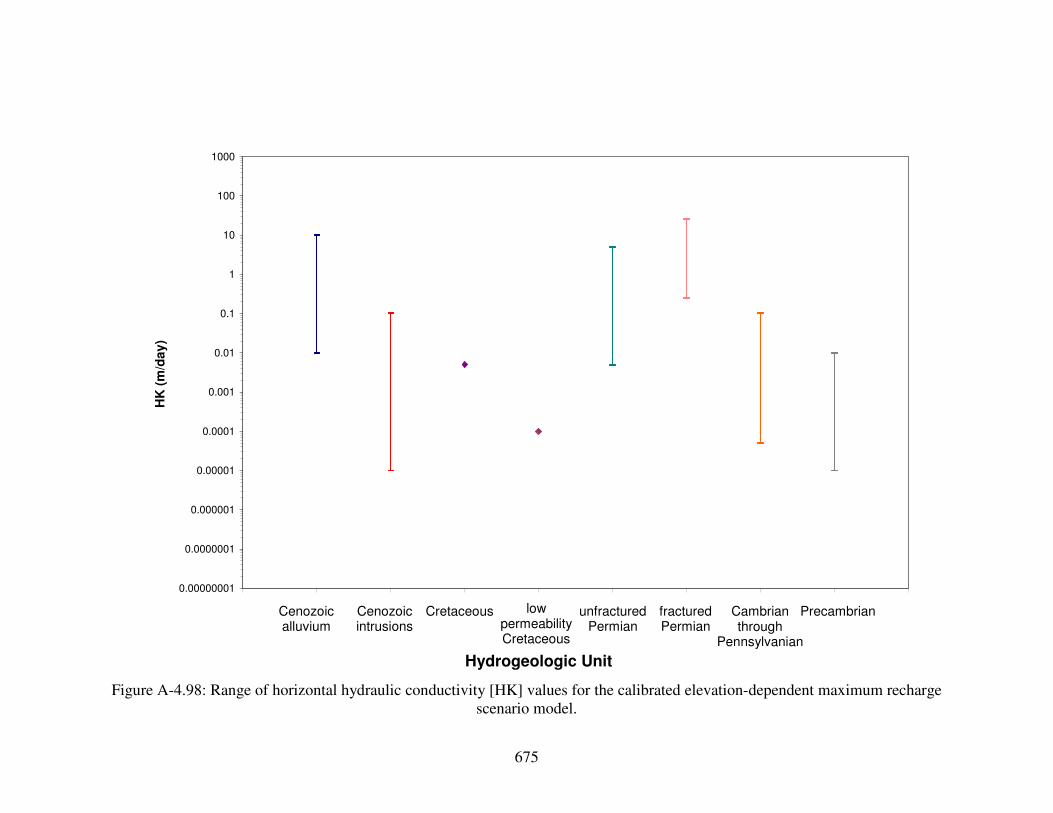
675
0.00000001
0.0000001
0.000001
0.00001
0.0001
0.001
0.01
0.1
1
10
100
1000H
K (
m/d
ay
)
Figure A-4.98: Range of horizontal hydraulic conductivity [HK] values for the calibrated elevation-dependent maximum recharge scenario model.
Cenozoic alluvium
Cenozoic intrusions
Cretaceous unfractured Permian
Hydrogeologic Unit
fractured Permian
Cambrian through
Pennsylvanian
Precambrian low permeability Cretaceous

676
Figure A-4.99: Distribution of aquifer transmissivity [T] for the calibrated water-balance
based minimum recharge scenario groundwater flow model.
(m2/day) T

677
Figure A-4.100: Distribution of aquifer transmissivity [T] for the calibrated water-
balance based average recharge scenario groundwater flow model.
(m2/day) T
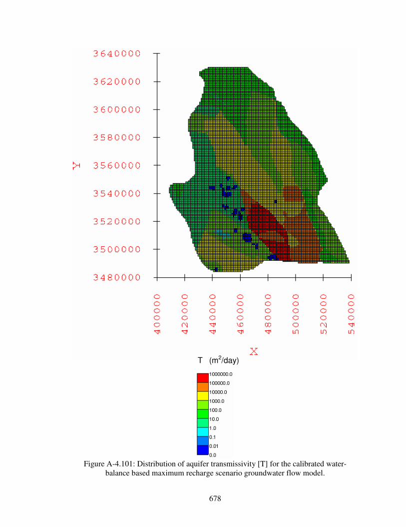
678
Figure A-4.101: Distribution of aquifer transmissivity [T] for the calibrated water-
balance based maximum recharge scenario groundwater flow model.
(m2/day) T

679
Figure A-4.102: Distribution of aquifer transmissivity [T] for the calibrated elevation-
dependent minimum recharge scenario groundwater flow model.
(m2/day) T

680
Figure A-4.103: Distribution of aquifer transmissivity [T] for the calibrated elevation-
dependent average recharge scenario groundwater flow model.
(m2/day) T
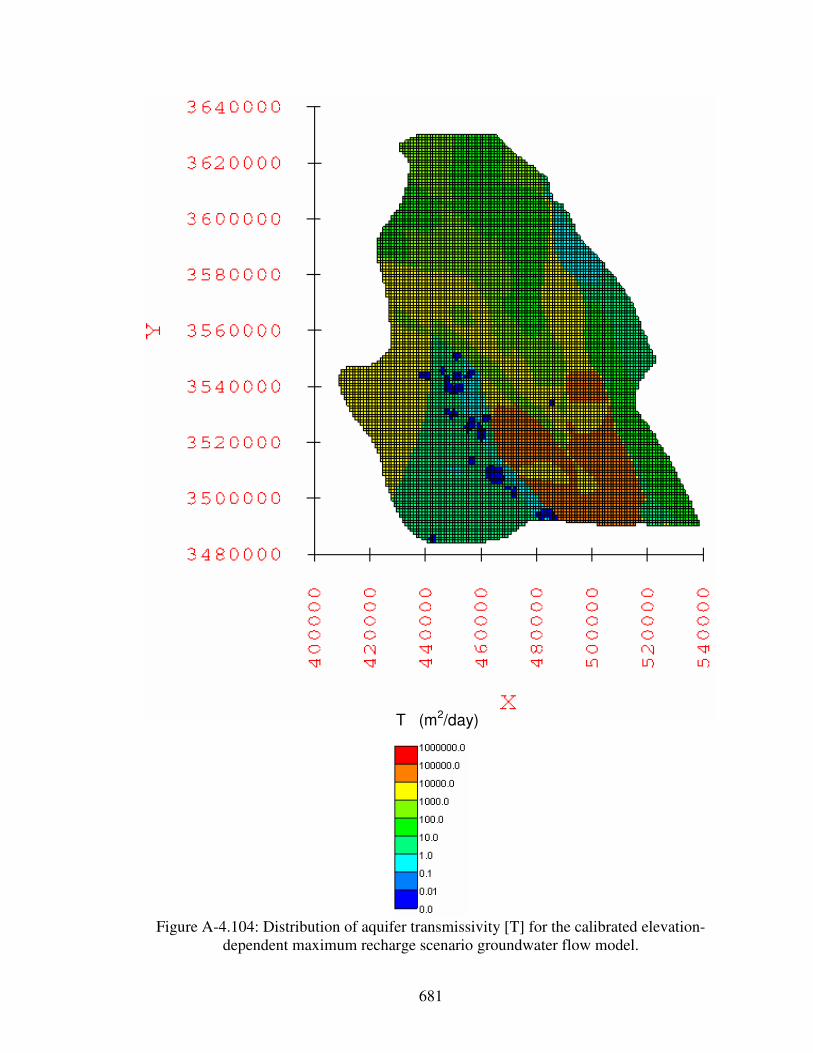
681
Figure A-4.104: Distribution of aquifer transmissivity [T] for the calibrated elevation-
dependent maximum recharge scenario groundwater flow model.
(m2/day) T
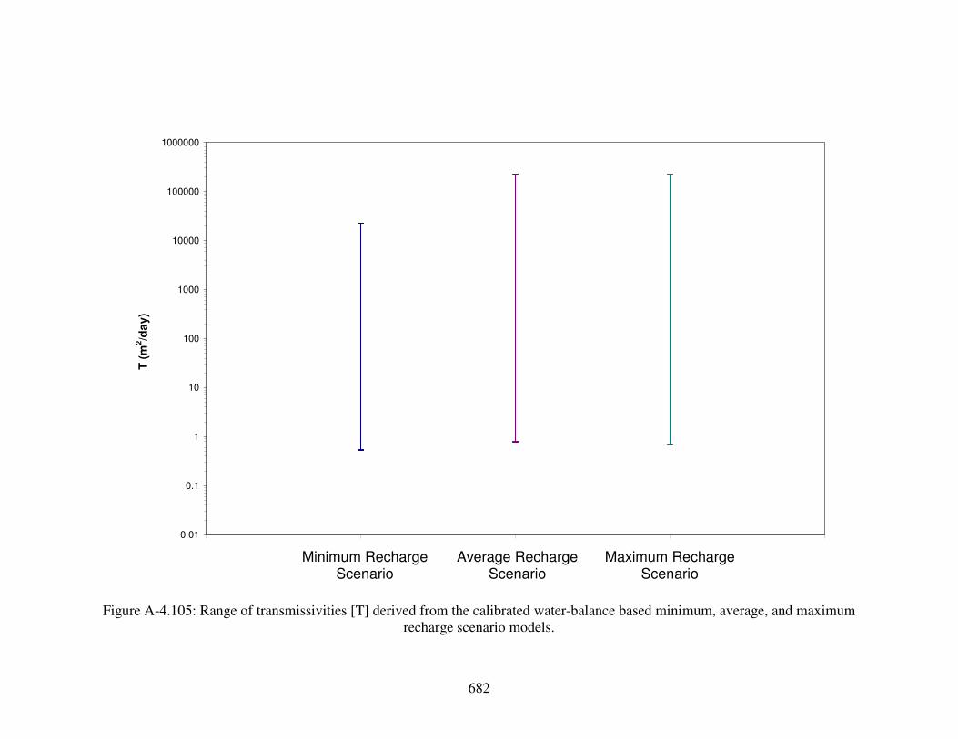
682
0.01
0.1
1
10
100
1000
10000
100000
1000000T
(m
2/d
ay
)
Figure A-4.105: Range of transmissivities [T] derived from the calibrated water-balance based minimum, average, and maximum recharge scenario models.
Minimum Recharge Scenario
Average Recharge Scenario
Maximum Recharge Scenario

683
0.01
0.1
1
10
100
1000
10000
100000
1000000T
(m
2/d
ay
)
Figure A-4.106: Range of transmissivities [T] derived from the calibrated elevation-dependent minimum, average, and maximum recharge scenario models.
Minimum Recharge Scenario
Average Recharge Scenario
Maximum Recharge Scenario

684
100
1,000
10,000
100,000
0 1 10 100 1,000 10,000 100,000 1,000,000 10,000,000
MODPATH Age (years)
NE
TP
AT
H A
ge
(y
ea
rs)
Min. n lower bound
Min. n upper bound
Avg. n lower bound
Avg. n upper bound
Max. n lower bound
Max. n upper bound
1:1 Line
Figure A-4.107: NETPATH versus MODPATH ages for the calibrated water-balance based minimum recharge scenario model using
minimum, average, and maximum porosities. Vertical and horizontal axes are logarithmic scale.
RMS Error (years): Minimum Porosity = 9,800 Average porosity = 9,400
Maximum porosity = 9,900
.1

685
100
1,000
10,000
100,000
0 1 10 100 1,000 10,000 100,000 1,000,000 10,000,000
MODPATH Age (years)
NE
TP
AT
H A
ge
(y
ea
rs)
Min. n lower bound
Min. n upper bound
Avg. n lower bound
Avg. n upper bound
Max. n lower bound
Max. n upper bound
1:1 Line
Figure A-4.108: NETPATH versus MODPATH ages for the calibrated water-balance based average recharge scenario model using
minimum, average, and maximum porosities. Vertical and horizontal axes are logarithmic scale.
RMS Error (years): Minimum Porosity = 9,700 Average porosity = 9,200
Maximum porosity = 9,000
.1

686
100
1,000
10,000
100,000
0 1 10 100 1,000 10,000 100,000 1,000,000 10,000,000
MODPATH Age (years)
NE
TP
AT
H A
ge
(y
ea
rs)
Min. n lower bound
Min. n upper bound
Avg. n lower bound
Avg. n upper bound
Max. n lower bound
Max. n upper bound
1:1 Line
Figure A-4.109: NETPATH versus MODPATH ages for the calibrated water-balance based maximum recharge scenario model using
minimum, average, and maximum porosities. Vertical and horizontal axes are logarithmic scale.
RMS Error (years): Minimum Porosity = 9,900 Average porosity = 9,500
Maximum porosity = 9,300
.1

687
100
1,000
10,000
100,000
0 1 10 100 1,000 10,000 100,000 1,000,000 10,000,000
MODPATH Age (years)
NE
TP
AT
H A
ge
(y
ea
rs)
Min. n lower bound
Min. n upper bound
Avg. n lower bound
Avg. n upper bound
Max. n lower bound
Max. n upper bound
1:1 Line
Figure A-4.110: NETPATH versus MODPATH ages for the calibrated elevation-dependent minimum recharge scenario model using
minimum, average, and maximum porosities. Vertical and horizontal axes are logarithmic scale.
.1
RMS Error (years): Minimum Porosity = 180,000 Average porosity = 450,000
Maximum porosity = 720,000
Collins outliers
RMS Error with outliers removed (years):
Minimum Porosity = 43,000 Average porosity = 120,000
Maximum porosity = 200,000

688
100
1,000
10,000
100,000
0 1 10 100 1,000 10,000 100,000 1,000,000 10,000,000
MODPATH Age (years)
NE
TP
AT
H A
ge
(y
ea
rs)
Min. n lower bound
Min. n upper bound
Avg. n lower bound
Avg. n upper bound
Max. n lower bound
Max. n upper bound
1:1 Line
Figure A-4.111: NETPATH versus MODPATH ages for the calibrated elevation-dependent average recharge scenario model using
minimum, average, and maximum porosities. Vertical and horizontal axes are logarithmic scale.
.1
RMS Error (years): Minimum Porosity = 140,000 Average porosity = 360,000
Maximum porosity = 570,000
RMS Error with outliers removed (years):
Minimum Porosity = 7,600 Average porosity = 25,000
Maximum porosity = 44,000
Evrage House and Collins outliers

689
100
1,000
10,000
100,000
0 1 10 100 1,000 10,000 100,000 1,000,000 10,000,000
MODPATH Age (years)
NE
TP
AT
H A
ge
(y
ea
rs)
Min. n lower bound
Min. n upper bound
Avg. n lower bound
Avg. n upper bound
Max. n lower bound
Max. n upper bound
1:1 Line
Figure A-4.112: NETPATH versus MODPATH ages for the calibrated elevation-dependent maximum recharge scenario model using
minimum, average, and maximum porosities. Vertical and horizontal axes are logarithmic scale.
.1
RMS Error (years): Minimum Porosity = 210,000 Average porosity = 690,000
Maximum porosity = 1,200,000
RMS Error with outliers removed (years):
Minimum Porosity = 6,800 Average porosity = 5,000
Maximum porosity = 9,400
Collins outliers
Evrage House outliers

690
Map Symbols
●: Particle origins
●: Groundwater age wells
Figure A-4.113: MODPATH pathlines and origins of particles for the water-balance based minimum recharge scenario using average porosity values.
Upper bound
Lower bound

691
Map Symbols
●: Particle origins
●: Groundwater age wells
Figure A-4.114: MODPATH pathlines and origins of particles for the water-balance based average recharge scenario using average porosity values.
Upper bound
Lower bound
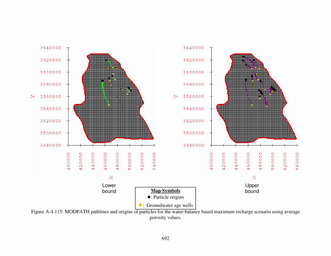
692
Map Symbols
●: Particle origins
●: Groundwater age wells
Figure A-4.115: MODPATH pathlines and origins of particles for the water-balance based maximum recharge scenario using average porosity values.
Upper bound
Lower bound

693
Map Symbols
●: Particle origins
●: Groundwater age wells
Figure A-4.116: MODPATH pathlines and origins of particles for the elevation-dependent minimum recharge scenario using average porosity values.
Lower bound
Upper bound

694
Map Symbols
●: Particle origins
●: Groundwater age wells
Figure A-4.117: MODPATH pathlines and origins of particles for the elevation-dependent average recharge scenario using average porosity values.
Upper bound
Lower bound

695
Map Symbols
●: Particle origins
●: Groundwater age wells
Figure A-4.118: MODPATH pathlines and origins of particles for the elevation-dependent maximum recharge scenario using average porosity values.
Upper bound
Lower bound
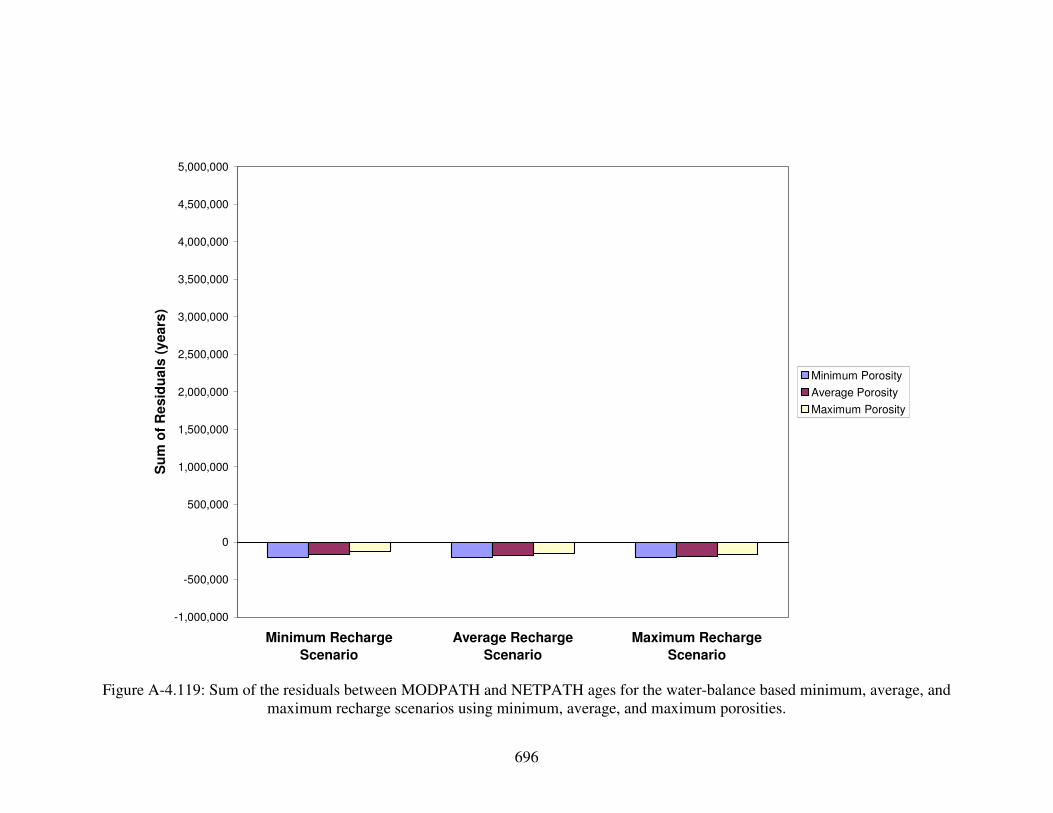
696
-1,000,000
-500,000
0
500,000
1,000,000
1,500,000
2,000,000
2,500,000
3,000,000
3,500,000
4,000,000
4,500,000
5,000,000
Minimum Recharge
Scenario
Average Recharge
Scenario
Maximum Recharge
Scenario
Su
m o
f R
es
idu
als
(y
ea
rs)
Minimum Porosity
Average Porosity
Maximum Porosity
Figure A-4.119: Sum of the residuals between MODPATH and NETPATH ages for the water-balance based minimum, average, and
maximum recharge scenarios using minimum, average, and maximum porosities.

697
0
500,000
1,000,000
1,500,000
2,000,000
2,500,000
3,000,000
3,500,000
4,000,000
4,500,000
5,000,000
Minimum Recharge
Scenario
Average Recharge
Scenario
Maximum Recharge
Scenario
Su
m o
f A
bs
ou
te V
alu
es
of
Re
sid
ua
ls (
ye
ars
)
Minimum Porosity
Average Porosity
Maximum Porosity
Figure A-4.120: Sum of the absolute values of the residuals between MODPATH and NETPATH ages for the water-balance based
minimum, average, and maximum recharge scenarios using minimum, average, and maximum porosities.

698
0
1
10
100
1,000
10,000
100,000
1,000,000
10,000,000
100,000,000
1,000,000,000
10,000,000,000
100,000,000,000
1,000,000,000,000
Minimum Recharge
Scenario
Average Recharge
Scenario
Maximum Recharge
Scenario
Su
m o
f S
qu
are
d R
es
idu
als
(ye
ars
2)
Minimum Porosity
Average Porosity
Maximum Porosity
Figure A-4.121: Sum of the squares of the residuals between MODPATH and NETPATH ages for the water-balance based minimum,
average, and maximum recharge scenarios using minimum, average, and maximum porosities. Vertical axis is logarithmic scale.

699
-1,000,000
-500,000
0
500,000
1,000,000
1,500,000
2,000,000
2,500,000
3,000,000
3,500,000
4,000,000
4,500,000
5,000,000
Minimum Recharge
Scenario
Average Recharge
Scenario
Maximum Recharge
Scenario
Su
m o
f R
es
idu
als
(y
ea
rs)
Minimum Porosity
Average Porosity
Maximum Porosity
Figure A-4.122: Sum of the residuals between MODPATH and NETPATH ages for the elevation-dependent minimum, average, and
maximum recharge scenarios using minimum, average, and maximum porosities.

700
0
500,000
1,000,000
1,500,000
2,000,000
2,500,000
3,000,000
3,500,000
4,000,000
4,500,000
5,000,000
Minimum Recharge
Scenario
Average Recharge
Scenario
Maximum Recharge
Scenario
Su
m o
f A
bs
ou
te V
alu
es
of
Re
sid
ua
ls (
ye
ars
)
Minimum Porosity
Average Porosity
Maximum Porosity
Figure A-4.123: Sum of the absolute values of the residuals between MODPATH and NETPATH ages for the elevation-dependent
minimum, average, and maximum recharge scenarios using minimum, average, and maximum porosities.

701
0
1
10
100
1,000
10,000
100,000
1,000,000
10,000,000
100,000,000
1,000,000,000
10,000,000,000
100,000,000,000
1,000,000,000,000
Minimum Recharge
Scenario
Average Recharge
Scenario
Maximum Recharge
Scenario
Su
m o
f S
qu
are
d R
es
idu
als
(ye
ars
2)
Minimum Porosity
Average Porosity
Maximum Porosity
Figure A-4.124: Sum of the squares of the residuals between MODPATH and NETPATH ages for the elevation-dependent minimum,
average, and maximum recharge scenarios using minimum, average, and maximum porosities. Vertical axis is logarithmic scale.

702
TABLES – CHAPTER 3

703
Well Name,
LeaseWell ID API Number Easting Northing
Well
Elevation
(m)
Reference
Level
(Source)
Well
Depth
(m)
Township
(S)
Range
(E)Section
Houston Oil & Minerals Corp.,
State L.G. "1453" #1HO&MSL1 3003520013 406876 3685414 1,511 GR 3,003 12 10 5
Houston Oil & Minerals Corp.,
J.M. Lewelling #1HO&MJL1 3003520010 402778 3684425 1,440 KB 2,852 12 9 12
Houston Oil & Minerals Corp.,
Lewelling #2HO&MCL2 3003520015 399960 3684444 1,373 GR 2,892 12 9 10
Houston Oil & Minerals Corp.,
Federal "A" #1HO&MFA1 3003520009 413617 3660369 1,619 GR 1,125 14 10 24
Leland A. Hodges, Trustee,
Houston #1LAHTHO1 3003520005 411157 3660302 1,529 GR 928 14 10 23
Houston Oil & Minerals Corp.,
State 3724 #1HO&MS31 3003520011 412512 3657622 1,540 GR 1,396 14 10 36
McClellan Oil Corp.,
Flying "H" Ranch Unit Tract 3 #1MCOCFH1 3000562244 497349 3652108 1,554 GR 1,557 15 19 14
McClellan Oil Corp.,
Gragg B #1MCOCGB1 3000561993 495371 3649683 1,529 GR 1,407 15 19 27
Humble Oil & Refining Co.,
Yates Federal #1HO&RYF1 3000560015 486777 3649300 1,648 GR 1,643 15 18 26
J. Cleo Thompson,
State A-6 #1JCTSA61 3000562988 477111 3646836 1,824 GR 1,203 16 17 6
Lubbook Machine & Supply Co., Inc.,
Anderson-Randell #1LM&SAR1 3000500003 472069 3645946 1,767 TH 563 16 16 3
Humble Oil & Refining Co.,
Humble-Yates N.M. State #1HO&RHY1 3000510521 488336 3643533 1,574 DF 1,802 16 18 8
W.H. Black Drilling Co.,
Shildneck #1WHBDCS1 3000500012 514561 3641046 1,330 ? 2,137 16 20 24
Continental Oil Company,
State NN #1COCSNN1 3000560185 492051 3640997 1,538 DF 1,677 16 18 22
J. Cleo Thompson,
Federal A-28 #1JCTFA28 3000562915 479948 3639939 1,649 GR 1,481 16 17 28
C & K Petroleum, Inc.,
Singer Lake State #1C&KSLS1 3000560320 495659 3637945 1,545 KB 1,617 16 19 31
Table A-3.1: New Mexico oil-and-gas exploratory wells used in this study. Key at bottom of table.

704
Well Name,
LeaseWell ID API Number Easting Northing
Well
Elevation
(m)
Reference
Level
(Source)
Well
Depth
(m)
Township
(S)
Range
(E)Section
Southern Production Co.,
Cloudcroft Unit #1SPCCLU1 3003500002 431152 3635650 1,511 ? (BH) 3,003 17 12 5
Yates Petroleum Corporation,
Dunken Nose Unit #1YPCDNU1 3000560383 491492 3635055 1,440 GR 2,852 17 18 10
Yates Petroleum Corporation,
Dunken Dome Unit #2YPCDDU2 3000560397 485994 3634588 1,373 GR 2,892 17 18 7
Yates Petroleum Corporation,
Dunken Dome Unit #1YPCDDU1 3000560374 486211 3634277 1,619 GR 1,125 17 18 7
Sun Exploration & Production Co.,
J.T. Jennings #1SE&PJT1 3000561103 489093 3633855 1,529 GR 928 17 18 9
C & K Petroleum, Inc.,
Little Cuevo State #1C&KLCS1 3000560324 501605 3632606 1,540 GR 1,396 17 19 15
Liberty Oil & Gas Corp.,
T.L. Watts #1LO>LW 3000560766 480341 3631643 1,554 ? (BH) 1,557 17 17 21
Magnolia,
Headley Federal #2MAGHEF2 NA 512347 3631229 1,529 ? 1,407 17 20 23
Yates Petroleum Corporation,
Little Cuevo Unit #1YPCLCU1 3000561785 488273 3631027 1,648 GR 1,643 17 18 20
Sunray DX Oil Company,
N.M. State "AV" #1SOCSAV1 3000510144 491916 3630614 1,824 GR 1,203 17 18 22
Westcoast Hydrocarbons, Inc.,
Black Hills Unit #1WHIBHU1 3000500013 508897 3629768 1,767 ? 563 17 20 28
Yates Petroleum Corporation,
Little Cuevo Unit #2YPCLCU2 3000562268 489571 3628557 1,574 GR 1,802 17 18 33
Magnolia,
Black HillsMAGBLHI NA 505927 3627975 1,330 ? 2,137 17 20 31
Gulf Oil Corporation,
Chaves State "U" #1GOCCSU1 3000500002 472386 3625264 1,538 DF 1,677 18 16 10
TEXACO Inc.,
Federal (USA) "E" #1TEXIFE1 3003520001 395308 3624999 1,649 GR 1,481 18 8 10
Yates Petroleum Corporation,
One Tree Unit #1YPCOTU1 3000562259 467160 3623529 1,545 KB 1,617 18 16 18
Table A-3.1 continued.

705
Well Name,
LeaseWell ID API Number Easting Northing
Well
Elevation
(m)
Reference
Level
(Source)
Well
Depth
(m)
Township
(S)
Range
(E)Section
Yates Petroleum Corporation,
Dog Canyon "YF" Federal #1YPCDCF1 3003520024 462754 3622676 1,511 KB 3,003 18 15 15
Texas Oil & Gas Corp.,
Federal "C" #1TO&GFC1 3000560017 512954 3622309 1,440 GR 2,852 18 20 23
Kewanee Oil Co.,
F-M Unit #1KOCFMU1 3000500009 493140 3619927 1,373 ? 2,892 18 18 26
TEXACO Inc.,
Federal (USA) "F" #1TEXIFF1 3003520006 410790 3619951 1,619 GR 1,125 18 10 30
Yates Petroleum Corporation,
One Tree Unit #2YPCOTU2 3000562276 468582 3619170 1,529 KB 928 18 16 29
TEXACO Inc.,
Federal (USA) "G" #1TEXIFG1 3003520004 394443 3619379 1,540 GR 1,396 18 8 33
Marathon Oil Co.,
Mesa Verde Ranch #1MOCMVR1 3003520022 455326 3618246 1,554 ? (BH) 1,557 18 14 35
Yates Petroleum Corp.,
Buckhorn AYU State Com #1YPCBAYU 3000560541 506142 3613140 1,529 ? (BH) 1,407 19 20 18
Texas Oil & Gas Corp.,
Federal "A" #1TO&GFA1 3000510431 506950 3613041 1,648 KB 1,643 19 20 17
Yates Petroleum Corporation
(aka Phoenix Resources Co.),
Bullis "AVW" State Com
(aka Ranch Road) #1
YPCBAVW 3000560557 507355 3612640 1,824 GR 1,203 19 20 20
Sun Oil Co.,
Pinon Unit #2SOCPIU2 3000500007 478157 3612259 1,767 DF 563 19 17 20
Sun Oil Co.,
Pinon Unit #1SOCPIU1 3000500006 476922 3611828 1,574 DF 1,802 19 17 19
U.V. Industries, Inc.,
Long Canyon Unit #1UVILCU1 3000560411 502547 3610225 1,330 KB 2,137 19 19 26
Gulf Oil Corp.,
Federal Munson #1GOCFMU1 3000510075 489407 3609839 1,538 DF 1,677 19 18 28
Plymouth Oil Co.,
Evans (aka Federal D) #1PLOCEV1 3003500003 404731 3604561 1,649 DF 1,481 20 9 15
Table A-3.1 continued.

706
Well Name,
LeaseWell ID API Number Easting Northing
Well
Elevation
(m)
Reference
Level
(Source)
Well
Depth
(m)
Township
(S)
Range
(E)Section
Texas Oil & Gas Corp.,
Federal "B" #1TO&GFB1 NA 510832 3603835 1,511 ? 3,003 20 20 15
Atlantic Refining Co.,
State "AV" #1ARCSAV1 3003510001 461443 3603143 1,440 ? (BH) 2,852 20 15 16
Zapata Petroleum Corp.,
Federal 14 #1ZPCF141 3003500006 454127 3603086 1,373 DF 2,892 20 14 14
Sun Oil Company,
T.J. Pearson #1SOCTJP1 3003500005 416750 3598464 1,619 ? 1,125 20 10 35
Terra Resources, Inc.,
Burro Canyon Unit #1-YTRBCU1Y 3003520017 511686 3596471 1,529 ? (BH) 928 21 20 2
Stanolind Oil & Gas,
Thorn Unit #1SO>U1 3003500007 453419 3593869 1,540 Topo 1,396 21 14 15
Standard of Texas,
Scarp Unit #1SOTSCU1 3003500009 487438 3593394 1,554 DF 1,557 21 18 18
Lefors Petroleum Co.,
Federal #1LEPCFE1 3003500008 471863 3592611 1,529 KB 1,407 21 16 22
Yates Petroleum Corporation,
Brainerd "IO" Federal #1YPCBIOF 3001522149 523000 3587630 1,648 KB 1,643 22 21 1
Tri-Service Drilling Co.,
Little Dog Federal #1TSDLDF1 3003520008 496060 3586992 1,824 GR 1,203 22 19 6
Otero Oil Co.,
McGregor #1OTOCMC1 3003500010 412151 3586894 1,767 ? 563 22 10 5
Brainerd Corp.
(aka Continental Oil Co.),
Federal "A"
(aka East Texas Hill Unit) #1
BRCFEA1 3001500005 523406 3586429 1,574 DF 1,802 22 21 1
Continental Oil Co.,
H.W. Bass #1COCHWB1 3001500004 516898 3586367 1,330 ? 2,137 22 21 5
Marathon Oil Company,
Box Canyon Unit #1MOCBCU1 3001510012 522193 3586059 1,538 DF 1,677 22 21 12
Pitts Energy Co.,
Federal "9" #1PIECF91 3001527563 518567 3585218 1,649 KB 1,481 22 21 9
Table A-3.1 continued.
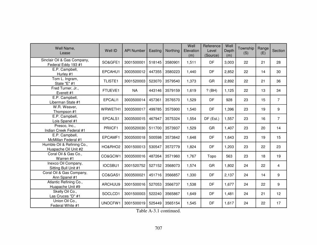
707
Well Name,
LeaseWell ID API Number Easting Northing
Well
Elevation
(m)
Reference
Level
(Source)
Well
Depth
(m)
Township
(S)
Range
(E)Section
Sinclair Oil & Gas Company,
Federal Eddy 193 #1SO&GFE1 3001500001 518145 3580901 1,511 DF 3,003 22 21 28
E.P. Campbell,
Hurley #1EPCAHU1 3003500012 447355 3580223 1,440 DF 2,852 22 14 30
Tom L. Ingram,
State "E" #1TLISTE1 3001520003 523070 3579540 1,373 GR 2,892 22 21 36
Fred Turner, Jr.,
Everett #1FTUEVE1 NA 443146 3579159 1,619 ? (BH) 1,125 22 13 34
E.P. Campbell,
Liberman State #1EPCALI1 3003500014 457361 3576570 1,529 DF 928 23 15 7
W.R. Weaver,
Thompson #1WRWETH1 3003500017 499785 3575900 1,540 DF 1,396 23 19 9
E.P. Campbell,
Lois Spanel #1EPCALS1 3003500015 467947 3575324 1,554 DF (Est.) 1,557 23 16 7
Presco, Inc.,
Indian Creek Federal #1PRIICF1 3003520030 511700 3573937 1,529 GR 1,407 23 20 14
E.P. Campbell,
McMillan Federal #1EPCAMF1 3003500018 500598 3573842 1,648 DF 1,643 23 19 15
Humble Oil & Refining Co.,
Huapache Oil Unit #2HO&RHO2 3001500013 530547 3572779 1,824 DF 1,203 23 22 23
Coral Oil & Gas Co.,
Warren #1CO&GCW1 3003500016 487264 3571960 1,767 Topo 563 23 18 19
Inexco Oil Company,
Sitting Bull Unit #1IOCSBU1 3001520752 527152 3568073 1,574 GR 1,802 24 22 4
Coral Oil & Gas Company,
Ann Spanel #1CO&GAS1 3003500021 451716 3566857 1,330 DF 2,137 24 14 9
Atlantic Refining Co.,
Huapache Unit #9ARCHUU9 3001500016 527053 3566737 1,538 DF 1,677 24 22 9
Skelly Oil Co.,
Las Cruces "D" #1SOCLCD1 3001500003 522240 3565867 1,649 DF 1,481 24 21 12
Union Oil Co.,
Federal White #1UNOCFW1 3001500019 525449 3565154 1,545 DF 1,617 24 22 17
Table A-3.1 continued.

708
Well Name,
LeaseWell ID API Number Easting Northing
Well
Elevation
(m)
Reference
Level
(Source)
Well
Depth
(m)
Township
(S)
Range
(E)Section
Humble Oil & Refining Co.,
Huapache Unit #5HO&RHU5 3001500018 531153 3564735 1,511 DF 3,003 24 22 14
Threshold Development Co.,
Chiricahua R 21 Federal #1TDCR21F 3003520034 489264 3563381 1,440 GR 2,852 24 18 21
Fred Turner, Jr.
(aka Pasotero Pet. Corp.),
Evans #1
FTUJEV1 3003500020 433355 3563003 1,373 ? (BH) 2,892 24 12 22
E.P. Campbell (aka John J. Eisner),
Federal #1EPCAFE1 3003500019 432641 3562887 1,619 DF 1,125 24 12 21
Flynn, Welch, Yates,
Donahue #1FWYDON1 NA 460768 3561350 1,529 ? (Dunn) 928 24 15 28
Franklin, Aston & Fair, Inc.,
Turkey Draw Unit #1FA&FTD1 3001521378 524583 3560015 1,540 GR 1,396 24 22 31
Union Oil Co.,
McMillan #1UNOCMC1 3003500028 440825 3557266 1,554 Topo 1,557 25 13 9
Union Oil Co.,
Verse 7 Federal #1UOCV7F1 3001520591 524435 3556316 1,529 GR 1,407 25 22 7
W.W. West,
West Dog Canyon Unit #1WWWWDC1 3003520007 505979 3555044 1,648 GR 1,643 25 20 18
Transocean Oil,
G.J. Ablah #1TROGJA1 3003520018 442810 3554817 1,824 GR 1,203 25 13 15
R.H. Ernest,
Located Land Co. #1RHELLC1 3003500023 382791 3553354 1,767 USGS 563 25 7 20
Threshold Development Co.,
Mescalero 28 Federal #1TDM28F1 3003520033 489514 3552255 1,574 GR 1,802 25 18 28
Beard Oil Company,
Ridge USA #1BOCRUS1 3001522547 524447 3551405 1,330 GR 2,137 25 22 30
Pennzoil Co.,
Southland "28" State #1PCS28S1 3003520019 479573 3551070 1,538 GR 1,677 25 17 28
Fred Turner, Jr.,
State #1FTUJST1 3003500027 475070 3550274 1,649 DF 1,481 25 16 36
Table A-3.1 continued.

709
Well Name,
LeaseWell ID API Number Easting Northing
Well
Elevation
(m)
Reference
Level
(Source)
Well
Depth
(m)
Township
(S)
Range
(E)Section
E.J. Dunigan,
Alpha Federal #1EJDALF1 3003520002 496594 3549815 1,511 KB 3,003 25 19 31
GDP 61-6 GDP61-6 NA 390213 3549130 1,440 WH 2,852 26 8 6
GDP 45-5 GDP45-5 NA 391837 3549102 1,373 WH 2,892 26 8 5
GDP 46-6 GDP46-6 NA 390223 3549119 1,619 WH 1,125 26 8 6
Hunt Oil Co.,
McMillan-Turner #1HUOCMT1 3003500029 469015 3547882 1,529 ? (Dunn) 928 26 16 5
Harvey E. Yates Co.,
Bennett Ranch Unit #1HEYBRU1 3003520027 435547 3545814 1,540 GR 1,396 26 12 14
Seaboard Oil Co.,
Trigg-Federal #1SEOCTF1 3003500032 418801 3545797 1,554 DF 1,557 26 11 18
GDP 51-8 GDP51-8 NA 393417 3545870 1,529 WH 1,407 26 8 16
E.P. Campbell,
Spiegel-Federal #1EPCSPF1 3003510002 511803 3544568 1,648 Topo 1,643 26 20 14
Sinclair Oil & Gas Co.,
Guadalupe Ridge Unit #1SO&GGR1 3001520176 519670 3543204 1,824 GR 1,203 26 21 22
Harvey E. Yates Co.,
Bennett Ranch Unit 25 #1HEYBR25 3003520031 437133 3542284 1,767 ? 563 26 12 25
Table A-3.1 continued:
API Number Key: NA = Not applicable. Reference Level (Source) Key: GR = Ground surface, KB = Kelley bushing, TH = Tubing head, DF = Derrick floor, WH = Well head, ? = unknown if elevation is from GR, KB, TH, DF, or WH, DEM = from USGS NED, Topo = GR from topo. map, BH = from Broadhead (2007), Est. = Estimated, Dunn = from Dunn NMGS (1954), USGS = from USGS.
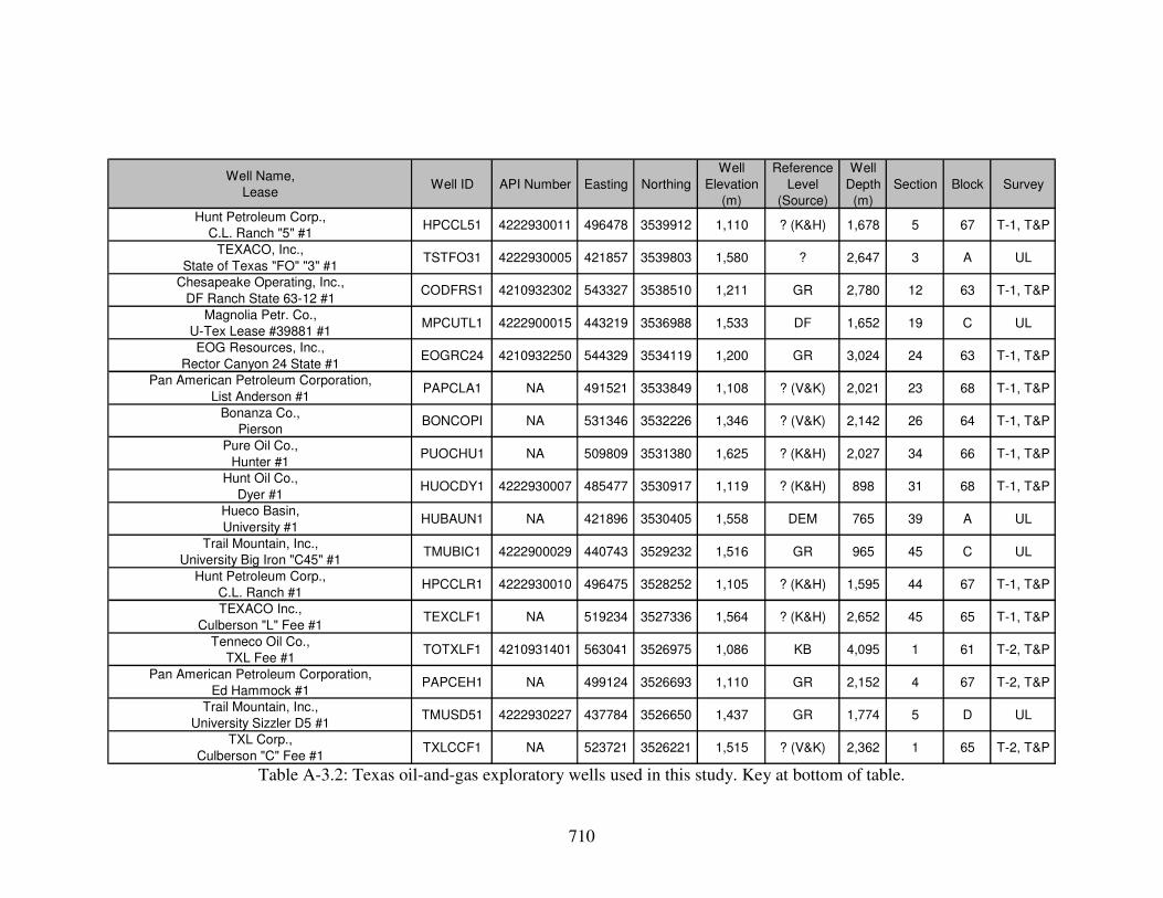
710
Well Name,
LeaseWell ID API Number Easting Northing
Well
Elevation
(m)
Reference
Level
(Source)
Well
Depth
(m)
Section Block Survey
Hunt Petroleum Corp.,
C.L. Ranch "5" #1HPCCL51 4222930011 496478 3539912 1,110 ? (K&H) 1,678 5 67 T-1, T&P
TEXACO, Inc.,
State of Texas "FO" "3" #1TSTFO31 4222930005 421857 3539803 1,580 ? 2,647 3 A UL
Chesapeake Operating, Inc.,
DF Ranch State 63-12 #1CODFRS1 4210932302 543327 3538510 1,211 GR 2,780 12 63 T-1, T&P
Magnolia Petr. Co.,
U-Tex Lease #39881 #1MPCUTL1 4222900015 443219 3536988 1,533 DF 1,652 19 C UL
EOG Resources, Inc.,
Rector Canyon 24 State #1EOGRC24 4210932250 544329 3534119 1,200 GR 3,024 24 63 T-1, T&P
Pan American Petroleum Corporation,
List Anderson #1PAPCLA1 NA 491521 3533849 1,108 ? (V&K) 2,021 23 68 T-1, T&P
Bonanza Co.,
PiersonBONCOPI NA 531346 3532226 1,346 ? (V&K) 2,142 26 64 T-1, T&P
Pure Oil Co.,
Hunter #1PUOCHU1 NA 509809 3531380 1,625 ? (K&H) 2,027 34 66 T-1, T&P
Hunt Oil Co.,
Dyer #1HUOCDY1 4222930007 485477 3530917 1,119 ? (K&H) 898 31 68 T-1, T&P
Hueco Basin,
University #1HUBAUN1 NA 421896 3530405 1,558 DEM 765 39 A UL
Trail Mountain, Inc.,
University Big Iron "C45" #1TMUBIC1 4222900029 440743 3529232 1,516 GR 965 45 C UL
Hunt Petroleum Corp.,
C.L. Ranch #1HPCCLR1 4222930010 496475 3528252 1,105 ? (K&H) 1,595 44 67 T-1, T&P
TEXACO Inc.,
Culberson "L" Fee #1TEXCLF1 NA 519234 3527336 1,564 ? (K&H) 2,652 45 65 T-1, T&P
Tenneco Oil Co.,
TXL Fee #1TOTXLF1 4210931401 563041 3526975 1,086 KB 4,095 1 61 T-2, T&P
Pan American Petroleum Corporation,
Ed Hammock #1PAPCEH1 NA 499124 3526693 1,110 GR 2,152 4 67 T-2, T&P
Trail Mountain, Inc.,
University Sizzler D5 #1TMUSD51 4222930227 437784 3526650 1,437 GR 1,774 5 D UL
TXL Corp.,
Culberson "C" Fee #1TXLCCF1 NA 523721 3526221 1,515 ? (V&K) 2,362 1 65 T-2, T&P
Table A-3.2: Texas oil-and-gas exploratory wells used in this study. Key at bottom of table.

711
Well Name,
LeaseWell ID API Number Easting Northing
Well
Elevation
(m)
Reference
Level
(Source)
Well
Depth
(m)
Section Block Survey
General Crude Oil Company,
Merrill and Voyles et al. #1GCOCMV1 NA 477481 3524877 1,580 DF 2,647 8 69 T-2, T&P
Magnolia Petro.,
No. A-1 Homer, CowdenMPNA1HC NA 544286 3524346 1,211 ? (V&K) 2,780 12 63 T-2, T&P
EOG Resources, Inc.,
Kenney 16 State #1HEOGKS1H 4210932270 527946 3523355 1,533 GR 1,652 16 64 T-2, T&P
EOG Resources, Inc.,
Kenney 16 State #2EOGKES2 4210932269 528404 3522559 1,200 GR 3,024 16 64 T-2, T&P
California Standard of Texas,
Theisen #1CASATT1 NA 426103 3521248 1,108 ? 2,021 19 E UL
D & J Equip Co.,
J.C. Hunter, Jr. #2DJJCHJ2 NA 512403 3519886 1,346 ? (V&K) 2,142 2 120 PSL
Trail Mountain, Inc.,
University Felina "D27" #1TMUFD27 4222930006 439917 3518350 1,625 GR 2,027 27 D UL
Border Exploration Co.,
Hammack et al. CT-1BECHCT1 4222930196 505172 3518026 1,119 ? (K&H) 898 20 120 PSL
TXL Oil Corp.,
Culberson B-T Fee #1TXLCBT1 NA 550456 3517797 1,558 ? (V&K) 765 33 62 T-2, T&P
A.R. Jones Co.,
E.C. Mowry #1ARJECM1 NA 474192 3516927 1,516 DF 965 36 70 T-2, T&P
Tipperary Corp.,
ST-1 Billye SparksTCST1BS 4222930195 474281 3516816 1,105 GR 1,595 36 70 T-2, T&P
J.L. Cowley,
E.C. Mowry #1JLCECM1 NA 473079 3515907 1,564 ? 2,652 37 70 T-2, T&P
Border Exploration Co.,
J.J. McAdoo 7 #1BECJJM1 4222930200 505794 3514682 1,086 ? (K&H) 4,095 7 119 PSL
T.E. Robertson Co., Inc.,
Mowry et al. #2TERCMO2 NA 471217 3514010 1,110 DF 2,152 47 70 T-2, T&P
The Superior Oil Company,
Covington State #1TSOCCS1 4210931405 565213 3512927 1,437 GR 1,774 1 115 PSL
Chesapeake Operating, Inc.,
Dela Minerals "3" State #701COIDM3S 4210932268 566918 3512065 1,515 GR 2,362 7 114 PSL
Trail Mountain, Inc.,
University Devil Woman L5 #1TMUDWL5 4222930253 477595 3510876 1,181 GR 1,461 5 L UL
Table A-3.2 continued.

712
Well Name,
LeaseWell ID API Number Easting Northing
Well
Elevation
(m)
Reference
Level
(Source)
Well
Depth
(m)
Section Block Survey
Samson Lone Star, L.L.C.,
University Lands 46-14 #2SALSUL2 4210932278 551660 3509591 1,110 KB 1,678 14 46 UL
Humble Oil & Ref. Co.,
M.C. Sibley #1HORMCS1 NA 533795 3508569 1,580 ? (V&K) 2,647 24 68 PSL
N. Amer. Royalties, Inc.,
Potter #1NARIPO1 NA 511738 3508091 1,211 ? (V&K) 2,780 31 119 PSL
Chesapeake Operating, Inc.,
University Lands 4627 #1COUL462 4210932287 550571 3507028 1,533 GR 1,652 27 46 UL
J.M. Huber Corp.,
Tom Potter #1JMHCTP1 NA 514111 3505748 1,200 ? (V&K) 3,024 2 118 PSL
EnCana Oil & Gas (USA) Inc.,
Sibley Ranch 47 State "25" #1EOGSR47 4210932251 544180 3505778 1,108 KB 2,021 25 47 PSL
Anderson & Prichard,
Bordens #1A&PBOR1 NA 521137 3505265 1,346 ? (V&K) 2,142 34 69 PSL
Trail Mountain, Inc.,
University Ooby Dooby L35 #1TMUODL1 4222930261 482251 3502319 1,625 KB 2,027 35 L UL
Petro-Hunt, L.L.C.,
Melissa Taylor State 27 #1-HPHMTS27 4210932255 563684 3501318 1,119 GR 898 27 109 PSL
Faith Minerals, Inc.,
Wesley West #1FMINWW1 4222930012 503401 3499500 1,558 GR 765 36 118 PSL
American Quasar Pet. Co.,
V.C. Rounsaville #1AQPVCR1 NA 563477 3498883 1,516 ? (V&K) 965 13 108 PSL
Hassle Hunt Trust,
Univ. "M-49" #1HHUM491 NA 450328 3497929 1,105 DF 1,595 9 M UL
EOG Resources, Inc.,
Wild Horse Draw 7 #1EOGWHD7 4210932256 536584 3497771 1,564 GR 2,652 7 106 PSL
Pan American Pet. Corp.,
Phillip F. Hass #1PAPPFH1 NA 422942 3494846 1,086 DF 4,095 14 13 PSL
Chesapeake Operating, Inc.,
Melissa Taylor State 105-3COMT105 4210932297 541293 3493028 1,110 GR 2,152 3 105 PSL
Transocean Oil, Inc.,
36-1 MSA Trustee, Inc.TO36MSA 4222930192 424652 3490962 1,437 KB 1,774 36 13 PSL
El Paso Co.,
No. 1 MontgomeryEPCN1MO NA 546957 3484390 1,515 ? (V&K) 2,362 17 100 PSL
Table A-3.2 continued.

713
Well Name,
LeaseWell ID API Number Easting Northing
Well
Elevation
(m)
Reference
Level
(Source)
Well
Depth
(m)
Section Block Survey
Gulf Oil Corp.,
M.A. Grisham #1GOCMAG1 NA 535928 3484129 1,110 ? (V&K) 1,678 18 99 PSL
Hassle Hunt Trust,
Mosely #1HAHUTM1 NA 449636 3483385 1,580 GR 2,647 27 24 PSL
Lockhart, Roseborough & Benton,
Gardner & Mosely #1
or
Western States Oil,
Gardner & Moseley #1
LR&BGM1
or
WSOG&M1
NA 442367 3480668 1,211 DF 2,780 12 18 PSL
Chesapeake Operating, Inc.,
State Street State #701COSS701 4210932271 546492 3478738 1,533 GR 1,652 7 97 PSL
Sinclair,
LooneySINCLOO NA 551319 3475371 1,200 ? (V&K) 3,024 22 97 PSL
Gulf Oil Corp.,
J. Burner-State "B" #1GOCJBS1 NA 441556 3472050 1,108 DF 2,021 14 19 PSL
Lockhart Bros.,
Gardner & Mosely (Formerly Public School) #1LOBG&M1 NA 446485 3468512 1,346 ? 2,142 5 21 PSL
Stanolind Oil & Gas Co. American Land,
No. 1 RoseboroughSOGAL1R NA 444464 3467169 1,625 ? (V&K) 2,027 7 21 PSL
J.P. Hurndall & R.A. Gray,
J.S. Pierce #1H&GJSP1 NA 479266 3465692 1,119 DEM 898 8 46 PSL
Fred A. Davis West and Armour,
Davis #1FADWAD1 NA 528309 3464645 1,558 ? (V&K) 765 5 86 PSL
Table A-3.2 continued:
API Number Key: NA = Not applicable. Reference Level (Source) Key: GR = Ground surface, KB = Kelley bushing, DF = Derrick floor, ? = unknown if elevation is from GR, KB, or DF, DEM = from USGS NED, K&H = from King and Harder (1985), V&K = from Veldhuis and Keller (1980).

714
Well Name,
LeaseWell ID API Number Easting Northing
Well
Elevation
(m)
Depth to Top
of
Precambrian
(m)
Elevation of Top
of
Precambrian
(m)
Source Note
Houston Oil & Minerals Corp.,
State L.G. "1453" #1HO&MSL1 3003520013 406876 3685414 1,511 2,999 -1,489 NMBG DL
Houston Oil & Minerals Corp.,
Lewelling #2HO&MCL2 3003520015 399960 3684444 1,373 2,713 -1,339 OCD
Houston Oil & Minerals Corp.,
J.M. Lewelling #1HO&MJL1 3003520010 402778 3684425 1,434 Est. -1,425 F Estimate from Foster (1978)
Houston Oil & Minerals Corp.,
State 3724 #1HO&MS31 3003520011 412512 3657622 1,540 1,372 169 OCD
McClellan Oil Corp.,
Flying "H" Ranch Unit Tract 3 #1MCOCFH1 3000562244 497349 3652108 1,554 1,432 122 OCD
Humble Oil & Refining Co.,
Yates Federal #1HO&RYF1 3000560015 486777 3649300 1,648 Est. -30 BH Estimate from Broadhead (2007)
J. Cleo Thompson,
State A-6 #1JCTSA61 3000562988 477111 3646836 1,824 1,180 644 OCD
Lubbook Machine & Supply Co., Inc.,
Anderson-Randell #1LM&SAR1 3000500003 472069 3645946 1,767 539 1,228 OCD
Humble Oil & Refining Co.,
Humble-Yates N.M. State #1HO&RHY1 3000510521 488336 3643533 1,574 1,798 -225 OCD
W.H. Black Drilling Co.,
Shildneck #1WHBDCS1 3000500012 514561 3641046 1,330 2,131 -801 NMBG SC
Continental Oil Company,
State NN #1COCSNN1 3000560185 492051 3640997 1,538 1,822 -284 OCD Estimate based on nearby wells
J. Cleo Thompson,
Federal A-28 #1JCTFA28 3000562915 479948 3639939 1,649 1,461 188 OCD
C & K Petroleum, Inc.,
Singer Lake State #1C&KSLS1 3000560320 495659 3637945 1,545 1,830 -285 OCD Estimate based on nearby wells
Southern Production Co.,
Cloudcroft Unit #1SPCCLU1 3003500002 431152 3635650 2,859 1,402 1,457 BH
Yates Petroleum Corporation,
Dunken Nose Unit #1YPCDNU1 3000560383 491492 3635055 1,602 1,860 -258 OCD Estimate based on nearby wells
Yates Petroleum Corporation,
Dunken Dome Unit #2YPCDDU2 3000560397 485994 3634588 1,631 1,726 -95 OCD Estimate based on nearby wells
Yates Petroleum Corporation,
Dunken Dome Unit #1YPCDDU1 3000560374 486211 3634277 1,643 1,763 -119 OCD
C & K Petroleum, Inc.,
Little Cuevo State #1C&KLCS1 3000560324 501605 3632606 1,464 2,152 -689 OCD Estimate based on nearby wells
Liberty Oil & Gas Corp.,
T.L. Watts #1LO>LW 3000560766 480341 3631643 1,633 1,751 -118 BH
Magnolia,
Headley Federal #2MAGHEF2 NA 512347 3631229 1,510 1,749 -239 BH Estimate based on nearby wells
Yates Petroleum Corporation,
Little Cuevo Unit #1YPCLCU1 3000561785 488273 3631027 1,633 1,751 -118 NMBG SC
Table A-3.3: Oil-and-gas exploratory wells used as control for the top of the Precambrian. Key at bottom of table.

715
Well Name,
LeaseWell ID API Number Easting Northing
Well
Elevation
(m)
Depth to Top
of
Precambrian
(m)
Elevation of Top
of
Precambrian
(m)
Source Note
Sunray DX Oil Company,
N.M. State "AV" #1SOCSAV1 3000510144 491916 3630614 1,582 1,795 -213 OCD
Westcoast Hydrocarbons, Inc.,
Black Hills Unit #1WHIBHU1 3000500013 508897 3629768 1,453 1,748 -295 NMBG SC Estimate based on nearby wells
Yates Petroleum Corporation,
Little Cuevo Unit #2YPCLCU2 3000562268 489571 3628557 1,618 1,666 -48 OCD Estimate based on nearby wells
Magnolia,
Black HillsMAGBLHI NA 505927 3627975 1,494 Est. -229 BH Estimate from Broadhead (2007)
Gulf Oil Corporation,
Chaves State "U" #1GOCCSU1 3000500002 472386 3625264 1,907 905 1,002 OCD
TEXACO Inc.,
Federal (USA) "E" #1TEXIFE1 3003520001 395308 3624999 1,219 Est. -1,285 F
Yates Petroleum Corporation,
One Tree Unit #1YPCOTU1 3000562259 467160 3623529 1,876 1,976 -100 NMBG SC
Yates Petroleum Corporation,
Dog Canyon "YF" Federal #1YPCDCF1 3003520024 462754 3622676 1,946 2,512 -566 NMBG SC
Texas Oil & Gas Corp.,
Federal "C" #1TO&GFC1 3000560017 512954 3622309 1,359 Est. -1,054 BH Estimate from Broadhead (2007)
TEXACO Inc.,
Federal (USA) "F" #1TEXIFF1 3003520006 410790 3619951 1,232 Est. -1,481 F Estimate from Foster (1978)
Kewanee Oil Co.,
F-M Unit #1KOCFMU1 3000500009 493140 3619927 1,579 2,307 -728 NMBG SC Estimate based on nearby wells
TEXACO Inc.,
Federal (USA) "G" #1TEXIFG1 3003520004 394443 3619379 1,276 Est. -1,242 F Estimate from Foster (1978)
Yates Petroleum Corporation,
One Tree Unit #2YPCOTU2 3000562276 468582 3619170 2,010 824 1,185 NMBG SC
Marathon Oil Co.,
Mesa Verde Ranch #1MOCMVR1 3003520022 455326 3618246 2,143 2,123 20 NMBG SC
Yates Petroleum Corp.,
Buckhorn AYU State Com #1YPCBAYU 3000560541 506142 3613140 1,440 Est. -962 BH Estimate from Broadhead (2007)
Texas Oil & Gas Corp.,
Federal "A" #1TO&GFA1 3000510431 506950 3613041 1,442 2,496 -1,054 BH Estimate based on nearby wells
Yates Petroleum Corporation (aka Phoenix Resources Co.),
Bullis "AVW" State Com (aka Ranch Road) #1YPCBAVW 3000560557 507355 3612640 1,478 2,553 -1,075 NMBG SC Estimate based on nearby wells
Sun Oil Co.,
Pinon Unit #2SOCPIU2 3000500007 478157 3612259 1,925 501 1,424 NMBG SC
Sun Oil Co.,
Pinon Unit #1SOCPIU1 3000500006 476922 3611828 1,995 526 1,469 NMBG SC
U.V. Industries, Inc.,
Long Canyon Unit #1UVILCU1 3000560411 502547 3610225 1,536 Est. -1,072 BH Estimate from Broadhead (2007)
Table A-3.3 continued.

716
Well Name,
LeaseWell ID API Number Easting Northing
Well
Elevation
(m)
Depth to Top
of
Precambrian
(m)
Elevation of Top
of
Precambrian
(m)
Source Note
Gulf Oil Corp.,
Federal Munson #1GOCFMU1 3000510075 489407 3609839 1,723 1,402 321 NMBG SC
Plymouth Oil Co.,
Evans (aka Federal D) #1PLOCEV1 3003500003 404731 3604561 1,233 Est. -1,141 F Estimate from Foster (1978)
Texas Oil & Gas Corp.,
Federal "B" #1TO&GFB1 NA 510832 3603835 1,463 2,837 -1,374 NMBG SC Estimate based on nearby wells
Atlantic Refining Co.,
State "AV" #1ARCSAV1 3003510001 461443 3603143 1,921 Est. -100 BH Estimate from Broadhead (2007)
Zapata Petroleum Corp.,
Federal 14 #1ZPCF141 3003500006 454127 3603086 2,109 Est. 326 F Estimate from Foster (1978)
Sun Oil Company,
T.J. Pearson #1SOCTJP1 3003500005 416750 3598464 1,344 Est. -302 F Estimate from Foster (1978)
Terra Resources, Inc.,
Burro Canyon Unit #1-YTRBCU1Y 3003520017 511686 3596471 1,572 Est. -466 BH Estimate from Broadhead (2007)
Stanolind Oil & Gas,
Thorn Unit #1SO>U1 3003500007 453419 3593869 1,914 Est. 72 F Estimate from Foster (1978)
Standard of Texas,
Scarp Unit #1SOTSCU1 3003500009 487438 3593394 1,628 786 842 NMBG SC
Lefors Petroleum Co.,
Federal #1LEPCFE1 3003500008 471863 3592611 1,642 677 964 NMBG SC
Tri-Service Drilling Co.,
Little Dog Federal #1TSDLDF1 3003520008 496060 3586992 1,940 Est. 451 BH Estimate from Broadhead (2007)
Brainerd Corp. (aka Continental Oil Co.),
Federal "A" (aka East Texas Hill Unit) #1BRCFEA1 3001500005 523406 3586429 1,397 3,248 -1,851 NMBG SC Estimate based on nearby wells
Continental Oil Co.,
H.W. Bass #1COCHWB1 3001500004 516898 3586367 1,680 1,636 43 NMBG SC Estimate based on nearby wells
Marathon Oil Company,
Box Canyon Unit #1MOCBCU1 3001510012 522193 3586059 1,426 3,206 -1,780 OCD Estimate based on nearby wells
E.P. Campbell,
Hurley #1EPCAHU1 3003500012 447355 3580223 1,404 Est. 198 F Estimate from Foster (1978)
Fred Turner, Jr.,
Everett #1FTUEVE1 NA 443146 3579159 1,476 Est. 248 F Estimate from Foster (1978)
E.P. Campbell,
Liberman State #1EPCALI1 3003500014 457361 3576570 1,326 819 507 K&H
W.R. Weaver,
Thompson #1WRWETH1 3003500017 499785 3575900 1,386 Est. 14 BH Estimate from Broadhead (2007)
E.P. Campbell,
Lois Spanel #1EPCALS1 3003500015 467947 3575324 1,408 908 500 K&H Estimate based on nearby wells
E.P. Campbell,
McMillan Federal #1EPCAMF1 3003500018 500598 3573842 1,319 Est. -98 BH Estimate from Broadhead (2007)
Humble Oil & Refining Co.,
Huapache Oil Unit #2HO&RHO2 3001500013 530547 3572779 1,358 3,823 -2,465 OCD
Table A-3.3 continued.

717
Well Name,
LeaseWell ID API Number Easting Northing
Well
Elevation
(m)
Depth to Top
of
Precambrian
(m)
Elevation of Top
of
Precambrian
(m)
Source Note
Coral Oil & Gas Co.,
Warren #1CO&GCW1 3003500016 487264 3571960 1,186 687 499 K&H
Inexco Oil Company,
Sitting Bull Unit #1IOCSBU1 3001520752 527152 3568073 1,650 2,329 -679 OCD Estimate based on nearby wells
Coral Oil & Gas Company,
Ann Spanel #1CO&GAS1 3003500021 451716 3566857 1,391 556 835 OCD
Skelly Oil Co.,
Las Cruces "D" #1SOCLCD1 3001500003 522240 3565867 1,749 2,411 -663 NMBG SC Estimate based on nearby wells
Union Oil Co.,
Federal White #1UNOCFW1 3001500019 525449 3565154 1,740 Est. -714 BH Estimate from Broadhead (2007)
Threshold Development Co.,
Chiricahua R 21 Federal #1TDCR21F 3003520034 489264 3563381 1,133 816 317 OCD
Fred Turner, Jr. (aka Pasotero Pet. Corp.),
Evans #1FTUJEV1 3003500020 433355 3563003 1,545 Est. 370 F Estimate from Foster (1978)
E.P. Campbell (aka John J. Eisner),
Federal #1EPCAFE1 3003500019 432641 3562887 1,497 1,138 358 NMBG SC Estimate based on nearby wells
Franklin, Aston & Fair, Inc.,
Turkey Draw Unit #1FA&FTD1 3001521378 524583 3560015 1,776 2,786 -1,010 OCD Estimate based on nearby wells
Union Oil Co.,
McMillan #1UNOCMC1 3003500028 440825 3557266 1,522 Est. -27 F Estimate from Foster (1978)
Union Oil Co.,
Verse 7 Federal #1UOCV7F1 3001520591 524435 3556316 1,801 2,842 -1,041 OCD Estimate based on nearby wells
Transocean Oil,
G.J. Ablah #1TROGJA1 3003520018 442810 3554817 1,509 1,376 133 K&H
R.H. Ernest,
Located Land Co. #1RHELLC1 3003500023 382791 3553354 1,249 Est. -987 F Estimate from Foster (1978)
Threshold Development Co.,
Mescalero 28 Federal #1TDM28F1 3003520033 489514 3552255 1,219 831 387 OCD
Beard Oil Company,
Ridge USA #1BOCRUS1 3001522547 524447 3551405 1,896 3,164 -1,267 OCD Estimate based on nearby wells
Pennzoil Co.,
Southland "28" State #1PCS28S1 3003520019 479573 3551070 1,206 1,181 25 K&H Estimate based on nearby wells
Fred Turner, Jr.,
State #1FTUJST1 3003500027 475070 3550274 1,317 939 379 K&H
E.J. Dunigan,
Alpha Federal #1EJDALF1 3003520002 496594 3549815 1,159 Est. -755 BH Estimate from Broadhead (2007)
GDP 61-6 GDP61-6 NA 390213 3549130 1,254 1,859 -605 F&J Estimate based on nearby wells
GDP 46-6 GDP46-6 NA 390223 3549119 1,252 1,853 -601 F&J Estimate based on nearby wells
GDP 45-5 GDP45-5 NA 391837 3549102 1,255 Est. -432 BH Estimate from Broadhead (2007)
Hunt Oil Co.,
McMillan-Turner #1HUOCMT1 3003500029 469015 3547882 1,269 573 696 BH
GDP 51-8 GDP51-8 NA 393417 3545870 1,253 Est. 223 BH Estimate from Broadhead (2007)
Table A-3.3 continued.

718
Well Name,
LeaseWell ID API Number Easting Northing
Well
Elevation
(m)
Depth to Top
of
Precambrian
(m)
Elevation of Top
of
Precambrian
(m)
Source Note
Harvey E. Yates Co.,
Bennett Ranch Unit #1HEYBRU1 3003520027 435547 3545814 1,554 2,154 -599 OCD
Seaboard Oil Co.,
Trigg-Federal #1SEOCTF1 3003500032 418801 3545797 1,618 Est. -894 F Estimate from Foster (1978)
Harvey E. Yates Co.,
Bennett Ranch Unit 25 #1HEYBR25 3003520031 437133 3542284 1,533 1,962 -429 OCD Estimate based on nearby wells
TEXACO, Inc.,
State of Texas "FO" "3" #1TSTFO31 4222930005 421857 3539803 1,580 2,647 -1,066 BEG SC In Precambrian at total well depth
Magnolia Petr. Co.,
U-Tex Lease #39881 #1MPCUTL1 4222900015 443219 3536988 1,533 1,654 -121 BEG SC Estimate based on nearby wells
EOG Resources, Inc.,
Rector Canyon 24 State #1EOGRC24 4210932250 544329 3534119 1,200 3,630 -2,430 RRC Estimate based on nearby wells
Pan American Petroleum Corporation,
List Anderson #1PAPCLA1 NA 491521 3533849 1,108 905 203 V&K
Pure Oil Co.,
Hunter #1PUOCHU1 NA 509809 3531380 1,625 2,149 -524 K&H Estimate based on nearby wells
Hunt Oil Co.,
Dyer #1HUOCDY1 4222930007 485477 3530917 1,119 1,212 -93 K&H Estimate based on nearby wells
Trail Mountain, Inc.,
University Big Iron "C45" #1TMUBIC1 4222900029 440743 3529232 1,516 1,667 -151 RRC Estimate based on nearby wells
Hunt Petroleum Corp.,
C.L. Ranch #1HPCCLR1 4222930010 496475 3528252 1,105 2,206 -1,101 K&H Estimate based on nearby wells
TEXACO Inc.,
Culberson "L" Fee #1TEXCLF1 NA 519234 3527336 1,564 2,850 -1,286 K&H Estimate based on nearby wells
Tenneco Oil Co.,
TXL Fee #1TOTXLF1 4210931401 563041 3526975 1,086 4,291 -3,205 RRC Estimate based on nearby wells
Pan American Petroleum Corporation,
Ed Hammock #1PAPCEH1 NA 499124 3526693 1,110 2,245 -1,135 V&K Estimate based on nearby wells
Trail Mountain, Inc.,
University Sizzler D5 #1TMUSD51 4222930227 437784 3526650 1,437 2,468 -1,031 RRC Estimate based on nearby wells
TXL Corp.,
Culberson "C" Fee #1TXLCCF1 NA 523721 3526221 1,515 2,943 -1,429 V&K Estimate based on nearby wells
General Crude Oil Company,
Merrill and Voyles et al. #1GCOCMV1 NA 477481 3524877 1,181 1,443 -262 BEG WR
Magnolia Petro.,
No. A-1 Homer, CowdenMPNA1HC NA 544286 3524346 1,194 3,722 -2,528 V&K Estimate based on nearby wells
EOG Resources, Inc.,
Kenney 16 State #1HEOGKS1H 4210932270 527946 3523355 1,372 2,999 -1,628 RRC Estimate based on nearby wells
EOG Resources, Inc.,
Kenney 16 State #2EOGKES2 4210932269 528404 3522559 1,365 3,076 -1,711 RRC Estimate based on nearby wells
California Standard of Texas,
Theisen #1CASATT1 NA 426103 3521248 1,557 1,439 119 BEG WR
Table A-3.3 continued.

719
Well Name,
LeaseWell ID API Number Easting Northing
Well
Elevation
(m)
Depth to Top
of
Precambrian
(m)
Elevation of Top
of
Precambrian
(m)
Source Note
Trail Mountain, Inc.,
University Felina "D27" #1TMUFD27 4222930006 439917 3518350 1,427 1,292 134 RRC Estimate based on nearby wells
Border Exploration Co.,
Hammack et al. CT-1BECHCT1 4222930196 505172 3518026 1,107 2,987 -1,880 K&H Estimate based on nearby wells
TXL Oil Corp.,
Culberson B-T Fee #1TXLCBT1 NA 550456 3517797 1,236 4,072 -2,836 V&K Estimate based on nearby wells
A.R. Jones Co.,
E.C. Mowry #1ARJECM1 NA 474192 3516927 1,230 1,577 -347 BEG SC Estimate based on nearby wells
J.L. Cowley,
E.C. Mowry #1JLCECM1 NA 473079 3515907 1,234 1,432 -198 BEG SC Estimate based on nearby wells
Border Exploration Co.,
J.J. McAdoo 7 #1BECJJM1 4222930200 505794 3514682 1,143 2,811 -1,668 K&H Estimate based on nearby wells
T.E. Robertson Co., Inc.,
Mowry et al. #2TERCMO2 NA 471217 3514010 1,222 1,512 -290 BEG SC Estimate based on nearby wells
Trail Mountain, Inc.,
University Devil Woman L5 #1TMUDWL5 4222930253 477595 3510876 1,221 1,745 -524 RRC Estimate based on nearby wells
Samson Lone Star, L.L.C.,
University Lands 46-14 #2SALSUL2 4210932278 551660 3509591 1,310 4,317 -3,007 RRC Estimate based on nearby wells
Chesapeake Operating, Inc.,
University Lands 4627 #1COUL462 4210932287 550571 3507028 1,300 4,295 -2,996 RRC Estimate based on nearby wells
EnCana Oil & Gas (USA) Inc.,
Sibley Ranch 47 State "25" #1EOGSR47 4210932251 544180 3505778 1,332 3,965 -2,633 RRC Estimate based on nearby wells
Trail Mountain, Inc.,
University Ooby Dooby L35 #1TMUODL1 4222930261 482251 3502319 1,230 2,050 -820 RRC Estimate based on nearby wells
Petro-Hunt, L.L.C.,
Melissa Taylor State 27 #1-HPHMTS27 4210932255 563684 3501318 1,150 4,779 -3,629 RRC Estimate based on nearby wells
American Quasar Pet. Co.,
V.C. Rounsaville #1AQPVCR1 NA 563477 3498883 1,178 4,833 -3,655 V&K Estimate based on nearby wells
Hassle Hunt Trust,
Univ. "M-49" #1HHUM491 NA 450328 3497929 1,497 2,505 -1,009 V&K
EOG Resources, Inc.,
Wild Horse Draw 7 #1EOGWHD7 4210932256 536584 3497771 1,510 3,464 -1,954 RRC Estimate based on nearby wells
Pan American Pet. Corp.,
Phillip F. Hass #1PAPPFH1 NA 422942 3494846 1,373 2,282 -910 BEG SC
Transocean Oil, Inc.,
36-1 MSA Trustee, Inc.TO36MSA 4222930192 424652 3490962 1,551 2,290 -739 BEG SC Estimate based on nearby wells
El Paso Co.,
No. 1 MontgomeryEPCN1MO NA 546957 3484390 1,370 2,265 -895 V&K Estimate based on nearby wells
Gulf Oil Corp.,
M.A. Grisham #1GOCMAG1 NA 535928 3484129 1,729 2,060 -331 V&K Estimate based on nearby wells
Hassle Hunt Trust,
Mosely #1HAHUTM1 NA 449636 3483385 1,447 1,706 -259 V&K Estimate based on nearby wells
Table A-3.3 continued.

720
Well Name,
LeaseWell ID API Number Easting Northing
Well
Elevation
(m)
Depth to Top
of
Precambrian
(m)
Elevation of Top
of
Precambrian
(m)
Source Note
Lockhart, Roseborough & Benton,
Gardner & Mosely #1
or
Western States Oil,
Gardner & Moseley #1
LR&BGM1
or
WSOG&M1
NA 442367 3480668 1,531 1,023 508 BEG SC Estimate based on nearby wells
Sinclair,
LooneySINCLOO NA 551319 3475371 1,310 3,220 -1,910 V&K Estimate based on nearby wells
Gulf Oil Corp.,
J. Burner-State "B" #1GOCJBS1 NA 441556 3472050 1,418 2,786 -1,369 BEG SC
Lockhart Bros.,
Gardner & Mosely (Formerly Public School) #1LOBG&M1 NA 446485 3468512 1,481 543 938 BEG SC
Stanolind Oil & Gas Co. American Land,
No. 1 RoseboroughSOGAL1R NA 444464 3467169 1,463 488 975 V&K
J.P. Hurndall & R.A. Gray,
J.S. Pierce #1H&GJSP1 NA 479266 3465692 1,488 456 1,032 BEG SC Estimate based on nearby wells
Fred A. Davis West and Armour,
Davis #1FADWAD1 NA 528309 3464645 1,146 1,417 -271 V&K Estimate based on nearby wells
Table A-3.3 continued. API Number Key: NA = Not applicable. Depth to Top of … Key: Est. = Estimate. Source Key: BEG SC = Scout cards from the Bureau of Economic Geology’s Austin Core Research Center, BEG WR = Well records from the Bureau of Economic Geology’s Austin Core Research Center, BH = Broadhead (2007), F = Foster (1978), F&J = Finger and Jacobson (1997), K&H = King and Harder (1985), NMBG DL = Driller’s logs from the New Mexico Subsurface Data Library at the New Mexico Bureau of Geology and Mineral Resources, NMBG SC = Scout cards from the New Mexico Subsurface Data Library at the New Mexico Bureau of Geology and Mineral Resources, OCD = Oil Conservation Division online well files, RRC = Railroad Commission of Texas, V&K = Veldhuis and Keller (1980).

721
Well Name,
LeaseWell ID API Number Easting Northing
Well
Elevation
(m)
Depth to Top
of Bliss
Sandstone (m)
Elevation of Top
of Bliss
Sandstone (m)
Source Note
Houston Oil & Minerals Corp.,
J.M. Lewelling #1HO&MJL1 3003520010 402778 3684425 1,440 2,841 -1,401 NMBG SC
Houston Oil & Minerals Corp.,
State 3724 #1HO&MS31 3003520011 412512 3657622 1,540 1,344 196 OCD
Humble Oil & Refining Co.,
Yates Federal #1HO&RYF1 3000560015 486777 3649300 1,648 1,631 17 OCD
J. Cleo Thompson,
State A-6 #1JCTSA61 3000562988 477111 3646836 1,824 1,140 684 OCD
Humble Oil & Refining Co.,
Humble-Yates N.M. State #1HO&RHY1 3000510521 488336 3643533 1,574 1,766 -193 OCD
W.H. Black Drilling Co.,
Shildneck #1WHBDCS1 3000500012 514561 3641046 1,330 2,027 -696 NMBG SC
J. Cleo Thompson,
Federal A-28 #1JCTFA28 3000562915 479948 3639939 1,649 1,420 229 OCD
Southern Production Co.,
Cloudcroft Unit #1SPCCLU1 3003500002 431152 3635650 2,859 1,373 1,486 BH
Yates Petroleum Corporation,
Dog Canyon "YF" Federal #1YPCDCF1 3003520024 462754 3622676 1,946 2,492 -545 NMBG SC
Yates Petroleum Corporation,
One Tree Unit #2YPCOTU2 3000562276 468582 3619170 2,010 800 1,210 NMBG SC
Marathon Oil Co.,
Mesa Verde Ranch #1MOCMVR1 3003520022 455326 3618246 2,143 2,070 73 BH
Standard of Texas,
Scarp Unit #1SOTSCU1 3003500009 487438 3593394 1,628 721 906 BH
Lefors Petroleum Co.,
Federal #1LEPCFE1 3003500008 471863 3592611 1,642 606 1,036 NMBG SC
Fred Turner, Jr.,
Everett #1FTUEVE1 NA 443146 3579159 1,476 Est. 336 K&H Estimated from K&H (1985)
Transocean Oil,
G.J. Ablah #1TROGJA1 3003520018 442810 3554817 1,509 1,334 176 K&H
Fred Turner, Jr.,
State #1FTUJST1 3003500027 475070 3550274 1,317 905 412 K&H
Harvey E. Yates Co.,
Bennett Ranch Unit #1HEYBRU1 3003520027 435547 3545814 1,554 2,108 -553 OCD
Magnolia Petr. Co.,
U-Tex Lease #39881 #1MPCUTL1 4222900015 443219 3536988 1,533 1,633 -99 BEG SC
General Crude Oil Company,
Merrill and Voyles et al. #1GCOCMV1 NA 477481 3524877 1,181 1,425 -244 BEG WR
California Standard of Texas,
Theisen #1CASATT1 NA 426103 3521248 1,557 1,333 224 BEG WR
Hassle Hunt Trust,
Univ. "M-49" #1HHUM491 NA 450328 3497929 1,497 2,401 -905 BEG SC
Table A-3.4: Oil-and-gas exploratory wells used as control for the top of the Bliss Sandstone. See key at bottom of Table A-3.3.

722
Well Name,
LeaseWell ID API Number Easting Northing
Well
Elevation
(m)
Depth to Top
of Bliss
Sandstone (m)
Elevation of Top
of Bliss
Sandstone (m)
Source Note
Pan American Pet. Corp.,
Phillip F. Hass #1PAPPFH1 NA 422942 3494846 1,373 2,198 -826 BEG SC
Lockhart, Roseborough & Benton,
Gardner & Mosely #1
or
Western States Oil,
Gardner & Moseley #1
LR&BGM1
or
WSOG&M1
NA 442367 3480668 1,531 914 617 BEG SC
Gulf Oil Corp.,
J. Burner-State "B" #1GOCJBS1 NA 441556 3472050 1,418 2,611 -1,193 BEG SC
J.P. Hurndall & R.A. Gray,
J.S. Pierce #1H&GJSP1 NA 479266 3465692 1,488 316 1,172 BEG SC
Table A-3.4 continued.

723
Well Name,
LeaseWell ID API Number Easting Northing
Well
Elevation
(m)
Depth to Top
of El Paso/
Ellenburger
Group (m)
Elevation of Top
of El Paso/
Ellenburger
Group (m)
Source Note
Houston Oil & Minerals Corp.,
State L.G. "1453" #1HO&MSL1 3003520013 406876 3685414 1,511 2,979 -1,469 NMBG DL
Houston Oil & Minerals Corp.,
J.M. Lewelling #1HO&MJL1 3003520010 402778 3684425 1,440 2,804 -1,365 OCD
Houston Oil & Minerals Corp.,
State 3724 #1HO&MS31 3003520011 412512 3657622 1,540 1,301 239 OCD
Humble Oil & Refining Co.,
Yates Federal #1HO&RYF1 3000560015 486777 3649300 1,648 1,581 67 OCD
J. Cleo Thompson,
State A-6 #1JCTSA61 3000562988 477111 3646836 1,824 1,074 750 OCD
W.H. Black Drilling Co.,
Shildneck #1WHBDCS1 3000500012 514561 3641046 1,330 1,935 -605 NMBG SC
J. Cleo Thompson,
Federal A-28 #1JCTFA28 3000562915 479948 3639939 1,649 1,351 297 OCD
Southern Production Co.,
Cloudcroft Unit #1SPCCLU1 3003500002 431152 3635650 2,859 1,148 1,711 BH
Yates Petroleum Corporation,
Dunken Dome Unit #1YPCDDU1 3000560374 486211 3634277 1,643 1,644 0 OCD
Liberty Oil & Gas Corp.,
T.L. Watts #1LO>LW 3000560766 480341 3631643 1,633 1,590 44 BH
Yates Petroleum Corporation,
Little Cuevo Unit #1YPCLCU1 3000561785 488273 3631027 1,633 1,590 44 NMBG SC
Sunray DX Oil Company,
N.M. State "AV" #1SOCSAV1 3000510144 491916 3630614 1,582 1,639 -57 OCD
Westcoast Hydrocarbons, Inc.,
Black Hills Unit #1WHIBHU1 3000500013 508897 3629768 1,453 1,619 -166 NMBG SC
Magnolia,
Black HillsMAGBLHI NA 505927 3627975 1,494 1,661 -167 NMBG SC
TEXACO Inc.,
Federal (USA) "E" #1TEXIFE1 3003520001 395308 3624999 1,219 2,300 -1,082 K&H
Yates Petroleum Corporation,
Dog Canyon "YF" Federal #1YPCDCF1 3003520024 462754 3622676 1,946 2,363 -417 NMBG SC
TEXACO Inc.,
Federal (USA) "F" #1TEXIFF1 3003520006 410790 3619951 1,232 2,508 -1,276 K&H
Yates Petroleum Corporation,
One Tree Unit #2YPCOTU2 3000562276 468582 3619170 2,010 655 1,354 NMBG SC
Marathon Oil Co.,
Mesa Verde Ranch #1MOCMVR1 3003520022 455326 3618246 2,143 1,885 258 BH
Plymouth Oil Co.,
Evans (aka Federal D) #1PLOCEV1 3003500003 404731 3604561 1,233 2,214 -982 BH
Standard of Texas,
Scarp Unit #1SOTSCU1 3003500009 487438 3593394 1,628 582 1,045 BH
Table A-3.5: Oil-and-gas exploratory wells used as control for the top of the El Paso/Ellenburger Group. See key at bottom of Table
A-3.3.

724
Well Name,
LeaseWell ID API Number Easting Northing
Well
Elevation
(m)
Depth to Top
of El Paso/
Ellenburger
Group (m)
Elevation of Top
of El Paso/
Ellenburger
Group (m)
Source Note
Lefors Petroleum Co.,
Federal #1LEPCFE1 3003500008 471863 3592611 1,642 527 1,115 NMBG SC
Tri-Service Drilling Co.,
Little Dog Federal #1TSDLDF1 3003520008 496060 3586992 1,940 1,205 735 NMBG SC
Brainerd Corp. (aka Continental Oil Co.),
Federal "A" (aka East Texas Hill Unit) #1BRCFEA1 3001500005 523406 3586429 1,397 3,190 -1,793 NMBG SC
Continental Oil Co.,
H.W. Bass #1COCHWB1 3001500004 516898 3586367 1,680 1,551 129 NMBG SC
Fred Turner, Jr.,
Everett #1FTUEVE1 NA 443146 3579159 1,476 Est. 515 K&H Estimated from K&H (1985)
W.R. Weaver,
Thompson #1WRWETH1 3003500017 499785 3575900 1,386 1,122 264 NMBG SC
Humble Oil & Refining Co.,
Huapache Oil Unit #2HO&RHO2 3001500013 530547 3572779 1,358 3,628 -2,270 OCD
Fred Turner, Jr. (aka Pasotero Pet. Corp.),
Evans #1FTUJEV1 3003500020 433355 3563003 1,545 841 704 BH
Fred Turner, Jr.,
State #1FTUJST1 3003500027 475070 3550274 1,317 647 671 K&H
Harvey E. Yates Co.,
Bennett Ranch Unit #1HEYBRU1 3003520027 435547 3545814 1,554 1,774 -219 OCD
Harvey E. Yates Co.,
Bennett Ranch Unit 25 #1HEYBR25 3003520031 437133 3542284 1,533 1,582 -49 OCD
Magnolia Petr. Co.,
U-Tex Lease #39881 #1MPCUTL1 4222900015 443219 3536988 1,533 1,274 259 BEG SC
Pan American Petroleum Corporation,
List Anderson #1PAPCLA1 NA 491521 3533849 1,108 774 334 V&K
Pure Oil Co.,
Hunter #1PUOCHU1 NA 509809 3531380 1,625 2,018 -393 K&H
TEXACO Inc.,
Culberson "L" Fee #1TEXCLF1 NA 519234 3527336 1,564 2,560 -997 K&H
Tenneco Oil Co.,
TXL Fee #1TOTXLF1 4210931401 563041 3526975 1,086 4,001 -2,916 RRC
Pan American Petroleum Corporation,
Ed Hammock #1PAPCEH1 NA 499124 3526693 1,110 2,114 -1,004 V&K
General Crude Oil Company,
Merrill and Voyles et al. #1GCOCMV1 NA 477481 3524877 1,181 1,125 56 BEG WR
Magnolia Petro.,
No. A-1 Homer, CowdenMPNA1HC NA 544286 3524346 1,194 3,432 -2,238 V&K
California Standard of Texas,
Theisen #1CASATT1 NA 426103 3521248 1,557 936 621 BEG WR
TXL Oil Corp.,
Culberson B-T Fee #1TXLCBT1 NA 550456 3517797 1,236 3,783 -2,546 V&K
Table A-3.5 continued.
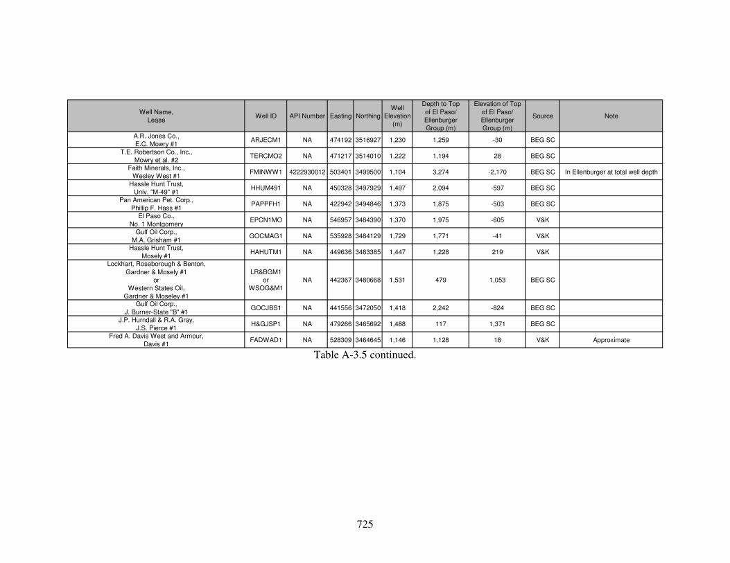
725
Well Name,
LeaseWell ID API Number Easting Northing
Well
Elevation
(m)
Depth to Top
of El Paso/
Ellenburger
Group (m)
Elevation of Top
of El Paso/
Ellenburger
Group (m)
Source Note
A.R. Jones Co.,
E.C. Mowry #1ARJECM1 NA 474192 3516927 1,230 1,259 -30 BEG SC
T.E. Robertson Co., Inc.,
Mowry et al. #2TERCMO2 NA 471217 3514010 1,222 1,194 28 BEG SC
Faith Minerals, Inc.,
Wesley West #1FMINWW1 4222930012 503401 3499500 1,104 3,274 -2,170 BEG SC In Ellenburger at total well depth
Hassle Hunt Trust,
Univ. "M-49" #1HHUM491 NA 450328 3497929 1,497 2,094 -597 BEG SC
Pan American Pet. Corp.,
Phillip F. Hass #1PAPPFH1 NA 422942 3494846 1,373 1,875 -503 BEG SC
El Paso Co.,
No. 1 MontgomeryEPCN1MO NA 546957 3484390 1,370 1,975 -605 V&K
Gulf Oil Corp.,
M.A. Grisham #1GOCMAG1 NA 535928 3484129 1,729 1,771 -41 V&K
Hassle Hunt Trust,
Mosely #1HAHUTM1 NA 449636 3483385 1,447 1,228 219 V&K
Lockhart, Roseborough & Benton,
Gardner & Mosely #1
or
Western States Oil,
Gardner & Moseley #1
LR&BGM1
or
WSOG&M1
NA 442367 3480668 1,531 479 1,053 BEG SC
Gulf Oil Corp.,
J. Burner-State "B" #1GOCJBS1 NA 441556 3472050 1,418 2,242 -824 BEG SC
J.P. Hurndall & R.A. Gray,
J.S. Pierce #1H&GJSP1 NA 479266 3465692 1,488 117 1,371 BEG SC
Fred A. Davis West and Armour,
Davis #1FADWAD1 NA 528309 3464645 1,146 1,128 18 V&K Approximate
Table A-3.5 continued.
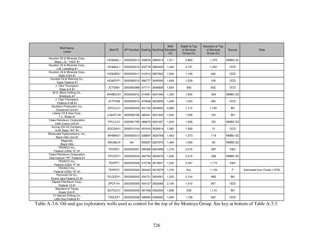
726
Well Name,
LeaseWell ID API Number Easting Northing
Well
Elevation
(m)
Depth to Top
of Montoya
Group (m)
Elevation of Top
of Montoya
Group (m)
Source Note
Houston Oil & Minerals Corp.,
State L.G. "1453" #1HO&MSL1 3003520013 406876 3685414 1,511 2,880 -1,370 NMBG DL
Houston Oil & Minerals Corp.,
J.M. Lewelling #1HO&MJL1 3003520010 402778 3684425 1,440 2,731 -1,291 OCD
Houston Oil & Minerals Corp.,
State 3724 #1HO&MS31 3003520011 412512 3657622 1,540 1,198 342 OCD
Humble Oil & Refining Co.,
Yates Federal #1HO&RYF1 3000560015 486777 3649300 1,648 1,539 109 OCD
J. Cleo Thompson,
State A-6 #1JCTSA61 3000562988 477111 3646836 1,824 992 832 OCD
W.H. Black Drilling Co.,
Shildneck #1WHBDCS1 3000500012 514561 3641046 1,330 1,835 -504 NMBG SC
J. Cleo Thompson,
Federal A-28 #1JCTFA28 3000562915 479948 3639939 1,649 1,263 386 OCD
Southern Production Co.,
Cloudcroft Unit #1SPCCLU1 3003500002 431152 3635650 2,859 1,114 1,745 BH
Liberty Oil & Gas Corp.,
T.L. Watts #1LO>LW 3000560766 480341 3631643 1,633 1,508 125 BH
Yates Petroleum Corporation,
Little Cuevo Unit #1YPCLCU1 3000561785 488273 3631027 1,633 1,508 125 NMBG SC
Sunray DX Oil Company,
N.M. State "AV" #1SOCSAV1 3000510144 491916 3630614 1,582 1,569 13 OCD
Westcoast Hydrocarbons, Inc.,
Black Hills Unit #1WHIBHU1 3000500013 508897 3629768 1,453 1,573 -119 NMBG SC
Magnolia,
Black HillsMAGBLHI NA 505927 3627975 1,494 1,559 -65 NMBG SC
TEXACO Inc.,
Federal (USA) "E" #1TEXIFE1 3003520001 395308 3624999 1,219 2,216 -997 K&H
Yates Petroleum Corporation,
Dog Canyon "YF" Federal #1YPCDCF1 3003520024 462754 3622676 1,946 2,215 -268 NMBG SC
TEXACO Inc.,
Federal (USA) "F" #1TEXIFF1 3003520006 410790 3619951 1,232 2,407 -1,175 K&H
TEXACO Inc.,
Federal (USA) "G" #1TEXIFG1 3003520004 394443 3619379 1,276 Est. -1,124 F Estimated from Foster (1978)
Plymouth Oil Co.,
Evans (aka Federal D) #1PLOCEV1 3003500003 404731 3604561 1,233 2,124 -892 BH
Zapata Petroleum Corp.,
Federal 14 #1ZPCF141 3003500006 454127 3603086 2,109 1,512 597 OCD
Standard of Texas,
Scarp Unit #1SOTSCU1 3003500009 487438 3593394 1,628 509 1,119 BH
Tri-Service Drilling Co.,
Little Dog Federal #1TSDLDF1 3003520008 496060 3586992 1,940 1,108 832 OCD
Table A-3.6: Oil-and-gas exploratory wells used as control for the top of the Montoya Group. See key at bottom of Table A-3.3.

727
Well Name,
LeaseWell ID API Number Easting Northing
Well
Elevation
(m)
Depth to Top
of Montoya
Group (m)
Elevation of Top
of Montoya
Group (m)
Source Note
Brainerd Corp. (aka Continental Oil Co.),
Federal "A" (aka East Texas Hill Unit) #1BRCFEA1 3001500005 523406 3586429 1,397 3,053 -1,656 NMBG SC
Continental Oil Co.,
H.W. Bass #1COCHWB1 3001500004 516898 3586367 1,680 1,433 247 NMBG SC
Fred Turner, Jr.,
Everett #1FTUEVE1 NA 443146 3579159 1,476 Est. 619 K&H Estimated from K&H (1985)
W.R. Weaver,
Thompson #1WRWETH1 3003500017 499785 3575900 1,386 1,033 353 NMBG SC
Humble Oil & Refining Co.,
Huapache Oil Unit #2HO&RHO2 3001500013 530547 3572779 1,358 3,486 -2,128 OCD
Fred Turner, Jr. (aka Pasotero Pet. Corp.),
Evans #1FTUJEV1 3003500020 433355 3563003 1,545 664 881 BH
Fred Turner, Jr.,
State #1FTUJST1 3003500027 475070 3550274 1,317 597 720 K&H
GDP 45-5 GDP45-5 NA 391837 3549102 1,255 1,109 146 F&J
Harvey E. Yates Co.,
Bennett Ranch Unit #1HEYBRU1 3003520027 435547 3545814 1,554 1,669 -114 OCD
Harvey E. Yates Co.,
Bennett Ranch Unit 25 #1HEYBR25 3003520031 437133 3542284 1,533 1,451 82 OCD
Magnolia Petr. Co.,
U-Tex Lease #39881 #1MPCUTL1 4222900015 443219 3536988 1,533 1,174 360 BEG SC
Pure Oil Co.,
Hunter #1PUOCHU1 NA 509809 3531380 1,625 1,912 -287 K&H
TEXACO Inc.,
Culberson "L" Fee #1TEXCLF1 NA 519234 3527336 1,564 2,424 -860 K&H
General Crude Oil Company,
Merrill and Voyles et al. #1GCOCMV1 NA 477481 3524877 1,181 1,053 128 BEG WR
Magnolia Petro.,
No. A-1 Homer, CowdenMPNA1HC NA 544286 3524346 1,194 3,289 -2,095 V&K
California Standard of Texas,
Theisen #1CASATT1 NA 426103 3521248 1,557 859 699 BEG WR
A.R. Jones Co.,
E.C. Mowry #1ARJECM1 NA 474192 3516927 1,230 1,197 33 BEG SC
T.E. Robertson Co., Inc.,
Mowry et al. #2TERCMO2 NA 471217 3514010 1,222 1,152 70 BEG SC
Hassle Hunt Trust,
Univ. "M-49" #1HHUM491 NA 450328 3497929 1,497 1,881 -384 BEG SC
El Paso Co.,
No. 1 MontgomeryEPCN1MO NA 546957 3484390 1,370 1,774 -404 V&K
Gulf Oil Corp.,
M.A. Grisham #1GOCMAG1 NA 535928 3484129 1,729 1,620 109 V&K
Table A-3.6 continued.

728
Well Name,
LeaseWell ID API Number Easting Northing
Well
Elevation
(m)
Depth to Top
of Montoya
Group (m)
Elevation of Top
of Montoya
Group (m)
Source Note
Lockhart, Roseborough & Benton,
Gardner & Mosely #1
or
Western States Oil,
Gardner & Moseley #1
LR&BGM1
or
WSOG&M1
NA 442367 3480668 1,531 399 1,132 BEG SC
Gulf Oil Corp.,
J. Burner-State "B" #1GOCJBS1 NA 441556 3472050 1,418 2,164 -746 BEG SC
Fred A. Davis West and Armour,
Davis #1FADWAD1 NA 528309 3464645 1,146 488 658 V&K Approximate
Table A-3.6 continued.

729
Well Name,
LeaseWell ID API Number Easting Northing
Well
Elevation
(m)
Depth to Top
of Fusselman
Formation (m)
Elevation of Top
of Fusselman
Formation (m)
Source Note
Houston Oil & Minerals Corp.,
State L.G. "1453" #1HO&MSL1 3003520013 406876 3685414 1,511 2,848 -1,338 NMBG DL
Houston Oil & Minerals Corp.,
J.M. Lewelling #1HO&MJL1 3003520010 402778 3684425 1,440 2,701 -1,261 OCD
Houston Oil & Minerals Corp.,
State 3724 #1HO&MS31 3003520011 412512 3657622 1,540 1,161 379 OCD
J. Cleo Thompson,
State A-6 #1JCTSA61 3000562988 477111 3646836 1,824 969 855 OCD
Humble Oil & Refining Co.,
Humble-Yates N.M. State #1HO&RHY1 3000510521 488336 3643533 1,574 1,591 -17 OCD
W.H. Black Drilling Co.,
Shildneck #1WHBDCS1 3000500012 514561 3641046 1,330 1,801 -471 NMBG SC
J. Cleo Thompson,
Federal A-28 #1JCTFA28 3000562915 479948 3639939 1,649 1,216 433 OCD
C & K Petroleum, Inc.,
Singer Lake State #1C&KSLS1 3000560320 495659 3637945 1,545 1,571 -26 OCD
Southern Production Co.,
Cloudcroft Unit #1SPCCLU1 3003500002 431152 3635650 2,859 1,072 1,787 BH
Yates Petroleum Corporation,
Dunken Nose Unit #1YPCDNU1 3000560383 491492 3635055 1,602 1,601 1 OCD
Yates Petroleum Corporation,
Dunken Dome Unit #2YPCDDU2 3000560397 485994 3634588 1,631 1,457 174 OCD
Yates Petroleum Corporation,
Dunken Dome Unit #1YPCDDU1 3000560374 486211 3634277 1,643 1,494 150 OCD
C & K Petroleum, Inc.,
Little Cuevo State #1C&KLCS1 3000560324 501605 3632606 1,464 1,923 -459 OCD
Liberty Oil & Gas Corp.,
T.L. Watts #1LO>LW 3000560766 480341 3631643 1,633 1,472 162 BH
Magnolia,
Headley Federal #2MAGHEF2 NA 512347 3631229 1,510 1,460 50 BH
Yates Petroleum Corporation,
Little Cuevo Unit #1YPCLCU1 3000561785 488273 3631027 1,633 1,472 162 NMBG SC
Sunray DX Oil Company,
N.M. State "AV" #1SOCSAV1 3000510144 491916 3630614 1,582 1,536 46 OCD
Westcoast Hydrocarbons, Inc.,
Black Hills Unit #1WHIBHU1 3000500013 508897 3629768 1,453 1,453 0 BH
Yates Petroleum Corporation,
Little Cuevo Unit #2YPCLCU2 3000562268 489571 3628557 1,618 1,397 220 OCD
Magnolia,
Black HillsMAGBLHI NA 505927 3627975 1,494 1,494 1 NMBG SC
TEXACO Inc.,
Federal (USA) "E" #1TEXIFE1 3003520001 395308 3624999 1,219 2,154 -935 K&H
Table A-3.7: Oil-and-gas exploratory wells used as control for the top of the Fusselman Formation. See key at bottom of Table A-3.3.

730
Well Name,
LeaseWell ID API Number Easting Northing
Well
Elevation
(m)
Depth to Top
of Fusselman
Formation (m)
Elevation of Top
of Fusselman
Formation (m)
Source Note
Yates Petroleum Corporation,
One Tree Unit #1YPCOTU1 3000562259 467160 3623529 1,876 1,856 20 BH
Yates Petroleum Corporation,
Dog Canyon "YF" Federal #1YPCDCF1 3003520024 462754 3622676 1,946 2,165 -219 NMBG SC
Texas Oil & Gas Corp.,
Federal "C" #1TO&GFC1 3000560017 512954 3622309 1,359 2,063 -704 BH
Kewanee Oil Co.,
F-M Unit #1KOCFMU1 3000500009 493140 3619927 1,579 1,993 -414 NMBG SC
TEXACO Inc.,
Federal (USA) "F" #1TEXIFF1 3003520006 410790 3619951 1,232 2,353 -1,120 K&H
TEXACO Inc.,
Federal (USA) "G" #1TEXIFG1 3003520004 394443 3619379 1,276 Est. -1,091 F Estimated from Foster (1978)
Marathon Oil Co.,
Mesa Verde Ranch #1MOCMVR1 3003520022 455326 3618246 2,143 1,797 346 NMBG SC
Yates Petroleum Corp.,
Buckhorn AYU State Com #1YPCBAYU 3000560541 506142 3613140 1,440 2,033 -593 NMBG SC
Texas Oil & Gas Corp.,
Federal "A" #1TO&GFA1 3000510431 506950 3613041 1,442 2,128 -685 BH
U.V. Industries, Inc.,
Long Canyon Unit #1UVILCU1 3000560411 502547 3610225 1,536 2,240 -703 BH
Gulf Oil Corp.,
Federal Munson #1GOCFMU1 3000510075 489407 3609839 1,723 1,033 690 BH
Plymouth Oil Co.,
Evans (aka Federal D) #1PLOCEV1 3003500003 404731 3604561 1,233 2,043 -811 BH
Atlantic Refining Co.,
State "AV" #1ARCSAV1 3003510001 461443 3603143 1,921 1,128 793 OCD
Zapata Petroleum Corp.,
Federal 14 #1ZPCF141 3003500006 454127 3603086 2,109 1,445 664 NMBG SC
Sun Oil Company,
T.J. Pearson #1SOCTJP1 3003500005 416750 3598464 1,344 1,308 36 BH
Terra Resources, Inc.,
Burro Canyon Unit #1-YTRBCU1Y 3003520017 511686 3596471 1,572 1,665 -93 BH
Standard of Texas,
Scarp Unit #1SOTSCU1 3003500009 487438 3593394 1,628 337 1,291 BH
Tri-Service Drilling Co.,
Little Dog Federal #1TSDLDF1 3003520008 496060 3586992 1,940 962 978 NMBG SC
Brainerd Corp. (aka Continental Oil Co.),
Federal "A" (aka East Texas Hill Unit) #1BRCFEA1 3001500005 523406 3586429 1,397 2,875 -1,478 NMBG SC
Continental Oil Co.,
H.W. Bass #1COCHWB1 3001500004 516898 3586367 1,680 1,263 416 NMBG SC
Marathon Oil Company,
Box Canyon Unit #1MOCBCU1 3001510012 522193 3586059 1,426 2,833 -1,407 OCD
Table A-3.7 continued.

731
Well Name,
LeaseWell ID API Number Easting Northing
Well
Elevation
(m)
Depth to Top
of Fusselman
Formation (m)
Elevation of Top
of Fusselman
Formation (m)
Source Note
E.P. Campbell,
Hurley #1EPCAHU1 3003500012 447355 3580223 1,404 666 737 K&H
Fred Turner, Jr.,
Everett #1FTUEVE1 NA 443146 3579159 1,476 Est. 735 K&H Estimated from K&H (1985)
W.R. Weaver,
Thompson #1WRWETH1 3003500017 499785 3575900 1,386 924 462 NMBG SC
E.P. Campbell,
Lois Spanel #1EPCALS1 3003500015 467947 3575324 1,408 758 650 K&H
E.P. Campbell,
McMillan Federal #1EPCAMF1 3003500018 500598 3573842 1,319 961 358 K&H
Inexco Oil Company,
Sitting Bull Unit #1IOCSBU1 3001520752 527152 3568073 1,650 1,820 -170 OCD
Union Oil Co.,
Federal White #1UNOCFW1 3001500019 525449 3565154 1,740 2,006 -265 BH
Fred Turner, Jr. (aka Pasotero Pet. Corp.),
Evans #1FTUJEV1 3003500020 433355 3563003 1,545 600 945 BH
E.P. Campbell (aka John J. Eisner),
Federal #1EPCAFE1 3003500019 432641 3562887 1,497 564 933 NMBG SC
Union Oil Co.,
McMillan #1UNOCMC1 3003500028 440825 3557266 1,522 1,079 443 BH
Transocean Oil,
G.J. Ablah #1TROGJA1 3003520018 442810 3554817 1,509 787 722 K&H
Pennzoil Co.,
Southland "28" State #1PCS28S1 3003520019 479573 3551070 1,206 839 367 K&H
E.J. Dunigan,
Alpha Federal #1EJDALF1 3003520002 496594 3549815 1,159 1,464 -304 K&H
GDP 45-5 GDP45-5 NA 391837 3549102 1,255 950 305 F&J
Harvey E. Yates Co.,
Bennett Ranch Unit #1HEYBRU1 3003520027 435547 3545814 1,554 1,516 38 OCD
Seaboard Oil Co.,
Trigg-Federal #1SEOCTF1 3003500032 418801 3545797 1,618 1,502 116 K&H
GDP 51-8 GDP51-8 NA 393417 3545870 1,253 455 798 F&J
Harvey E. Yates Co.,
Bennett Ranch Unit 25 #1HEYBR25 3003520031 437133 3542284 1,533 1,298 234 OCD
Magnolia Petr. Co.,
U-Tex Lease #39881 #1MPCUTL1 4222900015 443219 3536988 1,533 973 561 BEG SC
Pure Oil Co.,
Hunter #1PUOCHU1 NA 509809 3531380 1,625 1,630 -5 K&H
Hunt Oil Co.,
Dyer #1HUOCDY1 4222930007 485477 3530917 1,119 552 567 K&H
Hunt Petroleum Corp.,
C.L. Ranch #1HPCCLR1 4222930010 496475 3528252 1,105 1,546 -441 K&H
Table A-3.7 continued.

732
Well Name,
LeaseWell ID API Number Easting Northing
Well
Elevation
(m)
Depth to Top
of Fusselman
Formation (m)
Elevation of Top
of Fusselman
Formation (m)
Source Note
TEXACO Inc.,
Culberson "L" Fee #1TEXCLF1 NA 519234 3527336 1,564 2,154 -590 K&H
Tenneco Oil Co.,
TXL Fee #1TOTXLF1 4210931401 563041 3526975 1,086 3,512 -2,427 RRC
Trail Mountain, Inc.,
University Sizzler D5 #1TMUSD51 4222930227 437784 3526650 1,437 1,768 -331 RRC
General Crude Oil Company,
Merrill and Voyles et al. #1GCOCMV1 NA 477481 3524877 1,181 783 398 BEG WR
California Standard of Texas,
Theisen #1CASATT1 NA 426103 3521248 1,557 677 881 BEG WR
A.R. Jones Co.,
E.C. Mowry #1ARJECM1 NA 474192 3516927 1,230 935 295 BEG SC
Border Exploration Co.,
J.J. McAdoo 7 #1BECJJM1 4222930200 505794 3514682 1,143 2,151 -1,008 K&H
T.E. Robertson Co., Inc.,
Mowry et al. #2TERCMO2 NA 471217 3514010 1,222 882 340 BEG SC
American Quasar Pet. Co.,
V.C. Rounsaville #1AQPVCR1 NA 563477 3498883 1,178 4,239 -3,061 V&K
Hassle Hunt Trust,
Univ. "M-49" #1HHUM491 NA 450328 3497929 1,497 1,647 -151 BEG SC
Pan American Pet. Corp.,
Phillip F. Hass #1PAPPFH1 NA 422942 3494846 1,373 1,524 -151 BEG SC
Transocean Oil, Inc.,
36-1 MSA Trustee, Inc.TO36MSA 4222930192 424652 3490962 1,551 1,532 20 BEG SC
Hassle Hunt Trust,
Mosely #1HAHUTM1 NA 449636 3483385 1,447 954 493 V&K
Lockhart, Roseborough & Benton,
Gardner & Mosely #1
or
Western States Oil,
Gardner & Moseley #1
LR&BGM1
or
WSOG&M1
NA 442367 3480668 1,531 317 1,214 BEG SC
Gulf Oil Corp.,
J. Burner-State "B" #1GOCJBS1 NA 441556 3472050 1,418 1,842 -424 BEG SC
Table A-3.7 continued.

733
Well Name,
LeaseWell ID API Number Easting Northing
Well
Elevation
(m)
Depth to Top
of Devonian
(m)
Elevation of Top
of Devonian
(m)
Source Note
Southern Production Co.,
Cloudcroft Unit #1SPCCLU1 3003500002 431152 3635650 2,859 1,047 1,812 BH
Yates Petroleum Corporation,
Dunken Dome Unit #2YPCDDU2 3000560397 485994 3634588 1,631 1,455 176 OCD
TEXACO Inc.,
Federal (USA) "E" #1TEXIFE1 3003520001 395308 3624999 1,219 2,138 -919 K&H
Yates Petroleum Corporation,
Dog Canyon "YF" Federal #1YPCDCF1 3003520024 462754 3622676 1,946 2,137 -191 NMBG SC
Texas Oil & Gas Corp.,
Federal "C" #1TO&GFC1 3000560017 512954 3622309 1,359 2,048 -689 NMBG SC
TEXACO Inc.,
Federal (USA) "F" #1TEXIFF1 3003520006 410790 3619951 1,232 2,322 -1,089 K&H
TEXACO Inc.,
Federal (USA) "G" #1TEXIFG1 3003520004 394443 3619379 1,276 Est. -1,070 F Estimated from Foster (1978)
Marathon Oil Co.,
Mesa Verde Ranch #1MOCMVR1 3003520022 455326 3618246 2,143 1,769 374 BH
Yates Petroleum Corp.,
Buckhorn AYU State Com #1YPCBAYU 3000560541 506142 3613140 1,440 2,019 -579 NMBG SC
Texas Oil & Gas Corp.,
Federal "A" #1TO&GFA1 3000510431 506950 3613041 1,442 2,114 -671 NMBG SC
U.V. Industries, Inc.,
Long Canyon Unit #1UVILCU1 3000560411 502547 3610225 1,536 2,226 -689 NMBG SC
Plymouth Oil Co.,
Evans (aka Federal D) #1PLOCEV1 3003500003 404731 3604561 1,233 2,028 -796 BH
Texas Oil & Gas Corp.,
Federal "B" #1TO&GFB1 NA 510832 3603835 1,463 2,451 -988 NMBG SC
Atlantic Refining Co.,
State "AV" #1ARCSAV1 3003510001 461443 3603143 1,921 1,109 811 NMBG SC
Sun Oil Company,
T.J. Pearson #1SOCTJP1 3003500005 416750 3598464 1,344 1,305 39 BH
Terra Resources, Inc.,
Burro Canyon Unit #1-YTRBCU1Y 3003520017 511686 3596471 1,572 1,647 -76 BH
Brainerd Corp. (aka Continental Oil Co.),
Federal "A" (aka East Texas Hill Unit) #1BRCFEA1 3001500005 523406 3586429 1,397 2,867 -1,470 NMBG SC
Continental Oil Co.,
H.W. Bass #1COCHWB1 3001500004 516898 3586367 1,680 1,251 429 NMBG SC
Marathon Oil Company,
Box Canyon Unit #1MOCBCU1 3001510012 522193 3586059 1,426 2,827 -1,401 OCD
E.P. Campbell,
Hurley #1EPCAHU1 3003500012 447355 3580223 1,404 653 750 K&H
Fred Turner, Jr.,
Everett #1FTUEVE1 NA 443146 3579159 1,476 Est. 741 K&H Estimated from K&H (1985)
Table A-3.8: Oil-and-gas exploratory wells used as control for the top of the Devonian. See key at bottom of Table A-3.3.

734
Well Name,
LeaseWell ID API Number Easting Northing
Well
Elevation
(m)
Depth to Top
of Devonian
(m)
Elevation of Top
of Devonian
(m)
Source Note
E.P. Campbell,
Lois Spanel #1EPCALS1 3003500015 467947 3575324 1,408 745 663 K&H
E.P. Campbell,
McMillan Federal #1EPCAMF1 3003500018 500598 3573842 1,319 956 363 K&H
Humble Oil & Refining Co.,
Huapache Oil Unit #2HO&RHO2 3001500013 530547 3572779 1,358 3,292 -1,934 OCD
Union Oil Co.,
Federal White #1UNOCFW1 3001500019 525449 3565154 1,740 1,985 -245 BH
Fred Turner, Jr. (aka Pasotero Pet. Corp.),
Evans #1FTUJEV1 3003500020 433355 3563003 1,545 576 969 BH
Union Oil Co.,
McMillan #1UNOCMC1 3003500028 440825 3557266 1,522 1,062 460 BH
Transocean Oil,
G.J. Ablah #1TROGJA1 3003520018 442810 3554817 1,509 754 756 K&H
E.J. Dunigan,
Alpha Federal #1EJDALF1 3003520002 496594 3549815 1,159 1,440 -281 K&H
Harvey E. Yates Co.,
Bennett Ranch Unit #1HEYBRU1 3003520027 435547 3545814 1,554 1,495 59 OCD
Harvey E. Yates Co.,
Bennett Ranch Unit 25 #1HEYBR25 3003520031 437133 3542284 1,533 1,250 283 OCD
Magnolia Petr. Co.,
U-Tex Lease #39881 #1MPCUTL1 4222900015 443219 3536988 1,533 933 600 BEG SC
Pure Oil Co.,
Hunter #1PUOCHU1 NA 509809 3531380 1,625 1,587 39 K&H
Hunt Petroleum Corp.,
C.L. Ranch #1HPCCLR1 4222930010 496475 3528252 1,105 1,529 -424 K&H
TEXACO Inc.,
Culberson "L" Fee #1TEXCLF1 NA 519234 3527336 1,564 2,115 -551 K&H
Tenneco Oil Co.,
TXL Fee #1TOTXLF1 4210931401 563041 3526975 1,086 3,477 -2,391 RRC
Pan American Petroleum Corporation,
Ed Hammock #1PAPCEH1 NA 499124 3526693 1,110 1,691 -581 V&K
Trail Mountain, Inc.,
University Sizzler D5 #1TMUSD51 4222930227 437784 3526650 1,437 1,747 -309 RRC
TXL Corp.,
Culberson "C" Fee #1TXLCCF1 NA 523721 3526221 1,515 2,319 -804 V&K
General Crude Oil Company,
Merrill and Voyles et al. #1GCOCMV1 NA 477481 3524877 1,181 720 461 BEG WR
Magnolia Petro.,
No. A-1 Homer, CowdenMPNA1HC NA 544286 3524346 1,194 2,935 -1,741 V&K
California Standard of Texas,
Theisen #1CASATT1 NA 426103 3521248 1,557 642 916 BEG WR
Table A-3.8 continued.

735
Well Name,
LeaseWell ID API Number Easting Northing
Well
Elevation
(m)
Depth to Top
of Devonian
(m)
Elevation of Top
of Devonian
(m)
Source Note
Trail Mountain, Inc.,
University Felina "D27" #1TMUFD27 4222930006 439917 3518350 1,427 495 931 RRC
TXL Oil Corp.,
Culberson B-T Fee #1TXLCBT1 NA 550456 3517797 1,236 3,256 -2,020 V&K
A.R. Jones Co.,
E.C. Mowry #1ARJECM1 NA 474192 3516927 1,230 886 344 BEG SC
Border Exploration Co.,
J.J. McAdoo 7 #1BECJJM1 4222930200 505794 3514682 1,143 2,093 -950 K&H
T.E. Robertson Co., Inc.,
Mowry et al. #2TERCMO2 NA 471217 3514010 1,222 829 393 BEG SC
Trail Mountain, Inc.,
University Devil Woman L5 #1TMUDWL5 4222930253 477595 3510876 1,221 1,022 199 RRC
Samson Lone Star, L.L.C.,
University Lands 46-14 #2SALSUL2 4210932278 551660 3509591 1,310 3,692 -2,382 RRC
Chesapeake Operating, Inc.,
University Lands 4627 #1COUL462 4210932287 550571 3507028 1,300 3,670 -2,371 RRC
EnCana Oil & Gas (USA) Inc.,
Sibley Ranch 47 State "25" #1EOGSR47 4210932251 544180 3505778 1,332 3,341 -2,008 RRC
Trail Mountain, Inc.,
University Ooby Dooby L35 #1TMUODL1 4222930261 482251 3502319 1,230 1,327 -97 RRC
Petro-Hunt, L.L.C.,
Melissa Taylor State 27 #1-HPHMTS27 4210932255 563684 3501318 1,150 4,154 -3,004 RRC
American Quasar Pet. Co.,
V.C. Rounsaville #1AQPVCR1 NA 563477 3498883 1,178 4,184 -3,006 V&K
Hassle Hunt Trust,
Univ. "M-49" #1HHUM491 NA 450328 3497929 1,497 1,592 -96 BEG SC
Pan American Pet. Corp.,
Phillip F. Hass #1PAPPFH1 NA 422942 3494846 1,373 1,433 -61 BEG SC
Transocean Oil, Inc.,
36-1 MSA Trustee, Inc.TO36MSA 4222930192 424652 3490962 1,551 1,455 96 BEG SC
El Paso Co.,
No. 1 MontgomeryEPCN1MO NA 546957 3484390 1,370 1,428 -58 V&K
Gulf Oil Corp.,
M.A. Grisham #1GOCMAG1 NA 535928 3484129 1,729 1,210 519 V&K
Sinclair,
LooneySINCLOO NA 551319 3475371 1,310 2,595 -1,285 V&K
Gulf Oil Corp.,
J. Burner-State "B" #1GOCJBS1 NA 441556 3472050 1,418 1,835 -417 BEG SC
Table A-3.8 continued.

736
Well Name,
LeaseWell ID API Number Easting Northing
Well
Elevation
(m)
Depth to Top
of Mississippian
(m)
Elevation of Top
of Mississippian
(m)
Source Note
Houston Oil & Minerals Corp.,
State L.G. "1453" #1HO&MSL1 3003520013 406876 3685414 1,511 2,781 -1,271 NMBG DL
Houston Oil & Minerals Corp.,
J.M. Lewelling #1HO&MJL1 3003520010 402778 3684425 1,440 2,643 -1,203 OCD
Houston Oil & Minerals Corp.,
State 3724 #1HO&MS31 3003520011 412512 3657622 1,540 1,015 525 OCD
J. Cleo Thompson,
State A-6 #1JCTSA61 3000562988 477111 3646836 1,824 944 880 OCD
W.H. Black Drilling Co.,
Shildneck #1WHBDCS1 3000500012 514561 3641046 1,330 1,747 -416 NMBG SC
Continental Oil Company,
State NN #1COCSNN1 3000560185 492051 3640997 1,538 1,478 60 OCD
J. Cleo Thompson,
Federal A-28 #1JCTFA28 3000562915 479948 3639939 1,649 1,186 463 OCD
C & K Petroleum, Inc.,
Singer Lake State #1C&KSLS1 3000560320 495659 3637945 1,545 1,539 6 OCD
Southern Production Co.,
Cloudcroft Unit #1SPCCLU1 3003500002 431152 3635650 2,859 979 1,880 BH
Yates Petroleum Corporation,
Dunken Nose Unit #1YPCDNU1 3000560383 491492 3635055 1,602 1,540 62 OCD
Yates Petroleum Corporation,
Dunken Dome Unit #2YPCDDU2 3000560397 485994 3634588 1,631 1,420 211 OCD
Yates Petroleum Corporation,
Dunken Dome Unit #1YPCDDU1 3000560374 486211 3634277 1,643 1,447 197 OCD
C & K Petroleum, Inc.,
Little Cuevo State #1C&KLCS1 3000560324 501605 3632606 1,464 1,811 -348 OCD
Liberty Oil & Gas Corp.,
T.L. Watts #1LO>LW 3000560766 480341 3631643 1,633 1,433 200 BH
Magnolia,
Headley Federal #2MAGHEF2 NA 512347 3631229 1,510 1,390 119 NMBG SC
Yates Petroleum Corporation,
Little Cuevo Unit #1YPCLCU1 3000561785 488273 3631027 1,633 1,433 200 NMBG SC
Sunray DX Oil Company,
N.M. State "AV" #1SOCSAV1 3000510144 491916 3630614 1,582 1,451 131 OCD
Yates Petroleum Corporation,
Little Cuevo Unit #2YPCLCU2 3000562268 489571 3628557 1,618 1,329 288 OCD
Magnolia,
Black HillsMAGBLHI NA 505927 3627975 1,494 1,422 72 NMBG SC
TEXACO Inc.,
Federal (USA) "E" #1TEXIFE1 3003520001 395308 3624999 1,219 2,016 -797 K&H
Yates Petroleum Corporation,
One Tree Unit #1YPCOTU1 3000562259 467160 3623529 1,876 1,786 90 NMBG SC
Table A-3.9: Oil-and-gas exploratory wells used as control for the top of the Mississippian. See key at bottom of Table A-3.3.
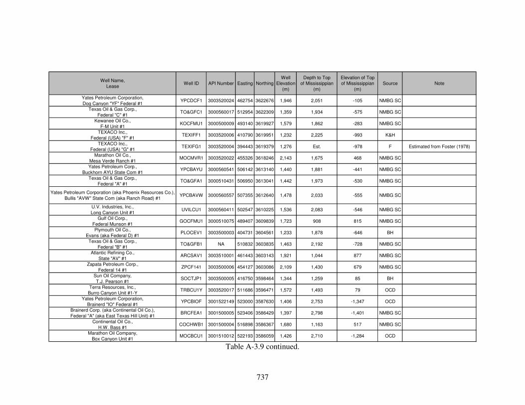
737
Well Name,
LeaseWell ID API Number Easting Northing
Well
Elevation
(m)
Depth to Top
of Mississippian
(m)
Elevation of Top
of Mississippian
(m)
Source Note
Yates Petroleum Corporation,
Dog Canyon "YF" Federal #1YPCDCF1 3003520024 462754 3622676 1,946 2,051 -105 NMBG SC
Texas Oil & Gas Corp.,
Federal "C" #1TO&GFC1 3000560017 512954 3622309 1,359 1,934 -575 NMBG SC
Kewanee Oil Co.,
F-M Unit #1KOCFMU1 3000500009 493140 3619927 1,579 1,862 -283 NMBG SC
TEXACO Inc.,
Federal (USA) "F" #1TEXIFF1 3003520006 410790 3619951 1,232 2,225 -993 K&H
TEXACO Inc.,
Federal (USA) "G" #1TEXIFG1 3003520004 394443 3619379 1,276 Est. -978 F Estimated from Foster (1978)
Marathon Oil Co.,
Mesa Verde Ranch #1MOCMVR1 3003520022 455326 3618246 2,143 1,675 468 NMBG SC
Yates Petroleum Corp.,
Buckhorn AYU State Com #1YPCBAYU 3000560541 506142 3613140 1,440 1,881 -441 NMBG SC
Texas Oil & Gas Corp.,
Federal "A" #1TO&GFA1 3000510431 506950 3613041 1,442 1,973 -530 NMBG SC
Yates Petroleum Corporation (aka Phoenix Resources Co.),
Bullis "AVW" State Com (aka Ranch Road) #1YPCBAVW 3000560557 507355 3612640 1,478 2,033 -555 NMBG SC
U.V. Industries, Inc.,
Long Canyon Unit #1UVILCU1 3000560411 502547 3610225 1,536 2,083 -546 NMBG SC
Gulf Oil Corp.,
Federal Munson #1GOCFMU1 3000510075 489407 3609839 1,723 908 815 NMBG SC
Plymouth Oil Co.,
Evans (aka Federal D) #1PLOCEV1 3003500003 404731 3604561 1,233 1,878 -646 BH
Texas Oil & Gas Corp.,
Federal "B" #1TO&GFB1 NA 510832 3603835 1,463 2,192 -728 NMBG SC
Atlantic Refining Co.,
State "AV" #1ARCSAV1 3003510001 461443 3603143 1,921 1,044 877 NMBG SC
Zapata Petroleum Corp.,
Federal 14 #1ZPCF141 3003500006 454127 3603086 2,109 1,430 679 NMBG SC
Sun Oil Company,
T.J. Pearson #1SOCTJP1 3003500005 416750 3598464 1,344 1,259 85 BH
Terra Resources, Inc.,
Burro Canyon Unit #1-YTRBCU1Y 3003520017 511686 3596471 1,572 1,493 79 OCD
Yates Petroleum Corporation,
Brainerd "IO" Federal #1YPCBIOF 3001522149 523000 3587630 1,406 2,753 -1,347 OCD
Brainerd Corp. (aka Continental Oil Co.),
Federal "A" (aka East Texas Hill Unit) #1BRCFEA1 3001500005 523406 3586429 1,397 2,798 -1,401 NMBG SC
Continental Oil Co.,
H.W. Bass #1COCHWB1 3001500004 516898 3586367 1,680 1,163 517 NMBG SC
Marathon Oil Company,
Box Canyon Unit #1MOCBCU1 3001510012 522193 3586059 1,426 2,710 -1,284 OCD
Table A-3.9 continued.

738
Well Name,
LeaseWell ID API Number Easting Northing
Well
Elevation
(m)
Depth to Top
of Mississippian
(m)
Elevation of Top
of Mississippian
(m)
Source Note
E.P. Campbell,
Hurley #1EPCAHU1 3003500012 447355 3580223 1,404 638 766 K&H
E.P. Campbell,
Lois Spanel #1EPCALS1 3003500015 467947 3575324 1,408 708 700 K&H
E.P. Campbell,
McMillan Federal #1EPCAMF1 3003500018 500598 3573842 1,319 925 394 K&H
Humble Oil & Refining Co.,
Huapache Oil Unit #2HO&RHO2 3001500013 530547 3572779 1,358 3,199 -1,841 OCD
Inexco Oil Company,
Sitting Bull Unit #1IOCSBU1 3001520752 527152 3568073 1,650 1,716 -66 OCD
Skelly Oil Co.,
Las Cruces "D" #1SOCLCD1 3001500003 522240 3565867 1,749 1,798 -50 NMBG SC
Union Oil Co.,
Federal White #1UNOCFW1 3001500019 525449 3565154 1,740 1,841 -101 BH
Flynn, Welch, Yates,
Donahue #1FWYDON1 NA 460768 3561350 1,303 439 864 BH
Franklin, Aston & Fair, Inc.,
Turkey Draw Unit #1FA&FTD1 3001521378 524583 3560015 1,776 2,173 -397 OCD
Union Oil Co.,
McMillan #1UNOCMC1 3003500028 440825 3557266 1,522 975 547 BH
Union Oil Co.,
Verse 7 Federal #1UOCV7F1 3001520591 524435 3556316 1,801 2,229 -428 OCD
Transocean Oil,
G.J. Ablah #1TROGJA1 3003520018 442810 3554817 1,509 686 823 K&H
Beard Oil Company,
Ridge USA #1BOCRUS1 3001522547 524447 3551405 1,896 2,551 -654 OCD
E.J. Dunigan,
Alpha Federal #1EJDALF1 3003520002 496594 3549815 1,159 1,317 -157 K&H
GDP 61-6 GDP61-6 NA 390213 3549130 1,254 533 721 F&J
GDP 45-5 GDP45-5 NA 391837 3549102 1,255 361 894 F&J
GDP 46-6 GDP46-6 NA 390223 3549119 1,252 527 725 F&J
Harvey E. Yates Co.,
Bennett Ranch Unit #1HEYBRU1 3003520027 435547 3545814 1,554 1,350 204 OCD
Seaboard Oil Co.,
Trigg-Federal #1SEOCTF1 3003500032 418801 3545797 1,618 1,431 187 K&H
GDP 51-8 GDP51-8 NA 393417 3545870 1,253 231 1,021 F&J
Harvey E. Yates Co.,
Bennett Ranch Unit 25 #1HEYBR25 3003520031 437133 3542284 1,533 1,138 394 OCD
Magnolia Petr. Co.,
U-Tex Lease #39881 #1MPCUTL1 4222900015 443219 3536988 1,533 639 895 BEG SC
EOG Resources, Inc.,
Rector Canyon 24 State #1EOGRC24 4210932250 544329 3534119 1,200 2,853 -1,653 RRC Estimate
Table A-3.9 continued.

739
Well Name,
LeaseWell ID API Number Easting Northing
Well
Elevation
(m)
Depth to Top
of Mississippian
(m)
Elevation of Top
of Mississippian
(m)
Source Note
Pure Oil Co.,
Hunter #1PUOCHU1 NA 509809 3531380 1,625 1,485 140 K&H
Trail Mountain, Inc.,
University Big Iron "C45" #1TMUBIC1 4222900029 440743 3529232 1,516 864 652 RRC
Hunt Petroleum Corp.,
C.L. Ranch #1HPCCLR1 4222930010 496475 3528252 1,105 1,515 -410 K&H
TEXACO Inc.,
Culberson "L" Fee #1TEXCLF1 NA 519234 3527336 1,564 2,020 -456 K&H
Trail Mountain, Inc.,
University Sizzler D5 #1TMUSD51 4222930227 437784 3526650 1,437 1,574 -137 RRC
TXL Corp.,
Culberson "C" Fee #1TXLCCF1 NA 523721 3526221 1,515 2,244 -729 V&K
General Crude Oil Company,
Merrill and Voyles et al. #1GCOCMV1 NA 477481 3524877 1,181 683 498 BEG WR
EOG Resources, Inc.,
Kenney 16 State #1HEOGKS1H 4210932270 527946 3523355 1,372 2,222 -850 RRC
EOG Resources, Inc.,
Kenney 16 State #2EOGKES2 4210932269 528404 3522559 1,365 2,298 -934 RRC
California Standard of Texas,
Theisen #1CASATT1 NA 426103 3521248 1,557 507 1,050 BEG WR
Trail Mountain, Inc.,
University Felina "D27" #1TMUFD27 4222930006 439917 3518350 1,427 360 1,066 RRC
Border Exploration Co.,
Hammack et al. CT-1BECHCT1 4222930196 505172 3518026 1,107 2,227 -1,120 K&H
A.R. Jones Co.,
E.C. Mowry #1ARJECM1 NA 474192 3516927 1,230 689 541 BEG SC
J.L. Cowley,
E.C. Mowry #1JLCECM1 NA 473079 3515907 1,234 672 561 BEG SC
Border Exploration Co.,
J.J. McAdoo 7 #1BECJJM1 4222930200 505794 3514682 1,143 1,983 -840 K&H
T.E. Robertson Co., Inc.,
Mowry et al. #2TERCMO2 NA 471217 3514010 1,222 694 528 BEG SC
Trail Mountain, Inc.,
University Devil Woman L5 #1TMUDWL5 4222930253 477595 3510876 1,221 696 525 RRC
Samson Lone Star, L.L.C.,
University Lands 46-14 #2SALSUL2 4210932278 551660 3509591 1,310 3,419 -2,110 RRC
Trail Mountain, Inc.,
University Ooby Dooby L35 #1TMUODL1 4222930261 482251 3502319 1,230 1,192 38 RRC
Petro-Hunt, L.L.C.,
Melissa Taylor State 27 #1-HPHMTS27 4210932255 563684 3501318 1,150 3,874 -2,724 RRC
Hassle Hunt Trust,
Univ. "M-49" #1HHUM491 NA 450328 3497929 1,497 1,561 -64 BEG SC
Table A-3.9 continued.
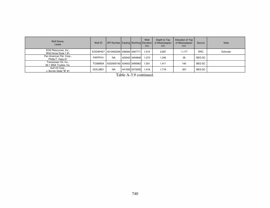
740
Well Name,
LeaseWell ID API Number Easting Northing
Well
Elevation
(m)
Depth to Top
of Mississippian
(m)
Elevation of Top
of Mississippian
(m)
Source Note
EOG Resources, Inc.,
Wild Horse Draw 7 #1EOGWHD7 4210932256 536584 3497771 1,510 2,687 -1,177 RRC Estimate
Pan American Pet. Corp.,
Phillip F. Hass #1PAPPFH1 NA 422942 3494846 1,373 1,345 28 BEG SC
Transocean Oil, Inc.,
36-1 MSA Trustee, Inc.TO36MSA 4222930192 424652 3490962 1,551 1,411 140 BEG SC
Gulf Oil Corp.,
J. Burner-State "B" #1GOCJBS1 NA 441556 3472050 1,418 1,718 -301 BEG SC
Table A-3.9 continued.
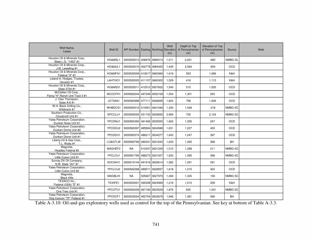
741
Well Name,
LeaseWell ID API Number Easting Northing
Well
Elevation
(m)
Depth to Top
of Pennsylvanian
(m)
Elevation of Top
of Pennsylvanian
(m)
Source Note
Houston Oil & Minerals Corp.,
State L.G. "1453" #1HO&MSL1 3003520013 406876 3685414 1,511 2,201 -690 NMBG DL
Houston Oil & Minerals Corp.,
J.M. Lewelling #1HO&MJL1 3003520010 402778 3684425 1,440 2,094 -654 OCD
Houston Oil & Minerals Corp.,
Federal "A" #1HO&MFA1 3003520009 413617 3660369 1,619 553 1,066 K&H
Leland A. Hodges, Trustee,
Houston #1LAHTHO1 3003520005 411157 3660302 1,529 416 1,113 K&H
Houston Oil & Minerals Corp.,
State 3724 #1HO&MS31 3003520011 412512 3657622 1,540 515 1,025 OCD
McClellan Oil Corp.,
Flying "H" Ranch Unit Tract 3 #1MCOCFH1 3000562244 497349 3652108 1,554 1,301 253 OCD
J. Cleo Thompson,
State A-6 #1JCTSA61 3000562988 477111 3646836 1,824 796 1,029 OCD
W.H. Black Drilling Co.,
Shildneck #1WHBDCS1 3000500012 514561 3641046 1,330 1,548 -218 NMBG SC
Southern Production Co.,
Cloudcroft Unit #1SPCCLU1 3003500002 431152 3635650 2,859 735 2,124 NMBG SC
Yates Petroleum Corporation,
Dunken Nose Unit #1YPCDNU1 3000560383 491492 3635055 1,602 1,355 247 OCD
Yates Petroleum Corporation,
Dunken Dome Unit #2YPCDDU2 3000560397 485994 3634588 1,631 1,227 403 OCD
Yates Petroleum Corporation,
Dunken Dome Unit #1YPCDDU1 3000560374 486211 3634277 1,643 1,247 397 OCD
Liberty Oil & Gas Corp.,
T.L. Watts #1LO>LW 3000560766 480341 3631643 1,633 1,265 368 BH
Magnolia,
Headley Federal #2MAGHEF2 NA 512347 3631229 1,510 1,298 211 NMBG SC
Yates Petroleum Corporation,
Little Cuevo Unit #1YPCLCU1 3000561785 488273 3631027 1,633 1,265 368 NMBG SC
Sunray DX Oil Company,
N.M. State "AV" #1SOCSAV1 3000510144 491916 3630614 1,582 1,291 291 OCD
Yates Petroleum Corporation,
Little Cuevo Unit #2YPCLCU2 3000562268 489571 3628557 1,618 1,215 403 OCD
Magnolia,
Black HillsMAGBLHI NA 505927 3627975 1,494 1,335 159 NMBG SC
TEXACO Inc.,
Federal (USA) "E" #1TEXIFE1 3003520001 395308 3624999 1,219 1,010 209 K&H
Yates Petroleum Corporation,
One Tree Unit #1YPCOTU1 3000562259 467160 3623529 1,876 835 1,041 NMBG SC
Yates Petroleum Corporation,
Dog Canyon "YF" Federal #1YPCDCF1 3003520024 462754 3622676 1,946 1,381 566 BH
Table A-3.10: Oil-and-gas exploratory wells used as control for the top of the Pennsylvanian. See key at bottom of Table A-3.3.

742
Well Name,
LeaseWell ID API Number Easting Northing
Well
Elevation
(m)
Depth to Top
of Pennsylvanian
(m)
Elevation of Top
of Pennsylvanian
(m)
Source Note
Texas Oil & Gas Corp.,
Federal "C" #1TO&GFC1 3000560017 512954 3622309 1,359 1,570 -211 NMBG SC
Kewanee Oil Co.,
F-M Unit #1KOCFMU1 3000500009 493140 3619927 1,579 1,506 73 NMBG SC
TEXACO Inc.,
Federal (USA) "F" #1TEXIFF1 3003520006 410790 3619951 1,232 1,817 -584 KH
TEXACO Inc.,
Federal (USA) "G" #1TEXIFG1 3003520004 394443 3619379 1,276 Est. 19 F Estimated from Foster (1978)
Marathon Oil Co.,
Mesa Verde Ranch #1MOCMVR1 3003520022 455326 3618246 2,143 1,243 900 BH
Yates Petroleum Corp.,
Buckhorn AYU State Com #1YPCBAYU 3000560541 506142 3613140 1,440 1,503 -63 NMBG SC
Texas Oil & Gas Corp.,
Federal "A" #1TO&GFA1 3000510431 506950 3613041 1,442 1,587 -144 OCD
Yates Petroleum Corporation (aka Phoenix Resources Co.),
Bullis "AVW" State Com (aka Ranch Road) #1YPCBAVW 3000560557 507355 3612640 1,478 1,602 -124 NMBG SC
U.V. Industries, Inc.,
Long Canyon Unit #1UVILCU1 3000560411 502547 3610225 1,536 1,798 -262 OCD
Plymouth Oil Co.,
Evans (aka Federal D) #1PLOCEV1 3003500003 404731 3604561 1,233 796 436 BH
Texas Oil & Gas Corp.,
Federal "B" #1TO&GFB1 NA 510832 3603835 1,463 1,728 -265 NMBG SC
Atlantic Refining Co.,
State "AV" #1ARCSAV1 3003510001 461443 3603143 1,921 777 1,144 NMBG SC
Zapata Petroleum Corp.,
Federal 14 #1ZPCF141 3003500006 454127 3603086 2,109 886 1,223 NMBG SC
Sun Oil Company,
T.J. Pearson #1SOCTJP1 3003500005 416750 3598464 1,344 591 752 BH
Terra Resources, Inc.,
Burro Canyon Unit #1-YTRBCU1Y 3003520017 511686 3596471 1,572 1,110 461 OCD
Stanolind Oil & Gas,
Thorn Unit #1SO>U1 3003500007 453419 3593869 1,914 1,186 728 BH
Yates Petroleum Corporation,
Brainerd "IO" Federal #1YPCBIOF 3001522149 523000 3587630 1,406 1,844 -438 OCD
Otero Oil Co.,
McGregor #1OTOCMC1 3003500010 412151 3586894 1,295 396 899 BH
Marathon Oil Company,
Box Canyon Unit #1MOCBCU1 3001510012 522193 3586059 1,426 2,308 -882 OCD
Presco, Inc.,
Indian Creek Federal #1PRIICF1 3003520030 511700 3573937 1,767 1,277 490 OCD
Humble Oil & Refining Co.,
Huapache Oil Unit #2HO&RHO2 3001500013 530547 3572779 1,358 2,090 -732 OCD
Table A-3.10 continued.

743
Well Name,
LeaseWell ID API Number Easting Northing
Well
Elevation
(m)
Depth to Top
of Pennsylvanian
(m)
Elevation of Top
of Pennsylvanian
(m)
Source Note
Inexco Oil Company,
Sitting Bull Unit #1IOCSBU1 3001520752 527152 3568073 1,650 1,385 264 OCD
Skelly Oil Co.,
Las Cruces "D" #1SOCLCD1 3001500003 522240 3565867 1,749 1,393 356 NMBG SC
Union Oil Co.,
Federal White #1UNOCFW1 3001500019 525449 3565154 1,740 1,420 320 BH
Humble Oil & Refining Co.,
Huapache Unit #5HO&RHU5 3001500018 531153 3564735 1,631 1,429 202 OCD
Franklin, Aston & Fair, Inc.,
Turkey Draw Unit #1FA&FTD1 3001521378 524583 3560015 1,776 1,561 216 OCD
Union Oil Co.,
McMillan #1UNOCMC1 3003500028 440825 3557266 1,522 683 840 BH
Union Oil Co.,
Verse 7 Federal #1UOCV7F1 3001520591 524435 3556316 1,801 1,592 210 OCD
Transocean Oil,
G.J. Ablah #1TROGJA1 3003520018 442810 3554817 1,509 529 980 K&H
Beard Oil Company,
Ridge USA #1BOCRUS1 3001522547 524447 3551405 1,896 1,856 40 NMBG SC
GDP 61-6 GDP61-6 NA 390213 3549130 1,254 433 822 F&J
GDP 45-5 GDP45-5 NA 391837 3549102 1,255 6 1,249 F&J
GDP 46-6 GDP46-6 NA 390223 3549119 1,252 205 1,047 F&J
Harvey E. Yates Co.,
Bennett Ranch Unit #1HEYBRU1 3003520027 435547 3545814 1,554 744 811 OCD
Seaboard Oil Co.,
Trigg-Federal #1SEOCTF1 3003500032 418801 3545797 1,618 1,156 462 K&H
GDP 51-8 GDP51-8 NA 393417 3545870 1,253 196 1,056 F&J
E.P. Campbell,
Spiegel-Federal #1EPCSPF1 3003510002 511803 3544568 1,868 1,369 499 K&H
Sinclair Oil & Gas Co.,
Guadalupe Ridge Unit #1SO&GGR1 3001520176 519670 3543204 2,215 2,222 -7 OCD
Harvey E. Yates Co.,
Bennett Ranch Unit 25 #1HEYBR25 3003520031 437133 3542284 1,533 529 1,004 OCD
Chesapeake Operating, Inc.,
DF Ranch State 63-12 #1CODFRS1 4210932302 543327 3538510 1,211 2,286 -1,075 RRC
EOG Resources, Inc.,
Rector Canyon 24 State #1EOGRC24 4210932250 544329 3534119 1,200 2,334 -1,134 RRC Estimate
Bonanza Co.,
PiersonBONCOPI NA 531346 3532226 1,346 1,943 -597 V&K
Pure Oil Co.,
Hunter #1PUOCHU1 NA 509809 3531380 1,625 1,011 614 K&H
Hueco Basin,
University #1HUBAUN1 NA 421896 3530405 1,558 754 805 BEG WR
Table A-3.10 continued.

744
Well Name,
LeaseWell ID API Number Easting Northing
Well
Elevation
(m)
Depth to Top
of Pennsylvanian
(m)
Elevation of Top
of Pennsylvanian
(m)
Source Note
Trail Mountain, Inc.,
University Big Iron "C45" #1TMUBIC1 4222900029 440743 3529232 1,516 520 996 RRC
Hunt Petroleum Corp.,
C.L. Ranch #1HPCCLR1 4222930010 496475 3528252 1,105 1,339 -235 K&H
TEXACO Inc.,
Culberson "L" Fee #1TEXCLF1 NA 519234 3527336 1,564 1,346 217 K&H
Tenneco Oil Co.,
TXL Fee #1TOTXLF1 4210931401 563041 3526975 1,086 2,846 -1,760 RRC
Trail Mountain, Inc.,
University Sizzler D5 #1TMUSD51 4222930227 437784 3526650 1,437 725 712 RRC
EOG Resources, Inc.,
Kenney 16 State #1HEOGKS1H 4210932270 527946 3523355 1,372 1,662 -290 RRC
EOG Resources, Inc.,
Kenney 16 State #2EOGKES2 4210932269 528404 3522559 1,365 1,662 -297 RRC
California Standard of Texas,
Theisen #1CASATT1 NA 426103 3521248 1,557 158 1,399 BEG WR
Trail Mountain, Inc.,
University Felina "D27" #1TMUFD27 4222930006 439917 3518350 1,427 273 1,153 RRC
Border Exploration Co.,
Hammack et al. CT-1BECHCT1 4222930196 505172 3518026 1,107 1,573 -466 K&H
A.R. Jones Co.,
E.C. Mowry #1ARJECM1 NA 474192 3516927 1,230 647 583 BEG SC
Tipperary Corp.,
ST-1 Billye SparksTCST1BS 4222930195 474281 3516816 1,230 930 300 BEG SC In Penn. at total well depth
J.L. Cowley,
E.C. Mowry #1JLCECM1 NA 473079 3515907 1,234 604 630 BEG SC
Border Exploration Co.,
J.J. McAdoo 7 #1BECJJM1 4222930200 505794 3514682 1,143 1,646 -503 K&H
T.E. Robertson Co., Inc.,
Mowry et al. #2TERCMO2 NA 471217 3514010 1,222 529 693 BEG SC
The Superior Oil Company,
Covington State #1TSOCCS1 4210931405 565213 3512927 1,140 3,314 -2,174 RRC
Trail Mountain, Inc.,
University Devil Woman L5 #1TMUDWL5 4222930253 477595 3510876 1,221 457 764 RRC
Samson Lone Star, L.L.C.,
University Lands 46-14 #2SALSUL2 4210932278 551660 3509591 1,310 3,214 -1,904 RRC
Humble Oil & Ref. Co.,
M.C. Sibley #1HORMCS1 NA 533795 3508569 1,458 2,301 -844 V&K
Chesapeake Operating, Inc.,
University Lands 4627 #1COUL462 4210932287 550571 3507028 1,300 3,167 -1,868 RRC
EnCana Oil & Gas (USA) Inc.,
Sibley Ranch 47 State "25" #1EOGSR47 4210932251 544180 3505778 1,332 2,804 -1,472 RRC
Table A-3.10 continued.

745
Well Name,
LeaseWell ID API Number Easting Northing
Well
Elevation
(m)
Depth to Top
of Pennsylvanian
(m)
Elevation of Top
of Pennsylvanian
(m)
Source Note
Anderson & Prichard,
Bordens #1A&PBOR1 NA 521137 3505265 1,391 1,524 -133 V&K In Penn. at total well depth
Trail Mountain, Inc.,
University Ooby Dooby L35 #1TMUODL1 4222930261 482251 3502319 1,230 775 455 RRC
Petro-Hunt, L.L.C.,
Melissa Taylor State 27 #1-HPHMTS27 4210932255 563684 3501318 1,150 3,841 -2,691 RRC
EOG Resources, Inc.,
Wild Horse Draw 7 #1EOGWHD7 4210932256 536584 3497771 1,510 2,298 -788 RRC Estimate
Pan American Pet. Corp.,
Phillip F. Hass #1PAPPFH1 NA 422942 3494846 1,373 701 671 BEG SC
Transocean Oil, Inc.,
36-1 MSA Trustee, Inc.TO36MSA 4222930192 424652 3490962 1,551 878 673 BEG SC
Chesapeake Operating, Inc.,
State Street State #701COSS701 4210932271 546492 3478738 1,422 1,520 -98 RRC
Gulf Oil Corp.,
J. Burner-State "B" #1GOCJBS1 NA 441556 3472050 1,418 799 619 BEG SC
Table A-3.10 continued.

746
Well Name,
LeaseWell ID API Number Easting Northing
Well
Elevation
(m)
Depth to Top
of Pow Wow
Conglomerate (m)
Elevation of Top
of Pow Wow
Conglomerate (m)
Source Note
Atlantic Refining Co.,
State "AV" #1ARCSAV1 3003510001 461443 3603143 1,921 766 1,155 NMBG SC
Zapata Petroleum Corp.,
Federal 14 #1ZPCF141 3003500006 454127 3603086 2,109 835 1,273 BH
Terra Resources, Inc.,
Burro Canyon Unit #1-YTRBCU1Y 3003520017 511686 3596471 1,572 1,089 483 BH
Stanolind Oil & Gas,
Thorn Unit #1SO>U1 3003500007 453419 3593869 1,914 986 928 BH
E.P. Campbell,
Hurley #1EPCAHU1 3003500012 447355 3580223 1,404 633 771 K&H
E.P. Campbell,
Liberman State #1EPCALI1 3003500014 457361 3576570 1,326 807 518 K&H
W.R. Weaver,
Thompson #1WRWETH1 3003500017 499785 3575900 1,386 861 525 NMBG SC
E.P. Campbell,
Lois Spanel #1EPCALS1 3003500015 467947 3575324 1,408 649 759 K&H
Presco, Inc.,
Indian Creek Federal #1PRIICF1 3003520030 511700 3573937 1,767 1,194 573 OCD
E.P. Campbell,
McMillan Federal #1EPCAMF1 3003500018 500598 3573842 1,319 855 464 K&H
Coral Oil & Gas Co.,
Warren #1CO&GCW1 3003500016 487264 3571960 1,186 641 544 K&H
Union Oil Co.,
Federal White #1UNOCFW1 3001500019 525449 3565154 1,740 1,380 361 BH
Union Oil Co.,
McMillan #1UNOCMC1 3003500028 440825 3557266 1,522 584 938 BH
W.W. West,
West Dog Canyon Unit #1WWWWDC1 3003520007 505979 3555044 1,771 1,167 603 OCD
Transocean Oil,
G.J. Ablah #1TROGJA1 3003520018 442810 3554817 1,509 503 1,006 K&H
Pennzoil Co.,
Southland "28" State #1PCS28S1 3003520019 479573 3551070 1,206 787 419 K&H
E.J. Dunigan,
Alpha Federal #1EJDALF1 3003520002 496594 3549815 1,159 1,208 -49 K&H
Hunt Oil Co.,
McMillan-Turner #1HUOCMT1 3003500029 469015 3547882 1,269 533 736 BH
Harvey E. Yates Co.,
Bennett Ranch Unit #1HEYBRU1 3003520027 435547 3545814 1,554 668 887 OCD
Seaboard Oil Co.,
Trigg-Federal #1SEOCTF1 3003500032 418801 3545797 1,618 936 683 K&H
Harvey E. Yates Co.,
Bennett Ranch Unit 25 #1HEYBR25 3003520031 437133 3542284 1,533 524 1,008 OCD
Table A-3.11: Oil-and-gas exploratory wells used as control for the top of the Pow Wow Conglomerate. See key at bottom of Table A-
3.3.

747
Well Name,
LeaseWell ID API Number Easting Northing
Well
Elevation
(m)
Depth to Top
of Pow Wow
Conglomerate (m)
Elevation of Top
of Pow Wow
Conglomerate (m)
Source Note
Pan American Petroleum Corporation,
List Anderson #1PAPCLA1 NA 491521 3533849 1,108 753 355 V&K
Pure Oil Co.,
Hunter #1PUOCHU1 NA 509809 3531380 1,625 499 1,126 K&H
Trail Mountain, Inc.,
University Sizzler D5 #1TMUSD51 4222930227 437784 3526650 1,437 668 770 RRC
General Crude Oil Company,
Merrill and Voyles et al. #1GCOCMV1 NA 477481 3524877 1,181 632 548 BEG WR
A.R. Jones Co.,
E.C. Mowry #1ARJECM1 NA 474192 3516927 1,230 596 634 BEG SC
T.E. Robertson Co., Inc.,
Mowry et al. #2TERCMO2 NA 471217 3514010 1,222 445 777 BEG SC
J.P. Hurndall & R.A. Gray,
J.S. Pierce #1H&GJSP1 NA 479266 3465692 1,488 112 1,376 BEG SC
Table A-3.11 continued.

748
Well Name,
LeaseWell ID API Number Easting Northing
Well
Elevation
(m)
Depth to Top
of Hueco Lm./Fm.
and Wolfcamp (m)
Elevation of Top
of Hueco Lm./Fm.
and
Wolfcamp (m)
Source Note
Houston Oil & Minerals Corp.,
State L.G. "1453" #1HO&MSL1 3003520013 406876 3685414 1,511 1,945 -434 NMBG DL
Houston Oil & Minerals Corp.,
J.M. Lewelling #1HO&MJL1 3003520010 402778 3684425 1,440 1,317 123 OCD
Houston Oil & Minerals Corp.,
Federal "A" #1HO&MFA1 3003520009 413617 3660369 1,619 273 1,346 K&H
Leland A. Hodges, Trustee,
Houston #1LAHTHO1 3003520005 411157 3660302 1,529 131 1,399 K&H
Houston Oil & Minerals Corp.,
State 3724 #1HO&MS31 3003520011 412512 3657622 1,540 148 1,392 OCD
McClellan Oil Corp.,
Flying "H" Ranch Unit Tract 3 #1MCOCFH1 3000562244 497349 3652108 1,554 991 563 OCD
McClellan Oil Corp.,
Gragg B #1MCOCGB1 3000561993 495371 3649683 1,529 1,022 508 OCD
Westcoast Hydrocarbons, Inc.,
Black Hills Unit #1WHIBHU1 3000500013 508897 3629768 1,453 1,308 146 NMBG SC
TEXACO Inc.,
Federal (USA) "E" #1TEXIFE1 3003520001 395308 3624999 1,219 618 600 K&H
Texas Oil & Gas Corp.,
Federal "C" #1TO&GFC1 3000560017 512954 3622309 1,359 1,195 164 NMBG SC
TEXACO Inc.,
Federal (USA) "F" #1TEXIFF1 3003520006 410790 3619951 1,232 1,423 -190 K&H
TEXACO Inc.,
Federal (USA) "G" #1TEXIFG1 3003520004 394443 3619379 1,276 Est. 436 F Estimated from Foster (1978)
Texas Oil & Gas Corp.,
Federal "A" #1TO&GFA1 3000510431 506950 3613041 1,442 1,122 321 NMBG SC
Yates Petroleum Corporation (aka Phoenix Resources Co.),
Bullis "AVW" State Com (aka Ranch Road) #1YPCBAVW 3000560557 507355 3612640 1,478 1,187 291 NMBG SC
U.V. Industries, Inc.,
Long Canyon Unit #1UVILCU1 3000560411 502547 3610225 1,536 1,140 397 NMBG SC
Plymouth Oil Co.,
Evans (aka Federal D) #1PLOCEV1 3003500003 404731 3604561 1,233 576 657 BH
Texas Oil & Gas Corp.,
Federal "B" #1TO&GFB1 NA 510832 3603835 1,463 1,247 216 NMBG SC
Atlantic Refining Co.,
State "AV" #1ARCSAV1 3003510001 461443 3603143 1,921 711 1,210 NMBG SC
Zapata Petroleum Corp.,
Federal 14 #1ZPCF141 3003500006 454127 3603086 2,109 747 1,362 NMBG SC
Sun Oil Company,
T.J. Pearson #1SOCTJP1 3003500005 416750 3598464 1,344 390 953 BH
Table A-3.12: Oil-and-gas exploratory wells used as control for the top of the Hueco Limestone/Formation and Wolfcamp Formation.
See key at bottom of Table A-3.3.

749
Well Name,
LeaseWell ID API Number Easting Northing
Well
Elevation
(m)
Depth to Top
of Hueco Lm./Fm.
and Wolfcamp (m)
Elevation of Top
of Hueco Lm./Fm.
and
Wolfcamp (m)
Source Note
Terra Resources, Inc.,
Burro Canyon Unit #1-YTRBCU1Y 3003520017 511686 3596471 1,572 932 639 BH
Stanolind Oil & Gas,
Thorn Unit #1SO>U1 3003500007 453419 3593869 1,914 838 1,076 BH
Yates Petroleum Corporation,
Brainerd "IO" Federal #1YPCBIOF 3001522149 523000 3587630 1,406 1,423 -18 OCD
Otero Oil Co.,
McGregor #1OTOCMC1 3003500010 412151 3586894 1,295 250 1,045 BH
Brainerd Corp. (aka Continental Oil Co.),
Federal "A" (aka East Texas Hill Unit) #1BRCFEA1 3001500005 523406 3586429 1,397 1,421 -24 NMBG SC
Continental Oil Co.,
H.W. Bass #1COCHWB1 3001500004 516898 3586367 1,680 1,140 540 NMBG SC
Marathon Oil Company,
Box Canyon Unit #1MOCBCU1 3001510012 522193 3586059 1,426 1,439 -13 OCD
E.P. Campbell,
Hurley #1EPCAHU1 3003500012 447355 3580223 1,404 468 936 K&H
E.P. Campbell,
Liberman State #1EPCALI1 3003500014 457361 3576570 1,326 728 598 K&H
W.R. Weaver,
Thompson #1WRWETH1 3003500017 499785 3575900 1,386 771 615 BH
E.P. Campbell,
Lois Spanel #1EPCALS1 3003500015 467947 3575324 1,408 639 770 K&H
E.P. Campbell,
McMillan Federal #1EPCAMF1 3003500018 500598 3573842 1,319 747 572 BH
Humble Oil & Refining Co.,
Huapache Oil Unit #2HO&RHO2 3001500013 530547 3572779 1,358 1,826 -468 OCD
Inexco Oil Company,
Sitting Bull Unit #1IOCSBU1 3001520752 527152 3568073 1,650 1,342 307 OCD
Coral Oil & Gas Company,
Ann Spanel #1CO&GAS1 3003500021 451716 3566857 1,391 425 966 OCD
Skelly Oil Co.,
Las Cruces "D" #1SOCLCD1 3001500003 522240 3565867 1,749 1,337 412 NMBG SC
Union Oil Co.,
Federal White #1UNOCFW1 3001500019 525449 3565154 1,740 1,144 596 BH
Humble Oil & Refining Co.,
Huapache Unit #5HO&RHU5 3001500018 531153 3564735 1,631 1,382 250 NMBG SC
E.P. Campbell (aka John J. Eisner),
Federal #1EPCAFE1 3003500019 432641 3562887 1,497 170 1,327 NMBG SC
Flynn, Welch, Yates,
Donahue #1FWYDON1 NA 460768 3561350 1,303 415 888 BH
Franklin, Aston & Fair, Inc.,
Turkey Draw Unit #1FA&FTD1 3001521378 524583 3560015 1,776 1,405 371 OCD
Table A-3.12 continued.

750
Well Name,
LeaseWell ID API Number Easting Northing
Well
Elevation
(m)
Depth to Top
of Hueco Lm./Fm.
and Wolfcamp (m)
Elevation of Top
of Hueco Lm./Fm.
and
Wolfcamp (m)
Source Note
Union Oil Co.,
McMillan #1UNOCMC1 3003500028 440825 3557266 1,522 259 1,263 BH
Union Oil Co.,
Verse 7 Federal #1UOCV7F1 3001520591 524435 3556316 1,801 1,418 383 OCD
W.W. West,
West Dog Canyon Unit #1WWWWDC1 3003520007 505979 3555044 1,771 869 902 OCD
Transocean Oil,
G.J. Ablah #1TROGJA1 3003520018 442810 3554817 1,509 315 1,194 K&H
Beard Oil Company,
Ridge USA #1BOCRUS1 3001522547 524447 3551405 1,896 1,743 153 NMBG SC
Pennzoil Co.,
Southland "28" State #1PCS28S1 3003520019 479573 3551070 1,206 473 733 K&H
Fred Turner, Jr.,
State #1FTUJST1 3003500027 475070 3550274 1,317 561 756 K&H
Hunt Oil Co.,
McMillan-Turner #1HUOCMT1 3003500029 469015 3547882 1,269 393 876 BH
Harvey E. Yates Co.,
Bennett Ranch Unit #1HEYBRU1 3003520027 435547 3545814 1,554 201 1,353 OCD
Seaboard Oil Co.,
Trigg-Federal #1SEOCTF1 3003500032 418801 3545797 1,618 223 1,395 K&H
Harvey E. Yates Co.,
Bennett Ranch Unit 25 #1HEYBR25 3003520031 437133 3542284 1,533 64 1,469 OCD
Chesapeake Operating, Inc.,
DF Ranch State 63-12 #1CODFRS1 4210932302 543327 3538510 1,211 1,943 -732 RRC
Pure Oil Co.,
Hunter #1PUOCHU1 NA 509809 3531380 1,625 421 1,204 K&H
Hueco Basin,
University #1HUBAUN1 NA 421896 3530405 1,558 137 1,421 BEG WR
Hunt Petroleum Corp.,
C.L. Ranch #1HPCCLR1 4222930010 496475 3528252 1,105 1,093 12 K&H
TEXACO Inc.,
Culberson "L" Fee #1TEXCLF1 NA 519234 3527336 1,564 1,198 365 K&H
Pan American Petroleum Corporation,
Ed Hammock #1PAPCEH1 NA 499124 3526693 1,110 1,169 -59 V&K
TXL Corp.,
Culberson "C" Fee #1TXLCCF1 NA 523721 3526221 1,515 1,466 49 V&K
Border Exploration Co.,
Hammack et al. CT-1BECHCT1 4222930196 505172 3518026 1,107 1,395 -288 K&H
A.R. Jones Co.,
E.C. Mowry #1ARJECM1 NA 474192 3516927 1,230 501 728 BEG SC
J.L. Cowley,
E.C. Mowry #1JLCECM1 NA 473079 3515907 1,234 454 779 BEG SC
Table A-3.12 continued.

751
Well Name,
LeaseWell ID API Number Easting Northing
Well
Elevation
(m)
Depth to Top
of Hueco Lm./Fm.
and Wolfcamp (m)
Elevation of Top
of Hueco Lm./Fm.
and
Wolfcamp (m)
Source Note
Border Exploration Co.,
J.J. McAdoo 7 #1BECJJM1 4222930200 505794 3514682 1,143 1,396 -253 K&H
T.E. Robertson Co., Inc.,
Mowry et al. #2TERCMO2 NA 471217 3514010 1,222 384 839 BEG SC
The Superior Oil Company,
Covington State #1TSOCCS1 4210931405 565213 3512927 1,140 2,295 -1,155 RRC
Samson Lone Star, L.L.C.,
University Lands 46-14 #2SALSUL2 4210932278 551660 3509591 1,310 1,990 -680 RRC
N. Amer. Royalties, Inc.,
Potter #1NARIPO1 NA 511738 3508091 1,186 1,115 71 V&K
Chesapeake Operating, Inc.,
University Lands 4627 #1COUL462 4210932287 550571 3507028 1,300 1,952 -652 RRC
EnCana Oil & Gas (USA) Inc.,
Sibley Ranch 47 State "25" #1EOGSR47 4210932251 544180 3505778 1,332 1,670 -338 RRC
Trail Mountain, Inc.,
University Ooby Dooby L35 #1TMUODL1 4222930261 482251 3502319 1,230 427 803 RRC
Petro-Hunt, L.L.C.,
Melissa Taylor State 27 #1-HPHMTS27 4210932255 563684 3501318 1,150 2,234 -1,084 RRC
American Quasar Pet. Co.,
V.C. Rounsaville #1AQPVCR1 NA 563477 3498883 1,178 2,718 -1,540 V&K
Chesapeake Operating, Inc.,
Melissa Taylor State 105-3COMT105 4210932297 541293 3493028 1,437 1,513 -76 RRC
Chesapeake Operating, Inc.,
State Street State #701COSS701 4210932271 546492 3478738 1,422 1,216 206 RRC
Sinclair,
LooneySINCLOO NA 551319 3475371 1,310 1,539 -229 V&K
Gulf Oil Corp.,
J. Burner-State "B" #1GOCJBS1 NA 441556 3472050 1,418 79 1,339 BEG SC
Table A-3.12 continued.

752
Well Name,
LeaseWell ID API Number Easting Northing
Well
Elevation
(m)
Depth to Top
of Abo
Formation (m)
Elevation of Top
of Abo
Formation (m)
Source Note
Houston Oil & Minerals Corp.,
State L.G. "1453" #1HO&MSL1 3003520013 406876 3685414 1,511 1,280 230 NMBG DL
Houston Oil & Minerals Corp.,
J.M. Lewelling #1HO&MJL1 3003520010 402778 3684425 1,440 991 449 OCD
Houston Oil & Minerals Corp.,
Federal "A" #1HO&MFA1 3003520009 413617 3660369 1,619 0 1,619 K&H
Leland A. Hodges, Trustee,
Houston #1LAHTHO1 3003520005 411157 3660302 1,529 0 1,529 K&H
McClellan Oil Corp.,
Flying "H" Ranch Unit Tract 3 #1MCOCFH1 3000562244 497349 3652108 1,554 834 721 OCD
McClellan Oil Corp.,
Gragg B #1MCOCGB1 3000561993 495371 3649683 1,529 788 741 OCD
Humble Oil & Refining Co.,
Yates Federal #1HO&RYF1 3000560015 486777 3649300 1,648 856 792 OCD
J. Cleo Thompson,
State A-6 #1JCTSA61 3000562988 477111 3646836 1,824 685 1,139 OCD
Lubbook Machine & Supply Co., Inc.,
Anderson-Randell #1LM&SAR1 3000500003 472069 3645946 1,767 503 1,264 OCD
Humble Oil & Refining Co.,
Humble-Yates N.M. State #1HO&RHY1 3000510521 488336 3643533 1,574 826 748 OCD
W.H. Black Drilling Co.,
Shildneck #1WHBDCS1 3000500012 514561 3641046 1,330 954 376 NMBG SC
Continental Oil Company,
State NN #1COCSNN1 3000560185 492051 3640997 1,538 823 715 OCD
J. Cleo Thompson,
Federal A-28 #1JCTFA28 3000562915 479948 3639939 1,649 604 1,045 OCD
C & K Petroleum, Inc.,
Singer Lake State #1C&KSLS1 3000560320 495659 3637945 1,545 870 675 OCD
Southern Production Co.,
Cloudcroft Unit #1SPCCLU1 3003500002 431152 3635650 2,859 658 2,201 BH
Yates Petroleum Corporation,
Dunken Nose Unit #1YPCDNU1 3000560383 491492 3635055 1,602 884 718 OCD
Yates Petroleum Corporation,
Dunken Dome Unit #2YPCDDU2 3000560397 485994 3634588 1,631 832 799 OCD
Yates Petroleum Corporation,
Dunken Dome Unit #1YPCDDU1 3000560374 486211 3634277 1,643 850 794 OCD
C & K Petroleum, Inc.,
Little Cuevo State #1C&KLCS1 3000560324 501605 3632606 1,464 942 522 OCD
Liberty Oil & Gas Corp.,
T.L. Watts #1LO>LW 3000560766 480341 3631643 1,633 933 700 BH
Magnolia,
Headley Federal #2MAGHEF2 NA 512347 3631229 1,510 891 619 NMBG SC
Table A-3.13: Oil-and-gas exploratory wells used as control for the top of the Abo Formation. See key at bottom of Table A-3.3.
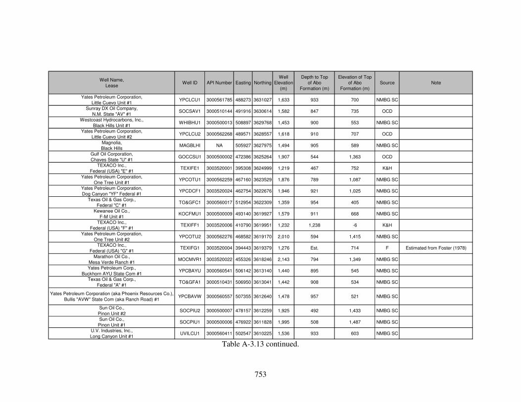
753
Well Name,
LeaseWell ID API Number Easting Northing
Well
Elevation
(m)
Depth to Top
of Abo
Formation (m)
Elevation of Top
of Abo
Formation (m)
Source Note
Yates Petroleum Corporation,
Little Cuevo Unit #1YPCLCU1 3000561785 488273 3631027 1,633 933 700 NMBG SC
Sunray DX Oil Company,
N.M. State "AV" #1SOCSAV1 3000510144 491916 3630614 1,582 847 735 OCD
Westcoast Hydrocarbons, Inc.,
Black Hills Unit #1WHIBHU1 3000500013 508897 3629768 1,453 900 553 NMBG SC
Yates Petroleum Corporation,
Little Cuevo Unit #2YPCLCU2 3000562268 489571 3628557 1,618 910 707 OCD
Magnolia,
Black HillsMAGBLHI NA 505927 3627975 1,494 905 589 NMBG SC
Gulf Oil Corporation,
Chaves State "U" #1GOCCSU1 3000500002 472386 3625264 1,907 544 1,363 OCD
TEXACO Inc.,
Federal (USA) "E" #1TEXIFE1 3003520001 395308 3624999 1,219 467 752 K&H
Yates Petroleum Corporation,
One Tree Unit #1YPCOTU1 3000562259 467160 3623529 1,876 789 1,087 NMBG SC
Yates Petroleum Corporation,
Dog Canyon "YF" Federal #1YPCDCF1 3003520024 462754 3622676 1,946 921 1,025 NMBG SC
Texas Oil & Gas Corp.,
Federal "C" #1TO&GFC1 3000560017 512954 3622309 1,359 954 405 NMBG SC
Kewanee Oil Co.,
F-M Unit #1KOCFMU1 3000500009 493140 3619927 1,579 911 668 NMBG SC
TEXACO Inc.,
Federal (USA) "F" #1TEXIFF1 3003520006 410790 3619951 1,232 1,238 -6 K&H
Yates Petroleum Corporation,
One Tree Unit #2YPCOTU2 3000562276 468582 3619170 2,010 594 1,415 NMBG SC
TEXACO Inc.,
Federal (USA) "G" #1TEXIFG1 3003520004 394443 3619379 1,276 Est. 714 F Estimated from Foster (1978)
Marathon Oil Co.,
Mesa Verde Ranch #1MOCMVR1 3003520022 455326 3618246 2,143 794 1,349 NMBG SC
Yates Petroleum Corp.,
Buckhorn AYU State Com #1YPCBAYU 3000560541 506142 3613140 1,440 895 545 NMBG SC
Texas Oil & Gas Corp.,
Federal "A" #1TO&GFA1 3000510431 506950 3613041 1,442 908 534 NMBG SC
Yates Petroleum Corporation (aka Phoenix Resources Co.),
Bullis "AVW" State Com (aka Ranch Road) #1YPCBAVW 3000560557 507355 3612640 1,478 957 521 NMBG SC
Sun Oil Co.,
Pinon Unit #2SOCPIU2 3000500007 478157 3612259 1,925 492 1,433 NMBG SC
Sun Oil Co.,
Pinon Unit #1SOCPIU1 3000500006 476922 3611828 1,995 508 1,487 NMBG SC
U.V. Industries, Inc.,
Long Canyon Unit #1UVILCU1 3000560411 502547 3610225 1,536 933 603 NMBG SC
Table A-3.13 continued.

754
Well Name,
LeaseWell ID API Number Easting Northing
Well
Elevation
(m)
Depth to Top
of Abo
Formation (m)
Elevation of Top
of Abo
Formation (m)
Source Note
Gulf Oil Corp.,
Federal Munson #1GOCFMU1 3000510075 489407 3609839 1,723 707 1,016 NMBG SC
Plymouth Oil Co.,
Evans (aka Federal D) #1PLOCEV1 3003500003 404731 3604561 1,233 355 878 BH
Texas Oil & Gas Corp.,
Federal "B" #1TO&GFB1 NA 510832 3603835 1,463 942 521 NMBG SC
Atlantic Refining Co.,
State "AV" #1ARCSAV1 3003510001 461443 3603143 1,921 641 1,279 NMBG SC
Zapata Petroleum Corp.,
Federal 14 #1ZPCF141 3003500006 454127 3603086 2,109 671 1,438 NMBG SC
Sun Oil Company,
T.J. Pearson #1SOCTJP1 3003500005 416750 3598464 1,344 250 1,094 BH
Terra Resources, Inc.,
Burro Canyon Unit #1-YTRBCU1Y 3003520017 511686 3596471 1,572 902 669 BH
Stanolind Oil & Gas,
Thorn Unit #1SO>U1 3003500007 453419 3593869 1,914 746 1,169 BH
Standard of Texas,
Scarp Unit #1SOTSCU1 3003500009 487438 3593394 1,628 259 1,369 BH
Lefors Petroleum Co.,
Federal #1LEPCFE1 3003500008 471863 3592611 1,642 509 1,133 NMBG SC
Yates Petroleum Corporation,
Brainerd "IO" Federal #1YPCBIOF 3001522149 523000 3587630 1,406 1,067 338 OCD
Tri-Service Drilling Co.,
Little Dog Federal #1TSDLDF1 3003520008 496060 3586992 1,940 777 1,163 NMBG SC
Brainerd Corp. (aka Continental Oil Co.),
Federal "A" (aka East Texas Hill Unit) #1BRCFEA1 3001500005 523406 3586429 1,397 1,081 316 NMBG SC
Continental Oil Co.,
H.W. Bass #1COCHWB1 3001500004 516898 3586367 1,680 870 810 NMBG SC
Marathon Oil Company,
Box Canyon Unit #1MOCBCU1 3001510012 522193 3586059 1,426 1,077 349 OCD
Pitts Energy Co.,
Federal "9" #1PIECF91 3001527563 518567 3585218 1,619 943 675 OCD
Sinclair Oil & Gas Company,
Federal Eddy 193 #1SO&GFE1 3001500001 518145 3580901 1,582 958 624 OCD
E.P. Campbell,
Hurley #1EPCAHU1 3003500012 447355 3580223 1,404 419 985 K&H
Tom L. Ingram,
State "E" #1TLISTE1 3001520003 523070 3579540 1,390 725 664 OCD
E.P. Campbell,
Liberman State #1EPCALI1 3003500014 457361 3576570 1,326 662 663 K&H
W.R. Weaver,
Thompson #1WRWETH1 3003500017 499785 3575900 1,386 736 650 NMBG SC
Table A-3.13 continued.
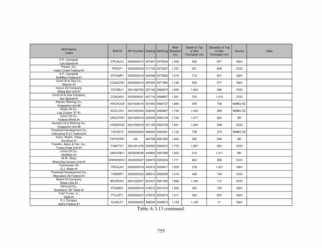
755
Well Name,
LeaseWell ID API Number Easting Northing
Well
Elevation
(m)
Depth to Top
of Abo
Formation (m)
Elevation of Top
of Abo
Formation (m)
Source Note
E.P. Campbell,
Lois Spanel #1EPCALS1 3003500015 467947 3575324 1,408 562 847 K&H
Presco, Inc.,
Indian Creek Federal #1PRIICF1 3003520030 511700 3573937 1,767 931 836 OCD
E.P. Campbell,
McMillan Federal #1EPCAMF1 3003500018 500598 3573842 1,319 712 607 K&H
Coral Oil & Gas Co.,
Warren #1CO&GCW1 3003500016 487264 3571960 1,186 609 577 K&H
Inexco Oil Company,
Sitting Bull Unit #1IOCSBU1 3001520752 527152 3568073 1,650 1,062 588 OCD
Coral Oil & Gas Company,
Ann Spanel #1CO&GAS1 3003500021 451716 3566857 1,391 376 1,014 OCD
Atlantic Refining Co.,
Huapache Unit #9ARCHUU9 3001500016 527053 3566737 1,686 978 708 NMBG SC
Skelly Oil Co.,
Las Cruces "D" #1SOCLCD1 3001500003 522240 3565867 1,749 1,050 699 NMBG SC
Union Oil Co.,
Federal White #1UNOCFW1 3001500019 525449 3565154 1,740 1,077 663 BH
Humble Oil & Refining Co.,
Huapache Unit #5HO&RHU5 3001500018 531153 3564735 1,631 1,064 568 OCD
Threshold Development Co.,
Chiricahua R 21 Federal #1TDCR21F 3003520034 489264 3563381 1,133 758 374 NMBG SC
Flynn, Welch, Yates,
Donahue #1FWYDON1 NA 460768 3561350 1,303 355 948 BH
Franklin, Aston & Fair, Inc.,
Turkey Draw Unit #1FA&FTD1 3001521378 524583 3560015 1,776 1,087 690 OCD
Union Oil Co.,
McMillan #1UNOCMC1 3003500028 440825 3557266 1,522 212 1,311 BH
W.W. West,
West Dog Canyon Unit #1WWWWDC1 3003520007 505979 3555044 1,771 863 908 OCD
Transocean Oil,
G.J. Ablah #1TROGJA1 3003520018 442810 3554817 1,509 278 1,231 K&H
Threshold Development Co.,
Mescalero 28 Federal #1TDM28F1 3003520033 489514 3552255 1,219 469 749 OCD
Beard Oil Company,
Ridge USA #1BOCRUS1 3001522547 524447 3551405 1,896 1,184 712 OCD
Pennzoil Co.,
Southland "28" State #1PCS28S1 3003520019 479573 3551070 1,206 454 753 K&H
Fred Turner, Jr.,
State #1FTUJST1 3003500027 475070 3550274 1,317 493 824 K&H
E.J. Dunigan,
Alpha Federal #1EJDALF1 3003520002 496594 3549815 1,159 1,129 31 K&H
Table A-3.13 continued.

756
Well Name,
LeaseWell ID API Number Easting Northing
Well
Elevation
(m)
Depth to Top
of Abo
Formation (m)
Elevation of Top
of Abo
Formation (m)
Source Note
Hunt Oil Co.,
McMillan-Turner #1HUOCMT1 3003500029 469015 3547882 1,269 375 895 BH
Harvey E. Yates Co.,
Bennett Ranch Unit #1HEYBRU1 3003520027 435547 3545814 1,554 104 1,451 OCD
Seaboard Oil Co.,
Trigg-Federal #1SEOCTF1 3003500032 418801 3545797 1,618 168 1,450 K&H
E.P. Campbell,
Spiegel-Federal #1EPCSPF1 3003510002 511803 3544568 1,868 1,033 835 K&H
Sinclair Oil & Gas Co.,
Guadalupe Ridge Unit #1SO&GGR1 3001520176 519670 3543204 2,215 1,009 1,206 OCD
Hunt Petroleum Corp.,
C.L. Ranch "5" #1HPCCL51 4222930011 496478 3539912 1,110 1,418 -308 K&H
Hunt Petroleum Corp.,
C.L. Ranch #1HPCCLR1 4222930010 496475 3528252 1,105 881 223 K&H
Pan American Petroleum Corporation,
Ed Hammock #1PAPCEH1 NA 499124 3526693 1,110 977 133 V&K
Table A-3.13 continued.

757
Well Name,
LeaseWell ID API Number Easting Northing
Well
Elevation
(m)
Depth to Top
of Yeso
Formation (m)
Elevation of Top
of Yeso
Formation (m)
Source Note
Houston Oil & Minerals Corp.,
Lewelling #2HO&MCL2 3003520015 399960 3684444 1,373 2,252 -879 OCD
Humble Oil & Refining Co.,
Yates Federal #1HO&RYF1 3000560015 486777 3649300 1,648 253 1,395 OCD
J. Cleo Thompson,
State A-6 #1JCTSA61 3000562988 477111 3646836 1,824 146 1,679 OCD
Humble Oil & Refining Co.,
Humble-Yates N.M. State #1HO&RHY1 3000510521 488336 3643533 1,574 224 1,350 OCD
W.H. Black Drilling Co.,
Shildneck #1WHBDCS1 3000500012 514561 3641046 1,330 313 1,018 NMBG SC
J. Cleo Thompson,
Federal A-28 #1JCTFA28 3000562915 479948 3639939 1,649 50 1,599 OCD
Southern Production Co.,
Cloudcroft Unit #1SPCCLU1 3003500002 431152 3635650 2,859 116 2,743 BH
Yates Petroleum Corporation,
Dunken Nose Unit #1YPCDNU1 3000560383 491492 3635055 1,602 274 1,327 OCD
Liberty Oil & Gas Corp.,
T.L. Watts #1LO>LW 3000560766 480341 3631643 1,633 255 1,378 BH
Magnolia,
Headley Federal #2MAGHEF2 NA 512347 3631229 1,510 282 1,228 NMBG SC
Yates Petroleum Corporation,
Little Cuevo Unit #1YPCLCU1 3000561785 488273 3631027 1,633 255 1,378 NMBG SC
Yates Petroleum Corporation,
Little Cuevo Unit #2YPCLCU2 3000562268 489571 3628557 1,618 230 1,387 OCD
Magnolia,
Black HillsMAGBLHI NA 505927 3627975 1,494 262 1,232 NMBG SC
TEXACO Inc.,
Federal (USA) "E" #1TEXIFE1 3003520001 395308 3624999 1,219 214 1,005 KH
Yates Petroleum Corporation,
One Tree Unit #1YPCOTU1 3000562259 467160 3623529 1,876 109 1,767 NMBG SC
Yates Petroleum Corporation,
Dog Canyon "YF" Federal #1YPCDCF1 3003520024 462754 3622676 1,946 163 1,783 NMBG SC
Texas Oil & Gas Corp.,
Federal "C" #1TO&GFC1 3000560017 512954 3622309 1,359 334 1,025 OCD
TEXACO Inc.,
Federal (USA) "F" #1TEXIFF1 3003520006 410790 3619951 1,232 931 301 K&H
Yates Petroleum Corporation,
One Tree Unit #2YPCOTU2 3000562276 468582 3619170 2,010 91 1,918 NMBG SC
TEXACO Inc.,
Federal (USA) "G" #1TEXIFG1 3003520004 394443 3619379 1,276 Est. 1,067 F Estimated from Foster (1978)
Marathon Oil Co.,
Mesa Verde Ranch #1MOCMVR1 3003520022 455326 3618246 2,143 199 1,944 BH
Table A-3.14: Oil-and-gas exploratory wells used as control for the top of the Yeso Formation. See key at bottom of Table A-3.3.

758
Well Name,
LeaseWell ID API Number Easting Northing
Well
Elevation
(m)
Depth to Top
of Yeso
Formation (m)
Elevation of Top
of Yeso
Formation (m)
Source Note
Texas Oil & Gas Corp.,
Federal "A" #1TO&GFA1 3000510431 506950 3613041 1,442 337 1,106 NMBG SC
Plymouth Oil Co.,
Evans (aka Federal D) #1PLOCEV1 3003500003 404731 3604561 1,233 158 1,074 BH
Texas Oil & Gas Corp.,
Federal "B" #1TO&GFB1 NA 510832 3603835 1,463 344 1,119 NMBG SC
Atlantic Refining Co.,
State "AV" #1ARCSAV1 3003510001 461443 3603143 1,921 172 1,749 BH
Zapata Petroleum Corp.,
Federal 14 #1ZPCF141 3003500006 454127 3603086 2,109 233 1,876 BH
Terra Resources, Inc.,
Burro Canyon Unit #1-YTRBCU1Y 3003520017 511686 3596471 1,572 381 1,191 BH
Stanolind Oil & Gas,
Thorn Unit #1SO>U1 3003500007 453419 3593869 1,914 223 1,692 BH
Standard of Texas,
Scarp Unit #1SOTSCU1 3003500009 487438 3593394 1,628 0 1,628 BH
Lefors Petroleum Co.,
Federal #1LEPCFE1 3003500008 471863 3592611 1,642 91 1,551 NMBG SC
Tri-Service Drilling Co.,
Little Dog Federal #1TSDLDF1 3003520008 496060 3586992 1,940 344 1,596 OCD
Brainerd Corp. (aka Continental Oil Co.),
Federal "A" (aka East Texas Hill Unit) #1BRCFEA1 3001500005 523406 3586429 1,397 433 964 NMBG SC
E.P. Campbell,
Hurley #1EPCAHU1 3003500012 447355 3580223 1,404 51 1,352 K&H
E.P. Campbell,
Liberman State #1EPCALI1 3003500014 457361 3576570 1,326 245 1,081 K&H
W.R. Weaver,
Thompson #1WRWETH1 3003500017 499785 3575900 1,386 290 1,096 NMBG SC
E.P. Campbell,
Lois Spanel #1EPCALS1 3003500015 467947 3575324 1,408 172 1,236 K&H
E.P. Campbell,
McMillan Federal #1EPCAMF1 3003500018 500598 3573842 1,319 288 1,031 K&H
Coral Oil & Gas Co.,
Warren #1CO&GCW1 3003500016 487264 3571960 1,186 235 950 K&H
Coral Oil & Gas Company,
Ann Spanel #1CO&GAS1 3003500021 451716 3566857 1,390 0 1,390 OCD
Atlantic Refining Co.,
Huapache Unit #9ARCHUU9 3001500016 527053 3566737 1,686 501 1,185 OCD
Union Oil Co.,
Federal White #1UNOCFW1 3001500019 525449 3565154 1,740 533 1,207 BH
Humble Oil & Refining Co.,
Huapache Unit #5HO&RHU5 3001500018 531153 3564735 1,631 495 1,136 OCD
Table A-3.14 continued.

759
Well Name,
LeaseWell ID API Number Easting Northing
Well
Elevation
(m)
Depth to Top
of Yeso
Formation (m)
Elevation of Top
of Yeso
Formation (m)
Source Note
Fred Turner, Jr. (aka Pasotero Pet. Corp.),
Evans #1FTUJEV1 3003500020 433355 3563003 1,545 85 1,460 BH
Flynn, Welch, Yates,
Donahue #1FWYDON1 NA 460768 3561350 1,303 0 1,303 BH
Union Oil Co.,
McMillan #1UNOCMC1 3003500028 440825 3557266 1,522 0 1,522 BH
Transocean Oil,
G.J. Ablah #1TROGJA1 3003520018 442810 3554817 1,509 0 1,509 K&H
Beard Oil Company,
Ridge USA #1BOCRUS1 3001522547 524447 3551405 1,896 647 1,249 OCD
Pennzoil Co.,
Southland "28" State #1PCS28S1 3003520019 479573 3551070 1,206 117 1,089 K&H
Fred Turner, Jr.,
State #1FTUJST1 3003500027 475070 3550274 1,317 195 1,123 K&H
E.J. Dunigan,
Alpha Federal #1EJDALF1 3003520002 496594 3549815 1,159 694 465 K&H
Hunt Oil Co.,
McMillan-Turner #1HUOCMT1 3003500029 469015 3547882 1,269 81 1,189 BH
Harvey E. Yates Co.,
Bennett Ranch Unit #1HEYBRU1 3003520027 435547 3545814 1,554 0 1,554 OCD
Seaboard Oil Co.,
Trigg-Federal #1SEOCTF1 3003500032 418801 3545797 1,616 0 1,616 K&H
E.P. Campbell,
Spiegel-Federal #1EPCSPF1 3003510002 511803 3544568 1,868 650 1,219 K&H
Harvey E. Yates Co.,
Bennett Ranch Unit 25 #1HEYBR25 3003520031 437133 3542284 1,533 0 1,533 OCD
Hunt Petroleum Corp.,
C.L. Ranch "5" #1HPCCL51 4222930011 496478 3539912 1,110 936 174 K&H
Hunt Oil Co.,
Dyer #1HUOCDY1 4222930007 485477 3530917 1,119 27 1,092 K&H
Hunt Petroleum Corp.,
C.L. Ranch #1HPCCLR1 4222930010 496475 3528252 1,105 347 758 K&H
General Crude Oil Company,
Merrill and Voyles et al. #1GCOCMV1 NA 477481 3524877 1,181 353 828 BEG WR
A.R. Jones Co.,
E.C. Mowry #1ARJECM1 NA 474192 3516927 1,230 333 897 BEG SC
J.L. Cowley,
E.C. Mowry #1JLCECM1 NA 473079 3515907 1,234 338 895 BEG SC
Table A-3.14 continued.

760
Well Name,
LeaseWell ID API Number Easting Northing
Well
Elevation
(m)
Depth to Top
of Bone Spring
Lm./Fm. (m)
Elevation of Top
of Bone Spring
Lm./Fm. (m)
Source Note
Humble Oil & Refining Co.,
Huapache Oil Unit #2HO&RHO2 3001500013 530547 3572779 1,358 341 1,017 OCD
Beard Oil Company,
Ridge USA #1BOCRUS1 3001522547 524447 3551405 1,896 434 1,463 OCD
EOG Resources, Inc.,
Rector Canyon 24 State #1EOGRC24 4210932250 544329 3534119 1,200 1,267 -67 RRC Estimate
Bonanza Co.,
PiersonBONCOPI NA 531346 3532226 1,346 905 441 V&K
Pure Oil Co.,
Hunter #1PUOCHU1 NA 509809 3531380 1,625 0 1,625 K&H
TEXACO Inc.,
Culberson "L" Fee #1TEXCLF1 NA 519234 3527336 1,564 477 1,087 K&H
Tenneco Oil Co.,
TXL Fee #1TOTXLF1 4210931401 563041 3526975 1,086 1,417 -332 RRC
EOG Resources, Inc.,
Kenney 16 State #1HEOGKS1H 4210932270 527946 3523355 1,372 1,349 23 RRC
EOG Resources, Inc.,
Kenney 16 State #2EOGKES2 4210932269 528404 3522559 1,365 1,349 16 RRC
D & J Equip Co.,
J.C. Hunter, Jr. #2DJJCHJ2 NA 512403 3519886 1,234 1,551 -317 V&K Approximate
Border Exploration Co.,
Hammack et al. CT-1BECHCT1 4222930196 505172 3518026 1,107 846 261 K&H
TXL Oil Corp.,
Culberson B-T Fee #1TXLCBT1 NA 550456 3517797 1,236 1,120 116 V&K
A.R. Jones Co.,
E.C. Mowry #1ARJECM1 NA 474192 3516927 1,230 378 852 BEG SC
Border Exploration Co.,
J.J. McAdoo 7 #1BECJJM1 4222930200 505794 3514682 1,143 860 283 K&H
The Superior Oil Company,
Covington State #1TSOCCS1 4210931405 565213 3512927 1,140 1,436 -296 RRC
Chesapeake Operating, Inc.,
Dela Minerals "3" State #701COIDM3S 4210932268 566918 3512065 1,142 1,490 -348 RRC
Humble Oil & Ref. Co.,
M.C. Sibley #1HORMCS1 NA 533795 3508569 1,458 559 898 V&K
J.M. Huber Corp.,
Tom Potter #1JMHCTP1 NA 514111 3505748 1,202 566 636 V&K
American Quasar Pet. Co.,
V.C. Rounsaville #1AQPVCR1 NA 563477 3498883 1,178 1,380 -202 V&K
Chesapeake Operating, Inc.,
Melissa Taylor State 105-3COMT105 4210932297 541293 3493028 1,437 697 740 RRC
Gulf Oil Corp.,
M.A. Grisham #1GOCMAG1 NA 535928 3484129 1,729 341 1,388 V&K
Table A-3.15: Oil-and-gas exploratory wells used as control for the top of the Bone Spring Limestone/Formation. See key at bottom of
Table A-3.3.

761
Well Name,
LeaseWell ID API Number Easting Northing
Well
Elevation
(m)
Depth to Top
of Bone Spring
Lm./Fm. (m)
Elevation of Top
of Bone Spring
Lm./Fm. (m)
Source Note
Chesapeake Operating, Inc.,
State Street State #701COSS701 4210932271 546492 3478738 1,422 649 773 RRC
Sinclair,
LooneySINCLOO NA 551319 3475371 1,310 905 405 V&K
Table A-3.15 continued.
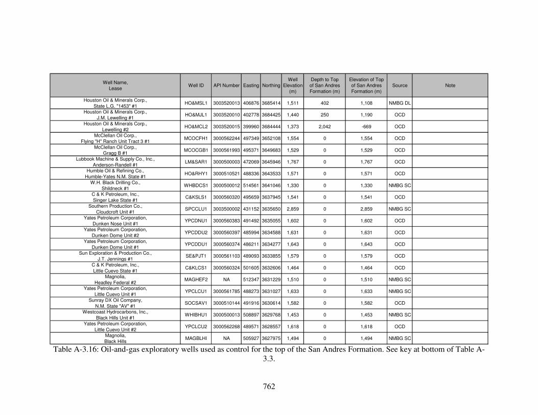
762
Well Name,
LeaseWell ID API Number Easting Northing
Well
Elevation
(m)
Depth to Top
of San Andres
Formation (m)
Elevation of Top
of San Andres
Formation (m)
Source Note
Houston Oil & Minerals Corp.,
State L.G. "1453" #1HO&MSL1 3003520013 406876 3685414 1,511 402 1,108 NMBG DL
Houston Oil & Minerals Corp.,
J.M. Lewelling #1HO&MJL1 3003520010 402778 3684425 1,440 250 1,190 OCD
Houston Oil & Minerals Corp.,
Lewelling #2HO&MCL2 3003520015 399960 3684444 1,373 2,042 -669 OCD
McClellan Oil Corp.,
Flying "H" Ranch Unit Tract 3 #1MCOCFH1 3000562244 497349 3652108 1,554 0 1,554 OCD
McClellan Oil Corp.,
Gragg B #1MCOCGB1 3000561993 495371 3649683 1,529 0 1,529 OCD
Lubbook Machine & Supply Co., Inc.,
Anderson-Randell #1LM&SAR1 3000500003 472069 3645946 1,767 0 1,767 OCD
Humble Oil & Refining Co.,
Humble-Yates N.M. State #1HO&RHY1 3000510521 488336 3643533 1,571 0 1,571 OCD
W.H. Black Drilling Co.,
Shildneck #1WHBDCS1 3000500012 514561 3641046 1,330 0 1,330 NMBG SC
C & K Petroleum, Inc.,
Singer Lake State #1C&KSLS1 3000560320 495659 3637945 1,541 0 1,541 OCD
Southern Production Co.,
Cloudcroft Unit #1SPCCLU1 3003500002 431152 3635650 2,859 0 2,859 NMBG SC
Yates Petroleum Corporation,
Dunken Nose Unit #1YPCDNU1 3000560383 491492 3635055 1,602 0 1,602 OCD
Yates Petroleum Corporation,
Dunken Dome Unit #2YPCDDU2 3000560397 485994 3634588 1,631 0 1,631 OCD
Yates Petroleum Corporation,
Dunken Dome Unit #1YPCDDU1 3000560374 486211 3634277 1,643 0 1,643 OCD
Sun Exploration & Production Co.,
J.T. Jennings #1SE&PJT1 3000561103 489093 3633855 1,579 0 1,579 OCD
C & K Petroleum, Inc.,
Little Cuevo State #1C&KLCS1 3000560324 501605 3632606 1,464 0 1,464 OCD
Magnolia,
Headley Federal #2MAGHEF2 NA 512347 3631229 1,510 0 1,510 NMBG SC
Yates Petroleum Corporation,
Little Cuevo Unit #1YPCLCU1 3000561785 488273 3631027 1,633 0 1,633 NMBG SC
Sunray DX Oil Company,
N.M. State "AV" #1SOCSAV1 3000510144 491916 3630614 1,582 0 1,582 OCD
Westcoast Hydrocarbons, Inc.,
Black Hills Unit #1WHIBHU1 3000500013 508897 3629768 1,453 0 1,453 NMBG SC
Yates Petroleum Corporation,
Little Cuevo Unit #2YPCLCU2 3000562268 489571 3628557 1,618 0 1,618 OCD
Magnolia,
Black HillsMAGBLHI NA 505927 3627975 1,494 0 1,494 NMBG SC
Table A-3.16: Oil-and-gas exploratory wells used as control for the top of the San Andres Formation. See key at bottom of Table A-
3.3.

763
Well Name,
LeaseWell ID API Number Easting Northing
Well
Elevation
(m)
Depth to Top
of San Andres
Formation (m)
Elevation of Top
of San Andres
Formation (m)
Source Note
TEXACO Inc.,
Federal (USA) "E" #1TEXIFE1 3003520001 395308 3624999 1,219 58 1,161 K&H
Yates Petroleum Corporation,
One Tree Unit #1YPCOTU1 3000562259 467160 3623529 1,872 0 1,872 NMBG SC
Yates Petroleum Corporation,
Dog Canyon "YF" Federal #1YPCDCF1 3003520024 462754 3622676 1,942 0 1,942 NMBG SC
Texas Oil & Gas Corp.,
Federal "C" #1TO&GFC1 3000560017 512954 3622309 1,359 0 1,359 NMBG SC
Kewanee Oil Co.,
F-M Unit #1KOCFMU1 3000500009 493140 3619927 1,579 0 1,579 NMBG SC
TEXACO Inc.,
Federal (USA) "F" #1TEXIFF1 3003520006 410790 3619951 1,232 744 488 K&H
Yates Petroleum Corporation,
One Tree Unit #2YPCOTU2 3000562276 468582 3619170 2,007 0 2,007 NMBG SC
Marathon Oil Co.,
Mesa Verde Ranch #1MOCMVR1 3003520022 455326 3618246 2,134 0 2,134 NMBG SC
Yates Petroleum Corp.,
Buckhorn AYU State Com #1YPCBAYU 3000560541 506142 3613140 1,440 0 1,440 NMBG SC
Texas Oil & Gas Corp.,
Federal "A" #1TO&GFA1 3000510431 506950 3613041 1,439 0 1,439 NMBG SC
Sun Oil Co.,
Pinon Unit #2SOCPIU2 3000500007 478157 3612259 1,925 0 1,925 NMBG SC
Sun Oil Co.,
Pinon Unit #1SOCPIU1 3000500006 476922 3611828 1,994 0 1,994 NMBG SC
U.V. Industries, Inc.,
Long Canyon Unit #1UVILCU1 3000560411 502547 3610225 1,533 0 1,533 NMBG SC
Gulf Oil Corp.,
Federal Munson #1GOCFMU1 3000510075 489407 3609839 1,723 0 1,723 NMBG SC
Atlantic Refining Co.,
State "AV" #1ARCSAV1 3003510001 461443 3603143 1,917 0 1,917 NMBG SC
Zapata Petroleum Corp.,
Federal 14 #1ZPCF141 3003500006 454127 3603086 2,105 0 2,105 NMBG SC
Terra Resources, Inc.,
Burro Canyon Unit #1-YTRBCU1Y 3003520017 511686 3596471 1,568 0 1,568 OCD
Stanolind Oil & Gas,
Thorn Unit #1SO>U1 3003500007 453419 3593869 1,914 0 1,914 NMBG SC
Lefors Petroleum Co.,
Federal #1LEPCFE1 3003500008 471863 3592611 1,639 0 1,639 OCD
Yates Petroleum Corporation,
Brainerd "IO" Federal #1YPCBIOF 3001522149 523000 3587630 1,402 0 1,402 OCD
Tri-Service Drilling Co.,
Little Dog Federal #1TSDLDF1 3003520008 496060 3586992 1,940 0 1,940 NMBG SC
Table A-3.16 continued.

764
Well Name,
LeaseWell ID API Number Easting Northing
Well
Elevation
(m)
Depth to Top
of San Andres
Formation (m)
Elevation of Top
of San Andres
Formation (m)
Source Note
Brainerd Corp. (aka Continental Oil Co.),
Federal "A" (aka East Texas Hill Unit) #1BRCFEA1 3001500005 523406 3586429 1,390 0 1,390 NMBG SC
Continental Oil Co.,
H.W. Bass #1COCHWB1 3001500004 516898 3586367 1,680 0 1,680 NMBG SC
Pitts Energy Co.,
Federal "9" #1PIECF91 3001527563 518567 3585218 1,615 0 1,615 OCD
E.P. Campbell,
Hurley #1EPCAHU1 3003500012 447355 3580223 1,404 0 1,404 K&H
E.P. Campbell,
Liberman State #1EPCALI1 3003500014 457361 3576570 1,326 0 1,326 K&H
W.R. Weaver,
Thompson #1WRWETH1 3003500017 499785 3575900 1,386 0 1,386 NMBG SC
E.P. Campbell,
Lois Spanel #1EPCALS1 3003500015 467947 3575324 1,408 0 1,408 K&H
Presco, Inc.,
Indian Creek Federal #1PRIICF1 3003520030 511700 3573937 1,767 0 1,767 OCD
E.P. Campbell,
McMillan Federal #1EPCAMF1 3003500018 500598 3573842 1,319 0 1,319 K&H
Coral Oil & Gas Co.,
Warren #1CO&GCW1 3003500016 487264 3571960 1,186 0 1,186 K&H
Atlantic Refining Co.,
Huapache Unit #9ARCHUU9 3001500016 527053 3566737 1,686 158 1,528 OCD
Skelly Oil Co.,
Las Cruces "D" #1SOCLCD1 3001500003 522240 3565867 1,749 111 1,637 NMBG SC
Union Oil Co.,
Federal White #1UNOCFW1 3001500019 525449 3565154 1,740 0 1,740 BH
Threshold Development Co.,
Chiricahua R 21 Federal #1TDCR21F 3003520034 489264 3563381 1,133 0 1,133 OCD
Fred Turner, Jr. (aka Pasotero Pet. Corp.),
Evans #1FTUJEV1 3003500020 433355 3563003 1,545 0 1,545 BH
E.P. Campbell (aka John J. Eisner),
Federal #1EPCAFE1 3003500019 432641 3562887 1,496 0 1,496 NMBG SC
Franklin, Aston & Fair, Inc.,
Turkey Draw Unit #1FA&FTD1 3001521378 524583 3560015 1,776 640 1,136 OCD
W.W. West,
West Dog Canyon Unit #1WWWWDC1 3003520007 505979 3555044 1,771 44 1,726 OCD
Threshold Development Co.,
Mescalero 28 Federal #1TDM28F1 3003520033 489514 3552255 1,219 0 1,219 OCD
Pennzoil Co.,
Southland "28" State #1PCS28S1 3003520019 479573 3551070 1,206 0 1,206 K&H
Fred Turner, Jr.,
State #1FTUJST1 3003500027 475070 3550274 1,315 0 1,315 K&H
Table A-3.16 continued.

765
Well Name,
LeaseWell ID API Number Easting Northing
Well
Elevation
(m)
Depth to Top
of San Andres
Formation (m)
Elevation of Top
of San Andres
Formation (m)
Source Note
E.J. Dunigan,
Alpha Federal #1EJDALF1 3003520002 496594 3549815 1,159 18 1,141 K&H
Hunt Oil Co.,
McMillan-Turner #1HUOCMT1 3003500029 469015 3547882 1,269 0 1,269 BH
E.P. Campbell,
Spiegel-Federal #1EPCSPF1 3003510002 511803 3544568 1,868 40 1,828 K&H
Pan American Petroleum Corporation,
List Anderson #1PAPCLA1 NA 491521 3533849 1,108 176 931 V&K
A.R. Jones Co.,
E.C. Mowry #1ARJECM1 NA 474192 3516927 1,230 0 1,230 BEG SC
Table A-3.16 continued.

766
Well Name,
LeaseWell ID API Number Easting Northing
Well
Elevation
(m)
Depth to Top
of Delaware
Mountain
Group (m)
Elevation of Top
of Delaware
Mountain
Group (m)
Source Note
Hunt Petroleum Corp.,
C.L. Ranch #1HPCCLR1 4222930010 496475 3528252 1,105 269 836 K&H
TEXACO Inc.,
Culberson "L" Fee #1TEXCLF1 NA 519234 3527336 1,564 0 1,564 K&H
Tenneco Oil Co.,
TXL Fee #1TOTXLF1 4210931401 563041 3526975 1,086 353 733 RRC
Border Exploration Co.,
Hammack et al. CT-1BECHCT1 4222930196 505172 3518026 1,107 587 521 K&H
Border Exploration Co.,
J.J. McAdoo 7 #1BECJJM1 4222930200 505794 3514682 1,143 407 736 K&H
The Superior Oil Company,
Covington State #1TSOCCS1 4210931405 565213 3512927 1,140 644 496 RRC
Chesapeake Operating, Inc.,
Dela Minerals "3" State #701COIDM3S 4210932268 566918 3512065 1,142 700 442 RRC
EnCana Oil & Gas (USA) Inc.,
Sibley Ranch 47 State "25" #1EOGSR47 4210932251 544180 3505778 1,332 202 1,131 RRC
Table A-3.17: Oil-and-gas exploratory wells used as control for the top of the Delaware Mountain Group. See key at bottom of Table
A-3.3.
Well Name,
LeaseWell ID API Number Easting Northing
Well
Elevation
(m)
Depth to Top
of Goat Seep
Dolomite/Lm./Fm.
(m)
Elevation of Top
of Goat Seep
Dolomite/Lm./Fm.
(m)
Source Note
Hunt Petroleum Corp.,
C.L. Ranch #1HPCCLR1 4222930010 496475 3528252 1,105 230 875 K&H
Border Exploration Co.,
Hammack et al. CT-1BECHCT1 4222930196 505172 3518026 1,107 571 536 K&H
Table A-3.18: Oil-and-gas exploratory wells used as control for the top of the Goat Seep Dolomite/Limestone/Formation. See key at
bottom of Table A-3.3.
Well Name,
LeaseWell ID API Number Easting Northing
Well
Elevation
(m)
Depth to Top
of Capitan
Lm./Fm. (m)
Elevation of Top
of Capitan
Lm./Fm. (m)
Source Note
Border Exploration Co.,
Hammack et al. CT-1BECHCT1 4222930196 505172 3518026 1,107 0 1,107 K&H
Border Exploration Co.,
J.J. McAdoo 7 #1BECJJM1 4222930200 505794 3514682 1,143 0 1,143 K&H
Table A-3.19: Oil-and-gas exploratory wells used as control for the top of the Capitan Limestone/Formation. See key at bottom of
Table A-3.3.

767
Well Name,
LeaseWell ID API Number Easting Northing
Well
Elevation
(m)
Depth to Top
of Cenozoic
Alluvium (m)
Elevation of Top
of Cenozoic
Alluvium (m)
Source Note
Houston Oil & Minerals Corp.,
Lewelling #2HO&MCL2 3003520015 399960 3684444 1,373 0 1,373 OCD
TEXACO Inc.,
Federal (USA) "E" #1TEXIFE1 3003520001 395308 3624999 1,219 0 1,219 K&H
TEXACO Inc.,
Federal (USA) "F" #1TEXIFF1 3003520006 410790 3619951 1,232 0 1,232 K&H
Plymouth Oil Co.,
Evans (aka Federal D) #1PLOCEV1 3003500003 404731 3604561 1,233 0 1,233 BH
Otero Oil Co.,
McGregor #1OTOCMC1 3003500010 412151 3586894 1,289 0 1,289 BH
W.W. West,
West Dog Canyon Unit #1WWWWDC1 3003520007 505979 3555044 1,771 0 1,771 OCD
E.J. Dunigan,
Alpha Federal #1EJDALF1 3003520002 496594 3549815 1,156 0 1,156 K&H
GDP 61-6 GDP61-6 NA 390213 3549130 1,254 0 1,254 F&J
GDP 45-5 GDP45-5 NA 391837 3549102 1,255 0 1,255 F&J
GDP 46-6 GDP46-6 NA 390223 3549119 1,252 0 1,252 F&J
GDP 51-8 GDP51-8 NA 393417 3545870 1,253 0 1,253 F&J
E.P. Campbell,
Spiegel-Federal #1EPCSPF1 3003510002 511803 3544568 1,868 0 1,868 K&H
Hunt Petroleum Corp.,
C.L. Ranch "5" #1HPCCL51 4222930011 496478 3539912 1,110 0 1,110 K&H
Hunt Oil Co.,
Dyer #1HUOCDY1 4222930007 485477 3530917 1,119 0 1,119 K&H
Hunt Petroleum Corp.,
C.L. Ranch #1HPCCLR1 4222930010 496475 3528252 1,105 0 1,105 K&H
Table A-3.20: Oil-and-gas exploratory wells used as control for the top of the Cenozoic alluvium. See key at bottom of Table A-3.3.
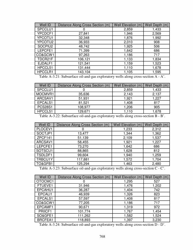
768
Well ID Distance Along Cross Section (m) Well Elevation (m) Well Depth (m)
SPCCLU1 0 2,859 1,433
YPCDCF1 27,841 1,946 2,569
YPCOTU1 32,348 1,876 1,992
YPCOTU2 36,933 2,010 908
SOCPIU2 48,742 1,925 506
LEPCFE1 71,399 1,642 686
CO&GCW1 97,263 1,186 717
TDCR21F 106,121 1,133 1,834
EJDALF1 121,541 1,159 1,523
HPCCL51 131,444 1,110 1,678
HPCCLR1 143,104 1,105 1,595 Table A-3.21: Subsurface oil-and-gas exploratory wells along cross-section A - A’.
Well ID Distance Along Cross Section (m) Well Elevation (m) Well Depth (m)
SPCCLU1 0 2,859 1,433
MOCMVR1 35,636 2,143 2,137
ARCSAV1 51,931 1,921 1,227
EPCALS1 81,521 1,408 817
PCS28S1 108,977 1,206 905
HPCCL51 129,671 1,110 1,678 Table A-3.22: Subsurface oil-and-gas exploratory wells along cross-section B - B’.
Well ID Distance Along Cross Section (m) Well Elevation (m) Well Depth (m)
PLOCEV1 0 1,233 2,312
SOCTJP1 13,477 1,344 1,362
ZPCF141 51,139 2,109 1,537
ARCSAV1 58,455 1,921 1,227
LEPCFE1 73,270 1,642 686
SOTSCU1 88,865 1,628 812
TSDLDF1 99,604 1,940 1,259
TRBCU1Y 117,881 1,572 1,704
TO&GFB1 125,294 1,463 2,480 Table A-3.23: Subsurface oil-and-gas exploratory wells along cross-section C - C’.
Well ID Distance Along Cross Section (m) Well Elevation (m) Well Depth (m)
OTOCMC1 0 1,295 527
FTUEVE1 31,946 1,476 1,202
EPCAHU1 36,287 1,404 742
EPCALI1 46,939 1,326 823
EPCALS1 57,597 1,408 817
CO&GCW1 77,205 1,186 717
EPCAMF1 90,671 1,319 972
PRIICF1 101,774 1,767 1,454
SO&GFE1 111,262 1,582 1,524
BRCFEA1 118,893 1,397 3,230 Table A-3.24: Subsurface oil-and-gas exploratory wells along cross-section D - D’.

769
Well ID Distance Along Cross Section (m) Well Elevation (m) Well Depth (m)
GDP 45-5 0 1,255 1,207
SEOCTF1 27,166 1,618 1,707
HEYBRU1 43,911 1,554 2,156
TROGJA1 55,479 1,509 1,617
HUOCMT1 83,689 1,269 663
FTUJST1 90,199 1,317 1,583
PCS28S1 94,772 1,206 905
TDM28F1 104,784 1,219 1,409
EJDALF1 112,272 1,159 1,523
WWWWDC1 123,016 1,771 1,390
UNOCFW1 144,954 1,740 2,053
HO&RHO2 154,127 1,358 3,835 Table A-3.25: Subsurface oil-and-gas exploratory wells along cross-section E - E’.

770
POD Number/
Well ID/
State Well
Number
Easting Northing
Ground
Surface
Elevation
(m)
Elevation
of
Well
Depth
(m)
Groundwater
Elevation
(m)
Aquifer County
Depth-
to-
Groundwater
Control
Point
Groundwater
Surface
Control
Point
Source Note
PN 00007 460240 3638479 2,000 1,787 1,791 NA Otero Y Y NMOSE *
SM-0098 476159 3637546 1,719 1,613 1,628 NA Chaves Y N SMHS *
PN 00058 482719 3637520 1,645 1,534 1,543 NA Eddy Y N NMOSE *
PN 01036 POD1 442482 3636947 2,291 2,154 2,200 NA Otero Y Y NMOSE *
PN 00737 445116 3636923 2,346 2,316 NA NA Otero Y N NMOSE *
PN 00049 453268 3636885 2,036 2,001 2,008 NA Otero Y Y NMOSE *
PN 00842 439450 3636685 2,501 2,410 NA NA Otero N N NMOSE *
RA 03777 497585 3636663 1,536 1,297 1,310 NA Chaves Y Y NMOSE *
PN 00079 462708 3636475 1,923 1,783 1,808 NA Otero Y Y NMOSE *
PN 00822 439437 3636284 2,371 2,187 2,206 NA Otero N N NMOSE *
SM-0144 470081 3636255 2,042 1,740 1,788 NA Chaves Y Y SMHS *
PN 00630 452766 3636193 2,058 2,053 2,053 NA Otero Y N NMOSE *
PN 00044 452865 3636092 2,056 2,006 2,019 NA Otero Y Y NMOSE *
SM-0135 472964 3636058 1,839 1,625 1,656 NA Chaves Y Y SMHS *
PN 01003 443816 3636026 2,249 2,172 2,197 NA Otero Y Y NMOSE *
PN 01090 POD1 452699 3636003 2,074 2,019 2,039 NA Otero Y Y NMOSE *
RA 11168 POD1 508183 3635914 1,432 1,173 1,237 NA Chaves Y Y NMOSE *
PN 00667 POD2 452861 3635895 2,056 2,020 2,041 NA Otero Y N NMOSE *
PN 00602 446786 3635832 2,218 2,197 2,203 NA Otero Y N NMOSE *
PN 00635 452762 3635796 2,058 2,040 2,052 NA Otero Y N NMOSE *
PN 00722 446292 3635739 2,145 2,111 2,127 NA Otero Y Y NMOSE *
PN 00865 446092 3635739 2,169 2,079 2,139 NA Otero Y Y NMOSE *
PN 00670 452661 3635695 2,061 1,963 2,018 NA Otero Y Y NMOSE *
PN 00667 452958 3635600 2,098 2,082 2,090 NA Otero Y N NMOSE *
PN 00217 425332 3635555 2,793 2,688 2,717 NA Otero Y Y NMOSE *
PN 00661 456937 3635554 2,071 1,888 1,934 NA Otero Y Y NMOSE *
PN 00031 A 445304 3635500 2,180 2,113 2,125 NA Otero Y N NMOSE *
PN 00219 POD2 425635 3635450 2,774 2,655 2,688 NA Otero N Y NMOSE * Table A-3.26: Groundwater surface and depth-to-groundwater control wells. Key at bottom of table.

771
POD Number/
Well ID/
State Well
Number
Easting Northing
Ground
Surface
Elevation
(m)
Elevation
of
Well
Depth
(m)
Groundwater
Elevation
(m)
Aquifer County
Depth-
to-
Groundwater
Control
Point
Groundwater
Surface
Control
Point
Source Note
PN 00080 486788 3635392 1,561 1,449 1,468 NA Chaves Y N NMOSE *
RA 03836 513345 3635360 1,364 1,083 1,102 NA Chaves Y Y NMOSE *
PN 00201 446482 3635350 2,153 2,120 2,129 NA Otero Y Y NMOSE *
PN 00077 447796 3635323 2,108 2,073 2,103 NA Otero Y Y NMOSE *
PN 00039 448555 3635276 2,103 2,071 2,097 NA Otero Y Y NMOSE *
SM-0133 475444 3635270 1,785 1,480 1,511 NA Chaves Y Y SMHS *
PN 00217 POD2 426036 3635242 2,761 2,627 2,674 NA Otero N Y NMOSE *
PN 00806 457244 3635239 2,038 1,858 1,917 NA Otero Y Y NMOSE *
PN 00031 444293 3635234 2,227 2,150 2,208 NA Otero Y N NMOSE *
PN 00754 457654 3635225 2,032 1,849 NA NA Otero Y Y NMOSE *
PN 00585 443691 3635217 2,192 2,182 2,188 NA Otero Y Y NMOSE *
PN 00124 POD2 450135 3635156 2,079 2,049 2,077 NA Otero Y Y NMOSE *
PN 00956 451657 3635122 2,202 2,117 2,166 NA Otero Y N NMOSE *
PN 00089 450641 3635119 2,106 2,068 2,104 NA Otero Y N NMOSE *
PN 00307 440858 3635117 2,270 2,215 2,255 NA Otero Y Y NMOSE *
PN 00983 450221 3635109 2,076 2,040 2,064 NA Otero Y Y NMOSE *
PN 00124 450012 3635101 2,078 2,059 2,074 NA Otero Y Y NMOSE *
PN 00019 449812 3635101 2,082 2,050 2,072 NA Otero Y N NMOSE *
PN 00175 449604 3635092 2,086 2,058 2,080 NA Otero Y Y NMOSE *
PN 00860 448972 3635070 2,123 2,075 2,090 NA Otero Y Y NMOSE *
PN 00912 441365 3635033 2,278 2,231 2,248 NA Otero Y Y NMOSE *
PN 00050 451558 3635023 2,144 2,082 2,093 NA Otero Y N NMOSE *
PN 00781 440959 3635018 2,239 2,162 2,192 NA Otero Y N NMOSE *
PN 00043 452751 3634995 2,079 2,039 2,047 NA Otero Y Y NMOSE *
PN 00266 439730 3634978 2,305 2,258 2,272 NA Otero Y Y NMOSE *
PN 00756 451262 3634929 2,087 2,062 2,076 NA Otero Y N NMOSE *
PN 00778 441058 3634917 2,241 2,160 2,194 NA Otero Y N NMOSE *
PN 00413 439421 3634864 2,282 2,224 2,270 NA Otero Y Y NMOSE * Table A-3.26 continued.

772
POD Number/
Well ID/
State Well
Number
Easting Northing
Ground
Surface
Elevation
(m)
Elevation
of
Well
Depth
(m)
Groundwater
Elevation
(m)
Aquifer County
Depth-
to-
Groundwater
Control
Point
Groundwater
Surface
Control
Point
Source Note
PN 00639 POD2 439221 3634864 2,324 2,236 2,266 NA Otero Y Y NMOSE *
PN 00639 439013 3634851 2,340 2,282 2,309 NA Otero Y Y NMOSE *
SM-0134 473847 3634846 1,842 1,705 1,723 NA Chaves Y N SMHS *
PN 00703 451363 3634832 2,061 1,981 2,033 NA Otero Y Y NMOSE *
SM-0151 465000 3634677 2,026 1,808 1,815 NA Otero Y Y SMHS *
PN 00256 442578 3634664 2,205 2,095 2,114 NA Otero Y N NMOSE *
PN 00412 468408 3634588 1,945 1,805 1,823 NA Otero Y N NMOSE *
RA 05467 490603 3634559 1,538 1,363 1,363 NA Chaves Y Y NMOSE *
PN 00796 438911 3634546 2,355 2,240 2,276 NA Otero N Y NMOSE *
PN 00360 438508 3634534 2,300 2,178 NA NA Otero N N NMOSE *
PN 00675 POD2 438028 3634534 2,356 2,247 2,300 NA Otero Y Y NMOSE *
PN 00675 428756 3634521 2,857 2,791 2,808 NA Otero Y N NMOSE *
PN 00510 455964 3634444 2,077 1,880 1,921 NA Otero N Y NMOSE *
PN 00352 437133 3634435 2,442 2,330 2,369 NA Otero Y Y NMOSE *
PN 00407 438425 3634427 2,320 2,202 2,231 NA Otero N N NMOSE *
PN 00695 442225 3634406 2,302 2,223 2,238 NA Otero Y Y NMOSE *
PN 00198 442161 3634253 2,308 2,177 NA NA Otero Y Y NMOSE *
PN 01073 POD1 458646 3634238 2,028 1,852 1,892 NA Otero Y N NMOSE *
PN 00795 456185 3634233 2,090 1,907 NA NA Otero Y Y NMOSE *
PN 00895 458651 3634205 2,025 1,857 1,882 NA Otero Y Y NMOSE *
RA 03407 510105 3634187 1,402 1,147 1,161 NA Eddy Y Y NMOSE *
PN 00510 POD2 441013 3634150 2,395 2,193 2,242 NA Otero N Y NMOSE *
T 01737 422914 3633828 2,304 2,230 2,265 NA Otero Y Y NMOSE *
PN 00392 434027 3633750 2,426 2,382 2,410 NA Otero Y Y NMOSE *
PN 00381 433827 3633750 2,400 2,354 2,391 NA Otero Y Y NMOSE *
PN 00881 462920 3633625 2,039 1,807 1,828 NA Otero Y Y NMOSE *
PN 00631 457024 3633611 2,067 1,864 1,899 NA Otero N Y NMOSE *
PN 01037 POD1 458019 3633590 2,029 1,846 1,889 NA Otero Y Y NMOSE * Table A-3.26 continued.

773
POD Number/
Well ID/
State Well
Number
Easting Northing
Ground
Surface
Elevation
(m)
Elevation
of
Well
Depth
(m)
Groundwater
Elevation
(m)
Aquifer County
Depth-
to-
Groundwater
Control
Point
Groundwater
Surface
Control
Point
Source Note
PN 00265 457552 3633285 2,037 1,853 1,885 NA Otero Y N NMOSE *
PN 01066 POD1 457632 3633191 2,043 1,860 1,902 NA Otero Y Y NMOSE *
PN 00844 457451 3633184 2,056 1,843 1,912 NA Otero Y Y NMOSE *
PN 00220 POD2 455975 3633018 2,124 1,936 1,962 NA Otero N Y NMOSE *
PN 00343 POD2 457020 3632990 2,061 1,854 1,878 NA Otero N N NMOSE *
PN 00343 456694 3632900 2,078 1,891 1,904 NA Otero N Y NMOSE *
PN 00245 457121 3632891 2,077 1,874 1,908 NA Otero N Y NMOSE *
PN 00345 456384 3632808 2,105 2,075 NA NA Otero Y N NMOSE *
PN 00882 458234 3632785 2,006 1,829 1,884 NA Otero Y Y NMOSE *
PN 00126 448392 3632652 2,356 2,092 2,113 NA Otero N Y NMOSE *
PN 00282 430011 3632612 2,497 2,445 2,476 NA Otero Y Y NMOSE *
PN 00499 449708 3632571 2,242 2,106 2,127 NA Otero Y Y NMOSE *
PN 00009 450106 3632566 2,285 2,155 2,163 NA Otero Y N NMOSE *
SM-0150 467259 3632518 1,977 1,785 1,807 NA Chaves Y Y SMHS *
PN 01032 POD1 459566 3632490 2,038 1,777 1,911 NA Otero Y N NMOSE *
RA 06874 POD2 512800 3632324 1,329 1,098 1,143 NA Chaves Y Y NMOSE *
PN 00666 458018 3632173 2,017 1,829 1,901 NA Otero Y Y NMOSE *
PN 00546 457650 3632172 2,029 1,864 1,878 NA Otero Y N NMOSE *
PN 00768 449107 3632170 2,252 2,069 2,206 NA Otero Y N NMOSE *
RA 03675 506224 3632085 1,369 1,125 1,227 NA Chaves Y Y NMOSE *
PN 00489 462307 3631988 2,013 1,774 1,800 NA Otero Y Y NMOSE *
PN 00123 448907 3631970 2,266 2,220 NA NA Otero Y N NMOSE *
PN 01006 POD1 448290 3631954 2,280 2,140 2,173 NA Otero Y Y NMOSE *
PN 00036 476427 3631844 1,740 1,494 1,512 NA Chaves Y Y NMOSE *
PN 00676 POD2 448622 3631773 2,276 2,017 NA NA Otero Y Y NMOSE *
PN 01041 POD1 448528 3631684 2,287 2,086 2,125 NA Otero N Y NMOSE *
PN 00676 448602 3631656 2,270 1,995 2,053 NA Otero N N NMOSE *
PN 00261 448186 3631243 2,304 2,199 2,211 NA Otero Y N NMOSE * Table A-3.26 continued.

774
POD Number/
Well ID/
State Well
Number
Easting Northing
Ground
Surface
Elevation
(m)
Elevation
of
Well
Depth
(m)
Groundwater
Elevation
(m)
Aquifer County
Depth-
to-
Groundwater
Control
Point
Groundwater
Surface
Control
Point
Source Note
PN 01025 POD1 457816 3631165 2,025 1,879 1,927 NA Otero Y Y NMOSE *
PN 00310 464326 3631160 1,995 1,752 1,858 NA Otero Y Y NMOSE *
PN 00609 450011 3631044 2,241 2,160 2,168 NA Otero Y N NMOSE *
PN 00311 466125 3630937 1,991 1,703 1,808 NA Otero Y Y NMOSE *
PN 01031 POD1 453015 3630869 2,145 2,030 2,054 NA Otero Y Y NMOSE *
PN 00032 POD1 481051 3630828 1,668 1,394 NA NA Chaves Y Y NMOSE *
PN 00032 481152 3630729 1,662 1,388 1,403 NA Chaves Y Y NMOSE *
PN 00112 441444 3630676 2,377 2,286 NA NA Otero Y Y NMOSE *
PN 00608 444188 3630649 2,422 2,248 2,312 NA Otero Y N NMOSE *
PN 00829 449712 3630539 2,231 2,174 2,207 NA Otero Y N NMOSE *
PN 00047 452294 3630371 2,165 2,040 2,074 NA Otero Y Y NMOSE *
PN 00879 449507 3630340 2,213 2,200 2,209 NA Otero Y N NMOSE *
PN 00730 449307 3630340 2,216 2,179 2,188 NA Otero Y N NMOSE *
PN 00122 450316 3630337 2,183 2,106 NA NA Otero Y Y NMOSE *
PN 00216 450721 3630335 2,204 2,154 2,174 NA Otero Y N NMOSE *
PN 00127 451698 3630149 2,173 2,089 2,122 NA Otero Y Y NMOSE *
PN 00804 450722 3630119 2,156 2,102 2,120 NA Otero Y Y NMOSE *
PN 00361 450926 3630115 2,158 2,091 2,108 NA Otero Y Y NMOSE *
PN 00200 452202 3630056 2,144 2,042 2,063 NA Otero Y Y NMOSE *
PN 00329 449410 3630031 2,182 2,044 2,057 NA Otero Y N NMOSE *
PN 00297 452924 3629955 2,163 2,041 2,056 NA Otero Y Y NMOSE *
PN 00298 451898 3629949 2,143 2,036 2,067 NA Otero Y Y NMOSE *
PN 00171 451512 3629932 2,179 2,121 2,139 NA Otero Y N NMOSE *
PN 00507 450423 3629810 2,183 2,077 2,169 NA Otero Y N NMOSE *
PN 00763 442570 3629791 2,356 2,235 2,311 NA Otero Y Y NMOSE *
PN 00817 437004 3629732 2,638 2,620 2,631 NA Otero Y N NMOSE *
PN 00443 451319 3629711 2,144 2,018 2,109 NA Otero Y Y NMOSE *
PN 00989 454590 3629707 2,095 1,962 1,983 NA Otero Y Y NMOSE * Table A-3.26 continued.

775
POD Number/
Well ID/
State Well
Number
Easting Northing
Ground
Surface
Elevation
(m)
Elevation
of
Well
Depth
(m)
Groundwater
Elevation
(m)
Aquifer County
Depth-
to-
Groundwater
Control
Point
Groundwater
Surface
Control
Point
Source Note
PN 00203 437505 3629632 2,536 2,493 2,501 NA Otero Y Y NMOSE *
PN 00783 437404 3629531 2,539 2,484 2,510 NA Otero Y Y NMOSE *
PN 00061 451711 3629525 2,148 2,071 2,087 NA Otero Y Y NMOSE *
PN 00176 451319 3629511 2,171 2,044 2,110 NA Otero Y Y NMOSE *
PN 01001 449106 3629511 2,179 2,141 2,158 NA Otero Y Y NMOSE *
PN 00223 451632 3629411 2,155 2,036 2,046 NA Otero Y N NMOSE *
PN 00731 450016 3629402 2,300 2,226 2,272 NA Otero Y N NMOSE *
PN 00834 451923 3629312 2,208 2,132 NA NA Otero Y N NMOSE *
PN 00299 451325 3629307 2,177 2,085 NA NA Otero Y Y NMOSE *
PN 01019 POD1 449107 3629302 2,207 2,146 2,168 NA Otero Y Y NMOSE *
PN 01002 448704 3629296 2,192 2,134 2,173 NA Otero Y Y NMOSE *
PN 00911 455633 3629273 2,083 1,870 1,916 NA Otero N N NMOSE *
PN 00682 477102 3629119 1,721 1,446 NA NA Chaves Y Y NMOSE *
PN 00005 447085 3629047 2,374 2,343 2,356 NA Otero Y N NMOSE *
PN 00239 435673 3629038 2,632 2,615 2,621 NA Otero Y Y NMOSE *
PN 00209 464199 3629035 2,020 1,775 1,829 NA Otero Y Y NMOSE *
PN 00308 442967 3628994 2,302 2,213 2,231 NA Otero Y Y NMOSE *
PN 00237 435787 3628929 2,618 2,603 2,613 NA Otero Y Y NMOSE *
PN 00119 453798 3628887 2,122 1,919 2,043 NA Otero Y Y NMOSE *
PN 00966 455641 3628866 2,078 1,932 1,988 NA Otero Y Y NMOSE *
PN 00071 451029 3628808 2,207 2,133 2,141 NA Otero Y N NMOSE *
PN 00962 445691 3628786 2,247 2,155 2,193 NA Otero Y N NMOSE *
PN 00087 447801 3628775 2,207 2,181 2,205 NA Otero Y N NMOSE *
PN 00225 447398 3628755 2,234 2,218 2,233 NA Otero Y N NMOSE *
PN 00856 435787 3628729 2,689 2,627 2,652 NA Otero Y N NMOSE *
PN 00046 449109 3628694 2,316 2,262 2,289 NA Otero Y N NMOSE *
PN 00561 445394 3628678 2,238 2,207 2,233 NA Otero Y Y NMOSE *
PN 00417 446288 3628596 2,225 2,199 2,219 NA Otero Y Y NMOSE * Table A-3.26 continued.

776
POD Number/
Well ID/
State Well
Number
Easting Northing
Ground
Surface
Elevation
(m)
Elevation
of
Well
Depth
(m)
Groundwater
Elevation
(m)
Aquifer County
Depth-
to-
Groundwater
Control
Point
Groundwater
Surface
Control
Point
Source Note
PN 00949 446088 3628596 2,232 2,189 2,207 NA Otero Y Y NMOSE *
SM-0075 447829 3628594 2,207 2,153 2,180 NA Otero Y Y SMHS *
PN 00872 445891 3628586 2,228 2,107 NA NA Otero Y Y NMOSE *
PN 00018 447500 3628450 2,219 2,182 NA NA Otero Y Y NMOSE *
PN 00857 447300 3628450 2,235 2,191 2,217 NA Otero Y N NMOSE *
PN 00750 445692 3628385 2,271 2,240 2,245 NA Otero Y Y NMOSE *
PN 00014 446998 3628333 2,243 2,193 2,229 NA Otero Y N NMOSE *
PN 00835 438193 3628324 2,567 2,421 NA NA Otero Y Y NMOSE *
PN 00196 POD2 442050 3628215 2,374 2,237 2,298 NA Otero Y Y NMOSE *
PN 00196 442155 3628153 2,361 2,286 2,292 NA Otero Y Y NMOSE *
PN 00708 441748 3628136 2,368 2,321 2,334 NA Otero Y Y NMOSE *
PN 00526 442254 3628052 2,324 2,263 2,294 NA Otero Y Y NMOSE *
PN 00594 442054 3628052 2,362 2,288 2,295 NA Otero Y Y NMOSE *
PN 00357 458020 3627889 2,109 1,915 1,938 NA Otero Y Y NMOSE *
PN 00681 473462 3627768 1,762 1,738 NA NA Chaves Y N NMOSE *
PN 00129 456540 3627762 2,119 2,072 2,087 NA Otero Y N NMOSE *
PN 00202 442148 3627748 2,309 2,270 2,274 NA Otero Y Y NMOSE *
PN 00174 441744 3627731 2,326 2,294 2,311 NA Otero Y Y NMOSE *
PN 00073 451331 3627670 2,164 2,062 2,085 NA Otero Y Y NMOSE *
PN 00679 471776 3627604 1,790 1,699 NA NA Chaves Y Y NMOSE *
PN 00004 447404 3627541 2,313 2,183 2,191 NA Otero Y Y NMOSE *
PN 00786 443258 3627488 2,380 2,360 2,371 NA Otero Y N NMOSE *
PN 00775 444171 3627420 2,356 2,311 2,347 NA Otero Y N NMOSE *
PN 00552 450369 3627370 2,240 2,054 2,075 NA Otero N Y NMOSE *
PN 00016 451191 3627359 2,179 2,077 2,102 NA Otero Y Y NMOSE *
PN 00587 441735 3627325 2,321 2,224 2,276 NA Otero Y Y NMOSE *
PN 00296 450990 3627158 2,244 2,141 2,145 NA Otero Y N NMOSE *
PN 00799 439811 3627141 2,432 2,396 2,418 NA Otero Y Y NMOSE * Table A-3.26 continued.
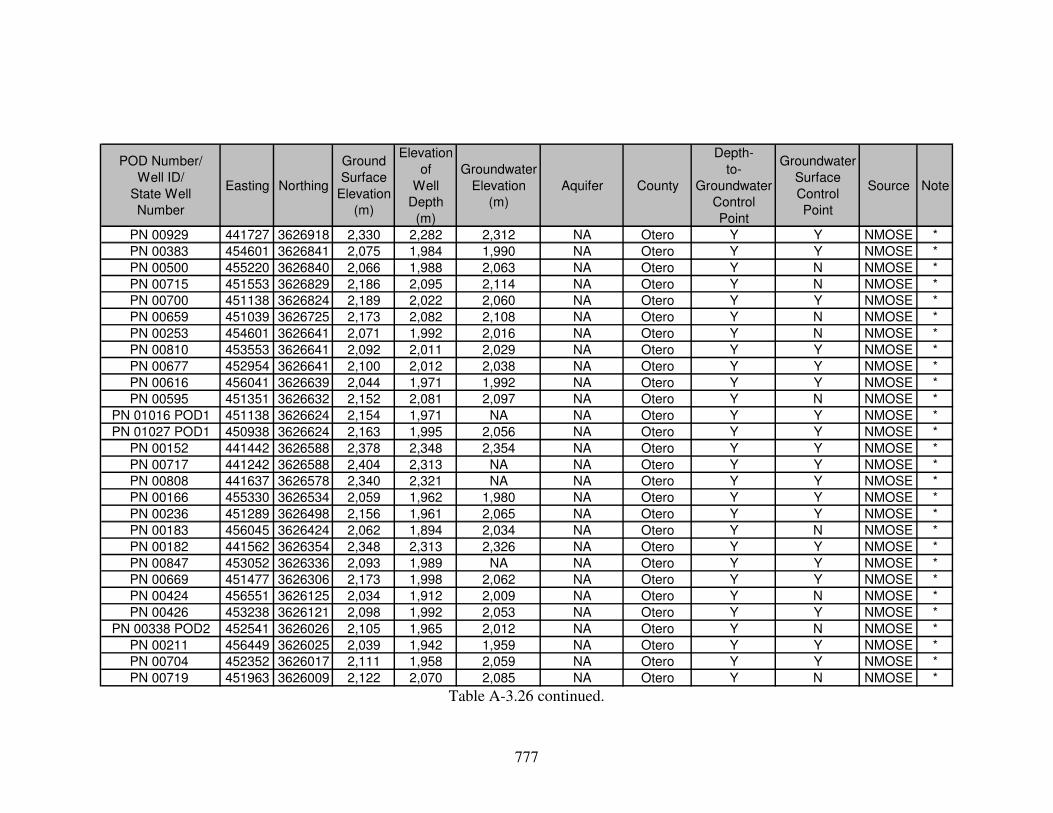
777
POD Number/
Well ID/
State Well
Number
Easting Northing
Ground
Surface
Elevation
(m)
Elevation
of
Well
Depth
(m)
Groundwater
Elevation
(m)
Aquifer County
Depth-
to-
Groundwater
Control
Point
Groundwater
Surface
Control
Point
Source Note
PN 00929 441727 3626918 2,330 2,282 2,312 NA Otero Y Y NMOSE *
PN 00383 454601 3626841 2,075 1,984 1,990 NA Otero Y Y NMOSE *
PN 00500 455220 3626840 2,066 1,988 2,063 NA Otero Y N NMOSE *
PN 00715 451553 3626829 2,186 2,095 2,114 NA Otero Y N NMOSE *
PN 00700 451138 3626824 2,189 2,022 2,060 NA Otero Y Y NMOSE *
PN 00659 451039 3626725 2,173 2,082 2,108 NA Otero Y N NMOSE *
PN 00253 454601 3626641 2,071 1,992 2,016 NA Otero Y N NMOSE *
PN 00810 453553 3626641 2,092 2,011 2,029 NA Otero Y Y NMOSE *
PN 00677 452954 3626641 2,100 2,012 2,038 NA Otero Y Y NMOSE *
PN 00616 456041 3626639 2,044 1,971 1,992 NA Otero Y Y NMOSE *
PN 00595 451351 3626632 2,152 2,081 2,097 NA Otero Y N NMOSE *
PN 01016 POD1 451138 3626624 2,154 1,971 NA NA Otero Y Y NMOSE *
PN 01027 POD1 450938 3626624 2,163 1,995 2,056 NA Otero Y Y NMOSE *
PN 00152 441442 3626588 2,378 2,348 2,354 NA Otero Y Y NMOSE *
PN 00717 441242 3626588 2,404 2,313 NA NA Otero Y Y NMOSE *
PN 00808 441637 3626578 2,340 2,321 NA NA Otero Y Y NMOSE *
PN 00166 455330 3626534 2,059 1,962 1,980 NA Otero Y Y NMOSE *
PN 00236 451289 3626498 2,156 1,961 2,065 NA Otero Y Y NMOSE *
PN 00183 456045 3626424 2,062 1,894 2,034 NA Otero Y N NMOSE *
PN 00182 441562 3626354 2,348 2,313 2,326 NA Otero Y Y NMOSE *
PN 00847 453052 3626336 2,093 1,989 NA NA Otero Y Y NMOSE *
PN 00669 451477 3626306 2,173 1,998 2,062 NA Otero Y Y NMOSE *
PN 00424 456551 3626125 2,034 1,912 2,009 NA Otero Y N NMOSE *
PN 00426 453238 3626121 2,098 1,992 2,053 NA Otero Y Y NMOSE *
PN 00338 POD2 452541 3626026 2,105 1,965 2,012 NA Otero Y N NMOSE *
PN 00211 456449 3626025 2,039 1,942 1,959 NA Otero Y Y NMOSE *
PN 00704 452352 3626017 2,111 1,958 2,059 NA Otero Y Y NMOSE *
PN 00719 451963 3626009 2,122 2,070 2,085 NA Otero Y N NMOSE * Table A-3.26 continued.

778
POD Number/
Well ID/
State Well
Number
Easting Northing
Ground
Surface
Elevation
(m)
Elevation
of
Well
Depth
(m)
Groundwater
Elevation
(m)
Aquifer County
Depth-
to-
Groundwater
Control
Point
Groundwater
Surface
Control
Point
Source Note
PN 00702 451763 3626009 2,128 2,037 NA NA Otero Y Y NMOSE *
PN 00195 441972 3625956 2,504 2,469 2,483 NA Otero Y N NMOSE *
PN 00660 452253 3625918 2,139 2,085 2,098 NA Otero Y N NMOSE *
PN 00184 456653 3625828 2,037 1,903 NA NA Otero Y Y NMOSE *
PN 00841 452352 3625817 2,118 2,048 2,067 NA Otero Y Y NMOSE *
PN 01015 POD1 452152 3625817 2,160 1,944 1,976 NA Otero N N NMOSE *
PN 00393 451288 3625692 2,148 2,071 2,099 NA Otero Y N NMOSE *
PN 00871 452147 3625610 2,148 2,017 2,061 NA Otero Y Y NMOSE *
PN 00738 452248 3625511 2,119 2,030 2,056 NA Otero Y Y NMOSE *
PN 00729 455646 3625420 2,107 1,964 2,010 NA Otero Y Y NMOSE *
PN 00758 452347 3625410 2,110 1,999 2,057 NA Otero Y Y NMOSE *
PN 00780 452147 3625410 2,133 2,050 2,079 NA Otero Y N NMOSE *
PN 00720 451373 3625397 2,236 2,114 2,151 NA Otero Y N NMOSE *
T 04695 421163 3625340 2,219 2,119 2,128 NA Otero N Y NMOSE *
T 04207 420963 3625340 2,203 2,050 NA NA Otero N Y NMOSE *
T 04186 420671 3625247 2,199 2,107 NA NA Otero Y Y NMOSE *
T 04443 420276 3625246 2,234 2,173 2,214 NA Otero Y N NMOSE *
PN 00683 472375 3625165 1,948 988 NA NA Chaves N N NMOSE *
PN 00382 435462 3625068 2,634 2,587 2,610 NA Otero Y Y NMOSE *
T 04187 420369 3624953 2,153 1,924 NA NA Otero N Y NMOSE *
T 03353 420169 3624953 2,155 2,094 NA NA Otero Y Y NMOSE *
T 04424 420270 3624854 2,147 2,088 2,127 NA Otero Y N NMOSE *
PN 00684 477394 3624730 1,751 1,553 NA NA Chaves Y Y NMOSE *
PN 00747 456761 3624707 2,024 1,982 NA NA Otero Y N NMOSE *
PN 00753 456660 3624606 2,035 1,989 2,006 NA Otero Y N NMOSE *
PN 00557 452126 3624101 2,181 2,062 2,102 NA Otero Y N NMOSE *
PN 00831 456030 3623803 2,053 1,977 2,004 NA Otero Y N NMOSE *
PN 00755 455225 3622995 2,074 1,976 2,016 NA Otero Y N NMOSE * Table A-3.26 continued.

779
POD Number/
Well ID/
State Well
Number
Easting Northing
Ground
Surface
Elevation
(m)
Elevation
of
Well
Depth
(m)
Groundwater
Elevation
(m)
Aquifer County
Depth-
to-
Groundwater
Control
Point
Groundwater
Surface
Control
Point
Source Note
PN 00761 454834 3622797 2,091 1,999 2,045 NA Otero Y N NMOSE *
ST 00062 432133 3621977 2,714 2,625 2,645 NA Otero Y Y NMOSE *
PN 00942 459827 3621825 2,023 1,846 1,888 NA Otero Y Y NMOSE *
T 01386 413314 3621642 1,251 1,179 1,179 NA Otero Y Y NMOSE *
T 01925 418686 3621600 2,178 2,138 2,160 NA Otero Y N NMOSE *
PN 00511 453047 3621586 2,142 1,959 1,979 NA Otero Y Y NMOSE *
PN 00224 477378 3620705 1,823 1,604 1,671 NA Chaves Y Y NMOSE *
RA 09265 484620 3620287 1,653 1,409 1,507 NA Chaves Y Y NMOSE *
PN 00787 449823 3619557 2,218 1,936 2,032 NA Otero Y Y NMOSE *
RA 04570 520714 3619405 1,287 1,073 1,089 NA Eddy Y Y NMOSE *
RA 05465 521117 3619405 1,282 1,046 1,072 NA Eddy Y Y NMOSE *
T 05008 POD1 425564 3617902 2,107 2,040 2,061 NA Otero Y Y NMOSE *
T 05126 POD1 425166 3617518 2,123 2,102 NA NA Otero N N NMOSE *
RA 05487 517807 3617479 1,325 1,046 1,085 NA Eddy Y Y NMOSE *
T 04531 424589 3617331 2,064 1,942 NA NA Otero Y Y NMOSE *
T 04385 425370 3617301 2,091 1,908 1,973 NA Otero Y Y NMOSE *
T 04137 425561 3617286 2,063 1,941 NA NA Otero Y Y NMOSE *
T 04530 424198 3617146 2,047 1,926 NA NA Otero Y N NMOSE *
T 04389 426542 3617057 2,112 2,021 2,032 NA Otero Y Y NMOSE *
T 04781 424592 3616921 2,058 1,869 NA NA Otero Y Y NMOSE *
T 03800 417107 3616826 1,281 976 NA NA Otero N Y NMOSE *
RA 07804 525020 3616698 1,246 1,035 1,090 NA Eddy Y Y NMOSE *
RA 06189 510157 3616661 1,407 1,355 NA NA Chaves Y Y NMOSE *
T 04329 425770 3616471 2,013 1,830 NA NA Otero Y Y NMOSE *
T 03040 414185 3616346 1,252 1,206 1,222 NA Otero Y Y NMOSE *
RA 10997 POD1 523043 3616281 1,270 986 1,111 NA Eddy Y Y NMOSE *
RA 05236 524162 3615894 1,247 827 1,083 NA Eddy Y Y NMOSE *
ST 00115 S-6 455056 3615809 2,048 1,834 NA NA Otero Y Y NMOSE * Table A-3.26 continued.

780
POD Number/
Well ID/
State Well
Number
Easting Northing
Ground
Surface
Elevation
(m)
Elevation
of
Well
Depth
(m)
Groundwater
Elevation
(m)
Aquifer County
Depth-
to-
Groundwater
Control
Point
Groundwater
Surface
Control
Point
Source Note
T 04783 425578 3615659 1,947 1,825 NA NA Otero Y Y NMOSE *
T 04150 426363 3615631 1,989 1,873 1,903 NA Otero Y Y NMOSE *
ST 00115 S-4 452993 3615570 2,100 1,886 NA NA Otero Y Y NMOSE *
ST 00115 S-7 458842 3615492 1,976 1,763 NA NA Otero Y Y NMOSE *
ST 00115 S-10 446461 3615401 2,267 1,961 2,041 NA Otero Y Y NMOSE *
ST 00231 458447 3615297 2,004 1,821 NA NA Otero Y Y NMOSE *
ST 00115 S 446659 3614999 2,293 2,080 NA NA Otero Y N NMOSE *
T 04532 426179 3614833 1,931 1,742 NA NA Otero Y Y NMOSE *
T 04468 426373 3614819 1,952 1,831 NA NA Otero Y Y NMOSE *
ST 00115 S-2 446459 3614799 2,308 2,094 NA NA Otero Y N NMOSE *
T 04538 425790 3614441 1,932 1,810 NA NA Otero Y Y NMOSE *
T 04533 425984 3614427 1,887 1,765 NA NA Otero Y Y NMOSE *
RA 03458 508453 3614347 1,415 1,073 1,112 NA Chaves Y Y NMOSE *
T 04782 425196 3614255 1,940 1,623 NA NA Otero Y Y NMOSE *
T 04534 426188 3614022 1,922 1,800 NA NA Otero Y Y NMOSE *
T 04535 426192 3613617 1,884 1,793 NA NA Otero Y Y NMOSE *
ST 00115 S-8 455267 3613559 2,067 1,853 NA NA Otero Y Y NMOSE *
T 04537 425798 3613431 1,892 1,770 NA NA Otero Y Y NMOSE *
ST 00246 435898 3612934 2,232 2,110 NA NA Otero Y Y NMOSE *
ST 00112 437925 3612859 2,236 2,205 2,228 NA Otero Y N NMOSE *
ST 00130 437721 3612712 2,230 2,211 2,222 NA Otero Y N NMOSE *
ST 00225 437319 3612712 2,212 2,166 NA NA Otero Y Y NMOSE *
ST 00115 S-5 452208 3612559 2,124 1,911 NA NA Otero Y Y NMOSE *
RA 11072 POD1 515918 3612553 1,346 910 1,091 NA Eddy Y Y NMOSE *
ST 00230 436113 3612527 2,221 2,038 NA NA Otero Y N NMOSE *
ST 00226 437519 3612512 2,230 2,184 NA NA Otero Y Y NMOSE *
ST 00111 S-3 434091 3612380 2,181 1,815 2,016 NA Otero Y N NMOSE *
ST 00168 434497 3612371 2,151 1,968 2,037 NA Otero Y N NMOSE * Table A-3.26 continued.

781
POD Number/
Well ID/
State Well
Number
Easting Northing
Ground
Surface
Elevation
(m)
Elevation
of
Well
Depth
(m)
Groundwater
Elevation
(m)
Aquifer County
Depth-
to-
Groundwater
Control
Point
Groundwater
Surface
Control
Point
Source Note
ST 00190 434497 3612171 2,159 2,109 2,141 NA Otero Y N NMOSE *
ST 00111 434903 3612163 2,129 1,980 2,096 NA Otero Y Y NMOSE *
ST 00005 481574 3612051 1,824 1,474 1,519 NA Chaves Y Y NMOSE *
ST 00008 469786 3612015 1,777 1,480 1,492 NA Chaves Y Y NMOSE *
ST 00009 467376 3611968 1,817 1,448 1,466 NA Chaves Y Y NMOSE *
ST 00205 434185 3611875 2,172 2,080 NA NA Otero Y N NMOSE *
ST 00142 434084 3611774 2,171 2,049 2,118 NA Otero Y N NMOSE *
ST 00111 S 435098 3611759 2,123 2,001 2,108 NA Otero Y N NMOSE *
ST 00185 431660 3611748 2,200 2,017 NA NA Otero Y N NMOSE *
ST 00010 475764 3611561 1,837 1,800 1,819 NA Chaves Y N NMOSE *
ST 00013 475555 3611403 1,885 1,874 1,876 NA Chaves Y N NMOSE *
ST 00111 S-4 434269 3610961 2,159 1,946 1,989 NA Otero Y Y NMOSE *
ST 00144 434069 3610961 2,160 2,023 NA NA Otero Y N NMOSE *
ST 00172 434679 3610957 2,162 2,028 2,114 NA Otero Y N NMOSE *
ST 00143 434871 3610745 2,147 1,965 NA NA Otero Y Y NMOSE *
T 01400 415047 3610599 1,295 1,099 1,225 NA Otero Y Y NMOSE *
ST 00119 461982 3610457 1,873 1,416 NA NA Otero Y Y NMOSE *
RA 07122 502745 3610425 1,519 970 NA NA Chaves Y Y NMOSE *
ST 00115 450857 3610382 2,152 1,939 NA NA Otero Y Y NMOSE *
ST 00165 457467 3610375 1,987 1,553 1,658 NA Otero Y Y NMOSE *
ST 00115 S-3 450788 3610184 2,135 1,922 NA NA Otero Y Y NMOSE *
ST 00115 S-9 450405 3610184 2,160 1,946 NA NA Otero Y Y NMOSE *
T 01412 418461 3610174 1,372 1,245 NA NA Otero Y Y NMOSE *
ST 00145 434214 3609956 2,118 1,981 NA NA Otero Y N NMOSE *
ST 00166 461985 3609637 1,865 1,448 1,515 NA Otero Y Y NMOSE *
ST 00113 437897 3609513 2,071 1,888 NA NA Otero Y Y NMOSE *
ST 00220 459873 3609158 1,932 1,413 NA NA Otero Y Y NMOSE *
ST 00006 483181 3608828 1,688 1,425 1,505 NA Chaves Y Y NMOSE * Table A-3.26 continued.

782
POD Number/
Well ID/
State Well
Number
Easting Northing
Ground
Surface
Elevation
(m)
Elevation
of
Well
Depth
(m)
Groundwater
Elevation
(m)
Aquifer County
Depth-
to-
Groundwater
Control
Point
Groundwater
Surface
Control
Point
Source Note
ST 00221 463074 3608381 1,831 1,332 1,446 NA Otero Y Y NMOSE *
ST 00001 485497 3608120 1,667 1,662 1,666 NA Chaves Y N NMOSE *
ST 00020 453685 3607880 1,995 1,666 1,797 NA Otero Y Y NMOSE *
SM-0046 442173 3607555 1,959 1,715 1,776 NA Otero Y Y SMHS *
ST 00003 478550 3606619 1,623 1,287 1,312 NA Chaves Y Y NMOSE *
ST 00002 485697 3606511 1,642 1,505 1,551 NA Chaves Y Y NMOSE *
RA 11056 488112 3605092 1,850 1,669 1,674 NA Chaves Y Y NMOSE *
RA 11074 POD1 516938 3604883 1,393 966 1,076 NA Eddy Y Y NMOSE *
ST 00007 485591 3603997 1,599 1,421 1,459 NA Chaves Y Y NMOSE *
ST 00021 465694 3603733 1,835 1,399 1,408 NA Otero Y Y NMOSE *
T 02408 403609 3603266 1,229 926 1,133 NA Otero Y Y NMOSE *
ST 00208 454125 3603086 2,091 1,848 NA NA Otero Y N NMOSE *
ST 00004 480157 3602997 1,560 1,362 1,392 NA Chaves Y N NMOSE *
ST 00236 POD1 481499 3602715 1,629 1,244 1,316 NA Chaves Y Y NMOSE *
ST 00098 450214 3601975 1,889 1,605 NA NA Otero Y Y NMOSE *
RA 10444 530277 3600916 1,299 970 1,093 NA Eddy Y Y NMOSE *
RA 06432 528356 3600600 1,289 695 NA NA Chaves Y Y NMOSE *
ST 00011 459040 3600344 1,899 1,582 1,853 NA Otero Y N NMOSE *
RA 06725 522565 3599257 1,353 1,201 NA NA Eddy Y N NMOSE *
ST 00080 451407 3598958 1,832 1,481 1,487 NA Otero Y Y NMOSE *
ST 00194 S 484877 3598063 1,453 1,178 1,194 NA Chaves Y Y NMOSE *
ST 00018 473476 3596830 1,743 1,353 1,392 NA Otero Y Y NMOSE *
RA 11300 POD1 533742 3595158 1,213 1,045 1,094 NA Eddy Y Y NMOSE *
ST 00194 484918 3594393 1,395 NA 1,349 NA Otero Y Y NMOSE *
RA 09633 520766 3593858 1,408 1,149 NA NA Eddy Y Y NMOSE *
ST 00068 485622 3592884 1,400 1,326 1,334 NA Otero Y Y NMOSE *
ST 00022 471858 3592609 1,648 825 1,225 NA Otero Y Y NMOSE *
RA 09961 500975 3592119 1,841 1,536 NA NA Otero Y Y NMOSE * Table A-3.26 continued.

783
POD Number/
Well ID/
State Well
Number
Easting Northing
Ground
Surface
Elevation
(m)
Elevation
of
Well
Depth
(m)
Groundwater
Elevation
(m)
Aquifer County
Depth-
to-
Groundwater
Control
Point
Groundwater
Surface
Control
Point
Source Note
RA 09631 500474 3591418 1,858 1,599 NA NA Otero Y Y NMOSE *
RA 08610 518659 3591136 1,440 1,078 NA NA Eddy Y Y NMOSE *
T 02263 397286 3590033 1,335 1,159 1,313 NA Otero Y Y NMOSE *
T 03849 399296 3589611 1,294 1,196 1,273 NA Otero Y Y NMOSE *
T 03846 399499 3589607 1,292 975 1,170 NA Otero Y Y NMOSE *
RA 09741 534813 3589438 1,217 1,156 1,162 NA Eddy Y Y NMOSE *
RA 09632 497261 3589022 1,919 1,660 NA NA Otero Y Y NMOSE *
RA 10046 532553 3588361 1,240 1,165 1,175 NA Eddy Y Y NMOSE *
ST 00200 483909 3588157 1,314 1,094 1,101 NA Otero Y Y NMOSE *
ST 00196 486119 3588154 1,342 1,108 1,116 NA Otero Y Y NMOSE *
ST 00019 476365 3588074 1,447 1,131 1,157 NA Otero Y Y NMOSE *
RA 05566 533690 3586838 1,264 1,193 1,221 NA Chaves Y N NMOSE *
RA 05242 535603 3586131 1,274 1,077 1,083 NA Eddy Y Y NMOSE *
ST 00081 454291 3584921 1,365 1,167 1,171 NA Otero Y Y NMOSE *
ST 00134 463908 3584910 1,642 1,449 NA NA Otero Y N NMOSE *
ST 00131 442247 3583759 1,435 1,106 NA NA Otero Y Y NMOSE *
ST 00075 487572 3583723 1,246 1,093 1,124 NA Otero Y Y NMOSE *
RA 09271 529149 3583521 1,310 1,054 1,103 NA Eddy Y Y NMOSE *
T 01680 397033 3582862 1,287 1,056 1,129 NA Otero Y Y NMOSE *
RA 05256 535796 3582806 1,267 1,102 1,106 NA Eddy Y Y NMOSE *
ST 00055 444554 3582645 1,416 1,106 1,136 NA Otero Y Y NMOSE *
T 05626 POD1 396643 3582089 1,277 1,094 NA NA Otero Y Y NMOSE *
RA 10184 526538 3581912 1,336 1,295 NA NA Eddy Y N NMOSE *
ST 00195 484099 3581318 1,232 1,095 1,098 NA Otero Y Y NMOSE *
ST 00132 444847 3580934 1,435 1,153 1,168 NA Otero Y Y NMOSE *
RA 10185 530765 3580706 1,332 1,095 NA NA Eddy Y Y NMOSE *
RA 06763 533616 3580505 1,288 1,255 1,261 NA Eddy Y N NMOSE *
ST 00056 447353 3580223 1,401 1,127 1,165 NA Otero Y Y NMOSE * Table A-3.26 continued.
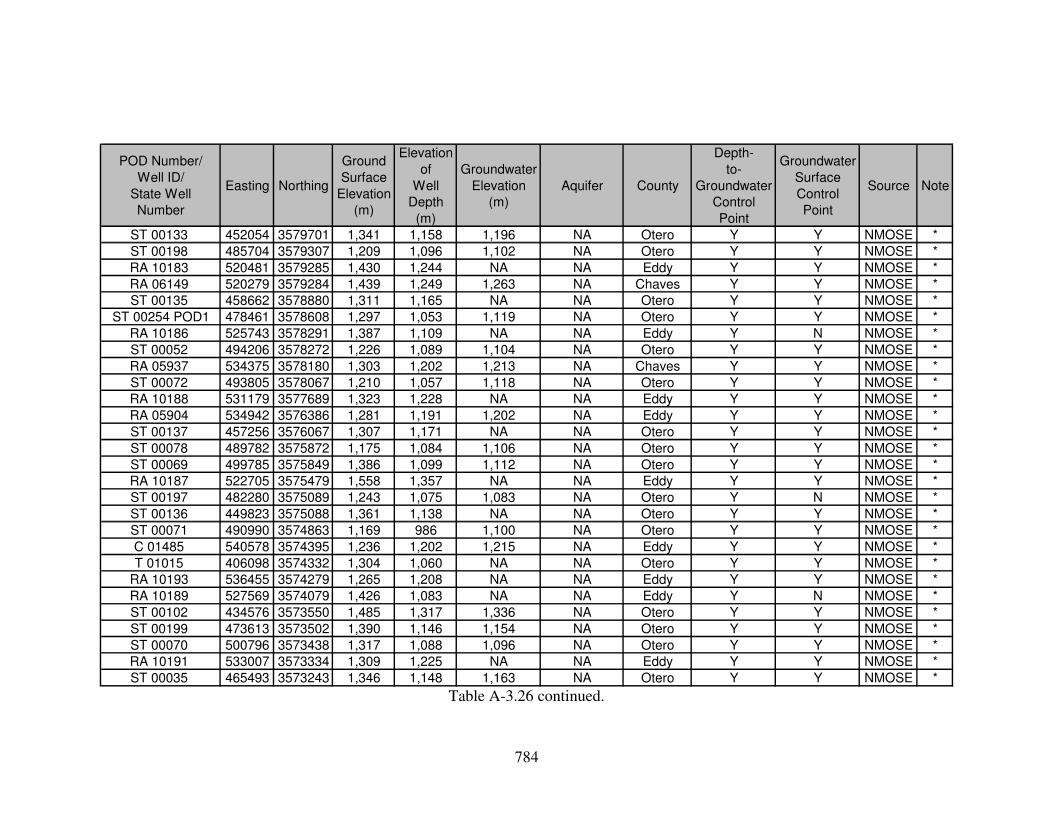
784
POD Number/
Well ID/
State Well
Number
Easting Northing
Ground
Surface
Elevation
(m)
Elevation
of
Well
Depth
(m)
Groundwater
Elevation
(m)
Aquifer County
Depth-
to-
Groundwater
Control
Point
Groundwater
Surface
Control
Point
Source Note
ST 00133 452054 3579701 1,341 1,158 1,196 NA Otero Y Y NMOSE *
ST 00198 485704 3579307 1,209 1,096 1,102 NA Otero Y Y NMOSE *
RA 10183 520481 3579285 1,430 1,244 NA NA Eddy Y Y NMOSE *
RA 06149 520279 3579284 1,439 1,249 1,263 NA Chaves Y Y NMOSE *
ST 00135 458662 3578880 1,311 1,165 NA NA Otero Y Y NMOSE *
ST 00254 POD1 478461 3578608 1,297 1,053 1,119 NA Otero Y Y NMOSE *
RA 10186 525743 3578291 1,387 1,109 NA NA Eddy Y N NMOSE *
ST 00052 494206 3578272 1,226 1,089 1,104 NA Otero Y Y NMOSE *
RA 05937 534375 3578180 1,303 1,202 1,213 NA Chaves Y Y NMOSE *
ST 00072 493805 3578067 1,210 1,057 1,118 NA Otero Y Y NMOSE *
RA 10188 531179 3577689 1,323 1,228 NA NA Eddy Y Y NMOSE *
RA 05904 534942 3576386 1,281 1,191 1,202 NA Eddy Y Y NMOSE *
ST 00137 457256 3576067 1,307 1,171 NA NA Otero Y Y NMOSE *
ST 00078 489782 3575872 1,175 1,084 1,106 NA Otero Y Y NMOSE *
ST 00069 499785 3575849 1,386 1,099 1,112 NA Otero Y Y NMOSE *
RA 10187 522705 3575479 1,558 1,357 NA NA Eddy Y Y NMOSE *
ST 00197 482280 3575089 1,243 1,075 1,083 NA Otero Y N NMOSE *
ST 00136 449823 3575088 1,361 1,138 NA NA Otero Y Y NMOSE *
ST 00071 490990 3574863 1,169 986 1,100 NA Otero Y Y NMOSE *
C 01485 540578 3574395 1,236 1,202 1,215 NA Eddy Y Y NMOSE *
T 01015 406098 3574332 1,304 1,060 NA NA Otero Y Y NMOSE *
RA 10193 536455 3574279 1,265 1,208 NA NA Eddy Y Y NMOSE *
RA 10189 527569 3574079 1,426 1,083 NA NA Eddy Y N NMOSE *
ST 00102 434576 3573550 1,485 1,317 1,336 NA Otero Y Y NMOSE *
ST 00199 473613 3573502 1,390 1,146 1,154 NA Otero Y Y NMOSE *
ST 00070 500796 3573438 1,317 1,088 1,096 NA Otero Y Y NMOSE *
RA 10191 533007 3573334 1,309 1,225 NA NA Eddy Y Y NMOSE *
ST 00035 465493 3573243 1,346 1,148 1,163 NA Otero Y Y NMOSE * Table A-3.26 continued.

785
POD Number/
Well ID/
State Well
Number
Easting Northing
Ground
Surface
Elevation
(m)
Elevation
of
Well
Depth
(m)
Groundwater
Elevation
(m)
Aquifer County
Depth-
to-
Groundwater
Control
Point
Groundwater
Surface
Control
Point
Source Note
ST 00053 492193 3572648 1,159 1,058 1,103 NA Otero Y Y NMOSE *
RA 10190 530196 3572471 1,369 1,170 NA NA Eddy Y Y NMOSE *
RA 10391 527178 3572272 1,535 394 1,145 NA Eddy Y N NMOSE *
RA 06403 535860 3572265 1,293 1,154 1,206 NA Eddy Y Y NMOSE *
RA 10194 539885 3572082 1,245 1,197 NA NA Eddy Y Y NMOSE *
ST 00017 481172 3571976 1,315 1,113 1,177 NA Otero Y N NMOSE *
ST 00014 487565 3571656 1,181 1,090 1,148 NA Otero Y N NMOSE *
ST 00076 491992 3571643 1,160 977 1,008 NA Otero Y N NMOSE *
RA 10197 534862 3570855 1,292 1,273 NA NA Eddy Y Y NMOSE *
RA 10195 541298 3570677 1,303 1,200 NA NA Eddy Y Y NMOSE *
RA 10196 539489 3570472 1,306 1,237 NA NA Eddy Y Y NMOSE *
ST 00016 486459 3570354 1,198 1,107 1,156 NA Otero Y N NMOSE *
RA 06204 518897 3570045 1,757 1,345 NA NA Chaves Y N NMOSE *
RA 10192 530018 3569865 1,433 1,334 NA NA Eddy Y Y NMOSE *
RA 09962 520110 3569851 1,743 1,439 NA NA Eddy Y Y NMOSE *
RA 09634 520011 3569749 1,743 1,484 NA NA Eddy Y Y NMOSE *
RA 11307 POD 1 517952 3569172 1,721 1,340 1,368 NA Eddy Y N NMOSE *
ST 00103 439978 3568708 1,443 1,272 1,294 NA Otero Y Y NMOSE *
ST 00073 494200 3568627 1,160 1,008 1,023 NA Otero Y N NMOSE *
C 02887 534069 3567939 1,340 1,295 NA NA Eddy Y Y NMOSE *
T 03875 389700 3567825 1,249 1,065 NA NA Otero Y Y NMOSE *
RA 05498 528556 3567464 1,461 1,407 NA NA Eddy Y Y NMOSE *
ST 00048 495206 3567420 1,167 1,133 1,138 NA Otero Y Y NMOSE *
ST 00036 467360 3566280 1,273 1,105 1,127 NA Otero Y Y NMOSE *
C 02247 537627 3565738 1,405 1,314 1,370 NA Eddy Y Y NMOSE *
ST 00086 492587 3565618 1,144 1,089 1,110 NA Otero Y Y NMOSE *
ST 00015 492488 3565519 1,143 1,089 1,113 NA Otero Y Y NMOSE *
C 02888 534480 3565392 1,418 1,319 NA NA Eddy Y Y NMOSE * Table A-3.26 continued.

786
POD Number/
Well ID/
State Well
Number
Easting Northing
Ground
Surface
Elevation
(m)
Elevation
of
Well
Depth
(m)
Groundwater
Elevation
(m)
Aquifer County
Depth-
to-
Groundwater
Control
Point
Groundwater
Surface
Control
Point
Source Note
ST 00037 500007 3565208 1,353 1,079 1,138 NA Otero Y Y NMOSE *
ST 00148 490272 3564919 1,138 955 NA NA Otero Y Y NMOSE *
RA 09964 521338 3564671 1,697 1,392 NA NA Eddy Y N NMOSE *
ST 00074 496386 3564607 1,154 1,016 1,108 NA Otero Y Y NMOSE *
ST 00077 508213 3564589 1,418 1,037 1,082 NA Otero Y Y NMOSE *
ST 00161 477637 3564446 1,276 1,029 1,124 NA Otero Y Y NMOSE *
ST 00095 508515 3564286 1,414 1,094 NA NA Otero Y Y NMOSE *
ST 00050 496187 3563804 1,147 1,086 NA NA Otero Y Y NMOSE *
RA 10121 526156 3563653 1,744 1,523 1,576 NA Eddy Y Y NMOSE *
C 02129 545792 3563338 1,268 1,218 1,241 NA Chaves Y Y NMOSE *
ST 00088 487550 3563011 1,132 1,025 1,098 NA Otero Y Y NMOSE *
RA 09620 526061 3562945 1,752 1,508 1,543 NA Eddy Y Y NMOSE *
RA 08041 526761 3562645 1,745 1,522 1,566 NA Eddy Y Y NMOSE *
RA 09403 525659 3562543 1,762 1,564 1,587 NA Eddy Y N NMOSE *
C 02496 544400 3562541 1,307 940 968 NA Chaves N N NMOSE *
RA 06737 533128 3562459 1,639 1,411 1,431 NA Eddy Y Y NMOSE *
RA 10056 526563 3562444 1,745 1,515 1,570 NA Eddy Y Y NMOSE *
RA 09089 525759 3562442 1,759 1,522 1,573 NA Eddy Y Y NMOSE *
RA 09932 525557 3562441 1,765 1,497 1,574 NA Eddy Y Y NMOSE *
RA 09628 525860 3562343 1,756 1,603 NA NA Eddy Y N NMOSE *
C 01394 543997 3562337 1,340 1,181 1,284 NA Chaves Y Y NMOSE *
RA 10198 524554 3562251 1,772 1,577 NA NA Eddy Y Y NMOSE *
RA 09920 526563 3562244 1,740 1,541 NA NA Eddy Y Y NMOSE *
RA 10126 526763 3562244 1,731 1,509 1,568 NA Eddy Y Y NMOSE *
RA 09040 526161 3562243 1,743 1,506 1,564 NA Eddy Y Y NMOSE *
RA 09993 525759 3562242 1,760 1,530 1,595 NA Eddy Y N NMOSE *
RA 09161 525959 3562242 1,754 1,524 1,577 NA Eddy Y Y NMOSE *
RA 10017 525357 3562241 1,769 1,524 1,578 NA Eddy Y Y NMOSE * Table A-3.26 continued.

787
POD Number/
Well ID/
State Well
Number
Easting Northing
Ground
Surface
Elevation
(m)
Elevation
of
Well
Depth
(m)
Groundwater
Elevation
(m)
Aquifer County
Depth-
to-
Groundwater
Control
Point
Groundwater
Surface
Control
Point
Source Note
RA 08043 525557 3562241 1,769 1,546 NA NA Eddy Y Y NMOSE *
RA 10008 524154 3562053 1,770 1,525 1,587 NA Eddy Y Y NMOSE *
RA 09401 524354 3562053 1,772 1,536 1,574 NA Eddy Y N NMOSE *
RA 09027 524556 3562050 1,774 1,522 1,592 NA Eddy Y Y NMOSE *
RA 10462 524756 3562050 1,773 1,530 1,563 NA Eddy Y N NMOSE *
RA 10704 POD1 524154 3561853 1,778 1,534 NA NA Eddy Y Y NMOSE *
RA 10517 524556 3561850 1,771 1,521 1,587 NA Eddy Y Y NMOSE *
RA 09055 524357 3561451 1,772 1,527 1,594 NA Eddy Y Y NMOSE *
RA 09963 513828 3561357 1,840 1,535 NA NA Eddy Y Y NMOSE *
C 01489 541999 3561329 1,369 1,292 NA NA Eddy Y Y NMOSE *
C 01519 541495 3561223 1,381 1,343 1,350 NA Eddy Y Y NMOSE *
RA 09830 523867 3561153 1,777 1,548 NA NA Eddy Y Y NMOSE *
ST 00162 481454 3561014 1,212 1,075 1,090 NA Otero Y Y NMOSE *
ST 00084 487747 3561001 1,136 1,064 1,102 NA Otero Y Y NMOSE *
ST 00087 487547 3561001 1,137 1,076 1,103 NA Otero Y Y NMOSE *
ST 00089 487950 3561000 1,134 1,004 1,100 NA Otero Y Y NMOSE *
RA 09635 513931 3560856 1,853 1,594 NA NA Eddy Y Y NMOSE *
ST 00092 444365 3560630 1,410 1,166 1,227 NA Otero Y Y NMOSE *
ST 00097 440344 3560061 1,430 1,278 1,403 NA Otero Y Y NMOSE *
ST 00141 S 488452 3559894 1,129 1,022 NA NA Otero Y Y NMOSE *
ST 00141 488248 3559694 1,129 855 NA NA Otero Y Y NMOSE *
ST 00180 S 488148 3559592 1,130 947 1,109 NA Otero Y Y NMOSE *
ST 00049 494596 3559387 1,131 1,104 1,106 NA Otero Y Y NMOSE *
C 01327 546421 3558638 1,412 1,384 1,387 NA Chaves Y N NMOSE *
ST 00038 458735 3558565 1,336 1,032 1,154 NA Otero Y Y NMOSE *
ST 00042 463561 3557747 1,304 1,121 1,152 NA Otero Y Y NMOSE *
ST 00163 479239 3557196 1,230 1,076 1,093 NA Otero Y Y NMOSE *
ST 00164 488754 3556577 1,126 1,088 1,106 NA Otero Y Y NMOSE * Table A-3.26 continued.

788
POD Number/
Well ID/
State Well
Number
Easting Northing
Ground
Surface
Elevation
(m)
Elevation
of
Well
Depth
(m)
Groundwater
Elevation
(m)
Aquifer County
Depth-
to-
Groundwater
Control
Point
Groundwater
Surface
Control
Point
Source Note
ST 00192 493185 3555562 1,121 1,030 1,102 NA Otero Y Y NMOSE *
ST 00191 494594 3555559 1,130 1,039 1,112 NA Otero Y Y NMOSE *
ST 00138 506116 3555044 1,754 901 NA NA Otero Y Y NMOSE *
RA 05286 REPAR 535065 3554824 1,792 1,706 1,733 NA Eddy Y Y NMOSE *
ST 00025 425104 3554803 1,584 1,419 1,431 NA Otero Y Y NMOSE *
ST 00147 489461 3554468 1,127 983 NA NA Otero Y Y NMOSE *
ST 00028 445541 3554322 1,482 1,421 1,426 NA Otero Y Y NMOSE *
ST 00054 489965 3553359 1,128 1,037 1,106 NA Otero Y Y NMOSE *
ST 00152 490568 3552754 1,120 1,044 NA NA Otero Y Y NMOSE *
ST 00033 492178 3552346 1,116 1,025 1,104 NA Otero Y Y NMOSE *
ST 00182 492380 3552344 1,116 1,070 1,101 NA Otero Y Y NMOSE *
ST 00026 438231 3552247 1,487 1,426 1,441 NA Otero Y Y NMOSE *
ST 00093 491775 3552147 1,116 1,076 NA NA Otero Y Y NMOSE *
ST 00110 491775 3551945 1,117 965 1,103 NA Otero Y Y NMOSE *
ST 00151 490771 3551748 1,122 970 NA NA Otero Y Y NMOSE *
ST 00027 441810 3551427 1,538 1,371 1,389 NA Otero Y Y NMOSE *
ST 00155 491877 3551242 1,117 1,099 NA NA Otero Y Y NMOSE *
ST 00212 490771 3551143 1,139 987 NA NA Otero Y Y NMOSE *
ST 00096 513359 3550998 1,657 1,123 NA NA Otero Y Y NMOSE *
ST 00153 485681 3550966 1,243 1,090 NA NA Otero Y Y NMOSE *
C 03116 544325 3550819 1,200 1,118 1,131 NA Chaves Y Y NMOSE *
C 02816 543319 3550626 1,212 1,132 1,154 NA Chaves Y Y NMOSE *
ST 00107 428705 3550603 1,528 1,412 1,443 NA Otero Y Y NMOSE *
ST 00043 465163 3550511 1,288 1,044 1,105 NA Otero Y Y NMOSE *
ST 00040 469119 3549792 1,269 1,086 1,117 NA Otero Y Y NMOSE *
ST 00158 492678 3549631 1,113 1,095 NA NA Otero Y Y NMOSE *
C 01392 538058 3549100 1,313 1,252 1,259 NA Eddy Y Y NMOSE *
T 03499 407862 3548799 1,549 1,465 NA NA Otero Y Y NMOSE * Table A-3.26 continued.

789
POD Number/
Well ID/
State Well
Number
Easting Northing
Ground
Surface
Elevation
(m)
Elevation
of
Well
Depth
(m)
Groundwater
Elevation
(m)
Aquifer County
Depth-
to-
Groundwater
Control
Point
Groundwater
Surface
Control
Point
Source Note
ST 00041 450338 3548063 1,490 1,398 1,413 NA Otero Y Y NMOSE *
C 00910 534470 3548020 1,403 1,345 NA NA Eddy Y Y NMOSE *
ST 00051 451746 3547855 1,468 1,389 1,406 NA Otero Y Y NMOSE *
ST 00187 S 481046 3547755 1,188 1,084 1,105 NA Otero Y Y NMOSE *
C 01025 533621 3547538 1,420 1,343 1,413 NA Eddy Y N NMOSE *
C 02318 519164 3547455 2,046 1,776 1,793 NA Eddy Y Y NMOSE *
ST 00024 438171 3547423 1,546 1,375 1,383 NA Otero Y Y NMOSE *
ST 00039 448727 3547265 1,532 1,425 1,447 NA Otero Y Y NMOSE *
ST 00154 491062 3547222 1,118 1,097 NA NA Otero Y Y NMOSE *
C 02267 533207 3547130 1,418 1,360 1,368 NA Eddy Y Y NMOSE *
ST 00106 437663 3546802 1,544 1,370 1,416 NA Otero N Y NMOSE *
ST 00044 466258 3546182 1,268 1,024 1,119 NA Otero Y Y NMOSE *
C 02411 536795 3545970 1,327 1,269 1,278 NA Eddy Y Y NMOSE *
ST 00032 453546 3545833 1,454 1,359 1,397 NA Otero Y Y NMOSE *
ST 00101 442084 3545493 1,609 1,365 1,423 NA Otero Y Y NMOSE *
ST 00046 474148 3545352 1,207 1,077 1,100 NA Otero Y Y NMOSE *
ST 00099 447914 3545254 1,596 1,535 1,550 NA Otero Y Y NMOSE *
ST 00108 432019 3545238 1,582 1,396 1,417 NA Otero Y Y NMOSE *
C 01285 535549 3544971 1,341 1,260 1,309 NA Eddy Y Y NMOSE *
ST 00090 417884 3544898 1,606 1,545 1,558 NA Otero Y Y NMOSE *
C 02252 533078 3544781 1,384 1,380 1,382 NA Eddy Y N NMOSE *
ST 00045 465851 3544774 1,264 1,002 1,157 NA Otero Y Y NMOSE *
ST 00160 511665 3544666 1,866 988 1,101 NA Otero Y Y NMOSE *
C 01008 539332 3544643 1,263 1,202 1,221 NA Eddy Y Y NMOSE *
ST 00186 S 487526 3544312 1,138 1,055 1,080 NA Otero Y Y NMOSE *
ST 00066 500206 3544281 1,118 1,096 NA NA Otero Y Y NMOSE *
T 05304 POD1 390017 3544257 1,246 1,124 NA NA Otero Y Y NMOSE *
C 02255 533069 3544175 1,374 1,317 1,336 NA Eddy Y Y NMOSE * Table A-3.26 continued.

790
POD Number/
Well ID/
State Well
Number
Easting Northing
Ground
Surface
Elevation
(m)
Elevation
of
Well
Depth
(m)
Groundwater
Elevation
(m)
Aquifer County
Depth-
to-
Groundwater
Control
Point
Groundwater
Surface
Control
Point
Source Note
ST 00253 POD1 489252 3544154 1,121 1,060 1,091 NA Otero Y Y NMOSE *
ST 00186 487526 3544112 1,130 1,053 1,096 NA Otero Y Y NMOSE *
ST 00123 489740 3544106 1,116 1,045 1,095 NA Otero Y Y NMOSE *
ST 00057 490345 3544103 1,114 1,066 1,090 NA Otero Y Y NMOSE *
ST 00091 416873 3544102 1,603 1,329 1,387 NA Otero Y Y NMOSE *
ST 00059 489135 3543905 1,117 986 1,092 NA Otero Y Y NMOSE *
ST 00116 B 487724 3543709 1,126 1,048 1,091 NA Otero Y Y NMOSE *
ST 00058 489939 3543499 1,114 983 1,092 NA Otero Y Y NMOSE *
ST 00187 479815 3543323 1,153 1,077 1,100 NA Otero Y Y NMOSE *
ST 00116 487320 3543307 1,124 1,069 1,090 NA Otero Y Y NMOSE *
ST 00034 449111 3543234 1,597 1,414 1,429 NA Otero Y Y NMOSE *
C 02185 543727 3542935 1,186 1,140 1,168 NA Chaves Y Y NMOSE *
ST 00116 S 486716 3542904 1,125 1,088 1,091 NA Otero Y Y NMOSE *
ST 00059 S-3 489332 3542899 1,113 806 1,092 NA Otero Y Y NMOSE *
ST 00031 455145 3542811 1,408 1,362 1,372 NA Otero Y Y NMOSE *
ST 00029 459818 3542789 1,331 1,117 1,127 NA Otero Y Y NMOSE *
ST 00047 468499 3542756 1,234 1,106 1,115 NA Otero Y Y NMOSE *
ST 00150 486311 3542703 1,129 1,015 NA NA Otero Y Y NMOSE *
ST 00060 S-2 487519 3542699 1,118 950 1,092 NA Otero Y Y NMOSE *
ST 00125 488927 3542696 1,120 NA 1,068 NA Otero Y Y NMOSE *
ST 00058 S-2 490136 3542693 1,112 1,072 NA NA Otero Y Y NMOSE *
ST 00060 487519 3542499 1,116 958 1,091 NA Otero Y Y NMOSE *
ST 00187 S-2 483837 3542303 1,169 1,049 1,095 NA Otero Y Y NMOSE *
ST 00120 486712 3542298 1,119 1,043 1,092 NA Otero Y Y NMOSE *
ST 00059 S 489128 3542292 1,113 982 1,088 NA Otero Y Y NMOSE *
ST 00159 494968 3542280 1,106 954 NA NA Otero Y Y NMOSE *
ST 00030 452522 3542012 1,490 1,394 1,399 NA Otero Y Y NMOSE *
C 02254 531230 3541986 1,408 1,353 1,362 NA Eddy Y Y NMOSE * Table A-3.26 continued.

791
POD Number/
Well ID/
State Well
Number
Easting Northing
Ground
Surface
Elevation
(m)
Elevation
of
Well
Depth
(m)
Groundwater
Elevation
(m)
Aquifer County
Depth-
to-
Groundwater
Control
Point
Groundwater
Surface
Control
Point
Source Note
ST 00146 486307 3541896 1,119 983 NA NA Otero Y Y NMOSE *
C 02253 525756 3541810 1,508 1,489 1,502 NA Eddy Y Y NMOSE *
C 02251 527971 3541795 1,465 1,378 1,396 NA Eddy Y Y NMOSE *
ST 00146 S 486307 3541696 1,118 1,064 NA NA Otero Y Y NMOSE *
ST 00248 POD1 515736 3541312 1,872 1,506 NA NA Eddy Y N NMOSE *
C 01302 539942 3541186 1,265 1,257 1,262 NA Eddy Y Y NMOSE *
C 01884 540752 3541185 1,259 1,229 1,256 NA Eddy Y Y NMOSE *
ST 00188 488115 3541086 1,111 1,026 1,090 NA Otero Y Y NMOSE *
C 02935 539640 3541084 1,261 1,220 1,254 NA Eddy Y Y NMOSE *
ST 00061 S 489122 3541081 1,111 1,085 1,097 NA Otero Y Y NMOSE *
C 02962 540864 3540881 1,240 1,225 1,234 NA Eddy Y Y NMOSE *
T 01559 POD2 408667 3540858 1,646 1,555 1,587 NA Otero Y Y NMOSE *
ST 00245 POD1 515724 3540530 1,895 1,784 1,798 NA Eddy Y Y NMOSE *
4806201 471768 3540444 1,201 866 1,111 318BSVP Hudspeth Y Y TWDB *
4807218 481398 3540422 1,137 619 1,093 318BSVP Hudspeth Y Y TWDB *
4807314 487616 3540412 1,111 1,044 1,096 318BSVP Hudspeth Y Y TWDB *
4807217 481817 3540390 1,135 NA 1,098 318BSVP Hudspeth Y N TWDB
ST 00061 489761 3540319 1,109 1,018 1,089 NA Otero Y Y NMOSE *
4807209 481004 3540269 1,138 NA 1,100 318BSVP Hudspeth Y N TWDB *
4808101 489111 3540195 1,110 NA 1,101 318BSVP Hudspeth Y N TWDB
ST 00219 514868 3539926 2,045 1,588 NA NA Eddy Y Y NMOSE
4807303 485962 3539922 1,119 1,075 1,101 318BSVP Hudspeth Y N TWDB *
4703204 529309 3539893 1,421 1,400 1,409 110AVPS Culberson Y Y TWDB
4703107 525583 3539883 1,517 1,387 1,458 310PRMN Culberson Y Y TWDB *
4808201 494201 3539760 1,106 NA 1,098 318BSVP Hudspeth Y Y TWDB *
4702103 515639 3539647 1,917 1,012 1,134 310PRMN Culberson Y N TWDB *
4807203 481029 3539560 1,132 1,047 1,098 318BSVP Hudspeth Y N TWDB *
4807208 481816 3539559 1,131 NA 1,104 318BSVP Hudspeth Y N TWDB Table A-3.26 continued.

792
POD Number/
Well ID/
State Well
Number
Easting Northing
Ground
Surface
Elevation
(m)
Elevation
of
Well
Depth
(m)
Groundwater
Elevation
(m)
Aquifer County
Depth-
to-
Groundwater
Control
Point
Groundwater
Surface
Control
Point
Source Note
4807219 482603 3539496 1,129 945 1,090 318BSVP Hudspeth Y Y TWDB
4807206 481002 3539407 1,131 1,065 1,094 318BSVP Hudspeth Y Y TWDB
4703302 532775 3539349 1,395 1,375 1,385 110AVPS Culberson Y Y TWDB
4703205 527579 3539272 1,446 1,435 1,441 110AVPS Culberson Y Y TWDB *
4704101 539099 3539248 1,275 1,244 1,253 312CSTL Culberson Y Y TWDB *
4703108 524588 3538926 1,543 1,470 1,520 310PRMN Culberson Y Y TWDB *
4807313 485961 3538875 1,124 1,043 1,089 318BSVP Hudspeth Y Y TWDB *
4807305 487010 3538781 1,112 1,036 1,103 318BSVP Hudspeth Y N TWDB *
4808102 488165 3538688 1,111 992 1,095 318BSVP Hudspeth Y Y TWDB
4807318 487325 3538658 1,112 NA 1,096 318BSVP Hudspeth Y Y TWDB *
4702302 520732 3538609 1,586 1,578 1,580 110AVPS Culberson Y Y TWDB
4806301 474466 3538497 1,179 889 1,095 318BSVP Hudspeth Y Y TWDB *
4807213 482706 3538418 1,124 852 1,095 318BSVP Hudspeth Y Y TWDB *
4704201 541072 3538147 1,251 1,196 1,228 312CSTL Culberson Y Y TWDB *
4806303 475173 3538033 1,172 NA 1,096 318BSVP Hudspeth Y Y TWDB
4807107 477456 3537967 1,160 798 1,089 318BSVP Hudspeth Y Y TWDB *
4702305 523436 3537907 1,528 1,505 1,510 110AVPS Culberson Y N TWDB *
4807302 487560 3537888 1,111 NA 1,101 318BSVP Hudspeth Y Y TWDB
4808103 489424 3537886 1,108 NA 1,098 318BSVP Hudspeth Y Y TWDB *
4807307 487035 3537858 1,112 NA 1,087 318BSVP Hudspeth Y Y TWDB *
4807108 477823 3537750 1,155 798 1,088 318BSVP Hudspeth Y Y TWDB *
4703203 529840 3537708 1,426 1,385 1,395 310PRMN Culberson Y Y TWDB *
4807106 477692 3537658 1,155 790 1,089 318BSVP Hudspeth Y Y TWDB
4703101 524304 3537293 1,506 1,464 1,473 310PRMN Culberson Y Y TWDB
4807207 480998 3537159 1,131 914 1,095 318BSVP Hudspeth Y Y TWDB
4807109 480210 3537130 1,136 1,016 1,093 318BSVP Hudspeth Y Y TWDB *
4807220 482126 3537095 1,125 744 1,097 318BSVP Hudspeth Y Y TWDB
4807204 482704 3537063 1,122 1,023 1,094 318BSVP Hudspeth Y Y TWDB Table A-3.26 continued.

793
POD Number/
Well ID/
State Well
Number
Easting Northing
Ground
Surface
Elevation
(m)
Elevation
of
Well
Depth
(m)
Groundwater
Elevation
(m)
Aquifer County
Depth-
to-
Groundwater
Control
Point
Groundwater
Surface
Control
Point
Source Note
4807101 476877 3537044 1,160 841 1,102 318BSVP Hudspeth Y Y TWDB *
4807315 485722 3537028 1,114 846 1,092 318BSVP Hudspeth Y Y TWDB *
4807308 485984 3537028 1,113 1,022 1,095 318BSVP Hudspeth Y N TWDB
4807110 480184 3536976 1,136 1,060 1,097 318BSVP Hudspeth Y Y TWDB *
4807306 487638 3536964 1,111 1,061 1,104 318BSVP Hudspeth Y N TWDB *
4806304 474357 3536958 1,176 NA 1,096 318BSVP Hudspeth Y Y TWDB *
4703102 525853 3536835 1,477 1,431 1,437 110AVPS Culberson Y Y TWDB
4807304 487533 3536656 1,111 1,050 1,095 318BSVP Hudspeth Y Y TWDB *
4807309 487585 3536656 1,111 1,050 1,101 318BSVP Hudspeth Y N TWDB *
4806305 476298 3536522 1,170 NA 1,104 318BSVP Hudspeth Y N TWDB
4807214 482703 3536386 1,121 969 1,095 318BSVP Hudspeth Y Y TWDB *
4806302 474434 3536373 1,175 810 1,092 318BSVP Hudspeth Y Y TWDB
4702301 521681 3536364 1,687 1,640 NA 313CPTN Culberson Y Y TWDB *
4807205 480996 3536266 1,131 1,053 1,103 318BSVP Hudspeth Y N TWDB *
4703206 530055 3536015 1,427 1,305 1,391 310PRMN Culberson Y Y TWDB
4807102 476875 3535967 1,157 836 1,094 318BSVP Hudspeth Y Y TWDB
4807111 479368 3535930 1,142 1,023 1,105 318BSVP Hudspeth Y N TWDB *
4807112 479447 3535930 1,141 1,065 1,105 318BSVP Hudspeth Y N TWDB *
4704501 540373 3535651 1,246 1,185 1,214 110ALVM Culberson Y Y TWDB
4807631 486008 3535334 1,113 NA 1,095 318BSVP Hudspeth Y Y TWDB
4807633 487557 3535332 1,111 NA 1,096 318BSVP Hudspeth Y Y TWDB
4806608 475193 3535324 1,171 NA 1,096 318BSVP Hudspeth Y Y TWDB
4806606 474458 3535295 1,180 845 1,097 318BSVP Hudspeth Y Y TWDB
4807606 484459 3535244 1,114 1,038 1,097 318BSVP Hudspeth Y Y TWDB *
4807611 484381 3535213 1,114 1,038 1,102 318BSVP Hudspeth Y N TWDB *
4807521 482700 3534847 1,121 NA 1,096 318BSVP Hudspeth Y Y TWDB *
4807403 479733 3534790 1,138 1,078 1,100 318BSVP Hudspeth Y N TWDB *
4807404 479812 3534790 1,138 NA 1,099 318BSVP Hudspeth Y N TWDB * Table A-3.26 continued.

794
POD Number/
Well ID/
State Well
Number
Easting Northing
Ground
Surface
Elevation
(m)
Elevation
of
Well
Depth
(m)
Groundwater
Elevation
(m)
Aquifer County
Depth-
to-
Groundwater
Control
Point
Groundwater
Surface
Control
Point
Source Note
4702604 522289 3534610 1,623 1,513 1,531 310PRMN Culberson Y Y TWDB
4806602 476031 3534583 1,166 837 1,097 318BSVP Hudspeth Y Y TWDB
4807603 486007 3534565 1,113 1,052 1,103 318BSVP Hudspeth Y N TWDB *
4807507 480835 3534480 1,130 1,037 1,102 318BSVP Hudspeth Y N TWDB
4806605 472986 3534467 1,197 837 1,097 318BSVP Hudspeth Y Y TWDB
4807417 476871 3534458 1,161 763 1,099 318BSVP Hudspeth Y N TWDB *
4806604 472592 3534438 1,198 839 1,096 318BSVP Hudspeth Y Y TWDB
4808403 488449 3534407 1,109 1,034 1,100 318BSVP Hudspeth Y Y TWDB
4703401 523838 3534398 1,537 1,529 1,536 110AVPS Culberson Y Y TWDB
4702603 522709 3534395 1,588 1,466 1,538 110AVPS Culberson Y Y TWDB
4807616 485797 3534349 1,117 1,041 1,109 318BSVP Hudspeth Y N TWDB
4807527 481806 3534294 1,124 1,013 1,095 318BSVP Hudspeth Y Y TWDB *
4701401 503150 3534217 1,135 1,127 1,127 110ALVM Hudspeth Y Y TWDB
4807522 481019 3534203 1,128 889 1,086 318BSVP Hudspeth Y Y TWDB *
4806603 472591 3534191 1,197 832 1,083 318BSVP Hudspeth Y Y TWDB *
4806609 475216 3534185 1,174 NA 1,096 318BSVP Hudspeth Y Y TWDB
4702304 522263 3534179 1,625 1,555 1,577 310PRMN Culberson Y Y TWDB *
4807632 484326 3534074 1,114 NA 1,095 318BSVP Hudspeth Y Y TWDB *
4703403 526989 3534005 1,437 1,410 1,419 110AVPS Culberson Y Y TWDB
4806601 473641 3534004 1,190 731 1,093 318BSVP Hudspeth Y Y TWDB
4703402 526517 3533973 1,436 1,329 1,424 310PRMN Culberson Y Y TWDB *
4807408 477736 3533779 1,153 1,046 1,105 318BSVP Hudspeth Y N TWDB *
4807418 476869 3533688 1,160 871 1,094 318BSVP Hudspeth Y Y TWDB *
4807423 480151 3533681 1,134 1,058 1,103 318BSVP Hudspeth Y N TWDB
4807405 478733 3533653 1,144 1,056 1,096 318BSVP Hudspeth Y Y TWDB *
4807407 479206 3533622 1,141 1,065 1,108 318BSVP Hudspeth Y N TWDB *
4807411 478628 3533592 1,145 1,073 1,103 318BSVP Hudspeth Y Y TWDB
4807610 486846 3533578 1,112 1,076 1,106 110ALVM Hudspeth Y N TWDB Table A-3.26 continued.

795
POD Number/
Well ID/
State Well
Number
Easting Northing
Ground
Surface
Elevation
(m)
Elevation
of
Well
Depth
(m)
Groundwater
Elevation
(m)
Aquifer County
Depth-
to-
Groundwater
Control
Point
Groundwater
Surface
Control
Point
Source Note
4807626 487634 3533577 1,110 1,019 1,098 318BSVP Hudspeth Y Y TWDB
4808401 488579 3533576 1,108 1,017 1,102 318BSVP Hudspeth Y N TWDB
4807604 486058 3533518 1,112 1,021 1,105 318BSVP Hudspeth Y N TWDB
4807504 481044 3533495 1,127 1,074 1,098 318BSVP Hudspeth Y N TWDB
4808406 488421 3533453 1,109 986 1,101 318BSVP Hudspeth Y Y TWDB *
4807619 486583 3533363 1,112 1,036 1,097 318BSVP Hudspeth Y Y TWDB
4808402 490600 3533358 1,103 1,094 1,100 100ALVM Hudspeth Y Y TWDB
4807412 477735 3533255 1,152 1,042 1,104 318BSVP Hudspeth Y Y TWDB
4807502 482697 3533246 1,118 1,057 1,095 318BSVP Hudspeth Y N TWDB
4807601 486583 3533209 1,112 1,033 1,101 318BSVP Hudspeth Y N TWDB *
4807512 482697 3533153 1,118 1,061 1,101 318BSVP Hudspeth Y Y TWDB *
4807526 483485 3533152 1,115 1,024 1,088 318BSVP Hudspeth Y N TWDB
4807612 484693 3533119 1,113 1,052 1,105 318BSVP Hudspeth Y N TWDB
4807508 481148 3532940 1,127 1,057 1,104 318BSVP Hudspeth Y N TWDB
4908601 401582 3532934 1,384 1,253 1,268 112HCBL El Paso Y Y TWDB *
4807511 482697 3532845 1,118 1,041 1,106 318BSVP Hudspeth Y N TWDB
4908603 401660 3532779 1,385 1,253 1,277 112HCBL El Paso Y Y TWDB *
4807420 476894 3532764 1,159 702 1,096 318BSVP Hudspeth Y Y TWDB
4807623 487659 3532592 1,110 1,041 1,097 318BSVP Hudspeth Y Y TWDB
4807624 485978 3532563 1,111 989 1,095 318BSVP Hudspeth Y Y TWDB *
4807501 481383 3532386 1,125 1,058 1,097 318BSVP Hudspeth Y Y TWDB *
4807505 481304 3532355 1,125 848 1,096 318BSVP Hudspeth Y Y TWDB
4702602 522793 3532117 1,543 NA 1,535 110AVPS Culberson Y Y TWDB
4807427 477680 3532085 1,151 NA 1,096 318BSVP Hudspeth Y Y TWDB *
4806610 475185 3532060 1,170 NA 1,097 318BSVP Hudspeth Y Y TWDB *
4808407 489365 3532005 1,107 732 1,096 318BSVP Hudspeth Y Y TWDB *
4807414 476892 3531933 1,157 950 1,096 318BSVP Hudspeth Y Y TWDB *
4807410 479360 3531928 1,138 NA 1,097 318BSVP Hudspeth Y Y TWDB * Table A-3.26 continued.

796
POD Number/
Well ID/
State Well
Number
Easting Northing
Ground
Surface
Elevation
(m)
Elevation
of
Well
Depth
(m)
Groundwater
Elevation
(m)
Aquifer County
Depth-
to-
Groundwater
Control
Point
Groundwater
Surface
Control
Point
Source Note
4807627 484875 3531918 1,112 1,013 1,092 318BSVP Hudspeth Y Y TWDB
4807607 485951 3531917 1,110 NA 1,095 318BSVP Hudspeth Y Y TWDB
4808408 490363 3531911 1,103 NA 1,102 UNKNOWN Hudspeth Y Y TWDB *
4908502 400443 3531898 1,360 NA 1,230 112HCBL El Paso Y Y TWDB *
4807409 480227 3531895 1,131 NA 1,103 318BSVP Hudspeth Y Y TWDB
4807628 484769 3531888 1,112 1,005 1,095 318BSVP Hudspeth Y N TWDB *
4807503 481907 3531861 1,120 1,048 1,102 318BSVP Hudspeth Y N TWDB *
4807510 482695 3531798 1,116 816 1,095 318BSVP Hudspeth Y Y TWDB *
4807509 481933 3531769 1,120 1,048 1,104 318BSVP Hudspeth Y N TWDB *
4807513 483693 3531704 1,113 NA 1,104 318BSVP Hudspeth Y Y TWDB
4808405 490415 3531696 1,103 1,099 1,102 100ALVM Hudspeth Y Y TWDB
4807402 478020 3531530 1,146 1,063 1,099 318BSVP Hudspeth Y N TWDB *
4807615 486056 3531332 1,110 1,064 1,103 318BSVP Hudspeth Y N TWDB
4807614 486029 3531301 1,110 1,065 1,104 318BSVP Hudspeth Y N TWDB *
4807613 486003 3531239 1,111 1,020 1,103 318BSVP Hudspeth Y N TWDB
4701701 502495 3531138 1,121 1,102 1,106 100ALVM Hudspeth Y Y TWDB *
4807901 487657 3531083 1,109 1,018 1,094 318BSVP Hudspeth Y Y TWDB
4807702 479358 3531004 1,136 NA 1,097 318BSVP Hudspeth Y Y TWDB *
4702801 518751 3531001 1,734 1,532 1,664 313CRCX Culberson Y Y TWDB
4807801 482667 3530906 1,115 1,054 1,094 318BSVP Hudspeth Y Y TWDB *
4701901 509822 3530865 1,633 -394 1,196 UNKNOWN Culberson Y Y TWDB *
4807802 482693 3530813 1,115 1,055 1,103 318BSVP Hudspeth Y N TWDB *
4807809 481852 3530661 1,119 849 1,094 318BSVP Hudspeth Y Y TWDB *
4807709 476652 3530579 1,154 925 1,098 318BSVP Hudspeth Y N TWDB
4807810 482693 3530413 1,116 948 1,090 318BSVP Hudspeth Y Y TWDB
4807914 485713 3530254 1,111 653 1,095 318BSVP Hudspeth Y Y TWDB *
4806901 476074 3530242 1,158 776 1,095 318BSVP Hudspeth Y Y TWDB *
4807806 482298 3530167 1,117 1,035 1,105 318BSVP Hudspeth Y N TWDB Table A-3.26 continued.

797
POD Number/
Well ID/
State Well
Number
Easting Northing
Ground
Surface
Elevation
(m)
Elevation
of
Well
Depth
(m)
Groundwater
Elevation
(m)
Aquifer County
Depth-
to-
Groundwater
Control
Point
Groundwater
Surface
Control
Point
Source Note
4807804 481300 3530108 1,123 1,032 1,105 318BSVP Hudspeth Y N TWDB
4807714 477596 3529992 1,150 982 1,098 318BSVP Hudspeth Y N TWDB
4807813 483795 3529949 1,115 955 1,083 318BSVP Hudspeth Y Y TWDB *
4907802 386467 3529272 1,238 1,113 1,128 112HCBL El Paso Y Y TWDB
4907801 386493 3529272 1,238 1,052 1,127 112HCBL El Paso Y Y TWDB
4702804 516286 3528964 1,777 993 1,110 318BSPG Culberson Y N TWDB
4807910 486367 3528960 1,109 731 1,093 318BSVP Hudspeth Y Y TWDB
4807706 480194 3528878 1,131 876 1,096 318BSVP Hudspeth Y Y TWDB *
4807908 485553 3528807 1,111 1,081 1,102 318BSVP Hudspeth Y N TWDB
4702807 517468 3528597 1,716 1,671 1,677 310PRMN Culberson Y Y TWDB *
4807902 485947 3528499 1,110 1,055 1,101 318BSVP Hudspeth Y N TWDB
4807905 484475 3528470 1,115 1,014 1,102 318BSVP Hudspeth Y N TWDB *
4807903 486052 3528468 1,110 1,052 1,101 318BSVP Hudspeth Y N TWDB *
4907804 386562 3528347 1,238 1,025 1,126 112HCBL El Paso Y Y TWDB *
4807904 484501 3528286 1,115 737 1,097 318BSVP Hudspeth Y Y TWDB *
4907806 386480 3528101 1,238 1,042 1,122 112HCBL El Paso Y Y TWDB
4807803 481060 3528014 1,125 973 1,097 318BSVP Hudspeth Y Y TWDB
4807805 481007 3527984 1,126 1,041 1,103 318BSVP Hudspeth Y N TWDB
4807815 481848 3527921 1,120 859 1,075 318BSVP Hudspeth Y Y TWDB
4807916 486944 3527851 1,108 NA 1,101 318BSVP Hudspeth Y N TWDB *
4807814 482241 3527704 1,118 966 1,096 318BSVP Hudspeth Y Y TWDB *
4807703 477749 3527559 1,147 1,056 1,098 318BSVP Hudspeth Y N TWDB *
4807716 480192 3527400 1,138 862 1,098 318BSVP Hudspeth Y N TWDB
4807705 477722 3527220 1,153 1,001 1,104 318BSVP Hudspeth Y N TWDB
4807712 476775 3526915 1,158 766 1,095 318BSVP Hudspeth Y Y TWDB
4807811 481846 3526874 1,122 994 1,084 318BSVP Hudspeth Y Y TWDB *
4807708 480191 3526846 1,135 653 1,092 318BSVP Hudspeth Y Y TWDB *
4807812 481898 3526812 1,122 861 1,078 318BSVP Hudspeth Y Y TWDB Table A-3.26 continued.

798
POD Number/
Well ID/
State Well
Number
Easting Northing
Ground
Surface
Elevation
(m)
Elevation
of
Well
Depth
(m)
Groundwater
Elevation
(m)
Aquifer County
Depth-
to-
Groundwater
Control
Point
Groundwater
Surface
Control
Point
Source Note
4808903 498765 3526796 1,109 1,105 1,106 110ALVM Hudspeth Y Y TWDB
4808902 498056 3526765 1,106 1,091 1,099 110ALVM Hudspeth Y Y TWDB
4807713 476591 3526700 1,163 806 1,096 318BSVP Hudspeth Y Y TWDB
4709208 504545 3526520 1,167 1,083 1,095 310PRMN Hudspeth Y N TWDB
4815105 478481 3526018 1,149 NA 1,092 318BSVP Hudspeth Y Y TWDB
4815204 482685 3525702 1,120 NA 1,104 318BSVP Hudspeth Y N TWDB *
4815303 484340 3525546 1,113 795 1,096 318BSVP Hudspeth Y Y TWDB *
4815203 481054 3525120 1,132 1,033 1,097 318BSVP Hudspeth Y Y TWDB *
4815201 483761 3525023 1,114 1,023 1,096 318BSVP Hudspeth Y Y TWDB *
4815202 481002 3524997 1,135 1,046 1,107 318BSVP Hudspeth Y N TWDB
4815101 477506 3524881 1,179 -283 1,097 318BSVP Hudspeth Y Y TWDB *
4815305 485180 3524867 1,111 1,026 1,101 318BSVP Hudspeth Y N TWDB *
4815302 487676 3524833 1,109 916 1,096 318BSVP Hudspeth Y Y TWDB
4815307 484365 3524745 1,113 921 1,095 318BSVP Hudspeth Y Y TWDB
4815104 480134 3524691 1,142 711 1,095 318BSVP Hudspeth Y Y TWDB *
4709201 505440 3524365 1,155 1,081 1,097 313CRCX Hudspeth Y N TWDB
4709202 505440 3524334 1,155 1,083 1,093 313CRCX Hudspeth Y N TWDB *
4815103 480159 3524260 1,145 686 1,095 318BSVP Hudspeth Y Y TWDB *
4815102 480133 3524137 1,146 784 1,096 318BSVP Hudspeth Y Y TWDB *
4916201 398291 3524128 1,336 NA 1,130 112HCBL El Paso Y Y TWDB
4709203 504047 3523810 1,127 1,081 1,099 112SLBL Hudspeth Y Y TWDB
4815301 484389 3523606 1,114 1,016 1,097 318BSVP Hudspeth Y Y TWDB *
4709205 503916 3523472 1,121 1,075 1,099 112SLBL Hudspeth Y Y TWDB
4710201 516032 3523391 1,447 1,069 1,103 310PRMN Culberson Y Y TWDB *
4709206 504468 3523379 1,129 1,083 1,098 112SLBL Hudspeth Y Y TWDB *
4709207 504258 3523287 1,123 746 1,093 313CRCX Hudspeth Y N TWDB
4709204 504153 3523133 1,121 1,075 1,098 112SLBL Hudspeth Y Y TWDB
4712101 535534 3523101 1,296 -1,624 1,140 NA Culberson Y Y TWDB Table A-3.26 continued.

799
POD Number/
Well ID/
State Well
Number
Easting Northing
Ground
Surface
Elevation
(m)
Elevation
of
Well
Depth
(m)
Groundwater
Elevation
(m)
Aquifer County
Depth-
to-
Groundwater
Control
Point
Groundwater
Surface
Control
Point
Source Note
4709101 503732 3522733 1,112 1,105 1,106 110ALVM Hudspeth Y Y TWDB
4812401 442513 3521907 1,376 579 1,029 300PLZC Hudspeth Y Y TWDB *
4710501 516904 3520621 1,386 1,051 1,142 318BSPG Culberson Y Y TWDB
4709502 505731 3520270 1,125 1,082 1,095 112SBCRC Hudspeth Y Y TWDB *
4812502 447994 3519292 1,354 1,077 1,110 318BSVP Hudspeth Y Y TWDB
4815601 487091 3519230 1,118 430 1,095 318BSVP Hudspeth Y Y TWDB
4816402 491218 3519103 1,114 1,071 1,100 318BSVP Hudspeth Y Y TWDB
4710401 514330 3518401 1,282 1,033 1,114 313CRCX Culberson Y Y TWDB
4709503 504970 3518084 1,110 16 1,090 313CRCX Hudspeth Y Y TWDB
4816501 492716 3517962 1,113 1,092 1,101 318BSVP Hudspeth Y Y TWDB *
4816403 491139 3517902 1,116 NA 1,098 318BSVP Hudspeth Y Y TWDB *
4916501 400281 3517858 1,298 824 1,115 112HCBL El Paso Y Y TWDB
4916701 395062 3516801 1,242 1,140 1,141 112HCBL El Paso Y Y TWDB *
4709806 505733 3516145 1,126 897 1,095 313CRCX Hudspeth Y Y TWDB *
4709805 505707 3516114 1,126 969 1,090 313CRCX Hudspeth Y Y TWDB *
4709801 505681 3516114 1,126 1,000 1,098 313CRCX Hudspeth Y N TWDB
4709804 505681 3516083 1,127 1,000 1,081 313CRCX Hudspeth Y Y TWDB *
4815801 480695 3515884 1,206 1,069 1,093 318BSVP Hudspeth Y Y TWDB *
4816702 491321 3515654 1,118 1,067 1,096 318BSVP Hudspeth Y Y TWDB *
4709908 508680 3515161 1,178 1,060 1,098 310PRMN Culberson Y Y TWDB *
4916901 402780 3515155 1,320 1,092 1,100 112HCBL El Paso Y Y TWDB *
4709910 508890 3515100 1,179 1,011 1,102 310PRMN Culberson Y Y TWDB *
4812901 451261 3515088 1,317 NA 1,112 318BSVP Hudspeth Y Y TWDB
4709904 508890 3515069 1,179 1,062 1,097 112SBCRC Culberson Y Y TWDB *
4812701 441475 3514955 1,379 1,028 1,150 318BSVP Hudspeth Y Y TWDB
4709807 505787 3514944 1,135 NA 1,093 313CRCX Hudspeth Y Y TWDB *
4709905 509522 3514885 1,181 1,003 1,093 313CRCX Culberson Y N TWDB *
4816703 491320 3514453 1,120 1,029 1,090 318BSVP Hudspeth Y Y TWDB * Table A-3.26 continued.

800
POD Number/
Well ID/
State Well
Number
Easting Northing
Ground
Surface
Elevation
(m)
Elevation
of
Well
Depth
(m)
Groundwater
Elevation
(m)
Aquifer County
Depth-
to-
Groundwater
Control
Point
Groundwater
Surface
Control
Point
Source Note
4709903 507918 3514391 1,159 961 1,093 313CRCX Culberson Y Y TWDB *
4709901 507918 3514330 1,160 980 1,098 112SBCRC Culberson Y Y TWDB *
4814801 471459 3513997 1,230 NA 1,075 318BSVP Hudspeth Y Y TWDB *
4814702 465119 3513955 1,270 1,042 1,101 318BSVP Hudspeth Y Y TWDB
4709802 507813 3513899 1,159 1,083 1,099 313CRCX Hudspeth Y Y TWDB
4709902 508234 3513868 1,169 1,071 1,109 313CRCX Culberson Y Y TWDB
4709907 508997 3513776 1,169 986 1,090 313CRCX Culberson Y Y TWDB
4709803 507840 3513344 1,156 NA 1,094 313CRCX Hudspeth Y Y TWDB
4709808 506656 3513220 1,142 898 1,088 313CRCX Hudspeth Y Y TWDB
4816705 488556 3513194 1,139 NA 1,090 318BSVP Hudspeth Y N TWDB
4709702 503446 3513188 1,113 1,092 1,098 112SLBL Hudspeth Y Y TWDB *
4816805 495501 3513096 1,106 NA 1,099 110ALVM Hudspeth Y Y TWDB
4815902 488056 3513071 1,138 1,062 1,092 318BSVP Hudspeth Y Y TWDB *
4709906 508997 3512883 1,165 1,055 1,094 313CRCX Culberson Y Y TWDB
4815903 487661 3512733 1,141 1,065 1,090 318BSVP Hudspeth Y Y TWDB *
4823202 481031 3512528 1,220 1,068 1,097 318BSVP Hudspeth Y Y TWDB *
4717220 507814 3512451 1,150 967 1,090 313CRCX Hudspeth Y Y TWDB *
4717324 510366 3512392 1,172 1,003 1,092 313CRCX Culberson Y N TWDB *
4823201 480847 3512312 1,222 1,039 1,091 318BSVP Hudspeth Y Y TWDB
4717315 508314 3512298 1,152 1,067 1,097 313CRCX Culberson Y Y TWDB
4717216 506472 3512297 1,138 NA 1,096 112SLBL Hudspeth Y Y TWDB *
4824203 492134 3512267 1,130 967 1,091 318BSVP Hudspeth Y Y TWDB
4824101 491370 3512083 1,136 NA 1,103 318BSVP Hudspeth Y Y TWDB
4717312 510919 3512023 1,178 1,031 1,107 313CRCX Culberson Y Y TWDB
4717317 507919 3512020 1,147 964 1,095 313CRCX Culberson Y Y TWDB *
4717201 507656 3511866 1,145 1,023 1,098 313CRCX Hudspeth Y Y TWDB
4717209 507025 3511866 1,140 1,038 1,095 313CRCX Hudspeth Y Y TWDB
4717212 507104 3511835 1,140 NA 1,091 313CRCX Hudspeth Y Y TWDB Table A-3.26 continued.

801
POD Number/
Well ID/
State Well
Number
Easting Northing
Ground
Surface
Elevation
(m)
Elevation
of
Well
Depth
(m)
Groundwater
Elevation
(m)
Aquifer County
Depth-
to-
Groundwater
Control
Point
Groundwater
Surface
Control
Point
Source Note
4717319 509419 3511714 1,159 NA 1,099 313CPTN Culberson Y Y TWDB
4717211 506209 3511712 1,132 1,016 1,096 313CRCX Hudspeth Y Y TWDB
4717323 509472 3511652 1,160 985 1,090 313CRCX Culberson Y N TWDB
4717304 509393 3511560 1,159 1,026 1,097 313CRCX Culberson Y N TWDB
4824201 495738 3511310 1,106 1,094 1,100 110ALVM Hudspeth Y Y TWDB
4717214 505973 3511219 1,129 1,050 1,097 112SLBL Hudspeth Y N TWDB
4717208 505999 3511188 1,129 615 1,095 313CRCX Hudspeth Y Y TWDB *
4717206 507604 3511127 1,141 912 1,109 313CRCX Hudspeth Y Y TWDB
4717307 509341 3511036 1,155 1,027 1,096 313CRCX Culberson Y N TWDB
4717318 508868 3511036 1,151 926 1,097 313CRCX Culberson Y N TWDB *
4717204 506210 3510911 1,128 854 1,093 313CRCX Hudspeth Y Y TWDB
4717313 509815 3510698 1,161 1,015 1,102 313DLRM Culberson Y N TWDB *
4717217 504210 3510694 1,109 1,095 1,099 110ALVM Hudspeth Y Y TWDB *
4717203 507842 3510235 1,138 986 1,098 313CRCX Hudspeth Y Y TWDB
4717205 506131 3510234 1,123 1,029 1,097 313CRCX Hudspeth Y Y TWDB *
4717202 505421 3510233 1,117 1,041 1,095 112SBCRC Hudspeth Y Y TWDB
4717320 511263 3510115 1,180 824 1,098 313CRDM Culberson Y N TWDB
4717321 511000 3510114 1,178 836 1,096 313CRDM Culberson Y Y TWDB *
4824202 494105 3510110 1,119 NA 1,096 318BSVP Hudspeth Y Y TWDB
4717301 509316 3510020 1,146 1,029 1,098 313CRCX Culberson Y Y TWDB *
4717207 506158 3510018 1,123 940 1,099 313CRCX Hudspeth Y Y TWDB
4717302 509316 3509990 1,146 1,031 1,096 313CRCX Culberson Y N TWDB
4717219 507868 3509988 1,136 771 1,092 313CRCX Hudspeth Y N TWDB *
4717314 509684 3509959 1,152 1,042 1,101 313CRDM Culberson Y N TWDB *
4717325 509421 3509959 1,149 966 1,092 313CRCX Culberson Y Y TWDB
4717322 511264 3509314 1,173 990 1,096 313DLRM Culberson Y N TWDB
4717215 506264 3508571 1,116 NA 1,100 112SLBL Hudspeth Y Y TWDB
4718101 513239 3508424 1,206 1,069 1,130 313DLRM Culberson Y Y TWDB Table A-3.26 continued.

802
POD Number/
Well ID/
State Well
Number
Easting Northing
Ground
Surface
Elevation
(m)
Elevation
of
Well
Depth
(m)
Groundwater
Elevation
(m)
Aquifer County
Depth-
to-
Groundwater
Control
Point
Groundwater
Surface
Control
Point
Source Note
4823101 479813 3508250 1,185 NA 1,106 318BSVP Hudspeth Y Y TWDB
4717218 506975 3508202 1,118 1,011 1,100 112SBCRC Hudspeth Y Y TWDB *
4718402 513450 3508085 1,205 839 1,095 313DLRM Culberson Y N TWDB *
4717606 509212 3507834 1,127 1,081 1,094 313CPTN Culberson Y N TWDB
4717607 511713 3507806 1,184 650 1,090 313DMBS Culberson Y N TWDB
4824501 495762 3507677 1,109 1,097 1,098 110ALVM Hudspeth Y N TWDB
4824401 488366 3507621 1,169 1,058 1,097 318BSVP Hudspeth Y Y TWDB *
4924415 395282 3507406 1,230 1,049 1,111 112HCBL El Paso Y Y TWDB
4824502 495788 3507031 1,112 1,027 1,092 318BSVP Hudspeth Y Y TWDB
4924418 395251 3506852 1,226 1,028 1,109 112HCBL El Paso Y Y TWDB
4820601 452194 3506555 1,323 NA 1,088 318BSVP Hudspeth Y Y TWDB
4924420 395035 3506362 1,226 1,034 1,106 112HCBL El Paso Y Y TWDB *
4821401 454403 3505991 1,312 919 1,106 318BSVP Hudspeth Y Y TWDB
4924401 395397 3505712 1,225 1,085 1,115 112HCBL El Paso Y Y TWDB *
4821502 460062 3505598 1,282 NA 1,104 318BSVP Hudspeth Y Y TWDB *
4717605 507872 3505124 1,110 1,095 1,099 112SLBL Hudspeth Y Y TWDB *
4717601 509610 3505095 1,136 1,075 1,101 112SBDM Culberson Y Y TWDB *
4717604 509610 3505064 1,135 1,087 1,095 112SBDM Culberson Y N TWDB *
4717602 509189 3504694 1,130 1,069 1,096 112SBDM Culberson Y Y TWDB *
4824601 497051 3504536 1,107 NA 1,097 318BSVP Hudspeth Y Y TWDB
4718404 513008 3503713 1,165 984 1,097 112SBDM Culberson Y N TWDB
4718707 512350 3503466 1,154 843 1,098 112SBDM Culberson Y Y TWDB
4718705 511902 3503435 1,148 965 1,097 112SBDM Culberson Y Y TWDB
4717904 511534 3503434 1,142 1,020 1,098 112SBDM Culberson Y N TWDB *
4718802 515905 3503286 1,219 1,065 1,119 120BLSN Culberson Y Y TWDB *
4718706 512324 3503004 1,151 988 1,100 112SBDM Culberson Y Y TWDB *
4718901 520172 3502832 1,306 1,056 1,093 313DLRM Culberson Y N TWDB *
4717903 511455 3502664 1,139 1,002 1,099 112SBDM Culberson Y Y TWDB Table A-3.26 continued.

803
POD Number/
Well ID/
State Well
Number
Easting Northing
Ground
Surface
Elevation
(m)
Elevation
of
Well
Depth
(m)
Groundwater
Elevation
(m)
Aquifer County
Depth-
to-
Groundwater
Control
Point
Groundwater
Surface
Control
Point
Source Note
4824901 499421 3501488 1,104 1,092 1,099 110ALVM Hudspeth Y N TWDB *
4718801 515960 3501439 1,195 1,116 1,095 120BLSN Culberson Y Y TWDB *
4824904 498025 3500503 1,114 NA 1,090 318BSVP Hudspeth Y Y TWDB *
4924801 397452 3500487 1,238 1,086 1,101 112HCBL El Paso Y Y TWDB *
4924802 398057 3500450 1,236 1,065 1,110 112HCBL El Paso Y Y TWDB *
4824903 496497 3499457 1,141 1,037 1,051 318BSVP Hudspeth Y Y TWDB
4823701 477319 3499450 1,243 NA 1,102 318BSVP Hudspeth Y Y TWDB
4726101 512593 3498170 1,109 1,085 1,095 112SBDM Culberson Y Y TWDB
4726102 514913 3497188 1,122 1,087 1,097 112SBDM Culberson Y Y TWDB
4832301 498867 3496962 1,109 1,035 1,097 100ALVM Hudspeth Y Y TWDB *
4829301 461266 3496603 1,305 1,097 1,103 318BSVP Hudspeth Y Y TWDB
4829101 455179 3496536 1,331 1,297 1,309 210CRCS Hudspeth Y Y TWDB
4829102 455205 3496536 1,330 1,300 1,309 210CRCS Hudspeth Y Y TWDB
4829103 455231 3496535 1,330 1,296 1,308 210CRCS Hudspeth Y Y TWDB
4829104 455205 3496505 1,330 1,302 1,309 210CRCS Hudspeth Y Y TWDB
4828301 452300 3495255 1,351 NA 1,332 210CRCS Hudspeth Y Y TWDB
4832601 499157 3493945 1,107 1,085 1,097 100ALVM Hudspeth Y Y TWDB *
4832602 497760 3493576 1,132 1,068 1,095 318BSVP Hudspeth Y Y TWDB
4726501 517081 3492912 1,107 1,073 1,094 112SLBL Culberson Y Y TWDB *
4831401 477540 3491814 1,299 963 1,085 318BSVP Hudspeth Y Y TWDB *
4830401 466018 3491476 1,305 970 1,118 318BSVP Hudspeth Y Y TWDB *
4725401 502426 3490097 1,114 1,092 1,099 112SLBL Hudspeth Y Y TWDB
4727401 525497 3489728 1,215 1,080 1,100 313DLRM Culberson Y Y TWDB
4725802 505538 3488897 1,145 1,095 1,101 112SLBL Hudspeth Y Y TWDB *
4827801 433360 3488370 1,543 1,323 1,427 210CRCS Hudspeth Y Y TWDB *
4726702 515638 3488199 1,107 1,077 1,095 112SLBL Culberson Y Y TWDB
4726701 511841 3488164 1,120 1,088 1,094 112SLBL Culberson Y Y TWDB *
4725801 504483 3487973 1,202 1,063 1,096 318BSVP Hudspeth Y Y TWDB * Table A-3.26 continued.

804
POD Number/
Well ID/
State Well
Number
Easting Northing
Ground
Surface
Elevation
(m)
Elevation
of
Well
Depth
(m)
Groundwater
Elevation
(m)
Aquifer County
Depth-
to-
Groundwater
Control
Point
Groundwater
Surface
Control
Point
Source Note
4705201 522100 3487534 1,144 1,133 1,139 312CSTL Culberson Y Y TWDB
4704301 522100 3487534 1,168 1,126 1,133 312CSTL Culberson Y Y TWDB *
4705301 522100 3487534 1,164 1,151 1,158 312CSTL Culberson Y Y TWDB *
4704302 522100 3487534 1,189 1,171 1,185 312CSTL Culberson Y N TWDB *
4704305 522100 3487534 1,185 1,164 1,177 312CSTL Culberson Y N TWDB *
4705602 522100 3487534 1,117 1,103 1,107 312CSTL Culberson Y Y TWDB *
4706602 522100 3487534 1,029 NA 1,027 312CSTL Culberson Y Y TWDB *
4706601 522100 3487534 1,029 NA 1,008 312CSTL Culberson Y Y TWDB *
4704601 522100 3487534 1,175 1,125 1,163 312CSTL Culberson Y N TWDB
4705401 522100 3487534 1,157 1,133 1,147 312CSTL Culberson Y Y TWDB *
4705402 522100 3487534 1,157 1,096 1,147 310PRMN Culberson Y Y TWDB
4705502 522100 3487534 1,116 1,092 1,111 312CSTL Culberson Y Y TWDB *
4705501 522100 3487534 1,116 NA 1,110 312CSTL Culberson Y N TWDB *
4704604 522100 3487534 1,164 NA 1,150 312CSTL Culberson Y Y TWDB *
4705404 522100 3487534 1,145 1,133 1,142 312CSTL Culberson Y Y TWDB
4705901 522100 3487534 1,086 NA 1,072 310PRMN Culberson Y Y TWDB *
4706701 522100 3487534 1,057 NA 1,051 312CSTL Culberson Y Y TWDB
4713102 522100 3487534 1,132 1,121 1,128 110ALVM Culberson Y Y TWDB *
4726902 522100 3487534 1,155 1,068 NA 112SLBL Culberson Y Y TWDB *
4725902 522100 3487534 1,229 1,227 1,094 300PLZC Culberson Y Y TWDB *
4725901 522100 3487534 1,231 1,221 1,096 300PLZC Culberson Y Y TWDB *
4725903 522100 3487534 1,237 1,064 1,090 300PLZC Culberson Y Y TWDB *
4733301 522100 3487534 1,172 1,085 1,097 300PLZC Culberson Y Y TWDB *
4734201 522100 3487534 1,110 1,096 1,096 112SLBL Culberson Y Y TWDB *
4734106 522100 3487534 1,101 1,096 NA 112SLBL Culberson Y Y TWDB *
4734102 522100 3487534 1,108 1,093 1,093 110ALVM Culberson Y Y TWDB *
4734101 522100 3487534 1,096 NA 1,091 112SLBL Culberson Y Y TWDB *
4735101 522100 3487534 1,156 1,063 1,083 112SLBL Culberson Y Y TWDB Table A-3.26 continued.

805
POD Number/
Well ID/
State Well
Number
Easting Northing
Ground
Surface
Elevation
(m)
Elevation
of
Well
Depth
(m)
Groundwater
Elevation
(m)
Aquifer County
Depth-
to-
Groundwater
Control
Point
Groundwater
Surface
Control
Point
Source Note
4734103 522100 3487534 1,114 1,086 1,091 112SLBL Culberson Y Y TWDB *
4734104 522100 3487534 1,115 1,083 1,091 112SLBL Culberson Y Y TWDB *
4734105 522100 3487534 1,117 1,053 1,086 112SLBL Culberson Y Y TWDB *
4734301 522100 3487534 1,134 NA 1,088 112SLBL Culberson Y Y TWDB
4734603 522100 3487534 1,122 831 1,085 313CRCX Culberson Y Y TWDB
4734602 522100 3487534 1,123 1,031 1,092 112SLBL Culberson Y Y TWDB *
4734401 522100 3487534 1,123 1,067 1,091 112SLBL Culberson Y Y TWDB
4734902 522100 3487534 1,127 870 1,088 313CRCX Culberson Y Y TWDB
4734903 522100 3487534 1,127 1,072 1,088 112SLBL Culberson Y Y TWDB
4734901 522100 3487534 1,127 1,088 1,097 112SLBL Culberson Y Y TWDB *
4734702 522100 3487534 1,132 NA 1,088 112SLBL Culberson Y Y TWDB
4734701 522100 3487534 1,133 1,085 1,088 112SLBL Culberson Y Y TWDB
4734703 522100 3487534 1,089 1,086 1,087 110ALVM Culberson Y Y TWDB
4735701 522100 3487534 1,127 1,084 1,096 112SLBL Culberson Y Y TWDB *
4737802 522100 3487534 1,316 1,298 1,304 312CSTL Culberson Y Y TWDB
4743204 522100 3487534 1,199 1,033 NA 112SLBL Culberson Y Y TWDB
4742101 522100 3487534 1,140 NA 1,089 112SLBL Culberson Y Y TWDB *
4745104 522100 3487534 1,386 1,374 1,382 310PRMN Culberson Y Y TWDB
4746101 522100 3487534 1,267 1,145 1,227 312RSLR Culberson Y Y TWDB *
4743201 522100 3487534 1,165 NA 1,084 112SBDM Culberson Y Y TWDB
4742201 522100 3487534 1,095 1,086 1,088 112SLBL Culberson Y Y TWDB
4742203 522100 3487534 1,143 NA 1,084 112SLBL Culberson Y Y TWDB
4742202 522100 3487534 1,142 1,095 NA 112SLBL Culberson Y Y TWDB *
4743101 522100 3487534 1,122 1,082 1,101 112SLBL Culberson Y N TWDB *
4745101 522100 3487534 1,355 1,336 1,339 310PRMN Culberson Y Y TWDB *
4743202 522100 3487534 1,154 986 1,079 112SBDM Culberson Y Y TWDB
4743203 522100 3487534 1,146 1,055 1,082 112SBDM Culberson Y Y TWDB *
4743504 522100 3487534 1,149 NA 1,078 112SLBL Culberson Y Y TWDB Table A-3.26 continued.

806
POD Number/
Well ID/
State Well
Number
Easting Northing
Ground
Surface
Elevation
(m)
Elevation
of
Well
Depth
(m)
Groundwater
Elevation
(m)
Aquifer County
Depth-
to-
Groundwater
Control
Point
Groundwater
Surface
Control
Point
Source Note
4743505 522100 3487534 1,146 NA 1,090 112SLBL Culberson Y Y TWDB
4743503 522100 3487534 1,156 980 1,077 313DLRM Culberson Y Y TWDB *
4742401 522100 3487534 1,127 1,082 1,087 310PRMN Culberson Y Y TWDB
4745504 522100 3487534 1,310 1,292 1,300 313CRCX Culberson Y Y TWDB *
4745501 522100 3487534 1,305 1,301 1,302 313CRCX Culberson Y Y TWDB *
4743502 522100 3487534 1,135 1,077 1,087 112SLBL Culberson Y Y TWDB
4742403 522100 3487534 1,270 1,144 1,154 318BSPG Culberson Y Y TWDB *
4745603 522100 3487534 1,273 1,254 1,261 313CRCX Culberson Y Y TWDB *
4743601 522100 3487534 1,169 1,062 1,079 313CRCX Culberson Y Y TWDB *
4744702 522100 3487534 1,219 1,052 1,066 313CRCX Culberson Y Y TWDB
4742701 522100 3487534 1,161 NA 1,087 318BSPG Culberson Y Y TWDB *
4743702 522100 3487534 1,117 1,069 1,081 112SLBL Culberson Y Y TWDB *
4743802 522100 3487534 1,126 NA 1,081 112SLBL Culberson Y Y TWDB *
4742901 522100 3487534 1,183 1,037 1,083 318BSPG Culberson Y Y TWDB
4745802 522100 3487534 1,260 -347 1,073 367ELBG Culberson Y Y TWDB *
4745803 522100 3487534 1,260 NA 1,073 UNKNOWN Culberson Y Y TWDB
4743801 522100 3487534 1,127 1,068 1,084 112SLBL Culberson Y Y TWDB *
4743701 522100 3487534 1,125 1,073 1,082 112SLBL Culberson Y Y TWDB
4744701 522100 3487534 1,186 1,075 1,079 313CRCX Culberson Y Y TWDB *
4751301 522100 3487534 1,120 1,074 1,096 112SLBL Culberson Y Y TWDB *
4752101 522100 3487534 1,162 1,055 1,074 313CRCX Culberson Y Y TWDB *
4752201 522100 3487534 1,286 1,051 1,081 313CRCX Culberson Y Y TWDB
4752301 522100 3487534 1,388 866 1,079 313CRCX Culberson Y Y TWDB
4752601 522100 3487534 1,396 963 1,076 313CRCX Culberson Y Y TWDB
4752602 522100 3487534 1,402 929 1,078 313CRCX Culberson Y Y TWDB
4753401 522100 3487534 1,543 933 1,072 313CRCX Culberson Y Y TWDB
4726901 522074 3487503 1,155 1,091 1,093 112SLBL Culberson Y Y TWDB
4728901 546770 3485276 1,376 NA 1,362 110ALVM Culberson Y Y TWDB Table A-3.26 continued.

807
POD Number/
Well ID/
State Well
Number
Easting Northing
Ground
Surface
Elevation
(m)
Elevation
of
Well
Depth
(m)
Groundwater
Elevation
(m)
Aquifer County
Depth-
to-
Groundwater
Control
Point
Groundwater
Surface
Control
Point
Source Note
4727701 526853 3485267 1,222 1,067 1,085 112SLBL Culberson Y Y TWDB *
4836101 441569 3484996 1,548 NA 1,426 210CRCS Hudspeth Y Y TWDB
4838101 465152 3484613 1,324 NA 1,275 210CRCS Hudspeth Y Y TWDB *
4836301 450425 3483318 1,447 NA 1,323 210CRCS Hudspeth Y N TWDB *
4836201 446803 3481950 1,488 NA 1,366 210CRCS Hudspeth Y Y TWDB
4839101 478917 3481898 1,331 NA 1,043 210CRCS Hudspeth Y Y TWDB *
4837302 463558 3481540 1,345 1,267 1,281 210CRCS Hudspeth Y Y TWDB
4837301 460600 3480719 1,358 1,324 1,336 210CRCS Hudspeth Y Y TWDB
4836601 451895 3475984 1,454 1,289 1,347 210CRCS Hudspeth Y Y TWDB
4835702 431327 3475975 1,289 1,070 1,109 210CRCS Hudspeth Y Y TWDB
4836801 444895 3475403 1,569 1,359 1,378 210CRCS Hudspeth Y Y TWDB
4835701 430974 3474592 1,275 1,113 1,129 112HCBL Hudspeth Y Y TWDB *
4834802 422048 3474532 1,180 NA 1,137 112HCBL Hudspeth Y Y TWDB
4834903 427775 3474121 1,250 1,024 1,135 112HCBL Hudspeth Y Y TWDB
4834902 427775 3474090 1,250 1,064 1,140 112HCBL Hudspeth Y Y TWDB *
4835801 435295 3472994 1,313 1,089 1,119 210CRCS Hudspeth Y Y TWDB
4833901 415486 3472982 1,183 1,071 1,083 210CRCS Hudspeth Y Y TWDB *
4838703 467251 3472568 1,376 1,091 1,104 210CRCS Hudspeth Y Y TWDB
4835901 437956 3471901 1,316 1,256 1,293 210CRCS Hudspeth Y Y TWDB *
4842101 419379 3470919 1,184 1,047 1,082 112HCBL Hudspeth Y Y TWDB *
4843101 431268 3467016 1,233 1,104 1,136 210CRCS Hudspeth Y Y TWDB *
4846301 472730 3466888 1,466 1,101 1,106 210CRCS Hudspeth Y Y TWDB *
4842501 422168 3465910 1,149 1,058 1,088 112HCBL Hudspeth Y Y TWDB *
4846401 467122 3465241 1,424 1,091 1,107 210CRCS Hudspeth Y Y TWDB
4843501 433052 3465065 1,222 NA 1,133 210CRCS Hudspeth Y Y TWDB
4842404 418354 3464861 1,100 1,019 1,073 112HCBL Hudspeth Y Y TWDB
4845601 461488 3463937 1,402 1,091 1,114 210CRCS Hudspeth Y Y TWDB
4845602 461275 3463507 1,392 1,039 1,109 210CRCS Hudspeth Y Y TWDB Table A-3.26 continued.

808
POD Number/
Well ID/
State Well
Number
Easting Northing
Ground
Surface
Elevation
(m)
Elevation
of
Well
Depth
(m)
Groundwater
Elevation
(m)
Aquifer County
Depth-
to-
Groundwater
Control
Point
Groundwater
Surface
Control
Point
Source Note
4845603 462171 3462826 1,398 1,063 1,106 210CRCS Hudspeth Y Y TWDB *
4845604 461271 3462460 1,405 1,097 1,107 210CRCS Hudspeth Y Y TWDB *
4845901 463009 3460545 1,444 1,100 1,105 210CRCS Hudspeth Y Y TWDB *
4844901 449971 3460137 1,278 1,096 1,206 210CRCS Hudspeth Y Y TWDB
4846701 466735 3459917 1,408 1,061 1,067 210CRCS Hudspeth Y Y TWDB *
4854201 469980 3457259 1,377 1,088 1,108 210CRCS Hudspeth Y Y TWDB *
4850202 424507 3456656 1,089 1,058 1,070 111RGRD Hudspeth Y Y TWDB
4850304 424586 3456594 1,088 1,058 1,075 111RGRD Hudspeth Y Y TWDB *
4854202 470267 3455904 1,372 1,096 1,097 210CRCS Hudspeth Y Y TWDB
4853101 453434 3453779 1,385 1,109 1,239 210CRCS Hudspeth Y Y TWDB *
4853104 452424 3452952 1,402 1,299 1,334 110AVTV Hudspeth Y Y TWDB
4853503 458561 3452341 1,433 1,236 1,295 210CRCS Hudspeth Y Y TWDB *
4752402 539007 3451655 1,158 946 1,081 313CPTN Culberson Y Y TWDB *
4853504 459562 3451168 1,415 1,266 1,273 210CRCS Hudspeth Y Y TWDB
4853501 459376 3450891 1,419 1,081 1,307 210CRCS Hudspeth Y Y TWDB *
4853502 459455 3450891 1,418 1,256 1,313 210CRCS Hudspeth Y N TWDB *
4854401 466255 3450405 1,399 1,063 1,105 210CRCS Hudspeth Y Y TWDB *
4853403 452995 3450333 1,462 1,401 1,437 120IVIG Hudspeth Y Y TWDB *
4853402 453048 3450333 1,461 1,433 1,445 120IVIG Hudspeth Y Y TWDB *
4751401 523979 3450101 1,147 1,077 1,082 112SLBL Culberson Y Y TWDB
4854410 465089 3449793 1,382 1,008 1,117 210CRCS Hudspeth Y Y TWDB *
4854502 471070 3449436 1,344 1,054 1,106 210CRCS Hudspeth Y Y TWDB *
4854402 465616 3449114 1,382 1,092 1,101 210CRCS Hudspeth Y Y TWDB *
4851601 437052 3448877 1,100 1,077 1,091 112HCBL Hudspeth Y Y TWDB *
4854406 466780 3448864 1,368 1,033 1,109 210CRCS Hudspeth Y Y TWDB *
4854404 467070 3448525 1,365 1,073 1,118 210CRCS Hudspeth Y Y TWDB *
4854405 467070 3448494 1,365 1,073 1,119 210CRCS Hudspeth Y Y TWDB *
4854503 468896 3448211 1,356 945 1,108 210CRCS Hudspeth Y Y TWDB * Table A-3.26 continued.

809
POD Number/
Well ID/
State Well
Number
Easting Northing
Ground
Surface
Elevation
(m)
Elevation
of
Well
Depth
(m)
Groundwater
Elevation
(m)
Aquifer County
Depth-
to-
Groundwater
Control
Point
Groundwater
Surface
Control
Point
Source Note
4856501 493938 3448198 1,455 1,418 1,435 400PCMB Hudspeth Y Y TWDB
4855902 487823 3448049 1,418 1,360 1,372 400PCMB Hudspeth Y Y TWDB *
4856804 494229 3447951 1,461 1,433 1,435 400PCMB Hudspeth Y Y TWDB *
4751714 524117 3447762 1,156 NA 1,098 112SLBL Culberson Y N TWDB *
4855901 487743 3447526 1,415 1,294 1,352 400PCMB Hudspeth Y Y TWDB *
4853804 458142 3446802 1,419 1,124 1,308 210CRCS Hudspeth Y N TWDB *
4856803 494890 3446781 1,451 1,411 1,428 400PCMB Hudspeth Y Y TWDB
4854901 473868 3446505 1,336 985 1,096 210CRCS Hudspeth Y Y TWDB *
4853803 457901 3446064 1,428 1,319 1,364 210CRCS Hudspeth Y Y TWDB
4853902 460733 3445930 1,415 1,335 1,350 210CRCS Hudspeth Y Y TWDB *
4854902 475005 3445701 1,334 1,080 1,106 210CRCS Hudspeth Y Y TWDB
4853802 457926 3445602 1,431 1,344 1,374 210CRCS Hudspeth Y Y TWDB
4853805 457925 3445571 1,432 1,341 1,364 210CRCS Hudspeth Y Y TWDB
4853801 457898 3445417 1,438 1,383 1,387 210CRCS Hudspeth Y Y TWDB *
4856802 493089 3445397 1,418 1,362 1,398 400PCMB Hudspeth Y Y TWDB *
4856805 493116 3445397 1,418 NA 1,401 400PCMB Hudspeth Y Y TWDB
4751717 524387 3445361 1,148 689 1,075 112SBCR Culberson Y Y TWDB
4854904 475771 3445115 1,329 1,049 1,106 210CRCS Hudspeth Y Y TWDB *
4854903 472831 3444722 1,327 1,077 1,106 210CRCS Hudspeth Y Y TWDB
4854701 468038 3444673 1,368 1,087 1,092 210CRCS Hudspeth Y Y TWDB *
4750901 523463 3444436 1,154 707 1,074 112SBCR Culberson Y Y TWDB
4863303 485249 3443435 1,442 1,378 1,393 400PCMB Hudspeth Y Y TWDB *
4861101 453997 3443401 1,535 1,400 1,453 120IVIG Hudspeth Y Y TWDB *
4758203 518406 3443317 1,243 1,054 1,078 UNKNOWN Culberson Y Y TWDB *
4758305 522803 3443264 1,158 737 1,076 112SBCR Culberson Y Y TWDB
4861104 453334 3443127 1,589 1,436 1,442 120IVIG Hudspeth Y Y TWDB *
4861103 453439 3442911 1,574 1,445 1,448 120IVIG Hudspeth Y Y TWDB *
4859305 439242 3442891 1,062 902 1,055 111RGRD Hudspeth Y Y TWDB Table A-3.26 continued.

810
POD Number/
Well ID/
State Well
Number
Easting Northing
Ground
Surface
Elevation
(m)
Elevation
of
Well
Depth
(m)
Groundwater
Elevation
(m)
Aquifer County
Depth-
to-
Groundwater
Control
Point
Groundwater
Surface
Control
Point
Source Note
4863302 487022 3442478 1,374 1,191 1,266 400PCMB Hudspeth Y Y TWDB *
4859303 438444 3442403 1,058 1,034 1,056 111RGRD Hudspeth Y Y TWDB
4759105 525957 3442256 1,149 962 1,082 112SLBL Culberson Y Y TWDB
4862301 474520 3442193 1,316 1,015 1,113 210CRCS Hudspeth Y Y TWDB
4758306 520634 3442121 1,177 727 1,076 112SBCR Culberson Y Y TWDB
4758204 517217 3442022 1,253 1,044 1,051 UNKNOWN Culberson Y Y TWDB *
4759110 525164 3441638 1,153 787 1,071 112SLBL Culberson Y Y TWDB
4758202 518410 3441563 1,222 874 1,075 112SBCR Culberson Y Y TWDB *
4759104 526171 3441548 1,151 950 1,078 112SLBL Culberson Y Y TWDB
4864301 499550 3441547 1,426 1,365 1,379 400PCMB Hudspeth Y Y TWDB
4758301 521933 3441385 1,169 893 1,081 112SLBL Culberson Y Y TWDB
4864302 496451 3441209 1,390 1,331 1,342 400PCMB Hudspeth Y Y TWDB *
4759116 524132 3441020 1,158 783 1,073 112SBCR Culberson Y Y TWDB
4758310 522808 3440955 1,166 735 1,076 112SBCR Culberson Y Y TWDB
4758304 520980 3440829 1,180 960 1,080 112SLBL Culberson Y Y TWDB *
4863101 478808 3440706 1,303 1,041 1,105 210CRCS Hudspeth Y Y TWDB *
4864201 494728 3440593 1,373 1,304 1,329 400PCMB Hudspeth Y Y TWDB *
4862101 468131 3440579 1,394 1,013 1,137 210CRCS Hudspeth Y Y TWDB
4759102 527208 3440104 1,155 989 1,078 112SBCR Culberson Y Y TWDB *
4759111 526757 3440103 1,155 989 1,077 112SLBL Culberson Y Y TWDB *
4758303 521008 3440090 1,183 958 1,080 112SLBL Culberson Y Y TWDB
4861201 459439 3439900 1,333 1,123 1,169 210CRCS Hudspeth Y Y TWDB *
4759118 526096 3439855 1,156 815 1,074 112SBCR Culberson Y Y TWDB
4759117 524824 3439852 1,159 842 1,073 112SBCR Culberson Y Y TWDB
4860101 441661 3439645 1,055 1,029 1,052 111RGRD Hudspeth Y Y TWDB
4758302 521010 3439259 1,189 969 1,081 112SLBL Culberson Y Y TWDB *
4758201 518281 3439253 1,215 1,011 1,078 112SBCR Culberson Y Y TWDB *
4759103 527713 3439120 1,156 866 1,084 112SBCR Culberson Y Y TWDB Table A-3.26 continued.

811
POD Number/
Well ID/
State Well
Number
Easting Northing
Ground
Surface
Elevation
(m)
Elevation
of
Well
Depth
(m)
Groundwater
Elevation
(m)
Aquifer County
Depth-
to-
Groundwater
Control
Point
Groundwater
Surface
Control
Point
Source Note
4861302 463013 3438933 1,305 1,079 1,176 112RLBL Hudspeth Y Y TWDB *
4759403 524085 3438772 1,167 746 1,075 112SBCR Culberson Y Y TWDB
4758606 522760 3438739 1,175 744 1,076 112SBCR Culberson Y Y TWDB
4759404 525409 3438714 1,161 893 1,073 112SBCR Culberson Y Y TWDB
4758605 521488 3438705 1,186 764 1,077 112SBCR Culberson Y Y TWDB
4864601 497933 3438622 1,376 1,322 1,323 400PCMB Hudspeth Y Y TWDB *
4863601 487097 3438568 1,339 1,068 1,126 210CRCS Hudspeth Y Y TWDB *
4758601 521065 3438427 1,191 970 1,080 112SLBL Culberson Y Y TWDB
4864605 499762 3438345 1,388 1,317 1,336 400PCMB Hudspeth Y Y TWDB *
4864604 497774 3438099 1,369 1,302 1,319 112EFBL Hudspeth Y Y TWDB *
4864603 497801 3438068 1,370 1,302 1,319 112EFBL Hudspeth Y Y TWDB *
4864602 499497 3438068 1,384 1,311 1,326 400PCMB Hudspeth Y Y TWDB
4759405 526842 3437917 1,160 NA 1,075 112SBCR Culberson Y Y TWDB
4860401 443002 3437759 1,053 1,032 1,050 111RGRD Hudspeth Y Y TWDB
4757401 500663 3437298 1,380 1,302 1,348 110ALVM Hudspeth Y Y TWDB *
4757403 500689 3437267 1,380 1,346 1,348 110ALVM Hudspeth Y Y TWDB *
4864501 494700 3436930 1,338 1,193 1,268 112EFBL Hudspeth Y Y TWDB *
4864502 492077 3436901 1,330 995 1,118 112EFBL Hudspeth Y Y TWDB *
4758608 519849 3436855 1,206 898 1,084 112SLBL Culberson Y Y TWDB *
4759402 525070 3436435 1,168 1,025 1,078 112SBCR Culberson Y Y TWDB *
4758607 519850 3436085 1,206 901 1,077 112SLBL Culberson Y Y TWDB *
4757502 504320 3435514 1,404 1,380 1,398 110ALVM Hudspeth Y Y TWDB *
4759401 526638 3434838 1,190 1,068 1,081 210CRCS Culberson Y Y TWDB
4757501 506043 3434837 1,380 1,258 1,348 400PCMB Hudspeth Y Y TWDB *
4758602 520621 3434732 1,196 998 1,078 112SLBL Culberson Y Y TWDB
4758504 515983 3434694 1,238 1,059 1,086 112SLBL Culberson Y Y TWDB
4758506 515983 3434694 1,238 992 1,085 112SLBL Culberson N Y TWDB *
4759503 528838 3434690 1,187 979 1,076 318VCPK Culberson Y Y TWDB Table A-3.26 continued.

812
POD Number/
Well ID/
State Well
Number
Easting Northing
Ground
Surface
Elevation
(m)
Elevation
of
Well
Depth
(m)
Groundwater
Elevation
(m)
Aquifer County
Depth-
to-
Groundwater
Control
Point
Groundwater
Surface
Control
Point
Source Note
4758503 515983 3434447 1,236 1,053 1,084 112SLBL Culberson Y Y TWDB
4758502 516646 3434356 1,232 1,048 1,086 112SLBL Culberson Y Y TWDB *
4758501 516461 3434356 1,233 1,052 1,089 112SLBL Culberson Y Y TWDB
4758505 516885 3434295 1,228 992 1,083 112SLBL Culberson Y Y TWDB
4862807 468271 3434206 1,248 1,097 1,115 112RLBL Hudspeth Y Y TWDB *
4757904 510417 3434194 1,300 1,273 1,288 400PCMB Culberson Y Y TWDB
4757903 509490 3434070 1,321 1,297 1,300 400PCMB Culberson Y Y TWDB
4862701 467263 3433932 1,254 1,094 1,118 112RLBL Hudspeth Y Y TWDB *
4861901 463446 3433913 1,335 1,247 1,277 210CRCS Hudspeth Y Y TWDB *
4757702 500689 3433881 1,364 1,339 1,350 110ALVM Hudspeth Y Y TWDB *
4757701 500663 3433850 1,364 NA 1,349 110ALVM Hudspeth Y Y TWDB *
4757704 500636 3433850 1,363 1,315 1,350 100ALVM Hudspeth Y N TWDB *
4757703 502174 3433450 1,394 1,339 1,379 400PCMB Hudspeth Y Y TWDB *
4758901 521711 3433257 1,183 1,083 1,141 112SLBL Culberson Y Y TWDB
4757802 505090 3433082 1,428 1,426 1,428 400PCMB Hudspeth Y Y TWDB *
4757902 508510 3433053 1,335 1,274 1,322 400PCMB Hudspeth Y Y TWDB *
4757801 504242 3432989 1,397 1,348 1,388 400PCMB Hudspeth Y Y TWDB *
4758902 521156 3432486 1,183 1,051 1,077 112SLBL Culberson Y Y TWDB
4758703 512779 3431672 1,255 1,035 1,084 112SLBL Culberson Y Y TWDB
4862801 470754 3431151 1,223 1,041 1,125 112RLBL Hudspeth Y Y TWDB *
4862806 469959 3431091 1,230 1,099 1,113 210CRCS Hudspeth Y Y TWDB *
4863902 487220 3430964 1,450 1,377 1,381 112EFBL Hudspeth Y Y TWDB *
4862802 471019 3430873 1,221 1,056 1,110 112RLBL Hudspeth Y Y TWDB
4862803 470912 3430750 1,222 1,058 1,111 112RLBL Hudspeth Y Y TWDB *
4862804 471310 3430657 1,220 1,055 1,112 112RLBL Hudspeth Y Y TWDB *
4757803 507716 3430621 1,342 1,239 1,326 400PCMB Hudspeth Y Y TWDB *
4864901 498330 3430526 1,302 997 1,116 112EFBL Hudspeth Y Y TWDB *
4864903 498356 3430526 1,302 NA 1,113 112EFBL Hudspeth Y Y TWDB * Table A-3.26 continued.

813
POD Number/
Well ID/
State Well
Number
Easting Northing
Ground
Surface
Elevation
(m)
Elevation
of
Well
Depth
(m)
Groundwater
Elevation
(m)
Aquifer County
Depth-
to-
Groundwater
Control
Point
Groundwater
Surface
Control
Point
Source Note
4864902 498356 3430495 1,302 997 1,116 112EFBL Hudspeth Y Y TWDB *
4758702 514744 3430012 1,222 1,039 1,084 112SLBL Culberson Y Y TWDB
4758701 515036 3429890 1,219 1,045 1,090 112SLBL Culberson Y Y TWDB
4863802 481332 3429865 1,314 1,276 1,277 210CRCS Hudspeth Y Y TWDB *
4863803 483983 3429676 1,382 1,317 1,375 210CRCS Hudspeth Y Y TWDB * Table A-3.26 continued.
Aquifer Key: 100ALVM = Alluvium, 110ALVM = Quaternary Alluvium, 110AVPS = Alluvium and Permian System, 110AVTV = Alluvium and Tertiary Volcanics, 111RGRD = Rio Grande Alluvium, 112EFBL = Eagle Flat Bolson, 112HCBL = Hueco Bolson, 112RLBL = Red Light Draw Bolson, 112SBCR = Salt Bolson and Cretaceous Rocks, 112SBCRC = Salt Bolson and Capitan Reef Complex, 112SBDM = Salt Bolson and Delaware Mountain Group, 112SLBL = Salt Bolson, 120BLSN = Bolson Deposits, 120IVIG = Intrusive Rocks, 210CRCS = Cretaceous System, 300PLZC = Paleozoic Erathem, 310PRMN = Permian System, 312CSTL = Castile Gypsum, 312RSLR = Rustler Formation, 313CPTN = Capitan Limestone, 313CRCX = Capitan Reef Complex and Associated Limestones, 313CRDM = Capitan Reef Complex - Delaware Mountain Group, 313DLRM = Delaware Mountain Formation or Group, 313DMBS = Delaware Mountain Group - Bone Spring Limestone, 318BSPG = Bone Spring Limestone, 318BSVP = Bone Spring and Victorio Peak Limestones, 318VCPK = Victorio Peak Limestone, 367ELBG = Ellenburger Group, 400PCMB = Precambrian Erathem, NA = Not applicable, UNKOWN = Unknown. Depth-to-Groundwater Control Point Key: Y = Yes, N = No. Groundwater Surface Control Point Key: Y = Yes, N = No. Source Key: NMOSE = New Mexico Office of the State Engineer’s New Mexico Water Rights Reporting System online database, SMHS = New Mexico Bureau of Geology & Mineral Resources’ Sacramento Mountains Hydrogeology Study, TWDB = Texas Water Development Board groundwater database. Note Key: * = One water level measurement.

814
Groundwater
Well
ID/
State
Well
Number
Location StateMin. K
(m/day)
Max. K
(m/day)
Average K
(m/day)
Median K
(m/day)Aquifer Method Source
NA NA NA NA NA
One to two orders
of magnitude higher than
Permian basin facies strata.
NA Capitan Reef Complex NA Hiss (1980)
NA
Mescalero
Apache
Indian
Reservation
NM 2.2E-03 1.1E-02 6.0E-03 NA
Yeso Fm.
(unfractured siltstone
and gypsum)
AT Wasiolek (1991)
NA
Mescalero
Apache
Indian
Reservation
NM 1.8E-01 4.6E-01 NA NAYeso Fm.
(fractured limestone)AT Wasiolek (1991)
Table A-3.27: Published values of hydraulic conductivity [K] for the Salt Basin region. Method Key: AT = Aquifer test.

815
Groundwater
Well
ID/
State
Well
Number
Location StateMin. T
(m2/day)
Max. T
(m2/day)
Average T
(m2/day)
Median T
(m2/day)
Aquifer Method Source
NA Beacon Hill area TX NA NA 5.0E+02 NA Capitan Limestone CSC Gates et al. (1980)
NA Beacon Hill area TX NA NA 1.5E+03 NA Capitan Limestone AT Gates et al. (1980)
NA
Mescalero
Apache
Indian
Reservation
NM 3.3E-01 1.7E+00 NA NA
Yeso Fm.
(unfractured siltstone
and gypsum)
AT Wasiolek (1991)
NA
Mescalero
Apache
Indian
Reservation
NM 4.2E+01 8.6E+01 NA NAYeso Fm.
(fractured limestone)AT Wasiolek (1991)
4 data points
Northeast Diablo Plateau,
according to
George et al. (2005)
TX 2.97E-02 2.13E+01 NA 1.07E+01Permian Rocks
on the Diablo PlateauAT
Mayer (1995),
referenced from
Kreitler et al. (1987)
2 data pointsOtero Mesa/
Diablo PlateauTX 4.44E+03 4.83E+03 NA 4.64E+03
Otero Mesa/
Diablo Plateau aquiferAT
Mayer (1995),
referenced from
Logan (1984)
4709207 Salt Flat TX NA NA 7.4E+03 NA
Capitan Reef Complex
and
Associated Limestones
CSC Angle (2001)
4717218 Salt Flat TX NA NA 2.3E+02 NA Salt Bolson CSC Angle (2001)
4717317 Salt Flat TX NA NA 1.0E+03 NA
Capitan Reef Complex
and
Associated Limestones
AT Angle (2001)
4717321 Salt Flat TX NA NA 4.2E+03 NA
Salt Bolson
and
Capitan Reef Complex
CSC Angle (2001)
4717903 Salt Flat TX NA NA 1.3E+02 NA Capitan Limestone AT Angle (2001)
4718402 Salt Flat TX NA NA 3.7E+01 NA
Delaware
Mountain
Group
AT Angle (2001)
4718404 Salt Flat TX NA NA 4.6E+01 NA
Salt Bolson
and
Delaware
Mountain
Group
CSC Angle (2001)
Table A-3.28: Published values of transmissivity [T] for the Salt Basin region. Key at bottom of table.

816
Groundwater
Well
ID/
State
Well
Number
Location StateMin. T
(m2/day)
Max. T
(m2/day)
Average T
(m2/day)
Median T
(m2/day)
Aquifer Method Source
4718707 Salt Flat TX NA NA 4.0E+02 NA
Salt Bolson
and
Delaware
Mountain
Group
CSC Angle (2001)
4734902 Wild Horse Flat TX NA NA 9.3E+02 NA
Capitan Reef Complex
and
Associated Limestones
AT Angle (2001)
4743503 Wild Horse Flat TX NA NA 1.0E+02 NA
Delaware
Mountain
Group
CSC Angle (2001)
4751403 Wild Horse Flat TX NA NA 1.8E+03 NASalt Bolson and
Permian RocksAT Angle (2001)
4751807 Wild Horse Flat TX NA NA 3.8E+02 NA Salt Bolson CSC Angle (2001)
4752301 Wild Horse Flat TX NA NA 4.6E+01 NA
Capitan Reef Complex
and
Associated Limestones
CSC Angle (2001)
4752601 Wild Horse Flat TX NA NA 1.0E+03 NA
Capitan Reef Complex
and
Associated Limestones
CSC Angle (2001)
4752602 Wild Horse Flat TX NA NA 1.9E+02 NA
Capitan Reef Complex
and
Associated Limestones
AT Angle (2001)
4758502 Wild Horse Flat TX NA NA 8.4E+01 NA Salt Bolson CSC Angle (2001)
4758505 Wild Horse Flat TX NA NA 1.5E+02 NA Salt Bolson CSC Angle (2001)
4758602 Wild Horse Flat TX NA NA 4.6E+02 NA Salt Bolson AT Angle (2001)
4758602 Wild Horse Flat TX NA NA 5.9E+02 NA Salt Bolson AT Angle (2001)
4759102 Wild Horse Flat TX NA NA 5.6E+02 NA
Salt Bolson
and
Cretaceous Rocks
AT Angle (2001)
4759209 Wild Horse Flat TX NA NA 2.4E+02 NA Cretaceous System AT Angle (2001)
4759307 Michigan Flat TX NA NA 1.8E+02 NA
Salt Bolson
and
Cretaceous Rocks
AT Angle (2001)
4759603 Michigan Flat TX NA NA 1.9E+02 NA Cretaceous System CSC Angle (2001) Table A-3.28 continued.

817
Groundwater
Well
ID/
State
Well
Number
Location StateMin. T
(m2/day)
Max. T
(m2/day)
Average T
(m2/day)
Median T
(m2/day)
Aquifer Method Source
4760404 Michigan Flat TX NA NA 9.3E+01 NA Salt Bolson CSC Angle (2001)
4760601 Michigan Flat TX NA NA 2.8E+00 NA Permian System CSC Angle (2001)
5102906 Lobo Flat TX NA NA 8.0E+02 NA Salt Bolson CSC Angle (2001)
5102918 Lobo Flat TX NA NA 1.0E+02 NA Salt Bolson CSC Angle (2001)
5102923 Lobo Flat TX NA NA 4.6E+02 NA Salt Bolson CSC Angle (2001)
5102926 Lobo Flat TX NA NA 2.3E+02 NA Salt Bolson AT Angle (2001)
5103702 Lobo Flat TX NA NA 5.9E+02 NA Salt Bolson CSC Angle (2001)
5103703 Lobo Flat TX NA NA 4.6E+01 NA Salt Bolson CSC Angle (2001)
5110306 Lobo Flat TX NA NA 1.4E+02 NA Salt Bolson CSC Angle (2001)
5110309 Lobo Flat TX NA NA 5.4E+02 NAAlluvium and
Tertiary VolcanicsCSC Angle (2001)
5110316 Lobo Flat TX NA NA 4.7E+02 NA Salt Bolson CSC Angle (2001)
5110317 Lobo Flat TX NA NA 2.2E+02 NAAlluvium and
Tertiary VolcanicsCSC Angle (2001)
5110321 Lobo Flat TX NA NA 6.4E+02 NA Salt Bolson CSC Angle (2001)
5110322 Lobo Flat TX NA NA 1.9E+02 NA Salt Bolson CSC Angle (2001)
5110328 Lobo Flat TX NA NA 4.5E+02 NA Salt Bolson CSC Angle (2001)
5110331 Lobo Flat TX NA NA 3.9E+02 NAAlluvium and
Tertiary VolcanicsCSC Angle (2001)
5110332 Lobo Flat TX NA NA 4.4E+02 NA Salt Bolson CSC Angle (2001)
5110603 Lobo Flat TX NA NA 2.8E+02 NA Salt Bolson AT Angle (2001)
5110603 Lobo Flat TX NA NA 2.2E+02 NA Salt Bolson CSC Angle (2001)
5110624 Lobo Flat TX NA NA 3.5E+01 NA Salt Bolson CSC Angle (2001)
5111105 Lobo Flat TX NA NA 3.2E+02 NA Salt Bolson CSC Angle (2001)
5111106 Lobo Flat TX NA NA 1.5E+02 NA Salt Bolson CSC Angle (2001)
5114501 Lobo Flat TX NA NA 6.5E+00 NA Volcanics CSC Angle (2001)
5119104 Lobo Flat TX NA NA 2.8E+02 NA Salt Bolson CSC Angle (2001)
5119301 Lobo Flat TX NA NA 4.8E+02 NA Salt Bolson CSC Angle (2001)
5120403 Lobo Flat TX NA NA 7.4E+01 NA Salt Bolson CSC Angle (2001)
5120404 Lobo Flat TX NA NA 1.6E+02 NA Salt Bolson CSC Angle (2001)
5127302 Ryan Flat TX NA NA 8.5E+01 NA Volcanics CSC Angle (2001)
5128303 Ryan Flat TX NA NA 1.8E+02 NA Salt Bolson CSC Angle (2001)
5128606 Ryan Flat TX NA NA 1.1E+02 NA Salt Bolson CSC Angle (2001)
5129104 Ryan Flat TX NA NA 2.8E+00 NA Salt Bolson CSC Angle (2001)
5129105 Ryan Flat TX NA NA 2.1E+01 NA Salt Bolson CSC Angle (2001) Table A-3.28 continued.

818
Groundwater
Well
ID/
State
Well
Number
Location StateMin. T
(m2/day)
Max. T
(m2/day)
Average T
(m2/day)
Median T
(m2/day)
Aquifer Method Source
5129403 Ryan Flat TX NA NA 1.9E+02 NA Salt Bolson CSC Angle (2001)
5128404 Ryan Flat TX NA NA 5.1E+02 NA Salt Bolson CSC Angle (2001)
5128406 Ryan Flat TX NA NA 2.8E+02 NA Salt Bolson CSC Angle (2001)
5128702 Ryan Flat TX NA NA 8.5E+02 NA Salt Bolson CSC Angle (2001)
5129704 Ryan Flat TX NA NA 1.8E+02 NA Salt Bolson CSC Angle (2001)
5129705 Ryan Flat TX NA NA 4.6E+02 NA Salt Bolson CSC Angle (2001)
5128701 Ryan Flat TX NA NA 9.3E-01 NA Salt Bolson AT Angle (2001)
5136601 Ryan Flat TX NA NA 9.2E+02 NA Salt Bolson AT Angle (2001)
NA Dell City area TX 1.1E+02 1.4E+03 NA NABone Spring-
Victorio Peak
CSC data presented
in Peckham (1963)Mullican and Mace (2001)
NA NA TX NA 1.50E+03 NA NA
Permian
Reef
Facies
NA
Uliana (2001),
referenced from
Reed (1965)
4717202 Salt Flat TX NA NA 1.43E+03 NA
Permian
Shelf
Facies
CSC,
according to
Nielson and Sharp (1985)
Uliana (2001),
referenced from
Davis and Leggat (1965)
4717204 Salt Flat TX NA NA 2.00E+02 NA
Permian
Shelf
Facies
CSC,
according to
Nielson and Sharp (1985)
Uliana (2001),
referenced from
Davis and Leggat (1965)
4717602 Salt Flat TX NA NA 4.02E+02 NA
Permian
Shelf
Facies
CSC,
according to
Nielson and Sharp (1985)
Uliana (2001),
referenced from
Davis and Leggat (1965)
4807203 Dell City area TX NA NA 5.12E+02 NA
Permian
Shelf
Facies
CSC,
according to
Nielson and Sharp (1985)
Uliana (2001),
referenced from
Davis and Leggat (1965)
4807206 Dell City area TX NA NA 1.65E+03 NA
Permian
Shelf
Facies
CSC,
according to
Nielson and Sharp (1985)
Uliana (2001),
referenced from
Davis and Leggat (1965)
4807207 Dell City area TX NA NA 9.59E+02 NA
Permian
Shelf
Facies
CSC,
according to
Nielson and Sharp (1985)
Uliana (2001),
referenced from
Davis and Leggat (1965)
4807302 Dell City area TX NA NA 3.34E+02 NA
Permian
Shelf
Facies
CSC,
according to
Nielson and Sharp (1985)
Uliana (2001),
referenced from
Davis and Leggat (1965) Table A-3.28 continued.

819
Groundwater
Well
ID/
State
Well
Number
Location StateMin. T
(m2/day)
Max. T
(m2/day)
Average T
(m2/day)
Median T
(m2/day)
Aquifer Method Source
4807601 Dell City area TX NA NA 1.12E+03 NA
Permian
Shelf
Facies
CSC,
according to
Nielson and Sharp (1985)
Uliana (2001),
referenced from
Davis and Leggat (1965)
4807605 NA TX NA NA 1.53E+03 NA
Permian
Shelf
Facies
CSC,
according to
Nielson and Sharp (1985)
Uliana (2001),
referenced from
Davis and Leggat (1965)
4807701 NA TX NA NA 1.95E+03 NA
Permian
Shelf
Facies
CSC,
according to
Nielson and Sharp (1985)
Uliana (2001),
referenced from
Davis and Leggat (1965)
4807901 Dell City area TX NA NA 1.31E+03 NA
Permian
Shelf
Facies
CSC,
according to
Nielson and Sharp (1985)
Uliana (2001),
referenced from
Davis and Leggat (1965)
4815201 Dell City area TX NA NA 8.81E+02 NA
Permian
Shelf
Facies
CSC,
according to
Nielson and Sharp (1985)
Uliana (2001),
referenced from
Davis and Leggat (1965)
4816501 Salt Flat TX NA NA 1.30E+03 NA
Permian
Shelf
Facies
CSC,
according to
Nielson and Sharp (1985)
Uliana (2001),
referenced from
Davis and Leggat (1965)
4816701 NA TX NA NA 1.60E+02 NA
Permian
Shelf
Facies
CSC,
according to
Nielson and Sharp (1985)
Uliana (2001),
referenced from
Davis and Leggat (1965)
NA Dell City area TX NA NA 3.11E+03 NA
Permian
Shelf
Facies
CSC,
according to
Nielson and Sharp (1985)
Uliana (2001),
referenced from
Scalapino (1950)
NA Southwest Diablo Plateau TX 4.6E+02 6.2E+02 NA NA
Cretaceous aquifer
on the
Diablo Plateau
NA
George et al. (2005),
referenced from
Kreitler et al. (1987)
10 Dell City area TX 1.4E+03 3.7E+03 2.5E+03 NABone Spring-
Victorio Peak
CSC data presented
in Scalapino (1950)Hutchison (2006)
17 Dell City area TX 1.2E+03 3.2E+03 2.2E+03 NABone Spring-
Victorio Peak
CSC data presented
in Scalapino (1950)Hutchison (2006)
21 Dell City area TX 7.2E+02 1.9E+03 1.3E+03 NABone Spring-
Victorio Peak
CSC data presented
in Scalapino (1950)Hutchison (2006)
24 Dell City area TX 1.6E+03 4.5E+03 3.0E+03 NABone Spring-
Victorio Peak
CSC data presented
in Scalapino (1950)Hutchison (2006)
Table A-3.28 continued.

820
Groundwater
Well
ID/
State
Well
Number
Location StateMin. T
(m2/day)
Max. T
(m2/day)
Average T
(m2/day)
Median T
(m2/day)
Aquifer Method Source
29 Dell City area TX 4.1E+02 1.0E+03 7.2E+02 NABone Spring-
Victorio Peak
CSC data presented
in Scalapino (1950)Hutchison (2006)
30 Dell City area TX 2.2E+02 5.4E+02 3.8E+02 NABone Spring-
Victorio Peak
CSC data presented
in Scalapino (1950)Hutchison (2006)
34 Dell City area TX 7.9E+02 2.0E+03 1.4E+03 NABone Spring-
Victorio Peak
CSC data presented
in Scalapino (1950)Hutchison (2006)
41 Dell City area TX 1.1E+03 2.9E+03 1.9E+03 NABone Spring-
Victorio Peak
CSC data presented
in Scalapino (1950)Hutchison (2006)
42 Dell City area TX 3.9E+03 1.2E+04 7.9E+03 NABone Spring-
Victorio Peak
CSC data presented
in Scalapino (1950)Hutchison (2006)
66 Dell City area TX 2.3E+02 5.8E+02 4.1E+02 NABone Spring-
Victorio Peak
CSC data presented
in Scalapino (1950)Hutchison (2006)
67 Dell City area TX 1.9E+02 4.6E+02 3.3E+02 NABone Spring-
Victorio Peak
CSC data presented
in Scalapino (1950)Hutchison (2006)
81 Dell City area TX 1.2E+03 3.3E+03 2.2E+03 NABone Spring-
Victorio Peak
CSC data presented
in Scalapino (1950)Hutchison (2006)
111 Dell City area TX 3.3E+03 9.6E+03 6.2E+03 NABone Spring-
Victorio Peak
CSC data presented
in Scalapino (1950)Hutchison (2006)
24.19.18.144 Crow Flats area NM 1.0E+04 4.2E+04 2.6E+04 NA
Permian
Shelf
Facies
CSC data presented
in Bjorklund (1957)Hutchison (2006)
26.18.28.113 Crow Flats area NM 4.0E+03 1.2E+04 7.9E+03 NA
Permian
Shelf
Facies
CSC data presented
in Bjorklund (1957)Hutchison (2006)
26.18.29.113 Crow Flats area NM 5.5E+03 1.9E+04 1.2E+04 NA
Permian
Shelf
Facies
CSC data presented
in Bjorklund (1957)Hutchison (2006)
26.18.29.113a Crow Flats area NM 6.4E+03 2.3E+04 1.4E+04 NA
Permian
Shelf
Facies
CSC data presented
in Bjorklund (1957)Hutchison (2006)
26.18.30.122 Crow Flats area NM 2.9E+03 8.4E+03 5.4E+03 NA
Permian
Shelf
Facies
CSC data presented
in Bjorklund (1957)Hutchison (2006)
Table A-3.28 continued.

821
Groundwater
Well
ID/
State
Well
Number
Location StateMin. T
(m2/day)
Max. T
(m2/day)
Average T
(m2/day)
Median T
(m2/day)
Aquifer Method Source
26.18.32.122 Crow Flats area NM 8.1E+02 2.1E+03 1.4E+03 NA
Permian
Shelf
Facies
CSC data presented
in Bjorklund (1957)Hutchison (2006)
26.18.33.111 Crow Flats area NM 1.0E+02 2.5E+02 1.7E+02 NA
Permian
Shelf
Facies
CSC data presented
in Bjorklund (1957)Hutchison (2006)
26.18.33.133 Crow Flats area NM 1.7E+02 4.1E+02 2.9E+02 NA
Permian
Shelf
Facies
CSC data presented
in Bjorklund (1957)Hutchison (2006)
4709207 Salt Flat TX 1.6E+03 4.4E+03 2.9E+03 NA
Capitan Reef Complex
and
Associated Limestones
CSC data presented
in White et al. (1980)Hutchison (2006)
4709207 Salt Flat TX 4.1E+03 1.3E+04 8.2E+03 NA
Capitan Reef Complex
and
Associated Limestones
CSC data presented
in White et al. (1980)Hutchison (2006)
4709801 Salt Flat TX 3.1E+02 7.6E+02 5.3E+02 NA
Capitan Reef Complex
and
Associated Limestones
CSC data presented
in White et al. (1980)Hutchison (2006)
4717202 Salt Flat TX 5.3E+02 1.3E+03 9.3E+02 NA
Salt Bolson
and
Capitan Reef Complex
CSC data presented
in White et al. (1980)Hutchison (2006)
4717203 Salt Flat TX 4.7E+02 1.2E+03 8.2E+02 NA
Capitan Reef Complex
and
Associated Limestones
CSC data presented
in White et al. (1980)Hutchison (2006)
4717204 Salt Flat TX 8.2E+01 2.0E+02 1.4E+02 NA
Capitan Reef Complex
and
Associated Limestones
CSC data presented
in White et al. (1980)Hutchison (2006)
4717206 Salt Flat TX 9.7E+01 2.4E+02 1.7E+02 NA
Capitan Reef Complex
and
Associated Limestones
CSC data presented
in White et al. (1980)Hutchison (2006)
4717208 Salt Flat TX 1.5E+02 3.7E+02 2.6E+02 NA
Capitan Reef Complex
and
Associated Limestones
CSC data presented
in White et al. (1980)Hutchison (2006)
4717218 Salt Flat TX 2.0E+02 4.9E+02 3.5E+02 NA Salt BolsonCSC data presented
in White et al. (1980)Hutchison (2006)
Table A-3.28 continued.

822
Groundwater
Well
ID/
State
Well
Number
Location StateMin. T
(m2/day)
Max. T
(m2/day)
Average T
(m2/day)
Median T
(m2/day)
Aquifer Method Source
4717317 Salt Flat TX 7.0E+02 1.8E+03 1.3E+03 NA
Capitan Reef Complex
and
Associated Limestones
CSC data presented
in White et al. (1980)Hutchison (2006)
4717321 Salt Flat TX 2.4E+03 6.6E+03 4.3E+03 NA
Salt Bolson
and
Capitan Reef Complex
CSC data presented
in White et al. (1980)Hutchison (2006)
4717602 Salt Flat TX 1.1E+02 2.6E+02 1.8E+02 NA
Salt Bolson
and
Delaware
Mountain
Group
CSC data presented
in White et al. (1980)Hutchison (2006)
4717904 Salt Flat TX 2.0E+02 4.9E+02 3.5E+02 NA
Salt Bolson
and
Delaware
Mountain
Group
CSC data presented
in White et al. (1980)Hutchison (2006)
4718706 Salt Flat TX 2.0E+02 4.9E+02 3.5E+02 NA
Salt Bolson
and
Delaware
Mountain
Group
CSC data presented
in White et al. (1980)Hutchison (2006)
Table A-3.28 continued:
Method Key: CSC = Calculated from specific capacity, AT = Aquifer test.

823
Groundwater
Well IDSource
Distance
Along
Cross
Section
(m)
14C Activity
from
Exponential
Trend [A]
(pmC)
[HCO3-]
from
Linear
Trend
(mmoles/L)
[Mg2+
]
from
Linear
Trend
(mmoles/L)
14C Activity
Calculated
Using
Dedolomitization
Model [A0]
(pmC)
14C Age (yr)
SM-0085 SMHS 537 84.4 6.4 0.3 NA
SM-0044 SMHS 20,294 64.1 6.0 0.8 82.3 2,067
Doll Day A&S 56,137 39.0 5.1 1.7 70.6 4,916
Uña A&S 66,705 33.6 4.8 2.0 69.9 6,049
Runyan A&S 71,399 31.5 4.7 2.1 69.8 6,572
Cauhape A&S 77,842 28.8 4.6 2.3 69.5 7,280
Harvey Lewis Well A&S 97,882 21.8 4.1 2.8 65.4 9,077
Evrage House A&S 118,245 16.4 3.6 3.3 59.9 10,694 Table A-3.29: Continuous parameters used in stoichiometric dedolomitization model, and
resultant 14C activities and groundwater ages. Source Key: SMHS = New Mexico Bureau of Geology & Mineral Resources’ Sacramento Mountains Hydrogeology Study, A&S = This study.

824
Geologic Unit
Sample
Depth
(m)
n
(%)
k
(mD)
K
(m/day)
Yeso 405 1.7 NA NA
Yeso 430 18.3 NA NA
Yeso 456 0 0.01 7.E-06
Yeso 470 12 NA NA
Yeso 482 5.1 0.01 7.E-06
Yeso 488 9.9 0 0
Yeso 519 9.5 0.15 1.1E-04
Yeso 546 8.8 0.43 3.2E-04
Yeso 564 0 0 0
Yeso 581 0 0.01 7.E-06
Yeso 588 0.2 NA NA
Abo 596 0 0 0
Abo 629 NA 1.75 1.30E-03
Abo 639 0.1 NA NA
Abo 641 0 0 0
Abo 648 0.1 0.01 7.E-06
El Paso/Ellenburger 691 No visible porosity. NA NA
El Paso/Ellenburger 693 Minor porosity. NA NA
El Paso/Ellenburger 710 0.3 0.000342 2.54E-07
Bliss 823 2.5 NA NA
Precambrian 833 0 0 0
Precambrian 841 0 0 0
Precambrian 849 0 0 0
Precambrian 858 0 0 0 Table A-3.30: Wellsite core analysis porosity [n] and permeability [k], and calculated
hydraulic conductivity [K] data from the Yates Petroleum Corporation, One Tree Unit #2 (YPCOTU2) well along cross-section A - A’.

825
Cross Section
Interval
K
with
n = 6.95%
(m/day)
K
with
n = 0.1%
(m/day)
K
with
n = 18.3%
(m/day)
SM-0085 to
SM-00446.38E-02 9.18E-04 1.68E-01
SM-0044 to
Doll Day1.51E-01 2.18E-03 3.98E-01
Doll Day to
Uña3.38E-01 4.86E-03 8.90E-01
Uña to
Runyan4.78E-02 6.88E-04 1.26E-01
Runyan to
Cauhape1.66E-01 2.39E-03 4.37E-01
Cauhape to
Harvey Lewis Well4.46E+00 6.42E-02 1.17E+01
Harvey Lewis Well
to Evrage House1.44E+00 2.08E-02 3.80E+00
Table A-3.31: Range of hydraulic conductivity [K] values calculated from stoichiometric
dedolomitization model groundwater ages along cross-section A - A’.
Cross Section
Interval
Average
Saturated
Aquifer
Thickness
Over Each
Interval (m)
T
with
n = 6.95%
(m2/day)
T
with
n = 0.1%
(m2/day)
T
with
n = 18.3%
(m2/day)
SM-0085 to
SM-0044763 4.87E+01 7.00E-01 1.28E+02
SM-0044 to
Doll Day564 8.53E+01 1.23E+00 2.25E+02
Doll Day to
Uña142 4.78E+01 6.88E-01 1.26E+02
Uña to
Runyan152 7.26E+00 1.04E-01 1.91E+01
Runyan to
Cauhape160 2.66E+01 3.82E-01 6.99E+01
Cauhape to
Harvey Lewis Well438 1.95E+03 2.81E+01 5.14E+03
Harvey Lewis Well
to Evrage House840 1.21E+03 1.74E+01 3.19E+03
Table A-3.32: Range of transmissivity [T] values calculated from stoichiometric
dedolomitization model groundwater ages along cross-section A - A’.
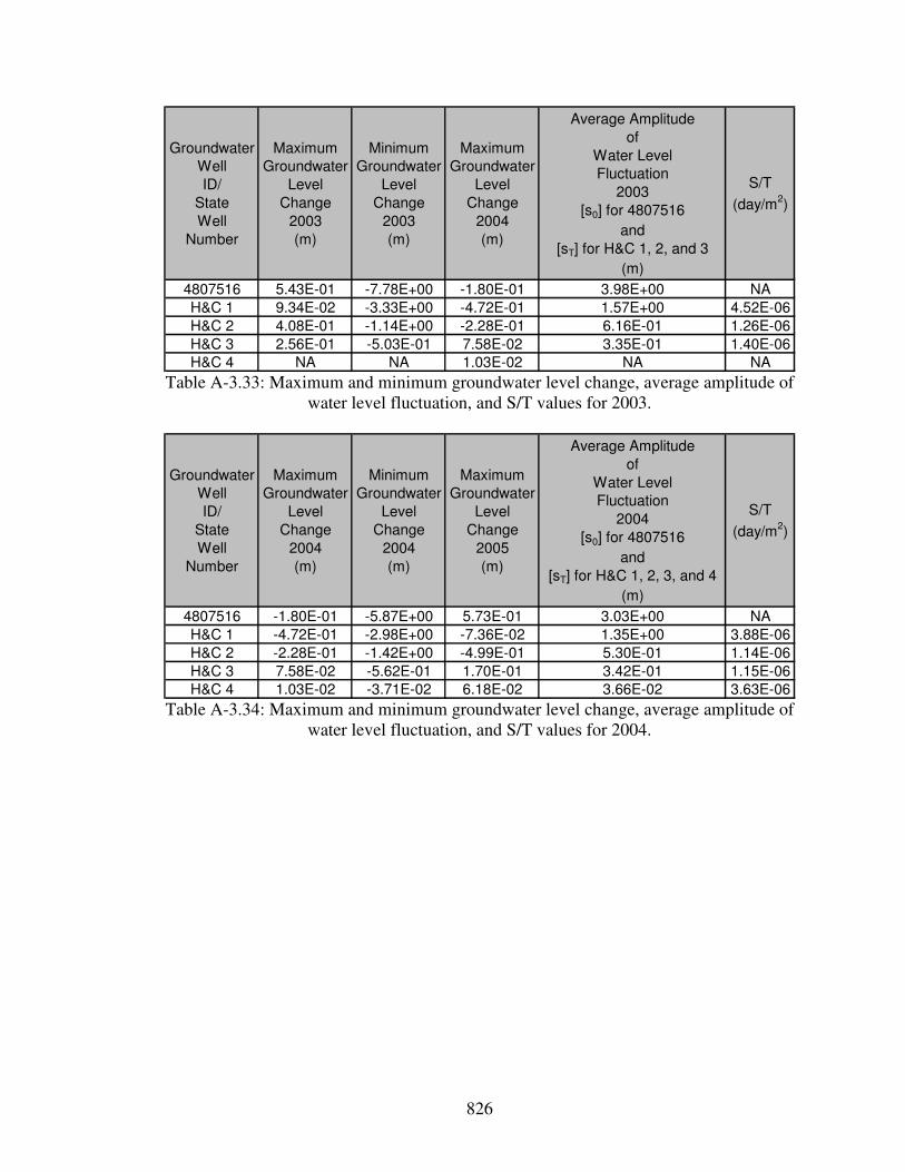
826
Groundwater
Well
ID/
State
Well
Number
Maximum
Groundwater
Level
Change
2003
(m)
Minimum
Groundwater
Level
Change
2003
(m)
Maximum
Groundwater
Level
Change
2004
(m)
Average Amplitude
of
Water Level
Fluctuation
2003
[s0] for 4807516
and
[sT] for H&C 1, 2, and 3
(m)
S/T
(day/m2)
4807516 5.43E-01 -7.78E+00 -1.80E-01 3.98E+00 NA
H&C 1 9.34E-02 -3.33E+00 -4.72E-01 1.57E+00 4.52E-06
H&C 2 4.08E-01 -1.14E+00 -2.28E-01 6.16E-01 1.26E-06
H&C 3 2.56E-01 -5.03E-01 7.58E-02 3.35E-01 1.40E-06
H&C 4 NA NA 1.03E-02 NA NA Table A-3.33: Maximum and minimum groundwater level change, average amplitude of
water level fluctuation, and S/T values for 2003.
Groundwater
Well
ID/
State
Well
Number
Maximum
Groundwater
Level
Change
2004
(m)
Minimum
Groundwater
Level
Change
2004
(m)
Maximum
Groundwater
Level
Change
2005
(m)
Average Amplitude
of
Water Level
Fluctuation
2004
[s0] for 4807516
and
[sT] for H&C 1, 2, 3, and 4
(m)
S/T
(day/m2)
4807516 -1.80E-01 -5.87E+00 5.73E-01 3.03E+00 NA
H&C 1 -4.72E-01 -2.98E+00 -7.36E-02 1.35E+00 3.88E-06
H&C 2 -2.28E-01 -1.42E+00 -4.99E-01 5.30E-01 1.14E-06
H&C 3 7.58E-02 -5.62E-01 1.70E-01 3.42E-01 1.15E-06
H&C 4 1.03E-02 -3.71E-02 6.18E-02 3.66E-02 3.63E-06 Table A-3.34: Maximum and minimum groundwater level change, average amplitude of
water level fluctuation, and S/T values for 2004.

827
Groundwater
Well
ID/
State
Well
Number
Maximum
Groundwater
Level
Change
2005
(m)
Minimum
Groundwater
Level
Change
2005
(m)
Maximum
Groundwater
Level
Change
2006
(m)
Average Amplitude
of
Water Level
Fluctuation
2005
[s0] for 4807516
and
[sT] for H&C 1, 2, 3, and 4
(m)
S/T
(day/m2)
4807516 5.73E-01 -6.46E+00 -6.10E-03 3.37E+00 NA
H&C 1 -7.36E-02 -3.12E+00 -5.07E-01 1.42E+00 4.18E-06
H&C 2 -4.99E-01 -1.99E+00 -1.19E+00 5.73E-01 1.17E-06
H&C 3 1.70E-01 -6.40E-01 -8.10E-02 3.42E-01 1.24E-06
H&C 4 6.18E-02 -2.90E-02 1.80E-02 3.45E-02 3.87E-06 Table A-3.35: Maximum and minimum groundwater level change, average amplitude of
water level fluctuation, and S/T values for 2005.

828
Groundwater
Well
ID/
State
Well
Number
Distance
from
Dell City
(m)
sT/s0
2003
S/T
2003
(day/m2)
sT/s0
2004
S/T
2004
(day/m2)
sT/s0
2005
S/T
2005
(day/m2)
4807516 NA NA NA NA NA NA NA
H&C 1 8,224 3.95E-01 NA 4.45E-01 NA 4.20E-01 NA
H&C 2 24,591 1.55E-01 NA 1.75E-01 NA 1.70E-01 NA
H&C 3 28,920 8.40E-02 NA 1.13E-01 NA 1.01E-01 NA
H&C 4 47,476 NA NA 1.20E-02 NA 1.02E-02 NA
5.68E-07 1.00E-06 1.07E-06 Table A-3.36: Values of sT/s0 for each year, and values of S/T calculated from
exponential trends of sT/s0 versus distance for each year.
Groundwater
Well
ID
Distance
from
H&C 1
(m)
Average
Annual
Phase Lag
between
H&C 1 and
Indicated Well
[tL] 2003
(days)
S/T
2003
(day/m2)
Average
Annual
Phase Lag
between
H&C 1 and
Indicated Well
[tL] 2004
(days)
S/T
2004
(day/m2)
Average
Annual
Phase Lag
between
H&C 1 and
Indicated Well
[tL] 2005
(days)
S/T
2005
(day/m2)
H&C 2 16,367 8 NA 19 NA 21 NA
H&C 3 20,696 17 NA 32 NA 34 NA
H&C 4 39,252 NA NA 81 NA 104 NA
1.30E-07 2.52E-07 4.65E-07 Table A-3.37: Average annual phase lag [tL] between each well pair for each year, and
values of S/T calculated from linear trends of tL versus distance for each year.

829
Year
S/T from the
Attenuation of
the Amplitude
of the Periodic
Water Level
Fluctuations
(day/m2)
Median T
from 14
C
Groundwater
Ages Along
Cross Section
A to A'
(m2/day)
S
Using
Median
T
Minimum T
from 14
C
Groundwater
Ages Along
Cross Section
A to A'
(m2/day)
S
Using
Minimum
T
Maximum T
from 14
C
Groundwater
Ages Along
Cross Section
A to A'
(m2/day)
S
Using
Maximum
T
2003 5.68E-07 4.78E+01 2.72E-05 1.04E-01 5.93E-08 5.14E+03 2.92E-03
2004 1.00E-06 4.78E+01 4.79E-05 1.04E-01 1.05E-07 5.14E+03 5.15E-03
2005 1.07E-06 4.78E+01 5.10E-05 1.04E-01 1.11E-07 5.14E+03 5.48E-03 Table A-3.38: Values of S calculated using S/T values estimated from the attenuation of
the amplitude of the periodic water level fluctuations.
Year
S/T from the
Phase Lag of
the Periodic
Water Level
Fluctuations
(day/m2)
Median T
from 14
C
Groundwater
Ages Along
Cross Section
A to A'
(m2/day)
S
Using
Median
T
Minimum T
from 14
C
Groundwater
Ages Along
Cross Section
A to A'
(m2/day)
S
Using
Minimum
T
Maximum T
from 14
C
Groundwater
Ages Along
Cross Section
A to A'
(m2/day)
S
Using
Maximum
T
2003 1.30E-07 4.78E+01 6.23E-06 1.04E-01 1.36E-08 5.14E+03 6.69E-04
2004 2.52E-07 4.78E+01 1.21E-05 1.04E-01 2.64E-08 5.14E+03 1.30E-03
2005 4.65E-07 4.78E+01 2.22E-05 1.04E-01 4.85E-08 5.14E+03 2.39E-03 Table A-3.39: Values of S calculated using S/T values estimated from the phase lag of
the periodic water level fluctuations.
Minimum
S
Maximum
S
Average
SAquifer Source
8.5E-04
Yeso Fm.
(unfractured siltstone
and gypsum)
Wasiolek (1991)
1.0E-05 1.0E-03 NA Confined Schwartz and Zhang (2003)
3.5E-04 2.E-03 NAMadison
aquifer system Greene (1993)
1.E-05 1.E-04 NA
Confined portion
of
Edwards-Trinity
aquifer system
Ryder (1996)
Table A-3.40: Range of S values reported in the scientific literature for confined and/or
predominantly carbonate aquifers.

830
TABLES – CHAPTER 4

831
Salt Basin Sub-basins
Delineated by JSAI (2010)
Minimum
Recharge
Rate
(cm/year)
Average
Recharge
Rate
(cm/year)
Maximum
Recharge
Rate
(cm/year)
Minimum
Recharge
(m3/day)
Average
Recharge
(m3/day)
Maximum
Recharge
(m3/day)
Minimum
Recharge
(acre-
feet/year)
Average
Recharge
(acre-
feet/year)
Maximum
Recharge
(acre-
feet/year)
Peñasco Basin 1.3 1.9 2.4 19,842 28,523 37,204 5,875 8,446 11,016
Upper Sacramento River and Upper Piñon Creek 0.5 1.0 1.2 9,637 19,275 22,166 2,854 5,707 6,564
Lower Piñon Creek 0.5 1.5 2.5 1,342 4,025 6,708 397 1,192 1,986
Collins Hills 1.0 2.5 5.0 3,970 9,925 19,850 1,176 2,939 5,878
Rim of the Guadalupes 2.0 2.8 4.0 8,542 11,746 17,085 2,529 3,478 5,059
Guadalupe Mountains 2.0 2.8 4.0 16,482 22,663 32,964 4,880 6,711 9,761
Upper Cornucopia Draw 1.0 2.5 3.5 3,888 9,720 13,607 1,151 2,878 4,029
limestone highlands 2.5 3.0 5.0 8,282 9,939 16,564 2,452 2,943 4,905
Lower Sacramento River and Otero Mesa 0.1 0.3 0.3 2,988 5,976 6,573 885 1,769 1,946
Lower Cornucopia Draw 2.5 3.0 5.0 28,064 33,676 56,127 8,310 9,972 16,620
Crow Flats 0.1 0.2 0.2 2,015 4,030 3,023 597 1,193 895
Shiloh Draw 0.1 0.2 0.2 1,655 4,413 4,965 490 1,307 1,470
Coffelt Draw 2.0 2.5 2.8 13,909 17,386 19,124 4,118 5,148 5,663
Big Dog Canyon 1.0 2.0 2.0 9,254 18,508 18,508 2,740 5,480 5,480
Long Canyon 2.0 3.0 3.3 3,559 5,339 5,784 1,054 1,581 1,713
Lewis Canyon 2.0 3.0 3.3 8,268 12,403 13,436 2,448 3,673 3,979
Brokeoff Mountains 0.8 1.5 1.5 5,709 11,417 11,417 1,690 3,381 3,381
Fourmile Draw 0.1 1.0 1.0 145 2,902 2,902 43 859 859
Cornudas Draw 0.5 1.5 1.8 6,817 20,452 23,861 2,019 6,056 7,065
Washburn Draw 0.1 0.1 0.1 348 695 695 103 206 206
Diablo Plateau 0.1 0.1 0.1 4,325 8,649 10,811 1,281 2,561 3,201
Delaware Mountains 0.8 1.5 1.5 5,647 11,294 11,294 1,672 3,344 3,344
Salt Flats 0.0 0.0 0.0 0 0 0 0 0 0
164,688 272,956 354,670 48,765 80,824 105,020Sum all sub-basins Table A-4.1: Water-balance based minimum, average, and maximum recharge rates and areal recharge applied to the Salt Basin sub-
basins within the 3-D MODFLOW groundwater flow model domain.

832
Minimum
Sacramento Mountains
Recharge Factor
(%)
Average
Sacramento Mountains
Recharge Factor
(%)
Maximum
Sacramento Mountains
Recharge Factor
(%)
4 22 44 Table A-4.2: Sacramento Mountains recharge factors from Newton et al. (2011).
Location
Minimum
Recharge
Rate
(cm/year)
Average
Recharge
Rate
(cm/year)
Maximum
Recharge
Rate
(cm/year)
Creek beds and depressions 0.028 0.242 0.457
Outside creek beds 0.005 0.0125 0.020 Table A-4.3: Kreitler et al. (1987) recharge rates for Diablo Plateau from Mayer (1995).

833
Range of
Average Annual
Precipitation in
Figure 1.11
Polygons
(cm/year)
Median
Average Annual
Precipitation in
Figure 1.11
Polygons
(cm/year)
Minimum
Recharge
Factor
(%)
Average
Recharge
Factor
(%)
Maximum
Recharge
Factor
(%)
Minimum
Recharge
Rate
(cm/year)
Average
Recharge
Rate
(cm/year)
Maximum
Recharge
Rate
(cm/year)
Minimum
Recharge
(m3/day)
Average
Recharge
(m3/day)
Maximum
Recharge
(m3/day)
Minimum
Recharge
(acre-
feet/year)
Average
Recharge
(acre-
feet/year)
Maximum
Recharge
(acre-
feet/year)
61 to 66 64 4 22 44 2.5 14.0 27.9
66 to 71 69 4 22 44 2.7 15.1 30.2
71 to 76 74 4 22 44 2.9 16.2 32.4
76 to 81 79 4 22 44 3.1 17.3 34.67,366 40,513 81,026 2,181 11,996 23,992
61 to 66 64 4 22 44 2.5 14.0 27.9
66 to 71 69 4 22 44 2.7 15.1 30.2
71 to 76 74 4 22 44 2.9 16.2 32.41,572 8,644 17,288 465 2,560 5,119
Sum Sacramento Mountains recharge zone
Sum Guadalupe Mountains recharge zone
Table A-4.4: Elevation-dependent minimum, average, and maximum recharge rates and areal recharge applied to the recharge zones within the 3-D MODFLOW groundwater flow model domain in the Sacramento and Guadalupe Mountains.
Location
Minimum
Recharge
Rate
(cm/year)
Average
Recharge
Rate
(cm/year)
Maximum
Recharge
Rate
(cm/year)
Minimum
Recharge
(m3/day)
Average
Recharge
(m3/day)
Maximum
Recharge
(m3/day)
Minimum
Recharge
(acre-
feet/year)
Average
Recharge
(acre-
feet/year)
Maximum
Recharge
(acre-
feet/year)
Creek beds and depressions 0.028 0.242 0.457
Outside creek beds 0.005 0.0125 0.02060 202 344 18 60 102
Creek beds and depressions 0.028 0.242 0.457
Outside creek beds 0.005 0.0125 0.02080 380 679 24 112 201
Sum Cornudas Mountains recharge zone
Sum Diablo Plateau recharge zone Table A-4.5: Elevation-dependent minimum, average, and maximum recharge rates and areal recharge applied to the recharge zones
within the 3-D MODFLOW groundwater flow model domain in around the Cornudas Mountains and on the Diablo Plateau.
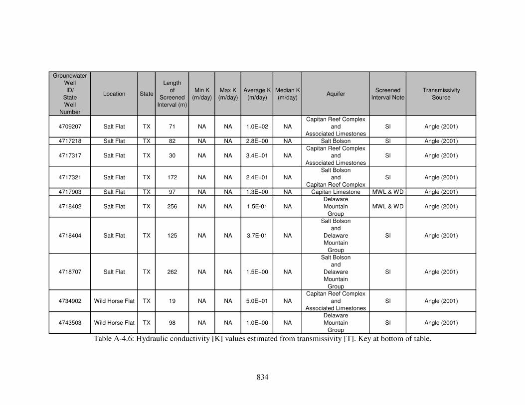
834
Groundwater
Well
ID/
State
Well
Number
Location State
Length
of
Screened
Interval (m)
Min K
(m/day)
Max K
(m/day)
Average K
(m/day)
Median K
(m/day)Aquifer
Screened
Interval Note
Transmissivity
Source
4709207 Salt Flat TX 71 NA NA 1.0E+02 NA
Capitan Reef Complex
and
Associated Limestones
SI Angle (2001)
4717218 Salt Flat TX 82 NA NA 2.8E+00 NA Salt Bolson SI Angle (2001)
4717317 Salt Flat TX 30 NA NA 3.4E+01 NA
Capitan Reef Complex
and
Associated Limestones
SI Angle (2001)
4717321 Salt Flat TX 172 NA NA 2.4E+01 NA
Salt Bolson
and
Capitan Reef Complex
SI Angle (2001)
4717903 Salt Flat TX 97 NA NA 1.3E+00 NA Capitan Limestone MWL & WD Angle (2001)
4718402 Salt Flat TX 256 NA NA 1.5E-01 NA
Delaware
Mountain
Group
MWL & WD Angle (2001)
4718404 Salt Flat TX 125 NA NA 3.7E-01 NA
Salt Bolson
and
Delaware
Mountain
Group
SI Angle (2001)
4718707 Salt Flat TX 262 NA NA 1.5E+00 NA
Salt Bolson
and
Delaware
Mountain
Group
SI Angle (2001)
4734902 Wild Horse Flat TX 19 NA NA 5.0E+01 NA
Capitan Reef Complex
and
Associated Limestones
SI Angle (2001)
4743503 Wild Horse Flat TX 98 NA NA 1.0E+00 NA
Delaware
Mountain
Group
SI Angle (2001)
Table A-4.6: Hydraulic conductivity [K] values estimated from transmissivity [T]. Key at bottom of table.

835
Groundwater
Well
ID/
State
Well
Number
Location State
Length
of
Screened
Interval (m)
Min K
(m/day)
Max K
(m/day)
Average K
(m/day)
Median K
(m/day)Aquifer
Screened
Interval Note
Transmissivity
Source
4751403 Wild Horse Flat TX 160 NA NA 1.1E+01 NASalt Bolson and
Permian RocksSI Angle (2001)
4751807 Wild Horse Flat TX 75 NA NA 5.1E+00 NA Salt Bolson SI Angle (2001)
4752301 Wild Horse Flat TX 168 NA NA 2.8E-01 NA
Capitan Reef Complex
and
Associated Limestones
SI Angle (2001)
4752601 Wild Horse Flat TX 47 NA NA 2.2E+01 NA
Capitan Reef Complex
and
Associated Limestones
SI Angle (2001)
4752602 Wild Horse Flat TX 94 NA NA 2.0E+00 NA
Capitan Reef Complex
and
Associated Limestones
SI Angle (2001)
4758502 Wild Horse Flat TX 30 NA NA 2.7E+00 NA Salt Bolson SI Angle (2001)
4758505 Wild Horse Flat TX 76 NA NA 2.0E+00 NA Salt Bolson SI Angle (2001)
4758602 Wild Horse Flat TX 80 NA NA 5.8E+00 NA Salt Bolson SI Angle (2001)
4758602 Wild Horse Flat TX 80 NA NA 7.3E+00 NA Salt Bolson SI Angle (2001)
4759102 Wild Horse Flat TX 92 NA NA 6.1E+00 NA
Salt Bolson
and
Cretaceous Rocks
SI Angle (2001)
4759209 Wild Horse Flat TX 61 NA NA 4.0E+00 NA Cretaceous System SI Angle (2001)
4759307 Michigan Flat TX 74 NA NA 2.4E+00 NA
Salt Bolson
and
Cretaceous Rocks
MWL & WD Angle (2001)
4759603 Michigan Flat TX 12 NA NA 1.6E+01 NA Cretaceous System SI Angle (2001)
4760404 Michigan Flat TX 82 NA NA 1.1E+00 NA Salt Bolson SI Angle (2001)
4760601 Michigan Flat TX 29 NA NA 9.6E-02 NA Permian System SI Angle (2001)
5102906 Lobo Flat TX 50 NA NA 1.6E+01 NA Salt Bolson SI Angle (2001)
5102918 Lobo Flat TX 79 NA NA 1.3E+00 NA Salt Bolson SI Angle (2001)
5102923 Lobo Flat TX 84 NA NA 5.4E+00 NA Salt Bolson SI Angle (2001)
5102926 Lobo Flat TX 37 NA NA 6.2E+00 NA Salt Bolson SI Angle (2001) Table A-4.6 continued.

836
Groundwater
Well
ID/
State
Well
Number
Location State
Length
of
Screened
Interval (m)
Min K
(m/day)
Max K
(m/day)
Average K
(m/day)
Median K
(m/day)Aquifer
Screened
Interval Note
Transmissivity
Source
5103702 Lobo Flat TX 143 NA NA 4.2E+00 NA Salt Bolson SI Angle (2001)
5103703 Lobo Flat TX 137 NA NA 3.4E-01 NA Salt Bolson SI Angle (2001)
5110306 Lobo Flat TX 62 NA NA 2.2E+00 NA Salt Bolson SI Angle (2001)
5110309 Lobo Flat TX 43 NA NA 1.2E+01 NAAlluvium and
Tertiary VolcanicsMWL & WD Angle (2001)
5110316 Lobo Flat TX 60 NA NA 7.9E+00 NA Salt Bolson MWL & WD Angle (2001)
5110317 Lobo Flat TX 66 NA NA 3.4E+00 NAAlluvium and
Tertiary VolcanicsSI Angle (2001)
5110321 Lobo Flat TX 80 NA NA 8.0E+00 NA Salt Bolson MWL & WD Angle (2001)
5110322 Lobo Flat TX 83 NA NA 2.2E+00 NA Salt Bolson MWL & WD Angle (2001)
5110328 Lobo Flat TX 73 NA NA 6.1E+00 NA Salt Bolson SI Angle (2001)
5110331 Lobo Flat TX 76 NA NA 5.2E+00 NAAlluvium and
Tertiary VolcanicsMWL & WD Angle (2001)
5110332 Lobo Flat TX 32 NA NA 1.4E+01 NA Salt Bolson SI Angle (2001)
5110603 Lobo Flat TX 30 NA NA 9.3E+00 NA Salt Bolson MWL Angle (2001)
5110603 Lobo Flat TX 30 NA NA 7.4E+00 NA Salt Bolson MWL Angle (2001)
5110624 Lobo Flat TX 52 NA NA 6.8E-01 NA Salt Bolson SI Angle (2001)
5111105 Lobo Flat TX 167 NA NA 1.9E+00 NA Salt Bolson SI Angle (2001)
5111106 Lobo Flat TX 141 NA NA 1.1E+00 NA Salt Bolson SI Angle (2001)
5114501 Lobo Flat TX 12 NA NA 5.3E-01 NA Volcanics SI Angle (2001)
5119104 Lobo Flat TX 58 NA NA 4.8E+00 NA Salt Bolson SI Angle (2001)
5119301 Lobo Flat TX 106 NA NA 4.5E+00 NA Salt Bolson MWL & WD Angle (2001)
5120403 Lobo Flat TX 119 NA NA 6.2E-01 NA Salt Bolson SI Angle (2001)
5120404 Lobo Flat TX 169 NA NA 9.3E-01 NA Salt Bolson SI Angle (2001)
5127302 Ryan Flat TX 69 NA NA 1.2E+00 NA Volcanics SI Angle (2001)
5128303 Ryan Flat TX 791 NA NA 2.2E-01 NA Salt Bolson SI Angle (2001)
5128606 Ryan Flat TX 769 NA NA 1.4E-01 NA Salt Bolson SI Angle (2001)
5129104 Ryan Flat TX 175 NA NA 1.6E-02 NA Salt Bolson MWL & WD Angle (2001)
5129105 Ryan Flat TX 162 NA NA 1.3E-01 NA Salt Bolson SI Angle (2001)
5129403 Ryan Flat TX 205 NA NA 9.1E-01 NA Salt Bolson SI Angle (2001)
5129704 Ryan Flat TX 390 NA NA 4.5E-01 NA Salt Bolson SI Angle (2001) Table A-4.6 continued.

837
Groundwater
Well
ID/
State
Well
Number
Location State
Length
of
Screened
Interval (m)
Min K
(m/day)
Max K
(m/day)
Average K
(m/day)
Median K
(m/day)Aquifer
Screened
Interval Note
Transmissivity
Source
5129705 Ryan Flat TX 255 NA NA 1.8E+00 NA Salt Bolson SI Angle (2001)
5128701 Ryan Flat TX 188 NA NA 4.9E-03 NA Salt Bolson SI Angle (2001)
5136601 Ryan Flat TX 91 NA NA 1.0E+01 NA Salt Bolson SI Angle (2001)
4807203 Delly City area TX 51 NA NA 9.99E+00 NA
Permian
Shelf
Facies
MWL & WD
Uliana (2001),
referenced from
Davis and Leggat (1965)
4807206 Delly City area TX 29 NA NA 5.76E+01 NA
Permian
Shelf
Facies
MWL & WD
Uliana (2001),
referenced from
Davis and Leggat (1965)
4807207 Delly City area TX 181 NA NA 5.29E+00 NA
Permian
Shelf
Facies
MWL & WD
Uliana (2001),
referenced from
Davis and Leggat (1965)
4807302 Delly City area TX 30 NA NA 1.11E+01 NA
Permian
Shelf
Facies
MWL
Uliana (2001),
referenced from
Davis and Leggat (1965)
4807601 Delly City area TX 35 NA NA 3.20E+01 NA
Permian
Shelf
Facies
SI
Uliana (2001),
referenced from
Davis and Leggat (1965)
4807605 NA TX 30 NA NA 5.10E+01 NA
Permian
Shelf
Facies
WD
Uliana (2001),
referenced from
Davis and Leggat (1965)
4807701 NA TX 30 NA NA 6.51E+01 NA
Permian
Shelf
Facies
WD
Uliana (2001),
referenced from
Davis and Leggat (1965)
4807901 Delly City area TX 76 NA NA 1.73E+01 NA
Permian
Shelf
Facies
MWL & WD
Uliana (2001),
referenced from
Davis and Leggat (1965)
4815201 Delly City area TX 82 NA NA 1.07E+01 NA
Permian
Shelf
Facies
SI
Uliana (2001),
referenced from
Davis and Leggat (1965) Table A-4.6 continued.
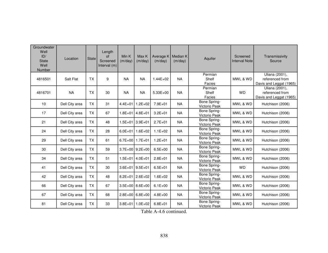
838
Groundwater
Well
ID/
State
Well
Number
Location State
Length
of
Screened
Interval (m)
Min K
(m/day)
Max K
(m/day)
Average K
(m/day)
Median K
(m/day)Aquifer
Screened
Interval Note
Transmissivity
Source
4816501 Salt Flat TX 9 NA NA 1.44E+02 NA
Permian
Shelf
Facies
MWL & WD
Uliana (2001),
referenced from
Davis and Leggat (1965)
4816701 NA TX 30 NA NA 5.33E+00 NA
Permian
Shelf
Facies
WD
Uliana (2001),
referenced from
Davis and Leggat (1965)
10 Dell City area TX 31 4.4E+01 1.2E+02 7.9E+01 NABone Spring-
Victorio PeakMWL & WD Hutchison (2006)
17 Dell City area TX 67 1.8E+01 4.8E+01 3.2E+01 NABone Spring-
Victorio PeakMWL & WD Hutchison (2006)
21 Dell City area TX 48 1.5E+01 3.9E+01 2.7E+01 NABone Spring-
Victorio PeakMWL & WD Hutchison (2006)
24 Dell City area TX 28 6.0E+01 1.6E+02 1.1E+02 NABone Spring-
Victorio PeakMWL & WD Hutchison (2006)
29 Dell City area TX 61 6.7E+00 1.7E+01 1.2E+01 NABone Spring-
Victorio PeakMWL & WD Hutchison (2006)
30 Dell City area TX 59 3.7E+00 9.2E+00 6.5E+00 NABone Spring-
Victorio PeakMWL & WD Hutchison (2006)
34 Dell City area TX 51 1.5E+01 4.0E+01 2.8E+01 NABone Spring-
Victorio PeakMWL & WD Hutchison (2006)
41 Dell City area TX 30 3.6E+01 9.5E+01 6.5E+01 NABone Spring-
Victorio PeakWD Hutchison (2006)
42 Dell City area TX 48 8.2E+01 2.6E+02 1.6E+02 NABone Spring-
Victorio PeakMWL & WD Hutchison (2006)
66 Dell City area TX 67 3.5E+00 8.6E+00 6.1E+00 NABone Spring-
Victorio PeakMWL & WD Hutchison (2006)
67 Dell City area TX 68 2.8E+00 6.8E+00 4.8E+00 NABone Spring-
Victorio PeakMWL & WD Hutchison (2006)
81 Dell City area TX 33 3.8E+01 1.0E+02 6.8E+01 NABone Spring-
Victorio PeakMWL & WD Hutchison (2006)
Table A-4.6 continued.

839
Groundwater
Well
ID/
State
Well
Number
Location State
Length
of
Screened
Interval (m)
Min K
(m/day)
Max K
(m/day)
Average K
(m/day)
Median K
(m/day)Aquifer
Screened
Interval Note
Transmissivity
Source
111 Dell City area TX 65 5.0E+01 1.5E+02 9.6E+01 NABone Spring-
Victorio PeakMWL & WD Hutchison (2006)
24.19.18.144 Crow Flats area NM 103 9.9E+01 4.1E+02 2.5E+02 NA
Permian
Shelf
Facies
MWL & WD Hutchison (2006)
26.18.28.113 Crow Flats area NM 110 3.6E+01 1.1E+02 7.2E+01 NA
Permian
Shelf
Facies
MWL & WD Hutchison (2006)
26.18.29.113 Crow Flats area NM 85 6.5E+01 2.2E+02 1.4E+02 NA
Permian
Shelf
Facies
MWL & WD Hutchison (2006)
26.18.29.113a Crow Flats area NM 75 8.5E+01 3.1E+02 1.9E+02 NA
Permian
Shelf
Facies
MWL & WD Hutchison (2006)
26.18.30.122 Crow Flats area NM 90 3.2E+01 9.3E+01 6.0E+01 NA
Permian
Shelf
Facies
MWL & WD Hutchison (2006)
26.18.32.122 Crow Flats area NM 82 9.9E+00 2.6E+01 1.8E+01 NA
Permian
Shelf
Facies
MWL & WD Hutchison (2006)
26.18.33.111 Crow Flats area NM 122 8.3E-01 2.0E+00 1.4E+00 NA
Permian
Shelf
Facies
MWL & WD Hutchison (2006)
26.18.33.133 Crow Flats area NM 124 1.3E+00 3.3E+00 2.3E+00 NA
Permian
Shelf
Facies
MWL & WD Hutchison (2006)
4709207 Salt Flat TX 71 2.3E+01 6.2E+01 4.1E+01 NA
Capitan Reef Complex
and
Associated Limestones
SI Hutchison (2006)
Table A-4.6 continued.
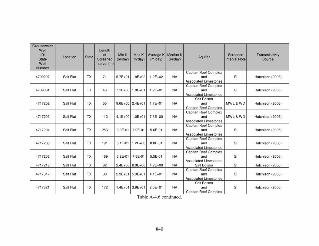
840
Groundwater
Well
ID/
State
Well
Number
Location State
Length
of
Screened
Interval (m)
Min K
(m/day)
Max K
(m/day)
Average K
(m/day)
Median K
(m/day)Aquifer
Screened
Interval Note
Transmissivity
Source
4709207 Salt Flat TX 71 5.7E+01 1.8E+02 1.2E+02 NA
Capitan Reef Complex
and
Associated Limestones
SI Hutchison (2006)
4709801 Salt Flat TX 43 7.1E+00 1.8E+01 1.2E+01 NA
Capitan Reef Complex
and
Associated Limestones
SI Hutchison (2006)
4717202 Salt Flat TX 55 9.6E+00 2.4E+01 1.7E+01 NA
Salt Bolson
and
Capitan Reef Complex
MWL & WD Hutchison (2006)
4717203 Salt Flat TX 112 4.1E+00 1.0E+01 7.3E+00 NA
Capitan Reef Complex
and
Associated Limestones
MWL & WD Hutchison (2006)
4717204 Salt Flat TX 253 3.3E-01 7.9E-01 5.6E-01 NA
Capitan Reef Complex
and
Associated Limestones
SI Hutchison (2006)
4717206 Salt Flat TX 191 5.1E-01 1.2E+00 8.8E-01 NA
Capitan Reef Complex
and
Associated Limestones
SI Hutchison (2006)
4717208 Salt Flat TX 469 3.2E-01 7.8E-01 5.5E-01 NA
Capitan Reef Complex
and
Associated Limestones
SI Hutchison (2006)
4717218 Salt Flat TX 82 2.4E+00 6.0E+00 4.2E+00 NA Salt Bolson SI Hutchison (2006)
4717317 Salt Flat TX 30 2.3E+01 5.9E+01 4.1E+01 NA
Capitan Reef Complex
and
Associated Limestones
SI Hutchison (2006)
4717321 Salt Flat TX 172 1.4E+01 3.9E+01 2.5E+01 NA
Salt Bolson
and
Capitan Reef Complex
SI Hutchison (2006)
Table A-4.6 continued.

841
Groundwater
Well
ID/
State
Well
Number
Location State
Length
of
Screened
Interval (m)
Min K
(m/day)
Max K
(m/day)
Average K
(m/day)
Median K
(m/day)Aquifer
Screened
Interval Note
Transmissivity
Source
4717602 Salt Flat TX 27 3.9E+00 9.6E+00 6.8E+00 NA
Salt Bolson
and
Delaware
Mountain
Group
MWL & WD Hutchison (2006)
4717904 Salt Flat TX 78 2.6E+00 6.3E+00 4.5E+00 NA
Salt Bolson
and
Delaware
Mountain
Group
MWL & WD Hutchison (2006)
4718706 Salt Flat TX 112 1.8E+00 4.4E+00 3.1E+00 NA
Salt Bolson
and
Delaware
Mountain
Group
MWL & WD Hutchison (2006)
Table A-4.6 continued.
Screened Interval Note Key: SI = total length of screened/open interval used for aquifer thickness, MWL & WD = distance from mean groundwater level to total well depth used for aquifer thickness, MWL = only mean groundwater level available; assumed 30 meters (98 feet) aquifer thickness, WD = only total well depth available; assumed 30 meters (98 feet) aquifer thickness.

842
Hydrogeologic
Unit
Model
Layers
Initial
Horizontal
K (m/day)
Vertical
Anisotropy
Calibrated
Water-balance
Based Minimum
Recharge
Scenario
Horizontal
K (m/day)
Calibrated
Water-balance
Based Average
Recharge
Scenario
Horizontal
K (m/day)
Calibrated
Water-balance
Based Maximum
Recharge
Scenario
Horizontal
K (m/day)
Cenozoic
alluvium1, 2, and 3 1 100 10 10 10
Cenozoic intrusions 1, 2, 3, 4, and 5 0.0001 1,000 0.00001 to 0.0001 0.00001 to 0.001 0.00001 to 0.001
Cretaceous 1 0.01 100 0.005 0.0075 0.0075
Low permeability
confining unit
beneath Cretaceous
2 0.000001 1,000 0.00000001 0.00000001 0.00000001
Unfractured Permian 1, 2, 3, 4, and 5 0.01 to 0.1 100 0.005 to 0.5 0.0075 to 1 0.01 to 2.5
Fractured Permian 1, 2, 3, 4, and 5 1 to 10 10 0.025 to 25 0.025 to 250 0.025 to 250
Paleozoic
(Cambrian through
Pennslyvanian)
2, 3, 4, 5, and 6 0.001 1,000 0.00005 to 0.5 0.00005 to 0.5 0.00005 to 0.5
Precambrian 1, 2, 3, 4, 5, and 6 0.001 1,000 0.00001 to 0.01 0.00001 to 0.01 0.00001 to 0.01 Table A-4.7: Initial horizontal hydraulic conductivity [K], vertical anisotropy, and final horizontal K assigned to each hydrogeologic
unit for the calibrated water-balance based minimum, average, and maximum recharge scenario models.

843
Hydrogeologic
Unit
Model
Layers
Initial
Horizontal
K (m/day)
Vertical
Anisotropy
Calibrated
Elevation-
dependent
Minimum
Recharge
Scenario
Horizontal
K (m/day)
Calibrated
Elevation-
dependent
Average
Recharge
Scenario
Horizontal
K (m/day)
Calibrated
Elevation-
dependent
Maximum
Recharge
Scenario
Horizontal
K (m/day)Cenozoic
alluvium1, 2, and 3 1 100 0.005 to 10 0.0075 to 10 0.01 to 10
Cenozoic intrusions 1, 2, 3, 4, and 5 0.0001 1,000 0.00001 to 0.1 0.00001 to 0.1 0.00001 to 0.1
Cretaceous 1 0.01 100 0.0005 0.0025 0.005
Low permeability
confining unit
beneath Cretaceous
2 0.000001 1,000 0.00000001 0.00001 0.0001
Unfractured Permian 1, 2, 3, 4, and 5 0.01 to 0.1 100 0.005 to 0.5 0.005 to 5 0.005 to 5
Fractured Permian 1, 2, 3, 4, and 5 1 to 10 10 0.0075 to 5 0.075 to 25 0.25 to 25
Paleozoic
(Cambrian through
Pennslyvanian)
2, 3, 4, 5, and 6 0.001 1,000 0.00005 to 0.1 0.00005 to 0.1 0.00005 to 0.1
Precambrian 1, 2, 3, 4, 5, and 6 0.001 1,000 0.00001 to 0.01 0.00001 to 0.01 0.00001 to 0.01 Table A-4.8: Initial horizontal hydraulic conductivity [K], vertical anisotropy, and final horizontal K assigned to each hydrogeologic
unit for the calibrated elevation-dependent minimum, average, and maximum recharge scenario models.

844
POD Number/
Well ID/
State Well
Number
Easting NorthingModel
Row
Model
Column
Model Layer
or Layers
Intersected by
Screened Interval
Elevation
of Top
of Screen
(m)
Elevation
of Bottom
of Screen
(m)
Observed
Groundwater
Elevation
(m)
Source Note
PN 00308 442967 3628994 108 23 1 2,231 2,213 2,231 NMOSE *
PN 00119 453798 3628887 97 23 1 2,043 1,919 2,043 NMOSE *
PN 00966 455641 3628866 96 23 1 1,988 1,932 1,988 NMOSE *
PN 00561 445394 3628678 106 23 1 2,233 2,207 2,233 NMOSE *
PN 00949 446088 3628596 103 23 1 2,207 2,189 2,207 NMOSE *
PN 00417 446288 3628596 105 23 1 2,219 2,199 2,219 NMOSE *
SM-0075 447829 3628594 105 23 1 2,180 2,153 2,180 SMHS *
PN 00750 445692 3628385 106 23 1 2,245 2,240 2,245 NMOSE *
PN 00196 POD2 442050 3628215 109 23 1 2,298 2,237 2,298 NMOSE *
PN 00196 442155 3628153 109 23 1 2,292 2,286 2,292 NMOSE *
PN 00708 441748 3628136 109 23 1 2,334 2,321 2,334 NMOSE *
PN 00594 442054 3628052 109 24 1 2,295 2,288 2,295 NMOSE *
PN 00526 442254 3628052 109 24 1 2,294 2,263 2,294 NMOSE *
PN 00357 458020 3627889 93 24 1 1,938 1,915 1,938 NMOSE *
PN 00202 442148 3627748 109 24 1 2,274 2,270 2,274 NMOSE *
PN 00174 441744 3627731 109 24 1 2,311 2,294 2,311 NMOSE *
PN 00073 451331 3627670 100 24 1 2,085 2,062 2,085 NMOSE *
PN 00004 447404 3627541 104 24 1 2,191 2,183 2,191 NMOSE *
PN 00552 450369 3627370 101 24 1 2,075 2,054 2,075 NMOSE *
PN 00016 451191 3627359 100 24 1 2,102 2,077 2,102 NMOSE *
PN 00587 441735 3627325 109 24 1 2,276 2,224 2,276 NMOSE *
PN 00799 439811 3627141 111 24 1 2,418 2,396 2,418 NMOSE *
PN 00929 441727 3626918 109 25 1 2,312 2,282 2,312 NMOSE *
PN 00383 454601 3626841 97 25 1 1,990 1,984 1,990 NMOSE *
PN 00700 451138 3626824 100 25 1 2,060 2,022 2,060 NMOSE *
PN 00677 452954 3626641 95 25 1 2,038 2,012 2,038 NMOSE *
PN 00810 453553 3626641 98 25 1 2,029 2,011 2,029 NMOSE *
PN 00616 456041 3626639 98 25 1 1,992 1,971 1,992 NMOSE *
PN 01027 POD1 450938 3626624 100 25 1 2,056 1,995 2,056 NMOSE * Table A-4.9: Calibration targets for the steady-state 3-D MODFLOW groundwater flow model. Key at bottom of table.

845
POD Number/
Well ID/
State Well
Number
Easting NorthingModel
Row
Model
Column
Model Layer
or Layers
Intersected by
Screened Interval
Elevation
of Top
of Screen
(m)
Elevation
of Bottom
of Screen
(m)
Observed
Groundwater
Elevation
(m)
Source Note
PN 00152 441442 3626588 96 25 1 2,354 2,348 2,354 NMOSE *
PN 00166 455330 3626534 110 25 1 1,980 1,962 1,980 NMOSE *
PN 00236 451289 3626498 100 25 1 2,065 1,961 2,065 NMOSE *
PN 00182 441562 3626354 100 25 1 2,326 2,313 2,326 NMOSE *
PN 00669 451477 3626306 110 25 1 2,062 1,998 2,062 NMOSE *
PN 00426 453238 3626121 98 25 1 2,053 1,992 2,053 NMOSE *
PN 00211 456449 3626025 95 26 1 1,959 1,942 1,959 NMOSE *
PN 00704 452352 3626017 99 26 1 2,059 1,958 2,059 NMOSE *
PN 00841 452352 3625817 99 26 1 2,067 2,048 2,067 NMOSE *
PN 00871 452147 3625610 99 26 1 2,061 2,017 2,061 NMOSE *
PN 00738 452248 3625511 99 26 1 2,056 2,030 2,056 NMOSE *
PN 00729 455646 3625420 96 26 1 2,010 1,964 2,010 NMOSE *
PN 00758 452347 3625410 99 26 1 2,057 1,999 2,057 NMOSE *
PN 00382 435462 3625068 116 27 1 2,610 2,587 2,610 NMOSE *
PN 00942 459827 3621825 91 30 1 1,888 1,846 1,888 NMOSE *
PN 00511 453047 3621586 98 30 1 1,979 1,959 1,979 NMOSE *
PN 00787 449823 3619557 101 32 1 2,032 1,936 2,032 NMOSE *
ST 00115 S-10 446461 3615401 105 36 1 2,041 1,961 2,041 NMOSE *
ST 00111 434903 3612163 70 40 1 2,096 1,980 2,096 NMOSE *
ST 00005 481574 3612051 81 40 1 1,519 1,474 1,519 NMOSE *
ST 00008 469786 3612015 116 39 1 1,492 1,480 1,492 NMOSE *
ST 00009 467376 3611968 84 40 1 1,466 1,448 1,466 NMOSE *
ST 00111 S-4 434269 3610961 117 41 1 1,989 1,946 1,989 NMOSE *
ST 00165 457467 3610375 94 41 1 1,658 1,553 1,658 NMOSE *
ST 00166 461985 3609637 89 42 1 1,515 1,448 1,515 NMOSE *
ST 00006 483181 3608828 68 43 1 1,505 1,425 1,505 NMOSE *
ST 00221 463074 3608381 88 43 1 1,446 1,332 1,446 NMOSE *
ST 00020 453685 3607880 98 44 1 1,797 1,666 1,797 NMOSE *
SM-0046 442173 3607555 109 44 1 1,776 1,715 1,776 SMHS * Table A-4.9 continued.

846
POD Number/
Well ID/
State Well
Number
Easting NorthingModel
Row
Model
Column
Model Layer
or Layers
Intersected by
Screened Interval
Elevation
of Top
of Screen
(m)
Elevation
of Bottom
of Screen
(m)
Observed
Groundwater
Elevation
(m)
Source Note
ST 00003 478550 3606619 73 45 1 1,312 1,287 1,312 NMOSE *
ST 00007 485591 3603997 66 48 1 1,459 1,421 1,459 NMOSE *
ST 00021 465694 3603733 86 48 1 1,408 1,399 1,408 NMOSE *
ST 00236 POD1 481499 3602715 70 49 1 1,316 1,244 1,316 NMOSE *
ST 00080 451407 3598958 100 53 1 1,487 1,481 1,487 NMOSE *
ST 00194 S 484877 3598063 66 54 1 1,194 1,178 1,194 NMOSE *
ST 00018 473476 3596830 78 55 1 1,392 1,353 1,392 NMOSE *
ST 00194 484918 3594393 66 57 1 1,349 1,319 1,349 NMOSE *, +
ST 00068 485622 3592884 66 59 1 1,334 1,326 1,334 NMOSE *
ST 00022 471858 3592609 79 59 1, 2, and 3 1,225 825 1,225 NMOSE *
ST 00200 483909 3588157 65 63 1 1,101 1,094 1,101 NMOSE *
ST 00196 486119 3588154 67 63 1 1,116 1,108 1,116 NMOSE *
ST 00019 476365 3588074 75 64 1 1,157 1,131 1,157 NMOSE *
ST 00081 454291 3584921 97 67 1 1,171 1,167 1,171 NMOSE *
ST 00075 487572 3583723 64 68 1 1,124 1,093 1,124 NMOSE *
ST 00055 444554 3582645 107 69 1 1,136 1,106 1,136 NMOSE *
ST 00195 484099 3581318 67 70 1 1,098 1,095 1,098 NMOSE *
ST 00132 444847 3580934 106 71 1 1,168 1,153 1,168 NMOSE *
ST 00056 447353 3580223 104 71 1 1,165 1,127 1,165 NMOSE *
ST 00133 452054 3579701 99 72 1 1,196 1,158 1,196 NMOSE *
ST 00198 485704 3579307 66 72 1 1,102 1,096 1,102 NMOSE *
ST 00254 POD1 478461 3578608 73 73 1 and 2 1,119 1,053 1,119 NMOSE *
ST 00052 494206 3578272 57 73 1 1,104 1,089 1,104 NMOSE *
ST 00072 493805 3578067 57 74 1 1,118 1,057 1,118 NMOSE *
ST 00078 489782 3575872 61 76 1 1,106 1,084 1,106 NMOSE *
ST 00069 499785 3575849 51 76 1 1,112 1,099 1,112 NMOSE *
ST 00071 490990 3574863 60 77 1 and 2 1,100 986 1,100 NMOSE *
ST 00102 434576 3573550 78 78 1 1,336 1,317 1,336 NMOSE *
ST 00199 473613 3573502 50 78 1 1,154 1,146 1,154 NMOSE * Table A-4.9 continued.

847
POD Number/
Well ID/
State Well
Number
Easting NorthingModel
Row
Model
Column
Model Layer
or Layers
Intersected by
Screened Interval
Elevation
of Top
of Screen
(m)
Elevation
of Bottom
of Screen
(m)
Observed
Groundwater
Elevation
(m)
Source Note
ST 00070 500796 3573438 117 78 1 1,096 1,088 1,096 NMOSE *
ST 00035 465493 3573243 86 78 1 1,163 1,148 1,163 NMOSE *
ST 00053 492193 3572648 59 79 1 1,103 1,058 1,103 NMOSE *
ST 00103 439978 3568708 111 83 1 1,294 1,272 1,294 NMOSE *
ST 00048 495206 3567420 56 84 1 1,138 1,133 1,138 NMOSE *
ST 00036 467360 3566280 84 85 1 1,127 1,105 1,127 NMOSE *
ST 00086 492587 3565618 59 86 1 1,110 1,089 1,110 NMOSE *
ST 00015 492488 3565519 59 86 1 1,113 1,089 1,113 NMOSE *
ST 00037 500007 3565208 51 86 1 1,138 1,079 1,138 NMOSE *
ST 00074 496386 3564607 55 87 1 and 2 1,108 1,016 1,108 NMOSE *
ST 00077 508213 3564589 43 87 1 1,082 1,037 1,082 NMOSE *
ST 00161 477637 3564446 74 87 1 1,124 1,029 1,124 NMOSE *
ST 00088 487550 3563011 64 89 1 1,098 1,025 1,098 NMOSE *
ST 00162 481454 3561014 70 91 1 1,090 1,075 1,090 NMOSE *
ST 00087 487547 3561001 63 91 1 1,103 1,076 1,103 NMOSE *
ST 00084 487747 3561001 64 91 1 1,102 1,064 1,102 NMOSE *
ST 00089 487950 3561000 63 91 1 1,100 1,004 1,100 NMOSE *
ST 00092 444365 3560630 107 91 1 1,227 1,166 1,227 NMOSE *
ST 00097 440344 3560061 111 92 1 1,403 1,278 1,403 NMOSE *
ST 00180 S 488148 3559592 63 92 1, 2, and 3 1,109 947 1,109 NMOSE *
ST 00049 494596 3559387 57 92 1 1,106 1,104 1,106 NMOSE *
ST 00038 458735 3558565 92 93 1 and 2 1,154 1,032 1,154 NMOSE *
ST 00042 463561 3557747 88 94 1 1,152 1,121 1,152 NMOSE *
ST 00163 479239 3557196 72 94 1 1,093 1,076 1,093 NMOSE *
ST 00164 488754 3556577 62 95 1 1,106 1,088 1,106 NMOSE *
ST 00192 493185 3555562 58 96 1 1,102 1,030 1,102 NMOSE *
ST 00191 494594 3555559 57 96 1 1,112 1,039 1,112 NMOSE *
ST 00028 445541 3554322 106 97 1 1,426 1,421 1,426 NMOSE *
ST 00054 489965 3553359 61 98 1 1,106 1,037 1,106 NMOSE * Table A-4.9 continued.

848
POD Number/
Well ID/
State Well
Number
Easting NorthingModel
Row
Model
Column
Model Layer
or Layers
Intersected by
Screened Interval
Elevation
of Top
of Screen
(m)
Elevation
of Bottom
of Screen
(m)
Observed
Groundwater
Elevation
(m)
Source Note
ST 00033 492178 3552346 59 99 1 1,104 1,025 1,104 NMOSE *
ST 00182 492380 3552344 59 99 1 1,101 1,070 1,101 NMOSE *
ST 00026 438231 3552247 113 99 1 1,441 1,426 1,441 NMOSE *
ST 00110 491775 3551945 59 100 1 and 2 1,103 965 1,103 NMOSE *
ST 00027 441810 3551427 109 100 1 1,389 1,371 1,389 NMOSE *
ST 00107 428705 3550603 86 101 1 1,443 1,412 1,443 NMOSE *
ST 00043 465163 3550511 123 101 1 1,105 1,044 1,105 NMOSE *
ST 00040 469119 3549792 82 102 1 1,117 1,086 1,117 NMOSE *
ST 00041 450338 3548063 101 104 1 1,413 1,398 1,413 NMOSE *
ST 00051 451746 3547855 99 104 1 1,406 1,389 1,406 NMOSE *
ST 00187 S 481046 3547755 70 104 1 1,105 1,084 1,105 NMOSE *
C 02318 519164 3547455 32 104 1 1,793 1,776 1,793 NMOSE *
ST 00024 438171 3547423 113 104 1 1,383 1,375 1,383 NMOSE *
ST 00039 448727 3547265 102 104 1 1,447 1,425 1,447 NMOSE *
ST 00106 437663 3546802 114 105 1 1,416 1,370 1,416 NMOSE *
ST 00044 466258 3546182 85 105 1 and 2 1,119 1,024 1,119 NMOSE *
ST 00032 453546 3545833 98 106 1 1,397 1,359 1,397 NMOSE *
ST 00101 442084 3545493 109 106 1 1,423 1,365 1,423 NMOSE *
ST 00046 474148 3545352 77 106 1 1,100 1,077 1,100 NMOSE *
ST 00099 447914 3545254 103 106 1 1,550 1,535 1,550 NMOSE *
ST 00108 432019 3545238 119 106 1 1,417 1,396 1,417 NMOSE *
ST 00090 417884 3544898 85 107 1 and 2 1,558 1,545 1,558 NMOSE *
ST 00045 465851 3544774 40 107 1 and 2 1,157 1,002 1,157 NMOSE *
ST 00160 511665 3544666 133 107 1 1,101 988 1,101 NMOSE *
ST 00186 S 487526 3544312 64 107 1 1,080 1,055 1,080 NMOSE *
ST 00253 POD1 489252 3544154 62 107 1 1,091 1,060 1,091 NMOSE *
ST 00186 487526 3544112 64 108 1 1,096 1,053 1,096 NMOSE *
ST 00123 489740 3544106 61 108 1 1,095 1,045 1,095 NMOSE *
ST 00057 490345 3544103 61 108 1 1,090 1,066 1,090 NMOSE * Table A-4.9 continued.

849
POD Number/
Well ID/
State Well
Number
Easting NorthingModel
Row
Model
Column
Model Layer
or Layers
Intersected by
Screened Interval
Elevation
of Top
of Screen
(m)
Elevation
of Bottom
of Screen
(m)
Observed
Groundwater
Elevation
(m)
Source Note
ST 00091 416873 3544102 62 108 1 and 2 1,387 1,329 1,387 NMOSE *
ST 00059 489135 3543905 134 108 1 1,092 986 1,092 NMOSE *
ST 00116 B 487724 3543709 63 108 1 1,091 1,048 1,091 NMOSE *
ST 00058 489939 3543499 61 108 1 and 2 1,092 983 1,092 NMOSE *
ST 00187 479815 3543323 71 108 1 1,100 1,077 1,100 NMOSE *
ST 00116 487320 3543307 64 108 1 1,090 1,069 1,090 NMOSE *
ST 00034 449111 3543234 102 108 1 1,429 1,414 1,429 NMOSE *
ST 00116 S 486716 3542904 65 109 1 1,091 1,088 1,091 NMOSE *
ST 00059 S-3 489332 3542899 62 109 1, 2, and 3 1,092 806 1,092 NMOSE *
ST 00031 455145 3542811 96 109 1 1,372 1,362 1,372 NMOSE *
ST 00029 459818 3542789 91 109 1 1,127 1,117 1,127 NMOSE *
ST 00047 468499 3542756 83 109 1 1,115 1,106 1,115 NMOSE *
ST 00060 S-2 487519 3542699 64 109 1 and 2 1,092 950 1,092 NMOSE *
ST 00125 488927 3542696 62 109 1 1,068 1,038 1,068 NMOSE *, +
ST 00060 487519 3542499 64 109 1 and 2 1,091 958 1,091 NMOSE *
ST 00187 S-2 483837 3542303 67 109 1 1,095 1,049 1,095 NMOSE *
ST 00120 486712 3542298 65 109 1 1,092 1,043 1,092 NMOSE *
ST 00059 S 489128 3542292 62 109 1 and 2 1,088 982 1,088 NMOSE *
ST 00030 452522 3542012 99 110 1 1,399 1,394 1,399 NMOSE *
ST 00188 488115 3541086 63 111 1 1,090 1,026 1,090 NMOSE *
ST 00061 S 489122 3541081 62 111 1 1,097 1,085 1,097 NMOSE *
ST 00245 POD1 515724 3540530 35 111 1 1,798 1,784 1,798 NMOSE *
4806201 471768 3540444 64 111 1 1,111 866 1,111 TWDB
4807218 481398 3540422 70 111 1, 2, 3, and 4 1,093 619 1,093 TWDB *
4807314 487616 3540412 79 111 1, 2, and 3 1,081 1,044 1,096 TWDB *
ST 00061 489761 3540319 61 111 1 1,089 1,018 1,089 NMOSE *
4808201 494201 3539760 57 112 1 1,098 1,068 1,098 TWDB *, +
4807219 482603 3539496 69 112 1, 2, and 3 1,032 945 1,090 TWDB
4807206 481002 3539407 70 112 1 1,094 1,065 1,094 TWDB Table A-4.9 continued.

850
POD Number/
Well ID/
State Well
Number
Easting NorthingModel
Row
Model
Column
Model Layer
or Layers
Intersected by
Screened Interval
Elevation
of Top
of Screen
(m)
Elevation
of Bottom
of Screen
(m)
Observed
Groundwater
Elevation
(m)
Source Note
4807313 485961 3538875 65 113 1 1,089 1,043 1,089 TWDB *
4808102 488165 3538688 63 113 1 and 2 1,095 992 1,095 TWDB
4807318 487325 3538658 64 113 1 1,096 1,066 1,096 TWDB *, +
4806301 474466 3538497 77 113 1, 2, and 3 1,169 889 1,095 TWDB *
4807213 482706 3538418 69 113 1, 2, and 3 1,095 852 1,095 TWDB
4806303 475173 3538033 76 114 1 1,096 1,066 1,096 TWDB *, +
4807107 477456 3537967 74 114 1, 2, and 3 1,143 798 1,089 TWDB
4808103 489424 3537886 62 114 1 1,098 1,068 1,098 TWDB *, +
4807307 487035 3537858 64 114 1 1,087 1,057 1,087 TWDB *, +
4807108 477823 3537750 73 114 1, 2, and 3 1,139 789 1,088 TWDB
4807106 477692 3537658 74 114 1, 2, and 3 1,138 790 1,089 TWDB
4807207 480998 3537159 70 114 1, 2, and 3 1,095 914 1,095 TWDB
4807109 480210 3537130 71 114 1 1,050 1,016 1,093 TWDB
4807220 482126 3537095 69 115 1, 2, and 3 1,097 744 1,097 TWDB *
4807204 482704 3537063 69 115 1 1,104 1,023 1,094 TWDB *
4807315 485722 3537028 65 115 1 1,092 846 1,092 TWDB *
4807308 485984 3537028 66 115 1, 2, and 3 1,104 1,022 1,095 TWDB *
4807110 480184 3536976 71 115 1 1,097 1,060 1,097 TWDB *
4806304 474357 3536958 77 115 1 1,096 1,066 1,096 TWDB *, +
4807304 487533 3536656 64 115 1 1,095 1,050 1,095 TWDB
4807214 482703 3536386 69 115 1 and 2 1,095 969 1,095 TWDB
4806302 474434 3536373 77 115 1, 2, and 3 1,092 810 1,092 TWDB
4807102 476875 3535967 74 116 1, 2, and 3 1,094 836 1,094 TWDB
4807631 486008 3535334 64 116 1 1,095 1,065 1,095 TWDB *, +
4807633 487557 3535332 65 116 1 1,096 1,066 1,096 TWDB *, +
4806608 475193 3535324 76 116 1 1,096 1,066 1,096 TWDB *, +
4806606 474458 3535295 77 116 1, 2, and 3 1,166 845 1,097 TWDB *
4807606 484459 3535244 67 116 1 1,093 1,038 1,097 TWDB Table A-4.9 continued.

851
POD Number/
Well ID/
State Well
Number
Easting NorthingModel
Row
Model
Column
Model Layer
or Layers
Intersected by
Screened Interval
Elevation
of Top
of Screen
(m)
Elevation
of Bottom
of Screen
(m)
Observed
Groundwater
Elevation
(m)
Source Note
4807521 482700 3534847 69 117 1 1,096 1,066 1,096 TWDB *, +
4806602 476031 3534583 75 117 1, 2, and 3 1,155 837 1,097 TWDB
4806605 472986 3534467 78 117 1, 2, and 3 1,181 837 1,097 TWDB
4806604 472592 3534438 63 117 1 1,181 839 1,096 TWDB *
4808403 488449 3534407 79 117 1, 2, and 3 1,100 1,034 1,100 TWDB
4807527 481806 3534294 69 117 1 1,087 1,013 1,095 TWDB *
4701401 503150 3534217 48 117 1 1,127 1,127 1,127 TWDB *
4807522 481019 3534203 70 117 1, 2, and 3 1,086 889 1,086 TWDB
4806603 472591 3534191 76 117 1 1,184 832 1,083 TWDB
4806609 475216 3534185 79 117 1, 2, and 3 1,096 1,066 1,096 TWDB *, +
4807632 484326 3534074 67 118 1 1,095 1,065 1,095 TWDB *, +
4806601 473641 3534004 78 118 1, 2, and 3 1,162 731 1,093 TWDB
4807418 476869 3533688 74 118 1, 2, and 3 1,094 871 1,094 TWDB
4807405 478733 3533653 72 118 1 1,126 1,056 1,096 TWDB
4807626 487634 3533577 63 118 1 1,098 1,019 1,098 TWDB *
4808401 488579 3533576 64 118 1 1,102 1,017 1,102 TWDB
4808406 488421 3533453 63 118 1 and 2 1,100 986 1,101 TWDB *
4807619 486583 3533363 61 118 1 1,069 1,036 1,097 TWDB *
4808402 490600 3533358 65 118 1 1,100 1,094 1,100 TWDB
4807502 482697 3533246 69 118 1 1,095 1,057 1,095 TWDB
4807526 483485 3533152 68 118 1 1,054 1,024 1,088 TWDB *
4807420 476894 3532764 74 119 1, 2, and 3 1,116 702 1,096 TWDB *
4807623 487659 3532592 64 119 1 1,097 1,041 1,097 TWDB *
4807624 485978 3532563 65 119 1 and 2 1,078 989 1,095 TWDB *
4807501 481383 3532386 70 119 1 1,088 1,058 1,097 TWDB
4807505 481304 3532355 70 119 1, 2, and 3 1,096 848 1,096 TWDB
4807427 477680 3532085 74 120 1 1,096 1,066 1,096 TWDB *, +
4806610 475185 3532060 76 120 1 1,097 1,067 1,097 TWDB *, +
Table A-4.9 continued.

852
POD Number/
Well ID/
State Well
Number
Easting NorthingModel
Row
Model
Column
Model Layer
or Layers
Intersected by
Screened Interval
Elevation
of Top
of Screen
(m)
Elevation
of Bottom
of Screen
(m)
Observed
Groundwater
Elevation
(m)
Source Note
4808407 489365 3532005 62 120 1 and 2 971 732 1,096 TWDB *
4807414 476892 3531933 61 120 1 1,096 950 1,096 TWDB
4807410 479360 3531928 65 120 1 1,097 1,067 1,097 TWDB +
4807627 484875 3531918 66 120 1 1,092 1,013 1,092 TWDB *
4807607 485951 3531917 72 120 1 1,095 1,065 1,095 TWDB +
4808408 490363 3531911 74 120 1 and 2 1,102 1,072 1,102 TWDB *, +
4807628 484769 3531888 66 120 1 1,095 1,005 1,095 TWDB *
4807510 482695 3531798 69 120 1 and 2 994 816 1,095 TWDB *
4808405 490415 3531696 61 120 1 1,102 1,099 1,102 TWDB *
4701701 502495 3531138 49 120 1 1,106 1,102 1,106 TWDB *
4807901 487657 3531083 64 121 1 1,094 1,018 1,094 TWDB
4807702 479358 3531004 72 121 1 1,097 1,067 1,097 TWDB +
4807801 482667 3530906 69 121 1 1,094 1,054 1,094 TWDB
4701901 509822 3530865 41 121 1, 2, 3, 4, and 5 1,196 -394 1,196 TWDB *
4807809 481852 3530661 69 121 1, 2, and 3 1,114 849 1,094 TWDB *
4807810 482693 3530413 69 121 1 980 948 1,090 TWDB *
4807914 485713 3530254 66 121 1, 2, 3, and 4 1,095 653 1,095 TWDB *
4806901 476074 3530242 75 121 1, 2, and 3 1,149 776 1,095 TWDB *
4807813 483795 3529949 67 122 1 and 2 1,083 955 1,083 TWDB
4807910 486367 3528960 65 123 1 926 731 1,093 TWDB *
4807706 480194 3528878 71 123 1, 2, and 3 1,113 876 1,096 TWDB
4807904 484501 3528286 67 123 1, 2, and 3 1,111 737 1,097 TWDB
4807803 481060 3528014 70 124 1 and 2 1,097 973 1,097 TWDB
4807815 481848 3527921 69 124 1, 2, and 3 1,075 859 1,075 TWDB *
4807814 482241 3527704 69 124 1 and 2 1,096 966 1,096 TWDB *
4807712 476775 3526915 74 125 1, 2, and 3 1,144 766 1,095 TWDB
4807811 481846 3526874 69 125 1 and 2 1,102 994 1,084 TWDB *
4807708 480191 3526846 71 125 1, 2, 3, and 4 1,092 653 1,092 TWDB Table A-4.9 continued.

853
POD Number/
Well ID/
State Well
Number
Easting NorthingModel
Row
Model
Column
Model Layer
or Layers
Intersected by
Screened Interval
Elevation
of Top
of Screen
(m)
Elevation
of Bottom
of Screen
(m)
Observed
Groundwater
Elevation
(m)
Source Note
4807812 481898 3526812 52 125 1 1,078 861 1,078 TWDB *
4808903 498765 3526796 69 125 1, 2, and 3 1,106 1,105 1,106 TWDB *
4808902 498056 3526765 53 125 1 1,099 1,091 1,099 TWDB *
4807713 476591 3526700 75 125 1, 2, and 3 1,149 806 1,096 TWDB
4815105 478481 3526018 73 126 1 1,092 1,062 1,092 TWDB *, +
4815303 484340 3525546 67 126 1, 2, and 3 1,033 795 1,096 TWDB *
4815203 481054 3525120 70 126 1 1,107 1,033 1,097 TWDB
4815201 483761 3525023 67 127 1 1,105 1,023 1,096 TWDB
4815101 477506 3524881 74 127 1, 2, 3, and 4 973 -283 1,097 TWDB
4815302 487676 3524833 64 127 1, 2, and 3 1,007 916 1,096 TWDB
4815307 484365 3524745 67 127 1, 2, and 3 1,095 921 1,095 TWDB *
4815104 480134 3524691 71 127 1, 2, and 3 1,094 711 1,095 TWDB
4815103 480159 3524260 71 127 1, 2, 3, and 4 1,099 686 1,095 TWDB
4815102 480133 3524137 71 127 1, 2, and 3 1,096 778 1,096 TWDB
4709203 504047 3523810 47 128 1 1,099 1,081 1,099 TWDB *
4815301 484389 3523606 67 128 1 1,097 1,016 1,097 TWDB
4709205 503916 3523472 47 128 1 1,099 1,075 1,099 TWDB *
4710201 516032 3523391 35 128 1 1,103 1,069 1,103 TWDB *
4709206 504468 3523379 47 128 1 1,098 1,083 1,098 TWDB *
4709204 504153 3523133 47 128 1 1,098 1,075 1,098 TWDB *
4709101 503732 3522733 47 129 1 1,106 1,105 1,106 TWDB *
4812401 442513 3521907 109 130 1, 2, 3, and 4 1,029 579 1,029 TWDB *
4710501 516904 3520621 34 131 1 1,142 1,051 1,142 TWDB *
4709502 505731 3520270 45 131 1 1,095 1,082 1,095 TWDB *
4812502 447994 3519292 64 132 1, 2, 3, and 4 1,348 1,077 1,110 TWDB *
4815601 487091 3519230 103 132 1 1,095 430 1,095 TWDB
4816402 491218 3519103 60 133 1 1,078 1,071 1,100 TWDB
4710401 514330 3518401 37 133 1 1,277 1,033 1,114 TWDB * Table A-4.9 continued.
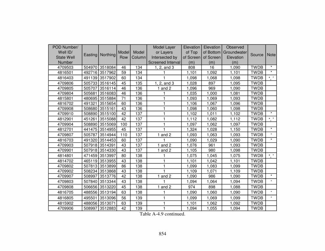
854
POD Number/
Well ID/
State Well
Number
Easting NorthingModel
Row
Model
Column
Model Layer
or Layers
Intersected by
Screened Interval
Elevation
of Top
of Screen
(m)
Elevation
of Bottom
of Screen
(m)
Observed
Groundwater
Elevation
(m)
Source Note
4709503 504970 3518084 46 134 1, 2, and 3 808 16 1,090 TWDB *
4816501 492716 3517962 59 134 1 1,101 1,092 1,101 TWDB *
4816403 491139 3517902 60 134 1 1,098 1,068 1,098 TWDB *, +
4709806 505733 3516145 45 135 1, 2, and 3 1,028 897 1,095 TWDB
4709805 505707 3516114 46 136 1 and 2 1,096 969 1,090 TWDB
4709804 505681 3516083 46 136 1 1,035 1,000 1,081 TWDB
4815801 480695 3515884 71 136 1 1,093 1,069 1,093 TWDB
4816702 491321 3515654 60 136 1 1,106 1,067 1,096 TWDB
4709908 508680 3515161 43 136 1 1,098 1,060 1,098 TWDB
4709910 508890 3515100 42 137 1 1,102 1,011 1,102 TWDB *
4812901 451261 3515088 42 137 1 1,112 1,082 1,112 TWDB *, +
4709904 508890 3515069 100 137 1 1,097 1,062 1,097 TWDB
4812701 441475 3514955 45 137 1 1,324 1,028 1,150 TWDB *
4709807 505787 3514944 110 137 1 and 2 1,093 1,063 1,093 TWDB +
4816703 491320 3514453 60 137 1 1,090 1,029 1,090 TWDB *
4709903 507918 3514391 43 137 1 and 2 1,076 961 1,093 TWDB
4709901 507918 3514330 43 137 1 and 2 1,105 980 1,098 TWDB
4814801 471459 3513997 80 138 1 1,075 1,045 1,075 TWDB *, +
4814702 465119 3513955 43 138 1 1,101 1,042 1,101 TWDB
4709802 507813 3513899 86 138 1 1,099 1,083 1,099 TWDB
4709902 508234 3513868 43 138 1 1,109 1,071 1,109 TWDB
4709907 508997 3513776 42 138 1 and 2 1,090 986 1,090 TWDB *
4709803 507840 3513344 43 138 1 1,094 1,064 1,094 TWDB +
4709808 506656 3513220 45 138 1 and 2 974 898 1,088 TWDB
4816705 488556 3513194 63 138 1 1,090 1,060 1,090 TWDB +
4816805 495501 3513096 56 139 1 1,099 1,069 1,099 TWDB +
4815902 488056 3513071 63 139 1 1,101 1,062 1,092 TWDB
4709906 508997 3512883 42 139 1 1,094 1,055 1,094 TWDB Table A-4.9 continued.

855
POD Number/
Well ID/
State Well
Number
Easting NorthingModel
Row
Model
Column
Model Layer
or Layers
Intersected by
Screened Interval
Elevation
of Top
of Screen
(m)
Elevation
of Bottom
of Screen
(m)
Observed
Groundwater
Elevation
(m)
Source Note
4815903 487661 3512733 64 139 1 1,090 1,065 1,090 TWDB
4823202 481031 3512528 70 139 1 1,097 1,068 1,097 TWDB
4717220 507814 3512451 43 139 1 and 2 1,090 967 1,090 TWDB *
4823201 480847 3512312 43 139 1 1,091 1,039 1,091 TWDB
4717315 508314 3512298 45 139 1 1,097 1,067 1,097 TWDB
4717216 506472 3512297 70 139 1 1,096 1,066 1,096 TWDB *, +
4824203 492134 3512267 59 139 1 and 2 1,091 967 1,091 TWDB *
4824101 491370 3512083 60 140 1 1,103 1,073 1,103 TWDB *, +
4717312 510919 3512023 40 140 1 1,107 1,031 1,107 TWDB *
4717317 507919 3512020 43 140 1 995 964 1,095 TWDB
4717201 507656 3511866 44 140 1 1,072 1,023 1,098 TWDB
4717209 507025 3511866 44 140 1 1,079 1,038 1,095 TWDB
4717212 507104 3511835 44 140 1 1,091 1,061 1,091 TWDB *, +
4717319 509419 3511714 42 140 1 1,099 1,069 1,099 TWDB *, +
4717211 506209 3511712 45 140 1 1,096 1,016 1,096 TWDB
4824201 495738 3511310 55 140 1 1,100 1,094 1,100 TWDB *
4717208 505999 3511188 45 140 1, 2, 3, and 4 1,084 615 1,095 TWDB
4717206 507604 3511127 44 140 1, 2, and 3 1,104 912 1,109 TWDB
4717204 506210 3510911 45 141 1, 2, and 3 1,107 854 1,093 TWDB
4717313 509815 3510698 41 141 1 1,102 1,015 1,102 TWDB *
4717203 507842 3510235 43 141 1 and 2 1,098 986 1,098 TWDB
4717205 506131 3510234 45 141 1 1,084 1,029 1,097 TWDB
4717202 505421 3510233 46 141 1 1,095 1,041 1,095 TWDB
4717320 511263 3510115 40 142 1, 2, and 3 1,003 824 1,098 TWDB
4824202 494105 3510110 57 142 1 1,096 1,066 1,096 TWDB *, +
4717301 509316 3510020 42 142 1 1,099 1,029 1,098 TWDB
4717207 506158 3510018 45 142 1, 2, and 3 1,037 940 1,099 TWDB
4717314 509684 3509959 42 142 1 1,101 1,042 1,101 TWDB * Table A-4.9 continued.

856
POD Number/
Well ID/
State Well
Number
Easting NorthingModel
Row
Model
Column
Model Layer
or Layers
Intersected by
Screened Interval
Elevation
of Top
of Screen
(m)
Elevation
of Bottom
of Screen
(m)
Observed
Groundwater
Elevation
(m)
Source Note
4717215 506264 3508571 45 143 1 1,100 1,070 1,100 TWDB *, +
4718101 513239 3508424 38 143 1 1,130 1,069 1,130 TWDB *
4823101 479813 3508250 71 143 1 1,106 1,076 1,106 TWDB *, +
4717218 506975 3508202 44 143 1 1,103 1,020 1,100 TWDB
4824401 488366 3507621 63 144 1 1,097 1,058 1,097 TWDB *
4824502 495788 3507031 55 145 1 1,087 1,028 1,092 TWDB *
4820601 452194 3506555 99 145 1 1,088 1,058 1,088 TWDB +
4821401 454403 3505991 97 146 1, 2, and 3 1,106 919 1,106 TWDB *
4821502 460062 3505598 91 146 1 1,104 1,074 1,104 TWDB *, +
4717605 507872 3505124 43 146 1 1,099 1,095 1,099 TWDB
4717601 509610 3505095 42 147 1 1,104 1,075 1,101 TWDB
4717602 509189 3504694 42 147 1 1,096 1,069 1,096 TWDB
4824601 497051 3504536 54 147 1 1,097 1,067 1,097 TWDB *, +
4718707 512350 3503466 39 148 1, 2, and 3 1,105 843 1,098 TWDB
4717904 511534 3503434 40 148 1 1,098 1,020 1,098 TWDB
4718802 515905 3503286 35 148 1 1,104 1,065 1,119 TWDB
4718706 512324 3503004 39 149 1 and 2 1,100 988 1,100 TWDB
4717903 511455 3502664 40 149 1 1,099 1,002 1,099 TWDB
4718801 515960 3501439 35 150 1 1,095 1,065 1,095 TWDB *, +
4824904 498025 3500503 53 151 1 1,090 1,060 1,090 TWDB *, +
4824903 496497 3499457 55 152 1 1,051 1,037 1,051 TWDB *
4823701 477319 3499450 74 152 1 1,102 1,072 1,102 TWDB *, +
4726101 512593 3498170 39 153 1 1,095 1,085 1,095 TWDB
4726102 514913 3497188 36 154 1 1,097 1,087 1,097 TWDB *
4832301 498867 3496962 52 155 1 1,097 1,035 1,097 TWDB *
4829301 461266 3496603 90 155 1 1,256 1,097 1,103 TWDB
4829101 455179 3496536 96 155 1 1,322 1,297 1,309 TWDB *
4829102 455205 3496536 96 155 1 1,323 1,300 1,309 TWDB * Table A-4.9 continued.

857
POD Number/
Well ID/
State Well
Number
Easting NorthingModel
Row
Model
Column
Model Layer
or Layers
Intersected by
Screened Interval
Elevation
of Top
of Screen
(m)
Elevation
of Bottom
of Screen
(m)
Observed
Groundwater
Elevation
(m)
Source Note
4829103 455231 3496535 96 155 1 1,324 1,296 1,308 TWDB *
4829104 455205 3496505 96 155 1 1,323 1,302 1,309 TWDB *
4828301 452300 3495255 99 156 1 1,332 1,302 1,332 TWDB *, +
4832601 499157 3493945 52 158 1 1,097 1,085 1,097 TWDB *
4832602 497760 3493576 53 158 1 1,095 1,068 1,095 TWDB *
4726501 517081 3492912 34 159 1 1,081 1,073 1,094 TWDB
4830401 466018 3491476 85 160 1, 2, and 3 1,118 970 1,118 TWDB
4836101 441569 3484996 110 167 1 1,426 1,396 1,426 TWDB *, +
Table A-4.9 continued.
Source Key: NMOSE = New Mexico Office of the State Engineer’s New Mexico Water Rights Reporting System online database, SMHS = New Mexico Bureau of Geology & Mineral Resources’ Sacramento Mountains Hydrogeology Study, TWDB = Texas Water Development Board groundwater database. Note Key: * = One water level measurement, Assumed 30 meter (98 feet) screened interval length.
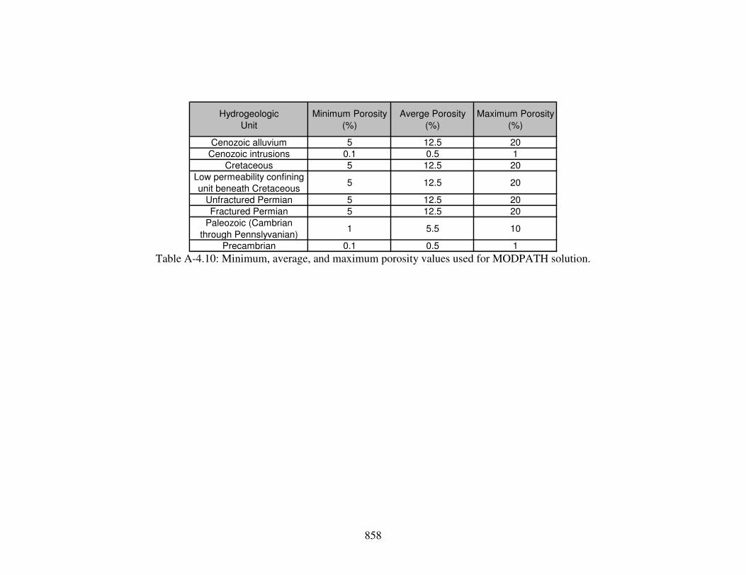
858
Hydrogeologic
Unit
Minimum Porosity
(%)
Averge Porosity
(%)
Maximum Porosity
(%)
Cenozoic alluvium 5 12.5 20
Cenozoic intrusions 0.1 0.5 1
Cretaceous 5 12.5 20
Low permeability confining
unit beneath Cretaceous5 12.5 20
Unfractured Permian 5 12.5 20
Fractured Permian 5 12.5 20
Paleozoic (Cambrian
through Pennslyvanian)1 5.5 10
Precambrian 0.1 0.5 1 Table A-4.10: Minimum, average, and maximum porosity values used for MODPATH solution.

859
Groundwater
Age Well IDPOD Number Easting Northing
Model
Row
Model
Column
Model
Layer
Ground
Surface
Elevation
(m)
Well
Depth
(m)
Elevation
of
Well
Depth
(m)
Note
Doll Day ST 00241 POD1 472590 3607544 79 44 1 1,718 475 1,243 Well depth from well owner
Piñon Well ST 00003 478550 3606619 73 45 1 1,623 335 1,287 Well depth from NMOSE
Webb House NA 465825 3606007 85 46 1 1,815 457 1,358 Well depth unkown; estimated
Uña ST 00018 473476 3596830 78 55 1 1,743 390 1,353 Well depth from NMOSE
Cauhape ST 00019 476365 3588074 75 64 1 1,447 315 1,131 Well depth from NMOSE
Jeffer's Well NA 467327 3585742 84 66 1 1,481 305 1,177 Well depth from well owner
Ellett Lower NA 469670 3578554 82 73 1 1,397 160 1,237 Well depth from well owner
Harvey Lewis Well ST 00014 487565 3571656 64 80 1 1,181 91 1,090 Well depth from NMOSE
Collins NA 499579 3568454 52 83 1 1,238 183 1,055 Well depth from well owner
Evrage House ST 00050 496187 3563804 55 88 1 1,147 61 1,086 Well depth from NMOSE
Lewis ST 00163 479239 3557196 72 94 1 1,230 154 1,076 Well depth from NMOSE
Butterfield Well ST 00044 466258 3546182 85 105 2 1,268 244 1,024 Well depth from NMOSE
Hunt 8 ST 00057 490345 3544103 61 108 1 1,114 48 1,066 Well depth from NMOSE Table A-4.11: Groundwater age wells incorporated into MODPATH particle tracking exercise.
POD Number Key: NA = Not applicable.

860
Elevation
of
Computed
Groundwater
Surface (m)
Elevation
of
Midpoint
(m)
Elevation
of
Bottom
of Cell
(m)
Elevation
of
Computed
Groundwater
Surface (m)
Elevation
of
Midpoint
(m)
Elevation
of
Bottom
of Cell
(m)
Elevation
of
Computed
Groundwater
Surface (m)
Elevation
of
Midpoint
(m)
Elevation
of
Bottom
of Cell
(m)
Doll Day 1,243 1,401 1,297 1,192 1,398 1,295 1,192 1,412 1,302 1,192
Pinon Well 1,287 1,359 1,256 1,154 1,349 1,251 1,154 1,368 1,261 1,154
Webb House 1,358 1,429 1,328 1,227 1,428 1,328 1,227 1,445 1,336 1,227
Una 1,353 1,334 1,227 1,120 1,323 1,222 1,120 1,338 1,229 1,120
Cauhape 1,131 1,276 1,167 1,058 1,254 1,156 1,058 1,267 1,163 1,058
Jeffer's Well 1,177 1,301 1,201 1,101 1,272 1,186 1,101 1,276 1,189 1,101
Ellett Lower 1,237 1,269 1,173 1,077 1,231 1,154 1,077 1,230 1,154 1,077
Harvey Lewis Well 1,090 1,157 1,087 1,018 1,143 1,080 1,018 1,154 1,086 1,018
Collins 1,055 1,169 1,093 1,018 1,152 1,085 1,018 1,164 1,091 1,018
Evrage House 1,086 1,146 1,093 1,040 1,135 1,088 1,040 1,144 1,092 1,040
Lewis 1,076 1,155 1,076 997 1,139 1,068 997 1,139 1,068 997
Butterfield Well 1,024 1,031 1,006 981 1,031 1,006 981 1,031 1,006 981
Hunt 8 1,066 1,110 1,054 997 1,109 1,053 997 1,111 1,054 997
Water-balance Based
Maximum
Recharge ScenarioGroundwater
Age Well ID
Elevation
of
Well
Depth
(m)
Water-balance Based
Minimum
Recharge Scenario
Water-balance Based
Average
Recharge Scenario
Table A-4.12: Elevations at which MODPATH particles were generated for the calibrated water-balance based minimum, average,
and maximum recharge scenario models. Orange highlighted rectangles indicate the vertical position of generated MODPATH particles chosen to represent the potential pathlines and residence times of groundwater sampled at each well.
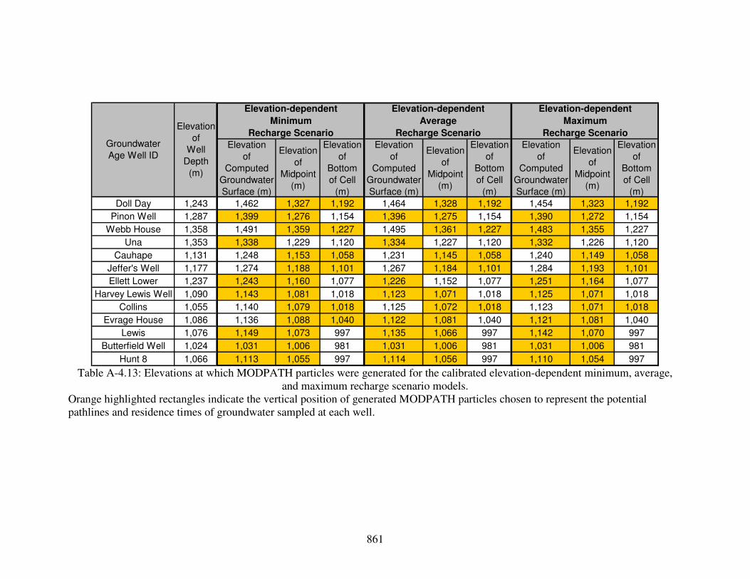
861
Elevation
of
Computed
Groundwater
Surface (m)
Elevation
of
Midpoint
(m)
Elevation
of
Bottom
of Cell
(m)
Elevation
of
Computed
Groundwater
Surface (m)
Elevation
of
Midpoint
(m)
Elevation
of
Bottom
of Cell
(m)
Elevation
of
Computed
Groundwater
Surface (m)
Elevation
of
Midpoint
(m)
Elevation
of
Bottom
of Cell
(m)
Doll Day 1,243 1,462 1,327 1,192 1,464 1,328 1,192 1,454 1,323 1,192
Pinon Well 1,287 1,399 1,276 1,154 1,396 1,275 1,154 1,390 1,272 1,154
Webb House 1,358 1,491 1,359 1,227 1,495 1,361 1,227 1,483 1,355 1,227
Una 1,353 1,338 1,229 1,120 1,334 1,227 1,120 1,332 1,226 1,120
Cauhape 1,131 1,248 1,153 1,058 1,231 1,145 1,058 1,240 1,149 1,058
Jeffer's Well 1,177 1,274 1,188 1,101 1,267 1,184 1,101 1,284 1,193 1,101
Ellett Lower 1,237 1,243 1,160 1,077 1,226 1,152 1,077 1,251 1,164 1,077
Harvey Lewis Well 1,090 1,143 1,081 1,018 1,123 1,071 1,018 1,125 1,071 1,018
Collins 1,055 1,140 1,079 1,018 1,125 1,072 1,018 1,123 1,071 1,018
Evrage House 1,086 1,136 1,088 1,040 1,122 1,081 1,040 1,121 1,081 1,040
Lewis 1,076 1,149 1,073 997 1,135 1,066 997 1,142 1,070 997
Butterfield Well 1,024 1,031 1,006 981 1,031 1,006 981 1,031 1,006 981
Hunt 8 1,066 1,113 1,055 997 1,114 1,056 997 1,110 1,054 997
Elevation-dependent
Maximum
Recharge ScenarioGroundwater
Age Well ID
Elevation
of
Well
Depth
(m)
Elevation-dependent
Minimum
Recharge Scenario
Elevation-dependent
Average
Recharge Scenario
Table A-4.13: Elevations at which MODPATH particles were generated for the calibrated elevation-dependent minimum, average,
and maximum recharge scenario models. Orange highlighted rectangles indicate the vertical position of generated MODPATH particles chosen to represent the potential pathlines and residence times of groundwater sampled at each well.

862
Boundary Condition Inflow (m3/day) Inflow (acre-feet/year) Outflow (m
3/day) Outflow (acre-feet/year)
Recharge 164,688 48,765
Wells (Discharge at Salt Flats) 0 0 164,688 48,765
Total 164,688 48,765 164,688 48,765 0
Boundary Condition Inflow (m3/day) Inflow (acre-feet/year) Outflow (m
3/day) Outflow (acre-feet/year)
Recharge 272,956 80,824
Wells (Discharge at Salt Flats) 0 0 272,956 80,824
Total 272,956 80,824 272,956 80,824 0
Boundary Condition Inflow (m3/day) Inflow (acre-feet/year) Outflow (m
3/day) Outflow (acre-feet/year)
Recharge 354,670 105,020
Wells (Discharge at Salt Flats) 0 0 354,670 105,020
Total 354,670 105,020 354,670 105,020 0
Percent
Difference
Water-balance Based Maximum Recharge Scenario
Percent
Difference
Water-balance Based Average Recharge Scenario
Percent
Difference
Water-balance Based Minimum Recharge Scenario
Table A-4.14: Mass balances for the calibrated water-balance based minimum, average, and maximum recharge scenario models.

863
Boundary Condition Inflow (m3/day) Inflow (acre-feet/year) Outflow (m
3/day) Outflow (acre-feet/year)
Recharge 9,078 2,688
Wells (Discharge at Salt Flats) 0 0 9,078 2,688
Total 9,078 2,688 9,078 2,688 0
Boundary Condition Inflow (m3/day) Inflow (acre-feet/year) Outflow (m
3/day) Outflow (acre-feet/year)
Recharge 49,738 14,728
Wells (Discharge at Salt Flats) 0 0 49,738 14,728
Total 49,738 14,728 49,738 14,728 0
Boundary Condition Inflow (m3/day) Inflow (acre-feet/year) Outflow (m
3/day) Outflow (acre-feet/year)
Recharge 99,337 29,414
Wells (Discharge at Salt Flats) 0 0 99,337 29,414
Total 99,337 29,414 99,337 29,414 0
Elevation-dependent Maximum Recharge Scenario
Percent
Difference
Percent
Difference
Elevation-dependent Average Recharge Scenario
Elevation-dependent Minimum Recharge Scenario
Percent
Difference
Table A-4.15: Mass balances for the calibrated elevation-dependent minimum, average, and maximum recharge scenario models.

864
Sum Residuals (m) 44
Sum Absolute Residuals (m) 11,780
Sum Squared Residuals (m2) 1,400,350
RMS Error (m) 61
Residual Mean (m) 0.1
Absolute Residual Mean (m) 16
Residual Standard Deviation (m) 61
Minimum Observed Hydraulic Head (m) 1,029
Maximum Observed Hydraulic Head (m) 2,610
Residual Standard Deviation/Range 0.039
Residual Mean/Range 0.00007
Sum Residuals (m) -649
Sum Absolute Residuals (m) 10,793
Sum Squared Residuals (m2) 1,379,233
RMS Error (m) 60
Residual Mean (m) -2
Absolute Residual Mean (m) 13
Residual Standard Deviation (m) 60
Minimum Observed Hydraulic Head (m) 1,029
Maximum Observed Hydraulic Head (m) 2,610
Residual Standard Deviation/Range 0.038
Residual Mean/Range -0.001
Sum Residuals (m) 236
Sum Absolute Residuals (m) 10,568
Sum Squared Residuals (m2) 1,318,998
RMS Error (m) 59
Residual Mean (m) 0.6
Absolute Residual Mean (m) 14
Residual Standard Deviation (m) 59
Minimum Observed Hydraulic Head (m) 1,029
Maximum Observed Hydraulic Head (m) 2,610
Residual Standard Deviation/Range 0.037
Residual Mean/Range 0.0004
Water-balance Based Minimum Recharge Scenario
Water-balance Based Average Recharge Scenario
Water-balance Based Maximum Recharge Scenario
Table A-4.16: Residual hydraulic head statistics for the calibrated water-balance based
minimum, average, and maximum recharge scenario models.

865
Sum Residuals (m) 1,364
Sum Absolute Residuals (m) 15,478
Sum Squared Residuals (m2) 2,208,280
RMS Error (m) 76
Residual Mean (m) 4
Absolute Residual Mean (m) 22
Residual Standard Deviation (m) 76
Minimum Observed Hydraulic Head (m) 1,029
Maximum Observed Hydraulic Head (m) 2,610
Residual Standard Deviation/Range 0.048
Residual Mean/Range 0.002
Sum Residuals (m) 1,621
Sum Absolute Residuals (m) 16,612
Sum Squared Residuals (m2) 2,291,432
RMS Error (m) 78
Residual Mean (m) 4
Absolute Residual Mean (m) 24
Residual Standard Deviation (m) 78
Minimum Observed Hydraulic Head (m) 1,029
Maximum Observed Hydraulic Head (m) 2,610
Residual Standard Deviation/Range 0.049
Residual Mean/Range 0.003
Sum Residuals (m) 951
Sum Absolute Residuals (m) 14,836
Sum Squared Residuals (m2) 2,018,583
RMS Error (m) 73
Residual Mean (m) 3
Absolute Residual Mean (m) 21
Residual Standard Deviation (m) 73
Minimum Observed Hydraulic Head (m) 1,029
Maximum Observed Hydraulic Head (m) 2,610
Residual Standard Deviation/Range 0.046
Residual Mean/Range 0.002
Elevation-dependent Average Recharge Scenario
Elevation-dependent Maximum Recharge Scenario
Elevation-dependent Minimum Recharge Scenario
Table A-4.17: Residual hydraulic head statistics for the calibrated elevation-dependent
minimum, average, and maximum recharge scenario models.

866
Recharge Scenario Minimum T (m2/day) Maximum T (m
2/day)
Water-balance Based Minimum 0.53 23,000
Water-balance Based Average 0.80 230,000
Water-balance Based Maximum 0.68 230,000 Table A-4.18: Range of transmissivity [T] values derived from the calibrated water-balance based minimum, average, and maximum
recharge scenario models.
Recharge Scenario Minimum T (m2/day) Maximum T (m
2/day)
Elevation-dependent Minimum 0.083 4,500
Elevation-dependent Average 0.31 23,000
Elevation-dependent Maximum 0.33 23,000 Table A-4.19: Range of transmissivity [T] values derived from the calibrated elevation-dependent minimum, average, and maximum
recharge scenario models.

867
MODPATH
Age on
Computed
Groundwater
Surface
(years)
MODPATH
Age on
Midpoint
(years)
MODPATH
Age on
Bottom
of Cell
(years)
MODPATH
Age on
Computed
Groundwater
Surface
(years)
MODPATH
Age on
Midpoint
(years)
MODPATH
Age on
Bottom
of Cell
(years)
MODPATH
Age on
Computed
Groundwater
Surface
(years)
MODPATH
Age on
Midpoint
(years)
MODPATH
Age on
Bottom
of Cell
(years)
Doll Day 2,900 NA 1,211 5,051 NA 3,027 12,627 NA 4,844 20,203
Pinon Well 4,200 2 639 NA 5 1,599 NA 8 2,558 NA
Webb House 1,000 2 2,163 NA 5 5,409 NA 8 8,654 NA
Una 7,100 1 NA NA 3 NA NA 4 NA NA
Cauhape 8,000 NA 290 6,541 NA 726 16,351 NA 1,161 26,162
Jeffer's Well 8,200 NA 223 462 NA 558 1,155 NA 893 1,848
Ellett Lower 13,800 0 214 NA 1 535 NA 2 856 NA
Harvey Lewis Well 12,000 7 301 NA 17 753 NA 28 1,204 NA
Collins 9,700 NA 447 1,087 NA 1,116 2,719 NA 1,786 4,350
Evrage House 12,800 NA 409 543 NA 1,023 1,358 NA 1,636 2,174
Lewis 11,000 NA 231 609 NA 577 1,523 NA 924 2,437
Butterfield Well 16,100 1,758 1,870 NA 4,396 4,675 NA 7,033 7,480 NA
Hunt 8 14,100 6 1,585 NA 14 3,961 NA 23 6,338 NA
Maximum
Porosity
Water-balance Based Minimum Recharge Scenario
Groundwater
Age Well ID
NETPATH
Age
(years)
Minimum
Porosity
Average
Porosity
Table A-4.20: NETPATH ages from Sigstedt (2010) and MODPATH ages from the calibrated water-balance based minimum
recharge scenario MODFLOW solution using minimum, average, and maximum porosities. Orange highlighted rectangles indicate the MODPATH ages chosen to bound the residence time of groundwater sampled at each well.

868
MODPATH
Age on
Computed
Groundwater
Surface
(years)
MODPATH
Age on
Midpoint
(years)
MODPATH
Age on
Bottom
of Cell
(years)
MODPATH
Age on
Computed
Groundwater
Surface
(years)
MODPATH
Age on
Midpoint
(years)
MODPATH
Age on
Bottom
of Cell
(years)
MODPATH
Age on
Computed
Groundwater
Surface
(years)
MODPATH
Age on
Midpoint
(years)
MODPATH
Age on
Bottom
of Cell
(years)
Doll Day 2,900 NA 772 3,631 NA 1,930 9,078 NA 3,087 14,525
Pinon Well 4,200 1 395 NA 2 989 NA 3 1,582 NA
Webb House 1,000 1 1,035 NA 3 2,588 NA 4 4,141 NA
Una 7,100 0 NA NA 1 NA NA 2 NA NA
Cauhape 8,000 NA 222 3,886 NA 554 9,716 NA 886 15,546
Jeffer's Well 8,200 NA 151 277 NA 377 692 NA 603 1,108
Ellett Lower 13,800 0 NA NA 1 NA NA 1 NA NA
Harvey Lewis Well 12,000 3 159 NA 8 397 NA 12 636 NA
Collins 9,700 NA 189 421 NA 472 1,052 NA 756 1,683
Evrage House 12,800 NA 365 368 NA 912 919 NA 1,459 1,471
Lewis 11,000 0 142 NA 1 356 NA 1 569 NA
Butterfield Well 16,100 1,483 2,462 NA 3,706 6,157 NA 5,930 9,850 NA
Hunt 8 14,100 3 1,254 NA 7 3,136 NA 11 5,017 NA
Water-balance Based Average Recharge Scenario
Groundwater
Age Well ID
NETPATH
Age
(years)
Minimum
Porosity
Average
Porosity
Maximum
Porosity
Table A-4.21: NETPATH ages from Sigstedt (2010) and MODPATH ages from the calibrated water-balance based average recharge
scenario MODFLOW solution using minimum, average, and maximum porosities. Orange highlighted rectangles indicate the MODPATH ages chosen to bound the residence time of groundwater sampled at each well.

869
MODPATH
Age on
Computed
Groundwater
Surface
(years)
MODPATH
Age on
Midpoint
(years)
MODPATH
Age on
Bottom
of Cell
(years)
MODPATH
Age on
Computed
Groundwater
Surface
(years)
MODPATH
Age on
Midpoint
(years)
MODPATH
Age on
Bottom
of Cell
(years)
MODPATH
Age on
Computed
Groundwater
Surface
(years)
MODPATH
Age on
Midpoint
(years)
MODPATH
Age on
Bottom
of Cell
(years)
Doll Day 2,900 NA 686 2,776 NA 1,715 6,939 NA 2,744 11,103
Pinon Well 4,200 0 339 NA 1 848 NA 2 1,357 NA
Webb House 1,000 1 1,053 NA 2 2,633 NA 4 4,212 NA
Una 7,100 0 NA NA 1 NA NA 1 NA NA
Cauhape 8,000 NA 137 2,499 NA 342 6,248 NA 547 9,997
Jeffer's Well 8,200 NA 85 159 NA 213 397 NA 341 634
Ellett Lower 13,800 0 NA NA 0 NA NA 1 NA NA
Harvey Lewis Well 12,000 5 119 NA 11 297 NA 18 476 NA
Collins 9,700 NA 210 445 NA 524 1,112 NA 838 1,779
Evrage House 12,800 NA 254 296 NA 635 739 NA 1,016 1,182
Lewis 11,000 0 134 NA 1 334 NA 1 534 NA
Butterfield Well 16,100 801 906 NA 2,002 2,265 NA 3,203 3,624 NA
Hunt 8 14,100 4 943 NA 10 2,359 NA 15 3,774 NA
Water-balance Based Maximum Recharge Scenario
Groundwater
Age Well ID
NETPATH
Age
(years)
Minimum
Porosity
Average
Porosity
Maximum
Porosity
Table A-4.22: NETPATH ages from Sigstedt (2010) and MODPATH ages from the calibrated water-balance based maximum
recharge scenario MODFLOW solution using minimum, average, and maximum porosities. Orange highlighted rectangles indicate the MODPATH ages chosen to bound the residence time of groundwater sampled at each well.
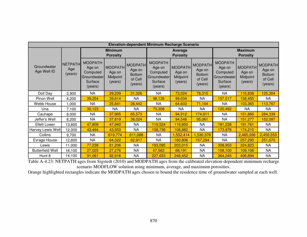
870
MODPATH
Age on
Computed
Groundwater
Surface
(years)
MODPATH
Age on
Midpoint
(years)
MODPATH
Age on
Bottom
of Cell
(years)
MODPATH
Age on
Computed
Groundwater
Surface
(years)
MODPATH
Age on
Midpoint
(years)
MODPATH
Age on
Bottom
of Cell
(years)
MODPATH
Age on
Computed
Groundwater
Surface
(years)
MODPATH
Age on
Midpoint
(years)
MODPATH
Age on
Bottom
of Cell
(years)
Doll Day 2,900 NA 29,209 31,326 NA 73,024 78,315 NA 116,838 125,304
Pinon Well 4,200 39,254 39,614 NA 98,136 99,034 NA 157,017 158,455 NA
Webb House 1,000 NA 25,841 28,442 NA 64,603 71,104 NA 103,365 113,767
Una 7,100 30,123 NA NA 75,308 NA NA 120,492 NA NA
Cauhape 8,000 NA 37,965 65,573 NA 94,912 174,911 NA 151,860 284,339
Jeffer's Well 8,200 NA 37,819 38,024 NA 94,548 95,061 NA 151,277 152,097
Ellett Lower 13,800 47,809 47,940 NA 119,524 119,850 NA 191,238 191,761 NA
Harvey Lewis Well 12,000 43,494 43,553 NA 108,736 108,882 NA 173,978 174,210 NA
Collins 9,700 NA 619,774 611,088 NA 1,552,414 1,530,378 NA 2,485,056 2,450,553
Evrage House 12,800 NA 64,322 62,917 NA 160,806 157,294 NA 257,290 251,670
Lewis 11,000 77,238 81,206 NA 193,095 203,015 NA 308,953 324,823 NA
Butterfield Well 16,100 27,025 27,276 NA 67,562 68,191 NA 108,100 109,106 NA
Hunt 8 14,100 91,061 92,916 NA 227,653 248,452 NA 364,245 406,894 NA
Maximum
Porosity
Elevation-dependent Minimum Recharge Scenario
Groundwater
Age Well ID
NETPATH
Age
(years)
Minimum
Porosity
Average
Porosity
Table A-4.23: NETPATH ages from Sigstedt (2010) and MODPATH ages from the calibrated elevation-dependent minimum recharge
scenario MODFLOW solution using minimum, average, and maximum porosities. Orange highlighted rectangles indicate the MODPATH ages chosen to bound the residence time of groundwater sampled at each well.

871
MODPATH
Age on
Computed
Groundwater
Surface
(years)
MODPATH
Age on
Midpoint
(years)
MODPATH
Age on
Bottom
of Cell
(years)
MODPATH
Age on
Computed
Groundwater
Surface
(years)
MODPATH
Age on
Midpoint
(years)
MODPATH
Age on
Bottom
of Cell
(years)
MODPATH
Age on
Computed
Groundwater
Surface
(years)
MODPATH
Age on
Midpoint
(years)
MODPATH
Age on
Bottom
of Cell
(years)
Doll Day 2,900 NA 5,057 8,541 NA 12,642 21,352 NA 20,227 34,163
Pinon Well 4,200 4,558 4,688 NA 11,396 11,721 NA 18,233 18,753 NA
Webb House 1,000 NA 4,131 5,751 NA 10,328 14,376 NA 16,525 23,002
Una 7,100 4,973 NA NA 12,434 NA NA 19,894 NA NA
Cauhape 8,000 NA 6,352 8,984 NA 15,880 22,459 NA 25,408 35,935
Jeffer's Well 8,200 NA 5,721 5,776 NA 14,303 14,439 NA 22,885 23,103
Ellett Lower 13,800 7,474 NA NA 18,685 NA NA 29,896 NA NA
Harvey Lewis Well 12,000 6,924 7,281 NA 17,311 18,203 NA 27,697 29,125 NA
Collins 9,700 NA 401,260 406,635 NA 1,003,149 1,016,589 NA 1,605,040 1,626,542
Evrage House 12,800 387,340 7,445 NA 968,351 18,612 NA 1,549,362 29,780 NA
Lewis 11,000 21,646 22,039 NA 54,115 55,098 NA 86,585 88,157 NA
Butterfield Well 16,100 5,094 5,217 NA 12,736 13,043 NA 20,377 20,869 NA
Hunt 8 14,100 24,184 33,523 NA 60,459 83,808 NA 96,734 134,093 NA
Elevation-dependent Average Recharge Scenario
Groundwater
Age Well ID
NETPATH
Age
(years)
Minimum
Porosity
Average
Porosity
Maximum
Porosity
Table A-4.24: NETPATH ages from Sigstedt (2010) and MODPATH ages from the calibrated elevation-dependent average recharge
scenario MODFLOW solution using minimum, average, and maximum porosities. Orange highlighted rectangles indicate the MODPATH ages chosen to bound the residence time of groundwater sampled at each well.

872
MODPATH
Age on
Computed
Groundwater
Surface
(years)
MODPATH
Age on
Midpoint
(years)
MODPATH
Age on
Bottom
of Cell
(years)
MODPATH
Age on
Computed
Groundwater
Surface
(years)
MODPATH
Age on
Midpoint
(years)
MODPATH
Age on
Bottom
of Cell
(years)
MODPATH
Age on
Computed
Groundwater
Surface
(years)
MODPATH
Age on
Midpoint
(years)
MODPATH
Age on
Bottom
of Cell
(years)
Doll Day 2,900 NA 2,446 4,669 NA 6,116 11,672 NA 9,785 18,675
Pinon Well 4,200 2,353 2,408 NA 5,882 6,020 NA 9,411 9,632 NA
Webb House 1,000 2,001 2,174 NA 5,002 5,435 NA 8,004 8,696 NA
Una 7,100 2,515 NA NA 6,287 NA NA 10,060 NA NA
Cauhape 8,000 NA 3,216 5,989 NA 8,039 14,971 NA 12,863 23,954
Jeffer's Well 8,200 NA 3,256 3,279 NA 8,140 8,197 NA 13,024 13,115
Ellett Lower 13,800 3,929 3,948 NA 9,824 9,871 NA 15,718 15,794 NA
Harvey Lewis Well 12,000 3,540 3,580 NA 8,851 8,950 NA 14,161 14,321 NA
Collins 9,700 NA 836,078 676,253 NA 2,734,009 2,107,019 NA 4,638,479 3,543,782
Evrage House 12,800 39,353 3,748 NA 98,381 9,370 NA 157,410 14,992 NA
Lewis 11,000 6,904 7,009 NA 17,259 17,522 NA 27,615 28,035 NA
Butterfield Well 16,100 2,512 2,520 NA 6,279 6,301 NA 10,046 10,081 NA
Hunt 8 14,100 7,254 7,517 NA 18,136 18,792 NA 29,017 30,067 NA
Elevation-dependent Maximum Recharge Scenario
Groundwater
Age Well ID
NETPATH
Age
(years)
Minimum
Porosity
Average
Porosity
Maximum
Porosity
Table A-4.25: NETPATH ages from Sigstedt (2010) and MODPATH ages from the calibrated elevation-dependent maximum
recharge scenario MODFLOW solution using minimum, average, and maximum porosities. Orange highlighted rectangles indicate the MODPATH ages chosen to bound the residence time of groundwater sampled at each well.
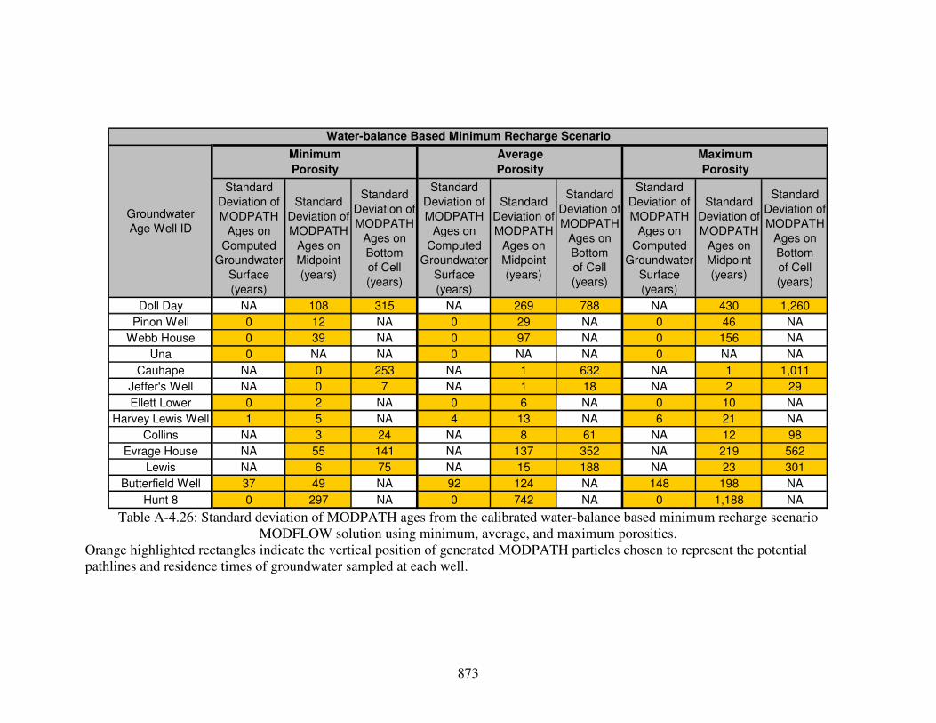
873
Standard
Deviation of
MODPATH
Ages on
Computed
Groundwater
Surface
(years)
Standard
Deviation of
MODPATH
Ages on
Midpoint
(years)
Standard
Deviation of
MODPATH
Ages on
Bottom
of Cell
(years)
Standard
Deviation of
MODPATH
Ages on
Computed
Groundwater
Surface
(years)
Standard
Deviation of
MODPATH
Ages on
Midpoint
(years)
Standard
Deviation of
MODPATH
Ages on
Bottom
of Cell
(years)
Standard
Deviation of
MODPATH
Ages on
Computed
Groundwater
Surface
(years)
Standard
Deviation of
MODPATH
Ages on
Midpoint
(years)
Standard
Deviation of
MODPATH
Ages on
Bottom
of Cell
(years)
Doll Day NA 108 315 NA 269 788 NA 430 1,260
Pinon Well 0 12 NA 0 29 NA 0 46 NA
Webb House 0 39 NA 0 97 NA 0 156 NA
Una 0 NA NA 0 NA NA 0 NA NA
Cauhape NA 0 253 NA 1 632 NA 1 1,011
Jeffer's Well NA 0 7 NA 1 18 NA 2 29
Ellett Lower 0 2 NA 0 6 NA 0 10 NA
Harvey Lewis Well 1 5 NA 4 13 NA 6 21 NA
Collins NA 3 24 NA 8 61 NA 12 98
Evrage House NA 55 141 NA 137 352 NA 219 562
Lewis NA 6 75 NA 15 188 NA 23 301
Butterfield Well 37 49 NA 92 124 NA 148 198 NA
Hunt 8 0 297 NA 0 742 NA 0 1,188 NA
Water-balance Based Minimum Recharge Scenario
Groundwater
Age Well ID
Minimum
Porosity
Average
Porosity
Maximum
Porosity
Table A-4.26: Standard deviation of MODPATH ages from the calibrated water-balance based minimum recharge scenario
MODFLOW solution using minimum, average, and maximum porosities. Orange highlighted rectangles indicate the vertical position of generated MODPATH particles chosen to represent the potential pathlines and residence times of groundwater sampled at each well.

874
Standard
Deviation of
MODPATH
Ages on
Computed
Groundwater
Surface
(years)
Standard
Deviation of
MODPATH
Ages on
Midpoint
(years)
Standard
Deviation of
MODPATH
Ages on
Bottom
of Cell
(years)
Standard
Deviation of
MODPATH
Ages on
Computed
Groundwater
Surface
(years)
Standard
Deviation of
MODPATH
Ages on
Midpoint
(years)
Standard
Deviation of
MODPATH
Ages on
Bottom
of Cell
(years)
Standard
Deviation of
MODPATH
Ages on
Computed
Groundwater
Surface
(years)
Standard
Deviation of
MODPATH
Ages on
Midpoint
(years)
Standard
Deviation of
MODPATH
Ages on
Bottom
of Cell
(years)
Doll Day NA 40 265 NA 99 661 NA 159 1,058
Pinon Well 0 20 NA 0 51 NA 0 82 NA
Webb House 0 20 NA 0 50 NA 0 79 NA
Una 0 NA NA 0 NA NA 0 NA NA
Cauhape NA 0 58 NA 1 145 NA 1 231
Jeffer's Well NA 2 12 NA 5 31 NA 7 49
Ellett Lower 0 NA NA 0 NA NA 0 NA NA
Harvey Lewis Well 0 6 NA 1 16 NA 2 26 NA
Collins NA 5 9 NA 12 22 NA 19 35
Evrage House NA 71 67 NA 178 169 NA 285 270
Lewis 0 1 NA 0 4 NA 0 6 NA
Butterfield Well 114 2,260 NA 286 6,384 NA 457 10,497 NA
Hunt 8 0 465 NA 0 1,164 NA 0 1,862 NA
Water-balance Based Average Recharge Scenario
Groundwater
Age Well ID
Minimum
Porosity
Average
Porosity
Maximum
Porosity
Table A-4.27: Standard deviation of MODPATH ages from the calibrated water-balance based average recharge scenario MODFLOW
solution using minimum, average, and maximum porosities. Orange highlighted rectangles indicate the vertical position of generated MODPATH particles chosen to represent the potential pathlines and residence times of groundwater sampled at each well.
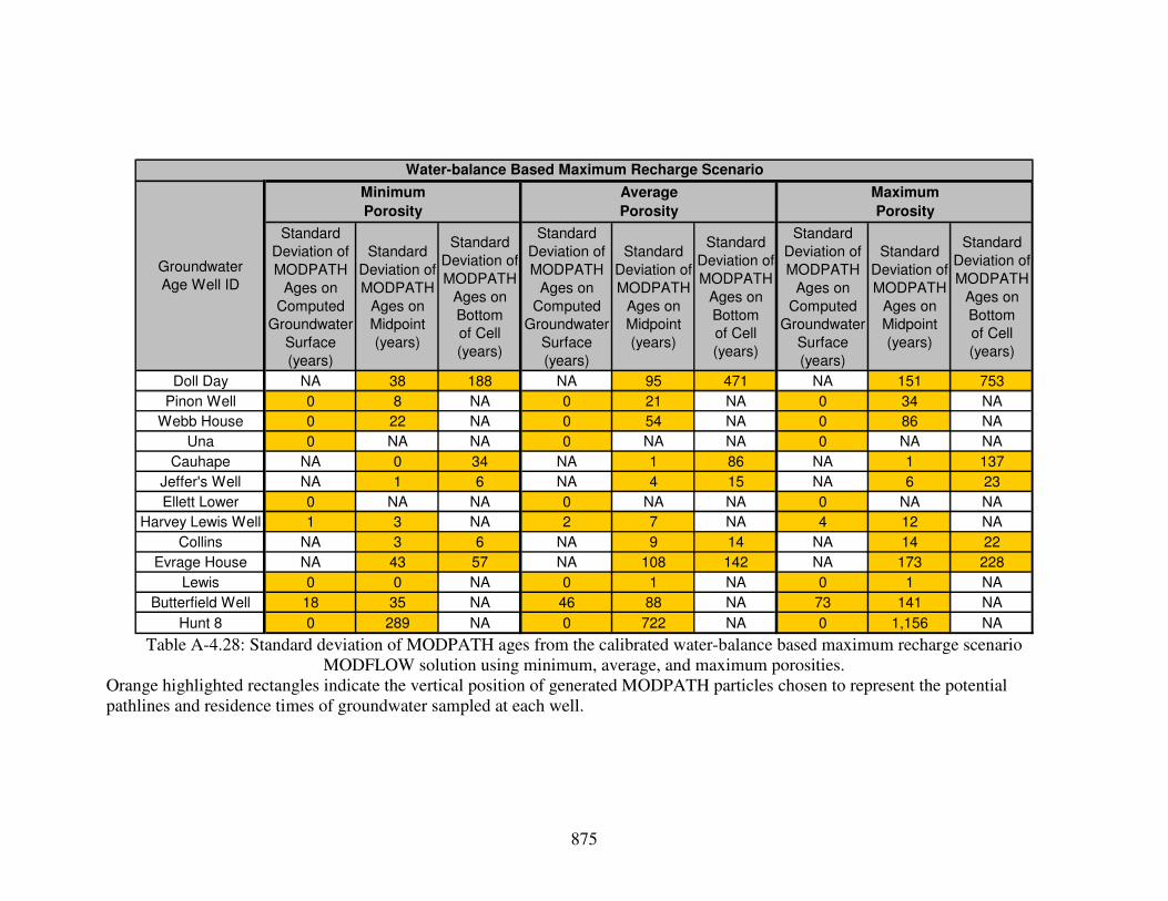
875
Standard
Deviation of
MODPATH
Ages on
Computed
Groundwater
Surface
(years)
Standard
Deviation of
MODPATH
Ages on
Midpoint
(years)
Standard
Deviation of
MODPATH
Ages on
Bottom
of Cell
(years)
Standard
Deviation of
MODPATH
Ages on
Computed
Groundwater
Surface
(years)
Standard
Deviation of
MODPATH
Ages on
Midpoint
(years)
Standard
Deviation of
MODPATH
Ages on
Bottom
of Cell
(years)
Standard
Deviation of
MODPATH
Ages on
Computed
Groundwater
Surface
(years)
Standard
Deviation of
MODPATH
Ages on
Midpoint
(years)
Standard
Deviation of
MODPATH
Ages on
Bottom
of Cell
(years)
Doll Day NA 38 188 NA 95 471 NA 151 753
Pinon Well 0 8 NA 0 21 NA 0 34 NA
Webb House 0 22 NA 0 54 NA 0 86 NA
Una 0 NA NA 0 NA NA 0 NA NA
Cauhape NA 0 34 NA 1 86 NA 1 137
Jeffer's Well NA 1 6 NA 4 15 NA 6 23
Ellett Lower 0 NA NA 0 NA NA 0 NA NA
Harvey Lewis Well 1 3 NA 2 7 NA 4 12 NA
Collins NA 3 6 NA 9 14 NA 14 22
Evrage House NA 43 57 NA 108 142 NA 173 228
Lewis 0 0 NA 0 1 NA 0 1 NA
Butterfield Well 18 35 NA 46 88 NA 73 141 NA
Hunt 8 0 289 NA 0 722 NA 0 1,156 NA
Water-balance Based Maximum Recharge Scenario
Groundwater
Age Well ID
Minimum
Porosity
Average
Porosity
Maximum
Porosity
Table A-4.28: Standard deviation of MODPATH ages from the calibrated water-balance based maximum recharge scenario
MODFLOW solution using minimum, average, and maximum porosities. Orange highlighted rectangles indicate the vertical position of generated MODPATH particles chosen to represent the potential pathlines and residence times of groundwater sampled at each well.

876
Standard
Deviation of
MODPATH
Ages on
Computed
Groundwater
Surface
(years)
Standard
Deviation of
MODPATH
Ages on
Midpoint
(years)
Standard
Deviation of
MODPATH
Ages on
Bottom
of Cell
(years)
Standard
Deviation of
MODPATH
Ages on
Computed
Groundwater
Surface
(years)
Standard
Deviation of
MODPATH
Ages on
Midpoint
(years)
Standard
Deviation of
MODPATH
Ages on
Bottom
of Cell
(years)
Standard
Deviation of
MODPATH
Ages on
Computed
Groundwater
Surface
(years)
Standard
Deviation of
MODPATH
Ages on
Midpoint
(years)
Standard
Deviation of
MODPATH
Ages on
Bottom
of Cell
(years)
Doll Day NA 329 493 NA 822 1,232 NA 1,315 1,971
Pinon Well 996 635 NA 2,490 1,588 NA 3,984 2,541 NA
Webb House NA 172 588 NA 429 1,471 NA 687 2,353
Una 171 NA NA 428 NA NA 685 NA NA
Cauhape NA 158 3,889 NA 396 21,983 NA 633 40,224
Jeffer's Well NA 253 456 NA 633 1,140 NA 1,012 1,825
Ellett Lower 1,205 623 NA 3,013 1,557 NA 4,821 2,491 NA
Harvey Lewis Well 839 543 NA 2,099 1,358 NA 3,358 2,174 NA
Collins NA 9,922 21,980 NA 24,816 50,286 NA 39,712 78,658
Evrage House NA 1,524 6,899 NA 3,809 17,248 NA 6,094 27,597
Lewis 495 289 NA 1,238 722 NA 1,981 1,155 NA
Butterfield Well 524 204 NA 1,309 509 NA 2,095 815 NA
Hunt 8 3,478 10,600 NA 8,695 44,605 NA 13,911 78,891 NA
Elevation-dependent Minimum Recharge Scenario
Groundwater
Age Well ID
Minimum
Porosity
Average
Porosity
Maximum
Porosity
Table A-4.29: Standard deviation of MODPATH ages from the calibrated elevation-dependent minimum recharge scenario
MODFLOW solution using minimum, average, and maximum porosities. Orange highlighted rectangles indicate the vertical position of generated MODPATH particles chosen to represent the potential pathlines and residence times of groundwater sampled at each well.

877
Standard
Deviation of
MODPATH
Ages on
Computed
Groundwater
Surface
(years)
Standard
Deviation of
MODPATH
Ages on
Midpoint
(years)
Standard
Deviation of
MODPATH
Ages on
Bottom
of Cell
(years)
Standard
Deviation of
MODPATH
Ages on
Computed
Groundwater
Surface
(years)
Standard
Deviation of
MODPATH
Ages on
Midpoint
(years)
Standard
Deviation of
MODPATH
Ages on
Bottom
of Cell
(years)
Standard
Deviation of
MODPATH
Ages on
Computed
Groundwater
Surface
(years)
Standard
Deviation of
MODPATH
Ages on
Midpoint
(years)
Standard
Deviation of
MODPATH
Ages on
Bottom
of Cell
(years)
Doll Day NA 27 733 NA 67 1,832 NA 106 2,931
Pinon Well 32 35 NA 79 87 NA 127 139 NA
Webb House NA 46 314 NA 114 784 NA 183 1,255
Una 30 NA NA 75 NA NA 121 NA NA
Cauhape NA 226 44 NA 566 110 NA 905 176
Jeffer's Well NA 42 77 NA 104 193 NA 167 309
Ellett Lower 90 NA NA 224 NA NA 359 NA NA
Harvey Lewis Well 46 57 NA 114 142 NA 182 227 NA
Collins NA 7,929 17,309 NA 19,821 43,273 NA 31,714 69,238
Evrage House 189,368 394 NA 473,424 984 NA 757,472 1,574 NA
Lewis 325 187 NA 812 468 NA 1,300 748 NA
Butterfield Well 129 318 NA 322 796 NA 514 1,274 NA
Hunt 8 162 23,465 NA 406 89,419 NA 650 157,061 NA
Elevation-dependent Average Recharge Scenario
Groundwater
Age Well ID
Minimum
Porosity
Average
Porosity
Maximum
Porosity
Table A-4.30: Standard deviation of MODPATH ages from the calibrated elevation-dependent average recharge scenario MODFLOW
solution using minimum, average, and maximum porosities. Orange highlighted rectangles indicate the vertical position of generated MODPATH particles chosen to represent the potential pathlines and residence times of groundwater sampled at each well.

878
Standard
Deviation of
MODPATH
Ages on
Computed
Groundwater
Surface
(years)
Standard
Deviation of
MODPATH
Ages on
Midpoint
(years)
Standard
Deviation of
MODPATH
Ages on
Bottom
of Cell
(years)
Standard
Deviation of
MODPATH
Ages on
Computed
Groundwater
Surface
(years)
Standard
Deviation of
MODPATH
Ages on
Midpoint
(years)
Standard
Deviation of
MODPATH
Ages on
Bottom
of Cell
(years)
Standard
Deviation of
MODPATH
Ages on
Computed
Groundwater
Surface
(years)
Standard
Deviation of
MODPATH
Ages on
Midpoint
(years)
Standard
Deviation of
MODPATH
Ages on
Bottom
of Cell
(years)
Doll Day NA 29 716 NA 74 1,793 NA 118 2,872
Pinon Well 20 12 NA 50 30 NA 80 49 NA
Webb House 19 28 NA 48 71 NA 77 113 NA
Una 14 NA NA 34 NA NA 54 NA NA
Cauhape NA 14 99 NA 34 247 NA 55 395
Jeffer's Well NA 49 64 NA 123 159 NA 196 254
Ellett Lower 53 29 NA 132 73 NA 211 118 NA
Harvey Lewis Well 78 40 NA 194 100 NA 310 160 NA
Collins NA 17,863 60,125 NA 71,110 145,820 NA 130,618 231,676
Evrage House 12,212 93 NA 30,531 232 NA 48,850 370 NA
Lewis 57 35 NA 143 88 NA 229 141 NA
Butterfield Well 77 54 NA 194 134 NA 310 215 NA
Hunt 8 304 500 NA 760 1,250 NA 1,216 2,000 NA
Elevation-dependent Maximum Recharge Scenario
Groundwater
Age Well ID
Minimum
Porosity
Average
Porosity
Maximum
Porosity
Table A-4.31: Standard deviation of MODPATH ages from the calibrated elevation-dependent maximum recharge scenario
MODFLOW solution using minimum, average, and maximum porosities. Orange highlighted rectangles indicate the vertical position of generated MODPATH particles chosen to represent the potential pathlines and residence times of groundwater sampled at each well.

879
Residual
Age on
Computed
Groundwater
Surface
(years)
Residual
Age on
Midpoint
(years)
Residual
Age on
Bottom
of Cell
(years)
Residual
Age on
Computed
Groundwater
Surface
(years)
Residual
Age on
Midpoint
(years)
Residual
Age on
Bottom
of Cell
(years)
Residual
Age on
Computed
Groundwater
Surface
(years)
Residual
Age on
Midpoint
(years)
Residual
Age on
Bottom
of Cell
(years)
Doll Day NA -1,689 2,151 NA 127 9,727 NA 1,944 17,303
Pinon Well -4,198 -3,561 NA -4,195 -2,601 NA -4,192 -1,642 NA
Webb House -998 1,163 NA -995 4,409 NA -992 7,654 NA
Una -7,099 NA NA -7,097 NA NA -7,096 NA NA
Cauhape NA -7,710 -1,459 NA -7,274 8,351 NA -6,839 18,162
Jeffer's Well NA -7,977 -7,738 NA -7,642 -7,045 NA -7,307 -6,352
Ellett Lower -13,800 -13,586 NA -13,799 -13,265 NA -13,798 -12,944 NA
Harvey Lewis Well -11,993 -11,699 NA -11,983 -11,247 NA -11,972 -10,796 NA
Collins NA -9,253 -8,613 NA -8,584 -6,981 NA -7,914 -5,350
Evrage House NA -12,391 -12,257 NA -11,777 -11,442 NA -11,164 -10,626
Lewis NA -10,769 -10,391 NA -10,423 -9,477 NA -10,076 -8,563
Butterfield Well -14,342 -14,230 NA -11,704 -11,425 NA -9,067 -8,620 NA
Hunt 8 -14,094 -12,515 NA -14,086 -10,139 NA -14,077 -7,762 NA
Water-balance Based Minimum Recharge Scenario
Groundwater
Age Well ID
Minimum
Porosity
Average
Porosity
Maximum
Porosity
Table A-4.32: Residual ages (i.e. MODPATH ages minus NETPATH ages) from the calibrated water-balance based minimum
recharge scenario MODFLOW solution using minimum, average, and maximum porosities. Orange highlighted rectangles indicate the vertical position of generated MODPATH particles chosen to represent the potential pathlines and residence times of groundwater sampled at each well.

880
Residual
Age on
Computed
Groundwater
Surface
(years)
Residual
Age on
Midpoint
(years)
Residual
Age on
Bottom
of Cell
(years)
Residual
Age on
Computed
Groundwater
Surface
(years)
Residual
Age on
Midpoint
(years)
Residual
Age on
Bottom
of Cell
(years)
Residual
Age on
Computed
Groundwater
Surface
(years)
Residual
Age on
Midpoint
(years)
Residual
Age on
Bottom
of Cell
(years)
Doll Day NA -2,128 731 NA -970 6,178 NA 187 11,625
Pinon Well -4,199 -3,805 NA -4,198 -3,211 NA -4,197 -2,618 NA
Webb House -999 35 NA -997 1,588 NA -996 3,141 NA
Una -7,100 NA NA -7,099 NA NA -7,098 NA NA
Cauhape NA -7,778 -4,114 NA -7,446 1,716 NA -7,114 7,546
Jeffer's Well NA -8,049 -7,923 NA -7,823 -7,508 NA -7,597 -7,092
Ellett Lower -13,800 NA NA -13,799 NA NA -13,799 NA NA
Harvey Lewis Well -11,997 -11,841 NA -11,992 -11,603 NA -11,988 -11,364 NA
Collins NA -9,511 -9,279 NA -9,228 -8,648 NA -8,944 -8,017
Evrage House NA -12,435 -12,432 NA -11,888 -11,881 NA -11,341 -11,329
Lewis -11,000 -10,858 NA -10,999 -10,644 NA -10,999 -10,431 NA
Butterfield Well -14,617 -13,638 NA -12,394 -9,943 NA -10,170 -6,250 NA
Hunt 8 -14,097 -12,846 NA -14,093 -10,964 NA -14,089 -9,083 NA
Water-balance Based Average Recharge Scenario
Groundwater
Age Well ID
Minimum
Porosity
Average
Porosity
Maximum
Porosity
Table A-4.33: Residual ages (i.e. MODPATH ages minus NETPATH ages) from the calibrated water-balance based average recharge
scenario MODFLOW solution using minimum, average, and maximum porosities. Orange highlighted rectangles indicate the vertical position of generated MODPATH particles chosen to represent the potential pathlines and residence times of groundwater sampled at each well.

881
Residual
Age on
Computed
Groundwater
Surface
(years)
Residual
Age on
Midpoint
(years)
Residual
Age on
Bottom
of Cell
(years)
Residual
Age on
Computed
Groundwater
Surface
(years)
Residual
Age on
Midpoint
(years)
Residual
Age on
Bottom
of Cell
(years)
Residual
Age on
Computed
Groundwater
Surface
(years)
Residual
Age on
Midpoint
(years)
Residual
Age on
Bottom
of Cell
(years)
Doll Day NA -2,214 -124 NA -1,185 4,039 NA -156 8,203
Pinon Well -4,200 -3,861 NA -4,199 -3,352 NA -4,198 -2,843 NA
Webb House -999 53 NA -998 1,633 NA -996 3,212 NA
Una -7,100 NA NA -7,099 NA NA -7,099 NA NA
Cauhape NA -7,863 -5,501 NA -7,658 -1,752 NA -7,453 1,997
Jeffer's Well NA -8,115 -8,041 NA -7,987 -7,803 NA -7,859 -7,566
Ellett Lower -13,800 NA NA -13,800 NA NA -13,799 NA NA
Harvey Lewis Well -11,995 -11,881 NA -11,989 -11,703 NA -11,982 -11,524 NA
Collins NA -9,490 -9,255 NA -9,176 -8,588 NA -8,862 -7,921
Evrage House NA -12,546 -12,504 NA -12,165 -12,061 NA -11,784 -11,618
Lewis -11,000 -10,866 NA -10,999 -10,666 NA -10,999 -10,466 NA
Butterfield Well -15,299 -15,194 NA -14,098 -13,835 NA -12,897 -12,476 NA
Hunt 8 -14,096 -13,157 NA -14,090 -11,741 NA -14,085 -10,326 NA
Water-balance Based Maximum Recharge Scenario
Groundwater
Age Well ID
Minimum
Porosity
Average
Porosity
Maximum
Porosity
Table A-4.34: Residual ages (i.e. MODPATH ages minus NETPATH ages) from the calibrated water-balance based maximum
recharge scenario MODFLOW solution using minimum, average, and maximum porosities. Orange highlighted rectangles indicate the vertical position of generated MODPATH particles chosen to represent the potential pathlines and residence times of groundwater sampled at each well.

882
Residual
Age on
Computed
Groundwater
Surface
(years)
Residual
Age on
Midpoint
(years)
Residual
Age on
Bottom
of Cell
(years)
Residual
Age on
Computed
Groundwater
Surface
(years)
Residual
Age on
Midpoint
(years)
Residual
Age on
Bottom
of Cell
(years)
Residual
Age on
Computed
Groundwater
Surface
(years)
Residual
Age on
Midpoint
(years)
Residual
Age on
Bottom
of Cell
(years)
Doll Day NA 26,309 28,426 NA 70,124 75,415 NA 113,938 122,404
Pinon Well 35,054 35,414 NA 93,936 94,834 NA 152,817 154,255 NA
Webb House NA 24,841 27,442 NA 63,603 70,104 NA 102,365 112,767
Una 23,023 NA NA 68,208 NA NA 113,392 NA NA
Cauhape NA 29,965 57,573 NA 86,912 166,911 NA 143,860 276,339
Jeffer's Well NA 29,619 29,824 NA 86,348 86,861 NA 143,077 143,897
Ellett Lower 34,009 34,140 NA 105,724 106,050 NA 177,438 177,961 NA
Harvey Lewis Well 31,494 31,553 NA 96,736 96,882 NA 161,978 162,210 NA
Collins NA 610,074 601,388 NA 1,542,714 1,520,678 NA 2,475,356 2,440,853
Evrage House NA 51,522 50,117 NA 148,006 144,494 NA 244,490 238,870
Lewis 66,238 70,206 NA 182,095 192,015 NA 297,953 313,823 NA
Butterfield Well 10,925 11,176 NA 51,462 52,091 NA 92,000 93,006 NA
Hunt 8 76,961 78,816 NA 213,553 234,352 NA 350,145 392,794 NA
Elevation-dependent Minimum Recharge Scenario
Groundwater
Age Well ID
Minimum
Porosity
Average
Porosity
Maximum
Porosity
Table A-4.35: Residual ages (i.e. MODPATH ages minus NETPATH ages) from the calibrated elevation-dependent minimum
recharge scenario MODFLOW solution using minimum, average, and maximum porosities. Orange highlighted rectangles indicate the vertical position of generated MODPATH particles chosen to represent the potential pathlines and residence times of groundwater sampled at each well.

883
Residual
Age on
Computed
Groundwater
Surface
(years)
Residual
Age on
Midpoint
(years)
Residual
Age on
Bottom
of Cell
(years)
Residual
Age on
Computed
Groundwater
Surface
(years)
Residual
Age on
Midpoint
(years)
Residual
Age on
Bottom
of Cell
(years)
Residual
Age on
Computed
Groundwater
Surface
(years)
Residual
Age on
Midpoint
(years)
Residual
Age on
Bottom
of Cell
(years)
Doll Day NA 2,157 5,641 NA 9,742 18,452 NA 17,327 31,263
Pinon Well 358 488 NA 7,196 7,521 NA 14,033 14,553 NA
Webb House NA 3,131 4,751 NA 9,328 13,376 NA 15,525 22,002
Una -2,127 NA NA 5,334 NA NA 12,794 NA NA
Cauhape NA -1,648 984 NA 7,880 14,459 NA 17,408 27,935
Jeffer's Well NA -2,479 -2,424 NA 6,103 6,239 NA 14,685 14,903
Ellett Lower -6,326 NA NA 4,885 NA NA 16,096 NA NA
Harvey Lewis Well -5,076 -4,719 NA 5,311 6,203 NA 15,697 17,125 NA
Collins NA 391,560 396,935 NA 993,449 1,006,889 NA 1,595,340 1,616,842
Evrage House 374,540 -5,355 NA 955,551 5,812 NA 1,536,562 16,980 NA
Lewis 10,646 11,039 NA 43,115 44,098 NA 75,585 77,157 NA
Butterfield Well -11,006 -10,883 NA -3,364 -3,057 NA 4,277 4,769 NA
Hunt 8 10,084 19,423 NA 46,359 69,708 NA 82,634 119,993 NA
Elevation-dependent Average Recharge Scenario
Groundwater
Age Well ID
Minimum
Porosity
Average
Porosity
Maximum
Porosity
Table A-4.36: Residual ages (i.e. MODPATH ages minus NETPATH ages) from the calibrated elevation-dependent average recharge
scenario MODFLOW solution using minimum, average, and maximum porosities. Orange highlighted rectangles indicate the vertical position of generated MODPATH particles chosen to represent the potential pathlines and residence times of groundwater sampled at each well.

884
Residual
Age on
Computed
Groundwater
Surface
(years)
Residual
Age on
Midpoint
(years)
Residual
Age on
Bottom
of Cell
(years)
Residual
Age on
Computed
Groundwater
Surface
(years)
Residual
Age on
Midpoint
(years)
Residual
Age on
Bottom
of Cell
(years)
Residual
Age on
Computed
Groundwater
Surface
(years)
Residual
Age on
Midpoint
(years)
Residual
Age on
Bottom
of Cell
(years)
Doll Day NA -454 1,769 NA 3,216 8,772 NA 6,885 15,775
Pinon Well -1,847 -1,792 NA 1,682 1,820 NA 5,211 5,432 NA
Webb House 1,001 1,174 NA 4,002 4,435 NA 7,004 7,696 NA
Una -4,585 NA NA -813 NA NA 2,960 NA NA
Cauhape NA -4,784 -2,011 NA 39 6,971 NA 4,863 15,954
Jeffer's Well NA -4,944 -4,921 NA -60 -3 NA 4,824 4,915
Ellett Lower -9,871 -9,852 NA -3,976 -3,929 NA 1,918 1,994 NA
Harvey Lewis Well -8,460 -8,420 NA -3,149 -3,050 NA 2,161 2,321 NA
Collins NA 826,378 666,553 NA 2,724,309 2,097,319 NA 4,628,779 3,534,082
Evrage House 26,553 -9,052 NA 85,581 -3,430 NA 144,610 2,192 NA
Lewis -4,096 -3,991 NA 6,259 6,522 NA 16,615 17,035 NA
Butterfield Well -13,588 -13,580 NA -9,821 -9,799 NA -6,054 -6,019 NA
Hunt 8 -6,846 -6,583 NA 4,036 4,692 NA 14,917 15,967 NA
Elevation-dependent Maximum Recharge Scenario
Groundwater
Age Well ID
Minimum
Porosity
Average
Porosity
Maximum
Porosity
Table A-4.37: Residual ages (i.e. MODPATH ages minus NETPATH ages) from the calibrated elevation-dependent maximum
recharge scenario MODFLOW solution using minimum, average, and maximum porosities. Orange highlighted rectangles indicate the vertical position of generated MODPATH particles chosen to represent the potential pathlines and residence times of groundwater sampled at each well.

885
StatisticMinimum
Porosity
Average
Porosity
Maximum
Porosity
Sum Residuals (years) -209,047 -170,567 -132,087
Sum Absolute Residuals (years) 215,675 215,796 222,213
Sum Squared Residuals (years2) 2,382,279,439 2,216,152,581 2,440,163,800
RMS Error (years) 9,762 9,415 9,880
StatisticMinimum
Porosity
Average
Porosity
Maximum
Porosity
Sum Residuals (years) -203,679 -177,848 -152,017
Sum Absolute Residuals (years) 205,212 196,812 197,014
Sum Squared Residuals (years2) 2,256,174,267 2,013,764,816 1,954,184,998
RMS Error (years) 9,696 9,160 9,024
StatisticMinimum
Porosity
Average
Porosity
Maximum
Porosity
Sum Residuals (years) -209,049 -191,273 -173,496
Sum Absolute Residuals (years) 209,155 202,616 200,321
Sum Squared Residuals (years2) 2,352,235,737 2,170,874,905 2,072,649,619
RMS Error (years) 9,900 9,511 9,293
Water-balance Based Maximum Recharge Scenario
Water-balance Based Minimum Recharge Scenario
Water-balance Based Average Recharge Scenario
Table A-4.38: Residual age statistics for the calibrated water-balance based minimum,
average, and maximum recharge scenario MODFLOW solutions using minimum, average, and maximum porosities.

886
StatisticMinimum
Porosity
Average
Porosity
Maximum
Porosity
Sum Residuals (years) 894,651 2,586,717 4,281,779
Sum Absolute Residuals (years) 894,651 2,586,717 4,281,779
Sum Squared Residuals (years2) 43,034,332,815 352,316,919,807 963,202,659,626
RMS Error (years) 176,283 449,210 722,450
RMS Error with outliers removed
(years)43,256 123,766 204,642
StatisticMinimum
Porosity
Average
Porosity
Maximum
Porosity
Sum Residuals (years) 16,661 324,702 632,743
Sum Absolute Residuals (years) 120,743 337,545 632,743
Sum Squared Residuals (years2) 1,159,868,251 12,142,411,637 38,117,422,665
RMS Error (years) 140,235 356,675 573,260
RMS Error with outliers removed
(years)7,615 24,640 43,656
StatisticMinimum
Porosity
Average
Porosity
Maximum
Porosity
Sum Residuals (years) -115,734 14,416 144,565
Sum Absolute Residuals (years) 123,621 90,478 168,711
Sum Squared Residuals (years2) 1,019,805,143 553,112,221 1,934,670,863
RMS Error (years) 212,501 687,851 1,165,130
RMS Error with outliers removed
(years)6,808 5,014 9,378
Elevation-dependent Maximum Recharge Scenario
Elevation-dependent Minimum Recharge Scenario
Elevation-dependent Average Recharge Scenario
Table A-4.39: Residual age statistics for the calibrated elevation-dependent minimum, average, and maximum recharge scenario MODFLOW solutions using minimum,
average, and maximum porosities.