08/5 UW1

Hydrodynamics and beyond in AdS/CFT

M. Natsuume (KEK)

122008 May

arXiv: 0712.2916 [hep-th] arXiv: 0712.2917 [hep-th] arXiv: 0801.1797 [hep-th]

in collaboration w/ Takashi Okamura (Kwansei Gakuin Univ.)

08/5 UW

Aim: “causal hydrodynamics” from AdS/CFT

Review: String theory & quark-gluon plasma

Basic idea of causal hydrodynamics

AdS/CFT results & implications

2

Plan

See alsoHeller - Janik, hep-th/0703243

Benincasa - Buchel - Heller - Janik, 0712.2025 [hep-th]Baier - Romatschke - Son - Starinets - Stephanov, 0712.2451 [hep-th]Bhattacharyya - Hubeny - Minwalla - Rangamani, 0712.2456 [hep-th]

Extensions:Loganayagam, 0801.3701 [hep-th]

Van Raamsdonk, 0802.3224 [hep-th]Bhattacharyya et al., 0803.2526 [hep-th]

Our 2nd time to have overlaps w/ Son & Starinets! ←

Northern suburb of Tokyo: A paradise of AdS/QCD

08/5 UW

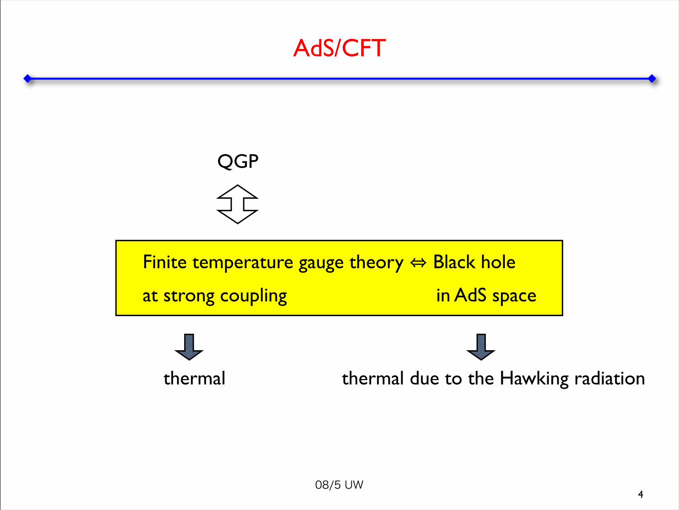
AdS/CFT

4

Finite temperature gauge theory ⇔ Black hole

at strong coupling in AdS space

QGP

thermal thermal due to the Hawking radiation

08/5 UW

BH and hydrodynamics

RHIC experiments → QGP: a fluid w/ a very low viscosity

BHs and hydrodynamic systems in fact behave similarly.

Water pond:

The dissipation: consequence of viscosity

BH:

The dissipation: consequence of BH absorption

5

08/5 UW

Relaxation phenomena

Relaxation phenomena (add perturbs. & see how they decay)

→ Nonequilibrium statistical mechanics or hydrodynamics

→ important quantities: transport coefficients

e.g. (bulk & shear) viscosity speed of sound thermal conductivity . . .

AdS/CFT: especially useful to determine η/s (η: shear viscosity, s: entropy density) due to

6

universality Kovtun - Son - Starinets (2004)

08/5 UW

Universality of η/s

According to AdS/CFT

True for all known examples → conformal (N=4 SYM) or nonconformal w/ chemical potential w/ flavors w/ time-dependence

RHIC may suggest

cf. naive extrapolation of perturbative QCD:

7

€

ηs

=h

4πkB

€

ηs~O 1( ) × h

kB

€

ηs~O(0.1)× h

kB? Teaney (2003) ...

Mas, 0601144; Son - Starinets, 0601157; Saremi, 0601159;Maeda - Natsuume - Okamura, 0602010 & many peopleʼs works

08/5 UW8

Basic idea of causal hydrodynamics

08/5 UW

The hydrodynamic description of QGP using AdS/CFT is very successful,

but this cannot be the END of the story.

1. Standard hydrodynamic eqs. do not satisfy causality

2. In order to restore causality, one is forced to introduce a new set of transport coefficients → “causal hydrodynamics” (also known as “2nd order hydrodynamics” or “Israel-Stewart theory”)

3. Such coefficients may become important in the early stages of QGP formation, but little is known about these coeffs.

9

Müller (1967)Israel (1976), Israel-Stewart (1979)

08/5 UW

Causal hydrodynamics has been widely discussed in heavy-ion literature:e.g. recent (2+1)-dim QGP simulations using causal hydrodynamics.

Some argue that η/s must be smaller than 1/(4π) to fit the experiment

If true, serious attack to AdS/QGP

There are several potential problems though.They use the AdS value for η/s, but use the weak coupling result for causal hydrodynamics.

10

Romatschke - Romatschke, 0706.1522 [nucl-th]Chaudhuri, 0708.1252 [nucl-th]

Song - Heinz, 0709.0742 [nucl-th]0712.3715 [nucl-th]

Dusling - Teaney, 0710.5932 [nucl-th]Luzum - Romatschke, 0804.4015 [nucl-th]

Is it really OK?

AdS/CFT

08/5 UW11

Adapted from slides by T. Hirano (UT, Hongo)

QGP hydro simulation example

Transverse plane Reaction plane

Energy density distribution

initial conditions → evolution (by hydrodynamics) → hadronization

08/5 UW

Hydrodynamic case is complicated due to the tensor nature of Tμν → R-charge diffusion

Basic eqs.

Conservation eq:

Constitutive eq:

(Conserv. eq.) + (Fick’s law) → ρ & : decouple

12

Prototypical example

€

Ji = −D∂i ρ

€

∂µJµ = 0

“Fick’s law”

↑ Def. of diffusion const. D

€

∂0ρ −D∂i2ρ = 0 →

Diffusion equation€

Ji

€

ω = −iDq2

€

Jµ = (ρ,Ji )

08/5 UW

Hydrodynamics is similar:

Conservation eq:

Constitutive eq:

Tensor decomposition (according to little group SO(2))

transport coeffs. appear in these channels (these coeffs. are associated w/ conserved quantities.)

Hydrodynamic case

13

€

∂µT µν = 0

€

T00

€

T0i

€

Tij

€

Tµν“sound mode” (scalar) e.g.“shear mode” (vector)tensor€

J0

€

Ji

€

Jµscalar e.g.vector

€

Tij =Pδij −η(∂iu j +∂ jui −23δij∂kuk ) − ςδij∂kuk

€

(ω,0,0{,q)

08/5 UW

Acausality

Diffusion eq.

Parabolic (1st derivative in t, 2nd derivative in x)

acausal

In fact, propagator

To restore causality, hyperbolic eq. such as Klein-Gordon eq.

14

€

∂0ρ −D∂i2ρ = 0

€

ρ ~ 14πDt

exp(− x 2

4Dt)

!4 !2 2 4

nonvanishing even outside the light-cone

08/5 UW

What’s wrong?

conservation eq. → must be true → Fick’s law should be the source of the prob.

Modify Fick’s law:

τJ = 0 → diffusion eq.

at some time → Fick’s law: immediately

Modified law: exponential decay

15

↑new parameter (transport coeff.)

€

∂iρ = 0

€

Ji = 0€

τJ∂0Ji + Ji = −D∂iρ

τJ: relaxation time for charge current

Do not confuse w/ relaxation time for charge density

€

τρ := DL⇔

08/5 UW

(Conserv. eq.) + (Modified law) → “telegrapher’s eq.”

The new term: important at early time

Hydrodynamics: just an effective theory, so infinite # of parameters phenomenologically.

From D and τJ, one gets a speed:

Dispersion relation as an effective theory:

16

→ hyperbolic

€

τJ∂02ρ +∂0ρ −D∂i

2ρ = 0

→ signal propagation

€

v ~ D / τJ

€

ω = −iDq2 − iD2τJq 4 +L

causal hydrodynamic correction

Just an effective theory expansion in higher orders

08/5 UW

Causal hydrodynamics

Israel (76) carried out a systematic analysis and introduced 5 new coefficients. (3 relaxation times: τJ, τπ, τΠ)

charge diffusion: scalar, vector EM tensor: sound, shear, tensor

But little is known about these coeffs.

AdS/CFT

Israel’s formalism: highly complicated→ linearized perturbations

→ charge diffusion & shear mode: just telegrapher’s form at the end of the day

17

08/5 UW18

Causal hydrodynamics from AdS/CFT

08/5 UW19

Outline of computations

Step1: identify appropriate bulk modes (from AdS/CFT dictionary)

Step 2: Bulk perturbation eqs.

Step 3: Solutions → transport coeffs. from dispersion relations

08/5 UW

Due to the interaction bet. bulk & boundary fields

Step 1: identify appropriate modes

20

graviton

x

y

gluon

Deviations from equilibrium Bulk fluctuations

Boundary (Gauge) Bulk (Gravity)

↑graviton ↑Maxwell (bulk)

€

Sint ~ d 4x hµνTµν∫ + AµJµ L

Hydrodynamics: Tμν ⇔ hμν

Charge diffusion: Jμ ⇔ Aμ

08/5 UW

Step 2 & 3: R-charge diffusion example

Boundary Bulk Global R-charge ↔ Gauge field

Solve Maxwell eq. in BH background

Look at scalar sector (ρ ↔ A0)

u=1: horizon u=0: asymptotic infinity

: normalized by temperature

21€

f = 1−u2€

∇µFµν = 0

€

A0(x,u) ~ dωdq e−iωt+iqz A0(q,u)∫€

′ ′ ′ A 0 +(uf ′ ) uf

′ ′ A 0 +ω 2 −q 2f

uf 2′ A 0 = 0

€

ω =ω2πT

,q = q2πT

€

ω , q

08/5 UW

More than 3 regular singularities (common for BH problems)

→ no analytic solution is known

We are interested only in hydrodynamic limit (ω→0, q→0)

→ Solve the eq. perturbatively in ω, q

O(ω, q2):

BC at horizon (ingoing) → determine the solution BC at asymptotic infinity → possible to impose if

cf. Charge diffusion const.

O(ω2, ωq2, q4):

22

€

ω = −iDq2

€

D =12πT

€

u = 0, ±1, ∞

€

ω = −iq 2

€

ω = −iq 2 − i(ln2)q 4 +L

€

τJ =ln22πT

€

ω = −iDq2 − iD2τJq 4 +Lcf.

08/5 UW

Tensor decomposition:

ς, τΠ = 0 for conformal theories

The other 2 coeffs. by Israel-Stewart vanish for BHs w/ no R-charge

Reminder

23

€

T00

€

T0i

€

Tij

€

Tµν“sound mode” e.g.“shear mode”tensor€

J0

€

Ji

€

Jµscalarvector

D τJ

η τπvs η ς τπ τΠ

↑ transport coeffs.

vs: speed of soundς: bulk viscosity

τπ (relaxation time for shear viscous stress)

08/5 UW

Lessons to be learned

We compute the relaxation time τπ

Universality or generic feature ?

→ Analyze various BHs or gauge theories: D3 (N=4 SYM), M2, M5

How does it change w/ coupling?

Any info: highly desirable since none is known

24

08/5 UW25

Results for τπ

Different τπ for different theories

relaxation time

AdS4 (M2)

AdS5 (D3)

AdS7 (M5)

€

18 − (9 ln3 − 3π )24πT

€

2 − ln22πT

€

36 − (9 ln3 + 3π )24πT

MN - Okamura, 0712.2916 [hep-th] 0801.1797 [hep-th]

08/5 UW26

Q1: universality or generic features?

No obvious universality, but numerical values are similarRecall → Use 1/T = 1 fm

€

hc ~ 197MeV fm

~ 0.18 fm

~ 0.21 fm

~ 0.27 fm

relaxation time

AdS4 (M2)

AdS5 (D3)

AdS7 (M5)

€

18 − (9 ln3 − 3π )24πT

€

2 − ln22πT

€

36 − (9 ln3 + 3π )24πT

MN - Okamura, 0712.2916 [hep-th] 0801.1797 [hep-th]

08/5 UW

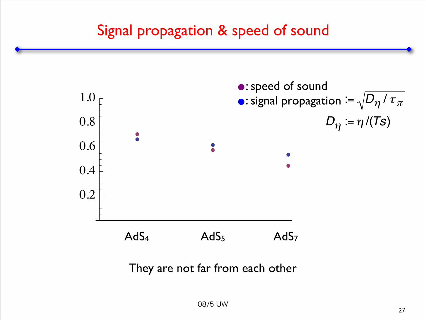
Signal propagation & speed of sound

27

: speed of sound: signal propagation

AdS4 AdS5 AdS7

0.2

0.4

0.6

0.8

1.0

They are not far from each other

€

:= Dη / τ πDη :=η /(Ts)

08/5 UW28

Different τπ for different theoriesτπ ~ 0.2 fm (for 1/T =1 fm)

The propagation speed is not far from the speed of sound

08/5 UW

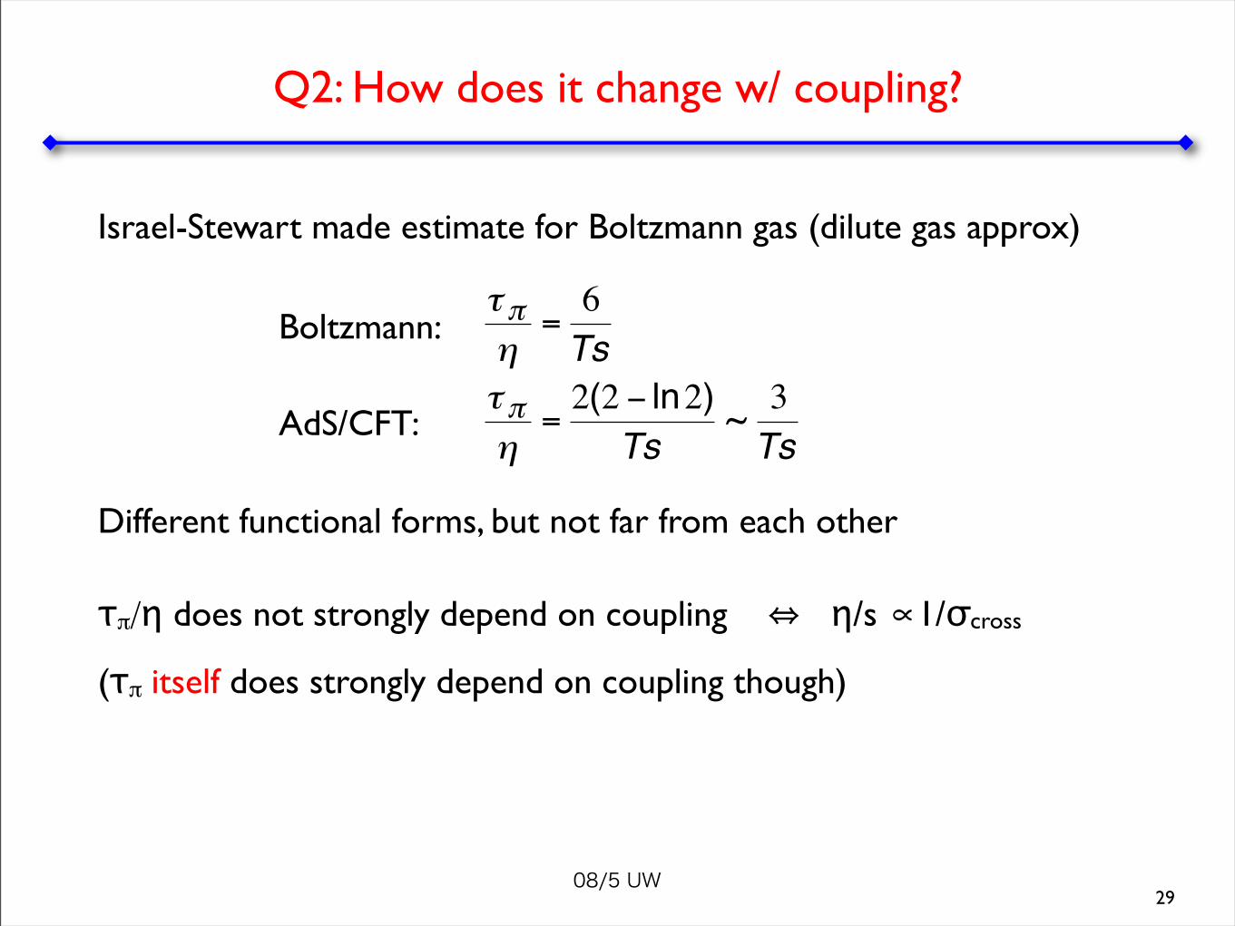
Q2: How does it change w/ coupling?

Israel-Stewart made estimate for Boltzmann gas (dilute gas approx)

Different functional forms, but not far from each other

τπ/η does not strongly depend on coupling ⇔ η/s ∝1/σcross

(τπ itself does strongly depend on coupling though)

29

€

τ πη

=6TsBoltzmann:

AdS/CFT:

€

τ πη

=2(2 − ln2)

Ts~ 3Ts

08/5 UW30

The ratio τπ/η does not strongly depend on coupling. Maybe OK to use Boltzmann gas approx. for simulations

08/5 UW31

Issue of formalism(s)

08/5 UW

Closely related works

Baier et al. have done the same analysis (only for N=4 SYM though).

In addition to the coeffs. by IS, they introduced 4 new coefficients from conf. inv.

32

See alsoHeller - Janik, hep-th/0703243

Benincasa - Buchel - Heller - Janik, 0712.2025 [hep-th]Bhattacharyya - Hubeny - Minwalla - Rangamani, 0712.2456 [hep-th]

MN - Okamura, 0712.2916 [hep-th] 0712.2917 [hep-th] 0801.1797 [hep-th]

Baier - Romatschke - Son - Starinets - Stephanov, 0712.2451 [hep-th]

The Israel-Stewart theory is not complete

08/5 UW

2nd order coefficients (so far)

Israel-Stewart theory:

τΠ τJ τπ (β0,1,2): relaxation times

α0 α1: couplings bet. Jμ and Tμν

Baier et al. ← conformal only

κ: effect of curved (boundary) spacetime

λ1,2,3: nonlinear terms

33

9 coefficients so far

08/5 UW

More complications ...

Various formalisms e.g.

1. Israel-Stewart

2. Israel-Stewart modified by Baier et al.

3. “divergence-type theories”

4. Carter’s formalism

At this moment, unclear how they are related to each other

34

These formalisms are all equivalent for linear perturbations (in flat space).

Unique formalism in this case (more or less)

Carter (1991)

Liu - Müller - Ruggeri (1986)Geroch - Lindblom (1990)

08/5 UW

No obvious universality: Different τπ for different theories

For practical users,

Be careful when you use the Israel-Stewart theory since it’s not complete.

τπ ~ 0.2 fm (for 1/T =1 fm), which is similar among the theories we consider. The propagation speed is not far from the speed of sound.

Maybe OK to use Boltzmann gas approx: The ratio τπ/η does not strongly depend on coupling.

String theory may shed more light on this aspect of hydrodynamics

35

Summary

08/5 UW36

Backup

08/5 UW

Equilibrium

cf. lst law

Off-equilibrium Assume

sμ: 1st order in currents → standard hydrodynamics

sμ: 2nd order → Israel-Stewart

Determine the generic form of constitutive eqs. so that ds > 0

37

€

ds =dεT−

µTdρ

€

s = s(ε,ρ)

€

sµ = sµ (T µν ,Jµ )

ds > 0

constitutive eq.

€

ds ~ −Ji∂iρ +L

€

Ji ~ −∂iρ

Basic procedure

08/5 UW

Shear vs sound mode

Dispersion relation from “shear mode”:

“sound mode” (for conformal theories)

The relaxation time τπ can be determined from both modes independently

38

€

ω = −iDηq2 − iDη2τ πq 4 +L

€

ω =vsq − ids −1ds

Dηq2 +1−1/ds2vs

Dη 2vs2τ π −ds −1ds

Dη

q 3 +L

€

Dη :=η /(Ts)

08/5 UW39

Results for τπ

shear mode sound mode

AdS4 (M2)

AdS5 (D3)

AdS7 (M5)

€

9 − (9 ln3 − 3π )24πT

€

1− ln22πT

€

18 − (9 ln3 + 3π )24πT

€

18 − (9 ln3 − 3π )24πT

€

2 − ln22πT

€

36 − (9 ln3 + 3π )24πT

Results from shear mode and sound mode do not coincide→ One should not take Israel-Stewart theory too literally

08/5 UW

O(q4) terms can appear at 3rd order which spoils the dispersion law:

40

Q: What’s wrong w/ shear mode?

€

τJ∂02ρ +∂0ρ −D∂i

2ρ = 0

€

ω = −iDq2 − iD2τJq 4 +L

08/5 UW

Q: Then, what happens to causality?

In reality, cannot be completely resolved since causal hydrodynamics is an effective theory.

To check causality, one needs a dispersion relation valid for all energy.

But then the other higher order terms can contribute.

Causality can be fully answered only if you sum all terms.

Acausality of 1st order theory: simply telling that you’re outside the domain of validity

Causality should be fine anyway in AdS/CFT (since GR respects it).

41

08/5 UW

Q: Then, how useful?

If causal hydrodynamics cannot really answer causality, how useful?

Actually, standard hydrodynamics has other difficulties such as

instability & lack of covariance

From practical pt of view,

No control on numerical simulations as soon as viscosity is introduced. One needs to take causal hydro. into account.

From fund. pt of view,

Standard hydro. spoils relativistic covariance. The covariance is assured only if you go 2nd order. But then one had better consider the complete 2nd order theory.

42

Israel (76)

Hiscock - Lindblom (85)

08/5 UW

Q: Appropriate to truncate at 2nd order?

Once 2nd order terms become important, all higher order terms can be important in general (common to EFT)

But one needs to know precise coeffs. to see this:

Case 1: 2nd order terms small → 1st order theory enough (not the case)

Case 2: 3rd order terms small → may be fine to truncate at 2nd order (not the case)

43

08/5 UW

Most generic constitutive eq. (conformal)

Fluid rest frame → Kubo-like formula

44

€

u = (1,r 0 )

→ boundary curvature effect =0 for flat boundaryBut it contributes to Kubo formula since it considers hxy perturbation (curve boundary slightly)

→ nonlinear terms=0 for linear perturbations

€

Πµν = −ησ µν + τ π<DΠµν> +

dd −1

Πµν (∇ ⋅u)

+κ R <µν> − (d − 2)uαRα<µν>βuβ{ }

+λ1η2

Πλ<µΠν>λ −

λ2ηΠλ

<µΩν>λ + λ3Ωλ<µΩν>λ

€

new terms