Hydrodynamicalcodefornumericalsimulationofinteracting … Acoustic 3d, 27.03.12 time =0.2 X Y 1,000...

Hydrodynamical code for numerical simulation of interacting galaxies

Hydrodynamical code for numerical simulation of interactinggalaxies

Dr. Igor Kulikov

Institute of Computational Mathematics and Mathematical GeophysicsSiberian Branch of the Russian Academy of Sciences

Interacting Galaxies and Binary Quasars: A Cosmic RendezvousTrieste, Italy. April 2-5, 2012

Hydrodynamical code for numerical simulation of interacting galaxiesIntroduction

Professor Tutukov A.V.(Institute of Astronomy RAS):

The movement of galaxies in dense clusters turns the collisions of galaxies intoan important evolutionary factor, because during the Hubble time an ordinary

galaxy may suffer up to 10 collisions with the galaxies of its cluster.The gas component plays a major role in the scenario of the collision of

galaxies.

Thus it is necessary to simulate the collision of galaxies by means of thehydrodynamical approach.


During the last 10 years, for the solution of the non-stationary astrophysicalproblems the two main approaches are employed from the wide range of thehydrodynamical methods:

1 The Lagrangian smoothed particle hydrodynamics (SPH) method.

2 The Eulerian methods within adaptive mesh refinement (AMR).

SPH advantages

Robustness of the algorithm

Galilean-invariant solution

Simplicity of implementation

Flexible geometries of problems

High accurate gravity solvers

SPH disadvantage

Artificial viscosity is parameterized

Variations of the smoothing length

The problem of shock wave and discontinuous solutions

Instabilities suppressed

The method is not scalable (maximum using cores by order ∼ 100)


During the last 10 years, for the solution of the non-stationary astrophysicalproblems the two main approaches are employed from the wide range of thehydrodynamical methods:

1 The Lagrangian smoothed particle hydrodynamics (SPH) method.

2 The Eulerian methods within adaptive mesh refinement (AMR).

AMR advantages

Approved numerical methods

No artificial viscosity

Higher order shock waves

Resolution of discontinuities

No suppression of instabilities

AMR disadvantage

The complexity of implementation

The effects of mesh

Problem of the minimal mesh resolution

Not galilean-invariant solution

The method is not scalable (maximum using cores by order ∼ 1000)


Software packages for simulation of astrophysical processes

The main properties of the widely used software packages are given in the table:Name of Numerical Correctness Collisioncode method checking of galaxies

GADGET-3 SPH — •Hydra SPH • —Gasoline SPH — —GrapeSPH SPH — —AMRCART Lax-Friedrichs — —NIRVANA Piecewise Parabolic — —FLASH Piecewise Parabolic • —ENZO Piecewise Parabolic — —

RAMSES Piecewise Parabolic • —ART Piecewise Parabolic — —Athena Roe’s linearized solver — —

Pencil Code Finite difference • —ZEUS-MP Finite difference — —

BETHE-Hydro Arbitrary Lagrangian-Eulerian — —AREPO Moving unstructured mesh — •PEGAS Fluid-in-cells • •


Features of the model interacting galaxies:

The three-dimensional nonstationary problem

The problem of shock wave

Self-gravitation and Jeans instabilities

Galilean-invariant problem

Gas-vacuum boundary simulation

A new numerical method must be:

Efficiency numerical method

Higher order shock waves

The conditionally stable numerical method

Galilean-invariant solution

No artificial viscosity

Gas-vacuum boundary simulation

Simplicity of implementation

A potentially infinite scalability

Hydrodynamical code for numerical simulation of interacting galaxiesNumerical Method Description

Gravitational gas dynamics equations

∂ρ

∂t+ div(ρ~v) = 0,

∂ρ~v∂t

+ div(~vρ~v) = −grad(p)− ρgrad(Φ + Φ0),

∂ρE∂t

+ div(ρE~v) = −div(p~v)− (ρgrad(Φ + Φ0), ~v)− q,

∂ρε

∂t+ div(ρε~v) = −(γ − 1)ρεdiv(~v)− q,

∆Φ = 4πρ,

p = (γ − 1)ρε,

where p is the pressure, ρ is the density, ~v is the velocity vector, ρE is thedensity of total energy, Φ is the gravitational potential of the gas itself, Φ0 isthe contribution of the central body to the gravitational potential, ε - the inner

energy, γ - adiabatic exponent, q - cooling function.


The initial conditions

3D Cartesian coordinate system

3D computation domain

Uniform mesh

• The gas component – 50 % masses of the galaxies• The stellar component and the dark matter – 50 % masses of the galaxies

The main characteristic parameters are:

The distance between galaxies, L = 10000 parsec

The mass of a galaxy M0 = 1011M¯

Gravitational constant G = 6.67 · 10−11 N m2/kg

The value of the energy source density q = 2 · 10−24 kg/sec 3 m


The method for the solution of gas dynamics equation is based on theFluids-In-Cells method. The initial system of the equations of gas dynamics is

solved by the two stages:

At first, Eulerian stage, the system ofequations describes the changing of gasvalues in the arbitrary flow domain due thepressure forces and also due to thedifference of potential and to the cooling.

∂ρ

∂t= 0

∂ρ~v∂t

= −grad(p)− ρgrad(Φ)

∂ρE∂t

= −div(p~v)−(ρgrad(Φ), ~v)−q∂ρε

∂t= −(γ − 1)ρεdiv(~v)− q

At second, Lagrangian stage, the system ofequations contains divergent items. TheLagrangian stage itself describes the convectivetransport of the gas quantities with the schemevelocity.


The modification of the base numerical method are:

The modification of the Eulerian stage is the employment of the Godunovtype scheme.

In order to eliminate the impact of the coordinate lines the operatorapproach is employed (The operator approach means that density,pressure, potential and impulse are defined in the cells and the only valuedefined in the nodes of the grid is the velocity vector. The cell averagingfunction is applied for the discrete analogues of the velocity vectorcomponents defined in the grid nodes).

The scheme velocity does not correspond to the desired gas velocity, thatis defined after the completion of the Lagrange stage. The gas velocityresults from the final values of impulse and density.

At each time-step the correction of energy balance is performed. In orderto achieve this the renormalization is performed for the scheme velocities.These velocities set the transport of mass, impulse and both kinds ofenergy at the Lagrangian stage of the Fluids-In-Cells method. Therenormalization results in the correction of the velocity vector length, itsdirection remaining the same. Such a modification of the FlIC methodkeeps the detailed energy balance.


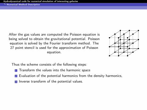
After the gas values are computed the Poisson equation isbeing solved to obtain the gravitational potential. Poissonequation is solved by the Fourier transform method. The27 point stencil is used for the approximation of Poisson

equation.

Thus the scheme consists of the following steps:

1 Transform the values into the harmonic space

2 Evaluation of the potential harmonics from the density harmonics,

3 Inverse transform of the potential values.


The Current parallel implementation

In order to create parallel implementation of the FlIC method domaindecomposition technique was chosen. The decomposition at the Eulerian stage

is performed with the one-layer overlapping of the boundary point of theadjacent subdomains. The Lagrangian stage domain decomposition is

performed with two-layer overlapping. 3D parallel Fast Fourier Transform isperformed by the subroutine from the freeware FFTW library.

Eulerian stage Lagrangian stage Poisson equation

This implementation is scalable only up to 200 cores


The Future parallel implementation

Motivation: We want to solve the problem on amesh of 10243 or bigger per day.

Solution: We will use the GPU cluster andtechnology MPI + CUDA

-1,5 -1,0 -0,5 0,0 0,5 1,0 1,5

-1,5

-1,0

-0,5

0,0

0,5

1,0

1,5

Hybrid, Acoustic 3d, 27.03.12time =0.2

X

Y

1,000

1,026

1,052

1,078

1,104

1,130

1,156

1,182

1,208

1,234

1,260

Now implemented (27th Mar 2012):

1 3d acoustic problem solved agodunov method on mesh 12003

2 300 time steps were calculated for30 minutes

3 were used 32 720 GPU cores


The Future parallel implementation

Future work:

1 implementation lagrangian stage as explicit numerical scheme

2 minimize data transfer between CPU and GPU

3 implementation algebraic solver of Poisson equation (SOR or hismodification)

4 main target: one step of time can be solved per 1 second (for mesh 10243)

5 representation of this implementation at a conference in October orNovember

Hydrodynamical code for numerical simulation of interacting galaxiesTesting of the implementation

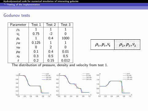
Godunov tests

Parameter Test 1 Test 2 Test 3ρL 1 1 1vL 0.75 -2 0pL 1 0.4 1000ρR 0.125 1 1vR 0 2 0pR 0.1 0.4 0.01x0 0.3 0.5 0.5t 0.2 0.15 0.012

The distribution of pressure, density and velocity from test 1.

0,0 0,2 0,4 0,6 0,8 1,00,0

0,2

0,4

0,6

0,8

1,0

X

p exact 50 cells 100 cells 200 cells

0,0 0,2 0,4 0,6 0,8 1,00,0

0,2

0,4

0,6

0,8

1,0

X

r exact 50 cells 100 cells 200 cells

0,0 0,2 0,4 0,6 0,8 1,0

0,0

0,5

1,0

1,5

2,0

X

n exact 50 cells 100 cells 200 cells


Godunov tests


0,0 0,2 0,4 0,6 0,8 1,00,0

0,2

0,4

0,6

0,8p

X

exact 50 cells 100 cells 200 cells

0,0 0,2 0,4 0,6 0,8 1,0

0,0

0,4

0,8

1,2

1,6

X


0,0 0,2 0,4 0,6 0,8 1,0

0,2

0,4

0,6

0,8

1,0

1,2

1,4e

X

exact 50 cells 100 cells 200 cells


0,0 0,2 0,4 0,6 0,8 1,0

0

200

400

600

800

1000

X

p exact 50 cells 100 cells 200 cells

0,0 0,2 0,4 0,6 0,8 1,00

2

4

6

8

X


0,0 0,2 0,4 0,6 0,8 1,0

0

5

10

15

20

25

30

X

n exact 50 cells 100 cells 200 cells


Aksenov test

The distribution of density

ρ = 1 + 0.5cos(x − vt)cos(ρt),

velocityv = 0.5sin(x − vt)sin(ρt)

and pressure p = ργ , γ = 3, t = π/2.

1 2 3 4 5 6

0,96

0,98

1,00

1,02

1,04

Density

x

h h/2 h/4

1 2 3 4 5 6-0,6

-0,4

-0,2

0,0

0,2

0,4

0,6

Velocity

x

h h/2 h/4


The derivation of the equilibrium configuration of the rotating gas cloud

The initial conditions8<:

∂p∂r = −M(r)ρ

r2∂M∂r = 4πr2ρ

p = (γ − 1)ρε

0 <12

Z

Ω

ρω2r2dΩ < −0.412

Z

Ω

ρΦdΩ

With the increase of the velocity theself-gravitating gas sphere takes the form of therotational ellipsoid. The semi-axes of theellipsoid might be approximated by thefunctions.

rx(ω) = 2.3510−3eω

0.15736 + 1.18171

rz(ω) = 2.5210−3eω

0.17686 + 1.03146

0,5 0,6 0,7 0,8 0,9 1,0

1,2

1,6

2,0

2,4

Rx

w

0,5 0,6 0,7 0,8 0,9 1,01,0

1,2

1,4

1,6

1,8

Rz

w


Collapse (FlIC vs. SPH) in (Kulikov et al. 2009)

The initial conditions

0 1 2 3 4 5 6

0,0

0,2

0,4

0,6

0,8

1,0

x

density

0,0 0,3 0,6 0,9 1,2 1,50

10

20

30

40

t

erro

r, %

h h/2 h/4 h/8

FlIC method:

-1,0 -0,5 0,0 0,5 1,0

0

20

40

60

80

x

dens

ity, F

lIC

a

SPH method:

-1,0 -0,5 0,0 0,5 1,0

0

2

4

6

8

10

12

x

dens

ity, S

PH

b


Collapse (FlIC vs. Lagrangian code) in (Moiseenko et al. 1996)

R0 = 3.81 · 1014mρ = 1.492 · 10−14kg/m3

p = 0.1548N/m2

ω = 2.008 · 10−12rad/sec

M¯ = 1.998 · 1030kg

γ =53


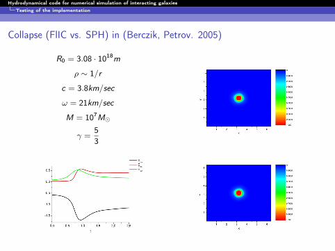
Collapse (FlIC vs. SPH) in (Berczik, Petrov. 2005)

R0 = 3.08 · 1018mρ ∼ 1/r

c = 3.8km/sec

ω = 21km/sec

M = 107M¯

γ =53


Wengen cloud collision test

2 4 6 8 10 12

2

4

6

8

10

12

(a)

0

0,2

0,4

0,6

0,8

12 4 6 8 10 12

2

4

6

8

10

12

(b)

0

0,2

0,4

0,6

0,8

12 4 6 8 10 12

2

4

6

8

10

12

(c)

0

0,2

0,4

0,6

0,8

1

2 4 6 8 10 12

2

4

6

8

10

12

(d)

0

0,2

0,4

0,6

0,8

12 4 6 8 10 12

2

4

6

8

10

12

(e)

0

0,2

0,4

0,6

0,8

12 4 6 8 10 12

2

4

6

8

10

12

(f)

0

0,2

0,4

0,6

0,8

1

2 4 6 8 10 12

2

4

6

8

10

12

(g)

0

0,2

0,4

0,6

0,8

12 4 6 8 10 12

2

4

6

8

10

12

(h)

0

0,2

0,4

0,6

0,8

12 4 6 8 10 12

2

4

6

8

10

12

(i)

0

0,2

0,4

0,6

0,8

1


Description of the Gas Sphere Collision Test

8<:

∂p∂r = −M(r)ρ

r2∂M∂r = 4πr2ρ

p = (γ − 1)ρε

0,0 0,5 1,0 1,5 2,0 2,5 3,0 3,5-8

-6

-4

-2

0

2

4

6

8

time

Eint Egrav Ekin

1 2 3 4 5 6

1

2

3

4

5

6

(a)

0

0,2

0,4

0,6

0,8

11 2 3 4 5 6

1

2

3

4

5

6

(b)

0

0,2

0,4

0,6

0,8

1

1 2 3 4 5 6

1

2

3

4

5

6

(c)

0

0,2

0,4

0,6

0,8

11 2 3 4 5 6

1

2

3

4

5

6

(d)

0

0,2

0,4

0,6

0,8

1

1 2 3 4 5 6

1

2

3

4

5

6

(e)

0

0,2

0,4

0,6

0,8

11 2 3 4 5 6

1

2

3

4

5

6

(f)

0

0,2

0,4

0,6

0,8

1

Hydrodynamical code for numerical simulation of interacting galaxiesNumerical simulation of a collision of the gas components of galaxies

The description of the stellar component and the dark matter

The stellar component and the dark matter of the galaxies is being simulatedby a single central body that has a shape of ellipsoid with the given mass M.The central body also brings its contribution to the general value of thepotential. The contribution is set by an analytical expression:

Φ0(r) =

(−M(r2−3)

2 , r ≤ 1,−M

r , r > 1.

where r is the normalized distance to the center of the central body.

The alteration of the velocities of the stellar components and the dark matterof the galaxies during the collision with the gravitational interaction only issmall. The following estimate might be given for this process:

Egrav

Ekin≈ 0.1


Cooling function

The galactic gas, that was heated during the collision up to the temperature∼ 104 − 108K , cools with the course of time The plasma cooling rateestimated with the temperature over ∼ 104, is 1:

εc ' 10−22 n2 erg cm−3,

where n is the plasma density given as the number of hydrogen atoms in acubic centimeter.

1Sutherland R., Dopita M.. Cooling functions for low-density astrophysical plasmas // TheAstrophysical Journal Supplement Series, V. 88, 1993. pp. 253-327


Statement of the problem

The scenario of the collision of galaxies might be:

The Mergers of Galaxies

Free expansion of the galactic gas

Formation of a new galaxy

The dissipation of galaxies10-4 10-3 10-2

1

2

3

4

5

The dissipation of galaxies

Free expansion of the galactic gas, formation of a new galaxy

The Mergers of Galaxies

L 0, 1

0 00

0 pc

Eint / |Egrav|

Collision results depending on the initial distance and the ratio of the internalenergy to the gravitational energy.


The scenarios of the collision of galaxies

The Mergers of Galaxies:

2 3 4 5

2

3

4

5

(a) 0

2

4

6

8

102 3 4 5

2

3

4

5

(b)

0

1

2

3

4

5

Free expansion of the galactic gas:

1 2 3 4 5 6

1

2

3

4

5

6

( )

0

2

4

6

8

101 2 3 4 5 6

1

2

3

4

5

6

(b)

0

1

2

3

4

51 2 3 4 5 6

1

2

3

4

5

6

(c)

0

0,60

1,2

1,8

2,4

3,0


The scenarios of the collision of galaxies

Formation of a new galaxy:

1 2 3 4 5 6

1

2

3

4

5

6

(a)

0

2

4

6

8

101 2 3 4 5 6

1

2

3

4

5

6

(b)

0

0,1

0,2

0,3

0,4

0,51 2 3 4 5 6

1

2

3

4

5

6

(c)

0

0,1

0,2

0,3

0,4

0,5

The dissipation of galaxies:

2 3 4 5

2

3

4

5

(a)

0

0,2

0,4

0,6

0,8

11 2 3 4 5

1

2

3

4

5

(b)

0

0,2

0,4

0,6

0,8

12 3 4 5

2

3

4

5

(c)

0

0,2

0,4

0,6

0,8

1


Road to ”Ring galaxy”

For ”Ring galaxies” do the following:

1 We choose the parameters for the merger of galaxies

2 We rotate one galaxy in a clockwise direction, another galaxycounterclockwise

3 We will increase the speed of rotation

As a result, disk fragmentation in the collision:

Hydrodynamical code for numerical simulation of interacting galaxiesConclusion

Future work1 Implementation of the complete system of equations for GPU cluster2 Creating a model of star formation as a two-component gas or gas with a

variable adiabatic index3 Creating new tests and numerical criteria for checking of solution


The Bibliography

Vshivkov V., Lazareva G., Snytnikov A., Kulikov I., Tutukov A.Hydrodynamical code for numerical simulation of the gas components ofcolliding galaxies // The Astrophysical Journal Supplement Series. 2011.V. 194, 47. 12 pp.

Tutukov A., Lazareva G., Kulikov I. Gas dynamics of a central collision oftwo galaxies: Merger, disruption, passage, and the formation of a newgalaxy // Astronomy reports. 2011. V. 55, 9. pp. 770-783.

Vshivkov V., Lazareva G., Snytnikov A., Kulikov I., Tutukov A.Computational methods for ill-posed problems of gravitationalgasodynamics // Journal of Inverse and Ill-posed Problems. 2011. V. 19, I.1. P. 151-166.

Vshivkov V., Lazareva G., Snytnikov A., Kulikov I. SupercomputerSimulation of an Astrophysical Object Collapse by the Fluids-in-CellMethod // PaCT-2009 proceedings. LNCS. 2009. V. 5698. pp. 414-422.

Vshivkov V., Lazareva G., Kulikov I. A modified fluids-in-cell method forproblems of gravitational gas dynamics // Optoelectronics,Instrumentation and Data Processing. 2007, V. 43. pp. 530-537.


Acknowledgments

Special thanks two federal program of Russian MinistryEducation and Science: The Federal Program ”Scientific andscientific-pedagogical cadres innovation Russia for 2009-2013”of the Federal Agency for Science and Innovation and FederalProgramme for the Development of Priority Areas of RussianScientific & Technological Complex 2007-2013, RussianMinistry Education and Science

Institute of Computational Mathematics and Mathematical Geophysics SB RAS

Hydrodynamicalcodefornumericalsimulationofinteracting … Acoustic 3d, 27.03.12 time =0.2 X Y 1,000...

Documents

Transcript of Hydrodynamicalcodefornumericalsimulationofinteracting … Acoustic 3d, 27.03.12 time =0.2 X Y 1,000...