Hydrodynamic interactions between two forced objects of arbitrary shape. I.Effect on alignmentTomer Goldfriend, Haim Diamant, and Thomas A. Witten Citation: Physics of Fluids 27, 123303 (2015); doi: 10.1063/1.4936894 View online: http://dx.doi.org/10.1063/1.4936894 View Table of Contents: http://scitation.aip.org/content/aip/journal/pof2/27/12?ver=pdfcov Published by the AIP Publishing Articles you may be interested in The Raspberry model for hydrodynamic interactions revisited. II. The effect of confinement J. Chem. Phys. 143, 084108 (2015); 10.1063/1.4928503 The raspberry model for hydrodynamic interactions revisited. I. Periodic arrays of spheres anddumbbells J. Chem. Phys. 143, 084107 (2015); 10.1063/1.4928502 Hydrodynamic interactions of spherical particles in Poiseuille flow between two parallel walls Phys. Fluids 18, 053301 (2006); 10.1063/1.2195992 Hydrodynamic interactions and orthokinetic collisions of porous aggregates in the Stokes regime Phys. Fluids 18, 013302 (2006); 10.1063/1.2166125 Parallel Computational Strategies for Hydrodynamic Interactions Between Rigid Particles ofArbitrary Shape in a Viscous Fluid J. Rheol. 33, 913 (1989); 10.1122/1.550040

This article is copyrighted as indicated in the article. Reuse of AIP content is subject to the terms at: http://scitation.aip.org/termsconditions. Downloaded

to IP: 132.66.11.212 On: Tue, 22 Dec 2015 16:37:20

PHYSICS OF FLUIDS 27, 123303 (2015)

Hydrodynamic interactions between two forced objectsof arbitrary shape. I. Effect on alignment

Tomer Goldfriend,1,a) Haim Diamant,2,b) and Thomas A. Witten3,c)1Raymond & Beverly Sackler School of Physics and Astronomy, Tel Aviv University,Tel Aviv 69978, Israel2Raymond & Beverly Sackler School of Chemistry, Tel Aviv University, Tel Aviv 69978, Israel3Department of Physics and James Franck Institute, University of Chicago,Chicago, Illinois 60637, USA

(Received 27 January 2015; accepted 13 November 2015; published online 22 December 2015)

We study the properties and symmetries governing the hydrodynamic interactionbetween two identical, arbitrarily shaped objects, driven through a viscous fluid. Wetreat analytically the leading (dipolar) terms of the pair-mobility matrix, affectingthe instantaneous relative linear and angular velocities of the two objects at largeseparation. We prove that the instantaneous hydrodynamic interaction linearly de-grades the alignment of asymmetric objects by an external time-dependent drive[B. Moths and T. A. Witten, “Full alignment of colloidal objects by programedforcing,” Phys. Rev. Lett. 110, 028301 (2013)]. The time-dependent effects of hydro-dynamic interactions are explicitly demonstrated through numerically calculatedtrajectories of model alignable objects composed of four stokeslets. In addition tothe orientational effect, we find that the two objects usually repel each other. Inthis case, the mutual degradation weakens as the two objects move away from eachother, and full alignment is restored at long times. C 2015 AIP Publishing LLC.[http://dx.doi.org/10.1063/1.4936894]

I. INTRODUCTION

The dynamics of colloid suspensions is crucially influenced by flow-mediated correlations.1,2

While these hydrodynamic interactions (HIs) have an important role in the dynamics of ambientsuspensions at thermal equilibrium,2 their effect becomes even more pronounced for objects driven outof equilibrium, where the total force acting on each object generates a long-ranged flow, decaying as1/R with the distance R between the objects. A well-known example is colloid sedimentation, where HIlead to strongly correlated motions and large-scale dynamic structures.3 Various types of driving, suchas electrophoresis, are widely used to control the transport of colloids and other polyatomic objects.2

Theoretical studies of driven colloids traditionally focus on regular particle shapes such as uniformspheres and ellipsoids. The driving of more asymmetric objects is richer4–7 as it generally includescoupling between translation and rotation — when the object is subjected to a force, it also rotatesand when it is under torque, it also translates.1 The choice of a rotation sense under a unidirectionalforce implies a chiral response of the driven object. Such richer responses can be exploited to obtain“steerable colloids” — objects whose orientation and transport can be controlled in much more detail.For example, applying a torque by a rotating uniform magnetic field was used to achieve efficienttransport of chiral magnetic objects.8 Another example, which is the main issue of the present work, isthe ability to achieve orientational alignment of asymmetric objects by applying an external force.9–11

The earlier theoretical works of Refs. 8–11 dealt with isolated asymmetric objects in Stokesflow, which exhibit a chiral response. The object’s chiral response is encoded in the off-diagonalblock of its self-mobility matrix, referred to as the twist matrix. Some objects have a twist matrix

a)Electronic mail: goldfriend@tau.ac.ilb)Electronic mail: hdiamant@tau.ac.ilc)Electronic mail: t-witten@uchicago.edu

1070-6631/2015/27(12)/123303/18/$30.00 27, 123303-1 ©2015 AIP Publishing LLC

This article is copyrighted as indicated in the article. Reuse of AIP content is subject to the terms at: http://scitation.aip.org/termsconditions. Downloaded

to IP: 132.66.11.212 On: Tue, 22 Dec 2015 16:37:20

123303-2 Goldfriend, Diamant, and Witten Phys. Fluids 27, 123303 (2015)

that leads them to align one axis in the body with the applied force. If the twist matrix has only asingle real eigenvalue, the object becomes “axially aligned” in this way,5,9 and the aligning directionis along the corresponding eigenvector. Hence, in the absence of HI and thermal fluctuations, a setof identical, axially aligning objects reach a partially aligned state, where all the objects rotate aboutthe same axis with the same angular velocity, but with an arbitrary phase. Furthermore, it was shownthat, by applying an appropriate time-dependent forcing, the system can be driven to a fully alignedstate, where all the objects are phase-locked with the force and rotate in synchrony.10,11

In view of the above, we use throughout this article the following terminology concerning theresponse of various objects: (i) symmetric objects (such as a uniform sphere); (ii) regular objects,which are asymmetric objects with a vanishing twist matrix (such as a uniform ellipsoid); (iii)irregular objects, having a non-vanishing twist matrix; (iv) axially alignable objects, which areirregular objects, whose twist matrix has a single real eigenvalue. We note that the twist matrixdepends on the position of the forcing point as well. For example, an ellipsoid whose forcing pointis displaced from its centroid, i.e., an ellipsoid with a non-uniform mass distribution under gravity,has a non-vanishing twist matrix and generally might be alignable.

The theoretical groundwork for treating the HI between arbitrary objects in Stokes flow waslaid by Brenner and O’Neill.12,13 The theory was subsequently applied to a pair of particles ofvarious regular shapes.14–20 To this, one should add many earlier studies of the collective dynamicsof suspensions made of ellipsoids.21–25 We note that there are key differences between asymmetricobjects, such as ellipsoids, and the irregular objects studied here. The symmetries of a uniform ellip-soid lead to (a) the absence of a translation-rotation coupling for a single object, and therefore lackof alignability; (b) the absence of a 1/R2 contribution to the relative velocity developed between twosuch objects at mutual distance R. Finally, several numerical techniques have been introduced totreat suspensions of arbitrarily shaped objects.26–30

In this work, we focus on simple, general properties of the pair HI between two arbitrarilyshaped objects at zero Reynolds number and the resulting effect on their orientational alignment.The study of translational effects will be presented in a separate publication.

The work is made of two distinct parts. The first part treats rigorously the instantaneous hydro-dynamic interaction, i.e., the pair-mobility matrix. We use Brenner’s analytical framework,31,32

specializing to the leading order of the HI in the distance between the objects (multipole expansion,also known as the method of reflections1). The second part addresses the time-dependent trajec-tories of forced objects. This is a multi-variable, highly non-linear dynamical system exhibitingcomplex and diverse dynamics. In this part, we are limited to numerical integration of the objects’trajectories. We provide typical examples for the time evolution of pairs of stokeslet objects.

We begin by discussing in Sec. II the general properties and symmetries of the pair-mobilitymatrix for two arbitrarily shaped objects and obtain results for the instantaneous HI at large dis-tances. In Sec. IV, we derive the resulting properties of stokeslet objects, and in Sec. V, we usethem to perform numerical time integration for the evolution of object pairs and their alignment.Finally, in Sec. VI, we discuss several consequences of our results. The dynamics of arbitrarilyshaped objects requires an elaborate notation, which is summarized for convenience in Appendix A.

II. PAIR-MOBILITY MATRIX: GENERAL CONSIDERATIONS

A. Structure of the pair-mobility matrix

The kinematics of a rigid object is represented by a translational velocity V , which refers to anarbitrary reference point rigidly affixed to the object, and an angular velocity ω. We designate thereference point as the origin of the object. Note that the angular velocity of the object is independentof the choice of its origin, and that the origin does not necessarily lie on the instantaneous axis ofrotation of the object.

Consider two arbitrarily shaped rigid objects, a and b, with typical size l, subjected to externalforces and torques Fa, Fb and τa, τb in an unbounded, otherwise quiescent fluid of viscosity η.In the creeping flow regime, the objects respond with linear and angular velocities to the externalforces and torques through a 12 × 12 pair-mobility matrix,

This article is copyrighted as indicated in the article. Reuse of AIP content is subject to the terms at: http://scitation.aip.org/termsconditions. Downloaded

to IP: 132.66.11.212 On: Tue, 22 Dec 2015 16:37:20

123303-3 Goldfriend, Diamant, and Witten Phys. Fluids 27, 123303 (2015)

*,

Va

Vb+-=

1ηl

*,

Maa Mab

Mba Mbb+-*,

F a

F b+-, (1)

where we define generalized velocity and generalized force 6-vectors, V x = (V x, lωx)T and F x =

(F x, τx/l)T for x = a,b. The diagonal blocks,Maa andMbb, correspond to the self-mobilities of theobjects (which nevertheless depend on the configuration of both objects). The off-diagonal blocks,Mab and Mba, describe the pair hydrodynamic interaction. We hereafter omit the factor (ηl)−1

(i.e., set ηl = 1). This, together with the representation of the generalized forces and velocities,makes M dimensionless and dependent on the geometry alone. Throughout the text, we designate6-vectors and matrices with calligraphic font and blackboard-bold letters, respectively. A detaileddescription of the notation used in the article is given in Appendix A.

Since V and τ depend on the choice of object origins, so does the pair-mobility matrix.The transformation between pair-mobility matrices corresponding to different origins is given inAppendix B.

The pair-mobility matrix is a function of the objects’ geometries, their orientations, and thevector connecting their origins, indicated hereafter by R. (We define the direction of R from theorigin of object b to the origin of object a.) The geometry of object x is denoted by rx. For example,if the object consists of a discrete set of Nx stokeslets (see Sec. IV A), then rx is a 3Nx-vectorspecifying the positions of the stokeslets; otherwise, it represents the surface of the object.

The pair-mobility matrix is positive-definite and symmetric.1,33,34 Hence, Mab = (Mba)T , andthe self-blocks can be written as

Mxx = *,

Axx (Txx)TTxx Sxx

+-.

As in the analysis for isolated objects,9 the self-mobility matrix contains the following 3 × 3 blocks:the alacrity matrix A (translational response to force), the screw matrix S (rotational response totorque), and the twist matrix T (translation–rotation coupling). The twist matrix characterizes thechiral response of the object (the sense of rotation under a force). In the present article, we dealwith alignable objects, whose individual T is necessarily non-vanishing. Furthermore, in the caseof a pair of objects, the presence of the other object makes the self-twist matrix, Txx, differ fromthe single-object one. As to the off-diagonal blocks of the pair-mobility matrix, the symmetry ofMimplies the following structure:

Mab = *,

Aab (Tba)TTab Sab

+-, Mba = *

,

(Aab)T (Tab)TTba (Sab)T

+-.

B. Further symmetries of the pair-mobility matrix

The discussion in Subsection II A has been for a general pair of objects, which are notnecessarily identical. In the present subsection, we focus on the case in which the two objects areidentical in shape and orientation, i.e., ra = rb ≡ r. Our goal is to understand what the instanta-neous relative velocities (linear and angular) between the two objects are, when the objects aresubjected to the same external forcing. The restriction to identical objects makesM invariant underexchange of objects. This additional symmetry is made of two operations: interchanging the blocksMaa ↔ Mbb andMab ↔ Mba, and inversion of R. That is,

M(r, R) = EM(r,−R)E−1, (2)

where E is a 12 × 12 matrix which interchanges the objects,

E = *,

0 I6×6

I6×6 0+-,

with I6×6 denoting the 6 × 6 identity matrix.The symmetry to object exchange, when combined with the parity of M (i.e., whether it re-

mains the same or changes the sign) under R-inversion,35 has important consequences for the effect

This article is copyrighted as indicated in the article. Reuse of AIP content is subject to the terms at: http://scitation.aip.org/termsconditions. Downloaded

to IP: 132.66.11.212 On: Tue, 22 Dec 2015 16:37:20

123303-4 Goldfriend, Diamant, and Witten Phys. Fluids 27, 123303 (2015)

of hydrodynamic interactions on alignment. If M has a definite parity, one can determine what therelative response of the objects to forcing is—i.e., whether they attain the same or the oppositelinear and angular velocities. If the term is symmetric to inversion, the velocities would be identicaland if it is antisymmetric, they would be opposite. This is because

*,

Maa(R) Mab(R)Mba(R) Mbb(R)

+-= ± *

,

Maa(−R) Mab(−R)Mba(−R) Mbb(−R)

+-= ± *

,

Mbb(R) Mba(R)Mab(R) Maa(R)

+-, (3)

where the second equality comes from the response to exchange of objects, Eq. (2). Consequently,under identical forcing of the two objects, one finds

Va =Maa +Mab

F = ±

Mbb +Mba

F = ±Vb. (4)

Thus, since anyM can be decomposed into even and odd terms, we find that only the odd ones causerelative motions of the two objects.

The pair-mobility as a whole, however, never has a definite parity under R-inversion, i.e., itis made of both even and odd terms. This becomes clear when M(r, R) is expanded in small l/R,i.e., in multipoles. A general discussion of the parity of each multipole term is given in Sec. III. Fornow, let us consider those two leading multipoles which are independent of the objects’ shape, andtherefore always exist. The monopole–monopole interaction (Oseen tensor), which is the leadingterm in Aab making object a translate due to the force on object b, is symmetric under R-inversion.The part of the monopole–dipole interaction causing the second object to rotate due to the forceon the first, i.e., the leading term in Tab, is antisymmetric. For example, even the most symmetricpair of objects — two spheres — has an R-symmetric Aab, leading to zero relative velocity, and anR-antisymmetric Tab, causing them to rotate with opposite senses.1 Thus, for a general object, thehighest order which maintains M of definite parity is the monopole 1/R Oseen one, which is even.(The self-blocks are constant up to order 1/R4, see below.)

From this discussion, we can immediately conclude that, to leading order in the separationof two identical, fully aligned objects, their instantaneous hydrodynamic interaction must linearlydegrade the alignment. The leading degrading term comes from Tab, their rotational response toforce, and is of order 1/R2. It is worthwhile to note again that such a rotational response is present aswell for a pair of uniform spheres or ellipsoids; yet, such regular objects are not alignable to beginwith.

The relation between object-exchange symmetry and the symmetry of the linear-velocityresponse is intimately related to the issue of hydrodynamic pseudo-potentials,36 which will bediscussed in detail in a forthcoming publication.

III. FAR-FIELD INTERACTION: MULTIPOLE EXPANSION

There are two characteristic length scales in our problem: the typical size of the objects, l, andthe distance between them, R = |R|. If l ≪ R, we can write the pair-mobility matrix as a powerseries in (l/R),

M = M(0) +M(1) +M(2) + · · ·,

where M(n) ∼ (l/R)n. The analysis of this expansion as given below holds for any pair of objects,whether identical or not. The zeroth order, M(0), is a block diagonal matrix which is made of theself-mobilities of the two non-interacting objects. (These should be distinguished from Maa andMbb, the self-mobilities of the interacting objects.)

The hydrodynamic multipole expansion (also known as the method of reflections) is based onthe Green’s function of Stokes flow, the Oseen tensor,1 given in our units (ηl = 1) by

Gi j(r) = 18π

lr

(δi j +

rir j

r2

), (5)

which is a symmetric 3 × 3 tensor, invariant under r-inversion. A point force at r0, δ(r − r0) f ,generates a velocity field u(r) = G(r − r0) · f .

This article is copyrighted as indicated in the article. Reuse of AIP content is subject to the terms at: http://scitation.aip.org/termsconditions. Downloaded

to IP: 132.66.11.212 On: Tue, 22 Dec 2015 16:37:20

123303-5 Goldfriend, Diamant, and Witten Phys. Fluids 27, 123303 (2015)

We obtain two general results concerning the multipoles of the hydrodynamic interactionbetween two arbitrary objects. The two objects need not be identical. The proofs are given inAppendix D.37

1. The leading interaction multipole in the self-blocks of the pair-mobility matrix is n = 4. Thatis, any response of one object to forces on itself, owing to the other object, must fall off withdistance R between the objects at least as fast as R−4.

2. The nth multipole has self-blocks of (−1)n parity, and coupling blocks of the opposite, (−1)n+1

parity. Thus, e.g., the leading term inMaa, proportional to R−4, is invariant under R-inversion,and the R−4 part ofMab changes sign under R-inversion. Likewise for the multipole varying asR−5, theMaa changes sign under R-inversion, whileMab remains invariant.35

These statements pertain to the mobility matrix. As to the propulsion matrix (the inverse of themobility matrix), the leading correction to the self-block becomes ∼1/R2, and the second statementconcerning parity remains intact.

We now consider for a moment two identical objects and specialize to the first and secondmultipoles, i.e., the hydrodynamic interaction up to order 1/R2. The discussion in Sec. II and thecurrent section implies the following form of the two leading terms in the pair-mobility matrix:

M(1) = *,

0 Mab(1)

Mab(1) 0

+-, M(2) = *

,

0 Mab(2)

−Mab(2) 0

+-. (6)

In more detail, there are no first- and second-order corrections to the objects’ self-mobility. Hence,these two multipoles have definite parities — the first is even and the second is odd. Consequently,the first multipole does not cause any relative motion of the two objects, whereas the secondmultipole makes them translate and rotate in opposite linear and angular velocities.

The essential characteristics of the first two multipoles are schematically illustrated in Fig. 1.The first multipole arises directly from the Green’s function,

Mab(1) = *

,

G(R) 00 0

+-, (7)

where G(R) is the Oseen tensor, given in Eq. (5).In the interaction described by the second multipole, one object sees the other as a point, see

Fig. 1. Accordingly, this term contains two types of interaction: (1) the response of object a to the

FIG. 1. Illustration of the two leading orders of the hydrodynamic interaction between two forced objects. The leading termin the pair-mobility matrix (light blue/dashed-dotted arrow between the objects’ origins), decaying as 1/R, comes from thepoint-like response of object a to the local flow caused by the force monopole on object b (blue/thick arrow). The next-orderterm, decaying as l/R2, has two contributions: (i) The point-like response of object a to the local flow caused by the forcedipole on object b (red/dashed arrow from the red/thin arrows at object b to the origin of a). (ii) The response of objecta to the local flow gradient caused by the force monopole on object b (magenta/dotted arrow from the origin of b to themagenta/thin arrows at object a).

This article is copyrighted as indicated in the article. Reuse of AIP content is subject to the terms at: http://scitation.aip.org/termsconditions. Downloaded

to IP: 132.66.11.212 On: Tue, 22 Dec 2015 16:37:20

123303-6 Goldfriend, Diamant, and Witten Phys. Fluids 27, 123303 (2015)

non-uniformity of the flow due to the force monopole at object b (regarded as a point); (2) theadvection of object a (regarded as a point) by the flow due to the force dipole acting at object b.These two effects are both proportional to ∇G(R) ∼ 1/R2. Each can be written as a product of atensor which arises from the medium alone, through derivatives of the Oseen tensor ∇G(R), andanother tensor which depends on the objects’ geometry. The second-order correction to the velocityof object a is given by the sum of these two effects, each expressed in terms of a coupling tensor Θand an object tensor Φ,

Va(2) =M

ab(2) · F

b

Mab(2) = Φ

a : Θ(R) − ΘT(R) : Φb, (8)

where the double dot notation denotes a contraction over two indices. Equation (8) contains threetensors of rank 3, denoted by capital Greek letters. The first, Φ, with dimensions 6 × 3 × 3, givesthe generalized velocity of the object in linear response to the velocity gradient of the flow in whichit is embedded. The second, Φ, having dimensions 3 × 3 × 6, gives the force dipole acting on thefluid around the object’s origin in linear response to the generalized force acting on it. Both Φ and Φdepend on the objects’ geometry alone.38 The third tensor, Θ, with dimensions 3 × 3 × 6, describesthe coupling of these object responses through the fluid. It is given by

Θsk j(R) ≡

∂sGk j(r)|R j = 1,2,3,0 j = 4,5,6.

(9)

Repeating the same procedure for Vb in response to F a while using the odd parity of Θ, we get

Mba(2) = Θ

T(R) : Φa − Φb : Θ(R). (10)

The tensors Φ and Φ are not independent.39 We now show that Φ = ΦT . The symmetry ofM implies that each multipole is also a symmetric matrix. Using Eqs. (8) and (10) and equating(Mba

(2))T = Mab(2) , we get Φa = (Φa)T and Φb = (Φb)T .

To summarize, the matrixM(2) is given by

M(2) = *,

0 Φa : Θ(R) − [Φb : Θ(R)]T

−Φb : Θ(R) + [Φa : Θ(R)]T 0+-. (11)

This results is valid for a general pair of objects. If the two objects are identical, the off-diagonalblocks have the same form with opposite signs. The additional condition that the entire M must besymmetrical implies then that each block by itself is antisymmetric.

By separating the tensors Φ and Θ into their symmetric and antisymmetric parts, the second-order term of the pair-mobility matrix can be simplified further. It should be mentioned, in addition,that the Φ tensor depends on the origin selected for the object. These two technical issues areaddressed in Appendices E and C, respectively. Finally, we note that the terms in these tensorscorresponding to the translational response vanish for spheres and ellipsoids. Consequently, twosuch regular objects develop relative velocity only to orders 1/R3 and above.

IV. NUMERICAL ANALYSIS FOR STOKESLET OBJECTS

In Secs. II and III, we have derived the general properties of the instantaneous hydrodynamicinteraction between two arbitrarily shaped objects. We now move on to the second part of thework, addressing the time evolution of the two objects. This complicated problem is not tractableanalytically, and we resort to numerical integration of specific examples. Because of the complexityof the problem, and since we are interested in generic properties, we allow ourselves to restrict theanalysis to the simplest, even if unrealistic, objects. Arguably, the simplest form of an arbitrarilyshaped object is the so-called stokeslet object — a discrete set of small spheres, separated by muchlarger, rigid distances, where each sphere is approximated as a point force. The sparseness of theseobjects makes them free-draining, which may be valid for macromolecules but not for compactobjects.

This article is copyrighted as indicated in the article. Reuse of AIP content is subject to the terms at: http://scitation.aip.org/termsconditions. Downloaded

to IP: 132.66.11.212 On: Tue, 22 Dec 2015 16:37:20

123303-7 Goldfriend, Diamant, and Witten Phys. Fluids 27, 123303 (2015)

FIG. 2. Two examples of axially alignable stokeslet objects, which were used in the simulations. The objects comprise offour stokeslets connected by dragless rods. The origin of the objects is at point (0,0,0) and the aligning direction is −z. Theobject on the left corresponds to the dark red/dotted trajectories in the left panels of Figs. 5 and 6, and the one on the rightcorresponds to the purple/dashed trajectories in the right panels of Figs. 3 and 4.

We treat pairs of identical objects, each made of four stokeslets. To obtain representative sampl-ing of numerical examples, we do not design these objects but create them randomly. Four pointsare placed at random distances ranging between 0 and 1 from an arbitrary origin. The origin is thenshifted to the points’ center of mass. The radius ρ of the stokeslets is taken as 0.01. The resultingconfiguration is checked to be “sufficiently chiral,” in the sense that the T-matrix of the individualobject is strongly asymmetric, having a single real eigenvalue of absolute value |λ3| > 0.005, whichmakes the object axially alignable (see Sec. I). Examples of the stokeslet objects we use areprovided in Fig. 2.

The way to calculate the mobility of a single stokeslet object was presented in Ref. 9. First,we briefly present in Sec. IV A the simple extension of this method to pair-mobilities. We calculateboth the pair mobility and the tensor Φ introduced in Secs. II and III. The latter allows us tocalculate pair mobilities up to second order in the multipole expansion. Section IV B describes howwe use the pair mobility to numerically calculate the time evolution of the pair configuration.

A. Pair-mobility andΦ tensor

The properties of a stokeslet object can be derived self-consistently from the linear relationswhich describe the stokeslets’ configuration. This is done without finding the stokeslets’ strengthsexplicitly. Below we find the pair-mobility matrix, and the Φ tensor associated with a single object,given the stokeslet configuration and the size of the spheres that they represent.

Each of the two objects, x = a,b, consists of Nx stokeslets, Fx = (F x1 , . . . , F

xNx), in a known

configuration, rx =(r x

1 , . . . , rxNx

). Here, we use the notation of a bold letter to denote a set of N

3-vectors, and r xn indicates the position 3-vector of the nth stokeslet in object x with respect to the

object’s origin. Each stokeslet is a sphere of radius ρ, where ρ < min(r x1 , . . . ,r

xNx). The boundary

conditions at the sphere surface enter only through its self-mobility coefficient. The velocities of thespheres, v xn , are known from the object’s linear and angular velocities,

*,

va

vb+-= *,

Ua 00 Ub

+-*,

Va

Vb+-, with Ux =

*....,

I3×3,−r x ×1 /l

...

I3×3,−r x ×Nx

/l

+////-

, for x = a,b, (12)

where the matrix y× obtained from the vector y is defined as ( y×)i j = ϵ ik j yk. Each stokeslet force isproportional to the relative velocity of the sphere that it represents, with respect to the flow around

This article is copyrighted as indicated in the article. Reuse of AIP content is subject to the terms at: http://scitation.aip.org/termsconditions. Downloaded

to IP: 132.66.11.212 On: Tue, 22 Dec 2015 16:37:20

123303-8 Goldfriend, Diamant, and Witten Phys. Fluids 27, 123303 (2015)

it as created by the other stokeslets. This gives a linear relation between the stokeslets and thevelocities of the spheres,40

*,

va

vb+-= *,

Laa Lab

LabTLbb

+-*,

Fa

Fb+-, where (13)

(Lxxnm)i j =

Gi j(r xn − r x

m) if n , mγ−1δi j else

,

(Labnm)i j = Gi j(R + ran − rbm), (14)

and γ = 6πρ/l.First we find the pair-mobility matrix as a generalization of the analysis in Ref. 9. The sum of

the stokeslets and the corresponding total torque must be equal to the external generalized forcesapplied on the objects. In a matrix form, we can write

*,

F a

F b+-= *,

(Ua)T 00 (Ub)T

+-*,

Fa

Fb+-. (15)

Using Eqs. (12) and (13), we have

*,

Ua 00 Ub

+-

T

· *,

Laa Lab

LabTLbb

+-

−1

· *,

Ua 00 Ub

+-· *,

Va

Vb+-= *,

F a

F b+-.

From this expression, we identify the pair-mobility matrix as

M =

*,

Ua 00 Ub

+-

T

· *,

Laa Lab

LabTLbb

+-

−1

· *,

Ua 00 Ub

+-

−1

. (16)

This expression allows to calculate the pair-mobility matrix, with the help of Eqs. (12) and (14),based on the stokeslets’ configuration and the Oseen tensor alone.

Next, we derive the Φx tensor of a stokeslet object x. From this tensor, we may readily obtainthe second multipole of the pair interaction (cf. Sec. III). The force dipole around the origin ofa forced object is given by Eq. (8), (rF)x ≡ (Φx)T · F x. Similar to the Ux matrix relating thestokeslets to the total generalized force, F x = (Ux)T · Fx, we define a tensor of rank 3, Υx, whichrelates the stokeslet forces to the total force dipole on the object by (rF)x = (Υx)T · Fx. (Note thatno force dipole is applied on the individual stokeslets; being arbitrarily small, they possess only aforce monopole.) Specifically, it is made of N blocks of 3 × 3 × 3, given by (Υn)i j s = rn,sδi j, n =1 . . . N , i, j, s = 1,2,3 (i.e., rn,s is the s Cartesian coordinate of the stokeslet n). Using Eqs. (12) and(13), we have (rF)a = (Υa)T · (Laa)−1 · Ua · Va. This implies (Φx)T = (Υx)T · (Lxx)−1 · Ux ·Mx

self.Recalling that the matricesMself and L are symmetric, we finally get

Φx = Mx

self · (Ux)T · (Lxx)−1 · Υx. (17)

It is important to note that in the above derivation, we computeM and Φ under the assumptionthat, for each object, the stokeslet sizes are arbitrarily small compared to the distances betweenthem, ρ ≪ l (where l is the object’s radius of gyration). However, in a more general case, one canuse the Rotne-Prager-Yamakawa tensor,41,42 which corrects the Oseen tensor for force distributionswith finite size.28

B. Numerical time integration

We present a numerical integration scheme for the dynamics of two stokeslet objects. Weshould first define the reference frames used in the scheme. Each rigid object is characterized byaxes which are affixed and rotate with it. We define the object reference frame (ORF) such that its zaxis coincides with the object’s alignment axis (the corresponding eigenvector of the T-matrix). Theother two axes are selected arbitrarily. The z axis of the laboratory frame is defined along the forcing

This article is copyrighted as indicated in the article. Reuse of AIP content is subject to the terms at: http://scitation.aip.org/termsconditions. Downloaded

to IP: 132.66.11.212 On: Tue, 22 Dec 2015 16:37:20

123303-9 Goldfriend, Diamant, and Witten Phys. Fluids 27, 123303 (2015)

direction. During the evolution, we follow the translation and rotation of the ORF in the laboratoryframe.

We represent the orientation of an object by the Euler-Rodrigues 4-parameters,43 defined by(Γ,Ω) ≡ (cos θ

2 , n sin θ2 ), where n and θ are the axis and angle of rotation.44 The following properties

hold for this 4-parameter representation: (a) The norm of (Γ,Ω) in 4D-space is unity, Γ2 +Ω2 = 1.(b) A rotation matrix is given by Rodrigues’ rotation formula,

R(Γ,Ω) = I3×3 + 2ΓΩ× + 2(Ω×)2. (18)

(c) The parameters are invariant under inversion, i.e., (Γ,Ω) and (−Γ,−Ω) correspond to the sameorientation. (d) Given the angular velocity of the object, the dynamics of its orientation simply reads

*,

Γ

˙Ω

+-=

12*,

0 −ωT

ω ω×+-*,

Γ

Ω+-. (19)

Since we choose the ORF such that the z-axis is the axis of alignment, the terminal orientation of anaxially alignable object under a constant force along the z-axis is (Γ,Ω) = (cos(ωt+α

2 ), z sin(ωt+α2 )),

where α is a constant phase which depends on the object’s initial orientation at time t = 0.The state of a pair of objects at time t is described by the position of the origins of the objects,

Ra(t) and Rb(t), and their orientation parameters, (Γa(t),Ωa(t)) and (Γb(t),Ωb(t)). We time-integratefrom the initial state, Ra

0 = (0,0,0), Ra0 − Rb

0 = R0, (Γa0 ,Ωa0 ), and (Γb0 ,Ωb

0 ), as follows. Given thepositions of the stokeslets at time t, the pair-mobility matrix, M(t), is calculated as explained inSec. IV A, either exactly or using the multipole approximation. Then, the linear and angular veloc-ities of the objects are given by (Va(t),Vb(t))T = M(t) · (F a(t), F b(t))T . From them, the originsand orientations of the objects at time t + dt are derived according to

Rx(t + dt) = Rx(t) + V x(t)dt, (20)

*,

Γx(t + dt)Ω

x(t + dt)+-= exp

dt2*,

0 −ωxT

ωx ωx×+-

*,

Γx(t)Ω

x(t)+-, (21)

for x = a,b. During the evolution, we make sure that the small stokeslet spheres do not overlap, andthat the pair mobility matrix remains positive-definite. In practice, we never encountered such prob-lems when using the exact pair mobility matrices; when it did happen in the case of the multipoleapproximation, we stopped the integration.

We define a scalar order parameter which characterizes the degree of mutual alignment of thetwo objects,

m ≡(Γa,Ωa) · (Γb,Ωb)2

=(ΓaΓb + Ωa · Ωb

)2. (22)

As required, the order parameter is invariant under 3-rotation. This can be verified by explic-itly applying a 3-rotation to the laboratory frame, or alternatively, by the following argument.Since 3-rotation leaves the norm of the 4-parameter orientation unchanged (property (a)), it isa unitary transformation in 4-space. Hence, the dot product is invariant. When the objects arealigned, (Γa,Ωa) = ±(Γb,Ωb), and m = 1; otherwise, 0 ≤ m < 1. In the case of partial alignment,m = cos2(∆α2 ), where ∆α is the mutual phase difference.45

Another scalar property of the two-object system is the energy dissipation rate. At time t, thelatter is given by Va(t) · F a(t) + Vb(t) · F b(t). Since the pair-mobility matrix is positive definite,the energy dissipation of the driven pair is positive at all times.

V. NUMERICAL RESULTS: EFFECT ON ALIGNMENT

We present in Figs. 3–8 several examples for the numerically integrated evolution of objectpairs under various conditions. One can immediately appreciate the diversity of possible trajec-tories. To make your way through this richness, it is important to make two distinctions betweentypes of trajectories. The first distinction is between constant forcing (as in sedimentation), which

This article is copyrighted as indicated in the article. Reuse of AIP content is subject to the terms at: http://scitation.aip.org/termsconditions. Downloaded

to IP: 132.66.11.212 On: Tue, 22 Dec 2015 16:37:20

123303-10 Goldfriend, Diamant, and Witten Phys. Fluids 27, 123303 (2015)

FIG. 3. Trajectories of object separation under time-dependent forcing. The three rows, from top to bottom, correspond,respectively, to the separation along the z direction, its projection onto the xy plane, and its total magnitude. The squares inthe middle row indicate the state at the end of the simulation. The panels show results for three different objects, starting fromeither a random mutual orientation (left column) or their fully aligned state (right column). The green/dashed trajectory onthe right panels was integrated longer than 150 time units to verify that it continues in a limit cycle.

can make the objects only partially aligned without synchronizing their phases of rotation,5,9 and atime-dependent forcing protocol, which is known to lock the phase of an individual object onto thatof the force.10,11 The main issue examined below is how the presence of hydrodynamic interactionaffects these two behaviors. The second distinction, therefore, is whether hydrodynamic interactionsare included (dashed, dotted, and dashed-dotted/colored curves) or turned off (solid gray curves). Inthe absence of hydrodynamic interactions (or when they get weak as the objects move far apart),the time-dependent aligning force will make the objects fully synchronized, whereas under constantforcing, the objects will generally become unaligned.

The results are presented in a dimensionless form, using units such that η = |ω0| = 1, whereω0 = λ3F is the angular velocity of a single object once self-aligned, and ρ = 0.01. The distances

This article is copyrighted as indicated in the article. Reuse of AIP content is subject to the terms at: http://scitation.aip.org/termsconditions. Downloaded

to IP: 132.66.11.212 On: Tue, 22 Dec 2015 16:37:20

123303-11 Goldfriend, Diamant, and Witten Phys. Fluids 27, 123303 (2015)

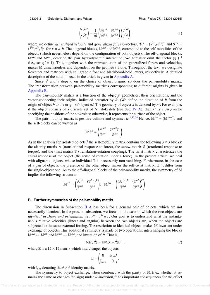
FIG. 4. Orientation order parameter as a function of time, under time-dependent forcing, for the examples of Fig. 3. (a)results for random initial orientations (examples on the left column of Fig. 3); the additional solid gray curves correspond tonon-interacting objects. (b) results for initially fully aligned object pairs (right column in Fig. 3).

between the stokeslets of each object are taken randomly between 0 and 1; hence, ρ ≪ l ∼ 1.The time-dependent forcing protocol is F = F0(− sin(ω0t) sin(θ),cos(ω0t) sin(θ),− cos(θ)), whereθ = 0.1π, F0 = −|λ3|−1, ω0 = sign(λ3), and λ3 is the real eigenvalue of the single-object twist ma-trix. We examine both the trajectories of the separation vector connecting the origins of the twoobjects and the corresponding evolution of the orientation order parameter.

We begin with the case of a time-dependent forcing, Figs. 3 and 4. The first observation, mostclearly demonstrated in Fig. 4(b), is that hydrodynamic interaction degrades the alignment of the twoobjects, as has been rigorously inferred based on symmetry considerations in Sec. II B. Another conclu-sion, supported by additional examples not shown here, is that most objects, which start sufficientlyfar apart, especially if they start fully aligned, tend to repel each other (Fig. 3). Even if they are notfully aligned, the growing distance and weakening interaction make them individually more alignedwith the forcing and therefore also mutually synchronized. Thus, the repulsion helps to restore thealignment at long times. The increasing separation occurs in the xy plane, while along the z axis, theseparation decreases and saturates to a finite distance, dependent on initial conditions, see Fig. 3.

The repulsion is accompanied by a decrease in dissipation rate (up to small oscillations), asdemonstrated in Fig. 7. When the HI is turned off, the dissipation rate reaches a constant value as thetwo independent objects set into their ultimate aligned state (solid curves in Fig. 7).

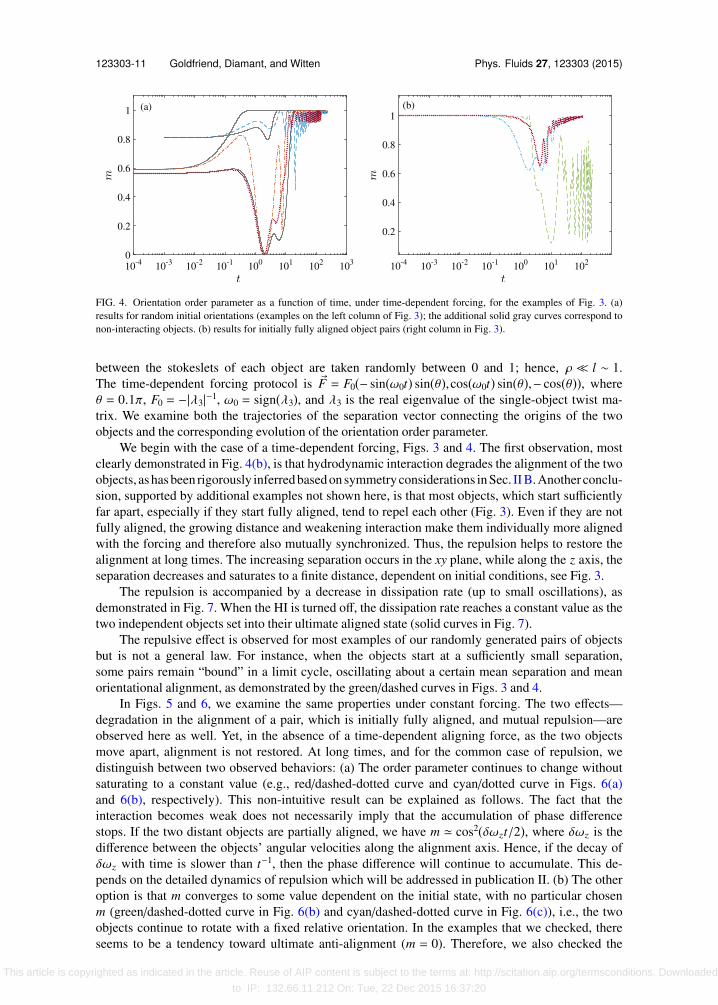
The repulsive effect is observed for most examples of our randomly generated pairs of objectsbut is not a general law. For instance, when the objects start at a sufficiently small separation,some pairs remain “bound” in a limit cycle, oscillating about a certain mean separation and meanorientational alignment, as demonstrated by the green/dashed curves in Figs. 3 and 4.

In Figs. 5 and 6, we examine the same properties under constant forcing. The two effects—degradation in the alignment of a pair, which is initially fully aligned, and mutual repulsion—areobserved here as well. Yet, in the absence of a time-dependent aligning force, as the two objectsmove apart, alignment is not restored. At long times, and for the common case of repulsion, wedistinguish between two observed behaviors: (a) The order parameter continues to change withoutsaturating to a constant value (e.g., red/dashed-dotted curve and cyan/dotted curve in Figs. 6(a)and 6(b), respectively). This non-intuitive result can be explained as follows. The fact that theinteraction becomes weak does not necessarily imply that the accumulation of phase differencestops. If the two distant objects are partially aligned, we have m ≃ cos2(δωzt/2), where δωz is thedifference between the objects’ angular velocities along the alignment axis. Hence, if the decay ofδωz with time is slower than t−1, then the phase difference will continue to accumulate. This de-pends on the detailed dynamics of repulsion which will be addressed in publication II. (b) The otheroption is that m converges to some value dependent on the initial state, with no particular chosenm (green/dashed-dotted curve in Fig. 6(b) and cyan/dashed-dotted curve in Fig. 6(c)), i.e., the twoobjects continue to rotate with a fixed relative orientation. In the examples that we checked, thereseems to be a tendency toward ultimate anti-alignment (m = 0). Therefore, we also checked the

This article is copyrighted as indicated in the article. Reuse of AIP content is subject to the terms at: http://scitation.aip.org/termsconditions. Downloaded

to IP: 132.66.11.212 On: Tue, 22 Dec 2015 16:37:20

123303-12 Goldfriend, Diamant, and Witten Phys. Fluids 27, 123303 (2015)

FIG. 5. Trajectories of object separation under constant forcing. The meaning of the various panels is the same as in Fig. 3.In all the examples shown here, the two objects repel each other except of the example which corresponds to the blue/dashedcurve in the left panels. (The repulsive trajectories were actually integrated to times longer than presented here.)

stability of anti-alignment in pairs which start from such a state. Fig. 6(d) examines the stability ofthis configuration for objects initially confined to the xy plane (perpendicular to the force). Whereasthe aligned pair (blue/dotted curve) is unstable, the anti-aligned one (red/dashed curve) remainsstable for the duration of integration. It may well be that this stability survives for a long but finitetime, see, e.g., dark red/dotted curve in Fig. 6(c). In addition, a separation of the pair along thez-axis destabilizes an anti-aligned pair as well (examples not shown). Finally, we note that even ifthe final phase difference were arbitrary and uniformly distributed, the value of m would be evenlydistributed around 1/2 but non-uniformly with larger weights on m = 0,1. (This follows from thedefinition of m, see Eq. (22).)

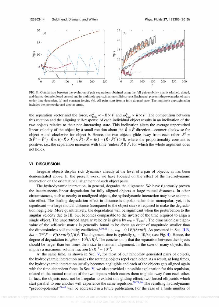
Figure 8 compares results obtained using the full pair-mobility matrix of the stokeslet objectswith those obtained from the multipole (dipole) approximation. As expected, the two calculationsagree for objects whose mutual distance increases with time and disagree for objects whose trajec-tories reach close proximity.

This article is copyrighted as indicated in the article. Reuse of AIP content is subject to the terms at: http://scitation.aip.org/termsconditions. Downloaded

to IP: 132.66.11.212 On: Tue, 22 Dec 2015 16:37:20

123303-13 Goldfriend, Diamant, and Witten Phys. Fluids 27, 123303 (2015)

FIG. 6. Orientation order parameter as a function of time, under constant forcing, for the examples of Fig. 5. (a) resultsfor random initial orientations (examples on the left column of Fig. 5); the solid gray curves correspond to non-interactingobjects. (b) results for initially fully aligned object pairs (right column in Fig. 3). (c) results for objects with initial partialalignment (rotating around the same axis with random initial phases). (d) the stability of anti-alignment, shows trajectoriesof two identical pairs, which start on the xy plane from the same separation and axes of rotation but with different relativephases. Blue/dotted and red/dashed curves represent, respectively, a pair which starts aligned (zero relative phase) and onewhich starts anti-aligned (relative phase of π).

Further investigation (not shown here) of the orientational dynamics of the objects suggests apossible explanation for the characteristic repulsion between two chiral objects. In the absence ofHI, each object rotates along F and translates on average along F. One contribution to the dipolarterm of the HI comes from the effect on each object by the vorticity of the Oseen flow causedby the other object. This perturbative angular velocity is along an axis which is perpendicular to

FIG. 7. Dissipation rate as a function of time for object pairs starting from arbitrary orientations, under time-dependentforcing (a) and constant forcing (b). Dashed-dotted and dotted colored curves correspond to the examples of the samestyles/colors in the preceding figures. Solid curves show the results in the absence of HI.

This article is copyrighted as indicated in the article. Reuse of AIP content is subject to the terms at: http://scitation.aip.org/termsconditions. Downloaded

to IP: 132.66.11.212 On: Tue, 22 Dec 2015 16:37:20

123303-14 Goldfriend, Diamant, and Witten Phys. Fluids 27, 123303 (2015)

FIG. 8. Comparison between the evolution of pair separations obtained using the full pair-mobility matrix (dashed, dotted,and dashed-dotted colored curves) and its multipole approximation (solid curves). Each panel presents three examples of pairsunder time-dependent (a) and constant forcing (b). All pairs start from a fully aligned state. The multipole approximationincludes the monopolar and dipolar terms.

the separation vector and the force, ωaflow ∝ −R × F and ωb

flow ∝ R × F. The competition betweenthis rotation and the aligning self-response of each individual object results in an inclination of thetwo objects relative to their non-interacting state. This inclination alters the average unperturbedlinear velocity of the object by a small rotation about the R × F direction—counter-clockwise forobject a and clockwise for object b. Hence, the two objects glide away from each other, R2 =

2(V a − V b) · R ∝ ((−R × F) × F) · R = R(1 − (R · F)2) ≥ 0, where the proportionality constant ispositive, i.e., the separation increases with time (unless R ∥ F, for which the whole argument doesnot hold).

VI. DISCUSSION

Irregular objects display rich dynamics already at the level of a pair of objects, as has beendemonstrated above. In the present work, we have focused on the effect of the hydrodynamicinteraction on the orientational alignment of such object pairs.

The hydrodynamic interaction, in general, degrades the alignment. We have rigorously proventhe instantaneous linear degradation for fully aligned objects at large mutual distances. In othercircumstances, such as nearby or unaligned objects, the hydrodynamic interaction may have an oppo-site effect. The leading degradation effect in distance is dipolar rather than monopolar; yet, it issignificant — a large mutual distance (compared to the object size) is required to make the degrada-tion negligible. More quantitatively, the degradation will be significant when the perturbation to theangular velocity due to HI, δω, becomes comparable to the inverse of the time required to align asingle object. The unperturbed angular velocity is given by ω0 = TselfF. The dimensionless eigen-value of the self-twist matrix is generally found to be about an order of magnitude smaller thanthe dimensionless self-mobility coefficient,8,10,11 i.e., ω0 ∼ 0.1F/(8πηl2). As presented in Sec. II B,δω ∼ TabF ∼ F/(8πηl2)(l/R)2. The alignment time is typically tal ∼ 10/ω0 (see Fig. 4). Hence, thedegree of degradation is talδω ∼ 102(l/R)2. The conclusion is that the separation between the objectsshould be larger than ten times their size to maintain alignment. In the case of many objects, thisimplies a maximum volume fraction (l/R)3 ∼ 10−3.

At the same time, as shown in Sec. V, for most of our randomly generated pairs of objects,the hydrodynamic interaction makes the rotating objects repel each other. As a result, at long times,the hydrodynamic interaction usually becomes negligible and each of the objects gets aligned againwith the time-dependent force. In Sec. V, we also provided a possible explanation for this repulsion,related to the mutual rotation of the two objects which causes them to glide away from each other.In fact, the objects need not be irregular to exhibit this gliding effect; two forced ellipsoids whichstart parallel to one another will experience the same repulsion.20,29,46 The resulting hydrodynamic“pseudo-potential”36,47 will be addressed in a future publication. For the case of a finite number of

This article is copyrighted as indicated in the article. Reuse of AIP content is subject to the terms at: http://scitation.aip.org/termsconditions. Downloaded

to IP: 132.66.11.212 On: Tue, 22 Dec 2015 16:37:20

123303-15 Goldfriend, Diamant, and Witten Phys. Fluids 27, 123303 (2015)

objects, the repulsion will help restore the alignment as the objects drift apart. It should be keptin mind, however, that the repulsion is not a general law. We observed it for a few dozen pairs ofstokeslet objects. As mentioned above, it also holds for a pair of well separated ellipsoids. Yet, a fewcounter-examples have been also provided in Sec. V.

An interesting counterpart of the effects discussed here is found in the interaction between aforced object and a nearby wall.1,48 The wall can be represented by an image (though not identical)object forced in the opposite direction.49 As a result, the object will rotate and, if it is non-spherical,also glide toward the wall, as was indeed shown for a rod falling near a wall.48 Obviously, theinteraction of an alignable object with a wall will also degrade the alignment.

An important distinction between regular and irregular objects, which we have not dealt withhere, concerns many-body interactions in forced systems. A pair of forced spheres does not developany relative translational velocity.1 The same holds for a pair of forced uniform ellipsoids to order1/R3 (for an ellipsoid, the components of Φ which correspond to the translational velocity vanish32).For a suspension of many objects, this implies that two-body effects on relative motion are eitherabsent (spheres) or negligible at low volume fraction (ellipsoids). By contrast, as we have shownhere, a pair of irregular objects develops a relative velocity already at order 1/R2, which shouldlead to significant two-body interactions in a suspension. This may bring about qualitative differ-ences between driven suspensions of regular and irregular objects in relation to such phenomena assedimentation.

This work shows that asymmetry in sedimenting objects leads to a wealth of hydrodynamicinteraction effects not seen for spheres. This study was undertaken to assess how interactionsdisrupt the rotational synchronization of such objects. However, it proves to have striking effectsindependent of this alignment. The prevalent repulsion, the occasional entrapment, and the intricatequasiperiodic motions shown above are examples. These effects could have significant impacts onreal colloidal dispersions, e.g., in fluidized beds of catalyst particles. Though we have studied onlypairwise interactions between identical objects, many of these effects are expected to apply moregenerally. The general treatment of hydrodynamic interaction and its dependence on the shape ofthe interacting objects, which we have developed here, should prove useful in exploring these phe-nomena. Our work in progress aims to achieve a more general understanding of the rich behaviorreported in Sec. V.

ACKNOWLEDGMENTS

We thank Robert Deegan and Alex Leshansky for helpful discussions and the James FranckInstitute and Tel Aviv University for their hospitality during part of this work. This research hasbeen supported by the US–Israel Binational Science Foundation (Grant No. 2012090).

APPENDIX A: NOTATION

The dynamics of arbitrarily shaped objects is complex and requires an elaborate notation. Weuse the following notation regarding vectors, tensors, and matrices:

1. 3-vectors are denoted by an arrow, v , and unit 3-vectors by a hat, v .2. 6-vectors are denoted by a calligraphic font, F .3. Matrices are marked by a blackboard-bold letter, e.g.,M, where the dimension of the matrix is

understood from the context.4. Tensors of rank 3 are denoted by a capital Greek letter, e.g., Φ.5. A set of N 3-vectors, representing N stokeslets, is denoted by a bold letter, e.g., va =

va1 , . . . , v

aN

.

6. Subscripts with parentheses, e.g.,M(2), represent a term in a multipole expansion.7. In×n is the n × n identity matrix.8. Tensor multiplication — the dot notation, ·— denotes a contraction over one index. The double

dot notation, :, denotes a contraction over two indices. Thus, given a tensor Υ of rank N

This article is copyrighted as indicated in the article. Reuse of AIP content is subject to the terms at: http://scitation.aip.org/termsconditions. Downloaded

to IP: 132.66.11.212 On: Tue, 22 Dec 2015 16:37:20

123303-16 Goldfriend, Diamant, and Witten Phys. Fluids 27, 123303 (2015)

and a tensor Ξ of rank M > N , the tensors Υ · Ξ and Υ : Ξ are tensors of ranks N + M − 2and N + M − 4. For example, for Υ of rank 2 and Ξ of rank 3, (Ξ · Υ)ik j = Υis Ξsk j and(Υ : Ξ) j = Υks Ξsk j.

9. The matrix Y× obtained from the vector Y is defined as (Y×)i j = ϵ ik jYk, such that, for any vectorX , Y× · X = Y × X .

APPENDIX B: PAIR-MOBILITY: CHANGE OF OBJECT ORIGIN

Here, we derive the transformation of the pair-mobility matrix under change of objects’ or-igins. Consider a new choice of origins given by Ra ′ = Ra + ha and Rb ′ = Rb + hb and denotethe objects’ properties with respect to the new origins with ′. Following Ref. 9, the transfor-mations for the generalized velocities and forces can be written as V x ′ = [I6×6 − (Bx)T]V x andF x ′ = [I6×6 + B

x]F x, for x = a,b, where

Ba = *,

0 0−ha× 0

+-

and Bb = *,

0 0−hb× 0

+-.

Using [I6×6 + Bx]−1 = [I6×6 − Bx], we have

*,

M′aa M′ab

M′ba M′bb+-= *,

[I6×6 − (Ba)T] 00 [I6×6 − (Bb)T]

+-*,

Maa Mab

Mba Mbb+-*,

[I6×6 − Ba] 00 [I6×6 − Bb]

+-. (B1)

APPENDIX C: PROPERTIES OF THE TENSORΦ

Below we provide a more detailed discussion regarding the tensor Φ introduced in Sec. III.We consider its symmetries and its dependence on the choice of origin. We separate Φ into atranslational part—linear velocity response to a flow gradient, denoted by Φtran, and a rotationalpart—angular velocity response to a flow gradient, denoted by Φrot. We show that Φtran is sym-metric with respect to its last two indices, while Φrot has also an antisymmetric part which is theLevi-Civita tensor. In addition, we show that Φtran depends on the choice of the object’s origin,whereas Φrot does not and derive the transformation of the former under change of origins.

In order to prove the symmetry properties of Φ, we consider its transpose tensor ΦT = Φ

which gives the force dipole around the object when subjected to external forcing, (rF) = Φ · F =Φtran · F + Φrot · τ. We write the force dipole as a sum of symmetric and anti-symmetric terms,12

(rF) + (rF)T + ϵ · τ = Φtran · F + Φrot · τ, where ϵ is the Levi-Civita tensor. The last equality im-plies that (Φtran)ski is symmetric with respect to s and k and that the anti-symmetric part of (Φrot)skiis 1

2 ϵ ski.Next we consider the transformation of Φ under change of origins. Let us assume that an object

is given in a constant, arbitrary shear flow u(r) = S · r , where S is not necessarily a symmetricmatrix. The object’s linear velocities measured about R and R′ = R + h are V = S · R + Φtran : S andV ′ = S · (R + h) + Φ′tran : S, respectively. The tensor Φrot does not depend on the choice of originsince the angular velocity of the object is independent of that choice, ω = Φrot : S = Φ′rot : S. Usingthe relation V ′ = V − h × ω, we find

Φ′tran : S = (Φtran − h× · Φrot) : S − S · h.

In general, with analogy to Eq. (B1), we can write

Φ′ = [I6×6 − (B)T] · Φ + ∆, (C1)

where

B = *,

0 0−h× 0

+-

and ∆ik s =

−δishk , i = 1 . . . 30 , i = 4 . . . 6

.

This article is copyrighted as indicated in the article. Reuse of AIP content is subject to the terms at: http://scitation.aip.org/termsconditions. Downloaded

to IP: 132.66.11.212 On: Tue, 22 Dec 2015 16:37:20

123303-17 Goldfriend, Diamant, and Witten Phys. Fluids 27, 123303 (2015)

APPENDIX D: PROOFS OF GENERAL PROPERTIES OF INTERACTION MULTIPOLES

Here, we prove the two general results presented in Sec. III concerning the interaction multipoles.Multipole expansions are constructed by repeated projections (“reflections”), between the two

objects, of the Green’s function and its derivatives. The self-blocks of the mobility matrix resultfrom even projections and the coupling blocks from odd projections. In our case, G, the Oseentensor, has even parity and scales as 1/R.

The Green’s function G itself appears only once in the expansion, in the first (1/R) multipole.This is because the force monopoles acting on the objects are prescribed. This monopolar (odd)interaction appears only in the coupling blocks. The leading multipole appearing in the self-blocksis constructed by projecting the induced force dipole on object 2 (proportional to ∇G) back ontoobject 1 (by another ∇G). Thus, this leading multipole is of 4th order, proportional to 1/R4. Thisproves the first result in Sec. III. Its particular manifestation for two spheres is well known.1

Now, consider the nth multipole, proportional to 1/Rn. Assume that it contains k G’s and n − kderivatives. Its parity is (−1)n−k. As explained above, for self-blocks, k is even, and for couplingblocks, it is odd. Hence, the parity of the nth multipole is (−1)n in the self-blocks and (−1)n+1 in thecoupling blocks. This proves the second result.

APPENDIX E: GENERAL FORM OFMab(2)

Below we provide a general form of the matrix Mab(2) , the 2nd-order multipole of the coupling

block in the pair-mobility matrix, and point out the number of its independent components. This isdone by decomposing the tensors Φ and Θ to their symmetric and anti-symmetric parts. Withoutloss of generality, we choose the separation vector between the two objects to be along the x axis,R = x. For two not necessarily identical objects, the matrixMab

(2) has the form

Mab(2) =

(lR

)2

*...........,

*...,

Aaxx − Ab

xx −Abyx −Ab

zx

Aayx 0 0

Aazx 0 0

+///-

*...,

−Tbxx −Tb

yx −Tbzx

0 0 10 −1 0

+///-

*...,

Taxx 0 0

Tayx 0 1

Tazx −1 0

+///-

0

+///////////-

, (E1)

where the Axi j and T x

i j are functions of R and the shape and orientation of object x, (x = a,b). Fortwo identical (in shape and orientation) objects, we have

Mab(2) =

(lR

)2

*...........,

*...,

0 −Ayx −Azx

Ayx 0 0Azx 0 0

+///-

*...,

−Txx −Tyx −Tzx

0 0 10 −1 0

+///-

*...,

Txx 0 0Tyx 0 1Tzx −1 0

+///-

0

+///////////-

. (E2)

1 J. Happel and H. Brenner, Low Reynolds Number Hydrodynamics: With Special Applications to Articulate Media (MartinusNijhoff, The Hague, 1983).

2 W. B. Russel, D. A. Saville, and W. R. Schowalter, Colloidal Dispersions (Cambridge University Press, 1989).3 S. Ramaswamy, “Issues in the statistical mechanics of steady sedimentation,” Adv. Phys. 50, 297 (2001).4 M. Makino and M. Doi, “Sedimentation of a particle with translation-rotation coupling,” J. Phys. Soc. Jpn. 72, 2699 (2003).5 O. Gonzalez, A. B. A. Graf, and J. H. Maddocks, “Dynamics of a rigid body in a Stokes fluid,” J. Fluid Mech. 519, 133

(2004).6 M. Doi and M. Makino, in Plenary Lectures World Polymer Congress, 40th IUPAC International Symposium on

Macromolecules [“Motion of micro-particles of complex shape,” Prog. Polym. Sci. 30, 876 (2005)].7 M. Makino and M. Doi, “Migration of twisted ribbon-like particles in simple shear flow,” Phys. Fluids 17, 103605 (2005).8 K. I. Morozov and A. M. Leshansky, “The chiral magnetic nanomotors,” Nanoscale 6, 1580 (2014).

This article is copyrighted as indicated in the article. Reuse of AIP content is subject to the terms at: http://scitation.aip.org/termsconditions. Downloaded

to IP: 132.66.11.212 On: Tue, 22 Dec 2015 16:37:20

123303-18 Goldfriend, Diamant, and Witten Phys. Fluids 27, 123303 (2015)

9 N. W. Krapf, T. A. Witten, and N. C. Keim, “Chiral sedimentation of extended objects in viscous media,” Phys. Rev. E 79,056307 (2009).

10 B. Moths and T. A. Witten, “Full alignment of colloidal objects by programed forcing,” Phys. Rev. Lett. 110, 028301 (2013).11 B. Moths and T. A. Witten, “Orientational ordering of colloidal dispersions by application of time-dependent external

forces,” Phys. Rev. E 88, 022307 (2013).12 H. Brenner, “The Stokes resistance of an arbitrary particle. II. An extension,” Chem. Eng. Sci. 19, 599 (1964).13 H. Brenner and M. E. O’Neill, “On the Stokes resistance of multiparticle systems in a linear shear field,” Chem. Eng. Sci.

27, 1421 (1972).14 A. Goldman, R. Cox, and H. Brenner, “The slow motion of two identical arbitrarily oriented spheres through a viscous

fluid,” Chem. Eng. Sci. 21, 1151 (1966).15 S. Wakiya, “Mutual interaction of two spheroids sedimenting in a viscous fluid,” J. Phys. Soc. Jpn. 20, 1502 (1965).16 B. Felderhof, “Hydrodynamic interaction between two spheres,” Physica A 89, 373 (1977).17 D. J. Jeffrey and Y. Onishi, “Calculation of the resistance and mobility functions for two unequal rigid spheres in low-

Reynolds-number flow,” J. Fluid Mech. 139, 261 (1984).18 W. Liao and D. A. Krueger, “Multipole expansion calculation of slow viscous flow about spheroids of different sizes,” J.

Fluid Mech. 96, 223 (1980).19 S. Kim, “Sedimentation of two arbitrarily oriented spheroids in a viscous fluid,” Int. J. Multiphase Flow 11, 699 (1985).20 S. Kim, “Singularity solutions for ellipsoids in low-Reynolds-number flows: With applications to the calculation of hydro-

dynamic interactions in suspensions of ellipsoids,” Int. J. Multiphase Flow 12, 469 (1986).21 E. J. Hinch and L. G. Leal, “The effect of Brownian motion on the rheological properties of a suspension of non-spherical

particles,” J. Fluid Mech. 52, 683 (1972).22 H. Brenner, “Rheology of a dilute suspension of axisymmetric Brownian particles,” Int. J. Multiphase Flow 1, 195 (1974).23 I. L. Claeys and J. F. Brady, “Suspensions of prolate spheroids in Stokes flow. Part 2. Statistically homogeneous dispersions,”

J. Fluid Mech. 251, 443 (1993).24 G. B. Jeffery, “The motion of ellipsoidal particles immersed in a viscous fluid,” Proc. R. Soc. A 102, 161 (1922).25 R. H. Davis, “Sedimentation of axisymmetric particles in shear flows,” Phys. Fluids A 3, 2051 (1991).26 S. J. Karrila, Y. O. Fuentes, and S. Kim, “Parallel computational strategies for hydrodynamic interactions between rigid

particles of arbitrary shape in a viscous fluid,” J. Rheol. 33, 913 (1989).27 T. Tran-Cong and N. Phan-Thien, “Stokes problems of multiparticle systems: A numerical method for arbitrary flows,”

Phys. Fluids A 1, 453 (1989).28 B. Carrasco and J. G. de la Torre, “Hydrodynamic properties of rigid particles: Comparison of different modeling and

computational procedures,” Biophys. J. 76, 3044 (1999).29 R. Kutteh, “Rigid body dynamics approach to Stokesian dynamics simulations of nonspherical particles,” J. Chem. Phys.

132, 174107 (2010).30 B. Cichocki, B. U. Felderhof, K. Hinsen, E. Wajnryb, and J. Bławzdziewicz, “Friction and mobility of many spheres in

Stokes flow,” J. Chem. Phys. 100, 3780 (1994).31 H. Brenner, “The Stokes resistance of an arbitrary particle,” Chem. Eng. Sci. 18, 1 (1963).32 H. Brenner, “The Stokes resistance of an arbitrary particle. IV. Arbitrary fields of flow,” Chem. Eng. Sci. 19, 703 (1964).33 D. W. Condiff and J. S. Dahler, “Brownian motion of polyatomic molecules: The coupling of rotational and translational

motions,” J. Chem. Phys. 44, 3988 (1966).34 L. Landau and E. Lifshitz, Statistical Physics, Part 1, 3rd ed. (Pergamon Press, 1980).35 Parity does not mean here symmetry under full spatial inversion, as such an operation would turn the chiral objects into

their enantiomers; rather, we mean here symmetry under the inversion of R.36 T. M. Squires, “Effective pseudo-potentials of hydrodynamic origin,” J. Fluid Mech. 443, 403 (2001).37 In fact, these results are not special to the hydrodynamic interaction but can be similarly proven for any multipole

expansion. As such, they were most probably derived before.38 These tensors are related to the two introduced by Brenner.32 Brenner’s tensors give the force and torque exerted on an

object in linear response to a flow gradient in which it is embedded. Our Φ is related to these two via the individualself-mobility matrix.

39 S. Kim and S. J. Karrila, Microhydrodynamics: Principles and Selected Applications (Dover Publications, Mineola, NY,2005).

40 More explicitly, consider the Stokeslet at position ran . The flow at that point which is created by the other Stokeslets,belonging to the two objects, is u(ran ) = Σm,nG(ran − ram)·Fa

m + ΣmG(R + ran − rbm)·Fbm. The Stokeslet at that point is

proportional to the velocity of the sphere relative to the local flow, Fan = γ (van − u(ran )). This gives Eq. (13).

41 J. Rotne and S. Prager, “Variational treatment of hydrodynamic interaction in polymers,” J. Chem. Phys. 50, 4831 (1969).42 H. Yamakawa, “Transport properties of polymer chains in dilute solution: Hydrodynamic interaction,” J. Chem. Phys. 53,

436 (1970).43 L. D. Favro, “Theory of the rotational Brownian motion of a free rigid body,” Phys. Rev. 119, 53 (1960).44 This is the same as the unit-quaternion representation.43

45 If the symmetry of the objects is such that their phase difference is unobservable (e.g., two ellipsoids rotating aroundtheir major axis), then we set it to zero.

46 I. L. Claeys and J. F. Brady, “Suspensions of prolate spheroids in Stokes flow. Part 1. Dynamics of a finite number of particlesin an unbounded fluid,” J. Fluid Mech. 251, 411 (1993).

47 T. Squires and M. Brenner, “Like-charge attraction and hydrodynamic interaction,” Phys. Rev. Lett. 85, 4976 (2000).48 W. B. Russel, E. J. Hinch, L. G. Leal, and G. Tieffenbruck, “Rods falling near a vertical wall,” J. Fluid Mech. 83, 273 (1977).49 C. Pozrikidis, Boundary Integral and Singularity Methods for Linearized Viscous Flow (Cambridge University Press, 1992).

This article is copyrighted as indicated in the article. Reuse of AIP content is subject to the terms at: http://scitation.aip.org/termsconditions. Downloaded

to IP: 132.66.11.212 On: Tue, 22 Dec 2015 16:37:20