
Hydraulic
218
-
Upload
amirthmech -
Category
Documents
-
view
295 -
download
5
Transcript of Hydraulic


EFH Chapter 3 Hydraulics August 2009
ENGINEERING FIELD HANDBOOK Chapter 3 (650.03) - Hydraulics
Acknowledgments This major chapter revision was prepared under the general direction of Claudia Hoeft, national hydraulic engineer, Natural Resources Conservation Service (NRCS), Washington, DC, with assistance from National Design, Construction, and Soil Mechanics Center staff, NRCS, Fort Worth, TX. Bill Irwin, national design engineer (retired), NRCS, Washington, DC, provided direction in the early stages of chapter revision. Gilberto Urroz, Ph.D., P.E., associate professor and researcher at Utah State University, Logan, UT, is the principal author of this manuscript. Larry Goertz, hydraulic engineer, M&E Consultants, Heidenheimer, TX, provided extensive edits. Extensive comments were supplied by Mike DiLuzio, civil engineer (retired), NRCS, Grand Junction, CO; Ben Doerge, civil engineer, NRCS, Fort Worth, TX; Jon Fripp, stream mechnics engineer, NRCS, Fort Worth, TX; Tony Funderburk, agricultural engineer, NRCS, Fort Worth, TX; Morris Lobrecht, civil engineer (retired), NRCS, Fort Worth, TX; Clarence Prestwich, agricultural engineer, NRCS, Portland, OR; Rick Schlegel, agricultural engineer, NRCS, Woodward, OK; Chuck Schmitt, civil engineer, NRCS, Casper, WY; Marty Soffran, agricultural engineer (retired), NRCS, Salina, KS; Karl Visser, hydraulic engineer, NRCS, Fort Worth, TX; and Jerry Walker, agricultural engineer, NRCS, Fort Worth, TX. August 2009
2

EFH Chapter 3 Hydraulics August 2009
Table of Contents 0300 Introduction.............................................................................................................. 11
0301 Dimensions and Units .......................................................................................... 11 0302 Unit Conversions ................................................................................................. 14 0303 Dimensional Homogeneity in Equations ............................................................. 14 0304 Physical Properties of Water................................................................................ 15
0310 Hydrostatics ............................................................................................................. 20 0311 Hydrostatic Pressure Relationships...................................................................... 20 0311.1 Piezometers and Manometers ........................................................................... 24 0312 Forces on Submerged Plane Surfaces .................................................................. 31 0313 Buoyancy Forces.................................................................................................. 36 0313.1 Buoyancy Applications..................................................................................... 36
0315 Hydrokinetics........................................................................................................... 40 0316 Flow Continuity ................................................................................................... 40 0317 Conservation of Energy ....................................................................................... 45 0317.1 Potential Energy................................................................................................ 46 0317.2 Pressure Energy ................................................................................................ 46 0317.3 Kinetic Energy .................................................................................................. 46 0317.4 Equation of Energy and Bernoulli’s Principle .................................................. 51 0317.5 Hydraulic and Energy Gradients....................................................................... 54
0320 Open Channel Flow ................................................................................................. 57 0321 Uniform Open Channel Flow............................................................................... 57 0321.1 Geometric Characteristics of Prismatic Channels............................................. 59 0321.2 Manning’s Equation.......................................................................................... 65 0321.3 Manning’s Resistance Coefficient .................................................................... 66 0321.4 Calculations in Uniform Flow .......................................................................... 68 0322 Specific Energy in Open Channels ...................................................................... 70 0322.1 Critical Flow ..................................................................................................... 73
0322.1.1 Flow Types…………………………………………………………………..75 0322.1.2 Critical Flow in a Rectangular Channel……………………………………..76
0322.2 Obstacles in Open Channels ............................................................................. 78 0323 Momentum Analysis in Open Channels .............................................................. 81 0323.1 Hydraulic Jumps ............................................................................................... 85 0324 Varying Open Channel Flow ............................................................................... 90
0324.1 Gradually-varied Flow………………………………...………………………91 0324.2 Classification of Gradually-varied Flow........................................................... 92 0324.3 Standard step method........................................................................................ 94 0325 Sediment Transport.............................................................................................. 96 0325.1 Sediment Properties .......................................................................................... 96 0325.2 Threshold of Sediment Motion ....................................................................... 101 0325.3 Suspended Sediment Load.............................................................................. 104 0325.4 Bed Sediment Load......................................................................................... 107 0325.5 Scour and Deposition in Channels.................................................................. 109
0330 Pipe Flow ............................................................................................................... 114 0331 Friction Loss Methods ....................................................................................... 115 0331.1 Manning’s Equation for Pipelines .................................................................. 115
3

EFH Chapter 3 Hydraulics August 2009
0331.2 Darcy-Weisbach Equation and Friction Factor……………………...……….120 0331.3 Laminar and Turbulent Friction Factor Equations.......................................... 122 0331.4 Pipe Flow Solutions Using the Darcy-Weisbach Equation ............................ 123
0331.5 Pipe Flow Solutions Using the Hazen-Williams Formula……………...........125 0331.6 Local Losses in Pipelines................................................................................ 130 0331.7 Pumps in Pipelines.......................................................................................... 137
0331.7.1 Pump Operational Characteristics………………………………………….138 0331.7.2 Pump Power and Efficiency………………..……….…..……….…………139
0332 Pipelines and Networks...................................................................................... 141 0332.1 Pipelines in Series ........................................................................................... 142 0332.2 Pipelines in Parallel......................................................................................... 145
0332.3 Pipelines Converging at a Single Point………………………………………147 0332.4 Pipeline Networks .......................................................................................... 150 0333 Appurtenances in Pipelines and Networks ........................................................ 150 0333.1 Air Vacuum and Release Valves .................................................................... 150
0333.2 Air Vents…………………………….…………………………..…………...154 0333.3 Pressure Control Valves.................................................................................. 155 0333.4 Surge/Air Chambers........................................................................................ 157 0333.5 Check Valves .................................................................................................. 159 0334 Hydraulic Transients (Water Hammer) ............................................................. 159 0335 Cavitation…………………………………………………..…………………..161 0336 Culverts ............................................................................................................. 164 0336.1 Culvert Flow with Inlet Control...................................................................... 165 0336.2 Culvert Flow with Outlet Control ................................................................... 167 0337 Sprinkler Irrigation............................................................................................. 170 0338 Microirrigation................................................................................................... 172
0340 Water Flow Measurements .................................................................................... 173 0341 Measurements in Pipelines……………………………………………..…….. 173 0341.1 Orifice Meters………………………………………………………………..173
0341.2 Venturi Meters ................................................................................................ 176 0341.3 Nozzle Meters ................................................................................................. 178 0341.4 Elbow Meters .................................................................................................. 179 0341.5 Magnetic and Ultrasonic Meters..................................................................... 181 0342 Measurements in Open Channels....................................................................... 181 0342.1 Depth Measurements ...................................................................................... 183 0342.2 Velocity Measurements .................................................................................. 183
0342.2.1 Propeller/ Paddle Wheel Meters………………………………………..….183 0342.2.2 Vortex Meter……………………………………………………………….183 0342.2.3 Doppler (Acoustic) Meters………………………………..……………….184 0342.2.4 Velocity Measurements with Floaters……………………………………..184 0342.2.5 Laser Doppler and Particle-Velocity Measurements………………………184
0342.3 Sharp-crested Weirs ........................................................................................ 184 0342.4 Broad-crested Weirs........................................................................................ 190 0342.5 Submerged Weir Flow .................................................................................... 192 0342.6 Flumes............................................................................................................. 194
0342.6.1 Long-throated Flumes...……………………………………………………194
4

EFH Chapter 3 Hydraulics August 2009
0342.6.2 Parshall Flumes..…………………………………………………………...194 0370 Hydraulic Modeling ............................................................................................... 195
0371 Similarity Between Models and Prototypes....................................................... 195 0372 Hydraulic Modeling in Enclosed Flows (Pipelines) .......................................... 197 0373 Hydraulic Modeling in Open-Channel Flow ..................................................... 198 0374 Limitations of Models………………………………………………………….199
REFERENCES ............................................................................................................... 200
List of Exhibits Exhibit 1 – Dimensions and units of measurement ........................................................ 202 Exhibit 2 – Selected conversion factors for units of measurement................................. 203 Exhibit 3 – The Greek alphabet ...................................................................................... 206 Exhibit 4 – Physical properties of water ......................................................................... 207 Exhibit 5 – Variation of atmospheric pressure with elevation........................................ 209 Exhibit 6 – Pipe-system analysis for pump selection....………………………………..210 Exhibit 7 – Culvert flow solutions using nomograms………………………………….212 List of Tables Table 1. Basic units of measurement in the S.I. and E.S. systems ................................... 12 Table 2. Manning’s resistance coefficients for open channel flow .................................. 68 Table 3. Types of uniform flow in open channels. ........................................................... 75 Table 4. Shape factors for sediment settling velocity ..................................................... 101 Table 5. Values of Manning’s resistance coefficient for pipe ........................................ 119 Table 6. Absolute roughness values for pipe materials .................................................. 121 Table 7. Values of the Hazen-Williams coefficient........................................................ 127 Table 8. Pipe entrance loss coefficients . ........................................................................ 132 Table 9. Local loss coefficients for selected pipe fittings............................................... 133 Table 10. Local head loss coefficients for a sudden pipe contraction. ........................... 143 Table 11. Effect of neglecting local losses on an example pipeline system................... 145 List of Figures Figure 1. Schematic of Newton’s viscosity experiment .................................................. 16 Figure 2. Cavitation damage on the propeller of a Francis turbine. ................................ 19 Figure 3. Schematic of pressure measurement in a liquid. .............................................. 20 Figure 4. Pressures within a liquid at rest. ....................................................................... 22 Figure 5. Calculation of pressures at different depths. .................................................... 23 Figure 6. Simple manometer (piezometer) ...................................................................... 24 Figure 7. Piezometers on a horizontal pipe flow. ............................................................ 25 Figure 8. Piezometers near an orifice meter in a pipeline................................................ 26 Figure 9. U-tube manometer ............................................................................................ 26 Figure 10. U-tube manometer for flow measurement in a pipeline................................. 28 Figure 11. Schematic of manometric measurements at an orifice plate in a pipe. .......... 29 Figure 12. Deformation manometer (Bourdon manometer). ........................................... 30 Figure 13. Force on a submerged horizontal surface....................................................... 31
5

EFH Chapter 3 Hydraulics August 2009
Figure 14. Point of application of a force on a submerged horizontal surface. ............... 31 Figure 15. Pressure distribution, force, and center of pressure on an inclined surface. .. 33 Figure 16. Pressure prism (a) and force location (b) for a vertical rectangular surface .. 35 Figure 17. Buoyancy and weight forces acting on a submerged body ............................ 37 Figure 18. Flow continuity in a pipe expansion............................................................... 41 Figure 19. Schematic of flow in branching pipelines. ..................................................... 42 Figure 20. Non-symmetric trapezoidal cross-section in an open channel flow............... 43 Figure 21. Contraction in a rectangular open channel. .................................................... 44 Figure 22. Rectangular open channel diversion............................................................... 45 Figure 23. Flow energies illustrated with a simple reservoir-sprinkler system ............... 46 Figure 24. Energy heads in pipe flow. ............................................................................. 47 Figure 25. Energy heads in open channel flow................................................................ 50 Figure 26. Sluice gate flow. ............................................................................................. 52 Figure 27. Schematic of uniform flow in open channels. ................................................ 57 Figure 28. Non-symmetric trapezoidal channel............................................................... 60 Figure 29. Channel cross-sections that can be derived from a non-symmetric trapezoidal cross-section...................................................................................................................... 61 Figure 30. Circular cross-section in open channel flow. ................................................. 63 Figure 31. Parabolic cross section………………………………...…………………….64 Figure 32. Specific energy curve for a trapezoidal open channel.................................... 71 Figure 33. Specific energy curve for a rectangular open channel.................................... 73 Figure 34. Relationship of cross-sectional area dA, flow depth d(d), and top width T ... 74 Figure 35. Types of uniform flow in open channels. ....................................................... 76 Figure 36. Hump at the bottom of a horizontal rectangular channel. .............................. 78 Figure 37. Forces and flow of momentum for sluice gate flow....................................... 81 Figure 38. Conjugate depths in the unit momentum function diagram for a rectangular open channel. .................................................................................................................... 84 Figure 39. Hydraulic jump produced by a stilling basin at the base of a spillway. ......... 85 Figure 40. Hydraulic jump observed at the foot of a model spillway (Courtesy of the Utah Water Research Laboratory). ................................................................................... 86 Figure 41. Forces and flow of momentum for a hydraulic jump. .................................... 86 Figure 42. Hydraulic jump over a baffle block................................................................ 89 Figure 43. Varying flow from a reservoir leading to uniform flow in an open channel.. 90 Figure 44. Gradually-varied flow (GVF) near an overfall............................................... 92 Figure 45. Gradually-varied flow (GVF) produced by a weir. ........................................ 92 Figure 46. Classification of gradually-varied flow (GVF) .............................................. 93 Figure 47. Gradually-varied flow (GVF) curves in a mild-slope open channel with a sluice gate and overfall. .................................................................................................... 93 Figure 48. Shield’s diagram for determining the threshold of sediment motion in open channel flow.................................................................................................................... 102 Figure 49. Channel bed degradation downstream of a dam due to reduction in sediment supply.............................................................................................................................. 109 Figure 50. Pipe Flow calculations with the USDA-NRCS Hydraulics Formula. .......... 118 Figure 51. Discharge from a pipe into a reservoir. ........................................................ 131 Figure 52. Entrance loss coefficients for typical pipe entrance shapes ......................... 132
6

EFH Chapter 3 Hydraulics August 2009
Figure 53. Solution for pipe flow with entrance loss using USDA-NRCS Hydraulics Formula........................................................................................................................... 133 Figure 54. Schematic of pipe flow between two reservoirs........................................... 134 Figure 55. Solution to pipe flow including all local losses using USDA-NRCS Hydraulics Formula........................................................................................................................... 137 Figure 56. Pump discharge-head graph. ........................................................................ 139 Figure 57. System schematic showing motor M, electric supply E, and pump P.......... 140 Figure 58. Three pipelines in series connecting two reservoirs..................................... 142 Figure 59. Three pipelines in parallel connecting two reservoirs.................................. 146 Figure 60. Three pipelines converging to a single delivery point.................................. 148 Figure 61. Location and dimensions of air vent chamber near a water intake. ............. 154 Figure 62. Schematic of pump-pipeline system protected with a surge chamber. ........ 158 Figure 63. Siphon conduit connecting two reservoirs. .................................................. 161 Figure 64. Flow regimes for submerged inlet flow in culverts...................................... 165 Figure 65. Central pivot irrigation system near Grace, Idaho........................................ 171 Figure 66. Schematic of a sprinkler system layout. ....................................................... 172 Figure 67. Schematic of flow through an orifice plate in a pipe…………………….....173 Figure 68. Contraction, velocity, and discharge coefficients for flow through orifices: (a) sharp thick wall, (b) rounded thick wall, (c) chiseled thin wall, (d) sharp thin wall. ..... 174 Figure 69. Schematic of orifice plate............................................................................. 175 Figure 70. Plexiglas pipe with an orifice meter and piezometric tubes, used in the laboratory to demonstrate orifice flow............................................................................ 175 Figure 71. Schematic of a Venturi meter ....................................................................... 176 Figure 72. Plexiglas Venturi meter with piezometric tubes to demonstrate flow through the meter.......................................................................................................................... 177 Figure 73. Venturi meter installed in a 4-inch pipeline, with manometer lines attached at the upstream end and at the throat of the meter. ............................................................. 177 Figure 74. Schematic of a nozzle meter......................................................................... 178 Figure 75. Schematic of an elbow meter. ...................................................................... 180 Figure 76. Values of the discharge can be interpolated graphically from the rating curve of a given device. ............................................................................................................ 181 Figure 77. Depth gage showing water surface elevation. .............................................. 182 Figure 78. Point gage in laboratory flume with Vernier scale reading of 23.7.............. 183 Figure 79. Suppressed sharp-crested weir in a rectangular channel. ............................. 185 Figure 80. Contracted sharp-crested weir in a rectangular channel............................... 185 Figure 81. Sharp-crested weir in operation (USDA). .................................................... 186 Figure 82. Contracted rectangular weir with n = 1 or n = 2 contractions. .................... 187 Figure 83. Contracted weir in a laboratory flume.......................................................... 188 Figure 84. Cipoletti weir schematic. .............................................................................. 188 Figure 85. Schematic of a triangular or v-notch weir. ................................................... 189 Figure 86. V-notch, or triangular, weir in a laboratory flume. ...................................... 189 Figure 87. Schematic of flow over a broad-crested weir. .............................................. 190 Figure 88. Submerged weir flow. .................................................................................. 192 Figure 89. Coefficient of submergence for sharp-crested weirs. ................................... 193 Figure 90. Model and prototype quantities. ................................................................... 195
7

EFH Chapter 3 Hydraulics August 2009
Figure 91. Prototype and model of an ogee spillway (courtesy of the Utah Water Research Laboratory, Utah State University). ................................................................ 196 Figure 92. Riprap hydraulic model (source: USDA - ARS).......................................... 199 List of Examples Example 1 – Pressure at depth in water ............................................................................ 23 Example 2 – Hydrostatic force on horizontal area............................................................ 32 Example 3 – Hydrostatic force on inclined area .............................................................. 34 Example 4 – Hydrostatic force on vertical gate................................................................ 36 Example 5 – Buoyancy force calculation – depth of a loaded barge................................ 37 Example 6 – Buoyancy force calculation – flotation safety of CMP inlet ....................... 38 Example 7– Equation of continuity in a pipe - discharge and velocity calculation.......... 41 Example 8 – Equation of continuity – velocity and discharge calculation in branching pipeline.............................................................................................................................. 43 Example 9 – Equation of continuity – velocity in a trapezoidal open-channel cross-section ............................................................................................................................... 44 Example 10 – Equation of continuity – channel width reduction..................................... 44 Example 11 – Equation of continuity – rectangular open channel diversion ................... 45 Example 12 – Calculation of pressure, velocity, piezometric and total head ................... 48 Example 13 – Calculation of total head............................................................................ 49 Example 14 – Velocity head, specific energy, and total head in open-channel flow ....... 50 Example 15 – Bernoulli’s principle applied to sluice gate flow....................................... 52 Example 16 – Energy equation in pipelines ..................................................................... 53 Example 17 – Energy equation in open channel flow ...................................................... 54 Example 18 – Hydraulic and energy gradients in pipe flow............................................. 55 Example 19 – Hydraulic and energy gradients in open channel flow .............................. 56 Example 20 – Shear stress in uniform open-channel flow ............................................... 58 Example 21 – Velocity calculation in open-channel flow using Chezy’s equation ......... 59 Example 22 – Geometric characteristics of a non-symmetric trapezoidal cross-section . 60 Example 23 – Hydraulic radius for wide rectangular channel.......................................... 62 Example 24 – Geometric characteristics of a symmetric trapezoidal cross-section in open channels............................................................................................................................. 62 Example 25 – Geometric characteristics of a circular cross-section in open channels .... 64 Example 26 – Geometric characteristics of a parabolic cross-section.............................. 64 Example 27 – Trapezoidal channel solution using USDA-NRCS Hydraulics Formula program............................................................................................................................. 68 Example 28 – Circular channel solution using USDA-NRCS Hydraulics Formula program............................................................................................................................. 69 Example 29 – Parabolic channel solution using USDA-NRCS Hydraulics Formula program............................................................................................................................. 69 Example 30 – Normal depth in a wide channel ................................................................ 70 Example 31 – Specific energy diagram for a rectangular channel cross-section ............. 72 Example 32 – Critical flow depth in a rectangular channel.............................................. 76
8

EFH Chapter 3 Hydraulics August 2009
Example 33 – Critical slope in uniform open-channel flow with rectangular cross-section........................................................................................................................................... 77 Example 34 – Change in channel bed elevation in a rectangular channel........................ 79 Example 35 – Calculation of the Froude number in a rectangular channel...................... 80 Example 36 – Rating curve for a broad crested-weir ....................................................... 81 Example 37 – Momentum function diagram for a rectangular channel ........................... 83 Example 38 – Calculation of force on sluice gate ............................................................ 84 Example 39 – Discharge, head loss, and length of a hydraulic jump in a rectangular channel .............................................................................................................................. 88 Example 40 – Flow depth, head loss, and length of hydraulic jump in a rectangular channel .............................................................................................................................. 88 Example 41 – Calculation of force on an obstacle producing a hydraulic jump in a rectangular channel ........................................................................................................... 89 Example 42 – Gradually-varied flow calculation in a rectangular channel...................... 95 Example 43 – Sediment size data analysis ....................................................................... 97 Example 44 – Determining settling velocity of spherical sediments.............................. 100 Example 45 – Determination of settling velocity for non-spherical sediments.............. 101 Example 46 – Sediment motion threshold analysis using Shield’s diagram .................. 103 Example 47 – Suspended sediment discharge calculation.............................................. 105 Example 48 – Bed sediment load rate calculation .......................................................... 108 Example 49 – Bed aggradation ....................................................................................... 111 Example 50 – Bed degradation downstream of dam ...................................................... 112 Example 51 – Bed degradation with constant downstream elevation ............................ 113 Example 52 – Pipeline discharge calculation using Manning’s equation....................... 117 Example 53 – Pipeline discharge calculation using the USDA-NRCS Hydraulics Formula software........................................................................................................................... 117 Example 54 – Flow velocity in a helical corrugated metal pipe using Manning’s equation......................................................................................................................................... 119 Example 55 – Head loss in a riveted and spiral steel pipe using Manning’s equation ... 119 Example 56 – Velocity in pipeline draining a reservoir – Manning’s equation ............. 120 Example 57 – Reynolds number used to classify pipe flow ........................................... 122 Example 58 – Pipe flow solutions with the Darcy-Weisbach equation.......................... 124 Example 59 – Flow in pipeline draining a reservoir – Darcy-Weisbach equation ......... 125 Example 60 – Pipe velocity calculation using the Hazen-Williams formula ................. 128 Example 61 – Pipe discharge calculation using the Hazen-Williams formula............... 129 Example 62 – Head loss calculation using the Hazen-Williams formula....................... 129 Example 63 – Diameter calculation using the Hazen-Williams formula ....................... 129 Example 64 – Flow in pipeline draining a reservoir – Hazen-Williams formula........... 129 Example 65 – Pipe flow calculation including local losses using the USDA-NRCS Hydraulics Formula software ......................................................................................... 133 Example 66 – Pipe flow between two reservoirs including local losses – Manning’s equation........................................................................................................................... 134 Example 67 – Pipe flow calculation including local losses using USDA-NRCS Hydraulics Formula........................................................................................................................... 137 Example 68 – Pump head and discharge analysis .......................................................... 138 Example 69 – Pump power and efficiency calculation................................................... 141
9

EFH Chapter 3 Hydraulics August 2009
Example 70 – Pipes in series using the Darcy-Weisbach equation ................................ 144 Example 71 – Pipes in series using the Manning’s equation.......................................... 145 Example 72 – Pipes in series using the Hazen-Williams formula .................................. 145 Example 73 – Pipes in parallel using the Manning’s equation....................................... 146 Example 74 – Pipes in parallel using the Hazen-Williams formula ............................... 147 Example 75 – Converging pipelines using Manning’s equation .................................... 148 Example 76 – Converging pipelines using Hazen-Williams formula ............................ 149 Example 77 – Air valve sizing........................................................................................ 151 Example 78 – Air vent chamber sizing........................................................................... 155 Example 79 – Pressure relief valve selection…………………………...……………...156 Example 80 – Pressure reducing valve selection…...……...…………………………...157 Example 81 – Surge chamber calculation....................................................................... 158 Example 82 – Pressure increase with sudden closing of a valve.................................... 160 Example 83 – Cavitation at high point of a siphon......................................................... 161 Example 84 – Circular culvert calculation with design under inlet control ................... 166 Example 85 – Circular culvert sizing.............................................................................. 168 Example 86 – Culvert discharge calculation .................................................................. 169 Example 87 – Flow discharge through an orifice meter ................................................. 176 Example 88 – Flow discharge through a Venturi meter ................................................. 177 Example 89 – Flow discharge through a nozzle meter ................................................... 179 Example 90 – Flow discharge through an elbow meter.................................................. 180 Example 91 – Flow velocity calculation using the float method.................................... 184 Example 92 – Discharge over a suppressed rectangular weir......................................... 186 Example 93 – Discharge over a suppressed rectangular weir......................................... 187 Example 94 – Discharge over a contracted weir ............................................................ 187 Example 95 – Discharge over a Cipoletti weir ............................................................... 189 Example 96 – Discharge over a triangular weir.............................................................. 190 Example 97 – Discharge over a broad-crested weir – critical depth measured .............. 191 Example 98 – Discharge over a broad-crested weir – head measured ........................... 191 Example 99 – Discharge over a submerged sharp-crested weir ..................................... 193 Example 100 – Discharge through a Parshall flume....................................................... 195 Example 101 – Geometric similarity calculations .......................................................... 196 Example 102 – Control valve model calculation (pressurized flow).............................. 197 Example 103 – Stilling basin model calculation (free-surface flow) ............................. 198
10

EFH Chapter 3 Hydraulics August 2009
0300 Introduction This chapter presents the hydraulic principles that apply to the design and operation of soil and water conservation measures. The chapter contains sections on dimensions and units, principles of water at rest (hydrostatics), and principles of water in motion (hydrokinetics). It also discusses the application of these principles to flow of water in pipes and open channels. The chapter also presents the more common methods of measuring flow of water in open channels and pipes. 0301 Dimensions and Units The word “dimensions” refers to physical quantities involved in describing a physical system. The basic dimensions of length (L), time (T), and mass (M) can be selected. In the analysis of hydraulic problems many derived quantities are used that combine these basic dimensions. Some of these derived quantities are listed next:
Velocity: V = L/T (velocity = length/time) Acceleration: a = V/T = L/T2 (acceleration = velocity/time) Force: F = Ma = ML/T2 (force = mass acceleration) Momentum: I = MV = ML/T (momentum = mass velocity) Work or energy: E = FL = ML2/T2 (work = force length) Power: P = W/T = ML2/T3 (power = work/time)
The definition of force given above, referred to as Newton’s second law of motion, indicates that the force F required to provide an acceleration to a body of mass m is given by F = m a. In terms of the basic dimensions (L, T, M), a force has dimensions of ML/T2, as indicated above. Sometimes, force (F) is used as a basic dimension together with L and T, and mass (M) is considered a derived quantity. In such case, the basic dimensions are (L, T, F) and mass has dimensions of M = FT2/L. Velocity and acceleration have the same dimensions when either mass or force is considered a basic dimendsion. Using (L, T, and F) as basic dimensions, the following derived quantities are written: Momentum: I = MV = (FT2/L)(L/T) = FT Work or energy: E = FL Power: P = W/T = FL/T The basic dimensions and the derived quantities referred to above are described in terms of units of measurement. There are two commonly used systems of units in modern engineering practice: the International System (referred to as S.I., or Systeme Internationale, in French) and the English System (referred to as E.S., and also known as the Imperial System of units). The International System uses length, time, and mass (L,T,M) as the basic dimensions, while the English System uses length, time, and force (L,T.F) as the basic dimensions. The following table shows the basic units in both systems:
11

EFH Chapter 3 Hydraulics August 2009
Table 1. Basic units of measurement in the S.I. and E.S. systems
System of units Length Time Mass Force International System (S.I.) meter (m) second (s) kilogram (kg) -- English System (E.S.) foot (ft) second (s) -- pound (lb)
Besides the foot, the inch (in), the yard (yd), and the mile (mi) are commonly-used units of length in the E.S. These units are defined as follows:
1 in = 1/12 ft, or 1 ft = 12 in
1 yd = 3 ft
1 mi = 5280 ft To define the unit of force in the S.I. or the unit of mass in the E.S. it is necessary to use the acceleration of gravity (g), a quantity that is essentially constant on the surface of the Earth and has the value
g = 32.2 ft/s2 =9.806 m/s2 With this acceleration we can define the weight of a given mass M as:
Weight: W = Mg (weight = mass gravity) This relationship allows the definition of a unit of force in the S.I., the newton (N), defined as:
1 N = (1 kg) (1 m/s2) = 1 kgm/s2 Similarly, by using the expression for mass in terms of weight:
Mass: M = W/g The unit of mass in the E.S., the slug, can be defined as:
1 slug = (1 lb)/ (1 ft/s2) = 1 lbs2/ft In the United States, the English System is the most commonly used system of units. Therefore, most of the problems presented in this chapter are worked using units of the English System. The following are basic units of the English System for the derived quantities presented earlier:
Velocity: 1 ft/s = 1 fps Acceleration: 1 ft/s2 Mass: 1 slug = 1 lbs2/ft. Momentum: 1 slugft/s = 1 slugfps = (1 lbs2/ft)(1 ft/s) = 1 lbs Work or energy: 1 lbft Power: 1 lbft/s
12

EFH Chapter 3 Hydraulics August 2009
The basic units of the International System for the derived quantities are as follows:
Velocity: 1 m/s Acceleration: 1 m/s2 Force: 1 N Momentum: 1 Nm/s Work or energy: 1 J = 1 Nm/s2 (joule) Power: 1 W = 1 J/s (watt)
The International System of units uses also a number of prefixes to indicate decimal fractions or multiples of a given unit. Some of those prefixes are listed below:
Kilo (k) 103 = 1 thousand Deci (d) 10-1 = 0.1 = one tenth Centi (c) 10-2 = 0.01 = one hundredth Milli (m) 10-3 = 0.001 = one thousandth
For example, a commonly used unit for measuring travel distance is the kilometer (1 km = 103 m = 1000 m), while small pipe diameters could be measured in centimeters (1 cm = 10-2 m = 0.01 m). The units of area and volume (e.g., for the measurement of flows) are also of interest in hydraulic applications. The basic units of area and volume in the E.S. are the square foot (1 ft2) and the cubic foot (1 ft3); however, other units of area and volume are also used:
1 acre (Ac) = 43560 ft2
1 acre-ft (Ac-ft) = 43560 ft3
1 ft3 = 7.48 gallons (gal)
A derived quantity commonly used in hydraulics is the discharge or flow rate, Q, defined as vol/T and can be calculated by multiplying velocity, V, times flow area, A, as:
Discharge or flow rate, Q= vol/T = VA The basic unit of discharge in the E.S. is 1 ft3/s commonly referred to as 1 cfs (cubic feet per second). As an alternative, the discharge in large rivers is sometimes measured in acre-ft/day. While the basic units of area and volume in the S.I. are the square meter and cubic meter, other units are also used:
1 hectare (ha) = 10000 m2
13
EFH Chapter 3 Hydraulics August 2009
1 m3 = 1000 liters (l) Exhibit 1 provides a list of basic dimensions and units for the English (E.S.) and International (S.I.) Systems of units. 0302 Unit Conversions Unit conversions are straightforward if the conversion factors are known. Some conversion factors were provided in the previous section. For example, given that 1 ft3 = 7.48 gal, 1 min = 60 s, and that a discharge is reported to be 0.5 cfs (0.5 ft3/s), determine the value of the discharge in gallons per minute (gpm). This unit conversion can be accomplished as follows:
min
6048.75.0
3
3 s
tf
gal
s
tf
gpmgpm 4.2246048.75.0
Exhibit 2 provides a list of commonly-used conversion factors for the English (E.S.) and International (S.I.) System of units. A number of unit conversion programs and spreadsheets are available for quick unit conversions. 0303 Dimensional Homogeneity in Equations In the analysis of hydraulic systems it is necessary to use a number of equations. Most equations are dimensionally homogeneous, meaning that the dimensions of both sides of the equation are the same. Equations that define a derived quantity (for example, Newton’s second law of motion, F = Ma), are, by definition, dimensionally homogeneous. For other equations, replacing the dimensions of the different variables using either length, time, and mass (L, T, M) or length, time, and force (L, T, F), will verify the dimensional homogeneity of the expression. The following example verifies the dimensional homogeneity of the equation used to define power in pipe flow (see section 0330 – Pipe Flow). The power P required to transport a discharge Q of water through a pipeline, with an energy head loss H, is given by:
P = QH [Eq. 1] where is the specific weight of water. Exhibit 3 presents the letters of the Greek alphabet, indicating those most commonly used in hydraulic equations. The specific weight of any material is defined as the weight per unit volume of the material:
Vol
W [Eq. 2]
14

EFH Chapter 3 Hydraulics August 2009
where W represents weight (in the English system, the pound, lb, is commonly used to measure weight), and Vol represents volume. In dimensional terms, using (L, T, and F) as basic dimensions, one can write:
33][
][ FLL
F
Vol
W
while [Q] = L3/T = L3T-1, and [H] = L. Thus, from the equation defining power, one can write:
[P] = [] [Q] [H] = (FL-3) ( L3T-1) (L) = FLT-1 Exhibit 1 shows that the dimensions of [P] = FLT-1; thus, the equation P = QH is shown to be dimensionally homogeneous. Manning’s equation (see section 0321.2) illustrates an equation that is not dimensionally homogeneous. The equation is given by:
2/10
3/2 SRn
CV u [Eq. 3]
where V is the velocity, Cu is a constant, R is the hydraulic radius and has dimensions of length, and So is the channel bed longitudinal slope and is a dimensionless quantity, and n is the Manning’s resistance coefficient, another dimensionless quantity. From the equation, one may obtain the dimensions of V as:
[V] = L2/3 However, from Exhibit 1, [V] = LT-1. Thus, Manning’s equation is not dimensionally homogeneous. Although not dimensionally homogeneous, the empirical Manning’s equation has proven to be very successful in modeling flow in open channels and pipelines. 0304 Physical Properties of Water Exhibit 4 presents tables with physical water properties (values may be interpolated for different temperatures) defined as follows: Density is the mass per unit volume:
Vol
M [Eq. 4]
Units of density in the S.I. are kg/m3, while in the E.S., they are slug/ft3.
15

EFH Chapter 3 Hydraulics August 2009
Specific Weight is weight per unit volume (see equation 2):
Vol
W
Units of specific weight in the S.I. are N/m3, while in the E.S., they are lb/ft3 or pcf (pounds per cubic feet). Because weight is defined as W = Mg, where g is the acceleration of gravity, one can also write = (W/Vol) = (Mg/Vol) = (M/Vol)g = g:
g [Eq. 5]
Specific gravity is the ratio of the density of any fluid to that of water at 39.2oF (4oC). Water density tends to increase with decreasing temperature to a maximum value at 39.2oF (4oC). As the temperature decreases further, the density of water decreases until the water turns into ice at 32oF or 0oC. Referring to the density of water at 39.2oF or 4oC as w = 1000 kg/m3 = 1.94 slug/ft3, or to its corresponding specific weight as w = 9806 N/m3 = 62.4 lb/ft3, the specific gravity of any fluid of density or specific weight , is defined as:
ww
S
[Eq. 6]
For example, mercury (chemical symbol = Hg), a liquid metal often used in pressure measurements in hydraulic laboratories, has a specific weight, = 846.14 lb/ft3. Therefore, the specific gravity of mercury is
6.13/4.62
/16.8463
3
ftlb
ftlbS
w
Viscosity is a property that measures the ability of water to resist shear deformation. The definition of viscosity can be understood by referring to an experiment that was first conducted by Newton, in which a moving wall is driven at a constant velocity, V, through a quiescent water tank. A schematic top view is shown below:
Figure 1. Schematic of Newton’s viscosity experiment
Measurements indicate that the local velocity varies linearly from zero at the fixed wall to V at the moving wall. Let F represent the force required to pull the moving wall, and A
16

EFH Chapter 3 Hydraulics August 2009
be the area of the wall in contact with the fluid. The shear stress on the moving wall is defined as:
A
F [Eq. 7]
Newton discovered that the shear stress is related to the velocity V and to the length H in the tank through the following relationship:
H
V [Eq. 8]
In this equation, the quantity is referred to as the absolute or dynamic viscosity of water. The kinematic viscosity is defined by:
[Eq. 9]
The units of absolute or dynamic viscosity are Ns/m2
= kg/(ms) in the S.I., and lbs/ft2 in the E.S. And, kinematic viscosity units are m2/s in the S.I. and ft2/s in the E.S. Notice that the units of kinematic viscosity are those of area per unit time. The dimensions of kinematic viscosity are [] = L2T-1, i.e., they involve only kinematic quantities (area, which is length squared, and time), hence the name kinematic viscosity. For example, at a temperature of 70oF, the kinematic viscosity of water is = 1.059x10⁻⁵ ft2/s, and its specific weight is = 62.3 lb/ft3. To determine the absolute or dynamic viscosity of water at that temperature, we use the formulas /g, and /g) = /g, where g = 32.2 ft/s2:
25
4
225
2
25
3
1005.21005.22.32
10059.13.62
ft
slb
sft
sftlb
s
ft
s
ft
ft
lb
g
In the technical literature there are references to two old units of viscosity, the poise ( P), a unit of dynamic viscosity, and the stokes ( St), a unit of kinematic viscosity. The conversion factors for these units into units of the E.S. are:
1 P = 2.088510-3 lbs/ft2
1 St = 1.07610-3 ft2/s In pipe flow, viscosity is used to define a quantity known as the Reynolds number:
17

EFH Chapter 3 Hydraulics August 2009
VDVD
Re [Eq. 10]
For example, to determine the Reynolds number in pipe flow in which water at 80oF is flowing at a velocity V = 0.3 ft/s through a pipeline of 6-inch diameter (D = 6 in = 6/12 ft = 0.5 ft), the value of the kinematic viscosity from Exhibit 4 is = 9.3010-6 ft2/s. The Reynolds number is calculated as:
03.16129
1030.9
5.03.0
26
s
ft
fts
ftVD
Re
The Reynolds number is a dimensionless number, i.e., a number without units or dimensions.
Vapor pressure and cavitation. Vapor pressure is the ambient (air) pressure at which water boils. For example, at mean sea level, where the atmospheric pressure is 14.697 psi (pounds per square inch), water boils at 212oF. However, at an elevation of 5000 ft (1524 m), where the atmospheric pressure is 12.23 psi, water boils at a temperature of approximately 203oF. Thus, at 212oF, the vapor pressure of water is 14.697 psi, whereas at 203oF, the vapor pressure of water is 12.23 psi. Exhibit 4 provides a table of vapor pressures for water at different temperatures. Exhibit 5 provides a table of the atmospheric pressure variation with elevation. In some pipe flows or within valves and other appurtenances, the local pressure may fall below that of the vapor pressure of water at a given temperature. In such locations it is possible to develop small vapor cavities that, when swept by the flow towards locations of higher pressure, may collapse onto themselves generating such force in the process that it may chip away at the pipe or valve walls. This condition is known as cavitation (see section 0335); it should be avoided to prevent damage to pipes or appurtenances. Figure 2, below, shows cavitation damage on the propeller of a Francis turbine.
18

EFH Chapter 3 Hydraulics August 2009
Figure 2. Cavitation damage on the propeller of a Francis turbine.
Modulus of elasticity and water hammer. Bulk modulus of elasticity is a measure of resistance of water to volume change under effect of pressure. Water and liquids, in general, are referred to as incompressible fluids because they experience very small volume changes when subject to very large pressure changes. Gases, on the other hand, have large volume changes when pressure changes, and are, therefore, referred to as compressible fluids. For any material, the bulk modulus of elasticity is defined as:
VV
pE
/
[Eq. 11]
where p is the change in pressure applied to the material with initial volume V, and V is the resulting change in volume. The negative sign in the equation signifies that an increase in pressure (positive p) will produce a decrease in volume (negative V). Thus, the bulk modulus of elasticity can be defined as the change in pressure per unit change in volume of a fluid. For example, at a temperature of 60oF, the modulus of elasticity of water is E = 311000 psi = 44784000 psf. If we wanted to reduce the volume of a water mass by V = - 0.1 ft3, and given that the original volume is V = 1 ft3, the equation above indicates that the required pressure increase is extremely large, namely:
psift
ftpsi
V
VEp 31100
)1(
)1.0(311000
3
3
19

EFH Chapter 3 Hydraulics August 2009
This calculation illustrates that water (and liquids, in general) are, for most practical purposes, incompressible. The incompressibility of water is a factor in producing a phenomenon known as water hammer (see section 0334). 0310 Hydrostatics Hydrostatics refers to the study of water (and other liquids) at rest. Such is the case, for example, of water contained in a storage tank with no flow in or out. Subjects of interest in hydrostatics include determination of pressures in a fluid, instruments for measuring pressure, calculation of forces on submerged surfaces (e.g., on gates or tank walls), and study of buoyancy. 0311 Hydrostatic Pressure Relationships Pressure is defined as the force per unit area that a fluid (liquid or gas) exerts on a surface submerged in the fluid. The pressures discussed here are those within a body of water at rest. Consider, for example, a water tank as shown in the figure below.
Figure 3. Schematic of pressure measurement in a liquid.
A small probe of area A is introduced at a point in the tank as shown. If the force that the water exerts on the probe tip is F, then the pressure at that point is
A
Fp [Eq. 12]
Changing the orientation of the probe’s tip at the same point, does not change the force exerted by the water on the tip. Thus, the pressure at any given point does not change with the orientation of the surface acted upon. Pressure is said to be isotropic, i.e., it is independent of the orientation in which it is measured. The following table lists some of the most commonly used units of pressure in the English System (E.S.) and International System (S.I.). Notice that pressure can also be
20

EFH Chapter 3 Hydraulics August 2009
expressed in terms of the height of a liquid column as shown below. In this table, H20 and Hg are the chemical symbols of water and mercury, respectively.
Unit of Pressure Definition or Equivalent__________ Basic Units psf 1 lb/ft2 = 0.006944 psi = 47.88 Pa psi 1 lb/in2 = 144 psf = 6894.76 Pa Pa (Pascal) 1 N/m2 = 0.02088 psf = 0.000145 psi
Other Units kPa (kilo Pascal) 1,000 Pa MPa (mega Pascal) 1,000 kPa = 1,000,000 Pa bar 14.50 psi = 100,000 Pa mb (millibar) 0.001 bar = 0.014504 psi = 100 Pa atm (atmosphere) 14.7 psi = 101,325 Pa
Height of Liquid Column 1 m H20 1.4209 psi = 9796.85 Pa 1 ft H20 0.4331 psi = 2986.08 Pa 1 in H20 0.03609 psi = 248.84 Pa 1 mm Hg 0.01934 psi = 133.32 Pa 1 in Hg 0.4912 psi = 3,386.39 Pa _______________________________________________________
Pressure, within a liquid at rest, increases linearly with depth. Referring to Figure 4, if the pressure at elevation z0 is known to be p0, then the pressure p at elevation z, is given by the hydrostatic law:
p = p0 + z where is the specific weight of the liquid, and z = z-z0 is the difference in elevation of the two points of interest. The elevations z and z0 are measured from any common horizontal level or datum.
21

EFH Chapter 3 Hydraulics August 2009
Figure 4. Pressures within a liquid at rest.
Atmospheric pressure refers to the pressure exerted by the weight of the air in the atmosphere. As there is greater weight of air above lower than higher levels on the surface of the earth, atmospheric pressure decreases as elevation increases. Exhibit 5 shows the typical values of atmospheric pressure at different elevations above mean sea level. Atmospheric pressure is measured with an instrument called a barometer. Typical values at mean sea level and at a temperature of 59oF (15oC) are
patm = 1 atm = 2116.22 psf = 14.70 psi = 101.33 kPa
patm = 760 mmHg = 407.19 in H2O = 29.92 in Hg Absolute pressure and gage pressure. Absolute pressure refers to the pressure measured with a zero value corresponding to a perfect vacuum, i.e., the total absence of matter in a volume. Absolute pressure, therefore, is always a positive quantity. Barometric pressure is an example of absolute pressure. To emphasize that a certain quantity is reported in units of absolute pressure, sometimes ”a” or ”abs” is added to the units of pressure. For example, atmospheric pressure is written as:
patm = 2116.22 psfa = 14.70 psia = 101.33 kPa-abs
patm = 760 mmHg-abs = 407.19 in H2O-abs = 29.92 in Hg-abs On the other hand, when measuring pressure with manometers (see next section), it is possible to shift the zero value of the scale to the level of atmospheric pressure. Thus, in this gage pressure scale, pressures above atmospheric will be positive, while those below atmospheric will be negative. Absolute and gage pressures are related by the following equation:
pabs = pgage + patm [Eq. 13]
22

EFH Chapter 3 Hydraulics August 2009
For example, if the atmospheric pressure is patm = 13.5 psi at a given location, and if a pressure gage on a pipe reads pgage = -12 psi, then the corresponding absolute pressure will be:
pabs = pgage + patm = -12 psi + 13.5 psi = 1.5 psi Gage pressure distribution in liquids. Consider a tank open to the atmosphere. The gage pressure at the free surface of the tank would be zero, by definition. The gage pressure at any point located at a depth h below the free surface will be given by
pgage = 0 + h = h [Eq. 14] If the tank is closed and the free surface is pressurized at pressure ps, then the pressure at a point at depth h below the free surface will be subject to a pressure given by
p = ps + h The pressure p, calculated above, would be an absolute or a gage pressure depending on whether ps is given as an absolute or gage pressure, respectively. Example 1 – Pressure at depth in water As an example, consider the water contained in a reservoir to a depth of 20-ft, as illustrated in Figure 5 below.
Figure 5. Calculation of pressures at different depths. Calculating the pressure at points 1, 2, and 3, located at elevations z1 = 15 ft, z2 = 10 ft, and z3 = 5 ft, measured from the reservoir’s bottom, requires that the water depths be calculated first:
h1 = 20 ft – z1 = 20 ft – 15 ft = 5 ft
h2 = 20 ft – z2 = 20 ft – 10 ft = 10 ft
23

EFH Chapter 3 Hydraulics August 2009
h3
= 20 ft – z3 = 20 ft – 5 ft = 15 ft Then, using = 62.4 lb/ft3 for the specific weight of water, the corresponding (gage) pressures are:
psiin
lb
ft
lbft
ft
lbhp 2.2
144
31231254.62
22311
psiin
lb
ft
lbf
ft
lbhp 3.4
144
624624104.62
22322
psiin
lb
ft
lbf
ft
lbhp 5.6
144
936936154.62
22333
0311.1 Piezometers and Manometers
Manometers are instruments used in the measurement of pressure. The simplest manometer consists of a u-tube with a leg attached to the point where the pressure will be measured, and the other leg open to the atmosphere. Such a manometer is illustrated in Figure 6.
Figure 6. Simple manometer (piezometer) The circle centered at B may represent, for example, the cross-section of a flowing pipe. The elevation of point A (open to the atmosphere) with respect of the pipe centerline B is equal to h. Suppose that the liquid (e.g., water) in the pipe and manometer has a specific weight , then, according to the hydrostatic law, the pressure at B is given by:
24

EFH Chapter 3 Hydraulics August 2009
pB = pA + h If we use gage pressure to report our result, then we can take pA = 0, and the pressure at the pipe centerline will be simply:
pB = h In pipeline flow we are often interested in determining the so-called piezometric head of the flow at a given location. The piezometric head, as illustrated in Figure 6, above, is the sum of the pressure head (h = pB/) plus the elevation of the pipe centerline zB. Thus, a manometer, as the one illustrated above, is also known as a piezometer, for it shows the piezometric head in a pipe flow. In many cases, piezometers are simply vertical tubes attached to the top of the pipeline, as illustrated in the figure below.
Figure 7. Piezometers on a horizontal pipe flow. The piezometers in Figure 7 above show the location of the hydraulic grade line (HGL), which, in a horizontal pipeline, illustrates the decrease in pressure along the pipeline in the direction of the flow. The piezometers in the figure show that the piezometric head decreases from A to B to C, thus, hA > hB > hC. The centerline elevation of points A, B, and C is the same, i.e., zA = zB = zC, therefore, the pressure heads (for point A, the pressure head is hA – zA ) will be such that hAP > hBP > hCP.
25

EFH Chapter 3 Hydraulics August 2009
The photograph in Figure 8, below, shows piezometers located before and after an orifice meter in a transparent pipeline, typically used in a laboratory setting. An orifice meter is used to measure flow discharge in a pipe. The piezometers are used to measure the pressure variation about the orifice meter.
Figure 8. Piezometers near an orifice meter in a pipeline The figure below shows a u-tube manometer being used to determine the pressure at the centerline of a flowing pipe (point C). The flowing fluid has a specific weight 1, while the manometric fluid has a specific weight 2.
Figure 9. U-tube manometer For the case shown in Figure 9, above, point A is open to the atmosphere, thus, using gage pressures, we can write pA = 0. The interface between the two liquids, point B, is
26

EFH Chapter 3 Hydraulics August 2009
called a meniscus. Point B is located at a depth h2 with respect to the free surface meniscus A. Thus, the gage pressure at point B can be calculated as:
pB = pA + 2h2 = 0 + 2h2 = 2h2 On the other hand, within the flowing fluid, the pressure at point B can be written as (hydrostatic law):
pB = pC + 1h1 Equating the two expressions found above for pB one can write:
pC + 1h1 = 2h2 from which it follows that:
pC = 2h2 - 1h1 If the flowing fluid is water, 1 = w (the specific weight of water), and 2 = Smw, where Sm is the specific gravity of the manometric fluid (e.g., for mercury, Sm = 13.56). Thus, one can write:
pC = Smwh2 - wh1 = w (Sm h2 - h1)
For example, to determine the pressure at point C in the figure above, given that the manometric fluid is mercury (Sm = 13.56), and that h2 = 6 in = 6/12 ft = 0.5 ft, h1 = 2 in = 2/12 ft = 0.167 ft, and w
= 62.4 lb/ft3, using the equation above:
pC = w (Sm h2 - h1) = (62.4 lb/ft3)(13.560.5 ft – 0.167 ft) = 412.7 lb/ft2, or
psipsiin
lbpC 387.2
144
7.4122
The photograph in Figure 10 shows a u-tube manometer used to measure flow discharge in the pipe located behind the manometer. The manometer legs in the photograph are attached to tubes connected to a Venturi meter (not shown). The manometric fluid shown is a red manometric fluid with a specific gravity Sm = 0.75.
27

EFH Chapter 3 Hydraulics August 2009
Figure 10. U-tube manometer for flow measurement in a pipeline.
Rules for manometer calculations. The following rules apply to the calculation of pressures in tube manometers involving a number of fluids:
Start at a point of known pressure or at a point where the pressure is required. Following the tube manometer to the next meniscus, add the product (specific
weight depth) if the meniscus is located below the starting point, or subtract the same product if the meniscus is located above the starting point.
Continuing the path to the next meniscus, add the product (specific weight depth) if the meniscus is located below the previous meniscus, or subtract the same product if the meniscus is located above the previous meniscus.
When reaching the ending point in the manometer path, make the resulting sum equal to the pressure at the ending point.
For example, for the piezometer in Figure 6, one can write:
pA + h= pB For the manometer of Figure 9, one can write:
pA+ 2h2 - 1h1 = pC
28
EFH Chapter 3 Hydraulics August 2009
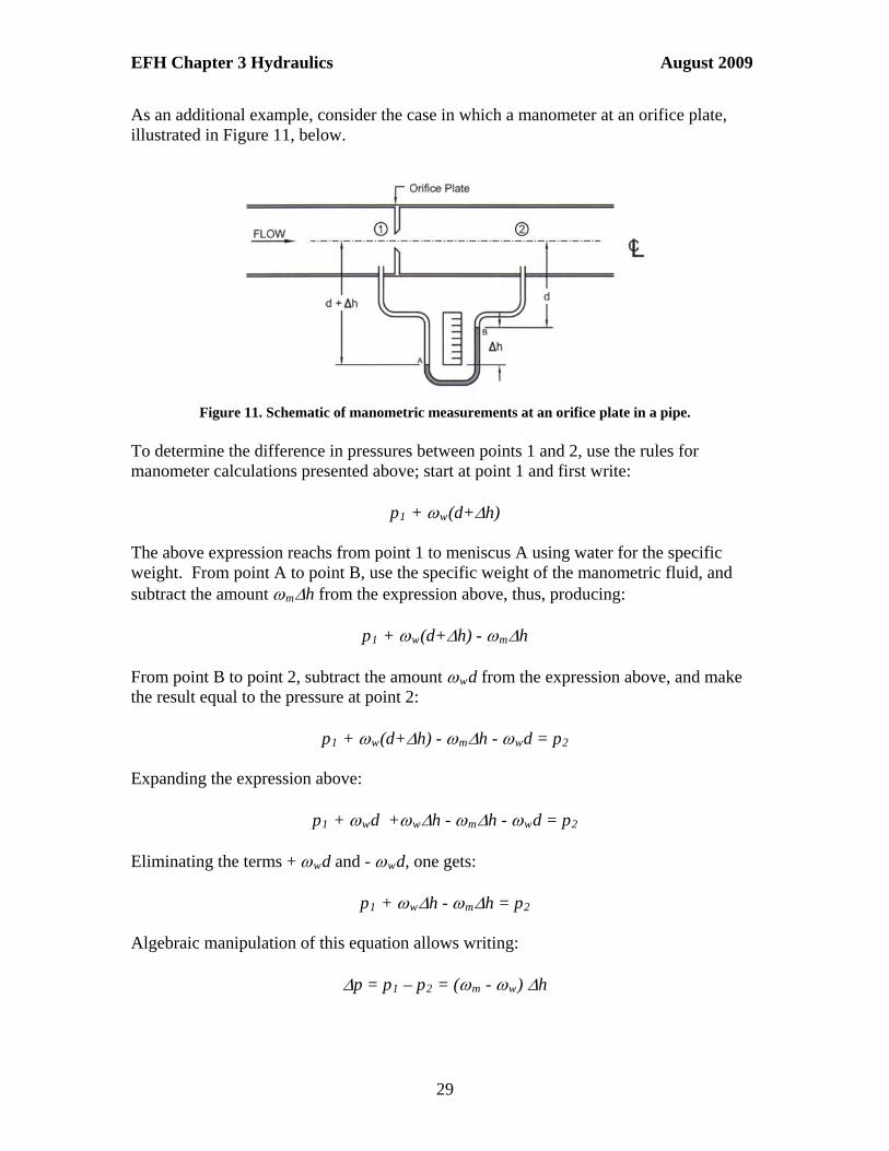
As an additional example, consider the case in which a manometer at an orifice plate, illustrated in Figure 11, below.
Figure 11. Schematic of manometric measurements at an orifice plate in a pipe.
To determine the difference in pressures between points 1 and 2, use the rules for manometer calculations presented above; start at point 1 and first write:
p1 + w(d+h) The above expression reachs from point 1 to meniscus A using water for the specific weight. From point A to point B, use the specific weight of the manometric fluid, and subtract the amount mh from the expression above, thus, producing:
p1 + w(d+h) - mh From point B to point 2, subtract the amount wd from the expression above, and make the result equal to the pressure at point 2:
p1 + w(d+h) - mh - wd = p2 Expanding the expression above:
p1 + wd +wh - mh - wd = p2 Eliminating the terms + wd and - wd, one gets:
p1 + wh - mh = p2 Algebraic manipulation of this equation allows writing:
p = p1 – p2 = (m - w) h
29

EFH Chapter 3 Hydraulics August 2009
The resulting equation can be simplified by introducing the specific gravity of the manometric fluid, i.e., m = Smw, thus:
p = wh (Sm -1) If w = 62.4 lb/ft3, h = 8 in = 8/12 ft = 0.666 ft, and Sm = 13.56 (for mercury), the difference in pressure, p is:
p = wh (Sm -1) = (62.4 lb/ft3)(0.666 ft)(13.56 - 1) = 521.97 lb/ft2 or
psiin
lbp 62.3
144
97.5212
Orifice plates may be used to measure flow in pipelines. The pressure difference, p, can be related to the pipeline discharge by calibration or by theoretical analysis. Examples of such analyses are presented in the next section. Deformation Manometers. Deformation manometers, such as the Bourdon manometer shown in the following figure, utilize the deformation of spiral tubes or of diaphragms to measure pressure. These manometers are calibrated by manufacturers or in the laboratory and provide a direct reading of the pressure at the manometric tap. Modern deformation manometers have digital readouts, making the reading of the pressure straightforward. The Bourdon manometer shown in Figure 12 has an analog scale, with the pressure marked by the pointer attached to the spiral tube located inside the manometer.
Figure 12. Deformation manometer (Bourdon manometer)
30

EFH Chapter 3 Hydraulics August 2009
0312 Forces on Submerged Plane Surfaces The calculation of the size, direction, and location of the forces on submerged surfaces is essential in the design of dams, bulkheads, water control gates, and other related appurtenances. Horizontal surface. The hydrostatic law indicates that pressure varies with depth. Thus, a horizontal surface within a liquid at rest is subject to the same pressure p over the entire surface, and the resultant force F on the surface is given by:
F = pA = hA [Eq. 15] where, A is the area of the surface.
Figure 13. Force on a submerged horizontal surface Figure 13 shows that the pressure on top of the horizontal surface is represented by vertical arrows of the same height pointing towards the surface. The pressure arrows and the horizontal surface form a three-dimensional figure known as the pressure prism. The resultant force vector on any surface coincides with the centroid (also referred to as the center of mass or center of gravity) of the pressure prism. The force on a horizontal surface will be vertical and applied to the centroid C of the surface as illustrated in Figure 14, below. The point of application of the force is referred to as the center of pressure P.
Figure 14. Point of application of a force on a submerged horizontal surface
31

EFH Chapter 3 Hydraulics August 2009
Example 2 – Hydrostatic force on horizontal area A circular tank 15 ft in diameter is filled with water to a depth of 2 ft. Determine the magnitude and location of the vertical force that the water applies on the tank bottom. The tank has a diameter D = 15 ft, therefore, the area of the tank bottom is that of a circle:
222
71.1764
)15(1416.3
4ft
ftDA
The magnitude of the pressure applied to the bottom of the tank can be calculated by using the specific weight of water, = 62.4 lb/ft3 and depth of the water in the tank, h = 2 ft:
p = h = (62.4 lb/ft3)(2 ft) = 124.8 lb/ft2 The magnitude of the force applied on the tank bottom is:
F = pA = (124.8 lb/ft2)(176.71 ft2) = 22053.41 lb The force is applied at the center of the circular bottom and is equivalent to the weight of the water. Inclined surface. For a surface located on an inclined plane, the pressure increases linearly from the top of the surface to the bottom of the surface. The magnitude of the force on the surface is calculated as:
F = pcA = hcA [Eq. 16] Where pc = hc is the pressure at the centroid of the figure. The force, F, is represented by the volume of the pressure prism.
Figure 15, below, shows the pressure distribution along an inclined surface and the resulting force on a rectangular region laid on the inclined surface. The rectangular region could represent a gate on the slope of a dam or dike. The inclined surface is located at an angle with respect to the horizontal. Alternatively, the slope can be indicated by the proportion zH(horizontal):1V(vertical) as shown in the figure. For the case illustrated in Figure 15, the angle is related to the slope by:
za
b 1)tan( [Eq. 17]
Figure 15 shows a system of coordinate axes, x and y, located on the inclined surface. The system is selected so that the x-axis is located along the free surface. Points on the inclined surface can be located by either their depth h or their y coordinate along the surface. These two distances are related by:
)sin( yh [Eq. 18]
32

EFH Chapter 3 Hydraulics August 2009
Point 1 is located at the top of the gate while point 2 is located at the bottom of the gate. The gate dimensions are B (width) and H (height). Point C represents the centroid of the gate, while point P represents the point of application of the hydrostatic force F on the gate, the center of pressure.
Figure 15. Pressure distribution, force, and center of pressure on an inclined surface. Unlike the case of a horizontal surface, the center of pressure on an inclined surface is located below the centroid of the surface along the plane of the surface, by a distance given by:
c
c
yA
Iy
[Eq. 19]
In this formula, yc is the location of the centroid of the surface measured from the free surface along the plane of the surface, and Ic is the moment of inertia of the surface with respect to a centroidal axis parallel to the x axis (i.e., an axis through point C). Thus, the center of pressure will be located at a distance
yp = yc + y = c
cc yA
Iy
[Eq. 20]
For the rectangular and circular figures of Figure 14, with the x axis representing the centroidal axis xc, the centroidal moments of inertia are the following:
Rectangular area: 3
12
1BHIc [Eq. 21]
33
EFH Chapter 3 Hydraulics August 2009
Circular area: 4
64DIc
[Eq. 22]
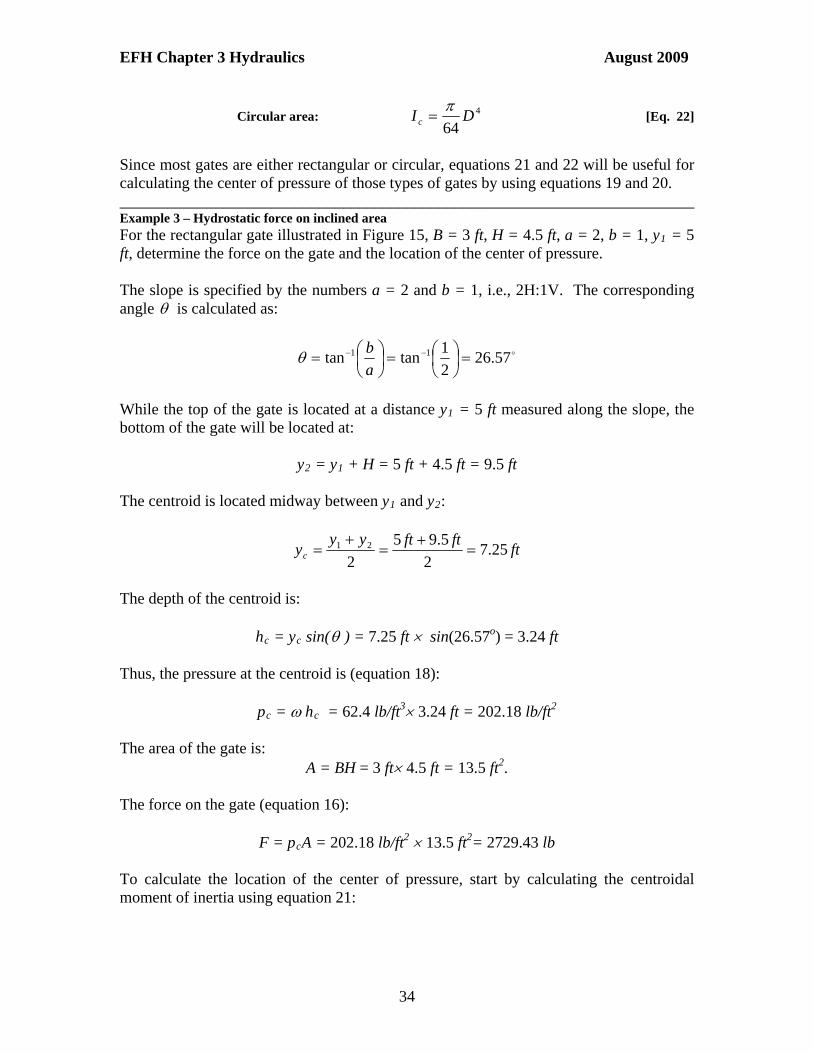
Since most gates are either rectangular or circular, equations 21 and 22 will be useful for calculating the center of pressure of those types of gates by using equations 19 and 20. ________________________________________________________________________ Example 3 – Hydrostatic force on inclined area For the rectangular gate illustrated in Figure 15, B = 3 ft, H = 4.5 ft, a = 2, b = 1, y1 = 5 ft, determine the force on the gate and the location of the center of pressure. The slope is specified by the numbers a = 2 and b = 1, i.e., 2H:1V. The corresponding angle is calculated as:
57.262
1tantan 11
a
b
While the top of the gate is located at a distance y1 = 5 ft measured along the slope, the bottom of the gate will be located at:
y2 = y1 + H = 5 ft + 4.5 ft = 9.5 ft The centroid is located midway between y1 and y2:
ftftftyy
yc 25.72
5.95
221
The depth of the centroid is:
hc = yc sin( ) = 7.25 ft sin(26.57o) = 3.24 ft Thus, the pressure at the centroid is (equation 18):
pc = hc = 62.4 lb/ft3 3.24 ft = 202.18 lb/ft2 The area of the gate is:
A = BH = 3 ft 4.5 ft = 13.5 ft2. The force on the gate (equation 16):
F = pcA = 202.18 lb/ft2 13.5 ft2= 2729.43 lb To calculate the location of the center of pressure, start by calculating the centroidal moment of inertia using equation 21:
34

EFH Chapter 3 Hydraulics August 2009
433 78.22)5.4(312
1
12
1ftftftBHIc
The distance between the centroid C and the center of pressure is calculated with equation 19:
ftftft
ft
yA
Iy
c
c 23.025.75.13
78.222
4
.
The center of pressure is located at the distance (equation 20):
yp = yc + y = 7.25 ft + 0.23 ft = 7.48 ft. And the depth of the center of pressure is (equation 18):
hp= yp sin() = 7.48 ft sin(26.56o) = 3.35 ft. ________________________________________________________________________ Vertical surface. In Figure 16, a rectangular surface of width B is located on a vertical plane and the free surface of the water reaches to a depth H.
Figure 16. Pressure prism (a) and force location (b) for a vertical rectangular surface The triangular distribution in Figure 16(b) represents the pressure distribution on the vertical surface. The pressure at the bottom is given by pB = H. The force F on the surface is equal to the volume of the pressure prism:
2
2
1
2
1BHBHpF B
[Eq. 23]
Using equations 20 and 21 and the area of this rectangular surface, A = BH, one can prove that the location of the center of pressure (point of application of the force) is given by:
35

EFH Chapter 3 Hydraulics August 2009
Hhy pp 3
2 [Eq. 24]
Thus, the force is applied at 2/3 of the depth measured from the surface, or 1/3 of the depth measured from the bottom as indicated in Figure 16 (b). Examples of this type surface include vertical gates and flashboards. ________________________________________________________________________ Example 4 – Hydrostatic force on vertical gate A wooden vertical gate with a width of 10 ft is used to close a canal. If the water depth on the gate is 2.5 ft, determine the hydrostatic force on the gate and its location. For this case B = 10 ft, H = 2.5 ft, and = 62.4 lb/ft3, thus, the force is (equation 23):
lbftftft
lbBHF 1950)5.2(104.62
2
1
2
1 23
2
The force is located at a distance from the surface (equation 24):
ftftHhy pp 67.15.23
2
3
2
________________________________________________________________________ The use of a spreadsheet application greatly facilitates calculation of forces on submerged plane surfaces. 0313 Buoyancy Forces Buoyancy is the upwards force experienced by solid bodies submerged in liquids or gases. Archimedes’ principle states that a solid body submerged in a fluid (i.e., liquid or gas) experiences a vertical upward force (the buoyancy force) equal to the weight of the volume of fluid it displaces. Thus, the buoyancy force, FB, experienced by a body of volume V submerged in a fluid of specific weight , is given by:
FB = V [Eq. 25]
0313.1 Buoyancy Applications
A solid body submerged is also acted upon by its own weight, which can be calculated as
W = sV [Eq. 26] where s is the specific weight (weight per unit volume) of the solid material. A solid body fully submerged in water is subject to its own weight W (equation 26) and the buoyancy force (equation 25) exerted by the water on the solid body. Figure 16
36
EFH Chapter 3 Hydraulics August 2009
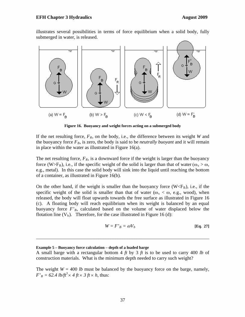
illustrates several possibilities in terms of force equilibrium when a solid body, fully submerged in water, is released.
erence between its weight W and e buoyancy force FB, is zero, the body is said to be neutrally buoyant and it will remain
e solid is larger than that of waters > , .g., metal). In this case the solid body will sink into the liquid until reaching the bottom
ced by an equal uoyancy force F’B, calculated based on the volume of water displaced below the
flotation line (Vb). Therefore, for
________________________
small barge with a rectangular bottom 4 ft by 3 ft is to be used to carry 400 lb of
he weight W = 400 lb must be balanced by the buoyancy force on the barge, namely, F’B = 62.4 lb/ft3 4 ft 3 ft h, thus:
Figure 16. Buoyancy and weight forces acting on a submerged body If the net resulting force, FR, on the body, i.e., the diffthin place within the water as illustrated in Figure 16(a). The net resulting force, FR, is a downward force if the weight is larger than the buoyancy force (W>FB), i.e., if the specific weight of theof a container, as illustrated in Figure 16(b). On the other hand, if the weight is smaller than the buoyancy force (W<FB), i.e., if the specific weight of the solid is smaller than that of water (s < , e.g., wood), when released, the body will float upwards towards the free surface as illustrated in Figure 16 (c). A floating body will reach equilibrium when its weight is balanb
the case illustrated in Figure 16 (d):
W = F’B = Vb [Eq. 27]
________________________________________________ Example 5 – Buoyancy force calculation – depth of a loaded barge Aconstruction materials. What is the minimum depth needed to carry such weight? T
37

EFH Chapter 3 Hydraulics August 2009
inftlb
h 1253.053.0400
= 6.36 in ftftftlb 34/4.62 3
e minimum length L must be L = d + 1ft to allow for
he factor of safety, F.S. for this case, is defined as the ratio of the net downward forces (Fd) to the net upward forces (Fu):
________________________________________________________________________ Example 6 – Buoyancy force calculation – flotation safety of CMP inlet The figure below shows a cylindrical CMP (corrugated metal pipe) vertical inlet of diameter d = 36 in = 3 ft, supported on a square footing of side length L, and height hb = 13.5 in = 1.125 ft The inlet footing is covered with saturated soil up to a depth h = 7 ft which corresponds to the level of the inlet crest. The CMP inlet weighs CMP = 38 lb/ft, the buoyant weight of saturated soil on the footing is SS = 60 lb/ft3, and the concrete in the footing weighs C = 150 lb/ft3. Determine the size L of footing required to make the CMP inlet safe from flotation with a factor of safety F.S.= 1.5. Assume that there is no frictional resistance between the inlet walls and the surrounding soil, and that no shear orces act on the outlet conduit. Thf
placement of reinforcing steel bars outside of the inlet with 3 in concrete cover and 2 in clearance between bars and inlet. T
u
d
FSF
F
..
ere, , indicates summatioH
1n of forces. By requiring that the factor of safety be F.S. =
.5, the downward forces are 50% larger than the upward forces ensuring that the inlet will be safe from flotation.
38

EFH Chapter 3 Hydraulics August 2009
Using the minimum length of footing:
L = d + 1ft = 3 ft + 1 ft = 4 ft The downward forces in this problem include the weight of the inlet, WCMP, the buoyant weight of saturated soil, WSS, and the weight of footing, WC. With the minimum length, these forces are calculated as follows:
WCMP = CMP (h+hb) = 38 lb/ft ×(7 ft + 1.125 ft) = 308.75 lb
WSS = SS (L2h – d2/4 h) = 60 lb/ft3 × ((4 ft)2-3.1416× (3ft)2/4) × (7 ft ) = 3,751.19 lb
WC = CL2hb = 150 lb/ft3×(4 ft)2×1.125 ft = 2,700 lb Thus,
Fd = WCMP + WSS + WC = 308.75 lb + 3,751.19 lb + 2,700 lb = 6,759.94 lb The upward forces include the buoyancy forces on the riser, FBCMP, and on the footing, FBC, which are calculated as:
FBCMP = w (d2/4) h = 62.4 lb/ft3× (3.1416×(3 ft)2/4) ×7 ft = 3,087.56 lb
FBC = w L2hb = 62.4 lb/ft3× (4 ft)2×1.125 ft = 1,123.2 lb
39

EFH Chapter 3 Hydraulics August 2009
Thus,
Fu = FBCMP +FBC =3,087.56 lb + 1,123.2 lb = 4,210.76 lb The factor of safety for a side of footing L = 4 ft is:
5.161.1lb 4,210.76
lb 6,759.94..
u
d
F
FSF
Since the factor of safety calculated is larger than 1.5 the CMP inlet should be safe for buoyancy. If F.S. < 1.5, try a larger footing side length or height, and recalculate the sum of forces and the factor of safety until it is larger than the required value of 1.5. ________________________________________________________________________ 0315 Hydrokinetics Hydrokinetics is the study of fluids in motion. Motion in fluids is produced by the action of forces. For example, in pressurized pipelines pressure forces act as the driving forces in the flow, whereas, in open channel flow, it is the weight of water mass (gravity forces) that produces the motion. In both cases, friction between the water and the walls of the pipe or channel act as opposing forces. In steady flows, driving and opposing forces are in equilibrium. The analysis of fluids in motion typically requires the determination of flow quantities such as discharge or velocity, or the determination of a linear quantity such as pipe diameter or flow depth in open channel flow. The determination of energy or head losses is also an important aspect of the analysis of fluids in motion. These analyses have practical applications in the operation of devices or systems through which fluids (water) flow, for example, irrigation pipes, outlet works from dams, and irrigation canals. The principles of flow continuity and of conservation of energy are used to analyze fluids in motion. 0316 Flow Continuity The equation of continuity represents a statement of conservation of mass in fluid flow. Consider, for example, a steady flow in a closed conduit of varying cross-section as shown in Figure 18 below. Let Q be the discharge through the conduit. The equation of continuity for steady flow (i.e., Q = constant) states that:
Q = V1A1 = V2A2 = V3A3 [Eq. 28] where V1, V2, and V3 represent the flow velocities at sections 1, 2, and 3 respectively. The areas of the corresponding cross-sections are A1, A2, and A3.
40

EFH Chapter 3 Hydraulics August 2009
Figure 18. Flow continuity in a pipe expansion. The cross-sectional area of a circular pipe of diameter D is given by:
4
2DA
[Eq. 29]
And the discharge can be written as:
4
2DVVAQ
[Eq. 30]
Knowing the discharge Q, the velocity V in a circular conduit of diameter D can be calculated as:
2
4
D
QV
[Eq. 31]
In units of the English System, the velocity V is given in ft/s (or fps), while the discharge Q is given in ft3/s or cfs. Using the International System, the velocity V is given in m/s and the discharge Q is given in m3/s. Other units of discharge in the English System include gal/min (or gpm) and gal/day (or gpd), which are commonly used in water supply applications. In the operation of large reservoirs, for example, the use of acre-foot/day as a unit of discharge is not uncommon. In the International System one could also use m3/min or m3/day for large discharge operations, while the units of liters/s or liters/min are used for small discharges. ________________________________________________________________________ Example 7 – Equation of continuity in a pipe - discharge and velocity calculation Suppose that in the pipeline of Figure 18 the diameters are D1 = 0.25 ft (3 in), D2 = 0.50 ft (6 in), and D3 = 0.75 ft (9 in), and that the velocity at section 3 is measured to be V3 = 0.5 fps. Find the velocities in sections 1 and 2 and the discharge. The discharge is calculated as:
41

EFH Chapter 3 Hydraulics August 2009
cfsft
sftD
VQ 22.04
)75.0(1416.3/5.0
4
223
3
The velocities at sections 1 and 2 are, therefore, calculated as:
fpsft
sft
D
QV 48.4
)25.0(1416.3
/22.0442
3
21
1
and
fpsft
sft
D
QV 12.1
)5.0(1416.3
/22.0442
3
22
2
________________________________________________________________________ A branching pipeline in which a pipe of diameter D1 splits into two pipelines with diameters D2 and D3 is shown below. Continuity requires that the discharges through sections 2 and 3 add to equal the discharge through section 1:
Q1 = Q2 + Q3 [Eq. 32]
Figure 19. Schematic of flow in branching pipelines.
In terms of areas and velocities, the continuity equation for the branching pipe case is written as:
V1A1 = V2A2 + V3A3 [Eq. 33] Replacing the areas in terms of the diameters:
444
23
3
22
2
21
1
DV
DV
DV
[Eq. 34]
Simplifying:
42

EFH Chapter 3 Hydraulics August 2009
V1D1
2 = V2D22 + V3D3
2 [Eq. 35]
_______________________________________________________________________ Example 8 – Equation of continuity – velocity and discharge calculation in branching pipeline A 12-in-diameter pipeline carrying water at a velocity of 3.5 fps branches into a 6-in-diameter pipeline and a 9-in-diameter pipeline. If the velocity in the 6-in pipeline is measured to be 4.0 fps, what is the velocity in the 9-in pipeline, and what is the total discharge through the 12-in pipeline? Using D1 = 12 in = 1 ft, V1 = 3.5 fps, D2 = 6 in = 0.5 ft, V2 = 4.0 fps, and D3 = 9 in = 0.75 ft, find V3 and Q1. From equation 35, i.e., V1D1
2 = V2D22 + V3D3
2, it follows that:
fpsft
ftfpsftfps
D
DVDVV 44.4
)75.0(
)5.0(0.4)1(5.32
22
23
222
211
3
The discharge through section 1 is:
cfsft
fpsD
VQ 75.24
)1(1416.35.3
4
221
11
________________________________________________________________________ The equation of continuity can also be applied to flow in open channels. Consider the flow in an open channel with a non-symmetric trapezoidal cross-section as illustrated in the figure below.
Figure 20. Non-symmetric trapezoidal cross-section in an open channel flow.
This cross-section is characterized by the bottom width b, the side slopes z1 and z2, and the flow depth d. The side slopes are interpreted as z1 H:1V, i.e., z1 units horizontal to 1 unit vertical. The top width T is the length of the free surface at the cross-section. For the non-symmetric trapezoidal cross-section shown above, the top width is given by
T = b + (z1+z2)d [Eq. 36] and the area is calculated as the average of trapezoid’s bases, b and T, multiplied by the height of the trapezoid, d :
ddzz
bdbT
A
2
)2
( 21 [Eq. 37]
43
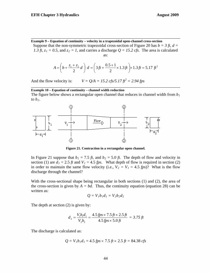
EFH Chapter 3 Hydraulics August 2009
________________________________________________________________________ Example 9 – Equation of continuity – velocity in a trapezoidal open-channel cross-section Suppose that the non-symmetric trapezoidal cross-section of Figure 20 has b = 3 ft, d = 1.3 ft, z1 = 0.5, and z2 = 1, and carries a discharge Q = 15.2 cfs. The area is calculated
as:
221 17.53.13.12
15.03
2ftftftftdd
zzbA
And the flow velocity is: V = Q/A = 15.2 cfs/5.17 ft2 = 2.94 fps ________________________________________________________________________ Example 10 – Equation of continuity – channel width reduction The figure below shows a rectangular open channel that reduces in channel width from b1 to b2.
Figure 21. Contraction in a rectangular open channel.
In Figure 21 suppose that b1 = 7.5 ft, and b2 = 5.0 ft. The depth of flow and velocity in section (1) are d1 = 2.5 ft and V1 = 4.5 fps. What depth of flow is required in section (2) in order to maintain the same flow velocity (i.e., V2 = V1 = 4.5 fps)? What is the flow discharge through the channel? With the cross-sectional shape being rectangular in both sections (1) and (2), the area of the cross-section is given by A = bd. Thus, the continuity equation (equation 28) can be written as:
Q = V1b1d1 = V2b2d2 The depth at section (2) is given by:
ftfps
ftftfps
bV
dbVd
0.55.4
5.25.75.4
22
1112
= 3.75 ft
The discharge is calculated as:
Q = V1b1d1 = 4.5 fps 7.5 ft 2.5 ft = 84.38 cfs
44

EFH Chapter 3 Hydraulics August 2009
________________________________________________________________________ Example 11 – Equation of continuity – rectangular open channel diversion Figure 22 shows a rectangular channel of width b1 from which water is diverted through a lateral rectangular channel of width b3. The section of the main channel downstream from the diversion has a width b2 = b1.
Figure 22. Rectangular open channel diversion.
Using b1 = b2 = 10 ft, d1 = 4.0 ft, V1 = 1.2 fps, d2 = 3.5 ft, b3 = 5.0 ft, d3 = 2.5 ft, and V3 = 0.6 fps, determine the flow velocity at section 2, V2, as well as, the discharges through sections 1, 2, and 3. For a branching channel as shown in Figure 22, continuity requires that Q1 = Q2 + Q3, i.e., V1b1d1 = V2b2d2 + V3b3d3. Thus, the velocity at section 2 is: V2 = (V1b1d1 - V3b3d3)/(b2d2) = (1.2 fps10 ft4 ft – 0.6 fps5 ft2.5 ft)/(10 ft3.5 ft) =
V2 = 1.157 fps The discharges through the three sections are calculated as follows:
Q1 = V1b1d1 = 1.2 fps10 ft4 ft = 48 cfs
Q2 = V2b2d2 = 1.157 fps10 ft3.5 ft = 40.5 cfs
Q3 = V3b3d3 = 0.6 fps5 ft2.5 ft = 7.5 cfs ________________________________________________________________________ 0317 Conservation of Energy In the analysis of fluid flow, three types of energy are typically considered: potential or elevation energy, pressure energy, and kinetic energy. Figure 23, below, illustrates these concepts using a simple reservoir-sprinkler system.
45

EFH Chapter 3 Hydraulics August 2009
Figure 23. Flow energies illustrated with a simple reservoir-sprinkler system
The elevation of the water in the reservoir represents potential energy since it is this elevation that provides the available energy for the system. As the water flows through the pipe and is discharged through the sprinkler, it acquires motion which converts some of the potential energy into kinetic energy (energy of motion). Also, at the sprinkler, a measurable pressure exists that is related to pressure energy at that particular point.
In a flowing fluid system as the one illustrated above, energy is conserved as it is converted from one type of energy (potential) into another (pressure or kinetic). In fluid flow these energies are typically converted to energy heads that can be easily visualized as in the potential energy head of Figure 23. The description of these energy heads follows in the next sections.
0317.1 Potential Energy
Potential energy is the ability of a water mass to perform work because of the elevation of that mass of water with respect to an arbitrary datum line or reference level. A mass of weight W, at an elevation of z feet, has a potential energy equal to Wz (ft-lb) with respect to the datum. The elevation head, z, expresses not only a linear quantity (ft), but also energy per unit weight, i.e., ft-lb/lb = ft.
0317.2 Pressure Energy
Pressure energy at a point of a fluid flow is produced by the local pressure at the point. This pressure could be the result of a pumping action in a pipeline or of the weight of water above a certain point in open channel flow. The pressure head (pressure energy per unit weight) in pipeline flow is calculated as p/, pressure divided by the specific weight of water. In open channel flow applications, the pressure head is equal to the flow depth, d, and the pressure distribution is assumed to be hydrostatic.
0317.3 Kinetic Energy
The kinetic energy (K) of a mass (M) of fluid moving at a velocity (V) is given by K =1/2 MV2. Since its weight is W = Mg, the kinetic energy per unit weight is calculated as:
46

EFH Chapter 3 Hydraulics August 2009
g
V
Mg
MV
W
Khv 2
2
12
2
[Eq. 38]
Where g is the acceleration of gravity (g = 32.2 ft/s2). The term hv in equation 38 is referred to as the velocity head. The total energy head, H, is the sum of the potential energy head (z), the pressure head (p/ or d), and the velocity head (V2/2g). All three forms of energy head may be expressed as a linear quantity (ft), or as energy per unit weight (ft-lb/lb). Energy heads in pipe flow. Figure 24 illustrates the three different energy heads applied to pipe flow. Notice that, typically, the potential energy head (elevation) in a pipe flow is referenced at the centerline of the pipe. The pressure head is measured from the pipe centerline, and the distance from the datum to the top of the pressure head represents the piezometric head:
p
zh [Eq. 39]
The difference between the total energy head and the piezometric represents the kinetic energy. The total energy in a pipe flow is given by:
g
Vpz
g
VhH
22
22
[Eq. 40]
The line representing the values of the total head, H, as function of position x along the pipeline is referred to as the Energy Line (E.L.), while that representing the values of the piezometric head, h, is referred to as the Hydraulic Grade Line (H.G.L.). Energy losses, hf, are the losses due to friction between sections (1) and (2).
Figure 24. Energy heads in pipe flow.
47
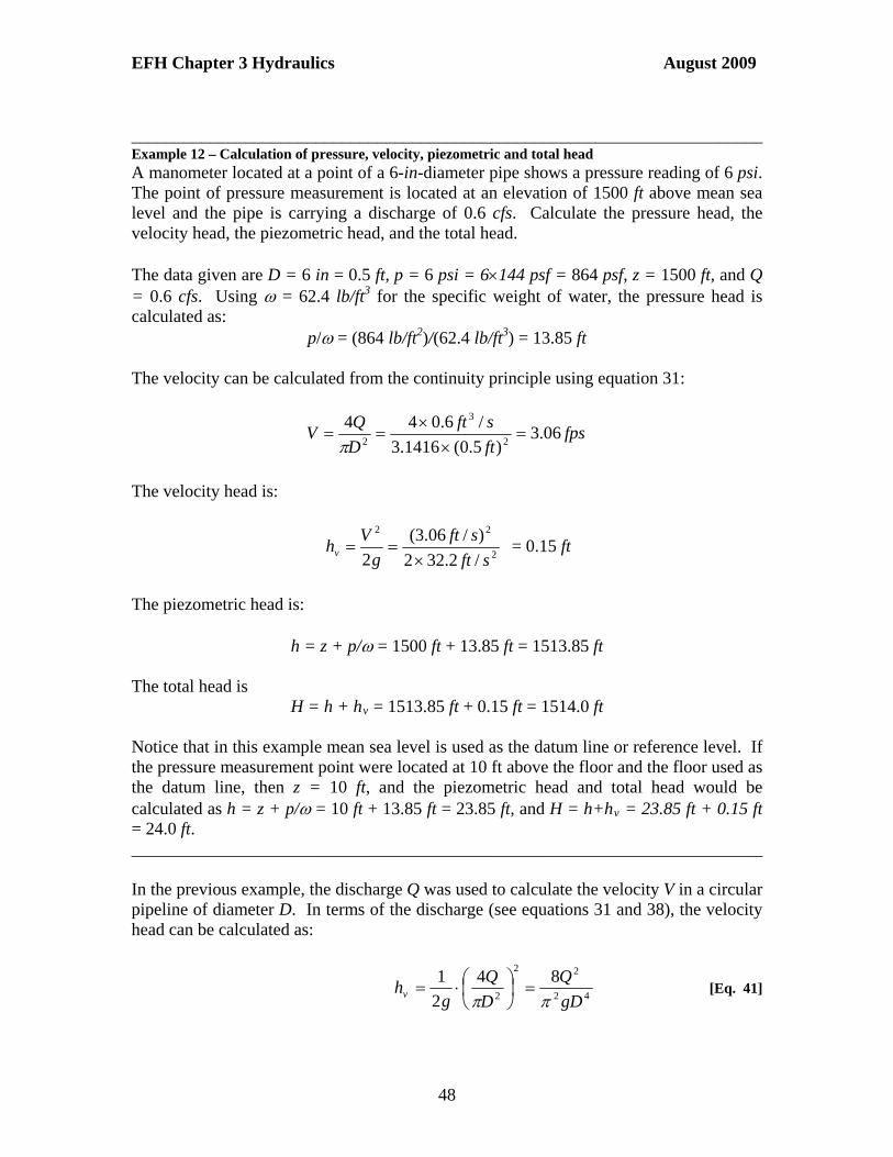
EFH Chapter 3 Hydraulics August 2009
________________________________________________________________________ Example 12 – Calculation of pressure, velocity, piezometric and total head A manometer located at a point of a 6-in-diameter pipe shows a pressure reading of 6 psi. The point of pressure measurement is located at an elevation of 1500 ft above mean sea level and the pipe is carrying a discharge of 0.6 cfs. Calculate the pressure head, the velocity head, the piezometric head, and the total head. The data given are D = 6 in = 0.5 ft, p = 6 psi = 6144 psf = 864 psf, z = 1500 ft, and Q = 0.6 cfs. Using = 62.4 lb/ft3 for the specific weight of water, the pressure head is calculated as:
p/ = (864 lb/ft2)/(62.4 lb/ft3) = 13.85 ft The velocity can be calculated from the continuity principle using equation 31:
fpsft
sft
D
QV 06.3
)5.0(1416.3
/6.0442
3
2
The velocity head is:
2
22
/2.322
)/06.3(
2 sft
sft
g
Vhv
= 0.15 ft
The piezometric head is:
h = z + p/ = 1500 ft + 13.85 ft = 1513.85 ft
The total head is
H = h + hv = 1513.85 ft + 0.15 ft = 1514.0 ft Notice that in this example mean sea level is used as the datum line or reference level. If the pressure measurement point were located at 10 ft above the floor and the floor used as the datum line, then z = 10 ft, and the piezometric head and total head would be calculated as h = z + p/ = 10 ft + 13.85 ft = 23.85 ft, and H = h+hv = 23.85 ft + 0.15 ft = 24.0 ft. ________________________________________________________________________ In the previous example, the discharge Q was used to calculate the velocity V in a circular pipeline of diameter D. In terms of the discharge (see equations 31 and 38), the velocity head can be calculated as:
42
22
2
84
2
1
gD
Q
D
Q
ghv
[Eq. 41]
48

EFH Chapter 3 Hydraulics August 2009
Using this result the total energy head in a pipeline of diameter D carrying a discharge Q is given by:
42
28
gD
QpzH
[Eq. 42]
________________________________________________________________________ Example 13 – Calculation of total head A 2-in diameter pipeline carries a flow discharge of 0.3 cfs. At a point of the flow, located at an elevation of 2.5 ft above the floor, the pressure is measured to be 2 psi. What is the total energy head at that point? Given D = 2 in = 2/12 ft = 0.166 ft, Q = 0.3 cfs, z = 2.5 ft, p = 2 psi = 2144 psf = 288 psf, and, with = 62.4 lb/ft3, the total head is:
ftftsft
sft
ftlb
ftlbft
gD
QpzH 1.10
)166.0(/2.321416.3
)/3.0(8
/4.62
/2885.2
8422
23
3
2
42
2
________________________________________________________________________ Energy heads in open channel flow. The energy heads for open channel flow are illustrated in Figure 25. The elevation head, z, refers to the location of the channel bed, while the pressure head is represented by the flow depth d. The sum of the potential energy head (z) and the flow depth (d) in open channel flow represents the water surface elevation or stage, WS = z + d. The difference between the total energy and the water surface elevation is the velocity head. The total energy in a channel flow is given by:
H = WS + V2/2g = z + d + V2/2g [Eq. 43] Of the total energy, the quantity called the specific energy is:
E = d + V2/2g [Eq. 44] This quantity represents the flow energy measured with respect to the channel bed at a given cross-section.
49
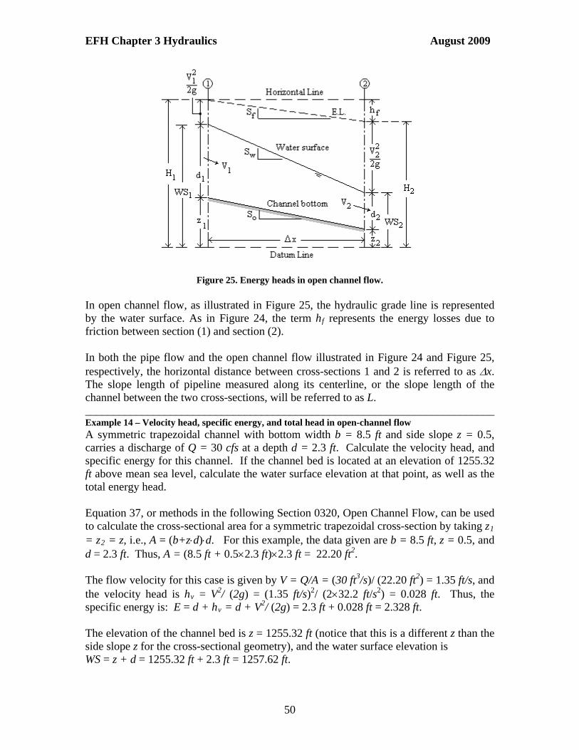
EFH Chapter 3 Hydraulics August 2009
Figure 25. Energy heads in open channel flow. In open channel flow, as illustrated in Figure 25, the hydraulic grade line is represented by the water surface. As in Figure 24, the term hf represents the energy losses due to friction between section (1) and section (2). In both the pipe flow and the open channel flow illustrated in Figure 24 and Figure 25, respectively, the horizontal distance between cross-sections 1 and 2 is referred to as x. The slope length of pipeline measured along its centerline, or the slope length of the channel between the two cross-sections, will be referred to as L. ________________________________________________________________________ Example 14 – Velocity head, specific energy, and total head in open-channel flow A symmetric trapezoidal channel with bottom width b = 8.5 ft and side slope z = 0.5, carries a discharge of Q = 30 cfs at a depth d = 2.3 ft. Calculate the velocity head, and specific energy for this channel. If the channel bed is located at an elevation of 1255.32 ft above mean sea level, calculate the water surface elevation at that point, as well as the total energy head. Equation 37, or methods in the following Section 0320, Open Channel Flow, can be used to calculate the cross-sectional area for a symmetric trapezoidal cross-section by taking z1 = z2 = z, i.e., A = (b+zd)d. For this example, the data given are b = 8.5 ft, z = 0.5, and d = 2.3 ft. Thus, A = (8.5 ft + 0.52.3 ft)2.3 ft = 22.20 ft2. The flow velocity for this case is given by V = Q/A = (30 ft3/s)/ (22.20 ft2) = 1.35 ft/s, and the velocity head is hv = V2/ (2g) = (1.35 ft/s)2/ (232.2 ft/s2) = 0.028 ft. Thus, the specific energy is: E = d + hv = d + V2/ (2g) = 2.3 ft + 0.028 ft = 2.328 ft. The elevation of the channel bed is z = 1255.32 ft (notice that this is a different z than the side slope z for the cross-sectional geometry), and the water surface elevation is WS = z + d = 1255.32 ft + 2.3 ft = 1257.62 ft.
50

EFH Chapter 3 Hydraulics August 2009
The total energy head is calculated as H = z + E = 1255.32 ft + 2.328 ft = 1257.65 ft. ________________________________________________________________________
0317.4 Equation of Energy and Bernoulli’s Principle
In the diagrams shown in Figure 24 and Figure 25, water flows from section (1) to section (2). The diagrams indicate that the total energy head at the upstream section (1) is larger than the total energy head at the downstream section (2), i.e., H1 > H2. The difference represents the energy losses hf due to friction as the water moves from section (1) to section (2). The law of conservation of energy for both pipe flow and open channel flow can be written as:
H1 = H2 + hf [Eq. 45]
where hf represents the energy losses due to friction between sections (1) and (2).
Specifically, for the pipe flow case illustrated in Figure 24:
f h g
V h
g
V h
22
22
2
21
1 [Eq. 46]
or
f h g
V
p z
g
V
pz
22
222
2
211
1 [Eq. 47]
The law of conservation of energy for open channel flow, as illustrated in Figure 25, is written as:
f h g
V WS
g
V WS
22
22
2
21
1 [Eq. 48]
or
f h g
V d z
g
V dz
22
22
22
21
11 [Eq. 49]
In some instances of pipe flow (or other enclosed flow), the fluid can be assumed to be ideal and the friction losses are zero. This is an assumption of the Bernoulli’s principle, and the equation of energy (Bernoulli’s equation) can be written as:
g
V
p z
g
V
pz
22
222
2
211
1
[Eq. 50]
In the most general case of pipe flow, however, friction losses, hf, and local losses, hL, (due to the presence of appurtenances in the pipe) must be included. Examples of appurtenances include elbows and valves. Taking into account both friction and local losses, the energy equation for pipelines can be written as:
51

EFH Chapter 3 Hydraulics August 2009
Lf h h g
V
p z
g
V
pz
22
222
2
211
1 [Eq. 51]
________________________________________________________________________ Example 15 – Bernoulli’s principle applied to sluice gate flow The figure below shows a schematic of a sluice gate in a rectangular channel of width b. The energy line (E.L.) and the hydraulic grade line (H.G.L.) are also depicted. The horizontal energy line suggests no energy losses as the flow passes under the gate. Determine the discharge Q if the upstream and downstream depths are measured as 3.5 ft and 1.0 ft and the channel width, b, is 10 ft.
Figure 26. Sluice gate flow.
Since there are no energy losses and a horizontal bed, Bernoulli’s equation reduces to:
g
V d
g
V d
22
22
2
21
1
Writing the velocity head in terms of the discharge, V1
2/2g = Q2/(2gA12) and V2
2/2g = Q2/(2gA2
2), and using A1 = bd1, A2 = bd2, Bernoulli’s equation becomes:
dgb
Q d
dgb
Q d
22
2
2
221
2
2
1 22
Solving for Q and simplifying the result produces:
2121
2
dd
gdbdQ
cfsftft
sftftftft
dd
gdbdQ 41.132
0.15.3
/2.3220.15.310
2 2
2121
52

EFH Chapter 3 Hydraulics August 2009
________________________________________________________________________ Example 16– Energy equation in pipelines Let the diagram in Figure 24 represent a pipeline of constant diameter D = 6 in carrying a discharge Q = 0.5 cfs. Let the elevations of points 1 and 2 be given by z1 = 7 ft and z2 = 12.5 ft with respect to an arbitrary horizontal reference level (datum line). The pressure at point 2 is measured to be p2 = 15.2 psi. Calculate the velocity head for this pipe flow. If the energy loss in the pipeline is estimated to be hf = 15 ft, what is the pressure at point 1, p1 (psi)? Use = 62.4 lb/ft3 for the specific weight of water. Since the pipeline has a constant diameter, D = 6 in = 6/12 ft = 0.5 ft, the velocities at points 1 and 2 are the same (equation 31):
V1 = V2 = V = 4Q/(D2) = 4 (0.5 ft3/s)/(3.1416(0.5 ft)2) = 2.55 fps The velocity head throughout the pipeline is the same and equal to (equation 38):
hv = V2/2g = (2.55 ft/s)2/(2 32.2 ft/s2) = 0.10 ft Also, the velocity head can be calculated in terms of the discharge as (equation 41):
ftftsft
sft
gD
Qhv 10.0
)5.0(/2.321416.3
)/5.0(88422
23
42
2
The equation of energy for the case of Figure 24 is given by (equation 47):
f h g
V
p z
g
V
pz
22
222
2
211
1
Since the velocities are the same (V1 = V2), the equation simplifies to:
f h p
z p
z
22
11
From which the pressure head at point 1 is solved for, as:
p1/ = z2 – z1+ p2/ + hf = 12.5 ft – 7 ft + (15.2144 lb/ft2)/(62.4 lb/ft3) + 15 ft
p1/ = 55.58 ft
Thus, the pressure at point 1 is:
p1 = 55.58 ft62.4 lb/ft3 = 3468.19 lb/ft2 = 3468.19/144 psi = 24.08 psi
53

EFH Chapter 3 Hydraulics August 2009
________________________________________________________________________ Example 17 - Energy equation in open channel flow Suppose that Figure 25 represents a reach in an open channel flow with a rectangular cross-section of width b = 12.5 ft. The depth of flow at sections 1 and 2 are measured to be d1 = 4.7 ft and d2 = 3.8 ft, respectively, and the velocity at section 1 is V1 = 4.2 fps. The channel bed elevations at sections 1 and 2 are given as z1 = 25 ft and z2 = 22.5 ft. Calculate the flow discharge Q and the energy loss, hf, between sections 1 and 2. The area at section 1 is A1 = bd1 = 12.5 ft 4.7 ft = 58.75 ft2, and the flow discharge is Q = V1A1 = 4.2 ft/s 58.75 ft2 = 246.75 cfs. The area at section 2 is A2 = bd2 = 12.5 ft 3.8 ft = 47.50 ft2, and the flow velocity at that location is V2 = Q/A2 = (246.75 ft3/s) / (47.50 ft2) = 5.19 fps. The energy equation for the case of Figure 25 is written as (equation 49):
f h g
V d z
g
V dz
22
22
22
21
11
From which:
hf = (z1 + d1 + V12/2g) – (z2 + d2 + V2
2/2g) =
= [(25 ft + 4.7 ft + (4.2 ft/s)2/(232.2 ft/s2)] - [(22.5 ft + 3.8 ft + (5.19 ft/s)2/(232.2 ft/s2)]
= 3.26 ft ________________________________________________________________________
0317.5 Hydraulic and Energy Gradients
Figure 24 and Figure 25 represent the variation of the different energy heads in pipe flow and open channel flow, respectively. In both types of flow the line joining the total energy heads along the pipeline or open channel is the energy line (E.L.). In pipe flow, the line joining the piezometric heads along the pipeline (h = z + p/) is the hydraulic grade line (H.G.L.), whereas, in open-channel flow the water surface represents the hydraulic grade line. For both pipe flow and open channel flow the energy gradient, or slope of the energy line, Sf, is defined as the rate of friction head loss, hf, per unit length, L, of the pipeline or open channel:
L
HH
L
hS f
f21 [Eq. 52]
However, in open channel flow, the channel bed slope, So, is typically very small such that the length of the channel, L, is approximately equal to the horizontal distance x, i.e., L x. The energy gradient for open channels, therefore, can be defined as:
54

EFH Chapter 3 Hydraulics August 2009
x
HH
x
hS f
f
21 [Eq. 53]
The hydraulic gradient is the slope of the hydraulic grade line. For pipe flow, such gradient is defined as the change in piezometric head per unit length of pipe:
L
hhSh
21 [Eq. 54]
Whereas, for an open channel flow the hydraulic gradient is the water surface slope. This slope is the change in water surface elevation, WS, per unit of horizontal distance along the channel path:
x
WSWSSw
21 [Eq. 55]
________________________________________________________________________ Example 18– Hydraulic and energy gradients in pipe flow The diameter of a 10-ft-long pipeline tapers from 1-ft-diameter at section 1 to 0.5-ft-diameter at section 2 of Figure 24. Let the pressure at section 1 be p1 = 6.0 psi and that at section 2 be p2 = 5.5 psi. The pipeline is laid so that point 1 is at elevation z1 = 12.5 ft and z2 = 6.2 ft. If the pipeline is carrying a flow Q = 1.5 cfs, determine the friction loss, hf, the hydraulic gradient, Sh, and the energy gradient, Sf, for the flow. For L = 10 ft, D1 = 1 ft, D2 = 0.5 ft, p1 = 6.0 psi, p2 = 5.5 psi, z1 = 12.5 ft, and z2 = 6.2 ft, the velocities are:
V1 = 4Q/(D12) = (41.5 ft3/s)/(3.1416(1ft)2) = 1.91 fps
and
V2 = 4Q/(D22) = (41.5 ft3/s)/(3.1416(0.5 ft)2) = 7.64 fps
The piezometric or pressure heads at sections 1 and 2 are:
ftftlb
ftlbft
pzh 35.26
/4.62
/1440.65.12
3
21
11
and
ftftlb
ftlbft
p z h 89.18
/4.62
/1445.52.6
3
22
22
The difference in piezometric heads is:
h = h1 – h2 = 26.35 ft – 18.89 ft = 7.46 ft
55
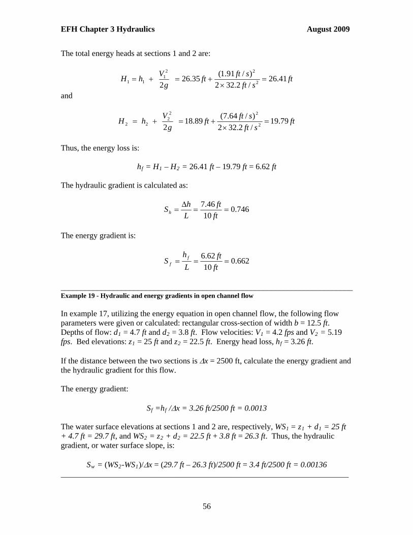
EFH Chapter 3 Hydraulics August 2009
The total energy heads at sections 1 and 2 are:
ftsft
sftft
g
V hH 41.26
/2.322
)/91.1(35.26
2 2
221
11
and
ftsft
sftft
g
V h H 79.19
/2.322
)/64.7(89.18
2 2
222
22
Thus, the energy loss is:
hf = H1 – H2 = 26.41 ft – 19.79 ft = 6.62 ft
The hydraulic gradient is calculated as:
746.010
46.7
ft
ft
L
hSh
The energy gradient is:
662.010
62.6
ft
ft
L
hS f
f
________________________________________________________________________ Example 19 - Hydraulic and energy gradients in open channel flow In example 17, utilizing the energy equation in open channel flow, the following flow parameters were given or calculated: rectangular cross-section of width b = 12.5 ft. Depths of flow: d1 = 4.7 ft and d2 = 3.8 ft. Flow velocities: V1 = 4.2 fps and V2 = 5.19 fps. Bed elevations: z1 = 25 ft and z2 = 22.5 ft. Energy head loss, hf = 3.26 ft. If the distance between the two sections is x = 2500 ft, calculate the energy gradient and the hydraulic gradient for this flow. The energy gradient:
Sf =hf /x = 3.26 ft/2500 ft = 0.0013 The water surface elevations at sections 1 and 2 are, respectively, WS1
= z1 + d1 = 25 ft + 4.7 ft = 29.7 ft, and WS2 = z2 + d2 = 22.5 ft + 3.8 ft = 26.3 ft. Thus, the hydraulic gradient, or water surface slope, is:
Sw = (WS2-WS1)/x = (29.7 ft – 26.3 ft)/2500 ft = 3.4 ft/2500 ft = 0.00136 _______________________________________________________________________
56

EFH Chapter 3 Hydraulics August 2009
0320 Open Channel Flow Open channel flow occurs when water is conveyed to a lower elevation through a conduit or channel open to the atmosphere or when a pipe flows without being full. Open channel flow is also referred to as free-surface flow. Flows in creeks, rivers, aqueducts, flumes, irrigation canals, gutters, and culverts are examples of open channel flows. Open channels occur on a slope. If the slope is in the direction of the flow it is referred to as a favorable slope. If the slope is opposite to the direction of the flow, then the slope is referred to as an adverse slope. An open channel could also have a horizontal bed, in which case the slope is zero. A channel of constant slope and constant cross-section which does not change its alignment is referred to as a prismatic channel. Such is often the case for constructed channels. Natural channels, on the other hand, are often highly irregular showing varying alignment, curves, and changing cross-sectional geometry. 0321 Uniform Open Channel Flow Uniform flow in a prismatic open channel occurs when the flow depth remains constant for a constant discharge. Uniform flow typically develops in long prismatic channels, away from head or tail sections. Natural channels rarely maintain uniform flow for long reaches. Figure 27 shows the forces acting on a section of length L of uniform flow on a channel laid on a slope So = tan(o). The slope is sufficiently small so that the distribution of pressure with depth in the flow is hydrostatic, and so that So = tan(o) sin(o) o (measured in radians).
Figure 27. Schematic of uniform flow in open channels.
57

EFH Chapter 3 Hydraulics August 2009
Because the flow depth and the cross-sectional shapes are the same at both ends of the flow element shown, the pressure forces acting at the upstream and downstream cross-sections of the flow element will cancel each other. The remaining driving force will be the component of the weight of the flow element parallel to the channel bed. This force is given by:
FD = Wsin(o) = ALsin(o) ALSo Where A is the cross-sectional area of the flow. Opposing this driving force is an opposite force due to friction on the channel walls, also known as the shear force. In Figure 27, o represents the bed shear stress (assumed uniform through the channel), and the total shear force is given by:
FS = oLP Where P, the wetted perimeter, is the length of the channel cross-section in contact with the water. For a uniform flow to occur, the driving force (weight component) and the shear force must be in equilibrium, i.e., FS = FD, or:
oLP = ALSo The bed shear stress is, therefore, given by:
ooo SRSP
A [Eq. 56]
Where R, the hydraulic radius, has been introduced:
R = A/P [Eq. 57] ________________________________________________________________________ Example 20 – Shear stress in uniform open-channel flow Calculate the shear stress on the bed of an open channel with a hydraulic radius, R = 0.75 ft, laid on a slope, So = 0.001. Use = 62.4 lb/ft3 for the specific weight of water. The shear stress is calculated as:
23
0468.0001.075.04.62ft
lbft
ft
lbSR oo
psiin
lb74.61440468.0
2
________________________________________________________________________
58

EFH Chapter 3 Hydraulics August 2009
The shear stress o can be written in terms of the mean flow velocity V, the density of water , and a dimensionless “drag” coefficient CD:
2
2
1VCDo
Substituting this result into equation 56 for o, and using = g:
oD SRgVC 2
2
1
From which it follows that the velocity can be calculated as:
ooD
SRCSRC
gV
2 [Eq. 58]
This result is known as Chezy’s equation, and the coefficient C is referred to as Chezy’s coefficient. Typical values of the Chezy coefficient range between 80 and 140. For example, the value C = 120 is typically used for concrete. ________________________________________________________________________ Example 21 – Velocity calculation in open-channel flow using Chezy’s equation Using the Chezy equation with C = 120, calculate the flow velocity in an open channel with a hydraulic radius R = 0.75 ft, laid on a slope So = 0.001. The velocity in the open channel flow is calculated as:
fpsSRCV o 29.3001.075.0120
________________________________________________________________________ While Chezy’s equation is dimensionally sound, a different equation, Manning’s equation, has been used for more than a century for solving practical problems of uniform flow in open channels. Manning’s equation has become the most widely used uniform flow equation, with many references available for the selection of a Manning’s coefficient. For historical notes on the development of both the Chezy’s and Manning’s equations, refer to Chow (1959). Manning’s equation is presented in section 0321.2.
0321.1 Geometric Characteristics of Prismatic Channels
In general, we are interested in calculating the following geometric characteristics of open channel cross-sections:
The cross-sectional area, A (ft2) The wetted perimeter, P (ft) The top-width of the section, T (ft)
59

EFH Chapter 3 Hydraulics August 2009
The hydraulic radius, R = A/P (ft) The hydraulic depth, D = A/T (ft)
uivalent rectangular ross-section of the same area and width equal to the top-width (T).
for open channels of regular-shaped cross-ctions is straightforward as indicated next.
h
The cross-sectional area, wetted perimeter, and hydraulic radius have been defined in section 0321. The top-width of the section (T) is the length of the water surface in the cross-section, whereas the hydraulic depth (Dh) is the depth of an eqc The calculation of geometric characteristics se Non-symmetric trapezoidal channel The figure below shows a non-symmetric trapezoidal channel cross-section.
Figure 28. Non-symmetric trapezoidal channel
epth, d, the geometric characteristics of the non-symmetric trapezoidal cross-section are:
A = ½ (2b+ (z1+z2) d) d, P = b + d (
Given the bottom width of the cross-section, b, the side slopes z1 and z2, and the flow d
22
21 11 zz ), T = b+ (z1+z2) d [Eq. 59]
t
ented as z2H:1V. If the angles 1 nd 2 are given, the side slopes can be calculated as:
__________
cal ne. Calculate the side slopes and the geometric characteristics for this cross-section.
irst, the side slopes, z1 and z2 are calculated as:
z1 = tan (1) = tan 30o = 0.5773
In this case, z1 and z2 represent the dimensionless side slope as horizontal displacemenper unit vertical rise. For example, on the left-hand side the channel bank slopes z1 ft horizontal per each vertical foot. This is also represented as z1H:1V (z1 ft horizontal to 1 ft vertical). The right-hand-side slope would be represa
z1 = tan (1), z2 = tan (2) [Eq. 60] ______________________________________________________________Example 22 – Geometric characteristics of a non-symmetric trapezoidal cross-section A non-symmetric trapezoidal channel flowing at a depth d = 1.5 ft, has a bottom width b = 6.5 ft, and side slopes laid on angles, 1 = 30o and 2 = 60o, with respect to a vertili F
60

EFH Chapter 3 Hydraulics August 2009
z = tan ( ) = tan 60o = 1.7320
he geometric characteristics of this cross-section are calculated as follows:
A = ½ (2b+ (z1+z2) d) d = ½ (2 x 6.5 ft + (0.5773+1.7320) 1.5 ft) 1.5 ft = 12.35 ft2
P = b + d(
2 2
T
22
21 11 zz ) ( 22 7320.115773.01 = 6.5 ft + 1.5 f t ) = 11.23 ft
R = A/P = 12.35 ft
T = b+(z1+z )d = 6.5 ft + (0.5773+1.7320) 1.5 ft = 9.96 ft
D = A/T = 12.35 ft2/9.96 ft = 1.24 ft
_______________________________________________________________________
ss-section. The geometric elements of some of them are resented in detail below.
2/11.23 ft = 1.10 ft
2
h
_ The figure below shows different cross-sections that can be derived from the non-symmetric trapezoidal crop
Figure 29. Channel cross-sections that can be derived from a non-symmetric trapezoidal cross-section.
Wide channels Channels of approximately rectangular shape that are much wider than they are deep, say, b/d > 10, are referred to as wide channels. For such channels, the hydraulic radius is pproximately equal to the channel depth and to the hydraulic depth:
a
R ≈ d ≈ Dh [Eq. 61]
61

EFH Chapter 3 Hydraulics August 2009
________________________________________________________________________
te the hydraulic radius sing the full formula and the approximation for a wide channel.
he hydraulic radius using the full definition for a rectangular channel is:
RR = bd/(b+2d) = (20 ft) (1.5 ft)/(20 ft + 2 1.5 ft) = 1.3 ft
e-channel approximation, R = d = 1.5 ft, results in about a 15%
_______________________________________________________________________
Example 23 – Hydraulic radius for wide rectangular channel For a rectangular channel with b = 20 ft and d = 1.5 ft, calculau T
Using the wid W
difference. _ Symmetric trapezoidal channel Many constructed trapezoidal channels are symmetric, thus, z1 = z2 = z, and the
eometric characteristics are calculated as:
A = (b+zd) d, P = b + 2d
g
21 z , T = b+2zd [Eq. 62]
_
ope 1.5
n channel. Also, determine the angle that the channel banks ake with a vertical line.
he solution is given by:
A = (b+zd)d = (2.5 ft + 1.5 0.75 ft = 2.72 ft2
P = b + 2d
_______________________________________________________________________Example 24 – Geometric characteristics of a symmetric trapezoidal cross-section in open channels A symmetric trapezoidal open channel with a bottom width b = 2.5 ft and side slH: 1 V (z = 1.5) flows with a water depth d = 0.75 ft. Determine the geometric characteristics for this opem T
0.75 ft)
21 z = 2.5 ft + 2 0.75 ft 25.11 = 5.20 ft
R = A/P = 2.72 ft
T = b+2zd = 2.5 ft + 2 1.5 0.75 ft = 4.75 ft
Dh = A/T = 2.72 f /4.75 ft = 0.57 ft
alculate the angle that the channel banks make with a vertical line, use z = tan (), r:
_______________________________________________________________________
2/5.20 ft = 0.52 ft t2
To co
oz 31.56)5.1(tan)(tan 11 _
62

EFH Chapter 3 Hydraulics August 2009
Circular channel A circular open channel results when water flows in a pipe or circular conduit with a free
rface, as shown below. su
Figure 30. Circular cross-section in open channel flow.
culate the geometric characteristics, the central angle (in radians) is
calculated as:
For such a cross-section, the diameter D and the flow depth d (with d<D) are typicallyknown. To cal
D
d21cos 1 [Eq. 63]
The geometric characteristics are calculated as:
)cos()sin(4
2
D
A [Eq. 64]
DP [Eq. 65]
)sin( DT [Eq. 66]
dians (r) and angles in degrees (o) is the same as the ratio of :360 = :180, or:
Note: A full circle is composed of 360o or 2 (= 6.2832) radians. The relationship between angles in ra2
01745.180
0
o
r
[Eq. 67]
29.57180
r
o
[Eq. 68]
63

EFH Chapter 3 Hydraulics August 2009
________________________________________________________________________ Example 25 – Geometric characteristics of a circular cross-section in open channels
pipeline 2.5-ft in diameter is flowing at a depth of 6 inches. Determine the geometric
For D = 2.5 ft and d = 6 in = 6/12 = 0.5 ft, the central angle is calculated as follows:
Acharacteristics of this cross-section.
r
ftD 5.2 ftd
9273.0)6.0(cos5.0
21cos21cos 111
The corresponding geometric characteristics are as follows:
222
70.0)9273.0cos()9273.0sin(9273.04
)5.2()cos()sin(
4ft
ftDA
ftftDP 32.25.29273.0
R = A/P = 0.70 ft2/2.32 ft = 0.30 ft
ftftDT 2)9273.0sin(5.2)sin(
________________________________________________________________________ Parabolic channel The parabolic cross-section is used to approximate some natural cross-sections. Some waterways are also constructed of parabolic shape. A parabolic cross-section is characterized by its top width T and its depth d, as shown in the figure below.
Figure 31. Parabolic cross-section
The geometric characteristics of this cross sectio
n are calculated as follows:
TdA 3
2 [Eq. 69]
64

EFH Chapter 3 Hydraulics August 2009
222
41
4ln
8
41
2 T
d
T
d
d
T
T
dTP [Eq. 70]
________________________________________________________________________ Example 26 – Geometric characteristics of a parabolic cross-section A parabolic waterway has a depth d = 2 ft and a top width T = 50 ft. Determine the geometric characteristics of the cross-section.
267.665023
2
3
2ftftftTdA
013.116.0ln28
)50(013.1
2
5041
4ln
8
41
2
2222
ft
ftft
T
d
T
d
d
T
T
dTP
ftP 26.50
ftft
ft
P
AR 33.1
26.50
67.66 2
ftft
ft
T
ADh 33.1
50
67.66 2
________________________________________________________________________
0321.2 Manning’s Equation
The widely-used Manning’s equation was introduced earlier as an example of a non-dimensionally homogeneous equation. The equation, named after the Irish engineer who proposed it in the late 1800’s, is given by:
2/10
3/2 SRn
CV u [Eq. 71]
where V is the flow velocity, Cu is a constant that depends on the system of units used (Cu = 1.0 in the S.I., and Cu = 1.486 in the E.S.), R is the hydraulic radius, So is the channel bed longitudinal slope, and n is the Manning’s resistance coefficient. Manning’s n-values are available from a variety of sources; some values are provided in the next section, Table 2. Manning’s resistance coefficients for open channel flow. Many times, it is preferable to write the Manning’s equation in terms of the water discharge Q = VA:
65

EFH Chapter 3 Hydraulics August 2009
2/10
3/2 SARn
CAVQ u [Eq. 72]
Since the hydraulic radius is defined as R = A/P, the Manning’s equation can also be written as:
2/103/2
3/5
SP
A
n
CQ u [Eq. 73]
The values of A and P depend on the cross-sectional geometry and the flow depth. If A and P are known, calculation of the discharge Q (see above), Manning’s n, or the bed slope So, is straightforward:
2/103/2
3/5
SP
A
Q
Cn u [Eq. 74]
and
3/10
3/42
A
P
C
nQS
uo
[Eq. 75]
The USDA-NRCS Hydraulics Formula program allows for the calculation of the discharge Q for a variety of cross-sections. Examples are provided below. (See section 0321.4). Calculations involving the geometric parameters (e.g., flow depth, channel width) are more complicated because the geometric characteristics A and P are raised to fractional powers (5/3, 2/3), and because the geometric characteristics are a function of the parameters. Solving the nonlinear equations for any of the geometric parameters typically requires an iterative procedure. The calculations are best done with a spreadsheet, which uses a numerical analysis method to automate the iterative procedure. Although the Darcy-Weisbach equation was originally developed for pipe flow (see section 0331.2, Darcy-Weisbach Equation and Friction Factor), it has been adapted for open channel flow. Refer to NEH 654.0609(d) for information on applying the Darcy-Weisbach equation to open channel flow.
0321.3 Manning’s Resistance Coefficient
Manning’s resistance coefficient, n (see equation 71), is assumed to be a dimensionless number in modern-day practice so that the same n-value can be used in both the English and International Systems of units. The n-value depends on a number of factors including:
Roughness of the channel lining Changes in channel alignment
66

EFH Chapter 3 Hydraulics August 2009
Changes in cross-section geometry Presence of obstructions Presence of vegetation Water depth
The selection of Manning’s n depends heavily on the practitioner’s experience. Photos and descriptions of channels and floodplains for which n-values have been calculated, based on measured discharges and high water marks, are useful (See Barnes, 1967, or Fasken, 1963). Photo galleries of n-values have been established online. When an n-value must be selected for a channel outside a practitioner’s experience, a more regimented approach is sometimes helpful (See Cowan, 1956; this method is also presented in Chow, 1959 and Fasken, 1963). In Cowan’s approach, n-values are selected and summed for five channel conditions:
Bed material Degree of surface irregularity Variation of channel cross section Effect of obstructions Vegetation
The summed n-value may be further adjusted based on the degree of channel meandering. After selection, n-values should be calibrated with any available high water marks and gaged flow data. In the calibration process, Manning’s n-values should be reasonably adjusted to match observed water surface profiles. The retardance potential of a grass-lined open channel, including vegetated earthen spillways, can be better evaluated with a retardance curve index rather than Manning’s n (See Temple, et.al., 1987). The retardance curve index is based on the grass stem length and stem density. The following table shows typical values of Manning’s resistance coefficients for constructed channels lined with different materials, as well as for natural streams, excavated earth channels, and floodplains. The values were compiled from many of the following references: Barnes (1967), Cowan (1956), Chaudhry (1993), Chow (1959), Fasken (1963), French (1985), Mays (1999), Munson et al. (1998), Streeter et. al. (1998), and Temple et al. (1987).
67

EFH Chapter 3 Hydraulics August 2009
Table 2. Manning’s resistance coefficients for open channel flow
Surface Manning's Surface Manning's lining n-value lining n-value
Concrete, finished 0.012 Clean, straight, natural streams 0.030
Concrete, unfinished 0.014 Excavated earth channels Gravel 0.029 Clean 0.022 Earth 0.025 With gravel 0.025 Wood 0.012 With brush 0.030 Clay tile 0.014 With cobbles, stones 0.035 Brickwork 0.015 Floodplains Asphalt 0.016 Pasture, farmland 0.035 Masonry 0.025 Light brush 0.050 Smooth steel 0.012 Heavy brush 0.075 Corrugated metal 0.022 Trees 0.150
Also see NEH654.0609(c) for additional discussion and examples of determining Manning’s resistance coefficient.
0321.4 Calculations in Uniform Flow
Calculation of discharge using Manning’s formula is straightforward for a variety of cross-sections by using the USDA-NRCS Hydraulics Formula program. Three examples are illustrated below. An example of normal depth calculation is also shown. ________________________________________________________________________ Example 27 – Trapezoidal channel solution using USDA-NRCS Hydraulics Formula program A trapezoidal channel of width b = 6.5 ft and side slope z = 1.5 flows at a depth d = 3.2 ft on a slope So = 0.0005. Use a Manning’s n = 0.018, and calculate the discharge. The solution is presented below using the USDA-NRCS Hydraulics Formula program for a trapezoidal cross-section:
68

EFH Chapter 3 Hydraulics August 2009
The result is Q = 106.12 cfs, with a velocity V = 2.93 fps. The program also shows the critical depth which is developed in the following section 0322.1. Note that a trapezoidal cross-section with side slope z = 0 represents a rectangular cross section. Also a trapezoidal cross-section with bottom width b = 0 represents a triangular cross section. ________________________________________________________________________ Example 28 – Circular channel solution using USDA-NRCS Hydraulics Formula program
A circular channel of diameter D = 3.5 ft = 3.5 12 in = 42 in flows at a depth d = 1.1 ft = 13.2 in on a slope So = 0.0055. Using a Manning’s n = 0.025, calculate the discharge. The solution is presented below using the USDA-NRCS Hydraulics Formula program for a circular cross-section:
________________________________________________________________________ Example 29 – Parabolic channel solution using USDA-NRCS Hydraulics Formula program A parabolic channel flows at a depth d = 5 ft and top width T = 35 ft on a slope So = 0.021. Using a Manning’s n = 0.017, calculate the discharge. The solution is presented below using the USDA-NRCS Hydraulics Formula program for a parabolic cross-section:
69

EFH Chapter 3 Hydraulics August 2009
________________________________________________________________________ Example 30 – Normal depth in a wide channel Consider a channel with a Manning’s n = 0.015 laid on a slope So = 0.00461. Suppose that the channel has a width b = 30 ft and it carries a flow Q = 100 cfs. Determine the normal depth, do. A wide channel is an approximately rectangular channel whose width b is at least 10 times larger than its depth, i.e., b/d>10. For wide channels, the hydraulic radius can be approximated by the flow depth (equation 61). The Manning’s equation for this case can be written as:
ou
o Sdn
CbdQ 3/2
0
Solving for the normal depth:
5/3
0
ou SbC
Qnd
ft66.0
00461.030486.1
015.01005/3
________________________________________________________________________ 0322 Specific Energy in Open Channels The specific energy in an open channel is the sum of energy heads referred to the channel bed, i.e., the flow depth added to the velocity head:
70

EFH Chapter 3 Hydraulics August 2009
g
VdE
2
2
[Eq. 76]
In terms of the discharge Q, with V = Q/A, and A = cross-sectional area, the specific energy is written as:
2
2
2gA
QdE [Eq. 77]
A specific energy diagram is a plot of the depth of flow, d, versus the specific energy, E. The following figure shows the specific energy diagram corresponding to a symmetric trapezoidal open channel of bottom b = 2 ft and side slopes z = 1.5 carrying a flow Q = 20 cfs.
Figure 32. Specific energy curve for a trapezoidal open channel. In Figure 32, the vertical axis represents the depth of flow and the horizontal axis the specific energy. Notice that the curve approaches the line d = E asymptotically as the depth of flow increases. Also, the lower branch of the curve approaches the value d = 0 as the specific energy E increases. The shape of the curve shown is typical of specific energy diagrams in open channel flow. A vertical line corresponding to a specific energy E = 0.8 ft is shown. Notice that this line intersects the specific energy curve at two points (1) and (2), indicating that there are two possible flow depths that would produce the same specific energy. These are referred to as alternate depths, d1 and d2. The specific energy diagram of Figure 32 also shows that there is a point, (c), where the specific energy is a minimum, E = Emin, for a given cross-section and discharge. This condition
71

EFH Chapter 3 Hydraulics August 2009
is known as critical flow and the corresponding flow depth is referred to as critical depth. The subject of critical flow is discussed in the following section 0322.1. ________________________________________________________________________ Example 31 – Specific energy diagram for a rectangular channel cross-section A diagram such as that of Figure 32 or 33 can be used to determine, graphically, the alternate depths of flow in a given channel. For a rectangular channel of width b = 5 ft and carrying a flow of 35 cfs, a table of values of the specific energy may be produced:
d(ft) A(ft2) V(fps) V2/2g
(ft) E(ft)
0.50 2.50 14.00 3.04 3.54
0.75 3.75 9.33 1.35 2.10
1.00 5.00 7.00 0.76 1.76
1.10 5.50 6.36 0.63 1.73
1.25 6.25 5.60 0.49 1.74
1.50 7.50 4.67 0.34 1.84
1.75 8.75 4.00 0.25 2.00
2.00 10.00 3.50 0.19 2.19
2.25 11.25 3.11 0.15 2.40
2.50 12.50 2.80 0.12 2.62
2.75 13.75 2.55 0.10 2.85
3.00 15.00 2.33 0.08 3.08
3.25 16.25 2.15 0.07 3.32
3.50 17.50 2.00 0.06 3.56
3.75 18.75 1.87 0.05 3.80
4.00 20.00 1.75 0.05 4.05
The resulting specific energy diagram is shown below.
72

EFH Chapter 3 Hydraulics August 2009
Figure 33. Specific energy curve for a rectangular open channel.
To find the alternate depths corresponding to a specific energy E = 3 ft for this case, draw a vertical line at that value of E and find the values of d where the line E = 3 ft intercepts the specific energy diagram. From the figure, the values for the alternate depths are estimated as d1 = 2.9 ft and d2 = 0.6 ft. The specific energy diagram also reveals that the critical depth is approximately dc = 1.1 ft corresponding to a specific energy Emin = 1.7 ft. ________________________________________________________________________
0322.1 Critical Flow
The specific energy diagrams shown in Figure 32 and Figure 33 indicate that there is a point (c) where the specific energy is minimal (E = Emin) for a given cross-section and discharge. This point represents a condition known as critical flow, and the corresponding depth of flow is known as the critical depth. Critical flow is important in the analysis of open channel flow because it represents conditions of minimal energy. Critical flow can be used for the practical measurement of fluid flows, as in the case of broad-crested weirs or Parshall flumes (see section 0342 – Measurements in Open Channels). To determine an equation that describes critical flow conditions, one can start from the definition of the specific energy in terms of the discharge, equation 77, written as:
22
2
2
)]([2)]([2
)( dAg
Qd
dAg
QddE
73

EFH Chapter 3 Hydraulics August 2009
Specific energy E, as well as, the area A of the channel’s cross-section, is a function of the flow depth d. To find the conditions of minimum energy, take the derivative of E(d) with respect to d and set it equal to zero:
0)(
1)(
)]([2
)2(1)( 3
23
2
dd
dA
gA
Q
dd
dAdA
g
Q
dd
dE
The derivative dA/d(d) can be shown to be equal to the top width of the cross-section, as illustrated in the figure below.
Figure 34. Relationship of cross-sectional area dA, flow depth d(d), and top width T . In the figure above, the increment in area, dA, due to a small increment in depth d(d), is dA = T d(d); thus, dA/d(d) = T, and a critical flow equation can be written as:
13
2
c
c
gA
TQ [Eq. 78]
Where the subscript, c is added to emphasize critical flow conditions. Re-writing to incorporate the critical velocity, Vc = Q/Ac:
1)/(
)/( 22
3
2
cc
c
c
cc
c
c
TAg
V
Ag
TAQ
gA
TQ
The ratio A/T was defined earlier as the hydraulic depth (Dh = A/T), thus, an equation for critical velocity can be written as:
1)(
2
ch
c
Dg
V [Eq. 79]
The left-hand side of the above equation is the square of the Froude number. This dimensionless number is relevant in open channel flow, and is defined, in general, as:
74

EFH Chapter 3 Hydraulics August 2009
hDg
VFr
[Eq. 80]
Thus, the conditions of critical flow require that the Froude number be equal to 1. Another result that can be derived from the critical conditions equation (equation 79) is that the velocity head is half of the hydraulic depth:
22
2hD
g
V [Eq. 81]
Critical depth may be calculated with the USDA-NRCS Hydraulics Formula(s) program as shown in examples 27 and 29, provided in section 0321.4. Calculations of critical depth for prismatic open channels often involve solving nonlinear equations, which requires an iterative procedure. The calculations are best done with a spreadsheet, which uses a numerical analysis method to automate the iterative procedure.
0322.1.1 Flow Types
For any energy larger than the minimum, E > Emin, there are two alternate depths of flow, as indicated in the specific energy diagrams of Figure 32 and Figure 33. One of the depths, d1 is larger than the critical depth (d1>dc), corresponding to a subcritical flow, while the second one, d2, is smaller than the critical depth, and corresponds to a supercritical flow. It can be shown by calculation with the Froude number equation that for subcritical flow the Froude number is less than 1 (Fr<1), while for supercritical flow the Froude number is greater than 1 (Fr>1). If an open channel is laid on a slope So such that the normal depth of flow do is equal to the critical depth of flow dc (do=dc) for a given discharge Q, then the channel bed slope So is said to be the critical slope for that flow, i.e., So = Sc. The critical slope for a channel can be found by replacing do = dc in the Manning’s equation. If the channel bed slope is smaller than the critical slope (So<Sc), the normal depth of flow is larger than the critical depth (do>dc), and the channel is said to have a mild slope. On the other hand, if the channel bed slope is larger than the critical slope (So>Sc), the normal depth of flow is smaller than the critical depth (do<dc), and the channel is said to have a steep slope. The different types of uniform flow possible in an open channel, and their corresponding slopes, are summarized in Table 3 and Figure 35.
Table 3. Types of uniform flow in open channels.
Type of flow Flow depth Slope Type of
slope Froude number
75

EFH Chapter 3 Hydraulics August 2009
Subcritical do> dc So< Sc Mild Fr < 1
Critical do= dc So= Sc Critical Fr = 1
Supercritical do< dc So. > Sc Steep Fr > 1
Figure 35. Types of uniform flow in open channels. It’s worth noting that the celerity, or wave speed, c, of a surface wave in a shallow open channel of depth d is the same as the critical velocity Vc. If the flow is subcritical, c>V, and wave fronts from a surface disturbance will travel downstream at a speed c+V >0, while travelling upstream at a speed c-V>0. Here, V is the flow velocity. Thus, surface disturbances in subcritical flow are able to travel both upstream and downstream from their point of origin. On the other hand, if the flow in supercritical, V>c, the velocity of surface disturbances travelling downstream is still positive c+V >0, but that of disturbances traveling upstream is negative c-V<0. This last result indicates that these disturbances cannot travel upstream. Thus, surface disturbances in supercritical flow can only travel downstream from points of origin.
0322.1.2 Critical Flow in a Rectangular Channel
In a rectangular channel, the area and the top width are A = bd and T=b. Thus, equation 78 produces the result:
1)/(
3
2
33
2
3
2
ccc
c
gd
bQ
dgb
bQ
gA
TQ
Introducing the unit discharge (or discharge per unit width of channel):
b
Qq [Eq. 82]
Substituting the unit discharge into the equation above, and solving for the critical depth:
3
2
g
qdc [Eq. 83]
________________________________________________________________________
76

EFH Chapter 3 Hydraulics August 2009
Example 32 – Critical flow depth in a rectangular channel Consider a rectangular channel of width, b = 30 ft and carrying a flow Q = 100 cfs. Determine the critical depth.
q = Q/b = 100 cfs/30 ft = 3.33 ft2/s,
ftg
qdc 70.0
2.32
33.33
2
3
2
________________________________________________________________________ Since for a rectangular channel the hydraulic depth is the same as the flow depth (Dh = d), the critical specific energy (minimum energy) is found to be equal to 3/2 of the critical depth (combining equations 76 and 81):
cc dEE2
3min [Eq. 84]
To find the critical slope, we can use the Manning’s equation (equation 73), with d = dc, A = bdc, P = b + 2dc, and So = Sc:
2/13/2
3/5
)2(
)(c
c
cu Sdb
bd
n
CQ
Solving for critical slope:
3/10
3/42
)(
)2(
c
c
uc bd
db
C
QnS
[Eq. 85]
________________________________________________________________________ Example 33 – Critical slope in uniform open-channel flow with rectangular cross-section A rectangular channel of width b = 4 ft, and Manning’s n = 0.012, is laid on a slope So = 0.00015 and carries a discharge Q = 20 cfs. (a) Determine the critical depth of flow. (b) Determine the critical slope. (c) What type of uniform flow is to be expected in this channel? (a) First, determining the unit discharge:
q = Q/b = (20 cfs)/(4 ft) = 5 ft2/s The critical depth is calculated as:
77

EFH Chapter 3 Hydraulics August 2009
ftsft
sft
g
qdc 92.0
/2.32
)/5(3
2
22
3
2
(b) The critical slope is:
00368.0)91.04(
)91.024(
486.1
012.020
)(
)2(3/10
3/42
3/10
3/42
c
c
uc bd
db
C
QnS
(c) Since So<Sc, the channel slope is mild, and a subcritical uniform flow is to be expected in this channel. ________________________________________________________________________
0322.2 Obstacles in Open Channels
Consider a horizontal rectangular open channel that includes a hump of height z at the bottom as illustrated on the left-hand side of Figure 36. The figure also shows the specific energy diagram for a given discharge Q in reference to the original channel bed.
Figure 36. Hump at the bottom of a horizontal rectangular channel.
Figure 36 shows the flow at a subcritical depth d1 upstream of the hump, and at a subcritical depth d2 over the hump. The figure also shows the energy heads in sections (1) and (2), assuming no energy losses over the hump. The energy equation written between sections (1) and (2) can be written as:
g
Vdz
g
Vd
22
22
2
21
1 [Eq. 86]
Alternatively, this equation can be written as:
21 EzE [Eq. 87]
78

EFH Chapter 3 Hydraulics August 2009
The specific energy diagram shows the energy levels E = E1 and E = E2 separated by a distance z, as indicated by equation 87, with E1>E2. The depth of flow corresponding to energy level E = E2 is d2 < d1, thus, the water surface over the hump drops as illustrated in Figure 36. If the flow depth is known at section (1), the specific energy E1 can be calculated as:
21
2
2
1
21
11 22 dgb
Qd
g
VdE
Combining equations 86 and 87 and making use of the continuity equation gives an equation to determine the depth, d2:
zEdgb
Qd 12
22
2
2 2 [Eq. 88]
________________________________________________________________________ Example 34 – Change in channel bed elevation in a rectangular channel
Refer to Figure 36. A hump of height z = 0.25 ft is placed on a rectangular open channel of width b = 5 ft carrying a discharge Q = 20 cfs. If the flow depth upstream of the hump is d1 = 2 ft, determine the flow depth atop the hump, d2. Applying equation 88 and using several trials, two values were found for d2, 1.73 ft and 0.42 ft. The iterative calculations may be facilitated by use of a spreadsheet. Since the flow for d1 = 2 ft is subcritical, the correct value is d2 = 1.73 ft (subcritical flow) ________________________________________________________________________ To confirm d2 = 1.73 ft, consider the specific energy diagram in Figure 36. If the flow conditions upstream of the hump correspond to point (1) in the diagram, the flow conditions atop the hump would correspond to point (2). If the flow conditions upstream of the hump correspond to point (1’) in the diagram, the flow over the hump would correspond to point (2’). In summary, if the flow upstream of the hump is subcritical, the flow above the hump should be subcritical (or at most, critical), while if the flow upstream of the hump is supercritical, the flow above the hump should be supercritical (or at most, critical). To check whether the flow at sections (1) and (2) are subcritical or supercritical, one can calculate the Froude number for those sections:
79

EFH Chapter 3 Hydraulics August 2009
1
11
dg
VFr
,
2
22
dg
VFr
.
The Froude numbers at sections (1) and (2) must both be either smaller than one (Fr1<1 and Fr2 < 1) for sub-critical flow, or larger than one (Fr1 > 1 and Fr2 > 1) for supercritical flow. ________________________________________________________________________ Example 35 – Calculation of the Froude number in a rectangular channel For the previous example 34, d1 = 2.00 ft, Q = 20 cfs, b = 5 ft, and V1 = Q/A = 2 ft/s. The Froude number at section (1) is:
1249.000.2/2.32
/00.22
1
11
ftsft
sft
dg
VFr ,
Thus, the flow upstream of the hump for this example is subcritical. Two possible depths of flow atop the hump were found, d2 = 1.73 ft and d2 = 0.42 ft. The Froude numbers corresponding to these depths are:
For d2 = 1.73 ft, 1309.073.1/2.32
)73.15/(20)/(2
2
2
2
22
ftsft
ftftcfs
dg
bdQ
dg
VFr
For d2 = 0.42 ft, 1589.242.0/2.32
)42.05/(20)/(2
2
2
2
22
ftsft
ftftcfs
dg
bdQ
dg
VFr
Thus, d2 = 1.73 ft corresponds to a subcritical flow atop the hump, while d2 = 0.42 ft, corresponds to supercritical flow atop the hump. Since the flow upstream was subcritical, the correct answer is d2 = 1.73 ft. ________________________________________________________________________ There is a possibility that the hump height z takes the value zmax so that the flow conditions on top of the hump are critical. In the specific energy diagram of Figure 36, critical flow conditions correspond to point (c), by making z = zmax, E2 = Emin. If the flow atop the hump is critical, the depth of flow d2 (above the hump) is the critical depth dc, which, for a rectangular channel, can be calculated using equations 83 or 84. If critical flow conditions are achieved atop the hump, it may be possible to measure the depth of flow in that location (d2 = dc). The discharge can then be calculated from equations 82 and 83, combined and rearranged:
3cgdbQ [Eq. 89]
80

EFH Chapter 3 Hydraulics August 2009
This unique relationship between the flow discharge Q and the depth atop the hump under critical conditions dc allows the use of relatively high humps as a discharge-measuring device known as a broad-crested weir. See section 0342.4, Broad-crested Weirs and and section 0342.6.1, Long-throated Flumes for additional examples and applications. ________________________________________________________________________ Example 36 – Rating curve for a broad-crested weir Draw the rating curve (i.e., Q –vs.-dc) for a broad-crested weir in a channel that is 3.5-ft wide, for the range 0 < dc < 5.0 ft. The table below was developed by applying equation 89 to produce the rating curve as shown below.
________________________________________________________________________ 0323 Momentum Analysis in Open Channels The energy loss represented by hf in the energy equation is not easily determined in the analysis of a hydraulic jump (see the following section 0323.1 for hydraulic jump analyses). The principle of impulse-momentum or conservation of momentum is more easily applied (than the energy equation) to analyses involving high internal energy changes, such as hydraulic jump or sluice gate flow analyses. Momentum may be thought of as “mass-in-motion” and an impulse as change in momentum. The principle of conservation of momentum is used to determine forces on moving fluids. Consider, for example, the case of the flow under a sluice gate illustrated in Figure 26. Figure 37 below shows a sluice-gate control volume with the forces acting on it, and the flow of momentum through the control surfaces.
81

EFH Chapter 3 Hydraulics August 2009
Figure 37. Forces and flow of momentum for sluice gate flow. Figure 37(a) shows hydrostatic forces Fp1 and Fp2 acting in the upstream and downstream sections of the control volume for the flow under a sluice gate. Included also in Figure 37(a) is the force FG that the gate exerts on the control volume. By Newton’s third law (principle of action-reaction), the flow exerts a force -FG in the opposite direction on the gate. Figure 37(b) shows the flow of momentum in (QV1) and out (QV2) of the control volume through the control surfaces at sections (1) and (2), respectively. The principle of impulse-momentum states that the sum of forces on the control volume is equal to the net flow of momentum out of the control volume, i.e., momentum flow out minus momentum flow in. This principle can be expressed as the following vector equation:
F = (QV) = (QV)out - (QV)in [Eq. 90] Specifically, for the case illustrated in Figure 37:
Fp1 - FG - Fp2 = QV2 – QV1
from which it follows that:
FG = (Fp1+QV1) - (Fp2+QV2) The hydrostatic forces Fp1 and Fp2 can be calculated by using equation 16:
Fp1 = (hcA)1, Fp2 = (hcA)2
Where hcA stands for the first moment of area with respect to the free surface of a given cross-section (hc is the depth of the centroid of the cross-section, and A is the area). Also, replacing V1 = Q/A1 and V2 = Q/A2, and using /g, the expression for FG becomes:
2
2
1
2
gA
QAh
gA
QAhF ccG
82

EFH Chapter 3 Hydraulics August 2009
The quantities between parentheses in the equation above is defined as the momentum function for open channel flow:
gA
QAhM cF
2
[Eq. 91]
The force on the gate can now be written as:
21 FFG MMF [Eq. 92]
For a rectangular channel, A = bd, and hc = d/2, thus, hcA = ½ bd2. Also, using the concept of the unit discharge (discharge per unit width), q = Q/b, the term Q2/gA = q2b/gd. The momentum function (equation 91) becomes:
gd
qdb
gd
bqbd
gA
QAhM cF
2222
2
22
1
Continuing, a unit momentum function (or momentum function per unit width) for a rectangular open channel can be defined as:
gd
qd
b
Mm F
F
22
2 [Eq. 93]
A unit momentum function diagram for a rectangular cross-section is a plot of the channel depth (d) against the unit momentum function (mF), as illustrated in the following example. ________________________________________________________________________ Example 37 – Momentum function diagram for a rectangular channel A rectangular channel of width b = 10 ft carries a discharge Q = 132 ft3/s; produce a unit momentum function diagram for this channel. The unit discharge is:
q = Q/b = (132 ft/s3)/(10 ft) = 13.2 ft2/s. The unit momentum function diagram, below, was developed by applying equation 93:
83

EFH Chapter 3 Hydraulics August 2009
________________________________________________________________________ Example 38 – Calculation of force on sluice gate In example 15 (the sluice gate of Figure 26), the values b = 10 ft, d1 = 3.5 ft, and d2 = 1.0 ft were used to calculate Q = 132 ft/s3, i.e, q = Q/b = 13.2 ft2/s. Calculate the force that the flowing water exerts on the gate. The force can be calculated by using the unit momentum function as follows:
22
222
1
221
1 67.75.3/2.32
)/2.13(
2
)5.3(
2ft
ftsft
sftft
gd
qdmF
22
222
2
222
2 91.50.1/2.32
)/2.13(
2
)0.1(
2ft
ftsft
sftft
gd
qdmF
With = 62.4 lb/ft3, the force on the gate, as given by equation 92, is:
2121 FFFFG mmbMMF
lbftftftftlbFG 24.109891.567.710/4.62 223
________________________________________________________________________
84

EFH Chapter 3 Hydraulics August 2009
An analysis of the unit momentum function diagram used in example 37 above indicates that there are two possible depths associated with a given value of mF. This is illustrated in the figure below. These two depths are referred to as conjugate depths.
Figure 38. Conjugate depths in the unit momentum function diagram for a rectangular open
channel. The unit momentum function diagram also shows that there is a point where the unit momentum function becomes a minimum, mF = (mF)min. It can be shown that this point of minimum momentum function corresponds to critical flow. Thus, for a given value of the momentum function there is a subcritical and a supercritical depth of flow, the conjugate depths.
0323.1 Hydraulic Jumps
A hydraulic jump consists of a sudden increase of water depth in an open channel from a supercritical depth (d1<dc) to a subcritical depth (d2>dc). A hydraulic jump could occur at the foot of a spillway as illustrated in the following figure.
85

EFH Chapter 3 Hydraulics August 2009
Figure 39. Hydraulic jump produced by a stilling basin at the base of a spillway.
The figure below, shows a photograph of a hydraulic jump at the base of a model of a dam spillway.
Figure 40. Hydraulic jump observed at the foot of a model spillway (Courtesy of the Utah Water
Research Laboratory). The hydraulic jump is typically an abrupt raise in the water surface showing a rough surface with strong turbulence and producing a large amount of air entrainment. This area of strong turbulence and marked air entrainment is referred to as the roller of the hydraulic jump. The sketch of the hydraulic jump shown in Figure 39 indicates an energy loss hj through the jump. Since energy is not conserved through the jump, analysis of the hydraulic jump is better performed through the use of the impulse-momentum principle. Forces on a control volume enclosing the jump, as well as the momentum flow through the corresponding control surfaces, are shown below.
86

EFH Chapter 3 Hydraulics August 2009
Figure 41. Forces and flow of momentum for a hydraulic jump. Besides the hydrostatic forces Fp1 and Fp2, the control volume is affected by a shear force at the wetted perimeter Fs. Using the principle of impulse-momentum for the jump results in an equation similar to that of the force on a sluice gate (equation 92):
21 FFS MMF
Since the hydraulic jump occurs along a relatively small length of the channel, the shear force Fs is negligible, and the impulse-momentum principle for the hydraulic jump results in:
(MF)1 = (MF)2 If the hydraulic jump occurs in a rectangular channel, the principle of impulse-momentum produces the result:
2
222
1
221
22 gd
qd
gd
qd
The depths of flow upstream (d1) and downstream (d2) of the jump are known as conjugate depths. Algebraic manipulation of the above equation gives the following results for a horizontal rectangular-channel hydraulic jump:
Unit discharge (discharge per unit width):
2
)( 2121 ddddgq
[Eq. 94]
Ratio of depths:
87

EFH Chapter 3 Hydraulics August 2009
31
2
1
2 811
2
1
gd
q
d
d [Eq. 95]
or,
32
2
2
1 811
2
1
gd
q
d
d [Eq. 96]
The energy head loss is equal to the difference in specific energy before and after the jump:
21
312
4
)(
dd
ddh j
[Eq. 97]
The length of the jump, Lj, cannot be determined from energy or momentum considerations. However, experimental results reveal that:
642
d
L j [Eq. 98]
Thus, the average value can be used as a first approximation to the jump length:
Lj = 5d2 [Eq. 99] ________________________________________________________________________ Example 39 – Discharge, head loss, and length of a hydraulic jump in a rectangular channel A hydraulic jump is observed in a rectangular channel and the upstream and downstream depths are measured to be d1 = 0.50 ft and d2 = 3.5 ft, respectively. Please refer to Figure 39 as a schematic. Determine (a) the discharge per unit width, (b) the energy head loss through the jump, and (d) an approximation to the jump length. The unit discharge is (equation 94):
sftftftftftsftddddg
q /62.102
)5.35.0(5.350.0/2.32
2
)( 22
2121
The energy head loss is (equation 97):
ftftft
ftft
dd
ddh j 86.3
5.350.04
)5.05.3(
4
)( 3
21
312
88

EFH Chapter 3 Hydraulics August 2009
An approximation to the jump length is (equation 99):
Lj = 5d2 = 53.5 ft = 17.5 ft ________________________________________________________________________ Example 40 – Flow depth, head loss, and length of hydraulic jump in a rectangular channel A hydraulic jump takes place in a rectangular channel of width b = 5.5 ft that carries a discharge Q = 25 cfs. Please refer to Figure 39 as a schematic. If the depth upstream of the jump is determined to be d1 = 0.75 ft, by means of water surface profile calculations, (see section 0324) determine: (a) the depth downstream of the jump, (b) the energy head loss through the jump, and (c) an approximation to the jump length. The unit discharge is:
q = Q/b = 25 cfs/5.5 ft = 4.55 ft2/s. From equation 95, d2 is found:
ftftsft
sftft
gd
qdd 987.0
)75.0(/2.32
)/55.4(811
2
75.0811
2 32
22
31
21
2
The energy head loss is (equation 97):
ftftft
ftft
dd
ddh j 0045.0
75.0987.04
)75.0987.0(
4
)( 3
21
312
An approximation to the jump length is (equation 99):
Lj = 5d2 = 50.987 ft = 4.94 ft ________________________________________________________________________ Figure 42 below illustrates a hydraulic jump occurring over an obstacle or a baffle block.
89

EFH Chapter 3 Hydraulics August 2009
Figure 42. Hydraulic jump over a baffle block. For the case illustrated in Figure 42, equations 94 through 97 no longer apply because the force that the obstacle or block exerts on the flow is not negligible. However, the principle of impulse-momentum may be applied in the same manner as it was for sluice-gate flow:
21 FFo MMF [Eq. 100]
Where (MF)1 and (MF)2 are the momentum functions (equation 92) for the sections upstream and downstream of the hydraulic jump, respectively. For a rectangular cross-section, the above equation can be written as:
])()[( 21 FFo mmbF [Eq. 101]
Where ω is the specific weight of water, b is the channel width, and the unit momentum function, mF, is calculated by equation 93. ________________________________________________________________________ Example 41 – Calculation of force on an obstacle producing a hydraulic jump in a rectangular channel A hydraulic jump in a rectangular channel of width b = 10 ft is produced by an obstacle at the channel bed. Please refer to Figure 42 as a schematic. If the depths upstream and downstream of the jump are determined to be d1 = 0.95 ft and d2 = 1.25 ft, respectively, and the discharge in the channel is Q = 80 ft/s3. Calculate the force that the flowing water exerts on the obstacle. The unit discharge is:
q = Q/b = 80 cfs/10 ft = 8 ft2/s The force can be calculated by using the unit momentum function (equation 93):
22
222
1
221
1 543.295.0/2.32
)/8(
2
)95.0(
2ft
ftsft
sftft
gd
qdmF
90

EFH Chapter 3 Hydraulics August 2009
22
222
2
222
2 37.225.1/2.32
)/8(
2
)25.1(
2ft
ftsft
sftft
gd
qdmF
With = 62.4 lb/ft3, the force on the obstacle, as given by equation 100, is:
21210 FFFF mmbMMF
lbftftftftlbF 6.107371.2543.210/4.62 223
0
________________________________________________________________________ 0324 Varying Open Channel Flow Uniform flow has a contant depth and is achieved when the driving force (gravity) is in balance with the resisting force (shear forces) on the channel boundary. The entrance from a reservoir into a long open channel, as illustrated in Figure 43, below, may include a zone of varying flow depth, before uniform flow is achieved.
Figure 43. Varying flow from a reservoir leading to uniform flow in an open channel.
A zone of varying flow depth, as the one illustrated in Figure 43, is referred to as gradually varied flow (GVF). Gradually varied flow zones may be very long. Hydraulic jumps (Figure 39) or flows over an obstacle (Figure 42), on the other hand, are examples of rapidly varied flow, with the flow depth changing quickly. Flow depths generally vary over the entire length of natural channels. 0324.1 Gradually-varied Flow Figure 25 shows the energy heads in a gradually varied flow between two sections separated by a horizontal distance x. The slopes shown in that figure include:
Slope of the energy line, Sf = hf /L, where hf = energy head loss, and L = length between sections (1) and (2) measured along channel.
Slope of the water surface, Sw = (WS1-WS2)/x, where WS1 and WS2 are the
water surface elevations at sections (1) and (2)
Slope of the channel bed, So = (z1-z2)/x, where z1 and z2 are the bed elevations at sections (1) and (2)
91

EFH Chapter 3 Hydraulics August 2009
Because typically the channel bed slope So is small, the length of channel L is approximately equal to the horizontal length x between sections (1) and (2), i.e., L x, and Sf hf /x. Two equations useful in calculating GVF parameters include the energy equation (see section 0317.4), written as:
fhg
Vdz
g
Vdz
22
22
22
21
11 [Eq. 102]
And Manning’s equation, used to estimate the energy slope, Sf:
23/2
2
)(
1
huf RAC
nQS
[Eq. 103]
Figures 44 and 45 illustrate two common forms of GVF. In Figure 44 a uniform flow in a mild-slope channel approaches an overfall. The GVF curve approaches the line of uniform flow (do) asymptotically at (a), while approaching the line of critical flow (dc) almost perpendicularly at (b). The GVF curve in the figure below is referred to as a drawdown curve.
Figure 44. Gradually-varied flow (GVF) near an overfall. Another example of GVF is shown in Figure 45. In this case, a weir across a channel forces the water depth above the normal depth of flow. The figure shows a GVF curve that approaches the normal depth line asymptotically at point (a). The curve in the figure below is referred to as a backwater curve.
92

EFH Chapter 3 Hydraulics August 2009
Figure 45. Gradually-varied flow (GVF) produced by a weir.
0324.2 Classification of Gradually-Varied Flow
GVF curves cannot cross the lines of normal depth (do) or of critical depth (dc). Thus, backwater curves or drawdown curves must be contained within the region limited by the channel bed and the closest of the do or dc lines, the region between those lines, or the region above the highest of the do and dc lines. These two or three regions are indicated in Figure 46. GVF curves are classified according to the type of slope of the channel and the region where they occur. For example, a curve above the do line in a mild-slope channel would be classified as M1, and so on. The different types of gradually varied flow curves are illustrated in Figure 46.
Figure 46. Classification of gradually-varied flow (GVF). The curves of Figure 46 can be used to sketch the type of gradually-varied flow expected on a given channel. The following figure illustrates the type of curves that can be generated by a sluice gate placed across the channel, so that it produces a supercritical flow under the gate. The channel ends with an overfall.
93

EFH Chapter 3 Hydraulics August 2009
Figure 47. Gradually-varied flow (GVF) curves in a mild-slope open channel with a sluice gate and overfall.
The sluice gate in Figure 47 produces an M1 curve upstream, and an M3 curve downstream of the gate. The M3 curve ends in a hydraulic jump (J) that raises the water level to the normal depth of flow before reaching the overfall. The overfall produces an M2 curve at the downstream end of the channel.
0324.3 Standard step method
Manning’s equation provides a good estimate of flow depth, when uniform flow conditions exist. See section 0321.4, Calculations in Uniform Flow. Because uniform flow conditions of constant depth and discharge do not normally exist in natural streams and in many reaches of constructed channels, other methods, such as the standard step, are needed to more accurately calculate flow profiles. The standard step method calculates a gradually varied flow (GVF) profile by solving the energy equation with an iterative procedure. One way of applying the method is by varying the flow depths. The calculations start at a point where the depth is known and the depth is changed by small increments or decrements until reaching a specified depth value. For each depth increment or decrement, the distance between sections, x, for the given depth change, is calculated. To develop an equation for the standard step method one may start from equation 102, re-written as follows:
fhEzEz 2211 [Eq. 104]
Using z1-z2 = Sox and hf = Sfx, we can solve for x, the horizontal distance between sections (1) and (2):
of SS
EEx
21 [Eq. 105]
The value of the energy slope to use is based on the Manning’s equation by using the average velocity and hydraulic radius for sections (1) and (2):
94

EFH Chapter 3 Hydraulics August 2009
212
1VVV , 212
1hhh RRR [Eq. 106]
The energy slope is calculated using Manning’s equation as:
2
3/2
hu
f RC
VnS [Eq. 107]
The calculation procedure starts by selecting a depth d1 and then postulating a depth d2 = d1 d, e.g., you could have d1 = 2.5 ft and d2 = 2.6 ft (with d = 0.1 ft). Then, proceeding to calculate the areas (A1, A2), wetted perimeters (P1, P2), hydraulic radii (Rh1, Rh2), velocities (V1, V2), specific energies (E1, E2), average hydraulic radius (Rh), average velocity (V), energy slope (Sf), and finally the increment ∆x from equation 105 is calculated. The procedure is repeated then by taking d1 = d2 and postulating a new value of d2. Tables of the calculation results are shown in the following example. ________________________________________________________________________
Example 42 – Gradually-varied flow calculation in a rectangular channel A rectangular flume is 5-ft wide (b = 5ft) and carries a flow Q = 60 cfs. The bed slope is So = 0.0006, and the Manning’s resistance coefficient is n = 0.012. At a certain section
the depth is d1 = 3 ft. Find the distance x to the section where the depth is 2.5 ft.
Using depth decrements of d = -0.1 ft, the depths d = 3.0 ft, 2.9 ft, 2.8 ft, 2.7 ft, 2.6 ft, and 2.5 ft are used in the calculation. Calculations are shown for the depths, 3.0 ft and 2.9 ft. For a rectangular cross section the area and wetted perimeter are given by A = bd = 5d, P = b + 2d = 5+2d, respectively. Thus:
For d1 = 3 ft, A1 = 5 3 = 15 ft, P1 = 5 + 2 3 = 11 ft, Rh1 = A1/P1 = 1.36 ft, V1
= Q/A1 = 4 ft/s, E1 = d1 + V12/2g = 3.2484 ft
For d2 = 2.9 ft, A2 = 5 2.9 = 14.5 ft, P2 = 5 + 22.9 = 10.8 ft, Rh2 = A2/P2 =
1.34 ft, V2 = Q/A2 = 4.14 ft/s, E2 = d2 + V22/2g = 3.166 ft
The average velocity and hydraulic radius are:
V = (V1+V2)/2 = 4.07 ft/s
Rh = (Rh1+Rh2)/2 = 1.35 ft The energy slope is calculated as follows:
95

EFH Chapter 3 Hydraulics August 2009
000721.0)35.1(486.1
07.4012.02
3/2
2
3/2
hu
f RC
VnS
Finally, the distance between cross sections is calculated as:
ftftft
SS
EEx
of
6800006.0000721.0
166.32484.321
The standard step solution is presented in the following tables.
Wetted Hydraulic Flow Specific Average Average
Depth Area Perimeter Radius Velocity Energy Hyd. R. Velocity d A P R = A/P V E R V
3.000 15.000 11.000 1.364 4.000 3.248 - - 2.900 14.500 10.800 1.343 4.138 3.166 1.353 4.069 2.800 14.000 10.600 1.321 4.286 3.085 1.332 4.212 2.700 13.500 10.400 1.298 4.444 3.007 1.309 4.365 2.600 13.000 10.200 1.275 4.615 2.931 1.286 4.530 2.500 12.500 10.000 1.250 4.800 2.858 1.262 4.708
Energy Spec. En. Distance Cumulative
Depth Slope Increment Increment Distance
d S E x x 3 - - - 0
2.9 0.000721 0.0826 680.11 680.11 2.8 0.00079 0.0807 425.5 1105.61 2.7 0.000867 0.0785 293.53 1399.14 2.6 0.000957 0.076 213.01 1612.15 2.5 0.001059 0.073 158.91 1771.05
The cumulative distance to the section where the depth is 2.5 ft is shown to be 1771 ft. ________________________________________________________________________ The best results in the standard step method are achieved by using an increment or decrement of depth as small as possible. Thus, implementation of the standard step solution in spreadsheet software facilitates the calculation, especially for the trapezoidal, parabolic, and circular shapes that occur in prismatic open channels. To achieve best results in the standard step method, the step computations should be carried upstream for subcritical flows and downstream for supercritical flows. For analyses of gradually-varied flow in prismatic or natural channels, one can use the U.S. Army Corps of Engineers’ Hydrologic Engineering Center’s HEC-RAS software.
96

EFH Chapter 3 Hydraulics August 2009
(RAS stands for River Analysis System.) The latest version of HEC-RAS can be downloaded at
http://www.hec.usace.army.mil/software/hec-ras/ HEC-RAS utilizes an iterative standard step method to solve for gradually varied flow. Details on the operation of HEC-RAS are available at the website shown above. 0325 Sediment Transport Earth-lined channels may carry sediments if the water velocities are large enough to produce erosion of the channel linings. Rivers may carry significant sediment load when the water discharge increases. The ability of a river to erode and carry sediments depends on the hydraulic characteristics of the stream as well as on the sediment properties. Refer to NEH 654, Chapter 13, for additional sediment transport information.
0325.1 Sediment Properties
The size of sediments can be determined by performing a sieve test on a sample of sediments. For very fine sediments a settling test performed in a settling tube may be necessary to determine the size distribution of the particles. Typically, sediment size follows a log-normal distribution of probabilities, with a median size D50, meaning the size for which 50% of the sample mass is retained. The diameters D84 and D16 represent the diameters for which 15.9% and 84.1% of the sample mass is retained. The standard deviation of the logarithms of the diameters is given by:
16
84
D
D [Eq. 108]
If the diameters of the sediment sample do not follow a log-normal distribution, the geometric mean can be used as a representative value of the sediment size:
1684 DDDg [Eq. 109]
________________________________________________________________________ Example 43 - Sediment size data analysis Sediment size data from a sieve analysis can be used to determine the characteristic diameters for a sediment sample. This information is useful in the prediction of sediment transport discharges in rivers and streams. The table below shows the results from a sieve analysis of a sample of sandy sediment:
sieve opening
(mm) 0.495 0.417 0.351 0.295 0.246 0.208 0.175 0.147 0.124 0.104 0.088 0.074 pan amount retained
(g) 0.85 1.56 3.08 3.82 5.35 5.69 4.31 5.06 2.37 1.16 0.21 0.12 0.04
97

EFH Chapter 3 Hydraulics August 2009
Using a probability-logarithmic plot, determine the values of D16, D50, and D84, calculate the standard deviation of the logarithms, and the geometric mean. From the table given above, we can produce the following table to determine the percentage finer than the given sieve size.
sieve weight percentage cumulative opening retained weight % weight percent
(mm) (g) retained retained finer 0.495 0.85 2.53 2.53 97.470 0.417 1.56 4.64 7.17 92.830 0.351 3.08 9.16 16.33 83.670 0.295 3.82 11.36 27.69 72.310 0.246 5.35 15.91 43.6 56.400 0.208 5.69 16.92 60.52 39.480 0.175 4.31 12.82 73.34 26.660 0.147 5.06 15.05 88.39 11.610 0.124 2.37 7.05 95.44 4.560 0.104 1.16 3.45 98.89 1.110 0.088 0.21 0.62 99.51 0.490 0.074 0.12 0.36 99.87 0.130 pan 0.04 0.12 100.00 0.000 sum 33.62 100.00 - -
The probability-logarithmic plot is shown below. The x axis denotes the sieve opening, in mm, in the logarithmic scale, while the y axis displays the percentage finer in the probability scale. The plot also shows the lines corresponding to 84.1%-, 50%-, and 15.9%-finer which are used to determine the values of D16, D50, and D84. These values are:
D16 = 0.15 mm, D50 = 0.23 mm, D84 = 0.34 mm The standard deviation of the logarithms of the diameters is:
505.115.0
34.0
16
84 mm
mm
D
D
The geometric mean of the diameters is:
mmmmmmDDDg 225.015.034.01684
98

EFH Chapter 3 Hydraulics August 2009
________________________________________________________________________ In the analysis of suspended sediment, i.e., those sediment particles that are entrained in the moving fluid, it’s important to consider the settling velocity of the sediments. Theoretical analysis of settling velocities indicate that the terminal velocity w of a spherical particle of diameter D is given by
13
4
3
4
s
D
s
D
SC
gD
C
gDw
[Eq. 110]
Where CD is the drag coefficient, g is the acceleration of gravity, and and s are the densities of the fluid and of the solid sediment particles, respectively. A typical value used for the specific density (gravity) of the solid sediment particles (sand) is Ss =s / = 2.65. The drag coefficient is related to the Reynolds number of the particle, namely:
Dw
Re [Eq. 111]
99

EFH Chapter 3 Hydraulics August 2009
where is the viscosity of water. For laminar flow, i.e., Re < 2:
...Re
20480
71Re
1280
19Re
16
31
Re
24 32DC [Eq. 112]
The approximation CD = 24/Re, applies for Re < 0.5. For turbulent flow, with Re < 800, the drag coefficient on a spherical particle is approximated by:
687.0Re150.01Re
24DC [Eq. 113]
________________________________________________________________________ Example 44 - Determining settling velocity of spherical sediments Determine the settling velocity of a spherical sediment particle with a diameter D = 0.23 mm = 7.5410-4 ft, in water at 60 oF ( = 1.21710-5 ft2/s). Use Ss = 2.65 for the specific gravity of the solid particles. (This type of information is useful for designing sediment settling basins). Determining the settling velocity, w, is a trial and error solution, since the settling velocity is related to a drag coefficient, which is related to the Reynolds number, which is, in turn, related to the settling velocity (the parameter to be calculated). For efficient calculations, an iterative procedure involving the above equations 110 thru 113 may be programmed in a spreadsheet to obtain the settling velocity, w = 0.0929 ft/s, with Re = 5.76, (in the turbulent regime). ________________________________________________________________________ The results from the previous example apply to spherical particles only. Natural sediments may have other shapes; therefore, the effect of that shape must be taken into account when calculating the settling velocity. A simple approach consists in multiplying the velocity calculated with equation 110 by a shape factor :
13
4
3
4
s
D
s
Dsphere S
C
gD
C
gDww
[Eq. 114]
Some typical values of the shape factor are provided in the table below.
100
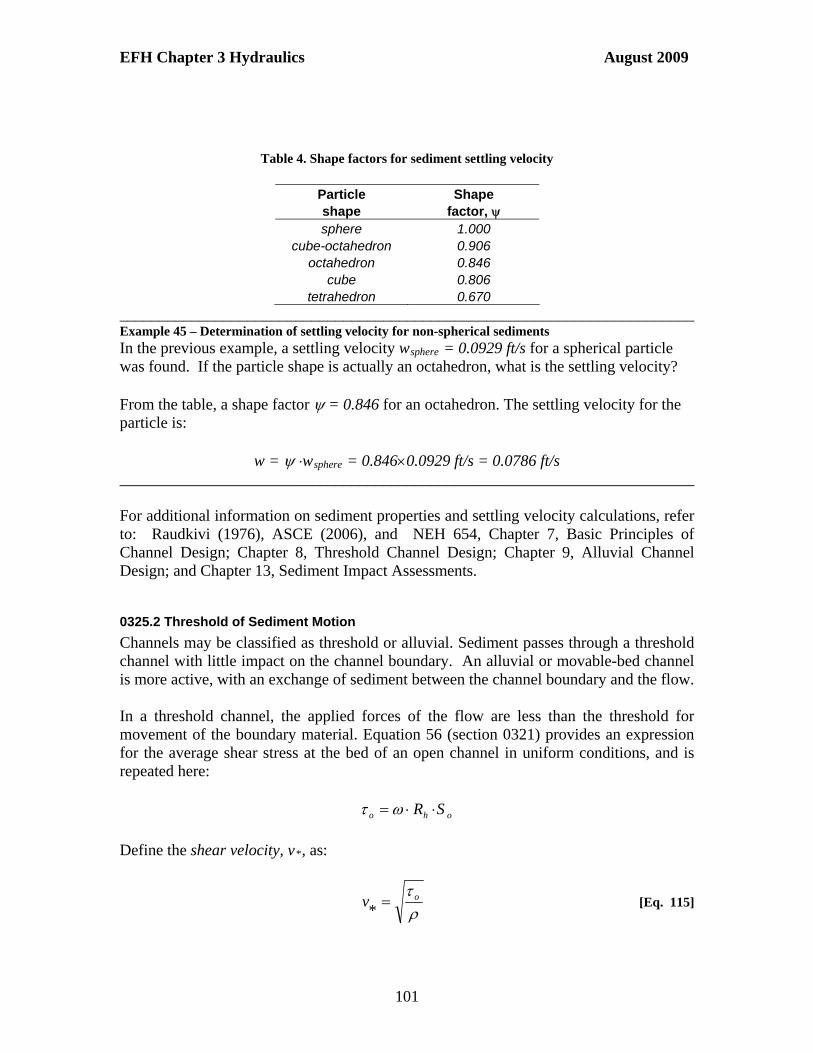
EFH Chapter 3 Hydraulics August 2009
Table 4. Shape factors for sediment settling velocity
Particle Shape shape factor, sphere 1.000
cube-octahedron 0.906 octahedron 0.846
cube 0.806 tetrahedron 0.670
________________________________________________________________________ Example 45 – Determination of settling velocity for non-spherical sediments In the previous example, a settling velocity wsphere = 0.0929 ft/s for a spherical particle was found. If the particle shape is actually an octahedron, what is the settling velocity? From the table, a shape factor = 0.846 for an octahedron. The settling velocity for the particle is:
w = wsphere = 0.8460.0929 ft/s = 0.0786 ft/s ________________________________________________________________________ For additional information on sediment properties and settling velocity calculations, refer to: Raudkivi (1976), ASCE (2006), and NEH 654, Chapter 7, Basic Principles of Channel Design; Chapter 8, Threshold Channel Design; Chapter 9, Alluvial Channel Design; and Chapter 13, Sediment Impact Assessments.
0325.2 Threshold of Sediment Motion
Channels may be classified as threshold or alluvial. Sediment passes through a threshold channel with little impact on the channel boundary. An alluvial or movable-bed channel is more active, with an exchange of sediment between the channel boundary and the flow. In a threshold channel, the applied forces of the flow are less than the threshold for movement of the boundary material. Equation 56 (section 0321) provides an expression for the average shear stress at the bed of an open channel in uniform conditions, and is repeated here:
oho SR
Define the shear velocity, v*, as:
ov
* [Eq. 115]
101

EFH Chapter 3 Hydraulics August 2009
Although this is not a velocity that can be measured in the flow, the quantity defined above has the units of a velocity, and, being related to the bed shear stress, is appropriately named the shear velocity. The bed shear stress, o, and the shear velocity, v*, (u* is used interchangeably with v*) can be used to define a set of parameters to analyze the threshold of sediment motion in open channels. The two parameters to consider are a Reynolds number based on the shear velocity:
Dv* [Eq. 116]
and a dimensionless shear stress:
DSD s
o
s
o
)1()( [Eq. 117]
where and (“γ” is used interchangeably with “”)are the kinematic viscosity and specific weight of water, respectively, and D and s are the diameter and the specific weight of the sediments. The specific gravity of the sediments is Ss = s / (Ss = 2.65 for sand). NEH 654, Chapter 8 (Threshold Channel Design), describes the origin and meaning of the Shield’s diagram. This diagram, shown in Figure 48, and based on the Reynolds number and the dimensionless shear stress (equations 116 and 117), has been extensively used for determining the threshold of sediment motion in open channel flow. For a given flow, points above the Shields’s curve indicate sediment motion, whereas points below the Shield’s curve would show no sediment motion.
Figure 48. Shield’s diagram for determining the threshold of sediment motion in open channel flow. ________________________________________________________________________
102

EFH Chapter 3 Hydraulics August 2009
Example 46 – Sediment motion threshold analysis using Shield’s diagram A rectangular channel of width b = 10 ft, with Manning’s n = 0.015, and laid on a slope So = 0.005, flows at a normal depth do = 0.5 ft. Using Shield’s diagram, determine if the flow is able to move sediment of diameter D = 0.20 mm = 6.5610-4 ft. Use Ss = 2.65 as the specific gravity of the sediments, and = 1.21710-5 ft2/s for the viscosity of water. The bed shear stress and the shear velocity are calculated as follows:
A = bdo = 10 ft 0.5 ft = 5 ft2 P = b + 2do = 10 ft + 20.5 ft = 11 ft
Rh = A/P = 5 ft2/11 ft = 0.4545 ft
o = RhSo = 62.4 lb/ft30.4545 ft0.005 = 0.1418 lb/ft2
v* = sftftsftSgRSRg
ohoho /2705.0005.04545.0/2.32 2
The parameters of the Shield’s diagram are calculated as follows:
6.14/10217.1
)1056.6(/2705.0*25
4
sft
ftsftDv
1.2)1056.6(/4.62)165.2(
/1418.0
)1( 43
2
ftftlb
ftlb
DSs
o
The point (14.6, 2.1) in the Shield’s diagram is well above Shield’s curve; therefore, sediment motion will occur for the flow specified above. Normally, sediment motion is assured if the shear stress parameter is a factor of “2” above the curve. And likewise if the shear stress parameter is less than half of the curve value, then sediment motion will not occur. ________________________________________________________________________ More recent work indicates that Shield’s diagram does not account for the absence of stream bed forms, the sporadic entrainment of sediment particles at low shear stress, or the effects of non-uniform bed material. See NEH 654.0804(b) to calculate a refined allowable shear stress parameter. Grass linings have been widely used to protect the erodible soil boundaries of waterways, floodways, and reservoir auxiliary spillways. An effective stress design approach is provided in the basic reference USDA AH 667. Waterway Design Tool software has been developed to design grassed waterways, following the procedures of AH 667. Refer to EFH, 650, Chapter 7, Grassed Waterways, for example designs of trapezoidal and parabolic-shaped grassed waterways, using an extensive set of design tables. Also, refer
103

EFH Chapter 3 Hydraulics August 2009
to NEH 654.0806 for more information and an example problem on the threshold design of a grass-lined channel.
0325.3 Suspended Sediment Load
Once sediment particles are moving, the finest particles may be entrained in the flow and kept in suspension by turbulent motions while being carried downstream by the bulk flow. The sediment thus transported is known as the suspended sediment load. The concentration C(y) of suspended sediment, in units of sediment mass per unit liquid mass, can be calculated using the following equation:
z
a y
a
ad
yd
C
yC
)(
[Eq. 118]
Where y is the distance from the channel bed, Ca is the concentration measured at a reference level y = a close to the channel bed, d is the flow depth, and z is a parameter calculated as:
*v
wz
[Eq. 119]
In this parameter, w is the settling velocity of the sediment particles, is the ratio of the sediment transport coefficient to the turbulent kinematic viscosity in the flow, is von Karman’s constant (related to the viscous stress model commonly used in open channel flow), and v* is the shear velocity. The value of is close to 1.0 for fine sediments and decreases as the particle size increases. Von Karman’s constant has been measured to be k = 0.40 in clear water, and lower for sediment-laden water. If we measure the concentration at the midpoint of the depth, i.e., Cmd = C(d/2), equation 118 can be written as follows (a = d/2):
z
md y
yd
C
yC
)( [Eq. 120]
The suspended sediment discharge Gss (mass per unit volume) in a rectangular channel of width b, can be calculated by integrating the product C(y)v(y) over the depth of flow, with v(y) being the flow velocity distribution in the vertical:
AAss dybyvyCdAyvyCG )()()()( [Eq. 121]
A typical velocity distribution in turbulent open channel flow is the logarithmic distribution given by:
104

EFH Chapter 3 Hydraulics August 2009
d
yvVyv ln1*)(
[Eq. 122]
where V is the mean flow velocity. The point near the channel bed where the velocity becomes zero is located at a distance yo from the channel bed. The value of yo can be found from the above equation by making v(yo) = 0, resulting in:
1
*exp
v
Vdyo
[Eq. 123]
This value becomes the lower limit for the integral of equation 121, the upper limit being the depth of flow d. The suspended sediment discharge per unit width can be calculated as:
dyd
yvV
y
ydCdyyvyC
b
Gg
d
y
z
md
d
y
ssss
oo
ln1*)()(
[Eq. 124]
A dimensionless unit sediment discharge can be obtained by dividing gss by the product qCmd, where q = Vd is the unit water discharge (or discharge per unit width). This dimensionless unit sediment discharge can be written as:
),(*),(*1*21 oo
md
ssss zI
V
vzI
V
v
Cq
gg
[Eq. 125]
Where o = yo/d, and the integrals I1(z,o) and I2(z,o), are calculated as:
1
1
1),(
o
dzIz
o
[Eq. 126]
and
1
2 )ln(1
),(o
dzIz
o
[Eq. 127]
________________________________________________________________________ Example 47 – Suspended sediment discharge calculation Consider a rectangular stream of width b = 20 ft, laid on a slope So = 0.00025, with Manning’s n = 0.025, flows at a normal depth do = d = 5.0 ft. The mid-depth concentration is measured to be Cmd = 0.05 gm/lt =0.00312 lb/ft3. The settling velocity of the particles has been calculated to be w = 0.12 ft/s. Calculate the suspended sediment discharge Gss, assuming that the parameter = 0.88. Proceeding to calculate the mean velocity and shear velocity:
105

EFH Chapter 3 Hydraulics August 2009
A = bdo = 20 ft 5 ft = 100 ft2
P = b + 2do = 20 ft + 25 ft = 30 ft
Rh = A/P = 100 ft2/30 ft = 3.33 ft
00025.033.3025.0
486.1 3/23/2oh
u SRn
CV 2.097 ft/s
v* = sftftsftSgRSRg
ohoho /1638.000025.033.3/2.32 2
The lower limit in the integral of equation 121 is calculated with = 0.40 as:
ftsft
sftft
v
Vdyo 0109.01
/1638.0
/097.24.0exp51
*exp
while the lower limit of the integrals in equations 126 and 127 is:
o = yo/d = 0.0109ft/5ft = 0.00219 The parameter z from equation 119 is calculated with = 0.40 as follows:
081.2/1638.040.088.0
/12.0
*
sft
sft
v
wz
The integrals in equations 126 and 127 can be calculated by using numerical integration in a spreadsheet, which calculates the integrals, I1 = 677.1623 and I2 = -3553.72. The dimensionless unit suspended sediment discharge is calculated with equation 125:
52.11572.3553097.24.0
1638.01623.677
097.24.0
1638.01*
ssg
The unit suspended sediment discharge is:
ftslbCqgg mdssss //78.300312.020
100097.252.115
The suspended sediment discharge is:
slbgG ssss /58.7520
106

EFH Chapter 3 Hydraulics August 2009
0325.4 Bed Sediment Load
Coarser sediment particles carried by a stream may move by rolling and saltation along the bed of the channel constituting what is known as bed sediment load. Refer to NEH 654, Chapter 9, for bed sediment load formulae and where to apply. Using the Meyer-Peter-Muller formula due to its simplicity:
2/32/3
3 1047.0'1
8
soh
s
sB S
k
k
D
SR
S
SDgg [Eq. 128]
In this formula, gB is the bed sediment discharge (mass per unit time) per unit width of a rectangular channel, is the specific weight of water, g is the acceleration of gravity, D = D50 is the sediment particle diameter, Ss is the specific gravity of sediments (e.g., Ss = 2.65 for sand), Rh is the hydraulic radius (which can be taken as Rh = d, the depth of flow, for a wide channel), and So is the bed slope. The coefficients k and k’ are Stickler coefficients defined by the following equations:
ohu
oh SRn
CSkRV 3/23/2 [Eq. 129]
''
'' 3/23/2 SRn
CSRkV h
uh [Eq. 130]
The first expression for V is Manning’s equation with the coefficient k accounting for the overall channel resistance, namely, bed form resistance (e.g., dunes, bars) and grain friction resistance. This velocity is defined in terms of the bed slope So. The second expression for V is Manning’s equation with the coefficient k’ accounting only for the grain friction resistance. This equation uses a slope S’ that corresponds to the grain friction resistance. Thus, S’ can be defined as a grain-friction energy slope. The ratio k/k’, that appears in the Meyer-Peter-Muller equation, can take values between 0.5 and 1.0, with k/k’ = 1.0 when no bed forms are present, and k/k’ = 0.5 when strong bed forms are present. The coefficient k’ can be calculated, using metric units, as:
6/190
3/1 /26'
D
smk [Eq. 131]
where D90 is the diameter of bed sediments for which 90% of the material is finer. In the English system of units the equation to use is:
6/190
3/1 /63.38'
D
sftk [Eq. 132]
107
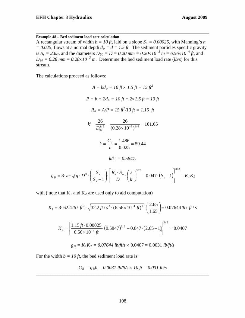
EFH Chapter 3 Hydraulics August 2009
________________________________________________________________________ Example 48 – Bed sediment load rate calculation A rectangular stream of width b = 10 ft, laid on a slope So = 0.00025, with Manning’s n = 0.025, flows at a normal depth do = d = 1.5 ft. The sediment particles specific gravity is Ss = 2.65, and the diameters D50 = D = 0.20 mm = 0.2010 -3 m = 6.5610 -4
ft, and D90 = 0.28 mm = 0.2810 -3 m. Determine the bed sediment load rate (lb/s) for this stream. The calculations proceed as follows:
A = bdo = 10 ft 1.5 ft = 15 ft2
P = b + 2do = 10 ft + 21.5 ft = 13 ft
Rh = A/P = 15 ft2/13 ft = 1.15 ft
65.101)1028.0(
2626'
6/136/190
Dk
44.59025.0
486.1
n
Ck u
k/k’ = 0.5847.
2/32/3
3 1047.0'1
8
soh
s
sB S
k
k
D
SR
S
SDgg = K1K2
with ( note that K1 and K2 are used only to aid computation)
sftlbftsftftlbK //07644.065.1
65.2)1056.6(/2.32/4.628 3423
1
0407.0165.2047.05847.01056.6
00025.015.12/3
2/3
42
ft
ftK
gB = K1K2 = 0.07644 lb/ft/s 0.0407 = 0.0031 lb/ft/s
For the width b = 10 ft, the bed sediment load rate is:
GB = gBb = 0.0031 lb/ft/s 10 ft = 0.031 lb/s ________________________________________________________________________
108

EFH Chapter 3 Hydraulics August 2009
0325.5 Scour and Deposition in Channels
A channel in equilibrium, from the point of view of sediment transport, is one which is not degrading (losing bed material) nor aggrading (gaining bed material). A decrease in the sediment supply to the channel may cause degradation. For example, if a dam has been built in a stream that typically carries sediment, the water downstream from the dam may contain much less sediment than before and, most likely, would pick up local materials to make up for the loss. On the other hand, an increase in the sediment supply to a channel may cause aggradation as the channel may not be able to carry the additional supply. Refer to NEH 654, Chapter 13, for additional information on local scour calculations. Consider a degrading channel, of infinite length, as consequence of the building of a dam. This situation is depicted in the following figure.
Figure 49. Channel bed degradation downstream of a dam due to reduction in sediment supply. Let So be the slope of the original bed position and S be the slope of the final bed position. The solution that describes the change in the bed elevation with respect to time t and space x, measured from the dam foot, is given by (see Raudkivi, 1976):
Kt
xerfcx
Kt
xtKSStxz o
24exp2)(),(
2
[Eq. 133]
Where K is a parameter defined in terms of an equation of flow (the Chezy equation) and the sediment discharge expression (equation 136), and erfc is the complementary error function defined as:
0
)exp(1)(1 derferfc [Eq. 134]
and erf is the error function. The Chezy equation for the flow:
109
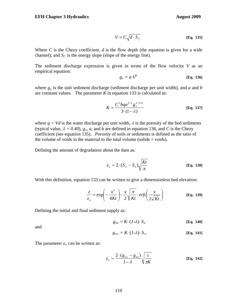
EFH Chapter 3 Hydraulics August 2009
fSdCV [Eq. 135]
Where C is the Chezy coefficient, d is the flow depth (the equation is given for a wide channel), and Sf is the energy slope (slope of the energy line). The sediment discharge expression is given in terms of the flow velocity V as an empirical equation:
gs = aVb [Eq. 136] where gs is the unit sediment discharge (sediment discharge per unit width), and a and b are constant values. The parameter K in equation 133 is calculated as:
)1(3
/312/32
bsgbqaC
K [Eq. 137]
where q = Vd is the water discharge per unit width, is the porosity of the bed sediments (typical value, = 0.40), gs, a, and b are defined in equation 136, and C is the Chezy coefficient (see equation 135). Porosity of soils or sediments is defined as the ratio of the volume of voids in the material to the total volume (solids + voids). Defining the amount of degradation about the dam as:
Kt
SSz oo )(2 [Eq. 138]
With this definition, equation 133 can be written to give a dimensionless bed elevation:
Kt
xerfc
Kt
x
Kt
x
z
z
o 224exp
2 [Eq. 139]
Defining the initial and final sediment supply as:
gso = K (1-) So [Eq. 140] and
gs = K (1-) S [Eq. 141] The parameter zo can be written as:
K
tggz sos
o
1
)(2 [Eq. 142]
110

EFH Chapter 3 Hydraulics August 2009
Notice that the solution provided by equation 133, applies equally to degradation (gso>gs) or aggradation (gso<gs). ________________________________________________________________________ Example 49 – Bed aggradation A laboratory flume is set at a slope So = 0.00356 and water flows at a uniform depth do = 2 inches = 0.167 ft, and a velocity V = 1.31 ft/s. Sediment is supplied into the flow at a rate gso = 1.59810-4 ft2/s until the channel reaches equilibrium. The estimated value of the parameter K is K = 0.0748 ft2/s, and the porosity of sediments is = 0.40. Without changing any of the flow conditions, the sediment supply rate is increased to gs = 7.9910-4 ft2/s, so that the channel bed starts aggrading. (a) Compute the maximum amount of aggradation after t = 1 hr = 3600 s, and (b) compute the amount of aggradation at a point x = 2.0 ft downstream of the point of sediment injection, after t = 1 hr = 3600 s. Assume that the channel is of infinite length. The maximum amount of aggradation at any given time occurs at position x = 0, and is given by equation 142:
K
tggz sos
o
1
)(2
inftsft
ssftsftzo 16.32637.0
/0748.01416.3
3600
4.01
)/10598.1/1099.7(22
2424
To find the aggradation elevation for x = 2 ft and t = 3600 hr, use equation 139:
Kt
xerfc
Kt
x
Kt
xzz o
224exp
2
The value of the function erfc may be found by use of an appropriate spreadsheet. The argument of the function for this example is:
0609.03600/0748.02
0.2
2 2
ssft
ft
Kt
x
The spreadsheet gives erfc(0.0609) = 0.931367. The required aggradation elevation is:
931367.03600/0748.0
1416.3
2
0.2
3600/0748.04
)0.2(exp2637.0
22
2
ssft
ft
ssft
ftftz
z = 0.2362 ft = 2.83 in
________________________________________________________________________
111

EFH Chapter 3 Hydraulics August 2009
Example 50 – Bed degradation downstream of dam. The initial slope of a river channel is So = 0.0094. It is estimated that, after construction of a dam, the resulting slope will be S = 0.0020. The parameter K is estimated to be 10750 ft2/day. The initial bed elevation at the dam site is zs = 1500 ft above mean sea level. Compute the expected bed elevation at a number of points along the stream channel after, (a) two months (60 days), and (b) 2 years (730 days) of the construction of the dam. The elevation at the dam site for t = 60 days, is calculated as:
ftdaydayftKt
SSz oo 71.61416.3
60/10750)0094.00020.0(2)(2
2
And for t = 730 days, the elevation zo is calculated as:
ftdaydayftKt
SSz oo 39.231416.3
730/10750)0094.00020.0(2)(2
2
In the following table and plot, the degradation elevations z for t = 0, t = 60 day, and t = 730 day, for a number of values of “x” are presented. The bed elevation is calculated as follows:
Bed elevation(x) = Bed elevation(x=0) + z(x) - Sox The calculations and plot of the data were performed with an appropriate spreadsheet.
112

EFH Chapter 3 Hydraulics August 2009
________________________________________________________________________ In some instances, a control on the downstream end of a channel of length L may exist such that the bed elevation at the downstream end remains constant even as the channel aggrades or degrades. If the starting bed slope is So and the ending bed slope is S, the elevation of the channel bed z(x,t) is given by the following equation (see Raudkivi, 1976): )(),( xLStxz
12
22
22 2
)12(cos
4
)12(exp
)12(
1)(8
k
o
L
xk
L
Ktk
k
SSL
[Eq. 143]
The coefficient K is calculated as in equation 137. ________________________________________________________________________ Example 51 – Bed degradation with constant downstream elevation
This example uses the same data as in the previous example, i.e., So = 0.0094, S = 0.0020, and K = 10750 ft2/day; however, a control of constant elevation occurs at the downstream end of a channel length L = 1.5 mi = 7920 ft. The initial bed elevation at the dam site is zs = 1500 ft. Compute the expected bed elevation at a number of points along the river channel after, (a) two months (60 days), (b) 2 years (730 days), and (c) 10 years (3650 days) of the construction of the dam. (Note: the value of S can be estimated from the terrain geometry and selected so as to produce a channel with a mild slope.) The calculations and plot of the data, shown below, were performed with an appropriate spreadsheet.
113

EFH Chapter 3 Hydraulics August 2009
0330 Pipe Flow The principles of pipe flow apply to the hydraulics of such structures as culverts, drop inlets, siphons, and various types of pipelines. Consider Figure 24 which shows the hydraulic grade line, energy line and the energy heads at two points of the flow. Most pipe flow occurs through constant-diameter pipe, thus, making the velocity heads at sections (1) and (2) the same (V1 = V2 = V). This in turn means that the energy line (E.L.) and hydraulic grade line (H.G.L.) are parallel. The energy equation for constant-diameter pipe is written as:
fhp
zp
z
22
11 [Eq. 144]
114

EFH Chapter 3 Hydraulics August 2009
Where hf represents the energy head losses between sections (1) and (2) in Figure 24. Because the energy head losses are due to the friction between the moving fluid mass and the walls of the pipe, hf is also referred to as the friction losses. Friction losses may be calculated by measuring the piezometric heads,
1
11
pzh , and
2
22
pzh , and taking the difference hf = h1-h2.
The energy slope, or slope of the energy line, is the ratio of the friction losses, hf, to the length of the pipe, L, and may be expressed as:
2
21
121 1 p
zp
zLL
hh
L
hS f
f [Eq. 145]
Flow in pipelines occurs in two different regimes, laminar and turbulent. Laminar flow occurs at relatively small velocities, and is characterized by fluid particles moving in stable flow layers and with a parabolic velocity distribution. Increasing the flow velocity sufficiently causes instabilities of the flow layers which, in turn, cause the flow to become turbulent. In turbulent flow the fluid particles no longer move in stable layers, but rather clump together to form different-sized eddies. Turbulent flow is characterized by a more uniform velocity distribution across the pipe typically described mathematically by logarithmic or power-law functions. 0331 Friction Loss Methods Calculation of friction losses is an important step in analyzing flow in pipes, and in the selection of pipe sizes for specific applications. The calculation of friction losses in pipe can be performed through the use of a number of methods such as Manning’s equation, the Darcy-Weisbach equation, or the Hazen-Williams formula. These methods are presented in detail next.
0331.1 Manning’s Equation for Pipelines
Manning’s equation for open-channel flow was presented as equation 71 in terms of the flow velocity V, the hydraulic radius R, the channel bed slope So, the Manning’s resistance coefficient n, and a constant Cu that depends on the system of units used (Cu = 1.0 for the International System, and Cu = 1.486 for the English System). When applied to pipelines, the bed slope So is replaced by the energy slope Sf = hf /L, while the hydraulic radius is calculated in terms of the area, A (equation 29 repeated here), and wetted perimeter, P, of a full circular cross-section of diameter D, using:
4
2DA
DP [Eq. 146]
which results in:
115
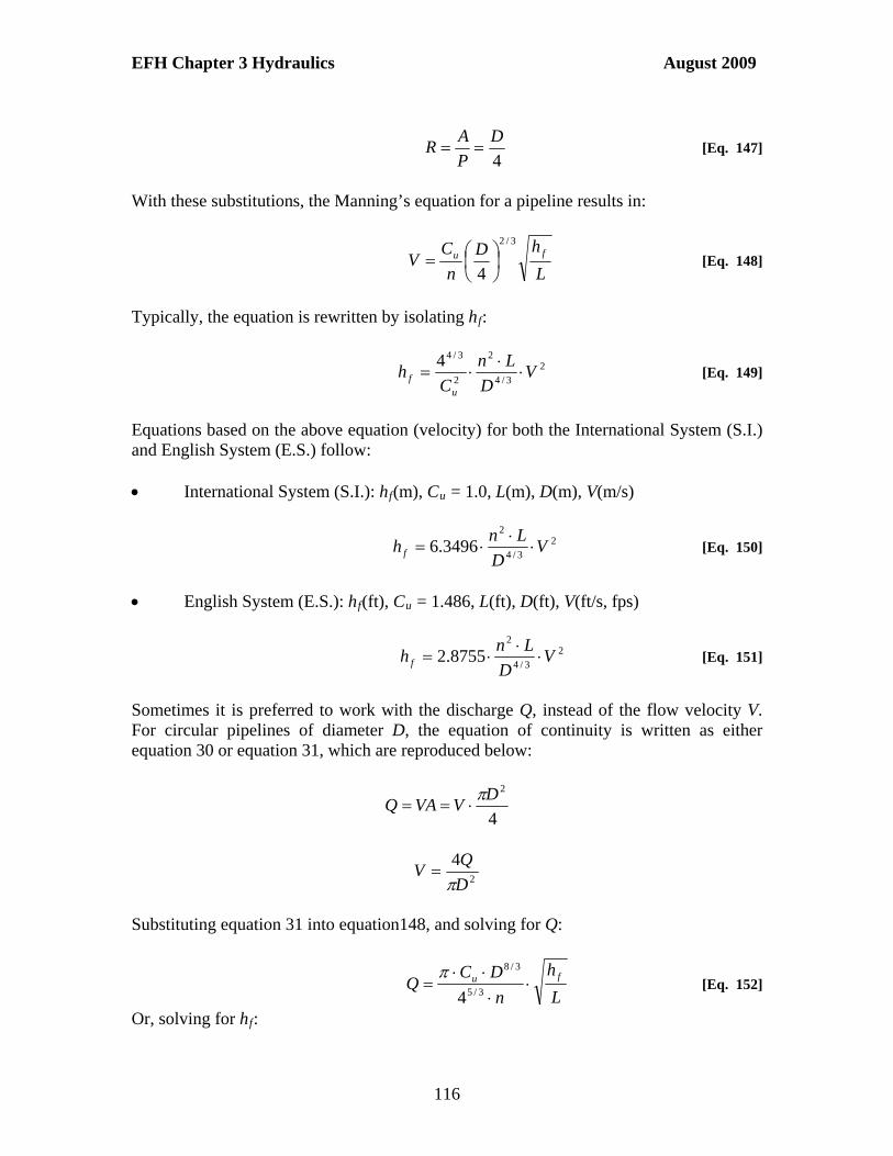
EFH Chapter 3 Hydraulics August 2009
4
D
P
AR [Eq. 147]
With these substitutions, the Manning’s equation for a pipeline results in:
L
hD
n
CV fu
3/2
4
[Eq. 148]
Typically, the equation is rewritten by isolating hf:
23/4
2
2
3/44V
D
Ln
Ch
uf
[Eq. 149]
Equations based on the above equation (velocity) for both the International System (S.I.) and English System (E.S.) follow: International System (S.I.): hf(m), Cu = 1.0, L(m), D(m), V(m/s)
23/4
2
3496.6 VD
Lnh f
[Eq. 150]
English System (E.S.): hf(ft), Cu = 1.486, L(ft), D(ft), V(ft/s, fps)
23/4
2
8755.2 VD
Lnh f
[Eq. 151]
Sometimes it is preferred to work with the discharge Q, instead of the flow velocity V. For circular pipelines of diameter D, the equation of continuity is written as either equation 30 or equation 31, which are reproduced below:
4
2DVVAQ
2
4
D
QV
Substituting equation 31 into equation148, and solving for Q:
L
h
n
DCQ fu
3/5
3/8
4
[Eq. 152]
Or, solving for hf:
116
EFH Chapter 3 Hydraulics August 2009
23/16
2
22
3/104Q
D
Ln
Ch
uf
[Eq. 153]
Equations based on the above equation (discharge) for both the International System (S.I.) and English System (E.S.) follow: International System (S.I.): hf(m), Cu = 1.0, L(m), D(m), Q(m3/s)
23/16
2
2936.10 QD
Lnh f
[Eq. 154]
English System (E.S.): hf(ft), Cu = 1.486, L(ft), D(ft), Q(ft3/s, cfs)
23/16
2
6615.4 QD
Lnh f
[Eq. 155]
________________________________________________________________________ Example 52 – Pipeline discharge calculation using Manning’s equation Determine the discharge Q that can be conveyed by a 3.0-in-diameter corrugated-plastic pipeline if a head hf = 10 ft, is to be dissipated in a length L = 100 ft. Use equation 152 to calculate the discharge. The data to use are the following: D = 3.0 in = 3.0/12 = 0.25 ft, hf = 10 ft, L = 100 ft, Cu = 1.486, n = 0.015 (from Table 5). The resulting discharge is:
cfsL
h
n
DCQ fu 24.0
100
10
015.04
)25.0()486.1()1416.3(
4 3/5
3/8
3/5
3/8
________________________________________________________________________ The software USDA-NRCS Hydraulics Formula provides for the calculation of pipe flow using Manning’s equation. To activate this solution select the Pipe Flow tab, which produces the entry form shown in Figure 50. The formula shown in the entry form is equivalent to equation 152, but with the diameter D in inches and with local loss coefficients equal to zero (i.e., Ke = 0, Kb = 0). ________________________________________________________________________ Example 53 – Pipeline discharge calculation using the USDA-NRCS Hydraulics Formula software Using the Pipe Flow tab in the USDA-NRCS Hydraulics Formula software, with Ke = 0, Kb = 0, determine the discharge Q conveyed by a 3-in-diameter corrugated-plastic pipeline if a head hf = 10 ft, is to be dissipated in a length L = 100 ft. These data are the same as for the previous example 52. The resulting discharge is 0.2 cfs.
117

EFH Chapter 3 Hydraulics August 2009
Figure 50. Pipe Flow calculations with the USDA-NRCS Hydraulics Formula.
The equation for pipe flow shown in the above figure will be derived after introducing the concept of local losses in pipe (see section 0331.6). ________________________________________________________________________
118

EFH Chapter 3 Hydraulics August 2009
Manning’s n values, shown in Table 5, for various pipe materials are assembled from many hydraulic references, including Brater and King (1996), FHWA (2001), and USACOE (2008).
Table 5. Values of Manning’s resistance coefficient for pipe
Manning's n Pipe material Minimum Design Maximum Cast-iron, coated 0.010 0.012 - 0.014 0.014 Cast-iron, uncoated 0.011 0.013 - 0.015 0.015 Wrought iron, galvanized 0.013 0.015 - 0.017 0.017 Wrought iron, black 0.012 0.015 Steel, riveted and spiral 0.013 0.015 - 0.017 0.017 Annular corrugated metal(1) 0.021 0.021 - 0.025 0.0255 Helical corrugated metal(1) 0.013 0.015 - 0.020 0.021 Wood stave 0.010 0.012 - 0.013 0.014 Neat cement surface 0.010 0.013 Concrete 0.010 0.012 - 0.017 0.017 Vitrified sewer pipe 0.010 0.013 - 0.015 0.017 Clay, common drainage tile 0.011 0.012 - 0.014 0.017 Corrugated plastic 0.014 0.015 - 0.016 0.017 PVC 0.009 -0.011 Smooth Interior PE 0.009 - 0.015 0.02 Aluminum 0.01 Gated Aluminum Pipe 0.013
(1) N-values for corrugated metal pipe vary with pipe diameter. See FHWA (2001) or USACOE (2008) to select a refined n-value
________________________________________________________________________ Example 54 – Flow velocity in a helical corrugated metal pipe using Manning’s equation Determine the flow velocity in a helical corrugated metal pipe (use n = 0.016, from Table 5), that is 5-in in diameter if it dissipates a head hf =6.5 ft in a length L = 300 ft. With D = 5 in = 5/12 ft = 0.4167 ft, and Cu = 1.486, equation 148 produces the following result:
fpsL
hD
n
CV fu 0.3
300
5.6
4
4167.0
016.0
486.1
4
3/23/2
________________________________________________________________________ Example 55 – Head loss in a riveted and spiral steel pipe using Manning’s equation Determine the head loss in 1500 ft of a riveted and spiral steel pipe (use n = 0.015) with a 24-in (2-ft) diameter that carries a discharge of 10 cfs. Using equation 155:
ftQD
Lnh f 9.310
0.2
1500015.06615.46615.4 2
3/16
22
3/16
2
________________________________________________________________________
119

EFH Chapter 3 Hydraulics August 2009
Example 56 – Velocity in pipeline draining a reservoir – Manning’s equation Consider a reservoir whose free surface is located at an elevation z1 = 60 ft, draining through a 0.5-ft-diameter, 100-ft-long, concrete pipe (n = 0.012) open to the atmosphere whose outlet is located at an elevation z2 = 55 ft. Determine the velocity in the pipeline. The system is depicted in the following figure. Entrance losses will be ignored.
Point 1 in the energy equation is at the reservoir free surface where p1 = 0 and V1 = 0. Point 2 is at the pipe outlet where p2 = 0 and V2 = V, the pipe velocity. The energy head, H = z1 – z2 = 60 ft – 55 ft = 5 ft, for this case. Applying the energy equation (equation 47) between points 1 and 2:
fhg
Vpz
g
Vpz
22
222
2
211
1
Using Manning’s equation to represent friction losses:
23/4
22
2
2
2 8755.22
0
2
00V
D
Ln
g
Vz
gHz
This simplifies to:
3/4
22 8755.2
2
1
D
Ln
gVH
Solving for the velocity, V, and using H = 5 ft, L = 100 ft, n = 0.012, D = 0.5 ft, g = 32.2 ft/s2:
sft
D
Ln
g
HV /46.6
5.0
100012.08755.2
2.322
1
5
8755.2
2
13/4
2
3/4
2
________________________________________________________________________ 0331.2 Darcy-Weisbach Equation and Friction Factor A second method for calculating friction losses in pipes is the Darcy-Weisbach equation written, in terms of the flow velocity V as:
120

EFH Chapter 3 Hydraulics August 2009
g
V
D
Lfh f 2
2
[Eq. 156]
The friction factor, f, is a function of a relative roughness, e/D, where e is known as the absolute roughness or equivalent sand roughness, and of the Reynolds number of the flow. The Reynolds number, defined in equation 10, is repeated here:
VDVD
Re
where is the density (mass per unit volume) of water, is the absolute or dynamic viscosity of water, and is the kinematic viscosity of water, defined by equation 9, = /. Values of the density and viscosity of water related to temperature are available in Exhibit 4. The absolute roughness of a pipe material is the average height of the irregularities of the inner wall of the pipe. The first experiments on head losses in pipes were conducted in the early 20th century by coating glass pipes with uniform-size sand grains. The diameter of the sand grains was used to represent the absolute roughness of the pipe, e. Typical values of the absolute roughness of various pipe materials are presented in Table 6. Absolute roughness values may be found in Streeter and Wylie (1998) and other similar fluid mechanics texts.
Table 6. Absolute roughness values for pipe materials
Pipe material e (mm) e (ft) Smooth surface (glass, plastic) 0 0 Drawn tubing, brass, lead, copper 0.0015 0.000005 Centrifugally spun cement 0.0015 0.000005 Bituminous lining 0.0015 0.000005 PVC pipe 0.002 0.0000066 Commercial steel 0.046 0.00015 Wrought iron 0.046 0.00015 Welded-steel pipe 0.046 0.00015 Asphalt-dipped cast iron 0.12 0.0004 Aluminum, with couplers 0.13 0.00043 Galvanized iron 0.15 0.0005 Cast iron 0.25 0.00085 Wood stave 0.18-0.9 0.0006-0.003 Concrete 0.3-3 0.001-0.01 Riveted steel 0.9-9 0.003-0.03
121

EFH Chapter 3 Hydraulics August 2009
The Darcy-Weisbach friction factor has different expressions for laminar or turbulent pipe flow, described in the following section.
0331.3 Laminar and Turbulent Friction Factor Equations
Water flowing at a very low velocity, or in a very small-diameter pipe, typically flows in a laminar flow regime. In laminar flow the flow takes place in layers (Latin, laminae) that remain very stable and are easily identifiable by dye injected into the flow. As the velocity increases, conditions are reached in which the flow becomes turbulent. In turbulent flow, layers of flow are no longer identifiable and the flow tends to break down into eddies that facilitate mixing. Laminar flow is rare, occurring at low flow velocity or small pipe diameter. Most pipe flows of interest are turbulent. Experiments to determine the laminar or turbulent nature of flow were carried out by Osborne Reynolds in the 19th century. Reynolds identified a dimensionless parameter, now known as the Reynolds number (equation 10), to determine if a flow is laminar or turbulent. There is also a transitional flow regime in which the flow is neither laminar nor turbulent but shifts between conditions. The typical values for classifying flows according to laminar, transitional, or turbulent regimes are shown next:
Laminar flow: Re<2000 Transitional flow: 2000 < Re < 4000 Turbulent flow: Re > 4000
The range Re < 4000 that encompasses laminar and transitional flow is a small range considering that Re can take values to 109 or larger. Thus, turbulent flow is more likely to occur in pipelines. ________________________________________________________________________ Example 57 – Reynolds number used to classify pipe flow Water is flowing in a 2-in diameter pipe at a rate of 0.08 cfs. If the water temperature is 70oF, determine the Reynolds number of the flow and classify it as laminar, transitional, or turbulent. The data given is D = 2 in = 2/12 ft = 0.167 ft, Q = 0.08 cfs, and from Exhibit 4 at a temperature of 70oF the kinematic viscosity of water is =.00001059 ft2/s = 1.05910 -5 ft2/s. The flow velocity is calculated as:
sftft
sft
D
Q
A
QV /7.3
)167.0(1416.3
/08.0442
3
2
And the Reynolds number is:
425
1083.558347/10059.1
)167.0()/7.3(Re
sft
ftsftVD
122

EFH Chapter 3 Hydraulics August 2009
Since Re > 4000, the flow is turbulent. ________________________________________________________________________ In the laminar regime, the Darcy-Weisbach friction factor, f, is a function of the Reynolds number, given as:
Re
64f [Eq. 157]
In the turbulent regime, an equation relating the friction factor, f, the Reynolds number Re, and the relative roughness, e/D, is the Colebrook-White equation:
fD
e
f Re
51.2
7.3log2
1 [Eq. 158]
The difficulty in using this equation is that it is not explicit in f and any solution involving this equation requires a numerical approach. To facilitate solving explicitly for f, a close approximation (2 – 5% error) to the Colebrook-White equation is provided by the Swamee-Jain equation:
9.02
Re
74.5
7.3log
25.0
D
ef [Eq. 159]
In the following section, solutions of turbulent pipe flow using the Darcy-Weisbach equation are presented.
0331.4 Pipe Flow Solutions Using the Darcy-Weisbach Equation
Since the discharge, Q, is often known or to be calculated, it is convenient to write the Darcy-Weisbach equation in terms of the discharge as follows:
52
28
Dg
QLfh f
[Eq. 160]
The Reynolds number Re can also be written in terms of the discharge Q as follows:
D
Q
D
Q
44Re [Eq. 161]
With this definition of the Reynolds number, the Swamee-Jain equation becomes:
123

EFH Chapter 3 Hydraulics August 2009
9.0
2 62.427.0log
25.0
Q
D
D
ef
[Eq. 162]
Combining the Darcy-Weisbach equation (equation 160) with the Swamee-Jain equation (equation 162), and solving for the discharge, Q, produces the following equation:
9.05
62.427.0log22.2Q
D
D
e
L
hgDQ f
[Eq. 163]
This equation’s variables are best solved for, by using a numerical spreadsheet application. Typically, there are three types of problems involving pipe friction losses, namely:
1. Head loss problem: calculate hf given D, Q or V, and g, L, e, . 2. Discharge problem: calculate Q or V, given D, hf and g, L, e, . 3. Sizing problem: calculate D, given Q, hf and g, L, e, .
Where hf is the friction loss, D is the pipe diameter, Q is the discharge, V is the velocity, g is the acceleration of gravity, L is the pipe length, e is the absolute roughness, and, v is the kinematic viscosity. ________________________________________________________________________ Example 58 – Pipe flow solutions with the Darcy-Weisbach equation Problem type 1. Given D = 0.3 ft, Q = 0.20 cfs, g = 32.2 ft/s2, L = 1000 ft, e = 0.002 in = 0.000166 ft, and = 1.13x10⁻⁵ ft2/s, find hf. A numerical spreadsheet application of equation 163 gives hf = 8.86 ft. Alternately, equation 163 can be solved directly for hf, with a hand calculator. Problem type 2. Given D = 0.7 ft, hf = 15 ft, g = 32.2 ft/s2, L = 750 ft, e = 0.005 in = 0.000416 ft, and = 1.2x10⁻⁵ ft2/s, find Q. A numerical spreadsheet application of equation 163 gives Q = 2.68 cfs. Alternately, equation 163 can be solved iteratively for Q, with a hand calculator, as shown in the following table:
Trial Q Calculated Q 1.5 2.63 2.1 2.66
124
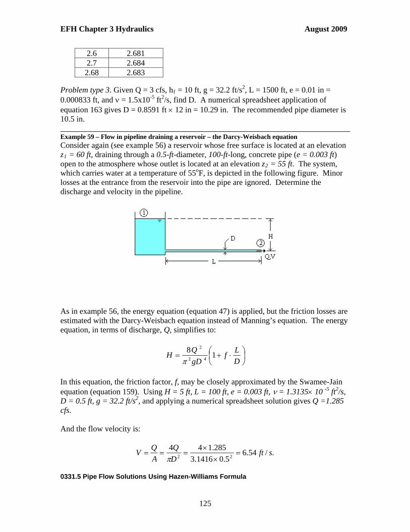
EFH Chapter 3 Hydraulics August 2009
2.6 2.681 2.7 2.684 2.68 2.683
Problem type 3. Given Q = 3 cfs, hf = 10 ft, g = 32.2 ft/s2, L = 1500 ft, e = 0.01 in = 0.000833 ft, and = 1.5x10⁻⁵ ft2/s, find D. A numerical spreadsheet application of equation 163 gives D = 0.8591 ft 12 in = 10.29 in. The recommended pipe diameter is 10.5 in. ________________________________________________________________________ Example 59 – Flow in pipeline draining a reservoir – the Darcy-Weisbach equation Consider again (see example 56) a reservoir whose free surface is located at an elevation z1 = 60 ft, draining through a 0.5-ft-diameter, 100-ft-long, concrete pipe (e = 0.003 ft) open to the atmosphere whose outlet is located at an elevation z2 = 55 ft. The system, which carries water at a temperature of 55oF, is depicted in the following figure. Minor losses at the entrance from the reservoir into the pipe are ignored. Determine the discharge and velocity in the pipeline.
As in example 56, the energy equation (equation 47) is applied, but the friction losses are estimated with the Darcy-Weisbach equation instead of Manning’s equation. The energy equation, in terms of discharge, Q, simplifies to:
D
Lf
gD
QH 1
842
2
In this equation, the friction factor, f, may be closely approximated by the Swamee-Jain equation (equation 159). Using H = 5 ft, L = 100 ft, e = 0.003 ft, = 1.3135 10 -5 ft2/s, D = 0.5 ft, g = 32.2 ft/s2, and applying a numerical spreadsheet solution gives Q =1.285 cfs. And the flow velocity is:
./54.65.01416.3
285.14422
sftD
Q
A
QV
0331.5 Pipe Flow Solutions Using Hazen-Williams Formula
125

EFH Chapter 3 Hydraulics August 2009
A third method for calculating friction head losses in pipes is the Hazen-Williams formula. The Hazen-Williams formula was developed from empirical data of water flow in pipes. In terms of flow velocity, V, the Hazen-William formula is expressed as follows: International System (S.I.): V(m/s)
54.063.0849.0 fHW SRCV [Eq. 164]
English System (E.S.): V(ft/s, fps)
54.063.0318.1 fHW SRCV [Eq. 165]
where V is velocity, CHW is the Hazen-Williams coefficient, R is the hydraulic radius (R=D/4), and Sf is the energy slope (Sf=hf/L). Using the definitions of R and Sf, the Hazen-Williams formula may be written as: International System (S.I.): hf(m), L(m), D(m), V(m/s)
54.0
63.0354.0
L
hDCV f
HW [Eq. 166]
English System (E.S.): hf(ft), L(ft), D(ft), V(ft/s, fps)
54.0
63.0550.0
L
hDCV f
HW [Eq. 167]
In terms of the discharge, the Hazen-Williams formula is written as: International System (S.I.): hf(m), L(m), D(m), Q(m3/s)
54.0
63.2278.0
L
hDCQ f
HW [Eq. 168]
English System (E.S.): hf(ft), L(ft), D(ft), Q(cfs)
54.0
63.2432.0
L
hDCQ f
HW [Eq. 169]
Solving for the head loss, hf, in the Q-based equations: International System (S.I.): hf(m), L(m), D(m), Q(m3/s)
126

EFH Chapter 3 Hydraulics August 2009
87.4
85.1
704.10D
L
C
Qh
HWf
[Eq. 170]
English System (E.S.): hf(ft), L(ft), D(ft), Q(cfs)
87.4
85.1
732.4D
L
C
Qh
HWf
[Eq. 171]
Solving for the diameter, D, in the Q-based equations: International System (S.I.): hf(m), L(m), D(m), Q(m3/s)
205.038.0
627.1
fHW h
L
C
QD [Eq. 172]
English System (E.S.): hf(ft), L(ft), D(ft), Q(cfs)
205.038.0
376.1
fHW h
L
C
QD [Eq. 173]
Table 7, below, shows typical values for the Hazen-Williams coefficient. Hazen-Williams coefficients may be found in Lamont (1981), Mays (1991) and other similar publications.
Table 7. Values of the Hazen-Williams coefficient.
Pipe description Condition CHW
Very smooth Straight alignment 140
Slight curvature 130
Cast iron, uncoated New 130
or steel pipe 5 years old 120
10 years old 110
15 years old 100
20 years old 90
30 years old 80
127

EFH Chapter 3 Hydraulics August 2009
Cast iron, coated All ages 130
Wrought iron or Diameter 12 in. and up 110
standard galvanized steel Diameter 4 to 12 in. 100
Diameter 4 in or less 80
Brass or lead New 140
Concrete Very smooth, excellent joints 140
Smooth, good joints 120
Rough 110
Vitrified clays 110
Smooth wooden; wood stave 120
Asbestos cement 140
Corrugated metal 60
Pipes of small diameter old, rough inside surface, as low as 40
PVC 150
Smooth interior PE 150
Aluminum 120
Aluminum gated pipe 110 Solutions to pipe-flow problems with the Hazen-Williams formula require the use of equations (equation 164) through (equation 173), depending on the data given and the required variable to be solved for. Some examples are shown next. ________________________________________________________________________ Example 60 – Pipe velocity calculation using the Hazen-Williams formula A pipe line with a length L = 1200 ft, diameter D = 0.75 ft, suffers a head loss hf = 12 ft. If the pipe is made of 5-year old steel pipe (CHW = 120), determine the pipe velocity. Using equation 167 as follows:
fpsL
hDCV f
HW 58.41200
1275.0120550.0550.0
54.063.0
54.0
63.0
________________________________________________________________________ Example 61 – Pipe discharge calculation using the Hazen-Williams formula Determine the discharge Q for a rough concrete pipeline (CHW = 110) with a diameter D = 1.5 ft, that produces a head loss hf = 8.5 ft on a length of L = 650 ft. Using equation 169 as follows:
cfsL
hDCQ f
HW 27.13650
5.85.1110432.0432.0
54.063.2
54.0
63.2
________________________________________________________________________ Example 62 – Head loss calculation using the Hazen-Williams formula
128

EFH Chapter 3 Hydraulics August 2009
Determine the head loss hf in a new brass pipeline (CHW = 140) of length L = 2000 ft and diameter D = 3.0 ft, that carries a discharge Q = 20 cfs. Using equation 171 as follows:
ftD
L
C
Qh
HWf 23.1
3
2000
140
20732.4732.4
87.4
85.1
87.4
85.1
________________________________________________________________________ Example 63 – Diameter calculation using the Hazen-Williams formula Determine the diameter of coated cast iron (CHW = 130) pipe that produces a friction head loss hf = 20 ft in a length L = 500 ft while carrying a discharge Q = 25 cfs. Using equation 173 as follows:
fth
L
C
QD
fHW
42.120
500
130
25376.1376.1
205.038.0205.038.0
The most likely value of commercial pipeline that can be used is D = 1.5 ft. ________________________________________________________________________ Example 64 – Flow in pipeline draining a reservoir – Hazen-Williams formula Consider once more (see examples 56 and 59) the case of a reservoir whose free surface is located at an elevation z1 = 60 ft, draining through a 0.5-ft-diameter, 100-ft-long, rough concrete pipe (CHW = 110) open to the atmosphere whose outlet is located at an elevation z2 = 55 ft. The system is depicted in the following figure. Local losses at the entrance from the reservoir into the pipe are ignored. Determine the discharge and velocity in the pipeline.
As in examples 56 and 59, the energy equation (equation 47) is applied, but the friction losses are estimated with the Hazen-Williams formula. The energy equation, in terms of discharge, Q, simplifies to:
87.4
85.1
42
2
732.48
D
L
C
Q
gD
QH
HW
.
Using H = 5 ft, L = 100 ft, CHW = 110, D = 0.5 ft, g = 32.2 ft/s2, and applying a numerical spreadsheet solution gives Q = 1.385 cfs, and the flow velocity is:
129

EFH Chapter 3 Hydraulics August 2009
./05.75.01416.3
385.14422
sftD
QV
________________________________________________________________________
The same concrete pipe material, diameter, length, and elevations were used in examples 56, 59, and 64. These examples illustrate the use of Manning’s equation, the Darcy-Weisbach equation (using Swamee-Jain equation for the friction factor), and the Hazen-Williams formula in estimating friction loss in pipe. The values of the flow velocity found using these three methods are listed below.
Manning’s equation: V = 6.46 fps Darcy-Weisbach (with Swamee-Jain): V = 6.54 fps Hazen-Williams formula: V = 7.05 fps
0331.6 Local Losses in Pipelines
Local losses are energy losses due to the presence of appurtenances or changes in the pipeline such as valves, elbows, curves, reductions or expansions. The term local losses indicate that these energy losses are concentrated at a location (rather than distributed along a pipeline as are friction losses). Local losses in pipelines are calculated using an equation of the form:
4
22 8
2 gD
QK
g
VKhL
[Eq. 174]
Where the local loss coefficient K, depends on the nature of the device or pipeline change producing the loss. Note that local losses are sometimes referred to as minor losses. In addition to losses at appurtenances, local losses occur at pipeline expansions and contractions; see section 0332.1. Also, local losses occur at entrances and discharge ends of pipe. Discharge loss Figure 51, below, shows the conditions of flow at the discharge end of a pipeline into a reservoir.
Figure 51. Discharge from a pipe into a reservoir.
At section (1), right before the entrance, the pressure head is p1/ = H, the elevation of the pipe centerline can be taken as z1 = 0, and the velocity is V1 = V. The curved line in the reservoir depicts a streamline of flow connecting the pipe outlet to the free surface of
130
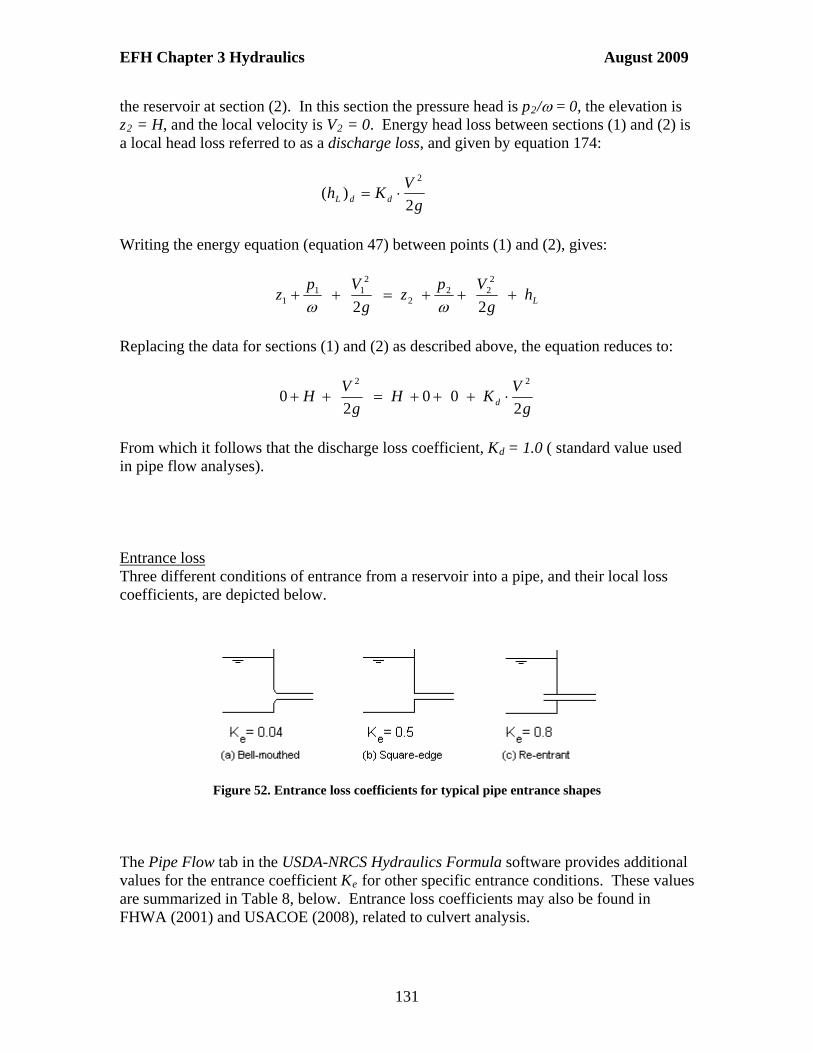
EFH Chapter 3 Hydraulics August 2009
the reservoir at section (2). In this section the pressure head is p2/ = 0, the elevation is z2 = H, and the local velocity is V2 = 0. Energy head loss between sections (1) and (2) is a local head loss referred to as a discharge loss, and given by equation 174:
g
VKh ddL 2
)(2
Writing the energy equation (equation 47) between points (1) and (2), gives:
L h g
V
p z
g
V
pz
22
222
2
211
1
Replacing the data for sections (1) and (2) as described above, the equation reduces to:
g
V K H
g
V H d 2
002
022
From which it follows that the discharge loss coefficient, Kd = 1.0 ( standard value used in pipe flow analyses). Entrance loss Three different conditions of entrance from a reservoir into a pipe, and their local loss coefficients, are depicted below.
Figure 52. Entrance loss coefficients for typical pipe entrance shapes The Pipe Flow tab in the USDA-NRCS Hydraulics Formula software provides additional values for the entrance coefficient Ke for other specific entrance conditions. These values are summarized in Table 8, below. Entrance loss coefficients may also be found in FHWA (2001) and USACOE (2008), related to culvert analysis.
131

EFH Chapter 3 Hydraulics August 2009
Entrance losses are calculated using the expression (equation 174):
42
22 8
2)(
gD
QK
g
VKh eeeL
Table 8. Pipe entrance loss coefficients.
Type of Structure and Entrance Design Ke Pipe, Concrete Projecting from fill, socket end [groove-end] 0.2 Projecting from fill, square cut end 0.5 Headwall or Headwall and wingwalls Socket end of pipe [groove-end] 0.2 Square-end 0.5 Rounded (radius = 1/12D) 0.2 Mitered to conform to fill slope 0.7 End section conforming to fill slope 0.5 Pipe or Pipe-Arch, Corrugated Metal Projecting from fill (no headwall) 0.9 Headwall or Headwall and wingwalls square-edge 0.5 Mitered to conform to fill slope 0.7 End section conforming to fill slope 0.5
________________________________________________________________________ Example 65 – Pipe flow calculation including local losses using the USDA-NRCS Hydraulics Formula software Using the Pipe Flow tab in the USDA-NRCS Hydraulics Formula software, calculate the discharge Q and flow velocity V for a 18-in-diameter, 1200-ft-long, corrugated plastic pipe (Manning’s n = 0.015) whose entrance is mitered to conform to a fill slope (Ke = 0.7). Head on the pipe is 10 ft. The solution, illustrated in the figure below indicates that Q = 8.1 cfs, and V = 4.6 ft/s.
132

EFH Chapter 3 Hydraulics August 2009
Figure 53. Solution for pipe flow with entrance loss using USDA-NRCS Hydraulics Formula. ________________________________________________________________________ Losses due to pipe fittings Pipe fittings such as valves, elbows, and bends produce local losses according to (equation 174). The values of selected pipe fittings are shown in Table 9, below.
Table 9. Local loss coefficients for selected pipe fittings.
133
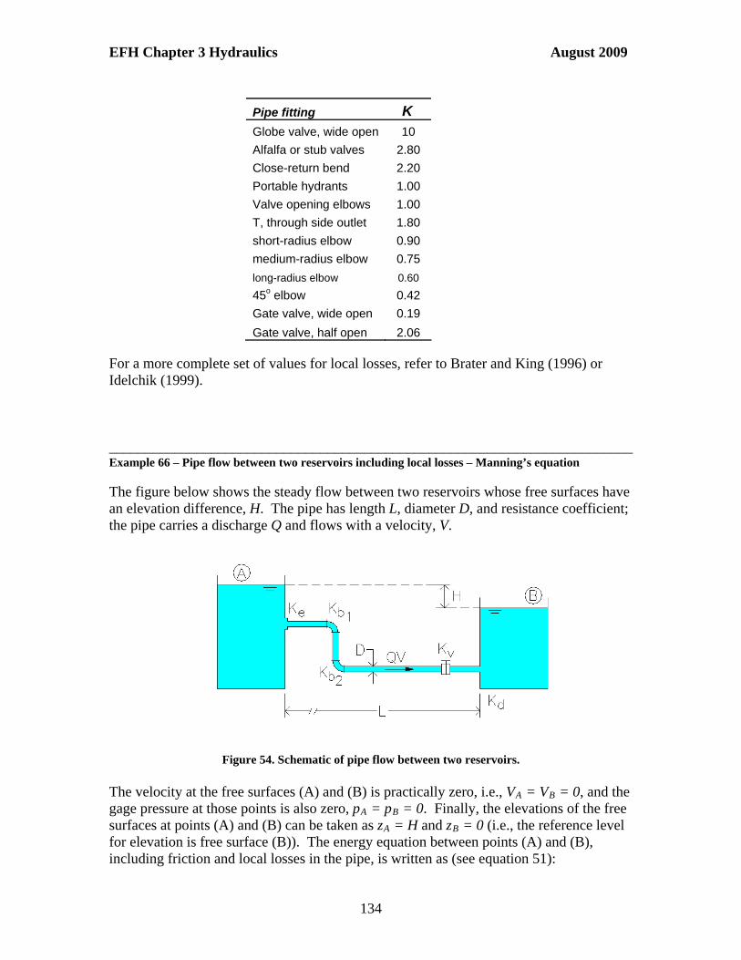
EFH Chapter 3 Hydraulics August 2009
For a more complete set of values for local losses, refer to Brater and King (1996) or Idelchik (1999). ________________________________________________________________________ Example 66 – Pipe flow between two reservoirs including local losses – Manning’s equation The figure below shows the steady flow between two reservoirs whose free surfaces have an elevation difference, H. The pipe has length L, diameter D, and resistance coefficient; the pipe carries a discharge Q and flows with a velocity, V.
Pipe fitting K Globe valve, wide open 10
Alfalfa or stub valves 2.80
Close-return bend 2.20
Portable hydrants 1.00
Valve opening elbows 1.00
T, through side outlet 1.80
short-radius elbow 0.90
medium-radius elbow 0.75
long-radius elbow 0.60
45o elbow 0.42
Gate valve, wide open 0.19
Gate valve, half open 2.06
Figure 54. Schematic of pipe flow between two reservoirs.
The velocity at the free surfaces (A) and (B) is practically zero, i.e., VA = VB = 0, and the gage pressure at those points is also zero, pA = pB = 0. Finally, the elevations of the free surfaces at points (A) and (B) can be taken as zA = H and zB = 0 (i.e., the reference level for elevation is free surface (B)). The energy equation between points (A) and (B), including friction and local losses in the pipe, is written as (see equation 51):
134

EFH Chapter 3 Hydraulics August 2009
LfBB
BAA
A h h g
V
p z
g
V
pz
22
22
Introducing Manning’s equation (equation 151) to estimate pipe friction losses, the local loss equation (equation 174), and the data presented above, the energy equation is written as:
g
VKV
D
Ln
g z
g Hz BB 2
8755.22
00
2
00 22
3/4
2
Results in: g
K
D
LnVH
28755.2
3/4
22
In terms of the flow discharge, this equation is written as:
g
K
D
Ln
D
QH
28755.2
163/4
2
42
2
The term K includes the sum of all local loss coefficients in the pipeline. Note that the Darcy-Weisbach equation or the Hazen-Williams formula is always an option to use in estimating pipe friction loss. Using the values L = 550 ft, D = 2 ft, n = 0.012, Q = 35 cfs, with the following local loss coefficients:
Entrance: Ke = 0.04 (bell-mouth entrance) Elbow 1: Kb1 = 0.90 (short-radius elbow) Elbow 2: Kb2 = 0.75 (medium-radius elbow) Valve: Kv = 0.19 (gate valve, wide open) Discharge: Kd = 1.00 (standard value for discharge coefficient)
Thus, for this case K = Ke + Kb1 + Kb2 + Kv + Kd = 0.04+0.90+0.75+0.19+1.00 = 2.88. Find the difference in elevations between the reservoirs, H. Using the equation developed above:
2.322
88.2
2
550012.08755.2
21416.3
35163/4
2
42
2
H
H =16.77 ft.
135

EFH Chapter 3 Hydraulics August 2009
If the elevation difference between reservoirs is known, the resulting equation above may be solved for V to determine the velocity in the pipe. Then the discharge may be determined with the continuity eqution, Q = VA. ________________________________________________________________________ Development of the Pipe Flow equation The equation from the Pipe Flow tab in the USDA-NRCS Hydraulics Formula software is shown Figure 53 and repeated here:
)(,5087
,1
23/4
2
indd
nKp
LKKK
gHaQ
pbe
[Eq. 175]
In order to develop this equation:
K = Ke + Kb + 1 with Ke being the entrance loss coefficient, Kb accounting for devices such as elbows and valves (referred to as Bend Coefficient in Figure 53), and Kd = 1 being the discharge coefficient. Thus, the energy equation presented in example 66 (Manning’s equation is used to estimate pipe friction losses) is written as:
18755.22
228755.2
3/4
22
3/4
22
be KKD
Lng
g
V
g
K
D
LnVH
Replacing the diameter D (in feet) with d (in inches) and defining:
3/4
25087
d
nK p
The energy equation becomes:
LKKKg
VKKLK
g
VH pbebep 1
21
2
22
Solving for V, gives the following equation:
LKKK
gHV
pbe
1
2
Multiplying this result by the area of the cross-section and substituting Q for VxA gives equation 175. ________________________________________________________________________ Example 67 – Pipe flow calculation including local losses using USDA-NRCS Hydraulics Formula
136
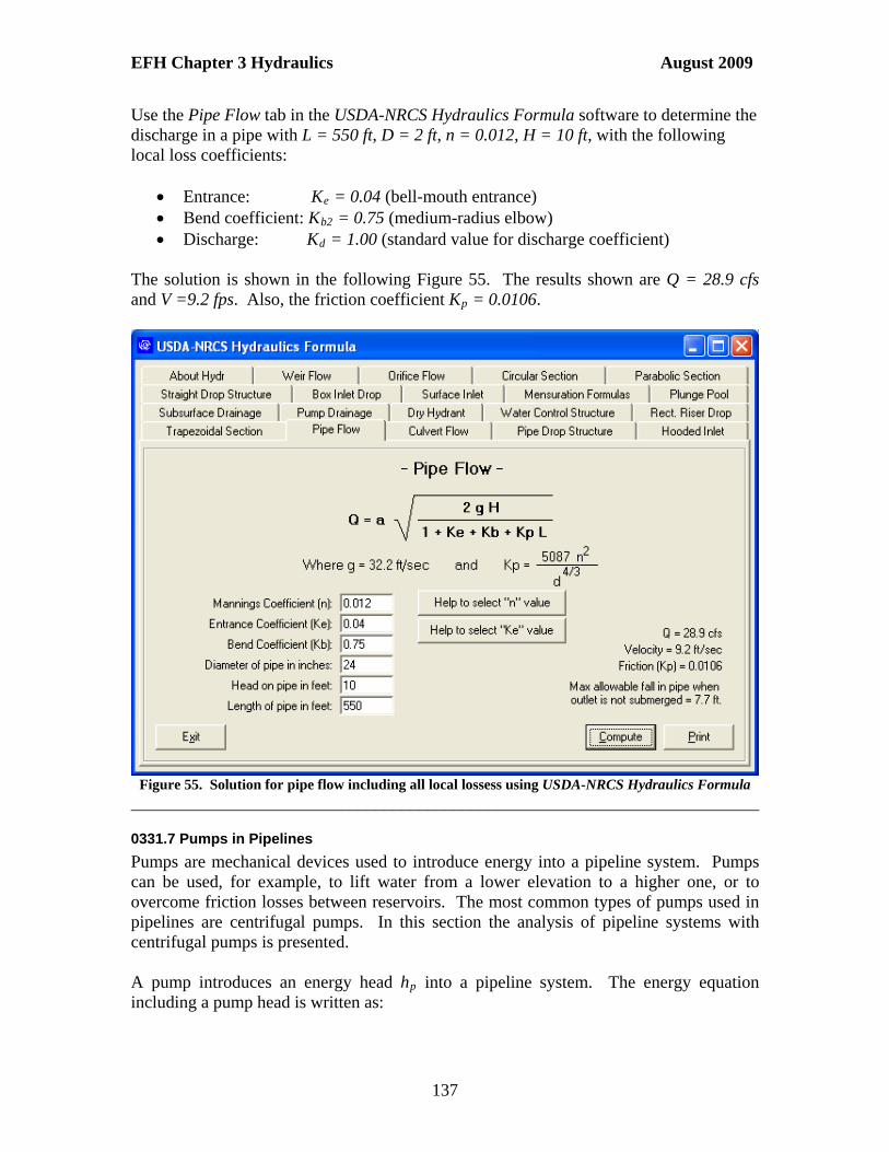
EFH Chapter 3 Hydraulics August 2009
Use the Pipe Flow tab in the USDA-NRCS Hydraulics Formula software to determine the discharge in a pipe with L = 550 ft, D = 2 ft, n = 0.012, H = 10 ft, with the following local loss coefficients:
Entrance: Ke = 0.04 (bell-mouth entrance) Bend coefficient: Kb2 = 0.75 (medium-radius elbow) Discharge: Kd = 1.00 (standard value for discharge coefficient)
The solution is shown in the following Figure 55. The results shown are Q = 28.9 cfs and V =9.2 fps. Also, the friction coefficient Kp = 0.0106.
Figure 55. Solution for pipe flow including all local lossess using USDA-NRCS Hydraulics Formula
________________________________________________________________________
0331.7 Pumps in Pipelines
Pumps are mechanical devices used to introduce energy into a pipeline system. Pumps can be used, for example, to lift water from a lower elevation to a higher one, or to overcome friction losses between reservoirs. The most common types of pumps used in pipelines are centrifugal pumps. In this section the analysis of pipeline systems with centrifugal pumps is presented. A pump introduces an energy head hp into a pipeline system. The energy equation including a pump head is written as:
137

EFH Chapter 3 Hydraulics August 2009
Lfp hhg
Vpzh
g
Vpz
22
222
2
211
1 [Eq. 176]
The normal convention is that energy added to the flow, such as the pump head hp, is placed on the left-hand side (upstream side) of the equation, while, energy extracted from or lost by the flow, such as the friction head hf and the sum of local losses hL, is placed on the right-hand side (downstream side) of the equation.
0331.7.1 Pump Operational Characteristics
In pipeline system hydraulics, an important operational characteristic of a pump is the variation of the pump head hp with the discharge Q passing through the pump. For centrifugal pumps the relationship between hp and Q is given by a quadratic equation (also called a polynomial equation of the second degree) of the form:
hp = aQ2 + bQ + c [Eq. 177] The coefficients a, b, and c, in this equation, can be determined by fitting data from tests performed on a given pump. The equation describing a given pump, or at least a graph of the relationship between hp and Q, should be available from the pump manufacturer. ________________________________________________________________________ Example 68 – Pump head and discharge analysis Tests on a pump produce the following discharge-head data:
Q(cfs) hp(ft) 0.0 25.3 5.0 22.0 10.0 18.3 15.0 12.0 20.0 4.2
The pump discharge graph and equation were produced with curve-fitting software and are shown in Figure 56 below.
138

EFH Chapter 3 Hydraulics August 2009
Figure 56. Pump discharge-head graph Notice from the graph that the energy head for zero discharge is hp = 25.143 ft. This is the “shut-off head” or maximum head for this pump. If valves are closed and no flow occurs, the pump is capable of building 25.143 ft of head. The maximum pump capacity at free discharge is calculated from the pump curve equation by setting hp (y) = 0 and solving for Q. This gives 0 = -0.0331Q2 - 0.3811Q + 25.143. The positive solution to this quadratic equation produces the free-discharge, Q = 22.4 cfs, which the pump delivers with hp = 0 (no discharge pressure). This discharge is what the pump would deliver if it were disconnected from any pipeline and allowed to discharge freely to the atmosphere. ________________________________________________________________________ An example of a pump-pipeline system analysis using manufacturer-provided pump curves is presented in Exhibit 6 - Pipe-system analysis .
0331.7.2 Pump Power and Efficiency
The hydraulic power developed by a pump represents the amount of energy per unit time introduced by the pump into the flow. The hydraulic power, Ph, is calculated as:
139

EFH Chapter 3 Hydraulics August 2009
Ph = Qhp [Eq. 178]
where is the specific weight of water. Using the units of the English system, namely, (lb/ft3), Q (cfs), and hp(ft), the power is given in units of lbft/s. A more commonly used unit of power in the English System is the horsepower (hp) defined as 1 hp = 550 lbft/s. Thus, in terms of horsepower the equation for the hydraulic power of a pump is:
550p
h
QhP
, Ph(hp) [Eq. 179]
In units of the International System (S.I.), namely, (N/m3), Q (m3/s), and hp(m), the pump power Ph is given in Watts (W). For the S,I, use equation 178 to calculate the power. To provide hydraulic power, Ph, the pump P is activated by a motor M as illustrated in Figure 57, below. The motor can be powered by electricity at connection E.
Figure 57. System schematic showing motor M, the electric supply E, and pump P
The motor provides the pump with input power Pm, however, due to energy losses by friction in the pump shaft (which is dissipated as heat in the environment), and other losses, not all of the motor power Pm is utilized by the pump to produce hydraulic power. Thus, in general, Ph < Pm, and the ratio between the hydraulic power and the motor power is a quantity smaller than one (Ph/Pm<1) known as the efficiency of the pump, p:
1m
hp P
P [Eq. 180]
The motor itself is provided with a certain amount of electric power Pe; however, due to losses in the transmission line as well as in the motor mechanism the motor power Pm is smaller than the electric power, i.e., Pm<Pe. Thus, the efficiency of the motor, m, is a quantity smaller than one (Pm/Pe <1), defined as:
1e
mm P
P [Eq. 181]
140

EFH Chapter 3 Hydraulics August 2009
The combined motor-pump system, in turn, has an efficiency m-p defined as
1 mpe
m
m
h
e
hpm P
P
P
P
P
P [Eq. 182]
The various efficiencies, i, can be expressed as a percent by multiplying by 100. ________________________________________________________________________ Example 69 - Pump power and efficiency calculation A pump produces a head hp = 41.67 ft with a discharge Q = 1.24 cfs. If the pump efficiency is 80% (p = 0.80) and the motor efficiency is 90% (m = 0.90), determine: (a) the hydraulic power provided by the pump to the flow, Ph; (b) the power that the motor needs to provide to the pump, Pm; (c) the electric power needed to be provided to the motor, Pe; and (d) the efficiency of the motor-pump system, m-p. (a) The hydraulic power (in hp) is calculated according to equation 179:
hpQh
P ph 86.5
550
67.4124.14.62
550
(b) The power provided by the motor follows from the definition of the pump efficiency (equation 180):
hpP
Pp
hm 33.7
80.0
86.5
(c) The electric power provided to the motor follows from the definition of the motor efficiency (equation 181):
hpP
Pm
me 14.8
90.0
33.7
(d) The efficiency of the motor-pump system can be calculated with equation 182:
%7272.090.080.0 mppm
or
%7272.014.8
86.5
e
hpm P
P
________________________________________________________________________ 0332 Pipelines and Networks Pipelines of different diameters can be combined into different configurations including pipes in series, pipes in parallel, pipes converging to a single point, and more complex pipe networks. These configurations are discussed in the following sections.
141

EFH Chapter 3 Hydraulics August 2009
0332.1 Pipelines in Series
Pipelines in series consist of segments of pipeline connected one after the other so that the flow discharge follows a single path. An arrangement of pipelines in series is presented in Figure 58, below.
Figure 58. Three pipelines in series connecting two reservoirs. Three pipelines of different diameters and lengths are shown carrying water between reservoirs (A) and (B). The pipelines have lengths L1, L2, and L3, with corresponding diameters D1, D2, and D3. In addition, the pipelines have different roughness coefficients. The elevation difference between reservoirs (A) and (B) is given by H. Local head losses due to an expansion or a contraction The system illustrated in Figure 58 shows an expansion in diameter between pipelines 1 and 2 (point X), and a contraction in diameter between pipelines 2 and 3 (point C). Expansions and contraction in pipelines produce local head losses. For a sudden expansion, the local head losses are calculated as:
g
V
D
D
g
V
D
D
g
VVh d
u
du
d
uduxL 2
12
12
)()(
2222
222
[Eq. 183]
The subscripts, u and d refer to the upstream and downstream pipelines. Notice that the head loss in a sudden expansion depends only on the diameters upstream and downstream of the expansion (Du, Dd). Defining expansion loss coefficients as:
22
1
d
uxu D
DK [Eq. 184]
or
142

EFH Chapter 3 Hydraulics August 2009
22
1
u
dxd D
DK [Eq. 185]
The general form of the local losses equation is written as:
g
VK
g
VKh d
xdu
xuxL 22)(
22
[Eq. 186]
For a sudden contraction, as the one between pipes 2 and 3 in Figure 58, the local head losses are given by the equation:
g
VKh d
ccL 2)(
2
[Eq. 187]
where Kc is the contraction loss coefficient given in Table 10, below, and Vd is the flow velocity in the downstream pipeline, i.e., the one with the smallest diameter. In Table 10, Dd and Du are the diameters of the pipe downstream and upstream of the contraction. See Brater and King (1996) or Idelchik (1999) for more information on pipeline contraction losses.
Table 10. Local head loss coefficients for a sudden pipe contraction.
Dd/Du Kc Dd/Du Kc 0.1 0.45 0.6 0.28 0.2 0.42 0.7 0.22 0.3 0.39 0.8 0.15 0.4 0.36 0.9 0.06 0.5 0.33 1.0 0.00
Energy equation for the three-pipeline system In writing the energy equation between reservoirs (A) and (B) in Figure 58 friction head losses in each pipeline will be included, as well as, entrance losses from reservoir (A) into pipeline 1, expansion losses at point (X), contraction losses at point (C), and discharge losses from pipeline 3 into reservoir (B). For the points (A) and (B) in the surface of the reservoirs, VA = VB = 0, pA = pB = 0, zA = zB + H. The expressions for the local losses are the following:
Entrance loss from reservoir (A) to pipe 1: g
VKh eeL 2
)(2
1 , with Ke = 0.5. See
Figure 52.
143
EFH Chapter 3 Hydraulics August 2009
Expansion from pipe 1 to pipe 2: g
VKh xxL 2
)(2
11 , with
22
2
11 1
D
DK x
Contraction from pipe 2 to pipe 3: g
VKh ccL 2
)(2
3 , with Kc from Table 10 as a
function of the ratio D3/D2.
Discharge loss from pipe 3 into reservoir (B): g
VKh ddL 2
)(2
3 , with Kd = 1.0,
always. The friction losses in each pipe may be calculated using either the Darcy-Weisbach equation, the Manning’s equation, or the Hazen-Williams formula. The total friction loss is the sum of each pipe’s friction loss. The energy equation for the system of Figure 58 is written as:
LfBB
BAA
A hhg
Vpz
g
Vpz
22
22
From which it follows that:
g
VK
g
VK
g
VK
g
VKh
gz
gHz dcxefBB 22222
00
2
00 23
23
21
1
21
or,
g
VK
g
VK
g
VK
g
VKhhhH dcxefLf 2222
23
23
21
1
21 [Eq. 188]
In most analyses of pipelines in series the diameters of the pipelines are known, and the problem consists in determining the discharge Q for a given available head H, or vice versa. The three examples of pipes in series presented below include the effect of local losses. ________________________________________________________________________ Example 70 – Pipes in series using the Darcy-Weisbach equation The system of Figure 58 has pipelines lengths, diameters, and roughness values: L1 = 200 ft, L2 = 400 ft, L3 = 150 ft, D1 = 1.00 ft, D2 = 1.50 ft, D3 = 1.00 ft, e1 = 0.0001 ft(concrete), e2 = 0.00004 ft(PVC), and e3 = 0.00025 ft(welded steel). The kinematic viscosity is = 110 -5 ft2/s. (a) If the discharge Q = 5 cfs, determine the needed head H. (b) If the available head between the reservoirs is H = 30 ft, determine the discharge through the pipes.
144

EFH Chapter 3 Hydraulics August 2009
A spreadsheet application gives the results. If the discharge is 5 cfs, the needed head is coincidentally 5 ft. If the available head is 30 ft, the discharge, Q = 12.58 cfs. ________________________________________________________________________ Example 71 - Pipes in series using the Manning’s equation Using the same data as example 70, the pipe lengths, diameters, and Manning’s n coefficients are given by L1 = 200 ft, L2 = 400 ft, L3 = 150 ft, D1 = 1.00 ft, D2 = 1.50 ft, D3 = 1.00 ft, n1 = 0.012(concrete), n2 = 0.01(PVC), and n3 = 0.013(welded steel). (a) If the discharge Q = 5 cfs, determine the needed head H. (b) If the available head between the reservoirs is H = 30 ft, determine the discharge through the pipes. A spreadsheet application gives the results. If the discharge is 5 cfs, the needed head is 8.12 ft. If the available head is 30 ft, the discharge, Q = 9.61 cfs. ________________________________________________________________________ Example 72 - Pipes in series using the Hazen-Williams formula Using the same data as examples 70 and 71, the pipe lengths, diameters, and Hazen-Williams coefficients are given by L1 = 200 ft, L2 = 400 ft, L3 = 150 ft, D1 = 1.00 ft, D2 = 1.50 ft, D3 = 1.00 ft, CHW1 = 120(concrete), CHW 2 = 150(PVC), and CHW 3 = 120(welded steel). (a) If the discharge Q = 5 cfs, determine the needed head H. (b) If the available head between the reservoirs is H = 30 ft, determine the discharge through the pipes. A spreadsheet application gives the results. If the discharge is 5 cfs, the needed head is 6.37 ft. If the available head is 30 ft, the discharge, Q = 11.39 cfs. ________________________________________________________________________ Calculations were also made ignoring local losses in examples 70, 71, and 72. Table 11 shows the effect of neglecting local losses on discharge.
Table 11. Effect of neglecting local losses on an example pipeline system
Friction loss method
Q (cfs) including local losses
Q (cfs) neglecting local losses
Percentage difference
Darcy-Weisbach 12.58 14.79 17.56% Manning's 9.61 10.47 8.95% Hazen-Williams 11.39 13.03 14.40%
The percentage differences in Table 11 are too large to neglect local loss. A generally accepted criterion is that local losses should be included in a pipe design analysis if the local losses exceed 5% of the total head loss.
0332.2 Pipelines in Parallel
Figure 59 illustrates reservoirs connected by three different parallel pipelines conducting water between the reservoirs. An energy equation can be written separately for each of
145

EFH Chapter 3 Hydraulics August 2009
the pipelines. Including entrance (he), discharge (exit) (hd), and friction (hf) losses for each pipeline, the corresponding energy equations can be written as:
333
222
111
)()(
)()(
)()(
fde
fde
fde
hhhH
hhhH
hhhH
[Eqs. 189]
Where the subscripts (1), (2), and (3) refer to each of the pipelines as illustrated in the figure below.
Figure 59. Three pipelines in parallel connecting two reservoirs.
A simplified analysis in which the local losses are neglected simplifies equation 189 to:
321 )()()( fff hhhH [Eq. 190]
A typical problem of parallel pipes consists in determining the total discharge Q delivered from the upstream to the downstream reservoir given the available head H between the reservoirs. Given H, the available head, the friction loss, hf, is known. Then using either the Darcy-Weisbach equation (requires spreadsheet application for efficient calculation), the Manning’s equation, or the Hazen-Williams formula, the individual discharges Q1, Q2, and Q3 can be obtained. The individual discharges are summed to obtain the total discharge. The examples using Manning’s equation and the Hazen-Williams formula presented below neglect local losses. ________________________________________________________________________ Example 73 - Pipes in parallel using the Manning’s equation The system of Figure 59 has pipelines lengths, diameters, and Manning’s n coefficients: L1 = 200 ft, L2 = 400 ft, L3 = 150 ft, D1 = 1.00 ft, D2 = 1.50 ft, D3 = 1.00 ft, n1 = 0.012, n2 = 0.018, and n3 = 0.010. If the available head is H = 30 ft, determine the total discharge between the reservoirs. The head loss through each pipeline is 30 ft. Manning’s equation (equation 152) is used to calculate the individual discharges:
146
EFH Chapter 3 Hydraulics August 2009
cfsL
h
n
DQ f 95.14
200
30
012.0
00.14632.0
)(4632.0
3/8
1
1
1
3/81
1
cfsL
h
n
DQ f 78.20
400
30
018.0
50.14632.0
)(4632.0
3/8
2
2
2
3/82
2
cfsL
h
n
DQ f 71.20
150
30
010.0
00.14632.0
)(4632.0
3/8
3
3
3
3/83
3
The total discharge is Q = 14.95 cfs + 20.78 cfs + 20.71 cfs = 56.44 cfs. Discharge calculations may also be made for individual pipes with Pipe Flow, NRCS Hydraulics Formula program, which uses Manning’s equation for friction losses. The discharges calculated will be slightly less than those shown above because Pipe Flow, NRCS Hydraulics Formula automatically accounts for a local loss at the pipe exit (Kd = 1.0). ________________________________________________________________________ Example 74 - Pipes in parallel using the Hazen-Williams formula The system of Figure 59 has pipelines lengths, diameters, and Hazen-Williams coefficients: L1 = 200 ft, L2 = 400 ft, L3 = 150 ft, D1 = 1.00 ft, D2 = 1.50 ft, D3 = 1.00 ft, CHW1 = 100, CHW 2 = 80, and CHW 3 = 120. If the available head is H = 30 ft, determine the total discharge between the reservoirs. The head loss through each pipeline is 30 ft. Using (equation 169), the individual pipe discharges are calculated as follows:
cfsL
hDCQ f
HW 50.15200
3000.1100432.0
)(432.0
54.063.2
54.0
1
163.2111
cfsL
hDCQ f
HW 79.24400
3050.180432.0
)(432.0
54.063.2
54.0
2
263.2222
cfsL
hDCQ f
HW 74.21150
3000.1120432.0
)(432.0
54.063.2
54.0
3
363.2333
The total discharge is Q = 15.50 cfs + 24.79 cfs + 21.74 cfs = 62.03 cfs. ________________________________________________________________________ 0332.3 Pipelines Converging at a Single Point Figure 60 shows a pipeline system consisting of three pipelines connecting reservoirs A, B, and C to a single delivery point J (for Junction), where a total discharge Q is to be delivered. Shown in the figure are also the elevations of the free surface of the reservoirs, namely, HA, HB, and HC, as well as the piezometric head elevation of the junction point, HJ.
147

EFH Chapter 3 Hydraulics August 2009
Figure 60. Three pipelines converging to a single delivery point. Neglecting local or minor losses, the energy equations for the three pipelines shown above are written as:
3
2
1
)(
)(
)(
fJC
fJB
fJA
hHH
hHH
hHH
[Eq. 191]
Where (hf)1, (hf)2, and (hf)3 are the friction losses in pipelines [1], [2], and [3], respectively. A typical problem for the system illustrated in Figure 60 consists in determining the discharge Q given the elevations of the free surfaces in reservoirs A, B, and C (HA, HB, HC) and that of point J (HJ). The individual pipe discharges are summed to obtain the total. The examples using Manning’s equation and the Hazen-Williams formula presented below neglect local losses. ________________________________________________________________________ Example 75- Converging pipelines using Manning’s equation The system of Figure 60 has pipelines lengths, diameters, and Manning’s n coefficients: L1 = 200 ft, L2 = 400 ft, L3 = 150 ft, D1 = 1.00 ft, D2 = 1.50 ft, D3 = 1.00 ft, n1 = 0.012, n2 = 0.018, and n3 = 0.010. The elevations of interest are HA = 280 ft, HB = 290 ft, HC = 310 ft, and HJ = 250 ft. Determine the total discharge delivered to junction J. The energy losses in each pipeline are calculated as follows:
(hf)1 = HA – HJ = 280 ft – 250 ft = 30 ft, (hf)2 = HB – HJ = 290 ft – 250 ft = 40 ft, (hf)3 = HC – HJ = 310 ft – 250 ft = 60 ft.
As in example 73, Manning’s equation is used to calculate the individual discharges as follows:
148

EFH Chapter 3 Hydraulics August 2009
cfsL
h
n
DQ f 95.14
200
30
012.0
00.14632.0
)(4632.0
3/8
1
1
1
3/81
1
cfsL
h
n
DQ f 99.23
400
40
018.0
50.14632.0
)(4632.0
3/8
2
2
2
3/82
2
cfsL
h
n
DQ f 29.29
150
60
010.0
00.14632.0
)(4632.0
3/8
3
3
3
3/83
3
The total discharge is Q = 14.95 cfs + 23.99 cfs + 29.29 cfs = 68.23 cfs As in the previous parallel pipes example 73, using Manning’s formula for friction losses, discharge calculations may also be made for individual pipes with Pipe Flow, NRCS Hydraulics Formula program. The discharges calculated will be slightly less than those shown above because Pipe Flow, NRCS Hydraulics Formula automatically accounts for a local loss at the pipe exit (Kd = 1.0). ________________________________________________________________________ Example 76 - Converging pipelines using Hazen-Williams formula The system of Figure 60 has pipelines lengths, diameters, and Hazen-Williams coefficients: L1 = 200 ft, L2 = 400 ft, L3 = 150 ft, D1 = 1.00 ft, D2 = 1.50 ft, D3 = 1.00 ft, CHW1 = 100, CHW 2 = 80, and CHW 3 = 120. The elevations of interest are HA = 280 ft, HB = 290 ft, HC = 310 ft, and HJ = 250 ft. Determine the total discharge delivered to junction J. The energy losses in each pipeline are calculated as follows:
(hf)1 = HA – HJ = 280 ft – 250 ft = 30 ft, (hf)2 = HB – HJ = 290 ft – 250 ft = 40 ft, (hf)3 = HC – HJ = 310 ft – 250 ft = 60 ft.
As in example 74, the Hazen-Williams formula is used to calculate the individual pipe discharges as follows:
cfsL
hDCQ f
HW 50.15200
3000.1100432.0
)(432.0
54.063.2
54.0
1
163.2111
cfsL
hDCQ f
HW 95.28400
4050.180432.0
)(432.0
54.063.2
54.0
2
263.2222
cfsL
hDCQ f
HW 60.31150
6000.1120432.0
)(432.0
54.063.2
54.0
3
363.2333
The total discharge is Q = 15.50 cfs + 28.95 cfs + 31.60 cfs = 76.05 cfs. ________________________________________________________________________
149

EFH Chapter 3 Hydraulics August 2009
AGPipe design software for irrigation and livestock pipe systems, is available at: http://www.wsi.nrcs.usda.gov/products/W2Q/water_mgt/Irrigation/irrig-mgt-models.html AGPipe software performs hydraulic calculations and contains databases of local loss factors and friction factors, which may be populated by the user. NRCS is also developing the Pipeline Design Tool for future field office use.
0332.4 Pipeline Networks
Pipe networks are utilized to supply water for urban and rural domestic and industrial uses. Networks are also used by irrigation districts and occasionally in livestock watering systems. A pipe network is simply a collection of pipes connected in a given geometric pattern and having at least one supply point and one delivery or consumption point. The points where individual pipelines join each other are known as junctions or nodes. Pipe networks are schematized as geometric constructs of lines representing the component pipes. The main purpose of analyzing a given pipe network is to determine the discharge in each pipe and the piezometric head at each node. These results can be used then to verify that certain design guidelines, such as minimum flow velocities and minimum junction pressures, are satisfied. The analysis of pipe networks requires the simultaneous solution of a number of mathematical equations that represent equations of continuity at the nodes, and equations of energy around closed loops and/or pseudo-loops. Analyses of simple pipe networks may be performed with a spreadsheet application, but spreadsheet use would become very tedious as the number of pipelines and loops increase. There are a number of publicly-available and commercial software that can be used for network solution in a more efficient manner, such as the U.S. Environmental Protection Agency’s EPANET software. 0333 Appurtenances in Pipelines and Networks In this section a number of appurtenances commonly used in pipelines and pipe networks are described.
0333.1 Air Vacuum and Release Valves
Entry and entrapment of air in a pipeline during filling and operation of a pipeline can cause development of air pockets. Air pockets tend to restrict and reduce flow or increase pumping costs in pipelines. Air pocket build-up in pumped pipelines can reduce flows by 5 to 15%. In low-head, gravity-driven flow, air pocket build-up can reduce flow up to 50%. On the other hand, a lack of air entry can cause pipe collapse if a vacuum develops behind flowing water as a pipeline empties. Air valves are of four types:
1. Air/vacuum relief valves, also known as kinetic air valves, large orifice air valves, vacuum breakers, low-pressure air valves, and air relief (not release) valves.
150

EFH Chapter 3 Hydraulics August 2009
Large volumes of air are discharged before a pipeline is pressurized, especially at pipe filling. Large quantities of air are admitted when the pipe drains and at the appearance of water column separation.
2. Continuous acting air and vacuum valves, also known as double orifice air valves,
or combination air valves, fill the functions of the air/vacuum relief valves and air release valves, admitting and releasing large quantities of air when needed, and releasing air continuously when the lines are pressurized.
3. Air release valves are also known as automatic air valves, small orifice air valves,
continuous acting air vents, and pressure air valves. These vents continue to discharge air, usually in smaller quantities, after the air vacuum valves close, as the line is pressurized.
4. Vacuum relief valves are large orifice valves for vacuum relief only. These
valves allow air to enter the pipeline. Guidelines for placement and sizing of air valves: 1. Locate air release valves or continuous-acting air and vacuum valves at all high
points and at 1/4 mile intervals on pipelines with constant grades. Locate an air release valve at the end of the line.
2. Aviod oversizing air release valves to lessen the possibility of water hammer. See
section 0334 for more information on water hammer. 3. Locate an air-and-vacuum valve or vacuum valve to allow air to enter behind the
water as a pipeline is emptied. Vacuum valves are generally not needed on pipelines of less than 3-inch diameter for protection from collapse; however, they may be needed to insure complete drainage of the line. On the other hand, vacuum valves are important on low head plastic irrigation pipe and large diameter steel pipe (>24”) to prevent collapse of the line.
Valve sizes may be determined for a pipeline by calculating: (1) flow for both filling and emptying the pipeline, (2) pipe collapse pressure, and (3) valve intake or discharge at a prescribed pressure across the valve as illustrated below. ________________________________________________________________________ Example 77 – Air valve sizing Given: 18” diameter, 80 psi, SDR 51, PVC pipe, on a slope of 0.05 ft/ft. Note that SDR is the pipe outside diameter divided by the wall thickness. a. Determine flow for draining the line using the Hazen-Williams formula (equation 169). CHW for PVC pipe is 150:
151

EFH Chapter 3 Hydraulics August 2009
cfsQ 34.3705.5.1150432.0 54.063.2 Valves must re-enter air at the same rate as the calculated water flow of 37.34 cfs. b. Determine pipe collapse pressure using equation for PVC pipe given in ASTM: Pc = [2E/(1-2 )] x [[1/ [do /t] [(do /t)-1]2 ]] Where: Pc = collapse pressure of PVC pipe (psi) E = Young’s modulus of elasticity (400,000 psi) = Poisson’s ratio (0.33) t = wall thickness (in.) do = outside diameter of pipe (in.) Pc = [(2)(400,000)/(1-0.332 )] [[1/ (51) [(51)-1]2 ]] = 7 psi Use the collapse pressure determined above or 5 psi, whichever is lower (standard design practice). c. Determine orifice diameter, using orifice equation (equation 198):
ghACQ d 2
where Cd = flow coefficient = 0.6 A = orifice area h = Pc (from above)/ωair where: specific weight of air = ωair = .0764 lbs/ft3 Pc = (5 lbs/in2 ) (144 in2/ ft2 ) = 720 psf Rearranging the orifice formula, A = Q/ [Cd (2gh).5]
A = 37.34/[0.6 [2(32.2) (720/ .0764)].5]
= 0.080 ft2 A = (.080 ft2 ) (144 in2 /ft2) = 11.52 in2 D = (4A/).5 = [(4)(11.52)/ )].5 = 3.83 in, orifice diameter
152
EFH Chapter 3 Hydraulics August 2009
d. Determine the size of orifice required when filling the pipe. When filling a line, good practice is not to exceed 1 fps (note: not all systems provide that much control of filling velocity, see next part (e) of this example). Using a filling velocity of 1 fps: Q = AV Q = (/4) (1.52) (1) = 1.77 cfs Therefore, air must be discharged from the line at a rate of 1.77 cfs Size the orifice for 2 psi pressure across the valve (standard design practice). Using the orifice formula, as before: Pc = (2 lbs/in2 ) (144 in2 /ft2 ) = 288 psf A = 1.77/[0.6 [2(32.2)(288/.0764)].5 ] = 0.006 ft2 A = (0.006 ft2 ) (144 in2 /ft2 ) = 0.86 in2 D = (4A/).5 =[(4)(0.86)/ ].5 = 1.05 in. orifice diameter. e. Alternative determination of orifice size required when filling the pipe. When filling a line, with an electric powered pumping plant not equipped with special controllers or valves, it may not be possible to limit filling velocity to 1 fps. The electric motor is on or off which might produce filling velocities of up to 5 fps. Using a filling velocity of 5 fps:
Q = AV
Q = (/4) (1.52) (5) = 8.84 cfs Therefore, air must be discharged from the line at a rate of 8.84 cfs Size the orifice for 2 psi pressure across the valve (standard design practice). Using the orifice formula, as before: Pc = (2 lbs/in2 ) (144 in2 /ft2 ) = 288 psf A = 8.84/[0.6 [2(32.2)(288/.0764)].5 ] = 0.03 ft2 A = (0.03 ft2 ) (144 in2 /ft2 ) = 4.32 in2 D = (4A/).5 =[(4)(4.32)/ ].5 = 2.35 in. orifice diameter Comparing orifice sizes of 3.83 in. diameter for vacuum relief and 1.05 or 2.35 in. diameter for air release shows that the 3.83 in. diameter orifice should be used if an air-and-vacuum valve, or continuous-acting air-and-vacuum valve, is to be used. If
153

EFH Chapter 3 Hydraulics August 2009
individual air release and vacuum relief valves are used, then they each may be of the size determined. ________________________________________________________________________ Additional information on the operation and settings for air valves is available from the valve manufacturers. 0333.2 Air Vents Air vents act similarly to air vacuum or air release valves, however, they allow for the release of large volumes of air near pumps or water intakes, pressure boxes, and check valves. Air vents are often used in low-head pipelines. The figure below shows a simple air vent consisting of a cylindrical chamber of diameter Dc located at a distance L from a water intake where air entrainment occurs. The height of the air vent chamber should be at least one-half the diameter of the pipe (D/2), and the chamber’s area should be at least half of the mainline pipe cross sectional area. For a cylindrical chamber, the minimum diameter is, therefore,
2
2DDc [Eq. 192]
Figure 61. Location and dimensions of air vent chamber near a water intake. The minimum length L, measured from the pipe entrance is given by, Roberson, et.al.(1956):
L = 1.76 V D [Eq. 193] Where: V is the flow velocity in the pipeline. This equation uses V in fps, D in ft, and L in ft. Using units of the International System (S.I.), the corresponding equation is:
L = 5.77 V D [Eq. 194]
where V is in m/s, D in m, and L in m.
154

EFH Chapter 3 Hydraulics August 2009
________________________________________________________________________ Example 78 – Air vent chamber sizing A 12-in diameter pipeline is to carry a discharge Q = 2.5 cfs. Determine the minimum diameter, height, and location of an air vent chamber from a water intake where air entrainment occurs. The pipe diameter is D = 1 ft, and the flow velocity can be calculated from equation 31:
fpsft
sft
D
QV 18.3
)1(1416.3
/5.2442
3
2
The chamber should have a height of D/2 = 0.5 ft = 6 in, and a minimum diameter of:
ftftD
Dc 707.02
)1(
2
22
The distance from the water intake to the air vent should be at least:
L = 1.76 V D = 1.76×3.18× 1 = 5.60 ft ________________________________________________________________________
0333.3 Pressure Control Valves
Pressure relief valves (or pressure safety valves) are used in pipeline systems to protect against excessive pressure. They are designed to open and discharge small amounts of water at a preset pressure limit. Excess pressure would open the valve and allow some water to be released. Pressure reducing valves are used where a predetermined lower pressure is necessary for the proper function of certain components such as emitters in microirrigation systems. They can be used in systems with variable pressure to maintain a lower constant pressure downstream of the valve. Pressure-sustaining valves consist of the basic valves and a three-way pressure-sustaining pilot. Pressure is sustained at the upstream of the valve to a preset level, while the valve outlet drains excessive pressure in order to maintain the preset inlet pressure. Pressure is maintained constant, regardless of upstream fluctuating pressure and flow rate. Pressure sustaining valves are used on hilly terrain to maintain pressure in elevated areas and many other applications where sustained pressure is necessary Details on the operation of pressure relief, reducing, and sustaining valves are available from the valve manufacturers. The pipeline system pressure range and capacity are parameters needed for valve selection.
155

EFH Chapter 3 Hydraulics August 2009
________________________________________________________________________ Example 79 – Pressure relief valve selection Given: 8” diameter, 80 psi, SDR 51, plastic irrigation pipe. Pipe inside diameter is 7.84 in = 0.65 ft. Design pipeline velocity is 5 fps. Select a pressure relief valve to protect against possible surge pressure at the end of the pipeline. The valve is set to relieve pressure at 80 psi, which is the pipe pressure rating. Size the pressure relief valve to pass the full flow at 150% of the pipe pressure rating: First, determining the pipeline flow: Q = AV Q = (/4) (0.652) (5) = 1.66 cfs Determining minimum orifice diameter, using orifice equation (equation 198):
ghACQ d 2
where Cd = flow coefficient = 0.6 A = orifice area P = 1.5 (80 lbs/in2 ) (144 in2/ ft2 ) = 17280 psf h = P /ωw where: specific weight of water = ωw = 62.4 lbs/ft3 Rearranging the orifice formula, A = Q/ [Cd (2gh).5]
A = 1.66 / [0.6 [2(32.2) (17280 /62.4)].5]
= 0.0207 ft2 A = (.0207 ft2 ) (144 in2 /ft2) = 2.98 in2 D = (4A/).5 = [(4)(2.98)/ )].5 = 1.95 in, orifice diameter Review of manufacturer’s literature indicate that pressure relief valves with 2-in and larger orifices are available. If, for safety concerns, the designer wishes to reduce the valve escape velocity, larger-size valves are available or multiple valves may be used. Find the dimensions of the valve opening using the continuity equation: A = Q/V.
156
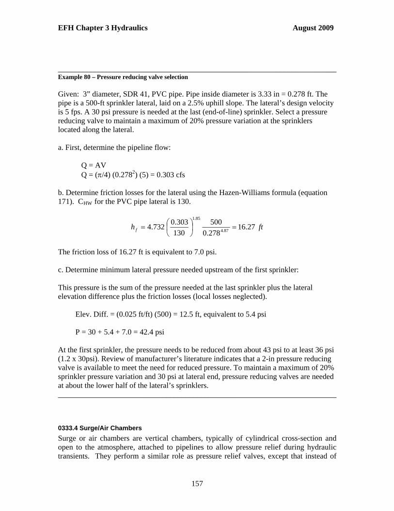
EFH Chapter 3 Hydraulics August 2009
________________________________________________________________________ Example 80 – Pressure reducing valve selection Given: 3” diameter, SDR 41, PVC pipe. Pipe inside diameter is 3.33 in = 0.278 ft. The pipe is a 500-ft sprinkler lateral, laid on a 2.5% uphill slope. The lateral’s design velocity is 5 fps. A 30 psi pressure is needed at the last (end-of-line) sprinkler. Select a pressure reducing valve to maintain a maximum of 20% pressure variation at the sprinklers located along the lateral. a. First, determine the pipeline flow: Q = AV Q = (/4) (0.2782) (5) = 0.303 cfs b. Determine friction losses for the lateral using the Hazen-Williams formula (equation 171). CHW for the PVC pipe lateral is 130.
fth f 27.16278.0
500
130
303.0732.4
87.4
85.1
The friction loss of 16.27 ft is equivalent to 7.0 psi. c. Determine minimum lateral pressure needed upstream of the first sprinkler: This pressure is the sum of the pressure needed at the last sprinkler plus the lateral elevation difference plus the friction losses (local losses neglected). Elev. Diff. = (0.025 ft/ft) (500) = 12.5 ft, equivalent to 5.4 psi P = 30 + 5.4 + 7.0 = 42.4 psi At the first sprinkler, the pressure needs to be reduced from about 43 psi to at least 36 psi (1.2 x 30psi). Review of manufacturer’s literature indicates that a 2-in pressure reducing valve is available to meet the need for reduced pressure. To maintain a maximum of 20% sprinkler pressure variation and 30 psi at lateral end, pressure reducing valves are needed at about the lower half of the lateral’s sprinklers. ________________________________________________________________________
0333.4 Surge/Air Chambers
Surge or air chambers are vertical chambers, typically of cylindrical cross-section and open to the atmosphere, attached to pipelines to allow pressure relief during hydraulic transients. They perform a similar role as pressure relief valves, except that instead of
157

EFH Chapter 3 Hydraulics August 2009
releasing water flow to another pipeline, they allow the water surface level in the chamber to increase in response to a local pressure increase. During a hydraulic transient (unsteady flow) the water surface in the chamber will oscillate until a steady state is recovered. Figure 62, below, shows a schematic of a surge chamber in a pump-pipeline system. The surge chamber in this case would help dissipate a pressure wave that may result after a sudden failure of the pump. The system also includes a check valve that shuts off flow as the flow reverses.
Figure 62. Schematic of pump-pipeline system protected with a surge chamber. For the situation illustrated in the figure above, if the cross-sectional area of the surge chamber is Ac and that of the pipeline is A, the maximum height S of the water surface in the chamber above its steady-state level (i.e., the amplitude of the oscillation) is calculated as:
gA
LA
A
QS c
c
2
[Eq. 195]
where Q is the steady-state discharge, L is the length of pipeline between the upstream reservoir and the check valve, and g is the acceleration of gravity (= 9.81 m/s2 = 32.2 ft/s2). The time in seconds required for the water level in the chamber to first reach its maximum height (one quarter of the period of oscillation) is calculated as, Tullis (1989):
gA
LAT c
2
[Eq. 196]
The water in the chamber will oscillate until friction in the pipe, and in the chamber, slows down the oscillation and produces a complete flow shut off in the pipe upstream of the check valve. Notice that in the absence of a check valve, flow reversal will occur through the pump which could affect its operation after start up. ________________________________________________________________________ Example 81 – Surge chamber calculation The pipeline in Figure 62 is a 1-ft diameter pipeline and the length from the supply reservoir to the check valve is 300 ft. If the pipe carries a steady-state discharge of 4 cfs, determine the maximum water surface increase in a surge chamber of cross-sectional area Ac = 0.785 ft2. If the static level at the chamber is H0 = 500 ft, how high will the water level reach in the surge tank? What is the time T required to reach the maximum water elevation?
158

EFH Chapter 3 Hydraulics August 2009
With D = 1.0 ft, the pipe area is:
A = D2/4 = 3.146× (1 ft)2 / 4 = 0.785 ft2 With L = 300 ft, Q = 4 cfs, g = 32.2 ft/s2, then:
ftsftft
ftft
ft
sft
gA
LA
A
QS c
c
43.24/2.32785.0
300785.0
2785.0
/4
2 22
2
2
3
Thus, the maximum water level is:
H = H0 + S = 500 ft + 24.43 ft = 524.43 ft The time required to reach the maximum water level:
ssftft
ftft
gA
LAT c 79.4
/2.32785.0
300785.0
2
1416.3
2 22
2
0333.5 Check Valves
Check valves are valves that allow flow only in one direction. The pressure of the flowing water opens the valves in the preferred direction. A sudden change in flow direction, such as the case of a pump failure, immediately closes the valve avoiding a reverse flow. The lack of a check valve leaves a pump unprotected against backflow, which may damage the pump and affect its operational efficiency. Details on the operation of check valves can be obtained from the valve manufacturers. 0334 Hydraulic Transients (Water Hammer) The term hydraulic transient refers to a pipeline flow, and its attendant pressure, changing rapidly with time. A hydraulic transient in a pipeline can be originated by the closing of a valve, a pump failure, or a sudden increase in pipeline demand. Water hammers can easily be produced by a sudden closure of a valve. In this case, a pressure wave originates at the valve that travels through the pipe at speeds of the order of 1,440 m/s or 4,700 ft/s. The pressure wave reflects at the other end of the pipeline, be it a reservoir or a main line connection, and travels back towards the valve where pressure builds up again. The process repeats many times until friction dampens the pressure wave and the water flow finally stops. Typically a hammering noise is produced by the transient, thus the name water hammer. Pipelines, appurtenances, and tanks subject to water hammer may suffer deformation and damage in joints and other locations. In designing pipelines, care should be taken to prevent the presence of the water hammer phenomenon by providing check valves, pressure relief valves, and surge chambers in the pipeline systems. Valve closure hydraulic transients can be minimized by closing the valve slowly. Unexpected hydraulic transients, such as a pump failure, will likely produce a high-magnitude pressure wave in pipelines with its attendant vibration. To prevent damage to
159

EFH Chapter 3 Hydraulics August 2009
the pipeline in such a case the pipeline should be provided with valves or surge chambers. The pipeline will be able to better survive a sudden hydraulic transient if it is buried, or otherwise anchored securely. The formal analysis of hydraulic transients in a pipeline includes the simultaneous solution of two partial differential equations involving the discharge Q and the total head H at different locations x along the pipeline and at different times t. This type of analysis requires complex computer programming, considered beyond the scope of this handbook. The closing of a valve is a common cause of hydraulic transients. If closing a valve changes the flow velocity in a pipe from V to Vf, the instantaneous increase in pressure near the valve, p, is calculated by using the equation:
Et
D
E
gVVp
v
f
1
/)(
[Eq. 197]
Where is the specific weight of water (typically, = 62.4 lb/ft3), g is the acceleration of gravity (= 32.2 ft/s2), Ev is the bulk modulus of elasticity of water, t is the pipe wall thickness, and E is the modulus of elasticity for the pipe material. A typical value of the modulus of elasticity for water is Ev = 311,000 psi at 60oF (see Exhibit 4). Modulus of elasticity values for common pipeline materials include steel (E = 30,000,000 psi), cast iron (E = 15,000,000 psi), concrete (E = 3,000,000 psi) and PVC (E = 400,000 psi, with some variation by manufacturing class). For additional information on water hammer analyses see Finnemore and Franzini (2002) or USDA (2005). ________________________________________________________________________ Example 82 – Pressure increase with sudden closing of a valve Consider a steel pipe (E = 30,000,000 psi) with a wall thickness t = 0.25 in = 0.25/12 ft = 0.02 ft, and a diameter D = 0.5 ft. Closing a valve in a pipe that reduces the flow velocity from V = 2.5 fps to Vf = 0.5 fps for water at 60oF in such a pipeline produces a pressure increase of:
22
23
/1443000000002.0
5.0
/144311000
1)/2.32/()/4.62(
)5.05.2(
ftlbft
ft
ftlb
sftftlbfpsfpsp
p = 16,604 lb/ft2 = 16,604 /144 psi = 115 psi
The typical value for atmospheric pressure is 14.7 psi, thus, an increase of 115 psi represents almost eight times the atmospheric pressure. Pipe should have adequate pressure ratings or otherwise be protected to withstand hydraulic transients.
160

EFH Chapter 3 Hydraulics August 2009
________________________________________________________________________ 0335 Cavitation When the local absolute pressure in a closed conduit (by virtue of its elevation and the hydraulic characteristics of the system) falls below the vapor pressure of water, vapor bubbles, or cavities, can form in the flow. These cavities are then carried with the flow towards zones of higher pressure where they implode (collapse onto themselves) producing a characteristic noise, vibration, and even pitting of the pipeline walls at the point of bubble collapse. Cavitation conditions are to be avoided because of their damaging effects, since cavitation can cause pitting and perforations in pipes, and even collapsing of pipes if the pressure drop at a given location is excessively large. Locations where cavitation may occur are the high point of a pipeline, or the suction side of a pump in a pipeline system. Cavitation is undesirable for pump operation since it can reduce pump efficiency and cause deterioration of the impeller. An example of cavitation analysis in a siphon is presented below. Cavitation was introduced in section 0304 Physical Properties of Water, in relation to the vapor pressure of water. ________________________________________________________________________ Example 83 – Cavitation at high point of a siphon Figure 63 below illustrates a conduit delivering water from reservoir (A) to reservoir (B). Such an arrangement, where the middle part of the conduit raises above the free surface of both reservoirs is called a siphon. To start the siphon, it is necessary to fill the conduit with water by using, for example, a vacuum pump at point (C). Once the water flow is established the vacuum pump can be removed and the system continues flowing as long as the free surface at reservoir (A) is higher than that at reservoir (B). Siphon systems can be set up to overcome a hill separating two reservoirs or to discharge water downstream over a dam.
Figure 63. Siphon conduit connecting two reservoirs. Suppose that the siphon has a diameter D = 1.0 ft, a length L =200 ft, and the material is smooth enough that the roughness can be taken as e = 0. Let the difference of elevation between the reservoirs be H = 20 ft, and the elevation difference of point (C) above the level of reservoir (A) be hC = 10 ft. Local loss coefficients are Ke = 0.5 and Kd = 1.0 for
161

EFH Chapter 3 Hydraulics August 2009
the entrance and discharge points at reservoirs (A) and (B), respectively. (a) Determine the discharge in the siphon. (b) Determine the absolute pressure at high point (C), located half way through the conduit, and check if cavitation is likely to occur. Assume that the water temperature is 60oF, and use an atmospheric pressure patm = 14.7 psi. (c) What is the maximum value of hC to prevent cavitation from taking place at point (C)? (a) Writing the energy equation between points (A) and (B), with VA = VB = 0, using gage pressures pA = pB = 0, taking zA = H and zB = 0, and including friction (using the Darcy-Weisbach equation to estimate friction losses) and local losses (K = 1.5), the resulting equation is:
K
D
L
D
Q
D
ef
gD
QH
4
,8
42
2
Exhibit 4 gives the kinematic viscosity, = 1.217x10⁻⁵ ft2/s, for water at 60oF. A spreadsheet application gives Q = 14.73 cfs. (b) To determine the absolute pressure pB at point (C) write the energy equation between points (A) and (C):
g
Vpzhh
g
Vpz CC
CLfAA
A 22
22
With VA = 0, gage pressure pA = 0, and elevations:
zA = H = 20 ft
zC = H + hC = 20 ft + 10 ft = 30 ft The flow velocity at point (C) is the constant value:
sftft
sft
D
QVV C /75.18
)0.1(1416.3
/73.14442
3
2
And the Reynolds number is:
625
1054.1/10217.1
0.1/75.18Re
sft
ftsftVD
With this value of the Reynolds number (indicating turbulent flow) and relative roughness e/D = 0, the Swamee-Jain equation (equation 162) produces the following friction factor:
162
EFH Chapter 3 Hydraulics August 2009
9.0
3
252
9.0
2
/73.14
0.1/10217.162.40log
25.0
62.427.0log
25.0
sft
ftsft
Q
D
D
ef
f = 0.0108
The friction losses (using the Darcy-Weisbach equation) and local head losses (entrance losses) are calculated as follows:
ftsft
sft
ft
ft
g
V
D
Lfh f 9.5
/2.322
)/75.18(
0.1
)2/200(0108.0
2
)2/(2
22
ftsft
sft
g
VKhL 73.2
/2.322
)/75.18(5.0
2 2
22
Substituting values calculated above into the energy equation:
2
2
/2.322
)/75.18(3073.29.5
2
0020
sft
sftpftftft
gft C
Solving for the pressure head at point (C):
ftpC 09.24
And, using = 62.4 lb/ft3, the gage pressure at point (C) is:
psipsipsfftft
lbpC 44.10
144
15031503)09.24(4.62
3
Calculating the absolute pressure at point (C) and comparing to the vapor pressure, pv = 0.26 psi, for water at 60oF (see Exhibit 4):
psipsipsipsippp atmCabsC 26.026.47.1444.10
Since the absolute pressure at point (C) is larger than the vapor pressure of water at a temperature of 60oF, no cavitation would occur at point (C) for the siphon system shown. (c) To determine the maximum height hC to avoid cavitation at point (C), the absolute pressure at point (C) is set equal to the vapor pressure of water at 60oF, and the value of hC from the energy equation between points (A) and (C) is calculated. The gage pressure at point (C) is:
163

EFH Chapter 3 Hydraulics August 2009
psipsipsippppp atmVatmabsCC 44.147.1426.0 .
The corresponding pressure head is:
ftftlb
psipsfpsi
ftlb
psipC 32.33/4.62
/14444.14
/4.62
44.1433
.
The velocity head, head losses, and elevation of point A are the same as in the energy equation used above. The elevation of point (C) is:
fthz CC 20)( max
Thus, the energy equation between (A) and (C) becomes:
2
2
max /2.322
)/75.18(32.3320)(73.29.5
2
0020
sft
sftftfthftft
gft C
The resulting value of hC is:
(hC )max = 19.23 ft ________________________________________________________________________ 0336 Culverts A culvert is a relatively short conduit connecting two open channels and typically located under a road or highway. Figure 64 below illustrates three possible flow regimes when a culvert’s inlet is submerged.
164

EFH Chapter 3 Hydraulics August 2009
Figure 64. Flow regimes for submerged inlet flow in culverts.
The flows of Figure 64 (i) and 64 (ii) are said to be under outlet control, while that of 64 (iii) is under inlet control. In Figure 64, V stands for the flow velocity in the full-flowing culvert; HW stands for head water and TW for tailwater depths, i.e., the depths of flow upstream and downstream of the culvert. D is the diameter of the culvert, h is the vertical distance from the head water surface to the centerline of the culvert, and h is the difference between the headwater and tailwater depths. Publication FHWA-NHI-01-020, HYDRAULIC DESIGN OF HIGHWAY CULVERTS, Hydraulic Design Series No. 5, 2001, (FHWA, HDS 5) available from the Federal Highway Administration (FHWA) provides detailed information for the analysis of culvert flow. This publication is available at: http://www.cflhd.gov/design/hyd/hds5_03r.pdf The FHWA also provides a computer program, HY-8, for calculating culvert flow. The program is available at: http://www.fhwa.dot.gov/engineering/hydraulics/software/hy8/
0336.1 Culvert Flow with Inlet Control
This case is represented in Figure 64(iii). The capacity of the culvert is limited by the capacity of the culvert opening, rather than by conditions farther downstream. In such case, the open-channel normal depth of flow d0 in the culvert is less than the barrel height
165

EFH Chapter 3 Hydraulics August 2009
(height of the culvert section), and the entrance does not allow enough water into the culvert to allow filling the full barrel height. Thus, the flow is under inlet control. The discharge Q into the culvert can be calculated using the following equation (orifice flow):
ghACQ d 2 [Eq. 198]
Where A is the area of the inlet section, Cd is a discharge coefficient, g is the acceleration of gravity, and h is the smaller vertical distance from the HW surface to the centerline of the inlet or the HW and TW depth difference. For inlet control, the required HW head is calculated as:
22
2
2 AgC
Qh
d
[Eq. 199]
Values of the discharge coefficient Cd vary from 0.62 (for a sharp-edged inlet without contraction suppression) to 1.0 (for a well-rounded inlet). Use the value of Cd = 0.60 as a conservative reference value. Contraction suppression refers to the absence of contracted flow at the inlet cross-section. Suppressed contraction at the bottom of the inlet occurs when the inlet invert is set at stream bed level. Partial contraction suppression can be achieved by using flared wingwalls at the inlet approach. As an alternative to equation 198 (general orifice flow equation), FHWA, HDS 5 includes a submerged inlet control equation, based on extensive laboratory testing. ________________________________________________________________________ Example 84 – Circular culvert calculation under inlet control A circular culvert of diameter D = 2 ft, carrying a discharge Q = 40 ft3/s, is to be designed under inlet control. What is the required headwater height, h, above the culvert centerline if the inlet discharge coefficient is Cd = 0.75. The pipe area is:
A = D2/4 = 3.1416× (2 ft)2 / 4 = 3.14 ft2 And the HW head is:
ftftsft
sft
AgC
Qh
d
48.4)1416.3(75.0/2.322
)/40(
2 222
23
22
2
Checking that HW depth exceeds 1.2D:
ftftftftftdepthHW 4.222.148.50.148.4 ________________________________________________________________________
166

EFH Chapter 3 Hydraulics August 2009
0336.2 Culvert Flow with Outlet Control
Figures 64(i) and 64(ii) show instances of flow under outlet control. In 64(i) the outlet is fully submerged, a condition that may result from inadequate channel capacity downstream or by an existing backwater from a connecting stream. Even if the tailwater depth is below the barrel height, as shown in Figure 64(ii), the normal flow depth d0 within the culver is greater than the culvert height D, and the culvert flows full. Analysis of flow for the outlet control cases of Figures 64(i) and 64(ii) is approached by writing the energy equation between the free surface of the headwater section (1) and that of the tailwater section (2). The elevation of the outlet (section 2) is taken as a reference, so that z1 = h, and z2 = 0. Using gage pressure, p1 = p2 = 0. Also, V1 = 0, and V2 = V. Including head losses in the culvert, the resulting energy equation is:
g
Vhh L 2
2
: [Eq. 200]
In the simplest case, the head losses hL include friction head losses hf and entrance losses he. Friction head losses are calculated using Manning’s equation:
3/42
22
huf RC
LVnh [Eq. 201]
Where n is Manning’s resistance coefficient, Cu is the coefficient in Manning’s equation (Cu = 1.0 for units of the SI, and Cu = 1.486 for English units), and Rh is the hydraulic radius in the culvert cross-section. Entrance losses are calculated using:
g
VKh ee 2
2
[Eq. 202]
A higher value for Ke, the entrance loss coefficient, gives a higher head loss. Values of the entrance loss coefficient are presented in Table 8, Section 0331.6 Local Losses in Pipelines. Also see FHWA, HDS 5 for additional values of entrance loss coefficients.
Substituting the sum of equations 201 and 202 for hL in equation 200 produces the equation:
g
V
RC
LgnKh
hu
e 21
2 2
3/42
2
[Eq. 203]
The approach presented in FHWA, HDS 5 includes the use of a bend coefficient Kb, and an exit coefficient Kx (to replace the value of 1 in equation 203); the resulting equation is:
167

EFH Chapter 3 Hydraulics August 2009
xbpe KKLKK
hgAQ
2
[Eq. 204]
Where Kp is the pipe friction loss coefficient, which, in equation 203, is equal to:
3/42
22
hup RC
gnK [Eq. 205]
A typical culvert design consists in determining the required diameter of a culvert given the design discharge, the inlet entrance conditions, the pipe material and length, the culvert slope, and the headwater and tailwater depths. The use of Culvert Flow, USDA-NRCS Hydraulics Formula program is illustrated in the following example. ________________________________________________________________________ Example 85 – Circular culvert sizing It is desired to install L = 50 ft of concrete culvert pipe, n = 0.012, in a drainage channel for a road crossing. The design discharge is Q = 80 cfs with a tailwater depth of d2 = 3.0 ft. The slope of the culvert is to be 0.002 ft/ft. The maximum headwater depth is d1 = 5.0 ft. Determine the required pipe diameter, if the inlet has a groove edge and a headwall. The elevation change in 50 ft of culvert is:
z = S0 L = 0.002 ft/ft× 50 ft = 0.1 ft Since the culvert outlet elevation is taken to be “0”, the inlet elevation is 0.1 ft. The figure below shows the calculation of the discharge for culvert flow using the Culvert Flow tab in the USDA-NRCS Hydraulics Formula program for a guessed diameter of 24 in = 2 ft. The result shows Q = 27.9 cfs, which is smaller than the required discharge of 80 cfs. The diameter is increased until Q = 80 cfs. The following table shows the convergence of values:
D (in) Q (cfs) 24 27.9 36 67.1 48 105.7 42 88.0 39 78.7 40 81.8
A standard sized concrete culvert of D = 42 in will carry the required 80 cfs.
168

EFH Chapter 3 Hydraulics August 2009
________________________________________________________________________ Example 86 - Culvert discharge calculation Calculate the discharge in a PVC culvert with a diameter of 2 ft (24 in), and a length of 30 ft if the head wall inlet has a groove edge. The inlet invert is located 0.23 ft above the outlet invert (set as zero), the headwater depth is 3.0 ft (headwater elevation = 3.23 ft), while the tailwater depth is 1.5 ft. The USDA-NRCS Hydraulics Formula program aids in the selection of the values of Manning’s n and the entrance coefficient Ke. The discharge calculation is shown below:
169

EFH Chapter 3 Hydraulics August 2009
Thus, the calculated discharge is Q = 22.9 cfs and the inlet controls the flow (the equations associated with inlet control apply, see section 0336.1). ________________________________________________________________________ In some applications the culvert headwater depth is below the barrel height producing free or unsubmerged inlet conditions. The techniques of open channel flow presented in section 0324.1 Gradually Varied Flow can be used to solve for the critical depth of flow and the headwater depth. This analysis can allow for entrance and exit losses. As an alternative, FHWA, HDS 5 includes an unsubmerged inlet control equation, based on extensive laboratory testing. An alternative for culvert flow calculations is the use of nomograms. Exhibit 7 shows examples of culvert flow calculations using nomograms for both inlet and outlet control. 0337 Sprinkler Irrigation Sprinkler systems irrigate by spraying water in a desirable pattern. Sprinkler systems typically include a pump, a main pipeline (or, simply, main), lateral pipelines (or, simply, laterals), risers, and sprinkler heads. Sprinkler systems can be classified as permanent, semi-permanent, portable, and continuous move. Permanent systems have permanently located main and lateral pipelines and pumping plant. Semi-permanent systems consist of a permanent pumping
170

EFH Chapter 3 Hydraulics August 2009
plant and main pipeline to which portable lateral pipelines can be attached. Portable sprinkler systems have both portable main and lateral pipelines. Continuous move systems include central pivot systems and linear move systems. Central pivot systems consist of a continuously moving lateral pipeline that rotates about a pivot point producing a circular irrigation pattern. A central pivot sprinkler system is shown below.
Figure 65. Central pivot irrigation system near Grace, Idaho. Sprinklers can be classified as low-pressure, medium-pressure, and high-pressure sprinklers. Specific characteristics for commercial sprinkler heads, such as the pressure and discharge ranges for their operation, and the wetted diameter (effective distance of water spraying) are typically provided by manufacturers. Sprinkler types that operate under higher operating pressure provide a larger wetted diameter. Low-pressure spray types of sprinklers include fixed sprays, spinners, and rotating sprays. Low-pressure sprinklers have become the most common sprinkler type today. A high-pressure sprinkler generally consists of one or two nozzles that rotate under the effect of a hammer blade. The water spray impinges on a hammer blade which produces an intermittent water spray and rotates the sprinkler head. A high-pressure sprinkler head is typically mounted on a 1-inch (25 mm) diameter riser attached to a pipe.
171

EFH Chapter 3 Hydraulics August 2009
Figure 66 shows an schematic for the layout of a sprinkler system with a pump (P), a main line, and two lateral lines. Basic information needed for the design of a sprinkler irrigation system includes a contour map of the plot to irrigate (this provides information on the ground slopes on which the pipelines will be laid), the soil characteristics (maximum application rate should not exceed the soil infiltration rate), source and quality of water available, crops to be irrigated, and local climate.
Figure 66. Schematic of a sprinkler system layout.
Some basic guidelines for sprinkler system alignment include: (1) the laterals should be perpendicular to the prevailing wind direction; (2) the main line should be as short as possible to reduce head losses; (3) the pump should be located at the center of the irrigated area if possible; and (4) provide for future expansion of the system. Detailed design guidelines and calculations for sprinkler irrigation systems are available in NRCS, NEH15, Irrigation, Chapter 11, Sprinkle Irrigation. This reference may be downloaded from the engineering handbooks listed at: http://directives.sc.egov.usda.gov/ 0338 Microirrigation Microirrigation (MI) is accomplished by the frequent application of small quantities of water as drops, tiny streams, or miniature spray through emitters or applicators placed along a water delivery line. MI encompasses a number of methods or concepts such as bubbler, drip, subsurface drip, mist and spray. The emitters are located at or near the plant root zone thus placing water only where the plant can use it. Thus, microirrigation can be very effective for widely spaced crops (such as orchards, melons, cucumbers). Microirrigation systems include a control unit or system through which water is controlled, filtered, and possibly provided with additives. The control unit is typically located at the highest place in the field, and the pipelines laid parallel to the terrain slope. As with sprinkler irrigation systems, the main line in a microirrigation system is often divided into secondary branches which connect to the lines with the emitters. The main
172

EFH Chapter 3 Hydraulics August 2009
and secondary lines are frequently fitted with flow or pressure regulators. Devices are usually provided at the end of the lines to flush and clean the system. Water is dissipated from a pipe distribution network under low pressure in a predetermined pattern. The shape and design of the emitter reduces the operating pressure in the supply line, and a small volume of water is discharged at the emission point. Detailed design guidelines and calculations for microirrigation systems are available in NRCS NEH15, Irrigation, Chapter 7 - Trickle Irrigation. This reference may be downloaded from the engineering handbooks section of NRCS eDirectives Electronic Directives System: http://directives.sc.egov.usda.gov/ 0340 Water Flow Measurements Water flow measurement devices and techniques for measuring pipe flow and open channel flow will be presented in this section. For additional details, refer to the USBR/USDA-NRCS/USDA-ARS (2001) Water Measurement Manual, available online at: http://www.usbr.gov/pmts/hydraulics_lab/pubs/wmm/ 0341 Measurements in Pipelines Most flow measurements in pipelines are accomplished by relating the pressure drop through a device to the discharge in the pipeline. 0341. 1 Orifice Meters An orifice meter consists of a reduction of the diameter of the flow by means of a ring inserted between two sections of a pipe. A schematic of an orifice meter is shown below.
Figure 67. Schematic of flow through an orifice plate in a pipe.
Downstream of the orifice, due to the curvature of the streamlines detaching from the orifice, the flow cross-section contracts such that the area at this vena contracta is smaller than the area of the orifice. Let Ao be the area of the orifice, then, the area of the vena contracta can be written as A2 = CcAo, where Cc (a value less than 1.0) is known as the contraction coefficient.
173

EFH Chapter 3 Hydraulics August 2009
Assuming that the contraction of the flow does not occur, an ideal velocity at section 2, say, Vi , could be calculated in terms of continuity, i.e., V1A1 = ViAo. The actual velocity at the vena contracta can be calculated by V2 = CvVi, where Cv is a velocity coefficient. The theoretical discharge would be Qi = ViAo, however, the real discharge is calculated as Q = V2A2 = (CvVi)(CcAo) = (CcCv)(ViAo) = CdQi. Thus, we have introduced a discharge coefficient Cd = CcCv to calculate the actual discharge in terms of the theoretical discharge.
Figure 68, below, shows typical values of the contraction (Cc), velocity (Cv), and discharge (Cd) coefficients for different orifices.
Figure 68. Contraction, velocity, and discharge coefficients for flow through orifices: (a) sharp thick wall, (b) rounded thick wall, (c) chiseled thin wall, (d) sharp thin wall.
To relate the discharge through the orifice to the drop in pressure between sections (1) and (2) in a horizontal pipeline, such as in Figure 67, the Bernoulli equation is used. Including a discharge coefficient, the discharge through the orifice is given by
22
21
2121
)(2
AA
hhgAACQ d
[Eq. 206]
Where h1 and h2 are the piezometric heads at sections (1) and (2), respectively, with h1 = z1 + p1/, and h2 = z2 + p2/. If the orifice meter is located in a horizontal pipeline, the piezometric heads may be written as h1 = p1/, and h2 = p2/. The piezometric heads are illustrated in the following figure.
174

EFH Chapter 3 Hydraulics August 2009
Figure 69. Schematic of orifice plate
Figure 70. Plexiglas pipe with an orifice meter and piezometric tubes, used in the laboratory to
demonstrate orifice flow
175

EFH Chapter 3 Hydraulics August 2009
________________________________________________________________________ Example 87 – Flow discharge through an orifice meter An orifice meter of diameter Do = 0.30 ft is placed in a pipeline of diameter D1 = 0.50 ft. Measurements of the piezometric heads upstream and downstream of the orifice indicate that h1 = 2.0 ft and h2 = 1.3 ft. Using a chiseled thin-walled orifice with a contraction coefficient Cc = 0.62 and a discharge coefficient Cd = 0.61, determine the flow through the pipe. The areas of the pipe and orifice are: A1 = D1
2/4 = (0.50)2/4 =0.196 ft2, Ao = Do2/4
= (0.30)2/4 = 0.070 ft2. The area of the vena contracta is A2 = CcAo = 0.620.070 = 0.043 ft2. The discharge is:
cfsAA
hhgAACQ d 18.0
043.0196.0
)3.10.2(2.322043.0196.061.0
)(2222
22
1
2121
________________________________________________________________________
0341.2 Venturi Meters
A Venturi meter consists of a contracted section (known as the throat) connected to the pipe upstream through a short contraction, and to the pipe downstream through a longer expansion. The diameter of the throat is D2, while that of the pipe is D1.
Figure 71. Schematic of a Venturi meter The equation for the discharge in the Venturi meter is the same as for the orifice meter, except that A2 corresponds to the throat area and is not calculated through a contraction coefficient. The discharge coefficient Cd can be found from calibration.
176

EFH Chapter 3 Hydraulics August 2009
Figure 72. Plexiglas Venturi meter with piezometric tubes, to demonstrate flow through the meter.
Figure 73. Venturi meter installed in a 4-inch pipeline, with manometer lines attached at the upstream end and at the throat of the meter.
________________________________________________________________________ Example 88 – Flow discharge through a Venturi meter A Venturi meter with a throat diameter D2 = 0.5 ft is installed in a pipe of diameter D1 = 1.0 ft. Measurements of the piezometric heads upstream and at the throat of the Venturi meter indicate that h1 = 2.5 ft and h2 = 0.5 ft. With a discharge coefficient Cd = 0.8, determine the flow through the pipe.
177
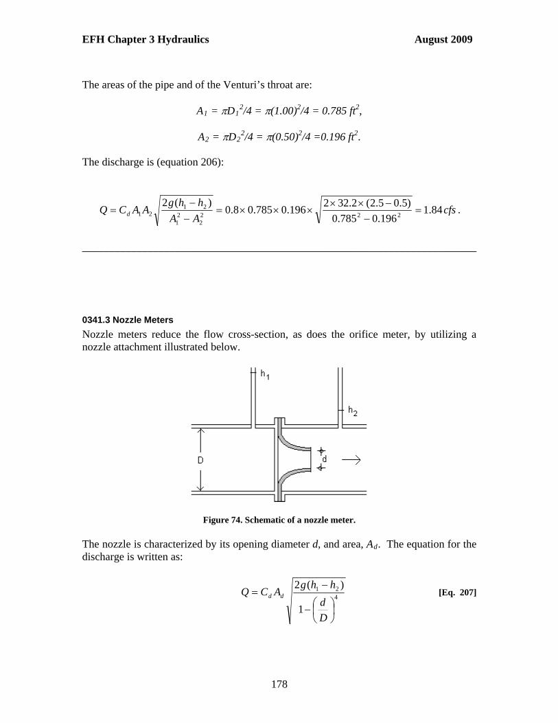
EFH Chapter 3 Hydraulics August 2009
The areas of the pipe and of the Venturi’s throat are:
A1 = D12/4 = (1.00)2/4 = 0.785 ft2,
A2 = D2
2/4 = (0.50)2/4 =0.196 ft2. The discharge is (equation 206):
cfsAA
hhgAACQ d 84.1
196.0785.0
)5.05.2(2.322196.0785.08.0
)(2222
22
1
2121
.
________________________________________________________________________
0341.3 Nozzle Meters
Nozzle meters reduce the flow cross-section, as does the orifice meter, by utilizing a nozzle attachment illustrated below.
Figure 74. Schematic of a nozzle meter. The nozzle is characterized by its opening diameter d, and area, Ad. The equation for the discharge is written as:
421
1
)(2
D
d
hhgACQ dd [Eq. 207]
178

EFH Chapter 3 Hydraulics August 2009
Where h1 and h2 are the piezometric heads at sections (1) and (2), respectively, and Cd is the discharge coefficient. The value of Cd depends on the type of nozzle, and is obtained by calibration. Calibration can be performed by attaching the nozzle to a pipe and measuring the discharge Q through the pipe for different pressure drops (h1-h2). Since the diameters d and D can be measured or are provided by the manufacturer, equation 207 can be used to obtain the discharge coefficient Cd. ________________________________________________________________________ Example 89 – Flow discharge through a nozzle meter A nozzle meter whose opening has a diameter d = 0.10 ft is placed in a pipeline of diameter D1 = 0.25 ft. Measurements of the piezometric heads upstream and downstream of the orifice indicate that h1 = 2.5 ft and h2 = 1.5 ft. With a discharge coefficient Cd = 0.90, determine the flow through the pipe. The area of the nozzle opening is:
Ad = d2/4 = (0.10)2/4 = 0.0078 ft2 The discharge is
cfs
D
d
hhgACQ dd 057.0
25.0
10.01
)5.15.2(2.3220078.090.0
1
)(244
21
________________________________________________________________________
0341.4 Elbow Meters
An elbow meter consists of attaching pressure transducers to the inner and outer walls of a pipe elbow, as shown in Figure 75 below. Let p = |p1-p2| be the absolute value of the pressure difference between the inner and outer walls of the elbow. Equivalently, the pressure difference can be written as p = h, where is the specific weight of the liquid. The discharge through the elbow can be calculated as
hCp
CQ
[Eq. 208]
where C is a calibration constant unique for a given elbow. If the pressure taps in the elbow meter were connected to a manometer, the quantity h could represent the reading in the manometer. Refer to section 0311.1 Piezometers and Manometers for detailed explanation of manometers.
179

EFH Chapter 3 Hydraulics August 2009
Figure 75. Schematic of an elbow meter. ________________________________________________________________________ Example 90 – Flow discharge through an elbow meter An elbow meter has been calibrated so that when the pressure difference between its inner and outer walls is measured in ft; the calibration constant is C = 15.2. Determine the discharge, in cubic feet per second (cfs), when h = 0.5 ft.
The discharge is: cfshCQ 75.105.02.15 ________________________________________________________________________ For the orifice, nozzle, Venturi, and elbow meters, the discharge Q varies with the square root of the piezometric head drop h. A plot of this relationship is referred to as the rating curve (of characteristic shape). Note that cross-section rating curves in open channel flow have the same characteristic shape, but with the axes exchanged. The elbow meter used in the example above has a rating curve shown in the figure below.
180

EFH Chapter 3 Hydraulics August 2009
Rating Curve - Elbow Meter
0.00
5.00
10.00
15.00
20.00
25.00
30.00
35.00
0.0 0.5 1.0 1.5 2.0 2.5 3.0 3.5 4.0
h (ft)
Q (cf
s
Figure 76. Values of the discharge can be interpolated graphically from the rating curve of a given device.
0341.5 Magnetic and Ultrasonic Meters
Magnetic meters are attached to the outside of a pipe or sometimes placed inside the pipe to measure discharge. In a magnetic meter the distortion in the magnetic field due to the moving water is related to the flow discharge. Magnetic meters are calibrated so that a voltage read in the meter can be converted to discharge. There are a variety of commercial magnetic meters. Instructions on the installation and operation of magnetic meters are available from the manufacturers. The ultrasonic flowmeter is a clamp-on device that measures pipeline flow using the principle of sonic beam phase shift. Instructions on the installation and operation of ultrasonic meters are available from the manufacturers. Research information may also be available from university extension services such as the March 2008 Using Ultrasonic Flow Meters in Irrigation Applications from the University of Nebraska-Lincoln Extension, Institute of Agriculture and Natural Resources: http://www.ianrpubs.unl.edu/epublic/live/g1426/build/g1426.pdf 0342 Measurements in Open Channels Measurements in open channel flow include depth, velocity, and discharge.
181

EFH Chapter 3 Hydraulics August 2009
0342.1 Depth Measurements
Depth measurements can be carried out by using a graduated rod or ruler, whether permanent or portable. The figure below shows a permanent depth gage in an open channel.
Figure 77. Depth gage showing water surface elevation. In small laboratory flumes, point gages with an attached Vernier scale can be used to measure the water depth. When using a point gage in a flume, the Vernier scale is read when the point gage touches the flume bed, and then when the point gage touches the surface of the water. The difference between these two readings is the water depth. Figure 78, below, shows a point gage with a Vernier scale.
182

EFH Chapter 3 Hydraulics August 2009
Figure 78. Point gage in laboratory flume with Vernier scale reading of 23.7.
0342.2 Velocity Measurements
Measurements of the water velocity in open channel flow can be performed through a variety of methods. Some of these methods are discussed in the following sections.
0342.2.1. Propeller/Paddle Wheel Meters
A propeller or paddle wheel meter consists of a moving propeller or buckets whose rate of rotation can be recorded and related to the local flow velocity. Calibration information for these meters can be obtained from the manufacturer or from laboratory tests. Small propeller meters can be used in laboratory flumes to measure local velocities. Propeller meters used in larger streams typically have a streamlined body attached to the propeller to minimize effects on the flow.
0342.2.2. Vortex Meter
Obstacles in a flow, such as a cylinder or a block, generate a train of vortices downstream of the obstacles. A vortex flow meter detects the vortex field produced by a given obstacle and relates it to the local velocity. Vortex flow meters are available from a
183

EFH Chapter 3 Hydraulics August 2009
number of manufacturers. Information on setting up and operating these meters can be obtained from the manufacturers.
0342.2.3. Doppler (Acoustic) Meters
Doppler (or acoustic) meters use an acoustic signal released into the water at a point and picked up by a sensor a short distance downstream. The time required to pick up the signal is related to the local flow velocity. A variety of commercial Doppler meters exists. Details for the set up and operation of these meters are available from the manufacturers.
0342.2.4 Velocity Measurements with Floaters
A simple way to measure velocity in open channels consists of measuring the time, t, required by a floater to travel a certain distance, x, in the channel. A straight channel reach is needed to perform floater velocity measurements. Neutrally-buoyant floaters are preferred because they are less impacted by wind. The flow velocity at the free surface is simply, x/t. Measurements in laboratory flumes indicate that the mean velocity is 0.85 times the free-surface velocity. ________________________________________________________________________ Example 91 – Flow velocity calculation using the float method While performing a floater velocity measurement in a straight reach of an irrigation canal it is found that the floater requires 56 sec to travel 100 ft. Estimate the surface velocity as well as the mean velocity in the canal. With x = 100 ft, and t = 56 sec, the surface velocity is Vs = x/t = 100ft/56 sec = 1.78 fps. The mean velocity is V = 0.85Vs = 0.851.78 fps = 1.52 fps. ________________________________________________________________________ 0342.2.5. Laser-Doppler and Particle-Velocity Measurements These types of velocity measurements are suitable in the laboratory. In a Laser-Doppler velocimeter, two or three laser beams are focused at a point in the flow. Air bubbles or any other impurity in the water passing through the laser focus point will produce a Doppler shift which is detected by an optical sensor. Calibration of the laser Doppler velocimeter allows for the determination of the local velocity at the laser focus point. In a Particle velocimeter, tracers introduced in the flow reflect light from a source and the location of the particles is optically traced allowing for the instantaneous description of flow fields.
0342.3 Sharp-crested Weirs
Sharp-crested weirs may be as simple as a thin plate placed across a rectangular open channel, as illustrated in Figure 79 below. Such a weir is referred to as a suppressed weir, as opposed to a contracted weir shown in Figure 80. The difference is that in a
184

EFH Chapter 3 Hydraulics August 2009
contracted weir the weir crest, length = L, does not extend the full width of the channel, b. Whereas in a suppressed weir b = L. In both cases of rectangular weirs P represents the weir height and H is the weir head. The head H is measured from the crest of the weir to the water surface at a point upstream so that the curvature of the flow streamlines is minimal (3 to 4 times the maximum value of H expected is suggested), as illustrated below.
Figure 79. Suppressed sharp-crested weir in a rectangular channel.
Figure 80. Contracted sharp-crested weir in a rectangular channel.
For the suppressed sharp-crested weir, the discharge Q over the weir is calculated using:
2/323
2HLgCQ d [Eq. 209]
Where Cd is a discharge coefficient, g is the acceleration of gravity (g = 9.806 m/s2 = 32.2 ft/s2). The quantities L and H were defined previously. The value of Cd can be obtained using Rehbock’s formulas:
P
H
HCd
08.0
305
1605.0 , H(ft), P(ft) [Eq. 210]
or,
P
H
HCd
08.0
1000
1605.0 , H(m), P(m) [Eq. 211]
185
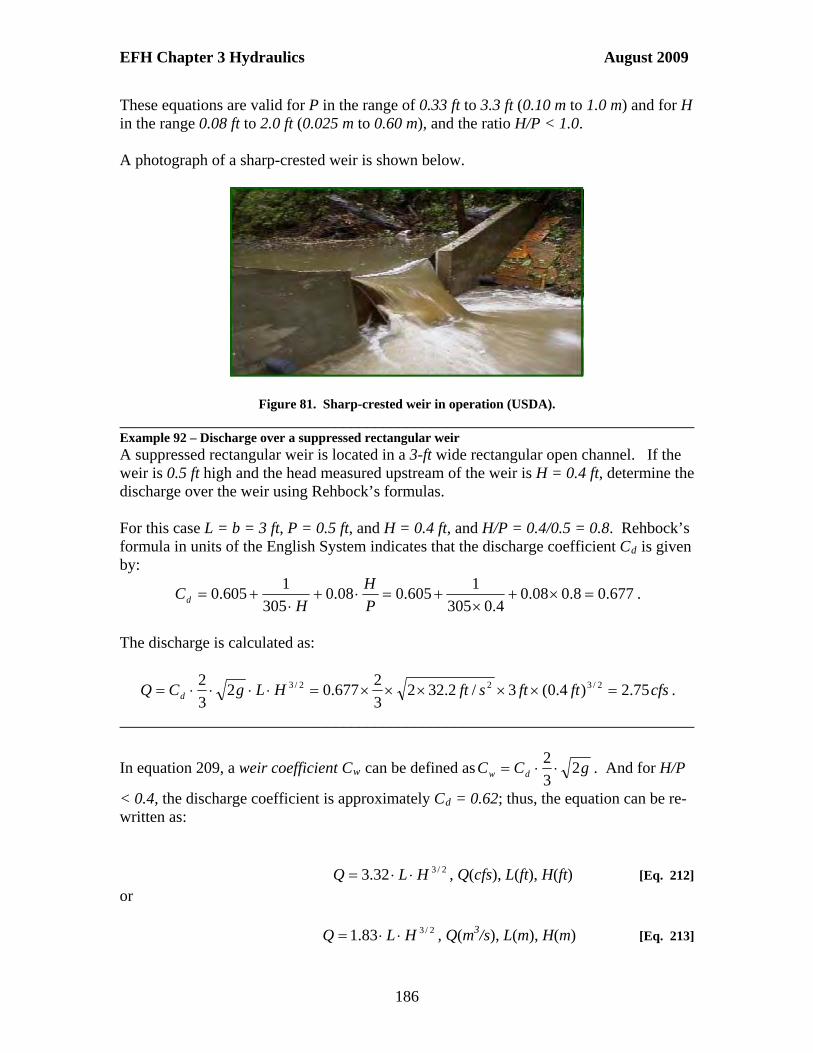
EFH Chapter 3 Hydraulics August 2009
These equations are valid for P in the range of 0.33 ft to 3.3 ft (0.10 m to 1.0 m) and for H in the range 0.08 ft to 2.0 ft (0.025 m to 0.60 m), and the ratio H/P < 1.0. A photograph of a sharp-crested weir is shown below.
Figure 81. Sharp-crested weir in operation (USDA). ________________________________________________________________________ Example 92 – Discharge over a suppressed rectangular weir A suppressed rectangular weir is located in a 3-ft wide rectangular open channel. If the weir is 0.5 ft high and the head measured upstream of the weir is H = 0.4 ft, determine the discharge over the weir using Rehbock’s formulas. For this case L = b = 3 ft, P = 0.5 ft, and H = 0.4 ft, and H/P = 0.4/0.5 = 0.8. Rehbock’s formula in units of the English System indicates that the discharge coefficient Cd is given by:
677.08.008.04.0305
1605.008.0
305
1605.0
P
H
HCd .
The discharge is calculated as:
cfsftftsftHLgCQ d 75.2)4.0(3/2.3223
2677.02
3
2 2/322/3 .
________________________________________________________________________
In equation 209, a weir coefficient Cw can be defined as gCC dw 23
2 . And for H/P
< 0.4, the discharge coefficient is approximately Cd = 0.62; thus, the equation can be re-written as:
2/332.3 HLQ , Q(cfs), L(ft), H(ft) [Eq. 212]
or
2/383.1 HLQ , Q(m3/s), L(m), H(m) [Eq. 213]
186

EFH Chapter 3 Hydraulics August 2009
________________________________________________________________________ Example 93 – Discharge over a suppressed rectangular weir A suppressed rectangular weir is located in a 4-ft wide rectangular open channel. If the weir is 1.0 ft high and the head measured upstream of the weir is H = 0.25 ft, determine the discharge over the weir using the formula for H/P<0.4.
cfsHLQ 66.1)25.0(0.432.332.3 2/32/3 ________________________________________________________________________ For a contracted sharp-crested weir, the equation to calculate the discharge is the Francis formula:
2/3)1.0( HHnLCQ w [Eq. 214]
The value of n is either “1” or “2”, depending on whether the contractions occur on one or two sides, as illustrated below.
Figure 82. Contracted rectangular weir with n = 1 or n = 2 contractions.
________________________________________________________________________ Example 94 – Discharge over a contracted weir A contracted weir of length L = 2 ft is set in a 3-ft wide rectangular open channel. Using a weir coefficient Cw = 3.32, determine the discharge for a head H = 0.20 ft with (a) n = 1 contraction, and (b) n = 2 contractions. The weir height is P = 0.5 ft. The ratio H/P = 0.20ft/0.5ft = 0.4, and the discharge is
(a) cfsHHnLCQ w 588.02.0)2.011.02(32.3)1.0( 2/32/3
(b) cfsHHnLCQ w 582.02.0)2.021.02(32.3)1.0( 2/32/3 ________________________________________________________________________ Figure 83 below shows a contracted rectangular weir in a laboratory flume.
187

EFH Chapter 3 Hydraulics August 2009
Figure 83. Contracted weir in a laboratory flume. A special type of a contracted weir is the Cipoletti weir consisting of a trapezoidal shape with side slopes 1H: 4V as shown below.
Figure 84. Cipoletti weir schematic.
The equation for the discharge over a Cipoletti weir is given by:
)(),(),(,367.3 2/3 ftHftLcfsQHLQ [Eq. 215]
188

EFH Chapter 3 Hydraulics August 2009
Where L = Lb + H/2, and Lb is the bottom or crest length of the Cipoletti weir. ________________________________________________________________________ Example 95 – Discharge over a Cipoletti weir Determine the discharge over a Cipoletti weir if the weir length is L = 1.5 ft, and the head is H = 0.5 ft. The discharge is .79.15.05.1367.3367.3 2/32/3 cfsHLQ ________________________________________________________________________
A triangular, or v-notch weir consists of a symmetric v-shaped notch in a thin wall placed across an open channel. A v-notch weir is used to measure low flows of less than 10 cfs. A schematic of a triangular (or v-notch) weir is shown below.
Figure 85. Schematic of a triangular or v-notch weir.
. Figure 86 below shows a small triangular weir in a laboratory flume.
Figure 86. V-notch, or triangular, weir in a laboratory flume.
The discharge for a triangular (or v-notch) weir is given by:
189

EFH Chapter 3 Hydraulics August 2009
2/5
2tan2
15
8HgCQ d
[Eq. 216]
Where Cd is a discharge coefficient, g is the acceleration of gravity (g = 9.806 m/s2 = 32.2 ft/s2), and is the angle of the v-notch. A typical value of the contraction coefficient is Cd = 0.58. ________________________________________________________________________ Example 96 – Discharge over a triangular weir
Determine the discharge over a v-notch weir if the weir angle is = 80o and the head is H = 0.55 ft. Use a discharge coefficient Cd = 0.58. The discharge is:
2/522/5 )55.0(2
80tan/2.322
15
858.0
2tan2
15
8
o
d sftHgCQ
cfsQ 467.0 ________________________________________________________________________
0342.4 Broad-crested Weirs
A broad-crested weir consists of an obstacle of height P placed in a rectangular open channel, as illustrated below. The flow over the broad crested weir becomes critical, so that the depth at that point is the critical depth yc.
Figure 87. Schematic of flow over a broad-crested weir. In a rectangular channel of width L, the discharge over the broad-crested weir is:
3cygLQ [Eq. 217]
If E represents the specific energy available over the weir, the critical depth can be
expressed as yc = E3
2, and the discharge is written as:
190

EFH Chapter 3 Hydraulics August 2009
2/32/3
2/3
3
2EgLygLQ c
[Eq. 218]
Expressing this equation in the form of a suppressed weir equation (equation 209), the discharge coefficient is given by:
2/3
3
1
H
ECd [Eq. 219]
Where H is the head measured upstream of the broad-crested weir, where the flow depth is y = P+H and the flow velocity is Vo. For a large value of H, Vo is small, and E becomes similar to H, i.e., E/H becomes 1.0 which provides a minimum value for the
discharge coefficient, (Cd )min = 3
1= 0.577. As the velocity Vo increases, the value of
E/H becomes larger than 1, and the discharge coefficient (equation 219) becomes larger than 0.577. If the critical depth can be measured over the weir, equation 217 provides the discharge. If the head H is measured use equation 209, instead, with a discharge coefficient larger than or equal to 0.577. These are the equations used to evaluate many of the long-throated flume types discussed in section 0342.6.1. ________________________________________________________________________ Example 97– Discharge over a broad-crested weir- critical depth measured Determine the discharge over a broad-crested weir if the critical depth of flow over the weir is measured to be yc = 0.52 ft. The channel has a width L = 2.5 ft. The discharge is:
cfsftsftftygLQ c 32.5)52.0(/2.325.2 323
________________________________________________________________________ Example 98 – Discharge over a broad-crested weir – head measured Determine the discharge over a broad-crested weir if the head measured upstream of the weir is measured to be H = 0.65 ft. The channel has a width L = 3.5 ft. Use a discharge coefficient Cd = 0.61. The discharge is (equation 209):
cfsftftsftHLgCQ d 99.5)65.0(5.3/2.3223
261.02
3
2 2/322/3
________________________________________________________________________
191

EFH Chapter 3 Hydraulics August 2009
Most hydraulic structures in natural resource conservation work incorporate broad-crested weirs, where their function is the control of flood flows. The crest is horizontal and long in the direction of flow so that the water lays on the crest rather than springing free as water does flowing over a sharp-crested weir. Roadways over bridges and culverts may be considered broad-crested weirs to estimate overtopping flows. These discharges are generally calculated with equation 209, where a weir coefficient, Cw, can
be defined as gCC dw 23
2. Cw ranges in value from 2.5 to 3.1.
0342.5 Submerged Weir Flow
Conditions downstream of a sharp-crested weir may produce submergence of the weir as illustrated. The equation used to calculate the discharge is the same as equation 212, modified by a submergence coefficient Cs, and replacing H with the upstream head Hu. The resulting equation is:
2/332.3 us HLCQ [Eq. 220]
Figure 88. Submerged weir flow.
The submergence coefficient is based on empirical data, as shown in Figure 89. A polynomial fitting of this empirical data gives the following equation for the coefficient of submergence as:
3319.1165.18395.5159.62152.28234
u
d
u
d
u
d
u
ds H
H
H
H
H
H
H
HC
[Eq. 221] for 0.38 < Hd/Hu < 1.0, or Cs = 1.0, for Hd/Hu < 0.38.
192

EFH Chapter 3 Hydraulics August 2009
Coefficient of submergence
0.00
0.10
0.20
0.30
0.40
0.50
0.60
0.70
0.80
0.90
1.00
0.00 0.10 0.20 0.30 0.40 0.50 0.60 0.70 0.80 0.90 1.00
Hd/Hu
Cs
Figure 89. Coefficient of submergence for sharp crested weirs.
________________________________________________________________________ Example 99 - Discharge over a submerged sharp-crested weir A sharp crested weir is operating under submerged conditions with upstream and downstream heads of Hu = 0.40 ft and Hd = 0.25 ft. If the weir has a length L = 3.5 ft, determine the discharge Q over the weir. The submergence ratio Hd/Hu = 0.25 ft/0.40 ft = 0.625, and the submergence coefficient is calculated as:
3319.1165.18395.5159.62152.28234
u
d
u
d
u
d
u
ds H
H
H
H
H
H
H
HC =
3319.1625.0165.18625.0395.51625.059.62625.0152.28 234 sC =
Cs = 0.93
With this coefficient, the discharge is calculated as:
193

EFH Chapter 3 Hydraulics August 2009
cfsHLCQ us 73.240.05.393.032.332.3 2/32/3
________________________________________________________________________ Submergence affects broad-crested weirs less than sharp-crested weirs. For broad-crested weirs, discharge begins to be reduced at 80% submergence; at 90% submergence, discharge is still greater than 90% of unsubmerged discharge, USACOE (2008).
0342.6 Flumes
Flumes are shaped, open channel flow sections that force flow to accelerate and pass through critical depth in the flume. When flow passes through critical depth, a unique water surface profile occurs within the flume for each discharge. Flow acceleration is produced by converging the sidewalls, raising the bottom, or a combination of both. Flumes range in size from 1- inch to over 50 ft wide, and are installed in ditches, laterals, and large canals to measure flow. 0342.6.1 Long-throated Flumes Long-throated flumes are coming into general use because they can be easily fitted into channel shapes. When the flume’s bottom is a raised overflow crest, with no side contractions, the flume is commonly called a broad-crested weir. Characteristics of long-throated flumes include:
1. Can have nearly any desired cross-sectional shape, 2. Can be made into portable devices, 3. Have few problems with floating debris and sediment, 4. May be designed and calibrated by computer techniques; WinFlume design
software and additional information can be downloaded at: http://www.wsi.nrcs.usda.gov/products/W2Q/water_mgt/Irrigation/irrig-mgt-models.html
5. And, generally have measurement errors less than +2%.
0342.6.2 Parshall Flumes Parshall flumes are used to measure water flow by custom or by law in some locales. The Parshall flume is an open-channel measurement structure that combines a contraction of the channel width with a drop in the channel bed. Both transitions contribute to the establishment of critical flow, thus providing a unique relationship between the flow depth and discharge through the flume. Parshall flumes are calibrated empirically, using other more precise and accurate water-measuring systems. Since the flumes are calibrated empirically, care must be taken to build Parshall flumes according to the design dimensions. If ha represents the water depth at the Parshall flume’s throat in ft, the discharge through the flume Q in cfs, can be calculated using the formula:
Q = C han, [Eq. 222]
194

EFH Chapter 3 Hydraulics August 2009
Where the coefficient C and the exponent n are given as functions of the flume’s width. Coefficients and exponents are given in tables found in the Water Measurement Manual. ________________________________________________________________________ Example 100 – Discharge through a Parshall flume For a flume of width 5 ft, and depth, ha = 1.2 ft, determine the discharge through the flume. From the Water Measurement Manual, C = 20 and n = 1.59. The resulting discharge is:
Q = C han = 20×1.21.59
= 26.73 cfs.
________________________________________________________________________
Other flumes have been designed for special uses, such as for measurement of flows containing large amounts of sediment. See the Water Measurement Manual for discussion of special-type flumes. 0370 Hydraulic Modeling Hydraulic modeling is the practice of testing small-scale hydraulic systems (the model) in the laboratory and translating the favorable results to equivalent quantities of the full-scale system (the prototype). Hydraulic modeling should be performed if sound design and dependable operation of the prototype cannot be accomplished with other recognized methods of analyses. The practice of hydraulic modeling is based on ensuring similarity between model and prototype. 0371 Similarity between Models and Prototypes The figure below illustrates the concept of prototypes and models. A prototype is the full-scale hydraulic system of interest, and is represented by the spillway on the left-hand side. A model is a small-scale reproduction of the prototype, as illustrated on the right-hand side of the figure.
Figure 90. Prototype and model quantities.
195

EFH Chapter 3 Hydraulics August 2009
The following figure shows the prototype and the model of a spillway flow.
Figure 91. Prototype and model of an ogee spillway (courtesy of the Utah Water Research Laboratory, Utah State University).
By building the model to resemble the shape of the prototype we ensure geometric similarity, as illustrated by the photographs of Figure 91. Referring to quantities in the model with the subscript m and those in the prototype with the subscript p, the ratio of corresponding lengths in model and prototype is referred to as the length ratio, Lr:
p
mr L
LL [Eq. 223]
Since area is calculated as the product of two lengths, the area ratio is defined as:
2r
p
mr L
A
AA [Eq. 224]
The volume ratio is, consequently, defined as:
3
)(
)()( r
p
mr L
Vol
VolVol [Eq. 225]
________________________________________________________________________ Example 101 – Geometric similarity calculations A spillway that is 24 ft high (Hp = 24 ft) is to be built at a dam. To check the hydraulic characteristics of the spillway a model with a length ratio Lr = 1/10 is to be built in the laboratory. (a) What would be the height of the model, Hm? (b) If the flow cross-section in the model will have an area Am = 1.2 ft2, what would be the equivalent area in the
196

EFH Chapter 3 Hydraulics August 2009
prototype? (c) If the volume of water over the prototype is estimated to be (Vol)p = 480 ft3, what is the estimated volume of water over the model, (Vol)m? (a) The model height is:
Hm = LrHp = (1/10)24 ft = 2.4 ft (b) The prototype area is:
Ap = Am/Ar = Am/Lr2 = 1.2 ft2/(1/10)2 = 120 ft2
(c) The model volume is:
(Vol)m = (Vol)r(Vol)p = Lr3(Vol)p = (1/10)3480 ft3 = 0.48 ft3
________________________________________________________________________ 0372 Hydraulic Modeling of Enclosed Flows (Pipelines) Enclosed flow models generally require that the Reynolds number, Re, of the model equals the Re of the prototype i.e. the Re ratio equals 1. Using Reynolds number similarity, the velocity, time, and discharge ratios are:
r
rr L
V
[Eq. 226]
r
r
r
rr
L
V
LT
2
[Eq. 227]
rrr
rrrrr L
LLVAQ
2 [Eq. 228]
Where the kinematic viscosity ratio, r, is the model kinematic viscosity divided by the prototype kinematic viscosity. ________________________________________________________________________ Example 102 – Control valve model calculation (pressurized flow) A model of a control valve for a water pipeline is to be tested in the laboratory. The prototype valve has a diameter Dp = 4.0 ft, while the model will have a diameter Dm = 0.5 ft. If the model is tested using air, determine the velocity, time, and discharge ratios. The kinematic viscosities to use are m =air =1.5810-4 ft2/s, and p = water = 1.2210-
5 ft2/s. The length ratio is:
Lr = Dm/Dp = 0.5 ft/4.0 ft = 1/8 While the kinematic viscosity ratio is:
197
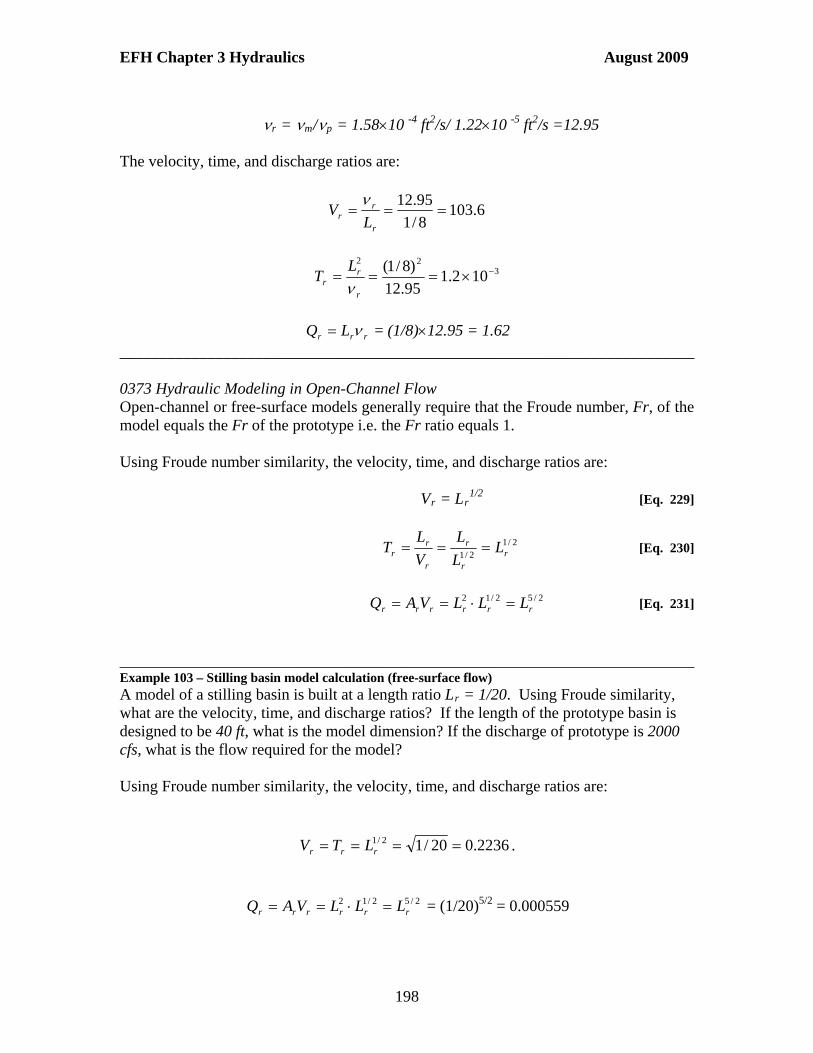
EFH Chapter 3 Hydraulics August 2009
r = m/p = 1.5810 -4 ft2/s/ 1.2210 -5 ft2/s =12.95
The velocity, time, and discharge ratios are:
6.1038/1
95.12
r
rr L
V
322
102.195.12
)8/1( r
rr
LT
rrr LQ = (1/8)12.95 = 1.62 ________________________________________________________________________ 0373 Hydraulic Modeling in Open-Channel Flow Open-channel or free-surface models generally require that the Froude number, Fr, of the model equals the Fr of the prototype i.e. the Fr ratio equals 1. Using Froude number similarity, the velocity, time, and discharge ratios are:
Vr = Lr1/2 [Eq. 229]
2/12/1 r
r
r
r
rr L
L
L
V
LT [Eq. 230]
2/52/12
rrrrrr LLLVAQ [Eq. 231]
________________________________________________________________________ Example 103 – Stilling basin model calculation (free-surface flow) A model of a stilling basin is built at a length ratio Lr = 1/20. Using Froude similarity, what are the velocity, time, and discharge ratios? If the length of the prototype basin is designed to be 40 ft, what is the model dimension? If the discharge of prototype is 2000 cfs, what is the flow required for the model? Using Froude number similarity, the velocity, time, and discharge ratios are:
2236.020/12/1 rrr LTV .
2/52/12rrrrrr LLLVAQ = (1/20)5/2 = 0.000559
198

EFH Chapter 3 Hydraulics August 2009
Given the prototype basin length Lp = 40 ft, then the model basin length is:
Lm = Lr Lp = (1/20) × 40 ft = 2 ft Finally, given the prototype discharge Qp = 2000 cfs, then the model discharge is:
Qm = Qr Qp = 0.000559×2000 cfs = 1.12 cfs ________________________________________________________________________ An important issue in modeling open channel flow is producing the proper scaling of the surface roughness of channel lining. For example, bed roughness in streams and hydraulic structures may be provided by large, stable, rock lining known as riprap. Riprap model studies can be conducted to ensure geometric similarity. However, density differences between the riprap model material and water need to be taken into account if buoyancy effects are to be simulated. Figure 92 illustrates the use of smaller rock (of like density) to simulate the larger rock in a drop structure.
Figure 92. Riprap hydraulic model (source: USDA - ARS) 0374 Limitations of Models The maximum size of hydraulic models is limited by laboratory physical installations (e.g., space, pumping capacity) and the minimum size of models is limited by the
199

EFH Chapter 3 Hydraulics August 2009
similarity laws. For example, if the model size in an open channel model that follows Froude similarity is too small, viscous effects may become significant. Viscosity may produce undesirable effects in such a model that are not properly scalable to the prototype. Also, if the resulting open-channel model is too shallow, surface tension effects (such as capillarity waves) may appear that would not otherwise be relevant to the prototype performance. In the case of distorted open-channel models (such as for wide, shallow streams), if the vertical model size is much larger than the horizontal size, the resulting flow may include secondary velocity components much larger than the prototype flow. The resulting flow field then would be too distorted to be scaled up to the prototype size. For a detailed discussion on model limitations and similarity laws please refer to Kobus (1980). REFERENCES
1. American Society of Civil Engineering (ASCE). 2006. Sedimentation Engineering. Manuals and Reports of Engineering Practice, No. 54 Vito A. Vanoni, ed, ISBN# 0784408238. Reston, VA.
2. Barnes, H.H. 1967. Roughness characteristics of natural channels. U.S. Geological Survey Water Supply Paper 1849. U.S. Government Printing Office. Washington, DC.
3. Brater E.F., and H.W. King. 1996. Handbook of hydraulics (seventh edition). McGraw-Hill. New York, NY.
4. Chaudhry, M. H. 1993. Open-channel flow. Prentice-Hall. 5. Chow, V.T. 1959. Open-channel hydraulics. McGraw-Hill. New York, NY. 6. Cowan, W. L. 1956. Estimating Hydraulic Roughness Coefficients. Agricultural
Engineering , 37(7). 7. Fasken, G. 1963. Guide for selecting roughness coefficients "n" values for
channels. USDA, Soil Conservation Service. 8. Federal Highway Administration. 2001. Hydraulic design of highway culverts,
hydraulic design series No. 5. (FHWA-NHI-01-020). 9. Finnemore, E.J., and J.B. Franzini. 2002. Fluid mechanics with engineering
applications. McGraw-Hill. New york, NY. 10. French, R. H. 1985. Open-channel hydraulics. McGraw-Hill. New York, NY. 11. Idelchik, I.E. 1999. Handbook of hydraulic resistance (third edition). Begell
House. New York, NY. 12. Kobus, H. 1980. Hydraulic modeling, bulletin 7 – German Association for
Water Resources and Land Improvements (issued in cooperation with the International Association for Hydraulic Research). Hamburg: Verlag Paul Prey.
13. Lamont, P.A. 1981. Common Pipe Flow Formulas Compared with the Theory of Roughness. Journal of the American Water Works Association, 73(5), 274.
14. Mays, L. W. 1999. Hydraulic design handbook. McGraw-Hill. New York, NY. 15. Munson, B. D. 1998. Fundamentals of fluid mechanics (third edition). John
Wiley and Sons. 16. Raudkivi, A. J. 1976. Loose boundary hydraulics. Pergamon Press. Oxford,
United Kingdom.
200

EFH Chapter 3 Hydraulics August 2009
17. Roberson, J.A., E.R. Tinney, and E.A. Sibley. 1956. Studies in breakage problems in concrete irrigation pipe, Bull. 225, Washington State Institute of Technology (Washinton State University).
18. Streeter, V. L., and E.B. Wylie. 1998. Fluid mechanics (ninth edition). McGraw-Hill. New York, NY.
19. USA Corps of Engineers (COE). 2008. HEC-RAS river analysis system hydraulic reference manual 4.0. Hydrologic Engineering Center. Davis, CA.
20. Temple, D.M., K.M. Robinson, R.M. Ahring, and A.G. Davis. 1987. Stability design of grass-lined open channels, Agricultural handbook 667. USDA, Agricultural Research Service. Washington, DC.
21. Tullis, J.P. 1989. Hydraulics of pipelines – pumps, valves, cavitation, transients. John Wiley and Sons. New York, NY.
22. USDA, NRCS. 2005. Structural design of flexible conduits. NEH 636, Chap. 52. Washington, DC.
23. USBR/USDA-NRCS/USDA-ARS. 2001. Water measurement manual (revised printing). http://www.usbr.gov/pmts/hydraulics_lab/pubs/wmm/.
24. USDA, NRCS. 2008. Stream restoration design handbook. NEH 654. Washington, DC.
201

EFH Chapter 3 Hydraulics August 2009
202
Exhibit 1 – Dimensions and units of measurement The following table (Table E1.1) shows the dimensions of a variety of physical quantities in terms of the basic units mass, length, time (M,L,T) or force, length, time (F,L,T). The table also shows the preferred units for those quantities in both the International System (S.I.) and the English System (E.S.) of units. Additional units commonly used for the quantities listed are shown in the last column of the table.
Table E1.1 – Dimensions and units of measurement
Dimensions Preferred units Other Quantity (M,L,T) (F,L,T) S.I. E.S. units Length (L) L L m ft in, mi Time (T) T T s s h, d, min
Mass (M) M FT2L -1 kg slug
Area (A) L2 L2 m2 ft2 Ac
Volume (Vol) L3 L3 m3 ft3 Ac-ft
Velocity (V) LT -1 LT -1 m/s ft/s or fps --
Acceleration (a) LT -2 LT -2 m/s2 ft/s2 --
Discharge (Q) L3T -1 L3T -1 m3/s ft3/s or cfs --
Kinematic viscosity () L2T -1 L2T -1 m2/s ft2/s St
Force (F) MLT -2 F N lb --
Pressure (p) ML -1T -2 FL -2 Pa lb/ft2 psi, atm
Shear stress () ML -1T -2 FL -2 Pa lb/ft2 psi
Density () ML -3 FT2L -4 kg/m3 slug/ft3 --
Specific weight () ML-2T -2 FL -3 N/m3 lb/ft3 --
Energy/Work/Heat (E) ML2T -2 FL J lb ft --
Power (P) ML2T -3 FLT -1 W lb ft/s hp
Dynamic viscosity () ML -1T -1 FTL -2 N s/m2 lb s/ft2 P The units used in Table E1-1 are defined as follows: Ac : acre, a unit of area Ac-ft : acre feet atm : atmosphere cfs : cubic feet per second fps : feet per second ft : foot or feet hp : horse power in : inch J : joule kg : kilogram lb : pound m : meter N : newton
mi : mile P : poise Pa : Pascal psi : pounds per square inch s : second St : stokes W : watt

EFH Chapter 3 Hydraulics August 2009
Exhibit 2 – Selected conversion factors for units of measurement
The following tables (Tables E2.1 and E2.2) show a number of selected conversion factors for units of measurement in both the English System (E.S.) and the International System (S.I.). The conversion factors are grouped by dimensions. The units are defined as follows: Ac : a unit of area atm : atmosphere (unit of pressure) bar : bar (unit of pressure) Btu : British thermal unit (unit of
work, energy, or heat) cal : calorie (work, energy, or heat) cm : centimeter (1/100 of a meter) cP : centipoise (1/100 of a poise) cSt : centistoke (1/100 of a stoke) d : day dyn : dyne = gcm/s2 (unit of force) ft : foot or feet ftH20 : feet of water (unit of pressure) g : gram (unit of mass) gal : gallon (unit of volume) h : hour ha : hectare (an S.I. unit of area) hp : horse power (unit of power) in : inch inH20 : inches of water (pressure) inHg : inches of mercury (pressure) J : Joule (work, energy, or heat) K : Kelvin (absolute temperature) kcal : kilocalorie (1000 calories, heat) kg : kilogram (1000 grams, mass) kip : kip (1000 lb, force) km : kilometer (1000 meters) kN : kilonewton (1000 newtons) kPa : kilopascal (1000 Pascals) kph : kilometers per hour kW : kilowatt (1000 watts, power) kWh : kilowatt-hour (work, energy, or
heat) l : liter (unit of volume) lb : pound (unit of force) m : meter mH2O : meters of water (pressure) mi : mile
min : minute ml : milliliter (1/1000 of a liter) mm : millimeter (1/1000 of a meter) mmHg : millimeters of mercury (press.) mph : miles per hour N : newton (unit of force) o : degree for angular measurement oC : Centigrade degree (temp.) oF : Fahrenheit degree (temp.) oR : Rankine degree (absolute temp) oz : ounce (1/16 pound, force) P : poise (dynamic viscosity) Pa : Pascal (unit of pressure) psf : pounds per square foot (lb/ft2,
pressure) psi : pounds per square inch (lb/in2,
pressure) r : radian (dimensionless, angle) s : second slug : slug unit of mass = lbs2/ft St : stokes (kinematic viscosity) W : watt (unit of power) yd : yard yr : year
203

EFH Chapter 3 Hydraulics August 2009
204
Table E2.1 – Selected conversion factors for units of measurement – part 1
DIMENSIONS BASIC CONVERSION FACTORS LENGTH 1 ft = 0.3048 m 1 m = 3.2808 ft MASS 1 slug = 14.5939 kg 1 kg = 0.0685 slug FORCE 1 lb = 4.4482 N 1 N = 0.2248 lb TIME (same basic units) 1 s = 1 s
ABSOLUTE TEMP. 1 oR = 5/9 K 1 K = 9/5 oR DIMENSIONS OTHER CONVERSION FACTORS LENGTH 1 ft = 0.3048 m 1 m = 3.2808 ft 1 ft = 30.48 cm 1 cm = 0.0328 ft 1 in = 2.54 cm 1 cm = 0.3937 in 1 mi = 1.609 km 1 km = 0.6214 mi
AREA 1 ft2 = 0.0929 m2 1 m2 = 10.7639 ft2
1 ha = 104 m2 1 Ac = 43560.1742 ft2 1 ha = 2.4710 Ac 1 Ac = 0.4047 ha
1 in2 = 6.4516 cm2 1 cm2 = 0.1550 in2
VOLUME 1 ft3 = 0.0283 m3 1 m3 = 35.3147 ft3
1 in3 = 16.3871 cm3 1 cm3 = 0.0610 in3
1 ft3 = 28.3168 l 1 l = 0.0353 ft3
1 ft3 = 7.4805 gal 1 gal = 0.1337 ft3
1 l = 1000 cm3 1 l = 0.001 m3
1 Acft = 43560.1742 ft3 1 ft3 = 2.2957 10-5 Acft VELOCITY 1 ft/s = 0.3048 m/s 1 m/s = 3.2808 ft/s 1 mph = 0.4470 m/s 1 m/s = 2.2369 mph 1 mph = 1.6093 kph 1 kph = 0.6214 mph
ACCELERATION acceleration of gravity, g = 32.174 ft/s2 = 9.8067 m/s2
1 ft/s2 = 0.3048 m/s2 1 m/s2 = 3.2808 ft/s2
DISCHARGE 1 ft3/s = 0.0283 m3/s 1 m3/s = 35.3147 ft3/s
1 ft3/s = 7.4805 gal/s 1 m3/s = 264.1720 gal/s
1 ft3/s = 448.8312 gal/min 1 m3/s = 15850.3231 gal/m
1 ft3/s = 28.3168 l/s 1 m3/s = 1000 l/s
1 l/s = 15.8503 gal/min 1 l/s = 0.001 m3/s MASS 1 slug = 14.5939 kg 1 kg = 0.0685 slug 1 slug = 14593.9029 g 1 kg = 1000 g 1 g = slug 1 g = 0.001 kg FORCE 1 lb = 4.4482 N 1 N = 0.2248 lb
1 lb = 16 oz 1 N = 105 dyn 1 lb = 0.001 kip 1 N = 0.0002 kips
1 kip = 1000 lb 1 dyn = 2.2480×10⁻⁶ lb

EFH Chapter 3 Hydraulics August 2009
205
Table E2.2 – Selected conversion factors for units of measurement – part 2
DIMENSIONS OTHER CONVERSION FACTORS (continued) ENERGY 1 ft-lb = 1.3558 J 1 J = 0.7376 ft-lb WORK 1 ft-lb = 0.0013 Btu 1 J = 0.0009 Btu HEAT 1 ft-lb = 0.3238 cal 1 kWh = 3600000 J TORQUE 1 Btu = 778.1693 ft-lb 1 kWh = 3412.1416 Btu
1 Btu = 251.9958 cal 1 J = 107 ergs 1 Btu = 1055.0559 J 1 J = 0.2388 cal POWER 1 ft-lb/s = 1.3558 W 1 W = 0.7376 ft-lb/s 1 hp = 550 ft-lb/s 1 kW = 737.5621 ft-lb/s 1 hp = 745.6999 W
PRESSURE 1 atm = 2116.2166 psf 1 bar = 105 Pa = 14.5038 psi
SHEAR STRESS 1 psf = 0.0069 psi 1 kPa = 103 Pa = 0.1450 psi 1 psf = 47.8803 Pa 1 ftH20 = 0.4331 psi 1 mmHg = 0.0193 psi 1 inH20 = 0.0361 psi 1 inHg = 0.4912 psi 1 mH20 = 0.9102 kPa
DENSITY 1 slug/ft3 = 515.3788 kg/m3 1 kg/m3 = 0.0019 slug/ft3
1 slug/ft3 = 0.5154 g/cm3 1 g/cm3 = 1.9403 slug/ft3
1 kg/m3 = 0.001 g/cm3 1 g/cm3 = 1000 kg/m3
SPECIFIC WEIGHT 1 lb/ft3 = 157.0875 N/m3 1 N/m3 = 0.0064 lb/ft3
1 kip/ft3 = 157087.4638 N/m3 1 N/m3 = 0.1 dyn/cm3
1 lb/ft3 = 15.7087 dyn/cm3 1 N/m3 = 6.3658×10⁻⁶ kip/ft3 KINEMATIC VISCOSITY 1 ft2/s = 0.0929 m2/s 1 m2/s = 10.7639 ft2/s
1 ft2/s = 929.0304 St 1 St = 0.001 ft2/s
1 St = 0.0001m2/s 1 m2/s = 10000 St
DYNAMIC VISCOSITY 1 lbs/ft2 = 47.8803 Ns/m2 1 Ns/m2 = 0.0209 lbs/ft2
1 lbs/ft2 = 478.8026 P 1 P = 0.0021 lbs/ft2
1 P = 0.1 Ns/m2 1 Ns/m2 = 10 P
TEMPERATURE 1 oR = 5/9 K 1 K = 9/5 oR
oR = oF + 459.67 K = oC + 273.15
oF = 9/5 oC + 32 oC = 5/9 (oF - 32)

EFH Chapter 3 Hydraulics August 2009
206
Exhibit 3 – The Greek alphabet The following table (Table E3.1) shows the letters of the Greek alphabet in their lower case and upper case forms, their name, and their closest English equivalent.
Table E3.1 – The Greek Alphabet
Lower Upper Letter English Lower Upper Letter English case case name equivalent case case name equivalent Alpha a Nu n Beta b Xi x Gamma g Omicron o Delta d Pi p Epsilon e Rho r Zeta z Sigma s Eta h Tau t Theta th Upsilon u Iota i Phi ph Kappa k Chi ch Lambda l Psi ps Mu m Omega o
Many of the letters of the Greek alphabet are used as symbols for variables used in hydraulics equations. Some common examples are:
(rho) Density (omega) Specific weight (some references use for specific weight) (mu) Dynamic viscosity (nu) Kinematic viscosity (tau) Shear stress (epsilon) Absolute roughness in pipes (pi) Ratio of length of circle to its diameter, constant value: 3.1416
In reference to angular measurements, the letters (alpha), (beta), (gamma), and (theta) are commonly used. The letter (upper-case delta) is typically used to indicate an increment of a quantity, thus, h may represent, for example, an increment on a depth h. The letter (epsilon) is typically used to indicate a very small quantity in solution of equations.
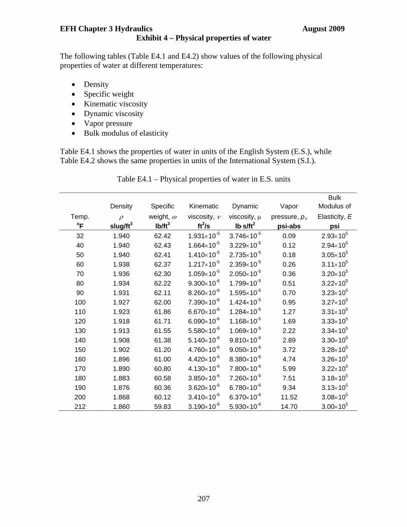
EFH Chapter 3 Hydraulics August 2009
207
Exhibit 4 – Physical properties of water The following tables (Table E4.1 and E4.2) show values of the following physical properties of water at different temperatures:
Density Specific weight Kinematic viscosity Dynamic viscosity Vapor pressure Bulk modulus of elasticity
Table E4.1 shows the properties of water in units of the English System (E.S.), while Table E4.2 shows the same properties in units of the International System (S.I.).
Table E4.1 – Physical properties of water in E.S. units
Bulk Density Specific Kinematic Dynamic Vapor Modulus of
Temp. weight, viscosity, viscosity, pressure, pv Elasticity, E oF slug/ft3 lb/ft3 ft2/s lbs/ft2 psi-abs psi
32 1.940 62.42 1.93110-5 3.74610-5 0.09 2.93105
40 1.940 62.43 1.66410-5 3.22910-5 0.12 2.94105
50 1.940 62.41 1.41010-5 2.73510-5 0.18 3.05105
60 1.938 62.37 1.21710-5 2.35910-5 0.26 3.11105
70 1.936 62.30 1.05910-5 2.05010-5 0.36 3.20105
80 1.934 62.22 9.30010-6 1.79910-5 0.51 3.22105
90 1.931 62.11 8.26010-6 1.59510-5 0.70 3.23105
100 1.927 62.00 7.39010-6 1.42410-5 0.95 3.27105
110 1.923 61.86 6.67010-6 1.28410-5 1.27 3.31105
120 1.918 61.71 6.09010-6 1.16810-5 1.69 3.33105
130 1.913 61.55 5.58010-6 1.06910-5 2.22 3.34105
140 1.908 61.38 5.14010-6 9.81010-6 2.89 3.30105
150 1.902 61.20 4.76010-6 9.05010-6 3.72 3.28105
160 1.896 61.00 4.42010-6 8.38010-6 4.74 3.26105
170 1.890 60.80 4.13010-6 7.80010-6 5.99 3.22105
180 1.883 60.58 3.85010-6 7.26010-6 7.51 3.18105
190 1.876 60.36 3.62010-6 6.78010-6 9.34 3.13105
200 1.868 60.12 3.41010-6 6.37010-6 11.52 3.08105
212 1.860 59.83 3.19010-6 5.93010-6 14.70 3.00105
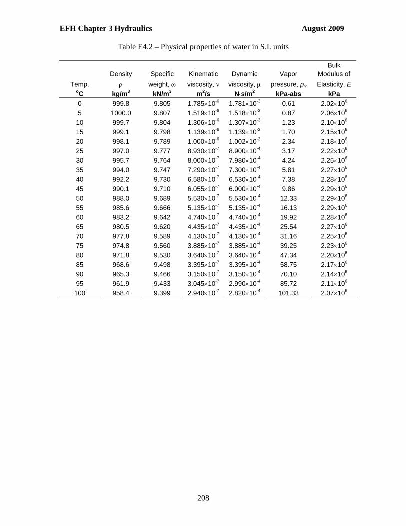
EFH Chapter 3 Hydraulics August 2009
208
Table E4.2 – Physical properties of water in S.I. units
Bulk Density Specific Kinematic Dynamic Vapor Modulus of
Temp. weight, viscosity, viscosity, pressure, pv Elasticity, E oC kg/m3 kN/m3 m2/s Ns/m2 kPa-abs kPa
0 999.8 9.805 1.78510-6 1.78110-3 0.61 2.02106
5 1000.0 9.807 1.51910-6 1.51810-3 0.87 2.06106
10 999.7 9.804 1.30610-6 1.30710-3 1.23 2.10106
15 999.1 9.798 1.13910-6 1.13910-3 1.70 2.15106
20 998.1 9.789 1.00010-6 1.00210-3 2.34 2.18106
25 997.0 9.777 8.93010-7 8.90010-4 3.17 2.22106
30 995.7 9.764 8.00010-7 7.98010-4 4.24 2.25106
35 994.0 9.747 7.29010-7 7.30010-4 5.81 2.27106
40 992.2 9.730 6.58010-7 6.53010-4 7.38 2.28106
45 990.1 9.710 6.05510-7 6.00010-4 9.86 2.29106
50 988.0 9.689 5.53010-7 5.53010-4 12.33 2.29106
55 985.6 9.666 5.13510-7 5.13510-4 16.13 2.29106
60 983.2 9.642 4.74010-7 4.74010-4 19.92 2.28106
65 980.5 9.620 4.43510-7 4.43510-4 25.54 2.27106
70 977.8 9.589 4.13010-7 4.13010-4 31.16 2.25106
75 974.8 9.560 3.88510-7 3.88510-4 39.25 2.23106
80 971.8 9.530 3.64010-7 3.64010-4 47.34 2.20106
85 968.6 9.498 3.39510-7 3.39510-4 58.75 2.17106
90 965.3 9.466 3.15010-7 3.15010-4 70.10 2.14106
95 961.9 9.433 3.04510-7 2.99010-4 85.72 2.11106
100 958.4 9.399 2.94010-7 2.82010-4 101.33 2.07106

EFH Chapter 3 Hydraulics August 2009
209
Exhibit 5 – Variation of atmospheric pressure with elevation The following table shows the variation of atmospheric pressure with elevation.
English System International System Elevation Atmospheric Elevation Atmosphericabove pressure above pressure
sea level patm sea level patm
(ft) (psia) (m) (kPa)0 14.69 0 101.32
1000 14.18 300 97.782000 13.67 600 94.343000 13.18 900 90.984000 12.70 1200 87.735000 12.23 1500 84.566000 11.78 1800 81.497000 11.34 2100 78.518000 10.92 2400 75.629000 10.50 2700 72.83
10000 10.10 3000 70.12 Based on the ICAO (*) Standard Atmosphere (*) International Civil Aviation Organization
The tables are based on the following data fitting of the atmospheric pressure-vs-elevation data:
Units of the English System: patm (psia) = atmospheric pressure, z (ft) = elevation
patm = 14.69 – 0.000525 z+6.56310 -9 z2
Units of the International System: patm (kPa) = atmospheric pressure, z (m) = elevation
patm = 101.32 – 0.01195 z+5.17210 -7 z2

EFH Chapter 3 Hydraulics August 2009
210
Exhibit 6 - Pipe-system analysis for pump selection
This example illustrates the use of manufacturer-provided pump curves in pump selection. The following figure shows the pump curves provided by a manufacturer for a number of pumps whose sizes are specified in the Figure E6.1.
Figure E6.1. Manufacturer-provided pump curves and pump sizes
Suppose that the pump is to be installed in a system as that shown in the following figure. The parameters of the system are the following: L = 1000 ft, D = 2 in, e = 0.000005 ft, g = 32.2 ft/s2, = 1.2010 -5 ft2/s, Ke = 0.5, Kd = 1.0, (i.e., K = 1.5), and z = 20 ft.
Figure E6-2. Pump-pipeline system for analysis.

EFH Chapter 3 Hydraulics August 2009
211
A numerical spreadsheet application was used to develop the system curve, which is the capacity and head needed for various operating conditions. The tabular data for this example’s system curve are shown below:
System hp (ft) Q (gpm) 21 4 30 22 55 45 93 67 142 90 275 135 451 180
The next step is to plot the system curve values of hp (ft) and Q(gpm) over the manufacturer’s pump curves, as shown in the figure below:
Figure E6-3. System curve plotted against pump curves
The points of intersection of the system curve with the pump curves are the operating points. The three system operating points for the pumps using 2-inch diameter pipe are: Pump SP3010X15AZ, Q = 59 gpm, hP = 80 ft Pump SP3015X20AZ, Q = 64 gpm, hP = 88 ft Pumps SP3020X25AZ and SP3025X30AZ, Q = 69 gpm, hP = 99 ft Generally, a pump should be selected with an operating point at 80 to 85% of the shut-off head (maximum head).

EFH Chapter 3 Hydraulics August 2009
212
Exhibit 7 – Culvert flow solutions using nomograms This exhibit includes nomograms for the calculation of culvert flow for different pipe materials. A nomogram is a graphical device used for solving equations. In a nomogram, the user pinpoints the location of two points in the scales provided and traces a straight line to a third scale. The intersection of the straight line with the third scale is the value of the unknown variable sought. Some nomograms include additional scales corresponding to different conditions for the problem, as well as turning lines to relate the solution to a third variable. The four nomograms included in this exhibit are the same as charts in FHWA-NHI-01-020, HYDRAULIC DESIGN OF HIGHWAY CULVERTS, Hydraulic Design Series No. 5, September 2001. FHWA, HDS 5 contains 55 additional charts for hydraulic analyses of culverts of different types and flow conditions. Examples are included for each of the nomograms in this exhibit. The culvert flow types for the four nomograms are illustrated in Figure 64, which is repeated below:
Figure 64. Flow regimes for submerged inlet flow in culverts [repeated].
The four nomograms for this exhibit are described as follows:

EFH Chapter 3 Hydraulics August 2009
213
Figure E7-1. Nomogram for headwater depth for concrete pipe culverts with inlet
control. Figure E7-2. Nomogram for headwater depth for corrugated metal (CM) pipe
culverts with inlet control. Figure E7-3. Nomogram for concrete pipe culverts flowing full with outlet
control, Manning’s n = 0.012. Figure E7-4. Nomogram for head for corrugated metal (CM) pipe culverts
flowing full with outlet control, n = 0.024.
The variables referenced in these nomograms are described as follows:
D = culvert pipe diameter (in) = Head water depth to culvert pipe diameter ratio (dimensionless)
Q = discharge (cfs) L = culvert length (ft) H or h = head (ft), the difference in elevation between the HW depth and
downstream depth in a culvert Notice that variable h in Figure 64 is the same as variable H in the nomograms of Figures E7-3 and E7-4 in this exhibit. Example E7-1. Concrete pipe culvert with inlet control Consider a concrete pipe culvert with diameter D = 42 in = 3.5 ft, carrying a discharge Q = 120 cfs. Determine the required head water depth (HW) for the following conditions: (1) Square edge with headwall; (2) Groove end with headwall; (3) Groove end projecting Using Figure E7-1, first locate D = 42 in on scale (4), then Q = 120 cfs on scale (3), and trace a straight line through these two points and extend it up to scale (1). The point of intersection of the EXAMPLE line with scale (1) corresponds to the value of HW/D = 2.5 for a square edge with headwall. To find the values of HW/D for the other cases (groove end with headwall and groove end projecting), draw a horizontal line from the point found in scale (1) to intersect scale (2) and scale (3), respectively. The values read in scales (2) and (3) are HW/D = 2.1 and HW/D = 2.2, respectively. The value of the corresponding headwater can be calculated multiplying the HW/D value by the pipe diameter D. Thus, for the three cases required in this example, the following results are obtained:
(1) Square edge with headwall, HW/D = 2.5, D = 2.5 × 3.5 ft = 8.75 ft ≈ 8.8 ft (2) Groove end with headwall, HW/D = 2.1, D = 2.1 × 3.5 ft = 7.35 ft ≈ 7.4 ft (3) Groove end projecting, HW/D = 2.2, D = 2.2 × 3.5 ft = 6.6 ft
The nomographs were computed assuming 2% culvert slopes, and are considered to be accurate within 10% for determining the required inlet control headwater.

EFH Chapter 3 Hydraulics August 2009
214
Figure E7-1. Nomogram for headwater depth for concrete pipe culverts with inlet control.

EFH Chapter 3 Hydraulics August 2009
215
Example E7-2. Corrugated metal (CM) pipe culvert with inlet control Consider a concrete pipe culvert with diameter D = 36 in = 3 ft, carrying a discharge Q = 66 cfs. Determine the required head water depth (HW) for the following conditions:
(1) Headwall; (2) Mitered to conform to slope; (3) Projecting Using Figure E7-2, first locate D = 36 in on scale (4), then Q = 66 cfs on scale (3), and trace a straight line through these two points and extend it up to scale (1). The point of intersection of the EXAMPLE line with scale (1) corresponds to the value of HW/D = 1.8 for a square edge with headwall. To find the values of HW/D for the other cases (mitered to conform to slope and projecting), draw a horizontal line from the point found in scale (1) to intersect scale (2) and scale (3), respectively. The values read in scales (2) and (3) are HW/D = 2.1 and HW/D = 2.2, respectively. The value of the corresponding headwater can be calculated multiplying the HW/D value by the pipe diameter D. Thus, for the three cases required in this example, the following results are obtained:
(1) Headwall, HW/D = 1.8, D = 1.8 × 3 ft = 5.4 ft (2) Mitered to conform to slope, HW/D = 2.1, D = 2.1 × 3 ft = 6.3 ft (3) Projecting, HW/D = 2.2, D = 2.2 × 3 ft = 6.6 ft
Example E7-3. Concrete pipe culvert flowing full with outlet control (n = 0.012) Determine the diameter of a concrete pipe culvert flowing full with a length L = 110 ft with an entrance loss coefficient ke = 0.5 if it is to carry a flow Q = 70 cfs with a head loss H = 0.94 ft. Using Figure E7-3, first, trace a straight line from the DISCHARGE scale at point Q = 70 cfs to the HEAD scale at H = 0.94. Next, locate the point L = 110 ft on the LENGTH scale corresponding to ke = 0.5, and trace a straight line through the intersection of the first line with the TURNING LINE, extending it all the way to the DIAMETER scale. The ending point of this second line represents the predicted value for the diameter. In this case, D = 48 in = 4 ft. Since this value is a standard value for pipe diameters, this will be the design diameter. On the other hand, if the diameter had been, say, D = 51 in, then, it is recommended to use the next larger standard diameter, D =54 in = 4.5 ft. Example E7-4. Corrugated metal (CM) pipe culvert flowing full with outlet control (n = 0.024) Determine the head loss H for a CM culvert with diameter D = 27 in and length L = 120 ft if it is to carry a discharge Q = 35 cfs. The entrance loss coefficient is ke = 0.9. Using Figure E7-4, first, trace a straight line from the DIAMETER scale at D = 27 in to the point L = 120 ft in the LENGTH scale corresponding to ke = 0.9. Next, locate the point Q = 35 cfs in the DISCHARGE scale, and trace a straight line through the intersection of the first line with the TURNING LINE, extending all the way to the HEAD scale. The end of this line will show the required value of, H = 0.75 ft.

EFH Chapter 3 Hydraulics August 2009
216
Figure E7-2. Nomogram for headwater depth for corrugated metal (CM) pipe culverts with inlet control.

EFH Chapter 3 Hydraulics August 2009
217
Figure E7-3. Nomogram for concrete pipe culverts flowing full with outlet control,
Manning’s n = 0.012.

EFH Chapter 3 Hydraulics August 2009
218
Figure E7-4. Nomogram for head for corrugated metal (CM) pipe culverts flowing full with outlet control, n = 0.024.