HYBRID SIMULATION BASED OPTIMIZATION FOR SUPPLY CHAIN ...

HYBRID SIMULATION BASED OPTIMIZATION FOR SUPPLY CHAIN

MANAGEMENT

by

NIHAR SAHAY

A dissertation submitted to the

Graduate School – New Brunswick

Rutgers, The State University of New Jersey

In partial fulfillment of the requirements

For the degree of

Doctor of Philosophy

Graduate Program in Chemical and Biochemical Engineering

Written under the direction of

Marianthi G. Ierapetritou

And approved by

____________________________

____________________________

____________________________

____________________________

New Brunswick, New Jersey

MAY, 2016

ii

ABSTRACT OF THE DISSERTATION

Hybrid Simulation based Optimization for Supply Chain Management

By NIHAR SAHAY

Dissertation Director:

Marianthi G. Ierapetritou

Supply chain management (SCM) has been recognized as one of the key issues in the

process industry. The growing size of the distributed supply chain structures, market

dynamics and variability involved in the internal operations pose a challenge to

efficiently managing the whole network. Globalization of supply chains and advances in

information technology have led to a greater need for integrated operations as they have

caused a more distributed network with potentially larger number of customers. It is

essential that the various bodies constituting the supply chain operate in an integrated

manner and their activities are synchronized towards a common goal. Thus, there is a

need for efficient integration of information and decision making among the various

functions of the supply chains.

The growing need for integrated information and decision-making necessitates the

development of a framework which allows the different entities of a supply chain to have

access to a common information system as well as provides them with advanced

decision-making tools. With the advancements in information technology, it is possible

iii

for supply chain members to share information and several such tools are also

commercially available. However there is a need to combine intelligent decision making

with information sharing to develop the required framework.

The main objective of this dissertation is the development of novel methodologies that

will facilitate intelligent decision-making and their application in the analysis of supply

chains for chemical industries. Simulation models are used to depict supply chain

dynamics so that they represent the decision-making by various entities. In order to

obtain improved decision-making, a hybrid simulation based optimization framework is

proposed. The framework considers the decision rules followed by the different entities

and guides the simulation model towards improved solutions. The benefits of these

methodologies include a more realistic representation of supply chain dynamics and

reduced computational times for large-scale problems. The framework is applied to a

number of case studies. Uncertainty in supply chain is also considered and the framework

is used to determine the flexibility of the supply chain and manage risk under uncertainty.

A derivative free optimization method is also proposed which has been applied to

optimize the performance of a multi-enterprise supply chain network.

iv

Acknowledgement

First and foremost, I would like to express my sincere gratitude to my advisor, Professor

Marianthi G. Ierapetritou. I would not have been able to complete this work without her

continuous support to my Ph.D study and research. Under her guidance and help, I have

learnt and grown not only academically and personally. I really appreciate her wisdom,

passion, and kindness that have made this journey productive and enjoyable. I would also

like to thank my committee members Professor Ioannis Androulakis, Professor Rohit

Ramachandran and Professor Jim Luxhoj for their valuable feedback and suggestions.

Throughout my time at Rutgers, my fellow graduate students and colleagues have

enriched my experience providing insight, encouragement, and, most of all, friendship:

Fani, Yijie, Jinjun, Zhaojia, Nikisha, Amanda, Guru, Sebastian, Parham, Zilong,

Ravendra, Shishir, Abhay and Lisia. I would also like to thank the friends I made outside

my lab group for their support and making life more enjoyable outside work. I would like

to especially thank Ankit, Deepika, Suprabhat, Sonam, Murtuza, Ruhi, Saumya, Prasoon,

Koushik and Daksh.

Finally, I would like to acknowledge my family who has been always the source of my

strength and courage. My parents and my brother have always motivated me to set higher

goals and work hard towards them. Last but not least, I would like to acknowledge my

wife, Kimmi, for her love and unwavering support. Undoubtedly, I would not have been

able to finish this journey without her support and encouragement.

v

TABLE OF CONTENTS

ABSTRACT OF THE DISSERTATION ....................................................................... ii

ACKNOWLEDGEMENT ............................................................................................... iv

LIST OF ILLUSTRATIONS ........................................................................................ viii

LIST OF TABLES …………………………………………………………………….xiv

1 DECISION MAKING IN THE PROCESS INDUSTRY ....................................... 1

1.1 Motivation ............................................................................................................... 2

1.2 Significance in the chemical industry ................................................................... 3

2 AGENT BASED SIMULATION MODELS IN SUPPLY CHAIN

MANAGEMENT .............................................................................................................. 6

2.1 Agents ...................................................................................................................... 7

2.2 Supply Chain Agents ............................................................................................. 9

3 SUPPLY CHAIN MANAGEMENT USING AN OPTIMIZATION DRIVEN

SIMULATION APPROACH ......................................................................................... 11

3.1 Optimization approaches .................................................................................... 11

3.2 Simulation approaches ........................................................................................ 13

3.3 Hybrid approaches............................................................................................... 14

3.4 Problem formulation ........................................................................................... 17

3.5 Case Studies .......................................................................................................... 29

3.6 Conclusions ........................................................................................................... 47

4 CENTRALIZED AND DECENTRALIZED SUPPLY CHAINS ....................... 52

vi

4.1 Background .......................................................................................................... 52

4.2 Problem definition ............................................................................................... 54

4.3 Optimization model ............................................................................................. 55

4.4 Simulation model ................................................................................................. 57

4.5 Centralized and Decentralized Decision Making .............................................. 65

4.6 Hybrid simulation-optimization approach ........................................................ 66

4.7 Case Studies .......................................................................................................... 69

4.8 Conclusions ........................................................................................................... 81

5 SYNCHRONOUS AND ASYNCHRONOUS DECISION MAKING

STRATEGIES IN SUPPLY CHAINS .......................................................................... 87

5.1 Background .......................................................................................................... 88

5.2 Problem Statement............................................................................................... 92

5.3 Asynchronous and Synchronous Decision Making Scenarios ......................... 93

5.4 Simulation model ................................................................................................. 96

5.5 Optimization model ........................................................................................... 101

5.6 Hybrid Simulation based Optimization ........................................................... 103

5.7 Case Studies ........................................................................................................ 106

5.8 Conclusion .......................................................................................................... 124

6 FLEXIBILITY ASSESSMENT AND RISK MANAGEMENT IN SUPPLY

CHAINS ......................................................................................................................... 129

6.1 Background ........................................................................................................ 131

6.2 Problem Statement............................................................................................. 134

6.3 Solution Methodology ........................................................................................ 135

6.4 Overall Framework ........................................................................................... 150

6.5 Risk Management .............................................................................................. 152

vii

6.6 Case Studies ........................................................................................................ 152

6.7 Conclusions ......................................................................................................... 165

7 DERIVATIVE FREE OPTIMIZATION FOR EXPENSIVE OR BLACK-BOX

OBJECTIVE FUNCTIONS ......................................................................................... 171

7.1 Background ........................................................................................................ 173


7.3 Case Studies ........................................................................................................ 184

7.4 Results ................................................................................................................. 186

7.5 Conclusions ......................................................................................................... 189

8 MULTI-ENTERPRISE SUPPLY CHAIN OPERATION ................................. 191

8.1 Background ........................................................................................................ 192

8.2 Problem Statement............................................................................................. 194


8.4 Case Studies ........................................................................................................ 200

8.5 Conclusion .......................................................................................................... 210

9 CONCLUSION ...................................................................................................... 212

ACKNOWLEDGEMENT OF PREVIOUS PUBLICATIONS ................................ 214

APPENDIX .................................................................................................................... 216

BIBLIOGRAPHY……………………………………………………………………………230

viii

List of Illustrations

Figure 1.1: Enterprise-wide decision-making ..................................................................... 2

Figure 2.1: A typical agent.................................................................................................. 8

Figure 2.2: Supply chain network ....................................................................................... 9

Figure 3.1: Coupling between simulation and optimization ............................................. 26

Figure 3.2: Iterative framework for the hybrid simulation–optimization approach ......... 28

Figure 3.3: Supply chain network for the case study 1 ..................................................... 29

Figure 3.4: Objective values of simulation and optimization models at each iteration for

emission equal to 1.4E+06 kgCO2e .......................................................................... 30

Figure 3.5: Breakdown of different cost components during the algorithm iterations ..... 33

Figure 3.6: Breakdown of different cost components for the final solution ..................... 33

Figure 3.7: Hybrid approach results for different capacities (a) warehouse capacity=375

production site capacity = 75 (b) warehouse capacity=200 production site capacity =

60 (c) warehouse capacity=425 production site capacity = 75 (d) warehouse capaci

ty=200 produ ction site capacity = 75 (e) warehouse capacity=450 production site

capacity = 75 (f) warehouse capacity=200 production site capacity = 90 ................ 35

Figure 3.8: Cost for different production capacities ......................................................... 36

Figure 3.9: Cost for different warehouse capacities ......................................................... 36

Figure 3.10: Comparison of results from hybrid model and independent optimization

model for different values of emission ...................................................................... 38

Figure 3.11: Objective values of simulation and optimization models at each iteration for

emissions equal to 1.9E+06 kgCO2e ......................................................................... 40

Figure 3.12: Breakdown of different cost components for the final solution ................... 42

ix

Figure 3.13: Hybrid approach results for different capacities (a) production capacity = 75,

warehouse capacity=200 (b) production capacity = 75, warehouse capacity=225 (c)

production capacity = 75, warehouse capacity=250 (d) production capacity = 40, w

arehouse capa city = 350 (e) production capacity = 50, warehouse capacity =350 (f)

production capacity = 60, warehouse capacity = 350 ................................................ 44

Figure 3.14: Cost for different production capacities ....................................................... 45

Figure 3.15: Cost for different warehouse capacities ....................................................... 45

Figure 3.16: Comparison of results from hybrid model and independent optimization

model for different values of emission ...................................................................... 46

Figure 4.1: Simulation with embedded optimization for centralized scenario ................. 66

Figure 4.2: Simulation with embedded optimization for decentralized scenario ............. 66

Figure 4.3: Iterative framework for the decentralized hybrid simulation–optimization

approach ..................................................................................................................... 68

Figure 4.4: Centralized supply chain network for the case study 1 .................................. 69

Figure 4.5: State task network for the batch production process ...................................... 70

Figure 4.6: Decentralized supply chain network for case study 1 .................................... 71

Figure 4.7: Solution of the hybrid framework for the decentralized and centralized

scenarios .................................................................................................................... 72

Figure 4.8: Comparison of cost components for the centralized and decentralized

scenarios .................................................................................................................... 73


scenarios .................................................................................................................... 74

x

Figure 4.10: Comparison of cost components for the centralized and decentralized models

................................................................................................................................... 75

Figure 4.11: Variation of total cost with warehouse capacity .......................................... 76

Figure 4.12: Variation of major cost components with warehouse capacity .................... 77

Figure 4.13: Variation of total cost with different levels of decentralization ................... 79

Figure 4.14: Variation of total cost with production capacity .......................................... 79

Figure 4.15: Variation of different cost components with production capacity ............... 81

Figure 5.1: Asynchronous implementation for supply chain agents in the study ............. 94

Figure 5.2: Synchronous Implementation for supply chain agents in the study ............... 94

Figure 5.3: Iterative framework for the decentralized hybrid simulation–optimization

approach ................................................................................................................... 105

Figure 5.4: Small – scale two stage supply chain network ............................................. 107

Figure 5.5: Total cost for synchronous and asynchronous operations ............................ 108

Figure 5.6: Cost components for synchronous and asynchronous operations ................ 109

Figure 5.7: Amount of product shipped by warehouses under synchronous operation .. 110

Figure 5.8: Amount shipped by warehouses under asynchronous operation (1, 4) ........ 111

Figure 5.9: Amount shipped by warehouses under (a) asynchronous operation 1,2 (b)

asynchronous operation 2,1 (c) asynchronous operations 1,3 and (d) asynchronous

operations 3,1........................................................................................................... 112

Figure 5.10: Small-scale two stage supply chain ............................................................ 113

Figure 5.11: State task network for the batch production process .................................. 114

Figure 5.12: Total cost for synchronous and asynchronous operations .......................... 115

xi

Figure 5.13: Cost components for synchronous and asynchronous operations (a)

backorder cost, (b) inventory cost, (c) production cost, (d) transportation cost ...... 117

Figure 5.14: Amount of products shipped by production sites under synchronous

operation .................................................................................................................. 118

Figure 5.15: Amount of products shipped by production sites under asynchronous

operation (4,1) ......................................................................................................... 119

Figure 5.16: Amount shipped by production sites under (a) asynchronous operation 1,2

(b) asynchronous operation 2,1 (c) asynchronous operations 1,3 and (d)

asynchronous operations 3,1.................................................................................... 120

Figure 5.17: Supply chain network for case study 3 ....................................................... 121

Figure 5.18: Objective values of simulation and optimization models at each iteration

under synchronous decision making strategy .......................................................... 122


under asynchronous decision making strategy ........................................................ 123

Figure 6.1: Rolling horizon approach ............................................................................. 136

Figure 6.2: Coupling between simulation and optimization ........................................... 148

Figure 6.3: Iterative framework for the hybrid simulation-optimization approach ........ 149

Figure 6.4: Solution framework ...................................................................................... 151

Figure 6.5: Supply chain network for case study 1 ......................................................... 153

Figure 6.6: Solution of the hybrid simulation based optimization model ....................... 154

Figure 6.7: Comparison of transportation capacity cost with variability on demand ..... 155

Figure 6.8: Variation of profit with demand variability ................................................. 156

Figure 6.9: Variation of secondary shipment with demand variability .......................... 157

xii

Figure 6.10: Variation of flexibility with risk ................................................................. 158

Figure 6.11: Variation of solution time with rolling horizon length............................... 160

Figure 6.12: Supply chain network for case study 2 ....................................................... 161

Figure 6.13: Variation of profit with demand variability ............................................... 162

Figure 6.14: Comparison of transportation capacity cost with variability...................... 163

Figure 6.15: Variation of secondary shipment with demand variability ........................ 164

Figure 6.16: Variation of flexibility with risk ................................................................. 165

Figure 7.1: Steps for surrogate-based optimization ........................................................ 172

Figure 7.2: Solution framework ...................................................................................... 176

Figure 7.3: Trust region method ..................................................................................... 183

Figure 7.4: Original function plots for (a) Branin, (b) Shubert, (c) Michalewicz, (d)

Ackley, (e ) Easom functions ................................................................................. 185

Figure 8.1: Bidding in the multi-attribute double auction .............................................. 197


Figure 8.3: Warehouse price bid for warehouse capacity=200....................................... 202

Figure 8.4: Effect of warehouse capacity on total cost (target inventory=0.2)............... 202

Figure 8.5: Effect of warehouse capacity on cost components ....................................... 203

Figure 8.6: Effect of warehouse capacity on service level ............................................. 204

Figure 8.7: Retailer and warehouse price bids during the planning horizon (a) target

inventory=0.2, (b) target inventory=0.4, (c) target inventory=0.6, (d) target

inventory=0.8 ........................................................................................................... 205


Figure 8.9: Retailer price bids during the planning horizon ........................................... 206

xiii

Figure 8.10: Retailer price bids (a) learning rate=1,0 (b) learning rate=1,1 ................... 207

Figure 8.11: Surrogate model after initial sampling ....................................................... 208

xiv

List of Tables

Table 3.1: Deterministic demand data for the markets during the planning horizon……31

Table 3.2: Computational results for the case study in terms of total cost of SC for

warehouse capacity=200, production capacity=75, production site storage capacity=100

……………………………………………………………………………………32


warehouse capacity=350, production capacity=100……………………………………..42

Table 5.1: Comparison of total cost values for different scenarios…………………….123

Table 7.1: Number of times the global minimum is found (total runs = 30)…………..187

Table 7.2: Average number of function calls…………………………………………..188

Table 7.3: Average number of function calls before local optimization……………… 188

Table 7.4: Average number of clusters…………………………………………………189

Table 8.1: Optima obtained using EI…………………………………………………...209

Table 8.2: Optima obtained using goal-seeking...……………………………………...210

Table A.3.1: Backorder costs for markets……………………………………..……….216

Table A.3.2: Distance of markets from warehouses……………………………………216

Table A.3.3: Holding cost for warehouses……………………………………………..216

Table A.3.4: Distance between production sites and suppliers………………………...217

xv

Table A.3.5: Distance between production sites and warehouses……………………..217

Table A.3.6: BOM relationship for production sites…………………………………..217

Table A.3.7: Production cost in different modes ($/lb)………………………………..217

Table A.3.8: Holding cost at production sites ($/lb/day)………………………………218

Table A.4.1: Distance between markets and warehouses… …………………………..219

Table A.4.2: Distance between warehouses and production sites …...…….…………..219

Table A.4.3: Distance between production sites and raw material suppliers..……..…..220

Table A.5.1: Maximum capacity of units when processing task …………….………...221

Table A.5.2: Mean processing times of tasks in different units (hrs)...………………...221

Table A.5.3: Transportation cost between market and warehouses ($/lb)……………...221

Table A.5.4: Distance between production sites and warehouses... …………………...222

Table A.5.5: Proportion of state produced by tasks……….…………………………...222

Table A.5.6: Proportion of state consumed by tasks……... …………………………...223

Table A.5.7: Distance between production sites and suppliers………………………...223

Table A.6.1: Distance of warehouses from markets and production sites ...…………...224

Table A.6.2: Distance of production sites from raw material suppliers ..……………...224

Table A.6.3: Distance of warehouses from markets …………………………………...225

Table A.6.4: Distance of warehouses from production sites ...………………………...225

xvi

Table A.6.5: Distance of production sites from raw material suppliers ..……………...225

Table A.8.1: Demand values during the planning horizon...…………………………...226

Table A.8.2: Demand for products at retailers……………..…………………………...227

Table A.8.3: Backorder cost ……………………………........………………………...227

Table A.8.4: Production cost …………………………….. …………………………...227

Table A.8.5: Holding cost at production sites ($/lb/day)… …………………………...228

Table A.8.6: Distance between production sites and suppliers ...……………………...228

Table A.8.7: Distance between production sites and warehouses ...…………………...228

Table A.8.8: Distance between warehouses and retailers ... …………………………...228

Table A.8.9: BOM for production sites ………………….. …………………………...229

1

1 Decision making in the process industry

Decision making in the process industry ranges across different scales, from process

control to supply chain management as shown in figure 1.1. The decisions taken at these

levels vary in terms of time horizon, complexity and objectives. On one end of the

spectrum, strategic decisions determine the configuration of the supply chain network and

usually have time horizons of years. On the other end, process control decisions have

time horizons of seconds and focus on transition periods when processes are subject to

disturbances. Although these levels are interconnected, they are considered in silos

traditionally. Separate decision-making at these levels either leads to infeasibility or sub-

optimality. Therefore there is a need to integrate these levels and make the decisions

simultaneously.

A supply chain (SC) is a complex dynamic system. Unlike the term suggests, it is usually

a network of various entities performing different functions instead of linear chains. The

operations of an SC usually proceed as local interactions among the entities rather than a

central entity coordinating all the operations. These interactions lead to flows of

information, material and money which in turn result in subsequent interactions.

Therefore the overall operations of an SC develop as a network of feedback loops of

interactions and information, material and money flows1,2. The term SCM has evolved to

encompass operations of supply, manufacturing and distribution as well as integration of

information and decision-making among the different entities constituting the supply

chain. Typically in the context of supply chains, a lot of emphasis is laid on distribution.

However with regard to the chemical industry, manufacturing plays an extremely

2

significant role. Grossmann uses the term “Enterprise-wide Optimization” and

distinguishes it from supply chain optimization by laying more emphasis on optimization

of the manufacturing facilities3.

Figure 1.1: Enterprise-wide decision-making

1.1 Motivation

Supply chain management (SCM) has been recognized as one of the key issues in process

industry. The growing size of the distributed SC structures, market dynamics and

variability involved in the internal operations pose a challenge to efficiently managing the

whole network. It is essential that the various bodies constituting the supply chain operate

in an integrated manner and their activities are synchronized towards a common goal.

Globalization of SC’s and advances in information technology they have caused a more

distributed network with potentially larger number of customers. That, in turn has led to a

3

greater need for integrated operations. Thus, there is a need for efficient integration of

information and decision making among the various functions of the supply chains3.

The growing need for integrated information and decision-making necessitates the

development of a framework, which allows the different entities of a supply chain to have

access to a common information system, as well as provides them with advanced

decision-making tools. With the advancements in information technology, it is possible

for supply chain members to share information and several such tools are also

commercially available. However there is a need to combine intelligent decision making

with information sharing to develop the required framework. This proposal targets the

development of novel methodologies that will facilitate intelligent decision-making and

analysis in supply chains for chemical industries.

1.2 Significance in the chemical industry

According to National Academies Workshop report4 80,000 chemicals are registered for

use in the US and 2,000 more are introduced each year. According to the American

Chemistry Council, the business of chemistry [in the United States] is a $460 billion

enterprise and although chemical companies invest more in R&D than any other business

sector, the effects of many chemicals on human health and the environment are far from

benign, and are often largely unknown. Among the grand challenges identified for the

chemical industry to move forward, most are related to better utilization of resources.

Due to its tremendous significance to the US economy, the increased complexity given

the highly diversified nature of the chemical industry, and the rapidly growing degrees of

freedom given by globalization, application of such decision-making methodologies to

the chemical supply chain can result in great benefits. In practice, managing and

4

designing chemical supply chains is a complex task. There are a number of very

important challenges:

• Most chemical companies use a variety of different tools including complex

spreadsheets, enterprise resource planning, and supply chain management applications

that in most times do not talk to each other and thus are not appropriate to track and

optimize the company’s assets throughout the entire enterprise

• Most of the times information is gathered and kept in different places and viewed

by different people. Thus different decision makers do not have the information that they

need to make the optimal decisions for the entire enterprise since they are missing part of

the picture.

• Most of the chemical companies utilize SC simulation to understand their

enterprise state using different simulation techniques, however very rarely the decision

makers have the capacity to study different scenarios before a decision is due and

moreover to understand what are the implications of different parameters in their SC state

as well as how far is their decision from the optimum one.

• Designing and operating a supply chain involves decisions that span strategic,

tactical, and operations spaces. These decisions have a wide span of time scales and

range from global in scope to the very localized. While these decisions are highly

interdependent it is a challenge for individual decision makers to consider this

interdependence. This results in outcomes that do not meet the expectations.

• Products often serve as basic raw materials far upstream from the final

consumers. This can lead to complicated market dynamics that are not easily understood

5

by decision makers. Thus market signals may be misinterpreted resulting in poor

planning decisions.

• Being capital intensive, chemical companies have very long capital planning

horizons that must deal with significant uncertainty and financial risk. It is a tremendous

challenge for chemical companies to design supply chains that are responsive to market

dynamics, changing energy availability, new regulations, and new technology.

• Extended supply chains involving raw material suppliers, manufacturing facilities,

distribution centers, and final customers can be global and involve many transportation

modes that are vulnerable to disruption. To be sustainable, supply chains need to be

flexible and resilient. Quantifying supply chain resiliency so that it can be rigorously

considered during design and operations is a difficult challenge.

• For a chemical company, sustainability requires consideration of the potential

environmental, social and economic impacts for all the company’s activities and to

improve not only what is in their direct control, but what they can influence or choose in

both upstream and downstream supply chains for their products and activities. Inclusion

of additional dimensions greatly increases the complexity of the supply chain

management, but chemical companies must take on this challenge if they are to

successfully find solutions that have farther-reaching and longer-lasting benefits.

6

2 Agent based Simulation Models in Supply Chain Management

Performance evaluation in supply chain management can basically be done using

analytical methods, physical experimentations or simulations.5 Analytical methods

become too complex to be solved for large scale systems and physical experimentations

are impractical due to technical and cost limitations. Simulation models are a practical

approach to study such systems and therefore have been widely used.

There are three main types of simulation models that have been used in the field of SCM.

System dynamics6 is a continuous simulation approach where the states vary

continuously. Enterprises can be seen as complex systems with flows of various types

and inventory or levels that can be determined by integrating flows over time. The

approach does not differentiate between different types of entities of the supply chain

network. Discrete event simulation modeling is widely used in job shop simulation. As

expected, it is also used in SCM. However the size of problems in SCM poses a challenge

for this approach. The large problem size results in prohibitively large number of events

which makes the approach infeasible for supply chain problems. Agent based modeling

and simulation has emerged as a more suitable approach for the supply chain research

field compared to the traditional methods. The industrial supply chain networks are

otherwise too complex to be adequately modeled. Also traditionally, a lot of assumptions

have been used to model such systems. Agent based simulation enable the relaxation of

such assumptions and thus facilitate a more realistic representation of the system.

A supply chain is a distributed and decentralized system with autonomous entities. For

such a system, it is suitable to model from a bottom-up perspective. Agent based

modeling can be a preferred approach to model a supply chain. In this work, agent-based

7

simulation models of the entire supply chain have been developed to provide a better

representation of the dynamic environment of the supply chain. The model has been

implemented using the Repast simulation platform and Java programming environment.

Java is an object-oriented language which makes it suitable for modeling the individual

agents. Each agent has been created as an instance of a class. The individual classes for

the agents derive from a parent class that has the common attributes each supply chain

agent should have.

2.1 Agents

An agent based model consists of ‘agents’. It has been difficult to have a universal

agreement on the precise definition of ‘agents’. However in simple terms, agents are

independent small computer programs that may be used to represent the individual

entities in the simulated world. These can interact with each other and help reveal or

explain phenomena. As shown in figure 2.1, agents can have diverse, heterogeneous and

dynamic attributes. While some authors believe any independent component to be an

agent, others believe that an agent should be able to learn from the environment and

therefore be adaptive. So essentially an agent can be coded as either as simple as a set of

if-then rules or as intelligent as possible by Artificial Intelligence7.

8

Figure 2.1: A typical agent

For practical modeling purposes, it is considered that agents should have the following

basic properties.

Agents should be autonomous. Given the environment, agents should function

independently and interact with other agents on their own. An agent’s decisions are a

function of the information it receives from the environment.

Agents should be discrete individuals that have a set of attributes and decision-

making ability. Discreteness helps determine whether an element, an attribute belongs

to a particular agent or is shared among agents.

Agent should interact with other agents. In the context of supply chain networks,

these interactions can be in the form of flow of information, material or money.

9

Apart from these basic properties, they may have additional properties based on the

system. For example, an agent may have the ability to learn or adapt. It may have specific

goals that drive its behavior7.

In the following chapters, agent based simulations have been used for supply chain

networks. All the agents have some common agents. However based on the specific

problem being studied, the simulation model may have additional agents or an agent may

have additional attributes and actions. Since the simulation models used in each of the

studies are different from each other in some aspects, the individual models are described

separately in each chapter.

2.2 Supply Chain Agents

Figure 2.2: Supply chain network

Figure 2.2 shows the overall structure of the supply chain networks used in all the work

presented. The actual size of the network is variable since that depends on the specific

case study being solved. As we can see in the figure, the network can be modeled as

consisting of 4 kinds of agents, namely markets, warehouses, production sites and raw

10

material suppliers. Additional agents and sub-agents have been included to add some

attributes and functionalities but these are the 4 basic agents present.

Each agent has its own characteristic behavior. They are able to interact with each other

and adapt their behavior accordingly. Communication among the agents is an important

feature of the supply chain. Since the agents can communicate with each other, they are

able to schedule actions for other agents after they have performed a particular action.

Apart from being connected by information flows, the agents are also connected by

material flows. Sharing of information among agents from different stages of the supply

chain has been considered in the model. The agents are able to share information

regarding their inventory, and time to fulfill orders with the downstream agents. This

enables coordination among the agents for demand allocation and order fulfillment.

11

3 Supply Chain Management using an Optimization Driven

Simulation Approach

Supply chain networks are often very complex with a large number of entities and

complex interactions among them like inventory policies, modes of transport and

stochastic demand. Different solution approaches have been used to model such systems.

Traditionally, mathematical optimization techniques have been used to solve such

problems. However it is often difficult to model the detailed behavior of each entity and

their interactions using these techniques. These models are therefore, simplified versions

of the actual system. For large networks, even these simplified models become so

computationally expensive that they do not remain solvable. Another approach for

solving such problems is building simulation models. Simulation models can incorporate

the individual behavior of the supply chain entities. They provide more flexibility and are

able to better represent the complex environment of a supply chain. However, they

provide a solution, which is often away from the optimal one. This section provides a

brief overview of the work that has been done in the area of supply chain optimization

problem.

3.1 Optimization approaches

The different optimization models present in the literature can be classified on the basis

of mathematical programming approaches used such as linear and nonlinear

programming, multi-objective programming, stochastic programming etc. Since our

proposed approach is based on the multi-objective optimization we are reviewing the

works in this category. Chen et al. 8 develop a multi-objective production and

distribution planning model to study fair profit distribution for a multi-enterprise supply

12

chain network. There are multiple objectives of the model such as profit maximization of

each enterprise, customer service level, safe inventory level and fair profit distribution.

The proposed method is shown to provide an improved solution for multi-objective

problems by using one numerical example. Chen and Lee 9 proposed a multi-product,

multi-stage, and multi-period scheduling model for a supply chain network. Uncertainty

of market demands and product prices has been considered and the model has multiple

goals which are incommensurable. Demand uncertainty has been modeled using different

scenarios. Fuzzy sets are used for describing the sellers’ and buyers’ incompatible

preference on product prices. A mixed integer nonlinear programming problem is

formulated for the supply chain scheduling model. It has conflicting objectives like fair

profit distribution among all participants, safe inventory levels, maximum customer

service levels, and robustness of decision to uncertain product demands. A numerical

example is used to prove the effectiveness of the proposed method in providing a

compromised solution for a supply chain network with uncertainty. Chern and Hsieh 10

solved master planning problems for a supply chain network using a heuristic algorithm.

The supply chain has multiple finished products. The different objectives of the algorithm

are minimization of delay penalties, minimization of use of outsourcing capacity and

minimization of cost. The algorithm was shown to be very efficient in solving master

planning problems. The results generated were sometimes the same as those of linear

programming model. Guillen-Gosalbez et al. 11 address the design of hydrogen supply

chains. A bi-criterion MILP is formulated to determine the optimal design of the

production-distribution network. The objectives considered are minimization of cost and

environmental impact. Life Cycle Assessment is used to quantify the environmental

13

impacts. Pareto solutions are obtained for the problem by using a bi-level algorithm. You

and Grossman 12 formulated a mixed-integer nonlinear program for finding out the

optimal design of process supply chains. The study is concerned with the economic and

responsive criteria of the supply chain. Minimization of cost is the economic objective

while minimization of maximum guaranteed service time is the responsiveness objective

of the model. The model is used to predict the optimal network structure, transportation

amounts and inventory levels. These values are obtained under different specifications of

responsiveness. For a detailed overview of the mathematical programming models for

supply chains, readers are suggested to refer to 13.

3.2 Simulation approaches

Optimization models have been proved useful in the past. However these models are

simplifications of the real supply chain and hence do not represent the actual picture.

Dynamic process simulation has been successfully used as a tool to understand and

improve decision-making processes. Different simulation approaches have been used in

the literature including system dynamics14-17, discrete event simulation 18-23 and agent-

based simulation24-38.

Agent based simulation is a powerful technique that has been used to develop dynamic

models for supply chain networks. In an agent based model, each entity of the supply

chain can be modeled as a separate agent with its own autonomous behavior.

Swaminathan et al. 39 proposed an approach where supply chain models are composed of

supply chain agents, their constituent control elements and their interaction protocols.

These are represented by different software components. The challenge of time and effort

required to develop simulation models for supply chains is overcome by the proposed

14

modeling framework. The approach enabled the analysis of performance from different

organizational perspectives. Julka et al. 40 proposed a framework to model, manage and

monitor supply chains. They classified the supply chain elements as entities, flows and

relationships. They consider different situations arising in a supply chain and use the

framework to analyze different business policies for those situations. They illustrated the

application of the framework to a refinery supply chain 41. Garcia-Flores and Xue Wang

42 described a multi-agent system to support the distributed supply chains over internet.

The agents communicated using the common agent communication language, knowledge

query message language. Dynamic distributed simulation of chain behavior allowed

compromise decisions to be taken rapidly and also evaluated quantitatively. For a

detailed overview of the agent based simulation models for supply chains, readers are

suggested to refer to 43.

3.3 Hybrid approaches

Advantages of both optimization and simulation approaches have been demonstrated. In

order to make use of both the models and their advantages, hybrid approaches which

combine the two approaches have been developed44-55. Shanthikumar and Sargent 56 have

differentiated between hybrid simulation/analytic modeling and hybrid

simulation/analytic models defining each of them. They classified both the categories and

gave examples of each of them. Lee and Kim 57 developed an integrated multi product,

multi period, multi shop production and distribution model. The objective was to meet

the retailers’ demand while keeping the inventory as low as possible. They proposed a

hybrid method combining mathematical programming and simulation model to minimize

the total cost which comprised production cost, inventory holding cost, distribution cost

15

and deficit cost. Gjerdrum et al. 58 constructed a distributed agent system for a supply

chain. They used gBSS (gBSS – © Process Systems Enterprise), a numerical

optimization program, to solve the scheduling problem at each production site and used

the agent system for tactical decision-making and control policies. They used the

framework to study different parameters like reorder point, reorder quantity and lead

time. Davidsson et al. 59 provided a very good comparative discussion of the strengths

and weaknesses of agent-based approaches and classical optimization techniques. They

concluded that the two approaches are complementary and thus it was beneficial to use

their combination. They presented two case studies studying two different aspects of

hybrid systems. They showed that the ability of agents to be reactive and the ability of

optimization techniques to find high quality solutions can be helpful in case of such

hybrid systems. Mele et al. 60 proposed a framework where they coupled an agent based

simulation model accurately representing a supply chain with a genetic algorithm to

improve supply chain operation under uncertain scenarios. The proposed approach did

not guarantee optimality of the solutions but provided reasonable and practical solutions.

Almeder et al. 61 used a combination of discrete event simulation and linear programming

to develop a general framework which supported operational decisions for supply chain

networks. They estimated cost parameters, production and transportation times for the

optimization model based on the initial simulation runs. The optimization model is used

to generate decision rules for the simulation model. This was done iteratively until a

small difference between subsequent solutions was reached. The proposed approach was

applied to test examples and the results showed that it was faster compared to

conventional mixed integer models in stochastic environment. In a recent work by

16

Nikolopoulou and Ierapetritou 62, a hybrid simulation optimization approach is proposed

to address the problem of supply chain management. They combined a mathematical

model with an agent-based model to minimize the total cost of the supply chain. The

performance of the supply chain was measured using only economic criteria whereas the

environmental impacts of the supply chain have not been considered. The hybrid

approach has been used to solve the optimization problem using profit as a single

objective. Compared to their work, the approach proposed in this work reduces the

amount of information exchanged between the optimization and the simulation model in

order to enable a more flexible solution approach where the optimization is only used as a

target setting. Moreover, a multi-objective problem is solved by taking the environmental

impact of the supply chain as an additional objective for decision-making.

In this study, a hybrid simulation based optimization approach has been proposed to solve

supply chain operation problems. It is assumed that the design for the supply chain has

been pre-determined. Decisions such as the location and capacities of the warehouses and

production sites, the modes of transportation to be used, products to be manufactured are

made during the design phase. So once the design of the supply chain is fixed, the

operation takes place within these constraints. A simulation model is used to capture the

realistic conditions of a sustainable supply chain by incorporating the characteristic

behavior of the entities while an optimization model is used to guide the simulation

towards optimality. The proposed framework couples the independent simulation and

optimization models iteratively to arrive at the optimal solution. The idea is to combine

the advantages of both the models by representing a dynamic SC and providing an

optimization method at the same time. The supply chain consists of a network of different

17

facilities (raw material suppliers, production sites, warehouses, markets) and different

transportation modes connecting these facilities. The goal is to reduce the overall cost,

which consists of transportation cost, inventory cost, production cost, and backorder cost

while keeping the environmental impact within a predefined upper limit. Two rather

small-scale supply chain operation problems have been solved using the proposed

framework to demonstrate its applicability.

The rest of the chapter is organized as follows. Section 3.2 presents the problem

formulation which also describes the independent optimization and simulation models as

well as the hybrid simulation-optimization framework. Section 3.3 presents the case

studies which have been studied using the hybrid approach which is followed by some

concluding remarks in section 3.4.

3.4 Problem formulation

A supply chain consisting of raw material suppliers, production sites, warehouses and

markets has been considered. The markets cater to demand of different products which

can be manufactured using three raw materials. A bill of material has been used to define

the relation between raw material consumption and amount of product manufactured.

Demand of products at the markets is known for a given number of planning periods. The

warehouses have limited storage capacity for products while the production sites have

storage capacities for products and raw materials. The production sites also have a limited

production capacity for products. The various capacities have been assumed to be

available and fixed. Information flow between the entities has been considered to take

place without any time delay while there is a time delay associated with material flows.

18

There are costs associated with transportation, inventory holding, production and

backorders. Shipments can take place through different modes of transport and

manufacturing of products can also be done using different technologies. The modes of

transport and production differ in cost and carbon emission. Shipment, inventory and

production information for all the planning periods have to be found out so as to

minimize cost while taking the environmental impacts into consideration. The

environmental impacts are required to be kept below a certain predefined level.

3.4.1 Optimization model

The multisite model includes supplier, production site, warehouse and market constraints.

The set of products (s ϵ PR) are stored at the warehouses (wh ϵ WH). Warehouses deliver

the products to meet the demands at the markets (m ϵ M) over the planning horizon (t ϵ

T). Warehouses receive products from various production sites (p ϵ PS) which in turn

manufacture these products from the raw materials (r ϵ R) obtained from raw material

suppliers (sup ϵ SUP). The planning horizon has been discretized into fixed time length

(daily production periods). There are no time delays associated with information and

material flows. Shipment and manufacture of products take place through different modes

of transport (mt ϵ MT) and production (mp ϵ MP) respectively. These different modes can

vary in the cost they incur and the carbon emission they produce. The total cost

associated with the supply chain is the summation of transportation costs, inventory

holding costs, production costs and backorder costs. Transportation cost has been

considered to be proportional to the amount of shipment. Inventory holding cost has been

considered proportional to the inventory level. Production cost is proportional to the

amount of product produced while backorder cost is proportional to the amount of

19

unfulfilled demand. Similarly carbon emissions have been considered to be proportional

to the amount of shipment and the amount of product manufactured. The model has been

formulated as a multi-objective mixed integer linear programming problem.

Minimization of total cost and minimization of total carbon emissions are the two

objectives. The model has been solved using the ε-constraint method.

The optimization model is as follows.

1

2

3

4

5

6

7

8

9

10

, , ,

sup sup, ,

sup

,

, , , , , ,

min wh wh t p p t p p t

s s s s r r

wh s PR p s PR p r R

t m t

r r s

r R m s PR

t

t t t

m p p p p ts t s

t t t p mp s

wh m wh m t p wh p wh ts s s s

mt m wh s PR m wh p s PR

h Inv h Inv h Inv

h Inv u U FixCost w VarCost P

d D d D

sup, sup, ,

supt t

p p tr r

t mt p r R

d D

, , -1 , , , st - , , ,m t m t m t

s s s

wh m ts

wh WH

U U Dem D s PR m M t T

, , -1 , , , ,- + , , WH,wh t wh t

s s

wh m t p wh ts s

m M p PS

Inv Inv D D s PR wh t T

, , -1 , , ,- , , ,p t p t p t

s s s

p wh ts

wh WH

Inv Inv P D s PR p PS t T

, , -1 , sup, ,

sup

, , ,p t p t p t

r r r

p tr

SUP

Inv Inv C D r R p PS t T

sup, sup , ,sup ,tr rInv stcap r R SUP t T

, , , ,p t pr rInv stcap r R p PS t T

, , , ,p t ps sInv stcap s PR p PS t T

, , , ,wh t whs sInv stcap s PR wh WH t T

,P , , ,p t p

s sprcap s PR p PS t T

20

11

12

The objective function in equation 1 minimizes the total cost which consists of inventory

costs, backorder costs, production costs and transportation costs. Equations 2-5 are the

inventory balance equations at the different nodes of the supply chain. Equation 2

describes the backorders at the markets. Any unfulfilled demand gets accumulated as

backorder. Equation 3 predicts the inventory at warehouses, shipments from warehouses

to markets and shipments from production sites to warehouses. Equation 4 predicts the

product inventory at production sites, production amounts and shipments from production

sites to warehouses during each planning period. Equation 5 predicts the inventory or raw

materials at production sites, consumption of raw materials for the manufacture of

products and shipments from raw material suppliers to production sites during each

planning period. Equations 6-10 are capacity constraints for the different nodes.

Equations 6–9 are storage capacity constraints for raw material suppliers, production sites

and warehouses respectively while equation 10 is the production capacity constraint for

production sites. Equation 11 and 12 are related to the total carbon emission occurring

due to transportation and production. Equation 11 describes the total amount of carbon

emission that occurs due to transportation and production while 12 defines the upper limit

on the emission that is allowed.

, , , , , ,

sup, ,sup, ,

sup

t t

t

wh m wh m t p wh p wh ts s

mt m wh s PR mt wh p s PR

p p t p p tr s

mt p r R t p mp s

E et D et D

et D ep P

E ecap

21

The optimization model results in a mixed integer linear programming problem which

has been implemented in GAMS 23.7.3 and solved using CPLEX 12.3.0.0 on Windows 7

operating system with an Intel Pentium D CPU 2.80 GHz microprocessor and 4.00 GB

RAM.

3.4.2 Simulation model

As mentioned in Chapter 2, agent based simulation models have been used to represent

the supply chain networks in this work. Each agent is an instance of a class and is

represented by a collection of attributes and behaviors. The classes also contain

implementations of different methods to define the behaviors of the agents. Below is a

description of each of the agents.

3.4.2.1 Market agent

Demand for products originates at the market agent. When a market receives a demand, it

sends requests for the required amounts of products to the warehouses. A request is not

the actual order for products. A request is a way to procure information from the

upstream agent regarding how much demand can be fulfilled and at what cost and time.

Based on the response from warehouses, the market agent distributes the demand among

the warehouses by following its ordering policy. As an ordering policy, the market gives

first preference to the warehouse which responds with the lowest cost. It assigns an order

of amount either equal to what the warehouse can fulfill or the demand amount,

whichever is smaller. If the total demand cannot be fulfilled by the lowest cost

warehouse, it assigns an order to the one with the cost next to the lowest cost warehouse.

Order amount is decided as either the amount the warehouse can fulfill or the remaining

demand, whichever is larger. Similarly, the market keeps assigning orders until the total

22

demand is assigned or all the warehouses have been considered. In case where more than

one warehouse responds with the same cost, the market chooses the one with the

maximum amount of demand it can fulfill and the least amount of time. It is desired that

the demand is fulfilled during each planning period. However, partial or no fulfillment of

demand is also allowed but at a backorder cost. In case of an oversupply from

warehouses, the superfluous amount is retained for the future planning periods. The costs

associated with this agent are inventory cost and backorder cost. Inventory cost is

proportional to the amount of inventory at the agent. Backorder cost is proportional to the

amount of backorders. These costs are calculated at the end of each day.

3.4.2.2 Warehouse agent

The warehouse agent maintains an inventory of products. On receiving a request from a

market, the warehouse sends a response in terms of the fraction of demand it would be

able to fulfill, the cost and time it would take to ship the products. In order to evaluate the

fraction of demand it can fulfill, it considers the demand from all the markets. However,

it has a preference level depending on contractual agreements. So it gives preference to

the demand from markets with the highest preference level and attempts to fulfill

demands from that market before fulfilling demands from markets with lower preference

levels. Based on the responses from all the warehouses, the markets send orders for

products. If the complete market demand has not been ordered, the markets send requests

to warehouses again with updated demand. The demand has been updated by reducing

the amount which has already been ordered. The process of sending requests to

warehouses, receiving response from warehouses and assigning orders to warehouses

continues until all the demand has been ordered or the wareshouses cannot fulfill any

demand from the markets. In this manner, all the warehouses, together attempt to fulfill

23

the market demand. Sharing of information between warehouses and markets has been

considered. If the demand cannot be fulfilled by a warehouse alone, the other warehouses

receive requests from markets and they evaluate if they would be able to fulfill the

demand. The warehouse agent fulfills the demand from the markets by using its inventory

of products. It has a limited storage capacity and regulates its inventory using a reorder

level-reorder amount inventory replenishment policy with continuous review. The reorder

level and reorder quantity for the agent are pre-defined. When the inventory at the

warehouse falls below the reorder level, it orders products from the production sites. In

order to distribute its demand among the production sites, the warehouse sends requests

to the production sites. The distribution is fixed based on the responses and ordering

policy of the warehouse. As an ordering policy, the warehouse gives first preference to

the production site which responds with the lowest cost. It assigns an order of amount

either equal to what the production site can fulfill or the demand amount, whichever is

smaller. If the total demand cannot be fulfilled by the lowest cost production site, it

assigns an order to the one next to the lowest cost. Order amount is decided as either the

amount the production site can fulfill or the remaining demand, whichever is smaller.

Similarly, the warehouse keeps assigning orders until the total demand is assigned or all

the production sites have been considered. In case more than one production site responds

with the same cost, the warehouse chooses the one with the maximum amount of demand

it can fulfill and the least amount of time. While sending shipments to the markets, the

warehouse is able to distribute the total shipment among the different transportation

modes available. It tries to minimize the transportation cost while keeping the total

24

carbon emission below a certain value. The costs associated with this agent are inventory

cost and transportation cost.

3.4.2.3 Production Site agent

The production site agent is responsible for the manufacture of products from raw

materials. A bill of material (BOM) relationship is defined for the conversion of raw

materials to products. It also maintains a small inventory of raw materials and products to

meet the demands from the warehouses. It has fixed production capacity and storage

capacities. On receiving request from a warehouse, the production site sends a response

in terms of the fraction of demand it would be able to fulfill, cost and time it would take

to ship the products. In order to evaluate the fraction of demand it can fulfill, it considers

the demand from all the warehouses. However, it has a preference level associated with

all the warehouses depending on contractual agreements. So it gives preference to the

demand from warehouses with the highest preference level and attempts to fulfill

demands from that warehouse before fulfilling demands from a warehouse with a lower

preference level. Based on the responses from all the production sites, the warehouses

send orders for products. If the complete warehouse demand has not been ordered, the

warehouses send requests to production sites again with updated demand. The demand

has been updated by subtracting the amount which has already been ordered. The process

of sending requests to production sites by warehouses, receiving response from

production sites and assigning orders to production sites continues until all the demand

has been ordered or the production sites cannot fulfill any demand from the warehouses.

In this manner, all the production sites, together attempt to fulfill the warehouse demand

since sharing of information between production sites and warehouses has been

considered. If the demand cannot be fulfilled by a production site alone, the other

25

production sites evaluate if they would be able to fulfill the demand. The production site

agent fulfills the demand from the warehouses by using its inventory of products. It

regulates its raw material and product inventories using a reorder level-reorder up-to level

inventory replenishment policy with continuous review. The reorder level and reorder up-

to level for the agent are pre-defined. When the inventory falls below the reorder level, it

orders raw materials from the suppliers. The production site orders raw materials from

the raw material supplier with the minimum cost. The bill of material relationship is used

to calculate the consumption of raw materials and production of products. While sending

shipments to the warehouses, the production site is able to distribute the total shipment

among the different transportation modes available. It tries to minimize the transportation

cost while keeping the total carbon emission below a certain value. Similarly for the

manufacture of products, the production mode can be chosen as to minimize the

production cost while keeping the carbon emissions below a certain level. The costs

associated with this agent are inventory cost, production cost and transportation cost.

Inventory cost and transportation cost are proportional to the amount of inventory stored

and amount of products transported, respectively. Production cost consists of the fixed

and variable cost components where the variable production cost component is

proportional to the amount of products produced.

3.4.2.4 Supplier agent

The supplier agent provides raw materials to the production sites on receiving any

demand. The supplier agent has been considered to have an unlimited storage capacity.

The costs associated with this agent are transportation cost and inventory cost. While

sending shipments to the production sites, the supplier is able to distribute the total

26

shipment among the different transportation modes available. It tries to minimize the

transportation cost while keeping the total carbon emission below a certain value.

3.4.3 Hybrid simulation-optimization approach

Figure 3.1: Coupling between simulation and optimization

The independent optimization and simulation models are developed independently as

discussed in sections 3.1 and 3.2, respectively. In the hybrid approach, the two

independent models are coupled together in order to take advantage of the benefits of

both models. For this work, the coupling of the optimization model with the simulation

model has been done using the following variables as shown in Figure 3.1: i) shipment

values obtained from optimization model set as parameters in the simulation model, ii)

emission values obtained from optimization model set as parameters in the simulation

model, iii) production site and warehouse inventory values from simulation model to

optimization model.

27

By passing the shipment values from optimization model to simulation model, the

simulation is provided with shipment targets. Simulation tries to achieve these targets so

as to reduce backorder and inventories. The simulation captures a more dynamic

environment of the supply chain and whether or not it is able to achieve those shipment

targets depends on the behaviors of the agents of the model. The resulting inventory

values from the simulation model are fixed as parameters in the optimization model. The

optimization model then gives the shipment values for the optimal solution corresponding

to those inventory values. The emission values passed from the optimization model to the

simulation model act as an additional constraint the model. The simulation model is

forced to restrict its total carbon emissions below the level, which is set in the

optimization model.

28

Figure 3.2: Iterative framework for the hybrid simulation–optimization approach

Using the hybrid approach proposed above, a solution methodology has been proposed

for the solution of supply chain optimization problems. The framework consists of an

iterative procedure as shown above in Figure 3.2, which is initialized by solving the

independent simulation model. The variables are then passed to the optimization model,

which is solved to obtain values of the decision variables. The two models calculate the

total cost for the planning horizon. The costs from both the models are compared. If the

difference is below a tolerance level, the procedure is terminated otherwise the values of

decision variables are passed back to the simulation model. This process is carried out

29

iteratively until the difference between the two costs falls below the tolerance level. The

above framework uses the simulation model as the master model, which is guided by the

optimization model towards the best solution it can achieve.

3.5 Case Studies

In this section, the hybrid simulation-optimization approach has been tested in two rather

small-scale supply chain management problems. The values of the parameters are listed

in Appendix Chapter 3.

3.5.1 Case study 1

Figure 3.3: Supply chain network for the case study 1

The supply chain consists of 3 markets, 2 warehouses, 3 production sites and 2 raw

material suppliers. There are 2 products and 3 raw materials. Transportation can be done

30

using 2 different modes of transport and production can also be done using 2 different

modes. Figure 3.3 above shows the network configuration of the supply chain. The

problem is solved for different emission levels. A difference of 1% of cost obtained from

simulation model is used as the termination criteria. Deterministic demand data are

provided below in Table 3.9. The problem is solved for a planning horizon of 10 planning

periods.

The results of the hybrid approach for a specific set of process parameters and maximum

emission level are shown in Table 3.2 and Figure 3.4 below. The results illustrate that the

framework converges to the optimal solution within 20 iterations. The total computation

time was 684 sec on Windows 7 operating system with an Intel Pentium D CPU 2.80

GHz microprocessor and 4.00 GB RAM. The optimization tries to improve the solution

given the simulation input iteratively by adjusting the shipment and emission targets.

Gradually the gap between the optimal solution and the realistic solution decreases.


for emission equal to 1.4E+06 kgCO2e

0.00E+00

1.00E+06

2.00E+06

3.00E+06

4.00E+06

5.00E+06

6.00E+06

7.00E+06

8.00E+06

0 1 2 3 4 5 6 7 8 9 1011121314151617181920

Co

st (

$)

Iteration

Simulation cost

Optimization cost

31

Table 3.1: Deterministic demand data for the markets during the planning horizon

Product Planning period Demand

Market 1 Market 2 Market 3

P1 1 41 58 87

P2 1 57 15 7

P1 2 60 74 65

P2 2 80 106 44

P1 3 75 35 28

P2 3 112 42 17

P1 4 58 16 74

P2 4 38 32 3

P1 5 55 55 16

P2 5 96 45 95

P1 6 58 42 87

P2 6 85 49 43

P1 7 51 91 78

P2 7 110 71 96

P1 8 8 90 7

P2 8 4 73 76

P1 9 72 77 7

P2 9 41 51 1

P1 10 100 15 20

P2 10 76 52 68

32


warehouse capacity=200, production capacity=75, production site storage

capacity=100

Iteration Simulation

cost

Optimization cost % difference

1 7.13E+06 1.08E+06 84.81

2 5.03E+06 1.79E+06 64.33

3 5.06E+06 3.13E+06 38.15

4 5.01E+06 4.16E+06 16.98

5 4.98E+06 4.29E+06 13.71

6 4.88E+06 4.36E+06 10.64

7 4.82E+06 4.35E+06 9.71

8 4.73E+06 4.41E+06 6.74

9 4.70E+06 4.43E+06 5.66

10 4.67E+06 4.43E+06 5.1

11 4.65E+06 4.43E+06 4.87

12 4.63E+06 4.42E+06 4.59

13 4.61E+06 4.42E+06 4.21

14 4.58E+06 4.41E+06 3.85

15 4.54E+06 4.38E+06 3.62

16 4.52E+06 4.33E+06 4.12

17 4.48E+06 4.29E+06 4.06

18 4.43E+06 4.27E+06 3.66

19 4.37E+06 4.27E+06 2.09

20 4.29E+06 4.29E+06 0.11

33

Figure 3.5: Breakdown of different cost components during the algorithm iterations

Figure 3.6: Breakdown of different cost components for the final solution

0.00E+00

1.00E+06

2.00E+06

3.00E+06

4.00E+06

5.00E+06

6.00E+06

7.00E+06

8.00E+06

1 2 3 4 5 6 7 8 9 10 11 12 13 14 15 16 17 18 19 20

Co

st (

$)

Iteration

Total Cost

SupplierTransportationCostProduction siteTransportationCostWarehouseTransportationCostSupplierInventory Cost

Production siteInventory Cost

Supplier transportation

cost24%

Productionsite transportation

cost6%

Warehouse transportation

cost4%

Productionsite inventory cost

21%Warehouse

inventory cost5%

Backorder cost38%

Production cost2%

34

Figure 3.5 above shows the variation in different components of total cost obtained from

the simulation model over the iterations while figure 3.6 shown above presents the

breakdown for the final solution. It can be seen that backorder costs are the main

component of the total cost and the trend of total cost closely resembles that of backorder

costs. Supplier transportation cost and production site inventory cost are the other two

most important components of the overall cost. The other cost components constitute

only small fractions of the total cost. The hybrid approach used sets shipment targets

obtained from optimization model with the idea that the optimized shipment targets

would guide the simulation towards reduced backorder costs.

The sensitivity of the model and the response of the solution approach for different

capacities of warehouses and production site capacities are studied and the results are

shown in Figure 3.7 below. Results show that for the range of parameters studied, the

framework showed consistent results. Optimization and simulation model results

converge as iterations increase. It can be observed that simulation cost and optimization

cost are not monotonically decreasing and increasing. The optimization model gives

shipment targets to the simulation model. The simulation model is a more realistic

representation of the SC and it may or may not be able to achieve those targets. The

different ordering policies, shipment policies and production policies impact the results of

the simulation model. Therefore the different agents may or may not have sufficient

inventory to meet the shipment targets proposed by the optimization model. So there can

be a few fluctuations observed in the graphs before the results of the optimization model

and simulation model converge.

35

Figure 3.7: Hybrid approach results for different capacities (a) warehouse

capacity=375 production site capacity = 75 (b) warehouse capacity=200 production

site capacity = 60 (c) warehouse capacity=425 production site capacity = 75 (d)

warehouse capaci ty=200 produ ction site capacity = 75 (e) warehouse capacity=450

production site capacity = 75 (f) warehouse capacity=200 production site capacity =

90

0.E+00

1.E+06

2.E+06

3.E+06

4.E+06

5.E+06

1 2 3 4 5 6 7 8 9 10 11

Co

st (

$)

Iteration

(a)

0.E+00

2.E+06

4.E+06

6.E+06

8.E+06

1 3 5 7 9 11 13 15 17

Co

st (

$)

Iteration

(b)

0.E+00

1.E+06

2.E+06

3.E+06

4.E+06

5.E+06

1 4 7 10 13 16 19 22 25 28

Co

st (

$)

Iteration

(c)

0.E+00

2.E+06

4.E+06

6.E+06

8.E+06

1 3 5 7 9 111315171921

Co

st (

$)

Iteration

(d)

0.E+00

5.E+05

1.E+06

2.E+06

2.E+06

3.E+06

3.E+06

4.E+06

4.E+06

1 2 3 4 5 6 7

Co

st (

$)

Iteration

(e)

0.E+00

2.E+06

4.E+06

6.E+06

8.E+06

1 4 7 10 13 16 19 22

Co

st (

$)

Iteration

(f)

36

Figure 3.8: Cost for different production capacities

Figure 3.9: Cost for different warehouse capacities

0.00E+00

1.00E+06

2.00E+06

3.00E+06

4.00E+06

5.00E+06

6.00E+06

20 30 40 50 60 70 80 90 100

Co

st (

$)

Production Capacity

0.00E+00

5.00E+05

1.00E+06

1.50E+06

2.00E+06

2.50E+06

3.00E+06

3.50E+06

4.00E+06

4.50E+06

150 200 250 300 350 400 450 500

Co

st (

$)

Warehouse Capacity

37

Figure 3.8 and 3.9 above show the trends of cost predicted by the model for varying

production and warehouse capacities, respectively. It can be observed that as the

production capacity increases, the predicted cost decreases. Backorders which account for

the highest fraction of the total cost reduce with increasing production capacities and

therefore result in a decrease in the overall cost. It can be observed in Figure 3.9 that the

total cost decreases with increasing warehouse capacity with a slight fluctuation in the

region of higher capacities. This is expected since as the warehouse capacity increases,

more demand is fulfilled which reduces the backorders. For higher capacities however -

around 375 - backorders are considerably reduced and backorder costs become

comparable to the inventory and transportation costs. Moreover, for increasing capacities,

inventory and transportation costs increase. So there can be fluctuations in the total cost

for higher capacities because of opposite trends in the relevant cost components.

Transportation and production can take place using two different transportation and

production modes, respectively. The two modes differ in cost and carbon emission levels.

Cost and carbon emissions have been formulated as two conflicting objectives. The

cheaper modes have higher environmental impacts. The hybrid approach has been used to

solve the multi-objective optimization problem. The multi-objective problem has been

solved using the ε-constraint method. The environmental criterion has been added as a

constraint and the economic performance has been optimized. The results are shown in

Figure 3.10 below.

38

Figure 3.10: Comparison of results from hybrid model and independent

optimization model for different values of emission

The two curves in the plot of Figure 3.10 represent the results obtained from the

independent optimization model and the hybrid model. Different emission levels were set

as constraints in both the cases and the minimum cost was obtained corresponding to the

emission constraints. It can be observed that the hybrid model generates a pareto set of

solutions like the independent optimization model. The curve with the higher values is

the one for hybrid model while the one with lower values is for the independent

optimization model. This shows that the hybrid model cannot find a better solution

without increasing the carbon emissions. The hybrid model predicts higher costs than the

optimization model since it is a better representation of the real supply chain.

It can be seen that the curve for the independent optimization model stops at an emission

value below 1.50E+06 kgCO2e while the one for the hybrid model continues further to

higher emission values. The optimization model predicts the minimum cost possible at an

0.00E+00

5.00E+06

1.00E+07

1.50E+07

2.00E+07

2.50E+07

0.00E+00 5.00E+05 1.00E+06 1.50E+06 2.00E+06 2.50E+06

Co

st (

$)

Emission (kgCO2e)

hybrid model

independentoptimizationmodel

39

emission value around 1.4E+06. If the emission is allowed to be higher than this value, it

does not alter the solution of the optimization model. However, the hybrid model reaches

the minimum cost it can predict at a higher emission value of 2.04E+06. This is expected

since the simulation model represents the more realistic scenario and thus leads to higher

cost and higher emissions.

3.5.2 Case study 2

In this case the supply chain consists of 3 markets, 6 warehouses, 8 production sites and 6

raw material suppliers. There are 2 products and 3 raw materials. Transportation can be

done using 2 different modes and production can also be done using 2 different modes. A

difference of 1% of cost obtained from simulation and optimization models is used as the

termination criterion as well in this case study. Demand is considered deterministic in this

case study too for the complete time horizon, which is 30 planning periods in this case

study.

The hybrid model is used to solve the problem for different sets of parameters, warehouse

storage capacity and production site capacity. Table 3.3 and Figure 3.11 below show the

results for a particular set of parameters. The solution converges in less than 40 iterations

for all the scenarios considered. The total computation time was less than 2890 sec for all

the scenarios on Windows 7 operating system with an Intel Pentium D CPU 2.80 GHz

microprocessor and 4.00 GB RAM.

40

Figure 3.11: Objective values of simulation and optimization models at each

iteration for emissions equal to 1.9E+06 kgCO2e

6.00E+06

8.00E+06

1.00E+07

1.20E+07

1.40E+07

1.60E+07

1.80E+07

1 3 5 7 9 11 13 15 17 19 21 23

Co

st (

$)

Iterations

simulation cost

optimization cost

41

Table 3.3: Computational results for the case study in terms of total

cost of SC for warehouse capacity=350, production capacity=100

Simulation cost Optimization cost % difference

1.64E+07 8.58E+06 47.77

1.57E+07 9.08E+06 42.05

1.36E+07 9.48E+06 30.54

1.23E+07 9.75E+06 21.01

1.21E+07 9.92E+06 18.00

1.19E+07 1.01E+07 15.66

1.18E+07 1.02E+07 13.58

1.18E+07 1.03E+07 13.12

1.20E+07 1.04E+07 13.02

1.20E+07 1.05E+07 12.19

1.15E+07 1.05E+07 8.16

1.16E+07 1.06E+07 8.69

1.16E+07 1.06E+07 8.72

1.12E+07 1.06E+07 4.92

1.09E+07 1.06E+07 2.71

1.08E+07 1.06E+07 1.59

1.08E+07 1.07E+07 1.38

1.08E+07 1.07E+07 1.73

1.09E+07 1.07E+07 1.72

1.08E+07 1.07E+07 1.33

1.09E+07 1.07E+07 1.89

1.08E+07 1.07E+07 1.28

1.11E+07 1.07E+07 4.09

1.07E+07 1.07E+07 0.68

42

Figure 3.12: Breakdown of different cost components for the final solution

Figure 3.12 shows the breakup of different cost components for the final solution. It can

be observed that the main component of the total cost is the production site inventory cost

unlike the backorder cost in the previous case. In fact, backorder cost is very low in this

case. This is probably because of the larger network of the supply chain available to meet

the demand. The number of markets in both cases has remained the same while the

numbers of other upstream agents have increased. The larger number of warehouses

enables the fulfillment of demand without creating the need for production sites to supply

products to the warehouses. So the inventory at the production sites increases and thus

the inventory cost increases too.

The sensitivity of the model for this case and the response of the solution approach for

different capacities of warehouses and production sites are studied and the results are

Supplier transportation

cost14%

Production site transportation

cost3%

Warehouse transportation

cost6%

Production site inventory cost

52%

Warehouse inventory cost

23%

Backorder cost1%

Production site production cost

1%

43

shown in Figure 3.13. Results show that for the range of parameters studied, the

framework showed consistent results in this case as well. However, as can be observed in

Figure 3.13, there are a few fluctuations observed in the graphs before the results of the

optimization and simulation model converge. This is similar to what has been also

observed for the first case study. The fluctuations are a result of the ordering policies,

shipment policies and production policies which have been incorporated in the simulation

model. The different agents may or may not have sufficient inventory to meet the

shipment targets proposed by the optimization model which results in the fluctuations

observed in the plot.

44

Figure 3.13: Hybrid approach results for different capacities (a) production

capacity = 75, warehouse capacity=200 (b) production capacity = 75, warehouse

capacity=225 (c) production capacity = 75, warehouse capacity=250 (d) production

capacity = 40, w arehouse capacity = 350 (e) production capacity = 50, warehouse

capacity =350 (f) production capacity = 60, warehouse capacity = 350

0.E+00

5.E+06

1.E+07

2.E+07

2.E+07

3.E+07

3.E+07

4.E+07

1 5 9 13 17 21 25 29 33 37

Co

st (

$)

Iteration

(a)

0.E+00

5.E+06

1.E+07

2.E+07

2.E+07

3.E+07

3.E+07

1 4 7 10 13 16 19 22 25 28

Co

st (

$)

Iteration

(b)

0.E+00

5.E+06

1.E+07

2.E+07

2.E+07

3.E+07

3.E+07

1 4 7 10 13 16 19 22 25

Co

st (

$)

Iteration

(c)

0.E+00

5.E+06

1.E+07

2.E+07

2.E+07

1 3 5 7 9 11 13 15 17 19 21

Co

st (

$)

Iteration

(d)

0.E+00

4.E+06

8.E+06

1.E+07

2.E+07

2.E+07

1 4 7 10 13 16 19 22 25 28

Co

st (

$)

Iteration

(e)

0.E+00

4.E+06

8.E+06

1.E+07

2.E+07

2.E+07

1 3 5 7 9 11 13 15 17 19

Co

st (

$)

Iteration

(f)

45

Figure 3.14: Cost for different production capacities

Figure 3.15: Cost for different warehouse capacities

Figure 3.14 and 3.15 show the trend of cost predicted by the model for varying

production capacity and warehouse capacity, respectively. In Figure 3.14, it is seen that

with increasing production capacity, the predicted cost first decreases but later increases.

This is because backorders decrease with increasing production capacities. However for

1.02E+07

1.03E+07

1.04E+07

1.05E+07

1.06E+07

1.07E+07

1.08E+07

1.09E+07

20 40 60 80 100 120 140

Co

st (

$)

Production Capacity

9.80E+06

1.00E+07

1.02E+07

1.04E+07

1.06E+07

1.08E+07

1.10E+07

200 220 240 260 280 300 320 340 360

Co

st (

$)

Warehouse Capacity

46

larger production capacities, the backorders are considerably low due to higher

production while more raw materials are transported from suppliers to production sites

which dominate over the reduced backorder costs. Therefore there is an overall cost

increase for higher production capacities. Similar trend can be seen in Figure 3.15 where

the total cost first decreases with increase in warehouse capacity but later increases.

Although higher warehouse capacity enables better fulfillment of demand, reduces

inventory at production sites, reduces transportation, but also increases the inventory at

warehouses which account for a considerable fraction of the total cost. This increase in

warehouse inventory raises the total cost predicted by the model.

Figure 3.16: Comparison of results from hybrid model and independent

optimization model for different values of emission

Like case study 1, ε-constraint method is used to solve the multi-objective optimization

problem in order to study the trade-off between environmental impact and economic

performance of the supply chain. Environmental impact and economic performance are

0.00E+00

4.00E+07

8.00E+07

1.20E+08

1.60E+08

2.00E+08

0.00E+00 1.00E+06 2.00E+06 3.00E+06 4.00E+06

Co

st (

$)

Emission (kgCO2e)

independentoptimization model

hybrid model

47

formulated as conflicting objectives. The results obtained are shown in Figure 3.16. It can

be seen that the hybrid model gives a pareto set of solutions like the independent

optimization model. The cost values are greater than those obtained for the independent

optimization model.

If we consider a particular emission level, it can be observed that the cost predicted by

the hybrid model is greater than that by the independent optimization model. The hybrid

model, which is a better representation of the real supply chain, predicts a higher cost

than the independent optimization model which represents a simplification of the actual

system.

3.6 Conclusions

In this chapter, we presented a hybrid simulation based optimization framework to solve

a supply chain operation problem. We developed a rather simple mathematical

optimization model and coupled it with a more detailed simulation model. A multi-

objective optimization problem was addressed using the hybrid framework. It was shown

that the framework can be utilized for multi-objective optimization problems as well. The

hybrid model was used to solve two small-scale optimization problems with one problem

being slightly larger than the other. The framework has been shown to work well for both

cases with the required number of iterations less than 40.

The approach can be used to study different supply chain strategies and get realistic

optimal solutions. It can also be used for more holistic sustainable supply chains by using

the Life Cycle Assessment technique to assess the environmental impacts. It is

envisioned that the proposed approach would prove to be more useful in cases of more

complex supply chain networks where the optimization mode will help the decision

48

makers, emulated using the simulation mode, to perform online optimization taking into

consideration the state of the supply chain at the specific time point.

Nomenclature

Indices

t planning period

p production site

sup supplier

m distribution market

wh Warehouse

s Product state

r Raw material state

mt Mode of transportation

mp Mode of production

Sets

T planning periods

PS production sites

SUP suppliers

M distribution markets

WH Warehouses

PR Product states

R Raw material states

49

MT Modes of transportation

MP

Modes of production

Parameters

holding cost of product s at warehouse wh

holding cost of product s at production site p

holding cost of raw material r at production site p

holding cost of raw material r at supplier sup

backorder cost of product s at distribution market m

unit transportation cost of product s from warehouse wh to market m

unit transportation cost of product s from production site p to

warehouse wh

unit transportation cost of raw material r from supplier sup to

production site p

fixed production cost of operation of production site p

unit variable cost of production at site p

demand of product s at market m for period t

Carbon emission due to unit transportation from warehouse wh to

market m

Carbon emission due to unit transportation from production site p to

warehouse wh

Carbon emission due to unit transportation from supplier sup to

wh

sh

p

sh

p

rh

sup

rh

msu

,wh msd

,p whsd

sup, prd

pFixCost

pVarCost

,m t

sDem

,wh met

,p whet

sup, pet

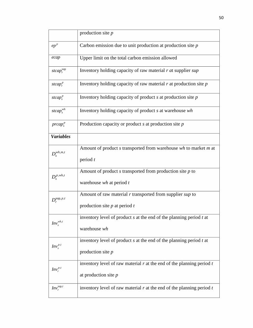
50

production site p

Carbon emission due to unit production at production site p

Upper limit on the total carbon emission allowed

Inventory holding capacity of raw material r at supplier sup

Inventory holding capacity of raw material r at production site p

Inventory holding capacity of product s at production site p

Inventory holding capacity of product s at warehouse wh

Production capacity or product s at production site p

Variables

Amount of product s transported from warehouse wh to market m at

period t

Amount of product s transported from production site p to

warehouse wh at period t

Amount of raw material r transported from supplier sup to

production site p at period t

inventory level of product s at the end of the planning period t at

warehouse wh


production site p

inventory level of raw material r at the end of the planning period t

at production site p

inventory level of raw material r at the end of the planning period t

pep

ecap

suprstcap

prstcap

psstcap

whsstcap

psprcap

, ,wh m tsD

, ,p wh tsD

sup, ,p trD

,wh t

sInv

,p t

sInv

,p t

rInv

sup,t

rInv

51

at supplier sup

Backorder amount of product s at the end of planning period t at

market m

Binary variable to decide whether production site p operates during

planning period t or not

Amount of product s produced at production site p during planning

period t

Total emission taking place over the planning horizon

,m t

sU

ptw

,p tsP

E

52

4 Centralized and Decentralized Supply Chains

A supply chain is usually formed by units which belong to different organizations and are

parts of more than just one supply chain. In such cases, visibility of the entire network

and information sharing among all the entities is not possible. The individual entities in

such a network have their own goals and objectives and make their decisions based on

their own local goals depending on the information available to them. Supply chains can

be distinguished into two main types based on their decision making policies: centralized,

where decisions are taken by a central authority by taking into consideration the other

entities of the supply chain, and decentralized where the decisions are taken by the

individual entities themselves. Centralized supply chains are known to be more

economically efficient than decentralized supply chains. However, complete

centralization is often not possible and practical in case of complex, distributed

enterprises. Often there are different extents of centralization that are followed by the

enterprises.

4.1 Background

This work involves two major aspects: hybrid simulation based optimization for supply

chains and centralized versus decentralized supply chains. The approach presented in

Chapter 3 proposes a flexible solution approach by reducing the amount of information

exchanged between the optimization and the simulation model and using the optimization

only as a target setting. Moreover, a multi-objective problem is solved by taking the

environmental impact of the supply chain as an additional objective for decision-making.

53

Researchers have also studied the effects of different supply chain decision-making

policies. Saharidis et al. 63 develop analytical models to solve the production planning

problem in supply chain involving several enterprises and compare the two types of

optimization – centralized and decentralized. They present a case where each enterprise

prefers to optimize its production plan without considering the other members of the

supply chain. They develop a simple model of decentralized optimization. They compare

the optimal profits obtained in both the centralized and decentralized cases. Duan and

Warren 64 discuss the optimal replenishment policies of capacitated supply chains under

two different control strategies (decentralized vs. centralized). They propose a hybrid

meta-heuristic algorithm to solve both the centralized and decentralized capacitated

supply chain inventory models. It consists of a differential evolution and harmony search,

and one local search method, the Hooke and Jeeves direct search. Palut and Ulengin 65

coordinate the inventory policies in a decentralized supply chain with stochastic demand

by means of contracts. They consider a decentralized two-stage supply chain with

independent suppliers and a manufacturer with limited production capacities. They model

the supply chain as a queuing system and then develop centralized and decentralized

models. They compare the solutions to these models and show that the supply chain

needs coordination. Jalbar et al. 66 consider a multi-echelon inventory/distribution system

with one warehouse and N retailers. They solve the problem of determining the optimal

reorder policy which minimizes the overall cost. They study two situations: centralized

where the retailers are considered branches of the same firm and decentralized where

retailers make decisions independently. They provide two separate solution methods for

the two cases.

54

In this work, hybrid simulation based optimization approaches are proposed to solve

supply chain operation problems. Centralized and decentralized decision making policies

have been considered for the supply chains and different approaches have been applied to

them. The hybrid approach couples an agent based simulation with optimization routines

to improve agent actions. In the decentralized case, the individual agents make their own

decisions based on limited interaction with the rest of the network. On the other hand, in

the centralized case, decision-making is done by an agent that acts as a central decision-

making authority and information sharing is enabled across the whole network. The

decision making authority inherently performs optimization to decide its action. Hence

embedded optimization is used for the agent in the centralized simulation model. The

hybrid simulation based optimization framework proposed in chapter 3 is employed for

the hybrid approach in each case to guide the simulation models towards better solutions.

The different methods used to couple simulation models with optimization models

illustrate the flexibility that can be provided to agent behavior. Two rather small scale

supply chain problems have been solved using the proposed frameworks to demonstrate

their applicability.

4.2 Problem definition


markets is considered in this work. The markets cater to demand of different products

which can be manufactured using three raw materials. Demand of products at the markets

is known for a given number of planning periods. The warehouses have limited storage

capacity for products while the production sites have storage capacities for products and

55

raw materials. The various capacities have been assumed to be available and fixed.

Information flow between the entities has been considered to take place without any time

delay while there is a time delay associated with material flows. There are costs

associated with transportation, inventory holding, production and backorders. Shipment,

inventory and production information for all the planning periods have to be found out so

as to minimize cost.

The supply chain is assumed to operate under two different decision-making strategies.

Decisions related to demand distribution have been considered vary depending on the

strategy adopted by the supply chain. In case of centralized decision-making, demand is

distributed among the upstream entities by a central planning authority. Information is

considered to be shared globally. On the other hand, in the decentralized case, the

decisions are taken by the individual entities. So the demand is distributed among the

upstream entities by the individual demand producing bodies. Also, information is not

shared globally among all the entities of the supply chain. It is shared only locally which

means that entities share information with the other entities that are geographically close

to them, thus resulting in geographical partitioning of the network.

4.3 Optimization model






56


(daily production periods). In the hybrid approach, the optimization model has been used

to guide the simulation towards better results. While the simulation model is more

detailed, the optimization model is kept rather simple. Therefore, no time delays have

been considered for information or material flows. The total cost associated with the

supply chain is the summation of transportation costs, inventory holding costs,

production costs and backorder costs. Transportation cost has been considered to be

proportional to the amount of shipment. Inventory holding cost has been considered

proportional to the inventory level. Production cost is proportional to the amount of

product produced while backorder cost is proportional to the amount of unfulfilled

demand. The model has been formulated as a linear programming problem and

minimization of total cost is the objective function. The optimization model is as follows.

1

2

3

4

5

6

7

, , ,

sup sup, ,

sup

,

, , , , , ,


s s s s r r


t m t

r r s

r R m s PR

t

t t t

m p p p p ts t s

t t t p mp s

wh m wh m t p wh p wh ts s s s

mt m wh s PR m wh p s PR

h Inv h Inv h Inv

h Inv u U FixCost w VarCost P

d D d D

sup, sup, ,

supt t

p p tr r

t mt p r R

d D

, , -1 , , , st - , , ,m t m t m t

s s s

wh m ts

wh WH

U U Dem D s PR m M t T

, , -1 , , , ,- + , , WH,wh t wh t

s s

wh m t p wh ts s

m M p PS

Inv Inv D D s PR wh t T

, , -1 , , ,- , , ,p t p t p t

s s s

p wh ts

wh WH

Inv Inv P D s PR p PS t T

, , -1 , sup, ,

sup

, , ,p t p t p t

r r r

p tr

SUP




57

8

9

The objective function in equation 1 minimizes the total cost which consists of inventory

costs, backorder costs, production costs and transportation costs. Equations 2-5 are the

inventory balance equations at the different nodes of the supply chain. Equation 2

describes the backorders at the markets. Any unfulfilled demand gets accumulated as

backorder. Equation 3 predicts the inventory at warehouses, shipments from warehouses

to markets and shipments from production sites to warehouses. Equation 4 predicts the

product inventory at production sites, production amounts and shipments from production

sites to warehouses during each planning period. Equation 5 predicts the inventory or raw

materials at production sites, consumption of raw materials for the manufacture of

products and shipments from raw material suppliers to production sites during each

planning period. Equations 6–9 are storage capacity constraints for raw material

suppliers, production sites and warehouses respectively.

The optimization model results in a linear programming problem which has been

implemented in GAMS 23.7.3 and solved using CPLEX 12.3.0.0 on Windows 7


RAM.

4.4 Simulation model

As mentioned earlier, agent based simulation is used to represent the supply chain

network. The different entities of the supply chain have been modeled as the agents. Two

, , , ,p t ps sInv stcap s PR p PS t T

, , , ,wh t whs sInv stcap s PR wh WH t T

58

separate simulation models have been developed for the centralized and decentralized

scenarios. Below is a brief description of the different agents in both the models.

Market agent

Demand for products originates at the market agent. The behavior of the agent regarding

demand distribution is different for the decentralized and centralized scenarios.

In the decentralized case, the agent itself is responsible for distributing demand among

the warehouses. When a market receives a demand, it sends requests for the required

amounts of products to the warehouses. A request is not the actual order for products. A

request is a way to procure information from the upstream agent regarding how much

demand can be fulfilled and at what cost. Based on the response from warehouses, the

market agent distributes the demand among the warehouses by following its ordering

policy. As an ordering policy, the market gives first preference to the warehouse which

responds with the lowest cost. It assigns an order of amount either equal to what the

warehouse can fulfill or the demand amount, whichever is smaller. If the total demand

cannot be fulfilled by the lowest cost warehouse, it assigns an order to the one with the

cost next to the lowest cost warehouse. Order amount is decided as either the amount the

warehouse can fulfill or the remaining demand, whichever is larger. Similarly, the market

keeps assigning orders until the total demand is assigned or all the warehouses have been

considered. In case where more than one warehouse responds with the same cost, the

market chooses the one with the maximum amount of demand it can fulfill and the least

amount of time. During this process, the market is able to communicate only with the

warehouses that are located within a specific distance from itself.

59

On the other hand, in the centralized case the market sends request to a central planner

agent responsible for demand distribution among the warehouses. As an individual agent,

the market does not decide how to distribute its demand.

It is desired that the demand be fulfilled during each planning period. However, partial or

no fulfillment of demand is also allowed but at a backorder cost. In case of an oversupply

from warehouses, the superfluous amount is retained for the future planning periods. The

costs associated with this agent are inventory cost and backorder cost.

Warehouse agent

The warehouse agent maintains an inventory of products. Its behavior also varies based

on whether it is the centralized or the decentralized scenario.

In the decentralized case, it receives a request from a market and sends a response in

terms of the fractional of demand it would be able to fulfill, cost and time it would take to

ship the products. In order to evaluate the fraction of demand it can fulfill, it considers the

demand from all the markets. Based on the responses from all the warehouses, the

markets send orders for products. If the complete market demand has not been ordered,

the markets send requests to warehouses again with updated demand. The demand is

updated by reducing the amount which has already been ordered. The process of sending

requests to warehouses, receiving response from warehouses and assigning orders to

warehouses continues until all the demand has been ordered or the warehouses cannot

fulfill any demand from the markets. In this manner, all the warehouses, together attempt

to fulfill the market demand. Sharing of information between warehouses and markets

has been considered. If the demand cannot be fulfilled by a warehouse alone, the other

60

warehouses receive requests from markets and they evaluate if they would be able to

fulfill the demand.

In the centralized case, the warehouse receives orders from the Planner agent. Since the

Planner agent has access to the inventory information of the warehouses, the warehouse

receives orders that it is able to fulfill. Even if the total market demand is not fulfilled, the

Planner agent does not try to reallocate the demand among the warehouses as it had

information about all the warehouses in the first instance itself.

The warehouse agent fulfills the demand from the markets by using its inventory of

products. It has a limited storage capacity and regulates its inventory using a reorder level

- order upto level inventory replenishment policy with continuous review. The warehouse

is capable of updating its reorder level continuously. On a continuous basis, the agent

calculates the average demand it receives per day. Then it calculates the reorder level

using the equation below.

Reorder level = Average daily demand per day x lead time in days + safety stock

Since transportation delays have been considered in the model, there is a lead time for the

agent. The safety stock and order-upto level for the agent are pre-defined. When the

inventory at the warehouse falls below the reorder level, it orders products from the

production sites.

The different decision-making strategies affect the way in which warehouse demand is

distributed among the production sites. For the decentralized scenario, in order to

distribute its demand among the production sites, the warehouse sends requests to the

production sites. The distribution is fixed based on the responses and ordering policy of

61

the warehouse. As an ordering policy, the warehouse gives first preference to the

production site which responds with the lowest cost. It assigns an order of amount either

equal to what the production site can fulfill or the demand amount, whichever is smaller.

If the total demand cannot be fulfilled by the lowest cost production site, it assigns an

order to the one next to the lowest cost. Order amount is decided as either the amount the

production site can fulfill or the remaining demand, whichever is smaller. Similarly, the

warehouse keeps assigning orders until the total demand is assigned or all the production

sites have been considered. In case more than one production site responds with the same

cost, the warehouse chooses the one with the maximum amount of demand it can fulfill

and the least amount of time. The costs associated with this agent are inventory cost and

transportation cost.

On the other hand, in the centralized case the warehouse sends request to a central

planner agent responsible for demand distribution among the production sites. As an

individual agent, the warehouse does not decide how to distribute its demand.

Production Site agent

The production site agent is responsible for the manufacture of products from raw

materials. It also maintains a small inventory of raw materials and products to meet the

demands from the warehouses. It has fixed production capacity and storage capacities.

In the decentralized case, on receiving request from a warehouse, the production site

sends a response in terms of the fraction of demand it would be able to fulfill, cost and

time it would take to ship the products. In order to evaluate the fraction of demand it can

fulfill, it considers the demand from all the warehouses. Based on the responses from all

the production sites, the warehouses send orders for products. If the complete warehouse

62

demand has not been ordered, the warehouses send requests to production sites again

with updated demand. The demand has been updated by subtracting the amount which

has already been ordered. The process of sending requests to production sites by

warehouses, receiving response from production sites and assigning orders to production

sites continues until all the demand has been ordered or the production sites cannot fulfill

any demand from the warehouses. In this manner, all the production sites, together

attempt to fulfill the warehouse demand since sharing of information between production

sites and warehouses has been considered. If the demand cannot be fulfilled by a

production site alone, the other production sites evaluate if they would be able to fulfill

the demand.

In the centralized case, the production site receives orders from the Planner agent. Since

the Planner agent has access to the inventory information of the warehouses, the

production site receives orders that it is able to fulfill. Even if the total warehouse

demand is not fulfilled, the Planner agent does not try to reallocate the demand since it

had access to the information about all the production sites in the first place.

The production site agent fulfills the demand from the warehouses by using the products

it already has in its inventory. It regulates its inventory using a reorder level order up-to

inventory replenishment policy with continuous review. The production site is capable of

updating its reorder level continuously. On a continuous basis, the agent calculates the

average demand it receives per day. Then is calculates the reorder level using the

equation below.

Reorder level = Average daily demand per day x production lead time in days + safety

stock

63

Since production delays have been considered in the model, there is a lead time for the

agent. The safety stock for the agent is pre-defined. When the product inventory falls

below the reorder level, it schedules the production of another batch. Similarly, the

production site has reorder level and order upto level for the raw material inventory

which are fixed. When the raw material inventory falls below the reorder level, it orders

raw materials from the most preferred supplier. It has the highest preference for the

supplier which is located closest. However, the model could easily be adjusted to include

a supplier selection process just as there is a selection process for the warehouses, and the

production sites. The selection process in that case could be based on transportation cost,

raw material cost, shipment time, and raw material availability. The costs associated with

this agent are inventory cost, production cost and transportation cost.

Manufacturing at the production sites is a batch production process. The agent uses an

embedded optimization program to schedule the manufacturing process. The embedded

scheduler minimizes the makespan for the maximum amounts of products produced. The

deterministic model for batch process scheduling follows the main idea of continuous

time formulation proposed by Ierapetritou and Floudas 67. The general model involves the

following constraints.

, , 1 , j

i j n

i I

wv j J n N

10

, , 1 , , , , 1 , , , , s i s i

p c

s n s n s n s i i j n s i i j n

i I j J i I j J

st st d b b s S n N

11

64

max

, , s n sst st s S n N 12

min max

, , , , , , , , , ,i j i j n i j n i j i j nv wv b v wv i I j J n N 13

, s n s

n

d r s S 14

, , , , , , , , , , , ,i j n i j n i j i j n i j i j nTf Ts wv b i I j J n N 15

, , 1 , , , ,(1 ) , ,i j n i j n i j n iTs Tf U wv i I j J n N 16

' ' ' '

' '

, , 1 , , , ,(1 ) , , , ,i j n ji j n i j n

Ts Tf U wv i i I i i j J n N 17

' '

'

, , 1 , , , ,(1 ) , , ,i j n ji j n i j n

Ts Tf U wv i i I j J n N 18

, , 1 , , , ,i j n i j n iTs Ts i I j J n N 19

, , 1 , , , ,i j n i j n iTf Tf i I j J n N 20

, , H , ,i j n iTs i I j J n N 21

, , H , ,i j n iTf i I j J n N 22

Supplier agent


demand. The costs associated with this agent are transportation cost and inventory cost.

Transportation cost is considered to be parallel to the amount of raw materials transported

and inventory cost is considered to be proportional to the amount of raw materials stored.

65

4.5 Centralized and Decentralized Decision Making

4.5.1 Central Planner agent

For the centralized simulation model, there are additional agents that handle demand

distribution among the upstream agents. Market agents send their demand information to

a Central Planner agent for it to find a suitable demand distribution among the

warehouses. Similarly when the warehouses create demand, they send that information to

another Central Planner agent to find a suitable demand distribution among the

production sites.

The planner agents are responsible for finding the optimal demand distribution. Since

their behavior involves optimization inherently, embedded optimization has been used for

this agent. The agent calls this optimizer whenever it has to distribute demand among the

upstream agents. As input to the optimizer, the agent passes information regarding the

current state of the supply chain, past demand and forecasted demand. The optimizer uses

this information to find the optimal shipment levels among the entities for all the future

planning periods. The agent fetches the output for the current planning period and uses to

set the demand distribution.

This agent is not present in the decentralized model as the demand distribution is done by

the individual agents themselves. The structure of the centralized model with the

inclusion of the planner agents is shown in figure 4.1 as opposed to the structure of the

decentralized model shown in figure 4.2.

66

Figure 4.1: Simulation with embedded optimization for centralized scenario

Figure 4.2: Simulation with embedded optimization for decentralized scenario

4.6 Hybrid simulation-optimization approach

The optimization and simulation models are developed independently as discussed in the

earlier sections. In the hybrid approach, the two independent models are coupled together

in order to take advantage of the benefits of both models. For this work, the coupling of

the optimization model with the simulation model has been done using the following

variables: i) shipment values obtained from optimization model set as parameters in the

67

simulation model, ii) production and consumption values from simulation model to

optimization model.

By passing the shipment values from optimization model to simulation model, the

simulation is provided with shipment targets. Simulation tries to achieve these targets so

as to reduce backorder and inventories. The simulation captures a more dynamic


targets depends on the behaviors of the agents of the model. Since the optimization model

is to be used only for the purpose of setting targets for the simulation model, it has been

kept quite simple by not including production scheduling in it. So, the simulation model

is used to set production and raw material consumption targets for the optimization

model. This provides the optimization model with information about the production

behavior. Based on these targets, the optimization model then gives the optimal shipment

values.

68

Figure 4.3: Iterative framework for the decentralized hybrid simulation–

optimization approach

Using the hybrid approach proposed above, the solution methodology proposed in

chapter 3 has been used. The framework consists of an iterative procedure as shown in

Figure 4.3, which is initialized by solving the independent simulation model. The

variables are then passed to the optimization model, which is solved to obtain values of

the decision variables. The two models calculate the total cost for the planning horizon.

The costs from both the models are compared. If the difference is below a tolerance level,

the procedure is terminated otherwise the values of decision variables are passed back to

the simulation model. This process is carried out iteratively until the difference between

the two costs falls below the tolerance level. The above framework uses the simulation

69

model as the master model, which is guided by the optimization model towards the best

solution it can achieve.

4.7 Case Studies

In this section, the different hybrid simulation-optimization approaches have been tested

for two rather small-scale supply chain management problems.

4.7.1 Case study 1

Figure 4.4: Centralized supply chain network for the case study 1

The supply chain consists of 8 markets, 6 warehouses, 2 production sites and 2 raw

material suppliers. There are 2 products and 3 raw materials. Figure 4.4 shows the

network configuration of the centralized supply chain. As discussed earlier, the network

also consists of two Central Planner agents that manage demand distribution. There is a

70

planner agent that connects the markets with the warehouses and another that connects

the warehouses with the production sites.

Manufacture of products is done by a batch production process. The production site agent

schedules the production using an embedded scheduler which is an optimization program.

Figure 4.5 below shows the state task network for the process.

Figure 4.5: State task network for the batch production process

For the decentralized supply chain, the configuration is shown in figure 4.6. Considering

figures 4.4 and 4.6, it can be seen how communication among the agents under the two

scenarios take place differently. In the centralized case, all the markets communicate with

a central planner agent. Similarly all the warehouses communicate with the other central

planner agent. On the other hand, in the decentralized case, the warehouses communicate

directly with the markets. A central agent is not present in this network. Also, there is

limited communication among the agents. For instance, a market does not communicate

71

with all the warehouses or a warehouse does not communicate with all the production

sites.

Figure 4.6: Decentralized supply chain network for case study 1

The problem is solved for a planning horizon of 10 planning periods. Figure 4.7 shows

the results of the hybrid framework for both the decentralized and centralized approaches.

The results illustrate that the framework converges to the optimal solution within 5

iterations. The optimization tries to improve the solution given the simulation input

iteratively by adjusting the shipment. Gradually the gap between the optimal solution and

the realistic solution decreases. The centralized model gives a total cost of $129,396 that

is around 9% lower than the cost of $142,386 predicted by the decentralized model. The

computation time for the decentralized scenario is 214 seconds while that for the

72

centralized scenario is 493 seconds. The centralized model requires longer computational

time due to the Planner agent, which distributes demand among all the upstream agents.


scenarios

1.0E+05

1.5E+05

2.0E+05

2.5E+05

3.0E+05

3.5E+05

4.0E+05

0 2 4 6

Tota

l co

st (

$)

Iteration

Simulation cost vs optimization cost for decentralized model

simulation optimization

1.0E+05

1.5E+05

2.0E+05

2.5E+05

3.0E+05

3.5E+05

4.0E+05

0 2 4 6

Tota

l co

st (

$)

Iteration

Simulation cost vs optimization cost for centralized model


73


scenarios

Figure 4.8 shows a comparison of the different cost components for the centralized and

the decentralized scenarios. Inventory cost, production cost and backorder cost are higher

in case of decentralized model compared to centralized model. In the centralized model,

information is shared across the whole network and also the central planner agents

distribute the demand among the upstream agents in a centralized manner. Therefore

more demand is able to be fulfilled which reduces the backorder cost. Better information

and proper coordination also enable the warehouses and production sites to be able to

fulfill demand while maintaining lower inventories. This results in lower inventory costs

as well. It can be noticed that in case of centralized model, the transportation cost comes

to be higher than in the case of decentralized model. This is quite expected because

demand is distributed locally in case of decentralized scenario. Communication within

the network is limited which means that demand is fulfilled by agents which are located

0.0E+00

1.0E+04

2.0E+04

3.0E+04

4.0E+04

5.0E+04

6.0E+04

transportation cost inventory cost backorder cost production cost

Co

st (

$)

decentralized centralized

74

close to each other. On the other hand, orders could be sent to agents that are situated

very far in order to reduce backorders. As the transportation cost is a function of distance,

it becomes higher in case of the centralized scenario.

4.7.2 Case study 2

The proposed frameworks were used to solve another case study with a larger supply

chain network. A network with 12 markets, 12 warehouses, 4 production sites and 4

suppliers was considered. The batch manufacturing process was considered to be the

same as that in the first case study with 2 products and 3 raw materials.


scenarios

Figure 4.9 shows the result of the iterative solution hybrid iterative framework for the

centralized and decentralized models. Again, convergence is reached in less than 6

iterations. The centralized model gives a total cost of $264,616 that is around 11.5%

75

lower than the cost of $299,353 predicted by the decentralized model. The computation

time for the decentralized scenario is 274 seconds while that for the centralized scenario

is 604 seconds.

Figure 4.10 shows a comparison of the cost components for the centralized and

decentralized scenarios based on the individual cost coefficients. For this example, a

larger supply chain network has been considered which is geographically more dispersed.

Therefore, in the centralized case transportation takes place over longer distances. The

benefits of centralization are reflected in the lower backorder cost and lower inventory

cost. Better coordination leads to less backorders and lower inventory levels. Due to

shipments taking place over longer distances, transportation cost is higher in the

centralized scenario.


models

0.0E+00

4.0E+04

8.0E+04

1.2E+05

1.6E+05

2.0E+05

transportationcost

inventory cost backorder cost production cost

Co

st (

$)


76

The sensitivity of the models with respect to the warehouse capacity was studied. Figure

4.11 shows how the total cost predicted by the centralized and decentralized models

varies with change in warehouse capacity.

Figure 4.11: Variation of total cost with warehouse capacity

It can be seen that both the models follow the same trend for the variation with

warehouse capacity. Total cost first decreases and then increases as the warehouse

capacity is increased. At lower warehouse capacities the total cost decreases with the

increase in capacity. This is expected as at very low warehouse capacities, the backorders

are high. As the capacity gradually increases, more demand can be fulfilled which

reduces the backorder cost and hence the overall cost. The trend can be understood by

looking at the how the individual cost components vary. It can be seen that while

backorder cost decreases, inventory and transportation cost keep increasing with the rise

in warehouse capacity. Beyond a certain warehouse capacity, the total cost is dominated

1.2E+05

1.3E+05

1.4E+05

1.5E+05

1.6E+05

1.7E+05

1.8E+05

1.9E+05

0 50 100 150 200 250

Co

st (

$)

Warehouse Capacity


77

by the increase in inventory and transportation costs rather than the decrease in the

backorder cost. As a result, there is an increase in the total cost beyond that warehouse

capacity. Figure 4.12, shows the variation in major cost components with warehouse

capacity for the decentralized model. Similar trend can be seen for the centralized model

as well.

Figure 4.12: Variation of major cost components with warehouse capacity

Figure 4.11 also shows a comparison of the costs obtained from the centralized and

decentralized models for the different warehouse capacities. It can be seen that at lower

warehouse capacities, results from the two models overlap. As the capacity increases, the

gap between the centralized and decentralized models increases. Centralized model

predicts a lower cost than the decentralized model. The difference is the maximum at a

warehouse capacity of 150 after which it again decreases. Below 125, the capacity is so

low that centralization is not able to offer any benefits. The warehouse inventories are

0.0E+00

2.0E+04

4.0E+04

6.0E+04

8.0E+04

1.0E+05

1.2E+05

0 50 100 150 200 250

Co

st (

$)

Warehouse Capacity

transportation cost inventory cost backorder cost production cost

78

exhausted by the nearby markets. Gradually, with higher capacities, it is advantageous to

be able to make centralized decisions and order outside the local region. As we saw

earlier that transportation cost and inventory cost start to dominate at higher warehouse

capacities, the gap between centralized and decentralized models starts to decrease at

higher warehouse capacities.

The effect of different levels of decentralization was also studied. The results are shown

in figure 4.13. It can be seen that around the value of 150 for the warehouse capacity

where the effects of decentralization are most apparent, the total cost decreases as the

level of decentralization decreases from ‘high’ to ‘low’. Level of decentralization here is

related to the extent of visibility in the network. A ‘high’ level of decentralization implies

that information about fewer warehouses and production sites is visible to the markets

and warehouses respectively compared to a ‘low’ level of decentralization where

information about more warehouses and production sites is available. In case of ‘high’

decentralization, the markets have been considered to have information about a maximum

of 2 warehouses and the particular warehouses depend on the structure of the network.

On the other hand, in case of ‘low’ decentralization, the markets have information about

all the 6 warehouses. ‘Medium’ decentralization refers to the scenario where the markets

have information about an intermediate number of warehouses between 2 and 6

depending on the structure of the network. It is seen that as the visibility increases, the

decentralized model approaches a solution closer to the centralized model.

79

Figure 4.13: Variation of total cost with different levels of decentralization

Figure 4.14: Variation of total cost with production capacity

1.2E+05

1.3E+05

1.4E+05

1.5E+05

1.6E+05

1.7E+05

1.8E+05

1.9E+05

0 50 100 150 200 250

Co

st (

$)

Warehouse Capacity

decentralized (high) decentralized (medium) decentralized (low)

1.6E+05

1.7E+05

1.8E+05

1.9E+05

0 1 2 3 4 5 6

Co

st (

$)

Production level


80

Figure 4.14 shows the variation in the cost predicted by the models for different levels of

production capacity. The different levels of production capacity indicate the different

capacities for the various units in the production site. The capacities increase with the

increasing levels. Production sites have a limited storage capacity which has been

considered to be fixed for all the levels production capacities. It can be seen that the total

cost decreases with the rise in production capacity for the centralized and decentralized

model. The centralized model predicts a lower cost than the decentralized model in all the

cases. Figure 4.15 shows the variation in different cost components for the decentralized

model with the increase in production capacity. A similar trend for the centralized

scenario is also obtained. As the production capacity increases, the production sites are

able to manufacture more products in order to meet the demands which results in a

decrease in backorder cost and a slight increase in production cost. Since more products

are manufactured and more demand is fulfilled, more amounts of shipments are

transported among the entities. Therefore, there is an increase in the transportation cost.

A similar plot for was obtained for the centralized case as well.

81

Figure 4.15: Variation of different cost components with production capacity

4.8 Conclusions

In this chapter, we demonstrated different methodologies to develop hybrid simulation

based optimization frameworks. The first methodology uses embedded optimization to

improve agent behavior while the second one uses optimization to set targets for the

simulation model and direct it towards the optimal solution. It illustrates the flexibility

with which agent based simulations can be coupled with optimization models to improve

the autonomous behavior of agents.

Embedded optimization was used for agents that perform optimization inherently. The

other approach where optimization directs the simulation towards optimality is used to

improve the performance of the different agents. The proposed hybrid simulation based

optimization frameworks offer the capability to incorporate either one or both of these

approaches and to improve the behavior of the supply chain entities.

0.0E+00

2.0E+04

4.0E+04

6.0E+04

8.0E+04

1.0E+05

1.2E+05

0 1 2 3 4 5 6

Co

st (

$)

Production level

decentralized backorder cost decentralized transportation cost

decentralized inventory cost decentralized production cost

82

The hybrid frameworks were used to study different supply chain decision-making

policies. The effects of centralized decision making where the decision maker acts as a

central authority with access to all the information are observed. It is observed that

centralization enables better fulfillment of customer demands due to better coordination

among the agents. The extent of benefit that centralization provides depends on the

design of the supply chain. However, the centralized model gives better or equal results

in all the cases considered.

This study illustrates that the agent based simulation model can be conveniently used to

capture supply chain dynamics under different scenarios. Also, the proposed hybrid

simulation based optimization framework can be effectively used to improve the behavior

of the agents. Apart from the two decision making policies considered in this work,

similar approach may be used to capture varied supply chain management scenarios.

Although the proposed framework was used for rather small scale supply chain problems,

it can conveniently be used for larger problems with more number of agents and also

where agents behave differently and follow different decision making policies.

Nomenclature

Indices

t planning period

p production site

sup supplier


83

wh Warehouse

s Product state


mt Mode of transportation

mp Mode of production

Sets

T planning periods

PS production sites

SUP suppliers


WH Warehouses

PR Product states


MT Modes of transportation

MP

Modes of production

Parameters

holding cost of product s at warehouse wh



holding cost of raw material r at supplier sup


wh

sh

p

sh

p

rh

sup

rh

msu

84


unit transportation cost of product s from production site p to warehouse

wh

unit transportation cost of raw material r from supplier sup to production

site p

fixed production cost of operation of production site p

unit variable cost of production at site p

demand of product s at market m for period t

Inventory holding capacity of raw material r at supplier sup




Production capacity or product s at production site p

Variables

Amount of product s transported from warehouse wh to market m at period

t

Amount of product s transported from production site p to warehouse wh at

period t

Amount of raw material r transported from supplier sup to production site p

at period t

inventory level of product s at the end of the planning period t at warehouse

,wh msd

,p whsd

sup, prd

pFixCost

pVarCost

,m t

sDem

suprstcap

prstcap

psstcap

whsstcap

psprcap

, ,wh m tsD

, ,p wh tsD

sup, ,p trD

,wh t

sInv

85

wh


production site p

inventory level of raw material r at the end of the planning period t at

production site p


supplier sup

Backorder amount of product s at the end of planning period t at market m

Binary variable to decide whether production site p operates during

planning period t or not

Amount of product s produced at production site p during planning period t

,p t

rC

Amount of raw materials r consumed at production site p during planning

period t

, ,i j nwv Binary whether or not task i in unit j starts at event point n

,s nst continuous, amount of state s at event point n

,s nd amount of state s delivered at event point n

,

p

s i ,

c

s i proportion of state s produced, consumed by task i, respectively

, ,i j nb continuous, batch size of task i in unit j at event point n

max

sst

available maximum storage capacity for state s

min

,i jv max

,i jv minimum amount, maximum capacity of unit j when processing task i

sr requirement for state s at the end of the time horizon

,p t

sInv

,p t

rInv

sup,t

rInv

,m t

sU

ptw

,p tsP

86

, ,i j nTf time that task i finishes in unit j while it starts at event point n

, ,i j nTs time that task i starts in unit j at event point n

,i j constant term of processing time of task i at unit j

,i j

variable term of processing time of task i at unit j expressing the time

required by the unit to process one unit of material performing task i

H Time horizon

87

5 Synchronous and Asynchronous Decision Making Strategies in

Supply Chains

The individual entities in such a network have their own goals and objectives. A supply

chain network may comprise entities belonging to the same or different organizations.

Due to the way the different business processes operate and update information, there is

often a disconnection between the physical actions of the entities and information. The

different business processes have their own individual goals and objectives and operate

on the basis of their own time-scales. Therefore, in an actual supply chain, it is not

practical to synchronize the operations of all the processes. The overall operation of the

supply chain, therefore, is a mix of synchronous and asynchronous processes.

In the case of real-world supply chains, it is impractical for a single decision maker to

have access to all the relevant information and make decisions for the whole network.

There are usually multiple decision makers who have access to their own sets of

information and make their own independent decisions. These decisions are not

synchronized and therefore the operations also take place at their own individual rates

and times. Due to this asynchronous nature of operations, the individual decision makers

make decisions based on the information available at those specific times.

Simulation models have been widely used to depict supply chain networks. The main

idea behind using detailed simulation models is to be able to capture the true dynamics of

the network. In a practical scenario, no supply chain operates completely synchronously

or asynchronously. It is therefore essential for the simulation models to include the

synchronicities and asynchronicities present in the network in order to capture the true

dynamics. The way these models are coded is important to get the right set of results.

88

Here is a brief description of some of the important works available in the literature

related to modeling of synchronous and asynchronous processes.

5.1 Background

In a practical scenario, asynchronous decision making within a supply chain is quite

common. There are quite a number of works which cover the distributed and

asynchronous nature of decision making68-75. We discuss some of those works related to

modeling of synchronous and asynchronous processes, particularly related to supply

chains. Carle et al.76 propose an agent-based metaheuristic to solve large-scale multi-

period supply chain network design problems. Using the concept of asynchronous agent

teams (A-teams), they propose an efficient hybrid metaheuristic called Collaborative

Agent Team (CAT). The generic model integrates design and modeling concepts and can

be used to reengineer real-world supply chain networks. They compare the results for

large-scale networks with those obtained with CPLEX. Tolone77 focuses on agility and

time-based manufacturing as critical factors for manufacturing enterprises in today’s

world. He considers a multi-company supply chain planning and execution environment

and emphasizes the importance of real-time and asynchronous collaboration technology

in allowing manufacturers to increase their supply chain agility. They propose Virtual

Situation Room technology to find and engage quickly the relevant members of a

problem solving team. The members are supported by highly interactive access to

information and control. They are enabled by business processes, security policies and

technologies, intelligence and integration tools. Zheng et al.78 present a multi-agent

architecture for SCM systems in which asynchronous teams (A-Team) of agents

exchange results and cooperate to give non-dominated solutions that show the tradeoffs

89

between objectives. They consider the complex processes, objectives and constraints in

today’s supply chains and state that agent-based architectures for supply chain

management are difficult to implement and maintain. Luh et al.79 focus on the issue of

coordination of activities across a network of suppliers to quickly respond to market

conditions. They combine mathematical optimization and the contract net protocol for

make-to-order supply network coordination. The overall problem is decomposed into

organizational sub-problems. Scheduling of activities by the individual organizations is

based on their internal situations and inter-organization prices. Coordination is carried out

in a distributed and asynchronous manner. Bond80 states that most work is organized, that

is it is carried out by many people cooperatively solving a set of shared problems. He

outlined his research in two areas, (i) cooperation in a vertical structure of an

organizational hierarchy and (ii) horizontal cooperation among a team of agents which

have different specializations and are solving a common problem. Akiyoshi and

Komoda81 study distributed organizations which can be categorized into demand and

supply sites. They state that in order to reach mutual agreement, negotiation based

commitment is needed. The negotiation process under asynchronous negotiation is a

complicated procedure. In their work, they investigate such a negotiation process.

Sohlenkamp and Chwelos82 present a novel environment called DIVA for group work.

The prototype virtual office environment supports communication, cooperation and

awareness in both synchronous and asynchronous modes. It is modeled after the standard

office and abstracts elements of physical offices required for collaborative work like

people, rooms, desks and documents.

90

In this work we use agent based simulation models for supply chain systems. Therefore

we present here a brief description of some work related to asynchronous and

synchronous agent based models, not particularly related to supply chains. Some of the

works focus on the specific modeling methodology followed in developing the models

with regards to update scheme for the different agents in the agent based models. Volf et

al.83 present a simulation framework designed to simulate entities to high details

requiring extended computation resources. They present the concept the dynamic

partitioning of the multi-agent simulations. Spatial partitioning and dynamic load

balancing are used. The simulation combined synchronous and asynchronous parts. They

verify the simulation framework by using it for the entire civilian air traffic touching the

national airspace of United States. Lormier et al.84 discuss that the success of individual

based models depends on its design and assumptions made during its construction. In

particular, they consider synchronous and asynchronous scheduling as two methods for

updating object characteristics during interaction. They show that the two methods

produce different results for a simple individual based model, particularly for high

population densities and increased interaction complexity. Cornforth et al.85 use 1-

dimensional cellular automata as a case study to compare synchronous, random

asynchronous and ordered asynchronous updating schemes in multi-agent systems. They

show that the type of updating scheme has an impact on the dynamic characteristics of

the system. They conclude that ordered asynchronous processes with local temporal

coupling play a role in self-organization within many multi-agent systems. Guo and Tay86

focus on the heterogeneity in update frequencies of the individual agents due to multi-

timescales in immunological phenomena. They apply an event-scheduling update scheme

91

which allows arbitrarily smaller timescales and avoids unnecessary execution and delays.

They use the scheme to model the B cell life cycle and compare its simulation

performance with the widely adopted uniform time-step update scheme. Boer et al.87

investigate how the market dynamics for continuous, asynchronous simulation are

different from discrete time simulation. They show that the continuous, asynchronous

simulation reveals more information and the market prices are different between the two

cases. Lawson and Park88 study the behavior of the artificial society and demonstrate that

very different behavior can be observed if agent events occur asynchronously instead of

synchronous time evolution which is used in most artificial society discrete event

simulations. Results show that by using an appropriate event list implementation,

acceptable computational performance can be achieved. Androulakis and Reklaitis89

developed a methodology for decentralized decision making for problems consisting of

interacting sub-systems where each is described by local properties and dynamics. The

methodology is based on the solution of a series of sub-problems where each minimizes

each local objective while maximizing a common Lagrangean function.

In this work, we investigate how the asynchronous operations of the different members of

the supply chain can affect its overall behavior. We consider that the different entities of

the network operate based on their timescales. Based on their own operating cycles, they

update the relevant information which impacts the information set available to others at

any particular point in time. In order to illustrate this, we use rather simple case studies.

We use agent based simulation models to capture the dynamics of these simple networks.

To include production scheduling for the manufacturing plants, we use embedded

optimization with the agent based simulation models. We also develop models for the

92

synchronous operation and compare the results for the scenarios. Both synchronous and

asynchronous decision-making are optimized using the hybrid simulation based

optimization approach proposed in chapter 3. The hybrid simulation based optimization

approach has been shown to be effective in predicting the optimal operation of the supply

chain while capturing the behavior of the individual agents90. We use this approach to

predict the optimal operation of the supply chain under the two decision making

strategies.

5.2 Problem Statement

A supply chain network consisting of different decision – making entities has been

considered. The entities specifically included in this study are market, warehouse and

production sites. Each entity has its own role in the network and performs its functions

based on its individual policies. The actions of the entities are dependent on the

information available to them and the state of the network which evolves as the entities

perform their functions. Information is exchanged among the decision – making entities

as they interact with each other. The market receives demand for products at specific time

intervals and assigns orders to the upstream entities based on its ordering policy. The

warehouses store products and transport them to fulfill market demand. They regulate

their inventory by following their own inventory replenishment policy. Similarly,

production sites also transport products to fulfill market demand. They manufacture

products to regulate their product inventory by following a production policy. They

maintain their raw material inventory by following an inventory replenishment policy.

93

Interaction among the entities can occur either synchronously or asynchronously. Unlike

synchronous interactions where information is exchanged among the entities

simultaneously, the exchange of information depends on individual operation cycles of

the entities in case of asynchronous interactions. The market ordering policy, inventory

replenishment policies and the production site production policy involve making

decisions based on the information available to the entities. For example, the market

orders products from the upstream entities based on the available information regarding

their inventory. Similarly the production site manufactures products based on the

available demand information. Consequently, availability of information plays an

important role in the dynamics of the network. It becomes significant whether the

interactions among the entities occur synchronously or asynchronously.

5.3 Asynchronous and Synchronous Decision Making Scenarios

In this section, we describe how synchronous and asynchronous interactions within the

supply chain network have been implemented in this study. As mentioned earlier, for the

synchronous scenario, information is shared with the different entities of the supply chain

simultaneously. In this way the operation of a particular entity is dependent on those of

the other entities as the demand site, considered as the market in the examples studied,

waits for responses from all the warehouses regarding fulfillment of demand. However

for the asynchronous decision making strategy, the operations of the different entities of

the supply chain do not necessarily depend on those of the other entities. Each entity has

its own independent operation cycle and the times at which they update their databases

and obtain the latest information are not synchronized.

94

Figure 5.1: Asynchronous implementation for supply chain agents in the study

Figure 5.2: Synchronous Implementation for supply chain agents in the study

95

Figures 5.1 and 5.2 depict an example of the implementation of the asynchronous and

synchronous decision-making in the supply chain where three entities are involved. In the

figures, the horizontal line depicts the time horizon for which the simulation is run.

Information is being shared by entity 2 with entity 1 and entity 3. The vertical lines

intersecting the horizontal line are the time points at which the entity performs a

particular operation. For example if entity 2 is a market, the line represents the time at

which the demand arrives at the market and it updates its database. If entity 1 is a

warehouse, it represents the time at which the warehouse obtains the demand from the

market and updates its database. The dashed lines connecting the entities represent the

exchange of information between the two. As we can see in figure 5.2, the update times

for the entities are synchronized and they have access to the same information

simultaneously. Figure 5.1 shows the asynchronous implementation where the time

points when entities 1 and 3 obtain information and when entity 2 updates information

are not synchronized. Hence entity 1 is able to receive the information updated by entity

2 during the 1st period while entity 3 obtains the information from entity 2 during the 2nd

period. Based on their individual operating cycles, either of the entities may be able to

obtain the latest information.

These scenarios depict how the operations within a supply chain network can occur

differently. Even within a single-company supply chain network, entities can operate

both synchronously and asynchronously. The different implementations that are adopted

here for the two different scenarios represent small portions of the overall dynamics of an

actual supply chain and are meant to give an idea of the effects that a combination of the

two scenarios would cause in the overall supply chain dynamics.

96

5.4 Simulation model

A supply chain is a distributed and decentralized system with autonomous entities. For

such a system, it is suitable to model using a bottom-up approach. Agent based modeling

has been used in the literature to model such systems. It has been shown that an agent

based model can be used to better represent the dynamics of a supply chain 62,91. In this

work, agent based simulation model has been implemented using Repast simulation

platform and Java programming environment. In order to model the synchronous and

asynchronous operations of the supply chain, two different simulations have been

developed. Here is a description of the agents in both the models.

5.4.1 Demand agent

Demand for products originates at the demand agent. The behavior of the agent regarding

demand distribution is different for the synchronous and asynchronous operations.

In the synchronous case, the agent distributes demand among the supply agents. When a

demand site receives a demand, it sends requests for the required amounts of products to

the supply sites. A request is not the actual order for products. A request is a way to

procure information from the upstream agent regarding how much demand can be

fulfilled and at what cost. Based on the response from supply sites, the demand agent

distributes the demand among the supply sites by following its ordering policy. As an

ordering policy, the demand agent gives first preference to the supply site which responds

with the lowest cost. It assigns an order of amount either equal to what the supply site can

fulfill or the demand amount, whichever is smaller. If the total demand cannot be fulfilled

97

by the lowest cost supply site, it assigns an order to the one with the cost next to the

lowest cost. Order amount is decided as either the amount the supply site can fulfill or the

remaining demand, whichever is larger. Similarly, the demand agent keeps assigning

orders until the total demand is assigned or all the supply sites have been considered. In

case where more than one supply site responds with the same cost, the demand agent

chooses the one with the maximum amount of demand it can fulfill and the least amount

of time. In such a scenario, it is ensured that all the supply sites have the same demand

updated information available to them at a particular time.

In the asynchronous case, the demand agent updates the demand information at regular

intervals. These intervals need not match with the specific time points at which it actually

receives the demand. The intervals at which the agent updates the demand information in

order to be available for the other entities is referred to as the ‘update cycle’ of the

market. The agent does not coordinate with all the supply sites for demand distribution.

The supply sites are allowed to run their own processes independently rather than in a

coordinated manner. When one or more supply site communicates with the demand agent

regarding demand fulfillment, the demand agent decides to receive product shipment

from the supply sites. In such a scenario, the supply sites do not operate in a coordinated

manner and need not have access to the same demand information at the same time.

5.4.2 Warehouse agent

The warehouse agent stores products and regulates its inventory using a fixed reorder

level and reorder quantity with continuous review. There is a fixed lead time for

inventory replenishment. There is a transportation delay between the warehouse and the

98

demand sites. In the asynchronous scenario, the warehouses obtain the updated demand

information at regular intervals that are not coordinated with the update cycles of the

demand sites. These regular intervals at which the warehouse obtains the latest demand

information from the demand sites is referred to as the ‘update cycle’ of the warehouse.

Based on which warehouse obtains the latest demand information first, the fulfillment of

demand by a particular warehouse is done.

On the other hand, in case of synchronous operations, the demand sites share the latest

demand information with the warehouses immediately. Therefore, in this case all the

warehouses get access to the demand information at the same time. When a warehouse

receives a request from a demand site, it sends a response which includes the cost, the

amount it can fulfill and the time it would take to fulfill the demand. Based on the

responses received from the warehouses, the demand sites send orders to the warehouses

which are fulfilled with the available inventory.

5.4.3 Production Site

The Production Site agent stores products and also regulates its inventory by

manufacturing products from raw materials. It sends products to the demand sites to

fulfill demand. There is a transportation delay between the production site and the

demand sites. The production site obtains demand information from the market. At a

particular planning period, the production site can obtain information about the future

demand for a fixed number of periods. The intervals at which the production site obtains

demand information from the demand sites is referred to as the ‘update cycle’ of the

production site. When the information available to a production site gets updated, it is

99

able to generate a production schedule so as to meet the future demand. The scheduling

horizon for the scheduler is the number of time periods for which the demand is known to

the production site. There is a production delay between the generation of a schedule and

actual change in inventory by manufacturing.

In the asynchronous case, a production site operates based on its own update cycle. It

may not obtain the latest demand information immediately. Therefore it may not be able

to generate an updated production schedule as soon as a new demand appears at the

demand site. An updated production schedule is generated only when the demand

information available to the production site gets updated.

On the other hand, in case of synchronous interactions, the demand sites share the latest

demand information with the production sites immediately. Therefore, in this case all the

production sites get access to the demand information at the same time. When a

production site receives a request from a demand site, it sends a response which includes

the cost, the amount it can fulfill and the time it would take to fulfill the demand. Based

on the responses received, the demand sites send orders to the production sites which are

fulfilled with the available inventory.

Manufacturing at the production sites is a batch production process. The agent uses an

embedded optimization program to schedule the manufacturing process. The embedded

scheduler minimizes the total cost involved for the scheduling horizon. The deterministic

model for batch process scheduling follows the main idea of continuous time formulation

proposed by Ierapetritou and Floudas 67. The general model involves the following

constraints.

100

1

2

3

4

5

6

7

8

9

10

11

12

13

5.4.4 Supplier

, , 1 , j

i j n

i I

wv j J n N

, , 1 , , , , 1 , , , , s i s i

p c

s n s n s n s i i j n s i i j n

i I j J i I j J

st st d b b s S n N

max

, , s n sst st s S n N

min max

, , , , , , , , , ,i j i j n i j n i j i j nv wv b v wv i I j J n N

, s n s

n

d r s S

, , , , , , , , , , , ,i j n i j n i j i j n i j i j nTf Ts wv b i I j J n N

, , 1 , , , ,(1 ) , ,i j n i j n i j n iTs Tf U wv i I j J n N

' ' ' '

' '

, , 1 , , , ,(1 ) , , , ,i j n ji j n i j n

Ts Tf U wv i i I i i j J n N

' '

'

, , 1 , , , ,(1 ) , , ,i j n ji j n i j n

Ts Tf U wv i i I j J n N

, , 1 , , , ,i j n i j n iTs Ts i I j J n N

, , 1 , , , ,i j n i j n iTf Tf i I j J n N

, , H , ,i j n iTs i I j J n N

, , H , ,i j n iTf i I j J n N

101


demand. The costs associated with this agent are transportation cost and inventory cost.

Transportation cost is considered to be proportional to the amount of raw materials

transported, and inventory cost is considered to be proportional to the amount of raw

materials stored.

The agents discussed above are those that have been specifically used in this study.

However, the agent based simulation model provides the flexibility to add similar

behavior related to asynchronous and synchronous interactions for other decision-making

entities very easily. Moreover different scheduling models and operating policies can be

considered by changing the scheduling agent.

5.5 Optimization model

The hybrid simulation based optimization approach uses an optimization model which is

coupled with the simulation model. This section provides the details regarding the

optimization model used in this work.







(daily production periods). In the hybrid approach, the optimization model has been used

to guide the simulation towards better results. While the simulation model is more

102

detailed, the optimization model is kept rather simple. Therefore, no time delays have

been considered for information or material flows. The total cost associated with the

supply chain is the summation of transportation costs, inventory holding costs,

production costs and backorder costs. Transportation cost has been considered to be

proportional to the amount of shipment. Inventory holding cost has been considered

proportional to the inventory level. Production cost is proportional to the amount of

product produced while backorder cost is proportional to the amount of unfulfilled

demand. The model has been formulated as a linear programming problem and

minimization of total cost is the objective function. The optimization model is as follows.

, , ,

sup sup, , ,

sup

, , , , , , sup, sup,


pr pr pr pr r r

t wh pr PR t p pr PR t p r R

t m m t p p t

r r pr pr pr

t r R t m pr PR t p pr

wh m wh m t p wh p wh t p p

pr pr pr pr r r

t m wh pr PR

h Inv h Inv h Inv

h Inv u U VarCost P

d D d D d D

,

sup

t

t wh p pr PR t p r R

14

, ,t 1 , , ,st , , ,m t m m t wh m t

pr pr pr pr

wh WH

U U Dem D pr PR m M t T

15

, ,t 1 , , , , , , wh WH,wh t wh wh m t p wh t

pr pr pr pr

m M p PS

Inv Inv D D pr PR t T

16

, ,t 1 , , , , , ,p t p p wh t p t

pr pr pr pr

wh WH

Inv Inv D P pr PR p PS t T

17

18

19

20

, , , ,p t p

pr prInv stcap pr PR p PS t T 21

wh, , , ,t wh

pr prInv stcap pr PR wh WH t T 22

, , -1 , sup, ,

sup

, , ,p t p t p t

r r r

p tr

SUP




103

The objective function in equation 14 minimizes the total cost which consists of

inventory costs, backorder costs, production costs and transportation costs. Equations 15-

18 are the inventory balance equations at the different nodes of the supply chain.

Equation 15 describes the backorders at the markets. Any unfulfilled demand gets

accumulated as backorder. Equation 16 predicts the inventory at warehouses, shipments

from warehouses to markets and shipments from production sites to warehouses.

Equation 17 predicts the product inventory at production sites, production amounts and

shipments from production sites to warehouses during each planning period. Equation 18

predicts the inventory of raw materials at production sites, consumption of raw materials

for the manufacture of products and shipments from raw material suppliers to production

sites during each planning period. Equations 19–22 are storage capacity constraints for

raw material suppliers, production sites and warehouses respectively.

The optimization model results in a linear programming problem which has been

implemented in GAMS 23.7.3 and solved using CPLEX 12.3.0.0 on Windows 7


RAM.

5.6 Hybrid Simulation based Optimization

In order to optimize the behavior of the agents, a hybrid simulation based optimization

approach has been used. The approach can effectively lead to the optimal solution while

capturing the individual behavior of the agents. The hybrid approach couples the agent-

based simulation model with the optimization model to improve agent actions. An

104

independent optimization model is developed which is coupled with the simulation

model. The approach allows both the models to take advantage of the benefits of each

other. For this work, the coupling of the optimization model with the simulation model

has been done using the following variables: i) shipment values obtained from

optimization model set as parameters in the simulation model, ii) production and

consumption values from simulation model to optimization model.

The optimization model provides the simulation with shipment targets by passing

shipment values to the simulation model. The simulation captures a more dynamic


targets depends on the behavior of the agents of the model. Since the optimization model

is to be used only for the purpose of target setting, production scheduling has not been

included and it has been kept quite simple. So, the simulation model is used to set

production and raw material consumption targets for the optimization model. This

provides the optimization model with information about the production behavior. Based

on these targets, the optimization model then gives the optimal shipment values.

105

Figure 5.3: Iterative framework for the decentralized hybrid simulation–

optimization approach


chapter 3 has been used. The framework consists of an iterative procedure as shown in

Figure 5.3, which is initialized by solving the independent simulation model. The

variables are then passed to the optimization model, which is solved to obtain values of

the decision variables. The two models calculate the total cost for the planning horizon.

The costs from both the models are compared. If the difference is below a tolerance level,

the procedure is terminated otherwise the values of decision variables are passed back to

the simulation model. This process is carried out iteratively until the difference between

the two costs falls below the tolerance level. The above framework uses the simulation

model as the master model, which is guided by the optimization model towards the best

solution it can achieve.

106

5.7 Case Studies

In this section, three case studies have been presented. In the first two, the simulation

models have been used to study two rather small-scale case studies to illustrate the effect

of applying different decision making strategies in supply chain management. The idea

behind considering these case studies is to be able to illustrate at a small scale, the

asynchronicities in supply chain operations that can occur in the industry and what are

their effects in SC decision making. In a large scale supply chain network, synchronized

interactions among entities is not always easy. For example, a production team may not

obtain information about the sales commitment decisions in a synchronized manner,

which could lead to incomplete fulfillment of the committed product orders. Due to

asynchronous operation of the production team and the sales team, there might be

insufficient time for the production of the required amount of products based on the due

dates of the committed sales. In the third case study, a larger problem with synchronous

and asynchronous decision making strategies is considered. The hybrid simulation based

optimization approach is used to study the optimal supply chain operation for both the

scenarios. The third case study aims at investigating how optimizing the supply chain

operation under asynchronous decision making strategy can improve its performance and

make it closer to or even better than operating under synchronous decision making

strategy but not optimized. Although at a small scale, these case studies illustrate the

impact such asynchronicities can have on the overall behavior of the supply chain and its

economics.

107

5.7.1 Case Study 1: Investigating different decision making strategies between

warehouse and sales

Figure 5.4 above shows a two stage supply chain with 1 demand site and 2 supply sites.

The supply sites in this case study are warehouses. Demand arrives at the demand site

during each planning period. Both the warehouses have limited storage capacities and

regulate their inventory following a (Q, r) policy with continuous review. The reorder

level and reorder quantity for the warehouses are assumed to be half their holding

capacity values. However they can very easily be changed to other values. Warehouse 1

is located closer to the demand site and also has a larger capacity than warehouse 2.

Therefore warehouse 1 is the primary warehouse for the demand site while warehouse 2

is the secondary warehouse. All the warehouses and the demand site belong to the same

company. There are constant lead times for inventory replenishment and delivery. There

is a single product being considered. There are costs associated with warehouse

inventory, transportation and backorders. Backorder cost is $30/lb/day.

Simulation models representing synchronous and asynchronous scenarios were used for

this case study. The simulation was run for particular demand data and different sets of

Demand

Wh 2

Wh 1

Figure 5.4: Small – scale two stage supply chain network

108

update frequencies for the two warehouses in the asynchronous scenario. It was observed

that the behavior of the entire supply chain varies as the update frequencies varied.

Figure 5.5: Total cost for synchronous and asynchronous operations

Figure 5.5 shows the total cost values obtained for the different scenarios. In the figure,

the x-axis value (1, 2) represents the asynchronous scenario where warehouse 1 (wh1)

has an update interval of 1 period while warehouse 2 (wh2) has an interval of 2 periods.

This means that wh1 obtains the latest demand information from the market during every

period while wh2 does that every two periods. It is considered that demand arrives at the

market during every period. It can be observed that the lowest cost obtained is in the

synchronous case where there is coordination among the demand site and the

warehouses. The total cost value increases with increase in update interval. However, an

increase in the update interval for wh1 causes a higher increase in total cost as compared

to the same increase in update intervals for wh2. This is because wh1 has a larger

0.0E+00

1.0E+04

2.0E+04

3.0E+04

4.0E+04

5.0E+04To

tal C

ost

($

)

Update Interval

109

capacity than wh2 and is therefore able to fulfill more demand when both have the same

update intervals. However when the update intervals for wh1 increase, there is less

fulfillment of demand as compared to when the update intervals for wh2 increase. This is

evident in figure 5.6 where higher values of backorder cost can be seen for higher update

intervals of wh1. As wh1 is located closer to the demand site compared to wh2, less

frequent updates for wh1 result in more transportation from wh2 to the demand site,

which in turn increases the transportation cost. The computation time for the simulation

runs was observed to be around 4 sec.

Figure 5.6: Cost components for synchronous and asynchronous operations

It is important to look into how the variation in costs is caused with the variation in

update intervals. As mentioned earlier, depending on which warehouse updates the

information and at what time, a particular warehouse picks up the demand. Since the

warehouses have different capacities and are located at different locations with one of

0.0E+00

5.0E+03

1.0E+04

1.5E+04

2.0E+04

2.5E+04

3.0E+04

Co

st (

$)

Update Interval

Backorder cost Inventory cost Transportation cost

110

them being closer to the demand site than the other, which specific warehouse picks up

the demand results in either higher or lower cost.

Figure 5.7 shows the amount of products shipped from warehouses to the demand site

during each period. Both the warehouses have been considered to have different storage

capacities and different inventory replenishment policies. It can be seen that although the

process happens synchronously, the demand site prefers wh1 which is closer over wh2.

Therefore it always attempts to fulfill the demand from wh1 first. During some of the

periods, since the demand is low, no shipment takes place from wh2. During other

periods, the total demand which includes the backorders is so high that wh1 sends a

shipment equal to its maximum capacity which has been considered as 100 in this

example. During asynchronous operations, the mechanism will be different since a

warehouse may not pick up the demand information immediately.

Figure 5.7: Amount of product shipped by warehouses under synchronous

operation

0

20

40

60

80

100

120

1 2 3 4 5 6 7 8 9 10

Am

ou

nt

ship

pe

d b

y w

are

ho

use

Period

wh1 wh2

111

Figure 5.8: Amount shipped by warehouses under asynchronous operation (1, 4)

Figure 5.8 shows the asynchronous scenario (1,4). It can be seen that wh2 receives

demand information only during periods 4 and 8 and therefore sends shipments at those

times. During other periods, only wh1 sends products to the demand site. Similar plots

for asynchronous operations with other update cycles are shown in Figure 5.9. When the

demand values including backorders are more than the warehouse storage capacities, the

warehouses send shipments equal to their maximum capacity to the demand site.

0

20

40

60

80

100

120

1 2 3 4 5 6 7 8 9 10

Am

ou

nt

ship

pe

d b

y w

are

ho

use

Period

wh1 wh2

112

Figure 5.9: Amount shipped by warehouses under (a) asynchronous operation 1,2

(b) asynchronous operation 2,1 (c) asynchronous operations 1,3 and (d)

asynchronous operations 3,1

0

20

40

60

80

100

120

1 2 3 4 5 6 7 8 9 10Am

ou

nt

ship

pe

d b

y w

are

ho

use

Planning Periodwh1 wh2

0

20

40

60

80

100

120

1 2 3 4 5 6 7 8 9 10

Am

ou

nt

ship

pe

d b

y w

are

ho

use


0

20

40

60

80

100

120

1 2 3 4 5 6 7 8 9 10

Am

ou

nt

ship

pe

d b

y w

are

ho

use

Planning Period

wh1 wh2

0

20

40

60

80

100

120

1 2 3 4 5 6 7 8 9 10Am

ou

nt

ship

pe

d b

y w

are

ho

use


(a) (b)

(c ) (d)

113

5.7.2 Case Study 2: Exploring different decision making strategies between sales and

production sites

Figure 5.10 above shows a two stage supply chain with 1 demand site and 2 supply sites.

The supply sites in this case study are production sites. Demand arrives at the demand

site during each planning period. Any arriving demand has a specific due date which has

been considered as 2 periods in this example. Both the production sites have limited

storage capacities and regulate their product inventory by manufacturing using raw

materials. They obtain raw materials from suppliers that have a limited capacity. The raw

material reorder level and reorder quantity for the production sites are assumed to be half

their raw material holding capacity values. However they can very easily be adjusted to

other values. Production site 1 (ps1) has a higher production capacity and is located

closer to the demand site than production site 2 (ps2). Therefore ps1 is the primary

production site for the demand site while ps2 is the secondary production site. All the

production sites and the demand site belong to the same company. The example considers

2 products and 3 raw materials. There are costs associated with production site inventory,

transportation, production and backorders. The production sites update their information

based on their update cycles. Therefore they need not have the updated demand

information at all times.

Demand

ps 2

ps 1

Figure 5.10: Small-scale two stage supply chain

114

Manufacture of products is done in batch operation mode. The production site schedules

the production using an embedded scheduler which relies on the solution of the

scheduling optimization problem. The state task network for the process is shown in

Figure 5.11. When the production site updates the demand information, the scheduler

gets to know the demand requirements for a certain number of planning periods in the

future. The scheduler generates a production schedule to minimize cost. The scheduling

horizon is the period for which the demand information is available to the scheduler.

Figure 5.11: State task network for the batch production process

Simulation models considering synchronous and asynchronous scenarios were used again

for the specific case study. The simulation was run for particular demand data and

different sets of update frequencies for the two production sites in the asynchronous

scenario. It was observed that the behavior of the supply chain as a whole varies as the

update frequencies varied. The computation time for the update intervals (1,3) was

observed to be 74 sec. The computation time is observed to be higher than it is in case

115

study 1 because of the additional execution time of the embedded scheduler used by the

production site agent.

Figure 5.12: Total cost for synchronous and asynchronous operations

It can be observed in Figure 5.12 that the synchronous operation of the market and the

production sites results in the lowest cost. As we introduce asynchronicity between their

operations, the cost increases. Similar to the previous case study, the x-axis in the plot

shows the update intervals of the two production sites where 1,4 represents an update

interval of 1 period for production site 1 (ps1) and 4 periods for production site 2 (ps2). It

can be observed that a greater update interval results in a higher cost. A higher value of

update interval means that the production site takes longer to receive the updated demand

information. This can either result in the production site missing the due date or give the

production site insufficient time to manufacture products and maintain its inventory. The

figure also shows a higher increase in cost when the update of ps1 is less frequent as

compared to when ps2 updates less frequently. The production site ps1 has a higher

116

capacity than ps2. Therefore when ps1 updates less frequently, the market has to order

from ps2, which is not able to manufacture as much products as ps1. Therefore the

backorders in this case are higher compared to when ps2 does not update frequently.

Figure 5.13 shows the variation of the different cost components with the update

intervals. It can be seen that backorder cost is the most dominating component. As the

update interval increases, the backorders keep increasing. At high update intervals, the

backorder cost becomes very high compared to the rest of the cost components. It can

also be seen that the other components decrease with the increase in update intervals.

This is because at less frequent updates, the production sites have less frequent access to

demand information and therefore manufacture fewer products. This results in a decrease

for the other cost components as the interval increases.

117

Figure 5.13: Cost components for synchronous and asynchronous operations (a)

backorder cost, (b) inventory cost, (c) production cost, (d) transportation cost

A better idea of how the two production sites behave can be obtained by looking at the

plots showing the shipment values from the production sites to the market during each

period. Figure 5.14 shows the amounts of products shipped by the production sites to the

market during each planning period for synchronous operation. As the due date for the

demand which arrives in the first period is the 3rd period, the first shipment takes place

during the 3rd period. Also as ps1 is closer to the market, it is selected over ps2 to receive

118

the orders. Production site ps1 has a higher capacity compared to ps2. Therefore during

the remaining periods, it can be seen that ps1 sends a larger shipment compared to ps2.

The asynchronous decision making scenario is shown in Figure 5.15. It can be seen that

based on the update intervals of the production site ps2, shipment from ps2 to the market

happens only intermittently rather than during every planning period.

Figure 5.14: Amount of products shipped by production sites under synchronous

operation

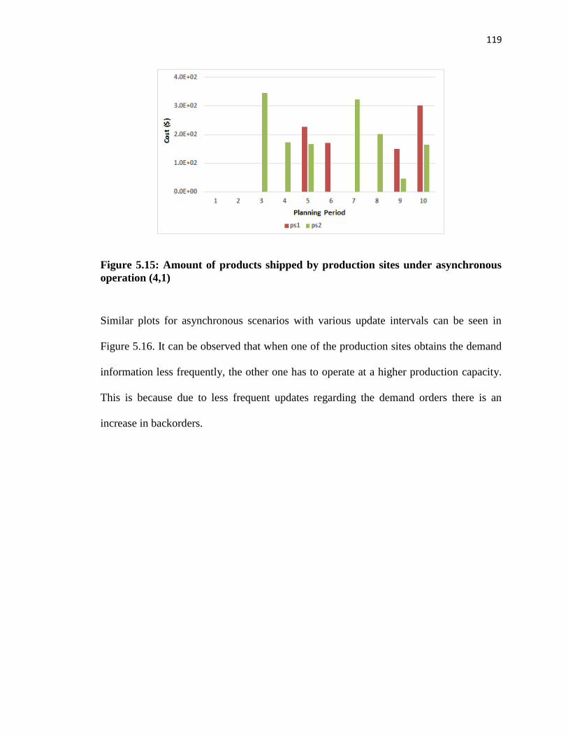
119

Figure 5.15: Amount of products shipped by production sites under asynchronous

operation (4,1)

Similar plots for asynchronous scenarios with various update intervals can be seen in

Figure 5.16. It can be observed that when one of the production sites obtains the demand

information less frequently, the other one has to operate at a higher production capacity.

This is because due to less frequent updates regarding the demand orders there is an

increase in backorders.

120

Figure 5.16: Amount shipped by production sites under (a) asynchronous operation

1,2 (b) asynchronous operation 2,1 (c) asynchronous operations 1,3 and (d)

asynchronous operations 3,1

5.7.3 Case Study 3: Exploring different decision making strategies for a larger supply

chain

Similar synchronous and asynchronous decision making strategies were implemented for

a larger supply chain network. A supply chain consisting of 4 markets, 4 warehouses, 4

production sites and 2 suppliers as shown in figure 5.17 was considered. Manufacture of

121

products is done in batch operation mode. The production site schedules the production

using an embedded scheduler which relies on the solution of the scheduling optimization

problem. The state task network for the process is the same as that in case study 2 and is

shown in figure 5.11. Backorder cost is $80/lb. Demand is considered to be a constant

value at 100 lb during every period.

Two decision making strategies have been considered. In the first one, all the entities

operate synchronously while in the other, a mix of synchronous and asynchronous

operations are considered. For the asynchronous case, a specific scenario is considered.

Raw material suppliers are considered to operate synchronously with the production sites

while markets, warehouses and production sites make decisions asynchronously. The

sup1

ps1

ps2

ps3

ps4

wh1

wh2

wh3

wh4

m1

sup2

m2

m3

m4

Information

flow Material flow

Figure 5.17: Supply chain network for case study 3

122

update intervals for the four warehouses are (2, 3, 1, 5) while those for the production

sites are (1, 2, 5, 3). The agent based simulation models were run for these two specific

scenarios. However, as shown in the previous case studies, the model can be used for

different sets of update intervals as well. For synchronous decision-making strategy, the

total cost obtained was $1,70,378 while that for the asynchronous decision-making

strategy was $2,71,739 which was around 60% higher.

The hybrid simulation based optimization approach was used to optimize the supply

chain operation under the two decision making strategies. The results of the hybrid

approach for the two specific cases are shown in figures 5.18 and 5.19. The hybrid

simulation based optimization framework converges in both the cases. The computation

time for the asynchronous scenario was observed to be 1360 sec while that for the

synchronous scenario was observed to be 3794 sec.


iteration under synchronous decision making strategy

0.00E+00

4.00E+04

8.00E+04

1.20E+05

1.60E+05

2.00E+05

1 2 3 4 5 6 7 8 9 10

Tota

l Co

st (

$)

Iteration


123


iteration under asynchronous decision making strategy

Table 5.1: Comparison of total cost values for different scenarios

Total Cost ($) % difference with (1)

1. Synchronous without optimization $170,378

2. Asynchronous without optimization $271,739 59.49

3. Synchronous with optimization $95,524 -43.93

4. Asynchronous without optimization $156,110 -8.37

A comparison of the total cost values obtained for the synchronous and asynchronous

scenarios with and without optimization are presented in table 5.1. The optimal solution

for the synchronous case gives a total cost of $95,524 while that for the asynchronous

case gives a total cost of $1,56,110. It can be seen that optimization results in a reduction

in total cost of around 44% and 43% for the synchronous and asynchronous scenarios

respectively. It can also be observed that the optimal solution for the asynchronous case

0.00E+00

5.00E+04

1.00E+05

1.50E+05

2.00E+05

2.50E+05

3.00E+05

1 2 3 4 5 6 7 8 9 10 11

Tota

l Co

st (

$)

Iteration


124

gives a cost around 8.4% lower than the cost for the synchronous case without

optimization. Since implementing synchronous operations for large scale supply chains is

not easy, optimized asynchronous operations can provide an alternative to synchronous

operations. However, optimized synchronous operation is still better than optimized

asynchronous operation.

5.8 Conclusion

The decision-making strategies of the different entities in a supply chain affect its

operation and performance. This chapter illustrates the effects of the different strategies

using agent based models. In particular, two different interaction schemes among the

decision-making entities of the network were considered, namely synchronous and

asynchronous.

Separate agent based simulation models were developed to capture the dynamics of the

two interaction schemes. In order to illustrate the impact of the interaction scheme alone,

two rather small scale case studies were used. The two schemes were compared on the

basis of the operating cost of the supply chain as well as the resulting dynamics. It was

shown that the interaction scheme and the information available to decision – making

entities can have a significant impact on cost and dynamics. It is observed that

synchronous interactions result in the lower cost compared to asynchronous interactions.

However, optimized asynchronous interactions can perform better than synchronous

interactions without optimization.

Since synchronous interactions are not always easy to implement, the model for the

asynchronous scenarios provides useful results regarding the operation of the supply

125

chain and its structure. The decision – making entities in the case studies involved

markets, warehouses, production sites and raw material suppliers. However agent based

simulation provides the flexibility to conveniently adapt the model for other decision –

making entities with different behaviors or to increase the size of the model with larger

number of decision – making entities. Similar concepts can be used for larger supply

chains where the overall operation is a complex combination of the both synchronous and

asynchronous operations. The case studies used in this study considered the entities

belonging to a single organization. A similar approach can be used to study a multi-

company supply chain network and gain insight into how cooperative behavior would

serve the objectives of the different companies under the different scenarios. For this case

different formulas can be used to assign cost to different companies and this will be the

subject of our future work.

Nomenclature

Indices

t planning period

s state

i task

j unit

n event point

wh warehouse

m market

P production site

126

sup supplier

r raw material

pr product

Sets

T planning periods

S states

I tasks

J units

WH warehouses

M markets

PS production sites

SUP suppliers

R raw materials

PR Products

Variables

Binary whether or not task i in unit j starts at event point n

continuous, amount of state s at event point n

amount of state s delivered at event point n

continuous, batch size of task i in unit j at event point n

requirement for state s at the end of the time horizon

time that task i finishes in unit j while it starts at event point n

time that task i starts in unit j at event point n

,p t

rC

Amount of raw material r consumed at production site p during time t

, ,i j nwv

,s nst

,s nd

, ,i j nb

sr

, ,i j nTf

, ,i j nTs

127

, ,wh m t

prD

Amount of product pr transported from warehouse wh to market m during time t

, ,p wh t

prD

Amount of product pr transported from production site p to warehouse wh during

time t

sup, ,p t

rD

Amount of raw material r transported from supplier sup to production site p during

time t

,p t

prP

Amount of product pr produced at production site p during time t

,m t

prU

Backorder of product pr at market m at time t

sup,t

rInv

Inventory of raw material r at supplier sup at time t

,wh t

prInv

Inventory of product pr at warehouse wh at time t

,p t

prInv

Inventory of product pr at production site p at time t

,p t

rInv

Inventory of raw material r at production site p at time t

Parameters

wh

prh

Inventory holding cost for product pr at warehouse wh

p

prh

Inventory holding cost for product pr at production site p

p

rh

Inventory holding cost for raw material r at production site p

sup

rh

Inventory holding cost for raw material r at supplier sup

m

pru

Backorder cost for product pr at market m

pVarCost

Production cost at production site p

,wh m

prd

Transportation cost per unit product pr between warehouse wh and market m

,p wh

prd

Transportation cost per unit product pr between production site p and warehouse

wh

128

sup, p

rd

Transportation cost per unit raw material r between production site p and supplier

sup

sup

rstcap

Inventory holding capacity for raw material r at supplier sup

wh

prstcap

Inventory holding capacity for product pr at warehouse wh

p

prstcap

Inventory holding capacity for product pr at production site p

H Time horizon

variable term of processing time of task i at unit j expressing the time required by

the unit to process one unit of material performing task i

constant term of processing time of task i at unit j

minimum amount, maximum capacity of unit j when processing task i

proportion of state s produced, consumed by task i, respectively

available maximum storage capacity for state s

,i j

,i j

min

,i jv max

,i jv

,

p

s i ,

c

s i

max

sst

129

6 Flexibility Assessment and Risk Management in Supply Chains

Many of the supply chains today are very efficiently designed and operate to maintain

consistent low cost, and high customer satisfaction. Over the years, there have been

tremendous advances in the field of information technology and with it, supply chains

have become much more globalized and complex. Increased globalization leads to

increased uncertainty, which has altered the way supply chain management has been

considered in the recent past. The need for flexible design and operation has gained

attention as an approach to offset the uncertainties in supply chain environment.

In an uncertain environment, the idea that supply chains can be optimized to account for

all possible scenarios is not realistic. Companies need to incorporate flexibility in their

supply chains in order to adapt to the changing circumstances. Uncertain conditions

increase the vulnerability of supply chains to failures. Moreover, companies have been

transformed from monolithic supply chains to smaller, distributed, more flexible

networks. The more complex, global and interdependent the supply chain, the more

vulnerable it becomes to uncertainties and has a higher exposure to risk. Complex

networks make it more difficult to identify all the vulnerabilities in the network and

manage the risk due to increased number of suppliers. Outsourcing is used as a cost-

effective measure but it can also result in the inclusion of more volatile suppliers. “Just in

time” approach followed by lean systems makes the supply chain more efficient but it can

expose also weaknesses in the supply network due to decreased inventory and capacity. It

is important to assess the impact of uncertainties on the performance of the supply chain

network and how the network operates in order to cope with uncertainties.

130

Mitigation of risks in the area of supply chains has gained so much attention that it has

led to the development of a separate field of study called “Supply Chain Risk

Management” 92-94. It attempts to eliminate the vulnerabilities in a supply chain by

identifying the failure points and involving the different entities of the supply chain to

ensure continuity in supply chain operation. Companies implement different steps like

dual sourcing, forward buying, safety stock, postponement, etc. to introduce flexibility

within their supply chains in order to mitigate risk 95-98.

In this work, we study the operation of a supply chain under demand uncertainty to

investigate different aspects such as flexibility assessment, risk management, and

economic performance of the supply chain. Multi-period supply chain planning with

uncertain demand leads to a stochastic optimization problem which is formulated as a

two-stage stochastic programming problem in a rolling horizon approach. The two-stage

optimization problem is solved using a hybrid simulation based optimization approach

that has been shown to effectively find the optimal solution while also retaining a realistic

picture of the dynamics of the actual supply chain. The benefits of the hybrid simulation

based optimization approach regarding realistic representation of supply chains and

reasonable execution times even for complex non-linear dynamics have been

demonstrated in the recent studies 62,91,99-101. The proposed framework is used to study the

trade-off between the economic performance and flexibility of the supply chain network

as well as how the behavior differs under risk-neutral and risk-averse conditions.

Flexibility is defined in terms of the bounds of uncertain demand within which the supply

chain operation is feasible.

131

6.1 Background

The important aspects covered in this chapter are supply chain flexibility and risk

management. The literature review presented here tries to cover the majority of the work

that appear in the literature in these areas.

Although supply chain flexibility has been studied for quite some time now, it has been

looked at from very diverse perspectives. A major portion of work in this area is focused

on manufacturing flexibility. However, it has been noticed that it should be studied from

a supply chain perspective since the actual competition is among supply chains rather

than manufacturing plants. Different definitions have been proposed and the benefits

have been assessed. Garaveli 102 proposes a simulation model to study the concept of

limited flexibility. Different configurations are selected to decide about the appropriate

degree of flexibility of the network. Two types of flexibilities are considered, namely

process flexibility and logistics flexibility. Tang and Tomlin 103 investigate how much

flexibility is needed to mitigate risks. They show that significant strategic value can be

obtained with a relatively low level of flexibility. Grave and Tomlin 104 analyze the

benefits of flexibility in multi-stage supply chains. A flexibility measure is developed to

account against the stage-spinning bottlenecks and floating bottlenecks. Kwon et al. 105

propose using agent-based web services to support collaboration within a supply chain

under internal and external uncertainties. Flexibility of the system is demonstrated

through two collaboration situations and simulation models are used to test the feasibility

of the approach. Chan and Chan 106 propose an adaptive make-to-order coordination

mechanism and study how the performance of two-level multi-product make-to-order

132

supply chains can be improved by flexibility and the proposed adaptability in delivery the

correct deliveries at the exact due dates. Two different coordination mechanisms are used

to account for flexibility and adaptability. The operations of the supply chain are modeled

by agent-based simulation models. It is shown that there is a trade-off between choosing

flexibility alone and adopting the proposed adaptive mechanism for different capacity

utilizations. Lainez et al. 107 propose a flexible formulation approach instead of a rigid

predefined network structure to solve the design-planning problem of supply chain

networks. NPV is considered as the key performance metric and is optimized in the

resulting mixed integer linear programming model. Mansoornejad et al. 108 study

sustainable decision-making regarding biorefinery strategies and consider economic,

social and environmental objectives. They state that in order to be robust to market

volatility, biorefinery strategies have to be flexible. Performance of the supply chain in a

dynamic environment is analyzed using the metrics of flexibility and robustness. The

change of robustness and profitability with respect to flexibility is studied. In process

engineering, a lot of work is based on the work of Grossmann and co-workers 109-113.

They presented a general framework for analyzing flexibility in chemical process design.

They define flexibility as a measure of the size of the parameter space over which

feasible steady-state operation of the plant is obtained by proper adjustment of the control

variables. Ierapetritou and Pistikopoulos 114 introduced an integrated metric to assess

future plan feasibility along with potential economic risk for two-period linear planning

models based on the concepts of flexibility and maximum regret. Finally Stevenson and

Spring 115 present a review of the literature on supply chain flexibility.

133

Various strategies and models have been investigated to mitigate the supply chain

disruptions and losses associated with the different types of risks. Talluri et al. 116

consider various risk categories and supply chain configurations and evaluate different

risk mitigation strategies for them. They provide insights for deciding the suitable

strategy corresponding to the particular context of risk and state that the suitability of the

mitigation strategy depends on the internal and external environments. Wu et al. 117

investigate how stockout disruptions impact a consumer goods supply chain. An agent-

based simulation is used to study stockouts in terms of consumers, retailers and

manufacturers. They state that an understanding of consumer response in the face of a

stockout disruption at both the manufacturer and retailer is required for developing

efficient risk mitigation strategies at both the levels. Javid and Seddighi 118 consider a

location-routing problem with production and distribution disruption risks. They solve

the problem of choosing, locating and allocating a set of potential producer-distributers

and building routes to meet supply chain demands. The objective is to minimize the total

cost of location, routing and disruption. The problem is solved under moderate, cautious

and pessimistic risk-measurement policies. Giannakis and Louis 119 consider the problem

of disruption risk management in manufacturing supply chains. A multi-agent based

framework is proposed for the design of a decision support system that enables

collaborative risk management. The framework is able to proactively mitigate a series of

risks at the operational and tactical levels of supply chain management. Hahn and Kuhn

120 develop an integrated value-based performance and risk management framework to

increase shareholder value holistically. The metric ‘Economic Value Added’ is applied to

mid-term sales and operations planning and robust optimization methods are used to

134

handle operational risks in supply chain management. Finally Tang 121 presents a review

of the various quantitative models for managing supply chain risks and relates the supply

chain risk management strategies in the literature with actual practices.



markets is considered in this work. The markets fulfill the demand of different products

that can be manufactured from raw materials. The daily demand for the future periods for

each product is assumed to be a random variable with a known normal distribution. The

bills of material relationships for the manufacture of products at the production sites are

known. The warehouses have a limited storage capacity for products while the production

sites have limited storage capacities for products and raw materials. There is a limited

production capacity for each production site. The various capacities are assumed to be

known and fixed. There is no time delay associated with information flow between

entities while there is a time delay associated with the material flows. Each market has a

primary warehouse to which it sends its orders. Similarly each warehouse has a primary

production site from which it procures products. However in the event of higher demand

values, orders can be sent to secondary warehouses and secondary production sites as

well. Also primary warehouses and production sites can increase their transportation

capacities for their corresponding markets and warehouses respectively. The amount of

products that warehouses and production can ship is limited by their transportation

capacities. Primary and secondary warehouses and production sites can accommodate

additional orders by increasing their transportation capacities. There are costs associated

135

with inventory holding, transportation, backorders, production and transportation

capacity increase. Demand is considered to be uncertain. Shipment, inventory and

production information for all the planning periods have to be found out in order to

maximize profit while taking risk into consideration. The risk is required to be kept

below a certain predefined level.

6.3 Solution Methodology

The multi-product supply chain planning problem under demand uncertainty gives rise to

a stochastic optimization problem. A two-stage stochastic linear programming in a rolling

horizon approach is proposed to solve the problem where hybrid simulation based

optimization approach is used to solve the first stage of the two stage problem. The basic

concepts related to the proposed methodology are described below.

6.3.1 Rolling horizon

The multi-period planning problem under uncertainty corresponds to a multi-stage

stochastic programming problem. Decisions have to be made sequentially at each period

based on the information available at that period. Such problems extend two-stage

programming to a multi-stage setting. Multi-stage stochastic programming problems

become computationally very expensive as the number of scenarios and stages increase.

The rolling horizon decomposes the actual problem into problems with less number of

periods and therefore fewer scenarios. The idea is to routinely revise the plan taking into

consideration more recent data as they are available. The approach reflects the way

decisions related to a firm’s business and activities are taken.

136

Figure 6.1: Rolling horizon approach

Figure 6.1 illustrates the implementation of the rolling horizon. At the beginning of t2,

the 2nd period, demand information up to t2 is revealed while the demand for the future

periods are uncertain. The first stage of the two-stage problem is solved to obtain the

solution for the first-stage decision variables. The solution is implemented for t2. Then at

the beginning of t3, the demand for t3 becomes known. The first stage problem is solved

again and the solution is implemented for t3. Similarly, at the beginning of each period,

the decisions for the current period are implemented by solving the first stage of the two-

stage problem. As the planning horizon at each period remains constant, a rolling horizon

is obtained.

6.3.2 Two-stage stochastic programming

Two-stage stochastic programming is based on the idea that decisions should be made on

the basis of information that is available at that time rather than information that might be

available in the future. The classical two-stage linear stochastic programming formulation

can be represented as

137

where is the optimal value of the second stage problem which is represented as

where x represents the first-stage decision vector, X is a polyhedral set, defined by a finite

number of linear constraints, y is the second stage decision vector and is

the second stage data 122. At the first stage, a “here and now” decision is taken based on

the first stage information available. The variables of the second stage are considered to

be a random vector. The second stage problem is a simple optimization problem solved

after the uncertain data is revealed. The second stage solution is considered as a recourse

action that is required to take due to the first stage decision.

In this work, we are only required to solve for the first stage decision variables at each

period. At the beginning of each new period, a new two-stage programming problem is

formulated and the first stage problem is solved. In the problem considered in this work,

the demand values are considered to be a random vector with known probability

distribution function. It is assumed that the random vector can be represented by a finite

number of possible scenarios. The probability for each scenario is considered to be equal.

Monte Carlo sampling technique is used to generate the scenarios. The required number

of scenarios for a particular level of accuracy is obtained using statistical methods123.

Less number of scenarios would not be able to represent the probability distribution of

demand. The two stage optimization problem uses the expected value of all the scenarios.

min{ ( ) : [ ( , )]}T

x Xg x c x E Q x

( , )Q x

min subject to T

yq y Tx Wy h

( , , , )q T W h

138

A less than sufficient number of scenarios could affect the quality of the solution

obtained as well as the feasibility of the problem.

The formulation gives rise to a large linear programming problem if the objective

function and the constraints are linear. The problem considered here involves complex

dynamics of the supply chain and thus it is not possible to formulate a mathematical

programming problem that is a good representation of the actual dynamics. Hybrid

simulation based optimization has been shown to be an effective approach to solve such

problems and is used to solve the two-stage problem in this work.

6.3.3 Hybrid Simulation based Optimization

Hybrid simulation based optimization approaches that aim to take advantages of

simulation models as well as mathematical programming approaches have been used to

solve supply chain optimization problems 91. Such approaches give a realistic

representation of the supply chain dynamics through the use of a detailed simulation

model while a simplified optimization model is used to guide the simulation towards the

optimal solution. Different decision-making strategies result in different dynamics in

supply chains. The approach therefore proves to be an effective way to capture these

decision-making strategies and provide the optimal supply chain operation 90,124.

In this work, the hybrid simulation based optimization approach is used to solve the two-

stage problem at the beginning of each period in the planning horizon. A description of

the hybrid simulation based optimization approach and its components, the simulation

model and the optimization model, are presented in the following subsections.

139

6.3.3.1 Optimization model

The mathematical programming model includes constraints related to suppliers,

production sites, warehouses and markets. Warehouses (wh ϵ WH) store products (s ϵ

PR) and transfer them to markets in order to fulfill the demand during the planning

horizon (t ϵ T). Warehouses replenish their inventory with the products they receive from

production sites (p ϵ PS). Production sites procure raw materials (r ϵ R) from raw material

suppliers (sup ϵ SUP) and manufacture products. In the hybrid approach, the role of the

optimization model is to guide the simulation towards better results. The optimization

model is kept quite simple compared to the simulation model which is more detailed.

Therefore, no time delays associated with information or material flows have been

considered. The total cost associated with the supply chain consists of inventory holding

costs, transportation costs, backorder costs, production costs and costs due to

transportation capacity increase. Inventory holding cost is considered to be proportional

to the inventory level. Transportation cost is considered to be proportional to the amount

of shipment. Backorder cost is proportional to the amount of unfulfilled demand while

production cost is proportional to the amount of product produced. Cost due to increase

in transportation capacity is proportional to the increase in capacity. Revenue is obtained

by fulfilling the demand at the selling price. The model has been formulated as a mixed

integer linear programming problem where the objective is to maximize the total profit.

The optimization model is as follows.

max Profit1 Profit2 / , sc

sc

nSC sc SC 1

140

,1 ,1 ,1

,1 ,1 , ,

, , , ,1 , , , ,1

Cost1 = wh wh p p p p

s s s s r r


m m p p wh wh m p p wh

s s s s s s s

m s PR p s m wh s PR wh p s PR

wh m wh m wh m p wh p wh p wh

s s s s

m wh s PR wh p s PR

r

h Inv h Inv h Inv

u U v P c CI c CI

d dis D d dis D

d

, sup, , ,1

sup

,

, , , , ,sup

sup p p sup p

r

p r R

dis D

s PR r R m M wh WH p P SUP

2

, , , , , ,

, , , , , , , , ,

, sup,

Cost2 =

wh wh t sc p p t sc p p t sc

sc s s s s r r

t wh s PR t p s PR t p r R

m m t sc p p t sc p wh p wh p wh t sc

s s s s s

t m s PR t p s t wh p s PR

sup p p

r

h Inv h Inv h Inv

u U v P d dis D

d dis

, , , , , , , ,

sup

,

, , , , ,sup , ,

sup p t sc wh m wh m wh m t sc

r s s

t p r R t m wh s PR

D d dis D

s PR r R m M wh WH p P SUP sc SC t T

3

4

5

6

7

8

9

10

11

, , , , , , , ,p wh t sc p p wh

s s sD trcap CI s PR p PS t T sc SC

12

, , , , , , , , ,wh m t sc wh wh m

s s sD trcap CI s PR wh WH m M t T sc SC 13

14

, , , 1, , , , , , , , ,m t sc m t sc m t sc wh m t

s s s s

wh WH

U U Dem D s PR m M t T sc SC

, , , 1, , , , , , , , , , ,wh t sc wh t sc wh m t sc p wh t sc

s s s s

m M p PS

Inv Inv D D s PR wh WH t T sc SC

, , , 1, , , , , , , , , ,p t sc p t sc p t sc p wh t sc

s s s s

wh WH

Inv Inv P D s PR p PS t T sc SC

, , , 1, , , sup, , ,

sup

, , , ,p t sc p t sc p t sc p t sc

r r r r

SUP

Inv Inv C D r R p PS t T sc SC

p, , p , ,p , ,t sc

r rInv stcap r R PS t T sc SC

p, , p , ,p , ,t sc

s sInv stcap s PR PS t T sc SC

, , , , , ,wh t sc wh

s sInv stcap s PR wh WH t T sc SC

, , , , , ,p t sc p

s sP prcap s PR p PS t T sc SC

DRisk R

141

,sc sc

sc

DRisk P sc SC 15

Profit1 Profit2 , 0, sc sc sc sc SC

16

, , , , ,m s scSl L m M s PR sc SC 17

, ,

, , , ,1 , , , ,

m t sc

s

tm s sc m t sc

s

t

U

Sl m M s PR sc SC t TDem

18

, , , 1, , ,

,Rev2 = * , , , ,m t sc m t sc m t sc

sc s m s s s

t s m

sp Dem U U s PR m M sc SC t T

19

,1 ,1

,Rev1 = * , ,m m

s m s s

s m

sp Dem U s PR m M 20

Profit1 Rev1 Cost1 21

Profit2 max Rev2 Cost2 , sc SCsc sc sc 22

Equation 1 refers to the objective for the first stage of the two-stage problem. The

objective function maximizes the profit for the first stage and the expected optimal profit

for the second stage considering all the scenarios. Equation 2 defines the cost for the first

stage while equation 3 gives the cost for the second stage decisions. The cost calculations

include backorder cost, inventory cost, production cost, transportation cost and cost due

to increase in transportation capacity. Equation 4 states that any unfulfilled demand

during the current period gets accumulated as backorder for the next period. Inventory

balance constraints at the warehouses are represented by equation 5. It relates warehouse

inventory to shipments from warehouses to markets and shipments from production sites

to warehouses. Equation 6 represents the product inventory balance constraint at the

142

production sites. It relates product inventory at production sites to shipments from

production sites to warehouses, and production amounts during each planning period.

Equation 7 represents the raw material inventory balance constraint at production sites. It

relates the raw material inventory at production sites to consumption of raw materials for

the manufacture of products and shipments from raw material suppliers to production

sites. Equations 8-12 represent the capacity constraints for the different nodes. Storage

capacity constraints for production sites and warehouses are given by equations 8–10

respectively while the production capacity constraint for production sites is given by

equation 11. Equations 12 and 13 state that shipment between a production site and a

warehouse, and between a warehouse and a market is less than the respective

transportation capacity. The metric, downside risk, is used to measure the risk of having a

total profit lower than a target profit. Equation 14 is a constraint on the value of the

downside risk. Equations 15 and 16 define the downside risk for the problem. Equation

17 is the service level constraint which restricts the amount of backorders. -service

level is used to calculate the service level. Equation 18 defines the service level in terms

of the backorders and demand at markets. Equations 19 and 20 represent the calculation

of revenue for the first stage and the second stage by the fulfillment of demand at the

markets. Equation 21 represents the calculation of profit for the first stage. Equation 22

represents the optimal profit for the second stage.

The optimization model results in a mixed integer linear programming problem which

has been solved using the Cplex library embedded in the Java application used for

simulation on Windows 7 operating system with an Intel(R) Xeon(R) CPU ES-1620 v2 D

CPU 3. 70 GHz microprocessor and 16.00 GB RAM.

143

6.3.3.2 Simulation model

Agent based modeling has been shown to be an effective approach to simulate the supply

chain. Using a bottom-up approach, it enables a realistic representation of the actual

supply chain dynamics. Repast simulation platform and Java programming environment

have been used to implement the model.

The agents in the simulation model represent the different entities of the supply chain.

The agents capture the characteristic behavior of the entities. There is interaction among

the agents and their behavior is adapted based on these interactions. Each agent performs

actions and schedules future actions for itself or other agents. They are connected by

information flows as well as material flows. Information about inventory, demand orders

and shipments are shared among the agents which allows them to coordinate demand

allocation and order fulfillment.

Each agent is a collection of attributes and behaviors which have been coded using Java,

an object oriented programming language. Different classes for different types of agents

are developed and are instantiated to create the particular agents. These classes contain

properties and methods to represent the attributes and behaviors respectively. A parent

class consists of the common attributes of each supply chain agent and the individual

classes for the agents derive from the parent class.

Market agent

Demand for products originates at the market agent. On receiving a demand, the market

agent sends requests to the warehouses. A request is a way to communicate to amount of

products required although it is not the actual order. It procures information about how

144

much demand can be fulfilled, how much time it will take and the cost of fulfilling the

demand. The warehouses respond to these requests and then the market agents distribute

the demand among the warehouses based on their ordering policies. Each market has a

primary warehouse. The market gives first preference to the primary warehouse and then

based on which warehouse responds with the lowest cost. While sending an order to any

warehouse, the market tries to order as much as possible to the warehouse. So if the

remaining demand is lower than the amount the warehouse can fulfill as per the response,

the market orders the remaining demand. Otherwise, the amount that the warehouse can

fulfill is ordered. The market stops assigning orders if the total demand amount has been

ordered or if the warehouses have no remaining inventory. For warehouses that respond

with equal cost, the market uses the higher amount of demand that can be fulfilled and

the lower time to fulfill as the deciding factors. Unfulfilled demand during any period is

added as backorder to the demand during the next period. Using this ordering policy, the

market does not receive any oversupply from warehouses. The markets earn revenue by

selling the products. Inventory and backorders have costs associated for this agent.

Backorder cost is proportional to the amount of backorders. Inventory cost is proportional

to the amount of inventory at the agent. These costs are calculated at the end of each day.

Warehouse agent

The warehouse agent fulfills the market demands by transferring products to the markets.

It maintains an inventory of products. When a warehouse receives a request from a

market, it responds in terms of the cost and time it would take to transfer the products,

and the fraction of demand it would be able to fulfill, In order to determine the fraction of

demand it can fulfill, it considers the aggregated demand from all the markets. The

145

warehouses have contractual agreements with markets. Therefore they have different

higher preference levels for some markets compared to others. It tries to fulfill demand

from the more preferred markets before the less preferred markets. Based on the

responses from all the warehouses, the markets send orders for products. If the markets is

not able to order the total demand to the warehouses, they update the requests and re-send

them to the warehouses. The requests are updated by adjusting the demand amount based

on what has already been ordered. Markets keep sending requests to warehouses and

assigning orders to warehouses as long as all the demand has not been ordered and the

warehouses can fulfill some demand from the markets. The warehouses attempt to fulfill

the demand from the markets collectively. The warehouse agent uses its inventory of

products to fulfill the demand from the markets. The storage capacity is limited and a

reorder level – reorder amount inventory replenishment policy with continuous review is

used to regulate the inventory. The reorder level and reorder quantity for the agent are

pre-defined. As soon as the warehouse inventory drops below the reorder level, it

generates a demand for products which is fulfilled by production sites. On generating a

demand, the warehouse agent sends requests to the production sites. A request is a way to

communicate the amount of products required although it is not the actual order. It

procures information about how much demand can be fulfilled, how much time it will

take and the cost of fulfilling the demand. The production sites respond to these requests

and then the warehouse agents distribute the demand among the production sites based on

their ordering policies. Each warehouse has a primary production site. The warehouse

gives first preference to the primary production site and then based on which responds

with the lowest cost. While sending an order to any production site, the warehouse tries

146

to order as much as possible to the production site. So if the remaining demand is lower

than the amount the production site can fulfill as per the response, the warehouse orders

the remaining demand. Otherwise, the amount that the production site can fulfill is

ordered. The warehouse stops assigning orders if the total demand amount has been

ordered or if the production sites have no remaining inventory. For production sites that

respond with equal cost, the warehouse uses the higher amount of demand that can be

fulfilled and the lower time to fulfill as the deciding factors. Inventory and transportation

have associated costs for this agent. Transportation cost and inventory cost are

proportional to the amount of products transported and the amount of inventory stored,

respectively.

Production Site agent

The production site agent fulfills the demand for products generated at the warehouses. It

maintains a small inventory of products by manufacturing them from raw materials. The

conversion of raw materials to products is defined by a bill of material (BOM)

relationship. A small inventory of raw material is also maintained. It has fixed production

capacity and storage capacities. When a production site receives a request from a

warehouse, it responds in terms of the cost and time it would take to transfer the products,

and the fraction of demand it would be able to fulfill, In order to determine the fraction of

demand it can fulfill, it considers the aggregated demand from all the warehouses. The

production sites have contractual agreements with warehouses. Therefore they have

different higher preference levels for some warehouses compared to others. It tries to

fulfill demand from the more preferred warehouses before the less preferred warehouses.

Based on the responses from all the production sites, the warehouses send orders for

147

products. If the warehouses are not able to order the total demand to the production sites,

they update the requests and re-send them to the production sites. The requests are

updated by adjusting the demand amount based on what has already been ordered.

Warehouses keep sending requests to production sites and assigning orders to production

sites as long as all the demand has not been ordered and the production sites can fulfill

some demand from the warehouses. The production sites attempt to fulfill the demand

from the warehouses collectively. The production site agent uses its inventory of products

to fulfill the demand from the warehouses. The storage capacity is limited and a reorder

level – reorder upto level inventory replenishment policy with continuous review is used

to regulate the raw material inventory. The reorder level and reorder up-to level for the

agent are pre-defined. As soon as the production site raw material inventory drops below

the reorder level, it generates a demand for raw materials which is fulfilled by the raw

material suppliers. The production site orders raw materials from the raw material

supplier with the minimum cost. Inventory, production and transportation have associated

costs for this agent. Transportation cost, inventory cost and production cost are

proportional to the amount of products transported, the amount of inventory stored, and

the amount of products produced, respectively.

Supplier agent

On receiving demand orders from production sites, the supplier agent sends raw materials

to them. The supplier agent is considered to have an unlimited storage capacity.

Transportation has associated costs for this agent.

148

6.3.3.3 Hybrid simulation based optimization methodology

As discussed in sections 6.3.3.1 and 6.3.3.2, the optimization and simulation models are

developed. In the hybrid approach, the two independent models are coupled together by

exchange of information between them, thus allowing taking advantage of the benefits of

both models. As shown in figure 6.2, the following variables are used to couple the

optimization model with the simulation model in this work: i) production and

consumption values from simulation model to optimization model, ii) shipment values

obtained from optimization model to simulation model.

Figure 6.2: Coupling between simulation and optimization

By communicating the shipment values from the optimization to the simulation model,

shipment targets are obtained by the simulation and it tries to achieve these targets,

thereby reducing backorders and inventories. The simulation represents a more realistic

dynamic environment of the supply chain and the behavior of the agents of the model

determines if it is able to achieve the shipment targets or not. Production and

consumption values obtained from the simulation model are set as parameters in the

149

optimization model. The optimization model then provides the shipment values for the

optimal solution corresponding to those production and consumption targets.

Figure 6.3: Iterative framework for the hybrid simulation-optimization approach


chapter 3 has been used. As shown in figure 6.3, an iterative procedure is used where the

framework is initialized by solving the simulation model for each scenario. The variables

associated with each scenario are then passed to the optimization model, which is solved

to obtain values of the decision variables. The total profit for the planning horizon is

150

calculated by the two models for each scenario. If the difference for each scenario is

below a tolerance level, the procedure is terminated otherwise the values of decision

variables for each scenario are passed back to the corresponding simulation model. This

process is repeated until the difference between the profits falls below the tolerance level

for each scenario. The above framework uses the optimization model to guide the

simulation model, used as the master model, towards the best solution that can be

achieved. The proposed algorithm considers a fixed supply chain design and starts by

solving the simulation model for that design. The algorithm always gives the same result

for a particular demand scenario and supply chain design. It uses the simulation model

and the optimization model to set values of some of the decision variables for each other.

These values are used as targets for each other. The framework is initiated by solving the

simulation model for each demand scenario. The optimization model is linear. It leads to

the optimal and the simulation moves to those targets if feasible.

The approach described above is implemented to solve the two stage problem at the

beginning of each period. It is to be noted that a separate simulation model is executed

for each scenario and the outputs from all the simulations are used as inputs to the

optimization model. The optimization model gives the optimal values of the decision

variables for each scenario which are used as input to each simulation model.

6.4 Overall Framework

The overall solution framework consists of the hybrid simulation based optimization

model incorporated in the rolling horizon. Figure 6.4 shows the different steps of the

framework.

151

Figure 6.4: Solution framework

The iterative framework starts at the first period. So the period is initialized to 1. At this

point, the planning horizon and the number of scenarios are fixed. At the beginning of

each period, the first step is to generate demand scenarios for all the future periods using

the Monte Carlo sampling technique. It is assumed that the current demand values are

known. Once all the scenarios are determined, the hybrid simulation based optimization

model is used to solve the first stage problem. The solution for the first stage is

implemented for the current period. The framework moves to the next period until the

last period of the planning horizon is reached. The framework allows taking the optimal

decisions based on the information available at the current period. The initial input

parameters for the hybrid model are updated during each period as they depend on the

decisions taken during the earlier periods. The initial backorder at the beginning of the

first period is 0 for the first period while it may be greater for subsequent periods.

Similarly initial inventory values also need to be updated. Also, information about any

152

shipments scheduled to arrive in a future period need to be incorporated as input

parameters in the hybrid model.

6.5 Risk Management

For the problem considered here, a key objective of decision-makers is not only to find

the optimal solution with the maximum profit but also to avoid the risk of lower profits

due to demand variability. Different risk metrics have been proposed in the literature 125-

127. You et al. 123 concluded that the downside risk model performs best to reduce the risk

of high cost without being computationally demanding. They showed that variance and

variability index are good at reducing the variance but shift the solution towards higher

expected cost. In this work, the downside risk model is used to manage risk. The model

can be expressed for profit as follows.

…………………………………………………………(14)

Profit1 Profit2 , 0, sc sc sc sc SC …………………………………...(15)

In order to solve the multi-objective problem, the - constraint method is used.

6.6 Case Studies

The proposed solution framework is used for two case studies. The first case study

involves a smaller network while the second is for a bigger more realistic network.

min DRisk( , ) s s

s

x P

153

6.6.1 Case study 1


The supply chain network considered in the first study consists of 3 markets, 3

warehouses, 3 production sites and 2 suppliers, as shown in figure 6.5. There are 2

products and 3 raw materials. For the hybrid simulation based optimization model, a

difference of 1% of profit obtained from simulation model is used as the termination

criterion. The planning horizon for the problem is 10 planning periods. The mean demand

was considered to be 80 for each product at each market during each period. The total

number of demand scenarios generated for the second stage was 500. The values of the

distances of warehouses from production sites and markets and between production sites

and raw material suppliers are provided in Tables A.6.1 and A.6.2.

154

Figure 6.6: Solution of the hybrid simulation based optimization model

The results from the proposed solution framework for the case study are presented here.

The solution of a hybrid simulation based optimization model for one scenario in the first

stage problem is shown in Figure 6.6. It can be seen that the profit values obtained from

the simulation model and the optimization for the particular scenario converge in 8

iterations. It should be noticed that similar plots can be obtained for all the 500 scenarios

at each period. However for each scenario, the number of iterations required for

convergence changes at every period due to changing input parameters (i.e. initial

inventory, and demand values due to backorders from previous period). Since the input

parameters are different at every period, the progress of the hybrid simulation based

optimization approach varies in every period, the number of iterations required to

converge could vary at each time period.

155

Figure 6.7: Comparison of transportation capacity cost with variability on demand

The different entities can increase their transportation capacity in order to accommodate a

rise in demand. However there is an associated cost with the increase in capacity, which

is referred as transportation capacity cost. Figure 6.7 shows a comparison of the

transportation capacity cost with demand variability. The y-axis represents the cost due to

increasing the transportation capacity in order to accommodate the uncertainty in

demand. The x-axis represents the coefficient of variation for the uncertain demand.

Coefficient of variation is a standardized measure of dispersion of the demand probability

distribution and is defined as the ratio of the standard deviation to the mean. Since

variability in demand is considered to be higher for a future period that is far from the

current period compared to one which is closer, the comparison is made between the cost

and coefficient of variation for the last period of the planning horizon. It can be seen that

increased transportation capacity is required as demand variability increases. Beyond a

certain level of demand variability, the value of transportation capacity cost does not

156

increase further. The increase in transportation capacity reached is not the highest value

possible.

Figure 6.8: Variation of profit with demand variability

157

Figure 6.9: Variation of secondary shipment with demand variability

As mentioned earlier, the markets sell products which bring revenue. It is important to

study whether the supply chain operation is profitable and how the profit varies with the

demand variability. Figure 6.8 shows how the profit of the supply chain operation varies

as demand variability changes. It can be seen that for lower levels of variability, the profit

increases with variability. However after a certain level of variability, the profit starts to

decrease. This is because the cost increases with increasing variability but the revenue

does not increase beyond a certain level as the amount of products available to sell is

limited by the capacity constraints. For lower levels of variability, although the total cost

increases with increasing variability, since a minimum service level is maintained, the

revenue also increases. It is to be noted that the trend obtained in figure 6.8 can vary

depending on the values of the parameters associated with the problem. The trend shown

is valid for the particular supply chain design considered. As shown in figure 6.7,

158

increased variability in demand results in an increase in transportation capacity.

Transportation capacities between secondary warehouses and production sites are

increased. The amount of transportation for demand fulfillment involving secondary

warehouses and production sites also increases with demand variability. Figure 6.9 shows

the variation in secondary shipment as demand variability changes. It can be seen that the

percentage of demand fulfilled through secondary shipment increases with demand

variability.

Figure 6.10: Variation of flexibility with risk

In this work, flexibility is defined as the upper bound on the coefficient of variation

within which supply chain operation is feasible. The model incorporates a lower bound

on the service level constraint which causes infeasibility beyond a certain level of

variability. In order to study the change in flexibility with downside risk, different values

of downside risk are used in the risk constraint and the value of flexibility is found out for

them. In order to find the value of flexibility, the demand variance is increased from a

159

low value and the value at which the problem becomes infeasible is found out. Figure

6.10 shows the change in flexibility with risk. It can be seen that as the value of downside

risk is increased, flexibility increases which means that the supply chain can operate for

higher values of demand variance if a higher value of risk is allowed. However it is seen

that beyond a certain level of risk, flexibility does not increase. This is because at higher

values of risk, the service level constraint becomes active before the risk constraint.

Therefore although a high probability of profit lower than the target profit is allowed, the

supply chain is not able to operate at very high values of demand variance. A β-service

level constraint is included in the model. It is to be noted that the target profit for the

calculation of risk is lower than the actual profit obtained from the solution. This is

because the backorders increase along the planning horizon which reduces the profit.

Therefore the profit obtained from the solution towards the end of the planning horizon is

lower. A higher target profit towards the end of the planning horizon would result in

infeasibility.

The computational time required to solve the case study at a particular risk level and

demand variance is 13893 sec. This solution time is obtained for demand with a

coefficient of variation of 0.30 and no risk constraint. The high computational time is due

to the number of scenarios considered. The hybrid simulation based optimization model

is required to converge for each scenario during each period.

160

Figure 6.11: Variation of solution time with rolling horizon length

The effect of the length of rolling horizon on the solution time is investigated. Figure

6.11 shows the change in computational time with the rolling horizon length. It is

observed that the solution time increases as the length of the rolling horizon is increased.

However it is also observed that the profits obtained from solving with lower rolling

horizon lengths are less than the value obtained for a rolling horizon length equal to the

planning horizon. For rolling horizon lengths of 3 and 4, the problem was found to be

infeasible. This means that if decisions during the initial periods are taken based on

shorter planning horizons, the service level constraint is not met later during the planning

horizon.

161

6.6.2 Case Study 2


A second case study was used to test the solution framework for a larger supply chain

network. The supply chain network considered in this case study consists of 6 markets, 6

warehouses, 6 production sites and 5 suppliers, as shown in Figure 6.12. There are 2

products and 3 raw materials. For the hybrid simulation based optimization model, a

difference of 1% of profit obtained from simulation model is used as the termination

criteria. The planning horizon for the problem is 10 planning periods. The mean demand

was considered to be 80 for each product at each market during each period. The total

number of demand scenarios generated for the second stage was 500. Tables A.6.3, A.6.4

and A.6.5 contain the values of distances between the different entities of the supply

chain network.

Figure 6.13 below shows how the operating profit of the network varies as the variability

in demand increases. The risk constraint is relaxed and the demand variability is

increased. It can be seen that the profit increases with demand variability. As the

162

variability increases, the total cost starts to increase. However since the desired service

level is maintained, the revenue also increases. Unlike the first case study, the profit does

not decreasing at higher levels of demand variability. Beyond a coefficient of variability

of value 0.30, the problem becomes infeasible as the service level constraint cannot be

satisfied. Therefore we know that there is an upper bound of 0.3 on the flexibility of the

network.

Figure 6.13: Variation of profit with demand variability

Figure 6.14 shows a comparison of the transportation capacity cost with demand

variability. Similar to case study 1, it can be seen that increased transportation capacity is

required as demand variability increases. However the highest value of transportation

capacity cost reached is observed to be still lower than the maximum value possible.

Unlike the first case study, the transportation capacity cost does not reach a constant

value beyond which it does not increase. This is because of the presence of other

163

constraints that make the problem infeasible for coefficient of variation higher than 0.3.

Figure 6.15 shows the variation in secondary shipment with demand variability. It can be

seen that increased secondary shipment is required to meet the required service level in

case of increased demand variability.

Figure 6.14: Comparison of transportation capacity cost with variability

164

Figure 6.15: Variation of secondary shipment with demand variability

The value of flexibility is obtained for different levels of risk. It is seen that just as in the

case of the first case study, the value of flexibility increases as the value of downside risk

is increased. However it reaches a constant value beyond a certain level of risk. The

target cost was considered to be $3E+05. It can be seen in figure 6.16 that for a

completely risk-averse condition where the downside risk is $0, the value of flexibility is

0.0. However for a downside risk of $1.6E+05, the value of flexibility increases to 0.3.

Beyond that level of risk, the flexibility does not change. This is because the service level

constraint becomes active in that region. For downside risk of less than $1.6E+05, the

downside risk constraint is active. Therefore the value of flexibility keeps increasing as

the downside risk is increased in that region.

165

Figure 6.16: Variation of flexibility with risk

The computational time required to solve the case study at a particular risk level and

demand variance is 30581 sec. This is higher than the time required to solve case study 1

due to the larger size of the supply chain network considered in this case study.

Compared with case study 1, the total number of agents has increased from 11 to 23

while the computational time has increased by around 120%. As the number of agents in

the model increases, the size of the optimization problem solved during each iteration of

the hybrid simulation based optimization approach grows larger. Reducing the solution

time for the optimization problem will be investigated in our future work.

6.7 Conclusions

In this work, a hybrid simulation based optimization framework is presented for

assessment of flexibility of supply chain operations and risk management. Uncertainty in

demand is considered and it is considered that planning decisions for the current period

166

are taken after the demand for that period have realized. Decisions are taken based on the

information available at that time. The framework enables the evaluation of flexibility of

the network and can provide risk-neutral as well as risk-averse solutions. The framework

determines the optimal decisions for the supply chain network at each period considering

the uncertainty in the future periods.

The hybrid simulation based optimization approach used in the study enables a detailed

representation of the supply chain dynamics. The agent based simulation approach

provides a convenient way to model the behavior of the different entities and can be

improved to depict the actual dynamics more realistically. Although the proposed

framework was used for rather small scale supply chain problems, it can conveniently be

used for larger problems with more number of agents and also where agents behave

differently and follow different decision making policies.

In this study, only demand uncertainty is incorporated in the model as the source of

uncertainty. Other sources of uncertainty can also be included. The flexibility metric in

that case would depend on the variability in other input parameters. Also, other measures

of making the supply chain more flexible should be included to have a systems approach.

In order to make the overall supply chain more flexible, different aspects of the supply

chain need to introduce flexibility. Different sources of uncertainty and flexibility will be

considered in our future work.

167

Nomenclature:

Indices

t planning period

p production site

sup supplier


wh Warehouse

s Product state


sc scenario

Sets

T planning periods

PS production sites

SUP suppliers


WH Warehouses

PR Product states


SC

Scenarios

Parameters

nSC total number of scenarios

holding cost of product s at warehouse wh wh

sh

168





unit transportation cost of product s from production site p to

warehouse wh

unit transportation cost of raw material r from supplier sup to

production site p

,wh mdis

distance between warehouse wh and market m

,p whdis

distance between production site p and warehouse wh

unit production cost at site p

wh

sc unit transportation increase cost at warehouse wh for product s

p

sc unit transportation increase cost at production site p for product s

demand of product s at market m for period t for scenario sc




Production capacity of product s at production site p

R Upper bound on downside risk

L Lower bound on service level

p

sh

p

rh

msu

,wh msd

,p whsd

sup, prd

, ,m t sc

sDem

prstcap

psstcap

whsstcap

psprcap

169

Variables

Cost1 Cost of the first stage

Cost2sc Cost of the second stage for scenario sc

Amount of product s transported from warehouse wh to market m at

period t for scenario sc

Amount of product s transported from production site p to warehouse

wh at period t for scenario sc

Amount of raw material r transported from supplier sup to production

site p at period t for scenario sc


warehouse wh for scenario sc


production site p for scenario sc


production site p for scenario sc


supplier sup for scenario sc

Backorder amount of product s at the end of planning period t at

market m for scenario sc

Amount of product s produced at production site p during planning

period t for scenario sc

, ,p t sc

rC

Amount of raw material r consumed at production site p during

planning period t for scenario sc

, , ,wh m t sc

sD

, , ,p wh t sc

sD

sup, , ,p t sc

rD

, ,wh t sc

sInv

, ,p t sc

sInv

, ,p t sc

rInv

sup, ,t sc

rInv

, ,m t sc

sU

, ,p t sc

sP

170

, ,wh t sc

sCI

Increase in transportation capacity at warehouse wh for product s at


, ,p t sc

sCI

Increase in transportation capacity at production site p for product s at


DRisk Value of downside risk

, ,m s scSl Service level for product s at market m for scenario sc

,s msp Selling price of product s at market m

scRev

Revenue for scenario sc

171

7 Derivative Free Optimization for Expensive or Black-box Objective

Functions

Derivative free optimization (DFO) methods are used for solving problems where the

analytic derivatives of the objective function are unavailable as well as difficult to

compute. Such problems are frequently encountered in various fields of engineering like

computational fluid dynamics, process flowsheet design, mechanical engineering design,

and large scale nonlinear partial differential equations. The complex processes associated

with such problems are usually described by expensive computational models. While the

analytic derivatives of such models are unavailable, their high computational cost does

not allow a large number of function evaluations thus making the calculation of

derivatives impractical. To overcome the issue of high computational cost, these methods

frequently employ surrogate approximations in place of the actual high fidelity complex

models.

Surrogate models have become increasingly popular in engineering and a lot of research

has been done in the area128-134. Besides reducing the computational time, the use of

surrogate models offers other benefits related to statistical analysis since they are usually

developed using a Design of Experiments (DOE) technique. Also, fitting surrogate

models can provide input-output relationships in cases where such functions are

unavailable. Most of the surrogate-based optimization methods proposed in the literature

follow some common steps, as shown in Figure 7.1. The first step involves fitting a

surrogate model using a few initial sampling points. An experimental design is used to

determine the initial sampling points. The next step is to improve the surrogate model by

evaluating the original function at promising locations, either in the regions of low

172

objective function values (in the case of minimization) or where there is less information

about the function. Evaluation of the original function and refitting of the surrogate

model are done iteratively until an improved model of the original function has been

obtained. Finally the surrogate model is optimized instead of the original objective

function to obtain local optima.

Although most of the algorithms follow these common steps, they differ in terms of the

models and the sampling technique they adapt. The surrogate models used can be broadly

classified into interpolating and non-interpolating models, among which interpolating

models have been shown to perform better135. The sampling techniques proposed in the

literature can be either two-step or one-step methods. In case of two-step methods, a

surrogate model is fitted based on the initial sampling points in the first step and that

model is used to determine the adaptive sample points in the second step. On the other

hand in case of one-step methods, model fitting and determination of adaptive sample

points are combined into a single step with the idea that the errors in model fitting are not

passed on to the determination of adaptive sample points.

Figure 7.1: Steps for surrogate-based optimization

173

In this chapter, we propose a surrogate based optimization framework for expensive

objective functions and also analyze the performance of different adaptive sampling

techniques. The problems considered are bounded unconstrained optimization cases. The

objective of the algorithm is to obtain the global minimum as well as local minima with

low number of function evaluations.

7.1 Background

A number of derivative free optimization methods have been proposed in the literature

addressing the different challenges associated with various optimization problems. Rios

and Sahinidis136 provide a comprehensive review of the derivative free optimization

algorithms and software implementations. They address the solution of bound

constrained optimization problems where the objective function values are available but

there is no derivative information. Amaran et al.137 review the algorithms related to

simulation optimization where the objective function and constraints can be evaluated

through a stochastic simulation. Among surrogate based methods, different surrogate

models have been proposed, such as kriging138, radial basis functions (RBF)139-141,

splines142, support vector regression143 etc. Cozad et al.144 proposed the automated

learning of algebraic models for optimization (ALAMO). The approach uses the best

subset technique to consider a large number of functional components in the model and

then builds a low-complexity surrogate model. As mentioned in the previous section,

interpolating models have been found to perform better than non-interpolating models. In

this work, we use the kriging model as the surrogate model in the optimization algorithm.

174

Kriging was originally developed in geostatistics by Daniel Krige 145. Later on, it was

applied to both deterministic and stochastic simulation models for developing input-

output relationships. Sacks et al.138 introduced it to the optimization literature. The

deterministic output was modeled as a realization of a stochastic process and the model

was also shown to be capable of identifying high uncertainty regions. Since then, kriging

has been used extensively to model black-box functions. Since kriging provides the

predicted value as well as the error at an unsampled point, its use allows the use of

Expected Improvement (EI)146, a function that gives the probability of any unsampled

point to have an improved objective function value or higher uncertainty. Therefore most

of the work involving kriging use the EI function for adaptive sampling. Davis and

Ierapetritou147 use a hybrid kriging-RSM methodology for the optimization of NLP

black-box systems lacking a closed-form mathematical description. They extended the

methodology to solve MINLP problems where the formulation contains black box

functions148. Boukouvala and Ierapetritou149 proposed an optimization methodology for

constrained black box functions. The methodology uses separate surrogate models for the

objective and feasibility functions. A modified EI function is used to locate the

boundaries of the feasible region. In a more recent work, Regis150 develops a new kriging

based optimization method for steep and narrow optima. The algorithm uses a trust

region method where each iterate maximizes the expected improvement function.

Kriging also has the ability to be used for highly nonlinear functions with noisy input

output data. In such cases, a nugget effect parameter is introduced that makes the model

noninterpolating. The nugget effect parameter controls the smoothing ability of the model

151.

175

The EI approach for adaptive sampling is widely used along with the kriging model and it

has been shown to work very well for most of the cases146. The approach uses the kriging

model determined beforehand and therefore its performance is also affected by how good

the surrogate model is. Therefore, for problems with steep optima or with sparse

sampling, where it is difficult to have a good surrogate model, the approach also may fail

to detect regions of optima. This drawback is addressed by one-step approaches for

adaptive sampling. The one-step approaches overcome the issue of poor parameter

estimation by performing estimation of parameters for the surrogate model and

determination of location of the next promising point in a single step. In particular, we

look at the goal seeking approach and EI with conditional lower bound. The goal-seeking

approach uses different goal values and maximizes the conditional likelihood function to

find the optimum locations of the goals. The method of EI with conditional lower bound

calculates a statistical lower bound for a goal using the likelihood ratio test. The lower

bound is used to calculate a variance estimate which is used in the EI function. In a way,

it incorporates the benefits of EI with the goal seeking approach.


The overall solution framework is shown in Figure 7.2. As shown in the figure, the

algorithm starts with an initial sampling based on DOE. In particular, Latin Hypercube

Sampling is used. We use 10n+1 samples where n is the number of dimensions. Using the

initial samples, an initial surrogate model is fitted. We use the Kriging model in this

work. After the initial model development, adaptive sampling is performed using either

176

the Expected Improvement or Goal-Seeking approaches. The performance of the

Expected Improvement and Goal-Seeking approaches are compared in the results section.

The final step is the local search step for which the trust region method is used. Local

search is performed starting from multiple starting points that are determined by

obtaining clusters containing the best points. The details of the different steps are

included below.

Figure 7.2: Solution framework

7.2.1 Surrogate model

Kriging is an inverse distance weighting method. It was first used in the field of

geostatistics to study the distribution of mineral deposits. But it has also become popular

in the area of optimization owing to the relatively low number of parameters and its

ability to identify promising regions of high uncertainty. Kriging models the function as a

177

realization of a random variable to capture the uncertainty in the value of the function at

an unsampled point. The random variable is considered to be normally distributed with a

mean and variance2 . The kriging predictor is a linear function of the observed yi’s.

However the coefficients are nonlinear functions of x.

For a continuous function, the predicted values y(xi) and y(xj) at the points xi and xj are

close if the points are close to each other. Therefore the correlation between the random

variables Y(xi) and Y(xj) will be high if the points are close and close to zero if the points

are very far apart. Equation 1 has these properties and can be used to define the

correlation between predicted values at different points.

1

, expd

pl

i j l il jl

l

Corr Y x Y x x x

....................................................... (1)

where l determines the influence of change in direction l on the predicted values. For

high values of l , there is a large change in function value with change in the x values in

the direction l . The smoothness of the function is determined by the parameter lp . For

smooth functions, the value is close to 2 while for rough, non-smooth functions, it is

close to 0.

The parameters of the model 2, , , p are determined by maximizing the likelihood

function. Using the correlation in equation 1, the predicted value at any point *x is given

by equation 2. Here the optimal value of , denoted by , is defined as shown in

equation 3. Similarly the optimal value of 2 is defined by equation 4. For n sampled

points, R is defined as the ( )n n matrix where the ( , )i j element is the correlation

178

between ( )iY x and ( )jY x . r is defined as the correlation vector between ( *)Y x and

( )iY x , for i=1,…n.

-1ˆ ˆ ˆy(x*) r' R (y-1 ) .................................................................................................. (2)

-1

-1

1' R yˆ

1' R 1 ........................................................................................................................ (3)

12 ˆ ˆ(y 1 )R (y 1 )

ˆn

............................................................................................... (4)

-1 22 2

-1

(1-r' R r)ˆ(x*) 1 r 'Rr

1' R 1s

................................................................................... (5)

The Mean Squared Error (MSE) of the predictor, derived using the standard stochastic

process approach is given by equation 5. Error calculation makes the model particularly

advantageous since it can be used to determine the high uncertainty regions in the

adaptive sampling stage. It should be noted that the predicted value and the mean squared

error are derived assuming that the parameters of the model are correct. However, the

correct values of the parameters are unknown and what we have are estimated values

based on the sampled points.

7.2.2 Adaptive Sampling

7.2.2.1 Expected Improvement

Depending on the search methodology used, DFO methods can be classified into local

and global methods. The drawback associated with local search methods is that the

convergence depends on the initial point and can get stuck in the local optimum closest to

179

the initial point. It is important to recognize that the response surface is uncertain and

there is a need to explore the sample space. Expected improvement is one of the popular

methods that balances between local and global search. It is commonly used as a criterion

in adaptive sampling to determine regions where the objective function values are low or

the function has not been sampled enough146,152.

The improvement at any point is a random variable and can be calculated as shown in

equation 6. Here improvement is calculated over the current best function value, minf . Y

is a normally distributed random variable with mean and standard deviation given by the

DACE predictor and its standard error. The expected value of this improvement is given

by equation 7. and denote the standard normal density and distribution functions in

equation 7. The expression for expected value has very desirable properties. As shown in

equations 8 and 9, its partial derivative with respect to y and s are always negative and

positive, respectively. Thus maximization of the expected improvement leads to lower

values of y and higher values of s . Therefore this figure of merit provides a balance

between local and global search.

minmax( ,0)I f Y ................................................................................................. (6)

min minmin

ˆ ˆˆE (x) ( )

f y f yI f y s

s s

...................................................... (7)

min

E ˆ0

ˆ

I f y

y s

................................................................................. (8)

min

E ˆ0

I f y

s s

........................................................................................ (9)

180

In case of Kriging model, the prediction error 𝑠 is equal to the root mean square error (MSE).

7.2.2.2 Goal seeking approach

As mentioned earlier, the goal-seeking approach proposed by Jones146 tries to overcome

the issue of poor parameter estimation in the first step of the EI approach due to poor

sampling. It is a one-step method where a hypothesis is made that the response surface

passes through a point x* where it achieves a goal f*. This hypothesis is evaluated by

calculating the conditional likelihood of the observed data under the assumption that the

surface passes through the point (x*, f*). By maximizing the conditional likelihood given

by equation 10, the optimal parameters of the surrogate model along with x* can be

determined for a given f*. Therefore the optimal parameters of the model are found so

that the hypothesis is true. It should be noted that this method would require the value of

f* for which the conditional likelihood needs to be maximized. Since the value of f* is

not readily available, several values of f* less than fmin, the minimum value of response

sampled so far, are used and the conditional likelihood function is maximized for each of

these goal values. Balance between local and global search can be obtained by adjusting

the goal values. A very low goal value leads to exploration of the search space while goal

values close to fmin leads to local search. It has been shown that the optimal values of x*

for the different goal values are obtained in clusters135. For each of the clusters, the points

associated with the least goal value can be sampled next. This approach has been shown

to provide robustness in case the initial sampling is not very good.

T -1 T2

2

1 (y-m) C (y-m)ˆln(2 ) ( ) ln

ˆ2 2 2 2cond

n nL C

........................................... (10)

181

where m=m+y ( yg - m) ...................................................................................... (11)

and C= T .............................................................................................. (12)

Jones135 suggests using 27 values for the goals. In order to reduce the computational time,

we use only 15 goal values. These values are less than fmin and the obtained points are

clustered into 2 clusters. Then the original function is evaluated in each of the clusters at

the point where the goal value is the least. This is repeated until a better point cannot be

obtained for three consecutive iterations.

7.2.2.3 One-Step Expected Improvement with Conditional Lower Bound

Since it is known that EI performs well, it is desired that a one-step adaptive sampling

technique incorporates EI. The goal-seeking approach described in the previous section

tries to address the issue of poor parameter estimation but does not include the benefits of

EI. The one-step EI method uses a goal for the predicted value that is determined

statistically using the likelihood ratio test as described by equation 13.

202ln (limit,dof)critical

cond

L

L ............................................................................... (13)

where 0L is the conditional likelihood of ˆ(x)y at x, while condL is the conditional

likelihood of the goal value. By solving the maximization problem using the appropriate

limit as shown in equation (14), the standard deviation can be obtained.

x, ,

20

ˆmax (x)

subject to 2 ln (erf (1/ 2),dof)(x, , )

h

h

y

criticalh

cond

y y

L

L y

................................ (14)

182

The estimate of the standard deviation is then used to calculate the EI. The overall infill

criterion can be implemented as shown in equation 15.

,

2x 0

ˆmax (x)

max x,subject to 2 ln (erf (1/ 2),dof)

(x, , )

h

h

y

criticalh

cond

y y

E I L

L y

.............. (15)

7.2.3 Local search

The global search methods do not guarantee convergence to optimal points. Therefore

once the adaptive sampling has been performed and a good surrogate model has been

obtained, a local search method is used to optimize it. Local search methods guarantee

convergence to first order and second order optimal points by reducing the search space

to zero. In particular, by ensuring that the surrogate model represents the original

function accurately, it can be proven that as the trust region radius reduces when a

descent direction is not found, the method will converge to a local optimum when the

radius is very small153.

Since trust region method is a local search method, it is able to find minima close to the

starting point. This lays importance to the selection of good starting points for the

algorithm. In order to increase the chances of finding the global minimum, clustering is

used to find good starting points that act as initial trust region centers. The g-means

clustering algorithm is used154. This method represents a wrapper around the k-means

algorithm that helps find clusters without the need to specify the number of clusters.

Since the number of clusters is not obvious, this method is used as it learns the number of

183

clusters as it proceeds. It is based on a statistical test for the hypothesis that a subset of

data follows a Gaussian distribution. The algorithm runs k-means with increasing k until

the hypothesis that the data assigned to each k-means center is Gaussian is accepted.

Figure 7.3: Trust region method

Once the clusters are determined, trust region search is used from each of the cluster

centers successively. During the search, the trajectory of search for each of the clusters is

stored. If the trajectory for a cluster gets very close to a previous one, the search for that

particular cluster is abandoned and the optimum associated with the previous cluster is

reported as the one for the current cluster. In a recent work, it is shown that maximizing

EI within the trust region performs well for steep and narrow minimum basins150. As

shown in Figure 7.3, this idea is incorporated in the trust region method implemented in

this work. If an improved solution is not obtained on optimizing the surrogate model

184

within the trust region, the EI is maximized. The adjustment of the trust region radius

then depends on a comparison of the expected improvement and the actual improvement.

7.3 Case Studies

The proposed algorithm is tested using standard mathematical functions. In order to test

the performance of the algorithm and compare the performance of the different infill

criteria on functions where the global optimum is difficult to find, we have included

functions with many local minima or very steep ridges. In particular, we investigated the

Branin, Shubert, Easom, Michalewicz, and the Ackley functions. The actual plots for

these functions are shown in figure 7.4. All these functions have multiple local minima.

Easom, Ackley and Michalewicz function have very steep minima. For comparison, the

results obtained from the EGO solver are also presented.

Since the initial sampling is random, we run the algorithm a number of times to observe

the average performance of the algorithm. The results shown here are for a total number

of 30 runs.

185

(a) (a)

(b)

(c)

(d)

(e)

Figure 7.4: Original function plots for (a) Branin, (b) Shubert, (c) Michalewicz, (d)

Ackley, (e ) Easom functions

-5

0

5

10

0

5

10

150

100

200

300

400

x1

Original Branin Function

x2

f(x)

-2

-1

0

1

2

-2

-1

0

1

2-200

-100

0

100

200

300

x1

Original Shubert Function

x2

f(x)

0

1

2

3

4

0

1

2

3

4-2

-1.5

-1

-0.5

0

x1

Original Michalewicz function

x2

f(x)

-40

-20

0

20

40

-40

-20

0

20

400

5

10

15

20

25

x1

Original Ackley Function

x2

f(x)

-20-10

010

20

-20

-10

0

10

20-1

-0.8

-0.6

-0.4

-0.2

0

0.2

0.4

x1

Original Easom Function

x2

f(x)

186

7.4 Results

The performance of the algorithm is evaluated on the basis of three factors, namely the

number of times the global minimum is obtained out of a given number of runs, the

average number of function calls and the average computational time required. There are

three stages during which the original function is evaluated during the algorithm. In the

initial sampling stage, it is evaluated for a pre-specified number of times. Then it is

evaluated during the adaptive sampling stage and the local search stage. In the local

search stage, the number of function calls depends on the number of clusters found by the

g-means algorithm. It is observed that the number of clusters vary from 1 to 12 for the

functions investigated. Clustering is performed on points over a mesh grid. By making

the grid fine or coarse or adjusting the number of points over the grid used for clustering,

the number of clusters obtained can be adjusted. It should be noted that although finding

more clusters provides more initial starting points for local search and thus increases the

chances of finding the global optimum, the total number of function calls and

computational time also increase.

Table 7.1 shows the number of times the global minimum was found out of the 30 runs.

The same initial samples are used for all the different methods compared. It can be seen

that the proposed algorithm, both in case of EI and goal-seeking, is able to find the global

minimum almost as frequently as EGO in case of the Branin, Easom and Michalewicz

functions. EGO performs slightly better for the Shubert function. The functions where

EGO does not perform well are the Easom function and the Ackley function. Both of

these functions have larger number of local minima. In case of Easom, the region of

187

global minimum occupies a very small area compared to the overall search domain. It is

observed that the proposed method performs very well when the goal seeking method is

used, finding the global minimum 29 times out 30, compared to only 21 times by EGO.

Table 7.1: Number of times the global minimum is found (total runs = 30)

Function

Number of times the global opt is found

EI Goal seeking EGO

Branin 30 30 30

Shubert 23 25 30

Easom 21 18 17

Michalewicz 30 28 30

Ackley 16 29 21

Table 7.2 shows a comparison of the number of function calls used by the different

methods. The average value over the 30 runs is presented. It can be seen that EGO uses

higher number of function calls for the Shubert, Easom and Ackley functions. Among

these, it performs better than the proposed method only in the case of the Shubert

function. For the rest of the functions, despite the higher number of function calls, EGO

is unable to find the global minimum more frequently and actually finds it less frequently

for the Ackley function. As mentioned earlier, the proposed method finds clusters and

uses them to perform local optimization. Therefore the number of function calls in Table

7.2 include the calls made during the local optimization step.

188

Table 7.2: Average number of function calls

Function

Average number of function calls

EI Goal seeking EGO

Branin 175.47 170.87 44.07

Shubert 222.73 193.63 308.79

Easom 249.30 208.60 368.00

Michalewicz 135.90 130.43 45.03

Ackley 125.20 65.20 247.83

For comparison, the function calls in the initial and adaptive sampling stages of the

proposed method are presented in Table 7.3. It is to be noted that the number of function

calls before local optimization in case of the Easom function using EI is very low which

indicates that the adaptive sampling step does not perform sufficient number of iterations.

This is possibly due to the low area occupied by the region of global minimum compared

to the overall search space. The table shows that a majority of function calls are used in

the local optimization stage where a trust region method is executed starting from each

cluster center. The average number of clusters detected are presented in Table 7.4.

Table 7.3: Average number of function calls before local optimization

Function

Average number of function calls before local optimization

EI Goal seeking

Branin 47.13 28.57

Shubert 50 31

Easom 23.53 29

Michalewicz 49.96 33.26

Ackley 30.47 29.43

189

Table 7.4: Average number of clusters

Function

Clusters

EI Goal seeking

Branin 3.00 3.13

Shubert 4.73 4.20

Easom 3.40 2.70

Michalewicz 2.67 3.00

Ackley 2.33 1.03

For the Shubert and Easom functions, where the EI and goal seeking approaches do not

perform well, the performance of one-step EI is evaluated. This method is

computationally more expensive due to the nested optimization that is solved to

determine the adaptive sampling point in each iteration. The method is executed for 10

replications. Out of the 10 replications, it is able to find the global minimum all 10 times

for the Shubert function while 6 times for the Easom function.

7.5 Conclusions

The optimization algorithm presented in this work combines local and global search and

is tested with problems that are difficult to minimize, either due to too many local optima

or steep and narrow minima. In the local optimization step, maximization of Expected

Improvement is incorporated to improve the chances of detecting steep and narrow

minima close to another region of minimum. Local optimization is done starting from

different cluster centers. The g-means algorithm is used for clustering. This bypasses the

requirement of specifying the number of clusters and enables the determination of

multiple local minima.

190

Different infill criteria are used for the adaptive sampling stage. Among the different

functions for which the results are presented, it is seen that the proposed method performs

better for the Ackley function when the goal seeking approach is used. However the goal

seeking approach is a parametric method since it depends on the goal values chances. In a

future work, the determination of goal values used for the approach will be investigated.

191

8 Multi-Enterprise Supply Chain Operation

Most of the work described in the earlier chapters considers single enterprise supply

chain networks. The previous chapters have not explicitly considered the interactions

among the different enterprises constituting a supply chain network. The advancements in

web technologies have seen the limitations with multi-enterprise global supply chain

networks dissolve. In fact, it is rare for a single enterprise to operate its supply chain

independently in the present scenario. Multi-enterprise supply chain operations can be

significantly different from that in a monolithic supply chain belonging to a single

enterprise.

Minimization of costs or maximization of profits is considered as a single objective in

most of the work related to integration of supply chain networks. These strategies lead to

the optimal solution for the entire network. However, those solutions might not be

suitable for the individual entities in the network. For instance, the optimal solution

strategy might require shipment of products at frequent intervals from a warehouse to a

downstream location. However that could mean increased transportation costs for the

warehouse, making the solution not suitable for the particular warehouse. In case of a

single enterprise network, it might be alright to not take into account such considerations.

However they gain more importance when the network consists more than one enterprise

and the optimal solution for the overall network is not beneficial for all the participating

enterprises. Under such circumstances, the model needs to take into consideration the

interaction among the entities in terms of transfer prices, coalition formation,

negotiations. When transactions among different enterprises are involved, the optimal

solution for the overall network might not be possible from a practical standpoint unless

192

the individual objectives of the entities are also satisfied. In this work, we consider the

supply chain network to be composed of more than one enterprise and incorporate

decision-making rules regarding transactions among different enterprises.

8.1 Background

Unlike the traditional methodology of supply chain optimization that takes a centralized

view, recent work include more studies involving multi-enterprise networks. Among the

initial studies discussing multi-enterprise networks, D’Amours et al.155 proposed a

network approach with multiple firms. The firms are selected and scheduled with the

objective of fulfilling demand at minimum cost. Collaborative approach is shown to be

more profitable and it suggested that electronic data exchange should be implemented for

communication among the firms. Over these years, companies have started widely using

electronic data exchange in order to communicate with each other. During the late

1990’s, many new supply chain paradigms evolved which were studied by many

authors156-158

Among the different ways enterprises may interact with each other for transactions,

auctions have been gained some emphasis recently. Although buyers usually rely on

contracts with suppliers for the critical products, auctions have become an efficient and

effective means to procure non-critical products. They help achieve lower acquisition

costs as well as enable new suppliers to enter the market. Advances in information

technology have enabled online marketplaces where auctions can be carried out and

buyers and sellers can exchange goods and money. Another advantage such marketplaces

193

offer is that they allow the buyers and sellers to determine price elasticity and

dynamically adjust their prices based on supply and demand. In the recent past, there has

been a growing body of literature in the field of operations management. Jin and Wu

study auctions in electronic markets. They show that apart from price-determination,

auctions also act as a coordination mechanism for the supply chain. They study the

buyer-supplier interactions for different kinds of market mechanisms. Beil and Wein159

consider a manufacturer who uses a procurement auction to determine which supplier

will be awarded the contract. They consider bids with both and price and non-price

attributes. The manufacturer learns from the bids of the suppliers in the previous rounds

of auction and then uses a scoring rule choose the bid such that its utility is maximized.

Chen160 study a problem with one buyer and multiple suppliers. The price and the

purchase quantity are determined through an auction. The buyer first designs a contract

specifying the payment for each possible purchase quantity. Then the suppliers bid for the

contract. The strategy is applied to a newsvendor model. Gallien and Wein161 propose a

procurement auction where multiple units can be awarded. A bidding support system is

proposed since the mechanism is not truth-inducing. Chen et al. propose VCG auctions

that include not only the price schedules but also the transportation costs. In this way,

they ensure that the allocation decisions are efficient for the whole supply chain. Moyaux

et al.162 study the supply chain as a network of auctions. The model is implemented using

the JASA simulator. They show that the price dynamics are more complicated than just

fulfilling consumer demand, using raw material supplies and using the capacities for

transformation. Gimpel and Makio163 propose a multi-attribute continuous time double

auction. The auction mechanism addresses how to choose a particular order among

194

multiple orders and also how to choose a particular point within the entire acceptable

attribute space. In this work we consider a multi-enterprise supply chain network. The

production sites and warehouses are considered to belong to one particular enterprise

while the retailers are different enterprises. The transaction between warehouses and

retailers happens through auctions.


A multi-enterprise supply chain consisting of different entities is considered. Specifically,

the constituting entities are retailers, warehouses, production sites and raw material

suppliers. The warehouses, production sites and raw material suppliers are considered to

belong to one enterprise while the retailers belong to different enterprises. Similar to the

problems that have been studied in the earlier chapters, the different entities of the

network follow have their own roles in the network and perform their functions based on

their individual policies. The warehouses store products and transport them to fulfill

market demand. They regulate their inventory by following their own inventory

replenishment policy. Similarly, production sites also transport products to fulfill

warehouse demand. They manufacture products to regulate their product inventory by

following a production policy. They maintain their raw material inventory by following

an inventory replenishment policy. The transactions between warehouses and retailers are

considered as inter-enterprise transactions and occur in the form of auctions. During

every period, both the warehouses and the retailers bid in terms of the price and the

quantity of products which results in multi-attribute double auctions. The participating

195

parties are considered to be able to learn from the previous rounds of auction and adjust

their bids accordingly.


The multi-enterprise supply chain operation is modeled using an agent-based simulation

model. The roles and functions that the agents retain from the previous work have been

included in the model. The changes that are made in the model for this work are related to

how the transactions take place between the warehouses and the retailers. Since these two

entities are considered to belong to different enterprises, the process of buying and selling

products by the retailers and the warehouses respectively is carried out in the form of

auctions. Also an auctioneer agent is added to the model. This agent is responsible for

executing the auctions among the warehouses and the retailers. Below is a description of

the auction mechanism that is implemented by the auctioneer agent.

8.3.1 Auction mechanism

The auction mechanism considered is a multi-attribute double auction. It is a double

auction since both the warehouses and the retailers submit their ‘asks’ and ‘bids’. It is

multi-attribute since the ‘asks’ and ‘bids’ contain not just the price but also the amount of

products. There are four general properties that double auctions should satisfy. Budget

balance implies that the auctioneer should not lose or gain money from the auction. The

transactions should take place between the buyers and sellers only. An auction is pareto

optimal if there is no other trade that makes all traders at least as well off and at least one

trader strictly better off. Individual rationality implies that the participants prefer taking

part in the auction to not taking part. An auction should also be coalition proof. This

196

implies that the traders should not find it profitable to form coalitions with each other and

trade outside the auction.

In every period, a round of auction takes place for each warehouse. In one round of

auction, a warehouse enters the auction as the seller and multiple retailers enter as buyers.

The auction mechanism proposed by Gimpel and Makio163 is used in this work The

auction mechanism between the warehouse and the retailers can be considered to consist

of two steps. The first step is matching which is followed by arbitration. As shown in

figure 8.1, in the matching phase first the buyers and the seller place their bids and ‘asks’.

These consist of two attributes, price and risk. The seller states the minimum price it is

willing to sell one unit of product for and the maximum amount of product it can sell.

Similarly the buyer states the maximum price it is willing to pay for one unit of product

and the maximum quantity it is willing to buy. As can be seen in figure 8.1, there are

overlapping regions of bids by the buyers and the seller. Trade can happen only within

these regions. So trade can happen between the seller and buyer 1 in the region (A+C)

while it can happen with buyer 2 in the region (B+C). Since there is only one seller, it

calculates its maximum possible payoff by trading with each of the buyers. The buyer

that provides that highest potential maximum payoff is chosen by the seller for trade.

197

Figure 8.1: Bidding in the multi-attribute double auction

This is followed by the arbitration phase. As shown in figure 8.1, trade can happen in the

shaded overlapping regions of the bids. The arbitration phase determines the actual trade

parameters within the shaded regions. So if the seller chooses buyer 1 in the figure shown

above, the arbitration phase determines the value of price and quantity with the region

(A+C) at which the trade actually happens. The Nash bargaining solution is used for

arbitration. The Nash solution determines the fair solution based on the payoffs. In this

work, the payoff for the warehouse is calculated based on the revenue obtained by selling

the products while that for the retailer is calculated based on the profit earned. These

calculations do not include the costs related to the overall supply chain like the

production cost, inventory cost and transportation cost. Incorporating those costs in the

calculations would provide a fair solution from the overall supply chain context. The

status quo point for the warehouse is the next highest maximum payoff possible for the

warehouse by trading with any of the other retailers. The status quo point for the retailer

is zero.

198

As mentioned earlier, a single warehouse and multiple retailers enter one round of

auction. Since the arbitration phase could lead to partial fulfillment of demand of a

retailer and there could be inventory left with the warehouse, a warehouse is allowed to

re-enter into auction after the other warehouses have already had their auctions.

Therefore the auctioneer keeps executing auctions in every period as long as there are

willing warehouses and retailers.

8.3.2 Bidding Strategy

Since the auction mechanism does not enforce truthfulness, a pricing strategy is

incorporated for the warehouses. The pricing strategy enables them to adjust their bids in

different periods. The price bids in a particular depend on the bids in the previous period,

the outcome of the previous round of auction and the state of the supply chain network

(demand for retailers and inventory for warehouses).

In case of retailers, it adjusts its bid on whether it had won the last round of auction with

the warehouse or not. In every period, the retailer tries to earn some profit on selling the

products to the customers. So its basic strategy is to adjust the profit it seeks in every

period. If it had won the last round of auction, it increases the profit it seeks by a pre-

specified amount. If not, it uses the information about the transaction price from the last

round of auction to adjust its bid. The current bid of the retailer is a function of the

transaction price in the previous round and its learning rate. The learning rate is the factor

that determines how much the retailer adjusts its profit percent to get close to the trade

price in the last round. So if the learning rate for the retailer is 1.0, the current bid by the

retailer becomes equal to the trade price in the previous round.

199

For the warehouses, the bidding strategy involves factors such as the trade price in the

previous round, their inventory level and their target inventory level. There is a minimum

bid which the warehouse can place. The minimum bid depends on the valuation of the

product by the warehouse. Valuation of the products is a non-trivial issue. It can be based

on scarcity of the products, effort needed for the manufacture of the products or the value

obtained by the sale of the products. Determination of true valuation of the products has

been considered out of scope of the present work and therefore a pre-specified value is

assigned. The bid by the warehouse in the current period is given by equation 8.1.

( ) ( 1)* ( )Bid t P t B f ........................................................................................ (8.1)

where

(1 )( ) 1.2 fB f ..................................................................................................... (8.2)

( )

target inventory

inv tf ................................................................................................ (8.3)

The strategy is adapted from Steiglitz et al.164 The formulation proposed by them has a

term for the gold inventory. Since gold inventory is ignored in this work, it is possible to

use a constant term like 1.2. The value 1.2 has been chosen to keep the bids comparable

to the bids of the retailers so that trade is enabled. This strategy makes the warehouse bid

a lower price if its inventory rises above the target inventory and a higher price if it falls

below the target inventory. Thus it reflects the desire of the warehouse to sell more if it

has higher inventory and sell less if it has lower inventory.

200

The bidding strategy related to quantities of products is simple. In case of retailers, the

bid is equal to the demand value during that period. Warehouses bid their inventory value

current available inventory.

8.4 Case Studies

Two small-scale case studies are presented to demonstrate how the bids of the

warehouses and the retailers vary over time. A third case study is also presented where

the derivative free optimization algorithm presented in chapter 7 is used to find the

optimal warehouse capacities. The performance of the supply chain network is

investigated in terms of the total cost of supply chain operations and the service level.

Service levels is defined in terms of the average backorders per period and the average

demand.

Expected backorders per time period1

Expected period demandServiceLevel ………………………….. (8.4)

8.4.1 Case Study 1


201

As shown in figure 8.2, a supply chain network with 1 raw material supplier, 3

production sites, 1 warehouse and 1 retailer is considered. The planning horizon

considered is 10 planning periods. The demand values of the retailer are provided in

figure A.8.1. Since there are just one retailer and one warehouse in the network, the case

study is used to observe how the bid of the warehouse changes. As mentioned earlier,

warehouse price bid depends on the current inventory level relative to the target

inventory. Figure 8.3 shows how the warehouse price bid changes over every period for

different values of target inventories. The warehouse capacity considered is 200 units. A

target=0.2 means that the target level is 20% of the total warehouse capacity.

It can be seen that the fluctuations in the warehouse price bids increase as the target

inventory increases. This is because the warehouse inventory falls below the target level

and the relative inventory level gets lower if the target value is higher. It can be seen that

the warehouse bid does not decrease below a value close to $520. This is the minimum

bid for the warehouse based on its valuation of the product.

202

Figure 8.3: Warehouse price bid for warehouse capacity=200

Figure 8.4: Effect of warehouse capacity on total cost (target inventory=0.2)

500

540

580

620

660

700

1 2 3 4 5 6 7 8 9 10

target=0.2 target=0.4 target=0.6 target=0.8 target=1.0

7.5E+5

8.0E+5

8.5E+5

9.0E+5

9.5E+5

1.0E+6

1.1E+6

100 150 200 250 300 350 400 450 500

Tota

l co

st (

$)

Warehouse capacity

203

Figure 8.5: Effect of warehouse capacity on cost components

The effect of warehouse capacity on the performance of the supply chain is evaluated.

Performance is evaluated on the basis of total cost and service level. Figure 8.4 shows the

effect of warehouse capacity on total cost while figure 8.6 shows the effect on service

level. The target inventory level used is 0.2. It can be seen that the total cost first

decreases as the warehouse capacity increases and then starts to increase. Total cost is the

aggregate of different cost components. The effect of warehouse capacity on the different

cost components is shown in figure 8.5. It can be seen that among the 4 components,

inventory cost and backorder cost have contradicting trends. While inventory cost

increases with increasing capacity, backorder cost keeps decreasing until it reaches a

steady value. This causes the initial decrease in total cost with capacity followed by an

increase.

0.0E+0

1.0E+5

2.0E+5

3.0E+5

4.0E+5

5.0E+5

6.0E+5

7.0E+5

100 150 200 250 300 350 400 450 500

Co

st (

$)

Warehouse capacity

Transportation cost Inventory cost

Backorder cost Production cost

204

Figure 8.6: Effect of warehouse capacity on service level

As can be seen in figure 8.5, service level keeps increasing with increase in warehouse

capacity. This is because more demand is fulfilled with the increase in capacity.

The trends of price bids by the retailer and the warehouse were also investigated. For this

the planning horizon was increased to 30 instead of 10. Also the demand values for both

the products were made equal to a constant value of 100. It can be seen that for all the

target inventory levels, the price bids of the retailer and the warehouse come closer with

every period. Retailer bid decreases from its initial value while warehouse bid increases.

For target inventory levels of 0.2 and 0.4, the bids reach a steady value while for the

higher target levels, they are still decreasing. On running the simulation for longer

planning horizons of 100 and 150, it was found that steady values were reached for

targets levels of 0.6 and 0.8 as well.

0.74

0.76

0.78

0.8

0.82

0.84

0.86

0.88

0.9

100 150 200 250 300 350 400 450 500

Serv

ice

leve

l

Warehouse capacity

205

Figure 8.7: Retailer and warehouse price bids during the planning horizon (a) target

inventory=0.2, (b) target inventory=0.4, (c) target inventory=0.6, (d) target

inventory=0.8

206

8.4.2 Case Study 2

As shown in figure 8.8, the second case study considers a supply chain network with 1

raw materials supplier, 3 production sites, 1 warehouse and 2 retailers. The demand

values for both the retailers are fixed at a constant value of 100.


Figure 8.9: Retailer price bids during the planning horizon

This case study is used to show how the retailers adjust their price bids in the presence of

other retailers. The effect of learning rates is shown. Figure 8.9 shows the price bids of

6.0E+2

6.5E+2

7.0E+2

7.5E+2

8.0E+2

8.5E+2

1 2 3 4 5 6 7 8 9 10

Ret

aile

r b

id (

$)

Period

retailer 1 retailer 2

207

the two retailers when the learning rates for both of them are 0. It can be seen that the

retailers do not adjust their bids in a period even if they had lost the auction in the

previous period. In period 1, retailer 1 wins the auction and therefore places a lower bid

in period 2. However retailer 2 does not adjust its bid even though it had lost the auction

in period 1. Figure 8.10 shows two plots. Plot (a) shows the case where retailer 1 has a

learning rate of 1 while retailer 2 has a rate of 0. Plot (b) shows the case where both the

retailers have learning rates of 1.

(a)

(b)

Figure 8.10: Retailer price bids (a) learning rate=1,0 (b) learning rate=1,1

8.4.3 Case Study 3

The supply chain network used in this case study consists of 1 raw material supplier, 3

production sites, 2 warehouses and 2 retailers. The derivative free optimization algorithm

proposed in chapter 7 is used to find the optimal warehouse capacities. The other

parameters are considered fixed. The target inventory levels for both the warehouses are

6.6E+2

6.8E+2

7.0E+2

7.2E+2

7.4E+2

7.6E+2

7.8E+2

8.0E+2

8.2E+2

1 2 3 4 5 6 7 8 9 10

Ret

aile

r p

rice

bid

($

)

Period


6.8E+2

7.0E+2

7.2E+2

7.4E+2

7.6E+2

7.8E+2

8.0E+2

8.2E+2

1 2 3 4 5 6 7 8 9 10

Ret

aile

r p

rice

bid

($

)

Period


208

fixed at 0.2 and the learning rates of both the retailers are fixed at 1. The demand for both

the retailers are provided in Table A.8.2. The search space for capacities is [200,500].

Both ‘Expected Improvement’ and ‘Goal seeking’ methods are used for adaptive

sampling. Figure 8.11 shows the surface plot obtained from the kriging model obtained

after the initial sampling.

Figure 8.11: Surrogate model after initial sampling

The algorithm was run for 10 times using both the adaptive sampling methods. Tables 8.1

and 8.2 show the results obtained. It can be seen that using EI leads to a higher number of

clusters on which the local search is performed. Goal-seeking leads to only one cluster in

every replication. Truncating the results to whole numbers, the optimal warehouse

200

300

400

500

200

300

400

5003.9

4

4.1

4.2

4.3

x 106

wh1 capacitywh2 capacity

tota

l cost

($)

209

capacities predicted by both the methods are 288 and 288 respectively. The average

number of function calls used in case of EI is 140.75 while that in case of goal-seeking is

92.2.

Table 8.1: Optima obtained using EI

Wh1 capacity

Wh2 capacity

Total cost ($)

Replication

288 288 3.9071E+06 1

288 288 3.9070E+06 2

288 289 3.9074E+06 3

288 290 3.9086E+06 4

288 289 3.9077E+06 5

290 288 3.9088E+06 5

289 289 3.9080E+06 5

289 289 3.9081E+06 6

289 294 3.9126E+06 6

289 289 3.9088E+06 6

289 284 3.9180E+06 6

288 289 3.9078E+06 7

290 292 3.9118E+06 7

289 292 3.9108E+06 8

288 288 3.9070E+06 9

288 288 3.9074E+06 10

210

Table 8.2: Optima obtained using goal-seeking

Wh1 capacity

Wh2 capacity

Total cost ($)

Replication

288 288 3.9072E+06 1

288 288 3.9071E+06 2

289 289 3.9081E+06 3

288 305 3.9205E+06 4

290 288 3.9086E+06 5

288 288 3.9072E+06 6

288 293 3.9115E+06 7

289 289 3.9080E+06 8

289 289 3.9080E+06 9

289 288 3.9075E+06 10

8.5 Conclusion

Multi-enterprise supply chains have a lot of additional factors affecting their dynamics

and performance compared to monolithic single enterprise supply chains. Factors related

to competition, cooperation, negotiation etc. become more significant in such a scenario.

Traditional studies have often ignored the effect of these factors. The study presented

above uses one particular approach of auctions to simulate these factors. The study

provides insights into how conveniently such scenarios can be represented through agent

based simulation models. A particular auction mechanism for the double auction between

warehouses and retailers has been implemented. However the model is flexible to

incorporate other mechanisms as well. Heuristic rules for the bidding strategies of the

agents have been implemented. Determination of optimal bid of the agents has not been

covered in this work, which leaves scope for improvement. It was observed that different

factors impact the performance of the supply chain. However it is assumed that the

211

behavior of the supply chain entities is fixed and therefore the optimal capacities of the

warehouses are determined using a derivative free optimization approach.

212

9 Conclusion

Obtaining optimal supply chain operation is a challenging task, especially with the

growing size of the global networks. Traditional optimization methods can only be used

to solve a simplified version of the real problem. It is not practical to represent the actual

supply chain dynamics in terms of mathematical equations. Both the size of the problem

and nonlinear dynamics pose a challenge to the optimization methods. In this work, agent

based simulation models have been shown to be an effective tool for realistic

representation of supply chain dynamics. These models overcome the challenges posed

by the large scale nature of the supply chain networks and are also efficient in capturing

the detailed dynamics resulting due to the individual decision-making of the supply chain

entities. The hybrid simulation based optimization framework proposed in this work

allows the simulation model to improve its solution on being guided by an approximate

optimization model of the problem. Since the algorithm only guides the simulation

towards improved solutions, the behaviors of the different supply chain entities are not

disturbed.

The application of the hybrid simulation based optimization method in chapters 4 and 5

demonstrates its effectiveness in being used as a framework which can be conveniently

applied to different problems without the need to make radical changes in the

methodology. In chapter 6, the framework is applied to a stochastic problem. The

solution methodology for the stochastic problem presents a way to make decisions as

uncertain events occur and trigger potential trajectories of events. The hybrid simulation

based optimization framework enables optimal decision making at the occurrence of each

213

such uncertain event. It is also shown how such a solution methodology can be applied to

study important aspects such flexibility of the supply chain network or to manage risk.

Chapter 7 presents a derivative free optimization methodology for non-convex functions.

Such problems can be widely found in the field of supply chain management. When

trying to optimize the performance of supply chains, derivatives are usually not available

and detailed simulation models can be too time consuming to be used to calculate

derivatives. The proposed surrogate based method is especially suitable for problems

where the simulation model is computationally very expensive. The algorithm is applied

to a multi-enterprise supply chain problem.

214

Acknowledgement of Previous Publications

Several sections of this dissertation have been published elsewhere or are being prepared

for publication. Following are acknowledged.

Chapter 3 has been published in full under the citation:

Sahay N, Ierapetritou M. Supply chain management using an optimization driven

simulation approach. AIChE Journal. 2013;59(12):4612-4626.


Sahay N, Ierapetritou M. Hybrid Simulation Based Optimization Framework for

Centralized and Decentralized Supply Chains. Industrial & Engineering Chemistry

Research. 2014/03/12 2014;53(10):3996-4007.


Sahay N, Ierapetritou M, Wassick J. Synchronous and asynchronous decision making

strategies in supply chains. Computers & Chemical Engineering. 2014;71:116-129.


Sahay N, Ierapetritou M. Flexibility assessment and risk management in supply chains.

AIChE Journal. 2015;61(12):4166-4178.

Chapter 7 has been submitted under the citation:

Sahay N, Ierapetritou M. Derivative free optimization for expensive or black-box

optimization problems. AIChE Journal.

Chapter 8 is being prepared for publication under the citation:

215

Sahay N, Ierapetritou M. Multi-Enterprise Supply Chains: Simulation and Optimization.

216

Appendix

Appendix Chapter 3

Table A.3.1: Backorder costs for markets

Market Backorder cost ($/lb)

Market 1 1000.00

Market 2 1200.00

Market 3 800.00

Table A.3.2: Distance of markets from warehouses

Distance (miles)

Market 1 Market 2 Market 3

Warehouse 1 20.0 25.0 30.0

Warehouse 2 30.0 20.0 25.0

Table A.3.3: Holding cost for warehouses

Holding cost ($/lb/day)

Warehouse 1 40

Warehouse 2 40

217

Table A.3.4: Distance between production sites and suppliers

Distance (miles)

Production site 1 Production site 2 Production site 3

Supplier 1 20.0 25.0 15.0

Supplier 2 20.0 30.0 20.0

Table A.3.5: Distance between production sites and warehouses

Distance (miles)

Production site 1 Production site 2 Production site 3

Warehouse 1 25.0 40.0 50.0

Warehouse 2 50.0 25.0 40.0

Table A.3.6: BOM relationship for production sites

A B C

P1 1.00 1.50 1.75

P2 1.30 2.00 0.80

Table A.3.7: Production cost in different modes ($/lb)

Production site P1 P2

Mode 1 Mode 2 Mode 1 Mode 2

218

Ps 1 20.0 22.0 25.0 27.0

Ps 2 25.0 27.0 20.0 22.0

Ps 3 30.0 32.0 15.0 17.0

Table A.3.8: Holding cost at production sites ($/lb/day)

P1 P2 A B C

Ps1 100 100 100 120 80

Ps2 120 120 100 120 80

Ps3 180 180 100 120 80

Appendix Chapter 4

List of parameter values

$15/lb/day

$15/lb/day

$15/lb/day

$20/lb

$1/lb/mile

$1/lb/mile

$1/lb/mile

wh

sh

p

sh

p

rh

msu

,wh msd

,p whsd

sup, prd

219

$50/lb

$200 lb

$200 lb

Table A.4.1: Distance between markets and warehouses

wh1 wh2 wh3 wh4 wh5 wh6

Market 1 10 50 70 50 10 70

Market 2 15 55 75 55 15 75

Market 3 50 10 50 70 50 50

Market 4 55 15 55 75 55 55

Market 5 70 50 10 50 70 10

Market 6 75 55 15 55 75 15

Market 7 50 70 50 10 50 50

Market 8 55 75 55 15 55 55

Table A.4.2: Distance between warehouses and production sites

wh1 wh2 wh3 wh4 wh5 wh6

PS 1 10 10 10 20 20 20

PS 2 20 20 20 10 10 10

pVarCost

prstcap

psstcap

220

Table A.4.3: Distance between production sites and raw material suppliers

sup1 sup2

PS 1 10 25

PS 2 20 15

Appendix Chapter 5

List of parameter values

wh

prh

$1/lb

p

prh

$5/lb

p

rh

$5/lb

pVarCost

$2/lb

,wh m

prd

$1/lb/mile

,p wh

prd

$1/lb/mile

sup, p

rd

$1/lb/mile

wh

prstcap

200 lb

p

prstcap

200 lb

2/3*mean processing time

,i j

221

Table A.5.1: Maximum capacity of units when processing task

Unit Max. capacity

heater 100

rtr1 50

rtr2 80

still 200

Table A.5.2: Mean processing times of tasks in different units (hrs)

heater rtr1 rtr2 sill

heating 1 0 0 0

rxn1 0 2 2 0

rxn2 0 2 2 0

rxn3 0 1 1 0

sepn 0 0 0 2

Table A.5.3: Transportation cost between market and warehouses ($/lb)

wh1 wh2

market 5 20

222


wh1 wh2 wh3 wh4

ps1 10 22 15 20

ps2 20 10 22 15

ps3 15 20 10 22

ps4 22 15 20 10

Table A.5.5: Proportion of state produced by tasks

heating rxn1 rxn2 rxn3 sepn

A 0 0 0 0 0

B 0 0 0 0 0

C 0 0 0 0 0

HA 1 0 0 0 0

IAB 0 0 0.6 0 0.1

IBC 0 1 0 0 0

IE 0 0 0 1 0

P1 0 0 0.4 0 0

P2 0 0 0 0 0.9

223

Table A.5.6: Proportion of state consumed by tasks

heating rxn1 rxn2 rxn3 sepn

A 1 0 0 0 0

B 0 0.5 0 0 0

C 0 0.5 0 0.2 0

HA 0 0 0.4 0 0

IAB 0 0 0 0.8 0

IBC 0 0 0.6 0 0

IE 0 0 0 0 1

P1 0 0 0 0 0

P2 0 0 0 0 0


ps1 ps2 ps3 ps4

sup1 10 20 0 0

sup2 25 15 0 0

224

Appendix Chapter 6

Table A.6.1: Distance of warehouses from markets and production sites

mkt1 mkt2 mkt3 ps1 ps2 ps3

wh1 10 20 15 10 15 20

wh2 15 10 20 20 10 15

wh3 20 15 10 15 20 10

Table A.6.2: Distance of production sites from raw material suppliers

sup1 sup2

ps1 10 15

ps2 20 10

ps3 15 10

225

Table A.6.3: Distance of warehouses from markets

mkt1 mkt2 mkt3 mkt4 mkt5 mkt6

wh1 10 35 30 25 20 15

wh2 15 10 35 30 25 20

wh3 20 15 10 35 30 25

wh4 25 20 15 10 35 30

wh5 30 25 20 15 10 35

wh6 35 30 25 20 15 10

Table A.6.4: Distance of warehouses from production sites

ps1 ps2 ps3 ps4 ps5 ps6

wh1 10 15 20 25 30 35

wh2 35 10 15 20 25 30

wh3 30 35 10 15 20 25

wh4 25 30 35 10 15 20

wh5 20 25 30 35 10 15

wh6 15 20 25 30 35 10

Table A.6.5: Distance of production sites from raw material suppliers

sup1 sup2 sup3 sup4 sup5

ps1 10 15 20 25 30

226

ps2 20 10 15 20 25

ps3 25 30 10 15 20

ps4 20 25 30 10 15

ps5 15 20 25 30 10

ps6 15 20 25 30 10

Appendix for Chapter 8

List of parameters

Transportation cost $3/lb/m

Holding cost at wh $40/lb/day

Table A.8.1: Demand values during the planning horizon

1 2 3 4 5 6 7 8 9 10

P1 57 66 53 36 50 53 38 43 59 52

P2 36 45 46 53 31 53 67 34 59 69

227

Table A.8.2: Demand for products at retailers

1 2 3 4 5 6 7 8 9 10

retailer 1

P1 57 66 53 36 50 53 38 43 59 52

P2 36 45 46 53 31 53 67 34 59 69

retailer 2

P1 54 59 42 48 32 45 44 42 63 48

P2 62 62 41 33 32 56 47 66 47 36

Table A.8.3: Backorder cost

Backorder cost ($/lb/day)

Retailer 1 500.00

Retailer 2 600.00

Table A.8.4: Production cost ($/lb)

P1 P2

Ps1 20.0 25.0

Ps2 25.0 20.0

228

Table A.8.5: Holding cost at production sites ($/lb/day)

P1 P2 A B C

Ps1 10.0 10.0 10.0 12.0 8.0

Ps2 12.0 12.0 10.0 12.0 8.0

Ps3 18.0 18.0 10.0 12.0 8.0


Ps1 Ps2 Ps3

Sup1 20.0 25.0 15.0

Sup2 20.0 30.0 20.0


Ps1 Ps2 Ps3

Wh1 25.0 40.0 50.0

Wh2 50.0 25.0 40.0

Table A.8.8: Distance between warehouses and retailers

Wh1 Wh2

Retailer 1 20.0 30.0

Retailer 2 20.0 20.0

229

Table A.8.9: BOM for production sites

A B C

P1 1.00 1.50 1.75

P2 1.30 2.00 0.80

230

Bibliography

1. Zhu X. Agent Based Modeling for Supply Chain Management: Examining the

Impact of Information Sharing, Kent State University; 2008.

2. Porter DE. Industrial Dynamics. Jay Forrester. M.I.T. Press, Cambridge, Mass.;

Wiley, New York, 1961. xv + 464 pp. Illus. $18. Science. 1962-02-09 00:00:00

1962;135(3502):426-427.

3. Grossmann I. Enterprise-wide optimization: A new frontier in process systems

engineering. AIChE Journal. 2005;51(7):1846-1857.

4. Perry RHG, Don W. Perry's Chemical Engineering Handbook. 5th ed. New York:

McGraw-Hill; 2005.

5. Thierry C, Bel G, Thomas A. The role of modeling and simulation in supply chain

management. SCS M&S Magazine. 2010;1(4):1-8.

6. Forrester JW. Industrial dynamics : a major breakthrough for decision makers.

The roots of logistics : a reader of classical contributions to the history and

conceptual foundations of the science of logistics. 2012:141-172.

7. Macal CM, North MJ. Agent-based modeling and simulation. Winter Simulation

Conference. Austin, Texas: Winter Simulation Conference; 2009:86-98.

8. Chen C-L, Wang B-W, Lee W-C. Multiobjective Optimization for a

Multienterprise Supply Chain Network. Industrial & Engineering Chemistry

Research. 03/29/2013/01/22 2003;42(9):1879-1889.

9. Chen C-L, Lee W-C. Multi-objective optimization of multi-echelon supply chain

networks with uncertain product demands and prices. Computers & Chemical

Engineering. 2004;28(6â€“7):1131-1144.

10. Chern CC, Hsieh JS. A heuristic algorithm for master planning that satisfies

multiple objectives. Computers & Operations Research. 2007;34(11):3491-3513.

11. Guillen-Gosalbez G, Mele FD, Grossmann IE. A Bi-Criterion Optimization

Approach for the Design and Planning of Hydrogen Supply Chains for Vehicle

Use. Aiche Journal. Mar 2010;56(3):650-667.

12. You FQ, Grossmann IE. Balancing Responsiveness and Economics in Process

Supply Chain Design with Multi-Echelon Stochastic Inventory. Aiche Journal.

Jan 2011;57(1):178-192.

13. Mula J, Peidro D, DÃaz-MadroÃ±ero M, Vicens E. Mathematical programming

models for supply chain production and transport planning. European Journal of

Operational Research. 2009;204(3):377-390.

14. Higuchi T, Troutt MD. Dynamic simulation of the supply chain for a short life

cycle product—Lessons from the Tamagotchi case. Computers & Operations

Research. 2004;31(7):1097.

15. Georgiadis P, Vlachos D. The effect of environmental parameters on product

recovery. European Journal of Operational Research. 9/1/ 2004;157(2):449-464.

16. Spengler T, Schr M, #333, ter. Strategic Management of Spare Parts in Closed-

Loop Supply Chains--A System Dynamics Approach. Interfaces. 2003;33(6):7-

17.

17. Schwaninger M, Vrhovec P. SUPPLY SYSTEM DYNAMICS: DISTRIBUTED

CONTROL IN SUPPLY CHAINS AND NETWORKS. Cybernetics and Systems.

// 2006;37(5):375-415.

231

18. Angulo A, Nachtmann H, Waller MA. SUPPLY CHAIN INFORMATION

SHARING IN A VENDOR MANAGED INVENTORY PARTNERSHIP.

Journal of Business Logistics. 2004;25(1):101-120.

19. Ganeshan R, Boone T, Stenger AJ. The impact of inventory and flow planning

parameters on supply chain performance: An exploratory study. International

Journal of Production Economics. 5/6/ 2001;71(1–3):111-118.

20. Gupta M, Ko H-J, Min H. TOC-based performance measures and five focusing

steps in a job-shop manufacturing environment. International Journal of

Production Research. 2002/01/01 2002;40(4):907-930.

21. van der Vorst JGAJ, Beulens AJM, van Beek P. Modelling and simulating multi-

echelon food systems. European Journal of Operational Research. 4/16/

2000;122(2):354-366.

22. Hung WY, Kucherenko S, Samsatli NJ, Shah N. A Flexible and Generic

Approach to Dynamic Modelling of Supply Chains. The Journal of the

Operational Research Society. 2004;55(8):801-813.

23. Koh SCL, Gunasekaran A. A knowledge management approach for managing

uncertainty in manufacturing. Industrial Management & Data Systems.

2006;106(3-4):439-459.

24. Hicks C, Hines SA, Harvey D, McLeay FJ, Christensen K. An agent based model

of supply chains. Simulation: Past, Present and Future. 1998:609-613.

25. Ferrarini A, Labarthe O, Espinasse B. Modelling and simulation of supply chains

with a Multi Agent system. Simulation in Industry 2001. 2001:893-897.

26. Guillen G, Mele FD, Urbano F, Espuna A, Puigjaner L. An agent-based approach

for supply chain retrofitting under uncertainty. European Symposium on

Computer-Aided Process Engineering-15, 20A and 20B. 2005;20a-20b:1555-

1560.

27. Allwood JM, Lee JH. The design of an agent for modelling supply chain network

dynamics. International Journal of Production Research. Nov 15

2005;43(22):4875-4898.

28. Wang YC, Fang LP. Design of an intelligent agent-based supply chain simulation

system. 2007 Ieee International Conference on Systems, Man and Cybernetics,

Vols 1-8. 2007:3629-3634.

29. Tan L, Xu SH, Meyer B, Erwin B. An Agent-Based Formal Framework for

Modeling and Simulating Supply Chains. Proceedings of the 2009 Ieee

International Conference on Information Reuse and Integration. 2008:224-229.

30. Wang JR, Li J, Zhang YH, Hu ZW. Simulation Study on Influences of

Information Sharing to Supply Chain Inventory System Based on Multi-agent

System. 2008 Ieee International Conference on Automation and Logistics, Vols 1-

6. 2008:1001-1004.

31. Chan HK, Chan FTS. Effect of information sharing in supply chains with

flexibility. International Journal of Production Research. 2009;47(1):213-232.

32. Bahroun Z, Moalla M, Baazaoui G, Campagne JP. Multi-agent modelling for

replenishment policies simulation in supply chains. European Journal of

Industrial Engineering. 2010;4(4):450-470.

232

33. Manataki A, Chen-Burger YH, Rovatsos M. Towards Improving Supply Chain

Coordination through Agent-Based Simulation. Trends in Practical Applications

of Agents and Multiagent Systems. 2010;71:217-224.

34. Li J, Sheng ZH. A multi-agent model for the reasoning of uncertainty information

in supply chains. International Journal of Production Research.

2011;49(19):5737-5753.

35. Sinha AK, Aditya HK, Tiwari MK, Chan FTS. Agent oriented petroleum supply

chain coordination: Co-evolutionary Particle Swarm Optimization based

approach. Expert Systems with Applications. May 2011;38(5):6132-6145.

36. Behdani B, Adhitya A, Lukszo Z, Srinivasan R. Negotiation-Based Approach for

Order Acceptance in a Multiplant Specialty Chemical Manufacturing Enterprise.

Industrial & Engineering Chemistry Research. May 4 2011;50(9):5086-5098.

37. Santa-Eulalia LA, D'Amours S, Frayret JM. Agent-based simulations for

advanced supply chain planning and scheduling: The FAMASS methodological

framework for requirements analysis. International Journal of Computer

Integrated Manufacturing. 2012;25(10):963-980.

38. Mohebbi S, Li XP. Designing intelligent agents to support long-term partnership

in two echelon e-Supply Networks. Expert Systems with Applications. Dec 15

2012;39(18):13501-13508.

39. Swaminathan JM, Smith SF, Sadeh NM. Modeling Supply Chain Dynamics: A

Multiagent Approach*. Decision Sciences. 1998;29(3):607-632.

40. Julka N, Srinivasan R, Karimi I. Agent-based supply chain management--1:

framework. Computers & Chemical Engineering. 2002;26(12):1755-1769.

41. Julka N, Srinivasan R, Karimi I. Agent-based supply chain management-2: A

refinery application. Computers and Chemical Engineering,. 2002b;26:1771.

42. Garcia-Flores R, Wang XZ. A multi-agent system for chemical supply chain

simulation and management support. OR Spectrum. 2002;24:343.

43. Lee JH, Kimz CO. Multi-agent systems applications in manufacturing systems

and supply chain management: a review paper. International Journal of

Production Research. 2008;46(1):233-265.

44. Kim B, Kim S. Extended model for a hybrid production planning approach.

International Journal of Production Economics. 2001;73(2):165-173.

45. Lee YH, Kim SH, Moon C. Production-distribution planning in supply chain

using a hybrid approach. Production Planning & Control. 2002;13(1):35-46.

46. Subramanian D, Pekny JF, Reklaitis GV. A simulation—optimization framework

for addressing combinatorial and stochastic aspects of an R&D pipeline

management problem. Computers & Chemical Engineering. 2000;24(2-

7):1005-1011.

47. Napalkova L, Merkuryeva G. Multi-Objective Stochastic Simulation-Based

Optimisation Applied to Supply Chain Planning. Technological and Economic

Development of Economy. Mar 2012;18(1):132-148.

48. Truong TH, Azadivar F. Simulation based optimization for supply chain

configuration design. Proceedings of the 2003 Winter Simulation Conference,

Vols 1 and 2. 2003:1268-1275.

233

49. Chen Y, Mockus L, Orcun S, Reklaitis GV. Simulation-optimization approach to

clinical trial supply chain management with demand scenario forecast. Computers

& Chemical Engineering. May 11 2012;40:82-96.

50. Tunali S, Ozfirat PM, Ay G. Setting order promising times in a supply chain

network using hybrid simulation-analytical approach: An industrial case study.

Simulation Modelling Practice and Theory. Oct 2011;19(9):1967-1982.

51. Wan XT, Pekny JF, Reklaitis GV. Simulation based optimization of supply chains

with a surrogate model. European Symposium on Computer-Aided Process

Engineering - 14. 2004;18:1009-1014.

52. Ding HW, Benyoucef L, Xie XL. A simulation-based optimization method for

production-distribution network design. 2004 Ieee International Conference on

Systems, Man & Cybernetics, Vols 1-7. 2004:4521-4526.

53. Wan XT, Pekny JF, Reklaitis GV. Simulation-based optimization with surrogate

models - Application to supply chain management. Computers & Chemical

Engineering. May 15 2005;29(6):1317-1328.

54. Almeder C, Preusser M. A toolbox for simulation-based optimization of supply

chains. Proceedings of the 2007 Winter Simulation Conference, Vols 1-5.

2007:1911-1918.

55. Jung JY, Blau G, Pekny JF, Reklaitis GV, Eversdyk D. A simulation based

optimization approach to supply chain management under demand uncertainty.

Computers & Chemical Engineering. 9/15/ 2004;28(10):2087-2106.

56. Shanthikumar JG, Sargent RG. A Unifying View of Hybrid Simulation/Analytic

Models and Modeling. Operations Research. 11/01 1983;31(6):1030-1052.

57. Young Hae L, Sook Han K. Optimal production-distribution planning in supply

chain management using a hybrid simulation-analytic approach. Paper presented

at: Simulation Conference, 2000. Proceedings. Winter; 2000, 2000.

58. Gjerdrum J, Shah, Nilay, Papageorgiou, Lazaros G. A combined optimization and

agent-based approach to supply chain modelling and performance assessment.

Production Planning & Control. 2000;12(1):81-88.

59. Paul D, Jan AP, Johan H. On the Integration of Agent-Based and Mathematical

Optimization Techniques. Proceedings of the 1st KES International Symposium

on Agent and Multi-Agent Systems: Technologies and Applications. Wroclaw,

Poland: Springer-Verlag; 2007.

60. Mele FD, Guillen G, Espuna A, Puigjaner L. A simulation-based optimization

framework for parameter optimization of supply-chain networks. Industrial &

Engineering Chemistry Research. Apr 26 2006;45(9):3133-3148.

61. Almeder C, Preusser M, Hartl R. Simulation and optimization of supply chains:

alternative or complementary approaches? Supply Chain Planning: Springer

Berlin Heidelberg; 2009:1-25.

62. Nikolopoulou A, Ierapetritou MG. Hybrid simulation based optimization

approach for supply chain management. Computers & Chemical Engineering.

12/20/ 2012;47(0):183-193.

63. Saharidis GK, Dallery Y, Karaesmen F. Centralized VERSUS decentralized

production planning. RAIRO - Operations Research. 2006;40(02):113-128.

234

64. Duan Q, Warren Liao T. Optimization of replenishment policies for decentralized

and centralized capacitated supply chains under various demands. International

Journal of Production Economics. 3// 2013;142(1):194-204.

65. Toktaş-Palut P, Ülengin F. Coordination in a two-stage capacitated supply chain

with multiple suppliers. European Journal of Operational Research. 7/1/

2011;212(1):43-53.

66. Abdul-Jalbar B, Gutiérrez J, Puerto J, Sicilia J. Policies for inventory/distribution

systems: The effect of centralization vs. decentralization. International Journal of

Production Economics. 1/11/ 2003;81–82(0):281-293.

67. Ierapetritou M, Floudas C. Effective continuous-time formulation for short-term

scheduling. 1. Multipurpose batch processes. Industrial & Engineering Chemistry

Research. 1998;37(11):4341-4359.

68. Ghosh S, Lee TS, Joo S-S. A frame of reference for the performance evaluation of

asynchronous, distributed decision-making algorithms. Journal of Systems and

Software. 11/5/ 2000;55(1):45-56.

69. Mathews GM, Durrant-Whyte H, Prokopenko M. Decentralised decision making

in heterogeneous teams using anonymous optimisation. Robotics and Autonomous

Systems. 3/31/ 2009;57(3):310-320.

70. Burgoon J, Chen F, Twitchell D. Deception and its Detection Under Synchronous

and Asynchronous Computer-Mediated Communication. Group Decision and

Negotiation. 2010/07/01 2010;19(4):345-366.

71. Soubie J-L, ZaratÉ P. Distributed Decision Making: A Proposal of Support

Through Cooperative Systems. Group Decision and Negotiation. 2005/03/01

2005;14(2):147-158.

72. Wang * KJ, Veeramani D, Chen J. Distributed production planning using a graph-

based negotiation protocol. International Journal of Production Research.

2004/08/01 2004;42(15):3077-3099.

73. Vakili G, Tabatabaee F, Khorsandi S. Emergence of cooperation in peer-to-peer

systems: A complex adaptive system approach. Systems Engineering.

2013;16(2):213-223.

74. Ilcinkas D, Pelc A. Impact of Asynchrony on the Behavior of Rational Selfish

Agents. Fundam. Inf. 2008;82(1-2):113-125.

75. Ghosh S. Understanding complex, real-world systems through asynchronous,

distributed decision-making algorithms. Journal of Systems and Software. 9/1/

2001;58(2):153-167.

76. Carle MA, Martel A, Zufferey N. The CAT metaheuristic for the solution of

multi-period activity-based supply chain network design problems. International

Journal of Production Economics. Oct 2012;139(2):664-677.

77. Tolone WJ. Virtual situation rooms: connecting people across enterprises for

supply-chain agility. Computer-Aided Design. Feb 2000;32(2):109-117.

78. Zheng YJ, Wang JQ, Xue JY. A-Team Based Supply Chain Management Agent

Architecture. International Journal on Artificial Intelligence Tools. Dec

2009;18(6):801-823.

79. Luh PB, Ni M, Chen HX, Thakur LS. Price-based approach for activity

coordination in a supply network. Ieee Transactions on Robotics and Automation.

Apr 2003;19(2):335-346.

235

80. Bond AH. Distributed decision making in organizations. Paper presented at:

Systems, Man and Cybernetics, 1990. Conference Proceedings., IEEE

International Conference on; 4-7 Nov 1990, 1990.

81. Akiyoshi M, Komoda N. Asynchronous Negotiation Protocol in Supply Chains.

Paper presented at: Computational Intelligence for Modelling, Control and

Automation, 2005 and International Conference on Intelligent Agents, Web

Technologies and Internet Commerce, International Conference on; 28-30 Nov.

2005, 2005.

82. Sohlenkamp M, Chwelos G. Integrating communication, cooperation, and

awareness: the DIVA virtual office environment. Proceedings of the 1994 ACM

conference on Computer supported cooperative work. Chapel Hill, North

Carolina, USA: ACM; 1994:331-343.

83. Volf P, Sislak D, Pechoucek M. Large-Scale High-Fidelity Agent-Based

Simulation in Air Traffic Domain. Cybernetics and Systems. 2011;42(7):502-525.

84. Caron-Lormier G, Humphry RW, Bohan DA, Hawes C, Thorbek P.

Asynchronous and synchronous updating in individual-based models. Ecological

Modelling. 4/10/ 2008;212(3–4):522-527.

85. Cornforth D, Green DG, Newth D. Ordered asynchronous processes in multi-

agent systems. Physica D: Nonlinear Phenomena. 5/1/ 2005;204(1–2):70-82.

86. Guo ZY, Tay JC. Multi-timescale event-scheduling in multi-agent immune

simulation models. Biosystems. Jan 2008;91(1):126-145.

87. Boer K, Kaymak U, Spiering J. From discrete-time models to continuous-time,

asynchronous modeling of financial markets. Computational Intelligence. May

2007;23(2):142-161.

88. Lawson BG, Park S. Asynchronous time evolution in an artificial society mode.

Jasss-the Journal of Artificial Societies and Social Simulation. Jan

2000;3(1):U35-+.

89. Androulakis IP, Reklaitis GV. Approaches to asynchronous decentralized

decision making. Computers & Chemical Engineering. 2/28/ 1999;23(3):341-355.

90. Sahay N, Ierapetritou M. Hybrid Simulation Based Optimization Framework for

Centralized and Decentralized Supply Chains. Industrial & Engineering

Chemistry Research. 2014/03/12 2014;53(10):3996-4007.

91. Sahay N, Ierapetritou M. Supply chain management using an optimization driven

simulation approach. Aiche Journal. 2013;59(12):4612-4626.

92. Handfield R, McCormack KP. Supply Chain Risk Management: Minimizing

Disruptions in Global Sourcing: Taylor & Francis; 2007.

93. Waters CDJ. Supply Chain Risk Management: Vulnerability and Resilience in

Logistics: Kogan Page; 2007.

94. Sodhi MMS, Tang CS. Managing Supply Chain Risk: Springer; 2012.

95. Tomlin B, Wang Y. On the Value of Mix Flexibility and Dual Sourcing in

Unreliable Newsvendor Networks. Manufacturing & Service Operations

Management. 2005;7(1):37-57.

96. Albrecht M. Determining near optimal base-stock levels in two-stage general

inventory systems. European Journal of Operational Research. Jan 16

2014;232(2):342-349.

236

97. Rodriguez MA, Vecchietti AR, Grossmann IE, Harjunkoski I. Supply Chain

Design and Inventory Management Optimization in the Motors Industry. Icheap-

11: 11th International Conference on Chemical and Process Engineering, Pts 1-

4. 2013;32:1171-1176.

98. You F, Grossmann IE. Integrated multi-echelon supply chain design with

inventories under uncertainty: MINLP models, computational strategies. AIChE

Journal. 2010;56(2):419-440.

99. Almeder C, Preusser M, Hartl R. Simulation and optimization of supply chains:

alternative or complementary approaches? Or Spectrum. 2009/01/01

2009;31(1):95-119.

100. Chen Y, Mockus L, Orcun S, Reklaitis GV. Simulation-based Optimization

Approach to Clinical Trial Supply Chain Management. In: Pierucci S, Ferraris

GB, eds. Computer Aided Chemical Engineering. Vol Volume 28: Elsevier;

2010:145-150.

101. Subramanian D, Pekny JF, Reklaitis GV, Blau GE. Simulation-optimization

framework for stochastic optimization of R&D pipeline management. Aiche

Journal. 2003;49(1):96-112.

102. Garavelli AC. Flexibility configurations for the supply chain management.


103. Tang C, Tomlin B. The power of flexibility for mitigating supply chain risks.


104. Graves SC, Tomlin BT. Process Flexibility in Supply Chains. Management

Science. 2003;49(7):907-919.

105. Kwon O, Im GP, Lee KC. An agent-based web service approach for supply chain

collaboration. Scientia Iranica. 2011;18(6):1545-1552.

106. Chan HK, Chan FTS. Comparative study of adaptability and flexibility in

distributed manufacturing supply chains. Decision Support Systems.

2010;48(2):331-341.

107. Laínez JM, Kopanos G, Espuña A, Puigjaner L. Flexible design-planning of

supply chain networks. AIChE Journal. 2009;55(7):1736-1753.

108. Mansoornejad B, Pistikopoulos EN, Stuart P. Metrics for evaluating the forest

biorefinery supply chain performance. Computers & Chemical Engineering.

2013;54(0):125-139.

109. Swaney RE, Grossmann IE. An index for operational flexibility in chemical

process design. Part I: Formulation and theory. AIChE Journal. 1985;31(4):621-

630.

110. Swaney RE, Grossmann IE. An index for operational flexibility in chemical

process design. Part II: Computational algorithms. AIChE Journal.

1985;31(4):631-641.

111. Grossmann IE, Floudas CA. Active constraint strategy for flexibility analysis in

chemical processes. Computers & Chemical Engineering. 1987;11(6):675-693.

112. Pistikopoulos EN, Grossmann IE. Optimal retrofit design for improving process

flexibility in linear systems. Computers & Chemical Engineering.

1988;12(7):719-731.

237

113. Varvarezos DK, Grossmann IE, Biegler LT. A sensitivity based approach for

flexibility analysis and design of linear process systems. Computers & Chemical

Engineering. 1995;19(12):1301-1316.

114. Ierapetritou MG, Pistikopoulos EN. Simultaneous incorporation of flexibility and

economic risk in operational planning under uncertainty. Computers & Chemical

Engineering. 1994;18(3):163-189.

115. Stevenson M, Spring M. Flexibility from a supply chain perspective: definition

and review. International Journal of Operations & Production Management.

2007;27(7):685-713.

116. Talluri S, Kull TJ, Yildiz H, Yoon J. Assessing the Efficiency of Risk Mitigation

Strategies in Supply Chains. Journal of Business Logistics. 2013;34(4):253-269.

117. Wu T, Simin H, Blackhurst J, Xiaoling Z, Shanshan W. Supply Chain Risk

Management: An Agent-Based Simulation to Study the Impact of Retail

Stockouts. Engineering Management, IEEE Transactions on. 2013;60(4):676-

686.

118. Ahmadi-Javid A, Seddighi AH. A location-routing problem with disruption risk.

Transportation Research Part E: Logistics and Transportation Review.

2013;53(0):63-82.

119. Giannakis M, Louis M. A multi-agent based framework for supply chain risk

management. Journal of Purchasing and Supply Management. 2011;17(1):23-31.

120. Hahn GJ, Kuhn H. Value-based performance and risk management in supply

chains: A robust optimization approach. International Journal of Production

Economics. 2012;139(1):135-144.

121. Tang CS. Perspectives in supply chain risk management. International Journal of

Production Economics. 2006;103(2):451-488.

122. Shapiro A, Dentcheva D, Ruszczynski A. Lectures on Stochastic Programming.

Lectures on Stochastic Programming. 2009;9:1-436.

123. You F, Wassick JM, Grossmann IE. Risk management for a global supply chain

planning under uncertainty: Models and algorithms. AIChE Journal.

2009;55(4):931-946.

124. Sahay N, Ierapetritou M, Wassick J. Synchronous and asynchronous decision

making strategies in supply chains. Computers & Chemical Engineering.

2014;71(0):116-129.

125. Ahmed S, Sahinidis NV. Robust Process Planning under Uncertainty. Industrial

& Engineering Chemistry Research. 1998/05/01 1998;37(5):1883-1892.

126. Barbaro A, Bagajewicz MJ. Managing financial risk in planning under

uncertainty. AIChE Journal. 2004;50(5):963-989.

127. OR Practice—A Scenario Approach to Capacity Planning. Operations Research.

1989;37(4):517-527.

128. Boukouvala F, Hasan MMF, Floudas CA. Global optimization of general

constrained grey-box models: new method and its application to constrained

PDEs for pressure swing adsorption. Journal of Global Optimization. 2015:1-40.

129. Viana FAC, Haftka RT, Watson LT. Efficient global optimization algorithm

assisted by multiple surrogate techniques. Journal of Global Optimization.

2012;56(2):669-689.

238

130. Regis RG. Constrained optimization by radial basis function interpolation for

high-dimensional expensive black-box problems with infeasible initial points.

Engineering Optimization. 2014/02/01 2014;46(2):218-243.

131. Jakobsson S, Patriksson M, Rudholm J, Wojciechowski A. A method for

simulation based optimization using radial basis functions. Optim Eng.

2009;11(4):501-532.

132. Forrester A, Sobester A, Keane A. Engineering design via surrogate modelling: a

practical guide: John Wiley & Sons; 2008.

133. Booker AJ, Dennis JE, Frank PD, Serafini DB, Torczon V, Trosset MW. A

rigorous framework for optimization of expensive functions by surrogates.

Structural optimization.17(1):1-13.

134. Forrester AIJ, Keane AJ. Recent advances in surrogate-based optimization.

Progress in Aerospace Sciences. 2009;45(1–3):50-79.

135. Jones DR. A Taxonomy of Global Optimization Methods Based on Response

Surfaces. Journal of Global Optimization.21(4):345-383.

136. Rios LM, Sahinidis NV. Derivative-free optimization: a review of algorithms and

comparison of software implementations. Journal of Global Optimization.

2012;56(3):1247-1293.

137. Amaran S, Sahinidis NV, Sharda B, Bury SJ. Simulation optimization: a review

of algorithms and applications. 4OR. 2014;12(4):301-333.

138. Sacks J, Welch W, Mitchell T, Wynn H. Design and Analysis of Computer

Experiments. Statistical Science. 1989;4(4):409-423.

139. Dyn N, Levin D, Rippa S. Numerical Procedures for Surface Fitting of Scattered

Data by Radial Functions. SIAM Journal on Scientific and Statistical Computing.

1986;7(2):639-659.

140. Mullur A, Messac A. Metamodeling using extended radial basis functions: a

comparative approach. Eng. with Comput. 2006;21(3):203-217.

141. Bj, #x00F6, rkman M, Holmstr, m K. Global Optimization of Costly Nonconvex

Functions Using Radial Basis Functions. Optim Eng.1(4):373-397.

142. Friedman JH. Multivariate Adaptive Regression Splines. 1991/03 1991(1):1-67.

143. Gunn SR. Support vector machines for classification and regression. ISIS

technical report. 1998;14.

144. Cozad A, Sahinidis NV, Miller DC. Learning surrogate models for simulation-

based optimization. Aiche J. 2014;60(6):2211-2227.

145. Krige D. A Statistical Approach to Some Basic Mine Valuation Problems on the

Witwatersrand. Journal of the Chemical, Metallurgical and Mining Society of

South Africa. 1951;52(6):119-139.

146. Jones DR, Schonlau M, Welch WJ. Efficient Global Optimization of Expensive

Black-Box Functions. Journal of Global Optimization.13(4):455-492.

147. Davis E, Ierapetritou M. A kriging method for the solution of nonlinear programs

with black-box functions. Aiche J. 2007;53(8):2001-2012.

148. Davis E, Ierapetritou M. A Kriging-Based Approach to MINLP Containing

Black-Box Models and Noise. Ind Eng Chem Res. 2008/08/01 2008;47(16):6101-

6125.

239

149. Boukouvala F, Ierapetritou MG. Derivative-free optimization for expensive

constrained problems using a novel expected improvement objective function.

AIChE Journal. 2014;60(7):2462-2474.

150. Regis RG. Trust regions in Kriging-based optimization with expected

improvement. Engineering Optimization. 2015:1-23.

151. Cressie NAC. Statistics for Spatial Data. Statistics for Spatial Data: John Wiley &

Sons, Inc.; 2015:1-26.

152. Jones DR, Schonlau M, Welch WJ. Efficient Global Optimization of Expensive

Black-Box Functions. J. of Global Optimization. 1998;13(4):455-492.

153. Conn AR, Scheinberg K, Vicente LN. Introduction to Derivative-Free

Optimization: Society for Industrial and Applied Mathematics; 2009.

154. Hamerly G, Elkan C. Learning the k in k-means. Paper presented at: Advances in

neural information processing systems 16: proceedings of the 2003

conference2004.

155. D'Amours S, Montreuil B, Lefrançois P, Soumis F. Networked manufacturing::

The impact of information sharing. International Journal of Production

Economics. 1999;58(1):63-79.

156. Bartezzaghi E. The evolution of production models: is a new paradigm emerging?

International Journal of Operations & Production Management. 1999;19(2):229-

250.

157. Lehtinen U. Subcontractors in a partnership environment:: A study on changing

manufacturing strategy. International Journal of Production Economics.

1999;60–61:165-170.

158. Lindsey JH, Samuelson W, Zeckhauser R. Selling Procedures with Private

Information and Common Values. Management Science. 1996;42(2):220-231.

159. Beil DR, Wein LM. An Inverse-Optimization-Based Auction Mechanism to

Support a Multiattribute RFQ Process. Manage. Sci. 2003;49(11):1529-1545.

160. Chen F. Auctioning Supply Contracts. Management Science. 2007;53(10):1562-

1576.

161. Gallien J, Wein, L. A Smart Market for Industrial Procurement with Capacity

Constraints. Management Science. 2005;51(1):76-91.

162. Moyaux T, McBurney P, Wooldridge M. A supply chain as a network of auctions.

Decision Support Systems. 2010;50(1):176-190.

163. Gimpel H, Mäkiö J. Towards Multi‐Attribute Double Auctions for Financial

Markets. Electronic Markets. 2006/05/01 2006;16(2):130-139.

164. Steiglitz K, Honig ML, Cohen LM. A computational market model based on

individual action. Market-based control: World Scientific Publishing Co., Inc.;

1996:1-27.

HYBRID SIMULATION BASED OPTIMIZATION FOR SUPPLY CHAIN ...

Documents

Transcript of HYBRID SIMULATION BASED OPTIMIZATION FOR SUPPLY CHAIN ...