J Supercomput (2009) 49: 234–247DOI 10.1007/s11227-008-0236-7

Hybrid shortest path algorithm for vehicle navigation

Hsun-Jung Cho · Chien-Lun Lan

Published online: 12 December 2008© Springer Science+Business Media, LLC 2008

Abstract Vehicle navigation is one of the important applications of the single-sourcesingle-target shortest path algorithm. This application frequently involves large scalenetworks with limited computing power and memory space. In this study, severalheuristic concepts, including hierarchical, bidirectional, and A∗, are combined andused to develop hybrid algorithms that reduce searching space, improve searchingspeed, and provide the shortest path that closely resembles the behavior of mostroad users. The proposed algorithms are demonstrated on a real network consisting374,520 nodes and 502,485 links. The network is preprocessed and separated into twoconnected subnetworks. The upper layer of network is constructed with high mobilitylinks, while the lower layer comprises high accessibility links. The proposed hybridalgorithms are implemented on both PC and hand-held platforms. Experiments showa significant acceleration compared to the Dijkstra and A∗ algorithm. Memory con-sumption of the hybrid algorithm is also considerably less than traditional algorithms.Results of this study showed the hybrid algorithms have an advantage over the tradi-tional algorithm for vehicle navigation systems.

Keywords Shortest path algorithm · Heuristics · Hierarchical network

1 Introduction

This study considers a single-source single-target shortest path problem (also knownas the point-to-point shortest path problem, P2P) involving a large scale static net-work. Some network preprocessing is introduced to accelerate the query time. Theproblem is especially interesting owing to its important role in numerous real world

H.-J. Cho (�) · C.-L. LanDepartment of Transportation, National Chiao Tung University, 1001 Ta-Hsueh Road, Hsinchu,Taiwane-mail: hjcho@cc.nctu.edu.tw

Hybrid shortest path algorithm for vehicle navigation 235

problems, i.e., transportation, communication networks, and some combinatorialmodels. A typical transportation application of the shortest path problem is the ve-hicle routing problem. With the maturation of Global Positioning System (GPS) andGeographic Information System (GIS) technology, the vehicle navigation system hasgradually attracted attention. During operation of the in-vehicle navigation system, arecommended path should be identified within a short period (a few seconds); withlimited computing power, little memory space, and a large network.

The Dijkstra algorithm with a Fibonacci heap data structure remains by far thefastest known algorithm for the general case of arbitrary nonnegative link cost net-works. Although some researchers have developed algorithms with average lineartime, but the limitation makes it unsuitable for road network [1]. However, the tradi-tional optimal shortest path algorithms, while remaining computationally intensive,do not meet the needs of vehicle navigation.

Traffic networks remain relatively constant over time, and thus preprocessing canbe done to improve the query time. The problem itself becomes a trade-off betweenstorage space and computation time. Although the precomputed shortest path can pro-vide near constant query time, but the O(n2) storage space prevents the real trafficnetworks with node numbers exceeding hundreds of thousands from doing the pre-computation. Some researchers reduced the search space of the Dijkstra algorithmto 50 ∼ 10% of the origin search space by using precomputed information that canbe stored in O(n + m) space [2]. While facing the on-board unit of vehicle naviga-tion equipment, the storage space and computing power is more limited; it becomesnecessary to introduce an even faster algorithm.

While dealing with a traffic network, a person can rapidly identify a reasonablyshort path between two arbitrarily selected nodes. Although this path may not be theactual shortest path, it is a good alternative. Humans treat networks hierarchically, andthe hierarchical concept can be introduced in an effort to solve the shortest path fornavigation systems. The contribution of this paper lies in combining the hierarchicalconcept and other techniques to establish a suitable algorithm for the on-board vehiclenavigation system. The algorithm developed with this combined approach has thepotential to be several thousand times faster than the traditional Dijkstra algorithm.We begin, in Sect. 2, with the preliminary discussion of shortest path algorithms. Thehybrid shortest path algorithm is proposed in Sect. 3, while its implementation resultsare discussed in Sect. 4. Conclusions are discussed in Sect. 5.

2 Preliminaries

2.1 Graphs

A weighted directed graph G = (N,A, c) comprising a finite set of nodes N , arcset A ⊆ N × N , and a real-valued nonnegative weight function c : A → R ≥ 0 isconsidered in this study. The weight of arc c(u, v) ∈ A with start node v and endnode u is denoted as c(u, v), if (u, v) /∈ A, c(u, v) = ∞. Throughout this study, thenumber of nodes |N | is denoted by n and the number of arcs |A| is denoted by m.The arc cost represents the impedance of a vehicle traveling through that arc, and

236 H.-J. Cho, C.-L. Lan

can generally be described as arc length (actual length) or travel time. A graph isconsidered sparse, if the number of arcs m is in O(n2); and is considered large ifit is only possible to afford a memory that is linear in the size of graph O(n + m).A path from an origin (s) to destination (t) is defined as a sequential list of links:(s, i), . . . , (j, t) and the path cost is the total costs of the individual links.

2.2 Shortest path algorithms

Given a distinguished source node s ∈ N and destination node t ∈ N , the single-source single-target shortest path problem is to derive the weight of the least weightpath from s to t . Traditional algorithms, also known as optimal algorithms, have beenstudied for over 40 years in various categories, such as transportation and computerscience. The majority of traditional shortest path algorithms are essentially applica-tions of dynamic programming, and the optimal shortest path was identified via arecursive decision-making.

The Dijkstra algorithm is one of the best known shortest path algorithms. Thisalgorithm is a width-first search method proposed by Dijkstra in 1959, and is basedon searching from a node and gradually expending the search space to neighboringlinks [3]. For each node, there is a super distance D(v) ≥ d(v); the super distanceD(v) the cost of current evaluated path from s to v, and the calculated minimumdistance between s and v is denoted as d(v). A set S ⊆ N is introduced, such that∀v ∈ S : D(v) = d(v) and ∀v /∈ S : D(v) = minu∈S{d(u) + c(u, v)}. The algorithmbegins with S = {s},D(s) = d(s) = 0, and ∀v = s : D(v) = c(s, v). A link relax-ation method, selecting neighbor nodes to the node v with minimum D(v), is thenrepeated to obtain the shortest path from the origin node to each expended node.Consequently, ∀(u, v) ∈ A, if D(u) + c(u, v) < D(v) then D(v) = D(u) + c(u, v).The algorithm stops when t ∈ S. Several related studies focused on designing effi-cient node structures, e.g., Dijkstra’s bucket and Dijkstra’s heap [4–6]. The algorithmtime complexity varies with data structure. As for the linear array, the complexityis O(n2 + m); moreover, with a binary and Fibonacci heap, the complexity is, re-spectively, O((n + m) logn) and O(m + n logn). These data structures represent animprovement over the original linear array [7, 8].

The Bellman–Ford algorithm has an advantage over the Dijkstra algorithm in deal-ing with links that have negative costs, but remains unable to deal with networksincorporating negative loops. The Bellman–Ford algorithm also utilizes a link relax-ation method to determine the shortest path between nodes [9]. This algorithm beginsfrom any node in the network, and after kth iterations, the algorithm is able to identifythe shortest path between the origin node and every node located within k links. Thecomplexity of the Bellman–Ford algorithm is O(mn); it is worse than the Dijkstraalgorithm and has even greater difficulty coping with large networks.

2.3 Heuristics

The traditional optimal shortest path algorithm is computationally too intensive forreal-time applications such as the in-vehicle route guidance system. This inefficiencycomes from the fact that it does not utilize any prior information contained in the

Hybrid shortest path algorithm for vehicle navigation 237

network structure, e.g., the location of origin node and destination node. If the originnode is located in the center of the network and the destination node is located onthe north side of the network, then intuitively the area between these nodes should besearched first. Heuristic algorithms can be classified into two categories: (i) limitingsearch space and (ii) search problem decomposition.

2.3.1 Limiting search space—A∗ algorithm

The traditional optimal search algorithms, e.g., Dijkstra, examine all possible nodesfrom the origin to the destination node without considering the possibility that theywill be included in the shortest path. If the algorithm utilizes the node location infor-mation and limits the search to a certain area, the search space can be reduced andthe search performance can be improved [10].

The A∗ algorithm, proposed by Hart, Nilsson, and Raphael, is one of the mosteffective methods of utilizing the limiting search space idea. A∗ algorithm is a best-first search algorithm with a heuristic evaluating function f (v) = g(v) + h(v). Thef (v) denotes the label of node v,g(v) represents the cost of current evaluated pathfrom origin node to node v, and h(v) : A → R is the estimated cost from node v todestination node t . The h(v) is important in these heuristics, and has the followingcharacteristics.

1. If the h(v) equals 0, then the A∗ algorithm performs as Dijkstra.2. If the h(v) is less than the actual distance between node v and the destination

node, then the A∗ algorithm is guaranteed of finding the optimal shortest path.The search space is increased with decreasing h(v).

3. If the h(v) is larger than the actual distance between node v and the destinationnode, then the A∗ is not guaranteed to find the optimal shortest path. Computa-tional speed increases with h(v).

Let h(v) and h′(v) denote two estimation functions that h(t) = h′(t) = 0 andh′(v) ≥ h(v), ∀v ∈ N . The set of nodes scanned by A∗ algorithm using h′(v) is con-tained in the set of nodes scanned by A∗ search using h(v) [11]. A∗ algorithm utilizesthe same search procedure as Dijkstra, except D(v) is now replaced with f (v).

In the worst case, the time complexity of A∗ algorithm is exponential. Regardingthe application of vehicle navigation, the estimated cost h(v) can be calculated basedon the Euclidian distance between node v and the destination node. Based on this es-timated cost, the search space of the A∗ algorithm tends to follow the same directionas the destination. The A∗ algorithm is the most efficient algorithm that guaranteesthe identification of an optimal solution. A study empirically found that the A∗ algo-rithm explores less than 10% of the nodes expanded by the Dijkstra algorithm [12].Some researchers demonstrated that A∗ algorithm identifies the shortest path in manyEuclidean graphs with an average polynomial computational complexity [13]. Owingto its performance and accuracy, the A∗ algorithm is the most popular algorithm cur-rently implemented in the vehicle navigation system. Figure 1(a) compares the searchspace with the Dijkstra algorithm.

238 H.-J. Cho, C.-L. Lan

2.3.2 Limiting search space—hierarchical concept

The hierarchical concept is known as an abstraction problem solving strategy. Thebasic idea is to first focus on the essential features of a complex problem with thedetails being completed later. Uchida et al. demonstrated that drivers prefer to se-lect a path based on the connectivity, familiarity, and road types rather than selectingthe optimal shortest path [14]. Huang and Jin proposed a hierarchical search methodcombined with a pre-calculated shortest path [15]. The study of Huang and Jin firstdivided a large network into several separated subnetworks and stored the all-to-allshortest path within the subnetworks. During the operation period, the shortest pathcan be derived using a look-up table. Though the speed is very fast, the in-vehiclenavigation is not able to afford such memory requirements. Car and Frank studied aseries of small networks and found that the hierarchical algorithm is twice as fast asa non-hierarchical algorithm. However, they also found that the paths generated bythe hierarchical algorithm are an average of 50% longer than the optimal paths [16].Jagadeesh et al. proposed a pre-check to ensure that the origin and destination nodesare not located in the same subgrid or two adjacent grids; otherwise, a nonhierarchi-cal shortest path algorithm is being introduced [17]. The computational accelerationresults from a hierarchical algorithm and are a function of network topology, searchrules incorporated, and trip length [18].

2.3.3 Search problem decomposition—bi-directional search method

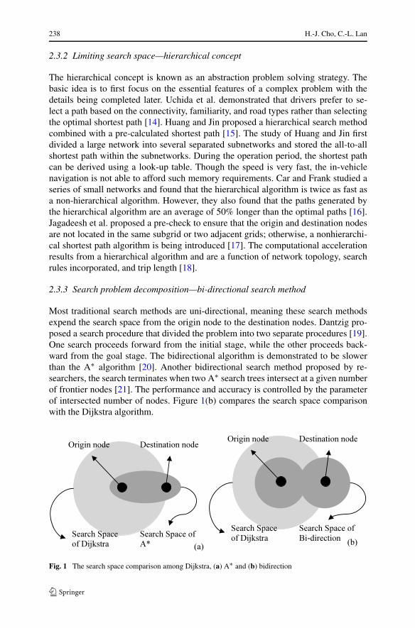
Most traditional search methods are uni-directional, meaning these search methodsexpend the search space from the origin node to the destination nodes. Dantzig pro-posed a search procedure that divided the problem into two separate procedures [19].One search proceeds forward from the initial stage, while the other proceeds back-ward from the goal stage. The bidirectional algorithm is demonstrated to be slowerthan the A∗ algorithm [20]. Another bidirectional search method proposed by re-searchers, the search terminates when two A∗ search trees intersect at a given numberof frontier nodes [21]. The performance and accuracy is controlled by the parameterof intersected number of nodes. Figure 1(b) compares the search space comparisonwith the Dijkstra algorithm.

Fig. 1 The search space comparison among Dijkstra, (a) A∗ and (b) bidirection

Hybrid shortest path algorithm for vehicle navigation 239

3 Hybrid shortest path algorithm

This section combines several algorithms mentioned above, namely the Dijkstra, A∗,hierarchical and bidirectional concepts.

3.1 Implementation of hierarchical and bi-directional concepts

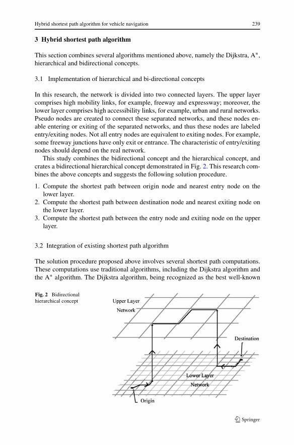
In this research, the network is divided into two connected layers. The upper layercomprises high mobility links, for example, freeway and expressway; moreover, thelower layer comprises high accessibility links, for example, urban and rural networks.Pseudo nodes are created to connect these separated networks, and these nodes en-able entering or exiting of the separated networks, and thus these nodes are labeledentry/exiting nodes. Not all entry nodes are equivalent to exiting nodes. For example,some freeway junctions have only exit or entrance. The characteristic of entry/exitingnodes should depend on the real network.

This study combines the bidirectional concept and the hierarchical concept, andcrates a bidirectional hierarchical concept demonstrated in Fig. 2. This research com-bines the above concepts and suggests the following solution procedure.

1. Compute the shortest path between origin node and nearest entry node on thelower layer.

2. Compute the shortest path between destination node and nearest exiting node onthe lower layer.

3. Compute the shortest path between the entry node and exiting node on the upperlayer.

3.2 Integration of existing shortest path algorithm

The solution procedure proposed above involves several shortest path computations.These computations use traditional algorithms, including the Dijkstra algorithm andthe A∗ algorithm. The Dijkstra algorithm, being recognized as the best well-known

Fig. 2 Bidirectionalhierarchical concept

240 H.-J. Cho, C.-L. Lan

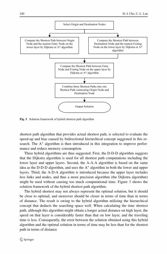
Fig. 3 Solution framework of hybrid shortest path algorithm

shortest path algorithm that provides actual shortest path, is selected to evaluate thespeed-up and bias caused by bidirectional hierarchical concept suggested in this re-search. The A∗ algorithm is then introduced in this integration to improve perfor-mance and reduce memory consumption.

Three hybrid algorithms are thus suggested. First, the D-D-D algorithm suggeststhat the Dijkstra algorithm is used for all shortest path computations including thelower layer and upper layers. Second, the A-A-A algorithm is based on the sameidea as the D-D-D algorithm, and uses the A∗ algorithm in both the lower and upperlayers. Third, the A-D-A algorithm is introduced because the upper layer includesless links and nodes, and thus a more precision algorithm (the Dijkstra algorithm)might be used without causing too much computational time. Figure 3 shows thesolution framework of the hybrid shortest path algorithm.

The hybrid shortest may not always represent the optimal solution, but it shouldbe close to optimal, and moreover should be closer in terms of time than in termsof distance. The result is owing to the hybrid algorithm utilizing the hierarchicalconcept that deducts the searching space well. When calculating the time shortestpath, although this algorithm might obtain a longer actual distance on high layer, thespeed on that layer is considerably faster than that on low layer, and the travelingtime is less. Consequently, the error between the solution obtained using this hybridalgorithm and the optimal solution in terms of time may be less than for the shortestpath in terms of distance

Hybrid shortest path algorithm for vehicle navigation 241

3.3 Direct access data structure

The method used to access stored network data can be either sequential access or di-rect access. The direct access method implies that data is stored at a known address,and has better performance than the sequential access method where a search is nec-essary to find where the data is stored. Searching algorithms are time consuming.Binary search, a fast and popular search algorithm, takes O(2 log2 n), while directaccess takes only O(1).

Extensive node search is performed during the node selection stage of the shortestpath algorithm. If the relationship between links and nodes is stored in matrix form,where the row subscript represents the node id, the column subscript represents thelink id, and the cost is the matrix element. The node can be directly accessed by thesubscripts without searching, improving the speed of node selecting stage. However,since the traffic network is sparse, the matrix storage method is extremely wasteful.A crucial problem is how to simultaneously maintain the speed of direct access andminimal storage space. To achieve this, the links were first sorted and assigned acontinuous id. These id numbers were then be stored immediately following eachnode structure according to the network structure; the id of the neighboring node wasalso stored. During the computation stage, when a node is selected, the connected linkid was also being obtained; link information could then be directly accessed via thelink id; and neighbor nodes that connected to the selected node can also be derived.

Most nodes in real traffic networks were connected to three or four links; it wasextremely rare for there to be more than six connections. The increase in storage spacecompared to the forward star structure was very limited, but the speed improvementwas significant.

4 Implementation and discussion

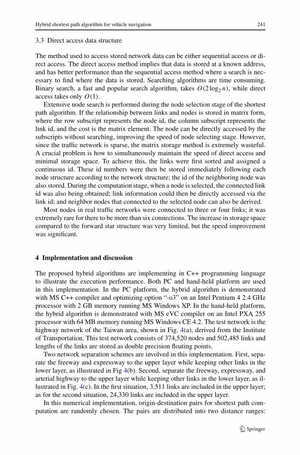
The proposed hybrid algorithms are implementing in C++ programming languageto illustrate the execution performance. Both PC and hand-held platform are usedin this implementation. In the PC platform, the hybrid algorithm is demonstratedwith MS C++ compiler and optimizing option “-o3” on an Intel Pentium 4 2.4 GHzprocessor with 2 GB memory running MS Windows XP. In the hand-held platform,the hybrid algorithm is demonstrated with MS eVC compiler on an Intel PXA 255processor with 64 MB memory running MS Windows CE 4.2. The test network is thehighway network of the Taiwan area, shown in Fig. 4(a), derived from the Instituteof Transportation. This test network consists of 374,520 nodes and 502,485 links andlengths of the links are stored as double precision floating points.

Two network separation schemes are involved in this implementation. First, sepa-rate the freeway and expressway to the upper layer while keeping other links in thelower layer, as illustrated in Fig 4(b). Second, separate the freeway, expressway, andarterial highway to the upper layer while keeping other links in the lower layer, as il-lustrated in Fig. 4(c). In the first situation, 3,511 links are included in the upper layer;as for the second situation, 24,330 links are included in the upper layer.

In this numerical implementation, origin-destination pairs for shortest path com-putation are randomly chosen. The pairs are distributed into two distance ranges:

242 H.-J. Cho, C.-L. Lan

Fig. 4 (a) Taiwan area highway network, (b) freeway and expressway highlighted, and (c) freeway, ex-pressway, and arterial highway highlighted

170 km (Taipei–Taichung) and 400 km (Taipei–Kaohsiung). The path costs in thisimplementation include: (i) actual link length and (ii) link travel time (estimated bydividing the link length by the link speed limit). Hybrid shortest path algorithms pro-posed in this research, including D-D-D, A-D-A, and A-A-A, are compared with theDijkstra and A∗ algorithm. The comparison involving (i) the computing time, (2) thecost of computed shortest path, and (3) the size of shortest path search space explored(the main factor of memory usage).

4.1 Implementation results on PC platform

The implementations on PC platform mainly focused on the network of separatingfreeway and expressway to upper layer, as demonstrated in Fig. 4(b). The other sep-aration scheme is also performed, but it shows a significant draw back on speedwith nearly unchanged solution correctness. Hence, the test network addressed heremainly focused on including freeway and expressway in the upper layer.

4.1.1 Implementation results—treat link distance as link cost

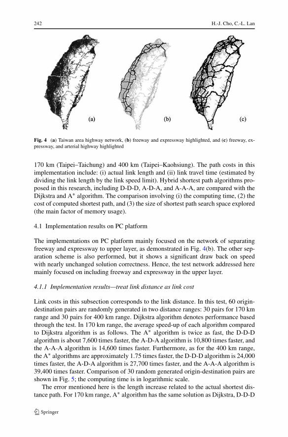
Link costs in this subsection corresponds to the link distance. In this test, 60 origin-destination pairs are randomly generated in two distance ranges: 30 pairs for 170 kmrange and 30 pairs for 400 km range. Dijkstra algorithm denotes performance basedthrough the test. In 170 km range, the average speed-up of each algorithm comparedto Dijkstra algorithm is as follows. The A∗ algorithm is twice as fast, the D-D-Dalgorithm is about 7,600 times faster, the A-D-A algorithm is 10,800 times faster, andthe A-A-A algorithm is 14,600 times faster. Furthermore, as for the 400 km range,the A∗ algorithms are approximately 1.75 times faster, the D-D-D algorithm is 24,000times faster, the A-D-A algorithm is 27,700 times faster, and the A-A-A algorithm is39,400 times faster. Comparison of 30 random generated origin-destination pairs areshown in Fig. 5; the computing time is in logarithmic scale.

The error mentioned here is the length increase related to the actual shortest dis-tance path. For 170 km range, A∗ algorithm has the same solution as Dijkstra, D-D-D

Hybrid shortest path algorithm for vehicle navigation 243

Fig. 5 Execute time comparison of (a) 400 km range and (b) 170 km range

has 18% of bias, A-D-A and A-A-A have the same result of 9% bias. As for 400 kmrange, A∗ has no bias while D-D-D has 4.5%, A-D-A and A-A-A have 3.4%.

The reason for larger bias with D-D-D lies on search directions. The search direc-tion of Dijkstra radiates from the origin with no preference, while that of A∗ radiatesfrom origin and toward destination. With the characteristic of different search di-rection, D-D-D tends to find the “nearest entry node” and probably finds an entrynode located in the opposite direction to the destination node; while A-D-A and A-A-A tend to find an entry node located in the same direction to the destination. Thatmakes A-D-A and A-A-A to have less bias compared to D-D-D.

4.1.2 Implementation results—link travel time as link cost

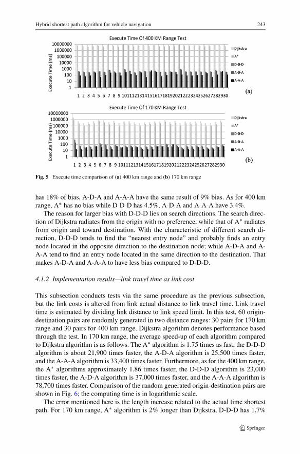
This subsection conducts tests via the same procedure as the previous subsection,but the link costs is altered from link actual distance to link travel time. Link traveltime is estimated by dividing link distance to link speed limit. In this test, 60 origin-destination pairs are randomly generated in two distance ranges: 30 pairs for 170 kmrange and 30 pairs for 400 km range. Dijkstra algorithm denotes performance basedthrough the test. In 170 km range, the average speed-up of each algorithm comparedto Dijkstra algorithm is as follows. The A∗ algorithm is 1.75 times as fast, the D-D-Dalgorithm is about 21,900 times faster, the A-D-A algorithm is 25,500 times faster,and the A-A-A algorithm is 33,400 times faster. Furthermore, as for the 400 km range,the A∗ algorithms approximately 1.86 times faster, the D-D-D algorithm is 23,000times faster, the A-D-A algorithm is 37,000 times faster, and the A-A-A algorithm is78,700 times faster. Comparison of the random generated origin-destination pairs areshown in Fig. 6; the computing time is in logarithmic scale.

The error mentioned here is the length increase related to the actual time shortestpath. For 170 km range, A∗ algorithm is 2% longer than Dijkstra, D-D-D has 1.7%

244 H.-J. Cho, C.-L. Lan

Fig. 6 Execute time comparison of (a) 400 km range and (b) 170 km range

of bias, A-D-A and A-A-A have the same result of 5.2% bias. As for 400 km range,A∗ has 1.2% bias while D-D-D has 0.72%, A-D-A and A-A-A have 2.73%.

Compared to the previous subsection where we treat the actual distance as linkcost, the bias of the hybrid algorithm is much smaller. The main reason of this re-sult lies on the path generated by the hybrid algorithm prefers the high mobility link(higher speed limit compare to local roads). Although the local roads might haveshorter distance, but when the speed is taken into account, major roads would haveshorter travel time. D-D-D performs best in this test due to the characteristic of Dijk-stra. In this test, link costs are treated as link travel time, and Dijkstra will seek for thenearest entry node (in the sense of time) and keep the path on the freeway/expresswayuntil it reaches the nearest junction to the destination (also in the sense of time).

4.2 Implementation results on hand-held platform

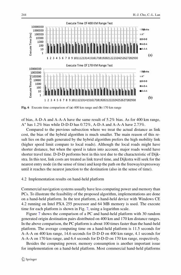
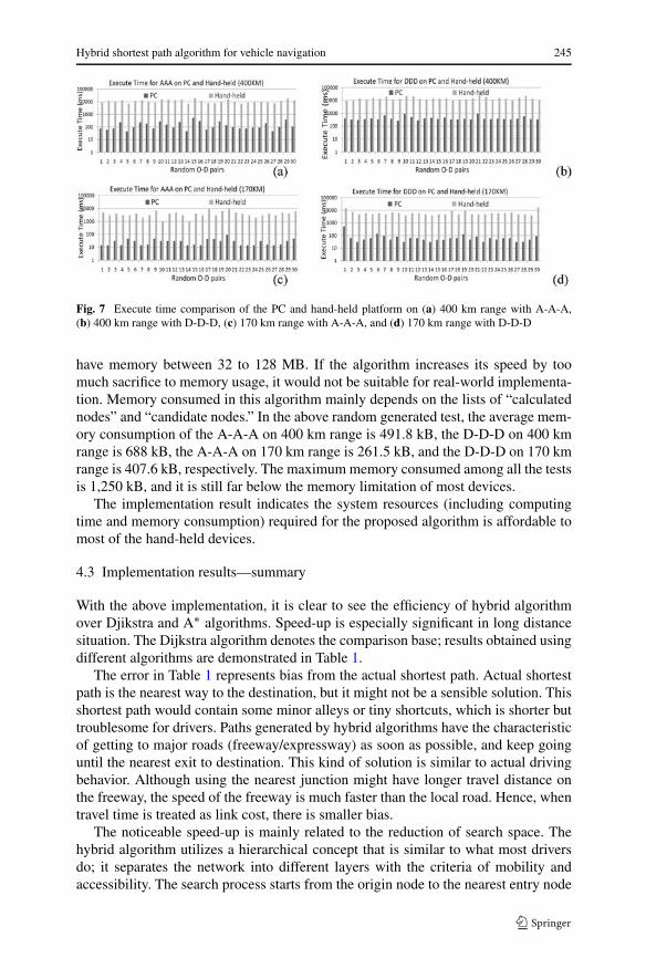
Commercial navigation systems usually have less computing power and memory thanPCs. To illustrate the feasibility of the proposed algorithm, implementations are doneon a hand-held platform. In the test platform, a hand-held device with Windows CE4.2 running on Intel PXA 255 processor and 64 MB memory is used. The executetime for each platform is shown in Fig. 7, using a logarithm scale.

Figure 7 shows the comparison of a PC and hand-held platform with 30 randomgenerated origin destination pairs distributed on 400 km and 170 km distance ranges.In the above comparison, the PC platform is about 100 times faster than the hand-heldplatform. The average computing time on a hand-held platform is 11.5 seconds forA-A-A on 400 km range, 14.6 seconds for D-D-D on 400 km range, 4.1 seconds forA-A-A on 170 km range, and 6.4 seconds for D-D-D on 170 km range, respectively.

Besides the computing power, memory consumption is another important issuefor implementation on a hand-held platform. Most commercial hand-held platforms

Hybrid shortest path algorithm for vehicle navigation 245

Fig. 7 Execute time comparison of the PC and hand-held platform on (a) 400 km range with A-A-A,(b) 400 km range with D-D-D, (c) 170 km range with A-A-A, and (d) 170 km range with D-D-D

have memory between 32 to 128 MB. If the algorithm increases its speed by toomuch sacrifice to memory usage, it would not be suitable for real-world implementa-tion. Memory consumed in this algorithm mainly depends on the lists of “calculatednodes” and “candidate nodes.” In the above random generated test, the average mem-ory consumption of the A-A-A on 400 km range is 491.8 kB, the D-D-D on 400 kmrange is 688 kB, the A-A-A on 170 km range is 261.5 kB, and the D-D-D on 170 kmrange is 407.6 kB, respectively. The maximum memory consumed among all the testsis 1,250 kB, and it is still far below the memory limitation of most devices.

The implementation result indicates the system resources (including computingtime and memory consumption) required for the proposed algorithm is affordable tomost of the hand-held devices.

4.3 Implementation results—summary

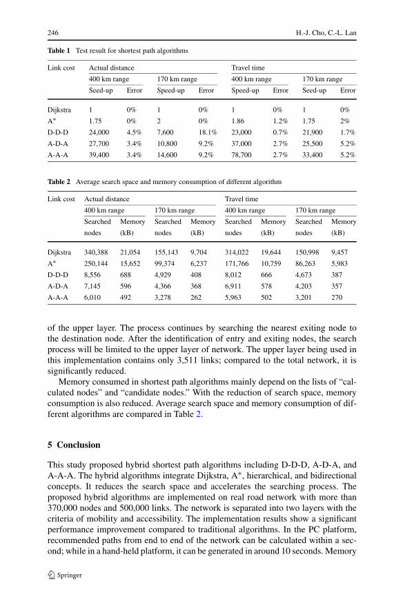
With the above implementation, it is clear to see the efficiency of hybrid algorithmover Djikstra and A∗ algorithms. Speed-up is especially significant in long distancesituation. The Dijkstra algorithm denotes the comparison base; results obtained usingdifferent algorithms are demonstrated in Table 1.

The error in Table 1 represents bias from the actual shortest path. Actual shortestpath is the nearest way to the destination, but it might not be a sensible solution. Thisshortest path would contain some minor alleys or tiny shortcuts, which is shorter buttroublesome for drivers. Paths generated by hybrid algorithms have the characteristicof getting to major roads (freeway/expressway) as soon as possible, and keep goinguntil the nearest exit to destination. This kind of solution is similar to actual drivingbehavior. Although using the nearest junction might have longer travel distance onthe freeway, the speed of the freeway is much faster than the local road. Hence, whentravel time is treated as link cost, there is smaller bias.

The noticeable speed-up is mainly related to the reduction of search space. Thehybrid algorithm utilizes a hierarchical concept that is similar to what most driversdo; it separates the network into different layers with the criteria of mobility andaccessibility. The search process starts from the origin node to the nearest entry node

246 H.-J. Cho, C.-L. Lan

Table 1 Test result for shortest path algorithms

Link cost Actual distance Travel time

400 km range 170 km range 400 km range 170 km range

Seed-up Error Speed-up Error Speed-up Error Seed-up Error

Dijkstra 1 0% 1 0% 1 0% 1 0%

A∗ 1.75 0% 2 0% 1.86 1.2% 1.75 2%

D-D-D 24,000 4.5% 7,600 18.1% 23,000 0.7% 21,900 1.7%

A-D-A 27,700 3.4% 10,800 9.2% 37,000 2.7% 25,500 5.2%

A-A-A 39,400 3.4% 14,600 9.2% 78,700 2.7% 33,400 5.2%

Table 2 Average search space and memory consumption of different algorithm

Link cost Actual distance Travel time

400 km range 170 km range 400 km range 170 km range

Searched Memory Searched Memory Searched Memory Searched Memory

nodes (kB) nodes (kB) nodes (kB) nodes (kB)

Dijkstra 340,388 21,054 155,143 9,704 314,022 19,644 150,998 9,457

A∗ 250,144 15,652 99,374 6,237 171,766 10,759 86,263 5,983

D-D-D 8,556 688 4,929 408 8,012 666 4,673 387

A-D-A 7,145 596 4,366 368 6,911 578 4,203 357

A-A-A 6,010 492 3,278 262 5,963 502 3,201 270

of the upper layer. The process continues by searching the nearest exiting node tothe destination node. After the identification of entry and exiting nodes, the searchprocess will be limited to the upper layer of network. The upper layer being used inthis implementation contains only 3,511 links; compared to the total network, it issignificantly reduced.

Memory consumed in shortest path algorithms mainly depend on the lists of “cal-culated nodes” and “candidate nodes.” With the reduction of search space, memoryconsumption is also reduced. Average search space and memory consumption of dif-ferent algorithms are compared in Table 2.

5 Conclusion

This study proposed hybrid shortest path algorithms including D-D-D, A-D-A, andA-A-A. The hybrid algorithms integrate Dijkstra, A∗, hierarchical, and bidirectionalconcepts. It reduces the search space and accelerates the searching process. Theproposed hybrid algorithms are implemented on real road network with more than370,000 nodes and 500,000 links. The network is separated into two layers with thecriteria of mobility and accessibility. The implementation results show a significantperformance improvement compared to traditional algorithms. In the PC platform,recommended paths from end to end of the network can be calculated within a sec-ond; while in a hand-held platform, it can be generated in around 10 seconds. Memory

Hybrid shortest path algorithm for vehicle navigation 247

consumption for the proposed algorithm is also lowered. Compared to nearly 20 MBfor the Dijkstra algorithm, the proposed algorithm uses no more than 1.5 MB amongall tests. The test results demonstrate a significant advantage for implementing theproposed algorithms in vehicle navigation systems.

Acknowledgements The authors would like to thank the National Science Council of the Republic ofChina, Taiwan, for financially supporting this research under Contract No. NSC 95-2221-E-009-346.

References

1. Meyer U (2001) Single-source shortest-paths on arbitrary directed graphs in linear average-case time.In: Proceeding of 12th annual ACM-SIAM symposium on discrete algorithms, 2001, pp 797–806

2. Wagner D, Willhalm T (2003) Geometric speed-up techniques for finding shortest paths in large sparsegraphs. Lect Notes Comput Sci 2832:776–787

3. Dijkstra EW (1959) A note on two problems in connexion with graphs. Numer Math 1:269–271.doi:10.1007/BF01386390

4. Whiting PD, Hillier JA (1960) A method for finding the shortest route through a road network. OperRes Q 11:37–40

5. Dail BR (1969) Algorithm 360:shortest path forest with topological ordering. Commun Assoc ComputMach 12:632–633

6. Bellman R (1958) On a routing problem. Q Appl Math 16:87–907. Fredman ML, Tarjan RE (1987) Fibonacci heaps and their uses in improved network optimization

algorithms. J ACM 34:596–615. doi:10.1145/28869.288748. Karimi HA (1996) Real-time optimal-route computation: a heuristic approach. Intel Transp Syst J

3:111–127. doi:10.1080/102480796089037129. Zhan FB (1997) Three fastest shortest path algorithms on real road networks: data structures and

procedures. J Geogr Inf Decis Anal 1:69–8210. Hart PE, Nilsson NJ, Raphael B (1968) A formal basis for the heuristic determination of minimum

cost paths. IEEE Trans Syst Sci Cybern 2:100–10711. Goldberg AV (2007) Point-to-point shortest path algorithms with preprocessing. Lect Notes Comput

Sci 4362:88–102. doi:10.1007/978-3-540-69507-3_612. Golden LB, Ball M (1978) Shortest paths with Euclidean distances: An explanatory model. Networks

8:297–314. doi:10.1002/net.323008040413. Sedgewick R, Vitter JS (1986) Shortest paths in Euclidean graphs. Algorithm 1:31–48.

doi:0.1007/BF0184043514. Uchida T, Iida Y, Nakahara M (1994) Panel survey on drivers’ route choice behavior under travel time

information. In: Proceeding of vehicle navigation and information systems, 1994, pp 383–38815. Huang Y, Jing N (1996) Evaluation of hierarchical path finding techniques for ITS route guidance. In:

Proceeding of annual meeting of ITS America, 1996, pp 340–35016. Car A, Frank AU (1994) General principles of hierarchical spatial reasoning—the case of way-finding.

In: Proceedings of the 6th international symposium on spatial data handling, 1994, pp 646–66417. Jagadeesh GR, Srikanthan T, Quek KH (2002) Heuristic techniques for accelerating hierarchical rout-

ing on road networks. IEEE Trans Intell Transp Syst 3:301–309. doi:10.1109/TITS.2002.80680618. Fu L, Sun D, Rilett LR (2006) Heuristic shortest path algorithms for transportation applications: state

of the art. Comput Oper Res 33:3324–3343. doi:10.1016/j.cor.2005.03.02719. Dantzig GB (1960) On the shortest route through a network. Manag Sci 6:87–9020. Fu L (1996) Real-time vehicle routing and scheduling in dynamic and stochastic traffic networks.

Ph.D. Thesis, University of Alberta21. Pohl I (1971) Bi-directional search. Mach Intel 6:127–140