Hybrid Propulsion System for CubeSat Applicationsepubs.surrey.ac.uk/812899/1/PhD_Thesis_AOD.pdf ·...
161
Hybrid Propulsion System for CubeSat Applications Ahmed Ozomata David Submitted for the Degree of Doctor of Philosophy from the University of Surrey Surrey Space Centre Department of Electronic Engineering Faculty of Engineering and Physical Sciences University of Surrey Guildford, Surrey, GU2 7XH, UK. September 2016 c ○Ahmed Ozomata David 2016
Transcript of Hybrid Propulsion System for CubeSat Applicationsepubs.surrey.ac.uk/812899/1/PhD_Thesis_AOD.pdf ·...
Hybrid Propulsion System for CubeSat
Applications
Ahmed Ozomata David
Submitted for the Degree of
Doctor of Philosophy
from the University of Surrey
Surrey Space Centre
Department of Electronic Engineering
Faculty of Engineering and Physical Sciences
University of Surrey
Guildford, Surrey, GU2 7XH, UK.
September 2016
cAhmed Ozomata David 2016

Abstract
The CubeSats platform has become a common basis for the development and flight of very
small, low cost spacecraft-particularly amongst University groups. The smallest CubeSats
are just 1 litre in volume-comprising a 10 𝑐𝑚 x 10 𝑐𝑚 x 10 𝑐𝑚 unit-“1𝑈”. Multiples of this
unit are also flown: 2𝑈 and 3𝑈 (which fit the standard launch “pod”) and, at the larger
scale, 6𝑈 , 12𝑈 and potentially 27𝑈 . The spacecraft generally do not carry propulsion
systems and so their orbit is dictated by the initial orbital injection from the launch
vehicle. This research aims at producing a novel chemical micropropulsion system based
on a mixture of sodium hydroxide and water (the oxidiser) and aluminium (the fuel)
suitable for CubeSats. The choice of the propellants was based on the availability and
cost of materials; long storage without degrading; moderate temperature and exothermic
reaction without any thermal control threat to the microsatellite structure; high energy
density per unit volume for the volume constraint satellite; and the propulsion system
will require minimal power from the CubeSat electrical bus system. Initial experimental
findings revealed that oxidiser of 12.50𝑚𝑜𝑙/𝑘𝑔 molar concentration produced the fastest
reaction rate, and a reaction of 6 𝑔 of fuel to 3 𝑔 of oxidiser produced a peak performance
of 0.032𝑁 thrust and 45 𝑠 specific impulse. Multiple injections of the oxidiser for repeat
cycles were also demonstrated with different fuel to oxidiser ratios. The energy utilisation
of the propulsion system was calculated and it revealed that about 98% of the exhaust
was water vapour , while only about 2% was hydrogen gas. It was also found out that
about 4% of the total generated enthalpy was converted into useful thrust, while the
remaining percentage was used by about 98% of the injected water to change phase from
liquid to gas. This result assumed that the reaction volume was essentially adiabatic.
Though the specific impulse of the propellant is moderate, the thruster is capable of
delivering a ΔV of about 57𝑚/𝑠 to a 1U CubeSat of 1.33 𝑘𝑔. However, one of the
drawbacks of the system is that the firing time is about 1 𝑚𝑖𝑛𝑢𝑡𝑒 after the injection of
oxidiser, making this system inappropriate for attitude control purposes.
ii

Acknowledgements
This enduring journey has been made possible by this set of special people that their
contributions toward the completion of this program can not just be mentioned by words.
Howbeit, let me use this privilege to acknowledge my Dad and Mum, Mr Amodu Oyibo
Lawal and Mrs Ayisetu Mariya Amodu, for your unending love, care and prayers. I am
deeply grateful. And to all my siblings especially Mr Oyibo Sunday Amodu and late
Mr Adeku Joseph Amodu, I say thank you. You saw this potential in me and did not
let go of it at that tiny age, and now this is it! A million thanks to my lovely wife and
children: Oziohu Glory and Adinoyi, Onimisi, Onize and Adavize. The smiles on your
faces during this sacrifice kept me going even when the journey seemed tough. We share
the research story together. Thanks also to my Uncle, Mr M.A. Momoh and Mummy,
late Mrs Ester Momoh. You took me as I was and gave me the opportunity to discover
myself. Am grateful. Thanks also to Mr Nathaniel Salawu and family for your valuable
advice and encouragement. To the staff and management of Nigerian Communication
Satellite Limited, you made it possible for me to achieve my dream, and so thank you
very much. To the financier of the PhD program, Petroleum Technology Development
Fund (PTDF) of Nigeria, I say thank you. Million thanks to my supervisors, Dr Aaron
Knoll and Prof. Phil Palmer for your unflinching supports and in-depth contributions
during the course of this program. Thanks also to all the SSC propulsion group-both
formal and the present members for the propulsion engineering and update discussions.
Thanks to the three Toms, Charlie, Andrea, Max, Antonio, Gebi and Ahmad for your
contributions. A very big thank you to all the administrative and technical staff of SSC:
Karen, Louise, Andy and David, for your supports and making my stay at Surrey a
very conducive one. Thanks also to my colleague: Yusuf, Pam, Ugah, Mahmoud and
Modibbo for our quality time together. Thanks to Dr Ibrahim, Dr Ikpaya, Dr Daji, Dr
Tanko and Dr Okonor for your valuable advice and supports during this program. Above
all, I give all thanks to God Almighty for His love, grace and mercy.
iii

Contents
Abstract ii
Acknowledgements iii
List of Figures vii
List of Tables xi
Nomenclature xii
1 Introduction 1
1.1 CubeSat . . . . . . . . . . . . . . . . . . . . . . . . . . . . . . . . . . . . . 1
1.1.1 CubeSats Flown with Propulsion Systems . . . . . . . . . . . . . 3
1.2 Overview of Micropropulsion Systems . . . . . . . . . . . . . . . . . . . 6
1.2.1 Electric Micropropulsion Systems . . . . . . . . . . . . . . . . . . 6
1.2.1.1 Resistojets . . . . . . . . . . . . . . . . . . . . . . . . . . 7
1.2.1.2 Arcjets . . . . . . . . . . . . . . . . . . . . . . . . . . . 9
1.2.1.3 Microcavity Discharge Thruster . . . . . . . . . . . . . 9
1.2.1.4 Ion Engines . . . . . . . . . . . . . . . . . . . . . . . . . 10
1.2.1.5 Hall Thrusters . . . . . . . . . . . . . . . . . . . . . . . . 11
1.2.1.6 Micro Pulse Plasma Thrusters . . . . . . . . . . . . . . 13
1.2.1.7 Micro Laser Ablation Thruster . . . . . . . . . . . . . . 14
1.2.1.8 Vacuum Arc Thruster . . . . . . . . . . . . . . . . . . . 15
1.2.1.9 Field Emission Electric Propulsion . . . . . . . . . . . . 16
1.2.2 Chemical Micropropulsion Systems . . . . . . . . . . . . . . . . . . 17
1.2.2.1 Cold Gas Thruster . . . . . . . . . . . . . . . . . . . . . . 17
1.2.2.2 Warm Gas Thruster . . . . . . . . . . . . . . . . . . . . 20
iv
1.2.2.3 Monopropellant Systems . . . . . . . . . . . . . . . . . . 21
1.2.2.4 Bipropellant Thrusters . . . . . . . . . . . . . . . . . . 22
1.2.2.5 Solid Rocket Motor . . . . . . . . . . . . . . . . . . . . 23
1.2.2.6 Hybrid Propulsion System . . . . . . . . . . . . . . . . 25
1.3 CubeSat Requirements for Propulsion System . . . . . . . . . . . . . . . 25
1.3.1 Propulsion Requirements for CubeSat Missions . . . . . . . . . . 26
1.3.2 Chemical Propulsion Trade-off . . . . . . . . . . . . . . . . . . . 28
1.3.2.1 Overview of Hybrid Rocket Motor . . . . . . . . . . . . 28
1.4 Motivation and Objectives . . . . . . . . . . . . . . . . . . . . . . . . . . 32
1.5 Novelty and Research Achievements . . . . . . . . . . . . . . . . . . . . 33
2 Theory 34
2.1 Overview . . . . . . . . . . . . . . . . . . . . . . . . . . . . . . . . . . . 34
2.2 Aluminium, Sodium Hydroxide, Water Oxidation Reaction . . . . . . . 36
2.3 Thermodynamics and Gas Dynamics . . . . . . . . . . . . . . . . . . . . 40
2.4 Theoretical Performance Analysis of the Propulsion System . . . . . . . 45
2.4.1 Thruster Design . . . . . . . . . . . . . . . . . . . . . . . . . . . 49
2.4.1.1 Reaction Chamber . . . . . . . . . . . . . . . . . . . . . 49
2.4.1.2 Nozzle . . . . . . . . . . . . . . . . . . . . . . . . . . . . 50
3 Experimental Setup 52
3.1 Overview . . . . . . . . . . . . . . . . . . . . . . . . . . . . . . . . . . . 52
3.2 Oxidizer Feed System . . . . . . . . . . . . . . . . . . . . . . . . . . . . 52
3.3 Data Acquisition System . . . . . . . . . . . . . . . . . . . . . . . . . . . 54
3.3.1 Temperature and Pressure Sensors . . . . . . . . . . . . . . . . . 54
3.3.2 DAQ Measurement Hardware . . . . . . . . . . . . . . . . . . . . 55
3.3.3 LabVIEW Software . . . . . . . . . . . . . . . . . . . . . . . . . 56
3.4 Vacuum Facilities and Thrust Balance . . . . . . . . . . . . . . . . . . . . 57
3.4.1 The Pagasus Vacuum Chamber . . . . . . . . . . . . . . . . . . . . 57
3.4.2 Thrust Balance Arrangement . . . . . . . . . . . . . . . . . . . . 58
3.4.3 Calibration and Data Analysis . . . . . . . . . . . . . . . . . . . 59
3.5 Complete Experimental Setup . . . . . . . . . . . . . . . . . . . . . . . . 62
4 Results and Discussion 64
4.1 Overview . . . . . . . . . . . . . . . . . . . . . . . . . . . . . . . . . . . 64
v
4.2 Stages of Experiments . . . . . . . . . . . . . . . . . . . . . . . . . . . . 64
4.2.1 Reaction Chemistry of the Propellants at Ambient Conditions . 64
4.2.2 Temperature and Pressure Rise in a control volume under Vacuum
Conditions . . . . . . . . . . . . . . . . . . . . . . . . . . . . . . 66
4.2.3 Effect of Oxidiser Concentration on Thruster Characterisation . 68
4.2.4 Fuel/Oxidiser Ratio on Thruster Performance . . . . . . . . . . . 72
4.2.5 Propellant Mass Effect on Thruster Performance . . . . . . . . . 74
4.2.6 Impact of Repeat Cycles on Thruster Performance . . . . . . . . 76
4.2.7 Effect of Nozzle throat Diameter on Thruster Performance . . . 78
4.3 Reaction Pattern of the Propulsion System . . . . . . . . . . . . . . . . 80
4.4 Energy Conversion Efficiency of the Propulsion System . . . . . . . . . . . 81
4.4.1 Chemical Analysis of the Residual Propellants . . . . . . . . . . . 87
4.5 Comparison Between Design Target, Theoretical and Prototype Performances 89
4.6 Comparison with the State-of-the-Art . . . . . . . . . . . . . . . . . . . . 91
4.7 Summary of Experimental Findings . . . . . . . . . . . . . . . . . . . . 92
4.7.0.1 Proposed Mechanical Design of the Hybrid Propulsion
System . . . . . . . . . . . . . . . . . . . . . . . . . . . 93
5 Conclusions and Future Work 96
5.1 Novelty and Research Achievements . . . . . . . . . . . . . . . . . . . . 98
5.2 Future Work . . . . . . . . . . . . . . . . . . . . . . . . . . . . . . . . . 99
References 101
Appendix A Detail Drawings of the Hybrid Propulsion Thruster 117
Appendix B Experiment Hardware 122
Appendix C Program Codes 136
C.1 Solenoid Valves Control Program . . . . . . . . . . . . . . . . . . . . . . 136
C.2 Thrust Balance Calibration Constant Program . . . . . . . . . . . . . . 138
C.3 Thrust Response Program of One-shot Experiment . . . . . . . . . . . . 142
C.4 Thrust Response Program of Repeat Cycle Injection . . . . . . . . . . . 143
vi

List of Figures
1.1 1U cube satellite [5] . . . . . . . . . . . . . . . . . . . . . . . . . . . . . . 1
1.2 Concept of constellation flight [17] . . . . . . . . . . . . . . . . . . . . . 2
1.3 CanX-2 NANOPS system [20] . . . . . . . . . . . . . . . . . . . . . . . 3
1.4 STRaND-1 propulsion systems: (a) Butane resistojet (b) Pulsed plasma
thruster [25] . . . . . . . . . . . . . . . . . . . . . . . . . . . . . . . . . . 4
1.5 Delfi-n3Xt cold gas generator thruster components [29] . . . . . . . . . . 5
1.6 Schematic and complete views of vaporizing liquid thruster . . . . . . . . 7
1.7 3-Watt CMOS resistojet on a 2-micron TinyChip die layout [40] . . . . 8
1.8 Schematic of an arcjet thruster [44] . . . . . . . . . . . . . . . . . . . . 9
1.9 Schematic of an insulated electrodes of a microcavity thruster [47] . . . 10
1.10 Schematic diagrams of a 3D view and a longitudinal cross-section view of
the ion thruster developed at Pennsylvania State University [48] . . . . . 11
1.11 Schematic diagram of an SPT Hall thruster, showing the electrodes and
the radial magnetic field [49] . . . . . . . . . . . . . . . . . . . . . . . . 12
1.12 Schematic diagram and photo shot of a low-power miniaturised Hall
thruster (TCHT-4) [50] . . . . . . . . . . . . . . . . . . . . . . . . . . . 13
1.13 𝜇PPT for concepts for microsatellites . . . . . . . . . . . . . . . . . . . . 14
1.14 Micro laser ablation thruster concept [57] . . . . . . . . . . . . . . . . . 14
1.15 Schematic diagram of a magnetically enhanced vacuum arc thruster [62] 15
1.16 Schematic diagram of a field emission electric propulsion [65] . . . . . . 16
1.17 Schematic view of cold gas thruster [38] . . . . . . . . . . . . . . . . . . 18
1.18 Schematic diagram of MPS-110 cold gas thruster developing by Aerojet [69] 19
1.19 Gas generator cartridges [72] . . . . . . . . . . . . . . . . . . . . . . . . 20
1.20 Schematic of a novel warm gas propulsion system [74] . . . . . . . . . . 20
vii
1.21 Model achitechture of a miniature hydrogen peroxide monopropellant
thruster, with a cross sectional view of the catalyst assembly [82] . . . . 22
1.22 Micro-bipropellant thruster from MIT [85] . . . . . . . . . . . . . . . . . 23
1.23 Schematic view of one solid propellant thruster [86] . . . . . . . . . . . . 24
1.24 Schematic of a conventional hybrid rocket motor [91] . . . . . . . . . . 25
1.25 (a) Vortex flow pancake hybrid model diagram [76] (b) Swirling of propel-
lant in a vortex flow [101] . . . . . . . . . . . . . . . . . . . . . . . . . . 30
2.1 Moles of hydrogen gas produced and the enthalpy of reaction against the
moles of reacted aluminium respectively . . . . . . . . . . . . . . . . . . 35
2.2 Selected energy density of some fuels [122] . . . . . . . . . . . . . . . . . . 37
2.3 Control volume with an attached nozzle: 𝐴𝑒 is the exit area of the nozzle,
𝐴𝑡 is the throat area, 𝑝𝑎 is the ambient pressure and 𝑝𝑒 is the exit pressure 41
2.4 Theoretical specific impulse performance against the expansion ratio of
the nozzle and the propellant mass flow rate . . . . . . . . . . . . . . . . . 47
2.5 ΔV performance versus the dry mass fraction for an 𝐼𝑠𝑝 of 118 𝑠 . . . . 48
2.6 Design model of the reaction chamber . . . . . . . . . . . . . . . . . . . 50
2.7 Swagelok cap and plug [143] adopted as nozzle . . . . . . . . . . . . . . . 51
3.1 Schematic of a pressure feed system . . . . . . . . . . . . . . . . . . . . 53
3.2 Feed system setup . . . . . . . . . . . . . . . . . . . . . . . . . . . . . . 53
3.3 Circuit connection of the arduino and the solenoid valves . . . . . . . . 54
3.4 Thermocouples: (a) Insulated thermocouple and (b) Fine wire thermocouple 55
3.5 Pressure transducer . . . . . . . . . . . . . . . . . . . . . . . . . . . . . 55
3.6 DAQ measurement hardware and connections . . . . . . . . . . . . . . . 56
3.7 Block diagram of the LabVIEW program used to control and acquire data
from sensors . . . . . . . . . . . . . . . . . . . . . . . . . . . . . . . . . . . 57
3.8 𝑃𝑒𝑔𝑎𝑠𝑢𝑠 vacuum chamber . . . . . . . . . . . . . . . . . . . . . . . . . . 58
3.9 Schematic of the thrust stand . . . . . . . . . . . . . . . . . . . . . . . . 59
3.10 DC stepper motor from RS Components Limited . . . . . . . . . . . . . 60
3.11 Geometry Of Thrust Calibration and Thrust Stand Sepup with Stepper
Motor . . . . . . . . . . . . . . . . . . . . . . . . . . . . . . . . . . . . . 60
3.12 Responses of Thrust Calibration . . . . . . . . . . . . . . . . . . . . . . . 61
3.13 Schematic of the complete experimental setup . . . . . . . . . . . . . . . 63
viii
4.1 Experimental setup for sodium hydroxide concentration on aluminium-
water reaction . . . . . . . . . . . . . . . . . . . . . . . . . . . . . . . . . 65
4.2 Effect of sodium hydroxide molality on aluminium-water reaction . . . . 66
4.3 Schematic of the initial lab setup . . . . . . . . . . . . . . . . . . . . . . . 67
4.4 Changes in temperature and pressure in the reaction for the same mass
and concentration of oxidiser but different mass of fuel . . . . . . . . . . 68
4.5 Thrust reponses for different oxidiser concentration . . . . . . . . . . . . 70
4.6 Temperature reponses for different oxidiser concentration . . . . . . . . . 71
4.7 Average thrust performance response to oxidiser concentration . . . . . 72
4.8 One-shot thrust characterisation of the propulsion system on different
propellant ratios . . . . . . . . . . . . . . . . . . . . . . . . . . . . . . . 73
4.9 Temperature reponses for different propellant ratios . . . . . . . . . . . 74
4.10 Thruster characterisation at different propellant mass combinations . . . 75
4.11 Temperature reponses for different propellant mass combinations . . . . 76
4.12 Scaling of propellant ratio for more repeat cycles . . . . . . . . . . . . . . 77
4.13 Temperature reponses for different propellant mass combinations . . . . 78
4.14 Thrust level performance for different nozzle throat diameter . . . . . . 79
4.15 Temperature reponses for different nozzle throat diameters . . . . . . . 79
4.16 Reaction pattern of the thruster parameters . . . . . . . . . . . . . . . . . 81
4.17 Thrust, temperature and pressure responses of a one-shot experiment for
energy efficiency analysis . . . . . . . . . . . . . . . . . . . . . . . . . . . 82
4.18 Illustration of energy conversion efficiency . . . . . . . . . . . . . . . . . 83
4.19 𝑝 − ℎ diagram of water showing the enthalpy-pressure relation in the
reaction chamber. The 𝑝 − ℎ diagram was drawn from data obtained
from [156]. The blue line represents saturated liquid water while the
red line represents dry saturated steam. The dome covers water-steam
composition with decreasing water content from left to right. . . . . . . 85
4.20 Energy iterations for the percentage of water vapour in the system . . . . 87
4.21 Physical examination of propellant residue . . . . . . . . . . . . . . . . . 88
4.22 Microstructure view of two propellant residues . . . . . . . . . . . . . . 89
4.23 MicroRamam spectrum analysis of the propellant residues . . . . . . . . 89
4.24 Schematic layout of the propulsion system . . . . . . . . . . . . . . . . . 93
ix
4.25 CAD drawing of hybrid propuldion system for CubeSat applications
showing its dimensions in a 1𝑈 CubeSat . . . . . . . . . . . . . . . . . . 94
5.1 Uncertainty in repeated experimental data . . . . . . . . . . . . . . . . . 98
A.1 Reaction chamber . . . . . . . . . . . . . . . . . . . . . . . . . . . . . . 118
A.2 Nozzle part 1 . . . . . . . . . . . . . . . . . . . . . . . . . . . . . . . . . 119
A.3 Nozzle part 2 (Modified from swagelok [143]) . . . . . . . . . . . . . . . 120
A.4 Thrust attachment to the thrust stand . . . . . . . . . . . . . . . . . . . . 121
B.1 Aluminium wool data sheet . . . . . . . . . . . . . . . . . . . . . . . . . 123
B.2 K-type insulated thermocouple data sheet . . . . . . . . . . . . . . . . . 124
B.3 PFA needle valve data page 1 . . . . . . . . . . . . . . . . . . . . . . . . 125
B.4 PFA needle valve data page 2 . . . . . . . . . . . . . . . . . . . . . . . . 126
B.5 PFA needle valve data page 3 . . . . . . . . . . . . . . . . . . . . . . . . . 127
B.6 PFA needle valve data page 4 . . . . . . . . . . . . . . . . . . . . . . . . 128
B.7 DC stepper motor data sheet . . . . . . . . . . . . . . . . . . . . . . . . 129
B.8 Swagelok cap and plug data sheet . . . . . . . . . . . . . . . . . . . . . . 130
B.9 Solenoid valve description and data sheet 1 . . . . . . . . . . . . . . . . . 131
B.10 Solenoid valve description and data sheet 2 . . . . . . . . . . . . . . . . 132
B.11 Arduino Uno SMD Rev3 data sheet . . . . . . . . . . . . . . . . . . . . 133
B.12 Laser displacement sensor (optoNCDT 1700-50) data page 1 . . . . . . . 134
B.13 Laser displacement sensor (optoNCDT 1700-50) data page 2 . . . . . . . 135
x
List of Tables
1.1 Performance characteristics of propulsion systems flown on board CubeSats 5
1.2 Classification of satellites showing 1𝑈 CubeSat limited resources . . . . 6
1.3 Performance comparison of micropropulsions as requirements for CubeSat
propulsion system . . . . . . . . . . . . . . . . . . . . . . . . . . . . . . 26
1.4 Propulsion requirements for nanosatellites for several missions [92] . . . . 27
1.5 Chemical propulsion trade-off for CubeSat applications . . . . . . . . . . 28
1.6 Thermochemical analysis of propellant combinations . . . . . . . . . . . . 31
2.1 Thermodynamic properties of the propellants . . . . . . . . . . . . . . . 36
2.2 Heat capacity coefficients . . . . . . . . . . . . . . . . . . . . . . . . . . 40
2.3 Hybrid propulsion system design parameters and performance . . . . . . 48
4.1 Experiment data for sodium hydroxide molality . . . . . . . . . . . . . . 65
4.2 Temperature and pressure rise in vacuum condition . . . . . . . . . . . . . 67
4.3 Data for effect of oxidiser concentration on thrust level . . . . . . . . . . 69
4.4 Data for fuel/oxidiser effect on one-shot experiment . . . . . . . . . . . 72
4.5 Experimental data for variation in propellant mass at constant ratio . . 75
4.6 Experimental data for scaling effect and repeat cycles . . . . . . . . . . . 77
4.7 Experimental data on the effect of different nozzle throat diameter . . . 79
4.8 Experimental data for the chemical reaction model of the thruster . . . 80
4.9 Data for a one-shot experiment . . . . . . . . . . . . . . . . . . . . . . . 82
4.10 Thermodynamic properties of the propellants . . . . . . . . . . . . . . . 84
4.11 Table of comparison between theory and experimental data . . . . . . . . 91
4.12 Mass estimation of the hybrid propulsion system . . . . . . . . . . . . . 95
xi
Nomenclature
Arcjet
Bipropellant Systems
Hybrid Propulsion System
Monopropellant Systems
Nanosatellites
Resistojet
Solid Rocket Motors
Vacuum Arc Thruster
Δℎ∘𝑓(𝑝𝑟𝑡𝑠) Specific standard heat of formation of the products, 𝑘𝐽/𝑘𝑔
Δℎ∘𝑓(𝑟𝑐𝑡𝑡𝑠) Specific standard heat of formation of the reactants, 𝑘𝐽/𝑘𝑔
Δℎ∘𝑟𝑥𝑛 Specific enthalpy of formation, 𝑘𝐽/𝑘𝑔
ΔV Net velocity change to the spacecraft,𝑚/𝑠
𝑒 Outlet mass flow rate, 𝑘𝑔/𝑠
𝑖 Inlet mass flow rate, 𝑘𝑔/𝑠
𝑐𝑣 Net rate of energy transfer by heat across the boundary of the
control volume, 𝐽/𝑠
𝑐𝑣 Net rate of energy transfer by work across the boundary of the
control volume, 𝐽/𝑠
𝛾 Ratio of specific heat capacities
𝜆 Thrust efficiency,%
𝑎 𝑏 𝑐 Heat capacity coefficients
𝑎𝑜 Acoustic velocity,𝑚/𝑠
𝐴𝑡 Nozzle throat area,𝑚2
𝐴𝐹𝑅𝐿 Air Force Research Laboratory
𝐴𝑇𝐼 Advanced Technology Institute
xii

𝑐 Effective exhaust velocity,𝑚/𝑠
𝑐* Characteristic velocity,𝑚/𝑠
𝑐𝐹 Coefficient of thrust
𝑐𝑝 Temperature-dependent heat capacity at constant pressure,𝐽
𝐶𝐴𝑁𝑋 − 2 Canadian Advanced Nanospace Experiment-2
𝐶𝐸𝐴 Chemical Equilibrium with Applications
𝐶𝐺𝐺 Cold Gas Generator
𝐶𝑀𝑂𝑆 Complementary Metal Oxide Semiconductor
𝐷𝐴𝑄 Data acquisition
𝑒 Nozzle area expansion ratio
𝐸𝑐𝑣 Energy of the control volume,𝐽
𝑒𝐿𝐼𝑆𝐴 Evolved Laser Interferometer Space Antenna
𝐸𝑆𝐴 European Space Agency
𝐹 Steady thrust force,𝑁
𝐹ℎ Holintal force,𝑁
𝐹𝐸𝐸𝑃 Field Emission Electric
𝐹𝑀𝑀𝑅 Free-Molecule Micro-Resistojet
𝑔 Acceleration due to gravity at the surface of the earth,𝑚/𝑠2
ℎ𝑒 Total specific enthalpy of outlet from the control volume, 𝑘𝐽/𝑘𝑔
ℎ𝑖 Total specific enthalpy of inlet to the control volume, 𝑘𝐽/𝑘𝑔
ℎ𝑐ℎ𝑒𝑚 Specific enthalpy of chemical reaction, 𝑘𝐽/𝑘𝑔
𝐻𝑇𝑃 High Test Peroxide
𝐻𝑇𝑃𝐵 Hydroxyl-Terminated Polybutadiene
𝐼𝑠𝑝 Specific impulse, 𝑠
𝐼𝑡𝑜𝑡 Total impulse,𝑁𝑠
𝐼𝑂𝑁 Illinois Observation Nanosatellite
𝐽𝑃𝐿 Jet Propulsion Laboratory
𝑙 Length of pendulum thread suspending the calibration mass,𝑚
𝐿𝑂 Liquid Oxygen
𝑀 Mach number
𝑚𝑐 Calibration mass, 𝑘𝑔
𝑚𝑓V Final mass of the satellite after the ejection of propellant, 𝑘𝑔
𝑚𝑖V Initial mass of the satellite including the propellant, 𝑘𝑔
xiii

𝑀𝑚 Gas molecular mass, 𝑘𝑔/𝑘𝑚𝑜𝑙
𝑀𝐶𝐷𝑇 Microcavity Discharge Thruster
𝑀𝐸𝑀𝑆 Micro-Electro-Mechanical Systems
𝑀𝑀𝐻 Mono-methyl-hydrazine
𝑁2𝐻4 Hydrazine
𝑁𝐴𝑁𝑂𝑃𝑆 Nano Propulsion System
𝑁𝐴𝑆𝐴 National Aeronautics and Space Administration
𝑁𝑇𝑂 Nitrogen-tetroxide
𝑝𝑜 Stagnation pressure, 𝑘𝑃𝑎
𝑃𝐴𝐶 Primex Aerospace Company
𝑃𝐸 Polyethylene
𝑃𝐸𝐸𝐾 Polyether-Ether-Ketone
𝑃𝑀𝑀𝐴 Poly-Methyl Methacrylate
𝑃𝑃𝑇 Pulsed Plasma Thruster
𝑃𝑃𝑈 Power Processing Unit
𝑃𝑇𝐹𝐸 Polytetrafluoroethylene
𝑝𝑣 Flow work,𝐽
𝑅 Universal gas constant, 𝐽/𝑘𝑚𝑜𝑙.𝐾
𝑅𝑜 Specific gas constant,𝐽/𝑘𝑔𝐾
𝑠 Horizontal displacement distance of mass from thrust stand,𝑚
𝑆𝐸𝐸 Secondary Electron Emission
𝑆𝐹6 Sulphur Hexafluoride
𝑆𝑃𝑇 Solid propellant thruster
𝑆𝑃𝑇 Stationary Plasma Thruster
𝑆𝑇𝑅𝑎𝑁𝐷 − 1 Surrey Training, Research and Nanosatellite Demonstrator-1
𝑇 Temperature at the point of interest the stagnation streamline,∘C
𝑡 Time, 𝑠
𝑇𝑜 Stagnation temperature, ∘C
𝑇𝐴𝐿 Thruster with Anode Layer
𝑢 Temperature-dependent internal energy, 𝐽
𝑉𝑒 Exhaust velocity,𝑚/𝑠
𝑣𝑒 Gas exit velocity,𝑚/𝑠
𝑣𝑖 Inlet velocity of the flow,𝑚/𝑠
xiv

𝑉 𝐿𝑇 Vaporizing Liquid Thruster
𝑋𝑅𝐷 X-ray power diffraction
𝑧𝑒 Vertical measurement of outlet from the control volume,𝑚
𝑧𝑖 Vertical measurement of inlet to the control volume,𝑚
H2O2 Hydrogen peroxide
LV Launch Vehicle
N2O Nitrogen oxide
xv
Chapter 1
Introduction
1.1 CubeSat
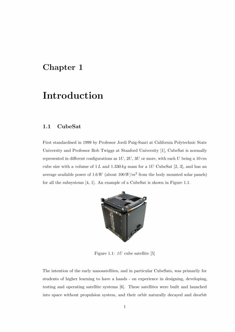
First standardised in 1999 by Professor Jordi Puig-Suari at California Polytechnic State
University and Professor Bob Twiggs at Stanford University [1], CubeSat is normally
represented in different configurations as 1𝑈 , 2𝑈 , 3𝑈 or more, with each 𝑈 being a 10 𝑐𝑚
cube size with a volume of 1𝐿 and 1.330 𝑘𝑔 mass for a 1𝑈 CubeSat [2, 3], and has an
average available power of 1.6𝑊 (about 100𝑊/𝑚2 from the body mounted solar panels)
for all the subsystems [4, 1]. An example of a CubeSat is shown in Figure 1.1.
Figure 1.1: 1U cube satellite [5]
The intention of the early nanosatellites, and in particular CubeSats, was primarily for
students of higher learning to have a hands - on experience in designing, developing,
testing and operating satellite systems [6]. These satellites were built and launched
into space without propulsion system, and their orbit naturally decayed and deorbit
1
1.1. CubeSat
into the atmosphere, and this has restricted the altitude of the nanosatellites to less
than 400 km in order to deorbit within the regulated 25 years without creating space
debris [7]. In some cases their attitude control was performed using magnetic torquers
and momentum wheels [8]. CubeSats are now becoming increasingly popular among
universities, governmental and non-governmental organisations such as European Space
Agency (ESA) [9] and National Aeronautics and Space Administration (NASA) [10], and
not just for university teaching tools, but for the purposes of earth observation, scientific
and technology demonstrations, surveillance, global positioning system navigation and
communication [11, 12]. This is due to the design, build and launch costs of these
satellites, recent changes in government policies and rapid advances in decreasing satellite
electronics size with increased capability at very low power consumption [13, 14]. The
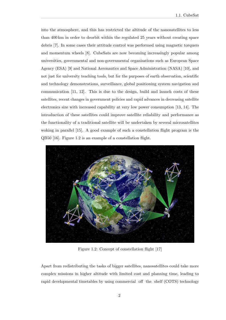
introduction of these satellites could improve satellite reliability and performance as
the functionality of a traditional satellite will be undertaken by several microsatellites
woking in parallel [15]. A good example of such a constellation flight program is the
QB50 [16]. Figure 1.2 is an example of a constellation flight.
Figure 1.2: Concept of constellation flight [17]
Apart from redistributing the tasks of bigger satellites, nanosatellites could take more
complex missions in higher altitude with limited cost and planning time, leading to
rapid developmental timetables by using commercial off the shelf (COTS) technology
2
1.1. CubeSat
[18, 15]. Limitations to this space technology development include: 1) miniaturisation of
conventional propulsion systems that would enable the spacecraft to take complex missions
in higher altitude (> 400 𝑘𝑚). This is because scaling well understood conventional
propulsion systems to the constraint size, mass, power and energy limitations of the
nanosatellites while still retaining their operation advantages and performances is difficult
and complex [12, 15, 19]; 2) the second limitation is the requirement to de-orbit the
satellite after the end of life operation, and within the 25 years regulated period to avoid
space debris.
1.1.1 CubeSats Flown with Propulsion Systems
Growing interest in CubeSats has necessitated the inclusion of micropropulsion systems
to expand their area of application. In the last decade for instance, there are only three
CubeSats that have been successfully flown with propulsion systems on board. These
include:
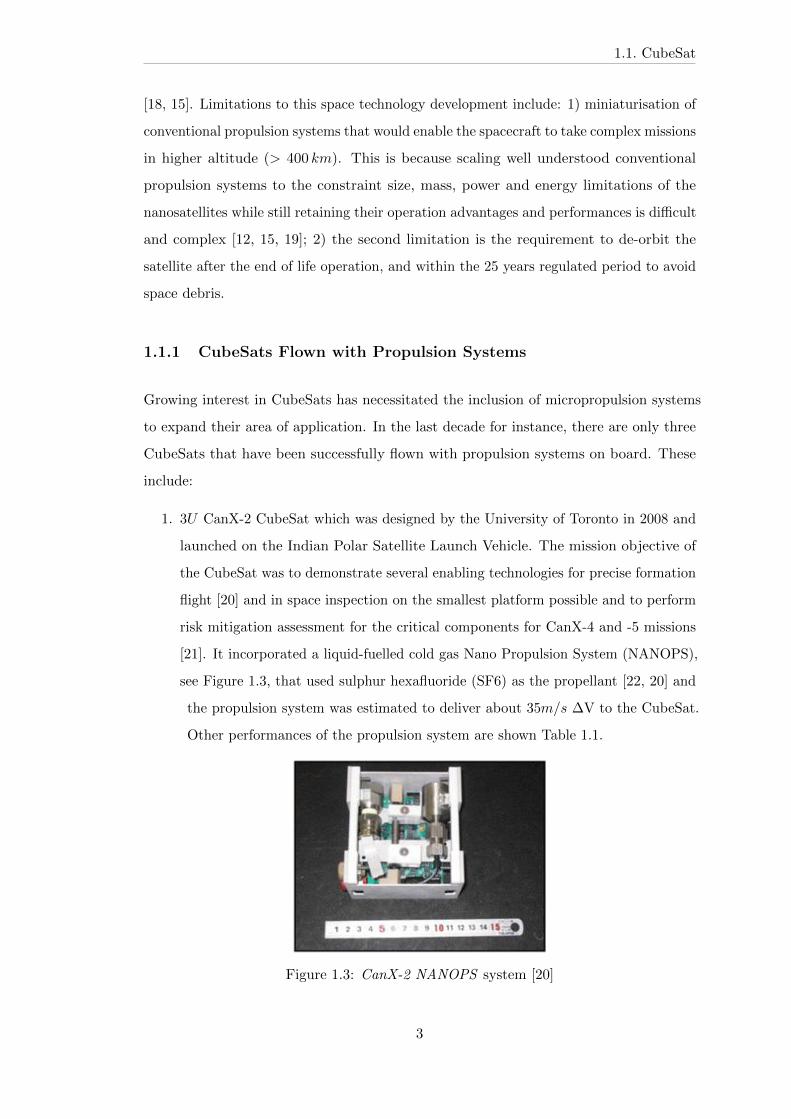
1. 3𝑈 CanX-2 CubeSat which was designed by the University of Toronto in 2008 and
launched on the Indian Polar Satellite Launch Vehicle. The mission objective of
the CubeSat was to demonstrate several enabling technologies for precise formation
flight [20] and in space inspection on the smallest platform possible and to perform
risk mitigation assessment for the critical components for CanX-4 and -5 missions
[21]. It incorporated a liquid-fuelled cold gas Nano Propulsion System (NANOPS),
see Figure 1.3, that used sulphur hexafluoride (SF6) as the propellant [22, 20] and
the propulsion system was estimated to deliver about 35𝑚/𝑠 ΔV to the CubeSat.
Other performances of the propulsion system are shown Table 1.1.
Figure 1.3: CanX-2 NANOPS system [20]
3
1.1. CubeSat
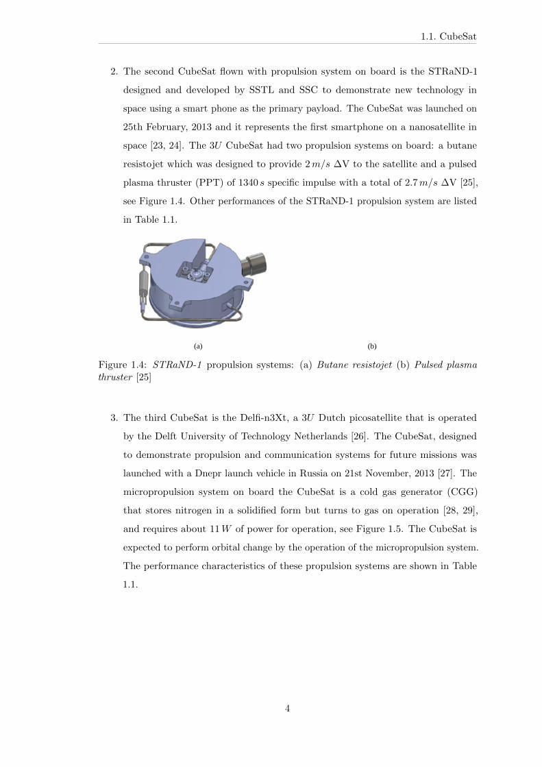
2. The second CubeSat flown with propulsion system on board is the STRaND-1
designed and developed by SSTL and SSC to demonstrate new technology in
space using a smart phone as the primary payload. The CubeSat was launched on
25th February, 2013 and it represents the first smartphone on a nanosatellite in
space [23, 24]. The 3𝑈 CubeSat had two propulsion systems on board: a butane
resistojet which was designed to provide 2𝑚/𝑠 ΔV to the satellite and a pulsed
plasma thruster (PPT) of 1340 𝑠 specific impulse with a total of 2.7𝑚/𝑠 ΔV [25],
see Figure 1.4. Other performances of the STRaND-1 propulsion system are listed
in Table 1.1.
(a) (b)
Figure 1.4: STRaND-1 propulsion systems: (a) Butane resistojet (b) Pulsed plasmathruster [25]
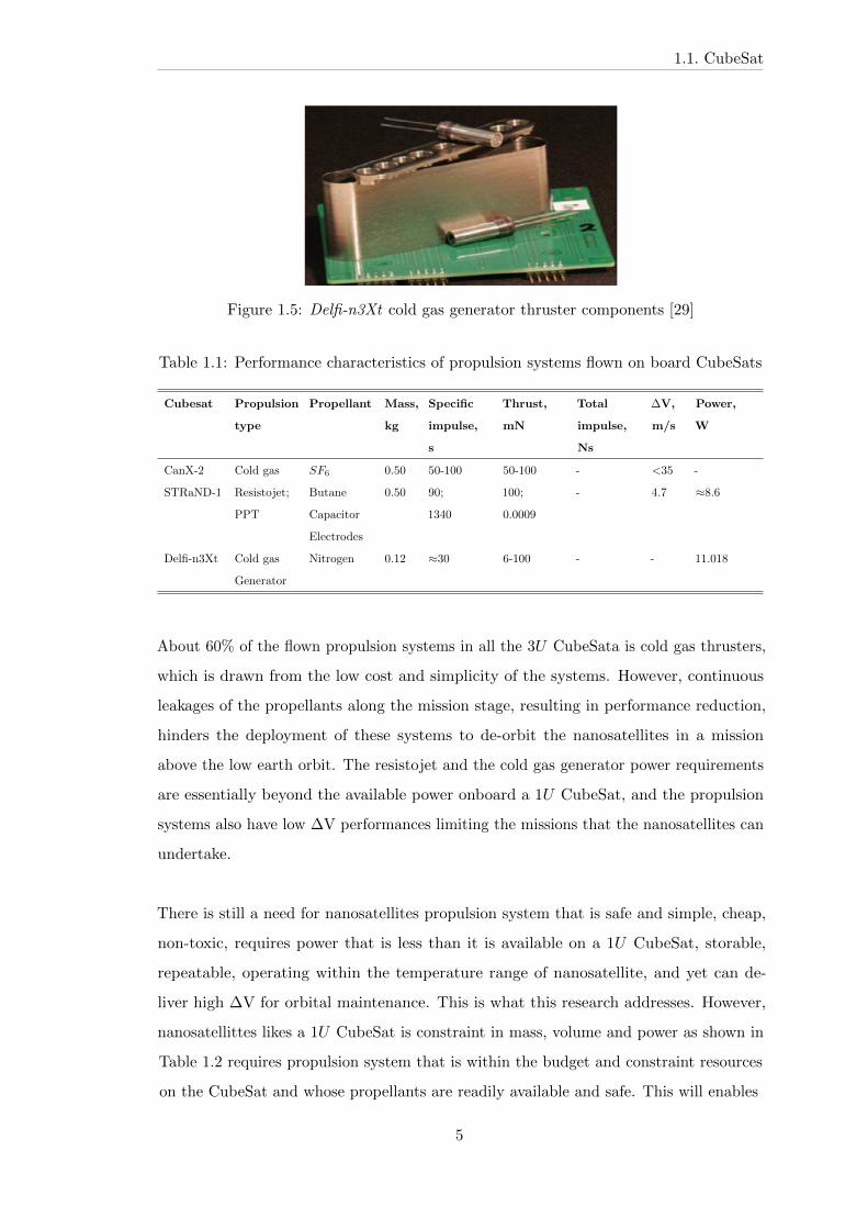
3. The third CubeSat is the Delfi-n3Xt, a 3𝑈 Dutch picosatellite that is operated
by the Delft University of Technology Netherlands [26]. The CubeSat, designed
to demonstrate propulsion and communication systems for future missions was
launched with a Dnepr launch vehicle in Russia on 21st November, 2013 [27]. The
micropropulsion system on board the CubeSat is a cold gas generator (CGG)
that stores nitrogen in a solidified form but turns to gas on operation [28, 29],
and requires about 11𝑊 of power for operation, see Figure 1.5. The CubeSat is
expected to perform orbital change by the operation of the micropropulsion system.
The performance characteristics of these propulsion systems are shown in Table
1.1.
4
1.1. CubeSat
Figure 1.5: Delfi-n3Xt cold gas generator thruster components [29]
Table 1.1: Performance characteristics of propulsion systems flown on board CubeSats
Cubesat Propulsion Propellant Mass, Specific Thrust, Total ΔV, Power,
type kg impulse, mN impulse, m/s W
s Ns
CanX-2 Cold gas 𝑆𝐹6 0.50 50-100 50-100 - <35 -
STRaND-1 Resistojet; Butane 0.50 90; 100; - 4.7 ≈8.6
PPT Capacitor 1340 0.0009
Electrodes
Delfi-n3Xt Cold gas Nitrogen 0.12 ≈30 6-100 - - 11.018
Generator
About 60% of the flown propulsion systems in all the 3𝑈 CubeSata is cold gas thrusters,
which is drawn from the low cost and simplicity of the systems. However, continuous
leakages of the propellants along the mission stage, resulting in performance reduction,
hinders the deployment of these systems to de-orbit the nanosatellites in a mission
above the low earth orbit. The resistojet and the cold gas generator power requirements
are essentially beyond the available power onboard a 1𝑈 CubeSat, and the propulsion
systems also have low ΔV performances limiting the missions that the nanosatellites can
undertake.
There is still a need for nanosatellites propulsion system that is safe and simple, cheap,
non-toxic, requires power that is less than it is available on a 1𝑈 CubeSat, storable,
repeatable, operating within the temperature range of nanosatellite, and yet can de-
liver high ΔV for orbital maintenance. This is what this research addresses. However,
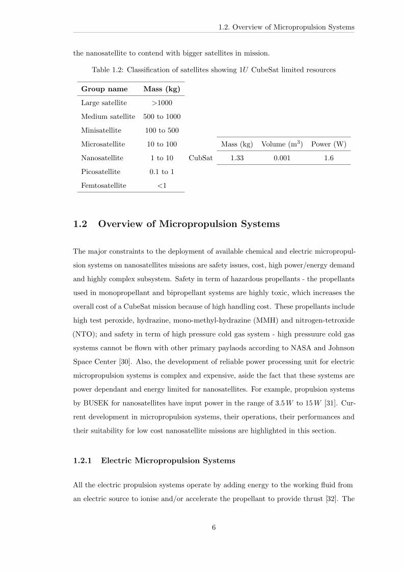
nanosatellittes likes a 1𝑈 CubeSat is constraint in mass, volume and power as shown in
Table 1.2 requires propulsion system that is within the budget and constraint resources
on the CubeSat and whose propellants are readily available and safe. This will enables
5
1.2. Overview of Micropropulsion Systems
the nanosatellite to contend with bigger satellites in mission.
Table 1.2: Classification of satellites showing 1𝑈 CubeSat limited resources
Group name Mass (kg)
Large satellite >1000
Medium satellite 500 to 1000
Minisatellite 100 to 500
Microsatellite 10 to 100 Mass (kg) Volume (m3) Power (W)
Nanosatellite 1 to 10 CubSat 1.33 0.001 1.6
Picosatellite 0.1 to 1
Femtosatellite <1
1.2 Overview of Micropropulsion Systems
The major constraints to the deployment of available chemical and electric micropropul-
sion systems on nanosatellites missions are safety issues, cost, high power/energy demand
and highly complex subsystem. Safety in term of hazardous propellants - the propellants
used in monopropellant and bipropellant systems are highly toxic, which increases the
overall cost of a CubeSat mission because of high handling cost. These propellants include
high test peroxide, hydrazine, mono-methyl-hydrazine (MMH) and nitrogen-tetroxide
(NTO); and safety in term of high pressure cold gas system - high pressuure cold gas
systems cannot be flown with other primary paylaods according to NASA and Johnson
Space Center [30]. Also, the development of reliable power processing unit for electric
micropropulsion systems is complex and expensive, aside the fact that these systems are
power dependant and energy limited for nanosatellites. For example, propulsion systems
by BUSEK for nanosatellites have input power in the range of 3.5𝑊 to 15𝑊 [31]. Cur-
rent development in micropropulsion systems, their operations, their performances and
their suitability for low cost nanosatellite missions are highlighted in this section.
1.2.1 Electric Micropropulsion Systems
All the electric propulsion systems operate by adding energy to the working fluid from
an electric source to ionise and/or accelerate the propellant to provide thrust [32]. The
6
1.2. Overview of Micropropulsion Systems
energy is processed by a subunit, which is complex to design. The generated thrust is
related to the input power by 𝐹 = 𝑃𝑖𝑛2𝜂𝑣𝑒, where 𝜂 is the power conversion efficiency
and 𝑣𝑒 is the propellant exit velocity. The thrust generated by this system is small due
to limited electric energy on-board the microsarellites. However, the thrusting time is
long with high propellant utilisation efficient with fine impulse. Electric propulsion is
further classified into electrothermal, electrostatic and electromagnetic according to the
acceleration of the propellant out of the system.
1.2.1.1 Resistojets
Resistojets are examples of electrothermal propulsion systems in which propellant is
heated through direct ohmic heating by passing it over a very hot metal element to elevate
the propellant temperature before passing it through an exhaust nozzle to generate thrust.
Resistojets use different working fluids as propellants ranging from water (𝐻2𝑂) [33],
ammonia (𝑁𝐻3), high test peroxide (𝐻𝑇𝑃 ) and hydrazine (𝑁2𝐻4) which also determine
their specific impulse and thrust performance levels [5]. Factors affecting the choice
of these propellants also include cost of propellants, ease of catalytic decomposition
and environmental and health concerns [12] For instance, a 1𝑘𝑔 of ammonia cost about
$0.31 and a 1 𝑘𝑔 of HTP cost about $0.17, whereas a 1 𝑘𝑔 of hydrazine cost about $17
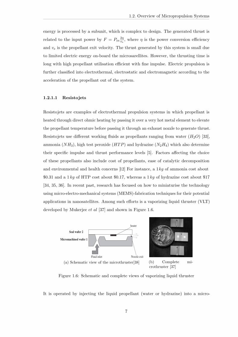
[34, 35, 36]. In recent past, research has focused on how to miniaturise the technology
using micro-electro-mechanical systems (MEMS)-fabrication techniques for their potential
applications in nanosatellites. Among such efforts is a vaporizing liquid thruster (VLT)
developed by Mukerjee 𝑒𝑡 𝑎𝑙 [37] and shown in Figure 1.6.
(a) Schematic view of the microthruster[38] (b) Complete mi-crothruster [37]
Figure 1.6: Schematic and complete views of vaporizing liquid thruster
It is operated by injecting the liquid propellant (water or hydrazine) into a micro-
7

1.2. Overview of Micropropulsion Systems
machined micro-chamber containing silicon heaters where it is vaporises and passes
through a micro-silicon nozzle to produce thrust. They have recorded an initial thrust
performance of 0.15𝑚𝑁 to 0.46𝑚𝑁 at an operating power of 5𝑊 to 10.8𝑊 with a
propellant input flow rate of about 0.09 𝑐𝑐/𝑠. A similar design was investigated by
Mueller 𝑒𝑡 𝑎𝑙 [39] at the NASA’s Jet Propulsion Laboratory (JPL). They used water as
the working fluid but at a heating power of 2𝑊 . Even at this power level, the thrust
value ranges between 50-280𝜇𝑁 with a thrust/power ratio of 200𝜇𝑁/𝑊 and at a specific
impulse of about 100 𝑠 while operating at low feed pressure.
Complementary metal oxide semiconductor (CMOS) resistojet from Janson at the
Aerospace Corporation, California [40] is another effort of making electro-thermal system
through batch-fabrication of MEMS. The heating element is provided by a polysilicon
layer sandwiched between 2 patterned passivation layers, which normally acts as gate
structure in a CMOS transistor [41]. After many iterations of development, they devel-
oped a 3-Watt CMOS microresistojet that incorporates a flow sensor and low resistance
power transistor as shown in Figure 1.7.
Resistojet 3
Flow RateMonitor
PowerTransistor
Poly Heater
Inlet
Plenum
Nozzle
TOPHALF:
BOTTOMHALF:
Pads
Figure 1.7: 3-Watt CMOS resistojet on a 2-micron TinyChip die layout [40]
Performance for the CMOS resistojet in literature was reported by Maurya 𝑒𝑡 𝑎𝑙 [42] where
they demonstrated thrust range of 5-120𝜇𝑁 at a heating power of 1-2.4𝑊 . Free-Molecule
Micro-Resistojet (FMMR) is another MEMS-based resistojet developed by Ketsdever 𝑒𝑡
𝑎𝑙 [43] at the Air Force Research Laboratory, California. The principle of operation is
similar to that of CMOS resistojet but has offered a higher thrust performance of near
0.25𝑚𝑁 at a specific impulse of almost 45 𝑠 when operated at a stagnation temperature
8
1.2. Overview of Micropropulsion Systems
of 600𝐾 using argon propellant. The major advantage of the MEMS-based resistojet
is their small size and weight, scalability ability with a very precise thrust impulse.
However, the power processing unit is complex and expensive for nanosatellites.
1.2.1.2 Arcjets
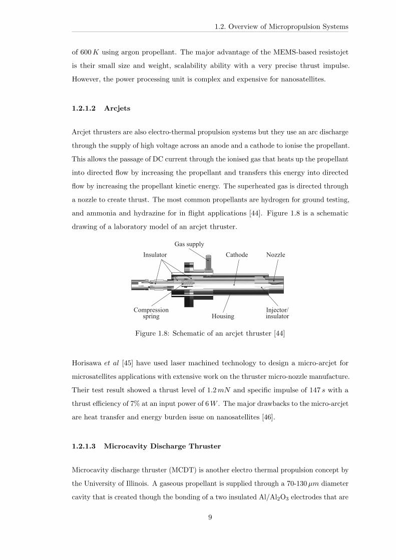
Arcjet thrusters are also electro-thermal propulsion systems but they use an arc discharge
through the supply of high voltage across an anode and a cathode to ionise the propellant.
This allows the passage of DC current through the ionised gas that heats up the propellant
into directed flow by increasing the propellant and transfers this energy into directed
flow by increasing the propellant kinetic energy. The superheated gas is directed through
a nozzle to create thrust. The most common propellants are hydrogen for ground testing,
and ammonia and hydrazine for in flight applications [44]. Figure 1.8 is a schematic
drawing of a laboratory model of an arcjet thruster.
Figure 1.8: Schematic of an arcjet thruster [44]
Horisawa 𝑒𝑡 𝑎𝑙 [45] have used laser machined technology to design a micro-arcjet for
microsatellites applications with extensive work on the thruster micro-nozzle manufacture.
Their test result showed a thrust level of 1.2𝑚𝑁 and specific impulse of 147 𝑠 with a
thrust efficiency of 7% at an input power of 6𝑊 . The major drawbacks to the micro-arcjet
are heat transfer and energy burden issue on nanosatellites [46].
1.2.1.3 Microcavity Discharge Thruster
Microcavity discharge thruster (MCDT) is another electro thermal propulsion concept by
the University of Illinois. A gaseous propellant is supplied through a 70-130𝜇𝑚 diameter
cavity that is created though the bonding of a two insulated Al/Al2O3 electrodes that are
9
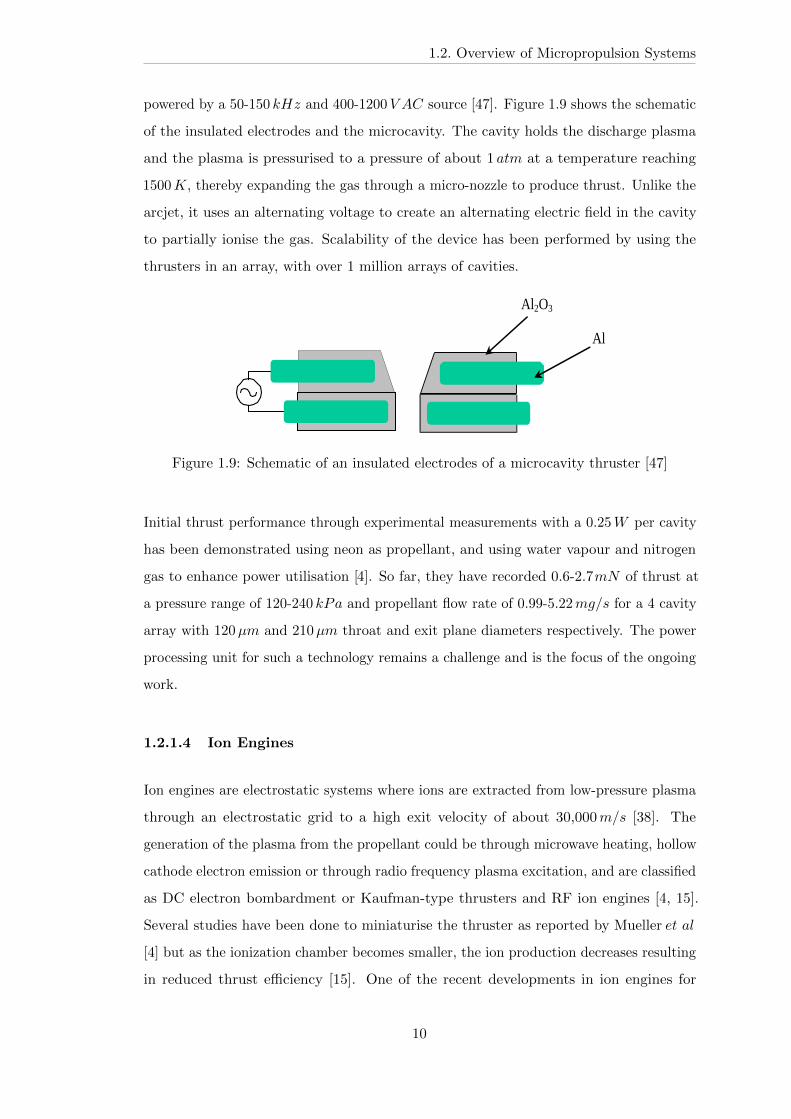
1.2. Overview of Micropropulsion Systems
powered by a 50-150 𝑘𝐻𝑧 and 400-1200𝑉 𝐴𝐶 source [47]. Figure 1.9 shows the schematic
of the insulated electrodes and the microcavity. The cavity holds the discharge plasma
and the plasma is pressurised to a pressure of about 1 𝑎𝑡𝑚 at a temperature reaching
1500𝐾, thereby expanding the gas through a micro-nozzle to produce thrust. Unlike the
arcjet, it uses an alternating voltage to create an alternating electric field in the cavity
to partially ionise the gas. Scalability of the device has been performed by using the
thrusters in an array, with over 1 million arrays of cavities.
Al2O3
Al
Figure 1.9: Schematic of an insulated electrodes of a microcavity thruster [47]
Initial thrust performance through experimental measurements with a 0.25𝑊 per cavity
has been demonstrated using neon as propellant, and using water vapour and nitrogen
gas to enhance power utilisation [4]. So far, they have recorded 0.6-2.7𝑚𝑁 of thrust at
a pressure range of 120-240 𝑘𝑃𝑎 and propellant flow rate of 0.99-5.22𝑚𝑔/𝑠 for a 4 cavity
array with 120𝜇𝑚 and 210𝜇𝑚 throat and exit plane diameters respectively. The power
processing unit for such a technology remains a challenge and is the focus of the ongoing
work.
1.2.1.4 Ion Engines
Ion engines are electrostatic systems where ions are extracted from low-pressure plasma
through an electrostatic grid to a high exit velocity of about 30,000𝑚/𝑠 [38]. The
generation of the plasma from the propellant could be through microwave heating, hollow
cathode electron emission or through radio frequency plasma excitation, and are classified
as DC electron bombardment or Kaufman-type thrusters and RF ion engines [4, 15].
Several studies have been done to miniaturise the thruster as reported by Mueller 𝑒𝑡 𝑎𝑙
[4] but as the ionization chamber becomes smaller, the ion production decreases resulting
in reduced thrust efficiency [15]. One of the recent developments in ion engines for
10
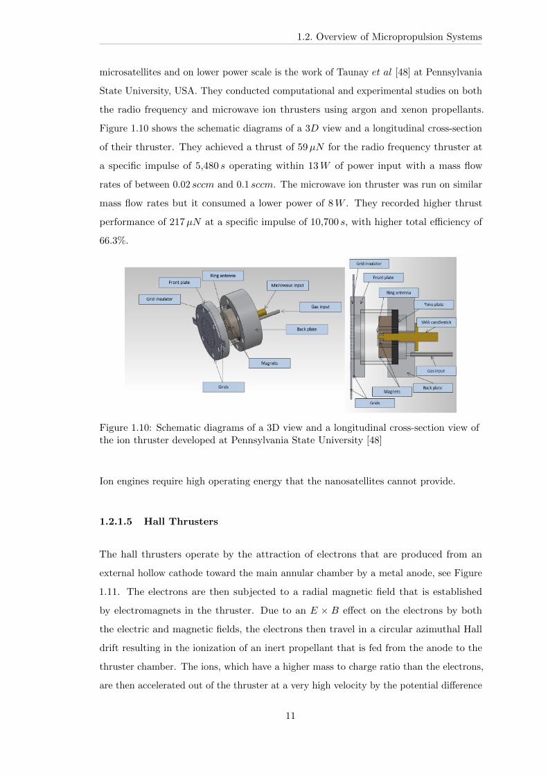
1.2. Overview of Micropropulsion Systems
microsatellites and on lower power scale is the work of Taunay 𝑒𝑡 𝑎𝑙 [48] at Pennsylvania
State University, USA. They conducted computational and experimental studies on both
the radio frequency and microwave ion thrusters using argon and xenon propellants.
Figure 1.10 shows the schematic diagrams of a 3𝐷 view and a longitudinal cross-section
of their thruster. They achieved a thrust of 59𝜇𝑁 for the radio frequency thruster at
a specific impulse of 5,480 𝑠 operating within 13𝑊 of power input with a mass flow
rates of between 0.02 𝑠𝑐𝑐𝑚 and 0.1 𝑠𝑐𝑐𝑚. The microwave ion thruster was run on similar
mass flow rates but it consumed a lower power of 8𝑊 . They recorded higher thrust
performance of 217𝜇𝑁 at a specific impulse of 10,700 𝑠, with higher total efficiency of
66.3%.
Figure 1.10: Schematic diagrams of a 3D view and a longitudinal cross-section view ofthe ion thruster developed at Pennsylvania State University [48]
Ion engines require high operating energy that the nanosatellites cannot provide.
1.2.1.5 Hall Thrusters
The hall thrusters operate by the attraction of electrons that are produced from an
external hollow cathode toward the main annular chamber by a metal anode, see Figure
1.11. The electrons are then subjected to a radial magnetic field that is established
by electromagnets in the thruster. Due to an 𝐸 × 𝐵 effect on the electrons by both
the electric and magnetic fields, the electrons then travel in a circular azimuthal Hall
drift resulting in the ionization of an inert propellant that is fed from the anode to the
thruster chamber. The ions, which have a higher mass to charge ratio than the electrons,
are then accelerated out of the thruster at a very high velocity by the potential difference
11

1.2. Overview of Micropropulsion Systems
across the magnetic field to produce thrust. There are two main types of hall thrusters:
stationary plasma thruster (SPT) and thruster with anode layer (TAL), with their major
difference in the construction materials of their channels [15]. While the SPT is made of
boron nitride walls, the TAL is made of stainless steel with a resultant effect in secondary
electron emission (SEE) [49].
Figure 1.11: Schematic diagram of an SPT Hall thruster, showing the electrodes and theradial magnetic field [49]
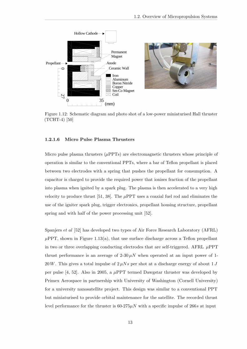
A novel cylindrical-type and lower-power miniaturised Hall thruster operating at an
input power of about 10𝑊 is the one developed by Ikeda 𝑒𝑡 𝑎𝑙 [50] at the Osaka Institute
of Technology, Japan. Tagged TCHT-4, as shown in Figure 1.12, the thruster was born
after some iteration of previous series of TCHT to improve the power utilisation. They
indicated thrust performance of up to 7.3𝑚𝑁 and a specific impulse of 940 𝑠 at an input
power of 10𝑊 , power which is high above the typical power rating of nanosatellite.
12
1.2. Overview of Micropropulsion Systems
W [2][3]. Detailed effects of magnetic fieldcylindrical Hall thrusters are unknown,
ch important to improve thrust performance.tigated the effects with the cylindrical Hall
d TCHT series in Osaka Institute ofdischarge chamber consists of only a circular
art with no coaxial parts. Although cylindricalde by Raitses and Smirnov have short coaxialpart was excluded from TCHT-series. Byradial magnetic field at the downstream
ruster TCHT-3B achieved higher thrustn TCHT-3A did at low power level because ofll losses[4]-[10]. However, when the position
( )
Figure 1. Cross-sectional view of TCHT-4.
Figure 2. Photo of TCHT-4.
Ceramic Wall
PermanentMagnet
Anode
(mm)
Hollow Cathode
Propellant
CoilSm-Co MagnetCopperBoron NitrideAluminumIron
27
35
0
0
Figure 1.12: Schematic diagram and photo shot of a low-power miniaturised Hall thruster(TCHT-4) [50]
1.2.1.6 Micro Pulse Plasma Thrusters
Micro pulse plasma thrusters (𝜇PPTs) are electromagnetic thrusters whose principle of
operation is similar to the conventional PPTs, where a bar of Teflon propellant is placed
between two electrodes with a spring that pushes the propellant for consumption. A
capacitor is charged to provide the required power that ionises fraction of the propellant
into plasma when ignited by a spark plug. The plasma is then accelerated to a very high
velocity to produce thrust [51, 38]. The 𝜇PPT uses a coaxial fuel rod and eliminates the
use of the igniter spark plug, trigger electronics, propellant housing structure, propellant
spring and with half of the power processing unit [52].
Spanjers 𝑒𝑡 𝑎𝑙 [52] has developed two types of Air Force Research Laboratory (AFRL)
𝜇PPT, shown in Figure 1.13(a), that use surface discharge across a Teflon propellant
in two or three overlapping conducting electrodes that are self-triggered. AFRL 𝜇PPT
thrust performance is an average of 2-30𝜇𝑁 when operated at an input power of 1-
20𝑊 . This gives a total impulse of 2𝜇𝑁𝑠 per shot at a discharge energy of about 1 𝐽
per pulse [4, 52]. Also in 2005, a 𝜇PPT termed Dawgstar thruster was developed by
Primex Aerospace in partnership with University of Washington (Cornell University)
for a university nanosatellite project. This design was similar to a conventional PPT
but miniaturised to provide orbital maintenance for the satellite. The recorded thrust
level performance for the thruster is 60-275𝜇𝑁 with a specific impulse of 266𝑠 at input
13
1.2. Overview of Micropropulsion Systems
power of 15.6-36𝑊 depending on charging rate and thrust frequencies [53]. Another
𝜇PPT, Figure 1.13(b), is being investigated in the UK by a collaboration between the
University of Southampton, Mars Space Ltd and Clyde Space Ltd. The main objective
of the project is to double the life span of a CubeSat when launched into LEO orbits of
altitude 600-650 𝑘𝑚 when included in its design [54]. Though their system has shown
a satisfactory results with a specific impulse of 640 𝑠 and a thruster mass of 500 𝑔, the
operating power for a single thrust unit is 10𝑊 [55].
(a) Schematic of an AFRL 3-electrode𝜇PPT concept [52]
(b) Assembled breech-fed 𝜇PPT[55]
Figure 1.13: 𝜇PPT for concepts for microsatellites
The major advantages of 𝜇PPT are their simplicity in design, high reliability, and
durability, but create electromagnetic interference for other payloads and high voltage
operation have so far limited their application [56].
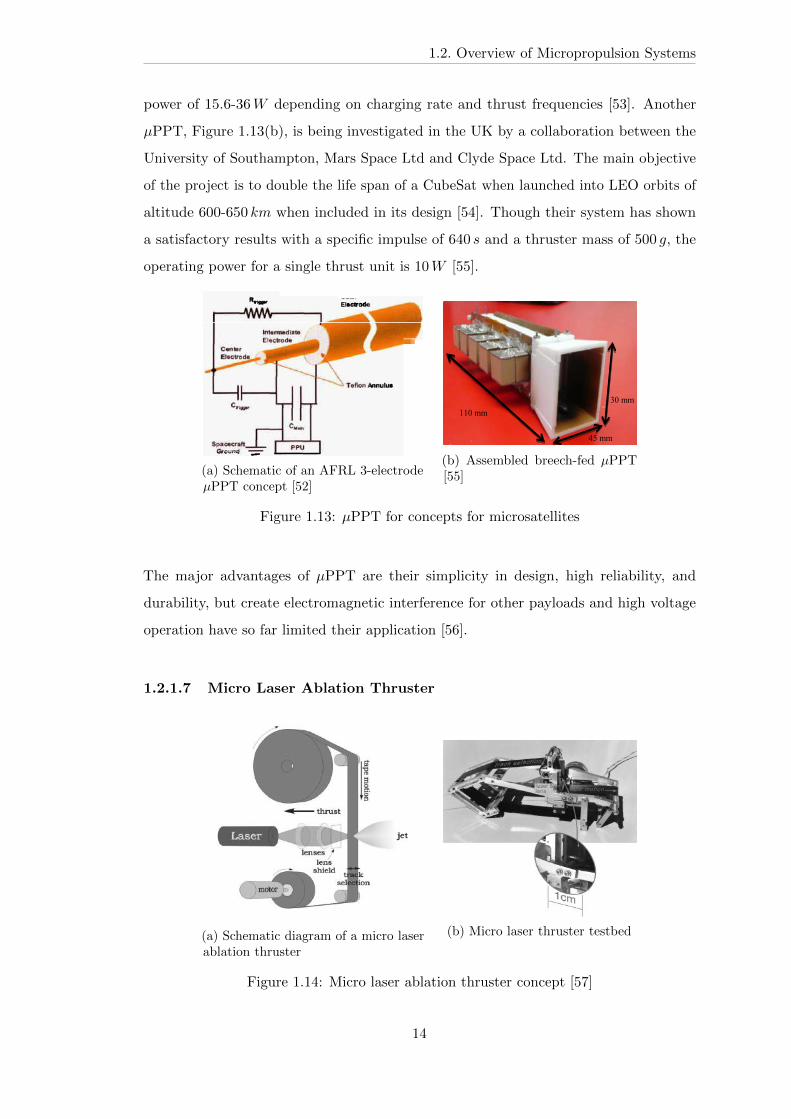
1.2.1.7 Micro Laser Ablation Thruster
(a) Schematic diagram of a micro laserablation thruster
(b) Micro laser thruster testbed
Figure 1.14: Micro laser ablation thruster concept [57]
14
1.2. Overview of Micropropulsion Systems
The micro laser ablation thruster, also known as micro laser plasma thruster, uses laser
diode technology [57] to produce thrust from an ablation target. Figure 1.14 shows the
operation principle of a micro laser ablation thruster and the thruster testbed. Lenses
are used to focus the diodes laser beams on the ablation target (a two-layer fuel tape)
with a transparent supporting layer upon which the laser light passes to produce a very
small jets of plasma that results in thrust by igniting an absorbing fuel layer [ 58]. The
operation of the motor provides a successive layer of the tape for the laser light for
ablation. Performance characteristic of the device indicated a thrust of 680𝜇𝑁 at a
specific impulse of about 400 𝑠 when operating with an optical power of 2.1𝑊 and 15𝑊
peak power of laser diode at a tape lifetime of 140ℎ [57]. It’s potential application is
in the area of precise attitude control in constellation for high accuracy interferometer
mission like the Evolved Laser Interferometer Space Antenna (eLISA) [59]. However, it
requires a complex and high input power for its operation.
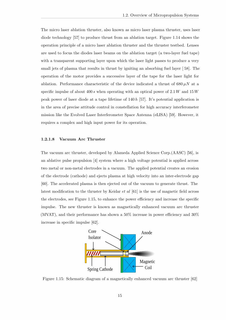
1.2.1.8 Vacuum Arc Thruster
The vacuum arc thruster, developed by Alameda Applied Science Corp.(AASC) [56], is
an ablative pulse propulsion [4] system where a high voltage potential is applied across
two metal or non-metal electrodes in a vacuum. The applied potential creates an erosion
of the electrode (cathode) and ejects plasma at high velocity into an inter-electrode gap
[60]. The accelerated plasma is then ejected out of the vacuum to generate thrust. The
latest modification to the thruster by Keidar 𝑒𝑡 𝑎𝑙 [61] is the use of magnetic field across
the electrodes, see Figure 1.15, to enhance the power efficiency and increase the specific
impulse. The new thruster is known as magnetically enhanced vacuum arc thruster
(MVAT), and their performance has shown a 50% increase in power efficiency and 30%
increase in specific impulse [62].
CoreIsolator
Anode
Magnetic CoilSpring Cathode
Figure 1.15: Schematic diagram of a magnetically enhanced vacuum arc thruster [62]
15
1.2. Overview of Micropropulsion Systems
Four micro vacuum arc thrusters were developed for the University of Illinois 2-cube
CubeSat-Illinois Observation Nanosatellite (ION), using a 150 𝑔 and 12-24𝑉 power
processing unit (PPU) that was designed and built by AASC [63]. The specific impulse
of the VAT was 3000𝑠 and its thrust to power ratio was about 10𝜇𝑁/𝑊 with an input
power ranging from 1-100𝑊 , depending on the required thrust. The satellite, which
was lost due to the failure of the launch vehicle in 2006, could not get to test the 2-axis
control and orbit translation abilities of the microVATs on board. The low thrust to
power ratio of VAT put a high power demand burden on nanosatellites for operations
involving large ΔV, with a limit on the thrust performance, even with the advantage of
high specific impulse.
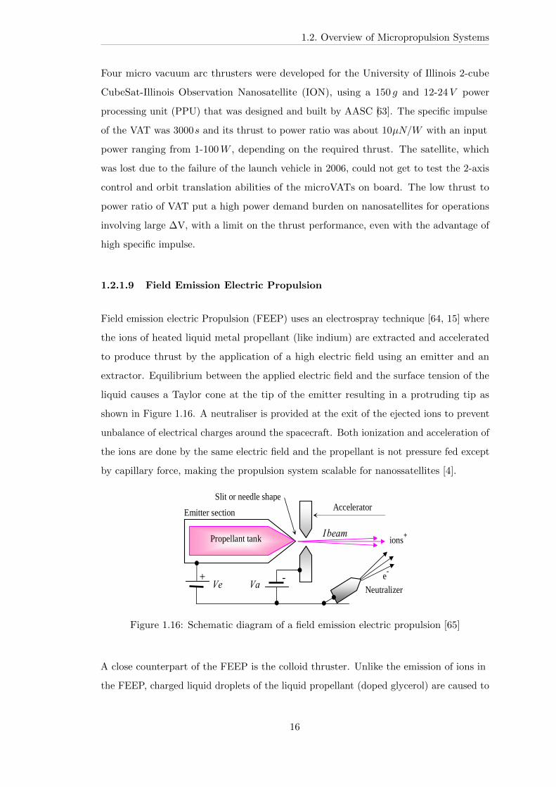
1.2.1.9 Field Emission Electric Propulsion
Field emission electric Propulsion (FEEP) uses an electrospray technique [64, 15] where
the ions of heated liquid metal propellant (like indium) are extracted and accelerated
to produce thrust by the application of a high electric field using an emitter and an
extractor. Equilibrium between the applied electric field and the surface tension of the
liquid causes a Taylor cone at the tip of the emitter resulting in a protruding tip as
shown in Figure 1.16. A neutraliser is provided at the exit of the ejected ions to prevent
unbalance of electrical charges around the spacecraft. Both ionization and acceleration of
the ions are done by the same electric field and the propellant is not pressure fed except
by capillary force, making the propulsion system scalable for nanossatellites [4].
ions+
Emitter section
Slit or needle shape
Ve Va
Ibeam
Accelerator
Propellant tank
+ - e-
Neutralizer
Figure 1.16: Schematic diagram of a field emission electric propulsion [65]
A close counterpart of the FEEP is the colloid thruster. Unlike the emission of ions in
the FEEP, charged liquid droplets of the liquid propellant (doped glycerol) are caused to
16
1.2. Overview of Micropropulsion Systems
break away due to the strong electric field across the electrodes [15]. Recent development
on the electrospray technology for a low power FEEP microthruster is the FT-150 FEEP
designed for LISA Pathfinder mission. The collaboration is between Astrium Space
Transportation in France and Austrian Research Centre and the thruster was to provide
fine positioning and attitude control on 𝜇N thrust range. The last iteration of the project
at ALTA SpA, Italy showed a thrust performance of 0.1-150 𝜇𝑁 and a specific impulse
range of 3000-4500 𝑠 at an input power of 6𝑊 [66]. Though the FEEP system is boastful
of high specific impulse, the thrust to power ratio is very low and it requires high energy
for orbital maintenance.
1.2.2 Chemical Micropropulsion Systems
In chemical propulsion systems, thrust is generated through thermodynamics using the
stored chemical energy in the propellants, and accelerating the ejected stream of gaseous
products through a converging and diverging nozzle to produce thrust. The generated
thrust, 𝐹 , is proportional to the product of the propellant mass flow rate, and the
exit velocity, 𝑣𝑒. That is, 𝐹 = 𝑝𝑣𝑒, and depending on the enthalpy and the pressure of
the chemical reaction, the thrust value can be moderate to high and occurring within a
short time. Chemical propulsion systems have flight heritage for attitude control and
orbital raising involving low to moderate ΔV requirements with a thrust-to-weight ratio
of 0.1− 0.3 [12] especially suitable for rapid orbital manoeuvres for traditional satellites.
However, their applications on nanosatellites missions have performance, safety, thermal
control and scaling concern issues that will be highlighted in this section. They are
classified into cold gas and hot gas propulsion systems based on the exhaust gas from the
nozzle. The propellant could be gaseous, liquid, solid or a combination of these.
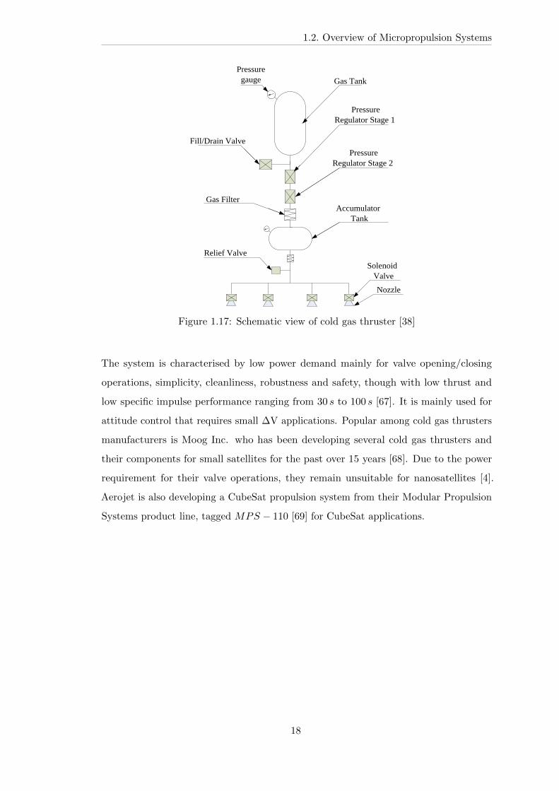
1.2.2.1 Cold Gas Thruster
In a cold gas system, gas from a high-pressure tank, vaporised liquid or solidified gas is
vented through a valve and nozzle to produce thrust. Figure 1.17 shows the schematic
description of a cold gas thruster with a detailed view of the component parts.
17
1.2. Overview of Micropropulsion Systems
Pressure gauge Gas Tank
PressureRegulator Stage 1
Fill/Drain Valve
Gas Filter
Relief Valve
PressureRegulator Stage 2
Accumulator Tank
Solenoid Valve
Nozzle
Figure 1.17: Schematic view of cold gas thruster [38]
The system is characterised by low power demand mainly for valve opening/closing
operations, simplicity, cleanliness, robustness and safety, though with low thrust and
low specific impulse performance ranging from 30 𝑠 to 100 𝑠 [67]. It is mainly used for
attitude control that requires small ΔV applications. Popular among cold gas thrusters
manufacturers is Moog Inc. who has been developing several cold gas thrusters and
their components for small satellites for the past over 15 years [68]. Due to the power
requirement for their valve operations, they remain unsuitable for nanosatellites [4].
Aerojet is also developing a CubeSat propulsion system from their Modular Propulsion
Systems product line, tagged 𝑀𝑃𝑆 − 110 [69] for CubeSat applications.
18
1.2. Overview of Micropropulsion Systems
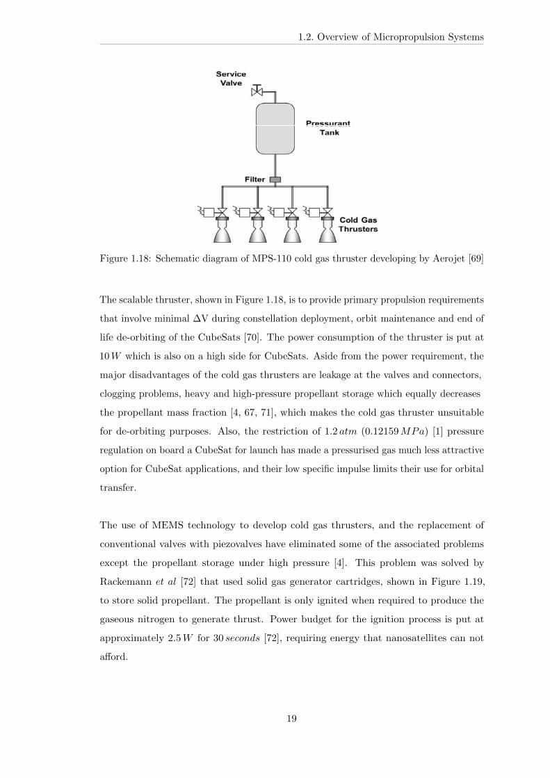
Figure 1.18: Schematic diagram of MPS-110 cold gas thruster developing by Aerojet [69]
The scalable thruster, shown in Figure 1.18, is to provide primary propulsion requirements
that involve minimal ΔV during constellation deployment, orbit maintenance and end of
life de-orbiting of the CubeSats [70]. The power consumption of the thruster is put at
10𝑊 which is also on a high side for CubeSats. Aside from the power requirement, the
major disadvantages of the cold gas thrusters are leakage at the valves and connectors,
clogging problems, heavy and high-pressure propellant storage which equally decreases
the propellant mass fraction [4, 67, 71], which makes the cold gas thruster unsuitable
for de-orbiting purposes. Also, the restriction of 1.2 𝑎𝑡𝑚 (0.12159𝑀𝑃𝑎) [1] pressure
regulation on board a CubeSat for launch has made a pressurised gas much less attractive
option for CubeSat applications, and their low specific impulse limits their use for orbital
transfer.
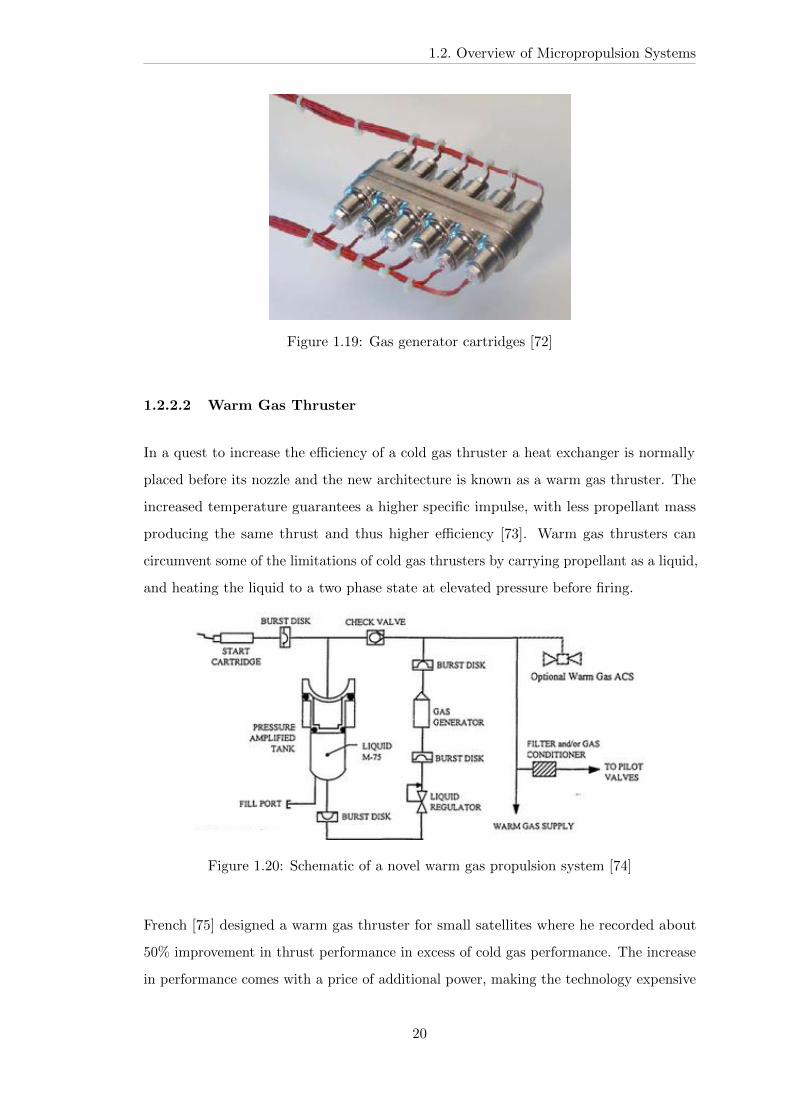
The use of MEMS technology to develop cold gas thrusters, and the replacement of
conventional valves with piezovalves have eliminated some of the associated problems
except the propellant storage under high pressure [4]. This problem was solved by
Rackemann 𝑒𝑡 𝑎𝑙 [72] that used solid gas generator cartridges, shown in Figure 1.19,
to store solid propellant. The propellant is only ignited when required to produce the
gaseous nitrogen to generate thrust. Power budget for the ignition process is put at
approximately 2.5𝑊 for 30 𝑠𝑒𝑐𝑜𝑛𝑑𝑠 [72], requiring energy that nanosatellites can not
afford.
19
1.2. Overview of Micropropulsion Systems
Figure 1.19: Gas generator cartridges [72]
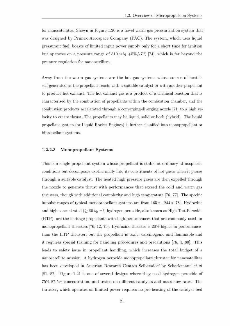
1.2.2.2 Warm Gas Thruster
In a quest to increase the efficiency of a cold gas thruster a heat exchanger is normally
placed before its nozzle and the new architecture is known as a warm gas thruster. The
increased temperature guarantees a higher specific impulse, with less propellant mass
producing the same thrust and thus higher efficiency [73]. Warm gas thrusters can
circumvent some of the limitations of cold gas thrusters by carrying propellant as a liquid,
and heating the liquid to a two phase state at elevated pressure before firing.
Figure 1.20: Schematic of a novel warm gas propulsion system [74]
French [75] designed a warm gas thruster for small satellites where he recorded about
50% improvement in thrust performance in excess of cold gas performance. The increase
in performance comes with a price of additional power, making the technology expensive
20
1.2. Overview of Micropropulsion Systems
for nanosatellites. Shown in Figure 1.20 is a novel warm gas pressurization system that
was designed by Primex Aerospace Company (PAC). The system, which uses liquid
pressurant fuel, boasts of limited input power supply only for a short time for ignition
but operates on a pressure range of 810 𝑝𝑠𝑖𝑔 +5%/-7% [74], which is far beyond the
pressure regulation for nanosatellites.
Away from the warm gas systems are the hot gas systems whose source of heat is
self-generated as the propellant reacts with a suitable catalyst or with another propellant
to produce hot exhaust. The hot exhaust gas is a product of a chemical reaction that is
characterised by the combustion of propellants within the combustion chamber, and the
combustion products accelerated through a converging-diverging nozzle [71] to a high ve-
locity to create thrust. The propellants may be liquid, solid or both (hybrid). The liquid
propellant system (or Liquid Rocket Engines) is further classified into monopropellant or
bipropellant systems.
1.2.2.3 Monopropellant Systems
This is a single propellant system whose propellant is stable at ordinary atmospheric
conditions but decomposes exothermally into its constituents of hot gases when it passes
through a suitable catalyst. The heated high pressure gases are then expelled through
the nozzle to generate thrust with performances that exceed the cold and warm gas
thrusters, though with additional complexity and high temperature [76, 77]. The specific
impulse ranges of typical monopropellant systems are from 165 𝑠 - 244 𝑠 [78]. Hydrazine
and high concentrated (≥ 80 𝑏𝑦 𝑤𝑡) hydrogen peroxide, also known as High Test Peroxide
(HTP), are the heritage propellants with high performances that are commonly used for
monopropellant thrusters [76, 12, 79]. Hydrazine thruster is 20% higher in performance
than the HTP thruster, but the propellant is toxic, carcinogenic and flammable and
it requires special training for handling procedures and precautions [76, 4, 80]. This
leads to safety issue in propellant handling, which increases the total budget of a
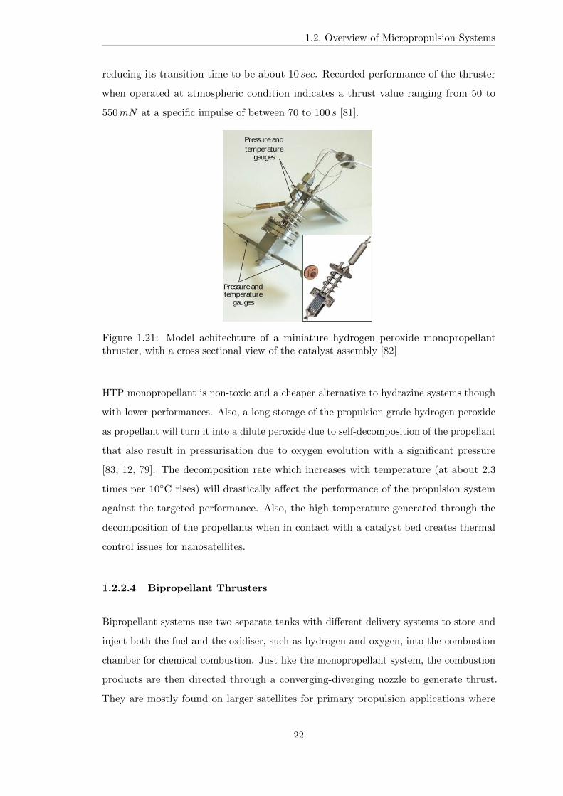
nanosatellite mission. A hydrogen peroxide monopropellant thruster for nanosatellites
has been developed in Austrian Research Centres Seibersdorf by Scharlemann 𝑒𝑡 𝑎𝑙
[81, 82]. Figure 1.21 is one of several designs where they used hydrogen peroxide of
75%-87.5% concentration, and tested on different catalysts and mass flow rates. The
thruster, which operates on limited power requires no pre-heating of the catalyst bed
21
1.2. Overview of Micropropulsion Systems
reducing its transition time to be about 10 𝑠𝑒𝑐. Recorded performance of the thruster
when operated at atmospheric condition indicates a thrust value ranging from 50 to
550𝑚𝑁 at a specific impulse of between 70 to 100 𝑠 [81].
Pressure andtemperature
gauges
Pressure andtemperature
gauges
Figure 1.21: Model achitechture of a miniature hydrogen peroxide monopropellantthruster, with a cross sectional view of the catalyst assembly [82]
HTP monopropellant is non-toxic and a cheaper alternative to hydrazine systems though
with lower performances. Also, a long storage of the propulsion grade hydrogen peroxide
as propellant will turn it into a dilute peroxide due to self-decomposition of the propellant
that also result in pressurisation due to oxygen evolution with a significant pressure
[83, 12, 79]. The decomposition rate which increases with temperature (at about 2.3
times per 10∘C rises) will drastically affect the performance of the propulsion system
against the targeted performance. Also, the high temperature generated through the
decomposition of the propellants when in contact with a catalyst bed creates thermal
control issues for nanosatellites.
1.2.2.4 Bipropellant Thrusters
Bipropellant systems use two separate tanks with different delivery systems to store and
inject both the fuel and the oxidiser, such as hydrogen and oxygen, into the combustion
chamber for chemical combustion. Just like the monopropellant system, the combustion
products are then directed through a converging-diverging nozzle to generate thrust.
They are mostly found on larger satellites for primary propulsion applications where
22

1.2. Overview of Micropropulsion Systems
high impulse thrust is required, with monomethyl hydrazine/nitrogen tetroxide thruster
being the most common choice for in-space propulsion [84], though with high toxicity
levels [82]. These propellants raise safety concern and cost on their applications on
nanosatellites. Bipropellant systems typically generate higher levels of thrust than what
is normally required for nanosatellites. But in recent years, MIT has developed micro
bipropellant engine from a stack of silicon wafers using MEMS-based technology [85] as
shown in Figure 1.22. The thruster system measuring 18𝑚𝑚× 13.5𝑚𝑚× 3𝑚𝑚 is an
integration of combustion chamber, turbine pumps, inlet valve and the nozzle [ 4]. The
high-pressure thruster has demonstrated 1𝑁 of thrust with a thrust power of 750𝑊
and at a chamber pressure of 12 𝑎𝑡𝑚. Bipropellant systems are generally complex for a
nanosatellite mission.
UN
CO
RR
Figure 1.22: Micro-bipropellant thruster from MIT [85]
1.2.2.5 Solid Rocket Motor
Solid rocket motors use a solid propellant mixture called grain for a one shot combustion.
The propellant, which contains both the fuel and oxidiser is stored in the combustion
chamber, and the hot gas from the combustion is accelerated through a hollow cavity
within the grain once the grain is ignited to generate thrust [12, 71]. The major advantages
of solid rocket motors over the liquid rocket engines are their simplicity, storability and
the size of volume the propellant occupies by the same propellant mass. However, there
is yet no mechanism to stop the burning once ignited. In view of this setback, engineers
in Laboratory for Analysis and Architecture of Systems (LAAS CNRS) in France came
up with the concept of solid propellant thruster (SPT) in 1997 [86]. Though the principle
of operation is still on a one shot basis for a high rate of combustion, several arrays of
23
1.2. Overview of Micropropulsion Systems
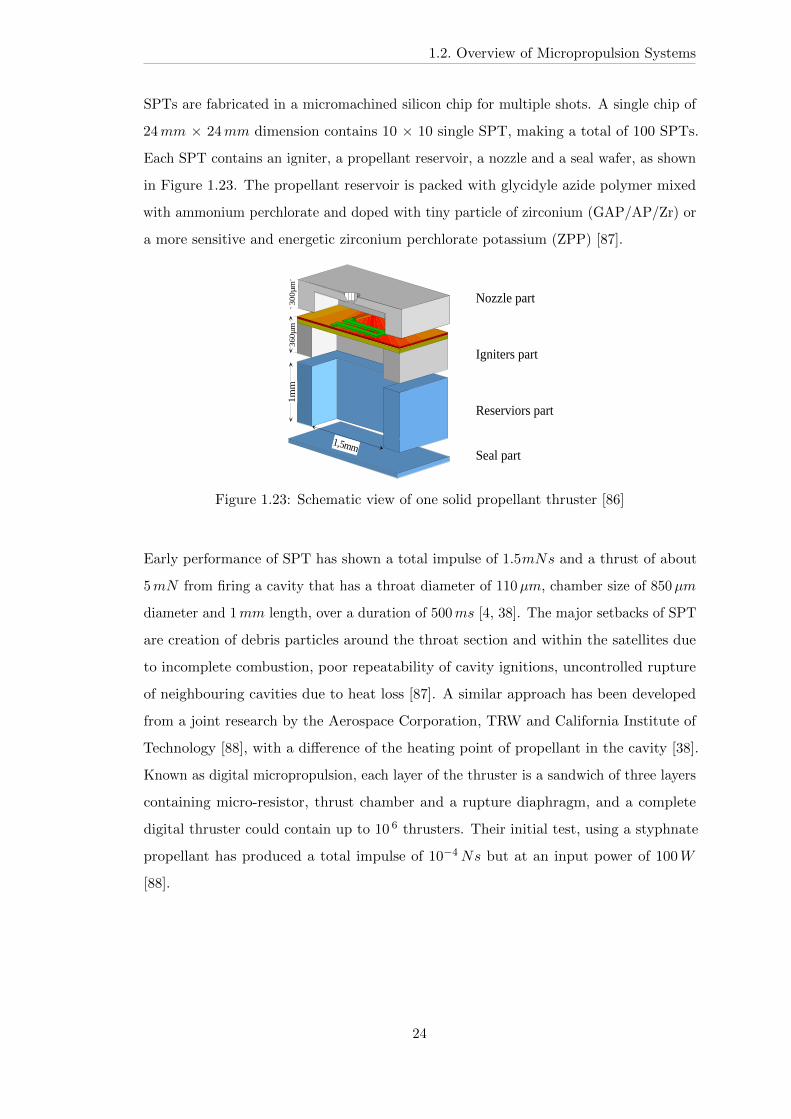
SPTs are fabricated in a micromachined silicon chip for multiple shots. A single chip of
24𝑚𝑚 × 24𝑚𝑚 dimension contains 10 × 10 single SPT, making a total of 100 SPTs.
Each SPT contains an igniter, a propellant reservoir, a nozzle and a seal wafer, as shown
in Figure 1.23. The propellant reservoir is packed with glycidyle azide polymer mixed
with ammonium perchlorate and doped with tiny particle of zirconium (GAP/AP/Zr) or
a more sensitive and energetic zirconium perchlorate potassium (ZPP) [87].
1,5mm
30
0µ
m3
60µ
m1
mm
Seal part
Reserviors part
Igniters part
Nozzle part
Figure 1.23: Schematic view of one solid propellant thruster [86]
Early performance of SPT has shown a total impulse of 1.5𝑚𝑁𝑠 and a thrust of about
5𝑚𝑁 from firing a cavity that has a throat diameter of 110𝜇𝑚, chamber size of 850𝜇𝑚
diameter and 1𝑚𝑚 length, over a duration of 500𝑚𝑠 [4, 38]. The major setbacks of SPT
are creation of debris particles around the throat section and within the satellites due
to incomplete combustion, poor repeatability of cavity ignitions, uncontrolled rupture
of neighbouring cavities due to heat loss [87]. A similar approach has been developed
from a joint research by the Aerospace Corporation, TRW and California Institute of
Technology [88], with a difference of the heating point of propellant in the cavity [38].
Known as digital micropropulsion, each layer of the thruster is a sandwich of three layers
containing micro-resistor, thrust chamber and a rupture diaphragm, and a complete
digital thruster could contain up to 10 6 thrusters. Their initial test, using a styphnate
propellant has produced a total impulse of 10−4𝑁𝑠 but at an input power of 100𝑊
[88].
24
1.3. CubeSat Requirements for Propulsion System
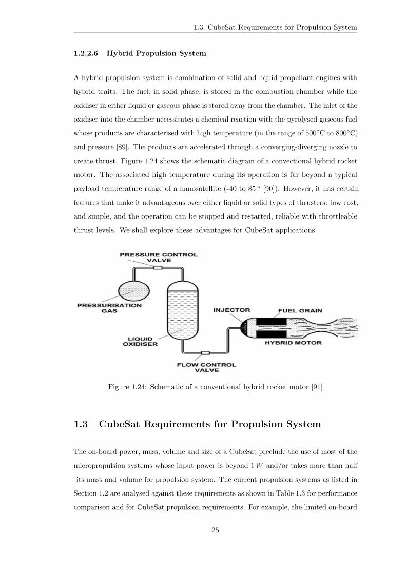
1.2.2.6 Hybrid Propulsion System
A hybrid propulsion system is combination of solid and liquid propellant engines with
hybrid traits. The fuel, in solid phase, is stored in the combustion chamber while the
oxidiser in either liquid or gaseous phase is stored away from the chamber. The inlet of the
oxidiser into the chamber necessitates a chemical reaction with the pyrolysed gaseous fuel
whose products are characterised with high temperature (in the range of 500∘C to 800∘C)
and pressure [89]. The products are accelerated through a converging-diverging nozzle to
create thrust. Figure 1.24 shows the schematic diagram of a convectional hybrid rocket
motor. The associated high temperature during its operation is far beyond a typical
payload temperature range of a nanosatellite (-40 to 85 ∘ [90]). However, it has certain
features that make it advantageous over either liquid or solid types of thrusters: low cost,
and simple, and the operation can be stopped and restarted, reliable with throttleable
thrust levels. We shall explore these advantages for CubeSat applications.
Figure 1.24: Schematic of a conventional hybrid rocket motor [91]
1.3 CubeSat Requirements for Propulsion System
The on-board power, mass, volume and size of a CubeSat preclude the use of most of the
micropropulsion systems whose input power is beyond 1𝑊 and/or takes more than half
its mass and volume for propulsion system. The current propulsion systems as listed in
Section 1.2 are analysed against these requirements as shown in Table 1.3 for performance
comparison and for CubeSat propulsion requirements. For example, the limited on-board
25
1.3. CubeSat Requirements for Propulsion System
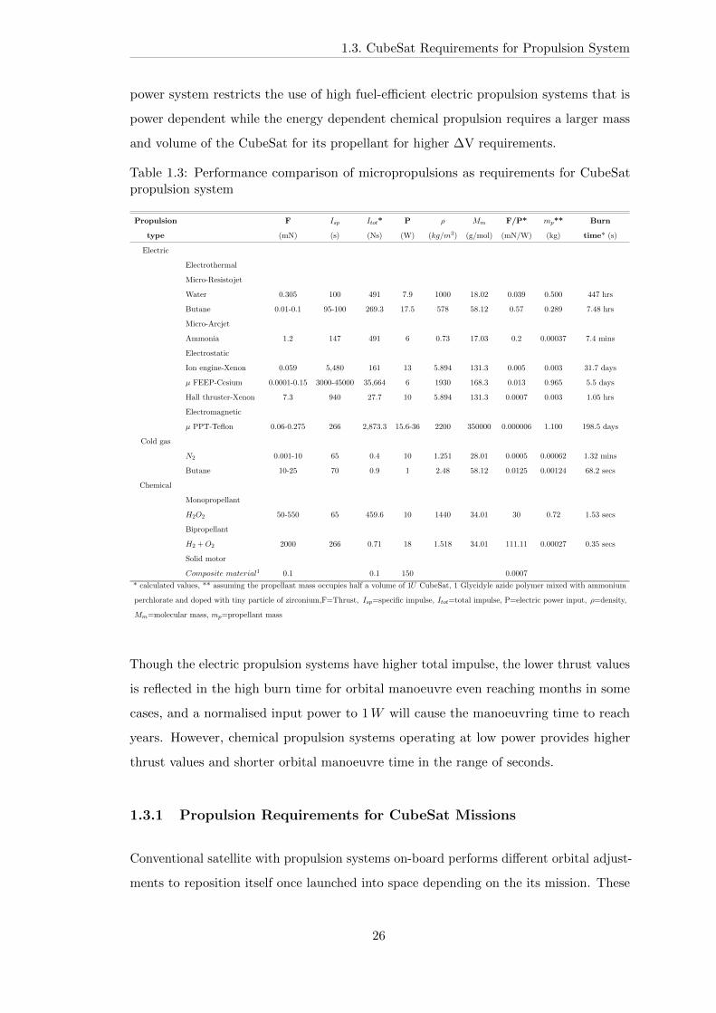
power system restricts the use of high fuel-efficient electric propulsion systems that is
power dependent while the energy dependent chemical propulsion requires a larger mass
and volume of the CubeSat for its propellant for higher ΔV requirements.
Table 1.3: Performance comparison of micropropulsions as requirements for CubeSatpropulsion system
Propulsion F 𝐼𝑠𝑝 𝐼𝑡𝑜𝑡* P 𝜌 𝑀𝑚 F/P* 𝑚𝑝** Burn
type (mN) (s) (Ns) (W) (𝑘𝑔/𝑚3) (g/mol) (mN/W) (kg) time* (s)
Electric
Electrothermal
Micro-Resistojet
Water 0.305 100 491 7.9 1000 18.02 0.039 0.500 447 hrs
Butane 0.01-0.1 95-100 269.3 17.5 578 58.12 0.57 0.289 7.48 hrs
Micro-Arcjet
Ammonia 1.2 147 491 6 0.73 17.03 0.2 0.00037 7.4 mins
Electrostatic
Ion engine-Xenon 0.059 5,480 161 13 5.894 131.3 0.005 0.003 31.7 days
𝜇 FEEP-Cesium 0.0001-0.15 3000-45000 35,664 6 1930 168.3 0.013 0.965 5.5 days
Hall thruster-Xenon 7.3 940 27.7 10 5.894 131.3 0.0007 0.003 1.05 hrs
Electromagnetic
𝜇 PPT-Teflon 0.06-0.275 266 2,873.3 15.6-36 2200 350000 0.000006 1.100 198.5 days
Cold gas
𝑁2 0.001-10 65 0.4 10 1.251 28.01 0.0005 0.00062 1.32 mins
Butane 10-25 70 0.9 1 2.48 58.12 0.0125 0.00124 68.2 secs
Chemical
Monopropellant
𝐻2𝑂2 50-550 65 459.6 10 1440 34.01 30 0.72 1.53 secs
Bipropellant
𝐻2 +𝑂2 2000 266 0.71 18 1.518 34.01 111.11 0.00027 0.35 secs
Solid motor
𝐶𝑜𝑚𝑝𝑜𝑠𝑖𝑡𝑒 𝑚𝑎𝑡𝑒𝑟𝑖𝑎𝑙1 0.1 0.1 150 0.0007
* calculated values, ** assuming the propellant mass occupies half a volume of 1𝑈 CubeSat, 1 Glycidyle azide polymer mixed with ammonium
perchlorate and doped with tiny particle of zirconium,F=Thrust, 𝐼𝑠𝑝=specific impulse, 𝐼𝑡𝑜𝑡=total impulse, P=electric power input, 𝜌=density,
𝑀𝑚=molecular mass, 𝑚𝑝=propellant mass
Though the electric propulsion systems have higher total impulse, the lower thrust values
is reflected in the high burn time for orbital manoeuvre even reaching months in some
cases, and a normalised input power to 1𝑊 will cause the manoeuvring time to reach
years. However, chemical propulsion systems operating at low power provides higher
thrust values and shorter orbital manoeuvre time in the range of seconds.
1.3.1 Propulsion Requirements for CubeSat Missions
Conventional satellite with propulsion systems on-board performs different orbital adjust-
ments to reposition itself once launched into space depending on the its mission. These
26
1.3. CubeSat Requirements for Propulsion System
orbital adjustment include attitude control for the satellite to control its orientation
for precise nadir pointing of its payload and detumble the angular rate of the satellite;
orbital maintenance which helps to prolong the satellite mission life by counteracting
atmospheric drag especially at lower altitude; and deorbting the satellite after the mission
life into a parking orbit or grave yard to mitigate against space debris. Expanding the
capability of CubeSat will require the nanosatellite to perform such orbital manoeuvra-
bility as the conventional satellites, and therefore need be equipped with propulsion
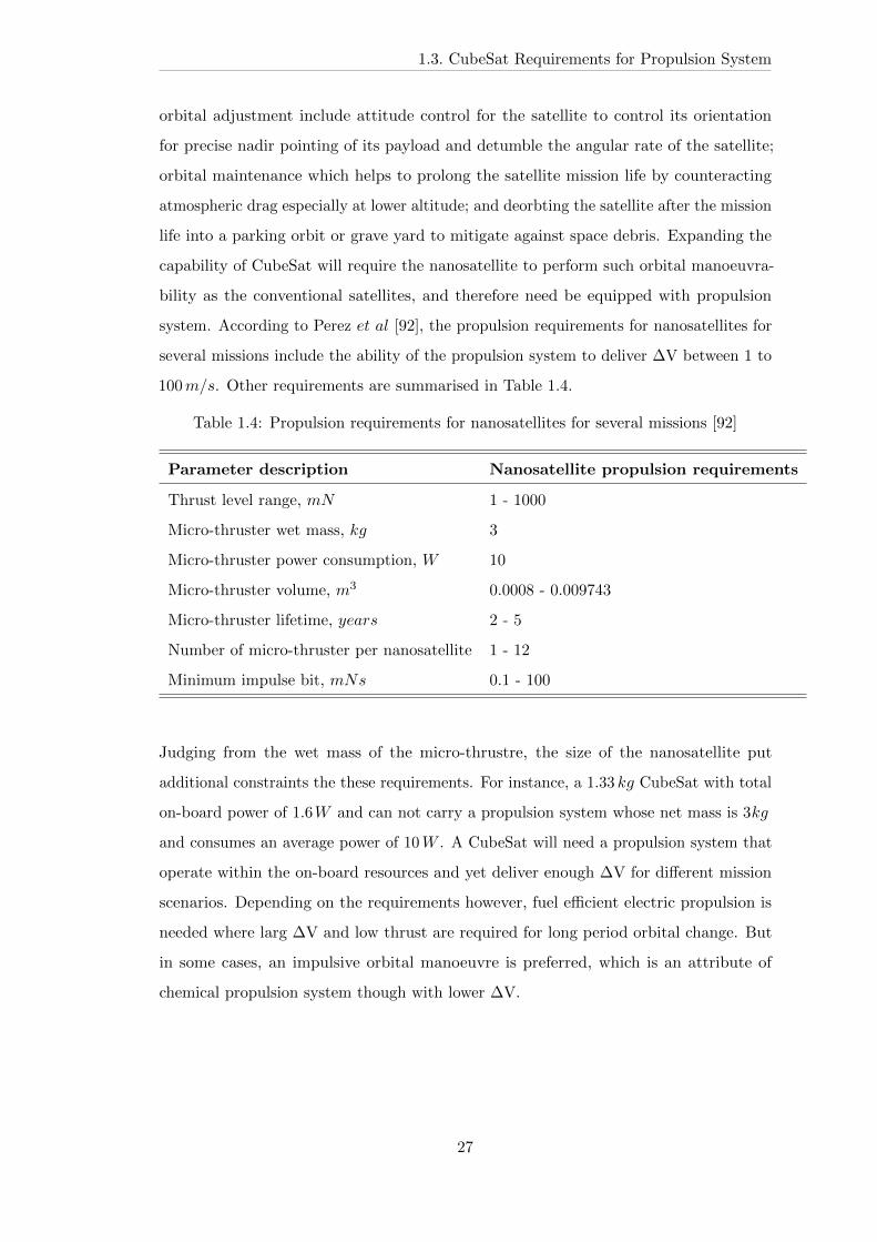
system. According to Perez 𝑒𝑡 𝑎𝑙 [92], the propulsion requirements for nanosatellites for
several missions include the ability of the propulsion system to deliver ΔV between 1 to
100𝑚/𝑠. Other requirements are summarised in Table 1.4.
Table 1.4: Propulsion requirements for nanosatellites for several missions [92]
Parameter description Nanosatellite propulsion requirements
Thrust level range, 𝑚𝑁 1 - 1000
Micro-thruster wet mass, 𝑘𝑔 3
Micro-thruster power consumption, 𝑊 10
Micro-thruster volume, 𝑚3 0.0008 - 0.009743
Micro-thruster lifetime, 𝑦𝑒𝑎𝑟𝑠 2 - 5
Number of micro-thruster per nanosatellite 1 - 12
Minimum impulse bit, 𝑚𝑁𝑠 0.1 - 100
Judging from the wet mass of the micro-thrustre, the size of the nanosatellite put
additional constraints the these requirements. For instance, a 1.33 𝑘𝑔 CubeSat with total
on-board power of 1.6𝑊 and can not carry a propulsion system whose net mass is 3𝑘𝑔
and consumes an average power of 10𝑊 . A CubeSat will need a propulsion system that
operate within the on-board resources and yet deliver enough ΔV for different mission
scenarios. Depending on the requirements however, fuel efficient electric propulsion is
needed where larg ΔV and low thrust are required for long period orbital change. But
in some cases, an impulsive orbital manoeuvre is preferred, which is an attribute of
chemical propulsion system though with lower ΔV.
27
1.3. CubeSat Requirements for Propulsion System
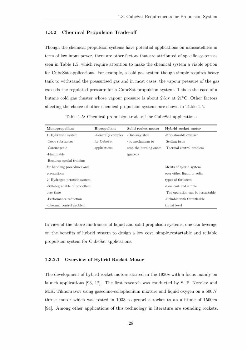
1.3.2 Chemical Propulsion Trade-off
Though the chemical propulsion systems have potential applications on nanosatellites in
term of low input power, there are other factors that are attributed of specific system as
seen in Table 1.5, which require attention to make the chemical system a viable option
for CubeSat applications. For example, a cold gas system though simple requires heavy
tank to withstand the pressurised gas and in most cases, the vapour pressure of the gas
exceeds the regulated pressure for a CubeSat propulsion system. This is the case of a
butane cold gas thuster whose vapour pressure is about 2 𝑏𝑎𝑟 at 21∘C. Other factors
affecting the choice of other chemical propulsion systems are shown in Table 1.5.
Table 1.5: Chemical propulsion trade-off for CubeSat applications
Monopropellant Bipropellant Solid rocket motor Hybrid rocket motor
1. Hybrazine system -Generally complex -One-way shot -Non-storable oxidiser
-Toxic substances for CubeSat (no mechanism to -Scaling issue
-Carcinogenic applications stop the burning onces -Thermal control problem
-Flammable ignited)
-Requires special training
for handling procedures and Merits of hybrid system
precautions over either liquid or solid
2. Hydrogen peroxide system types of thrusters:
-Self-degradable of propellant -Low cost and simple
over time -The operation can be restartable
-Performance reduction -Reliable with throttleable
-Thermal control problem thrust level
In view of the above hindrances of liquid and solid propulsion systems, one can leverage
on the benefits of hybrid system to design a low cost, simple,restartable and reliable
propulsion system for CubeSat applications.
1.3.2.1 Overview of Hybrid Rocket Motor
The development of hybrid rocket motors started in the 1930𝑠 with a focus mainly on
launch applications [93, 12]. The first research was conducted by S. P. Korolev and
M.K. Tikhonravov using gaseoline-collophonium mixture and liquid oxygen on a 500𝑁
thrust motor which was tested in 1933 to propel a rocket to an altitude of 1500𝑚
[94]. Among other applications of this technology in literature are sounding rockets,
28
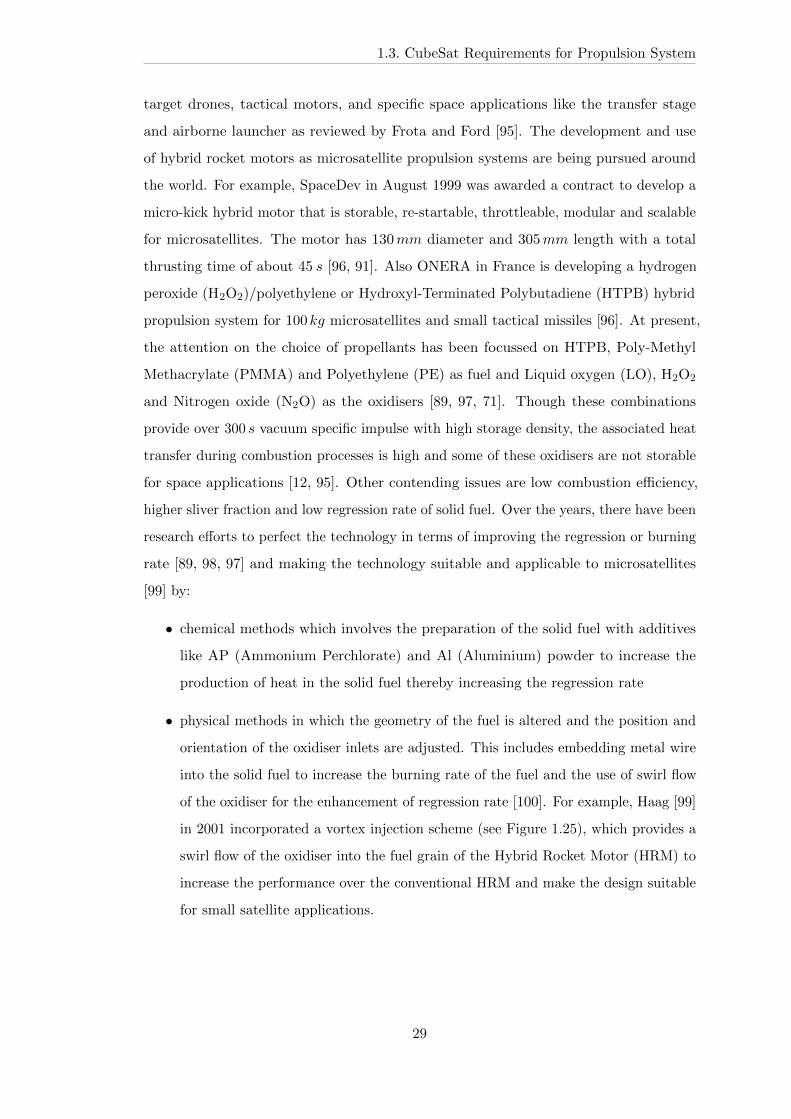
1.3. CubeSat Requirements for Propulsion System
target drones, tactical motors, and specific space applications like the transfer stage
and airborne launcher as reviewed by Frota and Ford [95]. The development and use
of hybrid rocket motors as microsatellite propulsion systems are being pursued around
the world. For example, SpaceDev in August 1999 was awarded a contract to develop a
micro-kick hybrid motor that is storable, re-startable, throttleable, modular and scalable
for microsatellites. The motor has 130𝑚𝑚 diameter and 305𝑚𝑚 length with a total
thrusting time of about 45 𝑠 [96, 91]. Also ONERA in France is developing a hydrogen
peroxide (H2O2)/polyethylene or Hydroxyl-Terminated Polybutadiene (HTPB) hybrid
propulsion system for 100𝑘𝑔 microsatellites and small tactical missiles [96]. At present,
the attention on the choice of propellants has been focussed on HTPB, Poly-Methyl
Methacrylate (PMMA) and Polyethylene (PE) as fuel and Liquid oxygen (LO), H2O2
and Nitrogen oxide (N2O) as the oxidisers [89, 97, 71]. Though these combinations
provide over 300 𝑠 vacuum specific impulse with high storage density, the associated heat
transfer during combustion processes is high and some of these oxidisers are not storable
for space applications [12, 95]. Other contending issues are low combustion efficiency,
higher sliver fraction and low regression rate of solid fuel. Over the years, there have been
research efforts to perfect the technology in terms of improving the regression or burning
rate [89, 98, 97] and making the technology suitable and applicable to microsatellites
[99] by:
∙ chemical methods which involves the preparation of the solid fuel with additives
like AP (Ammonium Perchlorate) and Al (Aluminium) powder to increase the
production of heat in the solid fuel thereby increasing the regression rate
∙ physical methods in which the geometry of the fuel is altered and the position and
orientation of the oxidiser inlets are adjusted. This includes embedding metal wire
into the solid fuel to increase the burning rate of the fuel and the use of swirl flow
of the oxidiser for the enhancement of regression rate [100]. For example, Haag [99]
in 2001 incorporated a vortex injection scheme (see Figure 1.25), which provides a
swirl flow of the oxidiser into the fuel grain of the Hybrid Rocket Motor (HRM) to
increase the performance over the conventional HRM and make the design suitable
for small satellite applications.
29
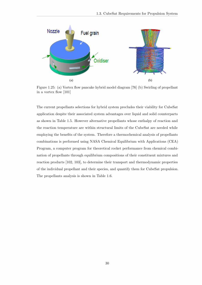
1.3. CubeSat Requirements for Propulsion System
(a) (b)
Figure 1.25: (a) Vortex flow pancake hybrid model diagram [76] (b) Swirling of propellantin a vortex flow [101]
The current propellants selections for hybrid system precludes their viability for CubeSat
application despite their associated system advantages over liquid and solid counterparts
as shown in Table 1.5. However alternative propellants whose enthalpy of reaction and
the reaction temperature are within structural limits of the CubeSat are needed while
employing the benefits of the system. Therefore a thermochemical analysis of propellants
combinations is performed using NASA Chemical Equilibrium with Applications (CEA)
Program, a computer program for theoretical rocket performance from chemical combi-
nation of propellants through equilibrium compositions of their constituent mixtures and
reaction products [102, 103], to determine their transport and thermodynamic properties
of the individual propellant and their species, and quantify them for CubeSat propulsion.
The propellants analysis is shown in Table 1.6.
30
1.3. CubeSat Requirements for Propulsion System
Table 1.6: Thermochemical analysis of propellant combinations
S/N Propellants Ratio Pc Tc 𝜌 Specific enthalpy 𝐼𝑠𝑝 Δ𝑉 *
(𝑏𝑎𝑟) (𝐾) (𝑘𝑔/𝑚3) (𝑘𝐽/𝑘𝑔) (𝑠) (𝑚/𝑠)
1F (Polyethylene(s))
5.55 44.7 3091.3855 -2704.0
325.3 412.2O (𝐻2𝑂2 (l)) 1580 -160815.7
2F (Polyethylene(s))
5.55 44.4 4609.8855 -2704.0
402.4 509.9O (𝑁2𝑂(l)) 808.6 431694.1
3F (Al(s))
5.55 44.7 3771.62800 189703.8
258.3 327.3O (𝑂2(l)) 1140 -12979.0
4F (Al(s))
5.55 44.4 1601.52800 189703.8
224.4 284.3O (𝐻2𝑂(l)) 1000 -260446.8
* calculated ΔV values assuming 88% dry mass ratio for 1𝑈 CubeSat, 𝑃𝑐 is the chamber pressure,
𝑇𝑐 is the chamber temperature, 𝜌 is the propellant density and 𝐼𝑠𝑝 is the specific impulse of the
combination
The propellants combinations are treated to the same ratio and nozzle expansion ratio
of 50. The result reveals that the hydrocarbon combustion reaction with hydrogen
peroxide and nitrogen tetra-oxide have higher specific impulse and ΔV for the same dry
mass ratio than the aluminium oxidation reaction. However, while hydrogen peroxide
self degrades over time and thus losses performance, nitrogen tetra-oxide is a harmful
and toxic gas that requires special training for handling procedures and precautions.
These combinations are well suitable for operation that does not require long storage
of propellant, especially during the launch operation. Another point to consider is the
chamber temperature. Thermal control is associated with the conventional hybrid rocket
motor where both hydrogen peroxide and nitrogen tetra-oxide are currently used as
oxidisers. But a prerequisite condition of a CubeSat propulsion system is to operate
within the structural temperature of the satellite thereby reducing the cost in employing
mechanism to control thermal runaway in the system. Therefore aluminium oxidation
reaction is considered as propellants combination choice. In this regard, both Al/LO and
Al/𝐻2𝑂 reactions are considered. While liquid oxygen is cryogenic in nature and it has
a boiling point of -183∘C, and requires special training and equipment for handling and
storage[104], liquid water is easy to store and has a boiling point of 100∘C. This reaction
is also known as water splitting reaction, which is normally used to generate hydrogen
gas. Therefore only liquid water oxidation reaction with aluminium is considered as
alternative propellant for CubeSat propulsion system in this research. This propellant
31

1.4. Motivation and Objectives
combination has theoretical performance of specific impulse of 224.4 𝑠 and is capable
of delivering a ΔV of about 284𝑚/𝑠 for a 1𝑈 CubeSat of 1.33 𝑘𝑔 assuming dry mass
fraction of 88%.
1.4 Motivation and Objectives
Until quite recently CubeSats did not have propulsion systems onboard and their orbits
were dictated by the injection orbit supplied by the launch vehicle (LV). That was
primarily due to the fact that CubeSats applications were for experimental purposes
within the university communities and were done on extremely low budgets. The involve-
ment of government establishments and private organisations in CubeSat applications
has brought the need to extend the capabilities and altitude of the CubeSat beyond
low earth orbit with the development of low-cost propulsion systems that is within the
power, size and mass of the nanosatellites thereby making the nano-group satellites
serious contenders for significant science missions. Missions beyond earth observation
to technology demonstration around other celestial bodies like the asteroid belt and
the outer solar system require significant orbital change and ΔV capability, as well as
ΔV requirements to de-orbit the satellite after the mission assignment. Available micro-
propulsion systems are considered and reviewed in the next section for a 1𝑈 CubeSat
against its limited on-board resources. Though electric propulsion systems are effective
in fuel efficient but these systems are complex and they put a power-demand burden on
CubeSat for moderate to high thrust applications. Chemical propulsion systems with
less fuel efficient could provide impulsive orbital change for CubeSat missions, but the
current propellants are toxic, carcinogenic, flammable, and they require special trainings
for handling procedures and precautions, and this will result in high mission cost. And
also, simple and cheap cold gas thruster loses its performance when used for end of
life de-orbiting purpose. Among the propellants combinations for a hybrid system for
CubeSat propulsion system, only Al/𝐻2𝑂 is chosen considering the ease of handling
and storing the propellant. Therefore a simple alternative system is investigated in this
study whose propellants are readily available and cheap for CubeSat budget, and whose
performance remains the same through the life span of the nanosatellite.
A propose propulsion system in this research is a high density propellant (alumini-
32

1.5. Novelty and Research Achievements
um/sodium hydroxide/water) hybrid propulsion system for CubeSat applications. It
involves the injection of liquid oxidiser (mixture of sodium hydroxide and water) into a
high density solid fuel (aluminium wool) which will produce water vapour and hydrogen
gas for thrust generation. Unlike a conventional hybrid rocket motor, the chemical
reaction is not a high temperature combustion process. On the contrary, this reaction is
self-sustaining and progresses at moderate temperature of about 150∘C, and therefore
scalable without thermal and combustion instability issues [41]. The materials are
storable, low cost and readily available, with aluminium having a high energy density
per unit volume. The propulsion system only requires minimal power, about 500𝑚𝑊 ,
from the CubeSat electrical bus system for valves operation. One of the drawbacks of
the system is that the firing time is about 99 𝑠 long, making this system inappropriate
for attitude control purposes.
1.5 Novelty and Research Achievements
The areas of novel contributions arising from the course of this work to the field of
micropropulsion systems for CubeSats include:
∙ The novel use of the chemical combination of aluminium wool/water/sodium
hydroxide as propellant for CubeSat propulsion.
∙ Developing a new CubeSat propulsion architecture that could potentially deliver
high ΔV capability for future CubeSat missions.
33
Chapter 2
Theory
2.1 Overview
This section reviews the reaction between aluminium, water and sodium hydroxide for the
generation of hydrogen gas, and shows how this reaction can be adopted for nanosatellites
propulsion system. It also discusses thermodynamics and dynamics of gas with suitable
assumptions for propulsion systems. Finally, it contains a o-dimensional propulsion
model and the ideal performance resulting from the analysis.
Water splitting reaction with reactive metals has been a subject of research for the
generation of hydrogen gas in automobile industries [105, 106, 107]. The reactive metals
have high energy densities such that a very small amount is suited for volume constraint
nanosatellites propulsion system. This exothermic reaction is adopted in this research
and among the metals (zinc, magnesium, calcium, aluminium, e.t.c) from the available
data in literature in term of cost, safety, availability, aluminium has the best bargain [107].
Aluminium is a very reactive metal that when placed into the atmosphere reacts quickly
to form a film of aluminium oxide on the surface of the metal. Though the aluminium
oxide film is microscopically thin, in the range of 50 to 100Angstroms [108], and gener-
ally very stable under the pH scale of 4 - 9 [109], it protects the surface of the metal
from further reaction with the surroundings thereby preventing the potential use of the
metal for energy application purposes except when treated. But when the thin layer
or barrier is broken down, the energy stored in this abundant metal becomes useful.
34
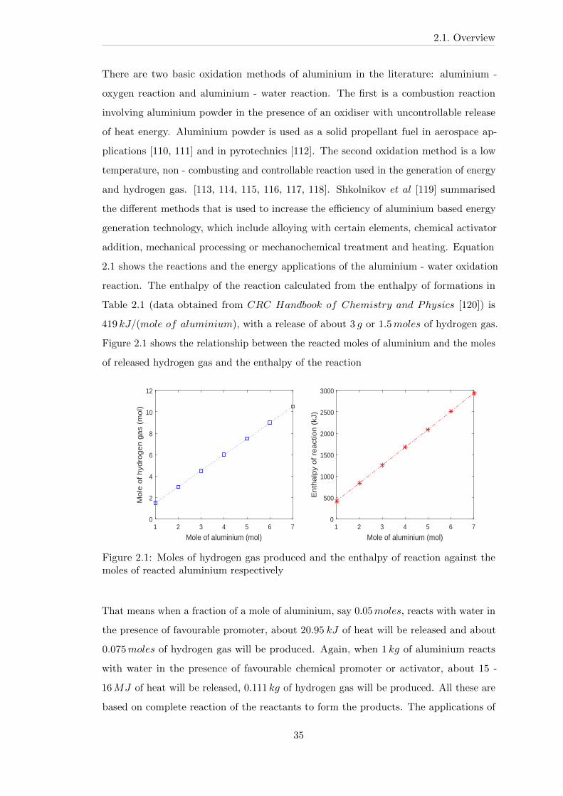
2.1. Overview
There are two basic oxidation methods of aluminium in the literature: aluminium -
oxygen reaction and aluminium - water reaction. The first is a combustion reaction
involving aluminium powder in the presence of an oxidiser with uncontrollable release
of heat energy. Aluminium powder is used as a solid propellant fuel in aerospace ap-
plications [110, 111] and in pyrotechnics [112]. The second oxidation method is a low
temperature, non - combusting and controllable reaction used in the generation of energy
and hydrogen gas. [113, 114, 115, 116, 117, 118]. Shkolnikov 𝑒𝑡 𝑎𝑙 [119] summarised
the different methods that is used to increase the efficiency of aluminium based energy
generation technology, which include alloying with certain elements, chemical activator
addition, mechanical processing or mechanochemical treatment and heating. Equation
2.1 shows the reactions and the energy applications of the aluminium - water oxidation
reaction. The enthalpy of the reaction calculated from the enthalpy of formations in
Table 2.1 (data obtained from 𝐶𝑅𝐶 𝐻𝑎𝑛𝑑𝑏𝑜𝑜𝑘 𝑜𝑓 𝐶ℎ𝑒𝑚𝑖𝑠𝑡𝑟𝑦 𝑎𝑛𝑑 𝑃ℎ𝑦𝑠𝑖𝑐𝑠 [120]) is
419 𝑘𝐽/(𝑚𝑜𝑙𝑒 𝑜𝑓 𝑎𝑙𝑢𝑚𝑖𝑛𝑖𝑢𝑚), with a release of about 3 𝑔 or 1.5𝑚𝑜𝑙𝑒𝑠 of hydrogen gas.
Figure 2.1 shows the relationship between the reacted moles of aluminium and the moles
of released hydrogen gas and the enthalpy of the reaction
1 2 3 4 5 6 7
Mole of aluminium (mol)
0
2
4
6
8
10
12
Mo
le o
f h
ydro
ge
n g
as
(mo
l)
1 2 3 4 5 6 7
Mole of aluminium (mol)
0
500
1000
1500
2000
2500
3000
En
tha
lpy
of
rea
ctio
n (
kJ)
Figure 2.1: Moles of hydrogen gas produced and the enthalpy of reaction against themoles of reacted aluminium respectively
That means when a fraction of a mole of aluminium, say 0.05𝑚𝑜𝑙𝑒𝑠, reacts with water in
the presence of favourable promoter, about 20.95 𝑘𝐽 of heat will be released and about
0.075𝑚𝑜𝑙𝑒𝑠 of hydrogen gas will be produced. Again, when 1 𝑘𝑔 of aluminium reacts
with water in the presence of favourable chemical promoter or activator, about 15 -
16𝑀𝐽 of heat will be released, 0.111 𝑘𝑔 of hydrogen gas will be produced. All these are
based on complete reaction of the reactants to form the products. The applications of
35
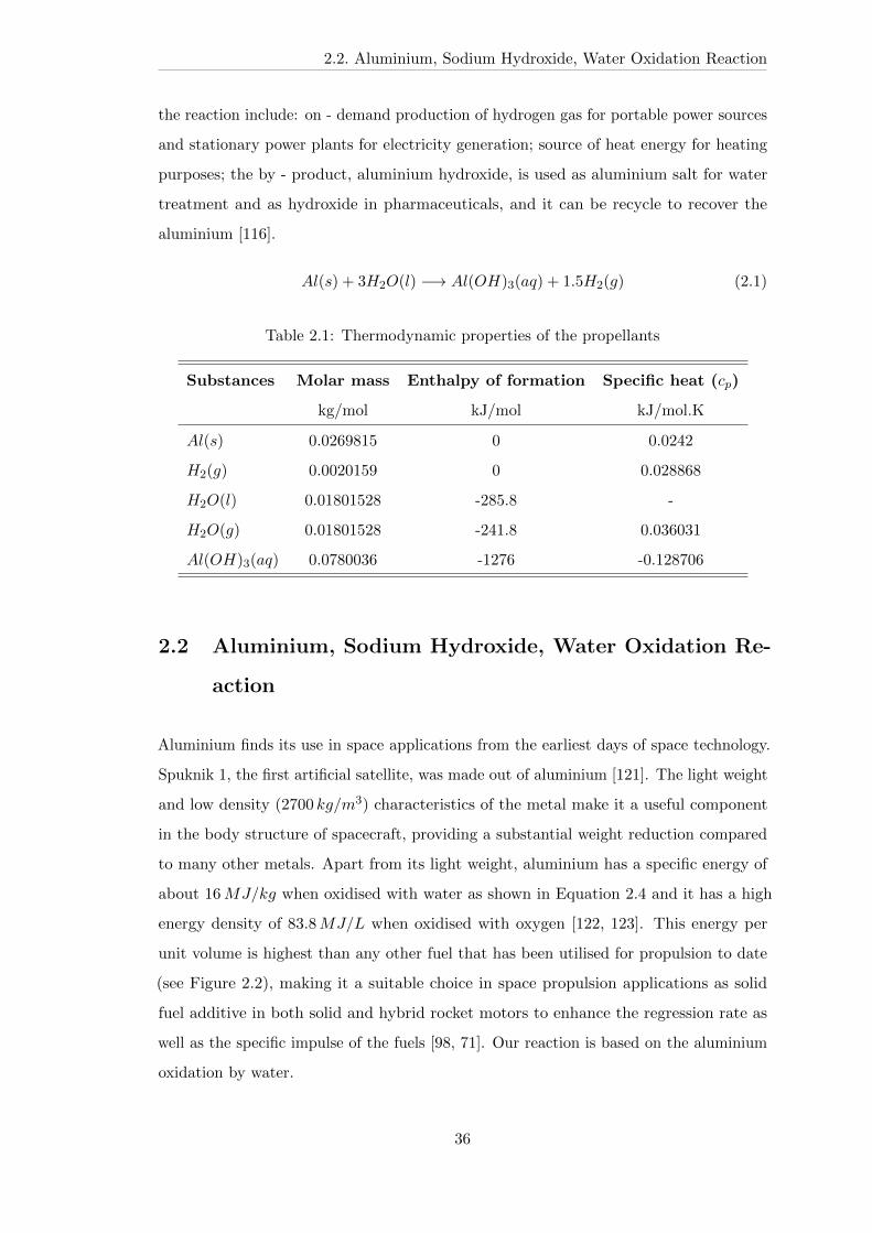
2.2. Aluminium, Sodium Hydroxide, Water Oxidation Reaction
the reaction include: on - demand production of hydrogen gas for portable power sources
and stationary power plants for electricity generation; source of heat energy for heating
purposes; the by - product, aluminium hydroxide, is used as aluminium salt for water
treatment and as hydroxide in pharmaceuticals, and it can be recycle to recover the
aluminium [116].
𝐴𝑙(𝑠) + 3𝐻2𝑂(𝑙) −→ 𝐴𝑙(𝑂𝐻)3(𝑎𝑞) + 1.5𝐻2(𝑔) (2.1)
Table 2.1: Thermodynamic properties of the propellants
Substances Molar mass Enthalpy of formation Specific heat (𝑐𝑝)
kg/mol kJ/mol kJ/mol.K
𝐴𝑙(𝑠) 0.0269815 0 0.0242
𝐻2(𝑔) 0.0020159 0 0.028868
𝐻2𝑂(𝑙) 0.01801528 -285.8 -
𝐻2𝑂(𝑔) 0.01801528 -241.8 0.036031
𝐴𝑙(𝑂𝐻)3(𝑎𝑞) 0.0780036 -1276 -0.128706
2.2 Aluminium, Sodium Hydroxide, Water Oxidation Re-
action
Aluminium finds its use in space applications from the earliest days of space technology.
Spuknik 1, the first artificial satellite, was made out of aluminium [121]. The light weight
and low density (2700 𝑘𝑔/𝑚3) characteristics of the metal make it a useful component
in the body structure of spacecraft, providing a substantial weight reduction compared
to many other metals. Apart from its light weight, aluminium has a specific energy of
about 16𝑀𝐽/𝑘𝑔 when oxidised with water as shown in Equation 2.4 and it has a high
energy density of 83.8𝑀𝐽/𝐿 when oxidised with oxygen [122, 123]. This energy per
unit volume is highest than any other fuel that has been utilised for propulsion to date
(see Figure 2.2), making it a suitable choice in space propulsion applications as solid
fuel additive in both solid and hybrid rocket motors to enhance the regression rate as
well as the specific impulse of the fuels [98, 71]. Our reaction is based on the aluminium
oxidation by water.
36
2.2. Aluminium, Sodium Hydroxide, Water Oxidation Reaction
Figure 2.2: Selected energy density of some fuels [122]
This high energy content can be accessed by reacting aluminium with water to form
its hydroxide or oxide, and hydrogen gas depending on the reaction temperature [106].
However, direct reaction of pure aluminium with water is inhibited by the formation of
a dense layer of Al2O3 which passivates the aluminium and stops any further reaction
[116, 119, 117, 123] thereby reducing its potential usage for energy and hydrogen genera-
tion.
Current efforts to increase the efficiency of the aluminium-water reaction include alloying
aluminium with a low melting point metals like gallium, indium, and tin [123], using
nanoparticle sizes of aluminium [124], addition of selected metallic salts [125], metal
oxide addition [126] and metal hydroxide addition [127, 115, 116]. In all these techniques,
oxidation of aluminium in alkaline solution to produce hydrogen occurs at moderate
temperature (about 150∘) and pressure [119], and among the alkaline additives, sodium
hydroxide is the best hydroxide for the reaction in view of reaction rate and conversion
37
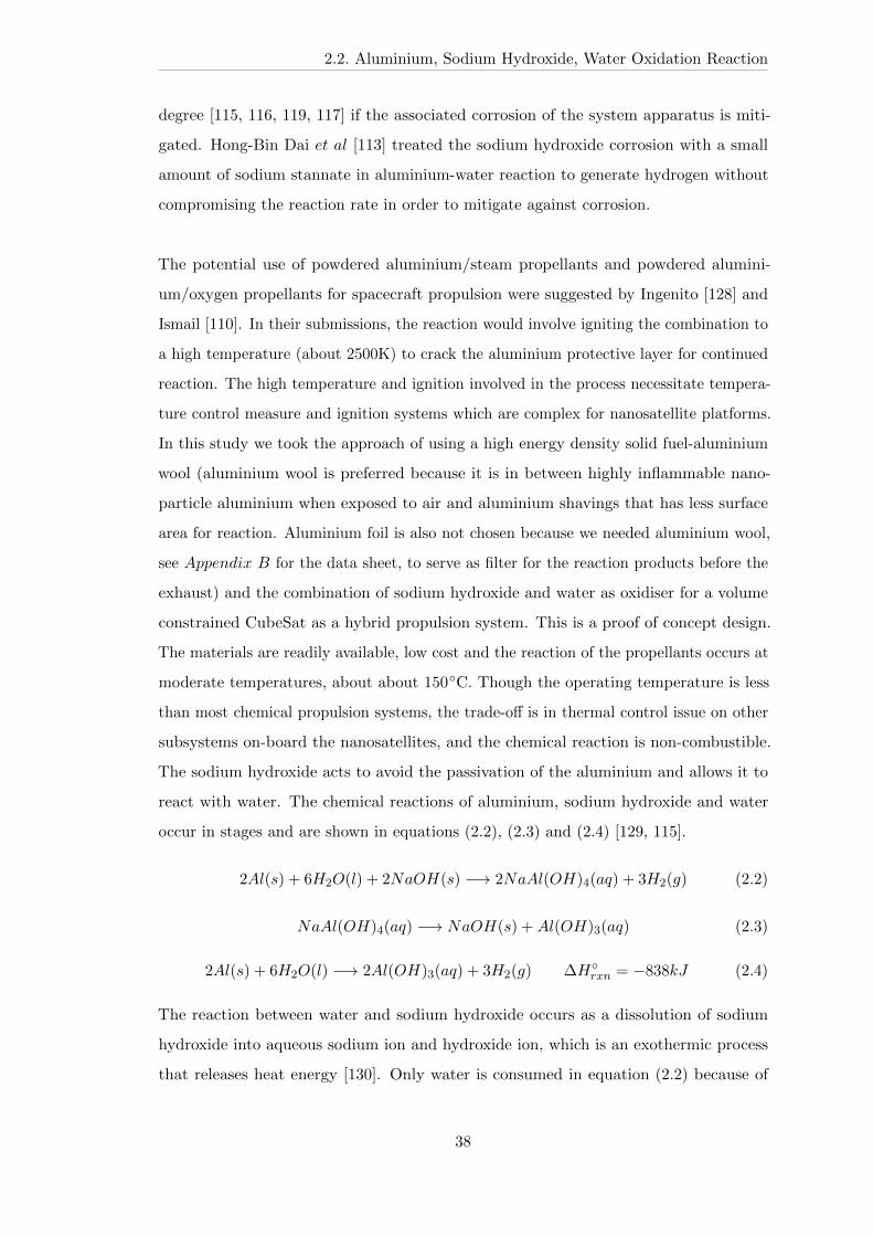
2.2. Aluminium, Sodium Hydroxide, Water Oxidation Reaction
degree [115, 116, 119, 117] if the associated corrosion of the system apparatus is miti-
gated. Hong-Bin Dai 𝑒𝑡 𝑎𝑙 [113] treated the sodium hydroxide corrosion with a small
amount of sodium stannate in aluminium-water reaction to generate hydrogen without
compromising the reaction rate in order to mitigate against corrosion.
The potential use of powdered aluminium/steam propellants and powdered alumini-
um/oxygen propellants for spacecraft propulsion were suggested by Ingenito [128] and
Ismail [110]. In their submissions, the reaction would involve igniting the combination to
a high temperature (about 2500K) to crack the aluminium protective layer for continued
reaction. The high temperature and ignition involved in the process necessitate tempera-
ture control measure and ignition systems which are complex for nanosatellite platforms.
In this study we took the approach of using a high energy density solid fuel-aluminium
wool (aluminium wool is preferred because it is in between highly inflammable nano-
particle aluminium when exposed to air and aluminium shavings that has less surface
area for reaction. Aluminium foil is also not chosen because we needed aluminium wool,
see 𝐴𝑝𝑝𝑒𝑛𝑑𝑖𝑥 𝐵 for the data sheet, to serve as filter for the reaction products before the
exhaust) and the combination of sodium hydroxide and water as oxidiser for a volume
constrained CubeSat as a hybrid propulsion system. This is a proof of concept design.
The materials are readily available, low cost and the reaction of the propellants occurs at
moderate temperatures, about about 150∘C. Though the operating temperature is less
than most chemical propulsion systems, the trade-off is in thermal control issue on other
subsystems on-board the nanosatellites, and the chemical reaction is non-combustible.
The sodium hydroxide acts to avoid the passivation of the aluminium and allows it to
react with water. The chemical reactions of aluminium, sodium hydroxide and water
occur in stages and are shown in equations (2.2), (2.3) and (2.4) [129, 115].
2𝐴𝑙(𝑠) + 6𝐻2𝑂(𝑙) + 2𝑁𝑎𝑂𝐻(𝑠) −→ 2𝑁𝑎𝐴𝑙(𝑂𝐻)4(𝑎𝑞) + 3𝐻2(𝑔) (2.2)
𝑁𝑎𝐴𝑙(𝑂𝐻)4(𝑎𝑞) −→ 𝑁𝑎𝑂𝐻(𝑠) +𝐴𝑙(𝑂𝐻)3(𝑎𝑞) (2.3)
2𝐴𝑙(𝑠) + 6𝐻2𝑂(𝑙) −→ 2𝐴𝑙(𝑂𝐻)3(𝑎𝑞) + 3𝐻2(𝑔) Δ𝐻∘𝑟𝑥𝑛 = −838𝑘𝐽 (2.4)
The reaction between water and sodium hydroxide occurs as a dissolution of sodium
hydroxide into aqueous sodium ion and hydroxide ion, which is an exothermic process
that releases heat energy [130]. Only water is consumed in equation (2.2) because of
38
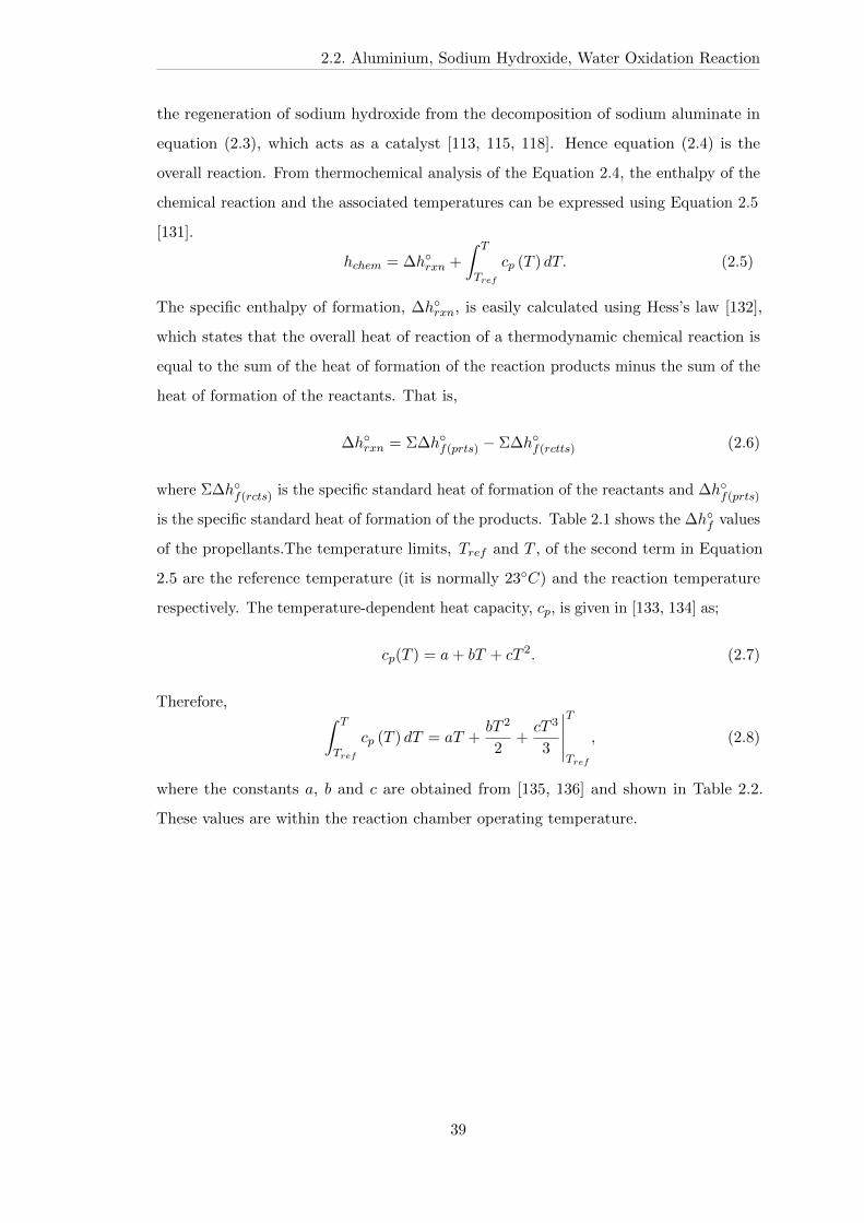
2.2. Aluminium, Sodium Hydroxide, Water Oxidation Reaction
the regeneration of sodium hydroxide from the decomposition of sodium aluminate in
equation (2.3), which acts as a catalyst [113, 115, 118]. Hence equation (2.4) is the
overall reaction. From thermochemical analysis of the Equation 2.4, the enthalpy of the
chemical reaction and the associated temperatures can be expressed using Equation 2.5
[131].
ℎ𝑐ℎ𝑒𝑚 = Δℎ∘𝑟𝑥𝑛 +
∫ 𝑇
𝑇𝑟𝑒𝑓
𝑐𝑝 (𝑇 ) 𝑑𝑇. (2.5)
The specific enthalpy of formation, Δℎ∘𝑟𝑥𝑛, is easily calculated using Hess’s law [132],
which states that the overall heat of reaction of a thermodynamic chemical reaction is
equal to the sum of the heat of formation of the reaction products minus the sum of the
heat of formation of the reactants. That is,
Δℎ∘𝑟𝑥𝑛 = ΣΔℎ∘𝑓(𝑝𝑟𝑡𝑠) − ΣΔℎ∘𝑓(𝑟𝑐𝑡𝑡𝑠) (2.6)
where ΣΔℎ∘𝑓(𝑟𝑐𝑡𝑠) is the specific standard heat of formation of the reactants and Δℎ∘𝑓(𝑝𝑟𝑡𝑠)
is the specific standard heat of formation of the products. Table 2.1 shows the Δℎ∘𝑓 values
of the propellants.The temperature limits, 𝑇𝑟𝑒𝑓 and 𝑇 , of the second term in Equation
2.5 are the reference temperature (it is normally 23∘𝐶) and the reaction temperature
respectively. The temperature-dependent heat capacity, 𝑐𝑝, is given in [133, 134] as;
𝑐𝑝(𝑇 ) = 𝑎+ 𝑏𝑇 + 𝑐𝑇 2. (2.7)
Therefore, ∫ 𝑇
𝑇𝑟𝑒𝑓
𝑐𝑝 (𝑇 ) 𝑑𝑇 = 𝑎𝑇 +𝑏𝑇 2
2+
𝑐𝑇 3
3
𝑇
𝑇𝑟𝑒𝑓
, (2.8)
where the constants 𝑎, 𝑏 and 𝑐 are obtained from [135, 136] and shown in Table 2.2.
These values are within the reaction chamber operating temperature.
39

2.3. Thermodynamics and Gas Dynamics
Table 2.2: Heat capacity coefficients
Substances Heat capacity coefficients from 300K to 1000K
𝑎𝐽/𝑚𝑜𝑙.𝐾
𝑏10−2𝐽/𝑚𝑜𝑙.𝐾2
𝑐10−5𝐽/𝑚𝑜𝑙.𝐾3
𝐴𝑙(𝑠)* 28.08920 -0.5414849 0.8560423
𝐻2(𝑔) 33.066178 -1.1363417 1.1432816
𝐻2𝑂(𝑙)** -203.6060 152.3290 -319.6413
𝐻2𝑂(𝑔)*** - - -
𝐴𝑙(𝑂𝐻)3(𝑎𝑞) 2.987191 10.7087 -8.95576* the range of temperature is from 298𝐾 to 933𝐾
** the range of temperature is from 298𝐾 to 500𝐾
*** no values at the operating temperature
Now, using Equations 2.4, 2.5, 2.6 and 2.8, and Tables 2.1 and 2.2, we can calculate
change in enthalpy of the reaction at 150∘𝐶, which is 418.6 𝑘𝐽/𝑚𝑜𝑙. This represents the
enthalpy of formation at 23∘𝐶 and the change in enthalpy at 150∘𝐶.
Roach 𝑒𝑡 𝑎𝑙 stated in their work that aluminium-water reaction produces a limited
amount of hydrogen gas because not all the aluminium takes part in the hydrogen-
formation reaction [137], which means the liberated energy in the reaction is less than
calculated above. This will be verified in the course of this research. However, if this
reaction is confined in a controlled volume with a small orifice, there will be a change of
water phase from liquid to gas due to low pressure environment and elevated temperature
of the reaction, and both the water vapour and hydrogen gas when directed through a
converging-diverging nozzle will produce thrust to propel the nanosatellites by expelling
the heated gas through a nozzle. The energy released in this reaction is about 838 𝐾𝐽
per 2𝑚𝑜𝑙𝑒𝑠 of aluminium.
2.3 Thermodynamics and Gas Dynamics
The first law of thermodynamics is a statement of energy conservation [ 138], and for a
control volume with one inlet and one exit, it is written as [139]:
𝑑𝐸𝑐𝑣
𝑑𝑡= 𝑐𝑣 − 𝑐𝑣 + 𝑖
(ℎ𝑖 +
𝑣2𝑖2
+ 𝑔𝑧𝑖
)− 𝑒
(ℎ𝑒 +
𝑣2𝑒2
+ 𝑔𝑧𝑒
)(2.9)
40

2.3. Thermodynamics and Gas Dynamics
where 𝐸𝑐𝑣 is the energy of the control volume at time 𝑡 and 𝑐𝑣 and 𝑐𝑣 represent the
net rate of energy transfer by heat and work across the boundary of the control volume.
𝑖 and 𝑒 are inlet and outlet mass flow rate, ℎ𝑖 and ℎ𝑒 are the total specific enthalpies
of inlet and outlet flow of the control volume, 𝑣𝑖 and 𝑣𝑒 are the inlet and exit velocities of
the flow, 𝑧𝑖 and 𝑧𝑒 are the vertical measurements of the inlet and outlet from the ground
level and 𝑔 is acceleration due to gravity at the surface of the earth. The bracket terms
represent the enthalpy, kinetic and potential energy that accompany the rate of mass
flow in and out of the control volume as a function of time. Consider a control volume
attached to a nozzle for the thermodynamic analysis of an expanded gas as shown in
Figure 2.3.
AtAe
peAepa Control volume
ThroatNozzle
Figure 2.3: Control volume with an attached nozzle: 𝐴𝑒 is the exit area of the nozzle, 𝐴𝑡
is the throat area, 𝑝𝑎 is the ambient pressure and 𝑝𝑒 is the exit pressure
Assuming the products of the reaction in the reaction chamber experience no significant
change in potential energy, no shaft work or shear work done, and under adiabatic and
steady flow conditions the process is given by [138]
ℎ1 +1
2𝑣21 = ℎ2 +
1
2𝑣22 (2.10)
That is, the sum of the specific enthalpy and the specific kinetic energy remain constant
for a given flow [131]. In this equation ℎ is the specific enthalpy (𝐽/𝑘𝑔) and 𝑣 is the flow
velocity (𝑚/𝑠).
If the gas in the control volume is stationary, then its enthalpy is converted into kinetic
energy, and equation (2.10) becomes
ℎ𝑜 = ℎ+1
2𝑣2, (2.11)
where the enthalpy, ℎ, is obtained by combining temperature-dependent internal energy,
41
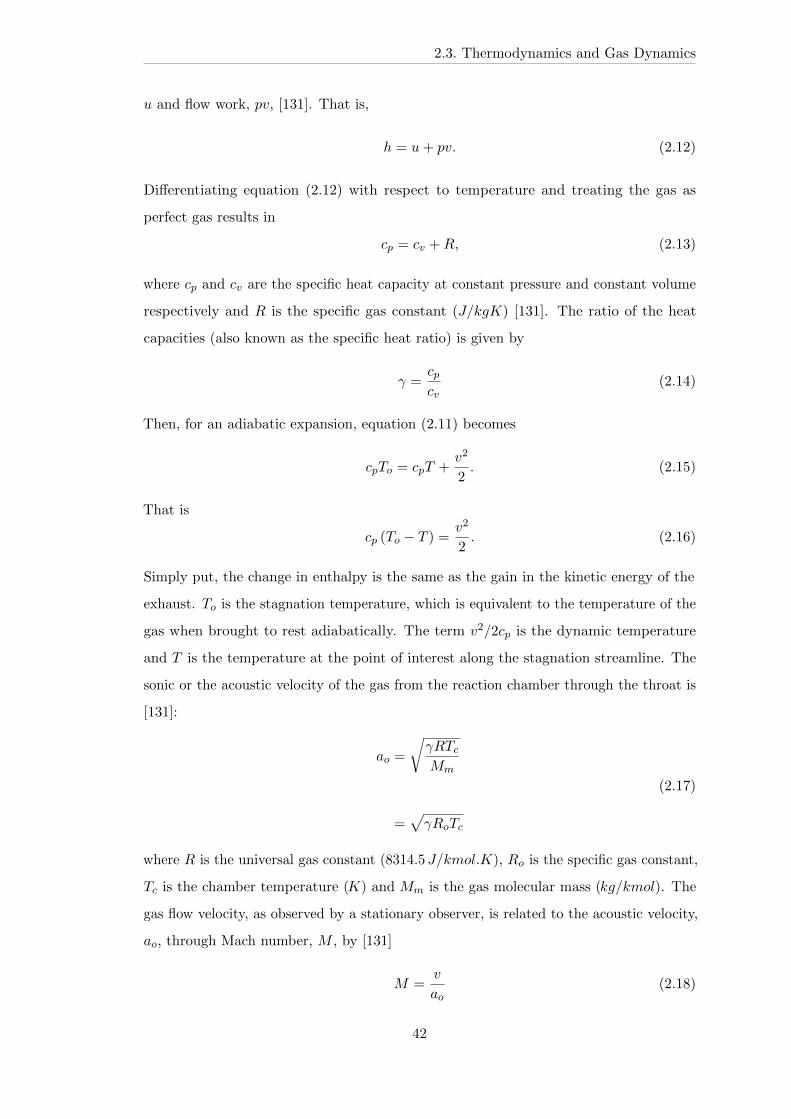
2.3. Thermodynamics and Gas Dynamics
𝑢 and flow work, 𝑝𝑣, [131]. That is,
ℎ = 𝑢+ 𝑝𝑣. (2.12)
Differentiating equation (2.12) with respect to temperature and treating the gas as
perfect gas results in
𝑐𝑝 = 𝑐𝑣 +𝑅, (2.13)
where 𝑐𝑝 and 𝑐𝑣 are the specific heat capacity at constant pressure and constant volume
respectively and 𝑅 is the specific gas constant (𝐽/𝑘𝑔𝐾) [131]. The ratio of the heat
capacities (also known as the specific heat ratio) is given by
𝛾 =𝑐𝑝𝑐𝑣
(2.14)
Then, for an adiabatic expansion, equation (2.11) becomes
𝑐𝑝𝑇𝑜 = 𝑐𝑝𝑇 +𝑣2
2. (2.15)
That is
𝑐𝑝 (𝑇𝑜 − 𝑇 ) =𝑣2
2. (2.16)
Simply put, the change in enthalpy is the same as the gain in the kinetic energy of the
exhaust. 𝑇𝑜 is the stagnation temperature, which is equivalent to the temperature of the
gas when brought to rest adiabatically. The term 𝑣2/2𝑐𝑝 is the dynamic temperature
and 𝑇 is the temperature at the point of interest along the stagnation streamline. The
sonic or the acoustic velocity of the gas from the reaction chamber through the throat is
[131]:
𝑎𝑜 =
√𝛾𝑅𝑇𝑐
𝑀𝑚
=√𝛾𝑅𝑜𝑇𝑐
(2.17)
where 𝑅 is the universal gas constant (8314.5 𝐽/𝑘𝑚𝑜𝑙.𝐾), 𝑅𝑜 is the specific gas constant,
𝑇𝑐 is the chamber temperature (𝐾) and 𝑀𝑚 is the gas molecular mass (𝑘𝑔/𝑘𝑚𝑜𝑙). The
gas flow velocity, as observed by a stationary observer, is related to the acoustic velocity,
𝑎𝑜, through Mach number, 𝑀 , by [131]
𝑀 =𝑣
𝑎𝑜(2.18)
42
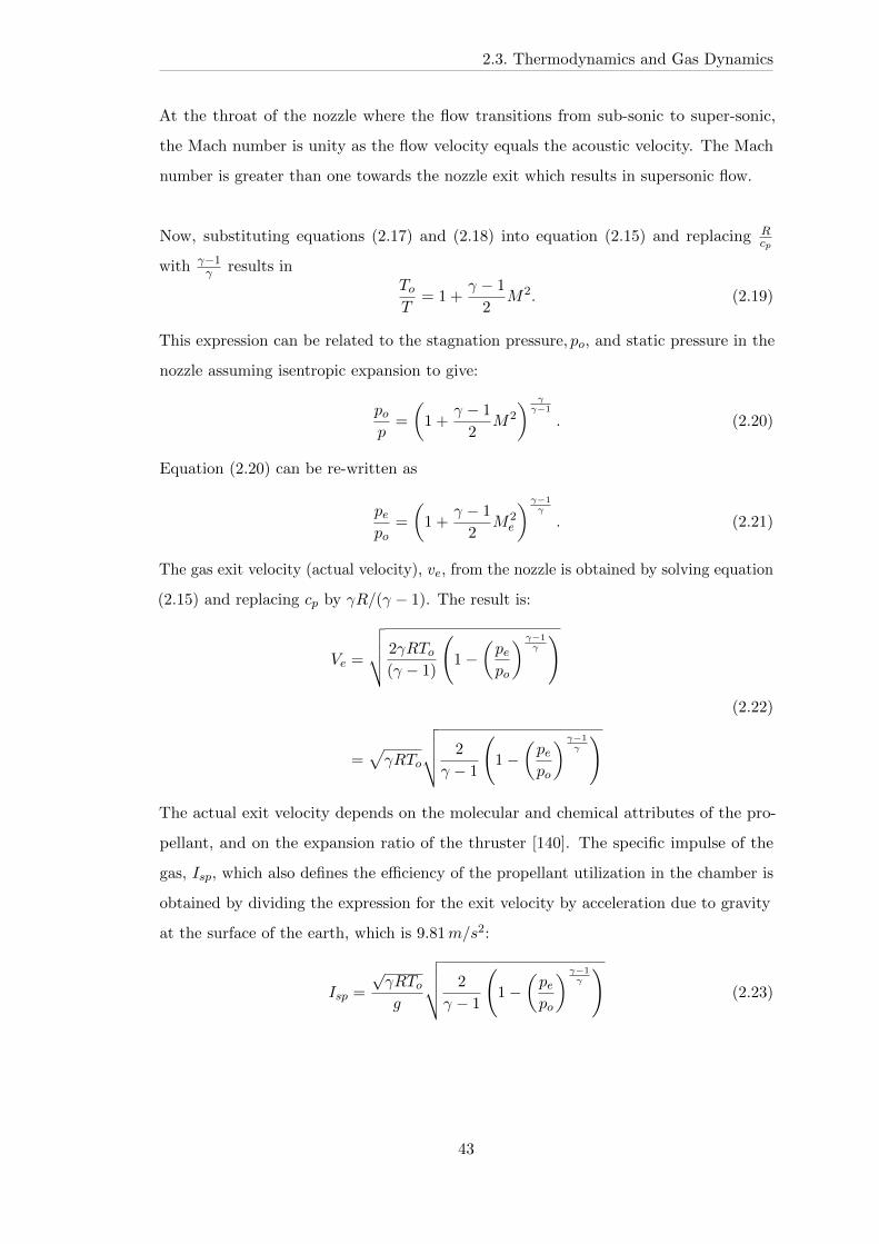
2.3. Thermodynamics and Gas Dynamics
At the throat of the nozzle where the flow transitions from sub-sonic to super-sonic,
the Mach number is unity as the flow velocity equals the acoustic velocity. The Mach
number is greater than one towards the nozzle exit which results in supersonic flow.
Now, substituting equations (2.17) and (2.18) into equation (2.15) and replacing 𝑅𝑐𝑝
with 𝛾−1𝛾 results in
𝑇𝑜
𝑇= 1 +
𝛾 − 1
2𝑀2. (2.19)
This expression can be related to the stagnation pressure, 𝑝𝑜, and static pressure in the
nozzle assuming isentropic expansion to give:
𝑝𝑜𝑝
=
(1 +
𝛾 − 1
2𝑀2
) 𝛾𝛾−1
. (2.20)
Equation (2.20) can be re-written as
𝑝𝑒𝑝𝑜
=
(1 +
𝛾 − 1
2𝑀2
𝑒
) 𝛾−1𝛾
. (2.21)
The gas exit velocity (actual velocity), 𝑣𝑒, from the nozzle is obtained by solving equation
(2.15) and replacing 𝑐𝑝 by 𝛾𝑅/(𝛾 − 1). The result is:
𝑉𝑒 =
⎯ 2𝛾𝑅𝑇𝑜
(𝛾 − 1)
(1−
(𝑝𝑒𝑝𝑜
) 𝛾−1𝛾
)
=√𝛾𝑅𝑇𝑜
⎯ 2
𝛾 − 1
(1−
(𝑝𝑒𝑝𝑜
) 𝛾−1𝛾
) (2.22)
The actual exit velocity depends on the molecular and chemical attributes of the pro-
pellant, and on the expansion ratio of the thruster [140]. The specific impulse of the
gas, 𝐼𝑠𝑝, which also defines the efficiency of the propellant utilization in the chamber is
obtained by dividing the expression for the exit velocity by acceleration due to gravity
at the surface of the earth, which is 9.81𝑚/𝑠2:
𝐼𝑠𝑝 =
√𝛾𝑅𝑇𝑜
𝑔
⎯ 2
𝛾 − 1
(1−
(𝑝𝑒𝑝𝑜
) 𝛾−1𝛾
)(2.23)
43
2.3. Thermodynamics and Gas Dynamics
The area ratio, 𝑒, of the nozzle in Figure 2.3 is given by the expression:
𝑒 =𝐴𝑒
𝐴𝑡=
1
𝑀𝑒
((2
𝛾 + 1
(1 +
𝛾 − 1
2𝑀2
𝑒
)) 𝛾+1𝛾−1
) 12
, (2.24)
where 𝑀𝑒 in the Mach number at the nozzle exit [131]. The mass flow rate of the gas
through the nozzle is:
=𝐴𝑡𝑝𝑜𝑎𝑜
𝛾
(2
𝛾 + 1
) 𝛾+12(𝛾−1)
, (2.25)
and𝑎𝑜
𝛾(
2𝛾+1
) 𝛾+12(𝛾−1)
= 𝑐* (2.26)
where 𝑐* is the characteristic velocity which helps to analyse the performance of the
propellants and the chamber performance away from the nozzle. Hence;
=𝐴𝑡𝑝𝑜𝑐*
. (2.27)
The throat area of the nozzle, 𝐴𝑡, when choked is obtained from equations (2.25) and
(2.17), and is given as;
𝐴* =
𝑝𝑜√𝛾.
√𝑅𝑇𝑜
𝑀
(2
𝛾 + 1
)− 𝛾+12(𝛾−1)
(2.28)
A steady thrust force, 𝐹 , generated by the exhausted gas at the exit of the nozzle from
Figure 2.3 is
𝐹 = 𝑉𝑒 + (𝑝𝑒 − 𝑝𝑎)𝐴𝑒, (2.29)
which is a sum of momentum thrust and pressure thrust. The velocity of the gas as it
expands through the nozzle exit, known as the effective exhaust velocity is:
𝑐 = 𝑉𝑒 +𝐴𝑒
(𝑝𝑒 − 𝑝𝑎) . (2.30)
Both the effective and actual velocities are equal when the ambient and exit pressures
are equal. The coefficient of the thrust 𝑐𝐹 that relates to the performance of the nozzle
is given by:
𝑐𝐹 =𝐹
𝐴𝑡𝑝𝑜
=𝑐
𝐴𝑡𝑝𝑜(𝑝𝑒 = 𝑝𝑎) .
(2.31)
44
2.4. Theoretical Performance Analysis of the Propulsion System
Combining equations (2.27) and (2.31) will also give the effective exhaust velocity
as:
𝑐 = 𝑐*𝑐𝐹 . (2.32)
The total impulse is related to the propellant mass, propellant exit velocity and specific
impulse by (2.33):
𝐼𝑡𝑜𝑡 =
∫ 𝑡2
𝑡1
𝐹𝑑𝑡 = 𝑚𝑝𝑣𝑒
𝑣𝑒 =𝐼𝑡𝑜𝑡𝑚𝑝
and 𝐼𝑠𝑝 =𝑣𝑒𝑔𝑜
(2.33)
where 𝐼𝑡𝑜𝑡 is the total impulse, and 𝑡1 and 𝑡2 are the time intervals for the thrusting
period.
2.4 Theoretical Performance Analysis of the Propulsion
System
This section analyses the design target performance and the efficiency of the propulsion
system. Some assumptions are made to obtain the design target parameters of the
propulsion system which were used in the model stage. These include:
∙ the chamber conditions are pressure, 𝑝𝑐 = 4 𝑏𝑎𝑟 (400𝑘𝑃𝑎) and temperature, 𝑇𝑐 =
150∘C (423.15𝐾). The chamber pressure is kept at this value (which is less than
the saturated vapour pressure of water at 150∘C) such that we can have substantial
component of the oxidiser in the vapour phase at the operating temperature
∙ water vapour and hydrogen gas are released from the reaction in 0.95:0.05 ratio.
This ratio is based on results of the analysis of series of experiments that were
performed before the design (detailed of the analysis is shown in 𝐶ℎ𝑎𝑝𝑡𝑒𝑟 4). This
ratio was used for the partial molar mass of the exhaust gases and the specific
heat ratio, which were calculated to be 17.215 𝑘𝑔/𝑘𝑚𝑜𝑙 (molar mass of water
and hydrogen gas are 18.015 𝑘𝑔/𝑘𝑚𝑜𝑙 and 2.015 𝑘𝑔/𝑘𝑚𝑜𝑙 respectively) and 1.324
(interpolated specific heat ratio for water vapour at 150∘C is 1.317 and the specific
heat ratio for hydrogen gas is 1.4) respectively.
45
2.4. Theoretical Performance Analysis of the Propulsion System
∙ the gases are treated as ideal gases
∙ the gases expand isentropically through a choked nozzle (Mach number is 1 at the
nozzle throat) in a steady flow
∙ for an impulsive chemical propulsion system, a thrust-to-spacecraft mass ratio of
0.22 is assumed and in compliance with similar designs in literature [131, 41, 12, 4,
56] , which is also ideal to de-orbit the nanosatellites. This ratio will give a thrust
of 0.29𝑁 for a 1.33 𝑘𝑔 CubeSat.
We therefore used the equations in Section 2.3 for the analysis. The acoustic velocity
of the gases from the chamber through the throat is obtained from Equation (2.17) as
520.18𝑚/𝑠. This value was used in Equation (2.26) for the characteristic velocity which
is 673.166𝑚/𝑠. The exhaust gases specific impulse, exit pressure, exhaust Mach number
and the cross sectional area of the nozzle exit are obtained from Equations (2.21), (2.23),
(2.24) and the specific impulse is plotted as a function of expansion ratio in Figure 2.4(a).
In this plot, there is sharp increase in the specific impulse performance at an expansion
ratio of 20 which begins to stabilise before 120𝑠 at an expansion ratio of 40. Hence the
expansion ratio of 40 was chosen. Figure 2.4(b) is a plot of the propellant specific impulse
as a function of mass flow rate, from Equation (2.29) using the desired thrust value and
assuming that the exit pressure equals the vacuum pressure. The plot shows a downward
trend in specific impulse as the mass flow rate of the propellant from the nozzle increases.
This shows that the utilisation efficiency of the propellant is inversely proportional to
its mass flow rate. However, propellant exhaust mass flow rate of 0.00025 𝑘𝑔/𝑠 from
the nozzle that correspond to the specific impulse of 118 𝑠 was used for the propulsion
design. This value was used to calculate the throat area of a choked nozzle from Equation
(2.28).
46
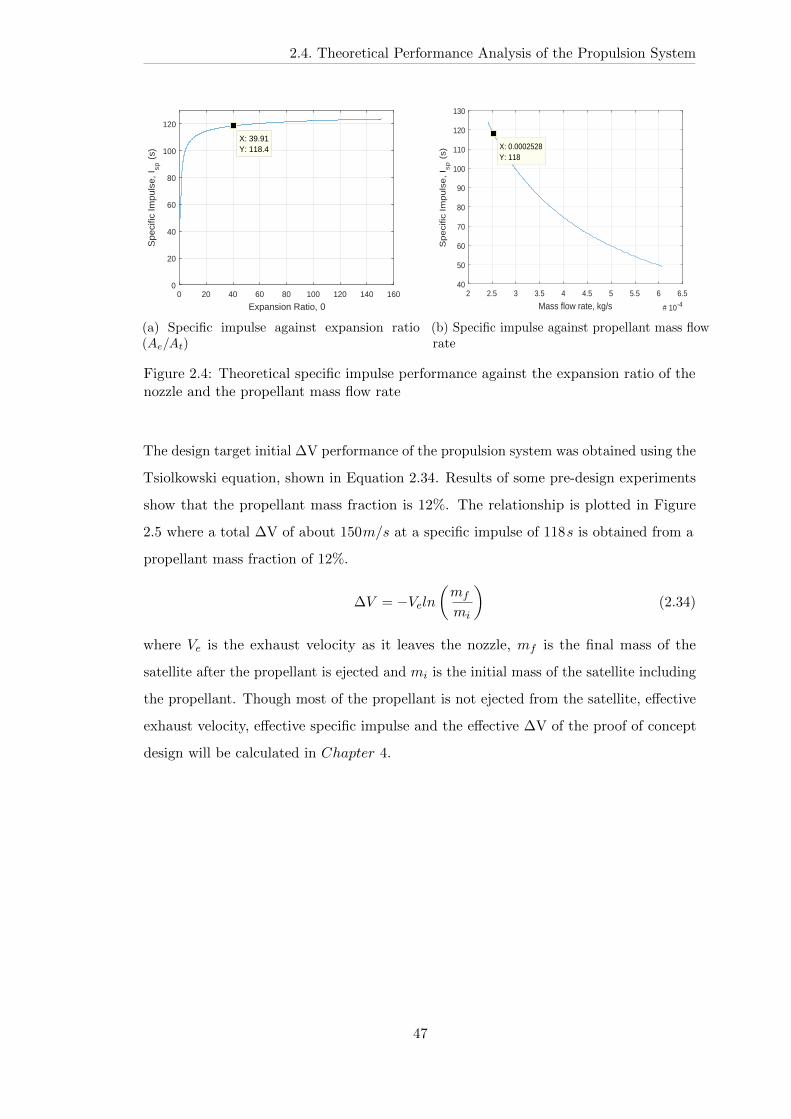
2.4. Theoretical Performance Analysis of the Propulsion System
0 20 40 60 80 100 120 140 160
Expansion Ratio, 0
0
20
40
60
80
100
120
Spe
cific
Impu
lse,
Isp
(s)
X: 39.91Y: 118.4
(a) Specific impulse against expansion ratio(𝐴𝑒/𝐴𝑡)
2 2.5 3 3.5 4 4.5 5 5.5 6 6.5
Mass flow rate, kg/s # 10-4
40
50
60
70
80
90
100
110
120
130
Sp
eci
fic Im
pu
lse
, I s
p(s
) X: 0.0002528Y: 118
(b) Specific impulse against propellant mass flowrate
Figure 2.4: Theoretical specific impulse performance against the expansion ratio of thenozzle and the propellant mass flow rate
The design target initial ΔV performance of the propulsion system was obtained using the
Tsiolkowski equation, shown in Equation 2.34. Results of some pre-design experiments
show that the propellant mass fraction is 12%. The relationship is plotted in Figure
2.5 where a total ΔV of about 150𝑚/𝑠 at a specific impulse of 118𝑠 is obtained from a
propellant mass fraction of 12%.
Δ𝑉 = −𝑉𝑒𝑙𝑛
(𝑚𝑓
𝑚𝑖
)(2.34)
where 𝑉𝑒 is the exhaust velocity as it leaves the nozzle, 𝑚𝑓 is the final mass of the
satellite after the propellant is ejected and 𝑚𝑖 is the initial mass of the satellite including
the propellant. Though most of the propellant is not ejected from the satellite, effective
exhaust velocity, effective specific impulse and the effective ΔV of the proof of concept
design will be calculated in 𝐶ℎ𝑎𝑝𝑡𝑒𝑟 4.
47
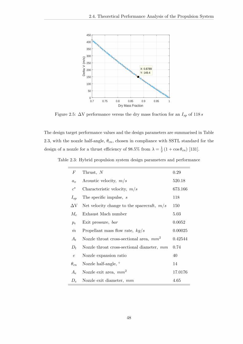
2.4. Theoretical Performance Analysis of the Propulsion System
0.7 0.75 0.8 0.85 0.9 0.95 1
Dry Mass Fraction
0
50
100
150
200
250
300
350
400
450
De
lta V
(m
/s)
X: 0.8789Y: 149.4
Figure 2.5: ΔV performance versus the dry mass fraction for an 𝐼𝑠𝑝 of 118 𝑠
The design target performance values and the design parameters are summarised in Table
2.3, with the nozzle half-angle, 𝜃𝑐𝑛, chosen in compliance with SSTL standard for the
design of a nozzle for a thrust efficiency of 98.5% from 𝜆 = 12 (1 + cos 𝜃𝑐𝑛) [131].
Table 2.3: Hybrid propulsion system design parameters and performance
𝐹 Thrust, 𝑁 0.29
𝑎𝑜 Acoustic velocity, 𝑚/𝑠 520.18
𝑐* Characteristic velocity, 𝑚/𝑠 673.166
𝐼𝑠𝑝 The specific impulse, 𝑠 118
ΔV Net velocity change to the spacecraft, 𝑚/𝑠 150
𝑀𝑒 Exhaust Mach number 5.03
𝑝𝑒 Exit pressure, 𝑏𝑎𝑟 0.0052
Propellant mass flow rate, 𝑘𝑔/𝑠 0.00025
𝐴𝑡 Nozzle throat cross-sectional area, 𝑚𝑚2 0.42544
𝐷𝑡 Nozzle throat cross-sectional diameter, 𝑚𝑚 0.74
𝑒 Nozzle expansion ratio 40
𝜃𝑐𝑛 Nozzle half-angle, ∘ 14
𝐴𝑒 Nozzle exit area, 𝑚𝑚2 17.0176
𝐷𝑒 Nozzle exit diameter, 𝑚𝑚 4.65
48

2.4. Theoretical Performance Analysis of the Propulsion System
2.4.1 Thruster Design
An experimental proof of concept to demonstrate the outlined objectives in Chapter 1
has been developed. There are two basic elements of the design: the reaction chamber
and nozzle. The thruster was designed and mounted on a moving plate of a thrust
balance for experimental thrust measurements. The components of the thruster are
described in this section.
2.4.1.1 Reaction Chamber
The chemical reaction of the propellants takes place in the reaction chamber. The
reaction chamber helps to convert the released chemical enthalpy and the random motion
of the exhaust gases into directed kinetic energy through the nozzle. Traditionally the
design of the thrust chamber is based on requirements that define its major parameters.
These requirements include the defined mission of the spacecraft, area of operation,
repeatability of the chemical process, reliability, mass and size of the thruster. At this
early stage of proof of concept testing of the model, our emphasis is on the repeatability
of the propulsion system and its ability to fit into the mass and volume of the spacecraft.
Since the chemical reaction in the chamber is non-combusting, there was no restriction
on its length and area, except to suit a CubeSat restricted volume. Hence the scaling
effect [141] of a characteristic chamber length for complete combustion in a conventional
chamber [142] was not considered in this design. The major requirement in the design is
for the chamber to contain as much propellant as needed for a 1𝑈 CubeSat as calculated
in section 2.3, and the chamber wall to withstand the generated pressure inside the
reaction volume. The reaction chamber was made from a 316 stainless steel and was
measured 42𝑚𝑚 × 30𝑚𝑚 in height and diameter respectively and a wall thickness of
1𝑚𝑚, just enough to take about 6 𝑔 fuel for the instance. The design of the reaction
chamber is shown in Figure 2.6, with the top images showing the inside of the chamber
while the bottom image shows the assembled part. The detailed manufacturing drawings
are provided in 𝐴𝑝𝑝𝑒𝑛𝑑𝑖𝑥 𝐴.
49
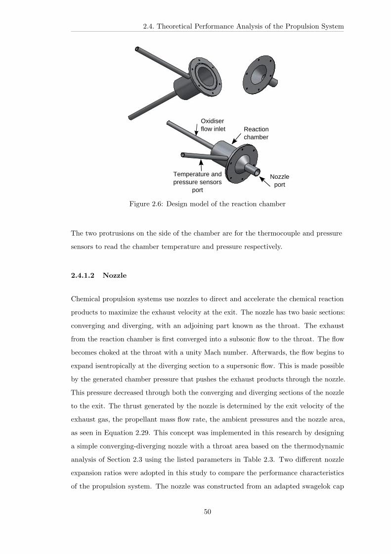
2.4. Theoretical Performance Analysis of the Propulsion System
AlldLenghtsdindmmAnglesd±X°dDistanced±dX SIZEjA4
PartdNamejdExpNozzlePartXXGdftScalejdXdjdX
Materialj
PartsdRequiredj
SurreydSpacedCentred)SSCUUniversitydofdSurreyBdBAdBuilding
GuildfordBdSurreyBdGUHdOXH
H7/7k/H7X7AhmeddOzomatadDavid
oa77XXO@surreyGacGuk 7O7 77 X
SteelXdX
ProjectdSheetjd Xdo
Oxidiserflow inlet Reaction
chamber
Temperature andpressure sensors
port
Nozzleport
Figure 2.6: Design model of the reaction chamber
The two protrusions on the side of the chamber are for the thermocouple and pressure
sensors to read the chamber temperature and pressure respectively.
2.4.1.2 Nozzle
Chemical propulsion systems use nozzles to direct and accelerate the chemical reaction
products to maximize the exhaust velocity at the exit. The nozzle has two basic sections:
converging and diverging, with an adjoining part known as the throat. The exhaust
from the reaction chamber is first converged into a subsonic flow to the throat. The flow
becomes choked at the throat with a unity Mach number. Afterwards, the flow begins to
expand isentropically at the diverging section to a supersonic flow. This is made possible
by the generated chamber pressure that pushes the exhaust products through the nozzle.
This pressure decreased through both the converging and diverging sections of the nozzle
to the exit. The thrust generated by the nozzle is determined by the exit velocity of the
exhaust gas, the propellant mass flow rate, the ambient pressures and the nozzle area,
as seen in Equation 2.29. This concept was implemented in this research by designing
a simple converging-diverging nozzle with a throat area based on the thermodynamic
analysis of Section 2.3 using the listed parameters in Table 2.3. Two different nozzle
expansion ratios were adopted in this study to compare the performance characteristics
of the propulsion system. The nozzle was constructed from an adapted swagelok cap
50

2.4. Theoretical Performance Analysis of the Propulsion System
and plug, and the design of the converging section of the nozzle is shown in Figure 2.7.
The detailed drawing of the nozzle is provided in 𝐴𝑝𝑝𝑒𝑛𝑑𝑖𝑥 𝐴
14o
Figure 2.7: Swagelok cap and plug [143] adopted as nozzle
51
Chapter 3
Experimental Setup
3.1 Overview
The section contains the description of an experimental lab setup to characterise the
propulsion system. This includes the description of the oxidiser feed system, data
acquisition system, vacuum facilities and the complete experimental setup.
3.2 Oxidizer Feed System
The propellant feed system determines how much of the sodium hydroxide + water
oxidiser is delivered per unit time to the reaction chamber containing the aluminium wool.
It consists of a tank to store the propellant, a feed mechanism that pushes the propellant
from the tank into the reaction chamber, piping, and a control mechanism to initiate
and regulate the propellant flow rate [144, 71]. Two conventional types of propellant
feed systems can be found in literature. They are the pump fed and the pressure fed
systems. The pump fed system pressurises the propellant into the reaction chamber
using turbopump at relatively high pressures [144]. This type of feed system is used for
short duration and high total impulse applications. The second type of feed system is a
pressure fed system. This is a simple method as it relies on the tank pressure to push
the propellant into the reaction chamber. This system is used for low total impulse and
long duration orbital missions. We adopted the pressure fed system for this propulsion
system for its simplicity, whose schematic is shown in Figure 3.1. It contains a cool gas
52
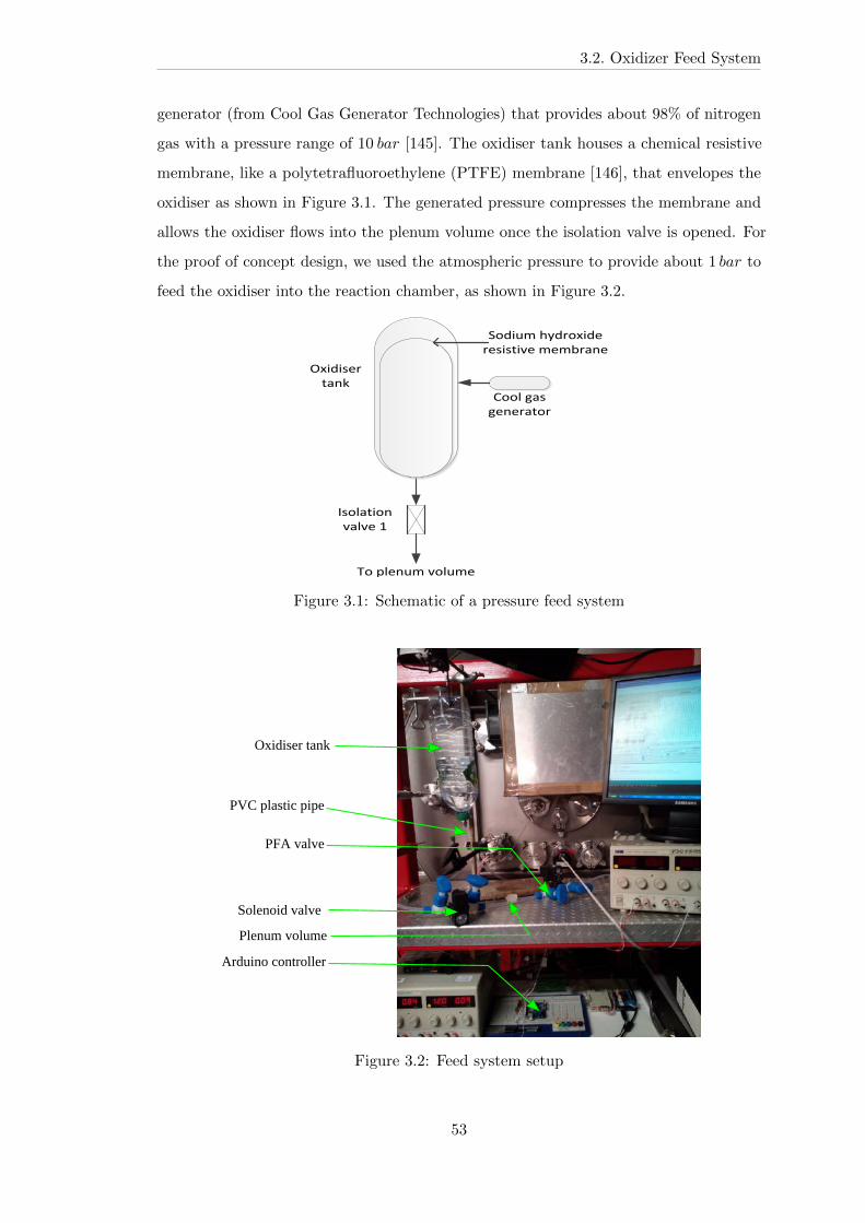
3.2. Oxidizer Feed System
generator (from Cool Gas Generator Technologies) that provides about 98% of nitrogen
gas with a pressure range of 10 𝑏𝑎𝑟 [145]. The oxidiser tank houses a chemical resistive
membrane, like a polytetrafluoroethylene (PTFE) membrane [146], that envelopes the
oxidiser as shown in Figure 3.1. The generated pressure compresses the membrane and
allows the oxidiser flows into the plenum volume once the isolation valve is opened. For
the proof of concept design, we used the atmospheric pressure to provide about 1 𝑏𝑎𝑟 to
feed the oxidiser into the reaction chamber, as shown in Figure 3.2.
Oxidiser tank
Cool gas generator
Isolation valve 1
Sodium hydroxide resistive membrane
To plenum volume
Figure 3.1: Schematic of a pressure feed system
Oxidiser tank
Solenoid valve
PFA valve
PVC plastic pipe
Plenum volume
Arduino controller
Figure 3.2: Feed system setup
53
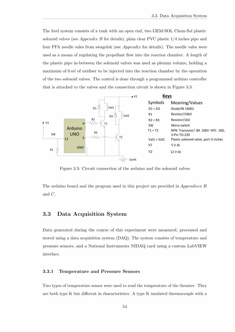
3.3. Data Acquisition System
The feed system consists of a tank with an open end, two GEM-SOL Chem-Sol plastic
solenoid valves (see 𝐴𝑝𝑝𝑒𝑛𝑑𝑖𝑥 𝐵 for details), plain clear PVC plastic 1/4 inches pipe and
four PFA needle vales from swagelok (see 𝐴𝑝𝑝𝑒𝑛𝑑𝑖𝑥 for details). The needle vales were
used as a means of regulating the propellant flow into the reaction chamber. A length of
the plastic pipe in-between the solenoid valves was used as plenum volume, holding a
maximum of 6𝑚𝑙 of oxidiser to be injected into the reaction chamber by the operation
of the two solenoid valves. The control is done through a programmed arduino controller
that is attached to the valves and the connection circuit is shown in Figure 3.3.
GND
¼
5-v
ArduinoUNO
D-
Dv
Val-
Valv
R-
Rv
Rp
V-
Vv
T-
TvSW
Keys
V-
Vv
T-e=eTv
Rve=eRp
SW
D-e=eDve
Symbols Meaning:ValuesDiode:INe-¼,,-
Resistor:-kΩ
Microeswitch
NPNe Transistor:e 8Ae -,,Ve HFE:e v,,HpFPineTOFvv,
5eVedc
-veVedc
Earth
R- Resistor:-,kΩ
Val-e=eValv PlasticesolenoidevalveHeporte¼einches
Figure 3.3: Circuit connection of the arduino and the solenoid valves
The arduino board and the program used in this project are provided in𝐴𝑝𝑝𝑒𝑛𝑑𝑖𝑐𝑒𝑠 𝐵
and 𝐶.
3.3 Data Acquisition System
Data generated during the course of this experiment were measured, processed and
stored using a data acquisition system (DAQ). The system consists of temperature and
pressure sensors, and a National Instruments NIDAQ card using a custom LabVIEW
interface.
3.3.1 Temperature and Pressure Sensors
Two types of temperature sensor were used to read the temperature of the thruster. They
are both type K but different in characteristics. A type K insulated thermocouple with a
54
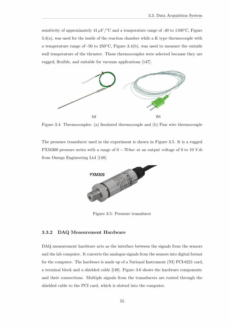
3.3. Data Acquisition System
sensitivity of approximately 41𝜇𝑉 /∘C and a temperature range of -40 to 1100∘C, Figure
3.4(a), was used for the inside of the reaction chamber while a K type thermocouple with
a temperature range of -50 to 250∘C, Figure 3.4(b), was used to measure the outside
wall temperature of the thruster. These thermocouples were selected because they are
rugged, flexible, and suitable for vacuum applications [147].
(a) (b)
Figure 3.4: Thermocouples: (a) Insulated thermocouple and (b) Fine wire thermocouple
The pressure transducer used in the experiment is shown in Figure 3.5. It is a rugged
PXM309 pressure series with a range of 0 − 70 𝑏𝑎𝑟 at an output voltage of 0 to 10 𝑉 𝑑𝑐
from Omega Engineering Ltd [148].
Figure 3.5: Pressure transducer
3.3.2 DAQ Measurement Hardware
DAQ measurement hardware acts as the interface between the signals from the sensors
and the lab computer. It converts the analogue signals from the sensors into digital format
for the computer. The hardware is made up of a National Instrument (NI) PCI-6221 card,
a terminal block and a shielded cable [149]. Figure 3.6 shows the hardware components
and their connections. Multiple signals from the transducers are routed through the
shielded cable to the PCI card, which is slotted into the computer.
55
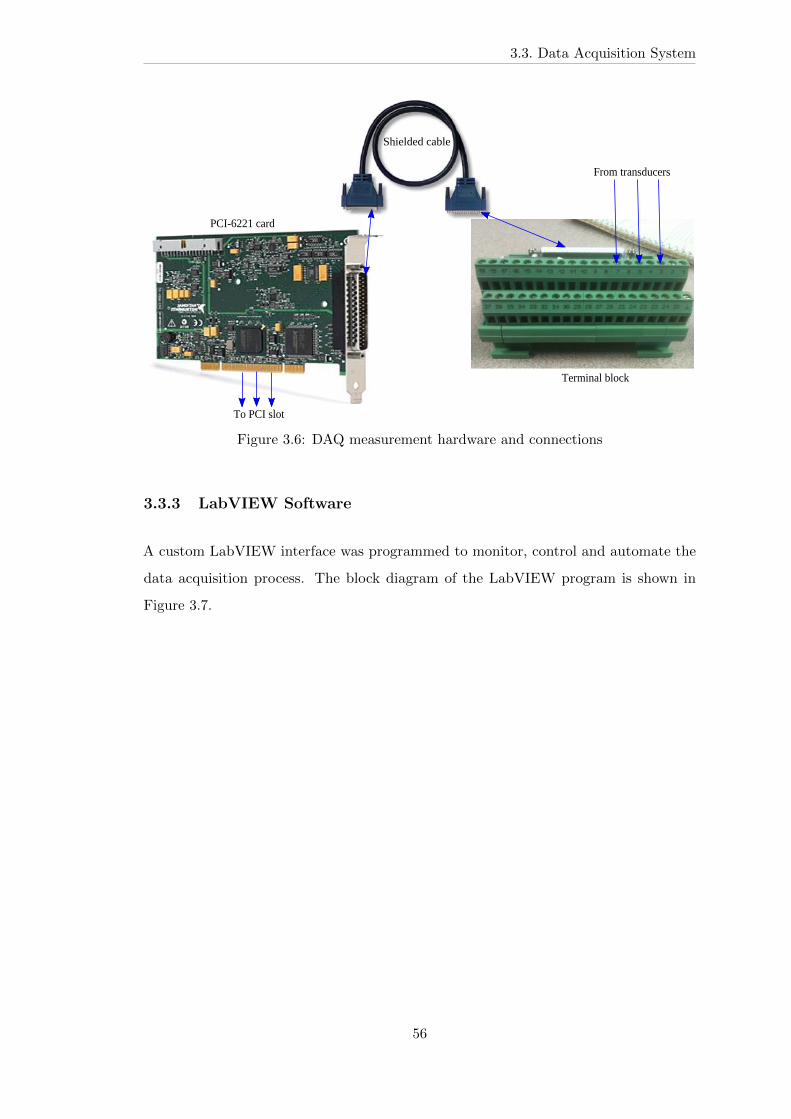
3.3. Data Acquisition System
To PCI slot
From transducers
PCI-6221 card
Terminal block
Shielded cable
Figure 3.6: DAQ measurement hardware and connections
3.3.3 LabVIEW Software
A custom LabVIEW interface was programmed to monitor, control and automate the
data acquisition process. The block diagram of the LabVIEW program is shown in
Figure 3.7.
56

3.4. Vacuum Facilities and Thrust Balance
Figure 3.7: Block diagram of the LabVIEW program used to control and acquire datafrom sensors
3.4 Vacuum Facilities and Thrust Balance
The propulsion lab of the Surrey Space Centre at the University of Surrey has four
vacuum facilities for high vacuum testing of propulsion systems. These include 𝐷𝑖𝑛𝑘𝑜,
𝐻𝑒𝑟𝑚𝑒𝑠, 𝑃𝑒𝑔𝑎𝑠𝑢𝑠 and 𝐷𝑎𝑒𝑑𝑎𝑙𝑢𝑠 vacuum facilities. The vacuum facilities, which contain
equipment that enables the testing and analysis of propulsion systems, provide adequate
conditions on earth to simulate the space environment and to validate the performance
characteristics of propulsion devices before they are flight ready.
3.4.1 The Pagasus Vacuum Chamber
Th 𝑃𝑎𝑔𝑎𝑠𝑢𝑠 chamber [150] is a horizontal stainless steel cylinder of 2𝑚 diameter and
1.5𝑚 length resulting in a total chamber volume of approximately 4.7𝑚3. The chamber
is connected to a rotary roughing pump and a turbo molecular pump with a combined
pumping speed of approximately 1700 𝑙/𝑠, which remove air, moisture and other gases
from the chamber. On the body of the chamber are multiple ports that are covered
57
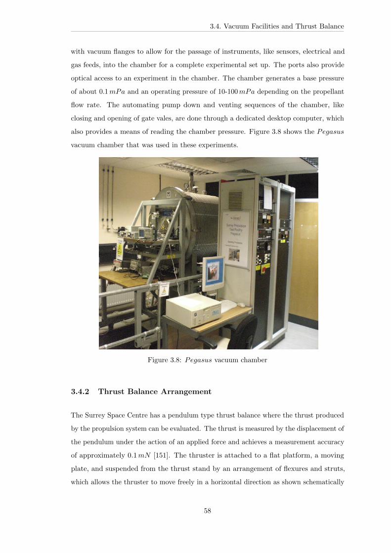
3.4. Vacuum Facilities and Thrust Balance
with vacuum flanges to allow for the passage of instruments, like sensors, electrical and
gas feeds, into the chamber for a complete experimental set up. The ports also provide
optical access to an experiment in the chamber. The chamber generates a base pressure
of about 0.1𝑚𝑃𝑎 and an operating pressure of 10-100𝑚𝑃𝑎 depending on the propellant
flow rate. The automating pump down and venting sequences of the chamber, like
closing and opening of gate vales, are done through a dedicated desktop computer, which
also provides a means of reading the chamber pressure. Figure 3.8 shows the 𝑃𝑒𝑔𝑎𝑠𝑢𝑠
vacuum chamber that was used in these experiments.
Figure 3.8: 𝑃𝑒𝑔𝑎𝑠𝑢𝑠 vacuum chamber
3.4.2 Thrust Balance Arrangement
The Surrey Space Centre has a pendulum type thrust balance where the thrust produced
by the propulsion system can be evaluated. The thrust is measured by the displacement of
the pendulum under the action of an applied force and achieves a measurement accuracy
of approximately 0.1𝑚𝑁 [151]. The thruster is attached to a flat platform, a moving
plate, and suspended from the thrust stand by an arrangement of flexures and struts,
which allows the thruster to move freely in a horizontal direction as shown schematically
58
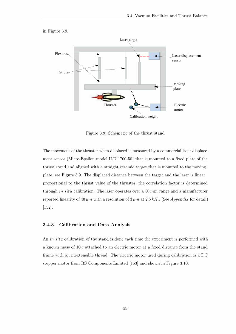
3.4. Vacuum Facilities and Thrust Balance
in Figure 3.9.
Laser displacement sensor
Moving plate
Electric motor
Calibration weight
Thruster
Struts
Flexures
Laser target
Figure 3.9: Schematic of the thrust stand
The movement of the thruster when displaced is measured by a commercial laser displace-
ment sensor (Micro-Epsilon model ILD 1700-50) that is mounted to a fixed plate of the
thrust stand and aligned with a straight ceramic target that is mounted to the moving
plate, see Figure 3.9. The displaced distance between the target and the laser is linear
proportional to the thrust value of the thruster; the correlation factor is determined
through 𝑖𝑛 𝑠𝑖𝑡𝑢 calibration. The laser operates over a 50𝑚𝑚 range and a manufacturer
reported linearity of 40𝜇𝑚 with a resolution of 3𝜇𝑚 at 2.5 𝑘𝐻𝑧 (See 𝐴𝑝𝑝𝑒𝑛𝑑𝑖𝑥 for detail)
[152].
3.4.3 Calibration and Data Analysis
An 𝑖𝑛 𝑠𝑖𝑡𝑢 calibration of the stand is done each time the experiment is performed with
a known mass of 10 𝑔 attached to an electric motor at a fixed distance from the stand
frame with an inextensible thread. The electric motor used during calibration is a DC
stepper motor from RS Components Limited [153] and shown in Figure 3.10.
59
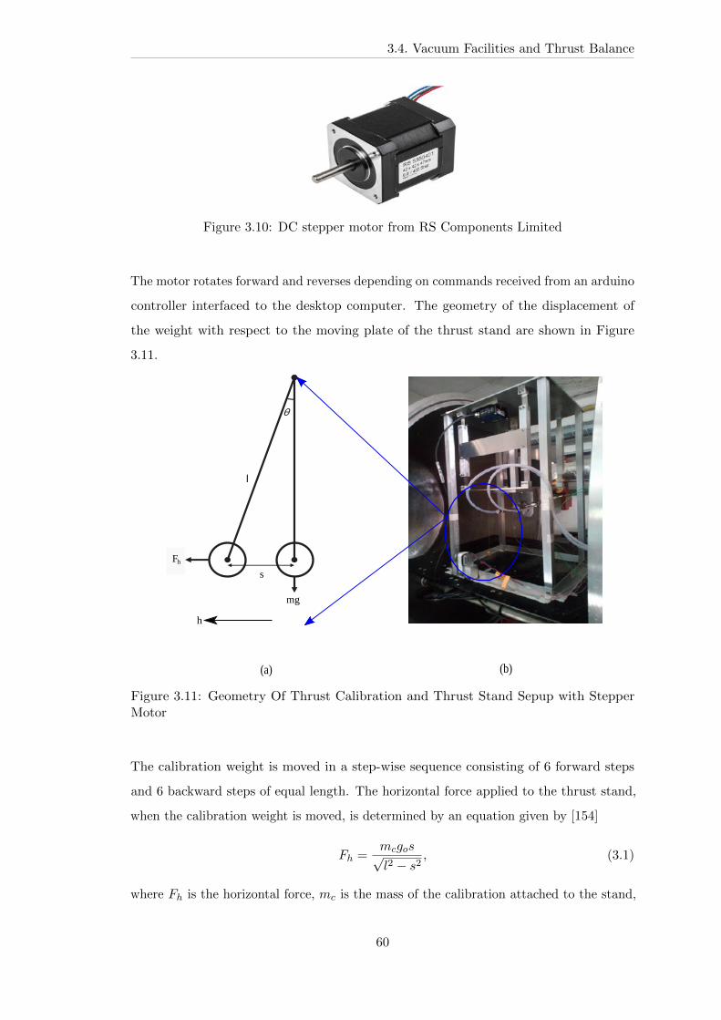
3.4. Vacuum Facilities and Thrust Balance
Figure 3.10: DC stepper motor from RS Components Limited
The motor rotates forward and reverses depending on commands received from an arduino
controller interfaced to the desktop computer. The geometry of the displacement of
the weight with respect to the moving plate of the thrust stand are shown in Figure
3.11.
θ
22 sls
mg−
=
zF
(a) (b)
h
s
mg
l
Fh
l
Figure 3.11: Geometry Of Thrust Calibration and Thrust Stand Sepup with StepperMotor
The calibration weight is moved in a step-wise sequence consisting of 6 forward steps
and 6 backward steps of equal length. The horizontal force applied to the thrust stand,
when the calibration weight is moved, is determined by an equation given by [154]
𝐹ℎ =𝑚𝑐𝑔𝑜𝑠√𝑙2 − 𝑠2
, (3.1)
where 𝐹ℎ is the horizontal force, 𝑚𝑐 is the mass of the calibration attached to the stand,
60

3.4. Vacuum Facilities and Thrust Balance
𝑠 is the horizontal displacement distance of the mass from the stand, and 𝑙 is the length
of the pendulum thread suspending the mass. The thrust stand has an accuracy of
±0.1𝑚𝑁 [155].
The plots of the moving plate in response to the applied force as a function of time is
shown in Figure 3.12(a). The stable position of the plate before the action of the electric
motor is indicated by about 21.9𝑚𝑚 mark on the vertical axis. At this point there is
no weight on the horizontal thread attached to the motor. The red signal represents
the addition of weight in the horizontal axis by the displacement of the moving plate
in forward and backward direction. The associated noise in the signal was filtered out
using a butterworth low pass filter, which is shown in blue line in the same figure. The
horizontal green line shows a repetition of the corresponding positions of the moving
plate when moving backward. Figure 3.12(b) shows the linear relationship of the thrust
balance to the applied force. Though six positions were considered for the thrust balance
calibration, the 50𝑚𝑚 range of the laser displacement sensor could accommodate a
higher force than applied. The gradient of the relationship of a particular calibration
gives a calibration constant of about 2.541𝑚𝑚/𝑁 or 0.39355𝑁/𝑚𝑚, and it gives the
corresponding relationship between the applied force and the deflection of the moving
plate.
0 10 20 30 40 50 60
21.75
21.8
21.85
21.9
21.95
Time (s)
Dis
pla
cem
en
t (m
m)
0.01 0.02 0.03 0.04 0.05 0.06 0.0721.75
21.8
21.85
21.9
Force (N)
Dis
pla
cem
en
t (m
m)
(a) (b)
Figure 3.12: Responses of Thrust Calibration
61
3.5. Complete Experimental Setup
3.5 Complete Experimental Setup
This section describes the integrated experimental setup. It also shows the flow path
of propellant from the oxidiser tank into the reaction chamber already containing fuel.
Figure 3.13 shows the schematic of the complete experimental setup.
The laser displacement sensor of Section 3.4.2, electric stepper motor and the cali-
bration weight of Section 3.4.3 are attached to the thrust stand and placed in the vacuum
chamber, with all the electrical cables interfaced through feedthroughs and connected
to the computer. At the start of each experiment, the thruster is pre-loaded with a
precise mass of aluminium wool fuel. A controlled volume of oxidiser, by the operation
of the two plenum valves, is released from the oxidiser tank into the reaction chamber to
commence the reaction. The rate of temperature and pressure change within the reaction
volume are recorded using the LabVIEW software program of Section 3.3.3 through their
respective sensors. The resulted thrust force produced by the device is sensed by the
laser sensor and recorded by the computer.
62
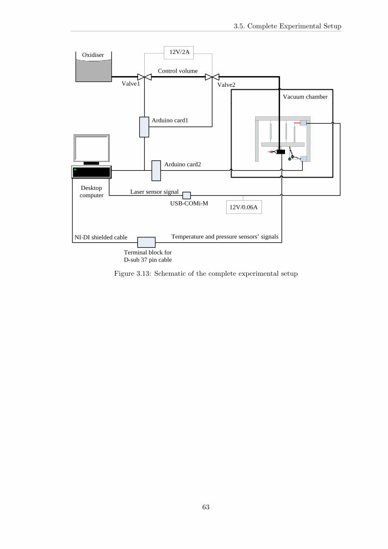
3.5. Complete Experimental Setup
Computer
Terminal block for D-sub 37 pin cable
USB-COMi-M
Arduino card2
Arduino card1
Desktopcomputer
Vacuum chamber
Control volume
Valve1 Valve2
Laser sensor signal
Temperature and pressure sensors’ signalsNI-DI shielded cable
12V/2A
12V/0.06A
Oxidiser
Figure 3.13: Schematic of the complete experimental setup
63
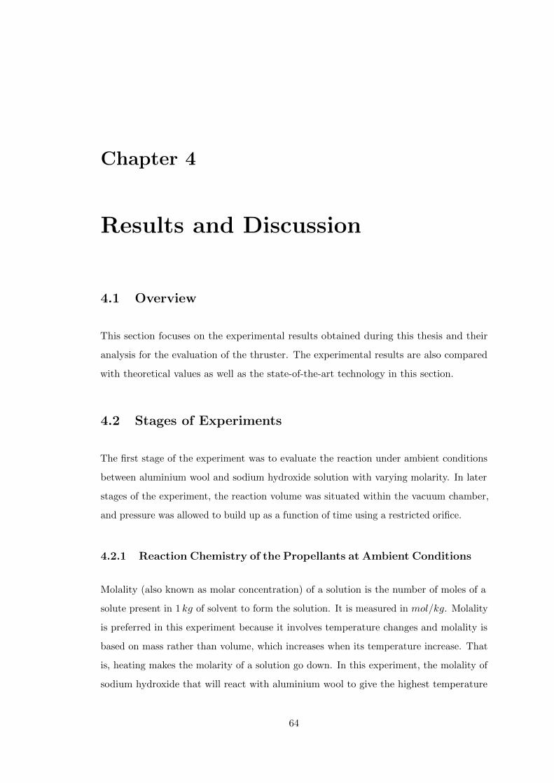
Chapter 4
Results and Discussion
4.1 Overview
This section focuses on the experimental results obtained during this thesis and their
analysis for the evaluation of the thruster. The experimental results are also compared
with theoretical values as well as the state-of-the-art technology in this section.
4.2 Stages of Experiments
The first stage of the experiment was to evaluate the reaction under ambient conditions
between aluminium wool and sodium hydroxide solution with varying molarity. In later
stages of the experiment, the reaction volume was situated within the vacuum chamber,
and pressure was allowed to build up as a function of time using a restricted orifice.
4.2.1 Reaction Chemistry of the Propellants at Ambient Conditions
Molality (also known as molar concentration) of a solution is the number of moles of a
solute present in 1 𝑘𝑔 of solvent to form the solution. It is measured in 𝑚𝑜𝑙/𝑘𝑔. Molality
is preferred in this experiment because it involves temperature changes and molality is
based on mass rather than volume, which increases when its temperature increase. That
is, heating makes the molarity of a solution go down. In this experiment, the molality of
sodium hydroxide that will react with aluminium wool to give the highest temperature
64
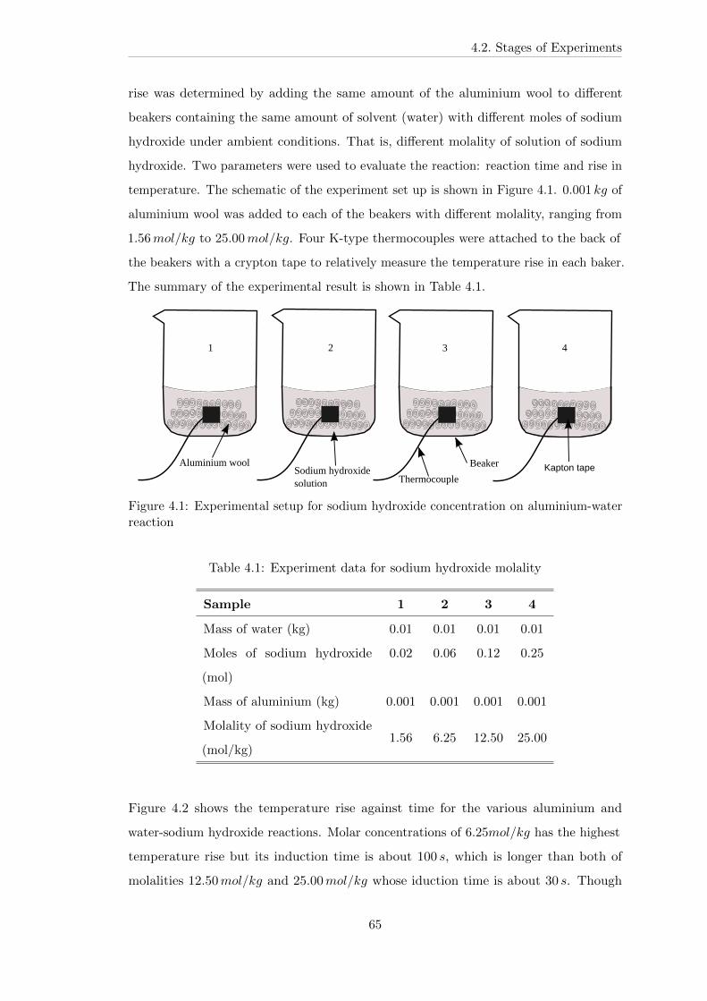
4.2. Stages of Experiments
rise was determined by adding the same amount of the aluminium wool to different
beakers containing the same amount of solvent (water) with different moles of sodium
hydroxide under ambient conditions. That is, different molality of solution of sodium
hydroxide. Two parameters were used to evaluate the reaction: reaction time and rise in
temperature. The schematic of the experiment set up is shown in Figure 4.1. 0.001 𝑘𝑔 of
aluminium wool was added to each of the beakers with different molality, ranging from
1.56𝑚𝑜𝑙/𝑘𝑔 to 25.00𝑚𝑜𝑙/𝑘𝑔. Four K-type thermocouples were attached to the back of
the beakers with a crypton tape to relatively measure the temperature rise in each baker.
The summary of the experimental result is shown in Table 4.1.
Thermocouple
Aluminium wool Crypton tapeSodium hydroxide solution
Beaker
1 2 3 4
Kapton tape
Figure 4.1: Experimental setup for sodium hydroxide concentration on aluminium-waterreaction
Table 4.1: Experiment data for sodium hydroxide molality
Sample 1 2 3 4
Mass of water (kg) 0.01 0.01 0.01 0.01
Moles of sodium hydroxide
(mol)
0.02 0.06 0.12 0.25
Mass of aluminium (kg) 0.001 0.001 0.001 0.001
Molality of sodium hydroxide
(mol/kg)1.56 6.25 12.50 25.00
Figure 4.2 shows the temperature rise against time for the various aluminium and
water-sodium hydroxide reactions. Molar concentrations of 6.25𝑚𝑜𝑙/𝑘𝑔 has the highest
temperature rise but its induction time is about 100 𝑠, which is longer than both of
molalities 12.50𝑚𝑜𝑙/𝑘𝑔 and 25.00𝑚𝑜𝑙/𝑘𝑔 whose iduction time is about 30 𝑠. Though
65
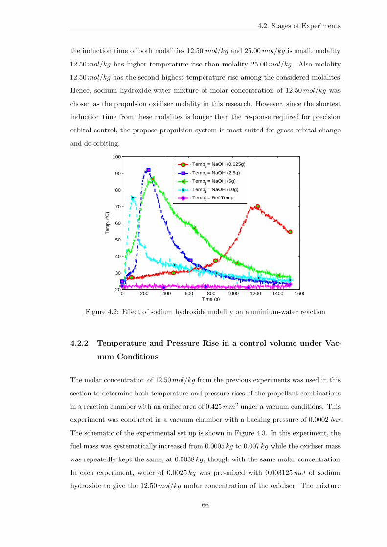
4.2. Stages of Experiments
the induction time of both molalities 12.50 𝑚𝑜𝑙/𝑘𝑔 and 25.00𝑚𝑜𝑙/𝑘𝑔 is small, molality
12.50𝑚𝑜𝑙/𝑘𝑔 has higher temperature rise than molality 25.00𝑚𝑜𝑙/𝑘𝑔. Also molality
12.50𝑚𝑜𝑙/𝑘𝑔 has the second highest temperature rise among the considered molalites.
Hence, sodium hydroxide-water mixture of molar concentration of 12.50𝑚𝑜𝑙/𝑘𝑔 was
chosen as the propulsion oxidiser molality in this research. However, since the shortest
induction time from these molalites is longer than the response required for precision
orbital control, the propose propulsion system is most suited for gross orbital change
and de-orbiting.
0 200 400 600 800 1000 1200 1400 160020
30
40
50
60
70
80
90
100
Time (s)
Tem
p. (°
C)
Temp1 = NaOH (0.625g)
Temp2 = NaOH (2.5g)
Temp3 = NaOH (5g)
Temp4 = NaOH (10g)
Temp5 = Ref Temp.
Figure 4.2: Effect of sodium hydroxide molality on aluminium-water reaction
4.2.2 Temperature and Pressure Rise in a control volume under Vac-
uum Conditions
The molar concentration of 12.50𝑚𝑜𝑙/𝑘𝑔 from the previous experiments was used in this
section to determine both temperature and pressure rises of the propellant combinations
in a reaction chamber with an orifice area of 0.425𝑚𝑚2 under a vacuum conditions. This
experiment was conducted in a vacuum chamber with a backing pressure of 0.0002 𝑏𝑎𝑟.
The schematic of the experimental set up is shown in Figure 4.3. In this experiment, the
fuel mass was systematically increased from 0.0005 𝑘𝑔 to 0.007 𝑘𝑔 while the oxidiser mass
was repeatedly kept the same, at 0.0038 𝑘𝑔, though with the same molar concentration.
In each experiment, water of 0.0025 𝑘𝑔 was pre-mixed with 0.003125𝑚𝑜𝑙 of sodium
hydroxide to give the 12.50𝑚𝑜𝑙/𝑘𝑔 molar concentration of the oxidiser. The mixture
66
4.2. Stages of Experiments
was shaken to avoid the solidification of the alkaline solution, allowed it to cool down to
dissipate the generated heat before injecting the mixture into the reaction chamber.
Thermocouple
Flow restrictor
Computer
Reaction Chamber
Restrictor Valve
Solid Fuel
Oxidiser Injector
Vacuum Chamber
Feedthrough
Feedthrough
Pressure relief valve
P Pressure gauge
Figure 4.3: Schematic of the initial lab setup
Each experiment was repeated at least twice to confirm the results. The summary of the
experiment is shown in Table 4.2.
Table 4.2: Temperature and pressure rise in vacuum condition
Experiments 1 2 3 4 5
Mass/Concentration of
oxidiser (kg)/(mol/kg)0.00375/12.50 0.00375/12.50 0.00375/12.50 0.00375/12.50 0.00375/12.50
Mass of fuel (kg) 0.0005 0.001 0.003 0.005 0.007
Change in temperature
(∘C)19.00 22.00 40.00 94.00 88.00
Change in pressure (bar) 0.06 0.12 0.37 0.83 0.47
67
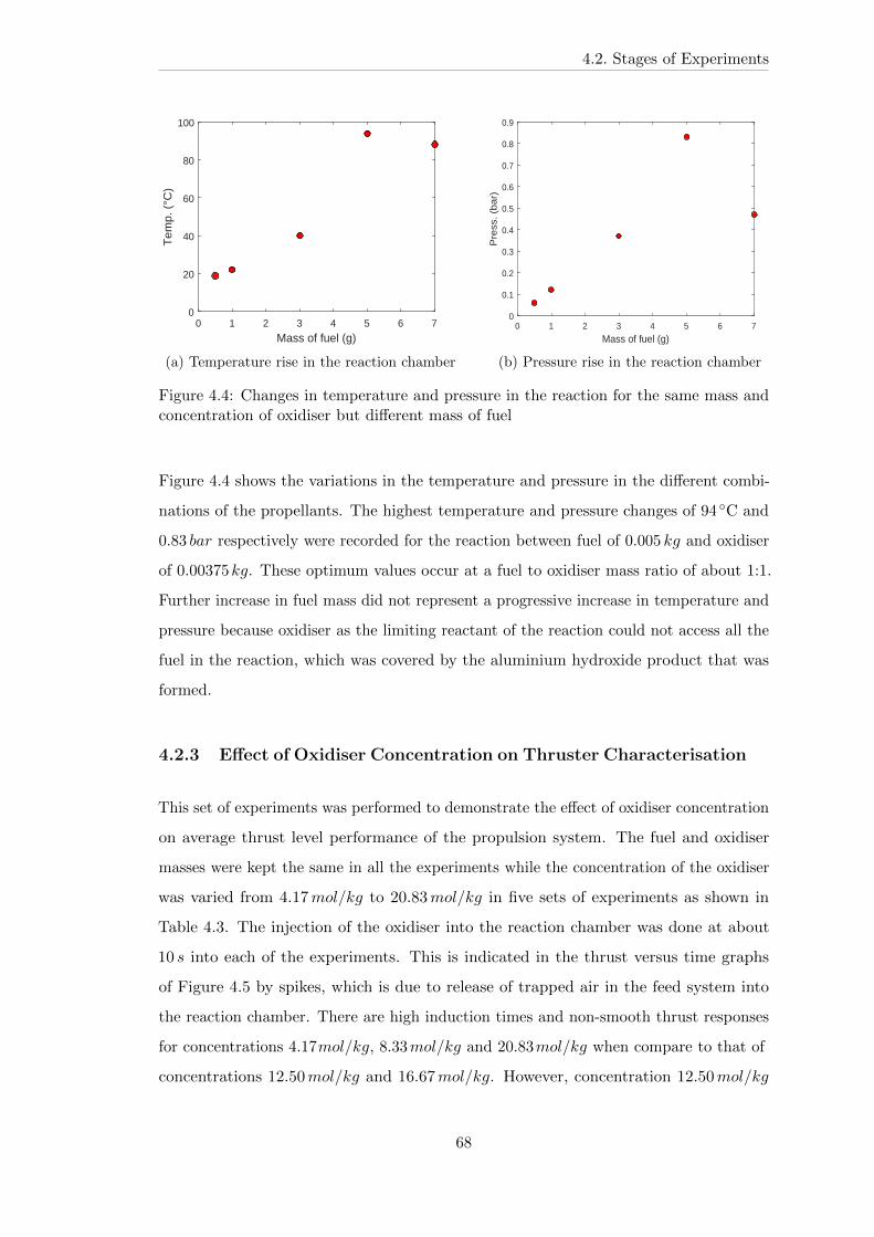
4.2. Stages of Experiments
0 1 2 3 4 5 6 7
Mass of fuel (g)
0
20
40
60
80
100
Tem
p. (
°C)
(a) Temperature rise in the reaction chamber
0 1 2 3 4 5 6 7
Mass of fuel (g)
0
0.1
0.2
0.3
0.4
0.5
0.6
0.7
0.8
0.9
Pre
ss. (b
ar)
(b) Pressure rise in the reaction chamber
Figure 4.4: Changes in temperature and pressure in the reaction for the same mass andconcentration of oxidiser but different mass of fuel
Figure 4.4 shows the variations in the temperature and pressure in the different combi-
nations of the propellants. The highest temperature and pressure changes of 94 ∘C and
0.83 𝑏𝑎𝑟 respectively were recorded for the reaction between fuel of 0.005 𝑘𝑔 and oxidiser
of 0.00375𝑘𝑔. These optimum values occur at a fuel to oxidiser mass ratio of about 1:1.
Further increase in fuel mass did not represent a progressive increase in temperature and
pressure because oxidiser as the limiting reactant of the reaction could not access all the
fuel in the reaction, which was covered by the aluminium hydroxide product that was
formed.
4.2.3 Effect of Oxidiser Concentration on Thruster Characterisation
This set of experiments was performed to demonstrate the effect of oxidiser concentration
on average thrust level performance of the propulsion system. The fuel and oxidiser
masses were kept the same in all the experiments while the concentration of the oxidiser
was varied from 4.17𝑚𝑜𝑙/𝑘𝑔 to 20.83𝑚𝑜𝑙/𝑘𝑔 in five sets of experiments as shown in
Table 4.3. The injection of the oxidiser into the reaction chamber was done at about
10 𝑠 into each of the experiments. This is indicated in the thrust versus time graphs
of Figure 4.5 by spikes, which is due to release of trapped air in the feed system into
the reaction chamber. There are high induction times and non-smooth thrust responses
for concentrations 4.17𝑚𝑜𝑙/𝑘𝑔, 8.33𝑚𝑜𝑙/𝑘𝑔 and 20.83𝑚𝑜𝑙/𝑘𝑔 when compare to that of
concentrations 12.50𝑚𝑜𝑙/𝑘𝑔 and 16.67𝑚𝑜𝑙/𝑘𝑔. However, concentration 12.50𝑚𝑜𝑙/𝑘𝑔
68
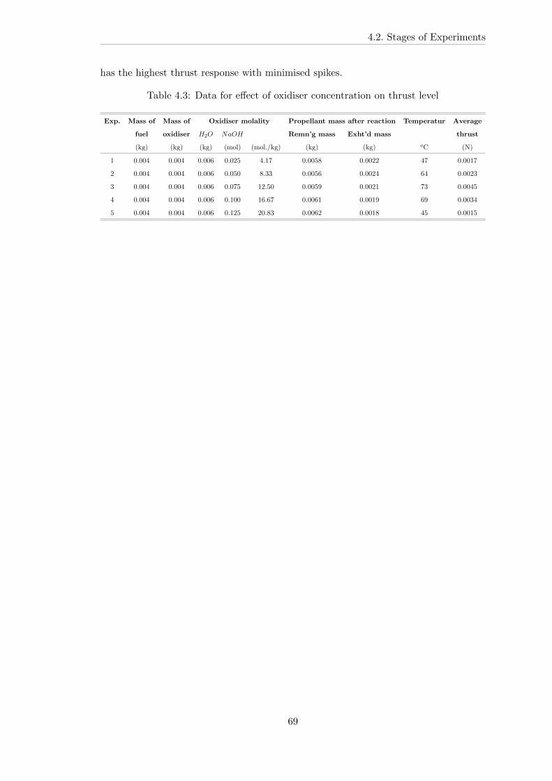
4.2. Stages of Experiments
has the highest thrust response with minimised spikes.
Table 4.3: Data for effect of oxidiser concentration on thrust level
Exp. Mass of Mass of Oxidiser molality Propellant mass after reaction Temperatur Average
fuel oxidiser 𝐻2𝑂 𝑁𝑎𝑂𝐻 Remn’g mass Exht’d mass thrust
(kg) (kg) (kg) (mol) (mol./kg) (kg) (kg) 𝑜C (N)
1 0.004 0.004 0.006 0.025 4.17 0.0058 0.0022 47 0.0017
2 0.004 0.004 0.006 0.050 8.33 0.0056 0.0024 64 0.0023
3 0.004 0.004 0.006 0.075 12.50 0.0059 0.0021 73 0.0045
4 0.004 0.004 0.006 0.100 16.67 0.0061 0.0019 69 0.0034
5 0.004 0.004 0.006 0.125 20.83 0.0062 0.0018 45 0.0015
69
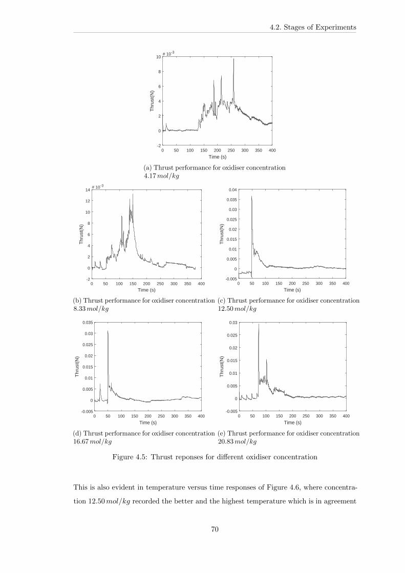
4.2. Stages of Experiments
0 50 100 150 200 250 300 350 400
Time (s)
-2
0
2
4
6
8
10
Thr
ust(
N)
# 10-3
(a) Thrust performance for oxidiser concentration4.17𝑚𝑜𝑙/𝑘𝑔
0 50 100 150 200 250 300 350 400
Time (s)
-2
0
2
4
6
8
10
12
14
Thr
ust(
N)
# 10-3
(b) Thrust performance for oxidiser concentration8.33𝑚𝑜𝑙/𝑘𝑔
0 50 100 150 200 250 300 350 400
Time (s)
-0.005
0
0.005
0.01
0.015
0.02
0.025
0.03
0.035
0.04
Th
rust
(N)
(c) Thrust performance for oxidiser concentration12.50𝑚𝑜𝑙/𝑘𝑔
0 50 100 150 200 250 300 350 400
Time (s)
-0.005
0
0.005
0.01
0.015
0.02
0.025
0.03
0.035
Th
rust
(N)
(d) Thrust performance for oxidiser concentration16.67𝑚𝑜𝑙/𝑘𝑔
0 50 100 150 200 250 300 350 400
Time (s)
-0.005
0
0.005
0.01
0.015
0.02
0.025
0.03
Th
rust
(N)
(e) Thrust performance for oxidiser concentration20.83𝑚𝑜𝑙/𝑘𝑔
Figure 4.5: Thrust reponses for different oxidiser concentration
This is also evident in temperature versus time responses of Figure 4.6, where concentra-
tion 12.50𝑚𝑜𝑙/𝑘𝑔 recorded the better and the highest temperature which is in agreement
70
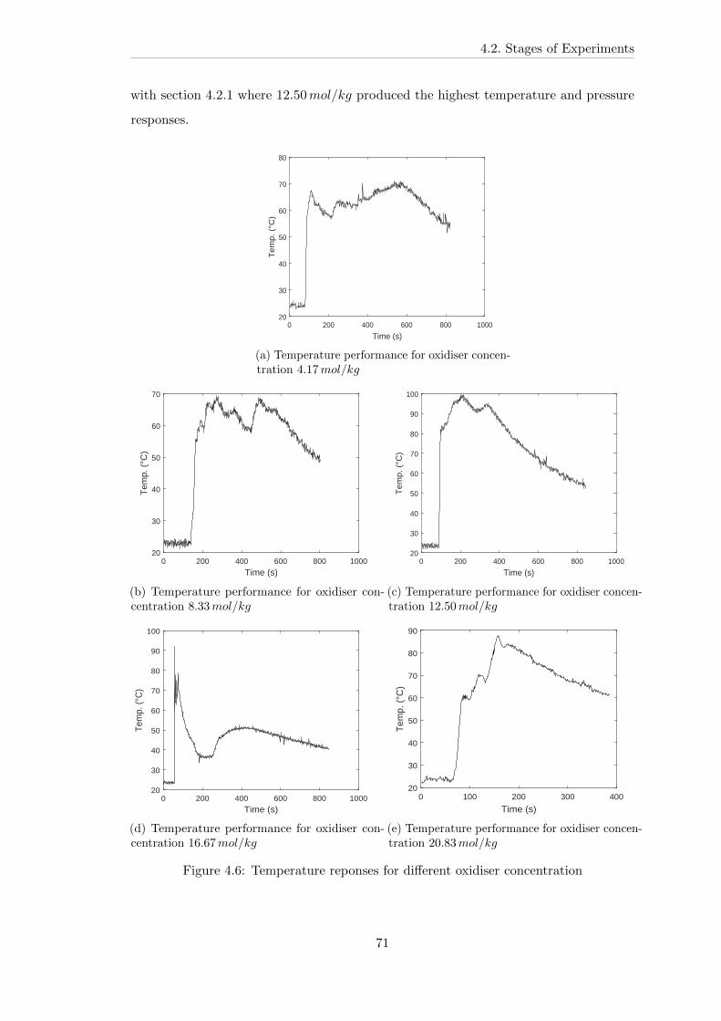
4.2. Stages of Experiments
with section 4.2.1 where 12.50𝑚𝑜𝑙/𝑘𝑔 produced the highest temperature and pressure
responses.
0 200 400 600 800 1000
Time (s)
20
30
40
50
60
70
80
Te
mp
. (°
C)
(a) Temperature performance for oxidiser concen-tration 4.17𝑚𝑜𝑙/𝑘𝑔
0 200 400 600 800 1000
Time (s)
20
30
40
50
60
70
Tem
p. (
°C)
(b) Temperature performance for oxidiser con-centration 8.33𝑚𝑜𝑙/𝑘𝑔
0 200 400 600 800 1000
Time (s)
20
30
40
50
60
70
80
90
100T
emp.
(°C
)
(c) Temperature performance for oxidiser concen-tration 12.50𝑚𝑜𝑙/𝑘𝑔
0 200 400 600 800 1000
Time (s)
20
30
40
50
60
70
80
90
100
Tem
p. (°
C)
(d) Temperature performance for oxidiser con-centration 16.67𝑚𝑜𝑙/𝑘𝑔
0 100 200 300 400
Time (s)
20
30
40
50
60
70
80
90
Tem
p. (
°C)
(e) Temperature performance for oxidiser concen-tration 20.83𝑚𝑜𝑙/𝑘𝑔
Figure 4.6: Temperature reponses for different oxidiser concentration
71
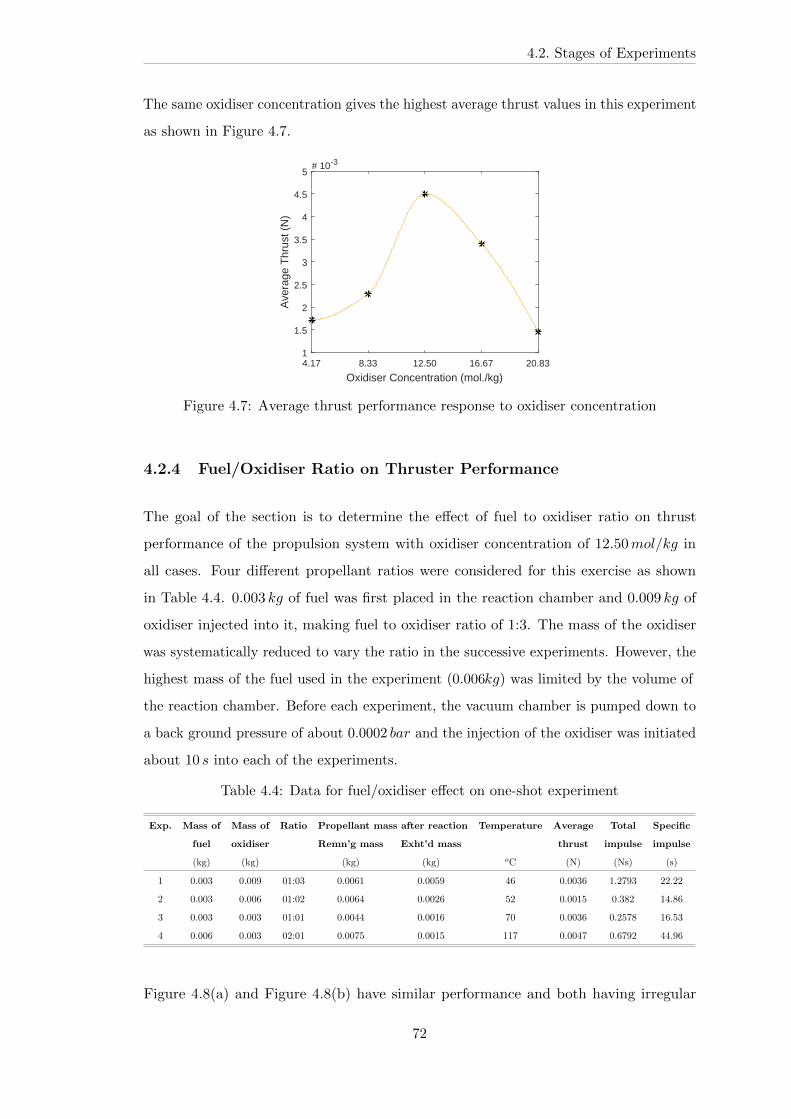
4.2. Stages of Experiments
The same oxidiser concentration gives the highest average thrust values in this experiment
as shown in Figure 4.7.
4.17 8.33 12.50 16.67 20.83
Oxidiser Concentration (mol./kg)
1
1.5
2
2.5
3
3.5
4
4.5
5
Ave
rage
Thr
ust (
N)
# 10-3
Figure 4.7: Average thrust performance response to oxidiser concentration
4.2.4 Fuel/Oxidiser Ratio on Thruster Performance
The goal of the section is to determine the effect of fuel to oxidiser ratio on thrust
performance of the propulsion system with oxidiser concentration of 12.50𝑚𝑜𝑙/𝑘𝑔 in
all cases. Four different propellant ratios were considered for this exercise as shown
in Table 4.4. 0.003 𝑘𝑔 of fuel was first placed in the reaction chamber and 0.009 𝑘𝑔 of
oxidiser injected into it, making fuel to oxidiser ratio of 1:3. The mass of the oxidiser
was systematically reduced to vary the ratio in the successive experiments. However, the
highest mass of the fuel used in the experiment (0.006𝑘𝑔) was limited by the volume of
the reaction chamber. Before each experiment, the vacuum chamber is pumped down to
a back ground pressure of about 0.0002 𝑏𝑎𝑟 and the injection of the oxidiser was initiated
about 10 𝑠 into each of the experiments.
Table 4.4: Data for fuel/oxidiser effect on one-shot experiment
Exp. Mass of Mass of Ratio Propellant mass after reaction Temperature Average Total Specific
fuel oxidiser Remn’g mass Exht’d mass thrust impulse impulse
(kg) (kg) (kg) (kg) 𝑜C (N) (Ns) (s)
1 0.003 0.009 01:03 0.0061 0.0059 46 0.0036 1.2793 22.22
2 0.003 0.006 01:02 0.0064 0.0026 52 0.0015 0.382 14.86
3 0.003 0.003 01:01 0.0044 0.0016 70 0.0036 0.2578 16.53
4 0.006 0.003 02:01 0.0075 0.0015 117 0.0047 0.6792 44.96
Figure 4.8(a) and Figure 4.8(b) have similar performance and both having irregular
72

4.2. Stages of Experiments
responses with longer settling time, though the former has higher thrust value than the
later. They are respectively for propellant ratios 1:3 and 1:2. On the basis of these, it
appears that excessive oxidiser to fuel diminishes the reaction temperature and reaction
rate and results in poor propulsive performance. On the contrary, Figure 4.8(c) and
Figure 4.8(d) of ratios 1:1 and 2:1 respectively have shorter settling time, higher thrust
values and smoother responses with higher propellant efficiency, providing a possibility of
repeatable injections. The spikes at the instance of oxidiser injection are due to release of
trapped air in the feed system. These later propellant ratios also show higher temperature
responses as indicated in the table and shown in Figure 4.9. Hence propellant ratio 2:1
gives the highest average thrust of 0.0047𝑁 and specific impulse of about 45 𝑠 for the
considered combinations.
0 50 100 150 200 250 300 350 400
Time (s)
-5
0
5
10
15
20
Th
rust
(N)
# 10-3
(a) Thrust performance for fuel to oxidiser ratioof 1:3
0 50 100 150 200 250 300 350 400
Time (s)
-2
0
2
4
6
8
Thr
ust(
N)
# 10-3
(b) Thrust performance for fuel to oxidiser ratioof 1:2
0 50 100 150 200 250 300 350 400
Time (s)
-0.005
0
0.005
0.01
0.015
0.02
0.025
Thr
ust(
N)
(c) Thrust performance for fuel to oxidiser ratioof 1:1
0 50 100 150 200 250 300 350 400
Time (s)
-0.02
-0.01
0
0.01
0.02
0.03
0.04
Th
rust
(N)
(d) Thrust performance for fuel to oxidiser ratioof 2:1
Figure 4.8: One-shot thrust characterisation of the propulsion system on differentpropellant ratios
73
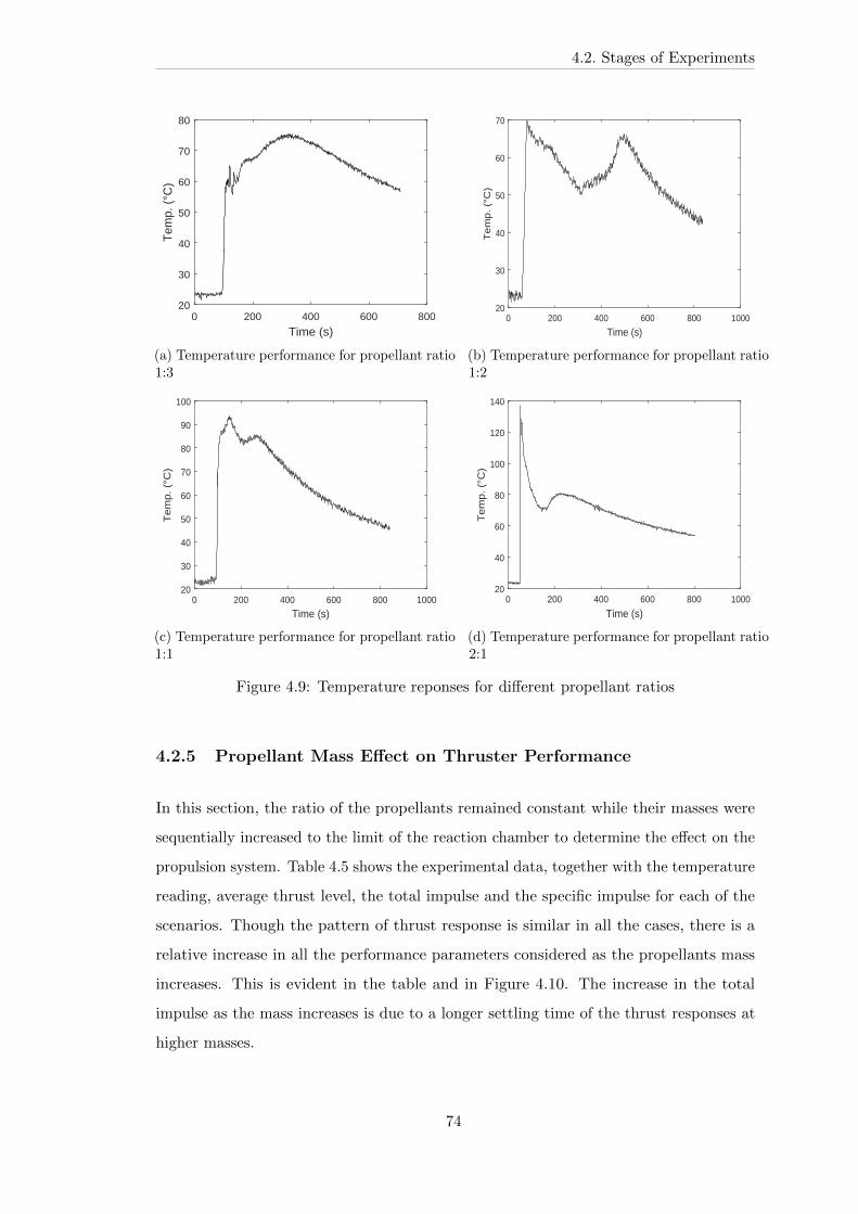
4.2. Stages of Experiments
0 200 400 600 800
Time (s)
20
30
40
50
60
70
80
Tem
p. (
°C)
(a) Temperature performance for propellant ratio1:3
0 200 400 600 800 1000
Time (s)
20
30
40
50
60
70
Te
mp
. (°
C)
(b) Temperature performance for propellant ratio1:2
0 200 400 600 800 1000
Time (s)
20
30
40
50
60
70
80
90
100
Te
mp
. (°
C)
(c) Temperature performance for propellant ratio1:1
0 200 400 600 800 1000
Time (s)
20
40
60
80
100
120
140
Te
mp
. (°
C)
(d) Temperature performance for propellant ratio2:1
Figure 4.9: Temperature reponses for different propellant ratios
4.2.5 Propellant Mass Effect on Thruster Performance
In this section, the ratio of the propellants remained constant while their masses were
sequentially increased to the limit of the reaction chamber to determine the effect on the
propulsion system. Table 4.5 shows the experimental data, together with the temperature
reading, average thrust level, the total impulse and the specific impulse for each of the
scenarios. Though the pattern of thrust response is similar in all the cases, there is a
relative increase in all the performance parameters considered as the propellants mass
increases. This is evident in the table and in Figure 4.10. The increase in the total
impulse as the mass increases is due to a longer settling time of the thrust responses at
higher masses.
74
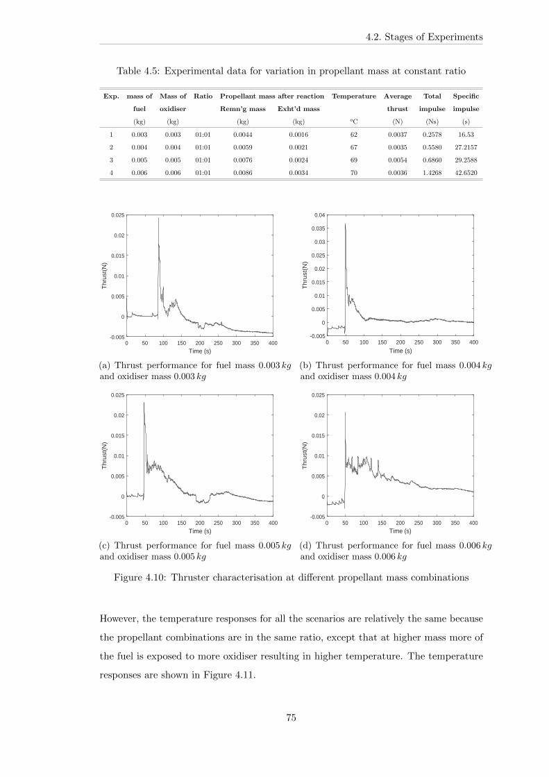
4.2. Stages of Experiments
Table 4.5: Experimental data for variation in propellant mass at constant ratio
Exp. mass of Mass of Ratio Propellant mass after reaction Temperature Average Total Specific
fuel oxidiser Remn’g mass Exht’d mass thrust impulse impulse
(kg) (kg) (kg) (kg) 𝑜C (N) (Ns) (s)
1 0.003 0.003 01:01 0.0044 0.0016 62 0.0037 0.2578 16.53
2 0.004 0.004 01:01 0.0059 0.0021 67 0.0035 0.5580 27.2157
3 0.005 0.005 01:01 0.0076 0.0024 69 0.0054 0.6860 29.2588
4 0.006 0.006 01:01 0.0086 0.0034 70 0.0036 1.4268 42.6520
0 50 100 150 200 250 300 350 400
Time (s)
-0.005
0
0.005
0.01
0.015
0.02
0.025
Thr
ust(
N)
(a) Thrust performance for fuel mass 0.003 𝑘𝑔and oxidiser mass 0.003 𝑘𝑔
0 50 100 150 200 250 300 350 400
Time (s)
-0.005
0
0.005
0.01
0.015
0.02
0.025
0.03
0.035
0.04
Th
rust
(N)
(b) Thrust performance for fuel mass 0.004 𝑘𝑔and oxidiser mass 0.004 𝑘𝑔
0 50 100 150 200 250 300 350 400
Time (s)
-0.005
0
0.005
0.01
0.015
0.02
0.025
Th
rust
(N)
(c) Thrust performance for fuel mass 0.005 𝑘𝑔and oxidiser mass 0.005 𝑘𝑔
0 50 100 150 200 250 300 350 400
Time (s)
-0.005
0
0.005
0.01
0.015
0.02
0.025
Th
rust
(N)
(d) Thrust performance for fuel mass 0.006 𝑘𝑔and oxidiser mass 0.006 𝑘𝑔
Figure 4.10: Thruster characterisation at different propellant mass combinations
However, the temperature responses for all the scenarios are relatively the same because
the propellant combinations are in the same ratio, except that at higher mass more of
the fuel is exposed to more oxidiser resulting in higher temperature. The temperature
responses are shown in Figure 4.11.
75
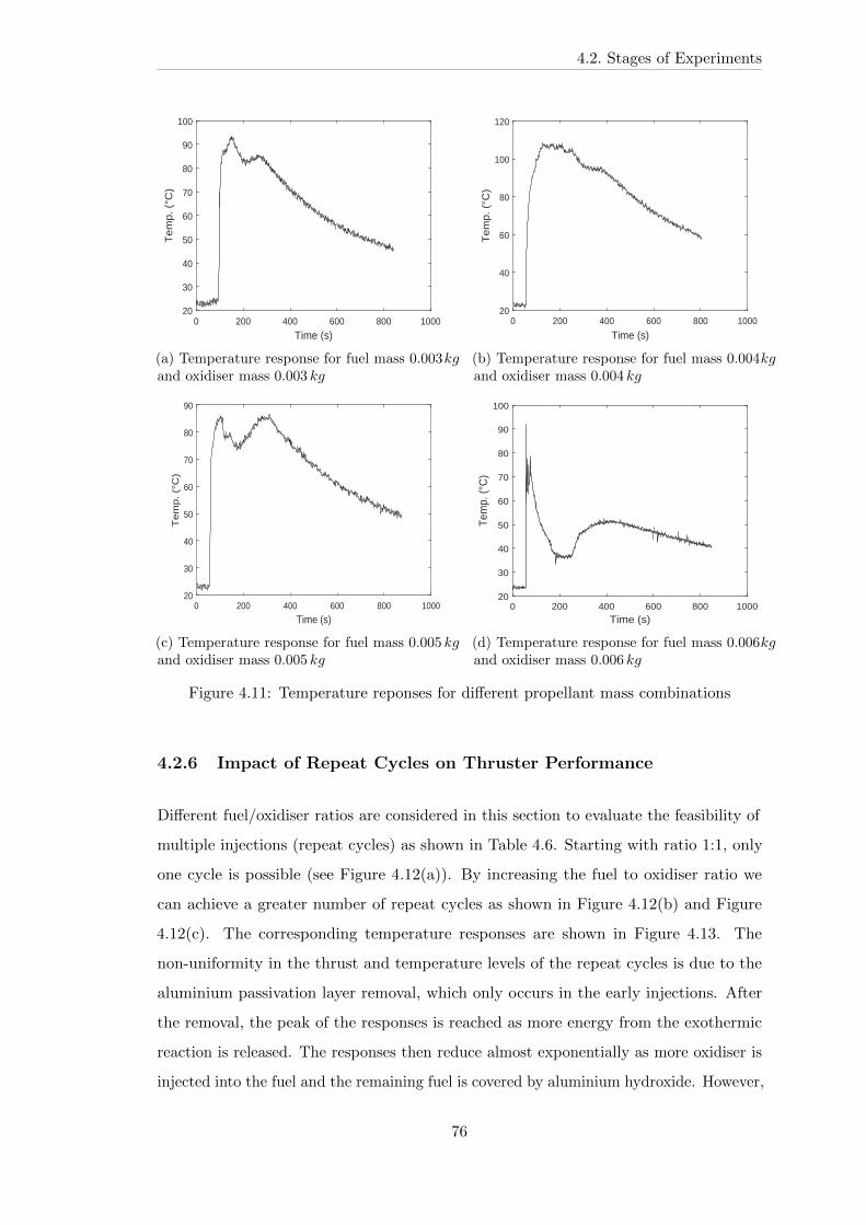
4.2. Stages of Experiments
0 200 400 600 800 1000
Time (s)
20
30
40
50
60
70
80
90
100
Te
mp
. (°
C)
(a) Temperature response for fuel mass 0.003𝑘𝑔and oxidiser mass 0.003 𝑘𝑔
0 200 400 600 800 1000
Time (s)
20
40
60
80
100
120
Te
mp
. (°
C)
(b) Temperature response for fuel mass 0.004𝑘𝑔and oxidiser mass 0.004 𝑘𝑔
0 200 400 600 800 1000
Time (s)
20
30
40
50
60
70
80
90
Te
mp
. (°
C)
(c) Temperature response for fuel mass 0.005 𝑘𝑔and oxidiser mass 0.005 𝑘𝑔
0 200 400 600 800 1000
Time (s)
20
30
40
50
60
70
80
90
100
Tem
p. (°
C)
(d) Temperature response for fuel mass 0.006𝑘𝑔and oxidiser mass 0.006 𝑘𝑔
Figure 4.11: Temperature reponses for different propellant mass combinations
4.2.6 Impact of Repeat Cycles on Thruster Performance
Different fuel/oxidiser ratios are considered in this section to evaluate the feasibility of
multiple injections (repeat cycles) as shown in Table 4.6. Starting with ratio 1:1, only
one cycle is possible (see Figure 4.12(a)). By increasing the fuel to oxidiser ratio we
can achieve a greater number of repeat cycles as shown in Figure 4.12(b) and Figure
4.12(c). The corresponding temperature responses are shown in Figure 4.13. The
non-uniformity in the thrust and temperature levels of the repeat cycles is due to the
aluminium passivation layer removal, which only occurs in the early injections. After
the removal, the peak of the responses is reached as more energy from the exothermic
reaction is released. The responses then reduce almost exponentially as more oxidiser is
injected into the fuel and the remaining fuel is covered by aluminium hydroxide. However,
76
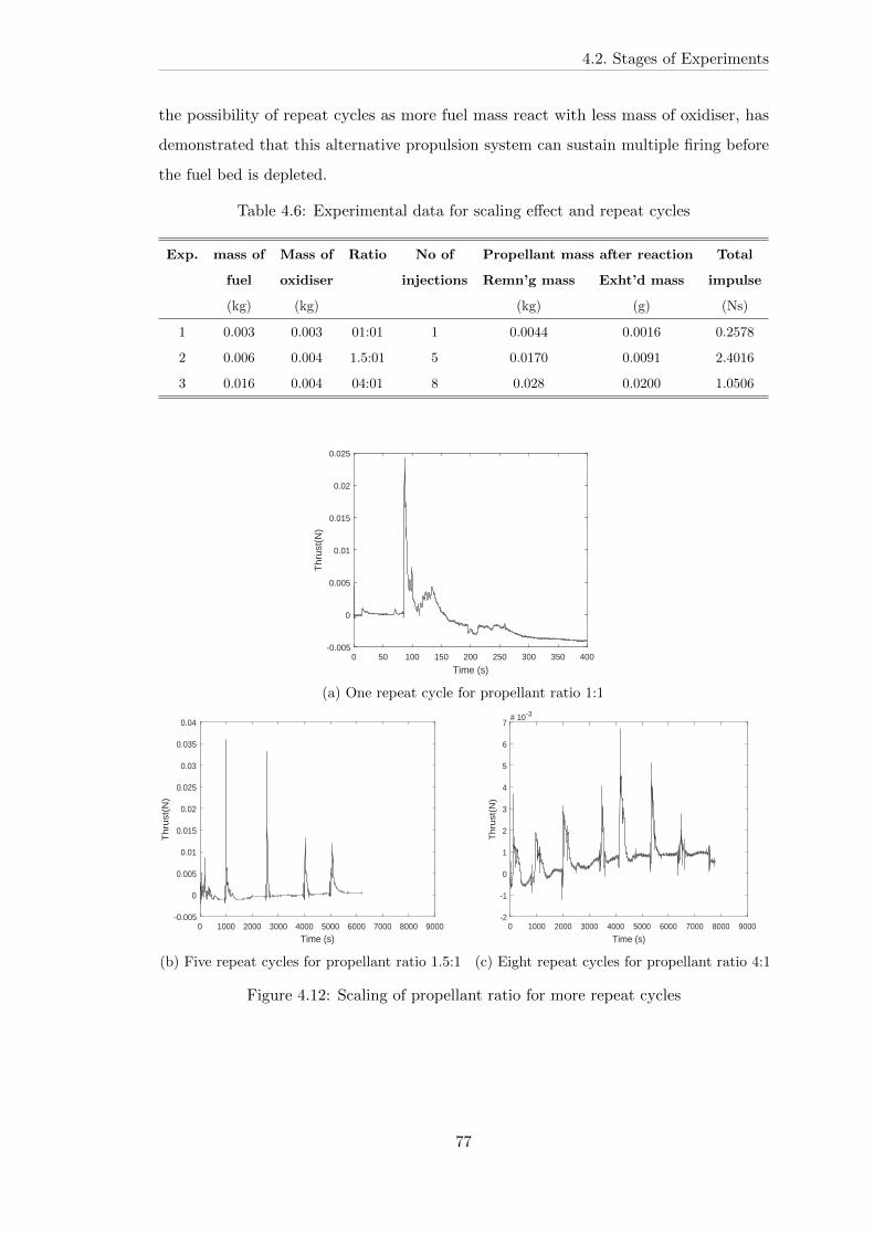
4.2. Stages of Experiments
the possibility of repeat cycles as more fuel mass react with less mass of oxidiser, has
demonstrated that this alternative propulsion system can sustain multiple firing before
the fuel bed is depleted.
Table 4.6: Experimental data for scaling effect and repeat cycles
Exp. mass of Mass of Ratio No of Propellant mass after reaction Total
fuel oxidiser injections Remn’g mass Exht’d mass impulse
(kg) (kg) (kg) (g) (Ns)
1 0.003 0.003 01:01 1 0.0044 0.0016 0.2578
2 0.006 0.004 1.5:01 5 0.0170 0.0091 2.4016
3 0.016 0.004 04:01 8 0.028 0.0200 1.0506
0 50 100 150 200 250 300 350 400
Time (s)
-0.005
0
0.005
0.01
0.015
0.02
0.025
Thr
ust(
N)
(a) One repeat cycle for propellant ratio 1:1
0 1000 2000 3000 4000 5000 6000 7000 8000 9000
Time (s)
-0.005
0
0.005
0.01
0.015
0.02
0.025
0.03
0.035
0.04
Th
rust
(N)
(b) Five repeat cycles for propellant ratio 1.5:1
0 1000 2000 3000 4000 5000 6000 7000 8000 9000
Time (s)
-2
-1
0
1
2
3
4
5
6
7
Th
rust
(N)
# 10-3
(c) Eight repeat cycles for propellant ratio 4:1
Figure 4.12: Scaling of propellant ratio for more repeat cycles
77
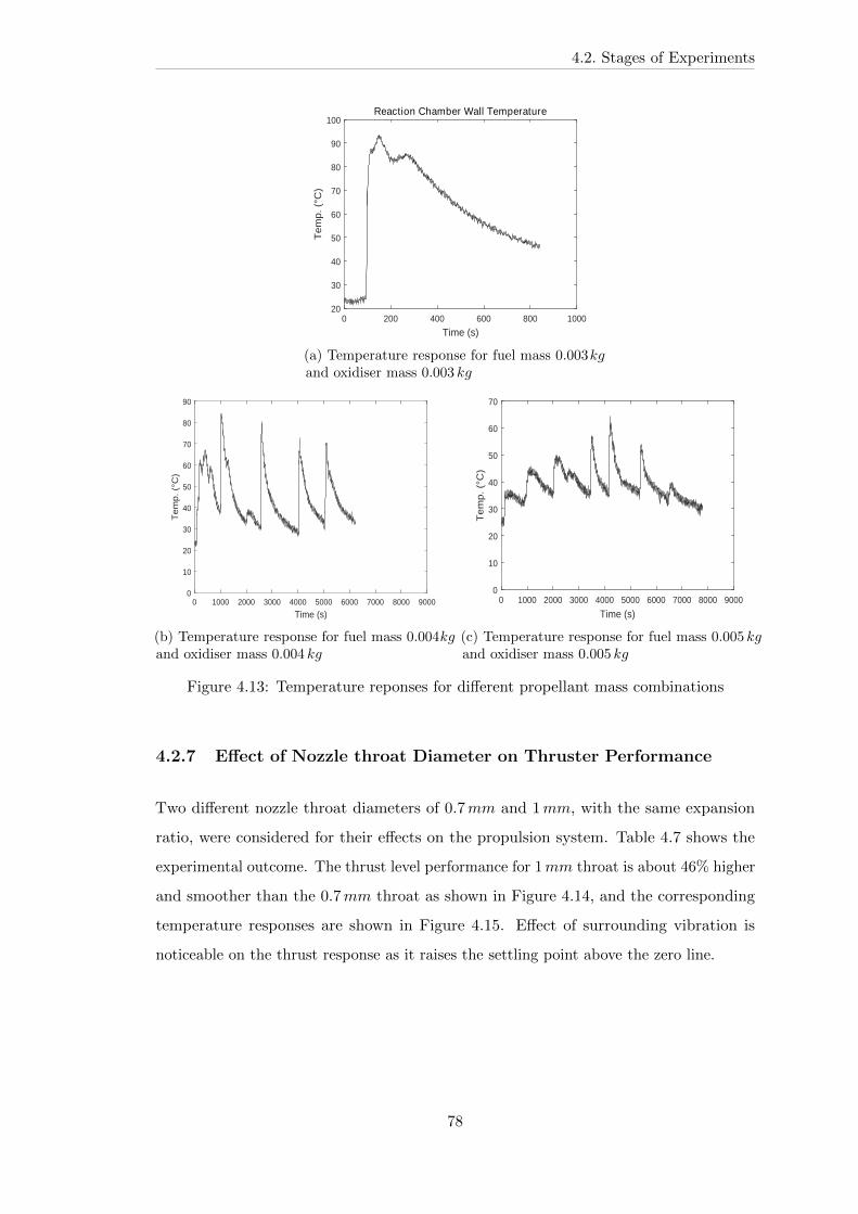
4.2. Stages of Experiments
0 200 400 600 800 1000
Time (s)
20
30
40
50
60
70
80
90
100
Te
mp
. (°
C)
Reaction Chamber Wall Temperature
(a) Temperature response for fuel mass 0.003𝑘𝑔and oxidiser mass 0.003 𝑘𝑔
0 1000 2000 3000 4000 5000 6000 7000 8000 9000
Time (s)
0
10
20
30
40
50
60
70
80
90
Te
mp
. (°
C)
(b) Temperature response for fuel mass 0.004𝑘𝑔and oxidiser mass 0.004 𝑘𝑔
0 1000 2000 3000 4000 5000 6000 7000 8000 9000
Time (s)
0
10
20
30
40
50
60
70
Te
mp
. (°
C)
(c) Temperature response for fuel mass 0.005 𝑘𝑔and oxidiser mass 0.005 𝑘𝑔
Figure 4.13: Temperature reponses for different propellant mass combinations
4.2.7 Effect of Nozzle throat Diameter on Thruster Performance
Two different nozzle throat diameters of 0.7𝑚𝑚 and 1𝑚𝑚, with the same expansion
ratio, were considered for their effects on the propulsion system. Table 4.7 shows the
experimental outcome. The thrust level performance for 1𝑚𝑚 throat is about 46% higher
and smoother than the 0.7𝑚𝑚 throat as shown in Figure 4.14, and the corresponding
temperature responses are shown in Figure 4.15. Effect of surrounding vibration is
noticeable on the thrust response as it raises the settling point above the zero line.
78

4.2. Stages of Experiments
Table 4.7: Experimental data on the effect of different nozzle throat diameter
Exp. Mass of Mass of Nozzle No of Propellant mass after reaction Total
fuel oxidiser diameter injections Remn’g mass Exht’d mass impulse
(kg) (kg) (𝑚𝑚) (kg) (kg) (Ns)
1 0.006 0.004 0.7 5 0.0190 0.0070 0.0016
2 0.006 0.004 1.0 5 0.0170 0.0091 0.0024
0 1000 2000 3000 4000 5000 6000 7000 8000 9000
Time (s)
-5
0
5
10
15
20
Th
rust
(N)
# 10-3
(a) Thrust response for 0.7𝑚𝑚 nozzle throat
0 1000 2000 3000 4000 5000 6000 7000 8000 9000
Time (s)
-0.005
0
0.005
0.01
0.015
0.02
0.025
0.03
0.035
0.04
Th
rust
(N)
(b) Thrust response for 1𝑚𝑚 nozzle throat
Figure 4.14: Thrust level performance for different nozzle throat diameter
0 2000 4000 6000 8000 10000
Time (s)
20
40
60
80
100
120
Tem
p. (
°C)
(a) Temperature response for nozzle throat diam-eter 0.7𝑚𝑚
0 1000 2000 3000 4000 5000 6000 7000
Time (s)
20
30
40
50
60
70
80
90
Tem
p. (
°C)
(b) Temperature response for nozzle throat diam-eter 1.0𝑚𝑚
Figure 4.15: Temperature reponses for different nozzle throat diameters
79

4.3. Reaction Pattern of the Propulsion System
4.3 Reaction Pattern of the Propulsion System
Data from the multiple injections experiments were analysed in this section for the
chemical reaction pattern of the propulsion system. These data are summarised in Table
4.8. There are three sections of the reaction pattern as observed in Figures 4.16(a),
(b) and (c) for reaction temperature, peak thrust and total impulse of the propulsion
system: these are upward slope, the peak and downward slope of the graph respectively.
The upward slope is the period of aluminium oxide/passivation layer removal, which is
characterised by slow reaction of the propellants at the first injection. The next phase of
the reaction is when more aluminium is already exposed for more reaction giving rise
to higher enthalpy of the reaction. At this point, the reaction is at peak with rapid
formation of aluminium hydroxide. The last phase is characterised by downward slope
towards the termination of the reaction. At this stage, any more injection of the oxidiser
will rapidly increase the dry mass fraction with less exhaust products due to the limited
enthalpies of the reaction.
Table 4.8: Experimental data for the chemical reaction model of the thruster
No of Experiments
repeat Tempt (∘C) Thrust (N) Total Impulse (Ns)
cycle 1 2 3 4 1 2 3 4 1 2 3 4
1 67.20 52.34 59.10 80.30 0.007883 0.02287 0.00221 0.007089 0.0700 0.3475 0.0634 0.2751
2 84.20 103.60 91.23 111.00 0.03499 0.1739 0.007009 0.01625 0.4665 1.5147 0.3017 0.6581
3 80.30 61.90 95.62 85.45 0.03332 0.004782 0.00347 0.007057 0.7574 0.3629 0.3449 0.2616
4 72.82 61.27 76.09 80.62 0.01272 0.007901 0.00125 0.007431 0.6188 0.0974 0.0905 0.3424
5 70.01 72.66 0.009892 0.003102 0.4889 0.0462
80
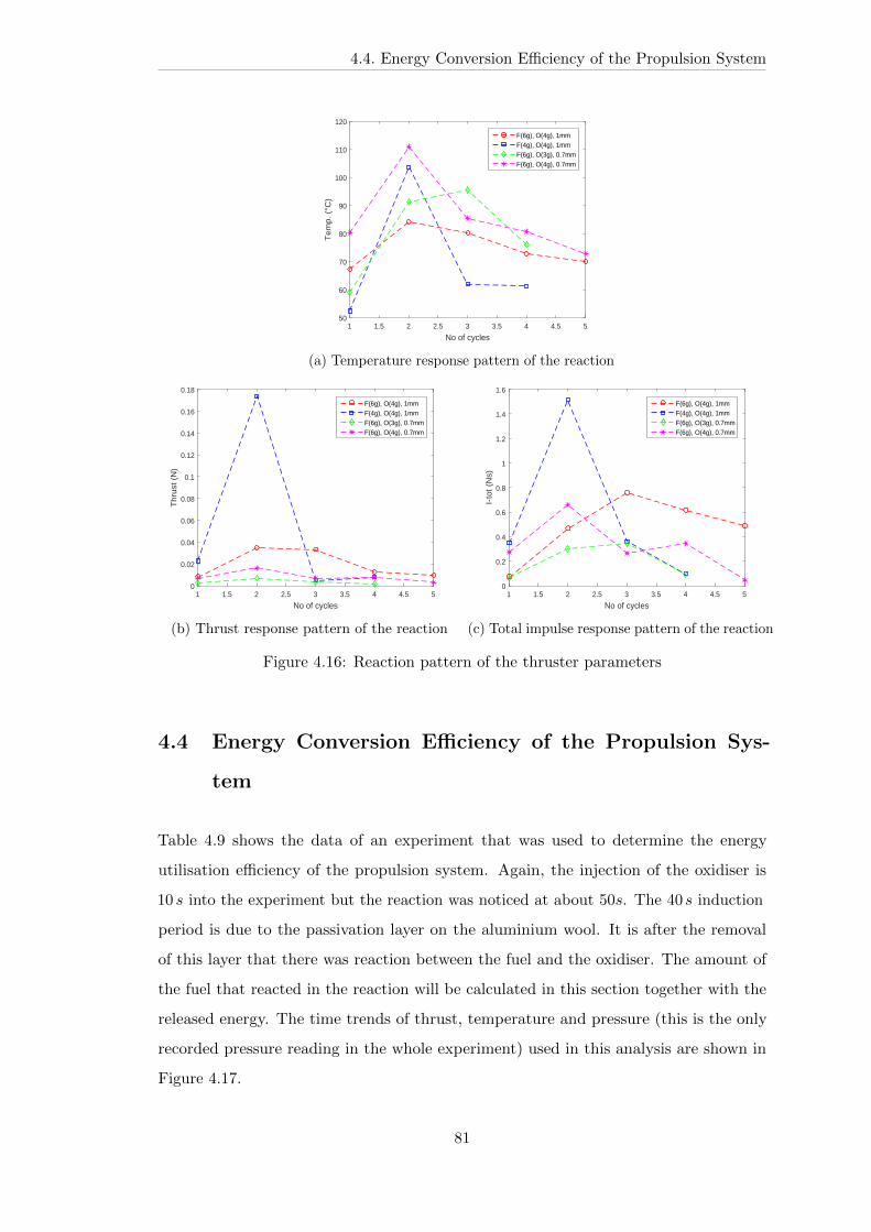
4.4. Energy Conversion Efficiency of the Propulsion System
1 1.5 2 2.5 3 3.5 4 4.5 5
No of cycles
50
60
70
80
90
100
110
120
Te
mp
. (°
C)
F(6g), O(4g), 1mmF(4g), O(4g), 1mmF(6g), O(3g), 0.7mmF(6g), O(4g), 0.7mm
(a) Temperature response pattern of the reaction
1 1.5 2 2.5 3 3.5 4 4.5 5
No of cycles
0
0.02
0.04
0.06
0.08
0.1
0.12
0.14
0.16
0.18
Th
rust
(N
)
F(6g), O(4g), 1mmF(4g), O(4g), 1mmF(6g), O(3g), 0.7mmF(6g), O(4g), 0.7mm
(b) Thrust response pattern of the reaction
1 1.5 2 2.5 3 3.5 4 4.5 5
No of cycles
0
0.2
0.4
0.6
0.8
1
1.2
1.4
1.6
I-to
t(N
s)
F(6g), O(4g), 1mmF(4g), O(4g), 1mmF(6g), O(3g), 0.7mmF(6g), O(4g), 0.7mm
(c) Total impulse response pattern of the reaction
Figure 4.16: Reaction pattern of the thruster parameters
4.4 Energy Conversion Efficiency of the Propulsion Sys-
tem
Table 4.9 shows the data of an experiment that was used to determine the energy
utilisation efficiency of the propulsion system. Again, the injection of the oxidiser is
10 𝑠 into the experiment but the reaction was noticed at about 50𝑠. The 40 𝑠 induction
period is due to the passivation layer on the aluminium wool. It is after the removal
of this layer that there was reaction between the fuel and the oxidiser. The amount of
the fuel that reacted in the reaction will be calculated in this section together with the
released energy. The time trends of thrust, temperature and pressure (this is the only
recorded pressure reading in the whole experiment) used in this analysis are shown in
Figure 4.17.
81
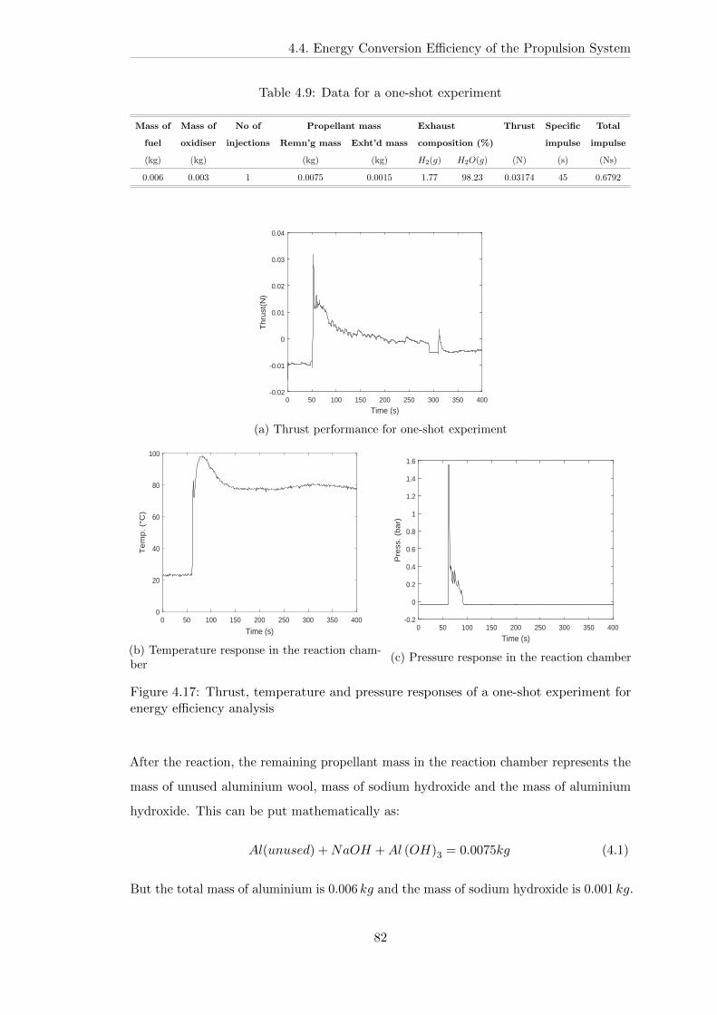
4.4. Energy Conversion Efficiency of the Propulsion System
Table 4.9: Data for a one-shot experiment
Mass of Mass of No of Propellant mass Exhaust Thrust Specific Total
fuel oxidiser injections Remn’g mass Exht’d mass composition (%) impulse impulse
(kg) (kg) (kg) (kg) 𝐻2(𝑔) 𝐻2𝑂(𝑔) (N) (s) (Ns)
0.006 0.003 1 0.0075 0.0015 1.77 98.23 0.03174 45 0.6792
0 50 100 150 200 250 300 350 400
Time (s)
-0.02
-0.01
0
0.01
0.02
0.03
0.04
Th
rust
(N)
(a) Thrust performance for one-shot experiment
0 50 100 150 200 250 300 350 400
Time (s)
0
20
40
60
80
100
Te
mp
. (°
C)
(b) Temperature response in the reaction cham-ber
0 50 100 150 200 250 300 350 400
Time (s)
-0.2
0
0.2
0.4
0.6
0.8
1
1.2
1.4
1.6
Pre
ss. (b
ar)
(c) Pressure response in the reaction chamber
Figure 4.17: Thrust, temperature and pressure responses of a one-shot experiment forenergy efficiency analysis
After the reaction, the remaining propellant mass in the reaction chamber represents the
mass of unused aluminium wool, mass of sodium hydroxide and the mass of aluminium
hydroxide. This can be put mathematically as:
𝐴𝑙(𝑢𝑛𝑢𝑠𝑒𝑑) +𝑁𝑎𝑂𝐻 +𝐴𝑙 (𝑂𝐻)3 = 0.0075𝑘𝑔 (4.1)
But the total mass of aluminium is 0.006 𝑘𝑔 and the mass of sodium hydroxide is 0.001 𝑘𝑔.
82
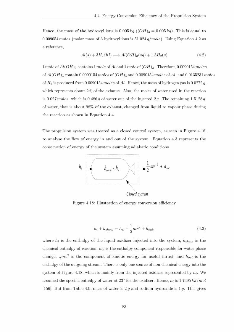
4.4. Energy Conversion Efficiency of the Propulsion System
Hence, the mass of the hydroxyl ions is 0.005 𝑘𝑔 ((𝑂𝐻)3 = 0.005 𝑘𝑔). This is equal to
0.009054𝑚𝑜𝑙𝑒𝑠 (molar mass of 3 hydroxyl ions is 51.024 𝑔/𝑚𝑜𝑙𝑒). Using Equation 4.2 as
a reference,
𝐴𝑙(𝑠) + 3𝐻2𝑂(𝑙) −→ 𝐴𝑙(𝑂𝐻)3(𝑎𝑞) + 1.5𝐻2(𝑔) (4.2)
1𝑚𝑜𝑙𝑒 of𝐴𝑙(𝑂𝐻)3 contains 1𝑚𝑜𝑙𝑒 of𝐴𝑙 and 1𝑚𝑜𝑙𝑒 of (𝑂𝐻)3. Therefore, 0.0090154𝑚𝑜𝑙𝑒𝑠
of𝐴𝑙(𝑂𝐻)3 contain 0.0090154𝑚𝑜𝑙𝑒𝑠 of (𝑂𝐻)3 and 0.0090154𝑚𝑜𝑙𝑒𝑠 of𝐴𝑙, and 0.0135231𝑚𝑜𝑙𝑒𝑠
of𝐻2 is produced from 0.0090154𝑚𝑜𝑙𝑒𝑠 of 𝐴𝑙. Hence, the mass of hydrogen gas is 0.0272 𝑔,
which represents about 2% of the exhaust. Also, the moles of water used in the reaction
is 0.027𝑚𝑜𝑙𝑒𝑠, which is 0.486𝑔 of water out of the injected 2𝑔. The remaining 1.5128𝑔
of water, that is about 98% of the exhaust, changed from liquid to vapour phase during
the reaction as shown in Equation 4.4.
The propulsion system was treated as a closed control system, as seen in Figure 4.18,
to analyse the flow of energy in and out of the system. Equation 4.3 represents the
conservation of energy of the system assuming adiabatic conditions.
ih wchem hh outhmv 2
21
systemClosed
+-
Figure 4.18: Illustration of energy conversion efficiency
ℎ𝑖 + ℎ𝑐ℎ𝑒𝑚 = ℎ𝑤 +1
2𝑚𝑣2 + ℎ𝑜𝑢𝑡, (4.3)
where ℎ𝑖 is the enthalpy of the liquid oxidizer injected into the system, ℎ𝑐ℎ𝑒𝑚 is the
chemical enthalpy of reaction, ℎ𝑤 is the enthalpy component responsible for water phase
change, 12𝑚𝑣2 is the component of kinetic energy for useful thrust, and ℎ𝑜𝑢𝑡 is the
enthalpy of the outgoing stream. There is only one source of non-chemical energy into the
system of Figure 4.18, which is mainly from the injected oxidizer represented by ℎ𝑖. We
assumed the specific enthalpy of water at 23∘ for the oxidiser. Hence, ℎ𝑖 is 1.7395 𝑘𝐽/𝑚𝑜𝑙
[156]. But from Table 4.9, mass of water is 2 𝑔 and sodium hydroxide is 1 𝑔. This gives
83
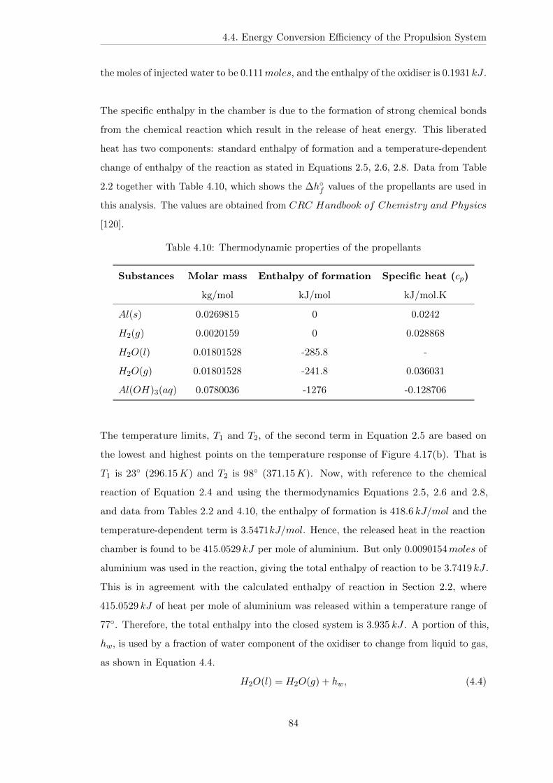
4.4. Energy Conversion Efficiency of the Propulsion System
the moles of injected water to be 0.111𝑚𝑜𝑙𝑒𝑠, and the enthalpy of the oxidiser is 0.1931 𝑘𝐽 .
The specific enthalpy in the chamber is due to the formation of strong chemical bonds
from the chemical reaction which result in the release of heat energy. This liberated
heat has two components: standard enthalpy of formation and a temperature-dependent
change of enthalpy of the reaction as stated in Equations 2.5, 2.6, 2.8. Data from Table
2.2 together with Table 4.10, which shows the Δℎ∘𝑓 values of the propellants are used in
this analysis. The values are obtained from 𝐶𝑅𝐶 𝐻𝑎𝑛𝑑𝑏𝑜𝑜𝑘 𝑜𝑓 𝐶ℎ𝑒𝑚𝑖𝑠𝑡𝑟𝑦 𝑎𝑛𝑑 𝑃ℎ𝑦𝑠𝑖𝑐𝑠
[120].
Table 4.10: Thermodynamic properties of the propellants
Substances Molar mass Enthalpy of formation Specific heat (𝑐𝑝)
kg/mol kJ/mol kJ/mol.K
𝐴𝑙(𝑠) 0.0269815 0 0.0242
𝐻2(𝑔) 0.0020159 0 0.028868
𝐻2𝑂(𝑙) 0.01801528 -285.8 -
𝐻2𝑂(𝑔) 0.01801528 -241.8 0.036031
𝐴𝑙(𝑂𝐻)3(𝑎𝑞) 0.0780036 -1276 -0.128706
The temperature limits, 𝑇1 and 𝑇2, of the second term in Equation 2.5 are based on
the lowest and highest points on the temperature response of Figure 4.17(b). That is
𝑇1 is 23∘ (296.15𝐾) and 𝑇2 is 98∘ (371.15𝐾). Now, with reference to the chemical
reaction of Equation 2.4 and using the thermodynamics Equations 2.5, 2.6 and 2.8,
and data from Tables 2.2 and 4.10, the enthalpy of formation is 418.6 𝑘𝐽/𝑚𝑜𝑙 and the
temperature-dependent term is 3.5471𝑘𝐽/𝑚𝑜𝑙. Hence, the released heat in the reaction
chamber is found to be 415.0529 𝑘𝐽 per mole of aluminium. But only 0.0090154𝑚𝑜𝑙𝑒𝑠 of
aluminium was used in the reaction, giving the total enthalpy of reaction to be 3.7419 𝑘𝐽 .
This is in agreement with the calculated enthalpy of reaction in Section 2.2, where
415.0529 𝑘𝐽 of heat per mole of aluminium was released within a temperature range of
77∘. Therefore, the total enthalpy into the closed system is 3.935 𝑘𝐽 . A portion of this,
ℎ𝑤, is used by a fraction of water component of the oxidiser to change from liquid to gas,
as shown in Equation 4.4.
𝐻2𝑂(𝑙) = 𝐻2𝑂(𝑔) + ℎ𝑤, (4.4)
84

4.4. Energy Conversion Efficiency of the Propulsion System
where ℎ𝑤 is the specific enthalpy of water at the pressure and temperature at the instance
of conversion. Data from Figures 4.17(b) and (c) were plotted on a 𝑝 − ℎ diagram
to calculate the specific enthalpy as shown in Figure 4.19. The 𝑆𝑡𝑎𝑟𝑡 𝑡𝑖𝑚𝑒 and the
𝑆𝑡𝑜𝑝 𝑡𝑖𝑚𝑒 on the graph represent the start of the reaction and the stop of the reaction
from the temperature and pressure graphs.
0 500 1000 1500 2000 2500 3000 3500 4000
Enthalpy (kJ/kg)
10-3
10-2
10-1
100
101
Pre
ssu
re (
MP
a)
p-h diagram for water
Start time = 61 s
137.91 kJ/kg 2679.24 kJ/kg
Stop time = 90 s
10 'C
40 'C
60 'C
200 'C
100 'C
400 'C 500 'C 600 'C
300 'C
Figure 4.19: 𝑝−ℎ diagram of water showing the enthalpy-pressure relation in the reactionchamber. The 𝑝− ℎ diagram was drawn from data obtained from [156]. The blue linerepresents saturated liquid water while the red line represents dry saturated steam. Thedome covers water-steam composition with decreasing water content from left to right.
The specific enthalpy required for the phase change is found to be 2541.33 𝑘𝐽/𝑘𝑔 (sub-
tracting the start point from the stop point). But the mass of water vapour from the
exhaust is 1.51275 𝑔, which represents about 97% of the exhaust. Therefore the energy
used for the water phase conversion is 3.8444 𝑘𝐽 .
Another portion of the generated energy is gained by the reaction exhaust gases that
increased their kinetic energy, 12𝑚𝑣2, resulting in the thrust generation. The kinetic
85
4.4. Energy Conversion Efficiency of the Propulsion System
energy can also be expressed as a function of the exhaust mass flow rate by:
𝐾𝐸 =1
2𝑚𝑣2
=
∫1
2𝑣2𝑑𝑡
(4.5)
If we assume a constant exhaust velocity, it implies the total impulse can be expressed
as:
𝐼𝑡𝑜𝑡 =
∫𝑣𝑑𝑡
𝐼𝑡𝑜𝑡 = 𝑚𝑣
(4.6)
Equation 4.5 can therefore be rewritten as
𝐾𝐸 =1
2
𝐼2
𝑚2
∫𝑑𝑡
=1
2
𝐼2
𝑚
(4.7)
Substituting values from Table 4.9, the kinetic energy is calculated to be 0.1498 𝑘𝐽 ,
which represents the enthalpy that got converted into the thrust. This value represents
about 3% of the generated heat in the reaction chamber.
In the above analysis, the sum of the kinetic energy and the energy used by the water to
change phase is more than the available energy in the chamber by 0.0592 𝑘𝐽 . To address
the difference, a plot of the reaction enthalpies versus the percentage of water in the
oxidiser that gets into the reaction chamber is obtained, as shown in Figure 4.20.
86

4.4. Energy Conversion Efficiency of the Propulsion System
0 2 4 6 8 10 12 14 16 18 20
5% multiples of injected water into the reaction chamber
0
0.5
1
1.5
2
2.5
3
3.5
4
En
erg
y (k
J) hchem
KE+hw
hw
KE
Figure 4.20: Energy iterations for the percentage of water vapour in the system
The point where the generated enthalpy equals the sum of the kinetic energy and the
energy for phase change is represented by the dash-dot line in the figure.
4.4.1 Chemical Analysis of the Residual Propellants
The reaction between the aluminium wool and the mixture of water and sodium hydroxide
is an exothermic reaction that releases hydrogen gas and forms sodium aluminate
as residue. Stoichiometrically, this reaction requires a mixture of 2𝑚𝑜𝑙𝑒𝑠 of sodium
hydroxide in 6𝑚𝑜𝑙𝑒𝑠 of water that will consume 2𝑚𝑜𝑙𝑒𝑠 of aluminium and then release
3𝑚𝑜𝑙𝑒𝑠 of hydrogen gas and form 2𝑚𝑜𝑙𝑒𝑠 of sodium aluminate as shown in Equation
2.2. That is, when 1 𝑘𝑔 of aluminium reacts with 1.6 𝑘𝑔 of sodium hydroxide in 2 𝑘𝑔 of
water, about 0.112 𝑘𝑔 of hydrogen gas will form leaving behind a precipitate of about
4 𝑘𝑔 of sodium aluminate. However in this proof of concept propulsion design and from
Section 4.4, we have reacted only 0.006 𝑘𝑔 of aluminium wool with 0.003 𝑘𝑔 of oxidiser
that contained 0.002 𝑘𝑔 of water and 0.001 𝑘𝑔 of sodium hydroxide. The experimental
calculations revealed that only about 0.00024 𝑘𝑔 of the aluminium wool was consumed
in the reaction. The remaining aluminium wool and the sodium aluminate that formed
constituted to the remaining 0.0075 𝑘𝑔 of propellants in the reaction chamber as shown in
Equation 4.1. These residual propellants were physically examined after the experiment
to see the part of the fuel that was consumed and what actually formed. Figure 4.21(a)
shows the part of the fuel that reacted and the residue of that reaction. Only the part
of fuel closed to the injected oxidiser reacted. A dissection of the fuel also confirms
87

4.4. Energy Conversion Efficiency of the Propulsion System
that there was no further reaction inside the fuel due to the formation of the reaction
residue as shown in Figure 4.21(b). The propellant residue was also examined using
(a) Propellant residue after reaction (b) Dissection of propellant residue
Figure 4.21: Physical examination of propellant residue
MicroRaman spectroscopy to determine the microscopic structure of the propellant
remnant at the Advanced Technology Institute (ATI), University of Surrey. A 20𝜇m view
of the residual propellant of two of the experiments shows similarity in the crystalline
structures and the Raman spectra of the samples. However, there is sparse formation of
aluminate in the reaction products due to the size and composition of the aluminium
wool that was used as fuel. Figure 4.22 is the 20𝜇m view of two samples of residual
propellant and Figure 4.23 is the Raman spectra of the propellant residues. There is low
crystallinity in Figure 4.22, which is as a result of the size of the particles of aluminium
in the aluminate. However, the spectral components or wave numbers of the propellant
residue at 1062 𝑐𝑚−1 ±5 𝑐𝑚−1, 3417 𝑐𝑚−1 ±2 𝑐𝑚−1 and 3530 𝑐𝑚−1 ±2 𝑐𝑚−1 confirms
the existence of aluminate in general and the presence of 𝐴𝑙(𝑂𝐻)3 in particular, which
is in agreement with the work of Nsoki [157]. Nonetheless, there were weaker signals of
other species as indicated at wave numbers 253𝑐𝑚−1 and 1067 𝑐𝑚−1, and this confirms
that the aluminium wool is not a pure aluminium but contains some impurities.
88
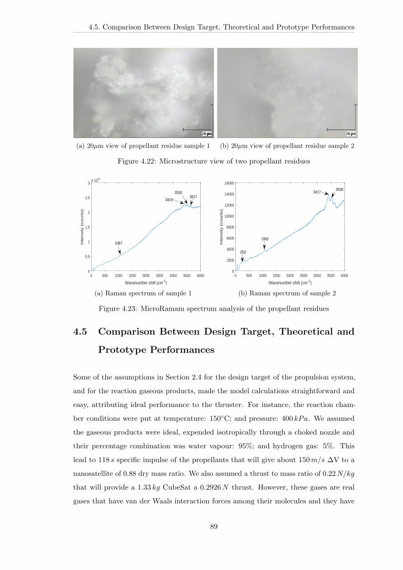
4.5. Comparison Between Design Target, Theoretical and Prototype Performances
(a) 20𝜇m view of propellant residue sample 1 (b) 20𝜇m view of propellant residue sample 2
Figure 4.22: Microstructure view of two propellant residues
0 500 1000 1500 2000 2500 3000 3500 4000
Wavenumber shift (cm-1)
0
0.5
1
1.5
2
2.5
3
Inte
nsity (
co
un
ts)
# 104
1067
35303617
3419
(a) Raman spectrum of sample 1
0 500 1000 1500 2000 2500 3000 3500 4000
Wavenumber shift (cm-1)
0
2000
4000
6000
8000
10000
12000
14000
16000
Inte
nsity (
co
un
ts)
253
1062
34173530
(b) Raman spectrum of sample 2
Figure 4.23: MicroRamam spectrum analysis of the propellant residues
4.5 Comparison Between Design Target, Theoretical and
Prototype Performances
Some of the assumptions in Section 2.4 for the design target of the propulsion system,
and for the reaction gaseous products, made the model calculations straightforward and
easy, attributing ideal performance to the thruster. For instance, the reaction cham-
ber conditions were put at temperature: 150∘C; and pressure: 400 𝑘𝑃𝑎. We assumed
the gaseous products were ideal, expended isotropically through a choked nozzle and
their percentage combination was water vapour: 95%; and hydrogen gas: 5%. This
lead to 118 𝑠 specific impulse of the propellants that will give about 150𝑚/𝑠 ΔV to a
nanosatellite of 0.88 dry mass ratio. We also assumed a thrust to mass ratio of 0.22𝑁/𝑘𝑔
that will provide a 1.33 𝑘𝑔 CubeSat a 0.2926𝑁 thrust. However, these gases are real
gases that have van der Waals interaction forces among their molecules and they have
89
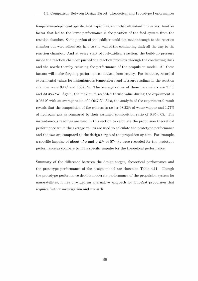
4.5. Comparison Between Design Target, Theoretical and Prototype Performances
temperature-dependent specific heat capacities, and other attendant properties. Another
factor that led to the lower performance is the position of the feed system from the
reaction chamber. Some portion of the oxidiser could not make through to the reaction
chamber but were adhesively held to the wall of the conducting duck all the way to the
reaction chamber. And at every start of fuel-oxidiser reaction, the build-up pressure
inside the reaction chamber pushed the reaction products through the conducting duck
and the nozzle thereby reducing the performance of the propulsion model. All these
factors will make forgoing performances deviate from reality. For instance, recorded
experimental values for instantaneous temperature and pressure readings in the reaction
chamber were 98∘C and 160 𝑘𝑃𝑎. The average values of these parameters are 71∘C
and 33.38 𝑘𝑃𝑎. Again, the maximum recorded thrust value during the experiment is
0.032𝑁 with an average value of 0.0047𝑁 . Also, the analysis of the experimental result
reveals that the composition of the exhaust is rather 98.23% of water vapour and 1.77%
of hydrogen gas as compared to their assumed composition ratio of 0.95:0.05. The
instantaneous readings are used in this section to calculate the propulsion theoretical
performance while the average values are used to calculate the prototype performance
and the two are compared to the design target of the propulsion system. For example,
a specific impulse of about 45 𝑠 and a ΔV of 57𝑚/𝑠 were recorded for the prototype
performance as compare to 111 𝑠 specific impulse for the theoretical performance.
Summary of the difference between the design target, theoretical performance and
the prototype performance of the design model are shown in Table 4.11. Though
the prototype performance depicts moderate performance of the propulsion system for
nanosatellites, it has provided an alternative approach for CubeSat propulsion that
requires further investigation and research.
90

4.6. Comparison with the State-of-the-Art
Table 4.11: Table of comparison between theory and experimental data
Symbols Meaning Design Theoretical Prototype
target performance performance
𝑇𝑐 Chamber temperature, ∘C 150 98 71
𝑃𝑐 Chamber pressure, 𝑘𝑃𝑎 400 160 33.38
𝐹 Thrust, 𝑁 0.2926 0.032 0.0047
𝛾 Specific heat ratio 1.324 1.33 1.33
𝑎𝑜 Acoustic velocity, 𝑚/𝑠 520.18 487.17 470.18
𝑐* Characteristic velocity, 𝑚/𝑠 673.17 630.45 606.13
Propellant mass flow rate, 𝑘𝑔/𝑠 0.00027 0.00027 0.000011
𝐼𝑠𝑝 The specific impulse, 𝑠 118 111 45
ΔV Net velocity change to the spacecraft, 𝑚/𝑠 150 140 57
4.6 Comparison with the State-of-the-Art
There have been extensive works on the propulsion systems for micro- and nanosatellites
as described in Section 1.2, and including the works of Busek, Marotta, Moog and
Vacco in the development of micropropulsion systems for nanosatellitess. Most of these
systems are in advance stage and are well suiatble for orbital operations that include
attitude control, orbital manoeuvre and rendezvous. However, most of their systems are
electrically based with operating input power in the range of 7.5𝑊 to 50𝑊 , far beyond
the on-board power of a typical 1𝑈 CubeSat. Those with low input power like the
Marotta cold gas micro-thruster and Vacco cold gas propulsion module [4, 158] operate
within 15 𝑏𝑎𝑟 to about 30 𝑏𝑎𝑟 pressure range, which is avoided on CubeSat platform as
the nanosatellites are still carried as a piggy-bag on a launcher for bigger satellites. Other
chemical micropropulsion systems are generally complex for nanosatellites applications,
with heat transfer and scaling related issues as mentioned in Section 1.2. For example,
hydrazine monopropellant systems are hazardous, toxic, carcinogenic and they require
special training for handling procedures and precautions, while the hydrogen peroxide
systems are self-degradable and reduce performance after long storage. However, when
the hybrid propulsion system for CubeSat applications is fully developed, aside that the
propellants are non- hazardous, cheap and storage with no special training for handling,
the on-demand operation pressure builds up gives it a pass to be launched with other
payloads on a launcher. Power demand is about 500𝑚𝑊 only for the operation of valves
91
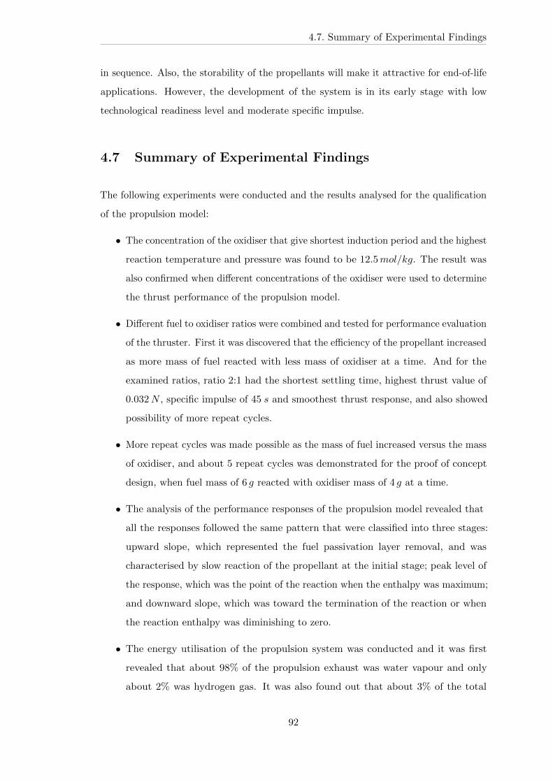
4.7. Summary of Experimental Findings
in sequence. Also, the storability of the propellants will make it attractive for end-of-life
applications. However, the development of the system is in its early stage with low
technological readiness level and moderate specific impulse.
4.7 Summary of Experimental Findings
The following experiments were conducted and the results analysed for the qualification
of the propulsion model:
∙ The concentration of the oxidiser that give shortest induction period and the highest
reaction temperature and pressure was found to be 12.5𝑚𝑜𝑙/𝑘𝑔. The result was
also confirmed when different concentrations of the oxidiser were used to determine
the thrust performance of the propulsion model.
∙ Different fuel to oxidiser ratios were combined and tested for performance evaluation
of the thruster. First it was discovered that the efficiency of the propellant increased
as more mass of fuel reacted with less mass of oxidiser at a time. And for the
examined ratios, ratio 2:1 had the shortest settling time, highest thrust value of
0.032𝑁 , specific impulse of 45 𝑠 and smoothest thrust response, and also showed
possibility of more repeat cycles.
∙ More repeat cycles was made possible as the mass of fuel increased versus the mass
of oxidiser, and about 5 repeat cycles was demonstrated for the proof of concept
design, when fuel mass of 6 𝑔 reacted with oxidiser mass of 4 𝑔 at a time.
∙ The analysis of the performance responses of the propulsion model revealed that
all the responses followed the same pattern that were classified into three stages:
upward slope, which represented the fuel passivation layer removal, and was
characterised by slow reaction of the propellant at the initial stage; peak level of
the response, which was the point of the reaction when the enthalpy was maximum;
and downward slope, which was toward the termination of the reaction or when
the reaction enthalpy was diminishing to zero.
∙ The energy utilisation of the propulsion system was conducted and it was first
revealed that about 98% of the propulsion exhaust was water vapour and only
about 2% was hydrogen gas. It was also found out that about 3% of the total
92
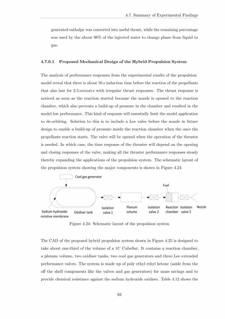
4.7. Summary of Experimental Findings
generated enthalpy was converted into useful thrust, while the remaining percentage
was used by the about 98% of the injected water to change phase from liquid to
gas.
4.7.0.1 Proposed Mechanical Design of the Hybrid Propulsion System
The analysis of performance responses from the experimental results of the propulsion
model reveal that there is about 50 𝑠 induction time before the reaction of the propellants
that also last for 2.5𝑚𝑖𝑛𝑢𝑡𝑒𝑠 with irregular thrust responses. The thrust response is
noticed as soon as the reaction started because the nozzle is opened to the reaction
chamber, which also prevents a build-up of pressure in the chamber and resulted in the
model low performance. This kind of response will essentially limit the model application
to de-orbiting. Solution to this is to include a Lee valve before the nozzle in future
design to enable a build-up of pressure inside the reaction chamber when the once the
propellants reaction starts. The valve will be opened when the operation of the thruster
is needed. In which case, the time response of the thruster will depend on the opening
and closing responses of the valve, making all the thruster performance responses steady
thereby expanding the applications of the propulsion system. The schematic layout of
the propulsion system showing the major components is shown in Figure 4.24.
OxidiserStank
CoolSgasSgenerator
IsolationSvalveS1
IsolationSvalveS2
ReactionSchamber
Nozzle
Fuel
PlenumSvolume
IsolationSvalveS3SodiumShydroxideS
resistiveSmembrane
Figure 4.24: Schematic layout of the propulsion system
The CAD of the proposed hybrid propulsion system shown in Figure 4.25 is designed to
take about one-third of the volume of a 1𝑈 CubeSat. It contains a reaction chamber,
a plenum volume, two oxidiser tanks, two cool gas generators and three Lee extended
performance valves. The system is made up of poly ethyl ethyl ketone (aside from the
off the shelf components like the valves and gas generators) for mass savings and to
provide chemical resistance against the sodium hydroxide oxidiser. Table 4.12 shows the
93
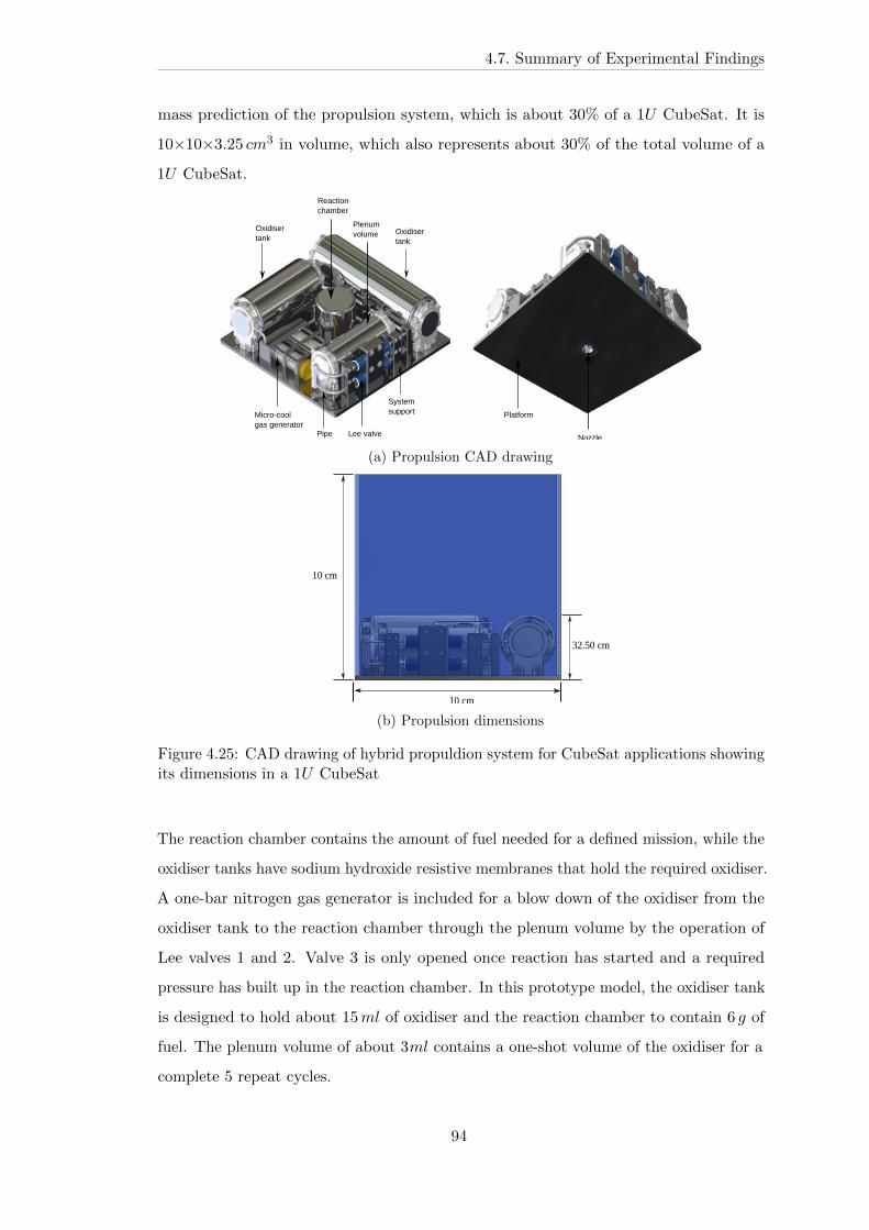
4.7. Summary of Experimental Findings
mass prediction of the propulsion system, which is about 30% of a 1𝑈 CubeSat. It is
10×10×3.25 𝑐𝑚3 in volume, which also represents about 30% of the total volume of a
1𝑈 CubeSat.
Micro-coolgas generator
Pipe Lee valve
Systemsupport Platform
Nozzle
Oxidisertank
Reactionchamber
Plenumvolume Oxidiser
tank
(a) Propulsion CAD drawing
10 cm
32.50 cm
10 cm
(b) Propulsion dimensions
Figure 4.25: CAD drawing of hybrid propuldion system for CubeSat applications showingits dimensions in a 1𝑈 CubeSat
The reaction chamber contains the amount of fuel needed for a defined mission, while the
oxidiser tanks have sodium hydroxide resistive membranes that hold the required oxidiser.
A one-bar nitrogen gas generator is included for a blow down of the oxidiser from the
oxidiser tank to the reaction chamber through the plenum volume by the operation of
Lee valves 1 and 2. Valve 3 is only opened once reaction has started and a required
pressure has built up in the reaction chamber. In this prototype model, the oxidiser tank
is designed to hold about 15𝑚𝑙 of oxidiser and the reaction chamber to contain 6 𝑔 of
fuel. The plenum volume of about 3𝑚𝑙 contains a one-shot volume of the oxidiser for a
complete 5 repeat cycles.
94
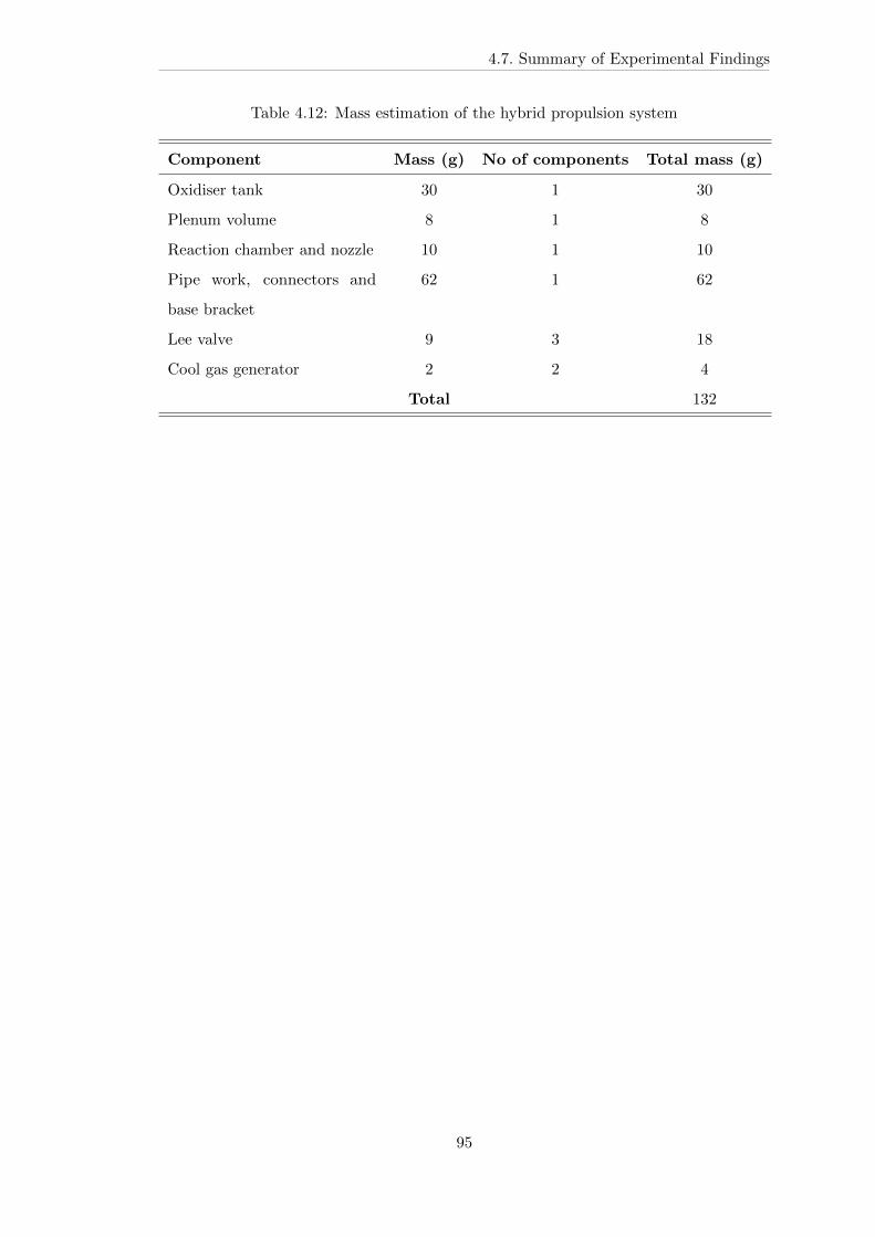
4.7. Summary of Experimental Findings
Table 4.12: Mass estimation of the hybrid propulsion system
Component Mass (g) No of components Total mass (g)
Oxidiser tank 30 1 30
Plenum volume 8 1 8
Reaction chamber and nozzle 10 1 10
Pipe work, connectors and
base bracket
62 1 62
Lee valve 9 3 18
Cool gas generator 2 2 4
Total 132
95
Chapter 5
Conclusions and Future Work
The almost four years journey of this research has taken us though comprehensive litera-
ture about nanosatellites and their micropropulsion systems. The nanosatellites were
initially thought to provide students of higher education institutions expertise in all the
aspect of satellite subsystems. Most of these satellites were launched without propulsion
system except for technological demonstration and were left in their injected orbit until
they spiralled into the atmosphere and de-orbited. The popularity of CubeSats continues
to grow, and non-governmental agencies have become major players in the design and
launching of the satellite due to their low cost. This has necessitated the emergence of
orbital control demonstration on the nanoosatellite platform to expand their capabilities.
We found out that these nanosatellites, especially the CubeSats, were without any form
of propulsion system until about two decades ago when the first nanosatellite to be
flown with propulsion was launched. Since that time a lot of works have been done
in literature in the area of micropropulsion systems for CubeSats. These include the
micro-electrothermal, micro-electrostatic and micro-electromagnetic propulsion systems,
and the various micro-chemical propulsion systems. A comprehensive review in this
area showed that it is difficult to miniaturise well understood and advanced propulsion
systems and still retain their operational advantages, and there is still scope to try a
novel chemical and physical process as the basis of a novel propulsion technology.
In a quest for an alternative chemical process in the design of a novel micropropul-
sion system for CubeSats, we considered water splitting reaction with aluminium wool
fuel using sodium hydroxide as a promoter. The choice of the propellants was based
96
CHAPTER 5. CONCLUSIONS AND FUTURE WORK
on the availability and cost of materials; long storage without degrading; moderate
temperature and exothermic reaction without any thermal control threat to the CubeSat
structure; and high energy density per unit volume for the volume constraint satellite.
Various efforts were identified in literature where the chemical combination was used
for an 𝑖𝑛− 𝑠𝑖𝑡𝑢 generation of hydrogen gas as a source of energy, and as a substitute
for depleting fossil fuels. This reaction is normally studied at standard temperature
and pressure. But as soon as this reaction is conducted at reduced pressure, there will
be formation of water vapour in conjunction with the hydrogen gas. Also, because the
reaction is exothermic, the released heat will elevate the kinetic energy of these products
and when passed through a diverging-converging nozzle, generate thrust.
We then looked at thermodynamic and gas laws that govern the flow of gas through a
chocked nozzle while treating the gas as ideal. This was done through specific engineering
assumptions, and the result was an ideal performance model of the propulsion system.
This led to the design of a proof of concept model of the thruster to verify the performance.
The proof of concept design provided a means of verifying the performance of the
thruster compared to the idealised model. Once the prototype thruster was designed,
an oxidiser feed system was constructed to deliver the required amount of oxidiser into
the reaction chamber. The prototype thruster was then placed on the moving plate of
thrust balance and stationed within the 𝑃𝑒𝑔𝑎𝑠𝑢𝑠 vacuum facility for in vacuum tests,
which led to a complete experimental set up. Series of experiments were conducted to
characterise the thruster. Though the experimental results were not smooth and linear
in order to predict the performance of the model, repeated experiments shows similar
trend as shown in Figure 5.1. The uncertainty in the repeated thrust measurements is
obtained as ±0.03𝑁 , while that of temperature readings is calculated as ±0.02∘C. The
uncertainty in the repeated pressure reading is obtained as ±0.6 𝑏𝑎𝑟. The uncertainty in
the pressure readings is more which is mostly due to different background pressure of
the vacuum chamber during different experiments. Other sources of errors in the course
of the experiments include:
∙ accuracy of the thrust stand
∙ accuracy of the thermocouples and pressure transducer
97
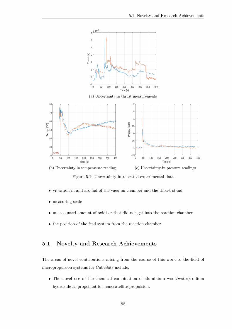
5.1. Novelty and Research Achievements
0 50 100 150 200 250 300 350 400
Time (s)
-1
0
1
2
3
4
5
6
Th
rust
(N)
# 10-3
(a) Uncertainty in thrust measurements
0 50 100 150 200 250 300 350 400
Time (s)
20
30
40
50
60
70
80
Te
mp
. (°
C)
(b) Uncertainty in temperature reading
0 50 100 150 200 250 300 350 400
Time (s)
-1.5
-1
-0.5
0
0.5
1
1.5
2
Pre
ss. (b
ar)
(c) Uncertainty in pressure readings
Figure 5.1: Uncertainty in repeated experimental data
∙ vibration in and around of the vacuum chamber and the thrust stand
∙ measuring scale
∙ unaccounted amount of oxidiser that did not get into the reaction chamber
∙ the position of the feed system from the reaction chamber
5.1 Novelty and Research Achievements
The areas of novel contributions arising from the course of this work to the field of
micropropulsion systems for CubeSats include:
∙ The novel use of the chemical combination of aluminium wool/water/sodium
hydroxide as propellant for nanosatellite propulsion.
98
5.2. Future Work
∙ Designing a low cost high impulsive CubeSat propulsion system that can deliver
high ΔV to de-orbit nanosatellite after its end of life.
5.2 Future Work
The vast literature in the area of microsatellite propulsion systems offered me the
opportunity to contribute to the dynamic field of satellite propulsion technology. However,
the research has also opened some areas that others can expend for direct continuation
of this work. These areas include and not limited to:
∙ Corrosion control: Water splitting reaction with aluminium wool using alkali salt
of sodium is safe on the containing materials if the material is non-metallic due to
corrosion. Sodium stannate salt was used in literature to reduce the associated
corrosion on the materials. In the same way, all our demonstrations in this work were
done on a reaction chamber made of stainless steel, leaving the long term aspects
of corrosion unchecked. An ideal stainless steel replacement for the qualification of
the design to higher technological level in order to mitigate against the corrosion is
polyether-ether-ketone (PEEK). It is a semi-crystalline thermoplastic material with
high performance applications in aerospace, automotive, chemical process industries
[159]. Its unique properties include outstanding resistance to chemical, solvent, fuel
and wear; insulating properties; very high temperature performance; melting point
of about 343∘C; and a high strength/weight ratio [159, 160]. The replacement of
the steel with PEEK will definitely increase the thruster performance by reducing
the dry mass ratio of the microsatellite.
∙ Addition of alcohol to the oxidizer: Water freezes in vacuum at reduced temperature
but we have performed all the experiments in a vacuum chamber whose surrounding
temperature is about 25∘C. Future work in qualifying the technology should examine
the use of alcohol (ethanol) to avoid the freezing of the oxidiser solution at low
temperature. The work should also verify the effect of alcohol to the oxidiser.
∙ Modification of the oxidizer structure: All of the experiments in this thesis relied
on a common aluminium wool with fixed fibre structure. Different structures of
the fuel (like a honeycomb structure) should be used in subsequent work, which
will provide more surface area of the fuel for reaction, and to possibly obtain a
99
5.2. Future Work
uniform level pattern of the erosion versus time.
∙ Heat losses: We had assumed that there was no heat loss to the surroundings in
analysing the heat conversion efficiency of the propulsion model. However there
could be losses through the metallic wall of the reaction chamber. These losses
should be adequately measured and accounted for in any subsequent experiments
to accurately define the efficiency of the thruster.
∙ X-ray power diffraction, 𝑋𝑅𝐷, inspection of the reaction products: Only physical
inspection of the reaction products were done at the end of every experiment for any
physical observation. A detailed understanding of the reaction and the products
could be done using X-ray power diffraction analysis.
∙ Aluminium wool: We have used an aluminium wool that is described as fine grade
and contained minimal trace of fibres [161], see the data sheet in 𝐴𝑝𝑝𝑒𝑛𝑑𝑖𝑥 B,
making it impure aluminium. Future work should try pure aluminium wool as
the propulsion fuel and compare their performances. There are also other choices
besides the nano-particles, such as honeycomb structure, pellets, rods, foils, etc.
These potential structures of aluminium should be considered in future.
100
References
[1] Selva, D. and Krejci, D., “A survey and assessment of the capabilities of Cubesats
for Earth observation,” Acta Astronautica, Vol. 74, 2012, pp. 50–68.
[2] Pignatelli, D., “CubeSat Design Specification, Provisional Release, Revision 13,”
http://cubesat.org/images/developers/cds_rev13_draft_c.pdf/, Accessed:
04, June 2013.
[3] Woellert, K., Ehrenfreund, P., Ricco, A. J., and Hertzfeld, H., “Cubesats: Cost-
effective science and technology platforms for emerging and developing nations,”
Advances in Space Research, Vol. 47, No. 4, 2011, pp. 663–684.
[4] Mueller, J., Hofer, R., and Ziemer, J., “Survey of propulsion technologies applicable
to cubesats,” 2010.
[5] Mueller, J., Ziemer, J., Hofer, R., Wirz, R., and ODonnell, T., “A survey of
micro-thrust propulsion options for microspacecraft and formation flying missions,”
5th Annual CubeSat Developers Workshop San Luis Obispo, CA, 2008.
[6] ESA, “CubeSats and Education: The Fly your Satellite! Programme,”
http://www.esa.int/Education/CubeSats_and_Education_the_Fly_Your_
Satellite!_programme/, Accessed: 28, August 2015.
[7] Lokcu, E., Ash, R. L., and Force, T. A., “A de-orbit system design for Cube-
Sat payloads,” 2011 5th International Conference on Recent Advances in Space
Technologies (RAST), 9-11 June 2011 , 2011, pp. 470–4.
[8] Kramer, H. J., Observation of the Earth and its Environment: Survey of Missions
and Sensors, Springer Science & Business Media, 2012.
[9] Walker, R., “Space Engineering and Technology,” http://www.esa.int/
101
REFERENCES REFERENCES
Our_Activities/Space_Engineering_Technology/Technology_CubeSats/, Ac-
cessed: 28, August 2015.
[10] Rob, G., “NASA’s science mission directorate Cube-
Sat initiative,” http://www.nasa.gov/content/goddard/
nasas-science-mission-directorate-cubesat-initiative, Accessed: 27,
October 2016.
[11] Jakhu, R. S. and Pelton, J. N., “The Development of Small Satellite Systems and
Technologies,” Small Satellites and Their Regulation, Springer, 2014, pp. 13–20.
[12] Mueller, J., “Thruster options for microspacecraft: a review and evaluation of
existing hardware and emerging technologies,” 33rd Joint Propulsion Conference
and Exhibit. DOI: 10.2514/6.1997-3058 , Vol. 3058, 1997, pp. 1997.
[13] Heidt, H., Puig-Suari, J., Moore, A., Nakasuka, S., and Twiggs, R., “CubeSat: A
new generation of picosatellite for education and industry low-cost space experi-
mentation,” 2000.
[14] Helvajian, H. and Janson, S. W., Small satellites: past, present, and future,
Aerospace Press, 2008.
[15] Wright, W. and Ferrer, P., “Electric micropropulsion systems,” Progress in
Aerospace Sciences. DOI: 10.1016/j.paerosci.2014.10.003 , Vol. 74, 2015.
[16] Gill, E., Sundaramoorthy, P., Bouwmeester, J., Zandbergen, B., and Reinhard,
R., “Formation flying within a constellation of nano-satellites: The QB50 mission,”
Acta Astronautica, Vol. 82, No. 1, 2013, pp. 110–117.
[17] Daily, D. I., “Small is beautiful: US military explores use
of microsatellites,” http://www.defenseindustrydaily.com/
Small-Is-Beautiful-US-Military-Explores-Use-of-Microsatellites-06720/,
Accessed: July 2015.
[18] Daily, D. I., “Small is Beautiful: US Military Explores
Use of Microsatellites,” http://defenseindustrydaily.com/
Small-Is-Beautiful-US-Military-Explores-Use-of-Microsatellites-06720/,
Accessed: 10, April 2015.
102
REFERENCES REFERENCES
[19] Yetter, R. A., Yang, V., Wu, M. H., Wang, Y., Milius, D., Aksay, I. A., and
Dryer, F. L., “Combustion issues and approaches for chemical microthrusters,”
International Journal of Energetic Materials and Chemical Propulsion, Vol. 6,
No. 4, 2007.
[20] Sarda, K., Grant, C., Eagleson, S., Kekez, D. D., and Zee, R. E., “Canadian
advanced nanospace experiment 2 orbit operations: two years of pushing the
nanosatellite performance envelope,” ESA Small Satellites, Services and Systems
Symposium, 2010.
[21] Mauthe, S., Pranajaya, F., and Zee, R., “The design and test of a compact propul-
sion system for CanX nanosatellite formation flying,” Small satellite conference,
2005.
[22] Sarda, K., Eagleson, S., Caillibot, E., Grant, C., Kekez, D., Pranajaya, F., and Zee,
R. E., “Canadian advanced nanospace experiment 2: Scientific and technological
innovation on a three-kilogram satellite,” Acta Astronautica, Vol. 59, No. 1, 2006,
pp. 236–245.
[23] Bridges, C., Kenyon, S., Underwood, C., and Lappas, V., “STRaND-1: The world’s
first smartphone nanosatellite,” Space Technology (ICST), 2011 2nd International
Conference on, IEEE, 2011, pp. 1–3.
[24] Bridges, C., Kenyon, S., Underwood, C., and Sweeting, M., “STRaND: Surrey
Training Research and Nanosatellite Demonstrator,” Proceedings of the1st IAA
Conference on University Satellite Missions and CubeSat Workshop, 2011.
[25] Kenyon, S., Bridges, C., Liddle, D., Dyer, R., Parsons, J., Feltham, D., Taylor, R.,
Mellor, D., Schofield, A., and Linehan, R., “STRaND-1: Use of a $500 Smartphone
as the Central Avionics of a Nanosatellite,” Proceedings of the 2nd International
Astronautical Congress 2011,(IAC11), 2011.
[26] De Jong, S., Maddox, E., Vollmuller, G., Schuurbiers, C., Van Swaaij, R., Ubbels,
W., and Hamann, R., “The Delfi-n3Xt nanosatellite: Space weather research and
qualification of microtechnology,” 59th International Astronautical Congress: IAC
2008, 29 September-3 October 2008, Glasgow, Scotland , 2008.
[27] William, G., “Russian Dnepr conducts record breaking 32
103
REFERENCES REFERENCES
satellite haul,” http://www.nasaspaceflight.com/2013/11/
russian-dnepr-record-breaking-32-satellite-haul.html/, Accessed:
11, December 2013.
[28] Bouwmeester, J., Brouwer, G., Gill, E., Monna, G., and Rotteveel, J., “Design
status of the Delfi-Next nanosatellite project,” 61st International Astronautical
Congress, Prague, Czech Republic, 27 September-1 October 2010 , International
Astronautical Federation, 2010.
[29] Muller, C., Lebbink, L. P., Zandbergen, B., Brouwer, G., Amini, R., Kajon, D.,
and Sanders, B., “Implementation of the T3𝜇PS in the Delfi-n3Xt Satellite,” Small
Satellite Missions for Earth Observation, Springer, 2010, pp. 411–424.
[30] Parker, K. I., “State-of-the-Art for Small Satellite Propulsion Systems,” 2016.
[31] Propulsion, B. S. and System, “Propulsion for CubeSata snf Nanosats,” http:
//www.busek.com/cubesatprop__main.htm, Accessed: 5, October 2016.
[32] Martinez-Sanchez, M. and Pollard, J. E., “Spacecraft electric propulsion-an
overview,” Journal of Propulsion and Power , Vol. 14, No. 5, 1998, pp. 688–699.
[33] Sweeting, M., Lawrence, T., and Leduc, J., “Low-cost orbit manoeuvres for
minisatellites using novel resistojet thrusters,” Proceedings of the Institution of
Mechanical Engineers, Part G: Journal of Aerospace Engineering , Vol. 213, No. 4,
1999, pp. 223–231.
[34] Realist, M., “What Impacted Nitrogen Fertilizer Prices,” http://marketrealist.
com/2016/03/weekly-ammonia-price-update-week-ending-march-4-2016/,
Accessed: 5, October 2016.
[35] Independence, A. E., “Hydrogen peroxide,” http://www.
americanenergyindependence.com/peroxide.aspx, Accessed: 5, October
2016.
[36] Exploration, S., “Why did SpaceX choose to use Hydrazine over newer green pro-
pellants for Dragon 2?” http://space.stackexchange.com/questions/8396/
why-did-spacex-choose-to-use-hydrazine-over-newer-green-propellants-for-dragon,
Accessed: 5, October 2016.
104
REFERENCES REFERENCES
[37] Mukerjee, E., Wallace, A., Yan, K., Howard, D., Smith, R., and Collins, S.,
“Vaporizing liquid microthruster,” Sensors and Actuators A: Physical , Vol. 83,
No. 1, 2000, pp. 231–236.
[38] Rossi, C., “Micropropulsion for SpaceA Survey of MEMS-based Micro Thrusters
and their Solid Propellant Technology,” Sensors update, Vol. 10, No. 1, 2002,
pp. 257–292.
[39] Mueller, J., Ziemer, J., Green, A., and Bame, D., “Performance characterization of
the vaporizing liquid micro-thruster (VLM),” 28th International Electric Propulsion
Conference, IEPC-2003-237, Toulouse, 2003.
[40] Janson, S., “Batch-fabricated resistojets: initial results,” International Electric
Propulsion Conference, 1997.
[41] Janson, S. W., Helvajian, H., Hansen, W. W., and Lodmell, J., “Microthrusters
for nanosatellites,” The Second International Conference on Integrated Micro
Nanotechnology for Space Applications (MNT99), 1999.
[42] Maurya, D., Das, S., and Lahiri, S., “Silicon MEMS vaporizing liquid microthruster
with internal microheater,” Journal of Micromechanics and Microengineering ,
Vol. 15, No. 5, 2005, pp. 966.
[43] Ketsdever, A. D., Wadsworth, D. C., and Muntz, E., “Predicted performance
and systems analysis of the Free Molecule Micro-Resistojet,” Micropropulsion for
small spacecraft, Reston, VA, American Institute of Aeronautics and Astronautics,
Inc.(Progress in Astronautics and Aeronautics., Vol. 187, 2000, pp. 167–183.
[44] Bock, D., Herdrich, G., Lau, M., Lengowski, M., Schonherr, T., Steinmetz, F.,
Wollenhaupt, B., Zeile, O., and Roser, H.-P., “Electric propulsion systems for small
satellites: the low earth orbit mission perseus,” Progress in Propulsion Physics,
Vol. 2, EDP Sciences, 2011, pp. 629–638.
[45] Horisawa, H., Noda, T., Onodera, K., and Kimura, I., “Micro-arcjet: microfab-
rication with UV lasers and thrust characteristics,” 29th International Electric
Propulsion Conference Paper, IEPC-2005-123 , 2005.
[46] Scharfe, D. B. and Ketsdever, A., A review of high thrust, high delta-V options for
microsatellite missions, Defense Technical Information Center, 2009.
105
REFERENCES REFERENCES
[47] Burton, R. L., Eden, J. G., Park, S.-J., Yoon, J. K., De Chadenedes, M., Garrett,
S., Raja, L. L., Sitaraman, H., Laystrom-Woodard, J., Benavides, G., et al.,
“Initial development of the microcavity discharge thruster,” Proceedings of the 31st
International Electric Propulsion Conference, 2009.
[48] Taunay P, Biln SG, M. M., “Numerical simulations of a miniature microwave
ion thruster,” In: Proceedings of the thirty-third international electric propulsion
conference, Electric Rocket Propulsion Society, Washington DC, USA; 2013. p.
IEPC2009194., 2013.
[49] Choueiri, E. Y., “Fundamental difference between the two Hall thruster variants,”
Physics of Plasmas (1994-present), Vol. 8, No. 11, 2001, pp. 5025–5033.
[50] Ikeda, T., Sugimoto, N., Togawa, K., Mito, Y., and Tahara, H., “Research and de-
velopment of high-efficiency hall-type ion engines for small spacecrafts,” Renewable
Energy Research and Applications (ICRERA), 2012 International Conference on,
IEEE, 2012, pp. 1–6.
[51] Cassady, R. J., Hoskins, W. A., Campbell, M., and Rayburn, C., “A micro
pulsed plasma thruster (PPT) for the Dawgstar spacecraft,” Aerospace Conference
Proceedings, 2000 IEEE , Vol. 4, IEEE, 2000, pp. 7–14.
[52] Spanjers, G. G., Bromaghim, D. R., Lake, J., White, D., Schilling, J. H., Bushman,
S., Antonsen, E. L., Burton, R. L., Keidar, M., and Boyd, I. D., AFRL MicroPPT
development for small spacecraft propulsion, Defense Technical Information Center,
2002.
[53] Rayburn, C. D., Campbell, M. E., and Mattick, A. T., “Pulsed plasma thruster
system for microsatellites,” Journal of spacecraft and rockets, Vol. 42, No. 1, 2005,
pp. 161–170.
[54] Guarducci, F., Coletti, M., and Gabriel, S., “Design and Testing of a Micro Pulsed
Plasma Thruster for Cubesat Application,” 32nd International Electric Propulsion
Conference, 2011, pp. 2011–239.
[55] Coletti, M., Ciaralli, S., and Gabriel, S. B., “PPT Development for Nanosatellite
Applications: Experimental Results,” Plasma Science, IEEE Transactions on,
Vol. 43, No. 1, 2015, pp. 218–225.
106

REFERENCES REFERENCES
[56] Storck, W., Billett, O., Jambusaria, M., Sadhwani, A., Jammes, P., and Cutler, J.,
“A Survey of Micropropulsion for Small Satellites,” 2006.
[57] Phipps, C., Luke, J. R., Lippert, T., Hauer, M., and Wokaun, A., “Micropropulsion
using a laser ablation jet,” Journal of Propulsion and Power , Vol. 20, No. 6, 2004,
pp. 1000–1011.
[58] Phipps, C., Birkan, M., Bohn, W., Eckel, H.-A., Horisawa, H., Lippert, T.,
Michaelis, M., Rezunkov, Y., Sasoh, A., Schall, W., et al., “Review: laser-ablation
propulsion,” Journal of Propulsion and Power , Vol. 26, No. 4, 2010, pp. 609–637.
[59] Phipps, C. R., Luke, J. R., Helgeson, W., and Johnson, R., “Performance test
results for the laser-powered microthruster,” AIP Conference Proceedings , Vol. 830,
IOP INSTITUTE OF PHYSICS PUBLISHING LTD, 2006, p. 224.
[60] Polk, J. E., Sekerak, M. J., Ziemer, J. K., Schein, J., Qi, N., and Anders, A., “A the-
oretical analysis of vacuum arc thruster and vacuum arc ion thruster performance,”
Plasma Science, IEEE Transactions on, Vol. 36, No. 5, 2008, pp. 2167–2179.
[61] Keidar, M., Schein, J., Wilson, K., Gerhan, A., Au, M., Tang, B., Idzkowski,
L., Krishnan, M., and Beilis, I. I., “Magnetically enhanced vacuum arc thruster,”
Plasma Sources Science and Technology , Vol. 14, No. 4, 2005, pp. 661.
[62] Zhuang, T., Shashurin, A., Denz, T., Chichka, D., and Keidar, M., “Micro-vacuum
arc thruster with extended lifetime,” Proc. 45th AIAA/ASME/SAE/ASEE Joint
Propulsion Conf. Exhib, 2009.
[63] Rysanek, F., Hartmann, J., Schein, J., and Binder, R., “Microvacuum arc thruster
design for a cubesat class satellite,” 2002.
[64] Jordan, I. J., “Electric propulsion: which one for my spacecraft,” Space Systems I
course at JHU, Whiting School of Engineering , 2000.
[65] Ceruti L, A. A. and A, P., “Power control unit for 𝜇N FEEP propulsion subsys-
tem,” The thirthieth international electric propulsion conference, Electric Rocket
Propulsion Society, Florence, Itary; 2007. p. IEPC-2007-283 , 2007.
[66] Paita, L., Ceccanti, F., Spurio, M., Cesari, U., Priami, L., Nania, F., Rossodivita,
A., and Andrenucci, M., “Altas FT-150 FEEP microthruster: development and
107
REFERENCES REFERENCES
qualification status,” Proceeding of the International Electric Propulsion Conference,
IEPC-09-186 , 2009.
[67] Nguyen, H., Kohler, J., and Stenmark, L., “The merits of cold gas micropropulsion
in state-of-the-art space missions,” 2002.
[68] Bzibziak, R., “Update of cold gas propulsion at Moog,” Spacecraft Propulsion, Vol.
465, 2000, p. 553.
[69] Carpenter, C. B., Schmuland, D., Overly, J., and Masse, R., “CubeSat Modular
Propulsion Systems Product Line Development Status and Mission Applications,”
Proceedings of the 49th AIAA/ASME/SAE/ASEE Joint Propulsion Conference,
2013.
[70] Rocketdyne, A., “MPS-110 Cold Gas Propulsion System,” https://www.rocket.
com/cubesat/mps-110/, Accessed: 24 November 2015.
[71] Sutton, G. P. and Biblarz, O., Rocket propulsion elements, John Wiley & Sons,
2010.
[72] Rackemann, N., Sanders, H., and Van Vliet, L., “Design and development of
a propulsion system for a cubesat-Based on solid propellant cool gas generator
technology,” AIAA 57th International Astronautical Congress, IAC 2006, 2-6
October 2006, Valencia, Spain (Conference code: 71578), 5, 3434-3442 , 2006.
[73] Louwerse, M. C., Cold gas micro propulsion, University of Twente, 2009.
[74] Maybee, J. C. and Krismer, D., “A novel design warm gas pressurization system,”
34TH AIAA/ASME/SAE/ASEEJoint Propulsion Conference and Exhibit. DOI:
10.2514/6.1998.4014 , 1998, pp. 98.
[75] French, J., “Warm gas propulsion for small satellites,” 1997.
[76] Haag, G., Sweeting, M., and Richardson, G., “Low cost propulsion development
for small satellites at the Surrey Space Centre,” Small satellite conference: SSC99-
XII-2 , 1999.
[77] Zakirov, V., Sweeting, M., Goeman, V., and Lawrence, T., “Surrey research on
nitrous oxide catalytic decomposition for space applications,” 2000.
108
REFERENCES REFERENCES
[78] Ivett, A., L, M., Y, W., A H Jr, R., V A, C., and M, Z., “Propulsion system,” http:
//dtic.mil/dtic/tr/fulltext/u2/a545862.pdf/, Accessed: 04, June 2013.
[79] Platt, D., “A monopropellant milli-Newton thruster system for attitude control of
nanosatellites,” Small satellite conference, 2002.
[80] Pasini, A., Torre, L., Romeo, L., Cervone, A., dAgostino, L., Musker, A. J.,
and Saccoccia, G., “Experimental characterization of a 5 N hydrogen peroxide
monopropellant thruster prototype,” AIAA Paper. DOI: 10.2514/6.2007-5465 ,
2007.
[81] Scharlemann, C., Schiebl, M., Marhold, K., Tajmar, M., Miotti, P., Kappenstein,
C., Batonneau, Y., Brahmi, R., and Hunter, C., “Development and test of a
miniature hydrogen peroxide monopropellant thruster,” AIAA Paper , Vol. 4550,
2006, pp. 2006.
[82] Tajmar, M. and Scharlemann, C., “Development of electric and chemical mi-
crothrusters,” International Journal of Aerospace Engineering , Vol. 2011, 2011.
[83] Jones, C. W., Applications of hydrogen peroxide and derivatives, Vol. 2, Royal
Society of Chemistry, 1999.
[84] De Groot, W., “Propulsion options for primary thrust and attitude control of
microspacecraft,” COSPAR Colloquia Series, Vol. 10, Elsevier, 1999, pp. 200–209.
[85] London, A., Ayon, A., Epstein, A., Spearing, S., Harrison, T., Peles, Y., and
Kerrebrock, J., “Microfabrication of a high pressure bipropellant rocket engine,”
Sensors and Actuators A: Physical , Vol. 92, No. 1, 2001, pp. 351–357.
[86] Larangot, B., Conedera, V., Dubreuil, P., Do Conto, T., and Rossi, C., “Solid pro-
pellant microthruster: an alternative propulsion device for nanosatellite,” Aerospace
Energetic Equipment Conference (Avignon, France), 2002.
[87] Rossi, C., Larangot, B., Lagrange, D., and Chaalane, A., “Final characterizations
of MEMS-based pyrotechnical microthrusters,” Sensors and Actuators A: Physical ,
Vol. 121, No. 2, 2005, pp. 508–514.
[88] Lewis, D. H., Janson, S. W., Cohen, R. B., and Antonsson, E. K., “Digital
109
REFERENCES REFERENCES
micropropulsion,” Sensors and Actuators A: Physical , Vol. 80, No. 2, 2000, pp. 143–
154.
[89] Chiaverini, M. J. and Kuo, K. K., Fundamentals of hybrid rocket combustion and
propulsion, American Institute of Aeronautics and Astronautics, 2000.
[90] NanoMind, “On-board omputer System for mission critical space ap-
plication with limited resources,” http://gomspace.com/documents/ds/
gs-ds-nanomind-a712d-1.6.pdf, Accessed: 5, October 2016.
[91] Venugopal, S., Rajesh, K., and Ramanujachari, V., “Hybrid Rocket Technology,”
Defence Science Journal , Vol. 61, No. 3, 2011, pp. 193–200.
[92] Perez, A., Coletti, M., and Gabriel, S., “Development of a microthruster module
for nanosatellite applications,” In: Proceedings of the thirty-second international
electric propulsion conference, Electric Rocket Propulsion Society, Wiesbaden,
Germany , , No. 1, 2011, pp. IEPC2011144.
[93] Chelaru, T.-V., Florin, M., Vasile, E., and Ion, N., “Scalability and dynamic
stability of hybrid rocket engines,” Recent Advances in Space Technologies (RAST),
2011 5th International Conference on, IEEE, 2011, pp. 723–728.
[94] Chelaru, T.-V. and Mingireanu, F., “Hybrid rocket engine, theoretical model and
experiment,” Acta Astronautica, Vol. 68, No. 11, 2011, pp. 1891–1902.
[95] Frota, O. and Ford, M., “Review on Hybrid Propellants,” ESA Special Publication,
Vol. 557, 2004, p. 33.
[96] Krishnan, S., Ahn, S.-H., and Lee, C.-W., “Design and development of a hydrogen-
peroxide rocket-engine facility,” Jurnal Mekanikal: An International Journal , ,
No. 30, 2010, pp. 24–36.
[97] Sellers, J. J., Meerman, M., Paul, M., and Sweeting, M., “A low-cost propulsion
option for small satellites,” Journal of the British Interplanetary Society, Vol. 48,
1995, pp. 129–138.
[98] Pastrone, D., “Approaches to low fuel regression rate in hybrid rocket engines,”
International Journal of Aerospace Engineering , Vol. 2012, 2012.
110

REFERENCES REFERENCES
[99] Haag, G. S., Alternative geometry hybrid rockets for spacecraft orbit transfer , Ph.D.
thesis, University of Surrey, 2001.
[100] Shin, K.-H., Lee, C., Chang, S. Y., and Koo, J. Y., “The enhancement of regression
rate of hybrid rocket fuel by various methods,” AIAA Paper , Vol. 359, 2005.
[101] Ashley, S., “Vortex rocket engine reaps the whirlwind,” http://articles.sae.
org/11560/, Accessed: August 2015.
[102] Gordon, S. and McBride, B. J., Computer program for calculation of complex
chemical equilibrium compositions and applications, Citeseer, 1996.
[103] Christopher, A. S., “Chemical Equilibrium with Applications by Glenn Research
Center, NASA,” https://www.grc.nasa.gov/WWW/CEAWeb/, Accessed: 4, Novem-
ber 2016.
[104] AirProducts, “Liquid oxygen,” http://www.airproducts.com/~/media/files/
pdf/company/safetygram-6.pdf/, Accessed: 8, November 2016.
[105] Alinejad, B. and Mahmoodi, K., “A novel method for generating hydrogen by
hydrolysis of highly activated aluminum nanoparticles in pure water,” International
Journal of Hydrogen Energy , Vol. 34, No. 19, 2009, pp. 7934–7938.
[106] U.S.A, D., “Reaction of Aluminium with Water to Produce Hydrogen,”
http://eere.energy.gov/hydrogenandfuelcells/pdfs/aluminum_water_
hydrogen.pdf/, Accessed: 06, December, 2013 2010.
[107] Parmuzina, A. and Kravchenko, O., “Activation of aluminium metal to evolve
hydrogen from water,” International Journal of Hydrogen Energy , Vol. 33, No. 12,
2008, pp. 3073–3076.
[108] FEDERATION, A. A., “UK Aluminium Industry FAst Sheet 2: Alu-
minium and Corrosion,” http://www.alfed.org.uk/files/Fact%20sheets/
2-aluminium-and-corrosion.pdf/, Accessed: 14, August 2015.
[109] Ltd, S. P. U., “Aluminium corrosion resistance,” http://www.aluminiumdesign.
net/design-support/aluminium-corrosion-resistance/, Accessed: 14, Au-
gust 2015.
[110] Ismail, A. M., Osborne, B., and Welch, C. S., “The Potential of Aluminium
111
REFERENCES REFERENCES
Metal Powder as a Fuel for Space Propulsion Systems,” Journal of the British
Interplanetary Society , Vol. 65, 2012, pp. 61–70.
[111] Meda, L., Marra, G., Galfetti, L., Severini, F., and De Luca, L., “Nano-aluminum
as energetic material for rocket propellants,” Materials Science and Engineering:
C , Vol. 27, No. 5, 2007, pp. 1393–1396.
[112] Pourmortazavi, S., Hajimirsadeghi, S., Kohsari, I., Fathollahi, M., and Hosseini,
S., “Thermal decomposition of pyrotechnic mixtures containing either aluminum
or magnesium powder as fuel,” Fuel , Vol. 87, No. 2, 2008, pp. 244–251.
[113] Dai, H.-B., Ma, G.-L., Xia, H.-J., and Wang, P., “Reaction of aluminium with
alkaline sodium stannate solution as a controlled source of hydrogen,” Energy &
Environmental Science, Vol. 4, No. 6, 2011, pp. 2206–2212.
[114] Hiraki, T., Takeuchi, M., Hisa, M., and Akiyama, T., “Hydrogen production from
waste aluminum at different temperatures, with LCA,” Materials transactions,
Vol. 46, No. 5, 2005, pp. 1052–1057.
[115] Ma, G.-L., Dai, H.-B., Zhuang, D.-W., Xia, H.-J., and Wang, P., “Controlled
hydrogen generation by reaction of aluminum/sodium hydroxide/sodium stannate
solid mixture with water,” international journal of hydrogen energy , Vol. 37, No. 7,
2012, pp. 5811–5816.
[116] Porciuncula, C., Marcilio, N., Tessaro, I., and Gerchmann, M., “Production of
hydrogen in the reaction between aluminum and water in the presence of NaOH
and KOH,” Brazilian Journal of Chemical Engineering , Vol. 29, No. 2, 2012,
pp. 337–348.
[117] Soler, L., Macanas, J., Munoz, M., and Casado, J., “Aluminum and aluminum
alloys as sources of hydrogen for fuel cell applications,” Journal of power sources,
Vol. 169, No. 1, 2007, pp. 144–149.
[118] Soler, L., Candela, A. M., Macanas, J., Munoz, M., and Casado, J., “Hydrogen
generation from water and aluminum promoted by sodium stannate,” International
journal of hydrogen energy , Vol. 35, No. 3, 2010, pp. 1038–1048.
[119] Shkolnikov, E., Zhuk, A., and Vlaskin, M., “Aluminum as energy carrier: Feasibility
112
REFERENCES REFERENCES
analysis and current technologies overview,” Renewable and Sustainable Energy
Reviews, Vol. 15, No. 9, 2011, pp. 4611–4623.
[120] Haynes, W. M., CRC handbook of chemistry and physics, CRC press, 2013.
[121] Start, J. R., “Soviet Craft (1957-1988),” http://burro.cwru.edu/stu/advanced/
20th_soviet_sputnik.html/, Accessed: 04, December 2013.
[122] Scott, D., “Selected energy density plot,” http://en.wikipedia.org/wiki/File:
Energy_density.svg/, Accessed: 04, December, 2013 2008.
[123] Wang, H., Leung, D., Leung, M., and Ni, M., “A review on hydrogen production
using aluminum and aluminum alloys,” Renewable and sustainable energy reviews,
Vol. 13, No. 4, 2009, pp. 845–853.
[124] Sarou-Kanian, V., Ouazar, S., Bocanegra, P. E., Chauveau, C., and Gokalp, I., “Low
temperature reactivity of aluminum nanopowders with liquid water,”Proceedings,
3rd European Combustion Meeting , 2007.
[125] Wang, H.-W., Chung, H.-W., Teng, H.-T., and Cao, G., “Generation of hydrogen
from aluminum and water–effect of metal oxide nanocrystals and water quality,”
International Journal of Hydrogen Energy , Vol. 36, No. 23, 2011, pp. 15136–15144.
[126] Teng, H.-T., Lee, T.-Y., Chen, Y.-K., Wang, H.-W., and Cao, G., “Effect of Al
(OH) 3 on the hydrogen generation of aluminum–water system,” Journal of Power
Sources, Vol. 219, 2012, pp. 16–21.
[127] Hiraki, T., Yamauchi, S., Iida, M., Uesugi, H., and Akiyama, T., “Process for recy-
cling waste aluminum with generation of high-pressure hydrogen,”Environmental
science & technology , Vol. 41, No. 12, 2007, pp. 4454–4457.
[128] Ingenito, A. and Bruno, C., “Using aluminum for space propulsion,” Journal of
Propulsion and Power , Vol. 20, No. 6, 2004, pp. 1056–1063.
[129] Kanehira, S., Kanamori, S., Nagashima, K., Saeki, T., Visbal, H., Fukui, T.,
and Hirao, K., “Controllable hydrogen release via aluminum powder corrosion in
calcium hydroxide solutions,” Journal of Asian Ceramic Societies, Vol. 1, No. 3,
2013, pp. 296–303.
113
REFERENCES REFERENCES
[130] Dulski, T. R., “A manual for the chemical analysis of metals,” ASTM West
Conshohocken. DOI: 10.1520/MNL25-EB, 1996.
[131] Humble, R. W., Henry, G. N., Larson, W. J., et al., Space propulsion analysis and
design, Vol. 1, McGraw-Hill New York, 1995.
[132] Smith, E. B., Basic chemical thermodynamics, Imperial College Press, 2004.
[133] Abu-Eishah, S., Haddad, Y., Solieman, A., and Bajbouj, A., “A new correlation
for the specific heat of metals, metal oxides and metal fluorides as a function of
temperature,” Latin American applied research, Vol. 34, No. 4, 2004, pp. 257–265.
[134] Green, D. W. et al., Perry’s chemical engineers’ handbook, Vol. 796, McGraw-hill
New York, 2008.
[135] NIST, “National Institute of Standards and Technology (NIST): Aluminum,” http:
//webbook.nist.gov/cgi/cbook.cgi?ID=C7429905&Mask=2/, Accessed: 21, Oc-
tober 2015.
[136] NIST, “National Institute of Standards and Technology (NIST): Aluminum hydrox-
ide,” http://webbook.nist.gov/cgi/cbook.cgi?ID=C20768676&Type=JANAFG&
Table=on/, Accessed: 20, October 2015.
[137] Roach, P. J., Woodward, W. H., Castleman, A., Reber, A. C., and Khanna, S. N.,
“Complementary active sites cause size-selective reactivity of aluminum cluster
anions with water,” Science, Vol. 323, No. 5913, 2009, pp. 492–495.
[138] Cengel, Y., Cimbala, J., and Turner, R., Fundamentals of thermal-fluid sciences
(SI units), Vol. 430733322, McGraw-Hill, Europe, Middle East and Africa. ISBN,
2008.
[139] Moran, M. J., Shapiro, H. N., Boettner, D. D., and Bailey, M. B., Fundamentals
of engineering thermodynamics, John Wiley and Sons, 2010.
[140] Turner, M. J., Rocket and spacecraft propulsion: principles, practice and new
developments, Springer Science & Business Media, 2008.
[141] Hulka, J. R., “Scaling of performance in liquid propellant rocket engine combustion
devices,” AIAA Paper. DOI: 10.2514/6.2008-5113 , 2008.
114
REFERENCES REFERENCES
[142] Huzel, D. K. and Huang, D. H., Modern engineering for design of liquid-propellant
rocket engines, Vol. 147, AIAA, 1992.
[143] Company, S., “Swagelok Cap and Plug,” https://swagelok.com/tools/
download_pdf.aspx?part=2507-400-C&configured=False/, Accessed: 14, Oc-
tober 2015.
[144] Cannon, J. L., “Liquid Propulsion: Propellant Feed System Design. Chapter 2.3.11,”
Encyclopedia of Aerospace Engineering. DOI: 10.1002/9780470686652.eae110 .
[145] Technologies, C., “The Cool Gas Generator,” http://cgg-technologies.com/
cool-gas-generator, Accessed: 30, August 2016.
[146] MembraneSolution, “Chemical resistance table for membrane filters,” https://
www.membrane-solutions.com/News_81.htm/, Accessed: 9, November 2016.
[147] Ltd, R. C., “K-Type Thermocouple,” http://uk.rs-online.com/web/p/
thermocouples/3971264/?/, Accessed: October 2014.
[148] Limited, O. E., “Pressure Transducer,” http://www.omega.co.uk/pptst/
pxm309-10v.html/, Accessed: October 2013.
[149] Corporation, N. I., “NI PCI6221 Card,” http://www.ni.com/datasheet/pdf/en/
ds-15/, Accessed: October 2013.
[150] Thomas, H., Aaron, K., and Vaios, J. L., “Performne Measurements of a High
Powered Quad Confinement Thruster,” Proceedings of the 33rd International
Electric Propulsion Conference, The George Washington University, Washington,
D. C., USA, October 6-10, 2013.
[151] Knoll, A., Byron, M., and Vaios, L., “The Quad Confirment Thruster-Preliminary
Performance Characterization and Thrust Vector Control,” Proceedings of the
thirty-second international electric propulsion conference, Electric Rocket Propulsion
Society, Wiesbaden, Germany , 2011.
[152] Micro-Epsilon, “Laser Triangular Displacement Sensors,” http:
//www.micro-epsilon.co.uk/download/products/_laser-sensor/
dax--optoNCDT-1700--en.html/, Accessed: October 2014.
115
REFERENCES REFERENCES
[153] Limited, R. C., “Stepper Motor,” http://uk.rs-online.com/web/p/
stepper-motors/5350401/, Accessed: October 2014.
[154] Knoll, A., Lamprou, D., Lappas, V., Pollard, M., and Bianco, P., “Thrust Balance
Characterization of a 200 W Quad Confinement Thruster for High Thrust Regimes,”
2013.
[155] Knoll, A., Lamprou, D., Lappas, V., Pollard, M., and Bianco, P., “Thrust Balance
Characterization of a 200 W Quad Confinement Thruster for High Thrust Regimes,”
IEEE Transactions on Plasma Science, Vol. 43, No. 1, 2015, pp. 185–189.
[156] NIST, “National Institute of Standards and Technology (NIST): Thermodynamical
Properties of Fluid Systems,” http://webbook.nist.gov/cgi/fluid.cgi?P=
1&TLow=10&THigh=100&TInc=1&Applet=on&Digits=5&ID=C7732185&Action=
Load&Type=IsoBar&TUnit=C&PUnit=atm&DUnit=mol%2Fl&HUnit=kJ%2Fmol&
WUnit=m%2Fs&VisUnit=uPa*s&STUnit=N%2Fm&RefState=DEF/, Accessed: 19,
November 2015.
[157] Phambu, N., “Characterization of aluminum hydroxide thin film on metallic
aluminum powder,” Materials Letters, Vol. 57, No. 19, 2003, pp. 2907–2913.
[158] VACCO, “MEPSI micro propulsion system,” http://www.cubesat-propulsion.
com/wp-content/uploads/2015/10/Mepsi-micro-propulsion-system.pdf/,
Accessed: October 2016.
[159] DirectPlastic, “All About PEEK Engineering Plastic,” http://www.
directplastics.co.uk/all-about-peek-engineering-plastic.html/, Ac-
cessed: 3, November 2015.
[160] Sakamoto, W., “Dielectric spectroscopy and thermally stimulated discharge current
in PEEK film,” Ecletica Quımica, Vol. 28, No. 2, 2003, pp. 49–53.
[161] Lustersheen-Online, “Lustersheen 1 lb. Aluminium Wool Rolls,” http:
//www.lustersheen-online.com/xcart/product.php?productid=16163&cat=
270&page=1/, Accessed: October 2016.
116

Appendix A
Detail Drawings of the Hybrid
Propulsion Thruster
117
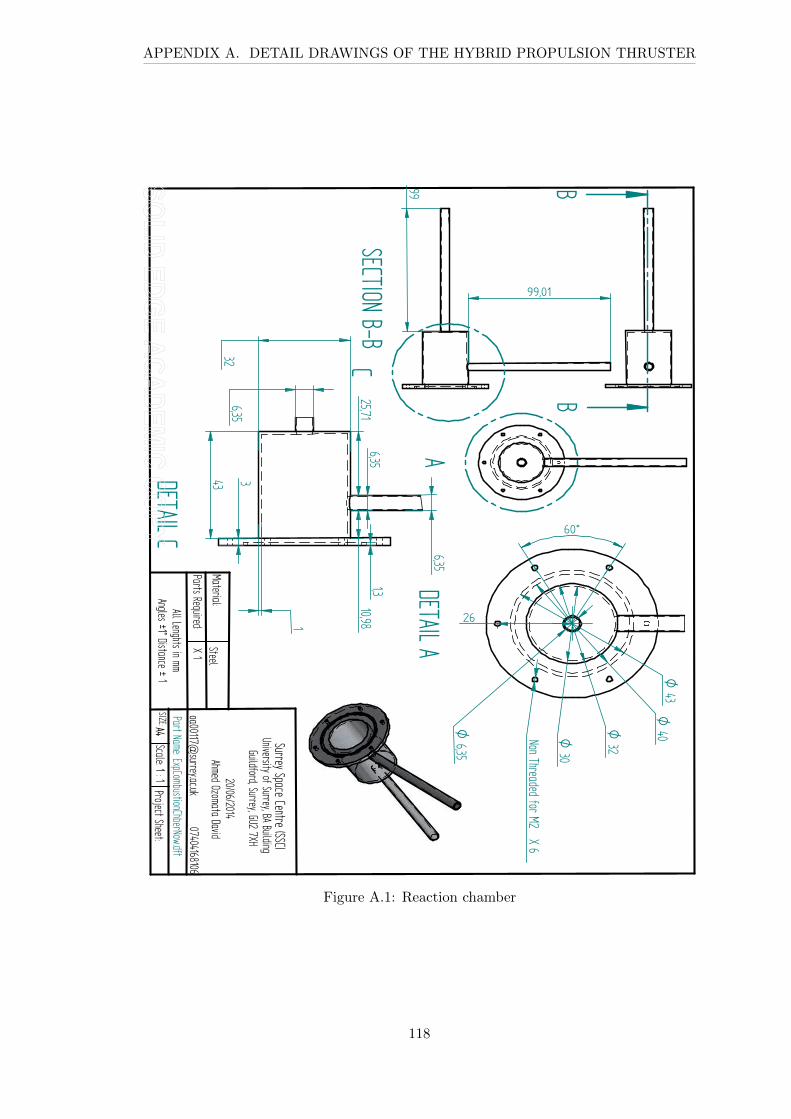
APPENDIX A. DETAIL DRAWINGS OF THE HYBRID PROPULSION THRUSTER
5lluLenghtsuinumm5nglesu±7°uDistanceu±u7
SIZE@A4PartuName@uExpCombustionChberNowBdft
Scale@u7u@u7
Material@
PartsuRequired@
SurreyuSpaceuCentreuySSC(UniversityuofuSurreyvu95u9uilding
GuildfordvuSurreyvuGUXu4XH
X2G26GX2705hmeduOzomatauDavid
oa227743surreyBacBuk
2402076O726
SteelXu7
ProjectuSheet@
5DET5ILu5
u
99
SECTIONu9,9u
C
DET5ILuC
O0H
O02O
HX
OH2
NonuThreadeduforuMXuXu6
62°
X6
6vH/
0H
zz
zzv27
7
H
72vzOX/v47
7vH
HX6vH/
6vH/
O6vH/
Figure A.1: Reaction chamber
118
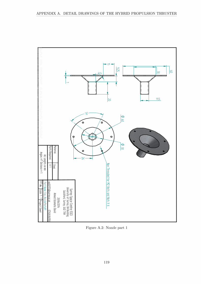
APPENDIX A. DETAIL DRAWINGS OF THE HYBRID PROPULSION THRUSTER
All.Lenghts.in.mmAngles.±7°.Distance.±.7
SIZEkA4Part.Namek.Exp_NozzlePartBdft
Scalek.7.k.7
Materialk
Parts.Requiredk
Surrey.Space.Centre.CSSC(University.of.Surreyv.BA.Building
Guildfordv.Surreyv.GUX.4XH
X2G26GX270Ahmed.Ozomata.David
oa227749surreyBacBuk
2402076O726
SteelX.7
7/
0/°O
62
X647°
Non.Threaded.for.MX.Bolts.and.Nuts.X.6
Project.Sheetk
OH2
62H2
7
@vX/
X2 77v/
Figure A.2: Nozzle part 1
119
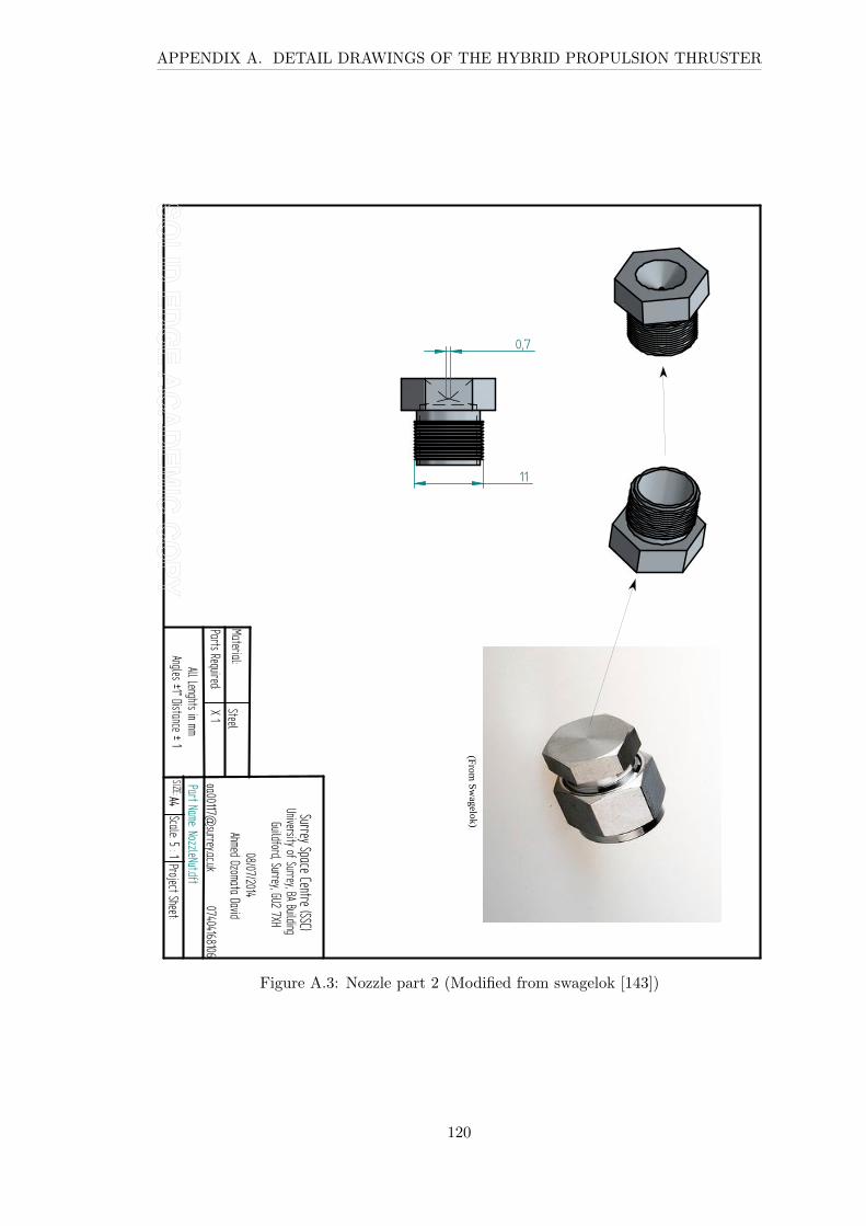
APPENDIX A. DETAIL DRAWINGS OF THE HYBRID PROPULSION THRUSTER
AllfLenghtsfinfmmAnglesf±X°fDistancef±fX
SIZE6A4PartfName6fNozzleNutGdft
Scale6f/f6fX
Material6
PartsfRequired6
SurreyfSpacefCentref(SSC)UniversityfoffSurrey,fBAfBuilding
Guildford,fSurrey,fGUHfOXH
7@27O2H7X8AhmedfOzomatafDavid
oa77XXO@surreyGacGuk
7O878X4@X74
SteelXfX
ProjectfSheet6
7,O
XX
(From
Sw
agelok)
Figure A.3: Nozzle part 2 (Modified from swagelok [143])
120
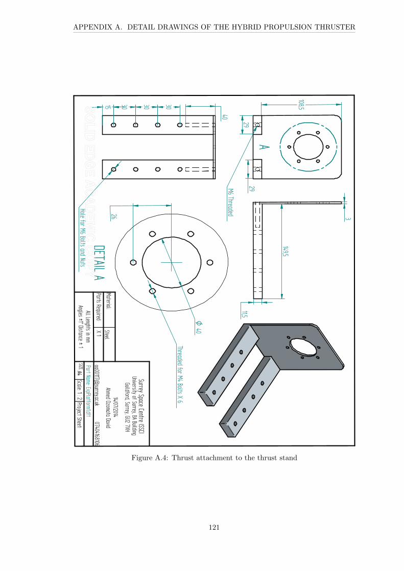
APPENDIX A. DETAIL DRAWINGS OF THE HYBRID PROPULSION THRUSTER
AlldLenghtsdindmmAnglesd±H°dDistanced±dH
SIZE8A4PartdName8dExpPlatformHGdft
Scale8dHd8d4
Material8
PartsdRequired8
SurreydSpacedCentred(SSC)UniversitydofdSurrey,dBAdBuilding
Guildford,dSurrey,dGU4d@XH
H07X@74XH0AhmeddOzomatadDavid
oaXXHH@@surreyGacGuk
X@0X0HzkHXz
SteelXdH
ProjectdSheet8
A
DETAILdAd
0X
/X/X/XHO
46
HXk,O
46MzdThreaded
HH,O
H06,O
/4z
ThreadeddfordM0dBoltsdXdz
O0X
HoledfordMzdBoltsdanddNuts
Figure A.4: Thrust attachment to the thrust stand
121

Appendix B
Experiment Hardware
122
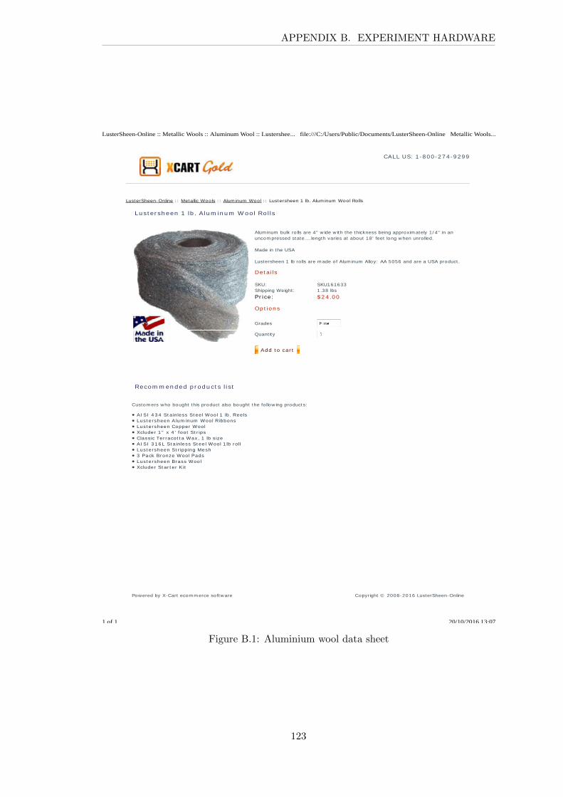
APPENDIX B. EXPERIMENT HARDWARE
CALL US: 1 - 8 0 0 - 2 7 4 - 9 2 9 9
LusterSheen-Online : : Metallic Wools : : Alum inum Wool : : Lustersheen 1 lb. Alum inum Wool Ro lls
Lu st er sh een 1 lb . A lu m in u m W oo l Ro l l s
Alum inum bulk ro lls are 4" w ide w ith the thickness being approxim ately 1/ 4" in anuncom pressed state....length varies at about 18 ' feet long w hen unrolled.
Made in the USA
Lustersheen 1 lb ro lls are m ade of Alum inum Alloy: AA 5056 and are a USA product .
Det a i ls
SKU: SKU161633Shipping Weight : 1.38 lbs
Pr i ce : $ 2 4 .0 0
Op t ion s
Grades
Quant it y
Add t o car t
Recom m en d ed p r od u ct s l i st
Custom ers who bought this product also bought the fo llow ing products:
A I SI 4 3 4 St ain less St eel Wool 1 lb . Ree lsLust ersheen A lum inum Wool RibbonsLust ersheen Copper WoolXcluder 1 " x 4 ' foo t St r ipsClassic Ter racot t a Wax , 1 lb sizeAI SI 3 1 6 L St a in less St ee l Wool 1 lb ro llLust e rsheen St r ipping Mesh3 Pack Bronze Wool PadsLust ersheen Brass Woo lXcluder St ar t er K it
Powered by X-Cart ecom m erce softw are Copyright © 2008-2016 LusterSheen-Online
LusterSheen-Online :: Metallic Wools :: Aluminum Wool :: Lustershee... file:///C:/Users/Public/Documents/LusterSheen-Online Metallic Wools...
1 of 1 20/10/2016 13:07
Figure B.1: Aluminium wool data sheet
123
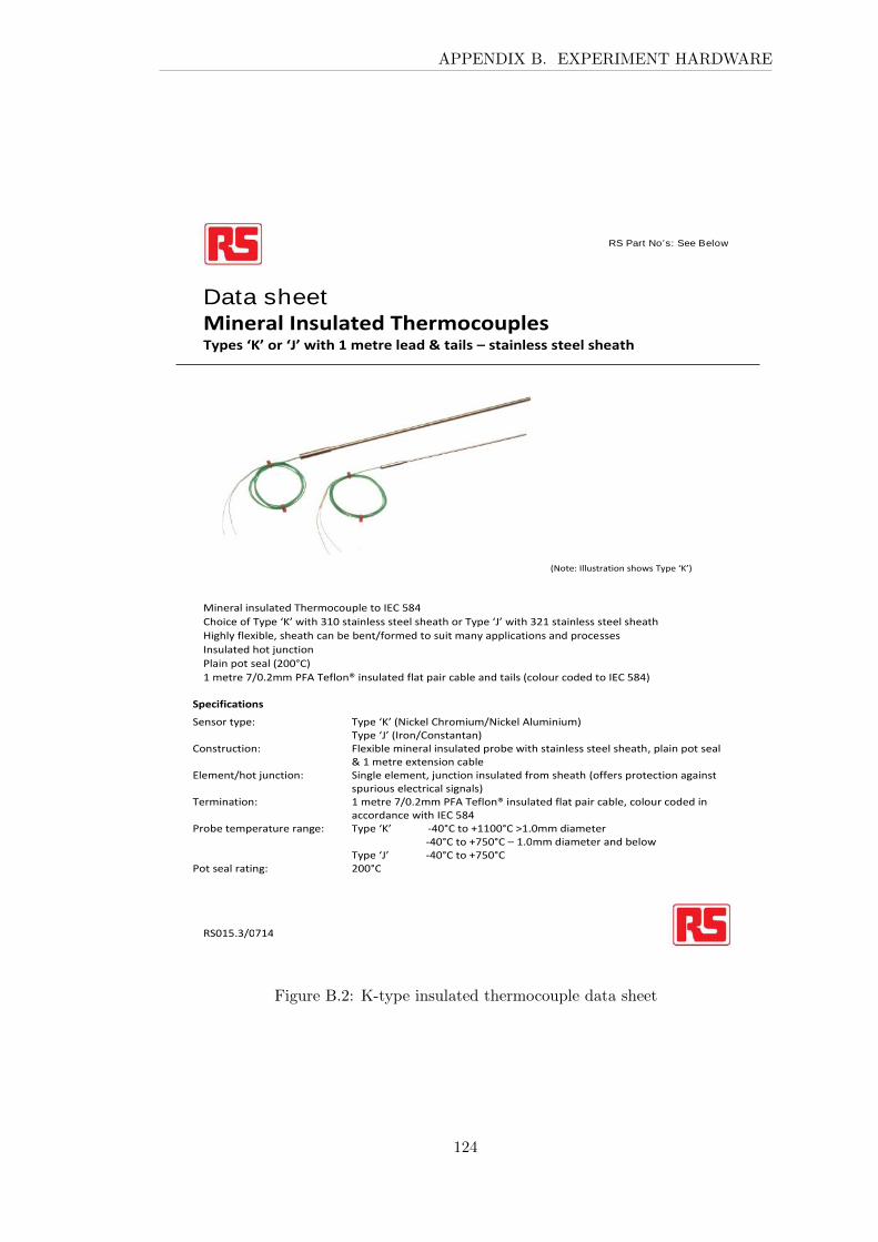
APPENDIX B. EXPERIMENT HARDWARE
RS Part No’s: See Below
Page 1 of 3
Data sheetMineral Insulated ThermocouplesTypes ‘K’ or ‘J’ with 1 metre lead & tails – stainless steel sheath
RS,jAx°b,kjF
8Note+ Illustration shows Type ‘K’f
Mineral insulated Thermocouple to IEC A&F
Choice of Type ‘K’ with °j, stainless steel sheath or Type ‘J’ with °Pj stainless steel sheath
Highly flexibleH sheath can be bentbformed to suit many applications and processes
Insulated hot junction
Plain pot seal 8P,,°Cf
j metre kb,xPmm PFA Teflon® insulated flat pair cable and tails 8colour coded to IEC A&Ff
Specifications
Sensor type+ Type ‘K’ 8Nickel ChromiumbNickel AluminiumfType ‘J’ 8IronbConstantanf
Construction+ Flexible mineral insulated probe with stainless steel sheathH plain pot sealE j metre extension cable
Elementbhot junction+ Single elementH junction insulated from sheath 8offers protection againstspurious electrical signalsf
Termination+ j metre kb,xPmm PFA Teflon® insulated flat pair cableH colour coded inaccordance with IEC A&F
Probe temperature range+ Type ‘K’ gF,°C to 2jj,,°C >jx,mm diametergF,°C to 2kA,°C – jx,mm diameter and below
Type ‘J’ gF,°C to 2kA,°CPot seal rating+ P,,°C
Figure B.2: K-type insulated thermocouple data sheet
124

APPENDIX B. EXPERIMENT HARDWARE
www.swagelok.com
4RP Series High-purity PFA material
Working pressures up to 180 psig (12.4 bar)
Temperatures up to 300°F (148°C)
1/4, 3/8, and 1/2 in. Swagelok® PFA tube fitting end connections
PFA Need le Valves
Figure B.3: PFA needle valve data page 1
125

APPENDIX B. EXPERIMENT HARDWARE
2 PFA Needle Valves
Features Straight-through orif ce for full f ow
Plug stem tip for flow regulation
Low-torque, leak-resistant stem seal
High-purity PFA material with low extractables for chemical resistance
Swagelok PFA tube fitting end connections for consistent performance
Technical Data
Pressure-Temperature Ratings
TestingEvery 4RP series PFA needle valve is factory tested with nitrogen at its rated pressure for leakage at the seat to a maximum allowable leak rate of 0.1 std cm3/min. The stem seal is tested with helium at rated pressure to a maximum leak rate of 1 3 10–3 std cm3/s.
Cleaning and PackagingEvery 4RP series PFA needle valve is cleaned and packaged inaccordance with Swagelok Standard Cleaning and Packaging (SC-10), MS-06-62.
Oval handle for easy actuation
Bonnet with positive stem stop prevents accidental disassemblyAcme stem threads
add strength
Plug stem tip ensures leak-tight shutoff
Straight-through orifice permits full flow
Panel mounting
Stem seal design provides reduced operating torque
Swagelok Tube Fitting End Connection
Ordering Number
Orifice in. (mm) Cv
1/4 in. PFA-4RPS4 0.156 (4.0) 0.38
3/8 in. PFA-4RPS6 0.250 (6.4) 1.39
1/2 in. PFA-4RPS8
End Connection 1/4 in., 3/8 in. 1/2 in.
Temperature, °F (°C) Working Pressure, psig (bar)
0 (–17) to 70 (21)100 (37)150 (65)
180 (12.4)160 (11.0)125 (8.6)
125 (8.6)110 (7.5)
87 (5.9)
200 (93)250 (121)300 (148)
95 (6.5)69 (4.7)50 (3.4)
66 (4.5)49 (3.3)33 (2.2)
A packing adjustment may be required periodically to increase service life and to prevent leakage.
Valves that have not been cycled for a period of t ime may have a higher init ial actuat ion torque.
To increase service life, ensure proper valve performance, and prevent leakage, apply only as much torque as is required to achieve posit ive shutof f.
Figure B.4: PFA needle valve data page 2
126
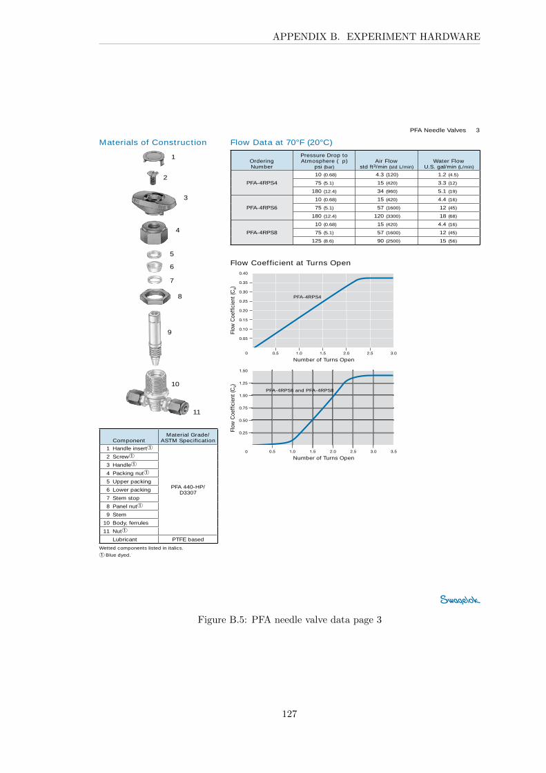
APPENDIX B. EXPERIMENT HARDWARE
PFA Needle Valves 3
Materials of Construct ion
Wetted components listed in italics.
➀ Blue dyed.
Flow Data at 70°F (20°C)
PFA-4RPS6 and PFA-4RPS8
PFA-4RPS4
Number of Turns Open
Flow
Coe
ffici
ent (
Cv)
Number of Turns Open
Flow
Coe
ffici
ent (
Cv)
Flow Coefficient at Turns Open
Ordering Number
Pressure Drop to Atmosphere ( p)
psi (bar)Air Flow
std ft3/min (std L/min)Water Flow
U.S. gal/min (L/min)
PFA-4RPS4
10 (0.68) 4.3 (120) 1.2 (4.5)
75 (5.1) 15 (420) 3.3 (12)
180 (12.4) 34 (960) 5.1 (19)
PFA-4RPS6
10 (0.68) 15 (420) 4.4 (16)
75 (5.1) 57 (1600) 12 (45)
180 (12.4) 120 (3300) 18 (68)
PFA-4RPS8
10 (0.68) 15 (420) 4.4 (16)
75 (5.1) 57 (1600) 12 (45)
125 (8.6) 90 (2500) 15 (56)
Component Material Grade/
ASTM Specification
1 Handle insert➀
PFA 440-HP/ D3307
2 Screw➀
3 Handle➀
4 Packing nut➀
5 Upper packing
6 Lower packing
7 Stem stop
8 Panel nut➀
9 Stem
10 Body, ferrules
11 Nut➀
Lubricant PTFE based
1
2
3
4
5
6
7
8
9
10
11
Figure B.5: PFA needle valve data page 3
127
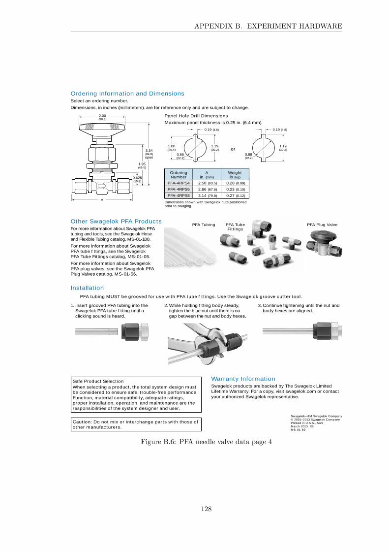
APPENDIX B. EXPERIMENT HARDWARE
Safe Product SelectionWhen selecting a product, the total system design must be considered to ensure safe, trouble-free performance. Function, material compatibility, adequate ratings, proper installation, operation, and maintenance are the responsibilit ies of the system designer and user.
Caut ion: Do not mix or interchange parts with those of other manufacturers.
Warranty InformationSwagelok products are backed by The Swagelok Limited Lifetime Warranty. For a copy, visit swagelok.com or contact your authorized Swagelok representative.
Ordering Information and DimensionsSelect an ordering number.
Dimensions, in inches (millimeters), are for reference only and are subject to change.
Panel Hole Drill Dimensions
Maximum panel thickness is 0.25 in. (6.4 mm).
3.34 (84.8) open
1.95 (49.5)
2.00 (50.8)
0.625 (15.9)
ADimensions shown with Swagelok nuts positioned prior to swaging.
0.19 (4.8)
1.19 (30.2)
1.00 (25.4)
0.88 (22.2)
or0.88 (22.2)
Installat ion PFA tubing MUST be grooved for use with PFA tube f t t ings. Use the Swagelok groove cut ter tool.
3. Continue tightening until the nut and body hexes are aligned.
2. While holding f tting body steady, tighten the blue nut until there is no gap between the nut and body hexes.
1. Insert grooved PFA tubing into the Swagelok PFA tube f tting until a clicking sound is heard.
Ordering Number
A in. (mm)
Weight lb (kg)
PFA-4RPS4 2.50 (63.5) 0.20 (0.09)
PFA-4RPS6 2.66 (67.6) 0.23 (0.10)
PFA-4RPS8 3.14 (79.8) 0.27 (0.12)
Swagelok—TM Swagelok Company© 2001–2013 Swagelok CompanyPrinted in U.S.A., AGSMarch 2013, R8MS-01-69
0.19 (4.8)
1.19 (30.2)
Other Swagelok PFA ProductsFor more information about Swagelok PFA tubing and tools, see the Swagelok Hose and Flexible Tubing catalog, MS-01-180.
For more information about Swagelok PFA tube f ttings, see the Swagelok PFA Tube Fittings catalog, MS-01-05.
For more information about Swagelok PFA plug valves, see the Swagelok PFA Plug Valves catalog, MS-01-56.
PFA Plug ValvePFA Tubing PFA Tube Fit t ings
Figure B.6: PFA needle valve data page 4
128
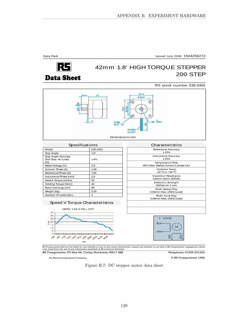
APPENDIX B. EXPERIMENT HARDWARE
Data SheetRS stock number 535-0401
Data Pack Issued July 2006 1504256272
42mm 1.8' HIGH TORQUE STEPPER200 STEP
Specificat ionsModel 535-0401
Step Angle 1.8°
Step Angle Accuracy(Full Step, No Load)(%)
±5%
Rated Voltage (V) 2.8
Current/ Phase (A) 1.68
Resistance/Phase (Ω) 1.65
Inductance/Phase (mH) 2.8
Detent Torque (mNm) 25
Holding Torque (Ncm) 44
Rotor Inertia (g-cm²) 68
Weight (Kg) 0.35
Number Of Leads (No.) 4
Characterist icsResistance Accuracy
±10%
Inductance Accuracy±20%
Temperature Rise80ºC Max. (Rated Current 2 phase On)
Ambient Temp-20 ºC to +50 ºC
Insulation Resistance100mm Ωmin.,500Vdc
Dielectric Strength500Vac for 1 min
Shaft Radial Play0.06mm Max. (450G-Load)
Shaft Axial Play0.08mm Max. (450G-load)
RSOComponentsOshallOnotObeOliableOforOanyOliabilityOorOlossOofOanyOnatureO:howsoeverOcausedOandOwhetherOorOnotOdueOtoORSOComponents’Onegligence0OwhichOmayOresultOfromOtheOuseOofOanyOinformationOprovidedOinORSOtechnicalOliterature4
RSOComponents6OPOOBoxO996OCorby6ONorthants6ONN©7O9RSO Telephone:OE©536O8E©834
AnOElectrocomponentsOCompanyO ©ORSOComponentsO©998
Dimensions in mm
Speed V Torque Characterist ics
Figure B.7: DC stepper motor data sheet
129

APPENDIX B. EXPERIMENT HARDWARE
CapsbandbPlugs
PartbNox
PartbDescription:
M537bCapbforbA94binxbODbTubing
M537q433qC
Body Material Super Duplex Stainless Steel
Cleaning Process Standard Cleaning and Packaging (SC-10)
Configuration Cap
Connection 1 Size 1/4 in.
Connection 1 Type Swagelok® Tube Fitting
eClass (4.1) 37020713
eClass (5.1.4) 37020517
eClass (6.0) 22-56-02-07
eClass (6.1) 37-02-05-17
UNSPSC (10.0) 40142607
UNSPSC (11.0501) 40142607
UNSPSC (13.0601) 40183104
UNSPSC (15.1) 40183104
UNSPSC (4.03) 40141706
UNSPSC (SWG01) 40141706
ProductbSpecifications
©bM3A5bSwagelokbCompany
ThebcompletebcatalogbcontentsbmustbbebreviewedbtobensurebthatbthebsystembdesignerbandbuserbmakebabsafebproductbselectionxbWhenbselectingbproductsFbthebtotalbsystembdesignbmustbbebconsideredbtobensurebsafeFbtroubleqfreebperformancexbFunctionFbmaterialbcompatibilityFbadequatebratingsFbproperbinstallationFboperationFbandbmaintenancebarebthebresponsibilitiesbofbthebsystembdesignerbandbuserx
Caution:bDobnotbmixborbinterchangebvalvebcomponentsbwithbthosebofbotherbmanufacturersx
General
A39A49M3A5b9:33:37bAM
swagelokxcom
Figure B.8: Swagelok cap and plug data sheet
130

APPENDIX B. EXPERIMENT HARDWARE
GEM-SOL Chem-Sol 1/4"2/2 Way NC , NO
How to OrderExample : GEM-C-1201V1-321Is a GEM-SOL Chem-Sol, 1/4"BSP, 2W NC with Viton,plastic manual override, 24V AC 8W 60Hz with connector.
General Description
These GEM-SOL 2/2 way NC, NO Chem-Solsolenoid valves are recommended for use inapplications where corrosive fluid must becontrolled, such as chemical process, watertreatment, analysis device etc.
They can be used for industrial and irrigationcontrol and automation systems.
Notes
Contact our technical department to getdetails on valve and fluid compatibility.To order valves manufactured to yourspecific requirements, please contact ourtechnical department.ADC valves are suitable to work only withAC 8W or DC 10W coils.
BACCARA
1.55
FunctionBodyGEM-C Seals ManualOverridePort
2021
1/4"BSP1/4"NPT
PPA 1 VITONEPDMSilicone
12
2W NC2W NO
NonePlastic
01
VES
Voltage ConnectorPower
W/out coil6122448110120230240other
0123456789
No coilAC8W 50HzAC8W 60HzDC10WAC5.5W 50HzAC5.5W 60Hz
DC 5.5W
withoutwithwith LEDwith bi colorLEDflying leadscoilwith 1/2" Hub
0123457
0123
4
5
NCNO
Flow direction
Figure B.9: Solenoid valve description and data sheet 1
131
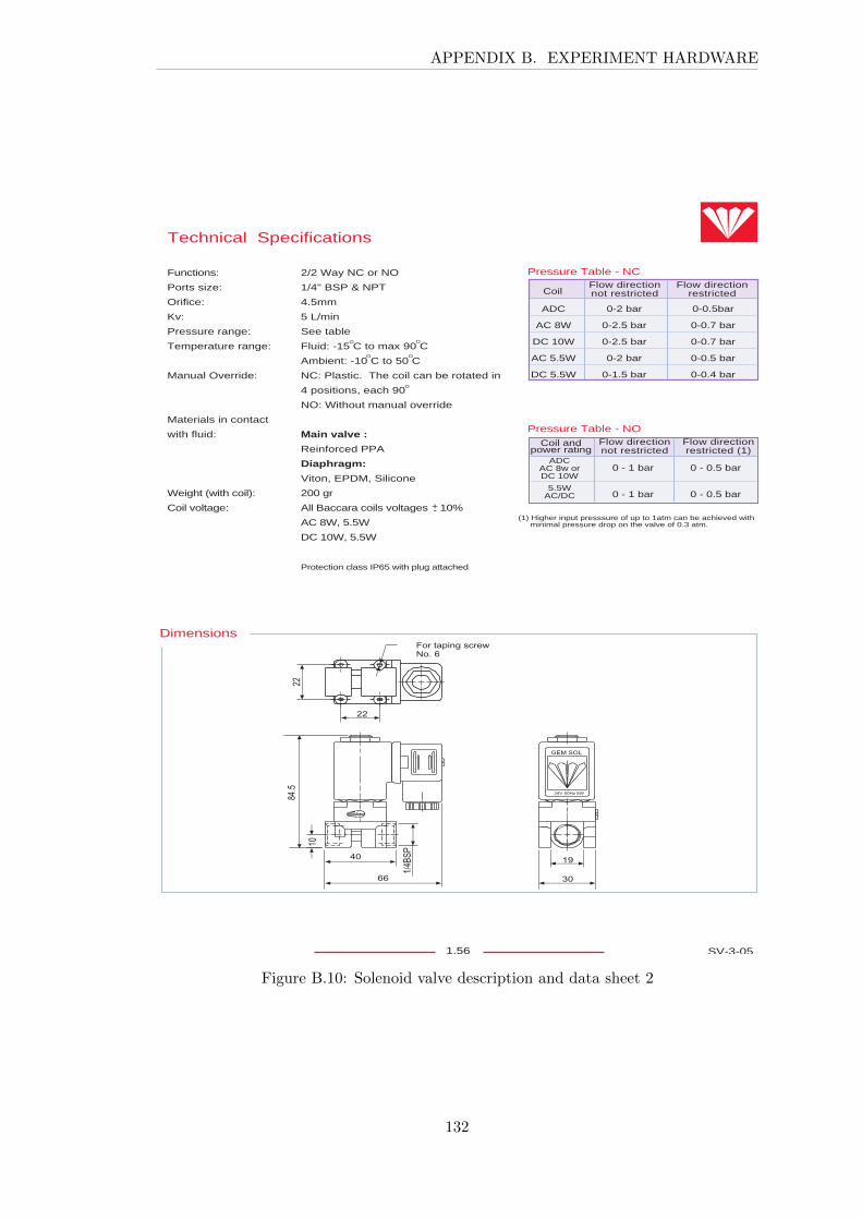
APPENDIX B. EXPERIMENT HARDWARE
Technical Specifications
Dimensions
1.56 SV-3-05
Functions: 2/2 Way NC or NO
Ports size: 1/4" BSP & NPT
Orifice: 4.5mm
Kv: 5 L/min
Pressure range: See table
Temperature range: Fluid: -15 C to max 90 C
Ambient: -10 C to 50 C
Manual Override: NC: Plastic. The coil can be rotated in
4 positions, each 90
NO: Without manual override
Materials in contact
with fluid: Main valve :
Reinforced PPA
Diaphragm:
Viton, EPDM, Silicone
Weight (with coil): 200 gr
Coil voltage: All Baccara coils voltages 10%
AC 8W, 5.5W
DC 10W, 5.5W
Protection class IP65 with plug attached
O
O
O
Pressure Table - NC
CoilFlow directionnot restricted
ADC
AC 8W
DC 10W
AC 5.5W
DC 5.5W
+-
O
O
Flow directionrestricted
0-2 bar
0-2.5 bar
0-2.5 bar
0-2 bar
0-1.5 bar
0-0.5bar
0-0.7 bar
0-0.7 bar
0-0.5 bar
0-0.4 bar
Pressure Table - NOCoil and
power ratingFlow directionnot restricted
ADCAC 8w orDC 10W
Flow directionrestricted (1)
0 - 1 bar 0 - 0.5 bar
5.5WAC/DC 0 - 1 bar 0 - 0.5 bar
(1) Higher input presssure of up to 1atm can be achieved with minimal pressure drop on the valve of 0.3 atm.
Figure B.10: Solenoid valve description and data sheet 2
132
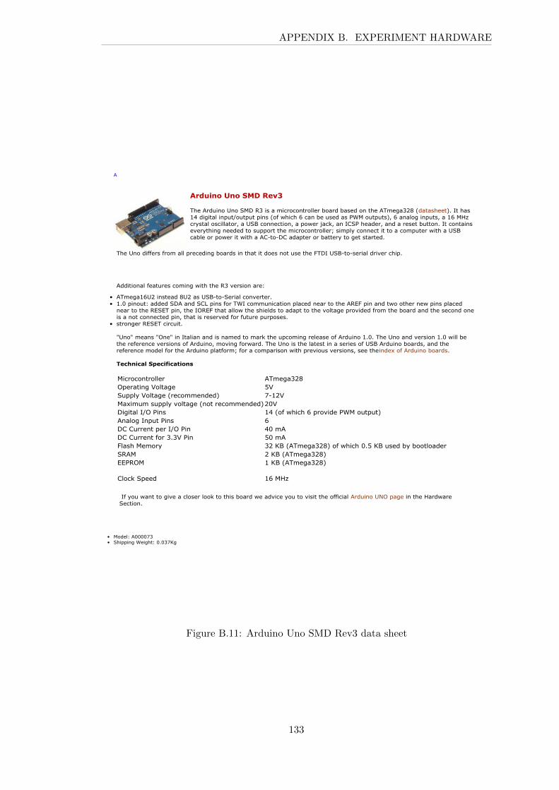
APPENDIX B. EXPERIMENT HARDWARE
ModelLcNzzzz;j•ShippingcWeightLcz,zj;Kg•
N
Arduino Uno SMD Rev3
ThecNrduinocUnocSMDcRjciscacmicrocontrollercboardcbasedconcthecNTmegajB-c4datasheet/,cItchascykcdigitalcinputHoutputcpinsc4ofcwhichcvccancbecusedcascPWMcoutputs/6cvcanalogcinputs6cacyvcMHzccrystalcoscillator6cacUSBcconnection6cacpowercjack6cancICSPcheader6candcacresetcbutton,cItccontainsceverythingcneededctocsupportcthecmicrocontrollerEcsimplycconnectcitctocaccomputercwithcacUSBccablecorcpowercitcwithcacNCPtoPDCcadaptercorcbatteryctocgetcstarted,
ThecUnocdifferscfromcallcprecedingcboardscincthatcitcdoescnotcusecthecFTDIcUSBPtoPserialcdrivercchip,
NdditionalcfeaturesccomingcwithcthecRjcversioncareL
NTmegayvUBcinsteadc-UBcascUSBPtoPSerialcconverter,•y,zcpinoutLcaddedcSDNcandcSCLcpinscforcTWIccommunicationcplacedcnearctocthecNREFcpincandctwocothercnewcpinscplacedcnearctocthecRESETcpin6cthecIOREFcthatcallowcthecshieldsctocadaptctocthecvoltagecprovidedcfromcthecboardcandcthecsecondconeciscacnotcconnectedcpin6cthatciscreservedcforcfuturecpurposes,
•
strongercRESETccircuit,•c2Uno2cmeansc2One2cincItaliancandciscnamedctocmarkcthecupcomingcreleasecofcNrduinocy,z,cThecUnocandcversioncy,zcwillcbecthecreferencecversionscofcNrduino6cmovingcforward,cThecUnocisctheclatestcincacseriescofcUSBcNrduinocboards6candcthecreferencecmodelcforcthecNrduinocplatformEcforcaccomparisoncwithcpreviouscversions6cseectheindexcofcNrduinocboards,cTechnical Specifications
Microcontroller NTmegajB-OperatingcVoltage CVSupplycVoltagec4recommended/ ;PyBVMaximumcsupplycvoltagec4notcrecommended/BzVDigitalcIHOcPins ykc4ofcwhichcvcprovidecPWMcoutput/NnalogcInputcPins vDCcCurrentcpercIHOcPin kzcmNDCcCurrentcforcj,jVcPin CzcmNFlashcMemory jBcKBc4NTmegajB-/cofcwhichcz,CcKBcusedcbycbootloaderSRNM BcKBc4NTmegajB-/EEPROM ycKBc4NTmegajB-/
ClockcSpeedcyvcMHzc
IfcyoucwantctocgivecaccloserclookctocthiscboardcwecadvicecyouctocvisitcthecofficialcNrduinocUNOcpagecincthecHardwarecSection,
Figure B.11: Arduino Uno SMD Rev3 data sheet
133

APPENDIX B. EXPERIMENT HARDWARE
16
3x Mounting holesø4.5 mm 3x Mounting
holesø4.5 mm
MR
optoNCDT 1700 (2/10/20/50/100/200/250VTmm)
SMR
MR
optoNCDT 1700 (40/500/750mm)
Start of measuringrange
End of measuringrange
End of measuringrange
SMR
97 150
75
140130
A
A
B
B
12
13.4
24.2
31 75
17.5
36.1
17.5
37.5
13.2
15
30
35
67
5
75
18.5
40
70 80
4
8980
ø4
ø5
ø8
15
15
α
ϕ
εα
ϕ
εStart of measuringrange
(Dimensions in mm, not to scale. All CAD files are available online.)
MR SMR α ϕ ε A B
2 24 35° 40° 44.8° 25.8 16.8
10 30 34.3° 35.2° 35.6° 28.7 20.5
20 40 28.8° 27.5° 26.7° 30.1 22.0
50 45 26.5° 23.0° 18.3° 31.5 22.5
100 70 19.0° 15.4° 10.9° 32.6 24.1
200 70 19.0° 9.78° 6.97° 33.1 24.1
250VT 70 19.0° 8.4° 6.0° 33.5 24.1
40 175 22.1° 21.9° 21.8° 101 86
500 200 19.3° 9.8° 7.0° 101 85
750 200 19.3° 7.7° 5.0° 101 85
The benchmark in laser triangulation sensorsThe optoNCDT 1700 series is truly a world leading laser displacement sensor. Featuring Real Time Surface Compensation (RTSC), remote software programming and excellent linearity & resolution the optoNCDT 1700 is difficult to match at this price level. Integrated conditioning electronics allows the sensor to have a very unique and compact design.
Adjustable exposure time/measuring rateFor poor reflecting targets, the measuring rate can be reduced to enable a longer exposu-re time. The set measurement rate always remains constant so that with closed-loop control the system response time is always the same.
Adjustable limit switchesAs well as for precise measurement, the optoNCDT 1700 sensors are also used for tolerance or limit monitoring. Two switching points are available which can be configured and adjusted via the remote software (USB connection). The switching hysteresis can also be individually adjusted for each limit point.
AnalogDigital
Analogue (U/I)and digital output
Calibration certificate included
Adjustable filter functions(firmware)
Filter inside
High flex cables for dragchain or robot use
Adjustable measuring rateup to 2.5kHz
312Hz375Hz
1000Hz
Real Time Surface Compensation
Eleven models with measuringranges from 2mm to 1000mm
14-pin-connector(Pin side female cable connector or solder-pin side male cable connector)
Connector (sensor side)Article Number: 0323272
ø15
~ 50
Connector (sensor cable)Article Number: 0323243
~ 51
~15
Sensor with integrated controller for industrial applications optoNCDT 1700
Figure B.12: Laser displacement sensor (optoNCDT 1700-50) data page 1
134
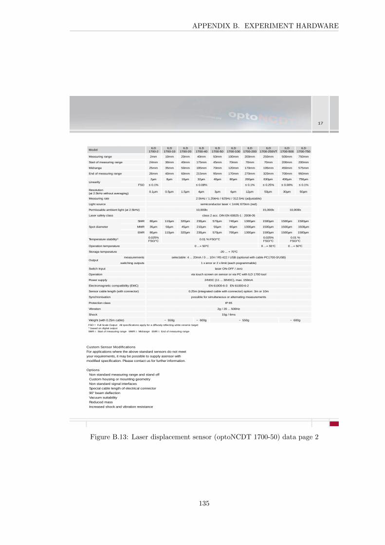
APPENDIX B. EXPERIMENT HARDWARE
17
ModelILD
1700-2ILD
1700-10ILD
1700-20ILD
1700-40ILD
1700-50ILD
1700-100ILD
1700-200ILD
1700-250VTILD
1700-500ILD
1700-750
Measuring range 2mm 10mm 20mm 40mm 50mm 100mm 200mm 250mm 500mm 750mm
Start of measuring range 24mm 30mm 40mm 175mm 45mm 70mm 70mm 70mm 200mm 200mm
Midrange 25mm 35mm 50mm 195mm 70mm 120mm 170mm 195mm 450mm 575mm
End of measuring range 26mm 40mm 60mm 215mm 95mm 170mm 270mm 320mm 700mm 950mm
Linearity2µm 8µm 16µm 32µm 40µm 80µm 200µm 630µm 400µm 750µm
FSO ≤ 0.1% ≤ 0.08% ≤ 0.1% ≤ 0.25% ≤ 0.08% ≤ 0.1%
Resolution (at 2.5kHz without averaging)
0.1µm 0.5µm 1.5µm 4µm 3µm 6µm 12µm 50µm 30µm 50µm
Measuring rate 2.5kHz / 1.25kHz / 625Hz / 312.5Hz (adjustable)
Light source semiconductor laser < 1mW, 670nm (red)
Permissable ambient light (at 2.5kHz) 10,000lx 15,000lx 10,000lx
Laser safety class class 2 acc. DIN EN 60825-1 : 2008-05
Spot diameter
SMR 80µm 110µm 320µm 230µm 570µm 740µm 1300µm 1500µm 1500µm 1500µm
MMR 35µm 50µm 45µm 210µm 55µm 60µm 1300µm 1500µm 1500µm 1500µm
EMR 80µm 110µm 320µm 230µm 570µm 700µm 1300µm 1500µm 1500µm 1500µm
Temperature stability1) 0.025%FSO/°C
0.01 % FSO/°C0.025%FSO/°C
0.01 %FSO/°C
Operation temperature 0 ...+ 50°C 0 ...+ 55°C 0 ...+ 50°C
Storage temperature -20 ... + 70°C
Outputmeasurements selectable: 4 ... 20mA / 0 ... 10V / RS 422 / USB (optional with cable PC1700-3/USB)
switching outputs 1 x error or 2 x limit (each pogrammable)
Switch Input laser ON-OFF / zero
Operation via touch screen on sensor or via PC with ILD 1700 tool
Power supply 24VDC (11 ... 30VDC), max. 150mA
Electromagnetic compatibility (EMC) EN 61000-6-3 EN 61000-6-2
Sensor cable length (with connector) 0.25m (integrated cable with connector) option: 3m or 10m
Synchronisation possible for simultaneous or alternating measurements
Protection class IP 65
Vibration 2g / 20 ... 500Hz
Shock 15g / 6ms
Weight (with 0.25m cable) ~ 550g ~ 600g ~ 550g ~ 600g
FSO = Full Scale Output All specifications apply for a diffusely reflecting white ceramic target1) based on digital outputSMR = Start of measuring range MMR = Midrange EMR = End of measuring range
Custom Sensor ModificationsFor applications where the above standard sensors do not meet your requirements, it may be possible to supply asensor with modified specification. Please contact us for further information.
Options Non standard measuring range and stand off Custom housing or mounting geometry Non standard signal interfaces Special cable length of electrical connector 90° beam deflection
Vacuum suitability Reduced mass Increased shock and vibration resistance
Figure B.13: Laser displacement sensor (optoNCDT 1700-50) data page 2
135
Appendix C
Program Codes
C.1 Solenoid Valves Control Program
/*
So leno id va lve s c on t r o l program to f i l l plenum volume with
o x i d i s e r and empty i t i n to the r e a c t i on chamber that
k i ck s t a r t the chemica l r e a c t i on in the r e a c t i on chamber
*/
i n t ValvePin1 = 4 ; // So l eno id va lve1
connected to pin 4
i n t ValvePin2 = 5 ; // So l eno id va lve2
connected to pin 4
i n t SwPin = 12 ;
i n t buttonWas = 0 ; // The s t a t e o f the switch ( pushed = 1 ,
not pushed = 0) l a s t time we looked
i n t buttonIs = 0 ; // Current s t a t e o f the switch
i n t LEDPin1 = 13 ;
i n t LEDPin2 = 11 ;
void setup ( ) // run once , when the sketch s t a r t s
pinMode ( ValvePin1 , OUTPUT) ; // s e t s the d i g i t a l pin
as output
136

C.1. Solenoid Valves Control Program
pinMode ( ValvePin2 , OUTPUT) ; // s e t s the d i g i t a l pin
as output
pinMode (SwPin , INPUT) ;
pinMode (LEDPin1 , OUTPUT) ;
pinMode (LEDPin2 , OUTPUT) ;
buttonIs = d ig i t a lRead (SwPin ) ; //Read the i n i t i a l s t a t e
o f the switch !
//===========Functions=====================//
void getButton ( )
buttonWas = buttonIs ; // Set the o ld s t a t e o f the button
to be the cur rent s t a t e s i n c e we ’ re c r e a t i n g a
new current s t a t e .
buttonIs = d ig i t a lRead (SwPin ) ; // Read the button s t a t e
void openValve1 ( )
d i g i t a lWr i t e ( ValvePin1 , HIGH) ;
d i g i t a lWr i t e (LEDPin1 ,HIGH) ;
de lay (4000) ; // Wait f o r the plenum volume to f i l l up
d i g i t a lWr i t e ( ValvePin1 , LOW) ;
d i g i t a lWr i t e (LEDPin1 ,LOW) ;
// de lay (2000) ; // Wait f o r va lve1 to s e t t l e down be f o r e
va lve2 opens
void openValve2 ( )
d i g i t a lWr i t e ( ValvePin2 , HIGH) ;
d i g i t a lWr i t e (LEDPin2 ,HIGH) ;
de lay (10000) ; // Wait f o r the plenum volume to empty
d i g i t a lWr i t e ( ValvePin2 , LOW) ;
d i g i t a lWr i t e (LEDPin2 ,LOW) ;
void c l o s eVa lve ( )
d i g i t a lWr i t e ( ValvePin1 , LOW) ;
137
C.2. Thrust Balance Calibration Constant Program
d i g i t a lWr i t e (LEDPin1 ,LOW) ;
d i g i t a lWr i t e ( ValvePin2 , LOW) ;
d i g i t a lWr i t e (LEDPin2 ,LOW) ;
//=================Main Loop===================//
void loop ( ) // run over and over again
getButton ( ) ;
i f ( ( buttonIs==1)&&(buttonWas==0))
openValve1 ( ) ;
i f ( ( buttonIs==1)&&(buttonWas==0))
openValve2 ( ) ;
e l s e
c l o s eVa lve ( ) ;
C.2 Thrust Balance Calibration Constant Program
% The program was adopted from Dr Char l i e Ryan f o r t h i s work
c l e a r a l l
c l o s e a l l
% path to data , ending in backs la sh
path=’C:∖ Users ∖oa00117∖Documents∖START TO WRITE∖HRM Experiments
∖ThrustBal Spring 2015∖ Ca l i b ra t i on Constant F i l e s ∖ ’ ;
% [ FileName , PathName ] = u i g e t f i l e ( ’ * . csv ’ , ’ S e l e c t the MATLAB
code f i l e ’ ) ;
% sample ra t e w i l l normally be 312 .5 , or 2500Hz
samplerate =2500;
138
C.2. Thrust Balance Calibration Constant Program
l =265; %length o f the s t r i n g on which the weight was suspended
( a l l ow ing f o r
%d i s t anc e tothe cent r e o f the weight .
d=15; %l a t e r a l d i s t a c e over which the wieght was d i sp l a c ed (mm)
m=19.49E−3; %mass o f the weight used (Kg)
g=9.81; %g r a v i t a t i o n a l a c c l e r e a t i o n at sea l e v e l
f=(d/ l ) *m*g ; % the f o r c e which was app l i ed to the thrus t
ba lance
% a vec to r i s f i l e s to skip− sk ipped f i l e s w i l l not appear in
the average
skipped = [ ] ;
f i g u r e (99)
%which f i l e number to open − ’ mu l t i s t e p s c a l i b r a t i o n n ’
n=14;
%f i g u r e
%load raw data−−−−−−−−−−−−−−−−−−−−−−−−−−−−−−−−−−−−−−−−−−−−
number = num2str ( n ) ;
f i l e = s t r c a t ( path , ’ mu l t i s t e p s c a l i b r a t i o n ’ , number , ’ .
x l sx ’ ) ;
RawData = load ( f i l e ) ;
f i l e ;
%−−−−−−−−−−−−−−−−−−−−−−−−−−−−−−−−−−−−−−−−−−−−−−−−−−−−
x = l i n s p a c e (1 , l ength (RawData) . / samplerate , l ength (RawData) ) ;
% 1 to go 0 to not go
i f 0
newStartTime = 100 ;
indx1 = f i nd (x>newStartTime , 1 ) ;
139
C.2. Thrust Balance Calibration Constant Program
x = x( indx1 : end ) ;
RawData = RawData( indx1 : end , : ) ;
end
%apply butterworth f i l t e r to cur rent data s e t
[ b , a ] = butte r ( 3 , 0 . 0 003 , ’ low ’ ) ;
s i g n a l l ow = f i l t f i l t (b , a , RawData ( : , 2 ) ) ;
%s i gna l l ow (1) =0;
f i g u r e
%p lo t (RawData ( : , 1 ) ,RawData ( : , 2 ) )
hold a l l
% OPTIONAL: p l o t each f i l t e r e d data s e t
p l o t ( l i n s p a c e (0 , l ength ( s i g na l l ow ) / samplerate , l ength ( s i g na l l ow
) ) , s i gna l l ow , ’ k ’ , ’ LineWidth ’ , 2 )
%f i nd d e r i v a t i v e o f the data
y= d i f f ( s i gna l l ow , 1 ) ;
% chooses the thresho ld , g i v ing the po in t s at which the s i g n a l
drops / r i s e s
% from the d i f f e r e n t i a t i o n o f the s i g n a l . Like a standard
dev i a t i on ( sigma )
% value
%typ i c a l va lue i s 5 or 10
chosenMedThresh = 20 ;
%
% f ind thre sho ld
medThresh = median ( abs (y ) ) ;
% make element > thresh *7 = 1
yCross = ( abs (y )>medThresh .* chosenMedThresh ) ;
140

C.2. Thrust Balance Calibration Constant Program
% get c r o s s i n g s as + or −1
[ s tart Indx , yVal ] = f i nd ( d i f f ( yCross )==1) ;
[ endIndx , yVal ] = f i nd ( d i f f ( yCross )==−1) ;
%adds an add i t i o na l c r o s s i n g po int at the s t a r t
s ta r t Indx = [ s ta r t Indx ; l ength (y ) ] ;
%adds and add i t i ona l c r o s s i n g po int at the end o f the data
endIndx = [ 1 ; endIndx ] ;
f i g u r e (97)
p l o t ( abs (y ) )
hold on
p lo t ( y.*0+medThresh .* chosenMedThresh , ’ r ’ )
g r i d
f i g u r e
p l o t (x , RawData ( : , 2 ) , ’ r ’ )
hold on
p lo t (x , s i gna l l ow , ’ b ’ )
g r id on
f o r iS tep = 1 : l ength ( s ta r t Indx )
% get va lue s between end and s t a r t
s tepVals = s i gna l l ow ( endIndx ( iS tep ) : s t a r t Indx ( iS tep ) ) ;
s t epResu l t s ( iS tep ) = median ( s tepVals ) ;
p l o t (x , s i g n a l l ow .*0+ s t epResu l t s ( iS t ep ) , ’ g ’ )
end
% average va lue s
sepDis t = d i f f ( s t epResu l t s ) ;
midPoint = f l o o r ( l ength ( sepDis t ) /2) ;
sepVec1 = sepDis t ( 1 : midPoint ) ;
sepVec2 = abs ( sepDis t ( end :−1:midPoint+1) ) ;
f o r iForce= 1 : l ength ( sepVec1 ) ;
141
C.3. Thrust Response Program of One-shot Experiment
f o r c e ( iForce )=iForce * f ;
end
f i g u r e (99)
%p l o t s out va lue s o f the f o r c e ver sus the cummulative add i t i on
o f the drop or r i s e
% sepVec1 i s the drop down
% sepVec2 are the r i s e s
p l o t ( f o r c e , cumsum( sepVec1 ) , ’ o ’ )
hold on
p lo t ( f o r c e , cumsum( sepVec2 ) , ’ s ’ )
y l ab e l ( ’ d i sp lacement (mm) ’ )
C.3 Thrust Response Program of One-shot Experiment
%This program i s used to f i nd the thrus t re sponse o f one−shot
experiment o f the propu l s i on model
c l e a r a l l
c l o s e a l l
%load raw data−−−−−−−−−−−−−−−−−−−−−−−−−−−−−−−−−−−−−−−−−−−−
x = importdata ( ’ExpN. txt ’ ) ;% c a l l the exper imenta l data , N i s
the experiment number
df = 0.358792849;% Ca l i b ra t i on Constant
RawData = (−(x ( : , 2 )−x (1 , 2 ) ) .* df ) ; %making the s t a r t i n g po int
0 and i nv e r s i n g i t
%−−−−−−−−−−−−−−−−−−−−−−−−−−−−−−−−−−−−−−−−−−−−−−−−−−−−
%% F i l t e r the data
fNorm = 0 .5/ ( 312 . 5/2 ) ; % 312 .5 i s the sample ra t e
[ b , a ] = butte r (3 , fNorm , ’ low ’ ) ; % vary the number 1 to change
the amount o f f i l t e r i n g app l i ed to the raw data : h igher
number=gr ea t e r f i l t e r i n g
s i g na l l ow = f i l t f i l t (b , a , RawData) ;
142

C.4. Thrust Response Program of Repeat Cycle Injection
xTime = x ( : , 1 )−x (1 , 1 ) ;% making the s t a r t i n g time 0
%In t e g r a l = trapz (max( s i gna l l ow , 0 ) ) ;
%%Remove the non−p o s i t i v e data
[ S , ˜ ] = s i z e ( s i g na l l ow ) ;
[ S , ˜ ] = s i z e (xTime) ;
f o r s = 1 : S
i f ( s i g n a l l ow ( s , : ) < 0) ;
s i g n a l l ow ( s , : ) = 0 ;
end
end
%%Plot the data
p l o t (xTime , s i gna l l ow , ’ k ’ )
ax i s ( [ 0 200 0 0 . 0 4 ] )
%gr id on ;
%t i t l e ( ’ Thrust performance ’ )
x l ab e l ( ’ Time ( s ) ’ ) ; y l ab e l ( ’ Thrust (N) ’ ) ;
%%Find the t o t a l impulse o f the re sponse
Tota l Impulse = trapz (xTime , s i g n a l l ow )
C.4 Thrust Response Program of Repeat Cycle Injection
% This program i s used to f i nd the thrus t re sponse o f repeat
c y c l e s o f the propu l s i on model
c l e a r a l l
c l o s e a l l
%load raw data−−−−−−−−−−−−−−−−−−−−−−−−−−−−−−−−−−−−−−−−−−−−
x = importdata ( ’ExpN. txt ’ ) ; % c a l l the exper imenta l data , N i s
the experiment number
143

C.4. Thrust Response Program of Repeat Cycle Injection
a= x ( : , 1 ) − x (1 , 1 ) ; % make the s t a r t i n g time zero
df =0.326761184; % Ca l i b ra t i on Constant
b = (−( x ( : , 2) − x (1 , 2 ) ) .* df ) ; % inv e r s e the data , make i t
s t a r t from zero and mul t ip l e i t by the c a l i b r a t i o n constant
%% F i l t e r the data
fNorm = 0 .5/ ( 312 . 5/2 ) ;
[ b1 , a1 ] = butte r (5 , fNorm , ’ low ’ ) ;
x f = f i l t f i l t ( b1 , a1 , b) ;
%%remove every non−p o s i t i v e value from the data
f o r i= 1 : l ength ( x f )
i f x f ( i )<0
xf ( i ) = 0 ;
end
end
%% Remove only the u s e f u l data and p lo t
xfNew1 = xf (43221 :99472) ; % 180
xfNew2 = xf (467191 :523442) ; %180
xfNew3 = xf (918443 :974693) ; %180
xfNew4 = xf (1374069 :1430319) ; %180
% xfNew5 = xf (3369698 :3425949) ; %180
t =0 :0 . 0032 : 180 ; % Divide the time i n t e r v a l on the time s c a l e by
the d i f f e r e n c e in the index
f o r i= 1 : l ength ( xfNew1 )
i f xfNew1 ( i )<0
xfNew1 ( i ) = 0 ;
end
end
144
C.4. Thrust Response Program of Repeat Cycle Injection
p l o t ( t , xfNew1 ( 1 : l ength ( t ) ) ) ; % Equate the dimensions o f the
two parameters .
%Use l ength ( xfNew1 ) , l ength ( t )
to conf i rm
%in the command window
% i f t i s l e s s you p lo t
o therwi se you subt rac t
% from t as p l o t ( t2 ( 1 : l ength ( t2 )
−1) , xfNew2 )
hold on
t2 =180:0 .0032:180+180; % Divide the time i n t e r v a l by the
d i f f e r e n c e in the index
f o r i= 1 : l ength ( xfNew2 )
i f xfNew2 ( i )<0
xfNew2 ( i ) = 0 ;
end
end
p lo t ( t2 , xfNew2 ( 1 : l ength ( t2 ) ) ) ; % Equate the dimensions o f the
two parameters .
%Use l ength ( xfNew1 ) , l ength ( t )
to conf i rm
%in the command window
% i f t i s l e s s you p lo t
o therwi se you subt rac t
% from t as p l o t ( t2 ( 1 : l ength ( t2 )
−1) , xfNew2 )
t3= 180+180:0.0032:180+180+180; % Divide the time i n t e r v a l by
the d i f f e r e n c e in the index
f o r i= 1 : l ength ( xfNew3 )
145

C.4. Thrust Response Program of Repeat Cycle Injection
i f xfNew3 ( i )<0
xfNew3 ( i ) = 0 ;
end
end
p lo t ( t3 , xfNew3 ( 1 : l ength ( t3 ) ) ) ;
t4= 180+180+180:0.0032:180+180+180+180; % Divide the time
i n t e r v a l by the d i f f e r e n c e in the index
f o r i= 1 : l ength ( xfNew4 )
i f xfNew4 ( i )<0
xfNew4 ( i ) = 0 ;
end
end
p lo t ( t4 , xfNew4 ( 1 : l ength ( t4 ) ) ) ;
hold o f f
g r i d on ;
t i t l e ( ’ Thrust performance ’ )
x l ab e l ( ’ Time ( s ) ’ ) ; y l ab e l ( ’ Thrust (N) ’ ) ;
%% %%Find the t o t a l impulse o f the response
Tota l Impulse = trapz ( t , xfNew1 ( 1 : l ength ( t ) ) ) + trapz ( t2 , xfNew2
( 1 : l ength ( t2 ) ) ) + trapz ( t3 , xfNew3 ( 1 : l ength ( t3 ) ) ) + trapz (
t4 , xfNew4 ( 1 : l ength ( t4 ) ) )
I 1= trapz ( t , xfNew1 ( 1 : l ength ( t ) ) )
I 2= trapz ( t2 , xfNew2 ( 1 : l ength ( t2 ) ) )
I 3=trapz ( t3 , xfNew3 ( 1 : l ength ( t3 ) ) )
I 4=trapz ( t4 , xfNew4 ( 1 : l ength ( t4 ) ) )
146