Hybrid heating and cooling system optimisation with TRNSYS · Hybrid heating and cooling system...

Hybrid heating and

cooling system

optimisation with

TRNSYS

Submitted in partial fulfilment with the requirements of the degree

MSc in Energy Systems and the Environment

DEPARTMENT OF MECHANICAL ENGINEERING

Lucas Lira

September 2008

2

Copyright Declaration

The copyright of this dissertation belongs to the author under the terms of the United

Kingdom Copyright Acts as qualified by University of Strathclyde Regulation 3.49.

Due acknowledgement must always be made of the use of any material contained in,

or derived from, this dissertation.

3

Acknowledgements

I would l ike to thank a ser ies of people that, in their own manner , made this

important moment of my l i fe become real ity:

My supervisor , Dr. Michaël Kummert, for his constant guidance and valuable

support through the development of this project.

Dr. Paul Strachan, representing al l the members of the staff , for reviving my

passion for engineering.

Cather ine Cooper from Scottish and Southern Energy, for the valuable

information provided.

My parents, for their constant presence, care and support, even from so far

away. For showing me that there is no l imit when one works with the heart.

My sisters, for be ing the best in the wor ld and for making my white hair come

out sooner.

My flatmates at James Goold Hal l , for sharing the adventure of l iv ing in a

strange country.

Katherine Wallace, for making a st range country not so strange and al l the

advice , support and a few white hairs.

My “Energy Systems and the Environment” course col leagues, for al l the good

and bad moments: the long days working at the communal room, the Friday

presentations, the parties, the food, the never ending discussion over how to

make the wor ld a better place.

4

"Earth provides enough to satisfy every man's need, but not every man's

greed."

Mahatma Gandhi

5

Abstract

The aim of this project is to optimise the design of a heating and cooling

system for a new bui lding development , based on a real case study.

The different system configurat ions were s imulated using TRNSYS, a transient

energy systems simulat ion program developed at the Univers ity of Wisconsin-

Madison. Detai led simulat ions were used to assess the advantages and

inconvenient of hybrid system conf igurat ions including combined heat and

power (CHP) engines and water-source heat pumps (WSHP). The comparison

looked at CO2 emissions, renewable energy share, and economic

performance.

The results show that hybrid systems with adapted control strategies al low to

maximise the benef its from the different technologies involved. This was

particularly important when a target for on-site renewable energy production

is introduced, as it often the case in sustainable bui ld ing codes and planning

requirements throughout the UK. In some cases, increasing the renewable

energy share of single-technology systems would have required s ignifi cant

extra investment costs, while they could be obtained s imply by modifying the

control strategy of a hybrid system.

The thesis al so points out the need to establ ish a clear def init ion of some of

the targets often required by local author it ies. Some rules currently used to

assess CO2 savings of microgenerat ion in residential bui ldings are unclear and

can easi ly be misinterpreted. On the other hand, the def in it ion of the

renewable energy share of heat pumps used for cooling simply could not be

found.

6

Contents

1. Introduction and objectives ................................................................................. 11

2. Back ground ......................................................................................................... 13

2.1. Historical motivation ................................................................................................... 13

2.2. Heat pumps ................................................................................................................. 14

2.2.1. Heat pump principle ............................................................................................ 15

2.2.2. Coefficient of performance ................................................................................. 16

2.2.3. The ground source heat pump ............................................................................ 17

2.3. Combined heat and power .......................................................................................... 18

2.4. Hybrid systems ............................................................................................................ 21

3. Methodology ....................................................................................................... 23

3.1. CO2 emission, conversion factor and savings .............................................................. 23

3.2. Renewable energy fraction ......................................................................................... 29

3.3. Simulation description ................................................................................................ 31

3.3.1. Case study ........................................................................................................... 31

3.3.2. Loads ................................................................................................................... 32

3.3.2.1. Heating Loads .............................................................................................. 32

3.3.2.2. Cooling Loads .............................................................................................. 34

3.3.2.3. Electrical Load ............................................................................................. 34

3.3.2.4. Yearly profile ............................................................................................... 35

3.4. The base case .............................................................................................................. 35

3.5. Financial Analysis......................................................................................................... 36

3.5.1. Energy Cost .......................................................................................................... 37

3.5.2. Internal rate of return ......................................................................................... 37

3.5.3. Capital, operational and maintenance costs ....................................................... 38

3.6. The main system components .................................................................................... 39

3.6.1. The heat pumps ................................................................................................... 39

3.6.1.1. General operation configuration ................................................................. 39

3.6.1.2. Heating period ............................................................................................. 39

3.6.1.3. Cooling period ............................................................................................. 40

3.6.1.4. Open loop configuration ............................................................................. 40

3.6.1.5. Closed loop configuration ........................................................................... 40

7

3.6.2. The combined heat and power generation ......................................................... 41

3.6.3. Storage system and heating circuit ..................................................................... 42

3.7. Storage system and cooling circuit ............................................................................. 42

4. Results ................................................................................................................. 43

4.1. First round of simulations – Impact of sizing and control over the outputs. .............. 43

4.1.1. CHP supplied system ........................................................................................... 43

4.1.2. Open loop water source heat pump supplied system ........................................ 47

4.1.3. Hybrid CHP + HP system ...................................................................................... 52

4.1.3.1. 2.8 MW heat pump + 2.8 MW(th) CHP ....................................................... 52

4.1.3.2. CHP 2.1 MW(th) + HP 5.1 MW .................................................................... 55

4.1.3.4. First round of simulation: results overview ................................................ 58

4.2. Second round of simulations – Hybrid systems with three different heat sources. ... 64

4.2.1. Loads ................................................................................................................... 64

4.2.1.1. Heating ........................................................................................................ 65

4.2.1.2. Cooling ......................................................................................................... 65

4.2.1.3. Electricity ..................................................................................................... 65

4.2.2. First case: Independent circuits .......................................................................... 65

4.2.3. Second case: Interconnected circuits equally feeding one load. ........................ 67

4.2.4. Third case: higher heat pump participation over the load. ................................ 67

4.2.4.1. First Results ................................................................................................. 68

4.2.5. Fourth case: higher combined heat and power participation over the load. ..... 78

4.2.5.1. Results ......................................................................................................... 79

4.2.6. Fifth case: Hybrid systems with photovoltaic cells. ............................................ 81

4.2.6.1. Results ......................................................................................................... 82

5. Conclusion ........................................................................................................... 85

5.1. CO2 reduction and renewable energy fraction ........................................................... 85

5.2. Advantages brought by combining technologies in a hybrid system ......................... 86

5.3. Combined heat and power and heat pumps in a hybrid system ................................ 87

5.4. The advantages of utilizing a simulation tool during the optimization process ......... 87

8

Figures

F igure 1 - Electr ical consumpt ion and energy source ............................................... 13

F igure 2 : Heat pump cycle ................................................................................................ 15

F igure 3 - Carnot cycle ........................................................................................................ 16

F igure 4 - Open loop conf igurat ion ................................................................................ 17

F igure 5 - Closed loop configurat ion .............................................................................. 18

F igure 6 - Gas boiler energy f low .................................................................................... 18

F igure 7 - CHP energy f low ................................................................................................. 19

F igure 8 - Hybrid system energy f low ............................................................................ 20

F igure 9 - CO2 calculat ion ................................................................................................... 28

F igure 10 – Case study......................................................................................................... 31

F igure 11 - Daily load behaviour ...................................................................................... 32

F igure 12 - Heating load profi le ....................................................................................... 33

F igure 13 - Heat load duration curve ............................................................................. 33

F igure 14 - Cool ing load prof i le ....................................................................................... 34

F igure 15 - Electr ical load prof i le .................................................................................... 35

F igure 16 - Annual load profi le ......................................................................................... 35

F igure 17 - Base case ........................................................................................................... 36

F igure 18 - Cash f low example .......................................................................................... 38

F igure 19 - Heating circuit ................................................................................................. 42

F igure 20 - Cool ing circuit .................................................................................................. 43

F igure 21 - CHP suppl ied distr ict ..................................................................................... 44

F igure 22 - Energy cost vs. Aux. boiler gas consumption ........................................ 44

F igure 23 - Load duration curve ....................................................................................... 45

F igure 24 - CHP electr ica l generation ............................................................................ 45

F igure 25 - CHP CO2 savings ............................................................................................... 46

F igure 26 - Cash f low CHP .................................................................................................. 46

F igure 27 - CHP IRR vs. CO2 reduction............................................................................ 47

F igure 28 - HP suppl ied district ........................................................................................ 48

F igure 29 - HP CO2 reduction vs. Renewable share .................................................. 49

F igure 30 - HP cash f low ..................................................................................................... 50

F igure 31 – Heat pump: IRR vs. CO2 reduction ............................................................ 50

F igure 32 - CHP and HP IRR vs. CO2 reduction ............................................................. 51

F igure 33 - Hybr id system supplied district ................................................................. 52

F igure 34 - Same share configurat ion ............................................................................ 53

F igure 35 - CHP leading conf igurat ion ........................................................................... 54

F igure 36 - HP leading configurat ion .............................................................................. 55

F igure 37 – 5.1 MW heat pump: HP leading conf igurat ion ..................................... 56

F igure 38 - 5.1 MW heat pump: CHP leading configurat ion ................................... 56

F igure 39 – 5.1 MW CHP: HP leading conf iguration .................................................. 57

F igure 40 - 5.1 MW CHP: CHP leading configurat ion ................................................ 58

F igure 41 - Hybr id system: renewable vs. CO2 part icipation .................................. 59

F igure 42 – Hybrid system: Cash f low ............................................................................ 59

F igure 43 - Hybr id system: IRR vs. Renewable share ................................................ 60

9

F igure 44 - Distr ict and PV array area ............................................................................ 61

F igure 45 - Hybr id system with PV: IRR vs. Renewable share ................................ 62

F igure 46 - Hybr id system: Cash f low with and without photovoltaic ................ 62

F igure 47 - Hybr id system no cool ing priority: IRR vs. Renewable share .......... 63

F igure 48 - Modif ied load duration curve ..................................................................... 65

F igure 49 – TRNSYS model .................................................................................................. 66

F igure 50 - Three sources : same share configurat ion .............................................. 67

F igure 51 - Three sources : HP leading conf igurat ion ................................................ 68

F igure 52 - Energy dis tr ibution ......................................................................................... 70

F igure 53 – Three sources : IRR vs. renewable part icipat ion .................................. 72

F igure 54 - Energy cost vs. heat transmiss ion losses ................................................ 73

F igure 55 - IRR vs. heat transmission losses ................................................................ 74

F igure 56 - CO2 emiss ion reduction ................................................................................ 74

F igure 57 - CHP electr icity destinat ion .......................................................................... 76

F igure 58 – Three heat sources: CO2 reduct ion vs. renewable partic ipat ion ... 76

F igure 59 – Three heat sources: IRR vs. renewable share ....................................... 77

F igure 60 - CHP leading conf igurat ion ........................................................................... 79

F igure 61 - CO2 reduction vs. renewable part icipat ion ............................................. 79

F igure 62 - CO2 reduction per energy type ................................................................... 80

F igure 63 - Hybr id system new configurat ion: IRR vs. renewable share ............ 80

F igure 64 - HP-->CHP-->HP configurat ion ..................................................................... 82

F igure 65 - Hybr id system with photovoltaic: IRR vs . renewable share ............. 83

F igure 66 - Hybr id system with photovoltaic: Cash flow ......................................... 84

F igure 67 - Hybr id system no cool ing pr iority: IRR vs. renewable share .......... 84

10

Tables

Table 1 - Primary energy savings ................................................................................................ 20

Table 2 - Example CO2 emission ................................................................................................. 25

Table 3 - CO2 emission including gas turbine ............................................................................. 26

Table 4 - CO2 emission including local generation ..................................................................... 27

Table 5 - CO2 emission no surplus ............................................................................................... 27

Table 6 - Energy price .................................................................................................................. 37

Table 7 – CHP: capital, operational and maintenance costs ....................................................... 38

Table 8 - Heat pumps: capital, operational and maintenance costs ........................................... 39

Table 9 - CHP & HP heating capacity ........................................................................................... 52

Table 10 - Non hybrid: energy distribution ................................................................................. 69

Table 11 - Hybrid same load share: energy distribution ............................................................. 69

Table 12 - Hybrid heat pump leading: energy distribution ......................................................... 70

Table 13 - Renewable participation ............................................................................................ 71

Table 14 - electricity selling price ................................................................................................ 75

Table 15 - purchased electricity price ......................................................................................... 75

Table 16 - emission coefficients .................................................................................................. 75

Table 17 - required photovoltaic array area ............................................................................... 83

11

1. Introduction and objectives

With the introduction of energy pol icies that target ever increasing CO2

emiss ion savings and a s ignif icant share of on-site renewable energy

generat ion, a new series of challenges and concerns are presented to energy

suppliers and end-users.

System designs that provide the best answer to these economical and

technical challenges often require a combination of technologies, e .g.

Ground-Source Heat Pump (GSHP) and Combined Heat and Power (CHP) , or

solar thermal / photovoltaic in combination with CHP or a conventional

system. These hybr id systems are more complex to design and optimise than

s ingle-technology systems, because of the need to integrate detai led control

strategies in the des ign problem. And s ince they integrate renewable energy

sources and often a s ignif icant amount of storage, the design must also take

into account the annual or multi-annual performance (up to 25 years for

GSHP systems).

The object ive of this dissertat ion is to present the design and optimisat ion of

a hybr id system designed to supply the heating and cool ing loads of a large-

scale bui ld ing development based on a real case study. The thesis presents

and discusses the results obtained in designing the system and compar ing it

to “s ingle-technology”, or non-hybr id, system conf igurat ions.

Chapter 2 presents the broad context of this study, including the historica l

events that led to the actual concern over the impact of energy generation at

the environment , including an example of the kind of act ion being taken to

control those impacts. The next sub-sect ions go through the basic

information related with the two main technologies ut i l ized in the case study:

Water source heat pumps and combined heat and power. The concept of

hybrid systems is then presented and its potential advantages are discussed.

Chapter 3 explains the methodology ut i l i zed to simulate the energy systems

performance evaluate the outputs of the simulat ions and provides some

detai ls on the models used in the simulat ions . . F irst , the defin it ion of CO 2

emiss ion savings and renewable energy fract ion is d iscussed, and the need

for clar i f icat ion of both definitions in build ing codes and local planning

documents is pointed out. The case study and the base case conf igurat ion

are then described and some key simulat ion assumptions are presented. The

base case configurat ion i s the system that wi l l serve as a basis to assess the

performance of al l other conf igurat ions. Economic calculat ions are then

presented and applied to the base case system. Capital , operational and

maintenance cost used in this study are provided. The last part of chapter 3

12

is dedicated to the heating and cool ing systems, and the dif ferent

configurat ions including heat pumps and combined heat and power are

described.

In chapter 4 the results from a series of s imulations are presented and

analysed. The s imulat ions were divided into two main groups: f i rst without

l imitat ion on the design capacity of the different system components , then

using component s izes obtained from the design team involved in the real

case study. The second group of s imulations is also used to perform a

sensit iv ity analys is to assess the impact of the methodology employed to

assess the simulat ion outputs.

The most relevant f indings and results are then summed up in the last

chapter , “Conclusions”.

13

2. Background

2.1. Historical motivation

Through history, di fferent sources of energy have been explored in order to

supply human needs. S ince the beginning, this energy extract ion, even though

in a smal ler scale , has followed some kind of environmental depredation.

Init ial ly the burning coal , uti l ized in large scale to feed steam machines, in

the early 19t h

century, gave place to the oil that , with the energy cr is is of

1973 and technological development , opened space to a broader variety of

sources, including here a higher penetrat ion of e lectr icity generated by

renewable sources into the market . (1)

Although new technologies have been created to a l low and optimize the

extraction of energy from a large amount of natural sources, i ts avai labil ity i s

not evenly spread around the g lobe, making many nations sti l l dependent on

the traditional fossi l fuels , which can be t ransported and stored convenient ly.

Added to this , is the actual growth of energy consumption. Being able to

generate or extract energy from new sources is not enough. I t is necessary to

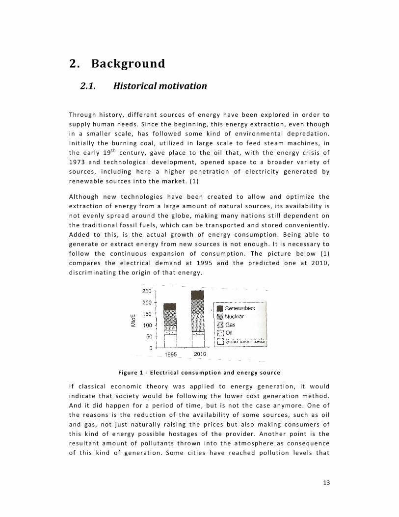
fol low the continuous expansion of consumption. The picture below (1)

compares the electr ica l demand at 1995 and the predicted one at 2010,

discr iminating the or igin of that energy.

Figur e 1 - E lectr ica l con sumption and en ergy so urce

I f c lass ica l economic theory was appl ied to energy generation, it would

indicate that society would be fol lowing the lower cost generation method.

And it d id happen for a period of t ime, but is not the case anymore. One of

the reasons is the reduct ion of the avai labi l ity of some sources, such as oi l

and gas, not just natural ly ra ising the prices but also making consumers of

this kind of energy possible hostages of the provider . Another point is the

resultant amount of pol lutants thrown into the atmosphere as consequence

of this kind of generation. Some cit ies have reached pollution levels that

14

make l iv ing in these areas as dangerous and unhealthy as being exposed to a

nuclear leakage l ike Chernobyl (2) .

The governments of di fferent countr ies, at this point, felt the need to step in

and create str icter rules and targets regarding the energy generation, aiming

the reduction of pollutants and the dependence of fossi l fuels .

One example is the Edinburgh code for sustainable bui ld ings which states

that “a minimum of 10% (20% in Areas of Major Change developments of

2000 sqm or 20 resident ial units or more) of its remaining energy

requirements to be suppl ied by on s ite renewable energy generation. This on-

s ite renewable energy generation must provide at least a further 10% (20% in

AMC’s) reduction in the development ’s CO2 emiss ions” (3).

Two technologies that have been gaining importance with this new real ity are

explained in the next sub-sections: Heat pumps and combined heat and

power systems.

2.2. Heat pumps

Heat pumps are equipment that do exactly what their name suggests. They

pump heat from one source where i t is abundant or not necessary, and

deliver to a second point, the heat s ink. No energy is generated, just

replaced, making the heat pumps different from most of the heating

technologies, which ut i l ize a combustion process to convert a pr imary source

of energy into heat and is very often related with sensit ive amount of losses.

With a moisture content of 20%, one ki lo of hardwood woodchip may produce

in a complete combustion process , 15.1MJ* of energy. Just 80% of this is

usually converted into heat at a biomass boiler , given its usual eff iciency.

With heat pumps, one unit of energy is used to extract around 3 units from

the source and deliver at the sink. There is no energy conversion and

correct ly select ing the sources and technologies may further improve this

relat ionship. In the case of uti l izing a renewable source to dr ive the heat

pump, the heating or cooling process may happen almost free of CO2

emiss ions.

The high eff iciency of the heat pumps, inc luding environments of extremely

cold or warm weather (4) , the capacity to add renewable energy to a heating

load and the possibi l i ty to work combined with electr icity generated through

renewable sources make the heatpumps attract ive options when dealing with

* Based on a calorific value of 4.2 kWh/kg for hardwood (21)

15

a sustainable development . More details about the heat pump technology are

shown bellow.

2.2.1. Heat pump principle

Changing thermal energy at low temperature to thermal energy at a higher

temperature is the main pr inciple of a heat pump. To achieve i t , the working

f luid is submitted through dif ferent pressure levels and change of states. The

picture below is a simpl i f ied i l lustrat ion of what happens with the working

f luid during the heating process .

Figur e 2 : Heat pu mp cyc l e (5)

At low pressure and temperature, the refr igerant l iquid is dr iven to the

evaporator , where heat exchange happens with the heat source. Being at a

lower temperature than the source, heat f lows to the working l iquid, which

results into a change of phase from l iquid to vapor state. The refr igerant i s

then driven through a compressor, where a pressure ri se takes place,

fol lowed by a r ise of the l iquid temperature. The now heated refrigerant

passes through a second heat exchanger , the evaporator, where energy f lows

from the working f lu id to the heat s ink. With the energy reduction, the

refrigerant changes state once more, becoming l iquid and being pumped back

towards the evaporator, passing f i rst through an expansion valve, where the

pressure is reduced. As a consequence, the temperature of the working f luid

also reduces. The cycle, then, starts again.

16

2.2.2. Coefficient of performance

The performance parameter for a heat pump is known as coeff icient of

performance, COP, which compares the quantity of heat transferred between

source and sink with the network input to the cycle , usual ly in the form of

electr icity, supplied to the compressor. The definit ion is :

�� = �� ℎ�� ℎ� ��

I t is desirable to del iver or extract a certa in amount of energy from a given

ambient with the minimum expenditure of work. In order to understand

which condit ions may improve the COP of a system, one must understand

that, fo l lowing the second law of thermodynamics , the COP of a cycl ic device

operating between two given reservoirs , with dif ferent thermal energy

stored, can’t be greater than a device operating on the reverse Carnot cycle .

This cycle consists into two revers ible isothermal processes, and two

revers ible adiabatic processes .

Figur e 3 - Carnot c yc l e

Imagining a heat pump working in such condit ions , with the isothermal

process happening at the heat source and s ink, and the expansion and

compression happening in an adiabatic process, the COP may be defined by:

�� = |�� !"#$�|%&$!'(#� !#% − %&�*(�+,�#%

After some simpl if icat ions, leads to:

�� = -.!"#$�-.!"#$� − -./+0

From there is easy to observe that , the smaller the difference in temperature

between the reservoirs , the greater wil l be the COP.

Given to pract ical di ff icult ies associated with the reversed

modif icat ions are made in practice at the heat pumps. For example, the

evaporat ion process is al lowed to

Another modif icat ion is the fact that

thrott l ing valve where the refrigerant undergoes an i rrevers ible isenthalpic

process.

2.2.3. The ground source heat pump

Heat pumps can be classi fied according to its funct ion (heat ing, cooling,

domestic hot water, etc) , h

working f luids (brine/water , water/water, air/air , etc) [2 ].

heat pumps use the soil or

depending of the desired application.

a s ink or source is i ts stabil ity and elevated temperature through the year

when compared with, for example, the air . This attr ibute al lows a higher COP

dur ing severe cl imatic s ituat ions (summer or winter) where the di

between internal and external temperature is more

If water i s available at a reasonable depth and temperature,

source a l lows the achievement of the highest COP.

also work with certain surface water , l ike fro

heat reject ion systems.

One of the possible configurations is knows as

or loop). Water is pumped from the source (water bed, lake, r iver, etc) ,

circulates through a heat exchanger and then returns to the origin.

Fi gure

I f water is not available , the ground can work as an effective heat source or

sink. Hor izontal or vertical collectors, depending of the avai lable area, are

bur ied into the ground and a working f lu id

energy that wi l l be used into the heating process (or del ivers the heat in the

case of cooling). This configurat ion may a

Given to pract ical d i ff icult ies associated with the reversed Carnot cyc le,


aporat ion process is al lowed to cont inue to the saturated vapor l ine.

Another modif icat ion is the fact that the expans ion process is replaced by a

throttl ing valve where the refr igerant undergoes an i rrevers ible isenthalpic

The ground source heat pump

Heat pumps can be class i f ied according to its funct ion (heat ing, cooling,

water , etc) , heat source (ground, ground-water , air , etc) and

working f luids (brine/water, water/water , a ir/air , etc) [2 ]. The ground source

heat pumps use the soil or the water present in it as the heat source or s ink,

depending of the desired appl icat ion. The advantage of having the ground as

a sink or source is it s stabil ity and elevated temperature through the year

when compared with, for example, the air . This attribute al lows a higher COP

during severe cl imatic s i tuat ions (summer or winter) where the di

tween internal and external temperature is more sensit ive.

If water is available at a reasonable depth and temperature, its uti l izat ion as

source a l lows the achievement of the highest COP. Water heat pumps can

also work with certain surface water, l i ke from rivers or lakes, and water in

One of the possible configurat ions is knows as open system (also open source

. Water is pumped from the source (water bed, lake, r iver, etc) ,

circulates through a heat exchanger and then returns to the origin.

Figur e 4 - Op en loop co nf igur at ion (5)

I f water is not avai lable, the ground can work as an effect ive heat source or

sink. Horizontal or vert ical collectors , depending of the avai lable area, are

ground and a working f lu id , circulat ing into them, extracts the

energy that wi l l be used into the heat ing process (or del ivers the heat in the

This configuration may also be ut i l ized at water source heat

17

arnot cycle ,


cont inue to the saturated vapor l ine.

the expansion process is replaced by a

thrott l ing valve where the refr igerant undergoes an irrevers ible isenthalpic

Heat pumps can be class i f ied according to its funct ion (heating, cooling,

water, air , etc) and

The ground source

it as the heat source or sink,

e of having the ground as

a s ink or source is it s stabil ity and elevated temperature through the year,

when compared with, for example , the air . This attr ibute al lows a higher COP

dur ing severe cl imatic s ituat ions (summer or winter) where the dif ference

its uti l izat ion as

Water heat pumps can

m r ivers or lakes, and water in

(also open source

. Water is pumped from the source (water bed, lake, river , etc) ,

I f water is not avai lable, the ground can work as an effect ive heat source or

sink. Hor izontal or vert ical collectors , depending of the avai lable area, are

extracts the

energy that wi l l be used into the heat ing process (or del ivers the heat in the

lso be ut i l ized at water source heat

18

pumps, in p laces where the open system is not desirable. In this case, the

heat col lector wil l be placed ins ide the water bed.

Figur e 5 - C losed loop c onf igurat ion (5)

2.3. Combined heat and power

The most conventional forms of electr icity generat ion works through the

convers ion of heat into mechanical power, which is then converted to

electr icity. The process usually presents overall eff iciency around 40%, not

counting losses related with the transmiss ion of the generated electr icity

unti l its final point of consumption.

The low eff iciency comes from the fact that part of the available init ial

energy is lost in the form of heat. Creating schemes that may use this unused

heat wi l l raise the system eff iciency. Also, having the generation and

consumption points located close from each other wil l reduce the

transmiss ion losses.

Combined heat and power plants works exact ly over those points. Electr icity

and heat are generated together , with the system usual ly supplying part of

the heat requirements and importing any extra energy needed. Also, at

moments of low electrical consumpt ion, electr icity may be sold to the grid.

S ince the CHP plants need to be close to the heating load, in order to avoid

thermal losses , electr ical losses are also reduced. Us ing the heat that at

other schemes of electr ical generation would be lost makes possible the

achievement of a 90% overal l eff i ciency.

The picture bellow shows two opt ions for a given locat ion that needs heating

and electr icity supply. F irst one, electricity and heat are generated

independently, the second, through CHP (st i l l connected to the gr id).

Figur e 6 - Gas bo i l er ener gy f low

19

Fi gure 7 - CHP ener gy f low

Two eff iciency f igures are used for CHP. The f irst one, a lready commented

before, is the overall energy eff iciency. It compares the amount of the energy

supplied to the load with the total of energy in the fue l consumed.

1 = 23425678

;

Q = Heat suppl ied to the load

E = Electrici ty supplied to the load

Q F u e l = Total energy suppl ied by the fuel

Other way to quant ify the eff ic iency of the CHP plant is through the

incremental electr ica l eff iciency. I t compares the electricity generated with

the total of heat that was actually used for that generat ion (6).

14 = 9�:"�; − �

1.

Q = Heat suppl ied to the load

E = Electrici ty supplied to the load

Q F u e l = Total energy suppl ied by the fuel

η S = Thermal eff iciency of steam production with a conventional boiler

I t is also important to say that CHP generation may be divided into two

different groups of systems. The f i rst one ut i l izes the heat generated by the

fuel to f irst produce electr icity and then the thermal energy at lower

temperature is ut i l ized to produce steam. These are cal led Topping Systems.

They are more common where the heating requirements do not need high

temperatures.

The Bottoming Systems uti l ize the heat from burning the fuel f irst to satisfy

the heat ing needs and then the residual heat is used to produce e lectr icity.

Several dif ferent schemes may be used to achieve a combined heat and

power generation. They differ from the kind of primary energy source ut i l ized

(biomass, coal , l iquid fuel , gas) , the dr iving engine (steam turbines, gas

turbines, reciprocat ing engine, etc)or even of how the thermal energy is

used.

The table bel low compares typical configurat ions and i ts energy consumpt ion.

Table

An important point at this moment is to highlight what has been said before

about the electr ical generat ion. It was supposed that the electr icity

generated and not used would be sold to the grid. Some times and locat ions

such option may not be avai lable , or even may not be economical ly

interest ing (with the price of the electr icity be ing sold bel low the price for

the imported electric ity) . The combinat ion of the CHP system with heat

pumps may be an interesting option to ens

be generated when there is a requirement for it . In other words, may be

interest ing to create a system where part of the thermal load wi l l be supplied

by a CHP plant and the other part wil l be suppl ied by a heat pump sys

using the electr icity generated by the combined heat and power process .

The thermal losses re lated with these processes may be a problem.

Figur e

The table bel low compares typical configurat ions and i ts energy consumption.

Table 1 - Primary energy savings (6)

An important point at this moment is to highl ight what has been said before

about the electr ical generat ion. It was supposed that the electricity

generated and not used would be sold to the gr id. Some times and locat ions

uch option may not be avai lable , or even may not be economically

interest ing (with the price of the electr ici ty be ing sold bel low the pr ice for

the imported electr ic ity) . The combinat ion of the CHP system with heat

pumps may be an interest ing opt ion to ensure that electricity and heat wi l l

be generated when there is a requirement for it . In other words , may be

interest ing to create a system where part of the thermal load wil l be supplied

by a CHP plant and the other part wil l be supplied by a heat pump sys

using the electr ici ty generated by the combined heat and power process.

The thermal losses related with these processes may be a problem.

Fi gure 8 - H ybr id syst e m en er gy f low

20

The table bel low compares typical configurat ions and i ts energy consumpt ion.

An important point at this moment is to highlight what has been said before

about the electr ical generat ion. It was supposed that the electr ici ty

generated and not used would be sold to the grid. Some t imes and locat ions

uch option may not be avai lable , or even may not be economically

interest ing (with the price of the electr ici ty be ing sold bel low the pr ice for

the imported electr ic ity) . The combinat ion of the CHP system with heat

ure that electric ity and heat wi l l

be generated when there is a requirement for it . In other words, may be

interest ing to create a system where part of the thermal load wil l be suppl ied

by a CHP plant and the other part wil l be suppl ied by a heat pump system,

using the electr icity generated by the combined heat and power process.

The thermal losses related with these processes may be a problem.

21

2.4. Hybrid systems

At a big transmission system, the power drawn by the customers osc i l lates

expressive ly during a day. Taking a city as example , whi le at late hours of

night , or early mornings , as most people are sleeping, the energy

consumption is most ly from street l ights, domest ic equipment on idle mode,

etc. At early evening, this consumption r ises noticeably when people return

to their homes, and commercial and industr ial faci l it ies are st i l l operating. It

is important to have this informat ion to mind when, for example, it is

planned to raise the participation of renewable energy sources into the

energy production, as matching demand and generation may be a problem.

Sun energy is only available a few hours a day and the wind leve ls may drop

exact ly when the demand for energy i s high. B iomass boi ler can rapidly burn

more fuel to fol low the demand variat ion, but its relatively low turn down

rat io* makes i t hard to match the peak demands or the hot water demand

during summer months.

Combining di fferent renewable technologies, or even t radit ional energy

generat ion methods, may raise expressively the rel iabi l ity of a system, sti l l

reducing its f inal CO 2 footprint . These arrangements , where the energy from

different sources is combined in order to achieve the same end, are called

hybrid systems. In the preceding example, the biomass boiler could have a

tradit ional gas boi ler running as backup, supplying the peak load during the

winter or the hot water demand during the summer, with the base load being

supplied by the biomass. This is a smal l example of a hybrid system.

For heat pumps, the expression hybrid system is often re lated with the

presence of di fferent heat s inks (or sources), a iming the reduction of the

imbalance between heat extract ion and reject ion during the year , at

locat ions with a predominant weather (7) . A number of studies were made in

this areas including ut i l iz ing s imulat ion tools in order to opt imize these

systems (8) (9). In these cases , the optimization process compared heat

exchanger options and sizes, also observing the best control methodologies

for a specif ic appl icat ion. What we plan to do at this dissertat ion is observe

the optimizat ion process where the heat pump wil l be deal ing not with an

extra heat sink/source, but an entirely di fferent technology.

The opt imizat ion of such systems wil l depend on not just knowing the

particularit ies of each technology involved, but also the creation of a specif ic

* Turn down ratio is the relationship between the maximum and minimum power output of the boiler.

The minimum output is defined by the minimum value at which the boiler will work with high efficiency.

22

control system to coordinate how they wi l l re late between themselves and

the object ives to be achieved.

The problem of dealing with renewable technology is that the site

environment , responsible by the consumption behavior, has also great

inf luence over the generation capacity. This makes it more di ff i cult for a

designer to work with pre prepared templates. The solution found at location

A may not be applicable at location B, even though both ut i l ize s imi lar

systems. The capacity to simulate how all the variants wil l behave is a

powerful tool during the design of these systems, giv ing enough f lexibi l ity to

the des igner to play with the variants , comparing the obtained results and

through that , optimizing the system.

During the optimizat ion process, the control system must be very wel l

defined, s ince i t wi l l inf luence the required s ize of equipment, storage tanks ,

etc. Circuit connections and f lu id temperatures may change expressive ly

depending on how the control wi l l coordinate the different technologies. The

start-up period of a biomass boiler may be reduced using the backup gas

boiler to pre heat i ts internal l ining. This may have impact over the necessary

storage tank. One can’t def ine i f the storage tank is over or undersized

without knowing the details about the heating circuit. Just looking for the

system load and boilers won’t g ive an accurate answer.

Another aspect that wil l def ine the eff i ciency of a system is i ts f inancial data.

Given the complexity of the energy changes that may happen in a hybr id

system, it may be complex to get a precise feedback about the f inancia l

savings that can be achieved without the presence of a s imulat ion tool.

23

3. Methodology

This chapter wi l l be dealing with the assumptions made and methods ut i l ized

during the analys is of the results , at chapter 4.

I t starts discussing the CO2 emission and renewable energy fract ion

ca lculations. Being introduced for the f irst t ime to the emiss ion factors table

in the government’s Standard Assessment Procedure for the energy

performance of dwel l ings (SAP) (10) some people may feel unsure how those

values must be used. Sect ion 3.1 ut i l i zes s imple examples and formulas

explain how SAP was ut i l ized at the present dissertat ion and the reasons for

i t.

In sect ion 3.2, the importance of how to define a system renewable energy

fract ion is discussed. The main point of this sub-topic is to h ighl ight the

importance to have a better definit ion of the capacity of a heat pump to

supply renewable energy and how it must be counted.

The remaining sect ions introduce the s tudied system, its loads, heating

circuits ’ configurat ion and how the data received was manipulated in order to

be ut i l ized at TRNSYS. The base case, from where the results wil l be used as

reference for comparing the outputs at the simulat ion stage, is also

presented.

In addit ion, in th is chapter can a lso be found the method uti l ized to define

the f inancial ga ins delivered by each studied system, including here the

equipment, operational and maintenance costs.

3.1. CO2 emission, conversion factor and savings

During the result analys is , an important output is the CO2 emiss ion related

with the energy product ion.

Tables relat ing the amount of CO2 emiss ion with the used energy source can

be found at dif ferent l i terature, such as Defra’s green house gas conversion

factor guideline (11) or the government Standard Assessment Procedure for

the energy performance of dwel l ings, SAP 2005-2008 (10), both used as

reference in this study. For heating, the process is quite s imple, once it does

not involve a complex and large network, such as with electr icity. The tota l

amount of CO2 emitted wil l be the tota l of fuel consumed mult ip l ied by

related conversion factor.

The CO2 emitted, although important informat ion, does not give a precise

idea of how effect ive the generat ion process real ly is . A good idea is to divide

the total CO2 emiss ion by the total energy delivered, result ing into the

24

amount of CO2 per kWh of energy made avai lable (what is basically the local

convers ion factor).

In the case of electr icity, the discuss ion becomes a more complex. Once the

electr icity is generated, there are two possibi l i t ies: i t wi l l be locally uti l ized

or sold to the grid.

The f irst option wil l reduce the load seen by the grid as i f energy savings

methods were applied, l ike h igher building insulation or ef f icient l ighting

insta lled.

To calculate the local emiss ions, SAP suggests the fol lowing method:

• The total emission of the generated electric i ty must be calculated;

• In case of e lectr icity exported to the gr id, the total energy must be

multipl ied by a base conversion value and then subtracted from the

previous result;

• Energy consumed must be mult ipl ied by the grid emiss ion coeff ic ient.

An interest ing point is that SAP applies a different conversion value to the

electr icity d isplaced from grid (0.568 kg CO2 per kWh) and imported from the

grid (0.422 kg CO2 per kWh). This may cause some discomfort to who is f irst

introduced to the formula s ince consumption and production are completely

related act iv it ies and one might expect that both have the same conversion

value.

To avoid instabi l ity problems in the grid, production and generation must

match. When a new source of energy is added to the grid, maintain ing the

load, somewhere one or more plants must reduce their product ion. The

amount of CO2 being produced changes, and i ts magnitude wil l depend of

how much CO2 the new source is producing to generate the displaced power.

An example is given below.

F irst let ’s imagine the CO2 emitted by the energy producer :

Power is being generated by the main producers connected to the gr id, each

one with its related emiss ion coeff icient, which mult ipl ied by the energy

production gives the total CO 2 emiss ion. It can be sa id that the total emiss ion

wi l l be the total product ion times a conversion factor.

9< ∗ �< + 9? ∗ �? + 9@ ∗ �@ + ⋯ + 9+ ∗ �+ = ��B ∗ C 9*+

*D<

Where En represents the energy generated by the producer n and Cn the

related emiss ion coeff icient . For example, i f 10 MWh was generated by a gas

turbine with eff iciency of 40%, the emiss ions would be: 10 000 x (0.194/0.4)

kg of CO2 . The value ins ide the bracket can be interpreted as producer

25

emiss ion coeff icient. Once the left side of the equat ion above in known, ��B

can be def ined.

Now let’s observe the CO2 emitted from the perspective of the energy

consumption:

S ince the energy generated wi l l be consumed somewhere, can be said that

the CO2 emissions re lated with the generation must match the emissions

related with the consumption. Being the left s ide defined by the energy

production, the r ight might represent the CO2 emission from the demand s ide

where ∑ 9*+*D< can be seen as the total energy from the grid consumed and ca v

the grid emission coeff icient.

A base case can be then buil t , imagining a system with a heating demand of

50 kWh and the electr ical one of 20 kWh. This energy wi l l be suppl ied by the

grid and a gas boiler with 80% eff ic iency:

Load

(kWh)

Eff iciency Used

energy

Emiss ion

coef. (kg per

kWh)

Kg of CO2

emitted

Heating 50 80% 63 0.194 12.1

Electr icity 20 100% 20 0.422 (ca v ) 8.5

Total 20 .6

Table 2 - Example CO2 emission

I t is assumed now that this same consumer has a gas turbine, with eff iciency

of 40% connected to the grid, not supplying any energy direct ly to his

bui ld ing. The load on site does not depend of the generation. Somewhere,

less energy wi l l be produced to balance this surplus added to the grid. This

reduct ion can be concentrated at a specif ic p lant or spread at several ones .

For simpl if ication reasons , it wi l l be assumed that just one plant wi l l have to

reduce its production. E3, for example. The new CO 2 emiss ion wi l l defined be

as shown below:

9< ∗ �< + 9? ∗ �? + (9@ − 9+�G) ∗ �@ + ⋯ + 9+ ∗ �+ + 9+�G ∗ �+�G = ��B? ∗ C 9*+

*D<

Which can also be written as:

9< ∗ �< + 9? ∗ �? + 9@ ∗ �@ + ⋯ + 9+∗�+ + 9+�G ∗ (�+�G − �@) = ��B? ∗ C 9*+

*D<

26

En e w and cn e w represents the amount of energy and the emiss ion coeff icient of

the new source (gas turbine in the example).

Is interest ing to observe that "9+�G ∗ (�+�G − �@)” does not represent the CO2

emiss ion of the new source, but i ts contribution over the changes at the tota l

CO2 level , giving credit to the “clean” producer over the new emiss ion. It s

importance becomes more evident when the calculat ion done at table 2 is

repeated.

I t is understood that the new energy source changed the emission factor

value, but wouldn’t be practica l to keep the table constantly updated. What

happens is that most of the t ime this value is changed at yearly bases. This

means that if a consumer ca lculates its CO 2 emission, the table 2 wouldn’t

change. What happens is that , now, the credit f rom the c leaner producer

must be appl ied. The r ight side of the previous formula can be rewritten as :

��B ∗ C 9*+

*D<+ 9+�G ∗ (�+�G − �@) = -�� 2 �KLL��

Or , showing the ent ire system

9< ∗ �< + 9? ∗ �? + (9@M9+�G) ∗ �@ + ⋯ + 9+∗�+ + 9+�G ∗ (�+�G)

= ��B ∗ C 9*+

*D<+ 9+�G ∗ (�+�G − �@)

SAP defines c3 ( the emiss ion coeff icient of the electr icity displaced from the

grid) as 0.568. Looking for the new consumer that now is also a producer , the

fol lowing table is buil t :

Load

(kWh)

Eff iciency Used

energy

Emiss ion

coef. (kg per

kWh)

Kg of CO2

emitted

Heating 50 80% 63 0.194 12.1

Electr icity 20 100% 20 0.422 (ca v ) 8.5

Gas

turbine

-2 60% 3.3 (0.194-

0.568)

-1.2

Total 19 .4

Table 3 - CO2 emission including gas turbine

27

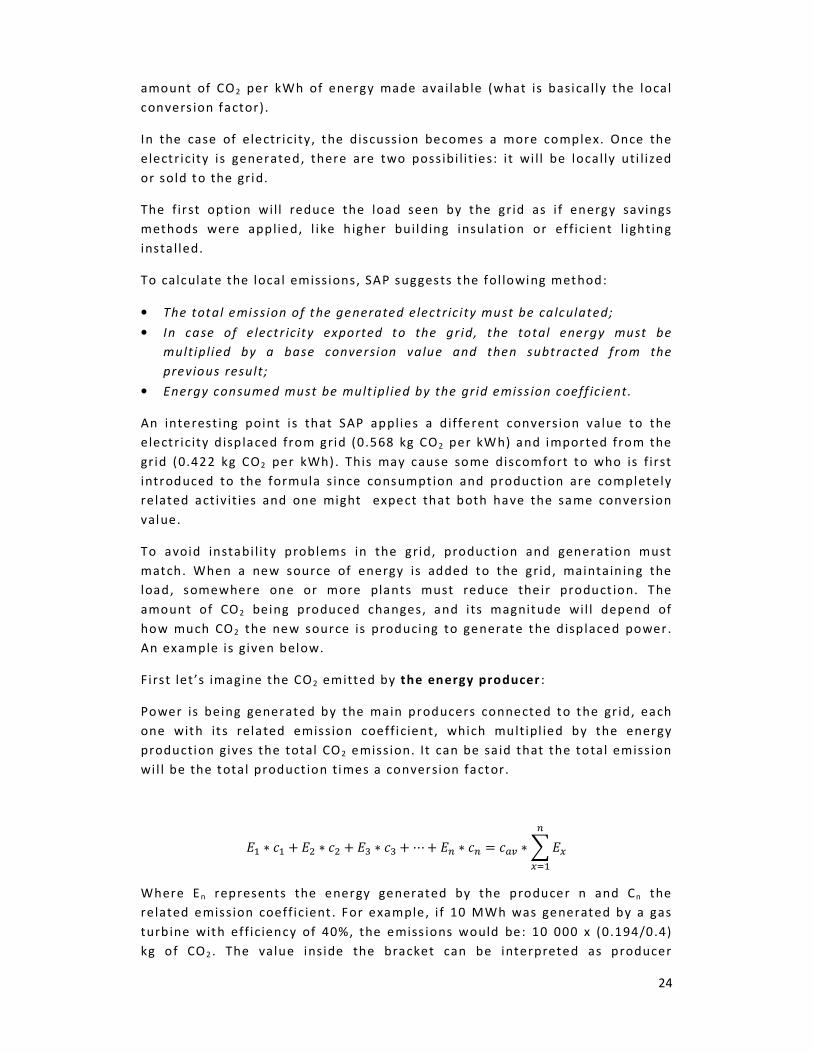
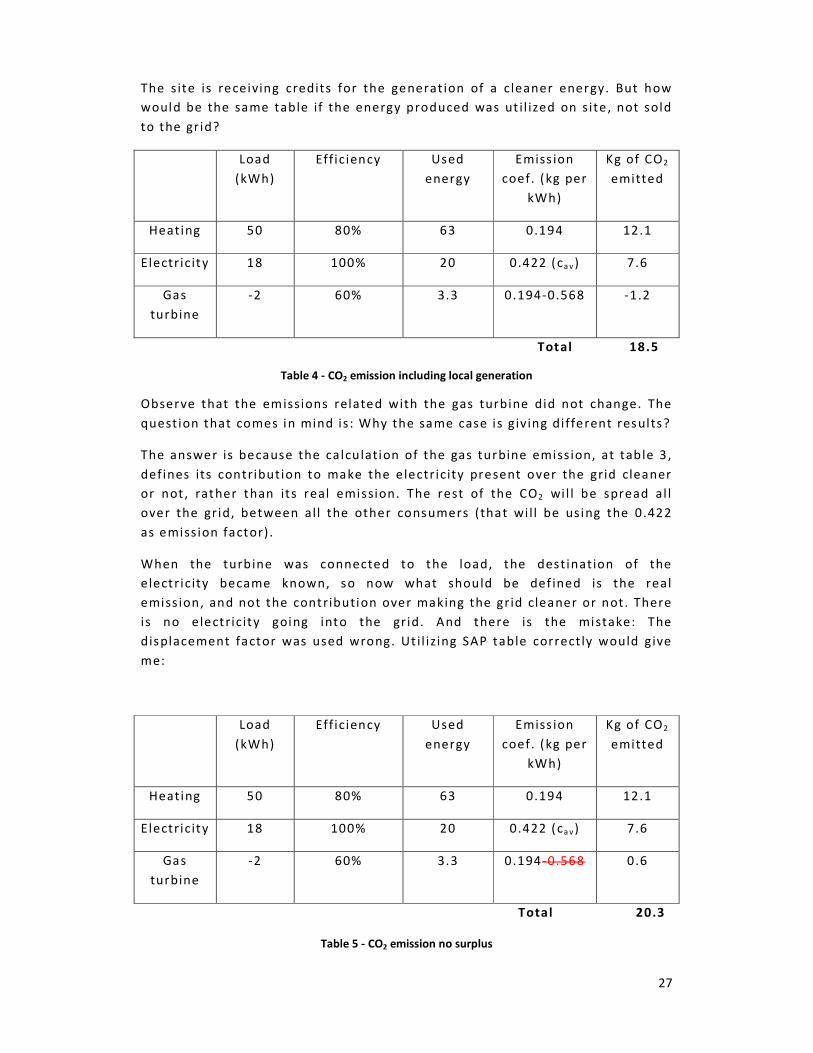
The s ite is receiving credits for the generation of a cleaner energy. But how

would be the same table if the energy produced was ut i l ized on s ite , not sold

to the grid?

Load

(kWh)

Eff iciency Used

energy

Emiss ion

coef. (kg per

kWh)

Kg of CO2

emitted

Heating 50 80% 63 0.194 12.1

Electr icity 18 100% 20 0.422 (ca v ) 7.6

Gas

turbine

-2 60% 3.3 0.194-0.568 -1.2

Total 18.5

Table 4 - CO2 emission including local generation

Observe that the emissions related with the gas turbine did not change. The

quest ion that comes in mind is : Why the same case is g iv ing different results?

The answer is because the ca lculation of the gas turbine emiss ion, at table 3 ,

defines its contribution to make the electr icity present over the grid cleaner

or not , rather than its real emission. The rest of the CO2 wi l l be spread al l

over the grid, between all the other consumers (that wi l l be using the 0.422

as emiss ion factor) .

When the turbine was connected to the load, the dest ination of the

electr icity became known, so now what should be def ined is the real

emiss ion, and not the contribution over making the grid cleaner or not. There

is no electricity going into the grid. And there is the mistake: The

displacement factor was used wrong. Ut i l izing SAP table correct ly would g ive

me:

Load

(kWh)

Eff iciency Used

energy

Emiss ion

coef. (kg per

kWh)

Kg of CO2

emitted

Heating 50 80% 63 0.194 12.1

Electr icity 18 100% 20 0.422 (ca v ) 7.6

Gas

turbine

-2 60% 3.3 0.194-0.568 0.6

Total 20.3

Table 5 - CO2 emission no surplus

28

The displacement coeff icient just can be appl ied i f the tota l grid load does

not depend of the amount of energy being sold. If e lectr icity that could be

internal ly used starts to be sent to the gr id, the total gr id load wi l l change,

making the previous formula inaccurate. This observat ion is important s ince

misunderstanding what SAP table means or using it with mal ice may show

lower emissions than the real ones. Someone producing 1 MWh from an

emiss ion free source and consuming 1MWh would calculate negat ive

emiss ion, instead of the real zero, if a l l the production was sold to the grid.

The important point to be aware here is that no energy production from

other sources wil l be reduced when electricity is being sold to the grid while

there is st i l l internal load to be supplied. It is be ing reduced (9 "#(;" +9;!�,) and then required 9;!�,. Observe that this energy consumed from the

grid wi l l have the same emiss ion coeff icient of the source that ended up not

being replaced (here represented by C3 or 0 .568 from SAP data) , and not the

grid average.

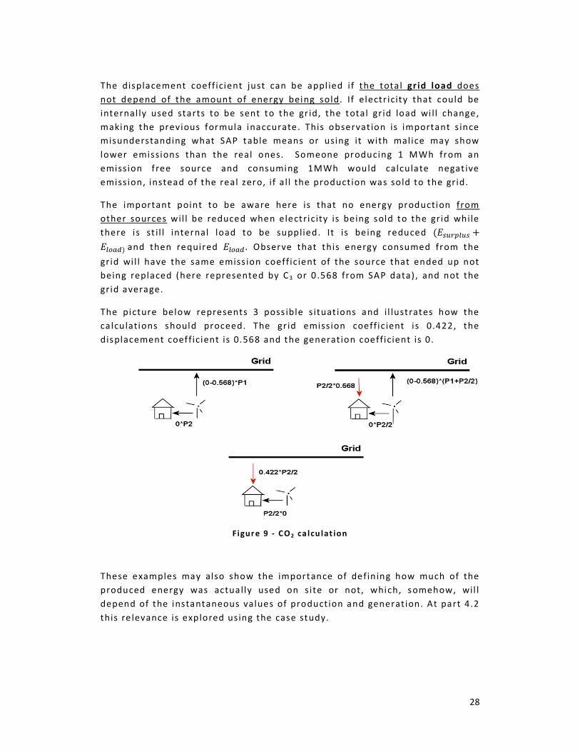
The picture below represents 3 poss ible s ituat ions and i l lustrates how the

calculations should proceed. The grid emiss ion coeff ic ient is 0.422, the

displacement coeff icient is 0.568 and the generation coeff icient is 0.

Figur e 9 - CO 2 ca lcu lat ion

These examples may also show the importance of defin ing how much of the

produced energy was actually used on s ite or not, which, somehow, wil l

depend of the instantaneous values of production and generation. At part 4.2

this re levance is explored using the case study.

29

3.2. Renewable energy fraction

In part caused by the rise over the pr ice of foss i l fuels and the exhaust ion of

i ts local sources, governments al l around the globe are realiz ing the

importance of updat ing their energy infrastructure. UK government , for

example, adopted a policy to achieve a 10% of renewable part icipat ion over

the electr icity generated (12). In March 2007, the European Counci l

committed the EU to a binding target of a 20% share of renewable energies in

overal l EU consumption by 2020 (13) .

These policies al l have in common the focus not just on CO2 emission, but the

share of renewable energy over the total energy generated (or consumed).

Energy producers now need to lead with renewable production targets and,

of course, be able to deal with them.

The “London des ign and construct ion planning guidance” (14), for example,

states that “Major developments are required to show how they wi l l generate

a proport ion of a scheme’s energy demand from renewable energy sources,

where technologies are feasible . The Mayor’s Energy Strategy states that this

proport ion should be a minimum of 10percent”.

The f i rst point is to make clear what is this proportion is calculated. Basica l ly,

the renewable energy fact ion can be seen as the share of e (14)nergy

supplied by a renewable source over the total of energy consumed. This

ca lculation can be quite stra ight forward when looking for electrical

generat ion but when the energy i s in the form of heat, some problems may

occur , specif ical ly when dealing with heat pumps.

A public consultation held in 2006 by the EU Init iat ive on heating and cooling

from renewable energy sources pointed one of the main obstacles to a wide-

spread of such technology the fol lowing problem:

• Heat pump status (renewable energy technology or not) not

harmonised in al l Member States

At U.K , heat pumps are accepted as renewable heat sources and its

importance over the EU target of renewable share is h ighl ighted (13) (15).

But some points are not yet clear.

Is easy to define the renewable heat share during the heating cycle . The

total heat supplied by the ground wi l l be the total load minus the total

electr ica l consumption. But what happens when the load is not heat but

cooling?

30

The heat pump wil l st i l l work in the same way, just changing its heat

source and s ink posit ions . This t ime it wil l see the ground or river as the

load to the heat being displace from a building. The problem is that the

bui ld ing load (cool ing) is the system heat source.

Some may aff irm that under this conf igurat ion there is no renewable

partic ipat ion over the load (cooling) , unless i t comes from the e lectr icity

consumed by the compressor. The diff i cul ty to f ight this argument is to

define what would be “renewable cool”. Any cooling load can be seen as a

heat source, and it inc ludes tradit ional chi l lers.

Cool ing systems, in analogy to heating ones, may be class i f ied as act ive or

passive , according to whether energy is specif ical ly added in order to

bring the col lector heat gain from the load areas or not (16). A passive

cooling system output does not depend of energy input provided by man.

An example would be a thick wall designed to, during day, absorb heat

from the interior of a building and during night, t ransmit i t to it s

surroundings. The heat transfer is driven by the temperature difference

between the wall and the inter ior of the bui lding, during day, and the

external temperature dur ing the night. Observing the cool ing load (the

amount of heat that needs to be displaced in order to keep acceptable

temperature levels) , what was the renewable part icipat ion over it? It may

be accepted that , g iven the fact that there was no energy input by the

man, the entire load was suppl ied by renewable sources.

Imagining now that the specif ical ly des igned wal l is not present and the

heat f rom the building is absorbed by a heat exchanger, through which

circulates cool water. The heat absorbed is st i l l thrown away from the

bui ld ing but now the temperature difference is achieved by, between

other processes, an electrica lly driven compressor. The principle is the

same: Using temperature dif ference to create the desired heat f low. If

previously the renewable part icipation over the load was 100%, what can

be defined in this new case? Imagining that the electr icity suppl ied by the

grid is equivalent to ¼ of the total cool ing load, one may, by analogy with

what was done with the wall case, say that the renewable part icipat ion i s

¾.

This approach does seem consistent with what was done with the heat

pump at the heat ing process. So during the cool ing demand it could be

said that the renewable energy is the total load (cool ing) minus the non

renewable one ut i l ized to drive the process.

This is , although, one assumption and does present f laws. There is no

clear posit ion about how to count the renewable share for cooling. One of

the reasons may be the fact that , i f th is analogy, or any other simi lar, is

accepted, the traditional air -conditioning systems may a lso be able to f ind

a renewable share over the ir load. Heat pumps are being sold as

renewable sources of energy but no attention is being clearly giving to

this issue. Although green cool is ment ioned

to calculate i t is done.

Because of this discuss ion, the calculation of renewable part icipat ion over

the load wil l count the entire energy from cooling processes as not

renewable. Not because it is the correct one, but because woul

easiest to be accepted at bui lding al lowances.

3.3. Simulation description

3.3.1. Case study

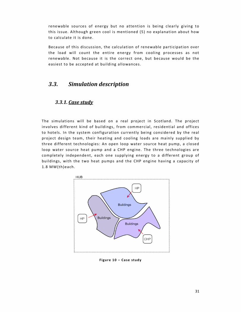
The simulat ions wil l be based on a

involves different kind of bui ldings, from commercial , resident ia l

to hote ls. In the system configurat ion currently being considered by the real

project design team, their

three dif ferent technologies: An open loop water

loop water source heat pump and a CHP

complete ly independent, each one supplying energy to a

bui ldings, with the two heat pumps

1.8 MW(th)each.


Although green cool is mentioned (5) no explanation about how

of this discussion, the calculat ion of renewable part icipat ion over

the load wil l count the entire energy from cooling processes as not

renewable. Not because it is the correct one, but because woul

easiest to be accepted at building a l lowances.

imulation description

The s imulat ions wi l l be based on a real project in Scotland. The

involves d ifferent kind of bui ld ings , from commercial , resident ia l and

In the system configuration currently being considered by the real

project design team, their heat ing and cool ing loads are mainly supplied by

three dif ferent technologies: An open loop water source heat pump, a closed

loop water source heat pump and a CHP engine. The three technologies

completely independent , each one supplying energy to a d ifferent

bui ld ings, with the two heat pumps and the CHP engine having a capacity of

Figur e 10 – Case study

31


no explanation about how

of this discussion, the calculat ion of renewable part icipat ion over

the load wil l count the enti re energy from cooling processes as not

renewable. Not because it is the correct one, but because would be the

Scot land. The project

and off ices

In the system configuration currently being considered by the real

mainly suppl ied by

heat pump, a closed

The three technologies are

d ifferent group of

a capacity of

32

The f i rst series of simulat ion wi l l be looking the entire project as one unique

huge load and wil l observe how dif ferent heat sources can supply its demand.

3.3.2. Loads

The data received assumed that the load behavior wil l repeat dai ly,

meaning that the peak demands and moments of lower consumption wil l

happen a lways at the same t ime, as show below.

Fi gure 11 - Da i ly load b eh aviour

I t was also suppl ied some data regarding the annual consumption for each

kind of energy. Although an important information, it , alone, is not enough to

be used by TRNSYS.

TRNSYS al lows the user to define the t ime steps at which the calculat ions wil l

be done. This value depends of the nature of the project but, does not matter

the magnitude selected, the data must match the t ime step select ion. In

other words, is not sensit ive to run a s imulat ion with a t ime step of 30

minutes when the load or weather data just informs weakly values . It was

necessary to convert the submitted information into something applicable to

TRNSYS.

This process wi l l be explained us ing the heat ing load as example.

3.3.2.1. Heating Loads

The total heat ing demand at the distr ict is of 26 000 MWh per year. This

value includes space heating and domestic hot water .

33

As said before, it was necessary to create an, at least, hourly based load

profi le. The peak demand dur ing the coldest day was def ined at 14 MW,

based at the load duration curve generated by this value and the size of the

original heat sources. It was also defined that at days with average

temperature above 16 °C there wil l be no heating requirement.

With those assumptions and the heat ing load behaviour , i t was possible to

generate a load profi le related with the dai ly ambient temperature, through

the year , as shown below:

Figure 12 - Heat in g load prof i le

S ince al l the controls and siz ing wi l l be focussing into the heat demand , i s

relevant to observe the load durat ion curve, which may explain some of the

results obtained. The graphic describes the amount of time that a heating

demand is above a given value.

Figur e 13 - Heat lo ad d urat ion cur ve

3.3.2.2. Cooling Loads

Given the level of insulat ion of the modern bui ldings , the load requirement is

more re lated with the internal casual gains and insolat ion leve ls then to the

instantaneous outside temperature itse lf

load profi le remains basically the same

above zero. There is no cool ing system at the res identia l bui ldings.

The total cooling requirement is of

F igur e

3.3.2.3. Electrical Load

The electr ica l load does not include any energy that wi l l be ut i l i zed by the

heating system. Its behavior does not

every day, with two peaks of

pm.

This load wi l l be supplied mostly by the gr id , with

the CHP and photovoltaic panels.

The total electr ica l demand during the year is of

Cooling Loads

insulat ion of the modern bui ldings, the load requirement is

more re lated with the internal casual gains and insolat ion leve ls then to the

instantaneous outside temperature itse lf . At the present distr ict , the

load prof i le remains basically the same during the three months where it is

above zero. There is no cooling system at the res identia l bui ldings.

cooling requirement is of 9600 MWh per year.

Figur e 14 - Cool in g load prof i le

Electrical Load

The electrica l load does not include any energy that wi l l be ut i l ized by the

heating system. Its behavior does not change during the year, repeating itself

two peaks of 4.5 MW, one around 8 am and the second at 5

This load wi l l be suppl ied mostly by the gr id , with some part icipat ion from

the CHP and photovoltaic panels.

The total e lectrica l demand dur ing the year is of 26 600 MWh.

34

insulat ion of the modern bui ldings , the load requirement is

more re lated with the internal casual gains and insolat ion levels then to the

he cool ing

where it is

The electr ica l load does not include any energy that wi l l be ut i l ized by the

during the year , repeating itself

MW, one around 8 am and the second at 5

part icipation from

Figur e

3.3.2.4. Yearly profile

The next figure represents the yearly demand profile of the three different loads present into

the simulation.

Figur e

3.4. The base case

The fol lowing conf igurat ion wi l l be uti l ized as base to compar

simulat ions results including:

� CO2 savings

� Energy savings

F igure 15 - E l ectr ica l lo ad profi le

Yearly profile


F igure 16 - Annual lo ad profi le

The base case

The following conf igurat ion wil l be ut i l ized as base to compare al l the other

simulat ions results including:

Energy savings

35


e al l the other

� Financial cost

The heat ing load wi l l be ent irely suppl ied by a gas boi ler with eff iciency of

80% over the higher heating value (HHV)

The cool ing load wi l l be supplied by a

2.5.

Electric ity wi l l be completely supplied by the gr id.

In a l l the other conf igurat ions , the heating water wil l be leaving the storage

tanks at around 40 °C, returni

configurat ions that include a heat pump, the energy required to top

domestic hot water to 65 °C is taken into account separate ly (and assigned to

auxi l iary gas boilers or CHP)

Regarding to the cooling circuit ,

at 10 °C , returning at 20 °C .

3.5. Financial Analysis

The financial analys is was done observing the investment required for each

system, the cost for supplying the energy, operating and maintaining the

equipment and comparing with the values for the base case. More details are

given below.

Financial cost

The heating load wil l be ent irely suppl ied by a gas boi ler with eff iciency of

over the h igher heating value (HHV) .

The cool ing load wi l l be suppl ied by a conventional chil ler system with COP of

Electr icity wil l be completely supplied by the gr id.

Figur e 17 - Base case

configurations, the heating water wil l be leaving the storage

tanks at around 40 °C, returning at 20 °C. I t should be noted that in the

configurat ions that include a heat pump, the energy required to top

°C is taken into account separately (and assigned to

auxi l iary gas boilers or CHP)

Regarding to the cool ing circuit , the water wi l l leave the cool ing storage tank

at 10 °C, returning at 20 °C.

Financial Analysis

The f inancial analys is was done observing the investment required for each


ipment and comparing with the va lues for the base case. More details are

36

The heating load wil l be ent irely suppl ied by a gas boi ler with eff iciency of

conventional chil ler system with COP of

configurations, the heating water wil l be leaving the storage

It should be noted that in the

configurat ions that include a heat pump, the energy required to top-up

°C is taken into account separate ly (and assigned to

the water wi l l leave the cool ing storage tank

The f inancial analys is was done observing the investment required for each


ipment and comparing with the va lues for the base case. More details are

3.5.1. Energy Cost

For al l the ca lculations, the fol lowing prices wi l l be used

Energy Source

Gas

Electr icity imported from the grid

Electr ici ty exported to the gr id

These values wil l define the total energy cost at each studied system. When

compared with the values of

savings. It wil l be an important att r ibute s ince the financia l study of the

system wil l be based on the internal rate of return related with each

configurat ion.

3.5.2. Internal rate of return

Before explaining the conce

observe the meaning of

how much a series of future payments would

account a given discount rate through the studied t ime.

For example, if the interest (or d iscount)

of £86.76 ha the same value as one payment of

another payment of £50 in two years

The £86.76 is the present value of the 100 pounds resultant of the two

payments done over two years,

The Internal Rate of Return

present value of zero for a series of future cash f lows. A net present value

of zero means that would be indifferent to apply the

investment or keep i t and apply into a bank

the IRR. The h igher the internal rate of return the better is the

investment.

Energy Cost

For al l the ca lculat ions, the fol lowing prices wi l l be used (10) (17) :

Price (pence per kWh)

2.1

Electricity imported from the gr id 7.2

Electr icity exported to the gr id 5.7

Table 6 - Energy price


compared with the values of the base case, they wil l def ine the energy

savings. It wil l be an important attr ibute since the financia l study of the

system wi l l be based on the internal rate of return related with each

Internal rate of return

Before explaining the concept of internal rate of return is important to

observe the meaning of the Net Present Value (NPV) . The NPV defines

how much a series of future payments would be worth today, tak

account a given discount rate through the studied t ime.

the interest (or discount) rate is 10% per year, a payment

ha the same value as one payment of £50 in one year and

another payment of £50 in two years: :


er two years, applying a d iscount rate of 10%.

Internal Rate of Return ( IRR) is the discount rate that results in a net

present value of zero for a ser ies of future cash f lows. A net present value

of zero means that would be indifferent to apply the money into the new

investment or keep it and apply into a bank with an interest rate equal to

The higher the internal rate of return the better is the

37

(pence per kWh)


the base case, they wil l def ine the energy

savings. It wi l l be an important attr ibute since the f inancia l study of the

system wil l be based on the internal rate of return related with each

pt of internal rate of return is important to

. The NPV defines

, taking into

a payment

one year and


) is the discount rate that results in a net

present value of zero for a ser ies of future cash f lows. A net present value

money into the new

with an interest rate equal to

The higher the internal rate of return the better is the

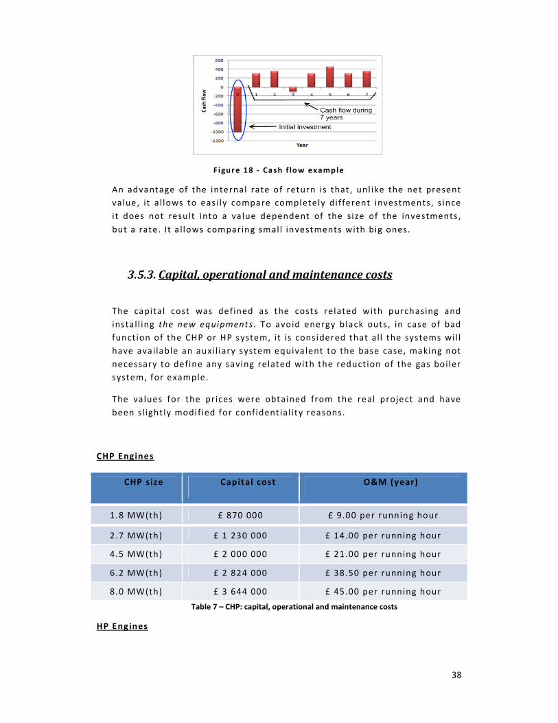
38

Figur e 18 - Cash f lo w example

An advantage of the internal rate of return is that , unl ike the net present

value, it a l lows to eas ily compare completely di fferent investments, s ince

i t does not result into a va lue dependent of the size of the investments ,

but a rate. It a l lows comparing smal l investments with big ones.

3.5.3. Capital, operational and maintenance costs

The capita l cost was defined as the costs related with purchasing and

insta ll ing the new equipments . To avoid energy b lack outs, in case of bad

function of the CHP or HP system, it is considered that al l the systems wil l

have available an auxi l iary system equivalent to the base case, making not

necessary to define any saving related with the reduction of the gas boiler

system, for example.

The values for the prices were obtained from the real project and have

been s l ightly modi fied for confident ial ity reasons.

CHP Engines

CHP size Capital cost O&M (year)

1.8 MW(th) £ 870 000 £ 9.00 per running hour

2.7 MW(th) £ 1 230 000 £ 14.00 per running hour




Table 7 – CHP: capital, operational and maintenance costs

HP Engines

39

HP s ize Capital cost O&M (year)

1.8 MW (closed loop) £ 603 000 1% of capita l cost

1.8 MW (open loop) £ 809 000 1% of capita l cost

2.5 MW (open loop) £ 853 000 1% of capita l cost

3.5 MW (open loop) £ 1 180 000 1% of capita l cost



Table 8 - Heat pumps: capital, operational and maintenance costs

The operat ional and maintenance cost of the auxil iary boi lers and chi l lers

were defined at 2% of the consumed energy cost.

3.6. The main system components

The main system components present in the s imulat ion are:

• Open loop water source heat pump

• Closed loop water source heat pump

• Gas boi ler

• Combined heat and power system

The gas boi ler was introduced in the base case descript ion, being also uti l ized

as an auxil iary system, connected to the storage tank of each HP or CHP

circuit. Details of the remaining components are shown below.

3.6.1. The heat pumps

For the heat pumps s imulat ion, data from commercial ly avai lable 130 kW

heat pump was uti l ized. [Appendix 1 and 2].

3.6.1.1. General operation configuration

The information below applies to each heat pump, independently, and may

vary depending of the system control conf igurat ion and connections. During

the simulat ions , any change over the values detailed bel low wil l be

highl ighted.

3.6.1.2. Heating period

Maximum temperature for the water leaving the heat pump wi l l be 52°C, with

a ΔT of 6°C between the temperature entering the heat pump and leaving it .

COP values up to 5 were achieved with this configurat ion.

40

3.6.1.3. Cooling period

During the cooling cycle , the water wi l l be leaving the heat pump, to the

load, at around 7°C. The ΔT between the temperature enter ing and leaving

the heat pump is around 5°C.

3.6.1.4. Open loop configuration

Flow rates uti l i zed

In order to keep the temperature levels at the values described before, the

f low rate through the heat pump was set always following the formula, based

at the information at attachment 1:

(N.P∗��/+Q $�(�$/�R[0T])<NV L/s dur ing the heating cycle [a]

(N.P∗��/+Q $�(�$/�R[0T])?VV L/s during the cooling cycle [b]

The water pump wi l l be switched on, at heating mode, once the temperature

of the water leaving the storage tank to the load is below 40 °C. It wi l l be

switched off once the temperature to the load reaches 50 °C.

For the cool ing circuit , the heat pump wi l l be turned on when the water

leaving the storage tank is above 10 °C being switched off once i t reaches

7°C.

This information is also valid for the closed loop configurat ion.

Source temperature

The project design team informed that the water temperature during the year would oscillate

between 4 and 16 °C.

To create a data compatible with TRNSYS requirement, it was defined a sinusoidal wave

oscillating between these values, with the peak at July and its lower value at January, and

applied as the river temperature through the year.

3.6.1.5. Closed loop configuration

Heat exchanger

The heat exchanger that wi l l be present at the heat source, a r iver or lake,

was s imulated through a cross f low unmixed heat exchanger. The hot side

(during heating periods) wil l c irculate water from the lake and the cold s ide

(during heating per iods) is f i l led with a solution of water and ant ifreeze

substance, result ing into a calor if ic va lue of 3.9 kJ/kg K (5) .

41

Flow rates util ized

The water from the lake wil l be entering the heat exchanger at a f low rate of

350 000 kg/h, being enough to keep the temperature above 0°C. The flow rate

of the solut ion of water and ant ifreeze wi l l circulate through the heat pump

at the same rate described by the formulas [a] and [b] .

Source temperatures

The water from the lake wi l l have its temperature oscil lating between 4 and

16 °C during the year , never leaving the heat exchanger under 0 °C.

The solut ion of water and anti freeze wil l leave the heat pump at -0.5 °C at

the coldest days, entering at 6 °C after absorbing heat f rom the source.

3.6.2. The combined heat and power generation

Electr ical capacity

The model is using an internal combustion engine based on Deutz TCG 2020K

internal combustion engine. The control system wi l l turn the engine on based

on the heating requirements, not the electr ical demand, and always working

close to i ts maximum capacity.

Heat ing capacity

The internal combustion engine used is able to provide 1.8 MW of heat to the

system in the form of heated water.

Eff ic iency

The engine was conf igurated to have an overall e ff ic iency of 94%. This means

that, to produce 94 kWh of ut i l izable energy, i t consumes 100 kWh of fue l.

Temperature

The control system wi l l start the CHP engine whenever the temperature

leaving the storage tank, to the load, is below 40 °C, switching it off once it

reaches 90 °C.

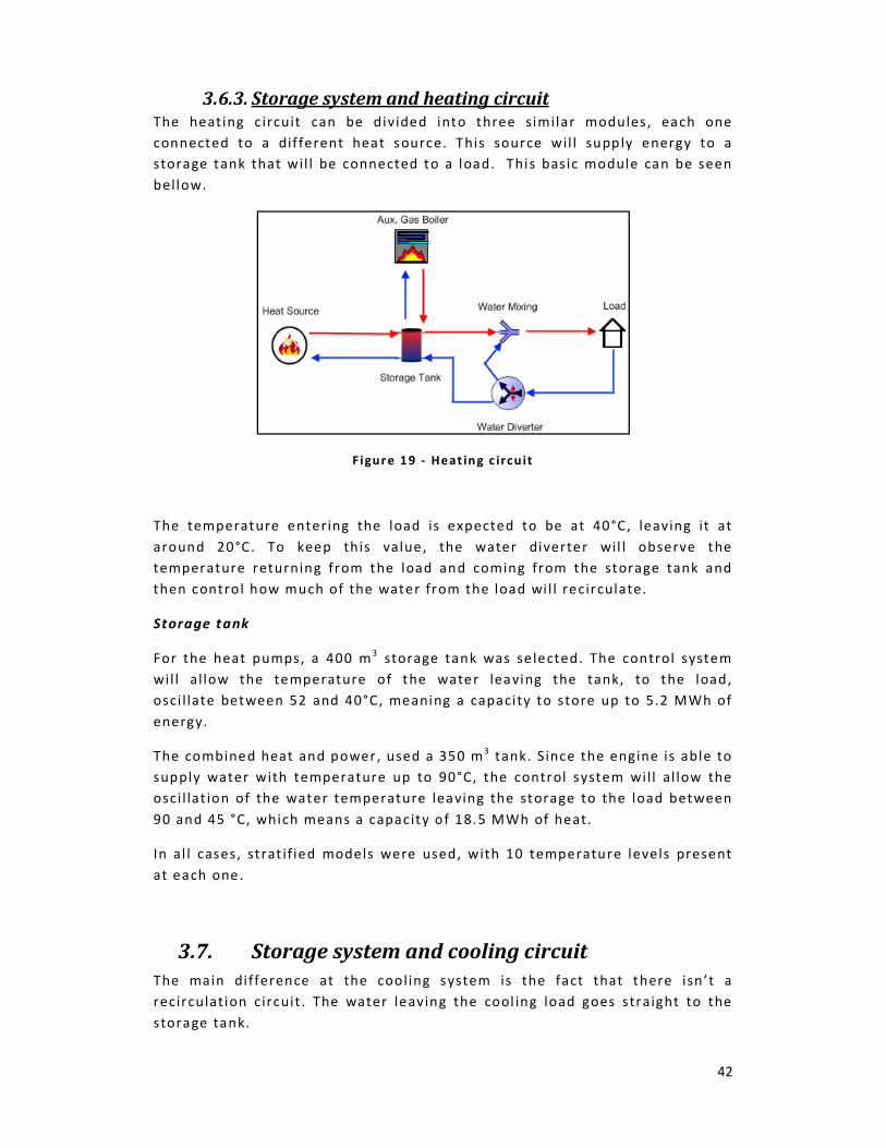
42

3.6.3. Storage system and heating circuit The heating c ircuit can be divided into three similar modules, each one

connected to a dif ferent heat source. This source wil l supply energy to a

storage tank that wil l be connected to a load. This basic module can be seen

bellow.

Figur e 19 - Heat in g c ircuit

The temperature entering the load is expected to be at 40°C, leaving it at

around 20°C. To keep this value, the water diverter wil l observe the

temperature returning from the load and coming from the storage tank and

then control how much of the water from the load wi l l recirculate .

Storage tank

For the heat pumps, a 400 m3 storage tank was se lected. The control system

wi l l al low the temperature of the water leaving the tank, to the load,

osci l late between 52 and 40°C, meaning a capacity to store up to 5.2 MWh of

energy.

The combined heat and power, used a 350 m3 tank. S ince the engine is able to

supply water with temperature up to 90°C, the control system wi l l al low the

osci l lat ion of the water temperature leaving the storage to the load between

90 and 45 °C, which means a capacity of 18.5 MWh of heat.

In al l cases, strat if ied models were used, with 10 temperature levels present

at each one.

3.7. Storage system and cooling circuit

The main difference at the cooling system is the fact that there isn’t a

recirculat ion circuit . The water leaving the cool ing load goes straight to the

storage tank.

The volume of the storage tank is of 350 m

model with 10 temperature levels.

The cool ing circuit is complete ly independent of the heating one and i s

present just at the heat pumps systems. Th

that , in case of heating and cool ing being requ

heat pumps wi l l operate at the cooling mode and the combined heat and

power system wi l l supply the heat demand.

4. Results

4.1. First round

control over the outputs.

The f i rst series of simulations won’t be l imited by the design

obtained from the design team for the real project

engines s izes and observe how the outputs behave as

di fferent capacities are compared between themselves. It wi l l be

a CHP only system, a heat pump only one and then both technologies

combined to observe the impact of siz ing and controls changes at the outputs

of the hybrid system.

The build ing si te wi l l a lso be considered as a whole , rather than three

different subsystems (the thermal and electr ica l loads for the three

subsystems are simply aggreg

capacity of the water source of supplying heat, al lowing the ut i l ization of any

size of source heat pump.

4.1.1. CHP supplied systemThe f i rst series of s imulation wi l l be observing a load suppl ied by the

fol lowing system:

The volume of the storage tank is of 350 m3, a lso simulated with a strat if ied

temperature levels .

The cool ing circuit i s completely independent of the heating one and is

present just at the heat pumps systems. The control was modeled in a way

that, in case of heating and cool ing being required at the same period, the


power system wi l l supply the heat demand.

Fi gure 20 - Coo lin g c ir cu it

round of simulations – Impact of sizing and

control over the outputs.

The f i rst series of simulat ions won’t be l imited by the design parameters

obtained from the design team for the real project , but wi l l p lay with the

engines s izes and observe how the outputs behave as heat sources of

different capacit ies are compared between themselves. It wi l l be considered

a CHP only system, a heat pump only one and then both technologies

observe the impact of s iz ing and controls changes at the outputs

The bui lding site wi l l a lso be cons idered as a whole , rather than three


subsystems are simply aggregated) . There won’t be any l imitat ion over the

water source of supplying heat, al lowing the ut i l izat ion of any

CHP supplied system The f i rst series of s imulat ion wi l l be observing a load suppl ied by the

43

, also simulated with a strat if ied

The cool ing circuit i s completely independent of the heating one and is

e control was modeled in a way

at the same period, the


Impact of sizing and

parameters

, but wi l l p lay with the

heat sources of

considered

a CHP only system, a heat pump only one and then both technologies wi l l be

observe the impact of s iz ing and controls changes at the outputs

The build ing site wi l l a lso be cons idered as a whole , rather than three


. There won’t be any l imitation over the

water source of supplying heat, al lowing the ut i l izat ion of any

The f i rst series of s imulat ion wi l l be observing a load suppl ied by the

Figur e

Four d ifferent s izes of CHP engines wil l be compared:

• 2.7 MW ( t h )

• 4.5 MW ( t h )

• 6.2 MW ( t h )

• 8.0 MW ( t h )

They wil l be supplying the base load with the auxil iary boiler supplying the

remaining, when necessary.

For the reasons described at sect ion

in case of generation higher then consumpt ion.

The graphic below represents the amount of gas consumed by the auxil iary

system against the total cost of the e

Fi gure 22 - Ener gy cost vs . Au x. b oi ler gas con s umpt ion

It can be observed at this graphic that the

auxi l iary system, the higher the annual energy cost

of the CHP from 6.2 to 8

F igure 21 - CHP supp l ied d i str ict

Four different s izes of CHP engines wil l be compared:

They wil l be supplying the base load with the auxil iary boiler supplying the

when necessary.

For the reasons described at sect ion 5 , e lectr ici ty wil l be sold to the gr id just

in case of generat ion higher then consumpt ion.


system against the total cost of the energy consumed on s ite.

En erg y c ost vs . Aux. b oi ler gas cons umpt ion

It can be observed at this graphic that the higher part icipation of the

auxi l iary system, the higher the annual energy cost . Also, improving the

of the CHP from 6.2 to 8 MW ( t h ) had small impact over the f inal result .

44

They wil l be supplying the base load with the auxil iary boi ler supplying the

, electr icity wil l be sold to the gr id just


higher part icipat ion of the

mproving the size

had small impact over the f inal result .

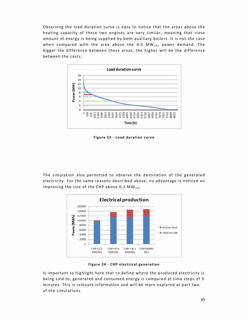
Observing the load duration curve is easy to

heating capacity of these two engines are very

amount of energy is being s

when compared with the area above the 4.5 MW

bigger the difference between these areas, the higher wi l l be the difference

between the costs.

Figur e

The s imulation a lso permitted to observe

electric ity. For the same reasons described above, no advantage is noticed on

improving the s ize of the CHP above 6.2 MW

Figur e

Is important to h ighlight here that to define where the produced e lectr icity is

being sold to, generated and consumed energy is compared at t ime

minutes. This is relevant information and wil l be more explored at pa

of the simulat ions.

Observing the load durat ion curve is easy to notice that the areas above the

heating capacity of these two engines are very s imilar , meaning that close

amount of energy is being supplied by both auxi l iary boi lers. It is not the case

the area above the 4.5 MW ( t h ) power demand.

bigger the d ifference between these areas , the higher wi l l be the difference

Fi gure 23 - Load durat io n curve

The simulat ion a lso permitted to observe the destinat ion of the generated

electr icity. For the same reasons described above, no advantage is noticed on

improving the s ize of the CHP above 6.2 MW ( t h )

Fi gure 24 - CHP electr ical gen erati on

Is important to h ighl ight here that to define where the produced e lectr icity is

generated and consumed energy is compared at t ime steps of 3

This is relevant information and wil l be more explored at pa

45

areas above the

, meaning that close

is not the case

power demand. The

bigger the d ifference between these areas , the higher wil l be the difference

the generated

electr ici ty. For the same reasons described above, no advantage is noticed on

Is important to h ighl ight here that to define where the produced e lectr ici ty is

steps of 3

This is relevant information and wil l be more explored at part two

A graphic very simi lar to the above is generated when the CO

reduction is p lotted for each CHP si ze. The reduction levels are relat ive to the

base case described previously.

Figur e

It can be seen how a higher saving leve l is achieved as the s ize of the engine

is risen although it does seems to saturate at a given level as the amount of

energy supplied by auxi l iary systems (responsible by a higher emission value)

stabi l izes (f igure 23).

To compare the internal rate of return of each engine, over the period of 20

years, the new CHP system capital cost was used as initial investment .

di fference between energy, operat ional and maintenance cost of each CHP

system and the base case wil l be used to define the cash f low, as shown

below:

With this data the internal rate of return against the CO

calculated for each CHP si ze.

A graphic very s imi lar to the above is generated when the CO2

reduct ion is plotted for each CHP s ize. The reduction levels are re lat ive to the

base case described previously.

Fi gure 25 - CHP CO 2 sav i ngs

It can be seen how a h igher saving leve l is achieved as the s ize of the engine

t does seems to saturate at a given level as the amount of

energy supplied by auxi l iary systems (responsible by a higher emiss ion value)


years, the new CHP system capital cost was used as initial investment .

difference between energy, operat ional and maintenance cost of each CHP

case wi l l be used to define the cash f low, as shown

Figur e 26 - Cash f low CHP

With this data the internal rate of return against the CO2 emiss ion could be

ca lculated for each CHP s ize.

46

emission

reduction is plotted for each CHP s ize. The reduction levels are re lat ive to the

It can be seen how a h igher saving leve l is achieved as the s ize of the engine

t does seems to saturate at a given level as the amount of

energy supplied by auxi l iary systems (responsible by a higher emiss ion value)


years, the new CHP system capital cost was used as initial investment. The

difference between energy, operat ional and maintenance cost of each CHP

case wi l l be used to define the cash f low, as shown

emiss ion could be

47

Figur e 27 - CHP IRR vs. CO 2 r edu ct ion

The smal l di fference between the cash f lows from the di fferent systems made

the initial investment as main factor defining the dif ferences between the

internal rates of return. The extra energy savings of the bigger machines are

not enough to overcome the fact the smal ler ones require less in it ia l

investment, which results into h igher IRR.

The graphic shows how improvements over the CO2 savings requires

expressive reduction over the IRR and seems to saturate close to the 25%.

This suggests that for the distr ict dist rict heating, CO2 savings above 20%

would result into high investment for smal l improvements.

4.1.2. Open loop water source heat pump supplied system

The next step is to s imulate the hypothetical case where the cooling and

heating load of the distr ict would be suppl ied by different s izes of heat

pumps with gas boi lers and conventional chi l lers working as auxil iary

systems. A schematic of what is being s imulated is shown below.

F igure

S imilar to what was done with the CHP engines , 4 d ifferent s izes of heat

pumps were ut i l ized. It was ignored any water source heating capacity

l imitat ion at this stage. The s izes are

• 2.5 MW ( t h )

• 3.5 MW ( t h )

• 5.5 MW ( t h )

• 8.0 MW ( t h )

It was achieved an average C

dur ing the cool ing ones.

Being able to supply renewable energy to the distr ict load, now is relevant to

observe not just CO 2 reduct ion over the emiss ion but also the renewable

share that each configuration is abl

compare the CO2 emission, at the vert ical axis , against the renewable share,

at the hor izontal one.

Figur e 28 - HP su ppl ied d is tr ic t

Similar to what was done with the CHP engines , 4 d ifferent s izes of heat

pumps were ut i l ized. It was ignored any water source heating capacity

l imitat ion at this stage. The s izes are

It was achieved an average COP of 4 dur ing the heating per iods and 6.5

Being able to supply renewable energy to the distr ict load, now is relevant to

reduction over the emiss ion but also the renewable

share that each configurat ion is able to bring on site. The next graph wi l l

emiss ion, at the vert ical axi s , against the renewable share,

48

S imilar to what was done with the CHP engines, 4 d ifferent si zes of heat

pumps were ut i l ized. It was ignored any water source heat ing capacity

OP of 4 dur ing the heat ing periods and 6.5

Being able to supply renewable energy to the distri ct load, now is relevant to

reduction over the emiss ion but also the renewable

e to bring on s ite. The next graph wi l l

emiss ion, at the vert ical axis , against the renewable share,

Figur e 29 -

As expected, the renewable share and

have h igher part icipat ion over the tota l load. This relat ionship between both

is not l inear. The red l ine on the graph makes easier to observe that the s ize

of the machine have higher impa

the CO2 reduct ion. This i s re lated with the fact that

from the ground to the building

from the gr id, which is associated with high emission levels (0.422 kg of CO

per kWh (10)) . Looking just for the heating demand, ignoring the electrical

consumption on s ite , the CO

share reaching 80% with the 8MW heat pump.

the buildings (26 000MWh per year) and the fact that i t is ent irely suppl ied

by the gr id makes the f ina l values more modest.

The init ial investment and the cash f lows during 20 years are shown

next graphic. It wi l l help to observe how each configurat ion affects the total

energy savings and to predict what wil l happen when the IRR for this period

is calculated.

HP CO 2 r edu ct ion vs . R en ewabl e sh are

As expected, the renewable share and CO2 savings improve as the heat pumps

have higher partic ipat ion over the tota l load. This relat ionship between both

is not l inear. The red l ine on the graph makes easier to observe that the si ze

higher impact over the renewable part icipat ion then at

reduction. This is related with the fact that , to transfer the energy

from the ground to the building, the heat pump needs to ut i l ize electrici ty

from the gr id , which is associated with high emission levels (0.422 kg of CO

Looking just for the heating demand, ignoring the electrical

consumption on s ite, the CO2 reduct ion is around 60% with the renewable

share reaching 80% with the 8MW heat pump. The high e lectr ical demand at

the buildings (26 000MWh per year) and the fact that i t is ent irely suppl ied

by the grid makes the f inal values more modest.

The init ial investment and the cash f lows during 20 years are shown

p to observe how each configurat ion affects the total

energy savings and to predict what wi l l happen when the IRR for this period

49

savings improve as the heat pumps

have h igher partic ipat ion over the tota l load. This relat ionship between both

is not l inear. The red l ine on the graph makes easier to observe that the size

ation then at

to transfer the energy

the heat pump needs to ut i l ize electr ici ty

from the gr id , which is associated with high emission leve ls (0.422 kg of CO 2

Looking just for the heating demand, ignoring the electr ical

reduction is around 60% with the renewable

The high e lectrical demand at

the buildings (26 000MWh per year) and the fact that it is ent irely suppl ied

The init ial investment and the cash f lows during 20 years are shown at the

p to observe how each configurat ion affects the total

energy savings and to predict what wi l l happen when the IRR for this period

50

Figur e 30 - HP cash f low

The 8 MW HP seems to be related with smaller savings then the 5.5 MW. In

part it is related with the fact that its operational and maintenance cost is

higher but is mostly related with the indication that it is overs ized for the

s ite load. Remembering the load duration curve, it is easy to understand that

most of the t ime the load demand wi l l be wel l below the 8MW. When

switched on, the heat pumps tend to work for a short per iod at reduced

eff iciency. This eff iciency reduction becomes more evident when the heat

pump is switched on and off at short period of t ime, which is what happens

when they are oversized and is what happens with the 8MW one in this

example. Its lower eff iciency makes the energy savings be smal ler than the

one of a 5.5 MW heat pump.

As commented before, where relevant , 20% of renewable part icipation wi l l be

the target to be achieved. Al l the conf igurat ions above are over this va lue, so

the IRR wi l l be p lotted just against the CO 2 emiss ion savings.

Figur e 31 – Heat pu mp: IRR vs. CO2 r educt ion

The extra energy savings of the bigger heat pumps, compared with the

smal ler ones , are not enough to overcome the price difference between the

51

init ial investments, result ing into lower internal rates of return. The

disadvantage caused by over s iz ing the heat pump is also evident when

comparing the 8 MW one with al l the others. The same CO2 reduct ion can be

achieved with smal ler machines that , requir ing smal lest init ial investment ,

may achieve higher internal rate of return at the observed per iod.

The 2.5 MW heat pump, a lthough presenting the best IRR, is below the target

of 20%, not leaving many options over what can be done to improve its CO2

emissions. At this stage, the best option is to ut i l i ze the 3 .5 MW heat pump.

I t might be a lso interesting to observe a l l the IRR and CO2 reduct ion of the

systems s imulated unt i l the present moment.

Figure 32 - CHP and HP IRR vs. CO 2 reduct ion

I f no target of renewable participation is set, ut i l iz ing CHP to reduce CO2

emiss ion seems to be a better opt ion. Even with the bigger machines, a

higher IRR of return, when compared with the heat pumps, i s achievable. Is

important to also h ighlight here that many companies apply the CO2

displacement factor (-0.568 kg of CO2 per kWh) for al l the electr icity

generated by the CHP, not just in case of production overcoming the

generat ion as how was done during the ca lculat ions here present , which may

result into even higher CO2 emission reduction.

The next stage is to observe how a hybrid system involving a CHP engine and

a heat pump behaves supplying the local load.

4.1.3. Hybrid CHP + HP system The hybrid system wi l l work as below:

Figure 33

Three d ifferent s izes of heat pumps and CHP engines wi l l be ut i l ized. Based

on the previous results it was decided that the lower l imit for the heat

capacity of the heat sources wi l l be 2.5 MW and the upper l imit wil l be 5.1 ,

keeping the system below the 8

signs of be ing oversized. The re

auxi l iary boiler.

The exact s izes are shown below:

CHP (heat capacity)

2.5 MW

2.8 MW

5.1 MW

Table

Unlike the previous cases , there wi l l be changes not just at the size of the

engines, but also at how they wi l l be controlled, def in ing when each one wi l l

be supplying the heating or

The studied conf igurat ions are the fol lowing:

4.1.3.1. 2.8 MW heat pump + 2.8 MW(th) CHP

This system wil l be ut i l iz ing the heat pump and the CHP engine with the same

heat capacity. Both systems wil l be connected at the load with their

part icipation over the load controlled by

storage tank. The controls are:

Hybrid CHP + HP system The hybrid system wil l work as below:

33 - Hybr id s yst em supp l ied d istr ict

Three different s izes of heat pumps and CHP engines wi l l be ut i l ized. Based


capacity of the heat sources wi l l be 2.5 MW and the upper l imit wi l l be 5.1,

keeping the system below the 8MW capaci ty, at which the system gave clear

overs ized. The remaining heating load wi l l be suppl ied by the

The exact s izes are shown below:

CHP (heat capacity) Heat pumps (heat capacity)

2.5 MW

2.8 MW

5.1 MW

Table 9 - CHP & HP heating capacity

Unlike the previous cases, there wi l l be changes not just at the size of the

engines, but also at how they wil l be controlled, def in ing when each one wi l l

be supplying the heating or cooling demand.

The studied configurat ions are the fol lowing:

2.8 MW heat pump + 2.8 MW(th) CHP



over the load controlled by the water f low through each system

storage tank. The controls are:

52

Three d ifferent s izes of heat pumps and CHP engines wi l l be ut i l ized. Based


capacity of the heat sources wi l l be 2.5 MW and the upper l imit wil l be 5.1 ,

gave clear

pplied by the

Heat pumps (heat capacity)

Unlike the previous cases, there wi l l be changes not just at the s ize of the

engines, but also at how they wil l be controlled, def in ing when each one wi l l



the water f low through each system

53

Same share

Figur e 34 - Same shar e confi gurat ion*

At this conf igurat ion the CHP and the heat pump wi l l be supplying equally the

total demand. This means that i f the tota l load is of 4 MW, for example, two

wi l l be suppl ied by the heat pump storage tank and two by the CHP one. This

control is done keeping the water f low from the load to each tank a lways

equal . When the total load is above the CHP+HP capacity, the auxil iary

heaters are turned on.

In case of heat ing and cool ing demand, the f irst one wi l l be supplied

exclus ive ly by the CHP system (no water wil l return from the load to the HP

storage tanks) , with the heat pump giving priority to the cool ing load. This

observation is val id to a l l the configurat ions here present .

* This graphic is a conceptual representation created to facilitate the comprehension of the control

configuration. It does not represent any result from the actual simulation or the precise load

distribution.

54

CHP Leading

Figur e 35 - CHP lead ing conf igurat ion*

CHP leading means that the control system wi l l let the CHP supply the load

alone, unti l i ts maximum capacity is reached, when the heat pump system

starts to he lp with the demand. At this point each one wil l be supplying the

same amount of energy. When the total load is above the CHP + HP capacity,

the auxi l iary heaters are turned on.

The control is done through the water f low from the load to the storage tank

of each system.



distribution.

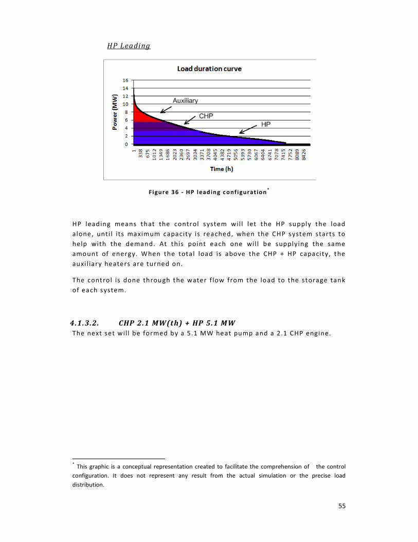
55

HP Leading

Fi gure 36 - HP lead in g c onf i gurat ion*

HP leading means that the control system wil l let the HP supply the load

alone, unti l its maximum capacity is reached, when the CHP system starts to

help with the demand. At this point each one wi l l be supplying the same

amount of energy. When the tota l load is above the CHP + HP capacity, the

auxi l iary heaters are turned on.

The control is done through the water f low from the load to the storage tank

of each system.

4.1.3.2. CHP 2.1 MW(th) + HP 5.1 MW

The next set wil l be formed by a 5.1 MW heat pump and a 2.1 CHP engine.



distribution.

56

HP leading

Figur e 37 – 5 .1 MW heat pu mp: HP l eadin g conf igurat ion*

The only dif ference between this configuration and the previous “heat pump

leading” one is that when both heat pumps are working, 60% of the load wi l l

be suppl ied by the heat pump system and 40% by the CHP.

CHP leading

Figur e 38 - 5 .1 MW h eat pump : CHP lead in g con f igur at ion*



distribution.

57

This configurat ion wil l fol low the same logic previous ly described at “CHP

leading”. The main difference is in the fact that , while both heat pump

system and CHP are working, 60% of the load wi l l be supplied by the HP and

40% by the CHP system.

4.1.3.3. CHP 5.1 MW(th) + HP 2.5 MW

The last configurat ion is formed by a 5.1 MW(th) CHP engine and a 2.5 MW

heat pump.

HP leading

Fi gure 39 – 5 .1 MW CHP: HP l eading conf igurat ion*

The heat pump wi l l supply the base load unti l the demand reaches 2.5 MW.

Above this va lue the CHP system wi l l supply 60% of the total required energy

while the heat pump 40%. The auxi l iary systems wi l l supply energy when the

demand reaches values above 7 .6 MW.



distribution.

58

CHP leading

Fi gure 40 - 5 .1 MW CHP: CHP leading conf igurat ion*

At this last case the CHP wil l supply alone the load as long as i t remains

below 5.1 MW. Above it , the heat pump system is jo ined to the previous one,

supplying 40% of the total energy demand with the CHP system supplying the

remaining 60%.

4.1.3.4. First round of simulation: results overview

The previous results may work as a guide to what is expected from the

combination of the two technologies . The new hybrid system al lows the

designer to combine the benefits observed from each technology in order to

try to achieve a given goal.

The renewable target of 20% wi l l come complete ly from the heat pumps. It

was observed that the part icipat ion of the heat pump over the load raises the

f inal renewable part icipation, but this improvement does saturate if

overs ized. The CO2 target seems to be easier to achieve s ince not just the

heat pump is able to reduce the overall emiss ion but the CHP also attested to

have a great capacity to improve the savings.

Looking for the CO2 emiss ion savings of each configurat ion and the renewable

share, the following graphic was generated. The colors were ut i l ized to

indentify each configurat ion easier.



distribution.

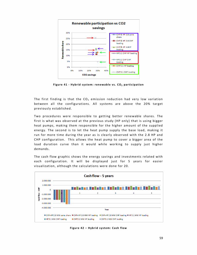
59

Fi gure 41 - Hybr id syst em: ren ewab le vs . CO2 part ic ipat ion

The f irst f inding is that the CO 2 emiss ion reduction had very low variat ion

between al l the configurat ions. Al l systems are above the 20% target

previously established.

Two procedures were responsible to gett ing better renewable shares . The

f i rst is what was observed at the previous study (HP only) that i s using bigger

heat pumps, making them responsible for the higher amount of the suppl ied

energy. The second is to let the heat pump supply the base load, making it

run for more t ime dur ing the year as is clearly observed with the 2.8 HP and

CHP conf igurat ion. This a l lows the heat pump to cover a bigger area of the

load duration curve than it would whi le working to supply just higher

demands.

The cash f low graphic shows the energy savings and investments related with

each configurat ion. It wil l be displayed just for 5 years for easier

v isual izat ion, although the calculations were done for 20.

Figur e 42 – Hybr id s yst em: Cash f low

The cash flow does not present any dramatic di fference between all the

configurat ions. This wi l l result into the initial investment being the main

variable responsible for defining the best IRR.

the best savings are related with the configurat ions with higher part icipat ion

of the CHP engine. The low price

be used on site or sold to the gr id , are the main reason for it .

interest ing to not ice that the best savings involves the configurat ion with the

smal lest machines (CHP+ HP 2.8 , CHP leading).

S ince a l l the configurat ions have s imilar

target, the internal rate of return wil l be plotted against the renewable

part icipation. The circles with colors were ut i l ized to make the visual izat ion

easier.

Fi gure 43 - H ybr id syst em: IR R vs . R enew ab le shar e

As possible to predict from the cash f low analysis , the configurat ions

involving the smallest in itia l investments resulted into better internal rates

of return. None of them, though, achieved the 2

It is interest ing to observe how setting the heat pump to supply the base load

makes their pos it ion into the graph move down at the IRR axis and right at

the renewable share one. CHP supplying the base load ra ises the internal rat

of return, reducing the renewable share. Better internal rates of return

comes with the cost of reduct ion

f inal load may be the main conclus ion

As a direct result of the previous observ

the 20% target presents one of the worst internal rates of return, which

makes it not so interest ing. I t may make the designer wonder i f there is any

change that can be done in order to move the conf igurat ions with best IRR to

not present any dramatic di fference between al l the

ons. This wi l l result into the init ial investment being the main

variable responsib le for defining the best IRR. It can be observed though that

the best savings are related with the configurations with higher participat ion

of the CHP engine. The low price of gas and high price of electr ici ty, that can

be used on s ite or sold to the grid, are the main reason for it .

interest ing to notice that the best savings involves the configurat ion with the

smal lest machines (CHP+ HP 2.8 , CHP leading).

S ince a l l the configurat ions have s imi lar CO2 savings and above the set 20%

target , the internal rate of return wil l be plotted against the renewable

The circles with colors were ut i l ized to make the visual ization

Hybr id s yst em: IR R vs . R enew ab le shar e

As possible to predict from the cash flow analys is , the configurat ions

involving the smal lest in it ia l investments resulted into better internal rates

of return. None of them, though, achieved the 20% target init ial ly set .

It is interest ing to observe how sett ing the heat pump to supply the base load

makes their posit ion into the graph move down at the IRR axis and right at

the renewable share one. CHP supplying the base load ra ises the internal rat


with the cost of reduction over the renewable part icipat ion at the

fina l load may be the main conclusion extracted from this graphic .

As a direct result of the previous observat ion, the only configurat ion above


makes i t not so interesting. It may make the designer wonder i f there is any


60

not present any dramatic di fference between all the

ons . This wi l l result into the initial investment being the main

It can be observed though that

the best savings are related with the configurat ions with higher part icipat ion

of gas and high price of electr ici ty, that can

be used on site or sold to the grid , are the main reason for it. Is a lso

interest ing to notice that the best savings involves the configurat ion with the

savings and above the set 20%

target, the internal rate of return wil l be plotted against the renewable

The circles with colors were ut i l ized to make the visual izat ion

As possible to predict from the cash f low analysis , the configurat ions

involving the smal lest in it ia l investments resulted into better internal rates

0% target init ial ly set .

It is interest ing to observe how sett ing the heat pump to supply the base load

makes their position into the graph move down at the IRR axis and r ight at

the renewable share one. CHP supplying the base load ra ises the internal rate


part icipation at the

the only configuration above


makes it not so interesting. It may make the designer wonder i f there i s any


the r ight into the graphic. Even though it may be fol lowed by it pos ition

lower ing into the y axis . A good candidate for that may be the

HP, HP leading”. I t presents the second best renewable share and is high into

the IRR axis .

A f i rst though may suggest as a good solut ion adding a new technology

looking forward the improvement of

generat ion may be a good candidate , adding renewable energy into the

electrical consumption. A f i rst analys is indicated

would be necessary. I t does sound huge value but when compared with the

total area occupied by the buildings, it starts to look a bit more reasonable ,

as shown below.

Fi gure

The array area seems acceptable, which is good new

20% being reached. Running the s imulation

the right into the graphic. Even though it may be fol lowed by it position

lowering into the y axis. A good candidate for that may be the “2.8 CHP and

, HP leading”. It presents the second best renewable share and is high into

h may suggest as a good solut ion adding a new technology

looking forward the improvement of the renewable share. Photovoltaic

generat ion may be a good candidate, adding renewable energy into the

A f i rst analysis indicated that an array of 15 000 m


total area occupied by the bui ldings, i t starts to look a bit more reasonable ,

Figur e 44 - Dis tr i ct and PV array ar ea

array area seems acceptable , which is good news since it wi l l a l low the

20% being reached. Running the s imulat ion, the following result was found.

61

the right into the graphic. Even though it may be fol lowed by it posit ion

2.8 CHP and

, HP leading”. It presents the second best renewable share and is high into

h may suggest as a good solut ion adding a new technology

hotovoltaic

generat ion may be a good candidate, adding renewable energy into the

ray of 15 000 m2


total area occupied by the bui ldings, i t starts to look a bit more reasonable ,

since it wi l l al low the

the following result was found.

62

Fi gure 45 - Hybr id syst em with PV : I RR vs . Ren ewab le share

Although the photovoltaic panels do add renewable and cheap electr icity to

the system, the required initial investment is rocketed. It was uti l ized the

Sanyo model HIP-200BA3, with peak capacity of 200 W. The capital ,

operational and maintenance cost are l isted below, fol lowed by the cash

f lows of the same system, with and without the PV array.

• Capital cost ( instal lation + equip) : £ 568 per 1 m2 (18) (19)

• O & M: £ 0.02 per kWh (20)

Figur e 46 - Hybr id s yst em: Cash f low w ith and wit hout pho tovolta ic

The photovoltaic panels produced extra 2 480 MWh per year. Al though a big

amount of energy, i t is smal l compared with the total energy consumed on

s ite, 55 MWh per year, making the extra savings not b ig enough to overcome

the massive extra investment required.

It is clear now that, at this case,

an option to solve the problem of reaching the 20% of renewable share

an IRR above the one of the 5.1 MW HP system.

possib le.

As seen before, changes over the control of each system did have an

express ive impact at the outputs. This is one b ig characteri st ic of hybr id

systems and can be used as an

can be easi ly changed with the new results rapidly being observed, al lowing

the system optimizat ion.

The previous s imulat ions h ighlighted how raising the heat pump

part icipation improves the renewable part icip

also sa id before how, in al l cases, it was set a command that would make the

HP system supply energy exclusively to the cooling load, in case of heating

and cool ing demand at the same time. This was made in order to avoid a

situat ion where both storage tanks require ref i l l ing at the same t ime. But

depending of the timing of the loads, durat ion and magnitude, th is si tuation

may not happen. The best option is to run a new simulat ion, taking out the

“exclusivity” command and observ

The change impl ied no alterat ion

to the load. It is a posit ive result which a l lowed the inclus ion of this new

configurat ion between the previous one and the recreation of the “IRR vs.

Renewable share” graph, shown below.

Figur e 47 - Hybr id s ystem no coo l in g pr ior i ty : IRR vs . R en ew able s hare

, at this case, re lying exclus ive ly on PV technology is not

an option to solve the problem of reaching the 20% of renewable share

the 5.1 MW HP system. But a solut ion may st i l l be


expressive impact at the outputs. This i s one big characteri st ic of hybr id

and can be used as an advantage. Through simulat ion these controls


The previous s imulat ions highlighted how raising the heat pump

participat ion improves the renewable part icipat ion of each system. It was

also sa id before how, in al l cases , it was set a command that would make the

HP system supply energy exclus ively to the cooling load, in case of heating

and cool ing demand at the same t ime. This was made in order to avoid a

uat ion where both storage tanks require ref i l l ing at the same time. But

depending of the t iming of the loads, durat ion and magnitude, this situation


“exclusivity” command and observe what would happen.

alteration into the quali ty of the heat be ing suppl ied

to the load. It is a posit ive result which al lowed the inclus ion of this new


ble share” graph, shown below.

H ybr id syst em no cool in g pr ior it y: IRR vs . R en ew able shar e

63

re lying exclus ive ly on PV technology is not

an option to solve the problem of reaching the 20% of renewable share with

But a solut ion may st i l l be


expressive impact at the outputs. This is one b ig characterist ic of hybrid

Through s imulation these controls


The previous s imulations highlighted how raising the heat pump

at ion of each system. It was

also sa id before how, in al l cases , it was set a command that would make the

HP system supply energy exclus ively to the cooling load, in case of heating

and cool ing demand at the same t ime. This was made in order to avoid a

uat ion where both storage tanks require ref i l l ing at the same t ime. But

depending of the t iming of the loads, durat ion and magnitude, this situat ion


heat be ing suppl ied

to the load. It is a posit ive result which al lowed the inclus ion of this new


H ybr id syst em no cool in g pr ior i t y: IRR vs . R en ewable shar e

64

The 20% target was achieved with an internal rate of return above 25%

thanks to the f lexibi l i ty of controll ing the hybrid system. It is important to

inform that the new conf igurat ion did change the CO 2 emiss ion reduction

value to 20%, exact ly the target previously set.

The capacity of changing the controls and observing how the entire system

behaved at each case, proved a useful a l ly to achieve this result .

All the s imulations above were made taking a l iberty that may not happen in

a real s i tuat ion, l i ke unl imited water heat source capacity or no extra losses

related with dif ferent configurations. This made the non hybrid system

involving just heat pump and gas boilers the best solut ion found. This part ly

results from the s impli f icat ions explained above and a lso from the very

ambit ious target of 20% renewable share. Given such an ambitious target ,

hybrid system configurations with solar thermal col lectors might have

provided a better economical performance.

The project design team informed us that two water sources were available

and that i t was possib le to extract 2 MW of heat from each, through an open

loop system in the f i rst case and a closed loop the second one. They a lso

decided to run each system independent ly, avoiding extra losses caused by

high t ransmission distances. These l imitations wi l l be explored in the next set

of s imulat ions where the analysis method wi l l also be observed.

4.2. Second round of simulations – Hybrid systems with

three different heat sources.

The fol lowing simulat ions wi l l reproduce the situat ion where the water

source wil l l imit the heat pumps sizes. On the studied s ite two water sources

can, and wi l l , be explored. Each one is able to supply up to 2 MW of heating

power. The remaining required energy wil l be supplied by a th ird heat source,

a CHP engine with a heating capacity of 1.8 MW(th).

4.2.1. Loads

Since these sizes of heat pumps and CHP engines would require a large

partic ipat ion of the auxi l iary system around the year , the conf igurat ion

changes were present ing not so expressive impacts over the results . It was

then taken the l iberty to scale down the load, making one of the three heat

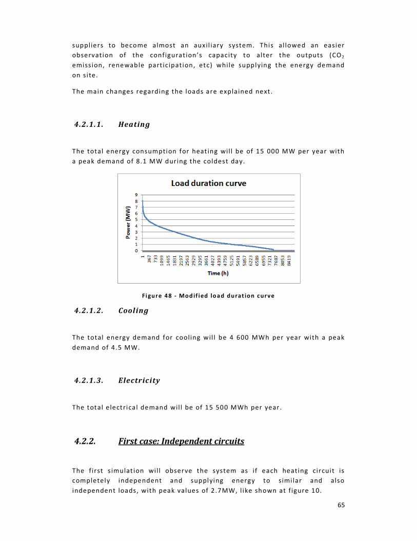
65

suppliers to become almost an auxil iary system. This al lowed an easier

observation of the configurat ion’s capacity to alter the outputs (CO2

emiss ion, renewable part icipat ion, etc) while supplying the energy demand

on s ite.

The main changes regarding the loads are expla ined next .

4.2.1.1. Heating

The total energy consumption for heat ing wi l l be of 15 000 MW per year with

a peak demand of 8.1 MW during the coldest day.

Fi gure 48 - Mod if ied lo ad durat ion curve

4.2.1.2. Cooling

The total energy demand for cooling wil l be 4 600 MWh per year with a peak

demand of 4 .5 MW.

4.2.1.3. Electricity

The total electrica l demand wil l be of 15 500 MWh per year .

4.2.2. First case: Independent circuits

The f irst s imulat ion wi l l observe the system as if each heating circuit is

completely independent and supplying energy to simi lar and also

independent loads, with peak values of 2 .7MW, l ike shown at f igure 10.

66

This conf igurat ion may reduce transmiss ion losses of the heated water, given

the fact that each heat source may feed just the closest loads , reducing the

transmiss ion distances. I t won’t be considered a hybrid system (although the

presence of auxil iary heaters and chi l lers may class ify the system as it) .

Fi gure 49 – TR NSYS mod el

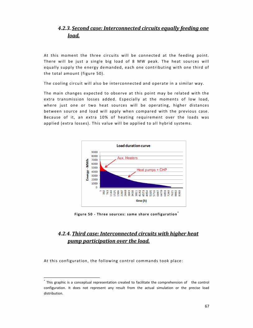
4.2.3. Second case: Interconnected circuits equally feeding one

load.

At this moment the three circuits wi l l be connected at the feeding point .

There wi l l be just a single big load of

equally supply the energy demanded, each one contribut ing with one third of

the total amount (f igure 50

The cool ing circuit wil l a lso be interconnected and operat

The main changes expected to observe at this point may be related with the

extra transmiss ion losses added.

where just one or two heat sources wil l be operat ing, higher distances

between source and load wi l l apply when compared w

Because of i t , an extra 10% of heat ing requirement over the loads was

applied (extra losses). This value wi l l be applied to a l l hybr id systems.

Figur e 50 - Three sources: s

4.2.4. Third case: Interconnected circuits with

pump participation over the load

At this conf igurat ion, the following control commands took p lace:


configuration. It does not represent any result from the actual simulation

distribution.

ase: Interconnected circuits equally feeding one

At th is moment the three circuits wi l l be connected at the feeding point .

just a s ingle big load of 8 MW peak. The heat sources wil l

equal ly supply the energy demanded, each one contribut ing with one third of

50) .

The cool ing circui t wil l a lso be interconnected and operate in a simi lar way.

nges expected to observe at this point may be related with the

extra transmission losses added. Especial ly at the moments of low load,


between source and load wil l apply when compared with the previous case.

Because of it , an extra 10% of heat ing requirement over the loads was

applied (extra losses). This va lue wi l l be applied to a l l hybr id systems.

Thr ee sources: same shar e conf igur at ion*

Third case: Interconnected circuits with higher heat

pump participation over the load.

the fol lowing control commands took p lace:

This graphic is a conceptual representation created to facilitate the comprehension of the control


67

ase: Interconnected circuits equally feeding one

At this moment the three circuits wi l l be connected at the feeding point.

The heat sources wil l

equally supply the energy demanded, each one contributing with one third of

in a s imilar way.

nges expected to observe at this point may be related with the

Especial ly at the moments of low load,


ith the previous case.

Because of it , an extra 10% of heat ing requirement over the loads was

applied (extra losses). This va lue wi l l be applied to a l l hybr id systems.

higher heat

This graphic is a conceptual representation created to facilitate the comprehension of the control

or the precise load

68

Heat ing

• I f the total system load is under 1.5 MW, the demand wil l be suppl ied

by the open source heat pump.

• I f the total system load is between 1.5 and 3 MW, the demand wil l be

supplied by the two heat pumps

• I f the tota l system load is above 3 MW, the demand wil l be suppl ied by

the heat pumps and the CHP system, which wi l l also be generating

electr icity.

Cooling

• I f the tota l cooling load is below 1.4 MW, the total demand wil l be

supplied just by the closed loop heat pump. In case the demand i s

above 1.4 MW, the open loop heat pump wil l also enter the circuit .

There wil l be priority for the cool ing load. In case of cool ing and heating

being required at the same moment and with high demand, meaning that the

energy of just one heat pump won’t be enough, the heat pumps wi l l supply

the cool ing load, leaving a l l the heat ing for the CHP and auxi l iary heaters .

Figur e 51 - Thr ee sourc es: HP l eading conf igur at ion*

4.2.4.1. First Results

At this stage the analysis wil l start slower, making poss ib le to observe how

the assumptions done can affect the f inal results .

At f i rst the outputs wil l be examined through the monthly results:

consumption and supplied loads. It wil l be evaluated how useful this data



distribution.

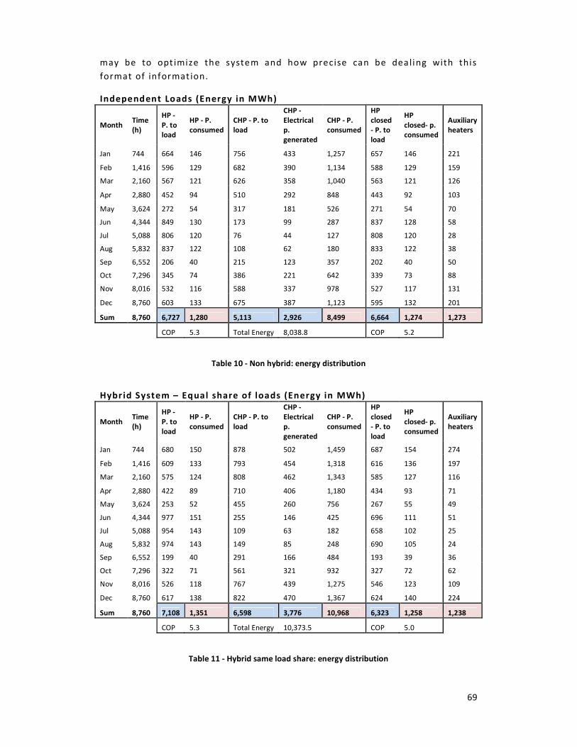
69

may be to opt imize the system and how precise can be dealing with this

format of informat ion.

Independent Loads (Energy in MWh)

Month Time

(h)

HP -

P. to

load

HP - P.

consumed

CHP - P. to

load

CHP -

Electrical

p.

generated

CHP - P.

consumed

HP

closed

- P. to

load

HP

closed- p.

consumed

Auxiliary

heaters

Jan 744 664 146 756 433 1,257 657 146 221

Feb 1,416 596 129 682 390 1,134 588 129 159

Mar 2,160 567 121 626 358 1,040 563 121 126

Apr 2,880 452 94 510 292 848 443 92 103

May 3,624 272 54 317 181 526 271 54 70

Jun 4,344 849 130 173 99 287 837 128 58

Jul 5,088 806 120 76 44 127 808 120 28

Aug 5,832 837 122 108 62 180 833 122 38

Sep 6,552 206 40 215 123 357 202 40 50

Oct 7,296 345 74 386 221 642 339 73 88

Nov 8,016 532 116 588 337 978 527 117 131

Dec 8,760 603 133 675 387 1,123 595 132 201

Sum 8,760 6,727 1,280 5,113 2,926 8,499 6,664 1,274 1,273

COP 5.3 Total Energy 8,038.8 COP 5.2

Table 10 - Non hybrid: energy distribution

Hybr id System – Equal share of loads (Energy in MWh)

Month Time

(h)

HP -

P. to

load

HP - P.

consumed

CHP - P. to

load

CHP -

Electrical

p.

generated

CHP - P.

consumed

HP

closed

- P. to

load

HP

closed- p.

consumed

Auxiliary

heaters

Jan 744 680 150 878 502 1,459 687 154 274

Feb 1,416 609 133 793 454 1,318 616 136 197

Mar 2,160 575 124 808 462 1,343 585 127 116

Apr 2,880 422 89 710 406 1,180 434 93 71

May 3,624 253 52 455 260 756 267 55 49

Jun 4,344 977 151 255 146 425 696 111 51

Jul 5,088 954 143 109 63 182 658 102 25

Aug 5,832 974 143 149 85 248 690 105 24

Sep 6,552 199 40 291 166 484 193 39 36

Oct 7,296 322 71 561 321 932 327 72 62

Nov 8,016 526 118 767 439 1,275 546 123 109

Dec 8,760 617 138 822 470 1,367 624 140 224

Sum 8,760 7,108 1,351 6,598 3,776 10,968 6,323 1,258 1,238


Table 11 - Hybrid same load share: energy distribution

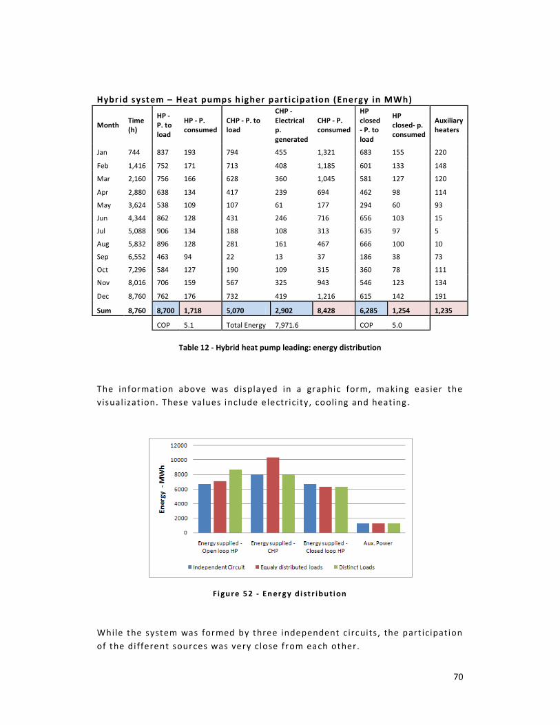
70

Hybr id system – Heat pumps higher participat ion (Energy in MWh)

Month Time

(h)

HP -

P. to

load

HP - P.

consumed

CHP - P. to

load

CHP -

Electrical

p.

generated

CHP - P.

consumed

HP

closed

- P. to

load

HP

closed- p.

consumed

Auxiliary

heaters

Jan 744 837 193 794 455 1,321 683 155 220

Feb 1,416 752 171 713 408 1,185 601 133 148

Mar 2,160 756 166 628 360 1,045 581 127 120

Apr 2,880 638 134 417 239 694 462 98 114

May 3,624 538 109 107 61 177 294 60 93

Jun 4,344 862 128 431 246 716 656 103 15

Jul 5,088 906 134 188 108 313 635 97 5

Aug 5,832 896 128 281 161 467 666 100 10

Sep 6,552 463 94 22 13 37 186 38 73

Oct 7,296 584 127 190 109 315 360 78 111

Nov 8,016 706 159 567 325 943 546 123 134

Dec 8,760 762 176 732 419 1,216 615 142 191

Sum 8,760 8,700 1,718 5,070 2,902 8,428 6,285 1,254 1,235


Table 12 - Hybrid heat pump leading: energy distribution

The information above was d isplayed in a graphic form, making easier the

visual izat ion. These values include e lectric ity, cooling and heat ing.

Fi gure 52 - En er gy d i str ibution

While the system was formed by three independent c ircuits , the part icipat ion

of the different sources was very close from each other.

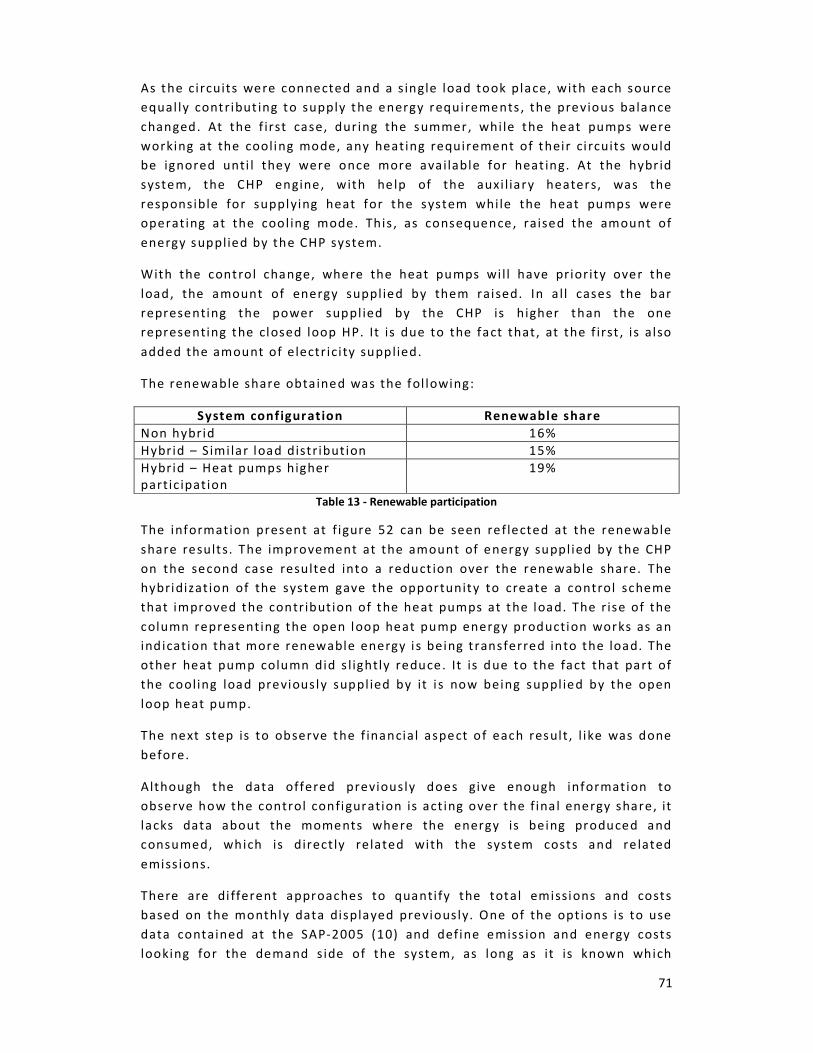
71

As the circuits were connected and a s ingle load took place, with each source

equal ly contribut ing to supply the energy requirements , the previous balance

changed. At the f irst case, during the summer, whi le the heat pumps were

working at the cooling mode, any heating requirement of their ci rcuits would

be ignored unti l they were once more available for heat ing. At the hybr id

system, the CHP engine, with help of the auxi l iary heaters, was the

responsible for supplying heat for the system whi le the heat pumps were

operating at the cool ing mode. This , as consequence, raised the amount of

energy supplied by the CHP system.

With the control change, where the heat pumps wi l l have priority over the

load, the amount of energy suppl ied by them raised. In a l l cases the bar

representing the power suppl ied by the CHP is higher than the one

representing the closed loop HP. It is due to the fact that, at the f irst , is also

added the amount of electr icity supplied.

The renewable share obtained was the fol lowing:

System conf iguration Renewable share

Non hybrid 16%

Hybrid – S imi lar load distr ibution 15%

Hybrid – Heat pumps higher

partic ipat ion

19%

Table 13 - Renewable participation

The information present at f igure 52 can be seen reflected at the renewable

share results. The improvement at the amount of energy suppl ied by the CHP

on the second case resulted into a reduct ion over the renewable share. The

hybridizat ion of the system gave the opportunity to create a control scheme

that improved the contribution of the heat pumps at the load. The r ise of the

column representing the open loop heat pump energy production works as an

indicat ion that more renewable energy i s being t ransferred into the load. The

other heat pump column did s l ightly reduce. It is due to the fact that part of

the cooling load previously suppl ied by it i s now being suppl ied by the open

loop heat pump.

The next step is to observe the f inancial aspect of each result , l ike was done

before.

Although the data offered previously does give enough information to

observe how the control configuration is act ing over the f inal energy share, it

lacks data about the moments where the energy is being produced and

consumed, which is direct ly related with the system costs and re lated

emiss ions.

There are di fferent approaches to quanti fy the total emissions and costs

based on the monthly data displayed previously. One of the options is to use

data contained at the SAP-2005 (10) and define emiss ion and energy costs

looking for the demand s ide of the system, as long as it is known which

technologies are supplying this load.

observed the fuel consumption instead of the load, fol lowing the assumptions

described at section 5. Making the analysi s through the demand data

be interesting if one does not have access to detai ls of the generation

system, but is too generic. For a heat pump, for example , the table wil l

assume that it is always working at a COP o

the energy consumption and related costs and emiss ions.

As explained at sect ion 5 , to have precise informat ion about

one must know i f the energy generated may be internal ly consumed or

constitutes energy surplus. This wi l l depend of instantaneous values of

generat ion and load. With

assumptions based on personal experie

For now, the fol lowing assumpt ions were made:

• It wil l be assumed that al l the e lectricity generated by the CHP wil l

a lways sold to the gr id.

• All the electr icity used by the heat pumps wi l l be purchased from the

grid.

• The electr icity purchased from the gr id wil l cost

hour and when sold to the gr id wi l l pay 5.7 per ki lowatt hour

• The gas consumed wil l cost 2.1 pence per kWh

• The emiss ions were calculated through the amount of energy

consumed and i ts source. For gas , it was assumed the va lue of 0.194 kg

of CO2 per kWh consumed, and for electr ici ty, 0.422 kg of

consumed from the gr id.

of CO2 per kWh (10)

Based on these assumptions,

share over the load generated the fol lowing graphic.

Fi gure 53 – Thr ee sourc es:

technologies are supplying this load. For the present analys is , it wil l be

observed the fuel consumption instead of the load, fo l lowing the assumptions

Making the analys is through the demand data

be interest ing if one does not have access to detai ls of the generation


assume that it is always working at a COP of 3.5 , and based on that , define

the energy consumption and related costs and emiss ions.

, to have precise informat ion about CO2

one must know i f the energy generated may be internal ly consumed or

const itutes energy surplus. This wi l l depend of instantaneous va lues of

generat ion and load. With just the information at the tables

assumptions based on personal experience or s imple guess needs to be done

For now, the fo llowing assumpt ions were made:

It wil l be assumed that al l the e lectr icity generated by the CHP wil l

sold to the gr id.

All the electr ici ty used by the heat pumps wi l l be purchased from the

The electrici ty purchased from the gr id wi l l cost 7.2 pence per ki lowatt

hour and when sold to the gr id wi l l pay 5.7 per ki lowatt hour

The gas consumed wil l cost 2.1 pence per kWh (17)

missions were calculated through the amount of energy

consumed and its source. For gas, i t was assumed the va lue of 0.194 kg

per kWh consumed, and for electr ici ty, 0.422 kg of CO2

consumed from the gr id. Electricity sold to the grid wil l save 0 .568 kg

(10).

Based on these assumptions , the internal rate of return versus the renewable

share over the load generated the fol lowing graphic.

Three sources: IRR vs . r en ewab le p art ic ipat ion

72

For the present analysis , it wil l be

observed the fuel consumption instead of the load, fol lowing the assumptions

Making the analys is through the demand data might

be interesting i f one does not have access to detai ls of the generat ion


f 3.5 , and based on that , define

emiss ions

one must know i f the energy generated may be internally consumed or

constitutes energy surplus. This wi l l depend of instantaneous va lues of

the information at the tables 6 – 8,

nce or s imple guess needs to be done.

It wil l be assumed that al l the e lectr icity generated by the CHP wi l l be

All the electr icity used by the heat pumps wi l l be purchased from the

pence per ki lowatt

hour and when sold to the gr id wi l l pay 5.7 per ki lowatt hour (10)

missions were calculated through the amount of energy

consumed and its source. For gas, i t was assumed the va lue of 0 .194 kg

2 per kWh

e 0.568 kg

the internal rate of return versus the renewable

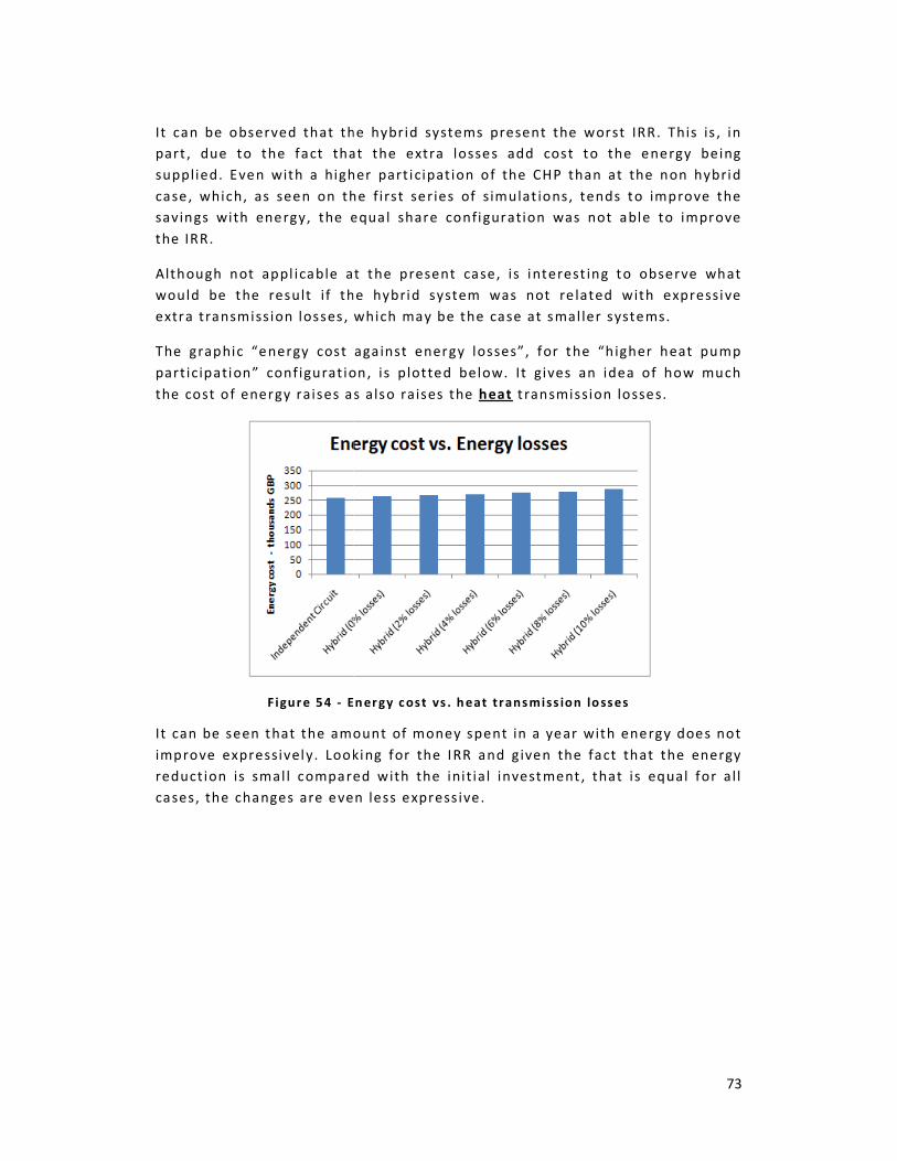
It can be observed that the hybrid systems present the

part , due to the fact that the extra losses add cost to the energy being

supplied. Even with a higher part icipat ion of the CHP than at the non hybrid

case, which, as seen on the f irst series of s imulat ions, tends to improve the

savings with energy, the equal share configuration was not able to improve

the IRR.

Although not appl icable at the present case, is interest ing to observe what

would be the result i f the hybrid system was not re lated with expressive

extra transmiss ion losses , which may be the case at smal ler systems.

The graphic “energy cost against energy losses

part icipation” configurat ion, is p lotted below. It gives an idea of how much

the cost of energy raises as

F igur e 54 - Ener gy cost vs . h

It can be seen that the amount of money sp

improve expressively. Looking for the IRR

reduction is smal l compared with the init ial investment , that is equal for al l

cases, the changes are even less expressive

It can be observed that the hybrid systems present the worst IRR. This is , in



e , which, as seen on the f i rst series of simulat ions, tends to improve the

savings with energy, the equal share configuration was not able to improve


f the hybrid system was not re lated with express ive

extra transmiss ion losses, which may be the case at smal ler systems.

energy cost against energy losses”, for the “higher heat pump

configuration, is plotted below. It gives an idea of how much

energy ra ises as also raises the heat t ransmission losses.

En er gy c ost vs . h eat trans miss ion lo ss es

It can be seen that the amount of money spent in a year with energy does not

improve express ively. Looking for the IRR and g iven the fact that the energy

reduct ion is small compared with the init ial investment , that is equal for al l

, the changes are even less express ive.

73

IRR. This is , in



e , which, as seen on the f i rst series of simulat ions, tends to improve the

savings with energy, the equal share configurat ion was not able to improve


f the hybrid system was not re lated with expressive

extra transmiss ion losses, which may be the case at smal ler systems.

h igher heat pump

configuration, is plotted below. It gives an idea of how much

ent in a year with energy does not

g iven the fact that the energy

reduction is small compared with the init ial investment , that is equal for al l

74

Figur e 55 - IRR vs. h eat transmiss ion lo ss es

The last point to be observed is the CO 2 emission reduction in each case.

Figur e 56 - CO 2 emis sion reduct ion

As said before, this analys is does present a f law: The assumption of al l

e lectr icity being sold to the gr id, as i t was electr ica l surplus. This gives

amazing advantage to CHP engines as CO2 emission reducers. The

configurat ions with higher CHP part icipat ion over the load presented the best

reduct ions . And in al l cases , the reduct ions were massive, above 40%. It is

relevant to know how much of the electr icity sold to the grid could be

internal ly used, which is imposs ib le unless generat ion and demand are

compared at an appropriate t ime step.

The power of s imulat ion becomes evident at these moments, al lowing to have

the results based at the instantaneous values, whenever necessary.

Through Trnsys , a routine able to compare at every 3 minutes the electrica l

generat ion and consumption of the system was created, permitt ing to

75

observe the origin of the ut i l ized energy or , in case of generation, it

dest ination.

The table with the uti l ized energy pr ices is shown below (10).

Energy Profit (pence per

kWh)

Electr icity sold to the grid 5.7

Electr icity sold to the bui ld ings 7.2

Electr icity sold to the heat pumps 0

Table 14 - electricity selling price

No e lectr icity wil l be sold to the grid if there is st i l l internal load to be

supplied.

Looking now for the internal energy consumption, the fol lowing prices wi l l be

applied (10) (17):

Energy Cost (pence per kWh)

E lectr icity purchased from the grid 7.2

Electr icity purchased from the CHP 0

Gas consumed by the CHP 2.1

Table 15 - purchased electricity price

CO2 emiss ion :

Energy Coefficient (kg of CO2 per kWh)

Electr icity from the grid 0.422

Electr icity sold to the grid (surplus) -0.568

Electr icity from CHP 0 ( i t wil l be counted at the gas

consumption)

Gas 0.194

Table 16 - emission coefficients

A new profi le can now be buil t. The graphic below wi l l compare the amount

of energy internal ly used and sold to the grid f rom the previous assumption

with the new method to calculate the energy f lux.

76

Figur e 57 - CHP el ectr ic i ty d est in at ion

Compar ing both analysi s is evident the change over the results obtained

init ial ly and the new ones. The high electr ica l consumption of the site makes

that a lmost al l the energy internally produced be a lso internally consumed.

This new analysis wi l l cause a reduction over the CO2 savings, given the fact

that a very smal l portion of the electr icity generated wi l l be considered as

displac ing energy produced somewhere else. The new values for CO2

reduct ion and renewable part icipation are shown below.

Figur e 58 – Three h eat sources: CO 2 r educt ion vs . r en ewabl e par ti c ipat ion

The CO2 reduct ion level , once the instantaneous analys is took place, made

the savings calculated drop from around 50% to 30%. This highl ights the

0

500

1000

1500

2000

2500

3000

3500

4000

En

erg

y g

en

era

ted

(M

Wh

)

Electrical production

Sold to the grid

Used on site

importance to make clear whether the

applied by any generated electr ica l energy or mu

surplus. At the previous analys is one of the hybrid conf igurat ion did had a

better CO2 reduct ion than the non hybrid one. This d ifference is not evident

at this moment anymore. Although the CHP production is sti l l higher , the

moments where it is generated ended up balancing both results. T iming the

heat generated not with the heating demand but based at moments of the

day where the electr ical consumption is low may be an option to improve

emiss ion savings, if needed. It wou

surplus, which can be sold to the grid and get the bonus of

There were no changes over the renewable part icipation once it does not

depend of the instantaneous value of any output

Having al l the options of CO

analys is of the internal rate of return wi l l be done against the renewable

share.

Fi gure 59 – Thr ee h eat sourc es:

During al l the results it was seen how running the CHP for longer periods

results on better energy savings. It is ref lected at the graphic above. With

simi lar initia l investment , the dif ference

depends almost exclusivel

electric ity be ing used internal ly, money i s being saved. It

kWh purchased from the grid , whi le sel l ing pays 5.

Economically, is more desirable to use the internal ly

than buy i t f rom an external source.

this t ime is h igher than the previous ones.

It is a lso interest ing to observe how renewable energy and costs are related.

The higher the amount of

internal rate of return. It is not exact ly a l inear relationship but may be

in mind while creat ing a control configurat ion.

importance to make clear whether the CO2 displacement factor can be

applied by any generated electr ica l energy or must be applied just in case of

At the previous analys is one of the hybrid conf igurat ion d id had a

reduct ion than the non hybrid one. This d ifference is not evident

at this moment anymore. Although the CHP production is st i l l higher, the

moments where i t is generated ended up balancing both results. T iming the

the heating demand but based at moments of the

day where the electr ical consumption is low may be an option to improve

emiss ion savings, if needed. It would raise the chance to have electr ical

can be sold to the gr id and get the bonus of CO2 di splacement .

There were no changes over the renewable part icipat ion once i t does not

depend of the instantaneous value of any output or input.

CO2 reduction above the selected target (20%) the


Three h eat sources: IRR vs. r enewable shar e

During al l the results i t was seen how running the CHP for longer per iods

savings. It is ref lected at the graphic above. With

simi lar init ia l investment , the dif ference between the internal rates of return

depends almost exclus ively of the energy savings . With almost al l the

electr icity being used internal ly, money is being saved. It costs 7.2 pence per

kWh purchased from the grid, whi le sel l ing pays 5.7 pence per kWh.

Economically, i s more desirable to use the internal ly generated electricity

than buy it from an external source. This expla ins why the IRR calculated at

this t ime is higher than the previous ones.

It is a lso interesting to observe how renewable energy and costs are related.

The higher the amount of energy extracted from the ground, the lower the

internal rate of return. It is not exact ly a l inear relationship but may be

while creating a control configurat ion.

77

displacement factor can be

st be applied just in case of

At the previous analys is one of the hybrid conf igurat ion d id had a

reduct ion than the non hybrid one. This d ifference is not evident

at this moment anymore. Although the CHP production is st i l l higher, the

moments where i t is generated ended up balancing both results. T iming the

the heating demand but based at moments of the

day where the electrical consumption is low may be an option to improve CO2

nce to have electr ical

displacement.

There were no changes over the renewable part icipat ion once it does not

reduction above the selected target (20%) the


During al l the results i t was seen how running the CHP for longer periods

savings. It is ref lected at the graphic above. With

between the internal rates of return

With almost al l the

costs 7.2 pence per

pence per kWh.

electr ici ty

This expla ins why the IRR calculated at

It is a lso interest ing to observe how renewable energy and costs are related.

, the lower the

internal rate of return. It is not exact ly a l inear relationship but may be kept

78

Changing the cool ing prior ity, as done before, may be a solut ion to move the

previous configurations to the right at the hor izontal axis , c loser to the 20%

target . But another interest ing change, in case the target of renewable

partic ipat ion is not so high, is to improve the CHP participat ion at the load,

looking forward a better internal rate of return or even CO2 emiss ion

reduct ion.

To observe how this last control option may affect the results , a new system

was created, as detai led next .

4.2.5. Fourth case: Interconnected circuits with higher

combined heat and power participation over the load.

The new system wil l have the fol lowing main characterist ics:

Heat ing

• I f the total system load is under 2MW, the demand wil l be suppl ied by

the energy generated by the CHP engine.

• I f the total system load is between 2 and 4 MW, the demand wil l be

supplied by the CHP and the open source heat pump, equal ly.


the heat pumps and the internal combustion machine, also equally.

• The electr icity produced by the CHP system wi l l be sold to the distr ict

bui ld ings, heat pumps and, in last case, to the gr id.

Cooling

• I f the tota l cooling load is below 1.4 MW, the total demand wi l l be


above this va lue, the open loop heat pump wi l l join the circuit .

• There wi l l be pr iority for the cooling load. In case of cooling and

heating being required at the same moment and with high demand,

meaning that the energy of just one heat pump won’t be enough, the

heat pumps wi l l supply exclusively the cooling load.

The extra 10% heating transmiss ion losses related with the higher

distances between sources and loads is st i l l being applied.

The load duration curve is shown below in order to make easier the

understanding of how this new configurat ion wi l l be working.

All the load distr ibution wi l l be done controll ing the water f low from the

bui ld ing to the storage tank of each system.

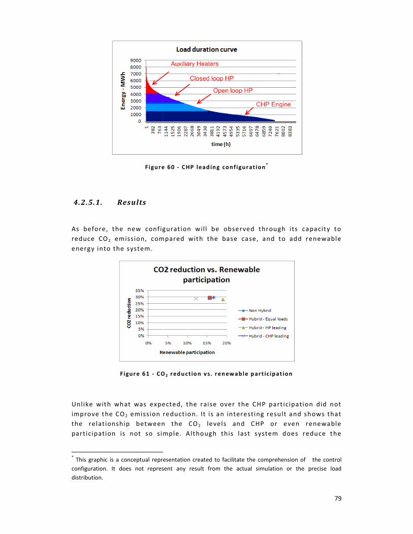
Fi gure

4.2.5.1. Results

As before, the new configurat ion wi l l be observed through its capacity to

reduce CO2 emiss ion, compared with the base case, and to add renewable

energy into the system.

Figur e 61 - CO

Unl ike with what was expected, the raise over the CHP part icipat ion did not

improve the CO2 emiss ion reduct ion. I t i s an interest ing result and shows that

the relat ionship between the

part icipation is not so simple. Although this last system does reduce the



distribution.

Figur e 60 - CHP lead in g conf igurat ion*

As before, the new conf igurat ion wil l be observed through its capacity to

emission, compared with the base case, and to add renewable

CO 2 red uct io n v s. ren ew ab le p art ic ipat ion

Unlike with what was expected, the raise over the CHP part icipation did not

emission reduct ion. It is an interest ing result and shows that

the relat ionship between the CO2 levels and CHP or even renewable

participat ion is not so s imple. A lthough this last system does reduce the

aphic is a conceptual representation created to facilitate the comprehension of the control


79

As before , the new conf igurat ion wil l be observed through i ts capacity to

emission, compared with the base case, and to add renewable

Unl ike with what was expected, the raise over the CHP part icipat ion did not

emission reduct ion. It is an interest ing result and shows that

renewable

part icipation is not so s imple. A lthough this last system does reduce the

aphic is a conceptual representation created to facilitate the comprehension of the control


emiss ion coeff icient related with the internally con

the amount of gas being burned,

heat generat ion. The balance between al l these var iat ions seems to be better

while CHP and HP are both supplying the same amount of heat during the

year.

Figur e 62

This graphic i l lustrates what was explained above. It was separated how much

of CO2 is being saved per kind of energy being consumed. The f irst case

observed the emiss ions re lated with th

the second focused on the e lectrical consumption emiss ions and the last

combined both, giving the result

With these results , and with the renewable share being below 20%, running

the system at the non hybrid mode seems to be a good option. Observing now

the IRR against the renewable share, the fol lowing graphic was generated.

F igur e 63 - Hybr id s yst em n ew conf igurat ion: IR R vs . r en ewab le share

The higher part icipat ion of the CHP system did return a better internal rate

of return. A target of 10% of renewable part icipat ion, for example , would

emiss ion coeff ic ient related with the internally consumed electr ici ty, it raises

the amount of gas being burned, improving the emiss ions re lated with the

heat generat ion. The balance between al l these var iat ions seems to be better


62 - CO 2 red uct io n p er en er gy t yp e


is being saved per kind of energy being consumed. The f irst case

observed the emissions related with the heating and cool ing consumpt ion,

the second focused on the electr ical consumption emissions and the last

combined both, giv ing the results observed before.


ybrid mode seems to be a good option. Observing now


H ybr id syst em n ew c onf i gurat ion: IRR vs . r en ewabl e share


of return. A target of 10% of renewable part icipat ion, for example , would

80

sumed electr icity, it raises

the emissions re lated with the

heat generat ion. The balance between al l these var iations seems to be better



is being saved per kind of energy being consumed. The f irst case

e heating and cool ing consumpt ion,

the second focused on the electr ical consumption emissions and the last


ybrid mode seems to be a good option. Observing now


H ybr id syst em n ew c onf igurat ion: IR R vs . r en ewab le shar e


of return. A target of 10% of renewable part icipation, for example, would

81

make the CHP leading configurat ion the best option between al l the previous

ones. It is true that the difference is not so expressive given the fact that the

init ial investment is set as the same.

A cr it ic that may be added here is that , actual ly, the hybr id system would

raise the complexity of the cooling/heating circuit , result ing into a higher

init ial cost. This extra value wasn’t applied because of the lack of information

over how much more the hybrid izat ion of the system would cost.

As observed before, looking for the renewable share target of 20%, a solution

that may occur to a designer may be the introduction of photovoltaic panels

to the system. I t has already been seen that, for th is distr ict , the energy

savings are not enough to overcome the ra ise of the needed in it ia l

investment caused by the high cost of the photovoltaic panels . It may be

interest ing to observe how much would be necessary to spend, and possible

benef its , to achieve the 20% share with each configurat ion opt ion through

the addit ion of photovolta ic panels .

A fourth configurat ion wi l l be also included.

4.2.6. Fifth case: Hybrid systems with photovoltaic cells.

This new case wi l l observe the impact of photovoltaic arrays over the

three previous hybr id system conf igurat ions and a fourth one.

Photovoltaic Panels

I t wi l l be ut i l i zed the Sanyo photovoltaic panel model HIP-190BA3, with peak

capacity of 190 W.

A t i lt of 55 degrees wi l l be applied, facing south.

The fourth hybrid system configurat ion

The fourth control configurat ion wil l work by the following criteria:

Heat ing

• I f the total system load is under 2MW, the demand wil l be suppl ied by

the open source heat pump.

• I f the total system load is between 2 and 4 MW, the demand wil l be

supplied by the open source heat pump and the CHP system, equal ly.


the heat pumps and the internal combustion machine, also equally.

82

• The electr icity produced by the CHP system wi l l be sold to the distr ict

bui ld ings, heat pumps and, in last case, to the gr id.

Cooling

• I f the tota l cooling load is below 1.4 MW, the total demand wi l l be


above this va lue, the open loop heat pump wi l l join the circuit .

• There wi l l be pr iority for the cooling load. In case of cooling and

heating being required at the same moment and with high demand,

meaning that the energy of just one heat pump won’t be enough, the

heat pumps wi l l supply exclusively the cooling load.

Figure 64 - HP-->CHP-->HP conf igurat ion*

4.2.6.1. Results

The photovolta ic panels were added in order to achieve the 20% renewable

share at each case. The tota l area required by each configuration is shown

below:

Control conf iguration Required photovoltaic area



distribution.

Non hybrid

Similar share of the load

Heat pump leading

CHP leading

HP �CHP�HP

Table

The total renewable share and internal rate of return obtained is shown

below, including a lso the va lues without the presence of any photovoltaic

array.

Figur e 65 - Hybr id syst em w ith phot ovolta ic: IR R vs. r enewab le shar e

Using the photovoltaic panels

obtained internal rate of return of most systems

pump leading conf iguration, where

was necessary.

8,000 m2

S imilar share of the load 10,000 m2

Heat pump leading 1,000 m2

15,000 m2

10,000m2

Table 17 - required photovoltaic array area



Hybr id s yst em w ith phot ovolta ic: IR R vs. r enewab le shar e

Using the photovolta ic panels to achieve the renewable target

obtained internal rate of return of most systems with except ion to the

pump leading conf igurat ion, where a smal ler amount of photovoltaic panels

83



Hybr id s yst em w ith phot ovolta ic: IR R vs. renewab le share

to achieve the renewable target sunk the

with except ion to the heat

amount of photovoltaic panels

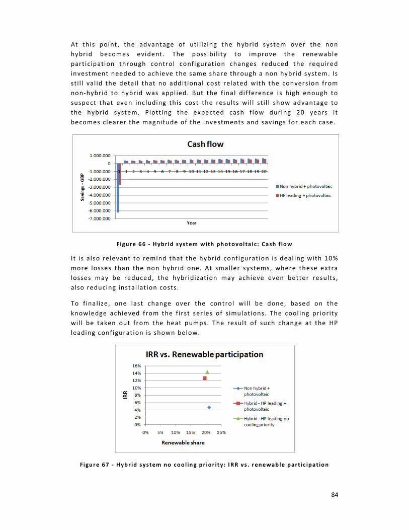
At this point , the advantage of ut i l i zing the hybrid system over the non

hybrid becomes evident. The possibi l ity to improve the renewable

part icipation through control configurat ion

investment needed to achieve the same share

st i l l val id the detai l that no addit ional cost related with the convers ion from

non-hybrid to hybrid was appl ied. But the f inal di

suspect that even including th is cost

the hybrid system. Plott ing the expected cash f low during 20 years it

becomes clearer the magnitude of the investments and savings for each case.

Figur e 66 - Hybr id s ystem w ith phot ovol ta ic: Cash f lo w

It is also relevant to remind that the hybrid configurat ion is deal ing with 10%

more losses than the non hybr id one. At smal ler systems, where these extra

losses may be reduced, the hybridizat ion may achieve even better results ,

also reducing instal lat ion costs .

To f ina lize, one last change over the control wi l l be done, based on the

knowledge achieved from the fi rst series of s imulations. The cool ing prior ity

wi l l be taken out from the heat pumps. The result of such change at the HP

leading configurat ion is shown below.

Figur e 67 - Hybr id s ystem no coo l in g pr ior i t y: IRR vs . r en ewab le part ic ipat ion

the advantage of uti l izing the hybrid system over the non

hybrid becomes evident. The possibi l i ty to improve the renewable

ontrol configurat ion changes reduced the required

investment needed to achieve the same share through a non hybrid system

sti l l va l id the detai l that no addit ional cost related with the convers ion from

hybr id to hybrid was appl ied. But the f ina l dif ference i s high enough to

t that even including this cost the results wil l sti l l show advantage to

Plotting the expected cash f low during 20 years it

the magnitude of the investments and savings for each case.

H ybr id syst em with phot ovol ta ic: Cash f lo w


more losses than the non hybrid one. At smal ler systems, where these extra

, the hybridization may achieve even better results ,

also reducing instal lat ion costs.

To f inal ize , one last change over the control wi l l be done, based on the

knowledge achieved from the f irst series of s imulations. The cool ing prior ity

from the heat pumps. The result of such change at the HP

leading configurat ion is shown below.

H ybr id sy st em no coo l in g pr ior it y: I RR vs . r en ewab le part ic ipat io n

84

the advantage of ut i l izing the hybrid system over the non

hybrid becomes evident. The possibi l ity to improve the renewable

reduced the required

through a non hybrid system. Is

st i l l va l id the detai l that no addit ional cost related with the convers ion from

high enough to

the results wil l st i l l show advantage to

Plotting the expected cash f low during 20 years i t

the magnitude of the investments and savings for each case.


more losses than the non hybrid one. At smal ler systems, where these extra

, the hybridization may achieve even better results ,

To f ina lize , one last change over the control wi l l be done, based on the

knowledge achieved from the f irst series of s imulations. The cool ing priority

from the heat pumps. The result of such change at the HP

Hybr id sy st em no coo l in g pr ior it y: IRR vs . r en ewable part ic ipat io n

85

The graphic shows how the same target could be achieved through different

methods and how the s imulat ion indicated a possib le best opt ion. The

capacity to analyze the results and how the load behaves for each change

done at the system allows the designer to visual ize the path that can be

fol lowed in order to optimize the system.

For the system being studied, this last conf igurat ion was able to provide al l

the set targets with the highest f inancial benefits and with a high difference

from the non hybr id system.

5. Conclusion

The new energy policies adopted by several countr ies, where targets of

renewable energy product ion and CO2 emiss ions levels are set, created a new

chal lenge for the energy suppliers: achieve those targets without

compromising the rel iabi l ity and profitabil ity of the energy supply. This is

especia l ly the case in the UK, with bui lding codes and local planning

requirements imposing increasingly stricter targets. The thesis went through

different steps of the design of a system aiming to achieve these targets for a

real case study, observing, at the end, possib le advantages brought by the

ut i l izat ion of a hybrid system. The performance of the dif ferent systems was

s imulated using the TRNSYS software, which al lows a dynamic s imulat ion of

the complex interact ion between component performance and control

strategies.

The most relevant observat ions are:

5.1. CO2 reduction and renewable energy fraction

A f irst point observed is the fact that , once these targets are set , is

important to have the methods of ca lculat ing them very clearly defined. If

these definit ions are easy to misunderstand or present flaws that can be

exploited, they wil l miss the point and not deliver the environmental benef its

that were deemed to be necessary when the CO2 and renewable energy

targets were set.

A good example of this could be eas ily observed when, in chapter 3, dif ferent

methods of calculat ing the CO 2 emission were compared. A d ifference of 20%

could be seen in some cases , which is 100% of the savings imposed by the

Edinburgh code for sustainable buildings, for example (3) .

A more broad study over the sensit iv ity of the CO2 emiss ion calculated would

be interesting, involving not just a part icular locat ion, as done at this thesis ,

but involving a series of consumers and producers. Maybe raising the total

86

load involved could result at changes not so signif icant at the CO2 emiss ion

calculated through each assumption.

A second point is the relevance of defining if heat pumps in cool ing mode

can be seen as a renewable technology or not. During the result analys is this

unclear posi tion led to the option of not including any possible benefit

brought by a heat pump to the system while it is working in the cool ing

mode. In many cases, this forced the ut i l izat ion of a second technology to

achieve the renewable target, with a negative impact over the economic

performance (as seen at f igures 47 and 65) .

With the current and expected growth of the UK heat pump market, this topic

should deserve specia l attent ion from the government. A clear definition of

renewable cooling is necessary, and might provide an extra boost to the heat

pump market if they are included in the def inition.

5.2. Advantages brought by combining technologies in a hybrid system

I t became clear how powerful the heat pumps can be when trying to achieve

the renewable targets or CHP while reducing the CO2 emiss ions (especial ly if

the reduction emiss ion factor i s appl ied to al l the generated energy) . At

chapter 4.1 the best f inancial result , between the systems that achieved both

CO2 and renewable targets , was obtained with the system including a 3.5 MW

heat pump + gas boiler as auxil iary heater. However, this solution was

obtained by relaxing the constra ints imposed by the real case study (the

available f low from the nearby r iver does not al low to provide heat for such a

large heat pump). Although interest ing and useful to understand how each

technology can contribute for each target , the result does not reflect the

constraints of the locat ion. But considering these constraints, which are

common to al l renewable energy technologies, reveals the interest and

importance of hybrid systems.

Through the introduction of a hybrid system design, the targets that before

were expensive to fulf i l became more achievable. The abil ity to work with a

more complex control creates the possibil ity to extract the most from each

technology involved, without compromising the reliabi l i ty of the system by

depending from just one source.

In chapter 4.2 , an attempt to use photovoltaic panels to meet the renewable

energy target resulted, as expected, in an unacceptably low internal rate of

return. Two options, though, achieved the target , reducing the IRR by a few

points but requir ing only some changes in the control strategy, without

s ignif icant extra capital costs. The solut ion was a control configurat ion where

the heat pumps were ut i l ized for the longest period possib le , with the CHP

act ing more as an auxi l iary system when the heating demand was too high,

with both technologies integrated into a hybrid system. The non-hybrid

87

system based on the same two technologies did not offer the same flexibi l ity

in control strategies, and resulted in a more expensive solution.

5.3. Combined heat and power and heat pumps in a hybrid system

Another aspect observed is the benefits of running CHP engines in a hybrid

system with water or ground source heat pumps. The f irst is able to not just

reduce the emiss ion levels of the system but a lso showed to be very f lexible

to accept the controls appl ied and with a helpful capacity to reduce the

energy costs ( in part caused by the high value paid for the electr icity

consumed from the gr id).

The heat pumps do present a high eff iciency but are l imited by the ground or

water source capacity to supply heat, making the CHP engine a good

candidate to work as the complementary source. Given the s ignif i cance of

heat demand in the total energy demand in the UK, heat pumps present a real

potential to de liver CO2 savings and renewable energy to meet the country’s

objectives, even without taking into account any “renewable cooling”.

5.4. The advantages of utilizing a simulation tool during the optimization

process

I t was very useful to be able to use a tool where, once a basic system was

created, small changes, involving less complexity or t ime spent, could be

done and the results of these changes rapidly obtained. The simulat ion tool

was able to compare different system configurations, component s iz ing, and

importantly di fferent control strategies which could be simulated in detai l .

Having a model of the whole system also al lowed to reject solut ion that

would have seem interest ing from an economical point of view but proved to

be technically unfeasible ( i .e. not able to meet the load) .

The discussion in chapter 3.1 revealed the relevance of taking into account

the energy generation and consumption using short t ime steps. TRNSYS

proved very f lexible to not just work with the required low t ime steps ( in this

case 3 minutes) but also to accept routines that would a lready del iver, as

result , the dest inat ion of the generated energy. It should also be noted that ,

although this was outside the scope of this study, it would have been

possible to model the bui ld ings together with the systems rather than using

an est imated load profi le.

The f lexibi l ity of the tool did have a cost which i s the complexity involving its

ut i l izat ion. The learning curve is a steep one, and the use of such a program

might be considered as too t ime-consuming for a designer deal ing with tight

deadl ines. The program also requires a thorough understanding of the

88

components and control strategies and does not offer the same level of user

comfort as s impler tools that provide a unique answer to a design problem.

One interest ing opt ion for future work is to develop more user-friendly user

interfaces based on basic systems configurat ions. Such interfaces would al low

users not famil iar ised with a complex tool l i ke TRNSYS to modify a few key

design parameters, saving t ime during the design process and avoiding the

need to tra in every designer in the use of a complex s imulat ion tool .

89

References

1. Jones, G., 2004. People and Environment: A Global Approach. New York: Pearson Prentice

Hall.

2. Smith, J.T, Beresfold, N.A., 2006. Chernobyl - Catastrophe and consequences. Springer Praxis

Books.

3. The planning comitee city of Edinburgh council, 2006. Edinburgh standards for sustainable

buildings.Edinburgh, UK. Available on the web at :

http://www.edinburgh.gov.uk/internet/environment/planning_buildings_i_i_/

4. Fisher, Daniel E., et al., 2006. Implementation and Validation of Ground-Source Heat Pump

System Models in an Integrated Building and System Simulation Environment. HVAC&R

RESEARCH. Vol. 12.

5. Oschner, K., 2008. Geothermal heat pumps - a guide for planning & installing. London :

Earthscan.

6. Sirchis, J., 1990. Combined production of heat and power: Cogeneration. New York : Elsevier

Applied Science.

7. Gentry, Jason E., et al., 2006. Simulation of Hybrid Ground Source Heat Pump Systems and

Experimental Validation. 7th International Conference on System Simulation in Buildings. Liége,

December 2006.

8. Ramamoorthy, M., et al., 2001. Optimal Sizing of Hybrid Ground- Source Heat Pump Systems

that Use a Cooling Pond as Supplemental Heat Rejector – A Systematic Simulation Approach.

ASHRAE Transactions.Vol 107 (1):p26-38.

9. Hackel, Scott, Nellis, Gregory and Klein, Sanford., 2008 Optimization of hybrid geothermal

heat pump system. 9th International IEA Heat Pump Conference , Zürich, Switzerland . May

2008.

10. BRE, 2008. SAP 2005 - The Government's Standard Assessment Procedure for Energy Rating

of Dwellings - 2005 edition, revision 2 (Version 9.82, June 2008). Building Research

Establishment, Garston, UK. Available on the web at: http://projects.bre.co.uk/sap2005/

11. DEFRA, 2008. Guidelines to Defra’s Greenhouse Gas (GHG) Conversion Factors for Company

Reporting - Annexes, June 2008. Department for Environment, food and rural affairs, London,

UK. Available on the web at:

http://www.defra.gov.uk/environment/business/envrp/conversion-factors.htm

12. Department of Trade and Industry , 2003 . Our energy future - creating a low carbon

economy. The Stationery Office. Available on web at: www.tso.co.uk/bookshop

13. Department of Trade and Industry, 2007. Meeting the energy challenge - a A white paper

on energy. The Stationery Office. Available on web at: www.tso.co.uk/bookshop

90

14. Greater London Authority, 2006. Sustainable design and construction - The london plan

suplementary planning guidance. London : Greater London Authority. Available on web at:

www.london.gov.uk.

15. BERR. Renewable Heat, 2007. [Online]. Available at:

http://www.berr.gov.uk/energy/sources/renewables/policy/renewable-heat/page15963.html

[Accessed: 10 09 2008.]

16. Sorensen, B. Renewable Energy- Its physics, engineering, environmental impacts,

economics & planning. Third edition. 2004.

17. Department for business enterprise and regulatory reform, 2008. Quaterly energy prices -

June. National Statistics. Available on web at:

http://www.berr.gov.uk/energy/statistics/publications/prices/index.html

18. Alter systems, 2008. Alter system on line shop. [Online]. Available at:

http://www.altersystems.com/catalog/index.php. [Accessed: 10 09 2008.]

19. Affordable solar, 2008. Sanyo HIP-200BA3 200W Solar Panel. [Online] Available at:

http://www.affordable-solar.com/Sanyo.HIP.200BA3.200W.PV.Module.htm [Accessed : 10 09

2008.].

20. Photovoltaic systems - Technologies and applications, 2008. PV resources. [Online]

Available at: http://www.pvresources.com/.[Accessed: 10 09 2008.]

21. Smisth, K.R., Kaltschmitt, M. and Thrän, D. , 2001. Renewable energy from biomass.

Contribution for the Encyclopedia of Physical Science and Technology. Academic Press, San

Diego, California, USA.

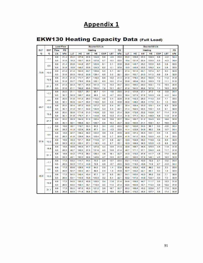
91

Appendix 1

92

Appendix 2

Hybrid heating and cooling system optimisation with TRNSYS · Hybrid heating and cooling system...

Documents

Transcript of Hybrid heating and cooling system optimisation with TRNSYS · Hybrid heating and cooling system...