
Hybrid Attitude Control and Estimation On SO(3)
198
Western University Western University Scholarship@Western Scholarship@Western Electronic Thesis and Dissertation Repository 11-29-2017 4:00 PM Hybrid Attitude Control and Estimation On SO(3) Hybrid Attitude Control and Estimation On SO(3) Soulaimane Berkane, The University of Western Ontario Supervisor: Tayebi, Abdelhamid, The University of Western Ontario A thesis submitted in partial fulfillment of the requirements for the Doctor of Philosophy degree in Electrical and Computer Engineering © Soulaimane Berkane 2017 Follow this and additional works at: https://ir.lib.uwo.ca/etd Part of the Acoustics, Dynamics, and Controls Commons, Controls and Control Theory Commons, and the Navigation, Guidance, Control and Dynamics Commons Recommended Citation Recommended Citation Berkane, Soulaimane, "Hybrid Attitude Control and Estimation On SO(3)" (2017). Electronic Thesis and Dissertation Repository. 5083. https://ir.lib.uwo.ca/etd/5083 This Dissertation/Thesis is brought to you for free and open access by Scholarship@Western. It has been accepted for inclusion in Electronic Thesis and Dissertation Repository by an authorized administrator of Scholarship@Western. For more information, please contact [email protected].
Transcript of Hybrid Attitude Control and Estimation On SO(3)
Western University Western University
Scholarship@Western Scholarship@Western
Electronic Thesis and Dissertation Repository
11-29-2017 4:00 PM
Hybrid Attitude Control and Estimation On SO(3) Hybrid Attitude Control and Estimation On SO(3)
Soulaimane Berkane, The University of Western Ontario
Supervisor: Tayebi, Abdelhamid, The University of Western Ontario
A thesis submitted in partial fulfillment of the requirements for the Doctor of Philosophy degree
in Electrical and Computer Engineering
© Soulaimane Berkane 2017
Follow this and additional works at: https://ir.lib.uwo.ca/etd
Part of the Acoustics, Dynamics, and Controls Commons, Controls and Control Theory Commons, and
the Navigation, Guidance, Control and Dynamics Commons
Recommended Citation Recommended Citation Berkane, Soulaimane, "Hybrid Attitude Control and Estimation On SO(3)" (2017). Electronic Thesis and Dissertation Repository. 5083. https://ir.lib.uwo.ca/etd/5083
This Dissertation/Thesis is brought to you for free and open access by Scholarship@Western. It has been accepted for inclusion in Electronic Thesis and Dissertation Repository by an authorized administrator of Scholarship@Western. For more information, please contact [email protected].
Abstract
This thesis presents a general framework for hybrid attitude control and estimation de-
sign on the Special Orthogonal group SO(3). First, the attitude stabilization problem
on SO(3) is considered. It is shown that, using a min-switch hybrid control strategy de-
signed from a family of potential functions on SO(3), global exponential stabilization on
SO(3) can be achieved when this family of potential functions satisfies certain properties.
Then, a systematic methodology to construct these potential functions is developed. The
proposed hybrid control technique is applied to the attitude tracking problem for rigid
body systems. A smoothing mechanism is proposed to filter out the discrete behaviour
of the hybrid switching mechanism leading to control torques that are continuous.
Next, the problem of attitude estimation from continuous body-frame vector mea-
surements of known inertial directions is considered. Two hybrid attitude and gyro bias
observers designed directly on SO(3) × R3 are proposed. The first observer uses a set
of innovation terms and a switching mechanism that selects the appropriate innovation
term. The second observer uses a fixed innovation term and allows the attitude state to
be reset (experience discrete transition or jump) to an adequately chosen value on SO(3).
Both hybrid observers guarantee global exponential stability of the zero estimation errors.
Finally, in the case where the body-frame vector measurements are intermittent, an
event-triggered attitude estimation scheme on SO(3) is proposed. The observer consists
in integrating the continuous angular velocity during the interval of time where the vector
measurements are not available, and updating the attitude state upon the arrival of the
vector measurements. Both cases of synchronous and asynchronous vector measurements
with possible irregular sampling periods are considered. Moreover, some modifications
to the intermittent observer are developed to handle different practical issues such as
discrete-time implementation, noise filtering and gyro bias compensation.
ii

To all those whom I love...
iii

Acknowledgement
I would like to express my deepest gratitude to my advisor, Professor Abdelhamid Tayebi,
for his support, motivation and guidance throughout the four years I have spent at
Western University. He taught me what it meant to be a high quality researcher who
carries fundamental values such as honesty, vision, passion and rigorousness. His timely
feedback and suggestions helped me to smoothly conduct my research and write my
thesis.
I am grateful to my friend, colleague and collaborator, Dr. Abdelkader Abdessameud,
with whom I have completed several parts of this research and shared countless discus-
sions in the research field. I am also thankful to my alternate supervisor at Western, Dr.
Ilia Polushin, who have helped me in several occasions.
I would also like to sincerely thank Prof. Jin Jiang and Dr. Lyndon Brown for taking
the time to serve as my PhD thesis examiners and for their constructive comments and
feedback.
I would especially like to thank Prof. Andrew R. Teel from the University of California
Santa Barbara for agreeing to review and examine my thesis. I have had several fruitful
discussions with him during our meetings at CDC and ACC conferences.
Lastly, I would like to extend my sincere appreciation to my family. To my mother,
Chahrazed, my sisters and my friends for their support and prayers in all my pursuits.
And of course, to my wife, Intissar, for her love, support and understanding.
iv

List of Symbols
• N and N>0 denote the natural and strictly positive natural numbers, respectively.
• R, R≥0 and R>0 denote the real, nonnegative and positive real numbers, respec-
tively.
• Rn is the n-dimensional Euclidean space .
• Rn×m is the set of real-valued n×m matrices.
• Given A ∈ Rn×m, A> denotes its transpose.
• Given A ∈ Rn×n, det(A) denotes its determinant.
• Given A ∈ Rn×n, tr(A) denotes the sum of its diagonal entries (trace).
• GivenA,B ∈ Rn×m, their Euclidean inner product is defined as 〈〈A,B〉〉 = tr(A>B).
• Given A ∈ Rn×m, its Frobenius norm is ‖A‖F =√〈〈A,A〉〉.
• Given x ∈ Rn, its Euclidean norm (2-norm) is given by ‖x‖ =√x>x.
• Sn = x ∈ Rn+1 : ‖x‖ = 1 is the unit n-sphere embedded in Rn+1.
• B = x ∈ Rn : ‖x‖ ≤ 1 is the closed unit ball in Euclidean space.
• SO(3) = R ∈ R3×3 : det(R) = 1, RR> = R>R = I is the Special Orthogonal
group of order 3 where I denotes the three-dimensional identity matrix.
• so(3) = Ω ∈ R3×3 : Ω> = −Ω is the set of all skew-symmetric 3× 3 matrices and
defines also the Lie algebra of SO(3).
• Q = (η, ε) ∈ R× R3 : η2 + ε>ε = 1 is the set of unit quaternions.
• Given a rotation matrix R ∈ SO(3), let us define |R|I = ‖I −R‖/√
8.
• The map E : R3×3 → R3×3 is defined as E(M) = 12(tr(M)I −M>).
• The map Ra : R × S2 → SO(3) is defined as Ra(θ, u) = I + sin(θ)[u]× + (1 −cos(θ))[u]2×.
• The map Ru : Q→ SO(3) is defined as Ru(η, ε) = I + 2[ε]2× + 2η[ε]×.
v

• The map Rr : R3 → SO(3) is defined as Rr(z) = 11+‖z‖2
((1− ‖z‖2)I + 2zz> + 2[z]×
).
• The map PSO(3) : R3×3 → SO(3) is defined as the projection of X ∈ R3×3 on SO(3)
(i.e. closest rotation matrix to X).
• The map Pso(3) : R3×3 → so(3) is defined as Pso(3)(M) = (M −M>)/2.
• The map [·]× : R3 → so(3) is defined as [x]×y = x × y for all x, y ∈ R3 where ×denotes the cross product on R3.
• The map vex : so(3)→ R3 is the inverse map of [·]×.
• The map ψ : R3×3 → R3 is defined as ψ = vex Pso(3) where the symbol is used
to denote function composition.
• The set ΠSO(3) = R ∈ SO(3) : tr(R) 6= −1 is the set of all rotations with an angle
different than 180. In other words, ΠSO(3) = SO(3) \Ra(π,S2).
• The set ΠQ = (η, ε) ∈ Q : η 6= 0 is the double cover of ΠSO(3) in Q.
• The map Pc : R3×R3 → R3, for a given c ∈ R≥0, defines the parameter projection
function which is given in (2.3).
• Given a set S, cl(S) denotes its closure (S together with all of its limit points).
• A set-valued map F :M⇒ N assigns to every x ∈M a set of values F(x) ⊆ N .
• Let F : M ⇒ N be a set-valued function. The domain of F is defined as the set
domF = x ∈M : F(x) 6= ∅ where ∅ denotes the empty set.
• Cn(M,N ) is the set of all functions f : M → N such that the first n ∈ Nderivatives of each function f ∈ Cn(M,N ) exist and are continuous.
vi
Contents
Abstract ii
Acknowlegements iv
List of Symbols v
List of Figures xi
1 Introduction 1
1.1 General Introduction . . . . . . . . . . . . . . . . . . . . . . . . . . . . . 1
1.2 Attitude Control . . . . . . . . . . . . . . . . . . . . . . . . . . . . . . . 2
1.3 Attitude Estimation . . . . . . . . . . . . . . . . . . . . . . . . . . . . . 5
1.4 Thesis Contributions . . . . . . . . . . . . . . . . . . . . . . . . . . . . . 7
1.5 List of Publications . . . . . . . . . . . . . . . . . . . . . . . . . . . . . . 10
1.6 Thesis Outline . . . . . . . . . . . . . . . . . . . . . . . . . . . . . . . . . 12
2 Background and Preliminaries 14
2.1 General Notations . . . . . . . . . . . . . . . . . . . . . . . . . . . . . . . 14
2.2 Rigid Body Attitude . . . . . . . . . . . . . . . . . . . . . . . . . . . . . 16
2.2.1 Attitude Parametrizations . . . . . . . . . . . . . . . . . . . . . . 18
2.2.1.1 Exponential Coordinates Representation . . . . . . . . . 18
2.2.1.2 Angle-Axis Representation . . . . . . . . . . . . . . . . . 19
2.2.1.3 Unit Quaternions Representation . . . . . . . . . . . . . 20
2.2.1.4 Rodrigues Vector Representation . . . . . . . . . . . . . 21
2.2.2 Metrics on SO(3) . . . . . . . . . . . . . . . . . . . . . . . . . . . 21
2.2.3 Attitude Visualization . . . . . . . . . . . . . . . . . . . . . . . . 23
2.2.4 Useful Identities and Lemmas . . . . . . . . . . . . . . . . . . . . 24
2.3 Hybrid Systems Framework . . . . . . . . . . . . . . . . . . . . . . . . . 28
2.3.1 Exponential Stability for Hybrid Systems . . . . . . . . . . . . . . 30
2.4 Numerical Integration Tools . . . . . . . . . . . . . . . . . . . . . . . . . 32
vii
2.4.1 Numerical Integration on Rn . . . . . . . . . . . . . . . . . . . . . 33
2.4.2 Numerical Integration on SO(3) . . . . . . . . . . . . . . . . . . . 34
2.4.3 Numerical Integration of Hybrid Systems . . . . . . . . . . . . . . 35
3 Hybrid Attitude Control on SO(3) 37
3.1 Introduction . . . . . . . . . . . . . . . . . . . . . . . . . . . . . . . . . . 37
3.2 Motivation Using Planar Rotations on S1 . . . . . . . . . . . . . . . . . . 38
3.3 Attitude Stabilization on SO(3) . . . . . . . . . . . . . . . . . . . . . . . 47
3.3.1 Problem Formulation . . . . . . . . . . . . . . . . . . . . . . . . . 47
3.3.2 Smooth Attitude Stabilization on SO(3) . . . . . . . . . . . . . . 48
3.3.3 Synergistic and Exp-Synergistic Potential Functions . . . . . . . . 51
3.3.4 Hybrid Attitude Stabilization on SO(3) . . . . . . . . . . . . . . . 53
3.3.5 Construction of Exp-Synergistic Potential Functions . . . . . . . . 55
3.3.6 Illustration of the Switching Mechanism . . . . . . . . . . . . . . 64
3.4 Attitude Tracking for Rigid Body Systems . . . . . . . . . . . . . . . . . 66
3.4.1 Problem Formulation . . . . . . . . . . . . . . . . . . . . . . . . . 66
3.4.2 Smooth Attitude Tracking on SO(3) . . . . . . . . . . . . . . . . 67
3.4.3 Hybrid Attitude Tracking on SO(3) . . . . . . . . . . . . . . . . . 69
3.4.4 Simulations . . . . . . . . . . . . . . . . . . . . . . . . . . . . . . 71
3.5 Conclusion . . . . . . . . . . . . . . . . . . . . . . . . . . . . . . . . . . . 74
4 Hybrid Attitude Estimation on SO(3) 76
4.1 Introduction . . . . . . . . . . . . . . . . . . . . . . . . . . . . . . . . . . 76
4.2 Attitude Estimation Using Continuous Vector Measurements . . . . . . . 77
4.2.1 Problem Formulation . . . . . . . . . . . . . . . . . . . . . . . . . 77
4.2.2 Synergistic-Based Approach . . . . . . . . . . . . . . . . . . . . . 79
4.2.3 Reset-Based Approach . . . . . . . . . . . . . . . . . . . . . . . . 83
4.2.4 Simulations . . . . . . . . . . . . . . . . . . . . . . . . . . . . . . 88
4.3 Attitude Estimation Using Intermittent Vector Measurements . . . . . . 90
4.3.1 Problem Formulation . . . . . . . . . . . . . . . . . . . . . . . . . 91
4.3.2 Attitude Estimation Using Synchronous Vector Measurements . . 93
4.3.3 Attitude Estimation Using Asynchronous Vector Measurements . 96
4.3.4 Practical Considerations . . . . . . . . . . . . . . . . . . . . . . . 98
4.3.4.1 Discrete-Time Implementation . . . . . . . . . . . . . . 98
4.3.4.2 Estimation Algorithms with Enhanced Filtering . . . . . 100
4.3.4.3 Smoothing of the Estimator Output . . . . . . . . . . . 103
4.3.4.4 Gyro Bias Compensation . . . . . . . . . . . . . . . . . 104
viii

4.3.5 Simulations . . . . . . . . . . . . . . . . . . . . . . . . . . . . . . 107
4.4 Conclusion . . . . . . . . . . . . . . . . . . . . . . . . . . . . . . . . . . . 111
5 Conclusion 113
5.1 Summary . . . . . . . . . . . . . . . . . . . . . . . . . . . . . . . . . . . 113
5.2 Perspectives . . . . . . . . . . . . . . . . . . . . . . . . . . . . . . . . . . 116
Bibliography 118
A Proofs of Lemmas 129
A.1 Proof of Lemma 2.2.1 . . . . . . . . . . . . . . . . . . . . . . . . . . . . . 129
A.2 Proof of Lemma 2.2.2 . . . . . . . . . . . . . . . . . . . . . . . . . . . . . 130
A.3 Proof of Lemma 2.2.3 . . . . . . . . . . . . . . . . . . . . . . . . . . . . . 130
A.4 Proof of Lemma 2.2.4 . . . . . . . . . . . . . . . . . . . . . . . . . . . . . 131
A.5 Proof of Lemma 2.2.5 . . . . . . . . . . . . . . . . . . . . . . . . . . . . . 132
A.6 Proof of Lemma 2.2.6 . . . . . . . . . . . . . . . . . . . . . . . . . . . . . 132
A.6.1 Proof of Lemma 2.2.7 . . . . . . . . . . . . . . . . . . . . . . . . . 134
A.7 Proof of Lemma 2.2.8 . . . . . . . . . . . . . . . . . . . . . . . . . . . . . 134
A.8 Proof of Lemma 3.3.9 . . . . . . . . . . . . . . . . . . . . . . . . . . . . . 135
A.9 Proof of Lemma 3.3.12 . . . . . . . . . . . . . . . . . . . . . . . . . . . . 136
A.10 Proof of Lemma 3.3.13 . . . . . . . . . . . . . . . . . . . . . . . . . . . . 137
A.11 Proof of Lemma 3.3.14 . . . . . . . . . . . . . . . . . . . . . . . . . . . . 139
B Proofs of Propositions 141
B.1 Proof of Proposition 3.2.1 . . . . . . . . . . . . . . . . . . . . . . . . . . 141
B.2 Proof of Proposition 3.2.2 . . . . . . . . . . . . . . . . . . . . . . . . . . 143
B.3 Proof of Proposition 3.3.10 . . . . . . . . . . . . . . . . . . . . . . . . . . 143
B.4 Proof of Proposition 3.3.15 . . . . . . . . . . . . . . . . . . . . . . . . . . 147
B.5 Proof of Proposition 3.3.16 . . . . . . . . . . . . . . . . . . . . . . . . . . 148
B.6 Proof of Proposition 3.4.3 . . . . . . . . . . . . . . . . . . . . . . . . . . 150
B.7 Proof of Proposition 4.2.6 . . . . . . . . . . . . . . . . . . . . . . . . . . 153
B.8 Proof of Proposition 4.2.7 . . . . . . . . . . . . . . . . . . . . . . . . . . 154
C Proofs of Theorems 156
C.1 Proof of Theorem 2.3.3 . . . . . . . . . . . . . . . . . . . . . . . . . . . . 156
C.2 Proof of Theorem 3.3.1 . . . . . . . . . . . . . . . . . . . . . . . . . . . . 159
C.3 Proof of Theorem 3.3.8 . . . . . . . . . . . . . . . . . . . . . . . . . . . . 159
C.4 Proof of Theorem 3.4.4 . . . . . . . . . . . . . . . . . . . . . . . . . . . . 161
ix
C.5 Proof of Theorem 3.4.5 . . . . . . . . . . . . . . . . . . . . . . . . . . . . 163
C.6 Proof of Theorem 4.2.3 . . . . . . . . . . . . . . . . . . . . . . . . . . . . 166
C.7 Proof of Theorem 4.2.4 . . . . . . . . . . . . . . . . . . . . . . . . . . . . 168
C.8 Proof of Theorem 4.3.1 . . . . . . . . . . . . . . . . . . . . . . . . . . . . 172
C.9 Proof of Theorem 4.3.2 . . . . . . . . . . . . . . . . . . . . . . . . . . . . 175
C.10 Proof of Theorem 4.3.3 . . . . . . . . . . . . . . . . . . . . . . . . . . . . 178
C.11 Proof of Theorem 4.3.4 . . . . . . . . . . . . . . . . . . . . . . . . . . . . 178
Curriculum Vitae 183
x
List of Figures
2.1 Coordinate systems: I (inertial reference frame) and B (body-attached
frame). . . . . . . . . . . . . . . . . . . . . . . . . . . . . . . . . . . . . . 16
2.2 Euclidean distance (red dashed) and Geodesic distance (green solid). . . 22
2.3 Visualization of 3D rotations using the body-frame unit axesR(t)e1, R(t)e2
and R(t)e3. The initial body frame is plotted in dashed and the final body
frame is plotted in bold. The trajectory is generated using the angular
velocity ω(t) = [e−t, e−2t, e−3t]> with R(0) = I and t ∈ [0, 20] seconds. . . 23
2.4 Visualization of 3D rotations using the exponential coordinates. The tra-
jectory is generated using the angular velocity ω(t) = [− sin(t), 0, 0.3 cos(t)]>
with R(0) = I and t ∈ [0, 10] seconds. . . . . . . . . . . . . . . . . . . . . 24
2.5 Visualization of 3D rotations using the angle-axis representation. The tra-
jectory is generated using the angular velocity ω(t) = [− sin(t), 0, 0.3 cos(t)]>
with R(0) = I and t ∈ [0, 10] seconds. . . . . . . . . . . . . . . . . . . . . 24
3.1 Control problem of planar rotations on S1. . . . . . . . . . . . . . . . . . 39
3.2 The Euclidean (Geodesic) distance between x and e1 plotted in dashed red
(solid green). . . . . . . . . . . . . . . . . . . . . . . . . . . . . . . . . . 40
3.3 Vector fields on S1 with control input ω = −x2 (potential function ΦE(x)).
The desired critical point e1 is plotted in green and the undesired critical
point −e1 is plotted in red. . . . . . . . . . . . . . . . . . . . . . . . . . . 41
3.4 Vector fields on S1 with control input ω = −f(x1)x2 (potential function
ΦG(x)). The desired critical point e1 is plotted in green and the singular
point −e1 is plotted in red. . . . . . . . . . . . . . . . . . . . . . . . . . . 42
3.5 Hybrid control on the unit circle S1 with two modes of operation. The
first (second) controller is allowed to activate on the red (blue) region.
The point c1 (c2) represents an undesired critical or singular point of the
first (second) controller. . . . . . . . . . . . . . . . . . . . . . . . . . . . 43
xi

3.6 Plot of the original potential function ΦE(x) (left) and the new composite
potential functions ΦE(Γ(x, 1)) and ΦE(Γ(x, 2)) (right) with k = 1/4. The
synergistic gap δ∗ between the two potential functions is equal to 16/9. . 46
3.7 Synergistic hybrid switching mechanism. . . . . . . . . . . . . . . . . . . 54
3.8 Plot of the attitude potential functions Ψ1 and Ψ2 with their corresponding
gradients norm for different values of the attitude angle (attitude axis is
fixed). The potential function Ψ1 has an undesired critical point at θ = π
while the attitude potential function Ψ2 is singular at θ = π. . . . . . . . 57
3.9 Plot of the function Ψ1 Γ(R(θ), q) (solid blue) for different values of q
along the path R(θ) = Ra(θ, [1, 2, 3]>/√
14) with θ ∈ [0, 2π], k = 0.7 and
um = em,m = 1, 2, 3. The gray filled area indicates when (R, q) ∈ JTand the white area indicates when (R, q) ∈ FT . The sets FT and JT are
defined in (3.46)-(3.47) with Φ = Ψ1 Γ and δ = 0.12. Note that all
critical points, marked with a circle, are contained in the jump set JT .
The downward arrows indicate that at a given critical point, q can be
switched to decrease the value of potential function Ψ1 Γ(R, q). . . . . . 59
3.10 Plot of the function Ψ2 Γ(R(θ), q) (solid blue) for different values of q
along the path R(θ) = Ra(θ, [1, 2, 3]>/√
14) with θ ∈ [0, 2π], k = 0.7 and
um = em,m = 1, 2, 3. The gray filled area indicates when (R, q) ∈ JTand the white area indicates when (R, q) ∈ FT . The sets FT and JTare defined in (3.46)-(3.47) with Φ = Ψ2 Γ and δ = 0.46. Note that
all singular points, marked with a cross, are contained in the jump set
JT . The downward arrows indicate that at a given critical point, q can be
switched to decrease the value of potential function Ψ2 Γ(R, q). . . . . . 60
3.11 The feasible region of the synergy condition (3.65) . . . . . . . . . . . . . 62
3.12 Plot of the potential function Φ(R, q) (first row) and its gradient’s norm
(second row) along the trajectories Ri(θ), i = 1, 2, 3, which passes through
the singular/critical points of Φ(R, 1). . . . . . . . . . . . . . . . . . . . . 65
3.13 Hybrid attitude tracking algorithm using an exp-synergistic potential func-
tion Φ : SO(3)×Q → R≥0. . . . . . . . . . . . . . . . . . . . . . . . . . . 69
3.14 Smoothed hybrid attitude tracking algorithm using an exp-synergistic po-
tential function Φ : SO(3)×Q → R≥0. . . . . . . . . . . . . . . . . . . . 71
3.15 Total attitude tracking error (Euclidean distance) versus time. . . . . . 72
3.16 Norm of the angular velocity tracking error versus time. . . . . . . . . . 72
3.17 True Euler angles (colored) and desired Euler angles (dashed) versus time. 73
3.18 Total attitude tracking error (Euclidean distance) versus time. . . . . . 73
xii
3.19 Norm of the angular velocity tracking error versus time. . . . . . . . . . 74
3.20 Torque components versus time. . . . . . . . . . . . . . . . . . . . . . . 74
3.21 Switching variable versus time. Note that the initial value is q(0, 0) = 2.
The hybrid controller immediately switches to the configuration q = 5 at
the start. . . . . . . . . . . . . . . . . . . . . . . . . . . . . . . . . . . . . 75
4.1 Schematic of the synergistic-based hybrid attitude and gyro bias observer
using algebraic attitude reconstruction. This estimation scheme can be
implemented using any exp-synergistic potential function Φ. . . . . . . . 81
4.2 Schematic of the synergistic-based hybrid attitude and gyro bias observer
using directly vector measurements (without the need to algebraically re-
construct the attitude). . . . . . . . . . . . . . . . . . . . . . . . . . . . . 83
4.3 Schematic of the reset-based hybrid attitude and gyro bias observer . . . 86
4.4 Angular velocity ω(t). . . . . . . . . . . . . . . . . . . . . . . . . . . . . 89
4.5 Attitude estimation error for the proposed hybrid observers. . . . . . . . 90
4.6 Gyro-bias estimation error for the proposed hybrid observers. . . . . . . . 91
4.7 Switching variable q for the synergistic-based hybrid observer. . . . . . . 91
4.8 Behaviour of the virtual variable τ (timer) introduced in (4.36)-(4.37). At
the arrival of a new measurement, the timer is reset back to zero (dashed
red) and flows linearly otherwise (blue solid). . . . . . . . . . . . . . . . 95
4.9 Behaviour of the virtual variables τ1 and τ2 (timers) introduced in (4.42)-
(4.49). The transmission (measurement) times tik with i ∈ 1, 2 satisfy
the constraints (4.28)-(4.29) with T 11 = 0.5, T 1
2 = 1.5, T 21 = 1 and T 2
2 = 3.
At the arrival of a measurement bi the corresponding timer τi is reset back
to zero. . . . . . . . . . . . . . . . . . . . . . . . . . . . . . . . . . . . . 97
4.10 Plot of the available information for the x-axis component of b1. Both
measurements of b1 and b2 are synchronously obtained at the same instants
of time. . . . . . . . . . . . . . . . . . . . . . . . . . . . . . . . . . . . . 108
4.11 Time evolution of the attitude estimation error (angle of rotation) of the
attitude estimation scheme proposed in Algorithm 1 using different values
of N . The region between 90s and 100s is enlarged. . . . . . . . . . . . . 108
4.12 Plot of the available information for the x-axis component of b1 (top) and
b2 (bottom). The measurements are collected asynchronously at different
sampling rates. . . . . . . . . . . . . . . . . . . . . . . . . . . . . . . . . 109
xiii
4.13 Time evolution of the attitude estimation error (angle of rotation) of the
attitude estimation scheme proposed in Algorithm 2 using different values
of N . The region between 90s and 100s is enlarged. . . . . . . . . . . . . 110
4.14 Time evolution of the attitude estimation error (angle of rotation) for the
observer proposed in (4.72)-(4.73) using different sampling periods T . . . 112
4.15 Time evolution of the bias estimation error for the observer proposed in
(4.72)-(4.73) using different sampling periods T . The region between 0
and 0.5 seconds is enlarged. . . . . . . . . . . . . . . . . . . . . . . . . . 112
xiv

Chapter 1
Introduction
1.1 General Introduction
Many mechanical systems can be modelled as a rigid body or an interconnection of
multiple rigid bodies. For instance, most aerospace and marine vehicles such as Un-
manned Aerial Vehicles (UAVs), Spacecraft, Satellite and Autonomous Underwater Ve-
hicles (AUVs) can be considered as rigid body systems. Robotic arms composed of
multiple rigid links and joints, also known as robot manipulators, are an example of
rigid multi-body systems which are used in various applications including welding au-
tomation, manufacturing, robotically-assisted surgery and space stations robotic arms.
The assumption of rigidity, which means non-deformation under the action of applied
forces, for these class of mechanical systems is very important to simplify the analysis
and controller design. In fact, the configuration of a rigid body can be fully described by
translation and rotation of a reference frame attached to the body. This is in contrast
to bodies that display fluid, elastic, and plastic behavior which require more parameters
to describe their configuration [Terzopoulos et al., 1987, Davatzikos, 1997, Elger and
Roberson, 2013].
The design of efficient attitude control algorithms is of great importance for success-
ful applications involving accurate positioning of rigid body systems such as satellites
and spacecraft. These control schemes are (roughly speaking) of proportional-derivative
type, where the proportional action is in terms of the orientation (attitude) and the
derivative action (generating the necessary damping) is in terms of the angular velocity.
In contrast to the angular velocity which can be directly measured using gyroscopes,
there are no sensors that directly measure the orientation. This fact calls for the de-
velopment of suitable attitude estimation algorithms that reconstruct the attitude using
appropriate sensors such as inertial measurement units (IMUs) that provide measure-
1
2 Chapter 1. Introduction
ments in the body-attached frame of some known inertial vectors. Consequently, the
attitude estimation and control problems have been the focus of many researchers from
the aerospace and control communities, which led to a large body of work since 1960’s.
These fundamental problems come with many theoretical and practical challenges related
to the topology of the motion space SO(3). Among, these challenges, the non-existence
of global continuous time-invariant attitude estimation and control schemes on compact
manifolds [Koditschek, 1988, Sanjay P. Bhat, 2000], which motivated the development
of new alternatives such as the hybrid techniques that will be the focus of this thesis.
This thesis proposes a general framework for the design of hybrid attitude control
and estimation algorithms. Within this framework, the global (singularity-free) attitude
representation as a rotation matrix on SO(3) is used. Using this coordinate-free rep-
resentation of the attitude, all the pitfalls of other attitude representations such as the
Euler angles, Rodrigues parameters and the unit quaternions are avoided.
1.2 Attitude Control
The rigid body attitude control problem has received a growing interest during the last
decades, with various applications in aerospace, marine engineering, and robotics see, for
instance, [Kreutz and Wen, 1988, Joshi et al., 1995, Pettersen and Egeland, 1999, Hughes,
1986, Tayebi and McGilvray, 2006]. Attitude control schemes can be categorized by the
choice of the attitude parametrization, such as Euler-angles, unit quaternion, Rodrigues
parameters and rotation matrices. The natural (intrinsic) representation of the attitude
is done using rotation matrices on SO(3) (9 parameters). Early works on attitude con-
trol have focused on the use of less number of parameters to represent the attitude. This
is motivated mainly by the need to save computational power and reduce the analy-
sis complexity. The minimum number of parameters to represent the attitude is three.
Examples of these 3-dimensional parametrizations are the Euler angles, the exponential
coordinates and the Rodrigues parameters. However, as shown in [Stuelpnagel, 1964],
it is topologically impossible to represent the attitude globally without singular points
using only 3 parameters. For instance, the angular velocity cannot be extracted (glob-
ally) from the Euler angles rates due to the singularity of transformation matrix relating
the time derivatives of the Euler angles to the angular velocity. This is a mathemat-
ical kinematic singularity which is often referred to as the gimbal lock [Hoag, 1963].
The Rodrigues parameters representation is also a three-parameters attitude represen-
tation, which allows to represent all attitudes except those of 180. This geometric
singularity implies that continuous control laws which use this representation are not
1.2. Attitude Control 3
globally defined. The unit-quaternion representation is a four-parameters attitude rep-
resentation which describes the attitude globally (singularity-free) compared to other
three-parameters representations. This has motivated their wide use in many practi-
cal applications to represent the rigid-body attitude. For example, quaternion feedback
has been used in spacecraft control [Wie et al., 1989, Wie and Barba, 1985], manip-
ulators control [Yuan, 1988], robot writs [Salcudean, 1988] and aerial vehicles [Tayebi
and McGilvray, 2006]. A comprehensive study of unit quaternion feedback control ap-
pears in [Wen and Kreutz-Delgado, 1991] where different quaternion-based control laws
have been investigated and compared. The controllers share the common structure of
a proportional-derivative feedback plus some feedforward Coriolis torque compensation
and/or adaptive compensation. Different robust [Joshi et al., 1995], adaptive [Egeland
and Godhavn, 1994], velocity-free [Lizarralde and Wen, 1996, Tayebi, 2008] quaternion
feedbacks have been also developed in the past decades. The main drawback of using
the unit-quaternion representation is the fact that every attitude can be represented,
equivalently, by two different quaternions. This nonuniqueness in representing the atti-
tude, if not taken carefully, might result in quaternion-based controllers with undesirable
phenomena such as the so-called unwinding phenomenon 1 [Sanjay P. Bhat, 2000]. There
have been some attempts to design quaternion-based attitude control systems that do
not suffer from the unwinding phenomena by introducing discontinuities, see for instance
[Thienel and Sanner, 2003]. However, these discontinuous attitude control systems suffer
from non-robustness to arbitrary small measurement disturbances as discussed in [May-
hew and Teel, 2011a]. In [Mayhew, 2010, Mayhew et al., 2011], hybrid controllers have
been proposed to ensure robust global asymptotic stabilization via quaternion feedback.
Also, other hybrid techniques where used in [Mayhew, 2010] to remove the ambiguity in
selecting the best quaternion to represent an attitude measurement on SO(3).
With the advance of computational ressources and the fact that all existing parame-
terizations fail to represent the attitude of a rigid body both globally and uniquely, which
results in control schemes that are either singular or exhibit some undesirable behavior,
recent trends in attitude control have focused on the use of rotation matrices on SO(3)
[Koditschek, 1988, Sanyal et al., 2009, Chaturvedi et al., 2011, Lee, 2012, Bayadi and
Banavar, 2014]. The group SO(3) has the distinct feature of being a boundaryless com-
pact manifold with a Lie group structure that allows the design and analysis of attitude
control systems within the well established framework of geometric control [Bullo, 2005].
The group SO(3) is not diffeomorphic to any Euclidean space and hence there does not
1The unwinding phenomenon refer to the situation where the rigid body may start arbitrary close tothe desired orientation yet rotates through large angles before converging to the desired attitude.

4 Chapter 1. Introduction
exist any continuous time-invariant feedback on SO(3) that achieves global asymptotic
stability [Sanjay P. Bhat, 2000]. In [Koditschek, 1988], for instance, a continuous time-
invariant control scheme has been shown to asymptotically track any smooth reference
attitude trajectory starting from arbitrary initial conditions except from a set of Lebesgue
measure zero. This is referred to as almost global asymptotic stability, and is mainly
due to the appearance of undesired critical points (equilibria) when using the gradient
of a smooth potential function in the feedback. In fact, any smooth potential function
on SO(3) is guaranteed to have at least four critical points where its gradient vanishes
[Morse, 1934].
In [Mayhew and Teel, 2011b], a hybrid feedback scheme has been proposed to over-
come the topological obstruction to global asymptotic stability on SO(3) and, at the
same time, ensure some robustness to measurement noise. The main idea in the latter
paper is to design a hybrid algorithm based on a family of smooth potential functions
and a hysteresis-based switching mechanism that selects the appropriate control action
corresponding to the minimal potential function. It was shown that a sufficient condi-
tion to avoid the undesired critical points, and ensure global asymptotic stability, is the
“synergism” property of the smooth potential functions. A family of potential functions
on SO(3) is said to be synergistic if at each critical point (other than the desired one) of
a potential function in the family, there exists another potential function in the family
that has a lower value. Moreover, if all the potential functions in the family share the
identity element I3×3 as a critical point then it is called a centrally synergistic family.
Thanks to the hysteresis gap, this type of hybrid controllers guarantee robustness to
small measurement noise. Despite the originality of the proposed hybrid control frame-
work, unfortunately, the search for families of potential functions on SO(3) enjoying the
synergism property is not a straightforward task.
The angular warping technique has been used in [Mayhew and Teel, 2011d] to con-
struct a central synergistic family of potential functions on SO(3) where the synergistic
property is verified by computation only. Although in [Casau et al., 2015b], necessary
and sufficient conditions for this family of potential functions to be synergistic were de-
rived, the major drawback of the angular warping approach is related to the difficulty
of determining the synergistic gap which is required for the implementation of the hy-
brid controller. In an attempt to solve this problem the authors in [Mayhew and Teel,
2013a] tried to relax the centrality assumption by considering scaled, biased and trans-
lated modified trace functions. However, the sufficient synergism conditions provided
therein were conservative, difficult to satisfy and only hand tuning of the parameters was
proposed. Another form of non-central synergistic potential functions appeared in [Lee,
1.3. Attitude Estimation 5
2015], by comparing the actual and desired directions, leading to a simple expression of
the synergistic gap. It is important to mention here that, in contrast to the non-central
approach, the control algorithm derived from each potential function in the central syn-
ergistic family guarantees (independently) almost global asymptotic stability results. It
is also worth pointing out that non-central and central synergistic potential functions
have been considered in [Mayhew and Teel, 2013b] and [Casau et al., 2015a] to ensure,
respectively, global asymptotic and global exponential stabilization on the n-dimensional
sphere. However, the extension of these approaches to the full attitude control problem
on SO(3) is not straightforward.
1.3 Attitude Estimation
It is unfortunate that there is no sensor that can provide direct measurements of a
rigid body’s attitude. Nevertheless, there exist many sensors (depending on the appli-
cation at hand) that provide partial information about the rigid body’ orientation. For
instance the attitude of a rigid body can be recovered (reconstructed) using available
body-frame measurements of known inertial directions. Small size UAVs are usually
equipped with IMUs that typically include accelerometers and magnetometers, which
provide body-referenced coordinates of the gravity vector and the Earth’s magnetic field,
respectively. For satellites, sun sensors and star trackers are usually used to provide
body-frame measurements of known inertial directions. The problem of determining the
attitude of a rigid body from vector measurements has been addressed, initially, as an
optimization problem, also known as Wahba’s problem [Wahba, 1965]. A great deal of
research work has been devoted to solving Wahba’s problem, see for instance [Shuster
and Oh, 1981, Markley, 1988]. However, these static attitude reconstruction techniques
are hampered by their inability to handle measurement noise. To overcome this problem,
researchers looked for dynamic estimators where other measurements (such as angular
velocity measurements) are used along with body-frame vector measurements to recover
the attitude while filtering measurement noise. The gist of the idea is that the angu-
lar velocity can be integrated to estimate the attitude in the short-term, and then make
long-term corrections using vector measurements. This leads to an attitude estimate that
is less vulnerable to vibrations (because gyroscopes are accurate at high frequencies) and
immune to long-term drift (because vector measurements are more reliable at low fre-
quencies). Dynamic estimators can be, roughly speaking, classified into two categories:
stochastic estimators (based on Kalman filtering techniques) and nonlinear estimators
(based on nonlinear observer design techniques).

6 Chapter 1. Introduction
Stochastic estimators are usually variants of the Extended Kalman Filter and can be
found in many references such as [Markley, 2003, Crassidis et al., 2007, Choukroun, 2009])
for quaternion-based filtering and [Markley, 2006, Barrau and Bonnabel, 2015, Mueller
et al., 2016, Barrau and Bonnabel, 2017] for rotation matrix-based filtering. Unfortu-
nately, the available stochastic attitude estimators have only locally proven stability and
performance properties (see for instance [Barrau and Bonnabel, 2017]). Recently, a new
class of dynamic nonlinear attitude estimators (observers) has emerged [Mahony et al.,
2008], and proved its ability in handling large rotational motions and measurement noise.
This approach, coined nonlinear complementary filtering, was inspired from the linear at-
titude complementary filters, e.g., [Tayebi and McGilvray, 2006], used to recover (locally)
the attitude using gyro measurements and body-frame measurements of known inertial
vectors. The smooth nonlinear complementary filters, such as those proposed in [Mahony
et al., 2008], are directly designed on SO(3) and are proved to guarantee almost global
asymptotic stability (AGAS), which is as strong as the SO(3) space topology could per-
mit. These smooth nonlinear observers ensure the convergence of the estimated attitude
to the actual one from almost all initial conditions except from a set of critical points
of zero Lebesgue measure. It has been noted, for instance in [Lee, 2012, Tse-Huai Wu
and Lee, 2015, Zlotnik and Forbes, 2017], that starting from a configuration close to
the undesired critical points, results in a slow convergence to the actual attitude. This
observation has been formally proven in our recent work [Berkane and Tayebi, 2017a].
Further performance and robustness improvements for the complementary filtering ap-
proach have also been proposed recently in [Zlotnik and Forbes, 2016, Zlotnik and Forbes,
2017] and in [Berkane and Tayebi, 2017a]. On the other hand, a class of (SO(3) non-
preserving) attitude observers has been proposed in [Batista et al., 2012a, Batista et al.,
2012b] leading to global stability results. Theses observers provide an attitude estimate
that is not confined to live in SO(3) but tends to it as time goes to infinity. A non-central
hybrid attitude observer on SO(3) has been proposed in [Tse-Huai Wu and Lee, 2015]
with global asymptotic stability. The term non-central means that individual observers
(from the family of observers used in the hybrid scheme) do not, in general, guarantee
(on their own) any estimation stability results (even locally). The design of globally
exponentially stable observers on SO(3) is an open problem that has been solved in this
thesis using hybrid techniques.
In the field of attitude estimation, most existing research developments consider either
continuous measurements or regular synchronous discrete measurements. The attitude
is not directly measurable, it is obtained from the fusion of different measurements from
sensors with (possibly) different bandwidths and subject to packet dropouts. For in-

1.4. Thesis Contributions 7
stance, landmark measurements using vision systems are obtained at much lower rates
than the vector measurements obtained from an IMU. Also, GPS readings are often used
in attitude estimation algorithms when linear accelerations are not negligible, such as in
[Hua, 2010, Roberts and Tayebi, 2011, Martin and Salaun, 2008]. These readings are
obtained at much lower rates compared to onboard IMU measurements. Therefore, it is
interesting to design attitude estimation algorithms that take into account these practi-
cal constraints. State estimation using intermittent observations dates back to the early
work that appeared in [Nahi, 1969, Hadidi and Schwartz, 1979]. Different versions of the
Kalman filter for linear systems with intermittent measurements have been discussed in
recent papers, see for instance [Smith and Seiler, 2003, Sinopoli et al., 2004, Plarre and
Bullo, 2009]. This problem is relevant when fusing sensors with multiple bandwidths
and/or observing a system over a sensor network in which the sensor and controller are
communicating over an unreliable link or a network subject to packets loss. In a deter-
ministic setting, observer design for state estimation of linear time-invariant systems and
some special classes of nonlinear systems with Lipschitz nonlinearities in the presence of
sporadically available measurements have been recently proposed in [Raff and Allgower,
2007, Andrieu et al., 2013, Ferrante et al., 2016]. In the context of attitude estima-
tion, the authors in [Barrau and Bonnabel, 2015] proposed an intrinsic attitude filter on
SO(3) with (synchronous) discrete-time measurements of two vector observations. The
proposed discrete invariant observer is shown to be almost globally convergent. In [Khos-
ravian et al., 2015], by exploiting the symmetry of the group SO(3), a predictor has been
proposed to continuously predict the intermittent vector measurements using forward
integration on SO(3) of the continuous angular velocity measurements. The measure-
ments are allowed to be asynchronous (multirate) and subject to known constant delays.
The proposed predictor can be, independently, combined with any asymptotically stable
attitude/filter such as the explicit complementary filter [Mahony et al., 2008].
1.4 Thesis Contributions
For general hybrid systems such as those modelled in the framework of [Goebel et al.,
2009, Goebel et al., 2012], new Lyapunov-based sufficient conditions for exponential sta-
bility are proposed. The derived conditions relax the conditions presented in [Teel et al.,
2013, Theorem 1] in the sense that the Lyapunov function is allowed to increase during
either the flow or the jump. This relaxation comes at the cost of imposing some condi-
tions on the hybrid time domain where solutions exist. The newly proposed sufficient
conditions are later used to prove some of the results presented in this thesis.

8 Chapter 1. Introduction
A new framework for global exponential stabilization on SO(3) is proposed. Our
framework can be seen as an extension to the work of [Mayhew, 2010, Mayhew and
Teel, 2011b, Mayhew and Teel, 2011d] on synergistic feedback on SO(3). In the former
work, synergistic potential functions are shown to be sufficient for the design of hybrid
controllers guaranteeing global asymptotic stability. In this work, a new class of poten-
tial functions, coined exp-synergistic, is proposed and shown to be sufficient for global
exponential stabilization on SO(3). Moreover, a systematic methodology for the construc-
tion of these exp-synergistic potential functions is provided [Berkane and Tayebi, 2017e].
Note that in [Mayhew and Teel, 2011d] only existence results are reported for synergistic
potential functions. Moreover, exp-synergism allows for non-everywhere differentiable
potential functions to be used which presents an andvantage over the synergism concept.
In fact, controllers derived from non-smooth potential functions have been shown to en-
sure better performance compared to those derived from traditional smooth potential
functions, see for instance [Lee, 2012, Zlotnik and Forbes, 2017] where nonsmooth poten-
tial functions on SO(3) have been used to improve the performance of existing attitude
control and estimation schemes. Using these hybrid tools, a hybrid control algorithm
that ensures global exponential tracking of any attitude trajectory is derived [Berkane
et al., 2017b]. To the best of our knowledge, global exponential tracking on SO(3) has
never been achieved before. Moreover, since discontinuities in the control might be un-
desirable in practical applications, a smoothing mechanism that moves the discontinuity
in the control one integrator behind is proposed. In other words, the jumps in the hybrid
controller are filtered and do not appear in the control torque. This smoothing approach
is simpler than the one proposed in [Mayhew and Teel, 2013a] and can be implemented
using only a first order low pass filter.
In the field of attitude estimation from continuous measurements, two hybrid estima-
tion schemes guaranteeing both global exponential stability of the attitude and gyro-bias
estimation errors are proposed [Berkane et al., 2017a, Berkane and Tayebi, 2017b]. Both
observers have a general structure of a nonlinear complementary filter on SO(3) × R3
where the attitude estimate evolves on SO(3) and the gyro-bias vector evolves on R3.
The first observer approach uses a synergistic-based technique to generate a family of
observer innovation terms among which the appropriate term is selected according to
the evolution of the estimates. Each innovation (correction) term is nothing but a gra-
dient of some cost function. A switching mechanism allows to jump to the innovation
term that generates the minimum cost function while avoiding the undesired critical and
singular points. An adequate choice of the cost function allows to express this hybrid
observer using directly body-frame vector measurements of known constant inertial di-
1.4. Thesis Contributions 9
rections without the need for attitude reconstruction. The second observer approach uses
a fixed innovation term but allows for the attitude state to jump (reset) to an adequately
selected value whenever the difference between the current cost function and the post
cost function (value of the cost function after a possible reset) exceeds certain threshold.
This threshold is selected in a way such that all undesired critical and singular points
of the cost function lie in the set where the observer states are reset. The proposed
reset-based hybrid observer can be directly expressed using body-frame measurements of
know, possibly time-varying, inertial vectors.
The problem of attitude estimation from intermittent measurements have been for-
mulated and tackled using measurement-triggered observers [Berkane and Tayebi, 2017d,
Berkane and Tayebi, 2017c]. First, in the case where the body-frame measurements
are collected synchronously at the same instants of time, an attitude observer on SO(3)
is proposed which consists of a forward integration of the continuous angular velocity
(propagation), and a jump equation (update) that uses the collected measurements to
reset the rotation estimate to a value guaranteeing a smaller estimation error. This es-
timation scheme has a similar structure as the one proposed in [Barrau and Bonnabel,
2015] but with the use of the Rodrigues map instead of the exponential map to simplify
the design. In the case where the measurements are collected asynchronously (not arriv-
ing at the same time) the update equation is executed at each instant of time where a
new measurement arrives. Although this problem can also be tackled using the predictor
based approach of [Khosravian et al., 2015], our approach is a predictor-free solution that
uses only a single vector measurement at a time to correct the attitude estimate, thus
saving memory and computation. To analyze the behaviour of the proposed attitude
estimation schemes, the closed-loop systems are extended with virtual timers which are
reset to zero at the arrival time of a new measurement. Each timer is allowed to flow
linearly when the corresponding measurement is not available. The extended closed-loop
system is modelled as an autonomous hybrid system and almost global exponential, re-
spectively asymptotic, stability is proved for the synchronous, respectively asynchronous,
measurement-triggered observers. Some practical issues related to the implementation of
the proposed estimation schemes are discussed which resulted in different extensions and
modifications to the original algorithms. The first tackled issue is the discrete time imple-
mentation of the proposed estimation schemes. The observers are discretized using first
order Euler-Lie method [Celledoni et al., 2014]. Interestingly, the interconnection of the
discrete version of the observer with a discrete approximation of the kinematic attitude
equation yields an almost globally convergent estimator. This property is strong and
does not hold, in general, for most existing continuous attitude estimators on SO(3) such
10 Chapter 1. Introduction
as [Mahony et al., 2008]. Secondly, for both observers (synchronous and asychronous) the
attitude estimate is further refined (filtered) through an averaging procedure on SO(3) us-
ing a shift register (containing the previous attitude estimates). A similar averaging idea
was proposed in [Brodtkorb et al., 2015] for a system evolving on the Euclidean space R6
where recursive states were introduced to filter out the noise in the intermittent position
and velocity measurements used as input to an observer for marine vessels. In the case
where the measurements are updated at very low frequencies, the discrete transitions in
the attitude state might become undesirable. In this case, the estimation scheme can
be smooth out by combing the intermittent observer with a smoother on SO(3) without
affecting the stability properties. Finally, the practical problem of biased angular velocity
measurements is considered. In this case the intermittent attitude observer is extended
with a measurement-triggered bias estimation scheme. In the case where the measure-
ments are synchronously available with a regular sampling, local exponential stability of
the overall closed-loop system is shown.
1.5 List of Publications
The material presented in this work is based on the following publications, including
submitted and under review papers:
Journal Articles
1. S. Berkane, A. Abdessameud and A. Tayebi, ”Hybrid Global Exponential Stabi-
lization on SO(3)”, Automatica, Vol. 81, pp. 279–285, 2017.
2. S. Berkane and A. Tayebi, ”Construction of Synergistic Potential Functions on
SO(3) with Application to Velocity-Free Hybrid Attitude Stabilization”, IEEE Trans-
actions on Automatic Control, Vol. 62, No. 1, pp. 495–501, 2017.
3. S. Berkane, A. Abdessameud and A. Tayebi, ”Hybrid Attitude and Gyro-bias
Observer on SO(3)”, IEEE Transactions on Automatic Control, (to appear), 2017.
4. S. Berkane and A. Tayebi, ”Attitude Estimation with Intermittent Measurements”,
Automatica (Submission No. 17-0878), 2017.
Peer-Reviewed Conference Proceedings
1. S. Berkane and A. Tayebi, “Attitude Observer Using Synchronous Intermittent
1.5. List of Publications 11
Vector Measurements”, In Proceedings of the 56th IEEE Conference on Decision
and Control (CDC), Melbourne, Australia, 2017.
2. S. Berkane and A. Tayebi, “A Globally Exponentially Stable Hybrid Attitude and
Gyro-bias Observer”, In Proceedings of the 55th IEEE Conference on Decision and
Control (CDC), Las Vegas, USA, 2016, pp. 308-313.
3. S. Berkane, A. Abdessameud and A. Tayebi, “Global Hybrid Attitude Estimation
on the Special Orthogonal Group SO(3)”, In Proceedings of the 2016 American
Control Conference, Boston, USA, 2016, pp. 113-118.
4. S. Berkane and A. Tayebi, “On the Design of Synergistic Potential Functions on
SO(3)”, In Proceedings of the 54th IEEE Conference on Decision and Control,
December 15-18, 2015. Osaka, Japan, pp. 270-275.
In addition, the work in the following papers has been carried out during the same period
of time and is not included in this thesis:
Journal Articles
1. S. Berkane and A. Tayebi, ”On the Design of Attitude Complementary Filters on
SO(3)”, IEEE Transactions on Automatic Control, 2017, (to appear).
2. S. Berkane, A. Abdessameud and A. Tayebi, ”Hybrid Output Feedback For Atti-
tude Tracking on SO(3)”, IEEE Transactions on Automatic Control (Submission
No. 16-1824), 2016.
Peer-Reviewed Conference Proceedings
1. S. Berkane and A. Tayebi, “Attitude and Gyro Bias Estimation Using GPS and
IMU Measurements”, In Proceedings of the 56th IEEE Conference on Decision and
Control (CDC), Melbourne, Australia, 2017.
2. S. Berkane, A. Abdessameud and A. Tayebi, “Global Exponential Angular Velocity
Observer for Rigid Body Systems”, In Proceedings of the 55th IEEE Conference on
Decision and Control (CDC), Las Vegas, USA, 2016, pp. 4154-4159.
3. S. Berkane, A. Abdessameud and A. Tayebi, “On Deterministic Attitude Ob-
servers on the Special Orthogonal Group SO(3)”, In Proceedings of the 55th IEEE
Conference on Decision and Control (CDC), Las Vegas, USA, 2016, pp. 1165-1170.
12 Chapter 1. Introduction
4. S. Berkane and A. Tayebi, “Velocity-Free Hybrid Attitude Stabilization Using In-
ertial Vector Measurements”, In Proceedings of the 2016 American Control Con-
ference, Boston, USA, 2016, pp. 6048-6053.
5. S. Berkane and A. Tayebi, “Some Optimization Aspects on the Lie Group SO(3)”,
In Proceedings of the 15th IFAC Symposium on Information Control Problems in
Manufacturing, May 11-13, 2015, Ottawa, Canada, pp. 1173-1177.
1.6 Thesis Outline
This thesis is organized as follows:
Chapter 2 introduces the mathematical background and preliminary results that are
used throughout the thesis. Section 2.1 provides the general notations used in this thesis.
Section 2.2 describes the rigid body attitude, attitude parametrizations, attitude metrics,
attitude visualization and useful identities and lemmas, some of which are newly derived
in this work. Section 2.3 presents the hybrid systems framework used in this work and
gives new relaxed conditions for exponential stability in hybrid systems. Finally, Section
2.4 presents some tools for numerical integration and simulation both on the Euclidean
and the rotation group and for hybrid systems as well.
Chapter 3 presents a framework for global exponential stabilization on the rotation
group SO(3) via hybrid feedback. After an introduction, Section 3.2 explains the topolog-
ical obstruction for global asymptotic stabilization on compact manifolds by considering
the simple example of the unit circle S1. This example also motivates the hybrid feedback
tools used in this work. Section 3.3 discusses the drawbacks of smooth stabilization on
SO(3) and introduces the concept of exp-synergism as well as the main structure of a hy-
brid synergistic feedback that achieves global exponential stability on SO(3). Systematic
methodologies for the construction of exp-synergistic potential functions from existing
smooth and nonsmooth potential functions on SO(3) are presented. Section 3.4 applies
the concept of hybrid synergistic feedback to the attitude tracking problem and simula-
tion results are provided to illustrate the effectiveness of the proposed control algorithms.
Chapter 4 is devoted to the attitude estimation problem on SO(3) using continu-
ous/intermittent measurements. Section 4.2 presents two techniques for the design of
globally exponentially stable attitude and gyro-bias observers on SO(3). The first tech-
1.6. Thesis Outline 13
nique uses exp-synergistic potential functions to derive different innovation terms for
the observer while the second technique is based on resetting the attitude matrix to an
adequate value if the current estimation error provides a “large” enough cost. Section
4.3 deals with the problem of attitude estimation from intermittent (sporadic) vector
observations. Both cases of synchronous and asynchronous measurements are treated.
Simulation results are provided in both sections to illustrate the effectiveness of the pro-
posed estimation algorithms.
Chapter 5 summarizes the findings of this thesis and presents some possible future
directions.
Appendices A, B and C give the detailed proofs for all the lemmas, propositions
and theorems, respectively, stated throughout the thesis.

Chapter 2
Background and Preliminaries
2.1 General Notations
For a general orthonormal basis V = v1, · · · , vn of Rn we use the notation x =
[x1, · · · , xn]>V if x =∑n
i=1 xivi. In particular, the notation x = [x1, · · · , xn]> is used when
x is represented with respect to the canonical (standard) basis of Rn denoted by ei1≤i≤n.
The ordered standard basis e1, · · · , en, along with the origin point x = [0, · · · , 0]> ∈ Rn
defines the Cartesian coordinate system on Rn. For a given square matrix A ∈ Rn×n,
the set Eλ(A) denotes the set of all eigenvalues of A. Note that if A is symmetric, all
the eigenvalues of A are real and thus Eλ(A) ⊂ R. The set Ev(A) denotes the set of
unit eigenvectors of A and ERv (A) corresponds to the set of real unit eigenvectors of
A. For simplicity, when Eλ(A) ⊂ R, the set of eigenvalues of A is ordered such that
λA1 ≤ λA2 · · · ≤ λAn where λAi is the i-th eigenvalue of A. In this case, λAmin and λAmax will
denote the smallest and largest eigenvalues of A, respectively. Moreover, for v ∈ Ev(A),
λAv denotes the eigenvalue of A associated to the eigenvector v. If a = [a1, a2, a3]>V and
b = [b1, b2, b3]>V are vectors in R3 expressed in the orthonormal basis V = v1, · · · , vn,then their cross product can be written as [Arfken et al., 1999]
a× b =∑m,n,l
εmnlambnvl, (2.1)
where εmnl is the Levi-Cevita symbol defined by
εmnl =
0 for m = n,m = l or n = l
+1 for (m,n, l) ∈ (1, 2, 3), (2, 3, 1), (3, 1, 2)−1 for (m,n, l) ∈ (1, 3, 2), (3, 2, 1), (2, 1, 3)
. (2.2)
14
2.1. General Notations 15
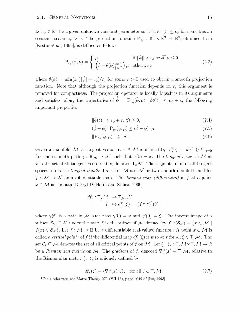
Let φ ∈ Rn be a given unknown constant parameter such that ‖φ‖ ≤ cφ for some known
constant scalar cφ > 0. The projection function Pcφ : R3 × R3 → R3, obtained from
[Krstic et al., 1995], is defined as follows:
Pcφ(φ, µ) =
µ if ‖φ‖ < cφ or φ>µ ≤ 0(I − θ(φ) φφ
>
‖φ‖2
)µ otherwise
. (2.3)
where θ(φ) = min(1, (‖φ‖ − cφ)/ε) for some ε > 0 used to obtain a smooth projection
function. Note that although the projection function depends on ε, this argument is
removed for compactness. The projection operator is locally Lipschitz in its arguments
and satisfies, along the trajectories of˙φ = Pcφ(φ, µ), ‖φ(0)‖ ≤ cφ + ε, the following
important properties
‖φ(t)‖ ≤ cφ + ε, ∀t ≥ 0, (2.4)
(φ− φ)>Pcφ(φ, µ) ≤ (φ− φ)>µ, (2.5)
‖Pcφ(φ, µ)‖ ≤ ‖µ‖. (2.6)
Given a manifold M, a tangent vector at x ∈ M is defined by γ′(0) := dγ(τ)/dτ |τ=0
for some smooth path γ : R≥0 → M such that γ(0) = x. The tangent space to M at
x is the set of all tangent vectors at x, denoted TxM. The disjoint union of all tangent
spaces forms the tangent bundle TM. Let M and N be two smooth manifolds and let
f : M → N be a differentiable map. The tangent map (differential) of f at a point
x ∈M is the map [Darryl D. Holm and Stoica, 2009]
dfx : TxM → Tf(x)Nξ 7→ dfx(ξ) := (f γ)′ (0),
where γ(t) is a path in M such that γ(0) = x and γ′(0) = ξ. The inverse image of a
subset SN ⊆ N under the map f is the subset of M defined by f−1(SN ) = x ∈ M |f(x) ∈ SN. Let f :M→ R be a differentiable real-valued function. A point x ∈ M is
called a critical point1 of f if the differential map dfx(ξ) is zero at x for all ξ ∈ TxM. The
set Cf ⊆M denotes the set of all critical points of f onM. Let 〈 , 〉x : TxM×TxM→ Rbe a Riemannian metric on M. The gradient of f , denoted ∇f(x) ∈ TxM, relative to
the Riemannian metric 〈 , 〉x is uniquely defined by
dfx(ξ) = 〈∇f(x), ξ〉x for all ξ ∈ TxM. (2.7)
1For a reference, see Morse Theory 279 (VII.16), page 1049 of [Ito, 1993].

16 Chapter 2. Background and Preliminaries
2.2 Rigid Body Attitude
Consider an inertial reference frame, denoted I, attached to the origin on R3 and asso-
ciated to the Cartesian coordinate system. The pose of a rigid body in 3D space is fully
described by the position of its center of mass and the orientation of a body-attached
frame, denoted B, with respect to the inertial frame of reference, see Figure 2.1.
Ie1
x
e2
ye3
z
B
e1b
e2b
e3b
Figure 2.1: Coordinate systems: I (inertial reference frame) and B (body-attachedframe).
The orientation of a rigid body is described by a rotation matrix, denoted R, that
describes the orientation of the inertial frame I with respect to the body-attached frame
B such that the body coordinate axes are defined by the unit vectors eib which are defined
as
eib = Rei, i ∈ 1, 2, 3. (2.8)
It turns out that the rotation matrix R is an element of the Special Orthogonal group of
order three defined by
SO(3) := R ∈ R3×3 : det(R) = 1, RR> = R>R = I, (2.9)
where I denotes the three-dimensional identity matrix. SO(3) is a matrix Lie group
under the matrix multiplication operator. The Lie algebra of SO(3) is denoted by so(3)
and consists of all skew-symmetric 3 by 3 matrices
so(3) :=
Ω ∈ R3×3 : Ω> = −Ω. (2.10)
2.2. Rigid Body Attitude 17
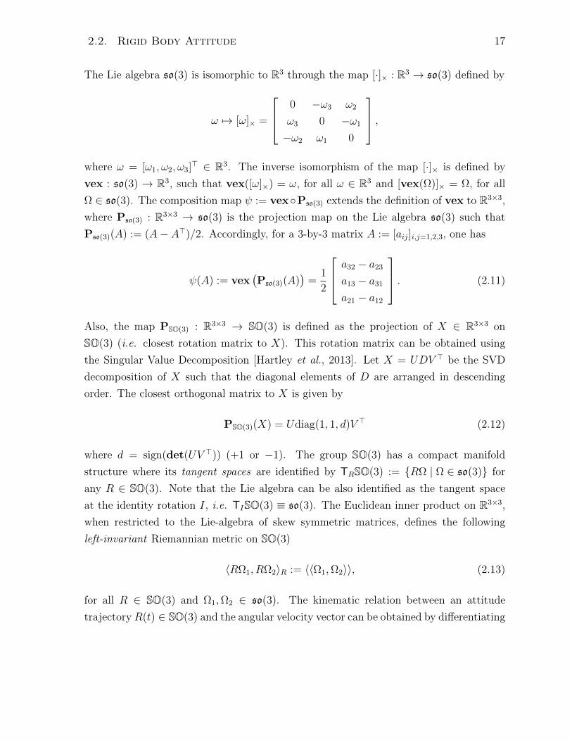
The Lie algebra so(3) is isomorphic to R3 through the map [·]× : R3 → so(3) defined by
ω 7→ [ω]× =
0 −ω3 ω2
ω3 0 −ω1
−ω2 ω1 0
,where ω = [ω1, ω2, ω3]> ∈ R3. The inverse isomorphism of the map [·]× is defined by
vex : so(3) → R3, such that vex([ω]×) = ω, for all ω ∈ R3 and [vex(Ω)]× = Ω, for all
Ω ∈ so(3). The composition map ψ := vexPso(3) extends the definition of vex to R3×3,
where Pso(3) : R3×3 → so(3) is the projection map on the Lie algebra so(3) such that
Pso(3)(A) := (A− A>)/2. Accordingly, for a 3-by-3 matrix A := [aij]i,j=1,2,3, one has
ψ(A) := vex(Pso(3)(A)
)=
1
2
a32 − a23
a13 − a31
a21 − a12
. (2.11)
Also, the map PSO(3) : R3×3 → SO(3) is defined as the projection of X ∈ R3×3 on
SO(3) (i.e. closest rotation matrix to X). This rotation matrix can be obtained using
the Singular Value Decomposition [Hartley et al., 2013]. Let X = UDV > be the SVD
decomposition of X such that the diagonal elements of D are arranged in descending
order. The closest orthogonal matrix to X is given by
PSO(3)(X) = Udiag(1, 1, d)V > (2.12)
where d = sign(det(UV >)) (+1 or −1). The group SO(3) has a compact manifold
structure where its tangent spaces are identified by TRSO(3) := RΩ | Ω ∈ so(3) for
any R ∈ SO(3). Note that the Lie algebra can be also identified as the tangent space
at the identity rotation I, i.e. TISO(3) ≡ so(3). The Euclidean inner product on R3×3,
when restricted to the Lie-algebra of skew symmetric matrices, defines the following
left-invariant Riemannian metric on SO(3)
〈RΩ1, RΩ2〉R := 〈〈Ω1,Ω2〉〉, (2.13)
for all R ∈ SO(3) and Ω1,Ω2 ∈ so(3). The kinematic relation between an attitude
trajectory R(t) ∈ SO(3) and the angular velocity vector can be obtained by differentiating

18 Chapter 2. Background and Preliminaries
the orthogonality condition RR> = I which gives
d
dt(R>R) = R>R + (R)>R = 0. (2.14)
It follows thatR(t)>R(t) ∈ so(3) for all times t ≥ 0 or, equivalently, there exists ω(t) ∈ R3
such that R(t)>R(t) = [ω(t)]×. This leads to write
R(t) = R(t)[ω(t)]×, (2.15)
which represents the attitude kinematics where ω(t) is referred to as the angular velocity
vector. If R is a rotation matrix describing the orientation of a body frame with respect to
an inertial frame then ω(t) is the body-referenced (expressed in body frame coordinates)
angular velocity of the body frame with respect to the inertial frame.
2.2.1 Attitude Parametrizations
The natural nine parameters representation of the attitude as an element of SO(3) is
unique and nonsingular. However, due to the presence of the constraints R>R = RR> =
I and det(R) = 1, it is possible to represent an attitude R ∈ SO(3) with fewer param-
eters. In this subsection, low order attitude parametrizations such as the exponential
coordinates, the angle-axis, the unit quaternions and the Rodrigues vector representa-
tions are described. Although not covered here, some other attitude representations
are used in the litterature such as the Euler angles, the modified Rodrigues parameters
amongst others. For more details on attitude representations the reader is referred to
[Shuster, 1993], [Murray et al., 1994], and [Hughes, 1986].
2.2.1.1 Exponential Coordinates Representation
Since the vector space so(3) corresponds to the Lie algebra of SO(3), it allows to rep-
resent elements of SO(3) via the exponential map. Given a rotation vector x ∈ R3, the
corresponding rotation matrix is given by the exponential map exp([x]×) ∈ SO(3) which
is defined by the following compact formula on SO(3)
exp([x]×) =
I x = 0
I + sin(||x||)||x|| [x]× + 1−cos(||x||)
||x||2 [x]2× x 6= 0. (2.16)
Equation (2.16) is referred to as Rodrigues formula. For a given rotation matrix R ∈SO(3) such that R = exp([x]×), the three-parameters vector x ∈ R3 is often referred to
2.2. Rigid Body Attitude 19
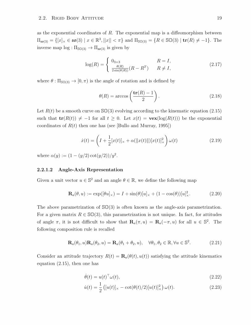
as the exponential coordinates of R. The exponential map is a diffeomorphism between
Πso(3) = [x]× ∈ so(3) | x ∈ R3, ||x|| < π and ΠSO(3) = R ∈ SO(3) | tr(R) 6= −1. The
inverse map log : ΠSO(3) → Πso(3) is given by
log(R) =
03×3 R = I,
θ(R)2 sin(θ(R))
(R−RT ) R 6= I,(2.17)
where θ : ΠSO(3) → [0, π) is the angle of rotation and is defined by
θ(R) = arccos
(tr(R)− 1
2
). (2.18)
Let R(t) be a smooth curve on SO(3) evolving according to the kinematic equation (2.15)
such that tr(R(t)) 6= −1 for all t ≥ 0. Let x(t) = vex(log(R(t))) be the exponential
coordinates of R(t) then one has (see [Bullo and Murray, 1995])
x(t) =
(I +
1
2[x(t)]× + α(‖x(t)‖)[x(t)]2×
)ω(t) (2.19)
where α(y) := (1− (y/2) cot(y/2))/y2.
2.2.1.2 Angle-Axis Representation
Given a unit vector u ∈ S2 and an angle θ ∈ R, we define the following map
Ra(θ, u) := exp([θu]×) = I + sin(θ)[u]× + (1− cos(θ))[u]2×. (2.20)
The above parametrization of SO(3) is often known as the angle-axis parametrization.
For a given matrix R ∈ SO(3), this parametrization is not unique. In fact, for attitudes
of angle π, it is not difficult to show that Ra(π, u) = Ra(−π, u) for all u ∈ S2. The
following composition rule is recalled
Ra(θ1, u)Ra(θ2, u) = Ra(θ1 + θ2, u), ∀θ1, θ2 ∈ R, ∀u ∈ S2. (2.21)
Consider an attitude trajectory R(t) = Ra(θ(t), u(t)) satisfying the attitude kinematics
equation (2.15), then one has
θ(t) = u(t)>ω(t), (2.22)
u(t) =1
2
([u(t)]× − cot(θ(t)/2)[u(t)]2×
)ω(t). (2.23)
20 Chapter 2. Background and Preliminaries
2.2.1.3 Unit Quaternions Representation
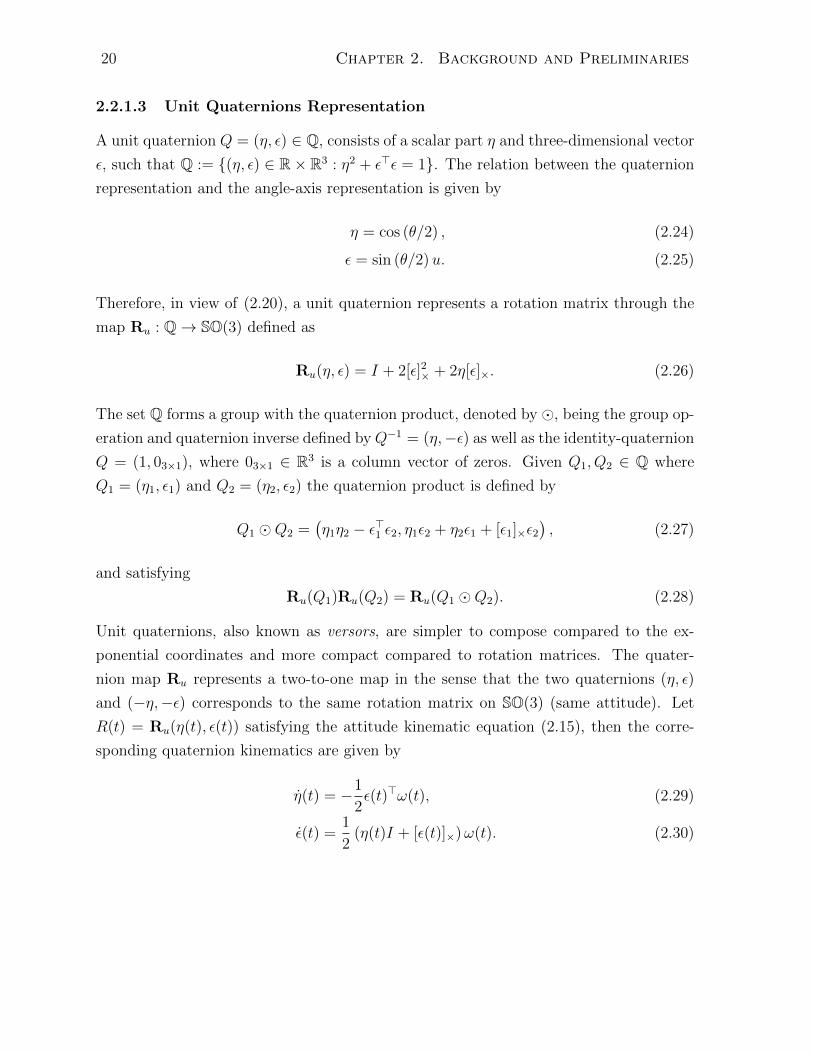
A unit quaternion Q = (η, ε) ∈ Q, consists of a scalar part η and three-dimensional vector
ε, such that Q := (η, ε) ∈ R× R3 : η2 + ε>ε = 1. The relation between the quaternion
representation and the angle-axis representation is given by
η = cos (θ/2) , (2.24)
ε = sin (θ/2)u. (2.25)
Therefore, in view of (2.20), a unit quaternion represents a rotation matrix through the
map Ru : Q→ SO(3) defined as
Ru(η, ε) = I + 2[ε]2× + 2η[ε]×. (2.26)
The set Q forms a group with the quaternion product, denoted by , being the group op-
eration and quaternion inverse defined by Q−1 = (η,−ε) as well as the identity-quaternion
Q = (1, 03×1), where 03×1 ∈ R3 is a column vector of zeros. Given Q1, Q2 ∈ Q where
Q1 = (η1, ε1) and Q2 = (η2, ε2) the quaternion product is defined by
Q1 Q2 =(η1η2 − ε>1 ε2, η1ε2 + η2ε1 + [ε1]×ε2
), (2.27)
and satisfying
Ru(Q1)Ru(Q2) = Ru(Q1 Q2). (2.28)
Unit quaternions, also known as versors, are simpler to compose compared to the ex-
ponential coordinates and more compact compared to rotation matrices. The quater-
nion map Ru represents a two-to-one map in the sense that the two quaternions (η, ε)
and (−η,−ε) corresponds to the same rotation matrix on SO(3) (same attitude). Let
R(t) = Ru(η(t), ε(t)) satisfying the attitude kinematic equation (2.15), then the corre-
sponding quaternion kinematics are given by
η(t) = −1
2ε(t)>ω(t), (2.29)
ε(t) =1
2(η(t)I + [ε(t)]×)ω(t). (2.30)
2.2. Rigid Body Attitude 21
2.2.1.4 Rodrigues Vector Representation
Another useful attitude representation is the well known Rodrigues vector on R3 which
is also associated to the Cayley transform. Consider the map Rr : R3 → SO(3) such that
Rr(z) = (I − [z]×)(I + [z]×)−1 =1
1 + ‖z‖2
((1− ‖z‖2)I + 2zz> + 2[z]×
). (2.31)
Note that since [z]× is skew-symmetric all its eigenvalues are pure imaginary. Thus, all
the eigenvalues of the matrix I + [z]× are non zero and therefore its inverse exists. The
map Rr is a diffeomorphism between R3 and ΠSO(3). The inverse map Z : ΠSO(3) → R3
is given by
Z(R) = vex((I −R)(I +R)−1
)=
2ψ(R)
1 + tr(R). (2.32)
It is not difficult to show that the following relations hold for all quaternions (η, ε) ∈ ΠQ
and all angle-axes (θ, u) ∈ R× S2, such that θ 6= kπ, k ∈ Z,
Z(Ru(η, ε)) =ε
η, (2.33)
Z(Ra(θ, u)) = tan(θ/2)u. (2.34)
The vector Z(R) ∈ R3 defines the vector of Rodrigues parameters. Note that the Ro-
drigues vector is sometimes defined using the unit quaternion or the angle-axis represen-
tation [Shuster, 1993]. It can be verified that the time derivative of the Rodrigues vector
Z(R) along the trajectories of (2.15) is given by
d
dtZ(R) =
1
2
(I + [Z(R)]× + Z(R)Z(R)>
)ω. (2.35)
2.2.2 Metrics on SO(3)
Roughly speaking, a metric (or distance) tells us how two elements of a given manifold are
close to each other. More rigorously, a metric on SO(3) is a function d : SO(3)×SO(3)→R≥0 that satisfies the following properties for all R1, R2, R3 ∈ SO(3):
• Non-negativity: d(R1, R2) ≥ 0.
• Identity of indiscernibles: d(R1, R2) = 0 if and only if R1 = R2.
• Symmetry: d(R1, R2) = d(R2, R1).
• Triangle inequality: d(R1, R3) ≤ d(R1, R2) + d(R2, R3).
22 Chapter 2. Background and Preliminaries
One possible way to measure the distance between two rotation matrices on SO(3) is to
use the Frobenious norm on the embedding Euclidean space R3×3 as follows:
dE(R1, R2) = ‖R1 −R2‖F , (2.36)
which defines the Euclidean (or Chordal) distance on SO(3). It can be verified that
dE(·, ·) satisfies the following property
dE(R1, R2) = dE(I, R1R>2 ) =
√2tr(I −R1R>2 ) ≤
√8, (2.37)
where the fact that R1R>2 ∈ SO(3), and hence tr(R1R2) ≥ −1, has been used to obtain
the upper bound of dE(·, ·). Throughout this work, the following normalized attitude
norm on SO(3) is used
|R|I =dE(I, R)√
8=‖I −R‖F√
8=
√tr(I −R)√
4. (2.38)
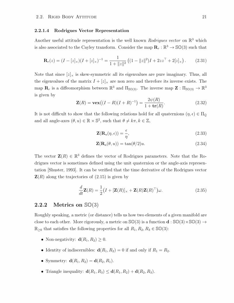
Another interesting attitude distance on SO(3) is what is known as the Geodesic or
SO(3)
•
so(3)
R2
R1
•
• log(R1R>2 )
Figure 2.2: Euclidean distance (red dashed) and Geodesic distance (green solid).
Riemannian metric (also known as the angular distance). It is defined as the length
of the shortest path on SO(3) between two rotation matrices. Formally, the geodesic
distance on SO(3) is defined as
dG(R1, R2) =1√2‖ log(R1R
>2 )‖F . (2.39)
Note that dG(R1, R2) measures the rotation angle between the two matrices R1 and R2
or, equivalently, the angle of the rotation error R1R>2 which lies in the interval [0, π].
2.2. Rigid Body Attitude 23
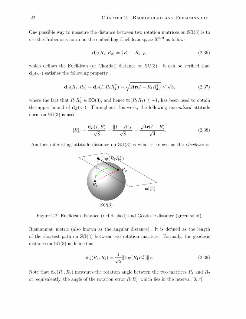
2.2.3 Attitude Visualization
Visualizing the orientation information of a rigid body in 3D space can be done in different
ways depending on the application at hand. One possible way consists in using the frame-
based description of the orientation as in Figure 2.1. In fact, assume a given trajectory
R(t) : R≥0 → SO(3) then three base vectors trajectories can be obtained as follows
eib(t) = R(t)ei, i ∈ 1, 2, 3, (2.40)
where each vector eib describes a trajectory on the unit sphere S2. Therefore, the rotation
path R(t) is visualized by plotting three trajectories on S2 as demonstrated in Figure 2.3.
Alternatively, if plotting three trajectories on the same sphere is cumbersome, one can
draw three spheres (instead on one sphere) and plot each trajectory R(t)e1, R(t)e2 and
R(t)e3 on each of these spheres.
Figure 2.3: Visualization of 3D rotations using the body-frame unit axes R(t)e1, R(t)e2
and R(t)e3. The initial body frame is plotted in dashed and the final body frame is plottedin bold. The trajectory is generated using the angular velocity ω(t) = [e−t, e−2t, e−3t]>
with R(0) = I and t ∈ [0, 20] seconds.
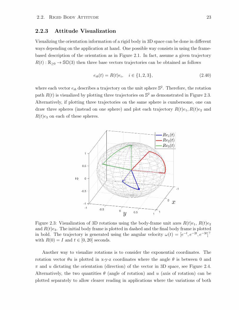
Another way to visualize rotations is to consider the exponential coordinates. The
rotation vector θu is plotted in x-y-z coordinates where the angle θ is between 0 and
π and u dictating the orientation (direction) of the vector in 3D space, see Figure 2.4.
Alternatively, the two quantities θ (angle of rotation) and u (axis of rotation) can be
plotted separately to allow clearer reading in applications where the variations of both
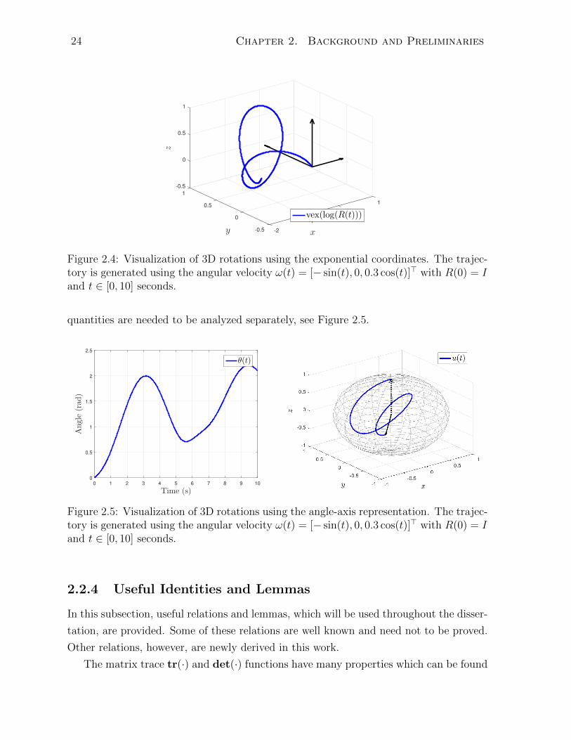
24 Chapter 2. Background and Preliminaries
-0.5
1
0
1
z
0.5
0.5
y
0
x
1
0-1
-0.5 -2
vex(log(R(t)))
Figure 2.4: Visualization of 3D rotations using the exponential coordinates. The trajec-tory is generated using the angular velocity ω(t) = [− sin(t), 0, 0.3 cos(t)]> with R(0) = Iand t ∈ [0, 10] seconds.
quantities are needed to be analyzed separately, see Figure 2.5.
0 1 2 3 4 5 6 7 8 9 10
Time (s)
0
0.5
1
1.5
2
2.5
Angle(rad
)
θ(t)
Figure 2.5: Visualization of 3D rotations using the angle-axis representation. The trajec-tory is generated using the angular velocity ω(t) = [− sin(t), 0, 0.3 cos(t)]> with R(0) = Iand t ∈ [0, 10] seconds.
2.2.4 Useful Identities and Lemmas
In this subsection, useful relations and lemmas, which will be used throughout the disser-
tation, are provided. Some of these relations are well known and need not to be proved.
Other relations, however, are newly derived in this work.
The matrix trace tr(·) and det(·) functions have many properties which can be found

2.2. Rigid Body Attitude 25
in linear algebra textbooks [Lang, 1987]. Here, some of these useful properties are re-
called. For any M,N ∈ R3×3, x, y ∈ R3 and α ∈ R one has
tr(M>) = tr(M), (2.41)
tr(M +N) = tr(M) + tr(N), (2.42)
tr(αM) = αtr(M), (2.43)
tr(MN) = tr(NM), (2.44)
tr(MN) = 0 (if M = M> and N = −N>) (2.45)
det(MN) = det(M)det(N) (2.46)
det(I + xy>) = 1 + x>y. (2.47)
Using these properties of the trace function, the following identities are easily derived in
a straightforward manner. For all x, y ∈ R3 and R,P ∈ SO(3) one has
tr(xy>) = x>y, (2.48)
tr(yx>(I −RP>)) =1
2‖R>x− P>y‖2 − 1
2‖x− y‖2. (2.49)
The cross product map [·]× has many interesting properties and appeared in many ref-
erences dealing with rigid body attitude applications [Shuster, 1993]. For any x, y ∈ R3
one has
[x]×y = x× y, (2.50)
[x]×y = −[y]×x, (2.51)
[x]3× = −‖x‖2[x]×, (2.52)
[x]×[y]× = −(x>y)I + yx>, (2.53)
x× y = 2ψ(yx>), (2.54)
[x× y]× = yx> − xy>, (2.55)
〈〈[x]×, [y]×〉〉 = 2x>y, (2.56)

26 Chapter 2. Background and Preliminaries
Moreover, for any x, y ∈ R3, M ∈ R3×3 and R ∈ SO(3) the following relations hold
〈〈M, [x]×〉〉 = 〈〈Pso(3)(M), [x]×〉〉, (2.57)
[(Mx)× (My)]× = M [x× y]×M>, (2.58)
M [x]× + [x]×M> = [(tr(M)I −M>)x]×, (2.59)
ψ(MR) = R>ψ(RM), (2.60)
R[x]×R> = [Rx]×. (2.61)
The matrix square of a rotation R ∈ SO(3) is also a rotation around the same axis and
with double angle. The rotation R2 can be obtained from R using the following relation
[Shuster, 1993]
R2 = R> + tr(R)R− tr(R)I. (2.62)
Using this relation, one obtains the following lemma whose proof is provided in Appendix
A.1.
Lemma 2.2.1 For any symmetric matrix M = M> ∈ R3×3 and R ∈ SO(3) one has
tr(M(I −R2)) = (1 + tr(R))tr(M(I −R)), (2.63)
Pso(3)(MR2) = tr(R)Pso(3)(MR) + Pso(3)(MR>) (2.64)
〈〈Pso(3)(R),Pso(3)(MR)〉〉 =1
2tr(M(I −R2)). (2.65)
It turns out that, in the field of attitude control and estimation, the following mapping
E : R3×3 → R3×3 defined by
E(M) =1
2
(tr(M)I −M>) (2.66)
is important and its properties are very handy when deriving the control laws and the
proofs of stability. The following lemmas are needed throughout the thesis and are proved
in Appendix A.
Lemma 2.2.2 Consider the map E : R3×3 → R3×3 defined in (2.66). Let M ∈ R3×3 and
let v be an eigenvector of M> associated to the eigenvalue λM>
v . Then, the following hold
i) E−1(M) = tr(M)I − 2M>.
ii) v is an eigenvector of E(M), respectively E−1(M), associated to the eigenvalue
λE(M)v = 1
2
(tr(M)− λM>v
), respectively λ
E−1(M)v = tr(M)− 2λM
>v .

2.2. Rigid Body Attitude 27
Lemma 2.2.3 Consider the map E : R3×3 → R3×3 defined in (2.66). Then, for any
symmetric matrix M ∈ R3×3, any rotation matrix R ∈ SO(3) and any vector x ∈ R3 one
has
x>[λE(M)min − E(MR)]x ≤ 1
2tr(M(I −R))‖x‖2, (2.67)
x>[E(M)− E(MR)]y ≤ 1
2tr(M(I −R))x>y +
1
2‖M(I −R)‖F‖x‖‖y‖, (2.68)
2λMmin − tr(M) ≤ tr(MR) ≤ max(tr(M), 2λMmax − tr(M)
), (2.69)
E(M) ≥ 0⇒ ‖E(MR)‖F ≤ ‖E(M)‖F . (2.70)
Lemma 2.2.4 Consider the trajectories of R(t) = R(t)[ω(t)]× with R(0) ∈ SO(3) and
ω(t) ∈ R3 for all t ≥ 0. Then, for all M ∈ R3×3
∇tr(M(I −R)) = RPso(3)(MR), (2.71)
d
dttr(M(I −R(t))) = 2ψ(MR(t))>ω(t), (2.72)
d
dtψ(MR(t)) = E(MR(t))ω(t). (2.73)
Lemma 2.2.5 Let M ∈ R3×3 be a symmetric matrix. Then, for all θ ∈ R, u ∈ S1, (η, ε) ∈Q and z ∈ R3, one has
tr(M(I −Ra(θ, u))) = 2(1− cos(θ))u>E(M)u, (2.74)
tr(M(I −Ru(η, ε))) = 4ε>E(M)ε, (2.75)
tr(M(I −Rr(z))) = 4[1 + ‖z‖2]−1z>E(M)z. (2.76)
Moreover, one has
ψ(MRa(θ, u)) = (sin(θ)I − (1− cos(θ))[u]×)E(M)u, (2.77)
ψ(MRu(η, ε)) = 2(ηI − [ε]×)E(M)ε, (2.78)
ψ(MRr(z)) = 2[1 + ‖z‖2]−1(I − [z]×)E(M)z. (2.79)
Lemma 2.2.6 Let M ∈ R3×3 be a symmetric matrix and R ∈ SO(3) be a rotation
28 Chapter 2. Background and Preliminaries
matrix. Then the following relations hold:
4λE(M)min |R|2I ≤ tr(M(I −R)) ≤ 4λE(M)
max |R|2I , (2.80)
‖ψ(MR)‖2 = α(M,R)tr(E−1(E(M)2)(I −R)), (2.81)
(1− |R|2I) ≤ α(M,R) ≤ (1− ξ2|R|2I) if E(M) ≥ 0, (2.82)
ψ(R)>ψ(MR) = ψ(R)>E(M)ψ(R), (2.83)
where α(M,R) = (1 − |R|2I cos2(u,E(M)u)), ξ = λE(M)min /λ
E(M)max and u ∈ S2 is the axis of
rotation R. Moreover, the following upper bound holds
‖ψ(MR)‖2 ≤ (λE(M)max )2ψ(ξ2), if E(M) ≥ 0, (2.84)
where ψ(·) is defined as ψ(ξ2) = 1/ξ2 if ξ2 ≥ 1/2 and ψ(ξ2) = 4(1− ξ2) otherwise.
Lemma 2.2.7 Let M =∑n
i=1 ρixix>i with n ≥ 1, ρi ∈ R and xi ∈ R3, i = 1, . . . , n.
Then, the following holds for any rotation matrices R,P ∈ SO(3):
tr(M(I −RP>)) =1
2
n∑i=1
ρi‖R>xi − P>xi‖2, (2.85)
ψ(MRP>) =1
2P
n∑i=1
ρi(R>xi × P>xi) (2.86)
Lemma 2.2.8 Let M be a symmetric matrix. For all (θ, u) ∈ R × S2 and v ∈ ERv (M),
the following holds
tr(M(I −Ra(π, v)Ra(θ, u))) = 4λE(M)v − 4 sin2(θ/2)∆(v, u), (2.87)
where ∆(v, u) is given by
∆(v, u) = v> (E(M) + [u]×E(M)[u]×) v. (2.88)
2.3 Hybrid Systems Framework
A hybrid system is a dynamical system that allows both continuous flows and discrete
jumps (transitions) of the state. In this thesis, the framework of hybrid systems developed
in [Goebel and Teel, 2006, Goebel et al., 2009, Goebel et al., 2012] is considered. Let
M be a given manifold embedded in Rn. A general model of a hybrid system takes the
2.3. Hybrid Systems Framework 29
form: x ∈ F(x), x ∈ F ,x+ ∈ J(x), x ∈ J ,
(2.89)
where the flow map, F :M⇒ TM (⇒ denotes a set-valued mapping) governs the con-
tinuous flow of x on the manifoldM, the flow set F ⊆M dictates where the continuous
flow could occur. The jump map, J : M ⇒M, governs discrete jumps of the state x,
and the jump set J ⊆M defines where the discrete jumps are permitted.
Solutions to hybrid systems are parametrized by the amount of time spent in the flow
set t ∈ R≥0 and by the number of jumps of the state j ∈ N. Solutions to hybrid systems
are therefore defined on a hybrid time domain. A subset H ⊂ R≥0 × N is a hybrid time
domain, if it is a union of finitely or infinitely many intervals of the form [tj, tj+1]× jwhere 0 = t0 ≤ t1 ≤ t2 ≤ ..., with the last interval, if existent, being possibly of the
form [tj, T ) × j with T finite or T = +∞. The ordering of points on each hybrid
time domain is such that (t, j) (t′, j′) if t ≤ t′ and j ≤ j′. A hybrid arc is a function
x : dom x → M, where the domain of the function x (i.e. dom x) is a hybrid time
domain and, for each fixed j, t 7→ x(t, j) is a locally absolutely continuous function on
the interval Tj = t : (t, j) ∈ dom x. A hybrid arc x is called complete if dom x is
unbounded and Zeno if it is complete and the projection of dom x on R≥0 is bounded.
The hybrid arc x is a solution to the hybrid system (2.89) if x(0, 0) ∈ F ∪J and the
following conditions are satisfied:
• Flow condition: for each j ∈ N such that Tj has a nonempty interior,
x(t, j) ∈ F(x(t, j)), for almost all t ∈ Tj, (2.90)
x(t, j) ∈ F , for all t ∈ [minTj, supTj). (2.91)
• Jump condition: for each (t, j) ∈ dom x such that (t, j + 1) ∈ dom x,
x(t, j + 1) ∈ J(x(t, j)), (2.92)
x(t, j) ∈ J . (2.93)
Consider a hybrid arc x that is not eventually discrete. Let j(t) = maxj : (t, j) ∈ dom xand let T = supt : (t, j) ∈ dom x, j ∈ N. Then, the time projection of x is defined as

30 Chapter 2. Background and Preliminaries
the function x↓t : [0, T )→M such that
x↓t = x(t, j(t)). (2.94)
In the framework [Goebel et al., 2012], three Basic Conditions (or Assumptions) have
been introduced to guarantee the existence of solutions, the robustness of stability to
small perturbations and other useful properties. The hybrid system (2.89) is said to
satisfy the basic conditions if:
C1) F and J are closed sets in Rn.
C2) The set-valued function F is outer semicontinuous2 and locally bounded3 on F and,
for all x ∈ F , the set F(x) is nonempty and convex4
C3) The set-valued function J is outer semicontinuous and locally bounded on J and,
for all x ∈ J , the set J(x) is nonempty.
2.3.1 Exponential Stability for Hybrid Systems
Since most of the stability results, derived in this thesis, are exponential, only the defi-
nition of exponential stability for hybrid systems of the form (2.89) is recalled here. The
reader is referred to [Goebel et al., 2012] for other definitions of stability and asymptotic
stability for hybrid systems.
Definition 2.3.1 (Exponential stability [Teel et al., 2013]) A closed set A ⊂ Mis said to be (locally) exponentially stable for the hybrid system (2.89) if there exist strictly
positive real numbers k, λ, µ such that each solution x satisfying |x(0, 0)|A < µ also sat-
isfies, for all (t, j) ∈ dom x,
|x(t, j)|A ≤ k exp(−λ(t+ j))|x(0, 0)|A (2.95)
where |x|A denotes a distance function from x ∈ M to A. It is said to be globally
exponentially stable if one allows µ→ +∞.
Note that in the above definition of exponential stability, the exponential convergence
is indeed uniform since the scalars λ and k are independent from the initial conditions.
2The set-valued function F is outer semicontinuous if its graph (x, y) : x ∈ M, y ∈ F(x) ⊂ R2n isclosed. Equivalently, for all x0 ∈ F one has lim supx→x0
F(x) ⊆ F(x0).3A set-valued function F is locally bounded on F if for every compact set K ⊂ F , F (K) is bounded.4A convex set is a subset of an affine space that is closed under convex combinations. Roughly
speaking, given any two points in a convex set, each point on the line joining these two points is in theset as well.
2.3. Hybrid Systems Framework 31
Throughout the text, the adjective “uniform” is omitted for simplicity. Given µ > 0,
define the set A + µB := x ∈ M : |x|A < µ. The following theorem [Teel et al., 2013]
provides sufficient conditions for exponential stability.
Theorem 2.3.2 For system (2.89), the closed set A ⊂M is locally exponentially stable
if there exist positive real numbers α, α, λ1, λ2, µ, p and a function V : domV→ R where
F ∪ J ∪ J(J ) ⊂ domV, that is continuously differentiable on an open set containing
cl(F) and satisfies
α|x|pA ≤ V(x) ≤ α|x|pA, ∀x ∈ (F ∪ J ∪ J(J )) ∩ (A+ µB), (2.96)
〈∇V(x), f〉 ≤ −λ1V(x), ∀x ∈ F ∩ (A+ µB), f ∈ F(x), (2.97)
V(g) ≤ exp(−λ2)V(x), ∀x ∈ J ∩ (A+ µB), g ∈ J(x). (2.98)
If these bounds hold with µ =∞ then the set A is globally exponentially stable.
The sufficient conditions for exponential stability provided in Theorem 2.3.2 require that
all solutions guarantee exponential decrease of the function V during both the flows and
the jumps. It turns out that for hybrid systems of the form (2.89) this condition is quite
restrictive. In other words, under some mild conditions on the solutions, exponential
stability can still hold even in the case where some solutions do not ensure a decrease in
V during either the flow or the jump.
Theorem 2.3.3 For system (2.89), the closed set A ⊂M is locally exponentially stable
if there exist positive real numbers α, α, µ, p, real numbers λ1, λ2 and a function V :
domV→ R where F ∪J ∪J(J ) ⊂ domV, that is continuously differentiable on an open
set containing cl(F) and satisfies
α|x|pA ≤ V(x) ≤ α|x|pA, ∀x ∈ (F ∪ J ∪ J(J )) ∩ (A+ µB), (2.99)
〈∇V(x), f〉 ≤ −λ1V(x), ∀x ∈ F ∩ (A+ µB), f ∈ F(x), (2.100)
V(g) ≤ exp(−λ2)V(x), ∀x ∈ J ∩ (A+ µB), g ∈ J(x), (2.101)
such that one of these conditions hold:
i) λ1 and λ2 are strictly positive scalars.
ii) λ2 ≤ 0, λ1 > −λ2γ and, for all (t, j) ∈ dom x, j ≤ γt+ J where γ ≥ 0 and J ∈ N.
iii) λ1 ≤ 0, λ2 > −λ1γ and, for all (t, j) ∈ dom x, t ≤ γj + T where γ, T ≥ 0.
If these conditions hold with µ =∞ then the set A is globally exponentially stable.

32 Chapter 2. Background and Preliminaries
Proof See Appendix C.1.
Compared to Theorem 2.3.2, the conditions of Theorem 2.3.3 do not require that both λ1
and λ2 are positive. Instead, only one of the two scalars λ1, λ2 is required to be positive
and the other one can take arbitrary values in R. This allows for scenarios where we
have either an increase during the flows or an increase during the jumps. The price to
pay is that some conditions on the hybrid time domain are imposed. These conditions
are often referred to as persistent flow (respectively persistent jump) conditions and have
been exploited in [Goebel et al., 2012, Section 3.3] and [Prieur et al., 2014] to derive
sufficient conditions for global uniform asymptotic stability in the case where there is
no strict decrease across the jumps (respectively flows). Many classes of hybrid systems
satisfy these persistent flow/jump conditions. For instance, hybrid systems that exhibit
dwell-time solutions5 can be shown to satisfy the persistent flow condition in item ii) of
Theorem 2.3.3. Moreover, in a state estimation problem using intermittent measurements
(such as the one discussed in Chapter 4) there exists a maximum time T such that the
observer state is updated every T period of time. Therefore the flow time t is naturally
bounded by t ≤ T (j + 1) which allows to use item iii) of Theorem 2.3.3.
Remark 2.3.4 In Theorem 2.3.3, global exponential stability of the set A is stated when
the scalar µ = +∞. When the set A is locally exponentially stable and the set M\R,
where R ⊆ M is contained in the region of attraction, has Lebesgue measure zero, the
exponential stability is stated as almost global exponential stability.
2.4 Numerical Integration Tools
In this section, the numerical integration schemes used in this work are discussed. Most
mechanical systems are governed by differential equations whose solutions are known to
evolve on a given manifold embedded in Rn. There are two main techniques to numerically
solve differential equations on general manifolds: embedded and intrinsic. In the first
method, one embeds the given manifold in Rn and then employs classical integration
methods on the Euclidean manifold Rn such as the Runge-Kutta methods. The drawback
of these methods when applied to manifolds is that, in general, it is not possible to
guarantee that the solution will stay on the given manifold. On the other hand, intrinsic
methods are developed to guarantee that the update rule for the integration scheme keeps
5A solution to a hybrid system is called a “dwell-time solution” if there is a minimum elapsed timebetween each two consecutive jumps. In other words, there is a dwell time τD > 0 such that jumps areseparated by at least τD amount of time.
2.4. Numerical Integration Tools 33
the state of the system on this manifold. The price to pay is that these methods might
be computationally expensive compared to the classical methods on Rn.
2.4.1 Numerical Integration on Rn
Consider the ordinary differential equation (ODE) on Rn
x = f(t, x), x(0) = x0. (2.102)
The objective of numerical integration methods is to approximate the time solution for
the above ODE given knowledge of the function f and the initial data (0, x0). The
most basic and simplest method is to use the well known explicit Euler method which is
named after Leonhard Euler, who treated it in his book Institutionum calculi integralis
(published 1768-70). Choose a value h for the size of every step and set tn = nh. Then,
it is possible to iteratively compute the approximate of x at time tn, denoted xn ≈ x(tn),
using the first order update rule
xn+1 = xn + hf(tn, xn), n ∈ N0. (2.103)
Higher order integration schemes can be used to obtain better accuracy. The Runge-
Kutta methods provide a family of implicit and explicit integration schemes to approx-
imate the solutions of an ODE. These methods were developed around 1900 by the
German mathematicians C. Runge and M. W. Kutta. Here, some of the commonly used
Runge-Kutta methods are recalled. Euler method mentioned above is the first order
Runge-Kutta method. The following are some common Runge-Kutta methods:
• Heun’s method (explicit trapezoidal rule) is given by the formula
xn+1 = xn +h
2(f1 + f2) , (2.104)
where f1 = f(tn, xn), and f2 = f(tn + h, xn + hf1).
• A Runge-Kutta method (3rd order, 3 stages) is given by the formula
xn+1 = xn +h
6(f1 + 4f2 + f3) , (2.105)
where f1 = f(tn, xn), f2 = f(tn + h2, xn + h
2f1), and f3 = f(tn + h, xn− hf1 + 2hf2).
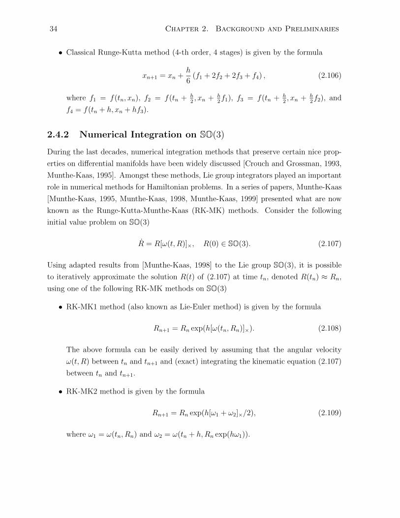
34 Chapter 2. Background and Preliminaries
• Classical Runge-Kutta method (4-th order, 4 stages) is given by the formula
xn+1 = xn +h
6(f1 + 2f2 + 2f3 + f4) , (2.106)
where f1 = f(tn, xn), f2 = f(tn + h2, xn + h
2f1), f3 = f(tn + h
2, xn + h
2f2), and
f4 = f(tn + h, xn + hf3).
2.4.2 Numerical Integration on SO(3)
During the last decades, numerical integration methods that preserve certain nice prop-
erties on differential manifolds have been widely discussed [Crouch and Grossman, 1993,
Munthe-Kaas, 1995]. Amongst these methods, Lie group integrators played an important
role in numerical methods for Hamiltonian problems. In a series of papers, Munthe-Kaas
[Munthe-Kaas, 1995, Munthe-Kaas, 1998, Munthe-Kaas, 1999] presented what are now
known as the Runge-Kutta-Munthe-Kaas (RK-MK) methods. Consider the following
initial value problem on SO(3)
R = R[ω(t, R)]×, R(0) ∈ SO(3). (2.107)
Using adapted results from [Munthe-Kaas, 1998] to the Lie group SO(3), it is possible
to iteratively approximate the solution R(t) of (2.107) at time tn, denoted R(tn) ≈ Rn,
using one of the following RK-MK methods on SO(3)
• RK-MK1 method (also known as Lie-Euler method) is given by the formula
Rn+1 = Rn exp(h[ω(tn, Rn)]×). (2.108)
The above formula can be easily derived by assuming that the angular velocity
ω(t, R) between tn and tn+1 and (exact) integrating the kinematic equation (2.107)
between tn and tn+1.
• RK-MK2 method is given by the formula
Rn+1 = Rn exp(h[ω1 + ω2]×/2), (2.109)
where ω1 = ω(tn, Rn) and ω2 = ω(tn + h,Rn exp(hω1)).

2.4. Numerical Integration Tools 35
• RK-MK3 method is given by the formula
Rn+1 = Rn exp([ω]×), (2.110)
ω =h
6(ω1 + 4ω2 + ω3) +
h2
36(4ω1 × ω2 + ω1 × ω3), (2.111)
where ω1 = ω(tn, Rn), ω2 = ω(tn + h/2, Rn exp(h[ω1]×/2)) and ω3 = ω(tn +
h,Rn exp(h[−ω1 + 2ω2]×)).
• RK-MK4 method is given by the formula
Rn+1 = Rn exp([ω]×), (2.112)
ω =h
6(ω1 + 2ω2 + 2ω3 + ω4) +
h2
36
∑i<j
ωi × ωj, (2.113)
where ω1 = ω(tn, Rn), ω2 = ω(tn+h/2, Rn exp(h[ω1]×/2)), ω3 = ω(tn+h/2, Rn exp(h[ω2]×/2)),
and ω4 = ω(tn + h,Rn exp(h[ω3]×)).
2.4.3 Numerical Integration of Hybrid Systems
The main objective when developing a numerical integration scheme is to approximate
with arbitrary precision, by adjusting the step size, the solutions of the mathematical
model under consideration. Moreover, when dealing with control systems it is desirable
that the simulated model preserves, for example, asymptotic stability even in a practical
sense. The theory of numerical simulation and integration for continuous time differen-
tial equations is well understood and developed and can be found in several textbooks.
However there is a little that has been done when the system under consideration is
a hybrid system; combining continuous and discrete dynamics. Under the framework
[Goebel et al., 2012], a hybrid simulator model for hybrid systems written in the form
(2.89) is introduced. The authors in [Sanfelice and Teel, 2006] established conditions on
the data of the hybrid simulator model such that the following properties hold:
• On compact hybrid time domains, every simulation to a hybrid system is arbitrarily
close to a solution of the hybrid system;
• Asymptotically stable compact sets for a hybrid system are semiglobally practically
asymptotically stable compact sets for the hybrid simulator;
• Asymptotically stable compact sets for the hybrid simulator are continuous in the
step size h.
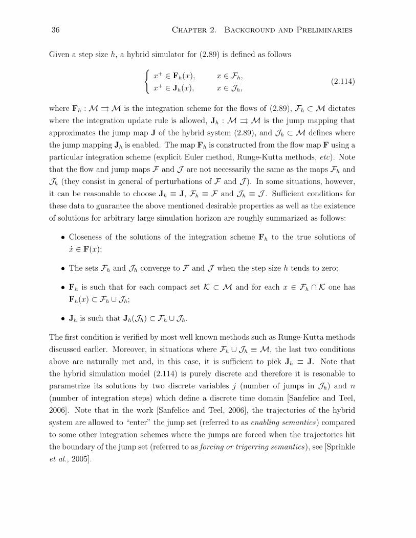
36 Chapter 2. Background and Preliminaries
Given a step size h, a hybrid simulator for (2.89) is defined as followsx+ ∈ Fh(x), x ∈ Fh,x+ ∈ Jh(x), x ∈ Jh,
(2.114)
where Fh :M ⇒M is the integration scheme for the flows of (2.89), Fh ⊂ M dictates
where the integration update rule is allowed, Jh : M ⇒ M is the jump mapping that
approximates the jump map J of the hybrid system (2.89), and Jh ⊂ M defines where
the jump mapping Jh is enabled. The map Fh is constructed from the flow map F using a
particular integration scheme (explicit Euler method, Runge-Kutta methods, etc). Note
that the flow and jump maps F and J are not necessarily the same as the maps Fh and
Jh (they consist in general of perturbations of F and J ). In some situations, however,
it can be reasonable to choose Jh ≡ J, Fh ≡ F and Jh ≡ J . Sufficient conditions for
these data to guarantee the above mentioned desirable properties as well as the existence
of solutions for arbitrary large simulation horizon are roughly summarized as follows:
• Closeness of the solutions of the integration scheme Fh to the true solutions of
x ∈ F(x);
• The sets Fh and Jh converge to F and J when the step size h tends to zero;
• Fh is such that for each compact set K ⊂ M and for each x ∈ Fh ∩ K one has
Fh(x) ⊂ Fh ∪ Jh;
• Jh is such that Jh(Jh) ⊂ Fh ∪ Jh.
The first condition is verified by most well known methods such as Runge-Kutta methods
discussed earlier. Moreover, in situations where Fh ∪ Jh ≡ M, the last two conditions
above are naturally met and, in this case, it is sufficient to pick Jh ≡ J. Note that
the hybrid simulation model (2.114) is purely discrete and therefore it is resonable to
parametrize its solutions by two discrete variables j (number of jumps in Jh) and n
(number of integration steps) which define a discrete time domain [Sanfelice and Teel,
2006]. Note that in the work [Sanfelice and Teel, 2006], the trajectories of the hybrid
system are allowed to “enter” the jump set (referred to as enabling semantics) compared
to some other integration schemes where the jumps are forced when the trajectories hit
the boundary of the jump set (referred to as forcing or trigerring semantics), see [Sprinkle
et al., 2005].

Chapter 3
Hybrid Attitude Control on SO(3)
3.1 Introduction
This chapter presents a framework for global exponential stabilization on the rotation
group SO(3) by means of hybrid feedback. First, the concept of synergism proposed in
[Mayhew and Teel, 2011b, Mayhew and Teel, 2011d, Mayhew and Teel, 2013a], which is
shown to be sufficient for global asymptotic stability, is extended to a new concept that is
coined “exp-synergism” which is shown to be sufficient for global exponential stability on
SO(3). Exp-synergism imposes more restrictive conditions on the potential functions used
in the attitude control design but allows for a broader class of potential functions which
are not necessarily differentiable everywhere on SO(3). In fact, exp-synergistic families
of “smooth” potential functions on SO(3) is synergistic but the opposite does not hold
in general. A min-switch hybrid control strategy along with an exp-synergistic family
of potential functions on SO(3) can be employed to guarantee robust global exponential
stabilization for the kinematic system on SO(3).
Next, we proceed to the construction of such families of potential functions on SO(3)
satisfying the exp-synergism property. It is shown that some existing and well known
smooth and nonsmooth potential functions on SO(3) (such as the trace function and the
geodesic distance) can be used along with a newly proposed angular warping map on
SO(3) to generate exp-synergistic families of potential functions. In contrast to other ex-
isting central synergistic families of potential functions on SO(3), our proposed approach
for the construction of exp-synergistic potential functions on SO(3) allows for the explicit
determination of the synergistic gap and therefore facilitate the real-time implementation
of the proposed hybrid control schemes.
Finally, using the proposed hybrid control approach, the attitude tracking problem
for rigid body systems (Spacecraft, Unmanned Aerial Vehicles (UAVs), Autonomous
37
38 Chapter 3. Hybrid Attitude Control on SO(3)
Underwater Vehicles (AUVs),...,etc) is tackeled. This results in a control algorithm guar-
anteeing robust and global exponential tracking, which are shown to exceed most existing
and commercial attitude control algorithms. To the best of our knowledge, there is no
similar solution to the full attitude tracking control problem in the literature. More-
over, an alternative design ensuring a continuous control input torque without sacrificing
the global exponential stability result is derived. The proposed smoothing procedure is
much simpler than the backstepping procedure proposed in [Mayhew and Teel, 2013a].
The results presented in this chapter are based on our work in [Berkane and Tayebi,
2017e, Berkane et al., 2017b, Berkane and Tayebi, 2015a]
3.2 Motivation Using Planar Rotations on S1
In this section, the example of planar rotations is considered to motivate some of the
results of this chapter. Working with the simple example of the unit circle S1, which is
a submanifold of SO(3), helps the reader to better understand the problem addressed in
this chapter and the rational behind some of the introduced techniques. Nevertheless,
the control of planar rotations is in fact an interesting control problem in its own right.
It arises in many engineering applications in robotics (autonomous planar vehicles, pen-
dulum systems, gimbal pointing mechanism...etc ), see for instance [Rue, 1969, Repoulias
and Papadopoulos, 2007, Masten, 2008, Mayhew et al., 2008, Osborne et al., 2008].
Consider a point mass with coordinates x = (x1, x2) ∈ R2 restricted to evolve on
the unit circle S1 with angular velocity ω ∈ R. The task is to design a control law for
the control input ω in order to globally stabilize the point mass to the coordinate point
e1 = [1, 0]> as demonstrated in Figure 3.1. Although it looks simple, this problem is far
from being trivial. In fact, the unit circle S1 is a compact manifold and hence it is not
diffeomorphic to any Euclidean space which prevents the existence of continuous time-
invariant state feedback which globally asymptotically stablizes any equilibrium point.
This is a well known topological obstruction on compact manifolds [Sanjay P. Bhat,
2000]. To better understand this issue, consider the kinematic equation of x
x =
[−ωx2
ωx1
]= ω
[0 −1
1 0
]x := ωSx. (3.1)
A routine for the design of controllers is to pick a suitable Lyapunov function (energy
function or potential function) and then design a controller such that the energy is de-
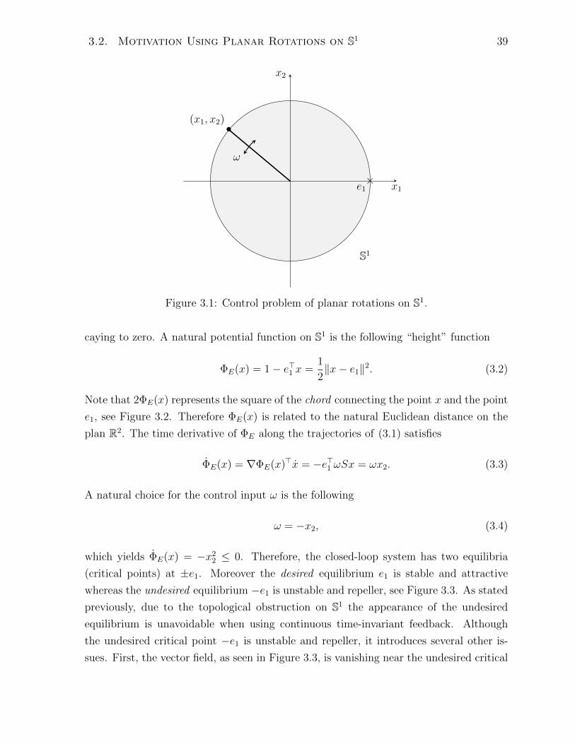
3.2. Motivation Using Planar Rotations on S1 39
S1
x1
x2
•
ω
e1×
(x1, x2)
Figure 3.1: Control problem of planar rotations on S1.
caying to zero. A natural potential function on S1 is the following “height” function
ΦE(x) = 1− e>1 x =1
2‖x− e1‖2. (3.2)
Note that 2ΦE(x) represents the square of the chord connecting the point x and the point
e1, see Figure 3.2. Therefore ΦE(x) is related to the natural Euclidean distance on the
plan R2. The time derivative of ΦE along the trajectories of (3.1) satisfies
ΦE(x) = ∇ΦE(x)>x = −e>1 ωSx = ωx2. (3.3)
A natural choice for the control input ω is the following
ω = −x2, (3.4)
which yields ΦE(x) = −x22 ≤ 0. Therefore, the closed-loop system has two equilibria
(critical points) at ±e1. Moreover the desired equilibrium e1 is stable and attractive
whereas the undesired equilibrium −e1 is unstable and repeller, see Figure 3.3. As stated
previously, due to the topological obstruction on S1 the appearance of the undesired
equilibrium is unavoidable when using continuous time-invariant feedback. Although
the undesired critical point −e1 is unstable and repeller, it introduces several other is-
sues. First, the vector field, as seen in Figure 3.3, is vanishing near the undesired critical
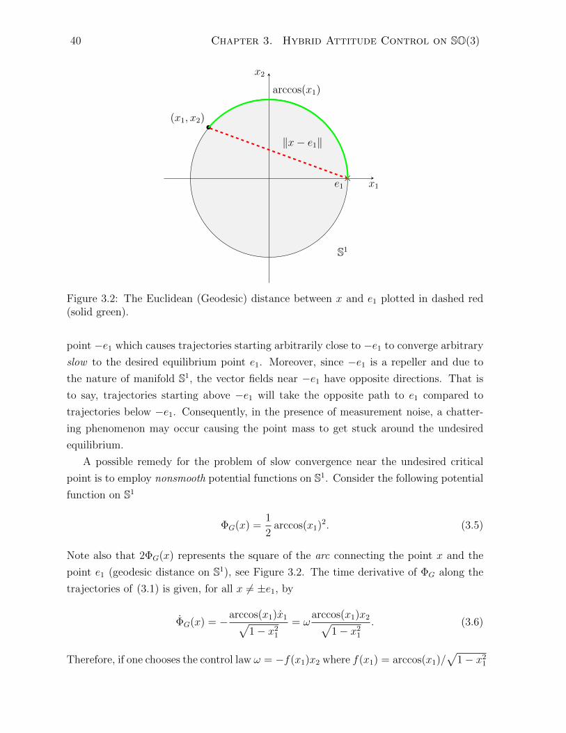
40 Chapter 3. Hybrid Attitude Control on SO(3)
S1
x1
x2
•(x1, x2)
e1×
‖x− e1‖
arccos(x1)
Figure 3.2: The Euclidean (Geodesic) distance between x and e1 plotted in dashed red(solid green).
point −e1 which causes trajectories starting arbitrarily close to −e1 to converge arbitrary
slow to the desired equilibrium point e1. Moreover, since −e1 is a repeller and due to
the nature of manifold S1, the vector fields near −e1 have opposite directions. That is
to say, trajectories starting above −e1 will take the opposite path to e1 compared to
trajectories below −e1. Consequently, in the presence of measurement noise, a chatter-
ing phenomenon may occur causing the point mass to get stuck around the undesired
equilibrium.
A possible remedy for the problem of slow convergence near the undesired critical
point is to employ nonsmooth potential functions on S1. Consider the following potential
function on S1
ΦG(x) =1
2arccos(x1)2. (3.5)
Note also that 2ΦG(x) represents the square of the arc connecting the point x and the
point e1 (geodesic distance on S1), see Figure 3.2. The time derivative of ΦG along the
trajectories of (3.1) is given, for all x 6= ±e1, by
ΦG(x) = −arccos(x1)x1√1− x2
1
= ωarccos(x1)x2√
1− x21
. (3.6)
Therefore, if one chooses the control law ω = −f(x1)x2 where f(x1) = arccos(x1)/√
1− x21

3.2. Motivation Using Planar Rotations on S1 41
S1
x1
x2
e1−e1
Undesiredequilibrium
Desiredequilibrium
Figure 3.3: Vector fields on S1 with control input ω = −x2 (potential function ΦE(x)).The desired critical point e1 is plotted in green and the undesired critical point −e1 isplotted in red.
then ΦG(x) = −f(x1)2x22 ≤ 0. Note that the function f has the following properties
limx1→1
f(x1) = 1, (3.7)
limx1→−1
f(x1) = +∞, (3.8)
Therefore, for x close to e1, the applied control ω = −f(x1)x2 becomes equivalent to
the control law based on ΦE developed above. However, when x gets closer to −e1,
the function f(x1) grows unbounded causing a singularity in the control. Note that
although f(x1) is unbounded near 180, the product f(x1)x2 is bounded and therefore
the control input ω is bounded near 180. As shown in Figure 3.4, the vector field
near −e1 is not vanishing compared to the previous control law. Hence, it is expected
that convergence rates starting from large rotations will be improved. However, this
control law, in addition to being singular at 180, is vulnerable to noise which may cause
chattering near 180. Note that although the singularity at 180 can be removed by
applying a memoryless discontinuous control law, the vulnerability to noise can not be
avoided. In fact, the results in [Mayhew and Teel, 2011a] show that when a compact set
cannot be globally asymptotically stabilized by continuous feedback due to topological
obstructions, it cannot be robustly globally asymptotically stabilized by discontinuous
feedback either.
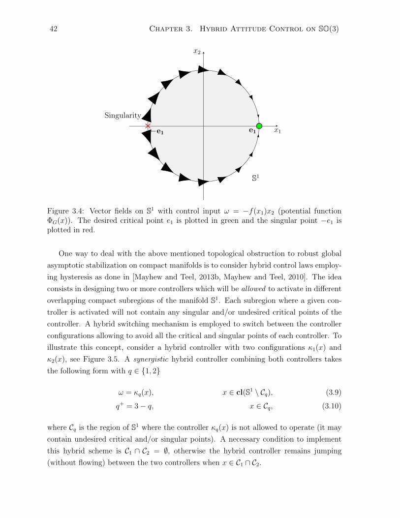
42 Chapter 3. Hybrid Attitude Control on SO(3)
S1
x1
x2
e1−e1
Singularity
Figure 3.4: Vector fields on S1 with control input ω = −f(x1)x2 (potential functionΦG(x)). The desired critical point e1 is plotted in green and the singular point −e1 isplotted in red.
One way to deal with the above mentioned topological obstruction to robust global
asymptotic stabilization on compact manifolds is to consider hybrid control laws employ-
ing hysteresis as done in [Mayhew and Teel, 2013b, Mayhew and Teel, 2010]. The idea
consists in designing two or more controllers which will be allowed to activate in different
overlapping compact subregions of the manifold S1. Each subregion where a given con-
troller is activated will not contain any singular and/or undesired critical points of the
controller. A hybrid switching mechanism is employed to switch between the controller
configurations allowing to avoid all the critical and singular points of each controller. To
illustrate this concept, consider a hybrid controller with two configurations κ1(x) and
κ2(x), see Figure 3.5. A synergistic hybrid controller combining both controllers takes
the following form with q ∈ 1, 2
ω = κq(x), x ∈ cl(S1 \ Cq), (3.9)
q+ = 3− q, x ∈ Cq, (3.10)
where Cq is the region of S1 where the controller κq(x) is not allowed to operate (it may
contain undesired critical and/or singular points). A necessary condition to implement
this hybrid scheme is C1 ∩ C2 = ∅, otherwise the hybrid controller remains jumping
(without flowing) between the two controllers when x ∈ C1 ∩ C2.
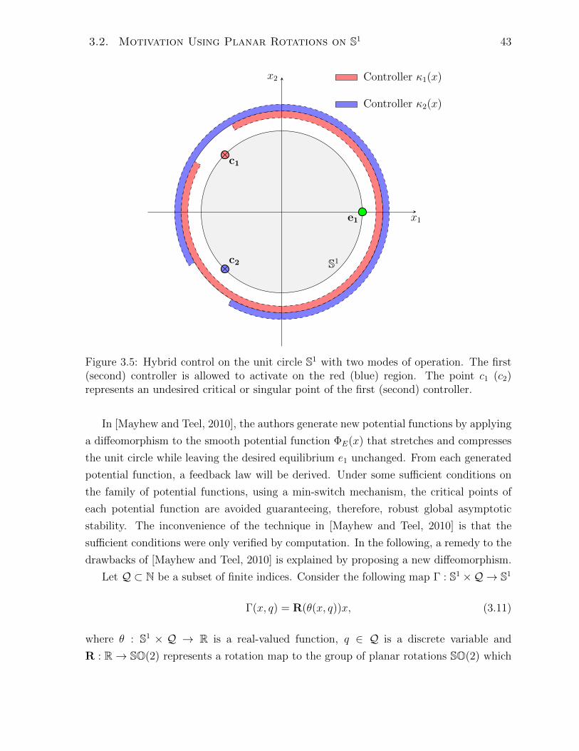
3.2. Motivation Using Planar Rotations on S1 43
S1
x1
x2 Controller κ1(x)
Controller κ2(x)
e1
×c1
×c2
Figure 3.5: Hybrid control on the unit circle S1 with two modes of operation. The first(second) controller is allowed to activate on the red (blue) region. The point c1 (c2)represents an undesired critical or singular point of the first (second) controller.
In [Mayhew and Teel, 2010], the authors generate new potential functions by applying
a diffeomorphism to the smooth potential function ΦE(x) that stretches and compresses
the unit circle while leaving the desired equilibrium e1 unchanged. From each generated
potential function, a feedback law will be derived. Under some sufficient conditions on
the family of potential functions, using a min-switch mechanism, the critical points of
each potential function are avoided guaranteeing, therefore, robust global asymptotic
stability. The inconvenience of the technique in [Mayhew and Teel, 2010] is that the
sufficient conditions were only verified by computation. In the following, a remedy to the
drawbacks of [Mayhew and Teel, 2010] is explained by proposing a new diffeomorphism.
Let Q ⊂ N be a subset of finite indices. Consider the following map Γ : S1 ×Q → S1
Γ(x, q) = R(θ(x, q))x, (3.11)
where θ : S1 × Q → R is a real-valued function, q ∈ Q is a discrete variable and
R : R→ SO(2) represents a rotation map to the group of planar rotations SO(2) which
44 Chapter 3. Hybrid Attitude Control on SO(3)
is given by
R(θ) =
[cos(θ) − sin(θ)
sin(θ) cos(θ)
]. (3.12)
The idea is to design a suitable angle function θ such that the undesired critical points
of the composite functions ΦE(Γ(x, q)), q ∈ Q have different locations while the desired
critical point at e1 remains unchanged; hence one needs Γ(e1, q) = e1 for all q ∈ Q.
Furthermore, the function θ(·, ·) need not to be singular anywhere on S1 as this might
introduce further complications when differentiating the map Γ. For simplicity of dis-
cussion let us consider a hybrid controller with two configurations such that Q = 1, 2.Using the map Γ, one can design two potential functions on S1 as follows:
Φ1(x) = ΦE(Γ(x, 1)), (3.13)
Φ2(x) = ΦE(Γ(x, 2)). (3.14)
For a fixed q ∈ 1, 2 the time derivative of Φq along the trajectories of (3.1) can be
shown to satisfy
Φq(x) = −e>1 Γ(x, q) = −ω(1 +∇θ(x, q)>Sx
)e>1 SΓ(x, q) (3.15)
where ∇θ(x, q) is the gradient of θ with respect to the first argument x. Therefore, the
following controller is derived:
ω = κ(x, q) :=(1 +∇θ(x, q)>Sx
)e>1 SΓ(x, q). (3.16)
Note that the above control input reduces to (3.4) when the map θ(x, q) ≡ 0 which
implies that Γ(x, q) ≡ x. The critical points can be obtained by vanishing the gradient
of Φq, which is equivalent of setting the above control input to zero. This leads to
Γ(x, q) = ±e1 (3.17)
and/or
1 +∇θ(x, q)>Sx = 0. (3.18)
Let us suppose for a moment that θ has been designed such that the condition (3.18) is
not met for all (x, q) ∈ S1 × Q. In this case, the critical points of Φq will be uniquely
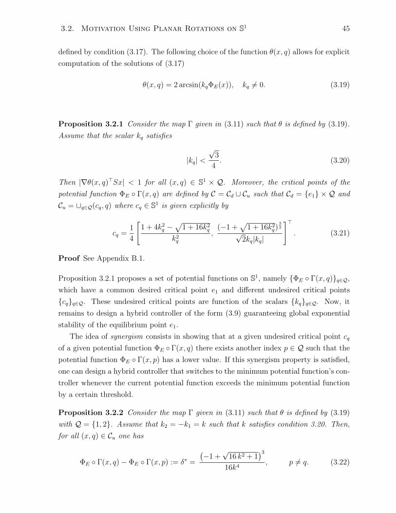
3.2. Motivation Using Planar Rotations on S1 45
defined by condition (3.17). The following choice of the function θ(x, q) allows for explicit
computation of the solutions of (3.17)
θ(x, q) = 2 arcsin(kqΦE(x)), kq 6= 0. (3.19)
Proposition 3.2.1 Consider the map Γ given in (3.11) such that θ is defined by (3.19).
Assume that the scalar kq satisfies
|kq| <√
3
4. (3.20)
Then |∇θ(x, q)>Sx| < 1 for all (x, q) ∈ S1 × Q. Moreover, the critical points of the
potential function ΦE Γ(x, q) are defined by C = Cd ∪ Cu such that Cd = e1 × Q and
Cu = ∪q∈Q(cq, q) where cq ∈ S1 is given explicitly by
cq =1
4
[1 + 4k2
q −√
1 + 16k2q
k2q
,(−1 +
√1 + 16k2
q)32
√2kq|kq|
]>. (3.21)
Proof See Appendix B.1.
Proposition 3.2.1 proposes a set of potential functions on S1, namely ΦE Γ(x, q)q∈Q,
which have a common desired critical point e1 and different undesired critical points
cqq∈Q. These undesired critical points are function of the scalars kqq∈Q. Now, it
remains to design a hybrid controller of the form (3.9) guaranteeing global exponential
stability of the equilibrium point e1.
The idea of synergism consists in showing that at a given undesired critical point cq
of a given potential function ΦE Γ(x, q) there exists another index p ∈ Q such that the
potential function ΦE Γ(x, p) has a lower value. If this synergism property is satisfied,
one can design a hybrid controller that switches to the minimum potential function’s con-
troller whenever the current potential function exceeds the minimum potential function
by a certain threshold.
Proposition 3.2.2 Consider the map Γ given in (3.11) such that θ is defined by (3.19)
with Q = 1, 2. Assume that k2 = −k1 = k such that k satisfies condition 3.20. Then,
for all (x, q) ∈ Cu one has
ΦE Γ(x, q)− ΦE Γ(x, p) := δ∗ =
(−1 +
√16 k2 + 1
)3
16k4, p 6= q. (3.22)
46 Chapter 3. Hybrid Attitude Control on SO(3)
Proof See Appendix B.2.
0
0.5
-1
1
1.5
2
-1
x2
0 -0.5
x1
00.5
1 1
ΦE(x)
0-1
0.5
-1
1
1.5
-0.5
2
-0.5
x1x2
000.50.5
11
ΦE(Γ(x, 1))ΦE(Γ(x, 2))
δ
Figure 3.6: Plot of the original potential function ΦE(x) (left) and the new compositepotential functions ΦE(Γ(x, 1)) and ΦE(Γ(x, 2)) (right) with k = 1/4. The synergisticgap δ∗ between the two potential functions is equal to 16/9.
Consequently, it is shown in Proposition 3.2.2 that at any given undesired critical point
of ΦE(Γ(x, q)), the potential function ΦE(Γ(x, p)) with p 6= q has a lower value with a
gap δ∗ > 0 given explicitly function of the scalar k. Using this property, the following
hybrid controller immediately follows
ω = κ(x, q), (x, q) ∈ F , (3.23)
q+ = arg minp∈Q
ΦE(Γ(x, p)), (x, q) ∈ J , (3.24)
where the flow set F and jump set J are defined as follows
F = (x, q) : ΦE Γ(x, q)−minp∈Q
ΦE Γ(x, p) ≤ δ, (3.25)
J = (x, q) : ΦE Γ(x, q)−minp∈Q
ΦE Γ(x, p) ≥ δ, (3.26)
where 0 < δ < δ∗ and the synergistic gap δ∗ is given in Proposition 3.2.2. The idea of
the proposed hybrid controller is to switch to the configuration with minimum potential
function ΦE Γ(x, q) whenever the gap between the current potential function and the
minimum one exceeds some threshold δ. If the potential function ΦE Γ(x, q) is taken
as a Lyapunov function candidate then the jump equation (3.24) allows to guarantee a
decrease in the Lyapunov function between jumps. The above proposed control scheme
can be shown to guarantee global exponential stability of the set e1 × Q. It should
be mentioned also that it is possible to use the non-smooth (geodesic) potential function
ΦG(x), given in (3.5), to derive a hybrid controller that avoids the singular points of

3.3. Attitude Stabilization on SO(3) 47
ΦG Γ(x, q) using a similar min-switch strategy. Since the objective of this thesis is the
control and estimation on SO(3), these discussions on the unit circle will not be pursued
further. The reader is referred to [Mayhew and Teel, 2013b, Casau et al., 2015a] for a
detailed treatment of hybrid control on the general unit sphere Sn. The ideas discussed
in this section for the hybrid control of planar rotations will inspire our proposed control
designs for the general group of 3D rotations, namely the Special Orthogonal group
SO(3) which will be the goal of the next sections.
3.3 Attitude Stabilization on SO(3)
In this section, an approach to design hybrid controllers for the attitude kinematics (first
order system) that achieves robust global exponential stability on SO(3) is proposed.
Discussions about stabilization and tracking for the full rigid body attitude dynamics
(second order system) will be detailed in the next section. First, the new concept of
exp-synergistic potential functions on SO(3) is introduced. Then, exp-synergistic poten-
tial functions are shown to be sufficient to design hybrid control algorithms guaranteeing
global exponential stability on SO(3). Lastly, a systematic methodology for the construc-
tion of such potential functions on SO(3) is provided.
3.3.1 Problem Formulation
Consider the following kinematics system on SO(3)
R = R[ω]×, (3.27)
where R ∈ SO(3) represents the attitude state and ω ∈ R3 is the control input. The
stabilization control problem for system (3.27) consists in designing an appropriate input
ω such that (R = I) is globally exponentially stable. Note that there is no loss of
generality in considering the stabilization problem of the identity rotation I. In fact,
assume that our problem is the tracking of the desired time varying trajectory Rd(t) =
Rd(t)[ωd(t)]× for some ωd(t) ∈ R3 and Rd(0) ∈ SO(3). Let R = RR>d be the attitude
tracking error and let the control input ω = ωd + Rdω for some virtual input ω ∈ R3.
Therefore, it is not difficult to show that one has ˙R = R[ω]× which implies that the
original tracking problem is reduced to a stabilization problem for the attitude tracking
error R.

48 Chapter 3. Hybrid Attitude Control on SO(3)
3.3.2 Smooth Attitude Stabilization on SO(3)
A natural solution to tackle this problem is to consider a gradient-based control approach.
Consider for example the following weighted trace potential function used in many atti-
tude control problems [Koditschek, 1988, Bullo and Murray, 1999, Sanyal et al., 2009]
Ψ1,A(R) =1
2tr(A(I −R)), (3.28)
where A ∈ R3×3 is a symmetric matrix. Note that the condition for Ψ1,A(R) to be a
valid (positive definite with respect to I) potential function on SO(3) is that the matrix
E(A), with the map E(·) defined in (2.66), is symmetric positive definite. Intuitively, by
looking at the expression of Ψ1,A(R) in terms of quaternions (see (2.75)) it can be seen
that Ψ1,A(R) is positive definite with respect to the quaternion (±1, 0), which represents
the identity rotation, if and only if E(A) is symmetric positive definite. Consider the
following gradient-based controller
ω = −2kψ(R>∇Ψ1,A(R)), k > 0. (3.29)
Then, by using Ψ1,A(R) as the Lyapunov function candidate one obtains the following
time derivative of the Lyapunov function along the trajectories of (3.27)
Ψ1,A(R) = 〈∇Ψ1,A(R), R〉R = 〈〈∇Ψ1,A(R), R[ω]×〉〉 = −2k‖∇Ψ1,A(R)‖2F ≤ 0. (3.30)
This shows that the equilibrium point R = I is stable. Moreover, using LaSalle’s in-
variance principle it can be concluded that all solutions must converge to the largest
invariant set where the gradient of Ψ1,A(R) vanishes (critical points). In view of (2.71)
the gradient of Ψ1,A(R) is given by ∇Ψ1,A(R) = 12RPso(3)(AR) which implies that the
closed-loop system under the feedback (3.29) can be written as
R = −kR[ψ(AR)]× = −k2R(AR−R>A) = −k
2(RAR− A). (3.31)
The equilibria of the above system which correspond to the critical points of Ψ1,A(R)
satisfy AR = R>A. This set of critical points is given by (see [Mayhew and Teel, 2013a,
Lemma 4])
CΨ1,A= I ∪Ra(π, ERv (A)), (3.32)
which contains the identity rotation and all the rotations of 180 around an eigenvector
of A. An other interesting observation from (3.31) is that if R is symmetric then R is

3.3. Attitude Stabilization on SO(3) 49
also symmetric and, therefore, the subset of SO(3) where R is symmetric is invariant
under the flows of (3.31). This set is identified by R = R> which implies that R2 = I.
It can be shown that the solutions of R2 = I are identified by the set I ∪Ra(π,S2).
Therefore starting inside the set Ra(π,S2) the trajectories of the system will eventually
converge to Ra(π, ERv (A)). Moreover during the flows of (3.31) one has
d
dttr(I −R) = −tr(R) = −k
2tr(A−RAR) = −k
2tr(A(I −R2)) ≤ 0. (3.33)
This implies that all trajectories starting outside Ra(π,S2) will converge to the desired
identity rotation R = I. In this case, the equilibrium R = I is said to be almost globally
asymptotically stable since from almost all initial conditions (specifically initial attitudes
with angle less than 180) the trajectories of the system converge to R = I. The set
Ra(π,S2) has a Lebegue measure of zero with respect to SO(3). Although the obtained
asymptotic stability result for the equilibrium R = I is strong the existence of the
undesired equilibria in Ra(π,S2) limits the performance of this control law as explained
hereafter.
First, let us derive the time-explicit solution of the differential equation (3.31) which
allows to study the trajectories of the system starting at different initial conditions outside
the set Ra(π,S2).
Theorem 3.3.1 Consider the dynamic system (3.31). Let R(0) ∈ ΠSO(3) then
R(t) = Rr(exp(−kE(A)t)Z(R(0))), t ≥ 0. (3.34)
Proof See Appendix C.2.
Theorem 3.3.1 provides a closed form solution for the attitude kinematics system (3.27)
under the gradient-based feedback (3.29) or, equivalently, the matrix differential equa-
tion (3.31) on SO(3). To the best of the author’s knowledge, there is no available work
providing such an explicit time solution. The obtained closed form solution is not only
appealing from a theoretical stand point but it is also beneficial to understand the be-
haviour of the trajectories of (3.31) without requiring complex analysis tools. From
(3.34) it can be noticed that the Rodrigues vector Z(R(t)) is exponentially decaying to
zero from all initial conditions. Note that this vector is only defined for rotations which
have an angle different from 180. It is worth pointing out that, although the Rodrigues
vector is converging exponentially, the attitude does not necessary converge exponentially
fast since there is a mapping Rr between the two quantities. The following Corollary

50 Chapter 3. Hybrid Attitude Control on SO(3)
provides an explicit expression of the attitude norm, which will be very useful in studying
the performance of the closed-loop system.
Corollary 3.3.2 Consider the dynamic system (3.31). Let R(0) ∈ ΠSO(3). Then, for all
t ≥ 0, one has
|R(t)|2I =ψ(R(0))>e−2kE(A)tψ(R(0))
4(1− |R(0)|2I)2 + ψ(R(0))>e−2kE(A)tψ(R(0)). (3.35)
Proof The result can be directly derived from Theorem 3.3.1 by noticing that
‖Z(R(t))‖2 = ‖e−kE(A)tZ(R(0))‖2 =ψ(R(0))>e−2kE(A)tψ(R(0))
4(1− |R(0)|2I)2, (3.36)
and from (2.76) |R(t)|2I = tr(I −R)/4 = ‖Z(R)‖2/(1 + ‖Z(R)‖2) which implies (3.35).
Corollary 3.3.2 provides an explicit expression showing the evolution of the Euclidean
distance |R(t)|I with respect to time. Note that it is not difficult to show that ψ(R) =
sin(θ)u where R = Ra(θ, u). Therefore, from (3.35), for the same initial attitude angle,
initial attitudes with rotation axis u(0) equals the eigenvector corresponding to the largest
eigenvalue of E(A) generates a larger attitude norm |R(t)|I compared to an initial attitude
with rotation axis u(0) equals the eigenvector corresponding to the smallest eigenvalue
of E(A). The following Corollary provides upper and lower bounds of |R(t)|I .
Corollary 3.3.3 Consider the dynamic system (3.31). Let R(0) ∈ ΠSO(3), then the
attitude norm is bounded as follows
β(|R(0)|I , t, kλE(A)max ) ≤ |R(t)|I ≤ β(|R(0)|I , t, kλE(A)
min ), (3.37)
for all t ≥ 0, such that β(s, t, λ) = se−λt/(1− s2(1− e−2λt)
) 12 .
Proof Note that
ψ(R(0))>e−2kE(A)tψ(R(0)) ≤ e−2kλE(A)min t‖ψ(R(0))‖2 = 4e−2kλ
E(A)min t|R(0)|2I(1− |R(0)|2I)
which, in view of (3.35) and the fact that the map x → x/(x + a) is non-decreasing for
all a ≥ 0, implies that
|R(t)|2I ≤ e−2kλE(A)min t|R(0)|2I/(1− |R(0)|2I + e−2kλ
E(A)min t|R(0)|2I) =
(β(|R(0)|I , t, kλE(A)
min ))2.
Following similar steps as above, the lower bound can be derived.
3.3. Attitude Stabilization on SO(3) 51
According to the upper bound on the attitude distance given in Corollary 3.3.3, it is
clear that for small initial conditions, i.e., |R(0)|I 1, the attitude satisfies |R(t)|I ≤|R(0)|I exp(−kλE(A)
min t) which shows the local exponential stability of the equilibrium point
|R|I = 0. Moreover, the convergence rate of the attitude to R = I is given in the following
corollary
Corollary 3.3.4 Starting from any initial condition R(0) ∈ ΠSO(3), the time tB necessary
to enter the ball of radius |R(tB)|I = B satisfies
tB ≥1
kλE(A)max
ln
(|R(0)|I(1−B2)
12
B(1− |R(0)|2I)12
). (3.38)
Proof Using the lower bound of (3.37), the time tB needs to satisfy the constraint
β(|R(0)|I , tB, kλE(A)max ) ≤ |R(tB)|I = B. Using straightforward algebraic manipulations,
this inequality reads e−kλE(A)max tB ≤ B2(1−|R(0)|2I)
|R(0)|2I(1−B2), which leads to the result of the corollary
by taking the ln(·) function on both sides of the last inequality.
According to Corollary 3.3.4, it is clear that large initial conditions, i.e., |R(0)|I → 1, will
result in low convergence rates. Whenever the initial attitude is closer to the manifold
of all rotations of 180 the stabilization task will take longer time. This fact about the
transient-response performance degradation of smooth attitude controllers on SO(3) has
been numerically and experimentally observed in recent works such as [Lee, 2012, Tse-
Huai Wu and Lee, 2015, Zlotnik and Forbes, 2017]. Moreover, it is possible to show
that the above control scheme is not robust to a certain class of small bounded vanishing
disturbances, see [Berkane and Tayebi, 2017a].
3.3.3 Synergistic and Exp-Synergistic Potential Functions
As discussed in the previous section, smooth controllers derived from smooth potential
functions on SO(3) suffer from performance degradation (low convergence rates, reduced
robustness) when the initial attitude is large. On the other hand, controllers derived
from nonsmooth potential functions on SO(3) are susceptible to singularities thus not
very desirable in practice. To cope with these shortcomings, one can design different
controllers from a “family” of potential functions which will be then coordinated in a
hybrid fashion to yield the desirable robust global exponential stabilization on SO(3).
This collective behaviour that leads to an improvement in the performance of the control
scheme is referred to as “synergism”. In this subsection, the formal definition of syner-
gism is recalled and the new notion of exp-synergism for a family of potential functions
52 Chapter 3. Hybrid Attitude Control on SO(3)
on SO(3) is defined.
Given a finite index set Q ⊂ N, let C0 (SO(3)×Q,R≥0) denote the set of positive-
valued and continuous functions Φ : SO(3)×Q → R≥0. If, for each q ∈ Q, the map R 7→Φ(R, q) is differentiable on the set Dq ⊆ SO(3) then the function Φ(R, q) is continuously
differentiable on D ⊆ SO(3) × Q, where D = ∪q∈QDq × q, in which case one denotes
Φ ∈ C1 (D,R≥0). Additionally, for all (R, q) ∈ D, ∇Φ(R, q) ∈ TRSO(3) denotes the
gradient of Φ, with respect to R, relative to the Riemannian metric (2.13).
Definition 3.3.5 (Potential Function) A function Φ is said to be a potential function
on D ⊆ SO(3)×Q with respect to the set IQ = I × Q ⊆ D if:
i) Φ is continuous, i.e. Φ ∈ C0 (SO(3)×Q,R≥0)
ii) Φ is continuously differentiable on D, i.e. Φ ∈ C1(D,R≥0)
iii) Φ is positive definite with respect to IQ, i.e. Φ(R, q) = 0 if (R, q) ∈ IQ and
Φ(R, q) > 0 otherwise
The set of all potential functions on D with respect to IQ is denoted as PD, where a
function Φ(R, q) ∈ PD can be seen as a family of potential functions on SO(3) encoded
into a single function indexed by q. When the finite index set Q reduces to a single
element, for example Q = 1, then the argument q is omitted and D ⊆ SO(3). For a
given potential function Φ(R, q) ∈ PD, the set of critical points of Φ is defined as follows
CΦ = (R, q) ∈ D : ∇Φ(R, q) = 0 . (3.39)
Note that if Φ(R, q) ∈ PD then the map R 7→ Φ(R, q) is positive definite on SO(3) with
respect to I for each q ∈ Q. Thus, the identity rotation I must be a critical point1 for
R 7→ Φ(R, q), ∀q ∈ Q and therefore the set IQ is included in the set of critical points of
Φ or, for short, IQ ⊆ CΦ.
Definition 3.3.6 (Synergism [Mayhew and Teel, 2013a]) For a given finite index
set Q ⊂ N, let Φ ∈ PSO(3)×Q. The potential function Φ is said to be centrally synergistic,
with gap exceeding δ > 0, if and only if the following condition holds
Φ(R, q)− minm∈Q
Φ(R,m) > δ, ∀(R, q) ∈ CΦ \ IQ. (3.40)
1In fact, for any locally smooth function f :M→ R such that f is locally positive definite functionabout x0, the point x0 is a critical point of f and the Hessian of f is positive semidefinite at x0.
3.3. Attitude Stabilization on SO(3) 53
Condition (3.40) implies that at any given undesired critical point (R, q) ∈ CΦ \ IQ,
there exists another point (R,m) ∈ SO(3)×Q such that Φ(R,m) has a lower value than
Φ(R, q). The term “central” refers to the fact that all the potential functions R 7→ Φ(R, q)
share the identity element I as a critical point such that ∇Φ(I, q) = 0 for all q ∈ Q.
Definition 3.3.7 (Exp-Synergism) Consider a set of parameters T = (Φ,Q, δ) con-
taining a potential function Φ ∈ PD, D ⊆ SO(3) × Q, a finite index set Q ⊂ N and a
scalar δ > 0. Let the subset FT ⊆ SO(3)×Q be defined as:
FT = (R, q) : Φ(R, q)− minm∈Q
Φ(R,m) ≤ δ. (3.41)
The potential function Φ is said to be exp-synergistic, with gap exceeding δ > 0, if and
only if there exist constants αi > 0, i = 1, . . . , 4, such that the following hold:
α1|R|2I ≤ Φ(R, q) ≤ α2|R|2I , ∀(R, q) ∈ SO(3)×Q, (3.42)
α3|R|2I ≤ ‖∇Φ(R, q)‖2F ≤ α4|R|2I , ∀(R, q) ∈ FT , (3.43)
FT ⊆ D. (3.44)
Definition 3.3.7 considers a wider class of potential functions, compared to Definition
3.3.6, by allowing each potential function R 7→ Φ(R, q) to be nondifferentiable on some
region of the manifold SO(3). However, the exp-synergism definition imposes more re-
strictive conditions as compared to Definition 3.3.6 in the sense that the potential function
and its gradient are quadratically bounded by the attitude distance on SO(3). It can
be verified that if Φ ∈ PD with D = SO(3) ×Q is an exp-synergistic potential function
then it is synergistic as well. In fact, condition (3.43) implies that the gradient ∇Φ(R, q)
does not vanish expect at IQ which is equivalent to condition (3.40). The opposite
does not hold in general. The exp-synergism property, as will become clear in the next
subsection, plays an important role to ensure desirable exponential decay when using a
gradient-based feedback on SO(3).
3.3.4 Hybrid Attitude Stabilization on SO(3)
In this subsection, exp-synergistic potential functions are shown to be instrumental for
the global exponential stabilization on SO(3). Let Q ⊂ N be a finite index set, Φ ∈ PDbe a potential function on D ⊆ SO(3)×Q and δ > 0. Define T = (Φ,Q, δ) and consider
the following switching mechanism of the discrete state variable q, which dictates the
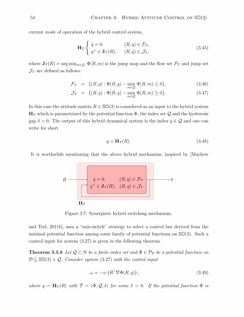
54 Chapter 3. Hybrid Attitude Control on SO(3)
current mode of operation of the hybrid control system,
HT
q = 0, (R, q) ∈ FT ,q+ ∈ JT (R), (R, q) ∈ JT ,
(3.45)
where JT (R) = arg minm∈Q Φ(R,m) is the jump map and the flow set FT and jump set
JT are defined as follows:
FT = (R, q) : Φ(R, q)− minm∈Q
Φ(R,m) ≤ δ, (3.46)
JT = (R, q) : Φ(R, q)− minm∈Q
Φ(R,m) ≥ δ. (3.47)
In this case the attitude matrix R ∈ SO(3) is considered as an input to the hybrid system
HT which is parametrized by the potential function Φ, the index set Q and the hysteresis
gap δ > 0. The output of this hybrid dynamical system is the index q ∈ Q and one can
write for short
q = HT (R). (3.48)
It is worthwhile mentioning that the above hybrid mechanism, inspired by [Mayhew
HT
q = 0, (R, q) ∈ FTq+ ∈ JT (R), (R, q) ∈ JT
R q
Figure 3.7: Synergistic hybrid switching mechanism.
and Teel, 2011b], uses a “min-switch” strategy to select a control law derived from the
minimal potential function among some family of potential functions on SO(3). Such a
control input for system (3.27) is given in the following theorem.
Theorem 3.3.8 Let Q ⊂ N be a finite index set and Φ ∈ PD be a potential function on
D ⊆ SO(3)×Q. Consider system (3.27) with the control input
ω = −ψ(R>∇Φ(R, q)
), (3.49)
where q = HT (R) with T = (Φ,Q, δ) for some δ > 0. If the potential function Φ is
3.3. Attitude Stabilization on SO(3) 55
exp-synergistic with gap exceeding δ, then the set A1 = I ×Q is globally exponentially
stable.
Proof See Appendix C.3.
The result in Theorem 3.3.8 provides a systematic method for the design of hybrid at-
titude control algorithms for system (3.27) guaranteeing global exponential stability. It
is worth pointing out that, in addition to the structurally simple expression of the con-
troller proposed so far, the result in this subsection reduces the stabilisation problem of
systems (3.27) to the problem of finding appropriate exp-synergistic potential functions,
in the sense of Definition 3.3.7, with some synergistic gap that can be specified using the
control parameters. This will be the objective of the next subsection.
3.3.5 Construction of Exp-Synergistic Potential Functions
The focus of this subsection will be on the design of exp-synergistic potential functions on
the rotation group SO(3) which are shown to be sufficient for the design of global hybrid
attitude stabilization schemes. The first work dealing with the construction of syner-
gistic potential functions on SO(3) appeared in [Mayhew and Teel, 2011d]. It consists
of stretching and compressing SO(3) by applying diffeomorphic transformations, which
allow to relocate the critical points while leaving the identity element unchanged leading
to a synergistic family of potential functions. Despite the originality of this approach,
it was abandoned mainly due to the difficulty in finding an explicit expression of the
synergistic gap. In this section, we build up from the ideas in [Mayhew and Teel, 2011d]
towards more generic constructions of exp-synergistic potential functions on SO(3) via
“angular warping”, while providing a thorough analysis of the synergism properties.
Lemma 3.3.9 Let Q ⊂ N be a finite index set and uqq∈Q ⊂ S2 be a set of unit vectors.
Let us consider the map2 Γ : SO(3)×Q → SO(3) such that
Γ(R, q) := RRa(θq(R), uq), (3.50)
where θq : SO(3)→ R is a real-valued differentiable function. Then, the following hold:
1. The time derivative of Γ(R, q), as defined in (3.50), along the trajectories of R =
R[ω]× is given byd
dtΓ(R, q) = Γ(R, q)[Θ(R, q)ω]×, (3.51)
2The multiplication by the additional rotation Ra(θq(R), u) is done on the right of the original rotationmatrix R for our convenience. It is left to the reader to explore the other option.
56 Chapter 3. Hybrid Attitude Control on SO(3)
where Θ(R, q)> = Ra(θq(R), uq) + 2ψ(R>∇θq(R))u>q .
2. If det(Θ(R, q)) 6= 0 for all (R, q) ∈ SO(3) × Q, then for each q ∈ Q the map
R 7→ Γ(R, q) is everywhere a local diffeomorphism.
3. If det(Θ(R, q)) 6= 0 for all (R, q) ∈ SO(3) × Q and Γ−1(I) = I × Q then for
any Ψ ∈ PDΨwith DΨ ⊆ SO(3) one has Ψ Γ ∈ PΓ−1(DΨ) and the set of critical
points of Ψ Γ is given by CΨΓ = Γ−1(CΨ).
Proof See Appendix A.8.
Lemma 3.3.9 shows that, under some conditions on the transformation Γ, one can
construct a new family of potential functions on SO(3) by considering the composition
of a basic potential function on SO(3) and the map Γ. What we will investigate next is
the search for a suitable basic function Ψ, a suitable angle function θq(·) and the set of
unit vectors uqq∈Q such that the composite function Ψ Γ(R, q) is an exp-synergistic
potential function.
Non-Weighted Potential Functions
Consider the following potential functions on SO(3):
Ψ1(R) =1
2tr(I −R), (3.52)
Ψ2(R) = 2−√
1 + tr(R). (3.53)
The smooth potential function Ψ1(R) has been widely used in the literature for attitude
control problems [Koditschek, 1988, Bullo and Murray, 1999, Sanyal et al., 2009]. The
nonsmooth potential function Ψ2(R) is non differentiable at tr(R) = −1 which corre-
sponds to the set of all attitudes of angle π. The potential function Ψ2(R) has been
used in [Lee, 2012] for attitude tracking to obtain faster convergence for large attitude
manoeuvres and also appeared in [Saccon et al., 2010] as a solution to the kinematic
optimal control on SO(3). Note that there exists a similar nonsmooth potential function
Ψ3(R) = 2π2‖ log(R)‖2
F which is related to the geodesic distance on SO(3) as defined
in (2.39) between the rotation matrix R and the identity rotation I. It has been used
for instance in [Bullo and Murray, 1995] for attitude stabilization and in [Berkane and
Tayebi, 2015b] for optimal kinematic attitude control on SO(3) and the results of this
section can be extended or modified to use Ψ3(R). It is interesting to see the expressions
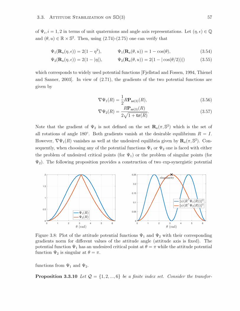
3.3. Attitude Stabilization on SO(3) 57
of Ψi, i = 1, 2 in terms of unit quaternions and angle axis representations. Let (η, ε) ∈ Qand (θ, u) ∈ R× S2. Then, using (2.74)-(2.75) one can verify that
Ψ1(Ru(η, ε)) = 2(1− η2), Ψ1(Ra(θ, u)) = 1− cos(θ), (3.54)
Ψ2(Ru(η, ε)) = 2(1− |η|), Ψ2(Ra(θ, u)) = 2(1− | cos(θ/2))|) (3.55)
which corresponds to widely used potential functions [Fjellstad and Fossen, 1994, Thienel
and Sanner, 2003]. In view of (2.71), the gradients of the two potential functions are
given by
∇Ψ1(R) =1
2RPso(3)(R), (3.56)
∇Ψ2(R) =RPso(3)(R)
2√
1 + tr(R). (3.57)
Note that the gradient of Ψ2 is not defined on the set Ra(π,S2) which is the set of
all rotations of angle 180. Both gradients vanish at the desirable equilibrium R = I.
However, ∇Ψ1(R) vanishes as well at the undesired equilibria given by Ra(π,S2). Con-
sequently, when choosing any of the potential functions Ψ1 or Ψ2 one is faced with either
the problem of undesired critical points (for Ψ1) or the problem of singular points (for
Ψ2). The following proposition provides a construction of two exp-synergistic potential
0 1 2 3 4 5 6
θ (rad)
0
0.5
1
1.5
2
Ψ1(R)Ψ2(R)
0 1 2 3 4 5 6
θ (rad)
0
0.05
0.1
0.15
0.2
0.25
‖ψ(R⊤Ψ1(R))‖2
‖ψ(R⊤Ψ2(R))‖2
singularity
Figure 3.8: Plot of the attitude potential functions Ψ1 and Ψ2 with their correspondinggradients norm for different values of the attitude angle (attitude axis is fixed). Thepotential function Ψ1 has an undesired critical point at θ = π while the attitude potentialfunction Ψ2 is singular at θ = π.
functions from Ψ1 and Ψ2.
Proposition 3.3.10 Let Q = 1, 2, ..., 6 be a finite index set. Consider the transfor-
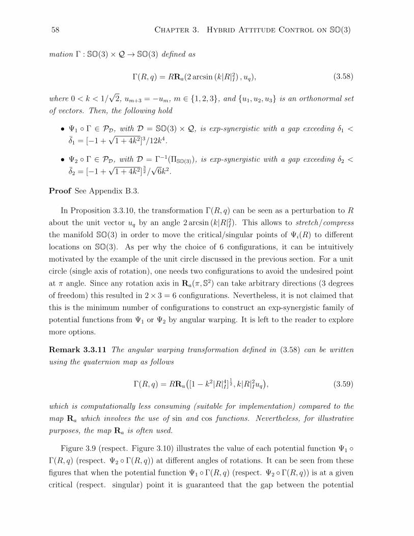
58 Chapter 3. Hybrid Attitude Control on SO(3)
mation Γ : SO(3)×Q → SO(3) defined as
Γ(R, q) = RRa(2 arcsin (k|R|2I) , uq), (3.58)
where 0 < k < 1/√
2, um+3 = −um, m ∈ 1, 2, 3, and u1, u2, u3 is an orthonormal set
of vectors. Then, the following hold
• Ψ1 Γ ∈ PD, with D = SO(3) × Q, is exp-synergistic with a gap exceeding δ1 <
δ1 = [−1 +√
1 + 4k2]3/12k4.
• Ψ2 Γ ∈ PD, with D = Γ−1(ΠSO(3)), is exp-synergistic with a gap exceeding δ2 <
δ2 = [−1 +√
1 + 4k2]32/√
6k2.
Proof See Appendix B.3.
In Proposition 3.3.10, the transformation Γ(R, q) can be seen as a perturbation to R
about the unit vector uq by an angle 2 arcsin (k|R|2I). This allows to stretch/compress
the manifold SO(3) in order to move the critical/singular points of Ψi(R) to different
locations on SO(3). As per why the choice of 6 configurations, it can be intuitively
motivated by the example of the unit circle discussed in the previous section. For a unit
circle (single axis of rotation), one needs two configurations to avoid the undesired point
at π angle. Since any rotation axis in Ra(π,S2) can take arbitrary directions (3 degrees
of freedom) this resulted in 2× 3 = 6 configurations. Nevertheless, it is not claimed that
this is the minimum number of configurations to construct an exp-synergistic family of
potential functions from Ψ1 or Ψ2 by angular warping. It is left to the reader to explore
more options.
Remark 3.3.11 The angular warping transformation defined in (3.58) can be written
using the quaternion map as follows
Γ(R, q) = RRu
([1− k2|R|4I ]
12 , k|R|2Iuq
), (3.59)
which is computationally less consuming (suitable for implementation) compared to the
map Ra which involves the use of sin and cos functions. Nevertheless, for illustrative
purposes, the map Ra is often used.
Figure 3.9 (respect. Figure 3.10) illustrates the value of each potential function Ψ1 Γ(R, q) (respect. Ψ2 Γ(R, q)) at different angles of rotations. It can be seen from these
figures that when the potential function Ψ1 Γ(R, q) (respect. Ψ2 Γ(R, q)) is at a given
critical (respect. singular) point it is guaranteed that the gap between the potential
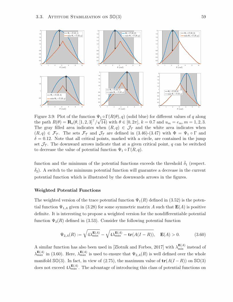
3.3. Attitude Stabilization on SO(3) 59
0 1 2 3 4 5 6
θ (rad)
0
0.2
0.4
0.6
0.8
1
1.2
1.4
1.6
1.8
2
Ψ1 Γ(R, 1)minΨ1 Γ(R, q)
0 1 2 3 4 5 6
θ (rad)
0
0.2
0.4
0.6
0.8
1
1.2
1.4
1.6
1.8
2
Ψ1 Γ(R, 2)minΨ1 Γ(R, q)
0 1 2 3 4 5 6
θ (rad)
0
0.2
0.4
0.6
0.8
1
1.2
1.4
1.6
1.8
2
Ψ1 Γ(R, 3)minΨ1 Γ(R, q)
0 1 2 3 4 5 6
θ (rad)
0
0.5
1
1.5
2
Ψ1 Γ(R, 4)
minΨ1 Γ(R, q)
0 1 2 3 4 5 6
θ (rad)
0
0.2
0.4
0.6
0.8
1
1.2
1.4
1.6
1.8
2
Ψ1 Γ(R, 5)minΨ1 Γ(R, q)
0 1 2 3 4 5 6
θ (rad)
0
0.2
0.4
0.6
0.8
1
1.2
1.4
1.6
1.8
2
Ψ1 Γ(R, 6)minΨ1 Γ(R, q)
Figure 3.9: Plot of the function Ψ1 Γ(R(θ), q) (solid blue) for different values of q alongthe path R(θ) = Ra(θ, [1, 2, 3]>/
√14) with θ ∈ [0, 2π], k = 0.7 and um = em,m = 1, 2, 3.
The gray filled area indicates when (R, q) ∈ JT and the white area indicates when(R, q) ∈ FT . The sets FT and JT are defined in (3.46)-(3.47) with Φ = Ψ1 Γ andδ = 0.12. Note that all critical points, marked with a circle, are contained in the jumpset JT . The downward arrows indicate that at a given critical point, q can be switchedto decrease the value of potential function Ψ1 Γ(R, q).
function and the minimum of the potential functions exceeds the threshold δ1 (respect.
δ2). A switch to the minimum potential function will guarantee a decrease in the current
potential function which is illustrated by the downwards arrows in the figures.
Weighted Potential Functions
The weighted version of the trace potential function Ψ1(R) defined in (3.52) is the poten-
tial function Ψ1,A given in (3.28) for some symmetric matrix A such that E(A) is positive
definite. It is interesting to propose a weighted version for the nondifferentiable potential
function Ψ2(R) defined in (3.53). Consider the following potential function
Ψ2,A(R) :=
√4λ
E(A)max −
√4λ
E(A)max − tr(A(I −R)), E(A) > 0. (3.60)
A similar function has also been used in [Zlotnik and Forbes, 2017] with λE(A)min instead of
λE(A)max in (3.60). Here, λ
E(A)max is used to ensure that Ψ2,A(R) is well defined over the whole
manifold SO(3). In fact, in view of (2.75), the maximum value of tr(A(I−R)) on SO(3)
does not exceed 4λE(A)max . The advantage of introducing this class of potential functions on
60 Chapter 3. Hybrid Attitude Control on SO(3)
0 1 2 3 4 5 6
θ (rad)
0
0.2
0.4
0.6
0.8
1
1.2
1.4
1.6
1.8
2
Ψ2 Γ(R,1)minΨ2 Γ(R, q)
0 1 2 3 4 5 6
θ (rad)
0
0.2
0.4
0.6
0.8
1
1.2
1.4
1.6
1.8
2
Ψ2 Γ(R,2)minΨ2 Γ(R, q)
0 1 2 3 4 5 6
θ (rad)
0
0.2
0.4
0.6
0.8
1
1.2
1.4
1.6
1.8
2
Ψ2 Γ(R,3)minΨ2 Γ(R, q)
0 1 2 3 4 5 6
θ (rad)
0
0.2
0.4
0.6
0.8
1
1.2
1.4
1.6
1.8
2
Ψ2 Γ(R,4)minΨ2 Γ(R, q)
0 1 2 3 4 5 6
θ (rad)
0
0.2
0.4
0.6
0.8
1
1.2
1.4
1.6
1.8
2
Ψ2 Γ(R,5)minΨ2 Γ(R, q)
0 1 2 3 4 5 6
θ (rad)
0
0.2
0.4
0.6
0.8
1
1.2
1.4
1.6
1.8
2
Ψ2 Γ(R,6)minΨ2 Γ(R, q)
Figure 3.10: Plot of the function Ψ2Γ(R(θ), q) (solid blue) for different values of q alongthe path R(θ) = Ra(θ, [1, 2, 3]>/
√14) with θ ∈ [0, 2π], k = 0.7 and um = em,m = 1, 2, 3.
The gray filled area indicates when (R, q) ∈ JT and the white area indicates when(R, q) ∈ FT . The sets FT and JT are defined in (3.46)-(3.47) with Φ = Ψ2 Γ andδ = 0.46. Note that all singular points, marked with a cross, are contained in the jumpset JT . The downward arrows indicate that at a given critical point, q can be switchedto decrease the value of potential function Ψ2 Γ(R, q).
SO(3) is to enhance the convergence rates when starting from large attitude errors. This
is a consequence of the additional state-dependent gain [4λEmax(A) − tr(A(I − R))]−12 in
the gradient of Ψ2,A(R), compared to the gradient of Ψ1,A(R), introduced by the square
root function. Note that Ψ2,A(R) has a mixture of critical and singular points. The sets
of critical and singular points for Ψ2,A(R) are given by
CΨ2,A= CΨ1,A
\ SΨ2,A, (3.61)
SΨ2,A=R ∈ SO(3) : R = R(π, v), v ∈ ERv (A),E(A)v = λE(A)
max v. (3.62)
Next, a construction, via angular warping, is given for two exp-synergistic potential
functions designed from the two weighted potential functions Ψ1,A(R) and Ψ2,A(R). For
this purpose, let us define the set of indices Q = 1, 2 and consider the transformation
Γ : SO(3)×Q → SO(3) defined as
Γ(R, q) = RRa(2 arcsin (ktr(A(I −R))) , uq), (3.63)
where u1 = −u2 = u ∈ S2.
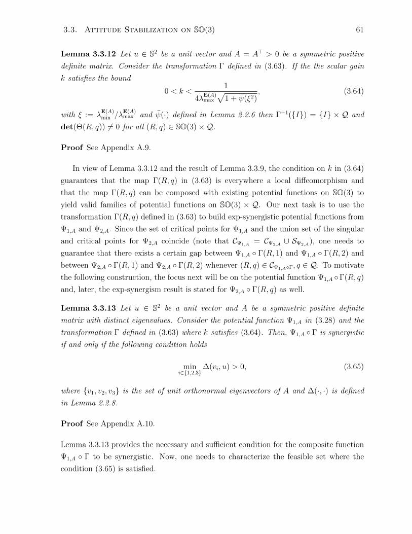
3.3. Attitude Stabilization on SO(3) 61
Lemma 3.3.12 Let u ∈ S2 be a unit vector and A = A> > 0 be a symmetric positive
definite matrix. Consider the transformation Γ defined in (3.63). If the the scalar gain
k satisfies the bound
0 < k <1
4λE(A)max
√1 + ψ(ξ2)
, (3.64)
with ξ := λE(A)min /λ
E(A)max and ψ(·) defined in Lemma 2.2.6 then Γ−1(I) = I × Q and
det(Θ(R, q)) 6= 0 for all (R, q) ∈ SO(3)×Q.
Proof See Appendix A.9.
In view of Lemma 3.3.12 and the result of Lemma 3.3.9, the condition on k in (3.64)
guarantees that the map Γ(R, q) in (3.63) is everywhere a local diffeomorphism and
that the map Γ(R, q) can be composed with existing potential functions on SO(3) to
yield valid families of potential functions on SO(3) × Q. Our next task is to use the
transformation Γ(R, q) defined in (3.63) to build exp-synergistic potential functions from
Ψ1,A and Ψ2,A. Since the set of critical points for Ψ1,A and the union set of the singular
and critical points for Ψ2,A coincide (note that CΨ1,A= CΨ2,A
∪ SΨ2,A), one needs to
guarantee that there exists a certain gap between Ψ1,A Γ(R, 1) and Ψ1,A Γ(R, 2) and
between Ψ2,A Γ(R, 1) and Ψ2,A Γ(R, 2) whenever (R, q) ∈ CΨ1,AΓ, q ∈ Q. To motivate
the following construction, the focus next will be on the potential function Ψ1,A Γ(R, q)
and, later, the exp-synergism result is stated for Ψ2,A Γ(R, q) as well.
Lemma 3.3.13 Let u ∈ S2 be a unit vector and A be a symmetric positive definite
matrix with distinct eigenvalues. Consider the potential function Ψ1,A in (3.28) and the
transformation Γ defined in (3.63) where k satisfies (3.64). Then, Ψ1,A Γ is synergistic
if and only if the following condition holds
mini∈1,2,3
∆(vi, u) > 0, (3.65)
where v1, v2, v3 is the set of unit orthonormal eigenvectors of A and ∆(·, ·) is defined
in Lemma 2.2.8.
Proof See Appendix A.10.
Lemma 3.3.13 provides the necessary and sufficient condition for the composite function
Ψ1,A Γ to be synergistic. Now, one needs to characterize the feasible set where the
condition (3.65) is satisfied.
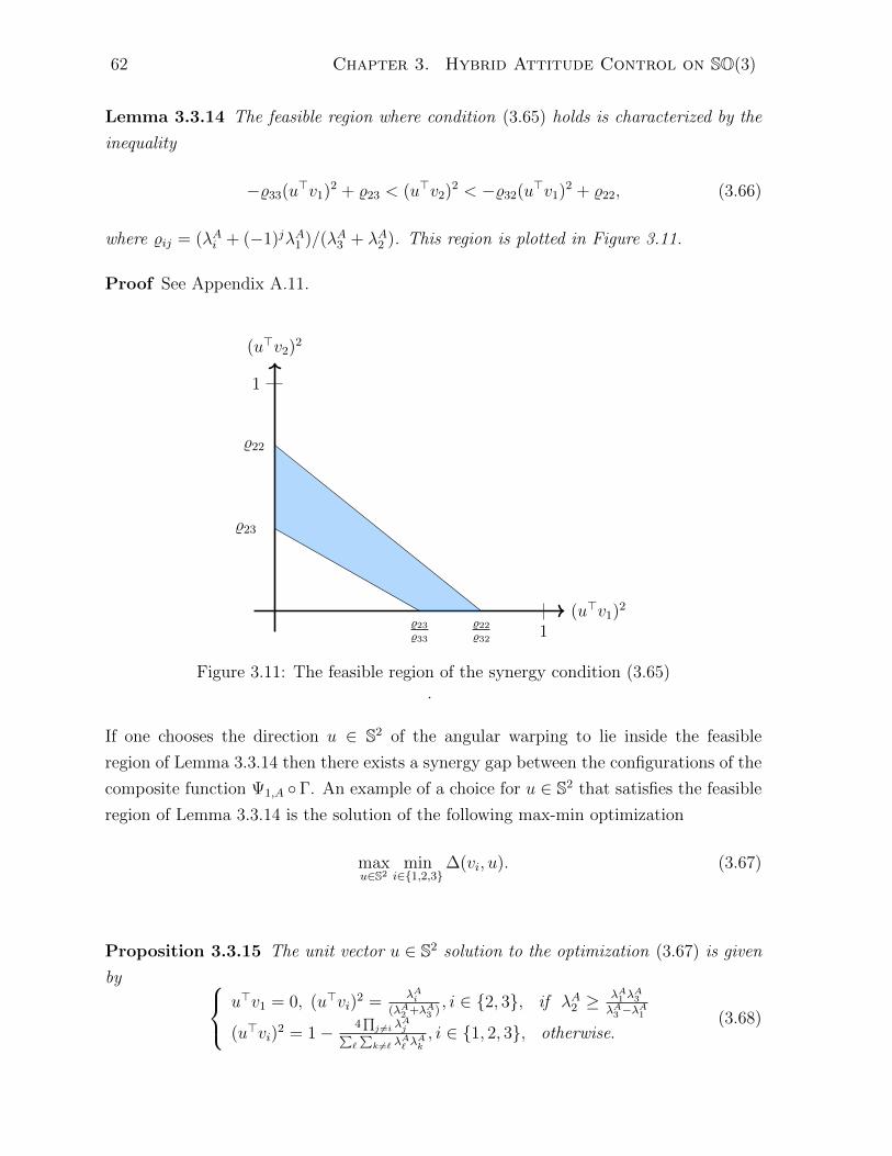
62 Chapter 3. Hybrid Attitude Control on SO(3)
Lemma 3.3.14 The feasible region where condition (3.65) holds is characterized by the
inequality
−%33(u>v1)2 + %23 < (u>v2)2 < −%32(u>v1)2 + %22, (3.66)
where %ij = (λAi + (−1)jλA1 )/(λA3 + λA2 ). This region is plotted in Figure 3.11.
Proof See Appendix A.11.
(u>v1)2
(u>v2)2
%22
%23
%22
%32
%23
%331
1
Figure 3.11: The feasible region of the synergy condition (3.65).
If one chooses the direction u ∈ S2 of the angular warping to lie inside the feasible
region of Lemma 3.3.14 then there exists a synergy gap between the configurations of the
composite function Ψ1,A Γ. An example of a choice for u ∈ S2 that satisfies the feasible
region of Lemma 3.3.14 is the solution of the following max-min optimization
maxu∈S2
mini∈1,2,3
∆(vi, u). (3.67)
Proposition 3.3.15 The unit vector u ∈ S2 solution to the optimization (3.67) is given
by u>v1 = 0, (u>vi)2 =
λAi(λA2 +λA3 )
, i ∈ 2, 3, if λA2 ≥λA1 λ
A3
λA3 −λA1
(u>vi)2 = 1− 4
∏j 6=i λ
Aj∑
`
∑k 6=` λ
A` λ
Ak, i ∈ 1, 2, 3, otherwise.
(3.68)
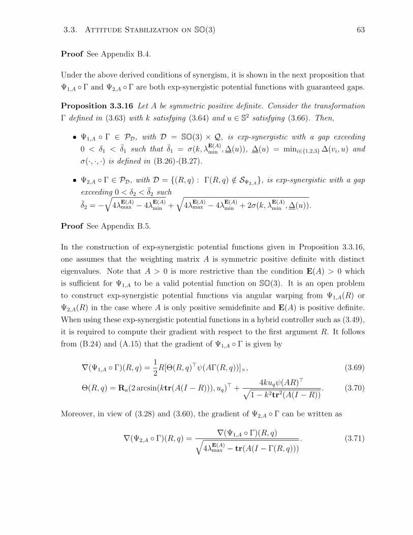
3.3. Attitude Stabilization on SO(3) 63
Proof See Appendix B.4.
Under the above derived conditions of synergism, it is shown in the next proposition that
Ψ1,A Γ and Ψ2,A Γ are both exp-synergistic potential functions with guaranteed gaps.
Proposition 3.3.16 Let A be symmetric positive definite. Consider the transformation
Γ defined in (3.63) with k satisfying (3.64) and u ∈ S2 satisfying (3.66). Then,
• Ψ1,A Γ ∈ PD, with D = SO(3) × Q, is exp-synergistic with a gap exceeding
0 < δ1 < δ1 such that δ1 = σ(k, λE(A)min ,∆(u)), ∆(u) = mini∈1,2,3∆(vi, u) and
σ(·, ·, ·) is defined in (B.26)-(B.27).
• Ψ2,A Γ ∈ PD, with D = (R, q) : Γ(R, q) /∈ SΨ2,A, is exp-synergistic with a gap
exceeding 0 < δ2 < δ2 such
δ2 = −√
4λE(A)max − 4λ
E(A)min +
√4λ
E(A)max − 4λ
E(A)min + 2σ(k, λ
E(A)min ,∆(u)).
Proof See Appendix B.5.
In the construction of exp-synergistic potential functions given in Proposition 3.3.16,
one assumes that the weighting matrix A is symmetric positive definite with distinct
eigenvalues. Note that A > 0 is more restrictive than the condition E(A) > 0 which
is sufficient for Ψ1,A to be a valid potential function on SO(3). It is an open problem
to construct exp-synergistic potential functions via angular warping from Ψ1,A(R) or
Ψ2,A(R) in the case where A is only positive semidefinite and E(A) is positive definite.
When using these exp-synergistic potential functions in a hybrid controller such as (3.49),
it is required to compute their gradient with respect to the first argument R. It follows
from (B.24) and (A.15) that the gradient of Ψ1,A Γ is given by
∇(Ψ1,A Γ)(R, q) =1
2R[Θ(R, q)>ψ(AΓ(R, q))]×, (3.69)
Θ(R, q) = Ra(2 arcsin(ktr(A(I −R))), uq)> +
4kuqψ(AR)>√1− k2tr2(A(I −R))
. (3.70)
Moreover, in view of (3.28) and (3.60), the gradient of Ψ2,A Γ can be written as
∇(Ψ2,A Γ)(R, q) =∇(Ψ1,A Γ)(R, q)√
4λE(A)max − tr(A(I − Γ(R, q)))
. (3.71)
64 Chapter 3. Hybrid Attitude Control on SO(3)
3.3.6 Illustration of the Switching Mechanism
To shed some light on how the hybrid switching mechanism, introduced in (3.45)-(3.47),
allows to achieve global results and improve the convergence rates compared to non-
hybrid algorithms, the hybrid switching mechanism is implemented, separately, as follows.
Consider the weighting matrix A = diag(1, 2, 3), index set Q = 1, 2 and unit vectors
u1 = −u2 = u such that u = [0,√
2/5,√
3/5]> which is chosen to satisfy (3.68). Let the
parameter k = 4.45 × 10⁻² which satisfies condition (3.64). The switching mechanism
(3.45)-(3.47) is implemented with the potential function Φ = Ψ2,A Γ and the hysteresis
gap δ = 0.95δ2 where δ2 is defined in Proposition 3.3.16. According to Appendix A.10,
for each q ∈ Q, the potential function Φ(R, q) admits three undesired critical/singular
points. In the case of q = 1, these undesired points, denoted R1, R2, R3, are explicitly
given by
Ri = Ra(π, vi)Ra(2 arcsin(kΨi), u1)>, (3.72)
Ψi =−1 +
√1 + 64k2∆(vi, u)λ
E(A)vi
8k2∆(vi, u), (3.73)
for i ∈ 1, 2, 3 where vi is the eigenvector associated to the eigenvalue λAi . Since A is
diagonal one has vi = ei for i = 1, 2, 3. Using (A.34) it can be verified that ∆(v1, u) = 0.7
and ∆(v2, u) = ∆(v3, u) = 0.5 which allows to compute the values
Ψ1 ' 9.59,
Ψ2 ' 7.81,
Ψ3 ' 5.89.
Therefore, making use of the composition of rotations, one can calculate the criti-
cal/singular points of Φ(R, 1) according to (3.72). One obtains Ri = Ra(θi, wi) for
some angles θi ∈ R and unit vectors wi ∈ S2. More, precisely, the unit vectors are
w1 = [0.9063, 0.3274,−0.2673]>,
w2 = [−0.2741, 0.9617, 0]>,
w3 = [0.1685, 0, 0.9857]>.
Now let us generate three attitude trajectories as follows: Ri(θ) = Ra(θ, wi) where θ ∈[0, 2π]. This guarantees that each trajectory Ri(θ) will pass through the singular/critical
point Ri for some value of θ. For each trajectory Ri(θ), the values of the individual

3.3. Attitude Stabilization on SO(3) 65
potential functions Φ(Ri(θ), 1) and Φ(Ri(θ), 2) as well as Φ(Ri(θ), q), where the index q
is initialized at q = 1 and evolves according to the hybrid dynamical system (3.45)-(3.47),
are calculated. The norm of the gradient of these potential function is also calculated and
the results are plotted in Figure (3.12). For instance, if one takes the second trajectory
(2nd column), Figure (3.12) illustrates how the switching mechanism allows, starting from
the initial configuration q = 1, to jump to the minimum potential function Φ(R, 2) when
the difference between the two configurations exceeds the threshold δ. Then, a second
switch happens when the difference between the current potential function, now Φ(R, 2),
and the minimum potential function, now Φ(R, 1), exceeds δ. It can be seen also that
the gradient of Φ(R, q) does not vanish, during the flows of the hybrid system, except at
the identity rotation. Similar discussions can be conducted for the other two trajectories
where one encounters a singular point (1st column) or a critical point (3rd column) for
Φ(R, 1). The hybrid switching mechanism allows to avoid the singularity and/or the
undesired critical point by switching between its two configurations. A similar discussion
can be derived using trajectories that pass through the singular/critical points for Φ(R, 2)
or when considering the potential function Φ = Ψ1,A Γ instead.
π/2 π 3π/2 2π
θ (rad)
0
1
2
3
4
Φ(R1(θ), 1)Φ(R1(θ), 2)Φ(R1(θ), q)
π/2 π 3π/2 2π
θ (rad)
0
0.5
1
1.5
2
Φ(R2(θ), 1)Φ(R2(θ), 2)Φ(R2(θ), q)
π/2 π 3π/2 2π
θ (rad)
0
0.5
1
1.5
Φ(R3(θ), 1)Φ(R3(θ), 2)Φ(R3(θ), q)
π/2 π 3π/2 2π
θ (rad)
0
0.2
0.4
0.6
0.8
1
1.2‖∇Φ(R1(θ), 1)‖F‖∇Φ(R1(θ), 2)‖F‖∇Φ(R1(θ), q)‖F
π/2 π 3π/2 2π
θ (rad)
0
0.2
0.4
0.6
0.8
1
‖∇Φ(R2(θ), 1)‖F‖∇Φ(R2(θ), 2)‖F‖∇Φ(R2(θ), q)‖F
π/2 π 3π/2 2π
θ (rad)
0
0.1
0.2
0.3
0.4
0.5
0.6
‖∇Φ(R3(θ), 1)‖F‖∇Φ(R3(θ), 2)‖F‖∇Φ(R3(θ), q)‖F
Figure 3.12: Plot of the potential function Φ(R, q) (first row) and its gradient’s norm(second row) along the trajectories Ri(θ), i = 1, 2, 3, which passes through the singu-lar/critical points of Φ(R, 1).

66 Chapter 3. Hybrid Attitude Control on SO(3)
3.4 Attitude Tracking for Rigid Body Systems
3.4.1 Problem Formulation
The attitude dynamics of a rigid body are given by
R = R[ω]×, (3.74)
IBω = [IBω]×ω + uτ , (3.75)
where R ∈ SO(3) denotes a rotation matrix from the body-attached frame B to the
inertial frame I, ω ∈ R3 is the angular velocity of the rigid body expressed in the body-
attached frame B, IB ∈ R3×3 is the constant symmetric positive-definite inertia matrix
of the rigid body with respect to the body-fixed frame and uτ ∈ R3 is the input torque
expressed in the body-fixed frame.
Assume that a good estimate of R can be obtained from the available measurements.
Although no available sensor can provide measurements of the full attitude matrix R,
body-frame vector measurements of known inertial directions can be used to reconstruct
or estimate the attitude. A detailed description and improved solutions for the attitude
estimation problem will be addressed in Chapter 4. Also, assume that the angular velocity
ω, which can be measured using a gyroscope, is available for feedback. Consider a time-
varying reference attitude trajectory Rd(t) ∈ SO(3), satisfying
Rd(t) = Rd(t)[ωd(t)]×, Rd(0) ∈ SO(3), (3.76)
for some desired angular velocity vector ωd(t) ∈ R3.
Assumption 3.4.1 The desired angular acceleration ωd(t) is uniformly bounded such
that there exists cωd > 0 and ‖ωd(t)‖ ≤ cωd for all t ≥ 0.
Note that, under the assumption of bounded ωd, the desired trajectory (3.76) can be
generated by the following autonomous differential inclusion
Rd = Rd[ωd]×
ωd ∈ cωdB
(Rd, ωd) ∈ SO(3)× R3. (3.77)
We may also need the following assumption on the boundedness of ωd.
Assumption 3.4.2 The desired angular velocity ωd(t) is uniformly bounded such that
there exists cωd > and ‖ωd(t)‖ ≤ cωd for all t ≥ 0.
3.4. Attitude Tracking for Rigid Body Systems 67
Our objective is to design a control law for the input uτ such that global tracking of
the reference attitude Rd(t) is achieved. To this end, the synergistic hybrid approach
developed in this chapter is adopted. Before this, let us discuss some of the existing
smooth attitude control schemes which our hybrid tracking controllers will be developed
upon.
3.4.2 Smooth Attitude Tracking on SO(3)
Using the SO(3) group operation, one defines the following “intrinsic” attitude tracking
errors
R = RR>d , R = R>d R. (3.78)
The attitude errors R and R are often called the left and right attitude errors, respectively.
In fact, the left (right) attitude error is invariant under left (right) matrix multiplication
in the sense that it preserves the Lie group invariance properties with respect to constant
rotations. Both attitude errors can be used as a measure of the error between the actual
attitude R and the desired attitude Rd. In fact it is easy to check that R = I is equivalent
to R = I thanks to the fact that R = RdRR>d . However, physically speaking the right
attitude error R is more meaningful than its counterpart R. The right attitude error
corresponds to the relative orientation generated by the difference of the actual angular
velocity and the desired angular velocity expressed in the body-attached frame. This fact
has motivated its wide use in attitude control problems, see [Meyer, 1971, Koditschek,
1988, Wen and Kreutz-Delgado, 1991, Egeland and Godhavn, 1994, Sanyal et al., 2009,
Lee, 2012, Mayhew and Teel, 2013a]. The left attitude error has appeared less frequently,
see for instance [Bullo and Murray, 1999, Forbes, 2013]. As will be discussed later, the
use of the left attitude error has several advantages compared to the right attitude error.
The corresponding left and right angular velocity errors can be obtained by differen-
tiating the left and right attitude errors which results in
˙R = R[Rdω]×, ω = ω − ωd, (3.79)
˙R = R[ω]×, ω = ω − R>ωd. (3.80)
The right angular velocity error ω represents the error between the body-frame angular
velocity ω and the body-frame representation, namely R>ωd, of the desired angular
velocity ωd. Therefore both quantities are compared in the same body frame. The

68 Chapter 3. Hybrid Attitude Control on SO(3)
control laws discussed in this thesis have the following structure
uτ = PD-like feedback + Feedforward compensation (3.81)
The proportional feedback is a function of the attitude error (left or right) and the
derivative feedback is in terms of the corresponding angular velocity error (left or right).
The PD action guarantees stability, error tracking and disturbance rejection while the
feedforward term is used to enhance the tracking performance by compensating for the
system dynamics.
The first smooth control law uses the left (attitude and angular velocity) tracking
errors and is given by (see [Bullo and Murray, 1999])
uτ = −R>d ψ(K1R)−K2ω + [ωd]×IBω + IBωd, (3.82)
where K2 is a positive definite matrix and K1 is a symmetric matrix such that E(K1) is
positive definite. The second control law uses the right tracking errors and is given by
(see [Tayebi, 2008, Lee, 2012])
uτ = −ψ(K1R)−K2ω + [R>ωd]×IBR>ωd + IBR
>ωd. (3.83)
Both controllers can be shown to guarantee almost global asymptotic tracking and local
exponential tracking, see [Bullo and Murray, 1999, Lemma 9]. Interestingly, one can
further simplify the feedforward term of the control law (3.82) as demonstrated in the
following proposition.
Proposition 3.4.3 Consider the desired reference trajectory (3.76) under Assumption
(3.4.2). Consider the attitude dynamics (3.74)-(3.75) under the control law
uτ = −R>d ψ(K1R)−K2ω + [ωd]×IBωd + IBωd, (3.84)
where K1 is a symmetric matrix such that E(K1) is positive definite and K2 is a positive
definite matrix satisfying
λK2min > λIBmaxcωd . (3.85)
Then the equilibrium point (R, ω) = (I, 0) is exponentially stable from all initial condi-

3.4. Attitude Tracking for Rigid Body Systems 69
tions such that
tr(K1(I − R(0))) + ω(0)IBω(0) < 4λE(K1)min .
Proof See Appendix B.6.
The control law (3.84) has a simpler feedforward term compared to the previously pro-
posed control laws (3.82) and (3.82). In fact, the feedforward term [ωd]×IBωd + IBωd
is state-independent and can be computed offline given the desired trajectory of the
rigid body’s attitude. This simplification in the control law comes at the cost of a gain
condition in (3.85).
3.4.3 Hybrid Attitude Tracking on SO(3)
As discussed in Section 3.3.2, smooth stabilization or tracking on SO(3) can not achieve
global results which might lead to performance degradation when considering large ma-
noeuvres. The proportional feedback for the attitude tracking control laws discussed
above can be modified and enhanced by including a hybrid dynamical system in the
spirit of the hybrid synergistic feedback approach discussed in subsection 3.3.4. In fact
the proportional term ψ(K1R) is related to the gradient of the potential function Ψ1,K1(R)
defined in (3.28). The idea of the hybrid tracking algorithm is to take, instead, a pro-
portional term which corresponds to a gradient of an exp-synergistic potential function
which changes configuration according to a min-switch strategy.
R>d × q = HT (R)
Switching Mechanism
−ψ(R>∇Φ(R, q))
Gradient Feedback
+ R = R[ω]×
IBω = IBω × ω + uτ
Attitude Dynamics
K2
−ωd
ωτ
R
[ωd]×IBωd + IBωd
Feedforward
ωdωd
R q
Figure 3.13: Hybrid attitude tracking algorithm using an exp-synergistic potential func-tion Φ : SO(3)×Q → R≥0.
70 Chapter 3. Hybrid Attitude Control on SO(3)
Theorem 3.4.4 Consider a desired reference trajectory generated by (3.77) under As-
sumptions (3.4.1)-(3.4.2). Consider the attitude dynamics (3.74)-(3.75) under the control
law
uτ = −R>d ψ(R>∇Φ(R, q))−K2ω + [ωd]×IBω + IBωd, (3.86)
where K2 is a positive definite matrix, Φ ∈ PD with D ⊆ SO(3)×Q, Q ⊂ N, δ > 0 and
q = HT (R) with T = (Φ,Q, δ) and HT (·) defined in (3.45)-(3.47). If Φ is exp-synergistic
with gap exceeding δ, then the set A2 = (R, q, ω, Rd, ωd) : R = I, ω = 0 is globally
exponentially stable.
Proof See Appendix C.4.
In Theorem 3.4.4 a hybrid controller has been derived using the left attitude and angular
velocity errors. It has the same structure as the smooth controller (3.84) with the pro-
portional term ψ(K1R) being replaced by ψ(R>∇Φ(R, q)) Φ ∈ PD with D ⊆ SO(3)×Qis an exp-synergistic potential function with gap exceeding δ > 0 and the index q is the
output of the hybrid dynamical system (3.45)-(3.47). Note that the feedforward term
[ωd]×IBω can be replaced by [ωd]×IBωd as in (3.84) under the gain condition (3.85) with-
out affecting the nature of the stability result. Also, a similar hybrid controller obtained
from the right attitude and angular velocity errors can be derived. It is left to the reader
to verify the global exponential stability result.
Note that the proposed hybrid attitude tracking scheme is subject to discontinuous
jumps due to the direct switching in the hybrid controller configuration. This might
be undesirable from a practical point of view as discontinuities in the torque might
excite unmoderated dynamics. To cope with this shortcoming, a dynamic extension is
proposed for the originally derived hybrid controllers to smooth out the proportional
term (which contains discontinuous jumps) and allows to obtain a continuous control
input guaranteeing the same exponential tracking results.
Theorem 3.4.5 Consider a desired reference trajectory generated by (3.77) under As-
sumptions (3.4.1)-(3.4.2). Consider the attitude dynamics (3.74)-(3.75) under the control
law
uτ = −R>d x−K2ω + [ωd]×IBω + IBωd, (3.87)
x = −K3(x− ψ(R>∇Φ(R, q))), x(0) ∈ cxB, (3.88)
where K2, K3 are positive definite matrices, Φ ∈ PD with D ⊆ SO(3)×Q, Q ⊂ N, cx > 0
and q = HT (R) with T = (Φ,Q, δ), δ > 0 and HT (·) defined in (3.45)-(3.47). If Φ is

3.4. Attitude Tracking for Rigid Body Systems 71
exp-synergistic with gap exceeding δ, then there exists a positive constant k3 such that
for K3 > k3I > 0, the set A3 := (R, q, ω, x, Rd, ωd) : R = I, ω = 0, x = 0 is globally
exponentially stable, where x = x− ψ(R>∇Φ(R, q)).
Proof See Appendix C.5.
The integral action on the hybrid term ψ(R>∇Φ(R, q)) in (3.88) moves the discontinuity
(jump) one integrator away from the control input uτ . Therefore, the output of the hybrid
controller (3.87)-(3.88) is made continuous without sacrificing the global exponential
stability.
R>d × q = HT (R)
Switching Mechanism
−ψ(R>∇Φ(R, q))
Gradient Feedback
k3
s+k3+ R = R[ω]×
IBω = IBω × ω + uτ
Attitude Dynamics
K2
−ωd
ωτ
R
[ωd]×IBωd + IBωd
Feedforward
ωdωd
R q
Figure 3.14: Smoothed hybrid attitude tracking algorithm using an exp-synergistic po-tential function Φ : SO(3)×Q → R≥0.
3.4.4 Simulations
In this section, some simulation results are provided to show the performance of the
proposed attitude tracking control schemes. The moment of inertia of the rigid body
considered in this simulation around the roll, pitch and yaw axes is given by
IB =
1.59 0 0
0 1.50 0
0 0 2.97
× 10−2 (Kg.m2) (3.89)
The desired attitude trajectory being set for the simulation tests is generated from
(3.76). The desired angular acceleration is
ωd(t) =
0.03 sin(0.1t+ 7π/12)
0.03 sin(0.3t+ π/2)
0.05 sin(0.1t+ π/2)
(rad/sec2), (3.90)

72 Chapter 3. Hybrid Attitude Control on SO(3)
0 5 10 15 20 25 30 35 40 45 50
Time (seconds)
0.1
0.2
0.3
0.4
0.5
0.6
0.7
0.8
0.9
1
Attitudeerror|R
|2 I
Smooth control (right error)Smooth control (left error)Hybrid control
Figure 3.15: Total attitude tracking error (Euclidean distance) versus time.
0 5 10 15 20 25 30 35 40 45 50
Time (seconds)
0
0.1
0.2
0.3
0.4
0.5
0.6
0.7
0.8
0.9
Angu
larvelocity
‖ω‖
Smooth control (right error)Smooth control (left error)Hybrid control
Figure 3.16: Norm of the angular velocity tracking error versus time.
and the initial desired angular rates and attitude matrix are ωd(0) = [0, 0, 0]> (rad/sec)
and Rd(0) = I, respectively. In the first simulation scenario, the initial conditions ω(0) =
[0, 0, 0]> (rad/sec) and R(0) = Ra(π, [0.6, 0.8, 0]>) are considered. The gains are set as
K1 = K2 = 5 × 10⁻²I for all controllers. Note that locally, all controllers (smooth or
hybrid, left or right error) are identical. Particularly, both the smooth control (right
error) which corresponds to the controller (3.83) and the smooth control (left error)
which corresponds to controller (3.84) are implemented. The hybrid control law (3.86)
is implemented using the non-weighted exp-synergistic potential function Ψ1 Γ with
parameters k = 0.64 and δ = 0.064 as in Proposition 3.3.10. In the second simulation

3.4. Attitude Tracking for Rigid Body Systems 73
0 5 10 15 20 25 30 35 40 45 50
-100
0
100
Roll(deg/sec)
Smooth control (right error)Smooth control (left error)Hybrid controlDesired trajectory
0 5 10 15 20 25 30 35 40 45 50
-80
-60
-40
-20
0
20
Pitch
(deg/sec)
0 5 10 15 20 25 30 35 40 45 50
Time (seconds)
-100
0
100
Yaw
(deg/sec)
Figure 3.17: True Euler angles (colored) and desired Euler angles (dashed) versus time.
scenario, the performance of the smoothed hybrid controller (3.87)-(3.88) is compared to
the raw hybrid controller (3.86). Consider the initial states as follows ω(0) = [−5,−2, 3]>
(rad/sec) and R(0) = Ra(π, [0, 1, 0]>). The control gain K3 in (3.87)-(3.88) is chosen as
K3 = 10I while the remaining parameters of the hybrid switching mechanism (Φ,Q, δ)are chosen as in the previous scenario.
0 1 2 3 4 5 6 7 8 9 10
Time (seconds)
0.1
0.2
0.3
0.4
0.5
0.6
0.7
0.8
0.9
Attitudeerror|R
|2 I
Hybrid controlSmoothed hybrid control
Figure 3.18: Total attitude tracking error (Euclidean distance) versus time.
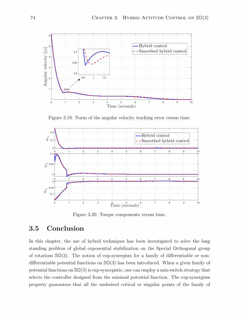
74 Chapter 3. Hybrid Attitude Control on SO(3)
0 1 2 3 4 5 6 7 8 9 10
Time (seconds)
1
2
3
4
5
6
Angu
larvelocity
‖ω‖ Hybrid control
Smoothed hybrid control
0.8 1 1.2
0.6
0.65
0.7
zoom
Figure 3.19: Norm of the angular velocity tracking error versus time.
0 1 2 3 4 5 6 7 8 9 10
0
0.1
0.2
uτ1 Hybrid control
Smoothed hybrid control
0 1 2 3 4 5 6 7 8 9 10
0
0.05
0.1
uτ2
0 1 2 3 4 5 6 7 8 9 10
Time (seconds)
-0.1
-0.05
0
uτ3
Figure 3.20: Torque components versus time.
3.5 Conclusion
In this chapter, the use of hybrid techniques has been investigated to solve the long
standing problem of global exponential stabilization on the Special Orthogonal group
of rotations SO(3). The notion of exp-synergism for a family of differentiable or non-
differentiable potential functions on SO(3) has been introduced. When a given family of
potential functions on SO(3) is exp-synergistic, one can employ a min-switch strategy that
selects the controller designed from the minimal potential function. The exp-synergism
property guarantees that all the undesired critical or singular points of the family of

3.5. Conclusion 75
0 1 2 3 4 5
Time (seconds)
0
1
2
3
4
5
6
Switchingvariab
leq
Hybrid control
Smoothed hybrid control
Figure 3.21: Switching variable versus time. Note that the initial value is q(0, 0) = 2.The hybrid controller immediately switches to the configuration q = 5 at the start.
potential functions must lie in the jump set of the hybrid controller. A rigorous Lyapunov
analysis for hybrid systems is used to show global exponential stability of the closed-
loop systems under investigation. Moreover, an insightful construction of exp-synergistic
potential functions, derived from already known individual weighted and non-weighted
potential functions on SO(3), is proposed. The proposed hybrid stabilization approach
has been applied to the attitude tracking problem for rigid body systems and yields
improved tracking performance compared to non-hybrid attitude tracking algorithms.
Chapter 4
Hybrid Attitude Estimation on SO(3)
4.1 Introduction
In this chapter, two different observer design problems related to the attitude estimation
on SO(3) are formulated. The first problem, similar to [Mahony et al., 2008], considers
the attitude estimation using a set of n ≥ 2 body-frame vector measurements of known
constant inertial vectors alongside biased gyro measurements. Our objective is to incor-
porate hybrid switching mechanisms to enlarge the domain of exponential stability of the
traditional nonlinear complementary filter on SO(3) [Mahony et al., 2008, Grip et al.,
2012a]. Two approaches are proposed: a synergistic-based approach and a reset-based
approach. In the synergistic-based approach, exp-synergistic potential functions from
Chapter 3 are used to design a set of innovation terms for the passive nonlinear com-
plementary filter [Mahony et al., 2008]. A hysteresis switching between these innovation
terms allows to keep the estimation error inside the region of exponential stability. The
second approach relies on resetting the attitude state to a different value (selected from a
set of adequately chosen rotation matrices) whenever the attitude error is close to leave
the domain of exponential stability. This condition is detected by comparing the value
of a cost function at the current rotation and at the rotation after a potential jump has
occurred. Both estimation approaches are shown to guarantee global exponential stabil-
ity, are expressed directly using vector measurements and provide improved performance
compared to the state of the art attitude estimators on SO(3). These results appeared
in our work [Berkane et al., 2017a, Berkane and Tayebi, 2017b].
The second problem that is addressed in this chapter is the attitude estimation on
SO(3) using intermittent vector measurements where the body frame vector measure-
ments are considered arriving at possibly different instants of time with possible packets
loss. This problem is mainly motivated by applications where multiple sensors (GPS,
76

4.2. Attitude Estimation Using Continuous Vector Measurements 77
landmarks, vision sensors, IMU) are centrally fused to estimate the attitude of a rigid
body. Measurement-triggered state observers on SO(3) are proposed to solve the problem
in the case where the measurements are synchronous and asynchronous. A hybrid sys-
tems framework is proposed to model and capture the dynamics of the event-triggered
behaviour of the closed-loop systems. Almost global exponential stability and almost
global asymptotic stability is shown for the synchronous observer and asynchronous ob-
server, respectively. The results of this part have been published in [Berkane and Tayebi,
2017c, Berkane and Tayebi, 2017d].
4.2 Attitude Estimation Using Continuous Vector
Measurements
In this section, the problem of attitude and gyro bias estimation from continuous body-
frame vector measurements and biased angular velocity readings is considered. This
problem has been tackled recently using nonlinear observer design on SO(3) see, for
instance, [Mahony et al., 2008, Grip et al., 2012b, Izadi and Sanyal, 2014, Zlotnik and
Forbes, 2017] . In this work, hybrid nonlinear observers on SO(3) are proposed to solve
this problem with global exponential stability results; a result that has not been achieved
in previous works.
4.2.1 Problem Formulation
Let R ∈ SO(3) denote a rotation matrix from the body-attached frame B to the inertial
frame I. The rotation matrix R evolves according to the kinematics equation
R = R[ω]×, (4.1)
where ω ∈ R3 is the angular velocity of the body-attached frame B with respect to
the inertial frame I expressed in the body-attached frame B. Assume that the angular
velocity ω(t) is uniformly bounded and a continuous biased measurement of ω(t), denoted
by ωy, is available such that
ωy = ω + bω. (4.2)
where bω ∈ R3 represents a constant or slowly varying bias. Also, suppose that a set
of n ≥ 2 sensors measuring direction vectors, denoted by bi, i = 1, . . . , n in the body-
attached frame which are associated to a set of n known (possibly time-varying) inertial

78 Chapter 4. Hybrid Attitude Estimation on SO(3)
vectors, denoted by ai, i = 1, . . . , n, such that
bi = R>ai. (4.3)
As in most attitude estimation problems, one needs to impose an observability condition
which requires that, at each instant of time, at least two inertial vectors are non-collinear.
This is formally stated as follows.
Assumption 4.2.1 For any t ≥ 0, there exist i, j ∈ 1, · · · , n such that the inertial
vectors ai(t) and aj(t) are non-collinear.
The body-frame vectors bi can be obtained, for example, from an IMU that typically
includes an accelerometer and a magnetometer measuring, respectively, the gravitational
field and Earth’s magnetic field expressed in the body-attached frame. Moreover, the
following realistic assumptions are needed.
Assumption 4.2.2 There exists constants cω, cω, cb > 0 such that ‖ω(t)‖ ≤ cω, ‖ω(t)‖ ≤cω for all t ≥ 0 and ‖bω‖ ≤ cb.
Our objective consists in designing an algorithm that provides attitude estimates on
SO(3) while estimating the gyro-bias vector, using the above described available mea-
surements, leading to global exponential stability results.
The available state-of-the-art attitude observer that solves a similar problem is the
explicit complementary filter (ECF) proposed in [Mahony et al., 2008]. The ECF takes
the following form:
˙R = R
[ωy − bω + k1w
]×, (4.4)
˙bω = −k2w, (4.5)
w =1
4
n∑i=1
ρi(bi × R>ai), (4.6)
where R(0) ∈ SO(3) and bω(0) ∈ R3 are the initial conditions of the attitude estimate
R and the gyro bias estimate bω, respectively. The gains k1, k2, ρ1, · · · , ρn are chosen
strictly positive. The structure of the ECF is very intuitive. The attitude estimate is
propagated using a forward integration of the biased angular velocity plus and innovation
term. The innovation term has a proportional-integral structure where the error vector
w is constructed by weighting and summing the “cross product vector errors” between
the measured direction vectors bi = R>ai and their corresponding estimates R>ai.
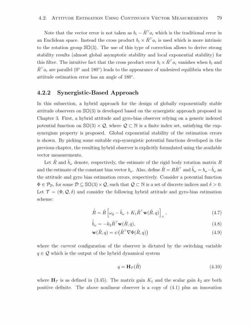
4.2. Attitude Estimation Using Continuous Vector Measurements 79
Note that the vector error is not taken as bi − R>ai which is the traditional error in
an Euclidean space. Instead the cross product bi × R>ai is used which is more intrinsic
to the rotation group SO(3). The use of this type of correction allows to derive strong
stability results (almost global asymptotic stability and local exponential stability) for
this filter. The intuitive fact that the cross product error bi× R>ai vanishes when bi and
R>ai are parallel (0 and 180) leads to the appearance of undesired equilibria when the
attitude estimation error has an angle of 180.
4.2.2 Synergistic-Based Approach
In this subsection, a hybrid approach for the design of globally exponentially stable
attitude observers on SO(3) is developed based on the synergistic approach proposed in
Chapter 3. First, a hybrid attitude and gyro-bias observer relying on a generic indexed
potential function on SO(3) ×Q, where Q ⊂ N is a finite index set, satisfying the exp-
synergism property is proposed. Global exponential stability of the estimation errors
is shown. By picking some suitable exp-synergistic potential functions developed in the
previous chapter, the resulting hybrid observer is explicitly formulated using the available
vector measurements.
Let R and bω denote, respectively, the estimate of the rigid body rotation matrix R
and the estimate of the constant bias vector bω. Also, define R = RR> and bω = bω−bω as
the attitude and gyro bias estimation errors, respectively. Consider a potential function
Φ ∈ PD, for some D ⊆ SO(3)×Q, such that Q ⊂ N is a set of discrete indices and δ > 0.
Let T = (Φ,Q, δ) and consider the following hybrid attitude and gyro-bias estimation
scheme:
˙R = R
[ωy − bω +K1R
>w(R, q)]×, (4.7)
˙bω = −k2R
>w(R, q), (4.8)
w(R, q) = ψ(R>∇Φ(R, q)
)(4.9)
where the current configuration of the observer is dictated by the switching variable
q ∈ Q which is the output of the hybrid dynamical system
q = HT (R) (4.10)
where HT is as defined in (3.45). The matrix gain K1 and the scalar gain k2 are both
positive definite. The above nonlinear observer is a copy of (4.1) plus an innovation
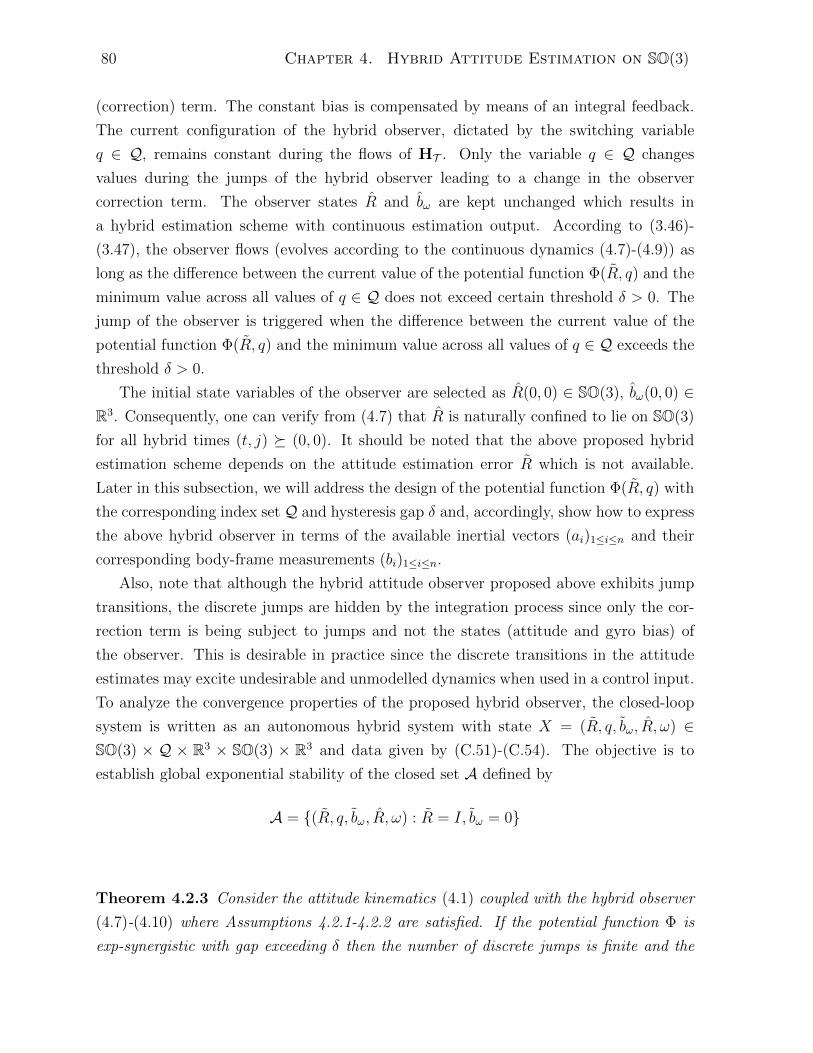
80 Chapter 4. Hybrid Attitude Estimation on SO(3)
(correction) term. The constant bias is compensated by means of an integral feedback.
The current configuration of the hybrid observer, dictated by the switching variable
q ∈ Q, remains constant during the flows of HT . Only the variable q ∈ Q changes
values during the jumps of the hybrid observer leading to a change in the observer
correction term. The observer states R and bω are kept unchanged which results in
a hybrid estimation scheme with continuous estimation output. According to (3.46)-
(3.47), the observer flows (evolves according to the continuous dynamics (4.7)-(4.9)) as
long as the difference between the current value of the potential function Φ(R, q) and the
minimum value across all values of q ∈ Q does not exceed certain threshold δ > 0. The
jump of the observer is triggered when the difference between the current value of the
potential function Φ(R, q) and the minimum value across all values of q ∈ Q exceeds the
threshold δ > 0.
The initial state variables of the observer are selected as R(0, 0) ∈ SO(3), bω(0, 0) ∈R3. Consequently, one can verify from (4.7) that R is naturally confined to lie on SO(3)
for all hybrid times (t, j) (0, 0). It should be noted that the above proposed hybrid
estimation scheme depends on the attitude estimation error R which is not available.
Later in this subsection, we will address the design of the potential function Φ(R, q) with
the corresponding index set Q and hysteresis gap δ and, accordingly, show how to express
the above hybrid observer in terms of the available inertial vectors (ai)1≤i≤n and their
corresponding body-frame measurements (bi)1≤i≤n.
Also, note that although the hybrid attitude observer proposed above exhibits jump
transitions, the discrete jumps are hidden by the integration process since only the cor-
rection term is being subject to jumps and not the states (attitude and gyro bias) of
the observer. This is desirable in practice since the discrete transitions in the attitude
estimates may excite undesirable and unmodelled dynamics when used in a control input.
To analyze the convergence properties of the proposed hybrid observer, the closed-loop
system is written as an autonomous hybrid system with state X = (R, q, bω, R, ω) ∈SO(3) × Q × R3 × SO(3) × R3 and data given by (C.51)-(C.54). The objective is to
establish global exponential stability of the closed set A defined by
A = (R, q, bω, R, ω) : R = I, bω = 0
Theorem 4.2.3 Consider the attitude kinematics (4.1) coupled with the hybrid observer
(4.7)-(4.10) where Assumptions 4.2.1-4.2.2 are satisfied. If the potential function Φ is
exp-synergistic with gap exceeding δ then the number of discrete jumps is finite and the
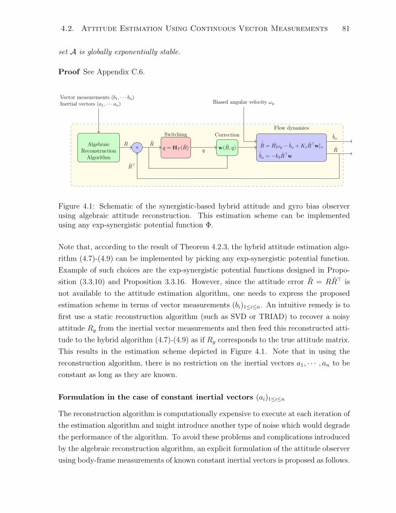
4.2. Attitude Estimation Using Continuous Vector Measurements 81
set A is globally exponentially stable.
Proof See Appendix C.6.
AlgebraicReconstruction
Algorithm
× q = HT (R)
Switching
w(R, q)
Correction
˙R = R[ωy − bω +K1R
>w]×˙bω = −k2R
>w
Flow dynamics
R Rq R
bω
R>
Vector measurements (b1, · · · bn)Inertial vectors (a1, · · · an) Biased angular velocity ωy
Figure 4.1: Schematic of the synergistic-based hybrid attitude and gyro bias observerusing algebraic attitude reconstruction. This estimation scheme can be implementedusing any exp-synergistic potential function Φ.
Note that, according to the result of Theorem 4.2.3, the hybrid attitude estimation algo-
rithm (4.7)-(4.9) can be implemented by picking any exp-synergistic potential function.
Example of such choices are the exp-synergistic potential functions designed in Propo-
sition (3.3.10) and Proposition 3.3.16. However, since the attitude error R = RR> is
not available to the attitude estimation algorithm, one needs to express the proposed
estimation scheme in terms of vector measurements (bi)1≤i≤n. An intuitive remedy is to
first use a static reconstruction algorithm (such as SVD or TRIAD) to recover a noisy
attitude Ry from the inertial vector measurements and then feed this reconstructed atti-
tude to the hybrid algorithm (4.7)-(4.9) as if Ry corresponds to the true attitude matrix.
This results in the estimation scheme depicted in Figure 4.1. Note that in using the
reconstruction algorithm, there is no restriction on the inertial vectors a1, · · · , an to be
constant as long as they are known.
Formulation in the case of constant inertial vectors (ai)1≤i≤n
The reconstruction algorithm is computationally expensive to execute at each iteration of
the estimation algorithm and might introduce another type of noise which would degrade
the performance of the algorithm. To avoid these problems and complications introduced
by the algebraic reconstruction algorithm, an explicit formulation of the attitude observer
using body-frame measurements of known constant inertial vectors is proposed as follows.
82 Chapter 4. Hybrid Attitude Estimation on SO(3)
Take the matrix A =∑n
i=1 ρiaia>i where ρi > 0, i = 1, · · · , n. This ensures that A is
positive definite provided that at least 3 inertial vectors, say a1, a2 and a3, are non-
collinear. In the case where only two non-collinear vectors a1 and a2 are available, it is
always possible to consider a third vector a3 = a1× a2, corresponding to the body-frame
measurement b3 = b1 × b2. Moreover, there exist positive scalars ρi such that A has
distinct eigenvalues. In this case, one can construct the potential function Φ ≡ Ψ1,A Γ
where Ψ1,A and Γ are defined in (3.28) and (3.63). Select the corresponding parameters
such as in Proposition (3.3.16) to ensure that Φ is exp-synergisitic with gap exceeding δ1
given in Proposition (3.3.16). Interstingly, this potential function as well as its gradient
can be computed directly using the vector measurements without the need for the attitude
matrix R. Using Lemma 2.2.7 and the definition of Γ in (3.63), one can show that the
potential function Φ(R, q) = Ψ1,A Γ(R, q) is expressed using vector measurements as
follows:
Φ((ai, bi)1≤i≤n, R, q) =1
4
n∑i=1
ρi‖bi − bqi‖2, (4.11)
where Φ((ai, bi)1≤i≤n, R, q) ≡ Φ(R, q), bqi = R>Ra(2 arcsin(kΨ), uq)ai and Ψ = 12
∑ni=1 ρi‖bi−
R>ai‖2. Using this explicit formulation of the potential function Φ(R, q), the hybrid
switching mechanism HT defined in (3.48) can be implemented directly using vector
measurements by replacing Φ(R, q) with Φ(a1, · · · , an, b1, · · · , bn, R, q). Let us denote by
HT the explicit implementation of the hybrid dynamical system HT so that
q = HT ((ai, bi)1≤i≤n, R). (4.12)
Moreover, in view of (3.69)-(3.70) and using again the result of Lemma 2.2.7 the gradient
of Φ can also be formulated using vector measurements as follows
w((ai, bi)1≤i≤n, R, q) =1
4Θ>
n∑i=1
ρi(bi × bqi ), (4.13)
where w((ai, bi)1≤i≤n, R, q) ≡ R>w(R, q) and Θ = I + 2k[1 − (kΨ)2]12 R>uq
∑ni=1 ρi(bi ×
R>ai)>. To sum up, the proposed hybrid observer can be implemented according to
Algorithm 1. It should be mentioned that another hybrid observer can be derived when
considering the potential function Φ = Ψ2,A Γ instead, where Ψ2,A is defined in (3.60).

4.2. Attitude Estimation Using Continuous Vector Measurements 83
q = HT ((ai, bi)1≤i≤n, R)
Switching Mechanism
w((ai, bi)1≤i≤n, R, q)
Correction term
˙R = R[ωy − bω +K1w]×˙bω = −k2w
Flow dynamics
q R
bω
Vector measurements (b1, · · · bn)Inertial vectors (a1, · · · an)
Biased angular velocity ωy
Figure 4.2: Schematic of the synergistic-based hybrid attitude and gyro bias observerusing directly vector measurements (without the need to algebraically reconstruct theattitude).
Algorithm 1 Synergistic-based observer using constant inertial vectors
Pick A =∑n
i=1 ρiaia>i where ρi > 0, i = 1, · · · , n.
Choose a scalar k to satisfy (3.64), a unit vector u as in Proposition 3.3.15 andQ = 1, 2.Initialize the observer states R(0, 0) ∈ SO(3), bω(0, 0) ∈ R3 and q(0, 0) ∈ Q and pick theobserver gains K1 and k2 to obtain the desirable performance.
1: for each set of measurements (bi)1≤i≤n do2: Calculate Φ(R, q) and minp∈QΦ(R, p) using (4.11).3: while (R, q) ∈ JT do4: Update q = arg minp∈QΦ(R, p).5: end while6: Calculate the correction term w(R, q) using (4.13).7: Update the states R and bω according to (4.7)-(4.8).8: end for
4.2.3 Reset-Based Approach
The synergistic-based approach for the design of hybrid observers discussed in the previ-
ous section is inspired from the hybrid control approach proposed in Chapter 3. In this
section, an alternative hybrid approach for the design of attitude observers is proposed
by allowing the estimation state to be reset to a certain value whenever it leaves the flow
set and enters the jump set.
Consider a potential function Φ ∈ PDΦwithDΦ ⊆ SO(3) and Ξ : SO(3)×R≥0 → R≥0 a
possibly time-varying potential function continuous and differentiable on the set DΞ×R≥0
where DΞ ⊆ SO(3). Consider the following hybrid attitude and gyro-bias estimation
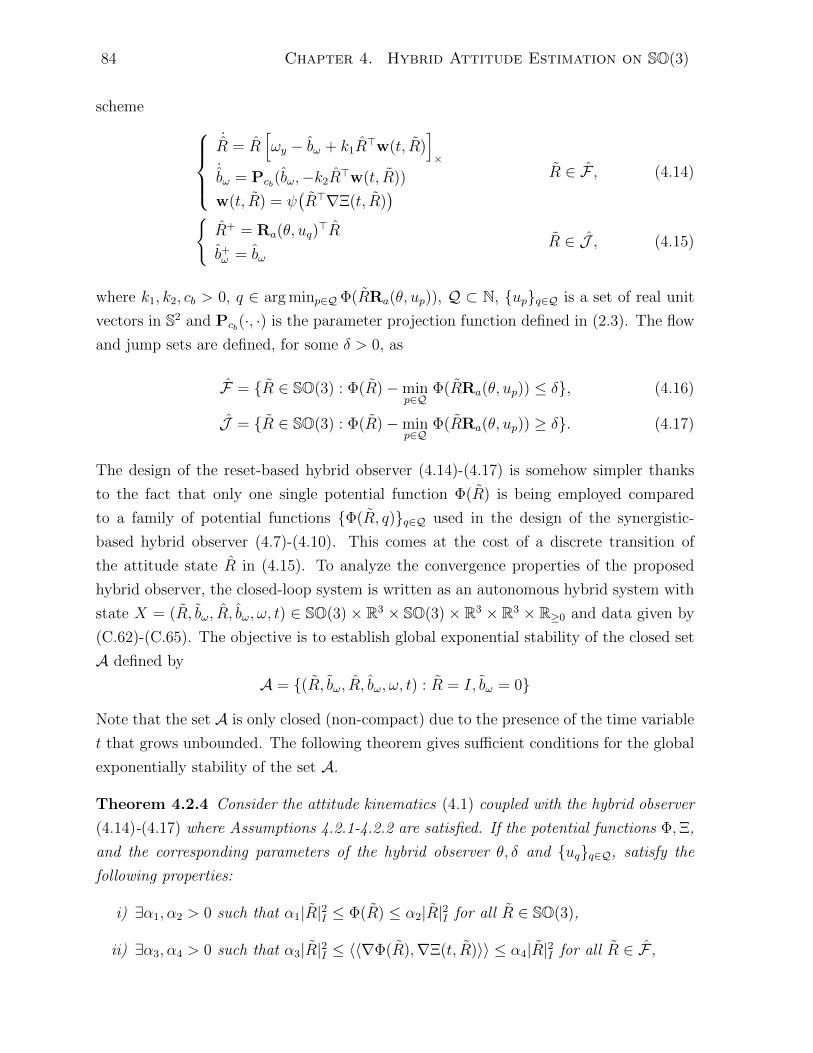
84 Chapter 4. Hybrid Attitude Estimation on SO(3)
scheme ˙R = R
[ωy − bω + k1R
>w(t, R)]×
˙bω = Pcb(bω,−k2R
>w(t, R))
w(t, R) = ψ(R>∇Ξ(t, R)
) R ∈ F , (4.14)
R+ = Ra(θ, uq)
>R
b+ω = bω
R ∈ J , (4.15)
where k1, k2, cb > 0, q ∈ arg minp∈QΦ(RRa(θ, up)), Q ⊂ N, upq∈Q is a set of real unit
vectors in S2 and Pcb(·, ·) is the parameter projection function defined in (2.3). The flow
and jump sets are defined, for some δ > 0, as
F = R ∈ SO(3) : Φ(R)−minp∈Q
Φ(RRa(θ, up)) ≤ δ, (4.16)
J = R ∈ SO(3) : Φ(R)−minp∈Q
Φ(RRa(θ, up)) ≥ δ. (4.17)
The design of the reset-based hybrid observer (4.14)-(4.17) is somehow simpler thanks
to the fact that only one single potential function Φ(R) is being employed compared
to a family of potential functions Φ(R, q)q∈Q used in the design of the synergistic-
based hybrid observer (4.7)-(4.10). This comes at the cost of a discrete transition of
the attitude state R in (4.15). To analyze the convergence properties of the proposed
hybrid observer, the closed-loop system is written as an autonomous hybrid system with
state X = (R, bω, R, bω, ω, t) ∈ SO(3)× R3 × SO(3)× R3 × R3 × R≥0 and data given by
(C.62)-(C.65). The objective is to establish global exponential stability of the closed set
A defined by
A = (R, bω, R, bω, ω, t) : R = I, bω = 0
Note that the set A is only closed (non-compact) due to the presence of the time variable
t that grows unbounded. The following theorem gives sufficient conditions for the global
exponentially stability of the set A.
Theorem 4.2.4 Consider the attitude kinematics (4.1) coupled with the hybrid observer
(4.14)-(4.17) where Assumptions 4.2.1-4.2.2 are satisfied. If the potential functions Φ,Ξ,
and the corresponding parameters of the hybrid observer θ, δ and uqq∈Q, satisfy the
following properties:
i) ∃α1, α2 > 0 such that α1|R|2I ≤ Φ(R) ≤ α2|R|2I for all R ∈ SO(3),
ii) ∃α3, α4 > 0 such that α3|R|2I ≤ 〈〈∇Φ(R),∇Ξ(t, R)〉〉 ≤ α4|R|2I for all R ∈ F ,

4.2. Attitude Estimation Using Continuous Vector Measurements 85
iii) F ⊆ DΞ,
iv) ∃α5, α6 > 0 such that ‖∇Ξ(t, R)‖F ≤ α5|R|I and ‖∇Φ(R)‖F ≤ α6|R|I .
Then the number of discrete jumps is finite and the set A = (R, bω, R, ω, t) : R =
I, bω = 0, for the hybrid system with data (C.62)-(C.65), is globally exponentially stable
if k1 > k1 > 0 for some gain k1 provided in the proof.
Proof See Appendix C.7.
The stability result of Theorem 4.2.4 is equivalent to the one obtained in Theorem 4.2.3
for the hybrid observer (4.7)-(4.10). However, in Theorem 4.2.4, a condition on the gain
k1 is imposed. This condition, as shown in the proof of Theorem 4.2.4, comes from
the fact that the correction term is allowed to be dependent on a possibly time-varying
potential function Ξ. If one takes Ξ = Φ (although not shown here) it can be verified that
the condition on the gain k1 is no longer needed to establish global exponential stability.
In some applications, as the case when the vector measurements are time-varying, the
functions Φ(R) and Ξ(t, R) may be chosen to be different [Grip et al., 2012a].
Moreover, compared to the synergistic-based observer, the use of the projection op-
erator in the bias adaptation law is necessary to establish the proof of Theorem 4.2.4
in the case where Ξ is time-varying. If one takes Ξ = Φ (time-invariant), one can still
guarantee global exponential stability without the use of the projection operator. Note
that restricting the bias estimates to lie inside a predefined ball is desirable in practice
to avoid unbounded growth due to the integration of measurement noise. The projection
operator can also be used in (4.8) for practical considerations although it was not needed
to establish the proof of exponential stability.
Remark 4.2.5 Note that in view of the definition of the jump set J in (4.17) and item
i) of Theorem 4.2.4 one has R ∈ J implies that
δ ≤ Φ(R)−minp∈Q
Φ(RRa(θ, up)) ≤ Φ(R) ≤ α2|R|2I ≤ α2. (4.18)
Therefore, in the case where δ > α2, it is clear that J = ∅ and F = SO(3). In this case
the reset-base observer is continuous since the jump mechanism is never executed. In this
case, the result of Theorem 4.2.4 cannot hold since the topological obstruction on SO(3)
prevents a continuous observer to guarantee global exponential stability. In fact, item ii)
cannot hold for all R ∈ SO(3) since the gradient of Φ needs to vanish at some critical
points other than R = I only.
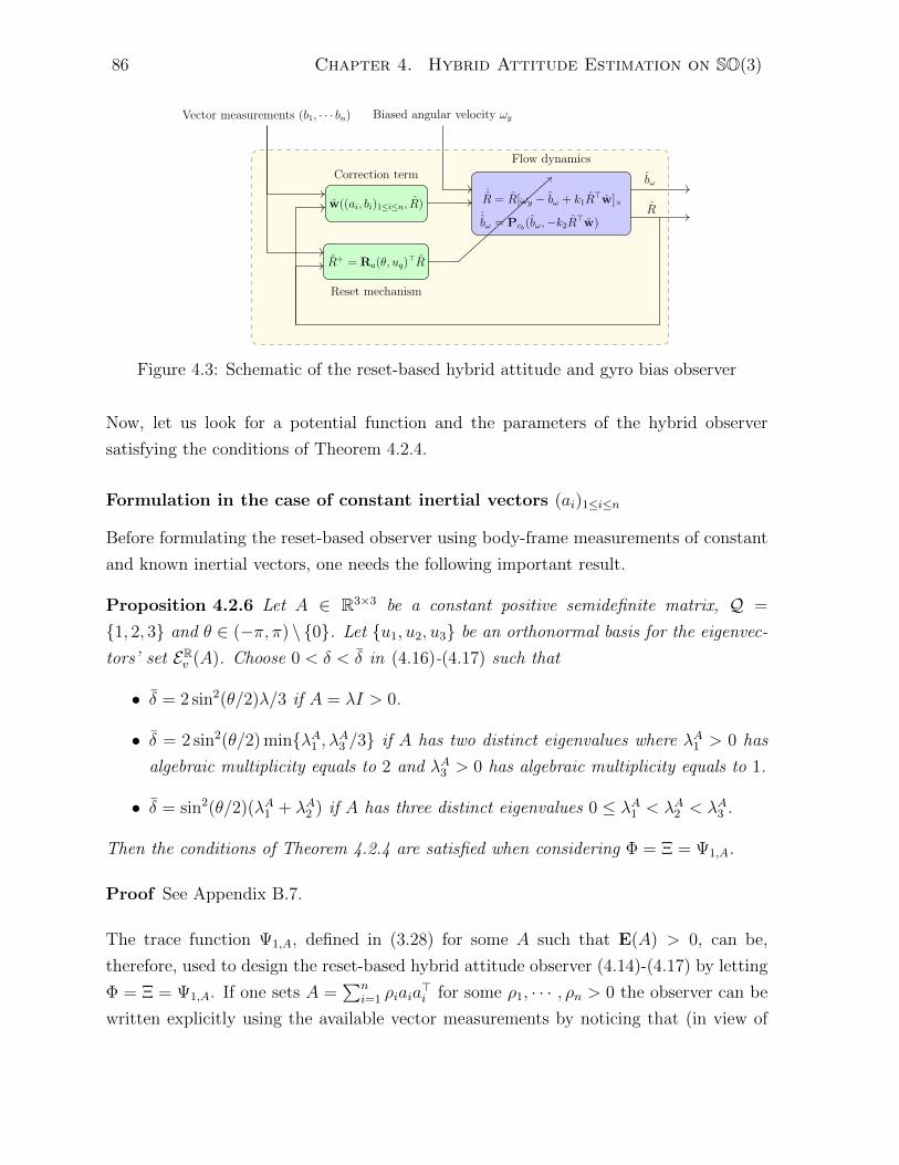
86 Chapter 4. Hybrid Attitude Estimation on SO(3)
w((ai, bi)1≤i≤n, R)
Correction term
R+ = Ra(θ, uq)>R
Reset mechanism
˙R = R[ωy − bω + k1R
>w]×˙bω = Pcb(bω,−k2R
>w)
Flow dynamics
R
bω
Vector measurements (b1, · · · bn) Biased angular velocity ωy
Figure 4.3: Schematic of the reset-based hybrid attitude and gyro bias observer
Now, let us look for a potential function and the parameters of the hybrid observer
satisfying the conditions of Theorem 4.2.4.
Formulation in the case of constant inertial vectors (ai)1≤i≤n
Before formulating the reset-based observer using body-frame measurements of constant
and known inertial vectors, one needs the following important result.
Proposition 4.2.6 Let A ∈ R3×3 be a constant positive semidefinite matrix, Q =
1, 2, 3 and θ ∈ (−π, π) \ 0. Let u1, u2, u3 be an orthonormal basis for the eigenvec-
tors’ set ERv (A). Choose 0 < δ < δ in (4.16)-(4.17) such that
• δ = 2 sin2(θ/2)λ/3 if A = λI > 0.
• δ = 2 sin2(θ/2) minλA1 , λA3 /3 if A has two distinct eigenvalues where λA1 > 0 has
algebraic multiplicity equals to 2 and λA3 > 0 has algebraic multiplicity equals to 1.
• δ = sin2(θ/2)(λA1 + λA2 ) if A has three distinct eigenvalues 0 ≤ λA1 < λA2 < λA3 .
Then the conditions of Theorem 4.2.4 are satisfied when considering Φ = Ξ = Ψ1,A.
Proof See Appendix B.7.
The trace function Ψ1,A, defined in (3.28) for some A such that E(A) > 0, can be,
therefore, used to design the reset-based hybrid attitude observer (4.14)-(4.17) by letting
Φ = Ξ = Ψ1,A. If one sets A =∑n
i=1 ρiaia>i for some ρ1, · · · , ρn > 0 the observer can be
written explicitly using the available vector measurements by noticing that (in view of

4.2. Attitude Estimation Using Continuous Vector Measurements 87
Lemma 2.2.7)
Φ(R) =1
4
n∑i=1
ρi‖bi − R>ai‖2, (4.19)
Φ(RRa(θ, u)) =1
4
n∑i=1
ρi‖bi − R>Ra(θ, u)ai‖2, (4.20)
w(t, R) =1
4R
n∑i=1
ρi(bi × R>ai). (4.21)
Algorithm 2 Reset-based hybrid observer using constant inertial vectors
Pick scalars ρi > 0, i = 1, · · · , n such that A =∑n
i=1 ρiaia>i has distinct eigenvalues.
Pick θ ∈ R \ 0 and 0 < δ < sin2(θ/2)(λA1 + λA2 ).Let Q = 1, 2, 3 and u1, u2, u3 an orthonormal basis for ERv (A).Initialize the observer states R(0, 0) ∈ SO(3), bω(0, 0) ∈ R3
Pick the observer gains k1 and k2 to obtain the desirable performance.
1: for each set of measurements (bi)1≤i≤n and (ai)1≤i≤n do2: Calculate Φ(R) and minp∈QΦ(RRa(θ, up)) using (4.19) and (4.20).
3: while R ∈ J do4: Update R+ = Ra(θ, uq)
>R where q ∈ arg minp∈QΦ(RRa(θ, up)).5: end while6: Calculate the correction term w(t, R) using (4.21).7: Update the states R and bω according to (4.14).8: end for
Formulation in the case of time-varying inertial vectors (ai)1≤i≤n
In the case where the inertial vectors are time-varying, the matrix A becomes time-
varying and thus the potential function Ψ1,A depends on time as well. It can not be
used as Φ = Ψ1,A since Φ in Theorem 4.2.4 was assumed to be state dependent only.
In this case, we construct a potential function Φ that does not depend on time. Let a1
and a2 be any two noncollinear inertial vectors which are guaranteed to exist thanks to
Assumption 4.2.1. Construct the following three orthonormal vectors r1 = a1/‖a1‖, r2 =
(a1 × a2)/‖a1 × a2‖ and r3 = r1 × r2. The corresponding body-frame measurements of
r1, r2 and r3 are given by s1 = b1/‖b1‖, s2 = (b1 × b2)/‖b1 × b2‖ and s3 = s1 × s2. Then,
in view of Lemma 2.2.7 and the fact that∑3
i=1 rir>i = I one obtains
Ψ1(R) =1
4
3∑i=1
‖si − R>ri‖. (4.22)
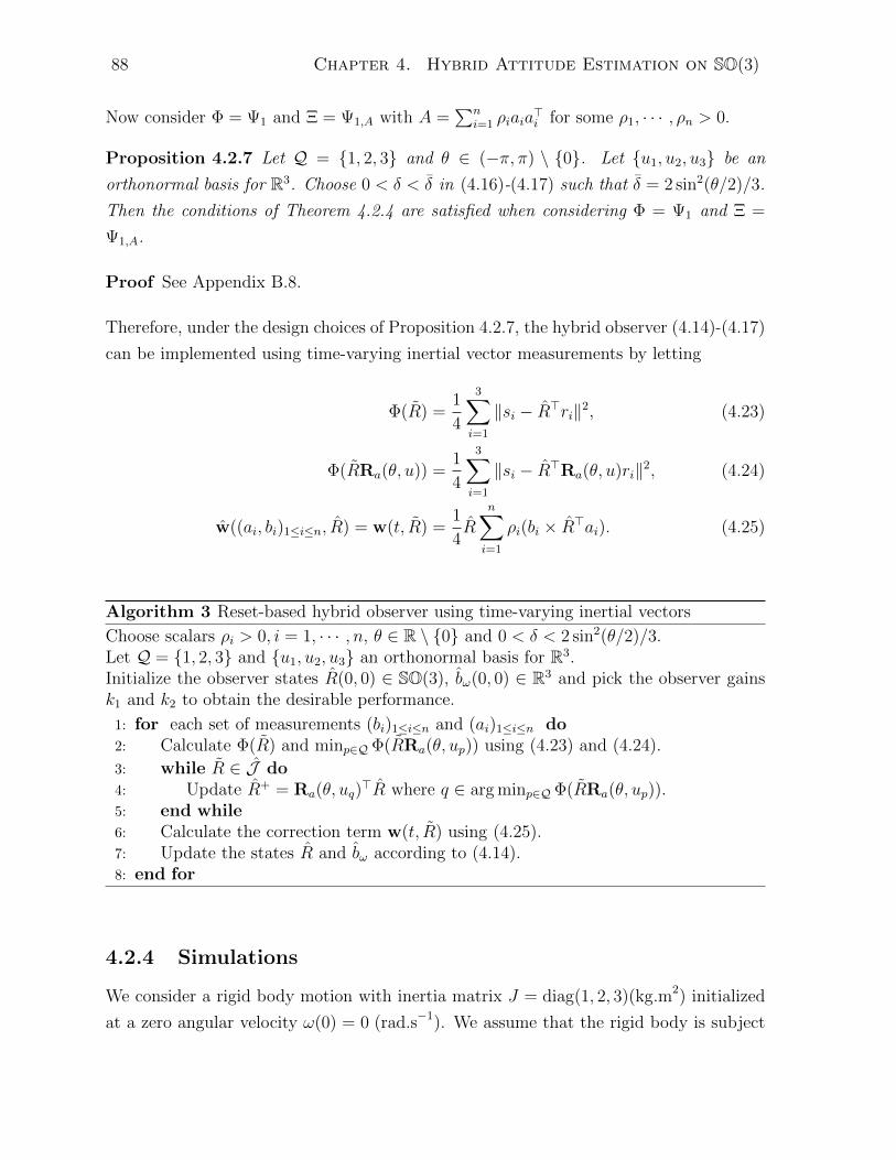
88 Chapter 4. Hybrid Attitude Estimation on SO(3)
Now consider Φ = Ψ1 and Ξ = Ψ1,A with A =∑n
i=1 ρiaia>i for some ρ1, · · · , ρn > 0.
Proposition 4.2.7 Let Q = 1, 2, 3 and θ ∈ (−π, π) \ 0. Let u1, u2, u3 be an
orthonormal basis for R3. Choose 0 < δ < δ in (4.16)-(4.17) such that δ = 2 sin2(θ/2)/3.
Then the conditions of Theorem 4.2.4 are satisfied when considering Φ = Ψ1 and Ξ =
Ψ1,A.
Proof See Appendix B.8.
Therefore, under the design choices of Proposition 4.2.7, the hybrid observer (4.14)-(4.17)
can be implemented using time-varying inertial vector measurements by letting
Φ(R) =1
4
3∑i=1
‖si − R>ri‖2, (4.23)
Φ(RRa(θ, u)) =1
4
3∑i=1
‖si − R>Ra(θ, u)ri‖2, (4.24)
w((ai, bi)1≤i≤n, R) = w(t, R) =1
4R
n∑i=1
ρi(bi × R>ai). (4.25)
Algorithm 3 Reset-based hybrid observer using time-varying inertial vectors
Choose scalars ρi > 0, i = 1, · · · , n, θ ∈ R \ 0 and 0 < δ < 2 sin2(θ/2)/3.Let Q = 1, 2, 3 and u1, u2, u3 an orthonormal basis for R3.Initialize the observer states R(0, 0) ∈ SO(3), bω(0, 0) ∈ R3 and pick the observer gainsk1 and k2 to obtain the desirable performance.
1: for each set of measurements (bi)1≤i≤n and (ai)1≤i≤n do2: Calculate Φ(R) and minp∈QΦ(RRa(θ, up)) using (4.23) and (4.24).
3: while R ∈ J do4: Update R+ = Ra(θ, uq)
>R where q ∈ arg minp∈QΦ(RRa(θ, up)).5: end while6: Calculate the correction term w(t, R) using (4.25).7: Update the states R and bω according to (4.14).8: end for
4.2.4 Simulations
We consider a rigid body motion with inertia matrix J = diag(1, 2, 3)(kg.m2) initialized
at a zero angular velocity ω(0) = 0 (rad.s−1). We assume that the rigid body is subject
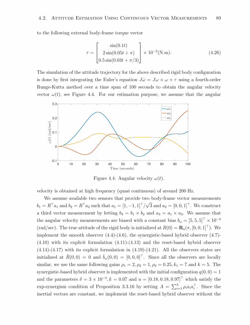
4.2. Attitude Estimation Using Continuous Vector Measurements 89
to the following external body-frame torque vector
τ =
sin(0.1t)
2 sin(0.05t+ π)
0.5 sin(0.03t+ π/3)
× 10−2(N.m). (4.26)
The simulation of the attitude trajectory for the above described rigid body configuration
is done by first integrating the Euler’s equation Jω = Jω × ω + τ using a fourth-order
Runge-Kutta method over a time span of 100 seconds to obtain the angular velocity
vector ω(t), see Figure 4.4. For our estimation purpose, we assume that the angular
0 10 20 30 40 50 60 70 80 90 100
Time (seconds)
-0.1
0
0.1
0.2
0.3
ω(t)(rad/sec)
ω1
ω2
ω3
Figure 4.4: Angular velocity ω(t).
velocity is obtained at high frequency (quasi continuous) of around 200 Hz.
We assume available two sensors that provide two body-frame vector measurements
b1 = R>a1 and b2 = R>a2 such that a1 = [1,−1, 1]>/√
3 and a2 = [0, 0, 1]>. We construct
a third vector measurement by letting b3 = b1 × b2 and a3 = a1 × a3. We assume that
the angular velocity measurements are biased with a constant bias bω = [5, 5, 5]> × 10−3
(rad/sec). The true attitude of the rigid body is initialized at R(0) = Ra(π, [0, 0, 1]>). We
implement the smooth observer (4.4)-(4.6), the synergistic-based hybrid observer (4.7)-
(4.10) with its explicit formulation (4.11)-(4.13) and the reset-based hybrid observer
(4.14)-(4.17) with its explicit formulation in (4.19)-(4.21). All the observers states are
initialized at R(0, 0) = 0 and bω(0, 0) = [0, 0, 0]>. Since all the observers are locally
similar, we use the same following gains ρ1 = 2, ρ2 = 1, ρ3 = 0.25, k1 = 7 and k = 5. The
synergistic-based hybrid observer is implemented with the initial configuration q(0, 0) = 1
and the parameters δ = 3 × 10⁻³, k = 0.07 and u = [0.18, 0.18, 0.97]> which satisfy the
exp-synergism condition of Proposition 3.3.16 by setting A =∑3
i=1 ρiaia>i . Since the
inertial vectors are constant, we implement the reset-based hybrid observer without the
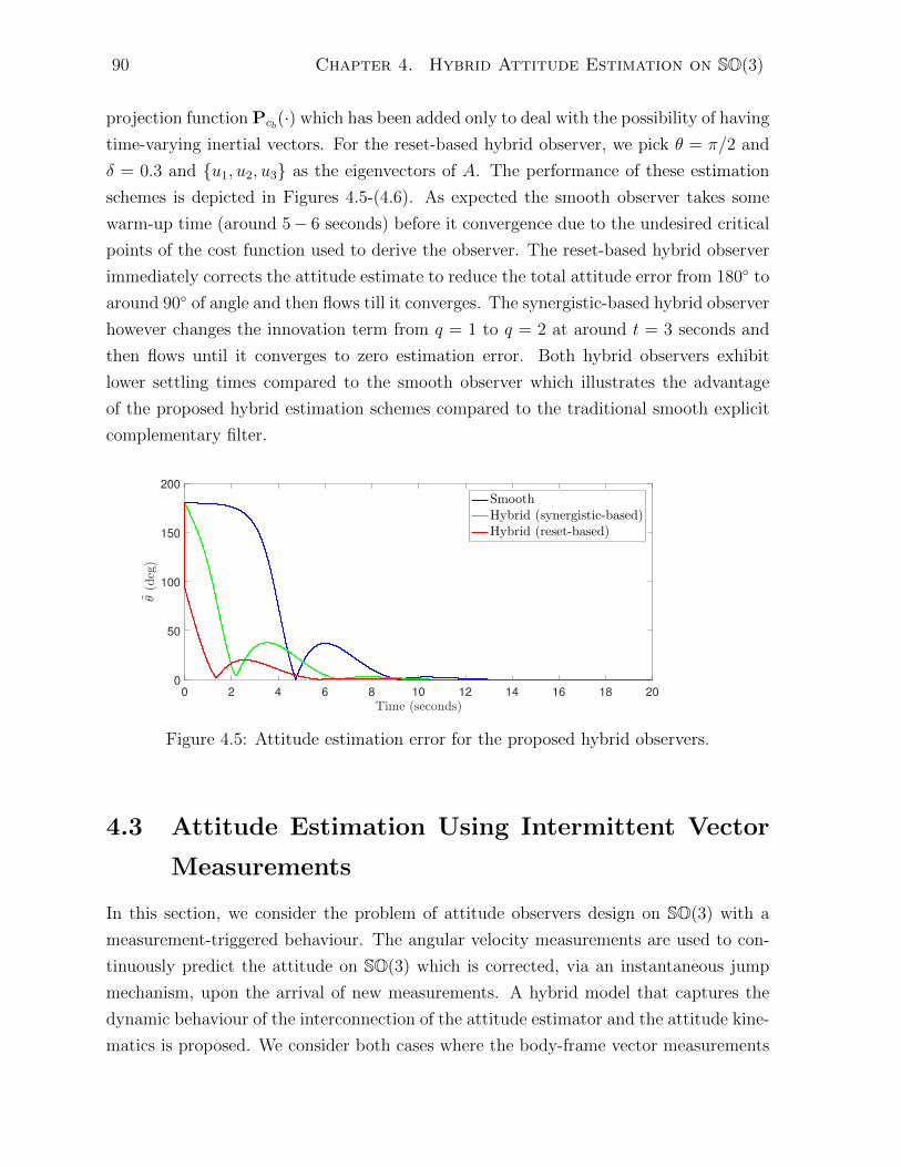
90 Chapter 4. Hybrid Attitude Estimation on SO(3)
projection function Pcb(·) which has been added only to deal with the possibility of having
time-varying inertial vectors. For the reset-based hybrid observer, we pick θ = π/2 and
δ = 0.3 and u1, u2, u3 as the eigenvectors of A. The performance of these estimation
schemes is depicted in Figures 4.5-(4.6). As expected the smooth observer takes some
warm-up time (around 5− 6 seconds) before it convergence due to the undesired critical
points of the cost function used to derive the observer. The reset-based hybrid observer
immediately corrects the attitude estimate to reduce the total attitude error from 180 to
around 90 of angle and then flows till it converges. The synergistic-based hybrid observer
however changes the innovation term from q = 1 to q = 2 at around t = 3 seconds and
then flows until it converges to zero estimation error. Both hybrid observers exhibit
lower settling times compared to the smooth observer which illustrates the advantage
of the proposed hybrid estimation schemes compared to the traditional smooth explicit
complementary filter.
0 2 4 6 8 10 12 14 16 18 20
Time (seconds)
0
50
100
150
200
θ(deg)
SmoothHybrid (synergistic-based)Hybrid (reset-based)
Figure 4.5: Attitude estimation error for the proposed hybrid observers.
4.3 Attitude Estimation Using Intermittent Vector
Measurements
In this section, we consider the problem of attitude observers design on SO(3) with a
measurement-triggered behaviour. The angular velocity measurements are used to con-
tinuously predict the attitude on SO(3) which is corrected, via an instantaneous jump
mechanism, upon the arrival of new measurements. A hybrid model that captures the
dynamic behaviour of the interconnection of the attitude estimator and the attitude kine-
matics is proposed. We consider both cases where the body-frame vector measurements
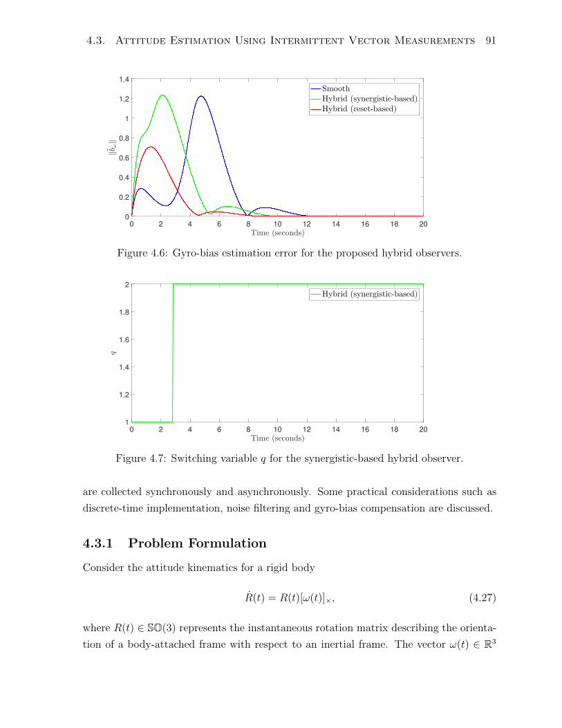
4.3. Attitude Estimation Using Intermittent Vector Measurements 91
0 2 4 6 8 10 12 14 16 18 20
Time (seconds)
0
0.2
0.4
0.6
0.8
1
1.2
1.4
‖bω‖
SmoothHybrid (synergistic-based)Hybrid (reset-based)
Figure 4.6: Gyro-bias estimation error for the proposed hybrid observers.
0 2 4 6 8 10 12 14 16 18 20
Time (seconds)
1
1.2
1.4
1.6
1.8
2
q
Hybrid (synergistic-based)
Figure 4.7: Switching variable q for the synergistic-based hybrid observer.
are collected synchronously and asynchronously. Some practical considerations such as
discrete-time implementation, noise filtering and gyro-bias compensation are discussed.
4.3.1 Problem Formulation
Consider the attitude kinematics for a rigid body
R(t) = R(t)[ω(t)]×, (4.27)
where R(t) ∈ SO(3) represents the instantaneous rotation matrix describing the orienta-
tion of a body-attached frame with respect to an inertial frame. The vector ω(t) ∈ R3
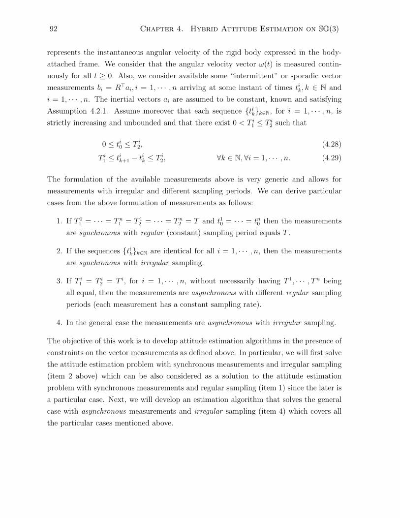
92 Chapter 4. Hybrid Attitude Estimation on SO(3)
represents the instantaneous angular velocity of the rigid body expressed in the body-
attached frame. We consider that the angular velocity vector ω(t) is measured contin-
uously for all t ≥ 0. Also, we consider available some “intermittent” or sporadic vector
measurements bi = R>ai, i = 1, · · · , n arriving at some instant of times tik, k ∈ N and
i = 1, · · · , n. The inertial vectors ai are assumed to be constant, known and satisfying
Assumption 4.2.1. Assume moreover that each sequence tikk∈N, for i = 1, · · · , n, is
strictly increasing and unbounded and that there exist 0 < T i1 ≤ T i2 such that
0 ≤ ti0 ≤ T i2, (4.28)
T i1 ≤ tik+1 − tik ≤ T i2, ∀k ∈ N,∀i = 1, · · · , n. (4.29)
The formulation of the available measurements above is very generic and allows for
measurements with irregular and different sampling periods. We can derive particular
cases from the above formulation of measurements as follows:
1. If T 11 = · · · = T n1 = T 1
2 = · · · = T n2 = T and t10 = · · · = tn0 then the measurements
are synchronous with regular (constant) sampling period equals T .
2. If the sequences tikk∈N are identical for all i = 1, · · · , n, then the measurements
are synchronous with irregular sampling.
3. If T i1 = T i2 = T i, for i = 1, · · · , n, without necessarily having T 1, · · · , T n being
all equal, then the measurements are asynchronous with different regular sampling
periods (each measurement has a constant sampling rate).
4. In the general case the measurements are asynchronous with irregular sampling.
The objective of this work is to develop attitude estimation algorithms in the presence of
constraints on the vector measurements as defined above. In particular, we will first solve
the attitude estimation problem with synchronous measurements and irregular sampling
(item 2 above) which can be also considered as a solution to the attitude estimation
problem with synchronous measurements and regular sampling (item 1) since the later is
a particular case. Next, we will develop an estimation algorithm that solves the general
case with asynchronous measurements and irregular sampling (item 4) which covers all
the particular cases mentioned above.

4.3. Attitude Estimation Using Intermittent Vector Measurements 93
4.3.2 Attitude Estimation Using Synchronous Vector Measure-
ments
In this subsection, we assume that the vector measurements are synchronized, which
means that the time sequences tikk∈N are identical for all i = 1, · · · , n and can be
denoted as tkk∈N by removing the index i. In this case, the lower and upper bound
on the transmission times T i1 and T i2 are also denoted by T1 and T2 for short. Observers
with impulsive-like dynamics for linear time invariant systems and some special classes of
nonlinear systems with Lipschitz nonlinearities have been discussed in [Raff and Allgower,
2007, Andrieu et al., 2013, Ferrante et al., 2016]. Motivated by these works, we propose
the following estimation scheme on SO(3)
˙R(t) = R(t)[ω(t)]×, t ∈ [tk−1, tk), k ∈ N, (4.30)
R(t+) = Rr (σ(t)) R(t), t = tk, k ∈ N, (4.31)
σ =n∑i=1
ρi(Rbi × ai), ρi > 0, (4.32)
where the notation R(t+) is used such that R(t+) = limh→0 R(t + h) and, without loss
of generality, it is assumed that R(t) = R(t−) = limh→0 R(t − h). Between two instants
of time tk−1 and tk, the attitude observer is a copy of the attitude kinematics (4.27).
This is similar to the “prediction step” in the traditional Kalman filtering technique.
The estimated attitude R(t) is updated (corrected) at each instant of time tk when a
new measurement becomes available. This correction step uses matrix multiplication to
preserve attitude estimates on SO(3) since the group SO(3) is closed under the matrix
multiplication operation. Specifically, we use a correction matrix that is built from the
error vector σ used in many continuous attitude estimation schemes [Mahony et al.,
2008, Berkane and Tayebi, 2016, Zlotnik and Forbes, 2017]. Note that in [Barrau and
Bonnabel, 2015] a similar observer structure has been proposed in the case of two vector
measurements, with the use of the exponential map exp(σ) as a correction rotation instead
of Rr(σ). The advantage of using Rr(σ) over exp(σ) is the computational efficiency since
Rr(σ) does not require the calculation of trigonometric functions. Moreover, this choice
facilitates considerably the proof of convergence which is conducted for a set of n ≥ 2
vector measurements compared to [Barrau and Bonnabel, 2015] where only two vector
measurements are used.
To analyze the stability of the proposed attitude estimation scheme, we define the

94 Chapter 4. Hybrid Attitude Estimation on SO(3)
following (left-invariant) attitude estimation error
R = RR>. (4.33)
During the flows of (4.30) the evolution of the attitude estimation error satisfies ˙R =
RR> + R˙R> = R[ω]×R
> − R[ω]×R> = 0. This implies that the attitude error is kept
constant while waiting for the arrival of a new measurement. Note that this property
holds true only when considering perfect angular velocity readings. In fact if the angular
velocity reading is biased or noisy then we would accept slight drift of the attitude
estimation error during the intervals of time where no measurements are available. For
sufficiently small measurement intervals and accurate enough gyros we expect that this
drift will be maintained small enough and stable. The interconnection of the jump-free
kinematic model (4.27) and the attitude observer (4.30)-(4.31) leads naturally to the
following closed-loop system
˙R(t) = 0, t ∈ [tk−1, tk), k ∈ N, (4.34)
R(t+) = R(t)Rr (−σ(t)) , t = tk, k ∈ N, (4.35)
where we have used the fact that during the jumps the true attitude R(t) is unchanged
and thus R(t+) = R(t). The correction term σ(t) in (4.32) can be expressed in terms of
the attitude error as σ =∑n
i=1 ρi[R>ai]×ai. Note that the dynamics of the attitude error
R is independent from the attitude trajectory in (4.27). This is a desirable behaviour
since the gains can be tuned and optimized off-line to yield the desirable behaviour
in real-time, independently from the trajectory of the attitude system dictated by the
angular velocity vector ω(t).
Now, we map the closed-loop system (4.34)-(4.35) into a hybrid model by augmenting
the system with a “hidden” timer (see [Jentzen et al., 2010]) as follows˙R = 0
τ = 1(R, τ) ∈ F , (4.36)
R+ = RRr (−σ)
τ+ = 0(R, τ) ∈ J , (4.37)
where the flow set F and jump set J are defined as
F =
(R, τ) ∈ SO(3)× R≥0 : τ ∈ [0, T2], (4.38)
J =
(R, τ) ∈ SO(3)× R≥0 : τ ∈ [T1, T2]. (4.39)
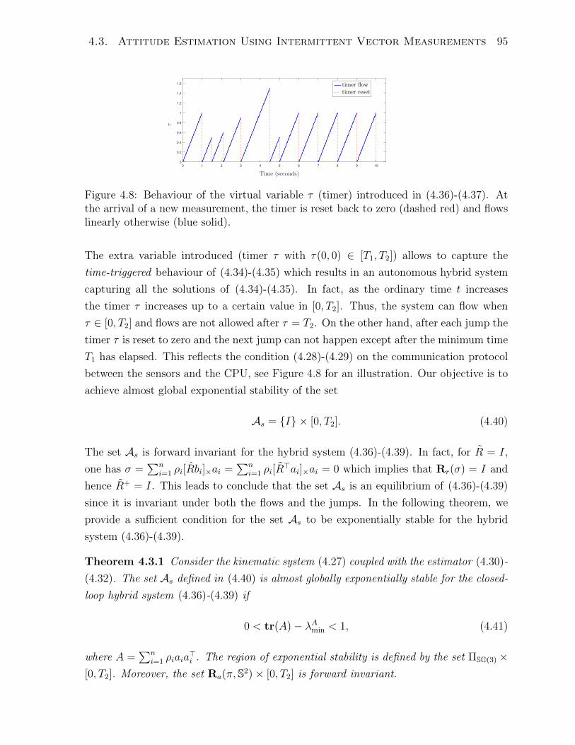
4.3. Attitude Estimation Using Intermittent Vector Measurements 95
0 1 2 3 4 5 6 7 8 9 10
Time (seconds)
0
0.2
0.4
0.6
0.8
1
1.2
1.4
1.6
τ
timer flowtimer reset
Figure 4.8: Behaviour of the virtual variable τ (timer) introduced in (4.36)-(4.37). Atthe arrival of a new measurement, the timer is reset back to zero (dashed red) and flowslinearly otherwise (blue solid).
The extra variable introduced (timer τ with τ(0, 0) ∈ [T1, T2]) allows to capture the
time-triggered behaviour of (4.34)-(4.35) which results in an autonomous hybrid system
capturing all the solutions of (4.34)-(4.35). In fact, as the ordinary time t increases
the timer τ increases up to a certain value in [0, T2]. Thus, the system can flow when
τ ∈ [0, T2] and flows are not allowed after τ = T2. On the other hand, after each jump the
timer τ is reset to zero and the next jump can not happen except after the minimum time
T1 has elapsed. This reflects the condition (4.28)-(4.29) on the communication protocol
between the sensors and the CPU, see Figure 4.8 for an illustration. Our objective is to
achieve almost global exponential stability of the set
As = I × [0, T2]. (4.40)
The set As is forward invariant for the hybrid system (4.36)-(4.39). In fact, for R = I,
one has σ =∑n
i=1 ρi[Rbi]×ai =∑n
i=1 ρi[R>ai]×ai = 0 which implies that Rr(σ) = I and
hence R+ = I. This leads to conclude that the set As is an equilibrium of (4.36)-(4.39)
since it is invariant under both the flows and the jumps. In the following theorem, we
provide a sufficient condition for the set As to be exponentially stable for the hybrid
system (4.36)-(4.39).
Theorem 4.3.1 Consider the kinematic system (4.27) coupled with the estimator (4.30)-
(4.32). The set As defined in (4.40) is almost globally exponentially stable for the closed-
loop hybrid system (4.36)-(4.39) if
0 < tr(A)− λAmin < 1, (4.41)
where A =∑n
i=1 ρiaia>i . The region of exponential stability is defined by the set ΠSO(3)×
[0, T2]. Moreover, the set Ra(π,S2)× [0, T2] is forward invariant.
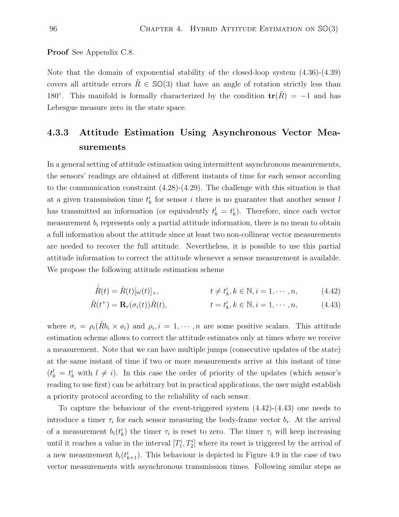
96 Chapter 4. Hybrid Attitude Estimation on SO(3)
Proof See Appendix C.8.
Note that the domain of exponential stability of the closed-loop system (4.36)-(4.39)
covers all attitude errors R ∈ SO(3) that have an angle of rotation strictly less than
180. This manifold is formally characterized by the condition tr(R) = −1 and has
Lebesgue measure zero in the state space.
4.3.3 Attitude Estimation Using Asynchronous Vector Mea-
surements
In a general setting of attitude estimation using intermittent asynchronous measurements,
the sensors’ readings are obtained at different instants of time for each sensor according
to the communication constraint (4.28)-(4.29). The challenge with this situation is that
at a given transmission time tik for sensor i there is no guarantee that another sensor l
has transmitted an information (or equivalently tlk = tik). Therefore, since each vector
measurement bi represents only a partial attitude information, there is no mean to obtain
a full information about the attitude since at least two non-collinear vector measurements
are needed to recover the full attitude. Nevertheless, it is possible to use this partial
attitude information to correct the attitude whenever a sensor measurement is available.
We propose the following attitude estimation scheme
˙R(t) = R(t)[ω(t)]×, t 6= tik, k ∈ N, i = 1, · · · , n, (4.42)
R(t+) = Rr(σi(t))R(t), t = tik, k ∈ N, i = 1, · · · , n, (4.43)
where σi = ρi(Rbi × ai) and ρi, i = 1, · · · , n are some positive scalars. This attitude
estimation scheme allows to correct the attitude estimates only at times where we receive
a measurement. Note that we can have multiple jumps (consecutive updates of the state)
at the same instant of time if two or more measurements arrive at this instant of time
(tlk = tik with l 6= i). In this case the order of priority of the updates (which sensor’s
reading to use first) can be arbitrary but in practical applications, the user might establish
a priority protocol according to the reliability of each sensor.
To capture the behaviour of the event-triggered system (4.42)-(4.43) one needs to
introduce a timer τi for each sensor measuring the body-frame vector bi. At the arrival
of a measurement bi(tik) the timer τi is reset to zero. The timer τi will keep increasing
until it reaches a value in the interval [T i1, Ti2] where its reset is triggered by the arrival of
a new measurement bi(tik+1). This behaviour is depicted in Figure 4.9 in the case of two
vector measurements with asynchronous transmission times. Following similar steps as
4.3. Attitude Estimation Using Intermittent Vector Measurements 97
0 2 4 6 8 10 12 14 16 18 20
Time (seconds)
0
0.5
1
1.5
2
2.5
3
τ1 flowτ1 resetτ2 flowτ2 reset
Figure 4.9: Behaviour of the virtual variables τ1 and τ2 (timers) introduced in (4.42)-(4.49). The transmission (measurement) times tik with i ∈ 1, 2 satisfy the constraints(4.28)-(4.29) with T 1
1 = 0.5, T 12 = 1.5, T 2
1 = 1 and T 22 = 3. At the arrival of a measurement
bi the corresponding timer τi is reset back to zero.
(4.34)-(4.39), we derive the hybrid model that captures the dynamics of the closed-loop
system as follows. Let us define the state X := (R, τ1, · · · , τn) ∈ SO(3) × Rn≥0. The
closed-loop system is governed by the hybrid dynamical model
X = F(X), X ∈ F , (4.44)
X+ ∈ J(X), X ∈ J , (4.45)
where the single-valued flow map F and set-valued jump map J are defined by
F(X) = (03×3, 1, · · · , 1), (4.46)
J(X) = Ji(X), X ∈ Ji, (4.47)
where Ji(X) = (RRr(−σi), τ1, · · · , τi−1, 0, τi+1, · · · , τn) and Ji = X ∈ SO(3) × Rn≥0 :
τi ∈ [T i1, Ti2]. The flow set F and jump set J are given by
F = SO(3)× [0, T 12 ]× · · · × [0, T n2 ], (4.48)
J = J1 ∪ · · · ∪ Jn. (4.49)
Note that the jumps in (4.43) are modelled by an inclusion and therefore the updated
state X+ can take any of the values from the set J(X). This captures the behaviour
when multiple measurements from different sensors arrive at the same instant of time.
In this case the closed-loop system is allowed to experience multiple consecutive jumps
in any order. The objective is to achieve almost global asymptotic stability of the set
Aa = I × [0, T 12 ]× · · · × [0, T n2 ].

98 Chapter 4. Hybrid Attitude Estimation on SO(3)
Theorem 4.3.2 Consider the kinematic system (4.27) coupled with the estimator (4.42)-
(4.43). The set Aa is almost globally asymptotically stable for the closed-loop hybrid
system (4.36)-(4.39) if the scalars ρi satisfy
0 < ρi <1
‖ai‖2, i ∈ 1, · · · , n. (4.50)
The region of asymptotic stability is defined by the set ΠSO(3) × [0, T 12 ]× · · · × [0, T n2 ].
Proof See Appendix C.9.
Note that the attitude estimation scheme (4.42)-(4.43), although developed for the gen-
eral case of asynchronous measurements, can also be used in the particular case of syn-
chronous measurements. In this case t1k = · · · = tik = · · · = tnk and equations (4.42)-(4.43)
can be rewritten as follows
˙R(t) = R(t)[ω(t)]×, t 6= tk, k ∈ N, (4.51)
R+(t) = Πni=1Rr(σi(t))R(t), t = tk, k ∈ N. (4.52)
The obtained algorithm is different from the one proposed in (4.30)-(4.31) for synchronous
measurements. The difference resides in the correction attitude matrix which is defined
by the product Πni=1Rr(σi) in (4.51)-(4.52) while in (4.30)-(4.31) it is defined by the
single rotation matrix Rr(∑n
i=1 σi). The latter requires less computational power and
this argument has motivated the introduction of algorithm (4.30)-(4.31) which suites
better the case of synchronous measurements.
4.3.4 Practical Considerations
In this section, we discuss some practical issues and improvements to the raw algorithms
presented in the previous sections.
4.3.4.1 Discrete-Time Implementation
The attitude estimation scheme proposed in (4.30)-(4.31) relies on continuous flow dy-
namics between each two instant of measurements tk and tk+1. The observer state is
updated (via instantaneous jumps) at each instant of time tk when a new measurement
arrives. To implement this attitude observer, we propose a discrete-time integration
scheme that emulates the behaviour of the observer during the continuous flow. Assume
4.3. Attitude Estimation Using Intermittent Vector Measurements 99
that the unbounded continuous time interval [0,∞) is sampled with a sampling period
Ts > 0. We obtain a series of discrete times smm∈N such that sm = mTs. We assume
that the sampling period Ts is small enough such that the angular velocity is constant
during each sampling period, i.e.,
ω(t) = ω(sm), t ∈ [sm, sm+1),m ∈ N. (4.53)
Consequently, in view of the flow dynamics (4.30), the following holds for all t ∈ [sm, sm+1)
and m ∈ N
d
dt
(R exp([ω(sm)t]×)
)= 0. (4.54)
An exact integration of the above equation, between the instants of time s+m and s−m+1 ≡
sm+1, leads to the following discrete-time update rule for the estimated attitude R, during
the flows of (4.30):
R(sm+1) = R(s+m) exp([ω(sm)Ts]×). (4.55)
The above prediction rule preserves the SO(3) structure since the group SO(3) is closed
under matrix multiplication and the exponential matrix exp([ω(sm)Ts]×) is indeed an
element of SO(3). It corresponds to the Euler-Lie method for numerical integration on
Lie groups [Celledoni et al., 2014]. Note that R(s+m) = limh→0 R(sm+h) which represents
the state of the observer after a “possible” jump in (4.31). For sufficiently small Ts, it is
reasonable to assume that the intermittent instants of time tk, where the measurements
are available, are elements of the discrete-time interval, i.e., tk ∈ smm∈N for all k ∈ N.
That is to say that for all k ∈ N, there exists m ∈ N such that tk = sm = mTs. Only at
these particular instants of time, the attitude estimate R is updated according to (4.31).
Therefore, one has
R(s+m) = Rr(σ(sm))R(sm), sm = tk, k ∈ N, (4.56)
R(s+m) = R(sm), sm 6= tk, k ∈ N. (4.57)
Equations (4.55)-(4.57) define the discrete-time implementation of the proposed attitude
estimation scheme (4.30)-(4.31). Compared to the traditional methods, the discrete
version of our proposed attitude estimation scheme is also asymptotically stable when
connected to a good discrete approximation model for the attitude kinematics (4.27). To
clarify this idea, let us exactly discretize the kinematic model (4.27) under assumption

100 Chapter 4. Hybrid Attitude Estimation on SO(3)
(4.53). Following similar steps as in (4.54)-(4.55), one obtains the following discrete
kinematic model:
R(sm+1) = R(sm) exp([ω(sm)Ts]×), m ∈ N. (4.58)
For a small enough sampling period Ts, the above discrete model is a good approximation
of the original continuous time kinematic model (4.27). We now state the following
theorem whose proof is given in Appendix C.10.
Theorem 4.3.3 Consider the discrete kinematic model (4.58) coupled with the discrete
attitude estimation scheme (4.55)-(4.57) under the conditions of Theorem 4.3.1. Then
for all initial attitude errors R(0) ∈ ΠSO(3) one has limm→∞ R(mTs) = I.
Following similar steps as in (4.53)-(4.57) we can derive the discrete version of (4.42)-
(4.43) which is suitable for the case of asynchronous vector measurements as follows
R(sm+1) = R(s+m) exp([ω(sm)Ts]×) (4.59)
R(s+m) = Rr(σi(sm))R(sm), sm = tik, (4.60)
R(s+m) = R(sm), sm 6= tik, (4.61)
such that m, k ∈ N and i ∈ 1, · · · , n. Moreover, the interconnection of the discrete
attitude kinematic model (4.58) and the discrete scheme (4.59)-(4.61) can be shown to
retain the almost global asymptotic convergence result under the conditions of Theorem
4.3.2. The proof follows similar lines as in the proof of Theorem 4.3.3 thus omitted.
4.3.4.2 Estimation Algorithms with Enhanced Filtering
We introduce recursive states to the observer (4.30)-(4.31) which, when averaged, yield
a better filtered attitude estimate. This can be done by using N ∈ N>0 attitude states
in the following attitude estimation scheme:
• Flow dynamics (Prediction step): for all h ∈ 1, · · · , N the h-th state of the
observer flows according to the kinematic equation
˙Rh(t) = Rh(t)[ω(t)]×, t ∈ [tk−1, tk), k ∈ N. (4.62)

4.3. Attitude Estimation Using Intermittent Vector Measurements 101
• Jump dynamics (Update step): during the instants of time t = tk, k ∈ N the
observer states are updated as follows
R1(t+) = Rr (σ(t)) R1(t), (4.63)
Rh(t+) = Rh−1(t), h ∈ 2, · · · , N, (4.64)
where the correction term σ is defined as σ =∑n
i=1 ρi(R1bi×ai) and ρ1, · · · , ρn are
positive scalars.
• Attitude estimate (averaged rotation): the final attitude estimate is obtained by
averaging all the observer states on SO(3) and is given by
R = PSO(3)
(N∑i=1
αhRh
), (4.65)
where αh are scalars satisfying, without loss of generality, the equality∑N
h=1 αh = 1,
and the projection map PSO(3)(·) is given in (2.12).
The idea of the attitude estimation scheme (4.62)-(4.65) is to expand the estimation
scheme (4.30)-(4.31) with (N−1) additional states which are averaged at the end to give
the final attitude state. At each measurement time t = tk, the attitude states Rh are
shifted one step with respect to the index h (i.e. each state Rh receives the value of the
state Rh−1) which implies that the “error” presented between the state Rh−1 and the true
attitude R is shifted to Rh for all i ∈ 2, · · · , N. Therefore, by averaging all the states
Rh, i ∈ 1, · · · , N, we aim to reduce the noise level compared to the use of a single
observer state. During the flows (when no measurements are available) all the states
of the observer are predicted using the continuous-time angular velocity measurements
which allows to maintain constant errors between each states of the observer and the
true attitude R.
The asymptotic convergence of the observer, under the conditions of Theorem 4.3.1,
can be argued in straightforward manner as follows. In view of Theorem 4.3.1 the at-
titude error R1 = RR1 = I is almost globally exponentially stable which implies that
limtk→∞R(tk)R>1 (t−k ) = I. Since R2(t+k ) = R1(t−k ) implies that limtk→∞R(tk)R
>2 (t+k ) = I
and therefore R2 also converges to R when time goes to infinity. The same argument can
be used to show that all the observer states will converge to R as time goes to infinity.
102 Chapter 4. Hybrid Attitude Estimation on SO(3)
Consequently
limt→∞
R(t) = limt→∞
PSO(3)
(N∑h=1
αhRh
)=
N∑h=1
αhPSO(3) (R) = R,
where we used the fact that∑N
h=1 αh = 1 and PSO(3)(R) = R ∈ SO(3). Therefore, the
estimation scheme (4.62)-(4.65) is also almost globally asymptotically stable under the
same conditions of Theorem 4.3.1.
Furthermore, thanks to the symmetry of the group SO(3), it is possible to considerably
reduce the computational complexity of the estimation scheme (4.62)-(4.65). Observe
that Rh evolves according to the same kinematic equation (4.62). Hence, the estimation
error RhR>1 is constant during the flows of the observer for t ∈ [tk−1, tk). Consequently,
one can write, for all h ∈ 2, · · · , N,∫ t
t+k−1
(RhR>1 )(τ)dτ = 0, t ∈ [tk−1, tk). (4.66)
By completing the above integral one obtains
Rh(t) = Rh(t+k−1)R1(t+k−1)>R1(t), t ∈ [tk−1, tk). (4.67)
Therefore, the value of Rh at a given time t ∈ [tk−1, tk) can be directly obtained from
the value of R1 at t and past values of Rh and R1 at time t = t+k−1 just after the
last jump has occurred. By creating an N dimensional register containing the values
of R1(t+k−1), · · · , RN(t+k−1), it is possible to calculate the values of the individual state
variables at any time t ∈ [tk−1, tk) without performing N integrations in (4.62) but only
once for the R1 attitude state. Moreover, the computation of the averaged rotation (4.65)
can be simplified by observing that for all t ∈ [tk−1, tk) one has
R(t) = PSO(3)
(N∑h=1
αhRh(t)
)= PSO(3)
(N∑h=1
αhRh(t+k−1)R1(t+k−1)>R1(t)
)
= PSO(3)
(N∑h=1
αhRh(t+k−1)
)R1(t+k−1)>R1(t)
:= P (k − 1)R1(t) (4.68)
where we used the fact that PSO(3)(XR) = PSO(3)(X)R for all X ∈ R3×3 and R ∈SO(3). Therefore the projection operation PSO(3)
(∑Nh=1 αhRh(t
+k−1)R1(t+k−1)>)
)needs

4.3. Attitude Estimation Using Intermittent Vector Measurements 103
to be executed at the discrete jump times tk−1 only. This resulting matrix P (k − 1) ∈SO(3) is stored and then used in (4.68) to provide a correction to R1(t). This avoids
to continuously project the mean of rotations in (4.65) for all t ∈ [tk−1, tk). Since the
attitude state Rh needs to be evaluated only at times t+k , we can define Ph(k) = Rh(t+k )
and use (4.67) to derive the following propagation equation for Ph(k)
Ph(k) = Ph−1(k − 1)P1(k − 1)>R1(t−k ), (4.69)
for all h ∈ 2, · · · , N. The new update for R1 is given by (4.63). The obtained estimation
algorithm is summarized in Algorithm 4.
Algorithm 4 Attitude Estimation Using Intermittent Synchronized Measurements
Initialize the states P1(0), · · · , PN(0) ∈ SO(3).Compute P (0) = PSO(3)(
∑Nh=1 αhPh(0))P1(0)>.
Set k = 1 and R1(0) = P1(0).
1: for each t ∈ R≥0 do2: if t = tk then3: R1(t+) = Rr(σ(t))R1(t) with σ =
∑ni=1 ρi(R1bi × ai).
4: P1(k) = R1(t+).5: for each h ∈ 2, · · · , N do6: Ph(k) = Ph−1(k − 1)P1(k − 1)>R1(t)7: end for8: P (k) = PSO(3)(
∑Nh=1 αhPh(k))P1(k)>
9: Update k = k + 110: end if11: Predict R1(t) according to
˙R1(t) = R1(t)[ω(t)]×.
12: Calculate the estimate R(t) = P (k − 1)R1(t).13: end for
Furthermore, we can also improve the filtering capabilities of the attitude estimation
scheme (4.42)-(4.43) which is developed for the case of asynchronous measurements. We
follow similar steps as above to derive Algorithm 5. Note that for practical implementa-
tion purposes the prediction step in Algorithm 4 or 5 (line 12 or 13) can be discretized
as in subsection 4.3.4.1 using Euler-Lie numerical integration method.
4.3.4.3 Smoothing of the Estimator Output
The discrete transitions of the attitude estimates in (4.31) or (4.43) can be undesirable
when feeding these states to a controller for feedback. As a remedy, we propose to cascade
the proposed attitude estimation algorithms with an attitude “smoother” on SO(3) to
104 Chapter 4. Hybrid Attitude Estimation on SO(3)
Algorithm 5 Attitude Estimation Using Intermittent Asynchronous Measurements
Initialize the states P1(0), · · · , PN(0) ∈ SO(3).Compute P (0) = PSO(3)(
∑Nh=1 αhPh(0))P1(0)>.
Set j = 1 and R1(0) = P1(0).
1: for each t ∈ R≥0 do2: if t = tik for some k ∈ N and i ∈ 1, · · · , n then3: Get i ∈ 1, · · · , n s.t. ∃k ∈ N and t = tik.4: R1(t+) = Rr(σi)R1(t) s.t. σi = ρi(R1bi × ai).5: P1(j) = R1(t+).6: for each h ∈ 2, · · · , N do7: Ph(j) = Ph−1(j − 1)P1(j − 1)>R1(t)8: end for9: P (j) = PSO(3)(
∑Nh=1 αhPh(j))P1(j)>
10: Update j = j + 111: end if12: Predict R1(t) according to
˙R1(t) = R1(t)[ω(t)]×.
13: Calculate the final estimate R(t) = P (j − 1)R1(t).14: end for
obtain a smooth attitude Rs(t) that does not involve jumps. The smoother is given by
˙Rs = Rs[ω + kψ(R>s R)]×, Rs(0) = R(0), k > 0, (4.70)
where R is either the output of Algorithm 1 or Algorithm 2 depending on the application.
It is not difficult to show that Rs converges to R from all initial conditions except those
attitudes satisfying tr(RR>s ) = −1 which are characterized by errors of angle strictly less
than 180. Due to the knowledge of R(0) (accessible to the designer), the smoother state
Rs can be initialized to R(0) and therefore the initial error between the smoothed attitude
Rs and the intermittent observer attitude R is zero. This implies that the smoother starts
inside the region of convergence. Moreover, during the jumps of (4.31), the correction
attitude Rr(σ) has an angle which is strictly less than 180. Therefore, it is guaranteed
that the error RR>s never reaches an attitude of angle 180 which, consequently, shows
that the interconnection of the observer-smoother preserves the convergence properties,
given in Theorem 4.3.1 and Theorem 4.3.2, for the standalone intermittent observers.
4.3.4.4 Gyro Bias Compensation
The algorithms developed in this section assumed continuous and perfect angular velocity
measurements. However, in practice, gyro rates measurements are subject to noise and
4.3. Attitude Estimation Using Intermittent Vector Measurements 105
bias. If ωy is the output of the gyro sensor then one has
ωy = ω + bω + nω, (4.71)
where bω is a constant bias and nω is a noise vector. Assuming Gaussian processes the
uncorrelated noise nω is filtered by the forward integration of the angular velocity and
therefore it has a little effect on the attitude estimates. However, bias in the angular
rates may cause the attitude estimates to drift over time especially if the sampling of
the vector measurements is not fast enough to correct the attitude before it drifts. It
is therefore, desirable from a practical point of view and for long run-time applications,
to be able to compensate for constant or slowly varying biases in the angular velocity
measurements. In the case of synchronous measurements with regular sampling equals
T > 0, we propose the following attitude estimation scheme with bias compensation:
˙R(t) = R(t)[ωy(t)− bω(t)]×˙bω(t) = 0
t ∈ [tk−1, tk), (4.72)
R(t+) = Rr (σ(t)) R(t)
bω(t+) = bω(t)− γbT−1R(t)>σ(t)
t = tk, (4.73)
where k ∈ N, γb > 0 and σ is defined in (4.32). Consider the attitude estimations error
R = RR> and the bias estimation error bω = bω − bω. By introducing the virtual timer
variable as in (4.36)-(4.37) and adding R and ω as states variables, the closed-loop system
can be written as a hybrid autonomous system as follows
˙R = R[−Rbω]×
τ = 1˙bω = 0˙R = R[ω + bω]×
ω ∈ cωB
(R, τ, bω, R, ω) ∈ SO(3)× [0, T ]× R3 × SO(3)× R3,
(4.74)
R+ = RRr(−σ),
τ+ = 0
b+ω = bω + γbT
−1R>σ
R+ = Rr(σ)R
ω+ = ω
(R, τ, bω, R, ω) ∈ SO(3)× T × R3 × SO(3)× R3,
(4.75)

106 Chapter 4. Hybrid Attitude Estimation on SO(3)
where we have used the fact that the angular velocity ω satisfies Assumption 4.2.2 so
that we can write the inclusion ω ∈ cωB. The objective of the next Theorem is to state
exponential stability of the set
A = I × [0, T ]× 0 × SO(3)× R3. (4.76)
Theorem 4.3.4 Consider the kinematic system (4.27) coupled with the estimator (4.72)-
(4.73) where Assumptions 4.2.1-4.2.2 are satisfied. Pick the gains ρi and γb such that
0 < λE(A)max <
1
2(4.77)
0 < γb <2(1− 2λ
E(A)max )
λE(A)max
(4.78)
where A =∑n
i=1 ρiaia>i . Then there exists an upper bound T (A, γb, cω) such that if the
sampling period T satisfies 0 < T < T (A, γb, cω) then the set A is locally exponentially
stable for the closed-loop system (4.74)-(4.75).
Proof Appendix C.11.
Theorem 4.3.4 shows that the attitude and bias estimation scheme in (4.72)-(4.73) is
locally exponentially stable if the maximum waiting time interval between two measure-
ments is less than an upper bound which is function of the gains and the bound on
the angular velocity. From the proof of Theorem 4.3.4, the upper bound on T can be
explicitly computed as follows:
T (A, γb, cω) =− ln(1− λLmin/λ
Pmax)
4cω(λPmax/λPmin)
(4.79)
where L ∈ R6×6 is any positive definite matrix and P is solution to the following discrete
Lyapunov equation
A>d PAd − P = −L,
such that the matrix Ad is as defined in (C.109). The exact computation of the upper
bound T (A, γb, cω) requires to solve the Lyapunov discrete equation for P using knowledge
of the stable matrix Ad. This computation might be avoided if one uses lower and upper
bounds on the eigenvalues of P such as those reported in [Tippett, 1998] which allows to
obtain a tighter bound for T than T (A, γb, cω).
4.3. Attitude Estimation Using Intermittent Vector Measurements 107
The proposed solution to the attitude and gyro bias estimation using intermittent
measurements given in this subsection is, to the author’s knowledge, unique since the
existing litterature on the topic, such as [Barrau and Bonnabel, 2015] and [Khosravian
et al., 2015], did not consider the bias in the angular velocity measurements. It is yet
an open problem to derive a similar solution for the other more general cases where the
measurements are synchronous irregular and/or asynchronous.
4.3.5 Simulations
In this section we conduct some simulation scenarios to illustrate the effectiveness of
the proposed attitude estimation algorithms in the presence of intermittent vector mea-
surements. We consider a rigid body subject to the angular velocity provided in Figure
4.4.
Synchronous measurements
In the first simulation scenario we assume available two sensors that provide two body-
frame vector measurements b1 = R>a1 and b2 = R>a2 such that a1 = [1, 0, 0]> and
a2 = [0, 1, 0]>. The true attitude of the rigid body is initialized at an attitude angle of
150 in the z−direction, i.e., R(0) = exp([θu]×) where θ = 10π/12 and u = [0, 0, 1]>.
The actual attitude trajectory is generated using the discrete-kinematic model (4.58)
with a sampling period of 1 ms. The measurements are corrupted by a Gaussian white
noise of zero mean and variance equals 0.1 in each axis. The information transmission
between the sensors and the CPU is done synchronously at a low sampling frequency
of 1 Hz which corresponds to a time period of 1 s. We also assume that information
is lost during the time interval [40, 60] seconds, see Figure 4.10. Now, we need to set
the scalar gains ρ1 and ρ2 in (4.32) such that condition (4.41) is satisfied. It can be
verified that the maximum eigenvalue of E(A) corresponds to (ρ1 + ρ2)/2. Therefore, it
is sufficient to pick (ρ1 + ρ2) < 1 to verify the condition. Here we chose ρ1 = ρ2 = 1/4.
Recursive Algorithm 1 is implemented for different values of N (number of states). The
values of the coefficients αh are selected arbitrary as α1 = · · · = αN = 1/N . All the
states P0, · · · , PN , R1 and R are initialized at the identity rotation I. Figure 4.11 depicts
the evolution of the attitude estimation error, given by the angle of the rotation matrix
R in degrees, versus time. For different values of N the proposed algorithm is capable
of forgetting the initial attitude error despite the blackout interval (information loss)
and the intermittent nature of the measurements. Moreover, it can be seen that as N
increases the level of noise in the attitude estimation error is reduced. However, it should

108 Chapter 4. Hybrid Attitude Estimation on SO(3)
0 10 20 30 40 50 60 70 80 90 100
Time (seconds)
-1.5
-1
-0.5
0
0.5
1
b11
True dataAvailable data
Figure 4.10: Plot of the available information for the x-axis component of b1. Bothmeasurements of b1 and b2 are synchronously obtained at the same instants of time.
Figure 4.11: Time evolution of the attitude estimation error (angle of rotation) of theattitude estimation scheme proposed in Algorithm 1 using different values of N . Theregion between 90s and 100s is enlarged.
be acknowledged that as N increases the transient response of the estimation algorithm
becomes slower. In fact, according to Algorithm 1, in the ideal case when R1 converges
to R, we need N additional steps to guarantee that all the register states P1, · · · , PNconverge to R and therefore R converges to R as well. Of course these steps depend on
the sampling rate of the measurements since the register is updated at each measurement.
The smaller the sampling period the smaller the lag introduced by increasing the value
of N .
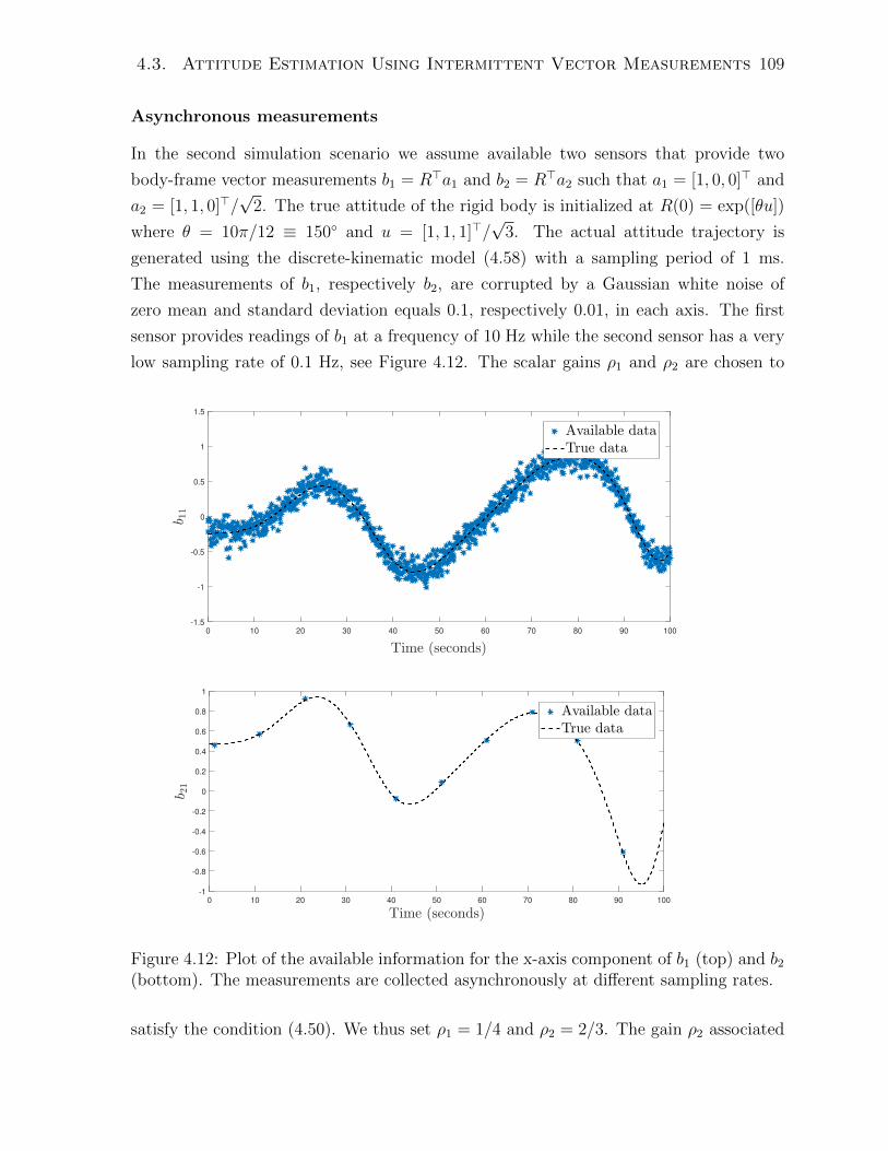
4.3. Attitude Estimation Using Intermittent Vector Measurements 109
Asynchronous measurements
In the second simulation scenario we assume available two sensors that provide two
body-frame vector measurements b1 = R>a1 and b2 = R>a2 such that a1 = [1, 0, 0]> and
a2 = [1, 1, 0]>/√
2. The true attitude of the rigid body is initialized at R(0) = exp([θu])
where θ = 10π/12 ≡ 150 and u = [1, 1, 1]>/√
3. The actual attitude trajectory is
generated using the discrete-kinematic model (4.58) with a sampling period of 1 ms.
The measurements of b1, respectively b2, are corrupted by a Gaussian white noise of
zero mean and standard deviation equals 0.1, respectively 0.01, in each axis. The first
sensor provides readings of b1 at a frequency of 10 Hz while the second sensor has a very
low sampling rate of 0.1 Hz, see Figure 4.12. The scalar gains ρ1 and ρ2 are chosen to
0 10 20 30 40 50 60 70 80 90 100
Time (seconds)
-1.5
-1
-0.5
0
0.5
1
1.5
b11
Available dataTrue data
0 10 20 30 40 50 60 70 80 90 100
Time (seconds)
-1
-0.8
-0.6
-0.4
-0.2
0
0.2
0.4
0.6
0.8
1
b21
Available dataTrue data
Figure 4.12: Plot of the available information for the x-axis component of b1 (top) and b2
(bottom). The measurements are collected asynchronously at different sampling rates.
satisfy the condition (4.50). We thus set ρ1 = 1/4 and ρ2 = 2/3. The gain ρ2 associated
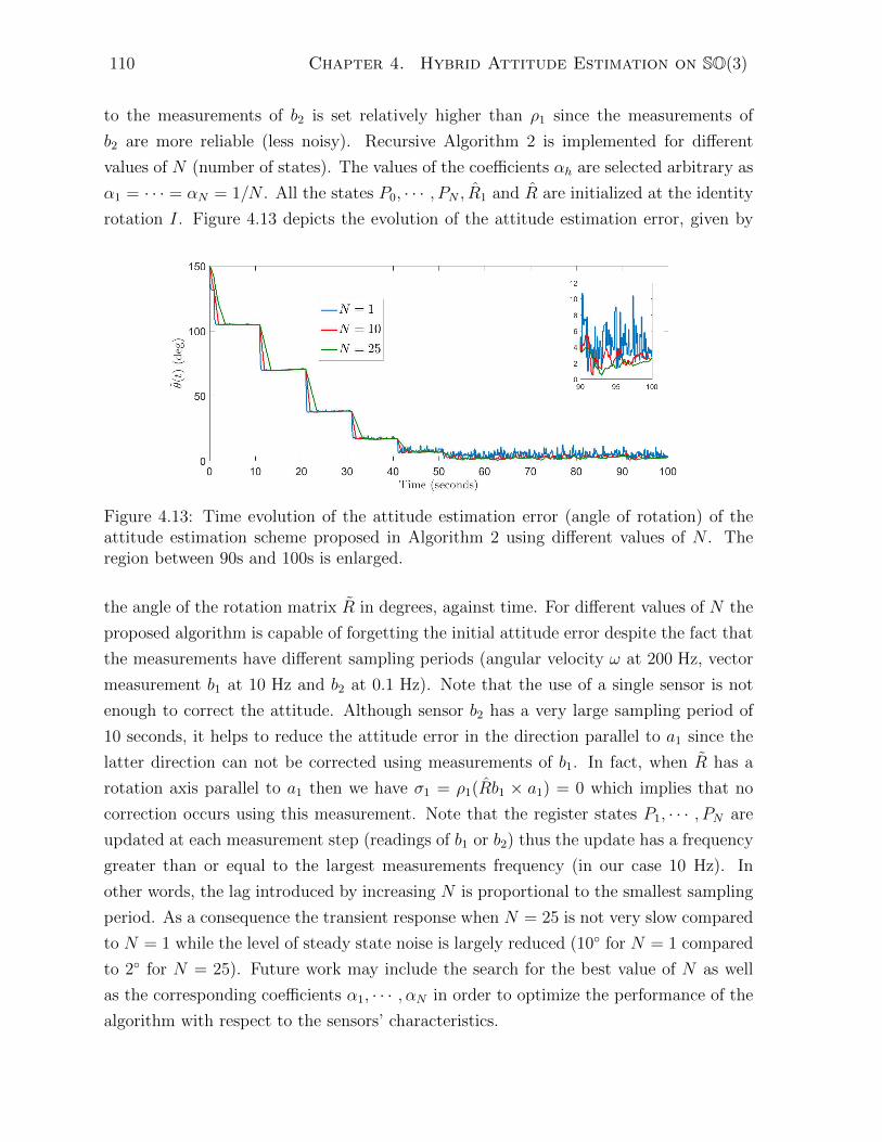
110 Chapter 4. Hybrid Attitude Estimation on SO(3)
to the measurements of b2 is set relatively higher than ρ1 since the measurements of
b2 are more reliable (less noisy). Recursive Algorithm 2 is implemented for different
values of N (number of states). The values of the coefficients αh are selected arbitrary as
α1 = · · · = αN = 1/N . All the states P0, · · · , PN , R1 and R are initialized at the identity
rotation I. Figure 4.13 depicts the evolution of the attitude estimation error, given by
Figure 4.13: Time evolution of the attitude estimation error (angle of rotation) of theattitude estimation scheme proposed in Algorithm 2 using different values of N . Theregion between 90s and 100s is enlarged.
the angle of the rotation matrix R in degrees, against time. For different values of N the
proposed algorithm is capable of forgetting the initial attitude error despite the fact that
the measurements have different sampling periods (angular velocity ω at 200 Hz, vector
measurement b1 at 10 Hz and b2 at 0.1 Hz). Note that the use of a single sensor is not
enough to correct the attitude. Although sensor b2 has a very large sampling period of
10 seconds, it helps to reduce the attitude error in the direction parallel to a1 since the
latter direction can not be corrected using measurements of b1. In fact, when R has a
rotation axis parallel to a1 then we have σ1 = ρ1(Rb1 × a1) = 0 which implies that no
correction occurs using this measurement. Note that the register states P1, · · · , PN are
updated at each measurement step (readings of b1 or b2) thus the update has a frequency
greater than or equal to the largest measurements frequency (in our case 10 Hz). In
other words, the lag introduced by increasing N is proportional to the smallest sampling
period. As a consequence the transient response when N = 25 is not very slow compared
to N = 1 while the level of steady state noise is largely reduced (10 for N = 1 compared
to 2 for N = 25). Future work may include the search for the best value of N as well
as the corresponding coefficients α1, · · · , αN in order to optimize the performance of the
algorithm with respect to the sensors’ characteristics.

4.4. Conclusion 111
Biased angular velocity measurements
In this simulation scenario we assume that the angular velocity measurements are biased
with a constant bias bω = [0.05, 0.05, 0.05]> (rad/sec). We assume available two sensors
that provide two body-frame vector measurements b1 = R>a1 and b2 = R>a2 such that
a1 = [1, 0, 0]> and a2 = [0, 1, 0]>. The true attitude of the rigid body is initialized at
an attitude angle of 45 in the z−direction, i.e., R(0) = exp([θu]×) where θ = π/4 and
u = [0, 0, 1]>. The actual attitude trajectory is generated using the discrete-kinematic
model (4.58) with a sampling period of 1 ms. The observers states are initialized at
R(0) = I and bω = [0, 0, 0]> (rad/sec). Note that although in Theorem 4.3.4 we provide
only a proof of local exponential convergence for the observer (4.72)-(4.73), the chosen
initial attitude error (45 angle) is large which suggests that the region of convergence of
the proposed estimation scheme is large. Now, we set the the observer gains as ρ1 = 14,
ρ2 = 12
and γb = 0.5 which satisfy the conditions of Theorem 4.3.4. To find the maximum
allowed sampling period T we compute the upper bound T in (4.79). The corresponding
matrix Ad can be computed form (C.109) and the solution of the discrete Lyapunov
equation is derived by pick L = I. We obtain a matrix P such that λPmax = 4.8895 and
λPmin = 1. The angular velocity bound cω is chosen as cω = 0.5 which is a very conservative
bound on the norm of the angular velocity. Therefore on obtains the condition on T
T < T (A, γb, cω) = 0.0234 seconds. (4.80)
The above is a conservative bound on the allowable sampling period which guarantees
local convergence of the attitude observer. To show that our observer works even when
the above bound is not satisfied, we pick different values of T between 0.02 and 5 seconds.
Simulation results are plotted in Figure 4.14 and (4.15) which shows convergences of the
attitude and bias estimation errors as zero. These simulation results suggest that a larger
bound on the allowable sampling period T exists, however it remains an open problem
to find the least conservative bound. Of course for larger values of the sampling period
T , the convergence is slower since fewer correction steps are executed in (4.72)-(4.73).
4.4 Conclusion
We dealt with the problem of attitude estimation on SO(3) using intermittent syn-
chronous and asynchronous vector measurements. The problem formulation takes into
account some practical constraints related to the sensors bandwidth and measurements
loss. The proposed hybrid attitude estimation scheme has a measurement-triggered struc-
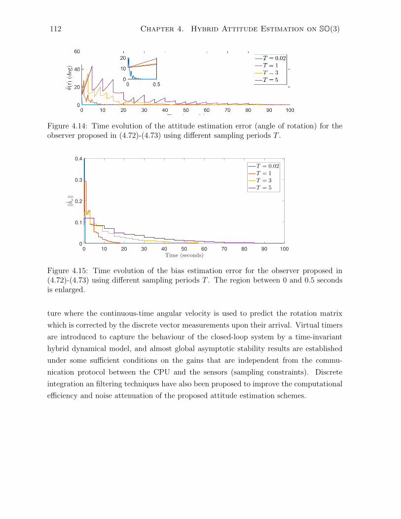
112 Chapter 4. Hybrid Attitude Estimation on SO(3)
Figure 4.14: Time evolution of the attitude estimation error (angle of rotation) for theobserver proposed in (4.72)-(4.73) using different sampling periods T .
0 10 20 30 40 50 60 70 80 90 100
Time (seconds)
0
0.1
0.2
0.3
0.4
‖bω‖
T = 0.02T = 1T = 3T = 5
Figure 4.15: Time evolution of the bias estimation error for the observer proposed in(4.72)-(4.73) using different sampling periods T . The region between 0 and 0.5 secondsis enlarged.
ture where the continuous-time angular velocity is used to predict the rotation matrix
which is corrected by the discrete vector measurements upon their arrival. Virtual timers
are introduced to capture the behaviour of the closed-loop system by a time-invariant
hybrid dynamical model, and almost global asymptotic stability results are established
under some sufficient conditions on the gains that are independent from the commu-
nication protocol between the CPU and the sensors (sampling constraints). Discrete
integration an filtering techniques have also been proposed to improve the computational
efficiency and noise attenuation of the proposed attitude estimation schemes.

Chapter 5
Conclusion
5.1 Summary
In Chapter 2, some preliminary results and useful lemmas on the rotation group SO(3)
have been presented. Some of these results are newly derived in this thesis and can
be used for the design and analysis of control systems on SO(3). Moreover, the hybrid
systems framework, used in this thesis, which is mainly inspired from [Goebel et al.,
2012] and related works has been recalled. A new result concerning exponential stability
of general hybrid systems is derived. Our proposed theorem relaxed, for certain class
of hybrid systems, some previously developed Lyapunov-based sufficient conditions for
exponential stability. These derived sufficient conditions for exponential stability are
then used in the thesis to analysis the stability of some closed-loop systems.
Chapter 3 was devoted to the problem of attitude control on SO(3). The simple
example of the unit circle S1, which is a submanifold of SO(3), was used as a motivation.
It helped to explain the limitations of existing smooth and discontinuous feedbacks and
motivated the use of hybrid controllers to solve the problem of global exponential stabi-
lization on compact manifolds such as SO(3). The new definition of “exp-synergistic” po-
tential functions has been proposed which, roughly speaking, means a family of (smooth
or nonsmooth) potential functions on SO(3) that enjoys the following properties: (1)
being quadratic (as well as their gradients) with respect to an attitude distance, and (2)
being synergistic1 with respect to the gradient’s singular and/or critical points. Then,
we showed that exp-synergistic potential functions are sufficient to design a hybrid con-
troller guaranteeing global exponential stability on SO(3). The proposed hybrid con-
troller, which is inspired from [Mayhew and Teel, 2011c], consists of a family of control
1The definition of “synergistic” potential functions is given in Definition 3.3.6 and can be found inreference [Mayhew and Teel, 2011c, Mayhew and Teel, 2013a].
113

114 Chapter 5. Conclusion
laws (each derived from a potential function within the family of exp-synergistic potential
functions) which are coordinated in a suitable manner. The hybrid controller selects the
control law corresponding to the potential function which has the minimal value among
the family. The min-switch mechanism has a hysteresis property that guarantees some
level of robustness to measurement noise. We proposed a systematic methodology to
construct exp-synergistic potential functions from existing (traditional) smooth and non-
smooth potential functions on SO(3). The construction is done by applying an adequate
transformation on SO(3) that stretches and compresses the manifold in a way to relocate
the undesired critical and singular points. This transformation is different from the one
proposed in [Mayhew and Teel, 2011d] and allows to explicitly derive the parameters
of the hybrid controller (e.g., synergistic gap). Finally, the proposed control strategy is
applied to the attitude tracking problem for rigid body systems. The resulting hybrid
tracking algorithm is made continuous by filtering the discrete transitions in the con-
troller using a first order low pass filter. We proved that global exponential convergence
of the tracking errors to zero is preserved.
The attitude estimation problem has been investigated in Chapter 4. The first objec-
tive in this chapter was to derive globally exponentially stable hybrid attitude and gyro
bias observers, developed directly on SO(3), using continuous sensor measurements. Our
motivation was driven by the fact that existing attitude observers on SO(3) are limited in
terms of their domain of convergence (local or almost global) and exhibit some robustness
and performance issues such as those discussed in our paper [Berkane and Tayebi, 2017a].
To achieve this first objective, we propose two hybrid attitude estimation schemes. The
first scheme uses the concept of exp-synergistic potential functions, discussed in Chapter
3, to derive a family of innovation (correction) terms for an attitude observer that has
a similar structure as the nonlinear complementary filter on SO(3). It is shown that
the exp-synergistic potential functions and their gradients, derived in Chapter 3, can be
explicitly written in terms of body-frame vector measurements of known constant iner-
tial vectors. Therefore, the proposed hybrid observer can be readily implemented using
available sensors depending on the application at hand. The second scheme uses rather
a fixed innovation term for the attitude observer but, however, allows the attitude state
to experience jumps. This reset behaviour of the attitude estimated matrix is done ade-
quately to guarantee that, after a jump, a given cost function is within the flow set. The
main purpose behind this reset-based approach is to avoid the undesired critical/singular
points of the cost function on SO(3) by simply jumping the attitude estimate to a region
where these undesired points do not belong. The advantage of the reset-based technique
over the synergistic-based technique resides in the design simplicity and the possibility of

5.1. Summary 115
using time-varying inertial vectors. However, the reset-based approach comes at the cost
of having possible discrete transitions in the observer output which might be undesirable
in practice when connecting the observer to the controller. The good news is that this
potential jumps are not likely to occur when the attitude estimation errors are small (an
observer operating near the true state values).
The second objective of Chapter 4 was to design attitude estimation schemes on
SO(3) that deal with the problem where the measurements are allowed to have different
bandwidths with possible information loss between the sensor and the control processing
unit. There are very few references that have dealt with this problem [Khosravian et al.,
2015, Barrau and Bonnabel, 2015]. At a first step, we have considered the simplified
problem where the measurements are collected synchronously at possibly irregular sam-
pling periods. We also assumed that the angular velocity measurements are unbiased and
available continuously. The last assumption is motivated by the high sampling frequency
of most existing commercial gyroscopes compared to other sensors such as landmarks,
GPS,...etc. We proposed a measurement-triggered observer which consists of forward in-
tegration on SO(3) of the continuous angular velocity and intermittent correction of the
attitude estimate at the arrival of the new measurements. Both the integration (predic-
tion) and the correction steps are done in a way to keep the attitude estimates within the
rotation group SO(3). To analyze the stability of the closed-loop system, we proposed to
extend the system with a virtual timer to capture the behaviour of the communication
protocol. The virtual time is reset at each time when the measurements are received.
The extended closed-loop system is modelled as an autonomous hybrid system which al-
lowed for hybrid systems tools to be applied to conduct the stability proofs. We showed
that the zero estimation error is almost globally exponentially stable. Secondly, we con-
sidered the more general case where the measurements are collected asynchronously (at
different sampling periods). In this case the observer state is updated at the arrival of
each single measurement. A virtual timer is introduced for each sensor to model the
communication protocol between that sensor and the processing unit. Again the closed-
loop system is modelled as a hybrid system and almost global asymptotic stability is
concluded using the invariance principle for hybrid systems. Finally, some practical is-
sues have been considered. First, when the gyro readings are biased we proposed an
extended measurement-triggered observer on SO(3) × R3 to estimate both the attitude
state and the gyro bias vector. We were able to prove local exponential convergence to
zero of the estimation errors only in the case where the measurements are synchronously
collected at a constant sampling period. A second practical consideration is the effect of
measurement noise on the output of the observer. We extended the observer with N ≥ 1

116 Chapter 5. Conclusion
states on SO(3) which are recursively updated and averaged to yield a better estimate.
We also proposed a discrete version of the observer which is obtained by discretizing
the integrator on SO(3) using a first order Lie group integration method. The discrete
version of the observer preserves the convergence properties of the original version of the
observer which is an advantage over most existing attitude estimation schemes on SO(3).
5.2 Perspectives
In many systems of practical and theoretical interest, the configuration space of the
system can be given the structure of a Lie group. Examples include unmanned aerial
vehicles, underwater vehicles, satellites and surface vessels. A future direction is to extend
the synergistic hybrid control strategy, developed on S1,S2 and SO(3) to fully-actuated
mechanical systems, when the configuration space is a general class of Lie groups, in
a differential geometric setting such as in [Maithripala et al., 2006, Chaturvedi et al.,
2006]. This requires to define intrinsic potential functions on a Lie group and propose an
efficient way to obtain the corresponding synergistic family via angular warping. This
task is challenging due to the difficulty in proving the synergism property on a general
Lie group and the fact that most compact identities used on SO(3), for instance, are
not available on a general Lie group. We wish as well to propose a unified framework
for the construction of hybrid, continuous and possibly smooth controllers for general
mechanical systems evolving on a Lie group.
In addition to the above future directions, the following are few perspectives “closely”
related to this thesis:
• In Section 3.3.5, we have successfully constructed two exp-synergistic families of
weighted potential functions but under the full knowledge of the eigenvalues and
eigenvectors of the matrix A. It would be interesting to derive weighted exp-
synergistic functions without requiring information about the spectrum of the
weighting matrix which might simplify the design process. Also, recall that these
exp-synergistic potential functions were used in Section 4.2 to derive attitude ob-
servers using directly vector measurements. The weighting matrix A was directly
related to the known and constant inertial vectors. In some applications, these
vectors are unknown or time varying which is obstacle towards the use of this class
of exp-synergistic potential functions.
• In certain applications, the information about the inertia matrix is uncertain. An
interesting direction is to make robust the proposed hybrid tracking control algo-

5.2. Perspectives 117
rithms using some adaptation laws for the inertia matrix while maintaining the
strong stability results.
• The proposed measurement-triggered observers are shown to have almost global
convergence properties. It is possible to extend these observers with a switching
mechanism (such as the reset-based approach) to enlarge the domain of conver-
gence to global. Moreover, it remains an open problem to estimate the region of
convergence of the proposed intermittent observer with bias estimation. We have
shown local exponential convergence only in the particular case of synchronous
measurement with constant sampling rate. Other more general cases where the
measurements are asynchronous and/or the sampling rate is irregular remains un-
solved. Simulations results, however, are very promising.
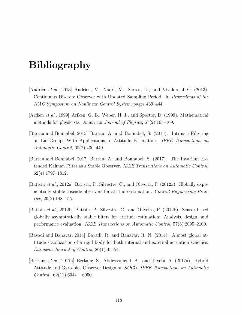
Bibliography
[Andrieu et al., 2013] Andrieu, V., Nadri, M., Serres, U., and Vivalda, J.-C. (2013).
Continuous Discrete Observer with Updated Sampling Period. In Proceedings of the
IFAC Symposium on Nonlinear Control System, pages 439–444.
[Arfken et al., 1999] Arfken, G. B., Weber, H. J., and Spector, D. (1999). Mathematical
methods for physicists. American Journal of Physics, 67(2):165–169.
[Barrau and Bonnabel, 2015] Barrau, A. and Bonnabel, S. (2015). Intrinsic Filtering
on Lie Groups With Applications to Attitude Estimation. IEEE Transactions on
Automatic Control, 60(2):436–449.
[Barrau and Bonnabel, 2017] Barrau, A. and Bonnabel, S. (2017). The Invariant Ex-
tended Kalman Filter as a Stable Observer. IEEE Transactions on Automatic Control,
62(4):1797–1812.
[Batista et al., 2012a] Batista, P., Silvestre, C., and Oliveira, P. (2012a). Globally expo-
nentially stable cascade observers for attitude estimation. Control Engineering Prac-
tice, 20(2):148–155.
[Batista et al., 2012b] Batista, P., Silvestre, C., and Oliveira, P. (2012b). Sensor-based
globally asymptotically stable filters for attitude estimation: Analysis, design, and
performance evaluation. IEEE Transactions on Automatic Control, 57(8):2095–2100.
[Bayadi and Banavar, 2014] Bayadi, R. and Banavar, R. N. (2014). Almost global at-
titude stabilization of a rigid body for both internal and external actuation schemes.
European Journal of Control, 20(1):45–54.
[Berkane et al., 2017a] Berkane, S., Abdessameud, A., and Tayebi, A. (2017a). Hybrid
Attitude and Gyro-bias Observer Design on SO(3). IEEE Transactions on Automatic
Control., 62(11):6044 – 6050.
118
BIBLIOGRAPHY 119
[Berkane et al., 2017b] Berkane, S., Abdessameud, A., and Tayebi, A. (2017b). Hybrid
Global Exponential Stabilization on SO(3). Automatica, 81:279–285.
[Berkane and Tayebi, 2015a] Berkane, S. and Tayebi, A. (2015a). On the Design of Syn-
ergistic Potential Functions on SO(3). In Proceedings of the Conference on Decision
and Control, volume 1, pages 270–275.
[Berkane and Tayebi, 2015b] Berkane, S. and Tayebi, A. (2015b). Some Optimization
Aspects on the Lie Group SO(3). In IFAC Symposium on Information Control in
Manufacturing , Ottawa, pages 1173–1177.
[Berkane and Tayebi, 2016] Berkane, S. and Tayebi, A. (2016). On Deterministic Atti-
tude Observers on the Special Orthogonal Group SO(3). In Proceedings of the Con-
ference on Decision and Control, pages 1165–1170.
[Berkane and Tayebi, 2017a] Berkane, S. and Tayebi, A. (2017a). On the Design of
Attitude Complementary Filters on SO(3). IEEE Transactions on Automatic Control
(to appear).
[Berkane and Tayebi, 2017b] Berkane, S. and Tayebi, A. (2017b). Attitude and Gyro-
bias Estimation Using GPS and IMU Measurements. In Proceedings of the Conference
on Decision and Control.
[Berkane and Tayebi, 2017c] Berkane, S. and Tayebi, A. (2017c). Attitude Estimation
With Intermittent Measurements. Submitted to Automatica.
[Berkane and Tayebi, 2017d] Berkane, S. and Tayebi, A. (2017d). Attitude Observer Us-
ing Synchronous Intermittent Vector Measurements. In Proceedings of the Conference
on Decision and Control.
[Berkane and Tayebi, 2017e] Berkane, S. and Tayebi, A. (2017e). Construction of Syner-
gistic Potential Functions on SO(3) with Application to Velocity-Free Hybrid Attitude
Stabilization. IEEE Transactions on Automatic Control, 62(1):495–501.
[Brodtkorb et al., 2015] Brodtkorb, A. H., Teel, A. R., and Sørensen, A. J. (2015).
Sensor-based Hybrid Observer for Dynamic Positioning. In Proceedings of the Confer-
ence on Decision and Control, pages 948–953.
[Bullo, 2005] Bullo, F. (2005). Geometric control of mechanical systems, volume 49.
Springer Science & Business Media.

120 BIBLIOGRAPHY
[Bullo and Murray, 1995] Bullo, F. and Murray, R. (1995). Proportional derivative (pd)
control on the euclidean group. In Proceedings of the European Control Conference,
volume 2, pages 1091–1097.
[Bullo and Murray, 1999] Bullo, F. and Murray, R. M. (1999). Tracking for fully actuated
mechanical systems : a geometric framework. Automatica, 35:17–34.
[Cai and Teel, 2009] Cai, C. and Teel, A. R. (2009). Characterizations of input-to-state
stability for hybrid systems. Systems & Control Letters, 58(1):47–53.
[Casau et al., 2015a] Casau, P., Mayhew, C. G., Sanfelice, R. G., and Silvestre, C.
(2015a). Global exponential stabilization on the n-dimensional sphere. In Proceed-
ings of the American Control Conference, pages 3218–3223.
[Casau et al., 2015b] Casau, P., Sanfelice, R. G., Cunha, R., and Silvestre, C. (2015b).
A globally asymptotically stabilizing trajectory tracking controller for fully actuated
rigid bodies using landmark-based information. International Journal of Robust and
Nonlinear Control, 25(18):3617–3640.
[Celledoni et al., 2014] Celledoni, E., Marthinsen, H., and Owren, B. (2014). An intro-
duction to Lie group integrators C basics , new developments and applications. Journal
of Computational Physics, 257:1040–1061.
[Chaturvedi et al., 2011] Chaturvedi, N., Sanyal, A., and McClamroch, N. (2011). Rigid-
body attitude control. IEEE Control Systems Magazine, 31(3):30 – 51.
[Chaturvedi et al., 2006] Chaturvedi, N. A., Bloch, A. M., and McClamroch, N. H.
(2006). Global stabilization of a fully actuated mechanical system on a riemannian
manifold: controller structure. In Proceedings of the American Control Conference,
pages 3612–3617.
[Choukroun, 2009] Choukroun, D. (2009). Novel stochastic modeling and filtering of the
attitude quaternion. The Journal of the Astronautical Sciences, 57(1-2):167–189.
[Crassidis et al., 2007] Crassidis, J., Markley, F., and Cheng, Y. (2007). Survey of nonlin-
ear attitude estimation methods. Journal of Guidance Control and Dynamics, 30(1):12.
[Crouch and Grossman, 1993] Crouch, P. E. and Grossman, R. (1993). Numerical Inte-
gration of Ordinary Differential Equations on Manifolds. J. Nonlinear Sci., 3:1–33.

BIBLIOGRAPHY 121
[Darryl D. Holm and Stoica, 2009] Darryl D. Holm, T. S. and Stoica, C. (2009). Geomet-
ric Mechanics and Symmetry. From Finite to Infinite Dimensions. Oxford University
Press.
[Davatzikos, 1997] Davatzikos, C. (1997). Spatial transformation and registration of
brain images using elastically deformable models. Computer Vision and Image Under-
standing, 66(2):207–222.
[Egeland and Godhavn, 1994] Egeland, O. and Godhavn, J. M. (1994). Passivity-Based
Adaptive Attitude Control of a Rigid Spacecraft. IEEE Transactions on Automatic
Control, 39(4):842–846.
[Elger and Roberson, 2013] Elger, D. F. and Roberson, J. A. (2013). Engineering fluid
mechanics. Wiley Hoboken (NJ).
[Ferrante et al., 2016] Ferrante, F., Gouaisbaut, F., Sanfelice, R. G., and Tarbouriech, S.
(2016). State estimation of linear systems in the presence of sporadic measurements.
Automatica, 73:101–109.
[Fjellstad and Fossen, 1994] Fjellstad, O. E. and Fossen, T. I. (1994). Quaternion feed-
back regulation of underwater vehicles. In Proceedings of International Conference on
Control and Applications, pages 857–862 vol.2.
[Forbes, 2013] Forbes, J. R. (2013). Passivity-Based Attitude Control on the Special
Orthogonal Group of Rigid-Body Rotations. Journal of Guidance, Control, and Dy-
namics, 36(6):1596–1605.
[Goebel et al., 2009] Goebel, R., Sanfelice, R. G., and Teel, A. R. (2009). Hybrid dy-
namical systems. IEEE Control Systems Magazine, 29(2):28–93.
[Goebel et al., 2012] Goebel, R., Sanfelice, R. G., and Teel, A. R. (2012). Hybrid Dy-
namical Systems: modeling, stability, and robustness. Princeton University Press.
[Goebel and Teel, 2006] Goebel, R. and Teel, A. (2006). Solutions to hybrid inclusions
via set and graphical convergence with stability theory applications. Automatica,
42:573–587.
[Grip et al., 2012a] Grip, H. F., Fossen, T., Johansen, T. A., Saberi, A., et al. (2012a).
Attitude estimation using biased gyro and vector measurements with time-varying
reference vectors. IEEE Transactions on Automatic Control, 57(5):1332–1338.

122 BIBLIOGRAPHY
[Grip et al., 2012b] Grip, H. F., Fossen, T. I., Johansen, T. a., and Saberi, A. (2012b).
A nonlinear observer for integration of GNSS and IMU measurements with gyro bias
estimation. In Proceedings of the American Control Conference, pages 4607–4612.
[Hadidi and Schwartz, 1979] Hadidi, M. and Schwartz, S. (1979). Linear recursive state
estimators under uncertain observations. IEEE Transactions on Automatic Control,
24(6):944–948.
[Hartley et al., 2013] Hartley, R., Trumpf, J., Dai, Y., and Li, H. (2013). Rotation
Averaging. International journal of computer vision, 103(3):267–305.
[Helmke and Moore, 1994] Helmke, U. and Moore, J. (1994). Optimization and Dynam-
ical Systems. New york: Springer.
[Hoag, 1963] Hoag, D. (1963). Apollo guidance and Navigation: Considerations of apollo
imu gimbal lock. Canbridge: MIT Instrumentation Laboratory, pages 1–64.
[Hua, 2010] Hua, M. D. (2010). Control Engineering Practice Attitude estimation for
accelerated vehicles using GPS / INS measurements. Control Engineering Practice,
18(7):723–732.
[Hughes, 1986] Hughes, P. (1986). Spacecraft attitude dynamics. John Wiley & Sons Inc.
[Ito, 1993] Ito, K. (1993). Encyclopedic dictionary of mathematics, volume 1. MIT press.
[Izadi and Sanyal, 2014] Izadi, M. and Sanyal, A. K. (2014). Rigid body attitude esti-
mation based on the lagrange–dalembert principle. Automatica, 50(10):2570–2577.
[Jentzen et al., 2010] Jentzen, A., Leber, F., Schneisgen, D., Berger, A., and Siegmund,
S. (2010). An improved maximum allowable transfer interval for Lp-Stability of net-
worked control systems. IEEE Transactions on Automatic Control, 55(1):179–184.
[Joshi et al., 1995] Joshi, S., Kelkar, A., and Wen, J.-Y. (1995). Robust attitude sta-
bilization of spacecraft using nonlinear quaternion feedback. IEEE Transactions on
Automatic Control, 40(10):1800–1803.
[Khosravian et al., 2015] Khosravian, A., Trumpf, J., Mahony, R., and Hamel, T. (2015).
Recursive Attitude Estimation in the Presence of Multi-rate and Multi-delay Vector
Measurements. In Proceedings of the American Control Conference, pages 3199–3205.
BIBLIOGRAPHY 123
[Koditschek, 1988] Koditschek, D. E. (1988). Application of a new lyapunov function to
global adaptive attitude tracking. In Proceedings of the Conference on Decision and
Control, pages 63–68.
[Kreutz and Wen, 1988] Kreutz, K. and Wen, J. T. (1988). Attitude control of an object
commonly held by multiple robot arms: A lyapunov approach. In Proceedings of the
American Control Conference, pages 1790–1794.
[Krstic et al., 1995] Krstic, M., Kanellakopoulos, I., and Kokotovic, P. V. (1995). Non-
linear and adaptive control design. Wiley.
[Lang, 1987] Lang, S. (1987). Linear Algebra, 3rd Edition. Springer-Verlag.
[Lee, 2012] Lee, T. (2012). Exponential stability of an attitude tracking control system
on SO(3) for large-angle rotational maneuvers. Systems & Control Letters, 61(1):231–
237.
[Lee, 2015] Lee, T. (2015). Global exponential attitude tracking controls on SO(3). IEEE
Transactions on Automatic Control, 60(10):2837–2842.
[Lizarralde and Wen, 1996] Lizarralde, F. and Wen, J. (1996). Attitude control without
angular velocity measurement: A passivity approach. IEEE Transations on Automatic
Control, 41(3):46817–472.
[Mahony et al., 2008] Mahony, R., Hamel, T., and Pflimlin, J.-M. (2008). Nonlinear com-
plementary filters on the special orthogonal group. IEEE Transactions on Automatic
Control, 53(5):1203–1218.
[Maithripala et al., 2006] Maithripala, D. S., Berg, J. M., and Dayawansa, W. P. (2006).
Almost-global tracking of simple mechanical systems on a general class of lie groups.
IEEE Transactions on Automatic Control, 51(2):216–225.
[Markley, 1988] Markley, F. (1988). Attitude determination using vector observations
and the singular value decomposition. Journal of the Astronautical Sciences, 36:245–
258.
[Markley, 2003] Markley, F. (2003). Attitude error representations for kalman filtering.
Journal of Guidance, Control, and Dynamics, 63(2):311–317.
[Markley, 2006] Markley, F. L. (2006). Attitude filtering on SO(3). The Journal of the
Astronautical Sciences, 54(3):391–413.

124 BIBLIOGRAPHY
[Martin and Salaun, 2008] Martin, P. and Salaun, E. (2008). An Invariant Observer for
Earth-Velocity-Aided Attitude Heading Reference Systems. Proceedings of the 17th
IFAC World Congress, pages 9857–9864.
[Masten, 2008] Masten, M. (2008). Inertially stabilized platforms for optical imaging
systems. IEEE Control Systems Magazine, 28(1):47–64.
[Mayhew, 2010] Mayhew, C. G. (2010). Hybrid Control for Topologically Constrained
Systems. PhD thesis, UC Santa Barbara.
[Mayhew et al., 2008] Mayhew, C. G., Sanfelice, R. G., and Teel, A. R. (2008). Robust
hybrid source-seeking algorithms based on directional derivatives and their approxi-
mations. In Proceedings of the Conference on Decision and Control, pages 1735–1740.
[Mayhew et al., 2011] Mayhew, C. G., Sanfelice, R. G., and Teel, A. R. (2011).
Quaternion-based hybrid control for robust global attitude tracking. IEEE Trans-
actions on Automatic Control, 56:2555–2566.
[Mayhew and Teel, 2011a] Mayhew, C. G. and Teel, A. (2011a). On the topological
structure of attraction basins for differential inclusions. Systems & Control Letters,
60(12):1045–1050.
[Mayhew and Teel, 2013a] Mayhew, C. G. and Teel, A. (2013a). Synergistic hybrid feed-
back for global rigid-body attitude tracking on SO(3). IEEE Transactions on Auto-
matic Control, 58(11):2730–2742.
[Mayhew and Teel, 2010] Mayhew, C. G. and Teel, A. R. (2010). Hybrid control of planar
rotations. In Proceedings of the American Control Conference, pages 154–159.
[Mayhew and Teel, 2011b] Mayhew, C. G. and Teel, A. R. (2011b). Hybrid control of
rigid-body attitude with synergistic potential functions. In Proceedings of the American
Control Conference, pages 287–292.
[Mayhew and Teel, 2011c] Mayhew, C. G. and Teel, A. R. (2011c). Hybrid control of
rigid-body attitude with synergistic potential functions. In Proceedings of the American
Control Conference, pages 287–292.
[Mayhew and Teel, 2011d] Mayhew, C. G. and Teel, A. R. (2011d). Synergistic potential
functions for hybrid control of rigid-body attitude. In Proceedings of the American
Control Conference, pages 875–880.
BIBLIOGRAPHY 125
[Mayhew and Teel, 2013b] Mayhew, C. G. and Teel, A. R. (2013b). Global stabilization
of spherical orientation by synergistic hybrid feedback with application to reduced-
attitude tracking for rigid bodies. Automatica, 49(7):1945–1957.
[Meyer, 1971] Meyer, G. (1971). Design and global analysis of spacecraft attitude control
systems. National Aeronautics and Space Administration, Ames Research Center.
[Morse, 1934] Morse, M. (1934). The calculus of variations in the large, volume 18.
American Mathematical Soc.
[Mueller et al., 2016] Mueller, M. W., Hehn, M., and DAndrea, R. (2016). Covariance
correction step for kalman filtering with an attitude. Journal of Guidance, Control,
and Dynamics.
[Munthe-Kaas, 1995] Munthe-Kaas, H. (1995). LIE-BUTCHER THEORY FOR
RUNGE-KUTTA METHODS. BIT, 35:572–587.
[Munthe-Kaas, 1998] Munthe-Kaas, H. (1998). RUNGE-KUTTA METHODS ON LIE
GROUPS. BIT, 381:92–111.
[Munthe-Kaas, 1999] Munthe-Kaas, H. (1999). High order Runge-Kutta methods on
manifolds. Applied Numerical Mathematics, 29:115–127.
[Murray et al., 1994] Murray, R., Li, Z., and Sastry, S. (1994). A mathematical introduc-
tion to robotic manipulation. CRC press.
[Nahi, 1969] Nahi, N. (1969). Optimal recursive estimation with uncertain observation.
IEEE Transactions on Information Theory, 15(4):457–462.
[Osborne et al., 2008] Osborne, J., Hicks, G., and Fuentes, R. (2008). Global analysis of
the double-gimbal mechanism. IEEE Control Systems Magazine, 28(4):44–64.
[Pettersen and Egeland, 1999] Pettersen, K. Y. and Egeland, O. (1999). Time-Varying
Exponential Stabilization of the Position and Attitude of an Underactuated Au-
tonomous Underwater Vehicle. IEEE Transactions on Automatic Control, 44(1):112–
115.
[Plarre and Bullo, 2009] Plarre, K. and Bullo, F. (2009). On Kalman Filtering for De-
tectable Systems With Intermittent Observations. IEEE Transactions on Automatic
Control, 54(2):386–390.
126 BIBLIOGRAPHY
[Prieur et al., 2014] Prieur, C., Teel, A. R., and Zaccarian, L. (2014). Relaxed persistent
flow/jump conditions for uniform global asymptotic stability. IEEE Transactions on
Automatic Control, 59(10):2766–2771.
[Raff and Allgower, 2007] Raff, T. and Allgower, F. (2007). Observers with impulsive
dynamical behavior for linear and nonlinear continuous-time systems. In Proceedings
of the Conference on Decision and Control, pages 4287–4292.
[Repoulias and Papadopoulos, 2007] Repoulias, F. and Papadopoulos, E. (2007). Pla-
nar trajectory planning and tracking control design for underactuated AUVs. Ocean
Engineering, 34:1650–1667.
[Roberts and Tayebi, 2011] Roberts, A. and Tayebi, A. (2011). On the attitude estima-
tion of accelerating rigid-bodies using gps and imu measurements. In Proceedings of
the Conference on Decision and Control and European Control Conference.
[Rue, 1969] Rue, A. K. (1969). Stabilization of Precision Electrooptical Pointing and
Tracking Systems. IEEE Transactions on Aerospace and Electronic Systems, AES-
5(5):805–819.
[Saccon et al., 2010] Saccon, A., Hauser, J., and Aguiar, A. P. (2010). Exploration of
kinematic optimal control on the Lie group SO(3). In Proceedings of the 8th IFAC
Symposium on Nonlinear Control Systems, pages 1302–1307.
[Salcudean, 1988] Salcudean, S. (1988). On the control of magnetically levitated robot
wrists. In Proceedings of the Conference on Decision and Control, pages 186–191.
[Sanfelice et al., 2007] Sanfelice, R. G., Goebel, R., and Teel, A. (2007). Invariance
principles for hybrid systems with connections to detectability and asymptotic stability.
IEEE Transactions on Automatic Control, 52(12):2282–2297.
[Sanfelice and Teel, 2006] Sanfelice, R. G. and Teel, A. R. (2006). On the Continuity of
Asymptotically Stable Compact Sets for Simulations of Hybrid Systems. In Proceeding
of the Conference on Decision and Control, pages 270–275.
[Sanjay P. Bhat, 2000] Sanjay P. Bhat, D. S. B. (2000). A topological obstruction to
continuous global stabilization of rotational motion and the unwinding phenomenon.
Systems & Control Letters, 39:63–70.
[Sanyal et al., 2009] Sanyal, A., Fosbury, A., Chaturvedi, N., and Bernstein, D. (2009).
Inertia-free spacecraft attitude tracking with disturbance rejection and almost global
stabilization. Journal of Guidance, Control, Dynamics, 32(4):1167–1178.
BIBLIOGRAPHY 127
[Shuster, 1993] Shuster, M. (1993). A survey of attitude representations. The Journal of
the Astronautical Sciences, 41(4):439–517.
[Shuster and Oh, 1981] Shuster, M. D. and Oh, S. D. (1981). Three-axis attitude deter-
mination from vector observations. Journal of Guidance and Control, 4:70–77.
[Sinopoli et al., 2004] Sinopoli, B., Schenato, L., Franceschetti, M., Poolla, K., Jordan,
M. I., and Sastry, S. S. (2004). Kalman filtering with intermittent observations. IEEE
Transactions on Automatic Control, 49(9):1453–1464.
[Smith and Seiler, 2003] Smith, S. C. and Seiler, P. (2003). Estimation with lossy mea-
surements: jump estimators for jump systems. IEEE Transactions on Automatic Con-
trol, 48(12):2163–2171.
[Sprinkle et al., 2005] Sprinkle, J., Ames, A. D., Pinto, A., Zheng, H., and Sastry, S. S.
(2005). On the partitioning of syntax and semantics for hybrid systems tools. In Pro-
ceedings of the Conference on Decision and Control and the European Control Confer-
ence,, pages 4694–4699.
[Stuelpnagel, 1964] Stuelpnagel, J. (1964). On the parametrization of the three-
dimensional rotation group. SIAM review, 6(4):422–430.
[Tayebi, 2008] Tayebi, A. (2008). Unit quaternion-based output feedback for the attitude
tracking problem. IEEE Transactions on Automatic Control, 53(6):1516–1520.
[Tayebi and McGilvray, 2006] Tayebi, A. and McGilvray, S. (2006). Attitude stabiliza-
tion of a vtol quadrotor aircraft. IEEE Transactions on Control Systems Technology,
14(3):562–571.
[Teel et al., 2013] Teel, A. R., Forni, F., and Zaccarian, L. (2013). Lyapunov-based
sufficient conditions for exponential stability in hybrid systems. IEEE Transactions
on Automatic Control, 58(6):1591–1596.
[Terzopoulos et al., 1987] Terzopoulos, D., Platt, J., Barr, A., and Fleischer, K. (1987).
Elastically deformable models. ACM Siggraph Computer Graphics, 21(4):205–214.
[Thienel and Sanner, 2003] Thienel, J. and Sanner, R. (2003). A coupled nonlinear space-
craft attitude controller and observer with an unknown constant gyro bias and gyro
noise. IEEE Transactions on Automatic Control, 48(11):2011–2015.
[Tippett, 1998] Tippett, M. K. (1998). Bounds for the solution of the discrete algebraic
Lyapunov equation. Automatica, 34(2):275–277.
128 BIBLIOGRAPHY
[Tse-Huai Wu and Lee, 2015] Tse-Huai Wu, E. K. and Lee, T. (2015). Globally asymp-
totically stable attitude observer on SO(3). In Proceedings of the Conference on De-
cision and Control, pages 2164–2168.
[Vanderbei, 1996] Vanderbei, R. J. (1996). Linear Programming: Foundations and Ex-
tensions. Citeseer.
[Wahba, 1965] Wahba, G. (1965). A least squares estimate of spacecraft attitude. SIAM
Review, 7(3):409.
[Wen and Kreutz-Delgado, 1991] Wen, J.-Y. and Kreutz-Delgado, K. (1991). The Atti-
tude Control Problem. IEEE Transactions on Automatic Control, 36(10):1148–1162.
[Wie and Barba, 1985] Wie, B. and Barba, P. M. (1985). Quaternion feedback for space-
craft large angle maneuvers. Journal of Guidance, 8(3):360–365.
[Wie et al., 1989] Wie, B., Weiss, H., and Arapostathis, A. (1989). A quaternion feed-
back regulator for spacecraft eigenaxis rotations. In Proceedings of the Guidance,
Navigation and Control Conference, page 4128.
[Yasuda and Hirai, 1979] Yasuda, K. and Hirai, K. (1979). Upper and lower bounds
on the solution of the algebraic Riccati equation. IEEE Transactions on Automatic
Control, 24(3):483–487.
[Yuan, 1988] Yuan, J. (1988). Closed-loop manipulator control using quaternion feed-
back. IEEE Journal on Robotics and Automation, 4(4):434–440.
[Zlotnik and Forbes, 2016] Zlotnik, D. E. and Forbes, J. R. (2016). Exponential conver-
gence of a nonlinear attitude estimator. Automatica, 72:11–18.
[Zlotnik and Forbes, 2017] Zlotnik, D. E. and Forbes, J. R. (2017). Nonlinear estimator
design on the special orthogonal group using vector measurements directly. IEEE
Transactions on Automatic Control, 62:149–160.

Appendix A
Proofs of Lemmas
A.1 Proof of Lemma 2.2.1
Using (2.62) and identities (2.41)-(2.44) of the trace function one has
tr(M(I −R2)) = tr(M)− tr(M(R> + tr(R)R− tr(R)I))
= tr(M)− tr(MR>)− tr(R)tr(MR) + tr(R)tr(M)
= tr(M)− tr(MR) + tr(R)(tr(M)− tr(MR))
= (1 + tr(R))tr(M(I −R)).
Moreover, using the fact that Pso(3)(A) = (A− A>)/2 and relation (2.62) one obtains
Pso(3)(MR2) =1
2(MR2 − (R2)>M)
=1
2M(R> + tr(R)R− tr(R)I)− 1
2(R + tr(R)R> − tr(R)I)M
=1
2(MR> −RM) +
1
2tr(R)(MR−R>M)
= tr(R)Pso(3)(MR) + Pso(3)(MR>).
Finally, using the fact that tr(R>MR) = tr(MRR>) = tr(M) and tr(RMR) = tr(MR2)
one has
〈〈Pso(3)(R),Pso(3)(MR)〉〉 =1
4tr((R> −R)(MR−R>M))
=1
4tr(R>MR)− 1
4tr(RMR)− 1
4tr((R>)2M) +
1
4tr(M)
=1
2tr(M)− 1
4tr(MR2)− 1
4tr((R>)2M) =
1
2tr(M(I −R2)).
129
130 Chapter A. Proofs of Lemmas
A.2 Proof of Lemma 2.2.2
Using the definition of the map E(·) in (2.66) one can verify that E−1(E(M)) = M and
E(E−1(M)) = M for any M ∈ R3×3. Let v be an eigenvector such that M>v = λM>
v v.
This implies, using the definition of the map E(·), that
E(M)v =1
2(tr(M)I −M>)v =
1
2tr(M)v − 1
2λM
>
v v =1
2(tr(M)− λM>v )v = λE(M)
v v,
E−1(M)v = (tr(M)I − 2M>)v = tr(M)v − 2λM>
v v = (tr(M)− 2λM>
v )v = λE−1(M)
v v.
A.3 Proof of Lemma 2.2.3
If M is symmetric and R ∈ SO(3), x ∈ R3 one has
x>[λE(M)min I − E(MR)]x =x>[λ
E(M)min I − 1
2(tr(MR)I −R>M)]x
=(λE(M)min − 1
2tr(MR))‖x‖2 +
1
2x>R>Mx
≤(λE(M)min − 1
2tr(MR))‖x‖2 +
1
2λMmax‖x‖2
=1
2tr(M(I −R))‖x‖2,
where the fact λE(M)min = 1
2(tr(M) − λMmax), from Lemma 2.2.2, has been used. Moreover,
for all x, y ∈ R3
x>[E(M)− E(MR)]y = x>E(M(I −R))y
=1
2tr(M(I −R))x>y +
1
2x>(I −R>)M>y,
≤ 1
2tr(M(I −R))x>y +
1
2‖M(I −R)‖F‖x‖‖y‖.
In view of (2.75) and item ii) of Lemma 2.2.2 one has
tr(M)− tr(MR) = 4ε>E(M)ε ≤ 4λE(M)max = 2(tr(M)− λMmin), (A.1)
where ε is the vector part of the unit quaternion associated to R (hence by definition one
has 0 ≤ ‖ε‖ ≤ 1). Similarly, one can write
tr(M)− tr(MR) ≥ min(0, 4λE(M)min ) = tr(M)−max(tr(M), tr(M)− 4λ
E(M)min )
= tr(M)−max(tr(M), 2λMmax − tr(M)), (A.2)
A.4. Proof of Lemma 2.2.4 131
which leads to (2.69). Finally, from (2.69) one deduces that tr(MR) ≤ tr(M) for
all R ∈ SO(3) if E(M) ≥ 0 since 2λE(M)min = tr(M) − λMmax ≥ 0 which implies that
max(tr(M), 2λMmax − tr(M)) = tr(M). Using this fact, one has
‖E(MR)‖2F = tr
(E(MR)>E(MR)
)=
1
4tr(M2 + tr2(MR)I − tr(MR)(MR +R>M)
)=
1
4(tr(M2) + tr2(MR))
≤ 1
4(tr(M2) + tr2(M))
=1
4tr ((tr(M)I −M)(tr(M)I −M))
=‖E(M)‖2F .
A.4 Proof of Lemma 2.2.4
Consider the trajectories of R(t) = R(t)[ω(t)]× with R(0) ∈ SO(3) and ω(t) ∈ R3 for all
t ≥ 0. Then, for all M ∈ R3×3 one has
d
dttr(M(I −R(t))) = −tr(MR(t)) = −tr(MR(t)[ω(t)]×) = 〈〈[ω(t)]×,MR(t)〉〉
= 〈〈[ω(t)]×,Pso(3)(MR(t))〉〉 = 2ω(t)>ψ(MR(t)),
where (2.56)-(2.57) have been used. Also, by the definition of the gradient in (2.7) one
has
d
dttr(M(I −R(t))) = 〈〈∇tr(M(I −R(t))), R(t)〉〉 = 〈〈R(t)>∇tr(M(I −R(t))), [ω(t)]×〉〉
= 〈〈[ω(t)]×,Pso(3)(MR(t))〉〉,
which leads to the gradient expression given in (2.71). Moreover, using (2.59) one has
d
dtψ(MR(t)) =
d
dtvex(Pso(3)(MR(t))) =
1
2vex(MR(t)[ω(t)]× + [ω(t)]×R(t)>M>),
=1
2[tr(MR(t))I −R(t)>M>]ω(t) = E(MR(t))ω(t).
132 Chapter A. Proofs of Lemmas
A.5 Proof of Lemma 2.2.5
Let (η, ε) ∈ Q be a unit quaternion representation. Using (2.26) and (2.57) one obtains
tr(M(I −Ru(η, ε))) = tr(M(−2[ε]2× − 2η[ε]×)) = −2tr(M [ε]2×) + 2η〈〈[ε]×,M〉〉
= −2tr(M [ε]2×) + 2η〈〈[ε]×,Pso(3)(M)〉〉
= −2tr(M [ε]2×)
where Pso(3)(M) = 0 is used since M is symmetric. Now, using (2.53) and then (2.48),
the above equation leads to
tr(M(I −Ru(η, ε))) = 2tr(ε>εM −Mεε>) = 2ε>(tr(M)I −M)ε = 4ε>E(M)ε.
Equation (2.74) (respectively (2.76)) can be inferred from (2.75) by noticing that Ru(η, ε) =
Ra(θ, u) (respectively Ru(η, ε) = Rr(z)) if η = cos(θ/2) and ε = sin(θ/2)u (respectively
z = ε/η). Again, using (2.26) and (2.50), one has
Pso(3)(MRu(η, ε)) =1
2(MRu(η, ε)−Ru(η, ε)
>M)
= Mεε> − εε>M + ηM [ε]× + η[ε]×M
= [ε×Mε]× + 2η[E(M)ε]×,
where (2.51) and (2.55) have been used. Consequently, one obtains
ψ(MRu(η, ε)) = ε×Mε+ ηE(M)ε = 2(ηI − [ε]×)E(M)ε.
Equation (2.77) (respectively (2.79)) can be inferred from (2.78) by noticing that Ru(η, ε) =
Ra(θ, u) (respectively Ru(η, ε) = Rr(z)) if η = cos(θ/2) and ε = sin(θ/2)u (respectively
z = ε/η).
A.6 Proof of Lemma 2.2.6
Let (η, ε) ∈ Q be the quaternion representation of the attitude matrix R. In view of
(2.38) and (2.75), it is clear that |R|2I = ‖ε‖2. Moreover, using again (2.75), one has
4λE(M)min |R|2I = 4λ
E(M)min ‖ε‖2 ≤ tr(M(I −R)) ≤ 4λE(M)
max ‖ε‖2 = 4λE(M)max |R|2I .
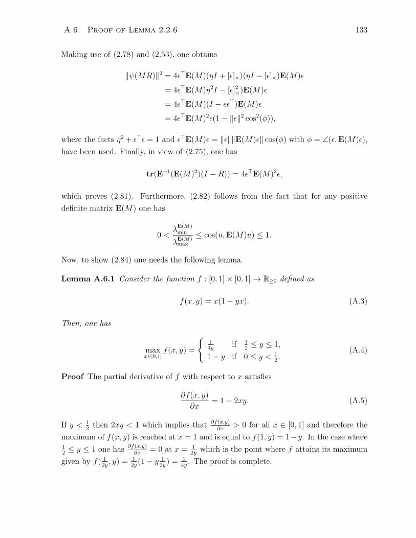
A.6. Proof of Lemma 2.2.6 133
Making use of (2.78) and (2.53), one obtains
‖ψ(MR)‖2 = 4ε>E(M)(ηI + [ε]×)(ηI − [ε]×)E(M)ε
= 4ε>E(M)η2I − [ε]2×)E(M)ε
= 4ε>E(M)(I − εε>)E(M)ε
= 4ε>E(M)2ε(1− ‖ε‖2 cos2(φ)),
where the facts η2 + ε>ε = 1 and ε>E(M)ε = ‖ε‖‖E(M)ε‖ cos(φ) with φ = ∠(ε,E(M)ε),
have been used. Finally, in view of (2.75), one has
tr(E−1(E(M)2)(I −R)) = 4ε>E(M)2ε,
which proves (2.81). Furthermore, (2.82) follows from the fact that for any positive
definite matrix E(M) one has
0 <λE(M)min
λE(M)max
≤ cos(u,E(M)u) ≤ 1.
Now, to show (2.84) one needs the following lemma.
Lemma A.6.1 Consider the function f : [0, 1]× [0, 1]→ R≥0 defined as
f(x, y) = x(1− yx). (A.3)
Then, one has
maxx∈[0,1]
f(x, y) =
14y
if 12≤ y ≤ 1,
1− y if 0 ≤ y < 12.
(A.4)
Proof The partial derivative of f with respect to x satisfies
∂f(x, y)
∂x= 1− 2xy. (A.5)
If y < 12
then 2xy < 1 which implies that ∂f(x,y)∂x
> 0 for all x ∈ [0, 1] and therefore the
maximum of f(x, y) is reached at x = 1 and is equal to f(1, y) = 1−y. In the case where12≤ y ≤ 1 one has ∂f(x,y)
∂x= 0 at x = 1
2ywhich is the point where f attains its maximum
given by f( 12y, y) = 1
2y(1− y 1
2y) = 1
4y. The proof is complete.

134 Chapter A. Proofs of Lemmas
Using (2.80)-(2.82) one has
‖ψ(MR)‖2 ≤ 4(λE(M)max )2(1− ξ2|R|2I)|R|2I = 4(λE(M)
max )2f(|R|2I , ξ2). (A.6)
Using the result of Lemma A.6.1 one obtains maxR∈SO(3) f(|R|2I , ξ2) = max|R|2I∈[0,1] f(|R|2I , ξ2) =
ψ(ξ2)/4 which implies that (2.84) holds.
A.6.1 Proof of Lemma 2.2.7
Making use of (2.48), one has
tr(xix>i (I −RP>)) =
1
2‖R>xi − P>xi‖2. (A.7)
Therefore, using the linear property of the trace function one obtains
tr
(n∑i=1
ρixix>i (I −RP>)
)=
1
2
n∑i=1
ρi‖R>xi − P>xi‖2. (A.8)
Furthermore, making use of (2.54) and (2.61) one has
ψ(xix>i RP
>) =1
2([PR>xi]×xi) =
1
2PR>[xi]×RP
>xi =1
2P (R>xi × P>xi), (A.9)
which leads to
ψ
(n∑i=1
ρixix>i RP
>
)=
1
2P
n∑i=1
ρi(R>xi × P>xi). (A.10)
A.7 Proof of Lemma 2.2.8
Let (η, ε) ∈ Q be a quaternion representation of the rotation matrix Ra(π, v)Ra(θ, u).
Using the quaternion multiplication rule (2.28) and the facts that Ra(π, v) = Ru(0, v)
and Ra(θ, u) = Ru(cos(θ/2), sin(θ/2)u), one obtains
ε = cos(θ/2)v + sin(θ/2)(v × u). (A.11)
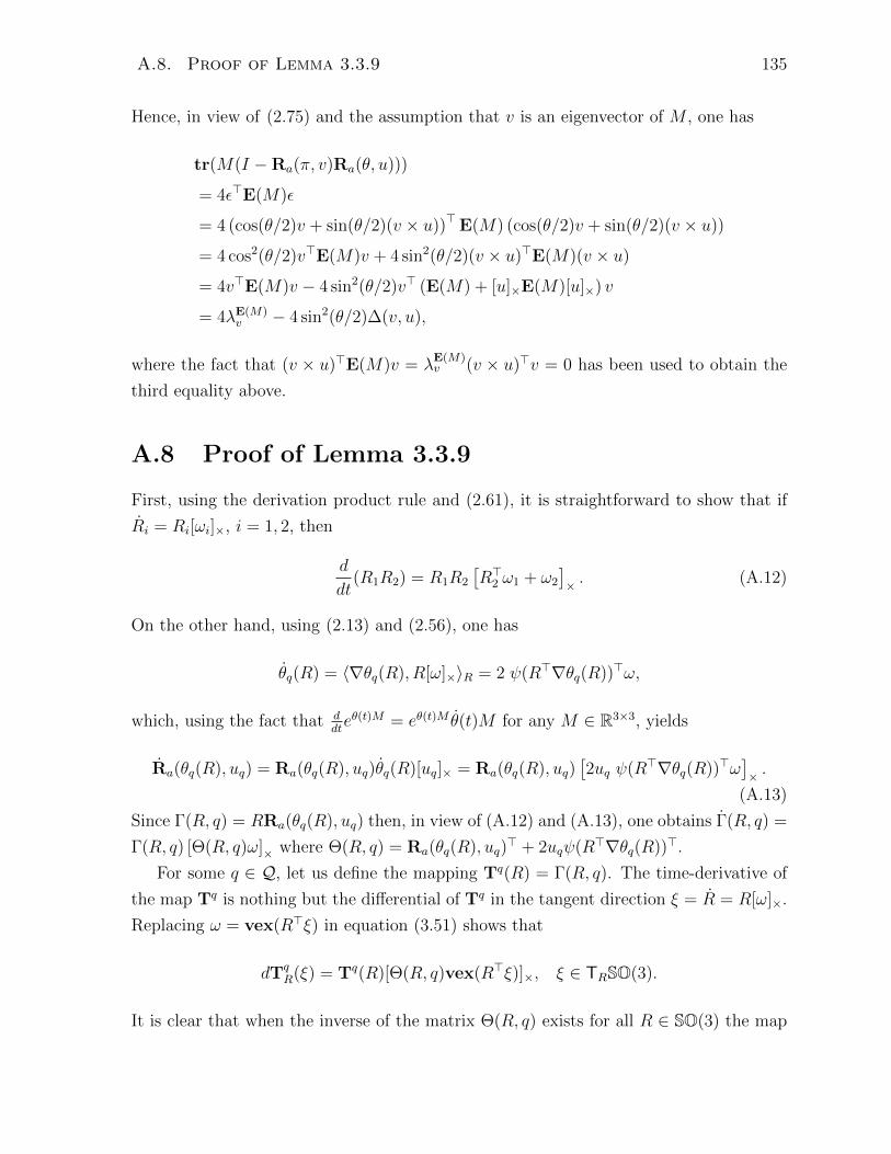
A.8. Proof of Lemma 3.3.9 135
Hence, in view of (2.75) and the assumption that v is an eigenvector of M , one has
tr(M(I −Ra(π, v)Ra(θ, u)))
= 4ε>E(M)ε
= 4 (cos(θ/2)v + sin(θ/2)(v × u))>E(M) (cos(θ/2)v + sin(θ/2)(v × u))
= 4 cos2(θ/2)v>E(M)v + 4 sin2(θ/2)(v × u)>E(M)(v × u)
= 4v>E(M)v − 4 sin2(θ/2)v> (E(M) + [u]×E(M)[u]×) v
= 4λE(M)v − 4 sin2(θ/2)∆(v, u),
where the fact that (v × u)>E(M)v = λE(M)v (v × u)>v = 0 has been used to obtain the
third equality above.
A.8 Proof of Lemma 3.3.9
First, using the derivation product rule and (2.61), it is straightforward to show that if
Ri = Ri[ωi]×, i = 1, 2, then
d
dt(R1R2) = R1R2
[R>2 ω1 + ω2
]× . (A.12)
On the other hand, using (2.13) and (2.56), one has
θq(R) = 〈∇θq(R), R[ω]×〉R = 2 ψ(R>∇θq(R))>ω,
which, using the fact that ddteθ(t)M = eθ(t)M θ(t)M for any M ∈ R3×3, yields
Ra(θq(R), uq) = Ra(θq(R), uq)θq(R)[uq]× = Ra(θq(R), uq)[2uq ψ(R>∇θq(R))>ω
]× .
(A.13)
Since Γ(R, q) = RRa(θq(R), uq) then, in view of (A.12) and (A.13), one obtains Γ(R, q) =
Γ(R, q) [Θ(R, q)ω]× where Θ(R, q) = Ra(θq(R), uq)> + 2uqψ(R>∇θq(R))>.
For some q ∈ Q, let us define the mapping Tq(R) = Γ(R, q). The time-derivative of
the map Tq is nothing but the differential of Tq in the tangent direction ξ = R = R[ω]×.
Replacing ω = vex(R>ξ) in equation (3.51) shows that
dTqR(ξ) = Tq(R)[Θ(R, q)vex(R>ξ)]×, ξ ∈ TRSO(3).
It is clear that when the inverse of the matrix Θ(R, q) exists for all R ∈ SO(3) the map

136 Chapter A. Proofs of Lemmas
dTqR(·) is an isomorphism. In fact, for all y := dTq
R(ξ) ∈ TTq(R)SO(3), the inverse is
explicitly given by
ξ = R[(Θ(R, q))−1 vex
(Tq(R)>y
)]× ∈ TRSO(3).
Consequently, the inverse function theorem [Helmke and Moore, 1994] guarantees that
Tq(R) is a local diffeomorphism for all R ∈ SO(3). Therefore, Γ is everywhere a local
diffeomorphism on SO(3) × Q which implies that if Ψ ∈ C1(DΨ,R≥0) then one has
Ψ Γ ∈ C1(Γ−1(DΨ),R≥0). If in addition Γ−1(I) = A then Ψ Γ(R, q) = 0 if and only
if (R, q) ∈ A which shows that Ψ Γ ∈ PΓ−1(DΨ),. In this case, the time-derivative of
Ψ Γ can be computed as follows
d
dtΨ Γ(R, q) = 〈∇Ψ(Γ(R, q)), Γ(R, q)〉Γ(R,q)
= 2 ψ(Γ(R, q)>∇Ψ(Γ(R, q))
)>ψ(
Γ(R, q)>Γ(R, q))
= 2 ψ(Γ(R, q)>∇Ψ(Γ(R, q))
)>Θ(R, q)ω
= 〈〈[Θ(R, q)>ψ
(Γ(R, q)>∇Ψ(Γ(R, q))
)]× , [ω]×〉〉
= 〈〈R[Θ(R, q)>ψ
(Γ(R, q)>∇Ψ(Γ(R, q))
)]× , R〉〉
where (2.13), (2.56) and (3.51) have been used. Consequently, in view of (2.7), the
gradient of Ψ Γ(R, q), with respect to the first argument R, is given by
∇(Ψ Γ)(R, q) = R[Θ(R, q)>ψ
(Γ(R, q)>∇Ψ(Γ(R, q))
)]× . (A.14)
Moreover, since the matrix Θ(R, q) is full rank, the set of critical points of Ψ Γ is
CΨΓ = (R, q) ∈ SO(3)×Q : ∇Ψ(Γ(R, q)) = 0 = Γ−1(CΨ).
A.9 Proof of Lemma 3.3.12
Let us define the angle function θ(R) = 2 arcsin (ktr(A(I −R))). Note that θ(·) is well
defined and differentiable on SO(3) thanks to the fact that ktr(A(I −R) ≤ 4kλE(A)max < 1
where (2.80) and (3.64) have been used. The gradient of the function θ(R) satisfies
∇θ(R) =2k∇tr(A(I −R))√1− k2tr2(A(I −R))
=2kRPso(3)(AR)√
1− k2tr2(A(I −R)),
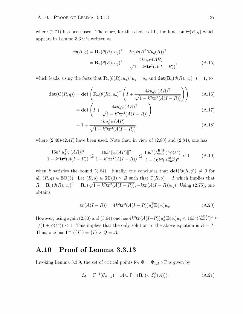
A.10. Proof of Lemma 3.3.13 137
where (2.71) has been used. Therefore, for this choice of Γ, the function Θ(R, q) which
appears in Lemma 3.3.9 is written as
Θ(R, q) = Ra(θ(R), uq)> + 2uqψ(R>∇θq(R))>
= Ra(θ(R), uq)> +
4kuqψ(AR)>√1− k2tr2(A(I −R))
, (A.15)
which leads, using the facts that Ra(θ(R), uq)>uq = uq and det(Ra(θ(R), uq)
>) = 1, to
det(Θ(R, q)) = det
(Ra(θ(R), uq)
>
(I +
4kuqψ(AR)>√1− k2tr2(A(I −R))
))(A.16)
= det
(I +
4kuqψ(AR)>√1− k2tr2(A(I −R))
)(A.17)
= 1 +4ku>q ψ(AR)√
1− k2tr2(A(I −R)), (A.18)
where (2.46)-(2.47) have been used. Note that, in view of (2.80) and (2.84), one has
16k2|u>q ψ(AR)|2
1− k2tr2(A(I −R))≤ 16k2‖ψ(AR)‖2
1− k2tr2(A(I −R))≤ 16k2(λ
E(A)max )2ψ(ξ2)
1− 16k2(λE(A)max )2
< 1, (A.19)
when k satisfies the bound (3.64). Finally, one concludes that det(Θ(R, q)) 6= 0 for
all (R, q) ∈ SO(3). Let (R, q) ∈ SO(3) × Q such that Γ(R, q) = I which implies that
R = Ra(θ(R), uq)> = Ru(
√1− k2tr2(A(I −R)),−ktr(A(I − R))uq). Using (2.75), one
obtains
tr(A(I −R)) = 4k2tr2(A(I −R))u>q E(A)uq. (A.20)
However, using again (2.80) and (3.64) one has 4k2tr(A(I−R))u>q E(A)uq ≤ 16k2(λE(A)max )2 ≤
1/(1 + ψ(ξ2)) < 1. This implies that the only solution to the above equation is R = I.
Thus, one has Γ−1(I) = I × Q = A.
A.10 Proof of Lemma 3.3.13
Invoking Lemma 3.3.9, the set of critical points for Φ = Ψ1,A Γ is given by
CΦ = Γ−1(CΨ1,A) = A ∪ Γ−1(Ra(π, ERv (A))). (A.21)
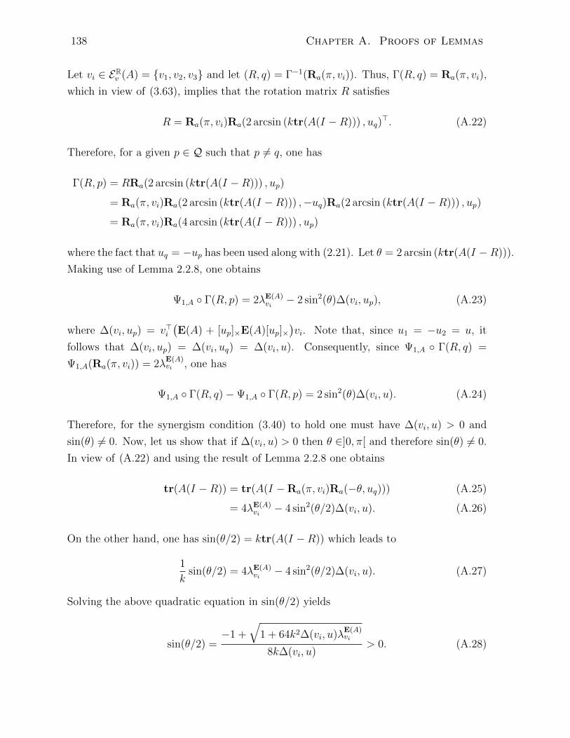
138 Chapter A. Proofs of Lemmas
Let vi ∈ ERv (A) = v1, v2, v3 and let (R, q) = Γ−1(Ra(π, vi)). Thus, Γ(R, q) = Ra(π, vi),
which in view of (3.63), implies that the rotation matrix R satisfies
R = Ra(π, vi)Ra(2 arcsin (ktr(A(I −R))) , uq)>. (A.22)
Therefore, for a given p ∈ Q such that p 6= q, one has
Γ(R, p) = RRa(2 arcsin (ktr(A(I −R))) , up)
= Ra(π, vi)Ra(2 arcsin (ktr(A(I −R))) ,−uq)Ra(2 arcsin (ktr(A(I −R))) , up)
= Ra(π, vi)Ra(4 arcsin (ktr(A(I −R))) , up)
where the fact that uq = −up has been used along with (2.21). Let θ = 2 arcsin (ktr(A(I −R))).
Making use of Lemma 2.2.8, one obtains
Ψ1,A Γ(R, p) = 2λE(A)vi− 2 sin2(θ)∆(vi, up), (A.23)
where ∆(vi, up) = v>i(E(A) + [up]×E(A)[up]×
)vi. Note that, since u1 = −u2 = u, it
follows that ∆(vi, up) = ∆(vi, uq) = ∆(vi, u). Consequently, since Ψ1,A Γ(R, q) =
Ψ1,A(Ra(π, vi)) = 2λE(A)vi , one has
Ψ1,A Γ(R, q)−Ψ1,A Γ(R, p) = 2 sin2(θ)∆(vi, u). (A.24)
Therefore, for the synergism condition (3.40) to hold one must have ∆(vi, u) > 0 and
sin(θ) 6= 0. Now, let us show that if ∆(vi, u) > 0 then θ ∈]0, π[ and therefore sin(θ) 6= 0.
In view of (A.22) and using the result of Lemma 2.2.8 one obtains
tr(A(I −R)) = tr(A(I −Ra(π, vi)Ra(−θ, uq))) (A.25)
= 4λE(A)vi− 4 sin2(θ/2)∆(vi, u). (A.26)
On the other hand, one has sin(θ/2) = ktr(A(I −R)) which leads to
1
ksin(θ/2) = 4λE(A)
vi− 4 sin2(θ/2)∆(vi, u). (A.27)
Solving the above quadratic equation in sin(θ/2) yields
sin(θ/2) =−1 +
√1 + 64k2∆(vi, u)λ
E(A)vi
8k∆(vi, u)> 0. (A.28)
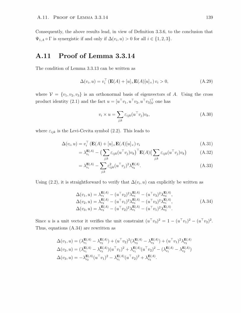
A.11. Proof of Lemma 3.3.14 139
Consequently, the above results lead, in view of Definition 3.3.6, to the conclusion that
Ψ1,A Γ is synergistic if and only if ∆(vi, u) > 0 for all i ∈ 1, 2, 3.
A.11 Proof of Lemma 3.3.14
The condition of Lemma 3.3.13 can be written as
∆(vi, u) = v>i (E(A) + [u]×E(A)[u]×) vi > 0, (A.29)
where V = v1, v2, v3 is an orthonormal basis of eigenvectors of A. Using the cross
product identity (2.1) and the fact u = [u>v1, u>v2, u
>v3]>V one has
vi × u =∑j,k
εijk(u>vj)vk, (A.30)
where εijk is the Levi-Cevita symbol (2.2). This leads to
∆(vi, u) = v>i (E(A) + [u]×E(A)[u]×) vi (A.31)
= λE(A)vi−(∑j,k
εijk(u>vj)vk
)>E(A)
(∑j,k
εijk(u>vj)vk
)(A.32)
= λE(A)vi−∑j,k
ε2ijk(u
>vj)2λE(A)
vk. (A.33)
Using (2.2), it is straightforward to verify that ∆(vi, u) can explicitly be written as
∆(v1, u) = λE(A)v1 − (u>v2)2λ
E(A)v3 − (u>v3)2λ
E(A)v2 ,
∆(v2, u) = λE(A)v2 − (u>v1)2λ
E(A)v3 − (u>v3)2λ
E(A)v1 ,
∆(v3, u) = λE(A)v3 − (u>v2)2λ
E(A)v1 − (u>v1)2λ
E(A)v2 .
(A.34)
Since u is a unit vector it verifies the unit constraint (u>v3)2 = 1 − (u>v1)2 − (u>v2)2.
Thus, equations (A.34) are rewritten as
∆(v1, u) = (λE(A)v1− λE(A)
v2) + (u>v2)2(λE(A)
v2− λE(A)
v3) + (u>v1)2λE(A)
v2
∆(v2, u) = (λE(A)v1− λE(A)
v3)(u>v1)2 + λE(A)
v1(u>v2)2 − (λE(A)
v1− λE(A)
v2)
∆(v3, u) = −λE(A)v2
(u>v1)2 − λE(A)v1
(u>v2)2 + λE(A)v3
.
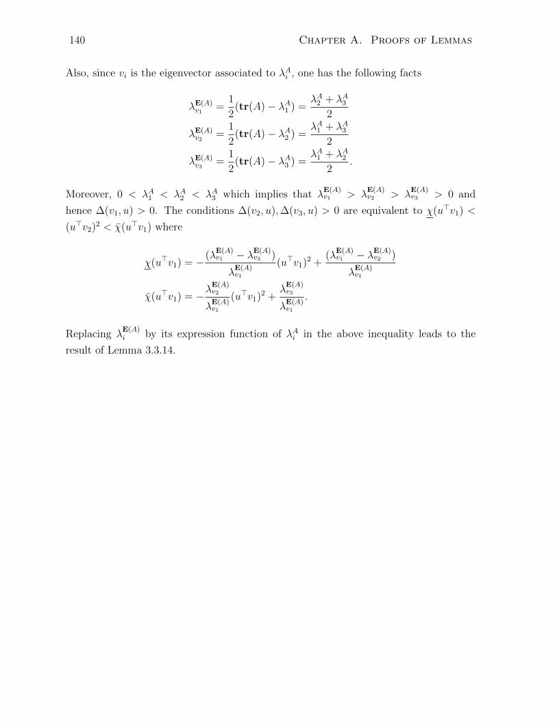
140 Chapter A. Proofs of Lemmas
Also, since vi is the eigenvector associated to λAi , one has the following facts
λE(A)v1
=1
2(tr(A)− λA1 ) =
λA2 + λA32
λE(A)v2
=1
2(tr(A)− λA2 ) =
λA1 + λA32
λE(A)v3
=1
2(tr(A)− λA3 ) =
λA1 + λA22
.
Moreover, 0 < λA1 < λA2 < λA3 which implies that λE(A)v1 > λ
E(A)v2 > λ
E(A)v3 > 0 and
hence ∆(v1, u) > 0. The conditions ∆(v2, u),∆(v3, u) > 0 are equivalent to χ(u>v1) <
(u>v2)2 < χ(u>v1) where
χ(u>v1) = −(λE(A)v1 − λE(A)
v3 )
λE(A)v1
(u>v1)2 +(λ
E(A)v1 − λE(A)
v2 )
λE(A)v1
χ(u>v1) = −λE(A)v2
λE(A)v1
(u>v1)2 +λE(A)v3
λE(A)v1
.
Replacing λE(A)i by its expression function of λAi in the above inequality leads to the
result of Lemma 3.3.14.

Appendix B
Proofs of Propositions
B.1 Proof of Proposition 3.2.1
First, it should be noted that in view of condition (3.20) and the fact that maxS1 ΦE(x) =
2, one has |kqΦE(x)| <√
3/2 < 1 for all (x, q) ∈ S1 × Q. This implies that the map
θ(x, q) is well defined and differentiable on the whole space. Now, let us compute the
gradient ∇θ(x, q) and show that (3.18) is not met for all (x, q) ∈ S1 × Q. Using (3.19)
one has
∇θ(x, q) =2kq∇ΦE(x)√1− k2
qΦE(x)2=
2kqe1√1− k2
qΦE(x)2. (B.1)
Therefore, one obtains
∇θ(x, q)>Sx =2kqx2√
1− k2q(1− x1)2
. (B.2)
Now, in view of the fact that x21 + x2
2 = 1, one has
4x22 + (1− x1)2 = 5− 2x1 − 3x2
1 ≤16
3, (B.3)
which implies, under the condition (3.20), that |∇θ(x, q)>Sx| < 1 and, hence, condition
(3.18) is not met for all (x, q) ∈ S1 × Q. Now, let us compute the critical points of the
composite potential function ΦE Γ(x, q) defined by (3.17). Consider (x, q) ∈ S1 × Q
141

142 Chapter B. Proofs of Propositions
such that Γ(x, q) = e1. Then, one has
x = R(−θ(x, q))e1 =
[cos(θ(x, q))
− sin(θ(x, q))
], (B.4)
which leads to
ΦE(x) = 1− e>1
[cos(θ(x, q))
− sin(θ(x, q))
]= 1− cos(θ(x, q)) = 2 sin2(θ(x, q)/2) = 2k2
qΦE(x)2.
(B.5)
Therefore ΦE(x)(1 − 2k2qΦE(x)) = 0 which leads to ΦE(x) = 0 (thus x = e1) since
2k2qΦE(x) < 6ΦE(x)/16 ≤ 12/16 < 1 and thus the quantity 1− 2k2
qΦE(x) cannot vanish.
Now, let us consider (x, q) ∈ S1 × Q such that Γ(x, q) = −e1. Then, in view of (3.11)
and (3.19), one obtains
x = −R(−θ(x, q))e1 =
[− cos(θ(x, q))
sin(θ(x, q))
], (B.6)
which leads to the following fact
ΦE(x) = 1− e>1
[− cos(θ(x, q))
sin(θ(x, q))
]= 1 + cos(θ(x, q)) = 2(1− sin2(θ(x, q)/2)) (B.7)
= 2(1− k2qΦE(x)2). (B.8)
The above quadratic equation in ΦE(x) can be solved to determine the unique value of
ΦE(x) ≥ 0 as follows
ΦE(x) =−1 +
√1 + 16k2
q
4k2q
. (B.9)
Once the value of ΦE(x) is computed, the solution x to (B.6) is readily obtained
x =
[2 sin2(θ(x, q)/2)− 1
2 sin(θ(x, q)/2) cos(θ(x, q)/2)
]=
2k2qΦE(x)2 − 1
2kqΦE(x)√
1− k2qΦE(x)2
= cq. (B.10)

B.2. Proof of Proposition 3.2.2 143
B.2 Proof of Proposition 3.2.2
Let (x, q) ∈ S1 × Q be an undesired critical point of ΦE(Γ(x, q)) which means that
Γ(x, q) = −e1. Now, for any p ∈ Q \ q, one has
Γ(x, p) = R(θ(x, p))x = −R(θ(x, p))R(−θ(x, q))e1 (B.11)
= −R(θ(x, p)− θ(x, q))e1 (B.12)
=
[− cos(θ(x, p)− θ(x, q))sin(θ(x, p)− θ(x, q))
]. (B.13)
Therefore, one obtains
ΦE Γ(x, p) = 1 + cos(θ(x, p)− θ(x, q)) = 2(1− sin2(θ(x, p)/2− θ(x, q)/2)), (B.14)
which leads to
ΦE Γ(x, q)− ΦE Γ(x, p)
= 2 sin2(θ(x, p)/2− θ(x, q)/2)
= 2 sin2(arcsin(kpΦE(x))− arcsin(kqΦE(x)))
= 2 sin2(
arcsin(kpΦE(x)
√1− k2
qΦE(x)2 − kqΦE(x)√
1− k2pΦE(x)2
))= 2
(kpΦE(x)
√1− k2
qΦE(x)2 − kqΦE(x)√
1− k2pΦE(x)2
)2
.
Taking kp = −kq = k and in view of (B.9) and the above equation, one obtains
ΦE Γ(x, q)− ΦE Γ(x, p) = 8k2ΦE(x)2(1− k2ΦE(x)2) =
(−1 +
√16 k2 + 1
)3
16k4.
B.3 Proof of Proposition 3.3.10
First, let us show that Ψ1 Γ is exp-synergistic with gap exceeding some δ1 > 0. Define
the parameters set T1 = Ψ1 Γ,Q, δ1. Let us verify that Ψ1 Γ is a valid potential
function. To do so, one needs to show that the transformation Γ proposed in Proposition
3.3.10 satisfies item 3) of Lemma 3.3.9 so that the composite function Ψ1 Γ ∈ PSO(3)×Q.
It should be mentioned that θ(R) = 2 arcsin(k|R|2I) is well defined thanks to the facts
k < 1/√
2 and |R|I ≤ 1. Moreover since the arcsin is differentiable on (−1, 1) and
k|R|2I < 1 it follows that the function θ(R) is differentiable on the whole manifold SO(3).
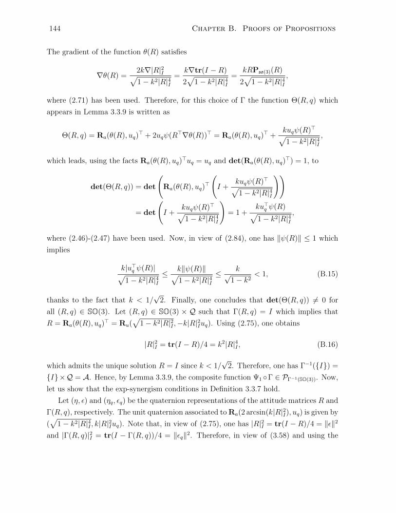
144 Chapter B. Proofs of Propositions
The gradient of the function θ(R) satisfies
∇θ(R) =2k∇|R|2I√1− k2|R|4I
=k∇tr(I −R)
2√
1− k2|R|4I=
kRPso(3)(R)
2√
1− k2|R|4I,
where (2.71) has been used. Therefore, for this choice of Γ the function Θ(R, q) which
appears in Lemma 3.3.9 is written as
Θ(R, q) = Ra(θ(R), uq)> + 2uqψ(R>∇θ(R))> = Ra(θ(R), uq)
> +kuqψ(R)>√1− k2|R|4I
,
which leads, using the facts Ra(θ(R), uq)>uq = uq and det(Ra(θ(R), uq)
>) = 1, to
det(Θ(R, q)) = det
(Ra(θ(R), uq)
>
(I +
kuqψ(R)>√1− k2|R|4I
))
= det
(I +
kuqψ(R)>√1− k2|R|4I
)= 1 +
ku>q ψ(R)√1− k2|R|4I
,
where (2.46)-(2.47) have been used. Now, in view of (2.84), one has ‖ψ(R)‖ ≤ 1 which
implies
k|u>q ψ(R)|√1− k2|R|4I
≤ k‖ψ(R)‖√1− k2|R|4I
≤ k√1− k2
< 1, (B.15)
thanks to the fact that k < 1/√
2. Finally, one concludes that det(Θ(R, q)) 6= 0 for
all (R, q) ∈ SO(3). Let (R, q) ∈ SO(3) × Q such that Γ(R, q) = I which implies that
R = Ra(θ(R), uq)> = Ru(
√1− k2|R|2I ,−k|R|2Iuq). Using (2.75), one obtains
|R|2I = tr(I −R)/4 = k2|R|4I , (B.16)
which admits the unique solution R = I since k < 1/√
2. Therefore, one has Γ−1(I) =
I×Q = A. Hence, by Lemma 3.3.9, the composite function Ψ1 Γ ∈ PΓ−1(SO(3)). Now,
let us show that the exp-synergism conditions in Definition 3.3.7 hold.
Let (η, ε) and (ηq, εq) be the quaternion representations of the attitude matrices R and
Γ(R, q), respectively. The unit quaternion associated to Ra(2 arcsin(k|R|2I), uq) is given by
(√
1− k2|R|4I , k|R|2Iuq). Note that, in view of (2.75), one has |R|2I = tr(I −R)/4 = ‖ε‖2
and |Γ(R, q)|2I = tr(I − Γ(R, q))/4 = ‖εq‖2. Therefore, in view of (3.58) and using the

B.3. Proof of Proposition 3.3.10 145
quaternion multiplication rule (2.28), one obtains
ηq = η√
1− k2‖ε‖4 − k‖ε‖2ε>uq, (B.17)
εq = kη‖ε‖2uq +√
1− k2‖ε‖4ε+ k‖ε‖2ε× uq. (B.18)
This leads to
‖εq‖2 = ‖ε‖2 + k2‖ε‖4η2 − cos2(ϕq)k2‖ε‖6 + 2kη‖ε‖3
√1− k2‖ε‖4 cos(ϕq)
where ϕq is the angle between ε and uq. Using the fact that |η| · ‖ε‖ ≤ 12, it follows that
‖εq‖2 ≤ ‖ε‖2[1 + k + k2/4] = [1 + k + k2/4]|R|2I .
Moreover, since k < 1√2
it is possible to show that
‖εq‖2 ≥ ‖ε‖2√
1− k2‖ε‖4[√
1− k2‖ε‖4 − 2k|η| · ‖ε‖]≥ ‖ε‖2
√1− k2‖ε‖4
[√1− k2 − k
]≥ ‖ε‖2
[1− k2 − k
√1− k2
]=[1− k2 − k
√1− k2
]|R|2I .
On the other hand, one has
Ψ1 Γ(R, q) =1
2tr(I − Γ(R, q)) = 2|Γ(R, q)|2I = 2‖εq‖2.
This shows that α1|R|2I ≤ Ψ1 Γ(R, q) ≤ α2|R|2I with α1 = 2[1−k2−k√
1− k2] and α2 =
[1+k+k2/4]. It is easy to check that α1 and α2 are strictly positive for all 0 ≤ k < 1/√
2.
Now, let us show the following fact: Γ(R, q) ∈ ΠSO(3) for all (R, q) ∈ FT1 , which implies
that the rotation Γ(R, q) cannot be of 180 angle whenever (R, q) ∈ FT1 . Let us prove
this by contradiction. Assume that Γ(R, q) /∈ ΠSO(3). Let Q = (η, ε), Qq = (ηq, εq) and
Qm = (ηm, εm) be the quaternion representation of the attitude R, Γ(R, q) and Γ(R,m),
respectively. Since Γ(R, q) /∈ ΠSO(3) it follows that Qq /∈ ΠQ or, equivalently, ηq = 0.
Therefore, in view of (B.17) one obtains ηm − ηq = ηm = k‖ε‖2ε>(uq − um). Moreover,
since um+3 = −um,m ∈ 1, 2, 3 there exist always three indices mi ∈ Q, i ∈ 1, 2, 3,such that umi is orthonormal to umj , for i 6= j and ε>umi and ε>uq have opposite signs.
Therefore, one has
maxm∈Q|ηm| = k‖ε‖2 max
m∈Q|ε>(uq − um)| ≥ k‖ε‖2 max
mi∈1,2,3|ε>umi | ≥ k‖ε‖3/
√3.

146 Chapter B. Proofs of Propositions
Furthermore if ηq = 0 then equation (B.17) implies that√1− ‖ε‖2
√1− k2‖ε‖4 = |k|‖ε‖3| cos(ϕq)|.
The above equation reads f(‖ε‖2) = 0 where f(x) := g(x) + sin2(ϕq)k2x3, and g(x) :=
1 − x − k2x2. It is easy to verify that f(x) and g(x) are decreasing on the interval
[0, 1] for all ϕq ∈ R. Therefore, since f(x) ≥ g(x), the solution xf ∈ [0, 1] to equation
f(xf ) = 0 is greater than or equals to xg ∈ [0, 1], with g(xg) = 0. Thus, it is clear
that f(‖ε‖2) = 0 implies that ‖ε‖2 ≥ (−1 +√
1 + 4k2)/2k2. Consequently, maxm∈Q
|ηm| ≥
[−1 +√
1 + 4k2]32/2√
6k2. Now, using the quaternion norm constraint, one obtains
Ψ1 Γ(R, q)− minm∈Q
Ψ1 Γ(R,m) = 2‖εq‖2 − 2minm∈Q‖εm‖2 = 2max
m∈Q|ηm|2
≥ [−1 +√
1 + 4k2]3
12k4= δ1 > δ1. (B.19)
Therefore (R, q) /∈ FT1 which confirms that Γ(R, q) ∈ ΠSO(3) for all (R, q) ∈ FT1 . In view
of (A.14) and (2.71), the gradient of Ψ1 Γ is given by
∇(Ψ1 Γ)(R, q) =1
2R[Θ(R, q)>ψ (Γ(R, q))
]× .
Now, in view of (2.80)-(2.82), one has tr(I −X) = 4|X|2I and α(I,X) = 1− |X|2I for all
X ∈ SO(3), from which one can write
‖ψ(X)‖2 = 4|X|2I(1− |X|2I) = (1 + tr(X))|X|2I (B.20)
Therefore ‖ψ(Γ(R, q))‖2 = |Γ(R, q)|2I(1 + tr(Γ(R, q))) which implies that, for all (R, q) ∈FT1 , there exists α > 0 such that α|Γ(R, q)|2I ≤ ‖ψ(Γ(R, q)‖2 ≤ 4|Γ(R, q)|2I since
Γ(R, q) ∈ ΠSO(3). Moreover since det(Θ(R, q)) 6= 0 for all (R, q) ∈ SO(3) × Q the
matrix Θ(R, q)Θ(R, q)> is full rank and positive definite for all (R, q) ∈ SO(3) × Q.
Therefore it is not difficult to find positive constants α3 and α4 such that the gradient
‖∇(Ψ1 Γ)(R, q)‖2F satisfies (3.43). Finally, Ψ1 Γ does not have any singular point
and therefore the condition FT1 ⊆ D = SO(3) × Q holds. It follows that Ψ1 Γ is an
exp-synergistic potential function with gap exceeding δ1.
Next, let us show that Ψ2 Γ is exp-synergistic. Define the parameters set T2 =
Ψ2 Γ,Q, δ2. A similar argument as above can be conducted to show that Ψ2 Γ ∈ PDwhere D = Γ−1(ΠSO(3)) = (R, q) ∈ SO(3) × Q | tr(Γ(R, q)) 6= −1. Moreover, since
Ψ1 Γ is quadratic in |R|I and by noticing that 12Ψ1(·) ≤ Ψ2(·) ≤ Ψ1(·) it follows
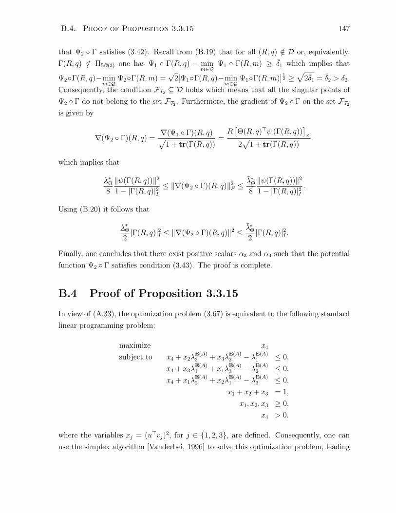
B.4. Proof of Proposition 3.3.15 147
that Ψ2 Γ satisfies (3.42). Recall from (B.19) that for all (R, q) /∈ D or, equivalently,
Γ(R, q) /∈ ΠSO(3) one has Ψ1 Γ(R, q) − minm∈Q
Ψ1 Γ(R,m) ≥ δ1 which implies that
Ψ2Γ(R, q)−minm∈Q
Ψ2Γ(R,m) =√
2[Ψ1Γ(R, q)−minm∈Q
Ψ1Γ(R,m)]12 ≥
√2δ1 = δ2 > δ2.
Consequently, the condition FT2 ⊆ D holds which means that all the singular points of
Ψ2 Γ do not belong to the set FT2 . Furthermore, the gradient of Ψ2 Γ on the set FT2is given by
∇(Ψ2 Γ)(R, q) =∇(Ψ1 Γ)(R, q)√
1 + tr(Γ(R, q))=R[Θ(R, q)>ψ (Γ(R, q))
]×
2√
1 + tr(Γ(R, q)).
which implies that
λ∗Θ8
‖ψ(Γ(R, q))‖2
1− |Γ(R, q)|2I≤ ‖∇(Ψ2 Γ)(R, q)‖2
F ≤λ∗Θ8
‖ψ(Γ(R, q))‖2
1− |Γ(R, q)|2I.
Using (B.20) it follows that
λ∗Θ2|Γ(R, q)|2I ≤ ‖∇(Ψ2 Γ)(R, q)‖2 ≤ λ∗Θ
2|Γ(R, q)|2I .
Finally, one concludes that there exist positive scalars α3 and α4 such that the potential
function Ψ2 Γ satisfies condition (3.43). The proof is complete.
B.4 Proof of Proposition 3.3.15
In view of (A.33), the optimization problem (3.67) is equivalent to the following standard
linear programming problem:
maximize x4
subject to x4 + x2λE(A)3 + x3λ
E(A)2 − λE(A)
1 ≤ 0,
x4 + x3λE(A)1 + x1λ
E(A)3 − λE(A)
2 ≤ 0,
x4 + x1λE(A)2 + x2λ
E(A)1 − λE(A)
3 ≤ 0,
x1 + x2 + x3 = 1,
x1, x2, x3 ≥ 0,
x4 > 0.
where the variables xj = (u>vj)2, for j ∈ 1, 2, 3, are defined. Consequently, one can
use the simplex algorithm [Vanderbei, 1996] to solve this optimization problem, leading
148 Chapter B. Proofs of Propositions
to the following result: If the condition
λA2 ≥λA1 λ
A3
λA3 − λA1(B.21)
is satisfied, then the optimal solution to (3.67) is given by
(u>v1)2 = 0, (u>v2)2 =λA2
λA2 + λA3, (u>v3)2 =
λA3λA2 + λA3
and the maximum is maxu∈S2
mini ∆(vi, u) = λA1 . Otherwise, the optimal solution is
(u>vi)2 = 1− 4
∏j 6=i λ
Aj∑
j 6=k λAj λ
Ak
, i ∈ 1, 2, 3
with the maximum being maxu∈S2
mini ∆(vi, u) = 4∏3j=1 λ
Aj∑
j 6=k λAj λ
Ak.
B.5 Proof of Proposition 3.3.16
First, let us show that Φ = Ψ1,A Γ is exp-synergistic. In view of Lemma 3.3.9 and
Lemma 3.3.12, it is clear that the composite function Ψ1,A Γ ∈ PSO(3)×Q. Let (η, ε) and
(ηq, εq) be, respectively, the unit quaternion representation of R and Γ(R, q). In view of
(3.63) and the fact that Ra(2 arcsin(ktr(A(I−R)), uq) corresponds to the unit quaternion
([1− k2tr(A(I −R))2)]12 , ktr(A(I −R))uq), and using the quaternion multiplication rule
(2.28), one can deduce that
εq = kηtr(A(I −R))uq + [1− k2tr(A(I −R))2]12 ε+ ktr(A(I −R))[ε]×uq.
Taking the norm square of εq yields
‖εq‖2 =(1− k2tr(A(I −R))2)‖ε‖2 + k2tr(A(I −R))2‖ε‖2 sin2(ϕq)+
k2η2tr(A(I −R))2 + 2kη‖ε‖tr(A(I −R))[1− k2tr(A(I −R))2]12 cos(ϕq),
where ϕq is the angle between ε and uq. Using the facts that |R|2I = ‖ε‖2 and |η| · ‖ε‖ =
‖ε‖√
1− ‖ε‖2 ≤ 1/2, and in view of (2.80), it follows that
‖εq‖2 ≤ ‖ε‖2[1 + 4kλE(A)max + 4(kλE(A)
max )2]. (B.22)
B.5. Proof of Proposition 3.3.16 149
Moreover, in view of (3.64) one has 4kλE(A)max < 1/
√2 and hence the following lower bound
can be derived
‖εq‖2 ≥ ‖ε‖2[1− k2tr(A(I −R))2 − 4kλE(A)max
√1− k2tr(A(I −R))2]
≥ ‖ε‖2[1− (4kλE(A)max )2 − 4kλE(A)
max
√1− (4kλ
E(A)max )2]. (B.23)
On the other hand, making use of (2.80), one has 4λE(A)min ‖εq‖2 ≤ Ψ1,A Γ(R, q) ≤
4λE(A)max ‖εq‖2 and, hence, there exist α1, α2 such that Ψ1,A Γ(R, q) satisfies (3.42).
In view of (A.14) and (2.71), the gradient of Ψ1,A Γ is given by
∇(Ψ1,A Γ)(R, q) =1
2R[Θ(R, q)>ψ(AΓ(R, q))]×. (B.24)
Now, for (R, q) ∈ SO(3)×Q, let λΘmin(R, q) and λΘ
max(R, q) denote, respectively, the small-
est and largest eigenvalue of Θ(R, q)Θ(R, q)>, and let the constants λ = minSO(3)×Q
(λΘmin(R, q))
and λ = maxSO(3)×Q
(λΘmax(R, q)). It is clear that λ, λ > 0 by the fact that Θ(R, q) is full
rank. Then, from (B.24) and using (2.80)-(2.82), one can show that
‖∇(Ψ1,A Γ)(R, q)‖2F =
1
2
∥∥Θ(R, q)>ψ(AΓ(R, q))∥∥2 ≤ 1
2λ ‖ψ(AΓ(R, q))‖2
≤ 2λ(λE(A)max )2α(A,Γ(R, q))|Γ(R, q)|2I
and
‖∇(Ψ1,A Γ)(R, q)‖2F =
1
2
∥∥Θ(R, q)>ψ(AΓ(R, q))∥∥2 ≥ 1
2λ ‖ψ(AΓ(R, q))‖2
≥ 2λ(λE(A)min )2α(A,Γ(R, q))|Γ(R, q)|2I
where α(A,Γ(R, q)) is given by
α(A,Γ(R, q)) = 1− |Γ(R, q)|2I cos2(u,E(A)u) (B.25)
such that u is the axis of rotation of Γ(R, q). Define the set of parameters T1 =
(Ψ1,A Γ,Q, δ1). Now, let us show that α(A,Γ(R, q)) > 0 for all (R, q) ∈ FT1 . First,
using the results from the proof of Lemma 3.3.13 provided in Appendix A.10, more pre-
cisely equations (A.23) and (A.28) one obtains for all undesired critical points (R, q) ∈
150 Chapter B. Proofs of Propositions
Γ−1(Ra(π, ERv (A)))
Ψ1,A Γ(R, q)−minp∈Q
Ψ1,A Γ(R, p)
= 8 sin2(θ/2)(1− sin2(θ/2))∆(v, u) = σ(k, λE(A)v ,∆(v, u)),
where v is some eigenvector of A and the function σ(·, ·, ·) is defined as follows
σ(k, λ,∆) = 8k2V (k, λ,∆)2(1− k2V (k, λ,∆)2)∆, (B.26)
V (k, λ,∆) =−1 +
√1 + 64k2∆λ
8k2∆. (B.27)
Moreover, by direct differentiation of the function σ(k, λ,∆) with respect to its argu-
ments, it is not difficult to show that the partial derivatives are positive and, therefore,
one obtains
σ(k, λE(A)v ,∆(v, u)) ≥ σ(k, λ
E(A)min ,∆(u)) > 0, (B.28)
where ∆(u) = mini∈1,2,3∆(vi, u). Therefore, one concludes that
∀(R, q) ∈ FT1 , Γ(R, q) /∈ Ra(π, ERv (A)). (B.29)
This is equivalent to say that for all (R, q) ∈ FT1 one has |Γ(R, q)| < 1 if cos2(u,E(A)u) <
1. Therefore, α(A,Γ(R, q)) > 0 for all (R, q) ∈ FT1 . Finally, one concludes that Ψ1,A Γ
satisfies (3.43). The last condition (3.44) is naturally satisfied since D = SO(3)×Q. The
proof of exp-synergism for Ψ1,A Γ is complete. Following similar steps as above, the
proof of exp-synergism for Ψ2,A Γ can be conducted.
B.6 Proof of Proposition 3.4.3
In view of (3.75) and (3.84), the angular velocity error ω satisfies
IB ˙ω = IBω × ω + uτ − IBωd (B.30)
= IBω × ω + IBω × ωd + IBωd × ωd + uτ − Jωd (B.31)
= [IBω]×ω − (K2 + [ωd]×IB)ω −R>d ψ(K1R). (B.32)
B.6. Proof of Proposition 3.4.3 151
Note that the term [IBω]×ω in the last equation is passive with respect to ω. Consider
the following Lyapunov function candidate
V(R, ω) =1
2tr(K1(I − R)) +
1
2ω>IBω. (B.33)
Using (2.72), (3.79), (B.32) and Assumption 3.4.2 one obtains
V = −ω>(K2 + [ωd]×IB)ω ≤ −(λK2min − λIBmaxcωd)‖ω‖2 ≤ −λ‖ω‖2 ≤ 0, (B.34)
where λ is a positive constant satisfying λK2min − λIBmaxcωd ≥ λ > 0 which exists thanks to
condition (3.85). Therefore, one concludes that the equilibrium point (R, ω) = (I, 0) is
stable and that the angular velocity error ω is bounded (note that R is naturally bounded
since SO(3) is compact). Since, by assumption, the desired angular velocity is bounded
it follows that the angular velocity ω = ω+ωd is also bounded. Let us denote by cω and
cω the upper bound on the norm of ω and ω, respectively. This implies that ˙ω is also
bounded and therefore one can easily show that V is bounded. By invoking Barbalat’s
Lemma it follows that V must converge to zero and therefore ω → 0 as well. Moreover,
one can show that ¨ω is bounded and using again Barbalat’s Lemma one has ˙ω → 0 which
leads to conclude that ψ(K1R) tends to zero in view of (B.32). Therefore the attitude
error must converge either to the desired equilibrium (R, ω) = (I, 0) or to one of the
undesired equilibria R ∈ Ra(π, ER3
v (A)). Now, let us show that the desired equilibrium
is exponentially stable. The set S = (R, ω) : V(R, ω) ≤ V(R(0), ω(0)) is an invariant
set for the closed-loop system. However, in view of (2.80), one has
2λE(K1)min |R|2I ≤
1
2tr(K1(I − R)) ≤ V(R, ω) ≤ V(R(0), ω(0)) < 2λ
E(K1)min , (B.35)
which leads to conclude that |R(t)|2I < 1 for all t ≥ 0. Now, consider the cross term
X = ψ(K1R)>RdIBω. The time derivative of X along the trajectories of (3.79) and
(B.32) satisfies
X = ψ(K1R)>Rd
([IBω]×ω − (K2 + [ωd]×IB)ω −R>d ψ(K1R)
)+
ω>JR>d E(K1R)Rdω + ψ(K1R)>Rd[ωd]×IBω, (B.36)
where (2.73) has been used. Moreover using (2.70) one has ‖E(K1R)‖F ≤ ‖E(K1)‖F :=
cE and using (2.80)-(2.84) one has ‖ψ(K1R)‖ ≤ 2λE(K1)max |R|I which implies that
X ≤ −‖ψ(K1R)‖2 + 2λE(K1)max |R|I‖ω‖
(cωλ
IBmax + λK2
max
)+ cEλ
IBmax‖ω‖2. (B.37)
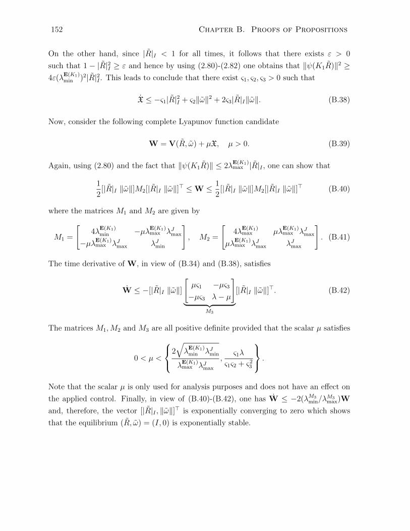
152 Chapter B. Proofs of Propositions
On the other hand, since |R|I < 1 for all times, it follows that there exists ε > 0
such that 1 − |R|2I ≥ ε and hence by using (2.80)-(2.82) one obtains that ‖ψ(K1R)‖2 ≥4ε(λ
E(K1)min )2|R|2I . This leads to conclude that there exist ς1, ς2, ς3 > 0 such that
X ≤ −ς1|R|2I + ς2‖ω‖2 + 2ς3|R|I‖ω‖. (B.38)
Now, consider the following complete Lyapunov function candidate
W = V(R, ω) + µX, µ > 0. (B.39)
Again, using (2.80) and the fact that ‖ψ(K1R)‖ ≤ 2λE(K1)max |R|I , one can show that
1
2[|R|I ‖ω‖]M2[|R|I ‖ω‖]> ≤W ≤ 1
2[|R|I ‖ω‖]M2[|R|I ‖ω‖]> (B.40)
where the matrices M1 and M2 are given by
M1 =
[4λ
E(K1)min −µλE(K1)
max λJmax
−µλE(K1)max λJmax λJmin
], M2 =
[4λ
E(K1)max µλ
E(K1)max λJmax
µλE(K1)max λJmax λJmax
]. (B.41)
The time derivative of W, in view of (B.34) and (B.38), satisfies
W ≤ −[|R|I ‖ω‖]
[µς1 −µς3−µς3 λ− µ
]︸ ︷︷ ︸
M3
[|R|I ‖ω‖]>. (B.42)
The matrices M1,M2 and M3 are all positive definite provided that the scalar µ satisfies
0 < µ <
2
√λE(K1)min λJmin
λE(K1)max λJmax
,ς1λ
ς1ς2 + ς23
.
Note that the scalar µ is only used for analysis purposes and does not have an effect on
the applied control. Finally, in view of (B.40)-(B.42), one has W ≤ −2(λM3min/λ
M3max)W
and, therefore, the vector [|R|I , ‖ω‖]> is exponentially converging to zero which shows
that the equilibrium (R, ω) = (I, 0) is exponentially stable.
B.7. Proof of Proposition 4.2.6 153
B.7 Proof of Proposition 4.2.6
Consider the trace function Ψ1,A defined in (3.28) for some A such that E(A) > 0 and
let Φ = Ξ = Ψ1,A. Clearly in view of (2.80) the potential function Ψ1,A satisfies the first
condition of Theorem 4.2.4. Moreover, the potential function Ψ1,A is smooth and does
not have any singular points which implies that the third condition of Theorem 4.2.4 is
also satisfied. It remains to show the second condition of Theorem 4.2.4. This condition
implies that the gradient of Φ does not vanish except at the identity rotation R = I
during the flows of F . Therefore, it is necessary to guarantee that all the undesired
critical points of Ψ1,A are inside the jump set J . Let R = Ra(π, v) where v ∈ ERv (A)
which represents an undesired critical point for Ψ1,A, see (3.32). Therefore, using (2.74),
one has Ψ1,A(R) = 2v>E(A)v = 2λE(A)v . Moreover, in view of Lemma 2.2.8, one has
Ψ1,A(RRa(θ, u)) = 2λE(A)v − 2 sin2(θ/2)∆(v, u). (B.43)
Hence, it follows that
Ψ1,A(R)−minq∈Q
Ψ1,A(RRa(θ, uq)) = 2 sin2(θ/2) maxq∈Q
∆(v, uq), (B.44)
where ∆(v, u) = v>(E(A) + [u]×E(A)[u]×)v = λE(A)v − (u × v)>E(A)(u × v). Three
different cases presents:
• A has the same positive eigenvalues λA1 = λA2 = λA3 = λ > 0. In this case ERv (A) =
S2 and therefore ∆(v, uq) = λ(1 − ‖uq × v‖2) = λ cos2∠(uq, v). It follows that∑3q=1 ∆(v, uq) = λ
∑3q=1 cos2∠(uq, v) = λ since uqq∈1,2,3 forms an orthonormal
basis. Hence maxq∈Q∆(v, uq) ≥ 13
∑3q=1 ∆(v, uq) = λ/3 for all v ∈ S2.
• A has two distinct eigenvalues λA1 = λA2 and λA3 > 0. In this case ERv (A) =
(spanu1, u2 ∩ S2) ∪ u3. Let v ∈ spanu1, u2 ∩ S2 such that v = α1u1 + α2u2.
This implies that u1 × v = α2u3, u2 × v = −α1u3 and u3 × v = −α2u1 + α1u2.
Hence, ∆(v, u1) = λE(A)u1 − α2
2λE(A)u3 , ∆(v, u2) = λ
E(A)u1 − α2
1λE(A)u3 and ∆(v, u3) = 0.
It follows that maxq∈Q∆(v, uq) ≥ 13
∑3q=1 ∆(v, uq) = 1
3(2λ
E(A)u1 − λE(A)
u3 ) = λA3 /3. In
the case where v = u3, then it is clear that maxq∈Q∆(v, uq) = ∆(v, u3) = λE(A)u3 =
12(λA1 + λA2 ) = λA1 .
• A has three distinct eigenvalues 0 ≤ λA1 < λA2 < λA3 . In this case ERv (A) =
u1, u2, u3. Let v = up for some p ∈ Q. Consequently maxq∈Q∆(v, uq) =
∆(up, up) = λE(A)up ≥ λ
E(A)min = 1
2(λA1 + λA2 ).
154 Chapter B. Proofs of Propositions
By choosing 0 < δ < maxq∈Q∆(v, uq), across all the possible values of v ∈ ERv (A), it
follows that all the undesired critical points of Ψ1,A are inside the jump set J defined in
(4.17). Now, in view of (2.71) and (2.80)-(2.82) one has
‖∇Ψ1,A(R)‖2F =
1
4‖Pso(3)(AR)‖2
F =1
2‖ψ(AR)‖2 ≤ 4(λE(A)
max )|R|2I (B.45)
≥ 4(λE(A)min )α(A, R)|R|2I (B.46)
where α(A, R) = 1 − |R|2I cos2(v,E(A)v) where v is the rotation axis of R. However,
α(A, R) = 0 implies that |R|2I = 1 and v ∈ Ev(A). In this case R = Ra(π, v) which is
a critical point of Ψ1,A. It follows that α(A, R) = 0 implies R ∈ J . Therefore, for all
R ∈ F one has α(A, R) > 0. Consequently, there exist α3, α4 > 0 such that
α4|R|2I ≤ ‖∇Ψ1,A(R)‖2F ≤ α4|R|2I . (B.47)
Therefore all the conditions of Theorem 4.2.4 are satisfied with Φ = Ξ = Ψ1,A.
B.8 Proof of Proposition 4.2.7
Since Φ(R) = Ψ1(R) = 12tr(I − R) = 2|R|2I then it is clear that item i) of Theorem 4.2.4
is satisfied. Moreover, in view of (2.71), one has
〈〈∇Φ(R),∇Ξ(R)〉〉 = 〈〈∇Ψ1(R),∇Ψ1,A(R)〉〉
= 〈〈RPso(3)(R), RPso(3)(AR)〉〉 (by (2.71))
= 〈〈Pso(3)(R),Pso(3)(AR)〉〉
= 2ψ(R)>ψ(AR) (by (2.56))
= 2ψ(R)>E(A)ψ(R) (by (2.83))
≤ 2λE(A)max ‖ψ(R)‖2 ≤ 8λE(A)
max |R|2I (by (B.20))
≥ 2λE(A)min ‖ψ(R)‖2 = 8λ
E(A)min |R|2I(1− |R|2I) (by (B.20)).
However, it is shown in the proof of Proposition 4.2.6 that for all R ∈ Ra(π,S2) (case
where A = I) one has R ∈ J if δ is chosen such that 0 < δ < δ = 2 sin2(θ/2)/3. It
follows that for all R ∈ F one has tr(R) > −1 or, equivalently, 1 − |R|2I > 0 which
implies that item ii) of Theorem 4.2.4 is also satisfied. Item iii) is naturally verified since
Ξ = Ψ1,A is smooth and does not have any singular points. The last item also can be
checked by noticing that ‖∇Ψ1,A(R)‖F = ‖Pso(3)(AR)‖F =√
2‖ψ(AR)‖ ≤ 2√
2λE(A)max |R|I

B.8. Proof of Proposition 4.2.7 155
where (2.80)-(2.82) have been used. Therefore, all conditions of Theorem 4.2.4 are met.

Appendix C
Proofs of Theorems
C.1 Proof of Theorem 2.3.3
• The proof of item i) follows directly from Theorem 2.3.2 since all the conditions of
the theorem are satisfied.
• Let us show item ii). Assume that λ2 ≤ 0, λ1 > −λ2γ and j ≤ γt + J for some
γ ≥ 0 and J ∈ N. Define the set
Ω = x ∈M : V(x) < αµp. (C.1)
Then, in view of (2.99), for all x ∈ Ω one has |x|pA ≤ 1αV(x) < µp which implies
that |x|A < µ and, thus, Ω ⊆ (A + µB). Consider the evolution of a solution x
satisfying
|x(0, 0)|A < exp((λ2(J + 1)− λJ)/p)(α/α)1pµ (C.2)
where λ = (λ1 + λ2γ)/(1 + γ) > 0. Note that |x(0, 0)|A < µ since the factor
exp((λ2(J+1)−λJ)/p)(α/α)1p in (C.2) is less than 1. Let us show that |x(t, j)|A < µ
for all (t, j) ∈ dom x. Assume that the solution x of (2.89) stays inside the set
(A + µB) up to (t, j) (0, 0). It is sufficient to show that, for all δ ≥ 0 such that
(t + δ, j + 1) ∈ dom x, one has x(t + δ, j + 1) ∈ (A + µB) as well. It follows from
arguments similar to the comparison lemma [Cai and Teel, 2009, Lemma C.1] and
from (2.100)-(2.101) that
V(x(t, j)) ≤ exp(−(λ1t+ λ2j))V(x(0, 0)). (C.3)
156
C.1. Proof of Theorem 2.3.3 157
However, using j ≤ γt+ J , λ2 ≤ 0 and λ1 + γλ2 > 0, one obtains
−(λ1t+ λ2j) ≤ −(λ1 + λ2γ)t− λ2J (C.4)
≤ −(λ1 + λ2γ)
1 + γt− (λ1 + λ2γ)
1 + γγt− λ2J (C.5)
≤ −(λ1 + λ2γ)
1 + γt− (λ1 + λ2γ)
1 + γ(j − J)− λ2J (C.6)
= −λ(t+ j) + (λ− λ2)J. (C.7)
It follows from (C.3) that
V(x(t, j)) ≤ exp((λ− λ2)J) exp(−λ(t+ j))V(x(0, 0)). (C.8)
Therefore, in view of (C.8), (2.99) and (C.2), one has V(x(t, j)) < α exp(λ2)µp ≤αµp. Let tj+1 be the instant of time where the (j + 1)-th jump happens, i.e.
(tj+1, j), (tj+1, j+1) ∈ dom x. Thus, it is clear that (t, j) (tj+1, j) (tj+1, j+1) (t+ δ, j + 1). Since V is nonincreasing during the flows, by (2.100), it is clear that
V(x(tj+1, j)) ≤ V(x(t, j)) < α exp(λ2)µp < αµp. Thus x(tj+1, j) ∈ Ω which implies
that x(tj+1, j) ∈ (A+ µB). Therefore, in view of (2.101), one obtains
V(x(tj+1, j + 1)) ≤ exp(−λ2)V(x(tj+1, j)) < αµp. (C.9)
This again implies that x(tj+1, j + 1) ∈ (A+ µB). Repeating the above argument,
it is easy to show that x cannot leave the set (A+ µB) by flowing between the two
hybrid times (tj+1, j + 1) and (t + δ, j + 1). Therefore x(t + δ, j + 1) ∈ (A + µB).
We have just shown that, starting from an initial condition satisfying (C.2), one
has x(t, j) ∈ (A + µB) for all (t, j) ∈ dom x which implies that the bound (C.8)
holds for all (t, j) ∈ dom x as well. Finally, in view of (2.99) and (C.8), it follows
that if x(0, 0) satisfies (C.2), x(t, j) satisfies the following exponential bound
|x(t, j)|A ≤[α exp((λ− λ2)J)
α
] 1p
exp(−λp−1(t+ j))|x(0, 0)|A. (C.10)
• Let us show item iii). Assume that λ1 ≤ 0, λ2 > −λ1γ and t ≤ γj + T for some
γ, T ≥ 0. Consider the evolution of a solution x satisfying
|x(0, 0)|A < exp((λ1(T + ε)− λT )/p)(α/α)1pµ (C.11)
158 Chapter C. Proofs of Theorems
where λ = (λ2 + λ1γ)/(1 + γ) > 0 and ε > 0 is any strictly positive constant. Let
us show that |x(t, j)|A < µ for all (t, j) ∈ dom x. First, in view of (2.99) and
(C.11), one has V(x(0, 0)) < αµp which implies that x(0, 0) ∈ Ω with Ω defined
in (C.1). Since λ2 > 0, V is decreasing during the jumps, one concludes that x
cannot leave Ω by jumping. Let us verify that x cannot leave Ω by flowing as well.
Let j ∈ N such that tj+1 − tj > 0 and (tj, j), (tj+1, j) ∈ dom x. That’s to say, the
time interval [tj, tj+1], associated to the j-th jump, is not empty. If the solution
x is purely discrete then this j does not exist. However, in this case of discrete
solutions, exponential convergence is trivial since one has exponential decrease of
V(x) at every jump and no flow occurs. Assume, moreover, that x(t′, j′) ∈ (A+µB)
for all (t′, j′) (t, j) ≺ (tj+1, j) where (t, j) ∈ dom x is a hybrid time between the
two hybrid times (tj, j) and (tj+1, j) . Then, from (2.100)-(2.101), one has
V(x(t, j)) ≤ exp(−(λ1t+ λ2j))V(x(0, 0)). (C.12)
However, using t ≤ γj + T , λ1 ≤ 0 and λ2 + γλ1 > 0, one obtains
−(λ1t+ λ2j) ≤ −(λ2 + λ1γ)j − λ1T (C.13)
≤ −(λ2 + λ1γ)
1 + γj − (λ2 + λ1γ)
1 + γγj − λ1T (C.14)
≤ −(λ2 + λ1γ)
1 + γj − (λ2 + λ1γ)
1 + γ(t− T )− λ1T (C.15)
= −λ(t+ j) + (λ− λ1)T. (C.16)
It follows that
V(x(t, j)) ≤ exp((λ− λ1)T ) exp(−λ(t+ j))V(x(0, 0)). (C.17)
It is clear that x(t, j) is still inside the set Ω. Now, let (t + ε′, j) ∈ dom x, with
0 < ε′ < ε, be a hybrid time after a small enough flow has occurred. Assume,
moreover, that V(x(t + ε′, j)) = αµp which corresponds to the boundary of the
open set Ω. Now, by integrating (2.100) between (t, j) and (t+ ε′, j), one has
V(x(t+ ε′, j)) ≤ exp(−λ1ε′)V(x(t, j)). (C.18)
C.2. Proof of Theorem 3.3.1 159
Therefore, combining (C.11), (C.17) and (C.18), one obtains
V(x(t+ ε′, j)) < exp(λ1(ε− ε′))αµp ≤ αµp (C.19)
which contradicts the assumption that V(x(t + ε′, j)) = αµp. Therefore, x cannot
leave Ω by flowing. Hence, it is true that x(t, j) ∈ Ω ⊆ (A + µB) for all (t, j) ∈dom x. This implies that the bound (C.17) holds as well for all times and jumps.
Consequently, using again (2.99), one deduces that
|x(t, j)|A ≤[α exp((λ− λ1)T )
α
] 1p
exp(−λp−1(t+ j))|x(0, 0)|A. (C.20)
C.2 Proof of Theorem 3.3.1
Assume that R(0) ∈ ΠSO(3) which implies, in view of the fact that Ra(π,S2) is a repeller,
that R(t) ∈ ΠSO(3) for all t ≥ 0. Therefore, the inverse map Z(R), defined in (2.32),
exists for all t ≥ 0 such that Rr(Z(R(t))) = R(t). Consequently, in view of (2.35), (2.79)
and (3.31), one obtains
d
dtZ(R) =
1
2
(I + [Z(R)]× + Z(R)Z(R)>
)ω = −k
(I + [Z(R)]× + Z(R)Z(R)>
)ψ(AR)
= −k(I + [Z(R)]× + Z(R)Z(R)>
)(I − [Z(R)]×)
1 + ‖Z(R)‖2E(A)Z(R)
= −k(I − [Z(R)]2× + Z(R)Z(R)>
)(1 + ‖Z(R)‖2)
E(A)Z(R) = −kE(A)Z(R), (C.21)
where [Z(R)]2× = −‖Z(R)‖2I+Z(R)Z(R)> is used to obtain the last equality. By simple
integration of (C.21), it follows that Z(R(t)) = e−kE(A)tZ(R(0)), for all t ≥ 0, which
yields (3.34).
C.3 Proof of Theorem 3.3.8
Let Φ ∈ PD, where D ⊆ SO(3) × Q, be an exp-synergistic potential function with gap
exceeding δ. Define the state X = (R, q) ∈ SO(3) × Q. The closed-loop system (3.27)
160 Chapter C. Proofs of Theorems
with (3.49) is written as
X = F(X) =
[−∇Φ(R, q)
0
]X ∈ FT , (C.22)
X+ ∈ J(X) =
[R
arg minm∈QΦ(R,m)
]X ∈ JT . (C.23)
Then, for all (R, q) ∈ FT , the time derivative of Φ along (C.22) satisfies
Φ(R, q) = 〈∇Φ(R, q), R〉R = −‖∇Φ(R, q)‖2F ≤ −α3|R|2I ≤ −
α3
α2
Φ(R, q)
where (2.13) and (3.42)-(3.43) are used. Moreover, for all (R, q) ∈ JT , one has
Φ(R+, q+) = minm∈Q
Φ(R,m) ≤ Φ(R, q)− δ < Φ(R, q).
The closed-loop system satisfies the following:
• The basic hybrid assumptions (C1)-(C3) (provided in Section 2.3). In fact, the sets
FT and JT are closed. The flow map F is continuous and single-valued and, there-
fore, locally bounded, outer semicontinuous, and the set F(X) is nonempty and
convex. The jump map J is outer semicontinuous, locally bounded, and nonempty.
• Every solution is precompact (complete and bounded). In fact, the configuration
manifold SO(3)×Q is compact and therefore all solutions are bounded preventing
finite escape time. Moreover, the space SO(3)×Q is viable under the flow (i.e. there
exists a nontrivial solution from any initial condition in FT ) and J(JT ) ⊂ FT ∪JT .
It follows from [Goebel and Teel, 2006, Proposition 2.4] that every solution is
complete.
• JT ∩ J(JT ) = ∅ since every jump maps the state (R, q) to the flow set FT .
Therefore, using [Sanfelice et al., 2007, Lemma 2.7], one concludes that there exists γ > 0
such that tj+1 − tj ≥ γ for all j ≥ 1 and (tj, j), (tj+1, j) ∈ dom(R, q). This means that
there is a minimum elapsed time between every two possible jumps. This leads to the
fact that t ≥ γ(j − 1) for all (t, j) ∈ dom x. Consequently, all the conditions of item ii)
of Theorem 2.3.3 are met, with λ1 = α3/α2, λ2 = 0, γ = 1/γ, J = 1, and one concludes
that the set A1 is globally exponentially stable.
C.4. Proof of Theorem 3.4.4 161
C.4 Proof of Theorem 3.4.4
Define the state X = (R, q, IBω, Rd, ωd) ∈ SO(3)×Q× R3 × SO(3)× R3. Note that Rd
and ωd are included in the state X so that one can write the closed-loop system as an
autonomous hybrid system. One can show that X follows the dynamics of an autonomous
hybrid system written in the general form (2.89) with the following data
F(X) =
R[Rdω]×
0
IBω × ω + IBωd × ω −K2ω −R>d ψ(R>∇Φ(R, q))
Rd[ωd]×
cωdB
, (C.24)
J(X) =[R> JT (R) (IBω)> R>d ω>d
]>, (C.25)
F = FT × R3 × SO(3)× R3, (C.26)
J = JT × R3 × SO(3)× R3. (C.27)
Consider the following Lyapunov function candidate
V(X) =1
2Φ(R, q) +
1
2ω>IBω. (C.28)
The time derivative of the function V along the flows of F satisfies
V(X) = −ω>K2ω ≤ 0. (C.29)
Moreover, for all X ∈ J and G ∈ J(X), one has
V(G)−V(X) =1
2(minm∈Q
Φ(R,m)− Φ(R, q)) ≤ −δ2< 0. (C.30)
It follows that V is nonincreasing during both the flows and jumps. Thus, the angular
velocity error ω is uniformly bounded. Also, since ωd is bounded by assumption, it
follows that ω = ω + ωd is bounded. Let us denote by cω, cω the upper bound on
the angular velocity and the angular velocity error, respectively. To show exponential
stability, consider the following Lyapunov function candidate
W(X) =1
2Φ(R, q) +
1
2ω>IBω + µω>JR>d ψ(R>∇Φ(R, q)), (C.31)
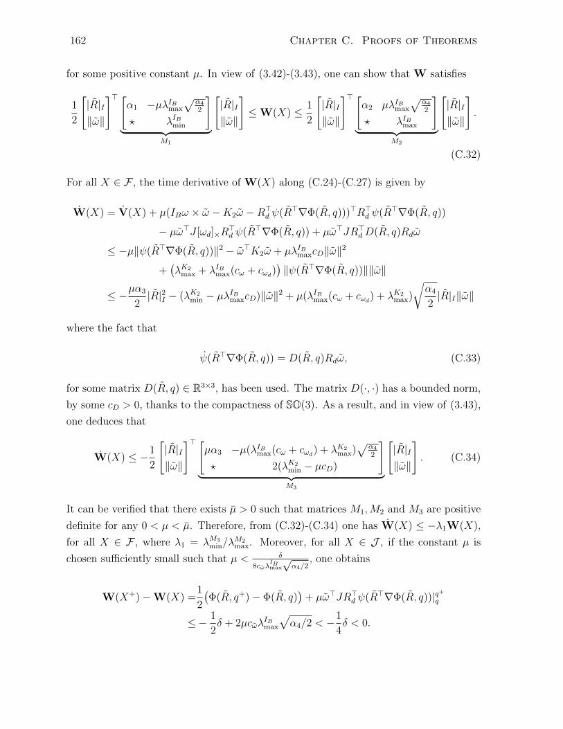
162 Chapter C. Proofs of Theorems
for some positive constant µ. In view of (3.42)-(3.43), one can show that W satisfies
1
2
[|R|I‖ω‖
]> [α1 −µλIBmax
√α4
2
? λIBmin
]︸ ︷︷ ︸
M1
[|R|I‖ω‖
]≤W(X) ≤ 1
2
[|R|I‖ω‖
]> [α2 µλIBmax
√α4
2
? λIBmax
]︸ ︷︷ ︸
M2
[|R|I‖ω‖
].
(C.32)
For all X ∈ F , the time derivative of W(X) along (C.24)-(C.27) is given by
W(X) = V(X) + µ(IBω × ω −K2ω −R>d ψ(R>∇Φ(R, q)))>R>d ψ(R>∇Φ(R, q))
− µω>J [ωd]×R>d ψ(R>∇Φ(R, q)) + µω>JR>dD(R, q)Rdω
≤ −µ‖ψ(R>∇Φ(R, q))‖2 − ω>K2ω + µλIBmaxcD‖ω‖2
+(λK2
max + λIBmax(cω + cωd))‖ψ(R>∇Φ(R, q))‖‖ω‖
≤ −µα3
2|R|2I − (λK2
min − µλIBmaxcD)‖ω‖2 + µ(λIBmax(cω + cωd) + λK2max)
√α4
2|R|I‖ω‖
where the fact that
ψ(R>∇Φ(R, q)) = D(R, q)Rdω, (C.33)
for some matrix D(R, q) ∈ R3×3, has been used. The matrix D(·, ·) has a bounded norm,
by some cD > 0, thanks to the compactness of SO(3). As a result, and in view of (3.43),
one deduces that
W(X) ≤ −1
2
[|R|I‖ω‖
]> [µα3 −µ(λIBmax(cω + cωd) + λK2
max)√
α4
2
? 2(λK2min − µcD)
]︸ ︷︷ ︸
M3
[|R|I‖ω‖
]. (C.34)
It can be verified that there exists µ > 0 such that matrices M1,M2 and M3 are positive
definite for any 0 < µ < µ. Therefore, from (C.32)-(C.34) one has W(X) ≤ −λ1W(X),
for all X ∈ F , where λ1 = λM3min/λ
M2max. Moreover, for all X ∈ J , if the constant µ is
chosen sufficiently small such that µ < δ
8cωλIBmax
√α4/2
, one obtains
W(X+)−W(X) =1
2
(Φ(R, q+)− Φ(R, q)
)+ µω>JR>d ψ(R>∇Φ(R, q))|q+
q
≤− 1
2δ + 2µcωλ
IBmax
√α4/2 < −
1
4δ < 0.
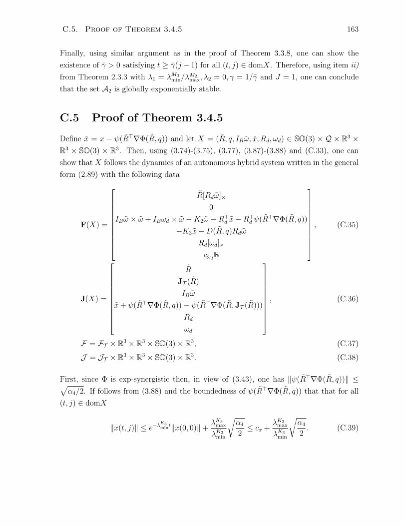
C.5. Proof of Theorem 3.4.5 163
Finally, using similar argument as in the proof of Theorem 3.3.8, one can show the
existence of γ > 0 satisfying t ≥ γ(j − 1) for all (t, j) ∈ domX. Therefore, using item ii)
from Theorem 2.3.3 with λ1 = λM3min/λ
M2max, λ2 = 0, γ = 1/γ and J = 1, one can conclude
that the set A2 is globally exponentially stable.
C.5 Proof of Theorem 3.4.5
Define x = x − ψ(R>∇Φ(R, q)) and let X = (R, q, IBω, x, Rd, ωd) ∈ SO(3) × Q × R3 ×R3 × SO(3) × R3. Then, using (3.74)-(3.75), (3.77), (3.87)-(3.88) and (C.33), one can
show that X follows the dynamics of an autonomous hybrid system written in the general
form (2.89) with the following data
F(X) =
R[Rdω]×
0
IBω × ω + IBωd × ω −K2ω −R>d x−R>d ψ(R>∇Φ(R, q))
−K3x−D(R, q)Rdω
Rd[ωd]×
cωdB
, (C.35)
J(X) =
R
JT (R)
IBω
x+ ψ(R>∇Φ(R, q))− ψ(R>∇Φ(R,JT (R)))
Rd
ωd
, (C.36)
F = FT × R3 × R3 × SO(3)× R3, (C.37)
J = JT × R3 × R3 × SO(3)× R3. (C.38)
First, since Φ is exp-synergistic then, in view of (3.43), one has ‖ψ(R>∇Φ(R, q))‖ ≤√α4/2. If follows from (3.88) and the boundedness of ψ(R>∇Φ(R, q)) that that for all
(t, j) ∈ domX
‖x(t, j)‖ ≤ e−λK3mint‖x(0, 0)‖+
λK3max
λK3min
√α4
2≤ cx +
λK3max
λK3min
√α4
2. (C.39)

164 Chapter C. Proofs of Theorems
Therefore, x is also bounded such that for all (t, j) ∈ domX
‖x(t, j)‖ ≤ cx := cx +
(λK3
max
λK3min
+ 1
)√α4
2. (C.40)
Let µ2 > 0 be a positive scalar satisfying
µ2 ≤δ
4c2x
, (C.41)
(1 + µ2cD)2
µ2λK2min
< λK3min. (C.42)
Consider the following Lyapunov function candidate
V(X) =1
2Φ(R, q) +
1
2ω>IBω +
1
2µ2‖x‖2. (C.43)
The time derivative of the function V along the flows of F satisfies
V(X) = −ω>K2ω − µ2x>K3x+ (1 + µ2cD)‖ω‖‖x‖ (C.44)
= −
[‖ω‖‖x‖
]> [λK2
min −(1 + µ2cD)/2
? µ2λK3min
][‖ω‖‖x‖
](C.45)
which, under the gain condition (C.41)-(C.42), is negative semidefinite such that V(X) ≤0. Moreover, for all X ∈ J one has
V(X+)−V(X) =1
2(minm∈Q
Φ(R,m)− Φ(R, q)) +1
2µ2‖x‖2|q+q (C.46)
≤ −δ2
+ µ2c2x ≤ −
δ
4< 0. (C.47)
It follows that V is nonincreasing during both the flows and jumps. Thus all signals are
bounded, including ω, ω and x. Let us denote by cω and cω the upper bounds on the
norm of the angular velocity ω and the angular velocity error ω. Let µ1 > 0 be a scalar
satisfying
µ1 < min
[2α1λ
IBmin]
12
λIBmax√α4
,δ/8√
2
cωλIBmax√α4
,µ2α3λ
K3min
α4
,α3λ
K2min
α4(λIBmax(cω + cωd) + λK2max) + 2α3cD
.
(C.48)
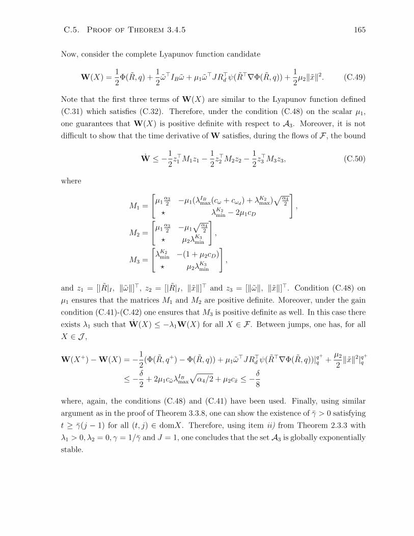
C.5. Proof of Theorem 3.4.5 165
Now, consider the complete Lyapunov function candidate
W(X) =1
2Φ(R, q) +
1
2ω>IBω + µ1ω
>JR>d ψ(R>∇Φ(R, q)) +1
2µ2‖x‖2. (C.49)
Note that the first three terms of W(X) are similar to the Lyapunov function defined
(C.31) which satisfies (C.32). Therefore, under the condition (C.48) on the scalar µ1,
one guarantees that W(X) is positive definite with respect to A3. Moreover, it is not
difficult to show that the time derivative of W satisfies, during the flows of F , the bound
W ≤ −1
2z>1 M1z1 −
1
2z>2 M2z2 −
1
2z>3 M3z3, (C.50)
where
M1 =
[µ1
α3
2−µ1(λIBmax(cω + cωd) + λK2
max)√
α4
2
? λK2min − 2µ1cD
],
M2 =
[µ1
α3
2−µ1
√α4
2
? µ2λK3min
],
M3 =
[λK2
min −(1 + µ2cD)
? µ2λK3min
],
and z1 = [|R|I , ‖ω‖]>, z2 = [|R|I , ‖x‖]> and z3 = [‖ω‖, ‖x‖]>. Condition (C.48) on
µ1 ensures that the matrices M1 and M2 are positive definite. Moreover, under the gain
condition (C.41)-(C.42) one ensures that M3 is positive definite as well. In this case there
exists λ1 such that W(X) ≤ −λ1W(X) for all X ∈ F . Between jumps, one has, for all
X ∈ J ,
W(X+)−W(X) = −1
2(Φ(R, q+)− Φ(R, q)) + µ1ω
>JR>d ψ(R>∇Φ(R, q))|q+
q +µ2
2‖x‖2|q+
q
≤ −δ2
+ 2µ1cωλIBmax
√α4/2 + µ2cx ≤ −
δ
8
where, again, the conditions (C.48) and (C.41) have been used. Finally, using similar
argument as in the proof of Theorem 3.3.8, one can show the existence of γ > 0 satisfying
t ≥ γ(j − 1) for all (t, j) ∈ domX. Therefore, using item ii) from Theorem 2.3.3 with
λ1 > 0, λ2 = 0, γ = 1/γ and J = 1, one concludes that the set A3 is globally exponentially
stable.
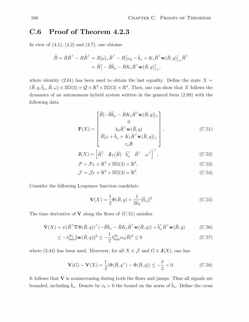
166 Chapter C. Proofs of Theorems
C.6 Proof of Theorem 4.2.3
In view of (4.1), (4.2) and (4.7), one obtains
˙R = RR> −R ˙R> = R[ω]×R
> −R[ωy − bω +K1R
>w(R, q)]×R>
= R[− Rbω − RK1R
>w(R, q)]×,
where identity (2.61) has been used to obtain the last equality. Define the state X =
(R, q, bω, R, ω) ∈ SO(3)×Q×R3 × SO(3)×R3. Then, one can show that X follows the
dynamics of an autonomous hybrid system written in the general form (2.89) with the
following data
F(X) =
R[−Rbω − RK1R
>w(R, q)]×
0
k2R>w(R, q)
R[ω + bω +K1R>w(R, q)]×
cωB
, (C.51)
J(X) =[R> JT (R) b>ω R> ω>
]>, (C.52)
F = FT × R3 × SO(3)× R3, (C.53)
J = JT × R3 × SO(3)× R3. (C.54)
Consider the following Lyapunov function candidate
V(X) =1
2Φ(R, q) +
1
2k2
‖bω‖2 (C.55)
The time derivative of V along the flows of (C.51) satisfies
V(X) = ψ(R>∇Φ(R, q))>(−Rbω − RK1R>w(R, q)) + b>ω R
>w(R, q) (C.56)
≤ −λK1min‖w(R, q)‖2 ≤ −1
2λK1
minα3|R|2 ≤ 0 (C.57)
where (3.44) has been used. Moreover, for all X ∈ J and G ∈ J(X), one has
V(G)−V(X) =1
2(Φ(R, q+)− Φ(R, q)) ≤ −δ
2< 0. (C.58)
It follows that V is nonincreasing during both the flows and jumps. Thus all signals are
bounded, including bω. Denote by cb > 0 the bound on the norm of bω. Define the cross

C.6. Proof of Theorem 4.2.3 167
term X(X) = b>ω R>ψ(R). In view of (C.51), the time derivative of X during the flows of
F is
X(X) = b>ω R>E(R)
(−Rbω − RK1R
>w(R, q)))− b>ω [ω + bω +K1R
>w(R, q)]×R>ψ(R)+
k2R>w(R, q)>R>ψ(R).
In addition, one has the following bound
−b>ω R>E(R)Rbω = −‖bω‖2 + b>ω R>(I − E(R))Rbω
≤ −‖bω‖2 +1
2tr(I − R)‖bω‖2 (by (2.67))
≤ −‖bω‖2 + 2c2b |R|2I (by (2.38))
Moreover, since Φ is exp-synergistic it satisfies (3.44) which implies that ‖w(R, q)‖ ≤√α4/2|R|I . It follows that
−b>ω R>E(R)RK1R>w(R, q) ≤
√3λK1
max
√α4/2|R|I‖bω‖
−b>ω [ω + bω +K1R>w(R, q)]×R
>ψ(R) = −b>ω [ω +K1R>w(R, q)]×R
>ψ(R)
≤ cω‖bω‖‖ψ(R)‖+ λK1max‖bω‖‖ψ(R)‖‖w(R, q)‖
≤ 2cω‖bω‖|R|I + 2λK1maxcb
√α4/2|R|2I , (by (B.20)).
Consequently, one deduces that there exist ς1, ς2 > 0 such that
X(X) ≤ −‖bω‖2 + ς1|R|2I + ς2‖bω‖|R|I , X ∈ F . (C.59)
Now, consider the following Lyapunov function candidate
W(X) = V(X) + µX(X), µ > 0. (C.60)
Since Φ satisfies (3.42) and in view of (B.20) one obtains the following lower and upper
bounds on W(X)
1
2[|R|I ‖bω‖]>
[α1 −2µ
? k−12
][|R|I‖bω‖
]≤W(X) ≤ 1
2[|R|I ‖bω‖]>
[α2 2µ
? k−12
][|R|I‖bω‖
]
Define the distance |X|2A = |R|2I + ‖bω‖2 from the set A to any point X on the manifold.
If µ is selected such that µ <√α1k
−12 /2 then it is clear from the above bound on W
that W(X) satisfies condition (2.99) of Theorem (2.3.3) with p = 2. Moreover, in view

168 Chapter C. Proofs of Theorems
of (C.59) and (C.57) one deduces that
W(X) = −1
2[|R|I ‖bω‖]>
[λK1
minα3 − 2µς1 −µς2? 2µ
][|R|I‖bω‖
], X ∈ F .
Assume that 0 < µ < 2λK1minα3/(4ς1 + ς2
2 ). Then, there exists λ1 > 0 such that W(X) ≤−λ1W(X) for all X ∈ F . Besides, for all X ∈ J and G ∈ J(X), one has
W(G)−W(X) = V(G)−V(X) =1
2(Φ(R, q+)− Φ(R, q)) ≤ −δ
2. (C.61)
Therefore, one has W(X(t, j)) ≤W(X(0, 0))− δ2j which implies that j ≤ 2W(X(0, 0))/δ.
Hence, the number of jumps is bounded (finite) for all initial conditions. Moreover,
following steps as in the last part of the proof of Theorem 3.3.8, one can show the
existence of γ > 0 satisfying t ≥ γ(j − 1) for all (t, j) ∈ domX. Therefore, using item ii)
from Theorem 2.3.3 with λ1 > 0, λ2 = 0, γ = 1/γ and J = 1, one concludes that the set
A is globally exponentially stable.
C.7 Proof of Theorem 4.2.4
In order to write the closed-loop system as an autonomous system, let us define the state
X = (R, bω, R, bω, ω, t) ∈ SO(3) × R3 × SO(3) × R3 × R3 × R≥0. Note that the time t
is included as a state variable which has the trivial hybrid dynamics t = 1 and t+ = t.
Then, in view of (4.1) and (4.14)-(4.17), one can show that X follows the dynamics of
an autonomous hybrid system written in the general form (2.89) with the following data
F(X) =
R[−Rbω − k1w(t, R)]×
Pcb(bω, k2R>w(t, R))
R[ω + bω + k1R>w(t, R)]×
−Pcb(bω, k2R>w(t, R))
cωB1
, (C.62)
J(X) =[Ra(θ, uq)
>R> b>ω R>Ra(θ, uq) b>ω ω> t]>, (C.63)
F = F × R3 × SO(3)× R3 × R3 × R≥0, (C.64)
J = J × R3 × SO(3)× R3 × R3 × R≥0. (C.65)
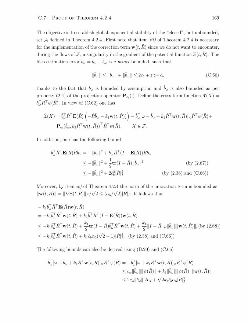
C.7. Proof of Theorem 4.2.4 169
The objective is to establish global exponential stability of the “closed”, but unbounded,
set A defined in Theorem 4.2.4. First note that item iii) of Theorem 4.2.4 is necessary
for the implementation of the correction term w(t, R) since we do not want to encounter,
during the flows of F , a singularity in the gradient of the potential function Ξ(t, R). The
bias estimation error bω = bω − bω is a priori bounded, such that
‖bω‖ ≤ ‖bω‖+ ‖bω‖ ≤ 2cb + ε := cb (C.66)
thanks to the fact that bω is bounded by assumption and bω is also bounded as per
property (2.4) of the projection operator Pcb(·). Define the cross term function X(X) =
b>ω R>ψ(R). In view of (C.62) one has
X(X) = b>ω R>E(R)
(−Rbω − k1w(t, R))
)− b>ω [ω + bω + k1R
>w(t, R)]×R>ψ(R)+
Pcb(bω, k2R>w(t, R)
)>R>ψ(R), X ∈ F .
In addition, one has the following bound
−b>ω R>E(R)Rbω = −‖bω‖2 + b>ω R>(I − E(R))Rbω
≤ −‖bω‖2 +1
2tr(I − R)‖bω‖2 (by (2.67))
≤ −‖bω‖2 + 2c2b |R|2I (by (2.38) and (C.66))
Moreover, by item iv) of Theorem 4.2.4 the norm of the innovation term is bounded as
‖w(t, R)‖ = ‖∇Ξ(t, R)‖F/√
2 ≤ (α5/√
2)|R|I . It follows that
− k1b>ω R>E(R)w(t, R)
= −k1b>ω R>w(t, R) + k1b
>ω R>(I − E(R))w(t, R)
≤ −k1b>ω R>w(t, R) +
k1
2tr(I − R)b>ω R
>w(t, R) +k1
2‖I − R‖F‖bω‖‖w(t, R)‖, (by (2.68))
≤ −k1b>ω R>w(t, R) + k1cbα5(
√2 + 1)|R|2I , (by (2.38) and (C.66))
The following bounds can also be derived using (B.20) and (C.66)
−b>ω [ω + bω + k1R>w(t, R)]×R
>ψ(R) = −b>ω [ω + k1R>w(t, R)]×R
>ψ(R)
≤ cω‖bω‖‖ψ(R)‖+ k1‖bω‖‖ψ(R)‖‖w(t, R)‖
≤ 2cω‖bω‖|R|I +√
2k1cbα5|R|2I .
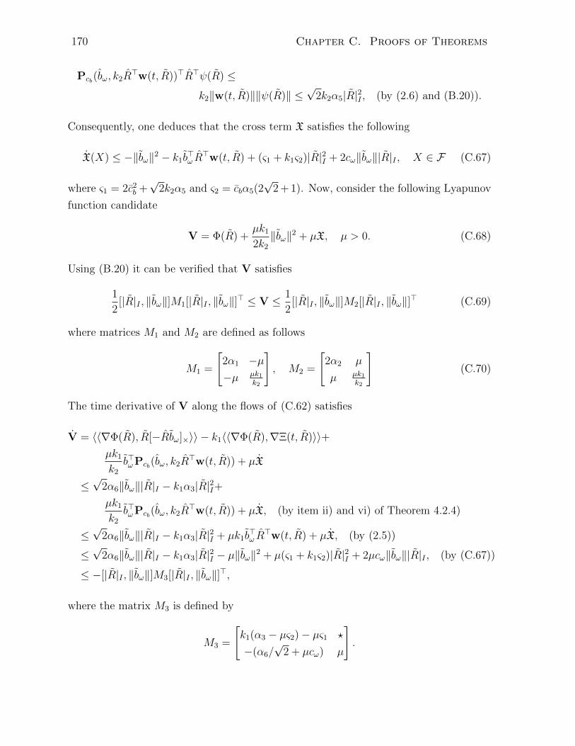
170 Chapter C. Proofs of Theorems
Pcb(bω, k2R>w(t, R))>R>ψ(R) ≤
k2‖w(t, R)‖‖ψ(R)‖ ≤√
2k2α5|R|2I , (by (2.6) and (B.20)).
Consequently, one deduces that the cross term X satisfies the following
X(X) ≤ −‖bω‖2 − k1b>ω R>w(t, R) + (ς1 + k1ς2)|R|2I + 2cω‖bω‖|R|I , X ∈ F (C.67)
where ς1 = 2c2b +√
2k2α5 and ς2 = cbα5(2√
2 + 1). Now, consider the following Lyapunov
function candidate
V = Φ(R) +µk1
2k2
‖bω‖2 + µX, µ > 0. (C.68)
Using (B.20) it can be verified that V satisfies
1
2[|R|I , ‖bω‖]M1[|R|I , ‖bω‖]> ≤ V ≤ 1
2[|R|I , ‖bω‖]M2[|R|I , ‖bω‖]> (C.69)
where matrices M1 and M2 are defined as follows
M1 =
[2α1 −µ−µ µk1
k2
], M2 =
[2α2 µ
µ µk1
k2
](C.70)
The time derivative of V along the flows of (C.62) satisfies
V = 〈〈∇Φ(R), R[−Rbω]×〉〉 − k1〈〈∇Φ(R),∇Ξ(t, R)〉〉+µk1
k2
b>ωPcb(bω, k2R>w(t, R)) + µX
≤√
2α6‖bω‖|R|I − k1α3|R|2I+µk1
k2
b>ωPcb(bω, k2R>w(t, R)) + µX, (by item ii) and vi) of Theorem 4.2.4)
≤√
2α6‖bω‖|R|I − k1α3|R|2I + µk1b>ω R>w(t, R) + µX, (by (2.5))
≤√
2α6‖bω‖|R|I − k1α3|R|2I − µ‖bω‖2 + µ(ς1 + k1ς2)|R|2I + 2µcω‖bω‖|R|I , (by (C.67))
≤ −[|R|I , ‖bω‖]M3[|R|I , ‖bω‖]>,
where the matrix M3 is defined by
M3 =
[k1(α3 − µς2)− µς1 ?
−(α6/√
2 + µcω) µ
].

C.7. Proof of Theorem 4.2.4 171
Therefore, it is sufficient to pick 0 < µ < min2α1k1/k2, α3/ς2 and k1 satisfying
k1 >
µ2ς1 + (α6/
√2 + µcω)2
µ(α3 − µς2)
to guarantee that all the matrices M1,M2 and M3 are positive definite. Therefore, there
exists λ1 > 0 such that V(X) ≤ −λ1V(X) for all X ∈ F . Moreover for all X ∈ J and
G ∈ J(X) one has
V(G)−V(X) = Φ(RRa(θ, uq))− Φ(R) + µbωR>(ψ(RRa(θ, uq))− ψ(R))
≤ −δ + 2cbµ, (by (2.84) and (C.66))
< −δ2, (C.71)
provided that µ is chosen such that µ < δ/4cb. Therefore, one has V(X(t, j)) ≤V(X(0, 0)) − δ
2j which implies that j ≤ 2V(X(0, 0))/δ. Hence, for all initial condi-
tions, the number of jumps is bounded (finite). Now, in contrast to the synergistic-based
approach, the reset-based observer do not guarantee that the elapsed time between two
consecutive jumps is bounded since the jumps do not (in general) map the state X to
the flow set. Let us show that the number of consecutive jumps (jumps that occur in a
row without flowing) is bounded. Let (t, j), (t, j′) ∈ domX such that j′ > j. Then, in
view of (4.15) and (4.17) one has
Φ(R(t, j))− Φ(R(t, j + 1)) ≥ δ (C.72)
... (C.73)
Φ(R(t, j′ − 1))− Φ(R(t, j′)) ≥ δ (C.74)
which implies that
Φ(R(t, j))− Φ(R(t, j′)) ≥ (j′ − j)δ. (C.75)
However, in view of item i) of Theorem 4.2.4 one has 0 ≤ Φ(R) ≤ α2|R|2I ≤ α2 for all
R ∈ SO(3). Therefore, one obtains the bound (j′ − j) ≤ α2/δ which shows that it is not
possible to have more than J := maxj ∈ N : j ≤ α2/δ number of jumps at the same
instant of time. Note that in view of Remark 4.2.5 one has necessarily α2 ≥ δ under the

172 Chapter C. Proofs of Theorems
conditions of Theorem 4.2.4. It follows that there exists γ > 0 such that
tj′ − tj ≥ γ, ∀(tj′ , j′), (tj, j) ∈ domX s.th. j′ > j + J . (C.76)
Let (t, j) ∈ domX which implies, by the structure of the hybrid time domain domX,
that t ∈ [tj, tj+1]. Let n ∈ N such that the jump index j satisfies
n(J + 1) ≤ j < (n+ 1)(J + 1). (C.77)
Note that n always exists for all j ∈ N. Then, one has
tj − tj−n(J+1) = tj − tj−(J+1) + tj−(J+1) − tj−2(J+1) + · · ·+ tj−(n−1)(J+1) − tj−n(J+1)
=n∑k=1
(tj−(k−1)(J+1) − tj−k(J+1)
)≥ nγ (C.78)
where (C.76) is used with the fact that j − (k − 1)(J + 1) > j − k(J + 1) + J for all
k ∈ 1, · · · , n. Therefore, in view of (C.77) and (C.78) one obtains
t ≥ tj ≥ nγ + tj−n(J+1) ≥ nγ >
(j
J + 1− 1
)γ. (C.79)
Therefore, all conditions of item ii) of Theorem 2.3.3 are met, with λ1 > 0, λ2 = 0, γ =
(J + 1)/γ and J = J + 1. It follows that the set A is globally exponentially stable.
C.8 Proof of Theorem 4.3.1
The quaternion representation of the attitude error R is used to proceed with the proof.
Let Q = (η, ε) ∈ Q be the quaternion representation of the attitude error R ∈ SO(3).
The quaternion Q(σ) := ([1 + ‖σ‖2]−12 , σ[1 + ‖σ‖2]−
12 ) is a quaternion associated to the
rotation matrix Rr(σ). It can be verified that the equivalent closed-loop hybrid system
for (4.36)-(4.37), using the quaternion representation, is written as followsQ = 0
τ = 1(Q, τ) ∈ Fq, (C.80)
Q+ = QQ(σ)−1
τ+ = 0(Q, τ) ∈ Jq, (C.81)
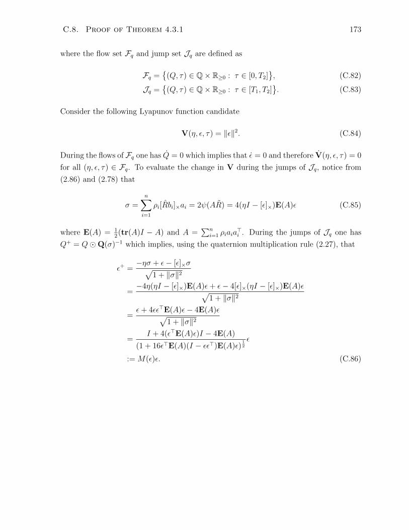
C.8. Proof of Theorem 4.3.1 173
where the flow set Fq and jump set Jq are defined as
Fq =
(Q, τ) ∈ Q× R≥0 : τ ∈ [0, T2], (C.82)
Jq =
(Q, τ) ∈ Q× R≥0 : τ ∈ [T1, T2]. (C.83)
Consider the following Lyapunov function candidate
V(η, ε, τ) = ‖ε‖2. (C.84)
During the flows of Fq one has Q = 0 which implies that ε = 0 and therefore V(η, ε, τ) = 0
for all (η, ε, τ) ∈ Fq. To evaluate the change in V during the jumps of Jq, notice from
(2.86) and (2.78) that
σ =n∑i=1
ρi[Rbi]×ai = 2ψ(AR) = 4(ηI − [ε]×)E(A)ε (C.85)
where E(A) = 12(tr(A)I − A) and A =
∑ni=1 ρiaia
>i . During the jumps of Jq one has
Q+ = QQ(σ)−1 which implies, using the quaternion multiplication rule (2.27), that
ε+ =−ησ + ε− [ε]×σ√
1 + ‖σ‖2
=−4η(ηI − [ε]×)E(A)ε+ ε− 4[ε]×(ηI − [ε]×)E(A)ε√
1 + ‖σ‖2
=ε+ 4εε>E(A)ε− 4E(A)ε√
1 + ‖σ‖2
=I + 4(ε>E(A)ε)I − 4E(A)
(1 + 16ε>E(A)(I − εε>)E(A)ε)12
ε
:= M(ε)ε. (C.86)

174 Chapter C. Proofs of Theorems
Now, let us compute the norm square of the quaternion vector part ε+. In view of (C.86)
and using the fact that ‖σ‖2 = 16ε>E(A)(I − εε>)E(A)ε, one has
‖ε+‖2 = ε>M(ε)2ε
=ε>(I + 4(ε>E(A)ε)I − 4E(A))(I + 4(ε>E(A)ε)I − 4E(A))ε
1 + ‖σ‖2
=ε>((1 + 4ε>E(A)ε)2I − 8(1 + 4ε>E(A)ε)E(A) + 16E(A)2)ε
1 + ‖σ‖2
=(1 + 4ε>E(A)ε)2‖ε‖2 − 8(1 + 4ε>E(A)ε)ε>E(A)ε+ 16ε>E(A)2ε
1 + ‖σ‖2
=(1 + 4ε>E(A)ε)2(‖ε‖2 − 1) + 1− 16(ε>E(A)ε)2 + 16ε>E(A)2ε
1 + ‖σ‖2
=(1 + 4ε>E(A)ε)2(‖ε‖2 − 1) + 1 + 16ε>E(A)(I − εε>)E(A)ε
1 + ‖σ‖2
=(1 + 4ε>E(A)ε)2(‖ε‖2 − 1) + 1 + ‖σ‖2
1 + ‖σ‖2
= ‖ε‖2 + (1− ‖ε‖2)1 + ‖σ‖2 − (1 + 4ε>E(A)ε)2
1 + ‖σ‖2
= ‖ε‖2 + (1− ‖ε‖2)8ε>(2E(A)2 − E(A))ε− 32(ε>E(A)ε)2
1 + 16ε>E(A)(I − εε>)E(A)ε
= ‖ε‖2 − (1− ‖ε‖2)f(ε,E(A)), (C.87)
where the function f(ε,E(A)) is defined as follows:
f(ε,E(A)) :=8ε>(E(A)− 2E(A)2)ε+ 32(ε>E(A)ε)2
1 + 16ε>E(A)(I − εε>)E(A)ε. (C.88)
Note that the following inequality holds:
f(ε,E(A)) ≥ 8ε>(E(A)− 2E(A)2)ε, ∀‖ε‖ ∈ [0, 1]. (C.89)
It follows that for all (η, ε, τ) ∈ Jq, one has
V(η+, ε+, τ+)−V(η, ε, τ) = ‖ε+‖2 − ‖ε‖2
= −(1− ‖ε‖2)f(ε,E(A)). (C.90)
However, in view of (4.41), one has 0 < λE(A)max < 1
2which implies that the matrix
B = 8(E(A) − 2E(A)2) is symmetric positive definite and all the eigenvalues of B sat-
isfy 0 < λB < 1. Hence, f(ε,E(A)) is lower by a positive definite quadratic function.
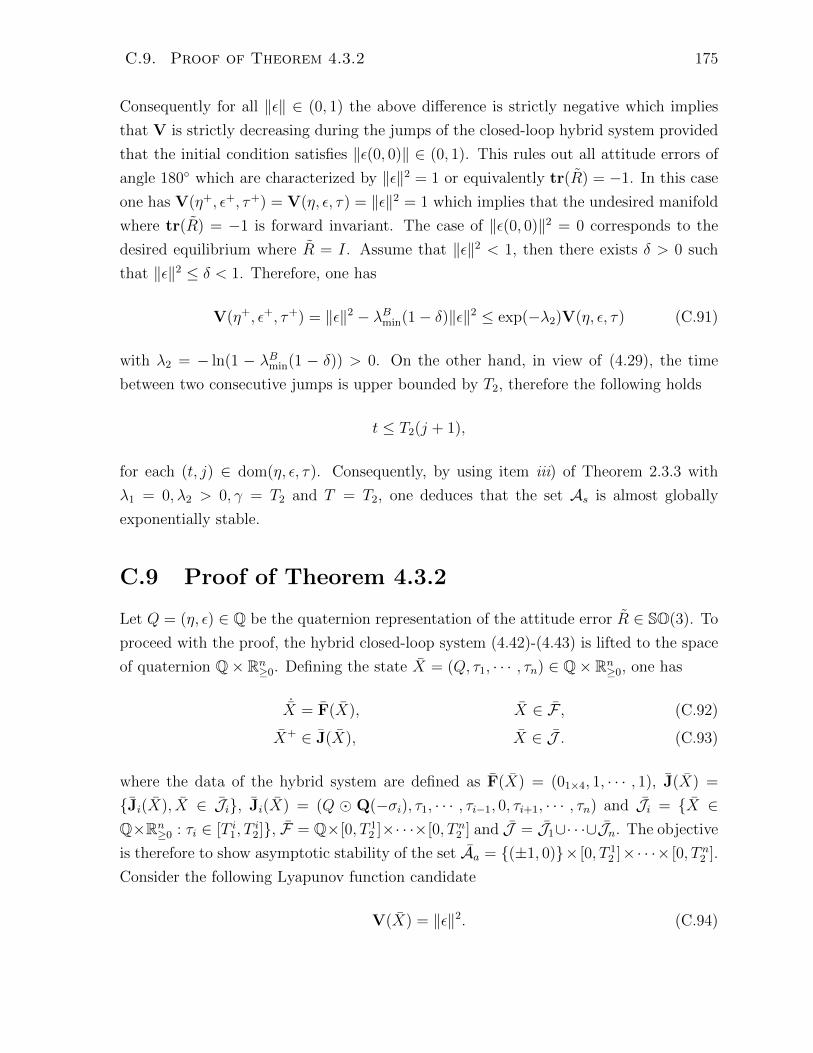
C.9. Proof of Theorem 4.3.2 175
Consequently for all ‖ε‖ ∈ (0, 1) the above difference is strictly negative which implies
that V is strictly decreasing during the jumps of the closed-loop hybrid system provided
that the initial condition satisfies ‖ε(0, 0)‖ ∈ (0, 1). This rules out all attitude errors of
angle 180 which are characterized by ‖ε‖2 = 1 or equivalently tr(R) = −1. In this case
one has V(η+, ε+, τ+) = V(η, ε, τ) = ‖ε‖2 = 1 which implies that the undesired manifold
where tr(R) = −1 is forward invariant. The case of ‖ε(0, 0)‖2 = 0 corresponds to the
desired equilibrium where R = I. Assume that ‖ε‖2 < 1, then there exists δ > 0 such
that ‖ε‖2 ≤ δ < 1. Therefore, one has
V(η+, ε+, τ+) = ‖ε‖2 − λBmin(1− δ)‖ε‖2 ≤ exp(−λ2)V(η, ε, τ) (C.91)
with λ2 = − ln(1 − λBmin(1 − δ)) > 0. On the other hand, in view of (4.29), the time
between two consecutive jumps is upper bounded by T2, therefore the following holds
t ≤ T2(j + 1),
for each (t, j) ∈ dom(η, ε, τ). Consequently, by using item iii) of Theorem 2.3.3 with
λ1 = 0, λ2 > 0, γ = T2 and T = T2, one deduces that the set As is almost globally
exponentially stable.
C.9 Proof of Theorem 4.3.2
Let Q = (η, ε) ∈ Q be the quaternion representation of the attitude error R ∈ SO(3). To
proceed with the proof, the hybrid closed-loop system (4.42)-(4.43) is lifted to the space
of quaternion Q× Rn≥0. Defining the state X = (Q, τ1, · · · , τn) ∈ Q× Rn
≥0, one has
˙X = F(X), X ∈ F , (C.92)
X+ ∈ J(X), X ∈ J . (C.93)
where the data of the hybrid system are defined as F(X) = (01×4, 1, · · · , 1), J(X) =
Ji(X), X ∈ Ji, Ji(X) = (Q Q(−σi), τ1, · · · , τi−1, 0, τi+1, · · · , τn) and Ji = X ∈Q×Rn
≥0 : τi ∈ [T i1, Ti2], F = Q×[0, T 1
2 ]×· · ·×[0, T n2 ] and J = J1∪· · ·∪Jn. The objective
is therefore to show asymptotic stability of the set Aa = (±1, 0)× [0, T 12 ]×· · ·× [0, T n2 ].
Consider the following Lyapunov function candidate
V(X) = ‖ε‖2. (C.94)

176 Chapter C. Proofs of Theorems
Clearly, one has V(X) = 0 for all X ∈ F . To evaluate the “discrete” change in V,
consider the following function [Sanfelice et al., 2007]
uD(X) =
maxξ∈J(X)
V(ξ)−V(X)
, X ∈ J ,
−∞, otherwise.
Now, let X ∈ J and define I(X) = i : X ∈ Ji. In view of the definition of the jump
map J(X), the function uD(X) can be written as
uD(X) =
maxi∈I(X)
V(Ji(X))−V(X)
, X ∈ J ,
−∞, otherwise.
On the other hand one has σi = 4(ηI − [ε]×)E(Ai)ε where E(Ai) = 12(tr(Ai)I −Ai) with
Ai = ρiaia>i . Using this result and the quaternion multiplication rule (similar step as
(C.86)), one can show that
QQ(−σi) = (αi(ε)η,Mi(ε)ε) (C.95)
where
αi =1 + 4ε>E(Ai)ε
(1 + 16ε>E(Ai)(I − εε>)E(Ai)ε)12
, (C.96)
Mi(ε) =I + 4(ε>E(Ai)ε)I − 4E(Ai)
(1 + 16ε>E(Ai)(I − εε>)E(Ai)ε)12
. (C.97)
Now, letting X ∈ J , it follows that
uD(X) = maxi∈I(X)
V(Ji(X))−V(X)
(C.98)
= maxi∈I(X)
‖Mi(ε)ε‖2 − ‖ε‖2 (C.99)
= −(1− ‖ε‖2) maxi∈I(X)
f(ε,E(Ai)) (C.100)
≤ 8(1− ‖ε‖2) maxi∈I(X)
ε>(2E(Ai)2 − E(Ai))ε. (C.101)
The matrix E(Ai) is explicitly given by E(Ai) = −ρi2
[ai]2× which is positive semi-definite.
The eigenvalues of E(Ai) are
0, ρi‖ai‖2
2, ρi‖ai‖
2
2
. The zero eigenvalue λ
E(Ai)1 = 0 of E(Ai)
corresponds to the eigenvector ai/‖ai‖ and leads to a zero eigenvalue of 2E(Ai)2−E(Ai).
The two other eigenvalues of E(Ai) are strictly positive and, under the condition of
Theorem 4.3.2, satisfy 0 < λE(Ai)2,3 < 1
2. In this case, the corresponding eigenvalues of
C.9. Proof of Theorem 4.3.2 177
2E(Ai)2 − E(Ai) are strictly negative. Consequently, one has
uD(X) ≤ 0, ∀‖ε‖ ∈ [0, 1). (C.102)
Therefore, by virtue of [Sanfelice et al., 2007, Theorem 7.6, Theorem 4.7], one concludes
that the compact set Aa is stable, and X must approach the largest weakly invariant set
in
V−1(r) ∩ u−1D (0) ∩ J(u−1
D (0)) (C.103)
for some r ∈ [0, 1). Let us show that the only weakly invariant subset of V−1(r) with r > 0
is the empty set. Assume that X(0, 0) ∈ V−1(r) which implies that ‖ε(0, 0)‖2 = r. Since
V(X) = 0 one must have ‖ε(t1, 0)‖2 = ‖ε(0, 0)‖2 = r where t1 is the time corresponding
to the first jump which is explicitly given by t1 = mini∈1,··· ,n ti0. After the first jump one
has ‖ε(t1, 1)‖2 = ‖Mi(ε(t1, 0))ε(t1, 0)‖2 ≤ ‖ε(t1, 0)‖2 = r for some i ∈ arg mini∈1,··· ,n ti0.
If ‖ε(t1, 1)‖2 < r, it means that X(t1, 1) has left the level set V−1(r). If on the other hand
‖ε(t1, 1)‖2 = ‖Mi(ε(t1, 0))ε(t1, 0)‖2 = r then this means that ε(t1, 0) is an eigenvector of
Mi(ε(t1, 0)) corresponding to the eigenvalue 1 which leads to the fact that ε(t1, 0) is an
eigenvector of E(Ai) corresponding to the eigenvalue 0. Therefore ε(t1, 0) must be parallel
to ai, the inertial vector corresponding to the sensor measurement bi. Now, let us define
the time t = minl,ktlk : tlk ≥ t1, al×ai 6= 0 which corresponds to the first instant of time
after t1 such that a sensor measurement bl has been received with a corresponding inertial
vector al not parallel to al. The existence of this time is guaranteed by Assumption 4.2.1.
Since the projection of the hybrid time domain on R≥0 is unbounded and the fact that t
corresponds to a measurement instant (thus there is a jump at time t) then there exists
j such that (t, j), (t, j + 1) ∈ domX. Therefore one has ε(t, j) = ε(t1, 0) = ε(0, 0) and
‖ε(t, j + 1)‖2 = ‖Ml(ε(0, 0))ε(0, 0)‖2 < ‖ε(0, 0)‖2 = r. One concludes that X must leave
the set V−1(r) for all r > 0. Then r in (C.103) must be zero. However V−1(r) = Aawhich implies that all trajectories must converge to a subset of Aa and hence Aa is
attractive. This proves that the set Aa is asymptotically stable.

178 Chapter C. Proofs of Theorems
C.10 Proof of Theorem 4.3.3
Now, using (4.55)-(4.57) and (4.58), the attitude estimation error R = RR> can be shown
to satisfy
R(sm+1) = R(sm)R(−σ(sm)), sm = tk, k ∈ N,
R(sm+1) = R(sm), sm 6= tk, k ∈ N.
During the instants of time sm such that sm 6= tk, the attitude estimation error is constant.
This leads to the following fact
R(tk+1) = R(tk)R(−σ(tk)), ∀k ∈ N.
Following similar steps as in (C.85)-(C.89), it can be shown that the quaternion vector
part of the attitude estimation error satisfies
ε(tk+1) = M(ε(tk))ε(tk), ∀k ∈ N,
and in particular one has
‖ε(tk+1)‖2 − ‖ε(tk)‖2 ≤ 8(1− ‖ε(tk)‖2)ε(tk)>(2E(A)2 − E(A))ε(tk),∀k ∈ N.
Now, since the initial attitude error satisfies tr(R(0)) 6= −1, then ‖ε(0)‖ = ‖ε(t1)‖ < 1.
The attitude matrix 2E(A)2 − E(A) is negative definite under the condition of Theo-
rem 4.3.1. Therefore, it is clear that ‖ε(tk+1)‖2 ≤ ‖ε(tk)‖2 ≤ · · · ≤ ‖ε(t1)‖2 < 1 for
all k ∈ N. It follows that ‖ε(tk+1)‖2 = ‖ε(tk)‖2 only when ε(tk) = 0 which implies
that limk→∞ ε(tk) = 0. This limit obviously corresponds to the attitude error R = I.
Therefore, the discrete version (4.55)-(4.57) of the proposed event-triggered attitude esti-
mation scheme (4.30)-(4.31) guarantees asymptotic stability as well when connected with
the discrete approximation (4.58) of the attitude kinematic system (4.27).
C.11 Proof of Theorem 4.3.4
Let us linearize the closed-loop system (4.74)-(4.75) around the equilibrium set where
R = I and bω = 0. For small rotations near I, one has R ≈ I + [z1]× for some z1 ∈ R3.
Define z2 = −Rbω then in view of (4.74) one has [z1]× = (I + [z1]×)[z2]× ≈ [z2]×. It
follows that, during the flows of (4.74), the linear dynamics for the variables z1 and z2

C.11. Proof of Theorem 4.3.4 179
are given by
z1 = z2, (C.104)
z2 = [Rω]×z2. (C.105)
On the other hand, the innovation term σ satisfies
σ =n∑i=1
ρi[Rbi]×ai =n∑i=1
ρi[R>ai]×ai ≈
n∑i=1
ρi[(I − [z1]×)ai]×ai
= −n∑i=1
ρi[[z1]×ai]×ai = −n∑i=1
ρi[ai]2×z1 = 2E(A)z1
where A =∑n
i=1 ρiaia>i . For small rotation errors and in view of (2.31), one has
Rr(−σ) ≈ I − 2[σ]×. Therefore, during the jumps of (4.75) and neglecting high or-
der terms for z1, one has
I + [z+1 ]× ≈ (I + [z1]×)(I − 2[σ]×) ≈ I + [z1]× − 4[E(A)z1]× = I + [(I − 4E(A))z1]×.
Moreover, in view of (4.73) and (4.75), one has
z+2 = −R+b+
ω = −Rr(σ)R(bω + γbT−1R>σ) = Rr(σ)z2 − γbT−1Rr(σ)σ ≈ z2 − γbT−1σ
where the facts that Rr(σ)σ = σ and R(σ)z2 ≈ (I − 2[σ]×)z2 = z2 − 4[E(A)z1]×z2 ≈ z2
have been used. It follows that the linear dynamics, during the jumps of (4.75), satisfy
z+1 = (I − 4E(A))z1, (C.106)
z+2 = z2 − 2γbT
−1E(A)z1. (C.107)
Consider the following change of variables
x1 = z1 − τz2,
x2 = Tz2.
180 Chapter C. Proofs of Theorems
Defining x = [x>1 , x>2 ]>, then in view of (4.74)-(4.75), (C.104)-(C.105) and (C.106)-
(C.107), one can show that
x = Ac(Rω, τ)x
τ = 1˙R = R[ω − R>x2/T ]×
ω ∈ cωB
(x, τ, R, ω) ∈ R6 × [0, T ]× SO(3)× R3, (C.108)
x+ = Adx
τ+ = 0
R+ = Rr(σ)R
ω+ = ω
(x, τ, R, ω) ∈ R6 × T × SO(3)× R3, (C.109)
where the matrices Ac(Rω, τ) and Ad are given by
Ac(Rω, τ) =
[0 −(τ/T )[Rω]×
0 [Rω]×
],
Ad =
[I − 4E(A) I − 4E(A)
−2γbE(A) I − 2γbE(A)
].
Let us show that the norm of the matrix Ac(Rω, τ) is uniformly bounded. Note that
Ac(Rω, τ)Ac(Rω, τ)> =
[−(τ/T )2[Rω]2× −(τ/T )[Rω]2×
−(τ/T )[Rω]2× −[Rω]2×
]. (C.110)
Therefore, one has ‖Ac(Rω, τ)‖2F = tr(Ac(Rωτ)Ac(Rωτ)>) = 2((τ/T )2+1)‖ω(t)‖2 ≤ 4c2
ω
thanks to the assumption that ω(t) is uniformly bounded. Now, let us establish the
necessary and sufficient condition for the matrix Ad to be Schur stable. Let λ be an
eigenvalue of Ad. Then
det(λI − Ad)
= det
[(λ− 1)I + 4E(A) −(I − 4E(A))
2γbE(A) (λ− 1)I + 2γbE(A)
]= det((λ− 1)2I + ((2γb + 4)(λ− 1) + 2γb)E(A))
= 0.

C.11. Proof of Theorem 4.3.4 181
This implies that 0 is the unique eigenvalue of the matrix (λ− 1)2I + ((2γb + 4)(λ− 1) +
2γb)E(A) and thus one obtains the equation
P (λ) = (λ− 1)2 + ((2γb + 4)(λ− 1) + 2γb)λE(A) = 0 (C.111)
where λE(A) is an eigenvalue of E(A). It follows that each eigenvalue of E(A) (total
3 eigenvalues) gives rise to 2 eigenvalues of Ad (total of 6 eigenvalues). The matrix
Ad is Schur stable if an only if all its eigenvalues are inside the unit circle. Consider
the bilinear transformation λ 7→ (1 + w)/(1 − w) which maps the left half-plane to
the open unit disc. Hence, P (λ) is Schur stable if and only if the polynomial Q(w) =
(1−w)2P ((1 +w)/(1−w)) is Hurwitz stable (poles in the left half-plane) and P (1) 6= 0.
After some algebra one obtains
Q(w) = (4− 8λE(A) − 2γbλE(A))w2 + 8λE(A)w + 2γbλ
E(A) = 0.
Using Routh-Hurwitz criterion, one derives the following necessary and sufficient condi-
tion for the poles of Q(w) to lie in the left half-plane
2(1− 2λE(A))− γbλE(A) > 0. (C.112)
Note that in view of condition (4.41), one has 0 < λE(A) < 12, and thus a sufficient
condition for Ad to be stable is
0 < γb <2(1− 2λ
E(A)max )
λE(A)max
. (C.113)
Assume that condition (C.113) is met, which implies that Ad is stable. Then, for any
symmetric positive semidefinite matrix L, there exists a unique positive definite matrix
P solution of the following discrete Lyapunov equation
A>d PAd − P = −L.
Consider the following Lyapunov function candidate V = x>Px where P is solution of
the discrete Lyapunov equation for some positive semidefinite matrix L. Then, during
182 Chapter C. Proofs of Theorems
the flows of the closed-loop system (C.108)-(C.109), one has
V(x) = x>(PAc + A>c P )x ≤ 2‖Ac‖F‖P‖‖x‖2 ≤ 2‖Ac‖F (λPmax/λPmin)V(x)
≤ 4cω(λPmax/λPmin)V(x)
:= −λ1V(x).
Moreover, during the jumps, one has
V(x+)−V(x) = x>(A>d PAd − P )x = −x>Lx ≤ −λLmin
λPmax
V(x).
Therefore, one can write
V(x+) ≤ exp(−λ2)V(x), (C.114)
where λ2 = − ln(1 − λLmin/λPmax) > 0 which is well defined thanks to λLmin/λ
Pmax ≤ 1 as
explained in the following. In fact, in view of [Yasuda and Hirai, 1979, Corollary 2], one
can obtain a lower bound on the maximum eigenvalue of P as follows
λPmax ≥ λLmin/(1−maxi|λAdi |2). (C.115)
Note that, sinceAd is Schur stable, one has maxi |λAdi |2 < 1. This implies that λLmin/λPmax ≤
1−maxi |λAdi |2 ≤ 1. Moreover, since the time between two consecutive jumps is equal to
T one has t ≤ T (j+1). Therefore, using item iii) of Theorem 2.3.3, a sufficient condition
for exponential stability of the set A is λ2 > −Tλ1 which leads to
T <− ln(1− λLmin/λ
Pmax)
4cω(λPmax/λPmin)
.
Curriculum Vitae
Name: Soulaimane Berkane
Post-Secondary 2017 Ph.D.Education and Robotics and ControlDegrees: University of Western Ontario
London, Ontario, Canada
2013 M.Sc. & Engineer DiplomaAutomatic ControlEcole Nationale PolytechniqueAlgiers, Algeria
Honours and Graduate Student Award for Excellence in ResearchAwards: University of Western Ontario
London, Ontario, Canada, 2017
Award for Outstanding Presentation in Research SymposiumUniversity of Western OntarioLondon, Ontario, Canada, 2017
Best Student Paper Award FinalistAmerican Control ConferenceBoston, MA, USA, 2016
Related Work Teaching AssistantExperience: The University of Western Ontario
London, Ontario, Canada2014 - 2017
Selected Publications:
• S. Berkane, A. Abdessameud and A. Tayebi, “Hybrid Global Exponential Stabi-
183
184 Chapter C. Proofs of Theorems
lization on SO(3)”, Automatica, Vol. 81, pp. 279–285, 2017.
• S. Berkane and A. Tayebi, “Construction of Synergistic Potential Functions on
SO(3) with Application to Velocity-Free Hybrid Attitude Stabilization”, IEEE Trans-
actions on Automatic Control, Vol. 62, No. 1, pp. 495–501, 2017.
• S. Berkane, A. Abdessameud and A. Tayebi, “Hybrid Attitude and Gyro-bias
Observer on SO(3)”, IEEE Transactions on Automatic Control, Vol. 62, No. 11,
pp. 6044 - 6050, 2017.
• S. Berkane and A. Tayebi, “On the Design of Attitude Complementary Filters on
SO(3)”, IEEE Transactions on Automatic Control, 2017, to appear.


