HW #3

Problem 5.7

a. To Find:

The distance from the high-pressure side at which the concentration of nitrogen in steel equals

2.0 kg/m3 under conditions of steady-state diffusion.

b. Given:

D = 6 × 10-11 m2/s at 1200

oC

J = 1.2 × 10-7 kg/m2-s

Concentration of nitrogen at high-pressure side, CA = 4 kg/m3.

Concentration of nitrogen within the surface (at the location in question), CB = 2 kg/m3

c. Assumptions:

(i) Linear concentration profile, i.e., steady state diffusion condition.

(ii) One-dimensional diffusion, i.e. diffusion occurs only along the axis parallel to the thickness

of the plate.

(iii) ‘Steel’ is a generic term. The diffusivity of nitrogen in steel may vary from grade to grade,

depending on the concentrations of alloying elements. It is assumed that the diffusivity values

mentioned correspond to the particular steel considered in the question.

d. Solution:

(It would be great but not necessary to have a figure here, illustrating the given situation.)

Let the axis parallel to the thickness of the plate be x axis.

Let the x co-ordinate of the high-pressure side be xA = 0.

Let the x co-ordinate where concentration of nitrogen is CB be xB.

Then, the distance from the high-pressure side at which the concentration of nitrogen in steel

equals 2.0 kg/m3 under conditions of steady-state diffusion = xB-xA.

From equation 5.3:

BA

BA

xx

CCDJ

=

−

−−

=

AB

AB

xx

CCDJ or

−

−−

�

−=

J

CCDxx BA -

A B

�

×

−×=

− smkg

mkgmkgx

-/10 2.1

/ 2 / 4 /sm 10 6 0 -

2

7

3

3211-

B )(

� Bx = 1 × 10-3 m = 1 mm

Hence, distance from high-pressure side = xB - xA = xB - 0 = xB equals

1 ×××× 10-3 m = 1 mm

Problem 5.8

a. To Find:

The diffusion co-efficient of C in Fe at 725 oC

b. Given:

xB – xA = 1 mm

J = 1.4 × 10-8 kg/m2-s

Concentration of C at x = xA, CA = 0.012 wt%

Concentration of C at x = xB, CB =0.0075 wt%.

c. Assumptions:

(i) Linear concentration profile, i.e., steady state diffusion condition.

(ii) C concentration at the two surfaces before quenching (suddenly cooling to room

temperature = C concentration at the two surfaces after quenching.

(iii) One-dimensional diffusion, i.e. diffusion occurs only along the axis parallel to the

thickness of the plate.

d. Solution:

Step 1:

For the units to be consistent, the C concentrations must be expressed in kg/m3.

This may be done using one of the following two methods:

Method 1: Equation 4.9 (a)

3

C 10

=(kg/m^3) ×+

Fe

Fe

C

C

C

CC

CC

ρρ

"

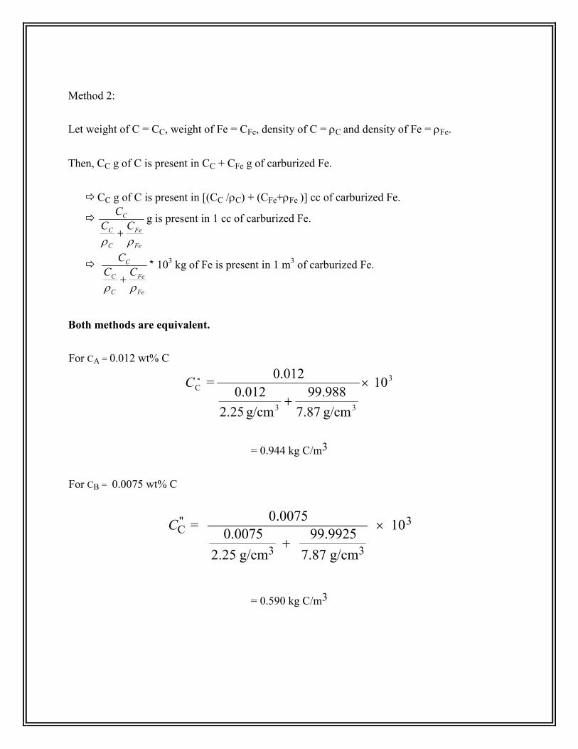
Method 2:

Let weight of C = CC, weight of Fe = CFe, density of C = ρC and density of Fe = ρFe.

Then, CC g of C is present in CC + CFe g of carburized Fe.

� CC g of C is present in [(CC /ρC) + (CFe+ρFe )] cc of carburized Fe.

�

Fe

Fe

C

C

C

CC

C

ρρ +

g is present in 1 cc of carburized Fe.

�

Fe

Fe

C

C

C

CC

C

ρρ +

* 103 kg of Fe is present in 1 m

3 of carburized Fe.

Both methods are equivalent.

For CA = 0.012 wt% C

3

33

C 10

g/cm 87.7

988.99

g/cm 25.2

012.0

012.0 = ×

+

"C

= 0.944 kg C/m3

For CB = 0.0075 wt% C

CC" =

0.0075

0.0075

2.25 g/cm3 +

99.9925

7.87 g/cm3

× 103

= 0.590 kg C/m3

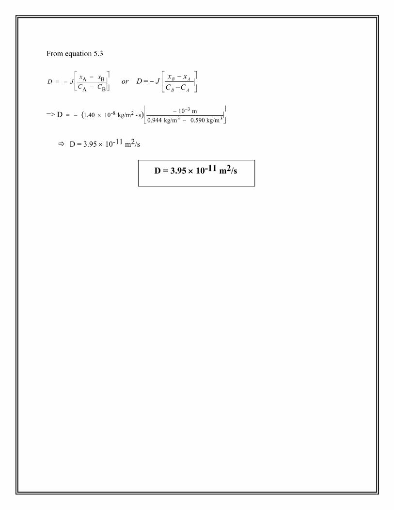
From equation 5.3

D = − J xA − xB

CA − CB

−

−−

=

A B

AB

CC

xxJD or

=> D = − (1.40 × 10-8 kg/m2 - s)− 10−3 m

0.944 kg/m3 − 0.590 kg/m3

� D = 3.95 × 10-11 m2/s

D = 3.95 ×××× 10-11 m2/s

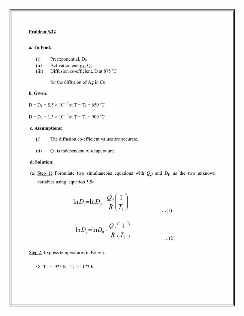
Problem 5.22

a. To Find:

(i) Preexponential, D0

(ii) Activation energy, Qd

(iii) Diffusion co-efficient, D at 875 oC

for the diffusion of Ag in Cu.

b. Given:

D = D1 = 5.5 × 10–16

at T = T1 = 650 oC

D = D2 = 1.3 × 10–13

at T = T2 = 900 oC

c. Assumptions:

(i) The diffusion co-efficient values are accurate.

(ii) Qd is independent of temperature.

d. Solution:

(a) Step 1: Formulate two simultaneous equations with Qd and D0 as the two unknown

variables using equation 5.9a

−=

1

01

1lnln

TR

QDD d

…(1)

−=

2

02

1lnln

TR

QDD d

…(2)

Step 2: Express temperatures in Kelvin.

� T1 = 923 K ; T2 = 1173

K

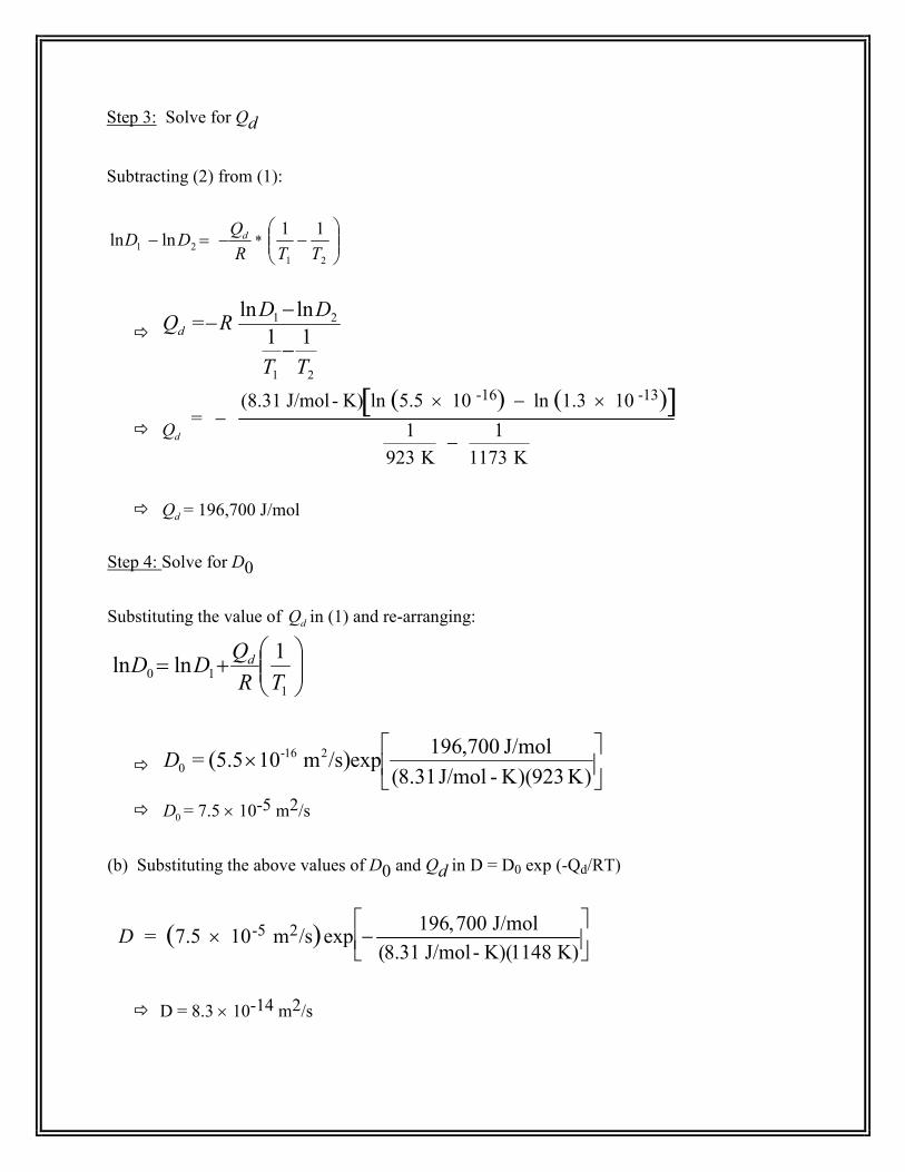
Step 3: Solve for Qd

Subtracting (2) from (1):

1lnD =− 2lnD R

Qd− *

−

21

11

TT

�

21

21

11

lnln =

TT

DDRQd

−

−−

� dQ = −

(8.31 J/mol - K) ln (5.5 × 10 -16) − ln (1.3 × 10 -13)[ ]1

923 K−

1

1173 K

� dQ = 196,700 J/mol

Step 4: Solve for D0

Substituting the value of dQ in (1) and re-arranging:

+=

1

10

1lnln

TR

QDD d

�

×

)K 923)(K-J/mol 31.8(

J/mol 700,196exp/sm 10 5.5 = )( 216-

0D

� 0D = 7.5 × 10-5 m2/s

(b) Substituting the above values of D0 and Qd in D = D0 exp (-Qd/RT)

D = (7.5 × 10-5 m2/s)exp −196,700 J/mol

(8.31 J/mol- K)(1148 K)

� D = 8.3 × 10-14 m2/s

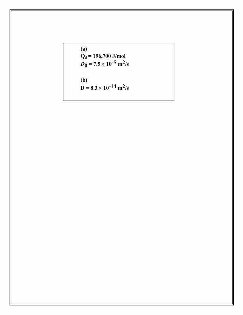
(a)

Qd = 196,700 J/mol

D0 = 7.5 ×××× 10-5 m2/s

(b)

D = 8.3 ×××× 10-14 m2/s

Problem 5.23

a. To Find:

Activation energy, Qd and prponeeexntial, D0 for the diffusion of Fe in Cr.

b. Given:

Plot of log10D versus 1000/T.

c. Assumptions:

(i) Qd is independent of temperature.

(ii) The plot is accurate.

d. Solution:

Step 1:

ln D = ln D0 – (Qd/RT) …(1)

� log D = log D0 – (Qd/2.303RT)

� The slope of the log D vs 1/T curve equals – Qd/2.303 R.

Step 2:

We could read the plot of log10D versus 1000/T as log10D versus 1/T if we multiplied the values

on the 1000/T axis with 10-3.

There are a certain points to keep in mind while reading the plot, as mentioned in Example

Problem 5.5:

(i) The actual D values and not the log D values are noted on the vertical axis.

(ii) The y-axis is on a log scale, so, a point midway between 10-15

and 10-16

is 10-15.5

and

not 5*10-16

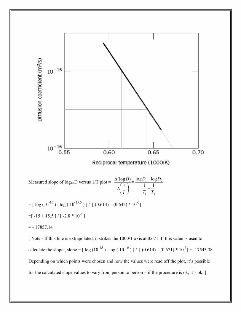
Measured slope of log10D versus 1/T plot =

21

21

11

loglog =

1

)(log

TT

DD

T

D

−

−

∆

∆

= [ log (10-15

) –log ( 10-15.5

) ] / [ (0.614) – (0.642) * 10-3]

=[ -15 + 15.5 ] / [ -2.8 * 10-5 ]

= - 17857.14

[ Note - If this line is extrapolated, it strikes the 1000/T axis at 0.671. If this value is used to

calculate the slope , slope = [ log (10-15

) –log ( 10-16

) ] / [ (0.614) – (0.671) * 10-3] = -17543.38

Depending on which points were chosen and how the values were read off the plot, it’s possible

for the calculated slope values to vary from person to person – if the procedure is ok, it’s ok. ]

Step 3:

From the above steps,

– Qd/2.303 R = - 17857.14

�

=> Qd = 2.303 * 8.314 * 17857.14 = 341913 J/mol or 3.something * 105 J/mol

Step 4:

Using

D0 = D expQd

RT

D0 = 10-15

exp (341913*0.614*10-3/8.314)

�

D0 = 9.25 * 10-5 m

2/s

[Note – If a different value of Qd is used, the value of D0 would be significantly different.

If the calculated value of slope is taken to be -17543.38, Qd = 335905 J/mol and D0 =

5.93 * 10-5. If the answer is of the same order and if the procedure is correct, it’s ok. ]

Qd ≈ 3 * 105 J/mol

D0 of the order of 10-5

m2/s

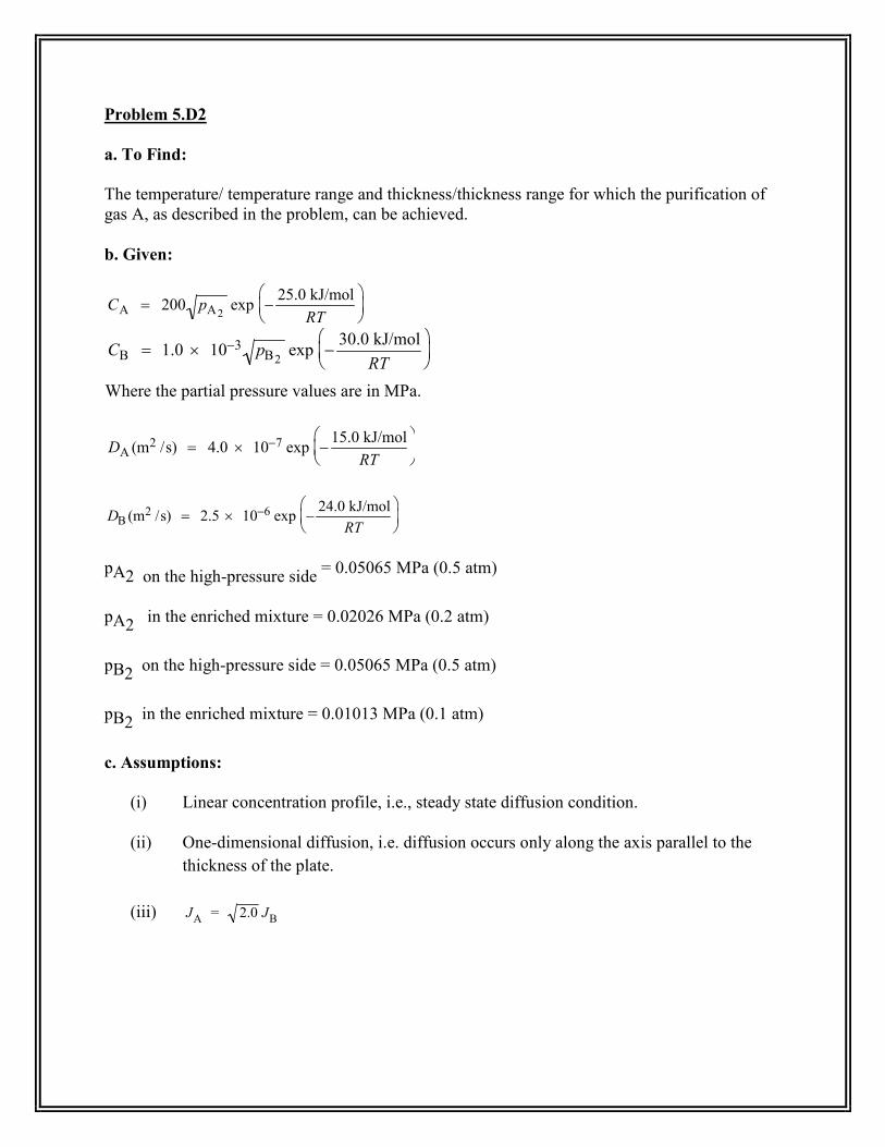
Problem 5.D2

a. To Find:

The temperature/ temperature range and thickness/thickness range for which the purification of

gas A, as described in the problem, can be achieved.

b. Given:

CA = 200 pA2

exp −25.0 kJ/mol

RT

CB = 1.0 × 10−3 pB2

exp −30.0 kJ/mol

RT

Where the partial pressure values are in MPa.

DA (m2 /s) = 4.0 × 10−7 exp −

15.0 kJ/mol

RT

DB (m

2 /s) = 2.5 × 10−6 exp −24.0 kJ/mol

RT

pA2 on the high-pressure side

= 0.05065 MPa (0.5 atm)

pA2 in the enriched mixture = 0.02026 MPa (0.2 atm)

pB2 on the high-pressure side = 0.05065 MPa (0.5 atm)

pB2 in the enriched mixture = 0.01013 MPa (0.1 atm)

c. Assumptions:

(i) Linear concentration profile, i.e., steady state diffusion condition.

(ii) One-dimensional diffusion, i.e. diffusion occurs only along the axis parallel to the

thickness of the plate.

(iii) JA = 2.0 JB

d. Solution:

If it is assumed that JA = 2.0 JB ,

Only then,

JA

=

1

∆x×

(200) 0.05065 MPa − 0.02026 MPa( ) exp −25.0 kJ

RT

(4.0 × 10−7 m2 /s)exp −

15.0 kJ

RT

= 2.0 JB

=

2.0

∆x×

(1.0 × 103) 0.05065 MPa − 0.01013 MPa( )exp −

30.0 kJ

RT

(2.5 × 10−6m2 /s)exp −

24.0 kJ

RT

� T = 395 K

The ∆x term always cancels out and hence, the purification occurs for all values of the thickness

of the sheet.

If no relation is assumed between Ja and Jb, it is possible to say that:

Based on the partial pressure values given, it is always possible to calculate Ja and Jb for all

temperatures and all thicknesses>0. As long as the 'concentrations' are reaching the desired

values, we don't really need to compare Ja and Jb. Thus, given that diffusion is steady state, it

appears that there are no restrictions on the values of temperature or thickness for the purification

to take place.

T = 395 K

Purification occurs independent of the thickness of the sheet