HVDC loss factors in the Nordic MarketAndrea Tosatto and Spyros Chatzivasileiadis

Dept. of Electrical Engineering, Technical University of Denmark, 2800 Kgs. Lyngby, Denmark{antosat, spchatz}@elektro.dtu.dk

Abstract—In the Nordic region, many interconnectors areformed by long High-Voltage Direct-Current (HVDC) lines.Every year, the operation of such interconnectors costs millionsof Euros to Transmission System Operators (TSOs) due to thehigh amount of losses that are not considered while clearing themarket. To counteract this problem, Nordic TSOs have proposedto introduce linear HVDC loss factors in the market clearingalgorithm. The assessment of such a measure requires a detailedmodel of the system under investigation. In this paper we developand introduce a detailed market model of the Nordic countriesand we analyze the impact of different loss factor formulations.We show that linear loss factors penalize one HVDC line overthe other, and this can jeopardize revenues of merchant HVDClines. In this regard, we propose piecewise-linear loss factors:a simple to implement but highly effective solution. Moreover,we demonstrate how the introduction of only HVDC loss factorsis a partial solution, since it disproportionally increases the AClosses. Our results show that the inclusion of AC loss factors caneliminate this problem.

Index Terms—Electricity markets, HVDC losses, HVDC trans-mission, loss factors, market operation, Nordics, power losses,zonal pricing.

I. INTRODUCTION

Over the last decades, more than 25,000 km of High-Voltage Direct-Current (HVDC) lines have been graduallyintegrated to the existing pan-European HVAC system. Thanksto their technical properties, HVDC lines allow the connectionof asynchronous areas and represent a cost-effective solutionfor long-distance submarine cables. For these two reasons,many interconnectors in the Nordic region are formed byHVDC lines. Contrary to AC ones, HVDC interconnectorsare often hundreds of kilometers long and produce a non-negligible amount of power losses, which are not consideredin the current market clearing process. In case of equal zonalprices between neighboring bidding zones, the cost of HVDClosses cannot be covered because of the zero-price-difference,and the cost is transferred to local Transmission SystemOperators (TSOs) who must procure sufficient power to coverthese losses. The problem is especially pronounced in transitcountries, as in the case of Denmark.

TABLE I shows the hours of operation with zero-price-difference of five intra-Nordic HVDC interconnectors andthe corresponding cost of losses in 2017 and 2018 [1]. Forexample, in 2017 the price difference between SE3 and FI,

This work is supported by the multiDC project, funded by Innovation FundDenmark, Grant Agreement No. 6154-00020B.

connected by Fennoskan [2], was zero for 8672 hours (99%of the time). During these hours, Svenska kraftnat paid half ofthe losses on the interconnector for exporting power to Finlandwithout recovering this cost through any price difference. Forthis interconnector, the cost of losses is 4 million Euros peryear on average.

In order to reduce costs, TSOs procure the necessarypower for covering losses in the day-ahead market. Basedon statistical data and load predictions, TSOs forecast lossesand place price-independent bids before the market is cleared;any mismatch is then covered during the balancing stage. Forlosses on interconnectors, since they are usually co-owned byTSOs, there exist special agreements, e.g. for Fennoskan alllosses are purchased by the exporting TSO (mostly Svenskakraftnat) and the importing TSO financially compensates halfof them. At the end, TSOs recover the cost of losses throughgrid tariffs.

Due to the high cost of HVDC losses, Nordic TSOs haveproposed the introduction of HVDC loss factors to implicitlyaccount for losses when the market is cleared [3]–[5]. The in-troduction of loss factors will force a price difference betweenthe two connected bidding zones that is equal to the marginalcost of losses. On the one hand, HVDC losses are no longerneeded to be purchased by TSOs in the day-ahead market butare directly paid by the market participants who create them;on the other hand, losses are implicitly minimized, resultingin cost savings for TSOs and the society.

The proposed loss factors are linear approximations of thequadratic loss functions [6]. The following questions arise: arelinear loss factors a good representation of quadratic losses? Isthe introduction of loss factors for only HVDC interconnectorsthe best possible action?

In [7], we have introduced a rigorous framework for ana-lyzing the inclusion of loss factors in the market clearing. Theresults showed that HVDC loss factors may lead to a decreaseof the social welfare for a non-negligible amount of time as

TABLE ICOST OF HVDC LOSSES

2017 2018

% LOSSES % LOSSESKONTISKAN 61% 1.2 Me 53% 1.5 MeSTOREBÆLT 73% 0.8 Me 74% 1.1 MeSKAGERRAK 47% 3.2 Me 46% 4.7 MeESTLINK 76% 3.1 Me 95% 6.7 MeFENNOSKAN 99% 3.8 Me 80% 4.2 Me

Total 12 Me 18 Me

arX

iv:1

910.

0560

7v1

[m

ath.

OC

] 1

2 O

ct 2

019

they may disproportionately increases the AC losses dependingon the topology of the system under investigation. Indeed, inmeshed grids there might exist parallel HVDC paths, or ACparallel paths to HVDC interconnectors, and the solver willchoose one option over the other based on approximationsof the quadratic loss functions, which might not be veryaccurate. For this reason, this paper aims at introducing adetailed market model of the Nordic countries and analyzingthe introduction of HVDC loss factors in the Nordic market.Moreover, the formulation used in [7] included losses in theform of inequality constraints: this relaxation is exact whenall prices are positive. In real power systems prices can benegative, thus an exact formulation with binary variables ispresented in this paper. More specifically, the contributions ofthis paper are the following:

• the introduction of a formulation with binary variablesfor covering the situations with negative prices;

• a detailed market model of the Nordic countries;• a rigorous analysis and recommendations on the imple-

mentation of implicit grid losses on HVDC interconnec-tors in the Nordics.

The paper is organized as follows. Section II describesthe market clearing algorithm with implicit grid losses usingbinary variables. Section III outlines the test case representingthe Nordic countries. Section IV presents the analyses on theintroduction of loss factors in the Nordics and Section Vgathers conclusions and final remarks.

II. FORMULATION

In the market clearing algorithm presented in [7], lossfunctions are included in the form of two inequality con-straints. This relaxation was adopted to keep the problem linearand convex, without the introduction of binary variables orabsolute operators. In [7], we proved that this relaxation isalways exact if Locational Marginal Prices (LMPs) are allpositive. If this condition is not satisfied, artificial losses arecreated by the solver to reduce the objective value.

Negative prices occur in reality [8]–[10], for example, inGermany electricity reached its lowest price of -52e/MWhin October 2017. This often happens during periods withlow demand and high renewable generation, when inflexiblegenerating units find more convenient to offer electricity fornegative prices than shutting down their plants.

For this reason, when it comes to test cases representingreal power systems, binary variables must be introduced toavoid artificial losses. In this section, a formulation with binaryvariables of the market clearing algorithm with implicit gridlosses is presented.

A. Market Clearing Problem

In the Nordic countries, as for the rest of Europe, a zonal-pricing scheme is applied. This means that the system is splitinto several bidding zones and the intra-zonal network is notincluded in the market model. When the market is cleared, asingle price per zone is defined. In case of congestion, pricedifferences arise only among zones [11].

The current day-ahead market coupling is based on Avail-able Transfer Capacity (ATC). In the day-ahead time frame,TSOs calculate ATCs based on the network situation andcommunicate them to the market operator. These values areused as bounds for inter-zonal power transfers in the spot-market. When the power exchanges are defined, TSOs managethe physical flows to guarantee these transactions and, ifnecessary, counter-trade at their own cost [12].

ATCs are computed as follows. First, TSOs calculate theTotal Transfer Capacity (TTC) based on thermal, voltage andstability limits. The TTC is reduced by the TransmissionReliability Margin (TRM), which covers the forecast uncer-tainties of tie-line power flows. This new value is referredto as Net Transfer Capacity (NTC). The ATC is calculated bysubtracting the Notified Transmission Flow (NTF) to the NTC.NTFs are the flows due to already accepted transfer contractsat the time of ATC calculation [12].

The difference between ATC-based and flow-based marketcoupling is that, in the first, congestion management is im-plicitly embedded in the market clearing by means of reducedcapacities, while in the second, it is explicitly embeddedthrough power flow constraints [13].

In its simplest form, the market-clearing algorithm based onATC can be formulated as the following optimization problem:

ming,f AC,f DC

cᵀg (1a)

s.t. G ≤ g ≤ G (1b)

−ATCAC ≤ f AC ≤ ATCAC(1c)

−ATCDC ≤ f DC ≤ ATCDC(1d)

IDD − IGg + IDCf DC + IACf AC + p loss = 0 (1e)

where c is the linear coefficient of generators’ cost functions,g is the output level of generators, D is the demand, IG and ID

are the incidence matrices of generators and load, G and Gare respectively the minimum and maximum generation levelof each generating unit, f AC and f DC are the power flows overAC and HVDC lines, IAC and IDC are the incidence matrices ofAC and HVDC lines, ATCAC and ATCDC are the availabletransfer capacities of AC and HVDC lines (lower and upperbars indicate in which direction) and p lossN are the losses.For now, it is assumed that losses are just parameters in theoptimization problem, which are estimated by TSOs using off-line models before the market is cleared.

The objective of the market operator is to minimize thesystem cost, expressed in (1a) as the sum of generator costs.Constraint (1b) enforces the lower and the upper limits ofgeneration, while constraints (1c) and (1d) ensure that linelimits are not exceeded and constraint (1e) enforces the powerbalance in each zone.

B. Linear Loss Functions

When linear loss functions are included in the model,constraints (1c) and (1d) are replaced by the following set

of constraints:

f = f+ − f− (2a)

0 ≤ f+ ≤ bATC (2b)

0 ≤ f− ≤ (1− b)ATC (2c)

p loss = α(f+ + f−) + β (2d)

with b ∈ {0, 1}. When b is equal to 1, f is positive and whenb is equal to 0, f is negative. In both cases, f+ and f− arepositive and can be used for calculating losses in (2d).

C. Piecewise-linear Loss FunctionsIn case of piecewise-linear approximation of loss functions,

constraints (1c) and (1d) are replaced by the following set ofconstraints:

f =

K∑k=1

f+k −

K∑k=1

f−k (3a)

(b+k − b+k+1)F k−1 ≤ f+

k ≤ (b+k − b+k+1)F k ∀k 6= K (3b)

(b+K)FK−1 ≤ f+K ≤ (b+K)FK (3c)

(b−k − b−k+1)F k−1 ≤ f−

k ≤ (b−k − b−k+1)F k ∀k 6= K (3d)

(b−K)FK−1 ≤ f−K ≤ (b−K)FK (3e)

b+k ≥ b+k+1 ∀k 6= K (3f)

b−k ≥ b−k+1 ∀k 6= K (3g)

p loss =

K∑k=1

αk(f+k + f−

k ) +

+

K−1∑k=1

βk(b+k − b

+k+1 + b

−k − b

−k+1) +

+ βK(b+K + b−K)

(3h)

with k the index of the segments, b+k , b−k ∈ {0, 1}, F k−1 and

F k the extreme points of segment k (F k−1 = 0 for k = 1) andK the total number of segments. When f is positive (withinsegment k), all b−k are equal to 0, all b+k with k ≤ k are equalto 1, and all b+k with k > k are equal to 0. In (3h), losses arecalculated using the right segment of the loss function.

Constraints (2a)-(2d) and (3a)-(3h) are valid both for ACand HVDC lines and, depending on the lines where implicitgrid loss is implemented (AC, HVDC or both), they can beincluded in problem (1).

The losses calculated in (2d) or (3h) are introduced in thepower balance equation as follows:

IDD − IGg + IDCf DC + IACf AC +

+ DDCplossDC + DACplossAC = 0(4)

where DDC and DAC are respectively the loss distribution matrixfor HVDC and AC lines, which are defined as follows:

Dz,l =

{0.5, if line l is connected to zone z

0, otherwise(5)

It’s important to point out that, if all LMPs are positive, therelaxation introduced in [7] is exact and the above formulationproduces the same results as the one presented in [7].

III. NORDIC TEST CASE

The Nordic test case developed in this paper is the combina-tion of two sets of data: the transmission system data publishedby Energinet [14] and the Nordic 44 test network [15].

The dataset provided by Energinet contains the static dataof the 132-150-400-kV Danish transmission system as it wasin 2017, together with the developments planned for 2020.As it is not possible to publicly share system data from theSwedish system, we use the Nordic 44 test network, whichrepresents with sufficient accuracy an equivalent of Sweden,Norway and Finland. The test case was initially developed fordynamic analyses and then adjusted in a variety of ways to beused for different purposes, reliability analyses [16] and NordPool market modeling [17] among others.

The two data sets are merged to obtain a detailed model ofthe Nordic power grid, which is described in this section. Allthe data is publicly available in a depository in GitHub [18].

A. System Topology

The test case comprises electrical nodes from three asyn-chronous areas:

• Nordic: Eastern Denmark, Norway, Sweden and Finland;• UCTE: Western Denmark, Germany, Poland and the

Netherlands;• Baltic: Estonia, Lithuania and Russia.

The focus of the test case is on the Nordic power grid,thus neighboring countries (Germany, the Netherlands, Poland,Lithuania, Estonia and Russia) are included in the modelonly for representing power exchanges. For this reason, onlyinterconnectors between Nordic countries and neighbors areconsidered, i.e. the connections between Poland and Germany,for example, are not modeled. The following interconnectorsare included in the model:

- NorNed: Norway-Netherlands, HVDC;- East coast corridor: Western Denmark-Germany, AC;- Skagerrak: Norway-Western Denmark, HVDC;- Kontiskan: Western Denmark-Sweden, HVDC;- Storebælt: Western Denmark-Eastern Denmark, HVDC;- Kontek: Eastern Denmark-Germany, HVDC;- Baltic cable: Sweden-Germany, HVDC;- SwePol: Sweden-Poland, HVDC;- NordBalt: Sweden-Lithuania, HVDC;- Estlink: Finland-Estonia, HVDC;- Vyborg HVDC: Finland-Russia, back-to-back HVDC.

The system consists of 368 buses, where Western and EasternDenmark account for 262 buses, Norway for 48 buses, Swedenfor 38 buses and Finland for 11 buses. The remaining busesrepresent the neighboring countries: 4 buses for Germany and5 buses for the Netherlands, Poland, Lithuania, Estonia andRussia. Neighboring countries are modeled with conventionalloads which can be negative (export) or positive (import).

B. Generation

For each country, a large number of generators is included,for a total of 390 units. Generator data have been obtained

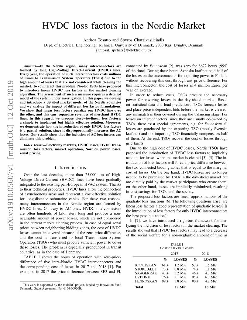
LEGEND:400-420kV node300kV node132-150kV nodeNeighboring country400-420kV AC line300kV AC line132-150kV AC lineAC interconnectorDC interconnector

Den

mar

k

Swed

en

Norway

Finland

TheNetherlands Germany Poland

Lithuania

Estonia

Russia

Fig. 1. Nordic power grid.

from different datasets. All the units listed in ENTSO-E Trans-parency Platform [19] are included; however, since ENTSO-Eprovides only the data of the major production units, additionalgenerating units (mainly hydro-power plants) were added tomeet the actual production of each country. The geographicallocation of generators in [19] was used to distribute themamong buses. The cost of production of each unit is basedon the generation type, according to [20]. Among units of thesame type, the production cost is assumed to decrease withincreasing plant size.

A large number of wind farms and PV power stations isincluded in the model, for a total of 122 wind farms and 119PV stations. For Norwegian, Swedish and Finnish wind farms,their location is based on [21]. For Denmark, Energinet dataset

TABLE IIGENERATION MIX [GW]

DK NO SE FI

Renewables

Biomass 0.36 - 0.10 0.66Hydro - 27.97 16.11 1.46Solar 0.50 - - -Wind 4.92 1.10 5.92 1.61

Fossil fuels

Gas 2.31 1.36 0.70 1.10Hard coal 1.87 - - 3.19Oil 0.07 - 2.25 0.76Peat - - 0.12 0.97

Nuclear - - 9.10 4.35

Other 0.20 - - 0.29

TOTAL 10.23 30.43 34.3 14.39

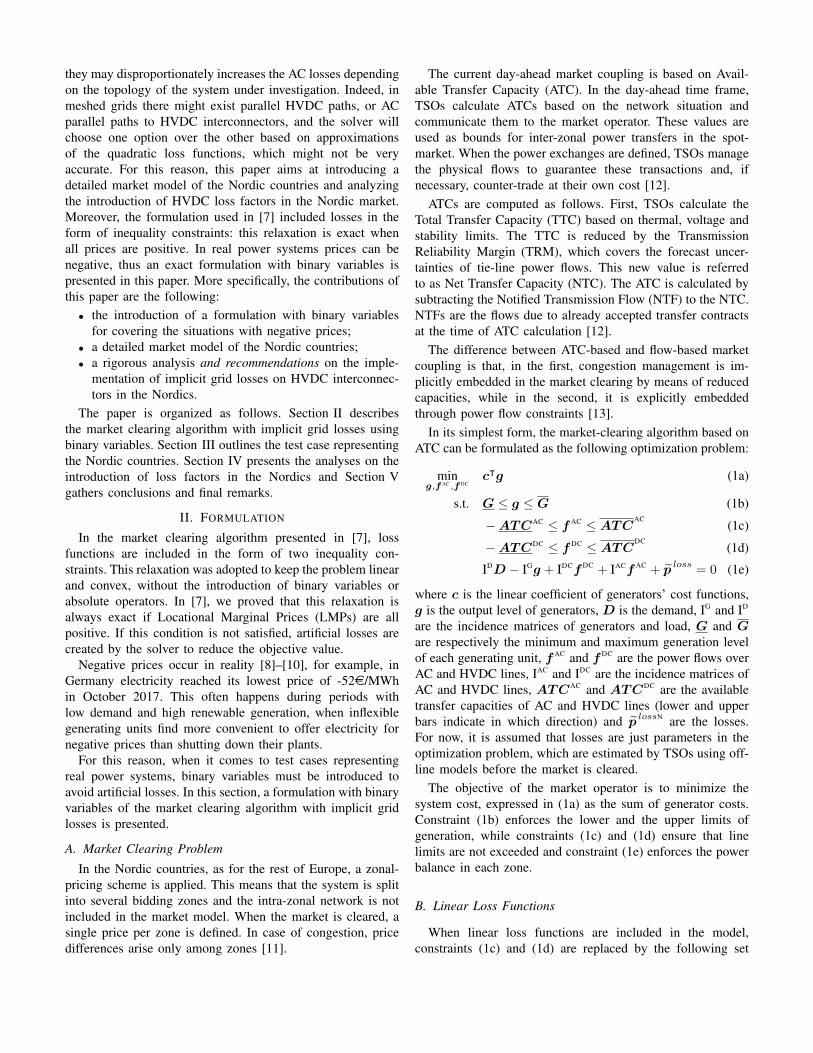
LEGEND:Bidding zoneAC interconnectorDC interconnector

NL DEPL

LT

EE

RU

DK1

DK2

SE4

SE3

SE2

SE1

FI

NO1

NO2

NO3

NO4

NO5

Fig. 2. Nordic market model.

contains all the wind farms and PV stations aggregated up tothe appropriate transmission substation. Both wind farms andPV stations are modeled as negative loads, and their outputsvary according to the wind and solar profile of each area.The wind profiles for Sweden and Denmark are obtained fromNord Pool [1], the wind profile for Finland from Fingrid [22]and for Norway from ENTSO-E [19]. The PV production ofDenmark is obtained from Energinet [23]. All the data referto the actual production in 2017 and the whole time series isused for the analyses in Section IV.

The generation mix of each country is provided in TA-BLE II, together with the total installed capacity.

C. Demand

All the original loads are kept in the model, for a total of 142loads. These loads are considered as the aggregation of all thedistribution loads to the proper transmission substation. Onlythe loads in Oslo and Oskarshamn have been spread amongthe neighboring nodes to avoid infeasibilities in the solutionof the optimization problem. The actual consumption of eacharea is taken from Nord Pool [1] and zonal load profiles areused to vary their consumption. All the data refer to the actualconsumption in 2017 and the whole time series is used for theanalyses in Section IV.

D. Transmission Network

The Nordic transmission network is divided into two asyn-chronous Regional Groups (RGs): Western Denmark is con-nected to Continental Europe (UCTE) and, thus, it is operatedat a different frequency from the rest of the Nordic countries.

Western Denmark counts 140 transmission lines (400 and150 kV) and 40 power transformers. The Nordic grid counts221 AC transmission lines (400 and 132 kV in EasternDenmark, 420 and 300 kV in Sweden, Finland and Norway),one HVDC line (Fennoskan, Sweden-Finland) and 114 powertransformers.

Western Denmark is connected to Germany through differ-ent AC lines, along a corridor which is usually referred to aseast coast corridor. Three HVDC links (Skagerrak, Kontiskanand Storebælt) connect Western Denmark to Norway, Swedenand Eastern Denmark.

RG Nordic is connected to Continental Europe throughfour additional HVDC links: NorNed (Norway-Netherlands),Kontek (Eastern Denmark-Germany), Baltic cable (Sweden-Germany) and SwePol (Sweden-Poland). Three other HVDClinks connect RG Nordic to RG Baltic: NordBalt (Sweden-Lithuania), Estlink (Finland-Estonia) and Vyborg HVDC(Finland-Russia).

A schematic representation of the transmission network isdepicted in Fig. 1. For illustration purposes, not all Danishlines and substations are represented in this picture.

The market model is obtained by aggregating all the nodeswithin each bidding zone and neglecting the internal networks.Fig. 2 shows the different bidding zones in the Nordic area andthe equivalent interconnectors. ATCs on the interconnectorsare obtained from Nord Pool [1] for each hour of 2017.

IV. NUMERICAL SIMULATIONS

In this section, the analysis on the introduction of lossfactors in the Nordic region is carried out. Five simulationsare run considering different loss factors at a time:

1) No loss factors2) Linear HVDC loss factors3) Piecewise-linear HVDC loss factors4) Linear AC and HVDC loss factors5) Piecewise-linear AC and HVDC loss factors

In each simulation, the market is cleared for each hour of theyear (8760 instances) using data from 2017.

The focus of the analysis is on the differences betweenlinear and piecewise-linear loss factors and between HVDCand AC+HVDC loss factors.

It is important to mention that all the cost-benefit analysesare limited to the introduction of loss factors in the intra-Nordic interconnectors, that means Fennoskan, Skagerrak,Storebælt, Kontiskan and only the AC interconnectors ofRG Nordic. Indeed, the power exchanges with neighboringcountries are fixed to the real exchanges, and so are the flowson the interconnectors (becoming unresponsive to any changeintroduced by loss factors).

A. Linear and Piecewise-linear HVDC Loss Factors

For this analysis, the outcomes of simulations 1, 2 and 3are compared focusing on HVDC losses only. In simulation 1,to make a fair comparison, HVDC losses are first “estimated”solving the optimization problem (1). The estimated valuesare then included as price-independent bids of TSOs in the

DK1

DK2

SE4

SE3

NO2

NO1

NO5

SE3

SE2

SE1

FI

Skagerrak

Kontiskan

Storebælt

Fennoskan

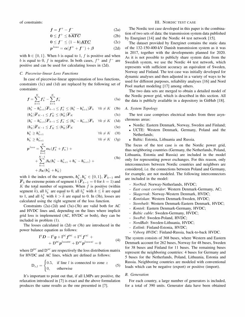
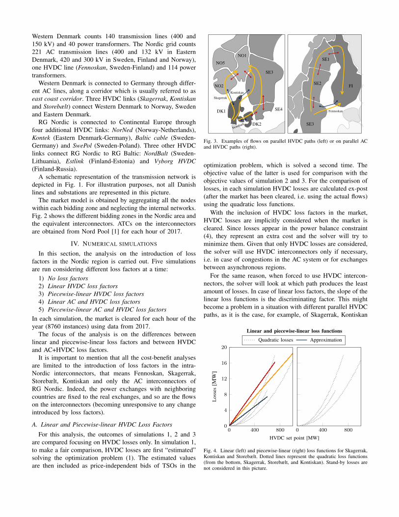
Fig. 3. Examples of flows on parallel HVDC paths (left) or on parallel ACand HVDC paths (right).

optimization problem, which is solved a second time. Theobjective value of the latter is used for comparison with theobjective values of simulation 2 and 3. For the comparison oflosses, in each simulation HVDC losses are calculated ex-post(after the market has been cleared, i.e. using the actual flows)using the quadratic loss functions.

With the inclusion of HVDC loss factors in the market,HVDC losses are implicitly considered when the market iscleared. Since losses appear in the power balance constraint(4), they represent an extra cost and the solver will try tominimize them. Given that only HVDC losses are considered,the solver will use HVDC interconnectors only if necessary,i.e. in case of congestions in the AC system or for exchangesbetween asynchronous regions.

For the same reason, when forced to use HVDC intercon-nectors, the solver will look at which path produces the leastamount of losses. In case of linear loss factors, the slope of thelinear loss functions is the discriminating factor. This mightbecome a problem in a situation with different parallel HVDCpaths, as it is the case, for example, of Skagerrak, Kontiskan

Los

ses

[MW

]

HVDC set point [MW]

Linear and piecewise-linear loss functions

0 400 8000

4

8

12

16

20

0 400 800

Quadratic losses Approximation

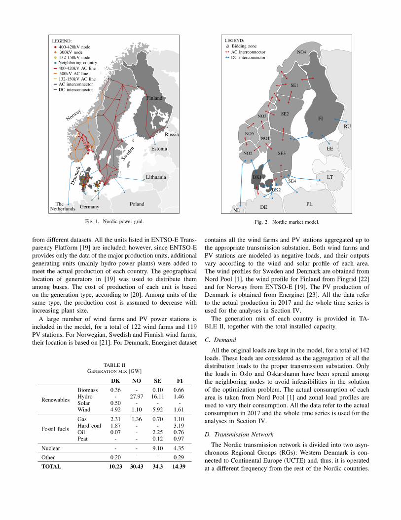
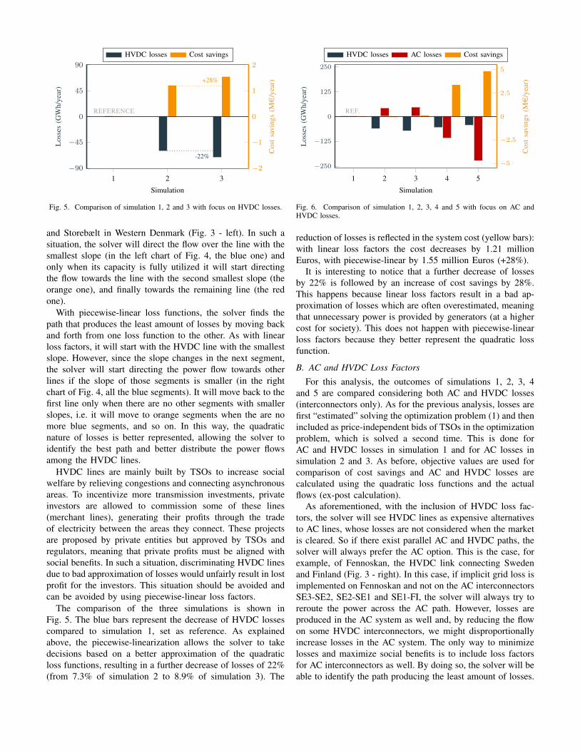
Fig. 4. Linear (left) and piecewise-linear (right) loss functions for Skagerrak,Kontiskan and Storebælt. Dotted lines represent the quadratic loss functions(from the bottom, Skagerrak, Storebælt, and Kontiskan). Stand-by losses arenot considered in this picture.

1 2 3−90

−45

0

45

90

Simulation

Los

ses

(GW

h/ye

ar)

HVDC losses Cost savings

−2

−1

0

1

2

Cos

tsa

ving

s(Me

/yea

r)

-22%

REFERENCE

+28%

Fig. 5. Comparison of simulation 1, 2 and 3 with focus on HVDC losses.

and Storebælt in Western Denmark (Fig. 3 - left). In such asituation, the solver will direct the flow over the line with thesmallest slope (in the left chart of Fig. 4, the blue one) andonly when its capacity is fully utilized it will start directingthe flow towards the line with the second smallest slope (theorange one), and finally towards the remaining line (the redone).

With piecewise-linear loss functions, the solver finds thepath that produces the least amount of losses by moving backand forth from one loss function to the other. As with linearloss factors, it will start with the HVDC line with the smallestslope. However, since the slope changes in the next segment,the solver will start directing the power flow towards otherlines if the slope of those segments is smaller (in the rightchart of Fig. 4, all the blue segments). It will move back to thefirst line only when there are no other segments with smallerslopes, i.e. it will move to orange segments when the are nomore blue segments, and so on. In this way, the quadraticnature of losses is better represented, allowing the solver toidentify the best path and better distribute the power flowsamong the HVDC lines.

HVDC lines are mainly built by TSOs to increase socialwelfare by relieving congestions and connecting asynchronousareas. To incentivize more transmission investments, privateinvestors are allowed to commission some of these lines(merchant lines), generating their profits through the tradeof electricity between the areas they connect. These projectsare proposed by private entities but approved by TSOs andregulators, meaning that private profits must be aligned withsocial benefits. In such a situation, discriminating HVDC linesdue to bad approximation of losses would unfairly result in lostprofit for the investors. This situation should be avoided andcan be avoided by using piecewise-linear loss factors.

The comparison of the three simulations is shown inFig. 5. The blue bars represent the decrease of HVDC lossescompared to simulation 1, set as reference. As explainedabove, the piecewise-linearization allows the solver to takedecisions based on a better approximation of the quadraticloss functions, resulting in a further decrease of losses of 22%(from 7.3% of simulation 2 to 8.9% of simulation 3). The

1 2 3 4 5

−250

−125

0

125

250

Simulation

Los

ses

(GW

h/ye

ar)

HVDC losses AC losses Cost savings

−5

−2.5

0

2.5

5

Cos

tsa

ving

s(Me

/yea

r)

REF.

Fig. 6. Comparison of simulation 1, 2, 3, 4 and 5 with focus on AC andHVDC losses.

reduction of losses is reflected in the system cost (yellow bars):with linear loss factors the cost decreases by 1.21 millionEuros, with piecewise-linear by 1.55 million Euros (+28%).

It is interesting to notice that a further decrease of lossesby 22% is followed by an increase of cost savings by 28%.This happens because linear loss factors result in a bad ap-proximation of losses which are often overestimated, meaningthat unnecessary power is provided by generators (at a highercost for society). This does not happen with piecewise-linearloss factors because they better represent the quadratic lossfunction.

B. AC and HVDC Loss Factors

For this analysis, the outcomes of simulations 1, 2, 3, 4and 5 are compared considering both AC and HVDC losses(interconnectors only). As for the previous analysis, losses arefirst “estimated” solving the optimization problem (1) and thenincluded as price-independent bids of TSOs in the optimizationproblem, which is solved a second time. This is done forAC and HVDC losses in simulation 1 and for AC losses insimulation 2 and 3. As before, objective values are used forcomparison of cost savings and AC and HVDC losses arecalculated using the quadratic loss functions and the actualflows (ex-post calculation).

As aforementioned, with the inclusion of HVDC loss fac-tors, the solver will see HVDC lines as expensive alternativesto AC lines, whose losses are not considered when the marketis cleared. So if there exist parallel AC and HVDC paths, thesolver will always prefer the AC option. This is the case, forexample, of Fennoskan, the HVDC link connecting Swedenand Finland (Fig. 3 - right). In this case, if implicit grid loss isimplemented on Fennoskan and not on the AC interconnectorsSE3-SE2, SE2-SE1 and SE1-FI, the solver will always try toreroute the power across the AC path. However, losses areproduced in the AC system as well and, by reducing the flowon some HVDC interconnectors, we might disproportionallyincrease losses in the AC system. The only way to minimizelosses and maximize social benefits is to include loss factorsfor AC interconnectors as well. By doing so, the solver will beable to identify the path producing the least amount of losses.

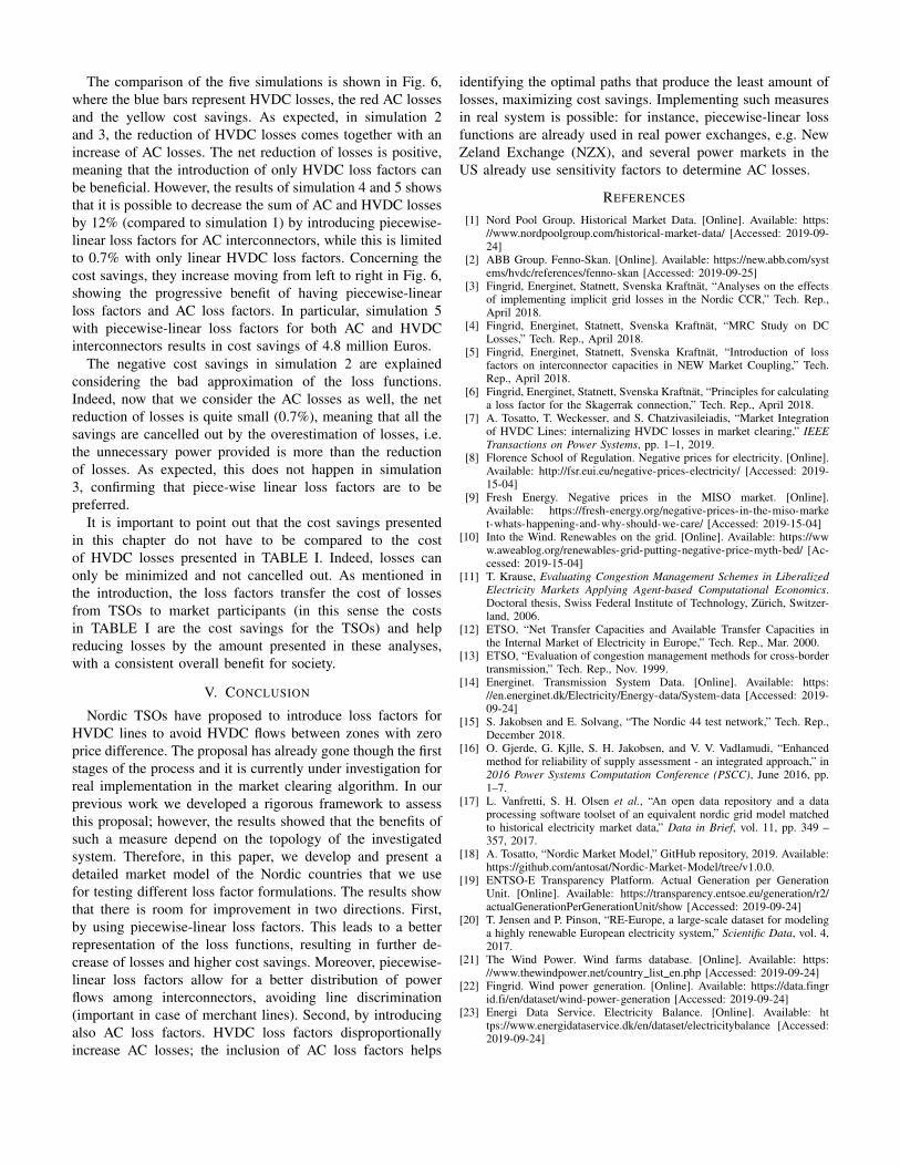
The comparison of the five simulations is shown in Fig. 6,where the blue bars represent HVDC losses, the red AC lossesand the yellow cost savings. As expected, in simulation 2and 3, the reduction of HVDC losses comes together with anincrease of AC losses. The net reduction of losses is positive,meaning that the introduction of only HVDC loss factors canbe beneficial. However, the results of simulation 4 and 5 showsthat it is possible to decrease the sum of AC and HVDC lossesby 12% (compared to simulation 1) by introducing piecewise-linear loss factors for AC interconnectors, while this is limitedto 0.7% with only linear HVDC loss factors. Concerning thecost savings, they increase moving from left to right in Fig. 6,showing the progressive benefit of having piecewise-linearloss factors and AC loss factors. In particular, simulation 5with piecewise-linear loss factors for both AC and HVDCinterconnectors results in cost savings of 4.8 million Euros.

The negative cost savings in simulation 2 are explainedconsidering the bad approximation of the loss functions.Indeed, now that we consider the AC losses as well, the netreduction of losses is quite small (0.7%), meaning that all thesavings are cancelled out by the overestimation of losses, i.e.the unnecessary power provided is more than the reductionof losses. As expected, this does not happen in simulation3, confirming that piece-wise linear loss factors are to bepreferred.

It is important to point out that the cost savings presentedin this chapter do not have to be compared to the costof HVDC losses presented in TABLE I. Indeed, losses canonly be minimized and not cancelled out. As mentioned inthe introduction, the loss factors transfer the cost of lossesfrom TSOs to market participants (in this sense the costsin TABLE I are the cost savings for the TSOs) and helpreducing losses by the amount presented in these analyses,with a consistent overall benefit for society.

V. CONCLUSION

Nordic TSOs have proposed to introduce loss factors forHVDC lines to avoid HVDC flows between zones with zeroprice difference. The proposal has already gone though the firststages of the process and it is currently under investigation forreal implementation in the market clearing algorithm. In ourprevious work we developed a rigorous framework to assessthis proposal; however, the results showed that the benefits ofsuch a measure depend on the topology of the investigatedsystem. Therefore, in this paper, we develop and present adetailed market model of the Nordic countries that we usefor testing different loss factor formulations. The results showthat there is room for improvement in two directions. First,by using piecewise-linear loss factors. This leads to a betterrepresentation of the loss functions, resulting in further de-crease of losses and higher cost savings. Moreover, piecewise-linear loss factors allow for a better distribution of powerflows among interconnectors, avoiding line discrimination(important in case of merchant lines). Second, by introducingalso AC loss factors. HVDC loss factors disproportionallyincrease AC losses; the inclusion of AC loss factors helps

identifying the optimal paths that produce the least amount oflosses, maximizing cost savings. Implementing such measuresin real system is possible: for instance, piecewise-linear lossfunctions are already used in real power exchanges, e.g. NewZeland Exchange (NZX), and several power markets in theUS already use sensitivity factors to determine AC losses.

REFERENCES

[1] Nord Pool Group. Historical Market Data. [Online]. Available: https://www.nordpoolgroup.com/historical-market-data/ [Accessed: 2019-09-24]

[2] ABB Group. Fenno-Skan. [Online]. Available: https://new.abb.com/systems/hvdc/references/fenno-skan [Accessed: 2019-09-25]

[3] Fingrid, Energinet, Statnett, Svenska Kraftnat, “Analyses on the effectsof implementing implicit grid losses in the Nordic CCR,” Tech. Rep.,April 2018.

[4] Fingrid, Energinet, Statnett, Svenska Kraftnat, “MRC Study on DCLosses,” Tech. Rep., April 2018.

[5] Fingrid, Energinet, Statnett, Svenska Kraftnat, “Introduction of lossfactors on interconnector capacities in NEW Market Coupling,” Tech.Rep., April 2018.

[6] Fingrid, Energinet, Statnett, Svenska Kraftnat, “Principles for calculatinga loss factor for the Skagerrak connection,” Tech. Rep., April 2018.

[7] A. Tosatto, T. Weckesser, and S. Chatzivasileiadis, “Market Integrationof HVDC Lines: internalizing HVDC losses in market clearing,” IEEETransactions on Power Systems, pp. 1–1, 2019.

[8] Florence School of Regulation. Negative prices for electricity. [Online].Available: http://fsr.eui.eu/negative-prices-electricity/ [Accessed: 2019-15-04]

[9] Fresh Energy. Negative prices in the MISO market. [Online].Available: https://fresh-energy.org/negative-prices-in-the-miso-market-whats-happening-and-why-should-we-care/ [Accessed: 2019-15-04]

[10] Into the Wind. Renewables on the grid. [Online]. Available: https://www.aweablog.org/renewables-grid-putting-negative-price-myth-bed/ [Ac-cessed: 2019-15-04]

[11] T. Krause, Evaluating Congestion Management Schemes in LiberalizedElectricity Markets Applying Agent-based Computational Economics.Doctoral thesis, Swiss Federal Institute of Technology, Zurich, Switzer-land, 2006.

[12] ETSO, “Net Transfer Capacities and Available Transfer Capacities inthe Internal Market of Electricity in Europe,” Tech. Rep., Mar. 2000.

[13] ETSO, “Evaluation of congestion management methods for cross-bordertransmission,” Tech. Rep., Nov. 1999.

[14] Energinet. Transmission System Data. [Online]. Available: https://en.energinet.dk/Electricity/Energy-data/System-data [Accessed: 2019-09-24]

[15] S. Jakobsen and E. Solvang, “The Nordic 44 test network,” Tech. Rep.,December 2018.

[16] O. Gjerde, G. Kjlle, S. H. Jakobsen, and V. V. Vadlamudi, “Enhancedmethod for reliability of supply assessment - an integrated approach,” in2016 Power Systems Computation Conference (PSCC), June 2016, pp.1–7.

[17] L. Vanfretti, S. H. Olsen et al., “An open data repository and a dataprocessing software toolset of an equivalent nordic grid model matchedto historical electricity market data,” Data in Brief, vol. 11, pp. 349 –357, 2017.

[18] A. Tosatto, “Nordic Market Model,” GitHub repository, 2019. Available:https://github.com/antosat/Nordic-Market-Model/tree/v1.0.0.

[19] ENTSO-E Transparency Platform. Actual Generation per GenerationUnit. [Online]. Available: https://transparency.entsoe.eu/generation/r2/actualGenerationPerGenerationUnit/show [Accessed: 2019-09-24]

[20] T. Jensen and P. Pinson, “RE-Europe, a large-scale dataset for modelinga highly renewable European electricity system,” Scientific Data, vol. 4,2017.

[21] The Wind Power. Wind farms database. [Online]. Available: https://www.thewindpower.net/country list en.php [Accessed: 2019-09-24]

[22] Fingrid. Wind power generation. [Online]. Available: https://data.fingrid.fi/en/dataset/wind-power-generation [Accessed: 2019-09-24]

[23] Energi Data Service. Electricity Balance. [Online]. Available: https://www.energidataservice.dk/en/dataset/electricitybalance [Accessed:2019-09-24]