Hurricane Weather Research and Forecasting (HWRF) · PDF file2 ACKNOWLEDGMENTS The authors...

1

Hurricane Weather Research and Forecasting

(HWRF) Model: 2011 Scientific Documentation

April 2011

Authors (in alphabetical order by last name):

Sundararaman Gopalakrishnan NOAA/AOML, Hurricane Research Division, Miami, FL

Qingfu Liu NOAA/NWS/NCEP/ Environmental Modeling Center, Camp Springs, MD

Timothy Marchok NOAA/OAR/Geophysical Fluid Dynamics Laboratory, Princeton, NJ

Dmitry Sheinin IMSG at NOAA/NWS/NCEP/ Environmental Modeling Center, Camp Springs, MD

Naomi Surgi Boulder, CO

Mingjing Tong NOAA/NWS/NCEP/ Environmental Modeling Center, Camp Springs, MD and UCAR, Boulder,CO

Vijay Tallapragada NOAA/NWS/NCEP/ Environmental Modeling Center, Camp Springs, MD

Robert Tuleya Center for Coastal Physical Oceanography, Old Dominion University, Norfolk, VA

Richard Yablonsky Graduate School of Oceanography, University of Rhode Island, Narragansett, RI

Xuejin Zhang RSMAS/CIMAS, University of Miami, Miami, FL

Editor: Ligia Bernardet

NOAA Earth System Research Laboratory, and CIRES / University of Colorado, Boulder, CO.

DEVELOPMENTAL TESTBED CENTER

2

ACKNOWLEDGMENTS

The authors wish to acknowledge the Development Tech Center (DTC) for facilitating the coordination of the writing of this document amongst the following institutions: NOAA/AOML, Hurricane Research Division ; NOAA/NWS/NCEP/ Environmental Modeling Center; NOAA/OAR/Geophysical Fluid Dynamics Laboratory; IMSG at NOAA/NWS/NCEP/ Environmental Modeling Center; Graduate School of Oceanography, University of Rhode Island; RSMAS/CIMAS, University of Miami; and NOAA Earth System Research Laboratory, Boulder, CO. The authors also wish to thank Carol Makowski of NCAR/RAL/JNT for providing edit support for this document and addressing a number of formatting issues.

3

TABLE OF CONTENTS

ACKNOWLEDGEMENTS ................................................................................................................................................................ 2

Introduction ......................................................................................................................................................................................... 5

1.0 HWRF Initialization ........................................................................................................................................................ 12

1.1 Introduction ........................................................................................................................................................... 13

1.2 HWRF cycling system ......................................................................................................................................... 12

1.3 Bogus vortex used in absence of previous 6‐h HWRF forecast or for weak storms ................. 15

1.4 Correction of vortex in previous 6‐H HWRF forecast ........................................................................... 15

1.4.1 Storm size correction ............................................................................................................................................. 15

1.4.2 Storm intensity correction ................................................................................................................................... 25

2.0 Princeton Ocean Model for Tropical Cyclones (POM‐TC) .................................................................................... 37

2.1 Introduction ............................................................................................................................................................. 37

2.2 Purpose ...................................................................................................................................................................... 38

2.3 Grid size, spacing, configuration, arrangement, coordinate system, and numerical scheme 38

3.0 Physics Packages in HWRF ............................................................................................................................................... 44

3.1 HWRF physics ......................................................................................................................................................... 44

3.2 Microphysics parameterization ...................................................................................................................... 45

3.3 Cumulus parameterization ................................................................................................................................ 46

3.4 Surface layer parameterization ....................................................................................................................... 48

3.5 Land‐surface model .............................................................................................................................................. 50

3.6 Planetary boundary layer parameterization .............................................................................................. 51

3.7 Atmospheric radiation parameterization .................................................................................................... 53

3.8 Physics interactions ............................................................................................................................................. 54

4.0 Moving Nest ............................................................................................................................................................................. 61

4

4.1 Grid design ................................................................................................................................................................ 61

4.2 Terrain treatment .................................................................................................................................................. 62

4.3 Fine grid initialization .......................................................................................................................................... 63

4.4 Boundary ................................................................................................................................................................... 63

4.5 Feedback ................................................................................................................................................................... 64

4.6 Movable nesting ..................................................................................................................................................... 65

4.7 Future work .............................................................................................................................................................. 65

5.0 Use of the GFDL Vortex Tracker ....................................................................................................................................... 66

5.1. Introduction ............................................................................................................................................................. 66

5.1.1 Purpose of the vortex tracker ............................................................................................................................. 66

5.1.2 Key issues in the design of a vortex tracker ................................................................................................ 67

5.2. Design of the tracking system ......................................................................................................................... 67

5.2.1 Input data requirements ....................................................................................................................................... 67

5.2.2 The search algorithm .............................................................................................................................................. 69

5.3. Parameters used for tracking ........................................................................................................................... 72

5.3.1 Description of the primary and secondary tracking variables ............................................................. 72

5.3.2 Computation of the mean position fix ............................................................................................................. 73

5.4. Intensity and wind radii parameters ........................................................................................................... 74

5.5. Tracker output ....................................................................................................................................................... 74

5.5.1 Description of the ATCF format ......................................................................................................................... 74

5.5.2 Output file with a modified ATCF format ....................................................................................................... 76

6. References .................................................................................................................................................................................. 78

5

An Introduction to the Hurricane Weather Research and Forecast (HWRF) System

The HWRF was transitioned into National Centers for Environmental Prediction (NCEP) operations for the 2007 hurricane season. Development of the HWRF began in 2002 at the NCEP/Environmental Modeling Center (EMC) in collaboration with NOAA’s Geophysical Fluid Dynamics Laboratory (GFDL) scientists and the University of Rhode Island (URI). To meet operational implementation requirements, it was necessary that the skill of the track forecasts from the HWRF and GFDL hurricane models be comparable. Since the GFDL model evolved as primary guidance for track prediction used by the National Hurricane Center (NHC), the Central Pacific Hurricane Center (CPHC) and the Joint Typhoon Warning Center (JTWC) after becoming operational in 1994, the strategy for HWRF development was to take advantage of the advancements made to improve track prediction through a focused collaboration between EMC, GFDL and URI and transition those modeling advancements to the HWRF. This strategy ensured comparable track skill to the GFDL forecasts for both the East Pacific and Atlantic (including Caribbean and Gulf of Mexico) basins. Additionally, features of the GFDL hurricane model that led to demonstrated skill for intensity forecasts, such as ocean coupling, upgraded air-sea physics and improvements to microphysics, were also captured in the newly developed HWRF system. The HWRF system is composed of the WRF model software infrastructure, the Non-Hydrostatic Mesoscale Model (NMM) dynamic core, the three-dimensional Princeton Ocean Model (POM), the NCEP coupler, and a physics suite tailored to the tropics, including air-sea interactions over warm water and under high wind conditions, and boundary layer and cloud physics developed for hurricane forecasts. Figure I.1 illustrates all components of HWRF supported by the Developmental Test Center (DTC), which also include the WRF Pre-processor (WPS), a vortex initialization package, the three-dimensional variational data assimilation system (3D-VAR) Gridpoint Statistical Interpolator (GSI), the Unified Post-processor, and the GFDL vortex tracker. It should be noted that, although the HWRF uses the same dynamic core as the NCEP North American Mesoscale (NAM) model, the NMM, the HWRF is a very different forecast system from the NAM and was developed specifically for hurricane/tropical forecast applications. The HWRF is configured with a parent grid and a high-resolution movable 2-way nested grid that follows the storm, is coupled to a three-dimensional ocean model and also differs from the NAM in its physics suite and diffusion treatment. The HWRF also contains a sophisticated initialization of both the ocean and the storm scale circulation. Additionally, unlike other NCEP forecast systems which run continuously throughout the year, the hurricane models, e.g. both the HWRF and the GFDL models, are launched for operational use only when NHC determines that a disturbed area of weather has the potential to evolve into a depression anywhere over NHC’s area of responsibility. After an initial HWRF or GFDL run is triggered, new runs are launched in cycled mode until either the storm dissipates after making landfall or becomes extratropical or degenerates into a remnant low, typically identified when convection becomes disorganized around the center of circulation. Currently, the HWRF runs in NCEP operations four times daily producing 5-day forecasts of mainly track and intensity to meet NHC operational forecast and warning process objectives.

6

Figure I.1. Components of the HWRF system. These include WPS, the vortex initialization, GSI, the HWRF atmospheric model, the atmosphere-ocean coupler, the ocean initialization, the POM, the post processor and the vortex tracker.

Since its initial operational implementation in 2007, various upgrades have been made to HWRF physics, to the vortex initialization and to the ocean initialization, particularly in the Gulf of Mexico. This documentation provides a description of the most recent version of the operational HWRF system (functionally equivalent to the model implemented for the 2011 hurricane season); however it needs to be emphasized that every year, prior to the start of the Eastern Pacific and Atlantic hurricane seasons (15 May and 1 June respectively), HWRF upgrades are provided to NHC by EMC so that NHC forecasters have improved hurricane guidance at the start of each new hurricane season. These upgrades are chosen based on extensive testing and evaluation (T&E) of model forecasts for at least two recent past hurricane seasons. The list of upgrades to the HWRF for the 2010 and 2011 hurricane seasons are available on EMC’s HWRF website: http://www.emc.ncep.noaa.gov/HWRF/index.html. These will also be made available on the WRF for Hurricanes website hosted by DTC (http://www.dtcenter.org/HurrWRF/users). The following paragraphs present an overview of the sections contained in this documentation. A concluding paragraph provides proposed future enhancements of the HWRF system for advancing track, intensity and structure prediction, along with modeling advancements to address issues of coastal inundation for landfalling storms.

7

HWRF Atmospheric Initialization

The HWRF vortex initialization consists of several major steps: definition of the HWRF domain based on the observed storm center position; interpolation of the analyzed NCEP global model fields onto the HWRF parent domain, removal of the global model vortex and insertion of a mesoscale vortex obtained from the previous cycle’s HWRF 6-hr forecast (if available) or from a synthetic vortex (cold start). The modification of the mesoscale hurricane vortex in the first guess field is a critical aspect of the initialization problem. Modification includes corrections to the storm size, intensity and to the three-dimensional structure. Each of these corrections requires careful rebalancing between the model winds, temperature, pressure and moisture fields. A detailed treatment of this procedure is described in Section 1. An advancement of the HWRF system over the GFDL model bogus vortex initialization is the capability of the HWRF to run in cycle to improve the 3-dimensional structure of the hurricane vortex. This capability provides a significant opportunity to add more realistic structure to the forecast storm and is a critical step towards advancing hurricane intensity/structure prediction. The operational HWRF initialization procedure mentioned above and described in Section 1 utilizes the community GSI. Apart from conventional observations, clear-sky radiance datasets from several geostationary and polar orbiting satellites are assimilated in the hurricane environment using GSI. At present, inner-core conventional observations (within 150 km from the storm center) are excluded from the data assimilation procedure. Section 1 provides more details on the application of GSI within the HWRF modeling system. Starting in 2011, DTC is providing support for the use of the community GSI in HWRF. It should be noted that to support future data assimilation efforts for the hurricane core, NOAA acquired the GIV aircraft in the mid 1990’s to supplement the radar-based data obtained by NOAA’s P-3s. The high altitude of the GIV allow for observations to help define the 3-dimensional core structure from the outflow layer to the near surface. For storms approaching landfall, the coastal 88-D high resolution radar data is also available. Observations from aircraft Tail Doppler Radar from NOAA-P3s are currently ingested in HWRF on experimental basis. In order to make use of these newly expanded observations, several advanced data assimilation techniques are being explored within the operational and research hurricane modeling communities, e.g., GSI, Ensemble Kalman Filter (EnKF), 4D-VAR, and a hybrid method consisting of both an EnKF and 3D-VAR/4D-VAR. The improvement of hurricane initialization has become a top priority in both the research and operational communities. Although much progress has been made in assimilating observations to improve the hurricane environment analyses, continuous improvements for the large scale are required and will necessarily include assimilation of next generation satellite data and advanced in situ data from aircraft and/or unmanned aerial vehicles (UAV’s).

8

Ocean Coupling

In 2001, the GFDL was coupled to a three-dimensional version of the POM modified for hurricane applications over the Atlantic basin (known as POM-TC, or POM for Tropical Cyclones). GFDL was the first coupled air-sea hurricane model to be implemented for hurricane prediction into NCEP’s operational modeling suite. Prior to implementation, many experiments were conducted over multiple hurricane seasons that clearly demonstrated the positive impact of the ocean coupling on both the GFDL track and intensity forecasts. Given the demonstrated improvements in the Sea Surface Temperature (SST) analyses and forecasts, this capability was also developed for the HWRF 2007 implementation. Since early experiments had shown the impact on intensity of storms traversing over a cold water wake generated by a previous hurricane, particular attention was given to the generation of the hurricane-induced cold wake in the initialization of the POM. Some of the most recent improvements to the ocean initialization include features-based circulations to produce more realistic ocean structures above what analysis and climatology can provide. These are: better initialization of the Gulf Stream, the loop current and the warm/cold eddies in the Gulf of Mexico (GOM). The GOM features have shown importance in more accurate predictions of hurricanes Katrina, Rita, Gustav and Ike for forecasts of intensification and weakening in the GFDL model. Much research is currently underway in the atmospheric/oceanic hurricane community to prioritize and determine the model complexity needed to simulate realistic air-sea interactions. This complexity will necessarily involve coupling to a more comprehensive three-dimensional ocean model with data assimilation capabilities, such as the Hybrid Coordinate Community Ocean Model (HYCOM) based on NCEP’s Real-Time Ocean Forecast System (RTOFS), an adaptable multi-grid wave model (WAVEWATCH III – WW3) and simulating wave-current interactions that may prove important to address coastal inundation problems for landfalling hurricanes. Section 2 describes the use of POM-TC used in HWRF and its initialization. Although the HWRF runs operationally in the North Atlantic and East North Pacific basins, it only runs in coupled mode over the Atlantic basin. In the future, this capability will be expanded to include other tropical cyclone basins when Global HYCOM becomes operational at NCEP.

HWRF Physics

Some of the physics in the HWRF evolved from a significant amount of development work carried out over the past 15 years in advancing model prediction of hurricane track with global models, such as the NCEP GFS, NOGAPS, and UKMO, and subsequently with the higher resolution GFDL hurricane model. These physics include representation of the surface layer, planetary boundary layer, microphysics, deep convection, radiative processes, and land surface. Commensurate with increasing interest in the ocean impact on hurricanes in the late 1990’s and the operational implementation of the coupled GFDL model in 2001, collaboration increased between the

9

atmospheric/oceanic research and operational communities that culminated in the Navy’s field experiment Coupled Boundary Layer Air-Sea Transfer (CBLAST) carried out in the eastern Atlantic in 2004. During CBLAST, important observations were taken that helped confirm that drag coefficients used in hurricane models were incorrect under high wind regimes. Since then, surface fluxes of both momentum and enthalpy under hurricanes remain an active area of hurricane scientific/modeling interest and are being examined in simple air-sea coupled systems and 3-D air-sea coupled systems with increasing complexity including coupling of air-sea to wave models. A detailed treatment of the HWRF physics is presented in Section 3. However, it must be re-emphasized that these physics, along with other HWRF upgrades, are subject to modification or change on an annual basis to coincide with continuous advancement to components of this system.

Grid Configuration, Moving Nest and Vortex Tracker

The current HWRF configuration used in operations contains two domains: a parent domain with 27-km horizontal grid spacing and a two-way interactive moving nest with 9-km spacing to capture multi-scale interactions. The parent domain covers roughly 80o x 80 o on a rotated latitude/longitude E-staggered grid. The large parent domain allows for rapidly accelerating storms moving to the north typically seen over the mid-Atlantic within a given 5-day forecast. The nest domain spans approximately 6 o x 6 o. The HWRF movable nested grid and the internal mechanism that assures the nested grid follows the storm are described in Section 4. The overall development of the movable nested grid required substantial testing to determine the optimal grid configuration, lateral boundary conditions and the domain size to accommodate the required 5-day operational hurricane forecasts with consideration for multiple storm scenarios occurring in any one basin. When more than one storm becomes active over the Atlantic, a separate HWRF run is launched with its unique storm following nested grid. Future configurations of the HWRF nesting will include multiple inner nests with variable resolutions. A third nest capability with a more advanced nest motion algorithm for running very high resolution HWRF experiments will become available in the future through the DTC. After the forecast is run, a post-processing step includes running the GFDL vortex tracker on the model output to extract attributes of the forecast storm. The GFDL vortex tracker is described in Section 5. Future HWRF direction: For the 2011 hurricane season, the atmospheric component of HWRF has been upgraded to be consistent with the community WRF v3.3. This will facilitate accelerated transition of developments from Research to Operations (R2O) supported by DTC. Advancements to atmospheric initialization

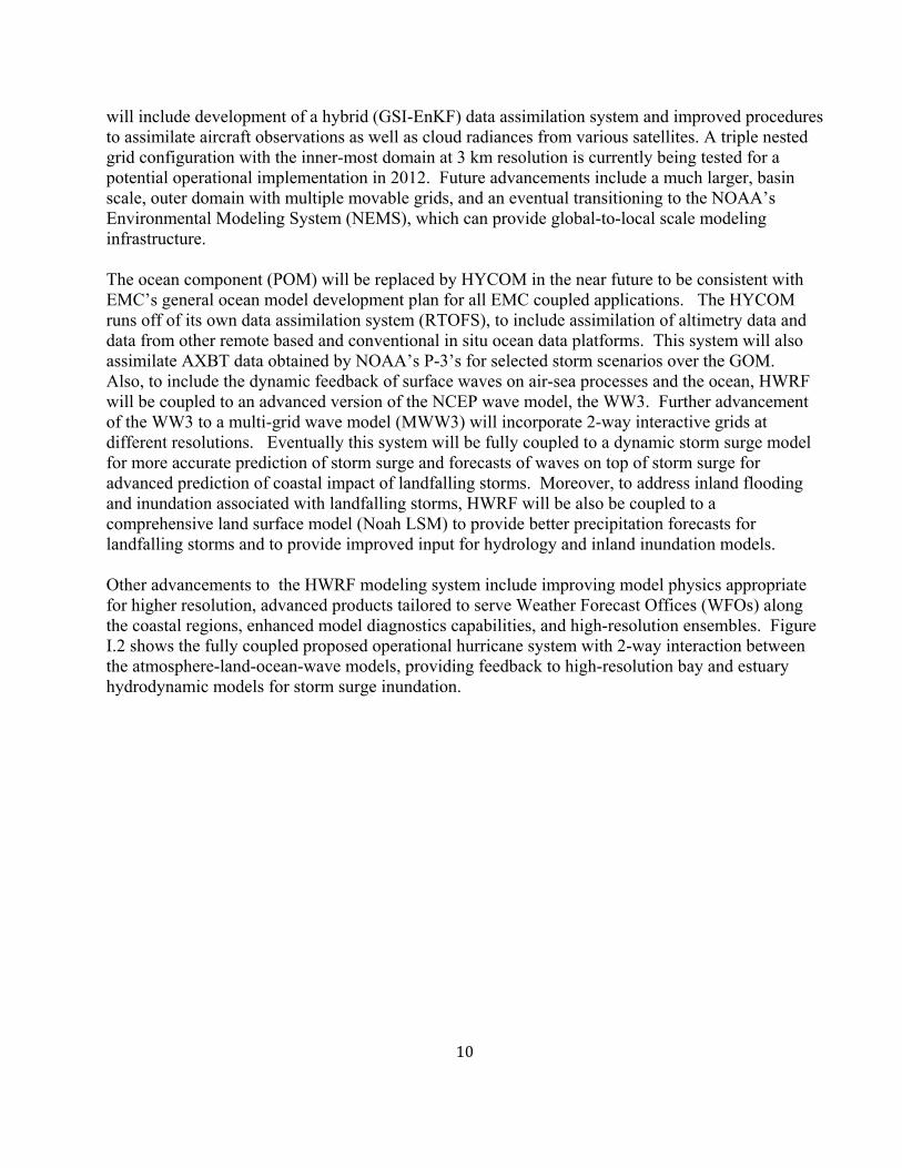
10

will include development of a hybrid (GSI-EnKF) data assimilation system and improved procedures to assimilate aircraft observations as well as cloud radiances from various satellites. A triple nested grid configuration with the inner-most domain at 3 km resolution is currently being tested for a potential operational implementation in 2012. Future advancements include a much larger, basin scale, outer domain with multiple movable grids, and an eventual transitioning to the NOAA’s Environmental Modeling System (NEMS), which can provide global-to-local scale modeling infrastructure. The ocean component (POM) will be replaced by HYCOM in the near future to be consistent with EMC’s general ocean model development plan for all EMC coupled applications. The HYCOM runs off of its own data assimilation system (RTOFS), to include assimilation of altimetry data and data from other remote based and conventional in situ ocean data platforms. This system will also assimilate AXBT data obtained by NOAA’s P-3’s for selected storm scenarios over the GOM. Also, to include the dynamic feedback of surface waves on air-sea processes and the ocean, HWRF will be coupled to an advanced version of the NCEP wave model, the WW3. Further advancement of the WW3 to a multi-grid wave model (MWW3) will incorporate 2-way interactive grids at different resolutions. Eventually this system will be fully coupled to a dynamic storm surge model for more accurate prediction of storm surge and forecasts of waves on top of storm surge for advanced prediction of coastal impact of landfalling storms. Moreover, to address inland flooding and inundation associated with landfalling storms, HWRF will be also be coupled to a comprehensive land surface model (Noah LSM) to provide better precipitation forecasts for landfalling storms and to provide improved input for hydrology and inland inundation models. Other advancements to the HWRF modeling system include improving model physics appropriate for higher resolution, advanced products tailored to serve Weather Forecast Offices (WFOs) along the coastal regions, enhanced model diagnostics capabilities, and high-resolution ensembles. Figure I.2 shows the fully coupled proposed operational hurricane system with 2-way interaction between the atmosphere-land-ocean-wave models, providing feedback to high-resolution bay and estuary hydrodynamic models for storm surge inundation.

11

Hurricane-Wave-Ocean-Surge-Inundation Coupled Models

High resolution Coastal, Bay & Estuarine hydrodynamic model

Atmosphere/oceanic Boundary Layer

HYCOM OCEAN MODEL

WAVE MODELSpectral wave model

NOAH LSM

NOSland and coastal waters

NCEP/Environmental Modeling CenterAtmosphere- Ocean-Wave-Land

runoff

fluxes

wave fluxes

wavespectra

windsair temp. SST

currents

elevationscurrents

3D salinitiestemperatures

other fluxes

surgeinundation

radiativefluxes

HWRF SYSTEM NMM hurricane atmosphere

Figure I.2. Proposed future operational coupled hurricane forecast system.

12

1.0 HWRF Initialization

1.1 Introduction

The operational initialization of hurricanes in the HWRF model consists of four major steps: 1) interpolation of the global analysis fields from the Global Forecast System (GFS) onto the operational HWRF model domain; 2) removal of the GFS vortex from the HWRF initialization; 3) inclusion of the HWRF vortex modified from the previous cycle’s 6-h forecast (if available); and 4) addition, through data assimilation, of large scale observations. Observational data on the hurricane scale are not operationally ingested in HWRF, and therefore the impact of using GSI with HWRF is small. Presently, HWRF uses the community GSI which is supported by DTC. The major differences from the GFDL model initialization (Kurihara et al. 1995) are steps 3 and 4, since the GFDL model uses neither GSI nor cycles its own vortex. The original design for the HWRF initialization (Liu et al. 2006a) was to continually cycle the HWRF model, applying the vortex relocation technique (Liu et al. 2000, 2006b) at every model initialization time. However, the results were problematic. Large scale flows can drift and the errors increased as cycles passed. To address this issue, the environmental fields from GFS analysis are now used at every initialization time. This section discusses the details of the atmospheric initialization, while the ocean initialization is described in Section 2.

1.2 HWRF cycling system

The location of the HWRF outer and inner domains is based on the observed hurricane current and projected center position. Therefore, if the storm is moving, the outer domain in the current cycle may be different from the previous cycle for the same storm. Once the domains have been defined, the GFS analysis and a vortex replacement strategy are used to create the initialization fields. If a previous 6-h HWRF forecast is available, the vortex is extracted from that forecast and corrected to be included in the current initialization. If the previous forecast is not available, a bogus storm is added to the current initialization. In the 2011 operational HWRF, unlike in previous years, if the maximum wind speed in the NHC storm message (TCVitals) is less than 12 ms-1, a bogus storm is used in the initialization even if the 6-h forecast exists. In operations, for most storms, only the first forecast in the lifetime of a storm has to be initialized with a bogus vortex, since previous forecasts are available for all subsequent initializations and the maximum wind speed in the TCVitals is usually greater than 12 ms-1. The vortex correction process (with GSI – Figure 1.1) involves the following steps: Interpolate the GFS analysis onto the HWRF model grids.

13

a) Remove the GFS vortex from the GFS analysis fields. The remaining large scale flow are termed “environmental field”.

b) Check availability of the HWRF 6-h forecast from the previous run (initialized 6h before the current run).

a. If the forecast is not available or the observed maximum wind speed is less than 12 ms-1(cold start), use bogus vortex.

b. If the forecast is available and the observed maximum wind speed is equal or more than 12 ms-1(cycled start)

i. Extract vortex from forecast fields.

ii. Correct the HWRF 6-h forecast vortex based on the TCVitals

1. Storm location (data used: storm center position)

2. Storm size (data used: radius of maximum surface wind speed and radius of the outmost closed isobar)

3. Storm intensity (data used: maximum surface wind speed and,

secondarily, the minimum sea level pressure)

c) Add vortex obtained in step b) to the environmental fields obtained in step a).

d) Interpolate the data obtained from c) onto outer domain and ghost domain (the ghost domain is created for GSI data assimilation only, and has the same resolution as the inner nest and is about three times larger than the inner nest), then run GSI separately for each domain. After the GSI analysis, merge the data from ghost domain onto outer domain and inner nest domain.

e) Run the HWRF model.

Because removing the GFS vortex from the background field changes the large scale flow near the storm area, in the future we may develop a version that keeps the GFS vortex and corrects it in the GFS environmental fields.

In the 2010 operational HWRF initialization, the HWRF vortex was only partially cycled (i.e., 6-h HWRF vortex is artificially multiplied by a factor less than 1.0). The current (2011) technique of fully cycling the vortex has a potential problem in that the upper level structure can be lost which may lead to the storm intensity forecasts being inconsistent among consecutive cycles. This potential problem has been mitigated for the 2011 operational implementation by an upgrade of the deep convection scheme, which leads to good upper level structures in the 6-h HWRF vortex, even for weak storms. The complete cycling of the HWRF vortex improves the

14

model consistency of the initialization, and contributes significantly to the reduction of the intensity forecast error for the first 24-36h. Details about the storm size and storm intensity corrections mentioned in step b) are discussed in Section 1.4.

1.3 Bogus vortex used in absence of previous 6h HWRF forecast or for weak storms

The bogus vortex is created from a 2D axi-symmetric synthetic vortex generated from a past model forecast. The 2D vortex only needs to be recreated when the model physics has undergone changes that strongly affect the storm structure. For the creation of the 2D vortex, a forecast storm (over the ocean) with small size and near axi-symmetric structure is selected. The 3D storm is separated from its environment fields, and the 2D axi-symmetric part of the storm is calculated. The 2D vortex includes the hurricane perturbations of horizontal wind component, temperature, specific humidity and sea-level pressure. This 2D axi-symmetric storm is used to create the bogus storm. To create the bogus storm, the wind profile of the 2D vortex is smoothed until its radius of maximum winds (RMW) or maximum wind speed matches the observed values. Next, the storm size and intensity are corrected following a procedure similar to the cycled system. The vortex in medium-depth and deep storms, receives identical treatment, while the vortex in shallow storms undergoes two final corrections: the vortex top is set to 700 hPa and the warm core structures are removed. The upgrade of the deep convection scheme in the 2011 HWRF will allow special treatment for medium-depth storms in future implementations.

15

Figure 1.1. Simplified flow diagram for HWRF initialization with GSI. Processes shown in white are always run. Processes shown in orange are run when cold-start is used or when the 6-h vortex is weaker than the observed storm. Processes shown in salmon are used only when cycled runs are performed.

1.4 Correction of vortex in previous 6H HWRF forecast

1.4.1 Storm size correction

Before starting to describe the storm size correction, some frequently used terms will be defined. Composite vortex refers to the 2D axi-symmetric storm which is created once and used for all

16

forecasts. The bogus vortex is created from the composite vortex by smoothing and performing size (and/or intensity) corrections. The background field, or guess field, is the output of the vortex initialization procedure, to which we can add observations data through data assimilation. The environment field is defined as the GFS analysis field after removing the vortex component.

For hurricane data assimilation, we need a good background field. Storms in the background field (this background field can be the GFS analysis or previous 6-h forecast) may be too large or too small, so the storm size needs to be corrected based on observations. We use two parameters: namely, the radius of maximum wind and radius of the outermost closed isobar to correct the storm size.

The storm size correction can be achieved by stretching/compressing the model grid. Let’s consider a storm of the wrong size in cylindrical coordinates. Assuming the grid size is linearly stretched along the radial direction

i

i

ii bra

r

r

*

(1.4.1.1)

where a and b are constants. r and *r are the distances from the storm center before and after the model grid is stretched. Index i represents the ith grid point.

Let mr and mR denote the radius of the maximum wind and radius of the outermost closed isobar

(the minimum sea-level pressure is always scaled to the observed value before calculating this radius) for the storm in the background field, respectively. Let *

mr and *mR be the observed radius of

maximum wind and radius of the outermost closed isobar (which can be redefined if in Equation (1.4.1.1) is set to be a constant). If the high resolution model is able to resolve the hurricane eyewall structure, mm rr /* will be close to 1, therefore, we can set 0b in Equation (1.4.1.1) and mm rr /*

is a constant. However, if the model doesn’t handle the eyewall structure well ( mm rr /* will be

smaller than mm RR /* ) within the background fields, we need to use Equation (1.4.1.1) to

stretch/compress the model grid. From now on, we assume that mmmm RRrr // ** ( 0b in Equation

(1.4.1.1) in the following discussion.

0 *mr mr

*mR mR

Integrating Equation (1.4.1.1), we have

17

2

00

*

2

1)()()( brardrbradrrrfr

rr

. (1.4.1.2)

We compress/stretch the model grids such that

At mrr , ** )( mm rrfr (1.4.1.3)

At mRr , ** )( mm RRfr . (1.4.1.4)

Substituting (1.4.1.3) and (1.4.1.4) into (1.4.1.2), we have

*2

2

1mmm rbrar (1.4.1.5)

*2

2

1mmm RbRaR . (1.4.1.6)

Solving for a and b, we have

)(

*22*

mmmm

mmmm

rRrR

RrRra

, )(

2**

mmmm

mmmm

rRrR

rRrRb

. (1.4.1.7)

Therefore,

2***22*

*

)()()( r

rRrR

rRrRr

rRrR

RrRrrfr

mmmm

mmmm

mmmm

mmmm

(1.4.1.8)

since mmmm RRrr // ** , 0b . We also need to have 0a from Equation (1.4.1.1); therefore,

m

m

m

m

m

m

m

m

R

R

r

r

R

r

R

R ***

(1.4.1.9)

or

m

mm

m

mm r

R

R

R

*

(1.4.1.10)

where m

mm r

r *

. (1.4.1.11)

18

There could be a limit on the grid compression. For example, if we didn’t want large changes in the model vortex size, we could set mm RR 8.0* (increase the observed radius of outermost closed

isobar). We then would set mm

mm r

R

rr 8.0* from Equation (1.4.1.9), which would mean that the

radius of maximum wind could be larger than that of the observed one. This limitation is not applied in the operational HWRF. If the guess field comes from a high resolution model (such as in HWRF) or the storms are weak,

m will be close to 1. If 15.185.0 m , we can choose to be constant so that

m

m

m

mm R

R

r

r **

(1.4.1.12)

where *mR is redefined here as ( mm RR * ).

As mentioned in Gopalakrishnam et al. (2010), to calculate the radius of the outmost closed isobar it is necessary to scale the minimum surface pressure to the observed value as discussed below. A detailed discussion is given in the following. We define two functions,f1 and f2, such that

for the 6-h HWRF vortex (vortex #1), ; (1.4.1.13)

for composite storm (vortex #2), (1.4.1.14) where p1 and p2 are the 2D surface perturbation pressures for vortices #1 and #2, respectively. p1c and p2c are the minimum values ofp1 and p2. pobs is the observed minimum perturbation pressure. The radius of outmost closed isobar for vortices#1 and #2 can be defined as the radius of the 1hPa contour from f1 and f2, respectively. We can show that after the storm size correction for vortices#1 and #2, the radius of the outmost closed isobar is unchanged for any combination of the vortices#1 and #2. For example (c is a constant),

obsc

pp

pf

1

11

obsc

pp

pf

2

22

cc

cc

pp

pcp

p

ppcp 2

2

21

1

121

19

At the radius of the1-hPa contour, we have f1 =1 and f2=1, or so, where we have used Similarly, to calculate the radius of 34 knot winds, we need to scale the maximum wind speed for vortices #1 and #2. We define two functions,g1 and g2, such thatfor the hh HWRF vortex (vortex #1), ; (1.4.1.15)

for the composite storm (vortex #2), (1.4.1.16) where v1m and v2m are the maximum wind speed for vortices #1 and #2, respectively, and (vobs v m) is the observed maximum wind speed minus the environment wind. The environment wind is defined as where U1m is the maximum wind speed at the 6-h forecast. The radius of 34 knot wind for vortices #1 and #2 are calculated by setting both g1 and g2 to be 34 knot. After the storm size correction, the combination of vortices #1 and #2 can be written as At the 34 knot radius, we have (g1 =34, g2 =34)

obscc pp

p

p

p

1

2

2

1

1

1)(1

2122

21

1

121

ccobs

cc

cc

pcpp

pp

pcp

p

ppcp

1 2( ) .c c obsp c p p

)(1

11 mobs

m

vvv

vg

)(2

22 mobs

m

vvv

vg

),0max( 11 mmm vUv

1 21 2 1 2

1 2

.m mm m

v vv v v v

v v

1 21 2 1 2 1 2

1 2

34( ) 34 .m m m m

m m obs m

v vv v v v v v

v v v v

20

Note we have used, In the 2010 operational HWRF initialization, only one parameter (radius of the maximum wind) was used in the storm size correction. The radius of the outmost closed isobar was calculated but never used. In the 2011 upgrade, a second parameter (radius of the outmost closed isobar or radius of the average 34 knots wind for hurricanes) is added by Kevin Yeh (HRD). Specifically, in the 2010 HWRF initialization, Equation (1.4.1.12) was used for storm size correction, and b was set to zero in Equation (1.4.1.1). In the 2011 operational model, a and b are calculated following Equation (1.4.1.7). Storm size correction can be problematic. The reason is that the eyewall size produced in the model can be larger than the observed one, and the model does not support observed small-size eyewalls. For example, the radius of maximum winds for 2005 Wilma was 9 km at 140 knots for many cycles. The model-produced radius of maximum wind was larger than 20 km. If we compress the radius of maximum winds to 9 km, the eyewall will collapse and significant spin-down will occur. So the minimum value for storm eyewall is currently set to 19km. The eyewall size in the model is related to model resolution, model dynamics and model physics. In the storm size correction procedure, we do not match the observed radius of maximum winds. Instead, we replace *

mr as the average between the model value and the observation. We also limit

the correction to be 15% of the model value. In the 2011 version, the limit is set as follows: 10% if *

mr is smaller than 20 km; 10-15% if *mr is between 20 and 40km; and 15% if *

mr is larger than 40

km. For the radius of the outmost closed isobar (or average 34 knots wind if storm intensity is larger than 64 knots), the correction limit is set to 30% of the model value. Even with the current settings, major spin-down occurs if the eyewall size is small and lasts for many cycles (due to the consecutive reduction of the storm eyewall size in the initialization). Further research needs to be done to find the minimum eyewall size that model can support, and the initial eyewall size should not be below this minimum. We can show that the horizontal convergence and vertical vorticity do not change signs in the hurricane area after the grids are stretched. Using cylindrical coordinates, the new horizontal divergence and the vertical vorticity are

]

)(

2/[

)2/(

11)(

1*

***

*

bra

br

r

u

bra

v

rur

rr

(1.4.1.17)

and

])(

2/[

)2/(

11)(

1*

***

*

bra

br

r

v

bra

u

rvr

rr zz

(1.4.1.18)

1 2( ) .m m m obsv v v v

21

where u and v are the radial and tangential components of the wind, respectively, and the original divergence and vorticity are

v

rru

rr

1)(

1 (1.4.1.19)

and

u

rrv

rrz

1)(

1 . (1.4.1.20)

If the last terms in Equations (1.4.1.15) and (1.4.1.16) can be neglected in the hurricane area, we can then show that Equations (1.4.1.13) and (1.4.1.14) can be rewritten as

0])2/(

2/[

)(

1*

bra

br

r

u

bra If 0 (1.4.1.21)

and

0])2/(

2/[

)(

1*

bra

br

r

v

bra zz If 0 . (1.4.1.22)

In the case where =constant (b=0), the divergence and vorticity will be the original values divided

by the constant =a.

1.4.1.1 Surface pressure adjustment after the storm size correction

In our approximation, we only correct the surface pressure of the axi-symmetric part of the storm. The governing equation for the axi-symmetric components along the radial direction is

rFr

pf

r

vv

z

uw

r

uu

t

u

1

)( 0 (1.4.1.1.1)

where u, v and w are the radial, tangential and vertical velocity components, respectively. F r is

friction and vH

uCF

Bdr where BH is the top of the boundary layer. rF can be estimated as

vFr610 away from the storm center, and vFr

510 near the storm center. Dropping the small terms, Equation (1.4.1.1.1) is close to the gradient wind balance.

We define the gradient wind stream function as

22

vrf

v

r

0

2 (1.4.1.1.2)

and

r

drvrf

v)(

0

2

. (1.4.1.1.3)

Due to the coordinate change, Equation (1.4.1.1.2) can be rewritten as the following

*

*

* rr

r

rr

vrf

rf

r

vv

rf

r

r

vv

rf

v

0*

2

0

*

*

2

0

2 )( ( )( *rrr ).

Therefore, the gradient wind stream function becomes (due to the coordinate transformation)

*

**

0*

*

*

2

*)(

)(

)(

)(

1r

drrvfrr

rf

r

v

r . (1.4.1.1.4)

We can also define a new gradient wind stream function for the new vortex as

vfr

v

r

0*

2

*

* (1.4.1.1.5)

where v is a function of *r .

*

0*

2* )(

*

drvfr

vr

(1.4.1.1.6)

Assuming the hurricane sea-level pressure component is proportional to the gradient wind stream function at model level 1 (roughly 40 m in height), i.e.,

)()()( *** rrcrp (1.4.1.1.7)

and

)()()( ***** rrcrp (1.4.1.1.8)

where )( *rc is a function of *r , we have

23

*

* pp ; (1.4.1.1.9)

where es ppp and es ppp ** are the hurricane sea-level pressure perturbations before and

after the adjustment, and ep is the environment sea-level pressure.

Note that the pressure adjustment is small due to the grid stretching. For example, if in Equation (1.4.1.1) α is a constant we can show that Equation (1.4.1.1.4) becomes

*

0*

2

)1

(

*

drvfr

vr

. (1.4.1.1.10)

This value is very close to that of Equation (1.4.1.1.6) since the first term dominates.

1.4.1.2 Temperature adjustment

Once the surface pressure is corrected, we need to correct the temperature field. Assume the environment field is in hydrostatic equilibrium

H

T

s

T

dz

R

g

p

p

0

ln (1.4.1.2.1)

where H and Tp are the height and pressure at the model top, respectively. The hydrostatic equation for the total field (environment field + vortex) is

H

T

s

TT

dz

R

g

p

pp

0 )(ln (1.4.1.2.2)

where p and T are the sea-level pressure and temperature perturbations for the hurricane vortex.

Since spp and TT , we can linearize Equation (1.4.1.2.2)

HH

sT

s

T

T

T

dz

R

g

TT

dz

R

g

p

p

p

p

00

)1()(

)1(ln . (1.4.1.2.3)

Subtract Equation (1.4.1.2.1) from Equation (1.4.1.2.3) and we have

24

H

s

dzT

T

R

g

p

p

02

)1ln(

or

H

s

dzT

T

R

g

p

p

02 . (1.4.1.2.4)

Multiplying Equation (1.4.1.2.4) by /)( ** r ( is a function of x and y only), we have

H

s

dzT

T

R

g

p

p

02 . (1.4.1.2.5)

So the temperature correction is proportional to the magnitude of the temperature perturbation, and the new temperature is

TTTTT e )1(* (1.4.1.2.6)

where T is the 3D temperature field before the surface pressure correction.

1.4.1.3 Water vapor adjustment

Assume the relative humidity is unchanged before and after the temperature correction, i.e.,

)()( **

*

Te

e

Te

eRH

ss

(1.4.1.3.1)

where e and )(Tes are the vapor pressure and the saturation vapor pressure in the model guess fields,

respectively. *e and )(* Tes are the vapor pressure and the saturation vapor pressure respectively,

after the temperature adjustment. Using the definition of the mixing ratio,

ep

eq

622.0 (1.4.1.3.2)

at the same pressure level and from Equation (1.4.1.3.1)

25

)(

)( ****

Te

Te

e

e

q

q

s

s . (1.4.1.3.3)

Therefore, the new mixing ratio becomes

qe

eqq

e

eq

e

eq

s

s

s

s )1(***

* . (1.4.1.3.4)

From the saturation water pressure

])66.29(

)16.273(67.17exp[112.6)(

T

TTes (1.4.1.3.5)

we can write

])66.29)(66.29(

)(5.243*67.17exp[

*

**

TT

TT

e

e

s

s . (1.4.1.3.6)

Substituting Equation (1.4.1.3.6) into (1.4.1.3.4), we have the new mixing ratio after the temperature field is adjusted.

1.4.2 Storm intensity correction

Generally speaking, the storm in the background field has a different maximum wind speed compared to the observations. We need to correct the storm intensity based on the observations, which is discussed in detail in the following sections.

1.4.2.1 Computation of

Let’s consider the general formulation in the traditional x, y and z coordinates; where *1u and *

1v are

the background horizontal velocity, and 2u and 2v are the vortex horizontal velocity to be added to the background fields. We define

22

*1

22

*11 )()( vvuuF (1.4.2.1.1)

and

22

*2

22

*12 )()( vvuuF . (1.4.2.1.2)

26

Function 1F is the wind speed if we simply add a vortex to the environment (or background fields).

Function 2F is the new wind speed after the intensity correction. We consider two cases here. Case I: 1F is larger than the observational maximum wind speed.

We set *1u and *

1v to be the environment wind component; i.e., Uu *1 and Vv *

1 (the vortex is

removed and the field is relatively smooth); and 12 uu and 12 vv are the vortex horizontal wind components from the previous cycle’s 6-h forecast (we call it vortex #1, which contains both the axi-symmetric and asymmetric parts of the vortex). Case II: 1F is smaller than the observational maximum wind speed.We add the vortex back into the

environment fields after the grid stretching, i.e., 1*1 uUu and 1

*1 vVv . We choose 2u and 2v

to be an axi-symmetric composite vortex (vortex #2) which has the same radius of maximum wind as that of the first vortex. In both cases, we can assume that the maximum wind speed for 1F and 2F are at the same model

grid point. To find , we first locate the model grid point where 1F is at its maximum. Let’s denote

the wind components at this model grid point as mu1 , mv1 , mu2 , and mv2 (for convenience, we drop the superscript m), so that 22

2*1

22

*1 )()( obsvvvuu (1.4.2.1.3)

where obsv is the 10m observed wind converted to the first model level.

Solving for, we have

)(

)()((2

22

2

22

*12

*1

22

22

22

*12

*1

vu

uvvuvuvvvuu obs

. (1.4.2.1.4)

The procedure to correct wind speed is as follows. First, we calculate the maximum wind speed from Equation (1.4.2.1.1) by adding the vortex into the environment fields. If the maximum of 1F is larger than the observed wind speed, we classify it as

Case I and calculate the value of . If the maximum of 1F is smaller than the observed wind speed, we classify it as Case II. The reason we classify it as Case II is that we don’t want to amplify the asymmetric part of the storm (amplifying it may negatively affect the track forecasts). In Case II, we first add the original vortex to the environment fields after the storm size correction, then add a small portion of an axi-symmetric composite storm. The composite storm portion is calculated from Equation (1.4.2.1.4). Finally, the new vortex 3D wind field becomes ),,(),,(),,( 2

*1 zyxuzyxuzyxu

27

),,(),,(),,( 2*1 zyxvzyxvzyxv .

1.4.2.2 Surface pressure, temperature and moisture adjustments after the intensity correction

If the background fields are produced by high resolution models (such as in HWRF), the intensity corrections are small and the correction of the storm structure is not necessary. The guess fields should be close to the observations, therefore, we have In Case I is close to 1;

In Case II is close to 0.

After the wind speed correction, we need to adjust the sea-level pressure, 3D temperature and the water vapor fields which are described below. In Case I, is close to 1. Following the discussion in Section.1.4.1.1, we define the gradient wind stream function as

20

2 vrf

v

r

(1.4.2.2.1)

and

r

drvrf

v)( 2

0

22 . (1.4.2.2.2)

The new gradient wind stream function is

r

new drvrf

v]

)([ 2

0

22 . (1.4.2.2.3)

The new sea-level pressure perturbation is

newnew pp (1.4.2.2.4)

28

where es ppp and enews

new ppp are the hurricane sea-level pressure perturbations before

and after the adjustment and ep is the environment sea-level pressure.

Generally speaking, newp may not exactly match the observation value. We use the modified version of (1.4.2.2.4)

c

obsnew

new

p

ppp

(1.4.2.2.5)

where cp is the minimum central pressure from Equation (1.4.2.2.4) and the ratio cobs pp / is

close to 1. In Case II, is close to 0. Let’s define

r

drvrf

v)( 1

0

21

1 (1.4.2.2.6)

r

drvrf

v]

)([ 2

0

22*

2 (1.4.2.2.7)

and the new gradient wind stream function is

r

new drvvrf

vv)](

)([ 21

0

221 . (1.4.2.2.8)

The correction is small, i.e., 12 vv , and the new sea-level pressure perturbation is

)( 21*

21

pppnew

new

(1.4.2.2.9)

or

)2

1)((0

21*21

21 drrf

vvppp

rnew

. (1.4.2.2.10)

Since 12 vv , the last term can be neglected, so the new surface pressure is

21 pppnew . (1.4.2.2.11)

The modified version of (1.4.2.2.11) in Case II is

29

)( 12

21 cobs

c

new ppp

ppp

. (1.4.2.2.12)

Equations (1.4.2.2.5) and (1.4.2.2.12) are supposed to match the observed surface pressure. However, if the model has an incorrect surface pressure-wind relationship, Equations (1.4.2.2.5) and (1.4.2.2.12) may be inconsistent with the model dynamics and the model will have to make a large adjustment once the model integration starts. In order to reduce this impact, we adjust the observed minimum surface pressure. Based on Brown et al. (2006), we have the observed surface pressure-wind relationship for tropical cyclones 6143.0)8.1015(354.8 pV (1.4.2.2.13)

where V is the Maximum Sustained Surface Wind (MSSW) in knots and p is the Mean Sea Level Pressure (MSLP) in hPa. The slope of the curve can be derived as

628.0)(1515.0 VV

p

(1.4.2.2.14)

where V is the MSSW in ms-1.

Assume obsV is the observed MSSW, and mV and mp are the model forecast MSSW and MSLP,

respectively. Then the new MSLP can be set to be )()(1515.0 628.0

mobsobsmnew VVVpp . (1.4.2.2.15)

The slope is replaced with the observed P-W slope (coefficients should be different for modeled P-W) which is smaller than that in the current HWRF model. So the pressure is reduced or increased less for the same wind increment. We also limit the maximum difference between the observed MSLP ( obsp ) and the new MSLP ( newp ) to 20 hPa.

The correction of the temperature field is as follows, In Case I, we define

c

obsnew

p

p

. (1.4.2.2.16)

Then we use Equation (4.1.2.6) to correct the temperature fields.

In Case II, we define

30

c

cobs

p

pp

2

1*

(1.4.2.2.17)

and

2*

2*

1* TTTTTT e (1.4.2.2.18)

where T is the 3D background temperature field (environment+vortex1), and 2T is the temperature perturbation of the axi-symmetric composite vortex. In the 2011 operational HWRF, the observed MSLP ( obsp ) is replaced by the estimated model-

consistent MSLP ( newp ), obsp is replaced by enewm ppp * , and the following pressure adjustment

equations are changed. Equation (1.4.1.1.9) in storm size correction is modified as,

*

.new

new m

c

pp p

p

(1.4.2.2.19)

Equation (1.4.2.2.5) for Case I and Equation (1.4.2.2.12) for Case II in storm intensity correction are modified as

c

mnew

new

p

ppp

*

(1.4.2.2.20)

and

*21 1

2

( ) .newm c

c

pp p p p

p

(1.4.2.2.21)

The model-consistent pressure adjustment is only a crude estimate here. The minimum central pressure is no longer matched to the observation. We set the maximum pressure difference as 75 hPa. Using the estimated surface pressure significantly reduces the spin-down problem for strong storms. The current calculation of surface pressure is only a crude linear estimation. For further improvement, the surface pressure estimated from Equation (1.4.2.2.15) needs to be modified to take into account the storm size correction and nonlinear effects. Fully model-consistent surface pressure should use Equation (1.4.2.2.4) for intensity correction in both Case I and Case II. In Case II, newneeds to be calculated as in Equation (1.4.2.2.8) and needs to be calculated as 1 in Equation (1.4.2.2.6).

31

The corrections of water vapor in both cases are the same as those discussed in Section 1.4.1.3.

1.4.2.3 Correction of the storm structure

Now let’s consider if we want to keep the GFS vortex, which may be much weaker than the observed storm. The wind speed correction is large and will be comparable to the background fields. The correction needs to satisfy both the observation and the dynamic constraints. First, we would like to comment that if two storms have similar intensities, adding them together will produce an incorrect storm structure, which needs to go through dynamic balancing even if the maximum wind and the minimum surface pressure match the observations, i.e., obsUUU 21 (1.4.2.3.1)

and

obsppp 21 (1.4.2.3.2)

where 1U and 2U are the maximum wind for the two storms and 1p and 2p are the sea-level minimum pressure perturbations. Equations (1.4.2.3.1) and (1.4.2.3.2) can be satisfied because of the observed linear relationship between surface minimum pressure and the maximum wind speed. For simplicity, let’s consider the axi-symmetric component in cylindrical coordinates. We assume that the sea-level pressure perturbation is proportional to the gradient wind stream function, i.e.,

r

drvrf

v)( 1

0

21

1 (1.4.2.3.3)

r

drvrf

v)( 2

0

22

2 (1.4.2.3.4)

3 [(v1 v2)

2

rf0

(v1 v2)]

r

dr . (1.4.2.3.5)

According to the dynamic balance, the new surface pressure 3p should be

drrf

vv

pp

p r

0

21

2121

3

21

3 211

. (1.4.2.3.6)

is always greater than 1 (i.e., 213 ppp ). In fact if 21 vv , is close to 2. In order to

reduce the value of 3 in Equation (1.4.2.3.5), the eyewall or band of strongest winds in the new

storm must contract in order to satisfy the observed linear pressure-wind relationship. In other

32

words, we can’t simply add two weak storms together to produce one strong storm without correcting the storm structure. This result has an important implication for the data assimilation. If the observation increment is large, flow dependent or fixed background error correlations may not produce good results in the hurricane analysis. The background error correlations must depend on the observed storm size and storm intensity. Assume that we have an axi-symmetric composite storm, which can be obtained from the previous cycle’s 6-h forecast or constructed from the earlier model forecast. We would like to add the composite storm on top of the previous background field. For simplicity, let’s consider the axi-symmetric component in cylindrical coordinates. We then have these gradient wind stream functions for storms 1 and 2

r

drvrf

v)( 1

0

21

1 (1.4.2.3.7)

r

drvrf

v]

)([ 2

0

22*

2 . (1.4.2.3.8)

The gradient wind stream function for the combined storm is

drvrf

vr

)( 30

23

3 (1.4.2.3.9)

where

213 vvv . (1.4.2.3.10)

From the observation point of view, we need to satisfy the linear surface pressure-wind relationship at the storm center, i.e.,

*213 . (1.4.2.3.11)

We know that Equation (1.4.2.3.9) does not satisfy the requirements of Equation (1.4.2.3.11), and we must correct the storm structure for Equation (1.4.2.3.11) to be valid. First, we define a reference wind profile ( fv3 ), then nudge the wind profile 3v toward this reference wind profile until

(1.4.2.3.11) is satisfied at the storm center (if Equation (1.4.2.3.11) can’t be satisfied, the wind profile fv3 you chose needs to be modified).

33

The reference wind profile can be obtained from the previous model forecast if the model is good, or can be defined based on observations and the climatological wind profile. The nudging not only adjusts the wind profile, but also changes the surface pressure field (see Equation (1.4.2.3.12)). After correcting the 3v wind profile (let’s denote the new wind profile as nv3 ), we need to correct the

upper level wind based on the ratio of 3v after and before the nudging adjustment ( 33 / vvn ).

The final pressure adjustment after the correction of storm structure will be

)( 21*21

33 ppp

n

. (1.4.2.3.12)

After the pressure correction, the temperature correction is

2121* )1()( TTTTTTT e (1.4.2.3.13)

where

*21

3

n

(1.4.2.3.14)

and

1TTT e . (1.4.2.3.15)

We correct the water vapor fields in the same way as discussed in Section 1.4.1.3.

We would like to mention that the storm intensity correction is, in fact, a data analysis. The observation data used here is the surface maximum wind speed (single point data), and the background error correlations are flow dependent and based on the storm structure. The storm structure used for the background error correlation is vortex #1 in Case I, and vortex #2 in Case II (except for water vapor which still uses the vortex #1 structure). Vortex #2 is an axi-symmetric vortex. If the storm structure in vortex #1 could be trusted, one could choose vortex #2 as the axi-symmetric part of vortex #1. In HWRF, the structure of vortex #1 is not completely trusted when the background storm is weak, and therefore an axi-symmetric composite vortex from old model forecasts is employed as vortex #2. When the observation increment is large, we can’t get correct background error correlations from either vortex #1 or vortex #2. Therefore, it would be advisable (but not used in HWRF) to use the observation and climatology data to define a new vortex structure and as a result, a new background error correlation.

34

1.5 Data assimilation through GSI in HWRF

After the vortex initialization procedure, data assimilation is performed using the Gridpoint Statistical Interpolation (GSI) analysis system. GSI is a unified global/regional three-dimensional variational data assimilation (3DVAR) system. The analysis in GSI is performed in model grid space, which allows for more flexibility in constructing background error covariances and makes it straightforward to unify the global and regional applications. (Wu et al. 2002, Kleist et al. 2009). The cost function to be minimized in GSI is

J xT B1x (Hx y)T R1(Hx y) Jc

where

x is the analysis increment vector

B is the background error covariance matrix

y is the innovation vector

R is the observational and representativeness error covariance matrix

H is the observation operator

Jc is the constraint term .

The analysis variables are: streamfunction, unbalanced part of velocity potential, unbalanced part of temperature, unbalanced part of surface pressure, pseudo-relative humidity (qoption = 1) or normalized relative humidity (qoption = 2), ozone mixing ratio, cloud condensation mixing ratio and satellite bias correction coefficients. Ozone and cloud variables are not analyzed in HWRF. The balanced part of velocity potential, temperature and surface pressure are calculated from a statistically derived linear balance relationship (Wu et al. 2002). The definition of the normalized relative humidity allows for a multivariate coupling of the moisture, temperature and pressure increments as well as flow dependence (Kleist et al. 2009), therefore this option is used for HWRF. A conjugate gradient minimization algorithm is used to find the optimal solution for the analysis problem. The iteration algorithm can be found in GSI User’s Guide Chapter 5, Section 5.2. Two outer loops with 50 iterations each are used for HWRF (miter=2,niter(1)=50,niter(2)=50). The outer loop consists of more complete (nonlinear) observation operators and quality control. Usually, simpler observation operators are used in the inner loop. Variational quality control, which is part of the inner loop is not used for HWRF (noiqc=.false.). The background error statistics estimated from the WRF-NMM NAM forecasts through the NMC method (Parrish and Derber 1992) is used for HWRF. The background error covariance obtained though the NMC method is isotropic and static. GSI has the option to use flow-dependent

35

anisotropic background error covariance. This option is not used in the 2011 operational HWRF (anisotropic=.false.), because it is relatively immature. Data assimilation for HWRF is performed on the HWRF outer domain (75x75 degrees, 0.18 degree horizontal resolution) and on the ghost domain (20x20 degree, 0.06 degree horizontal resolution). When using GSI with HWRF, ‘wrf_nmm_regional’ in GSI namelist should be set to ‘true’. In the 2011operational HWRF, GSI is only used if the observed storm is deep, which is indicated in the NHC storm message (TCVitals). The data assimilated into HWRF on both domains include:

1. Conventional data

Radiosonde

Aircraft reports (AIREP/PIREP, RECCO , MDCRS-ACARS, TAMDAR , AMDAR)

Surface ship and buoy observation

Surface land observations

Pibal winds

Wind profilers

VAD wind

Dropsondes

JMA IR/visible winds

EUMETSAT IR/visible winds

GOES IR winds

GOES water vapor cloud top winds

MODIS IR and imager water vapor winds

2. Satellite radiance observations

AMSU-A NOAA 15 Channel 1-10, 12, 13, 15 NOAA 18 Channel 1-8, 10-13, 15 METOP-a Channel 1-6, 8-13, 15

AMSU-B/MHS NOAA 15 Channel 1-3,5 NOAA 18 Channel 1-5 METOP-a Channel 1-5

HIRS NOAA 17 Channel 2-15 METOP-a Channel 2-15

AIRS AQUA 148 Channels

36

GOES-11, 12 sounders Sndrd1, sndrd2, sndrd3 and sndrd4 Channel 1-15

Conventional data within 150 km of the storm center are not assimilated because of their negative impact on the forecast. This is mainly due to the use of the static isotropic background error covariance, which cannot spread observation information properly around the storm center. Flow dependent anisotropic background error covariance can spread observation information better than isotropic and static background error covariance. This upgrade has been tested with the assimilation of NOAA P3 tail Doppler radar data but not yet implemented in operations. More advanced data assimilation schemes, e.g., hybrid EnKF-Variational scheme and 4DVAR, are being developed at EMC, and for those systems it is expected that inner core conventional data and airborne Doppler radar data will be ingested. For satellite radiance assimilation, bias correction coefficients obtained by GFS analysis are used as the first guess in the first cycle analysis. In later assimilation cycles, bias correction coefficients updated through HWRF’s own analysis will be used as the first guess in the next analysis cycle. After data assimilation, the ghost domain analyses are interpolated onto the HWRF inner domain and outer domain to initialize the forecast. For the HWRF outer domain, a blending zone is added around the ghost domain boundary area so that the model fields gradually change from the values of the ghost domain to the values of the HWRF outer domain.

37

2.0 Princeton Ocean Model for Tropical Cyclones (POMTC)

2.1 Introduction

The three-dimensional, primitive equation, numerical ocean model that has become widely known as the POM was originally developed by Alan F. Blumberg and George L. Mellor in the late 1970s. One of the more popularly cited references for the early version of POM is Blumberg and Mellor (1987), in which the model was principally used for a variety of coastal ocean circulation applications. Through the 1990’s and 2000’s, the number of POM users increased enormously, reaching over 3500 registered users as of October 2009. During this time, many changes were made to the POM code by a variety of users, and some of these changes were included in the “official” versions of the code housed at Princeton University (http://aos.princeton.edu/WWWPUBLIC/htdocs.pom/). Mellor (2004), currently available on the aforementioned Princeton University website, is the latest version of the POM User’s Guide and is an excellent reference for understanding the details of the more recent versions of the official POM code. Unfortunately, some earlier versions of the POM code are no longer supported or well-documented at Princeton, so users of these earlier POM versions must take care to understand the differences between their version of the code and the version described in Mellor (2004). In the mid-1990’s, a version of POM available at the time was transferred to the URI for the purpose of coupling to the (GFDL) hurricane model. At this point, POM code changes were made specifically to address the problem of the ocean’s response to hurricane wind forcing in order to create a more realistic sea surface temperature (SST) field for input to the hurricane model and ultimately to improve 3-5 day hurricane intensity forecasts in the model. Initial testing showed hurricane intensity forecast improvements when ocean coupling was included (Bender and Ginis 2000). Since operational implementation of the coupled GFDL/POM model at NCEP in 2001, additional changes to POM were made at URI and subsequently implemented in the operational GFDL model, including improved ocean initialization (Falkovich et al. 2005, Bender et al. 2007, Yablonsky and Ginis 2008). This POM version was then coupled to the atmospheric component of the HWRF model in the North Atlantic Ocean (but not in the North Pacific Ocean) before operational implementation of HWRF at (NCEP/EMC) in 2007. The remainder of this document primarily describes the POM component of the 2011 operational HWRF model used to forecast tropical cyclones in the North Atlantic Ocean, including the so-called “United” and “East Atlantic” regions (see “Grid Size, Spacing, Configuration, Arrangement, Coordinate System, and Numerical Scheme” below); this version of POM will henceforth be referred to as POM-TC. Alternative POM-TC configurations that deviate from the 2011 operational HWRF model version are clearly indicated in the text.

38

2.2 Purpose

The primary purpose of coupling the POM-TC (or any fully three-dimensional ocean model) to the HWRF (or to any hurricane model) is to create an accurate (SST) field for input into the HWRF. The SST field is subsequently used by the HWRF to calculate the surface heat and moisture fluxes from the ocean to the atmosphere. An uncoupled hurricane model with a static SST is restricted by its inability to account for SST changes during model integration, which can contribute to high intensity bias (e.g. Bender and Ginis 2000). Similarly, a hurricane model coupled to an ocean model that does not account for fully three-dimensional ocean dynamics may only account for some of the hurricane-induced SST changes during model integration (e.g. Yablonsky and Ginis 2009).

2.3 Grid size, spacing, configuration, arrangement, coordinate system, and numerical scheme

The horizontal POM-TC grid uses curvilinear orthogonal coordinates. There are currently two POM-TC grids in the North Atlantic Ocean. HWRF uses the current and 72-hour projected hurricane track to choose which of the two POM-TC grids to use for coupling. Operationally, when a previous forecast cycle is available, the projected track is based on the previous HWRF forecast. When no previous forecast cycle is available, the projected track is based on a simple extrapolation in time of the currently observed storm translation speed. The first grid covers the United region, which is bounded by 10°N latitude to the south, 47.5°N latitude to the north, 98.5°W longitude to the west, and 50°W longitude to the east. In the operational POM-TC United region, there are 225 latitudinal grid points and 254 longitudinal grid points, yielding ~18-km grid spacing in both the latitudinal and longitudinal directions. The second grid covers the newly expanded East Atlantic region, which is bounded by 10°N latitude to the south, 47.5°N latitude to the north, 69.93676°W longitude to the west, and 30°W longitude to the east. In the operational POM-TC East Atlantic region, there are 225 latitudinal grid points and 209 longitudinal grid points, yielding ~18-km grid spacing in both the latitudinal and longitudinal directions. A non-operational high-resolution POM-TC version has also been developed for both the United and East Atlantic regions with ~9-km grid spacing in both the latitudinal and longitudinal directions. The vertical coordinate is the terrain-following sigma coordinate system (Phillips 1957, Mellor 2004, Figure 1 and Appendix D). There are 23 vertical levels, where the level placement is scaled based on the bathymetry of the ocean at a given location. The largest vertical spacing occurs where the ocean depth is 5500 m. Here, the 23 half-sigma vertical levels (“ZZ” in Mellor 2004) are located at 5, 15, 25, 35, 45, 55, 65, 77.5, 92.5, 110, 135, 175, 250, 375, 550, 775, 1100, 1550, 2100, 2800, 3700, 4850, and 5500 m depth. These depths also represent the vertically-interpolated z-levels of the three-dimensional variables in the POM-TC output files, including temperature (T), salinity (S), east-west current velocity (U), and north-south current velocity (V) (see “Output Fields for Diagnostics” below).

39

During model integration, horizontal spatial differencing of the POM-TC variables occurs on the so-called staggered Arakawa-C grid. With this grid arrangement, some model variables are calculated at a horizontally-shifted location from other model variables. See Mellor (2004, Section 4) for a detailed description and pictorial representations of POM-TC’s Arakawa-C grid. In the POM-TC output files, however, all model output variables have been horizontally-interpolated back to the same grid; that is, the so-called Arakawa-A grid (see “Output Fields for Diagnostics” below). POM-TC has a free surface and a split time step. The external mode is two-dimensional and uses a short time step (13.5 s during coupled POM-TC integration, 22.5 s during pre-coupled POM-TC spinup) based on the well-known Courant-Friedrichs-Lewy (CFL) condition and the external wave speed. The internal mode is three-dimensional and uses a longer time step (9 min during coupled POM-TC integration, 15 min during pre-coupled POM-TC spinup) based on the CFL condition and the internal wave speed. Horizontal time differencing is explicit, whereas the vertical time differencing is implicit. The latter eliminates time constraints for the vertical coordinate and permits the use of fine vertical resolution in the surface and bottom boundary layers. See Mellor (2004, Section 4) for a detailed description and pictorial representations of POM-TC’s numerical scheme.

2.4 Initialization

Prior to coupled model integration of the HWRF/POM, POM-TC is initialized with a realistic, three-dimensional T and S field and subsequently integrated to generate realistic ocean currents and to incorporate the pre-existing hurricane-generated cold wake. The starting point for the ocean initialization is the Generalized Digital Environmental Model (GDEM) monthly ocean T and S climatology (Teague et al. 1990), which has 1⁄2° horizontal grid spacing and 33 vertical z-levels located at 0, 10, 20, 30, 50, 75, 100, 125, 150, 200, 250, 300, 400, 500, 600, 700, 800, 900, 1000, 1100, 1200, 1300, 1400, 1500, 1750, 2000, 2500, 3000, 3500, 4000, 4500, 5000, and 5500 m depth. In the United region, the GDEM climatology is then modified diagnostically by interpolating it in time to the POM-TC initialization date (using two months of GDEM), horizontally-interpolating it onto the POM-TC United grid, assimilating a land/sea mask and bathymetry data, and employing a feature-based modeling procedure that incorporates historical and near-real time observations of the ocean (Falkovich et al. 2005, Yablonsky and Ginis 2008). This feature-based modeling procedure has also been configured to utilize alternative T and S climatologies with 1⁄4° grid spacing, including a newer GDEM climatology and a Levitus climatology (Boyer and Levitus 1997), but preliminary tests with these climatologies in the GFDL model do not show increased skill over the original GDEM climatology used operationally (Yablonsky et al. 2006). In the East Atlantic region (unlike the United region), the only diagnostic modifications currently made to the GDEM climatology are horizontal interpolation onto the POM-TC East Atlantic grid and assimilation of a land/sea mask and bathymetry data; no feature-based modeling procedure is used in the East Atlantic region. The basic premise of the feature-based modeling procedure is that major oceanic fronts and eddies in the western North Atlantic Ocean, namely the Gulf Stream (GS), the Loop Current (LC), and Loop Current warm and cold core rings (WCRs and CCRs), are poorly represented by the GDEM

40

climatology’s T and S fields. By defining the spatial structure of these fronts and eddies using historical observations gathered from various field experiments (Falkovich et al. 2005, Section 3), cross-frontal “sharpening” of the GDEM T and S fields can be performed to obtain more realistic fields. These sharpened fields yield stronger geostrophically-adjusted ocean currents along the front than would be obtained directly from GDEM, causing the former to be more consistent with observations than the latter. In addition, algorithms were incorporated into the feature-based modeling procedure to initialize the GS and LC with prescribed paths and to insert WCRs and CCRs in the Gulf of Mexico based on guidance from near real-time observations, such as satellite altimetry (Yablonsky and Ginis 2008, Section 2). After the aforementioned diagnostic modifications to the GDEM climatology (including the feature-based modifications in the United region), at the beginning of what is referred to as ocean spinup “phase 1” (also commonly known as “phase 3” for historical reasons), the upper ocean temperature field is modified by assimilating the real-time daily SST data (with 1° grid spacing) that is used in the operational NCEP Global Forecast System (GFS) global analysis (hereafter NCEP SST; Reynolds and Smith 1994). Further details of the SST assimilation procedure used in the United region can be found in Yablonsky and Ginis (2008, Section 2); an older version of this procedure is still used in the East Atlantic region (although there are potential future plans to make the East Atlantic SST assimilation procedure consistent with the United procedure). Finally, the three-dimensional T and S fields are interpolated from the GDEM z-levels onto the 23 POM-TC vertical sigma levels, and the density (RHO) is calculated using the modified United Nations Educational, Scientific, and Cultural Organization (UNESCO) equation of state (Mellor 1991), ending the diagnostic portion of the ocean initialization. Ocean spinup phase 1 involves 48-h of POM-TC integration, primarily for dynamic adjustment of the T and S (and ultimately, RHO) fields and generation of geostrophically-adjusted currents. During phase 1, SST is held constant. Once phase 1 is complete, the phase 1 output is used to initialize ocean spinup “phase 2” (also commonly known as “phase 4” for historical reasons). During phase 2, the cold wake at the ocean surface and the currents produced by the hurricane prior to the beginning of the coupled model forecast are generated by a 72-h integration of POM-TC with the observed hurricane surface wind distribution provided by NOAA’s National Hurricane Center (NHC) along the storm track. Once phase 2 is complete, the phase 2 output is used to initialize the POM-TC component of the coupled HWRF.

2.5 Physics and dynamics

As previously stated, the primary purpose of coupling the POM-TC to the HWRF is to create an accurate SST field for input into the HWRF. An accurate SST field requires ocean physics that can generate accurate SST change in response to wind (and to a lesser extent, thermal) forcing at the air-sea interface. The leading order mechanism driving SST change induced by wind forcing is vertical mixing and entrainment in the upper ocean. Vertical mixing occurs because wind stress generates ocean surface layer currents, and the resulting vertical current shear leads to turbulence, which then mixes the upper ocean and entrains colder water from the thermocline up into the well-mixed ocean

41

surface layer, ultimately cooling the SST. In POM-TC, turbulence is parameterized using an imbedded second moment turbulence closure submodel, which provides the vertical mixing coefficients. This submodel is widely known as the Mellor-Yamada Level 2.5 turbulence closure model (Mellor and Yamada 1982, Mellor 2004, Section s 1 and 14). If vertical mixing (and the resulting entrainment) was the only ocean response to hurricane wind forcing that impacted SST, then a one-dimensional (vertical columnar) ocean model would be sufficient. Indeed, a simplified, one-dimensional, non-operational version of POM-TC has been developed for comparison with the fully three-dimensional, operational POM-TC, but idealized experiments show that one-dimensional POM-TC underestimates SST cooling for slow-moving hurricanes (Yablonsky and Ginis 2009), consistent with previous studies (e.g. Price 1981). The primary reason a one-dimensional ocean model fails to capture the magnitude of SST cooling for slow-moving storms is the neglect of upwelling, which is a fully three-dimensional process. The cyclonic wind stress induced by a hurricane creates divergent surface currents in the upper ocean, thereby causing upwelling of cooler water from the thermocline towards the sea surface. For slow-moving storms, this upwelling increases the efficiency with which vertical mixing can entrain cooler water from the thermocline into the well-mixed ocean surface layer, ultimately cooling the SST. Finally, horizontal advection, which is also neglected by one-dimensional ocean models, may impact the SST distribution, especially in ocean fronts and eddies where strong background currents exist; horizontal diffusion in POM-TC, which generally has relatively little impact on the SST over the time scale of the hurricane, uses Smagorinsky diffusivity (Smagorinsky 1963).

2.6 Coupling At NCEP, a coupler was developed to act as an independent interface between the HWRF atmospheric component and the POM-TC. While the technology of the atmosphere-ocean coupling in HWRF differs from the GFDL model, the purpose is the same. During forecast integration of HWRF, the east-west and north-south momentum fluxes at the air-sea interface (“wusurf” and “wvsurf” in Mellor 2004) are passed from the atmosphere to the ocean, along with temperature flux (“wtsurf”) and the short wave radiation incident on the ocean surface (“swrad”). During forecast integration of the POM-TC, the SST is passed from the ocean to the atmosphere. The time integration of the coupled system is carried out with three executables working in Multiple Program Multiple Data (MPMD) mode, for the HWRF atmospheric component, POM-TC, and the coupler. The coupler serves as a hub for MPI communications between HWRF atmosphere and POM-TC and performs the interpolation of the surface fluxes from the fixed and moving HWRF atmospheric grids to the POM-TC grid and of the SST from the POM-TC grid to the two HWRF atmospheric grids. A generalized bilinear interpolation for non-rectangular quadrilateral grid cells is used; only sea-point values of the surface fields are employed for the interpolation. For missing values due to model domain inconsistencies, a limited extrapolation within the relevant connected component of the model sea surface is used. The computations that establish the mutual configuration of the grids (interpolation initialization) are performed prior to the forecast, using an

42

algorithm with the number of operations reduced to the order of N3, where N is the number of points in a grid row. The coupler also provides run-time analysis and diagnostics of the surface data. Finally, the coupler includes the non-operational capability for three-way coupling, where the third model component is the WAVEWATCH III wave model. With the three-way option activated, HWRF atmosphere supplies WAVEWATCH III with surface wind data and the hurricane’s current geographical position, which is taken to be a circle circumscribed around HWRF’s moving domain. WAVEWATCH III is not currently supported by the DTC.

2.7 Output fields for diagnostics

At a given time interval, which can be as short as one hour but is typically either 6 hours or 24 hours (as prescribed in the PARAMETERS.inp file), some of the two-dimensional and three-dimensional variables are saved in individual FORTRAN binary output files for diagnostic purposes. The format of the names of these files is “X.YYMMDDHH,” where “X” is the variable name and “YYMMDDHH” is the two-digit year, month, day, and hour. The first output time is always the model initialization time (for the particular model phase being simulated) and can therefore be used to diagnose the current model phase’s initial condition. The default three-dimensional output variables are T in °C, U in m s-1, and V in m s-1, although other variables such as S in psu, RHO in kg m-3, and turbulent kinetic energy (Q2) in m2 s-2 may also be useful to output. The default two-dimensional (i.e. horizontal only) output variables are sea surface height (EL) in m, the east-west and north-south components of the wind stress at the sea surface (TXY) in kg m-1 s-2, written sequentially as TX and TY, and the east-west and north-south components of the vertically-averaged current velocity (UVA) in m s-1, written sequentially as UA and VA. Another output file, “GRADS.YYMMDDHH,” includes, sequentially: T, S, RHO, U, V, UA, VA, and EL; this file is intended for users of GRADS. Changing the output variables requires manipulation of SUBROUTINE OUTPUT, and care should be taken to ensure that any variable not calculated on the Arakawa-A grid during model integration is horizontally-interpolated to the Arakawa-A grid in SUBROUTINE OUTPUT before being written to an output file; similarly, all three-dimensional variables should be vertically-interpolated from sigma levels to z-levels (by calling SUBROUTINE INTERP). Also, some output variables include an offset, or bias, to reduce output file size. Of the output variables listed herein, only T, S, and RHO require bias adjustments, as follows: (1) the “T.YYMMDDHH” files (and variable T in the GRADS file) are written with a -10°C bias, so 10°C should be added to the values within these files during post-processing; (2) the “S.YYMMDDHH” files (and variable S in the GRADS file) are written with a -35 psu bias, so 35 psu should be added to the values within these files during post-processing; (3) the “RHO.YYMMDDHH” files (and variable RHO in the GRADS file) are written with a -1025 kg m-3 bias and a 10-3 non-dimensionalization, so a multiplicative factor of 1000 followed by an addition of 1025 kg m-3 should be applied to the values within these files during post-processing. Finally, the POM-TC land/sea mask is applied such that all land points for all output

43

variables are written with a value of -99.9990, so MATLAB users, for example, may wish to replace the land points with a value of “NaN” for plotting purposes.

44

3.0 Physics Packages in HWRF

The HWRF system was designed to utilize the strengths of the WRF software system, the well tested NMM dynamic core, and the physics packages of the GFDL and GFS forecast systems. Given that the HWRF system has been in operation since 2007, the HWRF group and its partners are now in a position to make improvements and upgrades to improve its performance. Accordingly, some changes were made to the 2011 HWRF operational model. Examples of recent improvements include bringing HWRF physics packages in line with observations of surface roughness and enthalpy and momentum surface fluxes. With the inclusion of the Ferrier cloud microphysics package into the 2006 GFDL operational system, the physics packages of the HWRF and the GFDL model became nearly identical. The physics packages of HWRF will be briefly described and contrasted with other NOAA models such as GFS, GFDL and NAM. A GFS model and physics descriptions can be found at http://www.emc.ncep.noaa.gov/GFS/doc.php and http://www.emc.ncep.noaa.gov/gmb/moorthi/gam.html,while more information on additional physics available in the WRF model are available in Skamarock et al. (2008) and at http://www.mmm.ucar.edu/wrf/users/tutorial/200907/Basic/WRF_Physics_Dudhia.pdf. See Bender et al. (2007) for more information on the GFDL hurricane model. Note that the POM ocean coupling component of HWRF is described in Section 2.

3.1 HWRF physics

This section outlines the physical parameterizations used in the operational HWRF model, which fall into the following categories: (1) microphysics, (2) cumulus parameterization, (3) surface layer, (4) planetary boundary layer (PBL), (5) land-surface model (LSM), and (6) radiation. It closely follows the basic WRF physics tutorial of Jimy Dudhia mentioned above. Horizontal diffusion, which may also be considered part of the physics, is not described in this section. The WRF system has been expanded to include all HWRF physics and, for each category, the operational HWRF employs a specific choice within the WRF spectrum of physics options. As mentioned above, the HWRF physics mostly follow the physics suite used by the benchmark operational GFDL hurricane model. In the WRF code, the physics section is insulated from the rest of the dynamics solver by the use of physics drivers. These drivers are located between the following solver-dependent steps: pre-physics preparations and post-physics modifications of the tendencies. The physics preparation involves filling arrays with physics-required variables, such as temperature, pressure, heights, layer thicknesses, and other state variables in MKS units at half-level and full levels. The velocities are de-staggered so that the physics code is independent of the dynamical solver's velocity staggering. Since HWRF uses the rotated E-grid of the WRF-NMM dynamic core, this involves interpolating the momentum variables from the velocity to the mass grid points. Physics packages compute tendencies for the un-staggered velocity components, potential temperature, and moisture fields. The solver-dependent post-physics step re-staggers the tendencies as necessary, couples tendencies with coordinate metrics, and converts to variables or units appropriate to the dynamics solver. As in other regional models, the physics

45

tendencies are generally calculated less frequently than dynamic tendencies for computational expediency. The interval of physics calls is controlled by namelist parameters.

3.2 Microphysics parameterization

Microphysics schemes include prognostic equations for water vapor, cloud, and precipitation processes. In contrast to cumulus parameterization, they explicitly resolve cloud elements. Such sophisticated treatment of water species such as rain, cloud, ice, and graupel was first utilized in the development of cloud models which simulated specific clouds and their interactions. Gradually, as it became more computationally feasible to run at high grid resolutions, microphysics schemes were incorporated into regional atmospheric models. They replaced large scale condensation schemes that simply condensed the water vapor in situ at the particular model level. At high enough resolution, convective parameterization of cloud processes may not be needed when running microphysics. In the simpler microphysics schemes, such as the one used in HWRF, only the mixing ratios of the water species are carried as predicted variables. The number concentration of variables is assumed to follow standard distributions. If number concentrations are predicted, the schemes are coined “second moment”. A further sophistication in microphysics schemes is introduced if the water species are predicted as a function of size. This added level of complexity is coined a “bin” scheme. The present HWRF model, like the NAM model, uses the Ferrier scheme, which is simplified so that the cloud microphysical variables are considered in the physical column, but only the combined sum of the microphysical variables, the total cloud condensate, is advected horizontally and vertically. A possible upgrade of HWRF microphysics would be to extend the Ferrier scheme to handle advection of cloud species. The adjustment of water vapor exceeding saturation values is also included inside the microphysics.

The Ferrier scheme

The present HWRF Ferrier microphysics scheme is based on the Eta Grid-scale Cloud and Precipitation scheme developed in 2001 and known as the EGCP01 scheme (Ferrier 2005). The WRF model has two versions of the Ferrier microphysics; one for general applications (used in the operational NAM model) and the other tailored for the tropics (used in HWRF). The latter duplicates some features used in the GFDL model implementation. For example, the number concentration of droplets is set to 60 cm-3 and 100 cm-3 in the HWRF and NAM versions, respectively. In addition, the onset of condensation above the planetary boundary layer in the parent grid of the tropical Ferrier is set to 97.5%, while the standard value of 100 % relative humidity is used throughout the domain in the general version. These changes for the tropics were implemented primarily to obtain a more realistic intensity distribution in HWRF and GFDL forecasts. The scheme predicts changes in water vapor and condensate in the forms of cloud water, rain, cloud ice, and precipitation ice (snow/graupel/sleet). The individual hydrometeor fields are combined into total condensate, and it is the water vapor and total condensate that are advected in the model. This is done for computational expediency. Local storage arrays retain first-guess information that extract contributions of cloud water, rain, cloud ice, and precipitation ice of variable density in the form of snow, graupel, or sleet (Figure 3.1). The density of precipitation ice is estimated from a local

46

array that stores information on the total growth of ice by vapor deposition and accretion of liquid water. Sedimentation is treated by partitioning the time averaged flux of precipitation into a grid box between local storage in the box and fall out through the bottom of the box. This approach, together with modifications in the treatment of rapid microphysical processes, permits large time steps to be used with stable results. The mean size of precipitation ice is assumed to be a function of temperature following the observational results of Ryan et al. (1996). Mixed-phase processes are now considered at temperatures warmer than -40 oC (previously -10 oC), whereas ice saturation is assumed for cloudy conditions at colder temperatures. Further description of the scheme can be found in Sec. 3.1 of the November 2001 NCEP Technical Procedures Bulletin (TPB) at http://www.emc.ncep.noaa.gov/mmb/mmbpll/eta12tpb/ and on the COMET page at http://meted.ucar.edu/nwp/pcu2/etapcp1.htm.

3.3 Cumulus parameterization

These parameterization schemes are responsible for the sub-grid-scale effects of convective and/or shallow clouds. The schemes are intended to represent vertical fluxes due to unresolved updrafts and downdrafts and compensating motion outside the clouds. In its early development, convective parameterization was believed to be necessary to avoid possible numerical instability due to inability to simulate convection at resolvable scales. The schemes operate only on individual vertical columns where the scheme is triggered and provides vertical heating and moistening profiles. Some schemes additionally provide cloud and precipitation field tendencies in the column, and additionally some schemes, such as the one used in HWRF, provide momentum tendencies due to convective transport of momentum. The schemes all provide the convective component of surface rainfall. Cumulus parameterizations are theoretically only valid for coarser grid sizes, (e.g., greater than 10 km), where they are necessary to properly release latent heat on a realistic time scale in the convective columns. While the assumptions about the convective eddies being entirely sub-grid-scale break down for finer grid sizes, sometimes these schemes have been found to be helpful in triggering convection in 5-10 km grid applications and accurately predicting rainfall patterns. Normally, they should not be used when the model itself can resolve the convective eddies (grid spacing less than approximately 5 km).

The Simplified Arakawa-Schubert (SAS) scheme

HWRF uses the SAS cumulus parameterization also employed, with some modifications, in the GFS (Pan and Wu 1995, Hong and Pan 1998, Pan 2003, Han and Pan 2010) and GFDL models. It was made operational in NCEP’s global model in 1995 and in the GFDL hurricane model in 2003. This scheme, which is based on Arakawa and Schubert (1974), was simplified by Grell (1993) to consider only one cloud top at a specified time and location and not the spectrum of cloud sizes, as in the computationally expensive original scheme. In 2011, HWRF will use a modification of the SAS scheme, also incorporated into the GFS, which considers only deep convective cloud tops and no longer considers a random distribution of cloud tops. The scheme was revised to make cumulus convection stronger and deeper by increasing the maximum allowable cloud base mass flux and having convective overshooting from a single cloud top.

47

In SAS, convection depends on the cloud work function, a quantity derived from the temperature and moisture in each air column of the model, which is similar to the convective available potential energy (CAPE). When the cloud work function exceeds a certain critical threshold, which takes into account the cloud base vertical motion, the parameterizations are triggered and the mass flux of the cloud, Mc, is determined using a quasi-equilibrium assumption. As the large-scale rising motion becomes strong, the cloud work function is allowed to approach zero (therefore approaching neutral stability). The temperature and moisture profiles are adjusted towards the equilibrium cloud work function within a specified time scale using the deduced mass flux, and can be determined on the resolvable scale by:

∂h/∂t = E(h‐h~) + D(h~‐h) + Mc∂h/∂z

∂q/∂t = E(q‐q~) + D(q~+l‐q) + Mc∂q/∂z

where h, l and q are the moist static energy, liquid water and specific humidity on the resolvable scale and the tilde refers to the environmental values in the entraining (E) and detraining (D) cloud regions. The cloud model incorporates a downdraft mechanism as well as the evaporation of precipitation. Entrainment of the updraft and detrainment of the downdraft in the sub-cloud layers is included. Downdraft strength is based on vertical wind shear through the cloud. In the revised SAS scheme in HWRF, the cloud top level is determined by the parcel method to be the level where the parcel becomes stable with respect to the environment. Detrained water is separated into condensate and vapor, with the condensate used as a source of prognostic cloud condensate above the level of the minimum moist static energy. In contrast to HWRF, the GFDL hurricane model version of SAS does not export condensate to the rest of the model. In the current implementation of SAS, the mass fluxes induced in the updrafts and the downdrafts are allowed to transport momentum (Pan 2003). The momentum exchange is calculated through the mass flux formulation in a manner similar to that of heat and moisture. The introduction of the effect of momentum mixing was made operational in NCEP’s GFS model in May 2001 and greatly reduced the generation of spurious vortices (Figure3.2) in the global model (see Han and Pan 2006). It has also been shown to have a significant positive impact on hurricane tracks in the GFDL model. The effect of the convection-induced pressure gradient force on cumulus momentum transport is parameterized in terms of mass flux and vertical wind shear (Han and Pan 2006). As a result, the cumulus momentum exchange is reduced by about 55 % compared to the full exchange in previous versions. It was found by Han and Pan (2011) that the revised SAS contributed to reductions in the root-mean-squared errors of tropical winds and yielded improved hurricane tracks (Figure 3.3). For more detailed information see: http://www.emc.ncep.noaa.gov/GFS/doc.php#conv.For some tests at NCEP, the HWRF has been configured to use a different scheme, the convective adjustment scheme of Betts-Miller-Janjic (BMJ - Janjic 1994, 2000), used in the operational NCEP NAM model. The BMJ scheme was derived

48

from the Betts-Miller (BM) convective adjustment scheme (Betts 1986, Betts and Miller 1986), but has been refined over the years of operations at NCEP to include refinements for higher horizontal resolutions. Generally speaking, when the HWRF model is run with the NAM physics suite, including the BMJ adjustment scheme, the hurricane intensity tends to be reduced. NAM physics may serve as a way to create a physics diversity ensemble using WRF.

3.4 Surface layer parameterization

The surface layer schemes calculate friction velocities and exchange coefficients that enable the calculation of surface heat and moisture fluxes by the LSM and surface stress by the PBL scheme. Over water, the surface fluxes and surface diagnostic fields are computed by the surface layer scheme itself. These fluxes, together with radiational surface fluxes and rainfall, are used as input to the ocean model. Over land, the surface layer schemes are capable of computing both momentum and enthalpy fluxes as well. However, if a land model is invoked, only the momentum fluxes are retained and used from the surface layer scheme. The schemes provide no tendencies, only the stability-dependent information about the surface layer for the land-surface and PBL schemes. Each surface layer option is normally tied to a particular boundary-layer option, but in the future more interchangeability may become available. The HWRF operational model uses a modified GFDL surface layer and the GFS PBL scheme. The GFS surface layer has been used as an alternate configuration of HWRF in some tests at NCEP.

The HWRF surface layer scheme

While the 2009 versions of HWRF and GFDL surface parameterization were nearly identical, both 2010 and 2011 versions of HWRF model use a modified surface layer parameterization over water based on Kwon et al. (2010), Powell et al. (2003) and Black et al. (2007). The air-sea flux calculations use a bulk parameterization based on the Monin-Obukhov similarity theory (Sirutis and Miyakoda 1990 and Kurihara and Tuleya 1974). The HWRF scheme retains the stability dependent formulation of the GFDL surface parameterization, but the momentum and enthalpy roughness lengths have been revised to conform to observations. In the 2010 operational HWRF, the momentum and enthalpy exchange coefficients were based on observations although the stability dependence of surface fluxes was assumed negligible at high wind speeds. The 2011 HWRF scheme retains the stability dependent formulation of the GFDL surface parameterization with the exchange coefficients now recast in terms of momentum and enthalpy roughness lengths. In this formulation, the neutral drag coefficient Cd is defined as:

Cd 2 ln

zm

z0

2

,

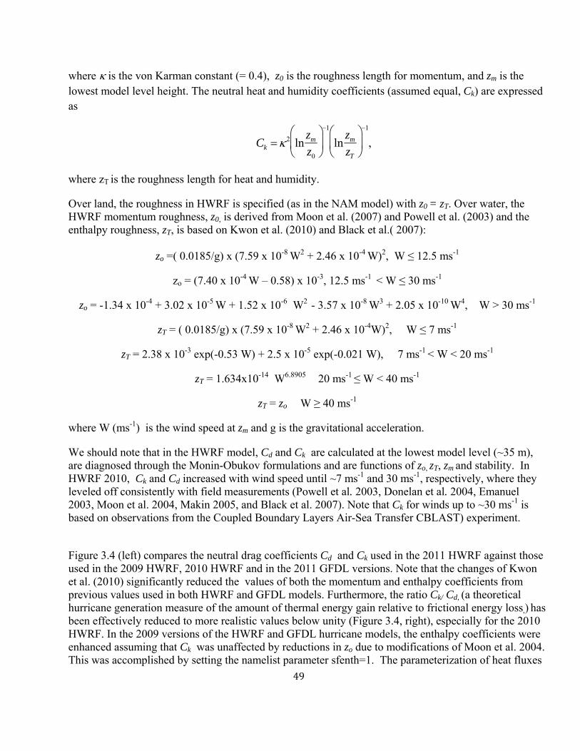
49

where is the von Karman constant (= 0.4), z0 is the roughness length for momentum, and zm is the lowest model level height. The neutral heat and humidity coefficients (assumed equal, Ck) are expressed as

Ck 2 ln

zm

z0

1

lnzm

zT

1

,

where zT is the roughness length for heat and humidity.

Over land, the roughness in HWRF is specified (as in the NAM model) with z0 = zT. Over water, the HWRF momentum roughness, z0, is derived from Moon et al. (2007) and Powell et al. (2003) and the enthalpy roughness, zT, is based on Kwon et al. (2010) and Black et al.( 2007):

zo =( 0.0185/g) x (7.59 x 10-8 W2 + 2.46 x 10-4 W)2, W ≤ 12.5 ms-1

zo = (7.40 x 10-4 W – 0.58) x 10-3, 12.5 ms-1 < W ≤ 30 ms-1

zo = -1.34 x 10-4 + 3.02 x 10-5 W + 1.52 x 10-6 W2 - 3.57 x 10-8 W3 + 2.05 x 10-10 W4, W > 30 ms-1

zT = ( 0.0185/g) x (7.59 x 10-8 W2 + 2.46 x 10-4W)2, W ≤ 7 ms-1

zT = 2.38 x 10-3 exp(-0.53 W) + 2.5 x 10-5 exp(-0.021 W), 7 ms-1 < W < 20 ms-1

zT = 1.634x10-14 W6.8905 20 ms-1 ≤ W < 40 ms-1

zT = zo W ≥ 40 ms-1

where W (ms-1) is the wind speed at zm and g is the gravitational acceleration.

We should note that in the HWRF model, Cd and Ck are calculated at the lowest model level (~35 m), are diagnosed through the Monin-Obukov formulations and are functions of zo, zT, zm and stability. In HWRF 2010, Ck and Cd increased with wind speed until ~7 ms-1 and 30 ms-1, respectively, where they leveled off consistently with field measurements (Powell et al. 2003, Donelan et al. 2004, Emanuel 2003, Moon et al. 2004, Makin 2005, and Black et al. 2007). Note that Ck for winds up to ~30 ms-1 is based on observations from the Coupled Boundary Layers Air-Sea Transfer CBLAST) experiment.

Figure 3.4 (left) compares the neutral drag coefficients Cd and Ck used in the 2011 HWRF against those used in the 2009 HWRF, 2010 HWRF and in the 2011 GFDL versions. Note that the changes of Kwon et al. (2010) significantly reduced the values of both the momentum and enthalpy coefficients from previous values used in both HWRF and GFDL models. Furthermore, the ratio Ck/ Cd, (a theoretical hurricane generation measure of the amount of thermal energy gain relative to frictional energy loss,) has been effectively reduced to more realistic values below unity (Figure 3.4, right), especially for the 2010 HWRF. In the 2009 versions of the HWRF and GFDL hurricane models, the enthalpy coefficients were enhanced assuming that Ck was unaffected by reductions in zo due to modifications of Moon et al. 2004. This was accomplished by setting the namelist parameter sfenth=1. The parameterization of heat fluxes

50

involves consideration of micro-scale physical processes near the sea surface, including spray production and advection, the characteristics of the interfacial sub layers, and the character of the surface sea state, including wave breaking and currents. Our understanding of these processes is still severely limited. Therefore, the effective values of Ck at hurricane wind speeds are still problematic and to reduce a known intensity bias in HWRF, the effective Ck was increased to values approaching Cd in the 2011 HWRF for wind speeds greater than 40 ms-1. In older versions of the GFDL hurricane model, z0 and zT were both calculated by the Charnock’s relation as 0.0185 u*

2/g, where u* is the friction velocity. Cd kept increasing with wind speed in the original GFDL model, which overestimated the surface drag at high wind speeds, leading to underestimation of the surface wind speed for a given central pressure in strong hurricanes (Ginis et al. 2004). The surface parameterization scheme used in GFS is also based on Sirutis and Miyakoda (1990) but modified by P. Long in the very stable and very unstable situations. The roughness length over ocean is updated with a Charnock formula after the surface stress has been obtained. The GFS thermal roughness over the ocean is based on a formulation derived from the Tropical Ocean Global Atmosphere Coupled Ocean Atmosphere Response Experiment (TOGA COARE, Zeng et al. 1998). Interestingly, the GFS scheme retains the Charnock formulation of roughness for momentum while the GFDL hurricane model retains the Charnock formulation for enthalpy. Therefore there is a distinction between momentum and enthalpy roughness among the HWRF, GFDL, and GFS surface flux schemes, with correspondingly different momentum and enthalpy coefficients at high wind speed. Another surface flux parameterization scheme that has been used experimentally in HWRF is the Mellor-Yamada-Janjic (MYJ) scheme, formerly referred to as the Eta surface layer scheme (Janjic 1996b, 2002) which is based on the similarity theory (Kurihara and Tuleya 1974). The scheme includes parameterizations of a viscous sub-layer. The surface fluxes are computed by an iterative method. This surface layer scheme is generally run in conjunction with the Eta MYJ PBL scheme, and therefore is referred to as the MYJ surface scheme. As mentioned previously, when the HWRF model is run with the NAM options, including the MYJ scheme, hurricane intensity tends to be reduced.

3.5 Landsurface model

LSMs use atmospheric information from the surface layer scheme, radiative forcing from the radiation scheme, and precipitation forcing from the microphysics and convective schemes, together with internal information on the land's state variables and land-surface properties, to provide heat and moisture fluxes over land points and sea-ice points. These fluxes provide a lower boundary condition for the vertical transport done in the PBL schemes (or the vertical diffusion scheme in the case where a PBL scheme is not run, such as in large-eddy mode). Land-surface models have various degrees of sophistication in dealing with thermal and moisture fluxes in multiple layers of the soil and also may handle vegetation, root, and canopy effects and surface snow-cover prediction. In WRF, the LSM provides no tendencies, but updates the land's state variables which include the ground (skin) temperature, soil temperature profile, soil moisture profile, snow cover, and possibly canopy properties. There is no horizontal

51

interaction between neighboring points in the LSM, so it can be regarded as a one-dimensional column model for each WRF land grid-point, and many LSMs can be run in a stand-alone mode when forced by observations or atmospheric model input. One of the simplest land models involve only one soil layer (slab) and predict surface temperature only. In this formulation, all surface fluxes (both enthalpy and momentum) are predicted by the surface layer routines. HWRF uses such a simple land model: the GFDL slab option.

The GFDL slab scheme

The GFDL slab model was developed by Tuleya (1994) based on Deardorff (1978). This simple one-level slab model, together with the GFDL radiation package, completed the requirement for realistic tropical cyclone behavior over land during the development of the GFDL hurricane model (see Figure 3.5). The surface temperature, T*, is the only predicted parameter in this system.

∂T*/∂t = (-σT*4 - Shfx - Levp + (S+F ))/(ρscsd), where

Shfx is the sensible heat flux, Levp is the evaporative flux, (S+F) is the net downward radiative flux, ρs

,cs, and d are the density, specific heat and damping depth of the soil, respectively. The surface wetness is assumed to be constant during the model forecast, with initial values based on the host model GFS analysis. Note that this simple model is able to realistically simulate the development of the ‘cool pool’ land temperature under landfalling tropical storms, thereby drastically reducing the surface evaporation over land leading to rapid decay over land. This simple slab model can be contrasted with the Noah LSM developed jointly by NCAR and NCEP, which is a unified code for research and operational purposes, being almost identical to the code used in the NAM Model. This is a 4-layer soil temperature and moisture model with canopy moisture and snow cover prediction. The layer thicknesses are 10, 30, 60 and 100 cm (adding to 2 meters) from the top down. It includes root zone, evapotranspiration, soil drainage, and runoff, taking into account vegetation categories, monthly vegetation fraction, and soil texture. The scheme provides sensible and latent heat fluxes to the boundary-layer scheme. The Noah LSM additionally predicts soil ice, and fractional snow cover effects, has an improved urban treatment, and considers surface emissivity properties. The Noah LSM is presently being run in test mode in HWRF.

3.6 Planetary boundary layer parameterization

The PBL parameterization is responsible for vertical sub-grid-scale fluxes due to eddy transports in the whole atmospheric column, not just the boundary layer. Thus, when a PBL scheme is activated, no explicit vertical diffusion (e.g. Smagorinsky-type diffusion) is activated with the assumption that the PBL scheme will handle this process. Horizontal and vertical mixing are therefore treated independently. The surface fluxes are provided by the surface layer and land-surface schemes. The PBL schemes determine the flux profiles within the well-mixed boundary layer and the stable layer, and thus

52

provide atmospheric tendencies of temperature, moisture (including clouds), and horizontal momentum in the entire atmospheric column. Most PBL schemes consider dry mixing, but can also include saturation effects in the vertical stability that determines the mixing. Conceptually, it is important to keep in mind that PBL parameterization may both complement and conflict with cumulus parameterization. PBL schemes are one-dimensional, and assume that there is a clear scale separation between sub-grid eddies and resolved eddies. This assumption will become less clear at grid sizes below a few hundred meters, where boundary layer eddies may start to be resolved, and in these situations the scheme should be replaced by a fully three-dimensional local sub-grid turbulence scheme, such as the Turbulent Kinetic Energy (TKE) diffusion scheme. HWRF uses the GFS PBL option.

The GFS PBL scheme

The HWRF code uses the same non-local scheme as the GFDL operational hurricane model (Hong and Pan 1996) which is based on Troen and Mahrt (1986), was implemented in GFS in 1995, and is similar to the current GFS scheme. Note that this scheme is similar, but not the same, as the Yonsei University (YSU) scheme and the Medium-Range Forecast (MRF) boundary layer scheme. Historically the GFS PBL scheme has been found to give reasonable tropical cyclone tracks for the global GFS and GFDL hurricane models when packaged with the SAS cumulus scheme. The scheme is a first-order vertical diffusion parameterization that uses the bulk-Richardson approach to iteratively estimate a PBL height starting from the ground upward. Once the PBL height is determined, the profile of the coefficient of diffusivity is specified as a cubic function of the PBL height. The actual values of the coefficients are determined by matching with the surface-layer fluxes. There is also a counter-gradient flux parameterization that is based on the fluxes at the surface and the convective velocity scale (Hong and Pan 1996). The non-local effect incorporates the contribution of large-scale eddies driven by surface layer conditions (see Figure 3.6). The local part of the diffusivity depends on the diagnosed height of the PBL which itself depends on the profile of virtual temperature from the top of the PBL to the surface, the wind speed of the PBL height and a critical Richardson number. The overall diffusive tendency of a parameter C can be expressed as: ∂C/∂t =∂/∂z[Kc (∂C/∂z –γc)] , where ∂C/∂z and γc are the local and non-local parts, respectively. In addition, in the GFS boundary layer formulation, there is a namelist parameter, disheat, that controls the amount of dissipative heating, that is, heat produced by molecular friction of air at high wind speeds (Bister and Emanuel 1998). This scheme can be contrasted with local schemes such as the Mellor-Yamada-Janjic (MYJ) PBL used in NAM, which is an option for experimental versions of HWRF. This parameterization of turbulence in the PBL and in the free atmosphere (Janjic 1990a,b, 1996a, 2002) represents a nonsingular implementation of the Mellor-Yamada Level 2.5 turbulence closure model (Mellor and Yamada 1982) through the full range of atmospheric turbulent regimes. In this implementation, an upper limit is imposed on the master length scale. This upper limit depends on the TKE as well as the buoyancy and shear of the driving flow. In the unstable range, the functional form of the upper limit is derived from the requirement that the TKE production be nonsingular in the case of growing turbulence. In the stable range, the upper limit is derived from the requirement that the ratio of the variance of the vertical velocity deviation and TKE cannot be smaller than that corresponding to the regime of vanishing turbulence. The TKE production/dissipation differential equation is solved iteratively. The empirical

53

constants used in the original Mellor-Yamada scheme have been revised (Janjic 1996a, 2002). Interestingly, the MYJ PBL scheme is quite similar to the Mellor-Yamada Level 2.5 scheme used in the early operational versions of the GFDL hurricane model. Note that the TKE in the MYJ boundary layer scheme has a direct connection to the horizontal diffusion formulation in the NAM dynamic core, but this has been turned off in HWRF.

3.7 Atmospheric radiation parameterization

Radiation schemes provide atmospheric heating due to radiative flux divergence and surface downward longwave and shortwave radiation for the ground heat budget. Longwave radiation includes infrared or thermal radiation absorbed and emitted by gases and surfaces. Upward longwave radiative flux from the ground is determined by the surface emissivity that in turn depends upon land-use type, as well as the ground (skin) temperature. Shortwave radiation includes visible and surrounding wavelengths that make up the solar spectrum. Hence, the only source is the Sun, but processes include absorption, reflection, and scattering in the atmosphere and at surfaces. For shortwave radiation, the upward flux is the reflection due to surface albedo. Within the atmosphere, radiation responds to model-predicted cloud and water vapor distributions, as well as specified carbon dioxide, ozone, and (optionally) trace gas concentrations and particulates. All the radiation schemes in WRF currently are column (one-dimensional) schemes, so each column is treated independently, and the fluxes correspond to those in infinite horizontally uniform planes, which is a good approximation if the vertical thickness of the model layers is much less than the horizontal grid length. This assumption would become less accurate at high horizontal resolution, especially where there is sloping topography. Atmospheric radiation codes are quite complex and computationally intensive and are therefore often invoked at less frequent intervals than the rest of the model physics. The HWRF radiation parameterizaton used in operations is that from GFDL (see below) and is similar to the one used in the NAM. Compared to extra-tropical phenomena, hurricanes are less dependent on radiative fluxes except when migrating out of the tropics and/or progressing over land. Radiation-cloud interactions may be more important than direct radiative impacts, except during extra-tropical transition.

The Eta Geophysical Fluid Dynamics Laboratory (GFDL) longwave scheme

This longwave radiation scheme follows the simplified exchange method of Fels and Schwarzkopf (1975) and Schwarzkopf and Fels (1991), with calculation over spectral bands associated with carbon dioxide, water vapor, and ozone. Included are Schwarzkopf and Fels (1985) transmission coefficients for carbon dioxide, a Roberts et al. (1976) water vapor continuum, and the effects of water vapor-carbon dioxide overlap and of a Voigt line-shape correction. The Rodgers (1968) formulation is adopted for ozone absorption. Clouds are randomly overlapped. More recent versions of the GFDL longwave radiation scheme, such as the one used in the NAM model but not adopted in HWRF, contain parameters for urban effects, as well as surface emissivities that can be different than 1.0.

54

The Eta Geophysical Fluid Dynamics Laboratory (GFDL) shortwave scheme

This shortwave radiation is a GFDL version of the Lacis and Hansen (1974) parameterization. Effects of atmospheric water vapor, ozone (both from Lacis and Hansen 1974), and carbon dioxide (Sasamori et al. 1972) are employed. Clouds are randomly overlapped. Shortwave calculations are made using a daylight-mean cosine solar zenith angle for the specific time and grid location averaged over the time interval (given by the radiation call frequency). The newest version of the GFDL shortwave radiation scheme, used for example in the NAM model but not adopted in HWRF, contains parameters for urban effects.

3.8 Physics interactions

While the model physics parameterizations are categorized in a modular way, it should be noted that there are many interactions between them via the model state variables (potential temperature, moisture, wind, etc.) and their tendencies, and via the surface fluxes. The surface physics, while not explicitly producing tendencies of atmospheric state variables, is responsible for updating the land-state variables as well as updating fluxes for ocean coupling. Note also that the microphysics does not output tendencies, but updates the atmospheric state at the end of the model time-step. The radiation, cumulus parameterization, and boundary-layer schemes all output tendencies, but the tendencies are not added until later in the solver, so the order of call is not important. Moreover, the physics schemes do not have to be called at the same frequency as each other or at the basic model dynamic time step. When lower frequencies are used, their tendencies are kept constant between calls or time interpolated between the calling intervals. In contrast to HWRF, note that the GFDL hurricane modeling system calls all physics packages once per time step except for radiation. The land-surface and ocean models, excluding simple ones, also require rainfall from the microphysics and cumulus schemes. The boundary-layer scheme is necessarily invoked after the land-surface scheme because it requires the heat and moisture fluxes.

55

Figure 3.1. Water species used internally in the Ferrier microphysics and their relationship to the total condensate. The left column represents the quantities available inside the microphysics scheme (mixing ratios of vapor, ice, snow, rain, and cloud water). The right column represents the quantities available in the rest of the model: only the water vapor and the total condensate get advected. After advection is carried out, the total condensate is redistributed among the species based on fractions of ice and rain water.

56

Figure 3.2. Comparison among a) verifying GFS mean sea level pressure (hPa) analysis and 132-h GFS model forecasts with b) no cumulus momentum mixing and c) and d) with some amount of cumulus momentum mixing. The GFS forecasts were initialized at 0000 UTC 22 Sep 2000. Note several spurious vortices west of 100 W in (b) and (d) (from Han and Pan 2006).

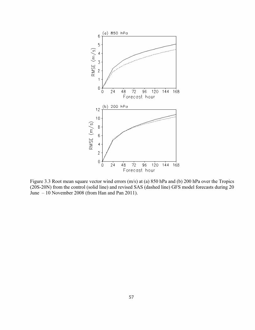
57

Figure 3.3 Root mean square vector wind errors (m/s) at (a) 850 hPa and (b) 200 hPa over the Tropics (20S-20N) from the control (solid line) and revised SAS (dashed line) GFS model forecasts during 20 June – 10 November 2008 (from Han and Pan 2011).

58

Figure 3.4. Left: over water, neutral drag momentum (Cd - solid) and enthalpy (Ck - dashed, dash-dotted) coefficients vs. lowest model level (~ 35 m) wind speed from the 2009, 2010, 2011versions of HWRF (note that the 2010 and 2011 Cd are identical). Right: ratio of enthalpy to momentum coefficient (Ck/ Cd) for the 2011, 2010 and 2009 HWRF versions (note that the 2010 HWRF is labeled V3R2 on the plots). These values of Ck and Cd do not include enthalpy enhancement. However, both the 2009 HWRF and the GFDL operational models used enhanced (sfenth=1) enthalpy surface exchange which results in effective values of Ck and Ck/ Cd greater than those indicated in the figure.

59

Figure 3.5. Fluxes employed in the LSM used in the GFDL and HWRF hurricane models. The surface land temperature is the only state variable predicted in this scheme. G represents the flux of heat into the ground and all other terms are defined in the text.

60

Figure 3.6. Time-pressure cross sections of the eddy diffusivity (m2 s-1) calculated with the local (dotted) and nonlocal (solid) schemes and for (a) thermal and (b) momentum. The GFS boundary layer uses the nonlocal formulation in which the eddy mixing is due in part to surface conditions (from Hong and Pan 1996).

61

4.0 Moving Nest

A hurricane is an intense atmospheric circulation characterized by strong multi-scale interactions between convective clouds, on the order of a few tens of kilometers, and the large scale environment, on the order of several hundreds to thousands of kilometers. In order to forecast such a system, both high resolution and a large domain are basic requirements. However, at this time, it is not possible to run operational models over domains of 75 to 100 degrees on a side with uniform resolution on the order of a few kilometers. Nevertheless, moving nested grids and more complex adaptive grid models (Gopalakrishnan et al. 2002) may be used as efficient forecasting tools for the hurricane problem. The NMM dynamic core of the WRF model, used in HWRF, supports moving, one- or two-way interactive nests. The model can handle multiple domains at the same nest level (no overlapping nest), and/or multiple nest levels (telescoping). The operational HWRF model always employs two domains: a coarse grid and a moving nest, with two-way interaction. When there is more than one tropical storm active in an oceanic basin, more than one run of HWRF is launched so that every storm has its own high-resolution nest. In the current implementation of the nesting algorithm, only horizontal refinement is available, i.e., there is no vertical nesting option. The nested grids must use a 1:3 ratio between the resolution of the coarse and fine grids. Similarly, the timestep ratio between the coarse and fine grids is also 1:3. The mass points of the nested grids are aligned with those of the coarser grid within which they are nested. The coincidence of grid points between the parent and nested domains simplifies remapping calculations and improves distributed memory performance and portability of the model within the WRF advanced software framework (Michalakes et al. 2004). WRF-NMM supports initialization and termination of nested grids at any time during the model run. However, in HWRF the nest is present throughout the entire run.

4.1 Grid design

As described in the NMM scientific documentation (Janjic et al. 2010), the WRF-NMM is a non-hydrostatic model formulated on a rotated latitude-longitude, Arakawa E-grid, with a vertical pressure-sigma hybrid coordinate system. The latitude-longitude coordinate is simply transformed in such a way that the coordinate origin is located in the center of the parent domain (Figure 4.1). In order to deal with multi-scale forecasting, a horizontal mesh refinement capability was developed for this dynamical core. The refinement capability, commonly referred to as telescopic mesh, supports one- or two-way interaction between a lower-resolution parent domain and one or more higher-resolution nests. All interpolations from the parent to the nested domain are done on a rotated latitude-longitude E-grid with the reference latitude-longitude located at the center of the parent domain. The nested domain can be freely moved anywhere within the grid points of the parent domain, yet the nested domain rotated latitude-longitude lines will always coincide with the rotated latitude-longitude lines of the parent domain at integer parent-to-nest grid-size ratio. (Figure 4.1).

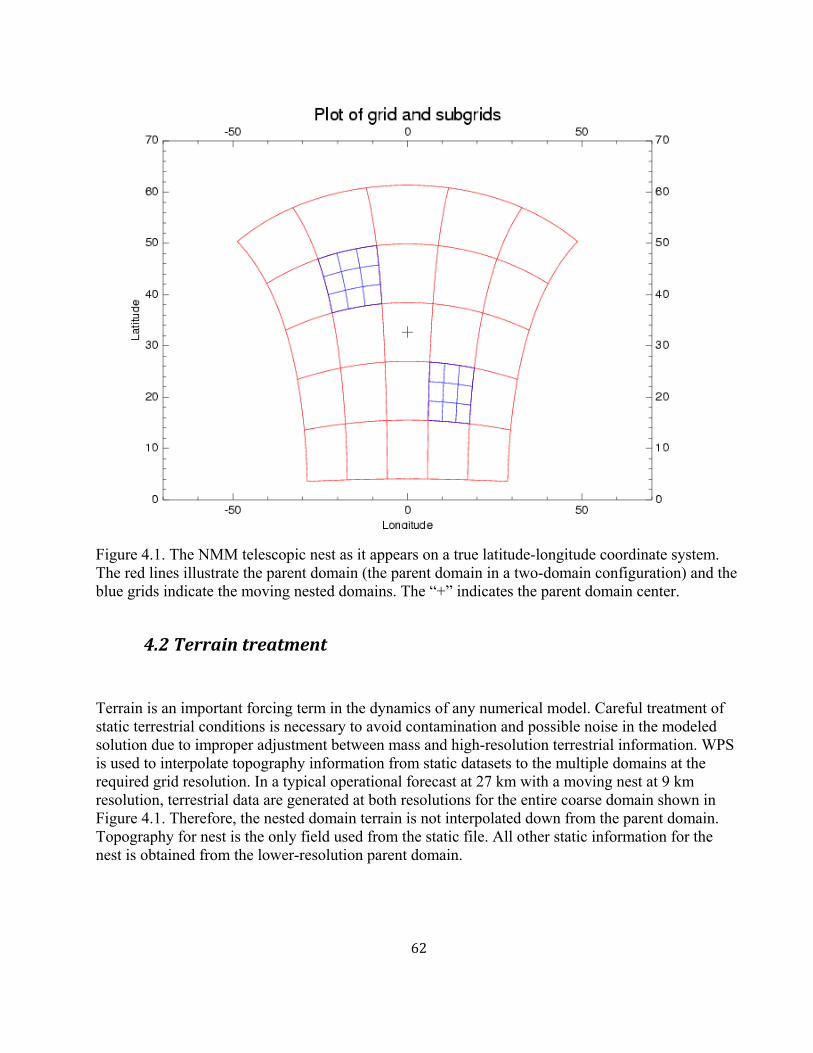
62

Figure 4.1. The NMM telescopic nest as it appears on a true latitude-longitude coordinate system. The red lines illustrate the parent domain (the parent domain in a two-domain configuration) and the blue grids indicate the moving nested domains. The “+” indicates the parent domain center.

4.2 Terrain treatment

Terrain is an important forcing term in the dynamics of any numerical model. Careful treatment of static terrestrial conditions is necessary to avoid contamination and possible noise in the modeled solution due to improper adjustment between mass and high-resolution terrestrial information. WPS is used to interpolate topography information from static datasets to the multiple domains at the required grid resolution. In a typical operational forecast at 27 km with a moving nest at 9 km resolution, terrestrial data are generated at both resolutions for the entire coarse domain shown in Figure 4.1. Therefore, the nested domain terrain is not interpolated down from the parent domain. Topography for nest is the only field used from the static file. All other static information for the nest is obtained from the lower-resolution parent domain.

63

4.3 Fine grid initialization

In WRF-NMM, all variables of the fine grid, except terrain, are initialized from a coarse grid, which itself is initialized using WPS. Although the terrain adjustment is advanced, in order to alleviate potential problems related to singularities due to isolated land grid points in the nested domain, the initialization of the other land variables, such as land-sea mask, soil temperature and vegetation type, has been simplified and is done through a nearest-neighbor approach. To obtain the temperature, geopotential, and moisture fields for the nest initialization, pseudo-hydrostatic mass balance is applied. The first step is to use cubic splines to vertically interpolate those fields from hybrid levels to constant pressure levels in each horizontal grid point of the parent grid. The second step is to bilinearly interpolate those fields in the horizontal from the parent grid to the nest. The third step is to use the high-resolution terrain and the geopotential to determine the surface pressure on the nest. Next, the pressure values in the nest hybrid surfaces are calculated. The final step is to compute the geopotential, temperature and moisture fields on the nest hybrid surfaces using a cubic spline interpolation in the vertical. The zonal and meridional components of the wind are obtained by first performing a horizontal interpolation from the parent to the nest grid points using a bi-linear algorithm over the diamond-shaped area indicated in grey in Figure 4.2. The wind components are then interpolated in the vertical from the parent hybrid surfaces onto the nest hybrid surfaces using cubic splines. Note that, while the hybrid levels of the nest and parent in sigma space coincide, the nest and the parent do not have the same levels in pressure or height space. This is due to the differing topography, and consequently different surface pressure between the nest and the parent. In HWRF, an important additional step is performed through the vortex initialization procedure (described in Section 1).

4.4 Boundary

Figure 4.2 illustrates a sample E-grid structure, in which the outermost rows and columns of the nest are termed the prescribed interface, and the third rows and columns are termed the dynamic interface. The prescribed interface is forced to be identical to the parent domain interpolated to the nest grid points. The dynamic interface is not directly altered by the parent domain, that is, its values are obtained from internal computations within the nest. The second rows and columns are a blend of the first and third rows/columns. Because of the E-grid structure and the fact that the prescribed interface is well separated from dynamic interface, nested boundaries can be updated at every time step of the parent domain exactly the same way as the parent domain boundary is updated from the external data source. While bi-linear interpolation from the parent onto the nested domain is used to prescribe the wind and the total condensate, the mass adjustment procedure adopted for initialization

64

is repeated at every timestep of the parent domain at the outermost boundaries. This approach is simple, and yet produces an effective way of updating the interface without excessive distortion or noise.

Figure 4.2. E-grid refinement on mass grid points. The diamond-shaped grid box indicates the bi-linear horizontal interpolation plan from coarse grid to fine grid. Large symbols indicate the coarse grid points; small symbols indicate the fine grid. Three arrows illustrate the prescribed, penultimate, and dynamic interfaces within a boundary of the nested domain.

4.5 Feedback

The feedback, i.e., two-way interactive nesting, is available in the current version. For the two-way interactive technique, the mass, momentum and scalar fields in the 13-points of the fine grid surrounding a coarse grid point are first averaged. Next, the value of the field in that coarse grid point is substituted by a weighted average between their original value and the average of the fine grid points. The weighting factor is 0.5, indicating that a coarse grid point retains half of its original value.

65

4.6 Movable nesting

Tropical cyclones are moving systems which can travel thousands of kilometers, requiring the high-resolution nest to move. The nest motion for tropical cyclones and tropical depressions is currently based on the concept of dynamic pressure (Gopalakrishnan et al. 2002). The stagnation point is chosen as the center of the storm. At the end of every time step of the nested domain, the dynamic pressure within this domain is determined. If the storm center has moved more than one grid point of the parent domain (3 grid points from the center of the nested domain for a 1:3 parent to nest grid ratio), the nested domain is moved to a new position so as to maintain the storm at the center of the nested domain. Some filtering is done to properly isolate the storm center in weak storms and/or over the land. The nest motion may be terminated if the nested domain is near the parent domain boundary. It should be noted that, while at every timestep data is exchanged between domains before and after the grid motion in the majority of the domain, the interpolation and pseudo hydrostatic mass balancing discussed earlier are also applied in the region of the leading edge of the moving nest.

4.7 Future work

Under the support of the NOAA Hurricane Forecast Improvement Project (HFIP), additional moving nest development is underway in the Hurricane Research Division (HRD) of NOAA’s Atlantic Oceanographic and Meteorological Laboratory. The new development includes multiple moving nests capability and a new algorithm to prescribe nest movement. In the future, this new development will replace the current moving nest algorithm.

66

5.0 Use of the GFDL Vortex Tracker

5.1. Introduction

Numerical modeling has become an increasingly important component of hurricane research and operational hurricane forecasting. Advances in modeling techniques, as well as in fundamental understanding of the dynamics of tropical cyclones, have enabled numerical simulations of hurricanes to become more realistic and contributed to hurricane forecasts becoming more skillful. One critical element of assessing the performance of a hurricane model is the evaluation of its track and intensity forecasts. These forecasts are typically represented in the form of text data that are output either directly from the forecast model or in a post-processing step of the modeling system using an external vortex tracker. This document provides a description of the GFDL vortex tracker (Marchok 2002), which operates as a standalone tracking system in a post-processing step. The GFDL vortex tracker has been used as an operational tool by NCEP since 1998, and it is flexible enough to operate on a variety of regional and global models of varying resolutions.

5.1.1 Purpose of the vortex tracker

A numerical model produces an abundance of digital output, with up to hundreds of variables on dozens of vertical levels, including variables for mass, momentum, density, moisture, and various surface and free-atmosphere fluxes. While a tropical cyclone’s center is defined by its low-level circulation features, a comparison of synoptic plots of various low-level parameters will often reveal a range of variability in a storm’s center position. This variability can be particularly large for storms that are either just forming or are undergoing extratropical transition. Figure 5.1 illustrates this variability for a case of Tropical Storm Debby (2006) in an analysis from NCEP/GFS. At this time, Debby was a weak, 40-knot tropical storm, and the variability in the center location fixes indicates that the model had not yet developed a coherent vertical structure for the storm. A vortex tracker is needed in order to objectively analyze the data and provide a best estimate of the storm’s central position and then track the storm throughout the duration of the forecast. Depending on the complexity of the tracker, additional metrics can be reported, including the minimum sea-level pressure, the maximum near-surface wind speed, the radii of gale-, storm- and hurricane-force winds in each storm quadrant, parameters that describe the thermodynamic structure or phase of the storm, and parameters that detail the spatial distribution of the near-surface winds. This document will focus primarily on the basic functioning of the tracker and its reporting of the track, intensity and wind radii parameters.

67

5.1.2 Key issues in the design of a vortex tracker

When designing a tracking scheme, there are a couple of fundamental issues that must be considered. The first issue is deciding on the method used to locate a maximum or a minimum in some field of values. There are numerous methods that can be used for this purpose. The simplest method is to scan the field of values and pick out the maximum or minimum at one of the model output grid points. However, this method restricts the maximum or minimum value to being located at one of the fixed data points on the grid. For many grids, especially those with coarser resolutions, the actual maximum or minimum value may fall between grid points. The data can be interpolated to a finer resolution, but interpolation is a procedure that can be both expensive and complicated to generalize for usage with both regional and global grids over a range of resolutions. In addition, a problem can still remain after interpolation in which the tracking scheme needs to choose between two or more candidate points with identical values that are located close to one another. The GFDL vortex tracker uses a scheme that employs a Barnes analysis of the data values at each candidate grid point to provide a field of values that have been weight-averaged based on distance from the candidate grid point. This technique, which will be described in detail below, helps to mitigate the issues described above. The second issue involves finding the right balance between making the scheme sensitive enough so that it can detect and track weaker storms, and making it overly sensitive such that it continues tracking for too long and tracks weak remnants that no longer resemble a cyclone, or worse, it jumps to a stronger passing storm and begins tracking that storm instead. There are several checks that have been included in the GFDL vortex tracker, some with thresholds that can be adjusted either in the source code or via namelists as inputs to the executable. These will be described below. The remainder of this document will describe in detail the design and functioning of the GFDL vortex tracker. Section 5.2 will focus on the design of the tracker and the input data that it needs. Section 5.3 presents a discussion of the various low-level parameters that are tracked and how they are combined to produce a mean position fix at a given lead time. Section 5.4 describes how the maximum wind and the various wind radii in each storm quadrant are obtained, and Section 5.5 provides detail on the tracker output.

5.2. Design of the tracking system

5.2.1 Input data requirements

The GFDL vortex tracker can operate in two different modes. In the basic mode, it will perform tracking only for storms that have been numbered by a Regional Specialized Meteorological Center (RSMC), such as the NHC. It can also operate in a mode in which it detects and tracks new storms

68

that a model generates during the course of a forecast, however only the basic mode will be described in this document since it is the only mode currently supported by the DTC. 5.2.1.1 Synoptic forecast data

The tracker requires input data to be in Gridded Binary (GRIB) version 1 format, on a cylindrical equidistant, latitude-longitude (lat/lon) grid. While the dx and dy grid increments each need to be uniform across the grid, dx does not need to be equal to dy. The data should be ordered so that j and i increment from north to south and east to west, respectively, such that point (1,1) is in the far northwestern part of the grid, and point (imax,jmax) is in the far southeastern part of the grid. Data files that instead have data values incrementing from south to north can be flipped prior to execution of the tracker using an external GRIB file manipulation tool. The data files do not need to have regular spacing for the lead time intervals. This flexibility allows the user to obtain tracker output using output model data at more frequent time intervals around a particular time of interest. The tracker reads in a list of forecast lead times from a text file that the user prepares. The tracker has the ability to process GRIB files that have the lead times identified in the Product Definition Section (PDS) of the GRIB header as either hours or minutes. The choice for using either minutes or hours is passed to the program via a namelist option. Regardless of which choice is made, those lead times must be listed in the user input text file as integers in units of minutes (the exact required format can be seen in the read statement in subroutine read_fhours), and then the tracker can manipulate the hours and minutes as needed. 5.2.1.2 Realtime observed storm data

The tracker works by searching for a vortex initially at a location specified by a 1-line text record that is produced by either NHC for storms in the Atlantic, eastern Pacific and central Pacific basins, or by the JTWC for storms in other global basins. This record contains just the basic, vital information necessary to define the observed location and intensity parameters of the storm, and it is commonly referred to as the “TC vitals” record. An example TC vitals record is shown here for Katrina for the observed time of 00 UTC 29 August 2005: NHC 12L KATRINA 20050829 0000 272N 0891W 335 046 0904 1006 0649 72 037 0371 0334 0278 0334 D 0204 0185 0139 0185 72 410N 815W 0167 0167 0093 0167

The critical information needed from the TC vitals record for tracking is the Automated Tropical Cyclone Forecast (ATCF) ID number for the storm (12L), the observed time (20050829 0000), and the location of the storm, indicated here as “272N 0891W”, or 27.2o North, 89.1o West. For this example, the tracker would start looking for Katrina in the 00 UTC 29 August 2005 analysis for a given model at 27.2o North, 89.1o West, and if it finds a storm near there, it records its position, writes out a record in a specific text format that contains critical storm forecast location and intensity

69

forecast data, and then makes a guess for the next position at the next forecast lead time to begin searching again.

5.2.2 The search algorithm

To locate a maximum or minimum value for a given variable, we employ a single-pass Barnes analysis (Barnes 1964, Barnes 1973) at grid points in an array centered initially around the NHC-observed position of the storm. We refer to this NHC-observed position as the initial guess position. For a given variable F, the Barnes analysis, B, at a given point, g, in this array is given as:

∑∑

where w is the weighting function defined by:

and where dn is the distance from a data point, n, to the grid point, g, and re is the e-folding radius. The e-folding radius is the distance at which the weighting drops off to a value of 1/e, and this value can be adjusted. Currently, most regional and global model grids fall into a category with output file grid spacing between about 0.1o and 1.25o , and for those we use a value of re = 75 km. For any models with resolutions coarser than 1.25o degree, we use a value of re = 150 km. For model grids with a grid spacing finer than 0.1o, we use a value of re = 60 km. The overriding idea is that we want to find a balance whereby we include enough points in the averaging process to produce a weighted average from the Barnes function that is representative of the surrounding region, but not so many points that finer scale details are smoothed out to the degree of making it difficult to differentiate the average value at one grid point from that of an adjacent point. The Barnes analysis provides an array of Gaussian weighted-average data values surrounding the initial guess position. The center is defined as the point at which this function is maximized (e.g., Northern Hemisphere relative vorticity) or minimized (e.g., geopotential height, sea level pressure, Southern Hemisphere relative vorticity), depending on the parameter being analyzed. As described above, the center location for a given parameter will often lie between grid points, and this is especially true for coarser resolution grids. In order to produce a position fix with enough precision such that center fixes for variables with center locations between grid points can be properly represented, it may be necessary to perform several iterations of the Barnes analysis. In the initial iteration, a Barnes analysis grid is defined with grid spacing equal to that of the input data grid, and the weighted values from the Barnes analysis are assigned to the points on the analysis grid. The difference between the input data grid and the Barnes analysis grid is that the input data grid has specific (i,j) locations that are fixed, while for the analysis grid we can define an array of points, relative to the guess position, in latitude-longitude space. After a position fix is returned from the first iteration of the Barnes analysis, we can perform an additional iteration of the Barnes

5.2.2.1

5.2.2.2

70

analysis, this time centering the analysis grid on the position fix from the first iteration. In this second iteration, the search area for the center location is restricted, and the grid spacing of the Barnes analysis grid is halved in order to produce a finer resolution position fix. We can iterate this process a number of times and run the Barnes analysis over increasingly finer resolution analysis grids in order to more precisely fix the center position. In the current version of the tracker, we specify a variable (“nhalf”) to indicate that five additional iterations of the Barnes analysis should be done for grids with spacing greater than 0.2o. For example, for a grid with original grid spacing of 1o, halving the analysis grid spacing five times would result in a final analysis grid spacing of approximately 3 km, which is already beyond the one-tenth of a degree precision contained in the observational Best Track dataset. For data grids with original spacing of less than 0.2o, such as the operational HWRF, only two additional Barnes iterations are performed, and for grids with spacing less than 0.05o, only one additional Barnes iteration is performed. 5.2.2.1 Tracking a vortex throughout a forecast

A tracking algorithm ultimately produces a set of points that contains information on the forecast location of the storm at discrete time intervals. A fundamental challenge is ensuring that the points that are connected from one lead time to the next do in fact represent points from the same storm and that there is no “contamination” introduced by accidentally having the tracker follow a different storm. This challenge becomes greater for model output with longer intervals between lead times. For example, it is far easier to know with certainty that a nearby storm is the same storm that we have been tracking up to this time if the last position fix only occurred 30 minutes ago in model time as opposed to it having occurred 12 hours ago. This section deals with how the model handles the tracking of a vortex from one lead time to the next and what types of quality control checks are applied.

a. Tracking from one lead time to the next

If the tracker finds a storm at a given lead time, it needs to know where to begin searching for the storm at the next lead time. There are two methods that the tracker employs for this purpose. In the first method, a Barnes analysis is performed for the location at which the tracker position fix was made for the current lead time. This analysis is performed for the winds at 500, 700 and 850 mb, using a relatively large e-folding radius of 500 km. The idea here is to create smoothed fields that represent the mean fields at each level. The mean values from these three levels are then averaged together to give a wind vector that can be used as a deep layer mean steering wind. A hypothetical parcel is then advected according to the deep layer mean wind for the length of the lead time interval in order to produce a dynamically generated guess position for the next lead time. The second method uses a basic linear extrapolation of the current model storm motion. For all lead times after the initial time, this method can be employed by using the previous and current forecast position fixes. For the initial time, there is obviously no previous position from the current model forecast to use for an extrapolation, however this extrapolation method is still used at the initial time by instead using the observed storm motion vector information that is read from the TC vitals record.

71

This method of using the storm motion vector is not as reliable, however, since the observed storm motion vector may differ from the model storm motion vector. The estimates from these two methods are averaged together to produce a position guess around which the tracker will begin searching for the storm at the next lead time. Both of these methods use estimates that are static in time, and therefore error is introduced in the position guesses. Those errors obviously become larger with increasingly longer lead time intervals. However, it is important to note that these are only position guesses, and the tracker will allow a position fix to be made up to a certain distance from that position guess. Experience in operations has shown the combination of these two methods to be a reliable means of providing position guesses for successive lead times, even for model output with lead time intervals of 12 hours. Cases which should be watched for trouble with the use of this method include those in which the storm begins to rapidly accelerate or decelerate, and those in which the storm is rapidly recurving into the westerlies.

b. Quality control checks

Once the tracker has produced a position fix at a given lead time, a number of checks are performed to help ensure that the system the tracker found is not only a storm, but also is the same storm that has been tracked to this point in the forecast. As a first check, the sea level pressures of the points surrounding the position fix are evaluated to determine if a pressure gradient exceeding a particular threshold exists and is sloped in the correct direction. This is a fairly easy criterion for a storm to satisfy since the requirement is only that it be satisfied for any azimuthal direction, and not that it be satisfied by a mean gradient value. The threshold can be set by the user in the run script by specifying its value in the “mslpthresh” variable. In the current version of the tracker, the mslpthresh variable is set to a value of 0.0015 mb/km, which is equivalent to 0.5 mb per 333 km. A second check involves the wind circulation at 850 mb. The tangential component of the wind (VT) is computed for all points within 225 km of the position fix, and the mean VT must be cyclonic and exceed a user-specified threshold. This threshold is also set in the run script by specifying the value of the v850thresh variable. This variable has units of m-1 and is set in the current version of the tracker to 1.5 m/s m-1. For a third check, the distance between the position fixes for two parameters is evaluated to ensure it does not exceed a specified distance. As will be described below in Section 5.3, the tracker finds the center location of several different low-level parameters. If the distance between the mean sea-level pressure (mslp) and 850 mb relative vorticity position fixes becomes too large, it could indicate either that the storm is becoming too disorganized due to dissipation or that it is undergoing extratropical transition and the tracker may have perhaps incorrectly “locked on” to a different storm nearby with one of those two parameter fixes. In either case, if that distance is exceeded, the tracker will stop tracking for this particular storm. That distance threshold is specified by the variable “max_mslp_850” in subroutine tracker, and it is currently set at 323 km for most models, including HWRF. One final check is made of the model storm’s translation speed. The current and previous position fixes are used to calculate the average speed that the model storm must have traveled in order to reach the current position, and if that speed exceeds a certain threshold, then the tracker assumes that it has incorrectly locked on to a different storm nearby and tracking is stopped for this storm. That

72

speed is specified by the “maxspeed_tc” variable in module error_parms and is currently set to a value of 60 knots. It should be noted here that during the evaluation of model forecasts from the HFIP High Resolution Hurricane (HRH) test in 2008, this storm translation speed check was responsible for erroneously stopping a number of forecasts. The problem arose for cases in which a very weak model storm center reformed after only 30 minutes of model time at a location more than 100 km away. While such behavior is reasonable for a very weak but developing storm to exhibit, this large shifting of storm position over a very short time period resulted in a computed translation speed that exceeded the threshold. If necessary, this problem can be circumvented by setting the maxspeed_tc threshold to an unrealistically high value. It is important to point out that while these last two quality control checks will occasionally terminate tracking for storms that are undergoing extratropical transition (ET), the intended purpose is not to stop tracking when ET is taking place. To the contrary, we want to continue tracking in order to provide track and intensity guidance for as long as possible in the forecast, and furthermore the model forecast of the onset of ET may not correspond at all to what happens with the observed storm. These last two checks are instead meant to stop tracking if the tracker detects that it may have erroneously begun to track a different, nearby storm. The current version of the tracker has code in it that will report on the thermodynamic phase of the system, that is, whether the system is tropical, extratropical, etc. This code requires input data that has been interpolated to certain levels and/or averaged. This capability is not currently supported by the DTC, and therefore is not described in this document.

5.3. Parameters used for tracking

The GFDL vortex tracker produces position fixes for several low-level parameters. The position fixes are then averaged together to produce the mean position fix that is reported for that lead time. This section describes the various parameters and how the tracker combines them in order to produce the mean position fix.

5.3.1 Description of the primary and secondary tracking variables There are six primary parameters and three secondary parameters that are used for tracking. All of these parameters are from the lower levels of the troposphere. The primary parameters include relative vorticity at 10 m and at 850 and 700 mb; mslp; and geopotential height at 850 and 700 mb. Most models, including HWRF, will output absolute vorticity, and for those models the tracker will subtract out the Coriolis component at each grid point. If vorticity is not included in the input GRIB data file, the tracker will compute it using the u- and v-components of the wind that have been read in. The Barnes analysis is performed for each of these six parameters. If the Barnes analysis returns a location for the maximum or minimum that is within a specified distance threshold, then that parameter’s location fix is saved for use later in computing the average position fix. If it is not

73

within that distance threshold, the position fix for that parameter is discarded for that lead time. If one or more of these parameters is missing from the input GRIB data file, the tracker simply continues tracking using the limited subset of available parameters. The distance thresholds are defined initially by the “err_gfs_init” and “err_reg_init” parameters in module error_parms. Values for this initial error parameter vary according to the resolution of the data grid, with finer resolution grids being assigned a threshold of 275 km and coarser resolution global grids being assigned a less restrictive 300 km threshold. For lead times after the initial time, this distance threshold is defined as a function of the standard deviation in the positions of the parameter location fixes including up to the three previous lead times. For example, for very intense, steady-state storms that have strong vertical coherence in their structure, the various parameter fixes are likely to be located closely together. In these cases, the distance threshold defined by the standard deviation of the parameter fixes will be small, as will be the tolerance for outliers in the parameter fixes. For weak systems, or for storms that are undergoing ET, there is less coherence to the vertical structure and often wider variance in location of the parameter fixes. In these cases, the larger distance thresholds defined by the larger standard deviation allow more flexibility in accepting parameter fixes that are not located close to the guess position for a given lead time. After the Barnes analysis is performed for the six primary tracking parameters, tracking is performed for three secondary wind-based parameters in order to refine the storm’s location fix. For these secondary parameters, a search is performed for the minimum in wind speed at the center of the storm at 10 m and at 850 and 700 mb. These are not included as primary parameters since, in an unrestricted search in the vicinity of a storm, it would be possible for the tracking scheme to focus in on a quiescent region outside of the storm instead of on the calm at the center of the storm. To help ensure that the search is focused as close to the storm center as possible, a modified guess position for the wind minimum search is created by averaging together the original guess position for this time and the locations of the primary parameter fixes for this lead time that are within 225 km of the original guess position. The Barnes analysis is then called to produce location fixes for the wind minimum at the three different vertical levels. It is important to note that if the tracker cannot make a position fix for any of the six primary parameters, then there will be no attempt to make a position fix using the three secondary wind-based parameters, and tracking will terminate for that particular storm.

5.3.2 Computation of the mean position fix

Once the Barnes analysis has been completed for the primary and secondary parameters, a mean location fix is computed for the storm. A parameter is only included in the mean computation if its location is found within the distance threshold, as described in Section 5.3.1. The mean computation is performed in two steps. In the first step, a mean position is computed using all available parameters found within the distance threshold. In the second step, the distance of each parameter fix from that mean position is computed, as is the standard deviation of the parameter fixes. The mean position fix is then recalculated by using a Gaussian weighting that is controlled by the standard deviation of the position fixes. The goal here is to minimize the impact of an outlier parameter fix by weighting the mean towards the larger cluster of parameter position fixes.

74

5.4. Intensity and wind radii parameters

The vortex tracker must also report on forecast data related to intensity and wind structure. For the mslp, the value that was reported during the search for the storm center was a smoothed value that came out of the Barnes analysis. A separate call is made to subroutine fix_latlon_to_ij in order to return the minimum gridpoint value of mslp near the storm center. The tracker then analyzes the near-surface wind data (10 m for HWRF and most other models) in order to report on the value of the maximum wind speed. For high resolution grids (spacing < 0.25o), the search for the maximum wind is restricted to points within 200 km of the center. For coarser resolution grids with spacing up to 1.25o, the search can extend out to 300 km from the center. The value of the radius of maximum winds is obtained at the same time. As large storms such as Katrina and Isabel have shown, it is important to have guidance on the structure of the wind field in addition to also having the forecast maximum wind value. The tracker provides for basic reporting of the forecast near-surface wind structure by obtaining the radii of 34-, 50- and 64-knot winds in each quadrant of the storm. The values that are reported indicate the maximum distance at which winds of these magnitudes were found anywhere in the quadrant and are not necessarily aligned along any particular azimuth within a quadrant. The values are then output in the standard ATCF text format, which will be described in the next section.

5.5. Tracker output

The motivation behind making this tracker operational in 1998 was to provide track and intensity guidance from forecasts for a number of models in as short a time as possible. One of the requirements was that the output data be in the same text ATCF format as that used by NHC. The two primary output files from the tracker include one file in ATCF format and another in a format just slightly modified from the ATCF format. The advantage of using the ATCF format is that user forecasts can easily be compared with those from some of the operational modeling centers.

5.5.1 Description of the ATCF format

The ATCF format contains information on the ocean basin, the storm number, the model ID, the initial date, the forecast hour, and various track, intensity and wind radii guidance. There can be up to three ATCF records that are output for each lead time. A sample segment with some ATCF records from a HWRF hurricane model forecast for Hurricane Ike is shown here:

75

AL, 09, 2008091012, 03, HWRF, 0, 238N, 852W, 80, 959, XX, 34, NEQ, 205, 189, 55, 98, 0, 0, 022 AL, 09, 2008091012, 03, HWRF, 0, 238N, 852W, 80, 959, XX, 50, NEQ, 56, 56, 27, 39, 0, 0, 022 AL, 09, 2008091012, 03, HWRF, 0, 238N, 852W, 80, 959, XX, 64, NEQ, 31, 31, 0, 25, 0, 0, 022 AL, 09, 2008091012, 03, HWRF, 6, 244N, 858W, 79, 955, XX, 34, NEQ, 247, 174, 154, 143, 0, 0, 030 AL, 09, 2008091012, 03, HWRF, 6, 244N, 858W, 79, 955, XX, 50, NEQ, 105, 113, 33, 35, 0, 0, 030 AL, 09, 2008091012, 03, HWRF, 6, 244N, 858W, 79, 955, XX, 64, NEQ, 36, 34, 0, 0, 0, 0, 030 AL, 09, 2008091012, 03, HWRF, 12, 250N, 868W, 74, 951, XX, 34, NEQ, 204, 219, 111, 141, 0, 0, 015 AL, 09, 2008091012, 03, HWRF, 12, 250N, 868W, 74, 951, XX, 50, NEQ, 121, 37, 34, 63, 0, 0, 015 AL, 09, 2008091012, 03, HWRF, 12, 250N, 868W, 74, 951, XX, 64, NEQ, 28, 21, 17, 33, 0, 0, 015 The first two columns represent the ATCF ID, here indicating that Ike was the 9th named storm in the Atlantic basin in 2008. The next column indicates the initial time for this forecast. The ‘03’ is constant and simply indicates that this record contains model forecast data. After the column with the model ID is a column indicating the lead time for each forecast record. The next two columns indicate the latitude and longitude, respectively, in degrees that have been multiplied by 10. The next two columns, respectively, are the maximum wind speed, in knots, and the minimum sea-level pressure, in mb. The “XX” is a placeholder for character strings that indicate whether the storm is a depression, tropical storm, hurricane, subtropical storm, etc. Currently, that storm type character string is only used for the observed storm data in the NHC Best Track data set. The next six columns are for reporting wind radii forecast data. The first in those six columns is an identifier that indicates whether this record contains radii for the 34-, 50- or 64-knot wind thresholds. The “NEQ” indicates that the four radii values that follow will begin in the northeast quadrant. Each subsequent value is from the next quadrant clockwise. The radii are listed in units of nautical miles (n mi). If the tracker has detected winds of at least 50 knots in the 10 m wind data, then an additional record will be output for this lead time. This record is identical to the first record, with the exception that the wind radii threshold identifier is ‘50’ instead of ‘34’, and the radii values are included for the 50-knot threshold. Similarly, if the tracker has detected winds of at least 64 knots at this lead time, then an additional record is output containing those 64-knot wind radii. For any of these thresholds for which at least one quadrant has wind value exceedance, if one or more of the remaining quadrants does not have exceedance, then for each of those quadrants a value of zero is output. Finally, the last column in each record indicates the radius of maximum winds, in n mi. This value is reported using the location of the maximum wind speed that the tracker returned.

76

5.5.2 Output file with a modified ATCF format

As described in Section 5.2, the tracker can process lead times that are not regular intervals. In addition, it can process sub-hourly lead times (e.g., tracking using data every 20 minutes). However, the standard ATCF format described in the previous section cannot represent non-integral, sub-hourly lead times. To handle this problem, a separate file with a format just slightly modified from the standard ATCF format is also output. The only difference is that the lead time in the modified format contains five digits instead of three and is represented as the lead time * 100. For example, a lead time of 34 hours, 15 minutes would be 34.25 hours and would be represented in the modified ATCF format as 03425. To summarize, the modified ATCF format can be output at every lead time, including sub-hourly, non-integral lead times. The standard ATCF format was only designed to handle integral, hourly lead times. Therefore, if a user is processing code that has data at sub-hourly temporal resolutions, a standard ATCF formatted record will not be output for those sub-hourly times. Furthermore, in the current version of the tracker, the code is set up to only produce standard ATCF output at an interval of every six hours. To modify that interval to something other than six hours, the user must edit the source code and change the “mod” statement arguments in the definition of the “leadtime_check” variable in subroutine tracker.

Figure 5.1: Mean sea level pressure (contours, mb), 850 mb relative vorticity (shaded, s-1*1E5) and 850 mb winds (vectors, ms-1) from the NCEP Global Forecast System analysis for Tropical Storm

77

Debby, valid at 06 UTC 24 August 2006. The triangle, diamond and square symbols indicate the locations at which the GFDL vortex tracker identified the center position fix for each of the three parameters. The notation to the left of the synoptic plot indicates that the distance between the 850 mb vorticity center and the MSLP center is 173 km.

78

6. References

Arakawa, A. and W. H. Schubert, 1974: Interaction of a Cumulus Cloud Ensemble with the Large‐Scale Environment, Part I. J. Atmos. Sci., 31(3), 674‐701.

Barnes, S.L., 1964: A technique for maximizing details in numerical weather map analysis. J. Appl. Meteor., 3, 396-409.

Barnes, S.L., 1973: Mesoscale objective analysis using weighted time-series observations. NOAA Tech. Memo. ERL NSSL-62, National Severe Storms Laboratory, Norman, OK 73069, 60 pp. [NTIS COM-73-10781].

Bender, M. A. and I. Ginis, 2000: Real case simulation of hurricane-ocean interaction using a high-resolution coupled model: Effects on hurricane intensity. Mon. Wea. Rev., 128, 917-946.

Bender, M. A., I. Ginis, R. Tuleya, B. Thomas and T. Marchok, 2007: The operational GFDL Coupled Hurricane-Ocean Prediction System and a summary of its performance. Mon. Wea. Rev., 135, 3965-3989.

Betts, A. K., 1986: A new convective adjustment scheme. Part I: Observational and theoretical basis. Quart. J. Roy. Meteor. Soc., 112, 677-691.

Betts, A. K. and M. J. Miller, 1986: A new convective adjustment schme. Part II: Single column tests using Gate wave, BOMEX, and activce air-mass data sets. Quart. J. Roy. Meteor. Soc ., 112, 693-709.

Bister, M. and K. A. Emanuel, 1998: Dissipative heating and hurricane intensity. Meteor. Atmos. Phys., 65, 233-240.

Black, P. G., E. A. D’Asaro, W. M. Drennan, J. R. French, T. B. Sanford, E. J. Terrill, P. P. Niiler, E. J. Walsh and J. Zhang, 2007: Air-Sea Exchange in Hurricanes: Synthesis of Observations from the Coupled Boundary Layer Air-Sea Transfer Experiment. Bull.Amer. Meteor. Soc., 88, 357-374.

Blumberg, A. F. and G. L. Mellor, 1987: A description of a three-dimensional coastal ocean circulation model. Three-Dimensional Coastal Ocean Models. N. Heaps, Ed., Vol. 4, Amer. Geophys. Union, 1-16.

Boyer, T. P. and S. Levitus, 1997: Objective Analysis of Temperature and Salinity for the World Ocean on a 1⁄4 Grid. NOAA Atlas NESDIS 11, 62 pp.

Brown, D. P., J. L. Franklin and C. Landsea, 2006: A fresh look at tropical cyclone pressure-wind relationships using recent reconnaissance based "best-track" data (1998-2005). Preprints, 27th Conference on Hurricanes and Tropical Meteorology, Monterey, CA.

Deardorff, J. W., 1978: Efficient prediction of groundsurface temperature and moisture, with inclusion of a layer of vegetation. J. Geophys. Res., 83, 1889-1903.

Donelan, M. A., B. K. Haus, N. Reul, W. J. Plant, M. Stiassnie, H. C. Graber, O. B. Brown and E. S. Saltzman, 2004: On the limiting aerodynamic roughness of the ocean in very strong winds, Geophys. Res. Lett., 31, L18306.

Emanuel, K. A., 2003: A similarity hypothesis for air-sea exchange at extreme wind speeds, J. Atmos. Sci., 60, 1420-1428.

Falkovich, A., I. Ginis and S. Lord, 2005: Ocean data assimilation and initialization procedure for the Coupled GFDL/URI Hurricane Prediction System. J. Atmos. Oceanic Technol., 22, 1918-1932.

79

Fels, S. B. and M. D. Schwarzkopf, 1975: The Simplified Exchange Approximation: A New Method for Radiative Transfer Calculations, J. Atmos. Sci., 32, 1475–1488.

Ferrier, B. S., 2005: An efficient mixed-phase cloud and precipitation scheme for use in operational NWP models., Eos., Trans. AGU, 86(18), Jt. Assem. Suppl., A42A-02.

Falkovich, A., I. Ginis and S. Lord, 2005: Ocean data assimilation and initialization procedure for the Coupled GFDL/URI Hurricane Prediction System. J. Atmos. Oceanic Technol., 22, 1918-1932.

Ginis, I, A. P. Khain and E. Morozovsky, 2004: Effects of large eddies on the structure of the marine boundary layer under strong wind conditions, J. Atmos. Sci., 61, 3049–3063.

Gopalakrishnan, S. G., D. P. Bacon, N. N. Ahmad, Z. Boybeyi, T. J. Dunn, M. S. Hall, Y. Jin, P. C. S. Lee, R. V. Madala, R. A. Sarma, M. D. Turner and T. Wait, 2002: An Operational Multi-Scale atmospheric model with grid adaptivity for hurricane forecasting, Mon. Wea. Rev., 130, 1830-1847.

Gopalakrishnan, S., Q. Liu, T. Marchok, S. Sheinin, N. Surgi, R. Tuleya, R. Yablonsky, and X. Zhang, 2010: Hurricane Weather Research and Forecasting (HWRF) Model Scientific Documentation. Edited By L. Bernardet. 75pp.

Grell, G.A., 1993: Prognostic evaluation of assumptions used by cumulus parameterizations. Mon. Wea. Rev., 121, 764-787.

Han, J. and H.-L. Pan, 2006: Sensitivity of hurricane intensity forecasts to convective momentum transport parameterization. Mon. Wea. Rev., 134, 664-674.

Han, J. and H.-L. Pan, 2011: Revision of Convection and Vertical Diffusion Schemes in the NCEP Global Forecast System. Wea. and Forec., In press.

Hong, S.-Y. and H.-L. Pan, 1996: Nonlocal boundary layer vertical diffusion in a medium-range forecast model. Mon. Wea. Rev., 124, 2322-2339.

Hong, S.-Y. and H.-L. Pan, 1998: Convective trigger function for a mass flux cumulus parameterization scheme. Mon. Wea. Rev., 126, 2621-2639.

Janjic, Z. I., 1990a: The step-mountain coordinate: physical package. Mon. Wea. Rev., 118, 1429-1443.

Janjic, Z. I., 1990b: The step-mountain coordinate model: further developments of the convection, viscous sublayer and turbulence closure schemes.. Mon. Wea. Rev. 122, 927-945.

Janjic, Z. I., 1994: The step-mountain Eta coordinate model – further developments of the convection, viscuous sublayer and turbulence closure schemes. Mon. Wea. Rev., 122(5), 927-945.

Janjic, Z. I., 1996a: The Mellor-Yamada level 2.5 scheme in the NCEP Eta model. 11th Conf. on Numerical Weather Prediction, Norfolk, VA, 19-23 August 1996; Amer. Meteor. Soc. Boston, MA, 333-334.

Janjic, Z. I., 1996b: The surface layer in the NCEP Eta model. 11th Conf. on Numerical Weather Prediction, Norfolk, VA, 19-23 August 1996; Amer. Meteor. Soc. Boston, MA, 354-355.

Janjic, Z. I., 2000: Comments on ”Development and Evaluation of a Convection Scheme for Use in Climate Models”, J. Atmos. Sci., 57, p. 3686.

Janjic, Z. I., 2002: Nonsingular Implementation of the Mellor–Yamada Level 2.5 Scheme in the NCEP Meso model, NCEP Office Note, No. 437, 61 pp.

Janjic, Z. I., R. Gall and M. E. Pyle, 2010: Scientific Documentation for the NMM Solver. NCAR Technical Note NO. NCAR/TN–477+STR, 1-125, 53 pp. [Available from NCAR, P.O. Box 3000, Boulder, CO 80307].

80

Kleist, D. T., D. F. Parrish, J. C. Derber, R. Treadon, R.M. Errico and R. Yang, 2009: Introduction of the GSI into the NCEP Global Data Assimilation System. Mon. Wea. Rev., 24, 1691‐1705

Kurihara, Y., M. A Bender, R. E Tuleya and R. Ross, 1995: Improvements in the GFDL Hurricane Prediction System. Mon. Wea. Rev., 123(9), 2791-2801.

Kurihara Y. and R. E. Tuleya, 1974: Structure of a tropical cyclone developed in a three-dimensional numerical simulation model. J. Atmos. Sci., 31, 893–919.

Kwon Y. C., and S. Lord, B. Lapenta, V. Tallapragada, Q. Liu and Z. Zhang, 2010: Sensitivity of Air‐Sea Exchange Coefficients (Cd and Ch) on Hurricane Intensity. 29th Conference on Hurricanes and Tropical Meteorology, 13C.1

Lacis, A. A. and J. E. Hansen, 1974: A parameterization for the absorption of solar radiation in the earth’s atmosphere. J. Atmos. Sci., 31, 118–133.

Liu, Q., S. Lord, N. Surgi, Y. Zhu, R. Wobus, Z. Toth and T. Marchok, 2006b: Hurricane relocation in global ensemble forecast system. Preprints, 27th Conf. on Hurricanes and Tropical Meteorology, Monterey, CA, Amer. Meteor. Soc., P5.13

Liu, Q., T. Marchok, H.-L. Pan, M. Bender and S. Lord, 2000: Improvements in Hurricane Initialization and Forecasting at NCEP with Global and Regional (GFDL) models. NCEP Office Note 472.

Liu, Q., N. Surgi , S. Lord, W.-S. Wu, S. Parrish, S. Gopalakrishnan, J. Waldrop and J. Gamache, 2006a: Hurricane Initialization in HWRF Model. Preprints, 27th Conference on Hurricanes and Tropical Meteorology, Monterey, CA.

Makin, V. K., 2005: A note on the drag of the sea surface at hurricane winds, Boundary-Layer Meteorol., 115, 169-176.

Marchok, T. P., 2002: How the NCEP tropical cyclone tracker works. Preprints, 25th Conf. on Hurricanes and Tropical Meteorology, San Diego, CA, 21-22.

Mellor, G. L., 1991: An equation of state for numerical models of oceans and estuaries. J. Atmos. Oceanic Technol., 8, 609-611.

Mellor, G. L., 2004: Users guide for a three-dimensional, primitive equation, numerical ocean model (June 2004 version). Prog. in Atmos. and Ocean. Sci, Princeton University, 56 pp.

Mellor, G. L. and T. Yamada, 1982: Development of a turbulence closure model for geophysical fluid problems. Rev. Geophys. Space Phys., 20, 851-875.

Michalakes, J., J. Dudhia, D. Gill, T. Henderson, J. Klemp, W. Skamarock and W. Wang, 2004: The Weather Research and Forecast Model: Software Architecture and Performance. Eleventh ECMWF Workshop on the Use of High Performance Computing in Meteorology, Reading, U.K., Ed. George Mozdzynski.

Moon I.-J., T. Hara, I. Ginis, S. E. Belcher and H. Tolman, 2004: Effect of surface waves on air–sea momentum exchange. Part I: Effect of mature and growing seas, J. Atmos. Sci., 61, 2321–2333.

Moon I.-J., I. Ginis and T. Hara, 2004: Effect of surface waves on air–sea momentum exchange. II: Behavior of drag coefficient under tropical cyclones, J. Atmos. Sci., 61, 2334–2348.

Moon, I., I. Ginis, T. Hara and B. Thomas 2007: Physics-based parameterization of air-sea momentum flux at high wind speeds and its impact on hurricane intensity predictions. Mon. Wea. Rev., 135, 2869-2878.

81

Pan, H.-L. and J. Wu, 1995: Implementing a Mass Flux Convection Parameterization Package for the NMC Medium-Range Forecast Model. NMC Office Note, No. 409, 40 pp. [Available from NCEP, 5200 Auth Road, Washington, DC 20233]

Pan, H.-L, 2003: The GFS Atmospheric Model. NCEP Office Note , No. 442, 14 pp. [Available from NCEP, 5200 Auth Road, Washington, DC 20233].

Parrish, D. F. and J. C. Derber, 1992: The National Meteorological Center’s spectral statistical-interpolation system. Mon. Wea.Rev., 120, 1747–1763.

Phillips, N. A., 1957: A coordinate system having some special advantages for numerical forecasting. J. Meteor., 14, 184-185.

Powell, M. D., P. J. Vickery and T. A. Reinhold, 2003: Reduced drag coefficient for high wind speeds in tropical cyclones, Nature, 422, 279-283.

Price, J., 1981: Upper ocean response to a hurricane. J. Phys. Oceanogr., 11, 153-175. Reynolds, R. W. and T. M. Smith, 1994: Improved global sea surface temperature analyses using

optimum interpolation. J. Climate, 7, 929-948. Roberts, R.E., J. E. A. Selby and L. M. Biberman, 1976: Infrared continuum absorption by

atmospheric water-vapor in 8–12 um range. Applied Optics, 1-91. Rodgers, C. D., 1968: Some extensions and applications of the new random model for molecular

band transmission. Quart. J. Roy. Meteor. Soc., 94, 99–102. Ryan, B. F., Wyser, K. and P. Yang ,1996: On the global variation of precipitating layer clouds.

Bull. Amer. Meteor. Soc., 77, 53-70. Sasamori T., J. London and D. V. Hoyt, 1972: Radiation budget of the Southern Hemisphere.

Meteor. Monogr, 35, 9–23. Schwarzkopf, M D. and S. Fels, 1985: Improvements to the algorithm for computing CO2

transmissivities and cooling rates. J. Geophys. Res., 90(C10), 10,541-10,550. Schwarzkopf, M. D. and S. Fels, 1991: The simplified exchange method revisited: An accurate,

rapid method for computation of infrared cooling rates and fluxes. J. Geophys. Res., 96(D5), 9075-9096.

Sirutis, J. J. and K. Miyakoda, 1990: Subgrid scale physics in 1-month forecasts. Part I: Experiment with four parameterization packages. Mon. Wea. Rev., 118(5), 1043-1064.

Skamarock, W. C., J. B. Klemp, J. Dudhia, D. O. Gill, D. M. Barker, M. G. Duda, X –Y. Huang, W. Wang and J. G. Powers, 2008: A Description of the Advanced Research WRF Version 3, NCAR Technical Note NO. NCAR/TN–475+STR, 1-125

Smagorinsky, J., 1963: General circulation experiments with primitive equations. Part I: The basic experiments. Mon. Wea. Rev., 91, 99-164.

Teague, W. J, M. J. Carron and P. J. Hogan, 1990: A comparison between the Generalized Digital Environmental Model and Levitus climatologies. J. Geophys. Res., 95, 7167-7183.

Troen, I. and L. Mahrt, 1986: A simple model of the atmospheric boundary layer: Sensitivity to surface evaporation. Bound. Layer Meteor., 37, 129-148.

Tuleya, R. E., 1994: Tropical storm development and decay. Sensitivity to surface boundary conditions. Mon. Wea. Rev., 122, 291-304

Wu, W.‐S., D. F. Parrish and R. J. Purser, 2002: Three‐dimensional variational analysis with spatially inhomogeneous covariances. Mon. Wea. Rev., 130, 2905–2916.

Yablonsky, R. M. and I. Ginis, 2008: Improving the ocean initialization of coupled hurricane-ocean models using feature-based data assimilation. Mon. Wea. Rev., 136, 2592-2607.

Yablonsky, R. M. and I. Ginis, 2009: Limitation of one-dimensional ocean models for coupled hurricane-ocean model forecasts. Mon. Wea. Rev., 137, 4410–4419.

82

Yablonsky, R. M., I. Ginis, E. W. Uhlhorn and A. Falkovich, 2006: Using AXBTs to improve the performance of coupled hurricane–ocean models. Preprints, 27th Conf. on Hurricanes and Tropical Meteorology, Monterey, CA, Amer. Meteor. Soc., 6C.4. [Available online at http://ams.confex.com/ams/pdfpapers/108634.pdf.]

Zeng, X., M. Zhao and R. E. Dickinson, 1998: Intercomparison of bulk aerodynamic algorithms for the computation of sea surface fluxes using TOGA COARE and TAO data, J. Climate, 11, 2628-2644.

Hurricane Weather Research and Forecasting (HWRF) · PDF file2 ACKNOWLEDGMENTS The authors...

Documents

Transcript of Hurricane Weather Research and Forecasting (HWRF) · PDF file2 ACKNOWLEDGMENTS The authors...