Human Health Effects of Ozone Depletion From … · Human Health Effects of Ozone Depletion From...
138
NASA / CR--2001-211160 Human Health Effects of Ozone Depletion From Stratospheric Aircraft U.S. Environmental Protection Agency Washington, DC Prepared under Interagency Agreement Reference #80938647, NASA Reference #C-30039-J National Aeronautics and Space Administration Glenn Research Center September 2001 https://ntrs.nasa.gov/search.jsp?R=20020009749 2018-08-03T17:55:30+00:00Z
Transcript of Human Health Effects of Ozone Depletion From … · Human Health Effects of Ozone Depletion From...

NASA / CR--2001-211160
Human Health Effects of Ozone Depletion
From Stratospheric Aircraft
U.S. Environmental Protection Agency
Washington, DC
Prepared under Interagency Agreement Reference #80938647,
NASA Reference #C-30039-J
National Aeronautics and
Space Administration
Glenn Research Center
September 2001
https://ntrs.nasa.gov/search.jsp?R=20020009749 2018-08-03T17:55:30+00:00Z

Acknowledgments
EPA greatly appreciates input received from invited experts and others who participated in two technical
workshops held ha November 1999 and August 2000 by EPA, and/or who provided input on drafts of the
report. These experts include:
Dr. Donald E. Anderson, National Aeronautics and Space Administration (NASA)
Dr. Steven L. Baughcum, The Boeing Company
Dr. John E. Frederick, The University of ChicagoMr. Warren Gillette, Federal Aviation Administration (FAA)
Dr. Charles Jackman, NASA
Dr. S. Randolph Kawa, NASA
Dr. Malcolm Ko, Atmospheric and Environmental Research (AER), Inc.
Dr. Ronald D. Let; University of New Mexico
Dr. Sasha Madronich, National Center for Atmospheric Research (NCAR)
Dr. Hugh Pitcher, Battelle Pacific Northwest National LaboratoriesDr. Ian C. Plumb, Commonwealth Scientific and Industrial Research Organization (CSIRO)
Dr. Jos6 M. Rodriguez, University of Miami
Ms. Karen Sage, Science Applications International Corporation (SAIC)
Mr. Howard L. Wesoky, FAA (retired)Dr. Donald Wuebbles, University of Illinois
EPA would also like to particularly thank two independent peer reviewers who evaluated this
report: Dr. Edward De Fabo, The George Washington Universi_, and Dr. Douglas Kinnison, NCAR.
Special appreciation is given to Dr. Frank Arnold, Dr. Janice Longstreth, Ms. Erin Meyer, Ms. Hyatt Nolan,
Ms. Katrin Peterson, and Mr. Mark Wagner of ICF for their role in preparing this report and in supporting the two
technical workshops.
EPA personnel participating in this effort include: Ms. Cindy Newberg, Dr. Reva Rubenstein (retired),
Mr. Bryan Manning, Ms. Tia Sutton, and Mr. Stephen Seidel.
The NASA Project Officer for this IAG is Dr. Chowen Wey. The EPA Project Officer for this IAG is Dr. Lisa Chang.
Trade names or manufacturers' names are used in this report for
identification only. This usage does not constitute an official
endorsement, either expressed or implied, by the National
Aeronautics and Space Administration.
NASA Center for Aerospace Information7121 Standard Drive
Hanover, MD 21076
Available from
National Technical Information Service
5285 Port Royal Road
Springfield, VA 22100
Available electronically at http:/./gltrs.grc.nasa.gov/GLTRS

Preface
This report was prepared by the U.S. Environmental Protection Agency (EPA) to fulfill commitments under an
Inter-Agency Agreement (IAG) with the National Aeronautics and Space Administration (NASA) (EPA IAGReference #80938647, NASA Reference #C-30039-J). The methods used in this report reflect input from invited
experts and others who participated in two technical workshops held in November 1999 and August 2000 by EPA,
and/or who provided input on drafts of the report. EPA's contractor supporting this effort is ICF Consulting, Inc.
(ICF). ICF also arranged for independent scientific review of this study, conducted in March-April of 2001. Two
reviewers were selected as recognized experts in the relevant atmospheric sciences and health sciences fields, based
upon recommendations from workshop participants. In addition to the independent review, ICF also provided the
invited experts who participated in the two workshops mentioned above, as well as other relevant experts, an
opportunity to provide additional comments during March-April of 2001.
As a critical part of the technology development process that focused on the commercial development of high-speed
(i.e., supersonic) civil transport (HSCT), the National Aeronautics and Space Administration (NASA) requested
that the United States Environmental Protection Agency (EPA) advise on potential environmental policy issues
associated with the future development of supersonic flight technologies. This report presents EPA' s initialresponse to NASA's request, through the evaluation of expected environmental and health effects related to the
stratospheric ozone impacts of a hypothetical HSCT fleet. The report also provides a comparison of the estimated
health impacts to those expected under previous and current control regimes for protecting stratospheric ozone.
Studies already completed under both national and international programs indicated that a future fleet of
stratospheric aircraft may contribute to stratospheric ozone depletion and global climate change (e.g., IPCC 1999
and NAS 1975). However, this study is significantly different in that it draws from updated assessments of theatmospheric impacts of a future fleet of HSCT (Kawa et al. 1999) and updated data on the relationship between
ultraviolet radiation (UVR) exposure and health effects; and it calculates impacts for health endpoints that more
readily allow for comparison of the HSCT risks with those arising from previous international policies on ozone-
depleting substances (ODS).
The authors of this report consulted with experts from government, industry, and academia in the fields of
atmospheric chemistry and dynamics, health effects of UVR, HSCT technology, atmospheric modeling, and healtheffects modeling (see Acknowledgments section). In two EPA-sponsored workshops (in November 1999 and
August 2000) these experts focused on choosing appropriate state-of-the-art methodology for this assessment.
Throughout the study implementation period discussion continued among the experts via conference calls and other
correspondence. Meeting participants reviewed an early draft of the document in August 2000, ensuring proper
implementation of the methodology, adequate treatment of uncertainty, and consideration of relevant scientificand/or technological advances since project initiation.
The penultimate document was peer reviewed for its technical content by Dr. Edward DeFabo of The George
Washington University and by Dr. Douglas Kinnison of the National Center for Atmospheric Research. The peer
reviewers were asked to draw upon their expertise in UVR biological effects assessment and atmospheric science,
respectively, to comment on whether the methods, tools, and approach used in the study reflect sound scientificpractice and adequately address the questions at hand. Throughout the process of preparing this report, workshop
participants also provided vital input that substantially improved the document.
Written comments were received from peer reviewers and several experts who participated in the workshops. In
these comments, all reviewers who comn_nted on the overall methodology stated that the methodology used in this
study represents a sound, state-of-the-art approach to assessing the ozone-related health effects of a potential HSCTfleet. A number of comments identified areas for clarification of specific technical items, all of which have been
considered by the authors. The reviewers and several experts stated that the report provides solid analysis and
discussion of results, given the scope of the work and the large number of uncertainties that currently exist in the
areas of ozone depletion and UVR health impacts estimation.
Several areas were highlighted during peer review of this report where additional research would enhance relevantassessment capabilities. Dr. DeFabo indicated that one of the greatest sources of uncertainty in estimating UVR-
NASA/CR--2001-211160 iii

inducedhealthimpactsisthelackofadequateexperinaentaldatafromwhichbiologicalactionspectrumformalignantmelanoma(aswellasbasalcellcarcinoma)canbedeveloped.Duetothislackofinformation,thisstudypredictscasesofmalignantmelanomabasedontheSCUP-hactionspectrumforsquamouscellcarcinoma.However,thisanalysisshouldbereconsideredif futurestudiesaimedatdevelopinganactionspectrumformalignantmelanomarevealthatitsshapeisnotcongruentwiththeSCUPactionspectrumforsquamouscellcarcinoma(i.e.,it doesnothavesimilarshape).Healsopointedoutthatuntilmoredataonthemechanismof UVBradiationoncataractinductionbecomesavailable(viaactionspectrumstudies,additionalepidemiologicaldata,etc.),riskassessmentregardingcataractformationandozonedepletionisalso"subjecttotheuncertaintiesasproperlyaddressedinthereport."Dr.Kinnisonstatedthatthestudyis limitedbyitsassessmentofUVReffectsonlyinthepopulationoflight-skinnedindividualsintheUnitedStates.Indeed,dataisneededforadditionalpopulationskin-typesinotherregionsoftheworldtocompleteamorecomprehensiveassessmentofhealtheffectsresultingfromUVRchangesthatcouldoccurworld-wide.EPAacknowledgesthatfurtherscientificresearchintheseandotherareascouldcomplementandsignificantlyenhancetheinformationpresentedin thisreport.
Workshopparticipantswhoreviewedthereportconveyedsimilarpoints.Mostothercommentswereeditorialremarksgenerallyintendedtoenhancetheclarityofthereport.All commentsofthereviewersandworkshopparticipantswereconsidered,andthedocumentwasmodifiedappropriately.
EPAwishestoacknowledgeeveryoneinvolvedinthisreportandthankallreviewersfortheirextensivetime,effort,andexpertguidance.Theinvolvementofpeerreviewers,workshopparticipants,andotherscientificandindustry,contactsgreatlyenhancedthetechnicalsoundnessofthisreport.EPAacceptsresponsibilityforallinformationpresentedandanyerrorscontainedinthisdocument.
GlobalProgramsDivision(6205J)OfficeofAtmosphericProgramsU.S.EnvironmentalProtectionAgency
Washington, DC 20460
NASA/CR--2001-211160 iv

Table of Contents
Executive Summary ........................................................ 1
Chapter 1. Introduction and Background ............................... 11
1.1 Potential atmospheric and biological impacts of stratospheric flight ..................... 11
1.1.1 How HSCT may contribute to ozone depletion .................................. 11
1.1.2 Current assessment of atmospheric impacts from stratospheric aircraft .............. 121.1.2.a. NASA's Assessment of the Effects of High-Speed Aircraft in the Stratosphere ..... 13
1.1.2.b. Aviation and the GlobalAtmosphere (IPCC 1999) ........................... 15
1.1.3 Biological effects of stratospheric ozone depletion ............................... 16
1.2 Relevant U.S. and international authorities and agencies ............................. 18
1.2.1 U.S. Environmental Protection Agency (EPA) .................................. 181.2.2 National Aeronautics and Space Administration (NASA) .......................... 20
1.2.3 Federal Aviation Administration (FAA) ........................................ 20
1.2.4 International Civil Aviation Organization (ICAO) ................................. 211.2.5 Montreal Protocol ......................................................... 22
1.2.6 UN Framework Convention on Climate Change (UNFCCC) ....................... 23
1.3 Commercial interest in supersonic technologies .................................... 25
1.3.1 Civil supersonic transport .................................................. 25
1.3.2 Space and defense ....................................................... 261.3.3 Supersonic business jets ................................................... 26
Chapter 2. Methods ........................................................ 27
2.1 Modeling overview ........................................................... 29
2.2 Estimated HSCT-induced ozone change .......................................... 312.2.1 NASA assessment selection of source of central values .......................... 31
2.2.2 Adaptation of CSIRO data and fleet growth schedule ............................ 32
2.2.2.a. Adaptation of CSIRO data .............................................. 322.2.2.b. Specification of fleet growth schedule ..................................... 34
2.3 Calculation of UVR change .................................................... 36
2.4 Calculation of health impacts ................................................... 38
2.4.1 Human health endpoints ................................................... 412.4.2 Other human health and environmental effects ................................. 44
2.4.3 Action spectra ........................................................... 452.4.4 Dose metrics ............................................................ 47
2.5 Model implementation ........................................................ 48
NASA/CR--200 I-211160 v

2.6 Uncertainty in estimated impacts ................................................ 49
2.6.1 Uncertainties associated with change in ozone estimates ......................... 502.6.2 Uncertainties associated with change in UVR estimates .......................... 53
2.6.3 Uncertainties associated with change in health effect estimates .................... 55
2.6.3.a. Uncertainty in the BAF ................................................. 552.6.3.b. Uncertainty in population projections ..................................... 55
2.6.3.c. Latency ............................................................. 562.6.4 Other sources of uncertainty ................................................ 57
2.6.4.a. Contributions to unknown uncertainties in change in ozone estimates ........... 57
2.6.4.b. Contributions to unknown uncertainties in change in health effect estimates ...... 58
2.7 Sensitivity of estimated health impacts to technological and operational change .......... 60
Chapter 3. Results and Discussion ..................................... 63
3.1 HSCT impacts of stratospheric ozone concentrations ................................ 633.1.1 Annual percent change in ozone ............................................. 63
3.1.2 Seasonal patterns ........................................................ 653.1.3 Latitudinal patterns ....................................................... 67
3.2 HSCT impacts on UVR ........................................................ 673.2.1 Seasonal patterns ........................................................ 70
3.2.2 Latitudinal patterns ....................................................... 70
3.3 HSCT impacts on human health ................................................ 703.3.1 Total incidence and mortality due to HSCT operation ............................ 71
3.3.2 Seasonal patterns ........................................................ 72
3.3.3 Latitudinal patterns ....................................................... 733.3.4 Estimates of annual changes in health effects .................................. 74
3.4 Uncertainty analyses ......................................................... 793.4.1 Uncertainties associated with change in ozone estimates ......................... 81
3.4.2 Uncertainties associated with change in UVR estimates .......................... 813.4.3 Uncertainties associated with change in health effects estimates ................... 82
3.4.3.a. Uncertainty in population projections ..................................... 823.4.3.b. Latency ............................................................. 83
3.4.4 Summary of uncertainty analyses ............................................ 85
3.5 Sensitivity to technological and operational change ................................. 86
Chapter 4. Synthesis ....................................................... 89
4.1 Findings in context of past ODS regulatory activities ................................ 89
4.1.1 Description of the Montreal Protocol: Amendments and adjustments ................ 89
4.1.2 Comparison of HSCT with ODS policy scenarios ................................ 914.1.3 Other stratospheric protection actions within and beyond
Montreal Protocol requirements ............................................. 95
4.2 Applicability of results to other scenarios ......................................... 97
Chapter 5. References .................................................... 99
NASA/CRy2001-211160 vi
Appendix A - Overview of Evaluation Methodology ....................................... 105
Appendix B - Description of the CSIRO Model .......................................... 107
Appendix C - Methodological Sensitivity: Use of Relative Versus Absolute Ozone Change ....... 109
Appendix D - Background Information on RAFs ......................................... 111
Appendix E - Information and Future Directions for Cataract Methodology .................... 115
Appendix F - Sensitivity to Choice of Reference Scenario ................................. 119
Appendix G - Summary of ODS Policy Controls ......................................... 121
NASA/CR---2001-211160 vii


Executive Summary
Introduction
The National Aeronautics and Space Administration (NASA) has asked the United States
Environmental Protection Agency (EPA) to advise on potential environmental policy issues
associated with the future development of supersonic flight technologies. Studies undertaken
under national and international programs indicate that a future fleet of stratospheric aircraft
may contribute to stratospheric ozone depletion and global climate change (Kawa et al. 1999,
IPCC 1999). NASA's request was initiated in 1998 by its High-Speed Research (HSR)
program, a focused technology development program intended to enable the commercial
development of high-speed (i.e., supersonic) civil transport (HSCT). Environmental policy
concerns are a critical element of the technology development process (Shaw et al. 1997).
Although the HSR program was terminated in fiscal year (FY) 1999 due to a changing market
outlook for HSCT, interest both domestically and internationally persists regarding potential
future supersonic aviation technology applications, including a supersonic business jet (SSBJ)
aircraft.
This report presents EPA's initial response to NASA's request. Consistent with the scope of the
study to which NASA and EPA agreed, EPA has evaluated only the environmental concerns
related to the stratospheric ozone impacts of a hypothetical HSCT fleet, although recent
research indicates that a fleet of HSCT is predicted to contribute to climate warming as well.
The report first briefly reviews the considerable existing literature related to this topic. Biological
and environmental concerns related to stratospheric ozone depletion are summarized, and
recent assessments of HSCT's atmospheric effects are described. EPA's present evaluation
relies heavily on these recent atmospheric assessments, which have been extensively reviewed
by the atmospheric sciences community (Kawa et aL 1999, IPCC 1999). This report also briefly
describes the international and domestic institutional frameworks established to address
stratospheric ozone depletion, as well as those established to control pollution from aircraft
engine exhaust emissions.
NASA/CR--2001-211160 1

The main focus of this report is to address the following questions:
What are the health impacts (and associated uncertainties) resulting from the
projected atmospheric ozone changes associated with a potential future HSCT fleet?
• How do these estimated health impacts compare with those expected under
previous and current control regimes for protecting stratospheric ozone?
This report also discusses the sensitivity of estimated health impacts to changes in
assumptions regarding HSCT technology or operational parameters.
Overview of HSCT health impacts analysis approach
The approach to evaluating the health impacts from NASA's conceptual HSCT fleet was
developed in consultation with experts from atmospheric science and health science
communities. The methods and assumptions used in this study were formulated through an
expert workshop hosted by EPA in November, 1999 (ICF 1999) and a meeting to review the
preliminary implementation of these methods held in August, 2000 (ICF 2000b).
Several established sources of input and models were used to estimate the health impacts from
HSCT-induced stratospheric ozone depletion. The results of a recent NASA scientific
assessment (Kawa et aL 1999) were used to characterize a potential civil supersonic transport
fleet's impacts on stratospheric ozone. These HSCT ozone impact estimates then served as
inputs to the Tropospheric Ultraviolet-Visible (TUV) model, which computes the amount of
ultraviolet radiation (UVR), or ultraviolet (UV) irradiance, reaching the earth's surface. 1
Estimated UV irradiance values produced by the TUV model, by month and latitude were input
directly to the Atmospheric Health Effects Framework (AHEF). The AHEF, previously reviewed
and used by EPA for over a decade, produces estimates of changes in skin cancer incidence
and mortality, as well as cataract incidence, for given changes in UV irradiance. The AHEF
was then used to generate estimates of incremental health effects from HSCT-induced ozone
depletion and change in UV irradiance.
TUV data tables are calculated for cloud-free conditions.
NASA/CR--2001-211160 2

HSCT fleet scenario
The estimates of HSCT ozone impacts used in the present study are associated with a highly
specific scenario of atmospheric, operational, and fleet technology parameters. The present
study starts with an HSCT fleet scenario (or "base case") selected, in consultation with
technology and assessment experts, from among the many scenarios evaluated by NASA
(Kawa et al. 1999). This scenario (1,000 HSCT in 2050) differed from the NASA assessment
"base case" scenario (500 HSCT in 2015), but was considered more appropriate to the present
state of technology development. The aircraft is specified as a 300 passenger, 5,000 nautical
mile range aircraft flying at Mach 2.4 (cruise altitude in the 17-20 km range). The engine NO×
emission index (El) was specified at 5 g/kg, the El(SO2) at 0.4 g/kg, and the amount of fuel
sulfur converted to particles in the wake was specified at 10 percent. Emissions inventories
(based on fuel use along flight paths) were developed in consultation with industry experts
based on detailed assumptions regarding future air traffic demand and HSCT market capture.
Output for this scenario (Scenario 36 in Kawa et aL 1999), as used in this study, was produced
by the same atmospheric model selected to provide the NASA assessment base case central
value. The absolute value of the uncertainty range for the NASA base case central value was
also adopted as the uncertainty range around the HSCT ozone impact central value used in this
study. The central value for the 1,000 HSCT, year 2050 scenario is -0.6 percent change in total
column ozone (annual average value for the Northern Hemisphere). The -0.6 percent change
represents the'change in column ozone when a projected subsonic fleet in 2050 is replaced by
a modified fleet consisting of 1,000 HSCT and fewer subsonic aircraft (to account for expected
replacement of some subsonic flights by supersonic flights). The accompanying uncertainty
range is defined by a range of -2.7 percent to +0.3 percent around a central value of
-0.6 percent.
Furthermore, for the present study, the estimated steady-state ozone impact values for this fleet
scenario were extrapolated to provide a time-dependent estimate of HSCT-induced ozone
change. This extrapolation assumed linear growth from 0 in-service HSCT in 2015 to
1,000 aircraft in 2050. A linear relationship between fleet size and estimated ozone impact is
also assumed. Fleet size (and also ozone impact) was held constant from 2050 to 2100, the
last year examined in this study.
NASA/CR---2001-211160 3
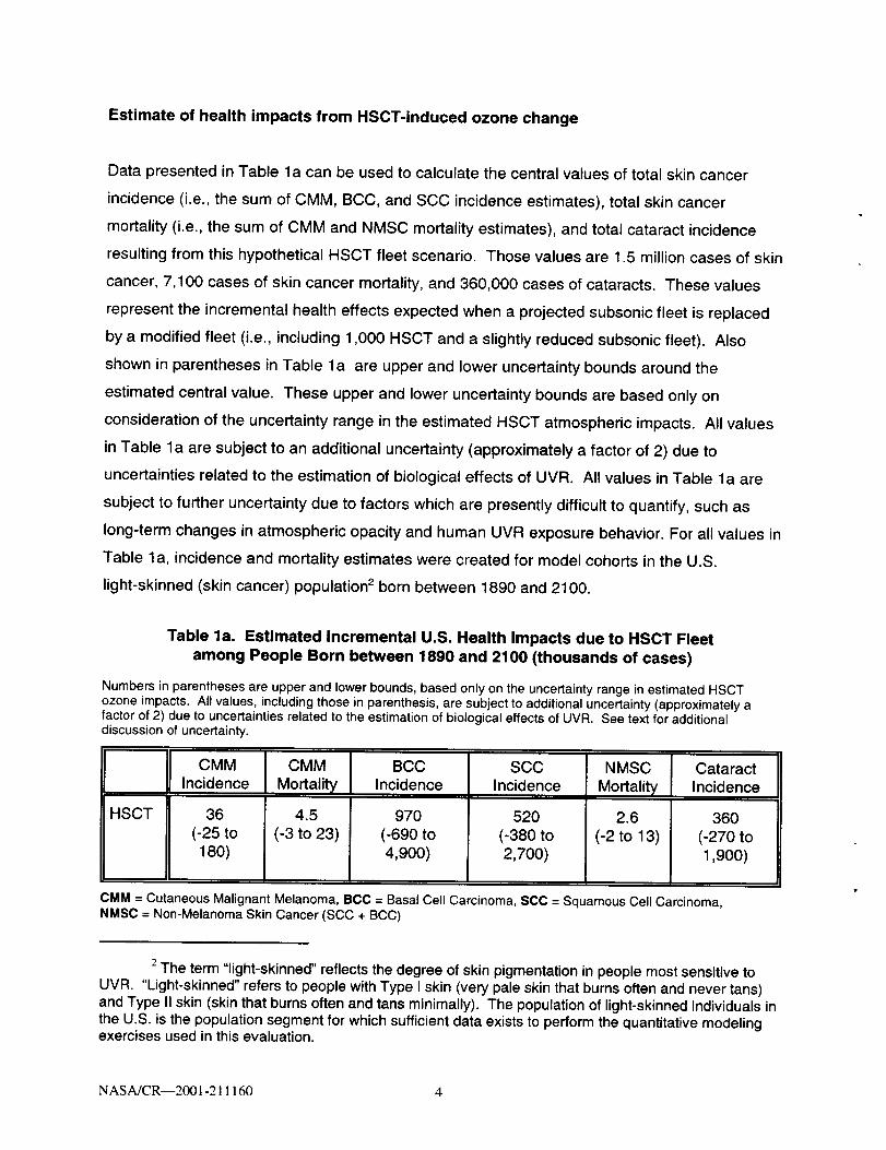
Estimate of health impacts from HSCT-induced ozone change
Data presented in Table la can be used to calculate the central values of total skin cancer
incidence (i.e., the sum of CMM, BCC, and SCC incidence estimates), total skin cancer
mortality (i.e., the sum of CMM and NMSC mortality estimates), and total cataract incidence
resulting from this hypothetical HSCT fleet scenario. Those values are 1.5 million cases of skin
cancer, 7,100 cases of skin cancer mortality, and 360,000 cases of cataracts. These values
represent the incremental health effects expected when a projected subsonic fleet is replaced
by a modified fleet (i.e., including 1,000 HSCT and a slightly reduced subsonic fleet). Also
shown in parentheses in Table la are upper and lower uncertainty bounds around the
estimated central value. These upper and lower uncertainty bounds are based only on
consideration of the uncertainty range in the estimated HSCT atmospheric impacts. All values
in Table la are subject to an additional uncertainty (approximately a factor of 2) due to
uncertainties related to the estimation of biological effects of UVR. All values in Table la are
subject to further uncertainty due to factors which are presently difficult to quantify, such as
long-term changes in atmospheric opacity and human UVR exposure behavior. For all values in
Table la, incidence and mortality estimates were created for model cohorts in the U.S.
light-skinned (skin cancer) population 2 born between 1890 and 2100.
Table la. Estimated Incremental U.S. Health Impacts due to HSCT Fleet
among People Born between 1890 and 2100 (thousands of cases)
Numbers in parentheses are upper and lower bounds, based only on the uncertainty range in estimated HSCTozone impacts. All values, including those in parenthesis, are subject to additional uncertainty (approximately afactor of 2) due to uncertainties related to the estimation of biological effects of UVR. See text for additionaldiscussion of uncertainty.
CMMIncidence
HSCT 36
(-25 to180)
CMM
Mortality
4.5
(-3 to 23)
BCCIncidence
970
(-690 to4,900)
SCCIncidence
520
(-380 to2,700)
NMSC
Mortality
2.6
(-2 to 13)
CataractIncidence
360
(-270 to1,900)
CMM = Cutaneous Malignant Melanoma, BCC = Basal Cell Carcinoma, SCC = Squamous Cell Carcinoma,NMSC = Non-Melanoma Skin Cancer (SCC + BCC)
2The term "light-skinned" reflects the degree of skin pigmentation in people most sensitive toUVR. "Light-skinned" refers to people with Type I skin (very pale skin that burns often and never tans)and Type II skin (skin that burns often and tans minimally). The population of light-skinned individuals inthe U.S. is the population segment for which sufficient data exists to perform the quantitative modelingexercises used in this evaluation.
NASA/CR--2001-211160 4

Health effects under previous stratospheric protection control regimes
Rows (a) through (d) of Table 1b show the number of "excess" health effects cases that were
estimated to occur under several ozone-depleting substance (ODS) policy scenarios relative to
1979 -1980 ("baseline") levels of ozone depletion. The same UVR and health effects models
were used for all scenarios presented in Tables la and lb, and health effects estimates were
based on consideration of the same baseline data and simulation period. The values in rows
(a) - (d) are taken from an earlier study (ICF 2000a). As with the values in Table la, the values
in Table 1b are subject to some uncertainty due to uncertainty in atmospheric inputs (discussed
in WMO 1999), and they are subject to additional uncertainty (approximately a factor of 2)
related to the estimation of biological effects of UVR.
Row (a) of Table lb shows that according to previous model studies, about 6.3 million "excess"
cases of CMM (i.e., in excess of baseline incidence of this malady) in the U.S. light-skinned
population would have occurred under an atmosphere reflecting worldwide compliance with the
controls set forth in the original 1987 Montreal Protocol. Row (d) shows that if all Parties
(i.e., nations) to the Montreal Protocol fully implement the Protocol, including all amendments
and adjustments (through the Montreal Adjustments), approximately 130,000 cases of CMM, in
excess of baseline CMM incidence, would still occur in the U.S. light-skinned population.
NASA/CRy2001-211160 5

Table lb. Estimated Excess U.S. Health Impacts among People Born between
1890 and 2100 under Several Ozone-Depleting Substance (ODS)Policy Scenarios (thousands of cases)
Source: ICF 2000(a). See text for additional discussion.
MontrealProtocol
(row a)
LondonAmendments
(row b)
CopenhagenAmendments
(row c)
Montreal
Adjustments
(row d)
CMMIncidence
6,300
330
160
130
CMM
Mortality
BCCIncidence
SCCIncidence
NMSC Cataract
Mortality Incidence
820
41
160,000
8,100
80,000
4,100
380
18
2O
17
4,000
3,300
2,000
1,600
8.3
6.9
140,000
3,500
1,700
1,400
CMM = Cutaneous Malignant Melanoma, BCC = Basal Cell Carcinoma, SCC = Squamous Cell Carcinoma,NMSC = Non-Melanoma Skin Cancer (SCC + BCC)
"MONTREAL PROTOCOL" of 1987: Freeze of CFC production and consumption at 1986 levels; 50% reduction in
CFC production by 1998 (for developed countries) and 2008 (for Article 5 (developing) countries); laterproduction freezes on halons, other halogenated compounds, carbon tetrachlodde (CCI4), and methylchloroform (CH3CCI3).
"LONDON AMENDMENTS" of 1990: Complete phase-out of CFCs, hydrochlorofluorocarbons (HCFCs), and CCI 4by 2000 (developed countries) and by 2010 (Article 5 countries); complete phase-out of CH3CCI 3 by 2005(developed countries) and by 2015 (developing countries).
"COPENHAGEN AMENDMENTS" of 1992: Accelerated phase-out of CFCs, CCI4, and CH3CCI 3 by 1996 andhalons b_/1994 (developed countries); and accelerated reduction of HCFCs and hydrobromofluorocarbons(HBFCs) (Article 5 countries).
"MONTREAL ADJUSTMENTS" of 1997: Complete phase-out of methyl bromide by 2005 (developed countries)and 2015 (Article 5 countries); HCFC phase-out schedule (Article 5 countries).
Comparison of HSCT Impacts with health effects under previous stratosphericprotection control regimes
A key manner in which the data in Table lb can be read is to indicate the incremental health
benefits (i.e., avoided health impacts) achieved by each set of amendments and adjustments to
the Montreal Protocol. For example, data in rows (c) and (d) of the table indicate that the
increase in the stringency of the Montreal Protocol through the Montreal Adjustments was
expected to decrease CMM incidence by approximately 30,000 cases (relative to health impacts
under the Montreal Protocol as amended and adjusted through the Copenhagen Amendments
of 1992; i.e., row (d) subtracted from row (c)).
NASA/CR--2001-211160 6

At the same time, the estimates in Table 1a indicate that the simulated incremental increase in
CMM incidence due to operation of an HSCT fleet is about 36,000 additional cases relative to
an atmosphere in the absence of this fleet (i.e. relative to the Montreal Adjustments). This
comparison indicates that the negative human health impacts associated with operation of the
proposed fleet of HSCT are of similar magnitude to the health benefits expected from recent
increases in stringency agreed upon by the Parties to the Montreal Protocol.
The Protocol serves as the chief forum for the establishment of effective global control
measures for protecting stratospheric ozone. Today, 175 countries have ratified the Montreal
Protocol, and 48 have ratified the Montreal Adjustments. The Parties to the Protocol also meet
regularly to consider further measures to protect stratospheric ozone, such as the "Beijing
Amendments" to which the Parties agreed in 1999. Although Parties to the Protocol must align
their domestic regulations with the control measures of the Protocol, any Party may adopt more
stringent measures.
Uncertainties in estimated health impacts
The sources of uncertainty in the estimated health impacts from the modeled HSCT fleet
originate at each modeling step in this assessment: (1) model calculations of the impact of the
HSCT fleet scenario on atmospheric ozone, (2) translation of the atmospheric ozone changes
to biologically-weighted UVR exposures, and (3) translation of weighted UVR exposures to skin
cancer incidence, skin cancer mortality, and cataract incidence. The same uncertainties arising
from (2) and (3) would also apply to the estimates of health impacts under ODS policy
scenarios. In addition, uncertainty in estimated health impacts associated with ODS-induced
ozone depletion also arises from uncertainties in projected atmospheric impacts of ODS policy
scenarios, which have been discussed elsewhere (WMO 1999).
The estimated HSCT health impact is uncertain to a factor of -1.7 to + 4.1 about the central
value due to uncertainties in estimated fleet atmospheric impacts (see Table 3-2). This is the
uncertainty range that is indicated in Table la. It should be noted that this uncertainty range
comprises not only the possibility for adverse health impacts of much larger magnitude than the
central value, but also the possibility that the impacts may be directionally different; an
atmosphere with HSCT-induced ozone change could lead to a reduction in skin cancer and
cataract occurrences, relative to a reference atmosphere. This latter estimated possibility
NASA/CR----2001-211160 7

arises from the uncertainty in the estimated column ozone response to HSCT. In addition to
providing an estimate of how much larger than the central value the estimated HSCT ozone
depletion could be, the NASA assessment concluded that there is a small possibility that the
HSCT fleet could lead to an increase in column ozone.
The estimated health impacts due to HSCT-induced ozone depletion (as well as the estimated
health impacts under the ODS policy scenarios) are estimated to be further uncertain to a factor
of approximately 2 due to presently quantified uncertainties in health effects parameters.
Finally, these uncertainty factors do not reflect consideration of all sources of uncertainty.
Additional sources include long-term, systematic changes in atmospheric opacity; changes in
human UVR exposure behavior; limited experimental data from which to derive certain effect-
specific UVR weighting functions; and improvements in medical care and increased longevity.
Assumptions have been made based on best available knowledge, but further quantitative tests
are needed to understand the sensitivity of simulated results to each of the assumptions.
Nevertheless, it can be seen that the estimated health impacts from the HSCT scenario
modeled in this study may be considerably less, or far greater than, the central value.
Accurate prediction of future changes in health effects would require consideration of the net
effect of all factors such as those listed above. This is a task that is beyond the ability of the
current state of the science, both atmospheric and epidemiological. Furthermore, it should be
recognized that no direct measurements (e.g., of future UV levels or skin cancer incidence) will
be able to attribute explicitly observed changes to any specific factor, unless such a factor is far
more important that all the others combined. Nevertheless, it is possible to examine one of
these effects, the HSCT impact, in isolation, under the assumption that the other factors are
maintained constant at current conditions. The validity of this principle is based on the
assumption that the HSCT impacts are independent of the other factors (e.g., behavioral
changes will occur regardless of whether an HSCT fleet is in place).
Sensitivity of estimated health impacts to technological and operational change
Previous work by NASA (Kawa et aL 1999) characterized the sensitivity of the predicted HSCT
ozone impact to selected changes in assumptions regarding fleet technology and operational
design options. For example, that study found that decreasing fleet cruise altitude by 2 km
reduced the average annual Northern Hemisphere column ozone impact by 50 percent.
NASA/CR--2001-211160 8

Elimination of fuel sulfur content decreased the column ozone response by 75 percent.
Changes in atmospheric ozone of this magnitude are simulated to lead to health effects
changes of similar proportion. For example, a 50 percent reduction in estimated ozone
depletion is expected to lead to roughly 50 percent decreases in estimated skin cancer and
cataract impacts. Thus, there may be some possibility to mitigate adverse health impacts of
HSCT-induced ozone depletion through changes in technological and operational parameters.
Applicability of results to other scenarios
The present study has evaluated a single conceptual scenario for a large fleet of long-range
supersonic commercial transport aircraft. The emissions inventory constructed to represent the
chemical inputs to the atmosphere from this fleet were based upon specific aviation traffic and
market scenario projections as well as narrowly-defined projections of aircraft performance and
emissions. Simulated atmospheric impacts, in turn, are sensitive to the fleet's emissions, cruise
altitude, and flight routes. The results of the present study should be considered highly specific
to the single scenario considered in this evaluation because UVR exposure and health
responses are sensitive to these simulated atmospheric impacts. Also, the results of this study
should not be directly extrapolated to estimate the health impacts from substantially different
future atmospheric or fleet operational or technological scenarios (e.g., a fleet of business jets
that fly in the stratosphere).
For substantially different fleet scenarios (e.g., different aircraft, different routes, different
altitudes, different emissions characteristics) the atmospheric impacts would likely have to be
re-assessed, including re-evaluation of uncertainties in atmospheric impacts. In addition, as the
scientific knowledge of stratospheric chemistry and dynamics, background atmosphere, global
atmospheric change, and human health effects evolves, the models and assumptions used in
future analyses should be updated accordingly. In contrast, the general methodology or
sequence of modeling tools used in the present study should be applicable to a wide range of
future stratospheric aviation scenarios, provided adequately updated and appropriate inputs are
used.
NASA/CR---2001-211160 9

Chapter summaries
Chapter 1 of this report provides a broad scientific and institutional context for the analyses
presented. Chapter 2 describes the modeling method used to evaluate the impacts of
estimated HSCT-induced column ozone changes on UVR and selected human health
endpoints. Chapter 3 presents the results of modeling simulations, and discusses uncertainties
and potential sensitivity of results to technological and operational factors. Chapter 4
discusses: 1) the results in the context of previous regulatory actions to protect stratospheric
ozone and 2) the applicability of the methods and results of this study to scenarios other than
the single HSCT fleet scenario evaluated in this report.
NASA/CR--2001-211160 10

Chapter 1. Introduction and Background
This chapter provides background information on recent assessments of the potential impacts
of stratospheric aircraft on the atmosphere, focusing on stratospheric ozone impacts and
biological and human health concerns associated with stratospheric ozone depletion. This
chapter also provides brief descriptions of institutional and regulatory bodies with authority or
interest relative to the environmental impacts of stratospheric aircraft, and it briefly describes
recent commercial interest in supersonic flight.
1.1 Potential atmospheric and biological impacts of stratospheric
flight
Activities that may contribute to the depletion of stratospheric ozone are a matter of concern
because lower levels of ozone can lead to adverse environmental and biological impacts. The
following discussion provides a brief explanation of the main impacts.
1.1.1 How HSCT may contribute to ozone depletion
High-speed civil transport (HSCT) is a type of supersonic aircraft that would cruise in the
stratosphere, carry approximately 300 passengers each, and travel at more than twice the
speed of current commercial subsonic aircraft (Mach 2.4, 1,600 mph). The estimated impacts
of HSCT on ozone depletion are based largely on three main constituents of the exhaust
emissions of HSCT: oxides of nitrogen (NO×), water vapor (H20), and oxides of sulfur (SOx).
In the middle and upper stratosphere, the primary process for ozone loss involves NO_ radicals
(Kawa et al. 1999). As NOx radicals from HSCT exhaust accumulate at altitudes above
22 kilometers (km), ozone depletion may be exacerbated. In the lower stratosphere, these
emissions can have varying effects on ozone depletion since NOx can moderate ozone loss
caused by other radicals such as hydrogen oxides (HOx), chlorine oxides (CIO_), and bromine
oxides (BrOx). In addition, NO× participates in the formation of polar stratospheric clouds
(PSCs) that provide a substrate for ozone depletion reactions and that are responsible for large
seasonal ozone loss in polar regions.
Water vapor in HSCT exhaust can affect stratospheric ozone depletion in several ways. First,
as the source of HOx radicals, increased water in the atmosphere leads to higher
NASA/CR--2001-211160 11

concentrations of HOx, which is as important as NO. in exacerbating ozone loss. Second,
increased water in the atmosphere affects the relative concentrations of radical species since it
increases the reactivity of aerosols toward gases such as hydrogen chloride (HCI) and chlorine
nitrate (CIONO2). Also, water vapor increases the condensation temperature in the atmosphere
and thus influences the composition and growth of aerosol particles (promoting the formation of
PSCs) (Kawa et al. 1999).
Finally, SOx in HSCT emissions may affect ozone loss by potentially increasing the aerosol
surface area throughout the stratosphere. Current studies show that stratospheric aerosol
surface area is sensitive to processes that convert SOx to sulfate particles in the aircraft wake,
although these processes are not well understood and large uncertainties remain. Increases in
aerosol surface area suppress NOx and enhance ozone loss caused by other radicals such as
CIOx and HOx. The net effect of aerosol in HSCT emissions is uncertain, but atmospheric
ozone is known to be sensitive to changing aerosol conditions (Kawa et al. 1999).
1.1.2 Current assessment of atmospheric impacts from stratospheric aircraft
Much of the evaluation of the impacts on human health presented in this document builds on
two atmospheric assessments: the National Aeronautics and Space Administration's (NASA)
Assessment of the Effects of High-Speed Aircraft in the Stratosphere published in 1999
(hereafter referred to as the NASA assessment) and the Intergovernmental Panel on Climate
Change's (IPCC) special report, Aviation and the GlobalAtmosphere (IPCC 1999).
Both of these assessments focus on the effects of aviation on the atmosphere, but the analyses
have a few key differences. The IPCC report emphasizes the aviation industry as a whole,
whereas the NASA assessment focuses on evaluating the incremental impacts of supersonic
aviation. Both assessments assumed that a fraction of the subsonic fleet was replaced by the
supersonic fleet. The IPCC study also evaluates potential fleet impacts on erythemally
weighted (i.e., sunburn-causing) ultraviolet radiation (UVR). 1 Both studies assume identical
The term "ultraviolet" refers to a portion of the electromagnetic spectrum with wavelengthsshorter than visible light. The sun produces UVR, which is by convention commonly split intothree bands: UV-A, UV-B, and UV-C. Although artificial sources of UVR (e.g., sun lamps) havebeen associated with adverse health effects, the term is used in this document to referexclusively to solar ultraviolet irradiance.
NASA/CR--2001-211160 12

scenarios with respect to the development and operation of an HSCT fleet, but results from
different atmospheric models were selected to provide the central-value estimates of ozone
change. The following section presents a brief summary of findings from the two assessments.
1.1.2.a. NASA's Assessment of the Effects of High-Speed Aircraft in theStratosphere
As part of the agency's Atmospheric Effects of Aviation Project, a component of its High-Speed
Research (HSR) program, NASA performed a comprehensive assessment of the potential
incremental impacts on atmospheric chemistry and climate when the projected subsonic fleet is
modified to include HSCT. This effort served as a follow-up to a previous HSCT assessment
performed by NASA (Stolarski et al. 1995). From 1989 to 1998, scientists from universities,
industry, NASA, other federal research facilities, and international research programs carried
out the assessment. The findings represent a broad consensus of the atmospheric research
community, including the report's authors, reviewers, and other contributors.
The assessment assimilated current scientific understanding of the fundamental physics and
chemistry of the atmosphere relevant to predicting HSCT impacts, including trends in major
trace chemical constituents of the stratosphere and present understanding of atmospheric
transport and photochemical processes. This understanding is based on recent observations
by atmospheric measurement campaigns from a variety of research platforms, as well as
laboratory studies of chemical reactions and rates. In conjunction with NASA and industry
technologists, the assessment also developed estimates of the future distribution of HSCT
emissions in the global atmosphere. In addition, the assessment integrated research on fluid
dynamics, chemistry, and particle microphysics as they relate to aircraft near-field, aircraft far-
field, and global scale dispersion.
The NASA assessment also addressed seasonal and geographic patterns in column ozone
impacts, assumptions regarding the composition of the future atmosphere, and sensitivities to
parameters that potentially could be controlled through regulation or technological and
operational modifications (e.g., developments in NOx combustor technology, fuel sulfur content
and subsequent oxidation, and fleet cruise altitude). Results of these evaluations are presented
in the _IASA assessment (Kawa et al. 1999).
NASA/CR--2001-211160 13

Overall, NASA predicted the annual average change in ozone for the Northern Hemisphere to
be -0.4 percent, assuming a fleet of 500 HSCT in 2015, with an uncertainty range of
-2.5 percent to +0.5 percentfl Both the estimated ozone impact and the uncertainty bounds
used in the evaluation are based on a combination of model results and expert judgment. The
uncertainty bounds were produced by listing uncertainties in the model (e.g., emissions to the
atmosphere, transport of emissions, chemical effect of emissions) and then assigning
qualitative confidence ratings and numerical uncertainty ranges to each contributing factor.
The ratings and ranges are based on a combination of numerical tests, comparison with
measurements, and theoretical expectations.
The assessment resulted in several key findings in addition to those described above:
Water vapor, an inherent byproduct of jet fuel combustion, accounts for a major part
of the estimated stratospheric ozone impact of a fleet of HSCT. Increased water
vapor in the stratosphere may contribute to global climate warming as well.
• Production of sulfate aerosol particles in the wake makes a potentially significant
contribution to the calculated ozone impact of a proposed HSCT fleet.
NO× emissions are an important parameter in the assessment of HSCT impacts on
ozone depletion. Although current atmospheric models do not indicate a high level
of sensitivity to very low emissions (EINox = 5 g/kg to 10 g/kg), higher NOx emissions
clearly increase the impact on stratospheric ozone, especially in the case of larger
fleets.
° Flying HSCT at lower altitudes reduces stratospheric ozone depletion.
* Exhaust build-up in polar regions presents additional concerns related to ozone
depletion, both in winter and summer.
2These results are based on the scenario of 500 HSCT in the year 2015 flying Mach 2.4 with a
NOx emission index of 5 g/kg, an EIs% of 0.4 g/kg, and 10 percent of fuel sulfur converted toparticles.
NASA/CR--2001-211160 14

The total climate forcing (radiative forcing) from 1,000 HSCT is calculated to be
+0.1 Watts per square meter (W/m 2) in 2050, with an uncertainty level approximated
by a factor of at least 3 due to uncertainty in exhaust accumulation and temperature
adjustment to a non-uniform perturbation of radiatively active gases in the
stratosphere. This level of climate forcing is disproportionately large for the
projected fuel use, and it is equivalent to approximately 50 percent of the predicted
forcing from the entire subsonic fleet projected for 2050.
1.1.2.b. Aviation and the Global Atmosphere (IPCC 1999)
The IPCC's report addresses the impacts of both subsonic and supersonic aviation on
atmospheric ozone, UVR at the ground, and climate change, in addition to analyzing regulatory
and market-based mitigation responses. The IPCC evaluated a scenario in which a fleet of
supersonic aircraft replaced a proportion of the subsonic fleet. The IPCC assumed that the
supersonic fleet would begin operation in 2015, growing to a maximum of 1,000 aircraft by
2050. The NASA assessment used the same model (2-D or 3-D) to estimate the impacts of
both subsonic and supersonic aviation on stratospheric ozone. In contrast, the IPCC
methodology combined 3-D model estimates generated for subsonic aircraft with 2-D model
estimates generated for HSCT to quantify the total impact of subsonic and supersonic aviation
on stratospheric ozone.
The IPCC evaluation predicted a reduction in stratospheric ozone as a result of the combined
fleet. The greatest effect was predicted for the month of July at 45°N, when the ozone column
change in 2050 relative to the scenario without aircraft is -0.4 percent, with the supersonic
component of the fleet contributing about -1.3 percent and the subsonic component contributing
about +0.9 percent. The IPCC also addressed the impacts on erythemal dose rate
(i.e., the irradiance on a horizontal surface adjusted to account for the sunburning effect of the
radiation). As compared with a no-aircraft scenario, the combined fleet would change the dose
rate at 45°N in July by +0.3 percent, with a two-thirds uncertainty range 3 of -1.7 percent to
3The IPCC report defines the two-thirds uncertainty range to mean that there is a 67 percentprobability that the true value falls within this range. The IPCC report also states that theconfidence interval was derived based in part on expert judgment of scientists contributing toeach relevant chapter and may include a combination of objective statistical models andsubjective expertise. It therefore does not imply one specific statistical model.
NASA/CR--2001-211160 15

+3.3 percent. The IPCC report predicted that by 2050 this combined fleet would increase the
radiative forcing under the reference scenario (0.19 W/m 2 assuming no supersonic aircraft) by
an additional 0.08 W/m 2, primarily as a result of the accumulation of stratospheric water vapor.
1.1.3 Biological effects of stratospheric ozone depletion
One significant effect of stratospheric ozone depletion is the increased transmission of UVR to
the Earth's lower atmosphere (the troposphere) and surface. Many biological and chemical
processes are known to be affected by UVR, and individual organisms can be harmed
considerably by UVR. As discussed in several United Nations Environment Programme
(UNEP) documents (UNEP 1991, 1994, and 1998), specific concerns include increases in the
incidence of skin cancer, ocular damage, and other health effects in humans and animals;
damage to terrestrial and oceanic vegetation; damage to some outdoor materials; changes in
the chemistry of the lower atmosphere (e.g., photochemical smog formation); and alterations of
the biogeochemical cycles of 1) non-living, 2) organic, and 3) inorganic matter whose
degradation depends on exposure to ambient solar radiation (Madronich et al. 1998).
Humans and animals are exposed to the UV-B rays in sunlight principally through the eyes and
skin. Effects of exposure occur as certain molecules, or chromophores, present in the tissues
and cells of these organs absorb solar energy. The absorption of this energy leads to
molecular changes that eventually can result in a biological effect (Longstreth et al. 1998).
Chromophores absorb light energy from various wavelengths with varying efficiencies. Five of
the chromophores present in skin and eye tissues that are key to the biological effects of UV-B
in humans and animals are DNA, tyrosine and tryptophan (two amino acids that are largely
responsible for UVR absorbance by proteins), trans-urocanic acid (a molecule present in
quantity in the outermost layer of skin), and melanin (the principal skin pigment). Research has
documented the effects of sunlight on health in three major organ systems: the eye, the
immune system, and the skin (Longstreth et al. 1998).
One of the key parameters required to predict biological impacts associated with increased
UVR is the action spectrum, which describes the relative effectiveness of UV-A and UV-B
wavelength radiation in the induction of a particular health effect (see Section 2.4.3). Due to
limited experimental data from which action spectra are derived, the best available action
NASA/CR--200I-211160 16

spectra for health effects such as melanoma skin cancer and cataracts still include a significant
degree of uncertainty. Uncertainties in action spectra are discussed in Sections 2.6.3 and 2.6.4
of this report.
Since the early 1970s, scientists have conducted research to better understand and
characterize the relationships between UVR exposure and biological effects. Research on the
relationships between UVR exposure and biological effects has been summarized in EPA
(1987) and UNEP (1991, 1994, and 1998). Quantitative risk estimates are available for some
UV-B-associated effects (e.g., cataract and skin cancer), but insufficient data are available to
develop similar estimates for effects such as immunosuppression.
Several efforts have been made to assess the human health impacts from stratospheric flight
and its atmospheric ozone effects. Cutchis examined relationships between human erythemal
dose rates and changes in stratospheric ozone that could arise from a future stratospheric flight
(Cutchis 1974). This work, however, did not consider specific aircraft fleet scenarios. The U.S.
Department of Transportation (DOT) Climate Impact Assessment Program (CLAP) assessed
the possible physical, biological, social, and economic effects that might result from future
aircraft operations in the stratosphere. A National Academies of Sciences and Engineering
committee (established to advise DOT on CLAP) reported on potential skin cancer and climate
impacts of stratospheric aircraft. The report from this committee provided estimates of the
percentage increases in the incidence of skin cancer likely to occur for given stratospheric
aircraft fleet scenarios and discussed uncertainties in the estimates (NAS 1975).
More recently, as noted in Section 1.1.2.b., the IPCC evaluated the potential impacts of future
worldwide aviation activity on atmospheric ozone and erythema. The scenarios of future
aviation activity included fleets with 500 to 1,000 supersonic aircraft operating in the
stratosphere. To project changes in UVR associated with fleet scenarios, the IPCC used ozone
change data produced by a set of atmospheric models. Changes in erythemal dose under the
world aircraft fleet, both with and without a supersonic component, were projected for the years
2015 and 2050.
The present study uses the recent assessment of the atmospheric impacts of a future fleet of
HSCT (Kawa et aL 1999) as well as updated data on the relationship between UVR exposure
and health effects to calculate impacts for health endpoints that more readily allow for
NASA/CR--2001-211160 17
comparison of the HSCT risks with those arising from previous international policies on ozone-
depleting substances (ODS).
1.2 Relevant U.S. and international authorities and agencies
Many organizations are or may potentially be interested in aircraft emissions as they pertain to
air quality, stratospheric ozone depletion, and the potential effects on global warming. An
understanding of the existing institutional framework is helpful to placing the findings of this
study into the appropriate context (see Chapter 4). The following sections provide background
information on this institutional framework, including these authorities:
• U.S. Environmental Protection Agency (EPA)
• National Aeronautics and Space Administration (NASA)
• Federal Aviation Administration (FAA)
• International Civil Aviation Organization (ICAO)
• Montreal Protocol
• United Nations Framework Convention on Climate Change (UNFCCC)
1.2.1 U.S. Environmental Protection Agency (EPA)
The mission of EPA is to protect human health and safeguard the natural environment - air,
water, and land - upon which life depends. As the U.S. Congress has passed legislation to
address environmental and human health threats, EPA has responded with a comprehensive
set of regulations aimed largely at controlling risks. EPA also employs innovative environmental
protection programs to achieve its goals. For example, EPA partners with the U.S. Department
of Energy (DOE) in the voluntary ENERGY STAR ® labeling program. In order to reduce carbon
dioxide emissions, ENERGY STAR identifies and promotes energy-efficient products, including
residential heating and cooling equipment, major appliances, office equipment, lighting,
consumer electronics, and other product areas.
Section 231 of the Clean Air Act (42 U.S.C. §7571) authorizes EPA to set emissions standards
for air pollutants emitted from aircraft engines that cause, or contribute to, air pollution
endangering public health or welfare. Under the authority of Section 231, EPA issued emission
standards in 1973 for air pollutants generated during the landing/take-off cycle of aircraft
NASA/CR--2001-211160 18

operation by subsonic and supersonic aircraft engines. In 1976, EPA adopted hydrocarbon
(HC), NOx, and carbon monoxide (CO) standards for supersonic aircraft engines. These
standards were revised in 1982 (by revision of HC standards and withdrawal of existing NOx
and CO standards).
At the international level, ICAO adopted HC, NO× and CO standards for supersonic engines in
1981. EPA has worked with ICAO and the U.S. FAA to continue developing appropriate
emission standards for aircraft engines. More recently, as directed by Section 231, EPA
promulgated regulations that adopt the international standards established by ICAO for NOx
and CO emissions from subsonic aircraft engines. The regulations include emission standards
for subsonic gas turbine engines, which power almost all of the U.S. commercial aviation fleet,
as well as engines designed for aircraft that operate at supersonic flight speeds.
Title VI of the Clean Air Act (CAA) provides EPA with broad regulatory authority to protect the
stratosphere. Under this title, EPA implements the requirements of the 1987 Montreal Protocol
on Substances that Deplete the Ozone Layer (see Section 1.2.5 below). Section 614 (b) of the
CAA (42 U.S.C. §7671 (m)) requires that in the case of any conflict "between any provision of
[Title VI] and any provision of the Montreal Protocol, the more stringent provision shall govern."
Section 615 of the CAA (42 U.S.C. §7671 (n)) authorizes EPA to promulgate regulations to
control any substance, practice, process, or activity that may reasonably be anticipated to affect
the stratosphere, and especially ozone in the stratosphere, where the effect may endanger
public health or welfare. Under Title VI, EPA has developed various regulatory programs to
protect the ozone layer, including programs to phase-out of production many ODS such as
CFCs and halons; product labeling programs; recycling programs for stationary and motor
vehicle refrigerants; and programs to review substitutes for ODS. EPA also engages in
communication and outreach activities related to the science and impacts of ozone depletion.
Section 103(a) of the CAA, 42 U.S.C. §7403(a), requires EPA to establish a national research
and development program for the prevention and control of air pollution. As part of this effort,
EPA is required to conduct and accelerate research, investigations, experiments,
demonstrations, surveys, and studies relating to the causes, effects (including health and
welfare effects), extent, prevention, and control of air pollution. Section 103(b), 42 U.S.C.
§7403(b), authorizes EPA to cooperate with other federal departments and agencies on the
research and other activities.
NASA/CR--2001-211160 19
1.2.2 National Aeronautics and Space Administration (NASA)
Among NASA's core missions is the preservation of the pre-eminent position of the United
States in the development and application of aeronautical science and technology. Given the
projected growth in commercial air travel and the strong international competition in the sale of
commercial aircraft, revolutionary aircraft technologies need to be developed rapidly in order to
ensure the welfare of the traveling public and create new markets for the U.S. aircraft industry.
The goal of such technologies will be to increase the safety and affordability of air travel and to
minimize any resulting effects on the environment (NRC 1997).
The HSR program (a 10-year, $1.2 billion partnership between NASA, Boeing,
McDonnell-Douglas, General Electric, and Pratt and Whitney) was one of two NASA programs
designed to achieve these results. As stated earlier, the HSR program was a focused
technology program intended to enable the commercial development of HSCT. Phase I
(Technology Exploration) of the program was completed in fiscal year (FY) 95 and produced
critical information regarding the ability of HSCT to satisfy environmental concerns
(i.e., noise and engine emissions). Phase II (Technology Development) focused on
development of specific technologies related to affordability, airframe durability, engine service
life, engine emissions, aircraft manufacturing and production, and range.
Despite excellent progress (NRC 1997), changes in the market outlook for the HSCT led to
termination of the focused HSR program in FY 1999. NASA continues work on supersonic
technologies under programs distributed among several newer initiatives such as the Ultra-
Efficient Engine Technology (UEET) program.
1.2.3 Federal Aviation Administration (FAA)
The primary responsibility of the FAA, an agency of the DOT, is to assure the safety of civil
aviation. This mission includes overseeing the development and implementation of programs
designed to control the environmental effects of civil aviation. Under Section 232 of the CAA,
the Secretary of Transportation is responsible for the enforcement of the aircraft emission
standards set forth by EPA under Section 231 of the CAA. Engine emissions certification
testing is conducted by engine manufacturers, and enforcement is conducted through program
administration and monitoring by the FAA. Within the FAA, the Office of Environment and
NASA/CR--200 !-211160 20

Energy develops, recommends, and coordinates national aviation policy as it relates to
environment and energy matters.
1.2.4 International Civil Aviation Organization (ICAO)
ICAO, established in 1944 under the Convention on International Civil Aviation (the "Chicago
Convention"), is the agency in the United Nations with global responsibility for the establishment
of standards, recommended practices, and guidance on various aspects of international civil
aviation, including the environment. In 1986, ICAO established the Committee on Aviation
Environmental Protection (CAEP) to address noise and emission-related problems associated
with aviation activities and to identify appropriate standards and recommended practices. 4
CAEP works closely with regional bodies and national airworthiness authorities to discuss and
propose changes in recommended environmental standards. In the evaluation process, CAEP
considers technical feasibility, economic reasonableness, and the environmental benefit of
proposals. If standards and recommendations proposed by CAEP are adopted by ICAO, they
are attached as Annexes to the Chicago Convention.
The Chicago Convention states that participating nations, such as the United States, have an
obligation to adopt the ICAO established standards to the extent possible. A country that
decides not to comply with the established standards must provide ICAO with a written
explanation describing why compliance is impractical or how compliance would compromise its
national interest. Most states take ICAO's international standards, recommended practices,
and guidance material into account in regulating their domestic aviation. To date, ICAO efforts
have focused on establishing standards for aircraft noise and emissions from subsonic and
supersonic aircraft engines during landing and takeoff cycles.
ICAO/CAEP's technical working group on emissions has held discussions concerning the
development of standards for a potential next-generation supersonic transport. Working papers
submitted by the aviation industry (Gerstle 1996, Baughcum 1997) identified important
considerations relative to potential emissions standards for a future supersonic transport:
4The Committee on Aircraft Engine Emissions and the Committee on Aircraft Noise werepredecessor to CAEP.
NASA/CRy2001-211160 21

Emissions of concern would be those related to a supersonic transport's ground-
level, climate, and stratospheric ozone impacts and would also include those already
regulated under existing landing and take-off standards;
• Standards would be a key factor in the design of a future supersonic transport;
Current standards for both subsonic and supersonic engines are based on
emissions during the landing and take-off phases of the flight cycle, but a supersonic
standard would need to consider cruise emissions as well;
The Parties to the Montreal Protocol on Substances that Deplete the Ozone Layer
("Montreal Protocol") potentially could specify restrictions to limit the stratospheric
impact; and
• The Parties to the UNFCCC also could elect to constrain supersonic transport
emissions due to climate considerations.
With respect to addressing the contribution of aviation to climate change, in 1998 the 32 ndICAO
Assembly recognized the work already done by CAEP in recent years. The CAEP work plan
calls for working groups to study technical and operational approaches as well as market-based
options for reducing greenhouse gas emissions. Furthermore, CAEP tasked the Secretariat
with continued attention to help bridge the efforts of CAEP and the UNFCCC.
1.2.5 Montreal Protocol
On September 16, 1987, the United States, along with 23 other nations and the European
Economic Community, signed the Montreal Protocol on Substances that Deplete the Ozone
Layer. The Protocol was soon ratified by 34 countries and became effective on
January 1, 1989. The Protocol originally placed limitations on the production and consumption
of chlorofluorocarbons (CFCs) and halons. Over the past 12 years, the Protocol has been
amended on several occasions to increase the array of ozone-depleting chemicals regulated
under it and to increase the stringency of the control measures. To date, over 170 countries
have ratified the original Protocol. Key provisions include the following:
NASAJCR--2001-211160 22

Developed countries must phase out CFCs, carbon tetrachloride, methyl chloroform,
and hydrobromofluorcarbons (HBFCs) by 1996; halons by 1994; methyl bromide by
2005; and hydrochlorofluorocarbons (HCFCs) by 2020 (although 0.5 percent of
production is permitted for maintenance purposes only until 2030);
Developing countries have a grace period before they must start their phaseout
schedules. The requirements for developing countries include a phaseout of CFCs,
halons, and carbon tetrachloride by 2010, methyl chloroform and methyl bromide by
2015, HBFCs by 1996, and HCFCs by 2040.
• The import of controlled substances from countries that are not Parties to the
Protocol is severely restricted, as is the export of such chemicals to non-Parties; and
The Parties must regularly reassess the Protocol, making revisions to policies on
controlled substances based on the latest scientific evidence. The Protocol also
requires the Parties to evaluate the effectiveness of the implementation of the
Protocol.
The Protocol has established assessment panels to evaluate, every four years, scientific,
technical, and economic issues related to proposed controls on ODS (UNEP 1992). Each year,
the panel of experts is convened by the Technology and Economic Assessment Panel (TEAP)
of the Parties to the Montreal Protocol. Each Party is responsible for taking the necessary
regulatory steps domestically to implement the requirements of the Protocol. Within the United
States, authority to implement the provisions of the Protocol was granted to EPA under Title VI
of the CAA.
1.2.6 UN Framework Convention on Climate Change (UNFCCC)
The UNFCCC, adopted in 1992, seeks to stabilize atmospheric concentrations of greenhouse
gases at safe levels. More than 170 Parties have ratified the Convention. The Convention's
principal policy body is the Conference of the Parties (COP), and the COP is supported by a
number of subsidiary bodies and working groups. The COP relies on the IPCC for scientific
and technical advice.
NASA/CR--2001-211160 23

The Convention's ultimate objective is to achieve stabilization of greenhouse gas
concentrations in the atmosphere at a level that would prevent dangerous anthropogenic
interference with the climate system. To achieve this objective, the Convention requires all
Parties to develop national inventories of greenhouse gas emissions; formulate national
programs to mitigate climate change; and promote technologies, practices, and processes that
control, reduce, or prevent emissions in all relevant sectors. The Convention initially had a
general aim (non-binding commitment) for developed countries and countries with economies in
transition (Annex I countries) to return greenhouse gas emissions to their 1990 levels by 2000.
In March 1995, at the First Session of COP (COP 1), the Parties adopted the "Berlin Mandate,"
which called for strengthened commitments by the Annex I countries. In December 1997 at
COP 3, the Berlin Mandate led to the Kyoto Protocol, which if ratified, would require Annex I
countries to reduce their collective emissions of greenhouse gases by approximately 5 percent
below baseline levels by the period 2008-2012. The Protocol sets emission targets for Annex I
nations but lets each nation determine its own strategies for achieving its target. The Kyoto
Protocol was opened for signature on March 16, 1999, and would enter into force if it is ratified
by at least 55 countries representing 55 percent of the total 1990 carbon dioxide emissions
from Annex I countries.
The Convention does not specifically refer to civil aviation. Instead it applies to all sources of
emissions of the specified greenhouse gases and therefore includes aviation. International civil
aviation currently is excluded from the Kyoto targets. Instead, a provision was included that
refers to ICAO and its role. The relevant text (Article 2, paragraph 2 of the Kyoto Protocol)
reads as follows:
The Parties included in Annex I shall pursue limitation or reduction of
emissions of greenhouse gases not controlled by the Montreal Protocol
from aviation and marine bunker fuels, working through the International
Civil Aviation Organization and the International Maritime Organization,
respectively.
NASA/CR--2001-211160 24

This provision clearly recognizes ICAO's leadership role in coordinating activities aimed at
reducing or limiting international emissions of greenhouse gases from civil aviation. ICAO
already has been active in addressing emissions from aviation that affect local air quality by
setting standards that appear in Annex 16 to the Chicago Convention.
1.3 Commercial interest in supersonic technologies
This section offers a brief description of some recent commercial activities related to supersonic
technology.
1.3.1 Civil supersonic transport
Civil supersonic transport aircraft were first produced in the 1970s in Europe and the former
Soviet Union, but due to economic and environmental concerns, the number of commercial
supersonic aircraft in regular service has remained low (fewer than 20 aircraft). The chief
example is the Concorde aircraft (developed in Europe), which has a 3,000 nautical mile range
with a payload of 128 passengers (Shaw et al. 1997).
In the 1980s and 1990s, developments in aviation technology and passenger demand indicated
that a substantially larger fleet of civil supersonic transport might be environmentally and
economically feasible in the early part of the 21 st century. More specifically, in the 1990s,
studies indicated that opportunity existed for a second-generation supersonic commercial
airliner to become a key part of the international air transportation system in the 21 stcentury.
Projections indicated that by the year 2015, due to strong increases in long-distance air travel,
more than 600,000 passengers per day would be traveling substantial distances, predominantly
over water. These routes would be among the most appropriate for HSCT, and beyond the
year 2000 this segment of the international air transportation market is expected to be the
fastest-growing. The potential market for an HSCT was then projected to be between
500-1,500 aircraft over the 2005-2030 time period, depending on available technology and
other factors (Shaw et al. 1997).
Consequently, as previously described (Section 1.2.2), the HSR program was formulated to
provide U.S. industry with the critical technologies needed to support an informed industry
NASAECR---2001-211160 25

decision about whether to launch a HSCT early in the 21 stcentury. Despite successful
completion of the first phase of this program, the HSR program was terminated in FY 1999 due
to changes in the commercial outlook for HSCT.
1.3.2 Space and defense
Supersonic flight also has further potential future applications in the space and military sectors.
Demilitarized supersonic aircraft have been considered as potential airborne launchers of
commercial space vehicles (Scott 1999). In addition, the U.S. military formulated a research
program to explore quiet supersonic aircraft technologies for potential applications such as
high-speed reconnaissance (Anonymous 2000, Wall 2000, Wall and Scott 2000).
1.3.3 Supersonic business jets
Another potential supersonic platform is a smaller "business" jet. Presently, the estimated
potential market for a supersonic business jet (SSBJ) is between 150-400 aircraft
(Sparaco 1998), and a development program for such aircraft could be launched by 2015.
Companies such as Dassault, Lockheed Martin, Gulfstream, and Boeing have expressed
interest in SSBJ technology.
NASA/CR--2001-211160 26

Chapter 2. Methods
This chapter describes the methodology used to address the health impacts associated with a
proposed HSCT fleet. The first three of the following questions were considered in the analysis
developed for this assessment. The answers to the questions are discussed in this chapter and
then compared with the results of other analyses to address the fourth question below:
1. What are the health impacts resulting from the projected atmospheric ozone
changes associated with a potential future HSCT fleet?
2. How large is the uncertainty in the estimated health impacts, and what are the major
sources of this uncertainty?
. How sensitive are the estimated health impacts to changes in projected ozone
concentrations arising from different assumptions regarding future technological or
operational parameters?
. How do the health impacts predicted to result from an HSCT fleet compare with
those expected under previous and current control regimes for protecting
stratospheric ozone?
The methods used to address these questions were developed in consultation with experts
from the atmospheric science, medical, and risk assessment disciplines, as well as with
participants in the NASA (Kawa et aL 1999) and IPCC (IPCC 1999) assessments of the effects
of HSCT on the atmosphere (ICF 1999, 2000b). To answer the fourth question, results of
earlier modeling studies of human health impacts under previous and current stratospheric
ozone protection policies were compared with the HSCT results estimated in this study.
As discussed in Chapter 1, past estimates are available for the stratospheric ozone, climatic,
and human health effects of supersonic aircraft (e.g., NAS (1975)). Since those eadier studies,
however, the atmospheric assessments of the impacts of stratospheric flight, as well as the
tools used to relate changes in UVR to human health impacts, have evolved greatly. In
particular, the NASA assessment described earlier in Section 1.1.2.a reported the results of a
NASA/CR----2001-211160 27

major, decade-long assessment of the projected impacts of HSCT on the atmosphere
(Kawa et. a11999). The NASA assessment was able to draw upon the atmospheric science
advances of the 1970s through 1990s produced by national and international programs to
understand and assess stratospheric perturbations caused by compounds such as CFCs.
Similarly, the modeling tools used by EPA to relate ozone protection policies to human health
effects have been updated to reflect the best available information. The methods described in
this chapter make the best and most appropriate use of these state-of-the-art modeling tools
and output.
This chapter is organized in the following sections:
Section 2.1 provides an overview of the modeling sequence used to project
health impacts from HSCT-induced ozone change;
Section 2.2 describes the data sources and methods used to estimate time-
dependent HSCT-induced ozone change;
Section 2.3 describes the calculation of associated UVR changes;
Section 2.4 details the steps followed to produce estimates of skin cancer
incidence, skin cancer mortality, and cataract incidence that could result from the
proposed fleet of HSCT;
Section 2.5 discusses the development of a health effects baseline estimate for
comparing the proposed HSCT fleet's impact on human health endpoints;
Section 2.6 describes the steps taken to evaluate the uncertainties that
accompany the results reported in this document; and
Section 2.7 describes the approach used to explore the impact of changes in
technological, atmospheric, or other parameters on predictions of future excess
cases of skin cancer and cataract, as well as skin cancer mortality.
NASA/CR--200I-211160 28

2.1 Modeling overview
This assessment is based on output from a series of models that analyze changes in
atmospheric ozone, changes in ground-level UVR, and human health effects attributable to the
proposed HSCT fleet. As described in Section 2.2, calculations of these ozone changes are
based on results from the Commonwealth Scientific and Industrial Research Organization
(CSIRO) model, which is one of the models that was used in the NASA assessment. 1 This
study uses archived CSIRO model results that provide estimates of changes in zonal-mean
total column ozone 2 that would result when a standard subsonic fleet is replaced by a hybrid
fleet containing 1,000 HSCT. These estimates are provided for each month by 5-degree
latitude increments across the US for the year 2050. These estimates are then converted to
fractional changes in ozone, as discussed in Section 2.2.2.a., and scared back to the year 2015
according to the fleet growth schedule detailed in Section 2.2.2.b.
Subsequently, the Tropospheric Ultraviolet-Visible (TUV) model is employed to estimate the
change in ground-level UVR resulting from CSIRO ozone change estimates, and finally the
Atmospheric Health Effects Framework (AHEF) is used to project the incremental health effects
associated with a growing fleet of HSCT.
Figure 2-1 depicts the dependence of predicted changes in human health effects on inputs
generated from these and other models, as well as data supplied from other sourcesfl The
modular structure of the AHEF is such that each set of inputs is separate and each set of
outputs is dependent on the inputs from the previous module. See Section 2.4 for a more
complete discussion of these input variables. This structure also allows for substitution of
individual modules without the need to reconfigure the entire modeling framework. This
flexibility is important for two reasons: (1) The framework can be tailored specifically to the
l See section 2.2.1 for a description of NASA analysis leading to the selection of the CSIROmodel to assess HSCT ozone impacts.
2The comparison of total column ozone estimates (tropospheric plus stratospheric ozone) is anaccurate way to assess the impact of supersonic aircraft on stratospheric ozone levels becauseoperation of a fleet of HSCT is not expected to affect tropospheric ozone significantly (ICF 1999).
3 Appendix A provides additional information on the relationship between the various inputs usedin this human health impact evaluation.
NASA/CR--2001-211160 29

needs of an HSCT risk assessment, and (2) When more accurate model algorithms or sources
of data become available, revisions can be incorporated easily into the AHEF.
/_SIRO modelX,,.J Estimatesfuture
_X percentchange in ,2ozone due to
HSCTfleet
imates percent _ j' Baseline
ge in ground-levelJ t incidence/ mortality J
/ Change in human \_, health effects relative to ,)
further depletlon/
Is Action _"_ ( Computation of UV _ _ EPA/NCl/SEER
pectrum / assumption / X / (serafino & Frederick / X / .aa[.a.sem-_Dase,ne /of no change in / / model / / mcloence/ mor[a,ty /
. behavior _,, _r- j_ rates j
FRegression analyses to-_ _ u.s. census Bureau _"_
Lestimate BAF coefficien_.J _ population projections J
f
,("- EPA / NCl / SEER 1
datasets = baselineincidence/ mortality
rates_.,
Figure 2-1. Relationship between the models used for this evaluation of human health
impacts. The symbols used in this diagram do not correspond to traditional flow chart notation. BAF = biologicalamplification factor. NCI = National Cancer Institute. SEER = Surveillance, Epidemiology, and End ResultsProgram.
NASA/CR--2001-211160 30

2.2 Estimated HSCT-induced ozone change
This section describes the source of estimates of the ozone changes associated with an HSCT
fleet and the adaptation of these estimates for application in the present study.
2.2.1 NASA assessment selection of source of central values
The CSIRO model was selected through the NASA assessment process as the source of
central HSCT ozone response predictions for the baseline scenario in the report of the NASA
assessment (Kawa et al. 1999).4 For the present study, the results of this model were also
chosen to provide central ozone response outputs for the baseline scenario after consultation
with atmospheric scientists who participated in both the NASA and IPCC assessments.
Briefly, the NASA assessment evaluated eight models that predict the change in ozone
resulting from HSCT engine emissions. The models included five two-dimensional (2-D)
models and three three-dimensional (3-D) models. The ozone change estimates generated by
these models exhibited a substantial degree of variability, mainly due to different model
representations of atmospheric transport (e.g., polar processes and the representation of polar
stratospheric clouds (PSCs)) (Kawa et al. 1999).
When estimates generated by the 2-D and 3-D models were compared with measurements, the
CSIRO model was considered to provide the most representative results among the eight
models evaluated, because it displayed better agreement with measured atmospheric
conditions for two important parameters: (1) the prediction of background NOys levels in the
lower stratosphere and (2) the age of stratospheric air. On the basis of these two diagnostics
the CSIRO model was considered likely to have provided a more realistic simulation of the
accumulation of HSCT exhaust in the stratosphere. Additional detail on the CSIRO model,
4 Scenario 4 assumes EINc_= 5 g/kg, 500 aircraft, 2015 conditions, and no sulfur conversion inthe aircraft wake.
5 NOy denotes total reactive nitrogen in the atmosphere. It includes NO, NO2, NO3, HNO3,CIONO2, N20 S,HO_NO2, BrONO2, and others. It does not include N2 or N20. NOx, a term commonlyused in atmospheric chemistry, denotes the sum of reactive nitrogen oxides NO + NO2, which are theprimary aircraft engine exhaust species, and it is a subset of NOy.
NASA/CR--2001-211160 31

including assumptions regarding the effect of zonal asymmetries on temperature distribution,
heterogeneous processes in the northern hemisphere, and representations of PSCs, are
provided in Appendix B.
2.2.2 Adaptation of CSIRO data and fleet growth schedule
The specific fleet scenario considered by this study (i.e., 1,000 in-service HSCT by the year
2050, described in more detail below) was selected from a limited number of fleet scenarios
analyzed in the NASA assessment. The following sections describe the specific scenario used
and how the outputs from the CSIRO model simulation of this scenario were adapted for use in
this study.
2.2.2.a. Adaptation of CSIRO data
Outputs were used from a CSIRO run for the year 2050 that includes a hybrid fleet with
1,000 HSCT flying at Mach 2.4, with an NOx emission index (EINox) of 5 g/kg, an Elso of
0.4 g/kg, and 10 percent fuel sulfur converted to particles. Cruise altitude (i.e., in the lower
stratosphere, between 17 and 20 km) is assumed to be identical to that of the NASA
Technology Concept Airplane, a 300-passenger aircraft projected to travel at Mach 2.4 with
a range of 5,000 nautical miles. These parameters correspond to Scenario 36 on Table 4-6
of the NASA assessment (Kawa et aL 1999). 6
The CSIRO data were provided by NASA through its contract with Science Applications
International Corporation (SAIC). The data consist of steady state monthly ozone column
estimates for two simulations, generated by 5-degree latitude bands for the Northern
Hemisphere. The first simulation is intended to reflect atmospheric conditions expected to be
present in 2050 with the operation of a projected subsonic fleet. In the second simulation, the
subsonic fleet is modified to include 1,000 HSCT while preserving the number of passenger-
6 It is important to note that changes in parameters such as different choices of Mach number
(which could change cruise altitude), aircraft design technology (which changes fuel bum and total massof emissions), combustor technology, route structure (the scenarios were based on a projection of airtraffic passenger demand in 2015), and aircraft utilization (the scenarios assumed very high (average of16 block hours/day) utilization by the entire HSCT fleet) could result in significant changes in the ozoneimpact resulting from a fleet of HSCT.
NASA/CR--2001-211160 32
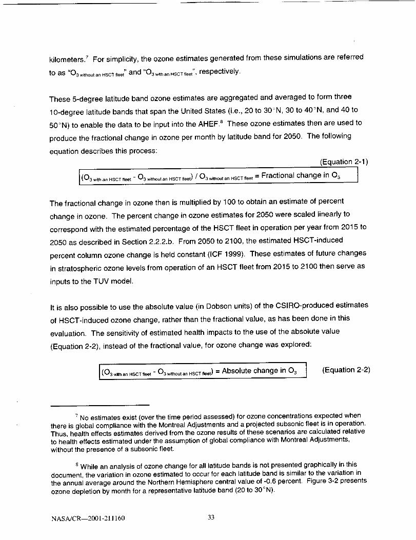
kilometers. 7 For simplicity, the ozone estimates generated from these simulations are referred
to as "03 without an HSCT fleet" and "03 with an HSCT fleet", respectively.
These 5-degree latitude band ozone estimates are aggregated and averaged to form three
10-degree latitude bands that span the United States (i.e., 20 to 30°N, 30 to 40°N, and 40 to
50°N) to enable the data to be input into the AHEF. 8 These ozone estimates then are used to
produce the fractional change in ozone per month by latitude band for 2050. The following
equation describes this process:
(Equation 2-1 )! i
[(03 with an HSCTfleet" 03 without an HSCT fleet) / 03 without an HSCT fleet = Fractional change in 03 II I
The fractional change in ozone then is multiplied by 100 to obtain an estimate of percent
change in ozone. The percent change in ozone estimates for 2050 were scaled linearly to
correspond with the estimated percentage of the HSCT fleet in operation per year from 2015 to
2050 as described in Section 2.2.2.b. From 2050 to 2100, the estimated HSCT-induced
percent column ozone change is held constant (ICF 1999). These estimates of future changes
in stratospheric ozone levels from operation of an HSCT fleet from 2015 to 2100 then serve as
inputs to the TUV model.
It is also possible to use the absolute value (in Dobson units) of the CSIRO-produced estimates
of HSCT-induced ozone change, rather than the fractional value, as has been done in this
evaluation. The sensitivity of estimated health impacts to the use of the absolute value
(Equation 2-2), instead of the fractional value, for ozone change was explored:
I 1(O3withan HSCT fleet " O3 without an HSCTfleet) "- Absolute change in 03 (Equation 2-2)
7 No estimates exist (over the time period assessed) for ozone concentrations expected whenthere is global compliance with the Montreal Adjustments and a projected subsonic fleet is in operation.Thus, health effects estimates derived from the ozone results of these scenarios are calculated relativeto health effects estimated under the assumption of global compliance with Montreal Adjustments,without the presence of a subsonic fleet.
8 While an analysis of ozone change for all latitude bands is not presented graphically in thisdocument, the variation in ozone estimated to occur for each latitude band is similar to the variation inthe annual average around the Northern Hemisphere central value of -0.6 percent. Figure 3-2 presentsozone depletion by month for a representative latitude band (20 to 30°N).
NASA/CR--2001-211160 33

See Appendix C for additional explanation of this analysis. Briefly, small differences (less than
1.5 percent) were observed in estimated health impacts when the absolute value for ozone
change was used instead of the fractional value. The results therefore are judged to be
relatively insensitive to the choice of absolute or relative ozone change, and this study employs
the approach based on the relative ozone change as described in Equation 2-1.
2.2.2.b. Specification of fleet growth schedule
Current evaluations of the impact of HSCT on the ozone layer (i.e., the IPCC and NASA
assessments) focus on total fleet size in a given future year but do not specify the annual rate
of deployment for HSCT needed to reach this total fleet size (IPCC 1999, Kawa et aL 1999).
Hence, creating a fleet growth schedule is the first step in modeling the impact that a growing
HSCT fleet will have on future changes in human health effects.
Based on discussions among an expert group, a linear fleet size ramp-up was assumed
(ICF 1999). The ultimate fleet size of 1,000 aircraft in passenger-service in 2050 is based on
projections of future demand and analyses of market capture (Kawa et aL 1999). Passenger-
kilometers per year follow subsonic market projections and are replaced from subsonic to
supersonic aircraft on a one-to-one ratio, with subsonic aircraft being phased out as more
HSCT enter passenger service. Figure 2-2 illustrates the in-service schedule used in this
evaluation.
The approach described above is somewhat different from either of those used in the NASA
and IPCC reports (Kawa et al. 1999, IPCC 1999). For example, the NASA assessment
envisioned a fleet of 500 HSCT in operation in 2015. However, full-scale fleet production
requires technological and design innovations that will not be available for commercial use for a
number of years. Therefore, it is no longer realistic to assume that a fleet of 500 HSCT would
exist in 2015, given the state of technology plus research and development activities. With
these limitations, 2015 was chosen as an earliest starting point for the HSCT fleet.
NASA/CR--2001-211160 34

1000-
Number
of
HSCT500 -
Aircraft
in
PassengerService
o2015 2033 2050
Year
Figure 2-2. HSCT fleet size. The operation of HSCT is assumed to begin in2015 and ramp up linearly until 1,000 aircraft are in operation in 2050. This evaluationthen assumes that 1,000 aircraft are in operation from 2050 to 2100.
The present study estimates time-dependent fractional ozone changes by scaling CSlRO data
for the year 2050 linearly back to 2015 whereas the NASA and IPCC reports base their ozone
change estimates on steady-state emissions of mature HSCT fleets in a given year
(Kawa et aL 1999, IPCC 1999). The time-dependent analysis used in this evaluation does not
attempt to account for possible geographic changes in HSCT utilization, instead assuming that
global air traffic patterns for HSCT would grow incrementally. This incremental growth
assumption was selected for ease of modeling, and actual HSCT growth patterns may be
different.
Moreover, the time-dependent ozone changes developed and used in this analysis do not
attempt to account for any departures from a linear relationship between fleet size and ozone
change that might occur due to a changing background atmosphere (e.g., changing
background NOx). The effects of changing background NO, on this assumption are expected to
be second order in magnitude and, thus, the assumption of a linear relationship was selected
as a reasonable initial approximation. The sensitivity of results to this assumption could be
evaluated in future work.
NASA/CR--200I-211160 35

2.3 Calculation of UVR change
The amount of UVR reaching the Earth's surface is computed using the TUV radiation model
(Madronich 1992, 1993b; Madronich and de Gruij11993; Madronich et al. 1996, 1998). The
TUV model is widely regarded as an accurate tool for calculating surface UVR levels and has
been updated many times to reflect current science. The accuracy of the TUV model has been
demonstrated in a number of comparisons to direct measurements of UVR at the Earth's
surface (e.g., Shetter et al. 1992, 1996; Kirk et aL 1994; Lantz et al. 1996). Since 1989, the
TUV model has been used in the scientific evaluations of ozone depletion (WMO 1989, 1991,
1995, 1999) and related environmental consequences (UNEP 1989, 1991, 1994, 1998) as
mandated under the Montreal Protocol.
The TUV model computes the radiation levels at any height in the atmosphere including the
Earth's surface. The spectral irradiance, F(h, x, t), incident at the Earth's surface, at time t,
location x, and wavelength A, may be represented symbolically as the product of the solar
spectral irradiance at the top of the atmosphere, Ftoa(A), and an atmospheric transmission
factor, T.
F(,k, x, t) = Ftoa(,_ ) T(_k, x, t; 0o, 03, clouds, aerosols .... ) (Equation 2-3)
Values of Ft,(A) are known from direct observations of the Sun by satellite-, balloon-, and
ground-based instruments. The values of T depend on parameters such as the solar zenith
angle, 0o, and the seasonal variation in Earth-Sun distance. They also depend on atmospheric
optical properties, specifically absorption by ozone, possibly some pollutant gases (NO2, S02),
and scattering by air molecules (known as Rayleigh scattering). Atmospheric particles (clouds
and aerosols) can contribute to both absorption (e.g., soot) and scattering (mathematically
described by the Mie theory) and may be used optionally in TUV. Surface reflections also are
included, as they can contribute substantially to the radiation incident at the surface (see for
example McKenzie et al. (1998)). Many of these factors are functions of location (latitude,
surface elevation, altitude above the surface) and time (day, year, and long-term trends), so
that F(_, x, t) is also a strong function of time and geographic site. The TUV model calculates T
by first subdividing the atmosphere into vertical layers (typically 1 km thick), each having an
NASA/CR--2001-211160 36

assumed uniform composition. The model uses vertical profiles of air density, temperature, and
ozone from the United States Standard Atmosphere 9 (USSA 1976).
When different ozone column values are considered (e.g., under different future Montreal
Protoco_ scenarios), the changes in ozone are applied to the reference scenario at each altitude
in proportion to the ratio of new to reference ozone column values, so that the shape of the
profile is conserved. Thus, since approximately 90 percent of the total ozone column is in the
stratosphere, most of the ozone changes are also located in the stratosphere.
In principle, not only changes in total ozone columns, but also the altitude at which ozone
perturbations occur, can have some effect because of the coupling between ozone absorption
and scattering by air molecules. In practice these considerations are important only when the
ozone perturbations occur in the lower-to-middle troposphere and are relatively insensitive to
perturbations that occur in the stratosphere (i.e., well above the region where scattering
occurs). The figure provided in Appendix D indicates that compared to the more complex
altitude-dependent effect, the simple scaling method is approximately accurate to better than
10 percent for perturbations occurring in the upper troposphere and lower stratosphere. For
example, ozone perturbation occurring near 20 kilometers reveals an RAF near "l.'12, while an
assumption of uniform column ozone change results in an RAF of 1.17. See Appendix D for
further discussion.
Within each uniform layer, the equation of radiative transfer is solved using an accurate
numerical scheme, a modified version of the discrete ordinates method developed by Stamnes
et al. (1988). The modifications, made by Madronich and co-workers, removed numerical
instabilities and improved accuracy at low Sun (when atmospheric curvature becomes
important) through the use of a pseudo-spherical technique. The solutions for each layer then
are matched at the interfaces to adjoining layers, and the entire system (the matching
equations for all 80 layers) is solved using matrix inversion methods. The result is the spectral
irradiance at any location and time, F(h, x, t).
9The US Standard Atmosphere (USSA) provides average values for a number of atmosphericparameters at different altitudes.
NASA/CR--2001-211160 37

The TUV model also calculates biologically weighted radiation, UVb_, defined as:
I UVb_ = j F(A, x, t) B(A)dA I (Equation 2-4)
where B(A) is a spectral sensitivity function (also known as an action spectrum or weighting
function) for the biological endpoint of interest. (See Section 2.4.3 for additional information on
action spectra.) For example, the action spectrum for erythema (i.e., sunburn), Bery(A), has
been determined from spectral exposure studies on humans, and the data have been
characterized by the following expression (McKinlay and Diffey 1987):
Iog_0B.ry(A) = 0.0 for A = (250-298 nm)= 0.094 (298-A) (298-328 nm)= 0.015 (139-A) (328-400 nm)
(Equation 2-5)
Action spectra for a number of other biological endpoints have been estimated (e.g., DNA
damage, ocular damage), and their sensitivity to UV changes associated with ozone depletion
have been tabulated (most recently by Madronich et al. (1998)).
The TUV model provides "look-up tables" (calculated for cloud-free conditions) as a function of
the total ozone column, solar zenith angle, and surface elevations. These tables are then used
to calculate cumulative UVR for a given latitude, time of day, day of month, 1° and amount of
ozone, as measured in Dobson units. These tables vary by action spectrum and serve as
inputs to the AHEF.
2.4 Calculation of health impacts
The AHEF consists of a series of modules that estimate changes in the incidence and/or
mortality of selected health effects resulting from past and future changes in stratospheric
ozone concentrations. These changes in health effects (i.e., cataract incidence and melanoma
10The look-up tables estimate the average irradiance per hour for every hour between 4 am and10 pm on the 15th day of a given month. These representative irradiance estimates then are multipliedby 30 to obtain an estimate of the average irradiance for the whole month.
NASA/CR--2001-211160 38

and non-melanoma incidence and mortality) typically are expressed relative to health effects
that would have occurred if ozone concentrations that existed in 1979-1980 had been
maintained through the time period of interest. Currently, EPA uses the AHEF to estimate
incremental changes in health effects associated with the Montreal Protocol, its subsequent
amendments, and other ODS phaseout and release scenarios (ICF 2000a).
The AHEF first computes projections of incidence and mortality based on historical rates
assuming ozone conditions identical to those existing in 1979-1980. The establishment of this
1979-1980 health effects baseline provides a standard from which all changes in health effects
resulting from ozone perturbations (e.g., from a fleet of HSCT) can be quantified. (See
Section 2.5 for an additional discussion of the baselines used in this evaluation of human health
impacts.) Baseline health impact estimates are calculated by combining historical data on
U.S. cataract incidence and skin cancer incidence and mortality (National Cancer Institute
(NCI)/EPA, National Institute of Health (NIH), and/or SEER data sets), with U.S. Census
Bureau age and sex group population projections. In developing the AHEF 1979-1980
baseline, only light-skinned populations are considered because baseline rates of
responsiveness to UV exposure are not well documented in other populations. In addition, to
account for latitudinal variations in UVR, baseline projections are estimated for three latitude
bands that span the United States (i.e., 20 to 30°N, 30 to 40°N, and 40 to 50°N) (ICF 2000a).
Next, the health impacts arising from a particular ozone perturbation can be determined by first
calculating an estimated UV dose for any location for the time periods encompassed by various
dose metrics. These UV exposures are calculated using the appropriate action spectra and
dose metrics, such as peak single day or cumulative annual exposures for either an individual's
entire life or selected ages (ICF 2000a).
Next, estimates of UV dose are combined with dose-response relationships for the health
effects to produce estimates of changes in health impacts due to the perturbation being
studied. These estimates then are compared with the AHEF estimates of 1979-1980 baseline
health effects to project future incremental levels of cataract incidence and skin cancer
incidence and mortality. The dose-response relationships are calculated by plotting weighted
UV exposures against data characterizing each health effect. The slopes of the resulting
curves are referred to as BAFs and are estimated separately for each health effect from actual
human incidence and mortality data (ICF 2000a).
NASA/CR--2001-211160 39

BAFs can also be defined as the percentage variation in skin cancer incidence and mortality
associated with a percentage change in UV exposure, controlling for factors such as age and
birth year. Age must be considered due to the lag period between exposure and detection for
skin cancer and cataracts and because skin cancer incidence and mortality depend upon
cumulative UV exposure. Further discussion of BAFs and RAFs can be found elsewhere
(UNEP 1994). An equation is used to generate BAF estimates since BAFs for the selected
health endpoints examined in this evaluation have not yet been derived from experimental data.
The following equation estimates the relationship between UV exposure and cutaneous
malignant melanoma (CMM) mortality, controlling for birth year (CMM only) and for age while
taking into account the intensity of UV exposure across different latitudes throughout the United
States. This power function is obtained by deriving a best-fit equation that describes the
appropriate dose-response curve:
Rij =e [B°+_ 8 cC'+_-.,_J A j+ _u,' in (UV_i }]-t-£ ij(Equation 2-6)
where R_ is the mortality rate for the Ith cohort and the ]th age group, and UVg is UV exposure
for the tth cohort and the ]th age group. The C_and Aj terms are cohort and age group dummy
variables, and Bc_and BAare the corresponding coefficients that control for the influence of
these factors on CMM mortality. 11 B0 is the regression coefficient, or intercept, and Buy is the
BAF for the health effect of interest (CMM, in this example). This equation is solved for each
latitude band of interest.
The TUV calculates the future annual percentage change in UV dose across the latitudinal
bands for the scenario based on the CSIRO model's outputs. This is multiplied by the BAF for
each health effect and yields the percent change in future health effects attributable to changes
in ozone concentration. Multiplying these percentages by the baseline projections for each
appropriate health effect and age group produces the change in future cases or mortality
attributable to the HSCT fleet scenario. The following equations summarize this process:
1_This regression is run using the maximum likelihood non-linear Poisson method because the
error term is no longer normally distributed after the natural log is applied to both sides of Equation 2-6.
NASA/CR--2001-211160 40

(Equation 2-7)
(Percent change in weighted UV relative to UVr_f) x (BAF) = Percent change in I/M relative to I/M,e for
Note: ref =reference scenario (e.g., Montreal Adjustments, 1979-1980 baseline); I/M = incidence or mortality
The remainder of this section highlights the human health endpoints analyzed in this evaluation
and then discusses the action spectra and dose metrics used to quantify and predict each
health effect. Table 2-1 presents a summary of the human health effects and their associated
parameters used in this analysis.
2.4.1 Human health endpoints
As described above, the human health endpoints examined in this evaluation are basal cell
carcinoma (BCC), squamous cell carcinoma (SCC), and CMM incidence; CMM and non-
melanoma skin cancer (NMSC) mortality; and cataract incidence. BCC and SCC are
collectively referred to as NMSC. These diseases were evaluated because their etiologies are
fairly well understood. In addition, action spectra and dose-response relationships have been
estimated for each of them, thus making it possible to quantitatively project potential changes in
these health effects due to increases in UVR. These diseases are also some of the most
serious human health impacts associated with UV exposure.
Humans develop three major forms of skin cancer thought to be etiologically related to UV
exposure: CMM, BCC, and SCC. These UV-associated tumors develop principally in light-
skinned individuals. Darker skinned individuals (e.g., Asians, Hispanics, and Blacks) also
develop these tumors but at much lower rates. In NCI's 1978-1979 survey in the United States,
for instance, the incidence of NMSC in African-Americans was nearly 100-fold less than that
observed in Caucasians and the incidence in Hispanics in New Mexico was one-sixth (males) to
one-eighth (females) of those observed in Anglos (Scotto et al. 1983).
NASA/CR--2001-211160 41

Table 2-1. Summary of Health Effects Parameters Examined
in this Human Health Impact Evaluation
Endaoint °
Melanoma Mortality
Melanoma Incidence
NMSC Mortality
NMSC Incidence--BCC
Action SDectrgm
SCUP-h
SCUP-h
SCUP-h
SCUP-h
NMSC Incidence--SCC SCUP-h
Cataract DNA_hbThese endpoints are evaluated on a cumulative annual basis over the lifetime of theindividual.
bThe action spectra for cataracts are currently being updated. The number of cataract
cases predicted by the AHEF for this human health impact evaluation is not expectedto change significantly as a result of these updates. See Appendix E for additionalinformation.
SCUP-h = Skin Cancer Utrecht Philadelphia action spectrum, adjusted for human skintransmission.
CMM develops from melanocytes, the pigment-producing cells of the skin. These tumors often
grow rapidly, frequently developing aggressive metastases. Although it is clear that exposure to
the UV in sunlight is a major risk factor for CMM development, the dose-response relationship
is not completely understood. There is some indication that intermittent high-dose exposure
(i.e., sunburns) may be important and that exposure early in life poses a greater health risk than
exposure later in life (Elwood and Jopson 1997).
NMSCs arise from keratinocytes, the principal cell of the epidermis, the outermost living layer of
the skin. BCCs develop from undifferentiated cells in the germinal, basal layer of the
epidermis. They are the predominant skin cancer in light-skinned populations, representing, in
the United States, about 80 percent of all skin cancer cases (Epstein 1996). BCCs tend to
grow slowly and usually appear on the neck, hands, face, and trunk. In addition, they rarely
metastasize and have a cure rate of greater than 95 percent if detected in the early stages
(de Gruijl and Van der Leun 1993). SCC is a neoplasm 12of keratinocytes as well, but it arises
from a more differentiated cell higher up in the epidermis. It typically is found on the ears, face,
or hands. SCC is much less common than BCC. However, SCC has the same cure rate as
BCC, given early detection, and is two to three times more common in men than in women
(Public Health Service 1996).
_2A neoplasm is a quickly reproducing growth of the abnormal cells that create a tumor.
NASA/CR--2001-211160 42

Although both BCC and SCC are tumors of keratinocytes, they appear to have somewhat
different dose-response relationships to UV. SCC risks appear to be related to an individual's
total accumulated exposure; populations at especially high risk are those with outdoor
occupations (e.g., farmers, foresters). In contrast, BCC risks, similar to those associated with
CMM, appear to be related to intermittent exposure with exposures in childhood being
particularly important (Kricker 1992, Armstrong et aL 1997).
A cataract is an agglomeration of protein on (or in) the lens of the eye that prevents light from
reaching the retina and thus interferes with vision. There are three major forms of
cataract: nuclear, cortical, and posterior subcapsular, so named because of their location in the
lens. Nuclear cataracts occur in the inner layers of the lens, cortical cataracts occur in the outer
layers of the lens, and posterior subcapsular occur at the back (posterior) interface of the lens
and its epithelial capsule. Frequently, these forms occur in combination
(Longstreth et al. 1998).
In a 1991 study (Italian American Cataract Study Group 1991 ), pure cortical cataract
represented slightly less than 50 percent of the cataracts occurring in individuals aged 45-79,
and mixed cataracts represented about 40 percent, with most of the mixed forms including a
cortical component. Although many factors such as poor nutrition, heavy drinking, diabetes,
exposure to radiation, and genetic predisposition can also increase the risk of cataract,
exposure to increased levels of UVR has been linked definitively to cortical cataract
(Italian American Cataract Study Group 1991, Klein et al. 1995, West and Valmadrid 1995,
West et aL 1998). Indeed, in the Klein et al. study (1995), heavy sun exposure was on a par
with diabetes or heavy drinking as a risk factor for cataract.
The social and economic consequences of cataracts are enormous. Worldwide, it is the
leading cause of blindness (West and Valmadrid 1995). In the United States, cataract surgery
constitutes a significant component of the health care budget, amounting to approximately
$3 billion in 1992 (Javitt and Taylor 1995). In this study, estimates of changes in cataract
incidence resulting from a fleet of HSCT is provided based on the best available information.
As technology evolves and researchers increase their ability to make quantitative predictions of
cataract incidence based on changes in UVR, updates to the cataract modeling methodology
can be made to increase the accuracy of the preliminary estimates presented in this evaluation.
Appendix E discusses the methodology used in this evaluation to estimate changes in cataract
NASA/CR--2001-211160 43
incidence and provides information on interim updates to the methodology as well as future
directions for cataract modeling.
2.4.2 Other human health and environmental effects
In addition to the health effects featured in the AHEF, UVR has been associated with other
human health consequences that are as yet unquantified. For example, UV exposure can
produce immunosuppression in humans that could lead to increases in the incidence and
severity of some infectious diseases or result in an increased failure rate of vaccination
programs (Longstreth et al. 1998). Numerous studies in animals have shown that UV exposure
depresses the immune responses to microorganisms (principally those that enter via the skin),
and results in more severe infections. Human infectious diseases in which animal tests have
shown such an effect include herpes, tuberculosis, leprosy, trichinosis, leishmaniasis, listeriosis,
and Lyme disease (Longstreth et al. 1998).
Although action spectra (defined below) have been derived for immunosuppression
(e.g., De Fabo and Noonan 1983), certain key data gaps would make it difficult to develop
estimates of health effects changes for this endpoint. For example, sufficient epidemiological
data do not presently exist that would allow the quantification of the number of affected
individuals necessary to estimate baseline incidence. In addition, no commonly accepted
method exists to measure the degree of UV-induced immunosuppression experienced by these
individuals. Finally, the scientific community is not in agreement as to which dose metric should
be used to assess the consequences of immunosuppression.
The first links between UVR and adverse human health impacts were discovered many years
ago. Researchers continue their efforts to understand the complex mechanisms by which the
Sun affects nearly every form of life on this planet. Many nonhuman impacts have been
associated with UVR, such as damage to agricultural crops. Enhanced UV levels have varied
repercussions on terrestrial ecosystems, ranging from decreased photosynthesis rates to
changes in competitive balance and increased susceptibility to disease (Caldwell et aL 1998).
Effects on aquatic ecosystems are predicted as well, including decreased species diversity and
reduced larval survival rates (Hader et aL 1998). Increased UVR also may degrade polymeric
NASA/CR--2001-211160 44

materials and thus reduce their useful life, which has far-reaching impacts on construction and
manufacturing industries (Andrady et al. 1998).
2.4.3 Action spectra
An action spectrum describes the relative effectiveness of (i.e., is used as a weighting function
for) UV-A and UV-B wavelength radiation in the induction of health effects (e.g., DNA damage,
skin cancer, erythema, and cataract) (ICF 2000a). Action spectra are determined through
controlled UV exposures on animal subjects to evaluate the effectiveness of a wavelength at
inducing a specific health effect. Figure 2-3 depicts commonly used action spectra for the
health effects examined in this evaluation.
10.00000
1.00000
(me- 0.10000OO.U}OI'_ 0.01000
Q
m 0.001o0n-
o.ooo1o
--SCUP-h
Setlow Fisho,oooo1
290 300 31o 320 330 340 350 360 370 380 390 400
Wavelength (nm)
Figure 2-3. UV action spectra. SCUP-h has been selected for use in this study toassess skin cancer incidence and morality, and DNA-h is used to evaluate cataract incidence, Inthis figure, the erythema (described in McKinlay and Diffey 1987) and Setlow fish melanoma actionspectra (described in Setlow et aL 1993) are presented for comparison purposes.
If an action spectrum is known, it can be combined with exposure data to determine effective
UV dose (i.e., the intensity at each wavelength weighted by effectiveness at producing the
health effect of interest). Researchers then can perform studies quantifying the responses of
organisms to particular doses of UVR, thus creating dose-response curves and BAFs for a
particular health effect. As described in Equation 2-6 above, the BAF is used by the AHEF to
relate changes in weighted ground-level UVR to changes in health effects.
NASA/CR--2001-211160 45

Several action spectra were proposed to evaluate the various human health effects examined in
this evaluation. The SCUP-h and DNA-h action spectrum were selected for further analysis.
SCUP-h was derived on the basis of induction of SCC in hairless mice and then adjusted for
human skin characteristics (de Gruijl et aL 1993), as described below. SCUP-h was chosen for
use in this evaluation because it is widely accepted and is believed to be the appropriate action
spectrum for SCC. SCUP-h also has been selected for BCC and CMM because both are
cancers of the skin and action spectra specific to either of these tumors do not exist
(Longstreth et aL 1998). The DNA-h action spectrum is a generalized DNA damage action
spectrum (derived from studies on bacteria and viruses as described below) and was selected
for cataract estimates because of research indicating that UV-induced damage in lens epithelia
(thought to be a precursor to cataract) can be reversed via photoreactivation
(i.e., repair of DNA in marsupials) (Tafoya et al. 1997).
This study, in using the SCUP-h action spectrum for CMM, has assumed that the action
spectrum for one type of skin cancer (SCC) can be used to make predictions about another
(CMM). This assumption introduces a presently unquantified source of uncertainty which may
be substantial. The results of analyses (such as the present one) which use the SCUP-h action
spectrum for CMM predictions are accurate to the extent that the shape of the as-yet
unidentified CMM-specific action spectrum is congruent or similar to that of SCUP-h. Similar
considerations apply to the use of the SCUP-h action spectrum for prediction of BCC, although
differences between BCC and SCC are considered biologically less significant than those
between melanoma and non-melanoma skin cancer. Similarly, as discussed in Appendix E, the
use of the DNA-h action spectrum to make predictions about cataract incidence may introduce
unquantified uncertainty. However, the information and tools used in this study represent the
best available approach and are consistent with current practices in risk assessment.
As noted above, SCUP-h is the action spectrum for SCC in mice that has been corrected for
transmission through human skin. Mouse skin and human skin have different absorption
spectra for UV light, principally because mouse epidermis is thinner than human epidermis and
thus more of the UVR gets through the layers of dead cells to the target at the base of the
epidermis (the outer viable layer in which skin cancer develops). In order to adjust for these
differences, the UV absorption spectra of mouse skin and human skin are compared across the
relevant wavelengths and the differences between them are then corrected for by multiplication
by the appropriate ratios. As an example, suppose that at 300 nanometers (nm), the thickness
NASA/CR--2001-21 I 160 46

of human skin prevents 5 percent less UVR from reaching the base of the epidermis than
mouse skin does. To compensate for this difference in absorption between mouse and human
skin, the dose plotted at 300 nm for mice would need to be reduced by 5 percent. Thus, the
action spectrum would be modified by 5 percent at 300 nm to account for the relative efficiency
of the incoming light in human skin.
A similar adjustment is made when Setlow's DNA action spectrum is corrected for human skin,
except in this instance it is not the difference in two species, but the difference between no skin
(i.e., in a petri dish) and what would be predicted for the same reaction occurring in human skin.
Setlow's DNA action spectrum is a generalized action spectrum that was developed from in
vitro experiments on a number of different microbial systems where the UV directly hits the
affected microbial targets. In skin, the UV first has to pass through a number of cell layers
before hitting DNA targets in live cells. These layers have a number of UV-absorbing
molecules (e.g., trans-urocanic acid, proteins) that selectively filter out some wavelengths of
UV; this filtration reduces the energy reaching the target so that the effective energy in skin is
somewhat less than that in a petri dish.
2.4.4 Dose metrics
The AHEF can examine a variety of dose metrics, which allows for evaluation of exposure early
in life. This early exposure is thought to be more important than cumulative exposures for
some health endpoints. Exposures for CMM mortality and incidence, as well as BCC incidence,
are approximated both as an average annual measure and as the exposure received on a peak
day (i.e., June 21) for each year. These two methods of characterizing exposure then can be
applied for every year of a person's life or only for exposures received at selected ages
(e.g., from ages 1 to 20). The exposures in this study are based on estimates of cumulative
annual lifetime exposure.
NASA/CR----2001-211160 47

2.5 Model implementation
This section discusses development of the Montreal Adjustments baseline used as a reference
scenario for this study.
The AHEF is designed to express changes in health effects due to a particular ozone
perturbation relative to the health effects that would have occurred if the 1979-1980 ozone
conditions were held constant through time. In the current application, however, the AHEF is
used to predict the incremental health effects associated with an HSCT-induced stratospheric
ozone perturbation relative to those that would have occurred in the absence of this
perturbation. Thus, the appropriate "baseline" for this evaluation is the set of health effects
expected under atmospheric conditions reflecting adherence to the Montreal Adjustments to the
Montreal Protocol._3
Since the AHEF expresses health effects relative to 1979 -1980 ozone conditions, the
incremental health effects for the Montreal Adjustments scenario in the absence of an HSCT
fleet must be estimated first. The AHEF then is used to estimate the health effects associated
with a fleet of HSCT relative to the 1979 -1980 ozone conditions. The incremental health
effects associated with the presence of an HSCT fleet relative to the Montreal Adjustments are
thus the difference between the results of these two AHEF model simulations. This concept is
illustrated qualitatively for skin cancer and cataract incidence in Figure 2-4.
_3The CSIRO model assumes global compliance with the Copenhagen Amendments to theMontreal Protocol. The AHEF, by contrast, generates estimates assuming compliance with the MontrealAdjustments to the Montreal Protocol. That is, the models assume a slightly different baseline orreference atmospheric scenario. The differing assumptions regarding reference scenario are not judgedto significantly affect this study's results because only the incremental differences in ozone between theCSIRO results with and without an HSCT fleet are used to generate the percent change in UV usingTUV-generated look-up tables (see Equation 2-1 and Section 2.3). To test this judgment, a sensitivityanalysis was performed to determine if choice of reference scenario would affect the resulting healtheffect estimates. Reasonable perturbations to the reference scenario lead to between approximately1 and 5 percent changes in estimated HSCT-induced health impacts. See Appendix F for a descriptionof these sensitivity tests.
NASAJCR--2001-211160 48

HSCT Fleet and
Montreal Adjustments
•
/ 1979-1980 Ozone Conditionsu)
L)
Years
Figure 2-4. Incremental health effects due to an HSCT fleet. Thisfigure depictsthe methodusedby the AHEF to estimatethe additional health effectsassociatedwiththeoperationof a fleet of HSCT relativeto the MontrealAdjustments.Note:The curves illustratethe relationship between variousemission scenarios, but providequalitative information only.
2.6 Uncertainty in estimated impacts
Several steps were taken to consider uncertainty in estimated HSCT health impacts. First, the
key calculation steps required to estimate human health impacts arising from HSCT-induced
ozone change were identified. The steps involved (1) the prediction, by atmospheric models, of
the precise ozone column changes under HSCT scenarios, (2) the calculation of consequent
changes in surface UVR, and (3) the quantification of the health impacts of the perturbed UVR
levels (Madronich 1999). In consultation with experts, the sources and magnitudes of the major
uncertainties associated with each step were identified. Table 2-2 summarizes these
uncertainties. In many cases, it was not possible to quantify the impact of various sources of
uncertainty. Some of the unquantified sources are presented in Table 2-3.
Second, for selected major individual sources of uncertainty (e.g., estimated changes in column
ozone, BAFs), the error range estimate was run through the sequence of models to evaluate
the uncertainty in the estimated health impact due just to the particular individual input
uncertainty. Other sources of uncertainty are also qualitatively discussed. Although a
comprehensive, integrated analysis of uncertainty in estimated health impacts due to all
NASA/CR--2001-2I 1160 49

sources was not performed, the results of the individual model runs were used to obtain an
initial sense of the uncertainty in the results of this study.
Table 2-2. Factors Contributin 9 Known Uncertainty
Factor
Change in OzoneEstimates
Change in UVREstimates
Changes in HealthEffect Estimates
Parameter
General
Atmospheric
RAF
Action
Spectrum
BAF
Uncertainty
a range of -2.7% to+0.3% around a centralvalue of -0,8% column
ozone depletion a
±10% radiation model
<2% ozone absorptionspectrum
50% c
30%
Explanation
Estimated usinginformation from NASA
assessment (Kawa etal. 1999) °
(Koepke et al. 1998)(De More et al. 1997)
(Table 11.8, UNEP1998)
(deGruijl et al. 1993,Lon_lstreth et al. 1998)
This corresponds to a -350 percent and +150 percent uncertainty range.
Kawa et aL (1999) estimated that the uncertainty of the predicted change in Northern Hemisphere ozone contentfor a fleet of 500 HSCT in 2015 is given by +0.5% to -2.5% around the central value of -0.4%. This corresponds toan upper bound obtained by adding an additional -2.1% ozone decrease and a lower bound obtained by adding a+0.9% ozone increase to the central value, respectively. In this study, the uncertainty range for a fleet of 1,000HSCT in 2100 was obtained by adding the same increments (-2.1% and +0.9%) to the central value of -0.6%.
c This estimate applies only if the action spectrum lies within the range of action spectra for biological effects inmammals.
2.6.1 Uncertainties associated with change in ozone estimates
An uncertainty range for the estimated HSCT column ozone impact was obtained from the
NASA assessment. Briefly, that assessment evaluated sources of potential error in the
modeling of processes controlling ozone impact. Sources addressed included exhaust particle
production; model representation of atmospheric transport; long-term circulation; exhaust
accumulation; chemical characteristics of the background atmosphere (halogen, NOy, and H20
distributions); and chemistry (reaction kinetics and treatment of heterogeneous processes).
Using a combination of tests of model prediction sensitivity to variations in these parameters,
evaluations of existing model biases involving these parameters, and existing information on
parameter uncertainty (e.g., measurement error in laboratory studies of reaction kinetics), an
estimate of error in central value attributable to each source of uncertainty was developed.
NASA/CR--2001-211160 50

Table 2-3. Factors with Unknown Contributions to Uncertainty
Factor
Change in Ozone
Estimates
Change in UVR
Estimates
Change in Health
Effect Estimates
Parameter
Composition of Future Atmosphere
Ability to Model Atmospheric Processes Accurately
Response of Ozone Layer to ODS Phaseout
Changes in Composition and Quantity of HSCT Emissions
Long-term Systematic Changes in Atmospheric Opacity
(e.g., clouds, aerosols, other pollutants)
Changes in Human UV Exposure Behavior
Improvements in Medical Care�Increased Longevity
Changes in Socioeconomic Factors
Latency
Changes in Population Composition and Size
An estimate of the total uncertainty in the central-value estimate arising from all of these
sources of uncertainty was derived by combining the root sums of squares of each of the
individual sources of uncertainty (Kawa et al. 1999).
The NASA assessment total uncertainty range was developed around a central value of
average annual Northern Hemisphere response to a fleet of 500 HSCT in the year 2015. Due
to the fact that other uncertainty estimates were not available, this same total uncertainty range
is applied in this study to the estimated ozone change for all latitudes and all months, even
though estimated ozone changes may be more uncertain at some latitudes and in some
seasons than others. Furthermore, the same total uncertainty range is used even though the
central value employed in this study is based on a 1,000 aircraft, year 2050 scenario. The use
of the 500-aircraft uncertainty range for the 1,000 aircraft scenario is reasonable for the
following three reasons (ICF 1999):
• First, some of the modeled processes (e.g., transport or chemical kinetics and
mechanisms) should not be very sensitive to the fleet size.
NASA/CR--200I-211160 51

• Second, the estimated uncertainties are conservative and should be applicable to
somewhat larger fleet sizes, as well.
Finally, the assumption that the 500-aircraft uncertainty range can be applied to a
fleet of 1,000 aircraft is consistent with the discussion in IPCC (1999) pointing out
that the ranges of model-predicted depletion are similar for the 500 plane fleet and
the 1,000 plane fleet.
In the evaluation presented here, the uncertainty range is therefore scaled linearly from zero to
500 aircraft and then assumed to remain constant from 500 to 1,000 aircraft. Although this
scaling approach is different from the simple linear scaling from 0 to 1,000 aircraft adopted for
the central value, it satisfies the decision to use the same uncertainty range for the 500 aircraft
and 1,000 aircraft central value estimates.
Recent research has reinforced estimates that 10 percent or less of fuel sulfur will be converted
to new particles (i.e., the lower end of the particle production range used in the assessment is
most probable). Thus, the uncertainty in ozone depletion associated with the conversion
processes, which was largely on the negative side, may be less than previously suspected.
This reduction in risk is counterbalanced, however, by new research on the partitioning of
NO_/NOy in the stratosphere, which suggests a greater effectiveness of aircraft NOx emissions
in destroying ozone. Because these new findings suggest offsetting changes in predicted
ozone impacts, no modifications in the uncertainty range were deemed necessary (ICF 2000b).
The uncertainty in estimated column ozone impacts was considered a major source of
uncertainty in this assessment. Because of the existence of a carefully developed estimate of
uncertainty in atmospheric inputs, the effect of this estimated uncertainty on health impacts was
quantified.
The placement of the upper and lower uncertainty bounds reflects the potential for actual ozone
changes to be either greater or less than predicted (see Figure 3-1 in Chapter 3). The upper
and lower uncertainty bounds are established by adding 0.9 and -2.1 percent, respectively, to
each derived value of percent column ozone change due to HSCT. A step-wise method was
used to estimate these bounds (i.e., scaling uncertainty from 0 to 1,000 aircraft and then
NASA/CR--2001-211160 52

holding these bounds constant from 2050 to 2100). The following equation is used to
determine the ozone change used for the atmospheric uncertainty analysis:
(Equation 2-8)
HSCT2o,5÷x= [No HSCT2ol_ * (1 +%_HSCT2o5o * PSF,)] + ( No HSCT2015*USFx)
where,
x = years 0-35 (2015-2050)
HSCT = ozone levels in the presence of HSCT (Dobson units)
No HSCT = ozone levels in the absence of HSCT (Dobson units)
%_HSCT = change in ozone levels due to HSCT (percent change in ozone is negative)
PSF = production scaling factor, a linear ramp-up from 1-1,000 jets between 2015 and 2050 (a percent
expressed as x / 35).
USF = uncertainty scaling factor, a linear scaling of the uncertainty range between 2015 and 2033. The
lower bound scales from 0.0 to -0.9 percent {-0.9% * (x / 18), for x = 0 to 18 and -0.9% for years
thereafter} and the upper bound scales from 0.0 to 2.1 percent {2.1% * (x / 18), for x = 0 to 18 and 2.1% for
years thereafter}.
2.6.2 Uncertainties associated with change in UVR estimates
Uncertainty involved in the estimation of weighted UV exposure at the surface is discussed and
quantified below. Although this UV estimation uncertainty was not specifically modeled, expert
opinion was solicited regarding the sensitivity of predicted health impacts to changes in UV
transfer calculation parameters. Those sensitivities are discussed in Chapter 3. In general, the
relationship between changes in ozone and changes in ground-level UVR is well known.
Uncertainties contributed by estimating the change in UVR are relatively small compared with
those inherent in other components of the analysis. The accuracy of any radiation model,
including the TUV model (used in this analysis), depends on the quantity being estimated. In
this evaluation, changes in UVR are generated by estimating the relative percent of UV
changes stemming from a specific change in ozone, under the strong assumption that all other
factors (e.g., air pollution, cloud cover) remain constant.
NASA/CR--2001-211160 53

The key quantity in this estimation process is the sensitivity factor, often known as the "radiation
amplification factor," or RAF. 14 The RAF is defined by:
[ (_UV/UV) ~- RAFx (z_OJO3). I (Equation 2-9)
For example, the RAF for human erythema and UV index is approximately 1.1. Errors in UV
are thus directly proportional to errors in the RAF. Of course, RAFs are not true constants, and
the approach that the TUV model uses is to compute local RAFs from tables of ground-level
UVR for a range of solar zenith angles, ozone column amounts, and surface elevations, is
Errors in estimating RAFs, and thus errors in estimating ground-level UVR, are dominated by
uncertainties in the following:
. Action spectra. The action spectra contribute by far the largest uncertainties. For
example, a variety of action spectra can be used to weight the wavelengths of UVR that
produce a given health effect. As discussed in UNEP (1998), for a given action
spectrum, the RAFs for skin cancer in mammals range between 1.1 and 1.7, suggesting
an uncertainty range of approximately 50 percent.
. Ozone absorption. The ozone absorption spectrum in the critical 300-320 nm
wavelengths is known to be accurate to better than 2 percent from many laboratory
studies (De More et al. 1997).
, Radiation model. Few systematic comparisons of RAFs from different radiation models
have been performed. In the 1989 Ozone Assessment, Table 3.2-10 compares RAFs
for different models and atmospheric conditions. Variations of a few percent are noted
14The RAF is commonly used to provide rough estimates of the response of surface UVR tochanges in the total ozone column. The RAF concept is used in this evaluation for illustrative purposesonly and a more accurate method of estimating ground-level UVR is used for the actual calculations thatcreate the look-up tables discussed in Section 2.3. Background information on the use of RAFs isprovided in Appendix D.
,5 A description of the effect that clouds and the altitude of an ozone perturbation could have onthese values is provided in Appendix D.
NASA/CR--200 I-211160 54

(WMO 1989). Many other important model differences are possible (e.g., spectral
resolution). Published comparisons of models and measurements show, in the best
circumstances, agreement to approximately 10 percent for spectral irradiances and
actinic fluxes (Koepke et al. 1998).
2.6.3 Uncertainties associated with change in health effect estimates
Health effects modeling contributes quantifiable uncertainties to the estimates of human health
effects resulting from a fleet of HSCT in two major areas: (1) the dose-response relationships
(expressed as a BAF) for the four endpoints of concern (i.e., cataract, BCC, SCC, and CMM),
and (2) the future size, behavior, and distribution of the populations that will be affected. These
sources of uncertainty are further described below. It should be noted that for this study, only
estimated uncertainty in the BAF parameter was quantified. Qualitative discussions of the
sensitivity of predicted impacts to other health effects modeling uncertainties are provided in
Chapter 3.
2.6.3.a. Uncertainty in the BAF
Health effects modeling, which incorporates dose-response information in the form of a BAF is
one source of uncertainty for change in health effect estimates. The model used in this
analysis, the AHEF (described in Section 2.4), incorporates information on the dose-response
relationships for cataract, BCC, SCC, and CMM through the use of a BAF (i.e., the slope of the
dose-response relationship). Estimates of BAFs generated for SCC and BCC using the SCUP o
h action spectrum are 2.5 + 0.7 and 1.4 ± 0.4, respectively (deGruijl et al. 1993, Longstreth et
al. 1998). This yields an uncertainty range of approximately 30 percent for changes in health
effects estimates.
2.6.3.b. Uncertainty in population projections
The AHEF combines U.S. population projections with a number of other parameters to predict
the absolute number of future skin cancer and cataract cases and/or deaths associated with a
proposed fleet of HSCT. Projections of U.S. population size are obtained from the U.S. Census
NASAJCR--2001-211160 55

Bureau grouped by state, age, sex, and race through 2025 (population by state) and 2050
(entire United States). These data then are further aggregated into latitude bands, as
described in ICF (2000a). This process is used both in this evaluation and in all other EPA
applications involving the AHEF.
The U.S. Census Bureau does not develop quantitative estimates of the uncertainty ranges
accompanying the population projection groupings used by the AHEF (i.e., by state, age, sex,
and race). However, the bureau does generate high and low estimates of the future population
by state, and quantitative estimates of the uncertainty accompanying the annual population
growth rate for the United States. The U.S. population is estimated to grow at a rate of
1 percent per year (Spencer personal communication). A _+0.1 percent uncertainty range
accompanies this annual estimate. This uncertainty range pertains only to the amount of yearly
increase experienced by the U.S. population as a whole, however, and does not consider the
uncertainty that may accompany the absolute estimate of the number of U.S. residents in a
given year. In addition, it does not address the uncertainty surrounding the population
groupings (i.e., age, state, sex, race) used by the AHEF.
Thus, applying this general estimate of uncertainty to the population groupings used by the
AHEF would be difficult. For example, the growth rate of the total U.S. population may vary by
± 0.1 percent, but the uncertainty accompanying the growth rate of various ethnicities within this
population may be much more or less than 0.1 percent. In addition, the uncertainties
accompanying the absolute sizes of these subpopulations are unknown. However, several
methodologies for testing uncertainty in population projections have been proposed. These
methods are discussed in Section 3.4.3.a.
2.6.3.c. Latency
In this evaluation, latency refers to the lag time between UV exposure and the manifestation of
skin cancer or cataract. Skin cancer latency and early life exposure have been identified as
potentially important risk factors associated with increased susceptibility to CMM. Modeling
this lag time accurately is difficult given the current state of knowledge about latency and its
mechanisms (Madronich 1999). Thus, quantitatively estimating the uncertainty contributed by
NASA/CR--2001-211160 56

this process is not possible at this time. However, the presence or absence of a formal
modeling of latency is not thought to contribute significantly to the uncertainty accompanying
the health effect estimates. The reasoning behind this expectation is as follows: The AHEF
currently offers the option of weighting UV exposures by age and by type of exposure
(e.g., peak-day exposure and annual exposure) summed over the lifetime of the individual, thus
approximating a type of latency. When varying assumptions regarding latency were assumed,
estimated health impacts were affected only moderately. The results of this analysis are
presented in Section 3.4.3.b.
2.6.4 Other sources of uncertainty
Many uncertainties in this evaluation either cannot be quantified or are currently so poorly
understood that an accurate estimate of their significance is not possible. For example,
alterations in the composition of the future atmosphere, as well as uncertainties about the
response of the ozone layer to changes in ODS emissions can combine with changes in HSCT
fleet emission characteristics to contribute an unknown amount of uncertainty to change in
ozone estimates. Similarly, laboratory techniques and instrumentation, changes in population
size and composition, fluctuations in human UV exposure patterns, and a variety of other
factors can greatly affect the uncertainty surrounding predictions of human health effects.
These and other factors are briefly discussed below.
2.6.4.a. Contributions to unknown uncertainties in change in ozone estimates
The exact composition of the future atmosphere as a result of compliance with different ODS
phaseout policies is unknown. As levels of atmospheric chlorine are reduced, the impact of
NO× species from the proposed HSCT fleet would change. In addition, future changes in
climate could result in increases in atmospheric water vapor, which could in turn increase cloud
cover. 16 The impacts of global warming on the composition of the future atmosphere also are
unknown. These elements could introduce a variety of uncertainties into estimates of skin
cancer and cataract incidence and/or mortality.
_6See Appendix D for a brief discussion of the effects of cloud cover on ground-level UVR.
NASAICR--2001-211160 57

Uncertainties also can be contributed by assumptions regarding the future behavior of the
ozone layer in response to the phaseout of ODS. When estimating future changes in ozone,
accurately modeling the effects of various policy scenarios (e.g., the Montreal Protocol and its
amendments) on ozone concentrations is important. In the future, some computer models
predict that the phaseout of ODS will slow and eventually stop the rate of ozone depletion.
Some of these models suggest that natural ozone-making processes will enable stratospheric
ozone to return to 1979-1980 ozone conditions and eventually result in increased
concentrations beyond those levels (see Chapter 12 in WMO 1998 for more detail). Because
knowledge about the interaction of ozone with chemical species in the future atmosphere is still
incomplete, no artificially created limit has been imposed on future ozone recovery in this
evaluation. That is, in both the CSIRO input and the Montreal Adjustments baseline, ozone
levels are allowed to recover beyond conditions observed in 1979-1980.17
In addition, improvements in engine design and technology may alter the emissions created by
an HSCT fleet. Evolving knowledge regarding factors such as atmospheric transport,
heterogeneous chemistry, climate change, and the representation of these factors in models,
also may lead to changes in estimates of ozone impacts resulting from fleet emissions.
2.6.4.b. Contributions to unknown uncertainties in change in health effect
estimates
Additional uncertainty can be contributed by the laboratory techniques and instrumentation used
for deriving the action spectra used to weight UV exposure. Discrepancies between the
wavelengths of UVR intended to be administered and the wavelengths actually received by the
test organism can result in orders of magnitude differences in the measured response. In
_7Whether this recovery scenario, called "ozone superabundance," is likely to occur is open todebate, particularly because of the potential for complex interactions between global climate change andstratospheric ozone dynamics. Model computations have predicted both future conditions of higher andlower amounts of ozone. Stratospheric temperature may be cooler due to increased emissions ofgreenhouse gases, and reactions that destroy ozone may consequently proceed more slowly. Thisscenario would lead to increases in ozone. Alternatively, the cooler temperatures could changestratospheric circulation and also may lead to increases in polar stratospheric clouds, which potentially
could lead to decreases in ozone, possibly preventing or delaying ozone recovery.
NASA/CR--2001-211160 58

addition, action spectra are derived using monochromatic light sources, which do not fully
simulate the polychromatic light received directly from the Sun.
Changes in socioeconomic factors, population composition and size, and human UV exposure
behavior also can have an impact on factors ranging from demand for air travel to the types of
skin cancer most commonly observed. For example, population composition changes such as
the expected increase in Hispanic populations, whose more pigmented skin decreases their
skin cancer risk, could have significant effects on future U.S. skin cancer rates. Improvements
in medical care and predictions of increased longevity for many population subgroups also
could affect estimates of future skin cancer incidence and mortality significantly. In addition,
this evaluation assumes that human exposure behavior remains constant through time and
does not take into account innovations in sun protection technology (e.g., sunglasses,
sunscreens), increases in public awareness of the effects of overexposure, and increased
sensitization to the need for early treatment of suspicious lesions. Factors such as these
cannot easily be quantified and are not addressed further in this evaluation.
These demographic and behavioral changes may also be augmented or offset by changes in
surface UVR due to atmospheric constituents other than stratospheric ozone (e.g., changes in
tropospheric ozone and aerosols from pollution, and changes in cloudiness stemming from
climate change and pollution). These factors, as well as those described above, may in some
cases result in UVR changes or health effect changes larger than those estimated to result
from the operation of a fleet of HSCT.
Accurate prediction of future changes in human health effects would require consideration of
the net effect of all factors described above. This challenge is beyond the ability of the current
state of atmospheric and epidemiological science. In addition, direct measurements
(e.g., of future UV levels or skin cancer incidence) cannot attribute explicitly observed changes
to any specific factor, unless that factor is far more important than all the others combined.
However, the principle of superposition can be used to examine the HSCT impact
(i.e., one effect, in isolation) under the assumption that the other factors remain constant at
current conditions. The validity of this principle is based on the assumption that the HSCT
NASA/CR--2001-211160 59

impacts are independent of the other factors (e.g., behavioral changes will occur regardless of
whether an HSCT fleet is in place).
2.7 Sensitivity of estimated health impacts to technological andoperational change
When evaluating the number of excess cataracts or skin cancers estimated by the AHEF for
the proposed HSCT fleet, it is important to consider the sensitivity of estimated health impacts
to possible alterations in various operational, technological, and atmospheric parameters. A
sensitivity analysis conducted along these lines can be a useful tool for decision-makers, as it
can assist in identifying and focusing resources on factors that exert the greatest influence on
ozone depletion and thus have the greatest ability to reduce expected health effects. For
example, a sensitivity analysis may indicate that changes in fleet cruise altitude have significant
impacts on ozone depletion whereas other changes might have only slight impacts. The NASA
assessment contained an analysis of plausible variations in fleet size, fuel sulfur content, NOx
emission index, and altitude (e.g., the parameters listed in Table 2-4). The NASA analysis
revealed that these changes could alter estimates of column ozone response by as much as
-0.4 to +0.3 percent relative to the baseline scenario of 500 HSCT in 2015 and 1,000 HSCT in
2050 examined in that study (Table 2-4) (Kawa et al. 1999).
A perturbation of ±0.1 percent column ozone change around the central ozone estimate
(approximately 17 percent of the central value) was selected as a representative perturbation to
explore the sensitivity of estimated health impacts due to variation in various control
parameters. Although this perturbation is smaller than the column ozone sensitivity to some of
the technological and operational parameters examined in the NASA assessment, the results of
this sensitivity study should provide a rough scaling factor between technological and
operational change and changes in estimated health impacts.
To implement this sensitivity test, from 2015 to 2033 (i.e., from 0 to 500 aircraft), the magnitude
of the perturbation was adjusted to reflect the growing number of HSCT in operation. The full
perturbation of ±0.1 percent was used to evaluate HSCT impacts between 2033 and 2100
(i.e., 500 to 1,000 aircraft).
NASA/CR--2001-211160 60

The following equation was used to apply the sensitivity bounds to the central value:
(Equation 2 -10
HSCT20_+, = [No HSCT2015 * (1 +%_HSCT20so * PSFJ] + ( No HSCT2o15* SSF,)
where,
x = years 0-35 (2015-2050)
HSCT = ozone levels in the presence of HSCT (Dobson units)
No HSCT = ozone levels in the absence of HSCT (Dobson units)
%_HSCT = change in ozone levels due to HSCT (percent change in ozone is negative)
PSF = production scaling factor, a linear ramp up from 1-1,000 jets between 2015 and 2050 (a percent
expressed as x / 35).
SSF = sensitivity scaling factor, a linear scaling factor of the sensitivity range of ±0.1 percent between 2015
and 2033 {+ 0.1% * (x / 18), for x = 0 to 18 and +0.1% for years thereafter}.
Figure 2-5 indicates the sensitivity bound as the inner shaded region ("inner envelope"),
whereas the uncertainty bound is the outer shaded region ("outer bound") around the central-
value line. Table 2-4 lists NASA's findings regarding the sensitivities associated with changes
in various parameters for a fleet of 500 aircraft. This evaluation assumes that these
relationships remain constant from 500 to 1,000 aircraft.
O
E
OO
Em
U.l
+0.6% -
+0.3% -0%-
-0.3% -
-0.6% -
2015
I t
2033 2050
Year
Central Values for 3. O_
_ SensJtivity' ol +0.1% -0.1%to
(inner envelope)
F7 Uncertainty range of
+0.9% to -2 1%
(outer enveloDe)
Figure 2-5. Sensitivity and uncertainty envelopes. This graph depicts the methodsused to estimate the uncertainty inherent in generating ozone estimates as well as the methodsused to quantify the sensitivity of the predicted ozone values to changes in various technical andoperational parameters.
NASA/CR--2001-211160 61
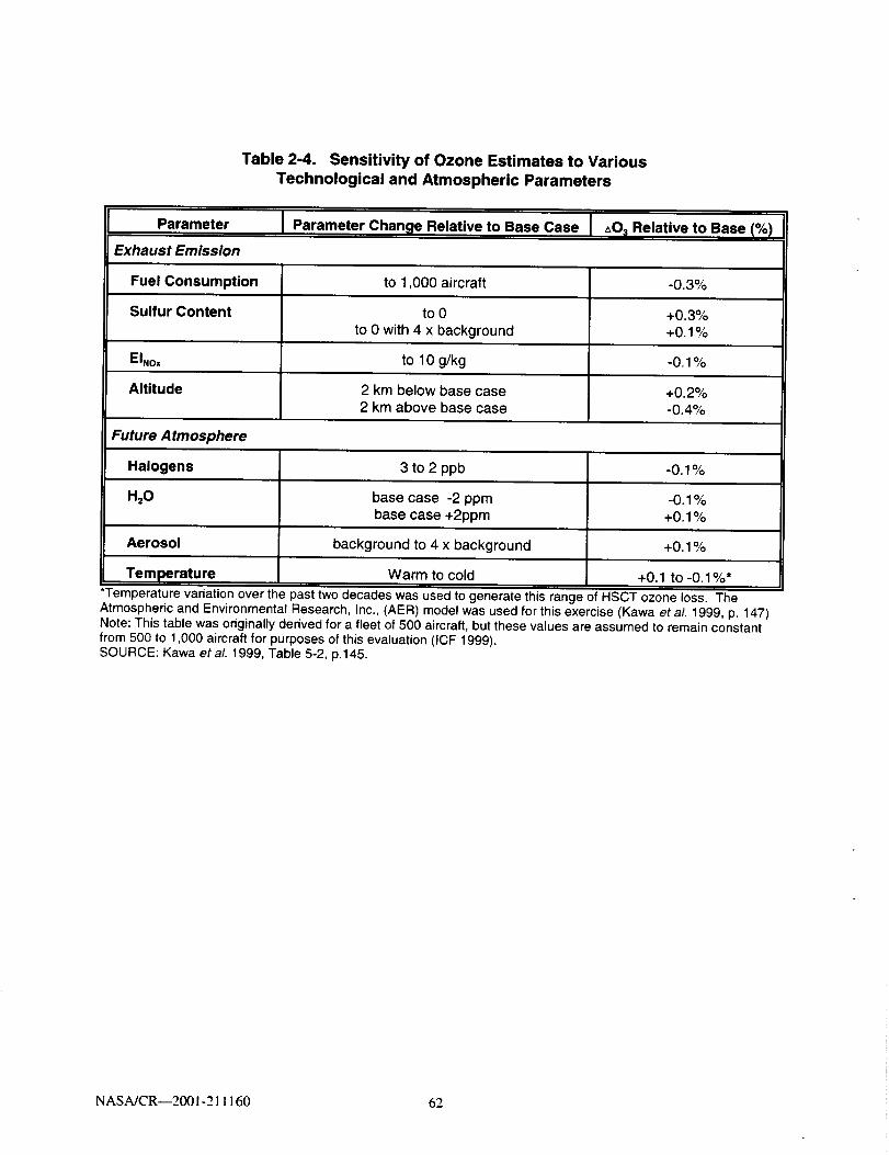
Table 2-4. Sensitivity of Ozone Estimates to VariousTechnological and Atmospheric Parameters
Parameter Parameter Change Relative to Base Case J _0; Relative to Base (%)
Exhaust Emission
Fuel Consumption
Sulfur Content
EINox
Altitude
to 1,000 aircraft
to 0to 0 with 4 x background
to 10 g/kg
2 km below base case2 km above base case
-0.3%
+0.3%+0.1%
-0.1%
+0.2%-0.4%
Future Atmosphere
Halogens
H20
Aerosol
Temperature
3 to 2 ppb
base case -2 ppmbase case +2ppm
background to 4 x background
Warm to cold
-0.1%
+0.1%
+0.1 to -0.1%*
*Temperature variation over the past two decades was used to generate this range of HSCT ozone loss. The
Atmospheric and Environmental Research, Inc., (AER) model was used for this exercise (Kawa et al. 1999, p. 147)Note: This table was originally derived for a fleet of 500 aircraft, but these values are assumed to remain constantfrom 500 to 1,000 aircraft for purposes of this evaluation (ICF 1999).SOURCE: Kawa etaL 1999, Table 5-2, p.145.
NASA/CR--2001-211160 62

Chapter 3. Results and Discussion
Chapter 3 presents results of the analyses performed to assess the impacts on human health of
a proposed HSCT fleet and discusses these results. Section 3.1 first describes changes in
stratospheric ozone concentrations due to HSCT and then compares the magnitude and
seasonality of the HSCT-induced change with those expected from ODS emissions for a
representative year (2033). Section 3.2 next describes the projected features of HSCT-induced
UVR changes. Section 3.3 summarizes the calculated change in skin cancer incidence, skin
cancer mortality, and cataract incidence from HSCT, relative to effects expected under
adherence to the Montreal Adjustments of the Montreal Protocol. Section 3.4 presents and
discusses the results of uncertainty analyses performed to provide information regarding the
uncertainty in estimated health impacts. Section 3.5 presents the results of a sensitivity
analysis performed to link changes in certain HSCT fleet technological and operational factors
and the degree of reduction or exacerbation of human health impacts. A comparison of the
estimated health impacts of HSCT with those of several past regulatory strategies for
stratospheric protection is provided in Chapter 4.
3.1 HSCT impacts on stratospheric ozone concentrations
Using outputs from a previous application of the CSIRO model (see Section 2.2.1 for
discussion), future changes in stratospheric ozone concentrations resulting from a fleet of
HSCT were estimated. These results then were scaled linearly to a starting point of zero
HSCT in service in 2015. The following subsections point out several features of these derived
time-dependent column ozone patterns.
3.1.1 Annual percent change in ozone
A critical first step in the evaluation of HSCT impacts on human health is to generate a time-
dependent series of annual estimates of the change in stratospheric ozone concentrations that
would be produced by a growing fleet of HSCT. As described in Section 2.2.1, CSIRO outputs
for the year 2050 were scaled based on the percent of the HSCT fleet in operation per year
NASA/CR--2001-211160 63

from 2015 to 2050. From 2050 to 2100, the estimated HSCT-induced percent column ozone
change is held constant at 2050 levels. Figure 3-1 presents the percent change in column
ozone estimated to occur as a result of an HSCT fleet operating from 2015 to 2100. The
positive change in ozone exhibited in the upper uncertainty bound suggests that ozone
concentrations could show a net increase during the time frame in which the fleet is in
operation. A net increase in ozone levels resulting from a fleet of HSCT, however, is
considered less likely than a decrease in ozone levels.
1,0% ...........................
" " " Upper Atmospheric Ur_ertalnty Bound
.... Lower Atmospheric Uncertainly Bound
°''''"=_''''"..... ................................. . .................
O,5%=*
.B
°°°*
0.0%-0.5%
,=o
; \•_ -1,0%
c
t_
-1.5%
-2,0%
-2,5%
-3.0%
\
\\
\
\
2015 2020 2025 2030 2035 2040 2045 2050 2055 2060 2065 2070 2075 2080 2085 2090 2095 2100
Year
Figure 3-1. Annual percent change in ozone relative to the MontrealAdjustments atmospheric conditions resulting from a fleet of HSCT grownfrom 0 in 2015 to 1,000 in 2050 (40°-50°N latitude band). Lowest curverepresentsthe lower uncertaintyboundof -2.1 percentrelativeto the centralvalue;middlecurveisthe centralchangeinozonevalue;highestcurveisthe upperuncertaintyboundof +0.9 percentrelativeto thecentralvalue. Extrapolatedfrom CSIRO simulationof the HSR program'sScenario36 (Table4-3, Kawaeta/. 1999). See moredetailed discussion of uncertaintyinSection2.6.1.
NASA/CR--2001-211160 64

3.1.2 Seasonal patterns
In general, ozone depletion resulting from the operation of an HSCT fleet has been found to
vary seasonally as temperature, circulation, and other changes influence atmospheric
processes. Estimates generated by the CSIRO model predict the greatest ozone depletion
during fall and winter months (i.e., from September to March) and the least depletion during
spring and summer months (i.e., from April to August). 1 Figure 3-2 illustrates the seasonal
fluctuations in the central-value ozone concentrations for the HSCT fleet per month in 2050.
Central-value ozone changes produced by an HSCT fleet fluctuate seasonally from
approximately -0.48 percent to -0.66 percent for the 20 ° to 30 ° latitude band.
0.5% _ .............. ,,
i
0.0% '
-0.5% ......
_-1.0% "-O
.=_
c='-1.5%tj
-2.0% t ......
_Upper Atmospheric Uncerlalnty Bound
_Central Value
_Lower Atmospheric Uncerlalnty Bound
-2.5%
-3.0%
Jan Feb Mar Apr May Jun Jut Aug Sep Oct Nov Dec
Month
Figure 3-2. Percent change in ozone by month for 2050 resulting from afleet of 1,000 HSCT. (For clarity, only the 20 to 30°N latitude band is presented.) The
seasonal ozone trends observed in this figure are relevant to trends in latitudinal bands examined
in this analysis. At higher latitudes the seasonal variation will differ.
The NASA assessment performed an analysis of ozone seasonal distribution and trends forfive 2-D models, including CSIRO (Kawa et aL 1999). This analysis compared the predicted seasonalbehavior from the models with actual climatology data. NASA concluded that most of the modelssatisfactorily represented the parameters examined.
NASA/CR--200 ! -21 I 160 65

Because discussions concerning ozone depletion are based on ODS emissions, it is instructive
to compare the seasonal patterns of ozone depletion resulting from these emissions with the
seasonal patterns of ozone depletion that would result from a proposed fleet of HSCT. In
general, ozone depletion resulting from the use of ODS (i.e., driven by estimates of equivalent
effective stratospheric chlorine, or EESC 2) occurs mainly in the winter and spring (i.e., January
to June) with relatively wide seasonal fluctuations (Figure 3-3). Seasonal fluctuation in ozone
depletion from HSCT, on the other hand, covers a much smaller range (i.e., the magnitude of
values is more constant throughout the year, see Figure 3-3). Thus, in summer months
(e.g., July) when little ozone depletion results from ODS emissions, ozone depletion resulting
from a fleet of HSCT may constitute a larger percentage of overall depletion. Similarly, in
winter months (e.g., February) when ODS-related ozone depletion is high, HSCT-related ozone
depletion may contribute a smaller percentage of the overall depletion. In the example provided
in Figure 3-3 for the year 2033, HSCT fleet impacts range between 6 and 11 percent of the total
(ODS- plus HSCT-driven) ozone depletion occurring from January to June and between 17 and
35 percent of the total (ODS- plus HSCT-driven) ozone depletion occurring from July to
December.
Figure 3-3 illustrates the seasonal impacts of ODS- and HSCT-related ozone depletion
assuming full compliance with the Montreal Adjustments to the Montreal Protocol. The lightly
shaded portion of the graph is the expected ozone depletion relative to atmospheric ozone in
1979-1980 due to ODS emissions for 2033, based on a separate analysis (calculations not
presented). 3 The darkly shaded portion in each of the bars in Figure 3-3 represents the
estimated incremental decrease associated with HSCT operation by month for 2033
(when half of the fleet is predicted to be in operation), as estimated by extrapolations performed
on the CSIRO outputs described in Section 2.2.
2 EESC is an expression of the ozone-depleting capability of a substance and its degradationproducts, expressed in terms of chlorine molecules. The EESC of substances that contain bromine canbe calculated by using a bromine efficiency factor that relates the ozone-depleting efficiency of bromineto that of chlorine.
-_ODS-induced ozone depletion was calculated as described in ICF (2000a), based upon ODSemissions projections assuming compliance with the Montreal Adjustments and empirical relationshipsbetween historical ODS emissions and observed ozone depletion, by latitude band.
NASA/CR--2001-211160 66

3.1.3 Latitudinal patterns
In general, ozone depletion resulting from use of ODS also varies by latitude, with greater
ozone depletion expected in colder northern regions (i.e., nearer the polar vortex) and less
depletion expected toward the equator. An inspection of the three latitude bands
(20 ° to 30°N, 30 ° to 40°N, and 40 ° to 50°N) used in this evaluation also indicates a trend of
decreasing ozone depletion with decreasing latitude.
4
A
oO
.c 3
i;&_ : i'
• HSCT fleet
[] Montreal Adjustments
May
• /L •¸ i
i,fiJan Feb Mar Apt Jun Jul Aug Sep Oct Nov Dec
Month
Figure 3-3. Comparison of ozone depletion due to ODS and HSCT in 2033relative to 1979-1980 ozone conditions (40 to 50°N latitude band). The bottomofeach column demonstrates the variable decrease in ozone throughout the months attributable toODS-related depletion, with the greatest amount of depletion occurring in winter. The top portionof each column shows the incremental additional ozone depletion due to HSCT. See Section 3.1.2for further discussion.
3.2 HSCT impacts on UVR
This section summarizes the estimated effects of an HSCT fleet on ground-level UVR. As
described in Section 2.3, the TUV model was used to calculate UVR from changes in ozone
inputs generated by the CSIRO model.
NASA/CR--2001-211160 67

To illustrate the approach used, a sample calculation of the changes in ground-level UVR
associated with a fleet of HSCT is provided. Extrapolated CSIRO data and a representative
RAF are used in the discussion presented here. Although the results of this approach agree
with the many output files generated by the TUV, these rough calculations are performed for
descriptive purposes only and are not used directly to estimate incremental UVR. In particular,
the TUV model used in this analysis is a more accurate tool for generating these incremental
UVR estimates because the look-up tables created from the TUV estimate a series of local
ground-level UVR values based on a wide variety of parameters including solar zenith angle,
time of day, and day of month (whereas an RAF is a single average value).
Figure 3-4 presents the change in weighted UVR associated with an HSCT fleet. To produce
this figure, the annual percent changes in ozone, estimated as described in Section 3.1.1, are
multiplied by the RAF for a representative action spectrum (SCUP-h = 1.4) to calculate an
average change in weighted UVR in the United States for each year from 2015 to 2050.
As illustrated in Figure 3-4, increases in UVR exhibit a linear relationship with increasing fleet
size. When the proposed HSCT fleet is in full operation in 2050 (i.e., 1,000 operating aircraft),
the annual percent change in ozone plateaus. The UVR associated with this level of annual
ozone change, however, does not level off, but increases slightly through 2100. This
phenomenon can be attributed to the following factors:
° After 2050, ozone concentrations continue to recover under the Montreal
Adjustments scenario, resulting in higher ozone levels ("superabundance,"
discussed in Section 2.6.4.a.).
, The column ozone percent depletion due to the HSCT fleet of 1,000 aircraft is
held constant after the year 2050.
, The column ozone depletion associated with HSCT operation is a fixed
percentage of the base ozone concentration; therefore, the absolute amount of
NASA/CR--2001-211160 68
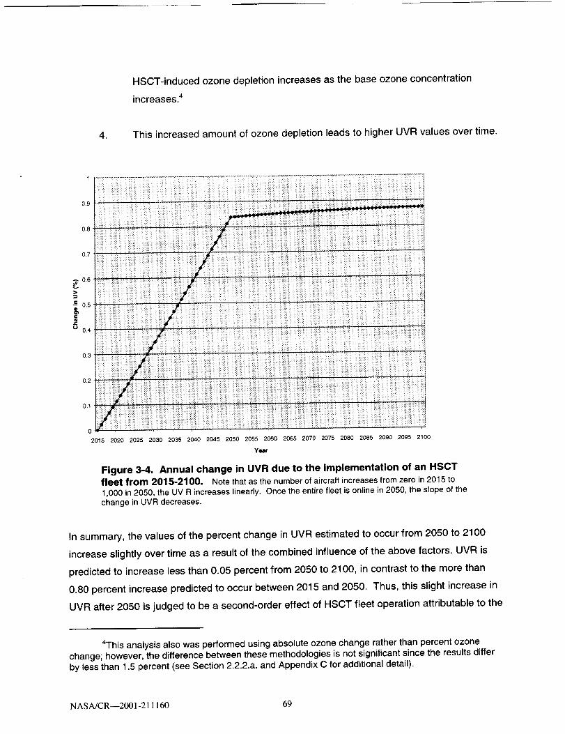
HSCT-induced ozone depletion increases as the base ozone concentration
increases. 4
4. This increased amount of ozone depletion leads to higher UVR values over time.
0
2015 2020 2025 2030 2035 2040 2045 2050 2055 2060 2065 2070 2075 2080 2085 2090 2095 2100
Year
Figure 3-4. Annual change in UVR due to the implementation of an HSCTfleet from 2015-2100. Notethat as the numberof aircraftincreasesfromzero in 2015 to1,000 in2050, the UV R increaseslinearly. Once the entirefleet is onlinein2050, the slope ofthechange in UVR decreases.
In summary, the values of the percent change in UVR estimated to occur from 2050 to 2100
increase slightly over time as a result of the combined influence of the above factors. UVR is
predicted to increase less than 0.05 percent from 2050 to 2100, in contrast to the more than
0.80 percent increase predicted to occur between 2015 and 2050. Thus, this slight increase in
UVR after 2050 is judged to be a second-order effect of HSCT fleet operation attributable to the
4This analysis also was performed using absolute ozone change rather than percent ozonechange; however, the difference between these methodologies is not significant since the results differby less than 1.5 percent (see Section 2.2.2.a. and Appendix C for additional detail).
NASA/CR--2001-211160 69

modeling approach (i.e., assuming a constant percentage decrease in ozone levels associated
with HSCT operation after 2050).
3.2.1 Seasonal patterns
Seasonal changes in UVR are closely related to the ozone changes presented in Figure 3-2
because as ozone concentrations decrease, UVR increases. For example, the greatest
percentage change in UVR is observed during the last six months of the year, with lower
proportions observed in the first six months. Because the magnitude of ODS-related ozone
depletion (i.e., EESC-driven) is higher between January and June, increases in ground-level
UVR resulting from an HSCT fleet are expected to account for a higher proportion of total UV
change (resulting from HSCT- and EESC-mediated ozone depletion) between the months of
July and December.
3.2.2 Latitudinal patterns
Latitudinal patterns in UVR also follow trends similar to those exhibited by ozone levels.
Because the greatest ozone depletion occurs in the higher latitudes, the greatest change in
irradiance is expected to occur in the 40 to 50°N latitude band, followed by the middle 30 ° to
40°N band, and then the 20 ° to 30°N band. This is demonstrated in Figure 3-5.
3.3 HSCT impacts on human health
This evaluation attempts to assess the changes in skin cancer and cataract cases and/or
deaths in the U.S. population that would occur over time as a result of changes in UV exposure
that would be produced by operation of an HSCT fleet. The AHEF combines information on
ozone change, UV exposure change, and dose-response information to quantify these
changes. The following sections describe the total incidence and mortality due to the operation
of an HSCT fleet, seasonal and latitudinal variations in human health effects, and the annual
estimates of changes in human health effects.
NASA/CR--2001-211160 70

1,2
0.8
>
l-o-- 0.6
O_i-
t-O
0.4
0.2
--40 to 50°N
-- 30 to 40°N
20 to 30_N
2015 2020 2025 2030 2035 2040 2045 2050 2055 2060 2065 2070 2075 2080 2085 2090 2095 2100
Year
Figure 3-5. Annual latitudinal differences in UVR caused by an HSCT fleet
(2015-2100). Lowest band represents the 20-30 N latitude band, middle band represents the30-40°N latitude band and highest band represents the 40-50°N latitude band,
3,3.1 Total incidence and mortality due to HSCT operation
Table 3-1 presents the estimated increase in health impacts among the U.S. light-skinned
population that would occur if an HSCT fleet were launched in 2015 and were to grow to an
in-service fleet size of 1,000 by the year 2050 and operate at this constant size from
2050 through 2100. The health impacts presented are total skin cancer incidence, skin cancer
mortality, and cataract incidence. Incidence and mortality estimates were performed for cohorts
born between 1890 (i.e., dying in 1980) and 2100 (i.e., dying in 2190). Although individuals
born after 2100 will receive additional UV exposures due to HSCT fleet operation, the model
estimates increased human health impacts due to higher cumulative UV exposures only for
individuals born through 2100.
The AHEF health effects estimates in Table 3-1 are presented for the central-value case. The
values presented in parentheses in Table 3-1 are upper and lower bounds around the central
value, based only on the uncertainty range accompanying estimated HSCT ozone impacts. To
NASA/CR--2001-211160 71

include the uncertainty contributed by the health effects estimates, the values presented in the
table, including those in parentheses, should be multiplied by a factor of 2 (see Section 3.4.4 for
derivation of this factor). Sections 2.6 and 3.4 provide discussion of these uncertainty factors.
As shown for the central-value case, the greatest predicted increase in skin cancer incidence
is for BCC (964,500 cases), and the greatest predicted increase in mortality is for CMM
(4,500 deaths).
Table 3-1. Total Predicted Incremental Incidence or Mortality in the United States amongPeople Born Between 1890 and 2100 due to HSCT Operation (thousands)
Central Value
CMM
Incidence
CMM
Mortality
36 4.5
(-25 to 180) (-3 to 23)
BCC
Incidence
960
(-690 to
4,900)
SCC
Incidence
523
(-380 to
2,700)
NMSC
Mortality
2.6
(-2 to 13)
Note: Numbers presented in parentheses are upper and lower bounds around the central value, based onluncertainty range accompanying estimated HSCT ozone impacts. To include the uncertainty contributed b
Cataract
Incidence
360
(-270 to
1,900)'on thethe health
effects estimates, the values presented in the table, including those in parentheses, should be multiplied b t a factor of 2(see Section 3.4.4). Further discussion of these results is provided in Chapter 4.
CMM = Cutaneous Malignant Melanoma, BCC = Basal Cell Carcinoma, SCC = Squamous Cell Carcinoma, andNMSC = Non-Melanoma Skin Cancer (SCC + BCC).SOURCE: Estimated for this report based on ICF 2000a.
3.3.2 Seasonal patterns
Increases in UV-related health effects are thought to be associated with repeated exposure to
UVR and often are assessed by examining cumulative doses (ICF 2000a). This dose metric
does not separate incremental health effects by season, recognizing that cumulative year-round
UV exposure is thought to be a more accurate predictor of skin cancer and cataract than is an
analysis of seasonal exposure trends. The method used in this study sums estimates of UV
exposure across all days in a given year and presents incremental health effects on an annual
basis.
NASA/CR--2001-211160 72

3.3.3 Latitudinal patterns
Figures 3-6 and 3-7 present annual excess SCC and BCC incidence by latitude band
associated with the proposed HSCT fleet. SCC and BCC were chosen for comparison because
they provide a good snapshot of the AHEF results by latitudinal gradient. The total incidence
and mortality estimates have been divided by the total affected population (i.e., light-skinned
individuals) and then multiplied by 100,000. By expressing these estimates as rates per
100,000 individuals, the influence of different population sizes across latitudes is removed.
When examining the excess number of cases for each latitude band, it is important to
remember that these incidence predictions are obtained as described in Equation 2-6. Of the
three inputs to the equation (i.e., the BAF, the percent change in annual UVR, and the historical
baseline incidence rate), the BAF stays constant across latitudes for a given health effect. Due
to the fact that ozone changes predicted by the atmospheric models are largest at higher
latitudes, the percent change in annual UVR for the HSCT fleet scenario is greatest in the north
(40 to 50°N latitude band) and lowest in the south (20 to 30°N latitude band). In contrast, the
historical baseline incidence rate for a given health effect is usually much higher at lower
latitudes due to the normally higher UV radiation levels prevailing there.
For SCC, presented in Figure 3-6, the high estimated number of cases of excess skin cancer
due to an HSCT fleet in the southern latitude band (20 ° to 30°N) is a result of the dominating
influence of historical baseline incidence rates that are many times higher than the percent
change in UVR for this region. The northern latitude band (i.e., 40 ° to 50°N) has a much
smaller historical baseline incidence rate. Thus, despite the larger HSCT impacts on ozone and
UVR at this latitude, excess skin cancer cases under the HSCT fleet scenario are smaller than
those calculated for lower latitudes.
For BCC, presented in Figure 3-7, the large baseline incidence rates in the southern latitude
band also produce the highest predicted incremental number of cases of this type of skin
cancer. However, in contrast to SCC, historical baseline incidence rates for BCC vary only
slightly between middle and northern latitudes, with northern incidence rates being slightly lower
than middle latitude rates.
NASA/CR--2001-211160 73

,5I
1.5
|
0.5
0
2015
--50-40°N
--40-30_N
30-2_N i
2020 2025 2030 2035 2040 2045 2050 2055 2060 2065 2070 2075 2080 2085 2090 2095 2100
Yosr
Figure 3-6. Annual estimates of excess SCC incidence per 100,000 bylatitude. The lowestline representsthe 40-50'N latitudeband;the middle linerepresentsthe30-40CNlatitudeband;the highestbandrepresentsthe 20-30°N latitudeband.
Because the equation used to estimate excess incidence holds the BAF constant, and because
the historical baseline incidence rates in the two regions are not significantly different, estimates
of excess incidence are more strongly influenced by estimates of percent change in UVR.
Because the percent change in UVR is greater in the north than in the middle latitude band, the
40 ° to 50°N latitudinal band has a higher excess incidence rate for BCC than the 30 ° to 40°N
band.
3.3.4 Estimates of annual changes in health effects
Estimates of annual changes in health effects illustrate the impact of a proposed HSCT fleet
over time relative to the Montreal Adjustments baseline. Figures 3-8 through 3-13 present
estimates for each health effect endpoint generated by the AHEF s. The shape of
5 Note that in these health effects graphs, unlike the figures depicting changes in ozone, the"upper" uncertainty bounds (i.e., representing less ozone depletion compared to the central value) arethe lower lines on the figures. Similarly, the "lower" uncertainty bounds, representing greater decreasesin ozone, are the upper lines on these figures. This "shifting" of results is explained by the relationshipbetween ozone concentrations and health effects. That is, increased levels of ozone lead to decreasedlevels of UVR at the Earth's surface and decreased incidence and mortality for human health effects.
NASA/CR--200 I-211160 74

4,5
3.5
-- 50_40ON
-- 40- 30° N
30-20°N
I
iii
0
2015 2020 2025 2030 2035 2040 2045 2050 2055 2060 2065 2070 2075 2080 2085 2090 2095 2100
Year
Figure 3-7. Annual estimates of excess BCC incidence per 100,000 bylatitude. The lowest line represents the 30-40°N latitude band; the middle line represents the
40-50°N latitude band; the highest band represents the 20-30°N latitude band.
each of these figures is very similar for all of the examined health effects. In each, the central
case exhibits a progressive increase in the predicted annual number of cases or deaths
expected to affect the U.S. population. The changes in predicted health effects do not track the
HSCT in-service schedule as closely as the ozone time series constructed for this study
because changes in UV exposure resulting from the HSCT fleet can continue to affect human
health for years after the HSCT fleet size has leveled off (i.e., manifestation of a health effect,
as modeled in this study, is due to cumulative lifetime exposure). This continuing effect is a
result of the decades-long latency periods associated with the various forms of skin cancer and
cataract (Madronich 1999).
NASA/CR--2001-211160 75

|
2OOO
1500
1000
500 '
0
" " " Lower Atmospheric UncerlaJnly Bound
_cerllral VaI,Je
- " - Upper Atmosphere: Uncertainty Bound
B"
g,
o
w
e
s
..o.o..--''''"
--o. .... ---°.......°..... ............................. . ................ . ........
-500 .........
2015 2020 2025 2030 2035 2040 2045 2050 2055 2060 2065 2070 2075 2080 2085 2090 2095 2100
Year
Figure 3-8. Annual estimates of excess CMM incidence for the U.S.
resulting from an HSCT fleet (2015-2100) relative to Montreal Adjustments.Lowest curve represents the estimated health impacts when the smallest value of the estimatedatmospheric input uncertainty range is used (upper uncertainty bound of +0.9 percent relative tothe central value). Middle curve is the estimated health impacts from the central-value scenario.Highest curve is the estimated health impacts when the highest value of the estimatedatmospheric input uncertainty bound is used (lower uncertainty bound of -2.1 percent relative tothe central value). Uncertainty in estimated health effects due to one major source of uncertainty(column ozone impacts) is shown for illustration purposes. The indicated uncertainty range thusreflects only one source of uncertainty and should be considered a minimum. See Sections 2.6and 3.4 for additional detail.
NASA/CR--2001-21 ! 160 76

250- - - Lower Atmospheric Ur'certalnfy Bound
_Cenlral Value
- " " Upper Atmospher=c Uncerta'mty Bound .
200 .......
150
60
|100
-5O
4
............. " ........... • ..................................................... ii
i
I
80000
40000
30000
|20000
10000
-10000
2015 2020 2025 2030 2035 2040 2045 2050 2055 2060 2065 2070 2075 2080 2085 2090 2095 2100
Year
Figure 3-9. Annual estimates of excess CMM mortality for the United
States resulting from an HSCT fleet (2015-2100) relative to MontrealAdjustments. See caption for Figure 3-8 for additional detail.
" " " Lower Atmospheric Uncerlainty Bour'pd
Central Value
" " " Upper Almospheric Uncerlainty Bound ..-_': 7"_"
2015 2020 2025 2030 2035 2040 2045 2050 2055 2060 2065 2070 2075 2080 2085 2090 2095 2100
Year
Figure 3-10. Annual estimates of excess BCC incidence for the United
States resulting from an HSCT fleet (2015-2100) relative to Montreal
Adjustments. See caption for Figure 3-8 for additional detail.
NASA/CR--2001-211160 77
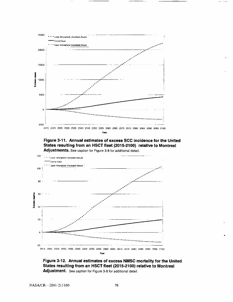
25000
2OOOO
15000
1O0O0
,,'I,
5OOO
0 :
-5000
= = = Lower Atmosphere Uncertainty Bound
_CenlraJ VaJue
- - - Upper Atmospheric UncertMlty Bound
20_5 2020 2025 2030 2035 2040 2045 2050 2055 2060 2065 2070 2075 2080 2085 2090 2095 2100
Year
120
100
8O
:_ 6O
ti
4o
2O
0
-2O
Figure 3-11. Annual estimates of excess SCC incidence for the United
States resulting from an HSCT fleet (2015-2100) relative to Montreal
Adjustments. See caption for Figure 3-8 for additional detail.
" " " Lower Atmospheric Unceilalnty Bound
_CentraJ Value
" " " Upper Atmospheric Uncertainty Bound
• !
._°•°
.... . ................................... ° ...............
2015 2020 2025 2030 2035 2040 2045 2050 2055 2060 2065 2070 2075 2080 2085 2090 2095 2100
Year
Figure 3-12. Annual estimates of excess NMSC mortality for the United
States resulting from an HSCT fleet (2015-2100) relative to Montreal
Adjustment. See caption for Figure 3-8 for additional detail.
NASA/CR--2001-21 1160 78

==
20000
150O0
1OOOO
5OOO
" " " Lower Atmospheric Uncertainty Bound
" " " Upper Atmospheric Uncertainty Bound
°.°
°,°
"-"::::.............................'..2'........................................
-5000 "
2015 2020 2025 2030 2035 2040 2045 2050 2055 2060 2065 2070 2075 2080 2085 2090 2095 2100
Year
Figure 3-13. Annual estimates of excess cataract incidence for the UnitedStates resulting from an HSCT fleet (2015-2100) relative to Montreal
Adjustments. See caption for Figure 3-8 for additional detail,
3.4 Uncertainty analyses
A series of quantitative and qualitative analyses were performed to analyze the uncertainty
associated with a variety of parameters examined in this evaluation. Table 3-2 summarizes the
quantitative uncertainty analyses, and Table 3-3 summarizes the qualitative analyses. See
Section 2.6 for additional detail on the methodology used for these analyses.
In this study, an integrated (e.g., Monte-Carlo style) analysis of uncertainty in estimated HSCT
health impacts was not performed. Instead, a combination of analyses and reasoning were
used to roughly characterize the uncertainty in projections of health impacts attributable to
HSCT-induced ozone depletion. For several major sources, estimated uncertainty was
quantified, based on consultation with experts and/or the literature. For two of these major
sources (i.e., BAFs and estimated changes in column ozone), the upper and lower bounds of
the estimated uncertainty range were modeled. The results are presented in Table 3-2.
NASA/CR--200I-21 I 160 79
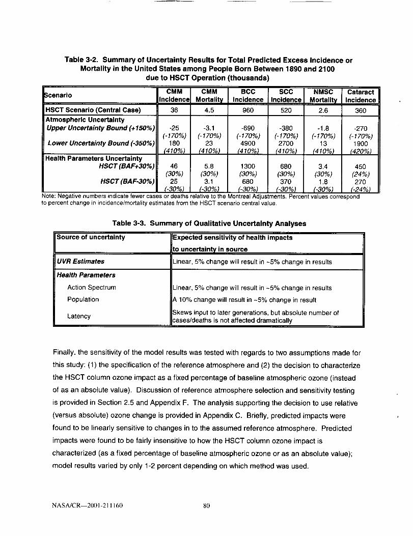
Table 3-2. Summary of Uncertainty Results for Total Predicted Excess Incidence or
Mortality in the United States among People Born Between 1890 and 2100
due to HSCT Operation (thousands)
_cenario
HSCT Scenario (Central Case)
!Atmospheric Uncertainty
Upper Uncertainty Bound (+ 150%)
Lower Uncertainty Bound (-350%)
Health Parameters UncertaintyHSCT (BAF+30%)
HSCT (BAF-30%)
CMMIncidence
36
-25
(-170%)180
(410%)
CMM
Mortality
4.5
-3.1
(- 170%)23
(410%)
BCC
Incidence
960
-690
(-170%)4900
(410%)
SCC
Incidence
520
-38O
(-170%)2700
(410%)
NMSC I CataractMortality Incidence
2.6 360
-1.8
(-170%)13
(410%)
3.4
(30%)1.8
(-30%)
46
_o%)25
_30%)
5.8
(3O%)3.1
(-30%)
1300
(30%)680
(-30%)
680
(30%)370
(-30%)
-270
(-170%)1900
_20%)
45O
(24%)270
(-24%)Note: Negative numbers indicate fewer cases or deaths relative to the Montreal Adjustments. Percent values correspondto percent change in incidence/mortality estimates from the HSCT scenario central value.
Table 3-3. Summary of Qualitative Uncertainty Analyses
Source of uncertainty
UVR Estimates
Health Parameters
Action Spectrum
Population
Latency
Expected sensitivity of health impacts
to uncertainty in source
Linear, 5% change will result in -5% change in results
Linear, 5% change will result in -5% change in results
A 10% change will result in -5% change in result
Skews input to later generations, but absolute number ofcases/deaths is not affected dramatically
Finally, the sensitivity of the model results was tested with regards to two assumptions made for
this study: (1) the specification of the reference atmosphere and (2) the decision to characterize
the HSCT column ozone impact as a fixed percentage of baseline atmospheric ozone (instead
of as an absolute value). Discussion of reference atmosphere selection and sensitivity testing
is provided in Section 2.5 and Appendix F. The analysis supporting the decision to use relative
(versus absolute) ozone change is provided in Appendix C. Briefly, predicted impacts were
found to be linearly sensitive to changes in to the assumed reference atmosphere. Predicted
impacts were found to be fairly insensitive to how the HSCT column ozone impact is
characterized (as a fixed percentage of baseline atmospheric ozone or as an absolute value);
model results varied by only 1-2 percent depending on which method was used.
NASA/CR--2001-21 I 160 80

3.4.1 Uncertainties associated with change in ozone estimates
Uncertainty in estimated HSCT-induced health impacts due to quantified uncertainty in
estimated HSCT-induced column ozone change is considerable (see Table 3-2). This large
uncertainty range comprises not only the possibility for adverse health impacts of much larger
magnitude than the central value, but also the possibility that the impacts may be directionafly
different: An atmosphere with HSCT-induced ozone change could lead to a reduction in skin
cancer and cataract occurrences, relative to a reference atmosphere. This latter possibility
arises from the uncertainty in the estimated column ozone response to HSCT. In addition to
providing an estimate of how much larger than the central value the estimated HSCT ozone
depletion could be, the NASA assessment concluded that there is a small possibility that the
HSCT fleet could lead to an increase in column ozone. However, the NASA uncertainty range
should be viewed as conservative, as it is considered less likely that an HSCT fleet will have a
positive impact on ozone (ICF 1999).
The analysis summarized in Table 3-2 indicates that a decrease in HSCT ozone impact
(i.e., an increase in column ozone) leads to a slightly larger percentage decrease in estimated
health impact, or a reduction in health impacts relative to an atmosphere without HSCT.
The increase in HSCT ozone depletion indicated by the lower bound of the estimated
uncertainty range for the column ozone response leads to a roughly five-fold increase in
adverse health impacts.
The column ozone uncertainty range is unique in several respects: (1) The uncertainty is
relatively large; (2) There is uncertainty regarding both magnitude of column ozone change, as
well as direction; and (3) This uncertainty, unlike uncertainty in the UV transfer and health
effects modeling steps, affects the HSCT health impact estimate uniquely. Uncertainty in the
other steps would affect both the HSCT health impact estimates as well as estimates of health
effects under ODS policy scenarios, with which the HSCT effects are compared.
3.4.2 Uncertainties associated with change in UVR estimates
Estimated health impacts show an approximately linear response to changes in the RAF value
associated with an action spectrum, at least for small changes in the action spectrum.
Consequently, it is assumed that the uncertainty in estimated health impacts of HSCT
attributable to the uncertainty in action spectrum values (discussed in Chapter 2, see Table 2-2)
NASA/CR--2001-211160 81

is approximately 50 percent. The discussion in Chapter 2 also indicates that the UV radiative
transfer modeling step induced approximately 5 percent uncertainty due to calculations relating
to radiative transfer. Table 3-3 illustrates that the small uncertainties of the radiative transfer
modeling step are expected to result in similarly small uncertainties in estimated health impacts.
3.4.3 Uncertainties associated with change in health effects estimates
Table 3-2 shows that changes of 30 percent in the BAF yield corresponding 30 percent
changes in estimated health effects. Moreover, separate analysis (see Table 3-4) illustrates
that when the choice of dose metric is changed from a cumulative lifetime UV exposure to
exposure only during the first 20 years of life, the estimated health impacts shift by less than
10 percent (and the timing of predicted skin cancer incidence and mortality and cataract
incidence also changes). Two additional sources of uncertainty in the health effects
parameters, although they have not been quantitatively treated in this study, should be noted:
uncertainty in population projections and uncertainty regarding latency. These are discussed
below.
3.4.3.a. Uncertainty in population projections
Although no quantitative analysis is provided at this time, three methods are possible for
determining th e ranges of uncertainty around the central value that are attributable to
population projection uncertainty. A description of each of these methods, along with the
advantages and disadvantages of each, is presented below.
In the first method, population projection uncertainty is estimated by multiplying all age and
cohort groups, past and future, by ±10 percent. Although this method is simple to perform, it is
highly inaccurate because the age group distribution for future populations is not known, and
past and near-future population estimates are not subject to this degree of uncertainty.
Immigration and emigration rates by state further confound this uncertainty.
The second method of estimating population projection uncertainty would involve adjusting the
size of each future cohort manually based on knowledge of state-by-state and county-by-county
demographic information. This method focuses on the cohorts and age groups that realistically
can be changed (i.e., future populations). However, it would take some time to analyze the
NASA/CR---2001-211160 82

appropriate populations and adjustments, and then to manually alter the population file
accurately.
Finally, the third method involves revisiting the original Bureau of Census projections used in
the AHEF and obtaining the high and low population projections by state. From these
disaggregated estimates, new U.S. population projection high and low estimates can be
generated. This is the most accurate method, but it does not create an uncertainty range, but
rather a set of high and low values. In addition, this method is extremely resource-intensive as
high and low estimates must be collected by state and then combined in the appropriate
manner.
Regardless of the method selected, some discussion of the expected impact of population
changes on health effects estimates is possible. Changes in future population size do not lead
to linear changes in a given health effect. Health effects of long-term changes in UVR
estimated by applying incidence and mortality rates to populations are typically summed over
historical, present, and future population cohorts. The characteristics of historical and present
populations are fixed/known, whereas those of future populations are uncertain. Clearly,
uncertainty in estimated health effects due to uncertainty in population projections would
therefore only arise for estimates made for future population cohorts.
3.4.3.b. Latency
The treatment of latency 6 in health effects modeling is often a source of controversy, because
little definitive research exists on the most accurate means of modeling the lag time between
UV exposure and the manifestation of skin cancer or cataract. Although not a true measure of
latency, Figure 3-14 presents the results of an AHEF simulation of changing the relationship
between age of exposure and the development of UV-related health effects. It should be noted
that the results illustrated in the figure are based on scenarios related to adherence to ODS
emission reduction requirements under the Montreal Adjustments policy scenario, in the
absence of HSCT. Enhanced exposures due to ODS-induced ozone depletion under the
Montreal Adjustments policy scenario in this simulation reach their highest level around 2050.
6 Latency can be defined as the length of time between the exposure to a stressor (e.g., UV-Bradiation) and the response to that stressor (e.g., skin cancer) (ICF 2000a).
NASA/CR--2001-211160 83

The figure depicts CMM mortality estimates using cumulative annual exposures computed
either by weighting all exposures equally over a person's lifetime (the methodology used in this
evaluation) or by considering only the exposures received between age 1 and age 20.
4O0
Bm
0
0W
00XLU
300
200
100
Year
Figure 3-14. Excess CMM mortality for the Montreal Adjustments scenario for
equal-age exposure weighting and weighting for exposures only for ages 1-20:cumulative annual exposure.
The results of this exercise suggest that by weighting and summing only early life exposures,
the health risk of ozone depletion is shifted from current to future generations (i.e., individuals
that would receive exposures prior to the age of 20). Again, this approach does not reflect a
formal modeling of latency, which would involve an elaborate method for assigning different
weights to exposures incurred at different ages. Rather, it results from the fact that additional
health risks of UV exposure are computed by multiplying the percentage change in UV
exposure by the associated BAF and the baseline rate of incidence or mortality - the bulk of
which occurs among the elderly. This suggests that if early life exposures are more important
in inducing CMM, the remaining health risks from ozone depletion will be borne largely by future
generations.
NASA/CR--2001-211160 84

It should be noted that aggregate incidence and mortality for the simulations in which only
early-life exposures are weighted is slightly higher than the aggregate incidence and mortality in
simulations in which all exposures through life are weighted equally (see Table 3-4). This
difference is attributable to the shifting of ozone impacts to future, larger populations. As
shown in Table 3-4, modeling only those exposures received between the ages of 1 and 20
produces a difference in the cohort group mortality estimates. However, the total mortality
estimates differ by less than 10 percent.
Table 3-4. Summary of Results for the MontrealAdjustments Scenario for CMM Mortality for the
SCUP-h Action Spectrum (thousands)
(Relative to 1979-1980 Average Column Ozone)
Coho_ Group
1890-19801985-20102015-20502055-2100
Equal Age
Weighting9163120
Ages 1-20
Weighted*21133.60
Totals 17 18
*Approximated by giving exposures received between the ages of1 and 20 a value of 1 and exposures received at all other ages avalue of 0.
3.4.4 Summary of uncertainty analyses
Based on the limited analyses presented above, it can be estimated that the HSCT health
impact is uncertain to a factor of approximately -1.7 to +4.1 around the central value due to
uncertainties in estimated fleet atmospheric impacts. The health effects uncertainty considered
quantitatively in this study can be summarized as follows: the uncertainties accompanying the
action spectrum values (0.50), the UV radiative transfer modeling step (0.05), the BAF (0.30),
and the choice of dose metric (0.10) (see Sections 3.4.2 and 3.4.3 for more detail). By
evaluating these uncertainty values "in quadrature," the square root of the sum of squares
results in a value of 0.6 (or a factor of 1.6) for uncertainty associated with health effects
estimates (not including choice of dose metric).
This statistical method of generating the uncertainty factor assumes that all the contributing
terms are independent variables. In this study, however, that is not the case. In fact, certain
parameters are negatively correlated. For example, the variation imparted by the TUV model is
inversely related to the estimated BAFs because both of these parameters are based on the
NASA/CR--2001-211160 85

same set of fixed epidemiological values and thus as one increases, the other must decrease.
The factor of 1.6 does not consider this relationship and thus, actual uncertainty is likely to be
less than a factor of 1.6. However, to be conservative, a factor of 2 is used in this study as an
estimate of the uncertainty contributed by health effects parameters.
It should be noted that the uncertainty intervals established for the atmospheric and health
effects estimates do not reflect consideration of all sources of uncertainty. As discussed in
Chapter 2, many other assumptions or sources of uncertainty have not been quantitatively
considered. These additional sources include long-term, systematic changes in atmospheric
opacity; changes in human UV exposure behavior; improvements in medical care; and
increased longevity. For this analysis, assumptions based on best available knowledge have
been made, but further quantitative tests are needed to understand the sensitivity of simulated
results to each of the assumptions made. Further analyses that could improve our
understanding of uncertainty include a more systematic evaluation of sensitivity to larger
changes in the action spectrum and an integrated analysis of uncertainty in results arising from
all sources of input or model uncertainty.
3.5 Sensitivity to technological and operational change
It is important to understand the sensitivity of expected health impacts to parameters over which
technologists and operators may have some design discretion. Such information provides
insight to policy makers and technologists as to the potential for mitigation of adverse
environmental impacts through technological or operational means. A simple sensitivity
analysis was completed to provide such insight into the estimation of health effects presented in
this study. This section presents the results of the atmospheric sensitivity analysis, as outlined
in Section 2.7.
When the estimated values of column ozone depletion were perturbed by ±0.1 percent
(i.e., ±17 percent of the central value - the Northern-Hemisphere annual average; see Section
2.7), estimated skin cancer and cataract cases responded with a change of between 18 percent
and 22 percent (see Table 3-5).
The test case of a ±0.1 percent change in column ozone inputs used in the present sensitivity
calculation was a modest perturbation, in comparison with the atmospheric sensitivities to
NASA/CR--2001-211160 86
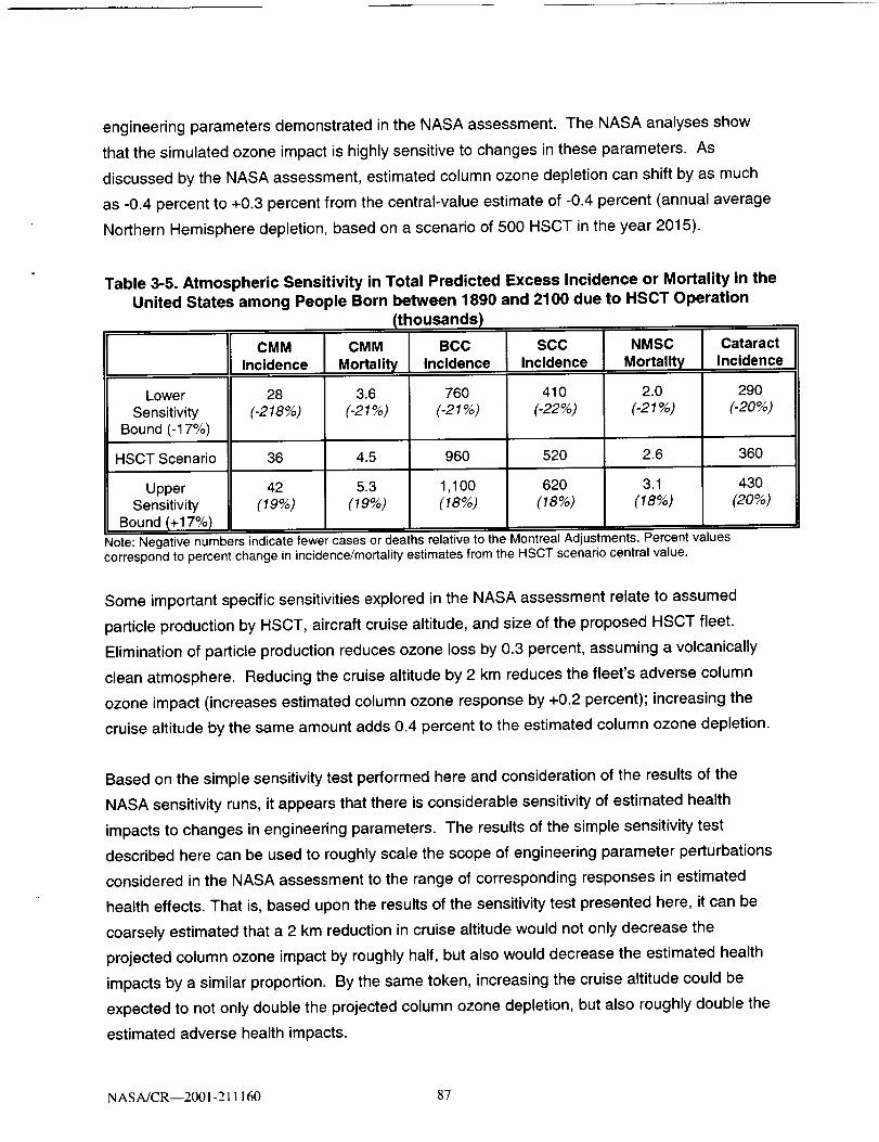
engineering parameters demonstrated in the NASA assessment. The NASA analyses show
that the simulated ozone impact is highly sensitive to changes in these parameters. As
discussed by the NASA assessment, estimated column ozone depletion can shift by as much
as -0.4 percent to +0.3 percent from the central-value estimate of -0.4 percent (annual average
Northern Hemisphere depletion, based on a scenario of 500 HSCT in the year 2015).
Table 3-5. Atmospheric Sensitivity in Total Predicted Excess Incidence or Mortality in theUnited States among People Born between 1890 and 2100 due to HSCT Operation
(thousands)
CMM CMM BCC SCC NMSC Cataract
Incidence Mortality Incidence Incidence Mortality Incidence
Lower 28 3.6 760 410 2.0 290
Sensitivity (-218%) (-21%) (-21%) (-22%) (-21%) (-20%)Bound (-17%)
HSCT Scenario 36 4.5 960 520 2.6 360
Upper 42 5.3 1,100 620 3.1 430Sensitivity (19%) (19%) (18%) (18%) (18%) (20%)
Bound (+17%)Note: Negative numbers indicate fewer cases or deaths relative to the Montreal Adjustments. Percent v Lluescorrespond to percent change in incidence/mortality estimates from the HSCT scenario central value.
Some important specific sensitivities explored in the NASA assessment relate to assumed
particle production by HSCT, aircraft cruise altitude, and size of the proposed HSCT fleet.
Elimination of particle production reduces ozone loss by 0.3 percent, assuming a volcanically
clean atmosphere. Reducing the cruise altitude by 2 km reduces the fleet's adverse column
ozone impact (increases estimated column ozone response by +0.2 percent); increasing the
cruise altitude by the same amount adds 0.4 percent to the estimated column ozone depletion.
Based on the simple sensitivity test performed here and consideration of the results of the
NASA sensitivity runs, it appears that there is considerable sensitivity of estimated health
impacts to changes in engineering parameters. The results of the simple sensitivity test
described here can be used to roughly scale the scope of engineering parameter perturbations
considered in the NASA assessment to the range of corresponding responses in estimated
health effects. That is, based upon the results of the sensitivity test presented here, it can be
coarsely estimated that a 2 km reduction in cruise altitude would not only decrease the
projected column ozone impact by roughly half, but also would decrease the estimated health
impacts by a similar proportion. By the same token, increasing the cruise altitude could be
expected to not only double the projected column ozone depletion, but also roughly double the
estimated adverse health impacts.
NAS A/CR---2001-211160 87


Chapter 4. Synthesis
Estimated human health impacts associated with predicted column ozone changes from a
hypothetical HSCT fleet have been discussed in this study. Impacts estimated were total skin
cancer incidence, skin cancer mortality, and cataract incidence expected among the U.S. light-
skinned population if an HSCT fleet were launched in 2015, grew to a fleet size of 1,000 aircraft
by the year 2050, and stayed in constant operation (i.e., at fleet size 1,000) from 2050 through
2100. This chapter provides a discussion of this study, in the context of previous international
stratospheric protection control measures for ozone-depleting substances (ODS) such as
chlorofluorocarbons (CFCs). Section 4.1 first provides background on specific features of these
previous measures. Next, the estimated health impacts from HSCT-induced ozone depletion
developed in this study are compared with health effects associated with the earlier control
measures. Section 4.1 also highlights the past stringency of stratospheric protection measures
taken by the international community and individual nations. Section 4.2 discusses the
applicability of the methods and results used in this study to scenarios other than the single
HSCT fleet scenario evaluated in this report.
4.1 Findings in context of past ODS regulatory activities
4.1.1 Description of the Montreal Protocol: Amendments and adjustments
As discussed in Chapter 1, the Montreal Protocol, signed in 1987, was designed to phase
out levels of CFCs and other ODS such as halons and methyl chloroform. The agreement
stipulated a freeze on CFC production and consumption at 1986 levels within one year
following the signing of the Protocol. The agreement targeted a 50 percent reduction on the
production of CFCs by 1998 for developed countries and by 2008 for Article 5 (developing)
countries. The agreement also established later production freezes on halons, other
halogenated compounds, carbon tetrachloride, and methyl chloroform.
As of March 2001, the Protocol has been amended or adjusted five times to increase the array
of controlled chemicals and the stringency of the control measures. Key features of the original
Protocol, and its five subsequent amendments or adjustments, are summarized in Appendix G.
NASA/CR--2001-211160 89

The Protocol still serves as the chief forum for the establishment of effective global control
measures for protecting the stratosphere (i.e., ozone layer). Several of these amendments and
adjustments are discussed in the following paragraphs.
Three years after the initial signing of the Protocol, the production and import of ODS was
further regulated. The London Amendments in 1990 stipulated the complete phase-out of
CFCs, hydrochlorofluorocarbons (HCFCs), and carbon tetrachloride by the year 2000 for
developed countries and by the year 2010 for developing nations. It also specified the
complete phase-out of methyl chloroform by 2005 for developed countries and by 2015 for
developing countries.
In 1992, the phase-out schedule was accelerated again, under the Copenhagen Amendments.
Developed countries agreed to ban the manufacture of CFCs, carbon tetrachloride, and methyl
chloroform by 1996. Similarly, a complete production ban on halons was scheduled to occur by
1994, instead of 2000. The amendments also set an accelerated timetable for the reduction of
HCFCs and hydrobromofluorocarbons (HBFCs) for developed countries.
The Montreal Adjustments were agreed to in 1997, and entered into effect in June 1998. These
adjustments brought a total phase-out of methyl bromide for developed countries by 2005 and
for developing countries by 2015. This agreement also established an HCFC phase-out
schedule for developing countries.
Today, 175 countries have ratified the Montreal Protocol, and 48 have ratified the Montreal
Adjustments. The Parties to the Protocol also meet regularly to proactively protect
stratospheric ozone through additional initiatives such as the Beijing Amendments of 1999,
which are discussed in more detail in Section 4.1.3.
NASA/CR--2001-211160 90

4.1.2 Comparison of HSCT with ODS policy scenarios
Chapters 2 and 3 of this report describe the human health impacts associated with predicted
column ozone changes from a hypothetical HSCT fleet, as estimated in this study. These
estimates were for total skin cancer incidence, skin cancer mortality, and cataract incidence
expected among the U.S. light-skinned population for the HSCT fleet scenario described
previously. Table 4-1a summarizes the central-value estimates associated with HSCT. The
results in Table 4-1a are identical to the results presented in Table 3-1 of Chapter 3. For
comparison, previous estimates of human health impacts under the ODS policy scenarios
described above in Section 4.1.1 are also presented in Table 4-1b.
Table 4-1a. Estimated Incremental U.S. Health Impacts due to HSCT Fleet
among People Born between 1890 and 2100 (thousands of cases)
Numbers in parentheses are upper and lowerbounds, based only on the uncertainty range in estimated HSCTozone impacts. All values, including those in parentheses, are subject to an additional uncertainty (approximately afactor of 2) due to uncertainties related to the estimation of biological effects of UVR. See text for additionaldiscussion of uncertainty.
HSCT
CMMIncidence
36
(-25 to 180)
CMM
Mortality
4.5
(-3 to 23)
BCCIncidence
970
(-690 to 4,900)
SCCIncidence
520
(-380 to 2,700)
NMSC
Mortality
2.6
(-2 to 13)
CMM = CutaneousMalignant Melanoma, BCC = Basal Cell Carcinoma,SCC = Squamous CellNMSC = Non-Melanoma Skin Cancer (SCC + BCC)
CataractIncidence
360
(-270 to 1,900)
._arcinoma,
As explained previously, for all (both HSCT and ODS policy) scenarios, incidence and mortality
estimates were created for model cohorts in the U.S. light-skinned population born between
1890 and 2100. The same UVR and health effects models were used for all scenarios, and
health effects estimates were based on consideration of the same baseline data and simulation
period. The methods used to estimate the ozone responses to ODS policy scenarios
(Table 4-1b) are described elsewhere (ICF 2000a). Briefly, for each ODS policy scenario, ODS
physical and chemical properties, ODS emission histories, and ODS emission projections were
used to calculate EESC loading. Previously developed empirical relationships between known
atmospheric EESC conditions and stratospheric ozone distributions (from Nimbus-7 satellite
data) by month and latitude band for the years 1978-1993 were used to project stratospheric
NASA/CR--2001-211160 91

ozone response to EESC trends for each ODS policy. The empirical relationships based on
Nimbus-7 data have been discussed elsewhere (WMO 1995, WMO 1999). Uncertainty in
estimates of future ozone depletion from ODS scenarios are discussed elsewhere
(WMO 1999).
Table 4-1b. Estimated Excess U.S. Health Impacts among People Born between 1890
and 2100 under Several Ozone-Depleting Substance (ODS)Policy Scenarios (thousands of cases)
Montreal Protocol
(row a)
London
Amendments
(row b)
Copenhagen
Amendments
(row c)
Montreal
Adjustments
CMM
Incidence
6,300
330
160
CMM
Mortality
820
41
20
BCC
Incidence
160,000
8,100
4,000
SCC
Incidence
80,000
4,100
2,000
NMSC Cataract
Mortality Incidence
380 140,000
18
8.3
130 17 3,300 1,600 6.9
3,500
1,700
1,400
(row d)'
¢MM = Cutaneous Malignant Melanoma, BCC = Basal Cell Carcinoma, SCC = Squamous Cell Carcinoma,NMSC = Non-Melanoma Skin Cancer (SCC + BCC)
"MONTREAL PROTOCOL" of 1987: Freeze of CFC production and consumption at 1986 levels; 50% reduction in
CFC production by 1998 (for developed countries) and 2008 (for Article 5 (developing) countries); later
production freezes on halons, other halogenated compounds, carbon tetrachloride (CCl4) , and methylchloroform (CH3CCl3).
"LONDON AMENDMENTS" of 1990: Complete phase-out of CFCs, hydrochlorofluorocarbons (HCFCs), and CCI 4by 2000 (developed countdes) and by 2010 (Article 5 countries); complete phase-out of CH3CCl 3 by 2005(developed countries) and by 2015 (developing countries).
"COPENHAGEN AMENDMENTS" of 1992: Accelerated phase-out of CFCs, CCl4, and CH3CCl 3 by 1996 andhalons by 1994 (developed countries); and accelerated reduction of HCFCs and hydrobromofluorocarbons(HBFCs) (Article 5 countries).
"MONTREAL ADJUSTMENTS" of 1997: Complete phase-out of methyl bromide by 2005 (developed countries)and 2015 (Article 5 countries); HCFC phase-out schedule (Article 5 countries).
SOURCE: ICF 2000a. See text for additional discussion.
] The Parties to the Protocol meet regularly to consider further measures to protect stratosphericozone. In 1999, the Parties to the Protocol agreed upon the "Beijing Amendments." As of June, 2001,this Amendment had not yet been ratified.
NASA/CR--2001-211160 92

Rows (a) through (d) of Table 4-1 b show the number of "excess" health effects cases that were
estimated to occur under each policy scenario relative to 1979-1980 levels of ozone depletion. 2
For example, row (a) shows that according to previous model studies, about 6.3 million "excess"
cases of CMM (i.e., in excess of baseline incidence of this malady) in the U.S. light-skinned
population would have occurred under an atmosphere reflecting worldwide compliance with the
controls set forth in the original 1987 Montreal Protocol. Subsequently, row (d) shows that if all
Parties (i.e., nations) to the Montreal Protocol fully implement the Protocol, including all
amendments and adjustments (through the Montreal Adjustments), approximately
130,000 cases of CMM, in excess of baseline CMM rates, would still occur in the U.S. light-
skinned population.
A key manner in which the data in Table 4-1 b can be read is to indicate the incremental health
benefits (i.e., avoided health impacts) achieved by each set of amendments and adjustments to
the Montreal Protocol. For example, data in rows (c) and (d) of the table indicate that an
increase in the stringency of the Montreal Protocol through the Montreal Adjustments was
expected to decrease CMM incidence by approximately 30,000 cases when compared to health
impacts under the Copenhagen Amendments (i.e., by subtracting row (d) from row (c)). By
comparison, data in Table 4-1a indicates that the simulated incremental increase in CMM
incidence, due to operation of an HSCT fleet is about 36,000 additional cases relative to an
atmosphere in compliance with the Montreal Adjustments but in the absence of this fleet. This
increase can be compared to the approximately 30,000 avoided cases of CMM achieved
through the Montreal Adjustments. This comparison suggests that the adverse human health
impacts associated with operation of the proposed fleet of HSCT may be of similar magnitude
to the health benefits expected from recent international stratospheric protection agreements
under the Montreal Protocol.
It should be reiterated that there is some uncertainty in the HSCT estimates presented in these
tables. The estimated HSCT health impact is uncertain to a factor of -1.7 to +4 about the
central value due to uncertainties in estimated fleet atmospheric impacts. This uncertainty
range is shown parenthetically in Table 4-1a, indicating the upper and lower uncertainty bounds
2As explained in Section 2.5 and Appendix F of this report, the "baseline" level of stratosphericozone used in this study was set equivalent to 1979-1980 ozone levels held constant through time tosimulate no further ozone depletion.
NASA/CR--2001-211160 93

around the estimated central value. The estimated health impact associated with ODS-induced
ozone depletion are also uncertain due to uncertainties in atmospheric impacts, as described
elsewhere (WMO 1999). The estimates of HSCT health impacts and estimates of health
impacts under ODS policy scenarios in both tables should all be considered uncertain to a
factor of approximately 2 due to uncertainties in the estimation of biological effects of UVR.
The development of these uncertainty factors is discussed in detail in Chapter 3.
Also, as discussed in Chapter 3, some possibility of mitigating the impacts of HSCT on column
ozone and UV-related health effects may exist. The sensitivity of estimated column ozone
response to HSCT design parameters such as cruise altitude and fuel sulfur content was
assessed in Kawa et al. (1999). This assessment indicated significant sensitivity of ozone
impact to changes in these design parameters. For example, decreasing fleet cruise altitude
reduced the average annual Northern Hemisphere column ozone impact by 50 percent.
Elimination of fuel sulfur content decreased the column ozone response by 75 percent. As
discussed in Chapter 3, reduced ozone impacts of this magnitude are projected to lead to
approximately proportional reductions in estimated health impacts.
Estimates of baseline rates of the maladies considered in this report are presented in Table 4-2.
These values are based on: (1) the assumption that 1979-1980 atmospheric conditions are
maintained throughout the period of consideration, (2) national cancer statistics (Scotto et aL
1983), and (3) Census Bureau information on population over this time period. In the absence
of any ozone depletion, these baseline rates are extremely large because UVR is a human
carcinogen (IARC 1992). Stratospheric ozone depletion is expected to lead to health impacts at
levels above these background rates.
Table 4-2. Estimated U.S. Baseline Health Impacts among People Born Between
1890 and 2100 (thousands of cases)
BCC SCCIncidence Incidence
CMM CMMIncidence Mortality
190,000
NMSCMortality
CataractIncidence
Baseline 18,000 2,200Atmosphere
55,000 1,200 250,000
CMM = Cutaneous Malignant Melanoma, BCC = Basal Cell Carcinoma, SCC = Squamous Cell Carcinoma,NMSC = Non-Melanoma Skin Cancer (SCC + BCC).
SOURCE: Estimated for this report based on ICF 2000a.
NASA/CR--2001-211160 94

Several additional issues should be highlighted, including the past stringency of stratospheric
protection measures taken by the international community and individual nations (Section 4.1.3)
and the applicability of the methods and results used in this study to scenarios other than the
single HSCT fleet scenario evaluated in this report (Section 4.2).
4.1.3 Other stratospheric protection actions within and beyond Montreal
Protocol requirements
The strong resolve of the Parties to prevent stratospheric ozone depletion is indicated by the
text of the Montreal Protocol and by implementation actions already taken around the world.
For example, the preambulatory text of the Montreal Protocol suggests a strict approach to
controlling substances that deplete the ozone layer. "The Parties are...," it states,
"...determined to protect the ozone layer by taking precautionary
measures to control equitably total global emissions of substances
that deplete it, with the ultimate objective of their elimination on the
basis of developments in scientific knowledge, taking into account
technical and economic considerations and bearing in mind the
developmental needs of developing countries..." (Source:
Preamble to the Montreal Protocol).
Despite harsh economic realities associated with initiatives to decrease ozone depletion, the
Parties are carrying out significant measures to implement the Montreal Prococol. In fact,
control measures established by the Montreal Protocol have led to pervasive transformations in
multiple industries. As an example, in the 1980s, CFCs were entrenched in the U.S. economy,
with more than $100 billion worth of equipment relying on these compounds, with no acceptable
alternatives commercially available for many applications. CFC applications included
refrigeration and air conditioning systems in automobiles, buildings, and supermarkets; cleaning
equipment for electronic components and medical instruments; and factories producing foam
cushions, insulation, and packaging. In spite of major anticipated economic impacts, the
Parties agreed to a ban on the production and consumption of CFCs throughout the
industrialized world as of January 1, 1996, except for essential uses such as for certain
NASA/CR--2001-211160 95
laboratory and analytical requirements and as propellants in metered-dose inhalers for
treatment of asthma and chronic obstructive pulmonary disease (Cook 1996).
The Parties to the Protocol have demonstrated their strong willingness to be proactive in
implementing this international agreement by collaboratively establishing control measures for
substances that have limited current applications, but the potential for substantially increased
use. For example, in the most recent amendment to the Protocol ("Beijing Amendment" of
1999), the Parties agreed to ban the production and consumption of chlorobromomethane
(CBM), an ODS with an estimated ODP of 0.12 and atmospheric lifetime of approximately
3 months.
In addition to the control measures set forth in the Montreal Protocol and its amendments and
adjustments, individual nations have instituted domestic requirements that are not otherwise
required under the Protocol. Parties to the Protocol must align their domestic regulations with
the control measures of the Protocol. Any Party, however, may adopt more stringent
governmental control measures than those specified by the Protocol (Article 2, Paragraph 11,
Montreal Protocol). Accordingly, several Parties have in fact instituted significant controls on
ODSs which exceed the measures required by the Protocol.
Parties that have instituted programs or regulations that place more stringent controls on ODS
include the United States and the nations in the European Community. Examples of such
programs or regulations include the following.
A regulation issued by the European Commission banning the sale and use of most
CFCs, halons, hydrobromofluorocarbons, and other ODS; and bans on the use of
HCFCs in certain applications, within the European Community. The regulation also
mandates the recovery and disposal of ODS in refrigeration, solvent, and fire
protection equipment.
• Refrigerant recycling rules in the United States. §§ 608 and 609 of the CAA require
EPA to develop and implement regulations to minimize ODS emissions from
NASA/CR--2001-211160 96

refrigeration and stationary and mobile air conditioning equipment during service,
maintenance, and disposal. Under the CAA §§ 608 and 609, EPA published several
regulations in the 1990s that mandate: service practices that maximize recycling of
ODS during the service, maintaining, and disposal of air conditioning and
refrigeration equipment; certification requirements for recycling and recovery
equipment, technicians, and businesses that purify reclaimed ozone-depleting
refrigerants; repair of substantial leaks in certain types of stationary air conditioning
and refrigeration equipment; and establishment of safe disposal requirements to
ensure removal of ozone-depleting refrigerants from goods that enter the waste
stream with the charge intact (e.g., cars, home refrigerators, and room air
conditioners).
The results of the HSCT health impacts analysis appear to indicate that the impacts of the
HSCT fleet scenario may be of similar magnitude to the impacts that have been avoided by
previous actions by the Parties to the Protocol. While not an indication that any action on
HSCT would be taken under the Montreal Protocol, ICAO, or domestic agencies, it is important
to consider the nature of ongoing efforts to protect stratospheric ozone in decisions on future
development of stratospheric flight.
4.2 Applicability of results to other scenarios
The present study has evaluated a single conceptual scenario for a large fleet of long-range
supersonic commercial transport aircraft. The results of this study should be considered highly
specific to the single scenario modeled in this evaluation. This is because the emissions
inventory constructed to represent the chemical inputs to the atmosphere from this fleet were
based upon specific aviation traffic and market scenario projections, narrowly defined projected
performance and emission characteristics of the NASA Technology Concept Airplane (TCA),
and other factors (Kawa et al. 1999). The emissions, cruise altitude, and flight routes of a
stratospheric fleet are sensitive to assumptions made in constructing scenarios such as those
used in the NASA assessment of atmospheric impacts of HSCT. Simulated atmospheric
impacts, in turn, are sensitive to the fleet's emissions, cruise altitude, and flight routes. Finally,
UV exposure and health response are sensitive to the atmospheric impacts arising from the
NASA/CR----2001-211160 97

fleet scenario. Thus, the results of this study, based upon many scenario-specific assumptions,
should be considered specific to the scenario considered in the study.
It may be possible to scale the results of this study to smaller HSCT fleet sizes or small HSCT
aircraft sizes, as long as flight routes, cruise altitudes, and emission characteristics are largely
similar to the fleet simulated in this study. However, results of this study should not be directly
extrapolated to estimate the health impacts from substantially different future stratospheric
aviation scenarios (e.g., a fleet of business jets that fly in the stratosphere). Some correction
for differences in flight routes or engine emission characteristics might be developed based on
sensitivity studies that already have been carried out for previous assessments (IPCC 1999,
Kawa et al. 1999). However, the scaling procedure would become more complex (Madronich
1999).
In short, the methodology or sequence of modeling tools used in the present study should be
applicable to a wide range of future stratospheric aviation scenarios. However, for substantially
different fleet scenarios (e.g., different aircraft, different routes, different altitudes, different
emissions characteristics), the atmospheric impacts would likely have to be re-assessed,
including re-evaluation of uncertainties in atmospheric impacts. In addition, as the scientific
knowledge of stratospheric chemistry and dynamics, background atmosphere, global
atmospheric change, and human health effects evolves, the models and assumptions used in
future analyses should be updated accordingly.
NASA/CR--2001-211160 98

Chapter 5. References
Andrady D.L., S.H. Hamid, X. Hu, and A. Torikai (1998), Effects of increased solar ultravioletradiation on materials, Photochemistry and Photobiology B: Biology 46:93-103.
Anonymous (2000), Darpa Eyes Supersonic Quiet Recce Aircraft. Aviation Week and Space
Technology, April 3, 2000, p. 39.
Armstrong B.K., A. Kricker and D.R. English (1997), Aetiology and pathogenesis of skin cancer,Aust J Dermato158 (Suppl): $1 -$6.
Baughcum, S.L. (1997), Requirements and evaluation criteria for supersonic cruise emissionsstandard. Working paper from ICCAIA, presented at the ICAO/CAEP/Working Group (WG) 3
meeting, January 15-16, 1997, Seville, Spain.
Caldwell M.M., L.O. Bjorn, J.F. Bornman, S.D. Flint, G. Kulandaivelu, A.H. Teramura, andM. Tevini (1998), Effects of increased solar ultraviolet radiation on terrestrial ecosystems,Photochemistry and Photobiology B: Biology 46:40-52.
Cook, E. (editor) (1996), Ozone protection in the United States: Elements of success. WorldResources Institute, Washington, DC: 120.
Cutchis, P. (1974), Stratospheric ozone depletion and solar UV radiation on Earth. Science
184(4132): 13-19.
De Fabo, E.C. and F.P. Noonan (1983), Mechanism of immune suppression by ultravioletirradiation in vivo. I. Evidence for the existence of a unique photoreceptor in skin and its role in
photoimmunology. J. Exp. Med. 158:84-98.
de Gruijl, F.R., H.J.C.M. Sterenborg, P.D. Forbes, R.E. Davies, C. Cole, G. Kelfkens,H. van Weelden, H. Slaper, and J.C. van der Leun (1993), Wavelength dependence of skincancer induction by ultraviolet irradiation of albino hairless mice, Cancer Research, 53 (1):53-60.
de Gruijl, F.R, and J.C. Van der Leun (1993), Influence of ozone depletion on the incidence ofskin cancer: quantitative prediction, in Environmental UV Photobiology, A.R. Young, L.O. Bjorn,J. Moan, and W. Nultsch (eds.), Plenum Press, New York: 1-39.
De More, W. B., S. P. Sander, D. M. Golden, R. F. Hampson, M. J. Kurylo, C. J. Howard,A. R. Ravishankara, C. E. Kolb, and M. J. Molina (1997), Chemical Kinetics and PhotochemicalData for Use in Stratospheric Modeling, JPL Publication 97-4, Jet Propulsion Laboratory,National Aeronautics and Space Administration, Pasadena.
NASA/CR--2001-211160 99
Elwood M. and J. Jopson (1997), Melanoma and sun exposure: an overview of publishedstudies, International Journal of Cancer 73:198-203.
EPA (U.S. Environmental Protection Agency) (1987), Regulatory Impact Analysis: Protection ofStratospheric Ozone, U.S. Environmental Protection Agency, Washington, DC.
EPA (U.S. Environmental Protection Agency) (1987), Assessing the Risks of Trace Gases ThatCan Modify the Stratosphere. EPA 400/1-87. Office of Air and Radiation, Washington, DC.Eight volumes.
EPA (U.S. Environmental Protection Agency) (1988), Regulatory Impact Analysis: Protectionof Stratospheric Ozone. Prepared by the U.S. Environmental Protection Agency, StratosphericProtection Program, Office of Program Development, Office of Air and Radiation.
EPA (U.S. Environmental Protection Agency) (1997), EPA Strategic Plan. EPA/190-R-97-002,September 1997. U.S. Environmental Protection Agency, Washington, DC: 108.
Epstein, J.H. (1996), Nonmelanoma skin cancer, Comprehensive Therapeutics 22:179-182.
Gerstle, J.H. (1996), Emission standards for SST. Working Paper 17, presented to theICAO/CAEP Working Group (WG) 3 meeting, May 30-31, 1996, Washington, DC.
Hader D.-P., H.D. Kumar, R.C. Smith, and R.C. Worrest (1998), Effects on aquatic ecosystems,Photochemistry and Photobiology B: Biology 46: 53-68.
IARC (International Agency for Research on Cancer) (1992), IARC Working Group on theEvaluation of Carcinogenic Risks to Humans. Monographs on Cancer Risks, Volume 55: Solarand Ultraviolet Radiation. Lyon, 11-18 February 1992. 316 pp.
ICF Consulting (1999), Summary of the Meeting on Next Generation Supersonic Civil TransportRisk Assessment Methods, Prepared for Stratospheric Protection Division, Office of Air and
Radiation, U.S. Environmental Protection Agency, by ICF Consulting, Washington, DC.November 18-19, 1999, and Addendum, February 9, 2000.
ICF Consulting (2000a), Human health benefits of stratospheric ozone protection. RevisedDraft Report Prepared by ICF Consulting for U.S. EPA, Stratospheric Protection Division. Officeof Air and Radiation, Washington DC. February 29, 2000.
ICF Consulting (2000b), Summary of the Second Meeting on Next Generation Supersonic CivilTransport Evaluation Methods, Prepared for Stratospheric Protection Division, Office of Air and
Radiation, U.S. Environmental Protection Agency, by ICF Consulting, Washington, DC. August8, 2000.
IPCC (Intergovernmental Panel on Climate Change) (1999), Aviation and the GlobalAtmosphere. J.E. Penner, D.H. Lister, D.J. Griggs, D.J. Dokken, and M. McFarland, editors.Cambridge University Press: 373.
NASA/CR--2001-211160 100

Italian American Cataract Study Group (1991), Risk Factors for age-related cortical, nuclearand posterior subcapsular cataracts, American Journal of Epidemiology 133: 542-553.
Javitt J.C., and H.R. Taylor (1995), Cataract and latitude, Documenta Ophthalmologica88:714-718.
Kawa, S.R., et al., (1999), Assessment of the Effects of High-Speed Aircraft in theStratosphere: 1998. NASA Technical Paper (TP) 1999-209237. National Aeronautics andSpace Administration (NASA), Washington, DC: 150 and appendices.
Kirk, J. T. O., B. R. Hargreaves, D. P. Morris, R. Coffin, B. David, D. Fredrickson, D. Karentz,D. Lean, M. Lesser, S. Madronich, J. H. Morrow, N. Nelson, and N. Scully (1994),Measurements of UV-B radiation in two freshwater lakes: an instrument intercomparison,
Archiv for Hydrobiologie 43:71-99.
Klein, B.E.K., J.K. Cruickshanks, and R. Klein (1995), Leisure time, sunlight exposure andcataracts, Documenta Ophthalmologica 88: 295-305.
Koepke, P., A. Bais, D. Balis, M. Buchwitz, H. De Backer, X. de Cabo, P. Eckert, P. Eriksen,D. Gillotay, A. Heikkila, T. Koskela, B. Lapeta, Z. Litynska, J. Lorente, B. Mayer, A. Renaud,A. Ruggaber, G. Schauberger, G. Seckmeyer, P. Seifert, A. Schmalwieser, H. Schwander,K. Vanicek, and M. Weber (1998), Comparison of Models Used for UV Index Calculations,Photochemistry and Photobiology (B:Photobiology) 67: (6) 657-662.
Kricker A. (1992), Sun exposure and non-melanocytic skin cancer, Dissertation, University ofWestern Australia, Perth.
Lantz, K. O., R. E. Shetter, C. A. Cantrell, S. J. Flocke, J. G. Calvert, and S. Madronich (1996),Theoretical, actinometric, and radiometric determinations of the photolysis rate coefficient of
NO2 during MLOPEX II, J. Geophysical Research 101 : 14613-14629.
Longstreth, J.D., F.R. de Gruijl, M.L. Kripke, S. Abseck, F. Arnold, H.I. Slaper, G. Velders,Y. Takizawa, and J.C. van der Leun (1998), Health risks, Photochemistry and Photobiology B:
Biology 46:20-39.
McKenzie, R. L., K. J. Paulin, and S. Madronich (1998), Effects of snow cover on UVirradiances and surface albedo: A case study, Journal of Geophysical Research 103:28785- 28792.
McKinlay, A.F. and Diffey, B.O. (1987), A reference action spectrum for ultraviolet-inducederythema in human skin, in Human Exposure to Ultraviolet Radiation: Risks and Regulations.W.R. Passchier and Bosnjakovic, B.F.M. (Eds); Elsevier, Amsterdam.
Madronich, S. (1992), Implications of recent total atmospheric ozone measurements forbiologically active ultraviolet radiation reaching the Earth's surface, Geophysical ResearchLetters 19: 37-40.
NASA/CR--2001-211160 101

Madronich, S. (1993a), The atmosphere and UV-B radiation at ground level, in EnvironmentalUVPhotobiology, A.R. Young, L.O. Bjorn, J. Moan, and W. Nultsch (eds.), Plenum Press, NewYork: 1-39.
Madronich, S. (1993b), UV radiation in the natural and perturbed atmosphere, in EnvironmentalEffects of UV (Ultraviolet) Radiation (M. Tevini, ed.), Lewis Publisher, Boca Raton: 17-69.
Madronich, S. and F. R. de Gruijl (1993), Skin cancer and UV radiation, Nature, 366: 23.
Madronich, S., E. Weatherhead, and S. Flocke (1996), Trends in UV radiation, Int. J. Environ.Sci. 51: 183-198.
Madronich, S., R. E. McKenzie, L. O BjSrn, and M. M. Caldwell (1998), Changes in biologicallyactive ultraviolet radiation reaching the Earth's surface, Journal of Photochemistry andPhotobiology B:Biology 46:5-19.
Madronich (1999), Some comments on the methods used to estimated the effects of HSCTs
on atmospheric ozone, surface UV radiation, and skin cancer incidence. Paper presented at aworkshop held by EPA, "Meeting on Next Generation Supersonic Civil Transport RiskAssessment Methods," November 18-19, 1999 at ICF Consulting, Washington, DC.
NAS (National Academy of Sciences) (1975), Environmental Impact of Stratospheric Flight.Biological and Climatic Effects of Aircraft Emissions in the Stratosphere. Climatic ImpactCommittee: 348.
NASA (National Aeronautics and Space Administration) (1999), Models and MeasurementsIntercomparison II, Langley Research Center, Hampton, VA, NASA/TM-1999-209554.
NRC (National Research Council) (1997), U.S. Supersonic Commercial Aircraft --AssessingNASA's High Speed Research Program. Report prepared by the Committee on High SpeedResearch, Aeronautics and Space Engineering Board, Commission on Engineering andTechnical Systems. National Academy Press, Washington, DC. 151 pp.
Pitts, D.G., A.P. Cullen, and P.D. Hacker (1977), Ocular effects of ultraviolet radiation from 295to 365 nm, Invest. Ophthalmol. Visual Sci. 16(10): 932-939.
Public Health Service (1996), National Skin Cancer Prevention Education Program:At-A-Glance, 1996, U.S. Department of Health and Human Services, Rockville, MD, NTISPB97-198048.
Scott, W.B. (1999), Ukraine OKs Sale of TY-160s as Space Launch Platform. Aviation Weekand Space Technology, January 11, 1999, pp. 444-445.
Scotto, J., T.R. Fears, and J.F. Fraumeni Jr. (1983), Incidence of nonmelanoma skin cancer inthe United States, U.S. Department of Health and Human Services, (NIH) 82-2433, Bethesda,MD.
NASA/CR--2001-211160 102

Setlow, R.B., E. Grist, K. Thompson, and A.D. Woodhead (1993), Wavelengths effective ininduction of malignant melanoma, Proc. Natl. Acad. Sci. USA 90: 6666-6670.
Shaw, R.J., L. Koops, and R. Hines (1997), Progress toward meeting the propulsion technologychallenges for a 21st century high-speed civil transport. NASA TM 113161, ISABE-97-7045.
Shetter, R. E., A. H. McDaniel, C. A. Cantrell, S. Madronich, and J. G. Calvert (1992),Actinometer and Eppley radiometer measurements of the NO2 photolysis rate coefficient duringMLOPEX, Journal of Geophysical Research 97:10349-10359.
Shetter, R.E., C. A. Cantrell, K. O. Lantz, S. J. Flocke, J. J. Orlando, G. S. Tyndall, T. M. Gilpin,S. Madronich, J. G. Calvert (1996), Actinometric and radiometric measurement and modeling ofthe photolysis rate coefficient of ozone to O(1D) during Mauna Loa Observatory PhotochemistryExperiment 2, Journal of Geophysical Research 101 : 14631-14641.
Sparaco, P. (1998), Dassault Explores SuperSonic Business Jet Perspectives. Aviation Weekand Space Technology, October 19, 1998. pp. 62-65.
Spencer, G. (2000), Personal communication with Greg Spencer of the US Census Bureau.
Stamnes, K., S. Tsay, W. Wiscombe, and K. Jayaweera (1988), A numerically stable algorithmfor discrete-ordinate-method radiative transfer in multiple scattering and emitting layered media,
Appl. Opt. 27: 2502-2509.
Stolarski, R.S., S.L. Baughcum, W.H. Brune, A.R. Douglass, D.W. Fahey, R.R. Friedl, S.C. Liu,R.A. Plumb, L.R. Poole, H.L Wesoky, and D.R. Worsnop. 1995 Scientific Assessment of theAtmospheric Effect of Stratospheric Aircraft. NASA Reference Publication 1381, Washington,DC, 1995.
Tafoya G.B., J.M. Gale, R.D. Ley (1997), Photorepair of ultraviolet radiation (UVR)-inducedpyrimidine dimers in lens epithelial DNA of Monodelphis domestica. Photochem Photobiol 1997Jan;65(1):125-8.
UNEP (United Nations Environment Programme) (1989, 1991, 1994, 1998), Environmentaleffects of ozQne depletion, UNEP Environmental Effects Panel Report, United NationsEnvironmental Programme, Nairobi, Kenya.
UNEP (United Nations Environment Programme) (1992), Methyl Bromide: Its AtmosphericScience, Technology, and Economics - Montreal Protocol Assessment Supplement," 1992.
UNEP (United Nations Environmental Programme) (1998), Environmental Effects of OzoneDepletion: 1998 Assessment: 193.
UNEP (United Nations Environment Programme) (2000), Handbook for the InternationalTreaties for the Protection of the Ozone Layer. Fifth Edition (2000). Ozone Secretariat, United
Nations Environment Programme. Available from UNEP, PO Box 30552, Nairobi, Kenya. Website: <http://www.unep.org/ozone>.
NASA/CR--2001-211160 103

USSA (1976), "U.S. Standard Atmosphere," National Oceanic and Atmospheric Administration(NOAA), National Aeronautics and Space Administration (NASA), United States Air Force,Washington, D.C.
Vohralik, P.F, L.K. Randeniya, I.C. Plumb, and K.R. Ryan (1998), Use of correlations betweenlong-lived atmospheric species in assessment studies, Journal of Geophysical Research 103:3611-3627.
Wall, R. (2000), Darpa Envisions New Supersonic Designs. Aviation Week and SpaceTechnology, August 28, 2000, p. 47.
Wall, R., and W.B. Scott (2000), Northrop Grumman Gets Quiet Supersonic Work. AviationWeek and Space Technology, November 13, 2000.
West S.K., B. Munoz, O.D. Schein, D.D. Duncan, G.S. Rubin (1998), "Racial differences in lensopacities - The Salisbury Eye Project," American Journal of Epidemiology, 148:1033-1039.
West, S.K. and C.T. Valmadrid (1995), "Epidemiology of risk factors for age-related cataract,"Surveys Ophthalmology, 39: 323-335.
West S.K., D.D. Duncan, B. Munoz, G.S. Rubin, L.P. Fried, K. Bandeen-Roche, O.D. Schein
(1998), "Sunlight exposure and risk of lens opacities in a population-based study," JAMA, 280:714-718.
WMO (World Meteorological Organization) (1989, 1991, 1995, 1998, 1999), Scientificassessments of ozone depletion, Global Ozone Research and Monitoring Project, WorldMeteorological Organization, Geneva, Switzerland.
NASA/CR--2001-211160 104

Appendix A - Overview of Evaluation Methodology
The schematic presented below provides a graphical summary of the methodology used in thisevaluation. Atmospheric inputs to the process are listed along the left-hand side and thevarious process stages are described along the bottom.
1
2
3
I1979--80column03, t
("nofurtherdepletion"),I• ..... • •" .... """"extendedto 2015-2100
MP-adjustedcolumnozone,
2015--2100
2050 2050atmosphere atmosphere+
HSCT
CSIRO20model
2050 2050column03 " column03 ----A(O_)HSCT
(w/HSCT)
MP-adjustedcolumn (ozone+ A(09 HSCT
2015-2100
A = changeinMP= MontrealProtocol
(i.e., the MontrealAdjustments)
AColumn
Ozone Inputs
BUV TransferCalculation
P= projected2015-2100U.S.population
E= empiricalepidemiologicaldata
"nfd"= nofurtherdepletion
i = eachhealtheffectendpoint(NMSC,BCC,cataracts)
AS= actionspectru¢
BAF= biologicalamplificationfactor
C OHearth Effect EstimatedComputation Health Effects
NASA/CR--2001-2I 1160 105


Appendix B - Description of the CSIRO Model
The CSIRO model is a two-dimensional (2-D) numerical chemical-transport model of theatmosphere. Like other numerical models of the atmosphere, the CSIRO model simulatestransport and chemical interactions of trace gases (such as ozone) to obtain their spatial andseasonal distributions.
The CSIRO model analyzes ozone changes from 90°S to 90°N in 5-degree intervals and from
ground level to 80 km with a vertical resolution of approximately 2 km. To generate ozoneestimates, the model combines information on atmospheric chemistry (e.g., diffusion, mixing,production, and loss patterns) for various chemical species (NASA 1999).
Model transport is provided by a combination of zonal mean diabatic 1circulation andappropriate diffusion terms. These terms are based on observed temperatures and ozonemixing ratio profiles. Zonal and monthly mean temperatures were calculated on an 8-yearaverage using National Meteorological Center values obtained from the 1992 Models andMeasurements database (Prather and Remsberg 1993 as cited in NASA 1999) and were notadjusted for zonal asymmetry (Kawa et al. 1999, NASA 1999).
Improvements in eddy diffusion terms have allowed for enhanced representation of tropical andmid-latitude mixing. Mixing ratios of N2, 02, and CO2 are held constant throughout the modelatmosphere. Tropospheric water concentrations are determined according to either Oort(1983 as cited in Kawa et al. 1999) climatology or SAGE-II model results from Prather andRemsberg (1992 as cited in NASA 1999). Stratospheric water concentrations are allowed tovary from a volume mixing ratio of 3 x 10 .6 established at the tropopause. Rainout and surfacedeposition rates for certain transported chemical families also are included in the model(NASA 1999). No rainout is assumed within 3 km of the tropopause (Kawa et al. 1999), and an
upper tropospheric source of NOy also is provided (NASA 1999).
The model includes a solar radiation module that uses ray-tracing techniques to allow for thecurvature of the Earth and includes the method of Meier et al. (1982 as cited in NASA 1999) to
provide fully interactive multiple scattering calculations. The solar radiation module examines158 wavelengths from 175 to 180 nm, as defined by the World Meteorological Organization
(1986 as cited in NASA 1999).
The family-based chemical module examines 67 different species and 213 reactions. Themodel also considers hydrolysis processes occurring with sulphuric acid aerosols but does notconsider heterogeneous reactions such as those occurring in polar stratospheric clouds(NASA 1999). Production and loss terms for long-lived species are updated every 10 days viaa diurnal calculation that establishes the 24-hour behavior of all examined species
(Vohralik et aL 1998).
l This term refers to solar-driven heating or cooling of an air parcel due to physical processessuch as latent heat release and radiative effects.
NASA/CR---2001-211160 107

References
Kawa, S.R., et al., (1999). Assessment of the Effects of High-Speed Aircraft in theStratosphere: 1998. NASA Technical Paper (TP) 1999-209237. National Aeronautics andSpace Administration (NASA), Washington, DC. 150 pp. plus appendices.
NASA (1999), Models and Measurements Intercomparison II, National Aeronautics and SpaceAdministration, Langley Research Center, Hampton, VA, NASA/TM-1999-209554.
Vohralik, P.F, L.K. Randeniya, I.C. Plumb, and K.R. Ryan (1998), Use of correlations betweenlong-lived atmospheric species in assessment studies, Journal of Geophysical Research, 103,3611-3627.
NASA/CR--2001-211160 108

Appendix C - Methodological Sensitivity:Use of Relative Versus Absolute Ozone Change
In this evaluation, ozone concentration estimates were obtained from the CSIRO model inDobson units for a fleet of 1,000 HSCT in 2050 and for zero HSCT in the year 2050. The
analysis presented in this evaluation used both of these CSIRO runs to calculate a fixedpercentage change in ozone for the year 2050. This percent change then was scaledaccording to the HSCT "in-service" fleet production schedule for the years 2015 to 2100 andapplied to a Montreal Adjustments ozone scenario that assumes zero HSCT. Section 2.2.2provides additional detail on this methodology.
Meeting participants at a workshop held to discuss preliminary results of this effort inquiredwhether performing this scaling operation using absolute Dobson units rather than the percentchange in ozone would have a material effect on the predicted health effects (ICF 2000b). Toanswer this question, the absolute difference between the two sets of CSIRO ozone estimatesfor 2050 was obtained by subtracting the monthly ozone estimates. This absolute number thenwas scaled from 2015 to 2100 according to the HSCT in-service fleet production schedule. Theadjusted incremental ozone estimates then were applied to the Montreal Adjustments ozonescenario described above and input to the AHEF to determine the effect of the methodology on
the human health impact estimates.
The sensitivity of the health effect results to these two methods of estimation is presented inTable C-1 as the central value incidence and mortality estimates for the HSCT scenario usingboth relative and absolute changes in ozone.
Table C-1. Relative vs. Absolute Results for Total Predicted Excess Incidence or
Mortality in the United States among People Born between 1890 and 2100
due to HSCT Operation (thousands)
Scenario CMM Cases CMM BCC Cases SCC Cases NMSC CataractDeaths Deaths Cases
Relative 36 4.5 970 520 2.6 360
Scaling*
Absolute 35 4.4 960 520 2.5 360
Scaling (1.3%) (1.5%) (0.9%,) (0. 7%) (1.4%) (1.3%,)
* This is the method currently used in the HSCT evaluation.Note: Percent values correspond to percent change in incidence/mortality estimates from the HSCT scenario centralvalue.
Only small differences (less than 1.5 percent) are observed between the incidence andmortality rates predicted as a result of the percent scaling technique versus the Dobson unitscaling technique. Thus, the results of the HSCT evaluation are judged to be relativelyinsensitive to the method used to scale ozone estimates, and the percent technique currently in
place will continue to be used.
NASA/CR--2001-211160 109

Reference
ICF Consulting (2000b), Summary of the Second Meeting on Next Generation Supersonic CivilTransport Evaluation Methods, Prepared for Stratospheric Protection Division, Office of Air andRadiation, U.S. Environmental Protection Agency, by ICF Consulting, Washington, DC.August 8.
NASA/CR--2001-211160 110

Appendix D - Background Information on RAFs
The RAF is a sensitivity coefficient indicating how surface UVR, weighted by the appropriateaction spectrum, responds to changes in the total ozone column. Because of the weighting byaction spectra, different biological action spectra have different RAF values. The RAF is acritically important number because it relates changes in ozone directly to changes in surfaceUVR.
The RAF is a simple and convenient number allowing a quick estimation of the sensitivity toozone changes. However, the RAF is not a true constant, even for a single action spectrum,and it can depend on various atmospheric conditions such as total ozone column amount,amount of ozone change, solar zenith angle, and possibly other factors (see below). Although
representative RAF values are useful for quick discussion purposes, a more accuratecalculation must use RAFs that are re-calculated for the specific conditions. Or equivalently
(as done in this work), the irradiance changes can be computed directly from pre-calculatedtables of UVR as a function of the ozone column and solar zenith angle.
The RAF is obtained by computing the UV irradiance for a given ozone column amount, _,
e.g., using the erythemal action spectrum Be_y(,k),
UV(erythemal) = f F(,K, Q) Be,y(_.)d )_
where F(,k, £2) is the spectral irradiance at the surface. Now suppose this calculation isrepeated for two different ozone column values, say £3land £_2, yielding the weightedirradiances UV1 and UV2, respectively. If the ozone changes are very small, say on the order of
1 percent or so, the RAF is simply the (percent) increase in UVR for a 1 percent decrease in theozone column:
RAF ~- [(UV 2- UV1)/UV1] / [(Q 2- Q 1)/ _ 1].
For larger changes, it has been shown (Madronich 1993) that weighted irradiances scale withozone column following a power equation, with the power being the RAF:
UVJUVl - (_ 21 Q i)-RAF
In this case, the RAF is computed from:
RAF ~- log (UVJUV1) /log (_ 2/ Q 1)
which for small changes is identical to the previous (percent) definition.
Unpublished calculations by S. Madronich have shown that the power rule arises naturally foraction spectra that decay exponentially in the ozone-sensitive 300-330 nm spectrum. Indeed, ifthe action spectrum decays exponentially in this band, e.g.,
B(A) _ exp[-13 _k]
and given that the ozone absorption cross section 0o3(A) also is approximated by anexponential decay in this band,
NASA/CR--2001-211160 111

ao_(h) _ exp[-a A]
then the RAF is given, to reasonable approximation, simply by the ratio of the two decay slopes:
RAF _- f3/a
In other words, the sensitivity of UVR to ozone changes is directly proportional to the steepnessof the action spectrum decay.
Effect of clouds on RAF values
Clouds can reduce surface UVR significantly. However, clouds have only a small effect on thespectral distribution of surface UVR; i.e., clouds are essentially white at these wavelengths.Thus, as long as cloud cover remains constant, the percent changes in surface UVR calculatedfor a given ozone depletion should be nearly the same for cloudy and cloud-free skies. Thisexpectation was confirmed by detailed calculations of the RAF for cloudy and clear conditions,reported in Table 3.2-10 of one of the earlier ozone assessments (WMO 1989). This tableshows that the RAF (for DNA damage, but entirely analogous for erythema) is essentiallyunchanged by the presence of clouds.
Altitude of ozone perturbation
In the present calculations, the change in ozone column is applied as a constant scaling factorat all altitudes (shape preserving), and the resulting UVR changes are interpolated from look-uptables of UV irradiances as functions of solar zenith angle and total ozone column. In principle,not only the total ozone column change, but also the altitude at which ozone perturbationsoccur, can have some effect because of the coupling between ozone absorption and scatteringby air molecules. For high sun, tropospheric scattering increases photon path lengthsubstantially, so that tropospheric ozone is, on a molecule-by-molecule basis, more effective inabsorbing UVR than is stratospheric ozone (e.g., BrC_hl and Crutzen 1989). For low sun, thereverse is known to occur (e.g., see Figures 12 and 13 in Madronich 1993), so thatstratospheric ozone molecules are more effective. In practice, these considerations areimportant only when the ozone perturbations occur in the lower to middle troposphere and arerelatively insensitive to the exact height of perturbations that occur the stratosphere, i.e., wellabove the region where scattering occurs.
The following figure shows the magnitude of'this effect. The thick curves (solid for overheadsun, dashed for solar zenith angle = 60 degrees) show the RAF for erythemal radiation, whenozone perturbations are applied at different altitudes. The enhanced absorption by troposphericozone is obvious below approximately 10 km. Changes occurring near 20 km (i.e., near theHSCT flight corridors) have an RAF near 1.12, while uniform column changes (thin verticallines) result in a slightly larger RAF, approximately 1.17. For 60 degrees solar zenith angle, theuniform column change yields RAF ~ 1.12, while perturbations at 20 km yield RAF ~ 1.09, againin fairly good agreement.
NASA/CR--2001-211160 112

ERYTHEMAL RAF
3O
25
-_ 20
(_ 15"5
5
0
1 1.2 1.4 1.6 1.8 2
RAF
_" Overhead Sun
- - • 60 Degree Solar ZenithAngle
Uniform Column Change forOverhead Sun
....... Uniform Co4umnChange for 60Degree Solar Zenith Angle
References
BrLihl, C. and P. J. Crutzen (1989). On the disproportionate role of tropospheric ozone as afilter against solar UV-B radiation, Geophys. Res. Lett., vol. 16, pp. 703-706.
Madronich, S. (1993). UV radiation in the natural and perturbed atmosphere, in EnvironmentalEffects of UV (Ultraviolet) Radiation (M. Tevini, ed.), Lewis Publisher, Boca Raton, pp. 17-69.
WMO (1989). Scientific Assessment of Stratospheric Ozone: 1989, (D. Albritton and R.Watson, eds.) World Meteorological Organization Report No. 20.
NASA/CR--2001-211160 113


Appendix E - Information and Future Directionsfor Cataract Methodology
Origin of current BAFs for cataract incidence
The current BAFs for cataract are based on the work of Hiller et aL (1983), in which a
multivariate logistic risk function was used to describe the correlation between the prevalence ofsenile cataract, the flux of UV-B, and a variety of other risk factors. Hiller and her colleagues
used data on 2,225 people aged 45-74 from the ophthalmological subsection of the 1971-1972National Health and Nutrition Examination Survey (NHANES). This population was divided into
two groups: those who either had cataract or were aphakic (i.e., had a lens removed) and thosewith neither cataract or aphakia. Of the 2,225 people in the selected population, 413(18.6 percent) were placed in the cataract/aphakia group. UV data were developed by theNational Oceanic and Atmospheric Administration (NOAA) for the 35 NHANES locations basedon a statistical analysis of data from Robertson-Berger meters located at 10 of the NHANESsites. Subsequent validation of the estimates at 6 locations indicated differences of about7 percent between the observed and estimated mean daily flux values. Hiller et al. (1983)modeled their data using the following logistic risk function:
P= 11 + e -(a.blXl+ .... bkX/_
where P is the probability of having a cataract and X,., are the risk factors examined. In additionto UV, the risk factors examined were age, race, sex, education, diabetes, systolic blood
pressure, and residence (urban versus rural). Hiller and her colleagues developedstandardized regression coefficients under three conditions: as a function of each factorindividually (univariate), as a function of each factor plus age (bivariate), and as a function of allrisk factors simultaneously (multivariate).
The logistic function is commonly used in epidemiology when it is clear that age has asignificant (and presumably independent) influence on risk (i.e., risk changes with ageirrespective of exposure). However, such a specification also has drawbacks in that the dose-response curve created from the Hiller et al. (1983) data is non-linear. Thus, different BAFsmust be used for each age cohort because of the changing slope of the curve. The followingfigure shows the dose-response relationships between UVR exposure and risk (prevalence) forthe three age cohorts examined in the NHANES study: 42-54, 55-65, and 65+. The BAFs forthese cohorts are 0.3, 1.3, and 4.3, respectively. Using this data, an age-weighted mean BAFthat can be applied to an entire population is about 1.5.
Selection of the current action spectrum for cataract incidence
In order to derive a BAF, a weighting scheme must first be selected that assigns varyingimportance to different wavelengths of UV light according to their effectiveness in inducing acertain response. Often, this scheme takes the form of an action spectrum, in whichmonochromatic light at different wavelengths is administered to a test organism and eachwavelength's effectiveness at inducing a specific health effect (e.g., tumors) is recorded.
NASA/CR--2001-211160 115
By contrast, in the Hiller et aL (1983) cataract study, Robertson-Berger (R-B) meters at variousNHANES sites measured light directly from the sun, weighting it as it was received from thenatural source. This weighting scheme was discovered to be very similar to that derived for theerythema action spectrum. However, no biological connection is felt to exist between cataractformation and the incidence of erythema (sunburn), and it was believed that insufficient
evidence existed at that time (i.e., 1983) to create an action spectrum based exclusively oncataract induction in laboratory animals. Thus, the Setlow DNA damage action spectrum,modified for human skin and renamed DNA-h, was suggested as a possible action spectrum toweight the wavelengths of solar radiation thought to be most effective in inducing cataract(Setlow et al. 1993). 2 Once an action spectrum is selected, it is integrated over the spectrum inquestion to generate one number, called the RAF. The RAF is used to weight the actual UVdoses administered, which then are plotted against the response observed at each effectivedose on a logarithmic scale. The slope of this curve is the BAF.
Use of the current RAF, obtained from the DNA-h action spectrum, to predict cataract incidencewas questioned by participants at the August HSCT meeting (ICF 2000b). In response to thesequestions, the following changes are proposed with respect to the selection of the actionspectrum, RAF, and dose-response curve used to derive the BAF for cataract incidence.
Interim solution
Pitts et al. (1977) have generated an action spectrum in rats for cataract incidence. A recentreview of the original document discussing this derivation process reveals that this actionspectrum is suited for use in the current application because it does in fact extend into the UVAwavelength range. Thus, the RAF from the Pitts et al. (1977) action spectrum will be used inthe AHEF to weight future UV doses and thus estimate BAFs for future cataract incidence. The
Robertson-Berger meter RAF and the BAFs obtained from the Hiller et al. (1983) study willcontinue to be used to estimate past cataract incidence. Using the updated BAF for cataractincidence will improve the predictions as compared with the prior methodology.
Future solution
The Salisbury Eye Project (West et aL 1998) measures cataract incidence (all major types)from a subset of the U.S. population. Once this project has concluded, its data will be used togenerate a linear dose-response curve. UV doses for this curve will be weighted using the RAFfrom the Pitts et al. (1977) action spectrum. Because the curve will be generated using a linearfunction, only one BAF will be applied to all age cohorts.
2The AHEF uses the DNA-h spectrum to derive the BAF for cataract incidence.
NASA/CR--2001-211160 116

References
Hiller, R., R. Sperduto, and F. Ederer (1983), "Epidemologic associations with cataracts in the1971-1972 National Health and Nutrition Examination Survey," American Journal ofEpidemiology, vol. 118, no. 2, pp. 239-249.
ICF Consulting (2000b), Summary of the Second Meeting on Next Generation Supersonic CivilTransport Evaluation Methods, Prepared for Stratospheric Protection Division, Office of Air andRadiation, U.S. Environmental Protection Agency, by ICF Consulting, Washington, DC.August 8.
Pitts, D.G., A.P. Cullen, and P.D. Hacker (1977), "Ocular effects of ultraviolet radiation from295 to 365 nm," Invest. Ophthalmol. Visual Sci., vol. 16, no. 10, pp. 932-939.
Setlow, R.B., E. Grist, K. Thompson, and A.D. Woodhead (1993), "Wavelengths effective ininduction of malignant melanoma," Proc. Natl. Acad. Sci. USA, vol. 90, pp. 6666-6670.
West S.K., B. Munoz, O.D. Schein, D.D. Duncan, G.S. Rubin (1998), "Racial differences in lensopacities - The Salisbury Eye Project," American Journal of Epidemiology, vol. 148,pp. 1033-1039.
West S.K., D.D. Duncan, B. Munoz, G.S. Rubin, L.P. Fried, K. Bandeen-Roche, O.D. Schein(1998), "Sunlight exposure and risk of lens opacities in a population-based study," JAMA,vol. 280, pp. 714-718.
NASA/CR---2001-211160 117


Appendix F - Sensitivity to Choice of Reference Scenario
In this study, it has been assumed that the appropriate "reference" atmospheric scenario forexpressing the health impacts of HSCT-induced stratospheric ozone depletion is one thatreflects worldwide compliance with the stratospheric ozone control provisions of the MontrealProtocol, as amended through the "Montreal Adjustments" of that Protocol (i.e., the "MontrealAdjustments" reference scenario). A description of the Montreal Protocol and its amendmentsand adjustments is provided in Appendix G. The use of the reference atmospheric scenario isdescribed in Section 2.5 and illustrated schematically in Figure 2-4.
Sensitivity tests indicate that modeled HSCT health impacts exhibit limited sensitivity to thespecification of the reference scenario. Two sensitivity tests were performed that illustrate thissensitivity. First, the atmospheric ozone values of the Montreal Adjustments reference scenariowere perturbed by ± 20 percent of the monthly differences between the Montreal Adjustmentsscenario and the 1979-1980 reference scenario ozone levels in 2015. This difference
represents the greatest possible error that could be associated with the Montreal Adjustmentsbaseline. The values for 2015 were selected because in later years the differences betweenthe scenarios decrease as ozone levels are expected to recover. The ± 20 percent monthly
differences for 2015 were then applied through 2050. Then, the ozone impacts resulting from afleet of HSCT (developed as described in Section 2.2.2.a and 2.2.2.b) were applied to theperturbed reference scenario, and incremental health effects of HSCT relative to the perturbedreference scenarios were calculated as described in Section 2.5. The results of these
simulations were then compared with the health impacts estimated relative to the "unperturbed"Montreal Adjustments reference scenario.
When the atmospheric ozone of the reference scenario was increased by 20 percent of thedifference between the two baseline scenarios, estimated health impacts decreased by
approximately 1.5 percent. Similarly, when reference scenario ozone was decreased by20 percent of the difference, estimated health impacts increased by approximately 1 percent(except for cataract incidence, which increased by 2 percent). Table F-1 summarizes theresults of these sensitivity tests.
Table F-1. Sensitivity of Reference Scenario Selection in Determining Total PredictedExcess Incidence or Mortality in the United States among People Born between
1890 and 2100 due to HSCT Operation (thousands)
Scenario CMM
Cases
CMMDeaths
BCC Cases SCC Cases NMSCDeaths
2.6
CataractCases
36OHSCT Scenario (Relative to 36 4.5 970 520
the Montreal Adjustments)
HSCT (2015 Baseline 35 4.4 950 520 2.5 360Difference + 20%) (ol.6%) (-1.6%) (-1.5%) (-1.4%) (-1.5%) (-1.3%)
HSCT (2015 Baseline 36 4.5 970 530 2.6 370
Difference- 20%) (1.0%) (1.0%) (0.8%) (0. 7%) (1.0%) (2.0%)
Note: Negative numbers indicate fewer cases or deaths relative to the Montreal Adjustments. Percent valuescorrespond to percent change in incidence/mortality estimates from the HSCT scenario central value. Negativepercentages reflect lives saved as a result of increased ozone concentrations.
NASA/CR--2001-211160 119

Second, an AHEF model simulation was performed in which atmospheric ozone amounts
representative of 1979-1980 conditions were used as the reference scenario. The incremental
health effects from HSCT relative to this reference scenario were estimated, and again
compared with the health impacts estimated relative to the "unperturbed" Montreal Adjustments
reference scenario. Incremental HSCT health impacts produced by the AHEF model using the
1979-1980 reference scenario were approximately 5 percent greater than those produced using
the Montreal Adjustments reference scenario. This sensitivity analysis represents the greatest
possible change in health effects that could be attributed to miscalculation in the baseline.
Table F-2 summarizes the results of this sensitivity test.
Table F-2.
Excess Incidence or Mortality in the United States among People Born between
Sensitivity of Reference Scenario Selection in Determining Total Predicted
1890 and 2100 due to HSCT O
I Scenario
HSCT Scenario (Relative tothe Montreal Adjustments)
CMMCases
36
CMMDeaths
4.5
4.7
(5.0%)
)eration (thousands)
BCC Cases
970
1,000(4.8%)
SCC Cases
52O
550
(4.6%)
NMSC I CataractDeaths Cases
2.6
HSCT (Relative to 1979-80Baseline)
360
390
(7.6%)Note: Percent values correspond to percent change in incidence/mortality estimates from the HSCT scenario centralvalue.
'3NASA/CR--,.001-211160 120

Appendix G - Summary of ODS Policy Controls
In Tables G-1 through G-4, this appendix presents the ODS phaseout schedules for both non-Article 5 (developed) and Article 5 (developing) countries under each of the policy scenariosdiscussed in Table 4-1 (i.e., the original Montreal Protocol, the London Amendments of 1990,the Copenhagen Amendments of 1992, and the Montreal Adjustments of 1997). In each table,
phaseouts are presented as percentages of a given base year.
Table G-1. Original Montreal Protocol
(1987)
Controls for Non-Article 5 Nations
CFCs Halons
Base Year 1986 1986
Controls
Year Percent of Percent ofBase Year Base Year
July 1, 1989 100% ---
1990 100% ---
1991 100% ---
1992 100% 100%
1993 80% 100%
1994 80% 100%
1995 80% 100%
1996 80% 100%
1997 80% 100%
1998 50% 100%
Controls for Article 5 Nations
CFCs Halons
Base Year 1996 1996
Controls
Year Percent of Percent ofBase Year Base Year
July 1, 1999 100% ---
2000 100% ---
2001 100%
2002 100%
2003 80%
8O%
100%
100%
2OO4 100%
2005 80% 100%
2006 80% 100%
2OO7 80% 100%
2008 50% 100%
NASA/CR--2001-211160 121

Table G-2. London Amendments (1990)
Controls for Non-Article 5 Nations
CFCs
Base Year 1986
Halons Carbon
Tetrachloride
(CC[4)
MethylChloroform
(CHsCCI3)
1986 1989 1989
Controls
Percent of Base Percent of Base Percent of Base Percent of Base
Year Year Year Year Year
July 1, 1989 100% .........
1990 100% .........
1991 100% .........
1992 100% 100% ......
1993 100% 100% --- 100%
1994 100% 100% --- 100%
1995 50% 50% 15% 70%
1996 50% 50% 15% 70%
1997 15% 50% 15% 70%
1998 15% 50% 15% 70%
1999 15% 50% 15% 70%
2000 0% 0% 0% 30%
2001 0% 0% 0% 30%
2002 0% 0% 0% 30%
2003 0% 0% 0% 30%
2004 0% 0% 0% 30%
2005 0% 0% 0% 0%
NASA/CR--2001-211160 122

Table G-2, continued
Controls for Article 5 Nations
CFCs Halons Carbon MethylTetrachloride Chloroform
(CCI4) (CH3CCI3)
Base Year 1996 1996 1999 1999
Controls
Percent of Base Percent of Base Percent of Base Percent of Base
Year Year Year Year Year
July 1, 1999 100% .........
2000 100% .........
2001 100% .........
2002 100% 100% ......
2003 100% 100% --- 100%
2004 100% 100% --- 100%
2005 50% 50% 15% 70%
2006 50% 50% 15% 70%
2007 15% 50% 15% 70%
2008 15% 50% 15% 70%
2009 15% 50% 15% 70%
2010 0%
2011 0%
0% 0% 30%
0% 0% 30%
2012 0% 0% 0% 30%
2013 0% 0% 0% 30%
2014 0% 0% 0% 30%
2015 0% 0% 0% 0%
NASA/CR---2001-211160 123

Table G-3. Copenhagen Amendments (1992)
Controls for Non-Article 5 Nations
CFCs Halons Carbon Methyl HCFCs* MethylTetrachloride Chloroform Bromide
(CCl,) (CH3CCl3) (CH3Br)**
Base Year 1986 1986 1989 1989 1989 (3.1%) 1991
Controls
Year
July 1, 1989
Percent of
Base Year
Percent
of Base
100%
Percent of
Base Year
Year
Percent of
Base Year
1990 100% ......
1991 100% ......
1992 100% 100% ---
1993 80% 100% ---
1994 25% 0% ---
1995 25% 0% 15%
1996 0% 0% 0%
1997 0% 0%
Percent of
Base Year
Percent of
Base Year
100% ......
50% ......
50% --- 100%
0% 100% 100%
0% 100%0% 100%
1998 0% 0% 0% 0% 100% 100%
1999 0% 0% 0% 0% 100% 100%
2000 0% 0% 0% 0% 100% 100%
2001 0% 0% 0% 0% 100% 100%
2002 0% 0% 0% 0% 100% 100%
2003 0% 0% 0% 0% 100% 100%
2004 0% 0% 0% 0% 65% 100%
2005 0% 0% 0% 0% 65% 100%
2010 0% 0% 0% 0% 35% 100%
2015 0% 0% 0% 0% 10% 100%
2020 0% 0% 0% 0% 0.5%
0%
100%
100%0%0%2030 0% 0%
* The baseline HCFC consum
consumption in 1989 plus 3.1:)tion, or HCFC cap, was calculated as the total ODP-weighted HCFC)ercent of the ODP-weighted CFC consumption in 1989.
** The methyl bromide freeze did not apply to post-harvesting uses (i.e. quarantine and pre-shipment).
NASA/CR--2001-211160 124

Table G-3, continued
Controls for Article 5 Nations
CFCs Halons Carbon MethylTetrachloride Chloroform
(CCl4) (CH3CCl3)
Base Year 1996 1996 1999 1999
Controls
Percent of Base Percent of Base Percent of Base Percent of Base
Year Year Year Year Year
July 1, 1999 100% .........
2000
2001
2002
2003
2004
2005
2006
2007
2008
2009
2010
2011
2012
2013
2014
2015
100%
100%
100%
80%
80%
5O%
5O%
15%
15%
100%
100%
100%
5O%
5O%
5O%
5O%
15%
15%
15%
15%
100%
100%
70%
7O%
7O%
7O%
15% 50% 15% 70%
0% 0% 0% 30%
0% 0% 0% 30%
0%0% O%
0% 0% 0%
0% 0% 0%
0% 0% 0%
30%
30%
30%
O%
Note: The Copenhagen Amendments did not change the Article 5 control schedule.
NASA/CR--2001-211160 125

Table G-4. Montreal Adjustment (1997)
Controls for Non-ArUcle 5 Nations
Base Year
CFCs
1986
Halons
1986
Carbon
Tetrachlorid
e (CCl4)
1989
Controls
Year Percent of Percent of Percent of
Base Year Base Year Base Year
July 1, 1989 100% ......
1990 100% ......
100%
100% ---
1991
0%
1992 100%
1993 80% 100% ---
1994 25% 0% ---
1995 25% 0% 15%
1996 0% 0% 0%
1997 0% 0% 0%
1998 0% 0%
0%1999 0% O%
2000 0% 0% 0%
2001 0% 0% 0%
2002 0% 0% 0%
2003 0% 0% 0%
2004 0% 0%
2005 0% 0%
0%
0%
0%
0%
2010 0%
2015 0%
2020
0%
0%
0%
0%
0%
O%
MethylChloroform
(CH3CCI3)
HCFCs*
1989
Percent of
Base Year
°..
100%
5O%
50%
0%
MethylBromide
(CH3Br)**
1989 (2.8%) 1991
Percent of Percent of
Base Year Base Year
---. ---
--- 100%
100% 100%
0% 100% 100%
0% 100% 100%
O% 100% 75%
100% 75%
100% 50%
100% 50%
100% 30%
65% 30%
0%
0%
0%
0%
0%
0% 65% 0%
0% 35% 0%
0% 10% 0%
0% 0.5% 0%
2030
0%
0%
* The baseline HCFC consum
consumption in 1989 plus 2.8
0%0%
3tion, or HCFC cap, is calculated as the total ODP-weighted HCFC
)ercent of the ODP-weighted CFC consumption in 1989.
O%
** The methyl bromide freeze does not apply to post-harvesting uses (i.e., quarantine and pre-shipment).
NASA/CR--2001-211160 126

Table G-4, continued
Controls for Article 5 Nations
Base Year
CFCs
1996 1996
Controls
Year
Halons CarbonTetrachlorid
e (CCI4)
1999
MethylChloroform(CH3CCI3)
1999
HCFCs
2015
Percent ofBase Year
Percent ofBase Year
MethylBromide
(CH3Br)*
Average of1995-1998
Percent ofBase Year
Percent ofBase Year
Percent ofBase Year
Percent ofBase Year
July 1, 1999 100% ...............
2000 100% ...............
2001 100% ...............
100%
100%100%
2OO2 100%
2003 80%
100%
100%
2004 80% 100% --- 100% --- 100%
2005 50% 50% 15% 70% --- 80%
2006 50% 50% 15% 70% --- 80%
2007 15%
2008 15%
2009 15%
O%2010
15%
15%
15%
O%
O%
7O%
O%
2011 0%
2012 0%
2013 0%
5O%
7O%
8O%
8O%5O%
5O%
O%
O%
0%
0%
2014 0% 0%
2015 0% 0%
2016 0% 0%
2O4O 0% O%
70% --- 80%
30% --- 80%
30% --- 80%
0% 30% --- 80%
0% 30% --- 80%
0% 30% --- 80%
0% 0% --- 0%
0% 0% 100% 0%
0% 0% 0%
The methyl bromide freeze does not apply to post harvesting uses (i.e., quarantine and pre-shipment).
NASA/CR--2001-211160 127

REPORT DOCUMENTATION PAGE FormApprovedOMB No. 0704-0188
Public reporting burden for this collection of information is estimated to average 1 hour per response, including the time for reviewing instructions, searching existing data sources,
gathering and maintaining the data needed, and completing and reviewing the collection of information. Send comments regarding this burden estimate or any other aspect of this
collection of information, including suggestions for reducing this burden, to Washington Headquarters Services, Directorate for information Operations and Reports, 1215 Jefferson
Davis Highway, Suite 1204, Arlington, VA 22202-4302, and to the Office of Management and Budget, Paperwork Reduction Project (0704-0188), Washington, DC 20503.
1. AGENCY USE ONLY (Leave b/ank) 2. REPORT DATE 3. REPORT TYPE AND DATES COVERED
4. TITLE AND SUBTITLE
September 2001 Final Contractor Report
5. FUNDING NUMBERS
Human Health Effects of Ozone Depletion From Stratospheric Aircraft
6. AUTHOR(S)
U.S. Environmental Protection Agency
7. PERFORMING ORGANIZATION NAME(S) AND ADDRESS(ES)
U.S. Environmental Protection Agency
Global Programs Division
1200 Pennsylvania Avenue, NW (6205J)
Washington, DC 20460
9. SPONSORING/MONITORING AGENCY NAME(S) AND ADDRESS(ES)
National Aeronautics and Space Administration
Washington, DC 20546-0001
;11. SUPPLEMENTARY NOTES
WU-714-01-20-00
Interagency Agreement
Reference #80938647,
NASA Reference #C-30039-J
8. PERFORMING ORGANIZATION
REPORT NUMBER
E-13018
10. SPONSORING/MONITORING
AGENCY REPORT NUMBER
NASA CR--2001-211160
This work was supported by NASA under RTOP 714-01-20--00 and by other contributions from the EPA.
Project Manager, Chowen Wey, Vehicle Technology Center, NASA Glenn Research Center, organization code 0300,216--433-8357.
12a. DISTRIBUTION/AVAILABILITY STATEMENT
Unclassified - Unlimited
Subject Category: 51 Distribution: Nonstandard
Available electronically at hltl_://_ltrs._c.nasa.gov/GL'l'RS
This publication is available from the NASA Center for AeroSpace Information, 301-621--0390.
12b. DISTRIBUTION CODE
13. ABSTRACT (Maximum 200 words)
This report presents EPA's initial response to NASA's request to advise on potential environmental policy issues associated
with the future development of supersonic flight technologies. Consistent with the scope of the study to which NASA and
EPA agreed, EPA has evaluated only the environmental concerns related to the stratospheric ozone impacts of a hypotheti-
cal HSCT fleet, although recent research indicates that a fleet of HSCT is predicted to contribute to climate warming as
well. This report also briefly describes the international and domestic institutional frameworks established to address
stratospheric ozone depletion, as well as those established to control pollution from aircraft engine exhaust emissions.
14. SUBJECT TERMS
Healthy impacts of supersonic aircraft
17. SECURITY CLASSIFICATION 18. SECURITY CLASSIFICATION
OF REPORT OF THIS PAGE
Unclassified Unclassified
NSN 7540-01-280-5500
19. SECURITY CLASSIRCATION
OF ABSTRACT
Unclassified
15. NUMBER OF PAGES
13816. PRICE CODE
20. LIMITATION OF ABSTRACT
Standard Form 298 (Rev. 2-89)Prescribedby ANSI Std. Z39-18298-102


!