Human Capital and Economic Opportunity: A Global Working Group

Working Paper Series

Human Capital and Economic Opportunity Working GroupEconomic Research CenterUniversity of Chicago1126 E. 59th StreetChicago IL 60637humcap@uchicago.edu

Working Paper No.

Gender Differences in Executive Compensation and Job Mobility

George-Levi Gayle, Limor Golan, Robert A. Miller∗

Tepper School of Business, Carnegie Mellon University

March 2011

Abstract

Fewer women than men become executive managers. They earn less over their careers, hold

more junior positions, and exit the occupation at a faster rate. We compiled a large panel data

set on executives and formed a career hierarchy to analyze mobility and compensation rates. We

find that, controlling for executive rank and background, women earn higher compensation than

men, experience more income uncertainty, and are promoted more quickly. Amongst survivors,

being female increases the chance of becoming CEO. Hence, the unconditional gender pay gap

and job-rank differences are primarily attributable to female executives exiting at higher rates

than men in an occupation where survival is rewarded with promotion and higher compensation.

I. Introduction

This paper studies gender differences in mobility and compensation among top executives based

on a large matched panel data set on executives and their firms. First we explore the difference in

mobility rates and compensation between male and female executives by education and employment

history. Then we develop a dynamic decomposition framework to quantify the effects of gender

differences in characteristics upon entering the market for top executives (age, education, rank, and

complete labor market history), exit rates from the top-executive occupation, and job transitions

throughout their executive careers (both internal rank transitions and transitions that involve

firm turnover) on the gender gap in compensation, expected career length, and the probability of

becoming a CEO.

While there is a large literature on gender gaps in the labor market, few studies focus on the

gender gap for top executives in publicly traded firms. Four exceptions are Bertrand and Hallock

(2001), Bell (2005), Albanesi and Olevetti (2008), and Selody (2010). While we used the same

primary data source for compensation as the above mentioned papers, our paper differs in three

major aspects. First, we match the compensation data with detailed executive-background charac-

teristics, allowing us to account for gender differences in educational attainment and actual labor

market experience.1 Second, we construct a detailed career hierarchy of rank and use it to analyze

gender differences in mobility patterns. Third, following the literature on executive compensation

(see Antle and Smith, 1985, 1986; Hall and Liebman, 1998; Margiotta and Miller, 2000; Gayle

and Miller, 2009a, among others), we used a comprehensive measure of total compensation that

includes direct compensation plus the changes in wealth from holding firm options and restricted

stocks, instead of accounting only for direct compensation.

In order to study gender differences in mobility (i.e., promotions, demotions and lateral moves),

we need to construct a hierarchy of ranks. Our approach builds on the case study of internal

promotions within a single firm by Baker, Gibbs, and Holmstrom (1994b), which follows the firm’s

white-collar workers over a broader span of their life cycle. Our framework, however, covers job

transitions within and between firms. In the spirit of Baker et al. (1994b), we adopt two axioms for

defining a job hierarchy: that promotions should reflect life-cycle job transitions and that employee

compensation, and payoff-relevant variables that change over time within a job spell, should not

determine rank. We add a third axiom that every hierarchy should satisfy, called transitivity: No

sequence of consecutive promotions should constitute a demotion.2 Defined this way, a hierarchy

is an example of a rational ordering. Our data on promotion and turnover are drawn from roughly

2,500 publicly listed firms, 30,000 executives and 60 job descriptions over a 16-year period. From

this large longitudinal data set compiled from observations on executives and their firms, we define

and construct a career hierarchy, ranking jobs in the executive market and reporting on their

transition matrices.

Only 5% of executive management is female. This fact suggests that female executives may be

drawn from a more select population than male executives are. Consequently, their characteristics

may differ from those of male executives. Assuming compensation and promotion rates do not

vary with gender, female executives being more qualified than male executives could suggest that

gender discrimination exists in this market. To address these selection issues, we augmented about

half the data on executive promotion, turnover, and compensation with the subjects’professional

1

and demographic background information compiled from the Marquis Who’s Who, which contains

details about listees’ age, gender, education, work experience, executive experience, and firms

that employ them. Our empirical analysis shows that male and female executives have different

background characteristics and experience. We find that women are paid more and that their

pay is tied more closely to the firm’s performance (i.e., they have higher pay-for-performance than

men), conditional on rank, background, and experience. We also find that women are promoted

faster internally, but display similar rates of external promotion and demotion. Female executives,

however, have higher exit rates than men. Both at age 39 and age 49, the probability of a female

executive becoming CEO is less than half that of male executives.

The decomposition shows that male executives’survival rate is twice that of female executives.

We find that the differences in initial rank and in transitions to ranks have almost no effect on

the differences in career length, suggesting that these differences are not because women begin in

or transition into “dead-end” positions. Instead, most of the gender differences in career length

are accounted for by the difference in exit rates. The gender differential of becoming a CEO is

explained jointly by the differences in initial rank and exit rates. In fact, conditional on survival

as an executive at any age, women have a higher probability of becoming a CEO than men. We

find that the average career compensation as well as overall career compensation are lower for

women than men at all ages. As suggested by the regression analysis, the differences are not

driven by unequal pay. The exit rate as well as initial assignments are the largest factors driving

the differences in average and total career compensation. Overall, our findings suggest that the

differential occupational exit rates between the genders create a spurious gap in average lifetime

compensation as average compensation rises with rank. While explaining the source of the gender

differences in exit rates is beyond the scope of this paper, our findings can be explained by women

acquiring more nonmarket human capital throughout their lives. Other existing theories of gender

discrimination can explain the higher exit rates and can be consistent with some of the evidence

but have diffi culty reconciling other patterns found in the data.

The results on the gender difference within executive management are mixed. Bell (2005), Al-

banesi and Olivetti (2008), and Selody (2010) find that women are paid less than men at equivalent

ranks, contradicting earlier work on this subject by Bertrand and Hallock (2001). With respect

to compensation level, our results confirm those of Bertrand and Hallock (2001), while our finding

2

on volatility contradicts findings in Albanesi and Olivetti (2008) and Selody (2010). We find that

women have the same pay sensitivity to bad outcomes, but they have higher sensitivity to good firm

performance than men have. This contradiction is mainly due to the highly nonlinear nature of

the dependence of pay on firm performance and the fact that, as documented in Hall and Liebman

(1998) and Gayle and Miller (2009a), most of the variability of compensation comes from changes

in wealth from holding firm options and restricted stocks.

Albrecht, Björklund, and Vroman (2003) recently concluded there is a glass ceiling in Sweden

because women are underrepresented in the upper quantiles of the wage distribution. Similarly,

Blau and Kahn (2004) concluded from their study of wage data for the United States that the

gender gap stopped shrinking 15 years ago and has not closed. Black, Haviland, Sanders, and

Taylor (2008) report that, although highly educated women earn approximately 30% less than

men, more than half, but typically less than all of the difference, is accounted for by background

variables such as age, education, and work experience. Their results are corroborated in a study

of successive cohorts of MBA graduates from the University of Chicago by Bertrand, Goldin, and

Katz (2010), who report that gender differences in the wages of young professionals can be largely

attributed to differences in college education, career interruptions, and weekly hours worked.

The gender differences in the executive labor market cannot be definitively understood with

wage data alone. Men and women are also distinguished by their promotion rates (or more generally

job transitions), as well as occupational exit rates. Ginther and Hayes (1999, 2003); McDowell,

Singell, and Zilliak (1999); and Ginther and Kahn (2004) compared the trajectories of male and

female academic faculty in the social sciences and humanities, finding that women tend be paid

less at any given rank and are also less likely to be promoted. Pekkarinen and Vartianinen’s (2004)

empirical study of metal workers in Finland found that women are internally promoted more slowly

than men. By way of contrast, we find that within executive management women are more likely

than men to be promoted conditional on rank, background, and experience. However, our results

on the differential exit rate between the genders are consistent with previous results found for

academics.

Section II describes our data and variable construction. Section III presents our empirical

analysis. Section IV presents our decomposition, and Section V discusses our findings and concludes.

3

II. Data and Hierarchy Constructions

The main sample for this study consists of data on the 2,818 firms from the December 2006

version of the Standard and Poors (S&P) ExecuComp database supplemented by the S&P COM-

PUSTAT North America database and monthly stock price data from the Center for Securities

Research database. We also gathered background history for a subsample of 16,300 executives,

recovered by matching the 30,614 executives from our COMPUSTAT database for the period 1991

to 2006 using their full name, year of birth, and gender with the records in the Marquis Who’s

Who, which contains biographies of about 350,000 executives.

A. Main Sample

Most of the characteristics of the executives and firms in the main sample require no (further)

explanation, but the construction of several variables merits remarks. The sample of firms was

initially partitioned into three industrial sectors by GICS code. Sector 1, called primary, includes

firms in energy (GICS:1010), materials (1510), industrials (2010, 2020, 2030), and utilities (5510).

Sector 2, consumer goods, consists of firms from consumer discretionary (2510, 2520, 2530, 2540,

2550), and consumer staples (3010, 3020, 3030). Firms in health care (3510, 3520), financial services

(4010, 4020, 4030, 4040), information technology, and telecommunication services (410, 4520, 4030,

4040, 5010) comprise Sector 3, which we call services. In the main sample, 35% of the firms belong

to the primary sector, 27% to consumer goods, and the remaining 38% to the services. Firm size

was categorized by total employees and total assets. The sample mean value of total assets is $13.3

billion (2006 US) with standard deviation $62 billion, while the sample mean number of employees

is 18,930 with standard deviation 52,520.

Top executives are rarely paid like most other professionals, at a rate more or less equalized

across a large market for similarly skilled workers after adjusting for cost of living and amenity

indices. Executive compensation is tied instead to various indicators of managerial effort, such

as the firm’s performance. As such, we followed the literature on executive compensation and

constructed the widely used measure of firm performance, abnormal returns on stock. Denote the

total wage bill of executives in all positions by Wt+1 and the dividend paid to shareholders by

Dt+1. Let et denote the equity value of the firm at time t and πt+1 denote the return on the market

portfolio. We then define the gross abnormal return to the firm before factoring the aggregate

4

compensation costs as

(1) πt+1 =et+1 − et +Dt+1

et+Wt+1

et− πt+1.

Abnormal return is then calculated using the formula in Equation (1), where the value of equity

at the beginning and end of the year and dividends paid during the year are taken from the S&P

COMPUSTAT North America database and the market return is calculated using monthly stock-

price data from the Center for Securities Research database.

B. Matched Sample

The matched sample consists of a subsample of 16,300 executives for whom we gathered back-

ground history. The matched data gives us unprecedented access to detailed firm characteristics,

including accounting and financial data, along with managers’ characteristics, namely the main

components of their compensation, including pension, salary, bonus, option, and stock grants plus

holdings, and their sociodemographic characteristics, including age, gender, education, and a com-

prehensive description of their career path sequence described by their annual transitions through

the 35 possible positions. In the matched sample, 36% of the firms belong to the primary sector (as

opposed to 35% for the main sample), 27% to consumer goods (the same as in the main sample) and

the remaining 37% to the services sector (as opposed to the 38% in the main sample). Therefore,

as far as the sectorial composition of the sample is concerned, the two sample are almost identical.

The matched sample mean value of total assets is $13.8 billion (2006 US) with standard deviation

$63.2 billion, while the matched sample mean number of employees is 19,600 with standard devia-

tion 54,000. The firms in the matched sample are slightly larger than the firms in the main sample

on both measures of firm size.

C. Hierarchy Construction

The question of gender differences in mobility presupposes a hierarchy of ranks. The approach

we take to constructing such a hierarchy builds on the personnel economics literature (see Baker,

Gibbs, and Holmstrom, 1994a; Gibbons, 1999; Barmby, Bridges, Treble, and van Gameren, 2001).

The purpose of the hierarchy is typically to study the relationship between job mobility and com-

pensation; in order to do that, the hierarchy is constructed independent of compensation. Here, we

5

follow the approach in Baker et al. (1994a) of building a hierarchy based on executives’transitions

across different jobs; we formalize the approach and generalize it to multiple firms. Because the

hierarchy is constructed using patterns of transitions across different job titles, it captures career

paths and life-cycle transitions. The data we use to construct a career hierarchy were compiled

from annual records on 30,614 individual executives, taken from the S&P ExecuComp database,

itemizing their compensation and describing their title. Each executive worked for one of the 2,818

firms comprising the (composite) S&P 500, Midcap, and Smallcap indices for at least one year

spanning the period 1991 to 2006, which covers about 85% of the U.S. equities market. In the years

for which we have observations, the executive was one of up to the top-paid eight in the firm, whose

compensation was reported to the SEC. We coded the position of each executive in any given year

with one of 35 abbreviated titles listed in Table 1, which formed the basis of our hierarchy.3

We define a career hierarchy as a rational (complete and transitive) ordering over a set of

job titles based on transitions. Specifically, let J denote a finite collection of job titles, denoted

j ∈ {1, . . . , J}. We denote the probability of switching from the jth to the kth job by pjk. Supposing

pjk ≥ pkj , we write j � k. We also impose the property of transitivity. Thus, if pjk ≥ pj′j ≥ pj′′j ,

then j � j′′. Finally, if j � k and k � j, then j ∼ k. If j � k but j � k, then j � k, in which

case we say that the jth job ranks higher than the kth. Thus, indifference occurs if pjk = pkj , or

if, for example, pjk > pkj but pkj ≥ pj′j ≥ pjk. An ordered rank is ascribed to each of the distinct

indifference sets, with Rank 1 topping the hierarchy.

Since there is only a finite number of jobs, the algorithm described above ensures the ranking is

complete. This ranking has a second desirable property. Suppose we strengthened the requirement

to say that pjk−pkj ≥ p for some p > 0 as a necessary condition for j � k, then it is straightforward

to show that we would end up with a coarser partition defining the hierarchy. Similarly relaxing

our definition to say that pjk − pkj ≥ p for some p < 0 as a suffi cient condition for j � k would

yield a coarser partition. In this respect, the definition we adopt maximizes the number of ranks.

Upon applying the algorithm to our data, summarized by the 35 job titles and the one-period

estimated probability of job transitions, 14 ranks emerged, which are displayed in Figure 1. The

numbered circles in the figure are keys to the job titles in Table 1, and each job title is aligned to

its rank indicated on the left. To convey a sense of the life-cycle flow through jobs, we have drawn

arrows pointing from title j to title k if at least 2% of the executives in job j move to job k the

6

next period. Because there are so few female executives, we further consolidated the 14 ranks into

seven as presented in Table 1. Most of the hierarchy conforms more or less to the commonly held

notion of the structure of the firm with the exception that Rank 1 is not the rank to which CEO

belongs. Rank 2 includes the CEO position, whereas Rank 1 is reserved for the chairman of the

board of directors, if that position is separated from the job of CEO. In hindsight, this is quite

reasonable based on the reporting structure of a firm. As will become clear later when we compare

compensation across this hierarchy, Rank 2 (to which CEO belongs) can be considered the top of

the hierarchy and Rank 1 is a type of retirement or monitoring position.

D. Measuring Total Compensation for Executives

We followed Antle and Smith (1985, 1986), Hall and Liebman (1998), Margiotta and Miller

(2000), and Gayle and Miller (2009a, 2009b) by using total compensation to measure executive

compensation. Total compensation is the sum of salary and bonus, the value of restricted stocks

and options granted, the value of retirement and long-term compensation schemes, plus changes

in wealth from holding firm options, and changes in wealth from holding firm stock relative to a

well-diversified market portfolio instead. Changes in wealth from holding firm stock and options

reflect the costs managers incur from not being able to fully diversify their wealth portfolios be-

cause of restrictions on stock and option sales. When forming their portfolio of real and financial

assets, managers recognize that part of the return from their firm-denominated securities should

be attributed to aggregate factors, so they reduce their holdings of other stocks to neutralize those

factors. Hence, the change in wealth from holding their firms’stock is the value of the stock at the

beginning of the period multiplied by the abnormal return, defined as the residual component of

returns that cannot be priced by aggregate factors the manager does not control. Table 2 shows the

characteristics of the matched (Panel A) and full (Pane B) samples. In the full sample, the average

total compensation is four times the average executive salary, confirming the well-documented fact

that more than 75% of an executive’s total compensation consists of firm-denominated securities

and bonuses. Note that the ratio is even higher in the matched sample. This is because overall

compensation and the fraction of nonsalary pay increases with firm size and the average firm is

larger in our matched sample than in our main sample.

7

E. Measuring Exit from the Occupation of Top Executives

General management is a very broad and loosely defined occupational category. The identi-

fying feature of the managers in our study is that they are so highly paid and exercise so much

discretion within their firms that their employers make available for public scrutiny their compen-

sation records, typically determined at the highest levels by an executive compensation committee.

So for the purposes of this study, we define executive management as an occupation of general

managers in publicly traded firms whose compensation and financial assets in their employer firm

are reported to the Securities and Exchange Commission. Although firms are only required to

report on their top five executives, the SEC accepts and publishes data from firms that provide

the records on more employees, and most firms do. For all such firms, the SEC requirement is not

a binding constraint, but a device to help the firms establish and maintain credibility with their

shareholders and bondholders.

Like any tightly defined occupation, executive management is porous. People become executive

managers through promotion within the firm or from another publicly traded company, transfer

from a privately held company or a nonprofit organization, or coming out of retirement. They exit

from executive management by retiring, by accepting less prestigious and less well-paid positions

within management (having been overtaken by other executives within the company and sidelined

without a title change or summarily demoted), by transferring to an organization not listed on an

exchange (such as starting a sole proprietorship), or entering another occupation (that makes more

use of previously acquired professional qualifications, for example). Nonetheless, it is instructive

to compare the fortunes of top executives by gender since executive management epitomizes the

pinnacle of employment within the firm. It is heavily dominated by men, but it is not their exclusive

domain.

We construct a sample measure of this population’s exit variable that captures the above

types of exit from executive management. As such, we define our outside option called exit as an

absorbing state: If an executive leaves all our data sets and does not return for four years, the

executive is classified as exited. Note that the following are not classified as exit: If an executive

disappears from the sample because the firm becomes a nonpublicly traded company; if the firm

drops from the COMPUSTAT data sets; if the company is merged with another company and does

not report any more; if the firm goes completely out of business; if the executive exits the sample

8

in the last four years of the sample. Less than 1% of those leaving for more than three years appear

again in our data sets, showing that any potential right censuring is minimal. By this measure,

20% of our executives leave during our sample period according to Column (1) of Panel B in Table

2. In the matched sample, the exit rate is 26%.

F. Measuring Human Capital

Two types of human capital are measured and used in the analysis: formal education and job

experience. There are five nondisjoint categories of formal education: No college degree, Bachelor

degree, Masters of Business Administration (MBA), Masters of Science/Arts (MS/MA), Doctor

of Philosophy (Ph.D.), and Professional Certification. While all the other categories are self-

explanatory, it is worth noting that Professional Certification includes accounting, engineering,

legal, financial, and other professional certifications, such as chartered public accountant or certified

financial analyst.

Four measures of experience were included to capture the potential different dimensions of

on-the-job training. Managerial experience is the number of years elapsed since the manager was

first recorded as holding one of the 41 titles listed in Table 1. Tenure is years spent working at the

executive’s current firm. We also track the number of different firms the executives have worked

for over their careers, as well as the number of moves before becoming an executive. Promotion is

an indicator variable for whether the manager was promoted in the previous year.

III. Empirical Results

This section documents gender differences in compensation and mobility patterns. Previous

literature on the gender gap has conclusively shown that a major part of the gender pay gap

can be attributed to gender differences in such background characteristics as education and work

experience. However, existing papers on the executive pay gap do not have measures of education

or work experience. In this section, we investigate whether a gender gap in executives’background

characteristics exists.

We then explore the sources of the gender differences in compensation. Bertrand and Hallock

(2001) find that after controlling for firm type and executive position, there is no economic or

significant pay gap between female and male executives. They postulate that discrimination can still

9

manifest itself via unequal access to promotion between men and women. We replicate Bertrand and

Hallock’s (2001) results and proceed to explore possible explanations for these gaps by analyzing the

effect of background characteristics and the gender differences in promotions, demotions, turnover,

and exit.

A. Executive Background

Table 2 displays summary measures of the background variables and firm types by gender.

Column (2) contains the men’s sample means, Column (3) the women’s sample means, and Column

(4) the test statistics for difference between the male and female sample means. Female executives

are less likely to hold a college degree than their male counterparts; 23% of female executives do

not have a college degree as compared to 21% of male executives. This difference is statistically

significant at the 5% level. Men and women executives are equally likely to obtain an MBA, which

means that a higher fraction of women with a first degree go on to get an MBA. Male executives

are more likely to have a Masters of Science or Arts, while female executives are more likely to have

a Ph.D. Women are more likely to have a professional certification than men.

On average, women have two years less tenure in the firm and two and a half years less executive

experience than men. Women are, on average, three years younger than men, they change firms

less frequently than men before becoming executives, but there is no difference in the total number

of firm changes. This means that women have more firms changes after becoming an executive.

As noted in previous studies, there is some degree of gender segmentation by sector, with women

concentrated more in the consumer goods sector while men are more concentrated in the primary

sector. The genders are equally represented in the service sector. There is no significant gender

difference in the size of firms.

Table 3 presents the characteristics of executives by rank. The average age declines from 60

to 52 between Ranks 1 and 3, but is more or less constant as rank falls off further. Similarly,

average tenure is roughly constant in the lower and middle ranks at 14, but rises to 15 and 17 for

Ranks 2 and 1, respectively. The average gap between Ranks 1 and 3 in executive experience is

six years. Relative to the lower ranks, Rank-1 and -2 executives are eight years older, with only

six years more executive experience and just two years more tenure. Executives with MBA degrees

are more concentrated in the top four ranks, those with other Masters or Ph.D. degrees are more

10

concentrated in the lower ranks. Average total compensation, its salary components, and their

respective standard deviations rise by more than a factor of two from Rank 7 to Rank 2, in which

they are at their maximum and even across genders, and decline slightly in Rank 1.

Table 3 also presents the sample means of executives’background characteristics, compensa-

tion, and firm characteristics by rank and gender. We focus on the gender differences in educational

attainment, age, and job experience. The table shows that the gender differences in background

characteristics are not constant across ranks. Women in Rank 1 are more educated than their

male counterparts. Women and men CEOs (Rank 2) are equally educated, and the same is true of

executives in Rank 3. At the lower ranks (i.e., Rank 3 through Rank 7), the results are less clear,

depending on the type of educational attainment, male or female executives may be considered

more educated. In Rank 4 women are less likely to have a college degree, MS/MA, Ph.D., or a

professional certification, whereas they are significantly more likely to have an MBA than men.

In Ranks 5 through 7, women are less likely to have a college degree than men. However, women

are similar to men on other dimensions of educational attainment. In Rank 6, women and men

are similar on all dimensions of educational attainment except that women are more likely to have

a Ph.D. and to be professionally certified. This pattern changes again in Rank 7, with men and

women equally likely to graduate from college, men more likely to have an MBA and women more

likely to have a Ph.D.

The age difference between men and women declines with rank and is eventually eliminated

by Rank 7. The exception to this general pattern is Rank 3, where there is no significant gender

age difference. A similar pattern to age obtains for managerial experience, except that the gender

difference is only equalized at Rank 7 and the gender difference is much larger than the gender

difference in age in Rank 1. Men have almost 10 years more managerial experience than women in

Rank 1, this difference falls to two years by Rank 2. A similar pattern holds for tenure. Women

worked in fewer firms than men in every rank with the exception of Rank 2, Rank 6, and Rank 7. It

is worth pointing out that women and men CEOs (i.e., Rank 2) are the same along this dimension

which is not true for the other experience variables considered; in fact, women CEOs worked in

more firms before becoming an executive than men.

In summary, female and male executives look very different in terms of educational attainment,

age, and work experience. See Mincer and Polachek (1974), O’Neill and Polachek (1993), Wellington

11

(1993), and Gayle and Golan (2011) for similar findings for nonexecutives. These differences vary

by rank and are smallest in Rank 2 and in low-level ranks.

B. Compensation

Table 2 shows the unconditional means of salary and total compensation by gender for the

matched and full samples along with test statistics of the difference in means. In the full sample,

men earn on average $80,000 more than women in salary and $540,000 more than women in total

compensation. In the matched sample, men earn on average $84,000 more in salary and $440,000

more in total compensation. Table 3 describes salary and total compensation by rank and gender,

showing that, controlling for rank, there is no gender pay difference in Rank 1, Rank 2 (i.e., CEOs),

Rank 3 and Rank 5. In Rank 4, Rank 6, and Rank 7, men are paid more than women in salary,

but not in total compensation. These results are consistent with Bertrand and Hallock (2001), who

find no gender pay gap after controlling for the executives’rank.

Since men and women differ with respect to their background characteristics, we further explore

the conditional gender pay gap. Table 4A presents the median regression estimates of gender’s effect

on total compensation, showing that including measures of educational attainment, age, and job

experience in the compensation equation dramatically increases the compensation premium paid

to female executives and their pay-for-performance sensitivity relative to male executives. It also

suggests that the compensation premium paid to female executives is related to female executives’

higher pay-for-performance sensitivity, relative to their male counterparts.

The results in Column (1) show that, without including any firm, sector, and executive-

characteristic controls, the median female executive is paid about $111,000 less than her male

counterparts. Column (2) adds measures of rank, abnormal return, age, firm size, and sector,

showing that there is a statistically insignificant female premium of $41,000. The female pay is

less sensitive to the firm’s performance: female executives earn about $253,000 less than male ex-

ecutives for a 1% increase in their firms’abnormal return. Including these variables increases the

regression’s R2 to 24% from 1%. Column (3) shows that adding measures of executive educational

attainment and job experience increases the female premium to $92,000, while the gender gap in

pay-for-performance sensitivity increases to $286,000 for a 1% increase in the firm’s abnormal re-

turn. The R2 of the regression increases slightly to 25%. Column (4) adds gender interactions

12

with the measures of job experience and educational attainment: the female premium increases to

$266,000 and the gender gap in pay-for-performance sensitivity increases to $327,000 per 1% in-

crease in the firm’s abnormal return. Column (4) further shows that the returns to job experience

do not differ by gender, but the returns to education do. Female executives receive $256,000 more

per year in compensation than their male counterparts if they do not have a college degree and

$292,000 more than men if they have an MBA degree.

To further explore the gender differences in pay for performance, Column (5) adds a dummy

variable which takes the value of 1 if the abnormal return of the firm is negative, an interaction of the

negative return dummy with abnormal returns, the negative abnormal return dummy interaction

with gender, and an interaction of the negative return dummy with both abnormal return and

gender. It shows that both the female pay premium and the gender gap in pay for performance

disappear. The female pay premium now loads on the female negative return dummy and the

gender gap in pay-for-performance sensitivity is now reversed; female executives are insured against

negative abnormal return by being paid $309,000 more than male executives when the abnormal

return is negative. They also received $489,000 more (less) than their male counterparts for a 1%

increase (decrease) in their firms’abnormal return. Column (5) also shows that there is no difference

between male and female executives’pay for performance when abnormal return is negative. These

results contradict Albanesi and Olivetti’s (2008) findings that female executives are punished more

for negative returns but are rewarded less for positive returns. To determine if the differences stem

from inclusion of background characteristics or because we use a more comprehensive measure of

total compensation than used in Albanesi and Olivetti (2008), we repeat the exercise in Column (5)

excluding the measures of executive background. The results are presented in Column (6), showing

that there is a negative and insignificant female premium, but female executives are rewarded more

for positive abnormal returns and punished less for negative abnormal returns than their male

counterparts. This suggests that the difference in results between this paper and Albanesi and

Olivetti (2008) are likely due to our more comprehensive measure of total compensation.

Table 4B presents the median regression estimates of the effect of gender on salary. It shows

that there is a significant gender gap in salary of $10,000 even when one includes measures of ex-

ecutive background. However, this gender salary gap disappears when we allow for gender-specific

returns to education and job experience. Column (1) does not include any control for rank, firm

13

characteristics, sector, or executive background characteristics, indicating that the median woman

is paid about $77,000 less than her male counterpart in salary. Column (2) adds measures of rank,

abnormal return, age, firm size, and sector; the gender effect decreases to a (statistically insignifi-

cant) $10,000 salary gap and female executives have the same salary-for-performance sensitivity as

their male counterparts. Column (3) adds measures of educational attainment and job experience,

indicating no change in the results from Column (2). Column (4) adds gender interactions with

the measures of job experience and educational attainment, showing that the gender salary gap

disappears, but that there is still a gender gap in salary-for-performance sensitivity. It also shows

that the returns to job experience do not differ by gender, whereas the returns to educational

attainment do. Column (5) adds a dummy variable for negative abnormal return, an interaction

of the negative return dummy with abnormal returns, the negative abnormal return dummy inter-

acted with gender, and an interaction of the negative return dummy with both abnormal return

and gender. There are, however, no significant changes in the results from Column (4).

C. Mobility

The results in Tables 4A and 4B do not rule out the possibility of gender discrimination;

fewer women than men make it to the top of the hierarchy and this could be a channel of gender

discrimination. Tables 5 and 6 present the internal and external transition-probability matrices by

gender. The two most conspicuous features of these tables are the small fraction of women versus

men in Rank 1 and the high incidence of women CEOs (Rank 2) who change firms and remain

CEOs compared to men. Only 57% of male CEOs who change firms remain CEOs in their new

firm while 93% of female CEOs remain CEOs in their new firm. Table 7 presents the results of the

chi-squared contingent-table test of the gender differences in transitions. Panel A uses the complete

transition matrix of all seven ranks and shows that both internal and external transitions differ

significantly by gender. Panel B normalizes the transition because there are significantly more

male than female executives; this does not have any effect on the results. Panel C excludes Rank

1 from consideration and the internal transitions differ significantly by gender but not the external

transitions.

The above results do not take into consideration executive and firm characteristics, which we

explore in the following regressions. Table 8 presents the multinominal logit coeffi cient estimates

14

of the effect of gender on one-period transitions. The dependent variable is a categorical variable

of the 14 Options defined for executives who are observed for two consecutive periods. Columns

(1) through (7) correspond to employment in Ranks 1 through 7 in the following period if the

executive remains employed in the current firm, whereas Columns (8) through (14) correspond to

employment in Ranks 1 through 7 in the following period if the executive is employed by a different

firm. The baseline omitted category is Option 2, thus the coeffi cient estimates are normalized

relative to being a CEO in your current firm. The estimation results show that there are significant

gender differences in both the external and internal transition, conditional on executive and firm

characteristics. It is diffi cult, however, to ascertain whether female executives are disadvantaged

relative male executives. For example, female executives in Rank 2 (i.e., CEOs) are less likely to

move to Ranks 3, 6, and 7 internally, relative to remaining in Rank 2. At the same time, they are

more likely than men to move internally to Rank 4. Women are more likely than men to move to

Rank 2 in a different firm and are less likely to move to any other position in a different firm. We

therefore estimated binary logits on promotion, demotion, and turnover to get a better sense of

differences in directional changes in mobility between men and women.

Table 9 presents the binary logit coeffi cient estimates of the effect of gender on one-period

promotions, demotions, and turnover. It shows that women are 27% more likely to be promoted

than men internally and are promoted at the same rates externally, while there is no gender differ-

ence in the rate of demotion and turnover. Column (1) includes neither educational attainment nor

job experience variables and indicates no significant gender differences in the rates of internal and

external transitions. Column (2) adds gender—age interactions, making the internal female effect

larger and significant. The external female effect remains insignificant. There is now a negative

female effect on age, showing that younger women are more likely to be promoted than younger

men. Column (3) shows that this general pattern is repeated even when educational attainment,

job experience, and gender interaction variables are included. Columns (4), (5), and (6) show that

there are no gender differences in demotions; Columns (7), (8), and (9) show that there are no

gender differences in the turnover.

We find significant differences between male and female mobility rates which, on the surface,

seem to favor women. Women are promoted more than men internally and at the same rate

externally. In addition, women are promoted at a younger age.

15

D. Occupation Exit Rates

An important question in the gender-gap literature is whether women have weaker attachment

to their jobs and the labor market than men do. For example, Gayle and Golan (2011) shows that

weaker labor market attachment among women accounts for the gender earnings gap at early ages.

Here, we analyze this question in the market for executives, who are normally beyond child-bearing

age. Thus, we do not attribute exit to fertility and childcare considerations.

Table 2 shows that in both the matched and full samples women exit the executive occupation

at a higher rate than men; in matched sample, there is a 5% differences in the exit probability and

3% in the full sample. Table 3 shows that most of this difference in exit rate can be attributed

to exit at the lower ranks. There is no difference in the occupation exit rates in Rank 1, Rank

2, and Rank 3, but women exit the occupation at a substantially higher rate in all other ranks.

Table 10 presents the binary logit coeffi cient estimates of the effect of gender on the occupation

exit rate. It shows that, controlling for executives and firms characteristics, women at all ranks

exit the executive occupation at higher rates than men. Column (1) includes neither educational

attainment nor job experience variables and indicates that women at all ranks are 76% more likely

to exit the executive occupation than similar men. Column (2) adds education and job experience

variables and gender interactions showing that the female effect increases to 158%.

Table 10 also shows that all executives are less likely to exit the occupation when their firms do

well; the coeffi cient estimates on abnormal return and lagged abnormal return are both negative and

significant. To examine if women executives are judged more harshly than their male counterparts,

or whether female executives are under more scrutiny because top management is a male-dominated

occupation, we add interaction terms of female and abnormal return. The results reported in

Column (3) show that the female coeffi cient is small and statistically insignificant, indicating that

there is no significant gender difference in the likelihood of exit when the firm performs worse than

the market. Column (4) adds negative abnormal return and gender interactions without changing

the previous results. Column (5) adds CEO and female interaction terms with negative abnormal

return; while CEOs are more likely than other executives to exit when the firm performs badly, we

do not find evidence for gender differences.

16

E. Summary and Robustness

The above empirical analysis shows that female and male executives differ with regards to

educational attainment and job experience. Female executives are on average two years younger

and have less job experience by most measures. It also shows that conditional on firm and executive

characteristics, female executives are paid more in total compensation and have higher pay for

performance than their male counterparts. The higher pay is related to the higher volatility in

pay induced by the higher pay for performance. In terms of mobility, women are promoted at a

higher rate than men but also exit at a much higher rate. These findings, however, are based the

matched sample which is not completely representative of the full sample. Table 2 Panel B presents

the summary statistics of the full sample. It shows that while the magnitudes are different, the

qualitative features of the full sample are preserved by the matched sample. The main differences

between the full and matched samples are the exit rates, compensation, and firm size. The exit

rates are higher in the matched sample, but the differences between male and female executives are

qualitatively similar. The compensation is also higher in the matched sample and the executives

are drawn from larger firms. These two features are intertwined in that compensation is positively

related to firm size. Panel B of Table 3 shows the characteristics of the full sample by rank. The

magnitudes are again different from the matched sample, but the qualitative patterns are similar.

Here we are able to confirm that in both samples there are no differences by gender in total

compensation conditional on rank. By using the matched sample in our analysis, the results may

overstate the magnitude of the gender differences. We are, however, confident that the qualitative

patterns are the same as in the full sample.

IV. Decomposition

Our empirical results suggest that three main factors might explain the findings that female

executives earn less than their male counterparts, even though they are paid significantly more at

most ranks for the same experience and their overall rate of promotion is greater than men’s. First,

women have different characteristics than men when they become top executives. Notably, they

differ in their mix of experience, which might affect their career trajectories through the executive

ranks. Second, in a profession that rewards experience, given the same background and experience,

women are more likely to exit the occupation. Third while, within the firm, women are promoted

17

more quickly than men, they are promoted at younger ages. To disentangle and quantify the effect

of these factors, we construct a dynamic system from the estimated equations obtained in the

previous sections to explain how they affect the length of careers, how high executives of different

types climb the career ladder, and how executive compensation evolves with rank and over time.

A. Framework

Let h denote a set of state variables characterizing firm-specific and general human capital

that help determine compensation and job transitions between and within firms. Let pt (r′, h′ |r, h)

denote the joint probability that an executive aged t ∈ {t0, t0 + 1, . . .} holding rank r ∈ {1, 2, . . . , R}

and experience h ∈ H moves to rank r′ ∈ {1, 2, . . . , R} and acquires experience h′ ∈ H next period,

conditional on remaining in executive management for another period. Let ptr0 (h) denote the

corresponding probability of retiring at age t from rank r and q (t0, r, h) denote the joint distribution

of r and h at some starting age t0. Then q (t, r, h)– the joint probability that a person who was an

executive at age t0 is still in the executive population at age t, and at that age holds rank r and

has experience h– is recursively defined by

(2) q(t+ 1, s, h′) =∑H

h

∑R

r=1pt(s, h′ | r, h

)[1− ptr0 (h)] qtr (t, r, h) .

Hence, the survivor function, denoted by Qt, can be expressed as

(3) Qt =∑R

r=1

∑H

h=1q (t, r, h) .

Summing over Qt, we obtain the expected future duration in management for an executive at age

t0 defined by

(4) T ≡∑∞

t=t0Qt.

Finally, let wtr (h) denote compensation as a function of human capital, rank, and age. The

expected undiscounted cumulative earnings are therefore

(5) W ≡∑∞

t=t0

∑R

r=1

∑H

h=1wtr (h) q (t, r, h) .

18

Hence, expected compensation per period, averaged over time spent in the occupation, is T−1W .

This framework is then used to conduct dynamic decompositions, illustrating the quantitative

impact of different features of the background variables; wage regressions; transition probabilities for

promotions, demotions, and firm mobility; and occupation exit rate on the gender gap in executive

careers.

B. The Effect of Occupation Exit

In principle, differential occupation exit rates, rank transition probabilities, or initial conditions

can explain the men’s longer duration in executive management. To quantify comparisons between

female and male executive careers, it is convenient to let an f superscript stand for women and anm

superscript stand for men, writing q(g) (t0, r, h) for q (t0, r, h) and p(g)t (s, h′ | r, h) for pt (s, h′ | r, h)

when referring to an executive of gender g ∈ {f,m}. Thus, the defective distribution of ranks

conditional on human capital, age, and gender is recursively defined as

(6) q(f)(t+ 1, s, h′) =H∑h

R∑r=1

p(f)t

(s, h′ | r, h

) [1− p(f)tr0 (h)

]q(f) (t, r, h) ,

for initial probabilities q(f) (t0, r, h), and for men in an analogous manner. As we have previously

shown, the differential occupational exit rates between the genders creates a spurious gap in average

lifetime compensation if average compensation rises with ranks that are defined using a life-cycle

criterion. The empirical results show that women are 158% more likely to exit the occupation than

men. To illustrate the quantitative importance of this point, we computed the survivor rates for

the population, and showed how they are affected by different features of gender-specific behavior.

In our empirical model, there are seven ranks (R = 7). Executive experience (EEXP t), tenure

with the firm (TEN t), the number of firm changes (NFC t), and the number of firm changes before

becoming an executive (NFCBE t) are affected by past outcomes and also help determine future

outcomes. We define experience by ht ≡ (EEXP t,TEN t,NFC t,NFCBE t). By definition, ht follows

the law of motion:

ht+1 = ktΓ1 (ht) + (1− kt) Γ0(ht),

19

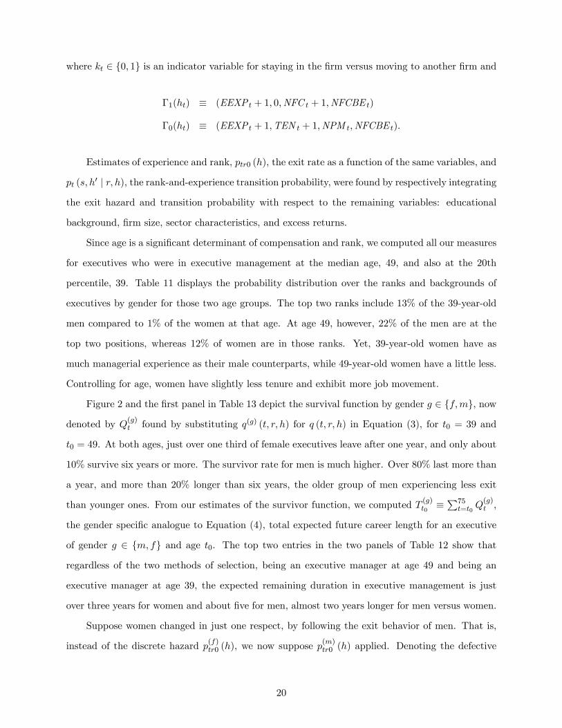
where kt ∈ {0, 1} is an indicator variable for staying in the firm versus moving to another firm and

Γ1(ht) ≡ (EEXP t + 1, 0,NFC t + 1,NFCBE t)

Γ0(ht) ≡ (EEXP t + 1,TEN t + 1,NPM t,NFCBE t).

Estimates of experience and rank, ptr0 (h), the exit rate as a function of the same variables, and

pt (s, h′ | r, h), the rank-and-experience transition probability, were found by respectively integrating

the exit hazard and transition probability with respect to the remaining variables: educational

background, firm size, sector characteristics, and excess returns.

Since age is a significant determinant of compensation and rank, we computed all our measures

for executives who were in executive management at the median age, 49, and also at the 20th

percentile, 39. Table 11 displays the probability distribution over the ranks and backgrounds of

executives by gender for those two age groups. The top two ranks include 13% of the 39-year-old

men compared to 1% of the women at that age. At age 49, however, 22% of the men are at the

top two positions, whereas 12% of women are in those ranks. Yet, 39-year-old women have as

much managerial experience as their male counterparts, while 49-year-old women have a little less.

Controlling for age, women have slightly less tenure and exhibit more job movement.

Figure 2 and the first panel in Table 13 depict the survival function by gender g ∈ {f,m}, now

denoted by Q(g)t found by substituting q(g) (t, r, h) for q (t, r, h) in Equation (3), for t0 = 39 and

t0 = 49. At both ages, just over one third of female executives leave after one year, and only about

10% survive six years or more. The survivor rate for men is much higher. Over 80% last more than

a year, and more than 20% longer than six years, the older group of men experiencing less exit

than younger ones. From our estimates of the survivor function, we computed T (g)t0≡∑75t=t0

Q(g)t ,

the gender specific analogue to Equation (4), total expected future career length for an executive

of gender g ∈ {m, f} and age t0. The top two entries in the two panels of Table 12 show that

regardless of the two methods of selection, being an executive manager at age 49 and being an

executive manager at age 39, the expected remaining duration in executive management is just

over three years for women and about five for men, almost two years longer for men versus women.

Suppose women changed in just one respect, by following the exit behavior of men. That is,

instead of the discrete hazard p(f)tr0 (h), we now suppose p(m)tr0 (h) applied. Denoting the defective

20

probability distribution for describing the survivors in this counterfactual by q(exit) (t, r, h), we

computed estimates of q(exit) (t, r, h) from the recursion

(7) q(exit)(t+ 1, s, h′) =

H∑h

R∑r=1

p(f)t

(s, h′ | r, h

) [1− p(m)tr0 (h)

]q(exit) (t, r, h)

by replacing p(f)tr0 (h) with p(m)tr0 (h) and q(f) (t, r, h) with q(exit) (t, r, h) in Equation (6). Summing

q(exit) (t, r, h) over h and r, we obtained the survivor function for women when they leave from the

sample population at the same rate as men given the same experience and rank. From Figure 2, we

see that this counterfactual exercise practically closes the gender gap between the survivor functions.

Reflecting the importance of this factor, Table 12 shows that the expected career duration increases

one and a half years to about four and a half years, not quite equalizing the expected career lengths

for the genders.

Another counterfactual, which speaks to the question of why women tend to have shorter

careers, is to replace p(f)t (s, h′ | r, h) with p(m)t (s, h′ | r, h) in Equation (7) to obtain

q(rank)(t+ 1, s, h′) =

H∑h

R∑r=1

p(m)t

(s, h′ | r, h

) [1− p(f)tr0 (h)

]q(rank) (t, r, h) .

This would generate the survivor function for women if they experienced the same rank transitions

as men throughout their careers in executive management, and tell us whether women executives

tend to gravitate to “dead-end” positions that are associated with higher rates of exit. We can

also calculate the differential effect of initial conditions on women by replacing q(f) (t0, r, h) with

q(m) (t0, r, h) and q(f) (t, r, h) with q(initial) (t, r, h) in Equation (7), defined in an analogous way.

Since there are fewer female executives than male executives, there may be greater selectivity into

the sample by those women who are less likely to leave the sample population, suggesting that the

aggregate rate of female exit in some sense understates the underlying process.

As an empirical matter, gender differences in the rank transition probabilities and initial condi-

tions affect the differences in the survivor functions only minimally. Replacing p(f)t (s, h′ | r, h) with

p(m)t (s, h′ | r, h) and q(f) (t, r, h) with q(rank) (t, r, h) in Equation (6) yields the survivor function for

women if they experienced the same rank transitions as men throughout their careers in execu-

tive management. Similarly, we calculated the differential effect of initial conditions on women by

replacing q(f) (t0, r, h) with q(m) (t0, r, h) and q(f) (t, r, h) with q(initial) (t, r, h) in Equation (6). In

21

both cases, the shift in the survivor function is barely visible at this level of resolution. From Table

10, swapping the initial conditions, or changing the transition probability, increases the expected

career length for female executives in the panel at 39 and 49 by less than a month. Summarizing,

the direct effect of exit rate explains most of the difference in career length of female and male

executive managers.

C. Is There a Glass Ceiling?

With estimates of q(g) (t, r, h), we can now answer whether women executives are less likely

than men to achieve the pinnacle of executive management and if so, why. The probability that an

executive in the population at t0 with gender g ∈ {f,m} is a CEO (in Rank 2) at age t ≥ t0 is

(8) q(g)(t, 2) =∑H

h=1q(g) (t, 2, h) .

The top two panels of Figure 3 show that executives in the sample at 49 are more than twice

as likely to be a CEO than an executive in the sample 10 years younger, reflecting our life-cycle

approach to the definition of a career hierarchy. Female executives in the population at either age

are less than half as likely to be CEOs as men.

What explains these gender differences? Are women promoted within the firm more slowly

and less likely to accept attractive offers from other firms? We set g = rank in Equation (8) and

checked how much the probability of being a CEO increased when women transitioned through

the ranks following the same transition matrix as men. Figure 3 and the last four panels of Table

13 show that the effect of this counterfactual is small. In other words, the gender differential in

probability of being a CEO is primarily due to differences in the other two factors, exit rate and

initial conditions.

Setting g = initial in Equation (8) yields the probability of a woman executive at age t0,

being a CEO at age t if she had been assigned the initial endowment of men. By construction,

the probability at t0 is equal, but it quickly falls off, partly because of the differential exit rates.

Breaking things down further, we investigated to what extent their initial assignment, conditional

on their past experience, is a determining factor, versus the different background they have at the

time. We found that only the initial rank counts, not initial differences in executive experience,

industry background, or education. Setting g = rinitial produces a line in Figure 3 that practically

22

overlays the g = initial line.

The higher rate of female exit shrinks the pool of female candidates eligible to be CEO,

thus contributing to the gender differences. If female exit patterns mimicked those of their male

colleagues, would the sequence of probabilities close the gap? Upon setting g = exit in Equation

(8), Figure 3 shows that the sequence of probabilities would increase, but not close the gap. Thus,

both initial conditions and exit rate are important explanatory factors for why women are less likely

to make CEO than men.

We can eliminate the effects of exit rate, and mitigate through the passage of time, the effects

of the initial conditions, by analyzing the pool of survivors. The probability of being a CEO with

gender g at age t conditional on belonging to the population at age t0 and remaining in it until at

least age t is

(9) q(g)(t, 2) =

∑Hh=1 q

(g) (t, 2, h)∑Rr=1

∑Hh=1 q

(g) (t, r, h).

The panels in the second row of Figure 3 (and the third panel in Table 13) have two notable

features that characterize both age groups. Conditional on survival, the probability of being a

CEO increases for more than a decade, rising to and then remaining above one half for a further

10 years (and longer for the younger group). More remarkably, amongst those who survive longer

than 15 years, a woman invariably has a higher probability of being a CEO than a man! This

finding contradicts the common belief that women face glass ceilings.

There are, of course, alternative definitions of top management, and we investigated whether

our conclusions are sensitive to them. In our career hierarchy, chairmen who are not also offi cers

directly under the CEO (such as the CFO and the COO) are classified in Rank 1. Rather than

focus on Expression (8) only, we also experimented with a more inclusive definition of top executive

position by combining the two top ranks, and recomputing the comparable panels of the second

row. The probability of being in the two top ranks with gender g at age t conditional on belonging

to the population at age t0 and surviving until age t at least is

q(g)(t, 2) + q(g)(t, 1) =

∑2r=1

∑Hh=1 q

(g) (t, r, h)∑Rr=1

∑Hh=1 q

(g) (t, r, h).

There is little to distinguish between the second-row panels and fourth-row panels, which depict

23

our estimates of q(g)(t, 2)+q(g)(t, 1). Using either definition of top management, our results provide

scant support for the view that female executives in publicly listed companies face glass ceilings.

An alternative approach to measuring female representation at the highest levels of manage-

ment is to compute, by gender, the fraction of executives who pass through the rank of CEO

before retiring. Denote by q(CEO,g)(t, 2) the number of executives who were in the sample at age

t0 ∈ {39, 49} and had at least one year of CEO experience by age t, as a fraction of the sum of this

number plus executives who are still waiting for the job of CEO, having neither quit the sample

by age t nor made CEO. Within our framework, this is equivalent to treating the CEO rank as

an absorbing state, thus eliminating CEO exit, leaving the other exit probabilities unchanged, and

assuming that an executive attaining the rank of CEO never changes rank again.4 Thus,

q(CEO,g)(t+ 1, s, h′) =H∑h

R∑r=1

p(CEO,g)t

(s, h′ | r, h

) [1− p(CEO,g)tr0 (h)

]q(CEO,g) (t, r, h)

and

q(CEO,g)(t, 2) =

∑Hh=1 q

(CEO,g) (t, 2, h)∑Rr=1

∑Hh=1 q

(CEO,g) (t, r, h).

From the third panel of Figure 3 (or fourth panel of Table 13), we see that the crossover occurs

earlier than in the second panel, thus validating our finding: Amongst survivors, women have

a higher probability of reaching the position of CEO than men. The fact that their crossover

age is about two years younger indicates that their tenure as a CEO is also a little lower, partly

attributable to their higher rate of exit.

D. Lifetime Compensation

Although female executives are paid more than male executives for a specific experience vector

at any given rank, and have a higher probability of attaining the position of CEO than male

executives conditional on remaining in top management, they exit more than men from these very

senior positions. This reduces the net present value of their lifetime earnings in this occupation.

In this section, we decompose the gender compensation gap into the amount due to differential

occupation exit rates, rank transition probability, and initial conditions. In this part of the study,

we focus on two measures of lifetime earnings. The first measure is the sum of discounted expected

24

earnings from executive management:

(10) V(g)t0≡∑∞

t=t0

∑R

r=1

∑H

h=1βt−t0w

(g)tr (h) q(g) (t, r, h) ,

where β is the subjective discount factor and w(g)tr (h) is the estimate of executives’expected com-

pensation conditional on age, gender, rank, and human capital. The second measure we use is

average annual career wages, which corresponds to the steady-state cross-sectional average earn-

ings. Average annual career earnings can be expressed as the ratio W (g)t0/T

(g)t0, where W (f)

t0is just

Equation (5) defined for women executives, undiscounted expected future earnings for t0-year-old

female executives, averaged over their experience and ranks:

(11) W(f)t0≡∑∞

t=t0

∑R

r=1

∑H

h=1w(f)tr (h) q(f) (t, r, h) .

Integrating the estimates obtained from the compensation regressions reported in Table 4A

to obtain wtr (h), we calculated estimates of average career wage over that time, W (f)t0/T

(f)t0, and

expected discounted sum of compensation V(f)t0

from age t0 onwards, as well as the analogous

quantities for men, setting the discount factor to β = 0.9. Then we computed counterfactuals for

these numbers by endowing female executives with some of the factors that determine the executive

careers of men.

The top entries in the middle column of the two panels of Table 12 imply that the estimated

gender gap in (undiscounted) annual compensation for executives at age 39 and 49 averaged over

the remainder of their management career is about $100,000. Given the longer career horizon of

men, at a 10% discount factor this translates to a present value of about $2 million, which can be

deduced from the third column. The gender gap in these career measures of executive compensation

is not attributable to unequal pay for equal work. Our compensation regressions, reported in Table

4A, showed that at any given rank women are paid more for the same experience credentials.

Substituting q(m) (t, r, h) for q(f) (t, r, h) in Equations (11) and (10) for t0 ∈ {39, 49}, we find that

the men would benefit about $100,000 per year on average from receiving the compensation package

of women, all else the same, which translates to about $400,000 in present value terms over their

careers as executives, numbers that follow from differencing the top from the bottom numbers in

the middle and right columns of Table 12.

25

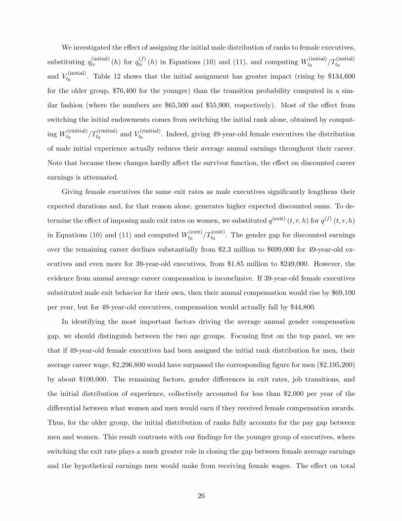
We investigated the effect of assigning the initial male distribution of ranks to female executives,

substituting q(initial)tr (h) for q(f)tr (h) in Equations (10) and (11), and computing W (initial)t0

/T(initial)t0

and V (initial)t0. Table 12 shows that the initial assignment has greater impact (rising by $134,600

for the older group, $76,400 for the younger) than the transition probability computed in a sim-

ilar fashion (where the numbers are $65,500 and $55,900, respectively). Most of the effect from

switching the initial endowments comes from switching the initial rank alone, obtained by comput-

ing W (rinitial)t0

/T(rinitial)t0

and V (rinitial)t0. Indeed, giving 49-year-old female executives the distribution

of male initial experience actually reduces their average annual earnings throughout their career.

Note that because these changes hardly affect the survivor function, the effect on discounted career

earnings is attenuated.

Giving female executives the same exit rates as male executives significantly lengthens their

expected durations and, for that reason alone, generates higher expected discounted sums. To de-

termine the effect of imposing male exit rates on women, we substituted q(exit) (t, r, h) for q(f) (t, r, h)

in Equations (10) and (11) and computed W (exit)t0

/T(exit)t0

. The gender gap for discounted earnings

over the remaining career declines substantially from $2.3 million to $699,000 for 49-year-old ex-

ecutives and even more for 39-year-old executives, from $1.85 million to $249,000. However, the

evidence from annual average career compensation is inconclusive. If 39-year-old female executives

substituted male exit behavior for their own, then their annual compensation would rise by $69,100

per year, but for 49-year-old executives, compensation would actually fall by $44,800.

In identifying the most important factors driving the average annual gender compensation

gap, we should distinguish between the two age groups. Focusing first on the top panel, we see

that if 49-year-old female executives had been assigned the initial rank distribution for men, their

average career wage, $2,296,800 would have surpassed the corresponding figure for men ($2,195,200)

by about $100,000. The remaining factors, gender differences in exit rates, job transitions, and

the initial distribution of experience, collectively accounted for less than $2,000 per year of the

differential between what women and men would earn if they received female compensation awards.

Thus, for the older group, the initial distribution of ranks fully accounts for the pay gap between

men and women. This result contrasts with our findings for the younger group of executives, where

switching the exit rate plays a much greater role in closing the gap between female average earnings

and the hypothetical earnings men would make from receiving female wages. The effect on total

26

earnings from spending an average of an extra 18 months in executive management is therefore

more pronounced at 39 than at 49.

Tables 12 and 13 show that the gender differences in compensation, expected career length,

and the probability of becoming a CEO are almost entirely accounted for by differences in exit

rates, transitions rates, and initial conditions. Table 12 presents a summary measure of all the

other components of the decomposition; it combines the per period compensation, expected career

length, and rank distribution into one measure, expected lifetime compensation. It shows that the

gender differences are more pronounced at age 49 than at age 39. At 49 the gaps are accounted

for by gender differences in the distributions of rank and experience at that age and the exit and

job-transition rates thereafter. At 39 the gaps are accounted for by the gender differences in exit

and job-transition rates. However the gender differences in the distributions of experience and rank

at age 39 are not important.

The differences between the distributions of rank and experience at ages 39 and 49 are due to

a combination of exit and job-transition rates during that time. This means that gender differences

in exit and job-transition rates are more important in explaining the gender differences in career

outcomes than gender differences in the distributions of rank and experience at age 39. This

suggests that differences in exit and job-transition rates before age 39 may account for the gender

differences observed at age 39.

V. Discussion and Conclusion

Our empirical analysis shows that female executives have different backgrounds and experience

from male executives and that women are paid more and have higher pay-for-performance sensitivity

than men conditional on rank, background, and experience. We also find that women are promoted

more quickly internally but display similar rates of external promotion to men; however, women and

men have similar demotion rates. The higher rate of promotion results in female executives at the

upper levels of the hierarchy having significantly less job experience than male executives. Female

executives, however, have a higher exit rate than men and the probability of a female executive

becoming CEO is less than half that of male executives at every age. Our decomposition shows

that the male executives’survival rate is twice that of female executives. The gender differences

in career length are accounted for completely by the difference in exit rates, and, conditional on

27

survival as an executive at any age, women have a higher probability of becoming a CEO. The

average career compensation of female executives is lower than that of male executives, but it is

higher than male executives’if female executives are assigned the male initial experience, the male

initial rank assignment, or the male career experience distribution.

Suppose executives have concave utility over consumption and there are no gender differences

in preferences and unobserved ability. Suppose that lower level ranks provide more opportunities

for investment in human capital and that a longer tenure and experience in these ranks increase

the productivity of executives more than tenure and experience in higher ranks. If women have an

exogenously higher non-market outside option than men, then a model of moral hazard, investment

in human capital, and career concerns can account for most of the above findings (see Gayle, Golan

and Miller (2011)).

An exogenously higher non-market outside option implies that women at all ranks and expe-

rience level would exit at higher rate than men. A higher female exit rate has two separate effects;

the first is that female executives would gravitate to higher ranks and spend less time investing

in human capital. This would explain the higher female promotion rate, the lower human capital

of female in higher ranks, and the unconditional gender pay gap. The second effect is that female

executives would have less incentive to exert effort than male executives because, on average, their

careers are shorter. Since their career concerns motive is weaker, females require more incentive pay

to align their incentives with those of their employer firms than their male counterparts. Therefore

their compensation is tied more closely to the firm’s performance with a higher risk premium.

Suppose that expected compensation reflects an executive’s marginal product, that marginal

product is equalized across genders, and females are paid the same expected compensation as

their male counterparts. Equalizing expected compensation with a higher risk premium implies

a lower certainty equivalent compensation. Being paid a lower certainty equivalent compensation

makes a job even less attractive to females, and thus amplifies the higher female quit rate. These

explanations appear consistent with our findings and are not based on discrimination.

There is still a question of why women have a higher nonmarket outside option than men. One

explanation is that women acquire more nonmarket human capital than men throughout their lives,

and hence find retirement a relatively attractive option. Women in the top executive market are

mostly beyond childbearing age, but there is evidence that such women are more likely to leave for

28

personal and other household reasons than their male counterparts. For example, Sicherman (1996)

finds that in a case study of a large insurance company, female executives were more likely than their

male counterparts to exit the firm because of better working conditions elsewhere, to be near home,

change of residence, household duties, personal heath, illness in the family, and positions abolished.

Most of those reasons, except position abolished, are voluntary departures related to home or family.

Other unobserved factors leading managers to exit could include more unpleasantness, indignities,

and tougher unrewarding assignments at work, examples of factors that reduce the attraction of

work without necessarily affecting productivity or human-capital acquisition. Perhaps women are

subject to this form of gender discrimination.

Another possible explanation for the higher female exit rates is differential treatment of men

and women with the same expected ability in this market. Perhaps there is more uncertainty about

women’s skills, when they enter the sample (see Lundberg and Startz (1983)); this hypothesis is

supported by the fact that when women enter, they are younger, have less experience, and fewer

qualifications than men. The hypothesis that there is more uncertainty about women’s ability is

consistent with the fact that women are more likely to exit and that those who remain are more

likely to get promoted and earn higher wages as more information about their ability is revealed

over time. Suppose that bad performance provides a signal on an executive’s ability. If firms have

more uncertainty about women’s ability than men, then the relationship between firm performance

and the rate of exit should differ by gender. However, we do not find any differences on that score.

A more involved model of promotions and uncertainty about abilities is developed in Scotchmer

(2008); it assumes no gender differences in abilities, but that men take more risk and therefore

provide less accurate information on their abilities than women. In her model men are more likely

than women to survive and get promoted more at early ages, and male survivors have lower average

ability than females. At older ages these roles are reversed; females are promoted more, and their

average ability is lower, than male survivors. For our sample we find that males are more likely to

survive at lower ranks than female, however, female are promoted more quickly than males at all

ranks and ages.

Another type of discrimination is suggested by Milgrom and Oster (1987). In their model

abilities of executives are known to employers, but initially males are more visible to outside em-

ployers than females allowing employers to extract more rents from female executives. Promotions

29

enhance visibility of workers to outside employers; this increases competition for female executives,

which in turn increases their compensation and reduces the employers’rents. Their model implies

that female executives would face a higher threshold for promotion than their male counterparts.

Further, it implies that the gender compensation gap in high ranks should be smaller than the gap

in lower ranks. We find that male and female executives are paid the same conditional on rank

alone. Conditional on background characteristics and job-experience female executives are paid

more than their male counterparts at all ranks. Moreover, we do not find differences in external

promotion rates between males and females, which might be expected if women were less visible

than men.

Whatever the mix of the explanations above, we do not find any clear evidence that aggregate

differences observed in the executive market between genders are driven by compensation packages

and promotion opportunities available to men and women. It is still possible that discrimination

explains, at least partially, the small fraction of women, compared to men who join the ranks of

executive management in publicly listed firms. We are unable to address this issue because our

data set comprises only of those who reach these positions, but our analysis identifies one reason

for the relative scarcity of female executives. Women executive managers are more likely to exit

than men, on average spending less time in those positions than male executives do.

In principle, a large longitudinal data set might be assembled to track men and women from

an early age in order to distinguish by gender the contribution of background variables of those

who attain the position of executive manager from those who do not. The results of our study

highlight two challenges that such an approach must overcome to yield convincing results. We have

established that executive managers are not drawn from an easily identified population. Because

they are drawn from very diverse backgrounds, because executive managers comprise a minute por-

tion of the general population, and because women are less than one tenth as likely to be executive

managers as men, a very large sample is required to obtain meaningful results that separate by gen-

der those who become executive managers from those who do not. A second challenge proponents

of a longitudinal approach would face, stems from the fact that many executive, enter the market

after a long period of acquiring education and other work experience, requiring a longitudinal study

to track respondents for more than 20 consecutive years, an expensive long-term research project

susceptible to choice-based attrition bias. In the meantime, we hope our results will encourage fu-

30

ture research on gender differences in executive management to turn away from compensation and

promotion, towards the nonpecuniary characteristics of executive management jobs and options

outside the marketplace.

31

References

Albanesi, Stefania and Claudia Olivetti. “Gender and Dynamic Agency: Theory and Evidence

on the Compensation of Top Executives.”Columbia University, 2008.

Albrecht, James, Anders Björklund, and Susan Vroman. “Is There a Glass Ceiling in

Sweden?” Journal of Labor Economics, 2003, 21, pp. 145—177.

Antle, Rick and Abbie Smith. “Measuring Executive Compensation: Methods and an Appli-

cation.”Journal of Accounting Research, 1985, 23, pp. 296—325.

Antle, Rick and Abbie Smith. “An Empirical Investigation of the Relative Performance Eval-

uation of Corporate Executives.”Journal of Accounting Research, 1986, 24, pp. 1—39.

Baker, George, Michael Gibbs, and Bengt Holmstrom. “The Internal Economics of the

Firm: Evidence from Personnel Data.”Quarterly Journal of Economics, November 1994a, 109(4),

pp. 881—919.

Baker, George, Michael Gibbs, and Bengt Holmstrom. “The Wage Policy of a Firm.”

Quarterly Journal of Economics, November 1994b, 109(4), pp. 921—955.

Barmby, Tim, Sarah Bridges, John Treble, and Edwin van Gameren. “The Internal

Economics of the Firm: Further Evidence from Personnel Data.”Labour Economics, 2001, 8(5),

pp. 531—552.

Bell, Linda A. “Women-Led Firms and the Gender Gap in Top Executive Jobs.”IZA Discussion

Paper 1689, July 2005.

Bertrand, Marianne, Claudia Goldin, and Lawrence F. Katz. “Dynamics of the Gender

Gap for Young Professionals in the Financial and Corporate Sectors.”American Economic Journal:

Applied Economics, 2010, 2(3), pp. 228—255.

Bertrand, Marianne and Kevin Hallock. “The Gender Gap in Top Corporate Jobs.”Industrial

and Labor Relations Review, 2001, 55(1), pp. 3—21.

Black, Dan A., Amelia M. Haviland, Seth G. Sanders, and Lowell J. Taylor. “Gender

Wage Disparities among the Highly Educated.”Journal of Human Resources, 2008, 43(Summer),

pp. 630—659.

32

Blau, Francine and Lawrence Kahn. “The US Gender Pay Gap in the 1990s: Slowing Con-

vergence.”NBER Working Paper 10853, 2004.

Gayle, George-Levi and Limor Golan. “Estimating a Dynamic Adverse-Selection Model:

Labor-Force Experience and the Changing Gender Earnings Gap 1968—1997.”Review of Economic

Studies, January 2011, Forthcoming.

Gayle, George-Levi, Limor Golan, and Robert A. Miller. “Promotion, Turnover, and

Compensation in the Executive Market,” February 2011, Tepper School of Business, Carnegie

Mellon University.

Gayle, George-Levi and Robert A. Miller. “Has Moral Hazard Become a More Important

Factor in Managerial Compensation?” American Economic Review, December 2009a, 99(5), pp.

1740—1769.

Gayle, George-Levi and Robert A. Miller. “Insider Information and Performance Pay.”

CESifo Economic Studies, May 2009b, 55(3—4), pp. 515—541.

Ginther, Donna K. and Kathy J. Hayes. “Gender Differences in Salary and Promotion in the

Humanities.”American Economic Review, May, 1999, 89(2), pp. 397—402.

Ginther, Donna K. and Kathy J. Hayes. “Gender Differences in Salary and Promotion for

Faculty in the Humanities 1977—95.”Journal of Human Resources, Winter 2003, 38(1), pp. 34—73.

Ginther, Donna K. and Shulamit Kahn. “Women in Economics: Moving Up or Falling Off

the Academic Career Ladder?” Journal of Economic Perspectives, 2004, 18(3), pp. 193—214.

Hall, Brian J. and Jeffrey B. Liebman. “Are CEOs Really Paid Like Bureaucrats?”Quarterly

Journal of Economics, August 1998, 113, pp. 653—680.

Lundberg, Shelley J, and Richard Richard Startz. “Private Discrimination and Social In-

tervention in competitive labor Markets.”American Economic Review, 1983, 73(3), pp. 340—347.

Margiotta, Mary M. and Robert A. Miller. “Managerial Compensation and the Cost of

Moral Hazard.”International Economic Review, August 2000, 41(3), pp. 669—719.

33

McDowell, John M., Larry D. Singell, Jr., and James P. Ziliak. “Cracks in the Glass

Ceiling: Gender and Promotion in the Economics Profession.”American Economic Review, May

1999, 89(2), pp. 392—396.

Milgrom, Paul and Sharon Oster. “Job Discrimination, Market Forces, and the Invisibility

Hypothesis”Quarterly Journal of Economics, August 1987, 102(3), pp. 453—476.

Mincer, Jacob and Solomon Polachek. “Family Investments in Human Capital: Earnings of

Women.”Journal of Political Economy, March—April 1974, 82(2) Part II, pp. 76—108.

O’Neill, June and Solomon Polachek. “Why the Gender Gap in Wages Narrowed in the 1980s.”

Journal of Labor Economics, January 1993, 11, pp. 205—228.

Pekkarinen, Tuomas and Juhana Vartiainen. “Gender Differences in Job Assignment and

Promotion on a Complexity Ladder of Jobs.”IZA DP No 1184, 2004.

Scotchmer, Suzanne. “Risk Taking and Gender in Hierarchies.”Theoretical Economics, 2008,

3(4), pp. 499—524.

Selody, Karen, “Is the Risk Worth the Reward for Female Executives?” 2010, Department of

Economics, University of California, Berkeley.

Sicherman, Nachum, “Gender Differences in Departures from a Large Firm.” Industrial and

Labor Review, 1996, 49(3), pp. 484—505.

Wellington, Alison J. “Changes in the Male/Female Wage Gap, 1976—85.” Journal of Human

Resources, 1993, 28, pp. 383—411.

34

Notes

∗For comments and suggestions, we thank Kenneth Wolpin, seminar participants at Washington

and Stanford Universities, and conference attendees at the Society of Labor Economists 2007 and

the 2008 World Congress on National Accounts and Economic Performance Measures for Nations.

This research is supported by the Center for Organizational Learning, Innovation and Performance

in Carnegie Mellon University and National Science Foundation Grant Award SES0721098.

1Mincer and Polachek (1974), O’Neill and Polachek (1993), Wellington (1993), and Gayle and

Golan (2011) have shown that actual labor market experience accounts for most of the gender wage

gap among ordinary workers.

2The data in Baker et al. (1994b) automatically satisfy the third axiom without further restric-

tions.

3We encountered a further 60 titles used fewer than three times each. These jobs were easy

to rank within the hierarchy we constructed, but our analysis and conclusions are not affected

by omitting the small number of observations involved either. We also experimented with finer

partitions of job titles, refining job title by firm size (doubling the number of titles with an indicator

designating big or small) and by sector (which triples the number of jobs). The main practical

diffi culty of increasing the number of job titles is the resulting small number of women in many job

title cells. On the overall sample, we found that the transition patterns were not sensitive to the

definitions of the partition we tested.

4Mathematically, we set p(CEO,g)t20 (h) = 0, leave p(CEO,g)tr0 (h) = p(g)tr0 (h) for all r 6= 2, and set

p(CEO,g)t (2, h′ | 2, h) = 1, which implies p(CEO,g)t (s, h′ |2, h) = 0 for all s 6= 2.

35

14a

13a

12c

13d 13e

12a

11b 11c 11d 11e 11f11a

8c

10a

9d9c9a 9b 9e 9f

8a 8b

7a

3b

4a

6a 6b

3a

5a

2a

1a

13c13b

12d

1

2

4

3

5

6

7

8

9

10

11

12

13

14

12b

Figure 1: Hierarchy

36

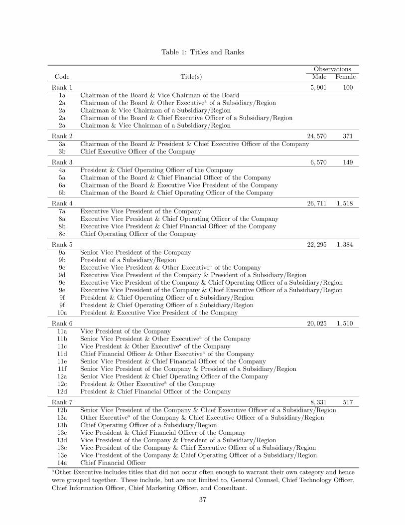
Table 1: Titles and Ranks

ObservationsCode Title(s) Male Female

Rank 1 5, 901 1001a Chairman of the Board & Vice Chairman of the Board2a Chairman of the Board & Other Executivea of a Subsidiary/Region2a Chairman & Vice Chairman of a Subsidiary/Region2a Chairman of the Board & Chief Executive Offi cer of a Subsidiary/Region2a Chairman & Vice Chairman of a Subsidiary/Region

Rank 2 24, 570 3713a Chairman of the Board & President & Chief Executive Offi cer of the Company3b Chief Executive Offi cer of the Company

Rank 3 6, 570 1494a President & Chief Operating Offi cer of the Company5a Chairman of the Board & Chief Financial Offi cer of the Company6a Chairman of the Board & Executive Vice President of the Company6b Chairman of the Board & Chief Operating Offi cer of the Company

Rank 4 26, 711 1, 5187a Executive Vice President of the Company8a Executive Vice President & Chief Operating Offi cer of the Company8b Executive Vice President & Chief Financial Offi cer of the Company8c Chief Operating Offi cer of the Company

Rank 5 22, 295 1, 3849a Senior Vice President of the Company9b President of a Subsidiary/Region9c Executive Vice President & Other Executivea of the Company9d Executive Vice President of the Company & President of a Subsidiary/Region9e Executive Vice President of the Company & Chief Operating Offi cer of a Subsidiary/Region9e Executive Vice President of the Company & Chief Executive Offi cer of a Subsidiary/Region9f President & Chief Operating Offi cer of a Subsidiary/Region9f President & Chief Operating Offi cer of a Subsidiary/Region10a President & Executive Vice President of the Company

Rank 6 20, 025 1, 51011a Vice President of the Company11b Senior Vice President & Other Executivea of the Company11c Vice President & Other Executivea of the Company11d Chief Financial Offi cer & Other Executivea of the Company11e Senior Vice President & Chief Financial Offi cer of the Company11f Senior Vice President of the Company & President of a Subsidiary/Region12a Senior Vice President & Chief Operating Offi cer of the Company12c President & Other Executivea of the Company12d President & Chief Financial Offi cer of the Company

Rank 7 8, 331 51712b Senior Vice President of the Company & Chief Executive Offi cer of a Subsidiary/Region13a Other Executivea of the Company & Chief Executive Offi cer of a Subsidiary/Region13b Chief Operating Offi cer of a Subsidiary/Region13c Vice President & Chief Financial Offi cer of the Company13d Vice President of the Company & President of a Subsidiary/Region13e Vice President of the Company & Chief Executive Offi cer of a Subsidiary/Region13e Vice President of the Company & Chief Operating Offi cer of a Subsidiary/Region14a Chief Financial Offi cer

aOther Executive includes titles that did not occur often enough to warrant their own category and hencewere grouped together. These include, but are not limited to, General Counsel, Chief Technology Offi cer,Chief Information Offi cer, Chief Marketing Offi cer, and Consultant.

37

Table 2: Executive Background by Gender(1) (2) (3) (4)All Male Female t(z)a

Panel A: Match SampleExit 0.26 0.25 0.30 −7.58Promotion 0.08 0.08 0.08 0.04Turnover 0.02 0.02 0.02 1.58No College Degree 0.21 0.21 0.23 −2.04Bachelors 0.79 0.79 0.77 2.04MBA 0.23 0.23 0.23 −0.05MS/MA 0.19 0.19 0.17 2.56Ph.D. 0.18 0.17 0.21 −4.60Professional Certification 0.22 0.22 0.24 −2.56Consumer Sector 0.27 0.27 0.38 17.22Service Sector 0.37 0.37 0.39 1.32Primary Sector 0.36 0.37 0.25 17.25

Age 53.70 53.80 50.90 15.75(9.30) (9.30) (10.10)

Managerial Experience 18.32 18.50 15.00 3.90(42.80) (43.70) (11.50)

Years of Tenure 14.37 14.50 12.54 7.67(11.48) (11.50) (10.80)

NFC 2.04 2.04 1.97 1.74(2.00) (2.00) (1.90)

NFCBE 0.82 0.82 0.77 2.23(1.34) (1.35) (1.24)

Salary (thousand 2006 US$) 461 465 381 17.88(299) (301) (244)

Total Compensation (thousand 2006 US$) 2,460 2,480 2,040 2.36(11,842) (11,952) (9,128)

Assets (millions 2006 US$) 13,753 13,678 15,315 1.84(63,180) (61,900) (85,532)

Employees 19,600 19,600 19,300 0.43(54,000) (54,000) (49,000)

No. of Observations 71,803 68,833 2,970

Panel B: Full SampleExit 0.20 0.19 0.22 −3.69Promotion 0.08 0.08 0.08 0.04Turnover 0.02 0.02 0.02 1.76Consumer Sector 0.27 0.26 0.37 17.10Service Sector 0.38 0.38 0.39 1.92Primary Sector 0.35 0.36 0.24 17.80

Salary (thousand 2006 US$) 410 414 333 24.70(287) (290) (222)

Total Compensation (thousand 2006 US$) 1,855 1,882 1,342 4.28(11,044) (11,130) (11,542)

Assets (million 2006 US$) 13,283 13,210 14,784 1.84(61,985) (60,733) (83,827)

Employees 18,930 18,930 18,670 0.37(52,520) (52,720) (48,130)

No. of Observations. 162,592 154,423 8,125Sources: The data are for top managers from the Standard and Poor’s ExecuCompdatabase for 1991 through 2006 matched with background data from the MarquisWho’sWho database. Note: Standard deviation in parenthesis. NFCBE is an executive’snumber of firm changes before becominng an executive. NFC is the total number of firmchanges. aStatistic for the difference in sample means and proportions between men andwomen within each row: distributed t for a mean and z for a proportion. Executiveswho leave all our data sets and do not return for four years are classified as exited.

38

Table3:ExecutiveBackgroundbyRank

Rank1

Rank2

Rank3

Rank4

Variables

Men

Women

t(z)

Men

Women

t(z)

Men

Women

t(z)

Men

Women

t(z)

MatchedSample

Exit

0.3

50.

390.

45

0.1

40.

19

−1.1

20.2

10.

17

0.82

0.2

60.

33

−2.

98

Promotion

0.2

70.

260.

21

0.0

80.

12

−2.3

60.2

00.

23

−1.

15

0.1

20.

13

−1.

08

Turnover

0.04

0.04

0.16

0.0

30.

05

−1.7

40.0

30.

04

−1.

02

0.0

20.

03

−0.

73

NoCollege

0.25

0.11

2.71

0.2

10.

21

−0.1

20.2

50.

24

0.17

0.2

10.

25

−2.

56

Bachelors

0.75

0.89

−2.7

10.7

90.

79

0.12

0.7

50.

76

−0.

17

.79

0.75

2.56

MBA

0.24

0.28

−0.8

30.2

60.

25

0.57

0.2

30.

22

0.20

0.2

50.

32

−4.

09

MS/MA

0.1

60.

26−

2.4

30.1

70.

14

1.48

0.1

70.

22

−1.

57

0.2

00.

14

3.69

Ph.D.

0.1

50.

29−

3.3

60.1

50.

14

0.38

0.1

40.

16

−0.

91

0.1

40.

11

2.18

ProfessionalCertification

0.1

50.

18−

0.6

80.1

40.

05

4.15

0.1

50.

10

1.87

0.2

20.

18

2.58

Age

59.7

051.8

011.

20

55.8

051.

60

10.

38

52.4

052.

00

0.47

52.1

049.

50

6.80

(9.8

0)(5.6

0)(7.6

0)

(6.7

0)

(7.9

0)

(9.9

0)

(8.8

0)

(9.5

0)

Exec.Exp.

22.4

013.0

08.

60

20.9

018.

90

2.70

18.2

014.

10

3.10

15.5

013.

80

3.30

(13.

30)

(8.5

0)(4

7.40)

(10.

20)

(66.

00)

(9.1

)(2

4.00)

(11.

00)

Tenure

17.2

011.6

03.

79

15.2

013.

20

2.60

13.7

011.

10

2.15

13.9

012.

90

2.00

(13.

60)

(10.

70)

(11.

70)

(11.

50)

(11.

40)

(10.

50)

(11.

10)

(11.

40)

NFC

1.9

51.

462.

77

1.9

12.

02

−0.9

41.7

51.

28

2.79

1.9

31.

77

2.24

(2.0

0)(1.3

9)(1.9

3)

(1.9

4)

(1.9

2)

(1.8

0)

(1.9

5)

(1.8

1)

NFCBE

0.9

10.

573.

08

0.9

31.

18

−2.8

00.7

30.

47

3.16

0.7

60.

66

2.66

(1.3

9)(0.9

2)(1.3

9)

(1.5

1)

(1.2

9)

(1.0

1)

(1.3

0)

(1.0

8)

Salary

623

607

0.54

730

758

−0.

85

552

563

−0.5

5408

394

2.52

(362

)(2

45)

(391)

(538)

(305)

(249)

(184)

(169)

Compensation

2,67

52,

946

−0.

20

3,7

95

2,992

0.6

83,7

29

2,965

0.5

72,3

21

2,677

−1.

33

(17,

874)

(11,

834)

(19,

632)

(19,

610)

(13,

791)

(16,

685)

(8,1

30)

(8,5

14)

N4,

293

7517,

953

286

5,201

148

13,

997

799

FullSample

Exit

0.3

50.

350.

00

0.1

60.

24

−1.8

60.2

30.

18

0.84

0.2

70.

34

−3.

38

Promotion

0.2

70.

260.

22

0.0

80.

12

−2.3

90.2

00.

23

−1.

17

0.1

20.

13

−0.

98

Tornover

0.04

0.04

0.03

0.0

30.

05

−1.4

40.0

30.

04

−1.

05

0.0

20.

02

0.49

Salary

613

596

0.62

707

715

−0.3

1535

547

−0.

67

395

384

2.48

(362

)(2

65)

(404)

(506)

(316)

(248)

(183)

(170)

Compensation

2,59

03,

355

−0.8

63,8

49

3,532

0.3

33,4

64

3,808

−0.

40

2,1

07

2,238

−0.

60

(16,

726)

(8,6

33)

(18,

385)

(7,9

09)

(13,

168)

(11,

830)

(7,8

97)

(8,1

92)

N5,

900

100

24,

573

371

7,903

209

25,

705

1,472

Sources:Thedataarefortopmanagersfrom

theStandardandPoor’sExecuCompdatabasefor1991through2006matchedwithbackgrounddata

from

theMarquisWho’sWhodatabase.

Note:Standarddeviationsinparenthesis.Salaryandcompensationmeasuredinthousandsof2006US$.NFCBEisanexecutive’snumberoffirm

changesbeforebecominnganexecutive.NFCisthetotalnumberoffirmchanges.Exec.Exp.measuresyearsofexecutiveexperience.

aStatistic

forthedifferenceinsamplemeansandproportionsbetweenmenandwomenwithineachrow:distributedtforameanandzforaproportion.

Executiveswholeaveallourdatasetsanddonotreturnforfouryearsareclassifiedasexited.

39

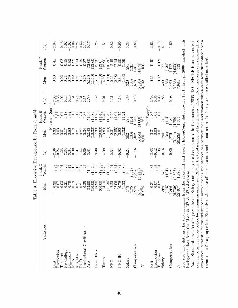
Table3:ExecutiveBackgroundbyRank(cont’d)

Rank5

Rank6

Rank7

Variables

Men

Women

t(z)

Men

Women

t(z)

Men

Women

t(z)

MatchedSample

Exit

0.30

0.37

−2.

86

0.3

00.

35

−2.

65

0.3

00.

41

−2.

84

Promotion

0.07

0.07

−0.

24

0.0

30.

03

0.38

Turnover

0.03

0.01

1.28

0.0

10.

01

1.02

0.0

20.

02

−0.

18

NoCollege

0.21

0.26

−3.

34

0.1

70.

18

−0.

46

0.2

10.

18

1.0

2Bachelors

0.79

0.74

3.34

0.8

30.

82

0.46

0.7

90.

82

−1.

02

MBA

0.19

0.19

0.00

0.1

80.

16

1.61

0.2

20.

22

0.0

6MS/MA

0.21

0.18

1.91

0.2

10.

19

0.74

0.2

10.

14

2.2

4Ph.D.

0.21

0.24

−1.

44

0.2

70.

34

−4.

31

0.1

70.

19

−0.

53

ProfessionalCertification

0.2

50.

24

0.60

0.3

40.

38

−2.1

50.2

90.

37

−2.

13

Age

52.9

051.

30

3.81

52.4

051.

30

2.50

52.2

052.

00

0.1

7(1

0.00)

(10.

40)

(10.

30)

(10.

80)

(11.

10)

(13.

60)

Exec.Exp.

18.9

015.

50

3.90

17.3

014.

70

4.52

16.7

015.

30

1.2

5(6

6.60)

(12.

50)

(29.

60)

(11.

40)

(11.

70)

(13.

0)

Tenure

14.1

012.

20

4.09

13.8

012.

40

2.91

14.2

012.

90

1.5

1(1

1.30)

(10.

30)

(11.

00)

(10.

50)

(10.

90)

(10.

30)

NFC

2.2

32.

01

2.64

2.3

12.

20

1.31

2.3

12.

45

−0.

82

(2.0

6)

(2.3

1)

(2.0

5)

(1.9

1)

(2.1

8)

(2.1

4)

NFCBE

0.7

80.

82

−0.

92

0.8

00.

75

1.18

0.8

40.

90

−0.

60

(1.3

3)

(0.8

0)

(1.3

2)

(1.2

4)

(1.4

3)

(1.3

9)

Salary

379

380

−0.

24

302

276

7.39

320

281

5.35

(175)

(302)

(130)

(114)

(188)

(131)

Compensation

1,979

2,282

−1.

46

1,4

02

1,347

0.4

31,6

78

1,461

0.8

5(6,7

17)

(6,4

15)

(5,4

54)

(4,0

60)

(6,2

98)

(4,5

74)

N10,

976

706

9,801

662

3,702

186

FullSample

Exit

0.31

0.37

−2.

88

0.3

10.

37

−3.

53

0.3

10.

40

−2.

63

Promotion

0.07

0.07

−0.

42

0.0

30.

03

0.35

Turnover

0.02

0.01

1.03

0.0

10.

01

0.98

0.0

20.

02

−0.

15

Salary

369

370

−0.

16

294

270

7.83

309

277

5.17

(175)

(184)

(134)

(114)

(186)

(134)

Compensation

1,866

2,008

−0.

80

1,2

79

1,289

−0.

08

1,4

89

1,122

1.6

0(6,7

39)

(6,3

52)

(5,1

44)

(4,7

50)

(6,5

33)

(4,9

30)

N22,4

07

1,386

20,2

38

1,495

7,9

84

513

Sources:Thedataarefortopmanagersfrom

theStandardandPoor’sExecuCompdatabasefor1991through2006matchedwith

backgrounddatafrom

theMarquisWho’sWhodatabase.

Note:Standarddeviationsinparenthesis.Salaryandcompensationmeasuredinthousandsof2006US$.NFCBEisanexecutive’s

numberoffirmchangesbeforebecominnganexecutive.NFCisthetotalnumberoffirmchanges.Exec.Exp.measuresyearsofexecutive

experience.

aStatisticforthedifferenceinsamplemeansandproportionsbetweenmenandwomenwithineachrow:distributedtfora

meanandzforaproportion.Executiveswholeaveallourdatasetsanddonotreturnforfouryearsareclassifiedasexited.

40

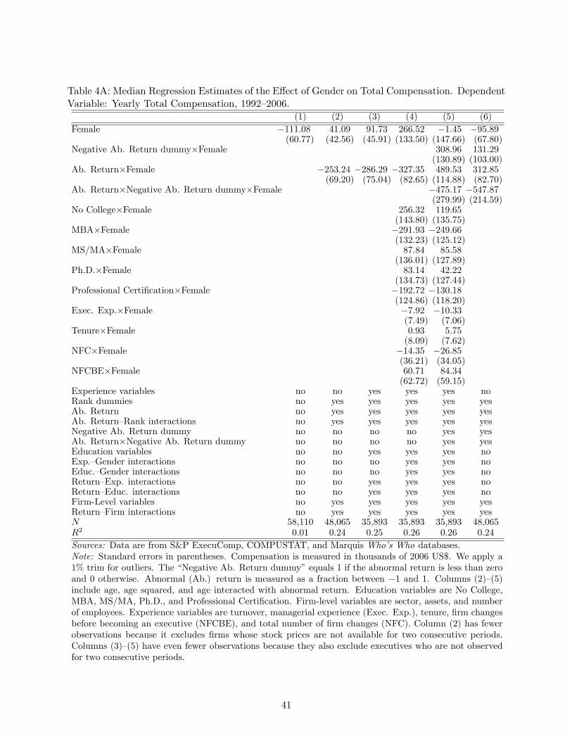
Table 4A: Median Regression Estimates of the Effect of Gender on Total Compensation. DependentVariable: Yearly Total Compensation, 1992—2006.

(1) (2) (3) (4) (5) (6)Female −111.08 41.09 91.73 266.52 −1.45 −95.89

(60.77) (42.56) (45.91) (133.50) (147.66) (67.80)Negative Ab. Return dummy×Female 308.96 131.29

(130.89) (103.00)Ab. Return×Female −253.24 −286.29 −327.35 489.53 312.85

(69.20) (75.04) (82.65) (114.88) (82.70)Ab. Return×Negative Ab. Return dummy×Female −475.17 −547.87

(279.99) (214.59)No College×Female 256.32 119.65

(143.80) (135.75)MBA×Female −291.93 −249.66

(132.23) (125.12)MS/MA×Female 87.84 85.58

(136.01) (127.89)Ph.D.×Female 83.14 42.22

(134.73) (127.44)Professional Certification×Female −192.72 −130.18

(124.86) (118.20)Exec. Exp.×Female −7.92 −10.33

(7.49) (7.06)Tenure×Female 0.93 5.75

(8.09) (7.62)NFC×Female −14.35 −26.85

(36.21) (34.05)NFCBE×Female 60.71 84.34

(62.72) (59.15)Experience variables no no yes yes yes noRank dummies no yes yes yes yes yesAb. Return no yes yes yes yes yesAb. Return—Rank interactions no yes yes yes yes yesNegative Ab. Return dummy no no no no yes yesAb. Return×Negative Ab. Return dummy no no no no yes yesEducation variables no no yes yes yes noExp.—Gender interactions no no no yes yes noEduc.—Gender interactions no no no yes yes noReturn—Exp. interactions no no yes yes yes noReturn—Educ. interactions no no yes yes yes noFirm-Level variables no yes yes yes yes yesReturn—Firm interactions no yes yes yes yes yesN 58,110 48,065 35,893 35,893 35,893 48,065R2 0.01 0.24 0.25 0.26 0.26 0.24Sources: Data are from S&P ExecuComp, COMPUSTAT, and Marquis Who’s Who databases.Note: Standard errors in parentheses. Compensation is measured in thousands of 2006 US$. We apply a1% trim for outliers. The “Negative Ab. Return dummy”equals 1 if the abnormal return is less than zeroand 0 otherwise. Abnormal (Ab.) return is measured as a fraction between −1 and 1. Columns (2)—(5)include age, age squared, and age interacted with abnormal return. Education variables are No College,MBA, MS/MA, Ph.D., and Professional Certification. Firm-level variables are sector, assets, and numberof employees. Experience variables are turnover, managerial experience (Exec. Exp.), tenure, firm changesbefore becoming an executive (NFCBE), and total number of firm changes (NFC). Column (2) has fewerobservations because it excludes firms whose stock prices are not available for two consecutive periods.Columns (3)—(5) have even fewer observations because they also exclude executives who are not observedfor two consecutive periods.

41

Table 4B: Median Regression Estimates of the Effect of Gender on Salary. Dependent Variable:Yearly Salary, 1992—2006.

(1) (2) (3) (4) (5)Female −77.69 −10.80 −10.69 20.29 12.15

(6.23) (4.35) (4.68) (12.56) (14.44)Negative Ab. Return dummy×Female −3.54

(12.75)Ab. Return×Negative Ab. Return dummy×Female −13.44

(26.60)Ab. Return×Female 6.24 9.13 6.70 −2.23

(6.48) (6.99) (6.89) (8.71)No College×Female 53.77 62.50

(13.16) (13.45)MBA×Female −29.19 −30.60

(12.03) (12.39)MS/MA×Female −0.75 2.88

(12.42) (12.72)Ph.D.×Female 22.51 26.67

(12.360) (12.67)Professional Certification×Female −22.864 −24.14

(11.45) (11.73)Exec. Exp.×Female −1.18 −0.65

(0.69) (0.70)Tenure×Female −0.47 −0.85

(0.74) (0.75)NFC×Female −4.20 −2.72

(3.32) (3.41)NFCBE×Female 6.47 2.39

(5.71) (5.86)Experience variables no no yes yes yesRank dummies no yes yes yes yesAb. Return no yes yes yes yesAb. Return—Rank interactions no yes yes yes yesNegative Ab. Return dummy no no no no yesAb. Return×Negative Ab. Return dummy no no no no yesEducation variables no no yes yes yesExp.—Gender interactions no no no yes yesEduc.—Gender interactions no no no yes yesReturn—Exp. interactions no no yes yes yesReturn—Educ. interactions no no yes yes yesFirm-Level variables no yes yes yes yesReturn—Firm interactions no yes yes yes yesN 59,256 49,112 36,625 36,625 36,625R2 0.003 0.37 0.37 0.39 0.39Sources: Data are from S&P ExecuComp, COMPUSTAT, and Marquis Who’s Who databases.Note: Standard errors in parentheses. Salary is measured in thousands of 2006 US$. We apply a1% trim for outliers. The “Negative Ab. Return dummy”equals 1 if abnormal return is less thanzero and 0 otherwise. Abnormal (Ab.) return is measured as a fraction between −1 and 1. Columns(2)—(5) include age, age squared, and age interacted with abnormal return. Education variablesare No College, MBA, MS/MA, Ph.D., and Professional Certification. Firm-level variables aresector, assets, and number of employees. Experience variables are turnover, managerial experience(Exec. Exp.), tenure, firm changes before becoming an executive (NFCBE), and total number offirm changes (NFC). Column (2) has fewer observations because it excludes firms whose stock pricesare not available for two consecutive periods. Columns (3)—(5) have even fewer observations becausethey also exclude executives who are not observed for two consecutive periods.

42

Table 5: Transition Probability Matrices for Internal Moves (percent from base rank)Panel A: Male

Rank 1 Rank 2 Rank 3 Rank 4 Rank 5 Rank 6 Rank 7 NRank 1 88.70 4.77 3.24 1.46 1.10 0.34 0.39 3,833 100.00Rank 2 3.41 96.09 0.24 0.15 0.06 0.01 0.04 19,598 100.00Rank 3 2.88 13.40 78.87 2.47 1.36 0.56 0.46 6,043 100.00Rank 4 1.01 2.18 3.26 86.74 4.06 1.65 1.09 18,635 100.00Rank 5 0.99 0.88 2.36 7.20 85.11 2.28 1.18 15,396 100.00Rank 6 0.16 0.44 0.91 6.28 6.29 83.96 1.97 14,342 100.00Rank 7 0.24 0.57 1.48 6.14 3.62 6.90 81.06 5,476 100.00

N 4,621 20,461 6,119 18,743 15,095 13,127 5,157 83,323Panel B: Female

Rank 1 Rank 2 Rank 3 Rank 4 Rank 5 Rank 6 Rank 7 NRank 1 81.82 6.06 6.06 1.52 0.00 0.00 4.55 66 100.00Rank 2 0.75 98.51 0.00 0.00 0.37 0.00 0.37 268 100.00Rank 3 2.60 9.74 79.22 3.90 1.95 2.60 0.00 154 100.00Rank 4 0.72 0.82 2.46 87.06 5.75 1.95 1.23 974 100.00Rank 5 0.35 0.69 1.27 8.99 85.02 2.07 1.61 868 100.00Rank 6 0.00 0.21 0.31 4.15 6.01 87.15 2.18 965 100.00Rank 7 0.00 0.65 0.00 6.17 2.92 8.12 82.14 308 100.00

N 70 301 164 992 865 907 304 3,603

Table 6: Incidence of Turnover between Firms (percent from base rank)Panel A: Male

Rank 1 Rank 2 Rank 3 Rank 4 Rank 5 Rank 6 Rank 7 NRank 1 48.56 34.16 8.23 7.00 2.06 0.00 0.00 243 100.00Rank 2 17.84 57.12 10.63 6.31 6.67 1.08 0.36 555 100.00Rank 3 8.23 40.33 22.22 14.81 10.70 1.23 2.47 243 100.00Rank 4 2.46 20.33 6.39 38.36 13.93 11.80 6.72 610 100.00Rank 5 2.10 28.74 9.11 18.69 31.07 7.01 3.27 428 100.00Rank 6 0.28 9.44 5.00 28.89 12.78 33.89 9.72 360 100.00Rank 7 0.64 11.46 5.73 28.66 10.83 21.66 21.02 157 100.00

N 263 797 238 551 349 267 131 2,596Panel B: Female

Rank 1 Rank 2 Rank 3 Rank 4 Rank 5 Rank 6 Rank 7 NRank 1 0.00 50.00 0.00 50.00 0.00 0.00 0.00 2 100.00Rank 2 0.00 92.86 0.00 0.00 7.14 0.00 0.00 14 100.00Rank 3 0.00 25.00 0.00 75.00 0.00 0.00 0.00 4 100.00Rank 4 5.71 5.71 2.86 45.71 17.14 11.43 11.43 35 100.00Rank 5 7.14 10.71 17.86 25.00 21.43 10.71 7.14 28 100.00Rank 6 0.00 0.00 5.56 38.89 11.11 33.33 11.11 18 100.00Rank 7 0.00 0.00 16.67 33.33 0.00 33.33 16.67 6 100.00

N 4 20 8 36 15 15 9 107

43

Table 7: Chi-Squared Contingent Table Test of Gender Differences in Transition

(1) (2)Internal External

Panel A: Full Transition MatrixTest Statistics 877.79 66.53Degrees of Freedoma 48 465% Critical Value 65.17 62.83P -Value 0.000 0.025

Panel B: Normalized Transition Matrixb

Test Statistics 129.86 55.46Degrees of Freedom 41 395% Critical Value 56.94 54.57P -Value 0.000 0.042

Panel C: Transition Matrix Excluding Rank 1Test Statistics 744.34 40.18Degrees of Freedom 35 355% Critical Value 49.80 49.80P -Value 0.000 0.251aThe degrees of freedom for the chi-squared test is number ofrows minus one multiplied by the number of columns minusone. We lost two degrees of freedom when using the full ornormalized external transitions because there is no observedexternal transitions from Rank 1 to Rank 6 or 7 for bothmen and women. bThe normalized transition test excludesall same-rank transitions from consideration. This in effectnormalized for the number of men and women in each rankand hence focuses on the executives who changed ranks.

44

Table8:MultinominalLogitCoefficientEstimatesofEffectofGenderontheOne-PeriodInternalandExternalTransitions

Variables

(1)

(2)

(3)

(4)

(5)

(6)

(7)

(8)

(9)

(10)

(11)

(12)

(13)

(14)

InternalRank

ExternalRank

12

34

56

71

23

45

67

Constant

−7.

80.0

−2.8

−2.

8−

2.3

−5.

2−

3.1

−24.

6−

2.3

−3.

3−

5.5

−13.7

−12.1

−13.9

(1.4

)(0.0

)(1.4

)(1.3

)(1.4

)(1.7

)(1.7

)(6.4

)(1.9

)(4.0

)(2.6

)(6.2

)(4.3

)(7.7

)Rank1

6.0

0.0

5.3

4.9

4.2

6.1

3.3

5.2

2.9

3.6

4.5

−6.

1−

7.6

−5.

5(0.1

)(0.0

)(0.3

)(0.5

)(0.5

)(1.1

)(1.1

)(0.3

)(0.2

)(0.5

)(0.6

)(0.3

)(0.6

)(1.0

)Rank3

1.9

0.0

7.6

4.8

4.0

5.8

4.5

1.7

1.8

3.4

3.6

3.0

2.1

−8.

9(0.2

)(0.0

)(0.2

)(0.4

)(0.4

)(1.1

)(0.6

)(0.5

)(0.2

)(0.3

)(0.5

)(0.5

)(1.2

)(1.0

)Rank4

2.6

0.0

6.2

10.2

7.1

8.4

6.7

1.0

2.3

3.6

6.3

4.2

6.1

6.1

(0.2

)(0.0

)(0.2

)(0.4

)(0.3

)(1.0

)(0.5

)(1.0

)(0.2

)(0.4

)(0.4

)(0.4

)(0.6

)(1.1

)Rank5

3.4

0.0

6.9

8.7

11.1

9.9

7.7

2.2

3.7

4.4

5.8

6.1

6.0

5.8

(0.2

)(0.0

)(0.3

)(0.4

)(0.4

)(1.0

)(0.6

)(1.0

)(0.2

)(0.4

)(0.5

)(0.4

)(0.7

)(1.3

)Rank6

2.4

0.0

6.7

9.4

9.2

14.2

8.9

3.1

3.3

4.3

7.6

6.0

8.2

7.9

(0.5

)(0.0

)(0.4

)(0.4

)(0.4

)(1.0

)(0.6

)(1.0

)(0.4

)(0.6

)(0.5

)(0.5

)(0.7

)(1.1

)Rank7

2.6

0.0

6.5

8.9

8.4

11.1

12.4

−6.

32.4

4.6

7.4

4.2

7.6

8.5

(0.7

)(0.0

)(0.5

)(0.5

)(0.5

)(1.1

)(0.6

)(0.4

)(0.8

)(0.7

)(0.6

)(1.1

)(0.8

)(1.2

)Rank1×Female

−0.

10.0

−7.5

2.3

−5.6

−5.

35.1

−7.

3−

7.6

−6.

4−

6.1

−0.

30.1

−0.

2(1.1

)(0.0

)(1.0

)(1.4

)(1.1

)(1.2

)(1.8

)(1.0

)(1.0

)(1.1

)(1.1

)(1.0

)(1.0

)(1.1

)Rank2×Female

−1.

20.0

−7.1

2.2

2.0

−4.

8−

5.3

−7.

91.4

−6.

9−

5.1

−6.

3−

6.3

−5.

1(1.0

)(0.0

)(0.2

)(1.1

)(1.1

)(1.0

)(0.5

)(0.3

)(0.4

)(0.3

)(0.4

)(0.4

)(0.6

)(1.1

)Rank3×Female

0.9

0.0

0.7

1.9

2.0

2.5

−6.

1−

5.2

1.1

−7.

0−

5.9

−6.

4−

4.1

−0.

1(1.2

)(0.0

)(0.6

)(0.9

)(1.2

)(1.2

)(0.7

)(0.8

)(1.2

)(0.6

)(0.7

)(0.7

)(1.2

)(0.6

)Rank4×Female

0.8

0.0

−0.0

0.8

1.0

1.6

1.2

−4.

60.5

−7.

11.5

−7.

40.6

1.6

(0.9

)(0.0

)(0.8

)(0.6

)(0.7

)(0.7

)(0.8

)(1.2

)(1.2

)(0.6

)(0.7

)(0.6

)(1.2

)(1.2

)Rank5×Female

−9.

20.0

−1.7

0.5

0.2

0.1

1.0

3.0

0.2

−7.

5−

7.6

0.4

1.1

−6.

4(0.7

)(0.0

)(1.2

)(0.8

)(0.7

)(0.9

)(0.9

)(1.6

)(1.0

)(0.8

)(0.8

)(1.0

)(1.3

)(1.0

)Rank6×Female

−7.

90.0

−9.7

−1.

6−

0.3

−0.

60.1

−5.

7−

8.6

0.8

−9.0

−0.

1−

1.3

−7.

7(0.9

)(0.0

)(0.8

)(0.9

)(0.8

)(0.7

)(0.8

)(1.3

)(0.8

)(1.4

)(0.8

)(1.3

)(1.3

)(0.8

)Rank7×Female

−1.

30.0

−2.9

6.6

6.3

6.0

7.2

0.2

−1.

9−

1.4

−1.8

−0.

3−

1.3

−1.

2(0.8

)(0.0

)(0.7

)(0.9

)(1.1

)(1.2

)(0.7

)(0.7

)(1.0

)(0.9

)(0.7

)(1.2

)(0.7

)(0.8

)N

25,314

25,314

25,314

25,314

25,314

25,314

25,314

25,314

25,314

25,314

25,314

25,314

25,314

25,314

Note:Allregressionsincludesectorialdummies,assets,employees,compensationlastperiod,andtwolagsofexcessreturns.Education

variablesaredummiesforNoCollege,MBA,MS/MA,Ph.D.,andProfessionalCertification.Experiencevariablesareyearsofmanagerial

experience,yearsoftenurewiththefirm,numberofpastfirmchangesbeforebecominganexecutiveandtotalnumberofpastfirmchanges.

SampleincludesallexecutivesintheMatchedSamplewithnomissingobservationsonallvariablesintwoconsecutiveperiodsfrom

1992

through2006.

45

Table 9: Binary Logit Coeffi cient Estimates of the Effect of Gender on Promotion, Demotion, andTurnover

Pomotiona Demotionb TurnovercVariables (1) (2) (3) (4) (5) (6) (7) (8) (9)

Constant 2.603 2.474 2.725 −2.343 −2.418 −2.253 −5.928 −5.827 −6.653(0.232) (0.238) (0.288) (0.643) (0.661) (0.843) (0.861) (0.866) (1.163)

Female 0.139 3.287 3.131 0.332 1.858 2.031 −12.405 −29.657 −21.912(0.204) (1.178) (1.432) (0.426) (3.023) (3.355) (40.810) (42.723) (86.321)

Rank 1 2.176 2.179 2.254 1.037 1.031 0.872(0.133) (0.134) (0.162) (0.172) (0.172) (0.203)

Rank 2 −1.122 −1.124 −1.130 −0.592 −0.592 −0.527 −0.018 −0.019 −0.105(0.043) (0.043) (0.050) (0.151) (0.151) (0.182) (0.156) (0.156) (0.182)

Rank 3 −0.122 −0.124 −0.159 1.051 1.050 1.131 0.273 0.274 0.270(0.051) (0.051) (0.061) (0.142) (0.142) (0.171) (0.174) (0.174) (0.202)

Rank 4 −0.217 −0.218 −0.230 1.535 1.534 1.620 0.216 0.217 0.125(0.042) (0.042) (0.049) (0.117) (0.117) (0.140) (0.158) (0.158) (0.185)

Rank 5 0.087 0.087 0.089 0.865 0.864 0.945 −0.013 −0.012 −0.098(0.042) (0.042) (0.049) (0.132) (0.132) (0.157) (0.166) (0.166) (0.195)

Rank 6 0.033 0.033 −0.005 −0.095 −0.095 −0.113(0.044) (0.044) (0.051) (0.170) (0.170) (0.197)

Rank 1×Female 0.490 0.550 0.832 11.700 11.523(0.679) (0.687) (0.845) (40.821) (42.712)

Rank 2×Female 0.005 0.086 0.139 −0.707 −0.654 −0.536 13.058 12.855 14.151(0.283) (0.287) (0.326) (1.105) (1.109) (1.135) (40.801) (42.720) (86.300)

Rank 3×Female −0.242 −0.183 0.080 0.297 0.319 0.664(0.313) (0.315) (0.402) (0.636) (0.639) (0.723)

Rank 4×Female 0.098 0.131 0.082 0.177 0.210 −0.021 12.710 12.583 14.112(0.233) (0.236) (0.269) (0.475) (0.478) (0.502) (40.821) (42.7) (86.331)

Rank 5×Female −0.088 −0.052 0.054 −0.326 −0.312 −0.301 12.956 12.843 13.941(0.235) (0.237) (0.271) (0.557) (0.557) (0.597) (40.800) (42.700) (86.300)

Rank 6×Female −0.267 −0.231 −0.259 11.806 11.756 13.387(0.237) (0.239) (0.272) (40.801) (42.7) (86.308)

External 2.064 2.063 1.986 2.138 2.138 2.091(0.069) (0.069) (0.081) (0.107) (0.107) (0.130)

External×Female −0.331 −0.283 −0.744 −0.149 −0.115 −1.021(0.370) (0.372) (0.420) (0.562) (0.564) (0.851)

Age −0.098 −0.093 −0.101 −0.054 −0.051 −0.058 0.098 0.093 0.132(0.008) (0.008) (0.010) (0.023) (0.023) (0.029) (0.031) (0.031) (0.042)

Age Sq. 0.001 0.001 0.001 0.000 0.000 0.000 −0.001 −0.001 −0.001(0.000) (0.000) (0.000) (0.000) (0.000) (0.000) (0.000) (0.000) (0.000)

Age×Female −0.113 −0.123 −0.063 −0.072 0.722 0.335(0.041) (0.050) (0.105) (0.118) (0.505) (0.447)

Age Sq.×Female 0.001 0.001 0.001 0.001 −0.007 −0.004(0.000) (0.000) (0.001) (0.001) (0.005) (0.004)

Experience variables no no yes no no yes no no yesExperience—Gender interaction no no yes no no yes no no yesEducation variables no no yes no no yes no no yesEducation—Gender interactions no no yes no no yes no no yesN 40,840 40,840 30,343 33,564 33,564 24,883 34,705 34,705 25,732Note: Standard errors in parentheses. aThe promotion variable is a binary variable equal one if an executivemoved to a higher rank next period and zero otherwise. Promotion is not defined for Rank-1 executives.bThe demotion variable is a binary variable equal one if an executive moved to a lower rank next periodand zero otherwise. Demotion is not defined for Rank 7 executives. The sample used is the Match Samplewith all observations for executives coded for two consecutive time periods. The sample for the estimationof promotion excludes all Rank 1 executives in the last period while the sample for demotion excludes allRank 7 executives in the last period. cTurnover is a binary variable equal to one if an executive changedfirms from one period to the next. The sample is the same as the promotion, but includes observations onall ranks including Rank 1. All regressions include sectorial dummies, assets, employees, compensation lastperiod, education variables, and job-experience variables.

46

Table 10: Binary Logit Coeffi cient Estimates of the Effect of Gender on Occupation Exit Rates(1) (2) (3) (4) (5)

Constant −2.238 −2.313 −2.313 −2.631 −2.612(0.348) (0.416) (0.416) (0.420) (0.420)

Female 0.650 1.119 1.127 1.124 1.076(0.341) (0.499) (0.500) (0.519) (0.521)

Ab. Return −0.203 −0.149 −0.148 0.126 0.121(0.039) (0.042) (0.043) (0.045) (0.045)

Ab. Return×Female −0.015 0.064 0.049(0.236) (0.308) (0.305)

Negative Return −0.991 −0.908(0.107) (0.114)

Negative Return×Female −0.090 −0.350(0.675) (0.694)

CEO’s Negative Return −0.441(0.205)

CEO’s Negative Return×Female 1.920(1.455)

Ab. Return Lagged −0.157 −0.166 −0.168 −0.171 −0.171(0.033) (0.038) (0.038) (0.037) (0.037)

Ab. Return Lagged×Female 0.082 0.093 0.088(0.214) (0.210) (0.211)

Rank 1 0.244 0.288 0.288 0.301 0.299(0.091) (0.103) (0.103) (0.103) (0.103)

Rank 2 −0.998 −0.967 −0.967 −0.981 −1.087(0.084) (0.095) (0.095) (0.096) (0.108)

Rank 3 −0.446 −0.393 −0.393 −0.395 −0.395(0.101) (0.116) (0.116) (0.116) (0.116)

Rank 4 −0.116 −0.091 −0.091 −0.087 −0.088(0.081) (0.092) (0.092) (0.092) (0.092)

Rank 5 0.056 0.058 0.058 0.068 0.067(0.081) (0.092) (0.092) (0.092) (0.092)

Rank 6 −0.065 −0.060 −0.060 −0.055 −0.055(0.083) (0.093) (0.093) (0.093) (0.093)

Rank 1×Female −0.645 0.434 0.441 0.571 0.593(0.803) (1.032) (1.033) (1.041) (1.043)

Rank 2×Female −0.220 −0.276 −0.267 −0.355 0.257(0.543) (0.625) (0.629) (0.638) (0.768)

Rank 3×Female −0.828 −0.647 −0.646 −0.616 −0.632(0.545) (0.788) (0.790) (0.795) (0.798)

Rank 4×Female −0.148 0.188 0.179 0.267 0.276(0.403) (0.504) (0.506) (0.512) (0.513)

Rank 5×Female −0.296 −0.020 −0.033 −0.001 0.004(0.389) (0.475) (0.477) (0.482) (0.483)

Rank 6×Female −0.367 0.010 0.005 0.090 0.094(0.388) (0.471) (0.473) (0.479) (0.481)

Experience variables no yes yes yes yesExperience—Gender interactions no yes yes yes yesEducation variables no yes yes yes yesEducation—Gender interactions no yes yes yes yesN 19,307 19,307 19,307 19,307 19,307Note: Standard errors in parentheses. Exit is an absorbing state, so executiveswho leave all our data sets and do not return for four years are classified as exited.Exit is a binary variable equal to one in the year an executive exits the data set.The sample excludes the last three years of data. All regressions include sector-ial dummies, assets, employees, compensation last period, and two lags of excessreturns. Education variables are dummies for No College, MBA, MS/MA, Ph.D.,and Professional Certification. Experience variables are years of managerial expe-rience, years of tenure with the firm, number of past firm changes before becomingan executive, and total number of past firm changes.

47

Table 11: Background and Rank by Cohort and GenderCohort 39 49

Gender Female Male Female MaleRank 1 0.01 0.03 0.02 0.03Rank 2 0.00 0.10 0.10 0.19Rank 3 0.02 0.08 0.05 0.09Rank 4 0.31 0.25 0.30 0.25Rank 5 0.21 0.20 0.26 0.19Rank 6 0.29 0.24 0.22 0.18Rank 7 0.17 0.11 0.07 0.07Exec. Exp. 11.2 11.2 12.9 13.2

(9.0) (9.3) (9.1) (8.8)Tenure 8.9 9.5 10.0 11.1

(7.8) (9.2) (8.3) (9.3)NFC 2.2 1.8 2.0 1.9

(1.7) (1.6) (1.8) (1.8)No. of Exec. Moves 0.6 0.5 0.8 0.7

(1.0) (0.9) (1.1) (1.2)

Table 12: Dynamic Gender-Gap Decomposition

Expected CareerLength (T )

Average CareerWage (W/T )

DiscountedEarnings

At Age 49:Male 4.8519 2,195,200 7,606,800Female 3.0901 2,106,100 5,303,700Female with Male Initial Assignment (q0) 3.0524 2,240,700 5,494,000Female with Male Job Transition (prs) 3.0887 2,171,600 5,415,700Female with Male Exit Rates (pr0) 4.5186 2,061,400 6,907,800Female with Male Initial Rank Assignment 3.2660 2,296,800 6,028,800Female with Male Career Distribution 4.8519 2,298,500 8,092,300

At Age 39:Male 4.9251 1,931,400 6,395,200Female 3.1381 1,820,900 4,540,800Female with Male Initial Assignment (q0) 3.0495 1,897,300 4,534,500Female with Male Job Transition (prs) 3.1853 1,876,800 4,672,200Female with Male Exit rate (pr0) 4.5752 1,890,000 6,146,000Female with Male Initial Rank Assignment 3.2653 1,875,800 4,790,100Female with Male Career Distribution 4.9251 2,034,400 6,862,000

48

Table 13: Gender Differential Shares of Counterfactual SimulationsInitial Age 39 Initial Age 49

Age (1) (2) (3) (4) (5) (6) (7) (8) (9) (10)Survival Probability

40 0.85 88 0 −29 745 0.41 85 2 2 850 0.21 73 5 5 7 0.81 67 −1 −10 955 0.11 63 4 3 4 0.44 98 −3 −1 860 0.07 63 4 2 3 0.21 80 2 6 965 0.04 59 3 1 2 0.14 72 2 5 770 0.03 54 3 1 1 0.10 70 2 4 5

Probability of Rank 2 over initial40 0.47 9 6 67 7645 0.30 34 13 19 2350 0.19 42 10 9 11 0.49 10 1 63 7755 0.11 46 6 5 6 0.29 33 10 19 2560 0.07 52 4 3 4 0.21 50 5 10 1465 0.05 57 3 2 2 0.15 64 2 7 970 0.04 52 3 1 2 0.11 67 2 5 7

Probability of Rank 2 conditional on survival40 0.55 −5 8 104 10345 0.72 −47 71 106 10350 0.90 −217 187 156 158 0.61 −6 2 106 11655 1.03 814 −302 −184 −214 0.67 −38 59 92 9060 1.07 310 −46 −38 −36 0.99 −2,379 1,005 1,220 1,29665 1.13 127 23 3 −10 1.12 169 4 −27 −3970 1.20 114 54 −12 −8 1.15 123 41 −14 −13

Probability of Ever Reaching Rank 240 0.55 71 8 106 10545 0.79 610 84 151 14750 1.04 −846 −233 −292 −293 0.61 91 2 108 11855 1.10 −57 −13 −19 −20 0.76 366 68 129 12560 1.04 −18 1 −6 −5 1.08 −188 −42 −75 −7865 1.02 −8 5 −2 −2 1.05 −34 1 −9 −1170 1.00 −4 6 −2 −1 1.01 −16 7 −4 −4

Probability of Rank 1 or 2 conditional on survival40 0.53 −4 11 97 9545 0.71 −44 71 102 9950 0.89 −195 176 141 142 0.59 −4 8 96 8455 1.02 1,225 −494 −277 −324 0.65 −36 60 88 7760 1.05 394 −77 −49 −46 0.97 −849 409 438 30565 1.11 151 10 4 −11 1.09 215 −19 −34 2470 1.17 131 46 −14 −10 1.12 150 29 −17 56Note: Columns (1) and (6) are the ratio of the women’s probability over men’sprobability. Columns (2)—(5) and (7)—(10), measured as percentages, are theshares of the gap closed by the each counterfactual simulation. Columns (2)and (7) are the counterfactuals of replacing women’s exit rates with men’s,holding all other inputs for women. Columns (3) and (8) are the counter-factuals of replacing women’s transition probabilities with men’s transitionprobabilities, holding all other inputs for women. Columns (4) and (9) arethe counterfactuals of replacing women’s initial distribution of both rank andhuman capital with men’s, holding all other inputs for women. Columns (5)and (10) are the counterfactuals of replacing women’s initial distribution ofrank with men’s, holding all other inputs for women.

49

Figure 2: Executives’Survival Probabilities

50

Figure 3: Probabilities of Being CEO, Chair(wo)man, or President

51