A METHODOLOGY FOR ASSESSING MODEL RISK AND ITSAPPLICATION TO THE IMPLIED VOLATILITY FUNCTION MODEL

Forthcoming: Journal of Financial and Quantitative Analysis

John Hull and Wulin Suo∗

This Version: July, 2001

∗ Joseph L. Rotman School of Management, University of Toronto, 105 St George Street,Toronto, Ontario, Canada M5S 3E6, and School of Business, Queen’s University, 99 Univer-sity Avenue, Kingston, Ontario, Canada K7L 3N6. We are grateful for helpful commentsfrom Phelim Boyle, Angelo Melino, Alan White, two anonymous referees, and seminarparticipants at the Courant Institute, Hong Kong University, University of Toronto, andQueen’s University

1

A METHODOLOGY FOR ASSESSING MODEL RISK AND ITSAPPLICATION TO THE IMPLIED VOLATILITY FUNCTION MODEL

Abstract

We propose a methodology for assessing model risk and apply it to the implied volatil-

ity function (IVF) model. This is a popular model among traders for valuing exotic options.

Our research is different from other tests of the IVF model in that we reflect the traders’

practice of using the model for the relative pricing of exotic and plain vanilla options at

one point in time. We find little evidence of model risk when the IVF model is used to

price and hedge compound options. However, there is significant model risk when it is

used to price and hedge some barrier options.

2

I. Introduction

In the 1980s and 1990s we have seen a remarkable growth in both the volume and the

variety of the contracts that are traded in the over-the-counter derivatives market. Banks

and other financial institutions rely on mathematical models for pricing and marking to

market these contracts. As a result they have become increasingly exposed to what is

termed “model risk”. This is the risk arising from the use of an inadequate model. Most

large financial institutions currently set aside reserves for model risk. This means that

they defer recognition of part of their trading profits when the profits are considered to be

dependent on the pricing model used.

Bank regulators currently require banks to hold capital for market risk and credit risk.

The Basel Committee on Banking Supervision has indicated that it intends to expand the

scope of the current capital adequacy framework so that it more fully captures the risks

to which a bank is exposed.1 In particular, it plans to require capital for operational risk,

one important component of which is model risk. As the Basel Committee moves towards

implementing its proposed new framework, banks are likely to come under increasing

pressure to identify and quantify model risk.

As pointed out by Green and Figlewski (1999), an inadequate model may lead to a

number of problems for a financial institution. It may cause contracts to be sold for too

low a price or purchased for too high a price. It may also lead to a bad hedging strategy

being used or cause market risk and credit risk measures to be severely in error.

Derman (1996) lists a number of reasons why a model may be inadequate. It may

be badly specified; it may be incorrectly implemented; the model parameters may not be

estimated correctly; and so on. In this paper we focus on model risk arising from the

specification of the model.

The specification of the model is not usually a significant issue in the pricing and

1 See Basel Committee for Banking Supervision (1999).

3

hedging of “plain vanilla” instruments such as European options on stock indices and

currencies, and U.S. dollar interest rate caps and floors. A great deal of information on

the way these instruments are priced by the market at any given time is available from

brokers and other sources. As a result, the pricing and hedging of a new or an existing

plain vanilla instrument is largely model independent.

Consider, for example, European options on the S&P 500. Most banks use a relative

value approach to pricing. Each day data is collected from brokers, exchanges, and other

sources on the Black–Scholes implied volatilities of a range of actively traded plain vanilla

options. Interpolation techniques are then used on the data to determine a complete func-

tion (known as the implied volatility surface) relating the Black–Scholes implied volatility

for a European option to its strike price and time to maturity. This volatility surface

enables the price of any European option to be calculated. When hedging traders attempt

to protect themselves against possible changes in the implied volatility surface as well as

against changes in the index. As a result model misspecification has much less impact

on the hedging effectiveness than would be the case if the traders relied solely on delta

hedging.

Consider what would happen if a trader switched from Black–Scholes to another model

(say, the constant elasticity of variance model) to price options on the S&P 500. Volatility

parameters and the volatility surface would change. But, if the model is used for relative

pricing in the same way as Black–Scholes, prices would change very little and hedging

would be similar. The same is true for most other models that are used by traders in

liquid markets.

Model risk is a much more serious issue when exotic options and structured deals are

priced. Unfortunately the measurement of model risk for these types of instruments is

not easy. The traditional approach of comparing model prices with market prices cannot

be used because market prices for exotic options are not readily available. (Indeed, if

market prices were readily available, there would be very little model risk.) One approach

4

used by researchers is to test directly the stochastic processes assumed by the model for

market variables. This often involves estimating the parameters of the stochastic process

from sample data and then testing the process out of sample. The goal of the approach

is the development of improved stochastic processes that fit historical data well and are

evolutionary realistic. Unfortunately however, the approach is of limited value as a test

of model risk. This is because, in assessing model risk we are interested in estimating

potential errors in a particular model as it is used in the trading room. Traders calibrate

their models daily, or even more frequently, to market data. Any test that assumes the

model is calibrated once to data and then used unchanged thereafter is liable to estimate

model risk incorrectly.

Some researchers have tested the effectiveness of a model when it is calibrated to

market data at one point in time, t1, and used to price options at a later time, t2. Dumas,

Fleming, and Whaley (1998) use this approach to test the implied volatility function model

for equity options. Recently a number of other papers have used the approach in interest

rate markets. For example, Gupta and Subrahmanyam (2000) look at interest rate caps

with multiple strike prices and find that, while one-factor models are adequate for pricing,

two-factor models are necessary for hedging. Driessen, Klaassen, and Melenberg (2000)

look at both caps and swap options and find that the difference between the use of one-

factor and two-factor models for hedging disappears when the set of hedge instruments

covers all maturities at which there is a payout.

These papers are interesting but still do not capture the essence of the risk in models

as they are used in trading rooms. As mentioned earlier, model risk is a concern when

exotic options are priced. Traders typically use a model to price a particular exotic option

in terms of the market prices of a number of plain vanilla options at a particular time.

They calibrate the model to plain vanilla options at time t1 and use the model to price an

exotic option at the same time, t1. Whether the model does well or badly pricing other

plain vanilla options at a later time, t2, is not necessarily an indication of its ability to

5

provide good relative pricing for exotic and plain vanilla options at time t1.2

Given the difficulties we have mentioned in using traditional approaches as tests of

model risk, we propose the following approach for testing the applicability of a model for

valuing an exotic option:

1. Assume that prices in the market are governed by a plausible multi-factor no-arbitrage

model (the “true model”) that is quite different from, and more complex than, the

model being tested.

2. Determine the parameters of the true model by fitting it to representative market

data.

3. Compare the pricing and hedging performance of the model being tested with the

pricing and hedging performance of the true model for the exotic option. When the

market prices of plain vanilla options are required to calibrate the model being tested,

generate them from the true model.

If the pricing and hedging performance of the trader’s model is good when compared to

the assumed true model, we can be optimistic (but not certain) that there is little model

risk. If the pricing and hedging performance is poor, there is evidence of model risk and

grounds for setting aside reserves or using a different model.

In some ways our approach is in the spirit of Green and Figlewski (1999). These

authors investigate how well traders perform when they use a Black–Scholes model that is

recalibrated daily to historical data. However, our research is different in that we assume

the model is calibrated to current market data rather than historical data. Also we use

the model for pricing exotic options rather than vanilla options.

Research that follows an approach most similar to our own is Andersen and Andreasen

(2001) and Longstaff, Santa-Clara, and Schwartz (2001). These authors test the effective-

2 Hull and White (1999) get closer to the way models are used in practice by investi-gating the relative pricing of caps and swaptions at a particular point in time. However,they do not look at exotic options.

6

ness of a one-factor interest-rate model rate in pricing Bermudan swap options in a world

where the term structure is driven by more than one factor. The one-factor model is

recalibrated daily to caps or European swap options or both.

We illustrate our approach by using it to assess model risk in the implied volatility

function model, which is popular among traders for valuing exotic options. Section II

describes the model and the way it is used by traders. Section III explains potential

errors in the model. Section IV describes our pricing tests for compound options and

barrier options. Section V describes our hedging tests. Section VI discusses the economic

intuition for our results. Conclusions are in Section VII.

7

II. The Implied Volatility Function Model

Many models have been developed to price exotic options on equities and foreign

currencies using the Black–Scholes assumptions. Examples are Geske’s (1979) model for

pricing compound options, Merton’s (1973) model for pricing barrier options, and Goldman

et al’s (1979) model for lookback options. If the implied volatilities of plain vanilla options

were independent of strike price so that the Black–Scholes assumptions applied, it would be

easy to use these models. In practice, the implied volatilities of equity and currency options

are found to be systematically dependent on strike price. Authors such as Rubinstein

(1994) and Jackwerth and Rubinstein (1996) show that the implied volatilities of stock and

stock index options exhibit a pronounced “skew”. For options with a particular maturity,

the implied volatility decreases as the strike price increases. For currency options, this

skew becomes a “smile”. For a given maturity, the implied volatility of an option on a

foreign currency is a U-shaped function of the strike price. The implied volatility is lowest

for an option that is at or close to the money. It becomes progressively higher as the option

moves either in or out of the money.

It is difficult to use models based on the Black–Scholes assumptions for exotic options

because there is no easy way of determining the appropriate volatility from the volatility

surface for plain vanilla options. More elaborate models than those based on the Black–

Scholes assumptions have been developed. For example, Merton (1976) and Bates (1996)

have proposed jump-diffusion models. Heston (1993), Hull and White (1987, 1988), and

Stein and Stein (1995) have proposed models where volatility follows a stochastic process.

These models are potentially useful for pricing exotic options because, when parameters

are chosen appropriately, the Black–Scholes implied volatilities calculated from the models

have a similar pattern to those observed in the market. However, the models are not widely

used by traders. Most traders like to use a model for pricing exotic options that exactly

matches the volatility surface calculated from plain vanilla options. Research by Rubinstein

(1994), Derman and Kani (1994), Dupire (1994), and Andersen and Brotherton–Ratcliffe

8

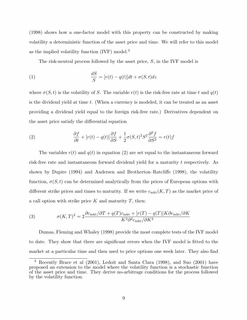
(1998) shows how a one-factor model with this property can be constructed by making

volatility a deterministic function of the asset price and time. We will refer to this model

as the implied volatility function (IVF) model.3

The risk-neutral process followed by the asset price, S, in the IVF model is

(1)dS

S= [r(t)− q(t)]dt+ σ(S, t)dz

where σ(S, t) is the volatility of S. The variable r(t) is the risk-free rate at time t and q(t)

is the dividend yield at time t. (When a currency is modeled, it can be treated as an asset

providing a dividend yield equal to the foreign risk-free rate.) Derivatives dependent on

the asset price satisfy the differential equation

(2)∂f

∂t+ [r(t)− q(t)]

∂f

∂S+

1

2σ(S, t)2S2 ∂

2f

∂S2= r(t)f

The variables r(t) and q(t) in equation (2) are set equal to the instantaneous forward

risk-free rate and instantaneous forward dividend yield for a maturity t respectively. As

shown by Dupire (1994) and Andersen and Brotherton–Ratcliffe (1998), the volatility

function, σ(S, t) can be determined analytically from the prices of European options with

different strike prices and times to maturity. If we write cmkt(K,T ) as the market price of

a call option with strike price K and maturity T , then:

(3) σ(K,T )2 = 2∂cmkt/∂T + q(T )cmkt + [r(T )− q(T )]K∂cmkt/∂K

K2∂2cmkt/∂K2

Dumas, Fleming and Whaley (1998) provide the most complete tests of the IVF model

to date. They show that there are significant errors when the IVF model is fitted to the

market at a particular time and then used to price options one week later. They also find

3 Recently Brace et al (2001), Ledoit and Santa Clara (1998), and Suo (2001) haveproposed an extension to the model where the volatility function is a stochastic functionof the asset price and time. They derive no-arbitrage conditions for the process followedby the volatility function.

9

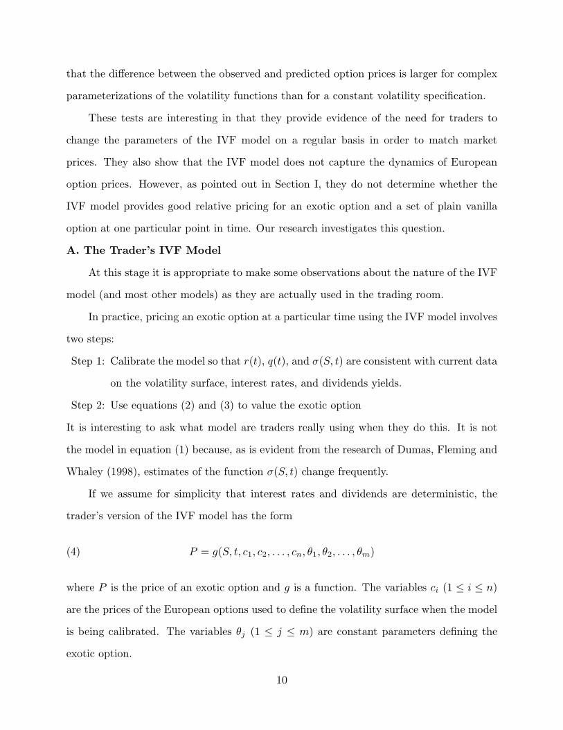
that the difference between the observed and predicted option prices is larger for complex

parameterizations of the volatility functions than for a constant volatility specification.

These tests are interesting in that they provide evidence of the need for traders to

change the parameters of the IVF model on a regular basis in order to match market

prices. They also show that the IVF model does not capture the dynamics of European

option prices. However, as pointed out in Section I, they do not determine whether the

IVF model provides good relative pricing for an exotic option and a set of plain vanilla

option at one particular point in time. Our research investigates this question.

A. The Trader’s IVF Model

At this stage it is appropriate to make some observations about the nature of the IVF

model (and most other models) as they are actually used in the trading room.

In practice, pricing an exotic option at a particular time using the IVF model involves

two steps:

Step 1: Calibrate the model so that r(t), q(t), and σ(S, t) are consistent with current data

on the volatility surface, interest rates, and dividends yields.

Step 2: Use equations (2) and (3) to value the exotic option

It is interesting to ask what model are traders really using when they do this. It is not

the model in equation (1) because, as is evident from the research of Dumas, Fleming and

Whaley (1998), estimates of the function σ(S, t) change frequently.

If we assume for simplicity that interest rates and dividends are deterministic, the

trader’s version of the IVF model has the form

(4) P = g(S, t, c1, c2, . . . , cn, θ1, θ2, . . . , θm)

where P is the price of an exotic option and g is a function. The variables ci (1 ≤ i ≤ n)

are the prices of the European options used to define the volatility surface when the model

is being calibrated. The variables θj (1 ≤ j ≤ m) are constant parameters defining the

exotic option.

10

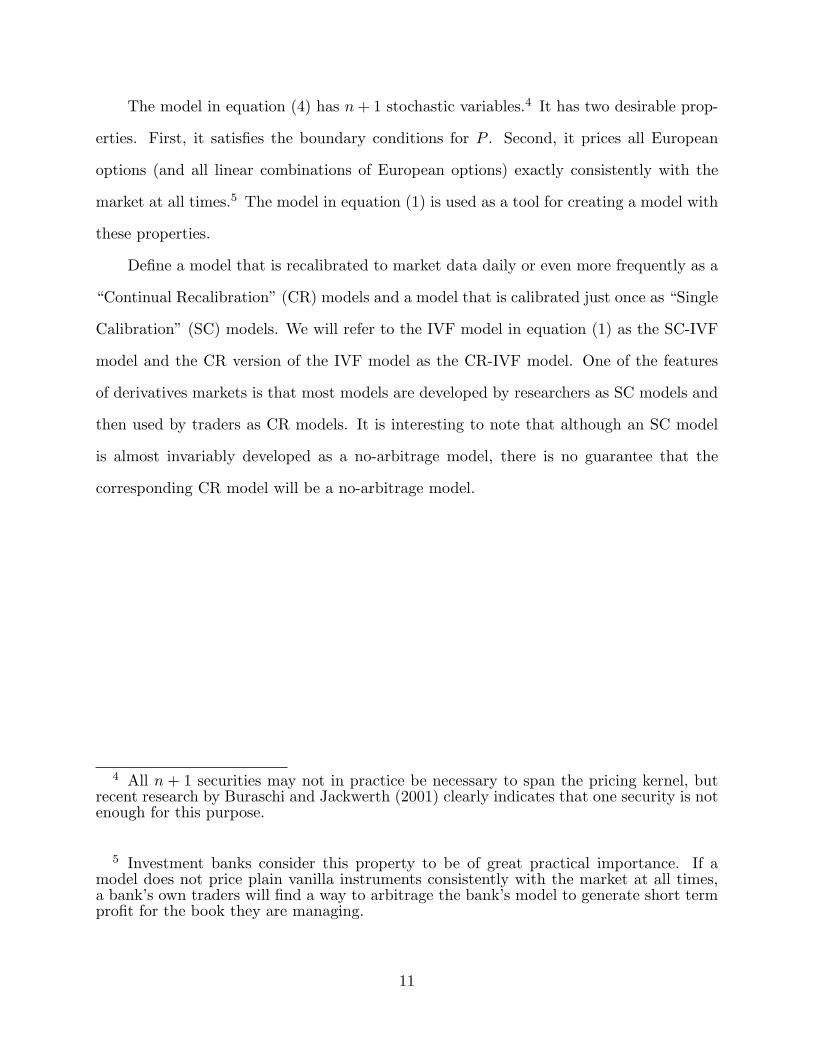
The model in equation (4) has n+ 1 stochastic variables.4 It has two desirable prop-

erties. First, it satisfies the boundary conditions for P . Second, it prices all European

options (and all linear combinations of European options) exactly consistently with the

market at all times.5 The model in equation (1) is used as a tool for creating a model with

these properties.

Define a model that is recalibrated to market data daily or even more frequently as a

“Continual Recalibration” (CR) models and a model that is calibrated just once as “Single

Calibration” (SC) models. We will refer to the IVF model in equation (1) as the SC-IVF

model and the CR version of the IVF model as the CR-IVF model. One of the features

of derivatives markets is that most models are developed by researchers as SC models and

then used by traders as CR models. It is interesting to note that although an SC model

is almost invariably developed as a no-arbitrage model, there is no guarantee that the

corresponding CR model will be a no-arbitrage model.

4 All n + 1 securities may not in practice be necessary to span the pricing kernel, butrecent research by Buraschi and Jackwerth (2001) clearly indicates that one security is notenough for this purpose.

5 Investment banks consider this property to be of great practical importance. If amodel does not price plain vanilla instruments consistently with the market at all times,a bank’s own traders will find a way to arbitrage the bank’s model to generate short termprofit for the book they are managing.

11

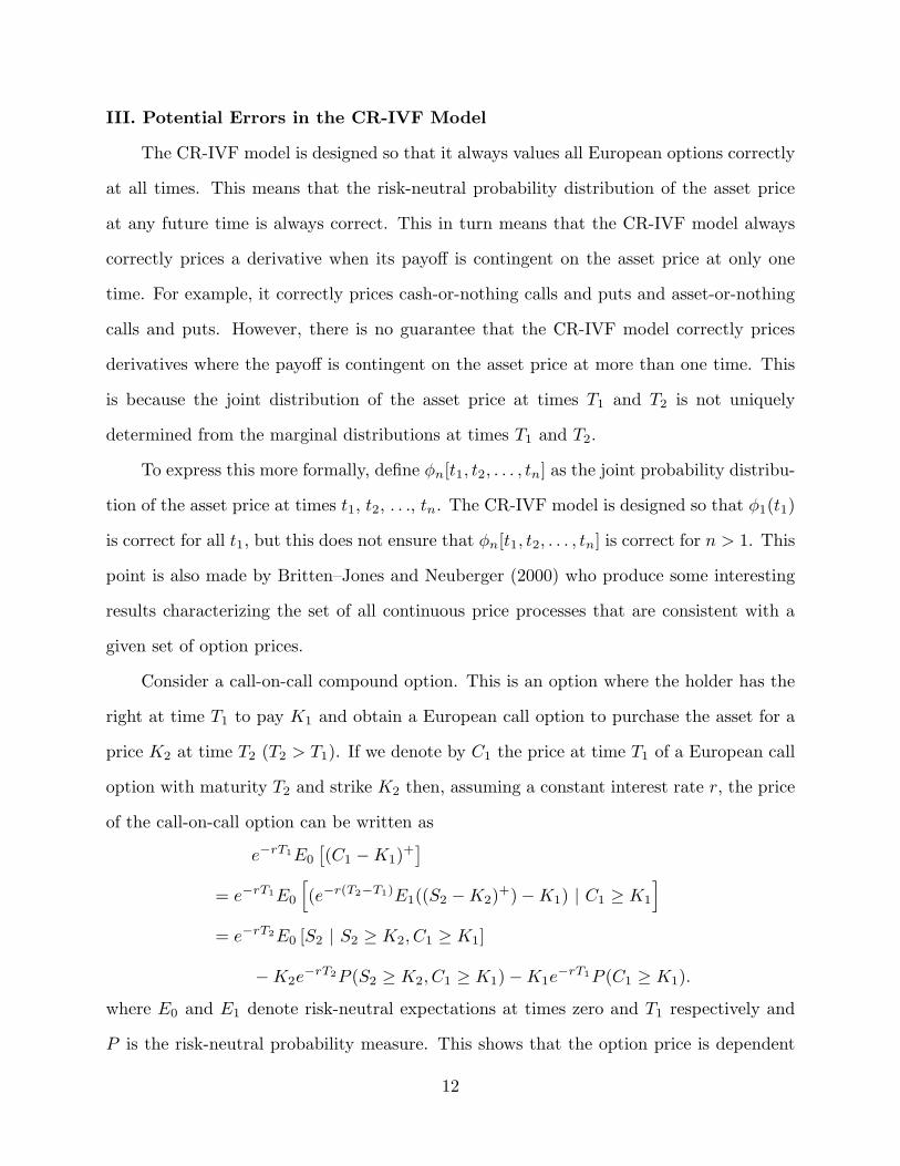
III. Potential Errors in the CR-IVF Model

The CR-IVF model is designed so that it always values all European options correctly

at all times. This means that the risk-neutral probability distribution of the asset price

at any future time is always correct. This in turn means that the CR-IVF model always

correctly prices a derivative when its payoff is contingent on the asset price at only one

time. For example, it correctly prices cash-or-nothing calls and puts and asset-or-nothing

calls and puts. However, there is no guarantee that the CR-IVF model correctly prices

derivatives where the payoff is contingent on the asset price at more than one time. This

is because the joint distribution of the asset price at times T1 and T2 is not uniquely

determined from the marginal distributions at times T1 and T2.

To express this more formally, define φn[t1, t2, . . . , tn] as the joint probability distribu-

tion of the asset price at times t1, t2, . . ., tn. The CR-IVF model is designed so that φ1(t1)

is correct for all t1, but this does not ensure that φn[t1, t2, . . . , tn] is correct for n > 1. This

point is also made by Britten–Jones and Neuberger (2000) who produce some interesting

results characterizing the set of all continuous price processes that are consistent with a

given set of option prices.

Consider a call-on-call compound option. This is an option where the holder has the

right at time T1 to pay K1 and obtain a European call option to purchase the asset for a

price K2 at time T2 (T2 > T1). If we denote by C1 the price at time T1 of a European call

option with maturity T2 and strike K2 then, assuming a constant interest rate r, the price

of the call-on-call option can be written as

e−rT1E0

[

(C1 −K1)+]

= e−rT1E0

[

(e−r(T2−T1)E1((S2 −K2)+)−K1) | C1 ≥ K1

]

= e−rT2E0 [S2 | S2 ≥ K2, C1 ≥ K1]

−K2e−rT2P (S2 ≥ K2, C1 ≥ K1)−K1e

−rT1P (C1 ≥ K1).

where E0 and E1 denote risk-neutral expectations at times zero and T1 respectively and

P is the risk-neutral probability measure. This shows that the option price is dependent

12

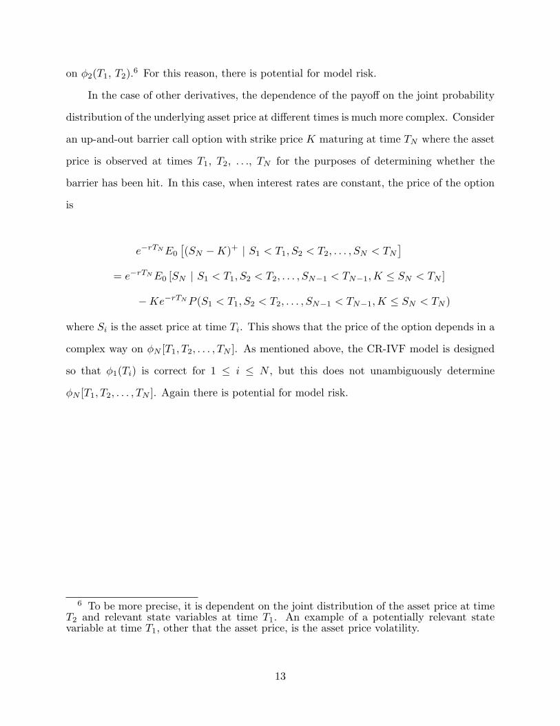
on φ2(T1, T2).6 For this reason, there is potential for model risk.

In the case of other derivatives, the dependence of the payoff on the joint probability

distribution of the underlying asset price at different times is much more complex. Consider

an up-and-out barrier call option with strike price K maturing at time TN where the asset

price is observed at times T1, T2, . . ., TN for the purposes of determining whether the

barrier has been hit. In this case, when interest rates are constant, the price of the option

is

e−rTNE0

[

(SN −K)+ | S1 < T1, S2 < T2, . . . , SN < TN

]

= e−rTNE0 [SN | S1 < T1, S2 < T2, . . . , SN−1 < TN−1,K ≤ SN < TN ]

−Ke−rTNP (S1 < T1, S2 < T2, . . . , SN−1 < TN−1,K ≤ SN < TN )

where Si is the asset price at time Ti. This shows that the price of the option depends in a

complex way on φN [T1, T2, . . . , TN ]. As mentioned above, the CR-IVF model is designed

so that φ1(Ti) is correct for 1 ≤ i ≤ N , but this does not unambiguously determine

φN [T1, T2, . . . , TN ]. Again there is potential for model risk.

6 To be more precise, it is dependent on the joint distribution of the asset price at timeT2 and relevant state variables at time T1. An example of a potentially relevant statevariable at time T1, other that the asset price, is the asset price volatility.

13

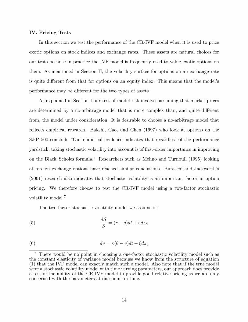
IV. Pricing Tests

In this section we test the performance of the CR-IVF model when it is used to price

exotic options on stock indices and exchange rates. These assets are natural choices for

our tests because in practice the IVF model is frequently used to value exotic options on

them. As mentioned in Section II, the volatility surface for options on an exchange rate

is quite different from that for options on an equity index. This means that the model’s

performance may be different for the two types of assets.

As explained in Section I our test of model risk involves assuming that market prices

are determined by a no-arbitrage model that is more complex than, and quite different

from, the model under consideration. It is desirable to choose a no-arbitrage model that

reflects empirical research. Bakshi, Cao, and Chen (1997) who look at options on the

S&P 500 conclude “Our empirical evidence indicates that regardless of the performance

yardstick, taking stochastic volatility into account is of first-order importance in improving

on the Black–Scholes formula.” Researchers such as Melino and Turnbull (1995) looking

at foreign exchange options have reached similar conclusions. Buraschi and Jackwerth’s

(2001) research also indicates that stochastic volatility is an important factor in option

pricing. We therefore choose to test the CR-IVF model using a two-factor stochastic

volatility model.7

The two-factor stochastic volatility model we assume is:

(5)dS

S= (r − q)dt+ vdzS

(6) dv = κ(θ − v)dt+ ξdzv

7 There would be no point in choosing a one-factor stochastic volatility model such asthe constant elasticity of variance model because we know from the structure of equation(1) that the IVF model can exactly match such a model. Also note that if the true modelwere a stochastic volatility model with time varying parameters, our approach does providea test of the ability of the CR-IVF model to provide good relative pricing as we are onlyconcerned with the parameters at one point in time.

14

In these equations zS and zv are Wiener processes with an instantaneous correlation ρ.

The variable v is a factor driving asset prices. The volatility of S is |v| and the model is

well defined when v is negative. The parameters κ, θ, and ξ are the mean-reversion rate,

long-run average volatility, and standard deviation of v, respectively, and are assumed

to be constants. We also assume the spot rate, r, and the yield on the asset, q, are

constants. The parameters of the model are chosen to minimize the root mean square

error in matching the observed market prices for European options. The model is similar

to the one proposed by Heston (1993) and has similar analytic properties.8

A valuation formula for the European call option price, csv(S, v, t;K,T ), in the model

can be computed through the inversion of characteristic functions of random variables. It

takes the form:

(7) csv(S, v, t;K,T ) = e−q(T−t)S(t)F1 − e−r(T−t)KF2

where F1 and F2 are integrals that can be evaluated efficiently using numerical procedures

such as quadrature. More details on the model can be found in Schobel and Zhu (1998).9

When considering S&P 500 options we chose model parameters to provide as close a fit

as possible to the volatility surface for the S&P 500 reported in Andersen and Brotherton–

Ratcliffe (1998). The parameters are

8 If V = v2 is the variance rate, the model we assume implies that

dV = (ξ + 2κθ√V − 2κV ) dt+ 2ξ

√V dzv

Heston’s model is of the form:

dV = (α− βV ) dt+ γ√V dzv

More details on the model’s analytic properties are available from the authors on request.

9 The results in Schobel and Zhu (1998) and Monte Carlo simulation were used as acheck of the implementation of equation (7).

15

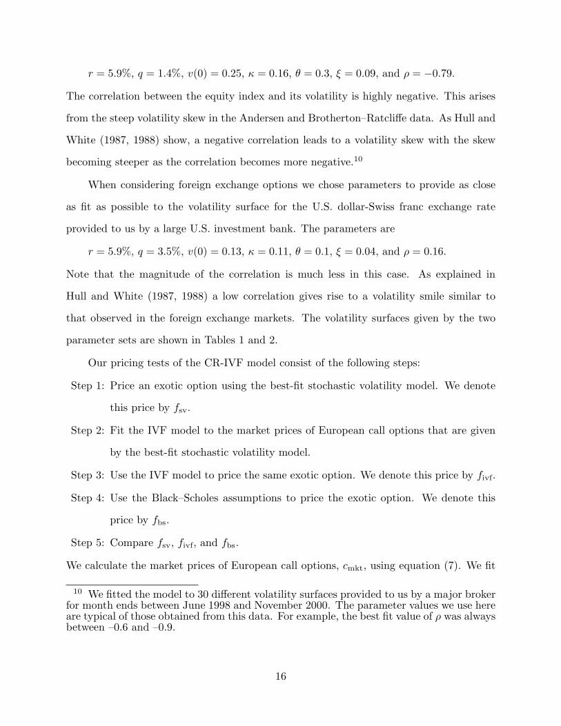
r = 5.9%, q = 1.4%, v(0) = 0.25, κ = 0.16, θ = 0.3, ξ = 0.09, and ρ = −0.79.

The correlation between the equity index and its volatility is highly negative. This arises

from the steep volatility skew in the Andersen and Brotherton–Ratcliffe data. As Hull and

White (1987, 1988) show, a negative correlation leads to a volatility skew with the skew

becoming steeper as the correlation becomes more negative.10

When considering foreign exchange options we chose parameters to provide as close

as fit as possible to the volatility surface for the U.S. dollar-Swiss franc exchange rate

provided to us by a large U.S. investment bank. The parameters are

r = 5.9%, q = 3.5%, v(0) = 0.13, κ = 0.11, θ = 0.1, ξ = 0.04, and ρ = 0.16.

Note that the magnitude of the correlation is much less in this case. As explained in

Hull and White (1987, 1988) a low correlation gives rise to a volatility smile similar to

that observed in the foreign exchange markets. The volatility surfaces given by the two

parameter sets are shown in Tables 1 and 2.

Our pricing tests of the CR-IVF model consist of the following steps:

Step 1: Price an exotic option using the best-fit stochastic volatility model. We denote

this price by fsv.

Step 2: Fit the IVF model to the market prices of European call options that are given

by the best-fit stochastic volatility model.

Step 3: Use the IVF model to price the same exotic option. We denote this price by fivf.

Step 4: Use the Black–Scholes assumptions to price the exotic option. We denote this

price by fbs.

Step 5: Compare fsv, fivf, and fbs.

We calculate the market prices of European call options, cmkt, using equation (7). We fit

10 We fitted the model to 30 different volatility surfaces provided to us by a major brokerfor month ends between June 1998 and November 2000. The parameter values we use hereare typical of those obtained from this data. For example, the best fit value of ρ was alwaysbetween –0.6 and –0.9.

16

the IVF model to these prices by calculating ∂cmkt/∂t, ∂cmkt/∂K, and ∂2cmkt/∂K2 from

equation (7) and then using equation (3).

We consider two types of exotic options: a call-on-call compound option and a knock-

out barrier option. We use Monte Carlo simulation with 300 time steps and 100,000

trials to estimate the prices of these options for the stochastic volatility model.11 For this

purpose, equations (5) and (6) are discretized to

(8) lnSi+1

Si=

(

r − q − v2i2

)

∆t+ viε1√∆t

(9) vi+1 − vi = κ(θ − vi)∆t+ ξε2√∆t

where ∆t is the length of the Monte Carlo simulation time step, Si and vi are the asset

price and its volatility at time i∆t, and ε1 and ε2 are random samples from two unit normal

distributions with correlation, ρ.

We estimate the prices given by the IVF model from equation (2) using the implicit

Crank-Nicholson finite difference method described in Andersen and Brotherton–Ratcliffe

(1998). This involves constructing a 120 × 70 rectangular grid of points in (x, t)-space,

where x = lnS. The grid extends from time zero to the maturity of the exotic option,

Tmat. Define xmin and xmax as the lowest and highest x-values considered on the grid. (We

explain how these are determined later.) Boundary conditions determine the values of the

exotic option on the x = xmax, x = xmin and t = Tmat edges of the grid. The differential

equation (2) enables relationships to be established between the values of the exotic option

at the nodes at the ith time point and its values at the nodes at the (i+ 1)th time point.

These relationships are used in conjunction with boundary conditions to determine the

value of the exotic option at all interior nodes of the grid and its value at the nodes at

time zero.

11 To reduce the variance of the estimates, we use the antithetic variable techniquedescribed in Boyle (1977).

17

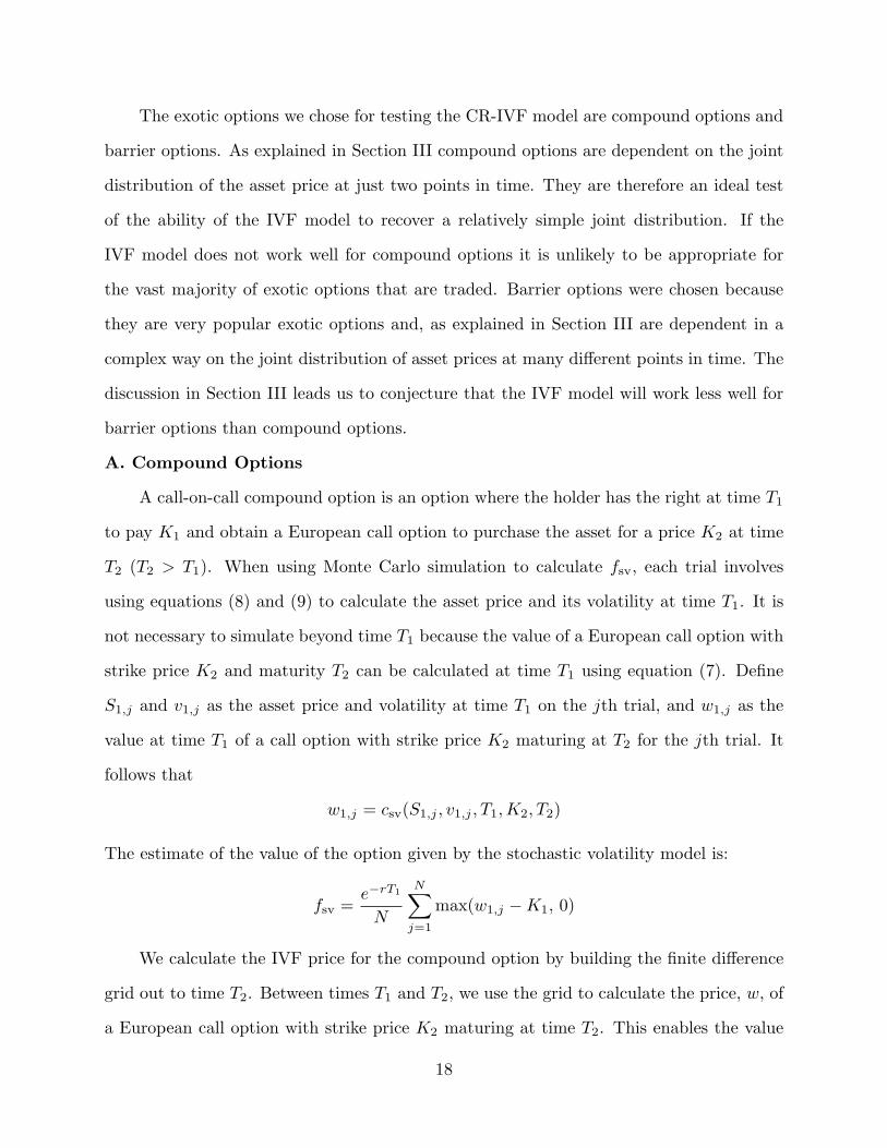
The exotic options we chose for testing the CR-IVF model are compound options and

barrier options. As explained in Section III compound options are dependent on the joint

distribution of the asset price at just two points in time. They are therefore an ideal test

of the ability of the IVF model to recover a relatively simple joint distribution. If the

IVF model does not work well for compound options it is unlikely to be appropriate for

the vast majority of exotic options that are traded. Barrier options were chosen because

they are very popular exotic options and, as explained in Section III are dependent in a

complex way on the joint distribution of asset prices at many different points in time. The

discussion in Section III leads us to conjecture that the IVF model will work less well for

barrier options than compound options.

A. Compound Options

A call-on-call compound option is an option where the holder has the right at time T1

to pay K1 and obtain a European call option to purchase the asset for a price K2 at time

T2 (T2 > T1). When using Monte Carlo simulation to calculate fsv, each trial involves

using equations (8) and (9) to calculate the asset price and its volatility at time T1. It is

not necessary to simulate beyond time T1 because the value of a European call option with

strike price K2 and maturity T2 can be calculated at time T1 using equation (7). Define

S1,j and v1,j as the asset price and volatility at time T1 on the jth trial, and w1,j as the

value at time T1 of a call option with strike price K2 maturing at T2 for the jth trial. It

follows that

w1,j = csv(S1,j , v1,j , T1,K2, T2)

The estimate of the value of the option given by the stochastic volatility model is:

fsv =e−rT1

N

N∑

j=1

max(w1,j −K1, 0)

We calculate the IVF price for the compound option by building the finite difference

grid out to time T2. Between times T1 and T2, we use the grid to calculate the price, w, of

a European call option with strike price K2 maturing at time T2. This enables the value

18

of the compound option at the nodes at time T1 to be calculated as max(w −K1, 0). We

then use the part of the grid between time zero and time T1 to calculate the value of the

compound option at time zero. We set xmin = lnSmin and xmax = lnSmax where Smin and

Smax are very high and very low asset prices, respectively. The boundary conditions we

use are:

w = max(ex −K2, 0) when t = T2

w = 0 when x = xmin and T1 ≤ t ≤ T2

w = ex −K2e−r(T2−t) when x = xmax and T1 ≤ t ≤ T2

fivf = 0 when x = xmin and 0 ≤ t ≤ T1

fivf = ex −K2e−r(T2−t) −K1e

−r(T1−t) when x = xmin and 0 ≤ t ≤ T1

The value of a compound option using the Black–Scholes assumptions was first pro-

duced by Geske (1979). Geske shows that at time zero:

fbs = S(0)e−qT2M(a1, b1;√

T1/T2)−K2e−rT2M(a2, b2;

√

T1/T2)− e−rT1K1N(a2)

where

a1 =ln[S(0)/S∗] + (r − q + σ2/2)T1

σ√T1

, a2 = a1 − σ√

T1

b1 =ln[S(0)/K2] + (r − q + σ2/2)T2

σ√T2

, b2 = b1 − σ√

T2

andM(a, b; ρ), is the cumulative probability in a standardized bivariate normal distribution

that the first variable is less than a and the second variable is less than b when the coefficient

of correlation between the variables is ρ. The variable S∗ is the asset price at time T1 for

which the price at time T1 of a European call option with strike price K2 and maturity

T2 equals K1. If the actual asset price is above S∗ at time T1, the first option will be

exercised; if it is not above S∗, the compound option expires worthless. In computing fbs

we set σ equal to the implied volatility of a European option maturing at time T2 with a

strike price of K2.

19

Table 3 shows fsv and the percentage errors when the option price is approximated

by fivf and fbs for the case where T1 = 1, T2 = 2, and K2 equals the initial asset price. It

considers a wide range of values of K1. The table shows that the IVF model works very

well. For compound options where the stochastic volatility price is greater than 1% of the

initial asset price, the IVF price is within 2% of the stochastic volatility price. When very

high strike prices are used with Parameter Set II this percentage error is higher, but this

is because the stochastic volatility price of the compound option is very low. Measured

as a percent of the initial asset price the absolute pricing error of the IVF model is never

greater than 0.08%.

The Black–Scholes model, on the other hand, performs quite badly. For high values

of the strike price, K1, it significantly overprices the compound option in the case of the

stock index data and significantly underprices it in the case of the foreign currency data.

The reason is that, when K1 is high, the first call option is exercised only when the asset

price is very high at time T1. Consider first the stock index data. As shown in Table

1, the implied volatility is a declining function of the strike price. (This is the volatility

skew phenomenon for a stock index described in Section I). As a result the probability

distribution of the asset price at time T1 has a more heavy left tail and a less heavy right

tail than a lognormal distribution when the latter is calculated using the at-the-money

volatility, and very high asset prices are much less likely than they are under the Black–

Scholes model. This means that the first option is much more likely to be exercised at

time T1 in the Black–Scholes world than in the assumed true world. Consider next the

foreign currency data. As shown in Table 2, the implied volatility is a U-shaped function.

(This is the volatility smile phenomenon for a currency described in Section I.) The results

in the probability distribution of the asset price having heavier left and right tails than a

lognormal distribution when the latter is calculated using the at-the-money volatility, and

very high asset prices are much more likely than they are under the Black–Scholes model.

This means that the first option is much less likely to be exercised in the Black–Scholes

20

world than in the assumed true world.

Traders sometimes try to make the Black–Scholes model work for compound options

by adjusting the volatility. Sometimes they use two different volatilities, one for the period

between time zero and time T1 and the other for the period between time T1 and time

T2. There is of course some volatility (or pair of volatilities) that will give the correct

price for any given compound option. But the price of a compound option given by the

Black-Scholes model is highly sensitive to the volatility and any procedure that involves

estimating the “correct” volatility is dangerous and liable to give rise to significant errors.

Based on the tests reported here and other similar tests we have carried out, the IVF

model is a big improvement over the Black–Scholes model when compound options are

priced. There is very little evidence of model risk. This is encouraging, but of course it

provides no guarantee that the model is also a proxy for all more complicated multifactor

models.

B. Barrier Options

The second exotic option we consider is a knock-out barrier call option. This is a

European call option with strike price K and maturity T that ceases to exist if the asset

price reaches a barrier level, H. When the barrier is greater than the initial asset price,

the option is referred to as an up-and-out call; when the barrier is less than the initial

asset price, it is referred to as a down-and-out call.

When using Monte Carlo simulation to calculate fsv, each trial involved using equa-

tions (8) and (9) simulate a path for the asset price between time zero and time T . For

an up-and-out (down-and-out) option, if for some i, the asset price is above (below) H at

time i∆t on the jth trial the payoff from the barrier option is set equal to zero on that

trial. Otherwise the payoff from the barrier option is max[S(T ) − K, 0] at time T . The

estimate of fsv is the arithmetic mean of the payoffs on all trials discounted from time T

to time zero at rate r.12

12 To improve computational efficiency we applied the correction for discrete observations

21

We calculate the IVF price for the barrier option by building the finite difference

grid out to time T . In the case of an up-and-out option, we set xmax = ln(H) and

xmin = lnSmin where Smin is a very low asset price; in the case of a down-and-out option,

we set xmin = ln(H) and xmax = lnSmax where Smax is a very high asset price. For an

up-and-out call option, the boundary conditions are:

fivf = max(ex −K2, 0) when t = T

fivf = 0 when x ≥ ln(H) and 0 ≤ t ≤ T

fivf = 0 when x = xmin and 0 ≤ t ≤ T

For a down-and-out call, the boundary conditions are similar except that

fivf = ex −K2e−r(T−t) when x = xmax

The value of knock-out options using the Black–Scholes assumptions was first pro-

duced by Merton (1973). He showed that at time zero, the price of a down-and-out call

option is

fbs = S(0)N(d1)e−qT −KN(d2)e

−rT − S(0)e−qT [H/S(0)]2λN(y)

+Ke−rT [H/S(0)]2λ−2N(y − σ√T )

and that the price of an up-and-out call is

fbs = S(0)e−qT [N(d1)−N(x1)]−Ke−rT [N(d2)−N(x1 − σ√T )]

+S(0)e−qT [H/S(0)]2λ[N(−y)−N(−y1)]

−Ke−rT [H/S(0)]2λ−2[N(−y + σ√T )−N(−y1 + σ

√T )]

where

discussed in Broadie, Glasserman, and Kou (1997).

22

λ =r − q + σ2/2

σ2

y =ln{H2/[S(0)K]}

σ√T

+ λσ√T

x1 =ln[S(0)/H]

σ√T

+ λσ√T

x2 =ln[H/S(0)]

σ√T

+ λσ√T

d1 =ln[S(0)/K] + (r − q + σ2/2)T

σ√T

d2 = d1 − σ√T

and N is the cumulative normal distribution function. In computing fbs we set σ equal

to the implied volatility of a regular European call option with strike price K maturing at

time T .

Tables 4 and 5 show fsv and the percentage errors when the option is approximated

by fivf and fbs for the cases where K are 90% and 100% of the initial asset price and

the time to maturity is two years. We consider a wide range of values for the barrier H.

(When H > 100 the option is an up-and-out call; when H < 100 it is a down-and-out call.)

A comparison of Table 3 with Tables 4 and 5 shows that the IVF model does not perform

as well for barrier options as it does for compound options. For some values of the barrier,

errors are high in both absolute terms and percentage terms in both the stock index and

foreign currency cases. We carried out some tests (not reported here) using options with

maturities other than two years. We found that the maximum potential percentage pricing

error in the IVF model increases with the maturity of the option.

We conclude from these and other similar tests that there is significant model risk

when the IVF model is used to price barrier options for some sets of parameter values.

This is an important result. Barrier option are amongst the most popular exotic options.

23

V. Hedging Using the CR-IVF Model

As already mentioned, when traders use the CR-IVF model, they hedge against

changes in the volatility surface as well as against changes in the asset price. The model

has the form shown in equation (4). Traders calculate ∂P/∂ci for 1 ≤ i ≤ n (or equivalent

partial derivatives involving attributes of the volatility surface) as well as ∂P/∂S and at-

tempt to combine their positions in exotic options with positions in the underlying asset

and positions in European options to create a portfolio that is riskless when it is valued

using the CR-IVF model.13 They means that they create a portfolio whose value, Π, (as

measured by the CR-IVF model) satisfies

∂Π

∂ci= 0

for (1 ≤ i ≤ n) and

∂Π

∂S= 0

Our test of the hedging effectiveness of the CR-IVF model is analogous to our test of

its pricing effectiveness. We assume that the fitted two-factor stochastic volatility model

in equations (5) and (6) gives the true price of an exotic option. This model has two

underlying stochastic variables: S, the asset price and v, the volatility. We test whether

that the CR-IVF model gives reasonable estimates of the sensitivities of the exotic option

price changes to S and v.14 We calculate numerically the partial derivative of exotic

option prices with respect to each of S and v for both the stochastic volatility model and

the CR-IVF model. The partial derivative with respect to S is the delta, ∆, and the partial

derivative with respect to v is the vega, V, of the exotic option.

13 Given the nature of the CR-IVF model the partial derivatives of P with respect to Sand the ci cannot be calculated analytically. They must be calculated by perturbing thestock price and each of the n option prices in turn, recalibrating the model, and observingthe effect on the exotic option price, P .

14 This is an indirect way of testing whether a hedge portfolio consisting of the underlyingasset and plain vanilla options will work.

24

In order to compute ∆, we increase the spot price by 1%, and compute the price

changes from both the stochastic volatility model and the CR-IVF model.15 To compute

vega we increase the initial instantaneous volatility by 1% and compute price changes for

both the stochastic volatility model and the CR-IVF model.16 Note that the calculation

of delta for the CR-IVF model involves calibrating the model twice to the option prices

given by the stochastic volatility model, once before and once after S has been perturbed.

The same is true of vega.

Our hedging results for the compound options considered in Table 3 are shown in

Table 6. The table shows that using the CR-IVF model for hedging gives good results in a

world described by the two-factor stochastic volatility model. Our hedging results for the

barrier option considered in Table 4 are shown in Table 7. The percentage errors in the

deltas calculated by the CR-IVF model are similar to the percentage pricing errors. The

vegas calculated for the CR-IVF model are quite often markedly different from the vegas

calculated using the stochastic volatility model. This is indication that volatility hedges

created using the CR-IVF model for barrier options may not be effective. The tests for

the barrier options in Table 5 and others we considered produced similar results.

15 We also computed delta for the SC-IVF model. These are not reported, but areslightly worse than the deltas from the CR-IVF model.

16 As already mentioned, in practice traders calculate vega by shifting the volatilitysurface. A number of vegas might be calculated, each corresponding to a different shift.Given our set up, which assumes that the stochastic volatility model is the true model andcomparing results with that model, we look at only one vega.

25

VI. Economic Intuition for Results

Our results show that the CR-IVF model works quite well for compound options and

much less well for barrier options. This is consistent with the observation in Section III

that the payoff from a compound option is much less dependent on joint distribution of

the asset price at different points in time than it is for barrier option.

Figure 1 provides another way of understanding the results. It shows the Black–

Scholes price of the equity index barrier option as a function of volatility when the strike

price is 100 and the barrier is 130. This has significant convexity. As shown by Hull

and White (1987), when there is zero correlation between the asset price and volatility,

the stochastic volatility price of a barrier option is its Black–Scholes price integrated over

the probability distribution of the average variance rate during the life of the option.

The convexity therefore leads to the value of the option increasing as the volatility of

the volatility increases in the zero correlation case. For the equity index, the correlation

between stock price and volatility is negative rather than zero. This increases the value of

the option still further because high stock prices tend to be associated with low volatilities

making it less likely that the barrier will be hit.

These arguments explain why the Black–Scholes price of the option we are considering

is 38.61% less than the stochastic volatility price. Consider next the IVF price. The IVF

model does incorporate a negative correlation between stock price and volatility. However,

it is a one-factor model and does not lead to as wide a range of high and low volatility

outcomes as the stochastic volatility model. As a result it does not fully reflect the impact

of the convexity in Figure 1 and gives a lower price than the stochastic volatility model.

Other big discrepancies between the IVF price and the stochastic volatility price in

Tables 4 and 5 can be explained similarly. For compound options, and for barrier options

when the IVF percentage error is low, there is very little convexity in the relationship

between the option price and volatility and as a result the IVF model works much better.

26

VII. Summary

It is important that tests of model risk reflect the way models are actually used by

traders. Researchers and traders often use models differently. A model when it is developed

by researchers is usually a SC (single calibration) model. When the same model is used by

traders it is a CR (continual recalibration) model and is used to provide relative valuation

among derivative securities. The researcher-developed SC models are usually arbitrage

free. The corresponding CR models used by traders are not necessarily arbitrage free.

This paper presents a methodology for testing the use of a CR model for valuing illiquid

securities and applies the methodology to the implied volatility function (IVF) model.

The CR-IVF model has the attractive feature that it always matches the prices of

European options. This means that the unconditional probability distribution of the un-

derlying asset price at all future times is always correct. An exotic option, whose payoff

is contingent on the asset price at just one time is always correctly priced by the CR-IVF

model. Unfortunately, many exotic options depend in a complex way on the joint proba-

bility distribution of the asset price at two or more times. There is no guarantee that the

CR-IVF model will provide good pricing and hedging for these instruments.

In this paper we examine the model risk in the CR-IVF model by fitting a stochastic

volatility model to market data and then comparing the prices of compound options and

barrier options with those given by the IVF model. We find that the CR-IVF model

gives reasonably good results for compound options. The results for barrier options are

much less satisfactory. The CR-IVF model does not recover enough aspects of the dynamic

features of the asset price process to give reasonably accurate prices for some combinations

of the strike price and barrier level. The hedge parameters produced by the model also

sometimes have large errors.

An analysis of the CR-IVF model leads to the conjecture that the performance of the

model should depend on the degree of path dependence in the exotic option being priced

where “degree of path dependence” is defined as the number of times the asset price must

27

be observed to calculate the payoff. The higher the degree of path dependence the worse

the model is expected to perform. Compound options have a much lower degree of path

dependence than barrier options. Our results are therefore consistent with the conjecture.

28

References

Andersen, L., and J. Andreasen. “Factor Dependence of Bermudan Swaptions: Factor Fiction.” Journal of Financial Economics, 62, 1 (2001), 3–37.

Andersen, L., and R. Brotherton-Ratcliffe. “The Equity Option Volatility Smile: AnImplicit Finite-Difference Approach.” Journal of Computational Finance, 1, 2 (1998),5-37.

Bakshi, G., C. Cao, and Z. Chen. “Empirical Performance of Alternative OptionPricing Models.” Journal of Finance, 52, 5 (1997), 2003-49.

Basle Committee on Banking Supervision. A New Capital Adequacy Framework.Bank for International Settlements, Basle, 1999.

Bates, D. “Jumps and Stochastic Volatilities: Exchange Rate Processes Implicit inthe Deutsche Mark Options.” Review of Financial Studies, 9 (1996), 69-107.

Black, F. and M. S. Scholes. “The Pricing of Options and Corporate Liabilities.”Journal of Political Economy, 81 (1973), 637-59.

Boyle, P. P. “Options: A Monte Carlo Approach.” Journal of Financial Economics, 4(1977), 323-38.

Brace, A., B. Goldys, F. Klebaner, and R. Womersley. “Market Model of Stochas-tic Implied Volatility with Application to the BGM Model.” Working Paper S01-1,Department of Statistics, University of New South Wales, 2001.

Britten–Jones, M., and A. Neuberger. “Option Prices, Implied Price Processes, andStochastic Volatility.” Journal of Finance, 55, 2 (2000), 839–66.

Broadie, M., P. Glassermann, and S. G. Kou. “A Continuity Correction for DiscreteBarrier Options.” Mathematical Finance, 7 (1997), 325–49.

Buraschi, A., and J. Jackwerth. “The Price of a Smile: Hedging and Spanning inoptions Markets.” Review of Financial Studies, 14, 2 (2001), 495–528.

Derman, E. (1996) “Model risk.” Quantitative Strategies Research Notes, GoldmanSachs, New York, NY, 1996.

Derman, E., and I. Kani. (1994), “The Volatility Smile and its Implied Tree.” Quan-titative Strategies Research Notes, Goldman Sachs, New York, NY, 1994.

Driessen, J., P. Klaassen, and B. Melenberg. “The Performance of Multi-Factor TermStructure Models for Pricing and Hedging Caps and Swaptions.” Working Paper,Department of Econometrics and CentER, Tilburg University, 2000.

Dumas, B., J. Fleming and R. E. Whaley. “Implied Volatility Functions: EmpiricalTests.” Journal of Finance 53, 6 (1998), 2059–2106.

Dupire, B. “Pricing with a Smile.” Risk, 7 (1994), 18–20.

Geske, R. “The Valuation of Compound Options.” Journal of Financial Economics,7, 1 (1979), 63-82.

Goldman, B., H. Sosin, and M. A. Gatto. “Path Dependent Options: Buy at the Low,Sell at the High.” Journal of Finance, 34, 5 (1979) 1111-27.

Green, T.C., and S. Figlewski. “Market Risk and Model Risk for a Financial Institu-tion Writing Options.” Journal of Finance, 54, 4 (1999), 1465-99.

29

Gupta A., and M. G. Subrahmanyam. “An Examination of the Static and DynamicPerformance of Interest Rate Models in the Dollar Cap–Floor Markets.” WorkingPaper, Weatherhead School of Management, Case Western Reserve University, 2000.

Heston, S. L. “A Closed-Form Solution for Options with Stochastic Volatility Appli-cations to Bond and Currency Options.” Review of Financial Studies, 6, 2 (1993),327-43.

Hull, J. and A. White. “The Pricing of Options with Stochastic Volatility.” Journalof Finance, 42, 2 (1987), 281-300.

Hull, J. and A. White. “An Analysis of the Bias in Option Pricing Caused by aStochastic Volatility.” Advances in Futures and Options Research, 3 (1988), 27-61.

Hull, J. and A. White. “Forward Rate Volatilities, Swap Rate Volatilities, and theImplementation of the LIBOR Market Model.” Journal of Fixed Income, 10, 2 (2000)46–62.

Jackwerth, J. C. and M. Rubinstein. “Recovering Probability Distributions fromOption Prices.” Journal of Finance, 51, 5 (1996), 1611–31.

Ledoit, O. and P. Santa-Clara. “Relative Pricing of Options with Stochastic Volatil-ity.” Working Paper, Anderson Graduate School of Management, University of Cali-fornia, Los Angeles, 1998.

Longstaff, F. A., P. Santa-Clara, and E. Schwartz. “Throwing away a Billion Dollars:The Cost of Suboptimal Exercise Strategies in the Swaptions Market, Journal ofFinancial Economics, 62, 1 (2001), 39-66.

Melino, A. and S. M. Turnbull. “Misspecification and the Pricing and Hedging ofLong-Term Foreign Currency Options.” Journal of International Money and Finance,14, 3 (1995), 373-93.

Merton, R. C. “Theory of Rational Option Pricing.” Bell Journal of Economicsand Management Science, 4 (1973), 141-83.

Merton, R. C. “Option Pricing when Underlying Returns are Discontinuous.” Journalof Financial Economics, 3 (1976), 125-44.

Rosenberg, J. “Implied Volatility Functions: A Reprise.” Journal of Derivatives, 7(2000), 51-64.

Rubinstein, M. “Implied Binomial Trees.” Journal of Finance, 49, 3 (1994) 771-818.

Schobel, R. and J. Zhu. “Stochastic Volatility with an Ornstein-Uhlenbeck Process:An Extension.” Working Paper, Eberhard-Karls-Universitat Tubingen, 1998.

Stein, E. and C. Stein. “Stock Price Distributions with Stochastic Volatilities: AnAnalytical Approach.” Review of Financial Studies, 4, 4 (1991), 727-52.

Suo, W. (2001), “Modeling Implied Black–Scholes Volatility.” Working Paper, Schoolof Business, Queens University.

30

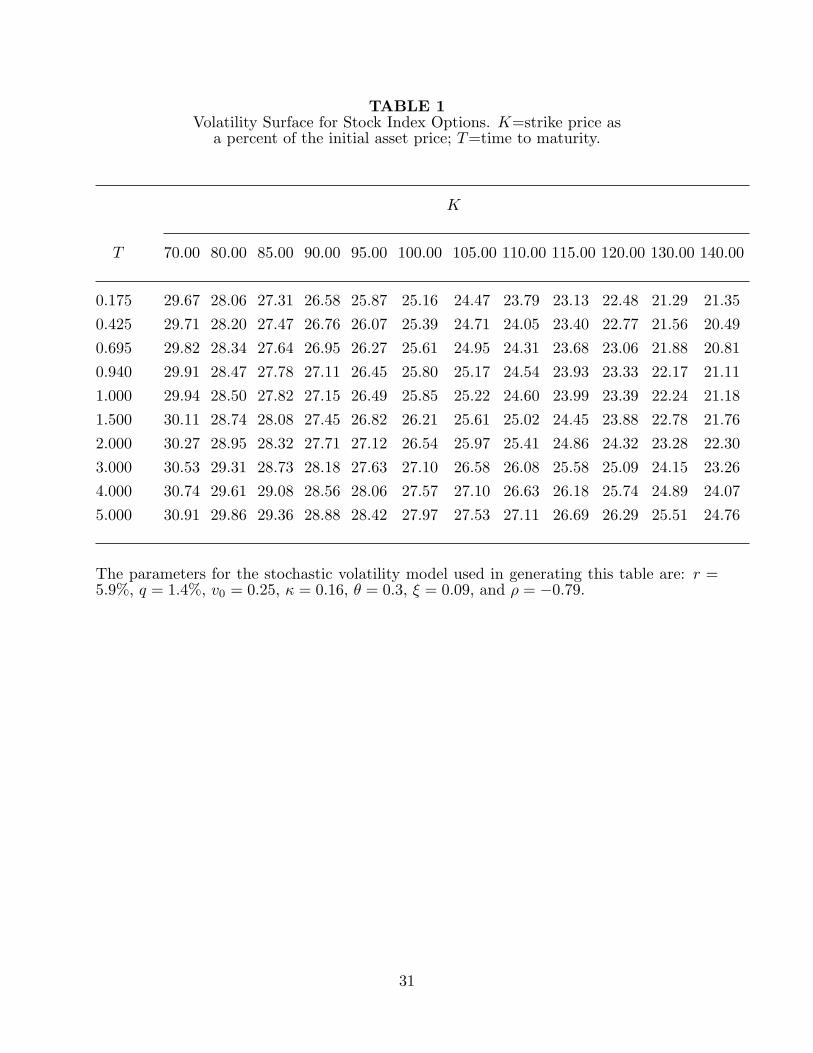
TABLE 1Volatility Surface for Stock Index Options. K=strike price as

a percent of the initial asset price; T=time to maturity.

K

T 70.00 80.00 85.00 90.00 95.00 100.00 105.00 110.00 115.00 120.00 130.00 140.00

0.175 29.67 28.06 27.31 26.58 25.87 25.16 24.47 23.79 23.13 22.48 21.29 21.35

0.425 29.71 28.20 27.47 26.76 26.07 25.39 24.71 24.05 23.40 22.77 21.56 20.49

0.695 29.82 28.34 27.64 26.95 26.27 25.61 24.95 24.31 23.68 23.06 21.88 20.81

0.940 29.91 28.47 27.78 27.11 26.45 25.80 25.17 24.54 23.93 23.33 22.17 21.11

1.000 29.94 28.50 27.82 27.15 26.49 25.85 25.22 24.60 23.99 23.39 22.24 21.18

1.500 30.11 28.74 28.08 27.45 26.82 26.21 25.61 25.02 24.45 23.88 22.78 21.76

2.000 30.27 28.95 28.32 27.71 27.12 26.54 25.97 25.41 24.86 24.32 23.28 22.30

3.000 30.53 29.31 28.73 28.18 27.63 27.10 26.58 26.08 25.58 25.09 24.15 23.26

4.000 30.74 29.61 29.08 28.56 28.06 27.57 27.10 26.63 26.18 25.74 24.89 24.07

5.000 30.91 29.86 29.36 28.88 28.42 27.97 27.53 27.11 26.69 26.29 25.51 24.76

The parameters for the stochastic volatility model used in generating this table are: r =5.9%, q = 1.4%, v0 = 0.25, κ = 0.16, θ = 0.3, ξ = 0.09, and ρ = −0.79.

31

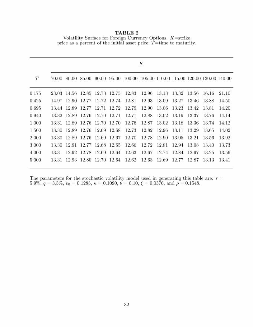
TABLE 2Volatility Surface for Foreign Currency Options. K=strike

price as a percent of the initial asset price; T=time to maturity.

K

T 70.00 80.00 85.00 90.00 95.00 100.00 105.00 110.00 115.00 120.00 130.00 140.00

0.175 23.03 14.56 12.85 12.73 12.75 12.83 12.96 13.13 13.32 13.56 16.16 21.10

0.425 14.97 12.90 12.77 12.72 12.74 12.81 12.93 13.09 13.27 13.46 13.88 14.50

0.695 13.44 12.89 12.77 12.71 12.72 12.79 12.90 13.06 13.23 13.42 13.81 14.20

0.940 13.32 12.89 12.76 12.70 12.71 12.77 12.88 13.02 13.19 13.37 13.76 14.14

1.000 13.31 12.89 12.76 12.70 12.70 12.76 12.87 13.02 13.18 13.36 13.74 14.12

1.500 13.30 12.89 12.76 12.69 12.68 12.73 12.82 12.96 13.11 13.29 13.65 14.02

2.000 13.30 12.89 12.76 12.69 12.67 12.70 12.78 12.90 13.05 13.21 13.56 13.92

3.000 13.30 12.91 12.77 12.68 12.65 12.66 12.72 12.81 12.94 13.08 13.40 13.73

4.000 13.31 12.92 12.78 12.69 12.64 12.63 12.67 12.74 12.84 12.97 13.25 13.56

5.000 13.31 12.93 12.80 12.70 12.64 12.62 12.63 12.69 12.77 12.87 13.13 13.41

The parameters for the stochastic volatility model used in generating this table are: r =5.9%, q = 3.5%, v0 = 0.1285, κ = 0.1090, θ = 0.10, ξ = 0.0376, and ρ = 0.1548.

32

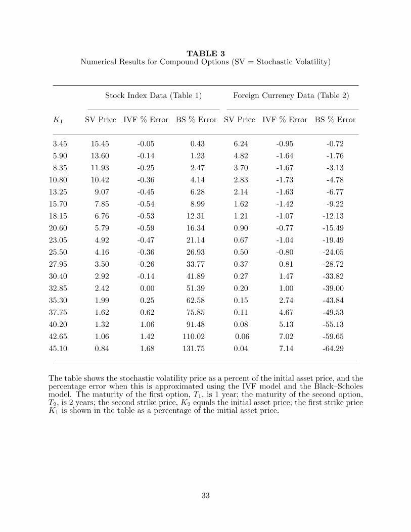
TABLE 3Numerical Results for Compound Options (SV = Stochastic Volatility)

Stock Index Data (Table 1) Foreign Currency Data (Table 2)

K1 SV Price IVF % Error BS % Error SV Price IVF % Error BS % Error

3.45 15.45 -0.05 0.43 6.24 -0.95 -0.72

5.90 13.60 -0.14 1.23 4.82 -1.64 -1.76

8.35 11.93 -0.25 2.47 3.70 -1.67 -3.13

10.80 10.42 -0.36 4.14 2.83 -1.73 -4.78

13.25 9.07 -0.45 6.28 2.14 -1.63 -6.77

15.70 7.85 -0.54 8.99 1.62 -1.42 -9.22

18.15 6.76 -0.53 12.31 1.21 -1.07 -12.13

20.60 5.79 -0.59 16.34 0.90 -0.77 -15.49

23.05 4.92 -0.47 21.14 0.67 -1.04 -19.49

25.50 4.16 -0.36 26.93 0.50 -0.80 -24.05

27.95 3.50 -0.26 33.77 0.37 0.81 -28.72

30.40 2.92 -0.14 41.89 0.27 1.47 -33.82

32.85 2.42 0.00 51.39 0.20 1.00 -39.00

35.30 1.99 0.25 62.58 0.15 2.74 -43.84

37.75 1.62 0.62 75.85 0.11 4.67 -49.53

40.20 1.32 1.06 91.48 0.08 5.13 -55.13

42.65 1.06 1.42 110.02 0.06 7.02 -59.65

45.10 0.84 1.68 131.75 0.04 7.14 -64.29

The table shows the stochastic volatility price as a percent of the initial asset price, and thepercentage error when this is approximated using the IVF model and the Black–Scholesmodel. The maturity of the first option, T1, is 1 year; the maturity of the second option,T2, is 2 years; the second strike price, K2 equals the initial asset price; the first strike priceK1 is shown in the table as a percentage of the initial asset price.

33

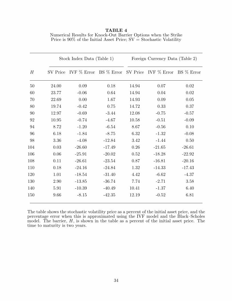
TABLE 4Numerical Results for Knock-Out Barrier Options when the StrikePrice is 90% of the Initial Asset Price; SV = Stochastic Volatility

Stock Index Data (Table 1) Foreign Currency Data (Table 2)

H SV Price IVF % Error BS % Error SV Price IVF % Error BS % Error

50 24.00 0.09 0.18 14.94 0.07 0.02

60 23.77 -0.06 0.64 14.94 0.04 0.02

70 22.69 0.00 1.67 14.93 0.09 0.05

80 19.74 -0.42 0.75 14.72 0.33 0.37

90 12.97 -0.69 -3.44 12.08 -0.75 -0.57

92 10.95 -0.74 -4.67 10.58 -0.51 -0.09

94 8.72 -1.20 -6.54 8.67 -0.56 0.10

96 6.18 -1.84 -8.75 6.32 -1.32 -0.08

98 3.36 -4.08 -12.84 3.42 -1.44 0.50

104 0.03 -26.60 -17.49 0.26 -21.65 -26.61

106 0.06 -25.91 -20.02 0.52 -18.28 -22.92

108 0.11 -26.61 -23.54 0.87 -16.81 -20.16

110 0.18 -24.16 -24.84 1.32 -14.33 -17.43

120 1.01 -18.54 -31.40 4.42 -6.62 -4.37

130 2.90 -13.85 -36.74 7.74 -2.71 3.58

140 5.91 -10.39 -40.49 10.41 -1.37 6.40

150 9.66 -8.15 -42.35 12.19 -0.52 6.81

The table shows the stochastic volatility price as a percent of the initial asset price, and thepercentage error when this is approximated using the IVF model and the Black–Scholesmodel. The barrier, H, is shown in the table as a percent of the initial asset price. Thetime to maturity is two years.

34

TABLE 5Numerical Results for Knock-Out Barrier Options when the Strike

Price Equals the Initial Asset Price.

Stock Index Data (Table 1) Foreign Currency Data (Table 2)

H SV Price IVF % Error BS % Error SV Price IVF % Error BS % Error

50 18.40 0.07 0.13 8.93 0.01 0.02

60 18.29 -0.05 0.54 8.93 0.01 0.02

70 17.61 0.11 2.12 8.93 0.02 0.04

80 15.61 -0.25 2.79 8.86 0.39 0.42

90 10.55 -0.54 0.52 7.72 0.48 0.37

92 8.96 -0.59 -0.37 6.91 1.14 1.10

94 7.18 -0.97 -1.91 5.84 1.11 1.10

96 5.12 -1.64 -3.91 4.39 0.30 0.64

98 2.80 -3.90 -7.96 2.45 0.04 0.88

104 0.00 -42.41 -9.93 0.01 -46.41 -34.04

106 0.00 -36.50 -19.52 0.03 -33.51 -29.92

108 0.01 -40.69 -28.23 0.09 -30.36 -25.62

110 0.03 -32.00 -27.10 0.19 -24.08 -21.73

120 0.34 -24.21 -33.29 1.44 -10.56 -4.18

130 1.39 -18.08 -38.61 3.41 -4.36 6.64

140 3.40 -13.40 -42.20 5.27 -2.33 10.12

150 6.20 -10.18 -43.88 6.62 -0.90 10.38

The table shows the stochastic volatility price as a percent of the initial asset price, and thepercentage error when this is approximated using the IVF model and the Black–Scholesmodel. The barrier, H, is shown in the table as a percent of the initial asset price. Thetime to maturity is two years.

35

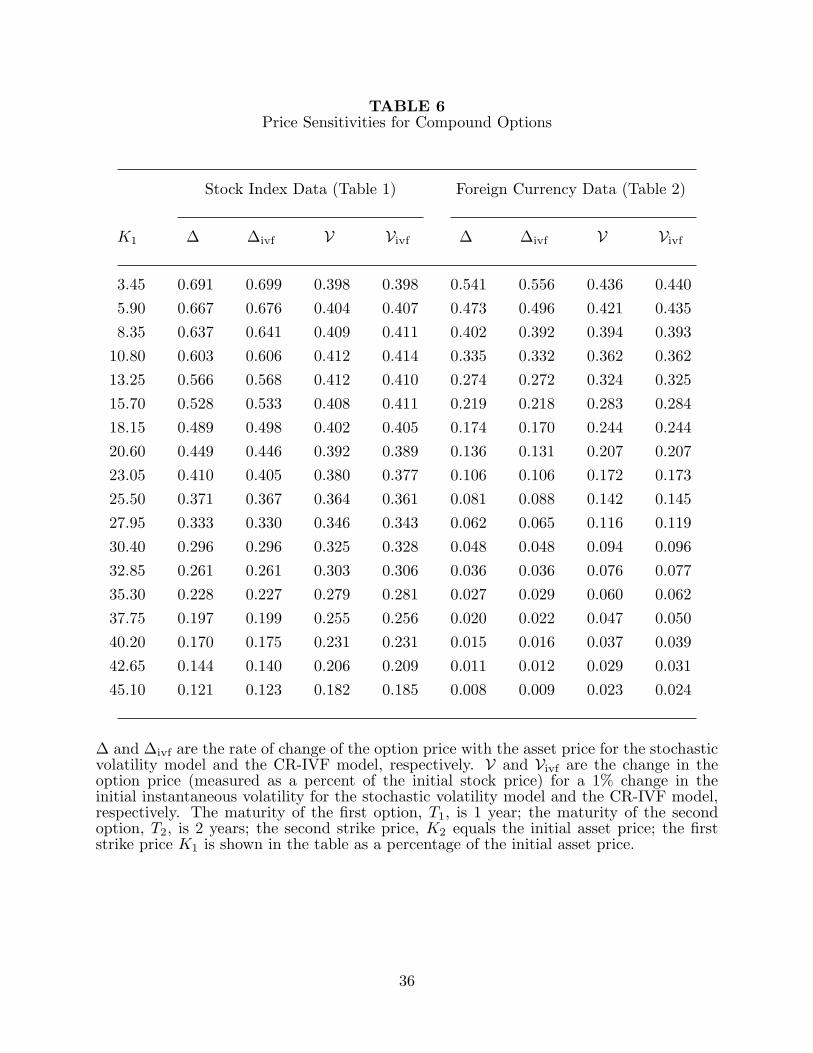
TABLE 6Price Sensitivities for Compound Options

Stock Index Data (Table 1) Foreign Currency Data (Table 2)

K1 ∆ ∆ivf V Vivf ∆ ∆ivf V Vivf

3.45 0.691 0.699 0.398 0.398 0.541 0.556 0.436 0.440

5.90 0.667 0.676 0.404 0.407 0.473 0.496 0.421 0.435

8.35 0.637 0.641 0.409 0.411 0.402 0.392 0.394 0.393

10.80 0.603 0.606 0.412 0.414 0.335 0.332 0.362 0.362

13.25 0.566 0.568 0.412 0.410 0.274 0.272 0.324 0.325

15.70 0.528 0.533 0.408 0.411 0.219 0.218 0.283 0.284

18.15 0.489 0.498 0.402 0.405 0.174 0.170 0.244 0.244

20.60 0.449 0.446 0.392 0.389 0.136 0.131 0.207 0.207

23.05 0.410 0.405 0.380 0.377 0.106 0.106 0.172 0.173

25.50 0.371 0.367 0.364 0.361 0.081 0.088 0.142 0.145

27.95 0.333 0.330 0.346 0.343 0.062 0.065 0.116 0.119

30.40 0.296 0.296 0.325 0.328 0.048 0.048 0.094 0.096

32.85 0.261 0.261 0.303 0.306 0.036 0.036 0.076 0.077

35.30 0.228 0.227 0.279 0.281 0.027 0.029 0.060 0.062

37.75 0.197 0.199 0.255 0.256 0.020 0.022 0.047 0.050

40.20 0.170 0.175 0.231 0.231 0.015 0.016 0.037 0.039

42.65 0.144 0.140 0.206 0.209 0.011 0.012 0.029 0.031

45.10 0.121 0.123 0.182 0.185 0.008 0.009 0.023 0.024

∆ and ∆ivf are the rate of change of the option price with the asset price for the stochasticvolatility model and the CR-IVF model, respectively. V and Vivf are the change in theoption price (measured as a percent of the initial stock price) for a 1% change in theinitial instantaneous volatility for the stochastic volatility model and the CR-IVF model,respectively. The maturity of the first option, T1, is 1 year; the maturity of the secondoption, T2, is 2 years; the second strike price, K2 equals the initial asset price; the firststrike price K1 is shown in the table as a percentage of the initial asset price.

36

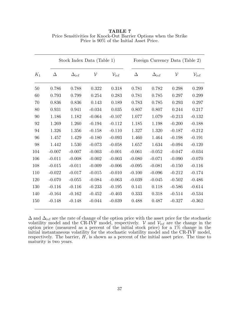
TABLE 7Price Sensitivities for Knock-Out Barrier Options when the Strike

Price is 90% of the Initial Asset Price.

Stock Index Data (Table 1) Foreign Currency Data (Table 2)

K1 ∆ ∆ivf V Vivf ∆ ∆ivf V Vivf

50 0.786 0.788 0.322 0.318 0.781 0.782 0.298 0.299

60 0.793 0.799 0.254 0.283 0.781 0.785 0.297 0.299

70 0.836 0.836 0.143 0.189 0.783 0.785 0.293 0.297

80 0.931 0.941 -0.034 0.035 0.807 0.807 0.244 0.217

90 1.186 1.182 -0.064 -0.107 1.077 1.079 -0.213 -0.132

92 1.269 1.260 -0.194 -0.112 1.185 1.198 -0.200 -0.188

94 1.326 1.356 -0.158 -0.110 1.327 1.320 -0.187 -0.212

96 1.457 1.429 -0.180 -0.093 1.460 1.464 -0.198 -0.191

98 1.442 1.530 -0.073 -0.058 1.657 1.634 -0.094 -0.120

104 -0.007 -0.007 -0.003 -0.001 -0.061 -0.052 -0.047 -0.034

106 -0.011 -0.008 -0.002 -0.003 -0.080 -0.071 -0.090 -0.070

108 -0.015 -0.011 -0.009 -0.006 -0.095 -0.081 -0.150 -0.116

110 -0.022 -0.017 -0.015 -0.010 -0.100 -0.096 -0.212 -0.174

120 -0.070 -0.055 -0.084 -0.063 -0.039 -0.045 -0.502 -0.486

130 -0.116 -0.116 -0.233 -0.195 0.141 0.118 -0.586 -0.614

140 -0.164 -0.162 -0.452 -0.403 0.333 0.318 -0.514 -0.534

150 -0.148 -0.148 -0.044 -0.039 0.488 0.487 -0.327 -0.362

∆ and ∆ivf are the rate of change of the option price with the asset price for the stochasticvolatility model and the CR-IVF model, respectively. V and Vivf are the change in theoption price (measured as a percent of the initial stock price) for a 1% change in theinitial instantaneous volatility for the stochastic volatility model and the CR-IVF model,respectively. The barrier, H, is shown as a percent of the initial asset price. The time tomaturity is two years.

37