IZA DP No. 3342

How Unilateral Divorce Affects Children

Julio Cáceres-DelpianoEugenio Giolito

DI

SC

US

SI

ON

PA

PE

R S

ER

IE

S

Forschungsinstitutzur Zukunft der ArbeitInstitute for the Studyof Labor

February 2008

How Unilateral Divorce Affects Children

Julio Cáceres-Delpiano Universidad Carlos III de Madrid

Eugenio Giolito

Universidad Carlos III de Madrid and IZA

Discussion Paper No. 3342 February 2008

IZA

P.O. Box 7240 53072 Bonn

Germany

Phone: +49-228-3894-0 Fax: +49-228-3894-180

E-mail: iza@iza.org

Any opinions expressed here are those of the author(s) and not those of IZA. Research published in this series may include views on policy, but the institute itself takes no institutional policy positions. The Institute for the Study of Labor (IZA) in Bonn is a local and virtual international research center and a place of communication between science, politics and business. IZA is an independent nonprofit organization supported by Deutsche Post World Net. The center is associated with the University of Bonn and offers a stimulating research environment through its international network, workshops and conferences, data service, project support, research visits and doctoral program. IZA engages in (i) original and internationally competitive research in all fields of labor economics, (ii) development of policy concepts, and (iii) dissemination of research results and concepts to the interested public. IZA Discussion Papers often represent preliminary work and are circulated to encourage discussion. Citation of such a paper should account for its provisional character. A revised version may be available directly from the author.

IZA Discussion Paper No. 3342 February 2008

ABSTRACT

How Unilateral Divorce Affects Children*

Using U.S. Census data for the years 1960-1980, we study the impact of unilateral divorce on outcomes of children (age 6-15) and their mothers. We find that the reform increased mothers’ divorce, decreased family income and increased the fraction of mothers below the poverty line. For children, we find not only negative results on investment, measured as the probability that a child goes to a private school, but also on child outcomes, measured by the likelihood of children aged 0-4 being held back in school at the time of the reform. We then analyze outcomes of the same cohorts of children 10 years later, by studying young men and women aged 16-25 using the 1970-1990 U.S. Census. We find an increase in marginality for these cohorts, measured as the probability of living in an institution (men) or the probability of being below the poverty line (women). We find that the impact in outcomes is particularly important for black children and young adults. JEL Classification: J12, J13 Keywords: unilateral divorce, child outcomes Corresponding author: Eugenio Giolito Department of Economics Universidad Carlos III de Madrid C/Madrid, 126 Getafe (Madrid) 28903 Spain E-mail: egiolito@eco.uc3m.es

* We thank Nezih Guner, Imran Rasul, Seth Sanders, Betsey Stevenson, Ernesto Villanueva and seminar participants at CEMFI and the III Workshop of the RTN Network “Economics of Education in Europe” for their helpful comments. Financial support from the Spanish Ministry of Education, Grant BEC2006-05710, and from the European Commission (MRTN-CT-2003-50496) are gratefully acknowledged. Errors are ours.

1

1 Introduction

From the late 1960s to the early 1980s, the majority of U.S. states introduced important

changes in divorce legislation to the extent that it has been called the ―Divorce Revolution‖.

Among those changes, unilateral divorce, the right of one spouse to ask for a divorce

without the consent of the other, is the aspect of the reform that has captured the greatest

attention in the literature during the last twenty years.

After a long debate about the effect of unilateral divorce on divorce rates (Peters, 1986;

Friedberg, 1998; Gruber, 2004), there is growing consensus in the literature regarding a

short-term increase in divorce rates (Wolfers, 2006). This evidence has been related by

scholars to a greater selection into and out of marriage in adopting states, and therefore to

an increase in the average match-quality of new and surviving marriages. This

interpretation has gained support from recent evidence about the lower divorce rate among

couples married under unilateral divorce, compared with those married under mutual

consent (Mechoulan, 2006). Additionally, evidence supports a reduction in the average

duration of marriages that end in divorce (Matouschek and Rasul, 2006).

Despite the direct effects of unilateral divorce on divorce rates, recent research has focused

on the role of the reform in several other aspects of individual behavior. Some examples are

studies on family formation (Drewianka, 2004; Rasul, 2004; Alesina and Giuliano, 2007),

female labor supply (Gray, 1998; Chiappori, Fortin and Lacroix, 2002; Stevenson, 2007

and 2007b) or domestic violence (Stevenson and Wolfers, 2006). Here the evidence also

2

points towards a change in behavior in those couples formed under the new legislation.

Stevenson (2007), using a sample of newlywed couples in 1970 and 1980, finds that, in

marriages formed under unilateral divorce laws there is less support of a spouse‘s

education, fewer children, greater female labor force participation and an increase in

households with both spouses engaged in full-time work.

Since divorce legislation acts as the dissolution clause of a marriage contract, the unilateral

reform can be seen as a retroactive change in the dissolution clause for those marriage

contracts already in place at the time of the reform. Therefore, the change in legislation

should have produced different effects over those individuals who had taken marriage,

fertility or investment decisions based on mutual consent divorce rules. Even though those

effects are transitional overall, they may become permanent for children of those families

―trapped‖ in the transition.

The literature on the effects of unilateral divorce on children is not extensive. Gruber

(2004),1 using a sample of adults (25 to 50 years old) from the US Census data for the

period 1960-1990, finds that those who were exposed to the reform as children have lower

educational attainments and lower family incomes, marry earlier but separate more often,

and have higher odds of adult suicide.

1 Another related paper is Johnson and Mazingo (2000). Using 1990 US Census data, they examine the amount of time individuals were exposed to unilateral divorce laws as children, finding results consistent with Gruber (2004).

3

We extend the current literature in several ways. First, instead of looking at outcomes of

adults exposed as children to unilateral divorce laws as in Gruber (2004), we examine

jointly children and their mothers during the period in which most states adopted unilateral

divorce, using Census data for the period 1960-80. By linking children (between ages 6 and

15) with their mothers, we are able to go further down the causal chain and analyze how

investment on children was affected by the change in legislation. Then, we study the same

cohorts of children ten years later, using 1970-1990 Census data in order to analyze

whether unilateral divorce has any effects on young men and women‘s marginality. Second,

we study the heterogeneity in the impact of the reform among children and families

exploiting the differences in age at which the child faced the reform. With this

specification, we are also able to study potential differential effects at the family or at the

child level, depending on at which point of the child‘s life the family has faced the reform.

Our main results are the following. First, we find that, because of the reform, mothers are

more likely to be below the poverty line, divorced and have lower family income. At the

same time, we find that children are less likely to attend a private school and, in the case of

black children, more likely to be repeating a grade (held-back). Third, analyzing the

heterogeneity by timing of family formation, measured by the age of the eldest child, we

find that families whose first child was five years old or older at the time of the reform are

approximately 16% more likely to be below the poverty line. They also face a 4% to 6%

decrease in family income, and children from those families are 16% to 24% less likely to

attend a private school. In all of these cases, we find no effects for families whose first

child was born after the reform. Nevertheless, when we analyze child outcomes we observe

4

that children of pre-school age at the time of the reform (age 0-4) are more likely to repeat a

grade. Finally, for young people age 16-25 (1970-1990 Census), we find that men who

were between 0 and 4 years old at the time of the reform are 27% more likely to live in an

institution (50% for blacks), which is in line with our findings for children. Moreover,

women who were between 5 and 15 years old are 9% more likely to be below the poverty

line (12% for black women).

The paper is structured as follows. In Section 2, after providing a brief review of the

characteristics of the divorce reform, we sketch some of the channels through which

unilateral divorce might affect children (investment and well-being) and the sources of

potential heterogeneity. In Sections 3 and 4 we describe our econometric specifications and

the data used. In Section 5 we present the results and Section 6 concludes.

2 Background

2.1 The Divorce Reform

Even though the most significant part of the divorce reform occurred during the 1970‘s, the

process started before 1950 in a number of states, by removing fault grounds in order for

spouses to ask for a divorce (Gruber, 2004).2 However, while this earlier reform allowed

2 This "fault" regime required proof of marital fault, such as adultery, desertion, physical abuse, for example. For a careful review of the characteristics of the reform, see Mechoulan (2005).

5

divorce without needing to cite a fault of the other spouse3 it still required that both spouses

mutually agree to divorce. In the early 1970's some states started introducing not only no-

fault grounds in the legislation but also allowed one spouse to ask for a divorce without the

consent of the other spouse, what is called "Unilateral divorce". Another important aspect

of the divorce revolution is related to the division of property and assets in the case of

divorce. Except for a few states (among them the states that follow community property

laws for classifying assets), before 1970 states had a regime that typically led to an unequal

division of property in divorce (Rasul 2004).4 However, by the end of 1970‘s the majority

of states had moved to a regime where property was more equally divided. Simultaneously

with the unilateral divorce reform, many states also eliminated fault in asset division and

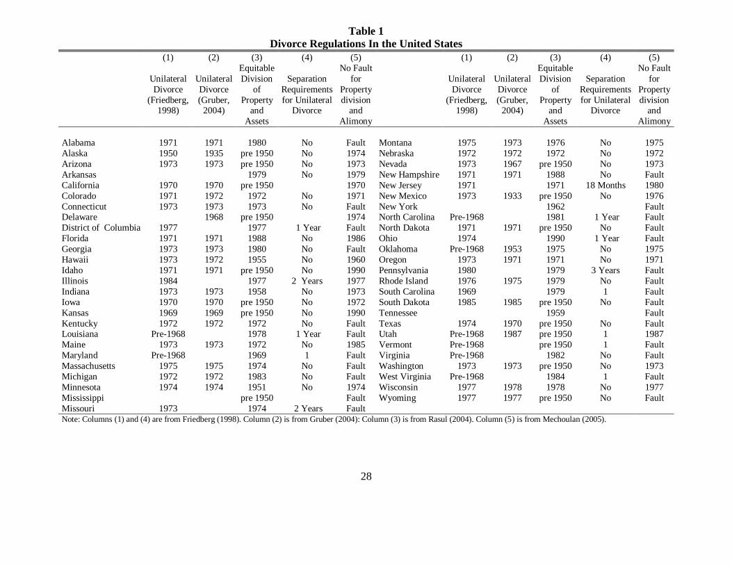
spousal support settlement. For a detail on the coding of the laws used in this paper, see

Table 1. 5

Despite the benefits that unilateral divorce may have brought to those who are married

under the unilateral regime, there is growing concern among some scholars, policy makers

and interest groups regarding potential negative consequences of this reform, related to the

3 That is, irreconcilable differences, irretrievable breakdown or incompatibility.

4 Rasul (2004) notes that in those "common law" regimes spouses were only entitled to the property that they owned before marriage, or fault was to play a role in the division of assets, or some states had explicit "two third" rules for property division.

5 This paper focuses on the effects of the unilateral divorce. However, since the way in which assets are divided in the case of divorce can play a key role either on divorce propensity or in resource allocation within marriage, we will account for both the equitable division and the "no fault for property division" laws in our analysis.

6

benefits that have been traditionally associated with marriage6. One example of this

concern is the range of state-level pro-family policies recently introduced in the United

States, including the introduction of covenant marriages, a legal scheme that allows couples

to choose to marry either under a unilateral divorce regime or under a stricter set of rules

regarding divorce.7 This legal experiment is interesting because the optimal degree of

commitment (and therefore the optimal marriage contract) may vary with the characteristics

of the sides involved. Excepting those covenant states, only one type of marriage contract

regarding dissolution clauses is available in each state. Since people cannot tailor the exit

clause to their needs, a reduction in the exit costs from marriage implied by unilateral

divorce may affect the composition of the married population under the new rules.

Furthermore, the change in legislation may have produced retroactive effects over those

people who had signed a contract with a different dissolution clause (mutual consent), made

decisions accordingly, and then faced the change in legislation.

6 Waite and Gallagher (2000) summarize a large body of literature that shows a robust correlation between being married and being healthy, earning higher wages, and accumulating more wealth. Similarly, Akerlof (1998) shows that men who

delay marriage or remain single are less likely to be employed, tend to have lower incomes and are more prone to crime and drug use.

7 Three states have passed such laws: Louisiana (1997), Arizona (1998), and Arkansas (2001). Covenant marriage generally requires pre-marital counseling, and an agreement to seek additional counseling if marital problems surface. Divorce is granted for specific ―fault-based‖ reasons, including adultery, domestic violence, commission of a felony, and alcohol or drug abuse. Couples that seek a divorce based on mutual consent (e.g., no-fault) must wait a specified amount of time (e.g., two years in Louisiana). For a detailed review of these policies, see Gardiner et al. (2002).

7

2.2 The Role of Unilateral Divorce on Children’s Well-Being

Unilateral divorce may have affected children‘s well-being through different channels8. The

most obvious candidate is parental divorce per se. A higher incidence of divorce implies

that a higher proportion of children have faced this event and are therefore forced to live

under nontraditional family structure. Empirical evidence has long shown that children of

divorced parents have lower achievements than children from intact families (Manski et al.,

1992; Haveman and Wolfe, 1995; Ginther and Pollak, 2003). Furthermore, Sampson (1987)

finds that family disruption increases the rates of black murder and robbery, especially

among juveniles. It is also known that divorce decreases the resources available for children

(McLanahan and Sandefur, 1994; Page and Stevens, 2004).9 Therefore, if growing up in a

two-parent household is beneficial for children, and the reform, at least in the short run,

increased the incidence of divorce in the adopting states (Friedberg, 1998; Gruber, 2004;

Wolfers, 2006), we should expect a worsening both in family economic conditions and in

child outcomes.

Second, the reform may have produced a change in the bargaining position of household

members (Chiappori, Fortin and Lacroix, 2002). There is vast literature on development

that has documented that the amount of resources allocated to children depends on the

relative bargaining position between husband and wife (Strauss and Thomas, 1995; Beegle,

8 A more in-depth discussion of some of these channels can be found in Gruber (2004).

9 For example, Page and Stevens (2004), find that, in the year following a divorce, family income falls by 41 percent and family food consumption falls by 18 percent. Six or more years later, the family income of the average child whose parent remains unmarried is 45 percent lower than it would have been if the divorce had not occurred.

8

Frankenberg and Thomas, 2000). In fact, this evidence shows that more resources in the

hands of women tend to benefit children and specifically girls. Therefore, if unilateral

divorce weakens the bargaining position of women within marriage, children may have

been negatively affected, independently of the occurrence of a divorce. Although the

change of the bargaining position within the household is unobservable in the data, we can

find out if the resources available for children in the family are affected by the presence of

unilateral divorce laws, either through a change in the bargaining position of the wife or

through divorce itself.

A third potential channel comes from the changes in incentives for relationship-specific

investments. Several scholars have analyzed marriage as a commitment device that fosters

cooperation and induces partners to make relationship-specific investments (Brinig and

Crafton, 1994; Matouschek and Rasul, 2006; Stevenson, 2007). As the unilateral divorce

undermines this commitment device, it also affects couples' incentives to make investments

in their marriage. Thus, changes in family laws potentially affect the incentives to make

investments whose returns are partly marriage-specific. Children (quantity) and child

investment (quality) can be considered marriage-specific and therefore the reform would

directly reduce the incentive to allocate resources to children.10

However, a higher incentive

10 Alesina and Giuliano (2007) find that total fertility and out-of-wedlock fertility decline after the introduction of unilateral divorce, with marital fertility rates remaining constant. Drewianka (2004) finds also a reduction in non-marital birth rates. However, he finds that unilateral divorce seems to increase aggregate and marital birth rates, and all of those effects seem to grow the longer the law is in effect.

9

to make market-specific investments such as labor employment (Stevenson, 2007), may

increase the amount of resources available for children

Fourth, the divorce law reform may have affected selection into marriage. Unilateral

divorce, as a decrease in the exit cost of marriage, may affect the composition of those

couples who want to marry in the first place, and it can have either a positive or a negative

effect on the probability of divorce depending on why people initially get married. On the

one hand, it may lead to a negative selection into marriage; a reduction in the divorce costs

mitigates the costs of marriage without affecting its benefits. Consequently, couples of

relatively low match quality are now willing to ―try‖ marriage, reducing the average match

quality of married couples and therefore increasing their marriage and divorce propensity

(Alesina and Giuliano, 2007). On the other hand, as unilateral divorce undermines the role

of marriage as a commitment device, couples with relatively low match quality no longer

marry, which increases the average quality of married couples and, therefore, decreases the

marriage and the divorce propensity (Matouschek and Rasul, 2006). Negative or positive

selection into marriage could also play a crucial role in the early stages of those children

born after unilateral divorce took effect. Empirically, evidence on divorce rates supports the

idea of a positive selection in marriage (Matouschek and Rasul, 2006; Wolfers, 2006).11

11 Matouschek and Rasul (2006) find supporting evidence of marriage as a commitment device; couples married after unilateral divorce took place are less likely to divorce during marriage. Weiss and Willis (1997), using data from the National Study of the High School Class of 1972, find that couples married under unilateral divorce are less likely to divorce than those who married under mutual consent. Mechoulan (2005) presents similar evidence from CPS data, and his results specifically hold for the law governing property division and spousal support.

10

However, the studies on marriage rates deliver mixed results (Drewianka (2004); Rasul,

2004; Alesina and Giuliano, 2007)12

.

2.3 Sources of Potential Heterogeneity

The factors described above may have affected mothers and children with different

intensity depending on how old they were at the time of the reform. For example, current

evidence on divorce rates (Matouschek and Rasul, 2006; Wolfers, 2006) points to a

decrease in the divorce rate for couples married after the reform. Therefore, we should

expect that children born into families formed under unilateral divorce would be less

affected by the reform than those children who were born under mutual consent in adopting

states.

Second, in the case where unilateral divorce increases the perceived risk of divorce, and

therefore changes the incentives of market-oriented investment with respect to relationship-

specific investments (Stevenson, 2007), the timing of family formation becomes relevant.

Couples who married under mutual consent in adopting states could have made home

(market) specialization decisions under dissolution rules that were later modified.

Therefore, those families who were married and already had children when the reform took

12 Drewianka (2004) finds no effects on marriage rates. Rasul (2004) provides evidence that after the adoption of unilateral divorce, marriage rates fell significantly and permanently in adopting states. Alesina and Giuliano (2007) have lately challenged this evidence finding that the number of women who have never married actually goes down with unilateral divorce.

11

place had some specific investment which reduced their degrees of freedom under the new

regime incentives. For example, women who at the time of the reform had already

completed their desired parity or had already spent time out of the labor force would face a

tougher setting than those who were able to consider the new information when they made

their supply/marriage/fertility decisions. Therefore, we would expect that those women who

were unaware that the rules regarding marital dissolution would eventually change at the

time they started a family would be more likely to be affected by the reform than those who

internalized the new rules.

When analyzing child outcomes we should also take into account the fraction of their lives

during which they were exposed to unilateral divorce laws. Specifically we would like to

know at which stage of their development they faced the reform. Literature on child

development has provided evidence that the impact of parents‘ divorce depends on the state

of development (Wolf, 1998). Since part of this development is chronologically

determined, we would expect that children who faced the reform at an early age were

affected differently than those who, at the time unilateral divorce ―hit‖, had already

completed their education or were old enough to understand the eventual changes occurring

at the family level.

12

3 Data and Variables

The data for this study come from the US Census PUMS 1% data for the years 1960,

1970 Form 2, 1980 and 1990.13

We construct two primary samples for our analysis. The

first sample contains data on children and their (non-stepmother) mothers for the period

1960-1980.14

The sample is restricted to ever married, U.S born mothers between 25 and 50

years old, the number of children living at home equal to the number of children ever born

to the woman and with the eldest child being no older than 18.15

With this data, we

construct two subsamples. In order to study child outcomes, the first subsample contains

information on children between 6 and 15 years old. For mother outcomes, we construct a

second subsample with one observation per household. Finally, in order to study the

outcomes of the same cohorts of children ten years later we construct a sample with young

men and women aged 16-25, using Census data for the period 1970-1990.

We define three groups of outcomes. The first group has three outcomes at the family

level or related to the child's mother. First, ―Currently Divorced‖ is a dummy variable that

takes a value of one if the child's mother is divorced, and zero otherwise.16

The second

13 Information on private school attendance, one of our outcomes of interest, is only available in Form 2 for the 1970

Census. Therefore, using Form 2 implies losing the information about age of first marriage and marriage number of the mother, available only in Form 1.

14 We exclude from the sample children whose mother is identified as a stepmother.

15 We make those restrictions in order to make sure that the eldest child at home is the mother‘s first child, in order to analyze mothers‘ heterogeneity.

16 We use ―Currently Divorced‖ instead of ―Ever Divorced‖ because in order to construct the latter variable we would need information on marriage number that is not available in Form 2 of the 1970 US Census data.

13

variable is ―Poverty‖, a dummy variable that equals one if the mother‘s income is below the

poverty line and zero otherwise and the third variable is the log of family income.

The second group of variables consists in outcomes at child level. The first variable,

defined for the census sample, "Private School" is a dummy variable that takes a value

equal to one if a child between 6 and 15 years of age attends a private institution or church

related school, and zero otherwise. Several authors have shown that educational outcomes

are better for students that attend private school. Although there is some question about

whether this impact is causation or correlation, there is no question that parents who enroll

their children in private schools are those with higher income. Despite those concerns, this

variable is useful as a measure of parents‘ investment on children‘s human capital. The

second variable, "Behind," is a dummy variable that equals one if the child's year of

education is lower than the mode by age and year, and zero otherwise. "Behind" identifies

whether children are progressing in school with their cohorts and is a measure of

educational attainment.

Finally, the third group of variables includes two outcomes of young men and women aged

16-25. The first outcome, ―Institution‖ is a dummy variable that takes a value equal to one

if the individual lives in an Institution, and zero otherwise17

. The second outcome is

―Poverty‖, as defined above.

17 US Census samples provide detailed information about group quarters. Specifically, we are able to know if an individual is living in a correctional or a mental institution. Nevertheless, from 1990 onwards, this detailed information on institutions is no longer available.

14

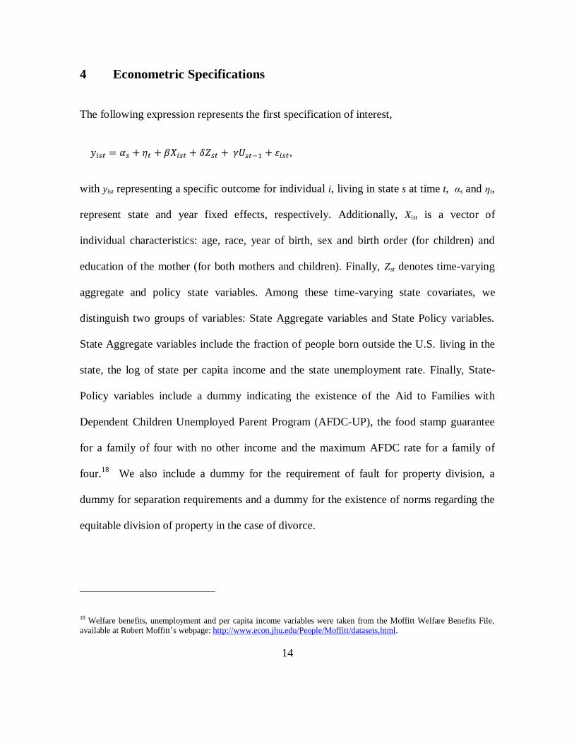
4 Econometric Specifications

The following expression represents the first specification of interest,

,

with yist representing a specific outcome for individual i, living in state s at time t, αs and ηt,

represent state and year fixed effects, respectively. Additionally, Xist is a vector of

individual characteristics: age, race, year of birth, sex and birth order (for children) and

education of the mother (for both mothers and children). Finally, Zst denotes time-varying

aggregate and policy state variables. Among these time-varying state covariates, we

distinguish two groups of variables: State Aggregate variables and State Policy variables.

State Aggregate variables include the fraction of people born outside the U.S. living in the

state, the log of state per capita income and the state unemployment rate. Finally, State-

Policy variables include a dummy indicating the existence of the Aid to Families with

Dependent Children Unemployed Parent Program (AFDC-UP), the food stamp guarantee

for a family of four with no other income and the maximum AFDC rate for a family of

four.18

We also include a dummy for the requirement of fault for property division, a

dummy for separation requirements and a dummy for the existence of norms regarding the

equitable division of property in the case of divorce.

18 Welfare benefits, unemployment and per capita income variables were taken from the Moffitt Welfare Benefits File, available at Robert Moffitt‘s webpage: http://www.econ.jhu.edu/People/Moffitt/datasets.html.

15

The variable of interest is Ust-1, which is a dummy variable that takes a value of one for

those states that had already adopted the unilateral reform the year before the census year.

We use Friedberg (1998) coding to define the existence of the unilateral divorce regime.19

To estimate the impact of the reform, γ, we rely on the standard source of identification that

is usual in the literature on unilateral divorce, a Dif-in-Dif approach; not all states moved to

the unilateral regime and those that adopted these new divorce laws did not move

simultaneously to the new regime. Finally, since the error term, εist, could be serially

correlated, we cluster the standard errors by the state of residence, following Bertrand,

Duflo, and Mullainathan (2004).

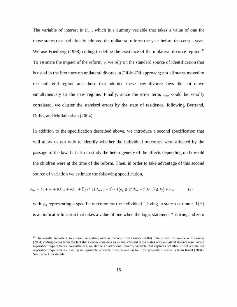
In addition to the specification described above, we introduce a second specification that

will allow us not only to identify whether the individual outcomes were affected by the

passage of the law, but also to study the heterogeneity of the effects depending on how old

the children were at the time of the reform. Then, in order to take advantage of this second

source of variation we estimate the following specification,

, (2)

with yist representing a specific outcome for the individual i, living in state s at time t. 1{*}

is an indicator function that takes a value of one when the logic statement * is true, and zero

19 Our results are robust to alternative coding such as the one from Gruber (2004). The crucial difference with Gruber (2004) coding comes from the fact that Gruber considers as mutual consent those states with unilateral divorce also having separation requirements. Nevertheless, we define an additional dummy variable that captures whether or not a state has separation requirements. Coding on equitable property division and on fault for property division is from Rasul (2004). See Table 1 for details.

16

otherwise. YBist is the year of birth for individuals i living in the state s at time t; YUnis is the

year of adoption of unilateral divorce in the state s. That is, represents the

child‘s age at the time of introduction of unilateral divorce. Then is understood as the

ceteris paribus contribution of unilateral divorce for those children whose age at the time of

the reform was in the range [ , in relationship to those individuals living in states that

have not adopted unilateral divorce ( . Three age groups at the time of the

introduction of unilateral divorce are defined: Born after the reform, >0;

between 0 and 4, and aged 5 or more at the time of the reform. Here we concentrate, in the

changes of the divorce law occurred since 1968.20

In this last specification, three are the

source of variation which we rely on to identify the parameter . In addition to the

differences in the timing of adoption of unilateral divorce and the fact that not all states

introduced it, we use in the specification the fact that the reform might have affected

individuals (children and families) at different points in their lives.

20 Therefore, states that adopted some kind of reform before 1968 (―Pre-1968‖ in Columns 1 and 4 of Table 1) are considered as ―non-adopting‖ in this part of the analysis.

17

This specification is similar to considering time of exposure to the law, but it has two

advantages. First, it allows us to identify a potential selection mechanism that makes

children (or families whose first child was) born after the law different. Second, since all

children born before the law in the same state have the same time exposure to the law, we

can test whether there are differential effects depending on their age at the time of the

reform.21

5 Results

5.1 Mothers and Children (1960-1980)

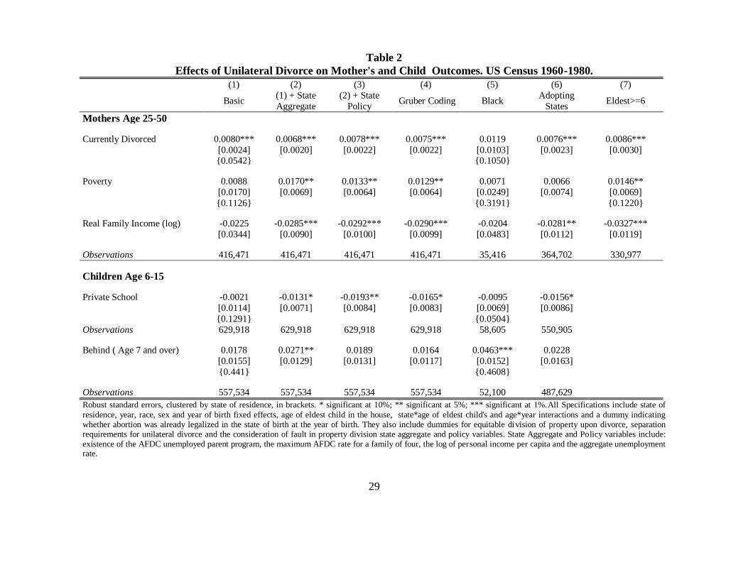
Table 2 shows the results of Equation (1) for mothers aged 25-50 (top panel) and for

children aged 6-15 (bottom panel). Column 1 shows the results for the basic specification

(state, year age, race, year of birth, sex and birth order fixed effects); in Column 2, we add

state aggregate variables and in Column 3 state policy variables as defined above. In

Column 4, we use an alternative divorce coding (Gruber, 2004). In Columns 5 and 6, we

restrict the samples of mothers and children to African-American and to individuals living

in adopting states, respectively. Finally, in Column 7 we restrict the sample of mothers to

those whose eldest child is aged six and over, in line with the children‘s sample. Mothers‘

results (top panel) show robustness across specifications. Our preferred specification

(controlling for state aggregate and policy variables), presented in Column 3, shows an

21 As we show later, our results are robust to the time of exposure as well as the source of variation.

18

increase in the probability of being a divorced mother of 7.8 percentage points (14.4% of

the sample mean), a 12% increase in the likelihood of being below the poverty line and a

2.9% decrease in family income. Coefficients for black mothers are of the same sign but

statistically insignificant. The bottom panel shows the results for children. In line with a

decrease in family income, we observe that the reform decreases the likelihood of going to

a private school by 1.93 percentage points (15% decrease). In the case of Behind we find a

significant increase when controlling by state aggregate variables, but the results are not

robust to the inclusion of state policy variables. However, for the sample of black children

the coefficient of Behind is indeed significant, with an increase of 9.2% of the sample

mean.

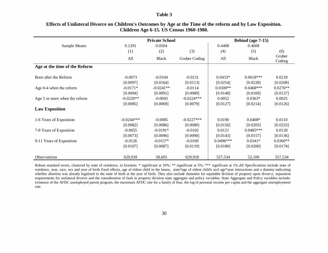
In the top panel of Table 3 we show the results of Equation (2). In addition to the controls

described above, here we add state-age interaction dummies. The bottom panel shows the

results considering time of exposure to the law as the source of variation. Columns 1 to 3

show the results for Private and Columns 4 to 6 those for Behind. Columns 1 and 4 show

the results for the whole sample; Columns 2 and 5 those for Black children and finally

Columns 3 and 6 display the results for the whole sample using Gruber (2004) coding. The

results of the top panel (Age at the Time of Reform) are consistent across the subsamples

and show heterogeneity across the different ages at which children faced the reform. In the

case of Private, we see that children born before the reform are less likely to attend private

school, while the coefficient for children born after unilateral divorce is not statistically

distinguishable from zero. For the whole sample (Column 1), we find that private school

attendance decreases by 1.71 percentage points (around 13% of the sample mean and

19

significant at a 10% level) for children that were aged 0-4 at the year of the reform and

around 17% for children aged 5 or more. In the sample of black children, this coefficient

shows a decrease of around 48% of the sample mean (2.41 percentage points). The results

for Behind also display heterogeneity but in this case it appears that the unaffected group is

that of children who were aged 5 or more at the time of the reform.

When we consider exposure to the law as the source of variation (bottom panel), the results

are significant for those children with 1 to 6 years of exposure (Private) and for those

whose exposure to the law was 9-11 years (Behind). These results are harder to interpret

but, in the case of Behind, suggest that the affected group is composed of those who were

either younger than age 4 or unborn in states that adopted the law in 1971 or earlier (see

Table 1). A potential reading for these findings is that unilateral divorce in the short run is

associated with a reduction in child investment (private) but it takes time for the impact to

manifest itself on child outcomes such as ―Behind.‖

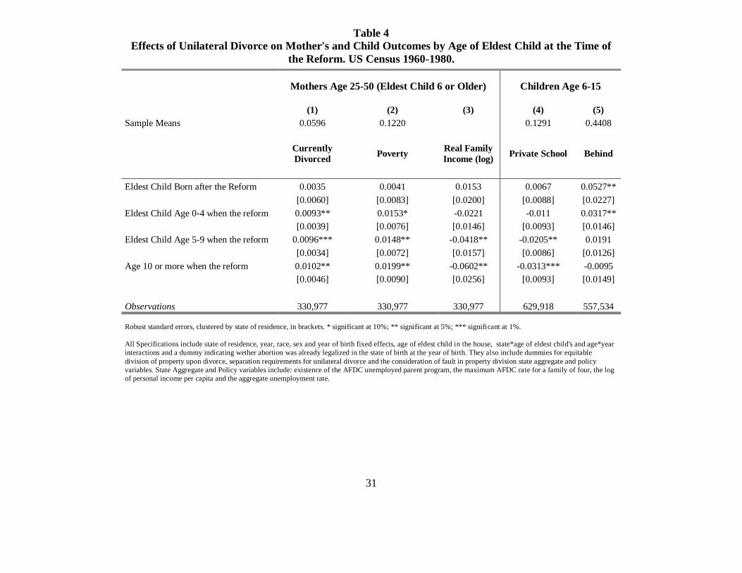
In order to study mother and child outcomes, we estimate our second specification using

one observation per family and the age of the eldest child to define in which point of life

the family faced the reform. In this specification, we add additional individual controls to

those contained in vector Xist: age of eldest child fixed effects and state-age of eldest child

interaction dummies. We also consider four categories: Eldest child born after the reform,

aged 0-4 at the time of the reform, aged 5-9 and aged 10 or more.

Columns 1 to 3 of Table 4 show the results for mothers whose eldest child is aged six or

older (in order to compare them with children results), which show heterogeneity

20

depending on the difference between the year of birth of their first child and the year that

the reform took place. We find that mothers in unilateral states whose first child was born

before the reform are 12% to 16% more likely to be below the poverty line. The coefficient

for mothers whose eldest child was born after the reform is statistically indistinguishable

from zero, and significantly lower than the one for mothers whose eldest child was aged 0-4

at the time of the reform. The pattern for Currently Divorced is similar but in this case,

even though the only coefficient that is not statistically significant is the one associated to

families in which the oldest child is born after the reform, we cannot ensure that it is

significantly different from the others. Finally, we find that mothers whose eldest child was

aged five and older faced a decrease from 4% to 6% in family income.

Columns 4 and 5 of Table 4 show the results for child outcomes. The pattern for Private

school, which can be considered an investment variable, is similar to that of mother‘s

economic variables (Poverty and Family Income). Children whose eldest sibling was aged

5-9 at the time of the reform were 16 % less likely to attend a private school (2.08

percentage points) while if the eldest child at home was 10 or older the decrease in Private

reaches 24%. The pattern for Behind is different. As can be observed in Column 5, we

observe significant increases for children whose eldest sibling was either too young to

attend school (aged 0-4) or not yet born when unilateral law was passed. This last result is

surprising, as we would have expected no effects in families whose first child was born

after the reform (because of selection into marriage and the evidence that the increase in

divorce rates was only in the short run). However, given that our sample ends in 1980 we

cannot be conclusive about what happened with mothers‘ divorce rates. As stated above,

21

the coefficient of Currently Divorced for mothers whose eldest child was born after the

reform (Column 1) is statistically indistinguishable from the others. Additionally, evidence

supports a reduction in the average duration of marriages that end in divorce (Matouschek

and Rasul, 2006), which may be a potential factor indicating that children whose parents

end up divorcing might start living in a single-parent household earlier in life.

5.2 Young Adults (1970-1990)

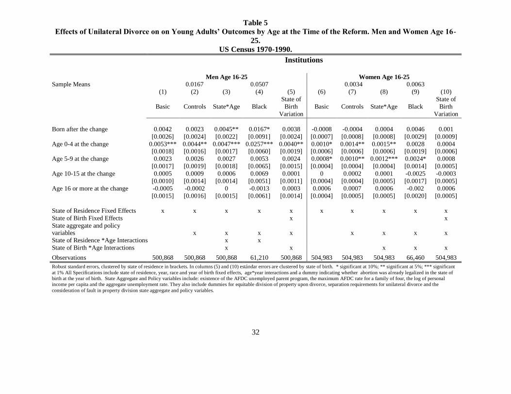
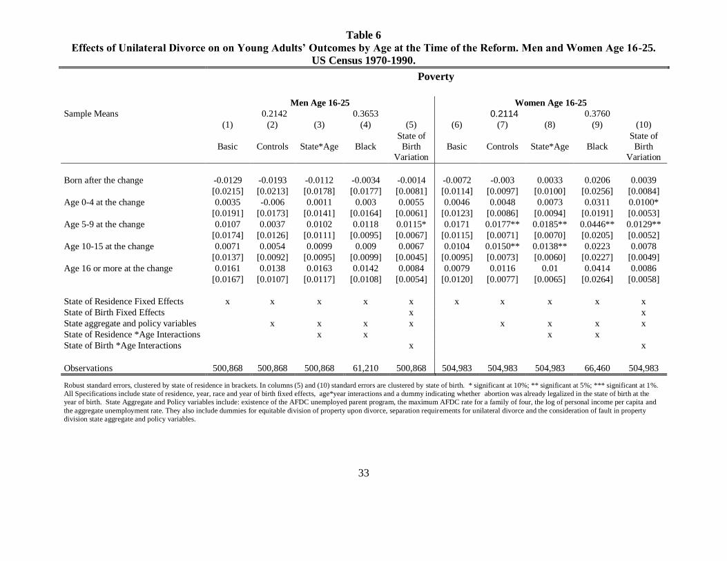
Next we analyze outcomes of the same cohorts of children ten years later. Tables 5 and 6

show the results of several specifications of Equation (2) for young men and women aged

16-25 using the 1970, 1980 and 1990 Census data. Table 5 shows the results for

Institutions for several specifications applied to a sample of men (Columns 1 to 5) and

women (Columns 6 to 10). The first column shows the results for the basic specification

(individual controls only), the second also includes time varying state variables and the

third includes state-age interaction dummies. The fourth column shows the results for a

sample of blacks only. Finally, the fifth column considers an alternative specification where

the source of variation (age at the time of the reform) is constructed using the state of birth

instead of the state of residence. The first three columns of Table 5 show that young men

who were younger than age five at the time of the reform were 24% to 27.5% more likely

to live in an Institution at the time of the Census. When we include state-age interactions as

covariates (Column 3), we also find that the coefficient for children born after the law is

also significant. When we restrict the sample to black men aged 16-25, we find a striking

50% increase in Institutions for those who were aged 0-4 at the time of the reform.

22

Nevertheless, the impact on institutions is associated not only to changes in incarceration

but also to the likelihood of being confined to a mental institution; our findings are

consistent with a positive impact of unilateral divorce on crime rates (Caceres-Delpiano and

Giolito, 2008).22

For women (Columns 6 to 10) the pattern is similar, although the results

are not robust to the specification where the dependent variables are constructed using state

of birth.

Finally, Columns 2 and 3 of Table 6 show that there is a significant increase in the

probability that women who were aged 5-9 or 10-15 at the time of the reform are below the

poverty line (8.75 and 6.5% increase over the sample mean, respectively). In the case of

black women, the coefficient is only significant for those women whose age at the time of

the reform was between 5 and 9 years old, but the increase in this case is around 12% of the

sample mean (4.46 percentage points).

6 Conclusion

In this paper, we study the effects of unilateral divorce on mothers and children. Unlike

previous literature, we jointly examine children and their mothers during the period that

most states adopted unilateral divorce, using Census data for the period 1960-80.

Therefore, we are able to study outcomes related to investment on children that have not

22 Caceres-Delpiano and Giolito (2008), using data from the FBI´s Uniform Crime Report program for the period 1965-1998, find that unilateral divorce has a positive and long-run impact on violent crime rates, with 8% to 12% average increase for the period under consideration.

23

previously been examined. We are also able to study different potential effects at the family

or child level depending on at which point of the child‘s life (or the ―family life‖ using the

year of birth of the first child) the family faced the reform.

We find that, because of the reform, mothers are more likely to be below the poverty line

and have lower family income. At the same time, we find that children are less likely to

attend a private school and in the case of black children, more likely to be repeating a

grade. In general, we find that the effect of unilateral divorce on investment variables

(family income, mother‘s poverty, private school attendance) mostly affect families whose

first child was born five or more years before the reform. However, when we study child

outcomes (the likelihood of repeating a class), the children affected are those who were

younger (or where the eldest child was younger) at the time of the enactment of the law.

We also study the cohorts of these same children ten years later (1970-1990 Census),

finding that men who were between 0 and 4 years old at the time of the reform are more

likely to live in an institution., in line with child outcomes. Moreover, women who were

between 5 and 15 years old are more likely to be below the poverty line (in line with the

pattern of investment variables). We find that the impact in outcomes is particularly

important for black children and young adults.

24

References

Akerlof, George. A. (1998). ‗‗Men Without Children,‘‘ Economic Journal, 108, 287–309.

Alesina, Alberto and Paola Giuliano (2007), ―Divorce, Fertility and the Value of Marriage‖.

Mimeo. Harvard University.

Bertrand, Marianne, Esther Duflo, and Sendhil Mullainathan (2004). ―How Much should

we trust differences-in-differences estimates?‖ Quarterly Journal of Economics 119,

no. 1:249–75.

Brinig, Margaret F. and Steven Crafton (1994) ―Marriage and Opportunism‖. Journal of

Legal Studies; 23, 869.

Chiappori, Pierre André, Bernard Fortin, and Guy Lacroix (2002), "Marriage Market,

Divorce Legislation, and Household Labor Supply." Journal of Political Economy, 85

(6), 1141-1187.

Cáceres-Delpiano, Julio, and Eugenio Giolito (2008), ―The Impact of Unilateral Divorce on

Crime‖. Mimeo. Universidad Carlos III de Madrid.

Drewianka, Scott (2004), "Divorce Law and Family Formation". Journal of Population

Economics, forthcoming.

Friedberg, Leora (1998), "Did Unilateral Divorce Raise Divorce Rates? Evidence from

Panel Data," American Economic Review, 88, 608-627.

25

Gardiner, Karen, Michael Fishman, Plamen Nikolov, Asaph Glosser and Stephanie Laud

(2002), ―State Policies to Promote Marriage, Final Report‖. Lewing Group.

Ginther, Donna K. and Robert Pollak (2004), ―Family Structure and Children's Educational

Outcomes: Blended Families, Stylized Facts, and Descriptive Regressions‖.

Demography - Volume 41, Number 4, November 2004, pp. 671-696

Gray, Jeffrey S. (1998), "Divorce-Law Changes, Household bargaining, and Married

Women's Labor Supply." American Economic Review, 88 (3), 628-642.

Gruber, Jonathan (2004), "Is Making Divorce Easier Bad for Children?‖. Journal of Labor

Economics, 22 (4), 799-833.

Haveman, Robert and Barbara Wolfe (1995), ―The determinants of children's attainments:

A review of methods and findings‖. Journal of Economic Literature 33, pp. 1829–

1979.

Johnson, John and Christopher Mazingo (2000), "The Economic Consequences of

Unilateral Divorce for Children". University of Illinois Office of Research Working

paper.

Manski, Charles, Gary Sandefur, Sara McLanahan and Daniel Powers (1992), ―Alternative

Estimates of the Effect of Family Structure During Adolescence on High School

Graduation‖. Journal of the American Statistical Association, Vol. 87, No. 417.

McLanahan, Sara, and Gary Sandefur (1994), Growing Up with a Single Parent: What

26

Hurts, What Helps. Cambridge, Mass.: Harvard University Press.

Mechoulan, Stéphane (2005), Economic Theory‘s Stance on No-Fault Divorce, Review of

the Economics of the Household 3: 337-359.

Mechoulan, Stéphane (2006), ―Divorce Laws and the Structure of the American Family‖.

Journal of Legal Studies 35(1): 143-174.

Page, Marianne, and Ann Stevens (2004), ―The Economic Consequences of Absent

Parents‖ .The Journal of Human Resources, Vol. 39, No. 1, pp. 80-107.

Peters, H. Elizabeth (1986), "Marriage and Divorce: Informational Constraints and Private

Contracting." American Economic Review, 76 (3), 437-454.

Rasul, Imran (2004), "The Impact of Divorce Laws on Marriage". Mimeo. University of

Chicago.

Sampson, Robert J. (1987), ―Urban Black Violence: The Effect of Male Joblessness and

Family Disruption‖. The American Journal of Sociology, Vol. 93, No. 2 (Sep., 1987),

pp. 348-382

Stevenson, Betsey (2007) "The Impact of Divorce Laws on Marriage-Specific Capital".

Journal of Labor Economics, 25, 1.

Stevenson, Betsey (2007b) “Divorce-Law Changes, Household Bargaining, and Married

Women‘s Labor Supply Revisited‖. Mimeo. The Wharton School.

27

Stevenson, Betsey and Justin Wolfers (2006), ―Bargaining in the Shadow of the Law:

Divorce Laws and Family Distress‖, Quarterly Journal of Economics, 121(1).

Waite, Linda J. and Maggie Gallagher (2000). The Case for Marriage: Why Married

People Are Happier, Healthier, and Better Off Financially. New York: Doubleday.

Weiss, Yoram and Robert Willis (1997), ―Match Quality, New Information, and Marital

Dissolution‖. Journal of Labor Economics 15: S293—99.

Wickelgren, Abraham (2005), ―Why Divorce Laws Matter: Incentives for Non-Contractible

Marital Investments under Unilateral and Consent Divorce,‖ mimeo University of

Texas.

Wolf, Anthony. 1998. "Why Did You Get a Divorce and WHEN Can I Get a Hamster": A

Guide to Parenting through Divorce. New York: Noonday Press.

Wolfers, Justin (2006), "Did Unilateral Divorce Raise Divorce Rates? A Reconciliation and

New Results." American Economic Review, Vol. 96, No. 5.

28

Table 1

Divorce Regulations In the United States

(1) (2) (3) (4) (5)

(1) (2) (3) (4) (5)

Unilateral

Divorce

(Friedberg, 1998)

Unilateral

Divorce

(Gruber, 2004)

Equitable

Division

of

Property and

Assets

Separation

Requirements

for Unilateral Divorce

No Fault

for

Property

division and

Alimony

Unilateral

Divorce

(Friedberg, 1998)

Unilateral

Divorce

(Gruber, 2004)

Equitable

Division

of

Property and

Assets

Separation

Requirements

for Unilateral Divorce

No Fault

for

Property

division and

Alimony

Alabama 1971 1971 1980 No Fault Montana 1975 1973 1976 No 1975

Alaska 1950 1935 pre 1950 No 1974 Nebraska 1972 1972 1972 No 1972

Arizona 1973 1973 pre 1950 No 1973 Nevada 1973 1967 pre 1950 No 1973

Arkansas

1979 No 1979 New Hampshire 1971 1971 1988 No Fault

California 1970 1970 pre 1950

1970 New Jersey 1971

1971 18 Months 1980

Colorado 1971 1972 1972 No 1971 New Mexico 1973 1933 pre 1950 No 1976

Connecticut 1973 1973 1973 No Fault New York

1962

Fault Delaware

1968 pre 1950

1974 North Carolina Pre-1968

1981 1 Year Fault

District of Columbia 1977

1977 1 Year Fault North Dakota 1971 1971 pre 1950 No Fault

Florida 1971 1971 1988 No 1986 Ohio 1974

1990 1 Year Fault

Georgia 1973 1973 1980 No Fault Oklahoma Pre-1968 1953 1975 No 1975

Hawaii 1973 1972 1955 No 1960 Oregon 1973 1971 1971 No 1971

Idaho 1971 1971 pre 1950 No 1990 Pennsylvania 1980

1979 3 Years Fault

Illinois 1984

1977 2 Years 1977 Rhode Island 1976 1975 1979 No Fault

Indiana 1973 1973 1958 No 1973 South Carolina 1969

1979 1 Fault

Iowa 1970 1970 pre 1950 No 1972 South Dakota 1985 1985 pre 1950 No Fault

Kansas 1969 1969 pre 1950 No 1990 Tennessee

1959

Fault

Kentucky 1972 1972 1972 No Fault Texas 1974 1970 pre 1950 No Fault Louisiana Pre-1968

1978 1 Year Fault Utah Pre-1968 1987 pre 1950 1 1987

Maine 1973 1973 1972 No 1985 Vermont Pre-1968

pre 1950 1 Fault

Maryland Pre-1968

1969 1 Fault Virginia Pre-1968

1982 No Fault

Massachusetts 1975 1975 1974 No Fault Washington 1973 1973 pre 1950 No 1973

Michigan 1972 1972 1983 No Fault West Virginia Pre-1968

1984 1 Fault

Minnesota 1974 1974 1951 No 1974 Wisconsin 1977 1978 1978 No 1977

Mississippi

pre 1950

Fault Wyoming 1977 1977 pre 1950 No Fault

Missouri 1973

1974 2 Years Fault

Note: Columns (1) and (4) are from Friedberg (1998). Column (2) is from Gruber (2004): Column (3) is from Rasul (2004). Column (5) is from Mechoulan (2005).

29

Table 2

Effects of Unilateral Divorce on Mother's and Child Outcomes. US Census 1960-1980.

(1) (2) (3) (4) (5) (6) (7)

Basic (1) + State

Aggregate

(2) + State

Policy Gruber Coding Black

Adopting

States Eldest>=6

Mothers Age 25-50

Currently Divorced 0.0080*** 0.0068*** 0.0078*** 0.0075*** 0.0119 0.0076*** 0.0086***

[0.0024] [0.0020] [0.0022] [0.0022] [0.0103] [0.0023] [0.0030]

{0.0542}

{0.1050}

Poverty 0.0088 0.0170** 0.0133** 0.0129** 0.0071 0.0066 0.0146**

[0.0170] [0.0069] [0.0064] [0.0064] [0.0249] [0.0074] [0.0069]

{0.1126}

{0.3191}

{0.1220}

Real Family Income (log) -0.0225 -0.0285*** -0.0292*** -0.0290*** -0.0204 -0.0281** -0.0327***

[0.0344] [0.0090] [0.0100] [0.0099] [0.0483] [0.0112] [0.0119]

Observations 416,471 416,471 416,471 416,471 35,416 364,702 330,977

Children Age 6-15

Private School -0.0021 -0.0131* -0.0193** -0.0165* -0.0095 -0.0156*

[0.0114] [0.0071] [0.0084] [0.0083] [0.0069] [0.0086]

{0.1291}

{0.0504}

Observations 629,918 629,918 629,918 629,918 58,605 550,905

Behind ( Age 7 and over) 0.0178 0.0271** 0.0189 0.0164 0.0463*** 0.0228

[0.0155] [0.0129] [0.0131] [0.0117] [0.0152] [0.0163]

{0.441}

{0.4608}

Observations 557,534 557,534 557,534 557,534 52,100 487,629

Robust standard errors, clustered by state of residence, in brackets. * significant at 10%; ** significant at 5%; *** significant at 1%.All Specifications include state of

residence, year, race, sex and year of birth fixed effects, age of eldest child in the house, state*age of eldest child's and age*year interactions and a dummy indicating whether abortion was already legalized in the state of birth at the year of birth. They also include dummies for equitable division of property upon divorce, separation requirements for unilateral divorce and the consideration of fault in property division state aggregate and policy variables. State Aggregate and Policy variables include: existence of the AFDC unemployed parent program, the maximum AFDC rate for a family of four, the log of personal income per capita and the aggregate unemployment rate.

30

Table 3

Effects of Unilateral Divorce on Children's Outcomes by Age at the Time of the reform and by Law Exposition.

Children Age 6-15. US Census 1960-1980.

Private School Behind (age 7-15)

Sample Means 0.1291 0.0504

0.4408 0.4608

(1) (2) (3) (4) (5) (6)

All Black Gruber Coding All Black Gruber

Coding

Age at the time of the Reform

Born after the Reform -0.0073 -0.0104 -0.0131 0.0433* 0.0618*** 0.0218

[0.0097] [0.0164] [0.0113] [0.0254] [0.0228] [0.0208]

Age 0-4 when the reform -0.0171* -0.0241** -0.0114 0.0300** 0.0468*** 0.0276**

[0.0094] [0.0091] [0.0089] [0.0148] [0.0169] [0.0137]

Age 5 or more when the reform -0.0220** -0.0043 -0.0224*** 0.0052 0.0363* 0.0025

[0.0085] [0.0069] [0.0079] [0.0127] [0.0214] [0.0126]

Law Exposition

1-6 Years of Exposition -0.0244*** -0.0085 -0.0227*** 0.0190 0.0408* 0.0110

[0.0082] [0.0086] [0.0080] [0.0156] [0.0203] [0.0233]

7-8 Years of Exposition -0.0055 -0.0191* -0.0102 0.0121 0.0485*** 0.0128

[0.0073] [0.0096] [0.0090] [0.0143] [0.0157] [0.0136]

9-11 Years of Exposition -0.0126 -0.0157* -0.0169 0.0496*** 0.0341* 0.0360**

[0.0107] [0.0087] [0.0119] [0.0180] [0.0200] [0.0174]

Observations 629,918 58,605 629,918 557,534 52,100 557,534

Robust standard errors, clustered by state of residence, in brackets. * significant at 10%; ** significant at 5%; *** significant at 1%.All Specifications include state of residence, year, race, sex and year of birth fixed effects, age of eldest child in the house, state*age of eldest child's and age*year interactions and a dummy indicating whether abortion was already legalized in the state of birth at the year of birth. They also include dummies for equitable division of property upon divorce, separation requirements for unilateral divorce and the consideration of fault in property division state aggregate and policy variables. State Aggregate and Policy variables include: existence of the AFDC unemployed parent program, the maximum AFDC rate for a family of four, the log of personal income per capita and the aggregate unemployment rate.

31

Table 4

Effects of Unilateral Divorce on Mother's and Child Outcomes by Age of Eldest Child at the Time of

the Reform. US Census 1960-1980.

Mothers Age 25-50 (Eldest Child 6 or Older) Children Age 6-15

(1) (2) (3) (4) (5)

Sample Means 0.0596 0.1220

0.1291 0.4408

Currently

Divorced Poverty

Real Family

Income (log) Private School Behind

Eldest Child Born after the Reform 0.0035 0.0041 0.0153 0.0067 0.0527**

[0.0060] [0.0083] [0.0200] [0.0088] [0.0227]

Eldest Child Age 0-4 when the reform 0.0093** 0.0153* -0.0221 -0.011 0.0317**

[0.0039] [0.0076] [0.0146] [0.0093] [0.0146]

Eldest Child Age 5-9 when the reform 0.0096*** 0.0148** -0.0418** -0.0205** 0.0191

[0.0034] [0.0072] [0.0157] [0.0086] [0.0126]

Age 10 or more when the reform 0.0102** 0.0199** -0.0602** -0.0313*** -0.0095

[0.0046] [0.0090] [0.0256] [0.0093] [0.0149]

Observations 330,977 330,977 330,977 629,918 557,534

Robust standard errors, clustered by state of residence, in brackets. * significant at 10%; ** significant at 5%; *** significant at 1%.

All Specifications include state of residence, year, race, sex and year of birth fixed effects, age of eldest child in the house, state*age of eldest child's and age*year

interactions and a dummy indicating wether abortion was already legalized in the state of birth at the year of birth. They also include dummies for equitable

division of property upon divorce, separation requirements for unilateral divorce and the consideration of fault in property division state aggregate and policy

variables. State Aggregate and Policy variables include: existence of the AFDC unemployed parent program, the maximum AFDC rate for a family of four, the log

of personal income per capita and the aggregate unemployment rate.

32

Table 5

Effects of Unilateral Divorce on on Young Adults’ Outcomes by Age at the Time of the Reform. Men and Women Age 16-

25.

US Census 1970-1990.

Institutions

Men Age 16-25 Women Age 16-25

Sample Means 0.0167 0.0507 0.0034 0.0063

(1) (2) (3) (4) (5) (6) (7) (8) (9) (10)

Basic Controls State*Age Black

State of

Birth

Variation

Basic Controls State*Age Black

State of

Birth

Variation

Born after the change 0.0042 0.0023 0.0045** 0.0167* 0.0038 -0.0008 -0.0004 0.0004 0.0046 0.001

[0.0026] [0.0024] [0.0022] [0.0091] [0.0024] [0.0007] [0.0008] [0.0008] [0.0029] [0.0009]

Age 0-4 at the change 0.0053*** 0.0044** 0.0047*** 0.0257*** 0.0040** 0.0010* 0.0014** 0.0015** 0.0028 0.0004

[0.0018] [0.0016] [0.0017] [0.0060] [0.0019] [0.0006] [0.0006] [0.0006] [0.0019] [0.0006]

Age 5-9 at the change 0.0023 0.0026 0.0027 0.0053 0.0024 0.0008* 0.0010** 0.0012*** 0.0024* 0.0008

[0.0017] [0.0019] [0.0018] [0.0065] [0.0015] [0.0004] [0.0004] [0.0004] [0.0014] [0.0005]

Age 10-15 at the change 0.0005 0.0009 0.0006 0.0069 0.0001 0 0.0002 0.0001 -0.0025 -0.0003

[0.0010] [0.0014] [0.0014] [0.0051] [0.0011] [0.0004] [0.0004] [0.0005] [0.0017] [0.0005]

Age 16 or more at the change -0.0005 -0.0002 0 -0.0013 0.0003 0.0006 0.0007 0.0006 -0.002 0.0006

[0.0015] [0.0016] [0.0015] [0.0061] [0.0014] [0.0004] [0.0005] [0.0005] [0.0020] [0.0005]

State of Residence Fixed Effects x x x x x x x x x x

State of Birth Fixed Effects

x

x

State aggregate and policy variables

x x x x x x x x

State of Residence *Age Interactions

x x

State of Birth *Age Interactions

x

x

x x x

Observations 500,868 500,868 500,868 61,210 500,868 504,983 504,983 504,983 66,460 504,983

Robust standard errors, clustered by state of residence in brackets. In columns (5) and (10) estándar errors are clustered by state of birth. * significant at 10%; ** significant at 5%; *** significant

at 1% All Specifications include state of residence, year, race and year of birth fixed effects, age*year interactions and a dummy indicating whether abortion was already legalized in the state of

birth at the year of birth. State Aggregate and Policy variables include: existence of the AFDC unemployed parent program, the maximum AFDC rate for a family of four, the log of personal

income per capita and the aggregate unemployment rate. They also include dummies for equitable division of property upon divorce, separation requirements for unilateral divorce and the

consideration of fault in property division state aggregate and policy variables.

33

Table 6

Effects of Unilateral Divorce on on Young Adults’ Outcomes by Age at the Time of the Reform. Men and Women Age 16-25.

US Census 1970-1990.

Poverty

Men Age 16-25 Women Age 16-25

Sample Means 0.2142 0.3653 0.2114 0.3760

(1) (2) (3) (4) (5) (6) (7) (8) (9) (10)

Basic Controls State*Age Black

State of

Birth

Variation

Basic Controls State*Age Black

State of

Birth

Variation

Born after the change -0.0129 -0.0193 -0.0112 -0.0034 -0.0014 -0.0072 -0.003 0.0033 0.0206 0.0039

[0.0215] [0.0213] [0.0178] [0.0177] [0.0081] [0.0114] [0.0097] [0.0100] [0.0256] [0.0084]

Age 0-4 at the change 0.0035 -0.006 0.0011 0.003 0.0055 0.0046 0.0048 0.0073 0.0311 0.0100*

[0.0191] [0.0173] [0.0141] [0.0164] [0.0061] [0.0123] [0.0086] [0.0094] [0.0191] [0.0053]

Age 5-9 at the change 0.0107 0.0037 0.0102 0.0118 0.0115* 0.0171 0.0177** 0.0185** 0.0446** 0.0129**

[0.0174] [0.0126] [0.0111] [0.0095] [0.0067] [0.0115] [0.0071] [0.0070] [0.0205] [0.0052]

Age 10-15 at the change 0.0071 0.0054 0.0099 0.009 0.0067 0.0104 0.0150** 0.0138** 0.0223 0.0078

[0.0137] [0.0092] [0.0095] [0.0099] [0.0045] [0.0095] [0.0073] [0.0060] [0.0227] [0.0049]

Age 16 or more at the change 0.0161 0.0138 0.0163 0.0142 0.0084 0.0079 0.0116 0.01 0.0414 0.0086

[0.0167] [0.0107] [0.0117] [0.0108] [0.0054] [0.0120] [0.0077] [0.0065] [0.0264] [0.0058]

State of Residence Fixed Effects x x x x x x x x x x

State of Birth Fixed Effects

x

x

State aggregate and policy variables

x x x x x x x x

State of Residence *Age Interactions

x x

x x

State of Birth *Age Interactions

x

x

Observations 500,868 500,868 500,868 61,210 500,868 504,983 504,983 504,983 66,460 504,983

Robust standard errors, clustered by state of residence in brackets. In columns (5) and (10) standard errors are clustered by state of birth. * significant at 10%; ** significant at 5%; *** significant at 1%.

All Specifications include state of residence, year, race and year of birth fixed effects, age*year interactions and a dummy indicating whether abortion was already legalized in the state of birth at the

year of birth. State Aggregate and Policy variables include: existence of the AFDC unemployed parent program, the maximum AFDC rate for a family of four, the log of personal income per capita and

the aggregate unemployment rate. They also include dummies for equitable division of property upon divorce, separation requirements for unilateral divorce and the consideration of fault in property

division state aggregate and policy variables.