How to Migrate From Operational LTE/LTE–A Networks to C ...
13
IEEE TRANSACTIONS ON NETWORK AND SERVICE MANAGEMENT, VOL. 15, NO. 4, DECEMBER 2018 1503 How to Migrate From Operational LTE/LTE–A Networks to C–RAN With Minimal Investment? Davit Harutyunyan and Roberto Riggio , Senior Member, IEEE Abstract—By leveraging the fully–centralized and virtualized cloud radio access network (C–RAN) architecture over densely deployed small cells, mobile network operators (MNOs) are expected to meet the ever–increasing coverage and capacity demands. Towards this end, finding the optimal numbers, and locations of centralized unit (CU) pools, and centralizing the base- band units of eNBs at the optimal CU pools plays a pivotal role in curtailing the required investments in order to transit from legacy decentralized RAN (D–RAN) to C–RAN. In this paper, we pro- pose an approach for MNOs to adopt the C–RAN architecture with minimal investment by using the available infrastructure (e.g., site locations and transmission links). Specifically, we pro- pose a decentralized unit – CU (DU–CU) mapping algorithm, which effectively selects the quantity and the locations of CU pools and assigns the CU of each DU to the appropriate CU pool. We then compare the traffic aggregation gains of C–RAN and traditional D–RAN. Lastly, in order to quantify the total cost of ownership savings that can be obtained by employing the legacy network infrastructure while migrating to C–RAN, we compare this scenario with the C–RAN migration scenario in which there is no available infrastructure. In both scenarios, the mapping algorithms are formulated as virtual network embed- ding problems using integer linear programming techniques. The results of the simulations, conducted using data traffic of 26 eNBs (209 cells) of an operational LTE–A mobile network, reveal that significant saving can be obtained by employing the available mobile network infrastructure while migrating to C–RAN. Index Terms—C–RAN, traffic aggregation, DU–CU mapping, multiplexing gain. I. I NTRODUCTION M OBILE data traffic has been snowballing over the last few years due to various applications with their diverse requirements in terms of latency, data rates and traffic volume [1], [2]. By leveraging the fully–centralized and vir- tualized Cloud Radio Access Network (C–RAN) architecture over densely deployed small cells, Mobile Network Operators (MNOs) are expected to satisfy their coverage and capacity demands, which have recently been increasing at an unprece- dented rate. In C–RAN, baseband units (termed Centralized Unit – CU) are decomposed from radio elements (termed Manuscript received April 1, 2018; revised July 30, 2018; accepted October 8, 2018. Date of publication October 18, 2018; date of current version December 10, 2018. Research leading to these results received funding from the European Unions H2020 Research and Innovation Action under Grant Agreement H2020-ICT-761592 (5G-ESSENCE Project). The associate editor coordinating the review of this paper and approving it for publication was W. Kellerer. (Corresponding author: Davit Harutyunyan.) The authors are with the Wireless and Networked Systems Unit, FBK CREATE-NET, 38123 Trento, Italy (e-mail: [email protected]; [email protected]). Digital Object Identifier 10.1109/TNSM.2018.2876666 Distributed Unit – DU), consolidated in large data–centers (termed Centralized Unit pool – CU pool) 1 and are shared among multiple cells [7], [8]. The separation of the base- band processing functionalities in the RAN protocol stack between the CU pool and the DU is known as functional split. It is worthwhile to mention that only the classical C–RAN functional split, also referred as the PHY–RF functional split (option 8 in [3]), is considered in this work, although other functional splits between the DU and the CU pool are also possible [9], [10]. By decoupling baseband processing from radio elements, C–RAN can lower the Total Cost of Ownership (TCO) for MNOs. The vaunted benefits of C–RAN are enhanced radio resource (i.e., Radio Frequency (RF) bandwidth) utilization, coordination across multiple cells as well as the multiplexing gain in terms of baseband processing resources. The draw- backs of C–RAN lie in the tight bandwidth and latency requirements imposed on the fronthaul (i.e., the link/network interconnecting CU pools with DUs) where protocols such as Common Public Radio Interface (CPRI) [11] are typically used to carry the In–phase/Quadrature (IQ) samples over optical fiber, which is the most prevalent fronthauling option capable of carrying huge fronthaul bandwidth with low latency. Nowadays, the baseband processing resources along with the radio resources of cellular networks are not used efficiently since MNOs allocate these resources to their eNBs in such a way as to be able to meet the peak hour traffic demand. Therefore, due to spatially and temporally fluctuating traffic, these resources are underutilized most of the time. Figure 1 is an example of a typical traffic utilization in a carrier/cell 2 of an eNB in residential and office areas of the operational LTE–A network considered in this study. It can be observed that the carrier load (i.e., traffic demand) varies significantly depending on the area and the time of the day. This traffic imbalance will be even more escalated with the network densification and with an increase in the volume of data traffic. By considering hourly traffic requirements at each cell of each eNB as well as the distance between DUs and CU pools, moving baseband processing of eNBs to the appropriate CU pools could provide 1 Notice that the 3GPP [3] terminology with a slight modification is used throughout this article. Specifically, the term CU is used for a BaseBand Unit (BBU) and the term CU pool is used as a BBU pool. However, also other terminologies such as Remote Radio Head (RRH) and BBU pool, Remote Radio Unit (RRU) and Radio Cloud Center (RCC), and Radio Unit (RU) and Digital Unit (DU) for the DU and CU can be found in the technical documents of, respectively, SCF [4], NGFI [5], NGMN [6]. 2 Notice that each carrier is considered as one cell in this article. The definition of a cell, a carrier and a sector is given in Section III-A. 1932-4537 c 2018 IEEE. Personal use is permitted, but republication/redistribution requires IEEE permission. See http://www.ieee.org/publications_standards/publications/rights/index.html for more information.
Transcript of How to Migrate From Operational LTE/LTE–A Networks to C ...
IEEE TRANSACTIONS ON NETWORK AND SERVICE MANAGEMENT, VOL. 15, NO. 4, DECEMBER 2018 1503
How to Migrate From Operational LTE/LTE–ANetworks to C–RAN With Minimal Investment?
Davit Harutyunyan and Roberto Riggio , Senior Member, IEEE
Abstract—By leveraging the fully–centralized and virtualizedcloud radio access network (C–RAN) architecture over denselydeployed small cells, mobile network operators (MNOs) areexpected to meet the ever–increasing coverage and capacitydemands. Towards this end, finding the optimal numbers, andlocations of centralized unit (CU) pools, and centralizing the base-band units of eNBs at the optimal CU pools plays a pivotal role incurtailing the required investments in order to transit from legacydecentralized RAN (D–RAN) to C–RAN. In this paper, we pro-pose an approach for MNOs to adopt the C–RAN architecturewith minimal investment by using the available infrastructure(e.g., site locations and transmission links). Specifically, we pro-pose a decentralized unit – CU (DU–CU) mapping algorithm,which effectively selects the quantity and the locations of CUpools and assigns the CU of each DU to the appropriate CUpool. We then compare the traffic aggregation gains of C–RANand traditional D–RAN. Lastly, in order to quantify the totalcost of ownership savings that can be obtained by employingthe legacy network infrastructure while migrating to C–RAN,we compare this scenario with the C–RAN migration scenario inwhich there is no available infrastructure. In both scenarios, themapping algorithms are formulated as virtual network embed-ding problems using integer linear programming techniques. Theresults of the simulations, conducted using data traffic of 26 eNBs(209 cells) of an operational LTE–A mobile network, reveal thatsignificant saving can be obtained by employing the availablemobile network infrastructure while migrating to C–RAN.
Index Terms—C–RAN, traffic aggregation, DU–CU mapping,multiplexing gain.
I. INTRODUCTION
MOBILE data traffic has been snowballing over thelast few years due to various applications with their
diverse requirements in terms of latency, data rates and trafficvolume [1], [2]. By leveraging the fully–centralized and vir-tualized Cloud Radio Access Network (C–RAN) architectureover densely deployed small cells, Mobile Network Operators(MNOs) are expected to satisfy their coverage and capacitydemands, which have recently been increasing at an unprece-dented rate. In C–RAN, baseband units (termed CentralizedUnit – CU) are decomposed from radio elements (termed
Manuscript received April 1, 2018; revised July 30, 2018; acceptedOctober 8, 2018. Date of publication October 18, 2018; date of current versionDecember 10, 2018. Research leading to these results received funding fromthe European Unions H2020 Research and Innovation Action under GrantAgreement H2020-ICT-761592 (5G-ESSENCE Project). The associate editorcoordinating the review of this paper and approving it for publication wasW. Kellerer. (Corresponding author: Davit Harutyunyan.)
The authors are with the Wireless and Networked Systems Unit,FBK CREATE-NET, 38123 Trento, Italy (e-mail: [email protected];[email protected]).
Digital Object Identifier 10.1109/TNSM.2018.2876666
Distributed Unit – DU), consolidated in large data–centers(termed Centralized Unit pool – CU pool)1 and are sharedamong multiple cells [7], [8]. The separation of the base-band processing functionalities in the RAN protocol stackbetween the CU pool and the DU is known as functional split.It is worthwhile to mention that only the classical C–RANfunctional split, also referred as the PHY–RF functional split(option 8 in [3]), is considered in this work, although otherfunctional splits between the DU and the CU pool are alsopossible [9], [10].
By decoupling baseband processing from radio elements,C–RAN can lower the Total Cost of Ownership (TCO) forMNOs. The vaunted benefits of C–RAN are enhanced radioresource (i.e., Radio Frequency (RF) bandwidth) utilization,coordination across multiple cells as well as the multiplexinggain in terms of baseband processing resources. The draw-backs of C–RAN lie in the tight bandwidth and latencyrequirements imposed on the fronthaul (i.e., the link/networkinterconnecting CU pools with DUs) where protocols such asCommon Public Radio Interface (CPRI) [11] are typically usedto carry the In–phase/Quadrature (IQ) samples over opticalfiber, which is the most prevalent fronthauling option capableof carrying huge fronthaul bandwidth with low latency.
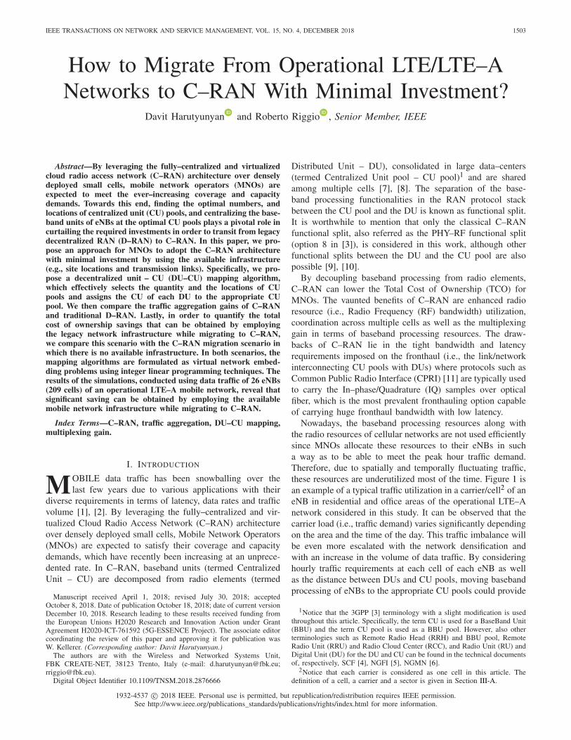
Nowadays, the baseband processing resources along withthe radio resources of cellular networks are not used efficientlysince MNOs allocate these resources to their eNBs in sucha way as to be able to meet the peak hour traffic demand.Therefore, due to spatially and temporally fluctuating traffic,these resources are underutilized most of the time. Figure 1 isan example of a typical traffic utilization in a carrier/cell2 of aneNB in residential and office areas of the operational LTE–Anetwork considered in this study. It can be observed that thecarrier load (i.e., traffic demand) varies significantly dependingon the area and the time of the day. This traffic imbalance willbe even more escalated with the network densification andwith an increase in the volume of data traffic. By consideringhourly traffic requirements at each cell of each eNB as wellas the distance between DUs and CU pools, moving basebandprocessing of eNBs to the appropriate CU pools could provide
1Notice that the 3GPP [3] terminology with a slight modification is usedthroughout this article. Specifically, the term CU is used for a BaseBand Unit(BBU) and the term CU pool is used as a BBU pool. However, also otherterminologies such as Remote Radio Head (RRH) and BBU pool, RemoteRadio Unit (RRU) and Radio Cloud Center (RCC), and Radio Unit (RU) andDigital Unit (DU) for the DU and CU can be found in the technical documentsof, respectively, SCF [4], NGFI [5], NGMN [6].
2Notice that each carrier is considered as one cell in this article. Thedefinition of a cell, a carrier and a sector is given in Section III-A.
1932-4537 c© 2018 IEEE. Personal use is permitted, but republication/redistribution requires IEEE permission.See http://www.ieee.org/publications_standards/publications/rights/index.html for more information.

1504 IEEE TRANSACTIONS ON NETWORK AND SERVICE MANAGEMENT, VOL. 15, NO. 4, DECEMBER 2018
Fig. 1. Traffic demand variation in office and residential areas.
significant multiplexing gain in terms of both radio resourcesand baseband processing resources, entailing a reduction inTCO of the network.
A sizable body of work has been published on the DU–CUmapping problem in the last few years (see Section II).However, most of the studies make assumptions that wouldnot be feasible/efficient to be applied to real mobile networks.For example, some studies assume that a direct optical lineexists from all DUs to a single CU pool, while others assumethat a CU pool could be deployed in any area where there isan eNB and they consider only the distance between the DUsand the CU pool while mapping DUs to CUs. One questionthat needs to be asked, however, is how to migrate from legacynetworks to future 5G networks with the C–RAN architecturewith minimal investment by exploiting the available mobilenetwork infrastructure and the statistics of the hourly trafficdemand per cell?
The contribution of this paper is threefold.• First, we propose a DU–CU mapping algorithm in
order to facilitate MNOs’ transition from their legacyDecentralized RAN (D–RAN) architecture of LTEnetworks to the C–RAN architecture. The algorithm com-putes the number of CU pools and determines theirlocations by taking into account the information aboutthe available inter–eNB transmission links, the distancebetween the DUs and the potential CU pools, consider-ing the available transport network, and the hourly trafficdemand per cell of the mobile network.
• Second, we compare the traffic aggregation gain ofC–RAN, which is obtained as a result of the inter–sector intra–carrier traffic aggregation, with the one ofD–RAN, which is obtained by activating the intra–sectorinter–carrier traffic aggregation feature.
• Third, in order to quantify the economic advantageof using the available infrastructure while transiting toC–RAN, we compare two C–RAN migration scenarios(i.e., DU–CU mappings): with and without using theavailable infrastructure. In both scenarios, the mappingproblems are modeled as Virtual Network Embedding(VNE) problems, formulated and solved employingInteger Linear Programming (ILP) techniques.
The rest of this paper is structured as follows. The relatedwork is discussed in Section II. The substrate and the virtualnetwork models are detailed in Section III. The input sets,
parameters and binary decision variables used in the problemformulations are defined in Section IV. The problem state-ments and the ILP problem formulations for the intra–sectorinter–carrier traffic aggregation problem and the DU–CU map-ping problem are presented in, respectively, Sections V and VI.The migration cost computations are presented in Section VII.The numerical results are reported in Section VIII. Finally,Section IX draws the conclusions, pointing out the futurework.
II. RELATED WORK
A considerable amount of literature has been publishedon the DU–CU mapping problem [12]–[20]. An optimizationalgorithm is presented in [12] for placing CUs overFixed/Mobile Converged optical networks. The authors formu-late an ILP problem, which calculates the required minimumnumber of CU pools, taking into account only the maximumallowed distance between DUs and their CU pools. The sameauthors put forward an energy–efficient CU placement algo-rithm for optical networks in [13], aiming to minimize theAggregation Infrastructure Power.
Traffic– and interference–aware dynamic DU–CU map-ping algorithm is proposed in [14]. Mutual coupling loss,which characterizes Cross–carrier Co–channel Interference(CCI) between DUs, is taken into account in order to findthe most optimal DU–CU mapping, which apart from loadbalancing CUs and minimizing power consumption, wouldalso minimize the CCI between DUs. Semi–static and adap-tive DU–CU switching schemes are proposed in [15]. Theseschemes, although have the same objective of minimizing therequired number of CU pools in order to meet the trafficdemand at each DU, differ in terms of the DU–CU switch-ing interval. Namba et al. [16] elaborate more on the DU–CUswitching plan, considering also the signaling load caused byusers’ handover while making DU–CU switching decisions. Inall aforementioned works, however, the authors do not studyhow to select CU pool locations and how to assign DUs toCU pools in the case of multiple CU pools in order to get thehighest statistical multiplexing gain of resources, since it isimportant to consider not only spatially and temporally fluc-tuating traffic, but also the distance between DUs and CUpools.
An energy–efficient DU–CU mapping algorithm is proposedin [17]. Aiming at minimizing the energy consumption atthe CU pools, the computing resource requirement of theDUs and the inter–DU traffic exchange are considered forassigning the DUs to the CU pools. While a reconfigurablemillimeter wave wireless fronthaul network is used in [21]with the goal of reducing the network–wide power consump-tion in the CU placement problem, Wang et al. [22] proposean energy-efficient scheme for the optical–transport–enabledC–RAN networks by introducing the concept of a virtual basestation and enabling baseband processing resource sharing ofCUs and line cards of optical line terminators.
A CU placement problem is studied in [23], considering dif-ferent LTE–A configurations and investigating the impact ofdifferent CU centralization levels on both CAPEX and OPEX

HARUTYUNYAN AND RIGGIO: HOW TO MIGRATE FROM OPERATIONAL LTE/LTE–A NETWORKS TO C–RAN WITH MINIMAL INVESTMENT? 1505
in an optical network–supported C–RAN. Chen et al. [18]propose a dynamic DU–CU mapping scheme employing aborrow–and–lend approach. The key idea is to migrate theDUs assigned to a highly utilized CU to a less utilized CU,having the objective of maximizing the utilization of everysingle CU inside the CU pool. However, only one CU poolis considered in these studies without tackling the problemof selecting the number and the locations of the CU poolsin order to cater the traffic demand of all the DUs in thenetwork. Moreover, the authors do not consider the CU place-ment problem simply assuming that all DUs are assigned to asingle CU pool via direct links.
An analytical model is derived in [19] for finding theoptimal ratio between optical fibers and microwave links,which would reduce the CAPEX required to build the fron-thaul network and, at the same time, meet the traffic require-ment at each cell site. Holm et al. [20] study the problem ofminimizing the CAPEX for those MNOs who want to designa mobile network from scratch, adopting the C–RAN architec-ture. Specifically, the authors study the trade–offs between themultiplexing gain in terms of baseband processing resource,which would increase by assigning more DUs to the sameCU pool, and the fronthaul network deployment cost, whichwould reduce if more CU pools were available for DUs tobe associated with. However, the authors make some simplis-tic assumptions which would be unreasonable to be appliedto existing mobile infrastructures. For example, they assumethat the fronthaul links are directly connected to the CU pool.They also categorize base stations into two types, office andresidential, and assume that the same number of office cellsare allocated to the CU pools. Nevertheless, they do not gointo the granularity of hourly traffic requirement of each cellin order to better understand the CU composition of whichDUs would provide the highest multiplexing gain in terms ofboth radio resource and baseband processing resource, sincethe traffic demand in some office and some residential areasmight be such that they would not provide high multiplexinggain being assigned to the same CU pool. An optimizationproblem similar to ours is presented in [24]. A CU place-ment problem is formulated aiming to find the optimal quantityand locations of CU pools with the goal of minimizing TCO.The migration cost is computed from an optical D–RANand a Microwave D–RAN to C-RAN, considering greenfieldand brownfield optical networks for macrocell, microcell and,nanocell deployments. The main difference compared to ourwork, however, is that the authors do not consider the realtraffic demand at each cell of the traditional D–RAN network,which plays a pivotal role in selecting the number and the loca-tions of the CU pools. While in [25], a CU placement problemis studied for the C–RAN network with Wavelength DivisionMultiplexing (WDM) aggregation networks. The authors for-mulate a joint and an independent CU and electronic switchplacement problems, considering their placement possibilitiesin different parts of the Optical Transport Network and theOverlay fronthaul transport network.
The research to date has tended to focus on building futuremobile networks from scratch based on the traffic demand.A common characteristic of the aforementioned works is that
none of them has studied how MNOs, owning legacy LTEnetworks, can upgrade the network by adopting the C–RANarchitecture with the minimal cost by employing the availablesite locations, transmission links, the knowledge of the CUpool candidate locations, and hourly traffic demand per cell.This is a relevant problem since we believe that a few MNOswould be willing to invest a huge amount of money in buildingC–RAN from scratch, when they can just reuse the legacyinfrastructure, and therefore, significantly curtail the requiredinvestments in order to deploy C–RAN.
III. NETWORK MODEL
This section details the substrate and the virtual networkmodels. The parameters (e.g., the locations of eNBs, the num-ber of sectors per eNB, the number of carriers/cells per sectorand the hourly traffic demand per cell), used in the models,are taken from an operational LTE–A network.
A. Definition of Basic Elements
Before introducing the substrate and the virtual networkmodels, let us provide a more precise definition of the termscarrier, cell and sector.
• Carrier: The RF bandwidth (in MHz) owned by theMNO is divided into smaller RF bands called carriers.For example, if an MNO owns 45MHz of RF bandwidththen such bandwidth may be distributed across a 10MHz,a 15MHz, and a 20MHz carrier.
• Cell: An eNB can have a different number of cellsdepending upon its configuration. In this work, weassume that each cell is assigned one and only one car-rier, regardless of its RF bandwidth and the LTE bandthat it belongs to.
• Sector: The coverage area of the antenna beam. Each eNBmay have one or more sectors, and each sector, in turn,may have one or more cells. In this work, each sector hasa maximum of 3 cells. For example, if the total coverageof an eNB is divided into 3 sectors, and each sector has3 carriers (10MHz, 15MHz and 20MHz) then it meansthat such eNB has a total of 9 cells.
B. Substrate Network Model
The considered substrate network is a small cluster (5 Km2)of an operational LTE–A network composed of 26 eNBs and ina total of 209 cells (see Fig. 2). Let Gs = (Ns,Es) be an undi-rected graph modeling the physical network (i.e., the networkto be transformed to C–RAN), where Ns = N du
s = Nenb isthe set of m = |Ns| DUs/eNBs. Each n ∈ N du
s DU has a vari-able number of sectors |N n
sct | in the set of {1, 2, 3, 4}, eachs ∈ N n
sct sector has a variable number of carriers/cells |N n,scar |
in the set of {1, 2, 3}, while each carrier c ∈ N n,scar has its max-
imum supportable downlink throughput ωtmaxs,c (see Table III).
A subset of the eNBs N cus ⊂ Ns can be candidates for CU
pools. More specifically, the candidate CU pools are selectedas follows. The eNBs are sorted in descending order accord-ing to the number of inter–eNB transmission links, whereasif some of them have equal number of inter–eNB links, theyare sorted according to their total link capacity, and the first

1506 IEEE TRANSACTIONS ON NETWORK AND SERVICE MANAGEMENT, VOL. 15, NO. 4, DECEMBER 2018
Fig. 2. An operational LTE–A network with 26 eNBs (in total 209 cells) in the city center of Yerevan. Each eNBs is composed of variable number ofsectors, which, in turn, is composed of variable number of carriers employing 20MHz, 15MHz and 10MHz RF bandwidths.
four eNBs are considered as CU pool candidates. The requirednumber of CU pool(s) are then picked starting from the firsteNB in the sorted list. Thus, the CU pool candidates (i.e.,anchor eNBs) are the eNBs that interconnect multiple eNBsand serve as a relay for them to transport their signals to thecore network. Selecting an anchor eNB as a CU pool enablesMNOs to exploit the available transport network (i.e., back-haul links) in an efficient manner without having to invest toomuch in building the fronthaul network while migrating to theC–RAN architecture. It is important to mention that, since inthe considered small cluster of the mobile network only opticalbackhaul links are available, we assume that those backhaullinks can be used as fronthaul links in the C–RAN architecture.
Each substrate node (i.e., DU/eNB) is also associated witha geographic location loc(n), as x, y coordinates. In order tomimic the real physical topology (i.e., the accurate inter–eNBdistance) of the considered LTE–A network, x, y coordinatesof the nodes are obtained by converting the real locations (lon-gitude and latitude) of the eNBs. Lastly, let Es model the setof inter–eNB links of the real network. An edge enm ∈ Es ifand only if a connection exists between DUs/eNBs n,m ∈ Ns.The substrate network parameters can be found in Section IV.
C. Virtual Network Model
The considered mobile network (D–RAN) is modeled asa virtual network, which has to be mapped to the substratenetwork (C–RAN). Let Gv = (Nv,Ev) be an undirectedgraph, where Nv = N du
v ∪ N cuv is the set of m1 = |N du
v |virtual DUs and m2 = |N cu
v | virtual CUs. Notice that sincein C–RAN an eNB is decomposed into a DU and a CU theneach m ∈ N du
v has to have its CU m ′ ∈ N cuv . Therefore, the
number of virtual DUs is equal to the number of virtual CUsand is equal to the number of substrate DUs m1 = m2 = m .
In essence, each m ∈ N duv virtual DU has its corresponding
n ∈ N dus substrate DU, and they have the same number of sec-
tors, carriers per sector and the same location.3 Additionally,at each hour h ∈ Nhr , each carrier c ∈ N n,s
car of each sectors ∈ N n
sct of each virtual DU n ∈ N duv has its traffic demand
ωcv,t (h), which is taken from the traffic demand statistics of
the considered mobile network.As opposed to the substrate network model, edges
enm ∈ Ev in the virtual network request represents the logicalmapping between virtual DUs and their corresponding CUs.As an additional constraint, we require each virtual CU to bemapped to one and only one substrate CU pool. Conversely,different virtual CUs from different DUs can be mapped tothe same CU pool. This enables advanced interference con-trol algorithms such as Joint Transmission/Reception to beemployed [26], which is one of the prominent advantagesof C–RAN. The virtual network parameters can be found inSection IV.
D. WDM–PON
We assume that the C–RAN fronthaul network is a WDMPassive Optical Network (PON), which is composed of twomain components, Optical Network Unit (ONU) and OpticalLine Terminator (OLT), performing electrical to an optical sig-nal and reverse conversion. The former is located at DUs whilethe latter is located at CU pools.
It is assumed that each CU pool has one OLT rack andone OLT shelf, which has eight OLT access modules. It isalso assumed that each OLT access module, through WDM
3Notice that a single notation is used for those parameters that are the samefor the substrate and the virtual network (e.g., the location of the DUs, thenumber of sectors and the number of carriers).

HARUTYUNYAN AND RIGGIO: HOW TO MIGRATE FROM OPERATIONAL LTE/LTE–A NETWORKS TO C–RAN WITH MINIMAL INVESTMENT? 1507
Mux/DeMux, is connected to a passive splitter by a single fiberlink that supports four wavelengths each with λb = 10Gbpscapacity [27]. There is one passive splitter with 16 ports ateach eNB site, while the number of ONUs at each eNBdepends on the fronthaul bandwidth requirement of each DU ateach eNB. For example, if an eNB has three sectors each hav-ing one 20MHz cell and one 15MHz cell (overall 6 cells) thenthe fronthaul bandwidth requirement, regardless of the cell uti-lization level,4 in total would be 7.37Gbps and 5.53Gbps for,respectively, 20MHz cells and 15MHz cells, assuming thatCPRI protocol is used and that each cell has 2 × 2 MIMOantenna configuration. This would require two wavelengths(λb = 2), in order to meet the fronthaul bandwidth demand,which translates to two ONUs since there is one to one map-ping between an ONU and a λb while four to one mappingbetween an ONU and an OLT access module.
IV. DEFINITION OF INPUT SETS, PARAMETERS AND
BINARY DECISION VARIABLES
In this section, we define the input sets, parameters andbinary decision variables used in the substrate and virtualnetwork models of the ILP problem formulations.
A. Input Sets and Parameters
Gs Substrate network graph.Gv Virtual network graph.Es Set of substrate links in Gs.Ev Set of virtual links in Gv.Nenb Set of eNBs in Gs.N n
sct Set of sectors of n ∈ Nenb eNB.N n,s
car Set of carriers of s ∈ N nsct sector of n ∈
Nenb eNB.N cu
s Set of predefined CU pool candidates in Gs.N cu
v Set of virtual CUs in Gv.N du
s Set of substrate DUs in Gs.N du
v Set of virtual DUs in Gv.Nhr Set of hours in a day.N du
� Number of DUs not co–located with a CU pool.ωc
v,t (h) Traffic on c ∈ N n,scar virtual carrier at h ∈ Nhr
hour.ωtmax
s,C Maximum traffic on C ∈ N n,scar substrate carrier.
Llen(e) Length of e ∈ Es substrate link [in Km].Llen Overall length of the substrate links [in Km].L�
len Overall length of the built fronthaul links [in Km].loc(n) Geographical location of n virtual/substrate node.WC Bandwidth of C ∈ N n,s
car carrier [in MHz].μb Big positive constant.μs Small positive constant.λb Lightpath capacity [in Gbps].
B. Binary Decision Variables
ΦC Shows if C ∈ N n,scar carrier of s ∈ Nsct sec-
tor of n ∈ Nenb eNB has been selected for trafficaggregation.
4For a given cell/carrier, fronthaul bandwidth requirement is fixed for thetraditional PHY–RF split in the C–RAN architecture and does not depend onthe traffic requirement of the considered cell as long as the cell is active [9].
Φc,t ,hC Shows if ωc
v,t (h) traffic of c ∈ N n,scar virtual carrier
at h ∈ Nhr time has been aggregated on C ∈ N n,scar
substrate carrier.Φm Shows if m ∈ N cu
s candidate CU pool has beenselected as a CU pool.
Φm′m Shows if m ′ ∈ N cu
v virtual CU has been mapped tom ∈ N cu
s substrate CU pool.Φn ′
n Shows if n ′ ∈ N duv virtual DU has been mapped to
n ∈ N dus substrate DU.
Φe′e Shows if e ′ ∈ Ev virtual link has been mapped to
e ∈ Es substrate link.
V. INTRA–SECTOR INTER–CARRIER
TRAFFIC AGGREGATION
In this section, we formally state the intra–sector inter–carrier traffic aggregation problem and present its ILP for-mulation.
A. Problem Statement: Intra–sector Inter–Carrier TrafficAggregation in D–RAN
In order to show how much the radio resource utilizationefficiency of the eNBs can be increased thanks to the statisticalmultiplexing gain obtained by the C–RAN architecture, wefirst need to quantify the radio resource utilization level of theeNBs of the current D–RAN architecture over the consideredperiod of time.
In mobile networks, data traffic undergoes significant fluc-tuations depending upon the location of eNBs and the timeof a day. When the traffic demand is low on carriers/cellsin traditional LTE networks, intra–sector inter–carrier trafficaggregation, as a feature, can be activated with the goal ofreducing power consumption by switching off unnecessarycarriers in sectors, and at the same time, ensuring that userstraffic demand is met. The upper part of Fig. 3 illustratesan example of the intra–sector inter–carrier traffic aggrega-tion technique. Two three–sector eNBs are considered eachhaving three carriers/cell under each sector. The tables belowthe eNBs show their corresponding average carrier/cell uti-lization per RF bandwidth per sector over the given period oftime. After performing intra–sector inter–carrier traffic aggre-gation per eNB, considering the maximum capacity of eachcarrier/cell (see Table III), we can observe that the algorithmaggregated the traffic of all carriers onto overall six carriers(three carrier per eNB, which are marked in gray in the tables).Notice that this is the minimum number of carriers since, as thename of the employed traffic aggregation technique suggests,the traffic aggregation takes place under each sector separately.As a side effect, this increases the radio resource utilizationof the active carriers (i.e., the carriers on which the traffic ofsome other carriers under the same sector have been aggre-gated). The radio resource utilization of the eNBs is computedafter activating the intra–sector inter–carrier traffic aggregationfeature, which has been formulated as an ILP problem that canbe formally stated as follows:
Given: a small cluster of an operational LTE–A networkwith the location of eNBs, the sectors per eNB and the

1508 IEEE TRANSACTIONS ON NETWORK AND SERVICE MANAGEMENT, VOL. 15, NO. 4, DECEMBER 2018
carriers/cells per sector with one–month statistics of theirhourly traffic demand.
Find: the number of carriers/cells that need to be active ateach eNB such that users hourly traffic demand is satisfied.
Objective: through intra–sector inter–carrier traffic aggrega-tion, curtail the number of active carriers per sector per eNB,thus reducing the power consumption in the network.
B. ILP Formulation: Intra–Sector Inter–Carrier TrafficAggregation in D–RAN
1) Objective Function: The objective function of theintra–sector inter–carrier traffic aggregation techniques is thefollowing:
minimize∑
n∈Nenb
∑
s∈N nsct
∑
C∈N n,scar
ΦCVC (1)
where VC is the cost for using the carrier C ∈ N n,scar for
traffic aggregation. VC is chosen to be proportional to the sizeof the carrier bandwidth. Given that the carrier has enoughcapacity to support the aggregated traffic, the wider is thecarrier bandwidth, the more expensive is its cost to be usedfor traffic aggregation. This is because it is assumed that thewider is the bandwidth of an active carrier, the more is theconsumed power. Note that by changing VC , MNOs can givemore/less priority to the carriers that they want to be used inthe traffic aggregation.
2) Constraints: In order to effectively achieve the afore-mentioned objective, all the following constraints have to berespected.
∑
c∈N n,scar
ωcv,t (h)Φc,t ,h
C ≤ ωtmaxs,C
∀n ∈ Nenb , ∀s ∈ N nsct , ∀h ∈ Nhr , ∀C ∈ N n,s
car (2)∑
c∈N n,scar
∑
h∈Nhr
Φc,t ,hC − μbΦC ≤ 0
∀n ∈ Nenb , ∀s ∈ N nsct , ∀C ∈ N n,s
car (3)∑
c∈N n,scar
Φc,t ,hC = 1 ∀n ∈ Nenb
∀s ∈ N nsct , ∀h ∈ Nhr , ∀C ∈ N n,s
car (4)
Constraint (2) ensures that data traffic on the carriers atwhich the traffic of other carriers have been aggregated is atmost equal to the maximum traffic capacity of the host carriers.Constraint (3) guarantees that if the traffic of any carrier ofany sector of any eNB at any time is mapped to any carrierof the same sector at the same time then the host carrier isselected in mappings. Notice that this constraint allows datatraffic of a carrier at different times to be mapped to differentcarriers belonging to the same sector of the same eNB. Lastly,Constraint (4) enforces the traffic of all carriers of all sectorsof all eNBs to be mapped/aggregated on the host carriers. Inother words, it makes sure that users’ traffic demand at anytime is met.
VI. DU–CU MAPPING
In this section, we formally state the DU–CU mappingproblem and present its ILP formulation.
Fig. 3. Examples of the intra–sector inter–carrier traffic aggregation (theupper part) and the inter–sector intra–carrier traffic aggregation (the lowerpart) techniques.
A. Problem Statement: DU–CU Mapping
In the DU–CU mapping problem, an inter–sector intra–carrier traffic aggregation is taking place, which is the aggre-gation of the traffic of the carriers that have the same RFbandwidth and belong to the same LTE band. Thus, the trafficon a carrier of a DU/eNB can be aggregated with the traf-fic on a carrier of another DU/eNB only if the CUs of thoseDUs are mapped to the same CU pool (i.e., their basebandsignal processing is taking place at the same CU pool), thosecarriers have the same RF bandwidth (i.e., either 20MHz or15MHz or 10MHz) and they are from the same LTE band.The rationale behind this approach is to guarantee a seam-less transition from the D–RAN architecture to the C–RANarchitecture, making sure that users experience no channelquality degradation during this transition. The lower part ofFig. 3 illustrates an example of the inter–sector intra–carriertraffic aggregation technique. The entire baseband processingof the eNBs is performed at the same CU pool, harvesting themultiplexing gain in terms of the baseband processing resourceas well as the radio resource. As a result, network–wide traf-fic aggregation is taking place. The traffic utilization of eachcell/carrier per eNB before the inter–sector intra–traffic aggre-gation is reported in the tables (see the upper part of Fig. 3).Notice that, as opposed to the intra–sector inter–carrier trafficaggregation that resulted in six carriers/cells being active at theeNBs (one carrier per eNB per sector), after employing inter–sector intra–carrier traffic aggregation, the traffic of all thecarriers is aggregated on four carries. Thus, the overall num-ber of active carriers/cells is reduced compared to the previoustraffic aggregation technique. More details on the inter–sectorintra–carrier traffic aggregation is provided in Section VIII-C2.The DU–CU mapping problem can be stated as follows:

HARUTYUNYAN AND RIGGIO: HOW TO MIGRATE FROM OPERATIONAL LTE/LTE–A NETWORKS TO C–RAN WITH MINIMAL INVESTMENT? 1509
Given: a small cluster of an operational LTE–A networkwith the location of eNBs, the transport network topology withthe capacity of each link, the sectors per eNB, the carriers/cellsper eNB with one–month statistics of its hourly traffic demandand the candidate locations for CU pools.
Find: the overall number of carriers/cells required to meetusers traffic demand, the number and location of CU pools,and DU–CU mappings.
Objective: through the inter–sector intra–carrier trafficaggregation minimize the overall number of carriers/cells, thenumber of CU pools required to support users hourly trafficdemand as well as minimize the fronthaul latency for eachvirtual link by mapping it onto the shortest substrate path.
B. ILP Formulation: DU–CU Mapping
The available network topology with traffic demand on thecarriers of each sector of each eNB is modeled as a virtualnetwork request. Upon arrival of the virtual network request,the substrate network must find the optimal mapping, aimingto minimize the objective function. Efficient mapping of vir-tual network requests onto a substrate network is known asa VNE problem [28]. The problem is NP–hard and has beenstudied extensively in [29]–[31]. The embedding process con-sists of two steps: the node embedding and the link embedding.In the node embedding step, each virtual node (i.e., a virtualDU or a virtual CU) in the request is mapped to a substratenode (i.e., substrate DU or substrate CU pool). In the linkembedding step, each virtual link is mapped to a single sub-strate path. In both steps, nodes and link constraints must besatisfied.
1) Objective Function: The DU–CU mapping problem hasbeen formulated as an ILP problem whose objective func-tion (see (5)) aims at minimizing the TCO for those MNOswho own an LTE/LTE–A network and want to migrate tothe C–RAN architecture. Specifically, the objective functionis composed of three parts:
• The first part aims at minimizing the deployment costof the CU pools by minimizing the required number ofCU pools. The candidate CU pool locations are pre–selected based on the inter–eNB connectivity ranking ofeach eNB. The more optical transmission links an eNBhas with its neighbors, the higher is the likelihood of theeNB to become a CU pool. The rationale behind thisapproach is to reuse the available transmission links asmuch as possible.
• The second part aims at minimizing the fronthaul deploy-ment cost by exploiting the available transmission links,and therefore, curtailing the investments required to buildthe fronthaul network for the C–RAN architecture. It alsominimizes the fronthaul delay for each virtual link bymapping it onto the shortest substrate path from the sub-strate DU, on which the virtual DU has been mapped,to the substrate CU pool that has hosted the basebandprocessing (virtual CU) of the virtual DU.
• The last part of the objective function minimizes therequired number of carriers in order to meet the trafficdemand on each carrier of each virtual DU at any time.
This radio resource multiplexing gain is achieved by con-sidering the hourly traffic demand on each carrier/celland aggregating the traffic of low utilized carriers intoa fewer carriers. Notice that contrary to the intra–sectorinter–carrier traffic aggregation (see Section V), in thiscase, an inter–sector intra–carrier traffic aggregation istaking place.
minimize∑
m∈N cus
VcuΦm +∑
e∈Es
∑
e′∈Ev
μsLlen (e)Φe′e
+∑
n∈N dus
∑
s∈N nsct
∑
C∈N n,scar
WCVmhzΦC (5)
where Vcu is a CU pool built–out cost while Vmhz is theannual spectrum fee per MHz (see Table I).
It is worthwhile to note that the second argument of theobjective function is very small compared to the rest of thearguments. This is because in the CAPEX savings computation(see Section VII-A1) we consider no fiber rollout cost sincein our case the backhaul links of the legacy mobile networkare employed as fronthaul links in the C–RAN deployment.Nevertheless, the second argument, although negligible, stillexists in order to find the shortest path among the availablesubstrate paths for mapping the virtual links.
2) Constraints:∑
m′∈N cuv
Φm′m − μbΦm ≤ 0 ∀m ∈ N cu
s (6)
∑
n∈Nenb
∑
s∈N nsct
ωcv,t (h)Φc,t ,h
C ≤ ωtmaxs,C
∀h ∈ Nhr , ∀c = C ∈ N n,scar (7)∑
n∈N dus
Φn ′n = 1 ∀n ′ ∈ N du
v (8)
∑
m∈N cus
Φm′m = 1 ∀m ′ ∈ N cu
v (9)
∑
e∈E�is
Φenm
e −∑
e∈E i�s
Φenm
e =
⎧⎪⎨
⎪⎩
−1 if i = n1 if i = m0 otherwise
∀i ∈ Ns, ∀enm ∈ Ev (10)∑
c∈N n,scar
Φc,t ,hC = 1 ∀n ∈ N cu
v
∀s ∈ N nsct , ∀h ∈ Nhr , ∀C ∈ N n,s
car (11)
Constraint (6) makes sure that a CU pool candidate isselected as a CU pool as long as it has assigned at least onevirtual CU. Notice that the case in which
∑m′∈N cu
vΦm′
m = 0and Φm = 1 is excluded since the objective function (5) alsoaims at minimizing the number of CU pools. Constraint (7)guarantees that traffic capacity limit of the host carriers isnot violated after traffic aggregation. While Constraints (8)and (9) make sure that each virtual DU and CU are, respec-tively, mapped to their corresponding substrate DU and CUpool, Constraint (10) enforces for each virtual link enm ∈ Ev
to be a continuous path established between the pair of thesubstrate DU and the CU pool on top of which the virtual DUn ∈ N du
v and the virtual CU m ∈ N cuv have been mapped.

1510 IEEE TRANSACTIONS ON NETWORK AND SERVICE MANAGEMENT, VOL. 15, NO. 4, DECEMBER 2018
In Constraint (10), E�is is the set of the fronthual links that
originate from any node and directly arrive at the node i ∈ Ns,while E i�
s is set of the fronthaul links that originate from thenode i ∈ Ns and arrive at any node directly connected to i.Lastly, Constraint (11) ensures that the traffic on all carriersfor all sectors of all virtual DUs are mapped; in other words,it is guaranteed that users’ traffic demand at each moment issatisfied.
Notice that, although C–RAN has a stringent fronthaullatency requirement, which translates to a maximum admissi-ble length of fronthaul links, which typically ranges between20 and 40 Km [7], we do not use the fronthaul latencyconstraint in the ILP formulation since in the considered oper-ational LTE–A network the maximum length of any possiblefronthaul route for CPRI flows is far smaller than the men-tioned maximum admissible length. Also, notice that we do nothave a fronthaul link bandwidth capacity constraint. Initially,given the fronthaul network topology, it is assumed that allthe fronthaul links have infinite capacity. This is becauseour goal is (i) to reuse the available links and (ii) to com-pute the additional bandwidth, therefore, the overall numberOLT access modules and ONUs required in order to meetthe network–wide fronthaul bandwidth demand in the C–RANarchitecture.
VII. MIGRATION COST COMPUTATION
In this section, we first analyze the TCO savings obtainedby migrating from legacy D–RAN to C–RAN. We then com-pare the migration costs of two C-RAN migration scenarios:the migration cost of C–RAN when the available transportnetwork is exploited and the migration cost of the C–RANin which the fronthaul infrastructure must be deployed fromscratch.
A. From D–RAN to C–RAN Migration Savings Computation
The are many advantages of adopting the C–RAN archi-tecture [7]. This advantages can be mainly divided into twogroups: feature– and cost–related advantages. The possibil-ity to exploit advanced interference avoidance/cancellationalgorithms such as FeICIC [32] or a coordinated schedulingalgorithm [33] are examples of feature–related advantages;whereas, the cost–related advantages are the reduction ofCAPEX and OPEX.
In this work, our focus is on the CAPEX and OPEX savingsthat can be obtained by using the available transport network(i.e., the links that are used to transport the backhaul traf-fic of the eNBs of legacy mobile networks) and the networkknowledge while transiting to C–RAN from legacy D–RAN.
1) CAPEX Savings: After mapping the virtual networkrequest onto the substrate network, we start the computationof CAPEX savings (C save
cpx ), which is computed as the summa-tion of the cost of the available OLT access modules, ONUsand the cost of the available fronthaul transport network (i.e.,fiber rollout cost). This is because the mentioned componentsare reused in the C–RAN deployment. Thus, CAPEX savings
can be computed as follows:
C savecpx =
∑
m∈N cus
ΦmVolt + |Nenb |Vonu + LlenVrol (12)
It is important to mention that while all the eNBs possessa single ONU, only a few of them (i.e., the anchor eNBs)possess an OLT access module.
2) OPEX Savings: The OPEX savings (C saveopx ), obtained
as a result of migrating from D–RAN to C–RAN, is the sum-mation of the following two costs: the annual fee for thespectrum usage per MHz per link and the annual cost of rent-ing cell sites. The former savings, thanks to the radio resourcemultiplexing gain of the C–RAN architecture, is obtained bycurtailing the required number of carriers with different RFbandwidths, making sure that mobile data traffic demand ismet at any hour. Whereas, the latter is the result of reducingthe cell site rent. Indeed, in the case of C–RAN, DUs beingcompact devices can be easily deployed in the street furniture(e.g., on a lamp post near to the original location of the eNBin order to provide seamless coverage to users), and there-fore, the cell site rent can be curtailed on average by a factor5
of α = 0.2, which is our assumption; while the cell site rentremains the same for the DUs that have a CU pool co–located.Thus, the annual OPEX savings can be computed as follows:
C saveopx =
∑
n∈Nenb
∑
s∈N nsct
∑
C∈N n,scar
(1 − ΦC )WCVmhz
+ αN du� Vrent (13)
Notice that, although the OPEX reduction of C–RAN isalso contributed by less power consumption compared toD–RAN [7], it is not considered in this study. There are sev-eral studies modeling and comparing the power consumptionof C–RAN with the one of the traditional D–RAN [22], [24].Table I summarizes all the cost parameters defined in theequations.
B. Migration Cost Computation of Two C–RAN MigrationScenarios
In order to show the advantage of using the availableinfrastructure in the C–RAN deployment in terms of CAPEX(OPEX is the same in both C–RAN migration scenarios), wecompare two C–RAN migration scenarios: the infrastructure–unaware C–RAN migration and the infrastructure–awareC–RAN migration. In the infrastructure–unaware C–RANmigration, we assume that the fronthaul network of theC–RAN deployment is designed without taking into accountthe available optical transport network of the legacy mobilenetwork; thus, no transport network exists, and therefore,it should be designed from scratch. Conversely, in theinfrastructure–aware C–RAN migration scenario, the fronthaulnetwork is available, which actually is the backhaul networkof the legacy D–RAN. Most of the links, however, do not have
5The exact value of α depends on the country, the exact location where theDUs are deployed, and on several other factors. However, it is a fact that inthe traditional C–RAN architecture (i.e., the PHY–RF functional split) curtailsthe site rent for the DUs due to their small space requirement for deploymentwith respect to the that of eNBs [7].

HARUTYUNYAN AND RIGGIO: HOW TO MIGRATE FROM OPERATIONAL LTE/LTE–A NETWORKS TO C–RAN WITH MINIMAL INVESTMENT? 1511
TABLE ICOST ASSUMPTIONS TAKEN FROM [27]
enough capacity in order to support the fronthaul bandwidthrequirement of C–RAN since there were originally designed tocarry the backhaul traffic of the legacy network, which is muchsmaller compared to the fronthaul bandwidth requirement ofC–RAN. Therefore, the capacity of the fronthaul links shouldbe increased by adding the required number of OLT accessmodules and ONUs.
For the infrastructure–aware C–RAN migration scenario, weuse the ILP formulation presented in Section VI-B. In thiscase, in order to compute the CAPEX (Cwith
cpx ), we first needto compute the fronthaul bandwidth Bfh(n) requirement ateach ∀n ∈ Nenb/N du
v eNB by using the equation in [34]:
Bfh(n) =∑
s∈N nsct
∑
c∈N n,scar
2fs(c)NoNQNR ∀n ∈ N duv (14)
where 2 accounts for the complex nature of the IQ samples,while the other parameters are reported in Table II. We cannow compute the CAPEX:
Cwithcpx =
∑
n∈Nduv
(⌈Bfh (n)
λb
⌉− 1
)Vonu
+∑
m∈Ncus
⎛
⎝
⎡
⎢⎢⎢
∑m′∈Ncu
vBfh
(m ′
�)Φm′
m
4λb
⎤
⎥⎥⎥− 1
⎞
⎠ΦmVolt
(15)
where m ′� is the corresponding virtual DU/eNB of m ′ virtual
CU. The first and the second fractions calculate the addi-tional number of, respectively, ONUs in DUs and OLT accessmodules in CU pools required in order to support the network–wide fronthaul bandwidth demand. It is important to mentionthat, since in this case, the optical transport network is avail-able, there is no fiber rollout cost in the CAPEX computation.Notice that we do not consider the cost of building CU poolssince, as we will see in Section VIII, the number of CU pools(not the candidate CU pools) after embedding is the same inboth migration scenarios.
For the infrastructure–unaware C–RAN migration scenario,we use the ILP formulation presented in Section VI-B with aslight modification in the objective function (5), while keep-ing the constraints the same. The objective function for thisscenario is the following:
minimize∑
m∈Ns
VcuΦm +∑
e∈Es
∑
e′∈Ev
VrolLlen(e)Φe′e
+∑
n∈N dus
∑
s∈N nsct
∑
C∈N n,scar
WCVmhzΦC (16)
TABLE IIPARAMETERS FOR CALCULATING FRONTHAUL DATA RATES
Notice that as opposed to (5), here the second argument isnot negligible and accounts for the fiber rollout cost of thefronthaul network, since in this case it is assumed that thefronthaul network is not given. Notice also that, as opposed tothe infrastructure–aware C–RAN migration scenario, in whichthe candidates for CU pools are predefined, in this scenario,any eNB is a potential candidate for a CU pool. Whereas likein the first scenario, also here it is initially assumed that themapped links have infinite capacity, meaning that there areenough number of OLT access modules and ONUs to host therequired fronthaul bandwidth on any fronthaul link. However,the exact fronthaul capacity of the mapped fiber links, whichis, the exact number of OLT access modules and ONUs iscomputed by considering the fronthaul requirements of themapped virtual links.
Considering that the fronthaul bandwidth requirement(Bfh(n)) for each DU n ∈ N du
v is the same in both scenarios,the CAPEX (Cwout
cpx ) in the infrastructure–unaware C–RANmigration scenario can be computed as follows:
Cwoutcpx =
∑
n∈N duv
⌈Bfh(n)
λb
⌉Vonu
+∑
m∈Ns
⌈∑m′∈N cu
vBfh(m ′
�)Φm′m
4λb
⌉Volt
+ L�lenVrol (17)
The first argument computes the cost of ONUs, the secondargument computes the cost of OLT access modules, while thelast argument computes the fiber rollout cost.
VIII. EVALUATION
The goal of this section is to compare the presented trafficaggregation algorithms and the C–RAN migration scenarios.We shall first describe the simulation environment used in ourstudy. We will then report on the outcomes of the numeri-cal simulations carried out using a discrete event simulatorimplemented in MATLAB.
A. Simulation Parameters
A small cluster (26 eNBs deployed on rooftops with 209cells in total) of an operational LTE–A mobile network in thecity center of Yerevan is considered in our simulations (seeFig. 2). The cluster provides mobile coverage in the area of5Km2. The average number of RRC connected users per eNBvaries between 450 and 2000 depending on the location ofeNBs, their carriers and the time of the day. Whereas, the

1512 IEEE TRANSACTIONS ON NETWORK AND SERVICE MANAGEMENT, VOL. 15, NO. 4, DECEMBER 2018
TABLE IIILTE–A NETWORK PARAMETERS
number of sectors per eNB, as well as the number of carri-ers/cells per sector, vary in the set of, respectively, {1, 2, 3, 4}and {1, 2, 3}, depending upon the need for providing eithercoverage or extra capacity in the given area. Three LTE car-riers, 20MHz, 15MHz and 10MHz, are used in the network,and only optical fiber links are used to connect the eNBs tothe core network. This is a representative of a dense urbanmobile network deployment scenario.
The maximum downlink traffic ωtmaxs,C per carrier/cell
C ∈ N n,scar , which has either 20MHz or 15MHz or 10MHz RF
bandwidth, is derived considering 2×2 MIMO antenna config-uration in every sector, the average modulation order, whichis assumed to be 16 QAM since eNBs are deployed densely,and 25% overhead such as PDCCH, reference signal, synchro-nization signals, PBCH and channel coding. Whereas, hourlydownlink traffic demands per carrier ωc
v,t (h) is derived fromthe traffic demand statistics of the RRC connected users in theconsidered LTE–A network. Table III shows the parametersused to derive the maximum downlink throughput per carrier.The simulations are conducted for each day separately, and thereported results are the average of 30 simulations (one month)with 95% confidence intervals.
B. Simulation Results
As it has been mentioned, the objective function of theintra–sector inter–carrier traffic aggregation problem (see for-mula (1)) aims at curtailing the number of active carriersby aggregating the traffic of low–utilized carriers on fewercarriers, and therefore, enabling MNOs to switch off theunnecessary carriers. For MNOs, the effect of minimizingthis objective function (i.e., the activation of the intra–sectorinter–carrier traffic aggregation feature) is the OPEX savingsobtained in the power consumption bills. However, we willlook at this objective from the perspective of the load at eNBs,since curtailing the number of active carriers increases the uti-lization of the remaining active carriers after switching off thelow–utilized carries.
Figure 4 displays the average traffic load per eNB over 24hours averaged for one month. The traffic load at each hourat each eNB is the summation of the carrier loads of thateNB. It can be observed that by activating the intra–sectorinter–carrier traffic aggregation feature, the load of the activecarriers per sector can be significantly increased. This is aconsequence of aggregating the traffic of the low–utilized andalready inactive carriers to the active carriers. It can also beobserved, however, that there is still room for increasing theload at eNBs, and therefore, resulting in a more efficient carrierutilization. Towards this end, we adopt the C–RAN architec-ture and study different scenarios for migration from legacyD–RAN to C–RAN.
Fig. 4. Traffic load per eNB.
Figure 5 illustrates the RF bandwidth utilization, the overallnumber of carriers, the number of carriers per RF bandwidthand the execution time of the considered traffic aggrega-tion before the intra–sector inter–carrier traffic aggregation(case 1), after the intra–sector inter–carrier traffic aggregation(case 2) and after the inter–sector intra–carrier traffic aggrega-tion in C–RAN (case 3). We can observe that in the consideredperiod of time the RF bandwidth utilization barely reaches20% at all the considered carriers before the intra–sectorinter–carrier traffic aggregation (see Fig. 5a). Although theintra–sector inter–carrier traffic aggregation feature increasesthe utilization of the active carriers, as we have also seen inFig. 4, it can still be significantly increased since 20MHz,15MHz and 10MHz carriers are underutilized by, respectively,56%, 46% and 31% with the maximum 5% of difference fromthe mean values in their confidence intervals. We can observethat after adopting the C–RAN architecture the utilization ofall the carriers with different RF bandwidths is increased upto approximately 95%.
The overall number of carriers for all the cases is depictedin Fig. 5b. Notice that, although the number of active carri-ers after intra–sector inter–carrier traffic aggregation (case 2)is reduced by 61%, this just curtails the power consumptionbills without exempting the MNO from paying the fee forusing the spectrum of temporarily unused carriers. Whereas,after adopting the C–RAN architecture (case 3), the numberof active carriers is curtailed by 80%, which not only reducesthe power consumption but also significantly lowers the over-all fee for using the spectrum. It is worthwhile to note that,regardless of different traffic requirements on the carriers indifferent days, there is no change in the overall number ofcarriers after the intra–sector inter–carrier traffic aggregation(i.e., the confidence interval is zero in case 2). This stemsfrom the fact that unlike the inter–sector intra–carrier trafficaggregation in C–RAN (case 3), the intra–sector inter–carriertraffic aggregation technique aggregated the traffic of carriersper sector individually.
Figure 5c shows the number of carriers per RF bandwidthfor case 1 and case 3. We remind the reader that each sec-tor has variable number of carriers (i.e., 20MHz, 15MHzor 10MHz RF bandwidth, maximum one carrier from eachRF bandwidth). As expected, C–RAN curtails the number

HARUTYUNYAN AND RIGGIO: HOW TO MIGRATE FROM OPERATIONAL LTE/LTE–A NETWORKS TO C–RAN WITH MINIMAL INVESTMENT? 1513
Fig. 5. RF bandwidth utilization, overall number of carriers, number ofcarriers per RF bandwidth and execution time for the considered cases.
of carriers in all RF bandwidths and distributes the overalltraffic more uniformly across the different RF bandwidths.Lastly, Fig. 5d compares the time required to execute the
Fig. 6. CAPEX in infrastructure–aware and infrastructure–unaware C–RANmigration scenarios, and TCO savings in the former scenario.
intra–sector inter–carrier traffic aggregation (case 2) and thetime to execute the inter–sector intra–carrier traffic aggrega-tion in C–RAN (case 3). It can be seen that in case 2 theexecution time is extremely shorter compared to the executiontime in case 3. This is justified by the fact that, as opposedto case 3 in which a global inter–sector intra–carrier trafficaggregation is taking place, in case 2 the intra–sector inter–carrier traffic aggregation is confined within each sector ofeach eNB. Even though one could suggest resorting to heuris-tics to address large instances of the problem, in our opinion,MNOs may agree to wait even a week in order to find theoptimal mapping solution for their CU–DU mapping problemrather than find a suboptimal solution very fast. This is becausethere is no need for performing this kind of DU–CU mappings(inter–sector intra–carrier traffic aggregation) very frequently.
In order to get an insight into what is the advantage of usingan infrastructure–aware C–RAN migration and how much theMNO can gain in terms of CAPEX and OPEX savings whilemigrating from their D–RAN to C–RAN, let us analyze Fig. 6.Figure 6a compares CAPEX of two C–RAN migration scenar-ios: infrastructure–aware and infrastructure–unaware migrationfrom D–RAN to C–RAN. We remind the reader that theformer scenario implies that the available infrastructure ofD–RAN (e.g., optical backhaul links, OLT access modules,ONUs, etc.) is used in the C–RAN. Whereas in the latterscenario, it is assumed that only the eNB site locations areavailable and the fronthaul infrastructure should be designedfrom scratch. Notice that the CU pool build–out cost is not

1514 IEEE TRANSACTIONS ON NETWORK AND SERVICE MANAGEMENT, VOL. 15, NO. 4, DECEMBER 2018
considered in CAPEX savings since in both C–RAN cases theILP–based DU–CU mapping algorithms select two CU poolsto be built in order to support centralized signal processingof all eNBs. We can observe that around seven times morecapital investment is required if the available infrastructure isnot considered the C–RAN deployment. The greatest share ofthis CAPEX constitutes the cost of building the optical fron-thaul network. Additionally, we can observe that, as opposed tothe infrastructure–unaware migration, the infrastructure–awaremigration requires no OLT deployment cost in this particularnetwork setup since after the DU–CU mapping the capacity ofthe OLTs available in the legacy LTE–A network is enough tomeet the fronthaul traffic demand in C–RAN. It is worthwhileto note that while there is no change in the OLT and the ONUshares in CAPEX for both migration scenarios, which essen-tially means that the required number of ONUs and OLTsis the same regardless of traffic variation in different daysat different carriers, the fiber rollout cost share in CAPEXchanges due to different fronthaul link mappings in differentdays. Therefore, the infrastructure–unaware fronthaul networkdesign requires careful analysis of the traffic pattern changeat different days at the eNBs.
Let us now analyze how much the MNO can gain fromthe considered small part of the LTE–A network in terms ofCAPEX and annual OPEX savings (see Fig. 6b) as a result ofemploying the available network infrastructure. CAPEX sav-ings come from three components: fiber rollout cost, ONUsand OLT access modules. As it is expected, the greatest partof CAPEX savings is obtained from the fronthaul deploymentcost. The cost of OLT access modules and ONUs is signif-icantly lower compared to the fiber rollout cost. Whereas,annual OPEX savings comes from reduced spectrum fee andcell site rent. It can be observed that in this particular scenariothe annual cell site rent of the curtailed cell sites is around fourtimes higher than the annual spectrum fee of the curtailed car-riers. It can also be observed that apart from the fiber rolloutcost variation, there is a negligible OPEX variation also in thespectrum fee. This is due to the fact that in the C–RAN archi-tecture, after the inter–sector intra–carrier traffic aggregation,the overall number of carriers and their RF bandwidth dependson the traffic demand per carrier before the aggregation, whichvaries in different days.
C. Discussion
1) Intra–Sector Inter–Carrier Traffic Aggregation inD–RAN: The intra–sector inter–carrier traffic aggregationfeature has several pros. For instance, if the traffic demandon the carriers is low then by activating this feature in currentLTE/LTE–A networks the overall power consumed by carrierscan be reduced by deactivating the unused carriers (see theupper part of Fig. 3). Whereas if the required traffic on thecarriers is high, the inactive carriers can then be reactivated,meeting the traffic demand and providing the possibility ofcarrier aggregation, which is one of the prominent features ofLTE–A technology. Nonetheless, the cons of the intra–sectorinter–carrier traffic aggregation lay in the fact that the overallOPEX can be reduced only in terms of power consumption
cost for the period in which some of the carriers are inactive.Moreover, by aggregating the intra–sector inter–carrier traffic,the host carriers may still be underutilized (see Fig. 4).
2) Inter–Sector Intra–Carrier Traffic Aggregation inC–RAN: The inter–sector intra–carrier traffic aggregation inC–RAN (case 3) has an important advantage over the intra–sector inter–carrier traffic aggregation (case 2). The carriersat different frequency bands (e.g., Band 3, Band 5, Band 7)with different RF bandwidths (e.g., 10MHz, 15MHz and20MHz) have their peculiarities. For example, high–frequencybands (e.g., Band 7, 2620-2690MHz) are more beneficialfor LTE networks construction in the regions with a largepopulation where high speed of data transfer is required.Whereas, LTE network deployments in the low–frequencybands (e.g., Band 5, 869-894MHz) is very appealing fromthe cost viewpoint and is ideal for the regions with lowpopulation (e.g., suburban areas, villages). The pros of sucha deployment are costs, better penetration inside buildingsand coverage of large territories. Thus, some users mayexperience performance degradation while forcing them tohandover from one carrier to another under the same sector.Whereas, this problem does not exist in case 3, since in thiscase an inter–sector intra–carrier traffic aggregation is takingplace.
3) Infrastructure–Aware C–RAN Migration: InSection VIII, we have seen that significant TCO sav-ings can be obtained by exploiting the legacy mobile networkinfrastructure while migrating to C–RAN. In this work, how-ever, just a small part of an operational LTE–A network isconsidered. The TCO savings will increase with the increaseof the network size. More accurate TCO savings estimationdepends not only on the size of the network but also onthe geographical areas (e.g., urban, suburban, rural), the linktypes of the transport network, population, traffic demandand on several other factors. Thus, although the consideredscenario the obtained results cannot be extrapolated to allkind of deployments, it is, however, a good example of anurban mobile network deployment.
IX. CONCLUSION
Recently, C–RAN has come to the fore as a promis-ing way to use the precious baseband processing and radioresources elastically and efficiently based on the actual needand, through better inter–cell coordination, overcome all thepossible performance degradation that may be entailed bynetwork densification.
In this paper, we propose an ILP–based algorithm to allowMNOs to transit to the C–RAN architecture with minimalinvestment by employing the available infrastructure in an effi-cient manner, and therefore, curtailing the required investmentsto adopt the C–RAN architecture. In order to quantify the TCOsaving, we compare infrastructure–aware and infrastructure–unaware C–RAN migration scenarios, showing the significantsavings that can be obtained by using the former approach.
Since only the classical C–RAN functional split is consid-ered in this study, the fronthaul network itself does not provideany multiplexing gain. As a future work, we are planning

HARUTYUNYAN AND RIGGIO: HOW TO MIGRATE FROM OPERATIONAL LTE/LTE–A NETWORKS TO C–RAN WITH MINIMAL INVESTMENT? 1515
to extend the problem formulation and, based on the trafficdemand statistics per cell and the availability of the transmis-sion links, consider the possibility of flexible functional splitat the RANs and study the impact of functional splits to thefronthaul multiplexing gain.
REFERENCES
[1] Global Mobile Data Traffic Forecast Update, 2016–2021 White Paper,Cisco, Vis. Netw. Index, San Jose, CA, USA, 2017.
[2] Y. Q. Bian. (2014). Small Cells Big Opportunities. [Online]. Available:https://www.huawei.com/ilink/en/download/HW330984
[3] “Technical specification group radio access network; study on new radioaccess technology; radio access architecture and interfaces, V2.0.0,”3GPP, Sophia Antipolis, France, Rep. TR 38.801, 2017.
[4] “Small cell virtualization functional splits and use cases, V7.0,” SmallCell Forum, London, U.K., Rep. 159.07.02, 2016.
[5] J. Huang and Y. Yuan. White Paper of Next Generation FronthaulInterface, Version 1. Accessed: Oct. 31, 2016. [Online]. Available:https://labs.chinamobile.com/cran
[6] “Further study on critical C-RAN technologies, V1.0,” Next Gener.Mobile Netw. Alliance, Frankfurt, Germany, Rep., 2015.
[7] K. Chen and R. Duan, “C-RAN the road towards green RAN,version 2.5,” Beijing, China, China Mobile Res. Inst., White Paper,2011.
[8] A. Checko et al., “Cloud ran for mobile network—A technologyoverview,” IEEE Commun. Surveys Tuts., vol. 17, no. 1, pp. 405–426,1st Quart., 2015.
[9] U. Dötsch et al., “Quantitative analysis of split base station processingand determination of advantageous architectures for LTE,” Bell LabsTech. J., vol. 18, no. 1, pp. 105–128, Jun. 2013.
[10] D. Harutyunyan and R. Riggio, “Flex5G: Flexible functional split in5G networks,” IEEE Trans. Netw. Service Manag., vol. 15, no. 3,pp. 961–975, Sep. 2018.
[11] “Common public radio interface, interface specification, V7.0,” CPRI,Bengaluru, India, Rep., 2015.
[12] N. Carapellese, M. Tornatore, and A. Pattavina, “Placement of base-bandunits (BBUs) over fixed/mobile converged multi-stage WDM-PONs,” inProc. IEEE ONDM, Brest, France, 2013.
[13] N. Carapellese, M. Tornatore, and A. Pattavina, “Energy-efficient base-band unit placement in a fixed/mobile converged WDM aggregationnetwork,” IEEE J. Sel. Areas Commun., vol. 32, no. 8, pp. 1542–1551,Aug. 2014.
[14] D. Zhu and M. Lei, “Traffic and interference-aware dynamic BBU-RRUmapping in C-RAN TDD with cross-subframe coordinated schedul-ing/beamforming,” in Proc. IEEE ICC, Budapest, Hungary, 2013,pp. 884–889.
[15] S. Namba, T. Warabino, and S. Kaneko, “BBU-RRH switching schemesfor centralized RAN,” in Proc. IEEE CHINACOM, Kunming, China,2012, pp. 762–766.
[16] S. Namba, T. Matsunaka, T. Warabino, S. Kaneko, and Y. Kishi,“Colony-RAN architecture for future cellular network,” in Proc. IEEEFutureNetw, Berlin, Germany, 2012, pp. 1–8.
[17] B. J. R. Sahu, S. Dash, N. Saxena, and A. Roy, “Energy efficient BBUallocation for green C-RAN,” IEEE Commun. Lett., vol. 21, no. 7,pp. 1637–1640, Jul. 2017.
[18] Y.-S. Chen, W.-L. Chiang, and M.-C. Shih, “A dynamic BBU–RRHmapping scheme using borrow-and-lend approach in cloud radio accessnetworks,” IEEE Syst. J., vol. 12, no. 2, pp. 1632–1643, Jun. 2018.
[19] R. Al-Obaidi, A. Checko, H. Holm, and H. Christiansen, “Optimizingcloud-RAN deployments in real-life scenarios using microwave radio,”in Proc. IEEE EuCNC, Paris, France, 2015, pp. 159–163.
[20] H. Holm, A. Checko, R. Al-Obaidi, and H. Christiansen, “Optimalassignment of cells in C-RAN deployments with multiple BBU pools,”in Proc. EuCNC, Paris, France, 2015, pp. 205–209.
[21] R. Riggio, D. Harutyunyan, A. Bradai, S. Kuklinski, and T. Ahmed,“SWAN: Base-band units placement over reconfigurable wireless front-hauls,” in Proc. CNSM, Montreal, QC, Canada, 2016, pp. 28–36.
[22] X. Wang et al., “Green virtual base station in optical-access-enabledcloud-RAN,” in Proc. ICC, London, U.K., 2015, pp. 5002–5006.
[23] A. Asensio, P. Saengudomlert, M. Ruiz, and L. Velasco, “Study of thecentralization level of optical network-supported cloud RAN,” in Proc.ONDM, Cartagena, Spain, 2016, pp. 1–6.
[24] S. S. Lisi, A. Alabbasi, M. Tornatore, and C. Cavdar, “Cost-effectivemigration towards C-RAN with optimal fronthaul design,” in Proc. ICC,Paris, France, 2017, pp. 1–7.
[25] F. Musumeci et al., “Optimal BBU placement for 5G C-RAN deploy-ment over WDM aggregation networks,” J. Lightw. Technol., vol. 34,no. 8, pp. 1963–1970, Apr. 15, 2016.
[26] S. Sesia, I. Toufik, and M. Baker, LTE—The UMTS Long TermEvolution: From Theory to Practice. Chicester, U.K.: Wiley, 2011.
[27] A. A. W. Ahmed, K. Chatzimichail, J. Markendahl, and C. Cavdar,“Techno-economics of green mobile networks considering backhauling,”in Proc. Eur. Wireless, Barcelona, Spain, 2014, pp. 1–6.
[28] A. Fischer, J. F. Botero, M. T. Beck, H. De Meer, and X. Hesselbach,“Virtual network embedding: A survey,” IEEE Commun. Surveys Tuts.,vol. 15, no. 4, pp. 1888–1906, 4th Quart., 2013.
[29] Z. Despotovic et al., “VNetMapper: A fast and scalable approach tovirtual networks embedding,” in Proc. IEEE ICCCN, Shanghai, China,2014, pp. 1–6.
[30] M. Chowdhury, M. R. Rahman, and R. Boutaba, “ViNEYard: Virtualnetwork embedding algorithms with coordinated node and link map-ping,” IEEE/ACM Trans. Netw., vol. 20, no. 1, pp. 206–219, Feb. 2012.
[31] R. Riggio, A. Bradai, D. Harutyunyan, T. Rasheed, and T. Ahmed,“Scheduling wireless virtual networks functions,” IEEE Trans. Netw.Service Manag., vol. 13, no. 2, pp. 240–252, Jun. 2016.
[32] H. Hu, J. Weng, and J. Zhang, “Coverage performance analysis ofFeICIC low-power subframes,” IEEE Trans. Wireless Commun., vol. 15,no. 8, pp. 5603–5614, Aug. 2016.
[33] O. D. Ramos-Cantor, J. Belschner, G. Hegde, and M. Pesavento,“Centralized coordinated scheduling in LTE-advanced networks,”EURASIP J. Wireless Commun. Netw., vol. 2017, no. 1, p. 122, 2017.
[34] D. Wubben et al., “Benefits and impact of cloud computing on 5G signalprocessing: Flexible centralization through cloud-RAN,” IEEE SignalProcess. Mag., vol. 31, no. 6, pp. 35–44, Nov. 2014.
Davit Harutyunyan received the bachelor’s andmaster’s degrees (Hons.) in telecommunication engi-neering from the National Polytechnic University ofArmenia in 2011 and 2015, respectively. He is cur-rently pursuing the Ph.D. degree with the Universityof Trento. He was a Radio Access NetworkOptimization Engineer with Orange Armenia. Hehas published nine papers in internationally rec-ognized journals/conferences. Since 2015, he hasbeen a member of the Wireless and NetworkedSystems Research Unit, FBK CREATE-NET. His
main research interests include cellular networks and software-defined mobilenetworking. He was a recipient of the IEEE CNSM 2017 Best Student PaperAward.
Roberto Riggio (SM’16) is currently the Headof the Wireless and Networked Systems ResearchUnit, FBK CREATE-NET. He is the Creator of5G-EmPOWER the first network operating systemfor 5G networks, which is currently used in sev-eral 5GPPP Projects. He has one granted patent, 81papers published in internationally refereed journalsand conferences, and has generated over 1.5M incompetitive funding. He has extensive experience inthe technical and project management of Europeanand industrial projects and he is currently a Project
Manager of the H2020 Vital Project. His research interests include networkoperating systems for wireless and mobile networks, active network slicingin 5G systems, and distributed management and orchestration of network ser-vices. He was a recipient of several awards, including the IEEE INFOCOM2013 Best Demo Award, the IEEE ManFI 2015 Best Paper Award, and theIEEE CNSM 2015 Best Paper Award. He serves in the TPC/OC of lead-ing conferences in the networking field and an Associate Editor for theInternational Journal of Network Management (Wiley), Wireless Networks(Springer), and the IEEE TRANSACTIONS ON NETWORK AND SERVICE
MANAGEMENT. He is the Co-Founder of the IEEE 5GMan Workshop. He isa member of ACM.