How the Financial Crisis and Great Recession Affected ...
57
This PDF is a selection from a published volume from the National Bureau of Economic Research Volume Title: How the Financial Crisis and Great Recession Affected Higher Education Volume Author/Editor: Jeffrey R. Brown and Caroline M. Hoxby, editors Volume Publisher: University of Chicago Press Volume ISBN: 978-0-226-20183-2 (cloth); 978-0-226-20197-9 (eISBN) Volume URL: http://www.nber.org/books/brow12-2 Conference Date: September 27–28, 2012 Publication Date: December 2014 Chapter Title: The Interaction of Spending Policies, Asset Allocation Strategies, and Investment Performance at University Endowment Funds Chapter Author(s): Keith C. Brown, Cristian Ioan Tiu Chapter URL: http://www.nber.org/chapters/c12857 Chapter pages in book: (p. 43 – 98)
Transcript of How the Financial Crisis and Great Recession Affected ...
This PDF is a selection from a published volume from the National Bureau of Economic Research
Volume Title: How the Financial Crisis and Great Recession Affected Higher Education
Volume Author/Editor: Jeffrey R. Brown and Caroline M. Hoxby, editors
Volume Publisher: University of Chicago Press
Volume ISBN: 978-0-226-20183-2 (cloth); 978-0-226-20197-9 (eISBN)
Volume URL: http://www.nber.org/books/brow12-2
Conference Date: September 27–28, 2012
Publication Date: December 2014
Chapter Title: The Interaction of Spending Policies, Asset Allocation Strategies, and Investment Performance at University Endowment Funds
Chapter Author(s): Keith C. Brown, Cristian Ioan Tiu
Chapter URL: http://www.nber.org/chapters/c12857
Chapter pages in book: (p. 43 – 98)
43
2.1 Introduction
Suppose that you are contemplating the launch of a new investment man-agement firm. Before determining the myriad logistical details involved with staffing and running the business, you must first make a basic decision on the general approach to managing assets that the company will adopt. Consider two alternative schemes for organizing the business:
Approach 1: Develop a thorough understanding of what the clients expect to accomplish by investing their financial capital and then design an invest-ment portfolio (i.e., asset allocation and security selection strategies) that represents the optimal solution to the clients’ “problem”; or,
Approach 2: Design the specific elements of an investment portfolio (i.e., asset allocation and security selection strategies) and then market that port-
2The Interaction of Spending Policies, Asset Allocation Strategies, and Investment Performance at University Endowment Funds
Keith C. Brown and Cristian Ioan TiuSpending Policies, Asset Allocation, and Investment Performance
Keith C. Brown is the University Distinguished Teaching Professor and the Fayez Sarofim Fellow at the McCombs School of Business at the University of Texas at Austin. Cristian Ioan Tiu is associate professor of finance at the University of Buffalo.
This study has benefitted greatly from input provided by all of the participants at the NBER conference “How the Great Recession Affected Higher Education,” in Cambridge, Massa-chusetts, September 2012. We are particularly grateful for the comments of Jeffrey Brown, Stephen Dimmock, Elroy Dimson, Thomas Gilbert, Will Goetzmann, Caroline Hoxby, Chris-topher Hrdlicka, and Scott Weisbenner. We would also like to express our appreciation to the following individuals connected to the endowment fund industry who have provided us with valuable resources as well as their comments: John Griswold and Bill Jarvis (Commonfund), Kenneth Redd (NACUBO), Uzi Yoeli and Bruce Zimmerman (UTIMCO), Andrea Reed and Scott Wise (Covariance Capital), Tim Nguyen (University of Connecticut Foundation), Ed Schneider (University at Buffalo Foundation), Chris Adkerson (Mercer), and Larry Tavares (TAP Inc.). Finally, we also thank Sergey Maslennikov and Woongsun Yoo for their research assistance. For acknowledgments, sources of research support, and disclosure of the authors’ material financial relationships, if any, please see http://www.nber.org/chapters/c12857.ack.
44 Keith C. Brown and Cristian Ioan Tiu
folio to investors for whom it represents an appropriate solution to their financial problem.
While both organizational formats are used widely in practice (e.g., private wealth management firms exemplify approach 1; the mutual fund industry is typical of approach 2), the question remains as to which is the more conceptually valid method. For many investors, approach 1 represents the proper sequence of events in that it starts with an understanding of what the investor is trying to accomplish before proceeding to form a portfolio that represents the optimal ex ante solution to that problem. Conversely, although approach 2 suffers the potential criticism of reversing that order (i.e., forming the portfolio “solution” first), it is often the more cost- effective scheme, particularly for those investors with relatively small amounts of capital to manage.
For firms managing institutional assets (e.g., defined- benefit pension plans, endowment funds and foundations, sovereign wealth funds), resolv-ing this question is critical if for no other reason than the amount of invested capital involved.1 Defined- benefit pension plans and university endowments are particularly interesting to contrast in this respect because both types of institutions face reasonably well defined, if otherwise dissimilar, investment problems. For example, asset allocations in pension fund portfolios are often made in response to complex asset- liability management problems, with a broad array of client- specific (e.g., annual payout needs, workforce age) and firm- and industry- wide (e.g., plan- funded status, legal and regula-tory restrictions) factors serving as constraints on the process. Further, this investment decision is complicated by the fact that defined- pension benefits are a legally binding obligation of the plan sponsor, which creates and man-ages the fund portfolio for the purpose of meeting those liabilities, but must also be prepared to cover the shortfall if fund income (or assets) proves to be insufficient. It is for this reason that Merton (2003) argues that the rele-vant investment risk in pension fund management is not that of the assets alone but rather the volatility of the surplus of fund assets over liabilities.
Endowment funds are even more intriguing entities because they simul-taneously combine some of the salient characteristics of other institutional investors with several features that make them truly unique. Like pension funds, the conventional endowment portfolio—as typified by the building and operating funds at a college or university—must be managed with regard to a well- specified set of spending rules. However, as Garland (2005) notes, an important difference between endowment funds and pension plans is that
1. For instance, by the end of 2005, professional managers for three of the most prominent institutions—mutual funds, defined-benefit pension funds, and endowment funds and foun-dations—controlled $8.9 trillion, $4.7 trillion, and $1.3 trillion in assets, respectively. These assets under management statistics are for US-based institutions and come from the Investment Company Institute (mutual funds) and Standard & Poor’s Money Market Directory (pension funds, endowments, and foundations).
Spending Policies, Asset Allocation, and Investment Performance 45
trustees of endowment funds “expect to preserve their capital for a very long time; trustees of pension funds expect their capital to be consumed” (44).2 In fact, endowment funds are among the only economic agents for which the assumption of an infinite investment horizon is not an approximation, making them especially well- suited laboratories for studying management practices under “textbook” conditions.3
Given this description, arguably the most significant conceptual challenge that any endowment fund must resolve is the tension that exists between the desire to increase the future wealth of the portfolio—and in so doing help to insure the long- term viability and autonomy of the institution it sup-ports—and the need to provide spending capital for the current generation. Addressing this tension, which can be viewed as the primary investment problem that endowment funds confront, is the chief role of the spend-ing policy, which is the formal statement that the educational institution’s governing authority adopts to express its intentions. Despite its apparent importance, though, the topics of how endowment funds are organized and how they determine their spending policies have received remarkably little attention in the literature. Further, much of this research is quite dated; for example, Cain (1960) summarizes the details of a survey of 200 institutions of higher education regarding a variety of operational issues ranging from specific investment holdings to the use of outside advisors and the existence of income reserve accounts.4
Still, from what has been written, there are two important hypotheses about the way in which endowments should define and revise their spending policies that remain untested. The first hypothesis involves the relationship between the organization’s spending and investment policies, and on this matter there are opposing predictions. One side of the argument is typi-fied by Litvack, Malkiel, and Quandt (1974), who concentrate on the more narrow question of how endowment income should be defined so as “to make investment management independent of the spending decisions of the university” (433), which is consistent with organizational approach 1. Other studies reflecting this view include Tobin (1974) and Garland (2005). On the other hand, Dybvig (1999) argues that an endowment’s choice of a spending rule should be linked to its asset allocation decision in an explicit and dynamic fashion, while Blume (2010) uses data simulations to conclude that a fund’s spending and investment strategies are best determined jointly,
2. Swensen (2009) reinforces this point as follows: “Investing with a time horizon measured in centuries to support the educational and research mission of society’s colleges and universi-ties creates a challenge guaranteed to engage the emotions and intellect of fund fiduciaries” (3, emphasis added).
3. There is a well-developed literature addressing the problem of optimal portfolio choice over an infinite planning horizon under the conditions of income consumption; see, for ex-ample, Samuelson (1969), Merton (1971), and Bodily and White (1982).
4. Cejnek et al. (2012) provide an excellent review of the endowment fund literature, which encompasses a number of relevant topics including the determination of spending policies.
46 Keith C. Brown and Cristian Ioan Tiu
which would be more in line with approach 2. Gilbert and Hrdlicka (2012), who examine the issue of the intergenerational fairness of the spending rule decision, come to a similar conclusion.
The second untested hypothesis from the extant literature on endowment spending involves the identity and temporal stability of the permanent payout policy that a given institution adopts. That is, what is the optimal spending policy in the face of the endowment’s specific circumstances and how fre-quently should that rule be adjusted? On this matter, the theoretical literature that exists is considerably less ambiguous. Specifically, Merton (1993) creates a formal model of an endowment fund as one of several tangible and intangible assets that a university possesses for the purpose of establishing the optimal spending and investment policies the fund should choose. In the context of the current discussion, he shows that (a) the optimal spending rule for any period t should be a constant proportion of the net worth of the fund in that same period, and that (b) the proportion of wealth expended is not stochastic given the underlying conditions of the model. Thus, absent a substantial change in the institution’s circumstances (e.g., the educational and research activities in which it engages), the optimal rule by which any given endowment deter-mines its annual expenditures should not vary over time. Woglom (2003), who expands Merton’s conceptual framework to explore the Tobin (1974) notion of “intergenerational fairness” in more detail, produces a more complex opti-mal spending rule but one that remains nonstochastic given the endowment’s intertemporal rate of substitution between current and future income needs.
In this study, we extend and test these lines of inquiry by providing a comprehensive examination of which endowment spending policies are used in practice as well as how frequently and why those mandates are revised over time. Starting with an overview of a typical endowment orga-nizational structure, we consider the role that both the institution’s spend-ing and investment policies play in the portfolio management process. In particular, we describe an endowment’s spending policy as consisting of two distinct elements: the spending rules, which represent the formal set of instructions used to determine the amount of capital that will be paid out of the endowment portfolio on an annual basis, and the policy payout rate, which is the particular percentage level used to convert the general spending rule into a specific dollar disbursement. Given the very long- term horizon of the sponsoring institution, as well as the relatively invariant nature of the present- versus- future trade- off that defines its investment problem, the underlying premise of our investigation is that the endowment spending policy should require modification on a very infrequent basis.
Our analysis is based on an examination of spending, asset allocation, and investment performance data for more than 800 public and private univer-sity endowment funds located mainly in North America. The primary data-base we utilize is constructed from the annual surveys of the organizational structure, spending and investment policies, and spending and investment

Spending Policies, Asset Allocation, and Investment Performance 47
practices that the National Association of College and University Business Officers (NACUBO) collects from its member institutions. Focusing of the survey years from 2003 to 2011, the period of time for which NACUBO collected information regarding spending rules and policy payout rates, we classify into one of seven broad categories the stated payout rules that every endowment fund adopted in each year. The frequency with which endow-ments adopt these seven spending rules is not uniform; in fact, the moving average rule, which sets the annual payout as a prespecified percentage of an average of past market values for the endowment portfolio, is used in roughly three- quarters of the cases. Further, we also document that there is a considerable degree of heterogeneity in spending rule adoption prac-tices within the endowment sample. Generally speaking, we find significant differences in the formulas favored by funds with disparate payout needs and that larger funds are far less reliant on moving average rules than are smaller endowments.
One of the most surprising results in the study is that endowment funds modify their spending policies to a far greater extent than the investment problems faced by the sponsoring institution would seem to warrant. In par-ticular, we show that while half of the funds in the sample maintained the same policy throughout the 2003–2011 period, the other half changed their permanent spending rules between one and eight times; the weighted mean frequency of endowments altering their spending policy in a given year was almost 25 percent. An analysis of the migration patterns in spending rule adoption practices showed that the various rule categories produced dra-matically different likelihoods of being retained or changed from one year to the next; for example, moving average rules (and more complex hybrid for-mulas involving moving average rules) had markedly larger retention rates than did simpler rules, such as payout formulas based on percentage of the income the fund generated in the current year.
Extending this investigation, we consider the effect that the global finan-cial market crisis that began in 2008 had on an endowment’s propensity to adjust its spending policy. By focusing on behavior in the postrecession period (i.e., 2009–2011), our analysis documents two significant findings. First, despite the additional funding burdens caused by a substantial loss of market value in their asset portfolios, endowments actually showed an increased tendency to maintain their existing permanent policies following the economic downturn. Second, roughly one in three funds imposed some form of temporary incremental appropriations to supplement their perma-nent spending rules after 2008. The combination of these effects can be viewed as a rational marginal response to what was perceived as a temporary, albeit severe, perturbation in normal economic conditions.
We also examine the issue of what motivates an educational institution to alter its stated payout policy. Our investigation of the economic determi-nants of spending rule changes reveals that the larger the endowment is and

48 Keith C. Brown and Cristian Ioan Tiu
the lower the return to its portfolio, the more likely it is to make a modifi-cation. Also, spending rule changes are significantly and negatively related to historical payout levels, but the percentage of the institution’s budget that the fund is responsible for delivering is not a meaningful factor. Our lead- lag analysis of the relationship between spending rule changes and asset allocation adjustments reveals that it is the former that tends to precede the latter and that adjustments to both types of policy are strongly persistent over time. Finally, despite the fact that endowment funds produce strong benchmark- adjusted returns as a group, there is no detectable difference in the investment performance between institutions that either did or did not alter their spending rules. Overall, we conclude that the typical educational endowment has changed its permanent spending policy far more frequently than might be reasonably expected and that these adjustments are linked to, or interact with, characteristics of the funds themselves (e.g., level of assets under management, historical payout level) as well as various aspects of the investment practices of the institution (e.g., asset allocation patterns).
The remainder of the chapter is organized as follows. In the next section, we provide an overview of how, and by whom, endowment spending rules and investment practices are determined. Section 2.3 discusses the data we use in our empirical analysis and describes our endowment fund sample, including summary statistics on fund size, annual investment returns, annual payout rates, asset class allocations, and the spending rules that are used in practice. In section 2.4 we present a detailed analysis of the way spending policy adop-tion has evolved over time, while section 2.5 identifies several economic deter-minants of these policy modifications. Section 2.6 examines the interaction between an endowment’s spending policy decision, its investment strategy, and the portfolio’s investment performance. Section 2.7 concludes the study.
2.2 Spending and Investment at University Endowment Funds
2.2.1 Endowment Organization: A Brief Overview
Generally speaking, endowment funds are portfolios of assets invested in support of the short- and long- term mission of a particular institution. Within the context of this broad definition, Hansmann (1990) notes that endowments can have several specific purposes, from helping the institution remain financially solvent by providing a source of funding to offset current operating expenses to insuring its continued existence and economic inde-pendence into the foreseeable future to enhancing the reputational capital of the sponsoring institution.5 As Kochard and Rittereiser (2008) discuss,
5. Hoxby (chapter 1, this volume) proposes a model of the university in which the institution’s objective function is to maximize its contribution to the intellectual capital of society. Within this framework, she argues that both endowment funds and tuition subsidies arise naturally in support of that mission.

Spending Policies, Asset Allocation, and Investment Performance 49
the presence of endowment funds can be traced back to fifteenth- century England, when wealthy donors provided churches and schools with financial gifts intended to support them in perpetuity. In the United States, university endowment investing ostensibly began in the mid- 1600s with a real estate gift bestowed upon what is now Harvard University by several of its alumni.
For most of their existence, educational endowments have been managed under “prudent man” laws, which have historically been rooted in state trust statutes as opposed to federal law, and tended to focus on the disposition of individual holdings rather than the development of the entire portfolio.6 As characterized by Sedlacek and Jarvis (2010), the management of university endowments began to gravitate toward the precepts of modern portfolio theory in the 1950s, culminating with the passage of the Uniform Manage-ment of Institutional Funds Act (UMIFA) in 1972, which standardized many of the rules regarding the way in which spending and investing could take place. In 2006, the UMIFA statutes were revised further with the Uni-form Prudent Management of Institutional Funds Act (UPMIFA). Among other things, UPMIFA updates the old standards, particularly with regard to the level of flexibility the endowment’s governing authority has to invest and spend assets, in the absence specific restrictions imposed by the original donor. Under UPMIFA, an institution is permitted to accumulate or spend as much of the endowment fund as the board deems appropriate, even to the point where the current value of the fund falls beneath the original level (i.e., the fund is “underwater”).
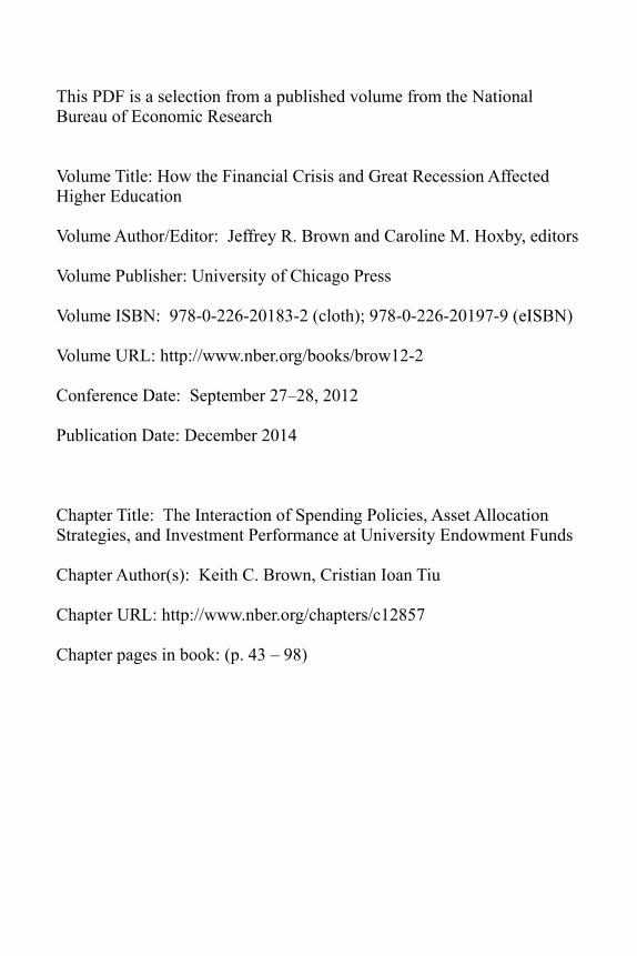
Figure 2.1 provides a stylized view of the way in which a typical university endowment is organized. The two main economic actors involved in the pro-cess of deploying the fund’s financial capital are the University/Endowment Board (i.e., “board”), which represents the governing authority ultimately responsible for the endowment’s assets, and the Investment Committee/Firm (i.e., “staff”), to which falls the day- to- day responsibilities of designing and maintaining the actual investment portfolio. Broadly speaking, the primary functions of the board are twofold: (a) create the policy statements that define the investment problem faced by the university (i.e., the spending policy), as well as the way in which the endowment’s financial assets should be invested to address this problem (i.e., the investment policy); and (b) mon-itor the staff’s ongoing operations on a regular basis to insure compliance with those policies. By contrast, the staff—which may comprise anything from a single individual to representatives of a multiperson committee of the board (e.g., Yale Investments Office) to an entirely separate operating firm (e.g., University of Texas Investment Management Company)—is charged with the responsibility of managing the fund’s assets in the most effective
6. Indeed, prudent man laws first came into existence with the Harvard College v. Amory case in 1830, which involved a dispute over how investments tied to the Harvard College endowment had been handled.

50 Keith C. Brown and Cristian Ioan Tiu
manner possible, within the context of the policy parameters set forth by the board.7 Thus, in the typical endowment there is a clear delineation between those responsible for defining the investment problem and setting the broad parameters for the investment solution and those who make those mandates operational.8
7. In its annual survey of educational endowment practices, NACUBO reported that for the 2010 fiscal year, the average number of full-time equivalent professional staff persons employed by the 842 funds in their sample was just 1.5. However, the cross-sectional distribu-tion of professional staffing levels is highly skewed; the mean number of full-time professionals employed by endowments with assets of over $1 billion is 10.0 (see Walda and Griswold 2011).
8. Two additional economic actors are represented in the exhibit: consultants, who can pro-vide guidance to either the board or the staff on a variety of topics, and portfolio subman-agers, who the staff may select to manage part or all of the endowment’s assets. This “external manager” model (i.e., in which staff selects investment managers from outside the endowment organization to construct asset class-specific security portfolios) is an increasingly popular format in practice and the role of the consultant is often to advise the board or staff on which submanagers to select. Walda and Griswold (2011) report that 80.0 percent of the endowments surveyed in 2010 employed an external consultant and 85.0 percent of those endowments using a consultant did so to advise them on the manager selection process.
Fig. 2.1 Typical endowment fund organizational structureNote: This exhibit illustrates the organizational structure of the typical educational endow-ment fund. The respective responsibilities of the university/endowment board (e.g., setting spending and investment policy, monitoring investment performance) and the staff of the investment committee/firm (e.g., designing portfolio strategy, selecting external investment managers) are highlighted.

Spending Policies, Asset Allocation, and Investment Performance 51
2.2.2 Endowment Spending Policy
We begin by formally defining the spending policy adopted by a particular endowment as consisting of two distinct components: (a) a spending rule, and (b) a prespecified payout rate. The distinction between these two entities is that the spending rule defines the general procedure by which the payout amount will be determined, whereas the payout rate represents the specific percentage that is to be applied within the context of the spending rule. For example, during the 2007 fiscal year Texas Christian University determined their annual endowment payout using a “50/50 hybrid” approach in which the institution calculated a weighting consisting of (a) 50 percent of the dollar amount of the prior year’s spending incremented by the Higher Edu-cation Price Index (HEPI) inflation index, and (b) 50 percent of an amount established by taking 5.0 percent of an average of the market values of the endowment portfolio over the previous four quarters, starting at the beginning of the current fiscal year. In this case, the rule used is actually a combination of two more fundamental rules (i.e., increase by percentage and moving average, as defined more formally below) while the rates specified are the HEPI inflation index for the increase by percentage rule and 5.0 percent for the moving average rule.9 In the analysis that follows, it is important to recognize that an endowment fund can change its spending policy by altering either the rule it uses or the rate that is applied within that rule.
For our purposes, two endowments will initially be considered to have comparable spending policies if those policies are based on the same spend-ing rule. That is, funds that adopt a moving average payout rule based on, say, annual portfolio valuations over the previous three years will be clas-sified in the same way regardless of what specific policy spending rate each fund applies to their respective average asset values. There are seven broad categories of spending rules used in practice, which in turn represent aggre-gated versions of twenty more detailed subclasses.10 While the appendix lists a more complete description of this spending rule taxonomy, the seven broad payout policy categories are given here as:
1. Decide on an appropriate rate annually: Determines the spending rate deemed appropriate on a yearly basis.
9. It is interesting to note that NACUBO reported that the actual payout rate for the Texas Christian University endowment fund for the 2007 fiscal year was 4.6 percent (expressed as a percentage of beginning-of-period fund assets). This indicates that there often can be a mea-surable difference between the ex ante policy payout rate and the ex post actual payout rate, par-ticularly when moving average spending rules that combine several past asset values are used.
10. This spending rule classification system was created after a comprehensive analysis of the series of annual NACUBO surveys, which began collecting this information in 2003. It dif-fers somewhat from other classification schemes (e.g., Lapovsky 2009; Blume 2010) primarily because the way in which NACUBO has reported spending rule data has evolved over time, particularly after Commonfund became involved in the reporting process in 2009. We provide a more complete discussion of the data acquisition process in section 2.3.

52 Keith C. Brown and Cristian Ioan Tiu
2. Increase prior year’s spending by a percentage: Adjusts spending upward each year, using either a simple formula or one based on the infla-tion rate.
3. Spend a percentage of a moving average of market values: Determines annual payout as a percentage of an average of beginning- of- period market values over a prespecified series of past periods.
4. Spend a percentage of current yield: Spend a percentage of current income generated during the investment period.
5. Spend a percentage of assets under management (AUM): Determines annual payout as a percentage the beginning- of- period fund assets for the current period.
6. Hybrid rules: Uses a simple formula to combine two or more different payout categories into a single spending rule.
7. Other payout rules: Uses a formula or approach that differs from those listed above or did not provide a complete set of information.
Thus, the TCU endowment fund from the previous example would be classi-fied as following a hybrid rule (i.e., category 6), which itself is a combination of category 2 (i.e., increase prior spending by percentage) and category 3 (i.e., moving average).
At a broad level, these spending rule categories can be differentiated by the nature of the dollar payout amount they produce. Clearly, the decide annually rule is the most flexible in that it allows the board to determine the exact amount of payout it wants to extract from the portfolio each year. Of course, this maximizes the tension on the board in managing the trade- off between spending in the present versus preserving the endowment’s value for future generations, particularly since UPMIFA removes the onus of making decisions that lead to an underwater fund. On the other hand, the increase by percentage rule makes the payout level exactly predictable and preserves the real spending level of the institution when the policy payout rate is tied to an inflation index. However, in years when asset values are falling, an increase by percentage rule will exacerbate the decline in the endowment portfolio’s value. By contrast, a percentage of AUM rule adjusts the payout to changes in the portfolio’s beginning- of- year value, which has the effect of making the dollar payout level extremely volatile in financial markets that are themselves volatile. Moving average rules attempt to mitigate this volatility by smoothing out the portfolio value to which the payout rate is tied, whereas percentage of yield rules are intended to set a payout that will not diminish the value of the endowment portfolio, which may be a fac-tor that the board of a fund that is already underwater might need to take into account. Finally, hybrid rules, which often combine moving average and increase by percentage inflation rules, seek a middle ground between predictable dollar payout and the preservation of the endowment’s market value.
Spending Policies, Asset Allocation, and Investment Performance 53
2.2.3 Endowment Investment Policy
Beyond setting the organization’s spending policy, figure 2.1 also highlights the role that the endowment fund’s board plays in determining the direction of its investment operation. As summarized in the endowment’s investment policy statement, the primary function of the board in this regard is two-fold: (a) to select the permissible asset classes that define the endowment’s allowable investable universe; and (b) to specify the target investment levels (i.e., weights) for each of these asset classes. Collectively, these two decisions represent the fund’s strategic asset allocation policy, which is widely acknowl-edged to be the single most important decision that an organization makes to increase the value of its investment portfolio over time; see, for example, Brinson, Hood, and Beebower (1986) and Ibbotson and Kaplan (2000). Fur-ther, Acharya and Dimson (2007) note that most endowment funds use a strategic allocation approach to arrive at their policy portfolios due largely to the long- term nature of the investment problem they face.11
Of course, a crucial aspect underlying the board’s strategic allocation judgment is the perceived level of risk tolerance characterizing the organi-zation. Like mutual funds, endowment fund assets are most often managed without a “safety net,” such as that provided for pension plans by the plan sponsor’s balance sheet or the Pension Benefit Guarantee Corporation. In this sense, endowment funds are often regarded as having risk tolerance similar to that of a tax- exempt wealthy individual investor, although Black (1976) argues that endowment funds generally require less diversification in their asset portfolios than do otherwise comparable individuals. However, this appears to be a notion that has fallen out of favor, as the so- called endowment model approach to investing prevalent today is grounded on the principle that a wide variety of both traditional (e.g., public fixed- income and equity securities) and nontraditional (e.g., hedge funds, private equity) asset classes should form the investable universe (see Leibowitz, Bova, and Hammond 2010). Finally, endowment funds generally face the wid-est variety of investment restrictions, most of which are institution- specific since there is comparatively little regulation in this industry.12 This suggests that, as an institutional class, endowment funds might have considerable range in their investment policies and thus represent a setting in which the manipulation of allocation strategies might be able to add substantial value to portfolio performance.
11. Typically, investment policy statements contain two additional features that are the responsibility of the board: (a) the permissible tactical ranges for the extent to which asset class-level investments can differ from their strategic target weights; and (b) the portfolios or indexes that represent the benchmarks for each asset class (e.g., the S&P 500 index for US public equity), which are used primarily for measuring the performance of the managed portfolio.
12. In fact, Hill (2006) implies that the largest and least restricted endowment funds essen-tially operate as hedge funds in their pursuit of superior risk-adjusted returns, an observation borne out by the recent experience at the Harvard Management Company.

54 Keith C. Brown and Cristian Ioan Tiu
Given the strategic allocation policy set by the board, figure 2.1 shows that the responsibility for designing and maintaining the actual endowment port-folio falls to the staff. A baseline (or passive) approach for this process would be to mimic the strategic allocation policy by investing in the permissible asset classes at exactly their target weights and replicating the contents of the benchmark indexes as closely as possible; this is what Leibowitz (2005) terms “beta grazing.” Within the context of the investment policy, the staff can also usually engage in active portfolio management (i.e., “alpha seeking”) in either of two ways: (a) tactical asset allocation, in which deviations from strategic asset class weights are selected; and (b) security selection, in which asset class- level security portfolios that differ from those in the respective benchmarks are held.13 In their analysis of the relationship between asset allocation and investment performance for university endowment funds, Brown, Garlappi, and Tiu (2010) find that while strategic policy portfolios are remarkably similar across their sample, actively managed endowments are able to generate significantly larger alphas than passively managed ones, largely through the staff’s use of its security selection skills. Indeed, Swensen (2009) argues that the ability to make high- quality active management deci-sions is the most important factor that distinguishes two otherwise similar investors. Thus, both board and staff appear to play an important role in the development and execution of an endowment’s investment policy.
2.3 Data and Descriptive Statistics
2.3.1 Data Description
The primary source of information for the spending and investment prac-tices of educational endowment funds comes from a database maintained by the National Association of College and University Business Officers (NACUBO), a service and advocacy organization formed in 1962 to repre-sent college, university, and higher education service providers throughout the United States, Canada, and Puerto Rico. Since 1984, NACUBO has surveyed its members on topics ranging from asset allocation and investment performance to endowment expenditures and other fund flows to organi-zational design and governance issues and then publishes a summary of that information in its annual Study of Endowments.14 Arguably, this survey represents the most comprehensive published source of data on college and
13. In addition to tactical range restrictions or restrictions on which securities can or cannot be held (e.g., no tobacco stocks), investment policy statements can also specify risk-control measures at the aggregate portfolio level, such as tracking error limits.
14. Since 2009, Commonfund has administered the survey process and jointly authored the studies with NACUBO. Before the current arrangement, other NACUBO partners involved in producing the annual surveys included TIAA-CREF (2000–2008) and Cambridge Associ-ates (1988 to 1999); the NACUBO Investment Committee generated the surveys prior to 1988.

Spending Policies, Asset Allocation, and Investment Performance 55
university endowments anywhere in the world. Although the underlying data are self- reported by the member institutions, the study is free of sur-vivorship bias as any college that could eventually have gone bankrupt but participated in the survey in the early years is retained in the database (see Brown et al. 1992). Indeed, the large cross section of colleges represented in the survey suggests that there is little self- selection bias. Furthermore, the study does not backfill data; that is, a college can only fill out the survey for the current year and not for previous years in which no information was originally provided.
For the analysis that follows, we have obtained access to the survey data for fiscal years from 1984 to 2011.15 For the purpose of our study, easily the richest part of the NACUBO database involves endowment investment practices. Specifically, information for some data items—such as the AUM for a particular fund, the annual investment return (net of fees) that it pro-duced—is available from the inception of the surveys in 1984. However, while aggregated sample- wide data on asset allocation patterns are avail-able from 1984, fund- specific asset allocation data (i.e., where it is possible to match each endowment with its actual asset class investment weights during the investment period) was only obtainable starting with the 1989 survey. Given the number of partners involved in producing the annual surveys for NACUBO, it is not surprising that the asset class definitions have been modified three times during the 1989–2011 sample period, most recently in 2009 with Commonfund’s administration of the surveys. To maintain consistency with the most recent reporting standards, we adopt the follow-ing ten different asset classes: US public equity, non- US public equity, fixed income, real estate, hedge funds, venture capital, private equity, natural resources, cash, and other assets. All of the asset allocation data dating to 1989 has been adjusted, where necessary, to correspond to these asset class definitions.16
Unfortunately, information on spending practices in the endowment sample does not extend as far back as does the investment data. The NACUBO began reporting the actual annual payout rate associated with a fund in 1994. This actual payout rate statistic is calculated as the total dollar amount of the payment from the endowment to the institution during a given fiscal year as a percentage of market value (i.e., AUM) of the portfolio at the beginning of the fiscal year. More specific information regarding the spending policy—both spending rule and policy rate—for every fund did not appear until the 2003 survey, meaning that we are able to trace the evo-
15. To match the academic calendar, the fiscal year for an endowment typically ends on June 30. So, the NACUBO survey for 2011 covers the period from July 1, 2010, through June 30, 2011.
16. For example, from 2001 to 2008, NACUBO reported twelve asset class categories by accounting for fixed income in two subcategories (i.e., United States and non-United States) and similarly listing real estate in its public (i.e., REITS) and private forms.

56 Keith C. Brown and Cristian Ioan Tiu
lution of this aspect of the endowment management process (as well as the link between spending and investment practices) over the 2003–2011 period. Further, the categories defining the spending rule classifications were modi-fied once during this time frame (i.e., when Commonfund got involved in the effort in 2009). Consequently, the seven spending rule categories listed in the previous section were defined with sufficient breadth to allow for the proper placement of all twenty of the subcategories used throughout the nine years for which these data were reported, as indicated in the appendix. Finally, rec-ognize that not every endowment self- reported spending policy data in each year for which they participated in the survey in other ways (e.g., reported asset allocation and investment performance results). As explained in more detail below, we assume the conservative posture that such omissions, when they occur, indicate that the endowment did not change its spending policy from the last reporting date.
2.3.2 Endowment Summary Statistics: Fund Size, Returns, and Payout Rates
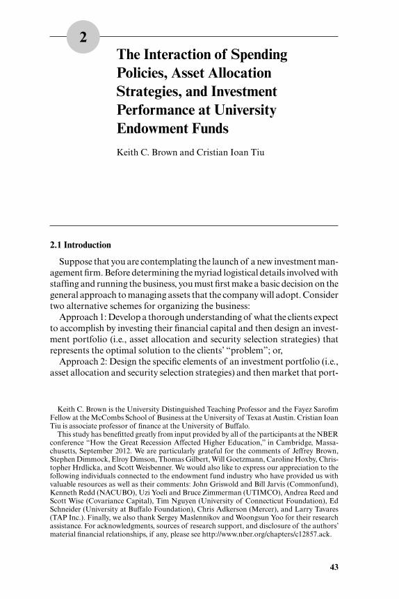
Table 2.1 provides a broad overview of the number and size, investment performance, and spending practices for our sample of endowment funds. Specifically, the display reports on a yearly basis summary statistics for three different variables: (a) assets under management (AUM), measured as the market value of the total assets held in a fund as of the end of the respective reporting year; (b) the overall investment return, reported net of all rele-vant fees; and (c) the payout rate, which is defined as the actual dollar- level of spending during the year in question expressed as a percentage of the beginning- of- period AUM of the fund. For all three of these statistics the table lists the mean, median, minimum, and maximum values and standard deviations for each of the annual cross sections.
The first thing to note from table 2.1 is that the number of institutions surveyed by NACUBO quadrupled (i.e., from 200 to 803) from 1984 to 2011 and that there was a roughly sixteenfold increase in the aggregate level of assets managed in the industry (i.e., from $25.4 billion to $408.0 billion) during that time. By contrast, the level of AUM for both the mean and median endowment increased only fourfold over the sample period—from $127.0 million to $508.1 million, on average—which represents a relatively modest compound annual growth rate in net- of- payout assets of 5.3 per-cent, especially given that none of the amounts listed have been adjusted for inflation. However, the remaining AUM data reported in the exhibit indicate that focusing on the behavior of the average endowment may provide a poor representation of the entire universe. For example, the difference between the largest and smallest funds reported annually (e.g., $31.7 billion versus $0.6 million in 2011) shows the tremendous cross- sectional heterogeneity in the sample and suggests that endowments of different sizes may face very different asset management problems.

Tab
le 2
.1
Sum
mar
y st
atis
tics
of
the
NA
CU
BO
/Com
mon
fund
end
owm
ent f
und
univ
erse
AU
M ($
mill
ions
)R
etur
nP
ayou
t
year
N
. obs
.
Tota
l
Mea
n M
edia
n
Std.
Min
M
ax
Mea
n M
edia
n
Std.
M
in
Max
Mea
n
Med
ian
Std
.
Min
M
ax
2011
803
407,
997.
4450
8.09
91.7
01,
902.
360.
5731
,728
.08
18.5
819
.70
5.44
–4.1
931
.75
4.49
4.68
3.31
0.00
85.0
020
1082
134
6,14
0.68
421.
6174
.14
1,59
6.50
0.43
27,2
23.2
211
.53
12.0
03.
86–5
.76
36.2
04.
434.
862.
050.
0016
.60
2009
817
306,
403.
5137
5.03
68.1
81,
455.
250.
6025
,662
.06
–17.
79–1
8.80
6.60
–39.
9615
.90
4.23
4.50
1.98
0.00
25.2
020
0869
830
3,70
5.38
447.
9493
.20
1,82
3.32
0.60
36,5
56.2
8–3
.08
–3.3
53.
97–2
2.60
12.1
04.
594.
502.
340.
0045
.60
2007
678
304,
482.
1246
3.44
97.6
51,
784.
910.
5734
,634
.91
17.3
817
.60
3.58
2.90
62.2
04.
594.
501.
920.
0036
.90
2006
731
283,
020.
6738
7.17
79.8
01,
451.
240.
4928
,915
.71
10.6
110
.80
3.38
–0.2
020
.50
4.66
4.60
1.32
0.00
15.5
020
0571
124
9,27
5.94
351.
5975
.41
1,29
1.35
1.26
25,4
73.7
29.
169.
003.
29–1
1.40
22.2
04.
794.
851.
400.
2417
.10
2004
707
228,
466.
6632
3.61
69.7
51,
136.
521.
9222
,143
.65
15.0
215
.70
4.41
–0.6
032
.10
4.89
5.00
1.62
0.00
18.4
020
0366
719
6,11
1.70
294.
0271
.65
1,00
1.70
0.32
18,8
49.4
92.
702.
603.
68–1
4.70
28.1
05.
225.
001.
500.
1022
.00
2002
534
176,
545.
3933
7.56
91.2
51,
053.
050.
1617
,169
.76
–5.9
6–6
.20
4.23
–19.
8010
.10
5.21
5.00
1.53
0.30
22.0
020
0157
221
8,18
5.98
390.
3110
5.65
1,16
7.41
1.15
17,9
50.8
4–3
.26
–3.6
06.
30–2
6.90
24.8
05.
175.
001.
430.
3014
.20
2000
507
222,
928.
5046
1.55
119.
961,
371.
556.
1918
,844
.34
12.6
910
.70
10.1
0–1
2.20
58.8
04.
975.
001.
400.
1013
.30
1999
468
181,
781.
6140
9.42
130.
241,
083.
107.
1914
,256
.00
10.9
010
.50
5.25
–15.
8060
.95
4.83
5.00
1.24
0.10
13.0
019
9844
515
9,62
0.93
371.
2111
3.08
991.
425.
1713
,019
.74
18.0
518
.00
3.97
3.70
31.8
04.
694.
701.
210.
3014
.70
1997
456
145,
122.
9732
8.33
98.3
785
8.05
5.78
10,9
19.6
720
.10
19.9
04.
446.
8046
.90
4.80
4.60
1.77
0.30
24.0
019
9640
611
2,60
3.94
281.
5181
.15
737.
703.
658,
811.
7817
.26
17.2
04.
020.
8039
.00
4.84
4.80
1.29
0.10
12.8
019
9542
399
,416
.70
235.
5871
.59
600.
030.
077,
045.
8615
.08
14.8
04.
160.
5037
.90
4.95
5.00
1.47
0.10
15.0
019
9437
570
,354
.31
189.
1261
.23
406.
580.
473,
529.
003.
293.
204.
27–1
3.00
43.0
05.
245.
001.
751.
8018
.20
1993
393
76,8
38.2
119
6.52
60.5
146
9.59
1.46
5,77
8.26
13.1
313
.30
4.30
–2.8
036
.30
n.a.
n.a.
n.a.
n.a.
n.a.
1992
317
62,2
36.1
219
6.95
54.2
253
4.68
1.73
5,31
5.47
13.4
013
.00
8.82
1.10
143.
00n.
a.n.
a.n.
a.n.
a.n.
a.19
9132
656
,023
.55
172.
9152
.03
439.
203.
395,
118.
127.
247.
104.
90–1
4.40
53.0
0n.
a.n.
a.n.
a.n.
a.n.
a.19
9029
851
,420
.16
174.
3158
.89
410.
972.
014,
653.
2310
.02
9.55
6.01
–10.
3075
.00
n.a.
n.a.
n.a.
n.a.
n.a.
1989
279
45,4
81.1
616
5.39
56.7
439
2.35
1.87
4,47
8.98
14.6
413
.40
13.4
6–6
.20
163.
00n.
a.n.
a.n.
a.n.
a.n.
a.19
8826
249
,467
.06
157.
0447
.64
381.
401.
654,
155.
781.
260.
704.
78–1
4.70
17.4
0n.
a.n.
a.n.
a.n.
a.n.
a.19
8727
645
,222
.98
152.
7846
.38
360.
681.
544,
018.
2713
.63
13.8
25.
69–6
.88
31.8
9n.
a.n.
a.n.
a.n.
a.n.
a.19
8625
839
,317
.86
150.
6446
.29
354.
881.
103,
435.
0127
.17
27.1
66.
725.
2452
.46
n.a.
n.a.
n.a.
n.a.
n.a.
1985
280
31,5
11.8
211
2.54
31.1
929
5.30
1.02
2,92
7.20
25.6
125
.95
6.96
1.25
52.1
2n.
a.n.
a.n.
a.n.
a.n.
a.19
84
200
25
,399
.06
127
.00
40
.12
28
9.12
0.9
7
2,48
6.30
–1
.40
–2
.24
15.
12 –
17.0
0 2
09.0
0
n.a.
n.
a.
n.a.
n.
a.
n.a.
Sou
rce:
The
exh
ibit
pre
sent
s ann
ual d
ata
sum
mar
izin
g va
riou
s asp
ects
of
the
colle
ge a
nd u
nive
rsit
y en
dow
men
t fun
ds c
onta
ined
in th
e N
AC
UB
O/C
omm
onfu
nd sa
mpl
e ov
er th
e pe
riod
fr
om J
uly
1, 1
983,
to J
une
30, 2
011.
N
otes
: In
addi
tion
to li
stin
g th
e nu
mbe
r of
fund
s in
clud
ed in
eac
h ye
arly
sur
vey
and
the
aggr
egat
e m
arke
t val
ue o
f th
ose
port
folio
s, th
e di
spla
y re
port
s cr
oss-
sect
iona
l mea
n, m
edia
n,
stan
dard
dev
iati
on, m
inim
um, a
nd m
axim
um s
tati
stic
s fo
r (a
) th
e fi
scal
- yea
r en
d m
arke
t va
lue
for
the
endo
wm
ent
port
folio
(as
sets
und
er m
anag
emen
t, o
r A
UM
); (
b) n
et- o
f- ex
pens
e po
rtfo
lio r
etur
n (R
etur
n), e
xpre
ssed
as
a pe
rcen
tage
of
begi
nnin
g- of
- per
iod
AU
M; a
nd (c
) the
act
ual p
ayou
t for
the
endo
wm
ent f
und
to th
e sp
onso
ring
inst
itut
ion
(Pay
out)
, exp
ress
ed
as a
per
cent
age
of b
egin
ning
- of-
peri
od A
UM
. Dat
a ar
e av
aila
ble
for
AU
M a
nd R
etur
n fo
r th
e 19
84–2
011
fisca
l yea
rs; P
ayou
t dat
a ar
e re
port
ed fo
r th
e 19
94–2
011
fisca
l yea
rs.

58 Keith C. Brown and Cristian Ioan Tiu
There are two other ways in which the reported statistics for fund invest-ment performance and payouts suggest that the endowment universe is extremely varied. First, while the annual distributions of the overall fund returns do not appear to be highly skewed (e.g., there is not a large discrep-ancy between the mean and median returns reported for most years), the difference between the best and worst performing funds is considerable.17 For instance, while the mean fund returned 9.2 percent in 2005, the minimum and maximum returns for the 711 participating endowments were –11.4 per- cent and 22.2 percent, respectively. The indicative range of performance for this particular year was by no means abnormally large; if anything, it is less pronounced than the most dramatic years in the sample (e.g., 1989, 2000, 2007–2009). While there are several factors that might explain these different investment outcomes, such as portfolio risk levels or manager- specific skills, they nevertheless underscore our earlier point regarding the diversity of the objectives, constraints, and characteristics that represent these institutions.
The final way in which college endowments can be differentiated with these data is by the amount of their annual spending needs. The last five col-umns in the exhibit summarize the annual distributions of the actual dollar expenditures (as a percent of AUM) paid out by the funds. The average annual value for this payout rate is about 4.8 percent, which did not appear to change much from one year to the next during the sample period. How-ever, this relative constancy in the average value masks a considerable degree of cross- sectional variation in actual payouts rates, where the spread of values in a given year ranges from 0 to 85.0 percent. Further, as indicated by both the cross- sectional standard deviations and difference between the minimum and maximum values, the sample- wide variation in payout rates appears to have increased substantially after 2008. In fact, this highly variable pattern of endowment spending over time is consistent with that reported by Nettleton (1987) for the pre- 1985 period. In the present context, the important point to consider is that fund spending policies may be linked to the risk tolerance of the endowment and, as a consequence, should be related to the allocation decision and ultimate investment performance, as suggested by Dybvig (1999).18
2.3.3 Endowment Summary Statistics: Asset Allocation
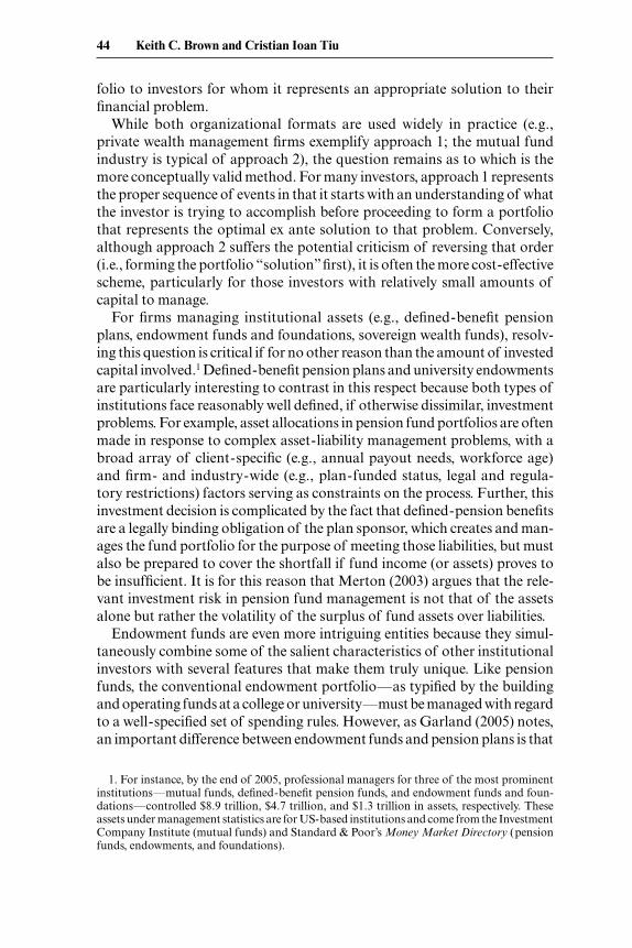
Table 2.2 lists the actual percentage allocations by the endowment fund universe to each of the ten NACUBO asset classes in use as of the 2011 sur-
17. The return data shown in table 2.1 are net of fund expenses, but they are not adjusted for risk. A more thorough analysis of the nature and sources of risk-adjusted performance across a comparable sample of endowment funds can be found in Brown and Tiu (2010).
18. In an interesting extension of this point, Dimmock (forthcoming) conducted a cross-sectional analysis of endowment fund allocation patterns during the year 2003 and concluded that factors such as the riskiness of a university’s nonfinancial income, cost structure, and credit constraints can also affect its investment decision making and performance.

Tab
le 2
.2
Ass
et a
lloca
tion
sta
tist
ics
for
the
NA
CU
BO
/Com
mon
fund
end
owm
ent f
und
univ
erse
US
Eq.
N
on- U
S E
q.
Fix
ed
inco
me
Rea
l es
tate
C
ash
O
ther
H
edge
fu
nds
V
C
PE
N
at.
res.
A
UM
($
mil.
) N
o. o
f ob
s.
2011
31
.7
17.0
19
.3
3.4
3.6
2.3
12.6
1.
3 5.
3 3.
5 50
8.1
803
2010
31
.7
15.3
22
.0
3.2
3.9
2.2
12.5
1.
1 5.
0 3.
0 42
1.6
821
2009
32
.9
14.7
21
.9
3.6
5.7
1.8
11.6
1.
2 4.
3 2.
3 37
5.0
817
2008
34
.5
17.1
18
.9
4.3
3.7
1.5
13.3
1.
1 3.
4 2.
3 44
7.9
698
2007
40
.0
17.4
17
.9
3.5
3.5
1.4
11.2
1.
0 2.
4 1.
6 46
3.4
678
2006
42
.3
15.3
20
.0
3.5
3.4
1.4
9.7
0.9
2.0
1.5
387.
2 73
1 20
05
45.7
12
.7
21.4
3.
2 3.
4 1.
4 8.
9 0.
8 1.
6 1.
0 35
1.6
711
2004
48
.7
11.0
21
.9
2.8
3.6
1.6
7.5
0.8
1.4
0.6
323.
6 70
7 20
03
47.4
9.
7 25
.7
2.8
3.9
1.6
6.3
0.8
1.4
0.4
294.
0 66
7 20
02
46.4
10
.1
27.0
2.
6 4.
0 1.
6 5.
6 1.
0 1.
2 0.
4 33
7.6
534
2001
49
.5
10.0
25
.0
2.1
4.0
5.9
0.6
1.5
1.0
0.4
390.
3 57
2 20
00
50.7
11
.6
23.3
2.
0 4.
0 4.
0 0.
7 2.
4 1.
0 0.
3 46
1.5
507
1999
53
.9
10.6
23
.8
1.9
3.9
0.6
3.1
1.3
0.7
0.2
409.
4 46
8 19
98
53.1
10
.9
25.5
3.
4 2.
3 0.
6 1.
6 0.
9 0.
5 1.
2 37
1.2
445
1997
52
.5
11.1
25
.7
2.0
4.6
0.5
2.2
0.8
0.3
0.2
328.
3 45
6 19
96
51.8
9.
4 27
.7
2.0
5.4
0.7
1.9
0.8
0.3
0.2
281.
5 40
6 19
95
47.0
7.
9 29
.9
2.1
6.5
3.9
1.6
0.7
0.2
0.3
235.
6 42
3 19
94
46.3
7.
4 31
.8
1.9
7.3
2.8
1.5
0.7
0.2
0.3
189.
1 37
5 19
93
48.3
4.
2 34
.8
1.6
7.3
2.0
0.7
0.2
0.6
0.3
196.
5 39
3 19
92
48.1
3.
0 35
.8
2.4
9.4
0.0
0.4
0.6
0.2
0.2
196.
9 31
7 19
91
47.6
2.
3 35
.8
2.8
10.2
0.
0 0.
3 0.
6 0.
2 0.
2 17
2.9
326
1990
47
.5
2.3
35.6
2.
9 10
.3
0.0
0.3
0.6
0.2
0.2
174.
3 29
8 19
89
47.0
1.7
31
.7
3.
0
12.8
2.9
0.
0
0.6
0.
2
0.1
16
5.4
27
9
Sou
rce:
The
tabl
e re
port
s an
nual
mea
ns o
f th
e ac
tual
ass
et a
lloca
tion
s m
aint
aine
d by
the
univ
ersi
ty e
ndow
men
t fun
ds c
onta
ined
in th
e N
AC
UB
O/C
om-
mon
fund
dat
abas
e ov
er th
e pe
riod
from
Jul
y 1,
198
8, to
Jun
e 30
, 201
1.
Not
es: C
ross
- sec
tion
al m
ean
allo
cati
on le
vels
(exp
ress
ed a
s a
perc
enta
ge o
f be
ginn
ing-
of- p
erio
d A
UM
) are
list
ed fo
r th
e fo
llow
ing
asse
t cla
ss d
efini
tion
s:
US
publ
ic e
quit
y (U
S E
q.),
non
- US
publ
ic e
quit
y (n
on- U
S E
q.),
fixe
d in
com
e, r
eal e
stat
e, c
ash,
oth
er a
sset
s (O
ther
), h
edge
fun
ds, v
entu
re c
apit
al (
VC
),
priv
ate
equi
ty (P
E),
and
nat
ural
res
ourc
es (N
at. r
es.)
. The
last
two
colu
mns
rep
ort t
he c
ross
- sec
tion
al m
ean
AU
M a
nd n
umbe
r of
end
owm
ents
con
tain
ed
in e
ach
year
ly s
urve
y, r
espe
ctiv
ely.
60 Keith C. Brown and Cristian Ioan Tiu
vey date: US public equity, non- US public equity, fixed income, real estate, hedge funds, venture capital, private equity, natural resources, cash, and other assets. The figures reported represent the equally weighted average annual values of the percentage of AUM allocated to a particular asset class using all of the participating funds in a given year starting in 1989. Viewed over time, there are several trends in these data that imply important shifts in the way endowment fund managers have approached the asset allocation process. First, the percentage invested in public equities (i.e., US equities and non- US equities) has changed substantially over time, while remaining well below the level advocated by Thaler and Williamson (1994). Interest-ingly, this allocation both started and ended the sample period at just under 50 percent, but maintained a level of 55 percent to 65 percent for the years between 1996 and 2007. Further, the composition of this allocation has changed dramatically over the entire period, with non- US equities experi-encing a substantial increase (e.g., from 1.7 percent in 1989 to 17.0 percent in 2011) while US equities declined significantly (e.g., from 47.0 percent to 31.7 percent). Allocations to the traditional fixed- income categories also declined dramatically during the sample period, from around 31.7 percent at the beginning of the sample period to just 19.3 percent in 2011.
It is the alternative asset classes—typically defined by endowment funds to include hedge funds, nonpublic equity positions (both venture capital and private equity [i.e., buyout] investments), real estate, and natural resources—that benefitted the most from the decreased allocation to traditional fixed- income products. Some of these allocation gains were modest, such as the increases from 0.6 percent to 1.3 percent for venture capital investments or from 3.0 percent to 3.4 percent in real estate.19 Clearly, then, the biggest beneficiary of the increased pattern of “alternatives” investing occurred in the hedge fund category, which represented just under 13.0 percent of the AUM of the average endowment fund by 2011, placing them in size just below the average dollar investment in non- US equity securities. Given that the first hedge fund allocation did not show up in the data until 1990, this represents a truly significant shift in the investment approach adopted by endowment managers. To underscore this point, we also computed a more complete cross- sectional analysis of the annual asset allocation samples, including the median, maximum, and minimum values as well as the stan-dard deviation of the distribution. Although not reported in table 2.2, these additional statistics are nevertheless useful in understanding the diversity in the investment commitment to hedge funds across the endowment universe.
19. Recall that beginning in 2009, NACUBO collapsed two real estate asset classes—public (i.e., REITS) and private—into a single category, moving the REIT allocation to US public equity. Consequently, to insure comparability with the reported allocation data from 1989 to 2008, we have added (subtracted) 1.20 percent to the real estate (US public equity) asset class for the years 2009 to 2011. This percentage represents the average REIT allocation for the five-year period ending in 2008.
Spending Policies, Asset Allocation, and Investment Performance 61
For instance, in 2005, the minimum allocation was 0.0 percent while the maximum allocation was 82.1 percent! Clearly, different endowments have very different strategies concerning alternative assets.
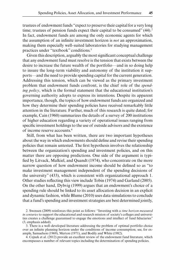
A significant factor related to these different asset allocation patterns is the size of the endowment fund. Simply put, larger funds invest assets in a very different fashion than do smaller funds. This phenomenon is illustrated in figure 2.2, which provides snapshots of endowment investments at different points of time and for funds of different size. To generate these comparisons, we separated the fund sample into quartiles based on beginning- of- period AUM for each year in the sample period. We then calculated mean asset allocation percentages for each quartile as an equally weighted average within the subsample, rebalancing those stratifications on a yearly basis. Further, for comparative ease, we consolidated the asset classes into four broader categories: public equity (US and non- US), fixed income, alterna-tives (real estate, hedge funds, venture capital and private equity, natural resources), and cash and other assets. Panel A of the display compares these aggregated allocation percentages across AUM quartiles at the beginning and end of the sample period, while panel B compares how those alloca-tion patterns evolved over time for the largest (Q4) and smallest (Q1) size quartiles.20
As both panels of the exhibit help make clear, while there were significant differences across asset classes, there were relatively small differences in asset allocations patterns across endowments of different size at the beginning of the sample period (e.g., investments in alternatives in 1989 were 3.9 per-cent and 6.5 percent for quartiles Q1 and Q4, respectively). However, this situation changed dramatically by 2011, when alternatives investing for the largest fund quartile rose to 45.0 percent while the alternatives allocation for the smallest funds remained relatively low at 9.6 percent. To finance this increased allocation to alternatives, the average Q4 endowment reduced its allocation to both public equity (50.7 percent in 1989 to 37.6 percent in 2011) and fixed income (29.5 percent to 12.2 percent). Conversely, the small-est endowments actually increased their public equity investments over this period (44.9 percent in 1989 to 56.2 percent in 2011) primarily by reduc-ing their cash allocation, whereas their fixed- income allocation remained relatively stable (32.2 percent to 26.3 percent). Thus, it is reasonable to conclude that the overall trend toward an increased allocation to alterna-tives at the expense of public equity and fixed income we noted earlier is predominantly the result of actions taken by the managers of the largest endowments.
20. To conserve space, figure 2.2 compares asset allocations for the various subsamples of the endowment universe for just two years: 1989 and 2011. It should be noted that data for the omitted years do not change our conclusions about how endowment allocation patterns have changed over time; we have produced a complete set of annual findings for the entire 1989–2011 sample period and these results are available upon request.

Fig
. 2.2
Com
para
tive
asse
t allo
cati
on p
atte
rns
over
tim
e an
d en
dow
men
t fun
d si
zeN
ote:
Thi
s fig
ure
illus
trat
es h
ow m
ean
asse
t cla
ss a
lloca
tion
per
cent
ages
for
the
endo
wm
ent f
und
sam
ple
have
cha
nged
ove
r ti
me
and
for
port
folio
s of
dif
fere
nt s
ize.
The
ten
asse
t cla
sses
repo
rted
in th
e N
AC
UB
O/C
omm
onfu
nd s
urve
ys a
re a
ggre
gate
d in
to th
e fo
llow
ing
four
cat
egor
ies:
pub
lic e
quit
y (U
S an
d no
n- U
S), fi
xed
inco
me,
alt
erna
tive
s (he
dge
fund
s, v
entu
re c
apit
al, p
riva
te e
quit
y,
real
est
ate,
and
nat
ural
res
ourc
es),
and
cas
h an
d ot
her
asse
ts. P
anel
A li
sts
asse
t allo
cati
on s
tati
stic
s fo
r fu
nds
in d
iffe
rent
AU
M
quar
tile
s (l
arge
st [Q
4] to
sm
alle
st [Q
1]) f
or tw
o di
ffer
ent y
ears
(198
9 an
d 20
11).
Pan
el B
list
s as
set a
lloca
tion
sta
tist
ics
acro
ss ti
me
(198
9, 2
003,
and
201
1) fo
r tw
o di
ffer
ent f
und
size
qua
rtile
s (Q
4 an
d Q
1).
A B

Spending Policies, Asset Allocation, and Investment Performance 63
2.3.4 Endowment Summary Statistics: Spending Rules
As discussed above, the annual NACUBO surveys have included details of the spending rules used by their sample of educational endowments since the 2003 fiscal year. For each yearly report between 2003 and 2011, we ana-lyzed the stated rule for every available fund and placed it into one of the twenty specific subcategories—which, in turn, led to its placement into one of the seven broader categories—described in the appendix. Table 2.3 sum-marizes these classifications, reporting for each year the following statistics: total number of sample endowments; percentage frequency of rule use; mean (median) actual payout, as a percentage of AUM; mean (median) AUM; mean (median) annual investment return; and mean (median) standard deviation of the policy (i.e., benchmark) portfolio corresponding to funds in that spending rule class.21 Further, starting with the fiscal year 2009, the spending rule por-tion of the NACUBO survey was expanded to include additional information regarding the relationship between endowment payout amounts and the insti-tution’s budget, as well as the funding status of the portfolio. Consequently, for the years 2009–2011, we also report summary statistics for mean (median) payout as percentage of budget; the mean number of endowments that impose a special spending appropriation (i.e., temporary expenditures in addition to the stated permanent policy); and the percentage of funds that are “underwa-ter” (i.e., has a current market value that is less than its original level).
Perhaps the most intriguing finding shown in the display is the sizeable fraction of endowment funds that base their spending policies on some form of a moving average of past portfolio values, which is intended to smooth out year- to- year variations in the dollar level of the portfolio pay-out. Looking at each of the annual samples, the fraction of funds using a moving average rule ranges from a low of about two- thirds (65.4 percent in 2010) to three- quarters (75.6 percent in 2008). By contrast, the second most frequently used spending rule—the decide annually category—is also the most flexible in the payout amount it allows from one period to the next and accounts for as much as 10.6 percent of funds in 2011 and as few as 4.9 percent in 2008.22 The remaining categories—increase by percentage,
21. More precisely, this volatility statistic was calculated as follows: First, for each fund in a given survey year and rule class, we observed their asset allocation weights. Second, using time-series return data for the benchmark indexes associated with each asset class (which are described in detail in section 2.6), we calculate a sample asset class variance-covariance matrix. Finally, a policy standard deviation statistic was then calculated for each fund as the square root of the product of its investment weights and the variance-covariance matrix; the exhibit lists the mean (median) of these values within each rule category.
22. To underscore this “smoothing versus flexibility” comparison, notice that in 2009 (i.e., the fiscal year incorporating the financial market decline of late 2008, 36.1 percent of the endow-ments using the decide annually rule were underwater, compared to just 22.1 percent using moving average rules. By 2011, the economic recovery that took place during the preceding two years had reduced the frequency of underwater funds in these two categories to be virtually the same (i.e., 5.5 percent and 4.9percent, respectively).

Tab
le 2
.3
Des
crip
tive
stat
isti
cs fo
r en
dow
men
t fun
d sp
endi
ng p
olic
y ru
les
Dec
ide
annu
ally
In
crea
se
by p
ct.
M
ovin
g av
erag
e
Pct
. of
yiel
d
Pct
. of
AU
M
Hyb
rid
rule
O
ther
ru
le
2011
U
se (%
) 10
.64.
766
.03.
53.
46.
25.
7n
= 8
04
Pay
out (
%)
4.2
(4.5
)5.
2(5
.1)
4.5
(4.6
)4.
2(4
.3)
4.1
(4.1
)4.
8(5
.0)
4.0
(4.5
)Si
ze ($
mill
ions
) 75
6.9
(75.
5)17
50.8
(514
.7)
326.
8(8
0.2)
268.
1(6
9.9)
642.
3(6
8.1)
1143
.3(1
86.7
)98
4.5
(79.
4)R
et. (
%)
18.3
(20.
0)19
.4(1
9.6)
18.6
(19.
7)18
.1(1
9.9)
16.2
(18.
3)19
.8(1
9.6)
19.6
(20.
5)V
ol. (
%)
9.9
(9.7
)10
.0(9
.9)
9.8
(9.8
)9.
9(1
0.3)
9.3
(9.2
)10
.4(1
0.1)
10.2
(10.
2)B
udge
t (%
) 13
.4(6
.6)
17.0
(12.
3)8.
3(3
.0)
7.6
(2.4
)2.
8(0
.9)
18.2
(9.4
)11
.1(3
.1)
App
ropr
iati
ons
(%)
20.4
24.4
17.6
18.8
13.3
25.9
29.4
Und
erw
ater
(%)
5.5
6.1
4.9
6.3
5.2
4.5
5.3
2010
U
se (%
) 9.
43.
765
.43.
33.
55.
49.
4n
= 8
22
Pay
out (
%)
4.2
(4.0
)5.
1(5
.4)
4.5
(4.9
)3.
7(3
.8)
3.4
(3.4
)4.
9(5
.0)
4.0
(4.5
)Si
ze ($
mill
ions
) 54
6.7
(60.
5)12
70.2
(346
.6)
269.
5(6
7.9)
161.
1(2
9.3)
80.3
(32.
7)10
05.7
(200
.0)
804.
1(7
8.7)
Ret
. (%
) 11
.7(1
1.9)
11.6
(12.
1)11
.5(1
2.0)
11.5
(12.
4)11
.6(1
2.0)
12.5
(12.
6)11
.9(1
2.1)
Vol
. (%
) 9.
3(9
.3)
9.5
(9.9
)9.
4(9
.4)
9.4
(9.7
)9.
4(9
.5)
9.9
(9.7
)9.
4(9
.4)
Bud
get (
%)
12.1
(2.9
)18
.4(1
4.1)
9.1
(3.2
)4.
2(0
.7)
11.4
(1.0
)24
.2(1
6.2)
13.7
(4.7
)A
ppro
pria
tion
s (%
) 24
.117
.619
.16.
715
.631
.922
.6U
nder
wat
er (%
) 16
.313
.113
.312
.914
.715
.913
.0
2009
U
se (%
) 8.
43.
566
.73.
83.
75.
68.
2n
= 8
18
Pay
out (
%)
4.1
(4.0
)4.
6(4
.7)
4.3
(4.5
)4.
1(4
.2)
4.2
(4.8
)4.
6(4
.5)
4.0
(4.6
)Si
ze ($
mill
ions
) 57
4.1
(36.
0)12
82.2
(448
.0)
263.
9(6
3.9)
203.
5(5
8.0)
86.7
(44.
3)86
6.7
(140
.8)
819.
9(9
2.0)
Ret
. (%
) –1
6.5
(–17
.6)
–19.
9(–
20.1
)–1
8.0
(–19
.0)
–16.
4(–
17.3
)–1
6.3
(–17
.8)
–18.
7(–
18.8
)–1
7.7
(–18
.3)
Vol
. (%
) 9.
3(9
.8)
9.8
(9.7
)9.
4(9
.5)
9.1
(9.5
)9.
5(9
.6)
9.9
(9.9
)9.
2(9
.5)
Bud
get (
%)
14.6
(2.4
)20
.1(1
4.8)
11.6
(4.3
)10
.2(3
.0)
11.0
(0.8
)24
.2(1
3.2)
14.7
(6.0
)A
ppro
pria
tion
s (%
) 28
.234
.518
.121
.23.
027
.719
.7U
nder
wat
er (%
) 36
.112
.122
.128
.120
.422
.521
.5
2008
U
se (%
) 4.
93.
275
.61.
83.
98.
81.
9n
= 7
75
Pay
out (
%)
5.0
(4.1
)4.
5(4
.3)
4.6
(4.5
)2.
8(3
.1)
4.3
(5.0
)5.
1(4
.5)
3.9
(4.0
)Si
ze ($
mill
ions
) (%
) 17
26.0
(46.
8)61
5.7
(398
.7)
322.
7(8
5.9)
61.1
(18.
8)69
.1(3
6.6)
957.
1(1
90.3
)32
0.5
(186
.3)
Ret
. (%
) –3
.1(–
3.5)
–1.0
(–0.
9)–3
.3(–
3.5)
–5.0
(–4.
8)–2
.7(–
3.9)
–1.6
(–1.
7)–2
.6(–
5.0)
Vol
. (%
) 10
.0(9
.8)
9.7
(9.9
)9.
9(1
0.0)
10.1
(9.6
)9.
6(9
.6)
9.8
(9.8
)9.
7(9
.6)
2007
U
se (%
) 5.
13.
373
.22.
75.
14.
76.
0n
= 7
47
Pay
out (
%)
4.5
(4.3
)4.
6(4
.6)
4.6
(4.5
)4.
1(4
.3)
4.3
(4.5
)4.
9(4
.5)
4.1
(4.3
)Si
ze ($
mill
ions
) (%
) 19
77.3
(70.
1)92
0.0
(544
.6)
341.
8(9
1.7)
175.
3(2
8.5)
432.
0(5
5.8)
1659
.8(4
09.3
)30
1.8
(191
.4)

Ret
. (%
) 18
.3(1
7.7)
20.0
(19.
3)17
.3(1
7.5)
15.8
(17.
4)16
.3(1
7.0)
19.6
(19.
3)17
.5(1
7.1)
Vol
. (%
) 10
.2(1
0.4)
10.3
(10.
0)10
.5(1
0.5)
11.0
(10.
7)10
.2(1
0.6)
10.4
(10.
4)10
.2(1
0.4)
2006
U
se (%
) 5.
82.
871
.32.
75.
44.
57.
5n
= 7
46
Pay
out (
%)
4.8
(4.3
)4.
8(4
.9)
4.6
(4.6
)4.
3(4
.3)
4.4
(4.5
)5.
2(4
.8)
4.3
(4.5
)Si
ze ($
mill
ions
) (%
) 13
64.3
(69.
0)69
1.7
(463
.1)
305.
6(8
1.2)
196.
1(3
8.7)
361.
0(5
1.6)
1287
.2(2
55.1
)21
1.9
(88.
0)R
et. (
%)
10.1
(10.
2)12
.5(1
2.2)
10.7
(10.
9)8.
8(9
.3)
10.0
(10.
4)12
.5(1
3.2)
10.3
(9.7
)V
ol. (
%)
10.2
(10.
1)10
.4(1
0.4)
10.5
(10.
6)9.
4(1
0.3)
10.2
(10.
3)10
.2(1
0.2)
10.4
(10.
5)
2005
U
se (%
) 9.
48.
466
.810
.64.
40.
30.
1n
= 7
35
Pay
out (
%)
4.7
(4.8
)4.
6(4
.5)
4.8
(5.0
)4.
5(4
.7)
4.8
(5.0
)4.
8(4
.8)
5.3
(5.3
)Si
ze ($
mill
ions
) (%
) 37
0.9
(99.
9)58
2.6
(156
.5)
325.
1(6
6.1)
558.
4(7
8.1)
308.
8(9
3.0)
276.
0(2
76.0
)18
9.3
(189
.3)
Ret
. (%
) 9.
4(9
.0)
10.0
(9.8
)8.
9(8
.8)
9.3
(9.5
)10
.3(1
0.2)
11.1
(11.
1)14
.0(1
4.0)
Vol
. (%
) 10
.5(1
0.3)
10.6
(10.
5)10
.4(1
0.5)
10.1
(10.
3)10
.7(1
0.6)
10.6
(10.
6)11
.0(1
1.0)
2004
U
se (%
) 9.
53.
670
.35.
55.
52.
82.
8n
= 7
10
Pay
out (
%)
4.9
(5.0
)5.
2(5
.3)
5.0
(5.0
)4.
6(4
.5)
4.0
(4.3
)5.
3(5
.3)
3.9
(4.5
)Si
ze ($
mill
ions
) (%
) 81
4.6
(65.
0)44
0.3
(322
.4)
239.
6(6
2.5)
310.
7(8
0.1)
253.
8(5
0.2)
1561
.2(3
59.7
)22
8.9
(131
.4)
Ret
. (%
) 14
.7(1
5.6)
16.2
(16.
6)15
.1(1
5.7)
14.2
(15.
8)13
.4(1
3.5)
15.6
(17.
0)14
.7(1
5.9)
Vol
. (%
) 10
.6(1
0.5)
10.5
(10.
6)10
.6(1
0.7)
10.1
(10.
3)10
.0(1
0.2)
10.3
(10.
2)10
.8(1
0.8)
2003
U
se (%
) 7.
02.
274
.36.
66.
73.
10.
0n
= 6
76
Pay
out (
%)
5.6
(5.0
)5.
1(5
.0)
5.3
(5.0
)4.
6(4
.8)
4.8
(5.0
)5.
4(5
.2)
Size
($ m
illio
ns) (
%)
871.
6(3
9.2)
873.
8(5
17.0
)23
6.9
(75.
0)24
2.5
(58.
5)24
5.6
(55.
7)13
64.4
(423
.4)
Ret
. (%
) 3.
0(3
.2)
2.6
(2.8
)2.
5(2
.5)
3.4
(4.0
)3.
2(3
.0)
3.2
(3.2
)
V
ol. (
%)
9.
7
(9.9
) 10
.5
(10.
5)
10.3
(1
0.4)
10
.0
(10.
3)
9.3
(9
.5)
9.6
(9
.6)
Not
es: T
his
exhi
bit s
umm
ariz
es s
ever
al c
hara
cter
isti
cs o
f th
e un
iver
sity
end
owm
ent s
ampl
e by
the
spen
ding
rul
e th
e fu
nd e
mpl
oys.
Fis
cal y
ear
data
are
rep
orte
d fo
r th
e pe
riod
Jul
y 1,
200
2, to
Jun
e 30
, 201
1, fo
r the
follo
win
g sp
endi
ng ru
le c
ateg
orie
s, a
s defi
ned
in th
e ap
pend
ix: d
ecid
e an
nual
ly, i
ncre
ase
by p
erce
ntag
e, m
ovin
g av
erag
e, p
erce
ntag
e of
yie
ld, p
erce
nt-
age
of A
UM
, hyb
rid
rule
, and
oth
er r
ule.
Cro
ss- s
ecti
onal
mea
n (m
edia
n) s
tati
stic
s ar
e re
port
ed fo
r: (a
) fre
quen
cy o
f ru
le u
se (U
se),
as
a pe
rcen
tage
of
tota
l end
owm
ents
rep
orti
ng
in a
giv
en s
urve
y ye
ar; (
b) a
ctua
l pay
out
(Pay
out)
, as
a pe
rcen
tage
of
beg
inni
ng- o
f- pe
riod
AU
M; (
c) b
egin
ning
- of-
peri
od A
UM
(Si
ze);
(d)
ann
ual i
nves
tmen
t re
turn
(R
et.)
, as
a pe
rcen
tage
of
begi
nnin
g- of
- per
iod
AU
M; (
e) c
ross
- sec
tion
al s
tand
ard
devi
atio
n of
the
polic
y (i
.e.,
benc
hmar
k) p
ortf
olio
for
the
rule
cat
egor
y (V
ol.)
. Dat
a ar
e al
so r
epor
ted
for
the
peri
od fr
om J
uly
1, 2
008,
to J
une
30, 2
011,
for
thre
e ad
diti
onal
var
iabl
es: (
a) th
e pe
rcen
tage
of
the
spon
sori
ng in
stit
utio
n’s
annu
al b
udge
t tha
t the
act
ual e
ndow
men
t pay
out r
epre
-se
nts
(Bud
get)
; (b)
the
perc
enta
ge o
f fu
nds
in a
rul
e ca
tego
ry th
at e
mpl
oy s
peci
al s
pend
ing
appr
opri
atio
ns (A
ppro
pria
tion
s); a
nd (c
) the
per
cent
age
of fu
nds
in a
rul
e ca
tego
ry th
at
have
cur
rent
AU
M le
ss th
an in
itia
l AU
M (U
nder
wat
er).
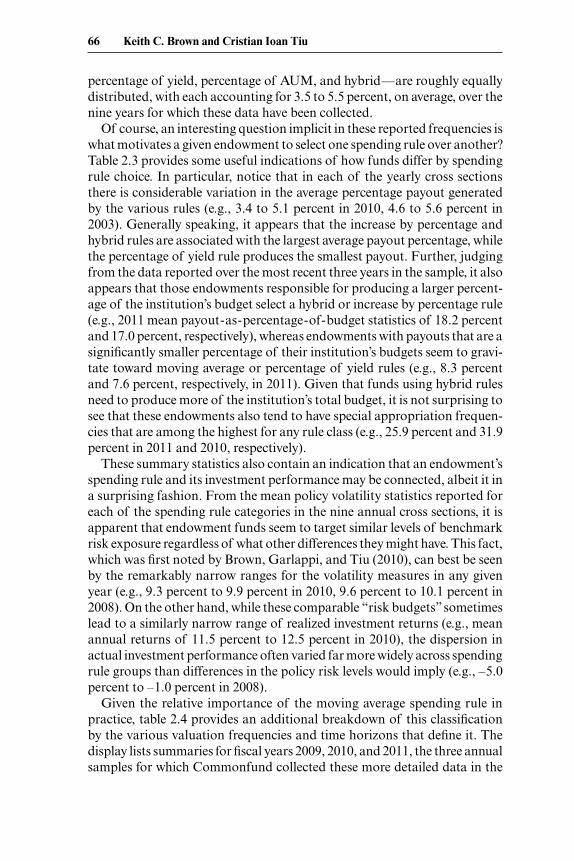
66 Keith C. Brown and Cristian Ioan Tiu
percentage of yield, percentage of AUM, and hybrid—are roughly equally distributed, with each accounting for 3.5 to 5.5 percent, on average, over the nine years for which these data have been collected.
Of course, an interesting question implicit in these reported frequencies is what motivates a given endowment to select one spending rule over another? Table 2.3 provides some useful indications of how funds differ by spending rule choice. In particular, notice that in each of the yearly cross sections there is considerable variation in the average percentage payout generated by the various rules (e.g., 3.4 to 5.1 percent in 2010, 4.6 to 5.6 percent in 2003). Generally speaking, it appears that the increase by percentage and hybrid rules are associated with the largest average payout percentage, while the percentage of yield rule produces the smallest payout. Further, judging from the data reported over the most recent three years in the sample, it also appears that those endowments responsible for producing a larger percent-age of the institution’s budget select a hybrid or increase by percentage rule (e.g., 2011 mean payout- as- percentage- of- budget statistics of 18.2 percent and 17.0 percent, respectively), whereas endowments with payouts that are a significantly smaller percentage of their institution’s budgets seem to gravi-tate toward moving average or percentage of yield rules (e.g., 8.3 percent and 7.6 percent, respectively, in 2011). Given that funds using hybrid rules need to produce more of the institution’s total budget, it is not surprising to see that these endowments also tend to have special appropriation frequen-cies that are among the highest for any rule class (e.g., 25.9 percent and 31.9 percent in 2011 and 2010, respectively).
These summary statistics also contain an indication that an endowment’s spending rule and its investment performance may be connected, albeit it in a surprising fashion. From the mean policy volatility statistics reported for each of the spending rule categories in the nine annual cross sections, it is apparent that endowment funds seem to target similar levels of benchmark risk exposure regardless of what other differences they might have. This fact, which was first noted by Brown, Garlappi, and Tiu (2010), can best be seen by the remarkably narrow ranges for the volatility measures in any given year (e.g., 9.3 percent to 9.9 percent in 2010, 9.6 percent to 10.1 percent in 2008). On the other hand, while these comparable “risk budgets” sometimes lead to a similarly narrow range of realized investment returns (e.g., mean annual returns of 11.5 percent to 12.5 percent in 2010), the dispersion in actual investment performance often varied far more widely across spending rule groups than differences in the policy risk levels would imply (e.g., –5.0 percent to –1.0 percent in 2008).
Given the relative importance of the moving average spending rule in practice, table 2.4 provides an additional breakdown of this classification by the various valuation frequencies and time horizons that define it. The display lists summaries for fiscal years 2009, 2010, and 2011, the three annual samples for which Commonfund collected these more detailed data in the
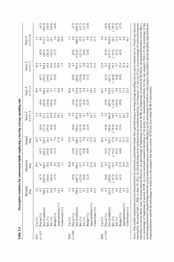
Tab
le 2
.4
Des
crip
tive
stat
isti
cs fo
r en
dow
men
t fun
ds e
mpl
oyin
g a
mov
ing
aver
age
spen
ding
rul
e
Mon
thly
fr
eq.
Q
uart
erly
fr
eq.
A
nnua
l fr
eq.
Y
ears
T
0 ≤
T <
3
Yea
rs T
3
≤ T
< 5
Y
ears
T
5 ≤
T <
7
Yea
rs T
7
≤ T
≤ 1
0
2011
U
se (%
) 2.
0 39
.9
34.7
1.
8 78
.3
18.8
1.
1 n
= 6
11
Pay
out (
%)
4.7
(4.7
) 4.
7 (4
.7)
4.3
(4.6
) 4.
9 (4
.6)
4.5
(4.7
) 4.
5 (4
.5)
4.6
(4.1
)Si
ze ($
mill
ions
) 50
6.5
(229
.5)
306.
1 (8
4.1)
35
2.7
(77.
5)
87.1
(6
5.0)
29
6.1
(79.
1)
394.
4 (9
4.1)
17
23.7
(3
03.3
)R
et. (
%)
19.3
(1
8.6)
18
.6
(19.
8)
18.5
(1
9.6)
15
.3
(18.
4)
18.2
(1
9.6)
19
.8
(20.
3)
22.3
(2
4.0)
Vol
. (%
) 10
.0
(10.
5)
9.9
(9.8
) 9.
7 (9
.8)
10.0
(1
0.4)
9.
7 (9
.7)
10.0
(1
0.1)
10
.7
(10.
6)B
udge
t (%
) 5.
8 (3
.3)
8.1
(3.7
) 7.
6 (2
.6)
15.0
(2
.4)
7.1
(3.0
) 12
.0
(3.7
) 5.
4 (4
.8)
App
ropr
iati
ons
(%)
12.5
18
.8
17.0
18
.2
16.8
19
.8
50.0
U
nder
wat
er (%
) 4.
3 5.
1 4.
3 13
.7
5.0
3.5
16.9
2010
U
se (%
) 1.
3 36
.4
37.8
1.
9 82
.8
14.0
1.
3 n
= 6
20
Pay
out (
%)
4.9
(4.8
) 4.
8 (5
.0)
4.3
(4.8
) 5.
4 (5
.4)
4.5
(4.9
) 4.
3 (4
.8)
5.6
(5.7
)Si
ze ($
mill
ions
) 29
0.0
(168
.7)
284.
1 (7
4.1)
26
0.2
(64.
1)
167.
6 (6
7.6)
23
5.9
(66.
8)
392.
4 (1
21.9
) 14
09.2
(4
56.3
)R
et. (
%)
11.2
(1
2.0)
11
.7
(12.
3)
11.4
(1
1.8)
10
.9
(11.
2)
11.4
(1
2.0)
12
.1
(12.
1)
12.8
(1
2.7)
Vol
. (%
) 9.
3 (9
.9)
9.5
(9.4
) 9.
4 (9
.4)
8.7
(8.8
) 9.
4 (9
.4)
9.8
(9.6
) 11
.3
(11.
7)B
udge
t (%
) 13
.6
(2.2
) 9.
3 (4
.0)
8.2
(2.3
) 5.
6 (2
.6)
8.7
(3.2
) 12
.2
(2.6
) 4.
0 (2
.8)
App
ropr
iati
ons
(%)
0.0
21.8
17
.9
16.7
18
.1
21.8
71
.4
Und
erw
ater
(%)
13.5
14
.2
12.3
12
.7
13.3
13
.2
27.5
2009
U
se (%
) 2.
0 33
.5
39.2
2.
4 84
.7
11.9
1.
0 n
= 6
10
Pay
out (
%)
4.5
(4.6
) 4.
5 (4
.5)
4.1
(4.4
) 5.
2 (5
.0)
4.3
(4.5
) 4.
2 (4
.4)
4.3
(4.2
)Si
ze ($
mill
ions
) 62
5.4
(224
.9)
247.
4 (7
1.8)
26
5.1
(56.
6)
486.
0 (6
9.5)
22
6.6
(62.
7)
434.
0 (1
15.7
) 10
39.4
(5
4.9)
Ret
. (%
) –1
7.6
(–18
.3)
–18.
5 (–
19.1
) –1
7.6
(–18
.9)
–18.
2 (–
17.9
) –1
7.7
(–18
.9)
–19.
3 (–
19.5
) –2
8.2
(–29
.7)
Vol
. (%
) 9.
4 (9
.7)
9.4
(9.5
) 9.
4 (9
.5)
9.7
(10.
2)
9.4
(9.4
) 9.
7 (9
.7)
12.4
(1
2.3)
Bud
get (
%)
19.0
(6
.2)
11.9
(4
.8)
11.1
(3
.6)
11.7
(9
.0)
11.2
(4
.0)
15.0
(4
.5)
6.2
(3.2
)A
ppro
pria
tion
s (%
) 6.
3 19
.9
17.2
26
.7
17.2
25
.4
0.0
Und
erw
ater
(%)
33
.5
22
.4
21
.2
32
.0
22
.5
16
.7
56
.1
Not
es: T
his
exhi
bit s
umm
ariz
es s
ever
al c
hara
cter
isti
cs fo
r un
iver
sity
end
owm
ent f
unds
that
repo
rted
usi
ng a
mov
ing
aver
age
spen
ding
rul
e in
a g
iven
ann
ual s
urve
y. F
isca
l yea
r da
ta a
re
repo
rted
for
the
peri
od J
uly
1, 2
008,
to
June
30,
201
1, fo
r th
e fo
llow
ing
cros
s- se
ctio
nal m
ean
(med
ian)
sta
tist
ics:
(a)
fre
quen
cy o
f ru
le u
se (
Use
), a
s a
perc
enta
ge o
f to
tal e
ndow
men
ts
repo
rtin
g in
a g
iven
sur
vey
year
; (b)
act
ual p
ayou
t (P
ayou
t), a
s a
perc
enta
ge o
f b
egin
ning
- of-
peri
od A
UM
; (c)
beg
inni
ng- o
f- pe
riod
AU
M (
Size
); (
d) a
nnua
l inv
estm
ent
retu
rn (
Ret
.),
as a
per
cent
age
of b
egin
ning
- of-
peri
od A
UM
; (e)
cro
ss- s
ecti
onal
sta
ndar
d de
viat
ion
of t
he p
olic
y (i
.e.,
benc
hmar
k) p
ortf
olio
for
the
rul
e ca
tego
ry (
Vol
.); (
f) t
he p
erce
ntag
e of
the
sp
onso
ring
inst
itut
ion’
s ann
ual b
udge
t tha
t the
act
ual e
ndow
men
t pay
out r
epre
sent
s (B
udge
t); (
g) th
e pe
rcen
tage
of
fund
s in
a ru
le c
ateg
ory
that
em
ploy
spec
ial s
pend
ing
appr
opri
atio
ns
(App
ropr
iati
ons)
; and
(h) t
he p
erce
ntag
e of
fund
s in
a r
ule
cate
gory
that
hav
e cu
rren
t AU
M le
ss th
an in
itia
l AU
M (U
nder
wat
er).

68 Keith C. Brown and Cristian Ioan Tiu
NACUBO surveys. The three frequency columns show that the vast majority of moving average rules in use are based on either quarterly or annual mea-sures of past AUM values. Further, these two measurement frequencies are used in roughly comparable amounts, although there appears to have been a slight shift toward the quarterly averaging process (i.e., 33.5 percent to 39.9 percent usage from 2009 to 2011) and away from annual averaging. Beyond that, as indicated by the four time- horizon columns, averaging the AUM base over a period between three to five years is easily the most popular single choice in all three cross sections, despite the fact that five- to seven- year averaging became more prevalent over the period (i.e., 11.9 percent usage in 2009, 18.8 percent in 2011).
Finally, as with the asset allocation patterns discussed above, endow-ment size is also apparently a factor in determining the spending rule that is selected. For example, from table 2.3, the mean AUM for funds in the hybrid rule category in 2011 is $1,143.3 million, compared to $756.9 million and $326.8 million mean portfolio values in the decide annually and moving average categories, respectively. To get a better sense of these size dynamics, we also calculated spending rule frequencies by fund- size quartile, from the smallest (Q1) to the largest (Q4), for each of the nine annual samples. Panel A of figure 2.3 illustrates these interquartile distributions at the two yearly end points of the sample while panel B shows the rules used in quartiles Q4 and Q1 for three different years. In 2003, it is apparent that the smallest endowments used moving average rules to a lesser extent than larger funds, in favor of a relatively bigger use of decide annually and percentage of AUM rules. However, by 2011, use of a pure moving average policy in the Q4 quartile had declined dramatically to the point that those funds had the lowest comparative frequency, with an increased use of hybrid rules provid-ing the offset. On the other hand, the use of moving average rules by Q1 funds remained much steadier over the same time frame. Thus, as with asset allocation changes over time, variations in spending rule use also appear to be driven primarily by the largest endowments in the sample, a topic we explore in more detail in the analysis that comes next.
2.4 The Evolution of Spending Policies over Time
Having just established some important cross- sectional differences in spending rule adoption practices, it is also useful to consider the issue of how a given endowment fund’s spending policy has changed (if at all) over time. In one sense, this is a more interesting question to address since, given the prediction of Merton (1993) in the context of the relatively static nature of the investment problem that most educational institutions face, it is not clear that there is any reason to expect an endowment to modify the fun-damental way in which it views its spending mandate from one year to the next. On the other hand, recent research suggests that endowments do face

Fig
. 2.3
Com
para
tive
spen
ding
rul
e pa
tter
ns o
ver
tim
e an
d en
dow
men
t fun
d si
zeN
ote:
Thi
s fig
ure
illus
trat
es h
ow s
pend
ing
rule
ado
ptio
n fr
eque
ncie
s fo
r th
e en
dow
men
t fun
d sa
mpl
e ha
ve c
hang
ed o
ver
tim
e an
d fo
r po
rtfo
lios
of d
iffe
rent
siz
es.
Usi
ng th
e se
ven
cate
gori
es d
efine
d in
the
appe
ndix
, pan
el A
list
s sp
endi
ng r
ule
freq
uenc
ies
for
fund
s in
dif
fere
nt A
UM
qua
rtile
s (l
arge
st [Q
4] to
sm
alle
st [Q
1]) f
or
two
diff
eren
t yea
rs (2
003
and
2011
). P
anel
B li
sts
spen
ding
rul
e fr
eque
ncie
s ac
ross
tim
e (2
003,
200
7, a
nd 2
011)
for
two
diff
eren
t fun
d si
ze q
uart
iles
(Q4
and
Q1)
.
A B

70 Keith C. Brown and Cristian Ioan Tiu
changing circumstances in the form of unexpectedly adverse economic condi-tions (see Brown et al. 2010) or competition for resources with peer institutions (see Goetzmann and Oster [chapter 3, this volume], and Lerner, Schoar, and Wang [2008]) that necessitate changing their spending policies on an occa-sional basis. However, there appears to be little in the way of a priori justifica-tion for a widespread frequency of changes to the nature of these statements.23
To analyze this issue, we examine how all of the endowment funds in the NACUBO sample specified their spending policies during every year between 2003 and 2011. Formally, for each endowment E, we examine its spending policy (i.e., both spending rule and policy rate) for every year T that it reported survey data and characterize its spending rule according to the taxonomy described earlier. Endowment E is considered to have changed its spending policy if at least one of two conditions occur: (a) the spending rule it uses in year T + 1 falls into a different category than its spending rule in year T (e.g., a switch from a decide annually rule in 2009 to a hybrid rule in 2010); or (b) a change from year T to year T + 1 in the designated policy payout rate specified within the same spending rule (e.g., a switch from a commitment to spend 4.0 percent of a twelve- quarter moving average of past portfolio values in 2005 to 5.0 percent of a similar moving average calculation in 2006). Notice that while an adjustment in either the spending rule or the designated rate applied within that rule is regarded as policy change, a modification in the former is considered to be a more extreme alteration of the way in which the endowment’s investment problem is viewed.24
2.4.1 Tabulating Spending Policy Changes on a Yearly Basis
Table 2.5 documents at a broad level the extent to which endowments alter their spending policies from one year to the next. Panel A summarizes the frequency of change to any aspect of the spending policy (i.e., rule or rate) while panel B isolates just those endowments that altered the nature of the spending rule to the extent that it switched categories in consecutive years. To interpret the exhibit, for the fiscal year 2009, there were 842 endowments that reported information about their spending policy in the annual survey.
23. In this discussion, it is important to keep in mind the distinction between permanent spending needs, as defined by Tobin (1974), and temporary needs that might be driven by changing macroeconomic or institution-specific factors. As documented in table 2.3, roughly one in three endowments exercised its capacity to make special appropriations as necessary, which mitigates the need to change their formal spending policies to accommodate temporary changes in circumstances.
24. With this definition, an endowment that altered its spending rule from a three-year mov-ing average based on an annual observation frequency to a five-year moving average based on a quarterly observation frequency would not be viewed as having made a policy change, assuming it also kept its designated payout rate the same. In this regard, the procedure we use for identifying spending policy changes that occurred in the sample is conservatively biased.
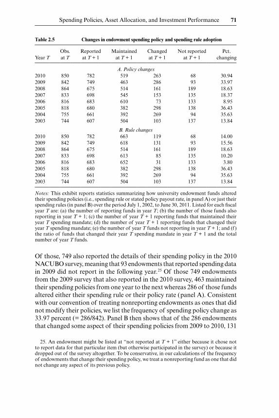
Spending Policies, Asset Allocation, and Investment Performance 71
Of those, 749 also reported the details of their spending policy in the 2010 NACUBO survey, meaning that 93 endowments that reported spending data in 2009 did not report in the following year.25 Of those 749 endowments from the 2009 survey that also reported in the 2010 survey, 463 maintained their spending policies from one year to the next whereas 286 of those funds altered either their spending rule or their policy rate (panel A). Consistent with our convention of treating nonreporting endowments as ones that did not modify their policies, we list the frequency of spending policy change as 33.97 percent (= 286/842). Panel B then shows that of the 286 endowments that changed some aspect of their spending policies from 2009 to 2010, 131
25. An endowment might be listed at “not reported at T + 1” either because it chose not to report data for that particular item (but otherwise participated in the survey) or because it dropped out of the survey altogether. To be conservative, in our calculations of the frequency of endowments that change their spending policy, we treat a nonreporting fund as one that did not change any aspect of its previous policy.
Table 2.5 Changes in endowment spending policy and spending rule adoption
Year T Obs. at T
Reported at T + 1
Maintained at T + 1
Changed at T + 1
Not reported at T + 1
Pct. changing
A. Policy changes2010 850 782 519 263 68 30.942009 842 749 463 286 93 33.972008 864 675 514 161 189 18.632007 833 698 545 153 135 18.372006 816 683 610 73 133 8.952005 818 680 382 298 138 36.432004 755 661 392 269 94 35.632003 744 607 504 103 137 13.84
B. Rule changes2010 850 782 663 119 68 14.002009 842 749 618 131 93 15.562008 864 675 514 161 189 18.632007 833 698 613 85 135 10.202006 816 683 652 31 133 3.802005 818 680 382 298 138 36.432004 755 661 392 269 94 35.632003 744 607 504 103 137 13.84
Notes: This exhibit reports statistics summarizing how university endowment funds altered their spending policies (i.e., spending rule or stated policy payout rate, in panel A) or just their spending rules (in panel B) over the period July 1, 2002, to June 30, 2011. Listed for each fiscal year T are: (a) the number of reporting funds in year T; (b) the number of those funds also reporting in year T + 1; (c) the number of year T + 1 reporting funds that maintained their year T spending mandate; (d) the number of year T + 1 reporting funds that changed their year T spending mandate; (e) the number of year T funds not reporting in year T + 1; and (f ) the ratio of funds that changed their year T spending mandate in year T + 1 and the total number of year T funds.

72 Keith C. Brown and Cristian Ioan Tiu
of them actually altered their spending rule in a way that caused a change in classification. This is represented in the last column as a rule frequency change of 15.56 percent (= 131/842).26
The clear and surprising implication from the findings in table 2.5 is that endowment funds adjust their spending policies far more often than might be reasonably expected given the long- term nature of their investment man-dates. Specifically, the data in panel A show that annual frequencies with which either spending rules or policy payout rates (or both) are changed range from 8.95 percent (2006) to 36.43 percent (2005). The weighted mean (as a percentage of reporting funds) for these annual change frequencies is 24.62 percent, meaning that, on average, one in four of the endowments in the sample altered its spending policy each year. Further, as summarized by panel B, the percentage of endowments changing their actual spending rule—the most extreme policy adjustment they could make—in a given year ranged from 3.80 percent to 36.43 percent, with a weighted mean annual change frequency of 18.35 percent.27
Although theory (i.e., Merton 1993; Woglom 2003) predicts that the expected number of spending policy changes in a given survey year is zero, it is difficult to say whether these change frequency patterns can be consid-ered extremely abnormal absent more information of how the investment problem faced by the sponsoring institutions might have changed. Neverthe-less, testing the observed frequencies against two different prospective null hypotheses is instructive. First, assuming that 5.0 percent of the endowments will modify their spending mandates in a given year (i.e., a 1- in- 20 event), the Pearson chi- squared statistics testing the goodness of fit between the observed and forecasted distributions for the spending policy and spending rule change samples are 6,350.46 and 3,843.25, respectively. Both of these statistics are statistically significant with p- values of less than 0.0001, indi-cating that endowments make adjustments far more frequently than might occur on a random basis if the true proportion of expected changes was zero. Beyond that, the respective chi- squared statistics testing whether the observed annual change frequencies equal the weighted mean frequencies (i.e., 24.62 percent for spending policy, 18.35 percent for spending rules only) are 269.45 and 413.38, which are also statistically reliable at better than a 0.0001 level. Thus, it is also the case that the spending policy changes shown in table 2.5 vary significantly from one another on a year- to- year basis.
Finally, as a supplement to this analysis of how frequently spending poli-cies changed annually, it is also useful to consider the total number of times
26. Of course, both of these change frequencies would be larger if based on just those funds from the 2009 survey that also reported data in 2010; 38.18 percent (= 286/749) and 17.49 percent (= 131/749) for policy and rule changes, respectively.
27. Prior to the 2006 survey, NACUBO did not report separate data for policy payout rates. So, for 2003–2005, the change frequencies for the total spending policy are based solely on changes to the reported spending rules.

Spending Policies, Asset Allocation, and Investment Performance 73
during the 2003–2011 sample period that each endowment altered its stated spending rule. To tabulate this information, we focused on the 628 funds that reported their rules continuously over the entire set of nine surveys for which spending data were collected. As before, a fund was considered to have made a modification if the spending rules it reported in year T and year T + 1 fall into different categories, so that the maximum number of changes that could be observed for any endowment E is eight. Figure 2.4 presents a histogram of these statistics. Exactly half (i.e., 314 of 628) of the funds did not adjust their spending rule at all during this interval, meaning that exactly half of the funds did make at least one formal adjustment. In fact, more endowments made two changes to their stated rule (129) than those that made only one modification (101). Further, 13.38 percent (84 of 628) changed this aspect of their spending policy three or more times and one endowment altered its spending rule in every one of the available surveys!
Fig. 2.4 Frequency of spending rule changesNote: This figure shows the frequency of spending rule changes for the endowments in the NACUBO/Commonfund sample over the period July 1, 2002, to June 30, 2011. For each en-dowment that reports sufficient spending policy data for at least two consecutive annual sur-veys, we calculate the number of times the endowment changes the spending rules it adopted for each fiscal year from 2003 to 2010. The figure depicts the histogram of the number of rule changes.

74 Keith C. Brown and Cristian Ioan Tiu
2.4.2 Spending Rule Migration Patterns
Given this unexpectedly large number of annual spending policy changes, a natural question to ask is which mandates are most likely to be abandoned and which are most likely to be subsequently adopted? Table 2.6 addresses this issue by focusing on the more narrow topic of spending rule migration trends. Specifically, for every endowment E, we observed the spending rule it adopted for both year T as well as in the following year T + 1. Then, for each year T spending rule classification, we tabulated which of the seven categories the same fund fit into in the next year. Notice that by this sorting process, we account for all possible outcomes for how a given endowment E can modify its spending rule, including the fact that it might not change it at all.
Panel A reports these annual transition frequencies for all of the sample funds over the entire 2003–2011 time horizon. The first column lists the seven spending rule categories that endowments adopted in year T. The remaining seven columns then summarize the spending rule category, a given endowment E fit into in year T + 1. The data in the table have been scaled by dividing the number of raw observations in a particular cell by the total number of original year T observations in that particular row. Thus, all of the entries represent the percentage of the funds using a certain rule at year T that now fall under the respective year T + 1 rule. For example, the first row of panel A in table 2.6 corresponds to those endowments that adopted the decide annually rule in year T. Of those, 47.72 percent remained in the decide annually rule (i.e., did not change) during the following year, while 39.82 percent of those endowments switched their spending policy to a mov-ing average rule. By construction, each of the rows in the display sums to 100.00 percent.28
Arguably the most interesting aspect of the reported findings is that the var-ious spending rules have dramatically different likelihoods of being retained from one survey year to the next. The diagonal elements of the matrix (start-ing from the top left cell) indicate the percentage of a particular spending rule category that did not change (i.e., was retained) in the following period. Clearly, with 88.12 percent and 79.85 percent retention, respectively, the mov-ing average and hybrid rule categories are the only ones that have a better than three- in- four chance of remaining in place in consecutive years and are therefore the only rules whose adoption appears to be stable. Conversely, the retention rate for percentage of yield rules is just 35.74 percent, meaning that approximately two out of three funds that adopted that mandate in year T formally altered their spending policies within the next twelve months.
28. Notice also that this exhibit is constructed so that each endowment is likely to appear mul-tiple times since a comparison of rules in place for year T and year T + 1 produces up to eight observations per fund over the nine-year time frame for which spending rule data were available. Of course, any fund that changed spending policies will see its data represented in different rows.
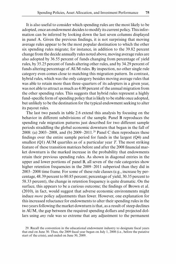
Spending Policies, Asset Allocation, and Investment Performance 75
It is also useful to consider which spending rules are the most likely to be adopted, once an endowment decides to modify its current policy. This infor-mation can be inferred by looking down the last seven columns displayed in panel A. Given the previous findings, it is not surprising that moving average rules appear to be the most popular destination to which the other six spending rules migrate; for instance, in addition to the 39.82 percent change from the decide annually rules noted above, moving average rules are also adopted by 36.55 percent of funds changing from percentage of yield rules, by 35.25 percent of funds altering other rules, and by 34.29 percent of funds altering percentage of AUM rules. By inspection, no other single rule category even comes close to matching this migration pattern. In contrast, hybrid rules, which was the only category besides moving average rules that was able to retain more than three- quarters of its adopters in a given year, was not able to attract as much as 4.00 percent of the annual migration from the other spending rules. This suggests that hybrid rules represent a highly fund- specific form of spending policy that is likely to be stable once adopted, but unlikely to be the destination for the typical endowment seeking to alter its payout rules.
The last two panels in table 2.6 extend this analysis by focusing on the behavior in different subdivisions of the sample. Panel B reproduces the spending rule migration patterns just described for two different sample periods straddling the global economic downturn that began in the fall of 2008: (a) 2003–2008, and (b) 2009–2011.29 Panel C then reproduces these findings over the entire sample period for funds in the largest (Q4) and smallest (Q1) AUM quartiles as of a particular year T. The most striking feature of these transition matrices before and after the 2008 financial mar-ket downturn is the marked increase in the probability that endowments retain their previous spending rules. As shown in diagonal entries in the upper and lower portions of panel B, all seven of the rule categories show higher retention frequencies in the 2009–2011 subperiod than they did in 2003–2008 time frame. For some of these rule classes (e.g., increase by per-centage, 48.39 percent to 80.85 percent; percentage of yield, 30.35 percent to 58.33 percent), the change in retention frequency is quite dramatic. On the surface, this appears to be a curious outcome; the findings of Brown et al. (2010), in fact, would suggest that adverse economic environments might induce more policy adjustments than fewer. However, one explanation for this increased reluctance for endowments to alter their spending rules in the two years following the market downturn is that, as a result of steep declines in AUM, the gap between the required spending dollars and projected dol-lars using any rule was so extreme that any adjustment to the permanent
29. Recall the convention in the educational endowment industry to designate fiscal years that end on June 30. Thus, the 2009 fiscal year began on July 1, 2008 (i.e., before the putative start of the crisis), and ended on June 30, 2009.
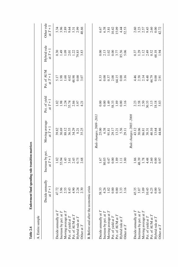
Tab
le 2
.6
End
owm
ent f
und
spen
ding
rul
e tr
ansi
tion
mat
rice
s
A. E
ntir
e sa
mpl
e
Dec
ide
annu
ally
at
T +
1 In
crea
se b
y pc
t.
at T
+ 1
Mov
ing
aver
age
at T
+ 1
Pct
. of
yiel
d at
T +
1 P
ct. o
f A
UM
at
T +
1 H
ybri
d ru
le
at T
+ 1
Oth
er r
ule
at T
+ 1
Dec
ide
annu
ally
at T
47
.72
1.82
39
.82
1.82
5.
170.
30
3.34
In
crea
se b
y pc
t. a
t T
3.96
55
.94
30.6
9 1.
98
1.98
1.49
3.
96
Mov
ing
aver
age
at T
2.
55
1.43
88
.12
2.24
1.
681.
09
2.89
P
ct. o
f yi
eld
at T
8.
43
3.61
36
.55
35.7
4 4.
022.
01
9.64
P
ct. o
f A
UM
at T
4.
90
2.45
34
.29
2.86
48
.98
1.22
5.
31
Hyb
rid
rule
at T
2.
24
0.75
8.
21
5.97
0.
0079
.85
2.99
O
ther
at T
2.30
2.68
35.2
5
4.21
3.07
3.
83
48
.66
B. B
efor
e an
d af
ter
the
econ
omic
cri
sis
Rul
e ch
ange
s, 2
009–
2011
Dec
ide
annu
ally
at T
58
.33
1.67
25
.00
0.00
8.
330.
00
6.67
In
crea
se b
y pc
t. a
t T
4.26
80
.85
6.38
0.
00
0.00
2.13
6.
38
Mov
ing
aver
age
at T
1.
02
0.47
91
.81
1.49
0.
371.
02
3.81
P
ct. o
f yi
eld
at T
0.
00
0.00
29
.17
58.3
3 2.
080.
00
10.4
2 P
ct. o
f A
UM
at T
0.
00
1.89
13
.21
1.89
64
.15
3.77
15
.09
Hyb
rid
rule
at T
3.
33
1.11
5.
56
0.00
0.
0085
.56
4.44
O
ther
at T
3.
16
3.80
29
.11
3.16
3.
165.
06
52.5
3
Rul
e ch
ange
s, 2
003–
2008
Dec
ide
annu
ally
at T
45
.35
1.86
43
.12
2.23
4.
460.
37
2.60
In
crea
se b
y pc
t. a
t T
3.87
48
.39
38.0
6 2.
58
2.58
1.29
3.
23
Mov
ing
aver
age
at T
3.
09
1.78
86
.81
2.50
2.
141.
12
2.57
P
ct. o
f yi
eld
at T
10
.45
4.48
38
.31
30.3
5 4.
482.
49
9.45
P
ct. o
f A
UM
at T
6.
25
2.60
40
.10
3.13
44
.79
0.52
2.
60
Hyb
rid
rule
at T
0.
00
0.00
13
.64
18.1
8 0.
0068
.18
0.00
O
ther
at T
0.97
0.97
44.6
6
5.83
2.91
1.
94
42
.72
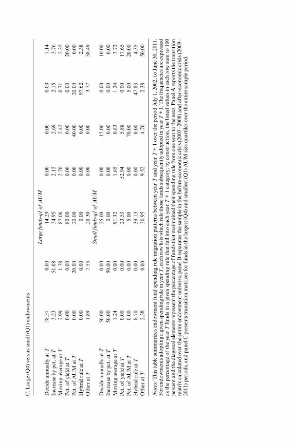
C. L
arge
(Q4)
ver
sus
smal
l (Q
1) e
ndow
men
ts
Lar
ge fu
nds-
q1 o
f A
UM
Dec
ide
annu
ally
at T
78
.57
0.00
14
.29
0.00
0.
000.
00
7.14
In
crea
se b
y pc
t. a
t T
3.23
51
.08
34.9
5 2.
15
2.69
2.15
3.
76
Mov
ing
aver
age
at T
2.
99
1.78
87
.06
2.70
2.
420.
71
2.35
P
ct. o
f yi
eld
at T
0.
00
0.00
80
.00
0.00
0.
000.
00
20.0
0 P
ct. o
f A
UM
at T
0.
00
20.0
0 20
.00
0.00
40
.00
20.0
0 0.
00
Hyb
rid
rule
at T
0.
00
0.00
0.
00
0.00
0.
0097
.62
2.38
O
ther
at T
1.
89
7.55
28
.30
0.00
0.
003.
77
58.4
9 S
mal
l fun
ds- q
1 of
AU
MD
ecid
e an
nual
ly a
t T
50.0
0 0.
00
25.0
0 0.
00
15.0
00.
00
10.0
0 In
crea
se b
y pc
t. a
t T
50.0
0 50
.00
0.00
0.
00
0.00
0.00
0.
00
Mov
ing
aver
age
at T
1.
24
0.00
91
.32
1.65
0.
831.
24
3.72
P
ct. o
f yi
eld
at T
0.
00
0.00
23
.53
52.9
4 5.
880.
00
17.6
5 P
ct. o
f A
UM
at T
0.
00
0.00
5.
00
0.00
70
.00
5.00
20
.00
Hyb
rid
rule
at T
8.
70
0.00
39
.13
0.00
0.
0047
.83
4.35
O
ther
at T
2.38
0.00
30.9
5
9.52
4.76
2.
38
50
.00
Not
es: T
his
tabl
e su
mm
ariz
es e
ndow
men
t fun
d sp
endi
ng r
ule
mig
rati
on p
atte
rns
betw
een
year
T a
nd y
ear
T +
1 o
ver
the
peri
od J
uly
1, 2
002,
to J
une
30, 2
011.
F
or e
ndow
men
ts a
dopt
ing
a gi
ven
spen
ding
rule
in y
ear T
, eac
h ro
w li
sts w
hich
rule
thos
e fu
nds s
ubse
quen
tly a
dopt
ed in
yea
r T +
1. T
he fr
eque
ncie
s are
exp
ress
ed
as th
e pe
rcen
tage
of
the
year
T fu
nds
in a
giv
en s
pend
ing
rule
that
fall
into
eac
h ye
ar T
+ 1
cat
egor
y; b
y co
nstr
ucti
on, t
he li
sted
val
ues
in e
ach
row
sum
to 1
00
perc
ent a
nd th
e di
agon
al e
lem
ents
repr
esen
t the
per
cent
age
of fu
nds t
hat m
aint
aine
d th
eir s
pend
ing
rule
from
one
yea
r to
the
next
. Pan
el A
repo
rts t
he tr
ansi
tion
m
atri
x ca
lcul
ated
ove
r th
e en
tire
end
owm
ent u
nive
rse,
pan
el B
sep
arat
es th
e sa
mpl
e in
the
bef
ore-
econ
omic
cri
sis
(200
3–20
08) a
nd a
fter
- eco
nom
ic c
risi
s (2
009–
2011
) per
iods
, and
pan
el C
pre
sent
s tr
ansi
tion
mat
rice
s fo
r fu
nds
in th
e la
rges
t (Q
4) a
nd s
mal
lest
(Q1)
AU
M s
ize
quar
tile
s ov
er th
e en
tire
sam
ple
peri
od.
78 Keith C. Brown and Cristian Ioan Tiu
policy guidelines would not have solved the problem. Instead, many endow-ments relied on temporary measures to close this spending gap; for instance, the summary statistics in table 2.3 show that about one out of every three endowments invoked special appropriations in the 2009, 2010, and 2011 fiscal years. Thus, consistent with the notion that the spending rule policy statement represents a vision of the long- term investment problem faced by the institution, boards tend to respond to extreme events of a temporary nature with solutions that are similarly short lived.
The transition matrices for the largest and smallest fund size quartiles shown in panel C of table 2.6 also indicate significant cross- sectional differ-ences in the way endowments with disparate AUM levels alter their spending policies. While the values reported for the various cells appear to be more erratic than those shown in panel B, due to the small frequencies associated the sample quartiles, they nevertheless indicate some similarities and dispari-ties. First, the retention rate for moving average rules was extremely high for both large (87.06 percent) and small (91.22 percent) endowments and the migration into this rule category (i.e., the data in the respective columns) occurred for both size quartiles with about the same frequency. Conversely, the retention rate in the large funds for hybrid rules was virtually 100.00 per- cent, indicating that the biggest endowments adopting this spending policy category essentially never change. For small endowments, however, the loy-alty to hybrid rules was far more suspect (47.83 percent retention), mean-ing that more Q1 endowments switched away from hybrid rules than kept them from one year to the next. For these funds, it was almost as probable (39.13 percent) that they would modify the spending rule by changing to a simpler moving average formula—which is likely to have been one of the rule categories combined in the hybrid approach—than retain the previous combination rule. Finally, notice that no small funds switched to an increase by percentage rule—and only 50.00 percent of previous adopters retained that policy—over the entire sample period and that no large funds retained an exclusive reliance on a percentage of yield rule.
2.5 The Determinants of Spending Rule Changes
The preceding results leave little doubt that, collectively, university endow-ment funds alter their formal spending policies far more frequently than might be expected. However, beyond some suggestions from the reported data that patterns in these rule and payout rate changes are linked to some cross- sectional and temporal differences in the sample, it is not clear what the determinants of spending policy modifications actually are. In this sec-tion, we address that question by examining the formal links between a mea-sure summarizing these changes and several variables observable in advance of a period in which an endowment either did or did not adjust its spending rules.

Spending Policies, Asset Allocation, and Investment Performance 79
2.5.1 Defining Potential Determinants
In the statistical analysis that follows, we begin by defining the dependent variable (POLCHGT+1) as an indicator variable assuming the value of 1 if endowment E changed its stated spending rule between the survey years T and T + 1, and 0 otherwise. Accordingly, each of the potential explanatory factors that we consider is observable as of year T. The following discussion describes these regressors, including how each of them is defined, as well as the direction of the predicted influence they have on POLCHG.
The findings discussed in section 2.3.4 revealed a potential connection between an endowment’s spending policy decision and the nature of the returns produced by its investment portfolio. Although the ranges in the mean levels of portfolio return and policy volatility reported in table 2.3 for the seven spending rule categories were fairly narrow, it is nevertheless a reasonable conjecture that both the amount and stability of the change in the fund’s market value could influence the institution’s decision to alter its payout formula. We therefore define as potential determinants the endow-ment portfolio’s year T investment return ( RETT ) and policy portfolio vola-tility level ( VOLT ), as described earlier. The relationship between POLCHG and VOL should be positive: the less predictable the portfolio’s asset value is, the more likely the endowment might have to alter its spending plan. Conversely, positive investment returns in a given fiscal year should make it less likely that the endowment will need to adjust its long- term policy, lead-ing to a negative predicted relationship between RET and PLCHG.30
Two other variables that were shown earlier to be connected to an endow-ment’s choice of spending policy are the level of its actual payout and the size of its investment portfolio. The year T values of these factors—which we label as PAYOUTT and LOGAUMT, respectively—are also included as potential determinants in the analysis reported below. As shown in table 2.3, funds with higher (lower) payout rates were more likely to use increase by percentage or hybrid (percentage of yield) rules over the sample period. Thus, the relationship between PAYOUT and POLCHG is likely to be nega-tive in that funds with higher required payouts are likely to have already adopted the rules that best serve that purpose. On the other hand, it is not clear what impact the market value of the endowment portfolio, which for scaling purposes is expressed here as the natural logarithm of the fund’s AUM, might have on POLCHG. The data summarized in figure 2.2 show that the largest funds have been far more willing and able to adjust their asset allocations than smaller endowments, which might suggest that they are also
30. The negative forecasted connection between RET and POLCHG might be better seen from the other direction. That is, negative portfolio returns might cause a spending policy change—perhaps in addition to the special appropriations discussed earlier—because the income generated by the portfolio, as well as the fund’s reduced AUM level, is not sufficient to generate the required expenditures under the old policy.
80 Keith C. Brown and Cristian Ioan Tiu
less likely to need to adjust their spending policy definition in changing economic environments, implying a negative relationship. However, as indi-cated by figure 2.3, it is also the case that large endowments appear to change their spending rules more frequently, perhaps because their organizational mobility permits making quick adjustments to all of their various operating policies.
It is possible that spending rule changes are also linked to the specific nature of an endowment’s asset allocation decision. In particular, it was also shown in section 2.3.3 that endowments vary considerably in the use of alternative assets and these investments are especially critical to determining both the absolute and risk- adjusted returns that an institutionally managed portfolio produces (see Lerner, Schoar, and Wongsunwai 2007; Brown, Gar-lappi, and Tiu 2010). Thus, as described earlier, we define ALTINVT as the percentage of an endowment’s year T portfolio that is invested in the hedge fund, private equity, real estate, and natural resources asset classes. The effect of ALTINV on POLCHG could go in either direction; the fact that larger allocations to alternatives might produce higher returns could generate the negative correlation hypothesized above for RET, but the greater degree of illiquidity associated with the alternative asset classes could create less investment policy flexibility, which in turn could lead to a higher likelihood of modifications to the spending policy.
Returns to the investment portfolio are not the only way that an endow-ment can fund its spending needs. Educational institutions routinely receive donations from a variety of public and private supporters that can either be used to increase the size of the current portfolio or be earmarked for direct expenditure (see Brown, Dimmock, and Weisbenner 2012). In either case, we posit that larger levels of these supplemental contributions would make it less likely that an endowment would have to modify its spending rule to meet its budgetary needs, implying a negative relationship between year T donations (labeled as DONATET ) and future POLCHG. The NACUBO database does not contain observations on donations directly, but these contributions can be inferred for a given fund by taking the difference between the portfolio’s value at the end and beginning of the period, adjusted for the returns earned during the period, plus the payout amount. That is, expressed as a percentage of assets, we have
(1)
DONATET = [AUMT +1 − AUMTX (1 + RETT )] / AUMT
+ PAYOUTT,
where the AUM levels are expressed as beginning- of- period asset values.Finally, the descriptive data in table 2.3 also strongly indicated that both
the percentage of the institution’s overall budget that the endowment was responsible for delivering as well as its ability to make special payout appro-priations were linked to the choice of permanent spending rule. We therefore allow for the possibility that the year T value of the budget variable (defined
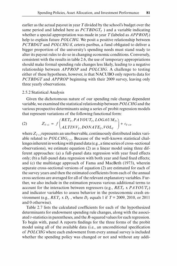
Spending Policies, Asset Allocation, and Investment Performance 81
earlier as the actual payout in year T divided by the school’s budget over the same period and labeled here as PCTBDGTT ) and a variable indicating whether a special appropriation was made in year T (labeled as APPROPT) help to explain future POLCHG. We posit a positive relationship between PCTBDGT and POLCHG if, ceteris paribus, a fund obligated to deliver a bigger proportion of the university’s spending needs must stand ready to alter its payout rules to do so in changing economic conditions. Conversely, consistent with the results in table 2.6, the use of temporary appropriations should make formal spending rule changes less likely, leading to a negative relationship between APPROP and POLCHG. A challenge to testing either of these hypotheses, however, is that NACUBO only reports data for PCTBDGT and APPROP beginning with their 2009 survey, leaving only three yearly observations.
2.5.2 Statistical Analysis
Given the dichotomous nature of our spending rule change dependent variable, we examined the statistical relationship between POLCHG and the various prospective determinants using a series of probit regression models that represent variations of the following functional form:
(2) ZT +1 = f
RETT, PAYOUTT, LOGAUMT,
ALTINVT, DONATET,VOLT
+ T +1,
where ZT +1 represents an unobservable, continuously distributed index vari-able related to POLCHGT +1. Because of the well- known statistical chal-lenges inherent in working with panel data (e.g., a time series of cross- sectional observations), we estimate equation (2) as a linear model using three dif-ferent approaches: (a) a full- panel data regression with year fixed effects only; (b) a full- panel data regression with both year and fund fixed effects; and (c) the multistage approach of Fama and MacBeth (1973), wherein separate cross- sectional versions of equation (2) are estimated for each of the survey years and then the estimated coefficients from each of the annual cross sections are averaged for all of the relevant explanatory variables. Fur-ther, we also include in the estimation process various additional terms to account for the interaction between regressors (e.g., RETT x PAYOUTT) and indicator variables to assess behavior in the posteconomic crash en-vironment (e.g., RETT x DT , where DT equals 1 if T = 2009, 2010, or 2011 and 0 otherwise).
Table 2.7 lists the calculated coefficients for each of the hypothesized determinants for endowment spending rule changes, along with the associ-ated t- statistics in parentheses, and the R- squared values for each regression. To begin with, panel A reports findings for the three forms of the probit model using all of the available data (i.e., an unconditional specification of POLCHG where each endowment from every annual survey is included whether the spending policy was changed or not and without any addi-
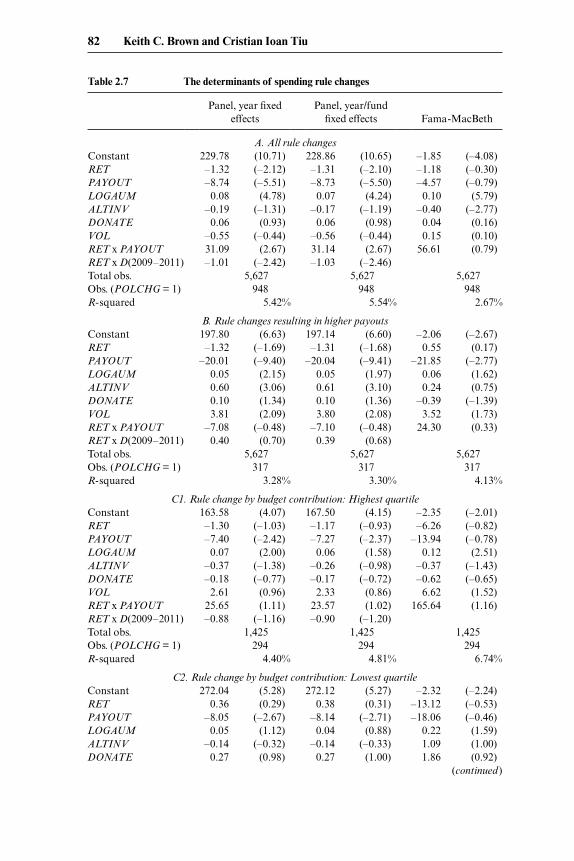
82 Keith C. Brown and Cristian Ioan Tiu
Table 2.7 The determinants of spending rule changes
Panel, year fixed
effects Panel, year/fund
fixed effects Fama- MacBeth
A. All rule changesConstant 229.78 (10.71) 228.86 (10.65) –1.85 (–4.08)RET –1.32 (–2.12) –1.31 (–2.10) –1.18 (–0.30)PAYOUT –8.74 (–5.51) –8.73 (–5.50) –4.57 (–0.79)LOGAUM 0.08 (4.78) 0.07 (4.24) 0.10 (5.79)ALTINV –0.19 (–1.31) –0.17 (–1.19) –0.40 (–2.77)DONATE 0.06 (0.93) 0.06 (0.98) 0.04 (0.16)VOL –0.55 (–0.44) –0.56 (–0.44) 0.15 (0.10)RET x PAYOUT 31.09 (2.67) 31.14 (2.67) 56.61 (0.79)RET x D(2009–2011) –1.01 (–2.42) –1.03 (–2.46)Total obs. 5,627 5,627 5,627 Obs. (POLCHG = 1) 948 948 948 R- squared 5.42% 5.54% 2.67%
B. Rule changes resulting in higher payoutsConstant 197.80 (6.63) 197.14 (6.60) –2.06 (–2.67)RET –1.32 (–1.69) –1.31 (–1.68) 0.55 (0.17)PAYOUT –20.01 (–9.40) –20.04 (–9.41) –21.85 (–2.77)LOGAUM 0.05 (2.15) 0.05 (1.97) 0.06 (1.62)ALTINV 0.60 (3.06) 0.61 (3.10) 0.24 (0.75)DONATE 0.10 (1.34) 0.10 (1.36) –0.39 (–1.39)VOL 3.81 (2.09) 3.80 (2.08) 3.52 (1.73)RET x PAYOUT –7.08 (–0.48) –7.10 (–0.48) 24.30 (0.33)RET x D(2009–2011) 0.40 (0.70) 0.39 (0.68)Total obs. 5,627 5,627 5,627 Obs. (POLCHG = 1) 317 317 317 R- squared 3.28% 3.30% 4.13%
C1. Rule change by budget contribution: Highest quartileConstant 163.58 (4.07) 167.50 (4.15) –2.35 (–2.01)RET –1.30 (–1.03) –1.17 (–0.93) –6.26 (–0.82)PAYOUT –7.40 (–2.42) –7.27 (–2.37) –13.94 (–0.78)LOGAUM 0.07 (2.00) 0.06 (1.58) 0.12 (2.51)ALTINV –0.37 (–1.38) –0.26 (–0.98) –0.37 (–1.43)DONATE –0.18 (–0.77) –0.17 (–0.72) –0.62 (–0.65)VOL 2.61 (0.96) 2.33 (0.86) 6.62 (1.52)RET x PAYOUT 25.65 (1.11) 23.57 (1.02) 165.64 (1.16)RET x D(2009–2011) –0.88 (–1.16) –0.90 (–1.20)Total obs. 1,425 1,425 1,425 Obs. (POLCHG = 1) 294 294 294 R- squared 4.40% 4.81% 6.74%
C2. Rule change by budget contribution: Lowest quartileConstant 272.04 (5.28) 272.12 (5.27) –2.32 (–2.24)RET 0.36 (0.29) 0.38 (0.31) –13.12 (–0.53)PAYOUT –8.05 (–2.67) –8.14 (–2.71) –18.06 (–0.46)LOGAUM 0.05 (1.12) 0.04 (0.88) 0.22 (1.59)ALTINV –0.14 (–0.32) –0.14 (–0.33) 1.09 (1.00)DONATE 0.27 (0.98) 0.27 (1.00) 1.86 (0.92)
(continued )

Spending Policies, Asset Allocation, and Investment Performance 83
Panel, year fixed
effects Panel, year/fund
fixed effects Fama- MacBeth
VOL –3.82 (–1.59) –3.85 (–1.61) –21.25 (–1.10)RET x PAYOUT –0.16 (–0.01) –0.26 (–0.01) 405.98 (0.53)RET x D(2009–2011) –2.06 (–1.94) –2.08 (–1.95)Total obs. 985 985 985 Obs. (POLCHG = 1) 192 192 192 R- squared 8.56% 8.64% 12.29%
D1. All rule changes, no appropriationsConstant 254.74 (9.13) 254.69 (9.12) –1.71 (–2.85)RET –0.85 (–1.02) –0.84 (–1.02) –3.60 (–0.51)PAYOUT –8.23 (–3.76) –8.23 (–3.75) –0.31 (–0.04)LOGAUM 0.07 (3.12) 0.07 (3.04) 0.11 (4.12)ALTINV –0.14 (–0.74) –0.14 (–0.73) –0.39 (–1.12)DONATE 0.08 (1.08) 0.08 (1.08) 0.01 (0.02)VOL –3.35 (–2.07) –3.34 (–2.07) –2.44 (–1.03)RET x PAYOUT 26.24 (1.68) 26.22 (1.67) 102.36 (0.86)RET x D(2009–2011) –1.07 (–1.98) –1.08 (–1.98)Total obs. 3,434 3,434 3,434 Obs. (POLCHG = 1) 559 559 559 R- squared 5.91% 5.91% 3.96%
D2. All rule changes, uses appropriationsConstant 305.67 (3.67) 311.83 (3.72) 0.33 (0.27)RET –0.65 (–0.24) –0.44 (–0.16) –29.97 (–0.82)PAYOUT –9.63 (–1.40) –9.77 (–1.40) –14.81 (–0.77)LOGAUM 0.05 (0.66) 0.05 (0.62) 0.07 (0.82)ALTINV –0.34 (–0.62) –0.32 (–0.57) –0.53 (–0.74)DONATE –0.89 (–0.78) –0.94 (–0.82) –3.08 (–1.06)VOL –5.82 (–1.13) –4.57 (–0.87) –12.24 (–2.60)RET x PAYOUT 25.53 (0.51) 20.03 (0.40) 448.52 (0.78)RET x D(2009–2011) –0.81 (–0.52) –0.68 (–0.43)Total obs. 380 380 380 Obs. (POLCHG = 1) 70 70 70 R- squared 8.53% 9.28% 12.27%
Notes: This table reports regression results examining the determinants of endowment spend-ing rule changes over the period July 1, 2002, to June 30, 2011. The primary dependent vari-able (POLCHG) is an indicator variable assuming a value of 1 if an endowment changed its spending rule in year T + 1, 0 otherwise. The base set of potential explanatory factors (observ-able at year T ) includes portfolio net- of- fee return (RET ), actual percentage payout (PAY-OUT ), logarithm of fund size (LOGAUM), percentage of portfolio invested in alternative assets (ALTINV), external contributions to the endowment (DONATE), and risk level of the policy- level investment portfolio (VOL). Three different forms of the probit regression in equation (2) are specified: (a) panel data with year fixed effects, (b) panel data with year and fund fixed effects, and (c) Fama- MacBeth. Panel A lists findings for the full sample using all rule changes. Panel B modifies the spending rule change definition to focus on just those changes that also resulted in a higher subsequent payout. Panel C reports results for the en-dowment sample quartiles with the highest (C1) and lowest (C2) average payout- as- percentage- of budget (PCTBDGT ) statistics. Panel D reports results for endowment subsamples that either did not (D1) or did (D2) use special payout appropriation measures. The t- statistics are listed parenthetically next to the respective coefficient estimates.
Table 2.7 (continued)

84 Keith C. Brown and Cristian Ioan Tiu
tional restrictions). Panel B then presents a modified analysis by focusing on just those rule changes that subsequently resulted in a larger payout from the endowment portfolio. Panel C reestimates the unrestricted model from panel A for two nonoverlapping subsets of the endowment fund sample determined by the relative amount of an institution’s budget that the payout represented over the 2009–2011 fiscal years. Specifically, panel C reports separate sets of estimated coefficients from equation (2) for funds that fall in the highest and lowest PCTBDGT quartiles in the sample.31 Finally, panel D reports regression estimates for two nonoverlapping subsets of the endow-ment fund sample according to whether the sponsoring institution either did or did not invoke a special spending appropriation in year T.
Looking first at the two fixed effects (FE) panel data regressions for the entire sample (panel A), the most statistically meaningful determinants of spending rule changes are LOGAUM, PAYOUT, and RET. In particular, the strong positive relationship between fund size and POLCHG suggests that it is the largest endowments that are the most likely to alter their spend-ing policies, a finding consistent with the notion that the greater degree of organizational flexibility that they possess permits a greater ability to make adjustments to all aspects of their operations. The t- statistics for the reported coefficients (i.e., 4.78 for the year FE parameter of 0.08, 4.24 for the year/fund FE parameter of 0.07) indicate that this relationship is highly tractable even after controlling for the possibility of variables omitted from the analysis, both across time and between endowments. Beyond that, the Fama- MacBeth coefficient for LOGAUM is also statistically reliable, which is especially notable given that this t- statistic (i.e., 5.79) is based on averaging parameter estimates from eight annual cross sections.32
The two other significant relationships documented in panel A involve the level of the endowment’s actual payout and the return to its investment portfolio. As predicted in section 2.5.1, the coefficients for both the PAY-OUT and RET variables are negative, implying that funds that have pro-duced smaller past payout levels and generated smaller investment returns are more likely to adjust the spending rules in the future. The coefficients for PAYOUT from the two FE models are particularly strong (e.g., a t- statistic of 5.51 for the year FE parameter of –8.74), but the statistical significance
31. As discussed earlier, data for the percentage of an institution’s budget supplied by the annual payout from its endowment portfolio have only been available since the 2009 survey year. We make the implicit assumption with our analysis in panel C that the PCTBDGT variable for a given fund is stable across time on a relative basis, meaning that the set of endowments with the greatest (least) budget responsibility does not change in a material way from one year to another.
32. Since the specification in equation (2) is a probit equation, it is also useful to provide an economic interpretation for the estimated coefficients. For instance, the LOGAUM parameter of 0.07 for the year/fund FE model corresponds to an increase in the probability of altering the spending policy of 0.15 percent for each incremental $10 million in the size of the endowment’s portfolio. For perspective, recall from the sample overview in table 2.1 that the AUM for the average endowment in 2011 was $508.09 million.

Spending Policies, Asset Allocation, and Investment Performance 85
of this variable is attenuated somewhat in the more severe conditions of the Fama- MacBeth model, although the sign of the coefficient does not change. The same pattern holds for the relationship between POLCHG and RET as well, with the additional observation that the negative effect becomes even stronger starting with the 2009 fiscal year ( RET2009−2011), emphasizing the effect that the financial market crisis had on running a university endowment fund. It is also interesting to note that the interaction between return and payout variables ( RETT x PAYOUTT) is also a significant determinant of POLCHG, but in a way that mitigates the two separate effects just described. Specifically, funds with lower past returns and lower past payouts are less likely to change their spending rules more frequently, a finding that is diffi-cult to explain beyond the possibility that these funds may also face more organizational barriers to affecting operating changes of any kind.
There are two other findings in involving these probit regressions for the entire unrestricted sample worth noting. First, endowment funds with a larger allocation to alternative assets tend to be less likely to modify their spending policies, as indicated by the consistently negative parameter values on ALTINV. Surprisingly, this relationship becomes more significant in the Fama- MacBeth regression than in either of the FE specifications. Since, as noted before, funds with larger alternative asset investments often produce higher risk- adjusted returns, this outcome suggests that there may be addi-tional aspects of investment performance beyond nominal portfolios returns (i.e., RET ) that are important in explaining the tendency to adjust formal spending mandates. Second, the effects that both the benchmark- level risk of the fund (VOL) or its external contributions from donors (DONATE) had on POLCHG were negligible. The former is not necessarily unexpected given the finding of Brown, Garlappi, and Tiu (2010) that endowments tend to target similar policy volatilities. However, it is surprising that the impact that supplemental contributions to the fund have on the decision to adjust spending policy is extremely unreliable as well as of the wrong sign.
Panel B of table 2.7 reexamines these relationships after altering the POL-CHG variable by assigning a value of 1 only to those observations for which (a) the spending rule was changed at year T + 1, and (b) PAYOUTT +1 exceeds
PAYOUTT .33 Presumably, this modification allows us to focus on those endowments whose express intention in changing their long- term spending mandate was to increase the future payout level of the fund. While the main findings from panel A continue to hold (e.g., large endowments with smaller past payout levels and lower past returns are more likely to change their rules), these new findings indicate some interesting differences. Most nota-bly, the relationship between PAYOUT and POLCHG becomes much more
33. By this construction, spending rule changes that did not result in an increased payout level are assigned a value of 0, so that the total number of observations in the sample does not change, but the number of observations for which POLCHG takes the value of 1 is reduced. These frequencies are listed in the exhibit for each set of regression output.
86 Keith C. Brown and Cristian Ioan Tiu
strongly negative than before, even becoming statistically significant in the Fama- MacBeth specification. This does indeed suggest that the experience of low past payout rates is a major factor driving an institution to seek a more accommodating set of rules. Further, there is also evidence that, for these specific funds, investing to a greater extent in alternative assets makes changing their policies more likely, which is consistent with the argument that increased illiquidity in the investment portfolio makes that dimension of the board’s decision making less flexible. Interestingly, it is also the case that the portfolio’s volatility level now matters, with the significant positive coefficient for VOL predicted in section 2.5.1 obtaining. Finally, the inter-action term between PAYOUT and RET and the indicator variable high-lighting returns in the postcrisis period are no longer statistically reliable.
The results contained in panel C restore the original definition of POLCHG (i.e., assigns a value of 1 for any spending rule adjustment), but divides the endowment sample into two subgroups representing the largest and smallest quartiles ranked by the average value of the PCTBDGT variable over the 2009–2011 period. The display lists a full set of probit regression findings for each of these sample divisions.34 The surprising result from a comparison of panel C1 (High PCTBDGT) and panel C2 (Low PCTBDGT) is that this variable appears to make virtually no difference to the fundamental relation-ships between POLCHG and its underlying determinants. For both sample divisions, the only variable that shows both the predicted sign and consistent statistical significance is PAYOUT, although LOGAUM does appear to be a stronger explanatory factor in the high PCTBDGT subsample. Portfo-lio returns in year T are not statistically reliable for either budget quar-tile, whether viewed over the entire sample period or just in the postcrisis years.
One possible explanation for PCTBDGT’s lack of influence is that, if an educational institution has the ability to extract incremental payouts from its endowment portfolio on a temporary basis, it may not need to change its permanent spending rules with any greater or lesser frequency regardless of how much of the budget the fund must cover. Thus, it could be the case that the presence of special appropriation measures mitigates the influence of budget percentage constraints. The final panel of table 2.7 reports spend-ing rule determinant regression output for those funds that either did not (panel D1) or did (panel D2) make use of a special payout appropriation during the last three years of the sample period for which these data were reported. The results support the notion that it is the set of endowments that do not—perhaps cannot—use temporary appropriations that changes its permanent spending rules in a more predictable manner, as indicated by the
34. To get a better sense of the range across the entire sample in the percentage of an institu-tion’s budget that the endowment fund is responsible for producing, the values of the three-year average PCTBDGT variable falling at the 75th and 25th percentiles are 13.2 percent and 1.0 percent, respectively.
Spending Policies, Asset Allocation, and Investment Performance 87
sign and statistical reliability of the PAYOUT and LOGAUM determinants. Neither of these variables are statistically significant for the uses appropria-tions subsample in panel D2, an outcome consistent with the spending rule transition results in section 2.4.2 that showed endowments using special payouts were more likely to retain their permanent policies from one year to the next.
2.6 The Interaction between Spending Policy, Asset Allocation, and Investment Performance
The findings reported so far support three stylized conclusions. First, the governing authorities of university endowment funds have changed both their spending policies and investment strategies (i.e., asset alloca-tion weights) quite often over the past several years. Second, at least with respect to spending policy changes, these modifications appear to occur too frequently to be consistent with hypothesized behavior given the rela-tively invariant nature of the institution’s long- term investment problem. Third, patterns in spending rule changes are significantly related to certain characteristics of the endowment’s operations and the investment perfor-mance of the portfolio. In this section, we address two additional ques-tions that involve the interaction between the endowment’s spending policy decision and both its ex ante investment policy decision and the ex post policy- adjusted portfolio performance.
2.6.1 The Relationship between Changes in Spending Rules and Investment Policy
As the introductory discussion in section 2.1 suggests, a strong argument (e.g., Litvack, Malkiel, and Quandt 1974) can be made that the most com-pelling way to organize an investment management operation begins with a clear definition of the institution’s investment problem and then designs a portfolio strategy that represents the “optimal” solution. In the context of university endowments, such a sequence of events clearly implies that the development of the endowment’s spending policy should both precede and inform the development of its investment policy. However, it is also plausible (e.g., Dybvig 1999) that spending and investment policies are best determined simultaneously. From the preceding analysis on the frequency and determinants of spending policy adjustments, it is not altogether clear which (if either) of these predictions is true.
To establish more precisely the nature of the interaction between spending rule changes and asset allocation changes for our endowment fund sample, we begin by defining a measure that captures the essence of how endowment E’s investment strategy evolves from year T – 1 to year T. Specifically, for each fund, we create an index of the change in the allocation weights (i.e.,
AACHGTE ) by summing the absolute values of the differences in the actual

88 Keith C. Brown and Cristian Ioan Tiu
investment levels for each of the ten asset classes representing the investable universe for the NACUBO sample during consecutive years:
(3) AACHGT
E = |i =1
10
∑ wi,TE − wi,T −1
E | .
Notice that, by construction, higher levels of AACHG indicate a greater adjustment in the endowment’s asset class investment strategy, due to either a change in its policy- level strategic allocation weights or a tactical rotation permitted within the existing policy.35
To see whether spending rule changes are more likely to precede or follow asset allocation changes, we use a vector autoregression (VAR) process to estimate the structural relationship between the two variables. Specifically, we estimate the VAR(1) model using: (a) POLCHGT +1 and AACHGT ; and (b) POLCHGT and AACHGT +1. Our null hypothesis is that the second form of the model (i.e., spending changes leading asset allocation changes) should provide the stronger results. The specific forms of the two panel data regres-sion equations comprising the VAR system are:
(4)
POLCHG(T + 1) = a1 + b11POLCHG(T ) + b12AACHG(T )
+ c11LOGAUM(T ) + c12PAYOUT(T ) + e1,T +1,
and
(5)
AACHG(T + 1) = a2 + b21POLCHG(T ) + b22AACHG(T )
+ c21LOGAUM(T ) + c22PAYOUT(T ) + e2,T +1.
Given their significance in earlier findings, we include LOGAUM and PAYOUT as control variables in the estimation of equations (4) and (5).
Table 2.8 tabulates these results, which contain two substantive find-ings. First, from equation (4), it is apparent that POLCHGT +1 is signifi-cantly and positively related to POLCHGT (i.e., estimated coefficient of 0.2550 with a t- statistic of 23.93) but its relationship with AACHGT is not statistically reliable (i.e., t- statistic of –0.65). This supports the conclusion that spending rule changes are indeed persistent over time, at least for the half of the endowment sample that altered their policies at all. Further, it also highlights the fact that institutions are not adjusting their spending rules in response to previous changes in asset allocation strategies that may have produced less- than- desirable portfolio performance. This is consistent with a hypothesized view of the investment management pro-cess holding that the statement of the investment problem should not be determined by the myriad aspects of the investment decision- making process.
35. The measure in equation (3) is a straightforward variation of the class of statistical dis-tance measures used elsewhere in the financial economic literature; see, for instance, Hansen and Jagannathan (1997).

Tab
le 2
.8
Spe
ndin
g ru
le c
hang
es a
nd a
sset
allo
cati
on c
hang
es
PO
LC
HG
(T +
1)
AA
CH
G (T
+ 1
)
Con
st.
P
OL
CH
G(T
) A
AC
HG
(T)
LO
GA
UM
(T)
PAY
OU
T(T
) C
onst
. P
OL
CH
G(T
) A
AC
HG
(T)
LO
GA
UM
(T)
PAY
OU
T(T
)
Coe
f. –0
.033
00.
2550
–0.0
134
0.01
19–0
.312
10.
1928
0.01
650.
2815
–0.0
031
0.23
25t-
stat
(–0.
91)
(23.
93)
(–0.
65)
(3.9
5)(–
1.45
)(5
.32)
(1.5
4)(1
3.72
)(–
1.02
)(1
.08)
Obs
.
4,10
1
Not
es: T
his
tabl
e re
port
s es
tim
ates
of
a pa
nel d
ata
vect
or a
utor
egre
ssio
n (V
AR
[1])
mod
el fo
r th
e re
lati
onsh
ip b
etw
een
chan
ges
in s
pend
ing
rule
s (P
OL
CH
G)
and
chan
ges
in a
sset
allo
cati
on (A
AC
HG
) in
the
NA
CU
BO
/Com
mon
fund
end
owm
ent f
und
sam
ple
over
the
peri
od fr
om J
uly
1, 2
002,
to J
une
30, 2
011.
The
m
odel
, whi
ch in
clud
es c
ontr
ols
for
endo
wm
ent f
und
size
(LO
GA
UM
) and
pas
t pay
out r
ate
(PA
YO
UT
), is
est
imat
ed a
ccor
ding
to e
quat
ions
(4) a
nd (5
) as:
PO
LC
HG
(T+
1)
=a 1
+b 1
1PO
LC
HG
(T)
+b 1
2AA
CH
G(T
)+
c 11L
OG
AU
M(T
)+
c 12P
AY
OU
T(T
)+
e 1,T
+1
AA
CH
G(T
+1)
=
a 2+
b 21P
OL
CH
G(T
)+
b 22A
AC
HG
(T)
+c 2
1LO
GA
UM
(T)
+c 2
2PA
YO
UT
(T)
+e 2
,T+1
. T
he t-
stat
isti
cs a
re li
sted
par
enth
etic
ally
ben
eath
the
resp
ecti
ve e
stim
ated
coe
ffici
ents
.

90 Keith C. Brown and Cristian Ioan Tiu
The second main finding in table 2.8 involves the estimated coefficients for equation (5), which indicate that the relationship between AACHGT +1 and AACHGT is also statistically significant (i.e., estimated coefficient of 0.2815 with a t- statistic of 13.72). This means that the typical endowment adjusts its asset allocation weights in a persistent manner over time, which can in turn be interpreted as suggesting that this dimension of its invest- ment policy is not static. Further, AACHGT +1 is positively correlated with
POLCHGT , although at a marginal level of statistical significance (i.e., esti-mated coefficient of 0.0165 with a t- statistic of 1.54). The implication of this finding is that future asset allocation changes are tied to past adjustments in spending rules, albeit with an attenuated level of strength. Specifically, an endowment that altered its payout rule in one year is more likely to modify its asset class- level investment strategy in the next year. This outcome implies that whatever it was that caused the fund to change its payout policy in the first place does indeed lead to a subsequent allocation adjustment in its portfolio construction.
2.6.2 Spending Rule Changes and Endowment Investment Performance
The findings in table 2.7 provide compelling evidence that the nominal level of an endowment fund’s investment performance helps influence the institution’s future spending policy decisions. It is not clear, though, whether endowments that change their spending rules perform appreciably better or worse than those that maintain stable payout mandates. A complication in addressing this issue is that a simple comparison of total portfolio returns between the two groups is not sufficient since we know that there is consid-erable variation in the asset allocation patterns—particularly for the alterna-tive asset classes—across the sample and that these allocation differences are alone sufficient to produce substantial variation in measured returns. Therefore, we proxy endowment E’s active return in year T ( ALPHAT
E ) as the difference between its actual total return ( RT
E) and its associated policy benchmark return ( RT
B):
(6) ALPHAT
E = RTE − RT
B = RTE − wi,T
E
i =1
10
∑ Ri,TB ,
where wiE is the fund’s allocation weight for the i- th asset class and Ri
B is the nominal return to the benchmark index representing the i- th asset class.36
36. Strictly speaking, the calculation in equation (6) measures the portion of the endowment’s active return that is associated with the endowment portfolio manager’s security selection skills. For ALPHA to include the contribution of both sources of active management skills (i.e., security selection and market timing), this calculation would need to be amended to include the set of strategic allocation weights from the endowment’s investment policy statement (i.e., [ wi
B ]). Unfortunately, the NACUBO/Commonfund database does not report these [ wiB] for
many funds in any given annual survey or for any fund over the entire sample period. However, as Brown, Garlappi, and Tiu (2010) show, the portion of the endowment’s true ALPHA gener-ated by the manager’s market timing skills is, on average, fairly negligible.
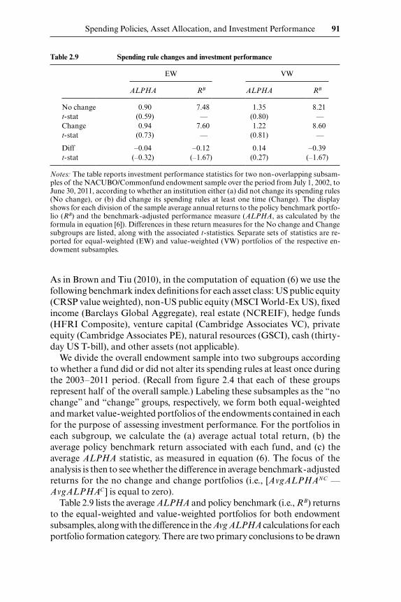
Spending Policies, Asset Allocation, and Investment Performance 91
As in Brown and Tiu (2010), in the computation of equation (6) we use the following benchmark index definitions for each asset class: US public equity (CRSP value weighted), non- US public equity (MSCI World- Ex US), fixed income (Barclays Global Aggregate), real estate (NCREIF), hedge funds (HFRI Composite), venture capital (Cambridge Associates VC), private equity (Cambridge Associates PE), natural resources (GSCI), cash (thirty- day US T- bill), and other assets (not applicable).
We divide the overall endowment sample into two subgroups according to whether a fund did or did not alter its spending rules at least once during the 2003–2011 period. (Recall from figure 2.4 that each of these groups represent half of the overall sample.) Labeling these subsamples as the “no change” and “change” groups, respectively, we form both equal- weighted and market value- weighted portfolios of the endowments contained in each for the purpose of assessing investment performance. For the portfolios in each subgroup, we calculate the (a) average actual total return, (b) the average policy benchmark return associated with each fund, and (c) the average ALPHA statistic, as measured in equation (6). The focus of the analysis is then to see whether the difference in average benchmark- adjusted returns for the no change and change portfolios (i.e., [ AvgALPHANC —
AvgALPHAC ] is equal to zero).Table 2.9 lists the average ALPHA and policy benchmark (i.e., RB) returns
to the equal- weighted and value- weighted portfolios for both endowment subsamples, along with the difference in the Avg ALPHA calculations for each portfolio formation category. There are two primary conclusions to be drawn
Table 2.9 Spending rule changes and investment performance
EW VW
ALPHA RB ALPHA RB
No change 0.90 7.48 1.35 8.21 t- stat (0.59) — (0.80) —Change 0.94 7.60 1.22 8.60 t- stat (0.73) — (0.81) —
Diff –0.04 –0.12 0.14 –0.39 t- stat (–0.32) (–1.67) (0.27) (–1.67)
Notes: The table reports investment performance statistics for two non- overlapping subsam-ples of the NACUBO/Commonfund endowment sample over the period from July 1, 2002, to June 30, 2011, according to whether an institution either (a) did not change its spending rules (No change), or (b) did change its spending rules at least one time (Change). The display shows for each division of the sample average annual returns to the policy benchmark portfo-lio (RB) and the benchmark- adjusted performance measure (ALPHA, as calculated by the formula in equation [6]). Differences in these return measures for the No change and Change subgroups are listed, along with the associated t- statistics. Separate sets of statistics are re-ported for equal- weighted (EW) and value- weighted (VW) portfolios of the respective en-dowment subsamples.
92 Keith C. Brown and Cristian Ioan Tiu
from these data. First, regardless of the institution’s spending policy revision strategy, it appears that endowment fund managers are good investors. The reported average benchmark- adjusted returns are uniformly positive and, at about 100 basis points per annum, relatively large (e.g., 0.90 percent for the equal- weighted no change portfolio, 1.22 percent for the value- weighted change portfolio). While the high level of cross- sectional performance volatil-ity within the subsamples renders these performance measures statistically insignificant (e.g., t- statistics of 0.59 and 0.81 for the two portfolios mentioned above), it nevertheless is the case that the average fund manager in each sub-group produced returns at least as good as his or her policy benchmark.
The second notable finding from the exhibit is that there is virtually no difference in the risk- adjusted investment performance statistics between those endowments that changed their spending policies with some frequency or those that maintained a single set of rules throughout the sample period. The reported values for [ AvgALPHANC — AvgALPHAC ]—which is shown as “Diff” in the next- to- last row—are just –0.04 percent (EW) and 0.14 percent (VW), with respective t- statistics of –0.32 and 0.27. Interestingly, there is a marginally significant difference in policy benchmark returns between the two categories (i.e., –0.12 percent [EW] and –0.39 percent [VW]), which suggests that they may face slightly different initial risk budgets. How-ever, once any such risk differentials are accounted for (even implicitly in the benchmark adjustment process), there is no indication that the frequency with which an institution revises its spending policy has any impact—either adverse or positive—on the returns its endowment portfolio produces.
2.7 Concluding Comments
The sponsors and asset managers associated with an endowment fund face an interesting intergenerational investment problem with at least two conflicting goals: they need to produce steady increases in the portfolio’s market value to insure the security and long- term viability of the institution and future beneficiaries, but they also need to produce sufficient current income to sustain existing operations. The endowment’s spending policy statement is the document in which the governing authority of the institu-tion expresses its intentions as to how this tension should be resolved. Once the permanent spending policy is set, prudent decisions can then be made concerning the investment policies and strategies that should be followed. While there is a growing body of research focusing on endowment invest-ment practices (e.g., Acharya and Dimson 2007; Brown, Garlappi, and Tiu 2010; Dimmock, forthcoming), there is a general dearth of analysis concern-ing the salient aspects of the spending policy decision, which is curious given its central role in the endowment management process.
In this study, we have addressed this perceived need by providing a com-prehensive examination of the spending policy decisions made by over 800

Spending Policies, Asset Allocation, and Investment Performance 93
university endowment funds during the period from 2003 to 2011. For each fund, during every year, we categorized the specific spending rule and policy payout rate it used and documented how frequently and why the sponsoring institution was motivated to change those mandates over time. While there is a considerable degree of variation within the sample, we showed that a sizable majority of endowments adopt a payout formula based on a percent-age of a moving average of the portfolio’s past values. However, the most surprising result in our analysis is that endowments altered their permanent spending policies far more often than what theory would predict given the nature of the investment problem they face; on average, 25 percent of the funds adjusted their policies in any given year, and half of the funds surveyed amended their stated rules at least once during the sample period. We also demonstrated that large endowments that had produced lower past returns and had lower actual payout levels were more likely to alter their long- term spending policies, but that funds with the ability to use special appropria-tions on a temporary basis were less likely to adjust their permanent rules, a tendency that became more pronounced in the aftermath of the global eco-nomic crisis of 2008. Further, we showed that payout rule changes are more likely to precede adjustments to the fund’s asset allocation strategy than the other way around and that the tendency for institutions to alter both types of policy is strongly persistent over time. Finally, despite their disparate characteristic profiles, we found no difference in the benchmark- adjusted investment performance for portfolios of endowments that either did or did not alter their spending policies during the sample period.
The intriguing questions that remain to be addressed are whether chang-ing the permanent spending policy too frequently represents suboptimal behavior on the part of the endowment’s decision makers and, if so, what the economic cost of such actions might be? Those may well be questions that are not easily answered, particularly in the absence of specific information about the investment problem an institution faces and whether sufficient changes in its underlying circumstances took place to warrant a revision of its previous rules. From our analysis, we do know that any expenses associ-ated with frequent payout policy revisions are not borne at the portfolio investment level. However, a diminution in risk- adjusted return perfor-mance is not the only possible cost that a fund might bear as a result of these changes—use of board and staff time, misaligned objectives for the institu-tion, loss of confidence among sponsors and donors, for example—and, while challenging, quantifying these values might tell a very different story. An equally challenging effort would involve trying to define and measure the incremental benefits that accrue to institutions that make frequent changes to their permanent policy; if such revisions to the formal statement of its investment problem do not lead to asset allocation solutions that generate superior returns, what might the benefits of those changes be? Certainly, considering these issues is fruitful ground for future research.

94 Keith C. Brown and Cristian Ioan Tiu
Appendix
A Taxonomy of Spending Policy Rules
The statistical summary presented in table 2.3 classifies the spending rules used by our sample of college and university endowment funds into seven separate categories. Further, several of the seven broad categories can be meaningfully split into two or more subdivisions. These classifications are based on those used in practice as defined and collected by the National Association of College and University Business Officers (NACUBO) and the Commonfund; see Mehrling, Goldstein, and Sedlacek (2005), Sedlacek and Jarvis (2010), and Murray (2011) for more details.
Listed below are spending rule categories and subcategories used in this study, along with descriptions and, where applicable, the formulas used for determining endowment payouts.
1. Decide on an appropriate rate annually. Gives the governing authority complete discretion to determine the spending rate it deems appropriate on a yearly basis.
2. Increase prior year’s spending by a percentage. Adjusts spending upward each year, using either a simple formula or one based on the inflation rate.
(a) Increase prior year’s spending by a prespecified percentage. Determines the annual payout as the previous year’s payout adjusted upward by a pre-specified rate.
(b) Increase prior year’s spending by the inflation rate. Determines the annual payout as the previous year’s payout adjusted for a prespecified infla-tion rate (I); that is, (Payout)t = (Payout)t −1 x (1 + I ).
(c) Increase prior year’s spending by a collared inflation rate. Determines the annual payout as the previous year’s payout adjusted for the actual infla-tion rate (e.g., CPI, HEPI) during the investment period, subject to prespeci-fied minimum and maximum rate levels.
3. Spend a percentage of a moving average of market values. Determines annual payout as a percentage (P percent, which can be either fixed or vari-able) of an average of beginning- of- period market values over a prespecified series of past periods; that is, P percent x average ( AUM0, AUM−1, . . . ,
AUM−N ), where AUM−t represents the fund’s assets under management t periods in the past.
(a) Spend a prespecified percentage of moving 12- quarter average of market values. Uses a quarterly frequency over three years to calculate the moving average of fund AUM.
(b) Spend a prespecified percentage of moving 3- year average of market values. Uses an annual frequency over three years to calculate the moving average of fund AUM.
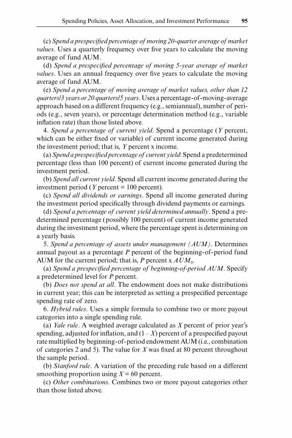
Spending Policies, Asset Allocation, and Investment Performance 95
(c) Spend a prespecified percentage of moving 20- quarter average of market values. Uses a quarterly frequency over five years to calculate the moving average of fund AUM.
(d) Spend a prespecified percentage of moving 5- year average of market values. Uses an annual frequency over five years to calculate the moving average of fund AUM.
(e) Spend a percentage of moving average of market values, other than 12 quarters/3 years or 20 quarters/5 years. Uses a percentage- of- moving- average approach based on a different frequency (e.g., semiannual), number of peri-ods (e.g., seven years), or percentage determination method (e.g., variable inflation rate) than those listed above.
4. Spend a percentage of current yield. Spend a percentage (Y percent, which can be either fixed or variable) of current income generated during the investment period; that is, Y percent x income.
(a) Spend a prespecified percentage of current yield: Spend a predetermined percentage (less than 100 percent) of current income generated during the investment period.
(b) Spend all current yield. Spend all current income generated during the investment period (Y percent = 100 percent).
(c) Spend all dividends or earnings. Spend all income generated during the investment period specifically through dividend payments or earnings.
(d) Spend a percentage of current yield determined annually. Spend a pre-determined percentage (possibly 100 percent) of current income generated during the investment period, where the percentage spent is determining on a yearly basis.
5. Spend a percentage of assets under management (AUM). Determines annual payout as a percentage P percent of the beginning- of- period fund AUM for the current period; that is, P percent x AUM0.
(a) Spend a prespecified percentage of beginning- of- period AUM. Specify a predetermined level for P percent.
(b) Does not spend at all. The endowment does not make distributions in current year; this can be interpreted as setting a prespecified percentage spending rate of zero.
6. Hybrid rules. Uses a simple formula to combine two or more payout categories into a single spending rule.
(a) Yale rule. A weighted average calculated as X percent of prior year’s spending, adjusted for inflation, and (1 – X) percent of a prespecified payout rate multiplied by beginning- of- period endowment AUM (i.e., combination of categories 2 and 5). The value for X was fixed at 80 percent throughout the sample period.
(b) Stanford rule. A variation of the preceding rule based on a different smoothing proportion using X = 60 percent.
(c) Other combinations. Combines two or more payout categories other than those listed above.

96 Keith C. Brown and Cristian Ioan Tiu
7. Other payout rules:(a) Rules not otherwise classified. Uses a formula or approach that differs
from those listed above (e.g., increases spending by a prespecified fixed per-centage unless a political or economic contingency event occurs, in which case the governing authority uses its discretion in setting the payout amount).
(b) Insufficient information. Endowment did not provide a complete set of information that allowed for the classification of its spending policy.
References
Acharya, Shanta, and Elroy Dimson. 2007. Endowment Asset Management. New York: Oxford University Press.
Black, Fischer. 1976. “The Investment Policy Spectrum: Individuals, Endowment Funds, and Pension Funds.” Financial Analysts Journal 32:23–31.
Blume, Marshall E. 2010. “Endowment Spending in Volatile Markets: What Should Fiduciaries Do?” Review of Quantitative Finance and Accounting 35:163–78.
Bodily, Samuel L., and Chelsea C. White. 1982. “Optimal Consumption and Port-folio Strategies in a Discrete- Time Model with Summary- Dependent Preferences.” Journal of Financial and Quantitative Analysis 17:1–14.
Brinson, Gary P., L. Randolph Hood, and Gilbert L. Beebower. 1986. “Determi-nants of Portfolio Performance.” Financial Analysts Journal 42:39–48.
Brown, Jeffrey R., Stephen G. Dimmock, Jun- Koo Kang, and Scott Weisbenner. 2010. “How University Endowments Respond to Financial Market Shocks: Evi-dence and Implications.” NBER Working Paper no. 15861, Cambridge, MA.
Brown, Jeffrey R., Stephen G. Dimmock, and Scott Weisbenner. 2012. “The Supply and Demand for Charitable Donations to Higher Education.” NBER Working Paper no. 18389, Cambridge, MA.
Brown, Keith C., Lorenzo Garlappi, and Cristian Tiu. 2010. “Asset Allocation and Portfolio Performance: Evidence from University Endowment Funds.” Journal of Financial Markets 13:268–94.
Brown, Keith C., and Cristian Tiu. 2010. “Do Endowment Funds Select the Optimal Mix of Active and Passive Risks?” Journal of Investment Management 8:62–86.
Brown, Stephen J., William Goetzmann, Roger G. Ibbotson, and Steven A. Ross. 1992. “Survivorship Bias in Performance Studies.” Review of Financial Studies 5:553–80.
Cain, J. Harvey. 1960. “Recent Trends in Endowment.” Review of Economics and Statistics 42:242–44.
Cejnek, Georg, Richard Franz, Otto Randl, and Neal Stoughton. 2012. “A Survey of University Endowment Management Research.” Working Paper, Research Institute for Capital Markets, Vienna.
Dimmock, Stephen G. Forthcoming. “Portfolio Choice, Background Risk, and Uni-versity Endowment Funds.” Review of Economics and Statistics.
Dybvig, Philip H. 1999. “Using Asset Allocation to Protect Spending.” Financial Analysts Journal 55:49–62.
Fama, Eugene F., and James D. MacBeth. 1973. “Risk, Return, and Equilibrium: Empirical Tests.” Journal of Political Economy 81:606–36.
Garland, James P. 2005. “Long- Duration Trusts and Endowments.” Journal of Port-folio Management 31:44–54.

Spending Policies, Asset Allocation, and Investment Performance 97
Gilbert, Thomas, and Christopher Hrdlicka. 2012. “Fairness and Risk- Sharing across Generations: An Application to University and Non- Profit Endowments.” Working Paper, University of Washington.
Hansen, Lars Peter, and Ravi Jagannathan. 1997. “Assessing Specification Errors in Stochastic Discount Factor Models.” Journal of Finance 52:557–90.
Hansmann, Henry. 1990. “Why Do Universities Have Endowments?” Journal of Legal Studies 19:3–42.
Hill, Joanne M. 2006. “Alpha as a Net Zero- Sum Game.” Journal of Portfolio Man-agement 32:24–32.
Ibbotson, Roger G., and Paul D. Kaplan. 2000. “Does Asset Allocation Policy Explain 40, 90, or 100 Percent of Performance?” Financial Analysts Journal 56:26–33.
Kochard, Lawrence E., and Cathleen M. Rittereiser. 2008. Foundation & Endowment Investing. Hoboken, NJ: John Wiley & Sons.
Lapovsky, Lucie. 2009. Endowment Spending: External Perceptions and Internal Practices. Wilton, CT: Commonfund Institute.
Leibowitz, Martin L. 2005. “Alpha Hunters and Beta Grazers.” Financial Analysts Journal 61:32–39.
Leibowitz, Martin L., Anthony Bova, and P. Brett Hammond. 2010. The Endowment Model of Investing: Return, Risk, and Diversification. Hoboken, NJ: John Wiley & Sons.
Lerner, Josh, Antoinette Schoar, and Jialan Wang. 2008. “Secrets of the Academy: The Drivers of University Endowment Success.” Journal of Economic Perspectives 22:207–22.
Lerner, Josh, A. Schoar, and W. Wongsunwai. 2007. “Smart Institutions, Foolish Choices: The Limited Partner Performance Puzzle.” Journal of Finance 42: 731–64.
Litvack, James M., Burton G. Malkiel, and Richard E. Quandt. 1974. “A Plan for the Definition of Endowment Income.” American Economic Review 64: 433–37.
Mehrling, Perry, Paul Goldstein, and Verne Sedlacek. 2005. “Endowment Spending: Goals, Rates, and Rules.” In Forum for the Future of Higher Education. Washing-ton, DC: Educause.
Merton, Robert C. 1971. “Optimum Consumption and Portfolio Rules in a Continuous- Time Model.” Journal of Economic Theory 3:373–413.
_____. 1993. “Optimal Investment Strategies for University Endowment Funds.” In Studies of Supply and Demand in Higher Education, edited by Charles T. Clotfelter and Michael Rothschild. Chicago: University of Chicago Press.
_____. 2003. “Thoughts on the Future: Theory and Practice in Investment Manage-ment.” Financial Analysts Journal 59:17–23.
Murray, Steve. 2011. Non- Profit Spending rules.” Working Paper, Russell Invest-ments. http://www.russell.com/us/institutional- investors/research/non- profit - spending- rules.page.
Nettleton, Minot B. 1987. “The Impact of Spending Rules on Endowments.” In The Challenges of Investing for Endowment Funds, edited by Cathryn E. Kittell. Insti-tute of Chartered Financial Analysts and Dow Jones- Irwin.
Samuelson, Paul A. 1969. “Lifetime Portfolio Selection by Dynamic Stochastic Pro-gramming.” Review of Economics and Statistics 51:239–46.
Sedlacek, Verne O., and William F. Jarvis. 2010. Endowment Spending: Building a Stronger Policy Framework. Wilton, CT: Commonfund Institute.
Swensen, David F. 2009. Pioneering Portfolio Management: An Unconventional Approach to Institutional Investment, 2nd ed. New York: Free Press.

98 Keith C. Brown and Cristian Ioan Tiu
Thaler, Richard H., and J. Peter Williamson. 1994. “College and University Endow-ment Funds.” Journal of Portfolio Management 21:27–37.
Tobin, James. 1974. “What Is Permanent Endowment Income?” American Economic Review 64:427–32.
Walda, John D., and John S. Griswold. 2011. Nacubo- Commonfund Study of Endow-ments. Washington, DC: National Association of College and University Business Officers.
Woglom, Geoffrey. 2003. “Endowment Spending Rates, Intergenerational Equity and the Sources of Capital Gains.” Economics of Education Review 22:591–601.


![MEEZAN Product Not Affected by Recession[1]](https://static.fdocuments.net/doc/165x107/546b1204b4af9fb5148b489b/meezan-product-not-affected-by-recession1.jpg)