How Mathematics Gives Us Superman X-ray Vision

Helen Moore, PhDBristol-Myers Squibb

January 28, 2017

Regular X-rays

• Picture of Anna Bertha Ludwig’s hand, taken by Wilhelm Röntgen, using x-rays, 1896

• Röntgen received the first Nobel Prize in Physics, 1901, for his discovery of x-rays

• We see shadows! Darkness shows density; cannot see inside the bones or tissue

Public domain image; https://commons.wikimedia.org/wiki/File:Wilhelm-Roentgen's-X-ray-photograph-of-his-wife's-hand.png 2

Superman X-ray Vision

Fair use File:Superboy98.jpgUploaded: 21 March 2008https://en.wikipedia.org/wiki/File:Superboy98.jpg#/media/File:Superboy98.jpg

Wired Magazine Online, March 22, 2016https://www.wired.com/2016/03/sure-superman-x-ray-vision-actually-work/

3

Computerized Tomography (CT) Scan/Scanner

By U.S. Navy photo by Chief Warrant Officer 4 Seth Rossman. - This Image was released by the United States Navy with the ID 030819-N-9593R-125. Public Domain, https://commons.wikimedia.org/w/index.php?curid=8196091

By Yale Rosen from USA - Adenocarcinoma - CT scan, CC BY-SA 2.0, https://commons.wikimedia.org/w/index.php?curid=31127656

4

How CT scans work

Distribution of log of attenuation, assuming density is uniform (so log of attenuation is proportional to width of object being scanned)

X-ray source

X-rays

Circular object being scanned

Projection screen

𝑦𝑦 = 2 1 − 𝑥𝑥2

Rotated

5

Potential problem

6

Solution: more angles

7

Game of Nonograms

• Published in the Sunday Telegraph (UK) since 1990• Invented by Non Ishida (independently by Tetsuya Nishio) • Fill in the number of contiguous blocks according to the numbers

listed for each column and row2 2

9 9 2 2 4 44 . .6

2 2 . .2 2 . .

64 . .2 . . . .2 . . . .2 . . . . 8

Nonogram Handout

9

Nonogram numbers can represent density

• Attenuation of photons is measured by the x-ray detector• The logarithm of attenuation is proportional to object density• If constant density, then log attenuation measures length of object• What if the density if not constant?

10

Nonograms with any non-negative integer

• These represent different densities

A B 3

C D 1

2 2

A B 1

C D 1

1 1

A B 2

C D 0

1 1

A B 5

C D 6

8 3

2 1

0 1

1 1

0 0

1 2

1 0

1 0

0 1

0 1

1 0

? ?

? ?

11

Solution: more angles

12

Nonograms with any non-negative integer

• Three angles

A B 3

C D 1

2 2

A B 1

C D 1

1 1

A B 5

C D 6

8 3

2 1

0 1

0 1

1 0

4 1

4 2

10

1

13

0

16

4

13

12

32

1

What if the grids are bigger?

• We need to use all possible angles for non-constant densities

A B C 3

D E F 3

G H I 3

3 3 3

2 0 1

0 1 2

1 2 0

0 2 1

2 1 0

1 0 2

14

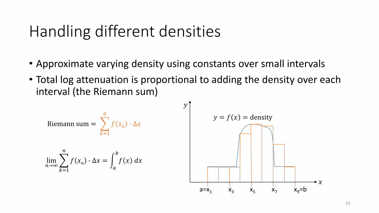
Handling different densities

• Approximate varying density using constants over small intervals• Total log attenuation is proportional to adding the density over each

interval (the Riemann sum)

Riemann sum = �𝑘𝑘=1

8

𝑓𝑓 𝑥𝑥𝑘𝑘 � Δ𝑥𝑥

lim𝑛𝑛→∞

�𝑘𝑘=1

𝑛𝑛

𝑓𝑓 𝑥𝑥𝑛𝑛 � ∆𝑥𝑥 = �𝑎𝑎

𝑏𝑏𝑓𝑓 𝑥𝑥 𝑑𝑑𝑥𝑥

x3 x7x5 x9=ba=x1

𝑦𝑦 = 𝑓𝑓 𝑥𝑥 = density

𝑦𝑦

𝑥𝑥

15

If we know the density line integrals for all lines through a slice, can we reconstruct the shapes in the slice?

16

“All lines”• 𝑦𝑦 = 𝑚𝑚𝑥𝑥 + 𝑏𝑏 gives all lines in the plane except vertical lines• For a given line ℓ, take a vector 𝑛𝑛 perpendicular to it

• There exists an angle 𝜃𝜃 such that 𝑛𝑛 is parallel to the unit vector coming from the origin at angle 𝜃𝜃 from the 𝑥𝑥-axis

• The line coming from the origin at angle 𝜃𝜃 is perpendicular to l and intersects it at a point 𝓅𝓅 = (𝑡𝑡 cos 𝜃𝜃 , 𝑡𝑡 sin𝜃𝜃)

• Every line ℓ𝑡𝑡,𝜃𝜃 in the plane can be characterized by a 𝑡𝑡 and 𝜃𝜃: the line through 𝓅𝓅 = (𝑡𝑡 cos 𝜃𝜃 , 𝑡𝑡 sin𝜃𝜃)perpendicular to the unit vector (cos 𝜃𝜃 , sin𝜃𝜃)

• For uniqueness, let 0 ≤ 𝜃𝜃 < 𝜋𝜋

𝑦𝑦

𝑥𝑥ℓ

𝑛𝑛

𝜃𝜃

𝓅𝓅 = (𝑡𝑡 cos𝜃𝜃, 𝑡𝑡 sin𝜃𝜃)

(cos𝜃𝜃, sin𝜃𝜃)

17

Line parametrization

• Each line ℓ𝑡𝑡,𝜃𝜃 can be described as the line through 𝓅𝓅=(𝑡𝑡 cos𝜃𝜃, 𝑡𝑡 sin𝜃𝜃) perpendicular to the unit vector (cos𝜃𝜃, sin𝜃𝜃)

• The vector (−sin𝜃𝜃 , cos𝜃𝜃) is perpendicular to (cos𝜃𝜃, sin𝜃𝜃) since the dot product of the two vectors is zero

• So ℓ𝑡𝑡,𝜃𝜃 can be parametrized as 𝑡𝑡 cos𝜃𝜃 , 𝑡𝑡 sin𝜃𝜃 + 𝑠𝑠(− sin𝜃𝜃 , cos𝜃𝜃)

𝑦𝑦

𝑥𝑥ℓ𝑡𝑡,𝜃𝜃

𝜃𝜃

𝓅𝓅 = (𝑡𝑡 cos𝜃𝜃, 𝑡𝑡 sin𝜃𝜃)

(cos𝜃𝜃, sin𝜃𝜃)

18

Radon transform and back transform

• Define the Radon transform (1917) of a function 𝑓𝑓 as• ℛ𝑓𝑓 𝑡𝑡,𝜃𝜃 = ∫−∞

∞ 𝑓𝑓(𝑡𝑡 cos 𝜃𝜃 − 𝑠𝑠 sin𝜃𝜃, 𝑡𝑡 sin𝜃𝜃 + 𝑠𝑠 cos 𝜃𝜃)𝑑𝑑𝑠𝑠• If 𝑓𝑓 is the density function, ℛ𝑓𝑓 gives the line integral for the density function

• Define the back transform of a function ℎ as• ℬℎ 𝑥𝑥,𝑦𝑦 = 1

𝜋𝜋 ∫0𝜋𝜋 ℎ(𝑥𝑥 cos 𝜃𝜃 + 𝑦𝑦 sin𝜃𝜃,𝜃𝜃)𝑑𝑑𝜃𝜃

• First, note that 𝑥𝑥,𝑦𝑦 ⋅ cos 𝜃𝜃 , sin𝜃𝜃 = 𝑥𝑥 cos 𝜃𝜃 + 𝑦𝑦 sin𝜃𝜃• So 𝑥𝑥 cos 𝜃𝜃 + 𝑦𝑦 sin𝜃𝜃 is the length of the projection of (𝑥𝑥,𝑦𝑦) on the line

determined by 𝜃𝜃• If ℎ = ℛ𝑓𝑓, then ℬℎ gives the average density function values of all lines that

pass through (𝑥𝑥,𝑦𝑦)

19

Does back transform give the reconstruction?

• The back transform calculates the average density at (𝑥𝑥,𝑦𝑦)• This gives a smoothed-out version of the original density at every

point• How do we know it is smoothed out? • Because lines with constant density would give same average

20

Fourier Transform and Inverse

• Fourier transform: ℱ𝑓𝑓 𝜔𝜔 = ∫−∞∞ 𝑓𝑓(𝑥𝑥) � 𝑒𝑒−𝑖𝑖𝜔𝜔𝑥𝑥𝑑𝑑𝑥𝑥

• This captures the part of 𝑓𝑓 that is at frequency 𝜔𝜔2𝜋𝜋

• Inverse Fourier transform: ℱ−1𝑔𝑔 𝑥𝑥 = ∫−∞∞ 𝑔𝑔(𝜔𝜔) � 𝑒𝑒𝑖𝑖𝜔𝜔𝑥𝑥𝑑𝑑𝜔𝜔

• CT scan image is given by :

𝑓𝑓 𝑥𝑥,𝑦𝑦 =12ℬ ℱ−1 𝑆𝑆 ℱ ℛ𝑓𝑓 𝑆𝑆,𝜃𝜃 (𝑥𝑥,𝑦𝑦)

• Inserting the Fourier transform allows us to “pull out” the density at each location (corresponding to a frequency) on a given line; applying the inverse later allows us to put it back

21

Notes

• We assumed rays leave the source parallel, but they actually spread like a fan – this does not change the results, since rotating the source still gives us all lines through the object of interest

• We assumed the rays continue straight into the object, or reflect back; but they might diffract and pass through at an angle

• In practice, we only measure a finite number of directions, and not each angle

22

References

• The Mathematics of Medical Imaging: A Beginner’s Guide, Timothy G. Feeman, Springer, New York, NY, 2010.

• Introduction to the Mathematics of Medical Imaging, Second Edition, Charles L. Epstein, SIAM, Philadelphia, PA, 2008.

23