How Effective Is the Minimum Wage

at Supporting the Poor? a

Thomas MaCurdy b

Stanford University

Revised: February 2014

Abstract

The efficacy of minimum wage policies as an antipoverty initiative depends on which families benefit from

the increased earnings attributable to minimum wages and which families pay for these higher earnings.

Proponents of these policies contend that employment impacts experienced by low-wage workers are

negligible and, therefore, these workers do not pay. Instead proponents typically suggest that consumers pay

for the higher labor costs through imperceptible increases in the prices of goods and services produced by

low-wage labor. Adopting this “best-case” scenario from minimum-wage advocates, this study projects the

consequences of the increase in the national minimum wage instituted in 1996 on the redistribution of

resources among rich and poor families. Under this scenario, the minimum wage increase acts like a sales tax

in its effect on consumer prices, a tax that is even more regressive than a typical state sales tax. With the

proceeds of this national sales tax collected to fund benefits, the 1996 increase in the minimum wage

distributed these bulk of these benefits to one in four families nearly evenly across the income distribution.

Far more poor families suffered reductions in resources than those who gained. As many rich families gained

as poor families. These income transfer properties of the minimum wage document its considerable

inefficiency as an antipoverty policy.

a Aspects of the arguments and approach in this study have appeared in several non-peer reviewed reports and working papers

written by the author (and different coauthors) since the late 1990s. These reports/papers greatly benefited from discussion,

comments and expert research assistance from Frank McIntrye, Peggy O’Brien-Strain and Selen Opcin. For this updated paper

and newly produced empirical results, the author gratefully acknowledges many useful contributions from Kevin Mumford.

b Professor, Department of Economics, and Senior Fellow, The Hoover Institution, Stanford University, Stanford, CA 94305.

Email:tmac@stanford.edu

1

1. Introduction

The widespread popularity of raising the minimum wage draws heavily on its appeal as an

antipoverty policy, which relies on two beliefs: first, raising the minimum wage will increase the incomes of

poor families; and second, the minimum wage imposes little or no public or social costs. Indeed, in 2006 a

group of more than 650 economists signed a widely distributed statement issued by the Economic Policy

Institute expressing these sentiments in support of legislation calling for a 40% increase in the federal

minimum wage. This support along with broad acceptance of these beliefs encouraged policymakers in

Washington DC to raise the minimum wage from $5.15 in 2007 to $7.25 in 2009.

The policy debate over the minimum wage principally revolves around its effectiveness as an

antipoverty program. A popular image used by both sides of the debate consists of families with

breadwinners who earn low wages to support their children. Policies that raise the wages of these workers

increase their earnings and contribute to their escaping poverty. As a counterbalance to this impact,

opponent of the minimum wage argue that wage regulation causes some low-wage workers to lose their

jobs and they will suffer income drops. The issue, then, becomes a tradeoff; some low-income

breadwinners will gain and others will lose. Promoters of the minimum wage retort that employment losses

are quite small and, consequently, the workers who gain far exceed those who lose.

In addition to potential adverse employment effects, opponents of minimum wages further counter

the belief that the minimum wage assists poor families by documenting that many minimum-wage workers

are not breadwinners of low-income families. They are, instead, often teenagers, single heads of household

with no children, or not even members of low-income families. Promoters of the minimum wage admit that

some of these groups may also benefit from the wage increase, but since few workers lose jobs, they

contend that the minimum wage still benefits low-income families with children.

The notion that the minimum wage can be increased with little or no economic cost underlies many

advocates’ assessments of the effectiveness of the minimum wage in its antipoverty role. Most economists

agree that imposing wage controls on labor will not raise total income in an economy; indeed, elementary

economics dictates that such market distortions lead to reduced total income implying fewer overall benefits

than costs. If, however, one presumes that employment losses do not occur and total income does not fall,

then the minimum wage debate becomes a disagreement over how it redistributes income. The efficacy of a

minimum wage hike as an antipoverty program depends on who benefits from the increase in earnings and

who pays for these higher earnings. Whereas a number of studies have documented who benefits, who

pays is far less obvious. But someone must pay for the higher earnings received by the low-wage workers.

At the most simplistic level, the employer pays for the increase. However, businesses don't actually

2

pay, for they are merely conduits for transactions among individuals. Businesses have three possible

responses to the higher labor costs imposed by the minimum wage. First, they can reduce employment or

adjust other aspects of the employment relationship (e.g., less fringes or training opportunities), in which

case some low-wage workers pay themselves through loss of their jobs or by receiving less non-salary

benefits; second, firms can lose profits, in which case owners pay; and, third, employers can increase prices,

wherein consumers pay.

Of these three sources, entertaining that low-wage workers bear any cost of the minimum wage has

been largely dismissed by proponents in recent years based on several (albeit much disputed) studies that

found little or no job loss following historical increases in federal and state minimum wages. While the

extra resources needed to cover higher labor costs could theoretically come out of profits, several factors

suggest that this source is the least likely to bear costs. Capital and entrepreneurship are highly mobile and

will eventually leave any industry that does not yield a return comparable to that earned elsewhere. This

means that capital and entrepreneurship, and hence profits, will not bear any significant portion of a “tax”

imposed on a particular factor of production. Stated differently, employers in low-wage industries are

typically in highly competitive industries such as restaurants and retail stores, and the only option for these

low profit margin industries becomes lowering exposure to low-wage labor or raising prices. With jobs

presumed to be unaffected, this leaves higher prices as the most likely candidate for covering minimum

wage costs. In fact, supporters of minimum and living wage initiatives often admit that slight price

increases pay for higher labor costs following minimum wage hikes.

To evaluate, then, the redistributive effects of the minimum wage adopting the view implicitly held

by its advocates, this study examines the antipoverty effectiveness of this policy presuming that firms raise

prices to cover the full amount of their higher labor costs induced by the rise in wages. In particular, the

analysis simulates the economy taking into account both who benefits and who pays for a minimum wage

increase assuming that its costs are all passed on solely in the form of higher consumer prices. The families

bearing the costs of these higher prices are those consumers who purchase the goods and services produced

with minimum-wage labor. In actuality, most economists expect some of these consumers would respond

to the higher prices by purchasing less, but such behaviors directly contradict the assertion of no

employment effects since lower purchases mean that fewer workers would be needed to satisfy demand.

Consequently, to keep faith with the view held by proponents, the simulations carried out in this study

assume that consumers do not alter their purchases of the products and services produced by low-wage

labor and they bear the full cost of the minimum wage rise. This approach, then, maintains the assumption

of a steady level of employment, the “best-case” scenario asserted by minimum-wage proponents.

3

Although highly stylized and probably unrealistic, the following analysis demonstrates that the minimum

wage can have unintended and unattractive distributional effects, even in the absence of the employment

losses predicted by economic theory.

To evaluate the distributional impacts of an increase in the minimum wage, this study investigates

the circumstances applicable in the 1990s when the federal minimum wage increased from $4.25 in 1996 to

$5.15 in 1997.1 To identify families supported by low-wage workers and to measure effects on their

earnings and income, this analysis uses data from waves 1-3 of the 1996 Survey of Income and Program

Participation (SIPP). To translate the higher earnings paid to low-wage workers into the costs of the goods

and services produced by them, this study relies on national input-output tables constructed by the

Minnesota Impact Analysis for Planning (IMPLAN) Group, matched to a time period comparable with

SIPP’s. To ascertain which families purchase the goods and services produced by low-wage workers and

how much more they pay when prices rise to pay for minimum wage increases, this study uses data from

the Consumer Expenditure Survey (CES), again matched to the same time period as SIPP’s. The

contribution of this study is not to estimate the distribution of benefits of the minimum wage, nor is it to

estimate the effect on prices; both of these impacts have already been done in the literature. Instead the goal

of this paper is to put the benefits and cost sides together to infer the net distributional impacts of the

minimum wage on different categories of families and to translate this impact into a format readily

accessible to economists and policymakers.

To provide an economic setting for evaluating the distributional measures presented here, this study

develops a general equilibrium (GE) framework incorporating minimum wages. This model consists of a

two-sector economy with the two goods produced by three factors of production: low-wage labor, high-

wage labor, and capital. A particular specification of this GE model justifies the computations performed in

the analysis, and entertaining alterations in its behavioral elements permits an assessment of how results

might change with alternative economic assumptions. The model proposed here goes well beyond what is

currently available in the literature, which essentially relies on a Heckscher-Ohlin approach with fixed

endowments (supplies) of labor and capital inputs. In contrast, the GE model formulated in this study

admits flexible elasticities for both input supplies and for consumer demand, as well as a wide range of other

economic factors.

Seven sections make up the remainder of this paper. Section 2 reviews the economics literature on

the responses available to employers to pay for the higher labor costs imposed by the minimum wage, and it

1 This increase was done in two steps: an increase from $4.25 to $4.75 on October 1, 1996 and then to $5.15 on September 1, 1997.

Adjusting for inflation, the $5.15 minimum wage in 1997 is worth about $7.00 in 2010.

4

relates these survey findings to the simulation method used in this paper. Section 3 overviews the

methodology and data used to carry out the simulations of minimum-wage impacts. Section 4 characterizes

who benefits from an increase in the national minimum wage, and Section 5 describes who pays for this

increase. Section 6 calculates the net distributional effects of a rise in the minimum wage. Section 7

discusses limitations of the analytical approach used here within a coherent GE model of the distributional

impacts of the minimum wage. Finally, Section 8 summarizes the findings.

5

2. Paying for the Minimum Wage

This section reviews the economics literature on how employers respond to the higher labor costs

imposed by the minimum wage and relates the findings from this literature to the simulation method used in

this paper. The distributional effects of a minimum wage increase depend in part on who pays the costs of

the policy change. The literature has focused on three possible responses (not mutually exclusive): first,

employers could respond by reducing the hours of work or number of employees (workers pay); second,

firms could increase prices (consumers pay); and/or third, businesses could not respond at all which would

leave them with lower profits (owners pay). The first three subsections below discuss the economic

reasoning and evidence for each of these responses, and the last subsection specifies the assumptions

maintained in the following simulation analysis.

2.1 Reducing Employment

Economics research on the minimum wage has predominantly focused on the issue of employment

losses. This focus draws on a fundamental tenet of economic theory: all else being equal, agents purchase

less of a good as its price rises. According to this theory, not only will employers reduce their employment

to mitigate costs associated with a minimum wage hike, they will also tend to reduce output and/or increase

the utilization of other factors of production. For each potential employee, the firm decides whether having

additional hours will increase the firm's revenue sufficiently to justify that worker's wage. For some firms,

the extra revenue generated by the least productive workers becomes insufficient to justify their wages, so

employment falls. In this scenario, low-wage workers bear part of the cost of an increase in the minimum

wage through reduction in employment and hours of work (also possibly through reductions in forms of

compensation other than earnings). 2 The vast majority of the debate over the minimum wage revolves

around measuring the rate at which a rise in the minimum wage affects employment.

Prior to the 1990s, economists widely held the view that minimum wage increases primarily

adversely affect the employment of young workers under age 25. In their survey of twenty-five time series

studies of youth employment published between 1970 and 1981, Brown, Gilroy, and Kohen (1982)

conclude that a 10% increase in the minimum wage can be expected to reduce teenage employment by 1 to

3% according to existing empirical evidence; in their review of a smaller number of cross-section studies,

the estimated decrease in teenage employment ranged of zero to over 3% for a 10% increase in the

minimum wage. The accumulated research of this era generally maintains that young adults beyond the

2 In addition to reducing fringe benefits and training, minimum wage employers can also presumably demand greater effort from the

minimum wage workers who remain employed. Given the limited fringe benefits and training in these jobs, effort may well

present a more important margin of adjustment.

6

teenage years experience notably smaller negative employment impacts than their teenage counterparts.

Research in the 1990s onward challenged this conventional wisdom through a series of studies that

exploited variation in state-specific minimum wages above the federal level as a primary source of data to

measure impacts of minimum wage. This literature, comprised of more than 100 papers written over the

past two decades, has become known as the “new minimum wage research.” The most influential work in

this literature finds no negative employment effects, and some studies even suggests that employment

increases in reaction to minimum wage hikes. Card and Krueger's 1995 book Myth and Measurement

compiles some of the most prominent work in this area. Card and Krueger (1994) examine fast-food

employment in New Jersey and Pennsylvania before and after the 1992 increase in New Jersey’s minimum

wage. With point estimates suggesting a positive employment effect, Card and Krueger conclude, “we

believe that, on average, the employment effects of a minimum-wage increase are close to zero” (p. 383).

Other studies discussed in Myth and Measurement, including Katz and Krueger (1992), Card (1992a), and

Card (1992b), further support this conclusion. More recent studies by Zavodny (2000), Card and Krueger

(2000), Dube, Naidu, and Reich (2007), Dube, Lester, and Reich (2010), and Allegretto, Dube, and Reich

(2011) produce similar findings. As economic rationales for explaining their empirical findings, this line of

research predominately cites two characterizations of labor markets: a monopsonistic labor market of the

sort discussed by Stigler (1946), and bilateral search models with heterogeneous workers of the sort

proposed in Lang and Kahn (1998).

This challenge of the conventional wisdom about minimum wage impacts has not gone

unanswered in the literature. Several studies directly critique the approaches used to derive the “new”

conclusions (e.g., Kim and Taylor (1995), Deere, Murphy and Welch (1995), Welch (1995), Neumark and

Wascher (2000), and Burkhauser, Couch, and Wittenburg (2000)). Others studies confirm the consensus

view of the 1980s and find negative employment effects primarily concentrated among younger workers

(e.g., Currie and Fallick (1996), Williams and Mills (2001), Neumark (2001), Neumark and Wascher

(2002), and Neumark, Schweitzer, and Washer (2004)).3 Further, the surveys of Brown (1999) and

Neumark and Wascher (2007) point out that much of the empirical work in the “new” research actually

estimates small and negative employment responses to increases in minimum wages.

Nevertheless, the widely-held view today in the economics profession maintains that relatively-

modest increases in the minimum wage exert negligible impacts on employment. In particular, according to

a survey of senior faculty from the top research universities in the US conducted by the Initiative on Global

3 The book entitled “Minimum Wages” published in 2010 by Neumark and Wascher summarizes the findings of these studies and

many others.

7

Markets (IGM), only 40% (confidence weighted) believe that raising the federal minimum wage would

make it noticeably harder for low-skilled workers to find employment.4 Advocates of the minimum wage

often cite such consensus when arguing that impacts on employment can be ignored.

2.2 Raising Prices

A cost of the minimum wage commonly acknowledged by its advocates concerns its impacts on

prices. The labor demand curve, which leads to the basic conclusions about employment effects, assumes

that product prices are held constant. This is a reasonable assumption for firms that compete with other

firms that are not affected by the minimum wage increase, such as overseas or high tech firms that employ

higher-wage workers. However, many of the industries that employ minimum wage workers do not

compete in such markets. These include the types of service industries that make up the largest share of

low-wage employers: eating and drinking places and retail trade. For these industries, an increase in the

minimum wage principally represents an industry-wide increase in costs. Therefore, prices for low-wage

goods will rise. (Output could also fall, depending on the price sensitivity of consumers, but this reaction is

presumed not to occur to avoid the implications for reduction in employment.) In this price-increase

scenario, some of the burden of the minimum wage increase falls on the consumers of low-wage products.

Although rigorous research on the subject is somewhat limited, a body of work has developed

examining the impact of a minimum wage on prices. The basic theoretical predictions were first noted by

Stigler (1946) and have been further described by Hamermesh (1993) and Aaronson and French (2007).

Lemos (2008) surveys the empirical literature in this area and presents evidence supporting the claim that

prices rise as a result of minimum wage increases. Synthesizing the findings of nearly 30 studies, this

survey assesses a range of 0.4 to 0.04 for the estimated elasticity of the rise in prices induced by a minimum

wage increase.

One set of studies directly estimates price impacts (e.g., Wessels (1980), Card and Krueger (1995),

Aaronson (2001), MacDonald and Aaronson (2006), Lemos (2006), and Aaronson, French, and

MacDonald (2008)). Considering several specific examples, Aaronson (1997) explores the effects of

increasing the minimum wage on restaurant prices using a competitive market model. Using several data

sources on restaurant prices in the United States and Canada, Aaronson’s results suggest that restaurant

prices rise almost one-for-one with increases in labor costs; a 1% increase in the minimum wage is

associated with an increase in restaurant prices of approximately 0.07% in both countries. Moreover, he

4 More precisely, 40% agree that raising the minimum wage would adversely impact the employment of low-wage workers; 38%

disagreed; and 22% are uncertain. Only 16% don’t favor indexing the minimum wage to inflation as a desirable antipoverty

policy. See http://www.igmchicago.org/igm-economic-experts-panel/poll-results?SurveyID=SV_br0IEq5a9E77NMV.

8

finds that these price adjustments are short-run phenomena concentrated in the quarters before and after the

enactment of the minimum wage increase. Instead of concentrating on a single industry, Wilson (1998)

looks at the macroeconomic price response attributable to a minimum wage increase. Using the Mark 11

U.S. Macro Model, an econometric model of the U.S. economy, he estimates that increasing the federal

minimum wage by $1.00 per hour over the course of two years (1999 and 2000) yields an increase in prices

of 0.2 percentage points in 1999 and 0.1 percentage points in 2000. Lastly, Card and Krueger (1995)

include information on price effects. Based on a comparison of price growth in New Jersey and

Pennsylvania after a minimum wage increase in New Jersey, Card and Krueger (1995, p.54) conclude that

"prices rose 4% faster as a result of the minimum-wage increase." In their cross-state comparisons, the

impacts on prices are imprecise estimated. Still, Card and Krueger surmise that two different sources of data

(city-specific CPIs and observations on hamburger prices collected by the American Chamber of

Commerce Research Association) indicate the same pattern of faster price increases in areas more affected

by minimum wage increases. In fact, they find that the relationship between higher wages and these higher

prices approximates the labor share of product costs, a result consistent with the theory that the majority of

the costs are being passed on in higher prices.

Another set of studies indirectly estimate price impacts of minimum wages using input–output

models to trace wage increase on the inter-industry flow of goods and services to simulate impacts on

employment, output and prices in the aggregate economy and various market sectors. Assuming full pass-

through effect, no substitution effects, no employment effects and no spillover effects, Wolf and Nadiri

(1981) used an input–output model and data from the Current Population Survey to estimate the price

effects attributable to the 1963, 1972 and 1979 minimum wage increases. They estimate that a 10%–25%

minimum wage increase raises prices by 0.3%–0.4%. Under similar assumptions, Lee and O’Roark (1999)

use an input-output model to estimate price effects in the food and food-service industries. They calculate

that a 50-cent minimum wage increase would raise consumer prices of food and kindred products by

approximately 0.3%. Moreover, the same increase would raise prices by 0.9% in eating and drinking

establishments, an industry with a higher concentration of minimum wage workers and a larger share of

labor costs. They also consider the potential impacts of wage spillovers that refer to increases in wages that

occur for those earning slightly more than the minimum wage. This spillover leads to consumer prices

increasing slightly more, but never by more than 1.5% in eating and drinking establishments and by 0.4% in

food and kindred products.

Not all empirical studies find evidence of rising prices in response to a minimum wage increase.

Katz and Krueger (1992), Machin et al. (2003), and Draca et al. (2011) do not obtain statistically significant

9

impacts. But this evidence is not compelling since the predicted impacts of minimum wage on prices are

small and price data is highly variable and influenced by many factors.

While the precise magnitude of the responsiveness of prices to minimum wages hikes is not firmly

established, the direction of the price response seems clear. Most economists and policy makers accept the

view that higher minimum wages translate into higher prices for the goods and services produced either

directly or intermediately by low-wage workers affected by these policies. At least some of the burden of

the increased wage bills faced by low-wage firms is passed on to the consumer through higher prices.

2.3 Reducing Profits

Since the minimum wage forces employers to pay higher wages, many policymakers and voters

presume that minimum wages will be paid out of employer profits. However, a variety of reasons lead one

to suspect that profits will not be a significant source for paying the costs of minimum wages. Most

economic theory does not suggest that profits are a likely source of covering costs. Rebitzer and Taylor

(1995), for example, show in a simple employment matching model with a large number of employers that

the introduction of a minimum wage does not reduce profits for employers. Also, Card and Krueger (1995)

demonstrate that the introduction of a minimum wage in an efficiency wage model does not reduce profits

for employers.

From a less formal perspective, low-wage employers are less likely than other employers to have

large profits. The firms that typically employ low-wage workers are in highly competitive industries.

Income tax return data for major industries that employ low-wage workers (e.g., food stores, eating and

drinking establishments, retail trade and department stores) show that most of these industries have lower

net incomes than the average across all industries.5 Low-wage workers are also more likely to work for

small employers (e.g., see Card and Krueger (1995)). Small employers face greater competition in both the

labor market and the product market, meaning that they are unable to command monopoly power in the

hiring of workers or in the setting of product prices, and therefore have lower profits.

Moreover, even among the most profitable firms, capital is unlikely to bear the costs of a wage

increase. This is especially true for large, publicly traded firms. It is a general result in public finance that

taxes are borne by those who are least able to adjust. Capital stock markets are extremely efficient, and the

supply of capital is very price sensitive, meaning that a small decrease in returns to capital will cause

investors to move their money into a firm with better returns. Firms therefore cannot reduce the returns on

their stock and still expect investment.

5 Source: Internal Revenue Service, Corporate Income Tax Returns, 1994.

10

Unfortunately, little empirical research exists on this subject. Card and Krueger (1995) use an event

study of stock prices of firms that employ many low-wage workers such as McDonald's and Wal-Mart.

However, stock prices follow investors’ expectations about future profitability, so the connection between

stock prices and the minimum wage is tenuous at best. Card and Krueger find little systematic relationship

between excess returns and news about minimum wage changes. Using data from the United Kingdom,

Draca, Machin, and Van Reenen (2011) find some evidence suggesting that the minimum wage reduces

firm profits in the very short run, but the long run impacts are left unanswered.

Thus, despite the popular belief that firms pay for minimum wage increases through lower profits,

there is little empirical evidence to date supporting this hypothesis, and basic economics suggests

compelling reasons why this would not occur. In fact, the discussion of the GE model described later in this

paper outlines why economic theory could predict that returns to capital (and, thus, profits) can be expected

to rise in response to an increase in a minimum wage when employment losses are assumed not to occur for

the labor receiving this wage.

2.4 Assumptions on Paying for Minimum Wages in Assessing Distributional Consequences

To depict the circumstances deemed most likely to apply by minimum wage advocates, the analysis

below assumes that no employment or profit losses occur as a result of minimum wage increases. Although

many economists remain convinced that increases in the minimum wage will decrease employment, the

recent literature on this subject has convinced most policymakers that such employment effects are very

minimal. While many in the public policy community intimate that minimum wage increases are paid out

of firm profits, no reliable evidence supports this position and few minimum wage advocates in the U.S. cite

this position.6 This leaves price adjustments as the source for paying for minimum wage increases. If all the

costs of the minimum wage are passed on to consumers in the form of higher prices, then price increases

should reflect the wage increase multiplied by labor's share of the total cost. In order to have no job or profit

loss, consumers must continue to purchase the same amount of low-wage goods at the higher price. Thus,

our simulations make three related assumptions:

• consumers do not reduce consumption as prices rise;

• all increased labor costs are passed on in higher prices; and

• low-wage workers remain employed at the same number of hours after the minimum wage

rises.

Taken together, these three assumptions provide a setting for simulating the expected effects of

6 If minimum wages do reduce profits, then their effects on the income distribution may be more progressive than measured in this

study, since stock holders tend to be more wealthy Americans. However, how much more progressive is unclear since many

Americans, even ones that are not particularly wealthy, own stock through private and public retirement portfolios.

11

minimum-wage increases in a relatively straightforward manner. One need not believe that all these

assumptions hold in reality, preferring instead to believe that firms pay for minimum wage hikes through all

possible sources. This simulation environment, however, depicts a world with no-job-loss which is the

notion popularly maintained by proponents of the minimum wage. The simulation findings provide a basis

for understanding the effectiveness of the minimum wage in redistributing resources across the household

income distribution.

12

3. Overview of Methodology and Data

Although the above discussion primarily focuses on payment sources for costs, one must also

consider the benefit side of the picture to understand the distributional effects of a minimum wage. The two

sides of the simulation analysis – benefits and costs – presented below require two different data sets. This

section provides an overview these data and the methodology applied to measure the benefits and costs of

an increase in the minimum wage.

3.1 Description of Data

To calculate the benefits of a minimum wage increase, the analysis relies on data from SIPP, a

nationally representative survey of households conducted by the U.S. Census Bureau. To depict

circumstances relevant to the 1996 increase in the federal minimum wage, this analysis uses data from

waves 1-3 of the 1996 SIPP, as the dates covered by these survey waves place them before the 1996 change

in minimum wage. The SIPP data provides information on households, families, and individuals over 15

years of age, including monthly data on income and earnings by source, wages, and hours worked,

demographic characteristics, family structure, and public assistance program participation. These data

permit identification of low-wage workers, their occupations and industries, their family income, and

sufficient information to determine income tax burdens under alternative income scenarios using the

National Bureau of Economics Research (NBER) income tax simulator (TAXSIM) program. The

following analysis uses SIPP to simulate both the before- and after-tax effects of a minimum wage increase

on the incomes of families with various characteristics.

To relate price increases to a family’s purchases, the analysis relies on data from the CES matched

to the same time period as the SIPP. This survey includes information on family expenditures on a wide

variety of goods and services. It also incorporates a number of income measures and demographic

characteristics, including family structure. Although the income and demographic measures are not as

precise as those in SIPP, both data sets allow identification of the same major categories of families, such as

their position in the income distribution, poverty level, and welfare status.

To trace the higher earnings of workers affected by the minimum wage to the products they

produce and then to the consumers of these products, the analysis uses national input-output tables. These

tables are constructed by the Minnesota IMPLAN Group from databases on employment, value added,

output, and product demand for 528 industrial sectors in all states and counties in the U.S.7

7 The IMPLAN data comes from data collected by the U.S. Bureau of Economic Analysis, the U.S. Bureau of Labor Statistics, and

the U.S. Census Bureau, among other sources.

13

3.2 Overview of Methodology

Figure 1 illustrates the steps comprising the methodology implemented below to simulate the

distributional consequences of increases in the minimum wage. In the figure, datasets are listed in bold font

and the arrows indicate inputs into the next step.

Using SIPP data, the first step calculates the effect of the 1996 increase in the minimum wage on

the earnings of affected workers and their family income. This is done assuming no change in hours

worked. Section 4.1 describes the precise formulation for these calculations. This information is used both

for the benefit and the cost sides of the computations.

On the benefits side, these SIPP calculations measure how much each individual family in the

survey benefit from the wage increase. The second step computes the distribution of these benefits across

families categorized by their income quintiles, poverty levels, extent of dependence on low-wage earnings,

welfare recipient status, and demographic characteristics. To translate benefits into after-tax values, the third

step applies the NBER TASXIM calculator to each family’s circumstances to determine how much of these

additional benefits (i.e., earnings) are reduced through federal, state, and payroll taxes. This produces the

final after-tax benefits for each family. The last step generates the distribution of after-tax benefits for the

same family categorizations as used for the before-tax distributions. Section 4 presents these findings.

Computations for the cost side of the minimum wage increase are far more challenging. Inferring

the shares of costs borne by the different categories of families requires two sets of calculations: (i) measures

how much prices rise by commodity in response to the minimum wage increase, and (ii) the effects of these

price increases on consumption costs by family given its consumption composition across commodities.

Computing price impacts require two steps after the first step described above comprised of the

SIPP calculations measuring how much the labor cost of each individual family in the survey rises due to a

minimum wage increase. Using information in SIPP on each low-wage worker’s industry of employment,

the second step computes the amounts that labor costs rise in each industry. In addition to higher wage

costs, employers must also pay higher payroll taxes, primarily in the form of employers’ contributions to

Social Security. Both higher wages and taxes are included in the increased labor costs computed by

industry. Then, using the IMPLAN input-output tables, the third step translates these higher employment

costs (i.e., direct costs) into price increases for each final consumer good and service. This is simply an

accounting exercise consistent with the assumption that firms respond to higher labor costs by increasing

prices. Section 5.1 presents details on using the input-output tables to calculate final price increases.

Turning to the consumption costs, and building off steps one through three above, the fourth step

uses data from the CES to identify the composition and levels of consumption by different family types for

14

each good and service. The fifth step translates the price increases calculated in previous steps into cost

increases for each consumer product. Families in the CES are categorized by income quintiles,

consumption quintile, poverty status, welfare participation, and other family characteristics. The sixth and

last step computes the additional cost to each family, assuming no change in the family’s consumption

behavior, by combining the information on the distribution of consumption with the implied price increases

for each commodity bundle. Section 5.3 presents these findings.

Finally, to infer the net effects of an increase in minimum wages, Section 6 integrates the benefits

and cost allocations across and within family types to compute the overall distributions for each category of

families. The analysis also calculates the aggregate benefits and costs transfers through a minimum wage

increase.

15

4. Who Benefits from Increases in the Minimum Wage?

This section first shows how to calculate the additional pre-tax and post-tax earnings for each family

induced by an increase in the minimum wage, and then examines how these additional earnings are

distributed across families by a variety of characteristics with emphasis on particular types of families that

might be considered the most important targets of minimum wage policy. Lastly, the section reviews

previous research done on the distribution of benefits.

4.1 Calculating Pre- and After-Tax Benefits of Families with Low-Wage Workers

Family gross earnings and income are raised by the combined increase in earnings of all family

members; this change in family earnings is the pre-tax benefit and is calculated as follows. For each worker

in the family identified as earning an hourly wage below the new legally specified minimum wage level in

1996, the analysis assumes his or her hourly wage rises to the new minimum, that is, from as low as $4.25

(the old minimum) to exactly $5.15 (in 1996 dollars). The computations use the new wage rate and annual

number of hours worked to calculate the implied increase in total earnings for each worker during the year

assuming that there is no change in hours of work. For workers earning less than the old minimum wage of

$4.25, the analysis assumes that they also receive a $0.90 wage increase, which does not bring them up to

the full $5.15 per hour. The computations assume no spillover benefits for workers already earning more

than the new minimum wage.

For the after-tax benefit, the analysis adjusts the increased income for federal and state income taxes

(including the Earned Income Tax Credit (EITC)) as well as payroll taxes using the NBER TAXSIM

program. These calculations account for the dependent status of young workers as this plays an important

role in determining tax liability.8 These calculations also assume that all married couples are joint taxpayers.

Because of data limitations, all taxpayers are assumed to take the standard deduction rather than itemize

their deductions, which should have little impact on low-income taxpayers.

4.2 Distribution of Benefits across Families by Income: Before and After Tax

Using the before- and after-tax benefits calculated for each family in SIPP, one can compute the

shares of benefits received by families sorted by a variety of characteristics, including income quintiles,

income as a multiple of the poverty level, presence of children, headship and marriage status, wage rate

8 In 1996, taxpayers could claim a dependent exemption if they had a dependent under age 18 or had a dependent under age 23 who

was a full time student. The computations here assume that any child under age 18 that lived at home for some part of the sample

period and earned less than $20,000 (in 1996 dollars) was claimed as a dependent by the parent(s). Children under age 23 who

reported being enrolled in college were also assumed to be claimed as dependents by the parent(s). The TAXSIM program fully

accounts for these factors in its calculations of income taxes and EITC.

16

levels, and dependency on public assistance. Table 1 presents the distributions of benefits across different

partitions of families.

To highlight the distribution of benefits across family income, the top set of rows of Table 1

segments families into five income quintiles and reports the average levels and distribution of benefits (i.e.,

higher earnings) across these quintiles. For each quintile, column (5) shows the share of families that

includes one or more minimum wage workers (i.e., those who benefit from the minimum wage increase).

The result is perhaps surprising for those unfamiliar with similar findings in the literature. The minimum

wage population is almost perfectly distributed across the income distribution. While 22.3% of all families

have one or more minimum wage workers, only slightly more (22.6%) of families in the lowest quintile

include low-wage workers and therefore benefit from the minimum wage increase. This is nearly identical

to the 22.7% of families in the highest income quintile that have a worker who benefits from a minimum

wage increase. Thus approximately one in five families benefit, regardless of their income.

The more relevant question of “where do the dollars go?” is addressed in columns (2) through (4) of

Table 1. If high-income households have low-wage workers who typically work fewer hours than the low-

wage workers at the bottom of the distribution (e.g., part-time teenagers as opposed to family breadwinners),

then one would expect the additional dollars from the wage increase to flow disproportionately to the poorer

families. Column (2) presents the distribution of additional earnings due to the minimum wage increase

across the five quintiles. If the benefits were identical distributed across all families, each quintile would

receive about 20% of the extra earnings, and more than its share of the additional earnings if it receives more

than 20%. This is essentially the story revealed in Table 1: benefits are evenly divided across quintiles. The

40% of families at the bottom of the income distribution receive only 38.3% of the additional earnings from

the minimum wage. Conversely, the top 40% of families receive 40.3% of the extra earnings. The

minimum wage increase distributes money to families at all income levels with little preference given to any

group.

Since the U.S. tax system is progressive, the distribution of extra earnings changes when calculating

the shares of earnings after taxes, as reported in column (3). The poorest families lose less of their extra

earnings to taxes: their share drops only 2.2 points from 19.9% to 17.7%. Those families in the highest

income quintile fare worse: their share drops 6 percentage points from 18.6% to 12.6%. The distributional

impact of the tax system is also apparent from comparing the average value of after-tax benefits for families

that have a minimum wage worker as reported in Column (4) of Table 1. Again, low-income families

benefit more than high-income families, though not by as much as might have been expected. Through

taxation, the government captures about one quarter of the total benefits from the minimum wage increase.

17

These calculations ignore the potential loss of cash and in-kind welfare benefits for families under

and near the poverty level whose income rises due to the minimum wage. The computation of after-tax

benefits performed in this analysis includes transfers from the EITC program, but not from such income

support programs as Temporary Assistance to Needy Families (TANF), Aid to Families with Dependent

Children (AFDC), and food stamps. Accounting for these welfare transfers would strictly worsen the

distributional consequences of the minimum wage conveyed by this study.

4.3 Benefits to Other Target Families

While ranking families by income does not take into account family size, poverty levels do. The

third set of rows in Table 1 report the shares of minimum wage benefits going to families with income and

sizes measured against multiples of the poverty threshold. As shown in the after-tax shares in Table 1,

13.4% of benefits go to families below the poverty threshold. However, nearly 30% of the after-tax benefits

go to families with incomes that are more than three times the poverty threshold. Thus, the majority of the

additional earnings do not go to poor (or near poor) families.

Another primary target of the minimum wage consists of families dependent on the earnings from a

low-wage worker for a substantial part of total family earnings. The fourth set of rows in Table 1 lists

results for four different specifications of families with children that rely on the earnings of low-wage

employees: families for which more than 50% of their total earnings come from employment paying (i) no

more than $5.15 per hour, (ii) no more than $6.00 per hour, (iii) no more than $7.50 per hour, and (iv) no

more than $10.00 per hour. Not surprisingly, Table 1 shows that these target families receive larger after-tax

benefits on average and receive a disproportionate share of minimum wage benefits. For example, families

in the third category above receive 20% of all minimum wage benefits, even though they make up only 7%

of all families. However, even when the low-wage threshold is expanded to include wages as high as

$10.00 per hour, only 22% of total after-tax minimum wage benefits go to these target families.

The last set of rows in Table 1 present projected allocations for married and single families,

distinguishing those with children. In general, families with children receive more benefits than those

without. Table 1 also gives results for families who received welfare at some time during the year.

Interpreting welfare as public cash aid and/or food stamps, welfare recipient families with children account

for 9.5% of families and they are projected to receive 13.8% of the after-tax additional earnings generated

by a minimum wage increase.

4.4 Previous Research on the Distribution of Benefits

This assessment of the distribution of benefits mostly replicates early work by Gramlich (1976),

18

Johnson and Browning (1983), Burkhauser and Finegan (1989), Horrigan and Mincy (1993), and

Burkhauser and Sabia (2007). These studies also document that many low-wage workers are members of

high-income families. This is especially true for teenagers who are distributed throughout the entire family

income distribution and often find employment in minimum wage jobs. This literature consistently shows

that while the minimum wage has a small effect on earnings inequality, it has virtually no effect on income

inequality. 9 Johnson and Browning (1983) and Horrigan and Mincy (1993) focus on the distribution of

minimum wage benefits by family income quintile and show that the additional minimum wage earnings

are only mildly redistributive, with somewhat larger benefits going to families in the second to lowest

income quintile. Burkhauser and Finegan (1989) and Burkhauser, Couch and Wittenburg (1996) focus on

the distribution of benefits by families income measured as multiples of the poverty threshold. They find

that the distribution of benefits is not significantly different from the population shares. Burkhauser and

Finegan (1989), for example, find that only 18% of workers who benefit from a minimum wage increase

had a family income that was below the poverty threshold. Burkhauser, Couch and Wittenburg (1996) find

that only 13% of affected workers were in poverty. Card and Krueger (1995) report similar results, as do

Burkhauser and Sabia (2007) which reports benefits shares not only on the distribution of minimum wage

benefits by family income quintile, but also for near-poor families defined by poverty levels.

4.5 Summary: Distribution of Benefits

Minimum wage policy offers an inefficient mechanism for boosting the incomes of families that

policymakers typically think of as the intended beneficiaries of minimum wage increases: poor families,

those supported primarily by low-wage work, and those on welfare. About 35% of the total increase in

after-tax benefits goes to families with income less than two times the poverty threshold, a common

definition of the working poor or near poor; nearly 13% goes to families principally supported by low-wage

workers defined as earning wages at or below 117% (=$6.00/$5.15) of the new 1996 minimum wage; and

only about 14% goes to families with children on welfare.

Unlike most public income support programs, increased earnings from the minimum wage are

taxable. Over 25% of the increased earnings are collected back as income and payroll taxes, including the

net effect of EITC which subsidizes low-earning families. Even after taxes, 27.6% of increased earnings go

to families in the top 40% of the income distribution.

9 Several sets of results in Table 1 are not elsewhere in the literature: most important, benefits going to families which depend on

low-wage employment for more than half of total family earnings and to families who participate in a welfare program. The

findings for these groups, however, fit with the well-established conclusion of this literature: the minimum wage represents a very

blunt policy instrument for providing benefits to low-income families.

19

5. Who Pays for Increases in the Minimum Wage?

If employment and profits are unaffected, then the cost of the minimum wage increase is covered

through higher prices. As prices rise on the goods and services produced by low-wage workers, all

consumers of these products are essentially subsidizing the low-wage workers. The following discussion

shows that prices rise on a wide variety of goods, imposing across-the-board price increases that hit all

consumers.

To assess the distributional impacts of these price increases, Section 5.1 relies on national input-

output tables to calculate how much individual product prices must rise to cover the new labor costs induced

by the minimum wage increase, and Section 5.2 summarizes the findings produced by this analysis. From

the employer's perspective, the increase in labor costs will be greater than the increase in earnings since

employers will also have to pay higher payroll tax contributions. These price calculations assume a national

market with the new prices imposed on all consumers. The analysis then translates these price increases

into total consumption cost by family, and Section 5.3 describes the allocation of these consumption costs

across families broken down by their income and demographic characteristics.

5.1 Attributing Labor Costs to Price Increases

The first step in determining who pays for the minimum wage hike involves calculating the impact

of the increased labor costs on the total cost of final goods and services. The following analysis assumes

that, if the cost of labor increases in a particular industry, then the price of that industry’s output will rise to

increase consumer expenditures by the same amount. There are two ways for the total cost of goods to

increase after a minimum wage increase. First, there is the direct effect on the cost of labor for industries

hiring low-wage workers. Second, there is the indirect effect through intermediate goods. While some

portion of an industry's output is consumed by final users (e.g. households and government), the rest of the

output is allocated to intermediate use, where the output of the original industry becomes an input for

another. Thus, even if an industry employs no minimum wage workers, the prices for that industry's output

may rise because the industry uses goods or contracts for services produced with minimum wage labor.

This feedback through intermediate uses continues ad infinitum, so the price shock from the wage hike

propagates throughout the economy.

The calculations begin by determining the industries that employ low-wage workers. From the

SIPP, one can identify all industries that employed workers at wages below the new minimum of $5.15.

Considering all low-wage workers in a given industry, one can infer the total increase in industry labor

costs, including additional employer contributions for Social Security, resulting from the wage hike. Denote

20

these increases by the vector x0.

The next step is to translate these cost changes into price increases on final goods. The input-output

tables provide information to construct the square matrix B, where the i,jth element of this matrix, bij,

represents the share of commodity j produced by industry i. In this representation of the economy, the

vector y0 = Bꞌ x0 specifies the initial increase in costs to produce each commodity or commodity bundle.10

Many of these commodities are used as inputs in the production of other commodities. The input-output

tables again provide the information needed to construct the square matrix U, where the i,jth element of this

matrix, uij, represents the proportion of commodity i’s output used by industry j. Finally, the diagonal

matrix F designates the fraction of commodity i’s total production that ends up in each of the following five

categories of final uses: households, gross investment, government, inventories, and exports and imports.

To close the system, changes in inventories are divided proportionally over the two domestic final users:

households and government. Investment is treated as the use of intermediate goods and is allocated in

proportion to the capital use of the industry as reported by the BEA 1992 Capital Flow Table.11 Residential

investment is treated as a final consumption good. Given these two simplifications, the vector y1 = F(I + Bꞌ

Uꞌ) y0 shows how the increased costs are passed directly to the household, government, and foreign

consumers of the commodity allowing for one round of price increases for intermediate goods. After a

sufficiently large number of iterations, the long-run vector of price increases passed on to final consumers

takes the form y∞ = F (I - Bꞌ Uꞌ)-1 Bꞌ x0.

The analysis is now parallel to the starting point on the benefits side. The Consumer Expenditure

Survey (CES) specifies the levels of goods and services levels consumed by each family. To calculate price

effects, one must bundle these products into industries and commodities consistent with the input-output

tables. For example, the commodities grocery stores, dairy product stores, retail bakeries and food stores are

mapped into the goods expenditure category "food inside the home". Given these mappings, one can apply

the price increases calculated above to compute how much more money each family must spend to

purchase the same amount that they purchased before. Adding up across bundles estimates the increased

expenditures required for a family to maintain its original level of consumption after the price increases

implied by the minimum wage increase.

As with the benefit side, analyzing costs at the family level relates expenditure increases to family

characteristics. In particular, one can measure the additional consumption costs allocated to families

10 Commodity bundles are given broad definitions such as food inside the home, food outside the home, rent or home ownership

costs, automobile expenditures, etc.

11 The Bureau of Economic Analysis investment data by using industry are available online at:

http://www.bea.gov/industry/capflow_data.htm. These 1992 data are closest to year 1996 which is analyzed in this study.

21

according to their income and consumption quintile, income relative to the poverty level, welfare status,

marriage status, classification as female headship, and the presence of children.

5.2 Price Increases from Increased Labor Costs

While the computations below account for all goods and services, one can better understand the

cost of the minimum wage on prices by considering the effect on a subset of heavily impacted industries.

Tale 2 lists the 23 industries with the largest number of minimum wage workers. Column (1) presents the

percent of all workers who benefit from the 1996 increase of $0.90 in the federal minimum wage employed

in the associated industry. These 23 most heavily impacted industries account for 75% of all minimum

wage jobs. Column (2) gives the percent of all hours worked by employees who benefit from the minimum

wage increase. Column (3) reports the percent of total direct labor cost increases by industry, and column

(4) lists the percent of total final costs (which includes the increased cost of intermediate goods).

For a number of consumption goods, the final cost increase is lower (in dollar value, not just

percentage) than the direct increase in labor costs. This can occur when the final users of the outputs live

outside the U.S. In these instances, we export some of the costs of the wage increase. Alternatively, the

costs may be redirected to government expenditures (which are not tracked). This also explains the cases

where final costs are greater than direct costs. Final costs can be larger than direct costs when the industry

uses as inputs the output from other industries employing low-wage workers. For example, a large part of

the construction industry is building residential homes. These homes then become an input to the real estate

industry that sells the home. Thus much of the direct costs to the construction industry show up in the real

estate industry’s final costs.

Table 3 reports the share of the total national cost increase paid through broad consumption

categories. Higher prices occur for a very long list of goods purchased by families. As expected, food

outside the home accounts for the largest share of additional costs since eating and drinking places are the

industry most affected by the increased labor costs.

The magnitude of the final price rise depends on the size of the labor cost increase relative to the

industry's overall costs of production. For each good, dividing the additional costs by the total expenditures

yields a percentage cost increase. The discussion below refers to these price increases as “implicit

incremental tax rates” on household consumption goods. Essentially, these tax rates identify the amount by

which consumer prices must increase to cover the total costs added by the minimum wage hike.

Table 3 presents these incremental price increases by broad commodity bundles in column (2).

These price increases may at first appear relatively small; one of the largest rates is only 1.85% food outside

22

the home. However, a 0.0185 tax rate increase is large when compared to common state-level sales tax

rates. The largest incremental price increases occur for education and social services, moving and storage,

miscellaneous personal services such as beauty and barber shops, and food outside the home. It is worth

noting that, although these price increases appear small enough to justify the assumption that consumption

levels do not change, most families facing these higher prices do not receive additional earnings, so the

higher prices will require either a reduction in consumption in non-affected goods or a reduction in savings.

The price increases reported in Table 3 are well within the range found elsewhere in the literature.

As reviewed briefly in Section 2, the estimated elasticities for responses in price rises to increases in the

minimum wage fall between 0.04 and 0.4. The computations in this paper consider a 21.2% increase in the

minimum wage from $4.25 to $5.15. This implies that price increases should be between 0.0085 and 0.085

on average. As shown in column (2) of Table 3, the implicit tax rates found in this paper are in the lower

part of this range on average.

5.3 Distribution of Costs across Families

Applying the implicit tax rates in Table 3 to the data on individual consumption goods and services

reported in CES for each family determines the costs paid by this family for the $0.90 increase in the 1996

minimum wage. Similar to the benefit side, one can further aggregate these costs by family characteristics

including income quintile, income relative to the poverty level and family structure.12 Additionally, one can

also aggregate costs for families by consumption quintile.

Table 4 reports the percent of minimum wage costs borne by those in the specified quintile or

family type in column (2) and the average annual cost in column (3). Families pay $136 (in 2010 dollars)

more on average per year for their purchases to pay for the 1996 increase in the minimum wage. The

amount a particular family pays depends on its level of consumer expenditures, which typically varies by

income. These costs range from $74 annually for families in the lowest category to $250 for the richest

families. Families in the highest income quintile pay 36.9% of the costs for the minimum wage, whereas

the poorest 20% pay only 10.8% of the costs. Families living in poverty pay only 9.7% of the costs,

compared to the 59.4% of costs paid by families with incomes greater than three times the poverty

threshold.

Unsurprisingly, the costs of the minimum wage increase are more correlated with consumption than

with income. According to Table 4, families in the lowest consumption quintile bare only 6.2% of the cost

12 No doubt, the broad industry categories applied in this analysis may mask some of the regressivity in calculated price increases.

Poor people shop at Walmart and eat at McDonalds, while the rich are more likely to eat and shop in places where few or no

workers earn the minimum wage.

23

while those in the highest consumption quintile bear 43.8%. Though, as seen in column (4), the cost is a

larger percentage of annual expenditure for those families in the lowest consumption quintile as compared

to those in the highest consumption quintile. This indicates that families with lower levels of consumption

disproportionately purchase the goods produced with the larger shares of minimum wage labor.

5.4 Summary: Cost Incidence of Minimum Wage Is More Regressive Than Sales Tax

One of the realities of minimum wage policy is that families are unlikely to associate these minor

price increases directly with the wage increase. Imagine, however, a sales tax that had the identical effect.

That is, instead of increasing wages, the government could impose a sales tax on specific products and

distribute the proceeds from the tax to supplement the earnings of low-wage workers. Of course, no such

tax is being considered, but it is useful to consider the price effects in this context.

Given this “sales tax” interpretation of the price increases, the implicit tax rates reported in Table 3

needed to pay for the 1996 hike in the minimum wage for the most-affected commodity groups fall in the

range 0.04% - 2.8%. The consequences of these differential tax rates across commodities on the total cost

of a family’s consumption depend on the degree to which the family purchases the commodities

apportioned the higher rates. Column (4) of Table 4 shows the combined impact of these implicit tax rates

given the consumption patterns of families grouped by various family characteristics. One sees from these

results that the poorest families typically pay the higher aggregated rates. Rates decrease monotonically

from 0.63% for families in the lowest consumption quintile to 0.52% in the highest. Rates are larger for the

lowest income quintile than for the highest, and even larger yet than for the middle quintiles. The same

pattern hold for families with income measured compared to the poverty level. Welfare recipients are the

only lower income group who incur lower implicit tax rates on consumption than the average incurred for

all families.

State sales taxes often specifically exclude goods that are considered necessities, such as health care,

housing, and food purchases. The aim of excluding these goods is to lessen the regressivity of the sale tax

since low-income families purchase a disproportionately larger share of these goods in their overall

spending. Interpreted as a sales tax, the minimum wage price increases do exactly the opposite. Prices tend

to go up most on those goods that make up a larger fraction of consumption for the poor. So although the

rich pay more in terms of dollars, a “minimum wage tax” is more regressive than a typical sales tax.

24

6. Net Effects of Minimum Wage Increases

The policy question posed in the introduction rests on the effectiveness of the minimum wage in

targeting resources to poor families, where effective targeting means that benefits accrue disproportionately

to low-income families and the costs fall disproportionately on high-income families. The previous two

sections separately examined the benefits and the costs of the minimum wage for different categories of

families, assuming that all costs are passed through as higher prices. Section 6.1 now brings these two sides

together to explore the net effects across different groups of families to assess the how well a minimum

wage increase targets resources to the poor. Section 6.2 summarizes the aggregate costs and benefits for

U.S. workers, consumers and taxpayers.

6.1 Net Distributional Effects by Family Characteristics

According to results from the previous sections, families paid $136 annually on average in higher

consumption costs to fund the 1996 increase of $0.90 in the federal minimum wage and families received

$114 on average annually in benefits through higher earnings. The cost is larger than the benefit on average

primarily because of taxation; the cost to employers including payroll taxation exceeds the after-tax benefit

to consumers.

Although the data from SIPP and CES are not fully compatible, integrating information in Tables 1

and 4 by matching the quintile estimates for benefits and costs provides evidence of the net distributional

effects of the minimum wage increase. Two kinds of families make up each income group, those with low-

wage workers and those without. These two kinds of families provide the basis for understanding the effect

of a minimum wage law on the income distribution, since not all families benefit but all families pay higher

prices. The average annual cost listed in Table 4 is the costs that all families pay due to the rise in prices.

The benefits listed in Table 1 only go to families with a minimum wage worker.

Table 5 integrates the findings of Tables 1 and 4 to depict the circumstances of families within each

income quintile and of the population at large. Column (3) reports the net benefits to families with a

minimum wage worker, and column (4) presents the net benefits to families without a minimum wage

worker. Because families without a minimum wage worker receive no benefits, column (4) comes directly

from the average annual cost given in column (3) of Table 4. The final column of Table 5 reports the net

benefit for all families in the income quintile (a weighted average of columns (3) and (4) where columns (1)

and (2) are the weights).

25

Table 5 reveals a large amount of income redistribution between families within the bottom income

quintile. 13 While the 22.6% of families in the bottom income quintile with a minimum wage worker gain

$521 on average, the 77.4% of families without a minimum wage worker lose $74 on average. Thus, the

minimum wage increase is equivalent to taking $74 from 3.4 poor families, for a total of $252, and then

giving this amount plus an additional $269 from non-poor families to one poor family with a minimum

wage worker. Nearly half the total income redistribution to families with minimum wage workers in the

lowest income quintile comes from other poor families. Looking at column (5), it is clear that there is

redistribution from wealthy families to poorer families, though there are large differences between families

with and without a minimum wage worker within each income quintiles.14

As one moves up the income distribution, the costs begin to outweigh the benefits, so that the

average family in the highest income quintile pays $154 more in cost than it receives in benefits. However,

high-income families with a minimum wage worker still averaged more in additional earnings than they

paid in higher prices. Averaging across all families yields a negative net effect since 25.5% of benefits go to

taxes.

6.2 Aggregate Costs and Benefits

In considering the benefits and costs, the previous discussion primarily concentrates on the

individual effects for different types of families. However, it is helpful to know the total magnitude and

distribution of the minimum wage increase among workers, taxpayers and consumers. Nationwide, the

above analysis predicts that the 1996 wage law resulted in higher annual expenditures of $15 billion in 2010

dollars. The cost of this minimum wage increase is nearly half the amount spent in 1996 by the federal

government on the EITC program, or on the AFDC/TANF program, or on the food stamp program.

The top panel of Table 6 summarizes the allocation of these total benefits across different economic

groups. From the national minimum wage increase, low-wage workers receive $14 billion annually in

higher gross earnings, but only $10 billion dollars in higher after-tax income. The remainder goes to income

and payroll taxes.

13 The benefits and costs calculated throughout this analysis represent only a snapshot of families in a year and fails to recognize that

the presence of minimum-wage workers in and the income quintiles of families invariably shift over time, potentially by large

amounts. Thus, when viewed in a life-cycle context, a far greater portion of families will benefit by having a member who is a

minimum-wage worker than portrayed in Table 5. At the same time, the share of benefits going to these families over a longer

horizon will be smaller than depicted in the table. Similar circumstances could, of course, arise in consumption patterns. An

interesting research task would be to follow households over longer periods, but this would require data beyond those used in this

study. 14 No standard errors associated with either estimation error or data quality appear in Table 5, nor in any other table. The

computational approach implemented in this study corresponds to familiar calibration methods applied throughout economics,

and the measured impacts presented here should be interpreted accordingly.

26

The lower panel of Table 6 presents the cost side of the ledger, with costs split among taxpayers and

consumers, both inside and outside the U.S. (due to exports). U.S. consumers pay nearly $13 billion

annually through higher prices, and consumers outside the U.S. and U.S. taxpayers roughly equally split

covering the $15 billion cost of the minimum wage increase. On net, the aggregate cost for domestic

consumers exceeds the increase in after-tax earnings by more than $2 billion. This net loss shows up in

Table 5 as the negative per family net benefit listed in the last row and column.

27

7. Projecting Impacts of Economic Factors on Distributional Effects

The measurement approach implemented above constitutes a simple accounting structure that

ignores the potential counterbalancing impacts of economic forces, which raises concerns about the validity

of the estimates since such behavioral factors will surely activate to prevent violation of budget constraints.

Economic models in the empirical minimum-wage literature do not offer an adequate framework for

assessing how such behavioral elements might change the above distributional findings because these

models focus on labor markets alone in partial equilibrium settings.15 To create a flexible framework for

evaluating the possible impacts of behavioral factors, the accompanying appendix formulates a general

equilibrium (GE) model that incorporates the essential economic elements needed to understand the

limitations of the empirical findings in this study.

GE models incorporating minimum wages can be found in the existing literature, but their features

make them unsuitable for this analysis. A series of studies in the international trade literature, spawned by

Johnson (1969) and Brecher (1974), construct GE models adapting the familiar Edgeworth-Bowley and

Heckscher-Ohlin frameworks to investigate the impacts of minimum wages. A critical drawback of these

frameworks relates to their dependence on fixed endowments of labor and capital inputs, implying absence

of any input supply responses. Moreover, these models mostly consider only a single type of labor and

household,16 and their key results primarily rest on assumptions about international trade.

The GE model developed in the accompanying appendix consists of a two commodity economy

with three factors of production: low-wage labor, high-wage labor, and capital. A “low-wage” commodity

is produced by all three factors of production, and a second “high-wage” good is produced without any low-

wage labor; the key feature is that only one of the commodities is produced by low-wage labor. Three types

of households make up the economy: low-wage households, high-wage households, and non-working

households. High-wage households own capital, but the key results do not critically rely on this

assumption. To complete compatibility with the empirical framework used above, the model also includes

both foreign and government sectors, with both sectors consuming both commodities along with all types of

households. Taxes on labor income fund government. Finally, a fixed-coefficient production function

comprises the production technology, which is consistent with the input-output analysis utilized above.

The following discussion considers three formulations of this GE model to interpret and qualify the

empirical findings presented above. The first specification fully justifies the calculations performed in the

15 For a review of economic models in the minimum wage literature, see Brown, Gilroy, and Kohen (1982). 16 An exception is Flug and Galor (1986) who introduce skilled and unskilled labors without capital. This study still maintains the

assumption of fixed labor supplies in the short run, and it focuses on analyzing the long run influence of a minimum wage on

encouraging skill acquisition through human capital accumulation.

28

above accounting exercise, making them entirely consistent with a particular variant of a market economy.

The second specification allows for flexible elasticities in the supplies of factor inputs in response to the

price increases resulting from a rise in the minimum wage. The third formulation briefly explores how

relaxing the key behavioral assumptions needed to produce no employment effects for minimum wage

workers could influence estimates of distributional impacts.

7.1 Economic Specification Supporting Simple Accounting Calculations

To impose the popular beliefs of no employment effects induced by increases in the minimum

wage, the first formulation of the GE model in the appendix assumes that all consumers groups (i.e., low-

wage households, high-wage households, non-working households, foreign households and government)

each have perfectly inelastic demands for the good produced by low-wage labor. This specification further

imposes the commonly held belief that high-wage workers are unresponsive to changes in their after-tax

wages.

This GE specification directly predicts the distributional numbers presented above. In response to

an increase in the minimum wage (i.e., the wage of low-wage workers), low-wage households increase their

consumption of high-wage goods to the same extent that other consumer groups jointly reduce theirs. The

degree of increase in consumption by low-wage households depends on the size of their hours worked

compared to the amounts they consume of low-wage goods, with increases being larger the lower the share

of low-wage goods consumed by minimum-wage households.

Tax revenues do indeed rise in this specification paid entirely by minimum-wage workers through

their higher earnings. Because of the perfect inelasticities assumed in the model, all households without

low-wage workers decrease their consumption of high-wage goods to cover the higher taxes and after-tax

earnings of low-wage workers. The input-output framework applied above allocates government resources

to the direct purchase of goods (e.g., supplies and services used by government, etc.) according to historical

purchase patterns and does not explicitly recognize government income transfers. One can, however,

conceptually entertain having government instead transfer added resources to various consumer groups and

have them undertake the consumption. 17 Assuming policy makers have the sole goal of undoing the

adverse distributional effects of a minimum wage increase, an interesting question becomes whether the

government has sufficient incremental resources and inclination to compensate the lowest income groups

for their losses.

17 To be fully consistent with computations performed in the previous analysis, consumer groups would need to undertake purchases

in the same composition as assumed for government in the IMPLAN input-output model.

29

To explore the viability of such income-transfer policy options, Table 6 predicts that government

receives $4.5 billion in additional taxes revenues and must spend 1.1 billion in higher costs on low-wage

goods to maintain its original demand. This leaves $3.4 billion to be spent on high-wage goods. Consider

having the government transfer these net resources to those households without minimum-wage workers

who reduced their consumption in response to higher prices, with the lowest income households receiving

priority in the transfers. To assess how far the government could conceptually make up the consumption

losses of the lowest income groups, one can calculate the net aggregate losses of each income quintile using

the results in Table 5 and numbers of households in each category. Converting the averages and shares

reported in this table to group totals,18 households without a minimum wage worker in the lowest income

quintile suffered an aggregate net cost of $1.1 billion due to the price increases induced by raising the

minimum wage; the 2nd lowest quintile without a minimum wage worker incurred $1.3 billion in aggregate

losses; and the middle quintile suffered $1.7 billion in aggregate losses. Thus, through transfers, the

government could conceptually cover the losses of the lowest-income households without minimum wage

workers up to about the median income.

The idea of using the extra tax revenues implied by this specialized specification of the GE model

as a governmental transfer to mitigate the adverse distributional consequences of a minimum-wage increase

has not been considered elsewhere in the literature to my knowledge. Nor has it ever been a part of

minimum-wage legislation. Operationalizing such a policy dictates that government would need to allocate

a significant share of the incremental tax resources to transfers to the poorest families without minimum-

wage workers; and, moreover, this allocation would need to be cash transfers appropriate for compensating

relevant disadvantaged families, such as social security for the elderly, unemployment insurance and

welfare for the nonworking poor, and income support (e.g., food stamps and EITC) for the working poor.

The determination of these transfers would be exceedingly complex, and government has not shown itself

to be especially capable of earmarking sources of tax revenues to spending priorities even when they are

simple and directly mandated by law (such as social security taxes for only pensions and gas taxes for only

highways).

7.2 Incorporating Supply Responses in Factor Inputs

The appendix next considers what happens in the GE model when the elasticities of the supply of

labor and capital are made flexible, allowing for complete responses to changes in economic circumstances.

18 The total number of households represented by the 1996 data used in the above empirical analysis is 95.5 million, with about 19.1

million making up each quintile.

30

The model still assumes perfectly inelastic demands for the good produced by low-wage labor for all

consumer groupers. This GE formulation implies that high-wage workers increase their labor supply in

response to the price increases resulting from a rise in the minimum wage. They do so to mitigate fully

reducing consumption of the high-wage good to pay for the increase in prices of the minimum-wage good.

Consumption of the high-wage good decreases for high-wage households, but less than otherwise would be

the case if their labor supply were completely unresponsive to changes in after-tax wage rates.

Consequently, the amount of tax revenue obtained by government will rise further, leaving more room for

government to potentially compensate low-income households for some of their losses assuming this were

deemed the priority of the transfer of extra revenues.

Contrary to a popular notion that costs for increasing the minimum wages come out of profits, the

GE model indicates that profits will rise in response to the increase if the model incorporates a positive

sloping supply function for capital inputs. In particular, the GE model shows that the returns to capital must

rise to provide for the expansion in production of high-wage goods induced by the increase in the labor

supply of high-wage households. This increased capital cost leads to higher prices of all goods, including

those produced by minimum wage workers. This lowers the amounts of the high-wage goods that can be

consumed by all households—recall that consumption of the low-wage good is constant—which worsen

the welfare of consumers. A household’s net position will depend on its extent of ownership of capital and

its composition of consumption of the capital intensive goods. Presuming that low-income households are

likely to be minor owners of capital, they will be made worse off with a flexible capital supply and more

government transfers would be required to compensate them for a minimum-wage increase.

7.3 GE Specifications Implying Employment Effects for Unskilled Workers

Relaxing the perfectly inelastic restriction on the demand of goods produced by minimum-wage

labor can be expected to induce a decline in the quantities of these goods in response to an increase in the

minimum wage, though the GE model formally implies unambiguous effects. The GE model predicts that

the consumption of low-wage goods declines for all consumer groups without minimum-wage workers;19

and for low-wage households, the consumption can conceptually go either way depending on the relative

elasticities of their preferences for hours of work versus the good produced by these hours and their shares in

the consumption and production of this good. The overall outcome in the GE model depends on the sizes of

these net effects and the share of low-wage households in the economy. Unless low-wage households

19 This ignores possible increases by households owning large amounts of capital, which could experience increases if the price of

capital rises sufficiently in response to a heightened minimum wage.

31

entirely make up for the declines in the demands by other groups, which is unlikely since only about one in

four households have a minimum-wage worker, the consumption of low-wage goods will decline overall

according to the GE model. Correspondingly, this demand decline translates into a loss of employment for

minimum-wage workers since the fixed-coefficient production technology dictates a proportional decrease

in the hours worked by low-wage households.

While such employment losses reduce the total benefits received by low-wage households

attributable to a minimum wage increase, the distributional impacts depend on how employment reductions

occur across these households. In particular, if job losses principally take place among minimum-wage

workers from high-income families (e.g., teenagers, secondary workers), then the employment effects

would enhance rather than diminish the transfer of income from the rich to the poor. Somewhat

paradoxically, then, such employment losses would contribute to the antipoverty properties of minimum

wage policy.

Alternatively, employment losses could function against low-income families and make the

redistribution effects even worse than portrayed above. Within the low-wage group, higher-skill workers

are more likely to remain employed (or be drawn into the labor force) while lower-skill workers would have

lower probability of employment. The issue becomes whether higher-skilled workers reside in low or high

income families. If teenagers, students and supplementary worker from the higher income families are the

higher skilled,20 then employment losses go disproportionately against low-income families and further

would retard the redistribution effectiveness of the minimum wage depicted above.

Another source of employment losses for minimum-wage workers would arise in the GE model if

the fixed-coefficient production technology were abandoned and factor inputs could be substituted for one

another at some flexible rate. Even with perfectly inelastic demands for good produced by low-wage labor,

a rise in the minimum wage would induce substitution of other factors of production for low-wage labor

resulting in reductions in employment. Similar to the discussion above, the distribution implications of such

employment effects would depend on who among minimum-wage households becomes unemployed.

It is well beyond the scope of this study to attempt to weigh the different impacts described above in

the GE settings allowing for employment effects to revise the measures of distributional impacts of the

minimum wage. One would need to specify the elasticities of consumer demands for all goods by all

groups (including foreign), their labor supply elasticities, capital supply elasticities, allocations of

income/resources across types of households, production technologies and intensities of labor and capital in

20 This feature arises, for example, in the search model developed by Lang and Kahn (1998). In testing this model, they find

evidence that minimum wage laws shift employment away from adults in favor of teenagers and students. Adult breadwinners

from lower-income families may be the least skilled.

32

the production of different goods, and even government behavior. The literature does not provide estimates

for many of these quantities in a context that would make them compatible with one another to produce a

coherent set of predictions.21

21 The challenges would be even more formidable to if one were to attempt directly to estimate who actually benefited from and who

actually paid for the 1996 increase in the federal minimum wage in a GE setting. Not only would the data requirements be

formidable, one would need compatible estimates for all consumer groups linked to the types of employers that they work for.

Moreover, complications would arise recognizing that neither labor nor goods can be segregated simply into a low-wage and

high-wage categories exploited in the GE framework developed in the appendix.

33

8. Summary of Findings

Advocates of higher minimum wages often cite helping poor families as the primary motive for

raising its value. They argue that families primarily supported by low-wage earnings will receive a

substantial portion of the benefits, and, moreover, that increasing minimum wages imposes very little public

or social cost. Supporters contend that employment impacts experienced by low-wage workers are small, if

any at all, and the pass through of labor costs to prices induces negligible changes.

Using data from SIPP and CES for the year 1996, the exercise described in this paper simulates the

distributional impacts of the rise in the federal minimum wage from $4.25 to $5.15 implemented in 1996-

97; in 2014 dollars, this increase corresponds to a change from $6.40 to $7.76. Following the assumptions

maintained by advocates, the simulation presumes (i) that low-wage worker earned this higher wage with

no change in their employment or any reduction in other forms of compensation, (ii) that these higher labor

costs were fully passed on to consumers through higher prices, and (iii) that consumers simply paid the extra

amount for the goods produced by low-wage labor with no change in their quantities purchased. The cost of

this increase is about 15 billion dollars, which was nearly half the amount spent by the federal government

on such antipoverty programs as the federal EITC, AFDC/TANF, or Food Stamp program. The analysis

assesses the extent to which various categories of families benefit from higher earnings, and the amounts

that these groups pay more as consumers through higher prices. Combining these two sides yields a picture

of who gains and who pays for minimum wage increases, including the net effects for families.

On the benefit distribution side, as other research has shown, the picture portrayed by this analysis

sharply contradicts the view held by proponents of the minimum wage. Low-wage families are typically

not low-income families. The increased earnings received by the poorest families is only marginally higher

than by the wealthiest. One in four families in the top fifth of the income distribution has a low-wage

worker, which is the same share as in the bottom fifth. Virtually as much money goes to the highest-income

families as to the lowest. While advocates compare the wage levels to the poverty threshold for a family to

make the case for raising the minimum wage, less than $1 in $5 of the additional earnings goes to families

with children that rely on low-wage earnings as their primary source of income. Moreover, as a pretax

increase, 22% of the incremental earnings are taxed away as Social Security contributions and state and

federal income taxes. The message of these findings is clear: raising wages wastefully targets the poor

contrary to conventional wisdom.

Turning to who pays the costs of an increase in the federal minimum wage through higher prices,

the analysis reveals that the richest fifth of families do pay a much larger share (three times more) than those

in the poorest fifth. This outcome reflects the fact that the wealthier families simply consume much more.

34

However, when viewed as a percentage of expenditures, the picture looks far less appealing. Expressed as a

percentage of families’ total nondurable consumption, the extra costs from higher prices are slightly above

0.5% for families at large. The picture worsen further when one considers costs as a percentage of the types

of consumption normally included in the calculation of state sales taxes, which excludes a number of

necessities such as food and health care. Here, the implied costs approximately double as a percentage of

expenditure. More important, the minimum-wage costs as a share of “taxable” annual expenditures

monotonically falls with families’ income. In other words, the costs imposed by the minimum wage are

paid in a way that is more regressive than a sales tax.

On net, the minimum wage does redistribute income slightly in favor of lower income families,

with higher-income families paying more in increased prices than they benefit from the rise in their

earnings. However, adverse impacts occur within income groups. Whereas less than one in four low-

income families benefit from a minimum wage increase of the sort adopted in 1996, all low-income families

pay for this increase through higher prices rendering three in four low-income families as net losers.

Meanwhile, many higher income families are net winners.

Political support for the minimum wage largely depends on the apparent clarity of who benefits and

the inability to trace who pays for the wage increase, irrespective of whether costs are paid through higher

prices, or lower profits, or cutbacks in jobs or employee benefits. As shown in this study, the benefits

created by the minimum wage goes families essentially evenly distributed across the income distribution;

and, when minimum wage increases are paid through higher prices, the induced rise in consumption

expenditures mimics the imposition of a sales tax with a higher tax rate enacted on the goods and services

purchased disproportionately by low-income families. Consequently, a minimum-wage increase effectively

emulates imposition of a “national tax” that is more regressive than a typical sales tax with its proceeds

allocated to families unrelated to their income. This characterizes the income transfer properties of the

minimum wage, which many might not view as an antipoverty program.

35

References

Aaronson, Daniel. 2001. “Price Pass-Through and the Minimum Wage.” Review of Economics and

Statistics 83: 158-169.

Aaronson, Daniel, and Eric French. 2007. “Product Market Evidence on the Employment Effects of the

Minimum Wage.” Journal of Labor Economics 25(1): 167-200.

Aaronson, Daniel, Eric French, and James MacDonald. 2008. “The Minimum Wage, Restaurant Prices,

and Labor Market Structure.” Journal of Human Resources 43(3): 688-720.

Allegretto, Sylvia A., Arindrajit Dube, and Michael Reich. 2011. “Do Minimum Wages Really Reduce

Teen Employment? Accounting for Heterogeneity and Selectivity in State Panel Data.” Industrial

Relations 50(2): 205-240.

Brecher, Richard. 1974. "Minimum Wage Rates and the Pure Theory of International Trade." The

Quarterly Journal of Economics Vol. 88, No. 1: 98-116.

Brecher, Richard. 1980. “Increased Unemployment from Capital Accumulation in a Minimum-Wage

Model of an Open Economy.” The Canadian Journal of Economics 13(1): 152-158.

Brown, Charles. 1999. “Minimum Wages, Employment, and the Distribution of Income.” In Orley

Ashenfelter and David Card (Eds.), Handbook of Labor Economics (New York: Elseview).

Brown, C., C. Gilroy, and A. Kohen. 1982. "The Effect of the Minimum Wage on Employment and

Unemployment." Journal of Economic Literature 20(2): 487-528.

Burkhauser, Richard V., Kenneth A. Couch, and David C. Wittenburg. 2000. “Who Minimum Wage

Increases Bite: an Analysis Using Monthly Data from the SIPP and the CPS.” Southern Economic

Journal 67(1): 16-40

Burkhauser, Richard V. and T. Aldrich Finegan. 1989. “The Minimum Wage and the Poor: The End of a

Relationship.” Journal of Policy Analysis and Management 8(1): 53-71.

Burkhauser, Richard V., and Joseph J. Sabia. 2007. “The Effectiveness of Minimum Wage Increases in

Reducing Poverty: Past, Present and Future.” Contemporary Economic Policy 25(2): 262-281

Card, David. 1992a. "Using Regional Variation in Wages to Measure the Effects of the Federal Minimum

Wage." Industrial and Labor Relations Review 46: 22-27.

Card, David. 1992b. "Do Minimum Wages Reduce Employment? A Case Study of California, 1987-

1989." Industrial and Labor Relations Review 46: 38-54.

Card, David and Alan B. Krueger. 1994. "Minimum Wages and Employment: A Case Study of the Fast-

Food Industry in New Jersey and Pennsylvania." American Economic Review 84(4): 772-793.

Card, David and Alan B. Krueger. 1995. Myth and Measurement: The New Economics of the Minimum

Wage. Princeton, NJ: Princeton University Press.

Card, David and Alan B. Krueger. 2000. "Minimum Wages and Employment: A Case Study of the Fast-

Food Industry in New Jersey and Pennsylvania: Reply." American Economic Review 90(5): 1397-

1420.

Currie, Janet, and Bruce C. Fallick. "The Minimum Wage & the Employment of Youth: Evidence from

the NLSY." Journal of Human Resources 31: 404-428, 1996.

Deere, Donald, Kevin M. Murphy and Finis Welch. 2011. "Employment and the 1990-1991 Minimum

Wage Hike." American Economic Review Papers and Proceedings 85: 232-37, 1995.

36

Draca, Mirko, Stephen Machin, and John Van Reenen. 2011. “Minimum Wages and Firm Profitability”

American Economic Journal: Applied Economics. 3(1): 129-151

Dube, Arindrajit, Suresh Naidu, and Michael Reich. 2007. “The Economic Effects of a Citywide

Minimum Wage.” Industrial and Labor Relations Review 60(4): 522-543.

Dube, Arindrajit, T. William Lester, and Michael Reich. 2010. “Minimum Wage Effects across State

Borders: Estimates Using Contiguous Counties.” Review of Economics and Statistics 92(4): 945-

964.

Flug, K., and Galor, O. 1986. “Minimum Wage in a General Equilibrium Model of International Trade and

Human Capital.” International Economic Review, 27(1), 149-164.

Gramlich, Edward M. 1976. “Impact of Minimum Wages on Other Wages, Employment and Family

Incomes.” Brookings Papers on Economic Activity 2: 409-451.

Hamermesh, Daniel S. 1993. Labor Demand. Princeton, NJ: Princeton University.

Horrigan, Michael and Ronald Mincy. 1993. “The Minimum Wage and Earnings and Income Inequality.”

in Sheldon Danziger and Peter Gottschalk, eds., Uneven Tides: Rising Inequality in America. New

York: Russell Sage Foundation.

Johnson, Harry G. 1969. "Minimum Wage Laws: A General Equilibrium Analysis." Canadian Journal of

Economics Vol. 2, No. 4: 599-604.

Johnson, William R. and Edgar K. Browning. 1983. “The Distributional and Efficiency Effects of

Increasing the Minimum Wage: A Simulation.” American Economic Review 73: 204-211.

Katz, Lawrence F. and Alan Krueger. 1992. "The Effect of the Minimum Wage on the Fast-Food

Industry." Industrial and Labor Relations Review 46:6-21.

Kim, Taeil, and Lowell J. Taylor. "The Employment Effect in Retail Trade of California's 1988 Minimum

Wage Increase." Journal of Business Economics and Statistics 13:175-82, 1995.

Lang, Kevin and Shulamit Kahn. 1998. “The Effect of Minimum-Wage Laws on the Distribution of

Employment: Theory and Evidence.” Journal of Public Economics 69(1): 67-82.

Lee, Chinkook and Brian O'Roark. "The Impact of Minimum Wage Increases on Food and Kindred

Product Prices: An Analysis of Price Pass-Through." Food and Rural Economics Division,

Economic Research Service, U.S. Department of Agriculture. Technical Bulletin No. 1877, 1999.

Lemos, Sara. 2006. “Anticipated Effects of the Minimum Wage on Prices.” Applied Economics 38(3):

325-337

Lemos, Sara. 2008. “A Survey of the Effects of the Minimum Wage on Prices.” Journal of Economic

Surveys 22(1): 187-212.

MacDonald, James M. and Daniel Aaronson. 2006. “How Firms Construct Price Changes: Evidence from

Restaurant Responses to Increased Minimum Wages.” American Journal of Agricultural

Economics 88(2): 292-307.

Machin, Stephen, Alan Manning, and Lupin Rahman. 2003. “Where the Minimum Wage Bites Hard:

Introduction of Minimum Wages to a Low Wage Sector.” Journal of the European Economic

Association 1(1): 154-180.

Neumark, David. 2001. “The Employment Effects of Minimum Wages: Evidence from a Prespecified

research Design.” Industrial Relations 40(1): 121-144.

37

Neumark, David, Mark Schweitzer, and William Wascher. 1998. “The Effects of Minimum Wages on the

Distribution of Family Incomes: A Non-Parametric Analysis.” NBER Working Paper No. 6536

Neumark, David, Mark Schweitzer, and William Wascher. 2004. “Minimum Wage Effects throughout the

Wage Distribution.” Journal of Human Resources 39(2) 425-450.

Neumark, David and William Wascher. 2000. "The New Jersey-Pennsylvania Minimum Wage

Experiment: A Re-Evaluation Using Payroll Records." American Economic Review 90(5): 1362-

1396.

Neumark, David and William Wascher. 2002. "State-Level Estimates of Minimum Wage Effects:

Evidence and Interpretations from Disequilibrium Models." Journal of Human Resources 37(1):

35-62.

Neumark, David and William L. Wascher. 2007. “Minimum Wages and Employment.” Foundations and

Trends in Microeconomics 3(1-2): 1-182.

Neumark, David and William L. Wascher. 2010. Minimum Wages. Cambridge, Massachusetts: The MIT

Press .

Rebitzer, James B. and Lowell J. Taylor. 1995. “The Consequences of Minimum Wage Laws: Some New

Theoretical Ideas.” Journal of Public Economics 56: 245-255.

Stigler, George J. 1946. "The Economics of Minimum Wage Legislation." American Economic Review

36: 358-65.

Welch, Finis. 1995. "Myth and Measurement: The New Economics of the Minimum Wage: A Review."

Industrial and Labor Relations Review 48: 842-49.

Wessels, Walter J. 1980. Minimum Wages, Fringe Benefits and Working Conditions. Washington, DC:

American Enterprise Institute.

Williams, Nicolas, and Jeffrey A. Mills. 2001. “The Minimum Wage and Teenage Employment: Evidence

from Time Series.” Applied Economics 33(3): 285-300.

Zavodny, Madeline. 2000. “the Effect of the Minimum Wage on Employment and Hours.” Labour

Economics 7(6): 729-750.

38

Appendix: A General Equilibrium Model Incorporating Minimum Wages

This appendix formulates a general equilibrium (GE) model that motivates the calculations

presented in this study and that allows for assessing the impacts of relaxing the stringent economic

behavioral assumptions need to fully justify these calculations. The following model includes two goods

produced by three factor inputs: low-wage labor, high-wage labor, and capital. Five groups consume these

goods: low-wage households, high-wage households, non-working households, a foreign sector and a

government sector. A key feature of this model is that only one of the goods uses low-wage labor as an

input and production has a fixed-coefficient technology, which enables development of a specification that

implies no employment effects in response to changes in the minimum wage.

Section A.1 describes the production technology of the GE model, and Section A.2 characterizes

the demand structure of its economy. Section A.3 presents the implications of raising the minimum wage

assuming perfectly inelastic demands for the low-wage good; this specification implies no employment

effects on minimum-wage workers. Section A.4 presents details of a specification of the GE model that is

consistent with the computations performed in this study. Finally, Section A.5 briefly explores how

alternative behavioral elements in the GE framework are likely to affect impacts of a minimum wage on

equilibrium values of goods and inputs and on distributional consequences.

A.1 Production Technology and Costs

This GE model consists of a two sector economy: a “low-wage” and a “high-wage” good. The

low-wage good (𝓍) is produced by all three factors of production: low-wage labor (ℓ), high-wage labor (ℎ),

and capital (k). The high-wage good (y) is produced with high-wage labor (ℎ) and capital (k), but without

any low-wage labor (ℓ). Consistent with the input-output framework used in the paper’s empirical

calculations, the following fixed-coefficient production functions comprise the production technology:

(A.1) min , ,h x k xx h k and min ,h y k yy h k .

The production-function coefficients αℓ , αh , αk , βh , and βk determine the intensities of labor and capital

inputs. The quantities hx and hy and kx and ky measure the amounts of high-wage labor and capital serving as

inputs in the production of the goods x and y; no subscript appears for the low-wage labor input ℓ since this

factor is only used in the production of good x.

A fixed-coefficient production technology is well known to imply the following relationships

linking factor inputs and outputs:

39

(A.2) h x k xx h k and

x

x

h

xh

x

k

xk

;

and

(A.3) h y k yy h k and y

h

yh

y

k

yk

.

Defining k = kx + ky and h = hx + hy , the above relationships imply

(A.4) = + = + = +h h h h h

x x

k k k kk

k k k h h h hx y y

,

which is exploited below in the derivation of comparative-static results.

The corresponding cost and price structure implied by this production technology takes the form:

(A.5)

1x x x

rC h rk x P xx

h k

and 1

y y y y

rC h rk y P y

h k

where ω denotes the wage of ℓ (relative to wage of high-skilled high-wage labor), r designates the input

price of capital (relative to wage of high skilled labor), Px equals the price of good x, and Py equals the price

of good y.

A.2 Household Sectors and Consumer Groups: Demands for Goods and Labor Supply

Three types of households make up the economy: “high-wage” households, “low-wage”

households, and “non-working” households. In addition, product demands are determined by a

government and foreign sector.

A.2.1 High-Wage Households

High-wage households select their consumer demands for goods yh and xh and their labor supply h

by solving the following utility optimization problem:

(A.6) max , ,h h hU y h x subject to h x h y hh rk q P x P y ;

the quantity τh in the budget constraint represents the income tax levied on hours of work h; τh = τh (h) is a

monotonically increasing convex function of h. This GE formulation presumes that only high-wage

households own capital, which accounts for the term rk-q in their budget constraint. The quantity rk

measures the income received by these households, and q constitutes the cost of supplying capital; q = q(k)

is a monotonically increasing convex function of k. One can think of the function q as incorporating

40

payments of taxes on capital income, but this is generalization is ignored in the current construction of the

GE model to simplify the exposition.

To characterize preferences for high-wage households, designate their marginal rates of substitution

(MRS) between the high-wage good and hours of work and between the low-wage good and hours of work

as

(A.7) , , 0

h

hh h h h

h

U

yM y h x M

U

h

and 0

h

hh

h

U

xS

U

h

.

Quasi-concavity of preferences in consumption yh and in leisure (i.e., -h) implies

(A.8)

< 0h

h

M

y

and 0hM

h

.

Analogous preference assumptions would imply the same inequality properties for Sh.

Equilibrium values of goods xh and yh and labor supply h must satisfy the first-order conditions:

(A.9)

1, , , ,

1

y

h h h h h x h h

y h

PM y h x M h rk q P x h x

P

and

  1

xh

h

PS

where   h > 0 denotes the marginal tax rate on hours of work h. Equilibrium values of capital inputs k satisfy

(A.10) 0q

r qk

and

2

20

qq

k

,

where the inequalities follow from the properties of the function q.

A.2.2 Low-Wage Households

Low-wage households select their consumer demands for goods yℓ and xℓ and their labor supply ℓ

by solving the following utility optimization problem:

(A.11) max , ,U y x subject to x yP x P y ;

the quantity τℓ in the budget constraint represents the income tax levied on hours of work ℓ; τℓ = τℓ (ωℓ) is a

monotonically increasing function of earning ωℓ.

One can define expressions for the MRSs relationships Mℓ and Sℓ analogous to (A.7) with properties

(A.8).

Equilibrium values of goods xℓ and yℓ and labor supply ℓ must satisfy conditions:

41

(A.12)

1, ,

1

y

x

y

PM P x x

P

and

  1

xSP

where   > 0 denotes the marginal tax rate on hours of work ℓ.

A.2.3 Non-Working Households

Non-working households select their consumer demands for goods xn and yn by solving the

following utility optimization problem:

(A.13) max ,n n nU y x subject to n x n y nP x P y ;

τn represents transfers from the government. One can also readily introduce capital returns as another

source of income for these households without any substantive change in the key results below, but again

this is not done to simplify the exposition.

One can define expressions for non-working households’ MRS function Rn between goods y and x

with properties analogous to (A.7).

Equilibrium values of goods yn and xn must satisfy conditions:

(A.14) 1

,y

n n n x n n

y x

PR R P x x

P P

.

A.2.4 Government and Foreign Sectors

The model includes both foreign and government sectors, with taxes on labor income funding

government. Goods demand for government must satisfy

(A.15) h n x g y gP x P y .

A similar representation can be introduced for the foreign sector.

A.3 GE Specification with Perfectly Inelastic Demands for the Minimum-Wage Good

The initial formulation of the GE model considered here assumes perfectly inelastic demands for

good x for all categories of consumers, which implies in equilibrium that all of the following quantities are

fixed: xh , xℓ, xn , xg , x, ℓ , hx and kx. Under this assumption, the discussion below describes the impacts of

raising the minimum wage on the behavior of the five consumer groups.

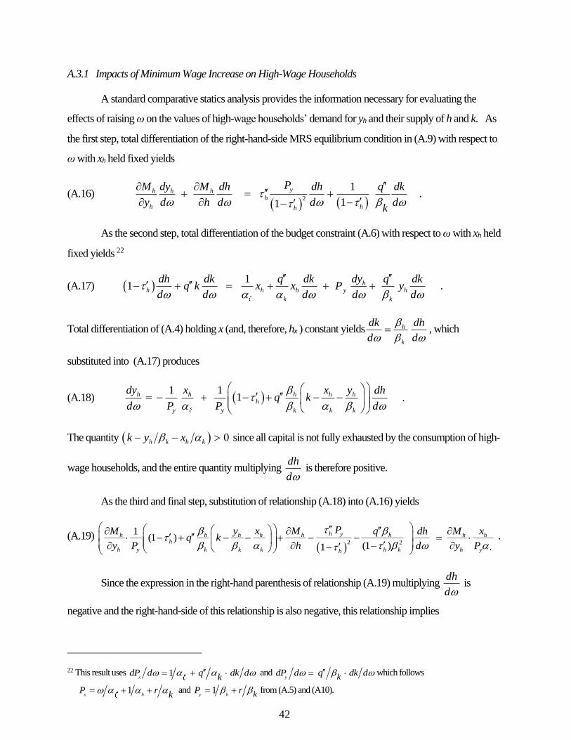
42

A.3.1 Impacts of Minimum Wage Increase on High-Wage Households

A standard comparative statics analysis provides the information necessary for evaluating the

effects of raising ω on the values of high-wage households’ demand for yh and their supply of h and k. As

the first step, total differentiation of the right-hand-side MRS equilibrium condition in (A.9) with respect to

ω with xh held fixed yields

(A.16)

2

1

11

yh h hh

h hh

PM dy M dh dh q dk

y d h d d dk

.

As the second step, total differentiation of the budget constraint (A.6) with respect to ω with xh held

fixed yields 22

(A.17) 1  1 h

h h h y h

k k

dh dk q dk dy q dkq k x x P y

d d d d d

.

Total differentiation of (A.4) holding x (and, therefore, hx ) constant yields h

k

dk dh

d d

, which

substituted into (A.17) produces

(A.18) 1 1

1h h h h hh

y y k k k

dy x x y dhq k

d P P d

.

The quantity 0h k h kk y x since all capital is not fully exhausted by the consumption of high-

wage households, and the entire quantity multiplying dh

d is therefore positive.

As the third and final step, substitution of relationship (A.18) into (A.16) yields

(A.19)

2 2

1(1 )

(1 )1

h yh h h h h h h hh

h y k k k h k h yh

PM y x M q M xdhq k

y P h d y P

.

Since the expression in the right-hand parenthesis of relationship (A.19) multiplying dh

d is

negative and the right-hand-side of this relationship is also negative, this relationship implies

22 This result uses 1x

dP d q dk dk

and y kdP d q dk d which follows

1x h

P rk

and 1y h kP r from (A.5) and (A10).

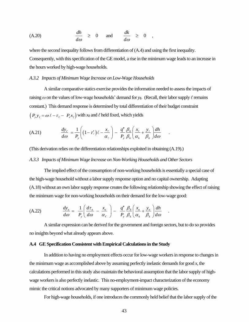
43

(A.20) 0dh

d and 0

dk

d ,

where the second inequality follows from differentiation of (A.4) and using the first inequality.

Consequently, with this specification of the GE model, a rise in the minimum wage leads to an increase in

the hours worked by high-wage households.

A.3.2 Impacts of Minimum Wage Increase on Low-Wage Households

A similar comparative statics exercise provides the information needed to assess the impacts of

raising ω on the values of low-wage households’ demand for yℓ. (Recall, their labor supply ℓ remains

constant.) This demand response is determined by total differentiation of their budget constraint

y xP y P x with xℓ and ℓ held fixed, which yields

(A.21) 1

1 h

y y k k k

dy x x yq dh

d P P d

.

(This derivation relies on the differentiation relationships exploited in obtaining (A.19).)

A.3.3 Impacts of Minimum Wage Increase on Non-Working Households and Other Sectors

The implied effect of the consumption of non-working households is essentially a special case of

the high-wage household without a labor supply response option and no capital ownership. Adapting

(A.18) without an own labor supply response creates the following relationship showing the effect of raising

the minimum wage for non-working households on their demand for the low-wage good:

(A.22) 1n n n h n n

y y k k k

dy d x x yq dh

d P d P d

.

A similar expression can be derived for the government and foreign sectors, but to do so provides

no insights beyond what already appears above.

A.4 GE Specification Consistent with Empirical Calculations in the Study

In addition to having no employment effects occur for low-wage workers in response to changes in

the minimum wage as accomplished above by assuming perfectly inelastic demands for good x, the

calculations performed in this study also maintain the behavioral assumption that the labor supply of high-

wage workers is also perfectly inelastic. This no-employment-impact characterization of the economy

mimic the critical notions advocated by many supporters of minimum wage policies.

For high-wage households, if one introduces the commonly held belief that the labor supply of the

44

high-wage households is entirely unresponsive to their wages, then (A.18) reduces to

(A.23)

10h h

y

dy x

d P

.

Comparison with (A.18) reveals that the decline in the demand for high-wage goods by high-wage

households is mitigated when these households have elastic labor supplies and respond positively to

compensate for the loss of resources arising from higher prices for the low-wage good induced by

increasing the minimum wage.

For low households, (A.21) simplifies to

(A.24) 1

y

dy x

d P

.

The quantity 0x since all of the low-wage good is not fully consumed by low-wage

households. Consequently, the consumption of the high-wage good by low-wage households increases

unless that the progressivity of taxation overcomes this effect.

Finally, for non-working households, (A.22) reduces to

(A.25) 1n n n

y

dy d x

d P d

.

Accordingly, consumption of the high-wage good by these households will decline due to the loss of

resources attributable to higher prices for the low-wage good induced a higher minimum wage, unless

sufficient governmental transfers make up for the difference. Note that all of these transfers come from

minimum-wage households through their higher taxation on earning.

Relationships (A.18), (A.19), (A.21) and (A.22) determine the effects of increasing the minimum

wage in a GE framework with the consumer demands for the low-wage good assumed to be perfectly

inelastic. With the labor supply response of high-wage workers also deemed to be perfectly inelastic, these

relationships become (A.23), (A.24) and (A.25). When combined with the analogous relationships for the

government and foreign sections, this specification of a GE model is consistent with the accounting

computations presented in this study.

A.5 Evaluating Minimum Wage Impacts Under More Flexible Behavioral Assumptions

The above relationships provide insights into how business owners share in the costs of increasing

the minimum wage in this GE setting. If the supply of capital inputs is perfectly elastic—which could arise

when international markets set rates of return and the foreign sector supplies incremental capital at constant

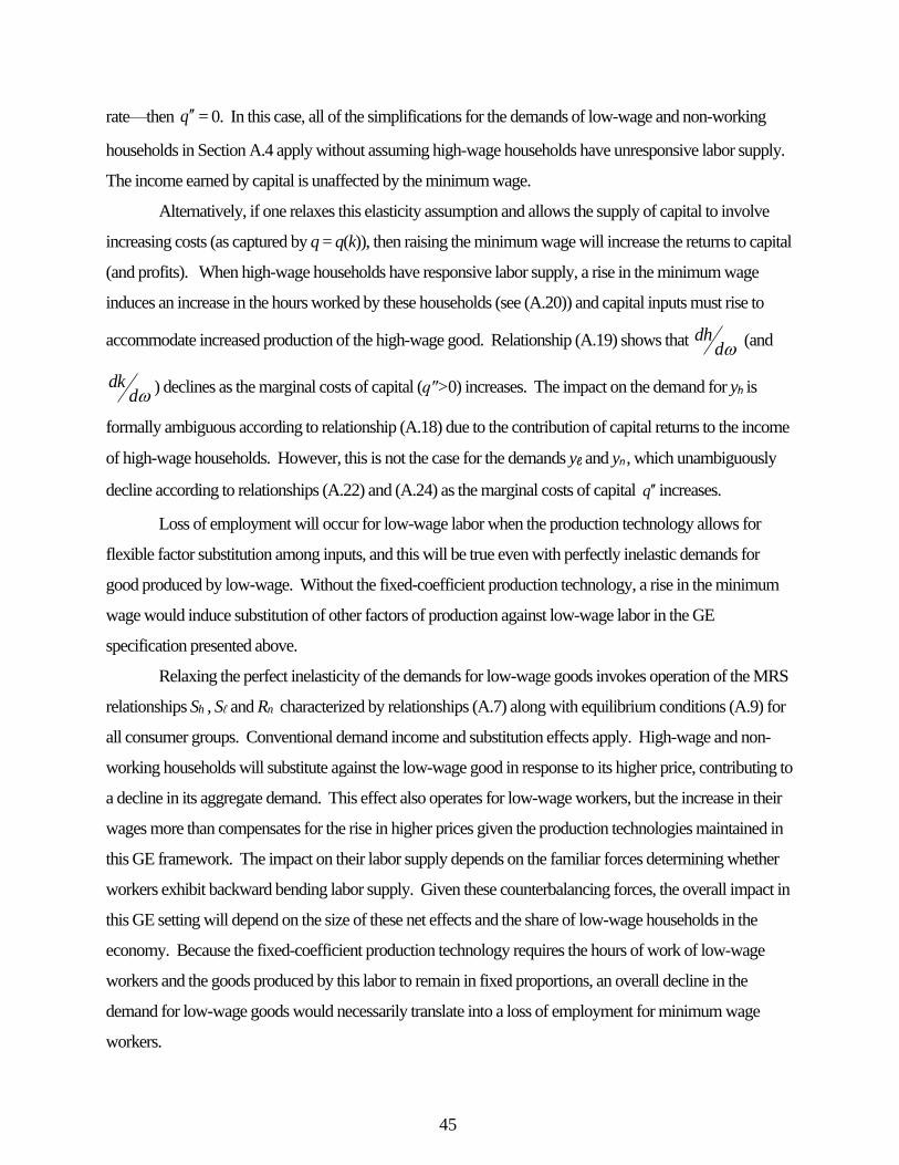
45

rate—then q= 0. In this case, all of the simplifications for the demands of low-wage and non-working

households in Section A.4 apply without assuming high-wage households have unresponsive labor supply.

The income earned by capital is unaffected by the minimum wage.

Alternatively, if one relaxes this elasticity assumption and allows the supply of capital to involve

increasing costs (as captured by q = q(k)), then raising the minimum wage will increase the returns to capital

(and profits). When high-wage households have responsive labor supply, a rise in the minimum wage

induces an increase in the hours worked by these households (see (A.20)) and capital inputs must rise to

accommodate increased production of the high-wage good. Relationship (A.19) shows that dhd

(and

dkd

) declines as the marginal costs of capital (q″>0) increases. The impact on the demand for yh is

formally ambiguous according to relationship (A.18) due to the contribution of capital returns to the income

of high-wage households. However, this is not the case for the demands yℓ and yn , which unambiguously

decline according to relationships (A.22) and (A.24) as the marginal costs of capital q increases.

Loss of employment will occur for low-wage labor when the production technology allows for

flexible factor substitution among inputs, and this will be true even with perfectly inelastic demands for

good produced by low-wage. Without the fixed-coefficient production technology, a rise in the minimum

wage would induce substitution of other factors of production against low-wage labor in the GE

specification presented above.

Relaxing the perfect inelasticity of the demands for low-wage goods invokes operation of the MRS

relationships Sh , Sℓ and Rn characterized by relationships (A.7) along with equilibrium conditions (A.9) for

all consumer groups. Conventional demand income and substitution effects apply. High-wage and non-

working households will substitute against the low-wage good in response to its higher price, contributing to

a decline in its aggregate demand. This effect also operates for low-wage workers, but the increase in their

wages more than compensates for the rise in higher prices given the production technologies maintained in

this GE framework. The impact on their labor supply depends on the familiar forces determining whether

workers exhibit backward bending labor supply. Given these counterbalancing forces, the overall impact in

this GE setting will depend on the size of these net effects and the share of low-wage households in the

economy. Because the fixed-coefficient production technology requires the hours of work of low-wage

workers and the goods produced by this labor to remain in fixed proportions, an overall decline in the

demand for low-wage goods would necessarily translate into a loss of employment for minimum wage

workers.

46

Figures and Tables

Figure 1: Data and Methodology Overview

SIPP Data

Hypothetical Minimum Wage Increase

Distribution of Additional Earnings

TAXSIM Calculator

Distribution of After-Tax Benefits

Increased Labor Cost by Industry (Direct Effect)

Input-Output Tables

Implied Commodity Bundle Price Increases

CES Data

Distribution of Consumption

Increased Cost of Consumption

Distribution of Final Cost

Benefit Side Cost Side

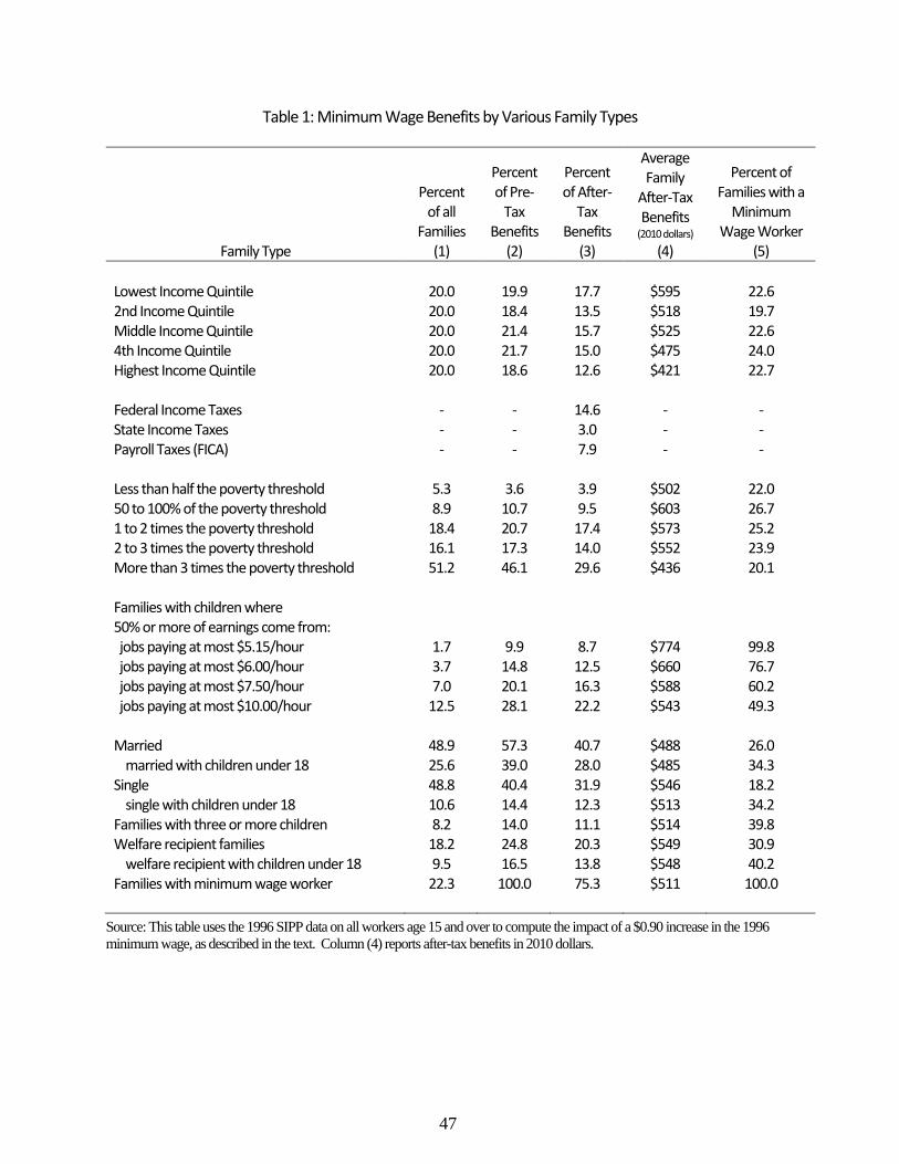
47

Table 1: Minimum Wage Benefits by Various Family Types

Family Type

Percent of all

Families (1)

Percent of Pre-

Tax Benefits

(2)

Percent of After-

Tax Benefits

(3)

Average Family

After-Tax Benefits

(2010 dollars)

(4)

Percent of Families with a

Minimum Wage Worker

(5)

Lowest Income Quintile 20.0 19.9 17.7 $595 22.6 2nd Income Quintile 20.0 18.4 13.5 $518 19.7 Middle Income Quintile 20.0 21.4 15.7 $525 22.6 4th Income Quintile 20.0 21.7 15.0 $475 24.0 Highest Income Quintile 20.0 18.6 12.6 $421 22.7 Federal Income Taxes - - 14.6 - - State Income Taxes - - 3.0 - - Payroll Taxes (FICA) - - 7.9 - - Less than half the poverty threshold 5.3 3.6 3.9 $502 22.0 50 to 100% of the poverty threshold 8.9 10.7 9.5 $603 26.7 1 to 2 times the poverty threshold 18.4 20.7 17.4 $573 25.2 2 to 3 times the poverty threshold 16.1 17.3 14.0 $552 23.9 More than 3 times the poverty threshold 51.2 46.1 29.6 $436 20.1 Families with children where 50% or more of earnings come from: jobs paying at most $5.15/hour 1.7 9.9 8.7 $774 99.8 jobs paying at most $6.00/hour 3.7 14.8 12.5 $660 76.7 jobs paying at most $7.50/hour 7.0 20.1 16.3 $588 60.2 jobs paying at most $10.00/hour 12.5 28.1 22.2 $543 49.3 Married 48.9 57.3 40.7 $488 26.0 married with children under 18 25.6 39.0 28.0 $485 34.3 Single 48.8 40.4 31.9 $546 18.2 single with children under 18 10.6 14.4 12.3 $513 34.2 Families with three or more children 8.2 14.0 11.1 $514 39.8 Welfare recipient families 18.2 24.8 20.3 $549 30.9 welfare recipient with children under 18 9.5 16.5 13.8 $548 40.2 Families with minimum wage worker 22.3 100.0 75.3 $511 100.0

Source: This table uses the 1996 SIPP data on all workers age 15 and over to compute the impact of a $0.90 increase in the 1996

minimum wage, as described in the text. Column (4) reports after-tax benefits in 2010 dollars.

48

Table 2: Minimum Wage Jobs and Cost Increase by Industry

Industry

Percent of all Minimum Wage Jobs

(1)

Percent of all Minimum

Wage Hours (2)

Percent of Direct Costs

(3)

Percent of Final Costs

(4)

Eating and Drinking Places 20.97 18.45 18.67 19.83 Other Retail Trade 6.36 5.6 5.02 5.20 Grocery Stores 6.31 5.24 4.49 4.58 Elementary and Secondary Schools 4.07 4.2 5.00 5.50 Households Misc. Personal Services 3.66 3.35 3.98 4.24 Government 2.96 3.42 4.19 1.43 Colleges and Universities 2.89 2.29 2.63 2.87 Misc. Entertainment and Recreation 2.86 2.26 2.15 2.42 Department Stores 2.69 2.31 1.78 1.97 Construction 2.52 3.00 2.94 2.63 Hotels and Motels 2.22 2.27 2.03 1.01 Wholesale Goods 2.02 2.47 2.37 1.44 Child Day Care Services 1.68 1.54 1.52 1.75 Apparel and Accessories 1.58 1.95 2.05 2.18 Agricultural Production Crops 1.55 1.92 2.15 0.81 Motor Vehicle Dealers 1.51 2.03 1.99 2.39 Movies and Videos 1.37 1.02 0.93 0.49 Real Estate 1.27 1.67 1.96 4.82 Health Services 1.24 1.22 1.14 1.51 Trucking and Warehousing 1.23 1.96 2.23 0.74 Apparel and Accessory Stores 1.21 0.89 0.76 0.88 Nursing and Personal Care Facilities 1.18 1.15 0.86 1.17 Religious Organization 1.16 1.22 1.45 1.69

Source: The 1996 SIPP data on all workers age 15 and over is used in columns (1) and (2) to determine the industry of workers who

benefit from the $0.90 increase in the 1996 minimum wage, as described in the text. The IMPLAN input-output tables are used in

combination with the SIPP data in columns (3) and (4) to calculate the direct and final costs as described in the text.

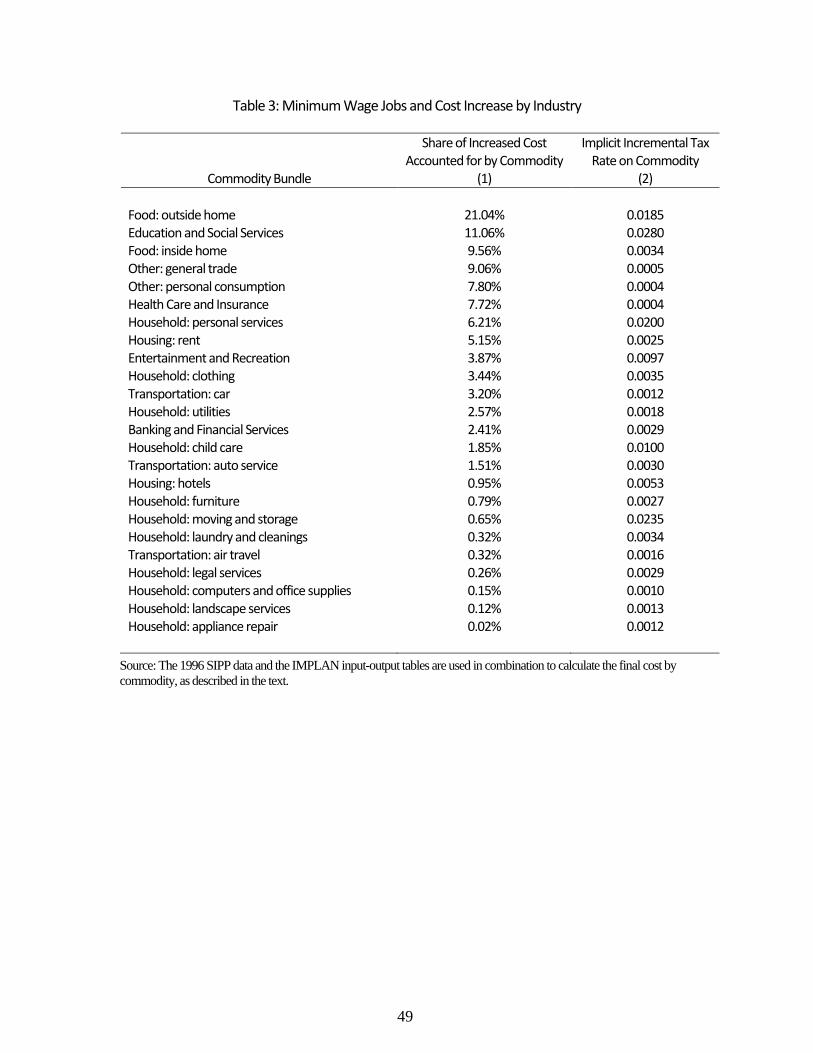
49

Table 3: Minimum Wage Jobs and Cost Increase by Industry

Commodity Bundle

Share of Increased Cost Accounted for by Commodity

(1)

Implicit Incremental Tax Rate on Commodity

(2)

Food: outside home 21.04% 0.0185 Education and Social Services 11.06% 0.0280 Food: inside home 9.56% 0.0034 Other: general trade 9.06% 0.0005 Other: personal consumption 7.80% 0.0004 Health Care and Insurance 7.72% 0.0004 Household: personal services 6.21% 0.0200 Housing: rent 5.15% 0.0025 Entertainment and Recreation 3.87% 0.0097 Household: clothing 3.44% 0.0035 Transportation: car 3.20% 0.0012 Household: utilities 2.57% 0.0018 Banking and Financial Services 2.41% 0.0029 Household: child care 1.85% 0.0100 Transportation: auto service 1.51% 0.0030 Housing: hotels 0.95% 0.0053 Household: furniture 0.79% 0.0027 Household: moving and storage 0.65% 0.0235 Household: laundry and cleanings 0.32% 0.0034 Transportation: air travel 0.32% 0.0016 Household: legal services 0.26% 0.0029 Household: computers and office supplies 0.15% 0.0010 Household: landscape services 0.12% 0.0013 Household: appliance repair 0.02% 0.0012

Source: The 1996 SIPP data and the IMPLAN input-output tables are used in combination to calculate the final cost by

commodity, as described in the text.

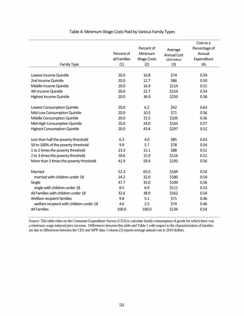
50

Table 4: Minimum Wage Costs Paid by Various Family Types

Family Type

Percent of all Families

(1)

Percent of Minimum

Wage Costs (2)

Average Annual Cost

(2010 dollars) (3)

Cost as a Percentage of

Annual Expenditure

(4)

Lowest Income Quintile 20.0 10.8 $74 0.59 2nd Income Quintile 20.0 12.7 $86 0.50 Middle Income Quintile 20.0 16.9 $114 0.51 4th Income Quintile 20.0 22.7 $154 0.54 Highest Income Quintile 20.0 36.9 $250 0.58 Lowest Consumption Quintile 20.0 6.2 $42 0.63 Mid-Low Consumption Quintile 20.0 10.5 $71 0.56 Middle Consumption Quintile 20.0 15.5 $105 0.56 Mid-High Consumption Quintile 20.0 24.0 $163 0.57 Highest Consumption Quintile 20.0 43.8 $297 0.52 Less than half the poverty threshold 6.3 4.0 $85 0.63 50 to 100% of the poverty threshold 9.9 5.7 $78 0.54 1 to 2 times the poverty threshold 23.3 15.1 $88 0.51 2 to 3 times the poverty threshold 18.6 15.9 $116 0.51 More than 3 times the poverty threshold 41.9 59.4 $193 0.56 Married 52.3 65.0 $169 0.54 married with children under 18 24.2 32.0 $180 0.54 Single 47.7 35.0 $100 0.56 single with children under 18 8.5 6.9 $111 0.53 All Families with children under 18 32.6 38.9 $162 0.54 Welfare recipient families 9.8 5.1 $71 0.46 welfare recipient with children under 18 4.6 2.5 $74 0.46 All Families 100.0 100.0 $136 0.54

Source: This table relies on the Consumer Expenditure Survey (CES) to calculate family consumption of goods for which there was

a minimum wage induced price increase. Differences between this table and Table 1 with respect to the characterization of families

are due to differences between the CES and SIPP data. Column (3) reports average annual cost in 2010 dollars.

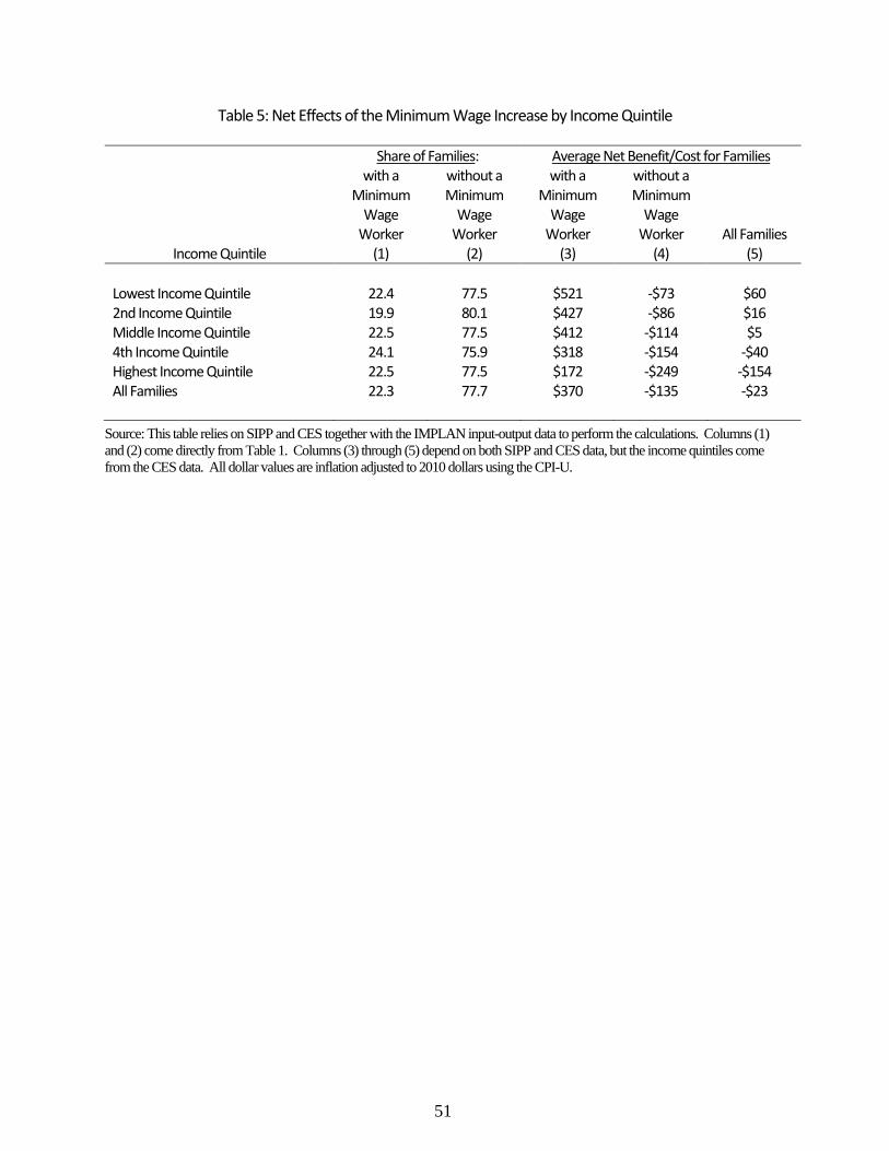
51

Table 5: Net Effects of the Minimum Wage Increase by Income Quintile

Share of Families: Average Net Benefit/Cost for Families

Income Quintile

with a Minimum

Wage Worker

(1)

without a Minimum

Wage Worker

(2)

with a Minimum

Wage Worker

(3)

without a Minimum

Wage Worker

(4) All Families

(5)

Lowest Income Quintile 22.4 77.5 $521 -$73 $60 2nd Income Quintile 19.9 80.1 $427 -$86 $16 Middle Income Quintile 22.5 77.5 $412 -$114 $5 4th Income Quintile 24.1 75.9 $318 -$154 -$40 Highest Income Quintile 22.5 77.5 $172 -$249 -$154 All Families 22.3 77.7 $370 -$135 -$23

Source: This table relies on SIPP and CES together with the IMPLAN input-output data to perform the calculations. Columns (1)

and (2) come directly from Table 1. Columns (3) through (5) depend on both SIPP and CES data, but the income quintiles come

from the CES data. All dollar values are inflation adjusted to 2010 dollars using the CPI-U.

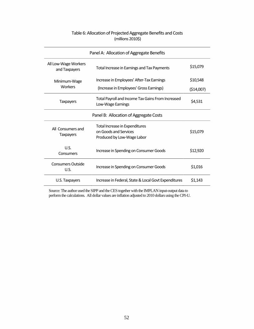
52

Table 6: Allocation of Projected Aggregate Benefits and Costs (millions 2010$)

Panel A: Allocation of Aggregate Benefits

All Low-Wage Workers and Taxpayers Total Increase in Earnings and Tax Payments $15,079

Minimum-Wage Workers

Increase in Employees’ After-Tax Earnings $10,548

(Increase in Employees’ Gross Earnings) ($14,007)

Taxpayers Total Payroll and Income Tax Gains From Increased Low-Wage Earnings

$4,531

Panel B: Allocation of Aggregate Costs

All Consumers and Taxpayers

Total Increase in Expenditures on Goods and Services Produced by Low-Wage Labor

$15,079

U.S. Consumers

Increase in Spending on Consumer Goods $12,920

Consumers Outside U.S.

Increase in Spending on Consumer Goods $1,016

U.S. Taxpayers Increase in Federal, State & Local Govt Expenditures $1,143

Source: The author used the SIPP and the CES together with the IMPLAN input-output data to

perform the calculations. All dollar values are inflation adjusted to 2010 dollars using the CPI-U.