SFB 649 Discussion Paper 2016-056

How Does Rising

House Price Influence Stock Market Participation

in China?

A Micro-Household Perspective

Xiaoyu Chen * Xiaohao Ji *

* Fudan University, People's Republic of China

This research was supported by the Deutsche Forschungsgemeinschaft through the SFB 649 "Economic Risk".

http://sfb649.wiwi.hu-berlin.de

ISSN 1860-5664

SFB 649, Humboldt-Universität zu Berlin Spandauer Straße 1, D-10178 Berlin

SFB

6

4 9

E

C O

N O

M I

C

R I

S K

B

E R

L I

N

1

How Does Rising House Price Influence Stock Market Participation in China? A Micro-Household Perspective

Xiaoyu Chen a1 and Xiaohao Ji b

a School of Public Health, School of Data Science, Fudan University, Shanghai, China b School of Mathematical Science, Fudan University, Shanghai, China

Abstract

This is an empirical study on the effect of house price on stock-market participation and its depths

based on unique China Household Finance Survey (CHFS) data in 2011 and 2013 including 36213

sample households. We mainly found that, with an increase of one thousand RMB per square

meter in macro house price, the probability to participate in the stock market will increase by 5.4%

before controlling for wealth effect and 2.84% afterwards, indicating the existence of wealth effect.

The participation depths of the stock-total asset ratio is expected to decrease by 0.23% and

absolute stock asset is observed to decrease by 5.8 thousand RMB in response to one thousand

RMB increase of per square meter house price. The effect of house price on participation decision

is also related to housing area, and the negative effect of house price on stock market participation

depths gets more intense with the increase of the stock-total asset ratio.

Keywords: Stock Market, Participation decision and depth, House Price, China, CHFS data

JEL: D13; G11; R21; R32

1 Introduction Since the reform and openness from the early 1980s, the saving rate in China keeps

high due to the severe capital control, which leave savers in China only a few

domestic investment vehicles. While the China’s stock market, as one of them, has

also experienced drastic growth, it is still in its nascent stage of development, with a

capitalization of slightly less than 20 trillion RMB in 2013. In contrary, 48.9% of

American households owned stock, either directly, or through mutual funds or other

1 Address correspondence to Xiaoyu Chen, School of Public Health and School of Data Science, Fudan University, Shanghai; E-mail: xiaoyuchen14@fudan.edu.cn. Financial support from the Deutsche Forschungsgemeinschaft via CRC Economic Risk and IRTG 1792 High Dimensional Non Stationary Time Series, Humboldt-Universität zu Berlin, is gratefully acknowledged.

2

means in 1998, which is still considered too low in some absolute sense in light of the

historically high returns to investing in stock market. On the other hand, China has

witnessed a great housing boom in the last decade, with an average annual real growth

of 13.1 percent in first-tier cities, 10.5 percent in second-tier cities and 7.9 percent in

the third-tier cities (Fang et al., 2015). This paper is mainly meant to investigate the

effect of the increase of house price on the decision and depths of China households’

stock-market participation.

This problem is worth studying upon firstly due to the considerably high

house-ownership rate in China, close to 90% according to CHFS data in 2011 and the

large proportion of housing asset in households' total asset. Real estate, as a rigid

demand, thus, plays a vital role in Chinese households' everyday investment decisions

in most aspects including these in the stock market. Secondly, theoretically speaking,

after the involvement of housing in the life-cycle model, the effect of wealth and life

cycle can be interpreted more reasonably (Cocoo, 2005). Many empirical works have

been carried out and the results are quite confusing since the model suggests that the

increase of housing asset should raise the stock participation while empirical results

indicate the opposite (Chetty and Sandor, 2016). This paper treats housing

independently from life cycle effect and using house price as a new entry point to

study on the effect of housing on stock-market participation, since endogeneity within

the effect of house price on stock-market participation is probably weaker than that

within the effect of housing.

Furthermore, the relationship between house price and stock-market participation is

quite complicated and different from that of housing itself. With the rise of house

price, the wealthy families normally consider the real estates to be a more profitable

and less risky investment choice in China, relative to the stock market, while those

families with no self-owned real estate will be pushed to increase their savings and be

limited in their investment in the stock market. On the other hand, the increase of

house price may contribute to the accumulation of wealth and therefore enables

households to participate in the stock market without too much financial burden. The

lack of relevant investigations on house price as one of the determinants of

stock-market participation in China makes the work in this paper very necessary.

3

The rest of the paper is organized as follows. Section 2 provides a literature review on

the research of the determinants of stock-market participation and the influence of

house price on the choices of households. Section 3 describes the CHFS data, the

overall status of stock market and house price in China, the model specified in this

paper. The most relevant variables used in this study will be also introduced. The

estimated effect of house price on stock-market participation decision and depths will

be discussed in details in Section 4. This paper concludes in Section 5.

2. Literature review There are many reasons to study upon the determinants of the stock-market

participation. The most important one is that the stock-market participation rate may

have a direct effect on the size of equity premium at the aggregate level, therefore the

research of which may enlighten the research on equity-premium puzzle of Mehra and

Prescott (1985). Another reason is that, despite the classic literature which suggest

that all investors should invest in all kinds of risky assets at a certain ratio depending

on personal risk preference, many existing researches have shown that households’

choices of investment in reality are much simpler and safer, even with lots of

households refusing the option of investing in the stock market (Markowitz, 1952;

Merton, 1969; Samuelson, 1969). Thus the determinants may help to explain the

limited household stock market participation. Furthermore, finding out the

determinants of stock-market participation may help to explain some aspects of the

investment decisions of households in China, and therefore may lead to the

adjustment of policies. Lastly, the behaviour of individual investors and the reasons

for the behaviour impinges directly on questions about the efficiency of financial

markets.

Since the theoretical work on household portfolios by Markowitz, Merton and

Samuelson, the researches on household portfolio choices have been an important part

of the study of finance. These classic works, however, lead to the contradiction

between empirical observations and the theoretical model (McCarthy, 2004). For

instance, most of the early models failed to explain the effects of wealth and age on

portfolio allocations. Thus the empirical study of the determinants of household

4

portfolio allocation, especially the impact on stock market participation, is very

important. Furthermore, the model developed by Deaton and extended later to allow

agents to buy both stocks and bonds suggests that the limited participation of

individuals in the stock market might be able to explain the equity premium puzzle

(McCarthy, 2004). On the other hand, including housing into the theoretical models

enables the models to explain more powerfully about the empirical results, including

the relatively low risky-asset rate.

As pointed out by Chetty and Sandor (2016), most previous models in relevant

literatures leads to the conclusion that housing should have a negative effect on the

demand for risky assets since it raises the households’ exposure to risk and illiquidity

(Flavin and Yamashita 2002). They also managed to solve the inconsistence between

models and previous empirical results (Heaton and Lucas, 2000b; Yamashita, 2002;

Cocco, 2005) by distinguishing between home equity wealth and mortgage debt, with

the estimation implying that a 10% decrease in household’s housing will lead to a 6%

rise of the mean stock share of liquid wealth, holding fixed wealth.

Many works have been done both in China and globally on the determinants of

household stock-market participation besides housing, including many aspects of

variables. Firstly, individual characteristics are thought to be vital to stock-market

participation. Age and stock-market participation are indicated to have a nonlinear

relation (Aizcorbe et al., 2003). Education level may play an important role in the

story (Bertaut et al. 2000). More specifically, the gain of financial literacy is expected

to increase the household stock-market participation (Yin et al., 2015). Personality

traits of individuals like trust risk aversion, ambiguity aversion and optimism are also

influential factors of the stock-market participation (Hong et al., 2004). Other

characteristics include marital statues, sex and wealth as well (Poterba and Samwick,

2002; Vissing-Jorgensen, 2002). Secondly, background risks, which involves housing,

are also included in the study. Entrepreneurial risk, more specifically the ownership of

private businesses and the risk of income are thought to influence negatively the

decision of private-business-owning household in stock market (Heaton and Lucas,

2000a; Faig and et al., 2002). While better health condition might have a positive

effect on household’s participation in the stock market (Rosen 2004). Thirdly, for the

5

interaction with the other individuals may cause effects on the investment in equity,

social interaction measured by household’s visits to neighbours and the church, local

social capital and neighbours’ participation in the stock market are all expected to

play a role in the story (Guiso et al., 2004; Hong et al., 2004; Brown and et al. 2008).

Other relevant determinants include saving motives, more specifically for investment

in housing, and retirement and professional investment advice, leading to a bigger

probability of stock-investment (Faig and Shum, 2006).

In China, a few researches relevant with the determinants of household stock-market

participation have also been carried out, following the release of the CHFS data.

Financial availability measured by financial services available in the neighbourhood,

investment experience and financial literacy are estimated to have significantly

positive effects on households’ participation in the stock market (Yin et al., 2014,

2015). The difference between rural and urban areas, household assets, income,

education, self-employment and social relations may all cause effects on household

stock-market participation (Zhu et al., 2014). Before the release of the CHFS data,

background risks (Jiang et al., 2009), social interaction and trust, life cycle and wealth

(Wu et al., 2010) had been investigated as the determinants of stock-market

participation. To the best of our knowledge, this paper is the only study which focuses

on the effect of the house price on the stock-market participation in China, as a

supplement to the theory of housing and portfolio choices, especially based on the

unique micro-CHFS data which will be introduced in the following section.

3. Data and model

3.1 CHFS data

The study of household portfolio allocation and more specifically stock-market

participation in China are constrained by the lack of micro-data and can hardly gain

inspiring empirical results until 2011 when Survey and Research Centre for China

Household Finance conducted a nationally representative household survey. The

completed 8438 sample households in 2011, for example, are located in 320

communities in 80 counties, both rural and urban, all across 25 provinces (Gan et al.

2013). The second survey was conducted in 2013, in which the sample households

6

increase to 27775, locating in 1048 communities in 262 counties across 29 provinces.

The CHFS focuses on the household data including household assets, financial assets,

debts, income, demographic characteristics and so on. The survey is continuously

carried out in 2015, one time every two year to make a panel data set, with an overall

refusal rate of 11.6%, which is relatively low compared to similar data set like CHIP,

CGSS or SCF. In this paper, we use the CHFS data in 2011 and 2013, covering totally

36213 sample households.

Table 1 depicts the households’ stock-market participation rate respectively in 2011

and 2013 calculated from the CHFS data. The Overall participation rate of 2011, 2013

are 8.8% and 8.1% respectively. In both 2011 and 2013, there are drastic appreciations

of participation rate with wealth, which is indicated by total assets, going from 1.1%

in the first quantile of the wealth distribution to 21.9% in the fourth quantile of the

wealth distribution in 2013, for example. The stock-market participation didn’t

increase with the time passing probably due to the bear market in 2013. An interesting

fact is that though high-income families were intimidated by the depressing climate,

there were a bigger proportion of low-income families that participated in the stock

market in 2013 than 2011, probably due to the lack of timely information or

overconfidence held by low-income family. The following analysis will separate the

data into different categories in order to show the possible relationship between

stock-market participation and some of its determinants.

Table 1: Stock market participation rate in 2011 and 2013

2011

2013

All household 8.8%

8.1%

The 1st wealth quantile 0.7%

1.1%

The 2nd wealth quantile 1.8%

2.5%

The 3rd wealth quantile 7.2%

6.8%

The 4th wealth quantile 25.5%

21.9%

Top 5% 43.8%

34.1%

Figure 1 shows the different stock-market participation rates among different cities by

wealth quantiles. The cities are divided into three categories: the first-tier, the

7

second-tier and the others. The first-tier cities include Beijing, Shanghai, Guangzhou

and Shenzhen, while the second tier cities include 33 cities like Changchun, Dalian,

Nanjing, Chongqing and etc. In both 2011 and 2013, households in the first-tier cities

were much more likely to participate in the equity market, as can be seen from Figure

1 clearly.

Figure 1: stock-market participation rate and city tiers

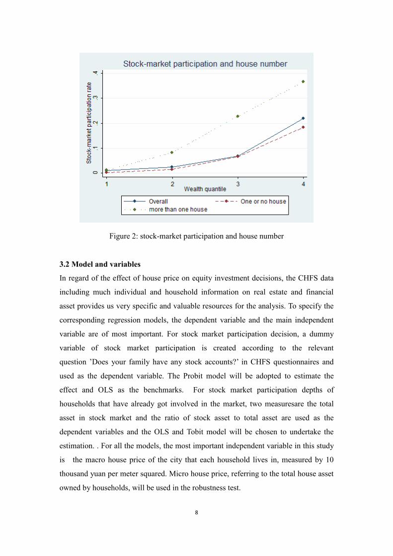
Figure 2 shows the stock-market participation rates of households with different

numbers of houses, through which the fact that households with more than one house

have apparently a much bigger chance to participate in the stock market than those

with at most one house. But whether or not the effect of number of real estates will

stay positive after controlling wealth and house price remains unsolved. These raw

results from the figures indicate a likely relationship between real-estate asset and

stock market participation, since residents of first-tier cities with higher house prices

seem to be more likely to participate in the stock market and the number of houses

also have much to do with the stock-market decision.

8

Figure 2: stock-market participation and house number

3.2 Model and variables

In regard of the effect of house price on equity investment decisions, the CHFS data

including much individual and household information on real estate and financial

asset provides us very specific and valuable resources for the analysis. To specify the

corresponding regression models, the dependent variable and the main independent

variable are of most important. For stock market participation decision, a dummy

variable of stock market participation is created according to the relevant

question ’Does your family have any stock accounts?’ in CHFS questionnaires and

used as the dependent variable. The Probit model will be adopted to estimate the

effect and OLS as the benchmarks. For stock market participation depths of

households that have already got involved in the market, two measuresare the total

asset in stock market and the ratio of stock asset to total asset are used as the

dependent variables and the OLS and Tobit model will be chosen to undertake the

estimation. . For all the models, the most important independent variable in this study

is the macro house price of the city that each household lives in, measured by 10

thousand yuan per meter squared. Micro house price, referring to the total house asset

owned by households, will be used in the robustness test.

9

The covariates include education, income, marital status, age and so on which could

be collected from the CHFS data. A dummy for rural residents are included according

to the information investigated on place of residence. The household variable of

education, income, marital status and age are taken to be the equivalents of the head

of each household. More specifically, education level is measured by a concrete

variable. Number 1 is used to indicate none education received while 9 stands for

PHD and above. Other important determinants of household stock market

participation that have already been studied upon are also included. For social

interaction with neighbours and others, the questionnaires include relevant questions

on transfer expenditures like receiving and giving money on weddings and funerals to

measure households’ social interaction, both with family members and others. The

background risk factors involve self-employment, which is measured by a dummy

created according to the question ‘Last year, did your family engage in any industrial

or commercial projects?’ As to personal traits, risk aversion is estimated by the

question of ‘Assume you have some assets to invest, which type of project would you

invest in?’ and number 1 stands for low risk aversion favouring high risks and high

return, while 5 stands for the opposite. A subjective measure of exposure to financial

information is also carried out in 2013, corresponding to the question 'To what extent

are you concerned with financial information?' while number 1 stands for

'considerably so' and 5 for never. The indicator of use of Internet is also limited to a

one-year data, since the question 'What is the major path for you to get information,’

including the answer of ‘Internet’, wasn't available in data of 2013.

Table 2: Descriptive statistics of continuous variables

2011 2013

stock-total asset

ratio

stock

asset

house

price

house

asset house area

stock-total

asset ratio

stock

asset

house

price

house

asset

house

area

mean 12.6% 13.9 0.56 48.3 153.8

11.2% 12.7 0.7 55.8 165.4

median 5.3% 5 0.38 17 115

4.3% 4.2 0.5 25 117

25% 2.1% 1.9 0.277 6.2 78

1.5% 1.3 0.38 9 78

75% 14.5% 14 0.68 45 200

11.5% 11 0.8 60 200

95% 51.7% 50.6 1.55 200 360 50.9% 50 1.71 225 425

10

Notes: stock-total asset ratio and stock asset are limited to those families involved in the stock market

while house asset and house area are limited to those who own houses. House price indicates the macro

house price of the cities where the household live. Stock asset and house asset are measured by ten

thousand RMB. House price is measured by ten thousand RMB per square meter. House area is

measured by squared meter.

Table 2 shows the descriptive statistics of the main continuous variables used in this

paper, including stock asset and stock-total asset ratio among those households that

own stocks, along with macro house price, house asset and house area. The mean

stock-total asset ratio among those that have already been involved in the stock

market decreased from 12.6% in 2011 to 11.2% in 2013, and stock asset decreased

from 139 thousand RMB to 127 thousand RMB, while the mean value of house asset

increased from 483 thousand to 558 thousand among those who own real estates. The

table also depicts the overall picture of housing and stock-market participation by

showing the quantiles of each variable.

4. Empirical results

4.1 The effect of house price on the stock-market participation

Table 3 shows the estimated effect of house price on the dummy variable of whether

or not to participate in the stock market. The columns (1) to (4) are estimated by OLS

and (5) to (8) are measured by Probit model. Column (1) and (5) report the baseline

estimation in which the wealth is not controlled. Following Hong and et al. (2004),

four dummies corresponding to the second, third, fourth and fifth wealth quintiles are

included later in columns (2) and (6). In column (3) and (7), the wealth indicator is

modified to be 19 wealth quantile dummies, rather than 4 dummies. In column (4) and

(8), more variables like marital status, party member dummy and self-employment

dummy (dummy variables) are included, and the social interaction indicator is also

included, measured by the transfer expenditures like receiving and giving money on

weddings and funerals. Year and provincial effects are all controlled.

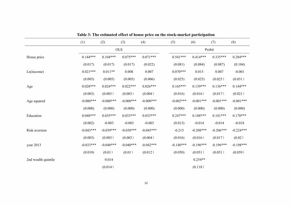
As can be seen from the Table 3, both estimation methods show the similar result that

house price has a significantly positive effect on the decision of stock-market

11

participation. Under the Probit estimation, column (5) suggests that with an increase

of one thousand yuan per meter squared in macro house price, the possibility of

stock-market participation is expected to increase by 5.41%, controlling for most

other variables except for wealth. And this estimated effect declines to 4.14% after

controlling for the 4 wealth quantile dummies and 3.35% after controlling for the 19

wealth quantile dummies. The OLS estimation leads to a similar result, despite the

fact that the estimated effect stops declining after controlling other variables such as

the social interaction indicator. The decline of estimated effect of house price after

controlling for the wealth indicators suggests that the increase of macro house may

contribute to higher stock-market participation rate by wealth accumulation. The

higher house price get, the more wealthy most family will be and the less likely they

are going to be faced with severe financial burden. It's also necessary to mention that

after the wealth indicators and most relevant variables are controlled, the estimated

positive effect of house price stays significant both economically and statistically,

which indicates a possible unobservable path through which the increase of house

price may spur stock-market participation, besides by the accumulation of wealth.

The coefficients of other variables in Table 3 are worth explaining and being

compared to existing literature. Risk aversion indicator has a significantly negative

marginal effect as expected, staying approximately the same controlling for more

variables. The significant inverted U effect of age is observed, peaking at

approximately 65 years old for the head according to the Probit model. The estimated

effect of the dummy for year 2013 is significantly negative in all the columns, which

indicates a large-scale escape from the stock-market due to the devastating financial

climate, consistent with the results shown in table 1 in the data section.

12

Table 3: The estimated effect of house price on the stock-market participation

(1) (2) (3) (4) (5) (6) (7) (8)

OLS

Probit

House price 0.144*** 0.104*** 0.075*** 0.071***

0.541*** 0.414*** 0.335*** 0.284***

(0.017) (0.017) (0.017) (0.022)

(0.081) (0.084) (0.087) (0.104)

Ln(income) 0.021*** 0.011** 0.008 0.007

0.070*** 0.015 0.007 -0.001

(0.005) (0.005) (0.005) (0.006)

(0.025) (0.025) (0.025） (0.031）

Age 0.028*** 0.024*** 0.022*** 0.026***

0.165*** 0.139*** 0.136*** 0.144***

(0.003) (0.003） (0.003） (0.004）

(0.016) (0.016） (0.017） (0.021）

Age squared -0.000*** -0.000*** -0.000*** -0.000***

-0.002*** -0.001*** -0.001*** -0.001***

(0.000) (0.000) (0.000) (0.000)

(0.000) (0.000) (0.000) (0.000)

Education 0.048*** 0.035*** 0.033*** 0.033***

0.247*** 0.188*** 0.181*** 0.170***

(0.002) -0.003 -0.003 -0.003

(0.013) -0.014 -0.014 -0.018

Risk aversion -0.043*** -0.039*** -0.038*** -0.045***

-0.215 -0.208*** -0.206*** -0.224***

(0.003) (0.003） (0.003） (0.004）

(0.016) (0.016） (0.017） (0.02）

year 2013 -0.033*** -0.040*** -0.040*** -0.042***

-0.140*** -0.196*** -0.196*** -0.198***

(0.010) (0.01） (0.01） (0.012）

(0.050) (0.051） (0.051） (0.059）

2nd wealth quintile 0.014

0.254**

(0.014）

(0.118）

13

3rd wealth quantile 0.012

0.363***

(0.014）

(0.11）

4th wealth quantile 0.075***

0.801***

(0.013）

(0.102）

5th wealth quantile 0.178***

1.082***

(0.014）

(0.102）

province dummies Yes Yes Yes Yes Yes Yes Yes Yes

19 wealth quantile dummies No No Yes Yes

No No Yes Yes

More controlled variables No No No Yes

No No No Yes

Notes: Independent variables include: macro house price of cities (‘House price,’ measured by ten thousand RMB per square meter), the log of income of the households’

head (‘Ln(income)’), age and age squared, an education indicator (‘Education,’ a discrete variable, taking on the number 1 for those households with heads who ‘Never

attended school’ and 9 for ‘PHD’), a risk-aversion indicator(‘Risk aversion,’ estimated by the question of ‘Assume you have some assets to invest, which type of project

would you invest in?’, and number 1 stands for low risk aversion favouring high risks and high return, while 5 stands for the opposite.) Other controlled variables are not

shown in the table.

14

Education has a significantly positive effect on stock-market participation, just the

same as argued by Bertaut and Starr-McCluer. (2000). The education indicator has

been tried as a dummy variable that indicates whether the head of the household had

received college or above education. The estimation suggests that the marginal effect

of households’ heads owning college or above degrees is 21.6 percent under Probit

estimation and 25.7 percent under OLS estimation (not shown). Besides, as

mentioned in the data section, the measure of financial information availability and

the availability of Internet is limited to data in 2011 and 2013 respectively, so in the

regressions of Internet availability, the data in 2011 are used, while in the regressions

of financial information, those of 2013 are used. The estimated marginal effects of

Internet availability under OLS and Probit estimation are 0.107 and 0.481, while the

estimated marginal effects of financial information are 0.056 and 0.264, all significant

at the one percent level (not shown).

Table 4 shows the effect of house price on stock-market participation with the

existence of house area under OLS and Probit estimation. The investment in real

estate may also have a negative effect for the reason argued by previous studies that

with the increase of real-estate asset, less money is left for equity market. In order to

have a deeper insight, 4 dummies of total area quantiles of each household’s real

estate and the total area of each household’s real estates will be incorporated into the

regression respectively. The sample is limited to the households that own real estate,

while wealth, income, age, risk aversion, social interaction indicator and other effects

are all controlled as former discussions. The table shows that the larger the area of

real estates that a certain household owns, the bigger the positive effect of house price

on stock-market participation gets. The estimated effects of the dummy of the 5th

house area dummy (not shown) are -4.8% and -3.2% under OLS and Probit

estimations, both significant at the 1% level. According to column (3) and (4), the

results show that the marginal effects of total house area are all significantly negative,

which are -0.007 and -0.059 respectively under OLS and Probit estimation, and before

adding the interaction of house price and total house area, the effect of house price

stays significantly positive. This also suggests that controlling house price, the more

real estates a certain household owns, the less likely they are to invest in the stock

market, since most of their assets are real estate assets. The interaction of total house

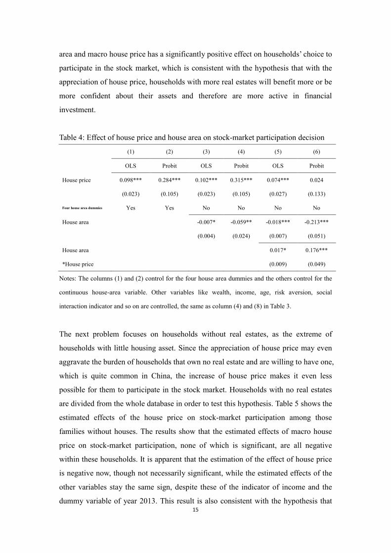
15

area and macro house price has a significantly positive effect on households’ choice to

participate in the stock market, which is consistent with the hypothesis that with the

appreciation of house price, households with more real estates will benefit more or be

more confident about their assets and therefore are more active in financial

investment.

Table 4: Effect of house price and house area on stock-market participation decision

(1) (2) (3) (4) (5) (6)

OLS Probit OLS Probit OLS Probit

House price 0.098*** 0.284*** 0.102*** 0.315*** 0.074*** 0.024

(0.023) (0.105) (0.023) (0.105) (0.027) (0.133)

Four house area dummies Yes Yes No No No No

House area

-0.007* -0.059** -0.018*** -0.213***

(0.004) (0.024) (0.007) (0.051)

House area

0.017* 0.176***

*House price

(0.009) (0.049)

Notes: The columns (1) and (2) control for the four house area dummies and the others control for the

continuous house-area variable. Other variables like wealth, income, age, risk aversion, social

interaction indicator and so on are controlled, the same as column (4) and (8) in Table 3.

The next problem focuses on households without real estates, as the extreme of

households with little housing asset. Since the appreciation of house price may even

aggravate the burden of households that own no real estate and are willing to have one,

which is quite common in China, the increase of house price makes it even less

possible for them to participate in the stock market. Households with no real estates

are divided from the whole database in order to test this hypothesis. Table 5 shows the

estimated effects of the house price on stock-market participation among those

families without houses. The results show that the estimated effects of macro house

price on stock-market participation, none of which is significant, are all negative

within these households. It is apparent that the estimation of the effect of house price

is negative now, though not necessarily significant, while the estimated effects of the

other variables stay the same sign, despite these of the indicator of income and the

dummy variable of year 2013. This result is also consistent with the hypothesis that

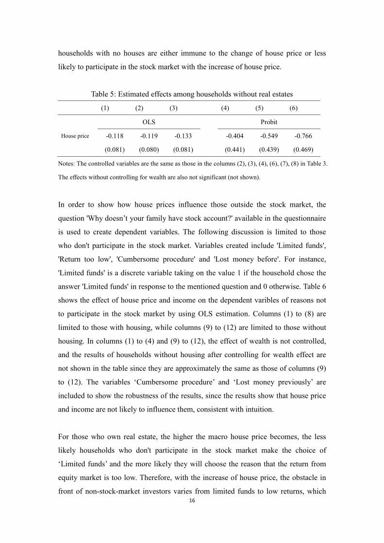
16

households with no houses are either immune to the change of house price or less

likely to participate in the stock market with the increase of house price.

Table 5: Estimated effects among households without real estates

(1) (2) (3) (4) (5) (6)

OLS

Probit

House price -0.118 -0.119 -0.133

-0.404 -0.549 -0.766

(0.081) (0.080) (0.081)

(0.441) (0.439) (0.469)

Notes: The controlled variables are the same as those in the columns (2), (3), (4), (6), (7), (8) in Table 3.

The effects without controlling for wealth are also not significant (not shown).

In order to show how house prices influence those outside the stock market, the

question 'Why doesn’t your family have stock account?' available in the questionnaire

is used to create dependent variables. The following discussion is limited to those

who don't participate in the stock market. Variables created include 'Limited funds',

'Return too low', 'Cumbersome procedure' and 'Lost money before'. For instance,

'Limited funds' is a discrete variable taking on the value 1 if the household chose the

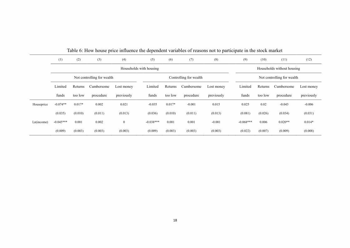
answer 'Limited funds' in response to the mentioned question and 0 otherwise. Table 6

shows the effect of house price and income on the dependent varibles of reasons not

to participate in the stock market by using OLS estimation. Columns (1) to (8) are

limited to those with housing, while columns (9) to (12) are limited to those without

housing. In columns (1) to (4) and (9) to (12), the effect of wealth is not controlled,

and the results of households without housing after controlling for wealth effect are

not shown in the table since they are approximately the same as those of columns (9)

to (12). The variables ‘Cumbersome procedure’ and ‘Lost money previously’ are

included to show the robustness of the results, since the results show that house price

and income are not likely to influence them, consistent with intuition.

For those who own real estate, the higher the macro house price becomes, the less

likely households who don't participate in the stock market make the choice of

‘Limited funds’ and the more likely they will choose the reason that the return from

equity market is too low. Therefore, with the increase of house price, the obstacle in

front of non-stock-market investors varies from limited funds to low returns, which

17

may mainly be explained by the appealing return in the equity market. But as

discussed in the previous section, the overall effect of house price is positive. Besides,

macro house prices seem to have little to do with the reasons of cumbersome

procedures and previous loss in the stock market, which is consistent with intuition.

With the increase of income, the barrier of funds is also of less importance, but the

expectation of return doesn't really change.

Furthermore, after controlling for the wealth quantile dummies, the estimation of the

effect of house price on the reason of 'Limited funds' is no longer significant, which is

consistent with previous discussion that the increase of house price will lead to the

accumulation of wealth and will be followed by less financial burden. On the other

hand, the reason why those households with no real estates choose not participate in

the stock market seems to have nothing to do with house price, whether or not

controlling for wealth. (The results after controlling for wealth are not shown since

similarly, they are all not significant.) Lastly, the estimated effect of house price on

the reason ‘Returns too low ’ is significantly negative both before and after

controlling for wealth effect, which indicates that the increase of house price may

induce households to invest in the real-estate market, since the return of housing

investment is seemingly higher due to the high house price. The effect of house price

is thus different than that of housing itself.

In a word, the estimated effect of house price on the reason of ‘Limited funds’ is

significantly negative before controlling for the wealth effect and not significant

anymore afterwards, which is consistent with the story that house price affects the

stock-market participation by wealth accumulation, while the effect of house price on

the reason of ‘Returns too low’ is significant both before and after controlling for the

19 wealth dummies. The effects of income are also included for the test of robustness,

and the results are consistent with intuition.

18

Table 6: How house price influence the dependent variables of reasons not to participate in the stock market

(1) (2) (3) (4) (5) (6) (7) (8) (9) (10) (11) (12)

Households with housing

Households without housing

Not controlling for wealth

Controlling for wealth

Not controlling for wealth

Limited

funds

Returns

too low

Cumbersome

procedure

Lost money

previously

Limited

funds

Returns

too low

Cumbersome

procedure

Lost money

previously

Limited

funds

Returns

too low

Cumbersome

procedure

Lost money

previously

Houseprice -0.074** 0.017* 0.002 0.021 -0.035 0.017* -0.001 0.015 0.025 0.02 -0.043 -0.006

(0.035) (0.010) (0.011) (0.013)

(0.036) (0.010) (0.011) (0.013)

(0.081) (0.026) (0.034) (0.031)

Ln(income) -0.045*** 0.001 0.002 0

-0.038*** 0.001 0.001 -0.001

-0.068*** 0.006 0.020** 0.014*

(0.009) (0.003) (0.003) (0.003) (0.009) (0.003) (0.003) (0.003) (0.022) (0.007) (0.009) (0.008)

19

4.2 The effect of house price on the participation depths in the stock market

Besides the effect of house price on the decision to invest in the stock market

investigated firstly, another intriguing problem is the effect of house price on the

participation depths in the stock market among households that have already been

involved. Two measures of the participation depths in the stock market are considered:

stock asset to total asset ratio and absolute stock asset. Table 7 shows the OLS and

Tobit estimation of the effects of macro house price on the depths variables of

absolute stock asset and stock-market asset relative to the household’s total asset. The

controlled variables are almost the same as those in Table 3, including the wealth

effect, income, age and age squared, education level, a year dummy, marital status, a

social-interaction indicator, a risk-aversion indicator, a party-member dummy, a

self-employment dummy and so on.

Table 7: The effect of house price on stock-market choices

(1) (2)

(3) (4)

(5) (6)

(7) (8)

Stock-total asset ratio Stock asset

OLS

Tobit

OLS

Tobit

House

price -0.024*** -0.026**

-0.023** -0.023**

-6.946*** -6.856**

-6.465** -5.769*

(0.009) (0.01)

(0.01) (0.011)

(2.656) (3.012)

(2.878) (3.271)

Region No Yes

No Yes

No Yes

No Yes

Notes: stock asset is measured by ten thousand RMB.

Despite the fact that the effect of house price on the stock-market participation

decision is significantly positive within the whole sample, this new result shows that

the appreciation of house price has a negative effect on the stock asset holdings of

households already involved, which is probably due to the fact that with higher house

price, households are more likely to invest in the real-estate market and therefore

reduce their investment in the equity market. Furthermore, the result stays strong and

almost the same, controlling regional effects, with estimated marginal effect of

approximately -2.5% for the relative asset and -6.9 for the absolute one, which

suggests that with an increase of one thousand RMB per square meter, the stock-total

20

asset ratio is expected to decrease by 0.23%（1.83% of the mean stock-total asset ratio）

and absolute stock asset is expected to decrease by 5.8 thousand RMB (4.17% of the

mean stock asset). Other measures of stock asset are also considered, including the

ratio of stock asset to financial asset. The result (not shown) isn’t significant as

expected mainly due to house price’s lack of influence on the decision made in the

financial asset.

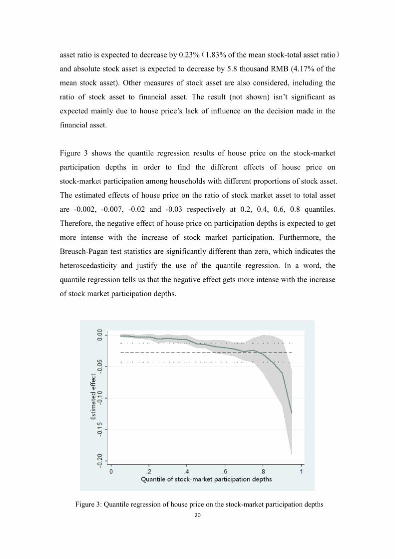
Figure 3 shows the quantile regression results of house price on the stock-market

participation depths in order to find the different effects of house price on

stock-market participation among households with different proportions of stock asset.

The estimated effects of house price on the ratio of stock market asset to total asset

are -0.002, -0.007, -0.02 and -0.03 respectively at 0.2, 0.4, 0.6, 0.8 quantiles.

Therefore, the negative effect of house price on participation depths is expected to get

more intense with the increase of stock market participation. Furthermore, the

Breusch-Pagan test statistics are significantly different than zero, which indicates the

heteroscedasticity and justify the use of the quantile regression. In a word, the

quantile regression tells us that the negative effect gets more intense with the increase

of stock market participation depths.

Figure 3: Quantile regression of house price on the stock-market participation depths

21

4.4 The robust test

The most important problem then is that the observed relations between house price

and household stock-stock market and its depts may reflect a considerable number of

unobservable influences that lead to spurious estimation even after controlling for

most observable variables. Intuitively, since the households are not randomly assigned

with macro house price, it’s reasonable to doubt that the estimation shown in the

previous sections are actually biased. Due to this endogeneity in this equation caused

by unobservable factors that may contribute to the change of house price and the

decision to participate in the stock market, one might argue that the coefficients

doesn't account for the real effect itself. Therefore we try to solve this problem by

firstly using instrumental variables, which is the average house price of the closest

four cities of the location of each specific household. For example, if one household

lives in Shanghai, the corresponding instrumental variable will be set as the average

macro house price of Suzhou, Jiaxing, Nantong and Wuxi. The instrumental variable

is considered effective because clearly it is very likely to be correlated with the local

house price and, furthermore, since it’s the average of house prices of provinces that

have little to do with the investigated households, the IV is unlikely to be correlated

with the households’ decisions choices anywhere.

Table 8 shows the regression results using the instrumental variable under different

estimation method and dependent variables. The controlled variables are the same as

their counterparts in the previous discussion after controlling for the wealth effect.

The OLS estimated coefficient suggests that a one thousand RMB appreciation in the

macro house price increases the probability that one will participate in the stock

market by 2.7 percentage points. The estimated marginal effect of house price under

Probit estimation is 0.979, both with the OLS estimation, are all higher than the

baseline estimation. In these regressions, variables controlled include income, wealth,

age, education, social interaction indicator and etc. Both fixed time and provincial

effects are included as well. Table 8 also shows the estimated effects of house price on

stock market asset holding, using the instrumental variable, which suggests that with a

one thousand RMB appreciation in house price, the ratio of stock asset to total asset

will decrease by 0.56% and absolute stock asset will decrease by 24 thousand RMB.

The corresponding estimated marginal effects under Tobit regression are also

22

significantly -0.041 and -21.088.

Table 8 Regression using the instrumental variable

(1) (2) (3) (4) (5) (6)

OLS Probit OLS Tobit OLS Tobit

Decision Decision

Stock-total

asset ratio

Stock-total

asset ratio Stock asset

Stock

asset

House

price 0.274** 0.979* -0.056** -0.041** -24.743* -21.088*

(0.12) (0.537) (0.024) (0.02) (14.973) (12.537)

Furthermore, we undertake the second robust test by replace macro house price with

the micro price level indexed by the total real-estate assets available in the CHFS data

in the previous regressions (not shown as table). The results are significantly

consistent with the previous results. The tables suggest that with a one million rise in

household’s real-estate asset, the possibility that the household will choose to

participate in the stock market is expected to increase 3.3 percent according to the

OLS estimation. Among these who are already involved in the stock market, each one

hundred thousand rise in real-estate asset will contribute to a 7.4 thousand RMB (5.3%

of the mean stock asset) decrease in the absolute stock asset and 0.31% (2.5% of the

mean stock-total asset ratio) decline in the stock to total asset ratio. The robust tests

justify our results in this study.

5. Conclusion The analyses based on the unique CHFS data in this study conclude that the macro

house price has both statistically and economically significant effect on the

households’ stock-market participation decision and their depths in the stock market.

With the increase of one thousand RMB per square meter in macro house price, the

probability that each household in that city to participate in the stock market will

increase by 5.4% before controlling for wealth effect and 2.84% afterwards

(indicating the existence of wealth effect within the effect of house price), the

stock-total asset ratio is expected to decrease by 0.23%（1.83% of the mean stock-total

asset ratio）and absolute stock asset is expected to decrease by 5.8 thousand RMB

23

(4.17% of the mean stock asset). Generally, though the increase of house price will

motive those who haven’t entered the stock market to participate in it, it’s actually

pulling back those who have already been involved and letting them invest less in the

stock market.

For the effect on the stock-market participation depths, the negative effect of house

price will get even more intense with the increase of the area of self-owned housing,

while the effect of house price on the decision whether or not to participate in the

stock market among those who own no housing is insignificantly negative.

Furthermore, the increase of house price will decrease the possibility of not

participating in the stock market due to the reason of ‘Limited funds’ and will increase

that due to the reason of ‘Returns too low’, for those who don’t participate in the

stock market, and the controlling of wealth will make the former one not significant

anymore, also indicating the effect of wealth. On the other hand, for the effect on the

participation depths in the stock market, the effect on stock-total asset ratio is more

intense among those with high stock-total asset ratio, according to the quantile

regression. The robustness test using IV and Micro house asset show the similar

results as those in the previous discussions.

An explanation for our results is that with the increase of house price, households in

China may have a bigger opportunity to participate in the stock market, partially

because of the accumulation of wealth and the decrease of the barrier to participation

(maybe most of them just have a stock account or a little investment in the stock

market), while the higher the house price is, the more likely these households who

have already been involved in the stock market will decrease their investment,

probably due to the high returns in the housing market (most of them are still

participating in the stock market, just investing less). We believe that the effect of

house price, independent from housing, can partially explain the influence of real

estate from a different direction and has important meanings under the context of the

housing boom and relatively low stock-market participation rate in China, as

discussed in the previous sections, but since the complicated nature of the portfolio

choices and the relatively narrow entry point of our research, the problem like the

effect of house price on the overall portfolio choice remains to be studied upon.

24

References Aizcorbe, Ana M., Arthur B. Kennickell and Kevin B. Moore (2003), ‘Recent changes in U.S.

family finances: Evidence from 1998 and 2001 Survey of Consumer Finances’, Federal Reserve

Bulletin 89, 1-32.

Bertaut, C. and M. Starr-McCluer, ‘Household Portfolios in the United States,’ Household

Portfolio, ed. by L. Guiso, M. Haliassos, and T. Jappelli. MIT Press, Cambridge, 2000.

Brown, J. R., Z. Ivković, P. Smith and S. Weisbenner (2008), ‘Neighbors Matter: Causal

Community Effects and Stock Market Participation,’ Journal of Finance, 63(3), 1509-1531.

Chetty, R. and Sandor, L. (2016), ‘The effect of housing on portofio choice’, NBER Working

Paper No. 15998

Cocco, J. (2005), ‘Portfolio Choice in the Presence of Housing,’ Review of Financial Studies 18,

535-567.

Fang, Hamming, Quanlin Gu, Wei Xiong and Li-An Zhou (2015), ‘Demystifying the Chinese

Housing Boom’, NBER Working Paper 21112

Faig, M. and P. M. Shum (2002), ‘Portfolio choice in the presence of personal illiquid projects’,

Journal of Finance 57, 303-328.

Faig, M. and P. M. Shum (2006), ‘What explains household stock holdings’, Journal of Banking

and Finance 30, 2579-2597.

Flavin, M. and Yamashita, T. (2002), ‘Owner-Occupied Housing and the Composition of the

Household Portfolio,’ American Economic Review, 92(1): 345-362.

Gan, Li, Zhichao Yin, Nan Jia, Shu Xu, and Shuang Ma. (2013), ‘Household Assets and

Household Demand for Housing in China.’ Journal of Financial Research, No 4, 2013.

Guiso, L., P. Sapienza and L. Zingales (2004), ‘The Role of Social Capital in Financial

Development,’ The American Economic Review: 94(3), 526-556(31)

Rosen, Harvey S. (2004), ‘Public Finance,’ The Encyclopedia of Public Choice: 252-262.

25

Heaton, John and Deborah Lucas (2000a), ‘Portfolio choice and asset prices: The importance of

enterpreneurial risk’, Journal of Finance 55, 1163-1198.

Heaton J. and Lucas, D.J. (2000b), ‘Portfolio Choice in the Presence of Background Risk,’

Economic Journal 110(460): 1-26.

Hong, Harrison, Jeffrey D. Kubik, and Jeremy Stein (2004), ‘Social interaction and stock-market

participation’, Journal of Finance 59, 137–163.

Jiang, C., Ma, Y. and An, Y. (2009), ‘An analysis of portfolio selection with background risk,’

Journal of Banking & Finance, 2009, 34(12): 3055-3060.

Markowitz, H. (1952), ‘Portolio Selection,’ the Journal of Finance, Volume 7, Issue 1, March

1952, Pages 77-91

McCarthy, D. (2004), ‘Household Portfolio Allocation: A Review of the Literature,’ Journal of

Economic Literature.

Mehra, R. , E.C. Prescott (1985), ‘The equity premium: A puzzle’, Journal of monetary

Economics 15 (2), 145-161

Merton, R. C. (1969), ‘Lifetime Portfolio Selection Under Uncertainty: The Continuous Time

Case,’ Review of Economics and Statistics 51, 247-257.

Poterba, J. M., and A. A. Samwick (1997), ‘Household Portfolio Allocation over the Life Cycle,’

NBER Working Paper, 6185.

Poterba, James M. and Andrew A. Samwick (2002), ‘Taxation and household portfolio

composition: US evidence from the 1980s and 1990s’, Journal of Public Economics, 87, 5-38.

Samuelson, P. A. (1969) ‘Lifetime Portfolio Selection by Dynamic Stochastic Programming,’

Review of Economics and Statistics, 51, 239–246.

Vissing-Jorgensen, A. (2002), ‘Towards an Explanation of Household Portfolio Choice

Heterogeneity: Nonfinancial Income and Participation Cost Structures,’ working paper,

Northwestern University.

26

Wu Weixing, Yi Jinran and Zhe Jianming (2010), ‘Empirical Analysis on the Effects of Life

Cycle, Wealth and House,’ Economic Research Journal, 2010, s1.

Yamashita, T. (2003), ‘Owner-Occupied Housing and Investment in Stocks: An Empirical Test,’

Journal of Urban Economics, 53(2): 220-237.

Yin, Zhichao, Yu Wu, and Li Gan (2015), ‘Financial Availability, Financial Market Participation

and Household Portfolio Choice,” Economic Research Journal, 3, 2015.

Yin Zhichao, Song Quanyun, and Wu Yu (2014), ‘Financial Literacy, Trading Experience and

Household Portfolio Choice,” Economic Research Journal, 4, 2014.

Zhu Guangwei, Du Zaichao and Zhanglin (2014), ‘Guanxi Stock-market Participation and Stock

Return,’ Economic Research Journal, 11, 2014.

SFB 649 Discussion Paper Series 2016 For a complete list of Discussion Papers published by the SFB 649, please visit http://sfb649.wiwi.hu-berlin.de. 001 "Downside risk and stock returns: An empirical analysis of the long-run

and short-run dynamics from the G-7 Countries" by Cathy Yi-Hsuan Chen, Thomas C. Chiang and Wolfgang Karl Härdle, January 2016.

002 "Uncertainty and Employment Dynamics in the Euro Area and the US" by Aleksei Netsunajev and Katharina Glass, January 2016.

003 "College Admissions with Entrance Exams: Centralized versus Decentralized" by Isa E. Hafalir, Rustamdjan Hakimov, Dorothea Kübler and Morimitsu Kurino, January 2016.

004 "Leveraged ETF options implied volatility paradox: a statistical study" by Wolfgang Karl Härdle, Sergey Nasekin and Zhiwu Hong, February 2016.

005 "The German Labor Market Miracle, 2003 -2015: An Assessment" by Michael C. Burda, February 2016.

006 "What Derives the Bond Portfolio Value-at-Risk: Information Roles of Macroeconomic and Financial Stress Factors" by Anthony H. Tu and Cathy Yi-Hsuan Chen, February 2016.

007 "Budget-neutral fiscal rules targeting inflation differentials" by Maren Brede, February 2016.

008 "Measuring the benefit from reducing income inequality in terms of GDP" by Simon Voigts, February 2016.

009 "Solving DSGE Portfolio Choice Models with Asymmetric Countries" by Grzegorz R. Dlugoszek, February 2016.

010 "No Role for the Hartz Reforms? Demand and Supply Factors in the German Labor Market, 1993-2014" by Michael C. Burda and Stefanie Seele, February 2016.

011 "Cognitive Load Increases Risk Aversion" by Holger Gerhardt, Guido P. Biele, Hauke R. Heekeren, and Harald Uhlig, March 2016.

012 "Neighborhood Effects in Wind Farm Performance: An Econometric Approach" by Matthias Ritter, Simone Pieralli and Martin Odening, March 2016.

013 "The importance of time-varying parameters in new Keynesian models with zero lower bound" by Julien Albertini and Hong Lan, March 2016.

014 "Aggregate Employment, Job Polarization and Inequalities: A Transatlantic Perspective" by Julien Albertini and Jean Olivier Hairault, March 2016.

015 "The Anchoring of Inflation Expectations in the Short and in the Long Run" by Dieter Nautz, Aleksei Netsunajev and Till Strohsal, March 2016.

016 "Irrational Exuberance and Herding in Financial Markets" by Christopher Boortz, March 2016.

017 "Calculating Joint Confidence Bands for Impulse Response Functions using Highest Density Regions" by Helmut Lütkepohl, Anna Staszewska-Bystrova and Peter Winker, March 2016.

018 "Factorisable Sparse Tail Event Curves with Expectiles" by Wolfgang K. Härdle, Chen Huang and Shih-Kang Chao, March 2016.

019 "International dynamics of inflation expectations" by Aleksei Netšunajev and Lars Winkelmann, May 2016.

020 "Academic Ranking Scales in Economics: Prediction and Imdputation" by Alona Zharova, Andrija Mihoci and Wolfgang Karl Härdle, May 2016.

SFB 649, Spandauer Straße 1, D-10178 Berlin http://sfb649.wiwi.hu-berlin.de

This research was supported by the Deutsche

Forschungsgemeinschaft through the SFB 649 "Economic Risk".

SFB 649, Spandauer Straße 1, D-10178 Berlin http://sfb649.wiwi.hu-berlin.de

This research was supported by the Deutsche

Forschungsgemeinschaft through the SFB 649 "Economic Risk".

SFB 649 Discussion Paper Series 2016 For a complete list of Discussion Papers published by the SFB 649, please visit http://sfb649.wiwi.hu-berlin.de. 021 "CRIX or evaluating blockchain based currencies" by Simon Trimborn

and Wolfgang Karl Härdle, May 2016. 022 "Towards a national indicator for urban green space provision and

environmental inequalities in Germany: Method and findings" by Henry Wüstemann, Dennis Kalisch, June 2016.

023 "A Mortality Model for Multi-populations: A Semi-Parametric Approach" by Lei Fang, Wolfgang K. Härdle and Juhyun Park, June 2016.

024 "Simultaneous Inference for the Partially Linear Model with a Multivariate Unknown Function when the Covariates are Measured with Errors" by Kun Ho Kim, Shih-Kang Chao and Wolfgang K. Härdle, August 2016.

025 "Forecasting Limit Order Book Liquidity Supply-Demand Curves with Functional AutoRegressive Dynamics" by Ying Chen, Wee Song Chua and Wolfgang K. Härdle, August 2016.

026 "VAT multipliers and pass-through dynamics" by Simon Voigts, August 2016.

027 "Can a Bonus Overcome Moral Hazard? An Experiment on Voluntary Payments, Competition, and Reputation in Markets for Expert Services" by Vera Angelova and Tobias Regner, August 2016.

028 "Relative Performance of Liability Rules: Experimental Evidence" by Vera Angelova, Giuseppe Attanasi, Yolande Hiriart, August 2016.

029 "What renders financial advisors less treacherous? On commissions and reciprocity" by Vera Angelova, August 2016.

030 "Do voluntary payments to advisors improve the quality of financial advice? An experimental sender-receiver game" by Vera Angelova and Tobias Regner, August 2016.

031 "A first econometric analysis of the CRIX family" by Shi Chen, Cathy Yi-Hsuan Chen, Wolfgang Karl Härdle, TM Lee and Bobby Ong, August 2016.

032 "Specification Testing in Nonparametric Instrumental Quantile Regression" by Christoph Breunig, August 2016.

033 "Functional Principal Component Analysis for Derivatives of Multivariate Curves" by Maria Grith, Wolfgang K. Härdle, Alois Kneip and Heiko Wagner, August 2016.

034 "Blooming Landscapes in the West? - German reunification and the price of land." by Raphael Schoettler and Nikolaus Wolf, September 2016.

035 "Time-Adaptive Probabilistic Forecasts of Electricity Spot Prices with Application to Risk Management." by Brenda López Cabrera , Franziska Schulz, September 2016.

036 "Protecting Unsophisticated Applicants in School Choice through Information Disclosure" by Christian Basteck and Marco Mantovani, September 2016.

037 "Cognitive Ability and Games of School Choice" by Christian Basteck and Marco Mantovani, Oktober 2016.

038 "The Cross-Section of Crypto-Currencies as Financial Assets: An Overview" by Hermann Elendner, Simon Trimborn, Bobby Ong and Teik Ming Lee, Oktober 2016.

039 "Disinflation and the Phillips Curve: Israel 1986-2015" by Rafi Melnick and Till Strohsal, Oktober 2016.

SFB 649, Spandauer Straße 1, D-10178 Berlin http://sfb649.wiwi.hu-berlin.de

This research was supported by the Deutsche

Forschungsgemeinschaft through the SFB 649 "Economic Risk".

SFB 649, Spandauer Straße 1, D-10178 Berlin http://sfb649.wiwi.hu-berlin.de

This research was supported by the Deutsche

Forschungsgemeinschaft through the SFB 649 "Economic Risk".

SFB 649 Discussion Paper Series 2016 For a complete list of Discussion Papers published by the SFB 649, please visit http://sfb649.wiwi.hu-berlin.de. 040 "Principal Component Analysis in an Asymmetric Norm" by Ngoc M. Tran,

Petra Burdejová, Maria Osipenko and Wolfgang K. Härdle, October 2016. 041 "Forward Guidance under Disagreement - Evidence from the Fed's Dot

Projections" by Gunda-Alexandra Detmers, October 2016. 042 "The Impact of a Negative Labor Demand Shock on Fertility - Evidence

from the Fall of the Berlin Wall" by Hannah Liepmann, October 2016. 043 "Implications of Shadow Bank Regulation for Monetary Policy at the Zero

Lower Bound" by Falk Mazelis, October 2016. 044 "Dynamic Contracting with Long-Term Consequences: Optimal CEO

Compensation and Turnover" by Suvi Vasama, October 2016. 045 "Information Acquisition and Liquidity Dry-Ups" by Philipp Koenig and

David Pothier, October 2016. 046 "Credit Rating Score Analysis" by Wolfgang Karl Härdle, Phoon Kok Fai

and David Lee Kuo Chuen, November 2016. 047 "Time Varying Quantile Lasso" by Lenka Zbonakova, Wolfgang Karl

Härdle, Phoon Kok Fai and Weining Wang, November 2016. 048 "Unraveling of Cooperation in Dynamic Collaboration" by Suvi Vasama,

November 2016. 049 "Q3-D3-LSA" by Lukas Borke and Wolfgang K. Härdle, November 2016. 050 "Network Quantile Autoregression" by Xuening Zhu, Weining Wang,

Hangsheng Wang and Wolfgang Karl Härdle, November 2016. 051 "Dynamic Topic Modelling for Cryptocurrency Community Forums" by

Marco Linton, Ernie Gin Swee Teo, Elisabeth Bommes, Cathy Yi-Hsuan Chen and Wolfgang Karl Härdle, November 2016.

052 "Beta-boosted ensemble for big credit scoring data" by Maciej Zieba and Wolfgang Karl Härdle, November 2016.

053 "Central Bank Reputation, Cheap Talk and Transparency as Substitutes for Commitment: Experimental Evidence" by John Duffy and Frank Heinemann, December 2016.

054 "Labor Market Frictions and Monetary Policy Design" by Anna Almosova, December 2016.

055 "Effect of Particulate Air Pollution on Coronary Heart Disease in China: Evidence from Threshold GAM and Bayesian Hierarchical Model" by Xiaoyu Chen, December 2016.

056 "How Does Rising House Price Influence Stock Market Participation in China? A Micro-Household Perspective" by Xiaoyu Chen and Xiaohao Ji, December 2016.

SFB 649, Spandauer Straße 1, D-10178 Berlin http://sfb649.wiwi.hu-berlin.de

This research was supported by the Deutsche

Forschungsgemeinschaft through the SFB 649 "Economic Risk".

SFB 649, Spandauer Straße 1, D-10178 Berlin http://sfb649.wiwi.hu-berlin.de

This research was supported by the Deutsche

Forschungsgemeinschaft through the SFB 649 "Economic Risk".