How Do Voters Respond to Information? Evidence from a ... · How Do Voters Respond to Information?...

American Economic Review 2015, 105(1): 322–353 http://dx.doi.org/10.1257/aer.20131063

322

How Do Voters Respond to Information? Evidence from a Randomized Campaign †

By Chad Kendall, Tommaso Nannicini, and Francesco Trebbi *

In a large-scale controlled trial in collaboration with the reelec-tion campaign of an Italian incumbent mayor, we administered (randomized) messages about the candidate’s valence or ideology. Informational treatments affected both actual votes in the precincts and individual vote declarations. Campaigning on valence brought more votes to the incumbent, but both messages affected voters’ beliefs. Cross-learning occurred, as voters who received information about the incumbent also updated their beliefs on the opponent. With a novel protocol of beliefs elicitation and structural estimation, we assess the weights voters place upon politicians’ valence and ideol-ogy, and simulate counterfactual campaigns. (JEL D12, D72, D83)

We study the causal impact of campaign messages on electoral outcomes and voters’ beliefs about political candidates in a large field experiment encompass-ing an entire electoral campaign. In collaboration with the incumbent mayor of a medium-sized Italian city who was running for reelection in 2011, eligible voters received hard and verifiable information, via mail or phone, about the valence or the ideological stance of the incumbent. The city was randomly divided into four areas, with the first receiving a campaign message about valence, the second about ideology, the third about both valence and ideology, and the fourth receiving no message. The informational treatments were administered by the incumbent as part of his campaign. Our direct mailing covered the entire voting population and our

* Kendall: Vancouver School of Economics, University of British Columbia, 1873 East Mall, Vancouver, BC V6T1Z1, Canada (e-mail: [email protected]); Nannicini: Department of Economics, Bocconi University, Via Roentgen 1, 20136 Milan, Italy and IGIER (e-mail: [email protected]); Trebbi: Vancouver School of Economics, University of British Columbia, 1873 East Mall, Vancouver, BC V6T1Z1, Canada (e-mail: [email protected]). We thank Matilde Bombardini, Claudio Ferraz, David Green, Andrea Mattozzi, Nolan McCarthy, Jim Snyder, and seminar participants at Alicante, Bank of Italy, Bocconi, Collegio Carlo Alberto, CBS, CIFAR, EIEF, EUI, Harris, Harvard, HSE Moscow, Kellog, KU Copenhagen, IFN Stockholm, IMT Lucca, LACEA, Leicester, LSE, Lugano, MILLS workshop, MIT, NES Moscow, Petralia workshop, Pompeu Fabra, Princeton, Rotterdam, SciencesPo, Toulouse, UBC, UK Leuven, USC, and Warwick for useful comments. Federico Cilauro, Francesco Maria Esposito, Jonathan Graves, Nicola Pierri, and Teresa Talo provided outstanding research assistance. A large number of people were instrumental in implementing our experimental design: the mayor of Arezzo, Giuseppe Fanfani, and his 2011 reelection campaign, in particular Claudio Repek, were extremely cooperative; Massimo Di Filippo, Fabrizio Monaci, and the team of “IPR Feedback” showed tremendous expertise in conducting the surveys. In the period 2002–2005, Tommaso Nannicini held positions in the regional organization of the same political party of the incumbent mayor who accepted the experimental design. This experience has been crucial to create mutual trust with the counterpart and implement the randomization of his entire electoral campaign with respect to mailers and phone calls. Apart from Nannicini’s past political experience, the authors declare that they have no other rele-vant or financial interests that relate to the research described in the paper. Nannicini also acknowledges financial support from the European Research Council (grant 230088).

† Go to http://dx.doi.org/10.1257/aer.20131063 to visit the article page for additional materials and author disclosure statement(s).

http://dx.doi.org/10.1257/aer.20131063

mailto:[email protected]





323Kendall et al.: How do Voters respond to InformatIon?Vol. 105 no. 1

phone bank covered about a quarter of all households in the city. Voters received only our mailers from the incumbent campaign, and only our phone calls from both the incumbent and the main challenger’s campaign. To the best of our knowledge, we provide the first experimental evidence of the impact of different strategies of persuasive communication by a politician on not only survey responses, but also on actual vote shares.1

Relative to the control group that received no campaign message, voters informed about the valence of the incumbent—via both mail and phone—increased their sup-port for the candidate by 4.1 percentage points as measured by precinct-level official vote shares, and by 9.5 percentage points as measured by vote declarations in sur-veys. Much weaker effects on vote choices were detected when information about the ideological stance of the incumbent was provided, or when campaigning was done by mail only.

This paper is not limited to the analysis of vote choices in the context of a ran-domized controlled trial, however. Our additional goal is to measure the extent of the response of individual agents to political messages and to understand the degree of sophistication in their subjective updating. The empirical application revolves around the assessment of the role of campaign ads in elections, but the point is more general than political advertising. Our methodology can extend to other forms of direct communication by politicians to voters, has implications beyond the political environment, and could be of interest for commercial advertising—or for any other type of informational treatment—as well. Examples may include informational ads on different product characteristics (as typical in automotive advertising) or political advocacy campaigns (as frequently employed by energy or consumer groups).

Using a novel elicitation protocol, we collected information about the distribu-tions of individual voters’ (multivariate) beliefs about the valence and ideological stance of both the incumbent and the main challenger through surveys both before and after the informational treatments were administered. We show how, by impos-ing a limited amount of structure on electoral preferences and belief distributions, prior and posterior beliefs of individual voters can be fully characterized. We also show that, although only the valence message was effective in changing votes, our informational treatments along both the valence and the ideological dimension had large effects on voters’ beliefs, moving both first and second moments of the belief distributions for the two main candidates. Indeed, campaign information affected not only voters’ beliefs about the candidate originating the message, but also their beliefs about the opponent. Intuitively, in Bayesian signaling games, receiving no message is valuable information and our evidence on cross-learning appears fully consistent with updating in the context of a Bayesian political signaling game.

The full characterization of the individual belief distributions we propose is the combination of a careful design of our surveys and structural estimation of a ran-dom utility voting model. The latter component of our methodology delivers precise estimates of utility weights in voters’ preferences for a candidate’s valence and ide-ology. We disclose a utility weight on valence roughly equal to that on ideological

1 See DellaVigna and Gentzkow (2010) for a comprehensive review of the empirical literature on persuasion in economics, marketing, and political science. Green and Gerber (2004) summarize a vast series of field experiments eval-uating the effect of get-out-the-vote campaigns—and not of partisan advertisement as in our case—on actual turnout.

324 THE AMERICAN ECONOMIC REVIEW jANuARy 2015

losses away from a voter’s bliss point. Interestingly, we also show that the preference weights are heterogeneous in the population and depend on the political stance of the voter, with voters on the right placing less emphasis on the valence dimension. Finally, we show that the ideological loss function away from the voter’s bliss point is concave in distance, not convex (e.g., quadratic losses) as commonly assumed in the theoretical literature.

The random utility model we use follows the method outlined in the theoretical paper of Ramalho and Smith (2013) to account for non-randomness in voters’ will-ingness to disclose their votes. While non-response in survey data is often assumed to be random, we demonstrate the importance of accounting for its endogeneity and suggest that this method should be more often utilized in empirical studies in which survey responses are relied upon.

We conclude our analysis by simulating counterfactual electoral campaigns to assess the effects of specific blanket or targeted electoral campaigns on vote out-comes. We find a blanket campaign of valence messages to be the most valuable in persuading voters, which is consistent with voters lacking prior information on the quality of candidates.

This paper is related to several strands of literature. The effectiveness of electoral campaigns is the subject of a large literature, including the influential work by Zaller (1992). Our work differs from his by focusing on rational updating as opposed to his Receive-Accept-Sample approach, which allows for additional dimensions of polit-ical awareness and salience but concentrates on the ideological dimension alone. This literature also includes several relevant empirical contributions, among these Ansolabehere et al. (1994); Ansolabehere and Iyengar (1995); Gerber and Green (2000); Green and Gerber (2004); Gerber, Green, and Shachar (2003); Nickerson (2008); and Dewan, Humphreys, and Rubenson (2010). Typically the focus of these empirical papers is either on self-declared outcomes for vote choices or on actual outcomes for turnout. Methodologically, these papers rely on either small-scale experiments for partisan ads or on randomized non-partisan campaigns for turnout. Our paper complements this literature by focusing on actual electoral outcomes in a large scale field experiment where partisan ads are randomized by a candidate’s campaign along multiple dimensions. The literature in development economics has also experimented with informational campaigning. Vicente (2014); Banerjee, Green, and Pande (2012); and Banerjee et al. (2011) focus on non-partisan infor-mational campaigns in either Sao Tome and Principe (educating voters about the side effects of vote buying) or India (providing information about the qualifications of candidates), and show that information matters for turnout, vote shares, and the incidence of vote buying. Wantchekon (2003) and Fujiwara and Wantchekon (2013) exploit randomized town-hall meetings in collaboration with presidential candidates in Benin, to eval uate the impact of clientelistic electoral promises on self-declared voting behavior.

We must clarify that our paper is not the first instance of a large scale randomized partisan campaign. Gerber et al. (2011) look at randomization over intensity of TV ads (with no control over the message content) on self-declared electoral choices during the 2006 Republican primary for the Texas gubernatorial election. They find large, but short-lived, effects of such TV ads, inconsistent with Bayesian updating. Different from their approach, we randomize the content of partisan ads and also


evaluate their impact on actual vote shares. Our paper also complements this liter-ature from a methodological standpoint by augmenting the reduced form approach with structural estimation.

From a substantive viewpoint, our paper is related to a vast literature on candi-date’s valence, initiated by Stokes (1963) and including Enelow and Hinich (1982); Ansolabehere and Snyder (2000); Groseclose (2001); Schofield (2003); Aragones and Palfrey (2002) among others. More recently, Ashworth and Bueno de Mesquita (2009); Kartik and McAfee (2007); and Bernhardt, Câmara, and Squintani (2011) provide interesting theoretical studies of strategic electoral competition with can-didates differentiated along both (ideological) policy platform and valence dimen-sions. Galasso and Nannicini (2011) study the empirical relationship between candidates’ valence and the contestability of electoral districts.

Our results also contribute to the debate on voters’ sophistication. Although voters are often portrayed as naïve or unresponsive in regards to their ability to process information, our finding that campaign advertisement affects voters’ beliefs strongly suggests that voters rationally update.2 Specifically, voters update their beliefs about the incumbent’s opponent upon receiving only information about the incumbent himself. This result must be interpreted as voters responding to the absence of a message from the opponent. Such a response is predicted in Bayesian signaling models such as those of Chappell (1994); Coate (2004); and Polborn and Yi (2006) among others, but is difficult to reconcile with a view that voters are simply per-suaded by charismatic politicians. This evidence of sophistication is of interest not only within the realm of politics, but also in industrial organization, where com-petitive advertising among oligopolists can be modeled as a multi-sender signaling game (e.g., see Hertzendorf and Overgaard 2001). Although we are not aware of any field evidence of sophisticated updating in the absence of messages, Mattes (2012) finds supporting evidence in a laboratory experiment.

Finally, we contribute to the growing literature on the elicitation and quantifica-tion of subjective beliefs. Elicitation of priors is the subject of Dominitz and Manski (1996); Manski (2004); Blass, Lach, and Manski (2010); Gill and Walker (2005); and Duffy and Tavits (2008) among others. To these studies, which mostly focus on the elicitation of economic expectations, our work provides a useful addition on the elicitation of multivariate beliefs. In particular, we show how to decouple informa-tion about marginal beliefs and their dependence using a copula function approach. We believe this approach may be of use outside the politico-economic application in our study.

The remainder of the paper is organized as follows. Section I presents the empirical model and describes our approach to beliefs elicitation through surveys. Section II describes the experimental design. Section III discusses the reduced form results on vote choices. Section IV focuses on the structural estimates of the model and Section V on the experimental effects on voters’ beliefs. Section VI simulates our counterfactual campaigns and discusses the implications of the heterogeneous response to information by voters. Section VII concludes.

2 On voters’ unresponsiveness to campaign information, see Campbell et al. (1960); more recently, Adams, Ezrow, and Somer-Topcu (2011) and Adams (2012) for a review. See DellaVigna and Gentzkow (2010) for a com-parison between early and recent empirical studies on political persuasion.


I. Empirical Model

This section presents our empirical model. As opposed to imposing a specific structure to the political game and to voters’ beliefs, which would severely limit the validity of our empirical approach if misspecified, we devise an environment with sufficient flexibility to accommodate for a very large class of equilibrium models of candidate’s positions.

A. Voters and Candidates

Consider an electoral race between two candidates, A , the incumbent, and B , the challenger. Let the set of voters be , with | | = N . Each voter i is characterized by an ideal policy point distributed over a finite and discrete policy space, Π , which is common across all voters, with policies P ∈ Π . The discreteness assumption is meant to capture an empirical feature of the survey data employed in the subsequent analysis. Voters are heterogeneous, with bliss points q ∈ Π , and receive disutility from a policy choice away from their bliss point. They also receive common utility from the level of valence of the elected candidate V ∈ Λ , where the set Λ is finite and discrete. When policy p is implemented by candidate j of valence v , the utility for voter i of type q is assumed to be

U(v, p; q) = γv − u (q − p) − χu (q − p) v + ε i, j ,

where the utility function includes a deterministic portion and a candidate-specific random utility component ε i, j , independent of V and P .3 The parameter γ indi-cates the relative preference weight of valence versus the policy stance. We assume u (0) = 0 , u′ ( x ) ≥ 0 for x > 0 , and u′ ( x ) ≤ 0 for x < 0 . Specifically, we assume the general form u ( x ) = |x| ζ with ζ ≥ 0 , which captures a quadratic loss away from voter i ’s bliss point as a special case.4 We also allow for interactions between valence and ideology that are governed by χ . The random utility compo-nent ε i, j of voter i for candidate j captures the personal appeal of j to i .

All voters participate in the election (voting is compulsory in our empirical setting). Voter i is assumed to have a joint prior distribution function over V and P , f

V, P i, j (v, p) , for j = A, B , evaluated at point (v, p) and defined over the support

Λ × Π . Importantly, we do not preclude V from being potentially correlated with P .Our experimental treatments induce a randomized change in the information sets

of voters, which we describe in detail in Section II. The discreteness of the experi-mental strategy induces a finite set of informational types of voters.

3 It is not important for our purposes to specify whether the two candidates A and B implement their respective ideal policy position P once in office (see Ansolabehere, Snyder, and Stewart 2001; Lee, Moretti, and Butler 2004) or strategically cater their policy to voters (e.g., as in a standard Downsian setting). We are interested in the voters’ utilities at the time they place their vote, which only depend upon their beliefs about each candidate’s position, and not on how the policy position came about or whether or not it is actually implemented. In general, our approach is robust to the details of the electoral competition structure.

4 Quadratic loss functions are standard in the literature (e.g., see Ansolabehere and Snyder 2000). For a dis-cussion of the axiomatic foundations for the general utility function that we employ in a multidimensional spatial model, see Eguia (2011).


Type 1: Receiving a message about V, but not P, of A.

Type 2: Receiving a message about P, but not of V, of A.

Type 3: Receiving a message about both V and P of A.

Type 4: Receiving no message about V or P of A .

For simplicity, a “message” indicates having (randomly) received a campaign information treatment, H ∈ {1, … , 4} . Let us indicate as (h) the set of voters treated with information type H = h and let f V, P i, A (v, p|H = h) indicate the sub-jective posterior probability that voter i , treated by message h , assigns to the event that candidate A has valence V = v and position P = p . The process of updating beliefs typically reflects the characteristics of the game played between voters and political candidates (e.g., a signaling game). Our approach allows us to leave the nature of such strategic interaction unspecified.

The expected utility from the election of candidate j for voter i , treated by h and with ideal point q , is defined as

E U j i (h, q i ) = ∑ p ∑

v f

V, P i, j (v, p|H = h)U(v, p; q i ) + ε i, j .

Under a random utility model of voting, the probability that i of type (h, q) supports candidate A is then given by

(1) Pr [ E U A i (h, q i ) ≥ E U B i (h, q i ) ] .

The random utility approach is a standard choice in modeling voting behavior in sincere voting environments, as well as in strategic voting environments with two candidates. It is however restrictive relative to political models with voters whose strategies are motivated by rule-utilitarianism or, more generally, by a desire of “doing their part.”5

Given the probability that a voter supports candidate A , we can consider a stan-dard, conditional Logit model, assuming ε i, j to be i.i.d. across voters and distrib-uted with a Type I extreme-value distribution with cumulative distribution function F( ε i, j ) = exp (− e − ε i, j ) . Provided information on the choice of i to vote for j , Y i = j , we obtain the log likelihood

ln (θ) = ∑ i=1

N ∑

j d ij ln Pr ( Y i = j) = ∑

i=1

N ∑

j d ij ln e EU j i (h, q i ) _________

∑ l e EU l i (h, q i )

,

where d ij is 1 if i votes for j , and 0 otherwise. Note that the vector of parameters of interest, θ , includes both preference parameters [γ, ζ, χ] and the parameters of the joint beliefs f

V, P i, j (·) , which we define in the following subsection.

5 The empirical identification of this latter class of models in terms of both voting behavior and turnout behavior is not a settled issue in the empirical literature and it is an avenue we do not pursue in this paper. See Coate and Conlin (2004) for an interesting application.


One potential problem with the standard Logit model in a setting employing vote declarations as opposed to actual votes is that voters, when surveyed, may prefer not to disclose their vote. If the sample of voters who do not disclose their vote is completely random, one can apply the Logit model to the subsample of responders. This is the approach typically followed in the literature, often without diagnostics in support of the crucial “missing completely at random” assumption, required for an unbiased estimate. We provide evidence in Section IV that indicates that the subsa-mple of voters that choose not to disclose their votes is predictable, so estimation of the standard Logit model would lead to biased estimates in our setting. We therefore apply a novel choice-based approach suggested by Ramalho and Smith (2013) that allows for non-random non-response under weak assumptions. The model assumes that, conditional on the voter’s actual vote, the probability with which a voter chooses to respond to the survey is constant, but that this probability can depend on their vote. Under this assumption, we can define the log likelihood as

ln (θ) = (

∑ i=1

N o i ∑

j d i j ln β j e E U j i (h, q i ) ________

∑ l e E U l i (h, q i )

+ (1 − o i ) ln (

1 − ∑ j β j e E U j i (h, q i ) ________

∑ l e E U l i (h, q i )

) )

,

where o i is 1 if i discloses the vote, and 0 otherwise. The additional β j parameters are the probabilities with which a voter discloses the vote for j . The first term of the log likelihood is the probability that a voter votes for j and discloses his vote. The second term reflects the probability that the voter votes for one of the candidates, but chooses not to disclose his vote. Note that when β j = 1 for all j , such that the vote is always observed, we obtain the standard Logit model as a special case.

B. Voters’ Subjective Updating

Here, we specify the process by which voters’ subjective beliefs are updated in the presence of campaign advertising. For illustrative purposes, consider the following time line.

Our first assumption is that voters consider the campaign information to be truth-ful. Sufficient freedom of the press in the Italian electoral context guarantees that such an assumption may be valid in the case of factual advertising, as we employ in our experimental setup. All messages are factual and can be independently validated.

1 2 3

Subjectivepriors

formed

Informationaltreatment

Subjective posteriors formed+ elections


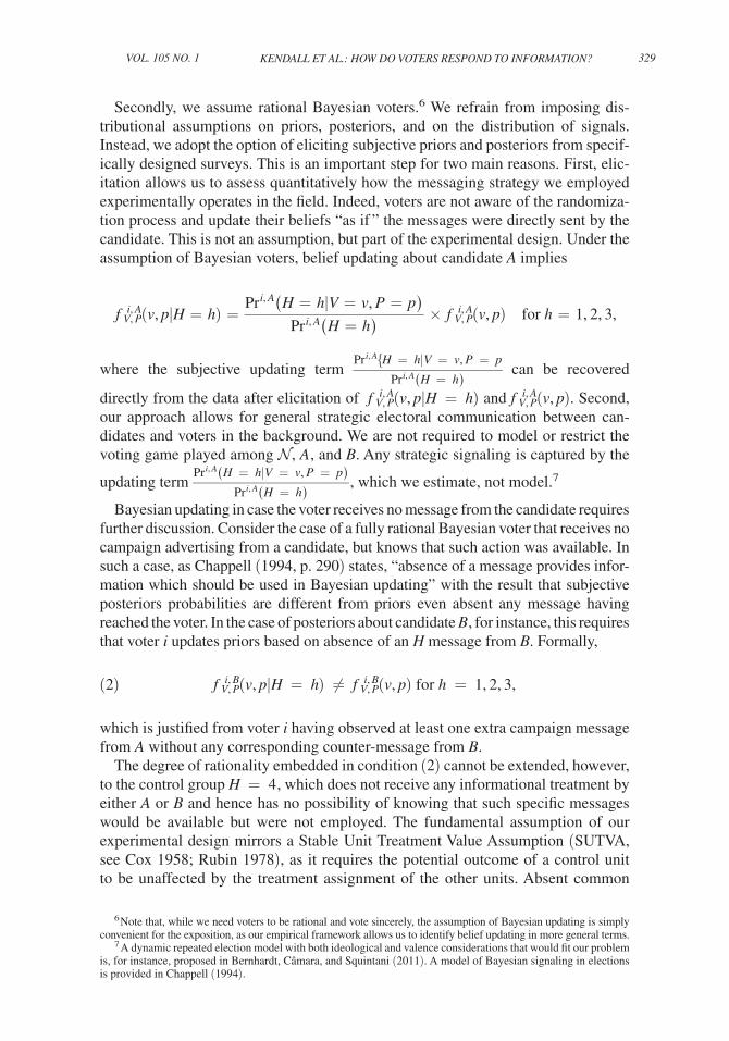
Secondly, we assume rational Bayesian voters.6 We refrain from imposing dis-tributional assumptions on priors, posteriors, and on the distribution of signals. Instead, we adopt the option of eliciting subjective priors and posteriors from specif-ically designed surveys. This is an important step for two main reasons. First, elic-itation allows us to assess quantitatively how the messaging strategy we employed experimentally operates in the field. Indeed, voters are not aware of the randomiza-tion process and update their beliefs “as if ” the messages were directly sent by the candidate. This is not an assumption, but part of the experimental design. Under the assumption of Bayesian voters, belief updating about candidate A implies

f V, P i, A (v, p|H = h) = Pr i, A ( H = h|V = v, P = p) _____________________

Pr i, A ( H = h)

× f V, P i, A (v, p) for h = 1, 2, 3,

where the subjective updating term Pr i, A { H = h|V = v, P = p

________________ Pr i, A ( H = h)

can be recovered

directly from the data after elicitation of f V, P i, A (v, p|H = h) and f V, P i, A (v, p) . Second, our approach allows for general strategic electoral communication between can-didates and voters in the background. We are not required to model or restrict the voting game played among , A , and B . Any strategic signaling is captured by the

updating term Pr i, A ( H = h|V = v, P = p) _________________

Pr i, A ( H = h) , which we estimate, not model.7

Bayesian updating in case the voter receives no message from the candidate requires further discussion. Consider the case of a fully rational Bayesian voter that receives no campaign advertising from a candidate, but knows that such action was available. In such a case, as Chappell (1994, p. 290) states, “absence of a message provides infor-mation which should be used in Bayesian updating” with the result that subjective posteriors probabilities are different from priors even absent any message having reached the voter. In the case of posteriors about candidate B , for instance, this requires that voter i updates priors based on absence of an H message from B . Formally,

(2) f V, P i, B (v, p|H = h) ≠ f V, P i, B (v, p) for h = 1, 2, 3,

which is justified from voter i having observed at least one extra campaign message from A without any corresponding counter-message from B .

The degree of rationality embedded in condition (2) cannot be extended, however, to the control group H = 4 , which does not receive any informational treatment by either A or B and hence has no possibility of knowing that such specific messages would be available but were not employed. The fundamental assumption of our experimental design mirrors a Stable Unit Treatment Value Assumption (SUTVA, see Cox 1958; Rubin 1978), as it requires the potential outcome of a control unit to be unaffected by the treatment assignment of the other units. Absent common

6 Note that, while we need voters to be rational and vote sincerely, the assumption of Bayesian updating is simply convenient for the exposition, as our empirical framework allows us to identify belief updating in more general terms.

7 A dynamic repeated election model with both ideological and valence considerations that would fit our problem is, for instance, proposed in Bernhardt, Câmara, and Squintani (2011). A model of Bayesian signaling in elections is provided in Chappell (1994).


shocks, we should assume that for H = 4 the posterior distribution is identical to the prior distribution, that is, for every i ∈ (4) , f

V, P i, j (v, p|H = 4) = f

V, P i, j (v, p) ,

with j = A, B .More generally, we consider a process of Bayesian updating which accommodates

common shocks across voters, under the (testable) assumption that the subjective probabilities on such shocks are identical across all i ∈ and independent of H . Consider, for instance, the case of posteriors elicited after a common informational shock, W , which can be thought of as the general campaign carried out by the can-didates besides the informational messages from A that we randomize at the margin. With respect to candidate j , voter i will be characterized by the following posteriors.

ASSUMPTION 1 (SUTVA):

f V, P

i, j (v, p|H = h, W) = Pr i, j ( H = h|V = v, P = p)

___________________ Pr i, j ( H = h)

× Pr j (W|V = v, P = p)

_______________ Pr j (W )

× f V, P

i, j (v, p) for h = 1, 2, 3; j = A, B

and

f V, P

i, j (v, p|H = 4, W) = Pr j (W|V = v, P = p) _________________

Pr j (W ) × f

V, P i, j (v, p) for j = A, B.

The credibility of Assumption 1 crucially rests on the experimental design described in Section II and is empirically validated in Section III.

Finally, the elicitation of multivariate beliefs, even on expert subjects, is not an obvious exercise (see Kadane and Wolfson 1998; Garthwaite, Kadane, and O’Hagan 2005) and is the object of a vast literature bordering statistics and psychology (dat-ing at least as far back as Savage 1971). We outline our approach next.

C. Elicitation of Multivariate Beliefs

Elicitation of beliefs and priors is increasingly common in economics and politi-cal science, and is standard in psychology and statistics.8 We describe a transparent protocol of elicitation we designed to be robust to the behavioral and technological constraints we face. Specifically, we sampled a large number of voters and need to elicit multivariate beliefs from each.

For each main candidate j = A, B and each voter i , joint valence and ideology subjective priors f

V, P i, j (v, p) and posteriors f

V, P i, j (v, p|H = h) are defined over Λ × Π .

In the remainder of this subsection, let us focus for brevity on the elicitation of subjective priors, with the understanding that the same process applies to posteri-ors. In the empirical analysis we will fix the cardinality of both Λ and Π to small integer figures, based on Miller (1956), and a large body of cognitive psychology suggesting that individuals can be quite precise in evaluating choices on relatively coarse unidimensional supports, but display hardly any precision on finer supports.

8 For recent examples in economics, see Dominitz and Manski (1996); Manski (2004); Blass, Lach, and Manski (2010); and Zafar (2009). See Gill and Walker (2005) and Duffy and Tavits (2008) for applications in political science.


Specifically, for reasons explained below, we assume the cardinality of Π to be equal to 5 and the cardinality of Λ to be equal to 10.

It is evident, however, that even for |Π| = 5 and |Λ| = 10 , “brute force” elicita-tion for both candidates would require each responder to answer 5 × 10 × 2 = 100 different questions on the subjective likelihood of each specific (v, p) realization, an effort which would likely frustrate political experts, let alone regular voters. Garthwaite, Kadane, and O’Hagan (2005) present an insightful discussion on the difficulty of elicitation for multivariate priors. To this issue, the reader versed in elic-itation may add the problem of effectively training telephone interviewers in the con-sistent elicitation of joint probabilities.9 Therefore, we follow an alternative route.

Marginal Belief Distributions.—We first focus on information more easily elicit-able from voters: the univariate marginals f

V i, j (v) and f

P i, j (p) . Even in this case, full

elicitation of marginals would require a large set of (|Π| + |Λ|) × 2 = 30 ques-tions. We streamline the process in order to maintain feasibility without excessive sacrifice of accuracy. We start by imposing a simple regularity assumption on the distribution of beliefs.

ASSUMPTION 2: Subjective belief distributions are unimodal.

Although restrictive, this assumption makes the interpretation of the elicited prob-abilities more direct. All of our remaining distributional assumptions can be illus-trated using the questions in our surveys by way of example. We focus only on A for brevity and consider first his ideological position P . We inquire about the central tendency of the marginal prior on ideology as follows.

Q1: How would you most likely define candidate A’s political position? Left (1); Center-Left (2); Center (3); Center-Right (4); Right (5); Don’t Know (−999).

A reasonable interpretation of the answer, with minimal confusion for the respon-dent, is that the mode is elicited. In particular, we allow the mode, p ˆ , to be only one of these five categories.

ASSUMPTION 3: Π = {1, … , 5} .

An answer of “Don’t Know/Don’t Know A ” implies flat priors, or f P i, A (p) = 1/|Π| = 0.2 for every p . Our choice of the set Π follows the established result in cognitive psychology that individuals are well versed in choices over discrete sets of limited dimensionality ( |Π| ≤ 10 ), but that this capacity deteriorates sharply when the number of options rises above small integers (Miller 1956). Such an assumption, however, has costs, as emphasized in Manski and Molinari (2010).

9 While the use of telephone interviews is not generally necessary, in our context it is was required to ensure timely elicitation of a large sample of the voting population as close as possible to election day.


Conditional on non-flat priors, we further inquire about the dispersion around the mode.10

Q2: How large is your margin of uncertainty around candidate A’s political posi-tion? Certain (1); Rather uncertain, leaning left (2); Very uncertain, leaning left (3); Rather uncertain, leaning right (4); Very uncertain, leaning right (5).

We indicate the level of increasing tightness of the priors with s ∈ Σ = {1, … , 4} , where s = 1 is maximal dispersion, i.e., the case of flat priors; s = 2 indicates substantial uncertainty (answers 3 or 5 to Q2); s = 3 indicates intermediate uncer-tainty (answers 2 or 4 to Q2); and s = 4 is maximal tightness, which coincides with a degenerate prior spiking at p ˆ (answer 1 to Q2). Q2 also elicits information about the skew of the beliefs. While we do not allow explicitly for an answer of symmetric dispersion for s = 2, 3 , not to overload the responder, the estimation below allows for symmetric belief distributions.11 Let us indicate with z ∈ {−1; 1} a negative (i.e., to the left) or positive (i.e., to the right) asymmetry in Q2.

Let us define the modal probability mass with ϕ P = f P i, A (p = p ˆ ) . Intuitively, we assume the probability mass at the mode f P i, A (p = p ˆ ) is lower the higher the level of uncertainty. We allow ϕ P to vary with s and estimate ϕ P, s , from the data for s = 2, 3 , imposing the bounds:

ASSUMPTION 4: 1/|Π| ≤ ϕ P, 2 ≤ ϕ P, 3 ≤ 1.

We further assume the off-mode mass, 1 − ϕ P, s , to be allocated asymmetrically around the mode depending on the indicated asymmetry, z . We assume the off-mode mass decays proportionally to the distance |p − p ˆ | from the mode at a con-stant rate, as dictated by a function g( x 1 , x 2 ): {1, … , |Π| − 1} × [0, 1] → [0, 1] with g x 1 ( x 1 , x 2 ) ≥ 0 and g x 2 ( x 1 , x 2 ) ≤ 0 .

ASSUMPTION 4′: f P i,A (p ≠ p ˆ ) = ⎧

⎪

⎨ ⎪

⎩ 1/|Π|

g( ϕ P,s , z × (p − p ˆ )) 0

for s = 1

for s = 2,3 for s = 4.

Concerning g(·) , we allocate α P (1 − ϕ P, s ) mass in the direction of the asymme-try imposing that α P ∈ [1/2, 1] , and allocate (1 − α P ) (1 − ϕ P, s ) in the opposite direction, assuming a linear decay of the off-mode mass in both directions. This specification of g allows for a very flexible, but parametrically parsimonious mar-ginal distribution.

Concerning the valence dimension V , we again inquire about the modal belief.

10 Interviewers were trained during pilot interviews to explain to voters that this question entailed uncertainty about subjective evaluations, and should not be interpreted as a right-or-wrong question.

11 In our surveys, we actually included a possible answer “uncertain” to assess the share of respondents indicat-ing symmetric dispersion around the mode. The share of respondents in that category was so low for ideology (and actually none for valence) that we omit it from exposition.


Q3: Setting aside his/her political position, how would you most likely grade can-didate A? From 1 (minimum competence) to 10 (maximum competence) or Don’t Know (−999).

The set Λ is then assumed to be as follows:

ASSUMPTION 5: Λ = {1, … , 10} .

This particular format of Q3 was driven by the familiarity of Italian voters with primary and secondary education grade scoring rules, with 10 indicating the best possible mark in a school assignment and failing grades being below 6 . The dis-persion around the valence mode and the skewness of valence beliefs are modeled similarly to Assumptions 4 and 4′ with Λ replacing Π in the construction of f V i, A (v) . We omit their description for brevity. For illustrative purposes, online Appendix Figure A1 provides an example of the modeled prior beliefs about the valence of A for one particular voter. The distribution in the figure is based upon the voter’s reported mode ( p ˆ = 7 ) and uncertainty ( s = 2 ) and the estimates we obtain for the parameters governing the distribution.

Finally, we must emphasize that we only elicit the beliefs about valence and ideol-ogy for the incumbent candidate, A , and his main challenger, B , due to the infeasibility of eliciting beliefs about all minor, third-party candidates participating in the elec-tion. In our estimation in Section IV, we assume that the beliefs of all non-incumbent candidates are the same as those elicited for the main challenger, B . While this is a stark assumption, we justify it by the fact that the main non- incumbent candidates were ideologically similar and their qualities were relatively unknown (flat beliefs along the valence dimension are quite common for non- incumbent candidates).12

Joint Belief Distributions: A Copula-Based Approach.—Having derived the univar-iate marginals, we now derive the joint distributions for all voters. Given any two (uni-variate) marginals, it is possible to construct a joint (bivariate) distribution in infinite ways. Copulas, introduced by Sklar (1959), are useful devices for providing a repre-sentation of a multivariate distribution in terms of its univariate marginal distributions.

Dropping the superscripts, given cumulative marginals, F V (v) = Pr (V ≤ v) and F P (p) = Pr (P ≤ p) , a copula function C satisfies F V, P (v, p) = C( F V (v), F P (p)) where F V, P (v, p) = Pr (V ≤ v, P ≤ p) is the joint cumulative distribution func-tion. C is unique for continuous densities. For discrete densities, as in our setting, typically the same joint distribution can be represented by different copulas, but a specific copula uniquely identifies a joint distribution. The marginal distributions carry all of the information related to the scaling and shape of the joint distribu-tion function, while the copula function incorporates the information concerning the dependence relationship among the random variables. For parsimony, we will focus on copula families characterized by one dependence parameter. Notice, however, that the dependence parameter does not coincide with a linear correlation parameter; nonlinear dependence is accommodated as well.

12 The main third-party challenger was also right-wing, like B , but was sidelined by their party due to pending legal litigation related to his previous stint in office. See Section II for more institutional details.


We investigate three popular types of copulas, allowing for different degrees of association ρ between V and P . First, independence between V and P produces the intuitive copula F V, P (v, p) = F V (v) × F P (p) . Second, we allow for common dependence across surveyed voters, given by association parameter −1 ≤ ρ ≤ 1 , employing the Farlie-Gumbel-Morgensen (Farlie 1960) family copula, F V, P (v, p) = F P (p) × F V (v) × (1 + ρ(1 − F P (p)) × (1 − F V (v))) , where ρ > 0 implies positive dependence and ρ < 0 negative dependence. Potentially, ρ could be made voter-type dependent (e.g., allowing for a different ρ for left- and right-wing voters), but not voter-specific. The FGM family is flexible, but allows only small departures from independence. The third type of copula family we consider is the Frank family, F V, P (v, p) = 1/ξ × log (1 + D(ξ)) , with D(ξ) = ( e ξ F P (p) − 1)( e ξ F V (v) − 1)/( e ξ − 1) and ρ = −ξ . The Frank family allows larger departures from independence and requires ρ ≠ 0 . Indeed, the Frank copula is well suited to model outcomes with strong positive or negative dependence.

The dependence parameter ρ is not elicited from the survey, but can be estimated. Recall that we observe vote decisions and such decisions are function of voters’ posteriors. Given a copula family, we can estimate a dependence parameter ρ , as part of the vector θ , by maximizing the likelihood of observing those votes as in equation (1). One can further employ standard generalized likelihood ratio tests to assess the relative quality of the assumptions on the copula family and select the preferred family. We follow this approach.

To sum up, our parameters of interest are θ = [ β A , β B , γ, ζ, χ, θ′ ] with belief parameters θ′ = [ ϕ P, 2 , ϕ V, 2 , ϕ P, 3 , ϕ V, 3 , α P , α V , ρ A , ρ B ] , where we allow the asso-ciation parameter to differ for A and B . Estimating θ′ from vote decisions is only feasible for the posterior joint distribution. The prior joint distribution can be char-acterized under an additional assumption.

ASSUMPTION 6: Subjective belief distributions have constant θ′ .

In particular, while we allow marginals to be affected by our informational treatment, we assume that the dependence between ideology and valence of the candidate is con-stant. For example, assuming that a moderate policy stance is positively correlated with smarter candidates, information that moves subjective priors toward higher levels of valence V is allowed to have an impact on the policy stance P , pushing it toward a more moderate stance, but it is not allowed to change the association between P and V .13

Online Appendix Figures A2 and A3 provide an example of the joint distributions for a particular voter’s beliefs about candidate A prior to the election campaign and after receiving the valence message treatment. Each joint distribution is determined assuming independence of the marginals and based on the estimates of the param-eters governing the marginal distributions. For this particular voter, receiving the valence message increased his belief about the valence of A and also reduced the uncertainty along both dimensions. In Section V, we will see that such changes in beliefs are representative of voters receiving the valence message treatment.

13 As an alternative to Assumption 6, one could calibrate ρ j for the prior distribution at specific values and observe the sensitivity of the results. A natural range of values could be the confidence interval of the dependence parameter for the posteriors. We do not pursue this avenue here.


II. Experimental Design

In May 2011, in collaboration with the reelection campaign of the incumbent mayor in the Italian city of Arezzo, we implemented the experimental strategy embedded in the above empirical model during the mayor’s actual electoral campaign. Specifically, we divided the city into four areas, randomizing at the precinct level, and the incum-bent sent different campaign messages both by mail and by phone call to voters in these areas. In this section, we describe the institutional setting, the experimental protocol, and the characteristics of the (randomized) campaign messages and tools.

A. Institutional Setting

In Italy, mayors of cities with more than 15,000 inhabitants are directly elected under plurality rule with runoff, that is, in the first round the candidate who obtains more than 50 percent of the votes is elected, otherwise the two candidates receiv-ing the most votes compete in a second round which takes place two weeks later. Mayoral candidates are supported by one or more party lists, but voters can cast separate votes for a candidate and a party list supporting another candidate. They can also vote only for a mayoral candidate, without expressing any preference for party lists, but the opposite is not allowed, because valid votes for a party list are automatically attributed to the candidate for mayor supported by that party.

Elected mayors serve a five-year term and are subject to a two-term limit. Italian municipalities are in charge of a wide range of services, from water supply to waste management, from municipal police to infrastructures, and from housing to welfare policies. Mayors are the key political players at the local level, as they can also appoint the executive officers and dismiss them at will. The city council, which acts as the legislative body, can force the mayor to resign with a no confidence vote, but in this case the council is also dissolved. Municipal elections have high salience and turnout is usually large.

Arezzo is a provincial capital city in the center of Italy, located in the province of the same name. In 2011, it had 100,455 inhabitants and 77,386 eligible voters. For electoral purposes, the city is divided into 95 precincts (the smallest electoral unit which usually coincides with a cluster of streets), which vote in 42 polling places (e.g., schools, public buildings). From a political point of view, the city was contestable. Giuseppe Fanfani, the incumbent mayor elected in 2006 who accepted randomization of a part of his reelection campaign, belonged to the center-left coa-lition, but before his first election the center-right coalition won for two terms in a row. In 2011, his main challenger was the official candidate of the center-right coa-lition, Maria Grazia Sestini, a former vice minister at the national level. Six other (minor) third-party candidates were also present in the ballot. The main third-party candidate was a former mayor of the center-right coalition, Luigi Lucherini, side-lined by his party due to pending legal trouble.14

14 The mayor of Arezzo (Mr. Fanfani) accepted our proposal to randomize his campaign not only because of a personal relationship and of his interest in receiving professional advice, but also because of the opportunity to collect potentially useful information in case of runoff. As the center-right coalition was split between a main chal-lenger (Ms. Sestini) and a less competitive one (Mr. Lucherini), the mayor expected either to win his reelection bid at the first round or to go to the second round for a runoff with Ms. Sestini. Therefore, our randomized trial could


Local political campaigns are not very sophisticated in Italy, and they mostly rely on public rallies, direct mailing, and TV appearances (but no ads). Phone banks are rarely used, and door-to-door canvassing almost never occurs.

B. Randomized Campaign

To operationalize our informational treatments, we studied the campaign mate-rials of the incumbent and assembled relevant information so as to isolate slogans based on either his competence as city manager (valence message) or his political stance (ideology message). Because we wanted to stay away from the strategic game between him, the other candidates, and the voters, we actually devised two different ideological messages: one leaning toward the left and one toward the center of the political spectrum. We then allowed him to choose between the two and he selected the left-leaning message.

Furthermore, although our treatment of interest coincides with partisan campaign messages delivered by one of the candidates, as opposed to non-partisan informa-tion, we wanted our informational treatments to be factual and non-emotional.15 For this reason, we matched the main slogans with bullet points based on verifiable information about the incumbent’s performance and policy choices during his first term in office. Future research should extend to emotional messages as well, but we did not explore this avenue here.

Online Appendix Figures A4 and A5 show the mail flyers containing the two mes-sages.16 The valence flyer is built around two keywords: competence and effort. The implicit message is that voters should reelect the incumbent because he was competent and effective as city manager. The factual information provided refers to the fact that Arezzo developed an urban development plan that was ranked first by the regional government and received extra funding because of its quality. The extra funding was used to rebuild monuments, roads, and parking slots in the city center. The ideology flyer is built around two keywords: awareness and solidarity. The implicit message is that voters should reelect the incumbent because he shares values that are commonly associated with the Italian left. The bullet points further reinforce the leftist tone as they point to “public” services, such as three childcare centers and food and housing facilities for the poor, which were expanded during his first term in office. Notice that the two mail flyers are identical in size, layout, colors, fonts, number of words, and photo of the candidate; only the content of the campaign message differs.

Clearly, in a laboratory experiment, we could have made the difference between the two messages even more extreme. In our case, however, obtaining the candi-date’s approval was crucial not only to implement the field experiment, but also to

provide him with an effective strategy for campaigning in the two weeks between the first and the second round, which in the end did not take place (see below).

15 The marketing and advertising literature (see Liu and Stout 1987) has explored subjective responses to factual versus emotional or non-factual messages, indicating systematic differences.

16 In the online Appendix, we report the English translation of the text of the flyers. Additional materials related to our randomized campaign (including the additional ideology message discarded by the candidate) can be found at www.igier.unibocconi.it/randomized-campaign.

www.igier.unibocconi.it/randomized-campaign


minimize intrusiveness and enhance its external validity, as our treatment of interest is the message sent by a politician during a real electoral campaign.17

The two campaign messages—valence and ideology—were supplied to voters in two ways, through direct mailing and phone calls. The randomization design was implemented as follows. We randomly divided the 95 precincts into four groups: (i) 24 precincts received the valence message; (ii) 24 precincts received the ideol-ogy message; (iii) 24 precincts received both messages; (iv) 23 precincts received no message (control group). Furthermore, we randomly split the first three groups into two subgroups: in the first, the treatment was administered by both direct mail and phone calls (12 precincts); in the second, by direct mail only (12 precincts).18 The candidate did not know the outcome of the randomization, as we were in charge of managing this part of his campaign once he approved the ads.

Online Appendix Table A1 reports the ex ante balance tests of predetermined variables at the precinct level. The available variables include the number of eli-gible voters, the neighborhood each precinct belongs to, and the past outcomes of national, regional, European, and municipal elections. As precincts were reshuffled in the last decade, some outcomes are not available for all precincts. All of the variables are balanced across treatment groups. Only the number of eligible voters displays a coefficient significant at the 10 percent level, because of the presence of a few small precincts in the countryside that could not be spread across all groups. Removing these precincts from the analysis, however, does not alter the results.

In order to increase the effectiveness of the campaign messages, we drew use-ful insights from the US experimental evidence summarized by Green and Gerber (2004). First, we acted in the week before election day. Second, we had our mail flyers designed by professionals and directly sent to individuals with their name and address on the envelope.19 Third, we did not use automated robocalls. We instead trained volunteers to make the campaign phone calls. Specifically, volunteers called all selected households with the following protocol: first, they were instructed to talk with the voters and ask for their opinion for about two minutes. Then, they would ask the voter to listen to a recorded message from the candidate. At the end of the call, the recorded voice of the candidate read a 30-second script with the above valence and ideology messages (or a combination of the two).20

Our randomized campaign used the above tools—mailers and phone calls—on a large scale. All households in the city received an envelope from the incumbent campaign. The envelope contained the official platform of the political parties

17 To validate our operationalization of the two informational treatments ex ante, we randomly assigned the two flyers to 50 university students at Bocconi University (in Milan) who did not know the mayor of Arezzo. We then asked them to give their subjective assessment of the politician’s valence and ideology using the same survey ques-tions described in Section I. For the 25 students who received the valence message, the average valence evaluation was 6.650 out of 10 (s.d. 0.963) and the average ideology evaluation was 3.100 (s.d. 0.700), recalling that 3 is the exact ideological center. For the 25 students who received the left-leaning message, these values were 5.450 (s.d. 0.973) and 2.050 (s.d. 0.669), respectively, so clearly to the left in the ideology spectrum and close to the valence midpoint, essentially validating our treatment design (and in line with our findings, as reported in what follows).

18 As we were already pushing the boundaries in terms of sample size, we decided that the accuracy loss could not justify an additional subgroup treated by phone calls only.

19 To avoid sending multiple envelopes to the same household, we randomized the name of the receiver within each household, because we did not want to target only household heads.

20 In the online Appendix, we report the English translation of the text of the three recorded messages. Original audio files are available at www.igier.unibocconi.it/randomized-campaign.

www.igier.unibocconi.it/randomized

www.igier.unibocconi.it/randomized-campaign


supporting the candidate plus one of our flyers (or both of them) according to the assigned treatment group. Voters in the control group received just the platform, but not the flyer with our informational treatment. This procedure allowed us to keep the candidate unaware of the randomization outcome. Clearly, the candidate approved all messages and paid for the costs of the campaign, but we gave him closed enve-lopes so that he could not infer which precincts were receiving one flyer as opposed to the other. In summary, all households with at least one member enlisted as an eli-gible voter received our mailers. On top of this, about 25 percent of the households in the treatment groups also received a campaign phone call.21

Our mailers were the only informational material sent by the incumbent. The oppo-nent also sent flyers by mail, emphasizing her previous experience as a vice-minister in the Italian government and her commitment to traditional family values. Our campaign phone calls were the only calls that the households received from both candidates, as the opponent did not use this campaigning technology. Furthermore, both the incumbent and the opponent campaigned in the city (town hall meetings) and in the public media (TV appearances and newspaper interviews). The above context has implications for the external validity of our findings, as mailers and phone calls might have different effects in more sophisticated environments (e.g., political campaigns where social media and canvassing are also used). Yet, such a context shares many features with local campaigns in most democracies, where budget and professional constraints limit the degree of sophistication.

C. Data

To elicit beliefs about the valence and ideology of the two main candidates along the lines described in Section I, we ran two surveys of 2,042 eligible voters distrib-uted across all treatment groups. We ran the first survey ten days before the election and, most importantly, before voters received the informational treatments, so as to measure priors and demographic characteristics. The second survey was conducted the day after the election and was meant to measure posteriors and (self-declared) vote choices. To implement our surveys, we contracted a company from another Italian region, so as to have interviewers with a different accent from the campaign volunteers and to remove any link between the campaign and the survey phone calls. Moreover, the script did not link the survey in any way to a political party or campaign. About 71 percent of the respondents in the first survey also replied to the question about whether they voted or not in the second survey. Therefore, our sample is made up of 1,455 voters, 1,306 of whom actually voted for one of the candidates. However, 231 of the 1,306 voters did not specify for which candidate they voted and for this reason we accommodate for potentially non-random non-responses in the model estimation.

To further validate our randomization design ex post, we checked for balancing of the characteristics of voters across treatment groups. Survey variables include demo-graphic characteristics, educational attainment, political orientation, home owner-ship, and how often voters read newspapers or watch TV. The results are reported in

21 Because of budget and time constraints, we could not reach all households by phone.


online Appendix Table A2. None of these (self-declared) individual characteristics is statistically different across treatment groups.22

Table 1 summarizes the aggregate results at the precinct level. The incumbent mayor obtained a share of 49.6 percent over all votes, which was enough to win his bid for reelection at the first round with a vote share 51.3 percent over valid votes. Table 2 shows the vote declarations of surveyed individuals. As often happens in post-electoral polls, there is a slight bandwagon effect in favor of the winning can-didate (57.1 percent). The bandwagon is not a concern for estimation under the (plausible) assumption that this effect is orthogonal to our treatment groups. In any case, recall that a strength of our approach is that we can cross-validate the consis-tency of treatment effects in the survey data (at the individual level) with those in the aggregate actual voting data (at the precinct level).

III. Evidence on Choices

In this section, we evaluate the effects of our informational treatments on voting choices at both the precinct and individual levels. Based on the experimental design described in the previous section, the (reduced-form) causal effects of campaigning on valence versus ideology can be estimated through the OLS model

(3) Y i = ∑ k=1

6 γ k D i k + η i ,

22 As an additional ex post validation of the randomization design, we built proxies of census characteristics at the precinct level. This exercise has two limitations, however. First, data from the last available census refer to 2001. Second, precincts are not easily matchable with census cells. To overcome the second limitation, we implemented the following geocoding procedure: (i) for each street (i.e., line) belonging to a precinct we calculated the weighted average of the characteristics of the census cells (i.e., polygons) overlapping with that street (with weights equal to the overlapping segments); (ii) for each precinct, we calculated the weighted average of the characteristics of the associated streets (with weights equal to the population living in each street). Online Appendix Table A3 reports the balancing tests of these census characteristics across treatment groups. Although these estimates are likely to suffer from attenuation bias due to measurement error, none of them is statistically different from zero.

Table 1—Aggregate Outcomes at a Glance

Mean Median SD Min Max Obs.

Turnout 0.708 0.714 0.050 0.389 0.788 95Incumbent share 0.496 0.492 0.059 0.344 0.629 95Incumbent parties 0.451 0.444 0.056 0.295 0.583 95

Notes: Descriptive statistics at the precinct level of the variables specified in the first column. “Incumbent parties” refer to the vote shares of the party lists supporting the incumbent.

Table 2—Vote Declarations at the Individual Level

Mean Median SD Min Max Obs.

Declared turnout 0.898 1.000 0.303 0.000 1.000 1,455Declared vote for the incumbent 0.571 1.000 0.495 0.000 1.000 1,306Declared vote for incumbent parties 0.493 0.000 0.500 0.000 1.000 1,306

Notes: Descriptive statistics at the individual level of the variables specified in the first column. “Incumbent parties” refer to the (self-declared) votes in favor of the party lists supporting the incumbent.


where Y i is the electoral outcome of interest, D i k are binary indicators capturing treatment group status, and η i is the error term.23 The six treatment groups, D k , include: valence message by phone (and mail); valence message by mail only; ide-ology message by phone (and mail); ideology message by mail only; double mes-sage by phone (and mail); and double message by mail only. Observations receiving no informational treatment are therefore the excluded reference group.

Table 3 summarizes the results in the aggregate sample, whose units of observa-tion are the 95 electoral precincts. Partisan ads have no impact on turnout. There is evidence, however, that campaigning on valence brings more votes to the incumbent when phone calls are used as a campaign tool. Phone calls delivering the valence message increase the incumbent’s vote share by 4.1 percentage points (i.e., by about 8.4 percent with respect to the average share in the control group). The estimated effect is sizable, because it must be interpreted as an intention-to-treat effect: in fact, only 25 percent of the households in the treated precincts received a campaign phone call and not all of them listened to the message recorded by the candidate. Because of the small sample size, however, coefficients are not precisely estimated and we cannot reject the null hypothesis that they are statistically equal to each other.

What we can reject in the aggregate data is the null that the two campaign tools—mailers versus phone banks—are equally effective. If we merge together all groups that received an informational treatment with the same campaign tool, we find that—with respect to the control group—phone calls increase the incumbent vote share by 2.7 percentage points (p-value: 0.019), while, statistically, the effect of mailers is both different from 2.7 and not different from zero. This result is in line with US experimental evidence showing that mailers are usually ineffective in polit-ical campaigns (see Green and Gerber 2004). In our case, however, mailers are also administered to voters who receive a phone call. Therefore, we cannot rule out the

23 To account for potential intra-class correlation between neighboring precincts we cluster standard errors at the polling place level, while to account for correlated time shocks in survey data we include fixed effects for the inter-view date; results are not sensitive to these modeling choices. Empirical results are qualitatively similar when we include predetermined variables as additional covariates, although the specification becomes demanding in terms of degrees of freedom in the aggregate data (results available upon request).

Table 3—Reduced-Form Aggregate Estimates, All Groups

Reference group: no message

Valenceby phone

Valenceby mail

Ideologyby phone

Ideologyby mail

Doubleby phone

Doubleby mail

Turnout −0.011 −0.000 0.013 0.010 −0.006 −0.006[0.031] [0.015] [0.011] [0.013] [0.009] [0.013]

Incumbent share 0.041** 0.004 0.013 0.021 0.027* −0.023[0.019] [0.025] [0.016] [0.025] [0.015] [0.015]

Incumbent parties 0.032* 0.018 0.015 0.029 0.021 −0.015[0.018] [0.023] [0.016] [0.026] [0.014] [0.015]

Notes: Observations: 95 precincts. OLS coefficients reported; dependent variables in row headings and treatment groups in column headings. Robust standard errors clustered at the polling place level in brackets.

*** Significant at the 1 percent level. ** Significant at the 5 percent level. * Significant at the 10 percent level.


possibility that mailers alone are ineffective, but they become effective when inter-acted with other campaign tools delivering the same message.

Based on the above evidence on the ineffectiveness of mailers alone, online Appendix Table A4 estimates equation (3) imposing this restriction: including both “mail” and “no message” in the control group. Standard errors are slightly lower, and the point estimates and the statistical significance of the regressors are almost identical with respect to the full model.

In order to validate the aggregate evidence and to gain statistical accuracy, we esti-mate equation (3) using the individual-level survey data, where sample size is less of an issue. The units of observation are 1,455 eligible voters for turnout or 1,306 actual voters for the vote shares. As the treatment was administered at the precinct level, we cluster standard errors by precinct.24 Estimation is by probit, as all out-comes are binary. The price we pay is that here outcomes are self-reported, that is, based on vote declarations and not on actual choices.25 Table 4 reports the estimates for all treatment groups. Results are consistent with the aggregate evidence. Phone calls on valence increase the incumbent’s vote share by 9.5 percentage points (i.e., by about 16 percent with respect to the control group). This effect is larger than in the aggregate data, but treatment intensity is also higher here, because all surveyed households received the campaign phone call, as opposed to only 25 percent in the aggregate data. Phone calls are still the most effective campaign tool (significant at the 1 percent level). More importantly, conditional on campaign tool, the valence message is now statistically more effective than the ideology message at the 10 percent level. Online Appendix Table A5 further emphasizes this point by focusing on treatments administered by phone: campaigning on valence brings more votes to the incumbent and his parties, and these point estimates are statistically larger than those of campaigning on ideology alone.

24 Results are identical if we cluster standard errors at the polling place level (available upon request). 25 The underlying assumption is that self-reporting bias is the same across treatment groups. As we document in

the next section, non-response in vote declarations is likely to be non-random, i.e., to be associated with individual characteristics such as ideology or prior beliefs. This does not imply, however, that (non-random) non-response should not be orthogonal to (random) treatment assignment.

Table 4—Reduced-Form Individual Estimates, All Groups

Reference group: no message

Valenceby phone

Valenceby mail

Ideologyby phone

Ideologyby mail

Doubleby phone

Doubleby mail

Turnout −0.024 −0.019 0.006 0.033 −0.019 −0.003[0.027] [0.034] [0.026] [0.022] [0.028] [0.029]

Incumbent share 0.095** −0.061 0.018 −0.028 0.035 0.004[0.039] [0.049] [0.049] [0.043] [0.050] [0.050]

Incumbent parties 0.109*** −0.007 −0.008 −0.044 0.009 −0.014[0.040] [0.060] [0.061] [0.046] [0.051] [0.049]

Notes: Observations: 1,455 eligible voters (turnout); 1,306 actual voters (vote shares). Prohibit marginal effects reported; dependent variables in row headings and treatment groups in column headings. Fixed effects for survey date included. Robust standard errors clustered at the precinct level in brackets.



With respect to both actual vote shares and vote declarations, the double mes-sage—valence plus ideology—seems ineffective. This (apparently) puzzling result might depend on the operationalization of our campaign phone calls. In order to limit each candidate’s recorded message to 30 seconds, we had to condense the valence and ideology messages into a short script for the candidate (see online Appendix Section A2 for the text). It is thus possible that the informational content of the double message was attenuated along both dimensions, or that multiple simultaneous mes-sages confused the receiver (akin to consumer confusion in the marketing literature).

Finally, in online Appendix Table A6, we evaluate the potential impact of spillovers across neighboring precincts. As a counterpart to Table 4, we estimate the effects on voting choices of the average treatment intensity in the same polling place, merging together precincts in different treatment groups. If Assumption 1 (SUTVA) is met, we expect these measures to have no impact on choices for treatments detected as ineffective in Table 4, and to have a less significant impact for treatments detected as effective. It is thus reassuring that none of these spillover estimates is statistically different from zero.26

IV. Model Estimation

We now report the results from the maximum likelihood (ML) estimation of our voting model. The ML procedure relies on directly fitting individual vote decla-rations, which—in Section III—we have shown to closely match actual vote out-comes.27 The specification selection warrants some discussion, however.

Section I discussed non-response parameters [ β A , β B ] , preference parameters [γ, ζ, χ] , belief parameters [ ϕ P, 2 , ϕ V, 2 , ϕ P, 3 , ϕ V, 3 , α P , α V , ρ A , ρ B ] , and the choice of a copula family [Independent; Frank; FGM] . Concerning the preference parameters, a large literature in political economics and political science has emphasized prefer-ence heterogeneity, for instance in the case of distaste for specific policy outcomes, such as inflation or unemployment.28 We can easily accommodate this feature by allowing a different [γ, ζ, χ] vector for left-wing (L), centrist (C), and right-wing (R) voters. We can as well accommodate heterogeneity in the dependence structure of the beliefs [ ρ A , ρ B ] by allowing them to differ for L, C, and R voters. Concerning the skewness of the marginal beliefs, one can experiment with relaxing the simple [ α P , α V ] to a more flexible [ α P, 2 , α V, 2 , α P, 3 , α V, 3 ] , thus allowing the extent of the skew to change with the variance. All these are testable parametric constraints that can be formally assessed based on likelihood ratio tests. On the other hand, the

26 Note that point estimates are not directly comparable with those in Table 4 because the regressors are no lon-ger dummies but shares. Compared to the average values and standard deviations of the spillover shares, however, estimates are generally small, and—as expected—they are larger for the valence message by phone, because in those cases the shares also include treated voters for whom a nonzero effect is at work.

27 The identification of the model is assessed through several rounds of Monte Carlo simulations. For given parameter values we simulated individual votes and ensured that the estimation based on the simulated data con-verged to the original structural values. Our likelihood function depends on a relatively small number of parameters. This allows for a fairly extensive search for global optima over the parametric space. We use the patternsearch algorithm of Matlab with differing initial values. Repeating the optimization procedure consistently delivers iden-tical global optima. We also employed a genetic algorithm (GA) global optimizer with a large initial population of 10, 000 values followed by a simplex search method using the GA values as initial values for the local optimizer. Both methods resulted in the same estimates but the patternsearch algorithm converges faster in our environment.

28 Among others, see Di Tella, MacCulloch, and Oswald (2001); Gerber and Lewis (2004).


choice of the copula family requires a generalized likelihood ratio test approach, as the copula families we consider are non-nested. The Vuong (1989) model selection test is appropriate for this purpose.

In online Appendix Tables A7 and A8 we report the full set of model estimates for all the relevant combinations of parametric and copula assumptions, which are pair-wise tested in online Appendix Tables A9, A10, and A11 through likelihood ratio tests and Vuong tests (for the copula). According to the tests, the preferred specifica-tion allows for heterogeneity in preference parameters along the voter’s self-declared ideological stance, for independence between the ideological and valence dimen-sions of both candidates, and for common [ α P , α V ] . Thus, the preferred model spec-ification estimates: θ = [ β A , β B , { γ z , ζ z , χ z } z=L, C, R , ϕ P, 2 , ϕ V, 2 , ϕ P, 3 , ϕ V, 3 , α P , α V ] . We report the ML estimates for this model in Table 5.

We first note that the estimates of the probability of response (i.e., the probability of disclosing one’s vote) are 0.76 and 0.99 for predicted votes for A ( β A ) and B ( β B ) , respectively, and are very precisely estimated. While we cannot reject the null that the probability of response is one for voters that voted for B , we can strongly reject the null for voters that voted for A, which justifies our choice of modeling non- random non-re-sponse.29 Interestingly, voters who are predicted to have voted B are more likely to disclose their vote, contrary to the possible hypothesis that those who voted for the win-ner ( A ) should be more willing to disclose their preference for the winner. This result squares with the intuition of conservative voters in Tuscany being particularly assertive.

Generally, the preference parameters are estimated with precision. The parameter governing the interaction between valence and ideology values for the voter, χ , is estimated to be a fairly precise zero. Imposing χ = 0 clarifies the interpretation of γ as the relative weight in preferences of valence ( x ′ ) to the weight of ideology ( 1 − x ' ). Hence, γ = x ' ____

1 − x ' = 1 implies equal weights along both dimensions and this is

what we find for L and C voters. The weight on valence for R voters is, however, much lower, around 27 percent, versus a 73 percent weight on ideology.

Concerning the curvature of the ideological loss function u (·) , surprisingly, we find ζ < 1 for all three types of voters, indicating increasing losses but at diminish-ing rates from policies further away from the voter’s bliss point. This is in contrast with the standard assumption of ζ = 2 , a quadratic loss function. For centrist vot-ers, ζ is actually estimated to be zero, although the estimate is rather imprecise. With ζ = 0 the loss is constant, and therefore centrist voters seem to be unresponsive to the candidate’s ideology.

The belief parameters are also precisely estimated for the most part. Interestingly, the specification feeds back information which allows us to assess certain features of the survey design. The model clearly captures an intermediate level of uncertainty between flat ( s = 1 ) and degenerate priors ( s = 4 ) for both valence and ideology. The on-the-mode probability mass, ϕ V, 3 , is estimated at around 0.40 for valence and the corresponding parameter for ideology, ϕ P, 3 , is estimated at around 0.58 . Hence,

29 As further evidence in support of the probability of disclosing one’s vote being non-random, we ran a probit regression of a dummy indicating whether or not a vote was disclosed on the elicited posterior beliefs and voter’s ideology. An F-test strongly rejects the null hypothesis of no explanatory power and hence random non-response (p-value = 0.000). Interestingly, the stronger voters’ beliefs about the valence of either candidate, the more likely voters are to disclose their vote.


voters answering 2 to 5 to Q2 are more certain than having flat priors, but definitely not sure about the candidate being at the mode (i.e., answer 1 to Q2). Along the valence dimension, voters do not perceive the distinction between “very uncertain” ( s = 2 ) and “rather uncertain” ( s = 3 ) given that, at the estimated values, ϕ V, 3 = ϕ V, 2 . However, along the ideology dimension, “rather uncertain” does result in less dis-persion in the marginal distribution. In addition, the answers given to the skew-ness dimension seem to be important only along the ideological dimension, where α P > 1/2 , but not on the valence dimension where α V is not significantly different from 1/2 , indicating a symmetric partitioning of the off-mode probability mass.

Finally, concerning the choice of the copula and the estimates of the dependence parameters, we note that, although both the FGM and Frank copula models have

Table 5—Model Estimates, Baseline Specification

Model’s parameters Estimate [SE]

β A = Pr(response | A) 0.76[0.01]

β B = Pr(response | B) 0.99[0.01]

γ L 1.08[0.21]

γ C 1.10[0.14]

γ R 0.37[0.13]

ζ L 0.34[0.21]

ζ C 0.00[0.49]

ζ R 0.98[0.32]

χ L 0.18[0.14]

χ C 0.02[0.09]

χ R −0.03[0.05]

ϕ V, 3 0.40[0.15]

ϕ V, 2 0.40[0.28]

α V 0.56[0.05]

ϕ P, 3 0.58[0.16]

ϕ P, 2 0.38[0.19]

α P 0.71[0.19]

log likelihood −1,043.60Observations 1,306

Notes: Asymptotic standard errors in brackets. The selected specification assumes indepen-dence of marginals, heterogeneous preference parameters, and forces same skew of marginal distribution of beliefs for different stated levels of uncertainty.


typically higher likelihood values than under independence, the loss of parsimony of the model does not justify the additional parameters according to the Vuong tests (see online Appendix Table A11). This result is likely due to the fact that we can only estimate [ ρ A , ρ B ] very imprecisely. The parameters [ ρ A , ρ B ] are essentially identified by voters that are: (i) close to a change in their vote choice between A and B and (ii) characterized by non-degenerate and non-flat beliefs along both the ideology and valence dimensions. These joint restrictions substantially reduce the number of observations providing useful identifying variation for estimating [ ρ A , ρ B ] . Notwithstanding the lack of precision, looking at the signs of the estimated dependence parameters in online Appendix Tables A7 and A8 is intriguing. We gen-erally find evidence of a positive association between left position and valence per-ceptions for A driven by left-wing voters, and a positive association between right position and valence perceptions for B driven by right-wing voters. More extreme positions appear to be correlated with higher valence, in accordance with the theo-retical results in Bernhardt, Câmara, and Squintani (2011). Also, the Frank copula is preferred over the FGM copula, although we cannot reject the null of equal fit.

The structural estimation has allowed us to fully recover the parameters needed to characterize the individual belief distributions. We study voters’ beliefs next.

V. Evidence on Beliefs and Heterogeneous Responses

The effect of partisan ads on beliefs is interesting per se, and it can shed light on both the robustness and on the mechanism of the impact of the same ads on voting choices, based on their mutual consistency and on the analysis of heterogeneous responses. To increase accuracy, we restrict our attention to informational treatments delivered by phone, that is, by means of the effective campaign tool. In Tables 6 and 7, we use survey responses to proxy first and second moments of the belief distributions of both valence and ideology of the incumbent and of the opponent, respectively. Specifically, the outcome variables are the (self-reported) mode and a binary measure of “uncertainty” (namely, a dummy capturing flat priors in survey responses). Estimation is by OLS for multivalued or continuous outcomes and by probit for binary outcomes.30 In online Appendix Tables A12 and A13, instead, we use estimates from the structural model as outcome variables, namely, the average and the standard deviation of the individual belief distributions.

For the incumbent, both the valence and ideology messages have the expected direct effects. Information on valence increases perceived competence by about 5 percent with respect to the average. The same holds for information on ideol-ogy, as perceived ideology decreases (i.e., moves to the left) by about 5 percent. Interestingly, second moments are also affected by the treatments: uncertainty about the incumbent’s valence or ideology is reduced by additional campaign information along the corresponding dimension.

With respect to ideology, information on the incumbent’s position has interesting cross-effects on the perception of the opponent’s position. Voters who received the ideology phone call from the incumbent campaign move their subjective evaluation

30 For the sake of intuition, we use OLS also for the ideology mode, which can only take five (ordinal) values. Results from ordered probit are qualitatively identical (available upon request).


of the opponent to the right by 3 percent. The treatment also reduces uncertainty along this dimension. This might be due to the increased salience of the left/right distinction or to its relative nature, and it is causal evidence of cross-learning between political campaigns. This finding is consistent with a sophisticated subjec-tive updating by voters. For example, this type of evidence would be consistent with (albeit not proof of) Bayesian updating in a two-candidate signaling game.

Overall, the impact of the ideology message on the perception of candidate’s ide-ology does not translate into more (or less) votes for the incumbent. Notwithstanding the large utility weight voters place on this dimension, the shift in the belief distribu-tions caused by the ideology phone calls does not affect voting choices. This might depend on the ideology message leading to opposite responses by different sets of voters. A quite intuitive mechanism would be that left-wing voters align with the

Table 6—Beliefs about Incumbent from Survey Responses

Reference group: mail or no message

Valenceby phone

Ideologyby phone

Doubleby phone

Valence mode 0.326** −0.039 −0.092[0.157] [0.144] [0.096]

Valence uncertainty −0.052*** 0.002 −0.003[0.013] [0.018] [0.018]

Ideology mode −0.049 −0.104* −0.052[0.052] [0.053] [0.059]

Ideology uncertainty −0.052* −0.046** −0.032[0.023] [0.019] [0.019]

Notes: Observations: 1,455 eligible voters. OLS coefficients (mode) or Probit marginal effects (uncertainty) reported; dependent variables in row headings and treatments groups in column headings. Fixed effects for survey date included. Robust standard errors clustered at the pre-cinct level in brackets.


Table 7—Beliefs about Opponent from Survey Responses

Reference group: mail or no message

Valenceby phone

Ideologyby phone

Doubleby phone

Valence mode −0.094 −0.043 −0.051[0.106] [0.133] [0.088]

Valence uncertainty −0.028 −0.029 0.008[0.047] [0.045] [0.054]

Ideology mode 0.023 0.141** −0.016[0.048] [0.062] [0.063]

Ideology uncertainty −0.044 −0.089*** 0.001[0.028] [0.030] [0.032]

Notes: Observations: 1,455 eligible voters. OLS coefficients (mode) or Probit marginal effects (uncertainty) reported; dependent variables in row headings and treatment groups in column headings. Fixed effects for survey date included. Robust standard errors clustered at the precinct level in brackets.



incumbent after being treated with the (leftist) ideological message, while right-wing voters do the opposite. What we find in our data is more nuanced, however. We do not detect heterogeneous responses based on the political affiliation of voters, as neither left-wing nor right-wing voters change their choice in response to the ideological message. Yet, we also find that these (extremist) voters do not update their beliefs on the candidates’ ideological position. Only centrist voters update their beliefs, perceiv-ing the incumbent as more leftist after receiving the ideological message from him. As a matter of fact, this effect is about 7 percent for centrist voters ( p-value, 0.058) but not statistically different from zero for the others. However, centrist voters are not particularly responsive to ideology, as indicated by their ideological loss function, which is basically flat in the structural estimation. This can explain why the ideology message has no effect on choices. A completely different mechanism takes place for the valence message. Heterogeneity results show that uninformed voters (that is, voters with uncertain priors on valence) are those who mainly update their beliefs in response to such a treatment. But in this case the affected voters are also responsive to the valence dimension in their utility function and thus change their choice.

Online Appendix Table A14 summarizes these and other findings on heterogeneous responses. Specifically, we reestimate the treatment effects in (pairs of) subsamples defined by voters’ characteristics, and evaluate the statistical significance of the dif-ference of the estimates in the subsamples. The heterogeneity dimensions we focus on are: (i) gender (males versus females); (ii) age (over 65 versus under 65); (iii) edu-cation (college versus non-college graduates); (iv) self-declared ideology (center-left versus center-right); (v) prior information on valence (i.e, whether voters had certain priors on the incumbent’s valence or not); and (iv) prior information on ideology (i.e., whether voters perceived the two candidates as close in the ideology space).

Voters’ self-declared ideology, as discussed, does not seem to influence the response to our informational treatments. When we split the sample based on whether voters had certain priors on the incumbent’s valence, instead, we observe that the beliefs of less informed voters are more affected by the valence message (the difference is statistically significant at the 5 percent level), and they thus tend to vote more for the incumbent when they receive information on his in-office performance.

Our analysis show heterogeneous responses with respect to socio-demographic characteristics too, although differences are only borderline significant at standard levels. The valence message by phone is more effective on females than males.31 Consistently with Zeller (1992), the valence message is also more effective on less educated (and possibly less informed) voters. Furthermore, only the beliefs of young voters about the incumbent’s ideology are influenced by the ideology message, but this effect does not affect their votes.

Online Appendix Table A14 also studies the differential treatment effect on voters with different prior beliefs about the two candidates’ ideologies. We find that the valence message is particularly effective on voters who have similar beliefs on the ideology of the incumbent and of the opponent (either because they place them on the same point in the ideology space or because they have a flat belief about both

31 Galasso and Nannicini (2013) show that females are more easily persuaded by political communication strat-egies based on positive messages, such as the emphasis on the candidate’s own valence, rather than negative and divisive messages on the weaknesses of competitors.


of them). Indeed, these voters respond much more to the valence treatment with respect to the others, and the difference is statistically significant at the 1 percent level. In line with our theoretical framework, when the two candidates are not distin-guishable, the valence dimension turns out to be crucial in affecting voters’ choice.

VI. Model Fit and Counterfactual Electoral Campaigns

To conclude our analysis we discuss model fit results and counterfactual electoral simulations based on our structural estimates. Overall, the structural model under the baseline specification predicts the actual vote correctly 88.7 percent of the time. In particular, we predict 95.9 percent of the votes for candidate A and 70.7 percent of the votes for B correctly. Here, the sample under consideration is restricted to the voters who disclosed their vote only, since we do not know the actual votes of those who chose not to disclose.

Turning to counterfactuals, no standard protocol exists in the literature for run-ning these types of exercises, so we have devised one. Suppose one wishes to assess what would have happened to the aggregate vote share of A if everybody in the city had received the valence message (i.e., H = 1 ). We simulate this counterfactual campaign using a five step procedure.

Under our stability Assumption 6, for each voter i, it is possible to generate prior belief distributions about A and B based upon their prior survey answers and θ′ , the structural parameter vector estimated from votes and posterior beliefs. This is the first step. Second, for each voter i ∈ (H) with H ≠ 1 (i.e., not treated with the valence message to begin with), it is always possible to find the nearest neighbor treated match in the group H = 1 , i ′ ∈ (1) , based on a Mahalanobis distance metric derived from covariates (such as age, gender, marital status, education, pri-ors, and ideology). Voter i ′ is the closest match to voter i for which the causal effect of valence on beliefs is actually observed. Essentially, this is the same intuition one would follow in propensity score estimation. Once the closest match i ′ has been identified, in the third step we compute the difference between i ′ ’s marginal pos-terior and prior beliefs at every point of the support of each of the valence and ideology dimensions. Fourth, we apply i ′ ’s pointwise changes in beliefs to i ’s priors to calculate the counterfactual posterior marginal beliefs of i , under the assumption that, had i gotten the same treatment as i ′ , she would have updated her beliefs in the same way as i ′ . Fifth, we compute joint posterior beliefs using the appropriate copula family and the estimated ρ s. Given the posteriors for each voter i , we obtain a simulated electoral outcome, by calculating the expected utility of each candidate and then predicting the vote for the candidate with the highest expected utility.

Importantly, this simulation procedure does not require the simulated electoral campaign to only focus on a single treatment: it can be modified to target specific subgroups with different treatments. For instance, we can simulate a campaign in which valence messages are sent to known centrist and right-wing voters, while ideological messages are sent to left-wing voters. This is of particular relevance at a point in time when political campaigns, especially in the United States, have increas-ingly turned to specialized companies, such as Aristotle, for micro data acquisition and selective campaign advertising, a trend well under way also in commercial and online marketing.


We explore some of the possible electoral counterfactuals in Table 8. For each counterfactual, we include all voters, even those who did not disclose their actual vote. Table 8 reports counterfactual electoral outcomes for five types of campaigns by A : (i) a blanket valence campaign; (ii) a blanket ideological campaign; (iii) a blanket double campaign; (iv) a targeted campaign of valence messages to center and right-wing voters and double messages to left-wing voters; (v) a targeted campaign of ideological messages to center and right-wing voters and double messages to left-wing voters. All results are benchmarked to the simulated electoral outcome that would have realized in the absence of any campaign message on our part. The coun-terfactuals are also assessed in their precision by constructing 95 percent asymptotic confidence intervals based on bootstrapping from the asymptotic distribution of the estimated parameters. All our counterfactual estimates appear statistically precise.

The most effective possible campaign is the electoral campaign in which valence messages alone are sent to all voters. A blanket valence campaign increases the vote share of A by 2.2 percentage points relative to no campaign, which is more than enough to make the difference in a closely-contested election. Interestingly, a blanket campaign of ideology messages actually reduces the vote share of A substantially, in fact by the same 2.2 percentage points that a blanket valence campaign would instead bring to A . In fact, the 95 percent confidence intervals for the two simulated campaigns do not overlap, so we can be reasonably certain that a blanket valence campaign would have outperformed a blanket ideology campaign. To understand why the ideology campaign reduces vote shares, recall that the ideological message in our experiment has a leftist bent, reducing the expected utility from A for R , C , and possibly the most moderate of the L voters. Overall, the loss of support from C and R in our sample turns out to be more than sufficient to offset the gain in L voters. For the same reason, a double campaign of both ideology and valence messages increases the vote share of A by 0.5 percentage points, which, while effective, is not as effec-tive as the blanket valence-only campaign. Finally, the mixed campaign in which L voters get both types of messages while C and R voters get valence messages only

Table 8—Predicted Vote Differences under Counterfactual Electoral Campaigns

Counterfactual treatmentPredicted vote difference

in percentage points

Blanket valence treatment 2.2[0.84, 3.25]

Blanket ideology treatment −2.2[−3.52, −0.42]

Blanket valence and ideology treatment 0.5[−0.84, 1.64]

Valence treatment to center and 1.3 right valence & ideology to left voters [−0.23, 2.34]Ideology treatment to center and −2.4 right valence & ideology to left voters [−4.13, −1.00]Actual electoral campaign effect 1.8

[1.30, 3.06]

Notes: Counterfactual additional votes (in percentage points) that candidate A would have obtained with the simulated campaigns described in the first column relative to no electoral treat-ment being administered. Bootstrapped 95 percent confidence intervals in brackets. Confidence intervals are based on 1,000 draws from the asymptotic distribution of the ML parameter vectors.


is almost as effective as the valence campaign, while the campaign in which L voters get both types of messages while C and R voters get ideology messages substantially decreases A’ s vote share. In summary, consistent with our overall results, campaign-ing on valence appears as the most effective tool to persuade voters.

Finally, it is important to notice that the structural counterfactuals we perform rely on counterfactual beliefs based on matching each individual to the closest treated voter on a set of covariates, hence do not impose any linearity of the treatment effects. In addition, by being implemented on the whole sample of surveyed voters for each exercise, each counterfactual always delivers an estimate of the treatment effect on the entire sample, not just on the treatment group. While this latter concern should be assuaged in an experimental setting where balance among treatment and control groups is achieved, in practice small imbalances may still be likely, espe-cially in small samples. The structural approach offers a methodological alternative robust to this specific concern.

VII. Conclusion

This paper presents novel evidence on the effects of campaign information on vot-ers’ decisions in a large-scale field experiment. Importantly, our effects are observed both in vote declarations of surveyed voters and in actual vote outcomes at the pre-cinct level. To the best of our knowledge, this is the first empirical randomization exercise in the literature that operates at the scale of an entire election and covers the entire voting population in a mature democracy. Both our reduced-form and struc-tural estimation results uncover large electoral gains from valence-based informa-tional campaigning, possibly due to the relatively higher lack of prior information about the candidates along this dimension.

An additional contribution of our paper is to present a belief elicitation protocol that allows us, when combined with information on the electoral choices of voters, to completely characterize voters’ beliefs about candidates along both the ideolog-ical and valence dimensions. Our methodology allows us to flexibly incorporate multivariate belief distributions within a structural random utility voting model. We then employ this empirical model to structurally estimate both belief distributions and voters’ preference parameters.

From a methodological viewpoint, we incorporate a general structure of beliefs updating that goes well beyond that which is achievable with standard assumptions in the political and commercial advertising literature. For instance, let us consider conjugate priors of the Gaussian family. With normal beliefs new signals cannot reduce the precision of the subjective distributions: they always reduce the variance of these distributions. But relying on such beliefs is very restrictive. To see this con-sider another intuitive belief distribution: a binomial. When there are two (or more generally finite) states, the probability of the “good” state can go up or down depend-ing on the signal value. As a result, the variance of the beliefs can actually increase or decrease after receiving additional information. Hence, leaving the beliefs family unrestricted is crucial for not forcing erroneous assumptions onto the data.

Our estimates show that the utility weight placed by voters on a candidate’s ideo-logical position is of approximately equal magnitude to that placed on a candidate’s valence and that the common assumption of convexity of the losses from ideological


distance is not supported by the data. We also show how the informational treatments we designed systematically influence both the first and second moments of voters’ marginal beliefs about both candidates in the electoral race, not only beliefs about the candidate originating the message. We believe this causal evidence of cross-cam-paign learning suggests a level of sophistication in subjective updating by voters.

Potential applications of our elicitation methodology and estimation appear to be quite wide, including, in addition to political campaigning, commercial advertising and marketing. Our approach could be of use for the assessment of any type of informa-tional treatment in randomized controlled trials, many of which are currently performed in developing countries. Finally, our incorporation of the probability of non-response may be applied in many other contexts in which non-random non-response to survey questions seems plausible (e.g., reports of income or other labor-related questions for which surveyed individuals may be uncomfortable disclosing information).

REFERENCES

Adams, James. 2012. “Causes and Electoral Consequences of Party Policy Shifts in Multiparty Elec-tions: Theoretical Results and Empirical Evidence.” Annual Review of Political Science 15: 401–19.

Adams, James, Lawrence Ezrow, and Zeynep Somer-Topcu. 2011. “Is Anybody Listening? Evidence that Voters Do Not Respond to European Parties’ Policy Programmes.” American Journal of Polit-ical Science 55 (2): 370–82.

Ansolabehere, Stephen, and Shanto Iyengar. 1995. Going Negative: How Political Advertisements Shrink and Polarize the Electorate. New York: The Free Press.

Ansolabehere, Stephen, Shanto Iyengar, Adam Simon, and Nicholas Valentino. 1994. “Does Attack Advertising Demobilize the Electorate?” American Political Science Review 88 (4): 829–38.

Ansolabehere, Stephen, and James M. Snyder, Jr. 2000. “Valence Politics and Equilibrium in Spatial Election Models.” Public Choice 103 (3/4): 327–36.

Ansolabehere, Stephen, James M. Snyder, Jr., and Charles Stewart, III. 2001. “Candidate Positioning in U.S. House Elections.” American Journal of Political Science 45 (1): 136–59.

Aragones, Enriqueta, and Thomas R. Palfrey. 2002. “Mixed Equilibrium in a Downsian Model with a Favored Candidate.” Journal of Economic Theory 103 (1): 131–61.

Ashworth, Scott, and Ethan Bueno de Mesquita. 2009. “Elections with Platform and Valence Compe-tition.” Games and Economic Behavior 67 (1): 191–216.

Banerjee, Abhijit, Donald Green, and Rohini Pande. 2012. “Can Voters be Primed to Choose Better Legislators? Evidence from Voter Campaigns in India.” Unpublished.

Banerjee, Abhijit, Selvan Kumar, Rohini Pande, and Felix Su. 2011. “Do Informed Voters Make Better Choices? Experimental Evidence from Urban India.” Unpublished.

Bernhardt, Dan, Odilon Câmara, and Francesco Squintani. 2011. “Competence and Ideology.” Review of Economic Studies 78 (2): 487–522.

Blass, Asher A., Saul Lach, and Charles F. Manski. 2010. “Using Elicited Choice Probabilities to Estimate Random Utility Models: Preferences for Electricity Reliability.” International Economic Review 51 (2): 421–40.

Campbell, Angus, Philip E. Converse, Warren E. Miller, and Donald E. Stokes. 1960. The American Voter. New York: John Wiley & Sons, Inc.

Chappell, Henry W., Jr. 1994. “Campaign Advertising and Political Ambiguity.” Public Choice 79 (3–4): 281–303.

Coate, Stephen. 2004. “Political Competition with Campaign Contributions and Informative Advertis-ing.” Journal of the European Economic Association 2 (5): 772–804.

Coate, Stephen, and Michael Conlin. 2004. “A Group Rule-Utilitarian Approach to Voter Turnout: Theory and Evidence.” American Economic Review 94 (5): 1476–504.

Cox, David R. 1958. Planning of Experiments. New York: John Wiley & Sons, Inc.DellaVigna, Stefano, and Matthew Gentzkow. 2010. “Persuasion: Empirical Evidence.” Annual Review

of Economics 2 (1): 643–69.Dewan, Torun, Macartan Humphreys, and Daniel Rubenson. 2010. “The Impact of Leaders and the

Messages They Convey.” Unpublished.

http://pubs.aeaweb.org/action/showLinks?crossref=10.1162%2F1542476042782251

http://pubs.aeaweb.org/action/showLinks?crossref=10.1146%2Fannurev-polisci-031710-101450

http://pubs.aeaweb.org/action/showLinks?crossref=10.1023%2FA%3A1005020606153

http://pubs.aeaweb.org/action/showLinks?crossref=10.1111%2Fj.1468-2354.2010.00586.x

http://pubs.aeaweb.org/action/showLinks?system=10.1257%2F0002828043052231



http://pubs.aeaweb.org/action/showLinks?crossref=10.1006%2Fjeth.2001.2821

http://pubs.aeaweb.org/action/showLinks?crossref=10.1007%2FBF01047774

http://pubs.aeaweb.org/action/showLinks?crossref=10.1146%2Fannurev.economics.102308.124309


http://pubs.aeaweb.org/action/showLinks?crossref=10.1093%2Frestud%2Frdq019

http://pubs.aeaweb.org/action/showLinks?crossref=10.1016%2Fj.geb.2008.11.007


Di Tella, Rafael, Robert J. MacCulloch, and Andrew J. Oswald. 2001. “Preferences over Inflation and Unemployment: Evidence from Surveys of Happiness.” American Economic Review 91 (1): 335–41.

Dominitz, Jeff, and Charles F. Manski. 1996. “Eliciting Student Expectations of the Returns to School-ing.” Journal of Human Resources 31 (1): 1–26.

Duffy, John, and Margit Tavits. 2008. “Beliefs and Voting Decisions: A Test of the Pivotal Voter Model.” American Journal of Political Science 52 (3): 603–18.

Eguia, Jon X. 2011. “Foundations of Spatial Preferences.” Journal of Mathematical Economics 47 (2): 200–5.

Enelow, James M., and Melvin J. Hinich. 1982. “Nonspatial Candidate Characteristics and Electoral Competition.” Journal of Politics 44 (1): 115–30.

Farlie, Dennis J. G. 1960. “The Performance of Some Correlation Coefficients for a General Bivariate Distribution.” Biometrika 47 (3/4): 307–23.

Fujiwara, Thomas, and Leonard Wantchekon. 2013. “Can Informed Public Deliberation Overcome Clientelism? Experimental Evidence from Benin.” American Economic Journal: Applied Econom-ics 5 (4): 241–55.

Galasso, Vincenzo, and Tommaso Nannicini. 2011. “Competing on Good Politicians.” American Polit-ical Science Review 105 (1): 79–99.

Galasso, Vincenzo and Tommaso Nannicini. 2013. “Men Vote in Mars, Women Vote in Venus: A Sur-vey Experiment in the Field.” Institute for the Study of Labor Discussion Paper 7483.

Garthwaite, Paul H., Joseph B. Kadane, and Anthony O’Hagan. 2005. “Statistical Methods for Elicit-ing Probability Distributions.” Journal of the American Statistical Association 100 (470): 680–700.

Gerber, Alan S., James G. Gimpel, Donald P. Green, and Daron R. Shaw. 2011. “How Large and Long-Lasting Are the Persuasive Effects of Televised Campaign Ads? Results from a Randomized Field Experiment.” American Political Science Review 105 (1): 135–50.

Gerber, Alan S., and Donald P. Green. 2000. “The Effects of Canvassing, Telephone Calls, and Direct Mail on Voter Turnout: A Field Experiment.” American Political Science Review 94 (3): 653–63.

Gerber, Alan S., Donald P. Green, and Ron Shachar. 2003. “Voting May Be Habit-Forming: Evidence from a Randomized Field Experiment.” American Journal of Political Science 47 (3): 540–50.

Gerber, Elisabeth R., and Jeffrey B. Lewis. 2004. “Beyond the Median: Voter Preferences, District Heterogeneity, and Political Representation.” Journal of Political Economy 112 (6): 1364–83.

Gill, Jeff, and Lee D. Walker. 2005. “Elicited Priors for Bayesian Model Specifications in Political Sci-ence Research.” Journal of Politics 67 (3): 841–72.

Green, Donald P., and Alan S. Gerber. 2004. Get Out the Vote! How to Increase Voter Turnout. Wash-ington, DC: Brookings Institution Press.

Groseclose, Timothy. 2001. “A Model of Candidate Location When One Candidate Has a Valence Advantage.” American Journal of Political Science 45 (4): 862–86.

Hertzendorf, Mark N., and Per Baltzer Overgaard. 2001. “Price Competition and Advertising Signals: Signaling by Competing Senders.” Journal of Economics and Management Strategy 10 (4): 621–62.

Kadane, Joseph, and Lara J. Wolfson. 1998. “Experiences in Elicitation.” Journal of the Royal Statis-tical Society: Series D (The Statistician) 47 (1): 3–19.

Kartik, Navin, and R. Preston McAfee. 2007. “Signaling Character in Electoral Competition.” Ameri-can Economic Review 97 (3): 852–70.

Kendall, Chad, Tommaso Nannicini, and Francesco Trebbi. 2015. “How Do Voters Respond to Infor-mation? Evidence from a Randomized Campaign: Dataset.” American Economic Review. http://dx.doi.org/10.1257/aer.20131063.

Lee, David S., Enrico Moretti, and Matthew J. Butler. 2004. “Do Voters Affect or Elect Policies? Evi-dence from the U.S. House.” Quarterly Journal of Economics 119 (3): 807–59.

Liu, Scott S., and Patricia A. Stout. 1987. “Effects of Message Modality and Appeal on Advertising Acceptance.” Psychology and Marketing 4 (3): 167–87.

Manski, Charles F. 2004. “Measuring Expectations.” Econometrica 72 (5): 1329–76.Manski, Charles F., and Francesca Molinari. 2010. “Rounding Probabilistic Expectations in Surveys.”

Journal of Business and Economic Statistics 28 (2): 219–31.Mattes, Kyle. 2012. “What Happens when a Candidate Doesn’t Bark? ‘Cursed’ Voters and Their

Impact on Campaign Discourse.” Journal of Politics 74 (2): 369–82.Miller, George A. 1956. “The Magical Number Seven, Plus or Minus Two: Some Limits on Our Capac-

ity for Processing Information.” Psychological Review 63 (2): 81–97.Nickerson, David W. 2008. “Is Voting Contagious? Evidence from Two Field Experiments.” American

Political Science Review 102 (1): 49–57.Polborn, Mattias K., and David T. Yi. 2006. “Informative Positive and Negative Campaigning.” Quar-

terly Journal of Political Science 1 (4): 351–71



http://pubs.aeaweb.org/action/showLinks?crossref=10.1017%2FS000305541000047X

http://pubs.aeaweb.org/action/showLinks?crossref=10.1017%2FS0022381611001630


http://pubs.aeaweb.org/action/showLinks?crossref=10.1016%2Fj.jmateco.2010.12.014

http://pubs.aeaweb.org/action/showLinks?crossref=10.1111%2F1467-9884.00113

http://pubs.aeaweb.org/action/showLinks?crossref=10.1002%2Fmar.4220040303



http://pubs.aeaweb.org/action/showLinks?system=10.1257%2Faer.91.1.335

http://pubs.aeaweb.org/action/showLinks?crossref=10.1037%2Fh0043158


http://pubs.aeaweb.org/action/showLinks?system=10.1257%2Faer.97.3.852


http://pubs.aeaweb.org/action/showLinks?crossref=10.1111%2F1540-5907.00038





http://pubs.aeaweb.org/action/showLinks?crossref=10.1198%2Fjbes.2009.08098




http://pubs.aeaweb.org/action/showLinks?crossref=10.1561%2F100.00000013



http://pubs.aeaweb.org/action/showLinks?system=10.1257%2Fapp.5.4.241


Ramalho, Esmeralda A., and Richard J. Smith. 2013. “Discrete Choice Non-Response.” Review of Economic Studies 80 (1): 343–64.

Rubin, Donald B. 1978. “Bayesian Inference for Causal Effects: The Role of Randomization.” The Annals of Statistics 6 (1): 34–58.

Savage, Leonard. 1971. “Elicitation of Personal Probabilities and Expectations.” Journal of the Amer-ican Statistical Association 66 (336): 783–801.

Schofield, Norman. 2003. “Valence Competition in the Spatial Stochastic Model.” Journal of Theoret-ical Politics 15 (4): 371–83.

Sklar, Abe. 1959. “Fonctions de répartition á n dimensions et leurs marges.” Publications de l’Institut de Statistique de l’Université de Paris 8: 229–31.

Stokes, Donald E. 1963. “Spatial Models of Party Competition.” American Political Science Review 57 (2): 368–77.

Vicente, Pedro C. 2014. “Is Vote Buying Effective? Evidence from a Field Experiment in West Africa.” Economic Journal 124 (574): F356–87.

Vuong, Quang H. 1989. “Likelihood Ratio Tests for Model Selection and Non-nested Hypotheses.” Econometrica 57 (2): 307–33.

Wantchekon, Leonard. 2003. “Clientelism and Voting Behavior: Evidence from a Field Experiment in Benin.” World Politics 55 (3): 399–422.

Zafar, Basit. 2009. “College Major Choice and the Gender Gap.” Federal Reserve Bank of New York Staff Report 364.

Zaller, John R. 1992. The Nature and Origin of Mass Opinion. Cambridge: Cambridge University Press.


http://pubs.aeaweb.org/action/showLinks?crossref=10.1093%2Frestud%2Frds018

http://pubs.aeaweb.org/action/showLinks?crossref=10.1353%2Fwp.2003.0018

http://pubs.aeaweb.org/action/showLinks?crossref=10.1214%2Faos%2F1176344064


http://pubs.aeaweb.org/action/showLinks?crossref=10.1080%2F01621459.1971.10482346

http://pubs.aeaweb.org/action/showLinks?crossref=10.1111%2Fecoj.12086


How Do Voters Respond to Information? Evidence from a ... · How Do Voters Respond to Information?...

Documents

Transcript of How Do Voters Respond to Information? Evidence from a ... · How Do Voters Respond to Information?...