How Do Public Sector Wages and Employment Respond to Economic Conditions?

This PDF is a selection from an out-of-print volume from the National Bureauof Economic Research

Volume Title: Public Sector Payrolls

Volume Author/Editor: David A. Wise, ed.

Volume Publisher: University of Chicago Press

Volume ISBN: 0-226-90291-9

Volume URL: http://www.nber.org/books/wise87-1

Publication Date: 1987

Chapter Title: How Do Public Sector Wages and Employment Respond toEconomic Conditions?

Chapter Author: Richard B. Freeman

Chapter URL: http://www.nber.org/chapters/c7154

Chapter pages in book: (p. 183 - 216)

8 How Do Public Sector Wages and Employment Respond to Economic Conditions? Richard B. Freeman

Nearly one in five full-time equivalent employees in the United States works for some branch of government; one-fifth of compensation of employees is paid by governments. In many labor markets such as those for school teachers, protective service workers, health sector workers, government plays an even larger, sometimes predominant role on the demand side of markets.

How do governments act as employers of labor? Are public sector wages and employment unresponsive to changing economic conditions, as is often held? Are government workers generally paid a premium over comparable private sector workers or do public-private pay differentials vary with economic conditions? What economic forces influence public pay and employment?

In spite of wide recognition of the importance of the public sector as an employer of labor, these questions pertaining to the responsiveness of the wage and employment of government workers have been rarely addressed. This chapter sets out the basic “facts” about public sector wage and employment patterns in the United States and develops a relatively simple empirical model of public sector wage and employment setting which answers the questions of concern.

The principle findings of this chapter are: 1. The pay of public sector workers relative to private sector workers

varies greatly over time. Contrary to the view that public sector pay is inflexible, variations in relative pay are due as much to fluctuations in public pay as to fluctuations in private pay.

2. The relatively high-paid public sector worker of the earl 1970s has within the span of a decade lost much of his or her advantage over

Richard B. Freeman is professor of economics at Harvard University and program director for labor studies at the National Bureau of Economic Research.

183

184 Richard B. Freeman

otherwise comparable private sector workers, seriously denting if not destroying the picture of the “overpaid” public employee which de- veloped in the early 1970s. The public sector workers who tend to be most highly paid in the United States relative to private sector workers are blacks and women, suggesting that the public sector has a better equal employment/affirmative action record than does the private sector.

3. Differentials in public and private sector pay vary greatly depending on the nature of comparisons. For example, Current Population Survey comparisons of individuals with similar broad human capital show federal employees to be higher paid than private employees, while Bureau of Labor Statistics surveys of wage rates in particular occupations show federal workers to be lower paid. 4. Public sector employment follows a very different pattern of change

than private sector employment. There is less annual variation in public sector than in private sector employment. The rate of growth of state and local employment tends to be countercyclical rather than cyclical, while federal employment growth tends to be countercyclical or less procyclical than private employment growth. In terms of demographic composition, the public sector employs relatively more blacks and women than the private sector, reinforcing the belief that the government offers their workers better job opportunities than the private sector.

5. Budgets are, not surprisingly, a major determinant of state and local public sector wage and employment. At the state and local level an increase in the ratio of budgets to GNP raises relative employment by much more than it raises relative wages. Because of differences in the response of the public sector and private sector to broad economic developments, public sector employment rises relatively in recessions and falls relatively in booms, while relative wages move in the opposite direction. Relative state and local public sector employment tends, moreover, to fall in periods of rapid inflation. By contrast, federal wage and employment, which constitute only a small proportion of budgets and can be financed by deficit financing, do not exhibit a well-defined relationship to various measures of budget size.

8.1 Changing Patterns of Pay

The principal phenomenon of concern to this study-changes in the relative pay of public sector workers-is depicted in figure 8.1. This figure shows that the ratio of total compensation of public sector workers relative to private sector workers in the National Income and Product Accounts (NIPA) has varied greatly in recent decades and in the Great Depression and World War 11. During the depression, nominal public pay remained roughly constant while private nominal pay fell, produc-

185 Public Sector Wages and Employment Response

RTALFDPR 1.71 I I I I I I I I I I I I I I I I I I I I I I I I I I 1 1 1

YEAR

Fig. 8.1 Ratio of federal civilian pay to private sector pay and of state and local government pay to private sector pay.

ing a substantial public pay advantage. During World War 11, private pay rose rapidly, lowering the public-private differential. From roughly the mid-1950s to the 1960s, public sector pay rose relative to private sector pay, while beginning in the mid-1970s relative public sector pay fell.

The changes in relative pay shown in figure 8.1 could have resulted largely from movements in private pay or largely from movements in public pay or from roughly equal movements in the two series. The notion that public pay is “inflexible” relative to private pay implies that it is movements of the latter that underly the changes in the figure.

To test this notion I have decomposed the relative pay measures in several ways, using variants of the basic variance decomposition formula:

(1) a2 In a = a2 In wg + 02 In wp - 2a (In w, In wp), [ (31 where wg = wage in government sector,

wp = wage in private sector, In = log, a2 = variance, u = covariance.


The variants of the decomposition formula I use are: (1) decomposition of the ratio of real wages; ( 2 ) decomposition of the level of real wages after removing a linear trend term; (3) decomposition of, or changes in money wages; (4) decomposition after an autoregressive adjustment of the underlying series.

The results of the exercise (summarized in table 8.A.1) show that public sector pay varies over time more or less as much as private sector pay, so the notion of a relatively inflexible public sector pay does not stand up to scrutiny. The changes in the ratio of public to private sector pay in figure 8.1 are due roughly as much to variations in the former as to variations in the latter.

8.2 The 1970s Decline in Relative Public Pay

The view that public sector workers are “overpaid” gained support as the result of a set of studies of public sector wages in the early 1970s. As Figure 8.1 shows, the ratio of public to private pay was especially high then and declined thereafter. Because the drop in the relative public pay in the 1970s calls into question the “overpaid public employee” whose wages are insulated from the economy, I examine a wide variety of data pertaining to relative public sector wages, including the payroll data of federal, state, and local governments, the Bureau of Labor Statistics comparability surveys, U.S. Civil Service Commission reports, and March and May Current Population Surveys of individuals. As my concern is more with changes than with levels of relative pay, I do not address the issue of who should be compared to whom for the purpose of deciding whether public workers are overpaid, nor do I deal with issues of job security, fringe benefits, turnover rates and the like, which must also enter an evaluation of relative public sector compensation.

8.3 NIPA and Payroll Data

Table 8.1 presents information on the ratio of public to private sector pay for all workers in the sectors from 1970 to 1983 as reported in the National Income and Product Accounts. Column (1) in table 8.1 records the ratio of “wages and salaries per full-time equivalent employees” for federal civilian employees relative to those in private industry. The drop of 15 points from the peak 1973 year to 1983 is sizeable, although it must be put into perspective by noting that relative pay increased by more than 15 points over the previous decade. Column ( 2 ) records comparable ratios for state and local government workers, including those in education. Here the drop is much less severe, with a partial


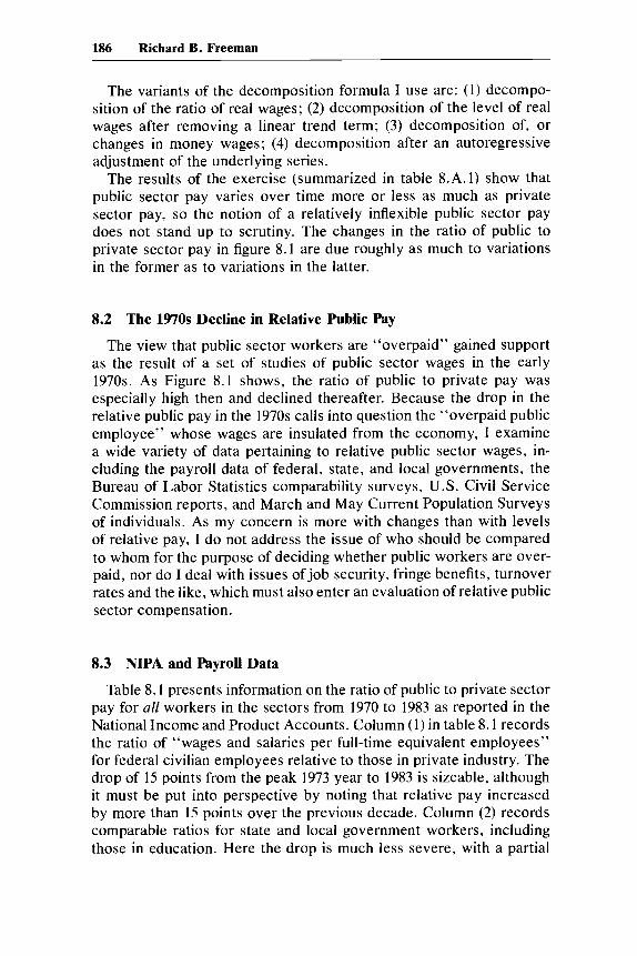
Table 8.1 Ratios of Federal Civilian and State and Local Government Wages and Salaries, to Private Industry Wages and Salaries, for Full-Time Equivalent Workers

Wage and Salary of Group Relative to Private

Federal Federal State & Local Civilian State & Local Enterprise Enterprise Education (1) (2) (3) (4) (5 )

1950 1.20 .91 1.10 1.06 .92 1960 1.25 .93 1.03 .98 .98 1970 1.42 I .06 1.14 1.07 1.06 1971 1.45 1.04 1.12 1.10 1.08 1972 1.46 1.03 1.18 1.11 1.08 1973 1.48 1.04 1.21 1.13 1.07 1974 1.43 1.02 1.24 1.06 1.04 1975 1.43 1.01 1.25 1.08 I .05 1976 1.42 1.01 I .27 1.08 1.05 1977 1.43 1.01 1.27 1.06 1.04 1978 1.44 .99 1.27 1.04 1.02 1979 1.39 .97 1.25 1.02 1.005 1980 1.35 .96 1.27 1.02 ,982 1981 1.34 .95 1.32 1.03 ,975 1982 1.33 .97 1.28 1.05 ,985 1983 1.33 1 .oo 1.29 1.08 1.01 A 1973-83 -.15 - .04 .08 - .05 - .06

Source: Calculated from U.S. Department of Commerce, Bureau of Economic Analysis, National Income and Product Accounts.

recovery for relative public sector pay from 1982 to 1983, when the economy entered its worst recession since the 1930s; at the same time, the increase in relative pay in earlier decades is also less marked.

How did relative public sector pay stand in 1983 compared to earlier years? In 1983 federal civilian pay was 33 percent above the private sector average; from 1950 to 1983 it averaged 32 percent above. In 1983 state and local pay stood at 3 percent below the private sector average; from 1950 to 1983 it averaged 4 percent below. Hence, by 1983 relative government pay seemed roughly to be at its post-1950 average.

The figures in columns (3) and (4) treat government enterprises. In the federal government this includes the Post Office, Tennessee Valley Authority, and related organizations. For the state and local governments, it includes public utilities and the like. A different pattern emerges in these data: a rise in the ratio of federal enterprise to private sector pay is contrasted with a decline in the ratio of state and local enterprise to private sector pay. Finally, column (5) treats education, where we find a decline of 10 points from 1970 to 1982, followed by an increase of .03 from 1982 to 1983.


The disparate patterns suggest the value of a more disaggregate look at various publicly employed groups distinguished by function, level of government, and occupation, to which we turn next.

Table 8.2 records data from the government employment and payroll survey of the Bureau of the Census. It shows a sharp decline in the pay of federal workers under the General Service schedule (GS) system (covering federal white-collar workers), which is roughly consistent with the NIPA figures, but a somewhat more complex pattern of change for workers paid under the WS (blue collar) and PS (postal employees) systems. In these cases relative wages turn down in the late 1970s rather than earlier and fall much less dramatically. For state and local government employees, the payroll data show a moderate decline in public-private pay differentials. Decomposed into education and other government functions, the figures for municipalities show a much greater concentration of the decline in the education sector than found in table 8.1, and also a partial recovery for both education and other municipal workers in the 1980s.

Because federal GS employee pay increases are legislated by Con- gress, it is possible to compare the observed changes in GS pay to the changes that would result if legislated increases were the sole cause of change. In the period 1972-82, legislated federal increases amounted to 84 percent of 1972 salary compared to an actual change

Table 8.2 Ratios of Public Sector Earnings Reported in Payroll Series to the Private Industry Wage and Salaries, 1970-82

Federal Municipal

GS WS PS State Local Education Other

I970 1971 I972 1973 1974 1975 1976 1977 1978 1979 1980 1981 1982 A, peak

year to 1982

1.44 .89 1.05 1.07 1.44 .92 1.09 1.06 1.45 .96 - 1.07 1.44 .98 - 1.09 1.38 1 .oo 1.19 1.08 1.34 I .03 1.23 I .06 1.33 1.07 1.23 1.06 1.32 1.16 1.23 1.06 1.33 1.18 1.23 1.05 1.29 1.16 - 1.04 1.25 1.12 1.14 1.03 1.26 1.12 1.09 1.03 1.25 1.10 - -

-.20 -.08 -.04 -.06

1.06 1.31 I .04 1.29 1.07 1.32 1.07 1.37 1.06 1.29 I .04 1.27 1.03 1.26 1.03 1 .oo .99 .98 1.14 .99 1.18 - 1.19

-.07 - . I3

I .06 1.08 1.10 1.10 1.11 1.09 1.08

1.02 1.05 1.06 - .05

Sources: Federal, state, local from U.S. Bureau of the Census Payroll Series; municipal from U.S. Bureau of the Census 1984, 309.


of 77 percent of 1972 salary. Increases in the average GS level of federal employees explain the change in salary above the legislated amount. As table 8.A.2 shows, these increases were concentrated in the latter part of the 1970s and early 1980s. From 1977 to 1982, grade increases (plus a minor “step creep,” defined as increases in pay due to changes in the “steps” of workers within a GS level) raised pay by 9 percent compared to an increase in pay due to grade increases of 3.4 percent from 1972 to 1977. Had the federal government not upgraded the GS level of its work force-which could represent a “true” increase in skill level, or a “creep” up in response to market conditions-the 1982 ratio of federal GS pay to private sector pay in column (1) would have been 1.19. This result implies that federal GS pay fell by 25 percentage points relative to private sector pay, grade held constant.

8.4 Rates of Pay for Comparable Workers

The comparisons of public and private pay thus far are crude in that they do not compare workers in the same occupation or with the same skills. There are two basic ways to make such more refined calculations: (1) use occupational wage rates on the pay in detailed occupations; (2) use individual-level data on the pay of workers with similar personal characteristics. The former method contrasts wage rates actually used in wage setting; the latter method contrasts earnings with those of workers having comparable age, education, and the like. Which is “better” depends on the quality of data and purpose of the comparison.

Table 8.3 uses federal professional, administrative, technical, and clerical (PATC) survey data to make such comparisons for white- collar workers. The PATC survey provides information on average annual wages for occupations in the private sector comparable to those in the public sector for each grade of the general schedule (white-collar workers) of the civil service. According to the principle of federal pay in the federal Pay Comparability Act of 1970, adjust- ments in general schedule salaries are supposed to ensure that Oc- tober federal wages are equal to comparable private sector wages of the previous March. When recommending actual wage increases to Congress, however, the president can suggest wage changes not based on the PATC, and of course Congress can enact higher or lower pay increases. Each year since 1977 the president has recommended lower increases.

The figures in table 8.3 report (unweighted) average ratios of federal to comparable private sector pay within GS classes. To assure comparability of data over time, the averages are limited to occupations


Table 8.3 Ratios of Federal GS Pay to Private Sector “Comparable” Pay for Occupations by GS Level

GS Level (number of occupations in comparison) 1972 1976 1978 1980 1983 A 1972-83

GS-I (2) GS-2 (3) GS-3 (4) GS-4 (2) GS-5 (7) GS-7 (8) GS-9 (8) GS-I1 (9)

GS-13 (5 ) GS-14 (5) GS-15 (2) All GS

GS-12 (6)

1.04 .91 .99 .93

1.02 .90 1.02 .91 1.12 .86 1 .0s .92 1.03 .93 .97 .94

1 .oo .94 1.02 .92 1.04 .91 I .07 .90 1.03 .91

.91

.90

.86

.92

.86

.90

.90

.90

.90

.90

.89

.90

.90

.89

.89

.84

.88

.83

.86

.86

.87

.86

.86

.83 ,233 .86

3 6 .87 .77 .82 .76 .80 .80 .81 .79 .78 .76 .75 .80

- . I 8 - . I2 - .25 - .20 - .36 - .2s - .23 - . I6 - .21 ~ .24 - .28 - .32 - .23

Source: Tabulated from U.S. Bureau of Labor Statistics. Noret For comparability over time, the figures report unweighted averages of occupational ratios only for occupations reporting in 1972 and in all later years. The pattern for other occupations included in later surveys is consistent with that in the table. I have left out GS-8 because there were no occupations in 1972 and GS-6 because only one occupation was reported in 1972.

that report pay in each year from 1972 to 1983. While the data can be summarized in other ways (weighted averages; inclusion of occupations contained in one year’s survey but not in another year’s survey), the pattern is sufficiently clear to require no more detailed computations. The effect of presidential recommendations of lower than comparable pay increases and of resultant congressional action in the 1970s has been to reduce relative federal pay falls sharply in all GS levels, with an unweighted average decline of 23 percentage points!

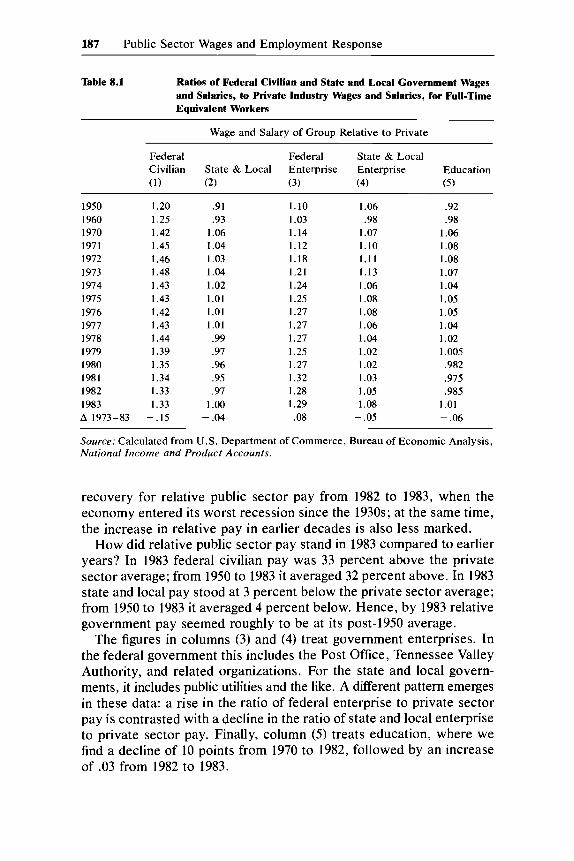
Table 8.4 records the results of similar comparisons for clerical and skilled maintenance workers for the federal government, for clerical and skilled maintenance workers in municipal government employment, and for fire fighters, police, and teachers. At the federal level we see the drop in relative pay for clerical workers but not for skilled maintenance workers. At the municipal level we see sharp drops for all occupations, with police and fire fighters experiencing surprisingly large declines, nearly as great as those for teachers.

All told, these comparisons of workers in given occupations suggest that the drop in public-private pay indicated in tables 8.1 and 8.2 may underestimate the fall in public sector pay, particularly for employees of local governments.


Table 8.4 Municipal and Federal Government Salaries Compared to Those in Private Industry, 1970-80

Ratio of Government Salary to Private Industry

1970 1975 1980 A

Federal Clerical - 1 .oo .85 - . I5 Skilled maintenance - 1.01 1 .oo - .01

Clerical - I .04 .98 - .06 Skilled maintenance - I .07 .97 - .I0 Policemen 1.10 1.05 .96 - .I4

Fire fighters 1.05 1.01 .91 - .I4

Teachers 1.21 1.09 1.04 - . I7

Municipal

(minimum scale)

(minimum scale)

Sources: U.S. Department of Labor, Clerical and Skilled Maintenance: A Comparison in Large Labor Markets, Monrhly Labor Review, July 1981, table 1. Police and fire fighters: U.S. Bureau of Census 1984, 187; Teachers: National Center for Education Statistics, The Condirion of Education, 1984, table 1.19.

8.5 Current Population Survey

An alternate, widely used way to compare workers with similar at- tributes is to use data on individuals from the Current Population Sur- vey tapes. These tapes provide detailed information on personal characteristics of workers but less adequate information on occupation and, in some cases, on type of employer. The CPS tapes contain two questions on public sector employment: a class-of-worker question, which divides workers between private employment, self-employment, and governmental employment, and the “industry”-of-employment question, which includes public administration by level of government. As the claim that government workers are overpaid received its strongest support in Sharon Smith’s analysis of CPS tapes in the mid-l970s, it is important to see how public-private pay differentials have changed in the CPS.

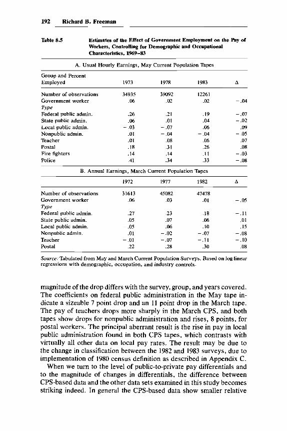
Table 8.5 presents the results of an analysis of usual hourly pay from the May CPS tapes for 1973, 1978, and 1983, and of annual earnings from the March CPS tapes for 1968, 1977, and 1982. While there are some inconsistencies between the two CPS surveys and between them and the earlier data sources, the general picture of declining public sector differentials in the 1970s holds for most government branches. In particular, both the May and March CPS files show declines in the relative pay of all government employees in the 1970s, though the


Table 8.5 Estimates of the Effect of Government Employment on the Pay of Workers, Controlling for Demographic and Occupational Characteristics, 1969-83

A. Usual Hourly Earnings, May Current Population Tapes

Group and Percent Employed 1973 1978 1983 A

Number of observations 34935 39092 1226 1 Government worker .06 .02 .02 - .04 Type

State public admin. .06 .01 .04 - .02 Local public admin. - .03 - .07 .06 .09 Nonpublic admin. .01 - .04 - .04 - .05

Federal public admin. .26 2 1 .I9 - .07

Teacher .01 - .08 - .06 - .07 Postal .18 .31 .26 .08 Fire fighters .I4 .14 . l l - .03 Police .41 .34 .33 - .08

B. Annual Earnings, March Current Population Tapes

1972 I977 1982 A

Number of observations Government worker T Y P Federal public admin. State public admin. Local public admin. Nonpublic admin. Teacher Postal

31613 .06

.27

.05 - .05

.01 - .01

.22

45082 .03

.23

.07

.06 - .02 - .07

.28

47478 .01 - .05

.I8 -.I1

.06 .01

.I0 .15 - .07 - .08 - . 1 1 - .I0

.30 .08

Source: Tabulated from May and March Current Population Surveys. Based on log linear regressions with demographic, occupation, and industry controls.

magnitude of the drop differs with the survey, group, and years covered. The coefficients on federal public administration in the May tape indicate a sizeable 7 point drop and an 11 point drop in the March tape. The pay of teachers drops more sharply in the March CPS, and both tapes show drops for nonpublic administration and rises, 8 points, for postal workers. The principal aberrant result is the rise in pay in local public administration found in both CPS tapes, which contrasts with virtually all other data on local pay rates. The result may be due to the change in classification between the 1982 and 1983 surveys, due to implementation of 1980 census definition as described in Appendix C.

When we turn to the level of public-to-private pay differentials and to the magnitude of changes in differentials, the difference between CPS-based data and the other data sets examined in this study becomes striking indeed. In general the CPS-based data show smaller relative


declines in public sector pay than do the payroll (NIPA) and occupation- based data and higher public-to-private ratios of relative pay, and also show significant differences in the levels of relative pay in some cases. In particular, in the PATC and other detailed job surveys we find federal GS workers paid less than other workers; in the CPS we find workers in federal public administration earning more than the typical private sector worker in the same occupation, with the same personal characteristics.

There are two basic reasons for this inconsistency. First, in contrast to the CPS which gathers data on all workers, the PATC survey is limited to workers in relatively large firms, whose pay traditionally exceeds that of workers in smaller firms. Whether this makes the CPS or PATC comparisons “better” is a matter of judgment. Some (Perloff and Wachter 1984) have interpreted comparability as calling for comparisons of federal employees with all workers. Others argue that it is wrong to compare employees of the largest single enterprise in the United States to workers from Joe’s corner store, making the PATC comparison a more accurate picture of where the federal government stands in labor markets. Second is the difference between comparisons of wages in well-defined jobs and of wages of persons with similar demographic characteristics. Here the PATC data has a clear advantage because it refers to specific occupations (computer programmer, ac- countant) for which the federal government hires persons, rather than to broadly defined groups (professionals, with college education, of a given age), most of whose members may lack the skill for the particular job.

Finally, it is important to recognize that part of the observed premium to federal public administration shown in table 8.5 reflects different public rather than private pay policies toward minorities and women. Table 8.6 documents this point for usual hourly earnings in May 1983 and for annual earnings, adjusted for hours and weeks worked in 1977 and 1982. In all periods and surveys, public employees tend to have smaller differences in pay by sex and by race than private employees, though there is some indication that the differential between sectors narrowed in the late 1970s and early 1980s. As Asher and Popkin (1984) have stressed, to the extent that government pay is relatively good because of more equal treatment of minorities and women, interpre- tation of Current Population Survey differentials in terms of “overpaid” government workers requires reconsideration by analysts.

8.6 Changing Patterns of Employment

It is well known that in the post-World War I1 period, public sector employment has risen relative to private sector employment. In 1950 15.6 percent of full-time equivalent workers were government employ-


Table 8.6 Regression Estimates and Standard Errors: Effect of Ethnicity and Sex on Pay, by Public and Private Sector

Hourly Earnings

Annual Earnings, Controlling for Hours and Weeks

May 1983

March Tapes 1977 1982

Black Private

Public

Federal

State

Local

Postal

Women Private

Public

Federal

State

Local

Postal

ees; in 1983 19 percent of full-time equivalent workers were government employees.

In this section I examine the pattern of change in public sector employment over the cycle, and by level of government and type of workers. The evidence shows public sector employment not only to be less variable over time than private sector employment but also to exhibit a strikingly different pattern of change over the business cycle. In addition, the public sector employs relatively more blacks and women than the private sector, which, in conjunction with the relatively higher pay shown in table 8.6, suggests greater public sector demand for those workers.

Figure 8.2 depicts the ratios of federal civilian to private employment and of state and local to private employment from 1950 to 1983, as


0.18-1 I I I I I I I I I I I 1 1

0.16 - State & Local/Private

0.14 -

0.12 -

0.10 -

0.08 -

Fig. 8.2 Ratio of federal government to private employment and state and local government to private employment.

given in the NIPA data set. With respect to state and local employment, the data show a marked rise until the mid-l970s, followed by a relatively sharp decline. Indeed, from 1981 to 1983 state and local employment actually fell, partly as a result of reductions in CETA employment, and partly as a result of declines in education due to changes in the size of the school age population. At the federal level, the employment share follows a very different pattern: from the early 1950s to the late 1960s it is roughly constant at 3.8 percent to 3.9 percent of nonagricultural employment. Thereafter it drops sharply to less than 3 percent of nonagricultural employment. The result is a striking change in the composition of public employment. In 1950 one in three public employees was a federal worker; in 1983 one in six was a federal worker.

What about the cyclical and short-term variation in public employment? To determine how public sector employment varies in the short run, I have performed a two-part analysis. First I calculated the standard deviation of log changes in employment annually for the public and private sectors, over the period 1955-82 (leaving out the Korean War period). Such a calculation confirms the widely held belief that public sector employment is less variable over time than private sector


employment, with the following calculated standard deviations: private nonagricultural employment (.026); federal civilian employment (.020); state and local employment (.017). Second, I examined changes in employment over NBER business cycles. As table 8.7 shows, there is a striking difference in cyclical changes in employment between sectors, particularly between state and local and private employment; in six of seven cyclical swings post-1953, state and local employment move countercyclically. The growth of federal employment moved countercyclically in the 1970s but varied with the cycle earlier. Even then, however, it showed smaller cyclic variation than private employment. In conjunction with our analysis of changes over time in public-private pay differentials, these calculations indicate that public sector payrolls vary differently over time than do private sector payrolls, and thus must be responding to unique public sector factors rather than to broad swings in the overall state of the economy.

8.7 Sex and Race

Our earlier analysis found that pay differentials by sex and race were smaller in public than in private employment. What about patterns of employment? Table 8.8 records the race and sex distribution of private and public employment in 1978 and 1983. It shows that governments tend to hire proportionally more blacks and women than does the private sector, though with noticeable variation among levels of growth. In the 1978-83 period, the proportion of blacks in government relative to the proportion of blacks in the private sector rose while the proportion of women in government increased above the 50 percent rate.

8.8 Budgets and Macrodeterminants of Public Sector Wage and Employment Changes

Preceding sections have shown that far from being inflexible or rigid, public sector wages have changed substantially relative to private sector wages over time, and that the growth of public sector employment varies over time. Can we identify the factors that affect the ratio of public to private pay, and that affect the variability of public sector employment?

In this section I examine the hypothesis that the public sector, like other “industries,” alters employment and wages in response to changes in the economic conditions and incentives facing it. What distinguishes public from private sectors is that the principal economic force on the public side is not the competitive economic market but budgets determined in political markets. In Dunlop’s words, “the public sector re- sponds to the discipline of the budget rather than to the discipline of

Table 8.7 Employment Changes over the Business Cycle, Public versus Private Employers

Average Percentage Change per Year

Recession Recovery Recovery-Recession

Period (peak-trough-peak) Private Federal State Local Private Federal State Local Private Federal State Local

July 53-May 54-Aug 57 Aug 57-Apr 58-Apr 60 Apr 60-Feb 61-Dec 69 Dec 69-Nov 70-Nov 73 Nov 73-Mar 75-Jan 80 Jan 80-July 80-July 81 July 81-Nov 82-June 84

-5.6 - 10.6 -5.7 -3.6 -4.4

1 .O ~ 2.4

-6.4 13.1 3.0 0.8 4.1 8.6 7.2 -9.0 -4.2 12.5 5.1 3.7 5.1 4.5 3.6 14.4 9.3 -8.0 -1 .5 -8.8 5.6 4.5 4.0 2.7 7.4 5.8 9.7 11.6 1.8 1.3 -5.1 7.9 5.5 3.8 -0.2 3.0 4.5 7.4 4.9 -4.9 - 1.0

2.0 5.9 4.3 4.4 0.3 1.9 2.1 8.8 -1.7 -4.0 - 2 . 2 10.3 6.6 10.8 3.2 -4.0 -0.4 -1.8 2.2 -15.3 -7.0 -12.6 2.9 5.9 4.1 4.9 2.2 -2.2 -0 .0 7.3 -0.7 -8.1 - 4.1

Source: Business cycles, based on NBER Reference Cycles Employment, from U.S. Department of Labor Employment and Earnings, various editions.


Table 8.8 Percentage of Female and Black Workers, by Employer, 1978-83

March Tapes

1978 1983

Blacks Private ,083 .073 Public ,114 ,115

Private .414 ,446 Public ,492 ,522

Women

Source: Calculated from March CPS tapes.

the market.” I shall take as given the sizes of budgets or tax rates, although in a complete model they are certainly endogenous, and examine how short-term variations in budgets influence public sector wages and employment in the same way that one might examine how short-term variations in industry output and prices (value added, pro- ductivity, profits) affect private wages and employment. Because of the very different way in which decisions are likely to be affected by budgets by level of government, such an analysis must distinguish between federal and state or local governments. State and local governments face, in general, hard budget constraints, whereas the federal government can run continual deficits to fund its outlays. There is a serious budget constraint in the one case, but not in the other, which we expect to produce differential employment and wage responses to budgetary changes.

To begin, table 8.9 presents readily available figures on payrolls and budgets in the period. It is designed to provide a crude indication of the extent to which governments faced budget “crunches” in the 1970s.

At the federal level, outlays as a share of GNP rose sharply in the period covered, without a compensating increase in taxes, producing a sizeable deficit. Despite increases in outlays, however, the ratio of federal compensation to GNP fell, indicative of a sizeable decline in the payroll share of budgets. As lines 2a-2d in table 8.9 show, the only budget figures against which payroll shares have not dropped drastically are “controllable outlays.”

At the state and local level, receipts have risen more rapidly than outlays, producing surpluses, and payrolls have risen relative to GNP (and to private sector payrolls). However, the share of payroll in budgets has been relatively fixed over time. Here, the problem with a simple “budget crunch” story of employment and pay changes is the surpluses run. Payrolls could have been increased by nearly 15 percent had the 1983 surplus been spent on payrolls and by 4 percent had the payroll share of receipts been constant at its 1970 level.

199 Public Sectcr Wages and Employment Response

Table 8.9 Federal and State and Local Finances and Civilian Payrolls, 1970-83

1970 1980 1983

Federal government 1. Financial variables

as percentage of GNP

b. Receipts 19.9 20.9 18.7

d. Civilian compensation 2.4 2.0 1.9 2. Payroll as percentage

of budget variables a. Outlays 14.6 10.1 8.7 b. “Controllable” outlays 39.5 37.0 36.7 c. “Civilian controllable” 127.9 89.4 96.7

d. Receipts 14.8 11.1 11.7

a. Outlays 20.2 22.9 25.2

c. Deficit -0.3 - 2.0 -6.5

outlays

State and local government Financial variables as percentage of GNP a. Outlays 13.5 13.5 13.1 b. Receipts 13.6 14.7 14.5 c. Surplus or deficit 0.2 1.2 1.3

Payroll as percentage of budget variables a. Outlays 53.4 53.4 55.6 b. Purchase of goods & 57.1 55.8 58.1

c. Receipts 52.5 49.2 50.4

d. Payroll compensation 7.6 7.7 7.8

services

Source:Lines la-c: U.S. Bureau of the Census 1984,315; lines Id, 3, and 4: U.S. Bureau of the Census, National Income and Product Accounts; lines 2a-c, U.S. Bureau of the Census 1984, 318, 333.

What the figures in table 8.9 suggest is that crude budget pressures on public sector payrolls are not enough to explain the observed patterns of change in public sector payrolls and thus in compensation and employment. The budget “constraints” is not hard enough to be the sole factor at work.

8.9 A Small Regression Model: State and Local Governments

As a final step in evaluating the pattern of change over time in public sector wages and employment, I have estimated the effect of budgets and selected macroeconomic variables on relative public sector wages and employment. More specifically, I have regressed the ratio of compensation and employment in various parts of the public sector on the


ratio of the relevant budget to GNP, the rate of inflation in the GNP deflator, and the level of unemployment.

The budget/GNP ratio is expected to be the key determinant of relative employment and wages, with the relative magnitude of the coefficients of interest. Inflation is expected to reduce relative public sector pay due to the likely slower response of public wages to inflation, while unemployment is expected to raise relative state and local employment due to the observed countercyclical movement of public sector employment.

Table 8.10 presents the results for state and local governments and for noneducation activities of these governments. Panel A treats the public sector variables relative to private sector variables. The importance of public budgets in determining employment and wage is clear in the results, with a 10 percent increase in budgets/GNP being divided between employment and wages in a ratio of roughly 2 to 1. The mac-

Table 8.10 Coefficients and Standard Errors for Macroeconomic and Budget Determinants of State and Local Public Sector Employment and Wages

A. Employment and Wages Relative to Private Sector

Expenditures/GNP P UNE R R*

State and Local 1. Employment .81 .02 .51 -.61 .965

~ 0 5 ) (.26) ~ 2 9 ) 2. Wages .29 - .41 - .47 - 5 8 .810

(.03) (. 17) (.21) State and Local Noneducation

3. Employment .65 - .09 .94 -.75 .922 (.W ( .22) (.39)

(.05) (.21) ( .30)

B. Employment and Wages

4. Wages .24 - .08 - .26 -.64 .580

State and Local 5 . Employment .66 .37 .01 -.67 .995

(.OI) (. 15) (.17) 6. Wages .35 - .78 -.52 -.62 .959

(.02) (.22) (.25) State and Local Noneducation

7. Employment .60 .32 .20 -.70 .986 ( .02) ~ 1 9 ) (.23)

(m (.21) (.25) 8. Wages .35 - .53 -.43 -.61 .948

Source: Calculated using NIPA data 1952-83. Notes: R = auto correlation coefficient; k = log (GNP deflator/GNP deflator (- 1)); UNE = rate of unemployment.


roeconomic factors affect relative pay and employment in the expected manner, suggesting that the drop in public sector pay relative to private sector pay in the 1970s was at least facilitated by inflation and that the weak labor market of the period masked an even greater slowdown in relative public sector employment than is indicated in figure 8.2. Some- what surprisingly, the figures also show some effect of unemployment on wages, with the level and ratio of public to private pay falling with high unemployment. Finally, panel B of the table focuses on the level of the public sector variables themselves. These calculations show the variability and responsiveness of public sector employment and wages and also inflation with respect to budgets.

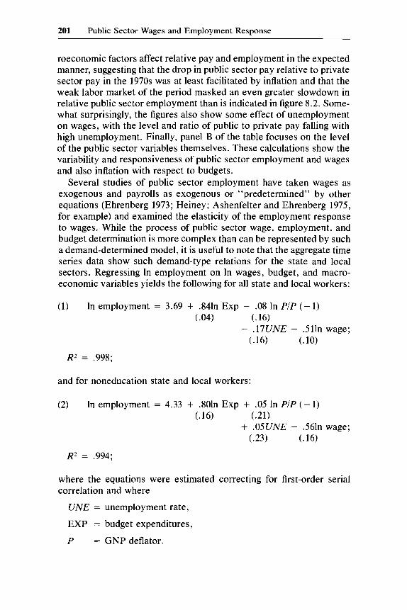
Several studies of public sector employment have taken wages as exogenous and payrolls as exogenous or “predetermined” by other equations (Ehrenberg 1973; Heiney; Ashenfelter and Ehrenberg 1975, for example) and examined the elasticity of the employment response to wages. While the process of public sector wage, employment, and budget determination is more complex than can be represented by such a demand-determined model, it is useful to note that the aggregate time series data show such demand-type relations for the state and local sectors. Regressing In employment on In wages, budget, and macroeconomic variables yields the following for all state and local workers:

(1) In employment = 3.69 + .841n Exp - .08 In PIP ( - 1) ( .04) (. 16)

- .17UNE - S11n wage; (. 10)

R2 = .998;

and for noneducation state and local workers:

(2) In employment = 4.33 + .801n Exp + .05 In PIP ( - 1) (. 16) (.21)

+ .05UNE - S61n wage; (.23) (. 16)

R2 = .994;

where the equations were estimated correcting for first-order serial correlation and where

UNE = unemployment rate,

EXP = budget expenditures,

P = GNPdeflator.


Both equations show that budget expenditures and wages are the predominant determinants of employment, with the negative impact of wages indicating that demand side behavior dominates the employment sphere. Even so, the calculations should be viewed cautiously. With nearly half of state and local government employees covered by col- lective bargaining, and the division of a budget a matter for both col- lective bargaining and public policy, it is clear that a more complex analysis is required to determine the underlying behavior. The devel- opment of an appropriate simultaneous employment, wage, and budget model lies, however, beyond the purview of this chapter. For our pur- poses, it suffices to note that fluctuations in pay and employment are related to broader macroeconomic factors and to budgets in a reasonable way over time.

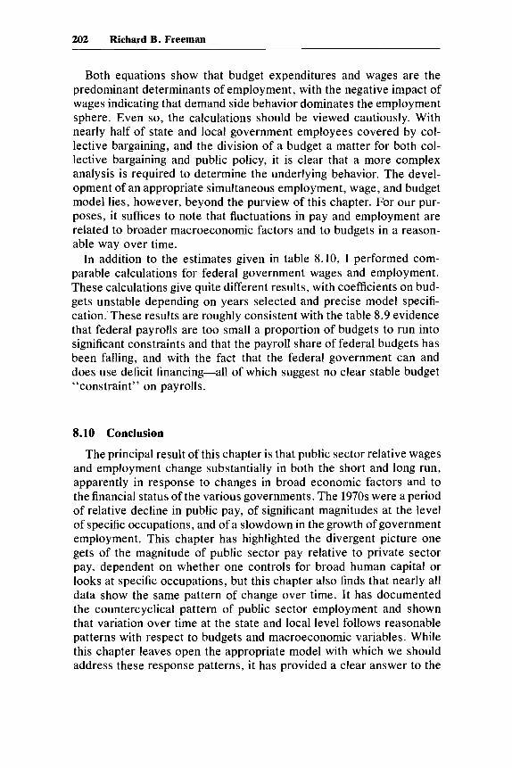
In addition to the estimates given in table 8.10, I performed comparable calculations for federal government wages and employment. These calculations give quite different results, with coefficients on budgets unstable depending on years selected and precise model specifi- cation. These results are roughly consistent with the table 8.9 evidence that federal payrolls are too small a proportion of budgets to run into significant constraints and that the payroll share of federal budgets has been falling, and with the fact that the federal government can and does use deficit financing-all of which suggest no clear stable budget “constraint” on payrolls.

8.10 Conclusion

The principal result of this chapter is that public sector relative wages and employment change substantially in both the short and long run, apparently in response to changes in broad economic factors and to the financial status of the various governments. The 1970s were a period of relative decline in public pay, of significant magnitudes at the level of specific occupations, and of a slowdown in the growth of government employment. This chapter has highlighted the divergent picture one gets of the magnitude of public sector pay relative to private sector pay, dependent on whether one controls for broad human capital or looks at specific occupations, but this chapter also finds that nearly all data show the same pattern of change over time. It has documented the countercyclical pattern of public sector employment and shown that variation over time at the state and local level follows reasonable patterns with respect to budgets and macroeconomic variables. While this chapter leaves open the appropriate model with which we should address these response patterns, it has provided a clear answer to the


question posed. Yes, public sector wages and employment respond to economic conditions.

Appendix A

To evaluate the relative contribution of variation in government and private pay to the observed change in the ratio of pay, we calculated the standard deviations of variation of each component separately, using four different forms:(l) variation in levels of log pay; (2) variation in first differences in log pay; (3) variation in the deviation of residuals of log pay from trend; (4) variation in the residual of log pay from an AR(2) process. The results are given in table 8.A. 1 for the period 1952-82.

Table 8.A.1 Standard Deviation of Relevant Measures of Wages

Private Federal State & Local

1 . Log of real wages .126 .I94 ,174 2. First difference of .020 .032 .026

3. Residual of log of .062 .08 1 ,089

4. Residual from AR(2) .029 .039 .033

log of real wages

real wages from trend

process

The variation in government pay exceeds that in private pay in lines 2 and 3 of table 8.A.1, but is less than the variation in private pay in lines 1 and 4. Since the results depend on the particular computation, we conclude that public sector pay is not noticeably less variable than private sector pay. Changes in the private sector denominator do not drive changes in relative public sector pay.

Appendix B Calculation of Relative Contributions of Scheduled Increases and Increases Due to “Grade Creep” and “Step Creep” in the GS Pay Schedule

There are eighteen grades and ten steps in the GS schedule. Grades are for promotion; steps are for longevity and merit pay increases. In


addition, longevity increases above step 10 are possible. (These additional increases cause some additional calculations below.)

The relative contributions of the three components were calculated as follows:

A. The average annual salary for the initial year was calculated by taking actual salaries (avsal).

B. The increase attributable to changes in the pay schedule was calculated by first-year employment by grade and sex to calculate a weighted average of the final-year pay structure. Since the number of workers above step 10 changes between years, this calculation required adjustment of the final-year wage schedule to reflect the number of persons above step 10 in the first year (acin).

C. Increase in average wage attributable to step and pay increases was calculated by taking first-year employment by grade to calculate a weighted average of final-year average wage by grade. This reflects both the increase in average step and the increase/decrease in the number of persons above step 10 (avslstep).

D. Increase in average wage attributable to step, pay, and grade increase was calculated by taking the average wage (avsal) in the final year. Thus pay increase = B - A; step increase = C - B; and grade increase = D - C . For the period 1972-82 these calculations are found in table 8.A.2.

Table S.A.2 Comparison of Scheduled Wage Increases with Increases Due to Step and Grade Creep

1972-82

Totals Contributors

Avsal 72 12552.8 Scheduled increase 9707 92.6%

Avslstep 22295.4 Grade creep 835.2 8.0% Acasl 23040.6 83.5% Overall increase 10487.8

Acin 72 82 2259.8 Step creep - 54.4

1972-77

Avsal 72 12552.8 28.4% Scheduled increase 3567.9 96.6% Acin 72 17 16120.7 Step creep - 66.9 Avslstep 16053.8 - 16.4 Grade creep 170.8 5.2% Acasl 77 16244.6 29.4 Overall increase 3691.8

1977- 82

Avsal 72 16244.6 38.1% Scheduled increase 6185.6 91.0% Acin 72 77 22430.2 Step creep 41.6 Avslstep 22471.8 -21. Grade creep 568.8 8.4 Acasl 77 23040.6 41.8% Overall increase 679.6


Appendix C Note on Sources for Public Sector Pay and Employment

Time series on relative wages were calculated from the following sources. 1. Average salary for full-time equivalent employees is found in the

National Income and Products Accounts produced by the Bureau of Labor Statistics.

2. Average salary for full-time federal employees (General Service, Wage System, Postal and other pay systems) employed on March 31 of each year is found in the Pay Structure of the Federul Civil Service published by the Office of Personnel Management.

3. Relative pay of general schedule employees for comparable occupations is calculated in the National Survey of Professional Admin- istration, Technical and Clerical employees (PATC surveys) published by the Bureau of Labor Statistics.

4. Average salaries and employment based on October payroll are found in the Bureau of the Census Series (Public Employment, Series

5. Relative pay differentials controlling for geographic personnel and human capital characteristics were calculated from the March and May Current Population Survey tapes for 1973, 1978, and 1983. The March tapes survey annual earnings for the previous year; only those workers for whom industry and occupation did not change were included. In- dustry and Occupation codes for 1980 were implemented in 1983. This led to some exaggeration of the increase in the coefficient on local

GE-1).

Table 8.A.3 Sample Sizes for Statistical Analysis

1973 1978 1983

March May March May March May

Postal 384 407 448 350 419 117

Federal public 827 700 1,082 83 I 1,105 260

State public 30 1 317 588 498 870 215

Local public 388 78 1 1,120 914 1,081 245

Teachers 1,446 1,389 1,596 1,498 1,609 415

administration

administration

administration

Nonpublic 2,532 3,325 4,812 4,125 4,813 1,183

Private 25,735 28,016 35,436 30,876 37,581 9,826 administration


public administration employees compared to similar regressions using the 1970 classifications on the 1982 data. Sample sizes for each level of government in each year are shown in table 8.A.3.

Note “How Do Public Sector Wages and Employment Respond to Economic

Conditions?” was written for NBER’s Public Sector Employment and Payroll Conference. Edward Funkhouser provided excellent research assistance for this project.

References Annable, J. E. 1974. Theory of wage determination in public employment.

Quarterly Review of Economics and Business 14:43-58. Ashenfelter, O., and R. G. Ehrenberg. 1975. The demand for labor in the public

sector. In Labor in the public and nonpro$t sectors, ed. Daniel S . Ham- mermesh. Princeton: Princeton University Press.

Asher, M., and J. Popkin. 1984. The effect of gender and race differentials on public-private wage comparisons: A study of postal workers. Industrial and Labor Relations Review 38: 16-25.

Baugh, W. H., and J. A. Stone. 1982. Teachers, unions and wages in the 1970s: Unionism now pays. Industrial and Labor Relations Review 35:368-76.

Bergstrom, T. C., and R. P. Goodman. 1973. Private demands for public goods. American Economic Review 63~280-96.

Borjas, G. J. 1980. Wage determination in the federal government. Journal of Political Economy 88: 11 10-47.

Carlsson, R., and J. Robinson. 1969. Toward a public employment theory. Industrial Labor Relations Review 22:243-48.

Courant, P. N., E . M. Gramlich, and D. L. Rubenfeld. 1979. Public employee market power and the level of government spending. American Economic Review 69:806-17.

Dunlop, John T., Private Discussion, May 1985. Harvard Univ., Cambridge Mass.

Ehrenberg, R. G. 1973. The demand for state and local government employees. American Economic Review 63:366-79.

Fogel, W., and D. Lewin. 1974. Wage determination in the public sector. In- dustrial and Labor Relations Review 27:410-31.

Freeman, R. B. 1984. Unionism comes to the public sector. NBER Working Paper No. 1452.

Freund, J. L. 1974. Market and union influences on municipal employee wages. Industrial and Labor Relations Review 27:391-404.

Hartman, R. W. 1983. Pay andpensions forfederal workers. Washington, D.C.: Brookings Institution.

Lazear, E. P. N.d. An analysis of federal worker compensation. National Bu- reau of Economic Research.

National Center for Education Statistics. 1984. The Condition of Education, table 1.19.


Peltzman, S. N.d. Government expenditures in the U S . : The last 100 years. Typescript. Univ. of Chicago.

Perloff, J. M., and M. L. Wachter. 1984. Wage comparability in the U S . postal service. Industrial and Labor Relations Review 38:26-35.

Reder, M. W. 1975. The theory of employment and wages in the public sector. In Labor in the public and nonprojit sectors, ed. Daniel S . Hamermesh. Princeton: Princeton University Press.

Smith, S. P. 1977a. Equal pay in the public sector: Fact or fantasy. Princeton: Princeton University, Industrial Relations Section.

. 1977b. Government wage differentials. Journal of Urban Economics

U.S. Bureau of the Census. National income and product accounts. Washing-

. 1984. Statistical abstract of the United States, 1984. Washington, D.C.:

U.S. Department of Labor. 1981. Clerical and skilled maintenance: A com-

4~248 - 7 1.

ton, D.C.: Government Printing Office.

Government Printing Office.

parison in large labor markets. Monthly Labor Review. July. Table 1.

Comment Sam Peltzman

Richard Freeman has, in his typically competent and thorough fashion, documented some important facts about the recent history of public sector wages and employment. The facts are, essentially, that the last decade has been “bad” for government employees while the previous decade was especially “good.” Neither my own limited expertise in these matters nor my respect for Freeman’s move me to quarrel with these results or comment on their detail. Instead I will try to fit the facts about government employment and wages into a larger perspective: that of trends in the allocation of resources within the public sector. In particular, I want to show that changes in the composition of public sector (especially federal) budgets have had an important bearing on some of the facts Freeman documents, perhaps more important than changes in the size of those budgets.

First, some essential, if elementary, background. As a broad gen- eralization, governments have two important tasks. They provide “public goods” such as defense and highways, and they redistribute wealth by providing private benefits that are, to some degree, financed by nonbeneficiaries. Most every government activity, including the provision of public goods, has redistributive elements-for example, decisions on the location of military bases and highways can generate or destroy economic rents. But the two most prominent forms of redistribution are direct money transfers to individuals (e.g., Social Se-

Sam Peltzman is professor of economics at the Graduate School of Business, Uni- versity of Chicago.


curity) and provision of publicly financed benefits in kind (e.g., free public education).

Over the last thirty years or so, government expenditures have grown relative to national income, and most of this growth has come from expansion of redistributive activities. For example, from 1950 to 1980 government spending at all levels-federal, state and local-rose from about 25 percent to 36 percent of GNP, or 11 percentage points. About 9 of these 1 1 percentage points are attributable to expansion of public education, public welfare, and Social Security. More recently-in the last decade or so-the composition of expenditures on redistribution has shifted away from education and toward expenditures on the aged and poor. In fact, since 1970, education expenditures have grown less than either GNP or government spending. These trends are, of course, related to corresponding demographic trends-the continual aging of the population and the post-World War I1 cycle in birth rates.

My emphasis on these compositional changes in government budgets is motivated by a simple fact: There is great heterogeneity among government programs in their “labor intensity.” That is, payrolls are allocated much differently than total expenditures. This is especially true at the federal level. Table C8.1 summarizes the basic facts for the five agencies with the most employees. Two agencies-Defense and Postal Service-account for over two-thirds of total federal civilian employment, but less than one-third of total spending. The labor intensity of these operations stands in sharp contrast to those of the rapidly growing redistributive programs centered in the Health and Human Services Department: HHS spends roughly 7 times as much per employee as the federal average, 10 times as much as Defense, and 50 times as much as the Postal Service. We need look no further for most of the explanation of the relative decline of federal employment over the last thirty years or so. While total spending has grown relative

Table CS.1 Civilian Distribution of Employment and Expenditures for Five Federal Agencies with Most Employees, 1982

Percent of Total Expenditures per Employee

Agency Employment Expenditures ($ooo) Defense 35.7% 24.8% 183 Postal service 23.2 3.1 35 Veterans 8.2 3.2 103 HHS 5.2 33.8 1709 Treasury 4.4 1.5 873 All other 23.3 33.6 379

TOTAL 100.0 100.0 262

Source: U.S. Bureau of the Census, Statistical Abstract of the U.S., 1982.


to GNP, spending at the two megaemployers has declined. For example, Defense and Postal expenditures declined from roughly 10 percent of GNP to 7 percent from 1955 to 1982. In short, because of the very rapid growth of non-labor-intensive transfers, the federal government is becoming much less labor intensive even as it grows moderately faster than the private economy. This “explains” one of Freeman’s facts-the steady shrinkage in relative employment-but not another- the sharp rise in relative pay in the late 1960s and early 1970s. I will leave that rise for others to explain. If I am correct about the shrinking demand for federal employment in this period, I can only suggest that we will have to look to labor supply factors for the explanation.

Changes in the composition of state and local spending have also contributed to changes in these governmental labor markets, but to a smaller degree than those at the federal level. Table C8.2, which is organized the same way as table (28.1, provides some background for this conclusion. Notice first that the state and local sector is both more labor intensive and less heterogeneous in this dimension than the federal sector. Spending per state and local employee is on the order of one-tenth of that of the federal level, and it ranges much less widely across functions. So the potential for shifts in the composition of state and local spending to induce important changes in the overall demand for employment is much smaller than at the federal level. Moreover, the shifts that have occurred have been milder. Education is and has been for a long time the most important factor by far in state and local spending and employment. Nor has its expenditure or employment share changed much over the last thirty years or so. The one notable change in this period has been in highway spending and employment. From 1955 to 1980 the share of both spending and employment on this activity fell by about half. Most of this drop had occurred by 1970, as

Table C8.2 Distribution of State and Local Expenditures and Employment, 1980

Function

Percent of Total Expenditures per Employee

Employment Expenditures ($ow Education 48.3% 36.2% 25 Health & hospitals 11.7 8.8 25 Police/fire 7.4 5.2 23 Highways 4.8 9. I 63 Welfare 3.4 12.4 121 Other 24.4 28.3 39

TOTAL 100.0 100.0 33

Source: US. Bureau of the Census, Statistical Abstract of the U.S. , 1980.


the large interstate highway building program wound down. Since the highway function is relatively non-labor intensive (see table C8.2), the shift away from it had moderately favorable implications for the demand for state and local labor employees. But this contribution to the rise in relative employment up to about 1970, which Freeman documents pales beside that of the growth of education.

Table C8.3 provides some relevant data for two subperiods: 1955- 70, when state and local relative employment and wages were both rising; and 1970-80, when the former was essentially unchanged and the latter fell. Noneducation relative employment has and continues to grow modestly. But something like two-thirds to three-fourths of the pre-1970 growth and all of the post-1970 flattening of total relative employment are coming from public education. Table C8.3 also shows the by now familiar demographic basis of the changes in the demand for education employment-the post-World War I1 rise and fall of the pupil population.

There is, I think, a broad conclusion to which this brief tour of employment and expenditure history leads. It is that changes in the demand for redistribution and its age composition are going to drive the demand for government labor in the future just as they have in the past. Unless birth rates increase dramatically, the population will continue to age. That has mainly negative implications for the demand for government labor: It will continue to restrict the demand for labor-intensive education services and increase the demand for non-labor-intensive transfers. Thus demography and a long-term shift from public goods to redistribution seem to portend a continued reduction in relative employment at both the federal and state and local levels.

Table C8.3 Relative Employment Trends and School Enrollment Rates, 1955-80

Variable 1955 1970 1980

State and local government employment as percent of total civilian employment

Total state and local 7.2% 10.8% 10.9% Noneducation 4.2 5.3 5.6 Public education 3.0 5.5 5.3

Public elementary and 18.0 22.7 18.2 secondary school enrollment as percent of population

Source: U.S. Bureau of the Census, Statistical Abstracts of the U.S. and Historical Statistics of the U.S.


No discussion of the demand for public employment can overlook the role of “politics.” After all, public budgets and payrolls are determined within a political process, and public employees are in the un- usual position of having the potential for affecting the demand for their services by organizing to bring pressure on that process. It is therefore tempting to search for a political explanation for seemingly anomalous facts, such as the late 1960s rise in the relative pay of federal workers. Indeed, the rapid growth of public sector unionization and the attendant increase in organized pressure just prior to the late 1960s make the connection plausible. Perhaps someone will show that unionization of the postal service can help explain what happened to federal employees in the late 1960s. But my reading of state and local data indicates that any increase in the political visibility of state and local employees had little impact on the demand for their services. For example, compare politically determined expenditures with private expenditures on elementary and secondary education. Since 1960 the private sector has steadily enrolled a bit under 15 percent of all such students. If the new public sector unions successfully raised the demand for public education, we ought to have seen a sharp increase in the ratio of expenditures per public school pupil to expenditures per private school pupil in the late 1960s. In fact this ratio was 1.2 in 1960, rose to 1.3 in 1966, and declined to 1.2 by 1970, where it has remained since. So both the public and private sectors seem to have responded to the same forces in about the same way.

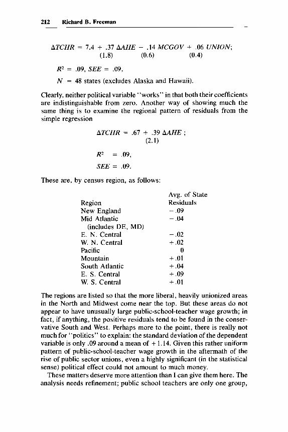
These aggregated data may, of course, be hiding important local effects of politics. One has to worry about this possibility because neither the rise of public sector unions nor the receptivity of governments to organized pressure on their behalf is regionally uniform. If there is a “political effect,” it should show up in heavily unionized “liberal” areas rather than in basically non-union “conservative” areas. However, a quick look at state-level data on growth of teacher salaries over the whole cycle beginning in the mid-1960s does not reveal any substantial local political effects. I regressed the 1965- 82 change in the log of average public elementary school teacher salaries (ATCHR) on the change in the 1965-82 log of average hourly earnings in manufacturing (AAHE) in the state and on two political variables: (1) the fraction of the state’s nonagricultural workers unionized in 1970 (UNZON), and (2) George McGovern’s share of the state’s 1972 popular vote (MCGOV). The latter is meant as a proxy for bedrock liberal sentiment among a state’s electorate, while UNZON is meant to proxy for both the degree of public sector unionization (I had no state-level data on this) and the importance of the public employees’ most natural political allies. The results were (t-ratios in parentheses)


ATCHR = 7.4 -I- .37 AAHE - .14 MCGOV + .06 UNION; (1.8) (0.6) (0.4)

R2 = .09, SEE = .09,

N = 48 states (excludes Alaska and Hawaii).

Clearly, neither political variable “works” in that both their coefficients are indistinguishable from zero. Another way of showing much the same thing is to examine the regional pattern of residuals from the simple regression

ATCHR = .67 + .39 AAHE ; (2.1)

R2 = .09,

SEE = .09.

These are, by census region, as follows:

Region New England Mid Atlantic

E. N. Central W. N. Central Pacific Mountain South Atlantic E. S. Central W. S. Central

(includes DE, MD)

Avg. of State Residuals - .09 - .04

- .02 + .02

0 + .01 + .04 + .09 + .01

The regions are listed so that the more liberal, heavily unionized areas in the North and Midwest come near the top. But these areas do not appear to have unusually large public-school-teacher wage growth; in fact, if anything, the positive residuals tend to be found in the conservative South and West. Perhaps more to the point, there is really not much for “politics” to explain: the standard deviation of the dependent variable is only .09 around a mean of + 1.14. Given this rather uniform pattern of public-school-teacher wage growth in the aftermath of the rise of public sector unions, even a highly significant (in the statistical sense) political effect could not amount to much money.

These matters deserve more attention than I can give them here. The analysis needs refinement; public school teachers are only one group,


though an important group, among a variety of public employees. And even if the political process did not respond much to the pressures engendered by the rise of public sector unions in the 1960s, this does not mean that the process never provides politically based rents to workers. However, in the specific case of the cycle that Freeman documents-the rise and fall of the demand for state and local public employees from the mid-1960s to now-the specific role of the rise in organized pressure from public employees seems modest beside that of demography and the more general political factors determining the allocation of budgets.

References

U.S. Bureau of the Census. Statistical Abstracts of the U S . Washington, D.C.:

U.S. Bureau of the Census. 1975. Historical Statistics of the U.S . , Colonial Government Printing Office.

Times to 1970. Washington, D.C.: Government Printing Office.

This Page Intentionally Left Blank

9 Promise Them Anything: The Incentive Structures of Local Public Pension Plans Howard L. Frant and Herman B. Leonard

Public pension systems have been much criticized, but their details have been studied relatively little. Studies of federal pension plans have revealed substantial accumulations of unfunded liabilities facing future taxpayers, and both government and private studies of state and local pension plans have indicated that these problems are common, though not universal, in lower-level jurisdictions as well. But while there have been some studies of the aggregate impacts of these plans, little attention has been paid to the level and form of the incentives they create. The differences across jurisdictions are frequently quite dramatic. The level and timing of pension benefits and of the accrual of pension rights by employees-and the work incentives thereby created-are strikingly variable across plans. Our primary purpose in what follows is to describe that variation and give some insight into its sources. We will not explicitly concern ourselves with developing a theory to account for the observed facts, but neither will we wholly resist the tendency of some of the more remarkable facts to speak for themselves about theory.

We examine 94 local employee public pension plans from thirty-three states. Of these, 67 cover general employees or teachers, and 27 cover police or fire employees. Some plans are state-administered; most are locally administered. The plans we describe are among those investi- gated in Arnold (1983); they represent a subset for which there were adequate data to conduct our examination. These systems cover more than 2.9 million employees.' The plans do not represent a random sample, so the statistics we will cite should be taken as roughly indicative rather than precisely descriptive.

Herman B. Leonard is associate professor of public policy at the John F. Kennedy

Howard L. Frant is a doctoral candidate in public policy at the John F. Kennedy School of Government, Harvard University.

School of Government, Harvard University.

215

216 Howard L. Frantmerman B. Leonard

This chapter describes the character and variety of public pension plans, examines the roles played by certain features of these plans, and assesses their relative importance. We focus on the time profile of pension wealth and wealth accruals. Pension wealth accrual is the in- crement to a worker’s wealth in a given year as a result of increases in pension rights granted in that year, just as conventionally measured labor income is the increase in a worker’s wealth resulting from wages and salaries. Pension wealth accruals are thus an element of total worker compensation; to understand the time profile and consequent incentive effects of public compensation, we need to understand the time profile of pension accruals.

Our work parallels research of Kotlikoff and Wise (1984) describing private sector plans. Aside from the fact that public sector plans cover large numbers of employees, there are two (possibly contradictory) reasons why we might be interested in looking at these plans. First, they may have different labor market properties or be determined by different factors than private sector plans. Second, because these plans are not covered by federal pension law, they represent a less con- strained and therefore richer universe of possible features.

9.1 Some Features of the Plans

Form. All of the plans we are examining are defined benefit plans- pensions are determined by formula, typically related to years of service and to salary in the last year or last few years before retirement. Nearly all of our plans have formulas of the form

Pension = BAR x YOS x SALAVG,

where BAR is the benefit accrual rate; YOS, the years of service; and SALAVG, the average salary received in a specified number of years prior to retirement. Three- and five-year final salary averaging are the most common, though pensions based only on salary in the last year are not uncommon in our plans. A few plans have two- or four-year final salary averaging; one plan averages salaries in the final ten years.

Benefit accrual rates. In general, these plans appear to be more generous than private sector plans. While Kotlikoff and Wise (1984) describe a typical private plan as having a benefit accrual rate (the percentage of average final earnings that the worker receives per year of service) of 1 percent, rates in public plans with a single rate ranged from 1 percent to 3.33 percent, with a mean of 1.9 percent and a mode and median of 2 percent. About three-fifths of the plans had some ceiling on accrual of benefits.

Cost-ofliving increases. Nearly half of the plans have explicit provision for a cost-of-living (COL) increase to pensioners. The provisions

How Do Public Sector Wages and Employment Respond to Economic Conditions?

Documents

Transcript of How Do Public Sector Wages and Employment Respond to Economic Conditions?