Illinois Divorce, IL Divorce, Divorce in Illinois, Illinois Divorce Lawyers

Brooklyn Law SchoolBrooklynWorks
Faculty Scholarship
1996
How Do Judges Decide Divorce Cases?: AnEmpirical Analysis of Discretionary DecisionMakingMarsha Garrison
Follow this and additional works at: https://brooklynworks.brooklaw.edu/faculty
Part of the Common Law Commons, Family Law Commons, and the Other Law Commons
This Article is brought to you for free and open access by BrooklynWorks. It has been accepted for inclusion in Faculty Scholarship by an authorizedadministrator of BrooklynWorks.
Recommended Citation74 N.C. L. Rev. 401 (1996)

HOW DO JUDGES DECIDE DIVORCE CASES?AN EMPIRICAL ANALYSIS OF
DISCRETIONARY DECISION MAKING
MARSHA GARRISON*
Judges today have more discretion in divorce cases than inany other field of private law. Although the extent of judicialdiscretion at divorce is highly controversial, little information onthe results of discretionary decision making has been available.
In this Article, Professor Marsha Garrison describes andanalyzes the results of an empirical study of judicial decisionmaking in New York during the decade following the adoption ofa new divorce law that expanded judicial discretion and changedthe legal standards governing alimony and property distribution atdivorce. She reports evidence supporting both discretion's criticsand its champions: Some types of decisions made by judges werehighly predictable and quite consistent with the statutory madate;others were altogether unpredictable, or evidenced the intrusion ofprivate values into the decision-making process. In interpretingthese results, Professor Garrison concludes that discretionarydecision making was influenced by the relative clarity and noveltyof the governing statutory provision, as well as social and publicopinion trends. Based on the research findings, she makes anumber of reform proposals aimed at striking a better balancebetween rule and discretion in divorce decision making.
INTRODUCTION ....................................... 403I. JUDICIAL DISCRETION AT DIVORCE: ITS EXTENT, ORIGINS,
AND ALTERNATIVES ............................... 409
* Professor of Law, Brooklyn Law School. The Alfred P. Sloan Foundationprovided funding for the research described in this Article. The Brooklyn Law SchoolFaculty Research Fund provided additional financial assistance. I owe thanks to manyindividuals for their contributions to the research project: to David Chambers, LindaEdwards, Carol Lefcourt, Robert J. Levy, and Martha Minow for serving as members ofthe project's advisory committee; to Brooklyn Law School students Jane Levin, HarveyMechanic, Dierdre Pearson, and Alyson Sinclair for collecting and checking case data; toNeil Cohen and Wayne Parsons for lending me their statistical expertise; to Mitt Regan,Tom Oldham, and Leslie Harris for their comments on earlier drafts of this Article; andto Arthur J. Singer of the Sloan Foundation for making this project possible.

NORTH CAROLINA LAW REVIEW
A. Divorce Law: The Model of Equity .............. 409B. The Debate Over Discretion ..................... 411C. Discretion vs. Rules: A Question of Values ......... 417D. The Recent History of Divorce Reform: A Study in
Paradox .................................... 419E. Prospects and Problems in Reducing Judicial Discretion 423
II. THE DECISION-MAKING BACKGROUND: THE LAW, THE
RESEARCH SAMPLE, THE JUDGES, AND THE LITIGANTS 426A. New York's Equitable Distribution Law ............ 426B. The Research Sample .......................... 430C. Who Decides: The Judges ...................... 433D. The Litigation Pyramid: Characteristics of the Judicial
Sample as Compared to the General Divorce Populationand the Settlement Case Sample .................. 438
III. JUDICIAL DECISION MAKING UNDER NEW YORK'SEQUITABLE DISTRIBUTION LAW: PROPERTY DIVISION,
ALIMONY, AND CHILD SUPPORT .................... 447A. Property Division ............................ 447
1. The Results of Judicial Decision Making vs.Settlement: The Judicial and SettlementSamples Compared ........................ 447a. Average Outcomes ..................... 447b. The Tendancy Toward Equal Division ...... 452
2. The Predictability of Equitable Property Division . 455a. Statutory Factors and Case Outcomes ...... 455b. The Predictability of Net Worth Distribution:
More Detailed Analysis ................. 461B. Alimony and Child Support ..................... 467
1. The Award of Alimony ..................... 467a. The Judicial and Settlement Samples Compared 467b. Changes in Judicial Alimony Decision Making
Over Time ........................... 4692. The Duration of Alimony ................... 471
a. The Judicial and Settlement Samples Compared 471b. The Impact of Statutory Change Upon Judicial
Awards ............................. 4723. The Value of Alimony and Child Support ....... 473
a. The Judicial and Settlement Samples Compared 473b. Payment of Legal Expenses .............. 475
4. Post-Divorce Income and Standard of Living .... 4775. The Predictability of Alimony and Child Support
Decision Making .......................... 480
[Vol. 74

DECISION MAKING AT DIVORCE
a. The Award of Alimony ................. 480b. The Duration of Alimony ................ 486c. The Value of Alimony and Child Support .... 490
i. Cases Involving Minor Children ........ 490ii. Cases Without Minor Children ......... 493
6. Alimony and Child Support Decision Making:A Summary ............................. 495
C. The Impact of Appellate Courts .................. 4961. The Likelihood of Affirmance ............... 4962. Property Division ......................... 4983. Alimony and Child Support ................. 5014. The Impact of Appellate Courts on Outcome
Predictability ............................ 502IV. JUDICIAL DECISION MAKING IN RETROSPECT: DIRECTIONS
FOR DIVORCE REFORM ............................. 505A. Interpreting the Data .......................... 505
1. Discretion's Diversity ...................... 5052. Explaining Discretion's Diversity ............. 506
a. Discretionary Standards Differ ............ 506b. "Familiarity Breeds Precedent" .. .......... 508c. Consensus Does Not Hold ............... 509
3. Evaluating Discretion's Results ............... 511a. Consistency, Gender Bias, and Settlement
Patterns ............................. 511b. Discretion and Rule: The Tendency Toward
Convergence ......................... 514B. Directions for Divorce Reform ................... 516
1. Discretion and Rule: Their Costs and Constraints 5162. Curtailing Judicial Discretion: Some Modest
Proposals ............................... 520CONCLUSION ......................................... 526TECHNICAL APPENDIX ................................. 528
INTRODUCTION
Divorce law has traditionally relied on judicial wisdom to achievefair results. Instead of bright-line rules, legislatures have typicallygiven judges in the divorce court almost unlimited discretion, boundedonly by indeterminate standards or lists of factors that may beconsidered. Judicial discretion has also been enhanced by the rarity
1996]

NORTH CAROLINA LAW REVIEW
of jury trials in divorce cases; in almost all divorce actions the judgeboth determines the facts and interprets the law.1
During the past two decades, judicial discretion in divorce caseshas expanded. Title-based property division has been succeeded bydiscretionary distribution principles rather than new bright-line rules.2The adoption of gender-neutral divorce laws has similarly enhancedthe role of judicial discretion in custody and alimony decisions? Insome states, judicial discretion in awarding alimony has been furtherexpanded as a result of the removal of fault barriers to an alimonyaward4 and the development of durational alimony as an alternativeto a permanent award.5 Only in the area of child support, as a resultof directives from the federal government,6 has judicial discretionbeen curtailed.
1. See HOMER H. CLARK, JR., THE LAW OF DOMESTIC RELATIONS IN THE UNITEDSTATES 540 (2d ed. 1988) ("Divorce cases are usually tried to the court without a jury,since historically they resembled suits in equity rather than actions at law."). Jury trialsare not even available in most states. See il at 540 n.16.
2. Forty-three states now mandate equitable division of marital property. SeeTimothy B. Walker, Family Law in the Fifty States: An Overview, 25 FAM. L.Q. 417, 445-46 tbl. IV (1992).
3. The development of gender-neutral standards was spurred by the Supreme Court'sdecision in Orr v. Orr, 440 U.S. 268 (1979), in which an alimony statute that authorizedalimony for wives only was found unconstitutional. Although the Supreme Court hasnever addressed the constitutionality of a gender preference in custody disputes, manystate courts have overruled such rules, either on constitutional grounds or on the basis ofconflict with a best interests of the child principle. See, e.g., Ex parte Devine, 398 So. 2d686 (Ala. 1981) (holding rule unconstitutional); Johnson v. Johnson, 564 P.2d 71 (Alaska1977) (holding that rule violates the best interests principle), cert. denied, 434 U.S. 1048(1978); Bazemore v. Davis, 394 A.2d 1377 (D.C. 1977) (en banc) (same).
4. By 1992, only four states had alimony rules under which an award was barred bymarital misconduct; 29 states had adopted alimony rules that prohibited the considerationof marital fault in the determination of an award. See Walker, supra note 2, at 462-63 tbl.VII.
5. Alimony was traditionally awarded until the death or remarriage of the recipient.By contrast, durational or "rehabilitative" alimony is awarded for a fixed time period.One survey conducted during the mid-1980s reported statutes or case law on durationalalimony in 33 states. Alan M. Grosman & Kathleen G. Heirich Casey, RehabilitativeAlimony: Myth and Reality, in NEW CONCEPTS IN ALIMONY MAINTENANCE & SUPPORT1, 23-40 (A.B.A. Sec. Fain. L. 1984).
6. In 1984, Congress enacted legislation that required each state to adopt numericalchild support guidelines by October 1987. Child Support Enforcement Amendments of1984, Pub. L. No. 98-378, § 18(a), 98 Stat. 1305, 1321-22 (codified as amended at 42 U.S.C.§ 667 (1988)). In 1988, Congress mandated that the child support guidelines adopted ineach state presumptively establish the appropriate child support obligation in all childsupport proceedings. Family Support Act of 1988, Pub. L. No. 100-485, § 103, 102 Stat.2343, 2346 (codified at 42 U.S.C. § 667 (1988)). Adherence to federal standards isrequired for continued federal funding of a state's Aid to Families with DependentChildren (AFDC) program. 45 C.F.R. § 301.10 (1994).
[Vol. 74

1996] DECISION MAKING AT DIVORCE 405
The expansion of judicial discretion in divorce cases has met withdecidedly mixed reviews. Some commentators have claimed thatindeterminate standards produce decisions that are inconsistent,expensive, and biased against women.7 Others have argued thatbright-line rules are too broad, too rigid, and too insensitive to casevariation to govern divorce decision making.8
Although the debate over judicial discretion in divorce casesoften replicates the larger controversy among legal scholars about therelative merits of discretion versus rules,9 the divorce context is aparticularly important one, both because judges wield more extensivediscretion in divorce cases than in other types of civil litigation ° andbecause of the frequency of divorce proceedings. Americans todayare more likely to experience divorce than any other type of civil
7. For representative criticism of discretionary standards in child custody ad-judication, see David L. Chambers, Rethinking the Substantive Rules for Custody Disputesin Divorce, 83 MICH. L. REV. 477, 479-90 (1984); Jon Elster, Solomonic Judgments:Against the Best Interest of the Child, 54 U. CHI. L. REv. 1 (1987); Robert H. Mnookin,Child-Custody Adjudication: Judicial Functions in the Face of Indeterminacy, 39 LAW &CONTEMP. PROBS., Summer 1975, at 226. For representative criticism of discretionarystandards in property and support adjudication, see infra sources cited in notes 27-29.
8. See, e.g., Joan M. Krauskopf, A Theory for "Just" Division of Marital Property inMissouri, 41 MO. L. REv. 165,175-76 (1976) (favoring discretion in property division); CarlE. Schneider, Discretion, Rules, and Law: Child Custody and the UMDA's Best-InterestStandard, 89 MICH. L. REV. 2215, 2298 (1991) (concluding that discretion should beretained in custody adjudication).
9. The literature on the rules versus discretion controversy is extensive and wide-ranging, encompassing the views of legal philosophers, social scientists, and economists.For some noteworthy examples from the perspective of legal philosophy, see, e.g.,AHARON BARAK, JUDICIAL DISCRETION (1989); STEVEN J. BURTON, JUDGING IN GOOD
FAITH (1992); RONALD DWORKIN, TAKING RIGHTS SERIOUSLY (1977); D.J. GALLIGAN,DISCRETIONARY POWERS: A LEGAL STUDY OF OFFICIAL DISCRETION (1986);FREDERICK SCHAUER, PLAYING BY THE RULES: A PHILOSOPHICAL EXAMINATION OF
RULE-BASED DECISION-MAKING IN LAW AND IN LIFE (1991); George P. Fletcher, SomeUnwise Reflections About Discretion, LAW & CONTEMP. PROBS., Autumn 1984, at 69; KentGreenawalt, Discretion and Judicial Decision: The Elusive Quest for the Fetters That BindJudges, 75 COLUM. L. REV. 359 (1975). For economic analyses, see, e.g., Colin S. Diver,The Optimal Precision of Administrative Rules, 93 YALE L.J. 65 (1983); Isaac Ehrlich &Richard A. Posner, An Economic Analysis of Legal Rulemaking, 3 J. LEGAL STUD. 257(1974); Louis Kaplow, Rules Versus Standards: An Economic Analysis, 42 DUKE L.J. 612(1992). For social science perspectives, see the various essays contained in THE USES OFDISCRETION (Keith Hawkins ed., 1992).
10. See infra note 26 and sources cited therein.

406 NORTH CAROLINA LAW REVIEW [Vol. 74
litigation." Fairness to the many families affected by divorce lawdemands standards that achieve predictable and consistent outcomes.
Evaluation of the arguments about judicial discretion at divorcehas been hampered, however, by the paucity of data on how judgesmake decisions under current discretionary standards. Although therehas been considerable research on divorce outcomes over the past twodecades, 2 research focusing on judicial decision making at divorcehas been rare. We know almost nothing about the characteristics ofthe decision-makers, the cases they decide, or the impact of appellatecourts. As to the outcomes produced by the judicial process, theevidence consists of a handful of reports that suggest contradictoryconclusions. 3
In order to decide how much discretion judges should have, weneed better information about the results of current discretionarydecision making: Do judges rely on many factors in reaching adecision or only a few? Do judges agree on which factors are
11. See Lee E. Teitelbaum & Laura DuPaix, Alternative Dispute Resolution andDivorce: Natural Experimentation in Family Law, 40 RUTGERS L. REV. 1093, 1112 n. 74,1116 (1988) (describing research on state court caseloads and reporting that "[d]ivorce andits incidents are, for most disputants, the only occasion on which they will come intocontact with law in its formal sense").
12. See ADVISORY COMMITTEE ON WOMEN IN THE COURTS, REPORT ON THEFINANCIAL IMPACT OF DIVORCE IN RHODE ISLAND (1991) (on file with author);BARBARA BAKER, ALASKA WOMEN'S COMM'N, FAMILY EQUITY AT ISSUE: A STUDY OFTHE ECONOMIC CONSEQUENCES OF DIVORCE ON WOMEN AND CHILDREN (1987) (on filewith author); LESLIE J. BRETT ET AL., WOMEN AND CHILDREN BEWARE: THEECONOMIC CONSEQUENCES OF DIVORCE IN CONNECTICUT (1990) (on file with author);GLORIA STERIN & JOS. M. DAVIS, DIVORCE AWARDS AND OUTCOMES: A STUDY OFPATTERN AND CHANGE IN CUYAHOGA COUNTY, OHIO, 1965-1978 (1981); LENORE J.WEITZMAN, THE DIVORCE REVOLUTION: THE UNEXPECTED SOCIAL AND ECONOMICCONSEQUENCES FOR WOMEN AND CHILDREN IN AMERICA (1985); Marsha Garrison,Good Intentions Gone Awry: The Impact of New York's Equitable Distribution Law onDivorce Outcomes, 57 BROOK. L. REV. 621 (1991); James B. McLindon, Separate ButUnequaL- The Economic Disaster of Divorce for Women and Children, 21 FAM. L.Q. 351(1987); Barbara R. Rowe & Jean M. Lown, The Economics of Divorce and Remarriage forRural Utah Families, 16 J. CONTEMP. L. 301 (1990); Barbara R. Rowe & Alice M. Morrow,The Economic Consequences of Divorce in Oregon After Ten or More Years of Marriage,24 WILLAMETrE L. REV. 463 (1988); Karen Seal, A Decade of No-Fault Divorce: WhatIt Has Meant Financially for Women in California, FAM. ADVOC., Spring 1979, at 10;Charles E. Welch, III & Sharon Price-Bonham, A Decade of No-Fault Divorce Revisited:California, Georgia, and Washington, 45 J. MARRIAGE & FAM. 411 (1983); Heather R.Wishik, Economics of Divorce: An Exploratory Study, 20 FAM. L.Q. 79 (1986). Forcomparable research findings outside the United States, see, e.g., JOHN EEKELAAR &MAVIS MACLEAN, MAINTENANCE AFTER DIVORCE (1986) (England); Margaret Harrisonet al., Payment of Child Maintenance in Australia: The Current Position, ResearchFindings, and Reform Proposals, 1 INT'L J.L. & FAM. 92 (1987) (Australia).
13. See infra notes 37-40 and sources cited therein.

DECISION MAKING AT DIVORCE
important and their relative weights? Does the pattern of decisionmaking vary depending on factors such as the judge's age, sex,experience, or location? Does it exhibit consistent biases based onlitigant characteristics such as gender or social class? Do judicialdecisions differ from the results of settled cases? Do the cases judgesdecide differ from the typical divorce action? Only when we knowhow judges make decisions, and how their decisions affect thesettlement process, can we decide whether and how judicial discretionshould be curtailed.
One reason for the lack of evidence on these questions is thatjudicial divorce decisions are in fact a rarity; the vast bulk of cases aresettled. 4 Divorce researchers, in attempting to portray overalloutcomes, have thus understandably given short shrift to judges.While the outcomes of settled cases might reveal the impact ofindeterminate rules on the settlement process, researchers havetypically described only aggregate data; my recent research on theimpact of New York's 1980 Equitable Distribution Law"5 was thefirst to assess the predictability and range of divorce outcomes. 6
In this article I describe and analyze the results of an empiricalstudy of judicial decisions on alimony, property distribution, and childsupport, dating from a major statutory reform in the research state'salimony and property distribution rules in 1980 to that reform's tenthanniversary. My analysis suggests that the exercise of discretion is acomplex phenomenon: Depending on which of the variousdiscretionary decisions made by judges we focus, the research findingsprovide evidence to support the claims of both discretion's critics andchampions. There is evidence of regional variation, class bias, theintrusion of private values into the decision-making process, of utter
14. Robert H. Mnookin & Lewis Kornhauser, Bargaining in the Shadow of the Law:The Case of Divorce, 88 YALE L.J. 950, 951 (1979) ("[T]he overwhelming majority ofdivorcing couples resolve distributional questions concerning marital property, alimony,child support, and custody without bringing any contested issue to court for ad-judication."). Experts generally estimate that no more than 10% of divorce actions arecontested. See, e.g., CLARK, supra note 1, at 755; Marc Galanter, Why the "Haves" ComeOut Ahead: Speculations on the Limits of Legal Change, 9 LAW & SOc'Y REV. 95, 108(1974); see also ELEANOR E. MACCOBY & ROBERT H. MNOOKIN, DIVIDING THE CHILD:SOCIAL AND LEGAL DILEMMAS OF CUSTODY 159 (1992) (finding that formal adjudicationoccurred in approximately 1.5% of California divorce sample); Margaret F. Brinig &Michael V. Alexeev, Trading at Divorce: Preferences, Legal Rules and Transactions Costs,8 OHIO ST. J. ON DISP. RESOL. 279,294 tbl. 11 (1993) (finding that 5.38% (Wisconsin) and10.13% (Virginia) of sample divorce cases went to trial).
15. 1980 N.Y. Laws 281 (codified as amended at N.Y. DOM. REL. LAW § 236B(McKinney 1986 & Supp. 1995)).
16. Garrison, supra note 12, at 685-96, 706-11.
1996]

NORTH CAROLINA LAW REVIEW
unpredictability, and of highly predictable decision making consistentwith the statutory standard; there is evidence both to support andcontradict the claim of gender bias in judicial decision making; thereis evidence of settlement results that are highly consistent-andinconsistent-with the decision-making patterns of judges.
In interpreting these results, I found that what at first glanceappears contradictory and chaotic in fact evidences the naturalevolution of discretionary decision making. While the claims on bothsides of the current debate over discretion in divorce cases typicallyrely on a static, "snap-shot" perspective, my research results supportan alternate view of discretion as a dynamic, evolutionaryphenomenon that is guided by the legislature's directives (or lackthereof), shaped by cumulative judicial experience, and set in ashifting social context. While this is not a novel view of discretion-ithas been variously embraced by theorists writing from both a socialscience and economic perspective' 7-it is one that is often neglectedin the debate over the appropriate role of discretion in divorce. It isalso a view of which we have had little empirical evidence.
In this article I offer empirical evidence on the results ofdiscretion and the influences to which it is subject. These data will,I believe, enrich both the current debate over discretion in the contextof divorce and our general understanding of discretionary decisionmaking. Part I of the article describes the discretion available tojudges under current divorce laws, the origins of that discretion, andthe comparative advantages of discretionary standards and rules. PartII describes the background against which the divorce decisionsstudied were made: the law under which the cases were decided, thejudges who made the decisions, and the divorcing couples wholitigated. Part III describes my findings on judicial decision making,before and after appeal, compares them with the settlement patternsthat emerged in my earlier research, and assesses the predictability ofjudicial decisions. Part IV offers an interpretation of my specificfindings and discusses its implications for the debate overdiscretionary decision making at divorce.
17. See, e.g., THE USES OF DISCRETION, supra note 9; Diver, supra note 9; Ehrlich &Posner, supra note 9; Kaplow, supra note 9; Richard Lempert, Discretion in a BehavioralPerspective: The Case of a Public Housing Eviction Board, in THE USES OF DISCRETION,supra note 9.
[Vol. 74

DECISION MAKING AT DIVORCE
I. JUDICIAL DISCRETION AT DIVORCE: ITS EXTENT, ORIGINS,
AND ALTERNATIVES
A. Divorce Law: The Model of Equity
The statute books today grant judges almost unlimited discretionin divorce cases. Consider, for example, New York's statutory rulegoverning alimony. The statute specifies that
the court may order temporary maintenance or maintenancein such amount as justice requires, having regard for thestandard of living of the parties established during themarriage, whether the party in whose favor maintenance isgranted lacks sufficient property and income to provide forhis or her reasonable needs and whether the other party hassufficient property or income to provide for the reasonableneeds of the other and the circumstances of the case and ofthe respective parties.'8
The court is also directed, in determining the amount and duration ofmaintenance, to consider ten factors that together take account ofspousal need, resources, contribution to the marriage, and economicmisconduct.' A catch-all clause additionally permits considerationof "any other factor which the court shall expressly find to be just andproper."' In sum, the statute directs the judge to base the alimony
18. N.Y. DOM. REL. LAWv § 236B(6)(a) (McKinney 1986 & Supp. 1995).19. The statute requires courts to consider:1. the income and property of the respective parties including marital property
distributed pursuant to subdivision five of this part;2. the duration of the marriage and the age and health of both parties;3. the present and future earning capacity of both parties;4. ability of the party seeking maintenance to become self-supporting and, if
applicable, the period of time and training necessary therefor;5. reduced or lost lifetime earning capacity of the party seeking maintenance
as a result of having foregone or delayed education, training, employment,or career opportunities during the marriage;
6. the presence of children of the marriage in the respective homes of theparties;
7. the tax consequences to each party;8. contributions and services of the party seeking maintenance as a spouse,
parent, wage earner and homemaker, and to the career or career potentialof the other party;
9. the wasteful dissipation of marital property by either spouse;10. any transfer or encumbrance made in contemplation of a matrimonial action
without fair consideration ....La
20. Id. § 236B(6)(a)(11).
1996]

410 NORTH CAROLINA LAW REVIEW [Vol. 74
decision on an appraisal of the parties' past conduct, present needs,and future life circumstances, but leaves the scope, methodology, anduse of that appraisal to judicial discretion.
The statute governing marital property distribution in New Yorkfollows a similar pattern. The judge is directed to distribute theproperty "equitably between the parties, considering the circumstan-ces of the case and of the respective parties."21 Equity is to bedetermined based on judicial consideration of twelve soup-to-nutsfactors plus the same catch-all clause.'
New York's rules are by no means atypical. Only seven statesrequire equal division of marital property or have adopted apresumption in favor of equal division; the other forty-threemandate "equitable" division, typically based on a lengthy factor list
21. Id. § 236B(5)(c) (McKinney 1986).22. The factors are:1. the income and property of each party at the time of marriage, and at the
time of the commencement of the action;2. the duration of the marriage and the age and health of both parties;3. the need of a custodial parent to occupy or own the marital residence and
to use or own its household effects;4. the loss of inheritance and pension rights upon dissolution of the marriage
as of the date of dissolution;5. any award of maintenance under subdivision six of this part;6. any equitable claim to, interest in, or direct or indirect contribution made to
the acquisition of such marital property by the party not having title,including joint efforts or expenditures and contributions and services as aspouse, parent, wage earner and homemaker, and to the career or careerpotential of the other party;
7. the liquid or non-liquid character of all marital property;8. the probable future financial circumstances of each party;9. the impossibility or difficulty of evaluating any component asset or any
interest in a business, corporation or profession, and the economicdesirability of retaining such asset or interest intact and free from any claimor interference by the other party;
10. the tax consequences to each party;11. the wasteful dissipation of assets by either spouse;12. any transfer or encumbrance made in contemplation of a matrimonial action
without fair consideration;13. any other factor which the court shall expressly find to be just and proper.
Id. § 236B(5)(d).23. California, Louisiana, and New Mexico require equal division of marital property.
CAL. FAM. CODE § 2550 (West 1994); LA. REV. STAT. ANN. § 9:2801(4)(b) (West 1991);N.M. STAT. ANN. § 40-4-7 (Michie 1994). Idaho, Texas, Washington, and Wisconsin haveestablished an equal division presumption. IDAHO CODE § 32-712(1) (1990 & Supp. 1995);TEx. FAM. CODE ANN. § 5.02 (West 1993); WASH. REV. CODE ANN. § 26.09.080 (West1994); WIs. STAT. ANN. § 766.31 (West 1995). For state-by-state categorization, see J.THOMAS OLDHAM, DIVORCE, SEPARATION AND THE DISTRIBUTION OF PROPERTY§ 13.02, at 13-8.1 n.9 (1994); Walker, supra note 2, at 445-46 tbl. IV.

DECISION MAKING AT DIVORCE
akin to that devised by the New York legislature.24 Alimony statutesare more diverse in their details but equally uniform in their lack ofrestrictions on judicial discretion in deciding whether alimony shouldbe awarded and in determining its duration and value.'
Today's alimony and property division rules, like current childcustody standards, thus invite the judge to evaluate each litigant's pastand to predict his or her future. They embody the ideal of th equitycourt in their quest for individual justice. In pursuit of equity, theygrant the trial judge more discretion than does any other field ofprivate law.26
B. The Debate Over Discretion
In recent years many commentators have argued that judicialdiscretion at divorce should be sharply curtailed. Some argue thatindeterminate standards have produced decisions that are arbitraryrather than equitable.27 Others contend that discretionary standardshave resulted in decisions that generally favor husbands at theexpense of their wives and children.' Critics of judicial discretion
24. For a comparison of state standards, see Family L. Rep. Reference File-StateDivorce Laws (BNA) 401-53 (1993); OLDHAM, supra note 23, § 13.02, at 13-8.1 to 13-26.4.For a list of states that mandate consideration of non-monetary contributions, economicmisconduct, and marital fault, see Walker, supra note 2, at 451-52 tbl. V.
25. For a comparison of state alimony rules, see Family L. Rep. Ref. File (BNA) 401-53 (1993).
26. For similar views, see, e.g., Gary Crippen, The Abundance of Family Law Appeals:Too Much of a Good Thing?, 26 FAM. L.Q. 85, 89 (1992) ("The uncertainty of manyfamily law standards is unique.") [hereinafter Crippen, Abundance]; Mary A. Glendon,Fixed Rules and Discretion in Contemporary Family Law and Succession Law, 60 TUL. L.REV. 1165, 1167 (1986) ("Family Law... is characterized by more discretion than anyother field of public law.").
27. See, e.g., OLDHAM, supra note 23, § 13.02(2), at 13-23 to 13-24; Glendon, supranote 26, at 1168-72; Jane C. Murphy, Eroding the Myth of Discretionary Justice in FamilyLaw: The Child Support Experiment, 70 N.C. L. REV. 209, 219-26 (1991).
28. See, e.g., MARY A. GLENDON, ABORTION AND DIVORCE IN WESTERN LAW 91-92(1987) (claiming that judges tend to protect the former husband's standard of living at theexpense of ex-wives and children); WEITZMAN, supra note 12, at 194-214, 395-400(describing and criticizing judicial attitudes toward economic decisions at divorce); Murphy,supra note 27, at 218-19 ("[D]iscretionary standards... have resulted in retention by menof a disproportionate share of family assets after divorce."); Deborah L. Rhode & MarthaMinow, Reforming the Questions, Questioning the Reforms: Feminist Perspectives onDivorce Law, in DIVORCE REFORM AT THE CROSSROADS 198-208 (Stephen D. Sugarman& Henna H. Kay eds., 1990) [hereinafter CROSSROADS] (claiming that current rulesreinforce gender inequalities).
1996]

412 NORTH CAROLINA LAW REVIEW [Vol. 74
also urge that bright-line rules would reduce the cost of divorcelitigation and foster settlement.2 9
Discretion's critics are undeniably right that vague rules increasethe likelihood that characteristics of the judge, the court, or thecommunity may affect case outcome." Nor can discretionarystandards provide as much certainty to litigants who want to settletheir cases as would rules;3 because the results of litigation areuncertain, the parties are dependent upon the expertise of lawyers orother experts in assessing their litigation prospects 2 and perhapsmore vulnerable to strong-arm negotiating tactics.33
29. See, e.g., OLDHAM, supra note 23, § 13.02(2), at 13-24 (concluding that currentdiscretionary rules discourage settlement); Glendon, supra note 26, at 1170 (concludingthat under current discretionary rules "the economically stronger party gains negotiatingleverage"); Stephen J. Brake, Note, Equitable Distribution vs. Fixed Rules: MaritalProperty Reform and the Uniform Marital Property Act, 23 B.C. L. REV. 761, 788 (1982)(arguing that a fixed rule system is preferable to equitable property distribution becauseit "is inexpensive, predictable, and able to minimize the need for litigation").
30. See generally KENNETH C. DAVIS, DISCRETIONARY JUSTICE 3-26, 52-96, 215-33(1969) (discussing potential for injustice when decision-maker possesses extensivediscretion). For empirical evidence on the impact of nonlegal factors on custody decisionmaking at divorce, see Jessica Pearson & Maria A. Luchesi Ring, Judicial Decision-Makingin Contested Custody Cases, 21 J. FAM. L. 703, 718-23 (1982-83) (reporting that youngerjudges in urban areas were more likely to award custody to fathers than were older judgesin rural locations).
31. Most litigation models suggest a higher litigation rate when the law is uncertain.See, e.g., Robert D. Cooter & Daniel L. Rubinfeld, Economic Analysis of Legal Disputesand Their Resolution, 27 J. ECON. LIT. 1067, 1092-93 (1989); George L. Priest & BenjaminKlein, The Selection of Disputes for Litigation, 13 J. LEGAL STUD. 1, 4 (1984) [hereinafterSelection of Disputes]; George L. Priest, Measuring Legal Change, 3 J.L. ECON. & ORG.193, 197-200 (1987); Steven Shavell, Suit, Settlement, and Trial: A Theoretical AnalysisUnder Alternative Methods for the Allocation of Legal Costs, 11 J. LEGAL STUD. 55,56-58(1982). For criticism of the thesis that uncertainty fuels litigation, see, e.g., TheodoreEisenberg, Commentary on "On the Nature of Bankruptcy": Bankruptcy and Bargaining,75 VA. L. REv. 205, 209-11 (1989); Peter H. Schuck, The Role of Judges in SettlingComplex Cases: The Agent Orange Example, 53 U. CHI. L. REV. 337, 346 n.30 (1986).
32. See, eg., Mnookin & Kornhauser, supra note 14, at 979 (stating that under anuncertain standard "[a] lawyer may be necessary simply for a person to learn what hisbargaining chips are"). For descriptions of the lawyer's role in the settlement process, seeHoward S. Erlanger et al., Participation & Flexibility in Informal Processes: Cautions fromthe Divorce Context, 21 LAW & SOC'Y REV. 585, 590-602 (1987); Herbert Jacob, TheElusive Shadow of the Law, 26 LAW & SOC'Y REv. 565,579-86 (1992); Marygold S. Melliet al., The Process of Negotiation: An Exploratory Investigation in the Context of No-FaultDivorce, 40 RUTGERS L. REV. 1133, 1144 (1988) [hereinafter Process of Negotiation];Austin Sarat & William L.F. Felstiner, Lawyers and Legal Consciousness: Law Talk in theDivorce Lawyer's Office, 98 YALE L.J. 1663, 1670-87 (1989); Austin Sarat & William L.F.Felstiner, Law and Strategy in the Divorce Lawyer's Office, 20 LAW & SOC'Y REv. 93, 99-125 (1986) [hereinafter Law & Strategy].
33. See, e.g., Erlanger et al., supra note 32, at 596-98 ("In divorce, the same flexibilitythat allows generosity and creative arrangements also allows emotional intimidation, asset-

DECISION MAKING AT DIVORCE
But these inevitable aspects of discretion do not inexorablyproduce arbitrariness, bias, or uncertainty. First of all, judicialdiscretion at divorce is not as unlimited as statutory law alone wouldsuggest. Judges are also bound, in Cardozo's words, by "[a] thousandlimitations."34 The most obvious of these limitations is the appellatecourt's power of reversal. In addition to this systemic restraint uponjudicial discretion, judges respond to precedent, to the informal normsof the courthouse, and to those of the profession. These constraintsestablish a perimeter beyond which judicial decisions are unlikely tostray." It is possible that the boundaries imposed by appellatecourts and informal norms sufficiently limit judicial discretion so as toensure a fairly high level of consistency. Coupled with the mediatingfunction of lawyers, these limitations may provide as much guidanceto litigants and the settlement process as would a bright-line ap-proach.36
Although the debate over discretion is central to divorce lawtoday, we have little evidence on how much inconsistency, bias, andexpense discretion has in fact produced. On the issue of inconsisten-cy, the reports are contradictory. Some studies of child supportdecisions report marked disparities in the results of like cases, thedecision-making patterns of different judges, and even the decisions
hiding, and the exertion of financial leverage."); Mnookin & Kornhauser, supra note 14,at 978-80 (noting that discretionary rules disadvantage the more risk-averse party and offergreater opportunities for strategic behavior).
34. BENJAMIN N. CARDOZO, THE GROWTH OF THE LAW 61 (1924), quoted in CarlE. Schneider, Discretion and Rules: A Lawyer's View, in THE USES OF DISCRETION, supranote 9, at 47, 79.
35. For more detailed analysis of these constraints, see Martha Feldman, Social Limitsto Discretion: An Organizational Perspective, in THE USES OF DISCRETION, supra note 9,at 163, 174-83; Schneider, supra note 34, at 79-88. For descriptions of the judicialsocialization process, see, e.g., Lenore Alpert et al., Becoming a Judge: The Transitionfrom Advocate to Arbiter, 62 JUDICATURE 325 (1979); Robert Carp & Russell Wheeler,Sink or Swim: The Socialization of a Federal District Judge, 21 J. PUB. L. 359 (1972).
36. For a detailed exposition of this position in the context of custody decision making,see Schneider, supra note 8, at 2252-60, 2290-93. The substitution of bright-line rules forvague standards does not necessarily decrease litigation. See Gary Crippen, StumblingBeyond the Best Interests of the Child- Reexamining Child Custody Standard-Setting in theWake of Minnesota's Four Year Experiment with the Primary Caretaker Preference, 75MINN. L. REV. 427, 452-59 (1990) (finding that custody litigation rate did not decreaseafter replacement of best interests test with primary caretaker presumption). Nor does thereplacement of a bright-line rule with a vague standard necessarily increase litigation. See,e.g., Lenore J. Weitzman & Ruth B. Dixon, Child Custody Awards: Legal Standards andEmpirical Patterns for Child Custody, Support and Visitation After Divorce, 12 U.C. DAVISL. REV. 473, 501-05 (1979) (finding that custody litigation rate did not increase afterreplacement of maternal presumption custody rule with best interests test).
1996]

414 NORTH CAROLINA LAW REVIEW [Vol. 74
of a single judge.37 But other reports describe child supportdecisions under discretionary standards as fairly predic-table38-- almost as predictable, indeed, as reported outcomes underdeterminate child support guidelines.39 On alimony40 and propertydivision" the data are also mixed. The claim of gender bias injudicial decision making finds support in post-divorce income surveys,which uniformly report that former wives and children in their
37. See JOSEPH I. LIEBERMAN, CHILD SUPPORT IN AMERICA 12 (1986) (finding thatamong sample of fathers with one child earning between $145 and $155 per week, supportordered ranged from $10 to $60 per week); Ann Nichols-Casebolt et al., ReformingWisconsin's Child Support System, in STATE POLICY CHOICES: THE WISCONSINEXPERIENCE 172, 176 tbl. 9.2 (Sheldon Danziger & John F. Witte eds., 1988) (finding thatawards ranged from zero to more than 100% of noncustodial parent's income); KennethR. White & Thomas Stone, Jr., A Study of Alimony and Child Support Rulings with SomeRecommendations, 10 FAM. L.Q. 75,76-83 (1976) (finding that alimony and child supportawards to families in similar circumstances varied widely based on differing judicialphilosophies); Lucy M. Yee, What Really Happens in Child Support Cases: An EmpiricalStudy of Establishment and Enforcement of Child Support Orders in the Denver DistrictCourt, 57 DENV. U. L. REv. 21, 27-30, 37-38 (1979) (finding that judicially ordered childsupport varied widely).
38. MARYGOLD S. MELLI, CHILD SUPPORT AWARDS: A STUDY OF THE EXERCISEOF JUDICIAL DISCRETION 41-42 (University of Wisconsin Institute for Research onPoverty Discussion Paper 734-83) (1983) (finding that variation in child support ordersmade by four judges was more a function of income differences than differing criteria);Melli et al., supra note 32, at 1164 (finding that among samples including both stipulatedand judicially determined cases, the number of children, income of supporting parent, andcouple's estimated net worth accounted for almost 50% of variation in value of childsupport).
39. See MACCOBY & MNOOKIN, supra note 14, at 120-23 tbl. 6.1, 156 tbl. 7.7 (findingthat 54% of variation in child support awards made under California's child supportguidelines was explicable; father's income and number of children were the most importantpredictive variables).
40. Compare MACCOBY & MNOOKIN, supra note 14, at 124 (finding that 50% ofvariation in alimony award values was explicable) and Robert F. Kelly & Greer L. Fox,Determinants of Alimony Awards: An Empirical Test of Current Theories and a Reflectionon Public Policy, 44 SYRACUSE L. REv. 641,696-97 tbl. 3,700 (1993) (finding that alimonydecision was predictable in 96% of dual-earner and 91% of single-earner cases) with White& Stone, supra note 37, at 80 (concluding that predictive alimony model could not bedeveloped because "[flew discernible trends appeared to exist in relation to each judge andalimony").
41. Compare Suzanne Reynolds, The Relationship of Property Division and Alimony:The Division of Property to Address Need, 56 FORDHAM L. REV. 827, 854-55 (1988)(reporting, based on survey of 138 judicial decisions, that judges seldom deviated from anequal division of marital property except in extraordinary circumstances, typically involvinga spouse in poor health) with Harriet N. Cohen & Adria S. Hillman, Diagnosis Confirmed:EDL Is Ailing, N.Y. ST. B. ASS'N FAM. L. REV. July 1985, at 3, 3 (reporting, based onsurvey of 70 judicial decisions, that judges generally awarded wives less than 50% of themarital property and de minimis shares of businesses and professional practices).

1996] DECISION MAKING AT DIVORCE 415
custody have lower per capita incomes4 2 and living standards43 thanformer husbands. But it ignores the substantial body of data showingthat, on average, wives fare better than husbands under discretionaryproperty distribution schemes.' As to the claims regarding the
42. BAKER, supra note 12, at i (finding that in Alaska divorce sample, wives' mean percapita income fell by 33% while husbands' rose by 17%); BREt T ET AL., supra note 12,at 7 (finding that in Connecticut divorce sample, wives' mean per capita income fell by16%, while husbands' rose by 23%); Garrison, supra note 12, at 720-21 (finding that inNew York divorce sample, wives' mean per capita income fell by 32% while husbands'rose by 82%); McLindon, supra note 12, at 392 (finding that in New Haven, Connecticut,divorce sample wives' mean per capita income declined by 31% while husbands' increasedby 90%); Wishik, supra note 12, at 98 (finding that in Vermont divorce sample, wives'mean per capita income fell by 33% while husbands' rose by 120%).
43. See WEITZMAN, supra note 12, at 337-43 (finding that one year after legal divorce,divorced wives experienced a 73% decline in their standard of living while divorcedhusbands experienced a 42% improvement); Greg J. Duncan & Saul D. Hoffnan, AReconsideration of the Economic Consequences of Marital Dissolution, 22 DEMOGRAPHY485, 488 (1985) (finding that in the first year after divorce, the economic status of divorcedwives who did not remarry fell an average of 30%); Saul D. Hoffman & Greg J. Duncan,What Are the Economic Consequences of Divorce?, 25 DEMOGRAPHY 641, 643-44 (1988)(reporting that a recalculation of Weitzman's data suggests that the average decline indivorced wives' standard of living was 33%); RHODE ISLAND ADVISORY COMMITTEEREPORT, supra note 12, at 22-23 (finding that the average decline in standard of living ofdivorced mothers with custody of minor children was 24%); Robert S. Weiss, The Impactof Marital Dissolution on Income and Consumption in Single-Parent Households, 46 J.MARRIAGE & FAM. 115 (1984) (finding that in the first year after divorce, the economicstatus of divorced wives fell an average of 30%). For similar research findings outside theUnited States, see, for example, EEKELAAR & MACLEAN, supra note 12, at 69-71 (UnitedKingdom); Margaret Harrison et al., Payment of Child Maintenance in Australia: TheCurrent Position, Research Findings and Reform Proposals, 1 INT'L J.L. & FAM. 92, 101-06(1987); see also Annemette Sorensen, Estimating the Economic Consequences of Separationand Divorce: A Cautionary Tale from the United States, in ECONOMIC CONSEQUENCES OFDIVORCE: THE INTERNATIONAL PERSPECrIVE 263 (Lenore J. Weitzman & MavisMaclean eds., 1992) [hereinafter INTERNATIONAL PERSPECrIVE] (surveying reports anddescribing methodological issues in measuring changes in standard of living).
44. See STERIN & DAVIS, supra note 12, at 112 (finding that divorced wives inCuyahoga County, Ohio received an average of 77% of net worth when divorce based onfault and 61% when divorce based on separation agreement); Garrison, supra note 12, at673 tbl. 18 (finding that divorced wives in three New York counties received an averageof 55% of net worth); McLindon, supra note 12, at 383 (finding that divorced wives in NewHaven, Connecticut received an average of 68% of net worth); Rowe & Morrow, supranote 12, at 475 (finding that divorced wives married for 10 or more years in three urbanOregon counties received an average of 50% of net worth when home owned and 64%when home not owned); Judith A. Seltzer & Irwin Garfinkel, Inequality in DivorceSettlements: An Investigation of Property Settlements and Child Support Awards, in CHILDSUPPORT ASSURANCE: DESIGN ISSUES, EXPECTED IMPACTS, AND POLITICAL BARRIERSAS SEEN FROM WISCONSIN 79, 90 tbl. 4.2 (Irwin Garfinkel et al. eds., 1992) (finding thatthe mean percentage of divorced mothers' total property award was 54%). But seeBAKER, supra note 12, at 8 (finding that divorced wives in Anchorage, Alaska received anaverage of 29% of net worth when divorced by dissolution and 50% when divorced bytraditional procedure).

NORTH CAROLINA LAW REVIEW
impact of discretionary standards on the settlement process, there iscurrently no direct evidence on how judicial decisions deviate, if at all,from the patterns exhibited in settled cases. And, although there aredata supporting the claim that discretionary standards breed morelitigation than do rules,45 there is also evidence suggesting thatdivorce litigants frequently reach settlement decisions with littleawareness of, or concern for, legal norms.46
Even if all the claims of discretion's critics are correct, evidenceshowing that the substitution of bright-line rules would improvematters is lacking. Rules, like discretion, entail inevitable disad-vantages. The most obvious of these is inflexibility. Hard and fastrules work well where there is broad consensus on the right results ineasily definable case categories. But where consensus is lacking orwhere the boundaries between case categories are blurred, the priceof certainty may well be inequity. These concerns are particularlyacute in areas of the law that aim, as has divorce law, at individuallytailored results.
Consider the federal government's recent reform of criminalsentencing.47 Prior to that reform, criminal sentencing was highlydiscretionary. The judge was expected to make an individualjudgment, akin to that expected by divorce law, about the defendant'spast and future." Reforms were introduced because of a growingperception that the result of discretion was inconsistency rather thanindividual tailoring.49 These concerns, similar to those that havebeen voiced in response to discretionary decision making at divorce,
45. See Brinig & Alexeev, supra note 14, at 294 tbl. II (reporting higher litigation ratefor Virginia divorce sample (indeterminate rules) than for Wisconsin divorce sample (morecertain rules)).
46. See, eg., Erlanger et al., supra note 32, at 600 ("Legal constraints are decidedlyless important [to divorce settlement than emotional and financial issues]; many partieseven disregard the advice of their attorneys."); Jacob, supra note 32, at 579-81,584-86 ("Indivorce it seems that attorneys do not typically conduct the negotiations [and] agreementsare often worked out in private with very little apparent law talk."); see also infra note 164and sources cited therein (describing low rate of legal representation in divorce cases).
47. Sentencing Reform Act of 1984, Pub. L. No. 98-473, 98 Stat. 1987 (codified asamended at 18 U.S.C. §§ 3551-59,3561-66,3571-74,3581-86 (1994) and 28 U.S.C. §§ 991-98(1988 & Supp. 1993)).
48. For a description of common law sentencing, see STANTON WHEELER ET AL.,SITTING IN JUDGMENT: THE SENTENCING OF WHITE-COLLAR CRIMINALS (1988).
49. The literature is extensive. See, e.g., ALFRED BLUMSTEIN ET AL., RESEARCH ONSENTENCING: THE SEARCH FOR REFORM (1983); MARVIN E. FRANKEL, CRIMINALSENTENCES: LAW WITHOUT ORDER (1972); PIERCE O'DONNELL ET AL., TOWARD AJUST AND EFFECTIVE SENTENCING SYSTEM: AGENDA FOR LEGISLATIVE REFORM (1977);ANTHONY PARTRIDGE & WILLIAM B. ELDRIDGE, THE SECOND CIRCUIT SENTENCINGSTUDY: A REPORT TO THE JUDGES OF THE SECOND CIRCUIT (1974).
[Vol. 74
DECISION MAKING AT DIVORCE
led to the introduction of sentencing "guidelines" that reduce judicialdiscretion in order to ensure more predictable, uniform punishments.But the result of reform has been a new wave of criticism suggestingthat the cure has been worse than the problem."0 Sentences underthe guidelines are undeniably more predictable, but also, in the eyesof many observers,5 much less fair.
C. Discretion vs. Rules: A Question of Values
A fundamental (and frequently overlooked) issue in the debateover discretion at divorce is thus the model of justice upon whichdivorce law rests. Should divorce law continue to strive for the resultsof a Solomon or seek instead those of a tax code? The formerapproach necessitates a large measure of discretion, the latter a largenumber of rules.
The modern attack on discretion impliedly assumes thatindividually tailored results are not a necessary, or perhaps even adesirable, goal of divorce law. Certainly a radically different decision-making model governs when marriage terminates through deathrather than divorce. Probate law nowhere permits judicial discretionin the determination of spousal rights. Under both communityproperty and common law elective share rules, the surviving spouse'sentitlement is fixed and unvarying; individual circumstances such asneed, resources, marital contribution, and fault are irrelevant to case
50. See, e.g. FEDERAL COURTS STUDY COMM., REPORT OF THE FEDERAL COURTS
STUDY COMMITTEE 135-43 (1990); Albert W. Alschuler, The Failure of SentencingGuidelines: A Plea for Less Aggregation, 58 U. CHI. L. REV. 901 (1991); Daniel J. Freed,Federal Sentencing in the Wake of the Guidelines: Unacceptable Limits on the Discretionof Sentencers, 101 YALE L.J. 1681 (1992); Gerald W. Heaney, The Reality of GuidelinesSentencing: No End to Disparity, 28 AM. CRIM. L. REV. 161 (1991); Stephen J. Schulhofer,Assessing the Federal Sentencing Process: The Problem Is Uniformity, Not Disparity, 29AM. CRIM. L. REV. 833 (1992); see also Michael Tonry, Twenty Years of SentencingReform: Steps Forward, Steps Backward, 78 JUDICATURE 169, 171-72 (1995) (describinglevel and sources of dissatisfaction with guidelines).
51. Only 7% of federal and state judges polled by the American Bar Associationindicated that the federal sentencing guidelines have worked "well" or "very well," while51% said that they had worked "very poorly" or "somewhat poorly." Don J. DeBenedic-tis, The Verdict Is In, A.B.A. J., Oct. 1993, at 79. Fifty-nine percent agreed with thestatement that "federal guidelines established to standardize prison sentences [should] bescrapped." Id.
1996]

418 NORTH CAROLINA LAW REVIEW [Vol. 74
outcome.51 Probate law thus strives for certainty at the expense ofindividualized equity.
The stark contrast between divorce and probate law, both ofwhich regulate spousal economic rights at marital dissolution, invitesinquiry: Why are the rules so different? The most commonexplanation focuses on the need for certainty in probate law, ascompared to the need for individualized results in family law.53 Butthis, of course, restates the difference rather than explains it.
A more fundamental explanation can be found in the historicalfoundations of these two bodies of law. Probate law derives fromproperty law; its primary goal has been the delineation of mechanismsfor the orderly transmission of powers and entitlements. Probatelaw's quest for certainty thus reflects its focus on rights, theirprotection, and their clarification.54 But the common law historicallygranted wives55 and children56 virtually no property or supportrights. Divorce law, which emerged from ecclesiastical57 and welfarelaw,58 was thus the exclusive province of fault-based remedies.
52. The surviving spouse's fractional share of the decedent's assets is specified withfinality by the legislature, as is the asset pool to which that fraction will apply. For adescription and comparison of spousal entitlements under community property andcommon law rules, see, e.g., WILLIAM M. MCGOVERN, JR. ET AL., WILLS, TRUSTS ANDESTATES 116-27, 133-49 (1988).
53. See, e.g., Glendon, supra note 26, at 1167.54. See Carol M. Rose, Crystals and Mud in Property Law, 40 STAN. L. REV. 577,577
(1988) (describing fixed property rules as "the very stuff of property: their greatadvantage, or so it is commonly thought, is that they signal to all of us, in a clear anddistinct language, precisely what our obligations are and how we may take care of ourinterests").
55. At marriage, the husband gained control of any property the wife ownedpreviously. The wife lost the ability to buy or sell land without her husband's consent, toenter into contracts, or even to make a will. See CLARK, supra note 1, § 8.1, at 498-501;RODERICK PHILLIPS, PUTTING ASUNDER: A HISTORY OF DIVORCE IN WESTERNSOCIETY 374-75 (1988); ELIZABETH B. WARBASSE, THE CHANGING LEGAL RIGHTS OFMARRIED WOMEN 1800-1861, at 7-29 (1987). After marriage, the wife's sole propertyentitlement was dower, which entitled the wife who survived her husband to a life estatein one-third of all real property owned by the husband during the marriage. CLARK, supranote 1, § 8.1, at 500-01.
56. Although the common law recognized a father's right to his child's labor, itaccorded children no corollary right of support or inheritance except in the case of entailedproperty. See Jacobus tenBroek, California's Dual System of Family Law: Its Origin,Development, and Present Status, Part I, 16 STAN. L. REV. 257, 287-90 (1964). Fordescriptions of the development of the child support obligation, see EEKELAAR &MACLEAN, supra note 12, at 1-3, 19-31; tenBroek, supra, at 289-312.
57. For a detailed historical description of the religious background of divorce law, seePHILLIPS, supra note 55, at 1-190.
58. For descriptions of the welfare law origins of divorce law support entitlements, seeEEKELAAR & MACLEAN, supra note 12, at 1-10, 19-22; tenBroek, supra note 56, at 262-63,

1996] DECISION MAKING AT DIVORCE
Alimony, like the divorce decree itself, was available only to the wifewho had been wronged by her husband.59 Although child supportlaws first arose to protect the public treasury rather than amatrimonial victim,' divorce statutes enacted during the nineteenthcentury6' merged the twin themes of public protection and remedialjustice.6" Alimony and child support were seen as compensation forthe virtuous wife and mother, punishment for the guilty husband andfather, and protection for the public against the specter of welfaredependence.63 Divorce law's reliance on discretion thus reflects itsorigins as an equitable remedy.
D. The Recent History of Divorce Reform: A Study in Paradox
It is possible to envision replacing discretion with rules todaybecause modem divorce law has shifted away from its traditional goal
300-06.59. The alimony remedy, first developed by the English ecclesiastical courts, was
designed to provide recompense to the wife whose husband had both profited fromproperty that she had brought into the marriage and caused the dissolution of the marriageitself. Alimony was from its inception an equitable remedy designed to mitigate theharshness of common law property rules. See EEKELAAR & MACLEAN, supra note 12, at6. For a description of the history and development of the alimony concept in Americanlaw, see HOMER H. CLARK, THE LAW OF DOMESTIC RELATIONS IN THE UNITED STATES420-27 (1st ed. 1968) [hereinafter CLARK, FIRST EDITION].
60. Child support was first identified as a legal obligation by the Elizabethan PoorLaws. For descriptions of the Poor Law origins of English and American child supportlaws, see EEKELAAR & MACLEAN, supra note 12, at 1-3, 19-31; Stefan A. Riesenfeld, TheFormative Era of American Public Assistance Law, 43 CAL. L. REV. 175, 199 (1955);tenBroek, supra note 56, at 278-86.
61. The liberalization of rules governing access to divorce over the last couple ofcenturies has been extensively documented. See, eg., LYNNE C. HALEM, DIVORCEREFORM: CHANGING LEGAL AND SOCIAL PERSPECTIVES 27-51,233-83 (1980); PHILLIPS,supra note 55, at 403-18; GLENDA RILEY, DIVORCE: AN AMERICAN TRADITION 34-49(1991); LAWRENCE STONE, ROAD TO DIVORCE: ENGLAND 1530-1987, at 149-59, 181-82(1990).
62. For a detailed description of the Field Code provisions relating to family law andtheir links with contemporary poverty law, see, e.g., tenBroek, supra note 56, at 291-317.
63. Public assistance schemes developed similar eligibility criteria. Benefits wereavailable only to the "worthy" poor, a group that excluded the wife who had abandoneda husband without good cause. Even the mother's pension movement of the earlytwentieth century extended welfare benefits only to widowed or abandoned mothers ofyoung children. See 2 CHILDREN AND YOUTH IN AMERICA: A DOCUMENTARY HISTORY369-97 (Robert H. Bremner ed., 1971) (quoting extensively from contemporary accountsof the mother's pension movement). For analyses of nineteenth century views on the linkbetween poverty and morality, see GERTRUDE HIMMELFARB, THE IDEA OF POVERTY:ENGLAND IN THE EARLY INDUSTRIAL AGE (1983); Calvin Woodard, Reality and SocialReform: The Transition from Laissez-Faire to the Welfare State, 72 YALE L.J. 286 (1962).The classic history of American welfare policy during this era is ROBERT H. BREMNER,FROM THE DEPTHS: THE DISCOVERY OF POVERTY IN THE UNITED STATES 204-68 (1956).
NORTH CAROLINA LAW REVIEW [Vol. 74
of remedial, fault-based justice. The most obvious example of thistrend is the widespread introduction of "no-fault" divorce grounds.A showing of marital fault is, in the vast majority of states, no longera requirement for obtaining a divorce;' divorce is thus a right ratherthan a remedy. In a growing number of states, the role of fault hasalso been dramatically curtailed in the determination of alimony6
and in property division.6
As the theme of fault in divorce law has waned,67 the theme ofdependency prevention has, not surprisingly, waxed. The redefinitionof alimony, from a remedy for the matrimonial victim to "main-tenance" for the ex-spouse incapable of self-support is a primeexample of this shift in emphasis.6" Another lies in the area of childsupport, where the federal government, pursuant to its authority overpublic assistance programs for children, has mandated major revisionsof the traditional rules.69
64. Some form of no-fault divorce is today available in all states. See Fam. L. Rep.Ref. File (BNA) 401-53 (1993). Only three states (Mississippi, New York, and Tennessee)restrict no-fault divorce to cases involving spousal agreement. See MISS. CODE ANN. § 93-5-2(1) (1994) (requiring joint petition with separation agreement); N.Y. DOM. REL. LAW§ 170(6) (McKinney 1988) (requiring husband and wife to live separate and apart for oneyear pursuant to a separation agreement before no-fault divorce will be granted); TENN.CODE ANN. § 36-4-101(12) (1991) (requiring separation agreement for couples with minorchildren).
65. See supra note 4.66. In a number of states, marital fault other than dissolution of marital assets may not
be considered in property division. See e.g., JOHN D. GREGORY, THE LAW OFEQUITABLE DISTRIBUTION § 9.03[1] (1989) (describing state rules). In other states, maritalfault may be considered by the decision-maker only when egregious. Id.
67. This development has produced a substantial critical literature. See, e.g., ALLENM. PARKMAN, NO-FAULT DIVORCE: WHAT WENT WRONG? (1992); MILTON C. REGAN,JR., FAMILY LAW AND THE PURSUIT OF INTIMACY 137-48 (1993); Elizabeth S. Scott,Rational Decisionmaking about Marriage and Divorce, 76 VA. L. REV. 9, 10 (1990); LynnD. Wardle, No-Fault Divorce and the Divorce Conundrum, 1991 B.Y.U. L. REV. 79, 79-80(1991). For expanations of the declining role of fault in family law, see REGAN, supra, at34-67; Carl E. Schneider, Moral Discourse and the Transformation of American FamilyLaw, 83 MICH. L. REV. 1803, 1833-70 (1985).
68. For descriptions and criticisms of this trend, see, e.g., Ann L. Estin, Maintenance,Alimony, and the Rehabilitation of Family Care, 71 N.C. L. REV. 721 (1993); Joan M.Krauskopf, Rehabilitative Alimony: Uses and Abuses of Limited Duration Alimony, 21FAM. L.Q. 573 (1988); Mary E. O'Connell, Alimony After No-Fault: A Practice in Searchof a Theory, 23 NEW ENG. L. REV. 437 (1988); Katherine K. Baker, Comment, Contractingfor Security: Paying Married Women What They've Earned, 55 U. CHI. L. REV. 1193,1202-12 (1988).
69. See ANDREA H. BELLER & JOHN W. GRAHAM, SMALL CHANGE: THEECONOMICS OF CHILD SUPPORT 1-6 (1993) (providing history of federal reforms); see alsoHarry D. Krause, Child Support Reassessed, in CROSSROADS, supra note 28, at 169-74(describing the federal requirements).

DECISION MAKING AT DIVORCE
The new emphasis on dependency prevention also enhances theappeal of rules, as welfare law has, like divorce law, shifted away fromeligibility determinations based on moral judgment toward a neutral,rule-based system of administration." It is thus no accident that thenew child support laws restrict judicial discretion, traditionally asextensive for child support as for alimony determination and propertydistribution,7' through numerical guidelines.72
Both the shift in divorce law away from fault-based outcomes andthe enhanced role of dependency prevention as a theme of divorcelaw thus contribute to the growing appeal of rules: Neither theprotection of rights nor the administration of public benefits are todaythought to require individualized equitable judgments. But theunderlying shift in social values regarding marriage, gender roles, andthe family73 that is reflected in these divorce law trends also,ironically, has enhanced the appeal of discretionary standards. Theabolition of gender-based standards in custody and alimony deter-uination, and the elimination of title-based property distribution rulesand fault barriers to an alimony award, have all produced more,rather than less, discretionary decision making.
Discretion has prevailed over rules because social consensusabout the right rules to apply to these decisions has been slow todevelop.74 The rapid acceptance of no-fault divorce laws simply did
70. For descriptions and analyses of this trend within public assistance law, seeKIRSTEN GR0NBJERG ET AL., POVERTY AND SOCIAL CHANGE 133-62 (1978); William H.Simon, Legality, Bureaucracy, and Class in the Welfare System, 92 YALE L.J. 1198, 1200(1983); William H. Simon, The Invention and Reinvention of Welfare Rights, 44 MD. L.REV. 1, 35-37 (1985).
71. New York's prior child support law, for example, directed the judge to "give suchdirection ... for the custody, care, education and maintenance of any child of the parties,as, in the court's discretion, justice requires, having regard to the circumstances of the caseand of the respective parties and to the best interests of the child." N.Y. DOM. REL. LAW§ 240(1) (McKinney 1986) (amended 1994).
72. For descriptions of the various numerical guidelines in effect, see CLAIRE B.GRIMM & JANICE T. MUNSTERMAN, NATIONAL CENTER FOR STATE COURTS, A
SUMMARY OF CHILD SUPPORT GUIDELINES (National Center for State Courts 1991); IrwinGarfinkel & Marygold S. Melli, The Use of Normative Standards in Family Law Decisions:Developing Mathematical Standards for Child Support, 24 FAM. L.Q. 157, 162-68 (1990).
73. For descriptions of these shifts, see e.g., ROBERT N. BELLAH ET AL., HABITS OFTHE HEART: INDIVIDUALISM AND COMMITMENT IN AMERICAN LIFE 85-112 (1985);
JOSEPH VEROFF ET AL., THE INNER AMERICAN: A SELF PORTRAIT FROM 1957 TO 1976
(1981); Arland Thornton, Changing Attitudes Toward Family Issues in the United States,51 J. MARRIAGE & FAM. 873 (1989).
74. The primacy of discretion may also reflect more general legal trends. Legaltheorists have seen a general tendency toward the expansion of judicial discretion duringthe modem era and have noted that "[m]uch of the trend derives from modem legislation
1996]

NORTH CAROLINA LAW REVIEW [Vol. 74
not produce consensus regarding divorce obligations and entitlements.Differing paradigms of gender and marital roles, coupled withcompeting visions of individual autonomy and commitment, haveinstead produced controversy over custody standards,' alimony,76
and property division.77 This controversy over divorce law standardsis part of a much larger national debate on the issues of family,gender, and individual responsibility, a debate that has been asdivisive as it has been impassioned." The "war over the family ' 79
has not been concluded, and it is thus unclear whether bright-linerules can be drafted that would embody any genuine public consensus.
Legislatures today therefore confront a paradox in divorce law.The declining role of fault, coupled with the increased importance ofdependency prevention as a theme of divorce law, argue in favor ofa rule-based system of justice. But the competing rules that haveemerged embody such vastly different, and emotionally charged,
which delegates very extensive powers to the judges to decide various questions as theythink fit, or as may seem just and equitable, rather than in accordance with pre-definedand fixed rules of law." P.S. ATIYAH, LAW AND MODERN SOCIETY 36 (1983); see P.S.ATIYAH, FROM PRINCIPLES TO PRAGMATISM: CHANGES IN THE FUNCTION OF THEJUDICIAL PROCESS AND THE LAW (1978) [hereinafter ATIYAH, PRINCIPLES TOPRAGMATISM]; GALLIGAN, supra note 9, at 72-84; ROBERTO M. UNGER, LAW IN MODERNSOCIETY 192-200 (1976).
75. Compare, e.g., MARTHA A. FINEMAN, THE ILLUSION OF EQUALITY: THERHETORIC AND REALITY OF DIVORCE 79-94, 180-84 (1991) (favoring primary caretakerpresumption) with Katharine T. Bartlett & Carol B. Stack, Joint Custody, Feminism andthe Dependency Dilemma, 2 BERKELEY WOMEN'S L.J. 9, at 35-41 (1986) (favoring jointcustody) and Elizabeth S. Scott, Pluralism, Parental Preferences, and Child Custody, 80CAL. L. REv. 615, 630-43 (1992) (favoring custody standard based on replication of pastparental roles) and Schneider, supra note 8, at 2293-98 (favoring retention of best interestsstandard).
76. Compare, e.g., Jane Rutherford, Duty in Divorce: Shared Income as a Path toEquality, 58 FORDHAM L. REv. 539,577-90 (1990) (favoring universal permanent alimonyin amount that would equalize spouses' post-divorce living standard) with Ira M. ElIman,The Theory of Alimony, 77 CAL. L. REV. 1, 53-74 (1989) (favoring alimony when spousemakes marital investment resulting in post-marriage reduction in earning capacity ifdecision is financially rational and results in increased marital income or if decision isbased on child care needs) and Jana B. Singer, Divorce Reform and Gender Justice, 67N.C. L. REV. 1103, 1117-21 (1989) (favoring alimony based on marital duration).
77. Compare, e.g., FINEMAN, supra note 75, at 36-52, 175-80 (favoring need-basedequitable property distribution) with WEITZMAN, supra note 12, at 108 (favoring equalproperty distribution).
78. See BRIGITTE BERGER & PETER L. BERGER, THE WAR OVER THE FAMILY:CAPTURING THE MIDDLE GROUND (1983). For academic commentary on family law asa means of promoting marital commitment and responsibility, see, e.g., GLENDON, supranote 28, at 107-11; REGAN, supra note 67, at 93-117. On the role of family law inpromoting gender equality, see, e.g., FINEMAN, supra note 75, at 51-52, 173-76; SUSAN M.OKIN, JUSTICE, GENDER, AND THE FAMILY 170-86 (1989).
79. See BERGER & BERGER, supra note 78.

DECISION MAKING AT DIVORCE
assumptions about the nature of marriage and parenthood that a grantof judicial discretion has appeared to be the better part of legislativevalor.
E. Prospects and Problems in Reducing Judicial Discretion
The likely result of this paradox is legislative initiatives that aimto channel, rather than eliminate, judicial discretion. Such channelingcan be accomplished in a variety of ways. Legislatures can: requirespecification of the facts that justify the decision to facilitate review;mandate, rather than merely invite, consideration of issues that aredeemed crucial; limit the issues judges may consider in reachingdecisions; delineate weights that factors should receive; or establishpresumptive outcomes. Nor need the choice be the same for all cases.The legislature might restrict or even eliminate discretion in onecategory of cases, while preserving it in others. The importantquestion for divorce law today thus is not whether rules shouldreplace discretion, but how discretion and rule should be balanced.80
This choice is not always an obvious one. Rule changes designedto achieve one goal can produce unanticipated, or even contrary,results. Consider California's adoption of an equal marital propertydivision rule to replace its prior equitable distribution regime.1 Thechange was predicated upon the assumption that, under the oldregime, property was typically divided into relatively equal shares; thenew rule was thus expected to curb variation without altering overalloutcomes.82 But researchers later determined that women hadtypically received more than half of the marital property under theold law and that deferred distribution of the marital home in casesinvolving minor children declined dramatically under the new one.83
The change in legal standards thus unexpectedly had a detrimentalimpact on wives and children.
Unintended results can also occur, of course, when bright-linerules are replaced with discretionary standards. New York's
80. For a similar perspective, see KENNETH C. DAVIS, POLICE DISCRETION 151-58(1975) ("Most practical problems about rule and discretion do not invite choosing betweenrule and discretion; they invite choosing between one mix of rule and discretion andanother mix of rule and discretion.").
81. For descriptions of California's divorce law reform, see, e.g., HERBERT JACOB,SILENT REVOLUTION: THE TRANSFORMATION OF DIVORCE LAW IN THE UNITED STATES43-61 (1988); Herma H. Kay, Equality and Difference: A Perspective on No-Fault Divorceand Its Aftermath, 56 U. CIN. L. REV. 1, 26-55 (1987).
82. See WEITZMAN, supra note 12, at 75.83. Id. at 74; Seal, supra note 12, at 12.
1996]

NORTH CAROLINA LAW REVIEW
Equitable Distribution Law, which replaced a title-based propertydistribution rule with an equitable distribution principle, was designedto benefit divorced wives, who were thought to receive considerablyless property than husbands under the title-based distribution law.'But because wives actually received, on average, slightly more netproperty than did husbands under the old rules, 5 the new law hadlittle impact on the average property distribution.
These examples suggest that the right mix of rule and discretioncannot be achieved without a detailed understanding of currentoutcomes and the manner in which they are produced. An understan-ding of judicial decision making can aid this inquiry in two importantways: Judges' decisions reveal both the range of current results (andthus the need for limitations on discretion) as well as the degree ofconsensus about appropriate outcomes in particular case categories.
One key issue in determining the right mix of rule anddiscretion, for example, is the extent to which judges actually employthe extensive discretion they possess. Researchers in a variety ofcontexts have noted the tendency of decision-makers to rely on asmall number of norms or key facts when determining case out-comes. 6 If judges decide most divorce cases on the basis of suchroutine norms-and there is evidence that comports with thishypothesis7---the negative impact on individual equity from theadoption of formal rules embodying these judicial norms should bequite modest. If the results of settled cases are considerably morevariable than those of cases decided by judges, the advantages of arule reducing judicial discretion could also be substantial. If theoutcomes of settled cases are fully consistent with judicial decisions,however, the advantages of a formal, bright-line rule would be slight.
84. For historical accounts of New York's divorce reform, see Isabel Marcus, LockedIn and Locked Out. Reflections on the History of Divorce Law Reform in New York State,37 BuFF. L. REV. 375 (1988-89); Isabel Marcus, Reflections on the Significance of theSex/Gender System: Divorce Law Reform in New York, 42 U. MIAMI L. REV. 55 (1987);Jessica C. Brynteson, Note, Recent Developments: Equitable Distribution in New York, 45ALB. L. REV. 483, 486-90 (1980-81).
85. See Garrison, supra note 12, at 673-74 tbls. 18 & 19.86. See, e.g., DAVIS, supra note 80, at 150-51; RICHARD LEMPERT & JOSEPH SANDERS,
AN INVITATION TO LAW AND SOCIAL SCIENCE 75-78 (1986); Lempert, supra note 17, at185, 216-17. For a list of research reports, see infra note 358.
87. See Reynolds, supra note 41, at 854-55 (reporting, based on evaluation of 138judicial opinions from six equitable distribution states, that judges rarely deviated fromequal property division except in extraordinary cases, which typically involved spousaldisability).
[Vol. 74

DECISION MAKING AT DIVORCE
Analysis of judicial decision making can also reveal the range offactors relevant to case outcome, the level of agreement among judgeson the importance and ordering of those factors, and the extent towhich judges' private values influence results. Ift for example, judgesexhibit a high degree of consensus on the relevant case variables, butthat consensus is not reflected in settled cases, a bright-line rulecapturing judicial consensus would seem both achievable and useful.If judicial decisions are highly variable, and more strongly correlatedwith judicial characteristics than with the factors specified by thelegislature, the case for reducing judicial discretion in order topromote consistency is also strong-but the inability of judges toreach consensus suggests difficulty in fashioning a rule that willachieve broad public support. f on the other hand, judges withvaried backgrounds, in different locations, consistently reach similarresults in similar cases, and those results are faithfully mirrored insettled cases, it is not apparent that judicial discretion should becurtailed at all.
An analysis of judicial decision making can also help usdetermine the type and level of restraint to impose upon judicialdiscretion in order to achieve desired results. If judicial decision-making patterns shift significantly after a minor statutory limitation isimposed, it is unlikely that major intrusions will be necessary toachieve legislative goals. The impact of appellate case law can, ofcourse, be similarly measured. Analysis of judicial decision makingthus offers one of the best available methods for measuring how muchwe need limitations on judicial discretion and how likely it is thatvarious limitations will work. Indeed, it is unlikely that legislativechange can be effective without such information.
Despite its importance, surprisingly little research on judicialdecision making at divorce is currently available." None of theavailable research provides a unified look at economic entitlements;child support, alimony, or property division are instead considered ina vacuum. None describes the characteristics of the decision-makersor the litigants. None compares the pattern of judicial decisions withthat of settled cases or analyzes the impact of appellate courts. Nonetracks the pattern of decisions over time or through a change in theapplicable legal standard.
My research on judicial decision making under New York'sEquitable Distribution Law was designed to fill some of these gaps.
88. See supra notes 37-41 and sources cited therein.
1996]

NORTH CAROLINA LAW REVIEW
The next section describes the background against which the researchwas conducted: the law, the research sample, the judges, and thecouples whose cases were decided.
II. THE DECISION MAKING BACKGROUND: THE LAW, THERESEARCH SAMPLE, THE JUDGES,
AND THE LITIGANTS
A. New York's Equitable Distribution Law
New York's Equitable Distribution Law89 was enacted in 1980after almost a decade of public debate and legislative negotiation.0At the time of the 1980 reform, New York had one of the mosttraditional American divorce regimes. Most states had by this pointadopted equitable property distribution principles 9a and introducedshort-term, rehabilitative alimony;9 in a growing number the role offault in alimony determination had also been substantially limited.93
But, at the time of the reform, property division in New York wasbased on title.94 Alimony rules were fault and gender based;95 theycontained no provision for short-term or rehabilitative alimony.
The reform brought New York's alimony and property divisionrules into the new divorce law mainstream.96 The new alimony laweliminated marital fault as a barrier to an alimony (renamed "main-tenance" under the new statute) award,97 made the determination of
89. N.Y. DOM. REL. LAW § 236b (McKinney 1986 & Supp. 1994).90. See supra note 12 and sources cited therein.91. In 1978 New York was one of only six states (Florida, Mississippi, New York,
Pennsylvania, Virginia, and West Virginia) that awarded property to the titleholder. DorisJ. Freed & Henry H. Foster, Jr., Divorce in the Fifty States: An Overview as of 1978, 13FAM. L.Q. 105, 116-17 tbl. IV (1979).
92. See supra note 5.93. Freed & Foster, supra note 91, at 118-26 tbl. V (listing trends that "downgrade
marital fault [in alimony determination]").94. N.Y. DOM. REL. LAW § 234 (McKinney 1977) (amended 1986).95. Under the former law, only wives were eligible for alimony; a wife who was guilty
of misconduct sufficient to justify a divorce was not entitled to alimony. See id. § 236A.96. The new law did not bring New York into the mainstream in terms of the grounds
for divorce. Although the majority of states had adopted some form of unilateral no-faultdivorce by 1980, New York did not. It remains one of a handful of states that permitdivorce only upon a showing of fault or spousal agreement. See supra note 64.
97. Compare N.Y. DOM. REL. LAW § 236 (McKinney 1977) with 1980 N.Y. Laws281(B)(6) (codified as amended at N.Y. DOM. REL. LAW § 236(B)(6) (McKinney 1986 &Supp. 1993)).
426 [Vol. 74

DECISION MAKING AT DIVORCE
alimony gender-neutral,9" and introduced the concept of short-term,rehabilitative alimony;99 a detailed factor list was also added."°
The new property division legislation adopted the view of marriageas an economic partnership in which both monetary contributions andservices as a spouse, parent, and homemaker contribute to the maritalestate; 1' it accordingly granted judges broad discretion to distributeproperty acquired during the marriage based on a lengthy factorlist"° and without regard to title.'°
While the Equitable Distribution Law thus adopted a mainstreamapproach to alimony and property division, New York courts, ininterpreting the new statute, have defined divisible property moreexpansively than have other state courts. In contrast to all other
98. Compare N.Y. DOM. REL. LAW § 236 (McKinney 1977) with 1980 N.Y. Laws281(B)(6) (codified as amended at N.Y. DOM. REL. LAW § 236(B)(6) (McKinney 1986 &Supp. 1993)).
99. See 1980 N.Y. Laws 281(B)(6) (codified as amended at N.Y. DOM. REL. LAW §236(B)(6) (McKinney 1986 & Supp. 1993)) (authorizing the court to determine the"duration of maintenance" and listing as factors for consideration "the present and futurecapacity of the person having need to be self-supporting" and "the period of time andtraining necessary to enable the person having need to become self-supporting"); see also1980 NEW YORK STATE LEGISLATIVE ANNUAL, MEMORANDUM OF ASSEMBLYMANGORDON W. BURROWS 130 [hereinafter ASSEMBLY MEMORANDUM] (describing theobjective of maintenance under the new statute as "award[ing] the recipient spouse anopportunity to achieve independence").
100. Compare N.Y. DOM. REL. LAW § 236 (McKinney 1977) (providing that "the courtmay direct the husband to provide suitably for the support of the wife as, in the court'sdiscretion, justice requires, having regard to the length of the marriage, the ability of thewife to be self-supporting, the circumstances of the case and of the respective parties")with 1980 N.Y. Laws 281(B)(6) (codified as amended at N.Y. DOM. REL. LAW § 23603)(6)(McKinney 1986 & Supp. 1993)) (listing 10 specific factors for the court to consider inawarding spousal maintenance). An additional factor has been added since 1980, bringingthe current total to 11. 1986 N.Y. Laws 436-37, codified at N.Y. DOM. REL. LAW§ 236(B)(6)(b)(5) (McKinney 1986).
101. See ASSEMBLY MEMORANDUM, supra note 99 (describing "basic premise" oflegislation as view that "modem marriage should be viewed as a partnership of coequals");1980 N.Y. Laws 1863, GOVERNOR'S MEMORANDUM (describing premise of legislation asview that marriage is an economic partnership).
102. 1980 N.Y. Laws 281 (codified as amended at N.Y. DOM. REL. LAW § 236(B)(5)(McKinney 1986 & Supp. 1993)). The original legislation contained nine factors plus acatch-all clause; three more factors have since been added. Factor lists of this type arenow the norm. Walker, supra note 2, at 451-52 tbl. V.
103. Premarital property, gifts (except between spouses), inheritances, and personalinjury awards were classified as separate property and thus unavailable for distribution.1980 N.Y. Laws 281 (codified as amended at N.Y. DOM. REL. LAW § 236B(1) (McKinney1988)). Most equitable distribution states have adopted similar classification schemes.Walker, supra note 2, at 445-46 tbl. IV.
1996]

NORTH CAROLINA LAW REVIEW
appellate courts that have considered the issue,"° the New YorkCourt of Appeals held that a professional degree or license acquiredduring the marriage constitutes divisible marital property;"'5 lowercourts have accordingly classified as divisible'0 6 assets that would beindivisible elsewhere.' 7
Although New York's highest court defined marital propertyexpansively, it has offered mixed signals on non-economiccontribution to the marital partnership. The court held that theincreased value of one spouse's separate property accrued during themarriage is subject to division when due, at least in part, to theindirect contributions of the other as a spouse and homemaker." 8
But it also ruled that homemaking contributions do not necessarilymandate an equal asset share.1°'
The impact of the new law on judicial decision making has beenhighly controversial. Some women's advocates and divorce lawyershave argued that many judges exhibit gender bias by undervaluing
104. For a listing of the cases and a description of their reasoning, see OLDHAM, supranote 23, § 9.02[1].
105. O'Brien v. O'Brien, 489 N.E.2d 712 (N.Y. 1985).106. See, e.g., Elkus v. Elkus, 572 N.Y.S.2d 901, 901 (N.Y. App. Div. 1991) (classifying
increased value of opera singer's career as marital property); Morimando v. Morimando,536 N.Y.S.2d 701, 701 (N.Y. App. Div. 1988) (classifying license and certification asphysician's assistant as marital property); McGowan v. McGowan, 535 N.Y.S.2d 990, 990(N.Y. App. Div. 1988) (classifying Master's degree in teaching as marital property);Morrongiello v. Paulsen, 16 Fam. L. Rep. (BNA) 1459, 1459 (N.Y. Sup. Ct. 1990)(classifying law degree as partly marital property where husband completed two years oflaw school after marriage), modified, 601 N.Y.S.2d 121 (N.Y. App. Div. 1993); McAlpinev. McAlpine, 539 N.Y.S.2d 680,681 (N.Y. Sup. Ct. 1989), modified, 574 N.Y.S.2d 385 (N.Y.App. Div.. 1991) (classifying Fellowship in Society of Actuaries as marital property).
107. See Lenore J. Weitzman, Marital Property in the United States, in INTERNATIONALPERSPECTIVE, supra note 43, at 132 tbl. 5.3 (summarizing state rules). Some states haveadopted rules that provide for monetary reimbursement to a spouse who has significantlycontributed to the other's acquisition of education during the marriage. Id.
108. Price v. Price, 503 N.E.2d 684 (N.Y. 1986). The New York statute, unlikecommunity property rules, does not specify that the title-holding spouse's efforts thatenhance the value of separate property during the marriage create divisible maritalproperty. On the contrasting community property rules, see, e.g., J. Thomas Oldham,Separate Property Businesses That Increase in Value During Marriage, 1990 Wis. L. REV.585, 587.
109. Arvantides v. Arvantides, 478 N.E.2d 199, 200 (N.Y. 1985) (upholding reductionof wife's share of husband's dental practice from 50% to 25% based on the "modestnature of plaintiffs contributions to the dental practice," and stating that since "theplaintiff.., also received an award of maintenance, medical expenses, insurance benefitsand the more valuable of the two homes owned by the parties, the distribution cannot besaid to be inequitable").
[Vol. 74

1996] DECISION MAKING AT DIVORCE 429
nonmonetary contributions to the marriage."' They have alsoclaimed that courts typically award wives de minimis shares ofprofessions and business assets, less than half of total maritalproperty, short-term alimony even after a long marriage, andinadequate counsel fees."' Other experts describe these claims asunfair and contend that judges have exercised their discretionevenhandedly.'
12
Although the charges on both sides have been largely based onanecdote rather than empirical proof, the New York legislature wassufficiently concerned about the claim that long-married wives weretypically awarded short-term alimony that, in 1986, it amended thealimony provisions of the statute.'1 3 The amendments did notreduce judicial discretion, however. Instead, they added new factorsdesigned to "inform the trial courts that long-term maintenanceawards were to be considered.""' The impact of these
110. NEW YORK TASK FORCE ON WOMEN IN THE COURTS, REPORT 121 (1986)[hereinafter TASK FORCE REPORT] (finding that "[m]any lower court judges havedemonstrated a predisposition not to recognize or to minimize the homemaker spouse'scontributions to the marital economic partnership"); Harriet N. Cohen & Adria S.Hillman, New York Courts Have Not Recognized Women as Equal Marriage Partners, 5EQurr. DIST. RPTR., Mar. 1985, at 93,94 [hereinafter Cohen & Hillman, New York Courts](concluding, based on analysis of 70 reported decisions, that judges undervalue homemakercontributions and exhibit gender bias); see also Georgia Dullea, Women's and Bar GroupsFault Divorce Law, N.Y. TIMES, Aug. 5, 1985, at Al (describing allegations of gender biasin application of Equitable Distribution Law).
111. See TASK FORCE REPORT, supra note 110, at 98-120 (describing testimony ofwitnesses at public hearings and results of attorney survey); Cohen & Hillman, New YorkCourts, supra note 110, at 94; Cohen & Hillman, supra note 41, at 3,4; Dullea, supra note110, at Al.
112. See, e.g., TASK FORCE REPORT, supra note 110, at 97-98 & n.160 (describingtestimony of witnesses at public hearings); id. at 109-18 (describing responses of attorneysurvey respondents); Henry H. Foster, A Second Opinion: New York's EDL Is Alive andWell and Is Being Fairly Administered, N.Y. ST. B. ASS'N FAM. L. REv. Apr. 1985, at 3,4-5 (criticizing Hillman & Cohen as "deceptive when they manipulate New York cases tofit a priori conclusions ... and ... unfair in their condemnations of the EDL and NewYork courts").
113. See 1986 NEW YORK STATE LEGISLATIVE ANNUAL, MEMORANDUM OF AS-SEMBLYWOMAN MAY W. NEWBURGER 356 (describing judicial misinterpretation ofmaintenance provisions of equitable distribution law as basis for amendments); see also1986 N.Y. Laws 3210, GOVERNOR'S MEMORANDUM (same).
114. Myrna Felder, Courts, Legislature Struggle to Answer Property Questions, N.Y. L.J.,July 19, 1990, at 1, 4; see 1986 N.Y. Laws 436-37 (codified at N.Y. DOM. REL. LAW §236(B)(6) (McKinney 1986). The "where practical and relevant" limitation on the maritalstandard of living factor was deleted, N.Y. DOM. REL. LAW § 236B(6)(a) (McKinney1986); "the ability of the ... [applicant] to be self-supporting" was added to the factorrequiring the court to consider "the time and training necessary ... to become self-supporting," id. § 236B(6)(b)(4)); and two new factors were added. One of the newfactors required the court to consider "reduced or lost lifetime earning capacity of the

NORTH CAROLINA LAW REVIEW
amendments, like the Equitable Distribution Law itself, remainscontroversial.'15
B. The Research Sample
My analysis of judicial decision making under the EquitableDistribution Law is part of a larger research project aimed atdetermining the impact of the change in legal standards upon divorceoutcomes."6 For analysis of the statute's overall impact, data weredrawn from the court files of approximately 900 divorces filed in 1978,two years before enactment of the Equitable Distribution Law, andfrom the files of approximately 900 divorces filed in 1984, four yearsafter the law's passage. In order to examine regional variation in caseoutcomes, cases were selected in equal numbers from three diversecounties: one from New York City, one from the suburban beltsurrounding it, and one representative of the mixed urban/ruralupstate region. 17 Analysis of the case data revealed that theaverage property distribution varied little over the research period butthat the frequency and duration of alimony awards declined marked-ly.118 Case outcomes for both time periods were also highlyvariable; the passage of the law thus appeared to have little effect inimproving the consistency of results."9
Judicial decision making under the new statute could not beanalyzed through data from this sample because, as a result of theextreme infrequency of divorce trials, it contained almost no judicialdecisions. A judicial case sample that represented decisions over alonger period was also desirable in order to detect shifts in decision-making patterns over time and the impact of the 1986 statutory
party seeking maintenance as a result of having foregone or delayed education, training,employment, or career opportunities during the marriage," id. § 236B(6)(b)(5); the otherexplicitly noted that the "court may award permanent maintenance," id. § 236B(6)(c)).
115. See, e.g., Cynthia Cooper, State's Lawyers Differ Over Law's Success in First TenYears, N.Y. L.J., July 19, 1990, at 1, 7 (reporting contrasting views of prominent divorcelawyers on achievements of Equitable Distribution Law).
116. Most states adopted equitable property distribution principles gradually or alteredthe grounds for divorce at the same time that standards governing property distributionand/or alimony were changed. The passage of New York's Equitable Distribution Lawthus offered an unusual research opportunity to test the impact of change in divorceentitlement rules upon divorce outcomes.
117. For more information on the research counties and relevant populationcharacteristics, see Garrison, supra note 12, at 643-48.
118. See id& at 675, 697-98.119. See id. at 685-96, 706-11.
[Vol. 74

DECISION MAKING AT DIVORCE
amendments. A separate sample of judicial opinions was thuscompiled.
The judicial sample was assembled from decisions publishedduring the first ten years after the Equitable Distribution Law becameeffective. All published trial court decisions on alimony and propertydistribution in New York State were included.12° Appellatedecisions were utilized to expand the sample: If an unpublished trialcourt decision could be determined either from the appellate decisionitself or from the appellate record, the case was included in thesample. This approach yielded a total of 383 decisions dating fromthe statute's effective date of September 1, 1980, to September 1,1990.121
It is impossible to ascertain to what extent this sample isrepresentative of the larger pool of judicial decisions, including thosethat are both unreported and unappealed, or even what fraction ofthe total it represents. New York State's Office of Court Ad-ministration maintains no statistics on the number of trial courtdecisions, the publication rate, or the appeals rate in divorce cases.Nor is it possible to determine whether, or how, the outcomes anddecision-making patterns revealed in the sample might deviate fromthose of the total pool of judicial decisions. Given the filtering effects
120. Sources of published decisions included, in addition to the official and Westreporters, the New York Law Journal and the Family Law Review, a publication of theFamily Law Section of the New York State Bar Association.
121. Because the records on appeal for appellate cases decided in 1990 wereunavailable at the time data collection terminated in August, 1992, only trial decisionscould be obtained for the year 1990. The number of 1990 decisions included in the studywas thus smaller than the total for each earlier year.
1996]

NORTH CAROLINA LAW REVIEW
of both publication' " and appeal,"z however, it is likely that somedeviation is present.
It is equally likely, however, that the decision-making patternsexhibited in the judicial sample reveal many aspects of the largerdecision-making reality. The sample is large and extends over a ten-year period. The cases come from all regions and judicial districts inthe state.124 (See Appendix, Figure Al.) Nearly two hundredjudges are represented. Moreover, it is from published opinions thattrial judges derive the legal principles that guide their decisionmaking; to stray too far from the norms of published opinion is toinvite appeal, reversal, and publication.
Published opinions also invite our attention because theyrepresent the public face of the law. Most observers of the divorceprocess know no more about divorce decision making than what theyread in published opinions or glean from experience in a particularcourt or locale. Journalists, legislators, law professors, and lawyers inother areas of practice rely heavily upon published opinions. Eventhe judge or lawyer who handles a high volume of divorce actions islikely to know little more than what is available from publishedopinions outside his or her geographic area. The body of publishedopinions is thus the primary determinant of public and professionalopinion about divorce." 5
122. See, e.g., Theodore Eisenberg & Stewart J. Schwab, What Shapes Perceptions ofthe Federal Court System?, 56 U. CHI. L. REV. 501, 527-28 (1989) (finding that successrates in constitutional tort litigation varied significantly when published appellate decisionswere compared with district court cases litigated to trial); Susan M. Olson, StudyingFederal District Courts Through Published Cases: A Research Note, 15 JUST. SYS. J. 782,782-83 (1992) ("Published cases are neither a representative sample of district court casesnor a selection of all important cases."); Peter Siegelman & John J. Donohue III, Studyingthe Iceberg From Its Tip: A Comparison of Published and Unpublished EmploymentDiscrimination Cases, 24 LAW & SOC'Y REV. 1133, 1133 (finding that publishedemployment discrimination cases differed from unpublished cases in significant andpredictable ways).
123. See, e.g., Theodore Eisenberg & Sheri Lynn Johnson, The Effects of Intent: DoWe Know How Legal Standards Work?, 76 CORNELL L. REV. 1151,1191-93 (1991) (findingthat a cross-section of intent-based civil rights actions that had been appealed was not arandom sample of cases decided by opinion at the trial level); Selection of Disputes, supranote 31, at 28-29 (finding that parties do not appeal a random cross-section of completedcases).
124. The case distribution of the sample by judicial district roughly tracks the overalldistribution of litigation in New York. See STATE OF NEW YORK, THIRTEENTH ANNUALREPORT OF THE CHIEF ADMINISTRATOR OF THE COURTS 22-23 tbl. 5 & 6 (1991).
125. See Eisenberg & Schwab, supra note 122, at 502-04 (comparing perspectives ofnonjudicial observer of courts, trial court judge, and appellate judge).
[Vol. 74

DECISION MAKING AT DIVORCE
The judicial sample does offer, however, a larger and moredetailed vision of trial court activity than is available to the observerwho relies on published opinions for information about trial processes.Most published opinions are authored by appellate courts, and thusmay focus narrowly on a particular aspect of the trial judge's orderwithout revealing either the decision as a whole or the backgroundinformation on which the trial judge relied. For appellate decisionsin the sample, this background information was obtained fromappellate records. Although appellate records are typically availableto the public in New York,"2 not even the most devoted student ofdivorce practice is likely to examine one more than occasionally.' 27
While the sample is thus not ideal, it represents as complete apicture of divorce decision making as we are likely to obtain.Previous studies of judicial decision making at divorce have relied onsamples that were significantly smaller, less geographically andjudicially diverse, and more limited in time and background infor-mation."s None of the earlier studies examined the entire range ofeconomic decisions, the impact of judicial characteristics uponoutcomes, or differences in the outcomes produced by judicialdecision in contrast to settlement.
C. Who Decides: The Judges
As it was rare for any judge to have decided more than one ortwo of the sample cases,29 198 different decision-makers, from all
126. In New York, unpublished trial court decisions in divorce actions are not availableto the public without a court order. See N.Y. DOM. REL. LAW § 235(1) (McKinney Supp.1986). Appellate records in divorce actions are public documents unless a court order isentered declaring the record confidential. This practice is rare. In constructing thesample, only nine cases were rejected because of confidential records. A list of these casesis on file with the author.
127. Examination of these records is inhibited by significant publication delays and poorindexing. The records for appeals filed prior to April 1984 are available in bound volumes,but no uniform index to these records could be located. Records for later cases areavailable on microfiche. As of September 1992, the microfiching of appeals decided in1989 remained incomplete. Eleven 1989 cases were thus rejected because the records onappeal were unavailable. As of September 1992, uniform yearly indices were availableonly through 1986. For later cases, it was thus necessary to consult five or six different"temporary" indices to find a particular case record; even then, some records could notbe found. A list of cases excluded because their records on appeal could not be locatedis on file with the author.
128. MELLI, supra note 38; Process of Negotiation, supra note 32, at 1138-42; Reynolds,supra note 41, at 844-52; White & Stone, supra note 37, at 75-76; 'fee, supra note 37, at21-22.
129. Sixty percent of the judges decided one sample case, 17% two, 12% three, 7%four, 2.5% five, and 3% more than five. The three most frequently represented judges
1996]

NORTH CAROLINA LAW REVIEW
parts of New York State, are represented. While the size andgeographic range of the group might suggest a fair amount of diversityamong the judges, in many respects they were a remarkablyhomogeneous group. Overwhelmingly, they were male, "sixtyish,"and the product of a local education. Only 7% of the judges werefemale. Only 18% were under the age of fifty-five; 48% wereclustered between the ages of fifty-five and sixty-four.13 Eighty-fivepercent attended either college or law school at a school in or nearthe community in which they sat as a judge; more than half attendedboth college and law school locally. 3'
The judges exhibited more diversity in the extent of their judicialexperience (see Table 1), and in their political party and religiousaffiliations.
3 2
(thirteen cases, ten cases, and nine cases) all served in special divorce parts in New YorkCity's busiest courts, and thus appear to be overrepresented because of the sheer volumeof divorce actions each adjudicated. The affirmance rate for these three judges was notsignificantly different from that of the entire group.
130. Their mean age was 60.6 years; their median age was 61.0 years (n=185).131. Fifty-three percent (n=175) attended both college and law school locally.
Seventeen percent attended a college with a national reputation; 15% attended a regionalcollege outside the judge's area; and 69% attended a local college (n=164). Twenty-fourpercent attended a law school with a national reputation; 4% attended a regional lawschool outside the judge's area; and 72% attended a local law school (n=175).
132. Information on religious affiliation was available for less than half (n=92) of thejudges, however.
[Vol. 74

DECISION MAKING AT DIVORCE
TABLE 1: JUDICIAL EXPERIENCE OF JUDGES WHO DECIDED
SAMPLE CASES, AT END OF RESEARCH PERIOD
(SEPTEMBER, 1990)
Years of Judicial Experience % Cumulative
(n=184) %
0 - 4 years 7% 7%
5 - 9 years 13% 19%
10 - 14 years 36% 56%
15 - 19 years 26% 82%
20 - 29 years 16% 98%
30 + years 3% 100%
Median Years of Experience 14.0Mean Years of Experience 14.6
In contrast to the judges' age,133 sex,IM education,135 and judicialexperience, 136 party 3 and religious affiliation were strongly andsignificantly correlated with the location of their courtrooms. Fifty-four percent of judges for whom political party affiliation could bedetermined 138 were Republican and 46% Democratic; given thedominance of the Democratic Party in New York City and of the
133. The judges' average age was 62.8 in New York City (n=49), 61.6 in the suburbancounties surrounding New York City (i.e. Nassau, Suffolk, and Westchester) (n=67), and58.2 in upstate counties (n=69).
134. Female judges (n=14) were not disproportionately concentrated in any single areaof the state. Thirty-six percent were located in New York City, 29% in suburban counties,and 36% in upstate counties.
135. Fifty-nine percent of New York City judges (n=46) attended both college and lawschool locally, as compared to 52% of suburban judges (n=63) and 50% of upstate judges(n=66). The average educational status score of New York City judges (n--43) was 3.8, ascompared to 4.2 for suburban judges (n=61) and 3.7 for upstate judges (n=64).
136. The average length of judicial experience was 14.9 years for New York City judges(n=45), 14.2 years for suburban judges (n=69), and 14.4 years for judges in upstate counties(n=70).
137. Chi-square=44.13359 D.F.=2; p<.00001..138. n=155. Although the vast majority of the judges represented in the sample were
elected, the common practice of cross-endorsement, see THE FUND FOR MODERN COURTS,JUDICIAL ELECrIONS IN NEw YORK: VOTER PARTICIPATION AND CAMPAIGN FINANCINGOF STATE SUPREME COURT ELECTIONS: 1981, 1982 AND 1983 (Oct. 1984) (on file withauthor), prevented determination of political party affiliation in some cases.
1996]

NORTH CAROLINA LAW REVIEW
Republican Party in upstate New York, it is not surprising that 88%of New York City judges were Democrat and 75% of upstate judgeswere Republican." 9
Religion, too, was highly correlated with geography."4 Overall,53% of the judges identified themselves as Catholic, 23% as Protes-tant, and 24% as Jewish. Protestant judges were disproportionatelyconcentrated in upstate counties, Jewish judges in New York City, andCatholic judges in the suburban counties.14 ' As a result, thereligious composition of the judiciary from each region was quitedifferent. 42
Given the lack of published data on the characteristics of the trialcourt judiciary in New York, the extent to which the sample judgesare representative of their peers on the trial bench is not altogetherclear.43 It was possible to obtain information on the age and sex ofNew York State judges active during 1992;'" on these bases, thejudges in the sample are a fairly representative group.141
139. Sixty-seven percent of the suburban judges (n=57) were Republican.140. Chi-square=21.37957 D.F.=4; p=.00027.141. Among judges identified as Protestant (n=20), 65% were located in upstate
counties, 20% in the suburban counties, and 15% in New York City. Among judgesidentified as Catholic (n=48), 50% were located in suburban counties, 40% upstate, and10% in New York City. Among judges identified as Jewish (n=24), 50% were located inNew York City, 29% in suburban counties, and 21% in upstate counties.
142. Among those judges for whom religious affiliation could be determined, in NewYork City (n=20), 60% were Jewish, 25% Catholic, and 15% Protestant. In the suburbancounties (n=35), 69% were Catholic, 20% Jewish, and 11% Protestant. In the upstatecounties (n=36), 51% were Catholic, 35% Protestant, and 14% Jewish.
143. Demographic information on judges represented in the sample was obtained froma variety of sources: M.L. HENRY, JR., THE FUND FOR MODERN COURTS, CHARACTERIS-TICS OF ELECTED VERSUS MERIT-SELECTED NEW YORK CITY JUDGES, 1977-1992 (1992)(on file with author); MARIE T. HOUGH (ED.), THE AMERICAN BENCH: JUDGES OF THENATION (1975-92 eds.); 10, 11 MARTINDALE-HUBBELL LAW DIRECTORY (1992); THEFUND FOR MODERN COURTS, supra note 137; THE FUND FOR MODERN COURTS,JUDICIAL ELECTIONS IN NEW YORK, VOTER PARTICIPATION AND CAMPAIGN FINANCINGOF STATE SUPREME COURT ELECTIONS 1978, 1979, AND 1980 (1982) (on file with author);New York State Unified Court System, Court Operational Services, COSJ Master in LastName Sequence (1992) (on file with author); Search of NEXIS, Northeast Region libraries(1993).
144. New York State Unified Court System, supra note 143.145. Fourteen percent (n=1420) of New York State judges active in 1992 were women;
the judges' average age was 58.67 years (n=1143); see also JOHN PAUL RYAN ET AL.,AMERICAN TRIAL JUDGES 128-29 (1980) (reporting average age for New York State trialjudges in 1977 as 58.3 and noting that American trial judges are "overwhelmingly" whiteand male); NEW YORK STATE TASK FORCE ON JUDICIAL DIVERSITY, REPORT 1-3 (1992)(on file with author) (reporting that about 12% of state's supreme-i.e., generaltrial-court justices are women and noting lack of racial and ethnic diversity among thestate's judiciary).
436 [Vol. 74

DECISION MAKING AT DIVORCE
Nor is it clear whether judicial characteristics typically play animportant role in determining case outcomes. Despite generalconsensus that judges' decisions may be affected by their pastexperience and personal values, litigation theorists do not agree onthe extent to which such influences can be detected and measured inthe outcomes of litigated cases."' The prevailing litigation modelsderived by economists typically posit no correlation between judicialcharacteristics and case outcomes, on the theory that litigants will takejudicial predilections into account during settlement negotiations.147
Litigation models developed by political scientists, by contrast, assumethat "the political values and orientations of the judges do affect theway they resolve judicial issues, especially when precedents areconflicting or when the court is being asked to tread in new anduncharted realms,"'48 and thus posit that judges' life experience andvalues 49 will have a measurable impact on judicial decision making.Empirical researchers have reported results that support both viewpoints'
146. The following discussion draws on an excellent summary of the debate in VickiSchultz & Stephen Patterson, Race, Gender, Work, and Choice: An Empirical Study of theLack of Interest Defense in Title VII Cases Challenging Job Segregation, 59 U. CHI. L. REv.1073, 1167-70 (1992).
147. See Selection of Disputes, supra note 31, at 35 ("The selection hypothesis ...presumes that the parties ... anticipate the predilections of a judge, just as they wouldanticipate the application of a legal rule or the collective attitudes of a jury. Thus, the rateof success in contested civil bench trials similarly ought to tend toward equality amongjudges."). The selection hypothesis has been criticized as inadequate in a number ofcontexts, however. See, eg., Eisenberg, supra note 31, at 211-12; Donald Wittman, DisputeResolution, Bargaining, and the Selection of Cases for Trial: A Study of the Generation ofBiased and Unbiased Data, 17 J. LEGAL STUD. 313 (1988).
148. ROBERT A. CARP & C.K. ROWLAND, POLICYMAKING AND POLMCS IN THEFEDERAL DISTRICt COURTS 52 (1983).
149. Judicial values have typically been determined through political party affiliation.See, e.g., Malcolm M. Feeley, Another Look at the "Party Variable" in Judicial DecisionMaking: An Analysis of the Michigan Supreme Court, 4 POLITY 91, 93 (1971) (describingparty affiliation as "a crude, but ... effective, background indicator of judges' valuesbecause it indicates a collection of like-minded persons .... is an important socializinginstitution, and is an important reference group for people active in public affairs").
150. See, e.g., CARP & ROVLAND, supra note 148, at 32-36, 64-73 (identifying theappointing president as an important predictor of federal judges' decisions, particularly incivil rights and civil liberties cases); Sue Davis et al., Voting Behavior and Gender on theU.S. Courts of Appeals, 77 JUDICATURE 129, 131-32 (1993) (revealing a significantdifference between decisions of male and female federal judges in employmentdiscrimination and search and seizure cases but not in obscenity cases); Eisenberg &Johnson, supra note 123, at 1190-91 (suggesting that federal judges' age, race, sex, priorprosecutorial experience, and prior judicial experience in state court were significantlycorrelated with case outcome in race discrimination cases, but that political affiliation wasnot); Sheldon Goldman, Voting Behavior on the United States Courts of Appeals Revisited,9 AM. POL. Sci. REv. 491, 501-03 (1975) (finding that judge's age and political party were
1996]

NORTH CAROLINA LAW REVIEW
One reason for the difference in results may be an underlyingdifference in the type of cases examined. The economists havetended to focus on routine tort and commercial litigation, while thepolitical scientists have typically addressed more controversial issuessuch as crime, civil rights, and civil liberties. Neither group hasexamined divorce. Nor has either group focused on outcomes, likethose that characterize much of divorce litigation, where the result isbest described as a "how much" rather than a "who won." Theresearch reported here thus offers the opportunity to assess theimpact of judicial characteristics on litigation outcomes in a new, andimportant, context.
D. The Litigation Pyramid: Characteristics of the Judicial Sample asCompared to the General Divorce Population and the SettlementCase Sample
While judges who decided sample cases are, in all probability,fairly representative of their peers on the trial court bench, thecouples whose cases they heard are definitely not representative ofthe larger divorce population. Nationally, half of divorcing couples
important background variables in civil liberties and criminal cases); Stuart S. Nagel,Judicial Backgrounds and Criminal Cases, 53 J. CRIM. L. CRIMINOLOGY & POLICE SCI.333, 334, 337 (1962) (finding that political party and religion were important predictors ofstate and federal supreme court judges' decisions in criminal court); Selection of Disputes,supra note 31, at 35-36 (finding substantially similar success rates in contract andnegligence cases decided between 1960 and 1980 before five different federal district courtjudges); Schultz & Patterson, supra note 146, at 1172, 1177 (finding that Democraticjudges, appointees, and courts were significantly more likely to rule in favor of sexdiscrimination plaintiffs than their Republican counterparts, but not more likely to rule infavor of race discrimination plaintiffs); see also Donald R. Songer & Sue Davis, The Impactof Party and Region on Voting Decisions in the United States Courts of Appeal, 1955-1986,43 W. POL. Q. 317, 322-23 (1990) (supporting the hypothesis that Democratic judges havemore liberal voting records than Republican judges); C. Neal Tate, Personal AttributeModels of the Voting Behavior of U.S. Supreme Court Justices: Liberalism in CivilLiberties and Economics Decisions, 1946-78, 75 AM. POL. SCI. REV. 355, 362-63 (1981)(suggesting that the appointing president and party identifiers are predictors of justices'voting records on civil liberty and economic issues); Timothy B. Tomasi & Jess A. Velona,All the Presidents' Men? A Study of Ronald Reagan's Appointments to the U.S. Courts ofAppeals, 87 COLUM. L. REV. 766 (1987) (finding that Reagan judicial appointees' votingpatterns did not differ significantly from those of other Republican judges); S. SidneyUlmer, The Political Party Variable in the Michigan Supreme Court, 11 J. PUB. L. 352, 360-62 (1962) (finding Democratic judges more favorably inclined to workmen's compensationand unemployment compensation claims than their Republican counterparts); S. SidneyUlmer, Social Background as an Indicator to the Votes of Supreme Court Justices inCriminal Cases: 1947-1956 Terms, 17 AM. J. POL. SCI. 622,625-27 (1973) (identifying age,federal administrative experience, and religion as primary factors accounting for UnitedStates Supreme Court Justices' voting records in criminal cases).
[Vol. 74

1996] DECISION MAKING AT DIVORCE 439
have been married for less than seven years,' and four of ten havenot had children together.' Half of divorcing wives are youngerthan thirty-three; half of divorcing husbands are younger than thirty-six.'53 Although national statistics on employment levels, income,education, and wealth at divorce do not exist, the available datademonstrate that divorce is more likely when the husband is poorlyeducateds 4 or unemployed;'55 the poverty rate among divorcingcouples is thus higher than that of married couples generally. 56
When compared to this general divorce population, the judicialsample was disproportionately older, longer married, and more likelyto have children. The median marital duration for the sample was
151. See BUREAU OF THE CENSUS, U.S. DEP'T OF COMMERCE, STATISTICALABSTRACT OF THE UNITED STATES 92 tbl. 132 (1992) [hereinafter STATISTICALABSTRACT] (stating that median marital duration at divorce is 7.0 years).
152. Thomas J. Oldham, Putting Asunder in the 1990s, 80 CAL. L. REV. 1091, 1100 n.4(1992).
153. See STATISTICAL ABSTRACT, supra note 151, at 92 tbl. 132 (reporting median ageat divorce in 1988 of 35.1 years for husbands and 32.6 years for wives).
154. See DONALD J. HERNANDEZ, BUREAU OF THE CENSUS, U.S. DEP'T OFCOMMERCE, STUDIES IN HOUSEHOLD AND FAMILY FORMATION: WHEN HOUSEHOLDS
CONTINUE, DISCONTINUE, AND FORM 10-12 tbl. E (Current Population Reports, SeriesP-23, No. 179) (1992) [hereinafter HOUSEHOLD CONTINUITY] (reporting that the rate ofdivorce or separation within two years was 6% when husband had completed four or moreyears of college, as compared to 13% when husband had completed eight or fewer yearsof school). Divorced persons are also somewhat less likely to have completed four ormore years of college education than are married persons with a spouse present. SeeSTATISTICAL ABSTRACT, supra note 151, at 144 tbl. 221 (reporting that 23% of marriedpersons with a spouse present have completed four or more years of college, as comparedto 17% of divorced persons).
155. See HOUSEHOLD CONTINUITY, supra note 154, at 12-15 tbls. F & G (reportingdivorce/separation rate among married couples of 6.9% over two-year period whenhusband worked, as compared to 10.9% when only wife worked and 14.2% when neitherworked).
156. Recent Census data suggest that divorce is approximately twice as likely amongcouples with incomes below the poverty line as it is among others. See HOUSEHOLDCONTINUITY, supra note 154, at 2, 18-21 tbl. I. Census researchers have also reported that,among families with children, 21% of those that experienced the loss of the father fromthe household during a two-year survey period were already poor, a poverty rate doublethat of married couple households generally. See SUZANNE M. BIANCHI, BUREAU OF THECENSUS, U.S. DEP'T OF COMMERCE, FAMILY DISRUPTION AND ECONOMIC HARDSHIP:THE SHORT-RUN PICTURE FOR CHILDREN 2 (Current Population Reports, Series P-70,No. 23) (1991). For complementary research reports, see Rand D. Conger et al., LinkingEconomic Hardship to Marital Quality and Instability, 52 J. MARRIAGE & FAM. 643 (1990);J. Haskey, Social Class and Socio-Economic Differentials in Divorce in England and Wales,1984 POPULATION STUD. 419; Jeffrey K. Liker & Glen H. Elder, Jr., Economic Hardshipand Marital Relations in the 1980s, 48 AM. SOC. REV. 343 (1983). For surveys of theresearch data, see WILLIAM J. GOODE, WORLD CHANGES IN DIVORCE PATrERNS 152-57(1993); Patricia Voydanoff, Economic Distress and Family Relations, 52 J. MARR. & FAM.1099, 1105-09 (1990).

NORTH CAROLINA LAW REVIEW
more than double that reported by the Census Bureau for divorcedcouples nationally; the median age of both husbands and wives wasabout a decade older. In contrast to the below-average educationalattainments and incomes of the general divorce population, themedian educational level,'57 family income,'58 and net worth159
of the judicial sample were markedly higher than those of marriedcouples in the United States. (See Table 2.)
157. In 1991, 81.4% of married, non-separated persons in the U.S. had completed highschool; 23% had completed four or more years of college. STATISTICAL ABSTRACr, supranote 151, at 144 tbl. 221.
158. In 1990, the median income of married couples' households was $39,895. BUREAUOFTHE CENSUS, U.S. DEP'T OF COMMERCE, MONEY INCOME OF HOUSEHOLDS, FAMILIES,AND PERSONS IN THE UNITED STATES: 1991, at 40 tbl. 13 (Current Population Reports,Series P-60, No. 180) (1992).
159. See T.J. ELLER, BUREAU OF THE CENSUS, U.S. DEP'T OF COMMERCE,HOUSEHOLD WEALTH AND ASSET OWNERSHIP: 1991, at xv tbl. J (Current PopulationReports, Series P-70, No. 34) (1994) [hereinafter HOUSEHOLD WEALTH] (stating that in1991, median net worth of U.S. married couples was $60,065).
[Vol. 74

DECISION MAKING AT DIVORCE
TABLE 2: SELECTED CHARACTERISTICS OF JUDICIALAND SETTLEMENT SAMPLES, AND U.S. DIVORCE POPULATION' 6°
Judicial Settle- U.S.Case Characteristic* Sample ment Divorce
(n=383) Sample Pop.(n=315)
Age (median years): husband 45.0 40.8 35.1wife 43.0 38.1 32.6
Income (median $1000s):family 63.3 49.5 n.a.husband 47.6 35.5
wife 10.7 12.8
Marital duration (median years) 17.3 12.7 7.1
Net worth (median $1000s) 181.3 29.6 n.a.
Children of the marriage:% with children 81.3 72.7 60.0
% with minor children 61.4 70.0 n.a.mean # minor children 1.2 1.3 0.9
Education (% 4 or more yearsof college): husbands 74.6 36.7 n.a.
wives 50.0 30.1
Employment (% working):husbands 87.3 92.9 n.a.wives 58.9 72.5
Occupational status (% in highstatus job)": husbands 30.3 18.1 n.a.
wives 3.9 3.3
All monetary values are in 1990 dollars. 162
160. All statistics for the U.S. divorce population are from STATISTICAL ABSTRACT,supra note 151, at 92 tbl. 132.
161. The following occupations were classified as high status: architects, businessexecutives, dentists, engineers, government officials and managers, lawyers, commissionedmilitary officers, physicians, professors, and scientists.
162. The multiplier was obtained by dividing the consumer price index for the year inwhich the trial court decided the case by the consumer price index for 1990. SeeSTATISTICAL ABSTRACT, supra note 151, at 468 tNl. 737. Dollar values throughout this
1996]

NORTH CAROLINA LAW REVIEW
These differences were marked, and statistically significant, evenwhen the judicial group was compared to the subset of my New Yorkdivorce sample in which the divorce was initially contested"'(hereinafter the "settlement sample") and thus had the potential togo to trial. Couples in the settlement sample were also older, longermarried, and higher income than the general divorce population.They were also far more likely to have employed attorneys than aredivorcing spouses generally; while the majority of divorcing couplestoday employ only one attorney or none at all,' 6' 97% of thecouples in the settlement group employed attorneys for bothspouses.' 65 The settlement sample thus appears to be fairlyrepresentative of that segment of the divorce population for whichlitigation is plausible."6 It represents the world of divorce as seenby the divorce lawyer rather than the judge.
When compared to the settlement group, couples in the judicialsample were still older, longer married, and higher income. But themost striking difference was in asset values. Approximately onequarter of the judicial sample had net assets exceeding half a milliondollars; the median value of their net assets was more than six times
Article represent 1990 dollars.163. A case was considered contested if it was initiated on fault grounds, see N.Y. DOM.
REL. LAW §§ 170(1)-(4) (McKinney 1988), and the defendant spouse answered thecomplaint. See Garrison, supra note 12, at 642-43. The settlement case samplecorresponds to the sample segment described as the "contested case sample" in my earlierreport on the impact of New York's Equitable Distribution Law. Id.
164. For descriptions of the data, see Jane C. Murphy, Access to Legal Remedies: TheCrisis in Family Law, 8 B.Y.U. J. PUB. L. 123 (1994); Jessica Pearson, Ten Myths AboutFamily Law, 27 FAM. L.Q. 280,281-82 (1993). The research reports include BAKER, supranote 12, at 2-3 (both spouses represented in 21% of Alaska divorce sample); Bruce D.Sales et al., Is Self-Representation a Reasonable Alternative to Attorney Representation inDivorce Cases?, 37 ST. Louis L.J. 553, 594 (1993) (both spouses represented in 10% ofArizona divorce sample, neither spouse represented in 52%).
165. By contrast, 11% of couples in the full, weighted divorce sample had two-partyrepresentation in one research county; 47% had such representation in another. In thethird research county, the proportion could not be determined due to missing data. SeeGarrison, supra note 12, at 646.
166. For most divorcing couples, the available evidence suggests that litigation is quiteimplausible. Researchers report that most agree on the terms of the divorce and thus havenothing to litigate. See, e.g., MACCOBY & MNOOKIN, supra note 14, at 159 (reporting thatthree-quarters of divorcing couples studied "experienced little if any conflict over the termsof the divorce decree"); Ralph C. Cavanagh & Deborah L. Rhode, Project, TheUnauthorized Practice of Law and Pro Se Divorce: An Empirical Analysis, 86 YALE L.J.104, 138 (1976) (reporting that more than 60% of sampled divorcing couples had resolvedall property, support, custody, and visitation issues themselves); Jacob, supra note 32, at579-81, 584-86 (reporting that many divorcing couples worked out an agreement beforeapproaching lawyer).
442 [Vol. 74

1996] DECISION MAKING AT DIVORCE 443
that of the settlement sample. (See Appendix, Table Al.) Althoughhigher asset values for judicial sample are expectable given thegroup's higher family incomes 67 and lengthier inarriages,' 1 themagnitude of the difference is still notable.
Most of the group's assets were acquired during the marriage andtherefore subject to division. Couples in the judicial sample were lesslikely to claim debts69 and no more likely to claim separate proper-ty than were their counterparts in the settlement sample.70 Nor didseparate property comprise, on average, a larger fraction of their totalassets.17 1 The median value of net marital assets in the judicialgroup was thus more than seven times greater than that of couples inthe settlement sample. (See Table 3.)
167. Family wealth is generally correlated with family income. See HOUSEHOLDWEALTH, supra note 159, at 2 tbl. 1. On the relationship between family income andwealth among divorcing couples, see, e.g., BAKER, supra note 12, at 7; WEITZMAN, supranote 12, at 59-60. Asset values were positively and significantly correlated with familyincome for both case groups. For the judicial sample, p<.001. For the settlement sample,p<.001.
168. Marital duration was significantly and positively correlated with asset values forboth case samples. For the judicial sample, p=.018. For the settlement sample, p=.011.Other divorce researchers have also noted a significant relationship between maritalduration and family wealth. See, e.g., WEITZMAN, supra note 12, at 58; Rowe & Morrow,supra note 12, at 470. Married couples with an older householder are also likely to havehigher asset values than those with a younger householder. HOUSEHOLD WEALTH, supranote 159, at xv tbl. J.
169. Debts were claimed by 49% (n=383) of couples in the judicial sample, as comparedto 82% (n=315) of those in the settlement group.
170. Thirty-three percent of couples in the judicial sample claimed separate property;37% of the settlement group did so.
171. The value of separate property comprised an average of 11% of the value of totalassets in the judicial group and 10% in the contested sample. In both groups, the valueof separate property tended to comprise a larger proportion of the asset values of couplesin short marriages. See Appendix, Table A2.

NORTH CAROLINA LAW REVIEW
TABLE 3:VALUE OF MARITAL ASSETS (1990 DOLLARS), BY CASE GROUP*
Judicial Sample Settlement SampleProperty
Value Gross Asset Net Asset Gross Asset Net AssetValue Value Value Value
% cum.% % cum.% % cum.% % cum.%
(NegativeValue) (4) (4) (22) (22)
$0-$9,999 14 14 12 16 29 29 17 39
$10,000-
$29,999 6 20 6 21 19 47 17 55
$30,000-$49,999 7 27 7 29 11 59 7 63
$50,000-$99,999 10 37 10 38 14 72 13 76
$100,000-$199,999 19 56 19 57 11 84 10 85
$200,000-$299,999 12 67 11 68 3 87 3 89
$300,000-$499,999 9 77 9 77 4 91 4 93
$500,000-$999,999 13 90 13 90 5 97 4 97
$1 mil. ormore 10 100 10 100 3 100 3 100
MedianValue $166,255 $159,632 $ 33,120 $ 22,916
MeanValue $572,840 $523,910 $281,312 $251,669
Percentages may not add to 100 due to rounding.
[Vol. 74444

DECISION MAKING AT DIVORCE
Couples in the judicial sample were also far more likely to owntheir own home and to possess business assets, real estate, and apension than were couples in the settlement group (see Appendix,Table A3) or married couples generally. Indeed, they werewealthy enough that they often failed even to list personal possessionsor household goods among their assets. The composition of each casegroup's average asset pool was thus quite different.
Most of the judicial sample's wealth was owned jointly or by thehusband. Property owned by the wife represented, on average, only9% of family assets, while joint property represented 52% andhusband-owned property 39%.73
The wealth gap between husbands and wives in the judicialsample was matched by a large disproportion in their average incomesand occupational status. 74 In half of the cases, the husband'sincome represented at least 85% of family income; 30% of husbandswere in high-status jobs, as compared to only 4% of wives. 75 Oneach measure, the average difference between husbands and wiveswas much larger in the judicial sample than in the settlementgroup. 6 (See Table 2.)
Whether and how the disproportionate wealth and status ofjudicial sample husbands might have affected the litigation process isunclear. Judicial sample cases took, on average, much longer toconclude than did those in the settlement sample,'77 but caseduration may have been enhanced by spiteful litigation tactics as wellas case complexity; in 22% of the judicial sample cases, for example,some portion of the interim support payments ordered by the court
172. See HOUSEHOLD WEALTH, supra note 159, at 8-9 tbl. 1.173. This gap was much smaller in the settlement sample, where the value of husband-
owned property represented, on average, 11% of total assets, and wife-owned propertyrepresented 7%. In the judicial sample, the median value of joint property was $72,019,of husband-owned property $35,923, and of wife-owned property $0. In the settlementsample, the median value of husband-owned property was $3136, and of wife-ownedproperty it was $2133.
174. The value of husband- and wife-owned property was also significantly correlatedwith individual income. For the relationship between the value of the husband's propertyand his income, p<.001. For the relationship between the value of the wife's property andher income, p<.001.
175. See supra Table 2.176. See supra note 173. For further detail, see Garrison, supra note 12, at 656-57
tbl. 7.177. The mean case duration in the judicial sample was 2.23 years (n=294), as compared
to 1.36 years in the settlement sample (n=310).
1996]

NORTH CAROLINA LAW REVIEW
were unpaid when the case went to trial.a8 Moreover, althoughresearchers have reported that social status influences the manner inwhich judges exercise discretion, 79 researchers have not investigatedintrafamilial litigation. We do not know whether judges view familymembers as having one uniform social status or, alternatively, viewthem as separate individuals. Nor do we know if the results thatresearchers have reported are equally applicable in the divorcecontext.
It is clear, however, that in comparison to the general divorcepopulation-and even the settlement group where litigation wasthreatened-the judicial sample was disproportionately composed ofcases involving very high stakes. In many cases, the income andoccupational status gap between husband and wife was sufficientlygreat that divorce had the potential to cause a long-married,economically dependent wife's standard of living to plummet from theextremely comfortable to the nearly impoverished.
The overrepresentation of such cases is not surprising. Litigationto trial appears to be most likely when the stakes are high." Butit serves as a reminder of the fact that the picture of divorce thatjudges see in the courtroom, and that is thus reflected in publishedopinions, is by no means representative of divorce generally; indeed,it is not even an accurate reflection of what the divorce lawyer seesin her office, a case set that likely resembles the settlement sample.
The judicial sample shows us only the tip of the litigationpyramid. Although these cases can thus tell us little about divorce asexperienced by the typical American couple, we have every reason tobelieve that they accurately represent what judges see in theircourtrooms. They can thus tell us a good deal about the reality ofjudicial decision making at divorce.
178. Typically these arrears were not trivial. The median value of unpaid child supportand alimony arrears was $8,110; the mean was $13,227 (n=68).
179. For descriptions of the research, see DONALD BLACK, THE BEHAVIOR OF LAW13-31 (1976) [hereinafter BLACK, BEHAVIOR]; DONALD BLACK, SOCIOLOGICAL JUSTICE9-13 (1989); M.P. Baumgartner, The Myth of Discretion, in THE USES OF DISCRETION,supra note 9, at 129, 142-48.
180. See, e.g., RICHARD J. POSNER, ECONOMIC ANALYSIS OF LAW § 21.4, at 522 (3ded. 1986); John P. Gould, The Economics of Legal Conflicts, 2 J. LEGAL STUD. 279 (1973);Selections of Disputes, supra note 31, at 25-29; see also Patricia M. Danzon & Lee A.Lillard, Settlement Out of Court: The Disposition of Medical Malpractice Claims, 12 J.LEGAL STUD. 345,362-67 (1983) (discussing the factors involved in the decision to settle);W. Kip Viscusi, The Determinants of the Disposition of Products Liability Claims andCompensation for Bodily Injury, 15 J. LEGAL STUD. 321,331-32 (1986) (discussing factorsinvolved in decision to drop a claim).
[Vol. 74

DECISION MAKING AT DIVORCE
III. JUDICIAL DECISION MAKING UNDER NEW YORK'S
EQUITABLE DISTRIBUTION LAW: PROPERTY DIVISION, ALIMONY,AND CHILD SUPPORT
A. Property Division
1. The Results of Judicial Decision Making vs. Settlement: TheJudicial and Settlement Samples Compared
a. Average Outcomes
Given the significant disparities between the judicial andsettlement samples in the ownership, composition, and value ofmarital property, it would not be surprising if the ultimatedistributions of marital property were different as well. But the meandivision of marital property and debt in the two case sets was in factextremely similar: At the trial level, judges awarded wives an averageof 49% of marital property, 24% of marital debt, and 49% of netmarital property; in the settlement sample, wives received an averageof 51% of marital property, 31% of marital debt, and 55% of netmarital property. On average, then, the results of litigation do notappear significantly different from those of settlement.' (SeeTables 6, 7, and 8).
The composition of the typical award to wives in. each group wasalso quite similar. In both case groups, the wife's average propertyaward was heavily concentrated in home equity, and the value ofnonliquid property substantially outweighed liquid assets. (See Figure1.)
181. The average division of marital property and net marital property did not differsignificantly. The average division of marital debt narrowly escaped significance (T=-1.94;p=.054).
1996] 447

448 NORTH CAROLINA LAW REVIEW [Vol. 74
FIGURE 1: COMPOSITION OF AVERAGE PROPERTY AWARD TO
SAMPLE WIVES, BY ASSET TYPE AND CASE GROUP
Marital Home
5 D Business Assets
• 17% Liquid Assets
4E Cars & Household Goods
fl Other
Judicial Case Group
. Marital Home
19910 Liquid Assets
7% Household Goods
EtCars
E1 Other
Settlement Case Group

DECISION MAKING AT DIVORCE
Although home equity constituted a larger percentage of theaverage award to wives in the judicial sample than it did in thesettlement group, the difference appears to reflect the lower homeownership rate of the latter case set more than an alternatedistributional pattern. Although wives in the judicial sample weresignificantly more likely to obtain occupancy of the home than weretheir counterparts in the settlement group (see Table 4),"8 theywere not more likely to obtain ownership. Sale of the home(immediate or future), typically with a relatively equal division of thenet proceeds, 18
3 was also more common in the judicial sample. Theaverage percentage of marital home equity received by wives in thetwo case groups was thus virtually identical.
182. The disposition of the marital home was strongly correlated with custodial status(chi-square--40.49478 D.F.=6; p<.0001). When the wife was the sole custodian of thecouple's minor children, she received occupancy or ownership of the home in 68% of thecases; husbands, too, were more likely to obtain occupancy of the home when serving asthe custodial parent, although the relationship was not as strong. But disposition of thehome was also strongly correlated with custody in the settlement group and, among wivesin that group with sole custody, a similar percentage (62%; n=95) obtained occupancy ofthe marital home. Nor did sale of the home differ significantly by case group. SeeGarrison, supra note 12, at 683 n.196; Appendix, Table A4.
The award of occupancy was also strongly correlated with marital duration (chi-square=37.22217 D.F.=6; p<.0001). Judicial sample wives married for less than 10 yearsobtained occupancy 45% of the time, as compared to 69% for wives married between 15and 20 years. A judicial decision was, again, not associated with a significantly higherlikelihood of an occupancy award. See Garrison, supra note 12, at 682.
183. Home equity was divided relatively equally (45%-55%) in 60% (n=296) of thejudicial sample cases (cases in which the home was determined to be separate propertyexcluded). The wife obtained no share of home equity in 5% of the cases; between 15%and 45% in 6% of the cases; between 56% and 99% in 9% of the cases; and 100% in 31%of the cases. The tendency toward equal division was slightly greater (63%) after appealswere taken into account.
1996]

NORTH CAROLINA LAW REVIEW
TABLE 4: DISPOSITION OF MARITAL HOME (WHEN OWNED),
BY CASE GROUP
Distribution of Marital Judicial Settlement DifferenceHome Sample % Sample %
(n=303) (n=188)
Title to Wife withPayment to Husband 5% 5% 0
Title to Wife withoutPayment to Husband 29% 36% +7
Occupancy to Wife 22% 6% -16
Total Occupancy toWife 56% 47% -9
Title to Husband withPayment to Wife 5% 11% + 6*
Title to Husbandwithout Payment to 5% 18% +13""Wife
Occupancy to Husband 2% 3% + 1
Total Occupancy toHusband 12% 32% +20""
Home Sold:Immediate 33% 21% -12"Future (after termin.
of occupancy order) 24% 9% -15TOTAL SALES 57% 30% -27*
Home Equity Division:Mean wife's % 64% 62% -2Median wife's % 50% 63% +13
p<.05, *" p<.O1, "** p<.O01
The greater importance of business assets and pensions ascomponents of the wife's share also appears to reflect ownership ratesmore than distributional differences. When the distribution ofindividual assets is considered by type, judicial sample wives' average
[Vol. 74

DECISION MAKING AT DIVORCE
share of business assets and pensions was not markedly higher thanthat of wives in the settlement sample; nor, indeed, did the averagedistribution of any asset type differ significantly by case group.' 84
(See Table 5.)
TABLE 5: DISTRIBUTION OF INDIVIDUAL MARITAL ASSETS,BY ASSET TYPE AND CASE GROUP
Judicial Sample Settlement SampleAsset Type
Wife's Wife'sMean % (n) Mean % (n)
Automobiles 48% (297) 42% (378)
Business Interests 23% (147) 19% (64)
Household Goods 76% (138) 58% (163)
Liquid Assets:Bank Accounts 49% (288) 48% (601)Other 40% (161) 40% (125)
Professional Licenses 18% (38) ,.185
Real Estate:Marital Home 64% (296) 63% (188)Other Real Estate 29% (174) 27% (95)
Retirement Assets:Pensions 31% (216) 29% (64)Other186 40% (135) 40% (91)
Other Assets 40% (244) 45% (339)
All Assets 45% (2130) 44% (2069)
All Debts 28% (249) 34% (1028)
184. Whether the wife was awarded a particular asset was highly correlated with theownership of that asset (p<.0001).
185. In the settlement groups, professional degrees and licenses were coded as businessassets due to the extreme infrequency with which they were listed as assets.
186. This category includes annuities, Keogh accounts, IRAs, and employee profit-sharing plans.
1996]

NORTH CAROLINA LAW REVIEW
Although judicial decision thus was not associated with anytangible advantage to wives in terms of the percentage or types ofmarital assets awarded, judicial sample wives nonetheless emergedfrom the divorce better off than their counterparts in the settlementgroup. The reason is simply that, because couples in the judicialsample generally had much more valuable assets, the wife's per-centage share was worth more. Indeed, the median value of thewife's net property award was approximately ten times higher in thejudicial sample than in the settlement group. 87
b. The Tendency Toward Equal Division
Although average outcomes in the judicial and settlement casegroups were not markedly different, the averages derive fromsignificantly different distributional patterns."' Settlement outcomeswere highly disparate and widely distributed along a zero to onehundred percent scale.1" Judicial outcomes, by contrast, exhibiteda strong tendency toward equality. Although marital debts weredisproportionately distributed to husbands in both case groups (Table6), judges divided marital assets (Table 7) and net marital wealth(Table 8) relatively equally in almost half of the cases for which adistribution could be determined."
187. The median value of the wife's net property award was $93,990 in the judicialsample and $9,375 in the settlement group. The average value of the wife's net propertyaward was, in the judicial sample, $282,954, and, in the settlement sample, $105,672.
188. The distributional pattern for marital debt did not vary significantly by case group.The differences in the distributional pattern for marital assets (chi-square=72.53542 D.F.=4;p<.0001) and net marital assets (chi-square=73.29290 D.F.=4; p<.0001) were highlysignificant.
189. See Garrison, supra note 12, at 685-87.190. Although an exact percentage distribution of marital debts, property, or net
marital property could not be calculated in some cases because of missing or suspectvaluations, these problems were much less common in the judicial sample than in thesettlement group. Even when an exact percentage could not be calculated, judges typicallyprovided enough information to permit approximation of the distribution within a fewpercentage points. Tables 6 through 8 are based on these approximations where relevant.Marital property and net marital property results excluding cases where approximationswere made were also calculated; they did not differ significantly. See infra Appendix,Tables A5 & A6. For a discussion of methodological issues in the calculation ofdistributional percentages, see Garrison, supra note 12, at 668-70.
[Vol. 74

DECISION MAKING AT DIVORCE
TABLE 6: PERCENTAGE DISTRIBUTION OF NET UNSECUREDMARITAL DEBTS (COUPLES WITH MARITAL DEBTS),
BY CASE GROUP
Debt Distribution Judicial Sample Settlement Sample
% (n=80) % (n=158)
67% + to Husband 68% 60%
56%-66% to Husband 5% 4%
Relatively Equal* 14% 8%
56%-66% to Wife 0% 3%
67% + to Wife 14% 25%
Median % to Wife 1% 10%
Mean % to Wife 24% 34%Relatively Equal = Between 45% and 55%
TABLE 7: PERCENTAGE DISTRIBUTION OF MARITAL ASSETS(COUPLES WITH MARITAL ASSETS), BY CASE GROUP
Asset Distribution Judicial Sample Settlement Sample% (n=277) % (n=142)
67% + to Husband 16% 34%
56%-66% to Husband 18% 7%
Relatively Equal* 46% 12%
56%-66% to Wife 9% 8%
67% + to Wife 13% 39%
Median % to Wife 50% 51%
Mean % to Wife 49% 51%
Relatively Equal = Between 45% and 55%
1996]

NORTH CAROLINA LAW REVIEW
TABLE 8: PERCENTAGE DISTRIBUTION OF MARITAL NET WORTH(COUPLES WITH POSITIVE NET WORTH), BY CASE GROUP
Judicial SettlementNet Marital Property Sample Sample
Distribution % (n=323) % (n=104)
67% or more to Husband 16% 33%
56%-66% to Husband 16% 5%
Relatively Equal* 48% 12%
56%-66% to Wife 7% 10%
67% or more to Wife 13% 41%
Median % to Wife 50% 54%
Mean % to Wife' 50% 55%Relatively Equal = Between 45% and 55%
While this is not as large a percentage of equal distributions as thatreported by another researcher who reviewed a substantial number ofreported judicial decisions on property division at divorce, 92 it isapproximately four times the proportion of the settlement sample witha relatively equal net asset distribution. (See Table 8.) Indeed, thedistributional patterns of the judicial and settlement groups are almostmirror images, with judicial outcomes clustered at the center andsettlements toward the extremes.
The judicial tendency toward equal division'93 also increasedsignificantly after the first few years of experience with equitableproperty distribution." Thirty-three percent of the cases decidedbetween 1980-83 resulted in a relatively even division of net worth, ascompared to 54% of those decided between 1984-86. The tendencytoward equal division appears to have levelled off at this point,
191. A trimmed mean (most extreme five percent of the cases eliminated) is reportedfor the settlement sample. See Garrison, supra note 12, at 673 n.174.
192. Reynolds, supra note 41, at 854-55 (reporting that courts seldom deviated from anequal division except in extraordinary circumstances).
193. The judicial preference for equal division was also apparent in the distribution ofspecific assets and debts. Judges tended to divide equally, or not at all. Judges awarded67% of listed marital assets and debts (n=2380) outright to one or another spouse anddivided 26% equally (i.e., exactly 50-50). Only 8% were divided disproportionately.
194. Chi-square=10.75732 D.F.=2; p=.00461.
[Vol. 74

DECISION MAKING AT DIVORCE
however, as the percentage of cases resulting in equal division did notincrease during the period from 1987 to 1990.195
The judicial sample differed from the settlement group in thedirection as well as the likelihood of a disproportionate outcome. Inthe judicial sample, 61% of disproportionate outcomes favored thehusband and 39% the wife. In the settlement sample, these per-centages were exactly reversed.'96
The tendency toward disproportion favoring the husband in thejudicial sample should be read in context, however. Because judgeswere far more likely to divide net assets equally, judicial sample wiveswere somewhat more likely to be awarded an equal or larger share ofnet marital assets than were their counterparts in the settlementgroup;"9 indeed, fewer than a third (32%) of husbands in thejudicial group were awarded a disproportionate share of net maritalassets. 9 ' The evidence thus fails to support the claim that judgestypically award wives less than half of the marital assets. 99 Itinstead suggests the emergence of an equal division norm.
2. The Predictability of Equitable Property Distribution
a. Statutory Factors and Case Outcomes
Disproportionate outcomes were not only less common within thejudicial sample but also more predictable. Among couples in thesettlement group, property outcomes were not significantly correlatedwith any of the litigant characteristics specified in the statute asrelevant to property distribution and for which case information wasavailable. Neither age, marital duration, employment, health, income,occupational status, the award of custody, or the award of alimonywas significantly correlated with the percentage division of net maritalassets.
195. Relatively equal division occurred in 47% of the 1987-90 cases (n=98).196. Cases with negative net worth are included. When cases with negative net worth
(where disproportion was particularly likely to benefit the wife and which were morenumerous in the settlement sample) were excluded, disproportionate outcomes favored thewife in 54% of settlement sample cases, and 38% of judicial sample cases.
197. The wife received a relatively equal or larger share of net marital assets in 68%of judicial sample cases and 63% in settlement group cases. See supra Table 8.
198. If cases involving professional degrees and licenses-assets that are notcharacterized as divisible marital property except in New York, see supra notes 104-07 andsources cited therein-are excluded, 70% of judicial sample wives were awarded arelatively equal or larger share of marital net worth.
199. See supra note 111 and sources cited therein.
1996]
NORTH CAROLINA LAW REVIEW
Judicial outcomes, by contrast, were significantly correlated withseveral of the statutory factors. Although marital duration, age, theaward of alimony, and the award of custody again evidenced nosignificance as predictive variables,' a cluster of variables relatedto the wife's relative need-her health, employment, income, oc-cupational status, and the percentage of family income that sheearned-were all significantly correlated with the percentage divisionof net marital assets at the .05 confidence level or better. 0 1
While a correlation between these variables and the propertydivision outcome is not surprising given the legislative requirementthat such factors be considered in marital property distribution,2°
it is intriguing that wives' income, employment, health, and oc-cupational status were significantly related to case outcomes whilehusbands' were not. Even more surprising is the direction of thecorrelations. Indications that the wife was particularly needy-poorhealth, unemployment, low income, low occupational status, andincome representing a small fraction of family income-were allnegatively correlated with the wife's percentage award.c 3 Wives inpoor health, for example, were significantly less likely to receive anequal or larger share of marital assets than were wives in goodhealth.' 4 Similarly, women earning half or more of family incomewere four times as likely to be awarded a disproportionate share ofthe net marital property as were their counterparts earning less thanten percent of family income.' ° (See Table 9.) These data stronglysupport the claim by women's advocates that judges tend to give more
200. For correlation coefficients and p values, see infra Appendix, Table A7.201. Among cases involving minor children, the percentage of the obligor's income
awarded in child support, and the value of combined alimony and child support, were alsosignificantly related to the division of net marital assets. See infra Appendix, Table A7.
202. See supra note 19 (listing statutory factors).203. All of these variables except occupational status were significantly correlated with
the wife's percentage of net marital assets at the .05 confidence level or better: the wife'shealth, p=.007; her unemployment, p=.028; her income, p=.022; her percentage of familyincome, p=.005. The correlation between the wife's occupational status and her percentageaward of net marital assets barely escaped significance at the .05 level (p=.051).
204. p=.007. In almost two-thirds of the cases in which the wife was identified ashaving poor health the husband was granted a disproportionate share of the net maritalassets; only 5% of wives in poor health received a disproportionate share themselves. Thisfinding contrasts with that of Professor Reynolds, who reported, based on a review of 138published property division decisions from six states, that disproportion in favor of onespouse was typically associated with that spouse's poor health. See Reynolds, supra note41, at 854-55.
205. p=.005. For a similar finding, see Seltzer & Garfinkel, supra note 44, at 99-100 tbl.4.5 (finding, based on analysis of Wisconsin sample composed of couples with children,that divorced mother's income was significant positive predictor of her property award).
[Vol. 74

DECISION MAKING AT DIVORCE
weight to monetary contributions than to contributions as a spouseand parent.2°6
TABLE 9: PERCENTAGE DISTRIBUTION OF NET MARITAL ASSETS(JUDICIAL SAMPLE: COUPLES WITH POSITIVE NET WORTH),
BY PERCENTAGE OF FAMILY INCOME EARNED BY WIFE
Wife's Income/Percentage Family Income
Distribution of Net 0%-9% 10%-29% 30%-49% 50% +Marital Assets (n=93) (n=73) (n=49) (n=25)
Disproportionate
Share to Husband 41% 31% 25% 28%
Relatively Equal* 48% 53% 49% 28%
DisproportionateShare to Wife 11% 16% 26% 44%
Relatively Equal = Between 45% and 55%
A cluster of property-related variables was also significantlylinked to the net distribution, and some of these relationships againsuggest a tendency to elevate monetary over other contributions. If,for example, the husband owned a business or possessed a profes-sional license-and husbands almost invariably held these assets whenthey were present in the pool of marital property2w-he was sig-nificantly more likely to obtain a disproportionate share of the maritalwealth."° (See Table 10.) Wives were awarded a relatively equalor larger share of net assets in three-quarters of the cases in which thehusband did not own such an asset, as compared to roughly half ofthe cases in which he did.2c
206. See supra note 110 and sources cited therein.207. Excluding assets classified as separate property, husbands owned 86% of
businesses (n=147) and 86% of professional degrees and licenses (n=36).208. Chi-square=19.21572 D.F.=4; p=.0007.209. Wives were generally awarded very low percentages of business and professional
assets. The average share of a husband-owned business (n=127) awarded the wife was16%; the median share was 0%. The average share of a husband-owned professionaldegree or license (n=13) awarded the wife was 17%; the median was 13%.
1996]

NORTH CAROLINA LAW REVIEW
TABLE 10: PERCENTAGE DISTRIBUTION OF NET MARITALASSETS (JUDICIAL SAMPLE: COUPLES WITH POSITIVE NET
WORTH), BY HUSBAND'S OWNERSHIP OF BUSINESS OR
PROFESSIONAL LICENSE
Husband Did Not Husband OwnedPercentage Own Business, Business, Profes-
Distribution of Professional sional Degree orMarital Net Worth Degree or License License
(n=231) (n=91)
Disproportionate
Share to Husband 25% 48%
Relatively Equal* 52% 40%
DisproportionateShare to Wife 23% 12%
Between 45% and 55%
Although husbands owning either a business or a professional degreewere disproportionately likely to obtain the lion's share of the maritalwealth, husbands with professional degrees did particularly well: Fully54% of this group obtained a disproportionate share of net maritalassets.10 This result is perhaps foreseeable given the novelty of theproperty interest at stake, the lack of consensus on whether it shouldbe treated as a divisible asset at all, and appellate case law findingdisproportionate division of professional assets equitable.1
But the correlation between title and the percentage division ofnet assets is more surprising. Although an express aim of New York'sEquitable Distribution Law was to ensure that title did not determinethe distribution of assets acquired during the marriage, the percentageof marital assets solely owned by the husband (but not the wife) wasa significant predictor of the divisional outcome. Husbands whoowned at least 60% of marital assets were more than twice as likelyto receive a disproportionate share as were their counterparts owningless than 20%. (See Table 11.) Title, unlike the litigant characteris-tics enumerated in the statute or the other property-related factors
210. n=26. Forty-four percent of husbands owning businesses (n=77) obtained adisproportionate share of net marital assets.
211. See supra notes 104-09 and accompanying text.212. p<001.
458 [Vol. 74

DECISION MAKING AT DIVORCE
considered, was also significantly correlated with the net propertydivision in the settlement group.213
TABLE 11: PERCENTAGE DISTRIBUTION OF NET M:ARITAL ASSETS
(JUDICIAL SAMPLE: COUPLES WITH POSITIVE NET WORTH),
BY PROPORTION OF MARITAL ASSETS OWNED BY HUSBAND
Relatively Equal = Between 45% and 55%
The other property variables significantly related to the divisionaloutcome do not suggest a uniform judicial preference for monetarycontribution as compared to need, however. The value of thehusband's (but not the wife's) separate property was positively, andsignificantly, correlated with the wife's percentage award;2 4 com-paratively needy wives whose husbands had substantial separateproperty tended to receive a disproportionate share of maritalproperty. The distributional outcome was also significantly correlatedwith the value of marital property; the smaller the value of net assets,the greater the likelihood that the wife would receive a dispropor-tionate share."' Thus in the handful of cases where debts exceededassets, 80% of husbands were required to assume disproportionate
213. p<.001. Among cases in the settlement sample, where wives tended to own alarger percentage of marital property, see supra text accompanying note 173, thepercentage of marital assets owned solely by the wife was also significantly correlated withthe net property division (p<.001).
214. p=.032. The ratio of the husband's separate property to marital property was alsosignificantly correlated with the percentage distribution of net marital assets (=.037).Neither the value of the wife's separate property, nor the ratio of her separate propertyto marital property, were significantly correlated with the percentage distribution of netassets. See Appendix, Table A7.
215. p=.013.
Percentage Husband's Property/Distribution of All Marital Property
Net Marital 0%-19% 20%-59% 60%-100%Assets (n=132) (n=89) (n=88)
Disproportionate
Share to Husband 20% 34% 48%
Relatively Equal* 53% 48% 39%
DisproportionateShare to Wife 27% 18% 12%
1996]
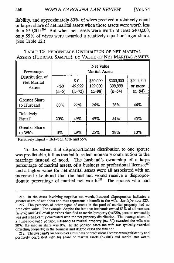
NORTH CAROLINA LAW REVIEW
liability, and approximately 80% of wives received a relatively equalor larger share of net marital assets when those assets were worth lessthan $50,000.216 But when net assets were worth at least $400,000,only 55% of wives were awarded a relatively equal or larger share.(See Table 12.)
TABLE 12: PERCENTAGE DISTRIBUTION OF NET MARITAL
ASSETS (JUDICIAL SAMPLE), BY VALUE OF NET MARITAL ASSETS
Net ValuePercentage Marital Assets
Distribution ofNet Marital $ 0 - $50,000 $200,000 $400,000
Assets <$0 49,999 199,000 399,999 or more(n=5) (n=72) (n=98) (n=54) (n=94)
Greater Shareto Husband 80% 22% 26% 28% 46%
RelativelyEqual' 20% 49% 49% 54% 45%
Greater Shareto Wife 0% 29% 25% 19% 10%
Relatively Equal = Between 45% and 55%
To the extent that disproportionate distribution to one spousewas predictable, it thus tended to reflect monetary contribution to themarriage instead of need. The husband's ownership of a largepercentage of marital assets, of a business or professional license,217
and a higher value for net marital assets were all associated with anincreased likelihood that the husband would receive a dispropor-tionate percentage of marital net worth.218 The spouse who had
216. In the cases involving negative net worth, husband disproportion indicates agreater share of net debts and thus represents a benefit to the wife. See infra note 225.
217. The presence of other types of assets in the pool of marital property had nopredictive value. For example, despite the fact that husbands owned 85% of all pensions(n=236) and 94% of all pensions classified as marital property (n=220), pension ownershipwas not significantly correlated with the net property distribution. The average share ofa husband-owned pension classified as marital property (n=180) awarded the wife was20%; the median share was 0%. In the pension cases the wife was typically awardedoffsetting property; in the business and degree cases she was not.
218. The husband's ownership of a business or professional license was significantly andpositively correlated with his share of marital assets (p<.001) and marital net worth
[Vol. 74

DECISION MAKING AT DIVORCE
contributed more income to the marriage tended to receive moreproperty. But this apparent judicial emphasis on monetarycontribution was not uniform. In cases of relative poverty, thewife-in all probability the needier party-tended to receive the lion'sshare of the assets. The husband's ownership of a relatively largeamount of separate property was, again, associated with disproportionin favor of the less-propertied wife.
b. The Predictability of Net Worth Distribution: More DetailedAnalysis
Property division outcomes were also analyzed taking intoaccount a variety of judicial characteristics and other case variablesunrelated to the legislative factors in order to determine whetherthese extra-statutory considerations had any value in predictingdivisional outcomes. They did not: Neither the judge's sex, age,religious affiliation, political party, judicial experience, nor educationalstatus score was significantly correlated with judicial sample net worthdistributions.219 Nor, in the judicial sample, did the case processingtime, case region, the gender of the spouse against whom the divorcewas granted, or the specific fault allegations upon which the divorcewas based demonstrate a significant relationship to the net worthdistribution.2"
For the settlement sample, variables that might suggest strategicbargaining behavior were also assessed. No significant predictiverelationships were found. Although litigation theorists have oftenposited that women confronted with the possibility of a custody battlemay make economic concessions to obtain custody.' an unrealizedcustody threat by the husband was insignificantly related to thedistributional outcome.' Nor did case processing time, another
(p<.001). The value of net marital assets and the husband's percentage share of thoseassets were also positively and significantly correlated (p<.001).
219. See infra Appendix, Table A7.220. The gender of the plaintiff and the fault findings were significantly linked to the
divisional outcome at the .05 confidence level in the settlement sample but did not, whenregression analysis was employed, significantly contribute to the predictive capacity of theregression model. For correlation coefficients and p values, see infra Appendix, Table A8.
221. See, e.g., MACCOBY & MNOOKIN, supra note 14, at 44-56; WEITZMAN, supra note12, at 242-43; Mnookin & Kornhauser, supra note 14, at 963-66; Robert H. Mnookin,Divorce Bargaining: The Limits of Private Ordering, 18 U. MICH. J.L. REFORM 1015, 1032-33 (1985).
222. A custody request by the husband is, of course, only a rough measure of thedegree of conflict over custody. Intense conflict may precede the filing of the divorcepapers; conversely, some lawyers may request custody for their client when the request
1996]

NORTH CAROLINA LAW REVIEW
potential conflict indicator,2' evidence a significant predictiverelationship.
Regression analysis 2 was then employed to determine therelative impact of property and litigant-related variables on propertydivision, as well as the extent to which these variables could be usedto predict disproportionate outcomes. Table 14 shows the results ofthat analysis for the judicial sample, excluding cases with negative networth.' The column headed "standardized regression coefficient"shows the magnitude and direction of the effect of the independentvariable upon the distribution of net marital property. 6 Thecolumn headed "t Stat." shows the t statistic, used to test thesignificance of an individual coefficient, and the level of significanceattained. 7 The Table shows the results when all variables sig-nificant at the .05 confidence level or better are used ("Full Model")and, in the right column ("Parsimonious Model"), the results when
lacks credibility. My finding on the lack of a significant relationship is, however, consistentwith that of Professors Maccoby and Mnookin, who employed parents' own conflict ratingsand still found no significant relationship between conflict level and support outcomes.See MACCOBY & MNOOKIN, supra note 14, at 154-57.
223. See id. at 138-39.224. For discussions of multiple regression analysis, see MICHAEL 0. FINKELSTEIN &
BRUCE LEVIN, STATISTICS FOR LAWYERS 323-442 (1990); MICHAEL S. LEWIS-BECK,APPLIED REGRESSION: AN INTRODUCTION 47-74 (1980).
225. In cases involving negative net worth the distributional percentage typically givesa misleading impression of case outcome. Suppose that a couple owns $7000 in assets and$10,000 in debts. If the wife is awarded $5000 in debts and $4000 in assets, while thehusband is awarded $5000 in debts and $3000 in assets, the wife gets 33% of net worth(-$1000/-$3000) and the husband 67% (-$2000/-$3000). But the wife is better off than herhusband. In order to include negative net worth cases in the analysis, the distribution ofproperty and debt was also analyzed by adding debts to assets and calculating eachspouse's share of the pool on a 100-point scale. This approach, which I have termed"distribution of the marital estate," was also employed in analysis of the settlement casesample property/debt distribution data. See Garrison, supra note 12, at 670-71. Only fivejudicial sample cases in which the division of net marital assets could be determinedinvolved negative net worth. Regression analysis of the distribution of the marital estate,including these cases, did not vary substantially from the analysis displayed in Table 14.The full and parsimonious regression models explicated 14% of the variability in outcomes;the parsimonious model eliminated the same variables.
226. More precisely, the regression coefficient shows the effect that one standarddeviation difference in the independent variable would have on the standardized score.For example, the regression coefficient for the wife's income is .148981, which means thata difference of one standard deviation in this variable is predicted to cause a difference of.148981 standard deviation in the percentage distribution of net marital property. Becausethe coefficient is positive, a higher income is predicted to produce a higher percentageshare of net marital property for the wife. See FINKELSTEIN & LEVIN, supra note 224, at332-36.
227. For a more detailed explanation of the t-statistic, see id. at 352-53.
[Vol. 74

DECISION MAKING AT DIVORCE
variables that fail to significantly improve the model's predictivepower are eliminated. After this elimination, only five variables-thehusband's ownership of a business or professional license, the wife'sincome, the value of net marital property, the proportion of maritalproperty owned by the husband, and the value of the husband'sseparate property-significantly contributed to the prediction of networth distribution. The predictive power of both the full and par-simonious regression models is also quite modest; both explain lessthan 15% of the variation in net property division outcomes.2"Moreover, the results displayed in Table 13 derive from a reductionof net property distribution percentages to five categories: When theregression model was employed to predict actual percentages, 9 itspredictive capacity was, not surprisingly, even smaller.
228. Regression analysis of results for the smaller group of cases involving minorchildren, where the percentage of the obligor's income awarded as child support was ahighly significant predictor of the net property division outcome, was somewhat moresuccessful in explicating the variation in outcomes. The full regression model, employingthe same variables listed in Table 14 and the child support percentage, explicatedapproximately 24% of the variation in outcomes.
229. The full model (n=159), employing the same variables, accounted for 12% of thevariance.
1996] 463

NORTH CAROLINA LAW REVIEW
TABLE 13: REGRESSION ANALYSIS OF NET MARITAL PROPERTYDISTRIBUTION JUDICIAL SAMPLE: TRIAL COURTS
(CASES WITH POSITIVE NET WORTH)DEPENDENT VARIABLE = PERCENTAGE AWARD TO WIFE 0
Full ParsimoniousIndependent (n=247) Model (n=247) Model
VariableStandard. t Stat. Standard. t Stat.Regression (p=) Regression (p=)Coefficient Coefficient
Husband OwnsMarital Business -.204901 - 3.179 -.203676 -3.254or Degree (.0017) (.0013)
Wife's -.068899 - .895
Employment (.3717)
Wife's Income .148981 1.904 .154735 2.499(.0581) (.0131)
Wife's Health -.039545 -.621(.5353)
Wife's Income/ -.058650 -.697Family Income (.4864)
Net Marital -.183989 -2.727 -.178067 2.499Property Value (.0069) (.0062)
% of MaritalProperty Owned -.131919 -2.044 -.132144 - 2.065by Husband (0421) (.0400)
Husband'sSeparate Property .175077 2.857 .175304 2.874Value (.0049) (.0044)
Constant 10.235 24.984(.0000) (.0000)
Proportion of variability explained by model:Y' 13.79% 14.24%
230. Coded as five ranks based on the wife's percentage award of net marital assets:1 = less than 34%; 2 = 34%-44%; 3 = 45%-55%; 4 = 56%-66%; 5 = more than 66%.
231. The percentages refer to the "adjusted R Square." The multiple correlationcoefficient, R, is the correlation between the regression estimates and the observed values
[Vol. 74

1996] DECISION MAKING AT DIVORCE 465
The data do support the claim that judges often fail to award anequal share of business or professional assets to the nontitled spouse.And in cases where the couple is relatively wealthy, the claim thatjudges give greater weight to monetary contributions than tocontributions as a spouse, parent, and homemaker finds some support.But these tendencies were by no means uniform and their value inexplaining outcome variation is modest. Some divisional outcomescould also be explained by reference to relatively unusual case facts.For example, when one spouse had committed a crime against afamily member, the other was almost invariably awarded the lion'sshare of the assets."2 Dissipation or concealment of significantmarital assets often produced a skewed distribution as well.z3 Bothof these situations are relevant to the distribution decision under theNew York statute2' and judges clearly took them into account.235
of the dependent variable. The squared multiple correlation coefficient, R Square, canthus be interpreted as the proportion of the total variability of the dependent variable thatis explained by the regression equation. R Square ranges between 0 (no association) and1 (a perfect fit). Since the regression equation is optimally fitted to the data, R Square isbiased upward; to compensate, R Square is generally adjusted downward, and the revisedestimate is called the adjusted R Square. See FINKELSTEIN & LEVIN, supra note 224, at345-46.
232. In four of the five sample cases in which the husband had committed criminal actsinvolving a family member, the wife received a disproportionate share of the net maritalproperty. See Brancoveanu v. Brancoveanu, 535 N.Y.S.2d 86, 90 (N.Y. App. Div. 1988),appeal dismissed, 538 N.E.2d 358 (N.Y. 1989), cert. denied, 502 U.S. 854 (1991); Thompsonv. Thompson, N.Y. L.J., 1/5/90, at 28, col. 3 (Sup. Ct.); Vasquez v. Vasquez, N.Y. L.J.,4/4/86, at 13, col. 1 (Sup. Ct.); Wenzel v. Wenzel, 472 N.Y.S.2d 830, 835 (Sup. Ct. 1984).In the one exception, Valenza v. Valenza, N.Y. LJ., 1/16/90, at 31, col. 4 (Sup. Ct.), thewife as well as the husband was found guilty of criminal misconduct.
233. See, e.g., Farenga v. Farenga, N.Y. L.J., 3/14/83, at 16, col. 1 (Sup. Ct.); Lenczyckiv. Lenczycki, 543 N.Y.S.2d 724, 726-27 (N.Y. App. Div. 1989); Mahon v. Mahon, 514N.Y.S.2d 446,447 (N.Y. App. Div. 1987); Whelan v. Whelan, N.Y. L.J., 9/24/81, at 12, col.5 (Sup. Ct.).
234. Dissipation of assets is specifically listed as a factor in property division. N.Y.DOM. REL. LAW § 236B(5)(d) (McKinney 1986). Marital fault is not listed as a factor but,interpreting the last clause of the statute authorizing the judge to consider "any otherfactor which the court shall expressly find to be just and proper," appellate courts haveruled marital fault relevant if egregious. See, e.g., Blickstein v. Blickstein, 472 N.Y.S.2d110, 113-14 (N.Y. App. Div. 1984). In interpreting this test, courts have found criminalviolence, including assault, rape, kidnapping, a long history of physical abuse, andattempted murder to constitute egregious fault, but have found that lesser offenses fail toqualify. For a useful summary of the cases, see McCann v. McCann, 593 N.Y.S.2d 917,920-22 (Sup. Ct. 1993).
235. Neither evidenced a significant predictive relationship, however. One reason whyasset dissipation evidenced no significant relationship with case outcome is the varyingmethodologies employed by judges confronting a case by dissipation. In some instancesjudges included the value of the unavailable property in the pool of marital assets subjectto distribution and assigned it to the guilty spouse. Trial court judges typically distributed

NORTH CAROLINA LAW REVIEW
But, overall, the explanatory value of the legislative factors is quiteslight. More often than not, judicial deviation from the new equaldivision norm is simply inexplicable from the data at hand.
Property distribution outcomes were, ironically, more predictablein the settlement sample, at least if cases involving negative net worthare excluded from the analysis. Using regression analysis, slightlymore than 30% of the variation in outcomes could be predicted. Butthe predictive variables were the percentages of marital property towhich each spouse held title. 6 Moreover, the inclusion of caseswhere debts exceeded assets-a far more numerous group in thesettlement than in the judicial sample and one where wives tended todo comparatively well-eroded the value of title as a predictivevariable substantially; 7 for this larger case set, only 6% of casevariation was explicable.
Thus, in neither the judicial nor the settlement sample is itpossible to explain much of the variation in results on the basis of theavailable case information. The lingering impact of title is apparentin both case sets. Some of the statutory factors were significantlycorrelated with case outcomes. But judicial consensus on when andhow to deviate from the new equal division norm is not apparent, andthe relative rarity of equal division in the settled cases, a result thatcannot be explained on the basis of strategic bargaining, is striking.What is perhaps most notable about the property division data issimply that they explain so little.
this enhanced pool relatively equally. See, e.g., Vogel v. Vogel, 549 N.Y.S.2d 438, 440(N.Y. App. Div. 1989); Contino v. Contino, 529 N.Y.S.2d 14, 14-15 (N.Y. App. Div. 1988);Gottlieb v. Gottlieb, N.Y. L.J. 6/29/82, at 15 col. 1 (Sup. Ct.); see also Harrell v. Harrell,502 N.Y.S.2d 57, 58-59 (N.Y. App. Div. 1986) (remitting case to trial court where thatcourt had failed to include value of dissipated assets in pool distributed and awardedhusband who had dissipated assets an equal share of those remaining). In other cases(particularly when the value of the missing assets could not be determined), the courtsimply awarded the lion's share of the remaining assets to the blameless spouse. See, e.g.,Lenczycki v. Lenczycki, 543 N.Y.S.2d 724, 727 (N.Y. App. Div. 1989); Mahon v. Mahon,514 N.Y.S.2d 446 (N.Y. App. Div. 1987); Farenga v. Farenga, N.Y. L.J., 3/14/83, at 16, col.1 (Sup. Ct.); Whelan v. Whelan, N.Y. L.J., 9/24/81, at 12 col. 5 (Sup. Ct.).
236. No other variables contributed significantly to the model's predictive capacity.237. Twenty-two percent of couples in the settlement sample had debts exceeding their
assets, as compared to 4% in the judicial sample. See supra Table 3.
[Vol. 74

DECISION MAKING AT DIVORCE
B. Alimony and Child Support
1. The Award of Alimony
a. The Judicial and Settlement Samples Compared
Although litigation to trial appeared to confer no remarkableadvantage on judicial sample wives with respect to property division,it was associated with a higher alimony rate. At the trial court level,62% of wives in the judicial sample were awarded alimony,"8 anaward rate more than four times that of divorced women in both NewYork state 9 and the nation,' and approximately double thealimony award rate of wives in the settlement sample.
The best predictors of alimony in both the judicial and settlementgroups were spousal income24' and marital duration;24 the highalimony rate for the judicial cases thus reflects, in part, the greaterproportion of lengthy marriages, low-income wives, and high-incomehusbands in this group. For example, the alimony rate for employedwomen married less than ten years varied insignificantly by casegroup. But there were approximately twice as many women withthese characteristics in the settlement group as in the judicial sample.(See Table 14.)
238. Three husbands (.8%) were awarded alimony as well.239. See Garrison, supra note 12, at 697 (alimony award rate in three New York
counties was 12% in 1984).240. See GORDON H. LESTER, JR., BUREAU OF THE CENSUS, U.S. DEP'T OF
COMMERCE, CHILD SUPPORT AND ALIMONY 1989 1 (Current Population Reports, SeriesP-60, No. 173) (1991) (reporting that 15% of women who had ever divorced or separatedas of 1990 had been awarded alimony).
241. For correlation coefficients and p values, see infra Appendix, Table A14.242. Similar relationships between alimony and income, and alimony and marital
duration, have been noted by other researchers. See, e.g., STERIN & DAVIS, supra note12, at 140-41; WErrzMAN, supra note 12, at 169, 179; Rosalyn B. Bell, Alimony and theFinancially Dependent Spouse in Montgomery County, Maryland, 22 FAM. L.Q. 225, 294(1988); McLindon, supra note 12, at 363-64; Rowe & Morrow, supra note 12, at 476-77;Wishik, supra note 12, at 88.
1996]

NORTH CAROLINA LAW REVIEW
TABLE 14: PERCENTAGES OF SAMPLE WIVES AWARDED ALIMONY, BY
MARITAL DURATION, WIFE'S EMPLOYMENT STATUS, AND CASE GROUP
Marital Duration & Judicial Settlement DifferenceWife's Employment Status Sample Sample
% (n) % (n)
Unemployed wives 83% (116) 49% (47) -34".married > 10 years
Unemployed wives 74% (31) 50% (32) -24"married < 10 years
All Unemployed Wives 82% (151) 52% (79) -30."
Employed wives married 53% (170) 27% (132) -34.">_ 10 years
Employed wives married 23% (39) 21% (73) -2<10 years
All Employed Wives 48% (214) 26% (208) -22."
p<..uJ, p<.uu.
The higher alimony award rate in the judicial group does notappear to result simply from sample composition, however. Long-married and low-income wives, who had the highest alimony awardrates in both case sets, had significantly higher award rates when thecase was judicially decided. Among women married twenty or moreyears, for example, 69% of the judicial group were awarded alimonycompared to 39% in the settlement sample. (See Table 15.)
TABLE 15: PERCENTAGES OF SAMPLE WIVES AWARDED
MARITAL DURATION AND CASE GROUP
ALIMONY, BY
Judicial SettlementMarital Duration Sample Sample Difference
% (n) % (n)
0 - 4 years 50% (14) 27% (44) -23
5 - 9 years 46% (59) 28% (71) -18"
10 - 14 years 58% (77) 29% (68) -29."
15 - 19 years 64% (73) 22% (51) -42"'.
20 or more years 69% (144) 39% (79) -30...
All Sample Cases 62% (377) 31% (313) -31."
p<.05, **' p<.001
468 [Vol. 74

DECISION MAKING AT DIVORCE
Similarly, 89% of wives who earned less than 10% of family incomewere awarded alimony by the judges, as compared to an alimonyaward rate of 58% for this group in the settlement sample.243
(See Table 16.)
TABLE 16: PERCENTAGES OF SAMPLE WivEs AWARDEDALIMONY, BY WIFE'S INCOME PERCENTAGE (WIFE'S
INCOME/FAMILY INCOME) AND CASE GROUP
Wife's Income/ Judicial SettlementFamily Income Sample Sample Difference
% (n) % (n)
0%- 9% 89% (113) 58% (76) -31**
10- 29% 76% (86) 31% (49) -45* *
30- 49% 39% (56) 12% (57) -27**
50% or more 4% (28) 4% (23) -0p<.01, "'* p<.001
Litigation to trial was thus associated with a higher alimony awardrate both because the judicial sample contained more long-marriedand low-income wives-the group with the best alimonyprospects-and because wives with these characteristics receivedalimony awards more frequently from judges than through thesettlement process.
b. Changes in Judicial Alimony Decision Making Over Time
The advantages of litigation were not consistent over the ten yearperiod reviewed. The judicial alimony award rate for the period 1980-83 was fourteen percentage points higher than for the period 1987-90;a later decision year was, in fact, a significant negative predictor of analimony award.2' Nor was the lower alimony rate for the laterperiod confined to women in short marriages. Women married fortwenty or more years experienced a decline in their alimony prospectsidentical to that experienced by women married for less than tenyears. (See Table 17).
243. Similar differences are observable in many segments of the sample population.For a comparison of alimony award rates by wife's income, husband's income, and custodystatus, see infra Appendix, Tables AS-A10.
244. p=.018.
1996]

NORTH CAROLINA LAW REVIEW
TABLE 17: JUDICIAL SAMPLE ALIMONY AWARDS,DURATION AND TIME PERIOD
BY MARITAL
Time Period
Marital Duration 1980-83 1984-86 1987-90% (n) % (n) % (n)
0 - 9 years 65% (20) 32% (25) 46% (28)
10 - 19 years 68% (37) 58% (72) 61% (41)
20 or more years 75% (44) 73% (59) 56% (41)
All Sample Cases 71% (102)1 60% (161) 57% (114)
The alimony prospects of women who earned an extremely smallpercentage of family income were unaffected by the lower award ratein later research years, however. Wives earning less than 10% offamily income were not significantly less likely to be awarded alimonyin the last triennial period than they were in the first. (See Table 18.)Women earning at least 30% of family income, on the other hand,saw their alimony prospects decline by almost half over the researchperiod. The declining alimony award rate over the ten year periodreviewed thus appears to reflect increased judicial emphasis on needas compared to other factors.
TABLE 18: JUDICIAL SAMPLE ALIMONY AWARDS, BY WIFE'S
INCOME PERCENTAGE AND TIME PERIOD
Wife's Income Time PeriodPercentage
(Wife's Income/ 1980-83 1984-86 1987-90Family Income) % (n) % (n) % (n)
0%- 9% 91% (32) 87% (53) 89% (28)
10-29% 78% (23) 74% (35) 75% (28)
30% or more 40% (25) 23% (35) 21% (24)
All Sample Cases 71% (102) 1 60% (161) [ 57% (114)
470 [Vol. 74

DECISION MAKING AT DIVORCE
2. The Duration of Alimony
a. The Judicial and Settlement Samples ComparedIn contrast to the markedly higher judicial alimony rate, litigation
to trial -was not associated with significantly enhanced prospects of apermanent alimony award. Only 35% of judicial alimony awardswere permanent, as compared to 31% in the settlement group.245
Nor were long-married and older women more likely to beawarded permanent alimony by judges than through the settlementprocess. Although marital duration was a highly significant predictorof a permanent award for both case groups,246 permanent awards tolong-married wives were no more frequent in the judicial sample thanin the settlement group. (See Table 19.)
TABLE 19: PERCENTAGES OF SAMPLE ALIMONY AWARDS THATWERE PERMANENT, BY CASE GROUP AND MARITAL DURATION
Judicial Settlement DifferenceMarital Duration Sample Sample
% (n) % (n)
0 - 9 years 24% (33) 28% (32) + 4
10 - 19 years 28% (93) 20% (30) - 8
20 or more years 46% (98) 45% (31) - 1
All Sample Cases 35% (230)1 31% (93) -4
Age, too, was a significant predictor of a permanent award for bothcase sets,247 but the likelihood of a permanent alimony award forwomen over fifty was actually somewhat lower in the judicial samplethan in the settlement group.2'
Nor, when time-limited alimony was awarded, were judicialawards likely to extend over a significantly longer period. The
245. The difference was not significant.246. For the judicial sample, p<.001. For the settlement sample, p=.024. The difference
in permanency rates by case group was not significant for any marital duration category.247. For the judicial sample, p=.003. For the settlement sample, the husband's rather
than the wife's age was statistically significant (p=.050). The difference in permanencyrates by case group was not significant in any age category.
248. For a more detailed presentation, see infra Appendix, Table A13.
1996]

NORTH CAROLINA LAW REVIEW
average length of a time-limited award was 5.0 years in the judicialsample249 and 4.6 years in the settlement group.2
b. The Impact of Statutory Change Upon Judicial AwardsAlthough the 1986 amendments to the Equitable Distribution
Law 1 were intended to reverse the trend toward durationalalimony, these amendments had no apparent impact. The proportionof alimony awards that were permanent was lowest in 1987-90, afterthe amendments went into effect. (See Table 20.) Indeed, a laterdecision year was a significant negative predictor of a permanentaward.22 The passage of the amendments was, however, associatedwith stabilization of the permanent alimony rate among long-marriedwives; although the permanent alimony rate for this group did notincrease after 1986, wives married twenty or more years did not seea further decline in their prospects of a permanent alimony award.Wives married for shorter periods, on the other hand, saw thelikelihood of permanent alimony continue to fall.
TABLE 20: PERCENTAGES OF JUDICIAL SAMPLE ALIMONYAWARDS THAT WERE PERMANENT, BY MARITAL DURATION
AND TIME PERIOD
Time PeriodMarital Duration 1980-83 1984-86 1987-90
% (n) % (n) % (n)
0 - 9 years 31% (13) 38% (8) 8% (12)
10 - 19 years 46% (24) 26% (43) 15% (26)
20 or more years 50% (32) 44% (43) 44% (23)
All Sample Cases1 44% (70)] 35% (97) 25% (63)
249. The median was 4.1 years; judicial awards ranged from 0.9 to 26.0 years (n=148).250. The median was 3.5 years; settlement awards ranged from 1.0 to 13.0 years (n=62).251. For a description of the amendments, see supra notes 113-14 and accompanying
text.252. p=.022.
[Vol. 74

DECISION MAKING AT DIVORCE
3. The Value of Alimony and Child Support
a. The Judicial and Settlement Samples Compared
In contrast to the similarity of judicial and settlement permanenceoutcomes, the average value of both alimony 3 and child sup-port' varied substantially by case group. The average value ofcombined alimony and child support in the judicial group 15 was,indeed, almost double its value in the settlement sample. 6 (SeeTable 21.)
TABLE 21: MEAN ALIMONY AND CHILD SUPPORT AWARDS
(1990 DOLLARS), BY CASE GROUP
Judicial SettlementMean Award Sample Sample Difference
(1990 Dollars) $ per month $ per month(n) (n)
Alimony:when awarded $1084 (233) $ 978 (98) - 106all cases $ 677 (373) $ 307 (312) - 370-
Child Support:per family $ 778 (225) $ 481 (196) - 297-per minor child $ 430 (225) $ 301 (196) - 129"
Total Alimony &Child support:
minor children $1474 (225) $ 709 (208) - 765""no minor children $ 675 (143) $ 429 (97) - 246all cases $1163 (368) $ 620 (305) - 543-
p<.01, "'" p<.O01
253. The median monthly alimony award was $685 in the judicial sample (n=233) and$405 in the settlement group (n=98).
254. The median monthly child support award was $683 in the judicial sample (n=196)and $378 in the settlement group (n=196).
255. Judicial awards were not more likely to include enhancements of the basic alimonyand child support package than were awards based on settlement, however. For acomparison of enhancements to child support by case group, see infra Appendix, TableA15. Provision for the payment of college expenses was, indeed, more common in thesettlement group than in the judicial sample. See infra Appendix, Table A15.
256. The median monthly combined award was $815 for the judicial sample (n=368) and$324 for the settlement sample (n=305).
1996]

NORTH CAROLINA LAW REVIEW
While the higher dollar values of judicial alimony and childsupport awards reflect, to some extent, the higher incomes of couplesin the judicial sample, judicial awards also constituted a largerpercentage of obligor income. For judicial cases involving minorchildren, the average percentage of obligor income awarded incombined alimony and child support was 31%, as compared to 23%in the settlement sample.17 Although the difference between thesettlement and judicial groups was not significant at all income levels(see Table 22), it was consistent over the ten-year periodreviewed.' 8
TABLE 22: MEAN PERCENTAGE OF OBLIGOR'S GROSS INCOME(1990 DOLLARS) AWARDED AS ALIMONY AND CHILD SUPPORT,
BY OBLIGOR'S INCOME AND CASE GROUP
Mean % of Income Mean % of IncomeObligor's Awarded as Child Awarded as Child
Gross Income Support Support & Alimony(1990 Dollars) J Group S Group J Group S Group
(n) (n) (n) (n)
$0-$34,999 29% 21%* 38% 24%"
(38) (76) (38) (76)
$35,000-$69,999 18% 17% 31% 22%*"
(77) (47) (77) (47)
$70,000 + 13% 9% 25% 19%
(59) (14) (59) (14)
All Sample 19% 18% 31% 23%...
Cases (174) (137) (174) (137)
J Group= Judicial Group; S Group=Settlement Group
Difference between group means: * p<.05, "' p<.01, *" p<.001
257. For cases not involving minor children, the average percentage of obligor incomeawarded as alimony in the judicial sample was 15%, if $0 awards are included in thecalculation, or 22%, if $0 awards are excluded; in the settlement sample, the averagepercentage was 8% ($0 awards included) or 21% ($0 awards excluded).
258. In the judicial sample, the average percentage of obligor income awarded as childsupport was 18% (n=49) in 1980-83; 18% (n=71) in 1984-86; and 22% (n=51) in 1987-90.The average percentage of obligor income awarded in combined alimony and child support(for cases involving minor children) was 31% (n=49) in 1980-83; 30% (n=73) in 1984-86;and 32% (n=52) in 1987-90.
[Vol. 74
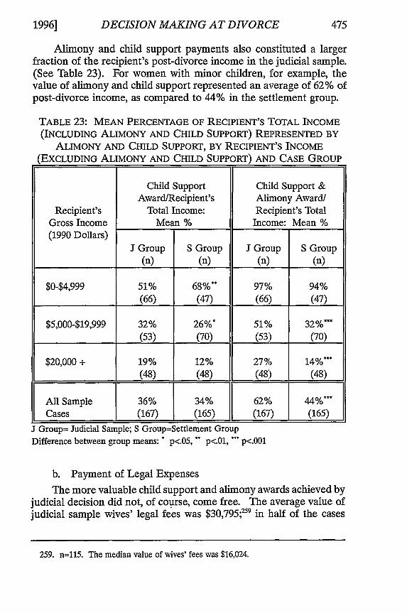
1996] DECISION MAKING AT DIVORCE
Alimony and child support payments also constituted a largerfraction of the recipient's post-divorce income in the judicial sample.(See Table 23). For women with minor children, for example, thevalue of alimony and child support represented an average of 62% ofpost-divorce income, as compared to 44% in the settlement group.
TABLE 23: MEAN PERCENTAGE OF RECIPIENT'S TOTAL INCOME
(INCLUDING ALIMONY AND CHILD SUPPORT) REPRESENTED BYALIMONY AND CHILD SUPPORT, BY RECIPIENT'S INCOME
(EXCLUDING ALIMONY AND CHILD SUPPORT) AND CASE GROUP
Child Support Child Support &Award/Recipient's Alimony Award/
Recipient's Total Income: Recipient's TotalGross Income Mean % Income: Mean %(1990 Dollars)
J Group S Group J Group S Group(n) (n) (n) (n)
$0-$4,999 51% 68%** 97% 94%(66) (47) (66) (47)
$5,000-$19,999 32% 26%* 51% 32%-(53) (70) (53) (70)
$20,000 + 19% 12% 27% 14%'**1 (48) (48) (48) (48)
All Sample 36% 34% 62% 44%***Cases (167) (165) (167) (165)
J Group= Judicial Sample; S Group=Settlement GroupDifference between group means: * p<.05, "" p<.01, * p<.001
b. Payment of Legal Expenses
The more valuable child support and alimony awards achieved byjudicial decision did not, of course, come free. The average value ofjudicial sample wives' legal fees was $30,795;'9 in half of the cases
259. n=115. The median value of wives' fees was $16,024.

NORTH CAROLINA LAW REVIEW
for which a comparison could be made, the wife's fees were equal tomore than a year of combined alimony and child supportpayments.26° Although judicial sample husbands were also morelikely to shoulder some or all of their wives' legal fees than were theircounterparts in the settlement case group,261 this difference stemmedlargely from a higher proportion of cases requiring joint payment ofthe wife's fees. In these joint payment cases, judges generally failedto specify either the wife's total fees or the percentage that thehusband was required to pay; information on the value of legal feeswas also rarely available in the settlement sample files. The datathus do not permit comparison of wives' legal expense obligations bycase group, but it is entirely possible that the higher child support andalimony awards to women in the judicial sample were more thanoffset by higher expenses associated with obtaining a litigated divorcejudgment. (See Table 24.)
260. n=89. The median ratio of a wife's fees to her combined annual alimony and childsupport award was 1.28; the mean ratio was 3.17.
261. In the settlement sample, payment of the wife's legal fees by the husband wassignificantly and positively correlated with the wife's award of alimony (p<.001), thehusband's income (p=.047 ), the value of combined alimony and child support (p=.025), andthe percentage of the husband's income awarded in combined alimony and child support(p<.001). Payment of the wife's legal fees by the husband was significantly and negativelycorrelated with the wife's income (p=.004). The wife's employment status, the custody ofminor children, the percentage of family income she earned, and marital duration were notsignificantly related to the payment of her counsel fees.
In the judicial sample, the husband's payment of the wife's counsel fees wassignificantly and positively correlated with the wife's award of alimony (p<.001), thehusband's income (p=.010), the value of combined alimony and child support (p<.001), thewife's employment status (p=.003), and the percentage of the husband's income awardedin alimony and child support (p<.001). The husband's payment of the wife's counsel feeswas also significantly - and negatively - correlated with the percentage of family incomeearned by the wife (p<001) and the wife's income (p<.001). Marital duration and custodystatus were not significantly related to the the husband's payment of the wife's counselfees.
[Vol. 74

1996] DECISION MAKING AT DIVORCE 477
TABLE 24: PAYMENT OF SAMPLE WIVES' LEGAL FEES. BY CASE GROUP
Cases with joint or split custody excluded.
4. Post-Divorce Income and Standard of Living
Even if the impact of their legal expenses is ignored, childsupport and alimony awards to women in the judicial sample weretypically inadequate to prevent a marked drop in their post-divorcestandard of living. Although women in this group suffered a slightlysmaller average decline in per capita income and standard of livingthan did women in the settlement sample, the difference wasinsignificant.262 In both case sets, the average woman's standard ofliving" fell markedly, while that of her husband improved. (See
262. A comparison of median per capita income changes produced comparable results.In the judicial sample, the median ratio of the husband's post to pre-divorce per capitaincome was 163%; the wife's was 61%. In the settlement sample, the median ratio of thehusband's post to pre-divorce per capita income was 172%; the wife's was 63%.
263. Per capita income fails to accurately measure standard of living because it ignoreseconomies of scale. A variety of equivalence scales have been developed to take accountof economies of scale and thus produce a more realistic measure of living standards.These equivalence scales typically adjust family income by family size raised to a powerranging between 0.2 to 1 (the size elasticity), with 1 representing per capita income and0.2 representing an adjustment that assumes very large economies of scale. For discussionsof equivalence scales, see, e.g., B. Buhmann et al., Equivalence Scales, Well-being,Inequality and Poverty: Sensitivity Estimated across Ten Countries using the LuxembourgIncome Study (LIS) Database, REV. INCOME & WEALTH 115 (June 1988); Sorensen, supranote 43, at 273-74. Change in post-divorce standard of living is extremely sensitive to theequivalence scale utilized. See Sorenson, supra note 43, at 280 tbl. 15.5 (comparing post-divorce change in living standards using four different measurements). Post-divorce
Wife Category Judicial Sample Settlement SampleFees Paid by: % (n) % (n)
Alimony Recipients Fees (205) (83)paid by: Husband 34% 39%
Joint 38% 18%Wife 28% 42%
Custodial Parents* (176) (142)Fees paid by: Husband 26% 25%
Joint 43% 18%Wife 31% 56%
All Wives (324) (266)Fees paid by: Husband 25% 22%
Joint 34% 16%Wife 41% 61%

NORTH CAROLINA LAW REVIEW
Table 25.) Because judicial sample wives were more likely to receivesome portion of the husband's post-divorce support obligation in theform of alimony, it is indeed possible, given the prevalence of short-term alimony awards, that they would be worse off than theirsettlement group counterparts within a few years after the divorce.
TABLE 25: CHANGES IN HUSBANDS' AND WIVES' PER CAPITA INCOME
AND LIVING STANDARDS POST-DIVORCE, BY CASE GROUP
Judicial Sample Settlement Sample
Median Per Median Per
Capita Income Capita Income
(1990 Dollars) (1990 Dollars)
Mean % (n) Mean % (n)
Pre-Divorce Family $20,544 (287) $14,781 (205)
Husband's household after
divorce: $35,177 (296) $27,028 (221)
Ratio of post to pre-divorce per
capita income: 172% (266) 182% (196)
Ratio of post to pre-divorce
living standard:* 126% 135%
Wife's household after divorce: $12,515 (292) $9,710 (262)
Ratio of post to pre-divorce
per capita income: 71% (266) 68% (196)
Ratio of post to pre-divorce
living standard:* 61% 57%
Measured as ratio of post to pre-divorce per capita income, adjusted by familysize(073).
In both case sets there was also significant variation in the ratioof the wife's to husband's post-divorce standard of living. In both
change in living standard was measured here using a size elasticity of 0.73, whichapproximates the size elasticity underlying the U.S. Bureau of Labor Statistics (BLS)standard budgets for urban families. See Buhmann et al., supra, at tbl. 2; Sorensen, supranote 43, at 273. Professor Weitzman also relied on the BLS equivalence scale in assessingpost-divorce change in living standards, but measured the change in income over the BLSLower Standard Budget for a family of comparable size. WEITZMAN, supra note 12, at338-39, 481-82 n. 19. The average living standard changes (+42% for husbands; -73% forwives) Weitzman reports, id. at 338-39, have been criticized by some demographers asunlikely results given her underlying data on per capita income changes. See Hoffman &Duncan, supra note 43, at 643-44.
[Vol. 74

DECISION MAKING AT DIVORCE
groups, wives in the highest income category married to husbands inthe lowest actually enjoyed a higher post-divorce living standard, onaverage, than did their husbands, while wives in the lowest incomecategory married to husbands in the highest experienced the largestrelative decline. (See Table 26 and Appendix, Table All.)
TABLE 26: MEAN RATIO OF WIFE'S POST-DIVORCE STANDARD OF
LIVING*YHUSBAND'S POST-DIVORCE STANDARD OF LIVING* (JUDICIAL
SAMPLE), BY HUSBAND AND WIFE PRE-DIVORCE INCOME
Husband's Income
Wife's Income $0 - $34,999 $35,000- $60,000 +$59,999
mean mean meanratio (n) ratio (n) ratio (n)
$ 0 - $4,999 .48 (21) .26 (32) .23 (42)
$5,000- $19,999 .42 (40) .45 (31) .33 (24)
$20,000 + 1.83 (19) .88 (29) .44 (29)
All SampleWives .77 (80) .52 (92) .32 (95)
Measured by post-divorce family income adjusted by size (0.73).
This pattern suggests that the prime determinant of post-divorceliving standards is the pre-divorce income of each spouse, rather thanincome transfers in the form of alimony and child support. The ratioof the wife's and husband's post-divorce living standards wassignificantly and positively correlated with the percentage of familyincome earned by the wife' and the value of her income 65 Theaward of alimony to the wife' and the value of combined alimonyand child support,2 67 on the other hand, were (at least for cases inthe judicial sample) significant negative predictors of the ratio.
264. In both the judicial and settlement samples, p<.001.265. In both the judicial and settlement samples, p<.001. In the judicial sample, the
ratio was not significantly correlated with the value of the husband's income (p=.244); inthe settlement sample it was significantly correlated (p=.003).
266. In the judicial sample, p=.008; in the settlement sample, p=.217.267. In the judicial sample, p=.020; in the settlement sample, p=.26 1.
1996]

NORTH CAROLINA LAW REVIEW
While a judicial decision was thus associated with the award ofmore valuable alimony and child support, in amounts representing ahigher proportion of obligor and recipient income, these transferswere, in the vast majority of cases, inadequate to ensure wives andchildren a post-divorce living standard equal to that enjoyed by thehusband."r Nor was the average gap between the post-divorceliving standards of wives and husbands significantly smaller in thejudicial sample than the settlement group.
It is important to note, however, that the post-divorce gap in theliving standards of husbands and wives produced by discretionarydecision making was not demonstrably greater than that which wouldbe produced under New York's new, determinate child supportguidelines. Although these guidelines curtailed judicial discretion inorder to reduce post-divorce income disparities,2 69 the averagepercentage of obligor income awarded as child support in both thejudicial and settlement samples was fairly equivalent to what onewould predict under the support guidelines. Although directcomparisons are not possible,27 the results of discretionary decisionmaking do not appear to be markedly different from those mandatedunder these new bright-line rules.
5. The Predictability of Alimony and Child SupportDecision Making
a. The Award of Alimony
In contrast to property division, where only a few of the factorsenumerated in the statute had explanatory value, the award ofalimony was significantly correlated with a long list of litigant
268. Only 16% of wives in the judicial sample had post-divorce adjusted incomes equalto or greater than their husbands' post-divorce adjusted incomes (n=267).
269. See supra note 43 and accompanying text (discussing such disparities).270. New York's child support guidelines describe the presumed child support amount
as a percentage of the obligor's gross income. For one child the percentage is 17%; fortwo, 25%. N.Y. DOM. REL. LAW § 240.1-b(b)(3) (McKinney Supp. 1995). As the averagenumber of children in the judicial sample was 1.2, one would expect the rate to be about19%. But the guidelines include alimony in the child support calculation only if theagreement or court order establishing the alimony award requires an adjustment in childsupport upon the termination of the alimony obligation, id. § 240.1-b(b)(5)(vii)(C), andmandates pro rata apportionment of reasonable child care expenses related to employmentor job training in addition to the percentage award, id. § 240.1(c)(4). The presumedpercentages also apply only to combined parental income less than $80,000. Id. § 240.1-b(c)(2).
[Vol. 74

DECISION MAKING AT DIVORCE
characteristics deemed relevant by the legislature."' In both thejudicial and settlement groups, the variables most strongly correlatedwith the award of alimony were the wife's income, employment, andthe percentage of family income that she earned. In the judicialsample, the wife's education, occupational status, health, maritalduration, whether the marriage produced children, the percentage ofthe husband's income paid in child support, and the husband's oc-cupational status were also significant at the .05 confidence level, aswere the value of the wife's assets, net marital assets, and her netproperty award.2n
Although a number of statutory variables that demonstratedsignificance within the judicial sample failed to do so within thesettlement group, the strength and direction of the variable cor-relations in the two case sets were often quite similar.273 Only onevariable, the husband's income, was significantly related to thealimony decision in the settlement case group and failed todemonstrate significance in the judicial sample.
The relationship between various nonstatutory factors andalimony awards was also assessed. In the judicial sample, thelikelihood of an alimony award varied significantly by case region; alater decision year was also significantly and negatively correlatedwith the alimony outcome.274 The only judicial characteristic thatdemonstrated significance at the .05 confidence level was the judge'sage,275 although the judge's sex narrowly escaped significance at the.05 confidence level.276 Neither the judge's political party, length ofjudicial experience, educational background, or religion was sig-nificantly correlated with the alimony outcome. In the settlementsample, variables suggesting strategic bargaining---case processing timeand an unrealized claim of custody by the husband-again failed to
271. For the statutory factors, see supra note 19.272. For correlation coefficients and p values of these variables (except value of wife's
assests), see infra Appendix, Table A12.273. Variables that were significantly correlated with the alimony decision in the judicial
but not the settlement sample included: whether the marriage had produced children, theaward of custody, the percentage of the husband's income paid in child support, the wife'seducation, the wife's health, marital duration, the value of the couple's net marital assets,the value of the wife's property, and the value of her net property award. For acomparison of correlation coefficients, see infra Appendix, Table A12.
274. AL275. Younger judges were less likely to award alimony than older judges (p=.039).276. Female judges were less likely to award alimony than male judges (p=.051).
1996]

NORTH CAROLINA LAW REVIEW
evidence a significant predictive relationship with the alimonydecision; the case's fault ranking did, however.2n
Logistic regression analysis278 was employed to determine therelative impact of statutory, judicial, and other case-related variableson alimony outcomes and the extent to which these variables couldbe used to predict alimony awards. Table 27 shows the results of thatanalysis for the judicial sample. The Table shows each variable's"odds multiplier,"279 a statistic that measures the variable's averageimpact upon the odds of obtaining alimony, and "R" value,' 0 astatistic that measures the extent to which, among all cases, thealimony outcome is predicted by this variable. The left columndisplays results for the full logistic regression model, taking intoaccount all independent variables significant at the .05 confidencelevel or better."8 The right column displays results for the mostparsimonious model that fits the data, in which variables that do notsignificantly enhance the predictability of alimony outcomes aredeleted.
277. The gender of the plaintiff also narrowly escaped significance at the .05 confidencelevel (p=.059).
278. Logistic regression is ordinarily employed instead of least-squares (multiple)regression when the dependent variable (in this case alimony) is dichotomous. SeeFINKELSTEIN & LEVIN, supra note 224, at 447-52; DAVID W. HOSMER & STANLEYLEMESHOW, APPLIED LOGISTIC REGRESSION (1989). For examples of logistic regressionanalysis applied to litigation outcomes, see DAVID C. BALDUS ET AL., EQUAL JUSTICEAND THE DEATH PENALTY (1990) (capital punishment); Eisenberg & Johnson, supra note123, at 1178-97 (federal civil rights actions); Schultz & Patterson, supra note 146, at 1095-1149 (Title VII litigation).
279. The odds multiplier is obtained by taking the antilog of the regression coefficient.See HOSMER & LEMESHOW, supra note 278, at 58. On the distinction between an oddsmultiplier and a probability multiplier, see BALDUS ET AL., supra note 278, at 383-84.
280. See BALDUS ET AL., supra note 278, at 71 n.34.281. One variable significant at the .05 confidence level, the wife's education, is
excluded from the analysis. The addition of this variable did not enhance the predictabilityof the model when included and would have necessitated, given the large number of caseswith missing data for this variable, the reduction of the sample size by almost half.
482 [Vol. 74

DECISION MAKING AT DIVORCE
TABLE 27: LOGISTIC REGRESSION ANALYSIS OF ALIMONYAWARDS (JUDICIAL SAMPLE: TRIAL COURTS)
DEPENDENT VARIABLE = AWARD OF ALIMONY TO WIFE
Full Model Parsimonious ModelIndependent (n=235) (n=235)
VariableOdds Odds
Multiplier R Multiplier R(p= ) Value (P= ) Value
Wife's Income/ .0104 (.0196) -.1041 .0334 (.0503) -.0781Family Income
Wife's Income .9999 (.0005) -.1861 .9999 (.0004) -.1887
Wife's 1.3026 (.4630) .0000Employment
Marital Duration 1.0412 (.0784) .0654 1.0429 (.0341) .0911
Marriage Pro- .7300 (.2899) .0000duced Children
Decision Year 1.0522 (.5663) .0000
Net Marital 1.0000 (.1628) .0000 1.0000 (.0023) -.1557Property Value
Wife's NetProperty Award 1.0000 (.4699) .0000Value
Wife's Job Status .7368 (.3295) .0000
Husband's Job .6205 (.0129) -.1196 .6115 (.0051) -.1394Status
Wife's Health 2.6286 (.0379) .0864
Judge's Age 1.0456 (.0700) .0592
Constant (.6709) (.0000)
% of Cases AccuratelyPredicted by Model: 85.11%
1996]
83.40%

NORTH CAROLINA LAW REVIEW
Both models produced accurate predictions of alimony outcomesin more than 80% of the cases, although the parsimonious model,which fit the data equally well, achieved predictive results almost asgood as the full model far more economically. With information onthe percentage of family income earned by the wife, the value of herincome, marital duration, the value of net marital property, and thehusband's job status, the model accurately predicted alimonyoutcomes for 83% of the cases, a rate considerably better than thatachievable by random assignment.' Although the model achievedhighly disparate results depending on whether alimony was awardedor not, the improvement over random assignment was substantial foreach category.' Application of the parsimonious model to thelarger set of cases in which values for the five predictive variableswere available produced equivalent predictive results.'
Given the potential use of alimony as a tax reduction device incases where child support is payable,' the sample was also sub-divided into two segments-one including all cases in which the wifewas awarded child custody and thus was eligible for child support("the child support segment"), the other including all cases in whichthe husband had no potential child support liability-in order todetect any differences in decision making based on tax considerations.Although the subdivision of the sample did not substantially alter theoverall predictability of the alimony award,s6 the variables that
282. Random assignment of 62% of the cases to the alimony group should produce anoverall 53% accuracy rate.
283. The full model accurately predicted 92% of the cases in which alimony wasawarded and 71% of those in which it was not; the parsimonious model accuratelypredicted 90% of the cases in which alimony was awarded and 70% of those in which itwas not. See supra Table A17. Random assignment of 62% (the alimony rate) of thecases to the alimony group should produce a 62% accuracy rate for the alimony cases and38% accuracy rate for the nonalimony cases.
284. The model correctly predicted 83.5% of the cases (n=261). Within this larger caseset, replacing the net value of marital property in the regression model with the value ofthe wife's net property award increased the accuracy rate from 83.5% to 84.2% (n=260).The substitution changed the prediction rate in the no alimony category to 68.2% and inthe alimony category to 92.4%.
285. For more detailed information on the taxability of alimony and child supportpayments, see JUDITH AREEN, FAMILY LAW: CASES AND MATERIALS 837-42 (3d ed.1992); IRA M. ELLMAN ET AL., FAMILY LAW: CASES, TEXT, PROBLEMS 757-94 (2d ed.1991).
286. In the child-support segment of the sample, the parsimonious model achieved anaccuracy rate of 65% for the no alimony cases and 91% for alimony cases. In the othersegment, the parsimonious model achieved a prediction rate of 67.5% for no alimony casesand 84.5% of alimony cases. In each case, the regression model's accuracy rate constitutedan improvement over random assignment to the alimony and no-alimony groups.
[Vol. 74
DECISION MAKING AT DIVORCE
were the most powerful predictors did differ. Among the childsupport segment, the percentage of family income earned by the wife,marital duration, and the value of the wife's net property award werethe most useful alimony predictors; the percentage of obligor incomeawarded as child support did not significantly contribute to thepredictive power of the model. In the other segment of the sample,the absolute value of the wife's income, her health, and the husband'sjob status were the most powerful predictive variables. These resultssuggest the possibility that cases in which alimony is an alternative tochild support may be subject to somewhat different decision-makingnorms than are those in which alimony represents the only possiblemeans of income transfer.
Regression analysis was also applied to alimony outcomes in thesettlement sample. The relative importance of the predictive variableswithin the regression model for this group was fairly consistent withthe results obtained for the judicial sample (the most important werethe percentage of family income earned by the wife and the husband'sjob status) although the accuracy rate achieved was several percentagepoints lower. This accuracy rate still constituted a substantialimprovement over random assignment overallf and within thealimony category; the improvement over random assignment withinthe no-alimony category was modest, however.28
While regression analysis thus suggests that much of the variationin alimony outcomes can be explained by reference to the statutoryfactors, the number of inexplicable outcomes was still substantial,particularly in the settlement case group.29 Forty-five percent ofsettlement sample wives earning less than 20% of family income werenot awarded alimony, and the case data fail to reveal why.2' Theimportance of the husband's job status as a predictive variable is alsonotable. The husband's status was, in both case sets, a more powerfulpredictive variable than his income, suggesting that socioeconomicclass may play a role in alimony determination, independent of its
287. The full regression model accurately predicted 72.8% of the cases; the par-simonious model predicted 75.7%. Random assignment should produce an overallaccuracy rate of 58%.
288. The full regression model accurately predicted 80.2% of no-alimony cases and60.0% of alimony cases; the parsimonious model accurately predicted 81.4% of the no-alimony cases and 66.0% of alimony cases. Random assignment, by contrast, shouldsuccessfully predict 70% of no-alimony cases and 30% of alimony cases.
289. See Garrison, supra note 12, at 706-11.290. See id. at 707-08 tbl. 46.
1996]

NORTH CAROLINA LAW REVIEW
correlation with income, that comparatively disadvantages women inlow-status families.
But the analysis also suggests that the legislative scheme did playa significant role at trial and in settlement negotiations. A substantialmajority of alimony outcomes could, for both case groups, beexplained on the basis of the statutory factors alone. The analysisalso reveals that, among all variables for which case information wasavailable, the spouses' relative need was the dominant factor inalimony determination. Indeed, with information on the percentageof family income earned by the wife alone, it was possible toaccurately predict 80% of alimony outcomes in the judicial sample29'and 72% of those in the settlement group.292 This result, coupledwith the failure of any fault-related variables to contribute sig-nificantly to the predictability of alimony results, suggests that the"rehabilitative" alimony concept adopted by the New York legis-lature, which posits alimony as a remedy for need rather than areward for marital virtue, now reigns as the governing principle inalimony determination.
b. The Duration of AlimonyIn contrast to the wealth of litigant characteristics recited in the
alimony statute that were significantly correlated with judges' alimonyaward decisions, only three variables-the wife's age, her health, andmarital duration-were significantly correlated with the decision toaward alimony for an unlimited time period.293 A similar patternwas evident in the settlement sample, where the wife's health, maritalduration, and (curiously) the husband's age were the only variables todemonstrate significance at the .05 confidence level or better.294
In the judicial sample, several nonstatutory factors were also sig-nificantly correlated with the permanence of alimony. The decisionyear was again a significant negative predictor of a permanentaward. 95 Democratic judges were significantly less likely to award
291. Using the wife's percentage of family income alone, it was possible to accuratelypredict 58.95% of the no-alimony cases, 90.96% of the alimony cases, and 80% overall(n=283).
292. Using the wife's percentage of family income alone, it was possible to accuratelypredict 77.54% of the no-alimony cases, 61.2% of the alimony cases, and 72.2% overall(n=205).
293. For correlation coefficients and p values, see infra Appendix, Table A14.294. See infra Appendix, Table A14.295. p=.022.
486 [Vol. 74

DECISION MAKING AT DIVORCE
permanent alimony than were Republican judges.296 (See Table 28.)And the judge's educational background was significantly correlatedwith alimony permanence as well. Judges with high educational statusscores297 and those who had attended both college and law schooloutside the region298 in which they served were significantly morelikely to award permanent alimony than judges educated locally andthose with low status scores.
TABLE 28: PERCENTAGE OF JUDICIAL ALIMONY AWARDS TOWIVES THAT WERE PERMANENT, BY JUDGE'S POLITICAL PARTY
Duration of Alimony Republican DemocraticAward Judges (n=101) Judges (n=83)
Permanent AlimonyAwarded 40% 25%
Durational AlimonyAwarded 60% 75%
In order to assess the relative importance of litigant and casecharacteristics in determining the permanence of judicial alimonyawards, logistic regression analysis was again employed, using allvariables that demonstrated significance at the .05 confidence level.Table 29 displays the results of that analysis.
296. Chi-square=4.76917 D.F.-1; p=.02897.297. p=.013. Educational status and the regionality of the judge's education were
themselves strongly correlated (p<.001). The judge's political party was not significantlylinked with either the regionality of the judge's education (p=.099) or the judge'seducational status score (p=.133).
298. Chi-square=18.18364 D.F.=2; p=.00011.
1996] 487

NORTH CAROLINA LAW REVIEW
TABLE 29: LOGISTIC REGRESSION ANALYSIS OF ALIMONY
PERMANENCE (JUDICIAL SAMPLE: TRIAL COURTS)
DEPENDENT VARIABLE = PERMANENT ALIMONY TO WIFE
Full Model Parsimonious Model
(n=137) (n=137)Variable
Odds Odds
Multiplier R Value Multiplier R Value
(p=) (p=)
Wife's Age 1.0258 .0000
(.4681)
Wife's Health .6537 .0000
(.1981)
Marital .9338 .1073 .9462 .1708Duration (.0443) (.0074)
Decision Year 1.2227 .0000(.2131)
Judge's 1.6568 .1402 1.5892 .1369
Political Party (.0191) (.0210)
Judge's .9127 .0000Education (.4232)
Constant (.3205) (.0001)
% of Cases AccuratelyPredicted by Model: 70.07% 67.15%
Both the parsimonious and full regression models attained anaccuracy rate around 70%,299 considerably lower than that achievedwith the decision whether to award alimony, and slightly lower thanthat produced by regression analysis of permanence outcomes in the
299. Application of the parsimonious regression model to the larger set of cases forwhich data on marital duration and the judge's political party were available (n=178)produced a similar overall prediction rate (67.4%), but with more extreme variation bycategory. The model accurately predicted 90.7% of permanent awards, but only 21.7%of those that were nonpermanent.
[Vol. 74

DECISION MAKING AT DIVORCE
settlement sample.3°° For both the judicial and settlement groups,the model's accuracy rate nonetheless constituted an improvementover random assignment overall0 t and for cases in which nonper-manent alimony was awarded;3°2 for permanent awards, however,the model failed to improve over random selection in either casegroup.3 The limited success of the regression model in predictingalimony permanence was also, for the judicial sample, dependent onthe judge's political party variable. Indeed, the judge's political partywas a more important predictor of alimony permanence than everyother variable except marital duration.
The length of the alimony period for nonpermanent awards waseven less predictable than alimony permanence. In the judicialsample, not a single litigant characteristic enumerated in the alimonystatute as relevant to the decision was significantly correlated with thelength of a durational alimony award. Several nonstatutory fac-tors-the case region, the appellate department, the judge's age, andthe judge's political party-were correlated, at the .05 confidence levelor better, with the length of the alimony period, but their explanatoryvalue was slight.3" Several litigant characteristics were significantlyrelated to the length of the alimony period in the settlementsample, 5 but regression analysis, employing these variables,explained less than 1% of the variation in durational outcomes. Thealimony duration decision thus presents a fairly marked contrast tothe more basic decision on whether alimony should be awarded.While the alimony award decision appears to be fairly predictable,
300. The prediction rate for both the full and parsimonious models was 74.7%.301. In the judicial sample, random assignment should produce an overall accuracy rate
of 55%; in the settlement sample, random assignment should produce an overall accuracyrate of 57%.
302. In the judicial sample, random assignment should produce an accuracy rate of 65%for nonpermanent award cases, while the regression model accurately predicted 86.5% (fullmodel) or 84.3% (parsimonious model) of nonpermanent awards. In the settlementsample, random assignment should produce an accuracy rate of 69% for nonpermanentawards, while the regression model accurately predicted 91.67% (full model) or 96.67%(parsimonious model).
303. In the judicial sample, random assignment should produce a 35% accuracy rate forpermanent awards, while the regression model correctly predicted 30.6% (full model) or35.4% (parsimonious model) of permanent awards. In the settlement sample, randomassignment should produce a 31% accuracy rate for permanent awards, while theregression model accurately predicted 37.0% (full model) or 25.9% (parsimonious model)of permanent awards.
304. The proportion of variability explained by these variables was 5.8%.305. The length of the marriage, as well as the husband's income, age, and education
were all significantly linked to the alimony period at the .05 confidence level or better.
1996]

NORTH CAROLINA LAW REVIEW
highly correlated with the specific factors and principles contained inthe alimony statute, and largely uninfluenced by personal judicialvalues, the alimony duration decision does not.
c. The Value of Alimony and Child Support
i. Cases Involving Minor Children
Although a range of income and status-related variables weresignificantly correlated with the value of both child support and childsupport combined with alimony,"6 the obligor's incomedemonstrated the strongest correlation with each."° In the judicialsample, two nonstatutory case variables, the decision year andappellate department, were significantly correlated with the value ofchild support, whether or not alimony was included.0 In thesettlement sample, the obligor's income was again the most importantpredictive variable, although the recipient's income demonstrated amuch stronger relationship with the child support outcome than it didin the judicial sample.30 9
Regression analysis was performed in order to determine therelative strength of the predictive variables and their utility inpredicting the value of the award. Table 30 shows the results of thatanalysis for cases in the judicial sample. 10
306. See infra Appendix, Table A16.307. For the value of child support and combined child support and alimony, p<.0001.308. Several other variables, including the case duration and region, demonstrated a
significant relationship with the value of child support depending on whether alimony wascounted as part of its value. See infra Appendix, Tables A16 & A17. None of thesevariables ultimately contributed to the predictability of child support when regressionanalysis was utilized.
309. Variables suggesting strategic bargaining (the case duration, and an unrealizedcustody threat by the husband) were also significantly linked to case outcomes. But therelationships were the opposite of what bargaining theory would suggest: a longer caseduration and an unrealized custody threat were both positively correlated with the valueof child support (although an unrealized husband's custody threat was not significantlycorrelated with the value of child support plus alimony). See Appendix, Tables A30 &A33. Use of a custody contest threat as a bargaining chip would, of course, suggest anegative correlation. Although the custody contest threat did not contribute significantlyto the regression model, the case duration variable did (at least when the value of alimonywas excluded).
310. Two variables significant at the .05 confidence level, the recipient's education andthe obligor's education, are excluded from the analysis. The addition of these variablesdid not enhance the predictability of the model when included and, given the large numberof cases with missing data for these variables, would have necessitated a large reductionin sample size.
490 [Vol. 74

1996] DECISION MAKING AT DIVORCE
TABLE 30: REGRESSION ANALYSIS OF CHILD SUPPORT AWARDS(ALIMONY EXCLUDED) (JUDICIAL SAMPLE: TRIAL COURTS)
DEPENDENT VARIABLE = VALUE OF CHILD SUPPORT(1990 DOLLARS)
Full Parsi- Model
(n=134) Model monious
Independent (n=134)
VariableStandard. t Stat. Standard. t Stat.
Regression (p=) Regression (p=)
Coefficient Coefficient
Obligor's Income .606522 7.843 (.0000) .594826 9.897
(.0000)
Obligor's Job Status -.058442 -.814 (.4171)
Recipient's .066505 1.644 (.1027)
Income/Family Income
Decision Year .161647 2.438 (.0162) .210526 3.499
(.0006)
# of Minor Children .271017 4.455 (.0000) .262227 4.427
(.0000)
Judge's Sex .102856 1.644 (.1027)
Judge's Experience -.032889 -.535 (.5938)
Sole Custody to Mother .126776 2.077 (.0399) .142092 2.409
(.0174)
Appellate Department:
1st -.030937 -.450 (.6538)
3rd .014028 .228 (.8201)
4th -.049351 -.808 (.4207)
Constant -2.811 (.0058) -4.028
(.0001)
Proportion of Variability Explained by Model.?" 53.74% 54.29%
311. The percentages refer to the adjusted R Square. See supra note 231 (defining theadjusted R Square).

NORTH CAROLINA LAW REVIEW
Both the full and parsimonious regression models explicatedslightly more than half of the variation in child support awards. Theobligor's income was by far the most powerful predictive variable, aresult quite consistent with those reported by other researchers whohave employed regression analysis to determine the predictability ofchild support under both discretionary standards 12 and presumptivechild support guidelines. 313 Interestingly, regression analysis did noteliminate the decision year as a predictive variable, thus suggesting atrend toward higher child support awards over the research period.
Adding the alimony award to the value of child support did notimprove, but instead slightly diminished, the predictability of case out-comes?14 Although the obligor's income remained the most impor-tant predictive variable, the recipient's percentage of family incomealso contributed significantly to the model when alimony was takeninto account. The regression models thus suggest that judges madechild support decisions with little regard to the characteristics andincome of the parent-recipient, using alimony as means of adjustment.They also suggest that extrastatutory factors (or at least those factorson which information was available) did not play an important rolein child support determination.
Regression analysis of child support values in the settlementgroup revealed slightly different predictive relationships and explaineda somewhat lower proportion of outcome variability."5 Theobligor's income was, again, by far the most powerful predictivevariable, but the recipient's relative need, as measured by herpercentage of family income, here demonstrated a significantpredictive relationship to the child support award, whether or notalimony was included in its value.
312. See Melli et al., supra note 32, at 1164 (finding that the number of children, incomeof supporting parent, and couple's estimated net worth accounted for almost 50% ofvariation in child support values).
313. See MACCOBY & MNOOKIN, supra note 14, at 122 tbl. 6.1,156 tbl. 7.7 (finding 54%of variation in child support awards explicable, with the father's earnings and the numberof children the most important predictive variables).
314. The adjusted R Square was .49520 for the full regression model and .50599 for theparsimonious model.
315. When the value of alimony was excluded, the adjusted R Square was A6553 forthe full and .44118 for the parsimonious regressionjmodel. When the value of alimony wasincluded, the adjusted R Square was .39572 for the full and .39436 for the parsimoniousregression model.
[Vol. 74

DECISION MAKING AT DIVORCE
ii. Cases Without Minor ChildrenAlthough several income and status-related variables were sig-
nificantly correlated with the value of alimony in judicial sample caseswithout minor children,316 regression analysis revealed the obligor'sincome to have little predictive weight as compared to the value ofthe obligor's property and the appellate department in which the casewas decided. (See Table 31.317) Although the small sample sizeprevents conclusive interpretation of the results, these two variablesexplicated approximately two-thirds of the variation in alimony values.The small number of settlement sample cases without minor childrenin which alimony was awarded1 . precluded regression analysis ofthese outcomes.
316. In the judicial sample, the husband's income, wife's income, percentage of familyincome earned by the wife, the husband's job status, the value of husband-owned property,the value of the wife's net property award, the fault ranking, the judge's political party,and the appellate division were significantly linked to the value of the alimony award atthe .05 confidence level or better. For correlation coefficients and p values, see infraAppendix, Table A18.
317. Two variables significant at the .05 confidence level, the husband's job status andthe judge's political party, are excluded from the analysis. The addition of these variablesdid not contribute significantly to the predictability of the model and would have reducedthe sample size by a fairly large margin.
318. n=28.
1996]

NORTH CAROLINA LAW REVIEW
TABLE 31: REGRESSION ANALYSIS OF ALIMONY VALUE (JUDICIAL
SAMPLE: TRIAL COURTS-CASES WITHOUT MINOR CHILDREN)
DEPENDENT VARIABLE = VALUE OF ALIMONY AWARD TO WIFE
(1990 DOLLARS)
Full Model Parsimonious Model(n= 41) (n= 41)
Independent Standard. t Stat. Standard. t Stat.Variable
Regression (p=) Regression (p=)Coefficient Coefficient
Fault Ranking .017450 .174 (.8628)
Husband's .079866 .712 (.4818)Income
Wife's Income .094304 .607 (.5481)
Wife's Income/ -.224294 -1.371 (.1802)Family Income
Wife's Net -.317090 -2.240 (.0324)Property AwardValue
Husband- .740757 5.066 (.0000) .509548 5.165Owned Property (.0000)Value
AppellateDivision:
1st .366469 3.431 (.0017) .476615 4.8313rd -.034322 - .368 (.7157) (.0000)4th -.076928 -. 771 (.4463)
Constant 2.244 (.0321) 5.333(.0000)
Proportion of VariabilityExplained by Model:319 71.70% 68.88%
319. The adjusted R Square.
[Vol. 74494

DECISION MAKING AT DIVORCE
6. Alimony and Child Support Decision Making: A Summary
A review of the data on the predictability of alimony and childsupport reveals a striking fact: Virtually every possible claimregarding discretionary decision making finds support somewhere.
On the issue of consistency, there is evidence of regionalvariation (the value of alimony in cases without minor children), classbias (the award of alimony), the intrusion of private values into thedecision-making process (alimony permanence), different decision-making patterns from one year to the next (alimony, alimonypermanence, child support values), utter unpredictability (the durationof nonpermanent alimony awards), and of highly predictable decisionmaking quite consistent with the statutory mandate (the award ofalimony, child support values).
On the issue of gender bias, there is evidence that judicialdecisions produced post-divorce income disparities, comparable tothose reported in settled cases,321 that seriously disadvantage womenand children. But the average percentage of obligor income judgesawarded under discretionary standards does not appear to be smallerthan the average percentage judges would presumptively award underthe determinate child support guidelines now in effect in New York.Judges were less prone to award alimony, and particularly permanentalimony, over the research period. But the decline in alimony wasoffset, for women with minor children, by higher child supportawards, a shift that, given the taxability of alimony and its loss uponremarriage, may have provided a net advantage to women with minorchildren.
On the issue of how discretionary decision making affects thesettlement process, the picture is also mixed. No strategic bargainingeffects were evident? 2' Depending on which decision we consider,settlements were either highly consistent with judicial decision-makingpatterns (alimony, child support) or quite inconsistent (alimonyduration).
320. See supra note 42 and sources cited therein.321. One possible explanation for this result is suggested by Seltzer and Garfinkel, who
found evidence of property for support trade-offs when husband and wife had relativelyequal incomes, but "[i]n most cases the parent who receive[d] a favorable propertysettlement also receive[d] a favorable support award." Seltzer & Garfinkel, supra note 44,at 105, 107. Based on this finding, they suggest that in the typical divorce negotiationcharacterized by inequality, the more powerful spouse does not need to engage instrategic bargaining.
1996]
NORTH CAROLINA LAW REVIEW
What we do not see in the alimony and child support data isoverall consistency. Depending on where we look, there is evidencethat suggests both discretion's success and its failure.
C The Impact of Appellate Courts
1. The Likelihood of Affirmance
Because many judicial sample cases were obtained from appellaterecords, the sample's overall appeal rate is very high; some aspect ofthe trial decision was appealed in 77% of the cases. In contrast to thepropensity of state appellate courts to affirm trial decisions reportedoutside the divorce context,"m in the majority of sample appeals thetrial court order was modified, the case remanded for reconsideration,or both. Only 30% of trial decisions appealed were fully af-firmed.3 (See Table 32.) Although the likelihood of affirmancedid not vary substantially over the research period, appellate courtswere significantly less likely to remand the case to the trial court inlater years than in earlier ones;324 37% of appeals resulted inremand during the first triennial period as compared to 17% duringthe last.
322. See, e.g., Thomas Y. Davies, Affirmed. A Study of Criminal Appeals and Decision-Making Norms in a California Court of Appeal, 1982 AM. B. FOUND. RES. J. 543, 574;James W. Meeker, Criminal Appeals over the Last 100 Years, 22 CRIMINOLOGY 551, 553(1984); Stanton Wheeler et al., Do the "Haves" Come Out Ahead? Winning and Losingin State Supreme Courts, 1870-1970, 21 LAW & SOc'Y REv. 403, 406-07 (1987); Note,Courting Reversak The Supervisory Role of State Supreme Courts, 87 YALE L.J. 1191,1209-10 (1978).
323. This rate is fairly consistent with that reported by another researcher whoevaluated appellate activity in family law appeals. See Crippen, Abundance, supra note26, at 94 tbl. 1 (finding that in 39% of published 1990 family law opinions by theMinnesota Court of Appeals the decision below was wholly affirmed, as compared to 52%of published opinions on all topics).
324. Chi-square=16.50258 D.F.=6; p=.0113.
[Vol. 74

DECISION MAKING AT DIVORCE
TABLE 32: APPELLATE AcrIONS, BY TIME PERIOD
Time Period
Appellate Action 1980-83 1984-86 1987-90% (n=80) % (n=144) % (n=74)
Affirmed 30% 32% 28%
Modified or Reversed 34% 39% 56%
RemandedFor lack of reasons 10% 6% 3%For reconsideration
of specific issues 14% 13% 7%Modified and
remanded 13% 11% 7%
The likelihood of affirmance was significantly correlated with thegender of the appellant. Although litigation theorists have tended toassume that the party with the greater resources has the best chancesof winning,'25 that conjecture was not borne out here. Husbands,who as a group had much higher incomes and more valuable assetsthan wives,326 had significantly smaller chances of obtaining aremand or modification of a trial court order.3" Although husbandswere almost twice as likely to appeal as were wives (see Table 33),the trial court's order was fully affirmed twice as often when thehusband appealed as when the wife did. The fact that husbands wereso much more likely to appeal may, indeed, be the reason for theirlower chances of success; one team of researchers has reported (notsurprisingly) the highest appellant success rates among litigants whoare highly selective in electing to appeal.32
325. See, eg., BLACK, BEHAVIOR, supra note 179, at 21-23; Galanter, supra note 14, at124-25 ; Marc Galanter, Afterward. Explaining Litigation, 9 LAW & SOC'Y REV. 347, 357(1975); Wheeler et al., supra note 322, at 438-43.
326. See supra text at notes 173-75.327. Chi-square=11.22773 D.F.=4; p=.0241.328. Wheeler et al., supra note 322, at 441.
1996]
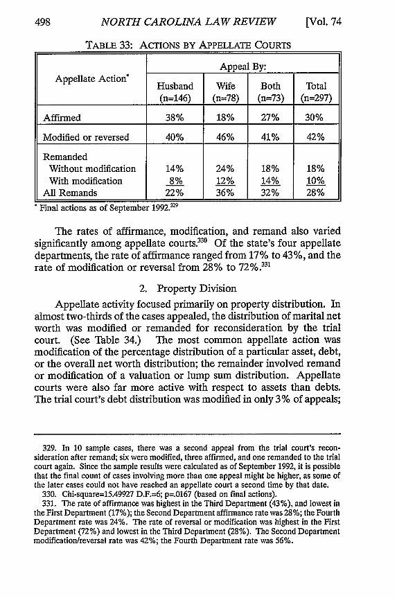
NORTH CAROLINA LAW REVIEW
TABLE 33: AcTIONS BY APPELLATE COURTS
Appeal By:Appellate Action* Husband Wife Both Total
(n=146) (n=78) (n=73) (n=297)
Affirmed 38% 18% 27% 30%
Modified or reversed 40% 46% 41% 42%
RemandedWithout modification 14% 24% 18% 18%With modification 8% 12% 14% 10%
All Remands 22% 36% 32% 28%Final actions as of September 1992.329
The rates of affirmance, modification, and remand also variedsignificantly among appellate courts 30 Of the state's four appellatedepartments, the rate of affirmance ranged from 17% to 43%, and therate of modification or reversal from 28% to 72%.331
2. Property Division
Appellate activity focused primarily on property distribution. Inalmost two-thirds of the cases appealed, the distribution of marital networth was modified or remanded for reconsideration by the trialcourt. (See Table 34.) The most common appellate action wasmodification of the percentage distribution of a particular asset, debt,or the overall net worth distribution; the remainder involved remandor modification of a valuation or lump sum distribution. Appellatecourts were also far more active with respect to assets than debts.The trial court's debt distribution was modified in only 3% of appeals;
329. In 10 sample cases, there was a second appeal from the trial court's recon-sideration after remand; six were modified, three affirmed, and one remanded to the trialcourt again. Since the sample results were calculated as of September 1992, it is possiblethat the final count of cases involving more than one appeal might be higher, as some ofthe later cases could not have reached an appellate court a second time by that date.
330. Chi-square=15.49927 D.F.=6; p=.0167 (based on final actions).331. The rate of affirmance was highest in the Third Department (43%), and lowest in
the First Department (17%); the Second Department affirmance rate was 28%; the FourthDepartment rate was 24%. The rate of reversal or modification was highest in the FirstDepartment (72%) and lowest in the Third Department (28%). The Second Departmentmodification/reversal rate was 42%; the Fourth Department rate was 56%.
[Vol. 74

DECISION MAKING AT DIVORCE
overwhelmingly these modifications were in the wife's favor.332
Overall, however, appellate modification of asset and debt distributiondid not favor either party. Wives benefitted in 52% of the cases inwhich the net worth distribution was modified, husbands in 48%.333
TABLE 34: APPELLATE MODIFICATION OF TRIAL COURTPROPERTY AND DEBT DISPOSITION
Appellate Action* (n297)
Modified
Valuation of debt or asset 12%
Amount of lump sum payment 3%
Percentage division of asset or debt 27%
Remanded
For reconsideration based on lack ofreasons for distribution 6%
For reconsideration of valuation orasset/debt distribution 17%
Total Property Remands and Modifications 65%Percentages do not add to 100 due to multiple appellate actions per case.
Although neither husbands nor wives consistently benefitted fromappellate modification of trial court property distribution orders,modification was significantly less likely when the trial court haddivided a couple's net worth relatively equally.3 (See Table 35.)Only 31% of trial court distribution orders were modified when thedivision of net worth was relatively equal, while more than twice thatnumber were modified when the husband received the lion's share ofnet assets. Appellate modifications also tended to benefit the partyto whom the trial court had awarded the smaller asset share.
332. In eight of nine cases in which the appellate court modified the debt distribution,the wife benefitted.
333. This pattern did not vary significantly over the 10 year period reviewed, nor wasthe direction of the altered distributional outcome significantly correlated with the incomeof either spouse, the value of their total assets, the value of their marital assets, or caselocation.
334. Chi-square=47.64651 D.F.=8; p<0001.
1996]

NORTH CAROLINA LAW REVIEW
In general, then, appellate activity enhanced the likelihood ofequal division rather than the fortunes of husbands or wives as agroup. The median and average percentage share of net propertyawarded to sample wives remained constant after appeals were takeninto account, but the proportion of cases in which relatively equaldivision was ordered rose from 48% to 58% of the total 33
TABLE 35: APPELLATE MODIFICATION OF TRIAL COURT ORDERSDIVIDING MARITAL ASSETS AND DEBTS, BY PERCENTAGE
DISTRIBUTION OF TRIAL COURT
Trial Court's % No Modification ModificationDistribution of Modification Benefiting Benefiting
Marital Net Worth (n=162) Husband Wife(n=53) (n=57)
67% + to Husband 33% 13% 54%
56%- 66% to 50% 7% 43%Husband
Relatively Equal* 69% 17% 14%
56% - 66% to 54% 39% 8%Wife _____ __________
67%+ to Wife 45% 42% 21%
Relatively Equal = Between 45% and 55%
335. Cases involving negative net worth are excluded (n=323). Post-appeal, 24% of thecases resulted in disproportion favoring the husband and 15% in disproportion favoringthe wife. If cases involving businesses or professional degrees are excluded, the proportionof cases resulting in relatively equal division rises to 62% (n=240). Among this smallergroup, disproportion favoring the husband occurred in 18% of the cases and disproportionfavoring the wife in 20%.
[Vol. 74

DECISION MAKING AT DIVORCE
3. Alimony and Child Support
Appellate action regarding alimony or child support was muchless common336 and more difficult to categorize. Trial courts'alimony decisions were almost never reversed. In only five cases didan appellate court reverse a trial court decision not to award alimony;in only three was a decision to award alimony overruled. Thealimony rate after appeal (63%) was thus almost identical to the trialcourt rate (62%).
Appellate modification of the value of alimony or child supportwas also relatively uncommon. The appellate court modified thevalue of alimony in only 12% of appeals where the trial court hadawarded alimony,"' and in only 9% of the child support caseswhere an appeal was taken.33 Some of the modifications simplyreallocated payments between alimony and child support. Thus, inonly nineteen cases was the total value of child support and alimonyaltered.339 Nine of these modifications were increases and ten weredecreases; they evidenced no particular pattern. Remands forreconsideration of alimony or child support were even more rare.Such orders were made in only nine cases, all involving the value ofthe alimony or child support award.
Appellate courts were somewhat more likely to alter the durationof an alimony award; in 17% of appeals from a trial court alimonyaward,' 4° the appellate court changed the duration of the award.Half of these modifications altered the permanence of the award; theother half altered the time period over which durational alimony waspayable. The modifications did not show that appellate courts weremore willing to award permanent alimony than trial courts, however.Among the seventeen cases in which the trial court was reversed onalimony permanence, approximately two-thirds (11 of 17) imposedtime-limited instead of permanent alimony. Overall, 33% of alimonyawards were thus permanent after appeal, as compared to 35% pre-
336. This finding is consistent with that of another divorce researcher. See Crippen,Abundance, supra note 26, at 91 n.28 (finding that Minnesota appellate courts havespecifically imposed or reduced a maintenance award on only three occasions during twodecades). It is also consistent with the finding of a low reversal rate by state appellatecourts generally. See supra note 322 and sources cited therein.
337. n=191.338. n=186.339. Cases in which the trial court's alimony order was reversed are excluded.340. n=191. The two cases in which the trial court's alimony award was reversed are
excluded here and in other portions of the analysis of appellate activity.
1996]

NORTH CAROLINA LAW REVIEW
appeal. Although the difference was not significant, the appellateprocess did enhance the likelihood of permanent alimony for long-married, older women and reduce it for others. 41 Age and maritalduration may thus have been given somewhat greater emphasis byappellate than by trial court judges.
Appellate modifications of the time period over which durationalalimony was payable evidenced no particular pattern, however. In theseventeen cases where appellate courts so modified the award, alonger payment period was imposed in 59%, and a shorter term in41% of the cases. The alterations did not appear to benefit anyparticular group, nor was the typical modification substantial. Onaverage, the term of the award, when modified, was altered by only2.5 years.
4. The Impact of Appellate Courts on Outcome Predictability
Although the actions of appellate courts did alter the predic-tability of alimony and property distribution outcomes slightly, theirimpact was not substantial. With respect to net worth distribution,the values of correlation coefficients and levels of significance oftenshifted, but only one variable (the wife's employment) that haddemonstrated significance at the .05 confidence level at the trial level,failed to do so post-appeal 42 And only two variables (the ratio ofthe wife's separate property to marital property and the appellatedepartment) that had failed to demonstrate significance at the triallevel did so after appeal. Regression analysis explained a somewhatlarger proportion of variability in appellate than trial outcomes,343
341. The following table illustrates this point:PERCENTAGE OF ALIMONY AWARDS THAT WERE PERMANENT
Wife's Marital Status and Age Trial Court Appellate Court% (n) % (n)
Wives Married At Least 15 Years 54% (63) 59% (63)and At Least 45 Years Old
Other Wives 28% (120) 23% (120)
Cases with missing data on wife's age or marital duration are excluded. The correlationcoefficients for marital duration and the wife's age both increased in value at the appellatelevel, as did the level of significance for each of these variables. See infra Appendix, TableA14.
342. For correlation coefficients and p values, see infra Appendix, Table A7.343. The regression model explained 20.0% of variability post-appeal, as compared to
13.8% pre-appeal.
[Vol. 74

DECISION MAKING AT DIVORCE
but the enhanced success of the regression model was partiallydependent on regional variation in case outcomes, with a decisionfrom the first appellate department a significant negative predictor ofthe wife's percentage share. The ratio of the wife's separate propertyto marital property also contributed significantly to the regressionmodel; counterintuitively, a higher ratio was positively correlated withthe wife's percentage award.
For alimony awards, appellate action altered the strength andsignificance of the variable correlations only in trivial respects."No litigant characteristic that had, at the trial level, demonstratedsignificance at the .05 confidence level failed to exhibit at least thatlevel of significance after appeal. No litigant characteristicdemonstrated significance after appeal that had failed to do sopreviously. Logistic regression analysis of post-appeal alimonyoutcomes yielded a model that varied insubstantially from the modelapplicable to trial courts, and yielded a prediction rate less than threepercentage points different.345
Although appellate courts were more active with respect to thepermanence and duration of alimony, their activity again failed tosubstantially alter the predictability of these decisions." Maritalduration remained the most important predictive variable (indeed, itspredictive value increased). Regression analysis of alimony per-manence did achieve a somewhat improved prediction rate,however.347 The judge's political party failed to contribute sig-nificantly to the regression model post-appeal, while the decision yeardid for the first time. The duration of a nonpermanent awardremained, post-appeal, altogether unpredictable.348
Perhaps most important, the appellate opinions do not evidenceclear, consistent guidance to trial courts. Trial judges had no apparentmethodology for computing the length of a durational alimony award,for example. But in modifying the duration of alimony, appellatecourts typically offered little methodological help. The factors mostfrequently mentioned by appellate courts as bases for changing the
344. For correlation coefficients and p values, see infra Appendix, Table A12.345. The full regression model accurately predicted 82.7% of the cases post-appeal,
compared to 85.1% pre-appeal.346. For correlation coefficients and p values, see infra Appendix, Table A14.347. The full regression model accurately predicted 76.4% of cases post-appeal, the par-
simonious model 72.9%. The full regression model predicted 70.1% of cases pre-appeal,the parsimonious model 67.15%.
348. Only one litigant characteristic, the award of sole custody to the wife, achievednew significance post-appeal (p=.015).
1996]

NORTH CAROLINA LAW REVIEW
alimony time period were the amount of time the wife would need tobecome self-sufficient and the age of the children. But it was rare foran appellate court to link self-sufficiency to any specific events,349
and no consensus on how the children's age should affect the alimonydecision was evident. Sometimes, indeed, the court offered noreasoning for altering the duration of alimony at all.35'
Appellate activity thus tended to enhance the predictability oftrial court outcomes, but only by modest margins. One reason for thisresult is that the norms established by appellate courts were followedquite faithfully by trial judges; consistently, the same variablesdemonstrated significant relationships at the trial and appellate levels.This pattern suggests that, where trial court judges exhibit confusion,appellate courts could produce more predictable results. Thatappellate courts have failed to do so seems to reflect a lack of consen-
349. See, e.g., Wood v. Wood, 526 N.Y.S.2d 608, 610 (N.Y. App. Div. 1988) (extendingalimony award from two to five years for homemaker married 3.5 years "to give heradequate time to prepare to reenter the job market"); Morton v. Morton, 515 N.Y.S.2d499, 500-01 (N.Y. App. Div. 1987) (extending alimony award from one to five years forwife married for 17 years and a homemaker for 16 years; "A period of five years ...should be sufficient to provide the defendant with the necessary financial support forretraining and readjustment." (citations omitted)); Durso v. Durso, 483 N.Y.S.2d 101, 102(N.Y. App. Div. 1984) (extending alimony award from three to six years for wife who wasmarried for 20 years and a homemaker for 18 years; "Until such time as she can earn asubstantially higher income, the defendant's sustained efforts to educate herself so that shecan become fully self supporting should not be a reason to limit the duration of themaintenance award."); Patti v. Patti, 472 N.Y.S.2d 20,21 (N.Y. App. Div. 1984) (extendingalimony award from two to four years for wife married 16 years and a homemaker for 14years; "four years requested by the plaintiff is a more appropriate period which wouldpermit her, after 14 years out of the work force, to refresh her skills and better prepareherself to become self supporting").
350. Among cases involving minor children, the children's age did not demonstrate asignificant predictive relationship to the duration of alimony before or after appeal; thelevel of correlation was slightly lower post-appeal. See infra Appendix, Table A14. Forcases discussing the children's age, see, e.g., Schoenfeld v. Schoenfeld, 563 N.Y.S.2d 500,502 (N.Y. App. Div. 1990) (reducing permanent alimony award to five years; "Such alimitation will allow the wife to remain at home until her children are thirteen and almosteleven years of age, respectively."); Stempler v. Stempler, 532 N.Y.S.2d 550, 552 (N.Y.App. Div. 1988) (extending alimony award from five to seven years "because of the age[six] of youngest child" [child's age is unspecified in opinion but available from record onappeal]); Patti v. Patti, 472 N.Y.S.2d at 21 (extending alimony award from two years tofour for homemaker of 14 years married 16 years; "likely that the son [14 years old] willlive with the plaintiff for at least four more years" (citations omitted)).
351. See, e.g., Weinstein v. Weinstein, 508 N.Y.S.2d 950, 951 (N.Y. App. Div. 1986)(extending alimony award from five to seven years; "Under all of the facts andcircumstances of this case, it is our view that maintenance in the amount of $200 per weekshould have been granted to the plaintiff wife for a period of seven years... rather thanfive years .... ").
[Vol. 74504

DECISION MAKING AT DIVORCE
sus at both levels of the litigation process on how to employ thediscretion granted by the legislature.
IV. JUDICIAL DECISION MAKING IN RETROSPECT: DIRECTIONSFOR DIVORCE REFORM
A. Interpreting the Data
1. Discretion's Diversity
If any single thing is apparent from this inquiry into judicialdecision making at divorce, it is that the results of discretionarydecision making are by no means uniform. Each discretionarydecision judges made-property division, the award of alimony, theduration of alimony, the value of alimony and/or child sup-port-presents its own unique features. Depending on whicheconomic decision we take as an example, evidence can be found tosupport the claims of either discretion's critics or its champions.
Discretion's champions might use the alimony award data, whichsuggest a fair degree of consensus among judges on the litigantcharacteristics that determine an alimony claim and on their relativeweight. That consensus not only reflects the factors specified in thelegislative scheme but, as the results of settlement track those ofjudicial decision making tolerably well, appears to have been quitefaithfully transmitted to the practicing bar. The data on alimony andchild support values similarly suggest a fair degree of consensusamong judges on a decision making model, a consensus that bothcomports with the statute and is reflected (albeit imperfectly) in theresults of settled cases.
Discretion's critics, on the other hand, might point to the alimonyduration data, which suggest the intrusion of private values asdecision-making criteria and the lack of developed consensus withinthe judiciary on the relevance and weight to be accorded particularlitigant characteristics. The apparent link between trial courtpermanence decisions and political party, for example, suggests justthe sort of arbitrariness that critics have complained about; so do theapparent class bias in alimony awards, the regional variation inalimony values, and the complete unpredictability of alimony durationdecisions. The property division data also lend weight to the critics'claims. Judges seem to agree on relatively equal division as aprototypical outcome, but do not appear to have reached sufficientconsensus on the factors that justify departure from equal division, to
1996]

NORTH CAROLINA LAW REVIEW
permit reliable outcome predictions. The infrequency of equaldivision in the settled cases also suggests that judges were not able, atleast during the Equitable Distribution Law's first few years, totransmit the new norm to the divorce bar. Moreover, the judicialtendency to award the ill and relatively needy wife less than half ofthe net assets certainly runs counter to the equal partnership principlethat underlies the statute.
Discretion thus sometimes produced outcomes that appear to relymore on private values than on public standards. Outcomes weresometimes unpredictable, and sometimes failed to reflect the factorsthat the legislature had specified as relevant. Judicial consensus wasnot necessarily reflected in the outcomes of settled cases. Butdiscretionary decision making was at times highly predictable andhighly correlated with the legislative scheme. The results of set-tlement sometimes mirrored, albeit imperfectly, those achievedthrough litigation, and no evidence of distortions in settlementoutcomes due to strategic bargaining could be found.
2. Explaining Discretion's Diversity
How can we explain these disparities?
a. Discretionary Standards DifferOne relevant factor may be differences in the discretionary
standards themselves. 5 2 Some discretionary standards subtly curtailthe exercise of discretion, while others do not. Professor Mnookin,for example, reports the "rather surprising" finding that everypregnant minor who sought judicial authorization for an abortionunder a statute permitting waiver of parental consent based on ajudicial finding that the minor is mature or that "an abortion wouldbe in her best interests" ultimately obtained it.353 His explanationfor this finding was that judges, many of whom personally opposedabortion, believed it impossible to justify finding both that a minorwas insufficiently mature to choose an abortion, and that it was alsoin her best interests to bear a child: "The law puts judges in the
352. See Lempert, supra note 17, at 214-15 (describing the importance of "the mandateand clarity of the law as understood by the decision-maker" in determining how discretionis exercised).
353. Robert H. Mnookin, Bellotti v. Baird: A Hard Case, in IN THE INTEREST OFCHILDREN: ADVOCACY, LAW REFORM, AND PUBLIC POLICY 149, 239-40 (Robert H.Mnookin ed., 1985).
[Vol. 74

DECISION MAKING AT DIVORCE
ridiculous position of being rubber stamps," one judge complained."There is no way you could substantiate such a decision.''a4
While no provisions of the Equitable Distribution Lawconstrained judicial discretion this tightly, there were differences inthe level of restraint imposed by specific statutory provisions. Somewere premised on coherent themes or principles that tended to reinin discretion; others were not. Viewed from this perspective, theunpredictability of durational alimony awards may derive, in part,from the "rehabilitation" concept that underlies the alimonyprovisions of the law.355 Judges, in an apparent attempt to conformtheir decisions to the rehabilitation principle, tended to focus on whenthe alimony recipient would become self-supporting. But while it iseasy to predict this time period when the alimony recipient plans toobtain further job training, neither the statute nor the rehabilitationconcept outlines any logical method for making such a prediction inthe far more typical case in which the recipient does not. Theeconomic circumstances of an older alimony recipient with littleeducation and a job history confined to low wage, dead-endemployment cannot be expected to improve. The predictive question,in these cases, verges on incoherence and thus may have enhanced theunpredictability of judicial response.
By contrast, the "partnership of coequals," '356 concept thatunderlies the property distribution rules offers a clear decision-makingprinciple applicable to each and every case: Equal partnership impliesequal treatment. Given this underlying statutory principle, it is nothard to see why judges gravitated to an equal division norm. Thestatute itself invites, indeed drives, judges in this direction. Nor is itsurprising that appellate courts have enhanced the tendency towardequality. With a statute premised on equal partnership, this is themost logical result and the one easiest to justify.
Given the equality norm underlying the property divisionprovisions of the statute, the extent of judicial consensus on equalityis perhaps less surprising than the number of departures from thatnorm. Even after appeals are taken into account, slightly more than40% of the cases resulted in unequal division. A partial explanationlies, again, in the nature of the constraints imposed by the statute: Itis an underlying principle that suggests equality, rather than a literalstatutory command. Moreover, the statute, by requiring a mul-
354. Id. at 240.355. See supra note 99 and accompanying text.356. See supra note 101 and sources cited therein.
1996]

508 NORTH CAROLINA LAW REVIEW [Vol. 74
tifaceted consideration of case circumstance, implies that departure isappropriate in a variety of circumstances. 5 7
b. "Familiarity Breeds Precedent"
A second explanation for the diversity of results derives, Ibelieve, from the relative novelty of some statutory commands ascompared to others: The extent of judicial experience under adiscretionary standard will, like the discretionary standard itself, affectthe manner in which judges exercise their discretion. The reasons forthis phenomenon are uncomplicated. Decision-makers gravitatetoward routine decision-making norms when repetitively confrontedwith cases of a similar type. 8 Judges, moreover, are expected tostrive for like results in like cases and thus rely heavily on ac-cumulated precedents.35 9 Routinized norms also serve a timeallocation function, permitting the decision-maker to give adequateconsideration to the atypical."6 Judges thus gravitate toward factualand legal stereotypes in order to achieve consistent and efficientresults.
As a result of this tendency toward consistency, the predictabilityof both judicial decisions and lawyer-negotiated settlements may varysubstantially based on a decision-making standard's age and case
357. Appellate courts have also endorsed departures from equality. See supra note 109.358. See DAVIS, POLICE DISCRETION, supra note 80, at 150-51; Lempert, supra note 17,
at 216-17; Schneider, supra note 8, at 2282-83. For contextual research describing thetendency toward routinized decision making, see ROBERT M. EMERSON, JUDGINGDELINQUENTS (1969) (juvenile court judges); H. LAURENCE Ross, SETTLED OUT OFCOURT: THE SOCIAL PROCESS OF INSURANCE CLAIMS ADJUSTMENTS 233-43 (1970)(insurance claims adjusters); Lempert, supra note 17, 216-26 (public housing evictionboard); Douglas W. Maynard, The Structure of Discourse in Misdemeanor Plea Bargaining,18 LAW & Soc'Y REv. 75 (1984) (prosecutors); Jerome H. Skolnick, Social Control in theAdversary System, 11 J. CONFLICT RESOL. 52 (1967) (public defenders and private defensecounsel); David Sudnow, Normal Crimes: Sociological Features of the Penal Code in aPublic Defender Office, 12 SOC. PROBS. 255 (1965) (public defenders). For discussion ofthe psychological factors that contribute to routinized decision making, see, e.g., DANIELKAHNEMAN ET AL., JUDGMENT UNDER UNCERTAINTY: HEURISTICS AND BIASES (1982);RICHARD NISBETr & LEE RoSS, HUMAN INFERENCE: STRATEGIES AND SHORTCOMINGSOF SOCIAL JUDGMENT (1980); Vladimir J. Konecni & Ebbe B. Ebbesen, The Mythologyof Legal Decisionmaking, 7 INT'L J.L. & PSYCHIATRY 5, 6-7, 15-16 (1984).
359. For a classic account of this process, see BENJAMIN N. CARDOZO, THE NATUREOF THE JUDICIAL PROCESS 28-36 (1921) [hereinafter CARDOZO, THE JUDICIAL PROCESS].
360. LEMPERT & SANDERS, supra note 86, at 83-88. Routinized decision-making normsthus offer many of the benefits of formal rules. As Professor Schauer has put it, "[W]eare able to do what we can precisely because rules free us from having to do anythingelse." SCHAUER, supra note 9, at 230.

DECISION MAKING AT DIVORCE
volume261 The intrusion of disparate private values into thedecision-making process, as indicated by the correlation of caseoutcomes with judicial characteristics, appears most likely when thedecision-making standard is young and when the case volume is light.Clear decision-making norms that rely on a few key facts are,conversely, more likely to be encountered as the standard ages and ascase volume increases.
The research results conform quite closely to this "naturalhistory" of discretionary decision making. Standards for determiningchild support did not change at all as a result of the 1980 EquitableDistribution Law.362 Judges could thus rely on an establishedconsensus developed over decades, and judicial decisions on the valueof child support were accordingly quite predictable. By contrast,durational alimony, where judicial decisions were quite unpredictable,was newly established as a norm by the 1980 law. Judges and lawyershad only the statute to guide the decision-making process. So, too,with property division. Given the fact that New York had no maritalproperty distribution scheme prior to the Equitable Distribution Law,judges and lawyers confronted a blank slate.
c. Consensus Does Not Hold
Yet another explanatory factor for the diverse results achievedby the Equitable Distribution Law is the dynamic nature of judicialconsensus. The flexibility inherent in a discretionary standard permitsdramatic shifts in judicial perceptions and decision-making pat-terns.363 Rules thus codify the consensus of a given moment;discretion embraces the consensus of yesterday, today, and tomor-row.3 4
The shifting nature of judicial consensus is evident in the fact thatthe year of decision was a significant predictor of the award ofalimony, the likelihood of a permanent alimony award, and the value
361. For a detailed discussion of the time factor in precedent promulgation and itsrelation to the choice between rules and discretionary standards, see Kaplow, supra note9, at 612-14; Gillian K. Hadfield, Bias in the Evolution of Legal Rules, 80 GEO. L.J. 583(1992); Ronald A. Heiner, Imperfect Decisions and the Law: On the Evolution of LegalPrecedent and Rules, 15 J. LEGAL STUD. 227 (1986).
362. Nor did the new alimony statute's specification of factors necessitate any majordeparture from traditional decision-making patterns for the alimony component of thetotal transfer payment.
363. For a fascinating example, see Lempert, supra note 17, at 204-13.364. See SCHAUER, supra note 9, at 160 (describing tendency of rules to enhance the
status quo and give power to the past).
1996]

NORTH CAROLINA LAW REVIEW
of child support (as well as child support and alimony combined).The flexibility inherent in a discretionary standard permitted childsupport awards to drift upward. It permitted the percentage of casesin which alimony and permanent alimony were awarded to driftdownward as well.
These shifts tracked social and public opinion trends. Over theten-year research period, increasingly large numbers of marriedwomen with young children were in the paid labor-force,365 a shiftthat decreased not only the need for both short- and long-termalimony, but public support for such transfers as well. The periodalso saw a genuine sea change in public sentiment regarding childsupport. Over the decade the low value of child support awards cameunder intense public and political scrutiny;366 during the later yearsof the research period, child support guidelines, which wouldeventually supplant discretionary decision making altogether, werebeing actively debated in the state legislature. 67 By contrast, judgeswere not required to respond to a new public opinion climate or tothe threat of major statutory change in the area of property division,and these outcomes were not significantly related to the decision year."
365. In 1980, 45.1% of married women with children under the age of six were in thepaid labor force, as compared to 59.9% in 1991. STATISTICAL ABSTRACT, supra note 151,at 388 tbl. 620.
366. Professors Belier and Graham report that the New York Times Index listed "childsupport" as a separate category for the first time in 1980; by 1986 the listings under thatheading had grown to two full columns. BELLER & GRAHAM, supra note 69, at 5.
367. Child support guidelines legislation was first introduced in the New Yorklegislature in 1985. In part due to the vigorous and effective opposition of the New YorkState Bar Association, the legislature did not enact a bill until 1989. See, e.g., PaulBrowne, State Bar Weight Felt Against Measure on Child Support, N.Y. L.J., August 12,1988, at 1; E.R. Shipp, Support Formula Stymied in Albany, N.Y. TIMES, Sept. 4, 1988, at36. The continuing debate over the legislation helped to focus media attention on childsupport issues, both in the popular press, see, e.g., Editorial, Divorce Lawyers Thrilled atBill's Demise, DAILY NEWS, Sept. 9,1988, at 12; Editorial, Cheapskates and Child Support,N.Y. TIMES, Dec. 5, 1988, at A22, and in the legal press, see, e.g., Henry H. Foster & GrierH. Raggio, An Analysis of Proposed Law for 'Equitable' Child Support, N.Y. L.J., May 14,1987, at 1; Martin Fox & Gary Spencer, New Drive for Child Support Guidelines, N.Y. L.J.,Dec. 13, 1988, at 1.
368. See infra Appendix, Table A19. Social consensus regarding the equal partnershipconception of marriage perhaps expanded during the research period, but did not changedirection. For example, the Uniform Probate Code provisions relating to the spousal rightof election were substantially revised in order "to bring elective-share law into line withthe contemporary view of marriage as an economic partnership." UNIF. PROBATE CODEart. 2, pt. 2, general cmt. (1990). Revisions to New York's estates law, introduced in thelegislature toward the end of the research period, enlarged the intestate share of asurviving spouse from one-third to one-half of the probate estate and enhanced the spousalright of election through the expansion of testamentary substitutes and abolition of the so-
[Vol. 74

DECISION MAKING AT DIVORCE
While it would be impossible to establish clear links between thedecision-making climate and judicial decisions themselves, "[t]he greattides and currents which engulf the rest of men, do not turn aside intheir course, and pass the judges by."369 The tides of social changedo not, of course, break with equal force upon all decision-makers, afact perhaps evidenced by the tendency of older judges to awardalimony more frequently than younger ones, and of Republican judgesto award permanent alimony more frequently than Democratic judges.
The variable rate and manner in which individual judges respondto changing social and legal conditions, coupled with the resultingtendency of judicial consensus to shift over time, thus ensure that theresults of discretionary decision making can never be perfectlypredictable. Indeed, given the rapid pace of change in public opinionand in gender and marital roles during the research period, it isperhaps surprising that the judicial decisions reviewed exhibited asmuch predictability as they did.
3. Evaluating Discretion's Results
a. Consistency, Gender Bias, and Settlement Patterns
The research findings, which at first glance appear chaotic andcontradictory, thus reveal, in the end, some consistent themes. Theyshow us judges struggling conscientiously to give form and content totheir discretionary mandate, a process guided by legislative directives(or lack thereof), shaped by experience, and set in a shifting historicalcontext. They show us the impact of individual values and socialclimate. And they also show us the channelling effect of institutionalnorms, appellate precedent, and legislative principle, which tend overtime to produce more uniform and predictable case outcomes.
On the issue of consistency, the research findings thus suggestthat if trial judges are given clear legislative and appellate guidance,discretionary divorce decision making may, over time, produce highlypredictable results. Discretionary decision making will, of course,remain subject to shifting trends,370 but the tendency of discretion
called "right of election trust." See Act of July 24, 1992, ch. 595, 1992 N.Y. Laws 595 §§8, 25 (codified at N.Y. EST. POWERS & TRUSTS LAW § 4-1.1, 5-1.1A (McKinney Supp.1995)).
369. CARDOZO, THE JUDICIAL PROCESS, supra note 359, at 168.370. For example, the alimony decisions of younger and Democratic judges (who were
less prone to award alimony and permanent alimony) appear to reflect an underlyingpreference for formal gender equality. But this model of equality has, at least since themiddle of the research period, been subjected to repeated criticism from feminist critics.
1996]

NORTH CAROLINA LAW REVIEW
to evolve toward routinized norms should ultimately produce patternsthat are more reliant on institutional values than on individual judicialpredilection.
That judges have failed to achieve predictable and consistentoutcomes in many areas of divorce decision making appears to derivefrom the novelty of the statutory provisions, coupled with theconflicting, and at times incoherent, principles upon which judges havebeen directed to base the decision-making process. Novelty will pass.But how fast and how well courts will evolve clear decision-makingprinciples where legislative guidance is sparse remains to be seen.The research findings thus suggest that discretion could produce fairlyconsistent results, but do not reveal whether it will.
On the issue of gender bias, the research findings suggest equallyambiguous conclusions. Judicial decisions often reflected traditionalgender stereotypes. For example, judges who awarded the wife asmall share of business or professional assets sometimes justified thatdecision by noting that the wife had been awarded substantialalimony, a choice that reflects, and reinforces, a tradition of wifelydependence upon an economically dominant husband who controlsthe family purse strings.37 t The tendency of judges to award hus-bands the lion's share of marital debts, and to require little or nochild support from women who did not obtain custody, also suggestreliance on this stereotype of wifely dependence.
But as these varied examples make plain, judicial adherence totraditional gender stereotypes did not uniformly advantage eitherhusbands or wives. The conscious and unconscious influence ofgender stereotype should not be confused with consistent bias. Of theformer, there is plentiful evidence. Of the latter, there is little.
See, e.g., FINEMAN, supra note 75; OKIN, supra note 78; Christine Littleton, ReconstructingSexual Equality, 75 CAL. L. REv. 1279 (1987); Joan C. Williams, Dissolving theSameness/Difference Debate: A Post-Modern Path Beyond Essentialism in Feminist andCritical Race Theory, 1991 DUtKE L.J. 296. As these criticisms of formal equality gain abroader audience, it is altogether possible that the preferences-and the decisions-ofthese judges will shift direction.
371. See, e.g., Arvantides v. Arvantides, 478 N.E.2d 199, 200 (N.Y. 1985) (upholdingreduction of wife's share of husband's dental practice: "When it is considered that [thewife] has also received an award of maintenance, medical expenses, insurance benefits andthe more valuable of the two homes owned by the parties, the distribution cannot be saidto be inequitable as a matter of law."). More typically, the pattern described is notexplicitly recognized by the court. See, e.g., Behrens v. Behrens, 532 N.Y.S.2d 893 (N.Y.App. Div. 1988); Wood v. Wood, 526 N.Y.S.2d 608 (N.Y. App. Div. 1988); Morton v.Morton, 515 N.Y.S.2d 499 (N.Y. App. Div. 1987); Pulitzer v. Pulitzer, N.Y. L.J., 10/22/85,at 11, col. 2B, modified, 523 N.Y.S.2d 508 (N.Y. App. Div. 1988); Ginter v. Ginter, N.Y.St. B. Ass'n Fam. L. Rev., Sept. 1990, at 23, 25.
[Vol. 74

DECISION MAKING AT DIVORCE
It is true that the results of the discretionary decision-makingprocess ultimately produced considerable inequality in post-divorceliving standards. On average, women and children suffered a sharpdecline in their standard of living, while men obtained animprovement. But we cannot attribute this result simply to judicialbias. The New York legislature, which reduced judicial discretion inawarding child support in order to improve children's post-divorceliving standards, adopted guidelines that would presumptively transferno more income to women and children than did judges acting underdiscretionary standards.3 For the typical family, where husbandearns substantially more than wife, this "improvement" overdiscretionary decision making produces outcomes fairly comparableto those produced by judges.373 We are all, as Professor Reganreminds us, "both cause and effect of the gender system, which meansthat we may unwittingly reproduce it even as we seek its demise."'374
As for the impact of discretionary decision making on thesettlement process, the research shows that settlements can track theresults of judicial decision making tolerably well. No adverse effectsdue to strategic bargaining behavior could be found; custody-for-money trade-offs, thought to be common under discretionarystandards, were not evident. But strategic behavior may takedifferent forms than theorists have supposed.375 More importantly,
372. See supra notes 262-69 and accompanying text.373. See David M. Betson et al., Trade-Offs Implicit in Child-Support Guidelines, 11 J.
POL'Y ANALYSIS & MGMT. 1, 12 tbl. 3 (1992) (assuming custodial parent earns $10,000and noncustodial $20,000, under a child support model similar to the New York statutoryguidelines, the ratio of post-divorce to pre-divorce scaled surplus income was 1.24 fornoncustodial household and 0.41 for custodial household with one child). The New Yorkstatute does provide for pro rata apportionment of child care expenses when custodialparent is working or in school, however, N.Y. DOM. REL. LAW § 240.1-b(c)(4) (McKinneySupp. 1995), which would tend to improve these ratios somewhat.
374. Milton C. Regan, Jr., Divorce Reform and the Legacy of Gender, 90 MICH. L. REV.1453, 1494 (1992).
375. The high rate of noncompliance with temporary support orders among cases in thejudicial sample may evidence strategic behavior, for example. It is also possible, of course,that strategic behavior is much less common than theorists have supposed. Researchershave noted, in varied contexts, that the existence of an ongoing relationship tends toreduce the likelihood of adversarial behavior. See; e.g., ROBERT C. ELLICKSON, ORDERWITHOUT LAW 270-75 (1991) (neighboring and concurrent landowners); MILTONHEUMANN, PLEA BARGAINING: THE EXPERIENCES OF PROSECUTORS, JUDGES, ANDDEFENSE ATTORNEYS (1977) (prosecutors and defense counsel); Stewart Macaulay, Non-contractual Relations in Business: A Preliminary Study, 28 AM. SOC. REV. 55,58-61, 63-64(1963) (parties to commercial contracts); Robert E. Scott, Conflict and Cooperation inLong-Term Contracts, 75 CAL. L. REV. 2005, 2040-42 (1987) (buyer-seller contractualrelationships).
1996]

NORTH CAROLINA LAW REVIEW
the tendency of settlements to predictably track judicial decisionpatterns, and the lack of strategic bargaining effects, may be due tothe high rate of legal representation in the settlement sample and thusunrepresentative of results in the general divorce population. 76
Overall, the research results suggest that discretionary decisionmaking at divorce is not clearly inferior to rule-based decisionmaking. It is capable of producing consistent, predictable results. Itis no more prone to gender bias than recent legislative rules. At leastif the settlement process is guided by lawyer intermediaries, adverseeffects resulting from discretionary standards are not demonstrable.
b. Discretion and Rule: The Tendency Toward Convergence
It is also probable that, in some instances, discretion and rule willproduce relatively equivalent results. The reasons for thisphenomenon derive from the contrary effects of rule and discretionon the decision-making process. As noted above, discretionarystandards will typically, through the development of informal rules ofthumb and formal precedents, become more rule-like. An historicalexample of this channelling tendency of discretion can be found inchild custody law. Courts, ostensibly deciding custody based on abroad examination of a child's best interests, over time adopted whatmight be best described as a set of presumptions: in favor of themother for a child of "tender years;" in favor of the parent preferredby a mature child; against the parent whose conduct exposes the childto immorality.
3 77
In contrast to the channelling tendency of discretion, rules tendto produce exceptions 78 Indeed, the narrower the rule thatconstrains the decision-making process, the greater the likelihood andthe number of exceptions that will occur. These exceptions may
376. Professors Maccoby and Mnookin, who also failed to find evidence of money-for-custody trade-offs in their research on divorce outcomes in California, hypothesized thatthe explanation lay in California's bright-line "child support schedules and communityproperty rules [which] substantially constrain such trade-offs" and in the difficulty of"fathers to engage in strategic behavior [regarding custody] that appears credible to theirspouses." MACCOBY & MNOOKIN, supra note 14, at 160. Lawyers, like bright-line rules,may significantly reduce the credibility of custody threats.
377. For a description of the rules and case law, see, e.g., CLARK, FIRST EDITION, supranote 59, at 584-87.
378. See, e.g., Rose, supra note 54, at 578-90 (giving detailed examples of how "thestraightforward common law crystalline rules [of property law] have been muddiedrepeatedly by exceptions and equitable second-guessing").
[Vol. 74

DECISION MAKING AT DIVORCE
result from judicial interpretation of the rule itself,379 rejection ofthe rule in favor of a competing rule or higher principle,.. or evenfrom legislative reaction to judicial rule enforcement that results inperceived injustice. 8'
As a result of these divergent tendencies, the results ofdiscretionary and rule-based decision making, if shaped by similarprinciples within the same historical context, may ultimately converge.Marital property distribution is a potential example of thisphenomenon. With only a few years' experience with equitableproperty distribution, it appears that New York courts already viewequal division as a prototypical outcome, or perhaps as an analyticalstarting point. Professor Reynolds, reviewing a collection of reportedequitable property distribution decisions from six states with olderequitable division regimes, reports that judges almost never dividedmarital property unequally? 2 By contrast, in a state like Californiathat has an established equal division rule, it has been necessary tocarve out exceptions to the equality requirement to meet equitableconcerns: for cases of negative net worth,3"' for cases in which thecustodial parent needs the home,3" and for cases of asset dis-sipation.385 Judicial decisions made under a mature equitableproperty distribution standard and a mature equal division rule thusmay not, in the end, differ greatly.
379. The law of wills offers some good examples. See, e.g., Engle v. Siegel, 377 A.2d892 (N.J. 1977) (excluding application of anti-lapse statute based on determination thattestator probably intended an inconsistent result); Johnson v. Johnson, 279 P.2d 928 (Okla.1954) (admitting to probate a typewritten, unsigned, and unexecuted will on theory thathandwritten addition republished will by codicil); see also BURTON, supra note 9, at 191-99(describing competing claims regarding judicial interpretation of the law).
380. The classic example is the case of Riggs v. Palmer, 22 N.E. 188 (N.Y. 1889), inwhich the New York Court of Appeals denied the beneficiary of a will who had murderedthe testator his legacy: "[A]ll laws ... may be controlled in their operation and effect bygeneral, fundamental maxims of the common law. No one shall be permitted to profit byhis own fraud ... or to acquire property by his own crime." Id. at 190. Riggs hasattracted the attention of many students of judicial discretion. See, e.g., BURTON, supranote 9, at 51-62; CARDOZO, THE JUDICIAL PROCESS, supra note 359, at 40-43; DWORKIN,supra note 9, at 23-39.
381. For example, legislatures have enacted elective share statutes that expand therange of includible assets in order to ensure that the elective share entitlement cannot becircumvented through will substitutes. See, e.g., LAWRENCE W. WAGGONER ET AL.,FAMILY PROPERTY LAW 488 (1991).
382. Reynolds, supra note 41, at 854-55.383. CAL. FAM. CODE § 2622(b) (West 1994).384. CAL. FAM. CODE §§ 3801-3802 (West Supp. 1994).385. CAL. FAM. CODE § 2602 (West 1994).
1996]

NORTH CAROLINA LAW REVIEW
B. Directions for Divorce Reform
1. Discretion and Rule: Their Costs and ConstraintsThe choice between discretion and rule is not, however,
immaterial. Like Professor Coase's well-known theorem positing theirrelevance of liability rules,386 a claim of immateriality might havemerit in a timeless world of perfect information and insignificanttransaction costs. But this is not the world of divorce litigation. Real-world constraints on time, information, and money not only renderthe theorem invalid, but offer a framework for determining theappropriate balance between discretion and rule. While the researchsuggests that discretionary and rule-based decision making at divorcecan, and ultimately may, produce similar results, the costs ofdiscretionary and rule-based decision making, and the actors on whomthey are imposed, are quite different. The choice between discretionand rule should take these differences into account.
One important difference is the greater cost of obtaininginformation about a law's content when it is embodied in adiscretionary standard. A rule provides its own notice of theapplicable legal standard. A discretionary standard does not. Lawyerintermediaries may, of course, offer litigants as much certainty aswould a rule-the findings from this research project confirms thatthey often do-but lawyer assistance is neither cheap nor certain.Based on an informal telephone survey of law offices that advertisedivorce as a specialty, an uncontested, uncomplicated divorce nowcosts, in New York City, almost $1,000."8 For the "typical" divorcelitigant, who has been married for perhaps seven years and hasdivisible marital assets consisting of a used car, household goods,
386. Ronald H. Coase, The Problem of Social Cost, 3 J.L. & ECON. 1 (1960).387. Ten law firms, all randomly selected from those listing divorce as a specialty in the
Brooklyn, Manhattan, or Queens, N.Y. telephone directory Yellow Pages, weretelephoned. A representative of each firm was asked the "likely cost" of representationin an uncontested divorce. The firm representative was told that the prospective divorcingcouple had been married for five years, had no children, and no property except for a jointbank account, a car, furniture, and a jointly owned condominium apartment (which theyplanned to sell and equally divide the proceeds). Estimates ranged from $469 to $1770;the mean was $931. There is no national data on lawyer fees for simple, uncontesteddivorces, but wide regional variation is probable. See Grace G. Blumberg, Who ShouldDo the Work of Family Law?, 27 FAM. L.Q. 213,218 (1993) (reporting anecdotal evidenceof regional variation in rate of pro se representation and cost of legal representation indivorce cases).
[Vol. 74

1996] DECISION MAKING AT DIVORCE 517
limited home equity, and a small bank account,3"' the price of legalrepresentation may well exceed any loss in post-divorce entitlementsthat legal representation could have averted.8 9 Without large-scalepublic funding of legal services, it is thus unlikely that the current,relatively low rate of legal representation at divorce will increase.3"Indeed, quite to the contrary, researchers have reported a trendtoward increased self-representation in divorce actions.39'
Although we have little systematic data on the extent of thelitigation disadvantage that accompanies lack of legal representationin divorce, it seems unlikely that the judicial norms on which lawyersrely in negotiating adversarial settlements carry over as well to thevast numbers of divorce actions where couples employ one lawyer toserve primarily as a scrivener, or no lawyer at all.3" These infor-
388. See Garrison, supra note 12, at 743 app. tbl. 5 (comparing asset ownership patternsfor state divorce samples).
389. See, e.g., Kaplow, supra note 9, at 571 ("Individuals acting in their self-interest willacquire such [legal] advice only if its perceived value exceeds its perceived cost.");Comment, On Letting the Laity Litigate: The Petition Clause and Unauthorized PracticeRules, 132 U. PA. L. REV. 1515, 1532 n.74 (1984) (stating that self-representation "simplyconstitutes a conscious and efficient allocation of human resources, from which there is noreason to 'protect' the consumer"). Researchers have reported that self-representation atdivorce is significantly correlated with income, age, education, occupation, whether themarriage produced children, property ownership, and marital duration. Sales et al., supranote 164, at 561-66; see also Cavanagh & Rhode, supra note 166, at 162 (finding thatdivorce litigants with no children and short marriages were more likely to representthemselves).
390. According to a New York state survey, "[r]elatively few legal services programsacross the state will accept matrimonials," and approximately 80% of pro bono legalassistance programs indicated that "divorce is an area where demand consistently exceedsthe supply of attorneys." COMMITTEE ON LEGAL AID, NEW YORK STATE BAR ASS'N,
THE NEW YORK LEGAL NEEDS STUDY 70-71 (1993). New York is by no means unique.Surveys uniformly report that only about 15%-20% of the legal needs of the poor and60% of the needs of moderate income Americans are currently met. See, e.g, AMERICANBAR ASSOCIATION CONSORTIUM ON LEGAL SERVICES ANID THE PUBLIC, TWO
NATIONWIDE SURVEYS: 1989 PILOT ASSESSMENTS OF THE UNMET LEGAL NEEDS OF THE
POOR AND OF THE PUBLIC GENERALLY 37 (1989); James Podgers, Legal Profession FacesRising Tide of Nonlawyer Practice, A.B.A. J., Dec. 1993, at 51,53 (estimating that 40% oflegal needs of moderate-income persons go unmet).
391. See Garrison, supra note 12, at 646 tbl. 2 (reporting decreased percentage ofdivorce cases with two-party representation between 1978 and 1984 in two New Yorkcounties); Sales et al., supra note 164, at 594 (reporting that the percentage of divorcecases in Maricopa County, Arizona involving at least one unrepresented party rose from24% in 1980 to 90% in 1990).
392. Among cases in my full research sample (excluding judicial decisions), the awardof alimony was highly correlated with the presence of counsel. Where both parties wererepresented by lawyers, 30% of wives received an alimony award; where neither spousewas represented by counsel, no wives obtained alimony awards. See Garrison, supra note12, at 710-11. To be sure, self-selection plays a role here. A wife with poor alimony
NORTH CAROLINA LAW REVIEW
mational costs of discretion are magnified by the sheer volume ofdivorce litigation today.393 While divorce may not yet be as certainas either death or taxes, some experts estimate that two-thirds ofcouples married during the 1990s will ultimately divorce orseparate 94 Even today, more than a million divorces are processedannually in the United States. 95 The price of our currentdiscretionary regime-in lawyers' fees necessitated by the imprecisionof current standards and in inappropriate outcomes that may resultfrom the failure to obtain legal advice-thus is likely substantial, andargues in favor of more rule-like standards.
Rules do not come without their own corollary set of disad-vantages, of course. The search for the right rule imposes heavy "up-front" costs on the rulemaking authority. If unsuccessful, rulemakingimposes additional costs on litigants, who may bear the burden ofbeing inappropriately categorized, and on courts that must attempt tofashion remedies.396
These are not insignificant difficulties. The most recent wave ofdivorce law reform, the introduction of numerical child supportguidelines, offers a good example of the problems. The federalmandate in favor of child support presumptions was designed toincrease award levels and decrease their variability.39 But researchon the impact of the new rules suggests that the failure of New York's
prospects-childless, earning an income close to that of her husband, married a shorttime-is less likely to obtain (and pay) for legal representation than is the unemployedhomemaker married for a long time to a high-income professional. It was impossible toascertain the magnitude of the legal representation effect for the full research sample,however, because income information was available only for the settlement group (wheretwo-party representation was almost invariable).
393. Experts agree that case volume is a key factor in choosing between rule anddiscretion. See, e.g., DAVIS, supra note 30, at 6 ("When more than a handful of parties areaffected, creation of a new law through either statutory enactment or administrativerulemaking is much more desirable than creation of new law through judicial decision.");Ehrlich & Posner, supra note 9, at 274 ("The benefits of detailing a rule will be greater thelarger the amount of activity governed by it.. . ."); Kaplow, supra note 9, at 621 ("Thecentral factor influencing the desirability of rules and standards is the frequency with whicha law will govern conduct.").
394. William J. Goode, World Changes in Divorce Patterns, in INTERNATIONALPERSPECTIVES, supra note 43, at 24; see also Teresa Martin & Larry Bumpass, RecentTrends in Marital Disruption, 26 DEMOGRAPHY 37, 40 (1989) (predicting that two-thirdsof recent first-marriages will experience "marital disruption").
395. STATISTICAL ABSTRACT, supra note 151, at 90 tbl. 127.396. See Ehrlich & Posner, supra note 9, at 267-70; Kaplow, supra note 9, at 579-80,
599-601.397. See BELLER & GRAHAM, supra note 69, at 164-65; Garfinkel & Melli, supra note
72, at 160-62.
[Vol. 74

1996] DECISION MAKING AT DIVORCE
support guidelines to improve upon the results of discretionarystandards is by no means unique. Researchers report that, in moststates, the introduction of guidelines was associated with relativelysmall increases in award levels39 and insubstantial improvements inaward variability.399 Although women's advocates vigorouslysupported the adoption of guidelines on the theory that they wouldsignificantly lessen the gap between husbands and wives post-divorce,there is no evidence that this has occurred.' Overall, it appearsthat the guidelines have had only a modest impact in achieving theiraims.4°t
The reasons why child support guidelines have not had a moredramatic effect are varied. First, no state adopted guidelines thatexplicitly aim at ensuring children a post-divorce standard of livingequal to that of the noncustodial parent.' Perhaps motivated byfears that this model would produce undesirable work disincentivesfor the custodial parent and payment disincentives for the obligor,'states instead adopted guidelines that aim to transfer to the custodialparent that portion of the obligor's income that would have been
398. The largest, and best-designed, research to date is reported in Nancy Thoennes etal., The Impact of Child Support Guidelines on Award Adequacy, Award Variability, andCase Processing Efficiency, 24 FAM. L.Q. 325,343 (1991) (reporting that in only one (theone with the lowest pre-guideline award level) of three research states did all incomegroups experience significant increases in the level of child support attributable tomandatory guidelines; in one state no income group did). For a listing and briefdescription of other research reports, see Marsha Garrison, Child Support and Children'sPoverty, 28 FAM. L.Q. 475, 489-90 n.80 (1994) (reviewing ANDREA H. BELLER & JOHNW. GRAHAM, SMALL CHANGE: THE ECONOMICS OF CHILD SUPPORT (1993); DONALDJ. HERNANDEZ, AMERICA'S CHILDREN: RESOURCES FROM FAMILY, GOVERNMENT ANDTHE ECONOMY (1993)).
399. See Garrison, supra note 398, at 489 n.79 (describing and summarizing researchreports).
400. See MACCOBY & MNOOKIN, supra note 14, at 260-61 (under California's childsupport guidelines sample mothers experienced decline in standard of living post-divorcewhile fathers experienced improvement). Maccoby & Mnookin's findings do not comparepost-divorce standard of living before and after guidelines, but the small increases insupport associated with the adoption of guidelines are clearly inadequate to significantlyaffect the gap in husbands' and wives' post-divorce living standards.
401. See Thoennes et al., supra note 398, at 345 (describing results of research in threestates and concluding that "the changes brought by passage of the guidelines have beenmodest"); see also BELLER & GRAHAM, supra note 69, at 248-50 (describing negative andpositive effects associated with the introduction of advisory guidelines).
402. See IRWIN GARFINKEL, ASSURING CHILD SUPPORT 88 (1992).403. For discussion of the work incentive effects of various guideline models, see
Betson et al., supra note 373, at 15-18.

NORTH CAROLINA LAW REVIEW
expended on children in the intact family.404 But for the typicalfamily in which the noncustodial parent earns the larger income, thisapproach appears to ensure, as we have seen, a post-divorce livingstandard gap of the same magnitude as that produced throughdiscretionary decision making. 4° Moreover, researchers have foundthat single parents typically spend a considerably larger fraction oftheir incomes on their children than do two-parent households. 46
As this recent history demonstrates, even with consensus on thebasic goals to be achieved, imperfect information and conflictingsubsidiary goals may produce a highly flawed rule. These problemsare magnified in the divorce context by lack of public consensus onwhich values should take precedence in the formulation of more rule-like standards. The rationale for continued reliance on discretion isthus the heterogeneity of values and fact patterns that must be accom-modated in divorce decision making.'
2. Curtailing Judicial Discretion: Some Modest Proposals
Given the competing advantages and disadvantages of rule anddiscretion, what, if any, type of limitations on discretion do theresearch results suggest as appropriate?
404. See GARFINKEL, supra note 402, at 88. The most widely used guideline model (the"income shares" model) sets child support as a percentage of family income, utilizingpercentages derived from research on the proportion of income spent on children in intactfamilies. Thirty-two states have adopted some form of the income shares model. Id. at87. The "percentage of income" model, which also derives from this research, has beenadopted in another nine states; eight other states use a modified version. Id.
405. See Betson et al., supra note 373, at 11-12 tbl. 3 (reporting that when noncustodialparent earns $20,000 and custodial parent earns $10,000, under income shares model thecustodial parent's ratio of post to pre-divorce scaled surplus income is 0.41, whilenoncustodial parent's ratio is 1.24).
406. See DAVID M. BETSON, ALTERNATIVE ESTIMATES OF THE COST OF CHILDRENFROM THE 1980-86 CONSUMER EXPENDITURE SURVEY (1990) (concluding that, based on1980-86 Consumer Price Survey (CPS) data, child-related percentage of total familyexpenditure in a two-child family was 35% in a two-parent and 53% in a single-parenthousehold); EDWARD P. LAZEAR & ROBERT T. MICHAEL, ALLOCATION OF INCOMEWITHIN THE HOUSEHOLD 90, 98 (1988) (concluding that, based on 1972-73 CPS data, theproportion of family income expended on children in a two-child family was 27% in a two-parent and 53% in a single-parent household). But see FAMILY ECONOMICS RESEARCHGROUP, U.S. DEP'T OF AGRICULTURE, EXPENDITURES ON A CHILD BY FAMILIES, 1992,10 (1992) (concluding that "expenses on a child in single-parent households are [only]slightly higher than those in two-parent households").
407. See, ag., ATIYAH, PRINCIPLES TO PRAGMATISM, supra note 74, at 11 ("[Divorce]law.., is now largely based on the assumption that the infinite variety of circumstancesis such that the attempt to lay down general rules is bound to lead to injustice. Justice canonly be done by the individualized, ad hoc approach .. ").
[Vol. 74
DECISION MAKING AT DIVORCE
First, the research results do not, in my view, support the claimthat divorce is too factually varied to permit more rule-like stan-dards."° For some divorce decisions, judges appear to rely heavilyon a few key facts. These key facts are objective variables, such asmarital duration and income, that do not hinge on a complex,individualized appraisal of relative spousal merit. It is indeed notablethat, even in a state where marital fault retains its vitality as a groundfor divorce, fault-related variables-the gender of the defendantagainst whom the divorce was granted, the specific fault findings-didnot significantly contribute to the predictability of any economicdecisions made by judges.'°9
That is not to say that the current discretionary regime is ripe forreplacement with rules as precise as those applicable to maritaldissolution at death. Judges do not appear to rely exclusively on afew key facts and they appear willing to take highly unusual casecircumstances, including extreme fault, into account. On some issues,the research results reveal no judicial consensus whatsoever. Whatappears warranted are modest limitations on judicial discretion thatclarify the results for typical case categories, while preserving judicialdiscretion to fashion appropriate remedies for the atypical.Limitations on discretion in awarding alimony and in distributingmarital property appear to be particularly desirable and achievable.
Alimony decision making is a good reform target because keyfacts can be identified that explain a substantial majority of alimonydecisions and that suggest presumptions altogether compatible withthe principles underlying the current discretionary standard. To statelegislatively a presumption in favor of alimony for the long-marriedspouse whose earnings (and earning capacity) constitute a relativelysmall fraction of family income, and against alimony when spousalearning capacity is relatively equal or when the marriage is short andchildless, would simply describe current judicial outcomes. 410 Such
408. Recent research on self-representation in divorce actions reveals that manylitigants do not experience divorce as necessitating complex and highly individualizeddecision making. Those who do not hire an attorney-the new majority- tend to describetheir divorces as simple and uncomplicated. See Sales et al., supra note 164, at 562, 598.
409. In the settlement sample, some or all of the fault-related variables weresignificantly correlated with the net marital property distribution, see infra Appendix,Table A7, the award of alimony, see infra Appendix, Table A12, and the value of childsupport, see infra Appendix, Table A16, but in no instance did a fault-related variablesignificantly contribute to the predictability of case outcomes when regression analysis wasutilized.
410. Eighty-eight percent of wives married 10 or more years who earned less than 30%of family income were awarded alimony.
1996]

NORTH CAROLINA LAW REVIEW
presumptions comport with-and would clarify-the principles thatunderlie the existing discretionary statute, in addition to enhancingthe predictability of case outcomes.
Property division is another obvious reform target due to thestrength of the equal division norm and the conformity of this normwith the statutory principles. Under a standard premised on the viewof marriage as a partnership of equals, and with more than half of allcases ultimately resulting in a relatively equal division of net assets,there is no obvious justification for failing to specify that relativelyequal division is the most typical outcome, or an anaiytical startingpoint.
These limitations on judicial discretion appear to be not onlywarranted but politically feasible. They rest upon values that thelegislature has already adopted and thus require no more than awillingness to codify current decision-making patterns: Such modestamendments would merely clarify what judges now do. The extent ofjudicial consensus on these issues also suggests that broad publicsupport for these limited reforms would be available.
While these are modest limitations on judicial discretion, theywould nonetheless provide considerable information to divorcelitigants who determine their own divorce entitlements withoutadversarial legal representation. They would also offer more guidanceto divorce lawyers and judges than does current law. By enablingjudges to focus on the appropriate circumstances for deviation fromthe norms, the development of precedents would be enhanced, aswould the likelihood of consistent outcomes in which like persons areaccorded like treatment. Finally, these modest measures wouldenhance what legal scholars have variously described as the hortatoryor expressive function of the law.4" By expressing the normativeprinciples that underlie divorce entitlements in more concrete,accessible form, the power of those principles to shape goals andconduct is expanded. These modest measures may thus accomplishmuch.
The data also point to a variety of procedural issues wheremodest reforms would be useful. The extent of noncompliance withtemporary child support and alimony orders, for example, suggests the
411. See, e.g., ATIYAH, PRINCIPLES TO PRAGMATISM, supra note 74, at 11; KatharineT. Bartlett, Re-Expressing Parenthood, 98 YALE L.J. 293 (1988); REGAN, supra note 67,at 176-84; Carl E. Schneider, The Channelling Function in Family Law, 20 HOFSTRA L.REv. 495 (1992); Carol Weisbrod, On the Expressive Functions of Family Law, 22 U.C.DAvIs L. REv. 991 (1989).
[Vol. 74

DECISION MAKING A T DIVORCE
need for stiffer sanctions.41 2 The overrepresentation of casesinvolving businesses and professional practices413 suggests the needfor-clearer legislative guidance on valuation and separate/maritalproperty apportionment.414 The conflicting methods judges utilizedwhen resolving a case of asset dissipation suggest the need for astandardized approach.15
The reforms I have outlined will not, of course, accomplish allthat is desirable. They would not, for example, improve currentresults on the duration of alimony at all. Here the research data offerno simple solutions. On alimony permanence, the data demonstratea strong correlation between permanence and marital duration, butthey also suggest that consensus on marital duration as the basis forpermanence has declined. On the duration of a nonpermanent award,they show the lack of any meaningful predictive relationships. Theseresults demonstrate the desirability of constraints on judicialdiscretion. They demonstrate the need for new decision-makingmodels. But they offer no guidance for cutting through the thicket ofcompeting values that the derivation of such standards will neces-sitate.
With respect to property division, the modest revisions of currentlaw I have outlined also represent a first step, rather than a completereform program. A description of the typical property divisionoutcome, for example, would ideally be stated as a presumption andcoupled with a concise list of circumstances, or common fact patterns,that justify deviation from the presumptive norm. But with more than40% of cases overall-and a majority in some casecategories-ultimately resulting in unequal division, it is not al-together clear that a presumption, placing the burden of persuasionon the litigant who urges a contrary result, is warranted.
The problem lies in the apparent lack of judicial consensus on thebases for deviation from equal division and the extent to whichdiscernible trends will almost certainly prove controversial. Thesignificant relationship between separate and marital property-a linkexplicitly authorized by the current statute-is unlikely to arouse
412. See supra note 178 and accompanying text.413. A business, professional practice, or degree figured in 38% of the cases decided
by judges.414. Many were small, closely-held family businesses that neither would be sold nor had
an obvious market value; apportionment issues were common as well. For a discussion ofhow valuation and apportionment issues contribute to litigation, see Robert J. Levy, AnIntroduction to Divorce-Property Issues, 23 FAM. L.Q. 147, 151-59 (1989).
415. See supra note 235 and accompanying text.
1996] 523

NORTH CAROLINA LAW REVIEW
controversy. But the apparent links between distributional outcomesand title, business ownership, and asset values are likely to producedebate over the extent to which such factors should influenceoutcomes. These tendencies did not explain much of the variation inresults, and it is far from clear that they represent any genuine judicialor public consensus on what is "equitable" when distributing maritalproperty.
Nor is it obvious whether (and how) these factors shouldinfluence case outcomes. Consider, for example, the link betweenasset values and property distribution. Judicial departures fromequality benefitted the needier spouse at the bottom of thesocioeconomic ladder and the spouse who had made greater monetarycontributions at the top. The tendency for the wife's percentageaward to vary based on wealth thus benefitted poor women andharmed those who were wealthy. A presumption of equality thatapplied regardless of asset values would, conversely, advance theinterests of wealthy women at the expense of their poorer-and farmore numerous--counterparts. This one example thus raises basicquestions about the relative roles of need, monetary contribution, andformal equality as bases for property division.416 Is it appropriateto prefer the needier spouse at the bottom of the socioeconomicladder; is it appropriate to prefer the asset producing spouse at thetop? Is wealth an appropriate basis for departure from equality atall? If it is, to what extent and how?4"
The relationship between the husband's ownership of a businessor his possession of a professional degree/license and propertydistribution outcomes also raises fundamental issues of equity andconsistency.4 18 Judges seemed loath to distribute these assets
416. For a more detailed discussion of the incompatibility of need and contribution asfactors in property distribution, see Martha L. Fineman, Societal Factors Affecting theCreation of Legal Rules for Distribution of Property at Divorce, 23 FAM. L.Q. 279,289-95(1989).
417. The possibilities are numerous. One might follow probate law and exempt certainassets from distribution. For example, household goods, the car, the family home, mightbe exempted based on the needs of minor children or on a more general need-basedstandard. One might apply different rules to debts than to assets, or to cases where debtsexceed assets.
418. The tendency to award the title-holding spouse a disproportionate share ofbusiness and professional assets remains evident in recent New York cases that post-datethe research period. See, e.g., Patricia B. v. Steven B., 588 N.Y.S.2d 874, 876 (N.Y. App.Div. 1992) (awarding wife one-third of husband's periodontal practice and holding that"there is no basis in law for beginning an analysis concerning a business or a professionalpractice with a presumption that the parties must divide such an asset on an equal basis").
524 [Vol. 74

DECISION MAKING AT DIVORCE
equally, at least in part due to the sense that they represent future in-come-the source of future alimony and child supportpayments-rather than tangible material wealth.419 With respect toprofessional degrees, the weight of critical commentary, as well asstatutory and appellate case law outside New York, concurs withjudicial sentiment."a Some commentators have suggested thecapitalization and distribution of future income in all cases.421 Butno commentator has endorsed the approach peculiar to New York,which treats as divisible the future income stream of the doctor (if sheobtained her degree while married) while ignoring that of theambulance driver, billing clerk, and hospital president.4' Thus,even though wives tended to obtain a small share of professionaldegree assets, they were still better off than their counterparts in theother forty-nine states. They were also better off than their NewYork counterparts whose spouses obtained degrees before marriageor whose future income was not dependent on the possession of sucha license. (This may be yet another reason for judicial reluctance todivide such assets equally.)
The judicial tendency to treat business assets like professionaldegrees is also intriguing and warrants further research. The primarycomponent of the value of a professional practice is often non-marketable goodwill;423 this may explain why judges tended to lumpthese assets in with degrees. But husbands who owned moretraditional businesses-a machine shop,424 soda distributorship,4"
419. The novelty of the property interest involved in some of these cases, on the otherhand, does not appear to have troubled the judges. They were entirely willing to treatintangible assets like pensions-the status of which was quite controversial at the beginningof the research period-much as they did the bank account and family car.
420. See Weitzman, supra note 107, at 132 tbl. 5.3 (summarizing state rules). Somestates have adopted rules that provide for monetary reimbursement to a spouse who hassignificantly contributed to the other's acquisition of education during the marriage. Seeid.
421. See, e.g., WEITZMAN, supra note 12, at 110-11 (urging division of "career assets"such as education, job experience, seniority, networks of professional contacts, or a trackrecord or reputation that commands a good salary); Deborah A. Batts, Remedy Refocus:In Search of Equity in "Enhanced Spouse/Other Spouse" Divorces, 63 N.Y.U. L. REV. 751,788 (1988) (arguing that the "source of the enhanced earning capacity.., is irrelevant");Cynthia Starnes, Divorce and the Displaced Homemaker, 60 U. Cl. L. REV. 67, 131-38(1993) (urging division of spouses' enhanced earning capacity at divorce).
422. See, e.g., OLDHAM, supra note 23, § 9.02[1], at 9-11 ("It would be Alice-in-Wonderlandish to say that education is property only sometimes.").
423. For detailed discussion of issues related to goodwill evaluation in professionalpractices, see OLDHAM, supra note 23, § 10.03[3].
424. Stein v. Stein, N.Y. L.J., Aug. 19, 1982, at 12 (N.Y. Sup. Ct.).425. Romano v. Romano, 519 N.Y.S.2d 850 (N.Y. App. Div. 1987).
1996]

NORTH CAROLINA LAW REVIEW
advertising agency,42 type-setting firm,427 glass and tile installationcompany,4' wholesale jewelry business429 -were also highly likelyto retain most of its value. Some of these outcomes could beexplained as a result of the highly personal nature of the business'sgoodwill4 0 or as a result of the statutory mandate that the ap-preciated value of premarital property remains separate unless due tothe efforts of the nontitled spouse.43' Interpreting the latter re-quirement, New York courts have held that homemakingcontributions suffice to create divisible marital property,43 2 but thestatutory language may nonetheless produce a tendency to considersuch assets as presumptively separate. The judges' decisions in thesecases also suggest, however, a larger tendency to view an assetrepresenting the source of the title-holder's livelihood as a hybridstanding somewhere between salaried employment and a traditionalproperty interest. These cases thus squarely raise the large, andcontentious, question of how marital assets should be defined.
The correlations between property division outcomes and bothasset values and business/degree ownership thus expose fundamentalissues of principle. The former correlation raises questions about themodel of equality upon which our divorce law should rest; the latter,the scope of the estate to which that model should apply. The modestreform of the property division statute that I have suggested cannotresolve these larger issues. Nor would its adoption make theirresolution less important.
CONCLUSION
The research results offer legislatures information on which tobase some modest, but nonetheless useful, limitations upon judicialdiscretion. They also offer legislatures-and the public-betterinformation to enrich the continuing debate over divorce standards.They underscore the importance of that debate by revealing theextent to which current standards have thus far failed to achieveconsistent, predictable outcomes for many aspects of divorce decisionmaking.
426. McCormack v. McCormack, N.Y. L.J., Oct. 29, 1982, at 7 (N.Y. Sup. Ct.).427. Beckerman v. Beckerman, 511 N.Y.S.2d 33 (N.Y. App. Div. 1987).428. Ginter v. Ginter, N.Y. St. B. Ass'n Fam. L. Rev., Sept. 1990, at 21, 23.429. More v. More, N.Y. L.J., Aug. 10, 1990, at 22 (N.Y. Sup. Ct. Aug. 9, 1990).430. See OLDHAM, supra note 23, § 10.03[2].431. N.Y. DOM. REL. LAW § 2360B)(5)(d)(6) (McKinney 1986).432. See supra note 108 and accompanying text.
526 [Vol. 74

1996] DECISION MAKING AT DIVORCE 527
The research data also offer a glimpse of divorce decision makingin transition. It is all here: the clash of values that pervades thenational debate on issues of family and gender, the chaos thataccompanies change, and tentative trends that may mark theemergence of new normative and legal standards. The data provideevidence of the shift in divorce law's central paradigm, from remedial,fault-based justice to a regime focused on formal equality anddependency prevention. They show us the traces of judicial per-sonality and those thousand limitations that constrain judicial choice.They show us the legacy of the past, the uncertainty of the present,and tantalizing hints of the future of judicial decision making atdivorce.

NORTH CAROLINA LAW REVIEW
TECHNICAL APPENDIX
cn -IT -4 c' D
1-4 .4 C' -4
V'0aS S~ .5N m' T In) %0 t- W % z~ 0-4
14-4
[Vol. 74
>4
0z0
i-4
00Ad '
ccB
E-Nc 90
4 -
• * . * .0. .
w .4 *L
$$.$ i

1996] DECISION MAKING AT DIVORCE 529
TABLE AlDISTRIBUTION OF COUPLES' TOTAL ASSET VALUES (1990
DOLLARS), BY CASE GROUP
Property Value Judicial Sample Settlement Sample
Gross Asset Value Net Asset Value Gross Asset Value Net Asset Value% cur.% % cum.% % eum.% % cur.%
(Negative Value) (3) (3) (18) (18)$ 0-$ 9,999 10 10 9 12 25 25 18 35$10,000 - $29,000 6 16 6 18 17 42 16 51$30,000 - $49,000 5 21 6 24 11 53 8 59$50,000 - $99,999 12 33 11 34 15 69 14 73$100,000 - $199,000 19 52 19 53 14 83 11 84$200,000 - $299,000 13 65 12 65 4 86 4 87$300,000 - $499,000 9 73 9 74 4 90 4 91$500,000-$1,000,000 15 89 15 89 6 96 5 97$1,000,000 or more 11 100 11 100 4 100 4 100
Median Value $189,326 $181,286 $ 41,045 $ 29,596Mean Value $637,277 $587,359 $300,148 $268,815
TABLE A2AVERAGE RATIO OF SEPARATE PROPERTY TO TOTAL PROPERTY,
BY MARITAL DURATION AND CASE GROUP
Marital Duration Judicial Sample Settlement Sample
% (n) % (n)
0 - 4 years 41% (12) 21% (44)5 - 9 years 20% (54) 10% (71)10 - 14 years 10% (73) 10% (68)15 - 19 years 7% (71) 7% (51)20 or more years 8% (140) 8% (78)
ALL SAMPLE CASES 11% (350) 10% (312)

NORTH CAROLINA LAW REVIEW [Vol. 74
TABLE A3OWNERSHIP RATE AND MEDIAN VALUE (1990 DOLLARS) OF
REPORTED ASSETS, BY CASE GROUP
Asset Type Judicial Sample Settlement Sample
Median Median% Owning Net Value % Owning Net Value
Automobiles 47% $ 5,960 79% $ 4,077Business Assets (all) 38% $186,080 18% $ 37,324
Professional degrees orlicenses 12% $325,809 ** **
Other business assets 33% $129,737 ** **
Household goods & furniture 54% $ 10,692 83% $ 5,018Liquid Assets
Bank accounts 55% $ 17,688 82% $ 1,616Other 35% $ 13,549 37% $ 6,799
Nonliquid AssetsPensions 49% $ 40,100 20% $ 17,315Other 28% $ 22,229 30% $ 6,383
Marital Home 82% $111,299 60% $ 48,929Other Real Estate 34% $102,675 25% $ 45,683Other Assets 33% $ 12,590 $ 2,950Debts 47% $ 14,864 82% $ 8,368
TABLE A4DISPOSITION OF THE MARITAL HOME, BY CUSTODY STATUS AND
CASE GROUP
Disposition ofMarital Home Custody Status & Case Group
Husband JtJSplit No MinorWife Custody Custody Custody Children
JS SS JS SS JS SS iS SSn=160 n=95 n=13 n=12 n=8 n=11 n=121 n=70
% % % % % % % %
Occupancy to Wife 68% 61% 8% 25% 50% 27% 46% 36%Occupancy to Husband 7% 16% 54% 58% 13% 73% 12% 41%Home sold 26% 23% 39% 17% 38% 0% 41% 23%
JS=Judicial Sample; SS--Settlement Sample

1996] DECISION MAKING AT DIVORCE
TABLE A5PERCENTAGE DISTRIBUTION OF MARITAL ASSETS (COUPLES WITH
MARITAL ASSETS AND COMPLETE ASSET INFORMATION),
BY CASE GROUP
Asset Distribution Judicial Sample Settlement Sample(n=162) (n=130)
67% + to Husband 16% 34%56%-66% to Husband 18% 7%Relatively Equal* 45% 12%56%-66% to Wife 8% 8%67% + to Wife 13% 39%Median % to Wife 50% 51%Mean % to Wife 50% 51%
* Relatively equal=Between 45% and 55%
TABLE A6PERCENTAGE DISTRIBUTION OF MARITAL NET WORTH (COUPLES
wmTH POSrrIvE NET WORTH AND COMPLETE ASSET & DEBT
INFORMATION), BY CASE GROUP
Net Marital Property Distribution Judicial Sample Settlement Sample(n=159) (n=104)
67% or more to Husband 17% 34%56%-66% to Husband 19% 5%Relatively Equal* 39% 14%56%-66% to Wife 6% 8%67% or more to Wife 19% 40%Median % to Wife 50% 54%Mean % to Wife 51% 55%
* Relatively Equal=Between 45% and 55%

532 NORTH CAROLINA LAW REVIEW [Vol. 74
TABLE A7NET PROPERTY DISTRIBUTION VARIABLE CORRELATIONS, BY CASE
GROUP (CASES wITH PosmvE NET WORTH) DEPENDENT
VARIABLE=WIFE'S NET MARITAL PROPERTY PERCENTAGE'
Independent Variable Case Group
JUDICIAL SETTLEMENTTrial Appellate
Pearson's R Pearson's R Pearson's R2
(n) (n) (n)p= p= p=
CASE CHARACTERISTICS
Fault Judgment3 -. 028 -. 0197 -. 2014(299) (299) (104)
p=.961 p=.734 p=.040Fault Ranking4 -. 0385 .0018 -. 2600
(273) (273) (104)p=.527 p=.977 p=.008
Gender of Plantiff* *** -. 1933(104)
p=.049
Length of Proceeding -. 0587 -.0486 .0850(232) (233) (100)
p=.373 p=A60 p=AO1
Region* 9.0(8) 9.1(8) 9.1(8)(323) (323) (104)p=.342 p=. 335 p=.336
Appellate Department* 20.7(12) 21.4(12)(323) (323)p=.055 p=.045
Year of Decision -. 0167 -. 0433(323) (323)
p=.765 p=.38JUDICIAL CHARACTERISTICS
Age .0200 ***
(305)p=.72 8
Educational Status Score6 -.0466(288)
p=.431Judicial Experience (years) .0376
(311)p=.509
Political Party7 .0461(270)
p=.450Regionality of Education -.0734
(293)p=.2 10
Religion* 14.8(8)(172)
p=.063Sex9 -.0056 *
(323)p=.920
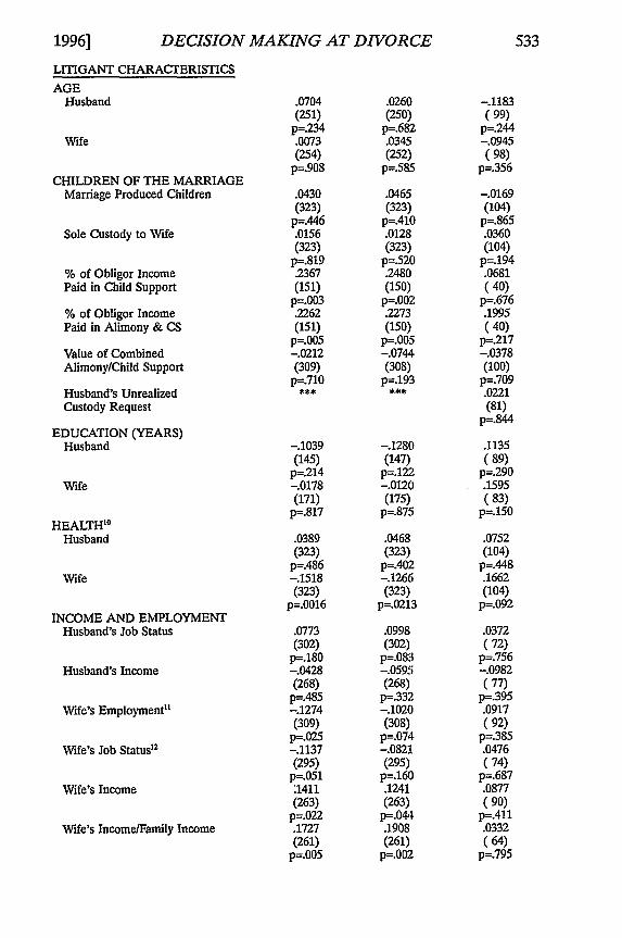
1996] DECISION MAKING AT DIVORCE
LITIGANT CHARACTERISTICS
AGEHusband
Wife
CHILDREN OF THE MARRIAGEMarriage Produced Children
Sole Custody to Wife
% of Obligor IncomePaid in Child Support
% of Obligor IncomePaid in Alimony & CS
Value of CombinedAlimony/Child Support
Husband's UnrealizedCustody Request
EDUCATION (YEARS)Husband
Wife
HEALTH"0
Husband
Wife
INCOME AND EMPLOYMENTHusband's Job Status
Husband's Income
Wife's Employmenti1
Wife's Job Status12
Wife's Income
Wife's Income/Family Income
.0704(251)p=.234
.0073(254)
p=.908
.0430(323)p=.446
.0156(323)
p=.819
.2367(151)
p=.003.2262(151)
p=.005
-.0212(309)
p=.7 10
-. 1039(145)
p=.214-. 0178(171)
p=.817
.0389(323)
p=.486-. 1518(323)
p=.0016
.0773(302)
p=.180
-. 0428(268)p=.485
-. 1274(309)
p=.025
-. 1137(295)p=.051
.1411(263)
p=.022.1727(261)
p=.0 05
.0260(250)
p=.682.0345(252)
p=.585
.0465(323)
p=.410.0128(323)
p=.520.2480(150)
p=.002.2273(150)
p=.005-. 0744(308)
p=.193
-. 1280(147)
p=.122-. 0120(175)
p=.875
.0468(323)p=.402-.1266(323)
p=.0213
.0998(302)
p=.083-.0595(268)
p=.332-.1020(308)
p=.074-. 0821(295)
p=.160.1241(263)
p=.044
.1908(261)
p=.002
-. 1183(99)
p=.244
-. 0945(98)
p=.3 56
-. 0169(104)
p=.865.0360(104)
p=.194.0681(40)
p=.676.1995(40)
p=.217-.0378(100)
p=.709.0221(81)
p=.844
.1135(89)
p=.290.1595(83)
p=.150
.0752(104)
p=.448.1662(104)
p=.092
.0372(72)
p=.756-. 0982(77)
p=.395.0917(92)
p=.385.0476(74)
p=.687.0877(90)
p=.411.0332(64)
p=.795

534 NORTH CAROLINA LAW REVIEW [Vol. 74
Wife Awarded Alimony -.0187 -. 034 .1515(317) (317) (104)
p=.740 p=.952 p=.125MARITAL DURATION (YEARS) .0511 .0711 -. 0630
(315) (315) (103)p=.366 p=.208 p=.527
Length of Separation .1046 .0990(years) (300) (301)
p=.071 p=.086MARITAL PROPERTY
Net Worth -. 1379 -. 1148 -. 1408(323) (322) (104)
p=.013 p=.040 p=.154
Marital debt -. 0920 -.0964 -. 1162(319) (319) (104)
p=.101 p=.086 p=.240Husband-Owned -. 1056 -. 1012 -. 1516Property Value (304) (304) (102)
p=.093 p=.067 p=.128Husband-Owned % of -.2326 -. 2775 -.4914Marital Property (301) (302) (102)
p=.000 p=.000 p=.000Husband Owns -.2250 -. 2661 -. 1299Business, Professional (323) (322) (104)Degree or License p=.000 p=.000 p=.189Husband Owns Pension -.0955 -. 0748
(323) (323)p=.094 p=.180
Wife-Owned Property Value .0552 .0649 .1596(225) (222) (103)
p=.410 p=.336 p=.107Wife-Owned % of .0124 .0103 .4331Marital Property (256) (256) (103)
p=.843 p=.870 p=.000SEPARATE PROPERTY
Value of Husband .1193 .1174 -. 1261Owned Property (323) (323) (104)
p=.032 p=.035 p=.202Ratio of Husband's .1191 .1262 .0700Separate Property (304) (304) (104)to Marital Property p=.037 p=.027 p=.480Value of Wife .0127 .0346 .0443Owned Property (323) (323) (104)
p=.820 p=.535 p=.655Ratio of Wife's .0305 .1127 .1043Separate Property (304) (306) (104)to Marital Property p=.594 p=.048 p=.292
'Coded as five rankings based on the wife's percentage of net marital assets. 1=less than 34%;2=between 34% and 44%; 3=between 45% and 55%; 4=between 56% and 66%; 5=more than66%.2For nondichotomous categorical variables (i.e., case region, appellate department, and judge'sreligion), the table displays the chi-square statistic followed by the applicable degrees of freedom(in parentheses).I Coded divorce judgment granted against husband only=1, against both spouses=2, against wifeonly=3.4 Coded 1 through 7, based on combined score taking into account fault judgment (1 through 3)and basis. Adultery ranked 1, cruel and inhuman treatment 2, abandonment 3, mental illness 4.
SCoded 1=wife, 2-=husband.6 Coded 2 through 8, based on combined status scores of judge's college and law school.SCoded 1=Democratic, 2=Republican.

1996] DECISION MAKING AT DIVORCE
I Coded 0=attended neither college or law school locally, 1=attended either college or lawschool locally, 3=attended both college and law school locally.I Coded 1=male, 2=female.10 Coded 1=good, 2=fair, 3=poor.11 Coded 1=employed, 2=unemployed.12 Coded 1=high status professional, 2=lower status professional (e.g., accountants, artists,clergymen, computer programmers, decorators and designers, journalists, librarians, musicians,nurses, pharmacists, high school or lower teachers), 3=small business owners, white collarworkers (e.g., sales personnel, clerks, cashiers, secretaries), and skilled blue collar workers (e.g.,machinists, printers, electricians, butchers, machine operators), 4=students, 5=unemployed,retired, or homemaker.
TABLE A8PERCENTAGES OF SAMPLE WIVES AWARDED ALIMONY, BY WIFE'S
INCOME (1990 DOLLARS) AND CASE GROUP
Wife's Income ($1990) Judicial Sample Settlement Sample Difference% (n) % (n)
$0 - $4,999 87% (114) 52% (92) -35***$5,000 - $19,999 68% (105) 28% (104) -40***$20,000 or more 33% (92) 8% (80) -25***
p<.001
TABLE A9PERCENTAGES OF SAMPLE WIVES AWARDED ALIMONY, BY
HUSBAND'S INCOME (1990 DOLLARS) AND CASE GROUP
Husband's Income ($1990) Judicial Sample Settlement Sample Difference% (n) % (n)
$0 - $39,999 50% (112) 26% (145) -24***$40,000 - $79,999 75% (120) 37% (60) -38***$80,000 or more 77% (84) 57% (30) -30*
*** p<.05; * p<.001
TABLE A1OPERCENTAGES OF SAMPLE WIVES AWARDED ALIMONY, BY
CUSTODY STATUS AND CASE GROUP
Custody Status+ Judicial Sample Settlement Sample Difference% (n) % (n)
Wife with sole custody 67% (191) 30% (132) -37***Wife without sole custody 56% (170) 29% (167) -28***
+Cases involving joint or split custody excluded; wife without sole custody category includescases involving husband custody and cases without minor children.*** p<.001

NORTH CAROLINA LAW REVIEW [Vol. 74
TABLE AllMEAN RATIO OF WIFE'S POST-DIVORCE ADJUSTED FAMILY
INCOME/HUSBAND'S POST-DIVORCE ADJUSTED FAMILY INCOME
(SETrLEMENT SAMPLE), BY HUSBAND AND WIFE
PRE-DIVORCE INCOME
Wife's Income Husband's Income$0 - $34,999 $35,000-$59,999 $60,000 +
mean ratio (n) mean ratio (n) mean ratio (n)
$ 0 - $4,999 .24 (26) .20 (23) .21 (21)$5,000 - $19,999 .84 (42) .41 (24) .51 ( 7)$20,000 + 1.23 (25) .67 (15) .45 (11)ALL SAMPLE WIVES .78 (93) .39 (62) .33 (39)
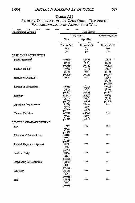
1996]
Independent Variable Case Group
JUDICIAL SETTLEMENTTrial Appellate
Pearson's R(n)p=
CASE CHARACTERISTICS
Fault Judgment2
Fault Ranking
Gender of Plaintiff4
Length of Proceeding
Region*
Appellate Department*
Year of Decision
JUDICIAL CHARACTERISTICS
Age
Educational Status Score5
Judicial Experience (years)
Political Partny
Regionality of Education 7
Religion*
Sex8
-. 0290(348)
p=.589-. 0565(326)
p=.309
-.0453(291)p=.44211.9(2)(377)
p=.0037.2(3)(377)
p=.067-. 1222(376)
p=.018
.1097(356)
p=.039.0418(339)
p=.443.0160(362)
p=.761.0352(313)
p=.535-. 0558(346)
p=.3015.5(2)(196)
p=.063-. 1008(376)
p=.051
DECISION MAKING AT DIVORCE
TABLE A12ALIMONY CORRELATIONS, BY CASE GROUP ])EPENDENT
VARIABLE=AWARD OF ALIMONY TO WIFE
Pearson's R1
(n)P=
.0876(313)
p=.122.1127(312)
p=.047.1067(314)
p=.059-.0169(310)p=.7673.6(2)(315)
p=.169
Pearson's R(n)p=
-.0493(348)
p=.360-.0776(326)
p=.162
-. 0123(291)
p=.82311.8(2)(377)
p=.0037.0(3)(377)
p=.072-. 1308(376)
p=.0 11

538 NORTH CAROLINA LAW REVIEW
LITIGANT CHARACTERISTICS
AGEHusband
Wife
CHILDREN OF THE MARRIAGEMarriage Produced Children
Sole Custody to Wife
% of Obligor IncomePaid in Child Support
Husband's UnrealizedCustody Request
EDUCATION (YEARS)Husband
Wife
HEALTH9
Husband
Wife
INCOME AND EMPLOYMENTHusband's Job Status
Husband's Income
Wife's Employment"0
Wife's Job Status"
Wife's Income
Wife's Income/Family Income
MARITAL DURATION (YEARS)
-.0241(290)
p=.682.0072(291)
p=. 903
.1478(377)
p=.005
.0955(377)
p=.064
-. 2394(170)
p=.002
.0431(169)
p=.578-.2403(201)
p=.001
-.0433(377)
p=.40 1
.1979(377)
p=.000
.1481(351)p=.007.0278(316)p=.623.3380(365)
p=. 000
-.3479(347)
p=.000
-.4518(311)
p=.00 0
-. 5581(283)
p=.000.1199(367)
p=.022
[Vol. 74
-. 0126(290)
p=.831
.0143(291)
p=.808
.1473(377)
p=.004
.0896(377)
p=.082
-.2092(174)
p=.006
.0431(169)
p=.578
-. 2466(201)
p=.000
-. 0126(377)
p=.807
.2019(377)
p=. 000
.1448(351)
p=.0 07
.0248(316)
p=.660
.3367(365)
p=.000
-. 3502(347)
p=.000
-.4622(311)
p=.000
-.5795(283)
p=.O00.1041(367)
p=.046
-.0220(305)
p=.702.0371(305)
p=.259
.0652(315)
p=.249
-. 0255(315)
p=.652
-. 0092(137)
p=.915.0870(200)
p=. 221
.0544(269)
p=.37 4
-.0404(261)
p=.516
-. 0238(315)
p=.674.1075(315)p=.057
.1277(237)
p=.050
.1077(235)
p=.05 0
.2435(286)
p=.0 00
-. 2070(246)
p=.O01-. 3725(258)
p=.000-.4510(205)
p=.000.0703(313)
p=.215

1996] DECISION MAKING AT DIVORCE 539
MARITAL PROPERTYNet Worth -. 1236 -. 1280 -. 0340
(373) (373) (315)p=.017 p=.013 p=.547
Percentage of Marital -. 0441 -. 0739 .1515Property Awarded to Wife 2 (323) (323) (104)
p=.429 p=.185 p=.125Value of Wife's Net -. 1287 -. 1358 -. 0362Property Award (373) (373) (315)
p=.013 p=.009 p=.522
'For nondichotomous categorical variables (i.e., case region, appellate department, and judge's
religion), the table displays the chi-square statistic followed by the applicable degrees of freedom( m parentheses).
ICoded divorce judgment granted against husband only=1, against both spouses=2, against wifeonly=3.3 Coded 1 through 7, based on combined score taking into account fault judgment (1 through 3)and basis. Adultery ranked 1, cruel and inhuman treatment 2, abandonment 3, mental illness 4.
Coded 1=wife, 2=husband.5 Coded 2 through 8, based on combined status scores of judge's college and law school.6 Coded 1=Democratic, 2=Republican.I Coded 0=attended neither college or law school locally, 1=attended either college or lawschool locally, 3=attended both college and law school locally.8 Coded 1=male, 2=female.I Coded 1=good, 2=fair, 3=poor.0 Coded 1=employed, 2=unemployed.11 Coded 1=high status professional, 2=lower status professional (e.g., accountants, artists,clergymen, computer programmers, decorators and designers, journalists, librarians, musicians,nurses, pharmacists, high school or lower teachers), 3=small business owners, white collarworkers (e.g., sales personnel, clerks, cashiers, secretaries), and skilled blue collar workers (e.g.,machinists, printers, electricians, butchers, machine operators), 4=students, 5=unemployed,retired, or homemaker.1 For cases with positive net worth, by five category rankings. For settlement case sample, ValidGroup.
TABLE A13PERCENTAGES OF ALIMONY AwARDs THAT WERE PERMANENT, BY
WIFE'S AGE AND CASE GROUP
Wife's Age (years) Judicial Sample Settlement Sample Difference% (n) % (n)
39 or less 26% (66) 26% (50) - 040-49 39% (70) 30% (27) -950 or more 52% (54) 60% (10) + 8

540 NORTH CAROLINA LAW REVIEW [Vol. 74
TABLE A14PERMANENCE OF ALIMONY CORRELATIONS DEPENDENT
VARIABLE=PERMANENCE OF ALIMONY AWARD TO WIFE'
Independent Variable Case Group
JUDICIAL SETTLEMENTTrial Appellate
Pearson's R Pearson's R Pearson's R2
(n) (n) (n)p= p= p=
CASE CHARACTERISTICS
Fault Judgmen .0488 .0005 .1726(215) (218) ( 93)
p=.477 p=.994 p=.098Fault Ranking4 .0833 .0261 .1949
(202) (205) ( 93)p=.23 9 p=.711 p=.061
Gender of Plaintiff5 .1748( 92)
P=.096Length of Proceeding .0195 -. 0127 -. 0770
(186) (187) ( 91)p=.792 p=.863 p=.68
Region* 2.4(3) 4.8(2) 1.9(2)(229) (232) ( 93)
p=.301 p=.091 p=.395Appellate Department* 4.7(3) 5.5(3)
(229) (232)p=.191 p=.138
Year of Decision .1516 .1650(229) (232)
p=.022 p=.012JUDICIAL CHARACTERISTICS
Age -. 0581(216)
p=.395
Educational Status Sscore6 -. 1736(202)
p=.013Judicial Experience (years) -. 0906
(219)p=.182
Political Party7 -. 1610(184)p=.029
Regionality of Education' .1720(207)p=.013
Religion* 4.2(2)(118)p=.123
Sex9 .0789(228)
p=.23 5

1996] DECISION MAKING AT DIVORCE
LITIGANT CHARACTERISTICS
AGEHusband
Wife
CHILDREN OF THE MARRIAGEMarriage Produced Children
Sole Custody to Wife
% of Obligor IncomePaid in Child Support
% of Obligor IncomePaid in Alimony & CS
Value of CombinedAlimony/Child Support
EDUCATION (YEARS)Husband
Wife
HEALTH 10
Husband
Wife
INCOME AND EMPLOYMENTHusband's Job Status
Husband's Income
Wife's Employmente
Wife's Job Status12
Wife's Income
Wife's Income/Family Income
-. 1123(183)
p=.130-. 2130(189)
p=.003
-. 0258(229)
p=.698.1154(229)p=.081
-. 0516(117)p=.581-.0868(117)
p=.352
-.0137(224)
p=.838
.1621(112)
p=.088
.1131(136)
p=.190
.0150(229)
p=.698-. 1544(229)
p=.019
.0609(221)
p=.368.0073(208)
p=.917
-.0694(223)
p=. 302
-.0491(221)
p=.467
.0173(198)
p=.809-. 0042(186)
p=.954
-. 1870(185)
p=.0 11
-. 3082(191)
p=.000
-.0661(232)
p=.316
.1896(232)
p=. 004
.0050(119)
p=.957.0342(119)
p=.712.0016(227)
p=.981
.0711(111)
p=.459.0554(134)
p=.525
.0390(232)p=.555-.2465(232)
p=.000
.0793(220)
p=.242
-. 0069(211)
p=.92 1-. 0872(226)
p=.192
-. 0270(221)
p=.690-. 0125(201)
p=.860.0148(189)
p=.840
-.2108( 87)
p=.050
-. 1233( 87)
p=.255
-. 1382( 93)
p=.106-. 0624( 93)
p=.552-. 3486( 93)
p=.552-.2009( 40)
p=.214
.0287( 89)
p=.789
.1895( 79)
p=.094
.2120(75)
p=.068
-. 0152( 93)
p=.885
-.2949( 93)
p=.004
-. 1468( 68)
p=.232.0268(75)
p=.819-.0891( 88)
p=.409-. 0575( 76)
p=.622.0915( 82)
p=.414.0434( 66)
p=.72 9

542 NORTH CAROLINA LAW REVIEW [Vol. 74
MARITAL DURATION (YEARS) -.2551 -.3699 -. 2344(226) (226) (93)
p=.000 p=.000 p=.024MARITAL PROPERTY
Net Worth (marital) .0118 -.0104 .1502(230) (230) ( 93)
p=.859 p=.876 p=.151Value Wife's Net -. 0759 -. 1057 .1151Property Award (229) (229) ( 93)
p=.256 p=.lll p=.272
'Coded 1=permanent, 2=durational.
2 For nondichotomous categorical variables (i.e., case region, appellate department, and judge's
religion), the table displays the chi-square statistic followed by the applicable degrees of freedom(in parentheses).I Coded divorce judgment granted against husband only=l, against both spouses=2, against wifeonly=3." Coded 1 through 7, based on combined score taking into account fault judgment (1 through 3)and basis. Adultery ranked 1, cruel and inhuman treatment 2, abandonment 3, mental illness 4.S Coded 1=wife, 2=husband.
Coded 2 through 8, based on combined status scores of judge's college and law school.Coded 1=Democratic, 2=Republican.Coded 0=attended neither college or law school locally, 1=attended either college or law
school locally, 3=attended both college and law school locally.I Coded 1=male, 2=female.10 Coded 1=good, 2=fair, 3=poor.n Coded 1=employed, 2=unemployed.12Coded 1=high status professional, 2=lower status professional (e.g., accountants, artists,clergymen, computer programmers, decorators and designers, journalists, librarians, musicians,nurses, pharmacists, high school or lower teachers), 3=small business owners, white collarworkers (e.g., sales personnel, clerks, cashiers, secretaries), and skilled blue collar workers (e.g.,machinists, printers, electricians, butchers, machine operators), 4=students, 5=unemployed,retired, or homemaker.

1996] DECISION MAKING AT DIVORCE
TABLE A15ENHANCEMENTS TO ALIMONY & CHILD SUPPORT, BY CASE GROUP
Type of Benefit Judicial Sample Settlement Sample% (n) % (n)
Automatic Salary or Cost of Living Adjustmentsalimony 1% (148) 5% (94)child support 1% (235) 2% (220)
Life Insurance on Obligorwhen minor children' 44% (212) 47% (200)spouse only 18% (130) 17% (113)
Medical Insurance Premiumsfor minor children2 57% (217) 63% (220)for recipient spouse 15% (343) 12% (312)
Unreimbursed Medical Costsfor minor children 3 14% (235) 18% (220)for recipient spouse 0% (383) 0% (315)
Other Child-Related Costschild care 6% (216) 7% (220)college expenses4 19% (230) 29% (220)private school 6% (235) 4% (220)other 5% (235) 5% (220)
'In the judicial sample, when provision for maintenance of life insurance was made, 96% of thecases required insurance to be maintained by the father, and 4% by both parents. In thesettlement sample, 82% of the cases required insurance to be maintained by the father, and, 1%by the mother, and 17% by both parents.
In the judicial sample, when maintenance of medical insurance was required, the father alonewas required to maintain coverage in 89% of the cases, the mother alone in 4%, and bothparents in 7%. In the settlement sample, the father alone was required to maintain coverage in83% of the cases, the mother in 8%, and both parents in 9%.3 In the judicial sample, when provision for unreimbursed medical expenses was made, 62%required payment by the father, 2% by the mother, and 36% by both parents. In the settlementsample, 52.5% required payment by the father, and 47.5% by both parents.4 In the judicial sample, when payment of college expenses was required, 71% required paymentof all expenses by the father and 29% required joint payment. In the settlement sample, 39%required payment by the father and 61% required joint payment.

NORTH CAROLINA LAW REVIEW [Vol. 74
TABLE A16CHILD SUPPORT CORRELATIONS DEPENDENT VARIABLE=VALUE OF
CHILD SUPPORT EXCLUDING ALIMONY ($1990)
Independent Variable
Pearson'(n)p=
Case Grou
JUDICIALAppellate
's R Pearson's R(n)p=
pSETTLEMENT
Pearson's R1(n)p=
CASE CHARACTERISTICS
Fault Judgment2
Fault Ranking
Gender of Plaintiff3
Length of Proceeding
Region*
Appellate Department*
Year of Decision
JUDICIAL CHARACTERISTICS
Age
Educational Status Score4
Judicial Experience (years)
Political Party5
Regionality of Education6
Religion*
Sex7
-. 1620(191)
p=.025-. 1026(190)
p=.159
-. 1246(192)
p=.085.2405(193)
p<.0003.352(196)
p=.037
-. 0954(214)
p=.164
-. 1182(203)
p=.093
.1097(176)
p=.1471.144(227)
p=.3213.442(227)
p=.O18.2039(227)
p=.0 02
-.0903(214)
p=. 188
-. 1101(203)
p=.118
.0974(176)
p=.198
1.062(227)
p=.3483.578(227)
p=.015.2002(227)
p=.002
.0538(211)
p=.437.0284(202)
p=.688.1664(218)
p=.014-. 0847(185)
p=.252.0275(202)
p=.697.286
(114)p=.752.1822(226)
p=.006

1996] DECISION MAKING AT DIVORCE
LITIGANT CHARACTERISTICS
AGEObligor
Recipient
CHILDREN OF THE MARRIAGESole Custody to Wife
Number of Children
Husband's UnrealizedCustody Threat
EDUCATION (YEARS)Obligor
Recipient
HEALTH'Obligor
Recipient
INCOME AND EMPLOYMENTObligor
Recipient
Recipient's Income/Family Income
Recipient's Job Status
Obligor's Job Status
-.0333(172)
p=.665
-.1092(172)
p=.154
.3617(227)
p=.0 00
.2913(227)
p=.000
.2503(112)
p=.008
.1617(134)
p=.062
-. 0983(227)
p=.140
-. 1257(227)
p=.059
.6108(175)
p=.000
-. 0418(164)
p=.595-.2113(163)
p=.007
.0151(209)p=.828
-.2498(211)
p=.000
-. 0427(172)
p=-578-. 1181(172)
p=.123
.3712(227)
p=.000
.2838(227)
p=.000
.2732(112)p=.004
.1787(134)p=.039
-. 1044(227)
p=.117
-.1212(227)
p=.068
.6178(175)
p=.000-.0706(164)
p=.369
-. 2317(163)
p=. 003
.0129(209)
p=.853-. 2689(211)
p=.0 00
.0283(190)
p=.690
.0077(189)
p=.916
.3206(196)
p=.000
.1581(196)
p=.027.1559(192)
p=.031
.2896(168)
p=.0 00
.2410(167)
p=.002
-. 0697(196)
p=.33 1
-. 1017(189)
p=.156
.4623(141)
p=.000
-. 1727(166)
p=.026-.4240(125)
p=.000
-.0871(160)
p=.274-.3962(151)
p=.000

546 NORTH CAROLINA LAW REVIEW [Vol. 74
MARITAL DURATION -. 1612 -. 1578 .0178(220) (220) (194)
p=.017 p=.019 p=.805MARITAL PROPERTY
Net Worth .0073 .0073 .0804(225) (225) (196)
p=.913 p=.913 p=.263Value of Recipient's .1220 .1237 .1456Net Property Award (221) (221) (182)
p=.070 p=.066 p=.050
For nondichotomous categorical variables (i.e., case region, appellate department, and judge'sreligion), the table displays the F statistic.2 Coded divorce judgment granted against obligor only=1, against both spouses=2, against
recipient only=3.3 Coded 1=wife, 2=husband.4 Coded 2 through 8, based on combined status scores of judge's college and law school.5 Coded 1=Democratic, 2-=Republican.6Coded 0=attended neither college or law school locally, 1=attended either college or law schoollocally, 3=attended both college and law school locally.7 Coded 1=male, 2=female.s Coded 1=good, 2=fair, 3=poor.

1996] DECISION MAKING AT DIVORCE
TABLE A17COMBINED ALIMONY AND CHILD SUPPORT CORRELATIONS (CASES
WITH MINOR CHILDREN) DEPENDENT VARIABLE=VALUE OF
ALIMONY PLUS CHILD SUPPORT ($1990)
Independent Variable Case Group
Trial
Pearson(n)p=
CASE CHARACTERISTICS
Fault Judgment2
Fault Ranking
Gender of Plaintiff3
Length of Proceeding
Region*
Appellate Department*
Year of Decision
JUDICIAL CHARACTERISTICS
Age
Educational Status Score4
Judicial Experience (years)
Political Party,
Regionality of Education
Religion*
Sex7
-. 087C(212)
p=.20-. 086'(201)
p=.22
.1512(174)
p=.04
5.713(225)
p=.00 43.026(225)
p=.03.1302(225)
p=.05
JUDICIALAppellate
's R Pearson's R(n)p=
0 -. 0966(212)
)7 p=.161;7 -. 0899
(201)1 p=.204
.1850(174)
p=.015
7.634(225)
}4 p=.0013.707(225)
8 p=.012.1380(225)
1 p=.039
SETTLEMENT
Pearson's R1
(n)p=
-. 0829(190)
p=.255-. 0390(189)
p-. 594
-. 0607(191)
p=.40 4
.2586(181)
p=.0 004.965(184)
p=.008
.0849(209)
p=.222.0912(196)p=.204.0975(216)p=.153
.0212(183)
p=.776.0015(200)
p=.9831.181(112)
p=.311.0248(224)
p=.712
547

NORTH CAROLINA LAW REVIEW
LITIGANT CHARACTERISTICS
AGEObligor
Recipient
CHILDREN OF THE MARRIAGESole Custody to Wife
% of Obligor IncomePaid in Child Support
Number of Children
Husband's UnrealizedCustody Request
EDUCATION (YEARS)Obligor
Recipient
HEALTH8
Obligor
Recipient
INCOME AND EMPLOYMENTObligor
Recipient
Recipient's Income/Family Income
Recipient's Job Status9
Obligor's Job Status
[Vol. 74
.0690(170)
p=.366.0679(170)
p=.379
.1492(225)
p=.025
-. 0763(171)
p=.321.2049(225)
p=.002
.2574(112)
p=.006.2450(133)
p=.004
-. 1048(225)p=.117
.0387(225)
p=.564
.6294(175)
p=.000
-. 1899(164)
p=.0 15
-. 3964(163)
p=.000.0998(208)
p=.152-. 3277(209)
p=.000
.0794(170)
p=.3 04
.0743(170)
p=.335
.1589(225)
p=.017-.0941(171)
p=.221
.1909(225)
p=.0 04
.2687(112)
p=.004.2770(133)
p=.001
-. 1042(225)
p=.l19.0926(225)
p=.166
.6286(175)
p=.000
-.2138(164)
p=.0O06-.4131(163)p=.000
.1192(208)
p=.086
-.3206(209)
p=.000
.0604(178)
p=.423.0752(177)
p=.328
.1190(208)
p=.087-. 0092(137)
p=.915.1208(184)
p=.102
.0876(191)
p=.228
.3210(132)
p=.00 0
.2266(158)
p=.004
.0037(184)
p=.960.1046(184)
p=.158
.5924(140)
p=.000-. 1703(165)
p=.029-.2382(165)
p=.002.0902(164)
p=.211-.4615(157)
p=. 000

1996] DECISION MAKING AT DIVORCE 549
MARITAL DURATION .0152 .0230 .0607(218) (218) (206)
p=.824 p=.736 p=.386MARITAL PROPERTY
Net Worth -.0160 -. 0107 .0261(223) (223) (208)
p=.812 p=.873 p=.708Value of Recipient's .1038 .1126 .0738Net Property Award (219) (219) (191)
p=.126 p=.096 p=. 310
1 For nondichotomous categorical variables (i.e., case region, appellate department, and judge'sreligion), the table displays the F statistic.2 Coded divorce judgment granted against obligor only=l, against both spouses=2, againstrecipient only=3.3 Coded 1=wife, 2=husband.4 Coded 2 through 8, based on combined status scores of judge's college and law school.5 Coded 1=Democratic, 2=-Republican.6 Coded 0=attended neither college or law school locally, 1=attended either college or law schoollocally, 2=attended both college and law school locally.Coded 1--male, 2=female.Coded 1=good, 2=fair, 3=poor.Coded 1=high status professional, 2=lower status professional (e.g., accountants, artists,
clergymen, computer programmers, decorators and designers, journalists, librarians, musicians,nurses, pharmacists, high school or lower teachers), 3--small business owners, white collarworkers (e.g., sales personnel, clerks, cashiers, secretaries), and skilled blue collar workers (e.g.,machinists, printers, electricians, butchers, machine operators), 4--students, 5=unemployed,retired, or homemaker.

550 NORTH CAROLINA LAW REVIEW [Vol. 74
TABLE A18ALIMONY AWARD VALUE CORRELATIONS (CASES WITHouT MINOR
CHILDREN) DEPENDENT VARTABLE=VALUE OF ALIMONY (1990DOLLARS)
Independent Variable
CASE CHARACTERISTICS
Fault Judgment2
Fault Ranking3
Gender of Plaintiff4
Length of Proceeding
Region*
Appellate Department*
Year of Decision
JUDICIAL CHARACTERISTICS
Age
Educational Status Score5
Judicial Experience (years)
Political Party6
Regionality of Education7
Religion
Sex
Case Group
JUDICIALTrial Appellate
Pearson's R Pearson's R(n) (n)p= p=
.0629 -. 0010(74) (75)
p=.595 p=.993.2467 .2439(66) (67)
p=.046 p=.047
.0580 .0452(63) (63)
p=.652 p=.725-1.216 -1.416(80) (81)
p=.302 p=.249-. 8.141 -8.310(80) (81)
p=.000 p=.000-. 0859 .0330(80) (81)p=.448 p=.770
.0612( 78)
p=.559.1759( 76)p=.12 8
-.0681(76)
p=.559-.2545( 65)
p=. 04 1
-.0042( 77)
p=.97 1
1.007(41)
p=.375
-. 1274( 80)
p=.260
SETTLEMENT
Pearson's R1
(n)p=
-.0431( 33)
p=. 812
-. 0734( 33)
p=.685-. 1073( 32)
p=.559.0743( 32)
p=.686.827
( 33)p=.447

1996] DECISION MAKING AT DIVORCE
LITIGANT CHARACTERISTICSAGE
Husband
Wife
CHILDREN OF THE MARRIAGEMarriage Produced Children
EDUCATION (YEARS)Husband
Wife
HEALTH9
Husband
Wife
INCOME AND EMPLOYMENTHusband's Job Status
Husband's Income
Wife's Job Status0
Wife's Income
Wife's Income/Family Income
MARITAL DURATION
MARITAL PROPERTYNet Worth
Husband-OwnedProperty Value
Wife-OwnedProperty Value
Value of Wife'sNet Property Award
.1980( 66)
p=.111.1232(70)
p=.310
-.1492( 80)
p=.209
-.0920( 30)
p=.629.2642( 38)
p=.109
-. 0140( 80)
p=.902-. 1151( 80)
p=.309
-.3410(77)
p=.0O02.4423(70)
p=. 000
.1400( 76)
p=.228-. 2715( 66)
p=.027
-. 4445( 63)
p=.00.1920( 78)
p=.092
.1165(79)p=.306.7848( 66)
p=.900
.0386(79)
p=.734
.5273( 78)
p=.000
.1938( 67)
p=.116.1406( 71)
p=.242
.1710( 81)
p=.127
-. 0702( 29)
p=.717.2651( 37)
p=.113
-. 0409( 81)p=.717-. 1057( 81)
p=.348
-. 2238(78)
p=.049.8086( 71)
p=.000.1587(77)
p=.168-. 2487( 67)
p=.042-. 3814(64)
p=.004.2401(79)
p=.039
.3971( 80)
p=.000.8078( 67)p=.000
.0105( 81)
p=.926.3795(79)
p=.0 01
.2351( 31)
p=.203.2118( 31)
p=.253
-.0711( 33)p=.694
.2351( 30)
p=.O01.2745(27)
p=.166
-. 0087( 33)
p=.962.2247( 33)
p=.209
-.5534(24)p=.005
.9222( 28)
p=.O00-.1012(25)
p=.630.0129( 30)
p=.946-.1432(26)
p=.485
.1921( 33)
p=.284
.5580( 33)
p=.0 01
.8006( 30)
p=.0 00
.1814( 30)
p=.337.3687( 33)
p=.035
1 For nondichotomous categorical variables (i.e., case region, appellate department, and judge'sreligion), the table displays the F statistic.

552 NORTH CAROLINA LAW REVIEW [Vol. 742 Coded divorce judgment granted against husband only=l, against both spouses=2, against wife
only=3.3 Coded 1 through 7, based on combined score taking into account fault judgment (1 through 3)and basis. Adultery ranked 1, cruel and inhuman treatment 2, abandonment 3, mental illness 4.4Coded 1=wife, 2=husband.S Coded 2 through 8, based on combined status scores of judge's college and law school.6Coded 1=Democratic, 2=Republican.7 Coded 0=attended neither college or law school locally, 1=attended either college or lawschool locally, 2=attended both college and law school locally.
Coded 1--male, 2=female.9Coded =good, 2=fair, 3=poor.10 Coded 1=high status professional, 2=lower status professional (e.g., accountants, artists,clergymen, computer programmers, decorators and designers, journalists, librarians, musicians,nurses, pharmacists, high school or lower teachers), 3=small business owners, white collarworkers (e.g., sales personnel, clerks, cashiers, secretaries), and skilled blue collar workers (e.g.,machinists, printers, electricians, butchers, machine operators), 4=students, 5=unemployed,retired, or homemaker.
TABLE A19PERCENTAGE DISTRIBUTION OF NET MARITAL ASSETS (JUDICIAL
SAMPLE: COUPLES wITH PosITIvE NET WORTH), BY WIFE'S
HEALTH
Percentage Distribution of NetMarital Assets Wife's Health
Good Fair Poor(n=273) (n=28) (n=22)
Disproportionate Share to Husband 30% 29% 63%Relatively Equal* 48% 57% 32%Disproportionate Share to Wife 22% 14% 5%
* Relatively Equal=Between 45% and 55%Chi-square=12,88728 D.F.=4; P=.01184