NBER WORKING PAPER SERIES

HOW DO ELECTRICITY SHORTAGES AFFECT INDUSTRY? EVIDENCE FROMINDIA

Hunt AllcottAllan Collard-WexlerStephen D. O'Connell

Working Paper 19977http://www.nber.org/papers/w19977

NATIONAL BUREAU OF ECONOMIC RESEARCH1050 Massachusetts Avenue

Cambridge, MA 02138March 2014

Previously circulated as "How Do Electricity Shortages Affect Productivity? Evidence from India."We thank Maureen Cropper, Jan De Loecker, Michael Greenstone, Peter Klenow, Kabir Malik, RohiniPande, Nick Ryan, Jagadeesh Sivadasan, Anant Sudarshan, and seminar participants at Brown, Drexel,Duke, the Federal Trade Commission, Harvard, the 2013 NBER Summer Institute, the 2014 NBERWinter IO/EEE meetings, Society for Economic Dynamics, Stanford, KU Leuven, Toulouse, Universidadde los Andes, University of Chicago, University of Cologne, and the World Bank for helpful comments.We are particularly grateful to Nick Bloom, Troy Smith, and Shaleen Chavda for insight into the textileindustry. We thank Deepak Choudhary, Anuradha Bhatta, Sherry Wu, and Mark Thomas for helpfulresearch assistance and the Stern Center for Global Economy and Business for financial support. Wehave benefited from helpful conversations with Jayant Deo of India Energy Exchange, Gajendra Haldeaof the Planning Commission, Partha Mukhopadhyay of the Centre for Policy Research, and Kirit Parikhof IGIDR. We also thank A. S. Bakshi and Hemant Jain of the Central Electricity Authority for helpin collecting archival data. Of course, all analyses are the responsibility of the authors, and no otherparties are accountable for our conclusions. Code for replication is available from Hunt Allcott’s website.The views expressed herein are those of the authors and do not necessarily reflect the views of theNational Bureau of Economic Research.

NBER working papers are circulated for discussion and comment purposes. They have not been peer-reviewed or been subject to the review by the NBER Board of Directors that accompanies officialNBER publications.

© 2014 by Hunt Allcott, Allan Collard-Wexler, and Stephen D. O'Connell. All rights reserved. Shortsections of text, not to exceed two paragraphs, may be quoted without explicit permission providedthat full credit, including © notice, is given to the source.

How Do Electricity Shortages Affect Industry? Evidence from IndiaHunt Allcott, Allan Collard-Wexler, and Stephen D. O'ConnellNBER Working Paper No. 19977March 2014, Revised August 2015JEL No. D04,D24,L11,L94,O12,O13,Q41

ABSTRACT

We estimate the effects of electricity shortages on Indian manufacturers, instrumenting with supplyshifts from hydroelectric power availability. We estimate that India’s average reported level of shortagesreduces the average plant’s revenues and producer surplus by five to ten percent, but average productivitylosses are significantly smaller because most inputs can be stored during outages. Shortages distortthe plant size distribution, as there are significant economies of scale in generator costs and shortagesmore severely affect plants without generators. Simulations show that offering interruptible retail electricitycontracts could substantially reduce the impact of shortages.

Hunt AllcottDepartment of EconomicsNew York University19 W. 4th Street, 6th FloorNew York, NY 10012and NBERhunt.allcott@nyu.edu

Allan Collard-WexlerDepartment of EconomicsDuke University233 Social SciencesDurham, NC 27708and NBERallan.collard-wexler@duke.edu

Stephen D. O'ConnellCity University of New YorkDepartment of EconomicsThe Graduate Center365 Fifth AveNew York, NY 10016-4309soconnell@gc.cuny.edu

How Do Electricity Shortages Affect Industry? Evidence from India

Hunt Allcott, Allan Collard-Wexler, and Stephen D. O’Connell∗

August 10, 2015

Abstract

We estimate the effects of electricity shortages on Indian manufacturers, instrumenting withsupply shifts from hydroelectric power availability. We estimate that India’s average reportedlevel of shortages reduces the average plant’s revenues and producer surplus by five to ten per-cent, but average productivity losses are significantly smaller because most inputs can be storedduring outages. Shortages distort the plant size distribution, as there are significant economiesof scale in generator costs and shortages more severely affect plants without generators. Simu-lations show that offering interruptible retail electricity contracts could substantially reduce theimpact of shortages.

JEL Codes: D04, D24, L11, L94, O12, O13, Q41.Keywords: Manufacturing productivity, India, electricity shortages.————————————————————————————

One of the potential contributors to the large productivity gap between developed and developingcountries is low-quality infrastructure, and one of the most stark examples of infrastructure failuresis electricity supply in India. In the summer of 2012, India suffered the largest power failure inhistory, a cascading blackout that plunged 600 million people into darkness at its peak (Yardley andHarris 2012). Even under normal circumstances, however, the Indian government estimates thatshortages currently amount to about ten percent of demand at current prices. In the 2005 World

∗Allcott: New York University, NBER, and Poverty Action Lab. NYU Economics Department, 19 W. 4th St.,New York, NY 10012. Email: hunt.allcott@nyu.edu. Collard-Wexler: Duke University and NBER. 223 SocialSciences Building, Durham, NC 27708. Email: allan.collard-wexler@duke.edu. O’Connell: City University of NewYork - Graduate Center. Department of Economics Room 5313, 365 5th Avenue, New York, NY 10016. Email:soconnell@gradcenter.cuny.edu. We thank Maureen Cropper, Jan De Loecker, Michael Greenstone, Peter Klenow,Kabir Malik, Rohini Pande, Nick Ryan, Jagadeesh Sivadasan, Anant Sudarshan, and seminar participants at Brown,Drexel, Duke, the Federal Trade Commission, Harvard, the 2013 NBER Summer Institute, the 2014 NBER WinterIO/EEE meetings, Society for Economic Dynamics, Stanford, KU Leuven, Toulouse, Universidad de los Andes,University of Chicago, University of Cologne, and the World Bank for helpful comments. We are particularly gratefulto Nick Bloom, Troy Smith, and Shaleen Chavda for insight into the textile industry. We thank Deepak Choudhary,Anuradha Bhatta, Sherry Wu, and Mark Thomas for helpful research assistance and the Stern Center for GlobalEconomy and Business for financial support. We have benefited from helpful conversations with Jayant Deo ofIndia Energy Exchange, Gajendra Haldea of the Planning Commission, Partha Mukhopadhyay of the Centre forPolicy Research, and Kirit Parikh of IGIDR. We also thank A. S. Bakshi and Hemant Jain of the Central ElectricityAuthority for help in collecting archival data. Of course, all analyses are the responsibility of the authors, and noother parties are accountable for our conclusions.

1

Bank Enterprise Survey, one-third of Indian business managers named poor electricity supply astheir biggest barrier to growth. According to these managers, blackouts are far more importantthan other barriers that economists frequently study, including taxes, corruption, credit, regulation,and low human capital.1

In this paper, we ask: how do electricity shortages affect input choices, revenue, and productivityin the Indian manufacturing sector? One potential prior is that because electricity is an essentialinput - most factories cannot produce anything without electricity for lights, motors, and machines- shortages could significantly reduce output. On the other hand, many firms might insure them-selves against outages by purchasing generators or otherwise substituting away from grid electricityprecisely because the potential losses are so large. The limited existing evidence could support ei-ther argument. Foster and Steinbuks (2009) and others argue that the cost of self-generation isrelatively small, and Alam (2013) and Fisher-Vanden, Mansur, and Wang (2015) highlight waysin which plants substitute away from electricity when shortages worsen. In contrast, Hulten, Ben-nathan, and Srinivasan (2006) argue that growth of roads and electric generation capacity accountsfor a remarkable 50 percent of productivity growth in Indian manufacturing between 1972 and1992.

There are at least two reasons why this question is difficult to answer empirically. First, thenecessary data on electricity shortages are typically not available: countries that have shortagesare often the same types of countries that do not gather and disclose high-quality data on theirinfrastructure. Second, shortages are not exogenous to productivity or production. For example,rapid economic growth could cause an increase in electricity demand that leads to shortages, orpoor institutions could lead to insufficient power supply and also reduce productivity. Either ofthese two mechanisms would bias estimates of the effects of shortages, albeit in opposite directions.

We begin by detailing an extensive array of data that we have gathered on the Indian electricpower sector, including official state-specific electricity shortage estimates dating to 1992. We havemade these data publicly available as the India Energy Data Repository (Allcott, Collard-Wexler,and O’Connell 2015). To our knowledge, these are the only systematic accounts of electricityshortages available historically in any country suffering endemic blackouts. We document howelectricity supply in India has continually lagged demand over the past 20 years, but shortagelevels vary substantially within states over time.

We present a modified Cobb-Douglas production function model to predict how variation inelectricity shortages affects existing plants. For plants with generators, shortages act like a time-varying electricity input tax: during a grid power outage, the plants self-generate electricity athigher cost. Plants without generators shut down during outages, as if hit by an infinite inputtax. This “input tax effect” causes all plants to contract, especially those without generators. Theprimary productivity loss is that plants without generators waste non-flexible inputs. For example,when textile plants shut down, their buildings and machines continue depreciating, but they leave

1For a tally of responses, see Online Appendix Table A1.

2

thread on the looms without waste. Percent revenue losses must exceed percent productivity losses,because productivity feeds directly into revenue and plants’ contraction due to the input tax effectfurther reduces revenue.

Drawing on the model, we then estimate how variation in shortages affects plants in India’sofficial manufacturing survey, the Annual Survey of Industries (ASI). We instrument for shortageswith shifts in electricity supply from hydroelectric power availability, conditional on state-levelrainfall and other controls. In support of the exclusion restriction, we show that these supply shiftsare not conditionally associated with agricultural output, electricity prices, or official estimates ofwhat demand would be in the absence of shortages.

Our instrumental variables estimates show that shortages have positive but economically smalleffect on variable energy input costs for plants with generators: a one percentage point increase inshortages increases their average fuel expenditures by 0.18 percent of revenues, and this is largelyoffset by the decrease in grid electricity purchases. Average revenues drop by 1.1 percent, butmaterials input drops by almost exactly that same amount. Since materials represent 70 percent ofrevenues on average, revenue productivity (TFPR) does not decrease nearly as much as revenues.The results are economically similar and statistically indistinguishable under a battery of alternativespecifications.

As the instrumental variables estimates are identified by annual variation in hydro availability,they capture primarily “short-run” effects of shortages, i.e. holding constant decisions such asgenerator capital stock and plant entry and exit. To shed light on long-run effects, we briefly studythe association between plant characteristics and the average shortages in the two years precedingplant entry. We find suggestive evidence that plants in electricity-intensive industries are less likelyto enter when shortages worsen, implying that shortages may have deeper effects on the compositionof Indian industry.

Finally, we apply our production function model to ASI plants to simulate the effects of short-ages. Analogous to Todd and Wolpin (2006), we validate the structural model using the agreementof the model’s prediction with the reduced form results. The simulated effects and IV estimatesare statistically indistinguishable, which builds confidence that the estimates are reasonable andthe model captures the first-order effects of shortages. The officially-assessed level of shortages iscontroversial because it is difficult to accurately assess demand in the absence of shortages. Subjectto that caveat, we simulate that the assessed level of shortages reduced producer surplus by 9.5percent, revenues by 5.6 percent, and productivity by 1.5 percent for the average plant in 2005.

Aside from these headline numbers, the simulations deliver two additional insights. First, short-ages more severely affect plants that do not have generators, and generator costs have significanteconomies of scale. We simulate that as a result, variable profit losses average 2-3 times largerfor small plants compared to large plants, which could distort India’s plant size distribution infavor of large plants. Second, we simulate the effect of interruptible electricity contracts, whichoffer plants reduced retail prices in exchange for accepting more frequent power outages. These

3

contracts efficiently allocate shortages to plants that can best deal with them, and our simulationsshow that if implemented nationwide, they could reduce producer surplus losses by more than anorder of magnitude. While interruptible contracts do require additional physical infrastructure toimplement, they may be a useful partial solution because political barriers have prevented reformsto India’s significantly distorted retail electricity prices.

The remainder of this section discusses related literature. Section I details the data. SectionII provides background on the Indian electricity sector, the causes of electricity shortages, andmanufacturers’ responses to shortages. Section III presents the production function model andTFPR estimates. Sections IV and V present the empirical strategy and results. Section VI detailsthe counterfactual simulations, and Section VII concludes.

Related Literature – Our paper builds on an extensive literature that estimates the economiceffects of investment in electricity, transportation, and other infrastructure. One early group ofstudies examines the effects of infrastructure investment on growth in panel data from U.S. states,including Aschauer (1989), Holtz-Eakin (1994), Fernald (1999), Garcia-Mila, McGuire, and Porter(1996); see Gramlich (1994) for a review. Easterly and Rebelo (1993), Esfahani and Ramirez (2002),and Roller and Waverman (2001) carry out analogous studies using cross-country panels.

The cross-state and cross-country literatures faced two basic problems. First, infrastructurespending is often endogenous to economic growth. Second, using aggregate infrastructure spendingor quantity as the independent variable often hides important variation in effects between infras-tructure of different types or quality levels. In the Indian context, for example, spending on powerplants does not necessarily translate into electricity provision, because plants are frequently offlinedue to mechanical failure or fuel shortages.

Our paper is part of a recently-growing literature that evaluates the effects of infrastructureby combining microdata with within-country variation generated by natural experiments. Thisincludes Banerjee, Duflo, and Qian (2012), Donaldson (2012), and Donaldson and Hornbeck (2013)on the effects of railroads in China, India, and the United States, Duflo and Pande (2007) onirrigation dams in India, Jensen (2007) on information technology, Baisa, Davis, Salant, and Wilcox(2008) on the benefits of reliable water provision in Mexico, and Baum-Snow (2007, 2013), Baum-Snow, Brandt, Henderson, Turner, and Zhang (2013), and Baum-Snow and Turner (2012) on urbantransport expansions in China and the United States.

A subset of this literature focuses on electricity supply: Chakravorty, Pelli, and Marchand(2013), Dinkelman (2011), Lipscomb, Mobarak, and Barham (2013), and Rud (2012a) study theeffects of electricity grid expansions, while Alby, Dethier, and Straub (2011), Foster and Steinbuks(2009), Steinbuks (2011), Steinbuks and Foster (2010), Reinikka and Svensson (2002), and Rud(2012b) study firms’ generator investment decisions. Several recent papers focus specifically onIndian electricity supply: Ryan (2013) estimates the potential welfare gains from expanding trans-mission infrastructure, Cropper, Limonov, Malik, and Singh (2011) and Chan, Cropper, and Malik(2014) study the efficiency of Indian coal power plants, Abeberese (2012) tests how changes in

4

electricity prices affect manufacturing productivity, and Alam (2013) studies how India’s steel andrice milling industries respond differently to variable electricity supply. Fisher-Vanden, Mansur,and Wang (2015) is perhaps the most closely related paper to ours. They quantify the impactsof electricity shortages in the early 2000s on a sample of the largest Chinese manufacturing firms,finding that as shortages worsened, firms purchased more electricity-intensive inputs.

Our main contribution to the literature is to estimate the effects of electricity shortages acrossan entire country’s manufacturing sector. Such an aggregate estimate is important because whileIndian policymakers are well aware that shortages are a problem, India also has many other prob-lems. Quantifying the losses from this and other distortions helps policymakers to allocate scarcetime and political capital to the most “binding” constraints to growth, as suggested by the frame-work of Hausmann, Rodrik, and Velasco (2008). Aside from quantifying the magnitude of theproblem, we also quantify a potential partial solution: interruptible contracts, which due to theirtechnocratic nature could be more politically feasible than market liberalization. In addition topolicy insights, we provide additional economic insights about industry in developing countries:we show how shortages might affect the plant size distribution and point out that while shortagesmight substantially affect manufacturing output, the short-run effects we estimate explain little ofthe manufacturing productivity gap between India and more developed countries.2

I Data

We have collected comprehensive data from 1992 to 2010 on weather, the power sector, and man-ufacturing production.3 All financial amounts are deflated to real 2004 Rupees (Rs).4 Throughoutthe paper, we use the word “state” to refer to states, Union Territories, and the National CapitalRegion (New Delhi).

I.A Weather Data

Rainfall data are from the University of Delaware, which provides monthly rainfall for geographicgridpoints spaced at 1/2 degree intervals (Willmott and Matsuura 2012). We sum to total annualrainfall by gridpoint, then calculate state-by-year average rainfall by averaging across all grid-points within each state. Temperature data are from the National Climate Centre, which providesdaily temperatures for geographic gridpoints at one degree intervals (Srivastava, Rajeevan, andKshirsagar 2009). For each day at each gridpoint, we construct cooling degrees in Fahrenheit:max0,Day’s Average Temperature - 65. We then calculate state-by-year average cooling degrees

2See Tybout (2000) and Hsieh and Olken (2014) for a broader discussion of the firm size distribution in developingcountries. See Banerjee and Duflo (2005), Hall and Jones (1999), Hsieh and Klenow (2009), and others for discussionsof the manufacturing productivity gap.

3All data are originally reported in, or calculated to correspond to, the Indian fiscal year, which is April 1 throughMarch 31. In this paper, “year” thus refers to the fiscal year, and for simplicity we refer to only the fiscal year’sinitial calendar year. (For example, “1998” always means “April 1998 through March 1999.”)

4The exchange rate was approximately Rs 50 per U.S. dollar at that time.

5

by averaging across gridpoints within each state.5 Panel A of Table 1 summarizes the state-by-yearobservations of weather data, as well as the power sector data described below.

I.B Power Sector Data

Power sector data are from India’s Central Electricity Authority (CEA). The CEA collects manyof the same data that the U.S. Energy Information Administration makes available online. Unfor-tunately, the CEA’s website includes only a scattered set of recent information, and their on-sitearchive of hard copies is incomplete, so individual data series must be hand-collected from CEAstaff. With the cooperation of CEA management and the help of several research assistants inNew Delhi, we gathered, digitized, and cleaned extensive data on the Indian power sector datingback to 1992 or before. The cleaned and digitized data are now available as the India Energy DataRepository, at www.indiaenergydata.info.

The primary measure of electricity shortages is the percent energy deficit reported in the LoadGeneration Balance Reports (CEA 1993-2011b). At the end of each year, analysts from the CEAand Regional Power Committees estimate the counterfactual quantity that would have been de-manded in each state and month at current prices in the absence of shortages. We refer to thisstate-level annual figure as “Assessed Demand.” “Energy Available” is the sum of electricity avail-able at power plants and from net imports. The CEA measure of shortages (hereafter, “Shortage”)is the percent of demand in state s in year t that is unmet:

Sst = AssessedDemandst − Energy AvailablestAssessedDemandst

(1)

Both Assessed Demand and Energy Available are growing rapidly due to economic growth:nationwide totals of both variables increased by a factor of 2.9 between 1992 and 2010. Thus,shortages can be thought of as the extent to which supply growth lags demand growth.

The CEA also estimates “Peak Shortage,” an analogous measure of power shortage in peakdemand periods. Peak Shortage and Shortage are highly correlated (R2 = 0.56), and robustnesschecks will show that results are similar when we use Peak Shortage instead of Shortage.

The Shortage variable depends on an administrative assessment of counterfactual demand, so itis almost certainly measured with error. Potential attenuation bias is one reason why it is importantto instrument for Shortage in our empirical analysis. However, correlations with independent datasuggest that the CEA’s estimates do contain meaningful information. Columns 1-3 of Table 2 showthat in the World Bank Enterprise Survey, plants in higher-Shortage states self-generate a largershare of electricity, report worse power quality, and are more likely to report that electricity is theirprimary obstacle to growth. Column 4 shows that coal power plant capacity factors are positively

5“Rainfall” is more precisely “precipitation,” as it includes winter snowfall in the Himalayan states. Universityof Delaware and NCC both provide precipitation and temperatures. We use the University of Delaware rainfallbecause of the finer geographic scale, although the two data sources are extremely highly correlated. We need dailytemperatures to construct cooling degrees, and the University Delaware only provides monthly average temperatures.

6

Table 1: Summary Statistics

Panel A: Weather and Power Sector Data (state-by-year)Mean SD Min. Max. Obs.

Rainfall (meters) 1.33 0.75 0.26 5.02 536Average Cooling Degrees (F) 12.2 3.33 2.67 18.3 536Assessed Demand (TWh) 20.5 22.4 0.14 128 536Energy Available (TWh) 18.6 19.9 0.12 107 536Shortage 0.076 0.075 0 0.36 536Peak Shortage 0.12 0.11 0 0.50 536Total Electricity Sold (TWh) 14.0 15.0 0.08 87.5 536Hydro Generation (TWh) 2.61 3.13 0.00 15.3 536Hydro Capacity (MW) 840 969 0 3618 536Total Capacity (MW) 2744 3099 0 16062 536Reservoir Inflows (billion cubic meters) 8.78 16.4 0 116 536Run-of-River Generation (TWh) 0.33 0.95 0 8.89 536Capacity Added in Previous Year (MW) 117 250 -472 2070 536

Notes: See text for variable sources and definitions. TWh stands for terawatt-hours of electricity, and MWstands for megawatts of capacity.

Panel B: Annual Survey of Industries Data (plant-by-year)Mean Std. Dev. Min. Max. Obs.

Plant Number of Observations 2.20 2.13 1 19 224,684Revenues (million Rupees) 139 2156 0 788,868 613,930Capital Stock (million Rupees) 51 1044 0 297,370 612,424Number of Employees 79 431 0 52,148 576,901Labor Cost (million Rupees) 6.39 70.5 0 16,074 602,124Materials Purchased (million Rupees) 90 1562 0 636,095 607,522Fuels Purchased (million Rupees) 5.07 102 0 39,360 596,036Electricity Purchased (million Rupees) 3.81 48.1 0 9,935 561,284Electricity Purchased (GWh) 0.95 19.2 0 6,545 594,925Electricity Self-Generated (GWh) 0.44 20.8 0 7,147 553,515Electricity Consumed (GWh) 1.38 30.0 0 7,357 596,0101(Self-Generator) 0.44 0.50 0 1 615,721Self-Generation Share 0.06 0.16 0 1 546,328Fuel Revenue Share 0.05 0.13 0 5.48 596,036Electric Intensity (kWh/Rs) 0.013 0.022 0 0.37 594,8821(Census Scheme) 0.14 0.34 0 1 615,721

Notes: Plant number of observations is reported at the plant level; all other variables are reported at theplant-by-year level. Rupees are constant 2004 Rupees. Means and standard deviations are weighted byASI sample weights. Observation counts differ due to non-response and due to variable-specific cleaningprocedures described in Online Appendix C.

7

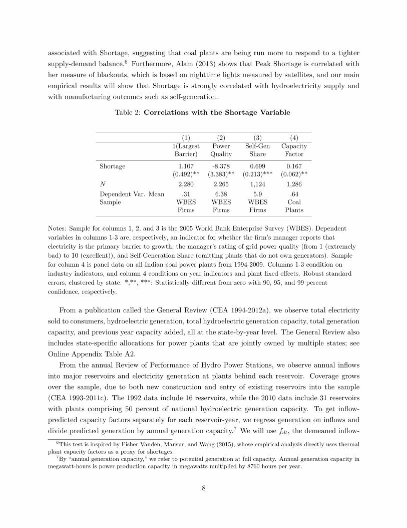
associated with Shortage, suggesting that coal plants are being run more to respond to a tightersupply-demand balance.6 Furthermore, Alam (2013) shows that Peak Shortage is correlated withher measure of blackouts, which is based on nighttime lights measured by satellites, and our mainempirical results will show that Shortage is strongly correlated with hydroelectricity supply andwith manufacturing outcomes such as self-generation.

Table 2: Correlations with the Shortage Variable

(1) (2) (3) (4)1(Largest Power Self-Gen CapacityBarrier) Quality Share Factor

Shortage 1.107 -8.378 0.699 0.167(0.492)** (3.383)** (0.213)*** (0.062)**

N 2,280 2,265 1,124 1,286Dependent Var. Mean .31 6.38 5.9 .64Sample WBES WBES WBES Coal

Firms Firms Firms Plants

Notes: Sample for columns 1, 2, and 3 is the 2005 World Bank Enterprise Survey (WBES). Dependentvariables in columns 1-3 are, respectively, an indicator for whether the firm’s manager reports thatelectricity is the primary barrier to growth, the manager’s rating of grid power quality (from 1 (extremelybad) to 10 (excellent)), and Self-Generation Share (omitting plants that do not own generators). Samplefor column 4 is panel data on all Indian coal power plants from 1994-2009. Columns 1-3 condition onindustry indicators, and column 4 conditions on year indicators and plant fixed effects. Robust standarderrors, clustered by state. *,**, ***: Statistically different from zero with 90, 95, and 99 percentconfidence, respectively.

From a publication called the General Review (CEA 1994-2012a), we observe total electricitysold to consumers, hydroelectric generation, total hydroelectric generation capacity, total generationcapacity, and previous year capacity added, all at the state-by-year level. The General Review alsoincludes state-specific allocations for power plants that are jointly owned by multiple states; seeOnline Appendix Table A2.

From the annual Review of Performance of Hydro Power Stations, we observe annual inflowsinto major reservoirs and electricity generation at plants behind each reservoir. Coverage growsover the sample, due to both new construction and entry of existing reservoirs into the sample(CEA 1993-2011c). The 1992 data include 16 reservoirs, while the 2010 data include 31 reservoirswith plants comprising 50 percent of national hydroelectric generation capacity. To get inflow-predicted capacity factors separately for each reservoir-year, we regress generation on inflows anddivide predicted generation by annual generation capacity.7 We will use fdt, the demeaned inflow-

6This test is inspired by Fisher-Vanden, Mansur, and Wang (2015), whose empirical analysis directly uses thermalplant capacity factors as a proxy for shortages.

7By “annual generation capacity,” we refer to potential generation at full capacity. Annual generation capacity inmegawatt-hours is power production capacity in megawatts multiplied by 8760 hours per year.

8

predicted capacity factor for reservoir d in year t, in our instrument.The Review of Performance of Hydro Power Stations also includes capacity and annual genera-

tion for all hydro plants in India. We divide generation by annual generation capacity and de-meanwithin plant to construct demeaned capacity factors fdt. We also have collected information oneach plant’s design, primarily from the Global Energy Observatory database (Gupta and Shankar2014). About 18 percent of plants have run-of-river designs without reservoirs, meaning that theycannot adjust generation in response to electricity demand.

The CEA has lost its reservoir data for 2000 and its hydro plant generation data for 1992, sowe impute data in those years using rainfall within the watershed.8 Online Appendix B providesmore information on the power sector data.

I.C Annual Survey of Industries Data

We use India’s Annual Survey of Industries (ASI) for establishment-level microdata. Registeredfactories with over 100 workers (the “census scheme”) are surveyed every year, while smaller estab-lishments (the “sample scheme”) are typically surveyed every three to five years. We use the ASIsample weights to produce estimates valid for the population of registered factories in India.9 Thepublicly available ASI includes establishment identifiers that are consistent across years beginningin 1998. While working in India, we also gained access to a version of the ASI with establishmentidentifiers before 1998, allowing us to construct a plant-level panel for the entire 1992-2010 sample.

The ASI is comparable to manufacturing surveys in the United States and other countries.Variables include revenues, value of fixed capital stock, total workers employed, total costs oflabor, materials, fuel, and grid electricity purchased, and the physical quantity of grid electricitypurchased, self-generated electricity, and electricity consumed. Industries are grouped using India’sNIC (National Industrial Classification) codes, which are closely related to SIC (Standard IndustrialClassification) codes. Online Appendix C gives more detail on the ASI data preparation andcleaning.

Panel B of Table 1 presents sample-weighted summary statistics for the ASI. There are 615,7218Specifically, we use GIS elevation maps and the latitude-longitude coordinate of each dam to determine each hydro

plant’s “watershed,” i.e. all higher elevations that drain through the plant. We aggregate rainfall across gridpointswithin the watershed to get annual within-watershed rainfall. For each plant (or reservoir), we run a regression ofrainfall on generation (or reservoir inflows) using all years of data, then predict generation in 1992 (or reservoir inflowsin 2000). Because there are not weather stations in every watershed, these within-watershed rainfall data are largelyinterpolated and/or simulated, so they are highly correlated with state-level rainfall and are not perfect predictors ofreservoir inflows or generation by run-of-river plants.

9While the weighted ASI sample is representative of factories registered under the Factories Act, not all manufac-turing establishments are registered. Small factories with fewer than ten workers (or those with fewer than 20 workerswithout electricity) are not required to register under the Factories Act and are thus excluded from the samplingframe. Nagaraj (2002) points out that there may also be some registration avoidance, especially for smaller plantsnear the registration threshold. While unregistered plants comprise around 80 percent of employment in the manu-facturing sector (Hsieh and Klenow 2014), they contribute a smaller share (around one-third) to total manufacturingoutput (Sincavage, Haub, and Sharma 2010). If these smaller unregistered plants are less likely to have generatorsor high-quality grid power, the effects of shortages on the full manufacturing sector could be larger than for our ASIsample.

9

plant-by-year observations at 224,684 unique plants, although observation counts differ across vari-ables due to non-response and cleaning procedures described in Online Appendix C. 107,032 plantswill be immediately dropped from our fixed effects and difference estimators because they are ob-served only once. For plants observed multiple times, 60 percent of intervals between observationsare one year, while 91 percent are five years or less.

The mean (median) plant employs 79 (34) people and has gross revenues of 139 million (20million) Rupees, or in U.S. dollars approximately $3 million ($400,000). 1(Self-Generator) is anindicator variable for whether a plant self-generates electricity.10 Self-Generation Share is theratio of electricity purchased to electricity consumed, and Fuel Revenue Share is the value of fuelspurchased divided by revenues. Forty-one percent of unweighted observations are in the censusscheme, although the table shows that 14 percent of registered factories are in the census schemeafter applying sample weights.

II Background

II.A Reasons for Systemic Shortages

At the end of our study period in 2010, India had 174 gigawatts of utility-scale power generationcapacity, or about one-sixth the U.S. total.11 Of this, 53 percent was coal, ten percent was naturalgas, and 22 percent was hydroelectric. While power generation has been open to private investmentsince India’s 1991 liberalization, 80 percent of electricity supply in 2010 remained governmentowned: 51 percent by states and 29 percent by the central government. Most retail distributioncompanies are also state-run, although some have been privatized.

The immediate reason for shortages is that the retail distribution companies cannot raise retailprices to clear the market. In fact, conditional on state and year effects, there is no correlationbetween the Shortage variable and the median electricity price paid by plants in the ASI. However,such a disconnect between retail price and market conditions is common to nearly all power systemsaround the world, including many that do not experience endemic shortages. There are severalunderlying reasons why shortages arise in India and many other developing countries.

The first reason is the “infrastructure quality and subsidy trap” (McRae 2015): distributioncompanies provide low-quality electricity, consumers tolerate this low quality because they pay lowprices, government subsidies cover distribution companies’ losses from the low prices, and politicianssupport the subsidies to avoid voter backlash. At least since the 1970s, state-run distributioncompanies have offered un-metered electricity at a monthly fixed fee and zero marginal cost to

10While the ASI does not explicitly ask plants whether they own a generator, 1(Self-Generator) is a very goodproxy, as it would be unusual in India for a plant to own a generator but never use it. Comparison with the 2005World Bank Enterprise Survey (WBES) provides supporting evidence: 81 percent of plants with 100 or more workersand 38 percent with fewer than 100 workers in the 2005 ASI ever self-generate electricity, while 83 percent of plantswith 100 or more workers and 46 percent with fewer than 100 workers in the 2005 WBES report owning generators.

11Capacity and ownership statistics in this paragraph are from the General Review (CEA 2012a).

10

agricultural consumers (Bhargava and Subramaniam 2009). These low agricultural prices are cross-subsidized by industrial electricity prices that are nearly four times higher. Furthermore, 26percent of electricity generated in India in 2010 was lost due to “technical and commercial losses,”meaning poor transmission infrastructure and uncollected bills.12 As a result of low prices andlosses, distribution companies’ revenues from power sales were 24 percent less than costs in 2010.

To cover the low agricultural prices, state governments promise large subsidies, which amountedto 20 percent of distribution companies’ revenues in 2009 and 11 percent in 2010. Even afterreceiving subsidies, however, distribution companies lost a total of $61 billion (in real 2004 dollars)between 1992 and 2010. Resulting financial constraints constrain infrastructure investment andmaintenance, and degraded infrastructure further increases the probability of power outages. Thegovernment bails out the state power utilities at irregular intervals.

A second underlying reason for shortages is underinvestment in new generation capacity: supplyis not keeping up with rapid demand growth. After the 1991 liberalization, investors signed 200memoranda of understanding with the government to build 50 gigawatts of generation capacity,but less than four gigawatts of this was actually built (Bhargava and Subramaniam 2009). Ofthe 71 gigawatts of capacity targeted to be built between 1997 and 2007, only half was actuallyachieved (CEA 2013). Potential power plant investors face concerns over both output demand andinput supply. Their main customers, the distribution companies, face serious financial problems.Meanwhile, the main coal supplier is Coal India, a government-run monopoly that is struggling tokeep pace with demand growth (Chilkoti and Crabtree 2014).

Furthermore, existing capacity is systematically underutilized. Between 1994 and 2009, Indiancoal power plants were offline about 28 percent of the time due to forced outages, planned main-tenance, coal shortages, and other factors. When capacity is utilized, India’s coal plants are alsosubstantially less efficient than comparable plants in the United States (Chan, Cropper, and Malik2014).

II.B Variation in Shortages

Figure 1 plots the average shortage for each state over our 1992-2010 study period against itsannualized per-capita GDP growth over the same period. The figure illustrates that shortages varysubstantially across states. The cross-sectional correlation between shortages and growth is noisybut potentially negative, suggesting that poor institutions and other factors both cause slow growthand worsen shortages.13 On the other hand, states such as Rajasthan and Punjab have both slowgrowth and low shortages, partially because slow growth makes it easier for supply to keep up withdemand. This discussion highlights the importance of instrumenting for shortages in the empiricalanalysis.

12Statistics on technical and commercial losses, average revenues and costs, subsidies, and losses by state distributioncompanies are from Power Finance Corporation (various years).

13The best fit line slopes downward (p = 0.032), but the correlation is less strong (p = 0.145) when excludingAndaman and Nicobar Islands and Pondicherry, which are very small Union Territories.

11

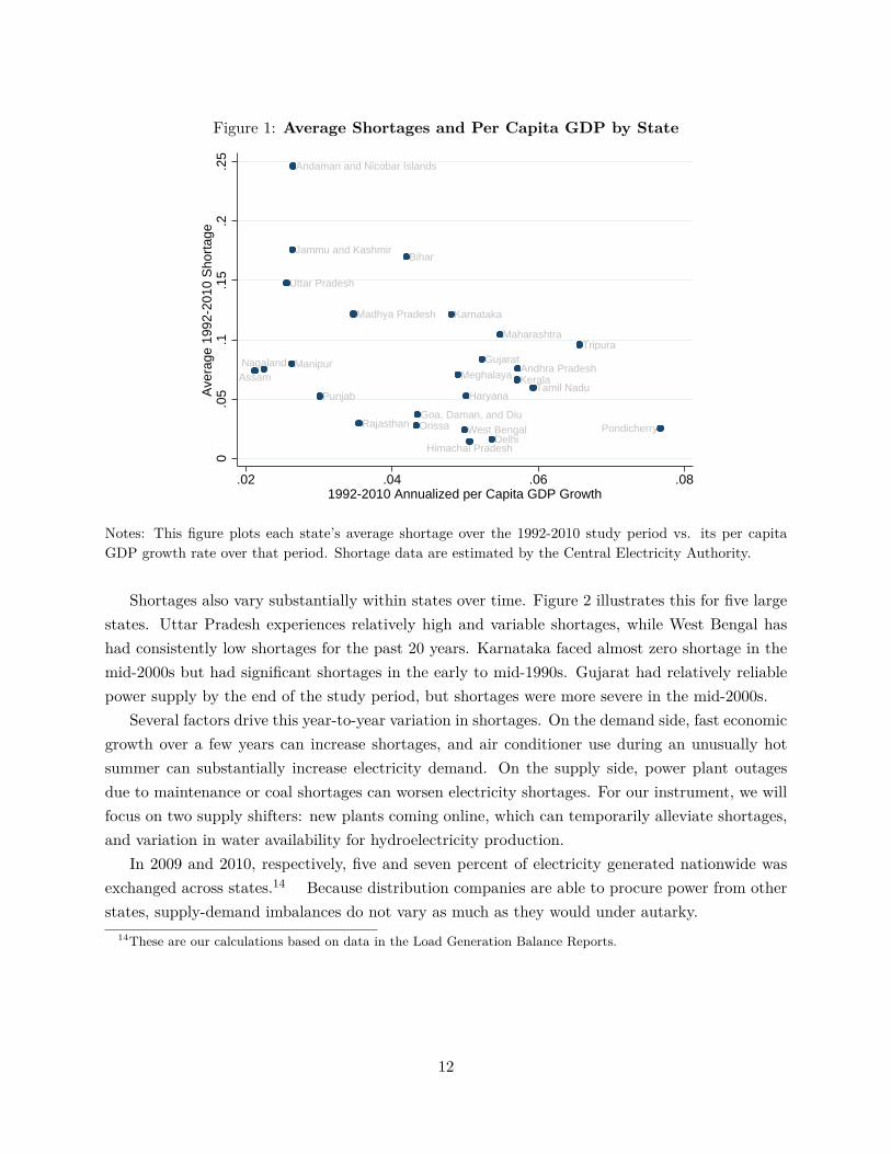
Figure 1: Average Shortages and Per Capita GDP by State

Andaman and Nicobar Islands

Andhra Pradesh

Bihar

Delhi

Goa, Daman, and Diu

Gujarat

Haryana

Jammu and Kashmir

Karnataka

Kerala

Madhya Pradesh

Maharashtra

ManipurMeghalaya

Orissa

Punjab

Rajasthan

Tamil Nadu

Tripura

Uttar Pradesh

West Bengal

NagalandAssam

Himachal Pradesh

Pondicherry

0.0

5.1

.15

.2.2

5A

vera

ge 1

992-

2010

Sho

rtag

e

.02 .04 .06 .081992-2010 Annualized per Capita GDP Growth

Notes: This figure plots each state’s average shortage over the 1992-2010 study period vs. its per capitaGDP growth rate over that period. Shortage data are estimated by the Central Electricity Authority.

Shortages also vary substantially within states over time. Figure 2 illustrates this for five largestates. Uttar Pradesh experiences relatively high and variable shortages, while West Bengal hashad consistently low shortages for the past 20 years. Karnataka faced almost zero shortage in themid-2000s but had significant shortages in the early to mid-1990s. Gujarat had relatively reliablepower supply by the end of the study period, but shortages were more severe in the mid-2000s.

Several factors drive this year-to-year variation in shortages. On the demand side, fast economicgrowth over a few years can increase shortages, and air conditioner use during an unusually hotsummer can substantially increase electricity demand. On the supply side, power plant outagesdue to maintenance or coal shortages can worsen electricity shortages. For our instrument, we willfocus on two supply shifters: new plants coming online, which can temporarily alleviate shortages,and variation in water availability for hydroelectricity production.

In 2009 and 2010, respectively, five and seven percent of electricity generated nationwide wasexchanged across states.14 Because distribution companies are able to procure power from otherstates, supply-demand imbalances do not vary as much as they would under autarky.

14These are our calculations based on data in the Load Generation Balance Reports.

12

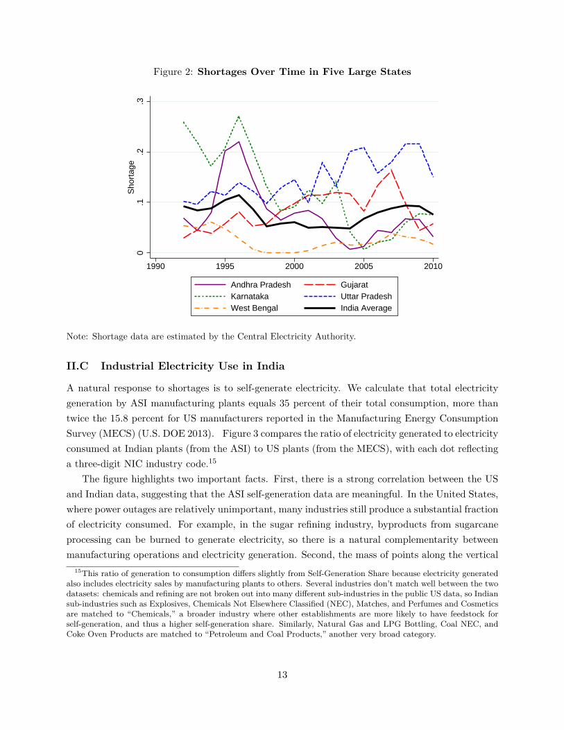
Figure 2: Shortages Over Time in Five Large States

0.1

.2.3

Sho

rtag

e

1990 1995 2000 2005 2010

Andhra Pradesh GujaratKarnataka Uttar PradeshWest Bengal India Average

Note: Shortage data are estimated by the Central Electricity Authority.

II.C Industrial Electricity Use in India

A natural response to shortages is to self-generate electricity. We calculate that total electricitygeneration by ASI manufacturing plants equals 35 percent of their total consumption, more thantwice the 15.8 percent for US manufacturers reported in the Manufacturing Energy ConsumptionSurvey (MECS) (U.S. DOE 2013). Figure 3 compares the ratio of electricity generated to electricityconsumed at Indian plants (from the ASI) to US plants (from the MECS), with each dot reflectinga three-digit NIC industry code.15

The figure highlights two important facts. First, there is a strong correlation between the USand Indian data, suggesting that the ASI self-generation data are meaningful. In the United States,where power outages are relatively unimportant, many industries still produce a substantial fractionof electricity consumed. For example, in the sugar refining industry, byproducts from sugarcaneprocessing can be burned to generate electricity, so there is a natural complementarity betweenmanufacturing operations and electricity generation. Second, the mass of points along the vertical

15This ratio of generation to consumption differs slightly from Self-Generation Share because electricity generatedalso includes electricity sales by manufacturing plants to others. Several industries don’t match well between the twodatasets: chemicals and refining are not broken out into many different sub-industries in the public US data, so Indiansub-industries such as Explosives, Chemicals Not Elsewhere Classified (NEC), Matches, and Perfumes and Cosmeticsare matched to “Chemicals,” a broader industry where other establishments are more likely to have feedstock forself-generation, and thus a higher self-generation share. Similarly, Natural Gas and LPG Bottling, Coal NEC, andCoke Oven Products are matched to “Petroleum and Coal Products,” another very broad category.

13

Figure 3: Manufacturing Electricity Generation in India vs. the U.S.

Sugar Refining

Sugar Cane

SaltNut Processing

Country LiquorBidi

Textiles NEC

Pulp and PaperPaper Bags

Special-Purpose Paper

Industrial Chemicals

Fertilizers and Pesticides

Plastics

PaintPerfumes and Cosmetics

Synthetic Fibers

Matches

Chemicals NEC

Petroleum Refining

Nat Gas and LPG Bottling

Candles

Coke Oven Products

Coal NEC

Iron and Steel

Aluminum

Computers

0.2

.4.6

.81

Indi

a G

ener

atio

n/Co

nsum

ptio

n

0 .2 .4 .6 .8 1U.S. Generation/Consumption

Notes: This figure presents the ratio of electricity generation to consumption by three-digit industry. Indianand U.S. data are from the Annual Survey of Industries and the Manufacturing Energy Consumption Survey,respectively.

axis implies that many industries in India produce much more than their counterparts in the U.S.For instance, plastics manufacturers in the U.S. produce none of their power, while production byIndian plastics manufacturers equals 70 percent of their electricity consumption.

III Model and Production Function Estimation

III.A Setup

This section presents a model of how electricity shortages affect manufacturing plants. τ indexespoints in time, which we refer to as “days.” Every day, a plant uses capital K, labor L, electricityE, and materials M to produce output Q. Qitτ denotes the output for plant i in year t on day τ ,and Qit ≡

´τ Qitτdτ is the annual aggregate. The measure of “days” in a year is normalized to one.

We do not model the possibility for inter-day substitution.16

The daily production function is a Cobb-Douglas aggregate of capital, labor, electricity, andmaterials, with physical productivity Ait17:

16In Online Appendix F, we present a model that does allow inter-day substitution.17Our earlier working paper used a production function that is Leontief in electricity, thus ruling out substitution

away from electricity during power outages: Qitτ = minAKαKitτ L

αLitτM

αMitτ ,

1λEitτ, where λ indexes the plant’s

electricity intensity. We show in Online Appendix F that for our particular outcomes of interest, the Leontief model’smain predictions are similar to those from the full Cobb-Douglas model.

14

Qitτ = AitKαKitτ L

αLitτM

αMitτ E

αEitτ . (2)

Since we observe revenues rather than physical quantities produced, we need to relate revenuesto our production function in Equation (2). We assume that plants sell into a perfectly competitiveoutput market with price p, and we define revenue productivity (TFPR) as Ωit = Aitp.18 Thisyields the following daily revenue-generating production function:

Ritτ = ΩitKαKitτ L

αLitτM

αMitτ E

αEitτ . (3)

III.B Power Outages, Inputs, and Timing

On each day, there are two states of the world - a power outage state and a no-outage state. Theoutage occurs with probability δ, and δ is known at the beginning of the year. If there is nooutage, plants can purchase electricity from the grid at price pE,G. If there is an outage, plantswith generators can self-generate electricity at price pE,S > pE,G. Plants without generators havezero electricity input during an outage, so they produce zero output. Notice that setting electricityinput to zero for δ percent of the year is different from a δ percent reduction in electricity use, andthe effect of power outages can be much larger than the electricity coefficient αE .

There are three types of inputs:

1. Fixed inputs are chosen before δ and Ωit are known. For the model and simulations, weassume that capital stock Kit is fixed.

2. Yearly-flexible inputs can be modified at the beginning of a year t after observing δ and Ωit,but they cannot be modified from day to day. For the model and simulations, we treat laboras yearly-flexible, as plants cannot hire and fire workers from one moment to the next asblackouts occur. This gives Litτ = Lit.19

3. Fully-flexible inputs can be modified for each day τ after observing whether or not there isan outage. We treat materials and electricity as fully flexible.

18We could alternatively assume that plants sell into an imperfectly competitive output market with daily demandcurve QD = BP ε. This yields identical results, except with revenue productivity redefined as Ω ≡ A1+ 1

εB− 1ε and

production function coefficients βX = αX(1+ 1ε) forX = K,L,M,E. Using a demand curve that depends on annual

output would introduce dynamics into this problem, as production on day τ would affect prices, and consequentlyinput choices, on other days of the year.

19In some industries such as plastics, material inputs can be spoiled during a power outage. In these cases, it mightbe more plausible to assume that materials are also semi-flexible, and it is straightforward to change the model inthis way.

15

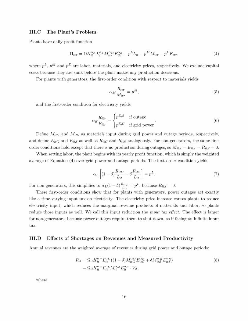
III.C The Plant’s Problem

Plants have daily profit function

Πitτ = ΩKαKit LαLit M

αMitτ E

αEitτ − p

LLit − pMMitτ − pEEitτ , (4)

where pL, pM and pE are labor, materials, and electricity prices, respectively. We exclude capitalcosts because they are sunk before the plant makes any production decisions.

For plants with generators, the first-order condition with respect to materials yields

αMRitτMitτ

= pM , (5)

and the first-order condition for electricity yields

αERitτEitτ

=

pE,S if outage

pE,G if grid power. (6)

Define MitG and MitS as materials input during grid power and outage periods, respectively,and define EitG and EitS as well as RitG and RitS analogously. For non-generators, the same firstorder conditions hold except that there is no production during outages, soMitS = EitS = RitS = 0.

When setting labor, the plant begins with its yearly profit function, which is simply the weightedaverage of Equation (4) over grid power and outage periods. The first-order condition yields

αL

[(1− δ)RitG

Lit+ δ

RitSLit

]= pL. (7)

For non-generators, this simplifies to αL(1− δ)RitGLit= pL, because RitS = 0.

These first-order conditions show that for plants with generators, power outages act exactlylike a time-varying input tax on electricity. The electricity price increase causes plants to reduceelectricity input, which reduces the marginal revenue products of materials and labor, so plantsreduce those inputs as well. We call this input reduction the input tax effect. The effect is largerfor non-generators, because power outages require them to shut down, as if facing an infinite inputtax.

III.D Effects of Shortages on Revenues and Measured Productivity

Annual revenues are the weighted average of revenues during grid power and outage periods:

Rit = ΩitKαKit LαLit ((1− δ)MαM

itG EαEitG + δMαM

itS EαEitS ) (8)

= ΩitKαKit LαLit M

αMit EαEit · Vit,

where

16

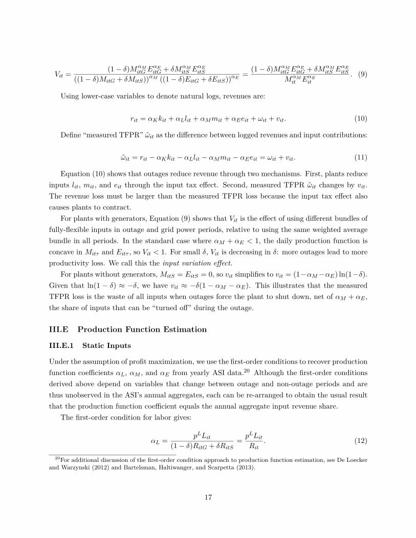
Vit = (1− δ)MαMitG E

αEitG + δMαM

itS EαEitS

((1− δ)MitG + δMitS))αM ((1− δ)EitG + δEitS))αE = (1− δ)MαMitG E

αEitG + δMαM

itS EαEitS

MαMit EαEit

. (9)

Using lower-case variables to denote natural logs, revenues are:

rit = αKkit + αLlit + αMmit + αEeit + ωit + vit. (10)

Define “measured TFPR” ωit as the difference between logged revenues and input contributions:

ωit = rit − αKkit − αLlit − αMmit − αEeit = ωit + vit. (11)

Equation (10) shows that outages reduce revenue through two mechanisms. First, plants reduceinputs lit, mit, and eit through the input tax effect. Second, measured TFPR ωit changes by vit.The revenue loss must be larger than the measured TFPR loss because the input tax effect alsocauses plants to contract.

For plants with generators, Equation (9) shows that Vit is the effect of using different bundles offully-flexible inputs in outage and grid power periods, relative to using the same weighted averagebundle in all periods. In the standard case where αM + αE < 1, the daily production function isconcave in Mitτ and Eitτ , so Vit < 1. For small δ, Vit is decreasing in δ: more outages lead to moreproductivity loss. We call this the input variation effect.

For plants without generators,MitS = EitS = 0, so vit simplifies to vit = (1−αM−αE) ln(1−δ).Given that ln(1 − δ) ≈ −δ, we have vit ≈ −δ(1 − αM − αE). This illustrates that the measuredTFPR loss is the waste of all inputs when outages force the plant to shut down, net of αM + αE ,the share of inputs that can be “turned off” during the outage.

III.E Production Function Estimation

III.E.1 Static Inputs

Under the assumption of profit maximization, we use the first-order conditions to recover productionfunction coefficients αL, αM , and αE from yearly ASI data.20 Although the first-order conditionsderived above depend on variables that change between outage and non-outage periods and arethus unobserved in the ASI’s annual aggregates, each can be re-arranged to obtain the usual resultthat the production function coefficient equals the annual aggregate input revenue share.

The first-order condition for labor gives:

αL = pLLit(1− δ)RitG + δRitS

= pLLitRit

. (12)

20For additional discussion of the first-order condition approach to production function estimation, see De Loeckerand Warzynski (2012) and Bartelsman, Haltiwanger, and Scarpetta (2013).

17

The first-order condition for materials shows that the materials to revenue ratio never varies,so

αM = pMMitτ

Ritτ= pMMit

Rit. (13)

To derive αE , we re-arrange the first-order condition and take a weighted average across outageand non-outage periods:

αE ((1− δ)RitG + δRitS) = (1− δ)pE,GEitG + δpE,SEitS . (14)

This gives

αE = (1− δ)pE,GEitG + δpE,SEitSRit

, (15)

where the numerator is total expenditures on grid electricity plus fuel for self-generated elec-tricity.21

We use median regressions to separately estimate each α parameter for each of 143 three-digit NIC industries, allowing separate linear time trends by two-digit industry. We prefer medianregressions because they are highly robust to outliers. See Online Appendix C for additional details.

III.E.2 Estimating the Capital Coefficient

It is not realistic to assume a static first-order condition for capital analogous to those for otherinputs, because capital has substantial adjustment costs and irreversibilities (Asker, Collard-Wexler,and De Loecker 2014). Instead, we estimate αK using GMM.

We define rit ≡ rit − αLlit − αMmit − αEeit as “transformed revenue,” after netting out thefitted contribution from labor, materials, and electricity. We then regress transformed revenue oncapital:

rit = αKkit + ωit. (16)

If more productive plants invest in more capital and if productivity ωit is serially correlated,E[ωitkit] 6= 0 and estimation in OLS would yield an upward-biased αK . We thus use a standardapproach from control function estimators, exploiting the fact that capital investments take timeto plan and implement. Specifically, we assume that capital requires a one year time-to-build, soKit = (1−κ)Kit−1 +I(Kit−1, ωit−1), where κ represents depreciation and I(Kit−1, ωit−1) representsthe investment policy function, which depends on past productivity. We allow productivity toevolve according to a general first-order Markov process ωit = g(ωit−1) + ξit. Under the one-yeartime-to-build assumption, the productivity innovation ξit is uncorrelated with contemporaneous

21pE,S is unobserved, so we assume that pE,S is 7 Rs/kWh, reflecting the median price reported in the 2005 WorldBank Enterprise Survey.

18

Table 3: Production Function Parameter Estimates and TFPR

(1) (2) (3)Mean 25% 75%

Labor (αL) 0.078 0.053 0.101Materials (αM ) 0.71 0.66 0.76Electricity (αE) 0.019 0.016 0.022Capital (αK) 0.16 0.10 0.21

Capital (αK) from OLS 0.19 0.12 0.24Returns to Scale 0.96 0.94 1.00

Measured TFPR (ωit) 2.12 1.44 2.61Notes: Distribution statistics for production function coefficients and returns to scale are based on 2,424three-digit NIC industry-by-year observations. Distribution statistics for measured TFPR are based on589,779 plant-year observations.

capital stock: E[ξitkit] = 0. We use this moment condition in GMM to estimate αK from Equation(16), with bootstrapped standard errors.22

III.E.3 Production Function Estimates

Table 3 presents summary statistics on the estimated production function parameters. There are 19years of coefficients for 143 different industries, so we present the mean and 25th and 75th percentilesof the distribution of each α. The mean labor, materials, electricity, and capital coefficients are0.078, 0.71, 0.019, and 0.16, respectively.

The mean returns to scale coefficient is 0.96. Slightly decreasing returns to scale are commonin the production function literature; see, for instance, Collard-Wexler and De Loecker (2015). Forcomparison, we also include the αK from OLS estimation of Equation (16). As predicted above,the OLS estimates are biased slightly upward.

IV Estimation Strategy

IV.A Translating the Model to an Estimating Equation

The model suggests a set of outcomes that might be affected by electricity shortages. Plantswith generators will use them during outages, so shortages should be positively associated withSelf-Generation Share and Fuel Revenue Share for self-generators. Both self-generators and non-generators will reduce electricity, materials, and labor inputs, and measured TFPR will also de-crease. Revenues should decrease due to decreases in both inputs and measured TFPR.

22We could also estimate equation (16) in OLS with first differences if we made the stronger assumption thatproductivity is a random walk, i.e. ωit = ωit−1 + ξit. Thus, the purpose of the GMM procedure is to allow a moreflexible time-series process for productivity.

19

We use i, j, s, and t, respectively, to index plants, two-digit NIC industries, states, and years.A simplified version of our estimation strategy is to regress outcomes Yijst on the CEA Shortagevariable Sst, controlling for year indicators θt, industry-by-year indicators µjt, and plant indicatorsφi:

Yijst = ρSst + θt + µjt + φi + εijst. (17)

This equation uses Shortage Sst as a proxy for the model’s outage probability δ. In reality, thesupply-demand imbalances captured by Sst are translated to plant-specific outage probabilities δthrough potentially-endogenous decisions by electricity distribution companies. For example, largeror more productive plants may be able to secure preferential electricity access as shortages worsen.Using Shortage instead of δ captures the “reduced form” of this process. Of course, estimates ofρ from this equation are also “reduced form” in the sense that they are not constrained by theassumptions of the model.23

IV.B Instrumenting for Shortages

There are several reasons why shortages might be endogenous in Equation (17). For example,improvements in state-level economic conditions or institutions could increase productivity andrevenue, and the resulting increase in electricity demand could cause shortages. Alternatively,shortages could be measured with error, causing attenuation bias.

A valid instrument for shortages must shift electricity supply but affect manufacturers onlythrough shortages. Our instrument exploits supply shifts from hydroelectricity generation: becausehydro plants have very low physical marginal cost, their annual output depends primarily on a wateravailability constraint determined by rainfall at higher elevations (or snowfall in the Himalayanstates). The instrument Zst is predicted hydro generation Hst as a share of predicted electricitydemand Qst:

Zst = Hst

Qst. (18)

Because shortages directly affect actual consumption, we predict state s electricity demandusing the product of total electricity sold in all other states in year t and the sample average ratio

23Several unmodeled effects of shortages might be relevant. First, if plants substitute production across days inresponse to outages, our estimates capture this by estimating net effects of shortages over a year. Second, if shortagesreduce output quality, this will appear in revenues and/or TFPR. Third, effects on input demand are not constrainedby our yearly-flexible vs. fully-flexible categorizations or by Cobb-Douglas substitution patterns. Fourth, if inputsor outputs are traded on local markets instead of national or international markets with exogenous prices, shortagescould affect plants through changes in other input or output prices, not just through the price and availability ofelectricity.

20

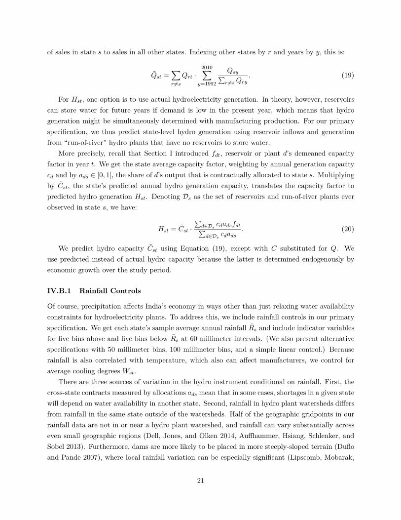
of sales in state s to sales in all other states. Indexing other states by r and years by y, this is:

Qst =∑r 6=s

Qrt ·2010∑y=1992

Qsy∑r 6=sQry

. (19)

For Hst, one option is to use actual hydroelectricity generation. In theory, however, reservoirscan store water for future years if demand is low in the present year, which means that hydrogeneration might be simultaneously determined with manufacturing production. For our primaryspecification, we thus predict state-level hydro generation using reservoir inflows and generationfrom “run-of-river” hydro plants that have no reservoirs to store water.

More precisely, recall that Section I introduced fdt, reservoir or plant d’s demeaned capacityfactor in year t. We get the state average capacity factor, weighting by annual generation capacitycd and by ads ∈ [0, 1], the share of d’s output that is contractually allocated to state s. Multiplyingby Cst, the state’s predicted annual hydro generation capacity, translates the capacity factor topredicted hydro generation Hst. Denoting Ds as the set of reservoirs and run-of-river plants everobserved in state s, we have:

Hst = Cst ·∑d∈Ds cdadsfdt∑d∈Ds cdads

. (20)

We predict hydro capacity Cst using Equation (19), except with C substituted for Q. Weuse predicted instead of actual hydro capacity because the latter is determined endogenously byeconomic growth over the study period.

IV.B.1 Rainfall Controls

Of course, precipitation affects India’s economy in ways other than just relaxing water availabilityconstraints for hydroelectricity plants. To address this, we include rainfall controls in our primaryspecification. We get each state’s sample average annual rainfall Rs and include indicator variablesfor five bins above and five bins below Rs at 60 millimeter intervals. (We also present alternativespecifications with 50 millimeter bins, 100 millimeter bins, and a simple linear control.) Becauserainfall is also correlated with temperature, which also can affect manufacturers, we control foraverage cooling degrees Wst.

There are three sources of variation in the hydro instrument conditional on rainfall. First, thecross-state contracts measured by allocations ads mean that in some cases, shortages in a given statewill depend on water availability in another state. Second, rainfall in hydro plant watersheds differsfrom rainfall in the same state outside of the watersheds. Half of the geographic gridpoints in ourrainfall data are not in or near a hydro plant watershed, and rainfall can vary substantially acrosseven small geographic regions (Dell, Jones, and Olken 2014, Auffhammer, Hsiang, Schlenker, andSobel 2013). Furthermore, dams are more likely to be placed in more steeply-sloped terrain (Dufloand Pande 2007), where local rainfall variation can be especially significant (Lipscomb, Mobarak,

21

and Barham 2013).Third, even if there were no cross-state contracts and every point in a state received the same

rainfall, the slope of the relationship between rainfall and Zst differs across states because statescapture different shares of rainfall for hydroelectricity generation. Some states, such as WestBengal, receive relatively high rainfall but convert little into hydroelectricity. Other states, suchas Karnataka, have lower-than-average rainfall but derive a relatively large share of electricityfrom hydro. The same variation in rainfall thus has a much larger effect on electricity supply inKarnataka than in West Bengal.24

IV.C Estimating Equation

Our empirical specification takes the intuition from Equation (17) and instruments for Sst, addingthe vector of rainfall bins Rst, cooling degree controls Wst, state-specific time trends ψst, and alsostate split indicators Λst that control for three changes in state geographic definitions:25

Yijst = ρSst + βRst + νWst + Λst + ψst+ θt + µjt + φi + εijst. (21)

Observations are weighted by ASI sample weights. Our primary specifications use the fixedeffects estimator, although we also present estimates using the difference estimator. Because Sstand Zst vary by state and year, errors are clustered by state-year. Our primary specifications usetwo-way clustering by plant and state-year (Cameron, Gelbach, and Miller 2011).26

IV.D Discussion

Several features of the empirical strategy merit discussion. First, we include state-specific trendsψst because they substantially improve first stage power. They are especially important in tworobustness checks, one which uses ln(Energy Available) instead of Shortage Sst as the endogenousvariable, and another that uses actual hydro generation for Hst. Both ln(Energy Available) andactual hydro generation have highly heterogeneous state-specific trends, the former because ofdiffering economic growth rates and the latter because of differing trends in the importance of

24In fact, the first stage relationship between hydro production and shortages is clearly visible in the raw datain Karnataka. We illustrate this in Online Appendix Figure A4. Online Appendix Figure A5 plots each state’ssample average rainfall against the average ratio of hydro generation to total consumption; the two quantities areuncorrelated.

25In November 2000, three new states (Chhattisgarh, Jharkhand, and Uttarakhand) were split from three existingstates (Madhya Pradesh, Bihar, and Uttar Pradesh). Weather, hydro plants and reservoirs, and ASI plants can beassigned to post-2000 state definitions in all years of the sample. However, the CEA reports Shortages and otherstate-level variables only for the combined state areas before 2001 or 2002 (depending on the variable). Before thoseyears, we assign data for the combined states to plants in either of the eventually-separate states. State split indicatorsΛst take different values when a state’s geographic definition changes.

26We do not have the downward-biased standard errors described by Bertrand, Duflo, and Mullainathan (2004).They study traditional differences-in-differences estimators, in which the dependent variable of interest is seriallycorrelated. By contrast, Online Appendix Table A6 shows that the instrument Zst is not serially correlated. Notwith-standing, we also present robustness checks with standard errors clustered by state.

22

hydro relative to other generation sources.27 Unless they are absorbed by the ψst controls, theseheterogeneous trends substantially reduce precision.

Second, because the estimates include year indicators, ρ measures effects of shortages Sst onplants in state s relative to plants in other states in the same year. If there are cross-state spillovereffects, for example if customers substitute to plants in other states as production in state s isslowed by outages, our estimates reflect some reallocation of output across states, not just a lossof aggregate output. Thus, the estimates are relevant for state-level policymakers who want toknow how improvements in electricity supply in their state affect outcomes for their manufacturersrelative to manufacturers in other states. The estimates are informative about a national-levelsupply improvement only if cross-state spillovers are relatively small.

Third, the coefficients will largely be identified by states with more variation in hydro generation,which tend to also be the states where hydro represents a large share of total supply. Whilesome hydro-heavy states are small mountainous areas such as Himachal Pradesh, Meghalaya, andUttarakhand, other states such as Andhra Pradesh, Karnataka, Kerala, Orissa, and Punjab areboth large and rely heavily on hydroelectricity.28

Fourth, the empirical estimates will primarily reflect short-run effects. Because of the plantfixed effects φi, the ρ parameter reflects impacts of shortages only on continuing plants. Entry,exit, and even generator adoption or resale are unlikely responses to variation in shortages Sstdriven by year-to-year variation in hydro availability Zst.

IV.E Evaluating the Instrument with State-Level Data

Table 4 evaluates the instrument. All regressions are analogues to the first stage, regressing adependent variable on the hydro instrument Zst, controlling for weather Rst and Wst, state trendsψst, year indicators θt, and state split controls Λst. These regressions are estimated at the state-by-year level, with observations weighted by the number of ASI establishments. Column 1 presentsthe direct analogue to the first stage, showing that a one percentage point increase in instrumentedsupply decreases shortages by 0.177 percentage points. The fact that the coefficient is smallerthan one (in absolute value) implies that states partially offset an increase in supply by decreasinggeneration from other sources and by importing less from or exporting more to other states.

For an instrument to be valid, it must shift supply without affecting manufacturing other thanthrough shortages. Columns 2 and 3 of Table 4 present evidence that this is the case. Recall that theCEA separately reports the two components of shortages: Assessed Demand and Energy Available.

27Online Appendix Figures A6 and A7 illustrate this. For example, the economy in Andhra Pradesh grows rapidlyover the study period, while Uttar Pradesh grows relatively slowly. Residual of year effects θt, ln(Energy Available)trends steeply downward in Uttar Pradesh and steeply upward in Andhra Pradesh. For hydro generation, states suchas Andhra Pradesh and Karnataka have relatively steep downward trends in the share of consumption supplied byhydro, while states such as Gujarat and West Bengal have small and relatively flat hydro generation over the studyperiod. Thus, residual of year effects θt, the instrument constructed with actual hydro generation slopes steeplydownward in Karnataka and steeply upward in West Bengal.

28Online Appendix Figure A5 and Table A4 present more detail.

23

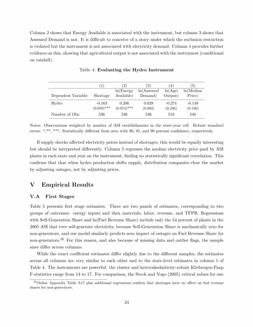
Column 2 shows that Energy Available is associated with the instrument, but column 3 shows thatAssessed Demand is not. It is difficult to conceive of a story under which the exclusion restrictionis violated but the instrument is not associated with electricity demand. Column 4 provides furtherevidence on this, showing that agricultural output is not associated with the instrument (conditionalon rainfall).

Table 4: Evaluating the Hydro Instrument

(1) (2) (3) (4) (5)ln(Energy ln(Assessed ln(Agri ln(Median

Dependent Variable: Shortage Available) Demand) Output) Price)

Hydro -0.163 0.206 0.029 -0.274 -0.149(0.059)*** (0.074)*** (0.092) (0.246) (0.140)

Number of Obs. 536 536 536 518 540

Notes: Observations weighted by number of ASI establishments in the state-year cell. Robust standarderrors. *,**, ***: Statistically different from zero with 90, 95, and 99 percent confidence, respectively.

If supply shocks affected electricity prices instead of shortages, this would be equally interestingbut should be interpreted differently. Column 5 regresses the median electricity price paid by ASIplants in each state and year on the instrument, finding no statistically significant correlation. Thisconfirms that that when hydro production shifts supply, distribution companies clear the marketby adjusting outages, not by adjusting prices.

V Empirical Results

V.A First Stages

Table 5 presents first stage estimates. There are two panels of estimates, corresponding to twogroups of outcomes: energy inputs and then materials, labor, revenue, and TFPR. Regressionswith Self-Generation Share and ln(Fuel Revenue Share) include only the 54 percent of plants in the2005 ASI that ever self-generate electricity, because Self-Generation Share is mechanically zero fornon-generators, and our model similarly predicts zero impact of outages on Fuel Revenue Share fornon-generators.29 For this reason, and also because of missing data and outlier flags, the samplesizes differ across columns.

While the exact coefficient estimates differ slightly due to the different samples, the estimatesacross all columns are very similar to each other and to the state-level estimates in column 1 ofTable 4. The instruments are powerful: the cluster and heteroskedasticity-robust Kleibergen-PaapF-statistics range from 14 to 17. For comparison, the Stock and Yogo (2005) critical values for one

29Online Appendix Table A17 plus additional regressions confirm that shortages have no effect on fuel revenueshares for non-generators.

24

instrument and one endogenous regressor are 8.96 and 16.38 for maximum 15 and 10 percent bias,respectively.

Table 5: First Stages for Base IV Estimates

Panel A: Energy Inputs(1) (2) (3)

Second Stage Self-Gen ln(Fuel ln(ElectricDependent Var: Share Rev Share) Intensity)Hydro -0.168 -0.171 -0.156

(0.0407)*** (0.0422)*** (0.0403)***Obs. 240,743 291,759 479,616Clusters 47,575 55,939 111,819Clusters (2) 535 535 5361st Stage F-Stat 17.00 16.53 14.98

Panel B: Materials, Labor, Revenue, and TFPR(1) (2) (3) (4) (5)

Second Stage ln(Earnings/Dependent Var: ln(Materials) ln(Workers) Worker) ln(Revenue) ln(TFPR)Hydro -0.152 -0.152 -0.161 -0.152 -0.155

(0.0403)*** (0.0403)*** (0.0422)*** (0.0404)*** (0.0400)***Obs. 495,043 502,724 456,443 501,130 479,313Clusters 115,040 116,803 110,213 116,231 112,371Clusters (2) 536 536 482 536 5361st Stage F-Stat 14.23 14.19 14.63 14.17 14.90

Notes: This table presents the first stage estimates for the IV regressions in Tables 6 and 7. The dependentvariable for these first stage regressions is Shortage Sst. Samples for columns 1 and 2 in Panel A arelimited to plants that ever self-generate electricity. F-statistic is for the heteroskedasticity and cluster-robust Kleibergen-Paap weak instrument test. Robust standard errors, with two-way clustering by plant andstate-year. *,**, ***: Statistically different from zero with 90, 95, and 99 percent confidence, respectively.

V.B Effects of Shortages

V.B.1 Energy Inputs

Table 6 presents estimates of Equation (21) for energy inputs. Panels A and B present OLS andinstrumental variables results, respectively. The IV estimates show that a one percentage point in-crease in Shortage (for example, an increase from 0.1 to 0.11) causes manufacturers to increase theshare of electricity self-generated by 0.442 percentage points. If manufacturing electricity demandwere fully inelastic and shortages mapped one-for-one into increases in outages δ for manufacturers,then the coefficient on Shortage in column 1 would be one. However, plants with generators willsubstitute away from electricity through the input tax effect, and electricity distribution compa-nies may impose more or less of the marginal shortage on manufacturers instead of agricultural,residential, or other consumers.

25

The IV estimate in column 2 shows that a one percentage point increase in Shortage increasesfuel revenue share by 3.294 percent. Using the fact that the mean fuel revenue share is 0.055, thepoint estimate suggests that a one percentage point increase in shortages increases fuel costs by(3.294×1%) × 0.055 ≈0.18 percent of revenues. Even a large shortage increase thus imposes only arelatively small fuel cost increase to plants with generators - and this is largely offset by a decreasein purchased electricity costs.

Can plants become less electricity-intensive, in the short-run, as electricity becomes scarce?Column 3 shows that on average, the answer is no: shortages do not statistically affect the ratio ofphysical electricity use to revenue. The standard errors rule out that the average plant respondsto a one percentage point increase in shortages by reducing electric intensity by more than about1.5 percent.

The OLS point estimates differ from the IV estimates, and the directions are consistent with twobiases hypothesized earlier: simultaneity bias (economic growth causes shortages) and measurementerror. Self-Generation Share is less subject to the former bias, as it is not clear that economic growthwould have any direct effect on this variable. The fact that the OLS point estimates are smallerthan the IV estimates suggests that instrumenting helps slightly to address attenuation bias. Thevariables in columns 2-3, however, are ratios to revenues, which increase with economic growth.The coefficients are thus strongly downward biased.

Table 6: Effects of Shortages on Energy Inputs

(1) (2) (4)Self-Gen ln(Fuel ln(Electric

Dependent Var: Share Rev Share) Intensity)Panel A: OLS

Shortage 0.282 0.917 -0.539(0.0337)*** (0.176)*** (0.122)***

Panel B: IVShortage 0.442 3.294 0.0926

(0.153)*** (1.032)*** (0.755)Obs. 240,743 291,759 479,616Clusters 47,575 55,939 111,819Clusters (2) 535 535 5361st Stage F-Stat 17.00 16.53 14.98

Notes: This table presents estimates of Equation (21). Panel B instruments for Shortage using hydroavailability. Samples for columns 1 and 2 are limited to plants that ever self-generate electricity. F-statisticis for the heteroskedasticity and cluster-robust Kleibergen-Paap weak instrument test. Robust standarderrors, with two-way clustering by plant and state-year. *,**, ***: Statistically different from zero with 90,95, and 99 percent confidence, respectively.

26

V.B.2 Non-Energy Inputs, Revenue, and TFPR

Table 7 presents effects of shortages on non-energy inputs, revenue, and revenue productivity.Column 1-3 measure impacts on materials and labor. Column 1 shows that a one percentage pointincrease in Shortage causes a 1.137 percent decrease in materials input. Column 2 shows thatshortages do not statistically affect labor input, as measured by total persons ever employed duringthe year. This is not entirely surprising, since our instrument captures year-to-year variation inshortages that might not be observed by the plant at the time it hires labor. Even though plantsmight not be able to reduce their number of workers, they might reduce hours worked in responseto shortages. However, column 3 confirms that plants are unable to reduce earnings per worker asshortages worsen. This suggests that materials inputs tend to be determined after plants recognizeelectricity supply shifts - perhaps on a day-to-day basis - while labor input is less flexible.

Table 7: Effects of Shortages on Materials, Labor, Revenue, and TFPR

(1) (2) (3) (4) (5)ln(Earnings/

Dependent Var: ln(Materials) ln(Workers) Worker) ln(Revenue) ln(TFPR)Panel A: OLS

Shortage -0.00711 -0.0138 0.161 0.116 0.0543(0.0631) (0.0461) (0.0421)*** (0.0631)* (0.0387)

Panel B: IVShortage -1.137 -0.243 -0.267 -1.091 -0.304

(0.511)** (0.339) (0.218) (0.536)** (0.259)Obs. 495,043 502,724 456,443 501,130 479,313Clusters 115,040 116,803 110,213 116,231 112,371Clusters (2) 536 536 482 536 5361st Stage F-Stat 14.23 14.19 14.63 14.17 14.90

Notes: This table presents estimates of Equation (21). Panel B instruments for Shortage using hydroavailability. F-statistic is for the heteroskedasticity and cluster-robust Kleibergen-Paap weak instrumenttest. Robust standard errors, with two-way clustering by plant and state-year. *,**, ***: Statisticallydifferent from zero with 90, 95, and 99 percent confidence, respectively.

Columns 4 and 5 present effects on log revenue r and log TFPR ω, respectively. The IV estimatesin column 4 show that a one percentage point increase in shortages causes a 1.091 percent decreasein revenues. In the special case distribution companies impose the marginal shortage proportionallyto manufacturers vs. other consumers, no plants self-generate, plants have no yearly-flexible inputs,and δ is small, this coefficient would be approximately one - for example, an increase in shortagesfrom 0 to 0.01 would reduce revenue by one percent. In reality, some plants have generators, whichattenuates the revenue effects, while all plants can reduce yearly-flexible inputs, which magnifiesthe revenue effects.

Column 5 shows that shortages have statistically zero effect on log TFPR, with a 90-percentconfidence interval from -0.69 to 0.085 percent. Given the standard errors, a statistically zero

27

effect is exactly what the model predicts. For plants without generators, Equation (11) predicts aln(TFPR) loss of vit = (1−αM −αE) ln(1−δ). As shown in Table 3, the mean αM and αE are 0.71and 0.019, respectively. Thus, a one percentage point increase in δ would reduce non-generators’TFPR by approximately (1-0.71-0.019)× 1% ≈ 0.27%, and the effect on self-generators’ TFPRshould be smaller. In Section VI, we show that our point estimate of -0.304 is very close to thesimulated model prediction.

The model also predicts that the ln(TFPR) loss is weakly smaller than the ln(revenue) loss,because the revenue loss equals the TFPR loss plus losses from reductions in yearly-flexible andfully-flexible inputs. The point estimates in columns 4 and 5 bear this out. Statistically, the TFPRcoefficient in column 5 is less negative than the revenue coefficient in column 4 with a p-value of0.077 in a one-sided test and 0.15 in a two-sided test.

Comparing the OLS estimates in Panel A to the IV estimates in Panel B strongly suggestssimultaneity bias. All input, output, and TFPR coefficients are positively biased relative to the IVestimates, suggesting that the improved economic conditions that increase shortages also increasewages, productivity, and revenue. Without instrumenting for shortages, one might falsely concludethat shortages are good for manufacturers.

V.C Robustness Checks

Tables 6 and 7 are highly robust to a battery of robustness checks and alternative specifications.Here we present the overview; see Online Appendix E for details.

Estimates are very similar and statistically indistinguishable when using the difference esti-mator, omitting industry-by-year controls µjt, eliminating or tightening the criteria for droppingoutliers, or using the CEA’s estimated Peak Shortage or supply (i.e. ln(Energy Available)) insteadof Shortage as the endogenous right-hand-side variable. The fact that using supply instead of Short-age as the endogenous variable gives similar estimates is unsurprising, because as shown in Table 4,the instrument affects only supply, not demand. It is reassuring, however, because unlike Shortage,Energy Available does not rely on the CEA’s assessment of counterfactual demand. The similarlyin results suggests that the Shortage variable does not suffer from some non-classical measurementerror that an instrumental variable cannot address. Clustering by state instead of using two-wayclustering only mildly changes the standard errors; no discrete significance levels change, and nofirst-stage F-statistic drops below 10.

Estimates are economically similar and statistically indistinguishable when using linear rainfallor 100mm or 50mm rainfall bins instead of 60mm bins, or when using rainfall data from the NationalClimate Centre instead of University of Delaware. Estimates are statistically indistinguishablewhen constructing the instrument with actual hydro generation for Hst instead the prediction fromreservoirs and run-of-river plants, except that the Self-Generation Share coefficient is statisticallylarger and the ln(Electric Intensity) coefficient is statistically negative. This latter result suggeststhat plants may indeed become less electric intensive as electricity shortages worsen. Finally,

28

results are qualitatively similar under six different approaches to calculating production functionsand TFPR.

V.D Associations with Longer-Term Shortage Variation

Our main IV results identify the effects of year-to-year shortage variation. How do shortages affectmanufacturers in the long run? Rigorous causal evidence is challenging, because we do not have aplausible instrument for long-run shortage variation. This section addresses long-run effects usingcorrelational evidence.

Specifically, we test how shortages preceding the year of entry are associated with entrant plants’technology choices. Define Yijst as an outcome for plant i which enters in year t, and define ζs asstate-specific indicator variables. Sst is the average of Shortage in state s in year t and the one yearbefore; this proxies for potential entrants’ beliefs about future shortages. Averaging over two yearsboth reduces measurement error and smooths over idiosyncratic year-to-year variation that shouldnot impact potential entrants’ beliefs about future shortages. We run the following regression withplant-level data:

Yijst = ρSst + Λst + ζs + θt + µjt + εst (22)

Standard errors are clustered by state.Table 8 presents results. Column 1 considers the industry average electric intensity, i.e. the

average ratio of electricity use to revenues for all plants in the same three-digit industry as planti. (This column excludes industry-by-year indicators µjt.) For readability, electric intensity isnormalized to units of kWh per 100 Rupees of revenue; the mean is 1.35 kWh/100 Rupees. Anegative coefficient would imply that plants in electricity-intensive industries are less likely to enterwhen shortages are higher. This would be predicted by an extension of our model in Section III inthe direction of Melitz (2003), in which potential entrant plants decide whether to enter based onexpectations of δ and their productivity shock Ωit. For each expected δ and production technologyα, there is a cutoff productivity Ω(δ, α) above which plants will enter. An increase in δ reducesprofitability more (and thus increases Ω(δ, α) more) for self-generators in industries with high αE ,because more self-generation causes larger cost increases when αE is large. Thus, an increase inexpected shortages should reduce entry more for higher-αE industries, reducing entrants’ overallaverage electric intensity. Indeed, the point estimate shows that a one percentage point increase inshortages is associated with a 0.00463 kWh/Rs decrease in the industry-level electric intensity ofentrant plants, or about 0.34 percent of the mean.

Higher shortages should also increase the return to generator ownership. Indeed, Column 2shows that shortages in the entry year Sst are positively associated with higher generator ownershiprates for entrants. This association is small, however: a one percentage point increase in shortagesis associated with a 0.246 percentage point increase in generator ownership. Such a small coefficientis quite remarkable: generator ownership rates vary substantially across states, ranging from a low

29

Table 8: Association Between Entering Plant Characteristics and Shortages

(1) (2) (3) (4) (5)Ind. Elec/ 1(Self ln(Capital/ ln(Labor/ ln(Matls/

Dependent Variable: Rev Gen) Rev) Rev) Rev)

Shortage at Entry -0.463 0.246 -0.701 -0.078 -0.025(0.179)** (0.074)*** (0.422) (0.135) (0.073)

Number of Obs. 100,496 100,496 99,306 100,246 99,529Industry-by-year effects No Yes Yes Yes Yes

Notes: This table presents estimates of Equation (22). “Shortage at Entry” is the mean of Sst in the plant’sentry year and the one year before. Robust standard errors, clustered by state. *,**, ***: Statisticallydifferent from zero with 90, 95, and 99 percent confidence, respectively.

near 10 percent in some lower-income states to more than 80 percent in Uttar Pradesh, New Delhi,and Haryana. Column 2 suggests that little of this variation is driven by state average shortages.

Aside from the generator adoption and extensive margin choices, entrant plants can also chooseproduction technologies. Columns 3-5 test whether shortages at the time of entry are associatedwith entrants’ factor shares.30 Theory gives no unambiguous prediction about whether shortagesshould increase or decrease various factor shares. For example, higher shortages increase generatoradoption, which mechanically increases capital stock. On the other hand, higher shortages alsodecrease expected capital utilization, especially for non-generators, and this could cause them toswitch to a less capital-intensive technology. Column 3 shows that a one percentage point increasein shortages is associated with a marginally significant 0.7 percent decrease in capital intensity.As predicted, additional (unreported) regressions shows that the negative association is stronger(ρ = −0.96) for non-generators. Columns 4 and 5 show that labor and materials shares are notassociated with Sst.

VI Simulations

VI.A Overview

In this section we apply the model in Section III to the plants and production function param-eters in the Annual Survey of Industries data. There are several objectives. First, we simulateeffects of shortages and test whether they line up with the estimates in Section V. Second, wesimulate heterogeneous effects of shortages, which we do not have the power to detect empirically.Third, we simulate a counterfactual policy, offering interruptible electricity contracts, which couldsubstantially reduce the effects of shortages.

30Specifically, these are the natural log of the ratio of average input to average revenue, where the averages aretaken across all years a plant is observed. The logs help to reduce the influence of outliers, which is the same rolethat median regressions play when estimating the production function parameters α in Section III.E.

30

The simulations consider the population of plants that appear in the ASI in 2005.31 Each plantis characterized by estimated production function parameters α and exogenous state variablesKi2005, Ωi2005, and generator ownership. For the price ratio of grid-purchased to self-generatedelectricity, we use the World Bank Enterprise Survey medians: pE,S/pE,G = 7/4.5 ≈ 1.56. Giventhis information and an assumed δ, we simulate production decisions using the first-order conditionsin Section III. See Online Appendix F for more details on the simulation procedure.

For the next several subsections until Section VI.E, our reported “effects of shortages” reflecta change from δ = 0 to δ = Ss2005, the CEA estimated Shortage in the plant’s state in 2005. Themean Ss2005 across all plants observed in 2005 is 7.2 percent. Although we have shown that thevariation in Sst is meaningful for empirical estimates, we caution that this official assessment is ahighly imperfect proxy for the level of Indian manufacturers’ true outage probability δ.

To more closely match our empirical estimates, we weight by each plant’s sampling weight andreport the weighted average simulated effect of the change in δ. This is different than reportingoutput-weighted effects, which might be informative about aggregate sectoral implications. As wediscuss below, output-weighted effects on most outcomes would be smaller, because the largestplants are much more likely to own generators.

VI.A.1 Modeling Generator Adoption

We model the decision to purchase a generator as a binary choice: either a plant owns a generatorthat is large enough to provide full backup during a power outage, or it does not own a generator.Because the ASI does not include data on generator capacity, we construct a back-of-the-envelopeestimate of each plant’s capacity requirement: we transform a plant’s total electricity consumptionEit (in kilowatt-hours) into required generation capacity assuming that plants use a constant flowof power while operating an average of six hours per day.32 Under this assumption, the mediangenerator capacity requirement is 500 kilowatts.

We model that a plant will purchase a generator if the simulated variable profit increase exceedsthe cost. The simulated variable profit increase is just the simulated profits with vs. withouta generator, given the plant’s α, Ki2005, Ωi2005, and an outage probability δ. We assume thatgenerator cost CG(ci) is log-linear in plant i’s required capacity ci, i.e. lnCG(ci) = σ0 + σ1 ln(ci).

We estimate σ0 and σ1 in GMM using the 1(Self-Generator) variable from the ASI and assumingδ = Sst, matching mean generator adoption and also the covariance between generator adoptionand ln(ci). Estimates reflect strong economies of scale in generator costs: the estimated σ1 is 0.83(se=0.01), and this is statistically and economically similar to direct quotes of generator purchasecosts. The estimated intercept σ0 is also comparable to direct price quotes, implying that fixed

31We chose 2005 because it allows comparison to the 2005 World Bank Enterprise Survey and because the assessedshortages are close to average: over the 1992-2010 sample, the average nationwide shortage ranged from 6.4 to 11.1percent, and the mean reported in Table 1 is 7.6 percent. Online Appendix Figure A8 presents predicted revenuelosses when simulating with each year between 1992 and 2010, showing that 2005 is not unusual.

32Changing this assumption about the number of operating hours per day would only rescale our generator costestimates; the simulation predictions would otherwise be unchanged.

31

costs are large enough to explain why so many Indian plants do not have generators. See OnlineAppendix VI.A.1 for details.

VI.B Effect of Shortages

VI.B.1 Comparing Empirical Estimates to Short-Run Simulations

Panel A of Table 9 presents the effects of changing δ from zero to Ss,2005 on average revenue,TFPR, self-generation share, material and labor inputs. Column 1 presents “exogenous generatorsimulations,” i.e. simulated short-run effects holding fixed the generator ownership observed inthe ASI. This is appropriate for comparison to the IV estimates because the instrument usesannual electricity supply shifters, and plants are unlikely to have responded by adopting or sellinggenerators. Column 2 adds predictions based on the instrumental variable estimates: the predictedeffects of a 7.2 percent shortage given the IV point estimates in Tables 6 and 7.33 Column 3 presentsthe p-value of a test that the simulation result differs from the IV estimate.

There is remarkable agreement between the empirical estimates and simulation results. Averagerevenue losses are 5.6 percent in the simulations and 7.7 percent from the IV. Both the simulationsand IV predict that TFPR losses are much smaller than revenue losses, with predictions of 1.5percent and 2.2 percent from the simulations and IV, respectively. Given that the TFPR effect isrelatively small, the decrease in revenues must be caused by decreased input use. This is indeedthe case: the model predicts a 5.6 percent decrease in materials and labor, respectively, while theIV estimates show 8.1 and 1.7 percent decreases. The simulated and estimated increases in Self-Generation Share also line up closely. Column 3 shows that the simulation and IV estimates arehighly statistically indistinguishable except for the effects on labor input, which has a p-value of0.11. The model assumes that labor is set with knowledge of the current year’s shortage; if workersare instead hired before the effects of new power plant capacity or hydro availability are known,this would explain the difference between the estimated and simulated effects.

Column 4 presents self-reported revenue losses from the 2005World Bank Enterprise Survey; thisnumber is closely comparable to the simulation and IV estimates. Overall, the close correspondencebetween our model and estimates using different datasets and identification strategies gives usconfidence in the empirical estimates as well as our understanding of the underlying mechanisms.

VI.B.2 Effects for Generators and Non-Generators

Panel B of Table 9 presents effects of the same change in δ (from zero to Ss2005) on producersurplus separately for plants with vs. without generators. Producer surplus is relevant becauseunder our modeling assumption that output markets are perfectly competitive and there are no

33Because the empirical estimates are identified off of relatively modest annual variation, column 2 is not a realisticestimate of the long-run effects of eliminating shortages. Online Appendix Table A21 shows very similar agreementbetween simulated and estimated results when comparing in terms of semi-elasticities, i.e. the effects of a onepercentage point change in shortage.

32

other market failures, the change in producer surplus is equivalent to overall welfare effects. Wedecompose producer surplus loss into generator fixed costs and variable profit changes, includingthe component due to decreases in measured TFPR. We compute fixed costs of generators observedin the 2005 ASI by applying estimated generator costs σ0 and σ1 to required capacity ci, and weassume for simplicity that no plants would own generators in the scenario with δ = 0. We findthat generator costs amount to 7.7 percent of profit losses for plants with generators, or 3.9 percentwhen averaged across all plants.

The simulations predict very different effects on plants with vs. without generators. Plantswith generators lose only 0.3 percent of variable profits. They lose no output to shutdown; allrevenue losses come from the decrease in the marginal products of materials and labor due tohigher-cost self-generated electricity. The decrease is small because this implicit tax is small:given that electricity costs increase by 55 percent when self-generating, electricity has a 5 percentrevenue share, and Ss2005 averages 7.2 percent, the weighted average input cost rises by only about55%×5%×7.2%≈0.2 percent of revenues.

In contrast, variable profits fall by 10 percent for the average plant without a generator. Thiseffect is larger than the 7.2 percent of the time when the plants shut down, because the inputtax effect magnifies the effect of shortages: expected power outages reduce the expected marginalrevenue product of the semi-flexible input (labor) by δ, causing plants to reduce labor input.

The bottom row of Panel B shows that predicted effects on measured TFPR are also verydifferent for non-generators vs. self-generators: 2.6 percent vs. almost zero, respectively, with anaverage over all plants of 1.5 percent. Recall that for plants with generators, the TFPR loss isdue to the input variation effect: with a concave daily production function, it would have beenmore efficient to produce with a constant input bundle instead of different input bundles duringoutage vs. non-outage periods. This input variation effect is so small because plants do not reduceproduction very much during outages given the small implicit input tax.

By contrast, the TFPR loss for non-generators is much larger. To understand the magnitude,recall from the model that measured TFPR loss vit ≈ −δ(1− αM − αE). In the limiting case withno fully flexible inputs, shutting down 7.2 percent of the time would cause a 7.2 percent TFPR loss.In another extreme with αM + αE = 1, there is also no TFPR loss, because with constant returnto scale in the daily production function the plant could costlessly shift production to a non-outageday. In the data, the average αE + αM is 0.73, and the simulations predict a TFPR loss is 2.6percent for the average plant without a generator.34

34Online Appendix E.F presents empirical estimates of how generator ownership moderates effects of shortages; wedo not have the power to detect differences between plants with vs. without generators. Notice that such empiricalestimates would likely understate the average causal effects of generator ownership because generator adoption isendogenous, so plants without generators will tend to have unobservably smaller losses. For example, plants withunobservably better electricity supply are both less likely to adopt generators and potentially less affected by anincrease in shortages.

33

Table 9: Effect of Shortages

Panel A: Effects of Shortages: Model and IV Estimates(1) (2) (3) (4)

p-Value for WorldIV Columns Bank

Simulation Estimate (1) vs. (2) SurveySelf-Generation Share Increase 3.1% 3.1% (0.98)Materials Reduction 5.6% 8.1% (0.49)Labor Reduction 5.6% 1.7% (0.11)Revenue Loss 5.6% 7.7% (0.57) 7.8%TFPR Loss 1.5% 2.2% (0.72)

Panel B: Producer Surplus Effects of ShortagesWith Non-

All Generators GeneratorsProducer Surplus Loss: 9.5% 8.0% 10.0%of which ∆ Generator Costs: 3.9% 7.7% N.A.of which ∆ Variable Profit: 5.6% 0.3% 10.0%

of which ∆ TFPR: 1.5% 0.0% 2.6%

Panel C: Producer Surplus Effects of Shortages with Interruptible ContractsWith Non-

All Generators GeneratorsShare of plants opting into interruptible contracts 8% 13% 3%Variable Profit Loss: 0.4% 0.1% 0.7%

of which ∆ TFPR: 0.0% 0.0% 0.1%Notes: This table presents the effects of changing δ from zero to the CEA’s 2005 assessed shortage level.In Panel A, “Simulation” refers to the predictions of the model using the 2005 ASI and described in thetext. “IV Estimate” refers to the estimates in Tables 6 and 7, extrapolated under a 7.2 percent shortage.“p-Value” is the p-value for the test of whether the model’s prediction with exogenous generators is equalto the IV estimate, with standard errors calculated using the Delta method. “World Bank Survey” refers toself-reported data from the 2005 World Bank Enterprise Survey. Panels B and C are simulated effects, asdescribed in the text.

34

VI.C Counterfactual with Interruptible Contracts

Given that 44 percent of manufacturing plants have generators, this “distributed generation” pro-vides production capacity that would optimally be exploited when power is scarce. Currently, thereare plants that have generators but do not use them because they receive grid power, while othernearby plants without generators simultaneously experience outages. Interruptible electricity con-tracts offer manufacturers and other electricity consumers a rebate for accepting outages duringtimes of scarcity. If distribution companies offer both uninterruptible and interruptible contractsand allow consumers to sort into their preferred contract, this provides a mechanism to allocateoutages to plants that are least affected.35

We simulate the effects of allowing plants to select into one of two electricity supply contracts,an uninterruptible contract with no outages and an interruptible contract that will allow outages14.4 percent of the time - twice the assessed national average outage rate. The market-clearingrebate for the interruptible contract is pinned down by the maximum profit loss among the plantscomprising 50 percent of manufacturers’ grid electricity consumption. When this 50 percent ofconsumption is interrupted 14.2 percent of the time, this allows the uninterruptible contracts tobe fulfilled. Panel C of Table 9 presents the effects of shortages under this contract structure.Because larger plants are more likely to have generators and are thus willing to accept interruptiblecontracts at lower rebates, only eight percent of plants need to opt into the interruptible contractto clear the market. Under this counterfactual policy, shortages of δ = Ss2005 instead of δ = 0reduce variable profits by 0.4 percent, more than an order of magnitude less than the 5.6 percentloss when outages are evenly distributed within states. With interruptible contracts, there is nonoticeable decrease in TFPR.

There are two important caveats to this analysis. First, it holds constant the manufacturingsector’s total power allocation. In practice, the grid electricity conserved through interruptiblecontracts with manufacturers could be allocated to homes, agriculture, or other sectors, where themarginal social value of electricity could be different. Second, even holding constant the manufac-turing power allocation, we do not observe which specific plants are subject to shortages, so thelosses without interruptible contracts could be larger or smaller than we simulate here.

VI.D Comparing Effects for Large vs. Small Plants

How do shortages differentially affect small vs. large plants? Panel (a) of Figure 4 shows thatthe share of plants that report self-generating electricity increases with plant size. The figurereflects the same economy of scale in generator ownership discussed above. Because outages moreseverely affect plants without generators, this economy of scale makes small plants more exposedto outages than large plants. The solid line in Panel (b) of Figure 4 illustrates this, showing

35Interruptible contracts have been studied by Baldick, Kolos, and Tompaidis (2006) and are common in the U.S.They are more suitable for large electricity consumers such as manufacturing plants, because a fixed cost is requiredto install switches to turn off electricity to the specific establishment.

35

the relationship between employment and the predicted variable profit loss from shortages in theexogenous generator simulation. While the average ten-employee plant is predicted to lose about sixpercent of profits, the average 100-employee plant loses only about two percent. These differencesbetween large and small plants are driven entirely by differential generator ownership: the dashedline in Panel (b) shows that the predicted profit losses would be roughly constant in plant size inan alternative simulation in which no plants have generators.

VI.E Effects of Shortages with Endogenous Generator Adoption

Given that generators moderate the effects of shortages, increased shortages should increase gener-ator adoption. How much does this moderate the producer surplus losses from shortages? Figure5 plots the effects of raising all plants’ δ from zero to a homogeneous δ up to 0.2, as listed onthe x-axis. Panel (a) uses the “exogenous generator simulations,” while Panel (b) uses “endoge-nous generator simulations,” which endogenize generator adoption at the given δ using the modeldetailed above in Section VI.A.1.36

In the exogenous generator simulation in Panel (a), the variable profit losses increase approxi-mately linearly from zero to 18 percent as shortages worsen from zero to 20 percent. Since generatorcapital stock is held fixed in this simulation, the fixed cost of generators is invariant to shortagesat 2.9 percent.

Panel (b) illustrates a starkly different pattern when generator ownership is endogenously ad-justed. As shortages worsen, the variable profit loss peaks at 1.7 percent with a three percentshortage, drops slightly, and approaches only 1.5 percent as shortages approach 20 percent. Thereason for this non-monotonicity is that many plants adopt generators at low levels of δ, and forthese low δ, generator adoption more than offsets the “direct effect” of an increase in δ. Once δ islarge and most plants have generators, the effects of shortages rise relatively slowly with increasesin δ. Generator investments are costly, however, and at a 20 percent shortage, generator fixedcosts decrease profits by 4.2 percent. Thus, as shortages worsen, the cost of shortages increasinglyconsists of the cost of purchasing backup generators.

36Online Appendix Table A22 presents more detailed statistics used to construct these figures, and Online AppendixFigure A9 presents generator adoption rates as a function of δ.

36

Figure 4: Generator Ownership and Shortage Effects by Plant Size

0.2

.4.6

.8S

hare

of P

lant

s th

at S

elf-

Gen

erat

e

0 1 2 3 4log10(Number of Employees)

kernel = epanechnikov, degree = 0, bandwidth = .12, pwidth = .18

(a) Generator Ownership and Plant Size

05

1015

Perc

ent P

rofit

Los

s

0 1 2 3 4log10(Number of Employees)

Profit loss Profit loss if no generators

(b) Simulated Profit Loss and Plant SizeNotes: Panel (a) presents local mean-smoothed estimates of the share of plants in all years of the AnnualSurvey of Industries that ever self-generate electricity, as a function of number of employees. Panel (b) showsthe simulated effect of shortages on profits as a function of the number of employees.

37

Figure 5: Counterfactuals Under Varying Shortage Levels

0

5

10

15

20Pe

rcen

t Pro

fit L

oss

0 .05 .1 .15 .2Shortage

Variable Profit LossGenerator Cost as Fraction of ProfitsTotal Profit Loss

(a) Profit Loss (Exogenous Generators)

0

2

4

6

Perc

ent P

rofit

Los

s

0 .05 .1 .15 .2Shortage

Variable Profit LossGenerator Cost as Fraction of ProfitsTotal Profit Loss

(b) Profit Loss (Endogenous Generators)Note: These figures show the simulated effects of assigning the δ on the x-axis to all plants in the 2005 ASI,relative to δ = 0. Panel (a) holds fixed the generator ownership observed in the ASI. Panel (b) uses themodel in Section VI.A.1 to endogenously adjust generator ownership at the given δ.

38

VII Conclusion

India’s lack of reliable electricity supply is a stark example of how poor infrastructure might affecteconomic growth. But while the problem is apparent, there had been no quantification of the result-ing losses, making it difficult to prioritize relative to other economic distortions. We estimate theeffects of shortages on manufacturers using archival data on shortages, instrumenting for shortageswith supply shifts from hydro availability.

There are four main conclusions. First, we estimate that shortages are a substantial drag onIndian manufacturing, reducing revenue by 5.6 percent (in the simulations) to 8.6 percent (in theIV estimates) for the average plant in the short run. Producer surplus drops by 9.5 percent forthe average plant, of which 3.9 percent is due to the capital costs of backup generators. Second,because plants also reduce inputs in response to shortages, shortages affect productivity much lessthan they affect revenue. Thus, the short-run effects of electricity shortages do not explain much ofthe productivity gap between firms in developing vs. developed countries discussed by Banerjee andDuflo (2005), Hall and Jones (1999), Hsieh and Klenow (2009), and others, although the long-runeffects could be different. Third, because shortages more strongly affect plants without generatorsand there are substantial economies of scale in generator costs, shortages more severely affectsmall plants. This adds another distortion to the firm size distribution in developing countries,related to the discussion of Hsieh and Olken (2014), Tybout (2000), and others. Fourth, policy canhelp: interruptible contracts or similar mechanisms can substantially reduce the costs of shortages.Because such contracts can be offered at a discount on an opt-in basis, they may be more politicallyfeasible than raising prices or changing allocations.

39

References

[1] Abeberese, Ama Baafra (2012). “Electricity Cost and Firm Performance: Evidence from India.” WorkingPaper, Columbia University (November).

[2] Alam, Muneeza (2013). “Coping with Blackouts: Power Outages and Firm Choices.” Working Paper,Yale University (November).

[3] Alby, Philippe, Jean-Jacques Dethier, and Stephane Straub (2011). “Let There be Light! Firms Op-erating under Electricity Constraints in Developing Countries.” Working Paper, Toulouse School ofEconomics (July).

[4] Allcott, Hunt, Allan Collard-Wexler, and Stephen D. O’Connell (2015). “The India Energy Data Repos-itory.” Available from www.indiaenergydata.info.

[5] Aschauer, David (1989). “Is Public Expenditure Productive?” Journal of Monetary Economics, Vol.23, No. 2 (March), pages 177-200.

[6] Asker, John, Allan Collard-Wexler, and Jan De Loecker (2014) “Dynamic Inputs and Resource(Mis)Allocation” Journal of Political Economy Vol. 122, No. 5, pages 1013-1063.

[7] Auffhammer, Maximilian, Solomon Hsiang, Wolfram Schlenker and Adam Sobel (2013). “Using WeatherData and Climate Model Output in Economic Analyses of Climate Change.” Review of EnvironmentalEconomics and Policy, Vol. 7, No. 2, pages 181-198.

[8] Baisa, Brian, Lucas Davis, Stephen Salant, andWilliamWilcox (2008). “TheWelfare Costs of UnreliableWater Service.” Journal of Development Economics, Vol. 92, No. 1 (May), pages 1-12.

[9] Baldick, Ross, Sergey Kolos, and Stathis Tompaidis (2006). “Interruptible electricity contracts from anelectricity retailer’s point of view: valuation and optimal interruption.” Operations Research, Vol. 54,No. 4, pages 627-642.

[10] Banerjee, Abhijit, and Esther Duflo (2005). “Growth Theory through the Lens of Development Eco-nomics.” In Aghion, Philippe, and Steven Durlauf, Eds., Handbook of Economic Growth.

[11] Banerjee, Abhijit, Esther Duflo, and Nancy Qian (2012). “On the Road: Access to TransportationInfrastructure and Economic Growth in China.” Working Paper, Yale University (February).

[12] Bartelsman, Eric, John Haltiwanger, and Stefano Scarpetta (2013). “Cross-Country Differences in Pro-ductivity: The Role of Allocation and Selection.” American Economic Review, Vol. 103, No. 1 (Febru-ary), pages 305-334.

[13] Baum-Snow, Nathaniel (2007). “Did Highways Cause Suburbanization?” Quarterly Journal of Eco-nomics, Vol. 122, No. 2, pages 775-805.

[14] Baum-Snow, Nathaniel (2013). “Urban Transport Expansions, Employment Decentralization, and theSpatial Scope of Agglomeration Economies.” Working Paper, Brown University (October).

40

[15] Baum-Snow, Nathaniel, Loren Brandt, J. Vernon Henderson, Matthew Turner, and Qinghua Zhang(2013). “Roads, Railroads, and the Decentralization of Chinese Cities.” Working Paper, Brown Univer-sity (October).

[16] Baum-Snow, Nathaniel, and Matthew Turner (2012). “Transportation and the Decentralization of Chi-nese Cities.” Working Paper, Brown University (May).

[17] Bertrand, Marianne, Esther Duflo, and Sendhil Mullainathan (2004). “How Much Should We TrustDifferences-In-Differences Estimates?” Quarterly Journal of Economics, Vol. 119, No. 1 (February),pages 249-275.

[18] Bhargava, Anjuli, and Kandula Subramaniam (2009). “Watts Not Happening.” Business World, July6th.

[19] Cameron, Colin, Jonah Gelbach, and Douglas Miller (2011). “Robust Inference with Multi-Way Clus-tering.” Journal of Business and Economic Statistics, Vol. 29, No. 2, pages 238-249.

[20] CEA (Central Electricity Authority) (1994-2012a). “All India Electricity Statistics: General Review.”New Delhi: Central Electricity Authority.

[21] CEA (Central Electricity Authority) (1993-2011b). “Load Generation Balance Report.” New Delhi:Central Electricity Authority.

[22] CEA (Central Electricity Authority) (1993-2011c). “Review of Performance of Hydro Power Stations.”New Delhi: Central Electricity Authority.

[23] CEA (Central Electricity Authority) (2013). “Planwise Capacity Addition.”http://www.cea.nic.in/reports/planning/plan_addition.pdf

[24] Chakravorty, Ujjayant, Martino Pelli, and Beyza Ural Marchand (2013). “Does the Quality of ElectricityMatter? Evidence from Rural India.” Working Paper, Tufts University (April).

[25] Chan, Hei Sing (Ron), Maureen Cropper, and Kabir Malik (2014). “Are Power Plants in India LessEfficient than Power Plants in the United States?” American Economic Review, Papers and Proceedings,forthcoming.

[26] Chilkoti, Avantika, and James Crabtree (2014). “India Eyes End to State Coal Monopoly.” FinancialTimes (October 23).

[27] Collard-Wexler, Allan and Jan De Loecker (2015). “Reallocation and Technology: Evidence from theUS Steel Industry” American Economic Review, Vol. 105, No. 1, pp. 131-71.

[28] Cropper, Maureen, Alexander Limonov, Kabir Malik, and Anoop Singh (2011). “Estimating the Impactof Restructuring on Electricity Generation Efficiency: The Case of the Indian Thermal Power Sector.”NBER Working Paper No. 17383 (September).

[29] De Loecker, Jan, and Frederic Warzynski (2012). “Markups and Firm-Level Export Status.” AmericanEconomic Review, Vol. 102, No. 6 (October), pages 2437-2471.

41

[30] Dell, Melissa, Benjamin Jones, and Benjamin Olken (2014). “What Do We Learn from the Weather?The New Climate-Economy Literature.” Journal of Economic Literature, Vol. 52, No. 3 (September),pages 740-798.

[31] Dinkelman, Taryn (2011). The Effects of Rural Electrification on Employment: New Evidence fromSouth Africa.” American Economic Review, Vol. 101, No. 7 (December), pages 3078-3108.

[32] Donaldson, David (2012). “Railroads of the Raj: Estimating the Impact of Transportation Infrastruc-ture.” American Economic Review, forthcoming.

[33] Donaldson, David, and Richard Hornbeck (2013). “Railroads and American Economic Growth: A“Market Access” Approach.” NBER Working Paper No. 19213 (July).

[34] Duflo, Esther, and Rohini Pande (2007). “Dams.” Quarterly Journal of Economics, Vol. 122, No. 2,pages 601-646.

[35] Easterly, William, and Sergio Rebelo (1993). “Fiscal Policy and Economic Growth.” Journal of MonetaryEconomics, Vol. 32, pages 417-458.

[36] Esfahani, Hadi Salehi, and Maria Teresa Ramirez (2002). "Institutions, Infrastructure, and EconomicGrowth.” Journal of Development Economics, Vol. 70, pages 443-477.

[37] Fernald, John (1999). “Roads to Prosperity? Assessing the Link Between Public Capital and Produc-tivity.” American Economic Review, Vol. 89, No. 3 (June), pages 619-638.

[38] Fisher-Vanden, Karen, Erin Mansur, and Qiong (Juliana) Wang (2015). “Electricity Shortages andFirm Productivity: Evidence from China’s Industrial Firms.” Journal of Development Economics, Vol.114, Pages 172-188.

[39] Foster, Vivien, and Jevgenijs Steinbuks (2009). “Paying the Price for Unreliable Power Supplies: In-House Generation of Electricity by Firms in Africa.” World Bank Policy Research Paper 4913 (April).

[40] Garcia-Mila, T., McGuire, T. and Porter, R. H., (1996). “The effect of public capital in state-levelproduction functions reconsidered.” The Review of Economics and Statistics, Vol. 78, No. 1 (February),pages 177-180.

[41] Gramlich, Edward (1994). “Infrastructure Investment: A Review Essay.” Journal of Economic Litera-ture, Vol. 32 (September), pages 1176-1196.

[42] Gupta, Rajan and Harihar Shankar (2014). Global Energy Observatory. Available:http://globalenergyobservatory.org/. Accessed: September 20, 2014.

[43] Hall, Robert and Charles Jones (1999) “Why do Some Countries Produce So Much More Output PerWorker than Others?” The Quarterly Journal of Economics (1999), Vol. 114, No. 1, pages 83-116.

[44] Hausmann, Ricardo, Dani Rodrik, and Andrés Velasco (2008). “Growth diagnostics.” in The Washingtonconsensus reconsidered: Towards a new global governance, edited by Narcís Serra and Joseph Stiglitz,pages 324-355.

42

[45] Holtz-Eakin, Douglas (1994). “Public-Sector Capital and the Productivity Puzzle.” Review of Economicsand Statistics, Vol. 76, No. 1 (February), pages 12-21.

[46] Hsieh, Chang-Tai, and Peter Klenow (2014). “The Life Cycle of Plants in India and Mexico.” QuaterlyJournal of Economics, Vol. 129, No. 3, pages 1035-1084.

[47] Hsieh, Chang-Tai, and Peter Klenow (2009). “Misallocation and Manufacturing TFP in China andIndia.” Quarterly Journal of Economics, Vol. 124, No. 4 (November), pages 1403-1448.

[48] Hsieh, Chang-Tai, and Benjamin Olken (2014). “The Missing “Missing Middle.”” The Journal of Eco-nomic Perspectives, Vol. 28, No. 3 (Summer), pp. 89-108.

[49] Hulten, Charles, Esra Bennathan, and Sylaja Srinivasan (2006). "Infrastructure, Externalities, andEconomic Development: A Study of the Indian Manufacturing Industry.”World Bank Economic Review,Vol. 20, No. 2, pages 291–308.

[50] Jensen, Robert (2007). “The Digital Provide: Information (Technology), Market Performance, andWelfare in the South Indian Fisheries Sector.” Quarterly Journal of Economics, Vol. 122, No. 3 (August),pages 879-924.

[51] Lipscomb, Molly, Ahmed Mushfiq Mobarak, and Tania Barham (2013). “Development Effects of Elec-trification: Evidence from the Topographic Placement of Hydropower Plants in Brazil.” AmericanEconomic Journal: Applied Economics, Vol. 5 No. 2, (April), pages 200–231.

[52] McRae, Shaun (2015). “Infrastructure Quality and the Subsidy Trap.” American Economic Review,Vol. 105, No. 1, pages 35-66.

[53] Melitz, Marc (2003). “The Impact of Trade on Intra-Industry Reallocations and Aggregate IndustryProductivity.” Econometrica, Vol. 71, No. 6 (November), pages 1695-1725.

[54] Nagaraj, R. (2002). “How to Improve India’s Industrial Statistics,” Economic and Political Weekly, Vol.37, No. 10 (Mar. 9-15), pages 966-970.

[55] Power Finance Corporation (various years). “Report on The Performance of The State Power Utilities.”New Delhi, India: Power Finance Corporation Limited.

[56] Reinikka, Ritva, and Jakob Svensson (2002). “Coping with Poor Public Capital.” Journal of Develop-ment Economics, Vol. 69, pages 51-69.

[57] Roller, Lars-Hendrik, and Leonard Waverman (2001). "Telecommunications Infrastructure and Eco-nomic Development: A Simultaneous Approach.” American Economic Review, Vol. 91, No. 4 (Septem-ber), pages 909-923.

[58] Ryan, Nicholas (2013). “The Competitive Effects of Transmission Infrastructure in the Indian ElectricityMarket.” Working Paper, MIT (September).

[59] Rud, Juan Pablo (2012a). “Electricity Provision and Industrial Development: Evidence from India.”Journal of Development Economics, Vol. 97, pages 352-367.

43

[60] Rud, Juan Pablo (2012b). “Infrastructure Regulation and Reallocations within Industry: Theory andEvidence from Indian Firms.” Journal of Development Economics, Vol. 99, pages 116-127.

[61] Sincavage, Jessica R., Carl Haub, and O.P. Sharma (2010). “Labor costs in India’s organized manufac-turing sector.” Monthly Labor Review, pages 3-22.

[62] Srivastava, AK, M Rajeevan, and SR Kshirsagar (2009). “Development of a high resolution daily griddedtemperature data set (1969–2005) for the Indian region.” Atmospheric Science Letters, Vol. 10, No. 4(October), pages 249-254.

[63] Steinbuks, Jevgenijs, and Vivien Foster (2010). “When Do Firms Generate? Evidence on In-HouseElectricity Supply in Africa.” Energy Economics, Vol. 32, pages 505-514.

[64] Steinbuks, Jevgenijs (2011). “Financial Constraints and Firms’ Investment: Results from a NaturalExperiment Using Power Interruption.” Working Paper, Purdue University (October).

[65] Stock, James, and Motohiro Yogo (2005). “Testing for Weak Instruments in Linear IV Regression.” InStock, James, and Donald Andrews, Eds., Identification and Inference for Econometric Models: Essaysin Honor of Thomas J. Rothenberg. Cambridge, England: Cambridge University Press.

[66] Todd, Petra and Kenneth Wolpin (2006) “Assessing the Impact of a School Subsidy Program in Mexico:Using a Social Experiment to Validate a Dynamic Behavioral Model of Child Schooling and Fertility”,American Economic Review, Vol. 96, No. 5, pages 1384-1417.

[67] Tybout, James (2000). “Manufacturing Firms in Developing Countries: How Well Do They Do, andWhy?” Journal of Economic Literature, Vol. 38, No. 1 (March), pages 11-44.

[68] U.S. DOE (Department of Energy) (2013). “Manufacturing Energy Consumption Survey.”http://www.eia.gov/consumption/manufacturing/index.cfm

[69] Willmott, Cort, and Kenji Matsuura (2012). “Terrestrial Precipita-tion: 1900-2010 Gridded Monthly Time Series (1900 - 2010) V3.02.”http://climate.geog.udel.edu/~climate/html_pages/download.html#P2011rev.

[70] Yardley, Jim, and Gardiner Harris (2012). “2nd Day of Power Failures Cripples Wide Swath of In-dia.” New York Times, July 31. http://www.nytimes.com/2012/08/01/world/asia/power-outages-hit-600-million-in-india.html

44

Online Appendix: Not for Publication

How Do Electricity Shortages Affect Industry? Evidence from India

Hunt Allcott, Allan Collard-Wexler, and Stephen D. O’Connell

45

Online Appendix Allcott, Collard-Wexler and O’Connell

A 2005 World Bank Enterprise Survey: Barriers to Growth

Table A1: Biggest Obstacle for Growth

Problem PercentElectricity 33High Taxes 16Corruption 10Tax Administration 8Cost of and Access to Financing 6Labor Regulations and Business Licensing 5Skills and Education of Available Workers 4Access to Land 3Customs and Trade Regulations 2Other 12

Notes: These data are from the 2005 World Bank Enterprise Survey in India. The table presents responsesto the question, “Which of the elements of the business environment included in the list, if any, currentlyrepresents the biggest obstacle faced by this establishment?”

46

Online Appendix Allcott, Collard-Wexler and O’Connell

B Power Sector Data Appendix

This appendix provides additional details on the power sector data in Section I.B.Appendix Table A2 presents the state allocations from jointly-owned power plants.Appendix Table A3 presents summary statistics for the reservoir and hydro plant microdata.

Panel A presents the reservoir microdata; 31 reservoirs ever appear. A reservoir scheme mayinclude multiple hydro plants, so generation and generation capacity are for all plants within thereservoir scheme. All reservoir data are missing for the year 2000, so inflows are imputed usingrainfall at gridpoints within the reservoir watershed. For each reservoir, we then run a regressionof generation on inflows; the fitted values are then divided by generation capacity and transformedinto a predicted capacity factor.

Panel B of Appendix Table A3 presents the hydro plant microdata; 181 plants ever appear, ofwhich 18 percent (32 plants) are known to be run-of-river plants. All plant-level data are missingfor the year 1992, and generation data are occasionally missing in other years. Just less thansix percent of generation observations are imputed using rainfall at gridpoints within the plant’swatershed.

Appendix Table A4 presents summary statistics on electricity supply for the ten largest states.Figures A1, A2, A3 present maps of shortage severity, hydro power plants and weather stations,

and four example hydro plant watersheds, respectively.

47

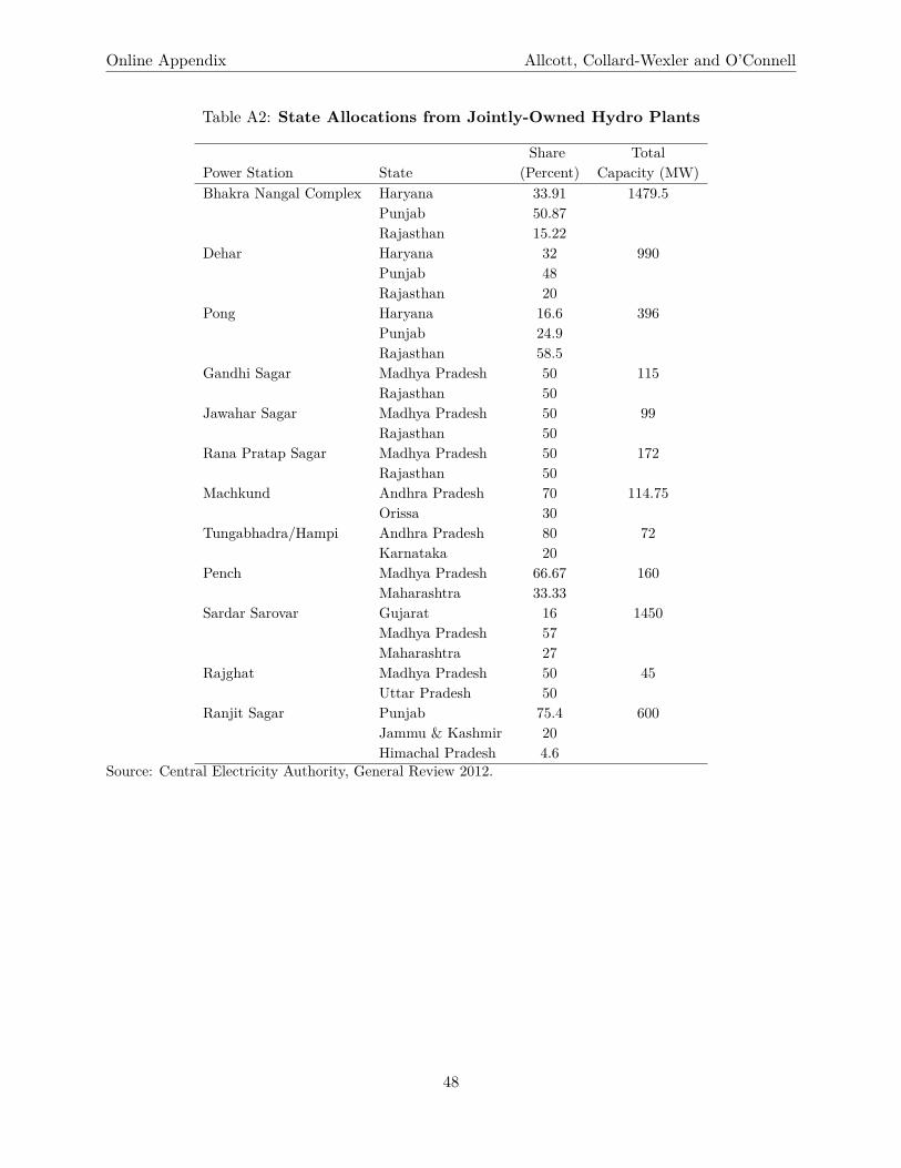
Online Appendix Allcott, Collard-Wexler and O’Connell

Table A2: State Allocations from Jointly-Owned Hydro Plants

Share TotalPower Station State (Percent) Capacity (MW)Bhakra Nangal Complex Haryana 33.91 1479.5

Punjab 50.87Rajasthan 15.22

Dehar Haryana 32 990Punjab 48Rajasthan 20

Pong Haryana 16.6 396Punjab 24.9Rajasthan 58.5

Gandhi Sagar Madhya Pradesh 50 115Rajasthan 50

Jawahar Sagar Madhya Pradesh 50 99Rajasthan 50

Rana Pratap Sagar Madhya Pradesh 50 172Rajasthan 50

Machkund Andhra Pradesh 70 114.75Orissa 30

Tungabhadra/Hampi Andhra Pradesh 80 72Karnataka 20

Pench Madhya Pradesh 66.67 160Maharashtra 33.33

Sardar Sarovar Gujarat 16 1450Madhya Pradesh 57Maharashtra 27

Rajghat Madhya Pradesh 50 45Uttar Pradesh 50

Ranjit Sagar Punjab 75.4 600Jammu & Kashmir 20Himachal Pradesh 4.6

Source: Central Electricity Authority, General Review 2012.

48

Online Appendix Allcott, Collard-Wexler and O’Connell

Table A3: Reservoir and Hydro Plant Microdata Summary Statistics

Panel A: Reservoir MicrodataMean Std. Dev. Min. Max. Obs.

Reservoir Years Observed 12.4 7.0 4 19 31Reservoir Inflows (billion cubic meters) 9.0 11.1 0.14 77.4 362Reservoir-Level Generation (GWh) 1926 1669 27 8016 367Reservoir-Level Generation Capacity (MW) 676 547 75 1956 383Capacity Factor Predicted by Inflows 0.36 0.14 0.09 0.75 383

Panel B: Hydro Plant Generation MicrodataMean Std. Dev. Min. Max. Obs.

Plant Years Observed 14.0 6.1 1 19 181Run-of-River Plant 0.19 0.4 0.00 1.0 177Generation (GWh) 654 1042 0 13211 2395Capacity (MW) 207 304 0 1956 2505Capacity Factor 0.37 0.19 0 1.57 2387

Notes: Reservoir Years Observed is at the reservoir level; all other variables in Panel A are at the reservoir-by-year level. Plant Years Observed and run-of-river categorization are at the plant level; all other variablesin Panel B are at the plant-by-year level.

Table A4: Electricity Statistics for the Ten Largest States

1992-2010 Shortages 2010 1992-2010Capacity Generation

State Mean Min. Max. (gigawatts) Share HydroAndhra Pradesh 0.08 0.01 0.22 10.8 0.21Gujarat 0.08 0.03 0.16 11.4 0.03Karnataka 0.12 0.01 0.27 9.1 0.47Madhya Pradesh 0.12 0.05 0.20 4.9 0.14Maharashtra 0.10 0.02 0.21 16.1 0.11Punjab 0.05 0.01 0.14 5.1 0.40Rajasthan 0.03 0.00 0.07 5.7 0.18Tamil Nadu 0.06 0.00 0.14 11.6 0.13Uttar Pradesh 0.15 0.10 0.22 5.5 0.11West Bengal 0.02 0.00 0.06 7.4 0.03

Notes: Shortage data are estimated by the Central Electricity Authority. 2010 Generation Capacity isreported in the CEA General Review 2012, and Generation Share Hydro is is the ratio of hydroelectricity tototal generation, both of which are reported in the General Review.

49

Online Appendix Allcott, Collard-Wexler and O’Connell

Figure A1: Map of Average Shortages by State

Notes: This figure presents each state’s average Shortage assessed by the Central Electricity Authority over1992-2010, with darker color illustrating higher Shortage.

50

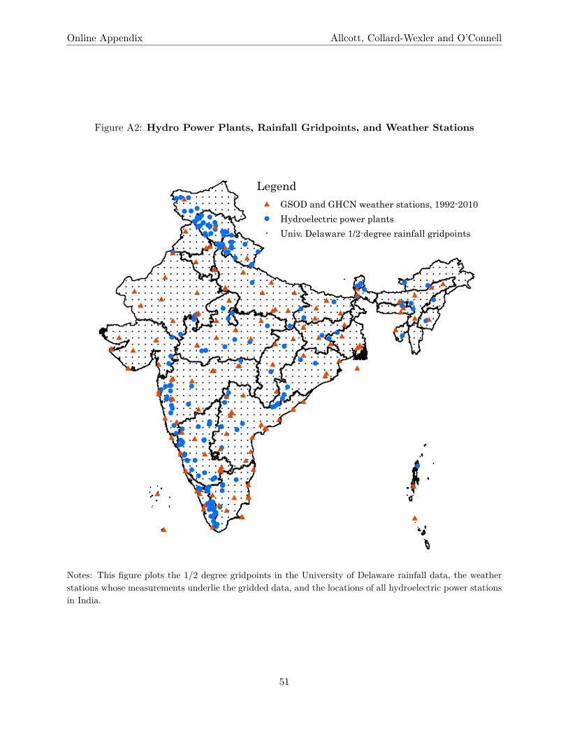
Online Appendix Allcott, Collard-Wexler and O’Connell

Figure A2: Hydro Power Plants, Rainfall Gridpoints, and Weather Stations

! !

! ! !

! ! ! ! !

! ! ! ! !

! ! ! ! ! ! !

! ! ! ! ! ! ! !

! ! ! ! ! ! ! !

! ! ! ! ! ! ! ! ! !

! ! ! ! ! ! ! ! ! ! !

! ! ! ! ! ! ! ! ! ! !

! ! ! ! ! ! ! ! ! ! ! !

! ! ! ! ! ! ! ! ! ! !

! ! ! ! ! ! ! ! ! ! !

! ! ! ! ! ! ! ! ! ! ! !

! ! ! ! ! ! ! ! ! ! ! !

! ! ! ! ! ! ! ! ! ! ! ! ! !

! ! ! ! ! ! ! ! ! ! ! ! ! ! !

! ! ! ! ! ! ! ! ! ! ! ! ! ! ! ! ! !

! ! ! ! ! ! ! ! ! ! ! ! ! ! ! ! ! ! !

! ! ! ! ! ! ! ! ! ! ! ! ! ! ! ! ! ! ! ! !

! ! ! ! ! ! ! ! ! ! ! ! ! ! ! ! ! ! ! ! ! !

! ! ! ! ! ! ! ! ! ! ! ! ! ! ! ! ! ! ! ! ! ! !

! ! ! ! ! ! ! ! ! ! ! ! ! ! ! ! ! ! ! ! ! ! ! !

! ! ! ! ! ! ! ! ! ! ! ! ! ! ! ! ! ! ! ! ! ! ! ! ! !

! ! ! ! ! ! ! ! ! ! ! ! ! ! ! ! ! ! ! ! ! ! ! ! ! ! ! !

! ! ! ! ! ! ! ! ! ! ! ! ! ! ! ! ! ! ! ! ! ! ! ! ! ! ! ! !

! ! ! ! ! ! ! ! ! ! ! ! ! ! ! ! ! ! ! ! ! ! ! ! ! ! ! ! ! ! ! ! !

! ! ! ! ! ! ! ! ! ! ! ! ! ! ! ! ! ! ! ! ! ! ! ! ! ! ! ! ! ! ! ! ! ! ! ! ! !

! ! ! ! ! ! ! ! ! ! ! ! ! ! ! ! ! ! ! ! ! ! ! ! ! ! ! ! ! ! ! ! ! ! ! ! ! ! ! ! !

! ! ! ! ! ! ! ! ! ! ! ! ! ! ! ! ! ! ! ! ! ! ! ! ! ! ! ! ! ! ! ! ! ! ! ! ! !

! ! ! ! ! ! ! ! ! ! ! ! ! ! ! ! ! ! ! ! ! ! ! ! ! ! ! ! ! ! ! ! ! ! ! ! ! ! ! ! ! ! !

! ! ! ! ! ! ! ! ! ! ! ! ! ! ! ! ! ! ! ! ! ! ! ! ! ! ! ! ! ! ! ! ! ! ! ! ! ! ! ! ! ! ! ! ! !

! ! ! ! ! ! ! ! ! ! ! ! ! ! ! ! ! ! ! ! ! ! ! ! ! ! ! ! ! ! ! ! ! ! ! ! ! ! ! ! ! !

! ! ! ! ! ! ! ! ! ! ! ! ! ! ! ! ! ! ! ! ! ! ! ! ! ! ! ! ! ! ! ! ! ! ! ! ! !

! ! ! ! ! ! ! ! ! ! ! ! ! ! ! ! ! ! ! ! ! ! ! ! ! ! ! ! ! ! ! ! ! ! ! ! ! ! ! ! ! ! ! ! !

! ! ! ! ! ! ! ! ! ! ! ! ! ! ! ! ! ! ! ! ! ! ! ! ! ! ! ! ! ! ! ! ! ! ! ! ! ! ! ! ! ! ! ! ! !

! ! ! ! ! ! ! ! ! ! ! ! ! ! ! ! ! ! ! ! ! ! ! ! ! ! ! ! ! ! ! ! ! ! ! ! ! ! ! ! ! ! ! ! ! ! ! ! !

! ! ! ! ! ! ! ! ! ! ! ! ! ! ! ! ! ! ! ! ! ! ! ! ! ! ! ! ! ! ! ! ! ! ! ! ! ! ! ! ! ! ! ! ! !

! ! ! ! ! ! ! ! ! ! ! ! ! ! ! ! ! ! ! ! ! ! ! ! ! ! ! ! ! ! ! ! ! ! ! ! ! ! ! !

! ! ! ! ! ! ! ! ! ! ! ! ! ! ! ! ! ! ! ! ! ! ! ! ! ! ! ! ! ! ! ! ! ! ! ! !

! ! ! ! ! ! ! ! ! ! ! ! ! ! ! ! ! ! ! ! ! ! ! ! ! ! ! !

! ! ! ! ! ! ! ! ! ! ! ! ! ! ! ! ! ! ! ! !

! ! ! ! ! ! ! ! ! ! ! ! ! ! ! ! !

! ! ! ! ! ! ! ! ! ! ! ! ! !

! ! ! ! ! ! ! ! ! ! ! ! ! !

! ! ! ! ! ! ! ! ! ! !

! ! ! ! ! ! ! ! !

! ! ! ! ! ! ! !

! ! ! ! ! !

! ! ! ! ! ! ! ! ! !

! ! ! ! ! ! ! ! ! !

! ! ! ! ! ! ! ! ! !

! ! ! ! ! ! ! ! ! !

! ! ! !

!

!

!!

!

!

!

!

!

!

!

!

!

!!

!

!!!

!

!

!

!

!

!

!

!

!

!

!!

!!

!

!!

!

!

!

!

!!!

!!

!

!

!!!

! !

!!

!

!

!

!

!

!

!

!

!!!

!

!

!

!

!

!

!

!

!

!

!!

!! !

!

!

!!!!

!

!

!!!

!!!

!

!

!

!!

!

!

!!

!

!

!

!

!

!

!

!!

!

!

!

!

!

!

!

!

!

!

!

!

!

!

!!! !

!

!!

!

!

!!

!!!

!

!

!

!

!!!

!

!

!

!

!

!

!!!

!

!

!

!!

!

!

!

!

!

!

!

!

!

!

!

!!

!

!

!!!!

!!

!

! !

!

!!

!

# ####

####

# #### #####

# #### ###

## ##

## ####

#### ## ##

## ##### # ### #

######

##### #### ##

### ### ## # #

## # ## # # ### ### #

# # # ## ### # ## ## # ##

###### ## # ## # ## #

###

####

##

# ##

##

#

Legend# GSOD and GHCN weather stations, 1992-2010! Hydroelectric power plants! Univ. Delaware 1/2-degree rainfall gridpoints

Notes: This figure plots the 1/2 degree gridpoints in the University of Delaware rainfall data, the weatherstations whose measurements underlie the gridded data, and the locations of all hydroelectric power stationsin India.

51

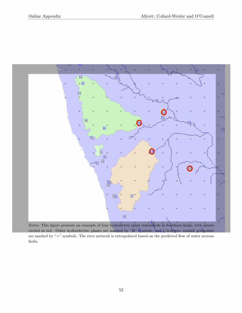
Online Appendix Allcott, Collard-Wexler and O’Connell

Figure A3: Example of Hydroelectric Plant Watersheds

D D D

D D D D D D

D D D D D

D D D D D D D

D D D D D D

D D D D D D D

D D D D D D D D D

D D D D D D D D D

D D D D D D D D D D

D D D D D D D D D D D

D D D D D D D D D D D

D D D D D D D D D D D D

D D D D D D D D D D D D

D D D D D D D D D D D D

D D D D D D D D D D D D D

D D D D D D D D D D D D D D

D D D D D D D D D D D D D D D D

D D D D D D D D D D D D D D D D D D D D D

D D D D D D D D D D D D D D D D D D D D D D D D D D

D D D D D D D D D D D D D D D D D D D D D D D D D D D

D D D D D D D D D D D D D D D D D D D D D D D D D D D D D

D D D D D D D D D D D D D D D D D D D D D D D D D D D D D D

D D D D D D D D D D D D D D D D D D D D D D D D D D D D D D D D

D D D D D D D D D D D D D D D D D D D D D D D D D D D D D D D D D

D D D D D D D D D D D D D D D D D D D D D D D D D D D D D D D D D D D D

D D D D D D D D D D D D D D D D D D D D D D D D D D D D D D D D D D D D D D

D D D D D D D D D D D D D D D D D D D D D D D D D D D D D D D D D D D D D D D D D

D D D D D D D D D D D D D D D D D D D D D D D D D D D D D D D D D D D D D D D D D D D D D D

D D D D D D D D D D D D D D D D D D D D D D D D D D D D D D D D D D D D D D D D D D D D D D D D D D D D

D D D D D D D D D D D D D D D D D D D D D D D D D D D D D D D D D D D D D D D D D D D D D D D D D D D D D D D D D

D D D D D D D D D D D D D D D D D D D D D D D D D D D D D D D D D D D D D D D D D D D D D D D D D D D D D D

D D D D D D D D D D D D D D D D D D D D D D D D D D D D D D D D D D D D D D D D D D D D D D D D D D D D D D D D D D D D

D D D D D D D D D D D D D D D D D D D D D D D D D D D D D D D D D D D D D D D D D D D D D D D D D D D D D D D D D D D

D D D D D D D D D D D D D D D D D D D D D D D D D D D D D D D D D D D D D D D D D D D D D D D D D D D D D D D D D D D D D D

D D D D D D D D D D D D D D D D D D D D D D D D D D D D D D D D D D D D D D D D D D D D D D D D D D D D D D D D D D D D D D

D D D D D D D D D D D D D D D D D D D D D D D D D D D D D D D D D D D D D D D D D D D D D D D D D D D D D D D D D D D D D D

D D D D D D D D D D D D D D D D D D D D D D D D D D D D D D D D D D D D D D D D D D D D D D D D D D D D D D D D D D D D D D

D D D D D D D D D D D D D D D D D D D D D D D D D D D D D D D D D D D D D D D D D D D D D D D D D D D D D D D D D D D D D D

D D D D D D D D D D D D D D D D D D D D D D D D D D D D D D D D D D D D D D D D D D D D D D D D D D D D D D D D D D D D D D

D D D D D D D D D D D D D D D D D D D D D D D D D D D D D D D D D D D D D D D D D D D D D D D D D D D D D D D D D D D D D D

D D D D D D D D D D D D D D D D D D D D D D D D D D D D D D D D D D D D D D D D D D D D D D D D D D D D D D D D D D D D D D

D D D D D D D D D D D D D D D D D D D D D D D D D D D D D D D D D D D D D D D D D D D D D D D D D D D D D D D D D D D D D D

D D D D D D D D D D D D D D D D D D D D D D D D D D D D D D D D D D D D D D D D D D D D D D D D D D D D D D D D D D D D D D

D D D D D D D D D D D D D D D D D D D D D D D D D D D D D D D D D D D D D D D D D D D D D D D D D D D D D D D D D D D D D D

D D D D D D D D D D D D D D D D D D D D D D D D D D D D D D D D D D D D D D D D D D D D D D D D D D D D D D D D D D D D D D

D D D D D D D D D D D D D D D D D D D D D D D D D D D D D D D D D D D D D D D D D D D D D D D D D D D D D D D D D D D D D D

D D D D D D D D D D D D D D D D D D D D D D D D D D D D D D D D D D D D D D D D D D D D D D D D D D D D D D D D D D D D D D

D D D D D D D D D D D D D D D D D D D D D D D D D D D D D D D D D D D D D D D D D D D D D D D D D D D D D D D D D D D D D D

D D D D D D D D D D D D D D D D D D D D D D D D D D D D D D D D D D D D D D D D D D D D D D D D D D D D D D D D D D D D D D

D D D D D D D D D D D D D D D D D D D D D D D D D D D D D D D D D D D D D D D D D D D D D D D D D D D D D D D D D D D D D D

D D D D D D D D D D D D D D D D D D D D D D D D D D D D D D D D D D D D D D D D D D D D D D D D D D D D D D D D D D D D D D

D D D D D D D D D D D D D D D D D D D D D D D D D D D D D D D D D D D D D D D D D D D D D D D D D D D D D D D D D D D D D D

D D D D D D D D D D D D D D D D D D D D D D D D D D D D D D D D D D D D D D D D D D D D D D D D D D D D D D D D D D D D D D

D D D D D D D D D D D D D D D D D D D D D D D D D D D D D D D D D D D D D D D D D D D D D D D D D D D D D D D D D D D D D D

D D D D D D D D D D D D D D D D D D D D D D D D D D D D D D D D D D D D D D D D D D D D D D D D D D D D D D D D D D D D D D

D D D D D D D D D D D D D D D D D D D D D D D D D D D D D D D D D D D D D D D D D D D D D D D D D D D D D D D D D D D D D D

D D D D D D D D D D D D D D D D D D D D D D D D D D D D D D D D D D D D D D D D D D D D D D D D D D D D D D D D D D D D D D

D D D D D D D D D D D D D D D D D D D D D D D D D D D D D D D D D D D D D D D D D D D D D D D D D D D D D D D D D D D D D D

D D D D D D D D D D D D D D D D D D D D D D D D D D D D D D D D D D D D D D D D D D D D D D D D D D D D D D D D D D D D D D

D D D D D D D D D D D D D D D D D D D D D D D D D D D D D D D D D D D D D D D D D D D D D D D D D D D D D D D D D D D D D D

"u

"u

"u

"u

"u

"u

"u

"u

"u

"u

"u

"u

"u

"u

"u

"u

"u

"u

"u

"u

"u

"u

"u

"u

"u"u

"u"u "u

"u

"u

"u

"u

"u

"u

"u

"u

"u

"u

Notes: This figure presents an example of four hydrolectric plant watersheds in Southern India, with plantscircled in red. Other hydroelectric plants are marked by “H” symbols, and 1/2-degree rainfall gridpointsare marked by “+” symbols. The river network is extrapolated based on the predicted flow of water accrossIndia.

52

Online Appendix Allcott, Collard-Wexler and O’Connell

C Annual Survey of Industries Data Appendix

This appendix presents additional information on the Annual Survey of Industries data.We extract a subset of variables from the raw data separately for each year and then stack all

years of data together to apply the following cleaning processes.37 We correct observations in 1993-94 to 1997-98 whose values have been supplied in “pre-multiplied” format from the India’s Ministryof Statistics and Programme Implementation (MOSPI). We create a separate consistently-definedstate variable which takes into account the creation of Jharkhand, Chhattisgarh and Uttaranchal(now Uttarakhand) in 2001 from Bihar, Madhya Pradesh and Uttar Pradesh, respectively. Weassign establishments to the last observed state, which correctly places establishments despite statesplits, as long as the establishment is surveyed after 2001.

India classifies manufacturing establishments with its National Industrial Classification (NIC),which resembles industrial classifications commonly used in other countries. The classificationswere revised in 1987, 1998, 2004, and 2008. We convert all industry classifications to the NIC-1987scheme using concordances provided by MOSPI.

All financial amounts are deflated to constant 2004-05 Rupees. Revenue (gross sales) is deflatedby a three-digit commodity price deflators as available in the commodity-based table “Index Num-bers Of Wholesale Prices In India – By Groups And Sub-Groups (Yearly Averages)” produced bythe Office of the Economic Adviser-Ministry of Commerce & Industry.38 Each three-digit NIC-1987code is assigned to a commodity listed in this table. The corresponding commodity deflator is usedto deflate revenues. To deflate material inputs, we construct the average output deflator of a givenindustry’s supplier industries based on India’s 1993-94 input-output table, available from the Cen-tral Statistical Organization. Fuel and electricity costs are deflated by the price index for “Fuel,Power, Light, and Lubricants.” Capital is deflated by an implied national deflator calculated from“Table 13: Sector-wise Gross Capital Formation” from the Reserve Bank of India’s Handbook ofStatistics on the Indian Economy.39 Electricity costs are deflated using a national GDP deflator.

The sampling rules have changed somewhat over time. The census scheme included factorieswith 100 or more workers in all years except 1997-2003, when it included only factories with 200or more workers. The sample scheme included one-third of factories until 2004 and one-fifth sincethen (MOSPI 2014).

The ASI data have at least two well-known shortcomings. First, while the data are represen-tative of small registered factories and a 100 percent sample of large registered factories, not allfactories are actually registered under the Factories Act. Nagaraj (2002) shows that only 48 per-cent and 43 percent of the number of manufacturing establishments in the 1980 and 1990 economic

37We thank Jagadeesh Sivadasan for helpful discussions and for providing Stata code that facilitated theread-in of 1992-1997 ASI data, and Olivier Dupriez for similarly helpful discussions and pointing us toread-in programs for ASI data from 1998 to 2007 available at the International Household Survey Network(http://catalog.ihsn.org/index.php/catalog/central).

38Available from http://www.eaindustry.nic.in/39Available from http://www.rbi.org.in

53

Online Appendix Allcott, Collard-Wexler and O’Connell

censes appear in the ASI data for those years. Although it is not clear how our results mightdiffer for unregistered plants, the plants that are observed in the ASI are still a significant share ofplants in India. Second, value added may be under-reported, perhaps associated with tax evasion,by using accounting loopholes to overstate input costs or under-state revenues (Nagaraj 2002). Aslong as changes in this under-reporting are not correlated with electricity shortages, this will notaffect our results.

C.A Determination of Base Sample

Appendix Table A5 details how the sample in Panel B of Table 1 is determined from the original setof observations in the ASI. The 1992-2010 ASI dataset begins with 949,992 plant-year observations.Plants may still appear in the data even if they are closed or did not provide a survey response. Wedrop 172,697 plants reported as closed or non-responsive. We drop a trivial number of observationsmissing state identifiers and observations in Sikkim, which has only been included in the ASIsampling frame in the most recent years. We drop 45,664 observations reporting non-manufacturingNIC codes. We remove a small number of observations (primarily in the early years of our sample)which are exact duplicates in all fields, assuming these are erroneous multiple entries made from thesame questionnaire form. Due to the importance of revenue and productivity results, we removethe 102,036 observations with missing revenues. We also drop the 9,095 observations with two ormore input revenue share flags, from the flagging process described below.

With this intermediate sample, we use median regression to estimate revenue productivity(TFPR) under a full Cobb-Douglas model in capital, labor, materials, and energy and assumingconstant returns to scale. This full Cobb-Douglas revenue productivity term is used only for thefinal sample restriction, which is to drop 4,521 plant-years which have log-TFPR greater than 3.5 inabsolute value from the sample median. Such outlying TFPR values strongly suggest misreportedinputs or revenues. The final sample includes 615,721 plant-year observations, of which 362,151 arefrom the sample scheme and 253,570 are from the census scheme.

C.B Variable-Specific Sample Restrictions

After the final sample is determined, there may still be observations which have correct data formost variables but misreported data for some individual variable. When analyzing specific variables(such as self-generation share, energy revenue share, or output in Table 6), we therefore additionallyrestrict the sample using the following criteria:

• We generate “input revenue share flags” for labor and materials if input cost is more thantwo times revenues, and we generate input revenue share flags for electricity and fuels if inputcost is greater than revenues.40 Because we also observe physical quantities for labor and

40The flags would be slightly different if applied to deflated inputs and revenues, but this will have minimalimplications for the results.

54

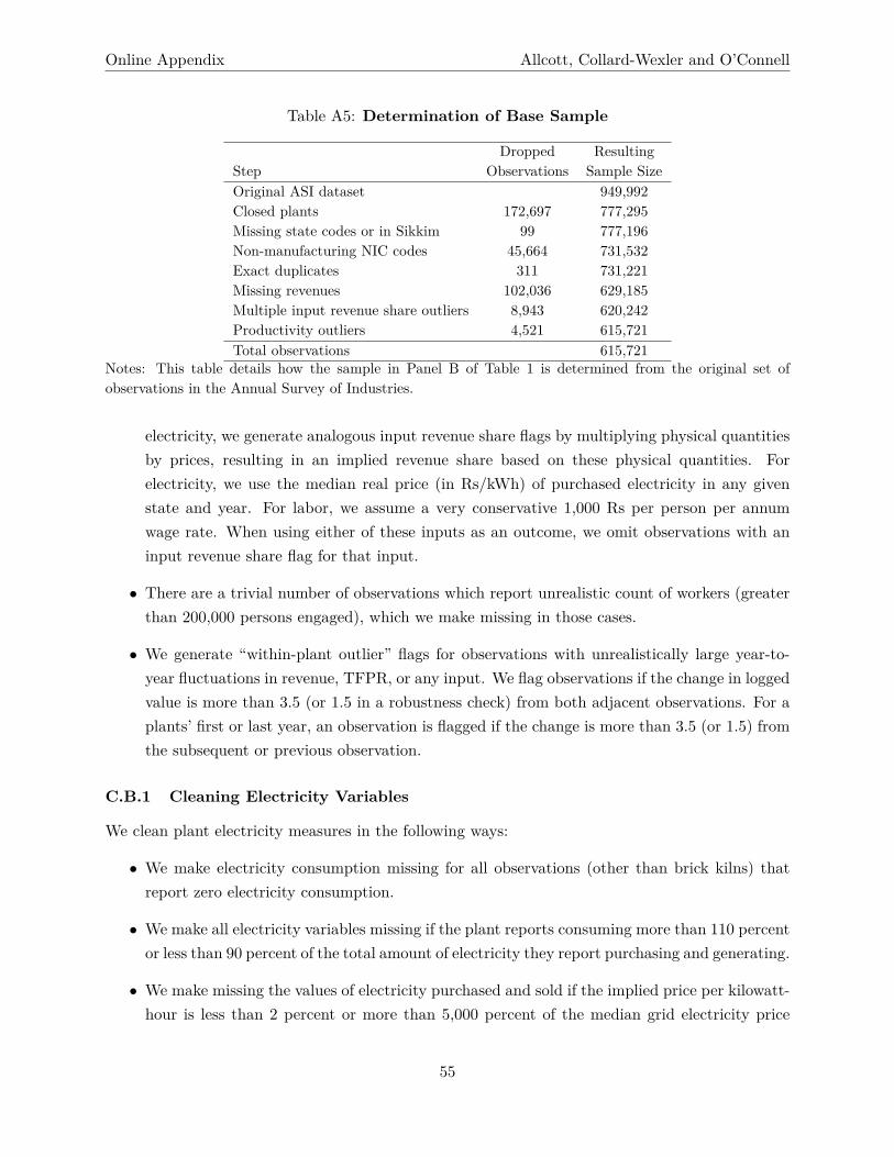
Online Appendix Allcott, Collard-Wexler and O’Connell

Table A5: Determination of Base Sample

Dropped ResultingStep Observations Sample SizeOriginal ASI dataset 949,992Closed plants 172,697 777,295Missing state codes or in Sikkim 99 777,196Non-manufacturing NIC codes 45,664 731,532Exact duplicates 311 731,221Missing revenues 102,036 629,185Multiple input revenue share outliers 8,943 620,242Productivity outliers 4,521 615,721Total observations 615,721

Notes: This table details how the sample in Panel B of Table 1 is determined from the original set ofobservations in the Annual Survey of Industries.

electricity, we generate analogous input revenue share flags by multiplying physical quantitiesby prices, resulting in an implied revenue share based on these physical quantities. Forelectricity, we use the median real price (in Rs/kWh) of purchased electricity in any givenstate and year. For labor, we assume a very conservative 1,000 Rs per person per annumwage rate. When using either of these inputs as an outcome, we omit observations with aninput revenue share flag for that input.

• There are a trivial number of observations which report unrealistic count of workers (greaterthan 200,000 persons engaged), which we make missing in those cases.

• We generate “within-plant outlier” flags for observations with unrealistically large year-to-year fluctuations in revenue, TFPR, or any input. We flag observations if the change in loggedvalue is more than 3.5 (or 1.5 in a robustness check) from both adjacent observations. For aplants’ first or last year, an observation is flagged if the change is more than 3.5 (or 1.5) fromthe subsequent or previous observation.

C.B.1 Cleaning Electricity Variables

We clean plant electricity measures in the following ways:

• We make electricity consumption missing for all observations (other than brick kilns) thatreport zero electricity consumption.

• We make all electricity variables missing if the plant reports consuming more than 110 percentor less than 90 percent of the total amount of electricity they report purchasing and generating.

• We make missing the values of electricity purchased and sold if the implied price per kilowatt-hour is less than 2 percent or more than 5,000 percent of the median grid electricity price

55

Online Appendix Allcott, Collard-Wexler and O’Connell

calculated across plants in the same state and year. We also make missing the reportedquantities of electricity purchased and sold if the respective price flag is triggered.

C.B.2 Production Function and Productivity Estimation

We recover production function coefficients given by Equations (12), (13), and (15) for each ofthe 143 three-digit industries in the dataset. (To ensure sufficient sample size in each three-digitindustry, we adjust industry definitions slightly to ensure each three-digit industry has at least 100plant-year observations.) We use separate median regression for each two-digit industry, allowingfor a linear time trend and separate intercepts for each underlying three-digit industry. Aftercalculating production function coefficients, we compute TFPR using Equation (11).

For our main TFPR estimates, we define materials to be the plant’s original reported materialsplus fuels not used for self-generation. This latter variable is: Total Fuel Cost - (7 Rs/kWh)×(kWhSelf-Generated), where 7 Rs/kWh is the median price reported in the 2005 World Bank EnterpriseSurvey. This allows us to account for the plant’s full input costs when calculating productionfunction parameters and TFPR. (In regressions where we use materials as the outcome variable,we use the original reported materials without adding any fuel costs.)

We use several alternative methods for calculating production function coefficients and TFPRfor robustness checks, seen in Appendix Table A16. In the order of that table, these are:

• Including or excluding all fuel costs from the materials variable

• Removing the linear time trend when estimating production coefficients, which amounts totaking the unconditional median revenue share by industry

• Relaxing the assumption that factor shares are constant by plant size, allowing all productionfunction coefficients to vary by plant median ln(Revenue). To implement, we add ln(Revenue)as a term in the median regressions for αL, αM , and αE and then segment plants into fivesize classes when estimating αK in GMM.

• Backing out the capital coefficient αK under an assumption of constant returns to scale

• Assuming production is Leontief in electricity and calculating the capital coefficient under anassumption of constant returns to scale. (This is the approach in our original working paper.)

None of these changes affects the estimated coefficient by more than about half of the standarderror.

56

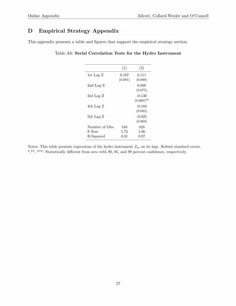
Online Appendix Allcott, Collard-Wexler and O’Connell

D Empirical Strategy Appendix

This appendix presents a table and figures that support the empirical strategy section.

Table A6: Serial Correlation Tests for the Hydro Instrument

(1) (2)

1st Lag Z 0.107 0.111(0.081) (0.088)

2nd Lag Z 0.008(0.075)

3rd Lag Z -0.130(0.066)**

4th Lag Z -0.104(0.083)

5th Lag Z -0.025(0.068)

Number of Obs. 540 420F-Stat 1.72 1.90R-Squared 0.01 0.07

Notes: This table presents regressions of the hydro instrument Zst on its lags. Robust standard errors.*,**, ***: Statistically different from zero with 90, 95, and 99 percent confidence, respectively.

57

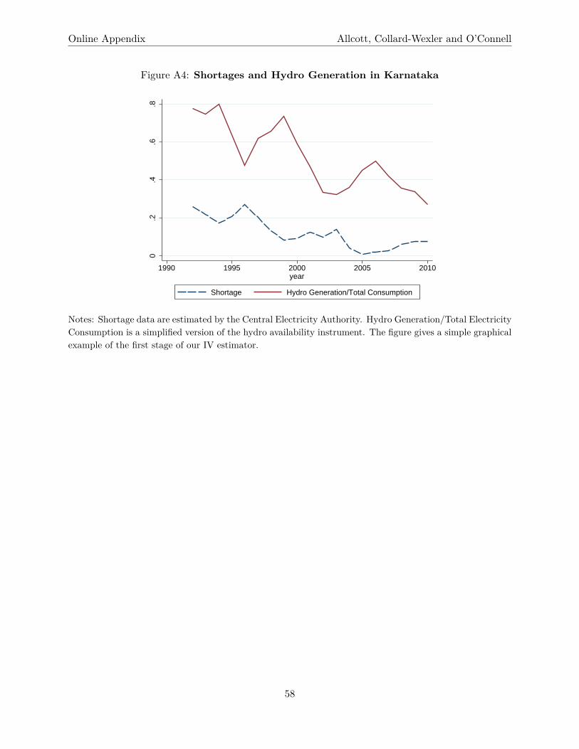
Online Appendix Allcott, Collard-Wexler and O’Connell

Figure A4: Shortages and Hydro Generation in Karnataka

0.2

.4.6

.8

1990 1995 2000 2005 2010year

Shortage Hydro Generation/Total Consumption

Notes: Shortage data are estimated by the Central Electricity Authority. Hydro Generation/Total ElectricityConsumption is a simplified version of the hydro availability instrument. The figure gives a simple graphicalexample of the first stage of our IV estimator.

58

Online Appendix Allcott, Collard-Wexler and O’Connell

Figure A5: Rainfall and Hydro Share of Electricity by State

Andaman and Nicobar Islands

Andhra Pradesh

Assam

Bihar

Chandigarh

CG

Delhi

GA

Gujarat

Haryana

Himachal Pradesh

Jammu and Kashmir

Karnataka

Kerala

Madhya PradeshMH

Manipur

Meghalaya

Nagaland

Orissa

Punjab

Rajasthan

Tamil Nadu

Tripura

UP

UK

West Bengal

01

23

419

92-2

010

Mea

n R

ainf

all (

met

ers)

0 .5 11992-2010 Mean of Hydro Generation/Total Consumption

Notes: This figure plots sample average annual rainfall against the mean ratio of hydroelectricity generationto total electricity consumption. The figure emphasizes that there is substantial variation in hydro generationconditional on rainfall.

Figure A6: Hydro Share of Predicted Consumption Over Time in Five Large States

0.2

.4.6

Hyd

ro G

ener

atio

n/P

redi

cted

Con

sum

ptio

n

1990 1995 2000 2005 2010

Andhra Pradesh GujaratKarnataka Uttar PradeshWest Bengal India Average

Notes: This figure presents the ratio of hydro generation to predicted consumption over 1992-2010 for fivelarge states. Different states have different slopes, illustrating the importance of including state-specific timetrends as control variables.

59

Online Appendix Allcott, Collard-Wexler and O’Connell

Figure A7: ln(Energy Available) Over Time in Five Large States

9.5

1010

.511

11.5

ln(E

nerg

y A

vaila

ble)

1990 1995 2000 2005 2010

Andhra Pradesh GujaratKarnataka Uttar PradeshWest Bengal

Notes: This figure presents the natural log of Energy Available over 1992-2010 for five large states. Differentstates have different slopes, illustrating the importance of including state-specific time trends as controlvariables.

60

Online Appendix Allcott, Collard-Wexler and O’Connell

E Robustness Checks for Tables 6 and 7

This appendix presents robustness checks for Tables 6 and 7. We first present estimates from thedifference estimator. We then present a series of robustness checks for the fixed effects estimator,including alternative weather controls, alternative instruments, and alternative constructions ofTFPR.

E.A Estimates with Difference Estimator

Tables A7, A8, and A9 are analogous to Tables 5, 6, and 7, except that they use the differenceestimator. Mechanically, we difference each variable within-plant and run OLS regressions with thedifferenced observations; the sample sizes thus differ from the fixed effects estimates. Note thatthe initial and final years of a differenced observation are not necessarily one year apart due to theirregularly-spaced ASI sample.

Table A7: First Stages Using the Difference Estimator

Panel A: Energy Inputs(1) (2) (3)

Second Stage Self-Gen ln(Fuel ln(ElectricDependent Var: Share Rev Share) Intensity)Hydro -0.189 -0.193 -0.174

(0.0401)*** (0.0405)*** (0.0405)***Obs. 177,822 234,384 363,572Clusters 504 504 506Clusters (2) 505 505 5061st Stage F-Stat 22.15 22.68 18.41

Panel B: Other Inputs and Outputs(1) (2) (3) (4) (5)

Second Stage ln(Earnings/Dependent Var: ln(Materials) ln(Workers) Worker) ln(Revenue) ln(TFPR)Hydro -0.170 -0.170 -0.178 -0.170 -0.173

(0.0404)*** (0.0403)*** (0.0432)*** (0.0405)*** (0.0404)***Obs. 378,256 385,716 332,324 384,713 360,996Clusters 506 506 451 506 506Clusters (2) 506 506 451 506 5061st Stage F-Stat 17.69 17.66 16.98 17.67 18.24

Notes: This table presents the first stage estimates for the IV regressions, estimated using the differenceestimator. The dependent variable for these first stage regressions is Shortage Sst. Samples for columns 1 and2 in Panel A are limited to plants that ever self-generate electricity.F-statistic is for the heteroskedasticityand cluster-robust Kleibergen-Paap weak instrument test. Robust standard errors, with two-way clusteringby state-by-initial year and state-by-final year of the differenced observation. *,**, ***: Statistically differentfrom zero with 90, 95, and 99 percent confidence, respectively.

61

Online Appendix Allcott, Collard-Wexler and O’Connell

Table A8: Effects of Shortages on Energy Inputs Using the Difference Estimator

(1) (2) (4)Self-Gen ln(Fuel ln(Electric

Dependent Var: Share Rev Share) Intensity)Panel A: OLS

Shortage 0.274 0.874 -0.595(0.0383)*** (0.202)*** (0.132)***

Panel B: IVShortage 0.349 2.419 0.339

(0.135)*** (0.713)*** (0.724)Obs. 177,822 234,384 363,572Clusters 504 504 506Clusters (2) 505 505 5061st Stage F-Stat 22.15 22.68 18.41

Notes: This table presents estimates of Equation (21) using the difference estimator. Panel B instruments forShortage using hydro availability. Samples for columns 1 and 2 are limited to plants that ever self-generateelectricity. F-statistic is for the heteroskedasticity and cluster-robust Kleibergen-Paap weak instrumenttest. Robust standard errors, with two-way clustering by state-by-initial year and state-by-final year of thedifferenced observation. *,**, ***: Statistically different from zero with 90, 95, and 99 percent confidence,respectively.

Table A9: Effects of Shortages on Materials, Labor, Revenue, and TFPR Using theDifference Estimator

(1) (2) (3) (4) (5)ln(Earnings/

Dependent Var: ln(Materials) ln(Workers) Worker) ln(Revenue) ln(TFPR)Panel A: OLS

Shortage 0.0203 0.0254 0.201 0.158 0.0724(0.0841) (0.0526) (0.0508)*** (0.0762)** (0.0394)*

Panel B: IVShortage -0.959 -0.397 -0.243 -0.828 -0.106

(0.460)** (0.315) (0.224) (0.491)* (0.238)Obs. 378,256 385,716 332,324 384,713 360,996Clusters 506 506 451 506 506Clusters (2) 506 506 451 506 5061st Stage F-Stat 17.69 17.66 16.98 17.67 18.24

Notes: This table presents estimates of Equation (21) using the difference estimator. Panel B instrumentsfor Shortage using hydro availability. F-statistic is for the heteroskedasticity and cluster-robust Kleibergen-Paap weak instrument test. Robust standard errors, with two-way clustering by state-by-initial year andstate-by-final year of the differenced observation. *,**, ***: Statistically different from zero with 90, 95, and99 percent confidence, respectively.

62

Online Appendix Allcott, Collard-Wexler and O’Connell

E.B Robustness Checks

This section presents robustness checks for Tables 6 and 7. Tables are organized separately foreach of the main outcomes for ease of comparison. Column 1 excludes industry-by-year effectsµjt. Column 2 uses a tolerance of 1.5 natural logs in the outlier flagging process described inOnline Appendix C.B, while column 3 does not exclude any flagged outliers. Columns 4 and 5use ln(Energy Available) and Peak Shortage, respectively, instead of Shortage. Column 6 clustersstandard errors by state.

We make two explanatory comments. First, the first stage F-statistics for ln(Energy Available)in column 4 are smaller than when using Shortage as the endogenous variable in the main estimates,which is unsurprising: unlike Shortage, ln(Energy Available) grows monotonically within states overthe sample, and the state-specific linear time trends ψst do not control very well for different states’actual growth rates. Second, the first stage F-statistics increase in two specifications when clusteringby state in column 6, and this may be a small sample bias from having only 30 state-level clusters.

Table A10: Robustness Checks: Energy Inputs

(1) (2) (3) (4) (5) (6)No Ind.- Tighter No Use Use Clusterby-Year Outlier Outlier ln(Energy Peak by

Change from Base Spec: Effects µjt Flags Flags Available) Shortage StateSelf-Generation Share

Shortage 0.455 0.394 0.450 0.433 0.404 0.442(0.156)*** (0.141)*** (0.158)*** (0.163)*** (0.169)** (0.129)***

Number of Obs. 240,743 223,128 293,866 240,743 240,743 240,743First Stage F-Stat 15.08 16.97 17.02 9.285 9.705 35.12

ln(Fuel Revenue Share)Shortage 3.675 2.700 3.022 3.133 3.107 3.294

(1.158)*** (1.001)*** (1.298)** (1.215)*** (1.274)** (0.961)***Number of Obs. 291,759 268,663 300,697 291,759 291,759 291,759First Stage F-Stat 14.79 16.49 16.56 9.829 8.773 37.85

ln(Electric Intensity)Shortage -0.177 -0.0320 0.0247 0.0764 0.0726 0.0926

(0.735) (0.708) (0.753) (0.616) (0.591) (0.694)Number of Obs. 479,616 453,482 483,843 479,616 479,616 479,616First Stage F-Stat 13.89 14.86 14.99 13.71 11.38 13.41

Notes: This table presents alternative estimates for Table 6, instrumenting for Shortage using hydro avail-ability. Samples for the first two panels are limited to plants that ever self-generate electricity. F-statistic isfor the heteroskedasticity and cluster-robust Kleibergen-Paap weak instrument test. Robust standard errors,with two-way clustering by plant and state-year. *,**, ***: Statistically different from zero with 90, 95, and99 percent confidence, respectively.

63

Online Appendix Allcott, Collard-Wexler and O’Connell

Table A11: Robustness Checks: Materials, Labor, Revenue, and TFPR

(1) (2) (3) (4) (5) (6)No Ind.- Tighter No Use Use Clusterby-Year Outlier Outlier ln(Energy Peak by

Change from Base Spec: Effects µjt Flags Flags Available) Shortage Stateln(Materials)

Shortage -1.048 -1.017 -1.237 -0.917 -0.915 -1.137(0.548)* (0.472)** (0.595)** (0.392)** (0.433)** (0.561)**

Number of Obs. 495,043 478,152 498,464 495,043 495,043 495,043First Stage F-Stat 13.20 14.20 14.22 13.91 10.29 12.52

ln(Workers)Shortage -0.230 -0.253 -0.248 -0.195 -0.196 -0.243

(0.358) (0.311) (0.349) (0.260) (0.271) (0.391)Number of Obs. 502,724 496,474 503,217 502,724 502,724 502,724First Stage F-Stat 13.15 14.21 14.20 14.12 10.27 12.45

ln(Earnings/Worker)Shortage -0.321 -0.384 -0.367 -0.234 -0.260 -0.267

(0.239) (0.220)* (0.244) (0.180) (0.241) (0.243)Number of Obs. 456,443 440,524 461,131 456,443 456,443 456,443First Stage F-Stat 13.45 14.76 14.45 12.49 7.354 9.508

ln(Revenue)Shortage -1.050 -0.993 -1.255 -0.877 -0.880 -1.091

(0.555)* (0.494)** (0.638)** (0.385)** (0.458)* (0.646)*Number of Obs. 501,130 484,753 503,664 501,130 501,130 501,130First Stage F-Stat 13.13 14.02 14.19 14.04 10.22 12.45

ln(TFPR)Shortage -0.0733 -0.246 -0.408 -0.247 -0.242 -0.304

(0.252) (0.231) (0.283) (0.203) (0.216) (0.348)Number of Obs. 479,313 472,612 480,243 479,313 479,313 479,313First Stage F-Stat 13.86 14.98 14.84 14.05 10.99 13.28

Notes: This table presents alternative estimates for Table 7, instrumenting for Shortage using hydro avail-ability. F-statistic is for the heteroskedasticity and cluster-robust Kleibergen-Paap weak instrument test.Robust standard errors, with two-way clustering by plant and state-year. *,**, ***: Statistically differentfrom zero with 90, 95, and 99 percent confidence, respectively.

64

Online Appendix Allcott, Collard-Wexler and O’Connell

E.C Alternative Weather Controls

This section presents estimates of Tables 6 and 7 with alternative weather controls. Column 1controls linearly for rainfall instead of including rainfall bins. Columns 2 and 3 use 100mm and 50mm rainfall bins, respectively, instead of 60mm bins. Column 4 uses rainfall data from the NationalClimate Centre instead of the University of Delaware.

Table A12: Alternative Weather Controls: Energy Inputs

(1) (2) (3) (4)100mm 50mm NCC

Linear Rainfall Rainfall RainfallChange from Base Spec: Rainfall Bins Bins Data

Self-Generation ShareShortage 0.412 0.458 0.442 0.406

(0.175)** (0.155)*** (0.153)*** (0.150)***Rainfall 0.00130

(0.00892)First Stage F-Stat 16.12 19.05 17.00 21.63

ln(Fuel Revenue Share)Shortage 2.797 3.049 3.294 1.901

(1.052)*** (0.934)*** (1.032)*** (0.826)**Rainfall 0.185

(0.0663)***First Stage F-Stat 15.41 18.20 16.53 20.98

ln(Electric Intensity)Shortage -0.0294 0.0583 0.0926 0.0894

(0.775) (0.696) (0.755) (0.665)Rainfall -0.0264

(0.0358)First Stage F-Stat 15.37 18.12 14.98 18.57

Notes: This table presents alternative estimates for Table 6, instrumenting for Shortage using hydro avail-ability. Samples for the first two panels are limited to plants that ever self-generate electricity. F-statistic isfor the heteroskedasticity and cluster-robust Kleibergen-Paap weak instrument test. Robust standard errors,with two-way clustering by plant and state-year. *,**, ***: Statistically different from zero with 90, 95, and99 percent confidence, respectively.

65

Online Appendix Allcott, Collard-Wexler and O’Connell

Table A13: Alternative Weather Controls: Materials, Labor, Revenue, and TFPR

(1) (2) (3) (4)100mm 50mm NCC

Linear Rainfall Rainfall RainfallChange from Base Spec: Rainfall Bins Bins Data

ln(Materials)Shortage -0.969 -1.014 -1.137 -0.915

(0.481)** (0.431)** (0.511)** (0.426)**Rainfall -0.0118

(0.0228)First Stage F-Stat 14.99 17.56 14.23 18.42

ln(Workers)Shortage -0.219 -0.228 -0.243 -0.249

(0.337) (0.301) (0.339) (0.297)Rainfall 0.00649

(0.0152)First Stage F-Stat 14.93 17.49 14.19 18.30

ln(Earnings/Worker)Shortage -0.181 -0.214 -0.267 -0.189

(0.206) (0.191) (0.218) (0.190)Rainfall 0.00188

(0.0116)First Stage F-Stat 16.14 18.24 14.63 20.50

ln(Revenue)Shortage -0.913 -0.988 -1.091 -0.792

(0.504)* (0.456)** (0.536)** (0.433)*Rainfall -0.0262

(0.0233)First Stage F-Stat 14.87 17.44 14.17 18.25

ln(TFPR)Shortage -0.299 -0.294 -0.304 -0.235

(0.254) (0.232) (0.259) (0.221)Rainfall -0.0142

(0.0116)First Stage F-Stat 15.55 18.13 14.90 18.87

Notes: This table presents alternative estimates for Table 7, instrumenting for Shortage using hydro avail-ability. F-statistic is for the heteroskedasticity and cluster-robust Kleibergen-Paap weak instrument test.Robust standard errors, with two-way clustering by plant and state-year. *,**, ***: Statistically differentfrom zero with 90, 95, and 99 percent confidence, respectively.

66

Online Appendix Allcott, Collard-Wexler and O’Connell

E.D Alternative Instruments

This section presents estimates of Tables 6 and 7 with alternative instruments. Column 1 repli-cates the base estimates except using actual hydro generation instead of generation predicted fromreservoirs and run-of-river plants. Columns 2 and 3 add Nst, the predicted generation from plantsthat came online in the previous year, as an additional supply shifter to increase power. BecauseIndian states are still not large compared to generation from a single plant, new plants generatelumpy reductions in shortages the year they come online. Power plants have a long and potentiallyunpredictable time-to-build, so we assume that the year that a plant comes online is exogenousconditional on state trends. The instrument in columns 2 and 3 is:

Zst = Hst +Nst

Qst. (23)

To get Nst, we simply multiply the capacity added in the previous year by the national averagethermal plant capacity factor in year t. Column 2 uses Hst from reservoirs and run-of-river plants(as in the base estimates), while column 3 instead uses actual hydro generation (as in column 1).

The results below show that adding Nst provides a moderate increase in precision but does nototherwise change the results. We used this in an earlier working paper version, although it doesnot appear in the body of the published version due to concerns about the exogeneity of Nst.

67

Online Appendix Allcott, Collard-Wexler and O’Connell

Table A14: Alternative Instruments: Energy Inputs

(1) (2) (3)Base With New Supply

Actual Predicted with ActualHydro Run-of-River Hydro

Instrument: Generation and Reservoirs GenerationSelf-Generation Share

Shortage 0.794 0.463 0.788(0.176)*** (0.142)*** (0.167)***

Number of Obs. 240,743 240,743 240,743First Stage F-Stat 17.61 19.74 19.44

ln(Fuel Revenue Share)Shortage 3.597 3.318 3.596

(1.049)*** (0.955)*** (1.003)***Number of Obs. 291,759 291,759 291,759First Stage F-Stat 17.76 19.36 19.72

ln(Electric Intensity)Shortage -1.392 0.173 -1.217

(0.718)* (0.698) (0.673)*Number of Obs. 479,616 479,616 479,616First Stage F-Stat 14.24 17.73 16.18

Notes: This table presents estimates of Table 6 with alternative instruments. Samples for the first twopanels are limited to plants that ever self-generate electricity. F-statistic is for the heteroskedasticity andcluster-robust Kleibergen-Paap weak instrument test. Robust standard errors, with two-way clustering byplant and state-year. *,**, ***: Statistically different from zero with 90, 95, and 99 percent confidence,respectively.

68

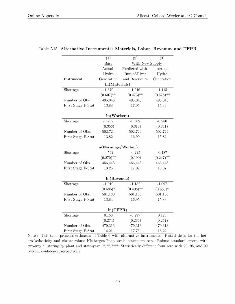
Online Appendix Allcott, Collard-Wexler and O’Connell

Table A15: Alternative Instruments: Materials, Labor, Revenue, and TFPR

(1) (2) (3)Base With New Supply

Actual Predicted with ActualHydro Run-of-River Hydro

Instrument: Generation and Reservoirs Generationln(Materials)

Shortage -1.370 -1.216 -1.415(0.607)** (0.473)** (0.576)**

Number of Obs. 495,043 495,043 495,043First Stage F-Stat 13.88 17.05 15.89

ln(Workers)Shortage -0.232 -0.302 -0.280

(0.356) (0.313) (0.341)Number of Obs. 502,724 502,724 502,724First Stage F-Stat 13.82 16.99 15.82

ln(Earnings/Worker)Shortage -0.542 -0.225 -0.487

(0.270)** (0.199) (0.247)**Number of Obs. 456,443 456,443 456,443First Stage F-Stat 13.25 17.09 15.07

ln(Revenue)Shortage -1.019 -1.182 -1.097

(0.586)* (0.498)** (0.560)*Number of Obs. 501,130 501,130 501,130First Stage F-Stat 13.84 16.95 15.83

ln(TFPR)Shortage 0.158 -0.297 0.128

(0.274) (0.236) (0.257)Number of Obs. 479,313 479,313 479,313First Stage F-Stat 14.21 17.75 16.22

Notes: This table presents estimates of Table 6 with alternative instruments. F-statistic is for the het-eroskedasticity and cluster-robust Kleibergen-Paap weak instrument test. Robust standard errors, withtwo-way clustering by plant and state-year. *,**, ***: Statistically different from zero with 90, 95, and 99percent confidence, respectively.

69

Online Appendix Allcott, Collard-Wexler and O’Connell

E.E Alternative TFPR Measures

Table A16 presents estimates of Equation (21), using alternative measures of TFPR described inAppendix C.B.2.

Table A16: Robustness Check: Estimates with Alternative TFPR Measures

(1) (2) (3) (4) (5) (6)Include Include No Time α Varies LeontiefAll Fuels No Fuels Trend by Size CRS CRS

Shortage -0.285 -0.150 -0.097 -0.112 -0.110 -0.211(0.240) (0.248) (0.211) (0.212) (0.221) (0.266)

Number of Obs. 479,609 479,484 480,100 494,210 479,755 477,720Number of Clusters 112,405 112,330 112,472 115,015 112,397 112,014Number of Clusters (2) 536 536 536 536 536 536First Stage F-Stat 14.87 14.88 14.84 14.32 14.85 14.89

Notes: F-statistic is for the heteroskedasticity and cluster-robust Kleibergen-Paap weak instrument test.Robust standard errors, with two-way clustering by plant and state-year. *,**, ***: Statistically differentfrom zero with 90, 95, and 99 percent confidence, respectively.

70

Online Appendix Allcott, Collard-Wexler and O’Connell

E.F Heterogeneous Effects of Shortages

Table A17 presents estimates of heterogeneous effects of shortages for plants with generators andfor plants in industries with above-median electric intensity. Denote Mi as a 3-by-1 vector of thesetwo moderators and a constant. The estimating equation is identical to Equation 21 except withMi interacted with all right-hand-side variables other than µjt.

Table A17 presents the estimated interactions with the Shortage variable. As expected, column2 shows that self-generators increase fuel use more when shortages worsen, while non-generators donot. However, we do not have the power to detect heterogeneous effects on revenues or TFPR. Asa benchmark, in the World Bank Enterprise Survey, generators and non-generators report 7.3 and8.4 percent losses from power cuts, respectively - a ratio of 8.4/7.3≈1.15. Our revenue estimatesare statistically indistinguishable from this benchmark ratio.

These empirical results are not interpretable as the average causal effects of generator ownership,because endogenous generator adoption decisions could imply that the plants without generatorshave unobservably smaller losses. For example, plants without generators might have unobservablybetter electricity supply, reducing their losses from not adopting generators and also reducing theeffects of an increase in shortages.

Table A17: Heterogeneous Effects of Shortages

(1) (2) (3) (4)Self-Gen ln(Fuel

Dependent Variable: Share Rev Share) ln(Revenue) ln(TFPR)

Shortage -0.027 -0.867 -0.478 -0.201(0.065) (1.748) (0.695) (0.445)

Shortage x Elec Intensive 0.022 0.189 -0.936 0.130(0.131) (2.181) (1.212) (0.551)

Shortage x Self-Generator 0.470 4.050 -0.384 -0.413(0.155)*** (1.956)** (0.716) (0.386)

Number of Obs. 428,969 477,005 501,130 479,313Number of Clusters 102,995 109,715 116,231 112,371Number of Clusters (2) 536 536 536 536

Notes: Robust standard errors, with two-way clustering by plant and state-year. *,**, ***: Statisticallydifferent from zero with 90, 95, and 99 percent confidence, respectively.

71

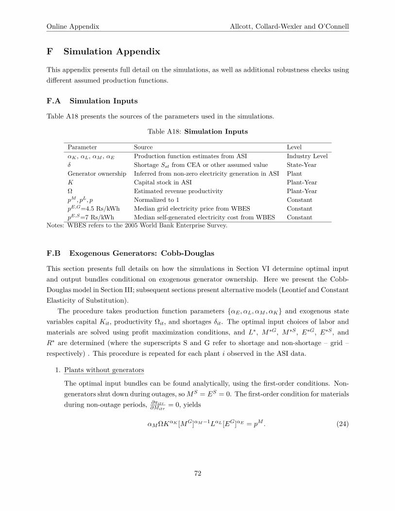
Online Appendix Allcott, Collard-Wexler and O’Connell

F Simulation Appendix

This appendix presents full detail on the simulations, as well as additional robustness checks usingdifferent assumed production functions.

F.A Simulation Inputs

Table A18 presents the sources of the parameters used in the simulations.

Table A18: Simulation Inputs

Parameter Source LevelαK , αL, αM , αE Production function estimates from ASI Industry Levelδ Shortage Sst from CEA or other assumed value State-YearGenerator ownership Inferred from non-zero electricity generation in ASI PlantK Capital stock in ASI Plant-YearΩ Estimated revenue productivity Plant-YearpM , pL, p Normalized to 1 ConstantpE,G=4.5 Rs/kWh Median grid electricity price from WBES ConstantpE,S=7 Rs/kWh Median self-generated electricity cost from WBES Constant

Notes: WBES refers to the 2005 World Bank Enterprise Survey.

F.B Exogenous Generators: Cobb-Douglas

This section presents full details on how the simulations in Section VI determine optimal inputand output bundles conditional on exogenous generator ownership. Here we present the Cobb-Douglas model in Section III; subsequent sections present alternative models (Leontief and ConstantElasticity of Substitution).

The procedure takes production function parameters αE , αL, αM , αK and exogenous statevariables capital Kit, productivity Ωit, and shortages δit. The optimal input choices of labor andmaterials are solved using profit maximization conditions, and L∗, M∗G, M∗S , E∗G, E∗S , andR∗ are determined (where the superscripts S and G refer to shortage and non-shortage – grid –respectively) . This procedure is repeated for each plant i observed in the ASI data.

1. Plants without generators

The optimal input bundles can be found analytically, using the first-order conditions. Non-generators shut down during outages, soMS = ES = 0. The first-order condition for materialsduring non-outage periods, ∂πitτ

∂Mitτ= 0, yields

αMΩKαK [MG]αM−1LαL [EG]αE = pM . (24)

72

Online Appendix Allcott, Collard-Wexler and O’Connell

Analogously, the FOC for electricity, ∂πitτ∂Eitτ

= 0, yields

αEΩKαK [MG]αMLαL [EG]αE−1 = pE,G. (25)

Finally, the FOC for labor, ∂πit∂Lit

= 0 yields

αL(1− δ)ΩKαK [MG]αMLαL−1[EG]αE = pL. (26)

Rearranging these three equations, we obtain:

M∗G =[ΩKαK

(αMpM

)1−αL−αE ((1− δ)αLpL

)αL ( αEpE,G

)αE] 11−αL−αM−αE

L∗ = (1− δ)pMαLpLαM

M∗G

E∗G = pMαEpEαM

M∗G

(27)

Annual revenue is thus:

R = (1− δ)ΩKαK [M∗G]αM [L∗]αL [E∗G]αE

Notice that if there are no shortages; δ = 0, the same equations can also be used to determineoptimal input bundles for all plants (assuming that pE,G < pE,S).

2. Plants with generators

There are five first-order conditions, ∂πitτ∂MS

itτ

= 0, ∂πitτ∂MG

itτ

= 0, ∂πitτ∂ESitτ

= 0, ∂πitτ∂EGitτ

= 0, and ∂πit∂Lit

= 0.These yield

αMΩKαK [MG]αM−1LαL [EG]αE = pM

αMΩKαK [MS ]αM−1LαL [ES ]αE = pM

αMΩKαK [MS ]αMLαL [ES ]αE−1 = pE,S

αMΩKαK [MG]αMLαL [EG]αE−1 = pE,G

αL(1− δ)ΩKαK [MG]αMLαL−1[EG]αE

+αLδpΩKαK [MS ]αMLαL−1[ES ]αE = pL

(28)

The set of equations in system (28) are solved numerically in MATLAB using the fsolve rou-tine. Rather than solving for L∗, E∗G, E∗,S , M∗G, and M∗S in levels, we solve in logarithms,since these values can differ by several orders of magnitude for different plants in the data.

73

Online Appendix Allcott, Collard-Wexler and O’Connell

The starting values for L∗, E∗G, E∗S , M∗G, and M∗S are given by the analytic values fromequation (27), the no-shortage values.

Annual revenue is:

R =(1− δ)ΩKαK [M∗G]αM [L∗]αL [E∗G]αE

+ δΩKαK [M∗S ]αM [L∗]αL [E∗S ]αE

F.C Exogenous Generators: Leontief in Electricity

Our original working paper used production functions that were Leontief in electricity and a Cobb-Douglas aggregate of capital, labor, and materials. For comparison, we include this below.

Denoting physical productivity as A, the physical production function is:

Q = minAKαKLαLMαM ,1λE (29)

The Leontief production function dictates that electricity is used in constant proportion 1λ

with output. Electricity intensity λ varies across industries. Having A inside the Cobb-Douglasaggregator ensures that electricity is used in fixed proportion to output instead of to the bundle ofother inputs.

Since we will observe total revenues rather than physical quantities produced, we need to relaterevenues to our production function in equation (29). We assume that plants sell into a perfectlycompetitive output market with price p, and denote Ω ≡ pA.

Firms have the following daily profit function Πitτ :

Πitτ =pminAitKαKit LαLit M

αMitτ ,

1λEitτ

− pLLit − pMMitτ − pEEitτ ,(30)

where pL pM are the prices of labor and materials, respectively. Capital is excluded, as it is sunkbefore the plant makes any production decisions.

Given the Leontief-in-electricity structure of production, cost minimization implies that for anydesired level of output Q, the firm produces at a “corner” of the isoquant where:

AitKαKit LαLit M

αMitτ = 1

λEitτ , (31)

Given this, one can rewrite the profit function, substituting in Ωit and the optimized value ofelectricity:

Πitτ = (1− λpE

p)ΩitAitK

αKit LαLit M

αMitτ − p

LLit − pMMitτ (32)

Let γ ≡ λpE,G

p = pE,GEitτpQitτ

= pE,GEitRit

, the electricity revenue share if a firm only uses electricity

74

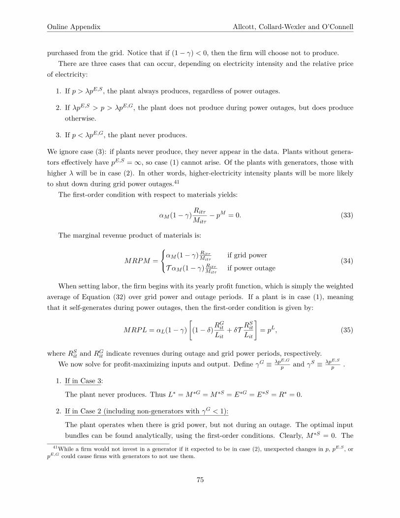
Online Appendix Allcott, Collard-Wexler and O’Connell

purchased from the grid. Notice that if (1− γ) < 0, then the firm will choose not to produce.There are three cases that can occur, depending on electricity intensity and the relative price

of electricity:

1. If p > λpE,S , the plant always produces, regardless of power outages.

2. If λpE,S > p > λpE,G, the plant does not produce during power outages, but does produceotherwise.

3. If p < λpE,G, the plant never produces.

We ignore case (3): if plants never produce, they never appear in the data. Plants without genera-tors effectively have pE,S =∞, so case (1) cannot arise. Of the plants with generators, those withhigher λ will be in case (2). In other words, higher-electricity intensity plants will be more likelyto shut down during grid power outages.41

The first-order condition with respect to materials yields:

αM (1− γ)RitτMitτ

− pM = 0. (33)

The marginal revenue product of materials is:

MRPM =

αM (1− γ) RitτMitτif grid power

T αM (1− γ) RitτMitτif power outage

(34)

When setting labor, the firm begins with its yearly profit function, which is simply the weightedaverage of Equation (32) over grid power and outage periods. If a plant is in case (1), meaningthat it self-generates during power outages, then the first-order condition is given by:

MRPL = αL(1− γ)[(1− δ)R

Git

Lit+ δT R

Sit

Lit

]= pL, (35)

where RSit and RGit indicate revenues during outage and grid power periods, respectively.We now solve for profit-maximizing inputs and output. Define γG ≡ λpE,G

p and γS ≡ λpE,S

p .

1. If in Case 3:

The plant never produces. Thus L∗ = M∗G = M∗S = E∗G = E∗S = R∗ = 0.

2. If in Case 2 (including non-generators with γG < 1):

The plant operates when there is grid power, but not during an outage. The optimal inputbundles can be found analytically, using the first-order conditions. Clearly, M∗S = 0. The

41While a firm would not invest in a generator if it expected to be in case (2), unexpected changes in p, pE,S , orpE,G could cause firms with generators to not use them.

75

Online Appendix Allcott, Collard-Wexler and O’Connell

FOC for materials during grid power periods, ∂πitτ∂Mitτ

= 0, yields

αM (1− γG)ΩKαK [MG]αM−1LαL = pM . (36)

The FOC for labor, ∂πit∂Lit

= 0 yields

αL(1− γG)(1− δ)ΩKαK [MG]αMLαL−1 = pL. (37)

Rearranging these first-order equation, we obtain

M∗G =[(1− γ)ΩKαK

(αMpM

)1−αL ((1− δ)αLpL

)αL] 11−αL−αM

L∗ = (1− δ)pMαLpLαM

M∗G

. (38)

Given labor and material choices, it is straightforward to compute revenue:

R = ΩKαK [M∗G]αM [L∗]αL .

Electricity consumption is:E∗G = γSR

Notice that if there are no shortages; δ = 0, the same equations can also be used to getoptimal input bundles and revenue for all plants.

3. If in Case 1 (plants with generators only):

The plant always operates, running its generator during outages. There are three first-orderconditions, ∂πitτ

∂MSitτ

= 0, ∂πitτ∂MG

itτ

= 0, and ∂πit∂Lit

= 0.

αM (1− γG)pΩKαK [MG]αM−1LαL = pM

αM (1− γS)pΩKαK [MS ]αM−1LαL = pM

αL(1− γG)(1− δ)pΩKαK [MG]αMLαL−1

+αLδ(1− γS)pΩKαK [MS ]αMLαL−1 = pL

(39)

The system of equations in (39) is solved numerically in MATLAB using the fsolve routine.

Finally, electricity usage is

E∗G = (1− δ)γGΩKαK [M∗G]αM [L∗]αL

E∗S = δγSΩKαK [M∗G]αM [L∗]αL .

76

Online Appendix Allcott, Collard-Wexler and O’Connell

Annual revenue is:

R =(1− δ)ΩKαK [M∗G]αM [L∗]αL

+ δΩKαK [M∗S ]αM [L∗]αL

F.D Exogenous Generators: Constant Elasticity of Substitution

One issue with the production functions that we have considered is that there is no direct intertem-poral substitution in production. Suppose instead that we consider a CES aggregator with constantelasticity of substitution σ between days given by:

Rit =[ˆ

τ(Ritτ )σdτ

] 1σ

Notice that this is a CES type aggregator, so there is symmetric substitution across all days ofthe year. If σ = 1, we have the process considered in the paper. If σ < 1, outputs are interdaycomplements, and if σ > 1, then there is inter-day substitution.

Given that in the daily production function, only materials and electricity can be varied, wecan think of the daily production function as being written as:

Rit = ΩitKαKit LαLit

[ˆτEitτ

σαEMitτσαMdτ

] 1σ

Notice that the daily returns to scale in the production function will be given by σ(αM + αE),an issue we return to below.

F.D.1 First-Order Conditions for Non-Generators

For firms that do not have generators, revenue is:

Rit =[ˆ

τ(Ritτ )σdτ

] 1σ

= [(1− δ)MσαMitτ EσαEitτ LσαLit KσαK

it ]1σ

= (1− δ)1σMαM

itτ LαLit E

αEitτ K

αKit

= (1− δ)1σ

(Mit

(1− δ)

)αM ( Eit(1− δ)

)αELαLit K

αKit

= (1− δ)1σ−αM−αEMαM

it EαEit LαLit K

αKit

(40)

where we have assumed that the same input choice will be optimal across days to go fromthe first to the second line of this equation. Notice that shortages can cause anything between azero and infinite decrease in revenues by changing σ, holding inputs fixed. Thus, our predictionsare not robust to a range of σ. Moreover, the only difference between this setup and the setup

77

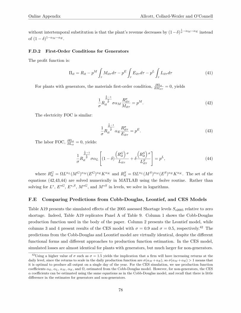
Online Appendix Allcott, Collard-Wexler and O’Connell

without intertemporal substitution is that the plant’s revenue decreases by (1−δ)1σ−αM−αE instead

of (1− δ)1−αM−αE .

F.D.2 First-Order Conditions for Generators

The profit function is:

Πit = Rit − pMˆτMitτdτ − pE

ˆτEitτdτ − pL

ˆτLitτdτ (41)

For plants with generators, the materials first-order condition, ∂Πit∂Mitτ

= 0, yields

1σR

1σ−1

1σ

it σαMRσitτMitτ

= pM . (42)

The electricity FOC is similar:

1σR

1σ−1

1σ

it αERσitτEitτ

= pE . (43)

The labor FOC, ∂Πit∂Lit

= 0, yields:

1σR

1σ−1

1σ

it σαL

(1− δ)

(RGit

)σ

Litτ+ δ

(RSit

)σ

LSitτ

= pL, (44)

where RGit = ΩLαL(MG)αM (EG)αEKαK and RSit = ΩLαL(MS)αM (ES)αEKαK . The set of theequations (42,43,44) are solved numerically in MATLAB using the fsolve routine. Rather thansolving for L∗, E∗G, E∗,S , M∗G, and M∗S in levels, we solve in logarithms.

F.E Comparing Predictions from Cobb-Douglas, Leontief, and CES Models

Table A19 presents the simulated effects of the 2005 assessed Shortage levels Ss2005 relative to zeroshortage. Indeed, Table A19 replicates Panel A of Table 9. Column 1 shows the Cobb-Douglasproduction function used in the body of the paper. Column 2 presents the Leontief model, whilecolumns 3 and 4 present results of the CES model with σ = 0.9 and σ = 0.5, respectively.42 Thepredictions from the Cobb-Douglas and Leontief model are virtually identical, despite the differentfunctional forms and different approaches to production function estimation. In the CES model,simulated losses are almost identical for plants with generators, but much larger for non-generators.

42Using a higher value of σ such as σ = 1.5 yields the implication that a firm will have increasing returns at thedaily level, since the returns to scale in the daily production function are σ(αM +αE), so σ(αM +αE) > 1 means thatit is optimal to produce all output on a single day of the year. For the CES simulation, we use production functioncoefficients αE , αL, αM , αK , and Ω, estimated from the Cobb-Douglas model. However, for non-generators, the CESα coefficients can be estimated using the same equations as in the Cobb-Douglas model, and recall that there is littledifference in the estimates for generators and non-generators.

78

Online Appendix Allcott, Collard-Wexler and O’Connell

Table A19: Predictions from Different Production Function Models

Cobb-Douglas Leontief CES σ = 0.9 CES σ = 0.5(1) (2) (3) (3)

Revenue Loss: Average 5.6% 5.7% 7.5% 18%Revenue Loss: Non-Generators 10.0% 9.8% 13% 32%Revenue Loss: Generators 0.4% 0.6% 0.4% 0.4%

TFPR Loss: Average 1.5% 1.3% 1.9% 5.8%TFPR Loss: Non-Generators 2.6% 2.4% 3.5% 10.6%TFPR Loss: Generators 0.0% 0.0% 0.0% 0.0%

Notes: This table presents the effects of the 2005 assessed Shortage levels relative to zero Shortage. Cobb-Douglas, Leontief, and CES, refer to the production functions used for estimation and prediction, and aredescribed in text.

F.F Endogenous Generators

For the model with endogenous generators, the equations given in Online Appendix F.B above areused to obtain the optimal input bundle, conditional on the presence of a generator at the plant.In this model, however, we also endogenously solve for generator adoption.

Plant i purchases a generator if and only if ΠGit−CGit > ΠNG , where ΠG and ΠNG are profitability

with and without generators, respectively, and CGit is the annualized generator cost.Profits ΠG and ΠNG are both

Πit = Rit − pLL∗ − pM(δM∗G + (1− δ)M∗S

)− δpE,SE∗S − (1− δ)pE,GE∗G, (45)

where optimal inputs are according to the equations in Online Appendix F.B above.

F.F.1 Estimating Generator Costs

We parametrize the generator cost as lnCGit = σ0 + σ1 ln(cit), where σ1 is the economy of scaleparameter, and cit is the generator capacity in kilowatts. We estimate σ0 and σ1 using GMM,matching the mean generator adoption rate and the covariance between generator adoption andlog generator capacity. We use the identity matrix as a weighting matrix, since the two momentsthat we match are of comparable scales. Column 1 of Table A20 presents GMM estimates of thegenerator cost function.

For comparison, we collected generator purchase price data from the United States. To compareto the estimated CG , we must first convert the purchase prices into yearly rental prices. First,we convert generators rated in KVA into KW using a 0.8 conversion ratio. Second, we convertUS dollars into Rupees using a 50 to 1 exchange rate. Finally, we convert the purchase price of agenerator into an annual rental price assuming a 30 percent discount rate, a ten percent depreciationrate, and a ten-year generator lifespan.43 This gives a 1.6:1 ratio between generator costs and rental

43This 30 percent discount rate is high by U.S. standards, but as Banerjee and Duflo (2014) discuss, Indian firms

79

Online Appendix Allcott, Collard-Wexler and O’Connell

Table A20: Generator Cost Estimates

(1) (2)GMM Estimates Observed Prices

σ0 10.67 11.14(0.18) (0.25)

σ1 0.83 0.79(economy of scale) (0.01) (0.05)

Observations 33,871 223Predicted Generator Takeup Rate 0.53 0.47Covariance: Generator Takeupand Generator Size 0.63 0.72

Note: Column 1 shows estimates of generator cost using generator adoption decisions via GMM as describedin text. Column 2 shows a regression of log generator rental rate on log generator capacity.

rates. Column 2 presents a regression of the natural logs of these observed prices on natural log ofcapacity.

The estimates of σ1 are close to 0.8 in both columns of Table A20. The estimates of σ0 are alsocomparable (10.67 vs. 11.14), although the point estimate in column 1 is smaller. This gives ussome confidence that the estimated generator costs are approximately reasonable and that generatorcosts can explain the fact that many manufacturing plants in the ASI do not have generators.

pay far higher interest rates - on the order of 30 to 60 percent, if they have access to capital at all.

80

Online Appendix Allcott, Collard-Wexler and O’Connell

F.G Additional Simulation Figures and Tables

81

Online Appendix Allcott, Collard-Wexler and O’Connell

Figure A8: Predicted Average Revenue Loss by Simulation Year

0

2

4

6

8

10

Perc

ent R

even

ue L

oss

1990 1995 2000 2005 2010year

Notes: In the body of the paper, we simulate effects of moving from δ = 0 to δ = Ss2005 for all plants in thedata in 2005. This figure presents revenue effects from the same simulations for each year of the 1992-2010sample, i.e. taking the sample of plants in year t and changing δ from δ = 0 to δ = Sst.

82

Online Appendix Allcott, Collard-Wexler and O’Connell

Figure A9: Generator Adoption Under Varying Shortage Levels

0

.2

.4

.6

.8

1

Gen

erat

or U

ptak

e

0 .05 .1 .15 .2Shortage

Note: These figures show the simulated generator adoption rate when the δ on the x-axis is assigned to allplants in the 2005 ASI, using the generator adoption model in Section VI.A.1. Note that generator takeupexceeds 90 percent at a seven percent δ, which may seem puzzling given that the generator cost estimatesare based on a 44 percent takeup rate in the ASI at a 7.2 percent mean shortage. The reason is that thedistribution of Ss2005 across plants is right skewed; the median of Ss2005 across plants is only 3.5 percent.

83

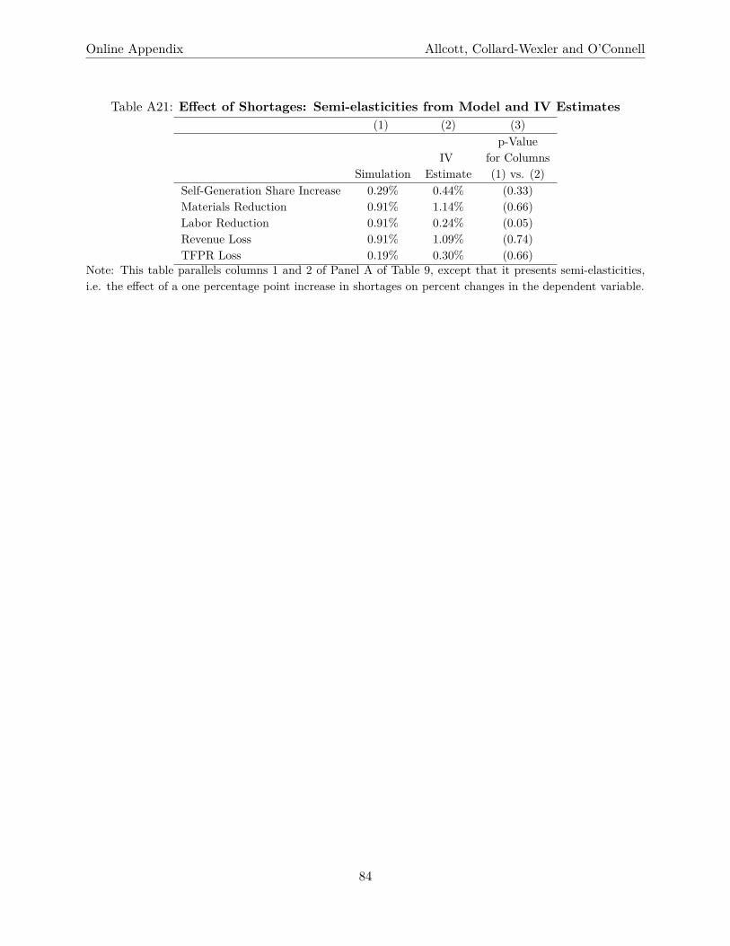
Online Appendix Allcott, Collard-Wexler and O’Connell

Table A21: Effect of Shortages: Semi-elasticities from Model and IV Estimates(1) (2) (3)

p-ValueIV for Columns

Simulation Estimate (1) vs. (2)Self-Generation Share Increase 0.29% 0.44% (0.33)Materials Reduction 0.91% 1.14% (0.66)Labor Reduction 0.91% 0.24% (0.05)Revenue Loss 0.91% 1.09% (0.74)TFPR Loss 0.19% 0.30% (0.66)

Note: This table parallels columns 1 and 2 of Panel A of Table 9, except that it presents semi-elasticities,i.e. the effect of a one percentage point increase in shortages on percent changes in the dependent variable.

84

Online Appendix Allcott, Collard-Wexler and O’Connell

Table A22: Counterfactuals Under Varying Shortage Levels

(1) (2) (3) (4) (5)Shortage Percent (δ): 3% 5% 7% 10% 20%Exogenous GeneratorsRevenue Loss: Average 2.5% 4.2% 5.8% 8.3% 16%Revenue Loss: Generators 0.2% 0.3% 0.5% 0.6% 1.3%Revenue Loss: Non-Generators 4.5% 7.4% 10% 15% 28%

TFPR Loss: Average 0.5% 0.9% 1.3% 1.9% 3.9%

Input Cost Increase: Generators 0.2% 0.3% 0.4% 0.5% 1.0%

Variable Profit Loss: Average 2.5% 4.2% 5.8% 8.2% 16%Generator Cost (Percent of Profits) 3.0% 3.0% 3.0% 3.1% 3.2%Total Profit Loss: Average 5.5% 7.2% 8.8% 12% 19%

Endogenous GeneratorsGenerator Take-up 66% 85% 91% 94% 98%

Revenue Loss: Average 1.7% 1.4% 1.3% 1.3% 1.7%Revenue Loss: Generators 0.2% 0.3% 0.4% 0.6% 1.2%Revenue Loss: Non-Generators 4.2% 7.1% 10% 15% 29%

TFPR Loss: Average 0.4% 0.2% 0.2% 0.2% 0.1%

Input Cost Increase: Generators 0.1% 0.2% 0.3% 0.5% 1.0%

Variable Profit Loss: Average 1.7% 1.4% 1.2% 1.2% 1.5%Generator Cost (Percent of Profits) 1.6% 2.7% 3.4% 3.8% 4.6%Total Profit Loss: Average 3.3% 4.1% 4.6% 5.1% 6.1%

Notes: This table presents predictions of the simulation model described in the text. The simulations with“exogenous” generators hold fixed the generator adoption decision observed in the ASI, while the simulationswith “endogenous” generators use the model’s prediction of which plants will purchase generators at thedifferent shortage levels. Input Cost Increase is reported as a share of revenues. In this table, the electricityshortage is uniform across all plants in all states.

85

Online Appendix Allcott, Collard-Wexler and O’Connell

References

[1] Banerjee, Abhijit and Esther Duflo (2014). “Do Firms Want to Borrow More? Testing Credit Con-straints Using a Directed Lending Program.” Review of Economic Studies, Vol. 81, pp. 572–607.

[2] MOSPI (Ministry of Statistics and Programme Implementation (2014). “Annual Survey of Industries.”Available at: http://mospi.nic.in/Mospi_New/upload/asi/ASI_main.htm?status=1&menu_id=88.Accessed 17 December 2014.

86