How Do Electricity Shortages A�ect Productivity? Evidence fromIndia

Hunt Allcott, Allan Collard-Wexler, and Stephen D. O’Connellú

March 23, 2014

Abstract

Endemic blackouts are a particularly salient example of how poor infrastructure might reducegrowth in developing economies. As a case study, we analyze how Indian textile plants respond toweekly “power holidays.” We then study how electricity shortages a�ect all Indian manufacturers,using an instrument based on hydroelectricity production and a hybrid Leontief/Cobb-Douglasproduction function model. Shortages reduce average output by about five percent, but becausemost inputs can be stored during outages, productivity losses are much smaller. Plants withoutgenerators have much larger losses, and because of economies of scale in generator capacity,shortages more severely a�ect small plants.

JEL Codes: D04, D24, L11, L94, O12, O13, Q41.Keywords: Manufacturing productivity, India, electricity shortages.————————————————————————————We thank Jan De Loecker, Michael Greenstone, Peter Klenow, Nick Ryan, Jagadeesh Sivadasan,

and seminar participants at the 2013 NBER Summer Institute, the 2014 NBER Winter IO/EEEmeetings, Stanford, and Toulouse for helpful comments. We are particularly grateful to NickBloom and coauthors for sharing the data from “Does Management Matter?” We thank TroySmith for help understanding those data, as well as Shaleen Chavda for insight into the textileindustry. We thank Deepak Choudhary for helpful research assistance and the Stern Center forGlobal Economy and Business for financial support in purchasing the ASI and other data. Wehave benefited from helpful conversations with Jayant Deo of India Energy Exchange, GajendraHaldea of the Planning Commission, Partha Mukhopadhyay of the Centre for Policy Research,and Kirit Parikh of IGIDR. We also thank A. S. Bakshi and Hemant Jain of the Central Electric-ity Authority for help in collecting archival data. Of course, all analyses are the responsibilityof the authors, and no other parties are accountable for our conclusions. Code for replication isavailable from Hunt Allcott’s website.

úAllcott: New York University and NBER. hunt.allcott@nyu.edu. Collard-Wexler: New York University andNBER. wexler@stern.nyu.edu. O’Connell: City University of New York - Graduate Center. soconnell@gc.cuny.edu.

1

1 Introduction

One of the potential contributors to the large productivity gap between developed and developingcountries is low quality infrastructure, and one of the most stark examples of infrastructure failuresis electricity supply in India. In the summer of 2012, India su�ered the largest power failurein history, which plunged 600 million people into darkness for two days. Even under normalcircumstances, however, the Indian government estimates that shortages currently amount to aboutten percent of demand at current prices, and many consumers have power only a few hours a day.In the 2005 World Bank Enterprise Survey, one-third of Indian business managers named poorelectricity supply as their biggest barrier to growth. According to these managers, blackouts are farmore important than other barriers that economists frequently study, including taxes, corruption,credit, regulation, and low human capital.1

This paper studies the e�ects of electricity shortages on manufacturing plants in India. Onepotential prior is that because electricity is an essential input - most factories cannot produceanything without electricity for lights, motors, and machines - shortages could significantly reduceoutput. On the other hand, precisely because the potential losses would be so large, many firmsmight insure themselves against outages by purchasing generators or otherwise substituting awayfrom grid electricity. The limited existing evidence could support either argument. Foster andSteinbuks (2009), Zuberi (2012), and others argue that the cost of self-generation is relatively small,and Alam (2013), Fisher-Vanden, Mansur, and Wang (2013), and others highlight ways in whichplants substitute away from electricity when shortages worsen. By contrast, Hulten, Bennathan,and Srinivasan (2006) argue that growth of roads and electric generation capacity accounts for aremarkable 50 percent of productivity growth in Indian manufacturing between 1972 and 1992.

There are three reasons why this question is di�cult. First, the standard production functionmodel needs to be adapted for the case of input shortages, when firms cannot procure electricityfor a part of the year. Second, the necessary data are di�cult to acquire: some industrial surveysdo not have useful questions on electricity use, and more detailed firm-level datasets are oftenunrepresentative. Meanwhile, countries that have electricity shortages are often the same types ofcountries that do not record or disclose high-quality data on the performance of public infrastruc-ture. Third, shortages are not exogenous to productivity. For example, rapid economic growthcould cause an increase in electricity demand that leads to shortages, or poor institutions couldlead to insu�cient power supply and also reduce productivity. Either of these two mechanismswould bias causal estimates of shortages, albeit in opposite directions.

We begin by providing background on electricity shortages and industrial electricity use in In-dia. First, there is significant variation in shortages within states over time, driven by weather, coalshortages, fluctuating hydroelectric production, and other factors. Second, Indian manufacturersself-generate approximately 35 percent of their electricity, more than twice the share in the UnitedStates. Third, because of economies of scale in generator capacity, self-generation is sharply in-

1For a tally of responses, see Appendix Table A20.

2

creasing in plant size: while only 10-20 percent of plants with fewer than 10 employees self-generate,about 75 percent of plants with more than 500 employees do so.

We then present a production function model in which output is Leontief in electricity and aCobb-Douglas aggregate of materials, capital, and labor. Shortages have very di�erent e�ects onfirms with vs. without generators. Firms that use generators face an increase in electricity costs(the input cost e�ect). This enters the profit function like an output tax and thus reduces demandfor other inputs (the output tax e�ect). Even if these firms never stop production during shortages,productivity is lower due to the input variation e�ect: using di�erent bundles of fully flexible inputsduring outage vs. non-outage periods is less e�cient than having a constant flow of production.Firms without generators shut down during shortages, which reduces output and causes waste ofnon-storable inputs (the shutdown e�ect). The waste reduces demand for non-storable inputs whenfirms foresee periods of higher shortages (the shutdown tax e�ect).

The empirical analysis begins with a case study of large textile manufacturers in Gujarat andMaharashtra, using data shared by Bloom et al. (2013). These plants face pre-scheduled “powerholidays” once each week, and they respond either by self-generation or by shutting down, dependingon the week. While these data include only 22 plants, all of which have generators, they give veryclean estimates of the e�ects of shortages. The e�ects of these weekly “power holidays” are quitesmall: energy costs rise by 0.24 percent of revenues, and while physical output drops by 1.1 percent,productivity only decreases by 0.05 percent because 95 percent of inputs (both labor and materials)can be flexibly adjusted on power holidays.

We then broaden our scope to all Indian manufacturing plants using data from the Annual Sur-vey of Industries (ASI). We use a di�erence estimator, exploiting changes in shortages within statesover time. To address the potential endogeneity of shortages - for example, economic growth bothincreases manufacturing output and worsens shortages - we instrument with changes in electricityproduction from dams, which are driven by changes in the amount of water flowing into reservoirs.We exploit a version of the ASI with consistent plant identifiers dating to 1992, which allows anunusually long panel of Indian plants. To complement this longer panel, we gathered archival datafrom India’s Central Electricity Authority on shortages, reservoir inflows, generation by hydro andother plants, and other aspects of the Indian power sector.

Our instrumental variables estimates show that for plants that own generators, a one percentagepoint increase in shortages increases the share of self-generated electricity by 0.57 percentage points,which raises total input costs by 0.02 to 0.07 percent of revenues. Across all plants, a one percentagepoint increase in shortages decreases revenues by 0.68 percent. The accompanying loss of revenueproductivity (TFPR), however, is much smaller: the e�ect is not statistically di�erent than zero,and the confidence interval bounds it at no more than 0.29 percent. In 2005, the nationwide averageshortage was 7.1 percent, and this is very close to the nationwide average shortage over our 1992-2010 sample. The empirical estimates multiplied by a 7.1 percent shortage translate into an inputcost increase of 0.13 to 0.5 percent of revenues and a revenue loss of 4.8 percent.

3

The e�ects of shortages vary in ways predicted by the model. Only plants that self-generateexperience an increase in total energy costs, while non-generators experience much larger revenuelosses. Firms in industries with higher electric intensity are more exposed to shortages, experiencinga larger increase in energy revenue share and a larger decrease in output. The results are essen-tially identical under a battery of alternative specifications, including using fixed e�ects instead ofdi�erences, controlling for rainfall, using an alternative measure of shortages, constructing TFPRin di�erent ways, omitting various controls, and trimming outliers with di�erent tolerances.

We then use simulations calibrated to ASI plants and production functions to calculate thenationwide e�ects of the 7.1 percent shortage, holding capital stock constant. The average plantloses 4.6 percent of revenue and 1.6 percent of TFPR. The simulated e�ects on output and TFPRare economically similar and statistically indistinguishable from the empirical estimates, whichbuilds confidence that the estimates are reasonable and that the model captures the first-orderissues.

As with the empirical estimates, however, simulated e�ects di�er starkly for plants with versuswithout generators: plants with generators see revenue and TFPR drop by 0.4 and 0.1 percent,respectively, while plants without generators experiences losses of 9.6 and 3.4 percent. For self-generators and non-generators, the reasons why output losses are larger than the percent of timeshut down are the output tax and shutdown tax e�ects: shortages act like taxes that cause firms toreduce other inputs. These input reductions are also one reason why TFPR losses are much smallerthan output losses; the other important reason is that when non-generators shut down, they loseoutput but only waste non-storable inputs. Thus, while electricity shortages are a large dragon manufacturing output, they do not in isolation explain much of the di�erence in productivitybetween India and more developed economies.2

Because our instrumental variables estimates are identified o� of annual variation, they are likelyto primarily identify “short-run” e�ects of shortages, i.e. holding generator capital stock constant.To extend this, we use additional simulations with simple assumptions about generator capitalcosts to endogenize each plant’s generator takeup decision. At the current level of shortages, thesesimulations confirm that despite the fact that generators largely ameliorate the negative e�ectsof shortages on revenues, TFPR, and variable profits, generators are su�ciently costly that onlya subset of plants should choose to purchase them. The simulations also show that increases inshortages have two o�setting e�ects on output. On the one hand, the “short-run” e�ects (holdinggenerator stock constant) increase almost exactly linearly in shortages. On the other hand, morefrequent outages induce more plants to purchase generators and continue production during poweroutages. This long-run e�ect of generator adoption substantially reduces the average impacts ofshortages.

Finally, we also use the simulations to explore how electricity shortages di�erentially a�ect smallversus large plants, which could distort the firm size distribution in developing economies. (See

2See Banerjee and Duflo (2005), Hsieh and Klenow (2009), and others for discussions.

4

Tybout (2000) for a broader discussion.) Hsieh and Olken (2014) show that average products oflabor and capital are significantly lower in small firms, and Hsieh and Klenow (2012) suggest thatlarge vs. small plants may have di�erential access to power from the electric grid. We build on thisidea, but we focus on a di�erent channel: economies of scale in generator capacity. Our simulationsshow that e�ects of outages on revenues and TFPR are 50 percent larger for plants with fewer than100 employees compared to larger plants, primarily due to the fact that small plants are much lesslikely to own generators.

The remainder of this section discusses related literature. Section 2 provides background onthe Indian electricity sector, the causes of electricity shortages, and manufacturers’ responses toshortages. Section 3 details the production function model. Section 4 is the case study of textilemanufacturing in western India, using data from Bloom et al. (2013). Sections 5 and 6 presentthe ASI data and empirical results. Section 7 details the counterfactual simulations, and Section 8concludes.

1.1 Related Literature

Our paper builds on an extensive literature that estimates the economic e�ects of investment inelectricity, transportation, and other types of infrastructure. One early group of studies examinesthe e�ects of infrastructure investment on growth in panel data from U.S. states, including Aschauer(1989), Holtz-Eakin (1994), Fernald (1999), Garcia-Mila, McGuire, and Porter (1996); see Gramlich(1994) for a review. Easterly and Rebelo (1993), Esfahani and Ramirez (2002), and Roller andWaverman (2001) carry out analogous studies using cross-country panels.

This literature has faced two basic problems. First, infrastructure spending is econometricallyendogenous to economic growth. There could be reverse causality: fast growth increases tax rev-enues, which allow more infrastructure spending. There is also economic endogeneity: infrastruc-ture may be specifically allocated to places that are growing more quickly or slowly. Second, usingaggregate infrastructure spending or quantity as the independent variable often hides importantvariation in e�ects between infrastructure of di�erent types or quality levels. In the Indian con-text, for example, spending on power plants does not necessarily translate into electricity provision,because plants are frequently o�ine due to mechanical failure or fuel shortages.

Our paper is part of a recently-growing literature that evaluates the e�ects of infrastructureby combining microdata with within-country variation generated by natural experiments. Thisincludes Banerjee, Duflo, and Qian (2012), Donaldson (2012), and Donaldson and Hornbeck (2013)on the e�ects of railroads in China, India, and the United States, Duflo and Pande (2007) onirrigation dams in India, Jensen (2007) on information technology, Baisa, Davis, Salant, and Wilcox(2008) on the benefits of reliable water provision in Mexico, and Baum-Snow (2007, 2013), Baum-Snow, Brandt, Henderson, Turner, and Zhang (2013), and Baum-Snow and Turner (2012) onurban transport expansions in China and the United States. A subset of this literature focuseson electricity supply: Chakravorty, Pelli, and Marchand (2013), Dinkelman (2011), Lipscomb,

5

Mobarak, and Barham (2013), Rud (2012a), and Shapiro (2013) study the e�ects of electricity gridexpansions, while Alby, Dethier, and Straub (2011), Foster and Steinbuks (2009), Steinbuks (2011),Steinbuks and Foster (2010), Reinikka and Svensson (2002), and Rud (2012b) study firms’ generatorinvestment decisions. Several recent papers focus specifically on Indian electricity supply: Ryan(2013) estimates the potential welfare gains from expanding transmission infrastructure, Cropper,Limonov, Malik, and Singh (2011) and Chan, Cropper, and Malik (2014) study the e�ciencyof Indian coal power plants, and Abeberese (2012) tests how changes in electricity prices a�ectmanufacturing productivity.

Three recent papers study the e�ects of blackouts on manufacturers. Fisher-Vanden, Mansur,and Wang (2013) show that when shortages become more severe, Chinese firms purchase moreenergy-intensive inputs, but they do not self-generate more electricity. Zuberi (2012) estimatesa dynamic model of manufacturing production using data from Pakistan, showing how firms re-allocate production to non-shortage periods. Alam (2013) studies how India’s steel vs. rice millingindustries respond di�erently to blackouts. Relative to these important papers, our study benefitsfrom particularly clean data and identification: we have a clear case study using the high-qualitytextile plant data from Bloom et al. (2013), newly-gathered archival data on the severity of short-ages across Indian states, and an instrument that addresses the endogeneity of blackouts withrespect to growth. Our paper also benefits from the way that we integrate theory and empirics:our model formalizes the major channels through which shortages a�ect production, and the closecorrespondence between simulation and empirical results builds confidence in the estimates.

2 Background

2.1 Power Sector Data

Our power sector data are from India’s Central Electricity Authority (CEA). Many of the sametypes of data available online from the U.S. Energy Information Administration are also collectedby the CEA. Unfortunately, however, the online data are incomplete, and the hard copies of someprinted materials have been misplaced, so data have to be hand-collected from CEA sta�. Withthe cooperation of CEA management and the help of research assistants in New Delhi, we wereable to compile, digitize, and clean about 25 years of data for this and related projects. Table 1details these power sector variables and other state-level data.3

The primary measure of electricity shortages is the percent energy deficit reported in the LoadGeneration Balance Report. Analysts at CEA and Regional Power Committees estimate the quan-tity that would be demanded for each state and month at current prices in the absence of shortages.The state-by-year sum is our “Assessed Demand” variable. “Shortage” is the percent di�erence be-tween this counterfactual quantity demanded and the actual quantity supplied. In the 2011-2012

3Throughout the paper, we use the word “state” to refer to both states and Union Territories.

6

fiscal year, nationwide shortage was 8.5 percent, and shortages average 7.2 percent over the sampleperiod. The CEA also estimates “Peak Shortage,” an analogous measure of power shortage in peakdemand periods. While (total kilowatt-hour) Shortage is more appropriate for our analysis, PeakShortage and Shortage are highly correlated, with an R2 of 0.5, and robustness checks show thatresults are similar when we use Peak Shortage instead of Shortage.4

From an annual report called the Review of the Performance of Hydro Power Stations, weobserve inflows into reservoirs behind 22 major dams covering about 40 percent of national hydro-electric capacity. From the CEA’s General Review, we observe each state’s total annual electricitygeneration by fuel type, including hydroelectric plants. From the General Review, we also collectedtotal quantity of electricity sold by utilities to end users for each state and year.

Aside from these electricity market variables, our empirical analysis also uses weather andtemperature data from the Meteorological Department of the National Climate Centre of India.These data provide daily average temperatures and rainfall at one-degree gridded intervals acrossIndia. Using state border coordinates, we associate the grid points with particular states to arriveat annual state-level measures. Cooling degrees is a commonly-used correlate of electricity demand;it is the di�erence between the day’s average temperature and 65 degrees Fahrenheit, or zero if theday’s average temperature is below 65.

2.2 Reasons for Systemic Shortages

As of February 2013, India had 214 gigawatts of utility-scale power generation capacity, or aboutone-fifth the US total (CEA 2013). Of this, 58 percent was coal, nine percent was natural gas, and18 percent was hydro-electric. While power generation has been open to private investment since1991, 70 percent of electricity supply remains government owned: 40 percent is owned by stategovernments, and 30 percent is owned by central government entities. Although some retail distri-bution companies have been privatized, most of distribution is managed by state-run companies,which are often called State Electricity Boards (SEBs).

The proximate reason for shortages is that distribution companies cannot raise retail pricesduring peak demand times in order to clear the market. In fact, conditional on state and yeare�ects, there is no correlation between shortages and the median electricity price paid by ASI plants.Aside from being stark evidence on how prices do not adjust to supply and demand conditions, thisalso means that the e�ects we estimate are caused by input shortages, not by input price changes.

There are several underlying systemic reasons for shortages. The first is the “infrastructure4Although it is likely that shortages are measured with error, correlations with independent data suggest that

the CEA’s estimates contain meaningful information. Alam (2013) shows that Peak Shortage is correlated with hermeasure of blackouts based on variation in nighttime lights measured by satellites; she does not report a correla-tion with Shortage. In the World Bank Enterprise Survey, plants in higher-Shortage states report a larger share ofself-generated electricity and are more likely to report that electricity is their primary obstacle to growth. Further-more, our empirical results show that Shortages are positively correlated with hydroelectric supply and correlated intheoretically-predicted ways with self-generation and other outcomes in the ASI.

7

quality and subsidy trap” (McRae 2013): distribution companies provide low-quality electricity toconsumers, who tolerate poor service because they pay very low prices, distribution companies’losses from low prices are covered by government subsidies, and politicians support the subsidiesto avoid voter backlash. At least since the 1970s, State Electricity Boards have o�ered un-meteredelectricity at a monthly fixed fee and zero marginal cost to agricultural consumers, largely to runwell pumps (Bhargava and Subramaniam 2009). In 2010, the national average retail electricity costpaid by agricultural consumers was 1.23 Rupees per kilowatt-hour (Rs/kWh), against Rs 4.78 forindustrial consumers and 3.57 Rs/kWh for all consumers. (The exchange rate is about 50 Rupeesper dollar, and the average electricity price across all consumers in the United States is about 10cents/kWh.)

Distortions in pricing are relevant only for consumers who actually pay for electricity. Twenty-six percent of electricity generated in India in 2010-2011 was lost due to “technical and commerciallosses,” meaning theft or poor transmission infrastructure. This is down from 34 percent in 2004-2005. Distribution companies thus have no ability to charge any price, let alone raise prices, on asignificant share of electricity.

Agricultural subsidies and technical and commercial losses have led to mounting losses. TheSEBs receive large annual payments from state governments to cover these losses, and in particularto fund the subsidies for agricultural consumers, but these payments and the cross-subsidy fromindustrial customers are not su�cient to cover the SEBs’ costs. Between 1992 and 2009, the SEBslost $54 billion dollars (again, in real 2004 dollars). These mounting losses caused the SEBs toreduce infrastructure investment, and degraded infrastructure further increases the probability ofblackouts. The SEBs are bailed out at irregular intervals by the government.

A second systemic reason for shortages is underinvestment in new generation capacity. Forexample, after the 1991 liberalization, 200 Memoranda of Understanding were signed betweenthe government and investors to build 50 gigawatts of generation capacity, but less than fourgigawatts of this was actually built (Bhargava and Subramaniam 2009). Of the 71 gigawatts ofcapacity targeted to be built between 1997 and 2007, only half was actually achieved (CEA 2013a).Potential power plant investors faced concerns over both output demand and input supply. Theirmain customers, the State Electricity Boards, faced serious financial problems, and it was not clearthat they would be able to honor contracts. Meanwhile, the main supplier of coal is Coal India, agovernment-owned monopoly that is struggling to keep pace with demand growth.

In addition, the existing capacity is systematically underutilized. Between 1994 and 2009,Indian coal power plants were o�ine about 28 percent of the time due to forced outages, plannedmaintenance, or other factors such as equipment malfunction, coal shortages, or poor coal quality.Furthermore, when capacity is utilized, it is substantially less e�cient than comparable plants inthe United States (Chan, Cropper, and Malik 2014).

One potential solution to problems with retail distribution companies is “open access”: allowingconsumers to contract directly with generators. The 2003 Electricity Act mandated open access,

8

but in practice direct power sales to bulk consumers have not materialized (GOI 2009, 2012),partially because states have imposed additional charges on open access consumers and have alsobanned export of power to open access consumers in other states.

2.3 Variation in Shortages

These systemic factors di�er across states, generating di�erences in shortages. A substantial partof these di�erences persist across years. Figure 1 shows that there is a negative association between2010 per capita GDP and average shortage over the sample. This suggests that low levels ofdevelopment are associated with poor institutions, bad management, and other factors that worsenprovision of public infrastructure. However, there is substantial variation conditional on GDP.Rajasthan, Jharkhand, and Sikkim have low GDP and low shortages, partially because their slowGDP growth makes it easier for supply to keep up with demand. Because end-of-sample GDP ishighly correlated with GDP growth, this implies that shortages could be correlated with factors thatalso a�ect manufacturing growth and productivity. This highlights the importance of instrumentingfor shortages in our empirical analysis.5

There is also substantial variation in shortages within states over time. Figure 2 shows thetime path of annual average shortage over our sample for five large states in di�erent parts of thecountry. West Bengal has had consistently low shortages for the past 20 years. Maharashtra, whichis now one of the highest-shortage states, had only small shortages in the early 1990s. Karnataka,which faced almost zero shortage in the mid-2000s, had significant shortages in the early to mid1990s. Gujarat has reliable power supply now, but in the mid-2000s was experiencing shortages.

Several factors drive year-to-year fluctuations in shortages. On the demand side, fast or sloweconomic growth over a few years can increase or decrease shortages. In addition, low rainfall ina given year can increase farmers’ utilization of groundwater pumps, which can markedly increaseelectricity demand. An unusually hot summer can also increase electricity demand to cool buildings.On the supply side, the electricity market is still small enough that individual plants can a�ect theaggregate supply-demand balance. Power plant outages for maintenance or due to fuel shortagescan cause electricity shortages, and new plants coming online can temporarily reduce shortages.Later in the paper, we will discuss one other factor: variation in hydroelectric production, due tovarying rainfall in the south and varying snowpack in the north.

About 7.5 percent of electricity consumed in 2011-2012 was generated in another state. Becausedistribution companies are able to procure power from other states, supply-demand imbalances donot vary as much as they would under autarky.

5Appendix Figure A1 is a map of average shortages by state over the sample period, with higher-shortages statescolored darker.

9

2.4 Industrial Electricity Use in India

A natural response to outages is to self-generate electricity. Manufacturers in India generate 35percent of manufacturing electricity consumption, more than twice the 15.8 percent for U.S. man-ufacturers reported in the Manufacturing Energy Consumption Survey (MECS) (U.S. DOE 2013).Figure 3 compares manufacturing electricity generation in India to the United States. Each dotreflects a three-digit industry code from India’s National Industrial Classification (NIC), comparingIndian data from the Annual Survey of Industries to U.S. data from the MECS.6

The figure highlights two important facts. First, there is a strong correlation between the USand Indian data, suggesting that the ASI self-generation data are meaningful. Many industriesin the United States - where power outages are relatively unimportant - produce a large share oftheir power. For instance, in the sugar refining industry, byproducts from sugarcane processingcan be burned to generate electricity, so there is a natural complementarity between manufacturingoperations and electricity generation. Second, the mass of points along the y-axis implies that manyindustries in India produce much more than their counterparts in the U.S. For instance, plasticsmanufacturers in the United States produce none of their power (U.S. DOE 2013), while in India,the plastics industry produces 70 percent of its electricity consumption.

2.5 Self-Generation and Plant Size

The reason why electricity is typically generated in large power plants instead of by individualmanufacturing plants is that there are strong economies of scale in generation. Even within therange of manufacturing plant sizes, generator costs rise meaningfully per kilowatt of capacity. Theresult is that larger plants are much more likely to self-generate power, as shown in Figure 4. Thiseconomy of scale has important implications for how electricity shortages might a�ect the plantsize distribution, an issue which we return to later in the paper.

Table 2 compares the 2005 World Bank Enterprise Survey (WBES) responses for “small” plants(<100 workers) and “large” plants. In the WBES, 46 percent of small plants and 83 percent oflarge plants have generators. This is closely consistent with the ASI data in Figure 4, in which 42percent of small plants and 77 percent of large plants ever self-generate. The WBES data also showthat although smaller plants may be more a�ected, large plants also report significant losses fromshortages. While small plants report that they lose eight percent of revenues to electricity inputdisruptions, large plants report losing five percent. Furthermore, 26 percent of large plants reportthe electricity is the biggest obstacle to growth.

6This ratio of generation to consumption di�ers slightly from Self-Generation Share because electricity generatedalso includes electricity sales by manufacturing plants to others. Several industries don’t match well between the twodatasets: chemicals and refining are not broken out into many di�erent sub-industries in the public US data, so Indiansub-industries such as Explosives, Chemicals Not Elsewhere Classified (NEC), Matches, and Perfumes and Cosmeticsare matched to “Chemicals,” a broader industry where other establishments are more likely to have feedstock forself-generation, and thus a higher self-generation share. Similarly, Natural Gas and LPG Bottling, Coal NEC, andCoke Oven Products are matched to “Petroleum and Coal Products,” another very broad category.

10

3 Model

3.1 Setup

In this section, we develop a model of how electricity shortages a�ect manufacturers. · indexespoints in time, which we refer to as “days.” Every day, a producer uses capital K, labor L, electricityE, and materials M to produce output Q. Qit· denotes the output for plant i in year t on day · , andQit ©

´· Qit· d· is the annual aggregate. We do not model the possibility for inter-day substitution

of production; this is covered nicely by Alam (2013) and Zuberi (2012). To the extent that firmscan adjust in this way, this reduces the losses from shortages relative to what we simulate in Section7.

The daily production function is Leontief in electricity and a Cobb-Douglas aggregate of capital,labor, and materials, with physical productivity A:

Q = min{AK–K L–LM–M ,1⁄

E} (1)

The Leontief production function dictates that electricity is used in constant proportion 1⁄ with

output. Electricity intensity ⁄ varies across industries. As is common, we assume that the Cobb-Douglas aggregate, AK–K L–LM–M , has constant returns to scale, so –K + –L + –M = 1. HavingA inside the Cobb-Douglas aggregator ensures that electricity is used in fixed proportion to outputinstead of to the bundle of other inputs.7

Since we will observe total revenues rather than physical quantities produced, we need to re-late revenues to our production function in equation (1). As in Foster, Haltiwanger, Syverson(2008), Bloom (2009), and Asker, Collard-Wexler, and De Loecker (2013), we consider a firmfacing a constant elasticity demand curve (CES) given by Qit = Bitp

≠‘it , where p is the output

price. Combining the production function and the demand curve, we obtain an expression for therevenue-generating production function Rit = min{�itK

—Kit L—L

it M—Mit , B

1‘it

1⁄Eit} where �it © AitB

1‘it ,

and —X © –X(1 ≠ 1‘ ), for X œ {K, L, M}. Following Foster, Haltiwanger, and Syverson (2008), we

refer to � as “revenue productivity,” or “TFPR.” We will use an elasticity of demand of ‘ = ≠10,but we will also verify our results with other elasticities such as ‘ = ≠4, the value used by Bloom(2009), and Asker, Collard-Wexler, and De Loecker (2013).

7We have also considered a production function which is Cobb-Douglas in K, L, M , and also E. There are twomain di�erences in this model’s predictions. First, plants that own generators will always self-generate at least asmall amount of electricity no matter how high the cost, because an input’s marginal revenue product approachesinfinity as quantity input limits to zero. By contrast, plants such as the textile factories in Section 4 sometimeschoose to shut down completely during outages even if they have generators. Second, higher costs of self-generatedelectricity act like an input tax on electricity, while they act like an output tax in the Leontief-in-electricity model.

Quantitatively, the e�ects of blackouts are the same in the two models for plants that do not have generators. Forplants that have and use generators, the Cobb-Douglas model would find a smaller e�ect of shortages on output andproductivity than our Leontief-in-electricity model, since there is scope for substituting electricity with other inputs.

11

3.2 Decision Variables

We assume that inputs fall into three categories: fixed, semi-flexible at the yearly level, and fullyflexible at the daily level.

1. Fixed Inputs are chosen before the current year and are exogenous in this analysis. We assumethat capital stock K is fixed.

2. Semi-Flexible Inputs can be modified at the beginning of a year t, but they cannot be modifiedfrom day to day. For the model and simulations, we treat labor as semi-flexible, since firmscannot hire and fire workers from one moment to the next as blackouts occur. This givesLit· = Lit. An alternative interpretation is that these are non-storable inputs, which cannotbe stockpiled and used another day.8

3. Fully Flexible Inputs can be modified for each day · . We treat materials and electricity asfully flexible.

3.3 Power Outages

Power outages occur on each day with probability ”, and firms observe whether there is a poweroutage before setting their fully flexible inputs. If there is not an outage, firms can purchaseelectricity from the grid at price pE,G. If there is an outage, firms with generators can self-produceelectricity at price pE,S > pE,G. Firms without generators will have zero electricity use during anoutage, and thus zero output.

3.4 The Firm’s Problem

Firms have the following daily profit function �it· :

�it· =p min{Ait1≠ 1

‘ K–Kit L–L

it M–Mit· ,

1⁄

Eit· }

≠ pLLit ≠ pM Mit· ≠ pEEit· ,(2)

where p, pL, pM are the prices of output, labor, and materials, respectively. Note that capital isexcluded, since it is fixed, and thus a sunk cost in the yearly decision problem.

Given the Leontief-in-electricity structure of production, cost minimization implies that for anydesired level of output Q, the firm produces at a “corner” of the isoquant where:

A1≠ 1

‘it K–K

it L–Lit M–M

it· = 1⁄

Eit· , (3)

8Some of the high self-generation in Indian industries, such as in plastics, is presumably due to inputs being spoiledduring a power outage. In these industries, it might be more plausible to assume that materials are also semi-flexibleinputs.

12

Given this, one can rewrite the profit function, substituting in for the optimized value of elec-tricity:

�it· = (1 ≠ ⁄pE

p)pA

1≠ 1‘

it K–Kit L–L

it M–Mit· ≠ pLLit ≠ pM Mit·

= (1 ≠ ⁄pE

p)�itK

—Kit L—L

it M—Mit· ≠ pLLit ≠ pM Mit· .

(4)

Let “ © ⁄pE

p = pEEpQ , the electricity revenue share. Notice that if (1 ≠ “) < 0, then the firm will

choose not to produce.There are three outcomes that can occur, depending on electricity intensity and the relative

price of electricity:

1. If p > ⁄pE,S , the firm always produces, regardless of power outages.

2. If ⁄pE,S > p > ⁄pE,G, the firm does not produce during power outages, but does produceotherwise.

3. If p < ⁄pE,G, the firm never produces.

We ignore case (3): if firms never produce, they never appear in the data. Firms without generatorse�ectively have pE,S = Œ, so case (1) cannot arise. Of the firms with generators, those with higher⁄ will be in case (2). In other words, higher-electricity intensity firms will be more likely to shutdown during grid power outages.9

The first-order condition with respect to materials yields:

—M (1 ≠ “) Rit·

Mit·≠ pM = 0. (5)

This is the usual Cobb-Douglas first-order condition for materials, except that the marginalrevenue product of materials is reduced by “. Since ⁄ is constant, “ is higher when a firm self-generates and pays a price for power of pE,S , rather than purchasing from the grid and paying pE,G.

One can thus interpret T ©1≠⁄ pE,S

p

1≠⁄ pE,G

p

as an implicit tax on output due to self-generation, and this

tax is higher for industries which are more electricity intensive.The marginal revenue product of materials is:

MRPM =

Y]

[—M (1 ≠ “) Rit·

Mit·if no power outage

T —M (1 ≠ “) Rit·Mit·

if power outage(6)

9While a firm would not invest in a generator if it expected to be in case (2), unexpected changes in p, pE,S , orpE,G could cause firms with generators to not use them.

13

The first-order condition for labor is more complicated, since a firm must integrate over outageand non-outage days when setting semi-flexible inputs. If a plant is in case (1), meaning that itself-generates during power outages, then the first-order condition is given by:

MRPL1 = —L(1 ≠ ⁄pE,G

p)

5(1 ≠ ”)RitG

Lit+ ”T RitS

Lit

6= pL, (7)

where RitS indicates revenue during a shortage period. This expression also includes an “outputtax” T during shortage periods. We call the reduction in the marginal revenue products of materialsand labor for self-generating plants the output tax e�ect.

For firms in case (2), i.e. firms without generators or firms that will not produce during outagessince ⁄pE,S < p, the marginal revenue product of labor is:

MRPL2 = (1 ≠ ”)(1 ≠ “)—LRitG

Lit= pL, (8)

where RitG indicates revenue during a non-shortage period.This is the usual Cobb-Douglas first-order condition, except that the marginal revenue product

is reduced by (1 ≠ “) and (1 ≠ ”), the fraction of the time the plant will be down due to powershortages. We call this reduction in marginal product of labor for non-generators the shutdown taxe�ect.

3.5 Productivity

3.5.1 Production Function Estimation

We use the first-order condition approach to production function estimation10 to recover productionfunction coe�cients —L, —M , —K and “ using yearly data from the Annual Survey of Industries.In our context, however, the first-order conditions depend on variables that vary between outageand non-outage periods and are thus unobserved in the yearly data. Below, however, we see thatfor plants that do not self-generate, the first-order conditions simplify to functions only of yearlyaggregates.

For non-self-generators, “ equals the revenue share of electricity over the year:

“ = pE,GEit·

Rit·= pE,GEit

Rit(9)

The latter equality holds because (1 ≠ ”)Eit· = Eit and (1 ≠ ”)Rit· = Rit: non-self-generatorsuse zero electricity and earn zero revenues during outages.

Similarly, the first-order condition for labor gives:10For additional discussion, see De Loecker and Warzynski (2012) and Haltiwanger, Bartelsman and Scarpetta

(2013).

14

—L = pLLit

(1 ≠ ”)Rit·

11 ≠ “

= pLLit

Rit

11 ≠ pE,GEit

Rit

. (10)

We thus have the usual Cobb-Douglas equality of —L with the revenue share of labor, exceptadjusted by the inverse of one minus the electricity revenue share.11

Likewise, the first-order condition for materials yields:

—M = pM Mit·

Rit·

11 ≠ “

= pM Mit

Rit

11 ≠ pE,GEit

Rit

. (11)

Again, the latter equality holds because Mit· = (1 ≠ ”)Mit, (1 ≠ ”)Eit· = Eit, and Rit· = (1 ≠ ”)Rit

for non-self-generators.Finally, using the constant returns to scale assumption that –K + –L + –M = 1, the capital

coe�cient is given by —K = (1≠ 1‘ )≠—̂L≠—̂M . We use median regression to estimate these coe�cients

by three-digit industry, using only plants in the ASI that never self-generate. See Appendix A foradditional details.

3.5.2 Productivity E�ect of Shortages

With no power shortages, revenue productivity is:

Êit = rit ≠ —Kkit ≠ —M mit ≠ —Llit (12)

where lower case variables denote the logarithms of variables in upper case; i.e., xit = log(Xit).For plants that do not have a generator or have one but choose not to self-generate, revenue is:

Rit =ˆ

·�itK

—Kit L—L

it M—Mit· d·

= (1 ≠ ”)1≠ 1‘ ≠—M �itK

—Kit L—L

it M—Mit

(13)

Taking logs, this yields:

rit = —Kkit + —M mit + —Llit + Êit + (—K + —L) log(1 ≠ ”)¸ ˚˙ ˝

Ê̂it

(14)

and since 1 ≠ ” Æ 1, log(1 ≠ ”) < 0, so shortages reduce measured revenue productivity Ê̂it relativeto Êit.

11In a production function that is Cobb-Douglas in electricity, a similar equation would hold with the absence ofthe 1

1≠“ adjustment.

15

If plants have generators and use them during outages, then revenue is given by:

Rit =ˆ

·�itK

—Kit L—L

it M—Mit· d·

= �itK—Kit L—L

it

1(1 ≠ ”)M—M

itG + ”M—MitS

2,

(15)

where MitS is the bundle of materials chosen during shortages, and MitG is the bundle of materialschosen otherwise.

Define C as the loss in output from using di�erent bundles of materials in shortage and non-shortage periods, relative to using the same bundle in both periods:

Cit = (1 ≠ ”)M—MitG + ”M—M

itS

((1 ≠ ”)MitG + ”MitS)—M. (16)

By Jensen’s inequality, C < 1, since1(1 ≠ ”)M—M

itG + ”M—MitS

2< ((1 ≠ ”)MitG + ”MitS)—M . Cit is

increasing in —M , as —M < 1 and C would be one for a —M = 1 and ‘ = ≠Œ, the linear productioncase. For small ”, Cit is decreasing in ”.

This gives after combiniing terms and taking logs:

rit = —Kkit + —M mit + —Llit + Êit + cit¸ ˚˙ ˝Ê̂it

. (17)

Since Cit < 1, cit < 0, so outages again decrease measured revenue productivity Ê̂it.Collecting our results, we have the e�ects of shortages on measured TFPR:

Ê̂it ≠ Êit =

Y]

[(—K + —L) log(1 ≠ ”) If no self-generation

cit If self-generation(18)

We call the first line the shutdown e�ect. The —L + —K term represents the share of inputs thatare not fully flexible - in this case, capital and labor. Thus, the shutdown e�ect on TFPR is justthe share of the year shut down multiplied by the share of inputs that are wasted during outages.We call the second line the input variation e�ect.

4 Case Study: Large Textile Manufacturers

Bloom et al. (2013) study how improved management practices increased productivity at textileplants in Gujarat, Maharashtra, and Dadra and Nagar Haveli. In the industrial areas where theseplants operate, there are scheduled “power holidays” on a given day of the week, during whichthere is typically no grid electricity. As a case study to illustrate and calibrate the model, thissection uses data shared by Bloom et al. (2013) to estimate how power holidays change inputs and

16

production.

4.1 Overview and Data

Bloom et al. (2013) selected an initial random sample of 66 firms from the set of textile firmsthat had between 100 and 1,000 employees based in two towns near Mumbai. These 66 firmswere contacted and o�ered free consulting services, and 17 agreed to participate in the consultingprogram. On average, the firms have 270 employees and revenues of $7.5 million per year. Thedata include 22 plants owned by the 17 firms.

The electric distribution companies spread power holidays throughout the week in order toreduce load on all days. Fourteen of the plants are in areas with power holidays on Fridays, whilethe remainder have holidays spread throughout the week. Appendix Table A1 presents informationon plant locations and scheduled power holidays, while Appendix Table A2 summarizes the data.

The plants typically operate continuously: 24 hours a day, every day. Before each power holiday,however, plant managers can choose to reduce output or fully shut down for all or part of the day.As they do this in advance, they can inform some or all workers that they need not come to work.Production workers are on 12 hour shifts, and they are paid if and only if they are called in. In thecontext of our model, labor is thus fully flexible. Similarly, materials such as yarn are fully flexible:they can be stored if the plant does not operate.

Physical output Q is measured in “picks,” where one pick is a single rotation of the weavingshuttle. Figure 5 presents the distributions of output at an example plant for each of the sevendays of the week. The dashed line is output on Fridays, when the plant has power holidays, whilethe solid lines represent output on each of the other six days. The distributions are very similar forthe six non-holidays, with a mode of about 12,000 picks per day. On most power holidays, outputdoes not appear to di�er. On some power holidays, however, output is roughly half, as the plantcancels one 12-hour shift. Output drops to zero on a small share of power holidays.

4.2 Empirical Estimates

4.2.1 Di�erences in Output on Power Holidays

We now estimate the reduction in output on power holidays. We observe physical output Qi· foreach plant i on each day · . ÂQi· is output normalized by plant i’s sample average production:ÂQi· = Qi· /Qi.12 „i is a vector of 22 plant indicators, while ◊· represents 1339 day-of-sampleindicators. The estimating equation is:

12We normalize because production varies substantially within and between the di�erent plants, and we do notwant the coe�cient estimates to be driven by outliers. This normalization is preferable to using ln(Qi· ) or ln(Qi· +1)as the dependent variable because Qi· = 0 on some days, and this large variation makes it incorrect to interpret thecoe�cients as approximately reflecting percent changes in Q.

17

ÂQi· = fl · 1(Power Holidayi· ) + „i + ◊· + Ái· (19)

Table 3 presents the results of this regression, with standard errors clustered by plant. Column1 presents the above specification, except without the day-of-sample controls ◊· . Column 2 is theexact specification above. These columns show that average production is 7.4 to 9.7 percent loweron power holidays.

Grid power is not necessarily o� for all 24 hours of the scheduled power holiday: outages aretypically shorter during the winter months when market-level electricity demand is lower. Duringall months, especially the summer months when electricity demand is higher, there can also beunscheduled power cuts on any day. Column 3 measures this by estimating how production onpower holidays and non-holidays varies with the monthly CEA shortage estimate for the statein which each plant is located. On non-power holidays, output is not statistically significantlyassociated with shortages. This is consistent with the fact that when power cuts occur on non-power holidays, plants typically self-generate instead of shutting down, as labor input for the dayhas already been fixed. In Column 3, the coe�cient on 1(Power Holiday) represents the interceptin months when the CEA estimates zero shortages; this is statistically zero. Output on powerholidays decreases by 0.6 percentage points as shortages increase by 1 percentage point.

Column 4 includes power holiday-by-month controls, to control for any time-varying factorssuch as demand or diesel prices. This does not change the results relative to Column 3. Theseresults suggest that the managers have some ability to predict when there will be more electricityon a scheduled power holiday, and when they expect more electricity they call in more workers andproduce more. This highlights that the e�ects of scheduled power holidays on production dependson the severity of the underlying shortage that the holidays are designed to address.13

4.2.2 Input Cost E�ect

We now estimate the input cost e�ect: the increase in electricity costs when power holidays force aswitch from grid electricity to self-generated electricity. We observe total energy costs - electricityplus generator fuel - at the monthly level, not for each day. After conditioning on total monthlyproduction, the relationship between energy costs and the share of production on power holidaystells us the incremental marginal cost of self-generated electricity.

Let Gim represent the share of output produced on power holidays at plant i during monthm. We denote ÂFim and ÂQim as plant i’s energy costs and output for month m, normalized by theplant’s average monthly values. Analogous to above, „i is a plant fixed e�ect, and ◊m is a full set ofmonth-of-sample dummies. ”im denotes the CEA’s estimated shortage in plant i’s state in monthm. The regression is:

13Our model does not capture potential e�ects of electricity shortages on output quality, and so we would understateproductivity losses if shortages a�ect output quality along with quantity. However, we have tested this using twomeasures of output quality, finding no statistical di�erence on power holidays vs. non-holidays.

18

ÂFim = ÷1Gim + ÷2 ÂQim + ÷3”im + „i + ◊m + Áim (20)

Table 4 presents the results, again with standard errors clustered by plant. Column 1 shows theunconditional correlation between energy costs and power holiday output share, while Columns 2-4progressively add controls for month-of-sample, normalized output, and shortages. The estimatesimply that shifting 100 percent of production from non-power holidays to power holidays wouldincrease monthly energy costs by 61 to 81 percent. This is closely consistent with the World BankEnterprise Survey data in Table 2, which suggest that grid electricity costs an average of Rs 4.5per kilowatt-hour, while generator electricity costs Rs 7 per kilowatt-hour, or 56 percent more.

4.3 Estimating Losses from Power Holidays

Table 5 uses the empirical estimates to calculate the input cost e�ect, output loss, and TFPRreduction from power holidays at this set of plants. The top panel calculates the input cost e�ect.This is the proportion of electricity that is self-generated, which we assume to be equal to the shareof production on power holidays (G), multiplied by the proportional increase in energy costs whenself-generating (‚÷1) and by the sample median14 energy revenue share. Power holidays increaseinput costs by 0.32 percent of revenues. This is e�ect is small, both because the energy inputrevenue share is small and because only one-ninth of production is on power holidays.

Estimating output losses requires the additional assumption from Section 3 that productionis not substitutable across days. During peak textile production seasons and when plants haveimpending delivery requirements, plants run at full capacity, and there is no opportunity for in-tertemporal substitution. By contrast, if plants can substitute production across days duringperiods when they are operating at less than full capacity, they should produce when lower-costgrid electricity is available. In this case, the reductions in output associated with power holidayswould not reflect a reduction in total output caused by power holidays - instead, they would repre-sent inter-day shifting of the same amount of production. If plants do substitute production acrossdays, estimated output losses assuming static production thus overstate the true output losses. Inadditional regressions, however, we see little evidence that intertemporal substitution causes thestatic model to overstate output losses.15

Under the static production assumption, the middle panel estimates that power holidays reduceoutput by 1.1 percent. This is the product of 1/7 days that are power holidays and an estimated7.4 percent output reduction on those days. While this is meaningful, it is small relative to average

14We use median instead of mean to avoid bias due to potential reporting error for revenues.15More specifically, we test for inter-day substitution in two ways. First, we find that days of week just before

power holidays do not have higher output, and the day immediately after a power holiday actually tends to haveslightly lower output, which suggests delays in restarting plants. Second, we exploit the fact that it is more di�cultto substitute production away from power holidays when already producing closer to capacity. Interday substitutionwould thus cause more output reduction during periods when plants are producing less. By contrast, we find thatoutput reductions are larger when plants are producing more.

19

output losses estimated later for all Indian plants, because this sample of textile plants all owngenerators and thus often do not shut down during outages. To the extent that there is anyundetected inter-day substitution, this only strengthens the qualitative conclusion that the outputlosses are small for these plants.

The bottom panel presents measured TFPR losses under the assumption that at a given time ona power holiday, a plant has either shut down completely or is operating at the typical productionrate for a non-power holiday. Under this assumption, there is no input variation e�ect, and measuredTFPR losses accrue through the shutdown e�ect. Under constant returns to scale and using theassumption that labor and materials are fully flexible, Equation (18) for the measured TFPR lossesfrom the shutdown e�ect can be modified to obtain the measured TFPR loss from power holidays:

Ê̂it ≠ Êit = (—K) log(1 ≠ ”) (21)

In this equation, ” is the percent of time shut down, which under our assumptions equals the1.1 percent output loss. We take —K from the ASI for textile plants (NIC 1987 code 230), whichis slightly less than five percent. (Variable profits are relatively low in this industry.) The tableshows that power holidays reduce measured TFPR by 0.05 percent. Intuitively, this e�ect is sosmall because the plants rarely shut down, and when they do they have the flexibility to reducethe vast majority of their inputs.

While these plants provide a clear case study of the model, the e�ects of blackouts might besmaller here compared to the average plant in India, because labor and materials are both storableduring planned power holidays, these plants all can self-generate instead of needing to always shutdown, and textile plants are only moderately electricity intensive. To learn more about the broaderIndian manufacturing sector, we now to turn to data from the Annual Survey of Industries.

5 Annual Survey of Industries: Data and Empirical Strategy

5.1 Data

We use India’s Annual Survey of Industries (ASI) from 1992-93 through 2010-11. The survey issplit into two schemes: the census scheme and the sample scheme. In each year, the census schemesurveys all manufacturing establishments with over 100 workers, while the sample scheme surveysa rotating sample of one-third of establishments below that size.16 A recent release of the ASIincludes establishment identifiers that are consistent across years back to 1998-99. We also have

16The sampling rules have changed somewhat over time. The census sector, from which 100 percent of factoriesare sampled, was factories with 50 or more workers (100 or more if without electric power) until 1986-1987, 100 ormore workers between that year and 1996-1997, 200 or more workers from then until 2003-2004, and then 100 ormore workers since then. One-fifth of smaller factories were sampled since 2004-2005. The selection was done as arotating panel such that plants are surveyed approximately once every third (or fifth) year, subject to constraintsthat su�cient numbers of factories had to be sampled to assure representativeness at the state and industry level(MOSPI 2009).

20

a version of the ASI data that contains consistent establishment identifiers for years before 1998.Combining these two datasets gives us an establishment-level panel for our entire sample period.

The ASI is comparable to manufacturing surveys in the United States and other countries. Itcontains several modules, covering value of fixed capital stock and inventories, loans and cash flowinformation, cost and quantities of labor, materials, fuels, and other inputs, value of output, andother occasional questions. The reporting period is the Indian fiscal year, which is April 1 throughMarch 31; when we refer to an individual survey year, we refer to the calendar year when the fiscalyear begins. All financial amounts are deflated to constant 2004 Rupees. Appendix A gives moredetail on the ASI data preparation and cleaning.

Table 6 gives descriptive statistics for the full ASI dataset.17 There are 616,129 plant-by-year observations. The median plant employs 34 people and has gross revenues of 20 millionRupees, or slightly less than $500,000. One of the benefits of the ASI over other manufacturingdatasets from India and other countries is that we observe the physical quantity of each plant’stotal electricity purchases and self-generation in each year. The sum of these two variables, minusreported sales of electricity, yields Electricity Consumed. Self-Generation Share equals ElectricitySelf-Generated divided by Electricity Consumed. Energy Revenue Share is the value of electricityand fuels purchased divided by revenues.

The mean plant uses 0.013 kWh per Rupee of revenues, which equals 5.7 percent of revenues attypical electricity prices of 4.5 Rupees/kWh. 1(Self-Generator) is an indicator variable for whether aplant self-generates electricity in at least one year; this is the variable graphed non-parametricallyin Figure 4. We combine the ASI with the state-by-year electricity market and weather datasummarized in Table 1.

5.2 Estimation Strategy

Define Yijst as an outcome at plant i in industry j in state s in year t. Our primary specificationsfocus on four outcomes: self-generation share, energy revenue share, revenues, and revenue produc-tivity. We use a di�erence estimator for our primary specifications, although we present robustnesschecks using the fixed e�ects estimator. The di�erence estimator is conceptually preferable becauseit identifies coe�cients using shorter-term variation, consistent with our focus on identifying theshort-run e�ects of shortages.

Because of non-response and the ASI’s irregular sampling procedure, the data form an unbal-anced panel with plants observed at irregular intervals. Sixty percent of intervals are one-year,while 91 percent are five years or less. Let �i denote the di�erence operator, and define ”st aselectricity shortage in state s in year t, ranging from zero to one. The variable �i”st is the di�er-

17The table excludes “within-plant outliers.” As discussed in Appendix A, these are observations of logged inputsor outputs that are flagged because they di�er from both preceding and subsequent observations by more than 3.5. Aone-time annual jump of 3.5 natural logs is almost certainly a reporting error, although robustness checks in AppendixB.3 show that the estimates are not sensitive to either tightening or eliminating this restriction.

21

ence between the shortage in year t and the shortage in the year of plant i’s previous observation.We include indicators ◊it for each “year di�erence,” by which we mean the initial and final yearcombination for each di�erenced observation. For example, there is a ◊it indicator that takes value1 for all plants observed in 2008 whose preceding observation was in 2005, and another ◊it indicatorfor all plants observed in 2008 whose preceding observation was 2004, etc. The variables µjt andÂs are vectors of indicators for two-digit industry-by-year and state, respectively.

The estimating equation is:

�i ln Yijst = fl�i”st + µjt + ◊it + Âs + Áijst (22)

To increase power, all observations are weighted equally in the empirical estimates. Notwith-standing, we will show that estimates are identical when using the ASI sampling weights, and thesimulations in Section 7 use the ASI sampling weights to construct estimates that are representativeof registered plants nationwide. Standard errors are robust and clustered at the level of variationin the year di�erence �i”st.18

In the model, electricity shortages a�ect firms only through input availability: demand is un-a�ected by shortages. This would reflect the case in which manufacturers sell into national orinternational markets. In reality, many manufacturers sell to customers within the same statewhose demand might also be a�ected by shortages. Thus, our empirical estimates capture e�ectsof shortages through both input availability and within-state demand. If there are geographicspillovers across states, perhaps as downstream consumers substitute away from plants experienc-ing increased shortages, our estimates measure a reallocation of output across states, not a loss ofaggregate output.

These empirical estimates are “reduced form” in the sense that they may capture additionale�ects not contemplated in the model in Sections 3 and 7. For example, if plants substituteproduction across days in response to outages, our empirical estimates capture the net e�ect ofoutages on output and other variables over the year. The estimates reflect the causal impact ofannual variation in blackouts except in the unlikely event that plants substitute production acrossyears. As another example, the empirical estimates let the data tell us whether materials and laborare semi-flexible or fully flexible.

18Sample sizes will di�er from the observation counts in Table 6 for precisely three reasons. First, the di�erenceestimator drops the approximately 107,000 plants observed only once. Second, the states of Jharkhand, Chhattisgarhand Uttaranchal (now Uttarakhand) were established in 2001 from parts of Bihar, Madhya Pradesh and UttarPradesh, respectively. State-level measures of shortages and hydroelectric generation thus do not represent consistentareas before vs. after the splits, so we drop observations that are di�erences of years that span this split. Third,when examining self-generation share or energy revenue share as the outcome in our basic specifications, we excludethe 46 percent of plants that never self-generate electricity.

22

5.3 Instruments and First Stages

Shortages could be econometrically endogenous to some outcomes, in particular output and pro-ductivity. For example, improvements in economic conditions within a state could increase pro-ductivity and output in manufacturing and other sectors, and the resulting increase in electricitydemand could cause shortages. Furthermore, shortages could also be measured with error, causingattenuation bias.

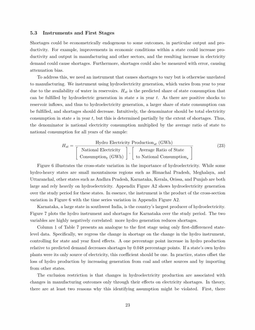
To address this, we need an instrument that causes shortages to vary but is otherwise unrelatedto manufacturing. We instrument using hydroelectricity generation, which varies from year to yeardue to the availability of water in reservoirs. Hst is the predicted share of state consumption thatcan be fulfilled by hydroelectric generation in state s in year t. As there are positive shocks toreservoir inflows, and thus to hydroelectricity generation, a larger share of state consumption canbe fulfilled, and shortages should decrease. Intuitively, the denominator should be total electricityconsumption in state s in year t, but this is determined partially by the extent of shortages. Thus,the denominator is national electricity consumption multiplied by the average ratio of state tonational consumption for all years of the sample:

Hst = Hydro Electricity Productionst (GWh)C

National ElectricityConsumptiont (GWh)

D

·C

Average Ratio of Stateto National Consumptions

D (23)

Figure 6 illustrates the cross-state variation in the importance of hydroelectricity. While somehydro-heavy states are small mountainous regions such as Himachal Pradesh, Meghalaya, andUttaranchal, other states such as Andhra Pradesh, Karnataka, Kerala, Orissa, and Punjab are bothlarge and rely heavily on hydroelectricity. Appendix Figure A2 shows hydroelectricity generationover the study period for these states. In essence, the instrument is the product of the cross-sectionvariation in Figure 6 with the time series variation in Appendix Figure A2.

Karnataka, a large state in southwest India, is the country’s largest producer of hydroelectricity.Figure 7 plots the hydro instrument and shortages for Karnataka over the study period. The twovariables are highly negatively correlated: more hydro generation reduces shortages.

Column 1 of Table 7 presents an analogue to the first stage using only first-di�erenced state-level data. Specifically, we regress the change in shortage on the change in the hydro instrument,controlling for state and year fixed e�ects. A one percentage point increase in hydro productionrelative to predicted demand decreases shortages by 0.048 percentage points. If a state’s own hydroplants were its only source of electricity, this coe�cient should be one. In practice, states o�set theloss of hydro production by increasing generation from coal and other sources and by importingfrom other states.

The exclusion restriction is that changes in hydroelectricity production are associated withchanges in manufacturing outcomes only through their e�ects on electricity shortages. In theory,there are at least two reasons why this identifying assumption might be violated. First, there

23

could be reverse causality: hydroelectricity generation could respond in equilibrium to changesin electricity demand associated with manufacturing outcomes. This is relatively unlikely: themarginal cost of hydroelectricity production is relatively low, and annual production is constrainedby the amount of water available behind reservoirs. By contrast, the exclusion restriction wouldbe violated for production technologies such as coal power plants that have higher marginal costs,because their output is determined in equilibrium with demand.

To substantiate this point, we gathered data from the Central Electricity Authority on inflowsinto 22 large reservoirs. Separately for each state with at least one reservoir, we regressed annualhydroelectricity generation on inflows and construct the fitted values. The R2 of the regression ofactual on predicted hydro generation is 0.86; this is illustrated in Appendix Figure A3. While theR2 should not be 1 because the data include reservoirs that supply only 40 percent of India’s hydro-electric generating capacity, the very high R2 indicates that inflows are the primary determinantsof hydroelectric production. Note that it is not possible to directly use inflows as our instrumentbecause only 2/5 of states that have positive hydro generation have reservoirs in the inflows data.

The second reason why the identifying assumption might be violated would be if rainfall or someother third variable influences both hydroelectricity generation and manufacturing productivity orinput or output prices. To address this, we can simply control for rainfall in our regressions, alongwith cooling degrees, which are correlated with rainfall and may a�ect agriculture. Although rainfallis associated with the hydro instrument, Column 2 of Table 7 shows that conditioning on rainfalland cooling degrees has very little impact on the state-level estimates aside from increasing thestandard error. By contrast, Column 3 shows that rainfall is associated with agricultural output,while there is a positive but not statistically significant association between the instrument andagricultural output.

Columns 4 and 5 of Table 7 present a placebo test that provides even more direct support forthe exclusion restriction. For an instrument to be valid, it needs to a�ect electricity supply butshould not be associated with demand. To test this, we exploit the fact that the CEA reports thetwo components of shortages: assessed quantity demanded at current prices as well as the actualquantity supplied. Column 4 shows that the instrument is associated with quantity supplied, butcolumn 5 shows that it is not associated with assessed demand. It is di�cult to conceive of astory under which the exclusion restriction is violated but the instrument is not associated withelectricity demand.

6 Empirical Results

6.1 First Stages

Table A3 in Appendix B.2 presents first stage estimates using microdata. In theory, the coe�-cient estimates might di�er from the state-level results in Table 7 because the microdata weights

24

states with more plants more heavily and because the microdata includes one-year and multi-yeardi�erences instead of only one-year di�erences. In practice, the microdata coe�cients are slightlylarger in absolute value but roughly comparable, ranging from -0.100 to -0.139. The instrumentsare powerful: the cluster and heteroskedasticity-robust Angrist-Pischke F-statistics range from 39to 53.19 For comparison, the Stock and Yogo (2005) critical values for one instrument and oneendogenous regressor are 8.96 and 16.38 for maximum 15 and 10 percent bias, respectively.

Appendix Tables A4 and A5 present first stages for the alternative specifications in the up-coming section that potentially have the least power. These two tables respectively consider thesample when self-generation share is the outcome variable, which is the smallest sample, and whenlog revenue is the outcome variable, which has the smallest F-stat in Appendix Table Table A3.When conditioning on rainfall and cooling degrees, including only one-year di�erences, or testinginteractions with shortages, the smallest F-statistic is 15.52. When clustering by state instead of bystate-by-year di�erence, the F-statistics are 12.52 and 7.51 for self-generation share and log output,respectively. In additional unreported regressions using two-way clustering by state-by-(final yearof the year di�erence) and state-by-(initial year of the year di�erence) based on the methodologyof Cameron, Gelbach, and Miller (2006), these F-statistics are 21.6 and 15.2, respectively.

6.2 Regression Results

Table 8 presents results of Equation (22) for four di�erent outcomes: self-generation share, naturallog of energy revenue share, natural log of revenues, and natural log of TFPR. Panels A and Bpresent OLS and instrumental variables results, respectively. The IV estimates are very reasonable.Columns 1 and 2 test for impacts on energy input, including in the sample only the 54 percent ofplants that ever self-generate. Column 1 shows that a one percentage point increase in shortages,which would increase the shortage variable from (for example) 0.1 to 0.11, causes a 0.57 percentagepoint increase in the share of self-generated electricity. If shortages a�ected manufacturers and allother consumers equally and manufacturing electricity demand were fully inelastic, this coe�cientshould be 1. In reality, state electricity boards may impose more or less of the marginal shortageon manufacturers instead of residential and agricultural consumers, and when manufacturers arefaced with shortages, they do not make up for them one-for-one with self-generation. Column 2shows that a one percentage point increase in shortages causes a 0.64 percentage point increase inenergy revenue share.

Either of columns 1 and 2 can be used to derive an estimate of the input cost e�ect for plantsthat self-generate. If pE,S ≠ pE,G=2.5 Rs/kWh (from the World Bank Enterprise Survey) and themean electric intensity is 0.013 kWh/Rupee (from Table 6), a one percentage point increase inshortages translates to a 1%◊0.57◊2.5◊0.013¥0.018 percent unit cost increase. In other words,

19The Angrist-Pischke F-statistics are identical to the Kleibergen-Paap F-statistics when there is one endogenousvariable. The Angrist-Pischke F-statistics are more appropriate in the parts of Appendix Tables A4 and A5 that testfor weak identification of individual endogenous regressors in regressions with multiple endogenous regressors.

25

a one percentage point increase in shortages increases self-generation by 0.57 percentage points,which increases average electricity costs by 0.57%◊2.5 Rs/kWh¥0.0142 Rs/kWh, which increasestotal unit costs by 0.0142 Rs/kWh*0.013 kWh/Rs¥0.018 percent of revenues. Similarly, using thefact that the mean energy revenue share is 0.11, the point estimate in Column 2 suggest that a onepercentage point increase in shortages increases energy input costs by 0.64%*0.11¥0.07 percent ofrevenues. While these two estimates di�er slightly, both imply that the input cost increase imposedon plants with generators is relatively small.

Columns 3 and 4 include all ASI plants, regardless of whether they self-generate or not. The IVestimates in column 3 show that a one percentage point increase in shortages causes a 0.68 percentdecrease in revenues. Hypothetically, if no plants self-generate and there were no shutdown taxe�ect (in which firms reduce semi-flexible inputs in response to shortages), this coe�cient wouldbe one. In reality, self-generation reduces the revenue loss for plants with generators. If firms canforesee and respond to changes in shortages driven by hydro generation, this would be o�set by thefact that both self-generators and non-generators reduce semi-flexible inputs through the outputtax e�ect and shutdown tax e�ect, respectively.

Column 4 shows that shortages have statistically zero e�ect on TFPR. The 90 percent confidenceinterval bounds the TFPR losses from a one percentage point increase in shortages at no more thana 0.29 percent decrease in TFPR. In our model, TFPR losses should be much smaller than outputlosses because the primary cause of TFPR loss is waste of inputs that are not fully flexible, andmost inputs are fully flexible - the average input cost share for materials across all plants is 70percent. Thus, the fact that TFPR losses are too small to detect is fully consistent with our model.

The OLS estimates are statistically and economically di�erent from the IV estimates, and thedirection suggest two forms of bias. With self-generation share in Column 1, we expect less omittedvariables bias in OLS. The fact that the IV estimates are substantially larger than OLS suggestthat the instrument corrects measurement error in the shortage variable. By contrast, with outputand TFPR in Columns 3 and 4, we expect potential upward bias in OLS, because economic growthcan cause shortages. Indeed, the OLS coe�cients are biased upwards from the IV coe�cients, andTFPR actually appears to be positively associated with shortages. This shows the importance ofusing instrumental variables: without the IV, one might erroneously conclude that shortages causeTFPR to increase.

6.2.1 Robustness Checks and Fixed E�ects Estimates

Appendix B.3 shows that the estimates in Table 8 are remarkably robust. None of the estimatesdi�ers statistically or loses statistical significance when weighting by the ASI sample weights, omit-ting the industry-by-year controls µjy, eliminating or tightening the flags for within-plant outliers,controlling for rainfall and cooling degrees, or using the CEA’s estimated Peak Shortage insteadof Shortage. When using only one-year di�erences, this focuses estimates on larger census schemeplants whose output is less a�ected by shortages and also reduces the sample size. This slightly

26

reduces the point estimate of e�ect on output and increases the standard error; the resulting coef-ficient is statistically indistinguishable from both the base case estimate and from zero. Clusteringat the state level instead of state-by-year di�erence increases the standard errors slightly but doesnot a�ect statistical significance. Appendix Table A14 shows that results are qualitatively similarunder five di�erent approaches to calculating production functions and TFPR.

Appendix B.4 estimates an analogue to Equation (22) using fixed e�ects instead of di�erences,including state-specific linear trends20 and clustering by state to address potential serial correlationin errors. The results are remarkably similar to Table 8, and none of the IV estimates di�erstatistically. However, the standard errors are slightly wider, and the first-stage F-statistics aresmaller. For these reasons, we focus on results from the di�erence estimator.

6.3 Moderators and Alternative Outcomes

The model in Section 3 generates predictions for how shortages should di�erentially a�ect di�erenttypes of plants. Electricity-intensive industries should be more likely to shut down instead of self-generate during shortages, meaning that revenues and TFPR should drop more. Furthermore,shortages should have much smaller e�ects on revenues and TFPR for plants that self-generate.Table 9 interacts the change in shortages with indicators for self-generation and whether the plant’sindustry is above-median electricity intensity; the regressions also include lower-order interactionswith ◊iy and Âs.

We fail to reject that more electric-intensive plants change self-generation the same amountin response to shortages, although their energy revenue share increases more. Shortages reduceoutput more for electric intensive plants and reduce output less for self-generators. The pointestimates suggest that non-generators’ revenues decrease more than one-for-one with shortages;this is consistent with the model, where non-generators lose output due to the shutdown e�ect andadditionally reduce semi-flexible inputs due to the shutdown tax e�ect. These standard errors arewider, however, and coe�cient magnitudes should be interpreted with caution. Precision would befurther reduced if we cut the data more finely or studied individual industries in isolation.

Table 10 tests for e�ects on other outcomes. The point estimate in column 1 suggests thatplants reduce labor input in response to shortages, but the e�ect is not close to being statisticallysignificant. Column 2 shows that a ten percentage point increase in shortages is associated withan 8.53 percent decrease in materials input. Column 3 shows that shortages decrease the materialsto labor ratio, consistent with columns 1 and 2. These estimates provide support for our modelingassumption in Section 7 that materials are fully flexible, while labor is not. Column 4 tests for

20Although excluding state-specific linear trends does not a�ect the non-IV estimates, the IV first stages have nopower when excluding the state-specific linear trends. The reason for this is suggested in Figure 7: the share of hydroin total electricity production has decreased over time in Karnataka and other states, so while annual changes in thehydro instrument are negatively associated with changes in shortages, levels of the instrument are not. Because thelevel of the hydro generation share decrease is mechanically larger in states with more hydro production, the yearindicators do not properly control for this in the fixed e�ects estimator.

27

e�ects on fuel revenue share, where fuels equal total energy net of electricity. The e�ect should beand is statistically larger than the e�ect on energy revenue share, because the latter includes anincrease in fuel input costs but a decrease in electricity purchases. Column 5 shows that shortagesdo not statistically a�ect electric intensity, measured in kWh per Rupee of revenues. In reality,there should be some small e�ect, consistent with the results from Fisher-Vanden, Mansur, andWang (2012) for Chinese manufacturers. Our standard errors rule out that a ten percent increasein shortages causes more than a 0.0005 kWh/Rupee decrease in electric intensity. This is about38 percent of the median, which is 0.013 kWh per Rupee. Although this could be economicallymeaningful, it provides some statistical support for our model’s simplifying assumption that ⁄ isexogenous.

7 Simulations

7.1 Overview

In this section, we calibrate the model in Section 3 to the distribution of plants and productionfunction parameters in the Annual Survey of Industries data. This parallels the empirical estimatesin that both are based on the ASI, but here we simulate shortage e�ects instead of estimating them.

First, we simulate e�ects of shortages holding fixed each plant’s observed generator adoption de-cision from the ASI; we call these the exogenous generator simulations. We also present simulationswith endogenous generator adoption decisions, which can be thought of as simulating the long-rune�ects of shortages. The endogenous generator simulations extend the empirical estimates fromthe previous section, which primarily identify short-run e�ects because they are largely identifiedo� of annual variation. We then study how shortages di�erentially a�ect small vs. large plants andconsider a counterfactual scenario using interruptible electricity contracts.

The simulations consider the population of plants that appear in the ASI in 2005. We report themean e�ect across plants, weighted by each plant’s sampling weight. This is di�erent than reportingoutput-weighted e�ects, which might be informative about aggregate sectoral implications. We dothis to more closely match our empirical estimates, which are also not weighted by output. Output-weighted e�ects on revenues, TFPR, and profits would be smaller, because the largest plants aremuch more likely to own generators.

Shortage ” is the CEA estimate for each plant’s state in 2005; this averages 7.1 percent acrossall plants.2122 Appendix Table A17 presents parameters used to calibrate the model. Production

21We chose 2005 because it is both recent and very close to average: over the 1992-2010 sample, the averagenationwide shortage ranged from 6.4 to 11.1 percent, and the mean reported in Table 1 is 7.2 percent.

22This assumes that all plants within a state are subject to the average outage rate. In reality, some plants orindustrial areas have preferential electricity access, while others are in areas with particularly poor supply, and thiswithin-state variation may be correlated with losses from outages. Unfortunately, this plant-specific variation isnot possible to quantify on a nationwide basis. We also assume that shortages only act through blackouts and notthrough variations in quality such as lower voltage. Note that the empirical estimates in Section 6 do not require theseassumptions: the empirical estimates reflect the causal relationship between state average shortage and manufacturing

28

function parameters are estimated as detailed in Section 3.5. For the relative cost of grid-purchasedvs. self-generated electricity (pE,G vs. pE,S), we use the World Bank Enterprise Survey medians.Only the ratio of pE,S to pE,G matters; from Table 2, this is 7/4.5 ¥ 1.56.

7.1.1 Modeling the Generator Purchase Decision

We model the decision to purchase a generator as a binary choice: either a plant owns a generatorwhich is large enough to provide full backup during a power outage, or it does not own a generator.Because the ASI does not include data on generator capacity, we first calculate a simple, back-of-the-envelope estimate of each plant’s capacity requirement. To do this, we transform a plant’stotal electricity consumption Eit (in kilowatt-hours) into the capacity required to provide thatconsumption assuming that plants use an equal flow of power for six hours per day, 365 days ayear. Under this assumption, the median plant, for example, would require a generator with about500 kilowatts (KW) of capacity.

A plant will purchase a generator if its generator cost is less than its variable profit increase. Thevariable profit increase is calculated by simulating variable profits with and without a generator, byinserting optimized labor and materials inputs into Equation (4). Based on conversations with threedi�erent generator vendors in India, we assume an annualized cost of Rs 1374 per KW capacity.

7.2 Predictions

Table 11 presents e�ects of shortages on manufacturers’ revenue, TFPR, and profits. Columns 1 and2 present simulated e�ects with exogenous and endogenous generators, respectively23. To facilitatecomparisons, the remainder of the columns restate results from earlier in the paper. Column 3 addspredictions based on the ASI empirical estimates: the predicted e�ects of a 7.1 percent shortagegiven the IV coe�cients in Table 8. Column 4 presents the p-value of a test that the exogenousgenerator simulation results di�er from the IV coe�cient, with standard errors calculated usingthe Delta method. Column 5 restates the textile case study results from Section 4, while Column6 gives self-reported output losses from the World Bank Enterprise Survey discussed in Section 2.

7.2.1 Exogenous Generator Predictions

The predictions with exogenous generators in Column 1 of Table 11 show that the average plantloses 4.6 percent of revenues due to a 7.1 percent electricity shortage. This revenue loss is verydi�erent for plants that have a generator versus those that do not. Plants with generators lose only0.4 percent of revenues. The reason why this is so small is that there is no “shutdown e�ect,” i.e.

outcomes, but they do not assume that manufacturers face that same average shortage or that the average shortagedoes not a�ect power quality.

23Since the model is not set up to exactly match each plant’s observed input choices of labor and materials, wesimulate both the shortage and no-shortage counterfactuals and present the di�erence. If we instead compared theobserved equilibrium to counterfactual simulations with no shortages, we would be capturing both the e�ects ofshortages and the model’s prediction error.

29

no output is lost due to shutdown. Instead, all revenue losses come through the output tax e�ect:the reduction in the marginal product of materials and labor due to higher-cost self-generatedelectricity. The implicit output tax T during outage periods is 2.8 percent: the 55 percent increasein electricity price when self-generating times the 5 percent revenue share of electricity. Given thatshortages occur 7.1 percent of the year, weighted average unit input cost across all periods wouldrise by 2.8%◊7.1%¥0.2% if output were constant, and slightly less given that plants reduce outputduring blackouts. The e�ect on revenue is small because this implicit tax is small.

By contrast, revenues fall by 9.6 percent for plants that do not have generators. This e�ect islarger than the 7.1 percent of the time when the plant cannot operate due to shortages, becausethe e�ect of shortages is amplified through the shutdown tax e�ect: expected power outages reducethe expected marginal revenue product of the semi-flexible input (labor) by ”, causing firms toreduce labor input. The large simulated e�ects for non-generators and small simulated e�ectsfor self-generators are closely consistent with the di�erential IV estimates for generators and non-generators reproduced in Column 3. This is also consistent with the small revenue losses for textileplants with generators reproduced in Column 5.

Table 11 also shows the predicted e�ects of shortages on measured TFPR. As with revenue, theTFPR losses are very di�erent for non-generators vs. self-generators: 3.4 percent vs. almost zero,respectively. The average TFPR loss is 1.6 percent. For plants that have generators, the TFPRloss is driven by the input variation e�ect: with a concave production function, it would have beenmore e�cient to produce with a constant input bundle instead of di�erent input bundles duringoutage vs. non-outage periods. Since plants that have generators do not reduce output very muchduring outages given the small implicit output tax T , the input variation e�ect is quite small.

By contrast, the shutdown e�ect on TFPR - non-generators’ loss of non-storable inputs of laborand capital during power outages - is much larger. If no inputs were fully flexible, then a 7.1 percentshortage would translate directly into a 7.1 percent TFPR loss for non-generators. However, plantsthat shut down during power outages can store materials. Given that the sum of labor and capitalshares averages 20 percent, the shutdown e�ect on TFPR is much less than the 7.1 percent of thetime that non-generators shut down due to outages.

7.2.2 Endogenous Generator Predictions

The large di�erence in losses between plants with vs. without generators begs the question of whymany plants choose not to purchase generators. Can the simulations rationalize decisions to notpurchase a generator?

The bottom part of Column 2 of Table 11 shows that 72 percent of plants are predicted topurchase generators. This is higher than the 54 percent of plants that ever report producingpower and appear in the 2005 ASI, but substantially less than 100 percent. We can thus easilyrationalize the incomplete generator adoption observed in the ASI: even if there are large lossesfrom not purchasing generators, the capital cost is high enough that many plants do not adopt. The

30

share of plants that purchase generators is not very sensitive to the assumed generator cost. Forexample, at costs of 940 and 1500 Rupees per KW-year, respectively, 78 and 70 percent of plantspurchase generators; the elasticity of generator adoption with respect to generator cost is -0.14.This inelasticity is due to a wide dispersion across plants of variable profit gains from generatorownership, which is primarily driven by the wide revenue productivity dispersion observed in theASI, which is ubiquitous in producer-level datasets (Syverson 2011).

Column 2 in Table 11 shows that when generator adoption is endogenous, shortages are predictedto reduce revenues by 0.8 percent, TFPR by 0.1 percent, and variable profits by 0.9 percent. Thevariable profit losses do not include generator capital costs. This cost represents another 1.6 percentof profits for plants with generators, for a total profit loss of 2.3 percent for plants with generators.Taking the mean across the 72 percent of plants with generators and the 28 percent of plants withoutgenerators, the total profit loss including generator capital costs is 72%◊2.3% + 28%◊1.6%¥2.1percent.

The predicted losses in Column 2 are much smaller than with exogenous generator ownershipin Column 1, because the simulation in Column 2 allocates generators to plants with the highestsimulated gains. By contrast, the generator adoption choices observed in the data depend onunobserved factors, so in Column 1 generators are not allocated to plants that are simulated tobenefit from them the most.

7.2.3 Predictions: Models versus Regressions

Because the empirical estimates are identified o� of annual variation in hydroelectric output, plantsare unlikely to respond by changing generator stock, so it is most appropriate to compare empiricalestimates to the exogenous generator simulations in Column 1. There is remarkable agreementbetween the empirical estimates and simulation results, especially once we account for the role ofgenerators. Column 3 shows that the IV estimates predict that 7.1 percent average shortages reduceaverage revenues by 4.8 percent, against a simulated value of 4.6 percent in Column 1. Both the IVestimates and simulations predict that revenue losses for generators are very small and that revenuelosses for non-generators are larger than the 7.1 percent average shortage. Finally, both the IV andsimulations predict that TFPR losses are much smaller than revenue losses and that TFPR lossesare focused on non-generators. Column 4 shows that all estimates are statistically indistinguishable,although one of the six is di�erent with only slightly less than 90 percent confidence.

The results of the textile case study and World Bank Enterprise Survey data are also qualita-tively consistent. All textile plants in the Bloom et al. (2013) data have generators, and revenueand TFPR losses from weekly power holidays are relatively small. The World Bank self-reportedrevenue losses are close to the simulation result and not statistically di�erent from our IV estimates,and non-generators report larger losses than self-generators. Interestingly, however, self-generatorsstill report 7.3 percent losses, which is larger than our empirical estimates or model can explain.

31

This highlights the importance of using actual empirical estimates instead of self-reports.24

Overall, the close correspondence between our model and estimates using di�erent datasets andidentification strategies gives us confidence in the empirical estimates as well as our understandingof the underlying mechanisms.

7.3 Robustness

How sensitive are the results to alternative assumptions? In the baseline estimates, we assume thatplants face a CES demand curve with demand elasticity ‘ = ≠10. This elasticity is important be-cause it determines the markup (‘ = ≠10 implies a -1/‘=10 percent markup) and thus profitability.It also determines how revenue responds to costs: when demand is more inelastic, a given change incosts results in a smaller change in output. When we use an elasticity of ‘ = ≠4 in the exogenousgenerator simulations, consistent with Bloom (2009) and Asker, Collard-Wexler, and De Loecker(2014), revenues drop by 4.0 percent instead of 4.6 percent.25 When we assume that self-generatedelectricity actually costs four times as much as grid electricity, or 18 Rupees/kWh instead of theWorld Bank median of 7, revenue losses are 5.5 percent instead of 4.6 percent. Appendix TableA18 presents the detailed results of these alternative simulations. While our assumptions on de-mand elasticity and price of self-generated electricity are relatively di�cult to substantiate, ourqualitative conclusions do not hinge on these assumptions.

7.4 Predictions Under Varying Shortage Levels

Table 12 simulates the e�ects of shortages at levels ranging from 3 to 20 percent relative to zeroshortage. While this table is structured similarly to Table 11, the exact results are not comparablebecause Table 12 assumes that all plants nationwide face the same shortage, instead of their state-specific shortage from 2005. The top and bottom panels present simulations with exogenous andendogenous generators, respectively.

With exogenous generator choices, average revenue losses increase linearly from 1.9 to 13 per-cent as average shortages increase from 3 to 20 percent. By contrast, with endogenous generatoradoption, the average revenue loss rise non-linearly from 0.7 percent to 1.5 percent as shortages

24It could be that managers of plants with generators interpreted the question as to include capital costs ofgenerators. Such alternative interpretations of self-reported data are yet another reason why empirical estimates areimportant.

25To get a sense of whether our simulations are reasonable, we can compare results to Davis, Grim, and Haltiwanger(2008), who investigate the elasticity of revenue with respect to the price of electricity in the United States. Since apower outage is equivalent to an increase in the price of electricity for plants with generators, we can compare theelasticity of revenue with respect to electricity price in our model to the one estimated in Davis, Grim and Haltiwanger(2008). We compute an elasticity of revenue with respect to the price of electricity of -0.2 when we assume ‘ = ≠10,and -0.4 when we assume ‘ = ≠20, while Davis, Grim and Haltiwanger (2008) find an elasticity of -0.6. If anything,our model thus under-predicts the response of revenue to shortages for generators, but not by a large amount. On theother hand, the Davis, Grim, and Haltiwanger (2008) estimate is quite large, and it is somewhat di�cult to explaingiven how small electricity is as a share to total costs.

32

increase from 3 to 20 percent. With endogenous generators, the average revenue loss reflects thecombination of two forces. First, revenue losses increase as shortages worsen for both generatorsand non-generators. Second, however, more plants adopt generators as shortages worsen, and rev-enue losses are smaller for plants with generators. This decreases the weighted average revenueloss.

Variable profit losses scale very closely with revenue losses in percentage terms. The second-to-bottom row in each panel presents generator capacity costs as a percent of profits. With exogenousgenerator choices, this is constant at 2.5 percent of profits. With endogenous choices, this increasesmonotonically in the shortage as takeup rate increases. Total profit losses are the sum of variableprofit losses and generator capacity costs.

7.5 Impact of Shortages by Plant Size

How do electricity shortages a�ect di�erent types of plants? Hsieh and Klenow (2012) proposethat electricity shortages combined with di�erential access to grid electricity could be an impor-tant factor benefiting large plants. We focus on a di�erent mechanism for di�erential impacts byplant size: economies of scale in self-generation. On a broader level, these economies of scale areimportant, and they explain why electricity is usually generated by a few centralized power plants.For manufacturers, capacity is much cheaper for larger plants: typical generator prices drop by 30to 45 percent as capacity increases from 60 to 1,000 KW.

Figure 8 presents the non-parametric relationship between plant size and predicted variableprofit losses in the exogenous generator simulation with 7.1 percent average shortages, which is thesame setup as Column 1 of Table 11. Plants with 10 workers face an average profit loss of sevenpercent, while plants with 1000 workers su�er a two percent average profit loss. These di�erencesare driven almost entirely by the empirical distribution of generator ownership: 23 percent of smallplants in 2005 have generators, while 55 percent of large plants have them. Appendix Table A19presents additional simulation results for large vs. small plants, as well as more vs. less electricintensive plants.

7.6 Counterfactual: E�ects of Shortages with Interruptible Contracts

Given that 54 percent of manufacturing plants use generators, this “distributed generation” pro-vides production capacity that would optimally be exploited during times of scarcity. Currently,there are plants that have generators but don’t use them because they receive grid power, whileother nearby plants without generators simultaneously experience outages. Interruptible electricitycontracts o�er consumers a rebate for accepting outages during times of scarcity. If distributioncompanies o�er both uninterruptable and interruptible contracts and allow consumers to sort intotheir preferred contract, this provides a mechanism to allocate outages to plants that are leasta�ected.

33

We simulate the e�ects of allowing plants to select into one of two contracts, one which willnever experience outages, and one which will experience outages 14.2 percent of the time - twicethe national average outage rate. The market-clearing rebate for the interruptible contract ispinned down by the maximum profit loss of the plants that comprise 50 percent of grid electricityconsumption. When this 50 percent of consumption is interrupted 14.2 percent of the time, thisallows the uninterruptible contracts to be fulfilled. Because larger plants have generators and arethus willing to accept interruptible contracts at lower rebates, only 8.9 percent of plants need toopt into the interruptible contract to clear the market. Under this counterfactual policy, revenue,TFPR, and variable profit losses average only 0.15, 0.04, and 0.20 percent, respectively. Theselosses are much smaller than the 4.6, 1.6, and 6.8 percent reported in Column 1 of Table 11.

8 Conclusion

India’s lack of reliable electricity supply provides a stark example of how poor infrastructure a�ectseconomic growth. We study the e�ects of shortages on manufacturing using archival data onshortages, previously-unavailable panel data from the Annual Survey of Industries, and a newinstrument for shortages based on variation in hydro reservoir inflows. We augment this with adetailed case study of how textile plants in Bloom et al. (2013) respond to planned power holidays.We use a hybrid Leontief/Cobb-Douglas production function model to clarify the di�erent ways inwhich input shortages a�ect firms and use simulations to confirm empirical results and extend tothe “long-run” case with endogenous generator adoption.

There are three main conclusions. First, electricity shortages are a large drag on Indian man-ufacturing, on the order of five percent of revenue. Second, however, electricity shortages a�ectproductivity much less than revenue, and shortages alone certainly do not explain much of theproductivity gap between firms in developing vs. developed countries. Third, shortages have het-erogeneous e�ects across plants with vs. without generators and with high vs. low electric intensity.Relatedly, because of economies of scale in self-generation, small plants are less likely to own gen-erators, meaning that shortages have much stronger negative e�ects on small plants. This addsanother distortion to the firm size distribution in developing countries, related to the discussion ofHsieh and Olken (2014), Tybout (2000), and others.

Even if it is infeasible to su�ciently increase generation capacity or to raise electricity pricesduring periods of scarcity, our analysis suggests that two policy changes could reduce losses fromshortages. First, our textile case study illustrates how advance knowledge of outages throughplanned power holidays can mitigate TFP losses by making additional inputs storable. Second,mechanisms such as interruptible contracts allow plants that have lower costs of outages to revealthis to the distribution company. This allows shortages to be “targeted” at firms that can moreeasily accommodate them.

34

References[1] Abeberese, Ama Baafra (2012). “Electricity Cost and Firm Performance: Evidence from India.” Working

Paper, Columbia University (November).

[2] Alby, Philippe, Jean-Jacques Dethier, and Stephane Straub (2011). “Let There be Light! Firms Op-erating under Electricity Constraints in Developing Countries.” Working Paper, Toulouse School ofEconomics (July).

[3] Aschauer, David (1989). “Is Public Expenditure Productive?” Journal of Monetary Economics, Vol.23, No. 2 (March), pages 177-200.

[4] Asker, John, Allan Collard-Wexler, and Jan De Loecker (2014). "Dynamic Inputs and Resource(Mis)Allocation.” Journal of Political Economy, forthcoming.

[5] Baisa, Brian, Lucas Davis, Stephen Salant, and William Wilcox (2008). “The Welfare Costs of UnreliableWater Service.” Journal of Development Economics, Vol. 92, No. 1 (May), pages 1–12.

[6] Banerjee, Abhijit, and Esther Duflo (2005). “Growth Theory through the Lens of Development Eco-nomics.” In Aghion, Philippe, and Steven Durlauf, Eds., Handbook of Economic Growth.

[7] Banerjee, Abhijit, and Esther Duflo (2010). “Giving Credit Where It Is Due.” Journal of EconomicPerspectives, Vol. 24, No. 3 (Summer), pages 61-80.

[8] Banerjee, Abhijit, and Esther Duflo (2012). “Do Firms Want to Borrow More? Testing Credit Con-straints Using a Directed Lending Program." Working Paper, MIT.

[9] Banerjee, Abhijit, Esther Duflo, and Nancy Qian (2012). “On the Road: Access to TransportationInfrastructure and Economic Growth in China.” Working Paper, Yale University (February).

[10] Bartelsman, Eric, John Haltiwanger, and Stefano Scarpetta (2013). “Cross-Country Di�erences in Pro-ductivity: The Role of Allocation and Selection.” American Economic Review, Vol. 103, No. 1 (Febru-ary), pages 305-334.

[11] Baum-Snow, Nathaniel (2007). “Did Highways Cause Suburbanization?” Quarterly Journal of Eco-nomics, Vol. 122, No. 2, pages 775-805.

[12] Baum-Snow, Nathaniel (2013). “Urban Transport Expansions, Employment Decentralization, and theSpatial Scope of Agglomeration Economies.” Working Paper, Brown University (October).

[13] Baum-Snow, Nathaniel, Loren Brandt, J. Vernon Henderson, Matthew Turner, and Qinghua Zhang(2013). “Roads, Railroads, and the Decentralization of Chinese Cities.” Working Paper, Brown Univer-sity (October).

[14] Baum-Snow, Nathaniel, and Matthew Turner (2012). “Transportation and the Decentralization of Chi-nese Cities.” Working Paper, Brown University (May).

[15] Bhargava, Anjuli, and Kandula Subramaniam (2009). “Watts Not Happening.” Business World, July6th.

[16] Bloom, Nicholas, Benn Eifert, Aprajit Mahajan, David McKenzie, and John Roberts (2013). “DoesManagement Matter? Evidence from India.” Quarterly Journal of Economics, Vol. 128, No. 1 (Febru-ary), pages 1-51.

[17] Cameron, Colin, Jonah Gelbach, and Douglas Miller (2006). “Robust Inference with Multi-Way Clus-tering.” NBER Technical Working Paper 327 (September).

[18] Central Electricity Authority (2013). “Monthly Executive Summary Report.”http://www.cea.nic.in/reports/monthly/executive_rep/feb13/feb13.pdf

[19] Central Electricity Authority (2013a). “Planwise Capacity Addition.”http://www.cea.nic.in/reports/planning/plan_addition.pdf

35

[20] Chakravorty, Ujjayant, Martino Pelli, and Beyza Ural Marchand (2013). “Does the Quality of ElectricityMatter? Evidence from Rural India.” Working Paper, Tufts University (April).

[21] Chan, Hei Sing (Ron), Maureen Cropper, and Kabir Malik (2014). “Are Power Plants in India LessE�cient than Power Plants in the United States?” American Economic Review, Papers and Proceedings,forthcoming.

[22] Cropper, Maureen, Alexander Limonov, Kabir Malik, and Anoop Singh (2011). “Estimating the Impactof Restructuring on Electricity Generation E�ciency: The Case of the Indian Thermal Power Sector.”NBER Working Paper No. 17383 (September).

[23] Davis, Steven, Cheryl Grim, and John Haltiwanger (2008). "Productivity Dispersion and Input Prices:The Case of Electricity." Working Paper 08-33, Center for Economic Studies, U.S. Census Bureau.

[24] De Loecker, Jan, and Frederic Warzynski (2012). “Markups and Firm-Level Export Status.” AmericanEconomic Review, Vol. 102, No. 6 (October), pages 2437-2471.

[25] Dinkelman, Taryn (2011). The E�ects of Rural Electrification on Employment: New Evidence fromSouth Africa.” American Economic Review, Vol. 101, No. 7 (December), pages 3078-3108.

[26] Donaldson, David (2012). “Railroads of the Raj: Estimating the Impact of Transportation Infrastruc-ture.” American Economic Review, forthcoming.

[27] Donaldson, David, and Richard Hornbeck (2013). “Railroads and American Economic Growth: A “Mar-ket Access” Approach.” NBER Working Paper No. 19213 (July).

[28] Duflo, Esther, and Rohini Pande (2007). “Dams.” Quarterly Journal of Economics, Vol. 122, No. 2,pages 601-646.

[29] Easterly, William, and Sergio Rebelo (1993). “Fiscal Policy and Economic Growth.” Journal of MonetaryEconomics, Vol. 32, pages 417-458.

[30] Esfahani, Hadi Salehi, and Maria Teresa Ramirez (2002). "Institutions, Infrastructure, and EconomicGrowth.” Journal of Development Economics, Vol. 70, pages 443-477.

[31] Fernald, John (1999). “Roads to Prosperity? Assessing the Link Between Public Capital and Produc-tivity.” American Economic Review, Vol. 89, No. 3 (June), pages 619-638.

[32] Fisher-Vanden, Karen, Erin Mansur, and Qiong (Juliana) Wang (2012). “Costly Blackouts? MeasuringProductivity and Environmental E�ects of Electricity Shortages.” NBER Working Paper No. 17741(January).

[33] Foster, Vivien, and Jevgenijs Steinbuks (2009). “Paying the Price for Unreliable Power Supplies: In-House Generation of Electricity by Firms in Africa.” World Bank Policy Research Paper 4913 (April).

[34] Government of India (GOI) (2009, 2012). Measures for Operationalising Open Access in the Power Sector.New Delhi, India: Secretariat for the Committee on Infrastructure.

[35] Holtz-Eakin, Douglas (1994). “Public-Sector Capital and the Productivity Puzzle.” Review of Economicsand Statistics, Vol. 76, No. 1 (February), pages 12-21.

[36] Hsieh, Chang-Tai, and Peter Klenow (2012). “The Life Cycle of Plants in India and Mexico.” WorkingPaper, University of Chicago (May).

[37] Hsieh, Chang-Tai, and Peter Klenow (2009). “Misallocation and Manufacturing TFP in China andIndia.” Quarterly Journal of Economics, Vol. 124, No. 4 (November), pages 1403-1448.

[38] Hsieh, Chang-Tai, and Benjamin Olken (2014). “The Missing “Missing Middle.”” NBER Working PaperNo. 19966 (March).

[39] Hulten, Charles, Esra Bennathan, and Sylaja Srinivasan (2006). "Infrastructure, Externalities, andEconomic Development: A Study of the Indian Manufacturing Industry.” World Bank Economic Review,Vol. 20, No. 2, pages 291–308.

36

[40] Jensen, Robert (2007). “The Digital Provide: Information (Technology), Market Performance, andWelfare in the South Indian Fisheries Sector.” Quarterly Journal of Economics, Vol. 122, No. 3 (August),pages 879-924.

[41] Lipscomb, Molly, Ahmed Mushfiq Mobarak, and Tania Barham (2013). “Development E�ects of Elec-trification: Evidence from the Topographic Placement of Hydropower Plants in Brazil.” American Eco-nomic Journal: Applied Economics, Vol. 5 No. 2, (April), pages 200–231.

[42] McRae, Shaun (2013). “Infrastructure Quality and the Subsidy Trap.” American Economic Review,forthcoming.

[43] Nagaraj, R. (2002). “How to Improve India’s Industrial Statistics,” Economic and Political Weekly, Vol.37, No. 10 (Mar. 9-15), pages 966-970.

[44] Rauch, James (1995). “Bureaucracy, Infrastructure, and Economic Growth: Evidence from U.S. CitiesDuring the Progressive Era.” American Economic Review, Vol. 85, No. 4 (September), pages 968-979.

[45] Reinikka, Ritva, and Jakob Svensson (2002). “Coping with Poor Public Capital.” Journal of DevelopmentEconomics, Vol. 69, pages 51-69.

[46] Restuccia, Diego, and Richard Rogerson (2008). “Policy Distortions and Aggregate Productivity withHeterogeneous Establishments.” Review of Economic Dynamics, Vol. 11, pages 707-720.

[47] Roller, Lars-Hendrik, and Leonard Waverman (2001). "Telecommunications Infrastructure and Eco-nomic Development: A Simultaneous Approach.” American Economic Review, Vol. 91, No. 4 (Septem-ber), pages 909-923.

[48] Ryan, Nicholas (2013). “The Competitive E�ects of Transmission Infrastructure in the Indian ElectricityMarket.” Working Paper, MIT (September).

[49] Rud, Juan Pablo (2012a). “Electricity Provision and Industrial Development: Evidence from India.”Journal of Development Economics, Vol. 97, pages 352-367.

[50] Rud, Juan Pablo (2012b). “Infrastructure Regulation and Reallocations within Industry: Theory andEvidence from Indian Firms.” Journal of Development Economics, Vol. 99, pages 116-127.

[51] Steinbuks, Jevgenijs, and Vivien Foster (2010). “When Do Firms Generate? Evidence on In-HouseElectricity Supply in Africa.” Energy Economics, Vol. 32, pages 505-514.

[52] Steinbuks, Jevgenijs (2011). “Financial Constraints and Firms’ Investment: Results from a NaturalExperiment Using Power Interruption.” Working Paper, Purdue University (October).

[53] Stock, James, and Motohiro Yogo (2005). “Testing for Weak Instrumentsin Linear IV Regression.” In Stock, James, and Donald Andrews, Eds.,Identification and Inference for Econometric Models: Essays in Honor of Thomas J. Rothenberg.Cambridge, England: Cambridge University Press.

[54] Straub, Stephane (2008). “Infrastructure and Development: A Critical Appraisal of the Macro-LevelLiterature.” World Bank Policy Research Working Paper No. 4590 (April).

[55] Chad Syverson, 2011. “What Determines Productivity?” Journal of Economic Literature, Vol. 49, No.2, pages 326-65 (June).

[56] Tybout, James (2000). “Manufacturing Firms in Developing Countries: How Well Do They Do, andWhy?” Journal of Economic Literature, Vol. 38, No. 1 (March), pages 11-44.

[57] U.S. DOE (Department of Energy) (2013). “Manufacturing Energy Consumption Survey.”http://www.eia.gov/consumption/manufacturing/index.cfm

[58] Zuberi, James (2012). “Estimating the Cost of Power Outages for Large Scale Manufacturing Firms.”Working Paper, University of California at Berkeley (November).

37

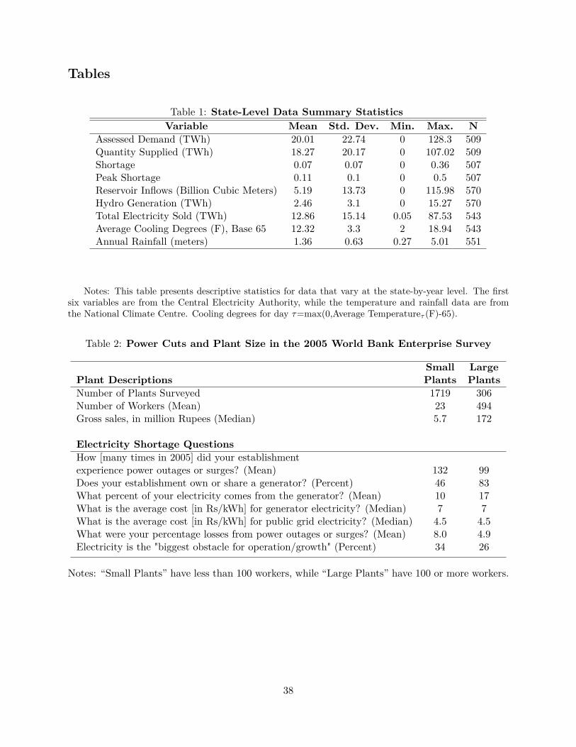
Tables

Table 1: State-Level Data Summary StatisticsVariable Mean Std. Dev. Min. Max. N

Assessed Demand (TWh) 20.01 22.74 0 128.3 509Quantity Supplied (TWh) 18.27 20.17 0 107.02 509Shortage 0.07 0.07 0 0.36 507Peak Shortage 0.11 0.1 0 0.5 507Reservoir Inflows (Billion Cubic Meters) 5.19 13.73 0 115.98 570Hydro Generation (TWh) 2.46 3.1 0 15.27 570Total Electricity Sold (TWh) 12.86 15.14 0.05 87.53 543Average Cooling Degrees (F), Base 65 12.32 3.3 2 18.94 543Annual Rainfall (meters) 1.36 0.63 0.27 5.01 551

Notes: This table presents descriptive statistics for data that vary at the state-by-year level. The firstsix variables are from the Central Electricity Authority, while the temperature and rainfall data are fromthe National Climate Centre. Cooling degrees for day ·=max(0,Average Temperature· (F)-65).

Table 2: Power Cuts and Plant Size in the 2005 World Bank Enterprise Survey

Small LargePlant Descriptions Plants PlantsNumber of Plants Surveyed 1719 306Number of Workers (Mean) 23 494Gross sales, in million Rupees (Median) 5.7 172

Electricity Shortage QuestionsHow [many times in 2005] did your establishmentexperience power outages or surges? (Mean) 132 99Does your establishment own or share a generator? (Percent) 46 83What percent of your electricity comes from the generator? (Mean) 10 17What is the average cost [in Rs/kWh] for generator electricity? (Median) 7 7What is the average cost [in Rs/kWh] for public grid electricity? (Median) 4.5 4.5What were your percentage losses from power outages or surges? (Mean) 8.0 4.9Electricity is the "biggest obstacle for operation/growth" (Percent) 34 26

Notes: “Small Plants” have less than 100 workers, while “Large Plants” have 100 or more workers.

38

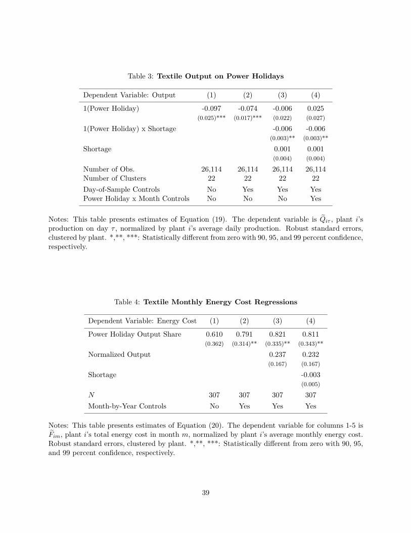
Table 3: Textile Output on Power Holidays

Dependent Variable: Output (1) (2) (3) (4)

1(Power Holiday) -0.097 -0.074 -0.006 0.025(0.025)*** (0.017)*** (0.022) (0.027)

1(Power Holiday) x Shortage -0.006 -0.006(0.003)** (0.003)**

Shortage 0.001 0.001(0.004) (0.004)

Number of Obs. 26,114 26,114 26,114 26,114Number of Clusters 22 22 22 22Day-of-Sample Controls No Yes Yes YesPower Holiday x Month Controls No No No Yes

Notes: This table presents estimates of Equation (19). The dependent variable is ÂQi· , plant i’sproduction on day · , normalized by plant i’s average daily production. Robust standard errors,clustered by plant. *,**, ***: Statistically di�erent from zero with 90, 95, and 99 percent confidence,respectively.

Table 4: Textile Monthly Energy Cost Regressions

Dependent Variable: Energy Cost (1) (2) (3) (4)

Power Holiday Output Share 0.610 0.791 0.821 0.811(0.362) (0.314)** (0.335)** (0.343)**

Normalized Output 0.237 0.232(0.167) (0.167)

Shortage -0.003(0.005)

N 307 307 307 307Month-by-Year Controls No Yes Yes Yes

Notes: This table presents estimates of Equation (20). The dependent variable for columns 1-5 isÂFim, plant i’s total energy cost in month m, normalized by plant i’s average monthly energy cost.Robust standard errors, clustered by plant. *,**, ***: Statistically di�erent from zero with 90, 95,and 99 percent confidence, respectively.

39

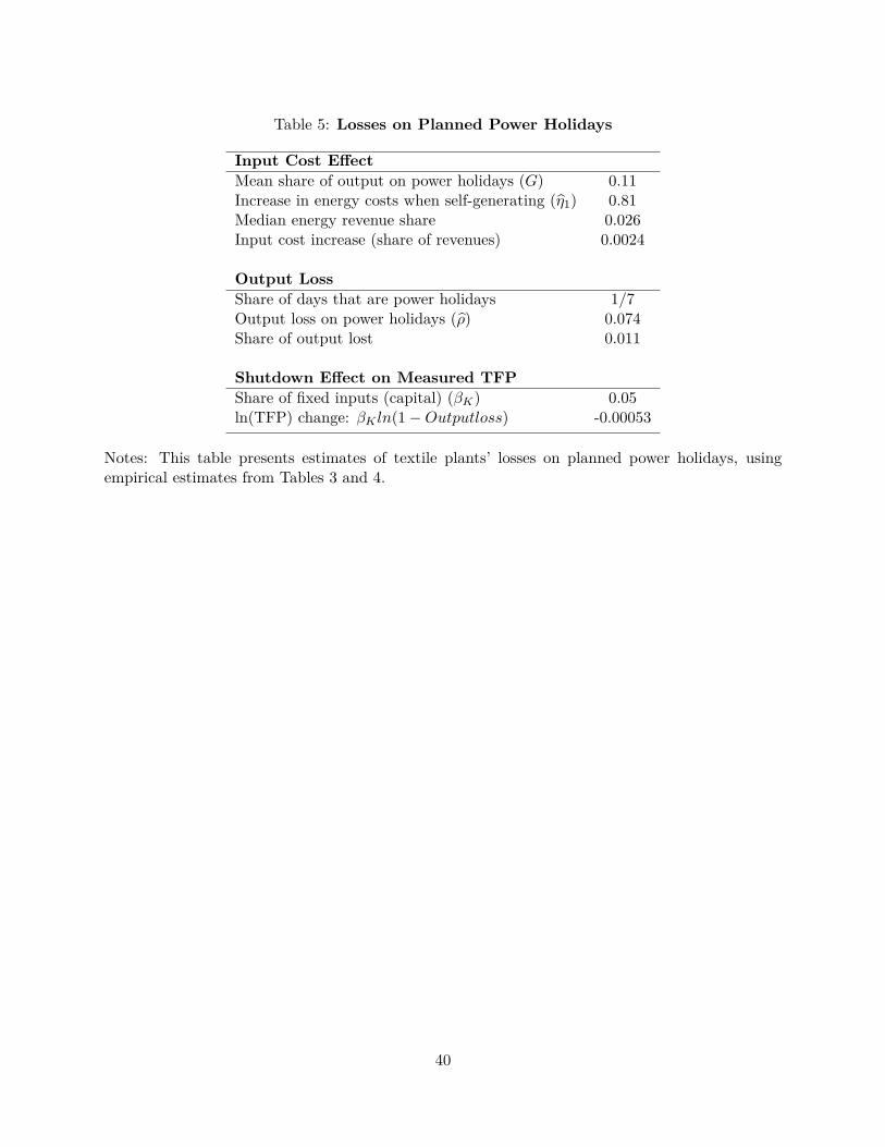
Table 5: Losses on Planned Power Holidays

Input Cost E�ectMean share of output on power holidays (G) 0.11Increase in energy costs when self-generating (‚÷1) 0.81Median energy revenue share 0.026Input cost increase (share of revenues) 0.0024

Output LossShare of days that are power holidays 1/7Output loss on power holidays (‚fl) 0.074Share of output lost 0.011

Shutdown E�ect on Measured TFPShare of fixed inputs (capital) (—K) 0.05ln(TFP) change: —K ln(1 ≠ Outputloss) -0.00053

Notes: This table presents estimates of textile plants’ losses on planned power holidays, usingempirical estimates from Tables 3 and 4.

40

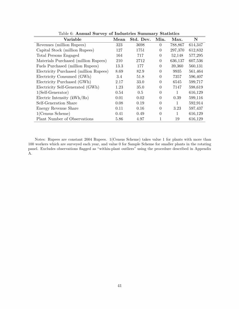
Table 6: Annual Survey of Industries Summary StatisticsVariable Mean Std. Dev. Min. Max. N

Revenues (million Rupees) 323 3698 0 788,867 614,347Capital Stock (million Rupees) 127 1751 0 297,370 612,832Total Persons Engaged 164 717 0 52,148 577,295Materials Purchased (million Rupees) 210 2712 0 636,137 607,536Fuels Purchased (million Rupees) 13.3 177 0 39,360 560,131Electricity Purchased (million Rupees) 8.69 82.9 0 9935 561,464Electricity Consumed (GWh) 3.4 51.8 0 7357 596,407Electricity Purchased (GWh) 2.17 33.0 0 6545 599,717Electricity Self-Generated (GWh) 1.23 35.0 0 7147 598,6191(Self-Generator) 0.54 0.5 0 1 616,129Electric Intensity (kWh/Rs) 0.01 0.02 0 0.39 599,116Self-Generation Share 0.08 0.19 0 1 592,914Energy Revenue Share 0.11 0.16 0 3.23 597,4371(Census Scheme) 0.41 0.49 0 1 616,129Plant Number of Observations 5.86 4.97 1 19 616,129

Notes: Rupees are constant 2004 Rupees. 1(Census Scheme) takes value 1 for plants with more than100 workers which are surveyed each year, and value 0 for Sample Scheme for smaller plants in the rotatingpanel. Excludes observations flagged as “within-plant outliers” using the procedure described in AppendixA.

41

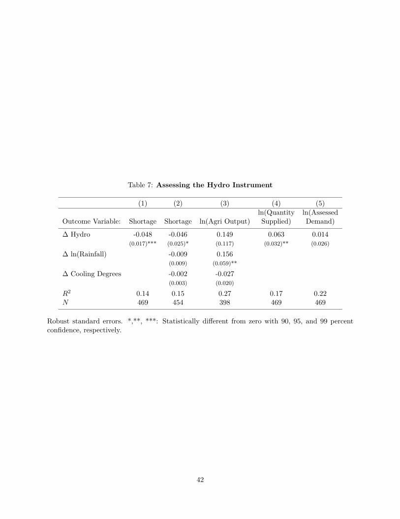
Table 7: Assessing the Hydro Instrument

(1) (2) (3) (4) (5)ln(Quantity ln(Assessed

Outcome Variable: Shortage Shortage ln(Agri Output) Supplied) Demand)

� Hydro -0.048 -0.046 0.149 0.063 0.014(0.017)*** (0.025)* (0.117) (0.032)** (0.026)

� ln(Rainfall) -0.009 0.156(0.009) (0.059)**

� Cooling Degrees -0.002 -0.027(0.003) (0.020)

R2 0.14 0.15 0.27 0.17 0.22N 469 454 398 469 469

Robust standard errors. *,**, ***: Statistically di�erent from zero with 90, 95, and 99 percentconfidence, respectively.

42

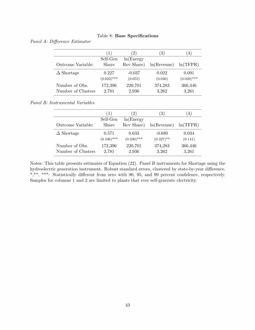
Table 8: Base SpecificationsPanel A: Di�erence Estimator

(1) (2) (3) (4)Self-Gen ln(Energy

Outcome Variable: Share Rev Share) ln(Revenue) ln(TFPR)

� Shortage 0.227 -0.037 0.022 0.091(0.023)*** (0.055) (0.040) (0.029)***

Number of Obs. 172,396 220,701 374,283 366,446Number of Clusters 2,781 2,936 3,262 3,261

Panel B: Instrumental Variables

(1) (2) (3) (4)Self-Gen ln(Energy

Outcome Variable: Share Rev Share) ln(Revenue) ln(TFPR)

� Shortage 0.571 0.633 -0.680 0.034(0.106)*** (0.230)*** (0.327)** (0.141)

Number of Obs. 172,396 220,701 374,283 366,446Number of Clusters 2,781 2,936 3,262 3,261

Notes: This table presents estimates of Equation (22). Panel B instruments for Shortage using thehydroelectric generation instrument. Robust standard errors, clustered by state-by-year di�erence.*,**, ***: Statistically di�erent from zero with 90, 95, and 99 percent confidence, respectively.Samples for columns 1 and 2 are limited to plants that ever self-generate electricity.

43

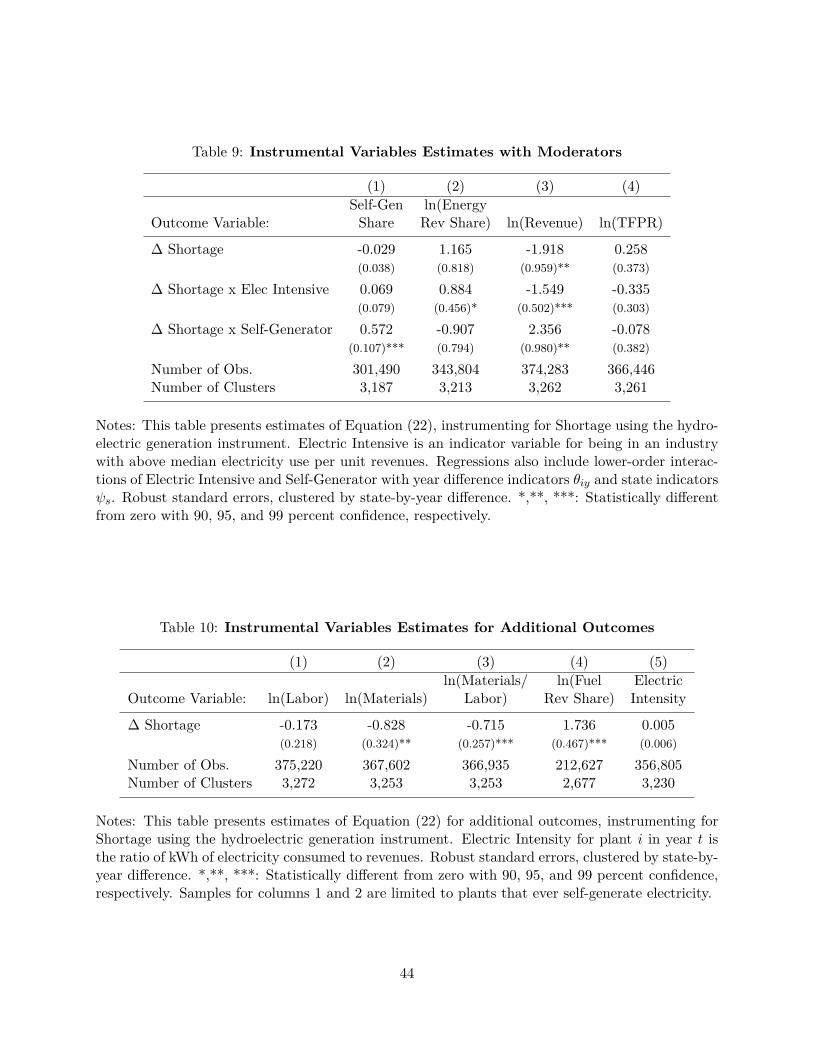
Table 9: Instrumental Variables Estimates with Moderators

(1) (2) (3) (4)Self-Gen ln(Energy

Outcome Variable: Share Rev Share) ln(Revenue) ln(TFPR)

� Shortage -0.029 1.165 -1.918 0.258(0.038) (0.818) (0.959)** (0.373)

� Shortage x Elec Intensive 0.069 0.884 -1.549 -0.335(0.079) (0.456)* (0.502)*** (0.303)

� Shortage x Self-Generator 0.572 -0.907 2.356 -0.078(0.107)*** (0.794) (0.980)** (0.382)

Number of Obs. 301,490 343,804 374,283 366,446Number of Clusters 3,187 3,213 3,262 3,261

Notes: This table presents estimates of Equation (22), instrumenting for Shortage using the hydro-electric generation instrument. Electric Intensive is an indicator variable for being in an industrywith above median electricity use per unit revenues. Regressions also include lower-order interac-tions of Electric Intensive and Self-Generator with year di�erence indicators ◊iy and state indicatorsÂs. Robust standard errors, clustered by state-by-year di�erence. *,**, ***: Statistically di�erentfrom zero with 90, 95, and 99 percent confidence, respectively.

Table 10: Instrumental Variables Estimates for Additional Outcomes

(1) (2) (3) (4) (5)ln(Materials/ ln(Fuel Electric

Outcome Variable: ln(Labor) ln(Materials) Labor) Rev Share) Intensity

� Shortage -0.173 -0.828 -0.715 1.736 0.005(0.218) (0.324)** (0.257)*** (0.467)*** (0.006)

Number of Obs. 375,220 367,602 366,935 212,627 356,805Number of Clusters 3,272 3,253 3,253 2,677 3,230

Notes: This table presents estimates of Equation (22) for additional outcomes, instrumenting forShortage using the hydroelectric generation instrument. Electric Intensity for plant i in year t isthe ratio of kWh of electricity consumed to revenues. Robust standard errors, clustered by state-by-year di�erence. *,**, ***: Statistically di�erent from zero with 90, 95, and 99 percent confidence,respectively. Samples for columns 1 and 2 are limited to plants that ever self-generate electricity.

44

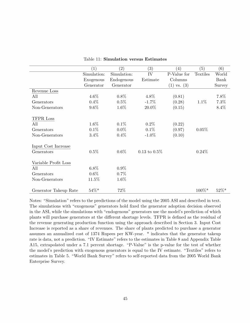
Table 11: Simulation versus Estimates

(1) (2) (3) (4) (5) (6)Simulation: Simulation: IV P-Value for Textiles WorldExogenous Endogenous Estimate Columns BankGenerator Generator (1) vs. (3) Survey

Revenue LossAll 4.6% 0.8% 4.8% (0.81) 7.8%Generators 0.4% 0.5% -1.7% (0.28) 1.1% 7.3%Non-Generators 9.6% 1.6% 20.0% (0.15) 8.4%

TFPR LossAll 1.6% 0.1% 0.2% (0.22)Generators 0.1% 0.0% 0.1% (0.97) 0.05%Non-Generators 3.4% 0.4% -1.0% (0.10)

Input Cost IncreaseGenerators 0.5% 0.6% 0.13 to 0.5% 0.24%

Variable Profit LossAll 6.8% 0.9%Generators 0.6% 0.7%Non-Generators 11.5% 1.6%

Generator Takeup Rate 54%* 72% 100%* 52%*

Notes: “Simulation” refers to the predictions of the model using the 2005 ASI and described in text.The simulations with “exogenous” generators hold fixed the generator adoption decision observedin the ASI, while the simulations with “endogenous” generators use the model’s prediction of whichplants will purchase generators at the di�erent shortage levels. TFPR is defined as the residual ofthe revenue generating production function using the approach described in Section 3. Input CostIncrease is reported as a share of revenues. The share of plants predicted to purchase a generatorassumes an annualized cost of 1374 Rupees per KW-year. * indicates that the generator takeuprate is data, not a prediction. “IV Estimate” refers to the estimates in Table 8 and Appendix TableA15, extrapolated under a 7.1 percent shortage. “P-Value” is the p-value for the test of whetherthe model’s prediction with exogenous generators is equal to the IV estimate. “Textiles” refers toestimates in Table 5. “World Bank Survey” refers to self-reported data from the 2005 World BankEnterprise Survey.

45

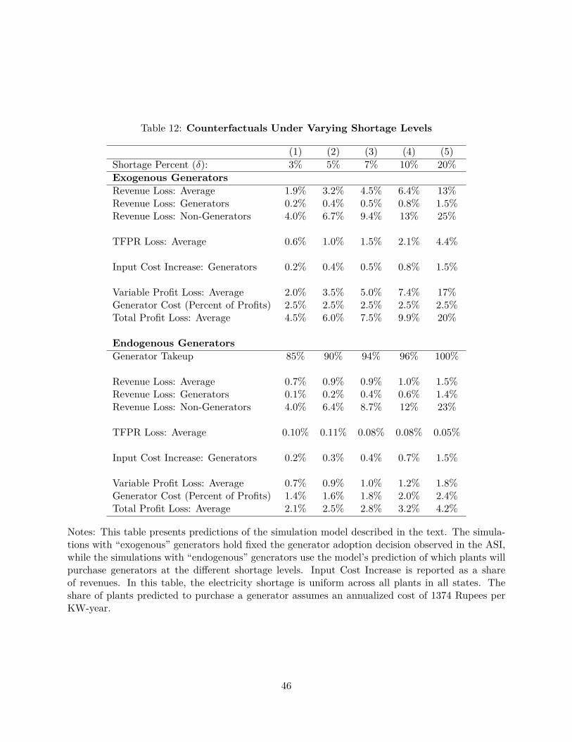
Table 12: Counterfactuals Under Varying Shortage Levels

(1) (2) (3) (4) (5)Shortage Percent (”): 3% 5% 7% 10% 20%Exogenous GeneratorsRevenue Loss: Average 1.9% 3.2% 4.5% 6.4% 13%Revenue Loss: Generators 0.2% 0.4% 0.5% 0.8% 1.5%Revenue Loss: Non-Generators 4.0% 6.7% 9.4% 13% 25%

TFPR Loss: Average 0.6% 1.0% 1.5% 2.1% 4.4%

Input Cost Increase: Generators 0.2% 0.4% 0.5% 0.8% 1.5%

Variable Profit Loss: Average 2.0% 3.5% 5.0% 7.4% 17%Generator Cost (Percent of Profits) 2.5% 2.5% 2.5% 2.5% 2.5%Total Profit Loss: Average 4.5% 6.0% 7.5% 9.9% 20%

Endogenous GeneratorsGenerator Takeup 85% 90% 94% 96% 100%

Revenue Loss: Average 0.7% 0.9% 0.9% 1.0% 1.5%Revenue Loss: Generators 0.1% 0.2% 0.4% 0.6% 1.4%Revenue Loss: Non-Generators 4.0% 6.4% 8.7% 12% 23%

TFPR Loss: Average 0.10% 0.11% 0.08% 0.08% 0.05%

Input Cost Increase: Generators 0.2% 0.3% 0.4% 0.7% 1.5%

Variable Profit Loss: Average 0.7% 0.9% 1.0% 1.2% 1.8%Generator Cost (Percent of Profits) 1.4% 1.6% 1.8% 2.0% 2.4%Total Profit Loss: Average 2.1% 2.5% 2.8% 3.2% 4.2%

Notes: This table presents predictions of the simulation model described in the text. The simula-tions with “exogenous” generators hold fixed the generator adoption decision observed in the ASI,while the simulations with “endogenous” generators use the model’s prediction of which plants willpurchase generators at the di�erent shortage levels. Input Cost Increase is reported as a shareof revenues. In this table, the electricity shortage is uniform across all plants in all states. Theshare of plants predicted to purchase a generator assumes an annualized cost of 1374 Rupees perKW-year.

46

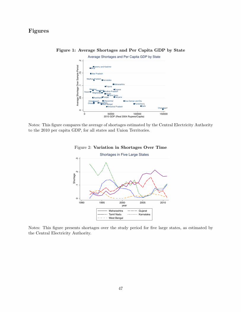
Figures

Figure 1: Average Shortages and Per Capita GDP by State

Andhra Pradesh

Bihar

Delhi

Goa Daman and Diu

Gujarat

Haryana

Himachal Pradesh

Jammu and Kashmir

Jharkhand

Karnataka

Kerala

Maharashtra

Pondicherry

Punjab

Rajasthan

Tamil Nadu

Tripura

Uttar Pradesh

UttaranchalWest Bengal

Chandigarh

Chhattisgarh

Madhya Pradesh

ManipurNagalandAssam Meghalaya

Orissa

0.0

5.1

.15

.2Av

erag

e Sh

orta

ge O

ver S

ampl

e Pe

riod

0 50000 100000 1500002010 GDP (Real 2004 Rupees/Capita)

Average Shortages and Per Capita GDP by State

Notes: This figure compares the average of shortages estimated by the Central Electricity Authorityto the 2010 per capita GDP, for all states and Union Territories.

Figure 2: Variation in Shortages Over Time

0.1

.2.3

Shor

tage

1990 1995 2000 2005 2010year

Maharashtra GujaratTamil Nadu KarnatakaWest Bengal

Shortages in Five Large States

Notes: This figure presents shortages over the study period for five large states, as estimated bythe Central Electricity Authority.

47

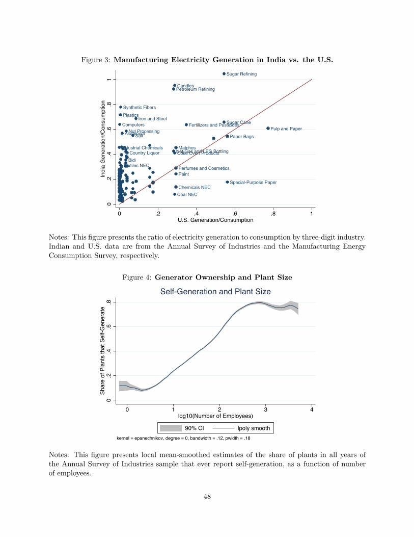
Figure 3: Manufacturing Electricity Generation in India vs. the U.S.

Sugar Refining

Sugar Cane

SaltNut Processing

Country LiquorBidi

Textiles NEC

Pulp and PaperPaper Bags

Special-Purpose Paper

Industrial Chemicals

Fertilizers and Pesticides

Plastics

PaintPerfumes and Cosmetics

Synthetic Fibers

Matches

Chemicals NEC

Petroleum Refining

Nat Gas and LPG Bottling

Candles

Coke Oven Products

Coal NEC

Iron and Steel

Aluminum

Computers

0.2

.4.6

.81

Indi

a G

ener

atio

n/Co

nsum

ptio

n

0 .2 .4 .6 .8 1U.S. Generation/Consumption

Notes: This figure presents the ratio of electricity generation to consumption by three-digit industry.Indian and U.S. data are from the Annual Survey of Industries and the Manufacturing EnergyConsumption Survey, respectively.

Figure 4: Generator Ownership and Plant Size

0.2

.4.6

.8Sh

are

of P

lant

s th

at S

elf-G

ener

ate

0 1 2 3 4log10(Number of Employees)

90% CI lpoly smoothkernel = epanechnikov, degree = 0, bandwidth = .12, pwidth = .18

Self-Generation and Plant Size

Notes: This figure presents local mean-smoothed estimates of the share of plants in all years ofthe Annual Survey of Industries sample that ever report self-generation, as a function of numberof employees.

48

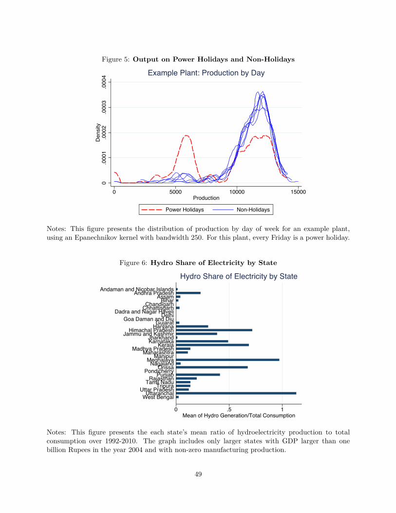
Figure 5: Output on Power Holidays and Non-Holidays

0.0

001

.000

2.0

003

.000

4D

ensi

ty

0 5000 10000 15000Production

Power Holidays Non-Holidays

Example Plant: Production by Day

Notes: This figure presents the distribution of production by day of week for an example plant,using an Epanechnikov kernel with bandwidth 250. For this plant, every Friday is a power holiday.

Figure 6: Hydro Share of Electricity by State

0 .5 1Mean of Hydro Generation/Total Consumption

West BengalUttaranchalUttar PradeshTripuraTamil NaduRajasthanPunjabPondicherryOrissaNagalandMeghalayaManipurMaharashtraMadhya PradeshKeralaKarnatakaJharkhandJammu and KashmirHimachal PradeshHaryanaGujaratGoa Daman and DiuDelhiDadra and Nagar HaveliChhattisgarhChandigarhBiharAssamAndhra PradeshAndaman and Nicobar Islands

Hydro Share of Electricity by State

Notes: This figure presents the each state’s mean ratio of hydroelectricity production to totalconsumption over 1992-2010. The graph includes only larger states with GDP larger than onebillion Rupees in the year 2004 and with non-zero manufacturing production.

49

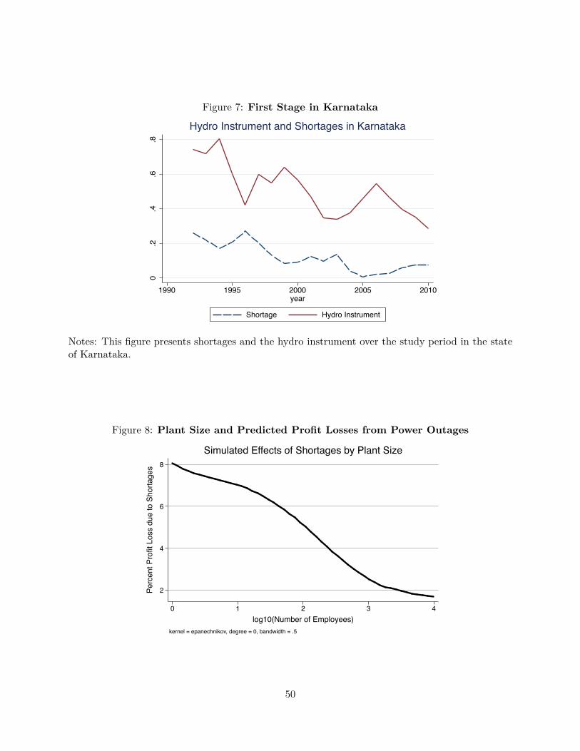
Figure 7: First Stage in Karnataka

0.2

.4.6

.8

1990 1995 2000 2005 2010year

Shortage Hydro Instrument

Hydro Instrument and Shortages in Karnataka

Notes: This figure presents shortages and the hydro instrument over the study period in the stateof Karnataka.

Figure 8: Plant Size and Predicted Profit Losses from Power Outages

2

4

6

8

Perc

ent P

rofit

Los

s du

e to

Sho

rtage

s

0 1 2 3 4log10(Number of Employees)

kernel = epanechnikov, degree = 0, bandwidth = .5

Simulated Effects of Shortages by Plant Size

50

Online Appendix: Not for Publication

How Do Electricity Shortages A�ect Productivity? Evidence from India

Hunt Allcott, Allan Collard-Wexler, and Stephen D. O’Connell

51

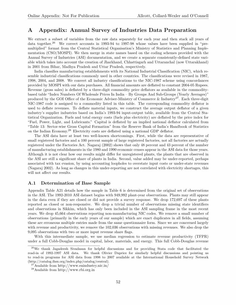
Online Appendix: Not For Publication Allcott, Collard-Wexler and O’Connell

A Appendix: Annual Survey of Industries Data PreparationWe extract a subset of variables from the raw data separately for each year and then stack all years ofdata together.26 We correct accounts in 1993-94 to 1997-98 whose values have been supplied in “pre-multiplied” format from the Central Statistical Organisation’s Ministry of Statistics and Planning Imple-mentation (CSO/MOSPI). We then merge in state names based on the coding schemes provided with theAnnual Survey of Industries (ASI) documentation, and we create a separate consistently-defined state vari-able which takes into account the creation of Jharkhand, Chhattisgarh and Uttaranchal (now Uttarakhand)in 2001 from Bihar, Madhya Pradesh and Uttar Pradesh, respectively.

India classifies manufacturing establishments with its National Industrial Classification (NIC), which re-semble industrial classifications commonly used in other countries. The classifications were revised in 1987,1998, 2004, and 2008. We convert all industry classifications to the NIC-1987 scheme using concordancesprovided by MOSPI with our data purchases. All financial amounts are deflated to constant 2004-05 Rupees.Revenue (gross sales) is deflated by a three-digit commodity price deflators as available in the commodity-based table “Index Numbers Of Wholesale Prices In India – By Groups And Sub-Groups (Yearly Averages)”produced by the GOI O�ce of the Economic Adviser-Ministry of Commerce & Industry27. Each three-digitNIC-1987 code is assigned to a commodity listed in this table. The corresponding commodity deflator isused to deflate revenues. To deflate material inputs, we construct the average output deflator of a givenindustry’s supplier industries based on India’s 1993-94 input-output table, available from the Central Sta-tistical Organization. Fuels and total energy costs (fuels plus electricity) are deflated by the price index for“Fuel, Power, Light, and Lubricants.” Capital is deflated by an implied national deflator calculated from“Table 13: Sector-wise Gross Capital Formation” from the Reserve Bank of India’s Handbook of Statisticson the Indian Economy.28 Electricity costs are deflated using a national GDP deflator.

The ASI data have at least two well-known shortcomings. First, while the data are representative ofsmall registered factories and a 100 percent sample of large registered factories, not all factories are actuallyregistered under the Factories Act. Nagaraj (2002) shows that only 48 percent and 43 percent of the numberof manufacturing establishments in the 1980 and 1990 economic censes appear in the ASI data for those years.Although it is not clear how our results might di�er for unregistered plants, the plants that are observed inthe ASI are still a significant share of plants in India. Second, value added may be under-reported, perhapsassociated with tax evasion, by using accounting loopholes to overstate input costs or under-state revenues(Nagaraj 2002). As long as changes in this under-reporting are not correlated with electricity shortages, thiswill not a�ect our results.

A.1 Determination of Base SampleAppendix Table A21 details how the sample in Table 6 is determined from the original set of observationsin the ASI. The 1992-2010 ASI dataset begins with 949,992 plant-year observations. Plants may still appearin the data even if they are closed or did not provide a survey response. We drop 172,697 of these plantsreported as closed or non-responsive. We drop a trivial number of observations missing state identifiersand observations in Sikkim, which has only been included in the ASI sampling frame in the most recentyears. We drop 45,664 observations reporting non-manufacturing NIC codes. We remove a small number ofobservations (primarily in the early years of our sample) which are exact duplicates in all fields, assumingthese are erroneous multiple entries made from the same questionnaire form. Since we are concerned largelywith revenue and productivity, we remove the 102,036 observations with missing revenues. We also drop the9,095 observations with two or more input revenue share flags.

With this intermediate sample, we use median regression to estimate revenue productivity (TFPR)under a full Cobb-Douglas model in capital, labor, materials, and energy. This full Cobb-Douglas revenue

26We thank Jagadeesh Sivadasan for helpful discussions and for providing Stata code that facilitated theread-in of 1992-1997 ASI data. We thank Olivier Dupriez for similarly helpful discussions and pointing usto read-in programs for ASI data from 1998 to 2007 available at the International Household Survey Network(http://catalog.ihsn.org/index.php/catalog/central).

27Available from http://www.eaindustry.nic.in/28Available from http://www.rbi.org.in

52

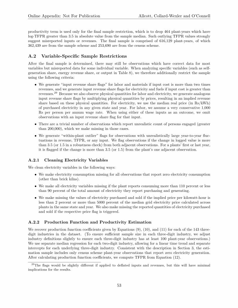
Online Appendix: Not For Publication Allcott, Collard-Wexler and O’Connell

productivity term is used only for the final sample restriction, which is to drop 464 plant-years which havelog-TFPR greater than 3.5 in absolute value from the sample median. Such outlying TFPR values stronglysuggest misreported inputs or revenues. The final sample is comprised of 616,129 plant-years, of which362,439 are from the sample scheme and 253,690 are from the census scheme.

A.2 Variable-Specific Sample RestrictionsAfter the final sample is determined, there may still be observations which have correct data for mostvariables but misreported data for some individual variable. When analyzing specific variables (such as self-generation share, energy revenue share, or output in Table 8), we therefore additionally restrict the sampleusing the following criteria:

• We generate “input revenue share flags” for labor and materials if input cost is more than two timesrevenues, and we generate input revenue share flags for electricity and fuels if input cost is greater thanrevenues.29 Because we also observe physical quantities for labor and electricity, we generate analogousinput revenue share flags by multiplying physical quantities by prices, resulting in an implied revenueshare based on these physical quantities. For electricity, we use the median real price (in Rs/kWh)of purchased electricity in any given state and year. For labor, we assume a very conservative 1,000Rs per person per annum wage rate. When using either of these inputs as an outcome, we omitobservations with an input revenue share flag for that input.

• There are a trivial number of observations which report unrealistic count of persons engaged (greaterthan 200,000), which we make missing in those cases.

• We generate “within-plant outlier” flags for observations with unrealistically large year-to-year fluc-tuations in revenue, TFPR, or any input. We flag observations if the change in logged value is morethan 3.5 (or 1.5 in a robustness check) from both adjacent observations. For a plants’ first or last year,it is flagged if the change is more than 3.5 (or 1.5) from the plant’s one adjacent observation.

A.2.1 Cleaning Electricity VariablesWe clean electricity variables in the following ways:

• We make electricity consumption missing for all observations that report zero electricity consumption(other than brick kilns).

• We make all electricity variables missing if the plant reports consuming more than 110 percent or lessthan 90 percent of the total amount of electricity they report purchasing and generating.

• We make missing the values of electricity purchased and sold if the implied price per kilowatt-hour isless than 2 percent or more than 5000 percent of the median grid electricity price calculated acrossplants in the same state and year. We also make missing the reported quantities of electricity purchasedand sold if the respective price flag is triggered.

A.2.2 Production Function and Productivity EstimationWe recover production function coe�cients given by Equations (9), (10), and (11) for each of the 143 three-digit industries in the dataset. (To ensure su�cient sample size in each three-digit industry, we adjustindustry definitions slightly to ensure each three-digit industry has at least 100 plant-year observations.)We use separate median regression for each two-digit industry, allowing for a linear time trend and separateintercepts for each underlying three-digit industry. Consistent with the description in Section 3, the esti-mation sample includes only census scheme plant-year observations that report zero electricity generation.After calculating production function coe�cients, we compute TFPR from Equation (12).

29The flags would be slightly di�erent if applied to deflated inputs and revenues, but this will have minimalimplications for the results.

53

Online Appendix: Not For Publication Allcott, Collard-Wexler and O’Connell

We use several alternative methods for calculating production function coe�cients and TFPR for ro-bustness checks:

• To check if our results are sensitive to assumptions about elasticity of demand, we calculate revenueproductivity terms for ‘ = ≠4 and ‘ = ≠Œ.

• We calculate an alternative materials term that adds the estimated cost of fuels not used for electricitygeneration. (To avoid relying on this estimated cost, our usual materials term does not include anyfuels, so these costs do not enter the production function.)

• Omitting the linear time trend when estimating production coe�cients, which amounts to taking theunconditional median by industry of the revenue shares for materials, labor, and electricity.

• Because in some industries plants with no self-generation may be unusual, we estimate productionfunctions and revenue productivity using all plants, i.e. including those that self-generate.

54

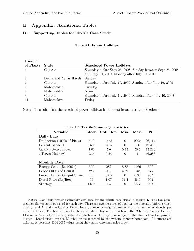
Online Appendix: Not For Publication Allcott, Collard-Wexler and O’Connell

B Appendix: Additional TablesB.1 Supporting Tables for Textile Case Study

Table A1: Power Holidays

Numberof Plants State Scheduled Power Holidays1 Gujarat Saturday before Sept 26, 2008; Sunday between Sept 26, 2008

and July 10, 2009; Monday after July 10, 20091 Dadra and Nagar Haveli Sunday1 Gujarat Saturday before July 10, 2009; Sunday after July 10, 20091 Maharashtra Tuesday1 Maharashtra None3 Gujarat Saturday before July 10, 2009; Monday after July 10, 200914 Maharashtra Friday

Notes: This table lists the scheduled power holidays for the textile case study in Section 4

Table A2: Textile Summary StatisticsVariable Mean Std. Dev. Min. Max. N

Daily DataProduction (1000s of Picks) 442 1455 0 9098 26,114Percent Grade A 55.3 28.5 0 100 12,489Quality Defect Index 4.02 5.0 0.13 56.6 13,2231(Power Holiday) 0.14 0.34 0 1 46,288

Monthly DataEnergy Costs (Rs 1000s) 300 282 8.88 1466 307Labor (1000s of Hours) 32.3 20.7 4.39 148 575Power Holiday Output Share 0.11 0.05 0 0.33 902Diesel Price (Rs/liter) 35 1.67 31.4 38.3 902Shortage 14.46 7.5 0 25.7 902

Notes: This table presents summary statistics for the textile case study in section 4. The top panelincludes the variables observed for each day. There are two measures of quality: the percent of fabric gradedquality level A, and the Quality Defect Index, a severity-weighted measure of the number of defects permeter of fabric. The bottom panel includes variables observed for each month. “Shortage” is the CentralElectricity Authority’s monthly estimated electricity shortage percentage for the state where the plant islocated. Diesel prices are the Mumbai prices recorded by the website mypetrolprice.com. All rupees aredeflated to constant 2004-2005 values using the textile wholesale price index.

55

Online Appendix: Not For Publication Allcott, Collard-Wexler and O’Connell

B.2 First Stages

Table A3: First Stages for Base IV Estimates

(1) (2) (3) (4)Self-Gen ln(Fuel

Outcome Variable: Share Rev Share) ln(Revenue) ln(TFP)

� Hydro -0.134 -0.139 -0.100 -0.101(0.020)*** (0.019)*** (0.016)*** (0.016)***

Number of Obs. 172,317 220,613 374,158 366,302Number of Clusters 2,781 2,936 3,262 3,261A-P F-Stat 43.98 52.51 39.36 39.6

Notes: This table presents the first stage estimates for the IV regressions in Panel B of Table 8.Samples for columns 1 and 2 are limited to plants that ever self-generate electricity. F-statistic is forthe heteroskedasticity and cluster-robust Angrist-Pischke weak instruments test. Robust standarderrors, clustered by state-by-year di�erence. *,**, ***: Statistically di�erent from zero with 90, 95,and 99 percent confidence, respectively.

56

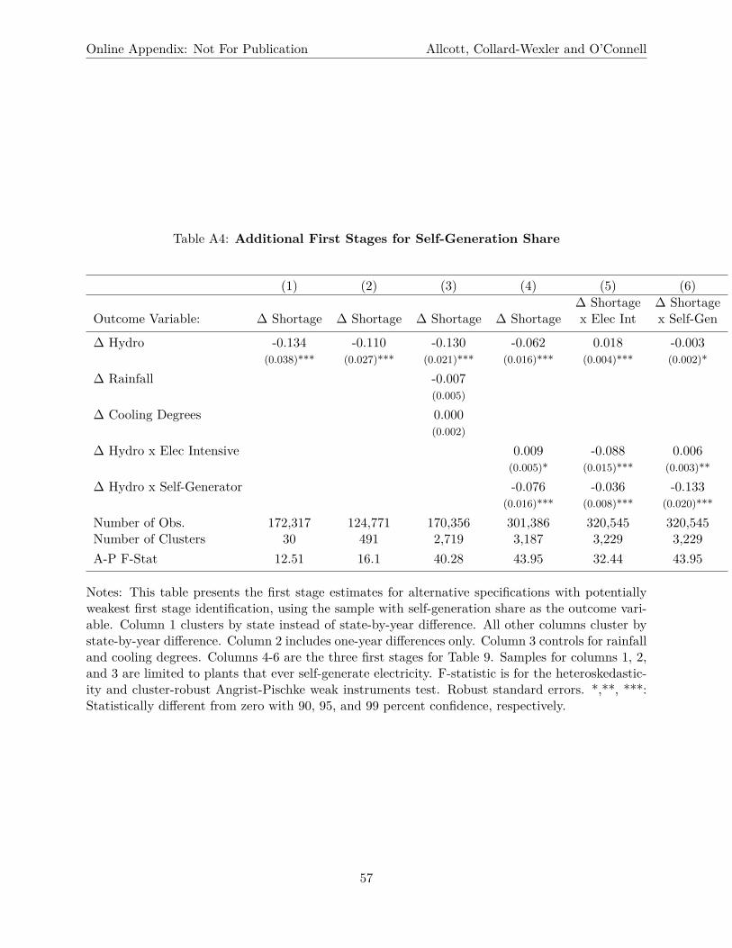
Online Appendix: Not For Publication Allcott, Collard-Wexler and O’Connell

Table A4: Additional First Stages for Self-Generation Share

(1) (2) (3) (4) (5) (6)� Shortage � Shortage

Outcome Variable: � Shortage � Shortage � Shortage � Shortage x Elec Int x Self-Gen

� Hydro -0.134 -0.110 -0.130 -0.062 0.018 -0.003(0.038)*** (0.027)*** (0.021)*** (0.016)*** (0.004)*** (0.002)*

� Rainfall -0.007(0.005)

� Cooling Degrees 0.000(0.002)

� Hydro x Elec Intensive 0.009 -0.088 0.006(0.005)* (0.015)*** (0.003)**

� Hydro x Self-Generator -0.076 -0.036 -0.133(0.016)*** (0.008)*** (0.020)***

Number of Obs. 172,317 124,771 170,356 301,386 320,545 320,545Number of Clusters 30 491 2,719 3,187 3,229 3,229A-P F-Stat 12.51 16.1 40.28 43.95 32.44 43.95

Notes: This table presents the first stage estimates for alternative specifications with potentiallyweakest first stage identification, using the sample with self-generation share as the outcome vari-able. Column 1 clusters by state instead of state-by-year di�erence. All other columns cluster bystate-by-year di�erence. Column 2 includes one-year di�erences only. Column 3 controls for rainfalland cooling degrees. Columns 4-6 are the three first stages for Table 9. Samples for columns 1, 2,and 3 are limited to plants that ever self-generate electricity. F-statistic is for the heteroskedastic-ity and cluster-robust Angrist-Pischke weak instruments test. Robust standard errors. *,**, ***:Statistically di�erent from zero with 90, 95, and 99 percent confidence, respectively.

57

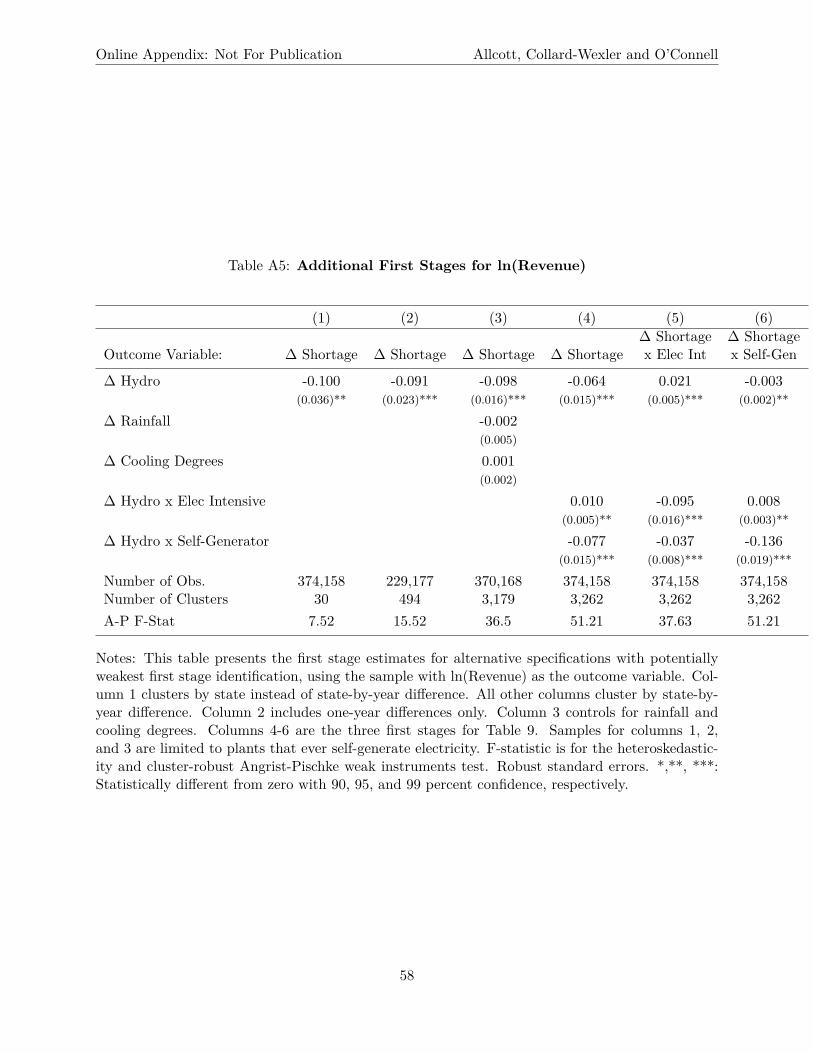
Online Appendix: Not For Publication Allcott, Collard-Wexler and O’Connell

Table A5: Additional First Stages for ln(Revenue)

(1) (2) (3) (4) (5) (6)� Shortage � Shortage

Outcome Variable: � Shortage � Shortage � Shortage � Shortage x Elec Int x Self-Gen

� Hydro -0.100 -0.091 -0.098 -0.064 0.021 -0.003(0.036)** (0.023)*** (0.016)*** (0.015)*** (0.005)*** (0.002)**

� Rainfall -0.002(0.005)

� Cooling Degrees 0.001(0.002)

� Hydro x Elec Intensive 0.010 -0.095 0.008(0.005)** (0.016)*** (0.003)**

� Hydro x Self-Generator -0.077 -0.037 -0.136(0.015)*** (0.008)*** (0.019)***

Number of Obs. 374,158 229,177 370,168 374,158 374,158 374,158Number of Clusters 30 494 3,179 3,262 3,262 3,262A-P F-Stat 7.52 15.52 36.5 51.21 37.63 51.21

Notes: This table presents the first stage estimates for alternative specifications with potentiallyweakest first stage identification, using the sample with ln(Revenue) as the outcome variable. Col-umn 1 clusters by state instead of state-by-year di�erence. All other columns cluster by state-by-year di�erence. Column 2 includes one-year di�erences only. Column 3 controls for rainfall andcooling degrees. Columns 4-6 are the three first stages for Table 9. Samples for columns 1, 2,and 3 are limited to plants that ever self-generate electricity. F-statistic is for the heteroskedastic-ity and cluster-robust Angrist-Pischke weak instruments test. Robust standard errors. *,**, ***:Statistically di�erent from zero with 90, 95, and 99 percent confidence, respectively.

58

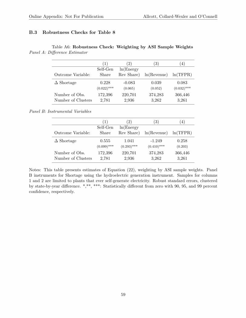
Online Appendix: Not For Publication Allcott, Collard-Wexler and O’Connell

B.3 Robustness Checks for Table 8

Table A6: Robustness Check: Weighting by ASI Sample WeightsPanel A: Di�erence Estimator

(1) (2) (3) (4)Self-Gen ln(Energy

Outcome Variable: Share Rev Share) ln(Revenue) ln(TFPR)

� Shortage 0.228 -0.083 0.039 0.083(0.022)*** (0.065) (0.052) (0.032)***

Number of Obs. 172,396 220,701 374,283 366,446Number of Clusters 2,781 2,936 3,262 3,261

Panel B: Instrumental Variables

(1) (2) (3) (4)Self-Gen ln(Energy

Outcome Variable: Share Rev Share) ln(Revenue) ln(TFPR)

� Shortage 0.555 1.041 -1.249 0.258(0.099)*** (0.293)*** (0.410)*** (0.203)

Number of Obs. 172,396 220,701 374,283 366,446Number of Clusters 2,781 2,936 3,262 3,261

Notes: This table presents estimates of Equation (22), weighting by ASI sample weights. PanelB instruments for Shortage using the hydroelectric generation instrument. Samples for columns1 and 2 are limited to plants that ever self-generate electricity. Robust standard errors, clusteredby state-by-year di�erence. *,**, ***: Statistically di�erent from zero with 90, 95, and 99 percentconfidence, respectively.

59

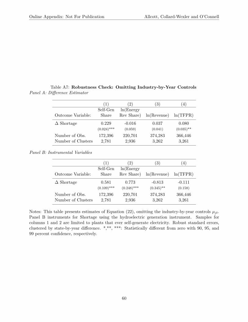
Online Appendix: Not For Publication Allcott, Collard-Wexler and O’Connell

Table A7: Robustness Check: Omitting Industry-by-Year ControlsPanel A: Di�erence Estimator

(1) (2) (3) (4)Self-Gen ln(Energy

Outcome Variable: Share Rev Share) ln(Revenue) ln(TFPR)

� Shortage 0.229 -0.016 0.037 0.080(0.024)*** (0.059) (0.041) (0.035)**

Number of Obs. 172,396 220,701 374,283 366,446Number of Clusters 2,781 2,936 3,262 3,261

Panel B: Instrumental Variables

(1) (2) (3) (4)Self-Gen ln(Energy

Outcome Variable: Share Rev Share) ln(Revenue) ln(TFPR)

� Shortage 0.581 0.773 -0.813 -0.111(0.109)*** (0.248)*** (0.345)** (0.158)

Number of Obs. 172,396 220,701 374,283 366,446Number of Clusters 2,781 2,936 3,262 3,261

Notes: This table presents estimates of Equation (22), omitting the industry-by-year controls µjt.Panel B instruments for Shortage using the hydroelectric generation instrument. Samples forcolumns 1 and 2 are limited to plants that ever self-generate electricity. Robust standard errors,clustered by state-by-year di�erence. *,**, ***: Statistically di�erent from zero with 90, 95, and99 percent confidence, respectively.

60

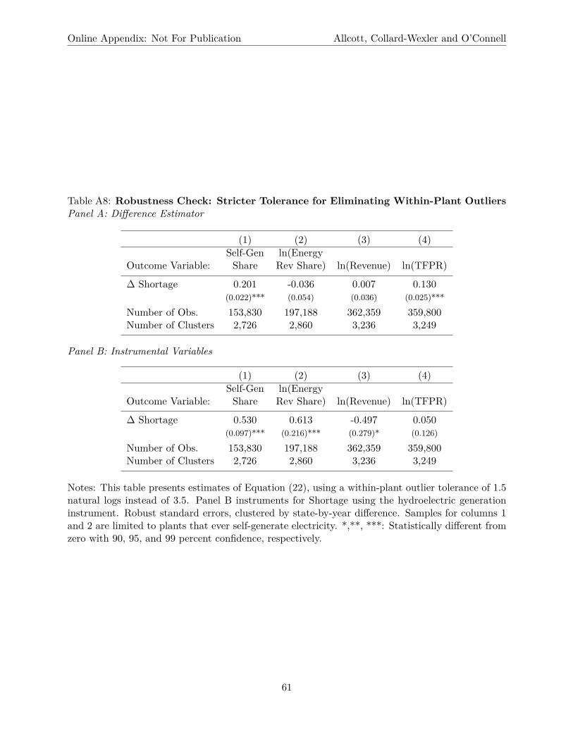
Online Appendix: Not For Publication Allcott, Collard-Wexler and O’Connell

Table A8: Robustness Check: Stricter Tolerance for Eliminating Within-Plant OutliersPanel A: Di�erence Estimator

(1) (2) (3) (4)Self-Gen ln(Energy

Outcome Variable: Share Rev Share) ln(Revenue) ln(TFPR)

� Shortage 0.201 -0.036 0.007 0.130(0.022)*** (0.054) (0.036) (0.025)***

Number of Obs. 153,830 197,188 362,359 359,800Number of Clusters 2,726 2,860 3,236 3,249

Panel B: Instrumental Variables

(1) (2) (3) (4)Self-Gen ln(Energy

Outcome Variable: Share Rev Share) ln(Revenue) ln(TFPR)

� Shortage 0.530 0.613 -0.497 0.050(0.097)*** (0.216)*** (0.279)* (0.126)

Number of Obs. 153,830 197,188 362,359 359,800Number of Clusters 2,726 2,860 3,236 3,249

Notes: This table presents estimates of Equation (22), using a within-plant outlier tolerance of 1.5natural logs instead of 3.5. Panel B instruments for Shortage using the hydroelectric generationinstrument. Robust standard errors, clustered by state-by-year di�erence. Samples for columns 1and 2 are limited to plants that ever self-generate electricity. *,**, ***: Statistically di�erent fromzero with 90, 95, and 99 percent confidence, respectively.

61

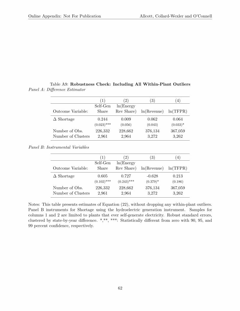
Online Appendix: Not For Publication Allcott, Collard-Wexler and O’Connell

Table A9: Robustness Check: Including All Within-Plant OutliersPanel A: Di�erence Estimator

(1) (2) (3) (4)Self-Gen ln(Energy

Outcome Variable: Share Rev Share) ln(Revenue) ln(TFPR)

� Shortage 0.244 0.009 0.062 0.064(0.023)*** (0.056) (0.043) (0.033)*

Number of Obs. 226,332 228,662 376,134 367,059Number of Clusters 2,961 2,964 3,272 3,262

Panel B: Instrumental Variables

(1) (2) (3) (4)Self-Gen ln(Energy

Outcome Variable: Share Rev Share) ln(Revenue) ln(TFPR)

� Shortage 0.605 0.727 -0.628 0.213(0.102)*** (0.243)*** (0.379)* (0.186)

Number of Obs. 226,332 228,662 376,134 367,059Number of Clusters 2,961 2,964 3,272 3,262

Notes: This table presents estimates of Equation (22), without dropping any within-plant outliers.Panel B instruments for Shortage using the hydroelectric generation instrument. Samples forcolumns 1 and 2 are limited to plants that ever self-generate electricity. Robust standard errors,clustered by state-by-year di�erence. *,**, ***: Statistically di�erent from zero with 90, 95, and99 percent confidence, respectively.

62

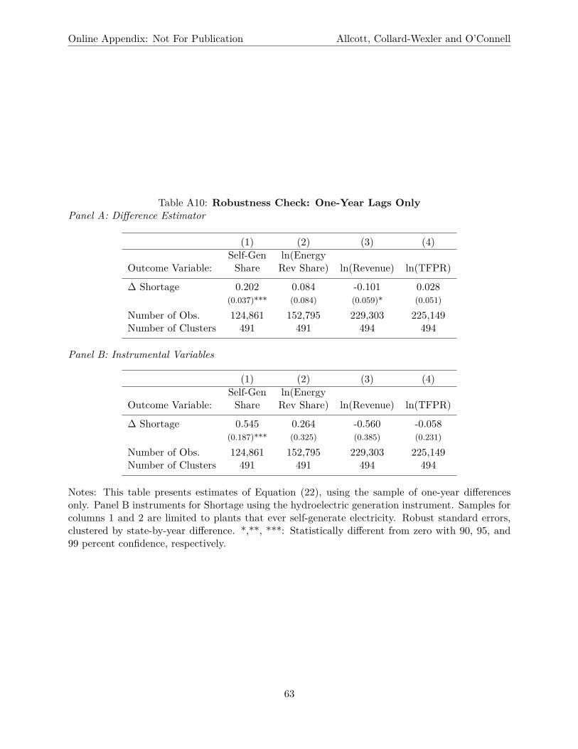
Online Appendix: Not For Publication Allcott, Collard-Wexler and O’Connell

Table A10: Robustness Check: One-Year Lags OnlyPanel A: Di�erence Estimator

(1) (2) (3) (4)Self-Gen ln(Energy

Outcome Variable: Share Rev Share) ln(Revenue) ln(TFPR)

� Shortage 0.202 0.084 -0.101 0.028(0.037)*** (0.084) (0.059)* (0.051)

Number of Obs. 124,861 152,795 229,303 225,149Number of Clusters 491 491 494 494

Panel B: Instrumental Variables

(1) (2) (3) (4)Self-Gen ln(Energy

Outcome Variable: Share Rev Share) ln(Revenue) ln(TFPR)

� Shortage 0.545 0.264 -0.560 -0.058(0.187)*** (0.325) (0.385) (0.231)

Number of Obs. 124,861 152,795 229,303 225,149Number of Clusters 491 491 494 494

Notes: This table presents estimates of Equation (22), using the sample of one-year di�erencesonly. Panel B instruments for Shortage using the hydroelectric generation instrument. Samples forcolumns 1 and 2 are limited to plants that ever self-generate electricity. Robust standard errors,clustered by state-by-year di�erence. *,**, ***: Statistically di�erent from zero with 90, 95, and99 percent confidence, respectively.

63

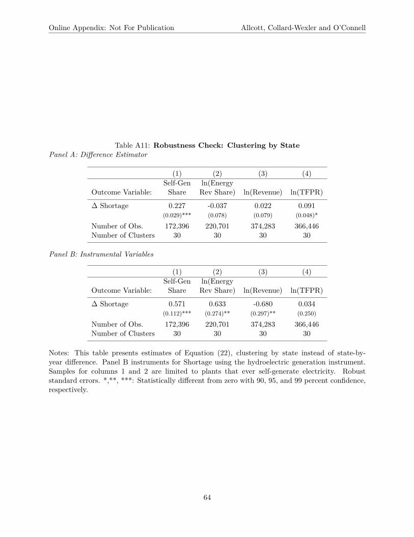
Online Appendix: Not For Publication Allcott, Collard-Wexler and O’Connell

Table A11: Robustness Check: Clustering by StatePanel A: Di�erence Estimator

(1) (2) (3) (4)Self-Gen ln(Energy

Outcome Variable: Share Rev Share) ln(Revenue) ln(TFPR)

� Shortage 0.227 -0.037 0.022 0.091(0.029)*** (0.078) (0.079) (0.048)*

Number of Obs. 172,396 220,701 374,283 366,446Number of Clusters 30 30 30 30

Panel B: Instrumental Variables

(1) (2) (3) (4)Self-Gen ln(Energy

Outcome Variable: Share Rev Share) ln(Revenue) ln(TFPR)

� Shortage 0.571 0.633 -0.680 0.034(0.112)*** (0.274)** (0.297)** (0.250)

Number of Obs. 172,396 220,701 374,283 366,446Number of Clusters 30 30 30 30

Notes: This table presents estimates of Equation (22), clustering by state instead of state-by-year di�erence. Panel B instruments for Shortage using the hydroelectric generation instrument.Samples for columns 1 and 2 are limited to plants that ever self-generate electricity. Robuststandard errors. *,**, ***: Statistically di�erent from zero with 90, 95, and 99 percent confidence,respectively.

64

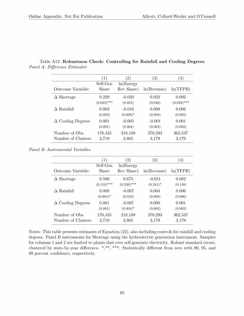
Online Appendix: Not For Publication Allcott, Collard-Wexler and O’Connell

Table A12: Robustness Check: Controlling for Rainfall and Cooling DegreesPanel A: Di�erence Estimator

(1) (2) (3) (4)Self-Gen ln(Energy

Outcome Variable: Share Rev Share) ln(Revenue) ln(TFPR)

� Shortage 0.229 -0.033 0.023 0.092(0.023)*** (0.055) (0.040) (0.029)***

� Rainfall 0.003 -0.016 0.008 0.006(0.003) (0.009)* (0.008) (0.005)

� Cooling Degrees 0.001 -0.005 -0.001 0.001(0.001) (0.004) (0.003) (0.002)

Number of Obs. 170,435 218,109 370,293 362,537Number of Clusters 2,719 2,865 3,179 3,179

Panel B: Instrumental Variables

(1) (2) (3) (4)Self-Gen ln(Energy

Outcome Variable: Share Rev Share) ln(Revenue) ln(TFPR)

� Shortage 0.586 0.675 -0.651 0.082(0.110)*** (0.249)*** (0.341)* (0.148)

� Rainfall 0.008 -0.007 0.004 0.006(0.004)* (0.010) (0.009) (0.006)

� Cooling Degrees 0.001 -0.007 0.000 0.001(0.001) (0.004)* (0.003) (0.002)

Number of Obs. 170,435 218,109 370,293 362,537Number of Clusters 2,719 2,865 3,179 3,179

Notes: This table presents estimates of Equation (22), also including controls for rainfall and coolingdegrees. Panel B instruments for Shortage using the hydroelectric generation instrument. Samplesfor columns 1 and 2 are limited to plants that ever self-generate electricity. Robust standard errors,clustered by state-by-year di�erence. *,**, ***: Statistically di�erent from zero with 90, 95, and99 percent confidence, respectively.

65

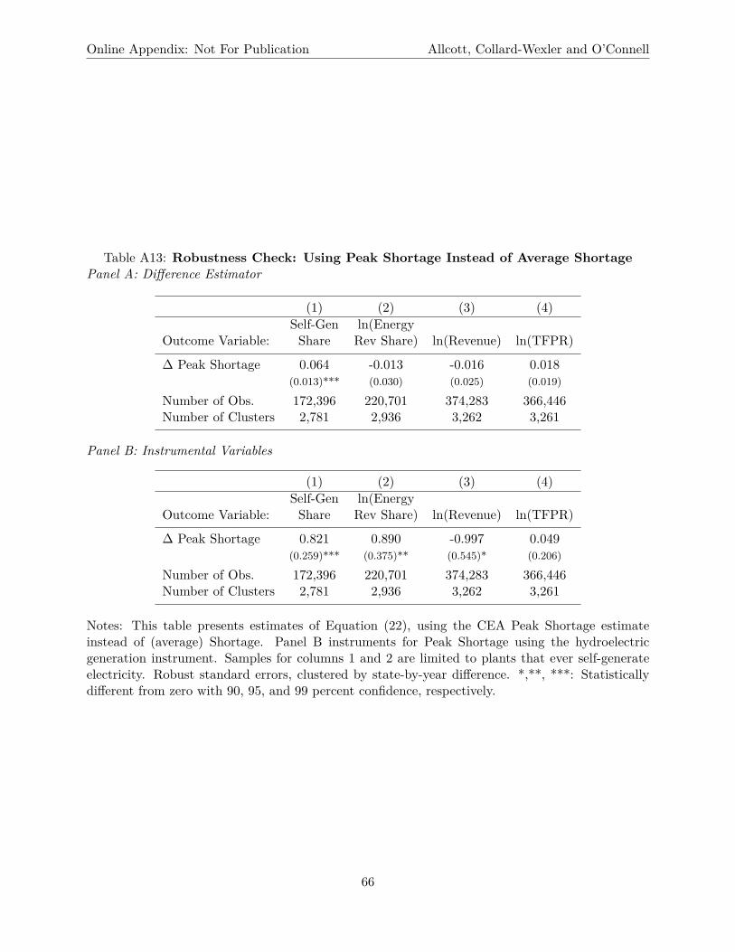
Online Appendix: Not For Publication Allcott, Collard-Wexler and O’Connell

Table A13: Robustness Check: Using Peak Shortage Instead of Average ShortagePanel A: Di�erence Estimator

(1) (2) (3) (4)Self-Gen ln(Energy

Outcome Variable: Share Rev Share) ln(Revenue) ln(TFPR)

� Peak Shortage 0.064 -0.013 -0.016 0.018(0.013)*** (0.030) (0.025) (0.019)

Number of Obs. 172,396 220,701 374,283 366,446Number of Clusters 2,781 2,936 3,262 3,261

Panel B: Instrumental Variables

(1) (2) (3) (4)Self-Gen ln(Energy

Outcome Variable: Share Rev Share) ln(Revenue) ln(TFPR)

� Peak Shortage 0.821 0.890 -0.997 0.049(0.259)*** (0.375)** (0.545)* (0.206)

Number of Obs. 172,396 220,701 374,283 366,446Number of Clusters 2,781 2,936 3,262 3,261

Notes: This table presents estimates of Equation (22), using the CEA Peak Shortage estimateinstead of (average) Shortage. Panel B instruments for Peak Shortage using the hydroelectricgeneration instrument. Samples for columns 1 and 2 are limited to plants that ever self-generateelectricity. Robust standard errors, clustered by state-by-year di�erence. *,**, ***: Statisticallydi�erent from zero with 90, 95, and 99 percent confidence, respectively.

66

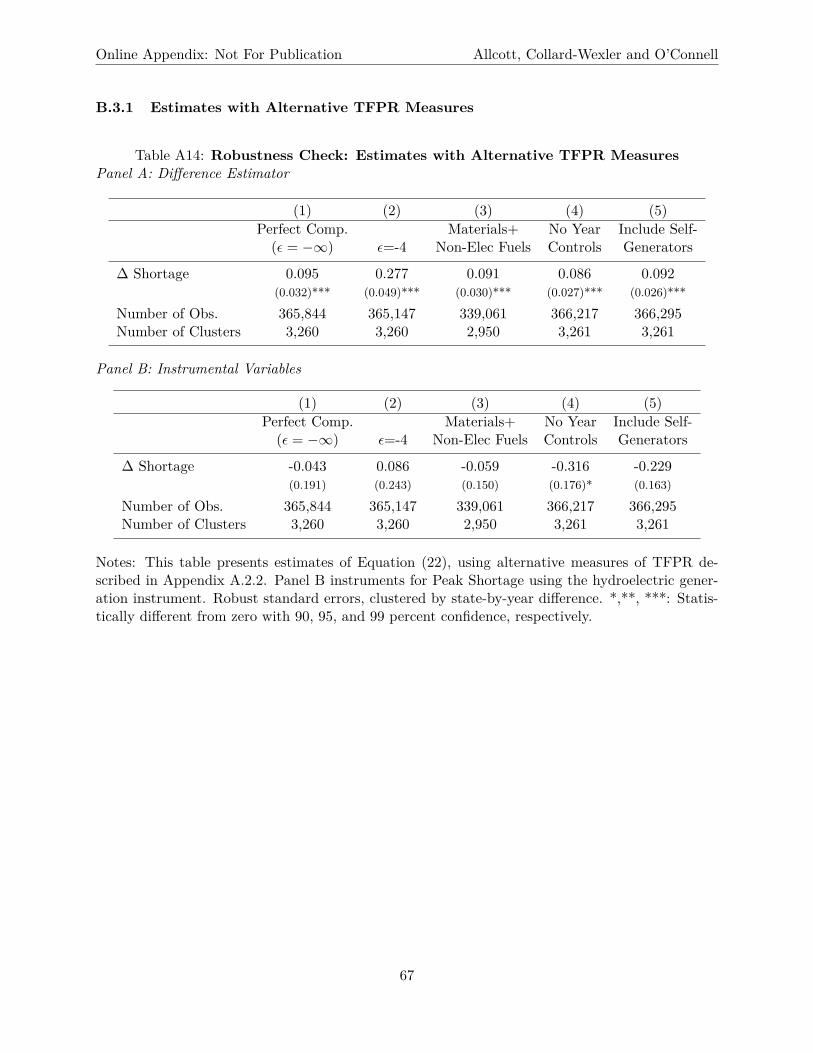
Online Appendix: Not For Publication Allcott, Collard-Wexler and O’Connell

B.3.1 Estimates with Alternative TFPR Measures

Table A14: Robustness Check: Estimates with Alternative TFPR MeasuresPanel A: Di�erence Estimator

(1) (2) (3) (4) (5)Perfect Comp. Materials+ No Year Include Self-

(‘ = ≠Œ) ‘=-4 Non-Elec Fuels Controls Generators

� Shortage 0.095 0.277 0.091 0.086 0.092(0.032)*** (0.049)*** (0.030)*** (0.027)*** (0.026)***

Number of Obs. 365,844 365,147 339,061 366,217 366,295Number of Clusters 3,260 3,260 2,950 3,261 3,261

Panel B: Instrumental Variables

(1) (2) (3) (4) (5)Perfect Comp. Materials+ No Year Include Self-

(‘ = ≠Œ) ‘=-4 Non-Elec Fuels Controls Generators

� Shortage -0.043 0.086 -0.059 -0.316 -0.229(0.191) (0.243) (0.150) (0.176)* (0.163)

Number of Obs. 365,844 365,147 339,061 366,217 366,295Number of Clusters 3,260 3,260 2,950 3,261 3,261

Notes: This table presents estimates of Equation (22), using alternative measures of TFPR de-scribed in Appendix A.2.2. Panel B instruments for Peak Shortage using the hydroelectric gener-ation instrument. Robust standard errors, clustered by state-by-year di�erence. *,**, ***: Statis-tically di�erent from zero with 90, 95, and 99 percent confidence, respectively.

67

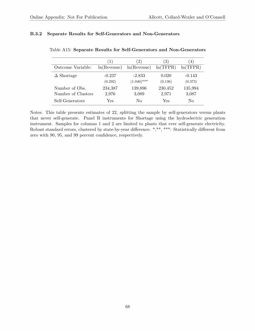
Online Appendix: Not For Publication Allcott, Collard-Wexler and O’Connell

B.3.2 Separate Results for Self-Generators and Non-Generators

Table A15: Separate Results for Self-Generators and Non-Generators

(1) (2) (3) (4)Outcome Variable: ln(Revenue) ln(Revenue) ln(TFPR) ln(TFPR)

� Shortage -0.237 -2.833 0.020 -0.143(0.292) (1.040)*** (0.136) (0.373)

Number of Obs. 234,387 139,896 230,452 135,994Number of Clusters 2,976 3,089 2,971 3,087Self-Generators Yes No Yes No

Notes: This table presents estimates of 22, splitting the sample by self-generators versus plantsthat never self-generate. Panel B instruments for Shortage using the hydroelectric generationinstrument. Samples for columns 1 and 2 are limited to plants that ever self-generate electricity.Robust standard errors, clustered by state-by-year di�erence. *,**, ***: Statistically di�erent fromzero with 90, 95, and 99 percent confidence, respectively.

68

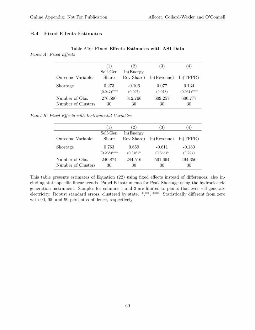
Online Appendix: Not For Publication Allcott, Collard-Wexler and O’Connell

B.4 Fixed E�ects Estimates

Table A16: Fixed E�ects Estimates with ASI DataPanel A: Fixed E�ects

(1) (2) (3) (4)Self-Gen ln(Energy

Outcome Variable: Share Rev Share) ln(Revenue) ln(TFPR)

Shortage 0.273 -0.106 0.077 0.134(0.042)*** (0.097) (0.078) (0.031)***

Number of Obs. 276,590 312,766 609,257 600,777Number of Clusters 30 30 30 30

Panel B: Fixed E�ects with Instrumental Variables

(1) (2) (3) (4)Self-Gen ln(Energy

Outcome Variable: Share Rev Share) ln(Revenue) ln(TFPR)

Shortage 0.763 0.659 -0.611 -0.180(0.238)*** (0.346)* (0.355)* (0.227)

Number of Obs. 240,874 284,516 501,664 494,356Number of Clusters 30 30 30 30

This table presents estimates of Equation (22) using fixed e�ects instead of di�erences, also in-cluding state-specific linear trends. Panel B instruments for Peak Shortage using the hydroelectricgeneration instrument. Samples for columns 1 and 2 are limited to plants that ever self-generateelectricity. Robust standard errors, clustered by state. *,**, ***: Statistically di�erent from zerowith 90, 95, and 99 percent confidence, respectively.

69

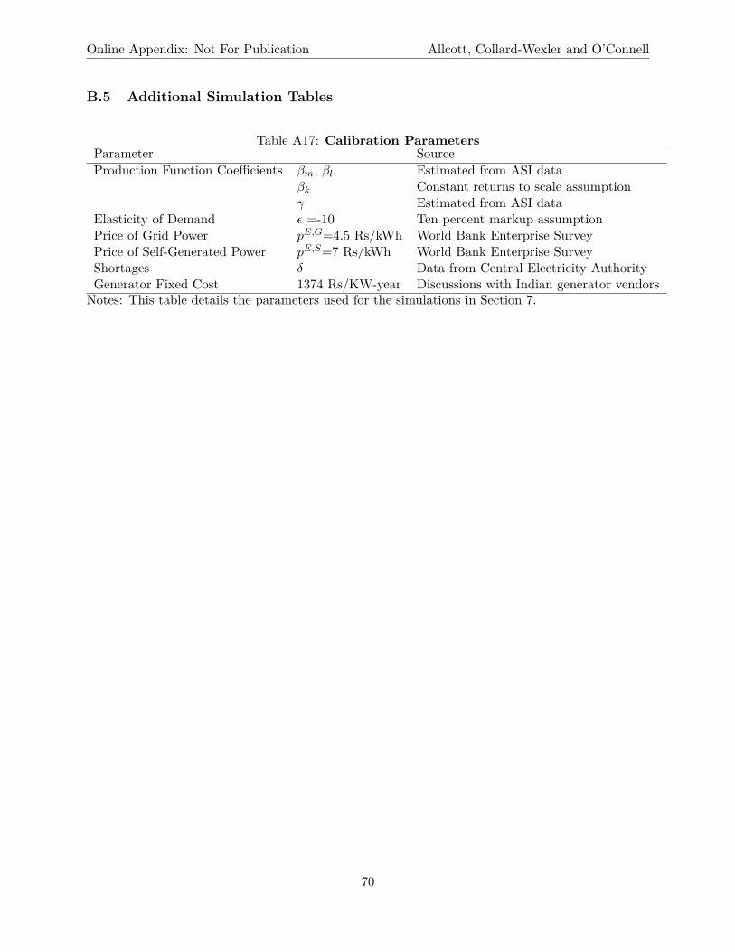
Online Appendix: Not For Publication Allcott, Collard-Wexler and O’Connell

B.5 Additional Simulation Tables

Table A17: Calibration ParametersParameter SourceProduction Function Coe�cients —m, —l Estimated from ASI data

—k Constant returns to scale assumption“ Estimated from ASI data

Elasticity of Demand ‘ =-10 Ten percent markup assumptionPrice of Grid Power pE,G=4.5 Rs/kWh World Bank Enterprise SurveyPrice of Self-Generated Power pE,S=7 Rs/kWh World Bank Enterprise SurveyShortages ” Data from Central Electricity AuthorityGenerator Fixed Cost 1374 Rs/KW-year Discussions with Indian generator vendors

Notes: This table details the parameters used for the simulations in Section 7.

70

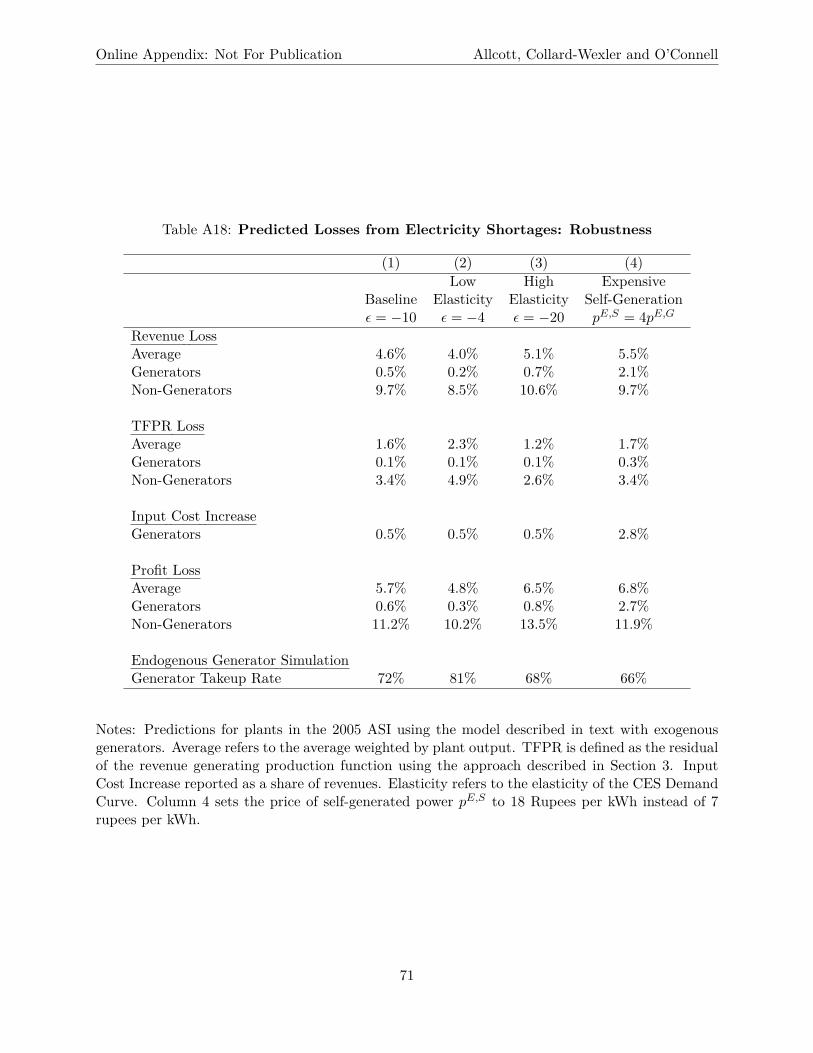
Online Appendix: Not For Publication Allcott, Collard-Wexler and O’Connell

Table A18: Predicted Losses from Electricity Shortages: Robustness

(1) (2) (3) (4)Low High Expensive

Baseline Elasticity Elasticity Self-Generation‘ = ≠10 ‘ = ≠4 ‘ = ≠20 pE,S = 4pE,G

Revenue LossAverage 4.6% 4.0% 5.1% 5.5%Generators 0.5% 0.2% 0.7% 2.1%Non-Generators 9.7% 8.5% 10.6% 9.7%

TFPR LossAverage 1.6% 2.3% 1.2% 1.7%Generators 0.1% 0.1% 0.1% 0.3%Non-Generators 3.4% 4.9% 2.6% 3.4%

Input Cost IncreaseGenerators 0.5% 0.5% 0.5% 2.8%

Profit LossAverage 5.7% 4.8% 6.5% 6.8%Generators 0.6% 0.3% 0.8% 2.7%Non-Generators 11.2% 10.2% 13.5% 11.9%

Endogenous Generator SimulationGenerator Takeup Rate 72% 81% 68% 66%

Notes: Predictions for plants in the 2005 ASI using the model described in text with exogenousgenerators. Average refers to the average weighted by plant output. TFPR is defined as the residualof the revenue generating production function using the approach described in Section 3. InputCost Increase reported as a share of revenues. Elasticity refers to the elasticity of the CES DemandCurve. Column 4 sets the price of self-generated power pE,S to 18 Rupees per kWh instead of 7rupees per kWh.

71

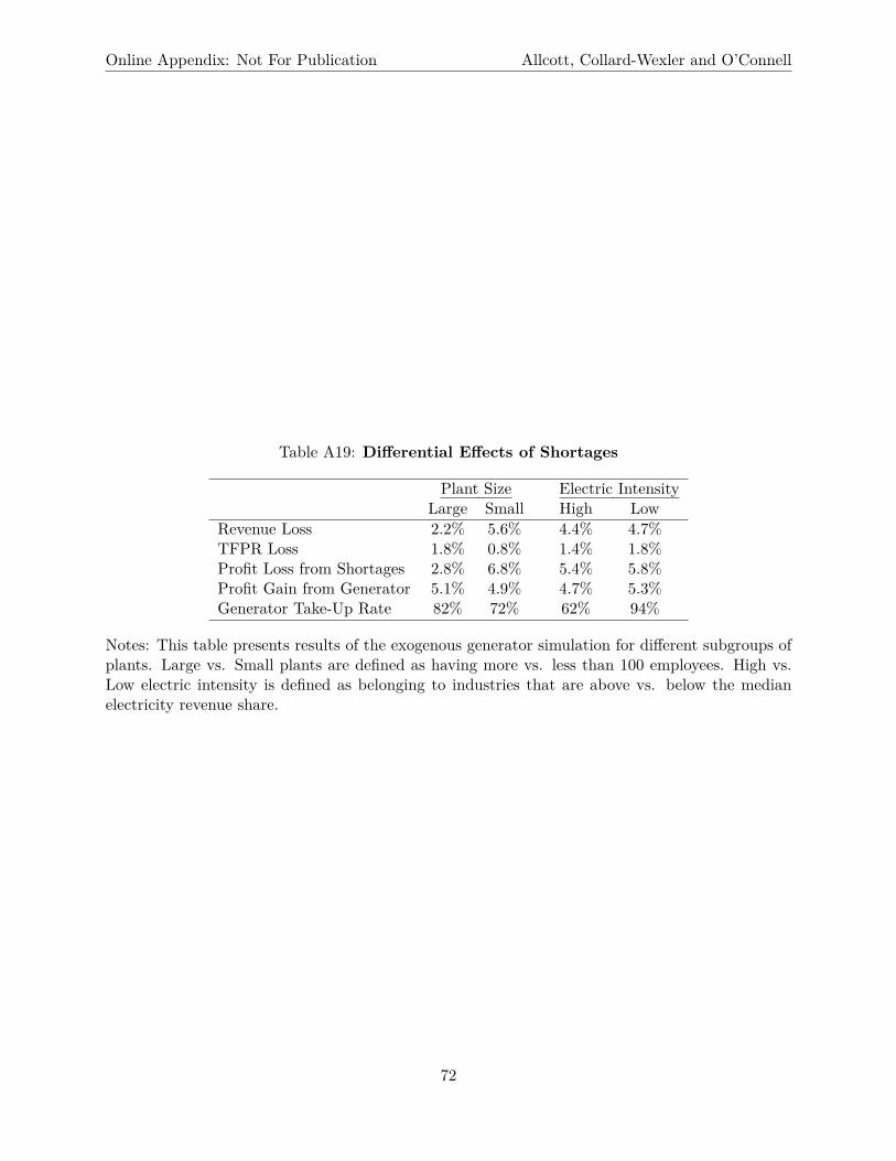
Online Appendix: Not For Publication Allcott, Collard-Wexler and O’Connell

Table A19: Di�erential E�ects of Shortages

Plant Size Electric IntensityLarge Small High Low

Revenue Loss 2.2% 5.6% 4.4% 4.7%TFPR Loss 1.8% 0.8% 1.4% 1.8%Profit Loss from Shortages 2.8% 6.8% 5.4% 5.8%Profit Gain from Generator 5.1% 4.9% 4.7% 5.3%Generator Take-Up Rate 82% 72% 62% 94%

Notes: This table presents results of the exogenous generator simulation for di�erent subgroups ofplants. Large vs. Small plants are defined as having more vs. less than 100 employees. High vs.Low electric intensity is defined as belonging to industries that are above vs. below the medianelectricity revenue share.

72

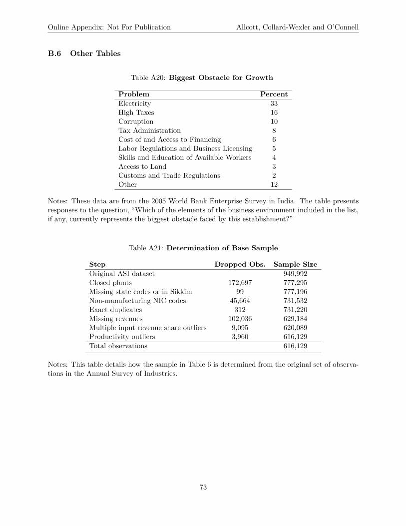
Online Appendix: Not For Publication Allcott, Collard-Wexler and O’Connell

B.6 Other Tables

Table A20: Biggest Obstacle for Growth

Problem PercentElectricity 33High Taxes 16Corruption 10Tax Administration 8Cost of and Access to Financing 6Labor Regulations and Business Licensing 5Skills and Education of Available Workers 4Access to Land 3Customs and Trade Regulations 2Other 12

Notes: These data are from the 2005 World Bank Enterprise Survey in India. The table presentsresponses to the question, “Which of the elements of the business environment included in the list,if any, currently represents the biggest obstacle faced by this establishment?”

Table A21: Determination of Base Sample

Step Dropped Obs. Sample SizeOriginal ASI dataset 949,992Closed plants 172,697 777,295Missing state codes or in Sikkim 99 777,196Non-manufacturing NIC codes 45,664 731,532Exact duplicates 312 731,220Missing revenues 102,036 629,184Multiple input revenue share outliers 9,095 620,089Productivity outliers 3,960 616,129Total observations 616,129

Notes: This table details how the sample in Table 6 is determined from the original set of observa-tions in the Annual Survey of Industries.

73

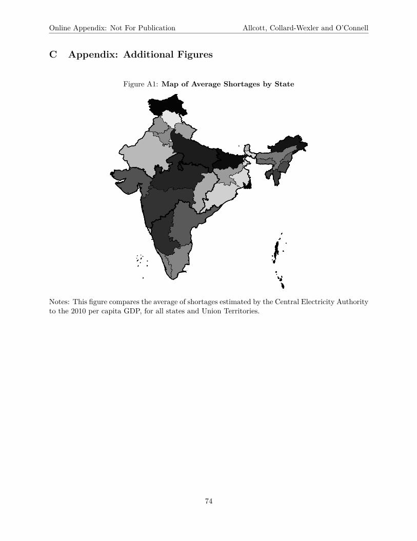
Online Appendix: Not For Publication Allcott, Collard-Wexler and O’Connell

C Appendix: Additional Figures

Figure A1: Map of Average Shortages by State

Notes: This figure compares the average of shortages estimated by the Central Electricity Authorityto the 2010 per capita GDP, for all states and Union Territories.

74

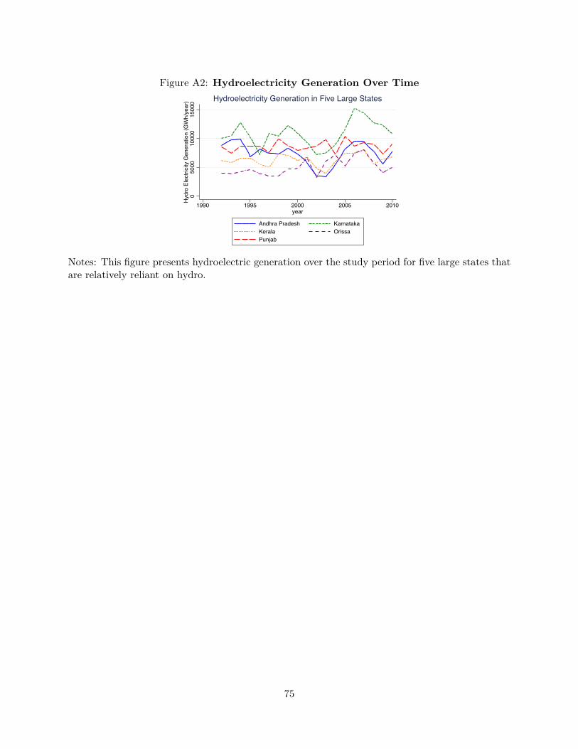
Figure A2: Hydroelectricity Generation Over Time

050

0010

000

1500

0H

ydro

Ele

ctric

ity G

ener

atio

n (G

Wh/

year

)

1990 1995 2000 2005 2010year

Andhra Pradesh KarnatakaKerala OrissaPunjab

Hydroelectricity Generation in Five Large States

Notes: This figure presents hydroelectric generation over the study period for five large states thatare relatively reliant on hydro.

75

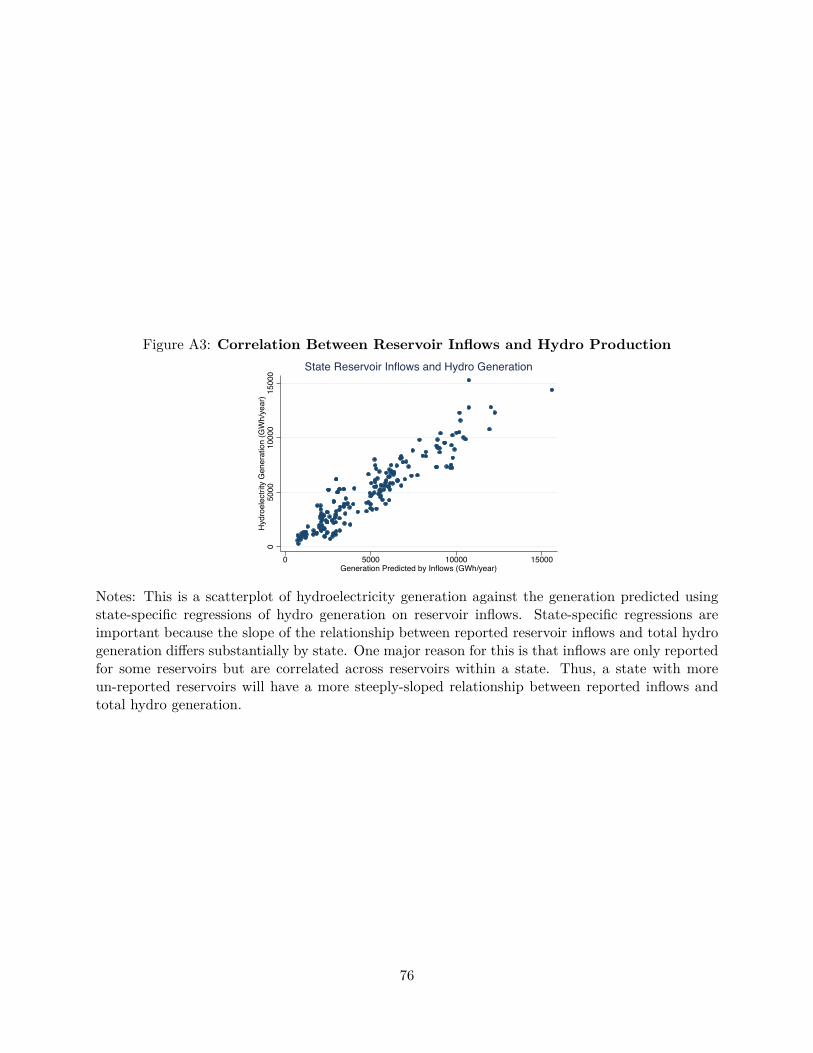
Figure A3: Correlation Between Reservoir Inflows and Hydro Production

050

0010

000

1500

0H

ydro

elec

trity

Gen

erat

ion

(GW

h/ye

ar)

0 5000 10000 15000Generation Predicted by Inflows (GWh/year)

State Reservoir Inflows and Hydro Generation

Notes: This is a scatterplot of hydroelectricity generation against the generation predicted usingstate-specific regressions of hydro generation on reservoir inflows. State-specific regressions areimportant because the slope of the relationship between reported reservoir inflows and total hydrogeneration di�ers substantially by state. One major reason for this is that inflows are only reportedfor some reservoirs but are correlated across reservoirs within a state. Thus, a state with moreun-reported reservoirs will have a more steeply-sloped relationship between reported inflows andtotal hydro generation.

76