HAL Id: hal-02057042https://hal.archives-ouvertes.fr/hal-02057042

Submitted on 5 Mar 2019

HAL is a multi-disciplinary open accessarchive for the deposit and dissemination of sci-entific research documents, whether they are pub-lished or not. The documents may come fromteaching and research institutions in France orabroad, or from public or private research centers.

L’archive ouverte pluridisciplinaire HAL, estdestinée au dépôt et à la diffusion de documentsscientifiques de niveau recherche, publiés ou non,émanant des établissements d’enseignement et derecherche français ou étrangers, des laboratoirespublics ou privés.

How Deep Learning Can Drive Physical SynthesisTowards More Predictable Legalization

Renan Netto, Sheiny Fabre, Tiago Fontana, Vinicius Livramento, LaércioLima Pilla, José Güntzel

To cite this version:Renan Netto, Sheiny Fabre, Tiago Fontana, Vinicius Livramento, Laércio Lima Pilla, et al.. HowDeep Learning Can Drive Physical Synthesis Towards More Predictable Legalization. InternationalSymposium on Physical Design, Apr 2019, San Francisco, United States. �10.1145/3299902.3309754�.�hal-02057042�

How Deep Learning Can Drive Physical SynthesisTowards More Predictable Legalization

Renan Netto1, Sheiny Fabre1, Tiago Augusto Fontana1, Vinicius Livramento2, Laércio Pilla3,José Luís Güntzel1

1Embedded Computing Lab, PPGCC, Federal University of Santa Catarina, Brazil2ASML, Netherlands

3LRI, Univ. Paris-Sud — CNRS, France{renan.netto,sheiny.fabre,tiago.fontana}@posgrad.ufsc.br

ABSTRACTMachine learning has been used to improve the predictability ofdifferent physical design problems, such as timing, clock tree syn-thesis and routing, but not for legalization. Predicting the outcomeof legalization can be helpful to guide incremental placement andcircuit partitioning, speeding up those algorithms. In this work weextract histograms of features and snapshots of the circuit from sev-eral regions in a way that the model can be trained independentlyfrom region size. Then, we evaluate how traditional and convo-lutional deep learning models use this set of features to predictthe quality of a legalization algorithm without having to executingit. When evaluating the models with holdout cross validation, thebest model achieves an accuracy of 80% and an F-score of at least0.7. Finally, we used the best model to prune partitions with largedisplacement in a circuit partitioning strategy. Experimental resultsin circuits (with up to millions of cells) showed that the pruningstrategy improved the maximum displacement of the legalized so-lution by 5% to 94%. In addition, using the machine learning modelavoided from 22% to 99% of the calls to the legalization algorithm,which speeds up the pruning process by up to 3×.

KEYWORDSPhysical synthesis, placement, legalization, machine learning

1 INTRODUCTIONThe high flexibility provided by machine learning (ML) models al-lows their use to predict the outcome of physical design algorithms.They have been employed so far to help choose between differentclock tree synthesis algorithms [11], to fix miscorrelations betweendifferent timing engines [7], and to identify detailed routing vio-lations during the placement stage [2, 17, 19]. The benefits of MLmodels come from their ability to improve the quality of physicaldesign algorithms by predicting information that would otherwisebe too costly to evaluate during execution.

Machine learning techniques have yet to be employed to help pre-dict the outcome of legalization algorithms. As technology nodes ad-vance, new challenges affect modern legalization algorithms. Someof these challenges include pin accessibility, usage of multi-row celllibraries, complex design rules, physical floorplan complexity, aswell as tight performance and power constraints. In addition, mod-ern legalization algorithms have to keep a low circuit displacementto avoid degrading the solution of upstream steps.

The prediction of the outcome of legalization algorithms by MLtechniques has multiple applications: (1) choosing, among multi-ple legalization algorithms, the one that will result in the lowestdisplacement for a given legalization region, similar to what hasbeen done for clock tree synthesis [11]; (2) guiding an incremen-tal placement technique. The ML models could predict which cellmovements result in the greatest improvement on different metrics,without requiring the execution of the legalization algorithm itself;(3) guiding a circuit partitioning strategy. Circuit partitioning canbe used to decompose the circuit in smaller disjoint parts, whichcan reduce the execution time of legalization algorithms by morethan one order of magnitude. However, it can also degrade somequality metrics since it reduces the solution space available to thelegalization algorithm.

In this work we explore mainly option (3) by integrating the pro-posed machine learning model into a circuit partitioning strategyto avoid partitions that result in large displacement. Furthermore,we partially explore option (2), because the proposed model can beused to predict when some optimizations will largely degrade thesolution obtained by upstream steps. We do so by training differentML models to detect when the maximum displacement of a givenpartition exceeds a specified threshold. Then, we select the modelwith the best results to be integrated in the partitioning strategy,acting as a pruning mechanism. The main contributions of thispaper are:

• We propose a feature extraction strategy for training ma-chine learning models using the information of circuit par-titions as input. This set of features is independent of thepartition size.• To the best of our knowledge, this is the first work to usemachine learning models to help a legalization algorithm.We evaluate different ML models in order to select the bestone for this problem (which achieved an accuracy of 80%and an F-score ≥0.7).• We employed the best ML model as a pruning mechanismfor a circuit partitioning strategy. Results using circuits fromboth ICCAD 2017 and ICCAD 2015 CAD Contests show thatthe pruning strategy reduced the maximum displacement ofthose circuits by up to 94%, and the use of ML acceleratedthe pruning by up to 3×.

The remaining sections are organized as follows. Section 2 dis-plays the related work on ML models used for physical design,and multi-row legalization. Sections 3 and 4 present the proposedML methodology and its integration into a legalization algorithm.

Finally, Section 5 shows the experimental results and Section 6provides concluding remarks.

2 RELATEDWORKMachine learning techniques have been used to solve different phys-ical design problems. The work from [11] trains a regression modelto predict the outcome of different clock tree synthesis engines.The authors extract features from architectural, floorplanning anddesign parameters. In order to handle a large number of linearlycorrelated parameters, they separate the features in two models,which are trained separately and combined using linear regression.Another application is predicting the outcome of golden signofftiming engines [7], where the authors propose a regression modelto correct miscorrelations between two commercial signoff tools.For that, they extract multiple features concerning capacitance,resistance and delay of cells and wires.

Recently, machine learning techniques have been used to predictthe violation of routability constraints in a placed netlist. For exam-ple, the work from [19] extracts features regarding pin distribution,routing blockage, global routes and local nets in order to predictthe number of DRC violations in a placed area. The work from [2]improves this idea by predicting the actual locations of the DRCviolations, using a different set of features. Finally, the work from[17] focuses on predicting only the existence of detailed routingshort violations, so that this information can be used in a detailedplacement flow, for example. Although different works make useof machine learning techniques, none of them aim to predict thequality of legalization algorithms, which is the focus of this work.Since legalization is performed not only after the global placement,but also after other placement optimization techniques, improvingthe legalization solution consequently improves the quality of thoseoptimizations.

Several recent works have been proposed to legalize circuitsfrom advanced technology nodes, which contain multi-row cells.For example, the works from [4] and [18] propose algorithms thatlegalize cells one at a time. Their algorithms enumerate a set ofvalid insertion points for each cell and place each in the locationthat minimizes circuit displacement. While the algorithm from [4]uses a greedy heuristic, the algorithm from [18] adapts the Abacuslegalization algorithm [16] that uses dynamic programming.

Instead of handling each cell at a time, the works from [10] and[3] propose algorithms that simultaneously legalize multiple cells.The authors of [10] propose an Integer Linear Programming (ILP)model to solve the multi-row legalization problem. Due to thehigh complexity of the ILP model, they divide the circuit into bins,solving the problem for multiple bins in parallel. Such strategy leadsto better results, but at the cost of longer run times. The authors of[3], by their turn, relax some constraints of the problem in order tomodel it as a Linear Complementarity Problem. This way, they canstill achieve better results than the previous works, but with a morereasonable run time. Finally, the work of [15] improves over [4]and considers additional metrics for legalization problem, such asroutability constraints.

A machine learning model that predicts the outcome of suchlegalization algorithms can be used to guide incremental optimiza-tion techniques or partitioning strategies. For example, the work of

[6] proposes a circuit partitioning strategy to speed up legalizationby executing the legalization algorithm in smaller regions of thecircuit. This way, the authors sped up the legalization, but at thecost of maximum displacement degradation, since the partitioningreduces the solution space of the legalization algorithm. Therefore,in this work we also integrate the proposed machine learning modelto this partitioning strategy, so that the model guides this processto avoid partitions with large displacement.

3 MACHINE LEARNING METHODOLOGYWe model the legalization outcome prediction as a binary classifica-tion problem. Given a legalization algorithm L, a partition of cellspi , and a displacement threshold ∆, the output of the ML model is abinary variable y ∈ {0, 1}, indicating whether L legalizes the cellsof pi without any cell displacement exceeding ∆1.

In this work, instead of using L and ∆ as inputs of the MLmodel, we train models for a specific combination of L and ∆. Asconsequence, the model receives as input the rectangular region(given by R(pi )) and cells of a partition (given by C(pi )), and mustpredict if the legalization algorithmL used to train themodel is ableto legalize this partition under a maximum displacement thresholdof ∆. In order to do so, we must provide a large number of samplesto train the ML model, so that it can identify which patterns leadto a partition with a large displacement.

3.1 Training data generationAlgorithm 1 shows how we generate the data for training and vali-dation of theMLmodel. Given a set of cells C = {c1, c2, ..., cn−1, cn },a legalization algorithm L and the rectangular area of the circuitR = (Xlef t ,Xr iдht ,Ytop ,Ybottom ), the algorithm aims to generatedata from partitions of different sizes. The first step consists indefining the number of samples that will be generated for eachpartition size (line 1). By generating the same number of samplesfor each size (1024 in this work), we avoid having the ML modelbecome biased to a specific partition size. In addition, increasingthe number of samples acts as a data augmentation strategy, whichgenerates more samples from the same circuit and helps avoidingoverfitting.

In order to generate the circuit partitions, we used the strategyfrom [6], which partitions the circuit using a k-d tree data structure,where each leaf node represents a partition. The strategy receivesas input a desired height for the k-d tree and generates 2heiдhtpartitions. Therefore, Algorithm 1 iterates over different values forthe tree height (line 3), and the necessary number of iterations togenerate the desired number of samples is calculated in line 4. Welimit the maximum height of the k-d tree to 9 because, as the heightincreases, the partitions become smaller. A height higher than 9would result in partitions with less than a few hundred of cells,which would be too small.

For each iteration, a new circuit partitioning is generated (line7). To ensure that the partitions are different from each other, weapply a vector of random movements to the cells in C (line 6). TheMOVE_CELLS function in Algorithm 2 is responsible for applying

1The displacement of a cell ci is given by the Manhattan distance between its le-galized location l (ci ) = (x (ci ), y(ci )) and its location before legalization l ′(ci ) =(x ′(ci ), y′(ci )).

2

Algorithm 1: GENERATE_DATA(C, L, R)1 n_samples ← 1024;2 max_heiдht ← 9; F ← �;3 for heiдht ← 1 tomax_heiдht do4 n_iterations ← n_samples

2heiдht;

5 for num_it ← 1 to n_iterations do6 MOVE_CELLS(C, R);7 P ← CIRCUIT_PARTITIONING(C, heiдht );8 foreach pi ∈ P do9 Λ, r esult ← L(C(pi ), R(pi ));

10 F ← F ∪ GET_FEATURES(C(pi ), R(pi ), Λ, r esult , ∆);11 end12 end13 end14 SAVE_DATA(F);

Algorithm 2:MOVE_CELLS(C, R)1 foreach ci ∈ C do2 rx ← RANDOM (−10000, 10000);3 ry ← RANDOM (−10000, 10000);4 x (ci ) ← x ′(ci ) + rx ;5 y(ci ) ← y′(ci ) + ry ;6 x (ci ) ←min(Xr iдht −w (ci ),max (Xle f t , x (ci )));7 y(ci ) ←min(Ytop − h(ci ),max (Ybottom, y(ci )));8 end

this movement. For each cell, two random variables rx , ry ∈ Z aregenerated representing the cell movement on x and y coordinates,respectively. We generate them using a uniform integer distribu-tion in the range [-10000, 10000] to ensure that the movement islarge enough to generate significantly different placements2. Af-ter moving the cells, we make sure that they lie within the circuitboundaries R (lines 6–7). Observe that theMOVE_CELLS functionis called before partitioning the circuit, so the amount of movementis not dependent of the partition size.

After generating the set of partitions P , Algorithm 1 legalizeseach partition (lines 8-11). Observe that it legalizes only the cells inC(pi ) inside the partition and the legalization area is limited to thepartition area R(pi ). In addition, the legalization function from line9 does not actually move the cells, it only finds legal locations forthe cells and returns those locations (denoted by Λ). It also returns aboolean variable indicating if the legalization was successful or not(denoted by result ), as the legalization may fail for a given partition.Observe that the proposed ML methodology is independent froma specific legalization algorithm, as long as the algorithm may beexecuted for a subset of the circuit cells and for a subregion of thecircuit area. For this reason, we do not present the pseudocode ofthe legalization algorithm, but we used an adaptation of the Abacuslegalization algorithm from [16] to handle multi-row cells.

3.2 Feature selectionGiven the legalization result and legal locations, the next step isobtaining the features for this partition. In the end, when all featuresare collected, the data is saved in an output file in line 14. In thiswork we evaluate traditional and convolutional neural networkmodels, so we need features for both of them. For convolutionalmodels, the input is simply a snapshot image of the partition. Weused different colors to distinguish between movable and fixed cells.2The smallest circuit used in the experiments has an area of 342000 × 342000, so thismovement corresponds to at most 3% of the circuit dimensions.

Movable cells are represented by shades of the same color. Thisway, the model can identify overlaps since they are represented bythe combined colors of multiple cells. On the other hand, for thetraditional models we need to select an appropriate set of features.Partitions become hard to legalize with low displacement whenthey have a high density of cells, or when they have many celloverlaps. Therefore, we selected the features presented in Table 1for our ML methodology.

Table 1: Features used by the ML model.

Feature MeaningD Density of the partition areaAh Area occupied by cells of each height

HaNormalized histogram of area occupiedby cells on each partition subrow

HoNormalized histogram of area occupiedby overlaps on each partition subrow

Algorithm 3: GET_FEATURES(C(pi ), R(pi ), Λ, result , ∆)1 Af ← 0; Am ← 0; Ar ← w (pi ) × h(pi ); Ah ← [];2 δmax ← −∞;3 foreach ci ∈ C(pi ) do4 if f ixed (ci ) then5 box ← intersect ion(ci , R(pi ));6 Af ← Af +w (box ) × h(box );7 else8 Am ← Am +w (ci ) × h(ci );

9 Ah [h(ci )] ← Ah [h(ci )] +w (ci )×h(ci )

Ar ;10 end11 δ (ci ) ← |l (ci ) − λ(ci ) |;12 δmax ← max(δmax, δ (ci ));13 end

14 ∆← AmAr −Af

;

15 y ← δmax ≤ ∆;16 A← [];O ← []; Σ← partition subrows;17 foreach σi ∈ Σ do18 C(σi ) ← cells intersecting σi ;19 a(σi ) ← 0; o(σi ) ← 0;20 foreach ci ∈ C(σi ) do21 a(σi ) ← a(σi ) +w (ci );22 end23 C′ ← cells intersecting inC(σi );24 foreach cj ∈ C′ do25 o(σi ) ← o(σi ) +w (cj );26 end

27 A[σi ] ←a(σi )w (σi )

;O [σi ] ←o(σi )w (σi )

;28 end29 Ha ← normalized histogram with values of A;30 Ho ← normalized histogram with values ofO ;31 return (y , ∆, Ah , Ha , Ho );

The first two features aim to represent global information of thepartition density. Since partitions with multi-row cells are harder tolegalize, we measure not only the cell density, but also the area oc-cupied by cells of each height. However, just the global informationis not enough to identify partitions that are hard to legalize, sincesome circuit rows may be more crowded than others. The third fea-ture aims to represent this information by means of an histogramof the area occupied by cells on each partition subrow. A subrow isa row segment that does not overlap with any macroblocks and/or

3

123

5

0

4

0.2 0.4 0.6 0.8 10

2

4

6

8

00.2 0.4 0.6 0.8 10

0.10.20.3

0.5

0

0.4

0.2 0.4 0.6 0.8 10

0.2

0.4

0.6

0.8

00.2 0.4 0.6 0.8 10

(b) Histogram of area occupied by cells in each subrow.

(a) Partition with 20 movable cells and one fixed cell.

(d) Normalized area histogram (Ha).

(c) Histogram of area occupied by overlaps in each subrow.

(e) Normalized overlap histogram (Ho).

Figure 1: Circuit features extracted for a hypothetical partition.

fixed cells. Finally, a subrow may be overcrowded but with fewcell overlaps, which makes it easier to legalize. Therefore, the lastfeature measures the area occupied by overlaps on each subrow, sothat the ML model can correlate this information to the result.

Figure 1 shows by means of an example how the histograms forthe last two features are generated for a given partition. Figure 1(a)illustrates a partition with 20 movable cells (blue rectangles), onefixed cell (gray rectangle) and 10 subrows (σ1 to σ10). Figures 1(b)and (c) show the area and overlap histograms for this partition.For illustration purposes, the histograms contain 5 bins, but weactually used histograms with 20 bins for better precision. Each binindicates the number of rows whose area of cells (or overlap of cells)is within a given range. We can see that the histogram in Figure 1(b)concentrates on the middle region, with most subrows having from40% to 60% of their area occupied by cells. On the other hand, thehistogram in Figure 1(c) concentrates on the 0% to 20% bin, withonly two subrows having more than 20% of their area occupied byoverlaps. However, using absolute values for the y axis of thosehistograms may bias the ML model to large partitions, since theywould have a larger number of subrows. In order to avoid this issue,we normalize the y axis with relation to the number of subrows inthe partition, resulting in the histograms Ha and Ho in Figures 1(d)and (e). Observe that they have the same structure of the previoushistograms, with the only difference being the normalized verticalaxis.

Algorithm 3 shows the details of how these features are collectedfrom a given partition. The loop from lines 3–13 calculates thevalues for the first two features (density and area occupied by cellsof each height), so it starts by initializing the necessary variables todo so. Those variables are: the area occupied by fixed cells (Af ), thearea occupied by movable cells (Am ), the area of the partition itself(Ar ) and a list with the areas occupied by cells of each height (Ah ).Observe that the area occupied by fixed cells is not considered inAh , since those cells are not moved by the legalization algorithm.However, their area is important to measure the partition density,which is given by the area occupied by movable cells Am dividedby the free area in the partition (Ar - Af ) in line 14. In addition, foreach height, Ah is normalized by the partition area. The first loopalso measures the maximum displacement of the legalized cells inlines 11–12. This information is used to determine the class of thispartition in line 15.

The loop from lines 17–29, on the other hand, is responsible forobtaining the data for the histograms Ha and Ho . This is done byiterating through all subrows σi ∈ Σ of the partition and, for eachone, measuring the width occupied by the cells intersecting thearea of σi , storing this information in variable a(σi ). In addition,for the subset of cellsC ′ ∈ C(σi ) that have some overlap with othercells in said subrow, we compute how much overlap there is usingvariable o(σi ). Finally, both a(σi ) and o(σi ) are normalized by thesubrow widthw(σi ) in line 27. This normalization ensures that theML model is not biased by large subrows that have larger absolutevalues of a(σi ) and o(σi ). The last part of the algorithm creates thenormalized histograms Ha and Ho in lines 30–31.

4 PHYSICAL DESIGN INTEGRATIONAfter training and validating the ML model proposed in Section 3,we integrated it in the circuit partitioning strategy of [6] as a usecase to evaluate the ML model. As mentioned in Section 3, theirwork partitions the circuit using a k-d tree data structure, in a waythat the leaf nodes represent the partitions, which are legalizedseparately. If a partition can not be legalized, it is merged with itssibling node, and the legalization proceeds to their parent node.In the end, the whole circuit legalization can be sped up, sincethe partitioning strategy reduces the input size of the legalizationalgorithm. However, doing so may degrade the solution quality,especially maximum displacement. Therefore, we modified theirpartitioning strategy to merge sibling nodes not only when thelegalization fails, but when it results in a large displacement as well.This way, we can prune partitions that would otherwise degradethe solution quality.

There are two ways of doing this pruning strategy: (1) runningthe legalization algorithm and measuring the displacement of theobtained solution; (2) using the ML model to predict the outcomeof the legalization without running the legalization algorithm. Wecompare these two solutions in order to evaluate the efficiency andimpact of the ML model.

Algorithm 4 shows how we implemented the first pruning strat-egy. The algorithm receives as input the partitions to be legalized(P), the legalization algorithm (L) and the maximum displacementthreshold (∆). Then, it iterates through all partitions trying to legal-ize them. For each partition pi , it runs the legalization algorithm(line 4) and measures the obtained maximum displacement δmax(lines 5–9). If δmax exceeds the threshold ∆ or if the legalization

4

Algorithm 4: PARTITIONED_LEGALIZATION (P, L, ∆)1 foreach pi in P do2 P ← P \ {pi };3 if parent (pi ) < P then4 Λ, r esult ← L(C(pi ), R(pi ));5 δmax ← −∞;6 foreach ci ∈ C(pi ) do7 δ (ci ) ← |l (ci ) − λ(ci ) |;8 δmax ← max(δmax , δ (ci ));9 end

10 if δmax > ∆ ∨ ¬r esult then11 P ← P ∪ {parent (pi )};12 else13 foreach ci ∈ C(pi ) do14 l (ci ) ← λ(ci );15 end16 end17 end18 end

Algorithm 5:ML_PARTITIONED_LEGALIZATION (P, L, ∆,M)1 foreach pi in P do2 P ← P \ {pi };3 if parent (pi ) < P then4 if M(C(pi ), R(pi )) then5 P ← P ∪ {parent (pi )};6 else7 Λ, r esult ← L(C(pi ), R(pi ));8 if ¬r esult then9 P ← P ∪ {parent (pi )};

10 else11 foreach ci ∈ C(pi ) do12 l (ci ) ← λ(ci );13 end14 end15 end16 end17 end

fails, the partition is ignored and its parent node is added to P tobe legalized instead (lines 10–11). Otherwise, its cells are placedin their legal locations (lines 13–15). Observe that, by adding theparent node of pi in P, it is possible to avoid the legalization of thesibling of pi as well with the verification of line 3. If the parent ofpi is already in P, this means the sibling of pi resulted in a largedisplacement or could not be legalized, so pi should be ignored aswell.

Running the legalization algorithm to prune partitions with largedisplacement results in several unnecessary calls to the legalizationalgorithm, which may take too much time. Therefore, the secondpruning strategy relies on the ML model to predict when a partitionshould be ignored, as detailed in Algorithm 5. Observe that nowthe algorithm receives as input the machine learning modelM aswell, which is used in line 4 to predict when the partition can bepruned. Then, it runs the legalization algorithm L only if it wasnot pruned (line 7), and checks only if the partition was legalized(lines 8–10). If the partition was successfully legalized, it places thecells in the legal locations. In the end, the whole circuit is legalized,but requiring fewer calls to the legalization algorithm L than inAlgorithm 4.

5 EXPERIMENTAL RESULTS5.1 Experimental setupThis work uses the benchmarks from ICCAD 2015 and ICCAD 2017CAD Contest [5, 13]. Table 2 presents the names and number ofcells of each circuit. We divided the circuits in three groups: train-ing, validation and test. The training and validation sets wereobtained by randomly separating the circuits from the ICCAD 2017CAD Contest into those groups using the holdout method for crossvalidation. They were used to evaluate different ML models andto select the best model for the integration described in Section 4.This way, the ML model is trained and validated using circuits withmulti-row cells, which are more challenging to legalize. On theother hand, the test set is used along with the validation one for asecond experiment, which evaluates the quality of the selected MLmodel when integrated in a circuit partitioning strategy. The test setis composed by the ICCAD 2015 CAD Contest benchmarks, whichwere not used when selecting the best ML model. Although thosecircuits do not contain multi-row cells, they are much larger thanthe others. Therefore, they provide a way to evaluate the speedupachieved by the ML model on large designs.

We performed all experiments in a Linux workstation with anIntel® Xeon® E5430 processor with 4 cores @ 2.66 GHz and 16GBDDR2 667MHz RAM. In order to identify the best ML model forour problem we evaluated three options: an artificial neural net-work (ANN) with a single hidden layer with 10 neurons, a decisiontree (DT) and a deep convolutional neural network (CNN), us-ing the resnet34 CNN architecture [8]. The first two models wereprototyped using the Knime platform [14], while the CNN wasprototyped using the fast.ai library [9]. After selecting the bestML model, it was retrained with the same parameters using the

Table 2: Benchmarks used in the experiments.

Benchmark # Cells of different heights Benchmarkset Group

1 2 3 4pci_bridge32_a_md1 26K 1.7K 597 448 ICCAD17 validationpci_bridge32_a_md2 25K 2K 1.1K 994 ICCAD17 validationpci_bridge32_b_md1 26K 1.7K 585 439 ICCAD17 validationpci_bridge32_b_md2 28K 292 292 292 ICCAD17 validationpci_bridge32_b_md3 27K 292 585 585 ICCAD17 trainingfft_2_md2 28K 2.1K 705 529 ICCAD17 trainingfft_a_md2 27K 2K 672 504 ICCAD17 trainingfft_a_md3 28K 672 672 672 ICCAD17 trainingdes_perf_a_md1 103K 4.6K 0 0 ICCAD17 trainingdes_perf_a_md2 105K 1K 1086 1K ICCAD17 trainingdes_perf_1 112K 0 0 0 ICCAD17 trainingdes_perf_b_md1 106K 5.8K 0 0 ICCAD17 trainingdes_perf_b_md2 101K 6.7K 2.2K 1.6K ICCAD17 trainingedit_dist_1_md1 118K 7.9K 2.6K 1.9K ICCAD17 trainingedit_dist_a_md2 115K 7.7K 2.5K 1.9K ICCAD17 trainingedit_dist_a_md3 119K 2.5K 2.5K 2.5K ICCAD17 trainingsuperblue18 768M 0 0 0 ICCAD15 testsuperblue4 795M 0 0 0 ICCAD15 testsuperblue16 981M 0 0 0 ICCAD15 testsuperblue5 1086M 0 0 0 ICCAD15 testsuperblue1 1209M 0 0 0 ICCAD15 testsuperblue3 1213M 0 0 0 ICCAD15 testsuperblue10 1876M 0 0 0 ICCAD15 testsuperblue7 1931M 0 0 0 ICCAD15 test

5

Table 3: Results of different ML models for different maximum displacement thresholds.

Max disp threshold of 5 rows Max disp threshold of 10 rows Max disp threshold of 15 rowsML model accuracy precision recall F-score accuracy precision recall F-score accuracy precision recall F-score

ANN 81% 86% 72% 0.78 85% 78% 73% 0.75 84% 69% 72% 0.70DT 76% 83% 63% 0.71 82% 76% 58% 0.66 83% 71% 63% 0.67CNN 82% 84% 83% 0.83 82% 72% 83% 0.77 80% 70% 66% 0.68

Table 4: Results when integrating the ANN model to the partitioning strategy

Max disp threshold of 5 row Max disp threshold of 10 row Max disp threshold of 15 rowDesign Avg disp Max disp HPWL Avg disp Max disp HPWL Avg disp Max disp HPWL

LEG ANN LEG ANN LEG ANN LEG ANN LEG ANN LEG ANN LEG ANN LEG ANN LEG ANNpci_bridge32_a_md2 0.92 0.92 0.77 0.77 0.95 0.95 0.92 0.92 0.77 0.77 0.95 0.95 0.92 0.92 0.77 0.77 0.95 0.95pci_bridge32_b_md1 0.69 0.69 0.30 0.30 0.99 0.96 0.69 0.69 0.30 0.30 0.99 0.96 0.69 1.01 0.30 0.91 0.99 1.00pci_bridge32_b_md2 0.90 0.91 0.33 0.33 0.98 0.98 0.90 0.91 0.33 0.33 0.98 0.98 0.90 0.87 0.33 0.45 0.98 0.98pci_bridge32_a_md1 0.89 0.89 0.95 0.95 0.98 0.98 0.89 0.89 0.95 0.95 0.98 0.98 0.89 0.89 0.95 0.95 0.98 0.98superblue10 1.01 1.01 0.21 0.21 1.00 1.00 1.01 1.01 0.21 0.21 1.00 1.00 1.01 1.01 0.21 0.21 1.00 1.00superblue18 0.96 0.96 0.11 0.11 1.00 1.00 0.96 0.92 0.11 0.11 1.00 1.00 0.96 0.92 0.11 0.24 1.00 1.00superblue4 0.87 0.87 0.17 0.17 1.00 1.00 0.87 0.87 0.17 0.17 1.00 1.00 0.87 0.85 0.17 0.17 1.00 0.99superblue7 1.04 1.04 0.13 0.13 1.00 1.00 1.04 1.04 0.13 0.13 1.00 1.00 1.04 1.04 0.13 0.13 1.00 1.00superblue1 1.08 1.08 0.06 0.06 1.00 1.00 1.08 1.08 0.06 0.06 1.00 1.00 1.08 1.08 0.06 0.06 1.00 1.00superblue16 1.06 1.06 0.52 0.52 1.00 1.00 1.06 1.06 0.52 0.52 1.00 1.00 1.06 1.06 0.52 0.52 1.00 1.00superblue3 1.01 1.01 0.18 0.18 1.00 1.00 1.01 1.01 0.18 0.18 1.00 1.00 1.01 0.94 0.18 0.28 1.00 1.00superblue5 1.05 1.05 0.12 0.12 1.00 1.00 1.05 1.05 0.12 0.12 1.00 1.00 1.05 0.96 0.12 0.34 1.00 1.00

Average 0.96 0.96 0.32 0.32 0.99 0.99 0.96 0.96 0.32 0.32 0.99 0.99 0.96 0.96 0.32 0.42 0.99 0.99Median 0.98 0.98 0.19 0.19 1.00 1.00 0.98 0.96 0.19 0.19 1.00 1.00 0.98 0.95 0.19 0.31 1.00 1.00

Keras framework [12], so that we could integrate the model in theC++ code of the circuit partitioning strategy. All experiments areavailable under public domain, so that they can be reproduced [1].

5.2 Evaluation of machine learning modelsTable 3 shows the results of the ML models on the validation setfor three different maximum displacement thresholds (∆): 5, 10,and 15 rows. We evaluated the models by their accuracy, precision,recall and F-score3. We selected the best results obtained for eachmodel. Since the number of samples of each class (true positive, falsepositive, etc.) is not necessarily balanced, it is important to evaluatenot only the accuracy of the model, but also the precision and recall.A low precision means a model assumes that some partitions wouldresult in a large displacement when that is not the case, resulting inworse execution times as it takes longer to legalize the larger parentpartition. On the other hand, a low recall means that the modelwill not prune some partitions that should have been pruned. Thiswill result in quality degradation, since Algorithm 5 will accept thelegalization even though it should not.

When the maximum displacement threshold is 5 rows, ANN andCNN are very similar in accuracy, with CNN achieving a better F-score. The DTmodel, on the other hand, seems to be the worst of thethree models, with lower accuracy, precision, and recall. When weincreased the maximum displacement threshold to 10 rows, there isa slight increase on the accuracy of the DT and ANN models, and

3F-score is calculated by the harmonic mean of precision and recall.

no difference for the CNN model. However, there was a reductionon the precision for all models, due to the more unbalanced datafor this displacement threshold. The recall was only affected onDT, which again makes it the worst of the three models. Finally,when the maximum displacement threshold is 15 rows, the datais even more unbalanced, with less positive instances. In this case,there was an F-score reduction on both ANN and CNN models. Theimpact was greater on the CNN, whose F-score dropped from 0.83(with threshold of 5 rows) to 0.68 (with threshold of 15 rows).

These results led us to the following conclusions: (1) DT hasa worse F-score for all maximum displacement thresholds, whichmakes it a poor model for the analyzed problem; (2) increasingthe maximum displacement threshold degrades the quality of allmodels, due to more unbalanced data. Thus, an evaluation witheven higher thresholds would require the generation of data withmore positive instances.

5.3 Integration with circuit partitioningBased on the evaluation of the ML models, we selected the ANNmodel to be integrated in the circuit partitioning strategy. Althoughthe CNN achieved a higher accuracy and F-score for the maximumdisplacement threshold of 5 rows, we selected ANN over CNNfor the following reasons: (1) the ANN model achieved a higheraccuracy and F-score for the highest displacement threshold (15rows), which suggests that this model is more robust to unbalanceddata; (2) the CNN model is more complex, and therefore it takeslonger to classify partitions using it. In order for this increased

6

run time to be compensated, the CNN model must have a muchhigher accuracy than ANN, which is not the case for the evaluatedmodels; (3) further experiments showed that the CNN model haslower accuracy on smaller partitions than on larger partitions. Sincesmaller partitions are the majority in the partitioning strategy, it isbetter to have a higher accuracy for them.

Table 4 shows the results of applying the pruning strategy pre-sented in Section 4 on the validation and test circuits with relation toaverage displacement, maximum displacement and half-perimeterwirelength (HPWL)4. Observe that none of the circuits presentedin this table were used for the model training. For each metric wepresent the ratio of the result when using the pruning strategy bythe original result from [6]. This way, a ratio lower than 1 for agiven metric means that its value was reduced (and improved) whenusing the pruning strategy. For each metric, the table shows theresults of two versions of the pruning strategy: LEG (Algorithm 4),and ANN (Algorithm 5 using the ANNmodel). In addition, the tableis divided in the same maximum displacement thresholds as Table 3(5, 10 and 15 rows).

First of all, observe that for LEG, the results remain the same forall metrics even when increasing the threshold from 5 to 15 rows.The ratios were on average 0.96, 0.32 and 0.99 for average displace-ment, maximum displacement and HPWL, respectively. This meansthat increasing themaximumdisplacement threshold does notmakea significant difference for those circuits. The improvement wasespecially high for the maximum displacement, since this is themetric being verified by the pruning strategy. In addition, therewas a significant reduction on the average displacement of circuitspci_bridдe32_a_md2, pci_bridдe32_b_md1, pci_bridдe32_b_md2,pci_bridдe32_a_md1, superblue18 and superblue4, which are thesmallest circuits used on this experiment. This happened because,for larger circuits, legalizing the parent nodes in the partitioningstrategy may increase the average displacement, since they havea larger area and, therefore, allow more cell movement. However,the increase on average displacement is largely compensated bythe reduction on maximum displacement.

When using the ANN model with a maximum displacementthreshold of 5 or 10 rows, the results were the same as LEG foralmost all circuits, which means the accuracy of the ML model wasenough to avoid degrading the solution quality. However, whenincreasing the maximum displacement threshold to 15 rows, thelower precision of the ANNmodel results in degradation of the maxdisplacement metric, whose average ratio becomes 0.42. However,this value is still much lower than the results from [6].

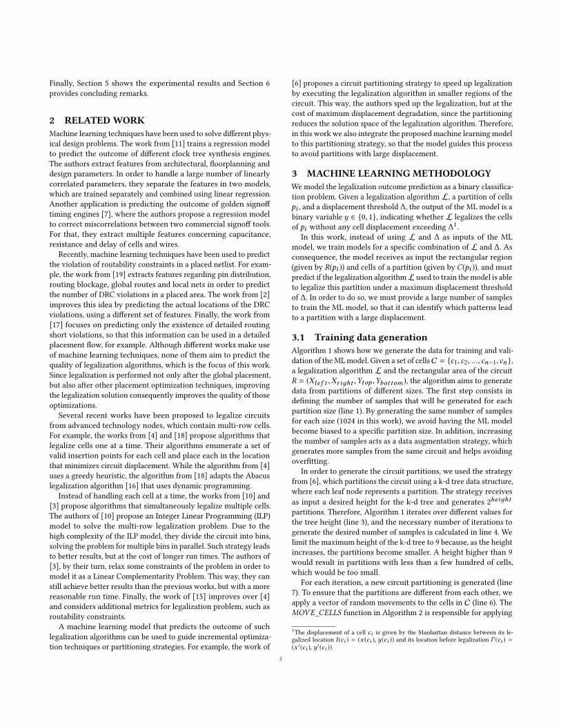
Besides analyzing the solution quality, it is important to also an-alyze how many calls to the legalization algorithm were avoided byusing ANN, andwhat was the impact on the execution time. Figure 2shows the ratio of the number of calls to the legalization algorithmperformed by ANN compared to LEG. For all cases, the ANN modelreduced the number of legalization calls, with a greater reduction inthe larger circuits. This happens because the larger number of cellsin these circuits increases the probability of a cell resulting in a largedisplacement, requiring more partition merges. In addition, thisreduction is greater with a threshold of 5 rows because it requires4Although circuit des_per f _b_md1 belongs to the validation set, it was not used inthis experiment because the legalization algorithm was not capable of legalizing thiscircuit.

AN

N /

LEG

Figure 2: Comparison between the number of calls to thelegalization algorithm done by LEG and ANN.

Figure 3: Comparison between LEG and ANN’s executiontimes (speedup = ratio LEG/ANN).

more merges, which increases the number of legalization calls forLEG. However, even in the worst case, ANN required 22% less callsto the legalization algorithm (pci_bridдe32_a_md1, 15 rows), butup to 99% in the best case (superblue7, 5 rows). This reduction onnumber of legalization calls resulted in the speedup presented inFigure 3. This figure shows the speedup only for ICCAD 2015 CADContest benchmarks, since the speedup is negligible for the othercircuits due to their small size. The speedup was calculated as theratio of the execution time of LEG by the execution time of ANN,so a speedup greater than 1 means ANN is faster.

The results in Figure 3 show that ANN is faster for all cases,except for superblue16 with the maximum displacement thresholdof 15 rows, achieving speedups from 0.86 to 3. In addition, formost cases, the speedup is higher when the maximum displacementthreshold is lower because, as observed in Figure 2, in those casesthe reduction in the number of legalization calls is greater. However,there are some exceptions, such as superblue18 for thresholds of 10and 15 rows, as well as superblue3 and superblue5 for thresholds of15 rows. These cases are also situations where the solution qualityhas changed when increasing the maximum displacement threshold(Table 4). In these cases, ANN failed to identify some partitionswith large displacement, which reduces the execution time but candegrade the solution quality.

7

Figure 4: Comparison of the execution times between LEGwith threshold of 15 rows and ANNwith threshold of 5 rows(speedup = ratio LEG/ANN).

Finally, although ANN degrades the quality of the pruning forsome circuits when using larger displacement thresholds, we ob-served that the pruning quality is the same for all thresholds whenusing LEG. Therefore, for the evaluated circuits, increasing themaximum displacement threshold does not improve the solutionquality, but only reduces the execution time. Figure 4 shows thespeedup achieved by the ANN results for the threshold of 5 rows(which achieved the best solution quality for ANN) compared to theresults of LEG for the threshold of 15 rows (which has the smallestexecution times for LEG). In this figure, it is possible to see thatthe best ANN solution is still faster than the best LEG solution byat least 1.14 and up to 2.3, which shows that ANN can effectivelyspeed up the pruning strategy without compromising the solutionquality. The speedup of at least 2 in some cases means that, forsome circuits, it is possible to evaluate two different maximumdisplacement thresholds using ANN in the time that only one couldbe evaluated with LEG.

6 CONCLUSIONSIn this work we evaluated how ML models can be used to improvethe predictability of legalization algorithms. We evaluated threemodels, including one deep convolutional neural network. The bestmodel was integrated into a circuit partitioning strategy, to actas a pruning mechanism to identify partitions that will result inlarge displacement after legalization. This pruning strategy greatlyreduces the maximum displacement of the legalized solution, andthe ML model accelerates this process by avoiding up to 99% of thecalls to the legalization algorithm.

As future work, we intend to investigate the possibility of usingML models not only to predict when a partition will violate a givendisplacement threshold, but to estimate the resulting displacementitself. This can be used to guide incremental placement algorithms,by using the ML model to evaluate the quality of different optimiza-tions (or different legalization algorithms), without requiring to callthe legalization algorithm.

7 ACKNOWLEDGMENTSThis study was financed in part by the Coordenação de Aperfeiçoa-mento de Pessoal de Nível Superior - Brasil (CAPES) - Finance Code001 and by the Brazilian Council for Scientific and Technological

Development (CNPq) through Project Universal (457174/2014-5)and PQ grants 310341/ 2015-9.

REFERENCES[1] Ophidian: an open source library for physical design research and teaching.

https://gitlab.com/renan.o.netto/ophidian-research.[2] W.-T. J. Chan, P.-H. Ho, A. B. Kahng, and P. Saxena. Routability optimization

for industrial designs at sub-14nm process nodes using machine learning. InProceedings of the 2017 ACM on International Symposium on Physical Design, pages15–21. ACM, 2017.

[3] J. Chen, Z. Zhu, W. Zhu, and Y.-W. Chang. Toward optimal legalization formixed-cell-height circuit designs. In DAC, page 52. ACM, 2017.

[4] W.-K. Chow, C.-W. Pui, and E. F. Young. Legalization algorithm for multiple-rowheight standard cell design. In DAC, pages 1–6. IEEE, 2016.

[5] N. K. Darav, I. Bustany, A. Kennings, and R. Mamidi. Iccad-2017 cad contest inmulti-deck standard cell legalization and benchmarks. In ICCAD, 2017.

[6] S. Fabre, J. L. Güntzel, L. L. Pilla, R. Netto, T. Fontana, and V. Livramento. En-hancing multi-threaded legalization through kd tree circuit partitioning. InSymposium on Integrated Circuits and Systems Design, 2018.

[7] S.-S. Han, A. B. Kahng, S. Nath, and A. S. Vydyanathan. A deep learning method-ology to proliferate golden signoff timing. In Proceedings of the conference onDesign, Automation & Test in Europe, page 260. European Design and AutomationAssociation, 2014.

[8] K. He, X. Zhang, S. Ren, and J. Sun. Deep residual learning for image recognition.In Proceedings of the IEEE conference on computer vision and pattern recognition,pages 770–778, 2016.

[9] J. Howard and R. Thomas. fast.ai - Making neural networks uncool again. http://www.fast.ai/, 2018. [Online; accessed 28-September-2018].

[10] C.-Y. Hung, P.-Y. Chou, andW.-K. Mak. Mixed-cell-height standard cell placementlegalization. In GLSVLSI, pages 149–154. ACM, 2017.

[11] A. B. Kahng, B. Lin, and S. Nath. High-dimensional metamodeling for predictionof clock tree synthesis outcomes. In System Level Interconnect Prediction (SLIP),2013 ACM/IEEE International Workshop on, pages 1–7. IEEE, 2013.

[12] Keras. Keras: The Python Deep Learning library. https://keras.io/, 2018. [Online;accessed 28-September-2018].

[13] M. Kim, J. Hu, J. Li, and N. Viswanathan. ICCAD-2015 CAD contest in incrementaltiming-driven placement and benchmark suite. 2015.

[14] Knime. Knime - open for innovation. https://www.knime.com/, 2018. [Online;accessed 28-September-2018].

[15] H. Li, W.-K. Chow, G. Chen, E. F. Young, and B. Yu. Routability-driven andfence-aware legalization for mixed-cell-height circuits. In Proceedings of the 55thAnnual Design Automation Conference, page 150. ACM, 2018.

[16] P. Spindler, U. Schlichtmann, and F. M. Johannes. Abacus: fast legalization ofstandard cell circuits with minimal movement. In ISPD, pages 47–53. ACM, 2008.

[17] A. F. Tabrizi, L. Rakai, N. K. Darav, I. Bustany, L. Behjat, S. Xu, and A. Kennings.A machine learning framework to identify detailed routing short violations froma placed netlist. In 2018 55th ACM/ESDA/IEEE Design Automation Conference(DAC), pages 1–6. IEEE, 2018.

[18] C.-H. Wang, Y.-Y. Wu, J. Chen, Y.-W. Chang, S.-Y. Kuo, W. Zhu, and G. Fan. Aneffective legalization algorithm for mixed-cell-height standard cells. In ASP-DAC,pages 450–455. IEEE, 2017.

[19] Q. Zhou, X. Wang, Z. Qi, Z. Chen, Q. Zhou, and Y. Cai. An accurate detailedrouting routability prediction model in placement. In Quality Electronic Design(ASQED), 2015 6th Asia Symposium on, pages 119–122. IEEE, 2015.

8