HOW AND WHEN QUANTUMPHENOMENA BECOME REAL

Ph. BlanchardFaculty of Physics and BiBoS

University of BielefeldUniversitatstr. 25D-33615 Bielefeld

A. JadczykInst. of Theor. PhysicsUniversity of Wroc law

Pl. Maxa Borna 9PL-50 204 Wroc law

Abstract

We discuss recent developments in the foundations of quantumtheory with a particular emphasis on description of measurement–likecouplings between classical and quantum systems. The SQUID-tankcoupling is described in some details, both in terms of the Liouvilleequation describing statistical ensambles and piecewise deterministicrandom process describing random behaviour of individual systems.

1

1 Introduction

Quantum theory is without doubt one of the most successful constructionsin the history of theoretical physics and moreover the most powerful theoryof physics: Its predictions have been perfectly verified until now again andagain. The new conception of Nature proposed by Bohr, Heisenberg and Bornwas radically different from that of classical physics and several paradoxeshave plagued Quantum Physics since its inception. Although the formalismof non relativistic quantum mechanics was constructed in the late 1920’sthe interpretation of Quantum Theory is still today the most controversialproblem in the foundations of physics. The mathematical formalism andthe orthodox interpretation of QM are stunningly simple but leave the gateopen for alternative interpretations aimed at solving the dilemma lying inthe Copenhagen interpretation. ”The fact that an adequate presentationof QM has been so long delayed is no doubt caused by the fact that NielsBohr brainwashed a whole generation of theorists into thinking that the jobwas done fifty years ago” wrote Murray Gell Mann 1979. It was also JohnBell’s point of view that ”something is rotten” in the state of Denmarkand that no formulation of orthodox quantum mechanics was free of fatalflows. This conviction motivated his last publication [1]. As he says ”Surelyafter 62 years we should have an exact formulation of some serious part ofquantum mechanics. By ”exact” I do not mean of course ”exactly true”. Ionly mean that the theory should be fully formulated in mathematical terms,with nothing left to the discretion of the theoretical physicist ...”. OrthodoxQuantum Mechanics considers two types of incompatible time evolution Uand R, U denoting the unitary evolution implied by Schrodinger’s equationand R the reduction of the quantum state. U is linear, deterministic, local,continuous and time reversal invariant while R is probabilistic, non-linear,discontinuous and acausal. Two options are possible for completing QuantumMechanics. According to John Bell [10] ”Either the wave functions is noteverything or it is not right ...”.

In recent papers [2, 3, 4] we propose mathematically consistent modelsdescribing the information transfer between classical and quantum systems.The class of models we consider aims at providing an answer to the questionof how and why quantum phenomena become real as a result of interac-tion between quantum and classical domains. Our results show that a simpledissipative time evolution can allow a dynamical exchange of information be-tween classical and quantum levels of Nature. Indeterminism is an implicit

2

part of classical physics and an explicit ingredient of quantum physics. Irre-versible laws are fundamental and reversibility is an approximation. R. Haagformulated a similar thesis as ”... once one accepts indetermination there isno reason against including irreversibility as part of the fundamental lawsof Nature” [5]. According to the standard terminology the joint systems inour models are open. Thus one is tempted to try to understand their be-haviour as an effective evolution of subsystems of unitarily evolving largerquantum systems. Although mathematically possible such an enlargement isnon-unique. Therefore we prefer to extend the prevailing paradigm and learnas much as possible how to deal directly with open systems and incompleteinformation.

With a properly chosen initial state the quantum probabilities are ex-actly mirrored by the state of the classical system and moreover the state ofthe quantum subsystem converges as t → +∞ to a limit in agreement withvon Neumann-Luders standard quantum mechanical measurement projectionpostulate R. In our model the quantum system

∑q is coupled to a classical

recording device∑c which will respond to its actual state.

∑q should affect∑

c, which should therefore be treated dynamically. We thus give a minimalmathematical semantics to describe the measurement process in QuantumMechanics. For this reason the simplest models that we proposed can beseen as the elementary building blocks used by Nature in the constant com-munications that take place between the quantum and classical levels. Inour framework a quantum mechanical measurement is nothing else as a cou-pling between a quantum mechanical system

∑q and a classical system

∑c

via a completely positive semigroup αt = etL in such a way that informationcan be transferred from

∑q to

∑c. A measurement represents an exchange

of information between physical systems and therefore involves entropy pro-duction. See [6] where a definition of entropy for non-commutative systemsis given, which is based on the concepts of conditional entropy and stationarycouplings between

∑q and

∑c. Moreover Sauvageot and Thouvenot show the

equivalence of this definition with the one proposed by Connes, Narnhoferand Thirring [12].

There have been many attempts to explain quantum measurements. Forrecent reviews see [7, 8, 9]. Our claim is, that whatever the mechanism usedto derive models of measurements starting from fundamental interactions is,this mechanism will lead finally to one model of the class we introduced.In fact any realistic situation will reduce to a model of our class since theoverwhelming majority of the properties of the counter and the environment

3

are irrelevant from the point of view of statistically predicting the result ofa measurement. We propose indeed to consider the total system

∑tot =∑

q⊗∑c, and the behaviour associated to the total algebra of observables

Atot = Aq ⊗ Ac = C(Xc) ⊗ L(Hq), where Xc is the classical phase spaceand Hq the Hilbert space associated to

∑q, is now taken as the fundamental

reality with pure quantum behaviour as an approximation valid in the caseswhen recording effects can be neglected. In Atot we can describe irreversiblechanges occuring in the physical world, like the blackening photographicemulsion, as well as idealized reversible pure quantum and pure classicalprocesses. We extend the model of Quantum Theory in such a way that thesuccessful features of the exisiting theory are retained but the transitionsbetween equilibria in the sense of recording effects are permitted. In Section2 we will briefly describe the mathematical and physical ingredients of thesimplest model and discuss the measurement process in this framework.

The range of applications of the model is rather wide as will be shownin Section 3 with a discussion of Zeno effect, giving an account of [11]. Tothe Liouville equation describing the time evolution of statistical states of∑tot we will be in position to associate a piecewise deterministic process

taking values in the set of pure states of∑tot. Knowing this process one

can answer all kinds of questions about time correlations of the events aswell as simulate numerically the possible histories of individual quantum-classical systems. Let us emphasize that nothing more can be expected froma theory without introducing some explicit dynamics of hidden variables.What we achieved is the maximum of what can be achieved, which is morethan orthodox interpretation gives. There are also no paradoxes; we cannotpredict individual events (as they are random), but we can simulate theobservations of individual systems. Moreover, we will briefly comment onthe meaning of the wave function. The purpose of Section 4 is to discussthe coupling between a SQUID and a damped classical oscillating circuit.Section 5 deals there with some concluding remarks.

The support of the Polish KBN and German Alexander von Humboldt-Foundation is acknowledged with thanks.

4

2 Communicating classical and quantum sys-

tems

Measurements provide the link between theory and experiment and theiranalysis is therefore one of the most important and sensitive parts of anyinterpretation.

For a long time the theory of measurements in quantum mechanics, elab-orated by Bohr, Heisenberg und von Neumann in the 1930s has been consid-ered as an esoteric subject of little relevance for real physics. But in the 1980sthe technology has made possible to transform “Gedankenexperimente” ofthe 1930s into real experiments. This progress implies that the measurementprocess in quantum theory is now a central tool for physicists testing exper-imentally by high-sensitivity measuring devices the more esoteric aspects ofQuantum Theory.

Quantum mechanical measurement brings together a macroscopic and aquantum system.

Let us briefly describe the mathematical framework we will use. A gooddeal more can be said and we refer the reader to [2, 3, 4]. Our aim is todescribe a non-trivial transfer of information between a quantum system

∑q

in interaction with a classical system∑c. To the quantum system there

corresponds a Hilbert space Hq. In Hq we consider a family of orthonor-mal projectors ei = e∗i = e2i , (i = 1, ..., n),

∑ni=1 ei = 1, associated to an

observable A =∑ni=1 λiei of the quantum mechanical system. The classical

system is supposed to have m distinct pure states, and it is convenient totake m ≥ n. The algebra Ac of classical observables is in this case nothingelse as Ac = Cm. The set of classical states coincides with the space of prob-ability measures. Using the notation Xc = s0, ..., sm−1), a classical state istherefore an m-tuple p = (p0, ..., pm−1), pα ≥ 0,

∑m−1α=0 pα = 1. The state

s0 plays in some cases a distinguished role and can be viewed as the neutralinitial state of a counter. The algebra of observables of the total system Atot

is given by

Atot = Ac ⊗ L(Hq) = Cm ⊗ L(Hq) =m−1⊕α=0

L(Hq), (1)

and it is convenient to realize Atot as an algebra of operators on an auxiliaryHilbert space Htot = Hq ⊗Cm =

⊕m−1α=0 Hq. Atot is then isomorphic to the

algebra of block diagonal m × m matrices A = diag(a0, a1, ..., am−1) with

5

aα ∈ L(Hq). States on Atot are represented by block diagonal matrices

ρ = diag(ρ0, ρ1, ..., ρm−1) (2)

where the ρα are positive trace class operators in L(Hq) satisfying moreover∑α Tr(ρα) = 1. By taking partial traces each state ρ projects on a ‘quantum

state’ πq(ρ) and a ‘classical state’ πc(ρ) given respectively by

πq(ρ) =∑α

ρα, (3)

πc(ρ) = (Trρ0, T rρ1, ..., T rρm−1). (4)

The time evolution of the total system is given by a semi group αt = etL ofpositive maps1 of Atot– preserving hermiticity, identity and positivity – withL of the form

L(A) = i[H,A] +n∑i=1

(V ∗i AVi −

1

2V ∗

i Vi, A). (5)

The Vi can be arbitrary linear operators in L(Htot) such that∑V ∗i Vi ∈

Atot and∑V ∗i AVi ∈ Atot whenever A ∈ Atot, H is an arbitrary block-

diagonal self adjoint operator H = diag(Hα) in Htot and , denotes anti-commutator i.e.

A,B ≡ AB +BA. (6)

In order to couple the given quantum observableA =∑ni=1 λiei to the classical

system, the Vi are chosen as tensor products Vi =√κei ⊗ φi, where φi act

as transformations on classical (pure) states. Denoting ρ(t) = αt(ρ(0)), thetime evolution of the states is given by the dual Liouville equation

ρ(t) = −i[H, ρ(t)] +n∑i=1

(Viρ(t)V ∗i −

1

2V ∗

i Vi, ρ(t)), (7)

where in general H and the Vi can explicitly depend on time.

Remarks:

1) It is possible to generalize this framework for the case where the quantummechanical observable A we consider has a continuous spectrum (as for in-stance in a measurement of the position) with A =

∫R λdE(λ). See [13, 14]

1In fact, the maps we use happen to be also completely positive.

6

for more details. It is also straightforward to include simultaneous measure-ments of noncommuting observables via semi–spectral measures (see [15]).2) Since the center of the total algebra Atot is invariant under any auto-morphic unitary time evolution, the Hamiltonian part H of the Liouvilleoperator is not directly involved in the process of transfer of informationfrom the quantum subsystem to the classical one. Only the dissipative partcan achieve such a transfer in a finite time.

In [2] we propose a simple, purely dissipative Liouville operator (i.e. weput H = 0) that describes an interaction of

∑q and

∑c, for which m = n+ 1

and Vi = ei ⊗ φi, where φi is the flip transformation of Xc transposing theneutral state s0 with si. We show that the Liouville equation can be solvedexplicitly for any initial state ρ(0) of the total system. Assume now that weare able to prepare at time t = 0 the initial state of the total system Σtot

as an uncorrelated product state ρ(0) = w⊗ P ε(0), P ε(0) = (pε0, pε1, ..., p

εn) as

initial state of the classical system parametrized by ε, 0 ≤ ε ≤ 1:

pε0 = 1− nε

n+ 1, (8)

pε1 =ε

n+ 1. (9)

In other words for ε = 0 the classical system starts from the pure stateP (0) = (1, 0, ..., 0) while for ε = 1 it starts from the stateP ′(0) = ( 1

n+1, 1n+1

, ..., 1n+1

) of maximal entropy. Computing pi(t) = Tr(ρi(t))and then the normalized distribution

pi(t) =pi(t)∑nr=1 pτ (t)

(10)

with ρ(t) = (ρ0(t), ρ1(t), ..., ρn(t)) the state of the total system we get:

pi(t) = qi +ε(1− nqi)

εn+ (1−ε)(n+1)2

(1− e−2κt), (11)

where we introduced the notation

qi = Tr(eiw), (12)

for the initial quantum probabilities to be measured. For ε = 0 we havepi(t) = qi for all t > 0, which means that the quantum probabilities are

7

exactly, and immediately after switching on of the interaction, mirrored bythe state of the classical system. For ε = 1 we get pi(t) = 1/n. The projectedclassical state is still the state of maximal entropy and in this case we get noinformation at all about the quantum state by recording the time evolutionof the classical one. In the intermediate regime, for 0 < ε < 1, it is easyto show that |pi(t) − qi| decreases at least as 2ε(1 + e−2κt) with ε → 0 andt → +∞. For ε = 0, that is when the measurement is exact, we get for thepartial quantum state

πq(ρ(t)) =∑i

eiwei + e−κt(w −∑i

eiwei),

so thatπq(ρ(∞)) =

∑i

eiwei, (13)

which means that the partial state of the quantum subsystem πq(ρ(t)) tendsfor κt → ∞ to a limit which coincides with the standard von Neumann-Luders quantum measurement projection postulate.

Remark:

The normalized distribution pi(t) is nothing else as the read off from theoutputs s1...sn of the classical system

∑c.

To discuss now the interplay between efficiency and accuracy by measure-ment, let us consider the case where

Vi =√κei ⊗ fi, (14)

fi being the transformation of Xc mapping s0 into si. In the Liouville equa-tion we consider also an Hamiltonian part. We find for the Liouville equation:

ρ0 = −i[H, ρ0]− κρ0,ρi = −i[H, ρi] + κeiρ0ei, (15)

where we allow for time dependence i.e. H = H(t), ei = ei(t). Settingr0(t) = Tr(ρ0(t)), ri(t) = Tr(ρi(t)), and assuming that the initial state is of

8

the form ρ = (ρ0, 0, ..., 0) we conclude that r0 = −κr0 and thus r0(t) = e−κt

which obviously implies that

n∑i=1

ri(t) = 1− e−κt, (16)

from which it follows that a 50 % efficiency requires log 2/κ time of recording.It is easy to compute ri(t) and

pi(t) =ri(t)∑nj=1 rj(t)

for small t. We get

pi(t) = qi +κ2t2

2

1

κ〈deidt〉ρ0 + o(t2), (17)

wheredeidt

=∂ei∂t

+ i[H, ei]. (18)

Efficiency requires κt >> 1 while accuracy is achieved if (κt)2 << κ〈ei〉ρ0

.

To monitor effectively and accurately fast processes we must therefore takeκ << 102〈ei〉ρ0 . Suppose now that H and ei does not depend on time. Thenit is easy to show that if either ρ0(0) or ei commutes with H, we get pi(t) = qiexactly and instantly.

In [3, 4] we describe and analyze a Stern Gerlach experiment and a modelof a counter for a one-dimensional ultra-relativistic quantum mechanical par-ticle.

3 Quantum Zeno Effect

Zeno of Elea is famous for the paradoxes whereby, in order to recommandthe doctrine of the existence of ”the one” (i.e. indivisible reality) he soughtto controvert the common-sense belief in the existence of ”the many” (i.e.distingnishable quantities and things capable of motion). The quantum Zenoeffect was described many years ago when it was claimed that is possibleto inhibit or even to stop the decay of an unstable quantum mechanicalsystem by performing a sequence of frequent measurements. The exponentialdecay law P (t) = e−γt is experimentally confirmed for most unstable particles

9

and nuclei in a wide range of time. The initial decay rate is in this case−dP

dt(0+) = γ. On the other hand, from quantum theory, we get for the

decay law Pψ(0) = 2Im < ψ,Hψ >= 0 with Pψ(t) = | < ψ, e−itHψ > |2.When the particle is observed at t/n, 2t/n, . . . then Pψ(t) = Pψ(t/n)n; nowif Pψ(0+) = 0 if follows that limn→+∞ Pψ(t/n)n = 1, which implies thatfrequent observations freeze the system in its initial state.

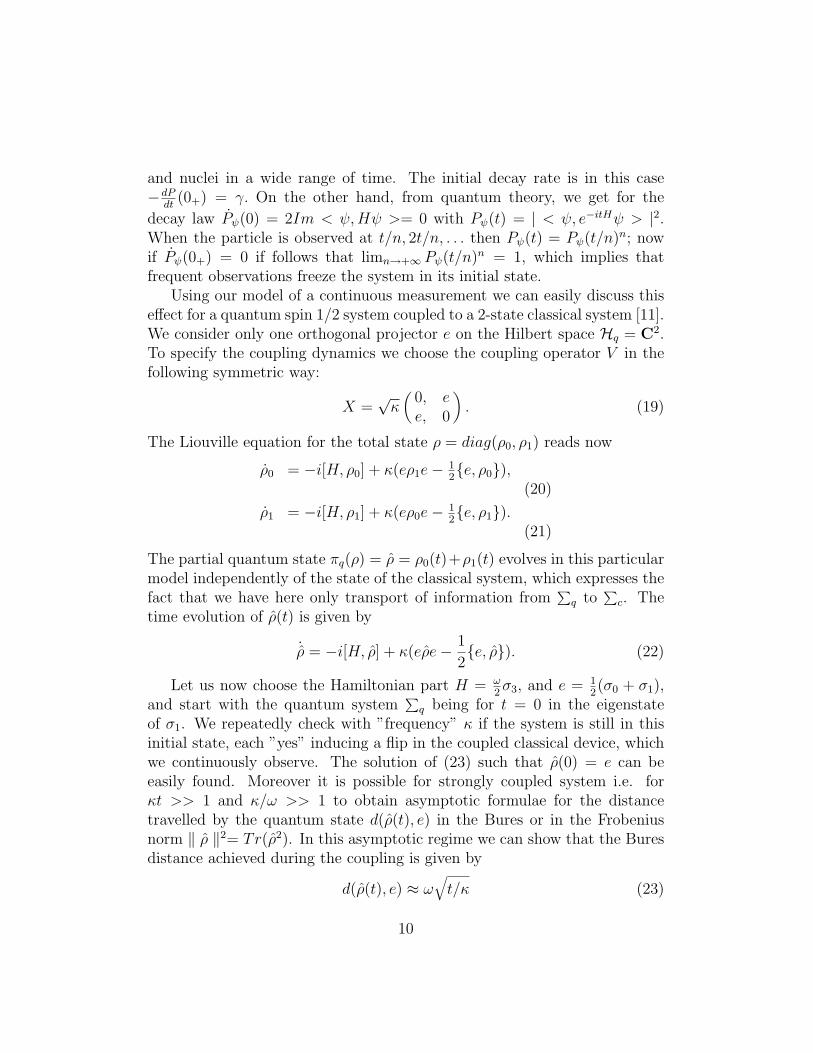
Using our model of a continuous measurement we can easily discuss thiseffect for a quantum spin 1/2 system coupled to a 2-state classical system [11].We consider only one orthogonal projector e on the Hilbert space Hq = C2.To specify the coupling dynamics we choose the coupling operator V in thefollowing symmetric way:

X =√κ(

0, ee, 0

). (19)

The Liouville equation for the total state ρ = diag(ρ0, ρ1) reads now

ρ0 = −i[H, ρ0] + κ(eρ1e− 12e, ρ0),

(20)

ρ1 = −i[H, ρ1] + κ(eρ0e− 12e, ρ1).

(21)

The partial quantum state πq(ρ) = ρ = ρ0(t)+ρ1(t) evolves in this particularmodel independently of the state of the classical system, which expresses thefact that we have here only transport of information from

∑q to

∑c. The

time evolution of ρ(t) is given by

˙ρ = −i[H, ρ] + κ(eρe− 1

2e, ρ). (22)

Let us now choose the Hamiltonian part H = ω2σ3, and e = 1

2(σ0 + σ1),

and start with the quantum system∑q being for t = 0 in the eigenstate

of σ1. We repeatedly check with ”frequency” κ if the system is still in thisinitial state, each ”yes” inducing a flip in the coupled classical device, whichwe continuously observe. The solution of (23) such that ρ(0) = e can beeasily found. Moreover it is possible for strongly coupled system i.e. forκt >> 1 and κ/ω >> 1 to obtain asymptotic formulae for the distancetravelled by the quantum state d(ρ(t), e) in the Bures or in the Frobeniusnorm ‖ ρ ‖2= Tr(ρ2). In this asymptotic regime we can show that the Buresdistance achieved during the coupling is given by

d(ρ(t), e) ≈ ω√t/κ (23)

10

The effect of slowing down the evolution of the quantum system can beconfirmed by an independent, strong but non-demolishing, coupling of a thirdclassical device. In [4, 13] we show moreover that a piecewise deterministicMarkov process taking values on pure states of the total system is naturallyassociated to the Liouville equation and that the coupling constant κ is theaverage frequency of jumps of the classical system between its two states.

Remarks on ”meaning of the wave function” It is tempting to use the

Zeno effect for slowing down the time evolution in such a way, that the stateof a quantum system Σq can be determined by carrying out measurementsof sufficiently many observables. This idea, however, would not work, sim-ilarly like would not work the proposal of ”protective measurements” of Y.Aharonov et al (see [16] [17]). To apply Zeno-type measurements just as toapply a ”protective measurement” one would have to know the state befor-hand. Our results suggest that obtaining a reliable knowledge of the quan-tum state may necessarily lead to a significant, irreversible disturbance ofthe state. This negative statement does not mean that we have shown thatthe quantum state cannot be objectively determined. We believe howeverthat dynamical, statistical and information-theoretical aspects of the impor-tant problem of obtaining a ”maximal reliable knowledge ;, of the unknownquantum state with a least possible disturbance” are not yet sufficiently un-derstood.

4 SQUID - Tank circuit interaction

Superconductivity was discovered 1911 by Kamerlingh Onnes. Two impor-tant properties of superconductors set them apart from normal metallic con-ductors; they exhibit zero electrical resistance to current flow and they expelmagnetic fields (the Meissner effect). In addition superconductors display aspecial characteristic when two are coupled through a thin insulating layer(the Josephson effect). Josephson devices consist of two superconductingfilms through which electrons can tunnel from one superconductor to theother. The tunneling can be by superconducting pairs via the Josephsoneffect. In a Josephson junction the current I is given by I = Ic sinφ, whereIc is the dissipationless current that the junction will sustain. The Josephsonenergy E, which is the kinetic energy of the current I flowing through thejunction is given by E = − h

2eIc cosφ and φ is the quantum mechanical phase

11

difference across the function.A SQUID is a ring-shaped superconducting circuit containing one or more

so called weak links whose behaviour is governed by the Josephson equationsof superconductivity. A magnetic field applied to a SQUID alters its electri-cal characteristics. The ring’s response can be interrogated with conventionalelectronics. SQUIDS posses a wide variety of macroscopic quantum mechan-ical properties. In recent years these has been considerable discussion of thedynamics of a system consisting of a SQUID coupled to a dissipative classicallinear oscillator [18, 19, 20, 21]. Our aim is to show that a continuous versionof our framework is very well adapted to discuss the behaviour of the cou-pled system consisting of a macroscopic classical system (tank circuit) and asingle macroscopic quantum object (SQUID).

4.1 SQUID coupled to a damped classical oscillator

A SQUID (Superconducting Quantum Interference Device) consists of a pieceof superconductor with two holes that nearly connect at the ”weak link”.Suppose now that the device is in a state where a current is flowing roundone of the holes and induces therefore a magnetic field whose field lines passthrough this hole. The magnetic flux in such a ring is quantized, where the”flux quantum” is given by h

2e. Under the assumption that the circulating

current is very small there is only one flux quantum say in the left hole. Amacroscopically distinct state would be the symmetric case where one fluxquantum is localized in the right hole. Quantum theory says that a SQUIDcan exits also in a state where the flux is delocalized between the two holes;flux quanta can pass from one hole to another by quantum tunnelling pro-cesses. SQUIDS are laboratory versions of Schrodinger’s cat. The flux Φtrapped through the ring is a macroscopic variable which obeys a standardSchrodinger equation with the mass M replaced by the capacitance of theJosephson junction and the potential V (Φ) such that lim|Φ|→∞ V (Φ) = +∞.Our aim is to describe the interaction between a SQUID and a classicaldamped oscillator. Both are macroscopic electromagnetic circuits. The clas-sical system can be seen as a model for a local environment for the SQUID.The Hamiltonian of the quantum system contains a source term through wichit can be coupled to the classical device.

The radiofrequency (rf) SQUID is a superconducting loop which is inter-rupted by a thin insulating layer (Josephson tunnel junction). The conduc-tion electrons in the superconductor are paired, and thus encounter negligible

12

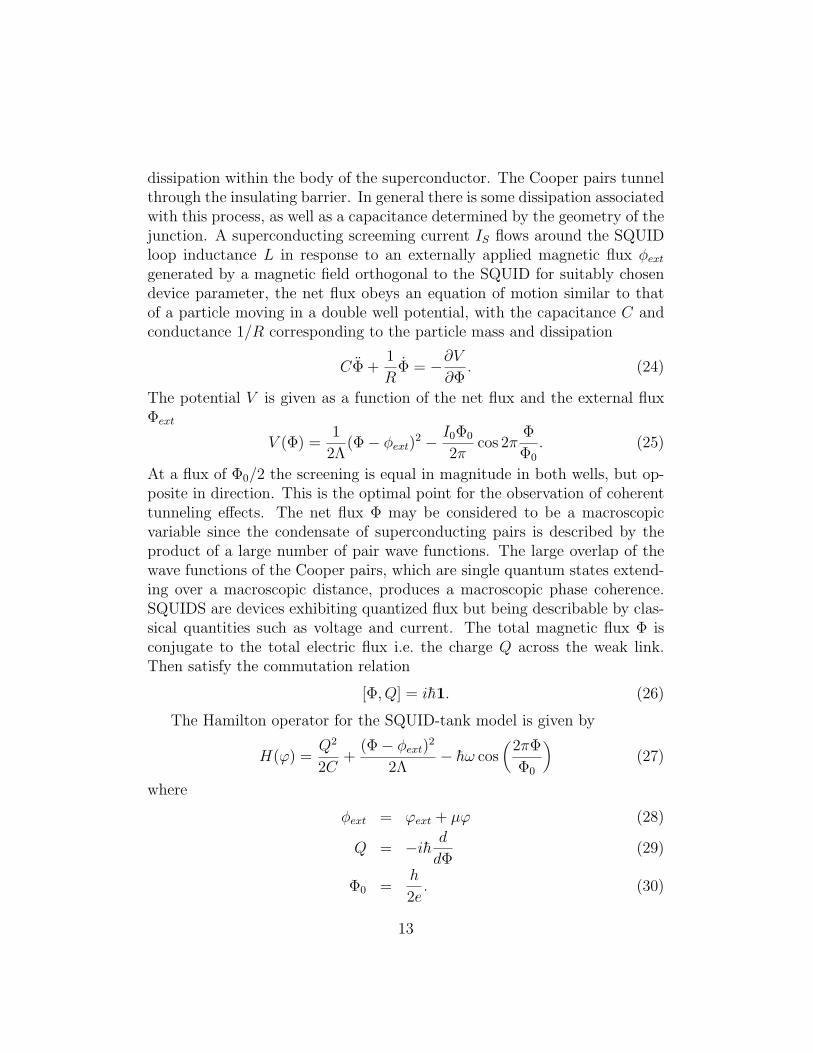
dissipation within the body of the superconductor. The Cooper pairs tunnelthrough the insulating barrier. In general there is some dissipation associatedwith this process, as well as a capacitance determined by the geometry of thejunction. A superconducting screeming current IS flows around the SQUIDloop inductance L in response to an externally applied magnetic flux φextgenerated by a magnetic field orthogonal to the SQUID for suitably chosendevice parameter, the net flux obeys an equation of motion similar to thatof a particle moving in a double well potential, with the capacitance C andconductance 1/R corresponding to the particle mass and dissipation

CΦ +1

RΦ = −∂V

∂Φ. (24)

The potential V is given as a function of the net flux and the external fluxΦext

V (Φ) =1

2Λ(Φ− φext)

2 − I0Φ0

2πcos 2π

Φ

Φ0

. (25)

At a flux of Φ0/2 the screening is equal in magnitude in both wells, but op-posite in direction. This is the optimal point for the observation of coherenttunneling effects. The net flux Φ may be considered to be a macroscopicvariable since the condensate of superconducting pairs is described by theproduct of a large number of pair wave functions. The large overlap of thewave functions of the Cooper pairs, which are single quantum states extend-ing over a macroscopic distance, produces a macroscopic phase coherence.SQUIDS are devices exhibiting quantized flux but being describable by clas-sical quantities such as voltage and current. The total magnetic flux Φ isconjugate to the total electric flux i.e. the charge Q across the weak link.Then satisfy the commutation relation

[Φ, Q] = ih1. (26)

The Hamilton operator for the SQUID-tank model is given by

H(ϕ) =Q2

2C+

(Φ− φext)2

2Λ− hω cos

(2πΦ

Φ0

)(27)

where

φext = ϕext + µϕ (28)

Q = −ih d

dΦ(29)

Φ0 =h

2e. (30)

13

For the tank equation following Spiller et al. [19] one obtains

ϕ+ϕ

RtCt+

ϕ

LtCt=

1

Ct

(IIN(t) + µ <

Φ− φextΛ

>

). (31)

Figure 1:

States of the classical system are probabilistic measures p on its phasespace Ω = (R2, dϕdπ); we take for the canonical variables: the magnetic fluxϕ and its rate of change π (thought of as ϕ). Because of dumping in thetank circuit, the equation of motion for ϕ cannot be written in a standardHamiltonian form (but it can be written using a complex Hamiltonian – see

14

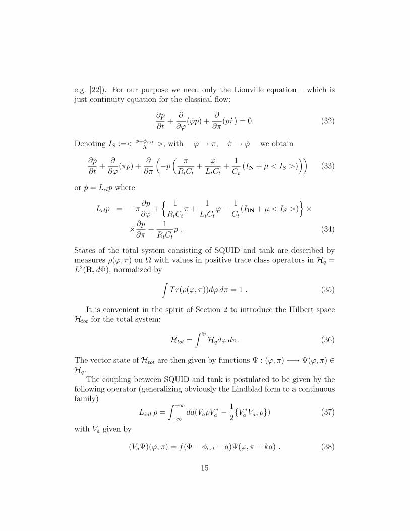
e.g. [22]). For our purpose we need only the Liouville equation – which isjust continuity equation for the classical flow:

∂p

∂t+

∂

∂ϕ(ϕp) +

∂

∂π(pπ) = 0. (32)

Denoting IS :=< φ−φext

Λ>, with ϕ→ π, π → ϕ we obtain

∂p

∂t+

∂

∂ϕ(πp) +

∂

∂π

(−p

(π

RtCt+

ϕ

LtCt+

1

Ct(IN + µ < IS >)

))(33)

or p = Lclp where

Lclp = −π ∂p∂ϕ

+

1

RtCtπ +

1

LtCtϕ− 1

Ct(IIN + µ < IS >)

×

×∂p∂π

+1

RtCtp . (34)

States of the total system consisting of SQUID and tank are described bymeasures ρ(ϕ, π) on Ω with values in positive trace class operators in Hq =L2(R, dΦ), normalized by∫

Tr(ρ(ϕ, π))dϕ dπ = 1 . (35)

It is convenient in the spirit of Section 2 to introduce the Hilbert spaceHtot for the total system:

Htot =∫ ⊕

Hqdϕ dπ. (36)

The vector state of Htot are then given by functions Ψ : (ϕ, π) 7−→ Ψ(ϕ, π) ∈Hq.

The coupling between SQUID and tank is postulated to be given by thefollowing operator (generalizing obviously the Lindblad form to a continuousfamily)

Lint ρ =∫ +∞

−∞da(VaρV

∗a −

1

2V ∗

a Va, ρ) (37)

with Va given by

(VaΨ)(ϕ, π) = f(Φ− φext − a)Ψ(ϕ, π − ka) . (38)

15

The function f can be thought of as defining a sensitivity window - it shouldbe odd or even:

f(x) = ±f(−x) . (39)

We denote

α =∫ +∞

−∞f 2(x)dx . (40)

The constant k (having dimension [time]−1) is the second constant charac-terizing the coupling. We first notice that∫ +∞

−∞V ∗a Vada = α · I (41)

so that

(Lintρ)(ϕ, π) =∫daf(Φ− φext − a)ρ(ϕ, π − ka)f(Φ− φext − a)

−αρ(ϕ, π) . (42)

The Liouville operator for the total system is then given by a sum of threeterms

(Lρ)(ϕ, π) = −i[H(ϕ), ρ(ϕ, π)] +

+(Lclρ)(ϕ, π) + (43)

+(Lintρ)(ϕ, π) .

In the following we will denote by < F > the average for a quantity F :

< F >=∫Tr(F (ϕ, π)ρ(ϕ, π))dϕ dπ . (44)

Therefore the time derivative of averages is given explicitly by

< F > =∫Tr(F (ϕ, π)ρ(ϕ, π))dϕ dπ =

=∫Tr(F (ϕ, π)(Lρ)(ϕ, π))dϕ dπ . (45)

Let us compute

< ϕ >=∫ϕTr((Lρ)(ϕ, π))dϕ dπ . (46)

Only the classical part contributes and we get

< ϕ >=< π > . (47)

16

We need also to compute < ϕ >=< π >

< π >=∫πTr(Lρ(ϕ, π))dϕ dπ . (48)

The quantum Hamiltonian does not contribute while the classical part givesnothing else as the RHS of the classical equations of motion:

−< ϕ >

RtCt− < ϕ >

LtCt+

1

CtIIN(t) . (49)

We compute next the term coming from Lint:∫πTr(f 2(Φ− φext − a)ρ(ϕ, π − ka)da dϕ dπ

−α∫πTr(ρ(ϕ, π))dϕ dπ . (50)

Let us consider the first term. Changing variables π − ka = π′ we get∫(π′ + ka)Tr(f 2(Φ− φext − a)ρ(ϕ, π′))da dϕ dπ′ . (51)

The π′ term cancels with the last term in (50). We change also the a variablesintroducing a′ by

a− Φ− φext = a′ (52)

and obtain just

k∫Tr((a′ + Φ− φext)f

2(a′)ρ(ϕ, π))da′ dϕ dπ . (53)

The term∫a′f 2(a′) gives zero because f 2 is assumed to be even. What

remains is

αk∫

Tr((Φ− φext)ρ(ϕ, π))dϕ dπ =

= αk < Φ− φext > . (54)

It follows that our evolution law for averages is compatible with that of Spiller[18] if we put

αk =µ

CtΛ, (55)

which fixes one of the parameters α, k in terms of the other.

17

For an arbitrary function F (Φ), we find that

d

dtF (Φ) = i[H(ϕ), F (Φ)] (56)

so that the dissipative coupling does not influence time evolution of theSQUID flux variables. It will, however, in general, influence functions ofits conjugate variable Q. In fact, we have

< Q >=< i[H(ϕ), Q] > + < δQ > (57)

where

< δQ > =∫Tr(Qf(Φ− φext − a)ρ(ϕ, π)f(Φ− φext − a)dϕ dπ da

−α < Q >= 0 (58)

because Qf − fQ ≡ f ′ and f ′f is odd, but < Q2 > can be already 6= 0.

18

4.2 The partially deterministic stochastic process as-sociated to SQUID-model

The total Liouville operator of the squid tank model splits as seen in Section4.1 into 3 parts

L = Lq + Lcl + Lint . (59)

The parts Lq and Lcl give us deterministic motion of pure states of thequantum and of the classical system. The time evolution is subject to thefollowing coupled system:

idΨ

dt= H(ϕ)Ψ

dΨ

dt= π (60)

dπ

dt= − π

RtCt− ϕ

LtCt.

They give us a vector field X acting on the product of pure states of thequantum and of the classical system. We write now Lint as acting on observ-ables ∫

Tr(ρ(ϕ, π)(LintA)(ϕ, π)) =∫Tr((Lintρ)(ϕ, π)A(ϕ, π)) . (61)

After a change of variables and using the cyclicity of the trace this term isthen given by∫Tr(ρ(ϕ, π)

[∫f(Φ− φext − a)A(ϕ, π + ka)f(Φ− φext − a)− αA(ϕ, π)

].

(62)Thus

(LintA)(ϕ, π) =∫daf(Φ− φext − a)A(ϕ, π + ka)f(Φ− φext − a)

−αA(ϕ, π) (63)

In order to construct a PD-process we compute now time evolution offunctions

FA(Ψ;ϕ, π) = (Ψ, A(ϕ, π)Ψ) (64)

19

we get

FA(Ψ, ϕ, π) = (Ψ, (LintA)(ϕ, π)Ψ) = (65)

=∫da(fΨ, A(ϕ, π + ka)fΨ)− αFA(Ψ;ϕ, π) =

=∫da‖fΨ‖2FA

(fΨ

‖fΨ‖, ϕ, π + ka

)− αFA(Ψ, ϕ, π)

=∫da‖fΨ‖2δ(Ψ′ − fΨ

‖fΨ‖)δ(ϕ′ − ϕ)δ(π′ − π − ka)FA(Ψ′;ϕ′, π′)− αFA(Ψ, ϕ, π) .

We write the integral kernel as

Q(Ψ, ϕ, π|Ψ′, ϕ′, π′) =∫da‖fΨ‖2δ

(Ψ′ − fΨ

‖fΨ‖

)× δ(ϕ′ − ϕ)δ(π′ − π − ka) . (66)

We can now perform the a integration and obtain

Q(Ψ, ϕ, π|Ψ′, ϕ′, π′) =1

k‖fΨ‖2δ

(Ψ′ − fΨ

‖fΨ|

)δ(ϕ′ − ϕ) (67)

where f = f(Φ− φext − π′−πk

).We compute next the rate function

λϕ,π(Ψ) =∫dΨ′

∫dϕ′

∫dπ′ Q(Ψ, ϕ, π|Ψ′, ϕ′, π′) =

=1

k

∫dπ′ ‖fΨ‖2 = α . (68)

Then introducing Q by

Q(Ψ;ϕ, π|Ψ′;ϕ′, π′) =Q

α(69)

we obtain for FA

FA(Ψ, ϕ, π) = α∫Q(Ψ, ϕ, π|Ψ′, ϕ′, π′)FA(Ψ′, ϕ′, π′)

−αFA(Ψ, ϕ, π) . (70)

This time evolution equation is obviously of the type discussed by Davis[23]. As a last remark we note that the partially deterministic time evolutioncan be described in the following way:

20

The system starts in the pure state (Ψ0, ϕ0, π0) and evolves deterministically– the classical system according to

ϕ+ϕ

RtCt+

ϕ

LtCt= 0 (71)

and the quantum system according to

iΨ = H(ϕ)Ψ (72)

until random time t1 governed by a Poisson process with constant rate α. Attime t1 quantum state jumps to

f(Φ− φext(ϕ)− π′−πk

)Ψ

‖f(Φ− φext(ϕ)− π′−πk

)Ψ‖(73)

and the classical system changes its state in the following way

ϕ −→ ϕ′ = ϕ (74)

π −→ π′ (75)

with probability density

1

k‖f(Φ− φext −

π′ − π

k)Ψ‖2 . (76)

Notice that ϕ′ = ϕ from which it follows that the trajectories of the classicalsystem are continuous. Only velocity π = ϕ jumps at random jump times.

5 Concluding remarks

The mathematical developments constituting Quantum Mechanics have beenoutstandingly successful in describing and computing (although we would notsay explaining) not only those phenomena for which it was invented but alsonumerous others making many wonderful advances in technology possible.On the other way it is fair to say that the conceptual basis of QuantumMechanics is still somewhat obscure. The class of models we introducedseems to provide a reliable means of extracting from mathematically consis-tent models of information transfer from

∑q to

∑c well defined predictions

for the outcome of any experiment we can envisage - apart of course from

21

the difficulty of solving the mathematical equations, which can be intricateand sophisticated. Physics is the study of reproducible phenomena and astatistical theory of the quantum world is all that theoretical physics whouldseek. But as a statistical theory Quantum Mechanics is still a deterministictheory. On the other hand recent advances in study of chaos and algorith-mic randomness suggest that near future can bring essentially new elementsto our understanding of randomness - both in the realm of foundations ofscience and in the Nature itself. Any progress in this area may influence ourcurrent quantum paradigm.

References

[1] J. S. Bell, Against ”Measurement ” Physics World, August 1990, 33-40.

[2] Ph. Blanchard, A. Jadczyk, On the interaction between classical andquantum systems, Physics Letters A 175 (1993) 157-164.

[3] Ph. Blanchard, A. Jadczyk, Classical and Quantum Intertwine, in Pro-ceedings of the Symposium of Foundations of Modern Physics, Cologne,June 1993, Ed. P. Mittelstaedt, World Scientific (1993).

[4] Ph. Blanchard, A. Jadczyk, From Quantum Probabilities to ClassicalFacts, in Advances in Dynamical Systems and Quantum Physics, Capri,May 1993, Ed. R. Figari, World Scientific (1994).

[5] R. Haag, Irreversibility introduced on a fundamental level,Comm. Math. Phys. 123 (1990) 245-251.

[6] J. L. Sauvageot, J. P. Thouvenot, Une nouvelle definition de l’entropiedynamique des systemes non commutatifs, Comm. Math. Phys. 145 411-423 (1992).

[7] P. Busch, P. J. Lahti, P. Mittelstaedt, The Quantum Theory of Mea-surement, Springer (1991).

[8] M. Namiki, S. Pascazio, Quantum Theory of Measurement Based onthe many-Hilbert-Space approach, Physics Reports 232 No. 6 (1993)301-411.

22

[9] N. G. van Kampen, Macroscopic Systems in Quantum Mechanics, Phys-ica A 194 (1993) 542-550.

[10] J. S. Bell, Are these quantum jumps? in Schrodinger, Centenary of aPolymath”, Cambridge University Press (1987).

[11] Ph. Blanchard, A. Jadczyk, Strongly coupled quantum and classicalsystems and Zeno’s effect, Physics Letters A 183 (1993) 272-276.

[12] A. Connes, H. Narnhofer, W. Thirring, Dynamical entropy of C∗-algebras and von Neumann algebras, Comm. Math. Phys. 112, 691-719(1987).

[13] Ph. Blanchard, A. Jadczyk, Coupled quantum and classical systems,measurement process, Zeno effect and all that, in preparation.

[14] Ph. Blanchard, A. Jadczyk, Nonlinear effects in coupling between clas-sical and quantum systems: SQUID coupled to a classical damped os-cillator, to appear.

[15] A. Jadczyk, Topics in Quantum Dynamics, to appear in Proc. FirstCaribbean Spring School of Math. and Theor. Phys., Saint Francois,Guadeloupe June 1993, World Scientific, to appear

[16] Y. Aharonov, J. Anadan, L. Vaidman, Meaning of the wave function,Phys. Rev. A47 (1993) 4616-4626.

[17] Y. Aharonov, L. Vaidman, Measurement of the Schrodinger wave of asimple particle, Phys. Letters A178 (1993) 38-42.

[18] T. P. Spiller, T. D. Clark, R. J. Prance, H. Prance, The adiabatic mon-itoring of quantum objects, Phys. Letters A170 (1992) 273-279.

[19] T. P. Spiller, T. D. Clark, R. J. Prance, A. Widom, Quantum Phe-nomena in Circuits at low temperature, Progress in Low TemperaturePhysics, Vol. XIII (1992) 221-265.

[20] J. F. Ralph, T. P. Spiller, T. D. Clark, R. J. Prance, H. Prance, Chaosin a coupled quantum-classical system, Phys. Letters A180 (1993) 56-60.

23

[21] J. F. Ralph, T. P. Spiller, T. D. Clark, H. Prance, R. J. Prance, A. J.Clippingdale, Non-linear behaviour of teh rf-SQUID magnometer, Phys-ica D63 (1993) 191-201.

[22] Dekker,H.:On the phase space quantization of the linearly damped har-monic oscillator, Physica 95 A (1979) 311 – 323

[23] Davis,M.H.A., Markov models and optimization, Chapman and Hall,London 1991

24