
Housing, the ‘Great Income Tax Experiment’, and the ... · earnings that are placed in a...
84
ISSN 1178-2293 (Online) University of Otago Economics Discussion Papers No. 1709 APRIL 2017 Housing, the ‘Great Income Tax Experiment’, and the intergenerational consequences of the lease Andrew Coleman Address for correspondence: Andrew Coleman Department of Economics University of Otago PO Box 56 Dunedin NEW ZEALAND Email: [email protected]
Transcript of Housing, the ‘Great Income Tax Experiment’, and the ... · earnings that are placed in a...
ISSN 1178-2293 (Online)
University of Otago Economics Discussion Papers
No. 1709
APRIL 2017
Housing, the ‘Great Income Tax Experiment’, and the intergenerational consequences of the lease
Andrew Coleman
Address for correspondence: Andrew Coleman Department of Economics University of Otago PO Box 56 Dunedin NEW ZEALAND Email: [email protected]

1
Housing, the ‘Great Income Tax Experiment’, and the intergenerational consequences of the lease.
Andrew Coleman February 2017
Abstract This paper provides an analysis of how the New Zealand tax system may be affecting
residential property markets. Like most OECD countries, New Zealand does not tax the
imputed rent or capital gains from owner-occupied housing. Unlike most OECD
countries, since 1989 New Zealand has taxed income placed in retirement savings funds
on an income basis, rather than an expenditure basis. The result is likely to be the most
distortionary tax policy towards housing in the OECD. Since 1989, these tax distortions
have provided incentives that should have lead to significant increases in house prices
and the average size of new dwellings, should have reduced owner-occupier rates, and
should have led to a worsening of the overseas net asset position. The tax settings are
likely to be regressive, and are not intergenerationally neutral, as they impose significant
costs on current and future generations of young New Zealanders (and new migrants).
Since it does not appear to be politically palatable to tax capital gains or imputed rent, to
reduce the distortionary consequences of the tax system on housing markets New
Zealand may wish to reconsider how it taxes retirement savings accounts by adopting the
standard OECD approach.
2
Executive Summary New Zealand has one of the most distortionary tax environments for housing markets of
any country in the OECD. The primary reason is not the failure to tax capital gains or
the imputed rent from owner-occupied housing (the implicit rent an owner-occupier
earns from leasing their own house to themselves), for most countries do not tax the
capital gains or imputed rent from owner-occupied housing. Rather, it is because New
Zealand taxes income from owner-occupied housing on a different basis than it taxes all
other capital income. This is not true in most other OECD countries, where owner-
occupied housing is taxed on a similar basis to a wide class of other assets. New Zealand
and the rest of the OECD have not always been so different. The difference began in
1989, when New Zealand began taxing funds placed in retirement income accounts on
an income-tax basis rather than an expenditure-tax basis, but did not change the way it
taxed owner-occupied housing.
What is the key distinction? Income can either be taxed when it is earned (an income
tax), or taxed when it is spent (an expenditure tax). Expenditure taxes can take several
forms, including goods and services taxes and cash-flow taxes. Cash-flow taxes are
typically implemented by applying a progressive tax to a person’s income adjusted for the
net purchase and sale of certain assets, on the basis that this total is close to a person’s
expenditure on consumption goods and services. For example, if someone earned
$100,000 and saved $15,000 in a retirement account, they would pay tax on $85,000.
Taxes can be distortionary or non-distortionary. Capital income can be classified into
three classes and if all three classes are taxed consistently on an income or expenditure
basis the tax system will not distort investment choices. In practice, few tax systems are
non-distortionary. Most OECD countries adopt an expenditure tax system but only
provide expenditure tax treatment to two of these classes, for example. The first class is
earnings that are placed in a government-sanctioned retirement saving fund. In the vast
majority of OECD countries, these are taxed on an expenditure basis by adopting an
‘Exempt-Exempt-Taxed’ (EET) rule. Income that is placed in a fund is not taxed when it
is earned; interest and dividend earnings and any capital gains are not taxed when they
accumulate in the fund; but when assets are withdrawn from the fund upon retirement,
they are taxed. The second class is owner-occupied housing. In this case, a prepayment
or ‘Taxed-Exempt-Exempt’ (TEE) expenditure tax rule is adopted: the house is

3
purchased or paid off from income that is taxed when it is earned, but no tax is paid on
the imputed rent produced by the property or any capital gain that accrues to the owner.
The third class is income from any other investments, including leased residential
housing. This is taxed on an income tax or ‘Taxed-Taxed-Exempt’ (TTE) basis: income
is taxed when it is first earned; it is taxed as it accumulates; but it is not taxed when it is
withdrawn and spent. Overall this tax regime distorts against the ‘other’ investment class,
but because it provides people with the opportunity to hold many classes of investments
in sanctioned retirement income funds on an equivalent basis as owner-occupied
housing, it provides few incentives to over-invest in housing.
If a country wishes to tax capital income on a neutral income-tax basis, it needs to do
three things: tax on retirement income accounts on a “Taxed-Taxed-Exempt” basis; tax
all capital gains (including those from owner-occupied housing) on an accrual basis; and
tax the imputed rent from owner-occupied housing. New Zealand attempted to move to
a non-distortionary income tax system in 1989. However, only the first of the three
changes were implemented. As a result, rather than eliminating the distortions associated
with the standard OECD approach, it created a new set of distortions. In particular,
owner-occupied housing was taxed at much lower rates than other assets, and leased
residential housing was taxed advantageously relative to debt instruments.
This paper adopts a ‘relative institutions’ approach to analyse the consequences of the
1989 change. Since 1989, the favourable tax environment for owner-occupied housing
relative to other assets has provided incentives for households to live in larger houses
than they otherwise would, and to bid up the price of land in locations that are
conveniently located to desirable amenities. The favourable tax environment for
investments in leased residential housing provides incentives for rent/price ratios to fall,
either through a reduction in rents (if the supply of residential property is elastic) or
through higher house prices (if the supply of residential property is inelastic.) Home
owner-ship rates should fall. It is plausible that since 1989 the changes in the tax regime
have provided incentives for people to increase the size of their houses by 25%, and to
pay twice as much for land in areas where there is significant transport congestion.
New Zealand’s property markets have changed in a manner consistent with these
incentives since 1989. The average size of newly constructed houses has increased faster

4
than in Australia or the United States and is amongst the largest in the world. Property
prices have soared, rent/price ratios have declined sharply, and the number of private
landlords has increased by more than 300 percent. However, it is not possible to
definitively attribute these changes to the tax changes, as other factors that affect housing
markets such as the international decline in interest rates and rising incomes have also
changed since 1989. The paper attempts regression analysis to unpick the importance of
the various affects, but concludes it is not possible to estimate the role of the tax
changes. The evidence is consistent with the conjecture that the tax changes are part of
the cause of the change, but cannot prove it.
What are the distributional consequences of the 1989 tax change? When housing is taxed
on an expenditure basis but other assets are taxed on an income basis, housing is taxed
on an advantaged basis. Standard theory suggests this should lead to higher land prices
and a boon for the first land owning generation. But the benefits accruing to the land-
owners of one generation do not come for free. They are offset by large costs that are
imposed on all generations born after the tax change was introduced. They generate a
higher net international debt position than would otherwise occur. And they are
regressive, falling disproportionately on first home owners with low equity and renters.
Since 1989, several investigations of New Zealand’s tax system have concluded that it
favours owners of housing assets by not taxing imputed rent or the capital gains on
owner-occupied housing. These investigations have typically concluded it is not
politically possible to introduce these taxes. This may be the case – few countries have
these taxes. But it should not be concluded that successive generations of New
Zealanders have to suffer the distortionary effects of a tax system that is regressive, that
places upward pressure on house prices, that encourages excessively large houses, and
which imposes large costs on all cohorts than the first generation of land-owners. The
root cause of the problem is taxing housing on an expenditure basis while other assets
are taxed on an income basis. New Zealand could correct this distortion by taxing other
assets on an expenditure basis, the solution adopted by most other countries. But if
nothing is changed, and the distortion is not corrected one way or the other, New
Zealanders will continue to have one of the most distortionary tax environments for
housing in the OECD.

5
1. Introduction New Zealand currently has one of the most distortionary tax environments for housing
markets of any country in the OECD. This claim may sound odd to people used to
hearing that New Zealand has some of the lowest and least distortionary labour market
taxes in the OECD. Yet both claims can be true, and both claims have their roots in
changes made to the tax system in the 1980s. One decision in particular contributed to
both. In 1989, the government changed the way retirement income savings were taxed.
To understand this argument, it is necessary to take one step backwards. Income can
either be taxed when it is earned, or taxed when it is spent. The former taxes are called
income taxes, while the latter taxes are called expenditure taxes. Each type of tax raises
revenues, and each causes distortionary effects by altering the way people behave. It has
long been understood that income taxes applied to capital income distort investment
patterns more than expenditure taxes, partly because not all capital income is taxed at the
same rate, which generates incentives to invest in lightly taxed assets. On the other hand,
the revenue raised when capital incomes are subject to income tax can be used to reduce
tax rates on labour income, reducing labour market distortions. This creates a quandary
for governments. By taxing people when income is spent, the distortionary effects on
capital markets are reduced, but taxes on labour incomes are high. In contrast, if people
are taxed when income is earned, tax rates on labour incomes are low, but the allocation
of capital is distorted unless all capital is taxed at the same rate.
While most OECD countries use a hybrid system, since the 1970s there has been a shift
towards expenditure taxes as their advantages have become clearer and implementation
costs have fallen. Expenditure taxes can take several forms. Countries can apply indirect
value-added taxes, which raise the price of goods and services. They may also apply
various retail sales taxes. And, following the insights of Fisher (1937), countries can apply
cashflow taxes that tax a person’s cashflow rather than their income. To do this, they
adjust earnings for the net purchase and sale of assets, on the basis that this total is close
to a person’s expenditure on consumption goods and services. For example, if someone
earned $100,000 and saved $15,000, they would pay tax on $85,000. Alternately, if
someone earned $100,000 and sold assets for $20,000, they would be taxed on $120,000.
6
Most OECD countries default to an income tax basis but provide expenditure tax
treatment to two classes of assets. The first class is earnings that are placed in a
government-sanctioned retirement saving fund. In the vast majority of OECD countries,
these are taxed on an expenditure basis by adopting an ‘Exempt-Exempt-Taxed’ (EET)
rule.1 Income that is placed in a fund is not taxed when it is earned; interest and dividend
earnings and any capital gains are not taxed when they accumulate in the fund; but when
assets are withdrawn from the fund upon retirement, they are taxed. The second class is
owner-occupied housing. In this case, a prepayment or ‘Taxed-Exempt-Exempt’ (TEE)
expenditure tax rule is adopted: the house is purchased or paid off from income that is
taxed when it is earned, but no tax is paid on the imputed rent produced by the property
(the value of the rent that would be earned if the owner leased the property to someone
other than themselves) or any capital gain that accrues to the owner. If tax rates on
income are constant, the ‘Taxed-Exempt-Exempt’ and the ‘Exempt-Exempt-Taxed’
versions of expenditure taxes have the same effective tax treatment.2 The whole system is
a hybrid because income from other investments is taxed on an income tax or ‘Taxed-
Taxed-Exempt’ (TTE) basis.3 Nonetheless, people who spend most of their income
other than what they place within a sanctioned retirement income fund or put aside to
purchase (or repay) owner-occupied housing effectively pay taxes on an expenditure
basis.
In the 1980s, New Zealand reformed its tax system in several ways. One of the reforms,
the introduction of a Goods and Services tax, pushed the tax system towards an
expenditure tax basis.4 A second reform pushed it towards an income tax basis. Until
1989, New Zealand, like most other OECD countries, had an ‘Exempt-Exempt-Tax’ 1 Austria, Belgium, Canada, Finland, France, Germany, Greece, Iceland, Ireland, Japan, Korea, Mexico, the Netherlands, Norway, Poland, Portugal, the Slovak Republic, Spain, Switzerland, Turkey, the United Kingdom, and the United States all have a version of an EET retirement income saving scheme. Hungary has its equivalent, a TEE scheme. Denmark, Italy, and Sweden have ETT schemes. New Zealand and Australia are the obvious outliers, and Australia provides some ‘concessions’ to the taxation of retirement income saving by having low taxes on employee contributions and low taxes on interest and dividend income. See Whitehouse (1999) or Yoo and de Serres (2004). 2 The “Taxed-Exempt-Exempt” and “Exempt-Exempt-Taxed” forms are not strictly equivalent, in part because realised capital gains are taxed under the latter rule but not the former, and different marginal tax rates may apply under the two forms. In expectation, they are sufficiently similar that it is widely considered that taxing one form of income under one rule and another form of income under the other should not distort investment choices. This issue is discussed at length by Kaldor (1955) and Batina and Ihori (2000). 3 This means income is taxed when it is earned; any interest or dividends or profits are taxed when they accumulate, and capital gains may be taxed on a realized rather than an accrual basis; but there is no further tax when the investment is sold. 4 The GST rate was further increased in 1989 and 2010 in response to the perceived advantages of expenditure taxes.
7
system for funds placed in sanctioned retirement income funds. This taxation treatment
was abolished in 1989, and since then retirement income funds have been taxed on an
income tax or TTE basis.5 Figure 1 depicts the change. Prior to 1989, owner-occupied
housing and savings placed in sanctioned retirement funds were taxed on an expenditure
basis, whereas other assets were taxed on an income basis. This meant there was a large
tax wedge between the taxation of housing and retirement funds, on one hand, and other
assets on the other. After 1989, the wedge between retirement assets and other assets was
closed but a large wedge between retirement funds and owner-occupied housing was
opened. Viewed in this light, the 1989 change can be considered New Zealand’s great
income tax experiment. It is perhaps worth noting that no other country copied New
Zealand’s move in the subsequent quarter century, and several former Eastern European
countries consciously adopted expenditure tax systems for funds placed in specified
retirement savings accounts. Moreover, one of the most in-depth tax reviews written
since then, the 2010 Mirrlees Tax Review in the United Kingdom, recommended
continuing the EET tax treatment of pensions, and suggested additional reforms should
be adopted to tax other assets on an expenditure basis.6
Why was the change undertaken in New Zealand? The 1987 Labour Government argued
that the EET treatment of retirement savings provided a costly, regressive tax concession
to the owners of capital. The 1988 Brash Committee, charged with investigating the
proposal, agreed. The Committee portrayed the EET treatment of retirement savings as
a distortionary tax concession that undermined the principle of tax neutrality, as it meant
income placed in some saving vehicles (sanctioned retirement-income funds) were taxed
much less that others (funds invested in businesses, or invested in other financial
institutions such as banks, or used to purchase shares or businesses). The change was
implemented providing a considerable short run increase in tax revenue.7 At the same
time, proposals to tax capital gains were not implemented, providing an incentive to
5 In 2007, the New Zealand Government introduced a subsidised voluntary retirement income scheme called KiwiSaver. People placing funds in the accounts are provided with a $0.50 subsidy for each dollar placed into the account for the first $1,043 contributed per year. In principle, a subsidy on a voluntary retirement savings account could have reduced the tax distortions favouring housing. In practice, the nature of the subsidy means retirement savings are still taxed on an income basis. Income that is contributed to the retirement income account in excess of $1043 per year is still taxed at normal income tax rates, and the capital income earnings of the accounts are also taxed at normal income tax rates. 6 Mirrlees and Adam (2010: chapter 14). This recommendation is consistent with the recommendations of the 1978 Meade Report (Institute for Fiscal Studies and Meade (1978)). 7 From 1989 income tax was paid on all earnings when they were earned, including earnings placed in a retirement income account, and the earnings from these accounts. Under the previous regime, taxes were paid when earnings were withdrawn at retirement.

8
invest in long horizon assets with low pre-tax yields.8 Nor was imputed rent taxed,
providing an incentive for people with housing equity to purchase more expensive
houses than they would have if housing were taxed the same way as other assets.9
Consequently, rather than eliminating the distortions in the tax system that came from
taxing some assets on an income basis and other assets on an expenditure basis, the 1989
reforms accentuated the different tax treatment of owner-occupied housing and other
assets by imposing income taxes on a wider class of assets. This produced a tax
environment for housing that can be considered quite distortionary relative to other
OECD countries, for in most of these countries people can invest in non-housing assets
on the same tax basis as they can invest in owner-occupied housing.
The 1988 report by the Brash Committee did not discuss the taxation of residential
housing, although it observed that it is important for the tax system to be neutral towards
the income earned by different asset classes. However, the OECD, the 2001 McLeod
Review and the 2010 Tax Working Group all expressed concern about the lack of
neutrality of the tax system towards residential housing. The OECD recommended that
imputed rent and capital gains should be taxed, with deductions allowed for mortgage
interest, depreciation, and repairs and maintenance. The McLeod review preferred a
different adjustment, the ‘Risk-Free Return Method’ in which tax should be levied on the
product of an agent’s equity in a property and the risk free interest rate (McLeod
Committee 2001, p iv) but perceived it would be difficult to implement and sustain such
a reform. The Tax Working Group analysed capital gains taxes, land taxes and the risk-
free return method, but there were no recommendations to change the way owner-
occupied housing is taxed, and no changes were implemented.
What are the effects of taxing housing differently from other assets? Standard analysis,
supported by the OECD, the 2001 McLeod Review and the 2010 Tax Working Group
suggests that taxing housing on an expenditure basis when other assets are taxed on an income
tax basis will lead to larger houses and higher property prices. This creates a transfer to
the first generation of owners at the expense of all future generations, who have to pay
higher prices for housing. Consequently, for a quarter of a century, New Zealand’s tax
8 Proposals to enact comprehensive changes to the taxation of capital income were forwarded in the 1989 document “Consultative Document on the Taxation of Income from Capital,” but were ignored. 9 The proposition that imputed rent could be taxed was first raised by the 2001 McLeod Review. The idea has a long history and imputed rent is taxed in some European countries such as Switzerland and the Netherlands.

9
environment has imposed costs on current and future generations of young people
because of the way it taxes housing and other assets.10
This paper provides a review of the way New Zealand’s tax system alters the incentives
to purchase property. Its purpose is to provide a wider perspective on the relationships
between tax and housing markets than has previously been undertaken, particularly the
impact on housing of the 1989 retirement saving tax reforms. In section 2, the effects of
the tax system on the incentives of landlords to alter rent/price ratios and the incentives
of owner-occupiers to construct different quality houses and bid up the price of different
quality land are analysed. This section suggests the 1989 reform provided an incentive to
construct larger houses as well as bid up the price of land which is conveniently located
to desirable amenities. Section 3 documents two aspects of New Zealand’s property
markets to see if they can be explained in terms of interest rates or taxes. The first is the
rent/price ratio; the second is the size of new houses in New Zealand relative to new
houses in the United States and Australia. It is shown that there was a large increase in
the size of new houses in New Zealand relative to those in Australia and the United
States after 1989, although it is not possible to be certain why this increase took place. In
section 4 some of the welfare consequences of the tax system’s effects on housing
markets are considered. While these depend on a variety of factors, particularly the rate
of ongoing house price inflation, it is reasonably clear that the current tax system has
regressive effects on younger people who wish to purchase their own homes. Moreover,
standard theoretical models suggest the distortions stemming from the partial nature of
the 1989 reforms have most likely imposed significant costs on all cohorts maturing after
1989. These cohorts include people who are currently young, as well as all people
intending to purchase property in New Zealand in the future. Conclusions are offered in
section 5.
2. Taxes and property markets: basic theoretical results.
New Zealand has taxed capital incomes using an income tax framework since 1989. All
capital incomes are subject to tax, with three main exceptions: the imputed rent
10 Several smaller modifications to the tax system were adopted after 2000, partly due to concerns about the distortionary effects of income taxes on investment choices. For instance, the top marginal tax rate was progressively reduced from 39% to 33%; the rate of GST was increased from 12.5% to 15% in 2010; and when KiwiSaver was introduced in 2007, the highest tax rate on investment earnings was capped at 28% to reduce the incentive to invest in more advantaged tax classes.

10
associated with the equity of an owner-occupier is not taxed; interest income earned by
non-residents is taxed at only a very low rate; and capital gains are not taxed. Each of
these exemptions creates incentives that distort the way that households and firms invest.
Samuelson (1964) analysed how investment patterns are distorted when capital incomes
are subject to income tax but capital gains are not taxed. One distortion occurs because
income taxes create an incentive to invest in low-yielding long-horizon assets that have
returns in different periods, because interest is compounded on an after-tax basis. A
related distortion occurs because income taxes create an incentive to invest too much in
indefinitely lived assets such as land. A third distortion occurs when there is inflation,
because nominal interest returns rather than real interest returns are taxed. Each of these
distortions is currently a feature of the New Zealand income tax system.
Samuelson showed these distortions could be corrected by an accrual-based capital gains
tax that allows for the deduction of depreciation and losses. If capital gains are taxed on
an accrual basis, when a firm produces an income-producing asset, (i) capital gains tax is
paid at time t on the value of the newly created asset, (ii) income tax is paid on the
income stream produced by the asset, and (iii) capital gains tax is paid on any change in
value of the asset in the year that this change takes place. This corrects the incentives to
make low-yielding long-term investments because of their tax advantages. In turn, the
present value of all assets will be independent of the tax rate, even if different agents
have different tax rates, and equal to the value of the asset in the absence of taxes. A
brief mathematical treatment of Samuelson’s results is provided in Appendix 1.
Since Samuelson’s results are general, they apply to investments in residential property.
Because residential property assets are long lived, income taxes without accrual-based
capital gains taxes raise the after-tax returns relative to interest-earning debt and
encourage over-investment in property. An accrual-based capital gains tax would correct
this distortion for both owner-occupiers and landlords. But this is not the only distortion
that affects New Zealand’s property markets, as the imputed rents accruing to owner-
occupiers are not taxed, providing additional incentives to invest in real estate.
In the following subsections, three distortionary effects of New Zealand’s tax system on
housing markets are considered. The first is the effect on the incentives of owner-

11
occupiers to construct larger or better quality houses than otherwise. The second is the
incentive for owner-occupiers to bid up the price of land that is conveniently located to
desirable amenities. These are treated separately because supply of buildings is very
elastic, whereas the supply of land is highly inelastic. The third concerns the effect on
landlords to alter the rent/price ratio for leased property.11 Each of these distortions is
considered independently from the others. To understand the overall effects of taxes on
property prices, however, it is necessary to model these incentives simultaneously in a
general equilibrium framework, along with other factors that affect the supply and
demand for housing, such as the extent that agents are affected by borrowing constraints
and the supply elasticities of new housing. Coleman (2010) provides an example of an
equilibrium model of housing markets that simultaneously incorporates many features of
New Zealand’s tax system and banking markets.
2.1 The effect of income taxes on residential property owner-occupiers.
When an owner-occupier purchases a property, neither the imputed-rent or the capital
gains obtained from the property are subject to income tax. In these circumstances,
income taxes distort choices about the size of houses people buy, and the price they will
pay for conveniently located land. The analysis in this subsection calculates the tax
distortions for households that own a property without a mortgage. About two-thirds of
New Zealand houses are owned by owner-occupiers, about half of which are owned
without a mortgage. The analysis also applies to owner-occupiers whose mortgage
interest is tax deductible, for the opportunity cost of purchasing a larger house is the
after-tax interest rate.12 The analysis partially applies to households that have a mortgage
and who expect to be mortgage free at some point in their lives, as the opportunity costs
of purchasing a house depend on future as well as current tax rates. The correct
opportunity cost of purchasing a house for households that have a mortgage is the
average of the pre-tax interest rate and the after-tax interest rate, where the weights are
11 It is possible that there is a fourth effect: that the tax rules affect the number of households and thus the quantity of houses that are demanded. For instance, young people may leave home at a different time in response to the tax rules, because of their effect on house prices and rents, or the divorce rate may change. Coleman (2010, 2014) models how the age at which children leave home may be affected by rents, and Coleman and Scobie (2009) provide a brief analysis of how the rate of household formation may have been affected by rents and house prices in New Zealand. They argue that housing demand is relatively price inelastic, which suggest the effect should be small. In any case, the effect of taxes on housing demand should be indirect: it should occur because of the effects of taxes on prices and rents. Consequently, it can be considered as an additional response to any price changes that occur. 12 Mortgage interest can be deducted against a taxpayer’s income if the loan is used to finance an asset that generates taxable income, such as a rental property or an investment in a public or private business. In this case the relevant interest rate is the mortgage rate, not the deposit rate.
12
the fractions of time the person expects to have a mortgage relative to the time they
expect to be mortgage free. This weighted average is straightforward to calculate, but to
enhance the clarity of the analysis in this subsection only the case where the opportunity
cost is the after-tax interest rate is presented. It follows that the results of this section
show the maximum tax-induced housing market distortions that apply to owner-
occupiers.13
Residential property is also subject to rates – a property tax – levied by local authorities.
The tax rate is typically under 0.5%, and while most authorities levy rates on the total
value of a property, some only assess land values. A tax on land values in an open
economy is largely non-distortionary, but a tax on housing structures provides an
incentive to purchase a lower quality house. Property taxes are included in the following
analysis even though they are not central to the story as they are imposed irrespective of
the central government tax regime. The following analysis incorporates these local
authority taxes, but focuses on the change in the total tax regime that occurs when there
is a change in the taxes levied by central government.
2.1.1 Taxes and the quality of houses (not land)
When purchasing a house, the opportunity cost of purchasing a larger house is the after-
tax return to lending. Consider the option of buying a house (a structure) of quality θ that
costs PH(θ) to build and returns an annual benefit H(θ) representing the real value of
shelter. It is convenient to think of quality as the size of a house.
Let π = inflation rate, assumed to be the rate at which PH(θ) increases
through time;
i = nominal interest rate;
δ = depreciation rate of houses;
τ = marginal tax rate on income;
τH = tax rate paid on imputed rent (currently zero);
τC = tax rate on capital gains (currently zero); and
τL = local property tax on capital value.
13 The model Coleman (2010) uses to study the effect of capital gains taxes on housing markets uses an opportunity cost that is the average of current and future after-tax interest rates.

13
Let ( , , , , | , , )H H C L iω θ τ τ τ τ π δ be the after-tax value of purchasing a house relative to the
after-tax value of lending. This is equal to the sum of the value of imputed rent plus the
future value of the house adjusted for any capital gains taxes or property taxes and the
opportunity cost of lending,
[ ]( )[ ] ))1(1)(()()1)(1)(()1)(1)((
))()()(1(),,|,,,,(
τθθδπθτδπθ
θτθτδπττττθω
−+−−−+−−++
−−=
iPPPPPHi
HHHC
H
HLHLCHH (1)
The quality level that maximises ωH is found by calculating the first order condition of
equation 1, and calculating the resultant marginal benefit to marginal price ratio:
(1 ) (1 )( )( ) ( )(1 )( ) ( )
CLH
H
idH ddP d
τ τ δ δπ πθ θ ττθ θ
− + − + −= +
− (2)
The marginal benefit/marginal price ratio denotes the annual marginal utility gain
someone should obtain from spending an extra dollar on the quality of a house. If a
house did not depreciate and there were no taxes, the ratio would equal the real interest
rate. When all tax rates on capital income are zero, or when the tax system is neutral
towards housing, either because taxes on imputed rent and on capital gains are equal to
the tax on other income, or because housing and other capital income is subject to
expenditure taxes, the ratio is equal to
( ) ( )( ) ( ) LH
dH d idP d
θ θ δ δπ π τθ θ
= + + − + (3)
When neither imputed rent or capital gains are taxed, but interest income is taxed, the
situation currently prevailing in New Zealand, the ratio is
( ) ( ) (1 )( ) ( ) LH
dH d idP d
θ θ τ δ δπ π τθ θ
= − + + − + (4)
Table 1 provides some sample values for the marginal utility/marginal house price ratio
for the current tax system, for a neutral tax system, and for the tax systems that would
occur if (i) capital gains were taxed but imputed rents were not taxed, and (ii) imputed
rent were taxed but capital gains were not taxed. The values are calculated under the
assumptions that the marginal tax rates are either 33% or 0%, and that the depreciation
rate is 2.5%. Construction costs are assumed to increase at the rate of inflation. The table
shows the average values for the decades of the 1990s, 2000s, and the five years to
December 2015.

14
The table indicates that the tax system in place since 1990 reduces the benefits needed to
justify an investment in better quality housing relative to other consumption by
approximately 20 - 30% (Row 4). This reduction occurs because interest is taxed but the
benefits of the larger house are not: a person deciding between spending $50,000 on a
larger house or purchasing consumption goods and services each year with the interest
from $50,000 will have an incentive to favour a larger house as the interest earnings are
taxed. If housing is a usual type of good, households should increase the quality of the
house until the marginal benefit of additional expenditure falls to the marginal benefit of
other consumption. To a first approximation, one might expect the tax distortion to
induce a 25% increase in the quality of the houses people choose.
Rows 5 and 6 show the marginal utility/ marginal house price ratios that would occur if
either capital gains taxes or a tax on imputed rent, but not both, were added to the
current tax system. When the inflation rate is approximately the same as the depreciation
rate, which has been the case in New Zealand since 1990, there is little change in the
value of a housing structure (not the land) and a capital gains tax will have little effect on
the demand for housing structures. In these circumstances the main housing market
distortion is the failure to tax imputed rent while interest income is taxed.
How can the tax system be reformed so that it does not encourage over investment in
housing structures? There are three basic ways. If the government wishes to pursue an
income tax strategy, there should be equal taxes on interest, imputed rent, and capital
gains. Alternately, it could adopt the ‘risk free return method’, in which owner-occupiers
and landlords would have to pay tax on their equity in the property multiplied by the
interest rate, for this method also generates the neutral outcome. Thirdly, it could pursue
an expenditure tax approach, which, assuming neither imputed rent nor capital gains
were taxed, would require interest income to be taxed on an expenditure basis. The latter
method is the standard approach in most OECD countries, through the use of EET
retirement income schemes. All of these reforms would correct the current tax incentive
for households to live in higher quality houses than they would otherwise choose.14
14 If an expenditure tax approach were adopted, not all of the distortions in the tax system would be eliminated as capital income from sources other than housing or assets in retirement savings accounts would not be taxed on an expenditure basis. In contrast, if the income tax approach were implemented, all forms of capital income would be taxed on an equivalent basis. This might suggest an income tax approach should be preferred. In practice, however, it has proved exceedingly difficult to tax housing income on a neutral income tax basis. This is one of the

15
If the income tax increases the incentive to build large houses, does it also increase the
price of these houses? This question is difficult to answer precisely as the answer requires
the simultaneous consideration of (i) heterogeneous housing quality, (ii) a housing
demand function that depends on rents, current house prices, the expected rate of
change of house prices in the future, and other factors such as the number of people in
the local housing market, their income, interest rates and taxes, (iii) knowledge of how
households form expectations about future house prices, (iv) a supply function for new
construction that is inelastic and subject to capacity constraints, and (v) a rule that
decides the order in which houses differing in terms of quality are built when the demand
to build is unusually high. Although not specifically about housing, the classic approach
was pioneered by Rosen (1974).
Rosen’s approach calculates a long-run market equilibrium that depends on long-run
supply and demand factors for goods that differ in terms of their quality, and then
calculates transition paths to this equilibrium. He observed that the demand for one
particular quality of housing depends on the prices for all quality types, as buyers make
price/quality comparisons and buy the quality type that offers them best value. In the
long run, prices must reflect production costs to ensure positive amounts of each quality
level are supplied. The amount of housing of each quality type that is produced depends
on the demand for each type of housing type when prices are equal to long-run
production costs. Consequently, factors such as interest rates or taxes should have little
effect on the price of houses in the long run, except to the extent that they directly raise
construction costs.
In the short and medium terms, however, the tax system may affect house prices as well
as the quality of houses. A change in factors such as income, the local population,
interest rates, or taxes can all induce an increase in housing demand. Some of these
factors, such as an increase in population, will modestly increase demand across all
quality levels, generating ordinary levels of new construction. Other factors, such as a
decrease in interest rates or a change in the tax treatment of housing, can be expected to
significantly increase most people’s demand for better quality housing all at once. When
reasons most OECD countries have chosen to tax retirement savings on an expenditure tax basis to reduce the non-neutrality of the tax system.

16
this occurs there is a mismatch between the quality of the existing housing stock and the
desired housing stock, and prices increase to match current demand with the available
supply.
The extent that prices need to increase depends on the extent that future prices are
expected to reduce. When expectations are rational, and the supply imbalance is small, a
small price increase may be sufficient to equate demand with the available supply, as
expected future price declines will reduce contemporaneous demand. If expectations are
not rational, or the demand imbalance is very large, large price increases may be
necessary to reduce demand to match the available supply. When the total increase in
demand is much greater than the available building capacity, as might occur in response
to a large reduction in interest rates or an increase in tax rates, prices can remain higher
than ordinary construction costs for some time, raising profit margins.15 For this reason,
changes in interest rates and tax rates can induce lengthy but ultimately temporary
increases in construction costs and the price of houses, even if construction costs are not
affected by these factors in the long run. Consequently, while interest rates and taxes
should ultimately only affect the average quality of housing, they can affect prices in the
medium term if the induced changes in demand are large relative to construction
capacity.
2.1.2 Taxes and the value of land (not housing structures)
A similar analysis can be applied to the circumstances where agents choose locations
because of their convenience to desirable amenities. Let C(λ) be the ‘convenience yield’
obtained from living at location λ, and let PL(λ) be the price of land at this location. The
convenience yield of a particular location depends on costs of going to a large range of
different amenities: leisure activities, workplaces, the airport, local schools, shopping
facilities and so on. If some of these amenities are rare and highly valued (e.g. a beach)
and transport costs are high, the slope of the convenience yield with respect to location
will be large and thus the price premium paid to live in these locations will be high. The
convenience yield also increases with income and the size of the population when
transport costs are high or transport times are slow, as income raises the value of being
conveniently located and population increases congestion. Households should choose
15 In response to the increases in prices associated with the additional demand, the most profitable types of houses are built first: these are houses at quality levels where the gap between prices and construction costs is largest.

17
locations where the marginal cost of changing location generates an increase in the
discounted value of the convenience yield equal to the value of goods and services that
could have otherwise been purchased.
Suppose the convenience yield increases through time at rate g, possibly because the
population is increasing and there is a rising opportunity cost of congestion, or because
incomes are growing and value of the time that is saved by living in a convenient location
increases. Let ( , , , , | , , )L R C L i gω θ τ τ τ τ π be the after-tax value of purchasing property at
location λ relative to the opportunity cost of lending:16
( , , , , | , , ) (1 )( ( ) ( ))
( )(1 )(1 ) ( ( )(1 )(1 ) ( )) ( )(1 (1 ))
LL R C L H L
L L L LC
i g C P
P g P g P P i
ω θ τ τ τ τ π τ λ τ λ
λ π τ λ π λ λ τ
= − − + + + − + + − − + −
(5)
The ratio of the marginal price of land to its marginal annual convenience yield is
(1 )( ) ( )( ) ( ) (1 ) (1 )( ) (1 )
LH
C H L
dP ddC d i g g
τλ λλ λ τ τ π π τ τ
−=
− − − + + + − (6)
This is the number of years of annual rent someone would be willing to pay for the
additional convenience yield obtained from a property in a particular location. When
there are no taxes, the ratio is
( ) ( ) 1( ) ( ) ( )
LdP ddC d i g g
λ λλ λ π π
=− + +
(7)
When interest income is taxed on an income tax basis, but neither imputed rent or capital
gains are taxed (the New Zealand case), the ratio is
( ) ( ) 1( ) ( ) (1 ) ( )
L
L
dP ddC d i g g
λ λλ λ τ π π τ
=− − + + +
(8)
Tables 2a and 2b shows how the value of the marginal price/marginal convenience-yield
ratio varies with the tax environment. Table 2a shows the ratios when real land prices are
stable (g = 0%) but there is nominal price inflation; Table 2b shows the ratios when land
prices increase in real terms at 1% per annum. The ratios are calculated for the values of
nominal interest rates and inflation rates that prevailed between 1990 and 2015.
16 Assume g+π < i(1-τ).

18
Consider first the case in which real property prices are stable. If the tax system were
neutral, the marginal land-price/ annual convenience yield ratio would be the reciprocal
of the real interest rate. Table 2a (row 1) indicates this ratio increased from 19 to 34 after
1990 due to the decline in real interest rates, suggesting that real land prices in places
where the marginal convenience yield is positive might have increased by 80% over the
period. (The factors that create a high marginal convenience yield are discussed below.)
New Zealand’s tax system has not been neutral toward housing since 1990, however; the
interaction of the tax system with inflation mean that the marginal price/annual
convenience yield ratios increased from 29 to 47 over the period (row 3). These ratios are
at least 60% higher than they would be if New Zealand had a neutral tax system with
local government property taxes, and 50% higher than they would be if New Zealand
had a neutral tax system without property taxes. This increase in the ratios occurs
because the nominal increases in house prices resulting from inflation are not taxed,
whereas nominal interest earnings are taxed, creating an incentive for households to bid
up the price of well located property.
If real land prices consistently increase over time, even by 1% per year, the incentive to
invest in residential property is even larger. Table 2b indicates that if there were neutral
taxes (except for the property tax) and the long run annual land price growth was 1% per
year, the decline in real interest rates since 1990 will have led to an increase in the
price/convenience yield ratio from 21 to 41, somewhat more than when real property
prices are stable. Under New Zealand’s tax system, however, the ratio will have increased
from 41 in the 1990s to 92 after 2010.17 These ratios show the adoption of a non-neutral
tax system significantly accentuated the incentives for households to bid up land prices as
real interest rates declined.
The extent that interest rates and taxes are capitalized into property values depends on
the supply elasticity of land that is conveniently located to desirable amenities. The
supply of conveniently located land will be large if transport costs are low or amenities
are widespread, for then people will have many potential places to live that have high
amenity value. These are circumstances that occur in some places such as the newer
sunbelt cities in the United States, but which do not appear to describe New Zealand
17 In the 2000s the ratio increased to 136, a number that reflects the very low after tax real interest rates prevailing due to the high inflation rates experienced that decade.

19
locations such as Auckland. Conversely, distant suburbs may not be close substitutes if
transport costs are high, roads are congested, natural amenities are unique and
concentrated near the city’s centre, or they have few facilities. In the latter circumstances
it seems likely that factors that increase the demand for housing will be strongly
capitalized into land values with high convenience yield.
How can the tax distortion be reduced? The solution is to adopt one of the three reforms
that can be used to eliminate the distortions affecting the taxation of housing structures.
If the government wants to have a neutral income tax system, it could have equal taxes
on interest, imputed rent, and capital gains or it could adopt the ‘risk free return method’.
If it wants to pursue an expenditure tax approach, interest income should be taxed on an
expenditure basis.
2.1.3 Combined land and house value
Tables 1 and 2 indicate the percentage distortionary effect of New Zealand’s tax system
on land prices is larger than its effect on the quality of housing structures. This is because
land does not suffer the depreciation that reduces the rate at which the price of
structures appreciates, and because the supply of conveniently located land is usually
considerably less elastic than the supply of newly constructed buildings.
The relative importance of the dollar value of tax distortions on structures and land
prices depends of the relative importance of the price of a structure and the price of land.
The dollar value effect of the tax distortion on land is much higher in Auckland than
small cities like Dunedin as the marginal convenience yield from conveniently located
land is higher than in these cities. However, the distortionary effects of the tax system on
the quality of housing structures should be similar all around the country.
Table 2b shows that the distortionary effects of the current tax system on land would
only be partially reduced if either an accrual-based capital gains tax or a tax on imputed
rent was introduced, but that a capital gains tax would have a larger effect than a tax on
imputed rent. In contrast, Table 1 shows that a capital gains tax will do little to correct
the effects of the current tax system on housing structures. This is unfortunate, because
it means a single tax reform - either a tax on capital gains or a tax on imputed rent - is
unlikely to simultaneously reduce the distortion on land prices and structures.

20
2.2 The effect of capital gains taxes on residential property investors.
The distortions facing landlords are different than those facing owner-occupiers as rental
income is taxed and mortgage interest payments are tax-deductible. This means the
absence of a capital gains tax is the main distortion when capital income is taxed on an
income tax basis. The following analysis assumes landlords enter the rental market until
the after-tax return from rental housing is equal to the after-tax return from lending
money. As the analysis examines the incentives on landlords, the focus is on the rent a
landlord obtains net of costs such as depreciation and property taxes.18
Let PR = taxable rent income net of costs such as property taxes;
πh = expected real rate of increase of property prices; and
P = price of properties.
In the absence of tax, equating the annual return from an investment of size P in
residential housing (rent plus house price appreciation) with the annual return from
lending the sum P means
(1 )(1 ) (1 )(1 )Rt t h tP P rπ π π+ + + = + +P (9)
(1 )( )Rt
ht
rP
π π⇒ = + −P (10)
With the current income tax system, equating the annual after-tax returns from an
investment in residential housing and lending P means
(1 ) (1 )(1 ) (1 (1 )( ))Rt t h tP P r rτ π π τ π π− + + + = + − + +P (11)
(1 ) (1 ) (1 )1
(1 )( ) ( )1
Rt h
t
h h h
P rP
r
π τ πτ π πτ
τπ π π π ππτ
+ − − − +⇒ =
−
= + − − + +−
(12)
Consequently, the income tax reduces the rent/price ratio by an amount that is an
increasing function of the inflation rate and the rate of real house price appreciation.
18 Landlords can deduct interest payments, property taxes, insurance costs, depreciation on furnishings, the cost of repairs and maintenance, and any fees paid to property managers. Prior to 2011, depreciation on buildings could also be claimed. Losses made from leased property are deductible against other income and are not ring-fenced.

21
This distortion is entirely corrected by an accrual-based capital gains tax on nominal
house price increases. While this correction is non-distortionary, when there is inflation it
would mean capital income from rental housing is taxed at much higher real rates than
the statutory rate, just as real interest earnings are currently taxed at higher rates than the
statutory rate when the inflation rate is positive. This distortion could be eliminated by
only taxing real capital gains and by only taxing real interest rates, for in this case
(1 ) (1 ( )(1 )) (1 ( )(1 ))
(1 )( )
t t
t
Rt h h
Rt
h
P P P r r
Pr
P
τ π π ππ τ π π τ
π π
− + + + + − = + + + −
⇒ = + − (13)
Table 3 shows the effect of the tax distortion evaluated at the interest and inflation rates
prevailing from 1990 to 2015, under the assumption that the ongoing real house price
appreciation rates are 0 or 1%. The decline in real interest rates over the period reduced
the rent/price ratio by approximately half, from 5.3% to 2.9%, if zero real house price
appreciation was expected, or from 4.2% to 1.9% if 1% annual real house price
appreciation was expected (row 1). The tax distortion is shown in rows 2 and 3 of the
table. When the rate of real property price appreciation is 1% a year and real interest
rates are small relative to the inflation rate, this distortion reduces the rent/price ratio by
at least a third and often by much more. In the five years to 2015, for instance, the tax
distortion means rent/price ratios would only be 47% of what they would be if the tax
system were neutral.
The arbitrage conditions facing landlords only determine the ratio of rents to house
prices. The decline in the ratios could have taken place as a decline in rents, a rise in
house prices, or a combination of both. The extent that house prices rise rather than
rents fall depends on the overall structure of the economy, including factors such as the
elasticity of supply of housing and the elasticity of demand for rental housing with
respect to rents. If the supply of housing is very elastic, the decrease in the rent/price
ratio will take place through a decline in rents, rather than an increase in prices.
Conversely, if the supply of housing is inelastic, the decrease in the rent/price ratio will
take place through an increase in house prices. Figure 3 (discussed in section 3.2) shows
the evolution of real house prices and real rents in the economy since 1975. The data
show rents have been rather stable, whereas house prices have increased sharply,
particularly since 2000. This suggests the decrease in the rent/price ratio has been
dominated by the rise in house prices.

22
What is the role of the changing tax treatment of retirement savings in this analysis?
Even though there was no capital gains tax prior to 1989, rental property was not tax
advantaged because it was taxed on an income-tax basis while investments in sanctioned
retirement saving funds were taxed on an expenditure-tax basis.19 Since 1989, the absence
of a capital gains tax means they are taxed more advantageously than investments in debt
instruments, even though investments in rental property are taxed on the same basis as
other equity investments.20 Consequently, the effects of the 1989 tax changes on rental
property markets may be greater than the change from neutral to tax-advantaged status
indicated in Table 3, as the 1989 starting position was not neutral but biased against
rental property. In light of the relative change in the tax system, it is perhaps not
surprising that the number of private landlords in New Zealand increased from 62,000 in
1991 to 276,000 in 2014.
2.3 Tax rules and home ownership rates
Given that the tax rules provide incentives for both owner-occupiers and landlords to
purchase property, is it possible to describe definitively the effect on owner-occupancy
rates? In short, the answer is ‘No’. There are now several theoretical papers that have
tried to analyse how owner-occupancy rates are affected by the tax system in settings in
which property prices are endogenously determined, using general equilibrium models
that incorporate agents who differ in terms of income, wealth, age, and in the amount
that they can borrow. For example, Coleman (2008, 2010, 2014) analyses the possible
effects of different tax rules on owner-occupancy rates in New Zealand, while Chambers,
Garriga and Schlagenhauf (2009) and Li and Yao (2007) provide an analysis for U.S.
conditions.21 The key insight of this literature is that when the tax system provides
incentives for both owner-occupiers and landlords to bid up house prices, the agents
with the tightest credit constraints are the least likely to purchase houses. In most cases,
young low-income households face tighter credit constraints than older, wealthier
19 A referee usefully pointed out that the tax system may have been less-than-neutral towards investment property in 1989 - that is, biased against property investment - as losses were technically ring-fenced. Consequently the post-1989 changes led to an even larger improvement in the tax position of some landlords (those who borrowed sufficiently large quantities that they made losses) than indicated here. 20 Prior to 1989, an investment in a rental property was tax disadvantaged relative to an investment in debt instruments that were held in a sanctioned retirement income fund, but they were tax-advantaged relative to an investment in debt instruments held outside a retirement income fund as these investments were taxed on an income tax basis. The difference occurs because income taxes raise the effective tax rate on nominal interest income when there is inflation, but expenditure taxes do not. 21 Also see Jeske (2005) for an overview of the generic issues.
23
landlords, so they are forced to delay their purchase of property and owner-occupancy
rates fall. The results depend on the tax rules and the extent that credit constraints affect
different classes of people, but it is entirely plausible that New Zealand’s current tax rules
reduce home-ownership rates. Coleman (2008, 2014) argues this is the case, and suggests
that the decline in owner-occupancy rates that took place in New Zealand after 1989 may
be partly attributable to the tax rules, although may also reflect the declines in interest
rates that occurred after that date.
3. House sizes and property prices in New Zealand. If real interest rates are an important determinant of property prices, rents and housing
quality in New Zealand, low interest rates should lead to low rent/house-price ratios,
high prices for land conveniently located to valuable amenities, and a demand for large or
high quality houses. In principle, the change in the tax system that occurred in 1989
should act as a natural experiment similar to a decline in real interest rates and lead to
distinct before-and-after effects. In practice, the effects of the tax change are not easy to
unpick. New Zealand experienced a raft of reforms and macroeconomic shocks in the
1980s and early 1990s, many of which should have significantly affected property
markets. First, there was a substantial decrease in the inflation rate and nominal interest
rates after the Reserve Bank of New Zealand Act was adopted in 1989. Real rates
subsequently fell, in line with the declines in real interest rates around the rest of the
world. Secondly, inward migration surged after 1990, following a reform of migration
policy. Thirdly, New Zealand experienced a financial crisis between 1987 and 1992,
beginning with the 1987 sharemarket crash. This crisis ultimately caused New Zealand’s
deepest post-war recession and made many people wary of investments in listed equities.
Fourthly, there was a sustained increase in incomes after the crisis ended in 1993. All of
these events mean it is foolish to attribute changes in real estate markets to any single
macroeconomic cause.22
22 A referee suggested it might be possible to analyse whether the effects of various changes in the tax system that were implemented after 1989 might be discerned in property markets. For instance, the GST rate was increased from 12.5% to 15% in 2010, and the top marginal tax rate was gradually reduced from 39% to 33%. The introduction of the PIE regime also limited tax payments on certain investments, and there have been changes to the type of expenses that can be charged against income by landlords. In principle, these suggestions could be pursued although they have not been examined in this paper. In practice, these changes are much smaller than the change undertaken in 1989 and the low power of tests used to analyse time-series data of this nature make it unlikely that statistically significant results (either way) could be obtained.

24
The reforms of the late 1980s and early 1990s are considered to have profoundly
changed the New Zealand economy. Since then there has been a significant increase in
population, nominal GDP, and wealth. Table 4 provides some basic information about
wealth in 1998 (the first year for which comprehensive information about wealth is
available from the Reserve Bank of New Zealand), 2007, and 2015. The table indicates
the value of housing and land wealth relative to GDP increased from 2 to 3.5 over the
period. In contrast, the value of other assets (total wealth minus the value of housing and
land) relative to GDP remained relatively stable. As a result, the value of housing and
land as a fraction of net wealth increased significantly, from 63 percent to 78 percent.
(The wealth held in Superannuation and Insurance funds fell from 38% of GDP in 1998
to 22% in 2007, before recovering to 30% in 2015 as a result of large inflows into the
new KiwiSaver accounts.)
The remainder of this section provides basic information about the behaviour of
property prices, rents, and the size of new houses in New Zealand, as well as providing a
brief comparison with house price movements in other OECD countries. As the data
make clear, property prices increased substantially more quickly after 1990 than prior to
1990, although the most rapid increases occurred after 2000, a decade after the tax
change. Indeed, between 1990 and 2016 New Zealand had the largest real increase in
house prices of any of the 23 OECD countries for which data are available from the
International House Price Database. In addition, the size of new houses increased
rapidly, with the most noticeable increases taking place after 1989. This evidence is
broadly consistent with the hypothesis that the 1989 tax changes should have lead to
increases in house prices, reductions in rent/price ratios, and increases in house sizes.
However, since it is not possible to control for all the other changes taking place in the
New Zealand economy, it cannot be claimed that the data confirm the hypothesis.
3.1 Trends in house prices and rents
Figure 2 shows the pattern of real house prices from 1923 to 2014. For the period 1962
to 2014 the data are a quality-adjusted property price index deflated by the consumer
price index.23 For the period 1923 to 1962 the data are the average selling price of houses
23 The data refer to the price of detached houses and are based on Quotable Value data compiled by the Reserve Bank of New Zealand. http://www.rbnz.govt.nz/statistics/key-graphs/key-graph-house-price-values

25
deflated by the consumer price index.24 As the latter data are simple averages and are not
adjusted for changes in the underlying quality of the properties, they are not directly
comparable with the data from 1962 to 2014. The dominant feature of the figure is the
sharp increase in real prices after 2000, which took place in conjunction with similar
increases in several other OECD countries. The growth rates of prices in different sub
periods are presented in Table 5.
From 1923 to 1962, the average selling price of houses increased by 3.3 % per year, of
which 2.2% can be attributed to generalized inflation and 1.5% represents a real increase
in the average selling price.25 It is likely that a large fraction – perhaps 80 percent – of the
real increase in the average selling price is due to changes in the quality of properties,
reflecting larger houses and the rising share of properties sold in Auckland.26 The
underlying rate of real price appreciation was probably less than 0.5% per year.
From 1962 to 2014, nominal property prices increased by 8.5% per annum, of which
6.0% was the result of generalized inflation, and 2.4% represents real price appreciation.
Property prices changed quite differently before and after 1990. From 1962 to 1990,
prices increased by 11.1% per year, of which 9.7% was the result of inflation and 1.3%
represents a real increase, but from 1990 to 2014 prices increased by 5.7% per year, of
which 2.1% was due to inflation and 3.5% represents a real increase. Most of the real
price increase took place after 2000: real house price increased by 2.5% per year from
1990 to 2000, whereas they increased by 4.2% per year from 2000 to 2014.
Data on rents are available from Statistics New Zealand for the period 1975-2014.27
Figure 3 shows the behaviour of real rents and real house prices over this period. From
1975 to 1990, rents increased at 0.9% per year, while house prices fell by 0.8% per year,
with most of the decline happening in the late 1970s. This means rent/price ratios
increased significantly, peaking in 1991. From 1990 to 2000 rents increased at a slightly
24 The average sales price is calculated as the total value of urban properties transferred under the Land Transfer Act divided by the number of properties transferred. The original data were compiled monthly and recorded either in the New Zealand Official Year Book or the (Monthly) Abstract of Statistics. 25 Most of the real price increase occurred in 1950 following the removal of price regulations. A similar increase occurred in Australia in 1950, for the same reason. 26 When trends in the average selling price are compared with trends in the average quality-adjusted price index over the period for which both series are available, 1962 to 1985, the average selling price increased by 1.2 percent per year faster than the quality adjusted index, but otherwise they exhibit very similar trends. 27 From 1975 to 1999, the series are CPY.SE9C1, rented dwellings, from the consumer price index. From 1999 onwards the series is CPI013AA.

26
lower rate than house prices. Thereafter there is a decided break in the pattern, as real
rents broadly stayed the same but real house prices sharply increased.28 It is clear,
therefore, that since 2000 changes in the rent/house-price ratio have been dominated by
changes in house prices, not rents.
3.2 International House Price Movements
New Zealand has not been alone in experiencing house price increases since 1990. Table
6 shows real house price changes for 23 OECD countries, using data from the
International House Price Database provided by the Federal Reserve Bank of Dallas,
based upon methodology described in Mack and Martínez-García (2011). The countries
include all members of the G-10 (the largest members of the OECD) as well as several
smaller countries including Australia, Denmark, Finland, Ireland, Israel and Norway. The
data show the increase in real house prices between 1975 (when the series begin) and
1990; the increase between 1990 and 1997 (when New Zealand went into a shallow
recession associated with the Asian crisis) and between 1990 and 2000; and the increase
between 1990 and the end of 2016.
The data indicate that many countries experienced large house price increases between
1990 and 2016, with real house prices increasing by more than 100 percent in eleven of
the twenty-three countries, and by more than 50 percent in a further three.29 Over the
full period, New Zealand experienced the largest price increase, 25 percent higher than
the next highest country. Most of this increase occurred after 2000, particularly after
2010. But New Zealand also had the fifth largest increases between 1990 and 2000, and
the third largest between 1990 and 1997 before the downturn associated with the Asian
Crisis took place. In contrast, New Zealand had the third lowest increase between 1975
28 The decrease in rents that occurred after 2000 largely reflects a decline in public, not private rents. 29 It is widely believed these increases reflect the steep decline in interest rates that occurred after 1990, although prices did not increase everywhere, falling in Italy, South Korea and Japan.
27
and 1990, possibly because real house prices peaked in 1975, following a large
immigration influx, before falling between 1977 and 1980 in response to high emigration.
Of course, these data do not show that the reason for New Zealand’s large increase in
house prices since 1990 is the 1989 tax change. There are many possible explanations for
the house price increase, of which tax changes are but one. They do indicate, however,
that the price increase has been large and persistent by international standards.
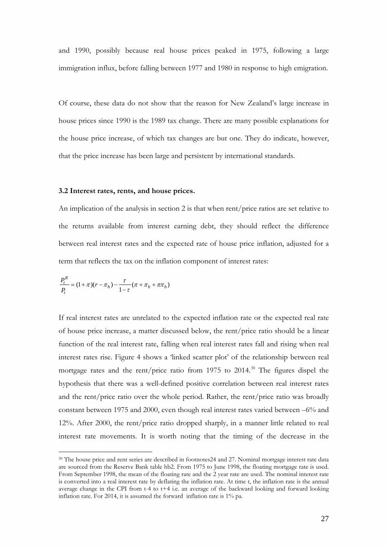
3.2 Interest rates, rents, and house prices.
An implication of the analysis in section 2 is that when rent/price ratios are set relative to
the returns available from interest earning debt, they should reflect the difference
between real interest rates and the expected rate of house price inflation, adjusted for a
term that reflects the tax on the inflation component of interest rates:
(1 )( ) ( )1
Rt
h h ht
Pr
Pτπ π π π ππτ
= + − − + +−
If real interest rates are unrelated to the expected inflation rate or the expected real rate
of house price increase, a matter discussed below, the rent/price ratio should be a linear
function of the real interest rate, falling when real interest rates fall and rising when real
interest rates rise. Figure 4 shows a ‘linked scatter plot’ of the relationship between real
mortgage rates and the rent/price ratio from 1975 to 2014.30 The figures dispel the
hypothesis that there was a well-defined positive correlation between real interest rates
and the rent/price ratio over the whole period. Rather, the rent/price ratio was broadly
constant between 1975 and 2000, even though real interest rates varied between –6% and
12%. After 2000, the rent/price ratio dropped sharply, in a manner little related to real
interest rate movements. It is worth noting that the timing of the decrease in the
30 The house price and rent series are described in footnotes24 and 27. Nominal mortgage interest rate data are sourced from the Reserve Bank table hb2. From 1975 to June 1998, the floating mortgage rate is used. From September 1998, the mean of the floating rate and the 2 year rate are used. The nominal interest rate is converted into a real interest rate by deflating the inflation rate. At time t, the inflation rate is the annual average change in the CPI from t-4 to t+4 i.e. an average of the backward looking and forward looking inflation rate. For 2014, it is assumed the forward inflation rate is 1% pa.
28
rent/price ratio coincides with an increase in the top marginal tax rate from 33% to 39%,
an increase that widened the after-tax wedge between the returns available from property
and interest earning debt.31 A very similar picture is obtained when the real deposit rate
is used instead of the real mortgage rate. The lack of a relationship between the
rent/price ratio and real (or nominal) interest rates is confirmed by regression analysis.
Simple regression analysis shows that the rent/price ratio and the real interest rate both
appear to be described by unit root processes, but the two variables are not cointegrated,
either over the full period or the period since 1990. As such, any linear relationship
between the series is spurious. (See Appendix 2 for the details of these results.32)
These data raise considerable doubts about the extent that trends in house prices and
rents since 1975 can be explained by real mortgage rates. There are at least three possible
ways to rehabilitate the theory. The first is to observe that a linear regression between the
rent/price ratio and the real interest rate will be misspecified if variables which affect the
rent/price ratio and which are correlated with the real interest rate series are omitted
from the regression. The two obvious variables are the expected rate of real house price
inflation, and the expected inflation rate (see equation 12). Unfortunately, series
measuring the expected rate of real house price appreciation or the expected rate of
inflation amongst landlords are not available. It is of course possible to use proxies.
Landlords may have lagged expectations, for example, and expect the future rate of real
house price increases (and the expected rate of general inflation) to be equal to past
rates: perhaps the rate over the previous year or the average rate over the preceding three
years. These proxies can be used in a regression, but these are unlikely to be accurate
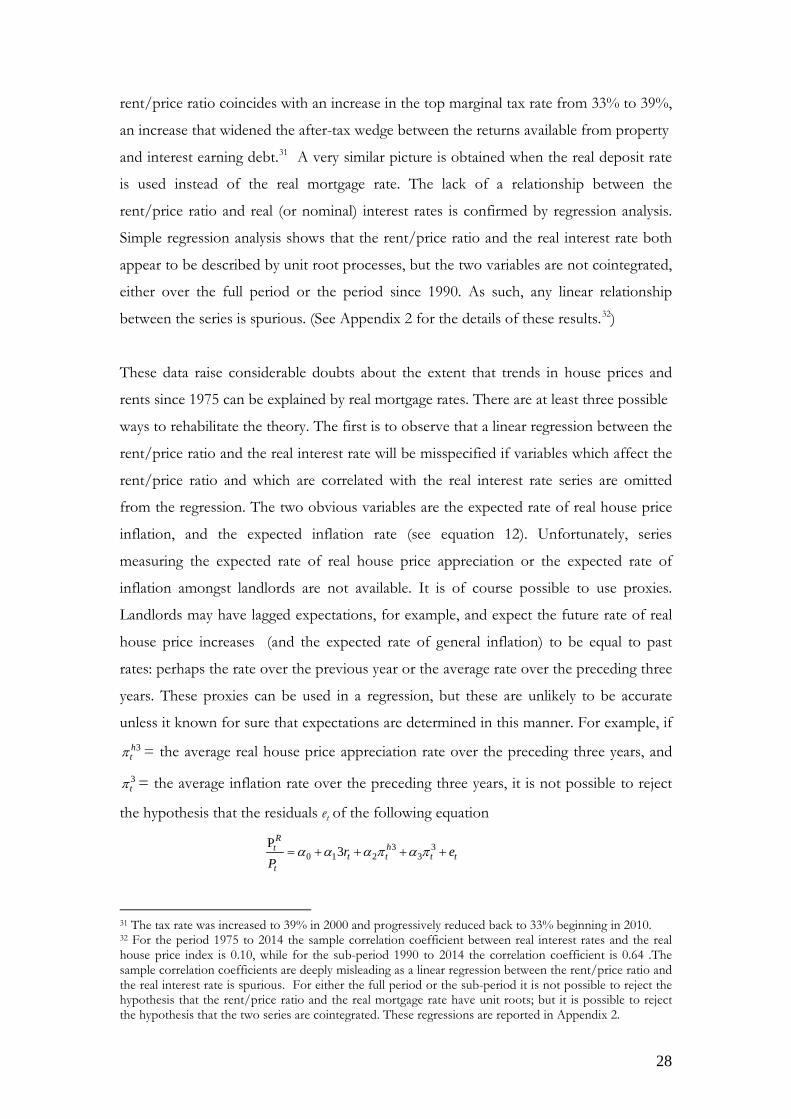
unless it known for sure that expectations are determined in this manner. For example, if 3h
tπ = the average real house price appreciation rate over the preceding three years, and
3tπ = the average inflation rate over the preceding three years, it is not possible to reject
the hypothesis that the residuals et of the following equation
3 30 1 2 3
P3
Rht
t t t tt
r eP
α α α π α π= + + + +
31 The tax rate was increased to 39% in 2000 and progressively reduced back to 33% beginning in 2010. 32 For the period 1975 to 2014 the sample correlation coefficient between real interest rates and the real house price index is 0.10, while for the sub-period 1990 to 2014 the correlation coefficient is 0.64 .The sample correlation coefficients are deeply misleading as a linear regression between the rent/price ratio and the real interest rate is spurious. For either the full period or the sub-period it is not possible to reject the hypothesis that the rent/price ratio and the real mortgage rate have unit roots; but it is possible to reject the hypothesis that the two series are cointegrated. These regressions are reported in Appendix 2.
29
have a unit root and thus that there is no long-run linear relationship between the
variables.33 34(See Appendix 2 for details.)
The failure to find a relationship between the rent/price ratio and real interest rates when
these and similar proxies for expectations are included in the regression suggests one of
two alternatives. First, it could be that expectations of future real house price changes
cannot be described by lagged expectations. A better measure of expectations is needed
to explain the evolution of rent/price ratios in the last 40 years. Secondly, the relative size
of the after-tax returns from rental housing and interest earning debt may not be an
important determinant of rent/price ratios. Some other factor is important, particularly
since 2000. It is possible, for example, that the increase in the top marginal tax rate to
39% between 2000 and 2010 may have changed attitudes towards property ownership
and investment and sparked a revaluation of house prices, although this theory cannot
adequately explain why property prices remained high after taxes were reduced in 2010.
The second explanation for why a linear relationship between rent/price ratios and real
interest rates has not existed since 1975 is based on the observation that New Zealand
had tightly controlled credit markets prior to 1985. It is plausible that any relationship
between real interest rates and the rent/house-price ratio would hold only after 1990,
once credit markets had been deregulated and inflation had been reduced to low levels.
However, as indicated above, it cannot be established that there was a linear relationship
between the two variables in the period since 1990 either. There was relatively little
variation in rent/price ratios between 1990 and 2000 despite considerable falls in real
interest rates; there was a steep decline in rent/price ratios between 2000 and 2010
despite relatively little variation in real interest rates; and there was little variation in
rent/price ratios from 2010 to 2014 despite variation in real interest rates.
A third explanation for the weak relationship between real interest rates and rent/price
ratios is based on the argument that nominal rather than real interest rates are the key
determinant of property prices because when people are credit constrained they are
33 The hypothesis cannot be rejected for either the whole period 1975 to 2014 or the sub-period 1990 to 2014. 34 The failure to show there is a long-run relationship between the rent/price ratio and either the real interest rate or the lagged change in property prices does not mean that there is not a short run relationship. Since changes in real house prices are serially correlated, such a relationship does exist: price increases or price decreases tend to occur in runs. This issue is also discussed in Appendix 2.

30
affected by nominal rather than real interest to income repayment ratios.35 The sample
correlation coefficients between nominal interest rates and real house prices are 0.10 for
the whole period and 0.57 for the period 1990 to 2014, but once again these correlation
coefficients are misleading as the regressions are spurious.
What can be concluded? Real interest rates clearly affect the relative returns from
investing in rental properties and interest earning debt. However, these relative returns
are not systematically related to rent/price ratios in any simple manner. Some other
factor is needed to explain the pattern of rent/price ratios since 1990.
3.3 The size of new residential housing construction.
Internationally, there is almost no systematic analysis of the size of new residential
construction. Figure 5 traces the size of newly constructed residential houses in Australia,
New Zealand, and the United States, the three countries for which data are available.36
(New houses in all three countries are now considerably larger than houses in European
countries.37) These data show the average size of newly constructed houses increased
steadily between 1980 and 2010 in all three countries, and that new houses in the U.S.
and Australia have been consistently larger than new houses in New Zealand.
Figure 6 shows the same data, but with each country’s house size normalised to equal
100 in 1989. The figure shows that the size of newly constructed housing was stable in
New Zealand from 1980 to 1989, at which point it increased sharply. (Between 1974 and
1979 newly constructed houses were very small, reflecting various regulations that
artificially reduced the average size of new buildings.38) The rate of increase in New
Zealand after 1989 is much higher than in either Australia or the United States.
35 This argument was made in the 1970s by Modigliani (1976) and Kearl (1979) among others.. 36 New Zealand data are from Statistics New Zealand, “Number, value and floor area by building type, nature and region” BLD075AA. Australian data are from the Australian Bureau of Statistics, “Building Approvals” February 2010 8731.0 (The series is no longer produced.) U.S data from 1999 are from http://www.census.gov/construction/chars/completed.html spreadsheet " SFForSaleMedAvgSqFt". Earlier data are from http://www.census.gov/construction/chars/historical_data/ . This site has a series of books with the data e.g. US Department of Commerce (2000) "Characteristics of New Housing 1999". 37 International data are not regularly compiled. The BBC reported some statistics in 2009. http://news.bbc.co.uk/2/hi/uk_news/magazine/8201900.stm Similar data are available from Demographia http://www.demographia.com/db-intlhouse.htm. Both sources suggest average house sizes in European countries range from 76m2 in the United Kingdom to 137m2 in Denmark. 38 There were two different regulations. Due to the large scale immigration that took place between 1973 and 1975, people applying for a building permit in excess of 1500 square feet (125 m2) were automatically
31
The relationship between the average quality of newly constructed houses and incomes,
interest rates and tax rates is conceptually complex. As incomes increase, there will be an
increased demand for better quality houses and a reduced demand for lesser quality
houses. This means there will be a mismatch between the distribution of two stock
variables: the desired quality distribution and the existing quality distribution. It can be
expected that new construction and alterations will take place to reduce the mismatch at
each quality level. However, there is no obvious reason why there would be a constant
relationship between the amount of new construction at different quality levels and
explanatory factors such as income, as the relationship will depend on the initial stock as
well as the desired stock. Nor is it clear which quality level will be most profitable to
build first if there are large changes in explanatory variables. All this means that the
average size of new houses should be positively related to per capita incomes and
inversely related to real interest rates, but there is no reason why the relationship should
be linear.
Figure 7 shows a scatter-plot tracing the relationship between real mortgage rates and the
average floor size of new dwellings between 1975 and 2014.39 For the post 1991 period,
it appears that there is a negative correlation between real mortgage rates and the average
size of building permits size, but from 1975 to 2014 the relationship appears rather
weaker. These data suggest that any attempt to find a consistent relationship between
house sizes and real interest rates using all of the data from 1975 to 2014 will not be
successful, although there is an apparent negative correlation after 1989.
Can the increase in the average size of newly constructed housing beginning in 1989 be
explained by the subsequent changes in income and interest rates? In a Scottish court,
the answer would probably be “Not Proven.” Using data from 1989 onwards, there is
clearly a positive correlation between the average size of new construction and per capita delayed by 18 months. This regulation was rescinded following the mass emigration to Australia beginning 1976. Secondly, the government offered concessional loans to young first home buyers so long as they built or purchased a new home. This raised the demand for new houses by young, credit constrained households; these houses tend to be small. The requirement that people could only use concessional loans to purchase new homes was rescinded on March 15 1979. 39Nominal mortgage interest rate data are sourced from the Reserve Bank table hb3. From September 1998, the preferred series is the mean of the floating rate and the 2 year rate. From 1975 to June 1998, the fixed rate series is not available and the floating mortgage rate is used instead. The nominal interest rate is converted into a real interest rate by deflating the inflation rate. At time t, the inflation rate is the annual average change in the CPI from t-4 to t+4 i.e. an average of the backward looking and forward looking inflation rate. For 2014, it is assumed the forward inflation rate is 1% pa.

32
incomes, and a negative correlation with real interest rates. The problem is that interest
rates have a downwards trend for the whole period, while building size and per capita
incomes have an upward trend. Once the trends are accounted for, it is not possible to
be sure that the relationships are not spurious. Formally, when each of the three series
have a unit root, testing whether the average size of new construction is a linear function
of incomes and real interest rates is equivalent to testing whether the three series are
cointegrated. Using data from 1989 to 2014 it is not possible to reject the hypothesis that
the series are not cointegrated. (The results are presented in appendix 2.) Consequently, it
is not possible to conclude statistically that the increase in the average size of new
construction since 1989 is due to the decrease in interest rates and the increase in
incomes taking place since then. Some additional explanation is needed.
3.4 Summary
What can be concluded from post 1989 housing market data? Relative to pre-1989
trends, there has been a substantially faster increase in property prices, a substantial
decline in rent/price ratios, and a large increase in the average size of new houses. These
changes are all consistent with the change in the incentives that followed the great
income tax experiment of 1989. Most of them are also consistent with the decline in real
interest rates, the reduction in inflation, and the increase in per capita incomes that have
taken place since then. Unfortunately, the statistical relationships between the rent/price
ratio and real interest rates, and between the average size of newly constructed houses
and real interest rates and incomes are too imprecisely estimated to know how much
these factors explain the changes in the housing market. For this reason, it is not possible
to estimate the residual role of the tax changes either, at least using aggregate data. This
means the data neither prove nor disprove the contention that the changes in incentives
that followed the changes to the tax system were actually responsible for the subsequent
change in the housing market.
4. Taxes and Housing Markets: Distributional Effects. Non-neutral taxes on property have two types of distributional consequences. First, taxes
redistribute income between members of a cohort, for if tax revenues are not obtained
by taxing the capital income produced by housing they must be obtained by taxing
someone or something else. Secondly, non-neutral taxes redistribute income between
cohorts, because property prices – particularly the land component of property prices –
33
change. When housing is tax advantaged, land prices increase and the first generation of
land owners receives a transfer at the expense of all subsequent generations.
The theoretical literature examining the intergenerational consequences of non-neutral
taxes on property income began with Feldstein (1977). He showed that in most
circumstances a tax on land rent in a closed economy will not only reduce the price of
land but will lead to a long run increase in the capital stock. This is because young agents
will have to spend less of their savings buying land, enabling them to invest more in
businesses and assets.40 Conversely, if land incomes are under-taxed relative to capital
incomes, land prices will rise and long term capital accumulation will decrease.41 Chamley
and Wright (1987) analysed the dynamic properties of Feldstein’s closed economy model,
also finding that taxes on property income usually resulted in an increase in capital
investment and a decline in land prices.42 Eaton (1988) extended this analysis by
examining the effect of property income taxes in a small open economy. He showed land
prices would unambiguously fall, since interest rates were determined in international
markets, and the long run net asset position of the country would improve as additional
local savings replaced foreign savings.
In each of these cases, an intergenerational transfer takes place at the time the tax change
is introduced. If taxes on property income are increased, the first generation of land
owners is worse off as the price of land declines. The welfare consequences for
subsequent generations depend on what happens to the tax revenues that are raised. If
they are refunded to contemporaneous generations, all of these generations will be
unambiguously better off as they pay the same total amount in taxes but have to pay less
for land. These generations will also be better off if the government uses the tax revenue
to purchase valued goods and services. In both of these circumstances, standard
economic theory indicates the discounted value of the gains by subsequent generations is
equal to the losses of the first generation. These conditions need not hold if the tax
revenue is wasted. Moreover, as Fane (1984) showed, if the government issued bonds to
40 The increase in capital should increase the marginal product of land, raising the pre-tax return from land. In some circumstances, the reduction in interest rates stemming from the greater capital levels can lead to a long run increase in the price of land, as total production in the economy increases. 41 Calvo, Kotlikoff and Rodriguez (1979) show that the latter result will be not hold if each generation of landowners bequeath to the subsequent generation a sum equal to the increase in land prices that stems from the concession tax treatment of land. 42 However, they also showed that land prices could increase if interest rates fell sufficiently low, but that the total value of any increase in land prices would be less than half of the tax revenue raised.

34
compensate the first generation for their land price loss, there would be no gain to
subsequent generations if the subsequent tax revenues were used to pay interest on the
bonds.
In contrast, if taxes on property income decrease, the first generation of land owners
would be better off as their land prices would increase. All subsequent generations would
be worse off as they would have to pay higher prices for land while still paying the same
total amount in taxes. Skinner (1996) specifically analysed the case of capital income
from residential property. He showed that when other forms of capital income were
taxed more heavily than housing, the price of housing increases, which, (in the absence
of altruistic bequests) leads to higher consumption by the first generation and lower
capital accumulation and consumption by all other generations. He argued that this
intergenerational shift is the most important consequence of taxing housing and other
forms of capital asymmetrically. Gervais (2002) examined how the tax code affects the
housing market and capital accumulation when property prices do not change. He argued
that favourable tax treatment – particularly the non-taxation of imputed rent – generates
an incentive to purchase better quality houses, leading to higher residential investment
but lower business investment. He argued that the elimination of the housing tax
concessions would raise welfare in the long run. More generally, Batina and Ihori (2000)
analysed how the incidence of various combinations of income and consumption taxes
affects land prices and residential property stocks, finding generally similar results,
although they also showed that the incidence of the tax depend on details of the tax
system such as whether or not housing maintenance expenses are subject to
consumption taxes.
The results of this literature strongly suggest that the distributional effects of New
Zealand’s non-neutral taxes on residential housing not only depend on the direct effects
of the taxes but also on the indirect effects stemming from changing land prices. It is
thus necessary to distinguish between the short run distribution effects of a tax, those
that occur before property prices change, and the long run effects that incorporate
changes in land prices. To do this analysis properly requires a full model in which land
prices adjust in response to taxes, and in which there are agents who differ by income,
home-ownership status, and, if they own, the extent they are mortgaged. The models also
have to take into account the way any tax additional taxes are raised or refunded.

35
Typically these models can only be solved under simplifying assumptions; for example,
Coleman (2010) examines the effect of introducing a capital gains tax under the
assumptions that there are only two classes of property, that there is no population
growth, and that all households accurately anticipate future house prices and rents.
This paper does not calculate the distributional effects of the taxation of property income
in a full general equilibrium model. Rather, it focuses on the key distribution features of
property income taxes by providing a series of numerical examples that capture the key
short run and long run effects. The first example shows the effect of exempting imputed
rent and capital gains from tax within an income tax system.
4.1 Income taxes, housing markets, and distribution
What are the distributional effects of moving from a neutral income tax system to one in
which imputed rent and capital gains are exempt from tax?43 Two scenarios are
presented. To highlight the effects of exempting imputed rent from tax, the first scenario
assumes there is no ongoing change in property prices, although prices can change in
response to taxes. To demonstrate the additional effects of exempting capital gains from
tax, the second scenario assumes property prices increase 1% per year. In each example
four tables are presented. The first table shows rents, capital incomes, and prices when
there are no taxes. The second shows the effects on renters, landlords, lenders and three
classes of owner-occupiers (those with 0%, 50% and 100% equity) when the income tax
system is neutral. The third table shows what happens when capital gains and imputed
rents are exempt from tax, assuming the price of property is unchanged. The last table
shows what might happen to future generations, when property prices have adjusted
upwards by $100,000 in response to the tax changes, but the rate of capital gains
continues at either 0% or 1% per annum. The last table is illustrative; for while prices
and rents are adjusted so that landlords make the same return as they would from lending
money, the marginal returns from lending and from investing in larger houses are not
equated.44
43 If the tax system were neutral with respect to property, (i) rental income net of depreciation, interest costs, repairs and maintenance, and property taxes would be taxed; (ii) the imputed rent earned by owner-occupiers, net of depreciation, interest costs and property taxes would be taxed; and (iii) capital gains would be taxed on an accrual basis. 44 The table is calculated under the assumption that landlords make the same returns from leasing property as they would from lending money. In practice, they normally demand an additional premium to reflect the

36
4.1.1 Exempting imputed rent from tax when property prices are stable.
Table 7a shows outcomes when there are no taxes. The annual benefits provided by
housing are valued at $22,000; rent and imputed rent are set equal to $20,000, providing a
consumer surplus of $2,000; interest rates are 5%; and the price of a house is assumed to
be $400,000.45 In these circumstances a household with $400,000 will be indifferent
between owning their own home, or renting and either investing in interest earning debt
or becoming a landlord.
Table 7b shows what happens when a neutral income tax system is introduced, with an
income tax rate of 30%. It is levied on rents or imputed rent net of other costs including
interest costs and property taxes. Rents are set at a level that mean the after-tax return to
the landlord is the same as if they earned interest on the price of a house. To reflect
current practice in New Zealand, a $2,000 property tax is also imposed on properties;
this tax is separate from the income tax, and does not alter its distributional neutrality in
the sense that the incidence of the tax falls equally on owner-occupiers and renters. To
reflect the effect of the property tax, rents are set at $22,000.
If a tax system is neutral, the relative returns to a landlord and a lender with equal capital,
and the financial returns to a person choosing either to own or rent and lend their equity,
should not depend on the tax rate. In Table 7b the tax system is neutral and has no
effects on house prices, but owners of capital have lower after-tax incomes as they pay
tax. In column 1, the renter gets $22,000 value from renting the house, but as rent is
$22,000 their net value is zero. Similarly in column 4 an owner-occupier with zero equity
gets $22,000 value from owning the house but pays $20,000 in interest and $2,000 in
property taxes. They pay no income tax. In columns 2, 3, 6, a person with $400,000 gets
the same return from becoming a landlord, from being an owner-occupier, or from
lending the money. Note that in column 6 the owner-occupier has to pay $6,000 tax to
the government every year on their imputed rent. In column 5 an owner occupier with
$200,000 equity in their house pays $3,000 tax on their net equity position and is left with
$7,000 after paying tax.
risks undertaken. These risk premiums could be incorporated into the analysis without changing the qualitative results, but have been omitted for simplicity. 45 In general the value of housing services will be greater than the value of rent, or else people will not use the house. The numbers are chosen to make comparisons easy when taxes are imposed, but none of the results are affected by the choice of numbers.
37
Table 7c shows what would happen if the government exempted imputed rent from tax,
if property prices did not change. This change has four main effects. First, the
government would lose tax revenue. If it increased income taxes to make up the lost
revenue, renters, landlords and lenders would pay more income tax but get no advantage
from the tax exemption and so will be worse off; but owner-occupiers as a class would
be better off as their tax cuts would be larger than their income tax increases.46 Secondly,
the tax advantage means renters with some equity will try and become owner-occupiers
to take advantage of the tax exemption. If property prices did not change, a renter with a
$200,000 deposit will gain $3,000 per year from becoming an owner-occupier (the
difference between column 1 plus half of column 3 and column 5). This would lead to an
increase in owner-occupancy rates. Thirdly, owner-occupiers with surplus funds will have
an incentive to build and buy bigger houses, because the additional benefits they get from
these houses are not taxed. As a consequence, the size and quality of the owner-occupied
housing stock should increase. Lastly, owner-occupiers will have an incentive to move to
locations that are conveniently located to desirable amenities, because these benefits are
also exempt from tax. Since the supply of conveniently located land is largely fixed, this
will increase land prices and provide a one-off capital gain to existing owners of land.
Table 7d shows the effect of exempting imputed rents on subsequent generations under
the assumption that prices are bid up to $500,000. Since the characteristics of the
property do not change, the annual value of living in the house remains the same. In
aggregate, the increase in house prices must make subsequent generations (and the first
generation of renters) worse off, assuming the government increases other taxes to offset
the loss of revenue from exempting imputed rent from tax. In aggregate, these
generations face an annual loss equal to the interest rate multiplied by the change in
house prices, as they will pay the same in taxes, but will have to pay more to rent or
purchase property. This loss is not evenly shared, however.
46 About one third of houses in New Zealand are owned without a mortgage, and another third are owned with a mortgage. If the size of these mortgages was uniformly distributed, this means the government would lose tax revenue of half the imputed rent tax levied on an average house – or $3,000 per household in this example. In practice the loss is larger as the houses owned by owner-occupiers are larger on average than those owned by renters.

38
(a) The next generation of landlords and lenders will make the same after-tax
percentage returns, so they will be in an unchanged position.47 Landlords will
only make the same returns if they increase rents to cover the higher property
prices, which means rents will increase by $5,000.48
(b) Renters will be worse off than previously. Rents will increase but the value
renters will get from the house will be the same. They also will be paying higher
income taxes than they would if imputed rent were taxed. They will have an
incentive to become owner-occupiers, but if they are restricted in the amount
they can borrow, they will be renters for longer as it takes them longer to save a
deposit to purchase a property (Coleman 2010).
(c) New generations of owner-occupiers will be worse off than in scenario 7c, as
they will have to pay more for property. The effects on their welfare relative to
the neutral tax regime are ambiguous, for while income taxes will increase and
they will pay more for property than they otherwise would have paid, they will
not pay tax on imputed rent. If all members of the new generation become
owner-occupiers, they will be worse off, as they will pay more for property and
their total tax bill will be the same.
Overall, the extent that some members of subsequent generations will be better off by
the tax change will depend on how much house prices increase and how the income tax
increase is distributed. Renters will almost certainly be worse off relative to a neutral tax
regime, suggesting the shift from a neutral tax regime will be regressive if renters have
lower average incomes than owner-occupiers.
4.1.2 Exempting imputed rent and capital gains from tax when property prices appreciate.
In the second scenario, the value of housing and property prices is assumed to increase at
1% per annum, and the starting level of house prices is increased to $500,000 to reflect
the higher discounted value of rents. Table 8a shows the outcomes when there are no
taxes and Table 8b shows the results of a neutral income tax system in which imputed
47 Table 7d has higher earnings than Tables 7b or 7c as the amount lent has increased from $400,000 to $500,000. 48 Note that this sentence is simply a statement of equation 10, which states that landlords will only enter the property market if they make a return similar to that which they expect elsewhere. Even though rents and prices are determined simultaneously in the market, equation 10 will hold so long as landlords participate in the market, in which case house prices will equal the expected present value of future rent streams. In this section it is assumed that property prices increase and therefore that rents must increase if landlords are to participate in the market; in more complete models such as Coleman (2010), rents and house prices are determined simultaneously subject to the landlord participation constraint.

39
rents, rents, and capital gains are taxed. The rent/property price and imputed
rent/property price ratios are less than 5 % per annum due to the capital appreciation
that property owners obtain.
When capital gains and imputed rents are both exempt from tax, landlords as well as
owner-occupiers pay less tax, but other tax rates increase. Competition between
landlords to obtain these gains leads to a reduction in the rent/price ratio, either through
a reduction in rents (if the supply of houses is elastic) or through an increase in prices (if
it is not). If property prices do not change, rents are reduced until the after tax-return
from being a landlord equal those obtained from lending and the benefits from
eliminating capital gains taxes are transferred to renters. The reduction in rents makes
renters better off relative to low-equity owner-occupiers, and reduces the incentive of
people with low equity to become owner-occupiers. Consequently, lenders and landlords
are unambiguously losers from the tax change if property prices do not change, as they
face higher other taxes. The effects on other groups are ambiguous, and depend on the
size of capital gains relative to the value of imputed rent.
If property prices increase in response to the tax change, renters will be worse off as they
will experience higher other taxes without obtaining lower rents. In these circumstances,
renters with some equity have an incentive to become owner-occupiers, to take
advantage of the tax exemption on imputed rents and capital gains. Moreover, both
landlords and owner-occupiers have an incentive to bid up the price of land, providing a
one-off capital gain to people who own land at the time the tax cuts are introduced.
Table 8d shows the effect on subsequent generations, assuming that base level prices
increase to $600,000 in response to the incentives for households and landlords to bid up
property prices. Prices are still assumed to appreciate at 1% per year, and landlords make
the same after-tax returns from property as if they were lenders. There are three main
effects.
First, rents will increase by less than the increase in house prices. As landlords are willing
to accept low rents so they can obtain tax-free capital gains, rents could even fall in
absolute terms, although they might increase because of the higher property prices.
40
Secondly, even ignoring the increase in other taxes which also makes them worse off,
first home owners with little equity are likely to be worse off than when taxes are neutral,
because the rise in house prices increases their interest costs by more than they gain from
the tax reductions. In contrast, the biggest winners - or the smallest losers - are those
with high equity stakes in owner occupied houses. Their after-tax returns may increase
because of the tax reduction even though they have spent more on their houses,. When
the increase in other taxes is taken into account, it is possible that owner-occupiers with
high equity lose out – and if all households become high equity owner-occupiers it is
certain they will be worse off.
Thirdly, future generations collectively face a loss from the tax changes to the first
generation of property owners. Overall they pay similar amounts of tax to government,
for the reductions in property taxes are offset by increases in income taxes. However,
they pay higher prices for their properties. This leads to an overall loss of income equal
to the interest rate on the higher property prices.
4.1.3: The distribution effects of taxing imputed rents and capital gains.
Tables 7 and 8 show the effects of exempting imputed rent and capital gains from tax. By
reversing the chain of logic, if New Zealand decided to tax imputed rents and capital
gains, with the revenue rebated by cutting other taxes, the following distributional effects
are likely.
(a) The first generation of owner-occupiers with large equity positions will be worse
off, as they will pay more in imputed rent taxes than they gain from lower other
taxes.
(b) The effect on the first generation of renters is ambiguous. To the extent that
capital gains taxes are artificially keeping rents low, they will be worse off; to the
extent that they pay less in other taxes they will be better off.
(c) There will be a decrease in land prices.
(d) There will be less incentive to build large or high quality houses, as imputed rent
will be taxed.
(e) In the long term, new generations of renters are likely to be better off as they will
pay lower rents for the same quality rentals and other taxes will be lower.
41
(f) In the long term, new generations of owner-occupiers will be in a mixed position
to the extent that they have lower income taxes and pay less for property, but
have to pay tax on imputed rent. Owner-occupiers with little equity are likely to
gain more than owner-occupiers with high equity.
(g) In the long term, new generations overall will be better off, as they have the same
total tax bills but pay lower prices for land and for rent. The flow of gains is equal
to the size of the land price decrease multiplied by the interest rate. The original
owners of the land will suffer a loss equal to the discounted sum of the gains of
all subsequent generations, a loss that reflects the removal of tax concessions that
artificially raise land prices.
The distributional results from simply imposing an imputed rent tax are clearer, as in this
case there would be no effect on short run rents and long run rents would decline in line
with the decline in property prices.
These results beg the question: if New Zealand currently taxed imputed rent, would there
be much demand to change the tax system? There is likely to be a political demand from
the first generation of owner-occupiers to exempt imputed rent from tax, as they would
gain from reducing the neutrality of the tax system, as they gain a tax break in the short
run and an increase in property prices in the long run. However, such a move would be
regressive, if renters are poorer than owner-occupiers, and would introduce distortions
that lead to houses that are too large and land prices that are too expensive. It would also
reduce living standards in the long run, by raising the price of property. Given these
effects, it would be difficult to recommend such a policy unless the administrative costs
of taxing imputed rent and capital gains were extremely high.
4.2. Expenditure taxes, housing markets, and distribution
The distributional effects when capital income from sanctioned retirement accounts is
taxed on an expenditure basis and capital gains and imputed rent are not taxed are
complex as the tax system lacks a coherent intellectual basis. The tax system is not
neutral overall, not just because owner-occupied housing and investments in sanctioned
retirement schemes are taxed on an expenditure basis whereas other asset classes
including leased residential property are taxed on an income basis, but also because the
failure to tax capital gains means debt instruments held outside retirement accounts are

42
further disadvantaged. Moreover, most countries limit the amounts that can be deposited
in retirement schemes that are taxed on an expenditure basis. Since most people do not
face binding limits on the amounts they can place in sanctioned retirement accounts, at
the margin they face a tax system that is neutral between investments in housing and
financial assets but non-neutral to investments in leased residential property or personal
businesses. In contrast, wealthy households are taxed at the margin on an income tax
basis so they face a tax system that is non-neutral between owner-occupied housing and
other assets but which is neutral to investments in leased residential property and other
equity assets.
Tables 9 and 10 shows the effects of taxing rental properties on an income basis (with an
exemption for capital gains) when owner occupied housing and interest earnings in
sanctioned retirement income funds are taxed on an expenditure basis. In Table 9 there
is no increase in property prices; a house costs $400,000 and provides annual rental
services valued at $20,000. In Table 10 property prices and the value of rental services
increase by 1% per year; rental services start at $20,000, and the price of the property is
$500,000. Each table is broken into three sections and considers the returns to four
classes of assets: owner-occupied property; deposits held in retirement accounts that are
taxed on an EET basis; other deposits; and rental property. Because the difference in
after-tax returns in income tax and expenditure tax systems depends on the investment
horizon, results are calculated assuming a ten year horizon.
In the first section, all assets are taxed on an expenditure basis. The tax system is neutral
and the returns to investing in owner-occupied housing, rental property, or interest
earning deposits are the same.49
In the second section, the marginal landlord is someone who cannot place additional
funds in a sanctioned retirement scheme and whose alternative investments are taxed on
an income tax basis. Rents are set so that the after-tax returns from investing in rental
property are the same as the after tax returns from deposits taxed on an income basis. In
these circumstances the rent on a property will remain $20,000 if there is no capital
appreciation or decline to $17,857 if there is capital appreciation. The decline in rents
49 Note in the first section of Table 9 and 10 a landlord who has enough money to purchase an owner-occupied house out of tax paid money has enough money to purchase 1/(1-τ) = 1.43 houses out of pretax money. The rent per house is therefore $20,000.

43
occurs because the capital gain is not taxed, and landlords have an incentive to reduce the
rent/price ratio to obtain tax-free capital gains rather than invest in debt securities that
are subject to income tax. Irrespective of the rate of capital appreciation, the returns to a
landlord are lower than the expected returns from investing in owner-occupied housing
or from placing funds in a retirement fund that is taxed on an EET basis. This makes it
unlikely that these landlords would be the marginal players in the property market. Nor
do ordinary households have an incentive to purchase larger houses or bid property
prices above the levels that would prevail under a neutral tax system, as they are taxed on
an equal basis whether they place funds in a retirement income fund or an owner-
occupied house. Consequently, in these circumstances it seems unlikely that the tax
system would produce incentives to bid property prices above the tax-neutral level.
In the third section the marginal landlord is someone whose alternative investments are
taxed on an expenditure basis. Rents are set so that the after-tax returns from investing in
rental property are the same as the after tax returns from deposits taxed on an
expenditure basis. In these circumstances, the rent/price ratio increases relative to the
neutral case, as rents are increased (to $28,571) to pay the income taxes, and the returns
are higher than the returns from investing in deposits that are taxed on an income basis.
These results show the effect on rents and property prices of a mixed expenditure and
income tax regime are crucially dependent on the identity of the marginal investor. If the
marginal investor is someone who cannot place additional funds in a sanctioned
retirement scheme, rent/price ratios will be similar or lower than in the neutral case, and
overall returns will be lower than the returns from owner-occupied housing or a
sanctioned retirement scheme. In these circumstances, residential property is likely to be
a minority investment class, and investors seem unlikely to place significant upward
pressure on property prices as property is tax-disadvantaged relative to funds in
retirement schemes. Alternately, if the marginal investor is someone whose alternative
investment is a sanctioned retirement scheme, rent/price ratios will be higher than when
the tax system is neutral, either because rents are high or because there is downward
pressure on house prices. In neither case, therefore, is the tax system likely to place the
type of upward pressure on house prices generated by New Zealand’s current tax system.

44
Which of the marginal conditions rent/price conditions is most likely to have
characterised New Zealand prior to 1989? At the time there were relatively few private
landlords, approximately 60,000, partly because owner-occupancy rates were high and
partly because a large number of rental properties were owned by the state. This suggests
that the returns to rental properties were probably set in reference to the returns available
from alternative investments that were taxed on an income tax basis. Given the high
rates of inflation prevailing in the 1970s and 1980s, rent/price ratios would be lower than
those prevailing under a neutral tax system; but there would be little pressure for
landlords to outcompete owner-occupiers, as after-tax returns to owner-occupiers would
be higher than those to landlords.
4.3. The Distribution Effects of the Great Income Tax Experiment
What, then, are the distributional effects of taxing retirement income schemes on an
expenditure basis? The answer depends on the tax scheme to which it is compared.
There are three obvious benchmarks: a neutral expenditure tax system; a neutral income
tax system; and New Zealand’s current tax system. The comparisons are most easily
made by noting that an EET retirement income tax scheme can be transformed into
New Zealand’s current tax scheme through a series of three steps:
(a) a shift from an EET retirement income tax scheme to a neutral expenditure tax
scheme, by taxing other capital income on an expenditure rather than income
basis;
(b) a shift from a neutral expenditure tax scheme to a neutral income tax scheme;
and
(c) a shift from a neutral income tax scheme to New Zealand’s current tax scheme,
by exempting imputed rent and capital gains from tax.
Figures 8 and 9 indicate schematically how different classes of income would be taxed
under these tax regimes.50 Figure 8 shows tax rates when sanctioned retirement income
schemes are taxed on an expenditure basis but other capital income is taxed on an
income basis (with an exemption for capital gains), along with a neutral expenditure tax
system. The neutral scheme should have higher statutory rates than the EET retirement
income scheme, as less revenue is received from the taxation of other capital income.
Consequently an EET retirement income tax scheme is likely to be more progressive 50 The diagram is schematic as the numbers are made up. They are designed to indicate how changes from neutral tax systems affect different types of income.

45
than the neutral scheme, as it has lower tax rates on labour incomes but higher tax rates
on capital incomes earned from assets held outside retirement scheme. As discussed in
section 4.2, it may also place slight downwards pressure on land prices.
Standard theory suggests that a neutral expenditure tax scheme will have higher tax rates
than a neutral income tax system, due to difference in the timing of income tax receipts,
but neither should affect land prices.51 The lower tax rates means a neutral income tax
scheme is likely to be more progressive than a neutral expenditure tax system, as saving
rates typically increase with income. A neutral income tax scheme is also likely to be
more progressive than an EET retirement income tax scheme since the taxes on capital
gains and imputed rent will fall disproportionately on high income people.
Figure 9 shows the effects of New Zealand’s current tax system and a neutral income tax
system in which both capital gains and imputed rent are taxed. The current tax system is
more regressive than a neutral income tax system as the exemption of imputed rent and
capital gains from tax favours high income households and leads to higher labour income
taxes. For this reason, shifting from an EET retirement income scheme to New
Zealand’s current tax system has ambiguous effects on distribution, even if the effect on
land prices is ignored. It may be a regressive change, due to the increase in labour income
taxes that occurs when retirement savings are not taxed at the time that income is earned;
but it may not, as imputed rent and capital gains are exempt from tax under the current
income tax system. In either case, the exemption of imputed rent and capital gains from
taxation significantly reduces any distributional advantages that could be achieved when a
government switches the tax system from an expenditure tax basis to an income tax
basis.
It is not possible to ignore the effect on land prices, however. In line with Feldstein’s
(1977) conjecture, when retirement income schemes are taxed on an expenditure basis
there is likely to be slight downward pressure on property prices. In contrast, when
retirement schemes are taxed on an income basis but imputed rent and capital gains are
exempt from tax, there is likely to be upward pressure on property prices. A switch from
an EET retirement income tax scheme to New Zealand’s current tax system will
therefore have a slightly larger effect on land prices than that discussed in section 2,
51 See, for instance, Batina and Ihori (2000).

46
which compared New Zealand’s current tax system with a neutral income tax system.
According to the calculations in Table 2b, this means that the current tax system could
more than double the willingness of owner-occupiers to pay for land with a high
marginal convenience yield relative to a tax system in which retirement income schemes
are taxed on an expenditure basis.
It will be recalled that the 1987 Labour Government and the 1988 Brash Committee
both argued that it was regressive to tax retirement income schemes on an expenditure
basis, as these schemes were primarily used by people on higher incomes. They may have
been wrong. It appears they may have substantially underestimated how the incidence of
the tax change could have been shifted within cohorts and across generations by the
induced change in land prices. If so, it was a mistake that inadvertently benefited the
generation of property owners alive at the time, and probably those who purchased
property in the subsequent decade while the New Zealand economy was still reeling
from the effects of the early 1990s financial crisis and a period of extraordinarily high real
interest rates. The benefits to these generations, however, come at the expense of all
subsequent generations. The losses to these generations in terms of the higher land
prices they have paid and will have to pay are most likely to be greater than any
redistribution gains stemming from taxing retirement saving accounts on an income
rather an expenditure basis.
5. Conclusion. It is a standard adage of economists that the incidence of a tax will fall on people
different to those paying the tax whenever a tax causes prices to change. Nowhere is this
adage more important than when taxes affect the price of land, for taxes that affect the
price of land shift the incidence of the tax across generations. As Feldstein (1977) and
Skinner (1996) observed, tax incentives favouring property should be capitalized into
property values, reducing the welfare of future generations, who would prefer to buy
land cheap and sell cheap rather than buy land dear and sell dear. They further argued the
higher price of land should reduce the country’s capital stock and lower the net foreign
asset position. While the intergenerational consequences of such policies should be a
central feature of fiscal policy analysis, they are frequently ignored as the resource
transfers induced by tax policy are not always directly associated with payments to the
government. A policy that exempts land income from tax will reduce the welfare of all

47
generations but the first generation of landowners, for instance, without ever generating
payments that are counted in standard analyses of government taxes and transfers.
New Zealand’s tax changes in the late 1980s are likely to have had significant
intergenerational consequences through their effects on land pries. By taxing retirement
savings on an income basis without simultaneously taxing imputed rent or capital gains,
New Zealand adopted a tax system that differentially favours income from residential
property. This means the tax advantage of residential property relative to other asset
classes is now greater in New Zealand than it is in most OECD countries. Some of this
advantage may have been inadvertent, since it proved politically impossible to introduce
simultaneously a tax on capital gains or imputed rent, the steps needed to adopted a
neutral income tax system. Inadvertent or not, most formal models analysing the
consequences of a non-neutral income tax system suggest they will lead to an increase in
the marginal price of conveniently located land. In places where use of the transport
system is close to capacity, or where amenities are concentrated, the tax system is likely
to lead to significant increases in land prices.
It is disappointing that the empirical evidence about the effect of the 1989 tax change is
so inconclusive. There is clear evidence that the average size of new construction
increased sharply relative to Australia and the United States after 1989; there is clear
evidence that property prices increased more rapidly after 1990 than before 1990, with
most of the increase occurring after 2000; and there is clear evidence that rent/price
ratios decreased significantly; and the number of private landlords increased rapidly. All
these changes are consistent with the predicted effects of the 1989 tax changes. But so
many other macroeconomic changes occurred at around the same time that the
econometric evidence is not even strong enough to definitively link the size of new
construction or the rent/price ratio to real interest rates, let alone tax changes. A
different econometric approach will be needed to unpick the relationships.
Both the 2001 Tax Review and the 2010 Tax Working Group conceded it would be
difficult to gain a political consensus to tax imputed rents from owner-occupied housing
or to apply a capital gains tax to all assets including owner-occupied housing, and these
taxes have not been imposed. This means New Zealand still has a tax system that is very
distortionary towards residential property. This leaves the country with four tax reform
48
options. The first option is to do nothing. This option is likely to be most attractive to
current land-owners, as they are favoured by the current tax system, but it is likely to be
less attractive to current and future generations of young people who face higher housing
prices. The second option is to finish the job started in 1989 and tax all capital income
consistently. This means introducing a capital gains tax on an accrual basis and taxing
imputed rent, or taxing housing using a risk free return method, using the revenues to
reduce income tax rates further. The third option is to adopt a series of partial ‘fixes’
which reduce the tax advantage of housing but do not address the fundamental issue. For
example, the treatment of the tax losses for landlords who have extensive debt could be
changed. Or a land tax could be introduced.52 The fourth option is to admit the great
income tax experiment of 1989 has not worked as intended, because it proved too
difficult to tax capital incomes properly, and undo the reforms. The simplest way to
undo the reforms is to tax some income placed in retirement income saving schemes on
an EET basis.53 This reform will reduce the distortions that favour owner-occupied
housing by taxing other assets on a similar basis, but will require increases in other taxes
to make up the revenue shortfall. None of these options are entirely attractive. But, after
a quarter of a century, it is surely time to evaluate whether the great income tax
experiment has succeeded as intended. If not, perhaps it is time to urgently pursue
further income tax reforms – or admit it has not worked as planned, and consider
reverting back to the tax approach adopted by the rest of the world.
This paper has not provided a full analysis of the consequences of changing the tax
system, either by taxing housing on an income basis or by taxing retirement saving on an
expenditure basis. This analysis would need to include estimates of the effects of
changing taxes on labour participation rates and labour income as well the effects of
different tax systems on housing markets and other capital investments. Such a model
would be extremely technically demanding and is beyond the scope of the current paper.
Nonetheless, as it is likely that there would be large economic consequences if retirement
52 Coleman and Grimes (2010) provides an analysis of the possible effects of different variants of land taxes in a New Zealand setting. A more general treatment is provided by Dye and England (2009). These authors are favourably disposed to the introduction of a land tax, arguing it is an efficient way of raising revenue. In most cases, a land tax can be expected to reduce land prices (although counter-examples are possible: see Chamley and Wright (1987) or Petrucci (2005)). It should be noted that a land tax could be introduced even if the tax treatment of capital income was not distortionary. 53 A referee pointed out that it may be possible tax retirement savings on an expenditure basis using the same pre-payment option that is applied to housing: that is, a “Taxed-Exempt-Exempt” method. There is an attractive symmetry to this proposition so long as households cannot borrow to place funds in a retirement income account that is taxed on this basis, but deduct interest payments against income tax.

49
saving were taxed differently, a proper analysis of these effects (including, for instance,
the fiscal effects, the effects on labour supply of other compensating tax changes, and the
transitional changes that might occur as the economy moved from one tax regime to
another) would be useful. It is clear the adverse consequences of the 1989 tax regime
shift were not fully anticipated or else the change may not have been undertaken; this
experience suggests that any future tax changes should be properly understood before
they are implemented. Fortunately, it should not be presumed that changing the tax
system would be detrimental to the New Zealand economy. There is a long-standing and
widespread belief amongst economists that expenditure taxes are less distorting than
income taxes, and OECD experience suggests it is easy in practice to tax retirement
savings on an expenditure basis. It is therefore to be hoped that the findings from this
paper provide a basis for a further investigation of the desirability of ending (or, perhaps,
continuing) New Zealand’s great income tax experiment.

50
References Batina, R. G. and Ihori, T. (2000) Consumption tax policy and the taxation of capital income
(Oxford: Oxford University Press).
Calvo, G.A, Kotlikoff, L. and Rodriguez, C.A. (1979) “The incidence of a tax on pure
rent: a new (?) reason for an old answer.” Journal of Political Economy 87(4) 869- 874.
Chambers, M., Garriga, C. and Schlagenhauf, D. (2009) “The loan structure and housing
tenure decisions in an equilibrium model of mortgage choice.” Review of Economic
Dynamics, 12(3), 444-468.
Chamley, C., and Wright, B. D. (1987) “Fiscal incidence in an overlapping generations
model with a fixed asset.” Journal of Public Economics 32(1) 3-24.
Coleman, A.M.G. (2008) “Tax, Credit Constraints, and the Big Costs of Small Inflation.”
Motu Working Paper 08/14.
Coleman, A.M.G. (2010) “The Long-term Impact of Capital Gains Taxes in New
Zealand.” New Zealand Economic Papers 44(2) 159-177.
Coleman, A.M.G. (2014) “Squeezed in and squeezed out: the effects of population
ageing on the demand for housing.” Economic Record 90(290) 301-315.
Coleman, A.M.G., & Grimes, A. (2010) “Fiscal, distributional and efficiency impacts of
land and property taxes.” New Zealand Economic Papers 44(2) 179-199.
51
Coleman, A.M.G. and Scobie, G.M. (2009) “A simple model of housing rental and
ownership with policy simulations.” New Zealand Treasury Working Paper 09-05.
Dye, R. F., & England, R. W. (2009) “ The principles and promise of land value taxation.
In Dye, R. F., & England, R. W. (Eds.) (2009) Land value taxation: theory, evidence, and
practice. (Lincoln Institute of Land Policy).
Eaton, J. (1988) “Foreign-owned land ,” American Economic Review 78(1) 76-88.
Ericsson, N. R., and MacKinnon, J. G. (2002) “Distributions of error correction tests for
cointegration.” The Econometrics Journal 5(2) 285-318.
Fane, G. (1984) “The incidence of a tax on pure rent: the old reason for the old answer.”
Journal of Political Economy 92(2) 329-333.
Feldstein, M. (1977) “The surprising incidence of a tax on pure rent: a new answer to an
old question.” Journal of Political Economy 85(2) 349 – 360.
Fisher, I. (1937) “Income in theory and income taxation in practice.” Econometrica 5(1) 1-
55.
Gervais, M. (2002) “Housing taxation and capital accumulation.” Journal of Monetary
Economics 49(7) 1461-1489.

52
Institute for Fiscal Studies (Great Britain), & Meade, J. E. (1978). The Structure and Reform
of Direct Taxation: Report of a Committee [set Up By] the Institute for Fiscal Studies [and] Chaired
by JE Meade. (Allen and Unwin [for] the Institute for Fiscal Studies).
Jeske, K. (2005) “Macroeconomic models with heterogeneous agents and housing.”
Economic Review (Federal Reserve Bank of Atlanta) 2005(Q4) 39-56.
Kaldor, N. (1955) An Expenditure Tax (London: George Allen and Unwin Ltd).
Kearl, J. R. (1979) “Inflation, Mortgages, and Housing.” Journal of Political Economy 87(5)
1115-1138.
Li, W. and Yao R. (2007) “The life-cycle effects of house price changes.” Journal of Money,
Credit and Banking 39(6) 1375-1409.
Mack, A., and Martínez-García, E. (2011) "A Cross-Country Quarterly Database of Real
House Prices: A Methodological Note." Globalization and Monetary Policy Institute
Working Paper no. 99 (Federal Reserve Bank of Dallas, December).
McLeod Committee (2001) Tax Review 2001 – Final Paper (Wellington: New Zealand
Government).
Mirrlees, J. and Adam, S. (2010) Dimensions of tax design: the Mirrlees review (Oxford: Oxford
University Press).
53
Modigliani, F. (1976) “Some economic implications of the indexing of financial assets
with special reference to mortgages.” pp 90-116 in The new inflation and monetary policy:
Proceedings of a conference organised by the Banca Commerciale Italiana and the Department of
Economics of Universit’ Bocconi in Milan, 1974, ed Monti, M. Macmillan, London and
Basingstoke.
New Zealand Government (1989) The Taxation of Income from Capital: An Overview.
(Wellington: New Zealand Government).
Petrucci, A. (2006) “The incidence of a tax on pure rent in a small open economy.”
Journal of Public Economics 90(4-5) 921-933.
Rosen, S. (1974) “Hedonic prices and implicit markets: product differentiation in pure
competition.” Journal of Political Economy 82(1) 34-55.
Samuelson, P.A. (1964) “Tax Deductibility of Economic Depreciation to Insure
Invariant Valuations.” Journal of Political Economy 72(6) 604-606.
Skinner, J. (1996) “The dynamic efficiency cost of not taxing housing.” Journal of Public
Economics 59(3) 397-417.
Whitehouse, E. (1999) “The tax treatment of funded pensions.” University Library of
Munich MPRA 14173.
Yoo, K.-Y. and de Serres, A. (2004) “The treatment of private pension savings in OECD
countries.” OECD Economic Studies 39 73-109.

54
Figure 1: Schematic description of taxes on capital income
Income Class Owner-occupied housing
Sanctioned RetirementFund
All other assets
Expenditure tax
Income tax
Tax treatment
Pre-1989
post-1989

55
Figure 2: Real Property Prices in New Zealand, 1923 – 2014
Real house price index for New Zealand1923- 2014
0
300
600
900
1200
1500
1800
19231925
1930
1935
1940
1945
1950
1955
1960
1965
1970
1975
1980
1985
1990
1995
2000
2005
2010
Unofficial index based on average price, not quality adjusted
RBNZ house price index , quality adjusted
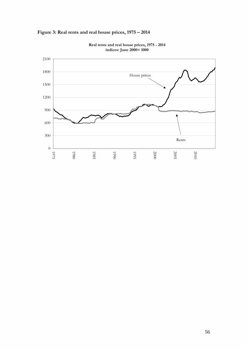
56
Figure 3: Real rents and real house prices, 1975 – 2014
Real rents and real house prices, 1975 - 2014indices: June 2000= 1000
0
300
600
900
1200
1500
1800
2100
1975
1980
1985
1990
1995
2000
2005
2010
Rents
House prices

57
Figure 4: Rent/House-price ratio versus real mortgage rates 1975- 2014
The blue-circle line traces the path of real interest rates and the rent/house-price ratio, 1975-1990. The red-square line traces the path from 1990 – 2015.
Rent/price ratio vs real mortgage rate1975-2014
400
600
800
1000
1200
1400
1600
1800
-8.0% -6.0% -4.0% -2.0% 0.0% 2.0% 4.0% 6.0% 8.0% 10.0% 12.0% 14.0%
real interest rates
rent
/pric
e ra
tio (i
ndex
)
1975
1980
1985
1990
1995
2000
2005
20102014

58
Figure 5: Average new house size, Australia, New Zealand and the United States,
1974-2014. Square metres.
100
120
140
160
180
200
220
240
260
1974 1979 1984 1989 1994 1999 2004 2009 2014
squa
re m
etre
s
USA: single houses
New Zealand: all dwellings
Australia: all dwellings
Australia: single houses

59
Figure 6: Average new house size, Australia, New Zealand and the United States,
1974-2014. Indices normalized with 1989 = 100
50
75
100
125
150
175
1974 1979 1984 1989 1994 1999 2004 2009 2014
New Zealand: all dwellings
Australia: single houses
USA: single houses

60
Figure 7: Average building permit size versus real mortgage rates , 1975-2014
Average floor size of new construction vs real interest rates1975-2014
100.0
120.0
140.0
160.0
180.0
200.0
220.0
-8.0% -6.0% -4.0% -2.0% 0.0% 2.0% 4.0% 6.0% 8.0% 10.0% 12.0%
real interest rates
1975-1979
The blue-circle line traces the path of real interest rates and the rent/house-price ratio, 1975-1990. The red-square line traces the path from 1991 – 2015.

61
Figure 8: Tax rates across different income classes. (i) Expenditure Tax System
0%
10%
20%
30%
40%
owner-occupier retirementaccount
rental property other equity other lending labour income(average)
labour income(when earned)
EET neutral Note: The tax rate on labour income when earned is lower than the tax rate on labour income (average) as taxes are paid when the income is spent and this will be a later date if some of the income is saved.
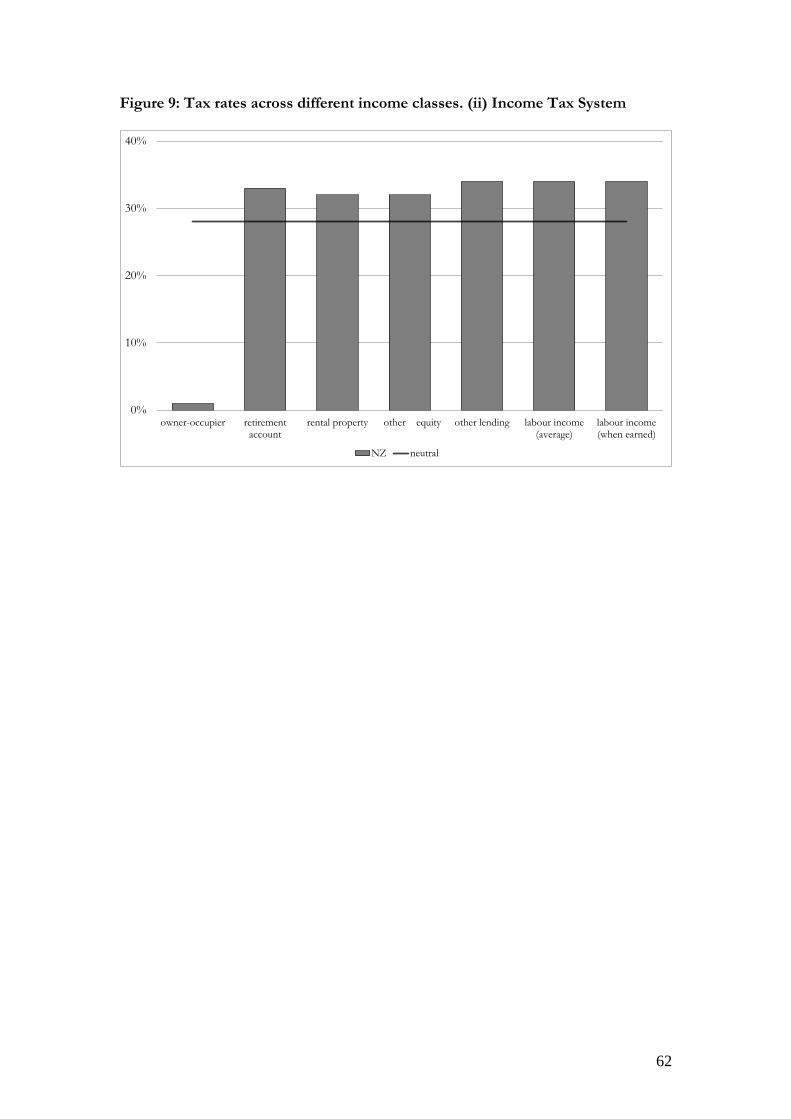
62
Figure 9: Tax rates across different income classes. (ii) Income Tax System
0%
10%
20%
30%
40%
owner-occupier retirementaccount
rental property other equity other lending labour income(average)
labour income(when earned)
NZ neutral

63
Table 1: the effect of taxes on the housing marginal utility/price ratio.
( ) ( )( ) ( )H
dH ddP d
θ θθ θ
1991-2000 π = 1.8 % i = 7.0 %
2001-2010 π = 2.7 % i = 5.9 %
2011-2015 π = 1.1 % i = 4.0 %
(1)Neutral taxes
i δ δπ π+ + − 7.8% 5.8% 5.5%
(2) Neutral taxes
+property tax Li δ δπ π τ+ + − + 8.3% 6.3% 6.0%
(3) Current income
taxes (1 ) Liτ δ δπ π τ− + + − +
6.0%
4.3%
4.6%
(4) Ratio (3)/(2)
72% 69% 78%
(5) Current taxes +
CGT (1 )( ) Liτ δ δπ π τ− + + − + 5.7% 4.4% 4.2%
(6)Current taxes +
imputed rent tax (1 )
1 Liτ δ δπ π τ
τ− + + −
+−
8.7% 6.2% 6.7%
Source: Author’s calculations.

64
Table 2a: the effect of taxes on the marginal land price/ convenience yield ratio.
Ongoing property price increases g = 0%
( ) ( )( ) ( )
LdP ddC d
λ λλ λ
1991-2000 π = 1.8 % i = 7.0 %
2001-2010 π = 2.7 % i = 5.9 %
2011-2015 π = 1.1 % i = 4.0 %
(1)Neutral taxes
1
( )i g gπ π− + + 19.0 31.1 34.0
(2) Neutral taxes
+property tax 1
( ) Li g gπ π τ− + + + 17.3 26.9 29.1
(3) Current taxes 1
(1 ) ( ) Li g gτ π π τ− − + + + 29.0 56.8 47.1
(4) Ratio (3)/(2)
1.6 2.1 1.6
(5) Current taxes +
CGT 1
(1 )( ) Li g gτ π π τ− − + + + 24.8 37.7 40.5
(6)Current taxes +
imputed rent tax
1(1 )( ) ( )Li g g
ττ τ π π
−− + − + +
20.4 42.0 34.2
Table 2b: the effect of taxes on the marginal land price/ convenience yield ratio.
Ongoing property price increases g = 1%
( ) ( )( ) ( )
LdP ddC d
λ λλ λ
1991-2000 π = 1.8 % i = 7.0 %
2001-2010 π = 2.7 % i = 5.9 %
2011-2015 π = 1.1 % i = 4.0 %
(1)Neutral taxes
1
( )i g gπ π− + + 23.5 45.7 51.8
(2) Neutral taxes
+property tax 1
( ) Li g gπ π τ− + + + 21.1 37.2 41.2
(3) Current taxes 1
(1 ) ( ) Li g gτ π π τ− − + + + 41.2 136.4 89.9
(4) Ratio (3)/(2)
2.0 3.7 2.1
(5) Current taxes +
CGT 1
(1 )( ) Li g gτ π π τ− − + + + 29.9 50.8 55.8
(6)Current taxes +
imputed rent tax
1(1 )( ) ( )Li g g
ττ τ π π
−− + − + +
29.6 117.9 70.7
Source: Author’s calculations.

65
Table 3: the effect of taxes on rent/price ratios.
R
PP
1991-2000 π = 1.8 % i = 7.0 %
2001-2010 π = 2.7 % i = 5.9 %
2011-2015 π = 1.1 % i = 4.0 %
long run real growth in land prices g = 0% (1)Neutral taxes (1 )( )hrπ π+ − 5.3% 3.2% 2.9%
(2) Current
income taxes
(1 )( )
( )1
h
h h
rπ πτ π π ππτ
+ −
− + +−
4.4% 1.9% 2.4%
(3) Ratio (2)/(1) 84% 59% 82%
long run real growth in land prices g = 1%
(1)Neutral taxes (1 )( )hrπ π+ − 4.2% 2.2% 1.9%
(2) Current
income taxes
(1 )( )
( )1
h
h h
rπ πτ π π ππτ
+ −
− + +−
2.9% 0.3% 0.9%
(3) Ratio (2)/(1) 68% 16% 47%
Source: Author’s calculations.
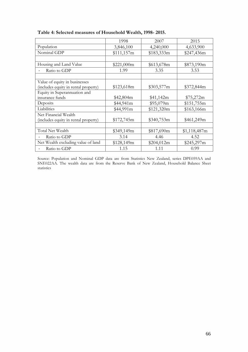
66
Table 4: Selected measures of Household Wealth, 1998- 2015.
1998 2007 2015 Population 3,846,100 4,240,000 4,633,900 Nominal GDP $111,157m $183,333m $247,436m Housing and Land Value $221,000m $613,678m $873,190m - Ratio to GDP 1.99 3.35 3.53 Value of equity in businesses (includes equity in rental property) $123,618m $303,577m $372,844m Equity in Superannuation and insurance funds $42,804m $41,142m $75,272m Deposits $44,941m $95,079m $151,755m Liabilities $44,991m $121,320m $163,166m Net Financial Wealth (includes equity in rental property) $172,745m $340,753m $461,249m Total Net Wealth $349,149m $817,690m $1,118,487m - Ratio to GDP 3.14 4.46 4.52 Net Wealth excluding value of land $128,149m $204,012m $245,297m - Ratio to GDP 1.15 1.11 0.99 Source: Population and Nominal GDP data are from Statistics New Zealand, series DPE059AA and SNE022AA. The wealth data are from the Reserve Bank of New Zealand, Household Balance Sheet statistics

67
Table 5: Annual average property price increases in New Zealand, 1923 – 2014
House prices 1923 – 2014
Nominal increase Inflation Real increase 1923:2 – 1963:2 3.7% 2.2% 1.5% 1962:2 – 1990:2 11.1% 9.7% 1.3% 1990:2 – 2014:4 5.7% 2.1% 3.5% 1975:1 – 1990:2 11.3% 12.2% -0.8% 1990:2 – 2000:1 4.3% 1.7% 2.5% 2000:1 – 2014:4 6.7% 2.4% 4.2% Rents, 1975 – 2014
Nominal increase Inflation Real increase 1975:1 – 1990:2 13.2% 12.2% 0.9% 1990:2 – 2000:1 4.0% 1.7% 2.3% 2000:1 – 2014:4 1.4% 2.4% -1.0% Source: Author’s calculations. The raw data for the period 1923 – 1962 are the average price of urban
properties transferred under the Land Transfer Act using data obtained from the New Zealand Official
Year Book and the Abstract of Statistics published by the New Zealand Department of Statistics. The data
from 1962 – 2014 are a quality adjusted index using data compiled by the Reserve Bank of New Zealand
from Quotable Value. See section 3.1 for more details.
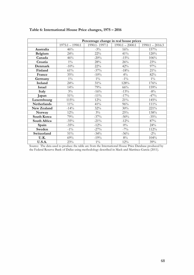
68
Table 6: International House Price changes, 1975 – 2016
Percentage change in real house prices 1975:1 – 1990:1 1990:1- 1997:1 1990:1 – 2000:1 1990:1 – 2016:3
Australia 46% -3% 16% 157% Belgium 24% 22% 41% 120% Canada 46% -20% -15% 106% Croatia 1% 28% 26% 23%
Denmark -10% 22% 42% 97% Finland 61% -37% -18% 21% France 35% -10% 4% 82%
Germany 1% 1% -1% 1% Ireland 24% 31% 128% 176% Israel 14% 79% 66% 159% Italy 3% -16% -13% -8% Japan 51% -11% -17% -47%
Luxembourg 115% 12% 21% 145% Netherlands 11% 41% 96% 111% New Zealand -14% 32% 30% 221%
Norway 12% 3% 25% 138% South Korea 79% -37% -50% -35% South Africa -35% -21% -12% 87%
Spain -35% -12% 0% 24% Sweden -1% -27% -7% 112%
Switzerland 51% -34% -36% -2% U.K. 69% -19% 8% 104%
U.S.A. 23% 1% 12% 39% Source: The data used to produce the table are from the International House Price Database produced by the Federal Reserve Bank of Dallas using methodology described in Mack and Martínez-García (2011).
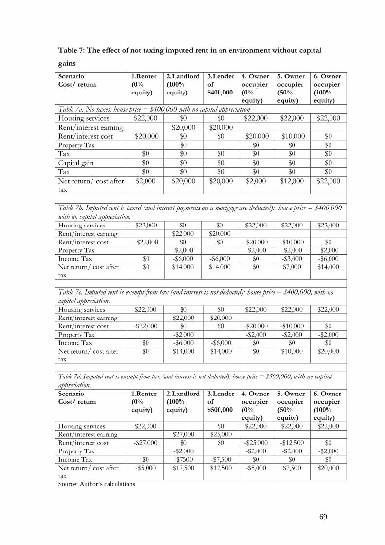
69
Table 7: The effect of not taxing imputed rent in an environment without capital
gains
Scenario Cost/ return
1.Renter (0% equity)
2.Landlord (100% equity)
3.Lender of $400,000
4. Owner occupier (0% equity)
5. Owner occupier (50% equity)
6. Owner occupier (100% equity)
Table 7a. No taxes: house price = $400,000 with no capital appreciation Housing services $22,000 $0 $0 $22,000 $22,000 $22,000 Rent/interest earning $20,000 $20,000 Rent/interest cost -$20,000 $0 $0 -$20,000 -$10,000 $0 Property Tax $0 $0 $0 $0 Tax $0 $0 $0 $0 $0 $0 Capital gain $0 $0 $0 $0 $0 $0 Tax $0 $0 $0 $0 $0 $0 Net return/ cost after tax
$2,000 $20,000 $20,000 $2,000 $12,000 $22,000
Table 7b. Imputed rent is taxed (and interest payments on a mortgage are deducted): house price = $400,000 with no capital appreciation. Housing services $22,000 $0 $0 $22,000 $22,000 $22,000 Rent/interest earning $22,000 $20,000 Rent/interest cost -$22,000 $0 $0 -$20,000 -$10,000 $0 Property Tax -$2,000 -$2,000 -$2,000 -$2,000 Income Tax $0 -$6,000 -$6,000 $0 -$3,000 -$6,000 Net return/ cost after tax
$0 $14,000 $14,000 $0 $7,000 $14,000
Table 7c. Imputed rent is exempt from tax (and interest is not deducted): house price = $400,000, with no capital appreciation. Housing services $22,000 $0 $0 $22,000 $22,000 $22,000 Rent/interest earning $22,000 $20,000 Rent/interest cost -$22,000 $0 $0 -$20,000 -$10,000 $0 Property Tax -$2,000 -$2,000 -$2,000 -$2,000 Income Tax $0 -$6,000 -$6,000 $0 $0 $0 Net return/ cost after tax
$0 $14,000 $14,000 $0 $10,000 $20,000
Table 7d. Imputed rent is exempt from tax (and interest is not deducted): house price = $500,000, with no capital appreciation. Scenario Cost/ return
1.Renter (0% equity)
2.Landlord (100% equity)
3.Lender of $500,000
4. Owner occupier (0% equity)
5. Owner occupier (50% equity)
6. Owner occupier (100% equity)
Housing services $22,000 $0 $22,000 $22,000 $22,000 Rent/interest earning $27,000 $25,000 Rent/interest cost -$27,000 $0 $0 -$25,000 -$12,500 $0 Property Tax -$2,000 -$2,000 -$2,000 -$2,000 Income Tax $0 -$7500 -$7,500 $0 $0 $0 Net return/ cost after tax
-$5,000 $17,500 $17,500 -$5,000 $7,500 $20,000
Source: Author’s calculations.

70
Table 8: The effect of not taxing imputed rent in an environment with capital
appreciation but no capital gains tax.
Scenario Cost/ return
1.Renter (0% equity)
2. Landlord (100% equity)
3.Lender of $500,000
4.Owner occupier (0% equity)
5.Owner occupier (50% equity)
6. Owner occupier (100% equity)
Table 8a. No taxes: house price = $500,000 and increases at 1% per year Housing services $22,000 $0 $0 $22,000 $22,000 $22,000 Rent/interest earning $20,000 $25,000 Rent/interest cost -$20,000 $0 $0 -$25,000 -$12,500 $0 Property Tax $0 $0 $0 $0 Income Tax $0 $0 $0 $0 $0 $0 Capital gain $0 $5,000 $0 $5,000 $5,000 $5,000 Capital Gain Tax $0 $0 $0 $0 $0 $0 Net return/ cost after tax
$2,000 $25,000 $25,000 $2,000 $14,500 $27,000
Table 8b. Imputed rent and capital gains are taxed: house price = $500,000 and increases at 1% per year Housing services $22,000 $0 $0 $22,000 $22,000 $22,000 Rent/interest earning $22,000 $25,000 Rent/interest cost -$22,000 $0 $0 -$25,000 -$12,500 $0 Property Tax -$2,000 -$2,000 -$2,000 -$2,000 Income Tax $0 -$6,000 -$7,500 $1,500 -$2,250 -$6,000 Capital gain $0 $5,000 $0 $5,000 $5,000 $5,000 Capital Gain Tax $0 -$1,500 $0 -$1,500 -$1,500 -$1,500 Net return/ cost after tax
$0 $17,500 $17,500 $0 $8,750 $17,500
Table 8c. No imputed rent or capital gains tax – house price: $500,000 and increases at 1% per year Housing services $22,000 $0 $0 $22,000 $22,000 $22,000 Rent/interest earning $19,857 $25,000 Rent/interest cost -$19,857 $0 $0 -$25,000 -$12,500 $0 Property Tax -$2,000 -$2,000 -$2,000 -$2,000 Tax $0 -$5,357 -$7,500 $0 $0 $0 Capital gain $0 $5,000 $0 $5,000 $5,000 $5,000 Capital Gain Tax $0 $0 $0 $0 $0 $0 Net return/ cost after tax
$2,143 $17,500 $17,500 $0 $12,500 $25,000
Table 8d. No imputed rent or capital gains tax: house price = $600,000 and increases at 1% per annum Housing services $22,000 $0 $0 $22,000 $22,000 $22,000 Rent/interest earning $23,428 $30,000 Rent/interest cost -$23,428 $0 $0 -$30,000 -$15,000 $0 Property Tax -$2,000 -$2,000 -$2,000 -$2,000 Tax $0 -$6,428 -$9,000 $0 Capital gain $0 $6,000 $0 $6,000 $6,000 $6,000 Tax $0 $0 $0 $0 Net return/ cost after tax
-$1,428 $21,000 $21,000 -$4,000 $11,000 $26,000
Source: Author’s calculations.

71
Table 9: Housing returns with expenditure taxes: no capital gains
Landlord Deposit (retirement )
Deposit (other)
Owner Occupier
Table 9a: Rents, housing, and all lending are taxed on an expenditure basis. Tax EET EET EET TEE Labour Income
Pre-tax income $571,429 $571,429 $571,429 $571,429 Tax $0 $0 $0 $171,429 After tax income $571,429 $571,429 $571,429 $400,000
Number of houses 1.43 0 0 1 Capital Income
Rental income $28,571 $20,000 Interest income $0 $28,571 $28,571 $0 Tax $0 $0 $0 $0 Capital gains $0 $0 $0 $0 After tax income $28,571 $28,571 $28,571 $20,000 Annual return 5.00% 5.00% 5.00% 5.00%
Total Return
Compound return $930,797 $930,797 $930,797 $651,558 Tax $279,239 $279,239 $279,239 $0 After tax return $651,558 $651,558 $651,558 $651,558
Table 9b: Rents and other lending are taxed on an income basis. Rents set to equate returns with other lending. Tax TTE EET TTE TEE Labour Income
Pre-tax income $571,429 $571,429 $571,429 $571,429 Tax $171,429 $0 $171,429 $171,429 After tax income $400,000 $571,429 $400,000 $400,000
Number of houses 1.00 0 0 1 Capital Income
Rental income $20,000 $20,000 Interest income $0 $28,571 $20,000 $0 Tax $6,000 $0 $6,000 $0 Capital gains $0 $0th $0 $0 After tax income $14,000 $28,571 $14,000 $20,000 Annual return 3.50% 5.00% 3.50% 5.00%
Total Return
Compound return $564,240 $930,797 $564,240 $651,558 Tax $0 $279,239 $0 $0 After tax return $564,240 $651,558 $564,240 $651,558
Table 9c: Rents and other lending is taxed on an income basis. Rents set to equate returns with lending in retirement scheme. Tax TTE EET TTE TEE Labour Income
Pre-tax income $571,429 $571,429 $571,429 $571,429 Tax $171,429 $0 $171,429 $171,429 After tax income $400,000 $571,429 $400,000 $400,000
Number of houses 1.00 0 0 1 Capital Income
Rental income $28,571 $20,000 Interest income $0 $28,571 $20,000 $0 Tax $8,571 $0 $6,000 $0 Capital gains $0 $0 $0 $0 After tax income $20,000 $28,571 $14,000 $20,000 Annual return 5.00% 5.00% 3.50% 5.00%
Total Return
Compound return $651,558 $930,797 $564,240 $651,558 Tax $0 $279,239 $0 $0 After tax return $651,558 $651,558 $564,240 $651,558
Source: Author’s calculations.
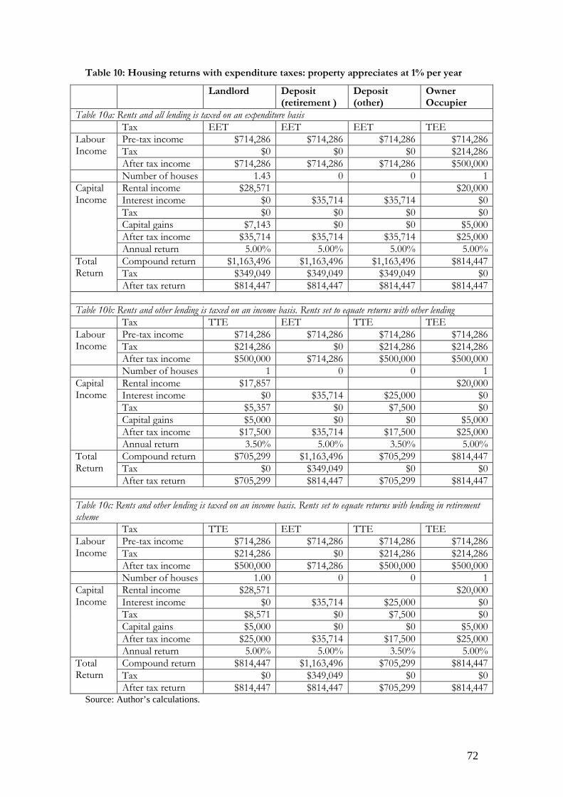
72
Table 10: Housing returns with expenditure taxes: property appreciates at 1% per year
Landlord Deposit (retirement )
Deposit (other)
Owner Occupier
Table 10a: Rents and all lending is taxed on an expenditure basis Tax EET EET EET TEE Labour Income
Pre-tax income $714,286 $714,286 $714,286 $714,286 Tax $0 $0 $0 $214,286 After tax income $714,286 $714,286 $714,286 $500,000
Number of houses 1.43 0 0 1 Capital Income
Rental income $28,571 $20,000 Interest income $0 $35,714 $35,714 $0 Tax $0 $0 $0 $0 Capital gains $7,143 $0 $0 $5,000 After tax income $35,714 $35,714 $35,714 $25,000 Annual return 5.00% 5.00% 5.00% 5.00%
Total Return
Compound return $1,163,496 $1,163,496 $1,163,496 $814,447 Tax $349,049 $349,049 $349,049 $0 After tax return $814,447 $814,447 $814,447 $814,447
Table 10b: Rents and other lending is taxed on an income basis. Rents set to equate returns with other lending Tax TTE EET TTE TEE Labour Income
Pre-tax income $714,286 $714,286 $714,286 $714,286 Tax $214,286 $0 $214,286 $214,286 After tax income $500,000 $714,286 $500,000 $500,000
Number of houses 1 0 0 1 Capital Income
Rental income $17,857 $20,000 Interest income $0 $35,714 $25,000 $0 Tax $5,357 $0 $7,500 $0 Capital gains $5,000 $0 $0 $5,000 After tax income $17,500 $35,714 $17,500 $25,000 Annual return 3.50% 5.00% 3.50% 5.00%
Total Return
Compound return $705,299 $1,163,496 $705,299 $814,447 Tax $0 $349,049 $0 $0 After tax return $705,299 $814,447 $705,299 $814,447
Table 10c: Rents and other lending is taxed on an income basis. Rents set to equate returns with lending in retirement scheme Tax TTE EET TTE TEE Labour Income
Pre-tax income $714,286 $714,286 $714,286 $714,286 Tax $214,286 $0 $214,286 $214,286 After tax income $500,000 $714,286 $500,000 $500,000
Number of houses 1.00 0 0 1 Capital Income
Rental income $28,571 $20,000 Interest income $0 $35,714 $25,000 $0 Tax $8,571 $0 $7,500 $0 Capital gains $5,000 $0 $0 $5,000 After tax income $25,000 $35,714 $17,500 $25,000 Annual return 5.00% 5.00% 3.50% 5.00%
Total Return
Compound return $814,447 $1,163,496 $705,299 $814,447 Tax $0 $349,049 $0 $0 After tax return $814,447 $814,447 $705,299 $814,447
Source: Author’s calculations.
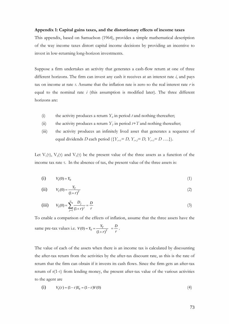
73
Appendix 1: Capital gains taxes, and the distortionary effects of income taxes
This appendix, based on Samuelson (1964), provides a simple mathematical description
of the way income taxes distort capital income decisions by providing an incentive to
invest in low-returning long-horizon investments.
Suppose a firm undertakes an activity that generates a cash-flow return at one of three
different horizons. The firm can invest any cash it receives at an interest rate i, and pays
tax on income at rate τ. Assume that the inflation rate is zero so the real interest rate r is
equal to the nominal rate i (this assumption is modified later). The three different
horizons are:
(i) the activity produces a return Y0 in period t and nothing thereafter;
(ii) the activity produces a return YT in period t+T and nothing thereafter;
(iii) the activity produces an infinitely lived asset that generates a sequence of
equal dividends D each period ({Yt+1= D, Yt+2= D, Yt+3= D ….}).
Let V1(τ), V2(τ) and V3(τ) be the present value of the three assets as a function of the
income tax rate τ. In the absence of tax, the present value of the three assets is:
(i) 1 0(0)V Y= (1)
(ii) 2 (0)(1 )
TT
YVr
=+
(2)
(iii) 31
(0)(1 )
jj
j
D DVrr
∞
=
= =+∑ (3)
To enable a comparison of the effects of inflation, assume that the three assets have the
same pre-tax values i.e. 0(0)(1 )
TT
YV Yr
= =+
Dr
= .
The value of each of the assets when there is an income tax is calculated by discounting
the after-tax return from the activities by the after-tax discount rate, as this is the rate of
return that the firm can obtain if it invests its cash flows. Since the firm gets an after-tax
return of r(1-τ) from lending money, the present after-tax value of the various activities
to the agent are
(i) 1 0( ) (1 ) (1 ) (0)V Y Vτ τ τ= − = − (4)

74
(ii) 2(1 ) (1 )( ) (1 ). (0)
1 (1 )(1 (1 ))
TT
TY rV V
rrτ
τ τττ
− += = − + −+ −
(5)
(iii) 31
(1 )( ) (0)
(1 (1 ))j
jj
D DV Vrr
ττ
τ
∞
=
−= = =
+ −∑ (6)
The after-tax returns are unequal, even though the tax rate on all cash flows are the same.
The after-tax returns of investments with the same pre-tax returns are different because
money lent at interest compounds at an after-tax rather than pre-tax rate of return. This
provides an incentive to invest in low-yielding long-term assets (especially indefinitely
lived assets) rather than higher-yielding short-term assets even though tax is paid on all
current and future earnings.54
Samuelson (1964) demonstrated that this distortion could be corrected by an accrual-
based capital gains tax that allows for the deduction of depreciation and losses, as this
will ensure all activities have the same post tax returns. He further showed that if capital
gains are taxed as income, (i) the present value of all assets will be independent of the tax
rate, even if different agents have different tax rates, and equal to the value of the asset in
the absence of taxes; and (ii) assets valued as the present value of future cash flows will
have an after-tax return of r(1-τ). It is relatively straightforward to demonstrate these
results for the above assets, as the two examples in Box 1 show. In turn, it follows that a
capital gains tax (i) corrects the incentive for agents to favour the production of long
lived assets over short term assets or current activity, and thus removes the incentive to
produce low yielding long term assets because of their tax advantages; and (ii) raises
additional revenue for the government.
2.2 Using accrual-based capital gains taxes to complement income taxes when
inflation is non-zero.
When there is general inflation, the taxation of the full nominal return on interest
earning assets causes a further distortion to asset allocation that can be addressed with
54 Note that when inflation is zero the value of an infinitely lived asset returning a constant dividend is independent of the tax rate even though the future cash-flows and dividends are taxed. The value of the asset is unchanged because the returns on alternative investments are also taxed. The case with inflation is considered below.

75
Box 1: The effect of capital gains taxes on asset values in the absence of inflation This box calculates the value of an asset when a firm undertakes an activity to produce an income producing asset and (i) capital gains tax is paid at time t on the value of the newly created asset, (ii) income tax is paid on the income stream produced by the asset, and (iii) capital gains tax is paid on any change in value of the asset. Example 1: An asset returning a sum Y1 in period t+1 (i.e. a type 2 asset with T=1). Let *
2tV be the value at time t of the asset paying Y1 at time t+1. In period t+1, the firm has income Y1, but the asset depreciates to have zero value. Consequently tax is paid on the income minus the loss in value of the asset. The value of the asset satisfies the following equation:
*
* 1 1 22
* 12
* 1 12
( )1 (1 )
(1 )1
1 (1 ) 1 (1 )(1 )
1 (1 ) 1
tt
t
t
Y Y VV
r
YVr r
Y YVr r
ττ
τττ τ
ττ τ
− −=
+ −
−⇒ − = + − + −
−⇒ = =
+ − − +
Clearly the value of the asset is independent of the tax rate. The taxes paid by the firm are
1 (1 )Y rτ + capital gains tax in period t and *1 2 1( ) (1 )tY V r Y rτ τ− = + income tax in period
t+1, or a total of 1Yτ . This is the same total tax that is paid under the income tax system, although most of the tax is paid in period t rather than period t+1 so the present value of the tax payments is higher. Example 2: An asset that returns a constant dividend (asset 3). Let *
3tV be the value at time t of the asset paying D in each period from t+1 onwards. The value of the asset is constant through time: therefore no capital gains tax is paid at time t+1or thereafter. * The value of the asset satisfies the following equation:
* * ** 3 1 3 1 3
3
*3
*3
(1 ) ( )1 (1 )
1 (1 )11 (1 ) 1 (1 )(1 ) (1 )
1 (1 ) 1 (1 )
t t tt
t
t
D V V VV
r
DVr r
D D DVr r r
τ ττ
ττ τ
τ ττ τ
+ +− + − −=
+ −
−⇒ − = + − + −
− −⇒ = = =
+ − − −
The value of the asset is independent of the tax rate. As the initial investment creates an asset with value 3 /V D r= , the firm pays capital gains tax 3 /V D rτ τ= at time t. Subsequently income tax τD is paid on the dividend each period, but no further capital gains tax are paid as the value of the asset is constant. Total taxes increase. *This result is derived from an iterated forward expansion of the equation for V*3t in terms of V*3t+1. The derivation in the more general case with inflation is provided in Box 2.

76
a tax on nominal capital gains.55 Suppose all dividends increase at rate π, and i is the
nominal interest rate, (1 ) (1 )(1 )i r π+ = + + . Recalculating cases (i) to (iii), assuming the
dividend increases at the inflation rate:
(i) 1 0( ) (1 ) (1 ) (0)V Y Vτ τ τ= − = − (7)
(ii) 2(1 ) (1 ) (1 )(1 )( ) (0)
(1 (1 )) (1 (1 ))
T TT
T TY iV Vi i
τ π τττ τ
− + − += =
+ − + − (8)
(iii) 31
(1 ) (1 )( )(1 (1 ))
j
jj
DVi
τ πττ
∞
=
− +=
+ −∑
(1 )(1 ) 1(1 (1 )) 1 (1 ) (1 (1 ))
(1 )(1 ) (0)(1 )
Di i
r Vi
τ πτ π τ
τ πτ π
− +=
+ − − + + −− +
=− −
(9)
Compared to the values when there is no tax or inflation, the incentive to produce
infinitely lived assets increases substantially as the inflation rate increases:
3 1(1 )( ) / ( )
(1 )rV V
iπτ τ
τ π+
=− −
(10)
For example, suppose the real interest rate is 3% and the tax rate is 33%. In the absence
of a capital gains tax, the additional income from investing in infinitely lived assets rather
producing for the present and investing the proceeds ranges between 49% when inflation
is zero to 186% when the inflation rate is 3%.
If nominal capital gains were subject to tax, the distortion induced by income tax would
be corrected and the after-tax returns of investments with different horizons would be
equalized – this result is shown for the same two asset classes in Box 2. It should be
noted, of course, that if a capital gains tax were applied to nominal capital gains the
effective tax rate on the real return from the investment will be significantly higher than
the statutory income tax rate, just as real interest income is currently subject to effective
tax rates that are significantly higher than the statutory rate. If a capital gains tax were
55 This is the case considered by Samuelson. However, his logic extends to the case that only real interest earnings are taxed, in which case a capital gains tax should only be applied to real capital gains.
77
applied to real capital gains, and real interest were taxed, the same neutrality results
would be achieved but real capital income would be taxed at the statutory rate.
The above analysis assumes a ‘pure’ accrual-based capital gains tax is introduced to
correct the distortions introduced by an income tax. In the real world, it is likely that the
tax would be realization based and introduced with significant exemptions, negating
some of the advantages of a capital gains tax. This of course does not detract from the
primary points: an income tax applied to capital income induces significant distortions in
the pattern of after-tax returns of different asset types, that these distortions are
magnified by inflation, and that these distortions can be corrected by an appropriately
designed capital gains tax.

78
Box 2: The effect of a capital gains tax on asset values with inflation. This box derives the effect of a capital gains tax on the value of two assets considered in Box 1 when there is inflation. The nominal interest rate is i, (1 ) (1 )(1 )i r π+ = + + . (i) An asset returning a sum Y1(1+π) in period t+1. Let *
2tV be the value at time t of the asset paying Y1(1+π) at time t+1. In period t+1, the firm has income Y1(1+π), but the asset depreciates to have zero value. Tax is paid on the income minus the loss in value of the asset. The value of the asset satisfies the following equation:
*
* 1 1 22
* 12
* 1 1 12
(1 ) ( (1 ) )1 (1 )
(1 )(1 )1
1 (1 ) 1 (1 )(1 )(1 ) (1 )1 (1 ) 1 1
tt
t
t
Y Y VV
i
YVi i
Y Y YVi i r
π τ πτ
τ πττ τ
τ π πτ τ
+ − + −=
+ −
− +⇒ − = + − + −
− + +⇒ = = =
+ − − + +
As this is the value of the asset when there is no tax or inflation, the value of the asset is independent of the tax rate or the inflation rate. (ii)An asset that returns an infinite stream of dividends that is constant in real terms. Let *
3tV be the value at time t of the asset paying a sequence of dividends {D(1+π), D(1+π)2, D(1+π)3….}. (The dividends are constant in real terms and increase in nominal terms at rate π.) The value of the asset satisfies the following equation:
( )
* * ** 3 1 3 1 3
3
** 3 1
3
* *3 3 1
** 3 1
3
(1 ) (1 ) ( )1 (1 )
(1 )(1 ) (1 )1
1 (1 ) 1 (1 )
1 (1 ) (1 )(1 ) (1 )
(1 )1 1
t t tt
tt
t t
tt
D V V VV
i
D VV
i i
V i D V
VDVi i
τ π ττ
τ π τττ τ
τ τ τ π τ
π
+ +
+
+
+
− + + − −=
+ −
− + + −⇒ − = + − + −
⇒ + − − = − + + −
+⇒ = +
+ +
But *2
* 3 23 1
(1 )1 1
tt
VDVi i
π ++
+= +
+ +
Hence iterating forward, 2 3
*3
2
(1 ) (1 ) (1 ) .....1 1 1
1 1 11 ....1 1
1 11 1 1 (1 )
tV D D Di i i
Dr r r
Dr r
Dr
π π π+ + + = + + + + + = + + + +
=+ − +
=
This is also the value of the asset when there is no tax or inflation.

79
Appendix 2: Regression results from section 3
A2.1 The rent/price ratio
In section 3.2 it was argued that there is no long term linear relationship between the
rent/price ratio and the real interest rate. The evidence for this statement is a sequence
of regressions showing that the rent/price ratio and the real interest rate are not
cointegrated. The evidence is presented in two parts. In the first part, it is shown that
when only the rent/price ratio and the real interest rate but no other variables are tested
for cointegration, it is not possible to reject the hypothesis that the two series are not
cointegrated. In the second part, cointegration is tested when two additional variables,
lagged changes in the house price index and lagged changes in the inflation rate, are
added to the analysis.
Table A2:1 presents the regression results when only the rent/ price ratio and the real
interest rate but no other variables are analysed. The table has two parts, presenting
results for 1975 to 2014 and 1990 to 2014 respectively. The table shows the results of (i)
unit root tests for the rent/price ratio and the real interest rate; (ii) a linear regression
between the rent/price ratio and the real interest rate, which generates the residual t̂e ;
and (iii) a linear regression between t̂e and 1t̂e − .56 For both periods, it is not possible to
reject the hypothesis (at the 5% significance level) that the real interest rate and the
rent/price ratio have unit roots. Nor is it possible to reject the hypothesis that the
residual of the ordinary least squares regression between the variables has a unit root; as
such the two variables are not cointegrated.
The second set of tests is complicated because the real house price series not only
appears to have a unit root, but quarterly changes in real house prices are strongly and
positively autocorrelated. For the whole period, 1975 – 2014, the following equation
shows the extent of this correlation:
10.007 0.68(0.005) (0.06)
t t tHP HP e−∆ = − + ∆ + 2 0.45 2.11 159R DW n= = =
A very similar regression was estimated for the sub-period 1990 – 2014.
56 This is the Engle-Granger test; more sophisticated tests give similar results.
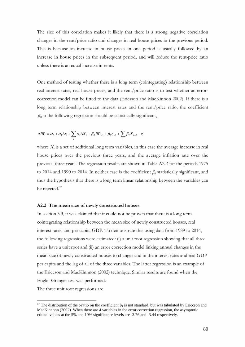
80
The size of this correlation makes it likely that there is a strong negative correlation
changes in the rent/price ratio and changes in real house prices in the previous period.
This is because an increase in house prices in one period is usually followed by an
increase in house prices in the subsequent period, and will reduce the rent-price ratio
unless there is an equal increase in rents.
One method of testing whether there is a long term (cointegrating) relationship between
real interest rates, real house prices, and the rent/price ratio is to test whether an error-
correction model can be fitted to the data (Ericsson and MacKinnon 2002). If there is a
long term relationship between interest rates and the rent/price ratio, the coefficient
0β in the following regression should be statistically significant,
0 1 0 1 1 1t t i t t t i t i ti i
RP r X RP r X eα α α β β β− − −∆ = + ∆ + ∆ + + + +∑ ∑
where Xt is a set of additional long term variables, in this case the average increase in real
house prices over the previous three years, and the average inflation rate over the
previous three years. The regression results are shown in Table A2.2 for the periods 1975
to 2014 and 1990 to 2014. In neither case is the coefficient β0 statistically significant, and
thus the hypothesis that there is a long term linear relationship between the variables can
be rejected.57
A2.2 The mean size of newly constructed houses
In section 3.3, it was claimed that it could not be proven that there is a long term
cointegrating relationship between the mean size of newly constructed houses, real
interest rates, and per capita GDP. To demonstrate this using data from 1989 to 2014,
the following regressions were estimated: (i) a unit root regression showing that all three
series have a unit root and (ii) an error correction model linking annual changes in the
mean size of newly constructed houses to changes and in the interest rates and real GDP
per capita and the lag of all of the three variables. The latter regression is an example of
the Ericcson and MacKinnnon (2002) technique. Similar results are found when the
Engle- Granger test was performed.
The three unit root regressions are
57 The distribution of the t-ratio on the coefficient β1 is not standard, but was tabulated by Ericcson and MacKinnnon (2002). When there are 4 variables in the error correction regression, the asymptotic critical values at the 5% and 10% significance levels are -3.76 and -3.44 respectively.

81
Mean size of newly constructed houses: MBS (Mean building size)
124.7 0.87(8.5) (0.049)
t t tMBS MBS e−= + + 1
2 1
ˆ
ˆ 10.93 1.80 25 2.56
ˆR DW n
α
ασ−
= = = = −
Real interest rates
10.013 0.79(0.008) (0.12)
t t tr r e−= + + 1
2 1
ˆ
ˆ 10.65 1.52 25 1.87
ˆR DW n
α
ασ−
= = = = −
Real GDP per capita
1600 1.00(1240) (0.03)
t t ty y e−= + + 1
2 1
ˆ
ˆ 10.98 0.98 25 0.00
ˆR DW n
α
ασ−
= = = =
The error correction regression is
1 1 161.2 127 0.0006 0.41 119 0.0006(22.6) (85) (0.0016) (0.13) (109) (0.0006)
t t t t t t tMBS r y MBS r y e− − −∆ = − ∆ + ∆ − − + +
0
2 0
ˆ
ˆ0.48 1.73 25 3.14
ˆR DW n
β
βσ
= = = = −
The test of the hypothesis that the three series are cointegrated is whether the coefficient
β0 on the variable MBSt-1 is zero or not. This test is performed by calculating the ratio of
the estimated coefficient to its estimated standard error. The coefficient is quite large
( 0ˆ 0.41β = − ) but as the ratio equals -3.14 it is not possible to reject the hypothesis that
the coefficient is zero and that there is no long-run cointegrating relationship between
the three variables.

82
Table A2.1: Testing for cointegration between the real interest rate and the rent/price
ratio.
Regressions between the rent/price ratio index and the real mortgage rate,
1975-2014
Rent/price ratio(RP)
0 1 1t t tRP RP eα α −= + + 19.3 1.005
(9.3) (0.0076)t t tRP RP e−= − + +
1
2
1
ˆ
0.99 1.23 159ˆ 1
0.66ˆ
R DW n
α
ασ
= = =−
=
Real mortgage (r)
0 1 1t t tr r eα α −= + + 10.0027 0.956
(0.0011) (0.0176)t t tr r e−= − + +
1
2
1
ˆ
0.95 1.18 159ˆ 1
2.5ˆ
R DW n
α
ασ
= = =−
= −
Linear regression
0 1t t tRP r eβ β= + +
0 1 1t t te e uγ γ −= + +
1146 793(35) (574)
t t tRP r e= − + +
13.3 1.005(2.3) (0.0079)
t t te e u−= − + +
2 0.01 0.01 160R DW n= = =
1
2
1
ˆ
0.99 1.27 159ˆ 1
0.63ˆ
R DW n
γ
γσ
= = =−
=
Regressions between the rent/price ratio index and the real mortgage rate,
1990-2014
Rent/price ratio(RP)
0 1 1t t tRP RP eα α −= + + 110.1 1.002
(8.3) (0.0072)t t tRP RP e−= − + +
1
2
1
ˆ
0.99 1.31 98ˆ 1
0.28ˆ
R DW n
α
ασ
= = =−
=
Real mortgage (r)
0 1 1t t tr r eα α −= + + 10.0032 0.942
(0.002) (0.031)t t tr r e−= + +
1
2
1
ˆ
0.91 1.25 98ˆ 1
1.9ˆ
R DW n
α
ασ
= = =−
= −
Linear regression
0 1t t tRP r eβ β= + +
0 1 1t t te e uγ γ −= + +
434 10954(81) (1240)
t t tRP r e= + +
13.8 0.971(7.4) (0.029)
t t te e u−= − + +
2 0.45 0.08 99R DW n= = =
1
2
1
ˆ
0.92 1.30 98ˆ 1
1.00ˆ
R DW n
γ
γσ
= = =−
=

83
Table A2.2: Using the Ericcson-MacKinnon ECM test to test for cointegration between
the rent/price ratio, the real interest rate, the lagged average house price change, and the
lagged inflation rate.
Dependent variable
tRP∆ 1975 - 2014
tRP∆ 1990 - 2014
coefficient s.e. t-ratio coefficient s.e. t-ratio Constant -9.6 9.8 -1.0 -2.9 11.4 0.3
tr∆ 129 246 0.5 1056 380 2.8 3*
tHP∆ -860 208 -4.1 -574 249 -2.3 3*tπ∆ -1251 954 -1.3 -1742 1850 -0.9
1tRP− -0.006 0.009 -0.7 -0.03 0.012 -2.4 1tr − 115 104 1.1 678 264 2.6
3*1tHP− -40 51 -0.8 -119 60 -2.0
3*1tπ − 84 51 1.7 -369 307 -1.2
R2 0.17 0.27 Nobs 146 98 DW 1.70 1.84