Housing Demand in Germany and Japan

Borsch-Supan, Heiss, and Seko,

JHE 10, 229-252 (2001)

Presented by Mark L. Trueman, 11/25/02

Commonalities

• Market economies with essentially private housing markets

• Strong government intervention in the form of housing subsidies/ market regulations

• Comparable standards of living• Comparable demographics…e.g. high elderly share• “Americanized”- similar consumption patterns

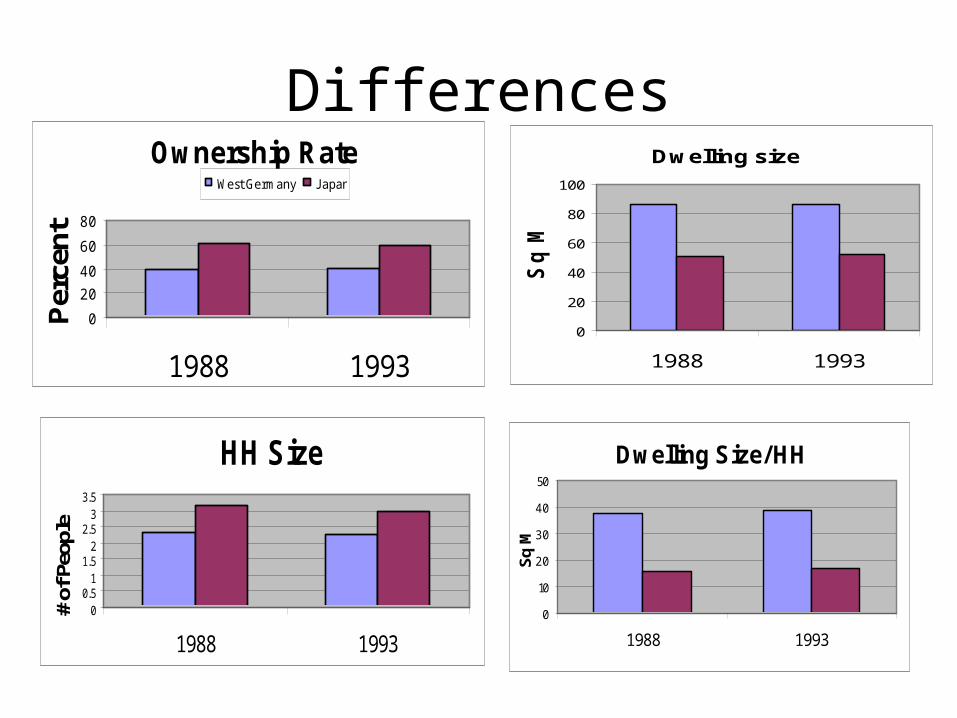
DifferencesDwelling size

0

20

40

60

80

100

1988 1993

Sq

M

HH Size

00.5

11.5

22.5

33.5

1988 1993

# of

Peo

ple

Dwelling Size/ HH

0

10

20

30

40

50

1988 1993

Sq

M

Ownership Rate

0

20

40

60

80

1988 1993

Per

cent

West Germany J apan

Problem/Approach• Problem:

– Typically, we draw inferences about components of demand by looking at differences and similarities across HH. Such cross-sectional data in a single country features little price variations.

• Goal: Exploit cross-national variation:1. Identify determinants of housing demand2. Separate differences in preference parameters from

HH attributes & socio-economic characteristics

• Econometric method: – A flexible discrete choice model is used- Mixed

Multinomial Logit Model (MMLM)

Methodology• Since housing is a durable good, use “permanent (or normal) income” when est. demand.

• Since housing is a heterogeneous good, normalize quality and quantity (i.e., find a well-defined, standard dwelling). Use classical hedonic approach.

• Model housing demand as a multidimensional choice- major attributes are tenure, size, structure type

Income Measures: 1993Quintile Borders

1st 2nd 3rd 4thGermany Current 18959 25169 31687 40491

Normal 20419 25175 29653 35347

Japan Current 19649 33684 33684 47719Normal 19806 33307 34144 47119

Distribution of Housing Alternatives (%s)Own Rent

SF MF SF MF SF MF SF MFLarge Small Large Small Large Small Large Small

Germany 1988 21.5 19.6 4.0 3.6 2.3 11.5 9.7 27.8Germany 1993 22.9 18.9 3.6 4.1 2.8 11.9 8.8 27.0Japan 1988 55.6 9.7 2.1 3.7 1.9 4.7 1.6 20.8Japan 1993 56.9 8.7 2.2 4.4 1.6 3.7 1.5 21.2

Prior Econometric Specifications

• The basic MNL models derive choice probabilities and a likelihood function.

• Mistaken assumption is that the error components which carry all unobserved heterogeneity are independent of each other.

• Problem: seriously biased parameter estimates of housing demand determinants.j

nj

nj

n xu '

J

k

kn

jnj

n

x

xP

1

)'exp(

)exp(

Enhanced Model Specification

• Model housing demand as a dynamic, decision making process using a mixed multinomial logit (MMNL) model.

• Model allows for: – a flexible substitution pattern among alternatives.– unobserved heterogeneity in panel data

)'(' jnn

jn

jn

jn zxu

J

kn

kn

kn

nj

nj

nn

jn

zx

zxP

1)'exp(

)'exp(),(

Model Summary

• Housing demand equations: joint-dependent variables are the probabilities of the 8 housing alternatives, explained by housing prices, HH income, set of socio-econ characteristics (age of HH, HH size; both quadratic forms)

• Plus, a linear time trend• Alternative specific constants-interaction of the

other variables with the 3 dimensions-tenure, type, size.

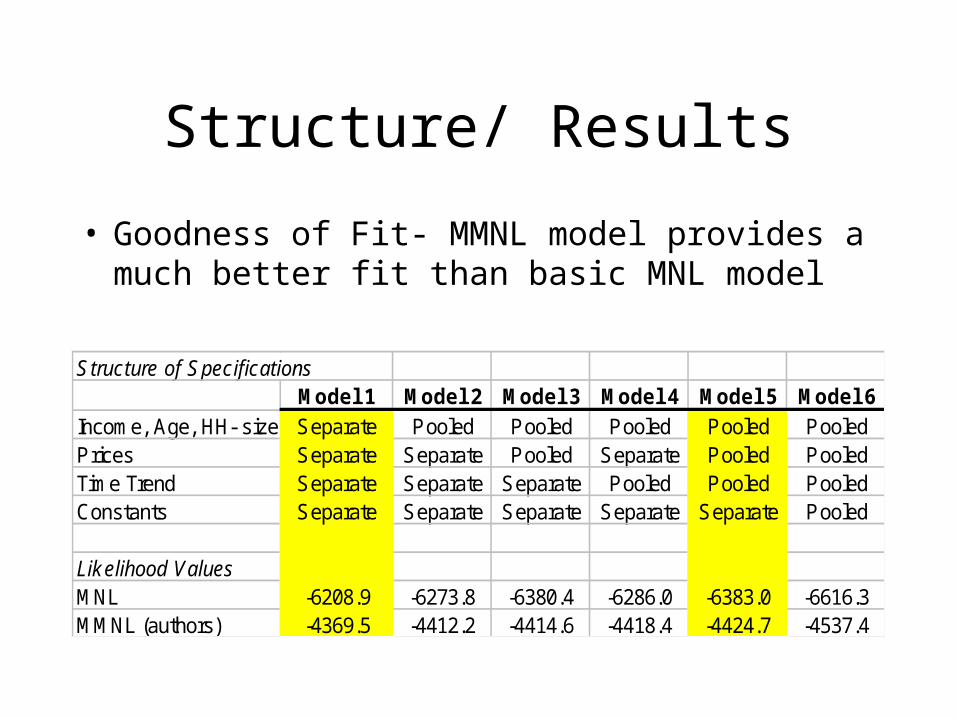
Structure/ Results

• Goodness of Fit- MMNL model provides a much better fit than basic MNL model

Structure of SpecificationsModel 1 Model 2 Model 3 Model 4 Model 5 Model 6

Income, Age, HH- size Separate Pooled Pooled Pooled Pooled PooledPrices Separate Separate Pooled Separate Pooled PooledTime Trend Separate Separate Separate Pooled Pooled PooledConstants Separate Separate Separate Separate Separate Pooled

Likelihood ValuesMNL -6208.9 -6273.8 -6380.4 -6286.0 -6383.0 -6616.3MMNL (authors) -4369.5 -4412.2 -4414.6 -4418.4 -4424.7 -4537.4

Interpreting Elasticities from Significant Coefficients

• Coefficients in discrete choice models carry little intuitive information.

• They must be converted to be meaningful.

• Effects are roughly symmetrical.

Effects of 10% Increase in (Normal) HH Incomeon Home Ownership

Germany JapanBaseline 48.60% 72.00%Model 1 MNL 5.26% 2.76%

1.08 0.38Model 5 MNL 3.33% 3.61%

0.67 0.51Model 1 MMNL 4.01% 2.83%

0.82 0.40Model 5 MMNL 2.06% 1.94%

0.42 0.27

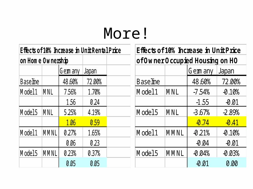
More!Effects of 10% Increase in Unit Rental Priceon Home Ownership

Germany JapanBaseline 48.60% 72.00%Model 1 MNL 7.56% 1.70%

1.56 0.24Model 5 MNL 5.25% 4.19%

1.06 0.59Model 1 MMNL 0.27% 1.65%

0.06 0.23Model 5 MMNL 0.23% 0.37%

0.05 0.05

Effects of 10% Increase in Unit Priceof Owner Occupied Housing on HO

Germany JapanBaseline 48.60% 72.00%Model 1 MNL -7.54% -0.10%

-1.55 -0.01Model 5 MNL -3.67% -2.89%

-0.74 -0.41Model 1 MMNL -0.21% -0.10%

-0.04 -0.01Model 5 MMNL -0.04% -0.03%

-0.01 0.00

Conclusions

• Key: pooling data from different countries offers more variation in explanatory variables.

• Result: we get better estimates of the income, age, and size effects (elasticities).