HOUSING AND FINANCIAL FRICTIONS IN A SMALLOPEN ECONOMY

Tim Robinson and Michael Robson

DRAFT

July 10, 2012

Economic Research DepartmentReserve Bank of Australia

For many useful comments and discussions we would like to thank AdamCagliarini and Mariano Kulish. Our discussant at the 2012 AustralasianMacroeconomics Workshop, Anella Munro, provided numerous insightfulcomments and suggestions. The views expressed are those of the authors and donot necessarily reflect the views of the Reserve Bank of Australia. Responsibilityfor any remaining errors rests with us.

Author: robinsont and robsonm at domain rba.gov.au

Media Office: rbainfo@rba.gov.au

Abstract

The role of the housing sector in the recent US crisis has served to emphasise theimportance of understanding how shocks originating in that sector can influencebroader economic activity. The crisis has also highlighted the importance of creditmarket linkages in amplifying real shocks. The comparatively high exposureof Australian households to housing-secured debt suggests that housing sectorand credit market developments are potentially important drivers of fluctuationsin the Australian economy. In this spirit we adapt a medium scale DynamicStochastic General Equilibrium (DSGE) model with a housing sector and anembedded financial accelerator mechanism following Iacoviello and Neri (2010),to an open economy setting and estimate using Australian data. We find that forsome parameterisations shocks to the housing sector have a substantial impact onthe broader economy and that the inclusion of the financial accelerator mechanismleads to consumption dynamics that are broadly consistent with wealth effectsfrom housing.

JEL Classification Numbers: E23, E32, E44, O33, R31Keywords: Housing, Credit, Financial Accelerator

i

Table of Contents

1. Introduction 1

2. Model 3

2.1 Related Models 32.1.1 Housing and Collateral Channels in General

Equilibrium models 3

2.2 The Model 52.2.1 Households 62.2.2 Production 122.2.3 Importers 142.2.4 Foreign Sector 152.2.5 Value-added 152.2.6 Aggregators 15

3. Data 16

4. Estimation 17

4.1 Methodology 17

4.2 Calibration 17

4.3 Priors 20

5. Results 22

5.1 Parameter Estimates 22

5.2 Impulse Response Functions 245.2.1 Model Comparison 31

5.3 Forecast-Error Variance Decomposition 33

5.4 Historical Decompositions 35

5.5 Growth Cycle Properties 39

5.6 Robustness 40

6. Conclusion 42

ii

References 61

iii

HOUSING AND FINANCIAL FRICTIONS IN A SMALLOPEN ECONOMY

Tim Robinson and Michael Robson

1. Introduction

At the most basic level housing is a durable good that provides shelter, but ina modern developed economy housing also serves as most households’ primarystore of wealth. The direct effects of residential investment on activity arerelatively well understood because demand for housing is strongly linked tothe need for housing services that naturally emerges as a result of populationgrowth (see Berger-Thomson and Ellis (2004) and Leamer (2007)). However, theimplications of the more prominent role of housing as a store of wealth that hasaccompanied financial market liberalisation are not as easy to identify.

One way housing may influence activity is through wealth effects on consumption.Numerous studies have tried to quantify indirect effects of housing wealth onactivity via consumption, with mixed results in Australia and abroad (see forexample Fisher, Otto and Voss (2010), Williams (2010) and Case, Quigley andShiller (2011)). Alternatively, there have been fewer attempts to investigate thepotential indirect effects of developments in the housing market on activitythrough changes in the household balance sheet. As housing is the primarystore of wealth for households it also serves as the collateral supporting mostborrowing. Fluctuations in house prices, therefore, have implications for the valueof households’ collateral, their access to credit and their demand for housing. Thispaper will assess each of these channels using a structural model that incorporateshousing production and credit.

The recent crisis in the US provides an example of the central role that housing canplay as a driver of the business cycle, initially as the source of the shock; and thenas an amplifier of the shock via financial linkages (Bernanke (2010)). Viewing thecrisis through this lens the decline in lending standards and related credit boomthrough the early 2000s were structural vulnerabilities that amplified the impactof the initial housing market correction. Once prices began to fall a deflationaryspiral followed driven by the elevated number of low credit quality borrowers with

2

high loan-to-valuation ratios that were particularly vulnerable to a fall in prices.The fallout in the housing market was exacerbated by a supply overhang whichemerged as new houses continued to enter the market despite the fall in demand, aresult of the inherent inertia in residential investment (Ellis (2010)). In this paperwe aim to investigate the importance of the housing sector as a driver of activityin the broader macroeconomy and its interaction with the financial sector, whichmay amplify housing sector specific shocks.

A range of existing studies have developed structural models exploring activityin the housing sector and spill-overs to the rest of the economy. Davis andHeathcote (2005) incorporate multiple production sectors (including housing) intoa Real Business Cycle (RBC) model and find this feature useful in matchingsome of the properties of the data. Another strand of literature embeds a financialaccelerator mechanism centered on housing credit into an otherwise standardDSGE model. In these models credit flows between two types of householdsdifferentiated by their willingness to borrow to fund current purchases, withhousing as collateral (Iacoviello 2005). Iacoviello and Neri (2010) extend theearlier model of Iacoviello (2005) to include key aspects of housing constructionfrom Davis and Heathcote (2005).

In this paper we build on Iacoviello and Neri (2010), adding open-economyfeatures and estimating the model using Australian data. We then examine how theshocks from the housing sector influence developments in the rest of the economy,and whether the inclusion of a financial accelerator mechanism improves theability of the model to match the data when compared to a model without credit.The inclusion international credit flows in the model also allows us to investigatethe importance of external shocks as a driver of fluctuations in domestic creditflows, a useful feature given the importance of foreign funding for the Australianbanking system.

The model also allows us to investigate the potential for housing relatedconsumption wealth effects. In the closed-economy model of Iacoviello andNeri (2010), estimated using US data, they find positive comovement ofconsumption and house prices that is evidence in favour of such effects. Empiricalstudies using Australian data, such as Tan and Voss (2003), Dvornak andKohler (2007), Fisher et al (2010) and Williams (2010), find varying degrees ofpositive consumption wealth effects from increases in house prices.1

3

Estimating the model using 14 observable variables we find that the modelwith housing is able to generate plausible results both in terms of parameterestimates and dynamics. Fluctuations in the housing market, while responsive tokey shocks in the model, are largely driven by the sector-specific shocks with thehousing preference shock particularly important. In contrast the housing-sectorspecific shocks have little influence on developments outside the housing sector formost parameterisations. The combination of the financial accelerator mechanismand a high steady-state loan-to-valuation ratio (LVR) is an exception. With thiscombination the model is able to replicate the comovement of consumption andhouse prices in response to a housing preference shock that is found in studiesusing US data. When the steady-state LVR is set at a low level the evidence ofconsumption wealth effects from housing is not present, nevertheless the inclusionof the financial accelerator mechanism does alter the model dynamics although theresults from a cycle-dating exercise suggesting that the strength of the financialaccelerator mechanism (governed by the steady-state LVR) has surprisingly littleinfluence on the models ability to match the growth cycle properties of the data.

The paper is structured as follows. Section 2 provides a more detailed discussionof related models before outlining the key details of the model employed here.Section 3 outlines the data used in the process of estimation. Section 4 discussesthe estimation methodology as well as the process of calibration and the choiceof priors. The results from estimation are presented in Section 5 includingparameter estimates, impulse response functions, forecast-error variance andhistorical decompositions for a selection of variables as well as some cycle-datingexercises. Section 6 concludes.

2. Model

2.1 Related Models

2.1.1 Housing and Collateral Channels in General Equilibrium models

The vein of literature that centers on adding housing to DSGE models hasexpanded rapidly over the past decade. Initial efforts focused on housing as

1 It is worth noting that in general these studies also find that it is long-run (or permanent) pricechanges, rather than short-term fluctuations, that have a significant effect on consumption.

4

collateral underpinning the borrowing behaviour of households. Aoki, Proudmanand Vlieghe (2004) present a model along the lines of Benanke, Gertler andGilchrist (1999) (BGG) in which the borrowing of the entrepreneurs in themodel is tied to housing rather than the firm’s net worth. Housing investmentin this model involves the transformation of the intermediate good subject to anadjustment cost, and the rate at which agents can borrow in this model is tied totheir leverage ratio.

Iacoviello (2005) moves away from the external finance premium as a mechanismfor constraining liquidity (as in the BGG model) and instead introduces financingconstraints by including two different types of households. One of group ofhouseholds is impatient (they discount future consumption more than the typicalhousehold) and borrow to fund current period expenditure. Impatient households’borrowing is constrained by the value of their holdings of housing. Movements inhouse prices in the initial period affect households ability to borrow in future andinitiate a potentially powerful amplification process. A shock causing a reductionin demand for housing by impatient households results in a fall in the value oftheir collateral holdings and a subsequent reduction in available credit. Since thesupply of housing in this model is fixed the user cost of housing must decline toencourage unconstrained households to purchase housing to clear the market andthus the price of housing declines further depressing collateral values in the initialperiod. The fall in collateral values implies a further fall in borrowing and housingdemand in the next period, in an intertemporal multiplier effect that compoundsthe contraction in the initial period. This structure allows the model to generatecomovement of real house prices and aggregate consumption in response to ashock to housing preferences as well as replicating the response of spending to aninflation shock. A drawback of this model is the fixed stock of housing precludesthe consideration of residential investment, which is one of the key variables ofinterest in the current study.

Iacoviello and Neri (2010) deal explicitly with the supply side of housing in moredetail. The paper draws heavily on earlier work by Davis and Heathcote (2005)which demonstrates that the introduction of a housing production sector inan RBC framework enables the model to match the relative volatility ofresidential investment (compared with business investment) and the comovementof consumption, GDP, and business and residential investment. Iacoviello andNeri (2010) incorporate this supply-side for housing into a model that is very

5

similar to that used in Iacoviello (2005). They remove entrepreneurs so that thecredit channel only operates between the two household types, and makes housinga combination of capital, intermediate goods, labour, and land. In this frameworkthe positive comovement of consumption and house prices in response to a housingpreference shock is maintained, additionally results from estimation using US datasuggest that shocks to technology and housing preferences explain most of thevariation of residential investment. The model of Iacoviello and Neri (2010) formsthe basis for the model employed here.

In this paper we incorporate some of the key small-open economy aspects that areimportant for Australia. Chistensen, Corrigan, Mendicino and Nishiyama (2009)undertake this exercise for Canada and Bao, Lim and Li (2009) adapt the modeldeveloped in Aoki et al (2004) and estimate it using Australia data. However,both papers employ a very simple production function for housing. Ratherthan including specific inputs to housing production they introduce housing asa transformed intermediate good. This potentially diminishes the channels bywhich the housing production sector may influence the broader economy. In thispaper housing specific labour, capital and domestic final goods are employed inproduction in an effort to strengthen linkages with the economy, which sourcessuch as input-output tables suggest are important in the Australian housing market.

2.2 The Model

The model consists of two types of households differentiated by their discountfactors. Patient households have a higher discount factor are more inclined tosave, households with a lower discount factor borrow to fund current periodconsumption and are labelled impatient. This assumption drives credit flowsbetween the households, with housing used as collateral in the model. This meansthat a shock that negatively impacts the value of impatient households holdingsof housing will negatively impact available collateral, and feed back into lowerdemand for housing and consumption goods, both contemporaneously and infuture periods, given the nature of the borrowing constraint. Housing is producedusing a technology which employs specialised labour from both household types,capital, domestic final goods and land. The supply of new land is fixed in eachperiod. Domestic firms produce differentiated goods using specialised labour andcapital, the goods are sold at a mark-up to final goods bundlers or exported. Finalgoods are consumed, transformed into capital by patient households or used in

6

the production of housing. Monopolistically competitive importing firms importforeign goods and sell them to households to be bundled with domestic goods toproduce final consumption goods. Monetary policy is conducted via a Taylor ruleand facilitated by transfers to households.

2.2.1 Households

The two types of households in the model work, consume final consumption goodsand accumulate housing. They derive utility from consumption, Cj,t , housing, Hj,t ,and real money balances, m j,t , and disutility from labour, L j,t . They maximiselifetime utility according to

U(Cj,t ,L j,t ,Hj,t ,Mj,t) = maxCj,t ,L j,t ,Hj,t ,m j,t

Et

•X

t=0

b

tj

kt ln

�Cj,t �WCj,t�1

�+ Jt lnHj,t + lnm j,t �ct

(Ld 1+x

j,t +Lh 1+x

j,t )1+y

1+x

1+y

�,

(1)

where j is equal to 1 for patient households and 2 for impatient households.Housing is included in the utility function because of the dual role it servesfor most households as a source of housing services (for example shelter) butalso as a significant store of wealth. The labour share of income representsthe economic size of each household type in the model. All households supplylabour to intermediate good firms, Ld

j,t , and housing producers, Lhj,t . Total labour

supplied by each household is a constant elasticity of substitution (CES) aggregateof the two types of industry specific labour. When the intersectoral elasticityof labour substitution, x , is positive and non-zero the two types of labour areimperfect substitutes, and wages will vary between the sectors, with a higher valueof x implying greater sector specificity of labour. In this we follow Iacovielloand Neri (2010) and Horvath (2000). All households are subject to a commonconsumption preference shock, kt , a housing preference shock, jt , which canbe thought of as an exogenous shock to housing demand, and a labour supplyshock, ct . They also exhibit external habits in consumption where householdpreferences reflect the desire to smooth consumption across time using the

7

aggregate consumption of their household type in the previous period as an anchoror reference point. The parameter W governs the degree of habit persistence.

Patient households maximise utility according to their real flow budget constraint

C1,t +Ph

tPt

Ith

+Ph

tPt

Ihth

+qht IH1,t +

Rt�1b1,t�1

pt+St

b ft

h

+m1,t

= b1,t +wd ⇤1,t Ld

1,t +wh ⇤1,t Lh

1,t +Ph

tPt

rkt

Kt�1h

+ rht

Kht�1h

+Ph

tPt

Pth

+

+Pm

th

+Pl1,t +

R ft�1Stb

ft�1

pthF(at�1,e

x

bt�1)+

m1,t�1

pt+ tm

1,t + tl1,t . (2)

The final consumption good is a CES bundle of the domestically produced goodand imported consumption goods.2

Patient households are able to invest in housing assets, IH1,t , with their holdingsH1,t evolving according to a standard law of motion that accounts for the effectsof depreciation. The real price of housing is qh

t (where the aggregate consumptiongood is the numeraire so that nominal house prices, are deflated by the CPI, Pt).Due to their lower rate of discounting patient households also lend to impatienthouseholds, with a positive value of b1,t indicating lending. Patient householdsreceive interest flows in each period stemming from the preceding periods lendingwhere Rt is the nominal gross interest rate. They also have access to internationalfinancial markets from which they can borrow, b f

t , with borrowing limited byintermediation costs similar to Benigno and Thoenissen (2008) ,F(), which are

2

Ct =

✓g

1s Ch s�1

s

t +(1� g)1s Cm s�1

s

t

◆ s

s�1,

where g will influence the degree of openness of the economy. The related price index (the CPI)is

Pt =⇣(1� g)Pm 1�s

t + gPh 1�s

t

⌘ 11�s

.

8

increasing in the nominal net foreign assets to output ratio, at , a standard methodapplied in ‘closing’ small-open economy models, and a shock, x

bt�1.3 R f

t is theforeign nominal gross interest rate.

Patient households invest in the stock of capital employed both by domesticintermediate goods firms, It , and the housing construction sector, Ih

t . Impatienthouseholds do not invest in the capital stock. Capital for both sectors (Kt andKh

t ) is formed from domestic final goods (priced at Pht ) and evolve according

to a standard law of motion subject to adjustment costs which are a function ofthe rate of investment as in Christiano, Eichenbaum and Evans (2005) and, forcapital employed by the intermediate goods producers, an investment efficiencyshock, et . After it is formed patient households provide the capital to the relevantproduction firm and receive rental payments at rates rk

t and rht . In each period

they also receive wages from these firms in return for their labour. The wage doesnot, however, flow directly from the firm to the household. Instead the householdssell their labour to a labour union, in return for real wages wi ⇤

t .4 The labourunions differentiate the labour and sell on to a costless labour bundler who rentsit to firms at a mark-up over the base wage charged by households (see Smetsand Wouters (2007) for a similar labour market structure). Patient householdsreceive transfers from the government in each period. In addition to the usualmoney transfers, tm

1,t , that allow the conduct of monetary policy in the model, theyreceive a share of the revenues derived from the sale of land to housing producers,tl1,t . Patient households also receive profits from the monopolistically competitive

firms they own - the domestic intermediate good producers Pt , importing firmsPm

t , and labour unions Plt .5

The patient household’s optimality conditions are:

3 We assume that in the steady state F(a,1) = 1, that the function is twice differentiable and thatF

x

b(a,1) = 1 and Fa(a,1)> 0.

4 There are four labour unions in the model, one for each sector-household combination

5 Note also that h is the population weight of the patient households while t

ht is the price of final

goods relative to the CPI. h is used to scale the variables whose evolution is determined by thepatient households alone and t

ht is applied to ensure that variables such as the return on capital

are consistently deflated both in the household and firms problems.

9

ktC1,t �WC1,t�1

= b1Rt

"kt+1�

C1,t+1 �WC1,t�

pt+1

#; (3)

wd ⇤1,t = ctL

d x

1,t (Ld 1+x

1,t +Lh 1+x

1,t )y�x

1+x

C1,t �WC1,t�1

kt; (4)

wh ⇤1,t = ctL

h x

1,t (Ld 1+x

1,t +Lh 1+x

1,t )y�x

1+x

C1,t �WC1,t�1

kt; (5)

Et

Rt

pt+1

�= R f

t Et

2

4p

st+1f(at ,e

x

bt )

pt+1

3

5 ; (6)

qht kt

C1,t �WC1,t�1=

JtH1,t

+b1Et

"qh

t+1(1�d

h)kt+1C1,t+1 �WC1,t

#; (7)

which are respectively the consumption Euler equation, the labour supplyexpressions for each production sector, an uncovered interest parity conditionand the housing optimality condition. Note here that p

st is the change in the

nominal exchange rate, pt is CPI inflation and p

ht is domestic final goods price

inflation. The money demand condition is standard and will not be discussedfurther. Patient households also choose the level of investment in each sectorscapital stock according to rules governing the respective Tobin’s Q variables, qtand qkh

t , and the investment optimality conditions

qt = b1Et

"p

ht+1Rt

⇣qt+1(1�d )+ rk

t+1

⌘#(8)

qkht = b1Et

"p

ht+1Rt

qkh

t+1(1�d

kh)+rht+1

t

ht

!#(9)

10

1 = qtet

✓1�S0

✓It

It�1

◆It

It�1�S✓

ItIt�1

◆◆

+b1Et

"qt+1

L1,t+1

L1,tet+1p

ht+1

1pt+1

S0✓

It+1It

◆✓It+1It

◆2!#

(10)

1 = qkht

1�S0

Ikht

Ikht�1

!Ikht

Ikht�1

�S

Ikht

Ikht�1

!!

+b1Et

2

4qkht+1

L1,t+1

L1,tp

ht+1

1pt+1

0

@S0

Ikht+1

Ikht

! Ikht+1

Ikht

!21

A

3

5 (11)

As previously discussed impatient households are not involved in investmentdecisions or in international transactions, and therefore their real budget constraintis

C2,t +qht IH2,t +

Rt�1b2,t�1

pt+m2,t = wd ⇤

2,t Ld2,t +wh ⇤

2,t Lh2,t +b2,t

+m2,t�1

pt+Pl

2,t + tm2,t + tl

2,t . (12)

As with the patient households impatient households work in both productionsectors, they receive transfers from the government both of money and of revenuesrelated to the sale of land. They also receive profits from labour unions. Theseinflows are supplemented by borrowing from patient households and are usedto purchase consumption goods and housing. Since patient households have noway of knowing the credit worthiness of the borrower or forcing them to repaytheir loans at the end of each period they require housing as collateral, and sincerepossession in the event of default is costly they limit borrowing to some fraction,mt , of available collateral which can be thought of as a loan-to-valuation ratio,and which evolves according to an AR(1) process. Default and repossession areassumed to occur in the period after the loan is taken out so that the borrowingconstraint is a function of the discounted value of housing assets in the next period:

11

Rtb2,t mtEt [qht+1H2,tpt+1]. (13)

Assuming that borrowing does not move too far away from its steady statethe constraint will always bind (this assumption is necessary since we log-linearise the model around the steady state). The timing here is important. Aspreviously outlined the static multiplier will act contemporaneously in the eventof a negative housing demand shock, the value of housing collateral held byimpatient households falls as the quantity held contracts and house prices fall. Butthe contraction in collateral in the initial period has implications for borrowingin future periods. A decline in available credit in the next period will result in afurther reduction in housing purchases and another contraction in collateral, whichwill again feed into housing demand in the next period and so on. Kiyotaki andMoore (1997) label this effect the dynamic multiplier and find that it is much moreimportant than the static multiplier in its effect on activity. The effect is harderto unambiguously identify here because where the supply of collateral (land)in Kiyotaki and Moore (1997) was fixed by assumption and the price forced toadjust to entice the patient agents to purchase it, whereas in this model a quantityadjustment is also likely to occur and manifest in a contraction in the productionof housing. This is likely to attenuate the dynamic multiplier to some degree butis unlikely to shut it off it entirely.

The first order conditions for impatient households are:

ktC2,t �WC2,t�1

= b2Rt

"kt+1�

C2,t �WC2,t�1�

pt+1

#+L2,2tRt ; (14)

wd ⇤2,t = ctL

d x

2,t (Ld 1+x

2,t +Lh 1+x

2,t )y�x

1+x

C2,t �WC2,t�1

kt; (15)

wh ⇤2,t = ctL

h x

2,t (Ld 1+x

2,t +Lh 1+x

2,t )y�x

1+x

C2,t �WC2,t�1

kt; (16)

12

qht kt

C2,t �WC2,t�1=

JtH2,t

+b2Et

"qh

t+1(1�d

h)kt+1C2,t+1 �WC2,t

#+L2,2tmtEt

hqh

t+1pt+1

i. (17)

These are the consumption Euler equation (where L2,2t is the Lagrange multplieron the borrowing constraint), the labour supply conditions for each sector and thehousing optimality condition, noting that the labour supply expressions are of thesame form as those for the patient households and that the Euler equation andhousing condition are also similar although each is augmented with a term derivedfrom the borrowing constraint. These terms are one channel linking borrowingand the decisions about consumption and housing taken by impatient householdsin the model.

2.2.2 Production

Domestic Goods

Intermediate goods producers minimise total costs, tct :

minLd D

1,t (i),Ld D2,t d(i),Kt�1(i)

tct =wh

1,t

t

ht

Ld D1,t (i)+

wh2,t

t

ht

Ld D2,t (i)+ rk

t Kt�1(i), (18)

subject to their production technology

Yt(i) = ZtKt�1(i)a(Ld D

1,t (i)µLd D2,t (i)1�µ)1�a , (19)

which is a Cobb-Douglas constant returns to scale production function with capitaland labour from each of the household types as inputs and an AR(1) technologyshock, Zt , and where i in this instance is a firm index.

The goods are differentiated and the market monopolistically competitive. Calvopricing is assumed, with Ph

t , the price of the domestic final good, a mark-up, Xht ,

over marginal cost. Firms that are unable to reset prices to the optimal level in anyperiod index to the previous period’s CPI inflation. This results in the standard

13

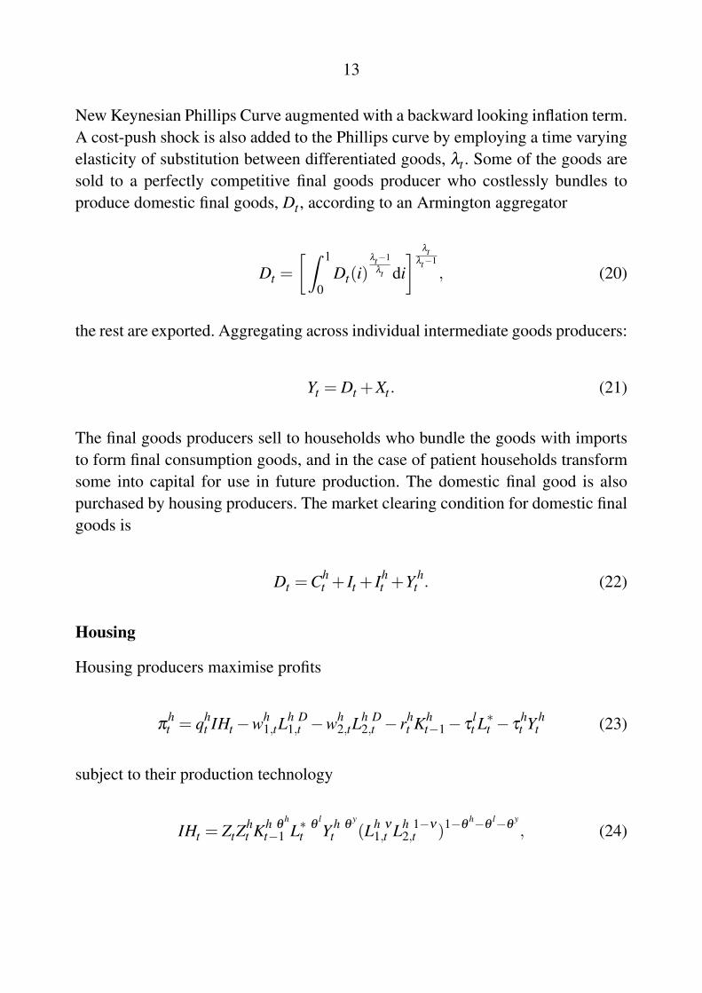
New Keynesian Phillips Curve augmented with a backward looking inflation term.A cost-push shock is also added to the Phillips curve by employing a time varyingelasticity of substitution between differentiated goods, lt . Some of the goods aresold to a perfectly competitive final goods producer who costlessly bundles toproduce domestic final goods, Dt , according to an Armington aggregator

Dt =

Z 1

0Dt(i)

lt�1lt di

� ltlt�1

, (20)

the rest are exported. Aggregating across individual intermediate goods producers:

Yt = Dt +Xt . (21)

The final goods producers sell to households who bundle the goods with importsto form final consumption goods, and in the case of patient households transformsome into capital for use in future production. The domestic final good is alsopurchased by housing producers. The market clearing condition for domestic finalgoods is

Dt =Cht + It + Ih

t +Y ht . (22)

Housing

Housing producers maximise profits

p

ht = qh

t IHt �wh1,tL

h D1,t �wh

2,tLh D2,t � rh

t Kht�1 � t

lt L⇤

t � t

ht Y h

t (23)

subject to their production technology

IHt = ZtZht Kh q

h

t�1 L⇤ q

l

t Y h q

y

t (Lh n

1,t Lh 1�n

2,t )1�q

h�q

l�q

y, (24)

14

which is a constant returns to scale Cobb-Douglas production function withcapital, Kh

t�1, domestic final goods, Y ht , specialised labour from both households,

Lh1,t and Ld

1,t , and land, L⇤t . As well as the economy wide technology shock,

Zt , there is an AR(1) sector specific technology shock, Zht . A set amount of

land, normalised to 1, is released in each period (this can be thought of as agovernment land release). The limited supply of land in each period has a similareffect to adding adjustment costs to production, so that housing production cannotcompletely adjust to changes in demand and will lead to increased house pricevolatility. This feature is included in an attempt to match the sluggish responseof residential investment to changes in demand for housing that is a well knownfeature of the housing market (Ellis (2010)). The inclusion of domestic final goodsas an input to housing production is an attempt to better capture the linkagebetween the housing sector and the rest of the economy and is supported byanalysis of input-output tables for Australia which suggest a strong multipliereffects from residential construction activity.6

2.2.3 Importers

Importers purchase homogeneous foreign consumption goods at price, Pm1t =

StPf

t , where St is the nominal exchange rate and P ft is the foreign price level.

Importers differentiate goods before selling them at a markup over marginal cost,Xm

t , to a good bundler who then sells to the households who combine the finalimported good with the domestic final good to produce the final consumptiongood. The monopolistically competitive importers are assumed to employ Calvopricing and index to the previous periods import price inflation when they areunable to optimally reset their prices. The result is a Phillips Curve of the sameform as that employed by the domestic intermediate goods producers, and as withthe domestic Phillips Curve a cost-push shock is incorporated. In the current modelit is assumed that all imports are consumed.7

6 One obvious limitation of this model is that the housing production sector only produces outputequivalent to new housing. In reality a significant portion of residential investment in any periodis likely to be alterations and additions to established dwellings. Incorporating this activity intothe model framework is a potentially interesting avenue for further research.

7 An interesting avenue for further research would be to allow some proportion of imports to flowinto the formation of capital.

15

2.2.4 Foreign Sector

We model export demand using a typical demand function followingKollmann (2002)

Xt =

Ph

t

StPf

t

!�l

f

Y ft . (25)

Combining the household budget constraints, expressions for profits, and marketclearing conditions we are able to derive an expression for the trade balance

XtYt

� Pm1t Cm

t

Pht Yt

= at �R ft�1F(at ,e

x

bt )

p

st

p

ht

1DYt

at�1.

The remainder of the foreign sector is modelled as a VAR(2) including foreigninflation, output and interest rates.

2.2.5 Value-added

We develop an expression for the combined value added of the two productivesectors. A simple summation of output from the sectors is not possible becausesome of the final goods serve as inputs to the production of housing. Our definitionof real value added is then

VAt = (Yt �Y ht )t

ht +qh

t IHt , (26)

where we deflate by the CPI.

2.2.6 Aggregators

Finally the aggregators for total consumption and housing are the populationweighted sums of each households respective holdings are

16

Ct = hC1,t +(1�h)C2,t , (27)

and

Ht = hH1,t +(1�h)H2,t . (28)

3. Data

Fourteen observable variables are employed in estimating the model, 11 in thecore model and 3 in the foreign VAR(2). The sample period is 1993:1-2011:1. Inthe model GDP, residential investment, business investment, consumption, houseprices, total hours worked and household credit (all real) are detrended using aHodrick-Prescott filter; the remainder, the domestic policy rate, domestic prices,unit labour costs and import prices are log-differenced and demeaned. 8 The dataentering the VAR is transformed in a similar way with major trading partner GDPdetrended and inflation and G7 policy rates log-differenced and demeaned. Onedraw-back of detrending the data is that we are unable to address the impactof population growth which may be expected to be an interesting avenue ofinvestigation in the housing market. The inclusion of trends in the model is oneobvious extension.

In this model, as in most macroeconomic models, the match between the availabledata and the equivalent model concept is not exact. While we do not anticipatethat the extent of measurement error in this model is especially great (relative tosimilar studies), it is worth discussing the mismatch between the data and modelconcepts of household credit. In our estimation we map total household credit to b2which is the credit extended to impatient households (Iacoviello and Neri (2010)do not employ credit as an observable variable in their estimation). In a closedeconomy this would be entirely appropriate and a very close conceptual match,but because we allow the patient households to borrow from the external sectorand use the borrowed funds for the purchase of consumption goods and housing(rather than all of these funds being on-lent to impatient households or used for

8 The key activity variables are all private non-government.

17

the purchase of investment goods), the household credit series we employ as anobservable is likely to include credit extended to both household types. The dataunderlying our credit observable do not allow us to construct a separate impatienthousehold credit series. In light of this we persist with the aggregate measure, butthis limitation should be kept in mind when interpreting the results, particularlythe importance of the loan-to-valuation ratio shock in explaining the credit series.

4. Estimation

4.1 Methodology

The model is linearised around the steady-state, and solved and estimated inDynare. We informally calibrate some of the key parameters in the model in anattempt to match the steady-state values for some of the key expenditure ratios inthe model to their sample means. We also set values for some parameters that areknown to be difficult to identify in estimation, in such cases we employ valuesthat are common in the literature. For the parameters to be estimated we employgenerally similar prior distributions to other Australian studies or Iacoviello andNeri (2010) (see Table 3). The posterior distributions of the parameters areestimated using the Metropolis-Hastings algorithm and Markov Chain MonteCarlo (MCMC) methods, using two chains of 500 000 draws and a burn-in phaseof 200 000 draws.

4.2 Calibration

For some of the parameters that are assigned values we follow Iacoviello andNeri (2010). There are two reasons for this. First, the core of the model here isobviously similar to that employed by Iacoviello and Neri (2010). Second, wehave little disaggregated data available for Australia (particularly disaggregatedindustry level labour and wages data) that could be used to inform our owncalibration or improve that used in the earlier paper. We set the shares of land,q

l, capital, q

h, and intermediate goods, q

y in housing construction to 0.1. Thepatient households discount factor, b1, is set to 0.9925 to achieve a steady-state real interest rate of 3 per cent. We set the value of b2 at 0.95 as used byIacoviello (2005).9 In the full model we assume that impatient households borrow

9 See Iacoviello (2005) for a discussion of the studies on which this value is based.

18

Table 1: Calibrated ParametersParameter Description Calibrated valueh Population weight 0.65b1 Patient household discount factor 0.9925b2 Impatient household discount factor 0.95j Housing weight 0.2m Steady-state loan-to-valuation ratio 0.6a Steady-state net foreign assets ratio 2.1a Capital weight in goods production 0.35µ HH1 labour weight in goods production 0.65qh Capital weight in housing production 0.1qy Goods weight in housing production 0.1ql Land weight in housing production 0.1n HH1 labour weight in housing production 0.65d Capital depreciation rate 0.025dh Housing depreciation rate 0.001y Inverse Frisch elasticity 1x Intersectoral labour elasticity of 0.75

substitutions Elasticity of substitution between 4

domestic and imported goodsg Domestic goods share in final consumption 0.6j Interest debt sensitivity of 0.001

foreign borrowingl

f Foreign good elasticity of substitution 1l Domestic good elasticity of substitution 4l

w Intrasectoral labour elasticity of 4substitution

l

m Imported good elasticity of substitution 8

at an LVR that is closer to the average found in Australian data, 0.6, rather thana higher LVR closer to what may be expected for the average first home buyeras used by Iacoviello and Neri (2010). Finally, we use roughly the mid-point ofthe Iacoviello and Neri (2010) estimates of the intersectoral elasticity of labour forpatient and impatient households, x = 0.75, as there is little Australian informationavailable to inform this choice.

The calibrated parameters are set to broadly match some of the key nominalactivity ratios found in data over the sample period, or, alternatively, on the basisof other data sources. In order to match the steady-state expenditure ratios we set

19

the steady-state weight on housing in the utility function, j, equal to 0.2 whichis somewhat higher than the value used in Iacoviello and Neri (2010), a is setto 0.35 which broadly matches the empirical evidence on the weight of capital indomestic goods production from the Australian National Accounts. The elasticityof substitution of imported goods, l

m, is set to 8 implying a steady-state mark-up of 14 per cent. The higher elasticity (in comparison with the elasticity ofsubstitution for domestic goods) narrows the gap between the ratio of exports tovalue-added found in the data (0.19) and that implied by the model (0.18). Theweight of domestic goods in final consumption, g , is set to 0.6, which is importantin matching the ratio of domestic consumption to value-added. Finally, we set s ,the elasticity of substitution of foreign and domestic goods, to 4. This value issomewhat higher than empirical estimates may suggest, however, as discussed inAdolfson, Laseen, Linde and Villani (2007) a high value of s may be needed toabsorb the discrepancy between the high volatility of imports in the data and therelative smoothness of domestic consumption. This parameterisation also allowsus to relatively closely match the investment ratios both for residential and non-residential investment which can be seen in Table 2.

Table 2: Nominal Ratios to Value-addedRatio Sample Mean Model ImpliedConsumption 0.76 0.77

Non-residential 0.18 0.20investment

Residential 0.07 0.06investment

Exports 0.19 0.18

The parameters governing external interactions are based on values common in thesmall-open economy literature. The interest rate sensitivity to the ratio of foreigndebt to output, j , is set to 0.001 within the range of values used by Benigno andThoenissen (2008). We set the elasticity of substitution for domestic goods, l , andintrasectoral labour, l

w, equal to 4 which implies a steady-state mark-up of 33 percent, following Cagliarini, Robinson and Tran (2011).

The quarterly depreciation rates for capital, d , and housing, d

h, are based on theimplied quarterly rates from the Annual National Accounts publication of the

20

Australian Bureau of Statistics (ABS). The steady-state net foreign assets ratiois set to the quarterly sample average of foreign debt to GDP which is 2.1. Thepopulation weight of the patient households, h , as well as their labour weight,both in good, µ , and housing production, n , are set to 0.65 based on the estimatethat around 35 per cent of Australian households have outstanding mortgage debt(see Australian Bureau of Statistics (2006).

4.3 Priors

The priors we employ are fairly standard in the small-open economy literatureand are outlined in Table 3. The priors for the Calvo parameter and the parametergoverning the degree of price indexation in the Phillip’s Curve are based on valuesthat are higher than microeconomic studies would suggest. This is a common issuein DSGE based studies, the value used are those widely agreed upon as necessaryto allow realistic inflation dynamics in the model (see Cagliarini et al (2011) forfurther discussion). The priors for the Taylor rule parameters are fairly standardwith the exception of the prior for the parameter on growth in value added which ishigher than that employed in other studies. We use this prior as some studies havefound that the response to growth is more important than the response to the outputgap (for example Justiniano and Preston (2010)). We employ fairly loose priors onthe autoregressive parameters in the model similar to Iacoviello and Neri (2010).The prior means on the standard deviations of the labour disutility, investmentefficiency and housing preferences shocks are set to 0.05 based on the expectationthat the series that these shocks directly influence are generally more volatile. Thevalue used for the remainder of the standard deviations is 0.01 for all except themonetary policy shock where the mean is set to 0.0025.

21

Table 3: Prior DistributionsParameter Density Mean Standard

Deviationz

i Beta 0.5 0.1z

p Normal 1.5 0.1z

va Beta 0.5 0.25z

Dva Beta 0.4 0.1S00 Normal 4 1q Beta 0.75 0.1q

d Beta 0.75 0.1q

m Beta 0.75 0.1w Beta 0.3 0.05w

d Beta 0.3 0.05w

m Beta 0.3 0.05r

z Beta 0.75 0.1r

zh Beta 0.75 0.1

r

x

bBeta 0.75 0.1

r

j Beta 0.75 0.1r

k Beta 0.75 0.1r

m Beta 0.75 0.1r

c Beta 0.75 0.1r

e Beta 0.75 0.1s

z Inv gamma 0.01 0.01s

zh Inv gamma 0.01 0.01

s

x

bInv gamma 0.01 0.01

s

j Inv gamma 0.05 0.01s

k Inv gamma 0.01 0.01s

m Inv gamma 0.01 0.01s

c Inv gamma 0.05 0.01s

e Inv gamma 0.05 0.01s

mp Inv gamma 0.0025 0.01s

l Inv gamma 0.01 0.01s

l

mInv gamma 0.01 0.01

22

5. Results

5.1 Parameter Estimates

Table 4: Parameter EstimatesParameter Prior Posterior

Mean Mode 90 Per Cent HPDz

i 0.5 0.79 0.75 0.84z

p 1.5 1.61 1.47 1.76z

va 0.5 0.04 0.00 0.07z

Dva 0.4 0.35 0.23 0.48W 0.3 0.58 0.46 0.70S00 4 2.30 1.54 3.06q 0.75 0.54 0.45 0.64q

m 0.75 0.95 0.93 0.97q

d 0.75 0.76 0.69 0.84w 0.3 0.25 0.18 0.33w

m 0.3 0.25 0.19 0.32w

d 0.3 0.23 0.16 0.29r

z 0.75 0.75 0.66 0.85r

zh 0.75 0.74 0.64 0.86

r

x

b0.75 0.88 0.84 0.92

r

j 0.75 0.98 0.98 0.99r

k 0.75 0.67 0.55 0.79r

m 0.75 0.72 0.62 0.82r

c 0.75 0.67 0.56 0.78r

e 0.75 0.46 0.33 0.60s

z 0.01 0.010 0.010 0.012s

zh 0.01 0.023 0.020 0.027

s

x

b0.01 0.005 0.004 0.007

s

epi 0.05 0.051 0.038 0.065s

mp 0.0025 0.001 0.001 0.002s

j 0.10 0.080 0.068 0.092s

l 0.01 0.008 0.006 0.009s

l

m0.01 0.015 0.013 0.017

s

k 0.01 0.016 0.011 0.020s

m 0.01 0.025 0.021 0.028s

c 0.05 0.025 0.022 0.028Notes: HPD denotes the 90 per cent highest probability density interval.

23

Table 4 shows some of the characteristics of the posterior distributions of theparameter estimates. The estimates of the Taylor rule parameters are relativelyclose to their prior means although the interest rate smoothing term is somewhathigher than expected. Aside from the fact that we find a substantial weight ongrowth in value-added in the Taylor rule (and a low weight on the level) ourestimates are also similar to those estimated by Iacoviello and Neri (2010). Theposterior mode of the curvature parameter governing the behaviour of investmentadjustment costs, S”, is lower than expected, and substantially lower than thatfound in other studies for Australia (Jaaskela and Nimark 2011) although the90 per cent highest probability density interval surrounding the estimate is fairlybroad and sensitivity analysis conducted by holding all other parameters constantand altering the value of the curvature parameter suggest that the model dynamicsare robust for reasonable values. We estimate that the degree of external habitpersistence is close to 0.5 which is higher than our prior and in general higherthan values found in other studies (Jaaskela and Nimark (2011) and Justiniano andPreston (2010)).

The estimate of the posterior mean of the Calvo parameter for imported goodssuggests that prices are reset very infrequently, resulting in a very flat importprice Phillips curve. In contrast, the implied frequency of adjustment in thedomestic goods sector is much higher than import prices, and higher than ourprior would suggest. The domestic Calvo parameter is estimated to be around0.5, which implies that domestic goods firms will on average be able to optimallyreset prices roughly every six months. This estimate while close to estimatesfrom some studies based on micro data from the US (see for example Bils andKlenow (2004)), is lower than estimates typically found to generate plausibledynamics in DSGE studies. We found that the estimated values for the Calvoparameter on wages were closer to the prior mean than those for domestic goodsor import prices, implying that the average firm optimally resets wages every5 quarters. The value of the wage Calvo parameter seems to exert substantialinfluence on the dynamics of business investment in this model, particularly interms of the short-run response to a positive monetary policy shock.

With the exception of the investment efficiency shock, which exhibits a low degreeof persistence, and the housing preference shock which is highly persistent, theestimates of the autoregressive parameters governing the shocks in the modelwere reasonably close to the mean of our priors. The estimate of the degree of

24

persistence in the housing preference shock is implausibly high in the model,however, we find a trade-off between the degree of persistence in this shockand its volatility. The high degree of persistence in the housing shock seems tobe important in generating comovement of consumption and house prices. Theposterior mean of the monetary policy shock standard deviation implies roughly a30 basis point increase in the annualised domestic interest rate (on impact).

5.2 Impulse Response Functions

In this section we will examine the properties of the full model that incorporatesthe financial accelerator (labelled FA in the charts below) via the impulseresponses to some of the main shocks of interest, particularly those related to thehousing sector. We will then contrast the results from the full model with thosefrom an estimated baseline model that does not include the financial acceleratormechanism, but which maintains the separate housing production sector (theresults from this model are labelled NoFA). In general we find that the financialaccelerator acts as expected to amplify the impact of most shocks on real variables,there are, however, cases in which the opposite occurs. We also find that the resultsfrom the model with the financial accelerator are sensitive to the value of thesteady-state LVR parameter.

25

Figure 1: IRFs to a monetary policy shock

A monetary policy shock increases the quarterly domestic interest rate by 8 basispoints (slightly more than the standard 25 basis point increment in the annualisedcash rate) and as expected results in a contraction in value-added (and all of itscomponents) (Figure 1). Domestic prices falls along with real house prices whichare down around 0.4 percentage points on impact. Residential investment fallsby 1 per cent on impact. Looking at how the responses develop over time wefind that total value added returns to baseline in just under 2 years. In contrast thedeclines in consumption, business investment and house prices are more persistentreturning to the steady-state level more than 5 years after the initial shock.

26

Figure 2: IRFs to an aggregate technology shock

The rise in residential investment in response to a positive aggregate technologyshock is pronounced, increasing by more than 5 per cent on impact (Figure 2).Interest rates and inflation fall but real house prices rise as the fall in inflationswamps the impact of technology improvement in the housing sector output fromthe goods sector rises as do consumption business investment and exports.

27

Figure 3: IRFs to a housing sector specific technology shock

In response to a housing specific technology shock residential investmentincreases strongly resulting in an increase in total value-added (Figure 3). Realhouse prices fall and are persistently lower reflecting the combination of thesharp increase in the supply of new housing, which rises by almost 10 per centon impact, and the increase in the domestic prices. Output in the goods sectorfalls as do consumption, business investment and exports in turn, a result of theshift in productive resources, particularly labour, from the goods sector to housingproduction.

28

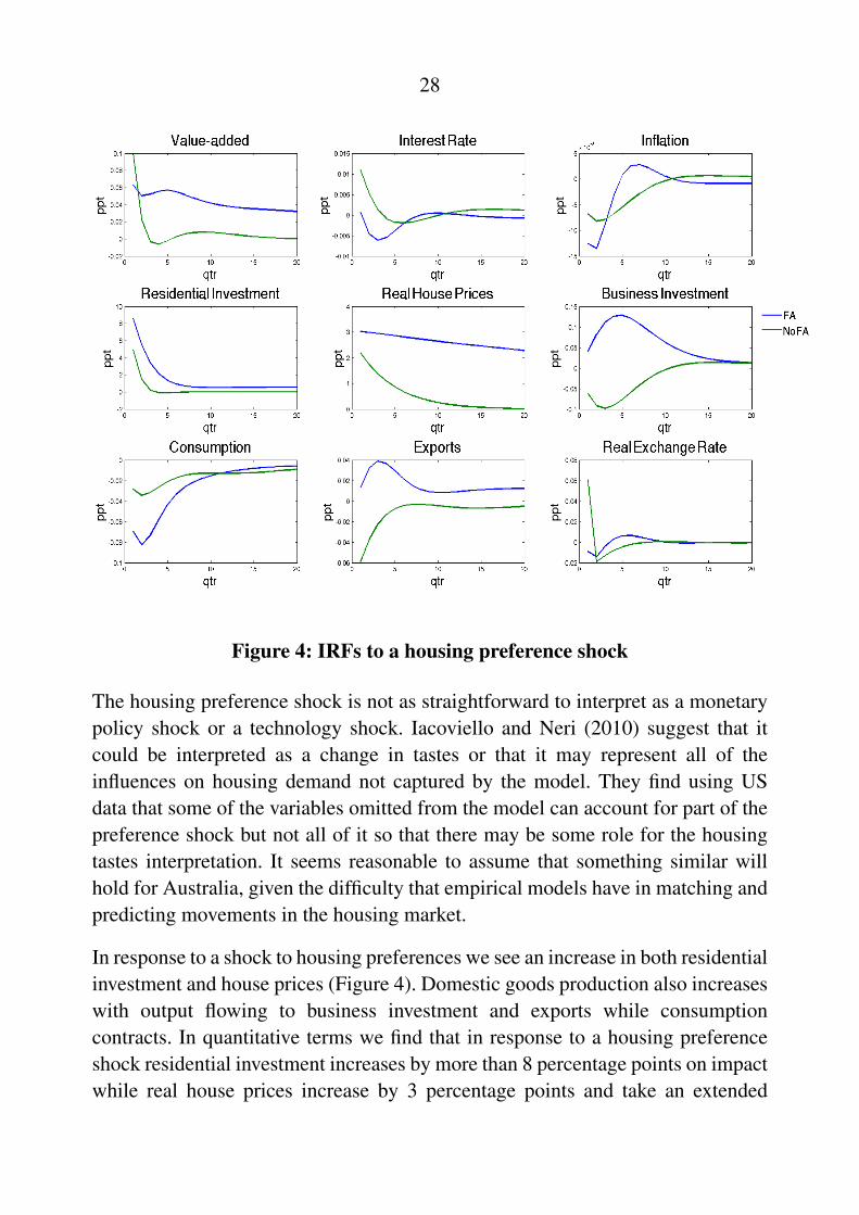
Figure 4: IRFs to a housing preference shock

The housing preference shock is not as straightforward to interpret as a monetarypolicy shock or a technology shock. Iacoviello and Neri (2010) suggest that itcould be interpreted as a change in tastes or that it may represent all of theinfluences on housing demand not captured by the model. They find using USdata that some of the variables omitted from the model can account for part of thepreference shock but not all of it so that there may be some role for the housingtastes interpretation. It seems reasonable to assume that something similar willhold for Australia, given the difficulty that empirical models have in matching andpredicting movements in the housing market.

In response to a shock to housing preferences we see an increase in both residentialinvestment and house prices (Figure 4). Domestic goods production also increaseswith output flowing to business investment and exports while consumptioncontracts. In quantitative terms we find that in response to a housing preferenceshock residential investment increases by more than 8 percentage points on impactwhile real house prices increase by 3 percentage points and take an extended

29

period of time to return to their baseline. The high degree of persistence in thehousing preference shock in large part explains these dynamics.

These results are sensitive to the value of the steady-state LVR, m, which can bethought of as a proxy for the intensity of the financial accelerator mechanism.In the full model we have set m equal to 0.6, however in the model comparisonsection we will investigate the impact of setting the steady-state LVR to a highervalue akin to that used by Iacoviello and Neri (2010) and find that it changes thesign of the consumption response to a shock to housing preferences and generatesthe comovement of consumption and house prices that has been found in existingAustralian empirical studies.

Figure 5: IRFs to a foreign risk premium shock

30

The risk premium shock is expected to result in a contraction in total output asthe higher cost of borrowing from abroad reduces funds available for investmentand lending to impatient households which in turn reduces the funds availablefor consumption and the purchase of housing. Instead we see an increase in goodsector output as labour flows out of housing production driven by a fall in demandas domestic credit flows decrease sharply, compounded by falling house priceswhich undermine households’ collateral holdings. Domestic inflation and interestrates both rise moderately on impact while the exchange rate depreciates andexports expand, gradually returning to steady state over an extended period.

Figure 6: Credit flows and the foreign risk premium shock

31

Focussing more directly on the credit channels in the model Figure 6 includesimpulse responses to a risk premium shock for net foreign assets, house pricesand domestic credit from the full model. It shows that the ratio of foreign lendingto domestic output (the net foreign asset ratio) increases on impact as domesticborrowing by the external sector becomes cheaper. Since in a net sense patienthouseholds are lending abroad there is less funding available for domestic lendingand this is reflected in the decline in domestic credit. The decline in domesticlending is amplified when the steady-state LVR is set a higher level but it has littleimpact on foreign lending or house prices.

5.2.1 Model Comparison

In analysing the properties of the full model we find that the dynamics ofresidential investment are largely governed by the sector-specific shocks with theinfluence of shocks to the wider economy on the housing sector via labour andgood market linkages more muted. This means that for this parameterisation thedirect spill-overs from the housing sector to the rest of the economy are limited.However, the indirect impact of the inclusion of housing in the model can onlybe assessed in comparison with a baseline model with no financial acceleratormechanism. In order to investigate the importance of the financial acceleratormechanism we estimated a model that includes housing but which has a singlerepresentative consumer and no credit flows.

The effect of a domestic monetary policy shock is amplified on impact forall variables in the model and for most of the key variables it is also morepersistent. Residential and real house prices both fall almost four times furtherin the model with credit while the response on impact of consumption is almostten times as large. The dynamics of the responses are also substantially differentfor many of the key variables. In the model without the financial accelerator thevariables respond on impact before tracing a smooth path back to the steady state.In the model with the financial accelerator the response is hump-shaped oftenovershooting the steady state level before falling back. This response pattern issensitive to the labour market structure in the model. Experiments with a lowfrequency of wage adjustment resulted in dynamics more similar to the modelwithout credit although the response on impact remained amplified.

32

Figure 7: IRFs to a housing preference shock with a varied LVR

The difference in the model dynamics in response to a housing preference shockis one of the most interesting results from the model. Comparing the impulseresponses from the full model with the baseline we see sharp differences invalue-added, business investment and exports while the decline in consumptionis more pronounced in the model with the financial accelerator. However, aspreviously stated the dynamics are sensitive to the value of the steady-state LVR.Figure 7 illustrates the impact of a change in the steady-state LVR to the highervalue used by Iacoviello and Neri (2010), 0.9, which increases the degree ofleverage households can attain in the steady state. When m is set at the higherlevel the rise in house prices that accompanies a housing preference shock isaccompanied by an increase in consumption, the opposite reaction to the lower-LVR and baseline cases. In addition many of the other variables are more volatile.The sign of the response of business investment and exports on impact changes asthey fall to accommodate the increase in domestic consumption, while domesticgood production, interest rates and inflation all increase sharply on impact. In the

33

model without credit consumption falls in response to a housing demand shock ashouseholds reduce consumption in order to fund their purchases of housing. Thenegative response of consumption also means that business investment and exportscontract less in the initial periods in the no credit model and actually rise abovetheir steady state level in later periods.

The response to the two technology shocks presents another interestingdivergence. While the response of key variables to the aggregate technology shockis similar in the full model and the baseline, in terms of the magnitude of theresponse on impact and the dynamics, the presence of the financial acceleratormechanism actually attenuates the response of most of the key variables to ahousing specific technology shock. Value-added rises less sharply in the modelwith the financial accelerator driven by a larger fall in goods output. This maybe due to the increase in residential investment (which is similar in both models),which positively influences households collateral and partially counters the initialnegative influence of house prices on access to credit. This diminishes theinfluence of the dynamic multiplier so that house prices fall less in the model withthe financial accelerator. 10 Impatient households therefore have more to spend onconsumption so that in aggregate consumption is stronger in the model with thefinancial accelerator.

5.3 Forecast-Error Variance Decomposition

Table 5: Forecast-Error Variance Decompositions for Full Model

Monetary Policy Technology Housing Cost push Foreign1Q 8Q 1Q 8Q 1Q 8Q 1Q 8Q 1Q 8Q

Value-added 5 2 17 38 1 1 28 23 25 8Consumption 6 3 1 2 1 1 7 7 1 1House prices 2 0 1 0 77 85 18 12 2 2Credit 2 1 0 0 93 97 45 65 4 9Residential 1 1 12 12 79 78 5 2 0 0investment

Forecast error variance decompositions are another way to examine the shocks thatare driving the variables in the model. A decomposition of the full model delivers

10 The fact that debt is nominal in the model may also play a role here, see Iacoviello (2005) forfurther discussion of the effect of the financial accelerator on supply versus demand shocks

34

results that are consistent with the impulse response analysis in suggesting thatoutcomes in the housing sector are mostly driven by sector specific shocks, whileat this calibration the housing specific shocks have little influence on the broadereconomy. Table 5 groups the shocks into four categories where the monetarypolicy shock and the technology shocks are simply the relevant individual shocks,housing shocks consist of the housing specific technology shock, the housingpreference shock and the LVR shock and the foreign shocks are those from theforeign VAR plus the risk premium shock. The cost-push shock combines theimpact of shocks to prices of domestic and imported goods. Results for one andeight quarter horizons are shown. It is worth noting that even with a fairly broaddefinition of foreign shocks they have a limited effect on the domestic economy afinding that is consistent with Justiniano and Preston (2010).

Table 6: Forecast-Error Variance Decompositions for Model with High LVR

Monetary Policy Technology Housing Cost push Foreign1Q 8Q 1Q 8Q 1Q 8Q 1Q 8Q 1Q 8Q

Value-added 7 3 10 32 31 13 22 22 14 6Consumption 6 4 0 2 55 22 6 52 3 7House prices 1 0 13 13 79 78 17 6 1 1Credit 1 0 1 0 79 98 25 11 2 2Residential 1 1 0 0 95 96 3 2 1 0investment

Table 6 shows decompositions from a re-estimated version of the model with thesteady-state LVR set at a higher level, 0.9. The key difference is the importance ofthe housing shocks as explanators of consumption in the model particularly at theshort horizon. Results from a quarter ahead decomposition suggest that housingshocks (and the finer detail shows that it is mostly the housing preference shock)account for more than half of the variation in consumption. The strong evidenceof spill-overs from the housing sector to consumption in this model is consistentwith the results from the impulse response analysis which showed evidence ofcomovement in consumption and house prices. By the eight quarter horizon theforeign shocks are the most prominent driver of consumption. However, shocksfrom the housing sector remain important and continue to explain around 20 percent of the variation in consumption.

35

Figure 8: Drivers of housing investment over time

5.4 Historical Decompositions

In general we find that the shocks that are specific to the housing sector,particularly the housing preference shock and the housing sector specifictechnology shock, account for most of the movement in the housing sectorvariables in the model. Historical shock decompositions, which describe thevariation of key variables in the model over time in terms of the structural shocks,support these findings and seem to confirm that the measures employed to furtherintegrate the housing sector into the broader economy, via the labour marketand the inclusion of intermediate goods in housing production, do not seem tostrengthen the influence of external shocks.

The housing preference shock in particular tends to dominate as the driver ofhousing market variables as can bee seen in each of the decompositions displayedin this section. In fact the housing preference shock has such a strong influence thata similarly strong shock of opposing effect is required to match the observed data

36

series. In the case of residential investment over the sample period the housingpreference is consistently matched by an offsetting housing specific technologyshock this obscures the meaning of the technology shock (Figure 8).

Figure 9: Drivers of credit over time

37

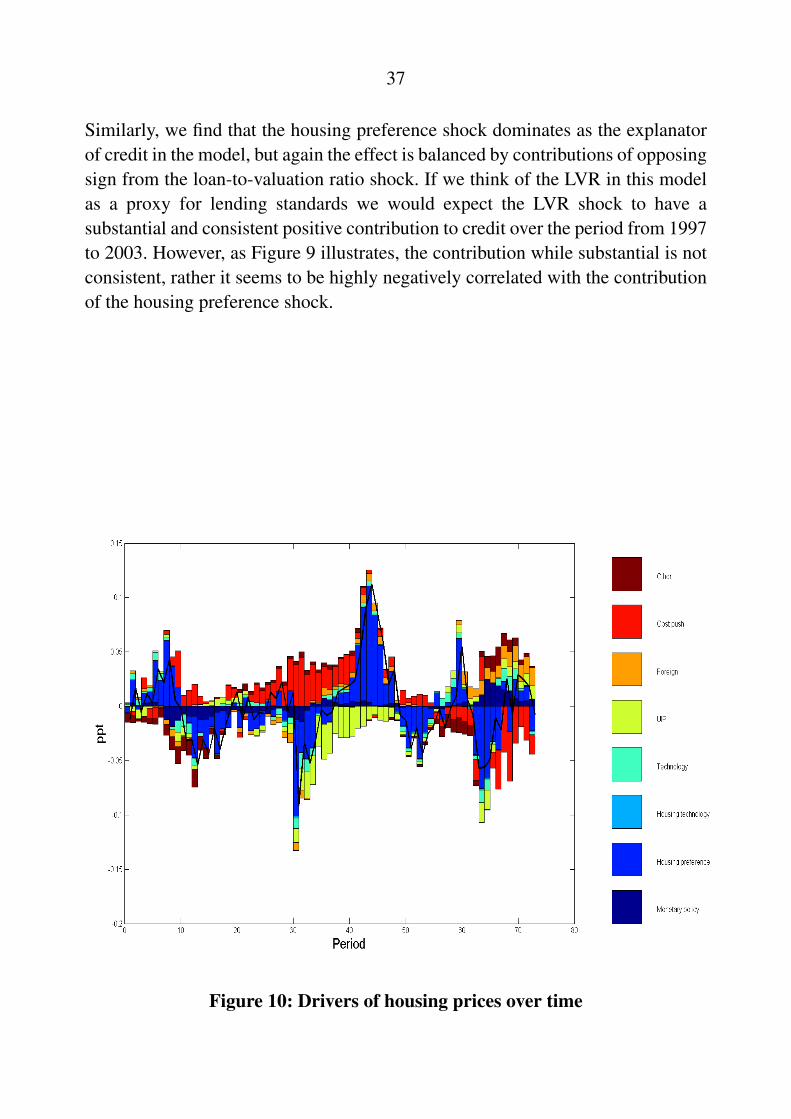
Similarly, we find that the housing preference shock dominates as the explanatorof credit in the model, but again the effect is balanced by contributions of opposingsign from the loan-to-valuation ratio shock. If we think of the LVR in this modelas a proxy for lending standards we would expect the LVR shock to have asubstantial and consistent positive contribution to credit over the period from 1997to 2003. However, as Figure 9 illustrates, the contribution while substantial is notconsistent, rather it seems to be highly negatively correlated with the contributionof the housing preference shock.

Figure 10: Drivers of housing prices over time

38

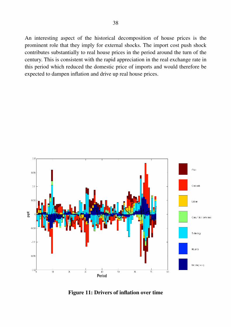
An interesting aspect of the historical decomposition of house prices is theprominent role that they imply for external shocks. The import cost push shockcontributes substantially to real house prices in the period around the turn of thecentury. This is consistent with the rapid appreciation in the real exchange rate inthis period which reduced the domestic price of imports and would therefore beexpected to dampen inflation and drive up real house prices.

Figure 11: Drivers of inflation over time

39

The decompositions for the key macroeconomic indicator variables - value-added,inflation, interest rates - are largely as expected. Inflation (see Figure 11) isprimarily driven by the cost push shocks to domestic good and import prices,with monetary policy also playing a role. Domestic interest rates and value addedare driven by a broader range of shocks although the strongest contributors arethe cost-push shocks, the aggregate technology shock and the housing preferenceshock.

5.5 Growth Cycle Properties

To examine how the inclusion of housing production and the financial acceleratormechanism influence the business cycles properties of the model we use theapproach outlined in Pagan and Robinson (2011). Specifically we simulate datafrom the full model and from the baseline model without the financial acceleratorand apply the Bry-Boschan Quarterly (BBQ) cycle-dating procedure due toHarding and Pagan (2002) to the simulated data. Because the data that enter themodel are filtered the results describe the properties of the growth cycle and aremore symmetrical than if the exercise were conducted on unfiltered levels databecause the positive growth trend over the long-run has been filtered out, and it isthis which creates much of the asymmetry typically evident in business cycles.

Table 7: Growth Cycle Characteristics

Data Full model Baseline model1993-2011 1960-2011 Low-LVR High-LVR

Durations (qtrs)Expansions 4.0 9.5 5.2 5.0 5.4Contractions 4.4 5.9 5.5 5.1 5.5Amplitude (%)Expansions 2.0 3.3 4.1 4.6 2.7Contractions -2.0 -3.6 -4.1 -4.6 -2.7Cumulative amplitude (%)Expansions 5.8 22.3 14.6 15.4 9.7Contractions -4.7 -12.1 -15.1 -15.3 -10.1

The results in Table 7 show that the model with the financial accelerator andthe baseline model produce similar estimates for the average duration of cycles,slightly higher than the duration found in the data. The simulated data fromthe baseline model are a better match to the amplitude of cycles than the full

40

model with the amplitude implied by the full model more than twice that foundin the data. These results contrast with those of a similar exercise conducted byPagan and Robinson (2011) with the model developed in Iacoviello (2005). Paganand Robinson (2011) find that the amplitude of cycles in data simulated fromIacoviello (2005) are significantly smaller than the amplitudes observed in thedata.

When cycle-dating was employed on simulated data from a version of the modelthat was estimated with the steady-state LVR set at a higher value than we use inthe initial estimation of the full model (and closer to the value used by Iacovielloand Neri (2010)), we found that it made little difference to the implied durationof cycles but that the implied cycle amplitudes were marginally further from theamplitudes found in the data than those from the full model with a lower LVR.This is surprising given that Pagan and Robinson (2011) find that increasing theLVR increases the absolute average amplitude of the growth cycle markedly in theIacoviello (2005) model, although the relationship appeared to be non-linear.

The implications of the cycle-dating exercise for the models ability to match theproperties of the underlying data are sensitive to the choice of sample. Thusfar we have focused on the comparisons with the properties of the data from1993-2011, the estimation sample. However, it may be argued that as this sampledoes not include a major business cycle contraction despite our focus on growthcycles it may be better to apply the cycle-dating procedure to a longer sample ofdata. Applying the procedure to data for the period 1960-2011 we find that theproperties of the data lie somewhere between the model including the financialaccelerator and the baseline. While the differences between the data and the cycle-dating results for the average duration of expansions and contractions are similar,the amplitude of cycles in the data is lower than that implied by the model withthe financial accelerator and higher than that in the baseline model.

5.6 Robustness

The results described above are mostly robust to a plausible range of values forthe parameters that we have calibrated or set. Simulating the model with a lowerwage share of patient households, µ , increases the sensitivity of key variables tomost shocks. This is not surprising given that the financial accelerator affect willbe stronger when more households are liquidity constrained. Decreasing the value

41

of g , which increases the degree of openness of the model, increases the sensitivityto external shocks without altering the responses to domestic shocks substantially.Altering the Frisch elasticity of labour supply or the degree of intersectoral labourmobility both have implications for the response to a housing sector specifictechnology shock, with lower labour mobility and greater sensitivity to changesin the real wage increasing the magnitude of the response to the sector specifictech shock. However, because the housing sector is small and the magnitude ofthe differences for the range of values are also small and have a negligible effecton aggregate activity.

The key exception to the general robustness of the model is its sensitivity tothe steady-state LVR parameter m, which, as previously discussed, when variedcan have a substantial impact on the dynamics of several of the key variablesin response to a shock to housing preferences. In the initial version of the fullmodel we set m to 0.6 a value more in line with available estimates for all loans inAustralia over the sample period (Ellis 2006), than that used by Iacoviello andNeri (2010). Alternatively, when a higher value of m closer to the value usedby Iacoviello and Neri (2010) is used in estimating the model we find, mostnotably, that the consumption and house prices both increase in response to apositive housing preference shock. Other than altering the response to a housingpreference shock altering m has little influence on the results. This finding iscommon to models that employ a similar underlying structure incorporating thefinancial accelerator mechanism (see Iacoviello (2005), Iacoviello and Neri (2010)and Chistensen et al (2009)) regardless of whether the model is open or closed, orwhether the supply of housing is fixed or flexible, although as previously discussedPagan and Robinson (2011) did find that it considerably altered the growth cyclecharacteristics.

The inclusion of wage rigidities was found to be important in generating plausibleimpulse responses to a monetary policy shock. In the absence of wage rigiditiesresidential investment increases in response to a monetary policy shock, clearlyat odds with the negative correlation of residential investment activity and thecash rate that is found in the data (Berger-Thomson and Ellis 2004). In additionsubstantial wage rigidity (a high q

d) was required to match the contraction ofbusiness investment found in the data in response to a monetary policy shock.

42

6. Conclusion

Estimating a model that includes housing and credit flows we are able to generateplausible parameter estimates and model dynamics. We find that fluctuations inthe housing market are mostly driven by the sector specific shocks but that thehousing sector specific shocks have little influence on developments outside thehousing sector. We are able to replicate the comovement of consumption and houseprices in response to a housing preference shock that is found in studies usingUS data. However, this requires a high steady-state LVR that is not supportedin the data for Australia. When the steady-state LVR is set at a lower level theevidence of consumption wealth effects from housing is not present, neverthelessthe inclusion of the financial accelerator mechanism does alter the model dynamicswith results from a cycle-dating exercise suggesting that the strength of thefinancial accelerator mechanism has surprisingly little influence on the modelsability to match the growth cycle properties of the data.

There are a numbers of ways that this model could be improved and augmented.The first and most obvious is the use of model consistent detrending whichwould allow us to address the role of population as well as sectoral productivitydifferentials. The treatment of land is simple in this model, while in the Australianhousing market fluctuations in land prices are likely to explain a substantial portionof the variation in house prices especially in major markets such as Sydney andMelbourne. Another inclusion that would likely help in fitting the data from thecredit and housing markets is the addition of a banking sector. One possibility isto extend the model along the lines of Gerali, Neri, Sessa and Signoretti (2010) Inaddition to allowing us to take the role of credit provider away from the patienthouseholds helping to resolve the conceptual issues encountered in mappingcredit data to the model, it would also allow us to further pursue questionsabout international funding of financial institutions that have only been brieflytouched on in this paper. Such a framework may also be appealing in investigatingthe interplay of household borrowing, house prices and the financial stability offinancial intermediaries.

43

Appendix A

The Log-Linearised Model

Households

Patient households

Labour supply

el1,t = ect +x

eld1,t +(y �x )el1,t � ew

d ⇤1,t (29)

el1,t = ect +x

elh1,t +(y �x )el1,t � ew

h ⇤1,t (30)

Labour market clearing

el1,t = eld1,t

✓Ld

1L1

◆1+x

+elh1,t

✓Lh

1L1

◆1+x

(31)

Consumption

el1,t = ekt �

11�W

�ec1,t �Wec1,t�1

�(32)

Money demand

el1,t = b1Et

hel1,t+1 � ept+1

i� (1�b1)+ em1,t (33)

Borrowing

el1,t = Et

hel1,t+1 � ept+1

i� eRt (34)

44

Tobin’s Q for physical capital

eqt = b1Et [eqt+1(1�d )+erkt+1rk]� (eRt �Et [ep

ht+1]) (35)

Physical capital investment optimality condition

eit =1

(1+b1)

✓1

S00(1)

✓eqt + e

it

◆+b1Et [eit+1]+eit�1

◆(36)

Tobin’s Q for housing capital

eqkht = (1�b1(1�d

kh))(erht+1 � et

ht + ept+1)+b1(1�d

kh)(eqkht + eph

t+1)� eRt (37)

Housing capital investment optimality condition

eiht =1

(1+b1)

✓1

Sh00(1)eqkh

t +b1Et [eiht+1]+ei

ht�1

◆(38)

Housing optimality condition

el1,t = (1�b1 ⇤ (1�d

h))(ejt �eh1,t)+b1(1�d

h)(Et [el1,t+1 + eq

ht+1 � eq

ht ]) (39)

Housing investment law of motion

eh1,t = d

heih1,t +(1�d

h)eh1,t�1 (40)

Impatient households

Labour supply

45

el2,t = ect +x

eld2,t +(y �x )el2,t � ew

d ⇤2,t (41)

el2,t = ect +x

elh2,t +(y �x )el2,t � ew

h ⇤2,t (42)

Labour market clearing

el2,t = eld2,t

✓Ld

2L2

◆1+x

+elh2,t

✓Lh

2L2

◆1+x

(43)

Consumption

el2,t = ekt �

11�W

�ec2,t �Wec2,t�1

�(44)

Money demand

el2,t = b2Et

hel2,t+1 � ept+1

i� (1�b2)+ em2,t (45)

Borrowing

el2,t =

b2b1

Et

hel2,t+1 � ept+1

i+ eRt +

(b1 �b2)

b2b1(el2,2t + eRt) (46)

Housing optimality condition

el2,t = (1�b2(1�d

h)+ m(b1 �b2))(ejt �eh2,t)+b2(1�d

h)Et [el2,t+1 + eq

ht+1]

+ m(b1 �b2)(el2,2t + emt +Et [ept+1 + eq

ht+1])� eq

ht (47)

46

Housing investment law of motion

eh2,t = d

heih2,t +(1�d

h)eh2,t�1 (48)

Net worth

eb2,tb2Y

= ec2,tC2Y

+qhH2

Y(d heqh+eh2,t �(1�d

h)eh2,t�1)+1b1

b2Y(eRt�1+eb2,t�1� ept)�

(ewd2,t +el

d2,t)

wd2Ld

2Y

� (ewh2,t +el

h2,t)

wh2Lh

2Y

� et lt

t

Y(49)

Aggregate households

Consumption aggregator

ect = hec1,tC1C

+(1�h)ec2,tC2C

(50)

Housing market clearing

eht = h

eh1,tH1H

+(1�h)eh2,tH2H

(51)

Housing investment aggregator

eht = d

heiht +(1�d

h)eht�1 (52)

Demand for domestic consumption goods

echt = ect �s

et

ht (53)

47

Demand for imported consumption goods

ecmt = ect �s

et

mt (54)

Constraints

Borrowing constraint

eb2,t = emt +eh2,t +Et [eqht+1 + ept+1]� eRt (55)

Physical Capital law of motion

ekt = (1�d )ekt�1 +d lne

it +d

eit (56)

Housing Capital law of motion

ekht = (1�d

kh)ekht�1 +d

kheiht (57)

Foreign sector

Uncovered interest parity

⇣eRt �pt+1

⌘�⇣eR f

t �p

ft+1

⌘= Et [rert+1]� rert � eatj + ex b

t (58)

Current account

a✓eat �

1b1

⇣eR f

t�1 � epf

t + eat�1 +ex

bt � epd

t + ept ��eyt �eyt�1

�+�frert �frert�1

�⌘◆

= (ext �eyt)XY� 1

t

hCm

Y(et f

t +ecmt ) (59)

48

Export demand

ext = l

f et

ft +ey f

t (60)

Domestic intermediate goods producers

Demand for Capital

ekt�1 = eWt �erkt +eyt (61)

Demand for labour from patient households

eld1,t = eWt +eyt + et

ht � ew

d1,t (62)

Demand for labour from impatient households

eld2,t = eWt +eyt + et

ht � ew

d2,t (63)

Real marginal costs

eWt = aerkt +µ(1�a)ewd

1,t +(1�µ)(1�a)ewd2,t �ezt � (1�a)eth

t (64)

Housing producers

Demand for housing capital

ekht�1 = eq

ht + eiht �er

ht (65)

Demand for patient household labour

49

elh1,t = eq

ht + eiht � ew

h1,t (66)

Demand for impatient households labour

elh2,t = eq

ht + eiht � ew

h2,t (67)

Return on land

et

lt = eq

ht + eiht (68)

Demand for intermediate goods

eyht = eq

ht + eiht � et

ht (69)

Production function

eiht = ezt +ezht +qh

ekht�1 +q

yeyht +(1�q

h �q

l �q

y)(nelh1,t +(1�n)elh

2,t) (70)

Prices

Goods Phillips curve

ep

ht = µ f ep

ht+1 +µbep

ht�1 +µ

mceWt +elt (71)

Wage Phillips curves

ep

w d1,t = µ

df 1ep

w d1,t+1 +µ

db 1ep

w d1,t�1 +µ

mc d1 ewd

1,t (72)

50

ep

w h1,t = µ

hf 1ep

w h1,t+1 +µ

hb 1ep

w h1,t�1 +µ

mc h1 ewh

1,t (73)

ep

w d2,t = µ

df 2ep

w d2,t+1 +µ

db 2ep

w d2,t�1 +µ

mc d2 ewd

2,t (74)

ep

w h2,t = µ

hf 2ep

w h2,t+1 +µ

hb 2ep

w h2,t�1 +µ

mc h2 ewh

2,t (75)

Import Phillips curve

ep

mt = µ

mf ep

mt+1 +µ

mb ep

mt�1 +µ

m mceWmt +el m

t (76)

Importers marginal costs

eWmt = frert � et

mt (77)

Aggregate price index (in changes)

ept = g

ep

ht +(1� g)epm

t (78)

Relative price of aggregate domestic good to aggregate consumption good

et

ht = eph

t � ept + etht�1 (79)

Relative price of aggregate import good to aggregate consumption good

et

mt = epm

t + etmt�1 � ept (80)

Relative price of domestic good faced by the foreign sector, to foreign prices

51

et

ft = frert � et

ht (81)

Wage maps

ewd ⇤1,t = ewd

1,t � eXd1,t (82)

ewh ⇤1,t = ewh

1,t � eXh1,t (83)

ewd ⇤2,t = ewd

2,t � eXd2,t (84)

ewh ⇤2,t = ewh

2,t � eXh2,t (85)

Monetary Policy

Taylor rule

eRt = z

ReRt�1 +(1�z

R)(z p ept +z

va evat +z

gr � evat � evat�1�+ et) (86)

Aggregate transfers

et⇤t = M✓ect � (h em1,t�1 +(1�h)em2,t�1)� ekt � eRt

b11�b1

◆(87)

Goods market clearing condition

eyt = echtCh

Y+eit

IY+eiht

Ih

Y+ext

XY+eyh

tY h

Y(88)

52

Total value added

eva = (eyt + etht )

Y t

h

VA� (eyh

t + etht )

Y ht

h

VA+(eqh

t + eiht)qh ¯IHVA

(89)

Shock processes

ezt = r

zezt�1 + e

z (90)

ezht = r

zhezht�1 + e

zh (91)

ect = r

c ect�1 + e

c (92)

er ft = r

R fer f

t�1 + e

R f(93)

ex

bt = r

x

bex

bt�1 + e

x

b(94)

ee

it = r

e

iee

it�1 + e

e

i(95)

ep

ft = r

p

fep

ft�1 + e

p

f(96)

ey ft = r

y fey f

t�1 + e

y f(97)

ejt = r

jejt�1 + e

j (98)

53

emt = r

m emt�1 + e

m (99)

ekt = r

kekt�1 + e

k (100)

elt = e

l (101)

el

mt = e

l

m(102)

54

Appendix B

The Steady State

Constants

rk =1b1

� (1�d ) (103)

rh = (1b1

� (1�d

kh))th (104)

mc =l �1

l

(105)

Xm =l

m

l

m �1(106)

Xw d1 =

l

w d1

l

w d1 �1

(107)

Xw h1 =

l

w h1

l

w h1 �1

(108)

Xw d2 =

l

w d2

l

w d2 �1

(109)

Xw h2 =

l

w h2

l

w h2 �1

(110)

55

t

h =

"1� (1� g)Xm 1�s

g

# 11�s

(111)

t

m = Xm (112)

Pm = (1� g)(Xm �1)Xm �s (113)

k1 =J

1�b1(1�d

h)(114)

k2 =J

1�b2(1�d

h)� m(b1 �b2)(115)

k3 =1

1+(1�b1)mk2(116)

z1 = h(1+k1d

h(1+q

h(d

kh

rh t

h �1)� (1�q

h �q

l �q

y)n �hq

l)

� (1� g)(Xm �1)Xm �s ) (117)

z2 = (1�h)(k2d

h(q h(d

kh

rh t

h �1)� m(1�b1)

d

h � (1�q

h �q

l �q

y)n �hq

l)

� (1� g)(Xm �1)Xm �s ) (118)

z3 = t

h(1� mc(da

rk +(1�µ)(1�a))) (119)

56

z4 = hk1d

h((n �1)(1�q

h �q

l �q

y)� (1�h)q l) (120)

z5 = (1�h)(1+k2d

h(1+m(1�b1)

d

h � (1�n)(1�q

h �q

l �q

y)� (1�h)q l))

(121)

z6 = mc(1�µ)(1�a)th (122)

Steady state ratios

K = a

mc

rk Y (123)

Kh =q

hd

h

rh qhH (124)

L⇤ =q

ld

h

t

l qhH (125)

L⇤ = 1 (126)

Y h

Y=

q

yd

h

t

h qhH (127)

IY= d

KY

(128)

57

Ih

Y= d

kh Kh

Y(129)

CY=

1�d

KY �d

kh Kh

Y � Y h

YCh

C + 1t

hCm

C

(130)

XY

=1t

hCm

Y(131)

Cm

C= (1� g)Xm �s (132)

Ch

C= gt

h �s (133)

wd1Ld D

1 = µ(1�a)mcY t

h (134)

wd2Ld D

2 = (1�µ)(1�a)mcY t

h (135)

wh1Lh D

1 = n(1�q

h �q

l �q

y)d hqhH (136)

wh2Lh D

2 = (1�n)(1�q

h �q

l �q

y)d hqhH (137)

C2Y

=z6z1 �z4z3z5z1 �z2z4

(138)

58

C1Y

=z3z5 �z6z2z1z5 �z4z2

(139)

C1C

=C1Y

YC

(140)

C2C

=C2Y

YC

(141)

qhH1Y

= k1C1Y

(142)

qhH2Y

= k2C2Y

(143)

qhHY

= h

qhH1Y

+(1�h)qhH2

Y(144)

H1H

=qhH1

YY

qhH(145)

H2H

=qhH2

YY

qhH(146)

b2Y

= b1mqhH2

Y(147)

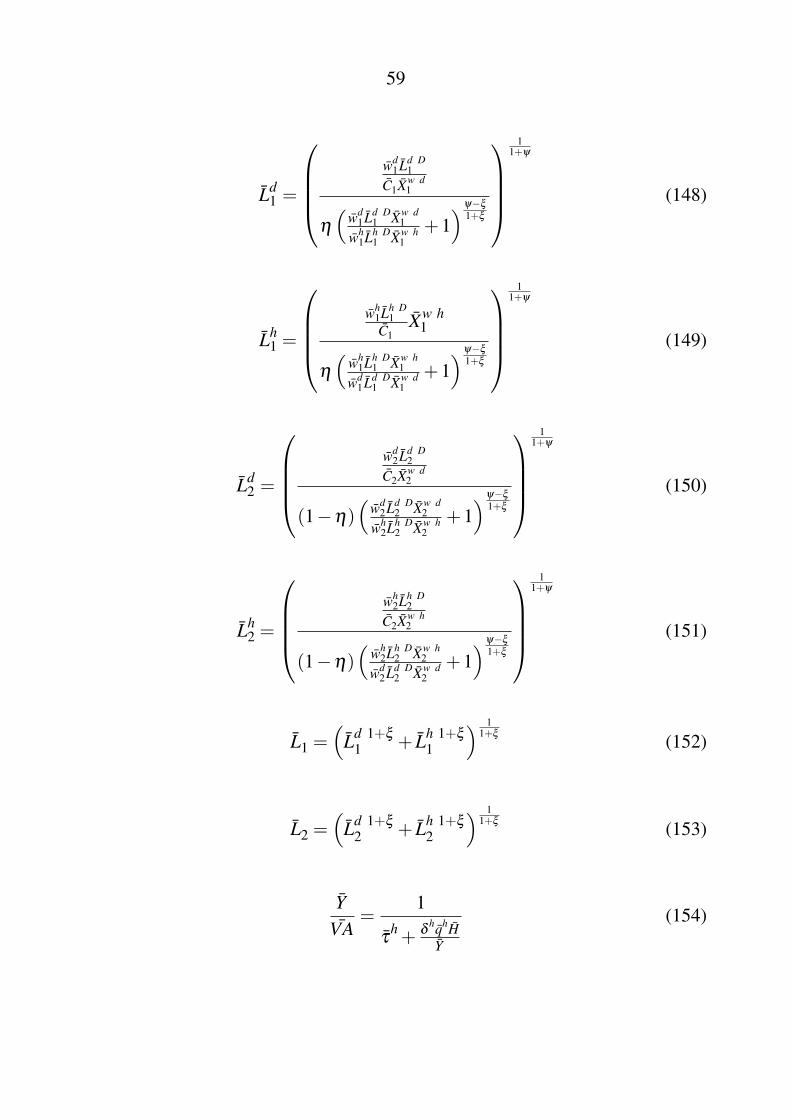
59

Ld1 =

0

BBB@

wd1 Ld D

1C1Xw d

1

h

⇣wd

1 Ld D1 Xw d

1wh

1Lh D1 Xw h

1+1⌘y�x

1+x

1

CCCA

11+y

(148)

Lh1 =

0

BBB@

wh1Lh D

1C1

Xw h1

h

⇣wh

1Lh D1 Xw h

1wd

1 Ld D1 Xw d

1+1⌘y�x

1+x

1

CCCA

11+y

(149)

Ld2 =

0

BBB@

wd2 Ld D

2C2Xw d

2

(1�h)⇣

wd2 Ld D

2 Xw d2

wh2Lh D

2 Xw h2

+1⌘y�x

1+x

1

CCCA

11+y

(150)

Lh2 =

0

BBB@

wh2Lh D

2C2Xw h

2

(1�h)⇣

wh2Lh D

2 Xw h2

wd2 Ld D

2 Xw d2

+1⌘y�x

1+x

1

CCCA

11+y

(151)

L1 =⇣

Ld 1+x

1 + Lh 1+x

1

⌘ 11+x (152)

L2 =⇣

Ld 1+x

2 + Lh 1+x

2

⌘ 11+x (153)

YVA

=1

t

h + d

hqhHY

(154)

60

qh ¯IHVA

= 1� YVA

t

h (155)

t l = t

l (156)

MY

= h

11�b1

C1Y

+(1�h)1

1�b2

C2Y

(157)

Y =

✓KY

◆ a

1�a

Lµ

1 L1�µ

2 (158)

61

References

Adolfson M, S Laseen, J Linde and M Villani (2007), ‘Bayesian estimationof an open economy DSGE model with incomplete pass-through’, Journal ofInternational Economics, 72, pp 481–511.

Aoki K, J Proudman and G Vlieghe (2004), ‘House Prices, Consumption,and Monetary Policy: A Financial Accelerator Approach’, Journal of FinancialIntermediation, 13, pp 414–435.

Australian Bureau of Statistics (2006), Census of Population and Housing.

Bao Y, G Lim and S Li (2009), ‘A Small Open Economy Model with a HousingSector’, Australian Conference of Economists, .

Benanke B, M Gertler and S Gilchrist (1999), ‘The Financial Accelerator in aQuantitative Business Cycle Framework’, Handbook of Monetary Economics, 1,pp 1341–1393.

Benigno G and C Thoenissen (2008), ‘Consumption and real exchange rates withincomplete markets and non-traded goods’, Journal of International Money andFinance, 27, pp 926–948.

Berger-Thomson L and L Ellis (2004), ‘Housing Construction Cycles andInterest Rates’, Reserve Bank of Australia Research Discussion Paper, 2004-08.

Bernanke B (2010), ‘Statement before the Financial Crisis Inquiry Commission’.

Bils M and P Klenow (2004), ‘Some Evidence on the Importance of PriceStickiness’, Journal of Political Economy, 112, pp 947–985.

Cagliarini A, T Robinson and A Tran (2011), ‘Reconciling Microeconomic andMacroeconomic Estimates of Price Stickiness’, Journal of Macroeconomics, 33,pp 102–120.

Case C, J Quigley and R Shiller (2011), ‘Wealth Effects Revisited 1978-2009’,NBER Working Paper, 16848.

Chistensen I, P Corrigan, C Mendicino and SI Nishiyama (2009),‘Consumption, Housing Collateral, and the Canadian Business Cycle’, Bank ofCanada Working Paper 2009-26, .

62

Christiano L, Eichenbaum and C Evans (2005), ‘Nominal Rigidities and theDynamic Effects of a Shock to Monetary Policy’, Journal of Political Economy,113, pp 1–45.

Davis M and J Heathcote (2005), ‘Housing and the Business Cycle’,International Economic Review, 46, pp 751–784.

Dvornak N and M Kohler (2007), ‘Housing Wealth, Stock Market Wealthand Consumption: A Panel Analysis for Australia’, The Economic Record, 83,pp 117–130.

Ellis L (2006), ‘Housing and Housing Finance: The View from Australia andBeyond’, Reserve Bank of Australia Research Discussion Paper, 2006-12.

Ellis L (2010), ‘The Housing Meltdown: Why Did it Happen in the United States’,International Real Estate Review, 13, pp 351 – 394.

Fisher L, G Otto and G Voss (2010), ‘The Response of Australian Consumptionto Housing Wealth’, Journal of Macroeconomics, 31, pp 284–299.

Gerali A, S Neri, L Sessa and F Signoretti (2010), ‘Credit and Banking ina DSGE Model of the Euro Area’, Journal of Money, Credit and Banking, 42,pp 107–141.

Harding D and A Pagan (2002), ‘Dissecting the Cycle: a MethodologicalInvestigation’, Journal of Monetary Economics, 49, pp 365–381.

Horvath M (2000), ‘Sectoral Shocks and Aggregate Fluctuations’, Journal ofMonetary Economics, 45, pp 69–106.

Iacoviello M (2005), ‘House Prices, Borrowing Constraints, and Monetary Policyin the Business Cycle’, American Economic Review, 95, pp 739–764.

Iacoviello M and S Neri (2010), ‘Housing Market Spillovers: Evidence froman Estimated DSGE Model’, American Economic Journal: Macroeconomics, 2,pp 125–164.

Jaaskela J and K Nimark (2011), ‘A Medum-Scale New Keynesian OpenEconomy Model of Australia’, The Economic Record, 87, pp 11–36.

63

Justiniano A and B Preston (2010), ‘Can Structural Small Open-EconomyModels Account for the Influence of Foreign Disturbances?’, Journal ofInternational Economics, 81, pp 61–74.

Kiyotaki N and J Moore (1997), ‘Credit Cycles’, Journal of Political Economy,105, pp 211–248.

Kollmann R (2002), ‘Monetary Policy Rules in the Open Economy: Effects onWelfare and Business Cycles’, Journal of Monetary Economics, 49, pp 989–1015.

Leamer E (2007), ‘Housing is the Business Cycle’, Proceedings Federal ReserveBank of Kansas City, pp 149–233.

Pagan A and T Robinson (2011), ‘Assessing Some Models of the Impact ofFinancial Stress upon Business Cycles’, Reserve Bank of Australia ResearchDiscussion Paper, .

Smets F and R Wouters (2007), ‘Shocks and Frictions in U.S. Business Cycles:A Bayesian DSGE Approach’, American Economic Review, 87, pp 586–606.

Tan A and G Voss (2003), ‘Consumption and Wealth in Australia’, The EconomicRecord, 79, pp 39–56.

Williams D (2010), ‘Consumption, Wealth and Credit Liberalisation in Australia’,Oxford University Economics Series Working Papers, 492.