Household Welfare from Disaggregate Demands

ESTIMATING HOUSEHOLD WELFARE FROM DISAGGREGATEEXPENDITURES

ETHAN LIGON

Abstract. Existing models of life-cycle demand typically assume that expenditure sharesfor particular goods within a period are fixed, but this is at sharply at odds with strongempirical evidence, including Engel’s Law. We show how one can exploit variation in thecomposition of expenditures to estimate demand systems that are flexible and may featurehighly non-linear Engel curves; this same procedure yields an index of household welfareclosely related to the marginal utility of expenditures within a period. We use these methodswith repeated cross-sectional expenditure surveys from Uganda to estimate an incompletedemand system and household welfare in different periods.

[email protected] of California

Berkeley, CA 94720–3310

. Date: September 14, 2018.

. Much of this paper came together during a sabbatical stay at the UCL, and so I’d like to particularlythank Orazio Attanasio, Richard Blundell and their colleagues for their hospitality and encouragement. Imust also thank Pascaline Dupas, Marcel Fafchamps, Laura Schechter, and Duncan Thomas for very helpfulcritical comments.

Measures of household or individual-level consumption expenditures are central to policy-relevant statistics such as poverty rates in most low income countries, and are also criticalinputs to a wide variety of important research questions in many fields of economics, partic-ularly in models involving risk, inequality, or life-cycle behavior (e.g., Angelucci and Giorgi2009; Lise and Yamada 2017).1 The household surveys used to collect these data almostinvariably record disaggregate expenditures; that is, expenditures on many different kindsof goods or services. However, empirical work employing these data to measure changes inhousehold welfare typically focuses on the sum of these disaggregate expenditures, dividedby a price index, or total real household consumption expenditures.2 Information on thecomposition of the household’s consumption portfolio is usually discarded. The questionof this paper: How can information on the composition of the consumption portfolio beexploited to measure households’ material well-being?

To answer this question we introduce two main innovations. The first is to devise a newincomplete demand system which allows for variation in both the scale and composition ofhouseholds’ consumption portfolios to flexibly arise from changes in prices or householdsbudgets. Second is to construct a simple estimator of this demand system which allows usto recover not only critical demand elasticities, but also household-specific latent variableswhich we show can be interpreted as the household-specific multipliers (λ) associated withhouseholds’ within-period budget constraints.

We call our new demand system the Constant Frisch Elasticity (CFE) demand system. Itis unique in that it is globally regular, has unrestricted rank (in the sense of Lewbel 1991),and can be shown to nest most of the theory-consistent demand systems in the empiricalliterature. We further devise a novel but simple method of estimation which exploits infor-mation in both the first and second moments of the distribution of log expenditures. Thesefeatures allow us to estimate the first example of a globally-regular demand system withunrestricted rank which can be used to measure consumer welfare even if expenditures ononly some goods and services are observed.

We next show how the demand system we derive can be estimated using one or more roundsof cross-sectional data on disaggregate household expenditures, in a specification involvinglogarithms of those disaggregate expenditures. This estimator delivers “Frisch elasticities”and estimates of the index λ of each household’s marginal utility of expenditures (MUE),along with estimates of the effects of various observable household characteristics on demand.Importantly, unobserved household characteristics are naturally introduced in such a waythat they do not bias estimates of the key demand elasticities.

1. See Attanasio and Pistaferri (2016) for a survey focused on the US case.2. For example, while Browning, Crossley, and Winter (2014) provides an excellent recent survey of

methods for measuring household consumption expenditures, the authors choose to focus exclusively ontotal household consumption expenditures.

1

Our estimator is implemented in two steps. The effects of prices and household charac-teristics on expenditures are obtained in a first seemingly-unrelated regression (SUR) step.A distinctive feature of our approach is that information regarding the composition of theconsumption portfolio is then obtained using a singular value decomposition of the matrixof residuals, yielding estimates of Frisch elasticities and λs.

We observed above that measures of consumption expenditures are critical inputs to mea-suring poverty, inequality, and risk. We use our methods to explore these aspects of welfareusing four rounds of data on household expenditures in Uganda, spanning the period of2006–2012. These data are instances of the World Bank’s Living Standards MeasurementSurveys (Deaton 1997), which have now been conducted in many countries across manyyears, but the Ugandan data have particular interest because they span a period which in-cludes the global “food price” crisis of 2008 during which the prices of important cerealsmore than doubled, as well as a “great recession” experienced by Uganda in 2010. Withnothing more more than cross-sectional variation in expenditures in these data, we’re ableto obtain estimates of both the parameters of the demand system and the households’ λs,and to measure the consequences of these shocks for rates of poverty, inequality, and riskaversion for differently situated households.

1. Related Literature

Our paper is related to several distinct threads of research, which we discuss in turn. Thefirst is a body of research which attempts to leverage “Engel’s Second Law” to obtain mea-sures of welfare from disaggregate expenditures. As the name suggests, the idea of measuringwelfare from disaggregate expenditures is as old as Engel (1857), but there’s been recent in-terest in using the details of household expenditures or Engel curves for particular goods toconstruct welfare-related measures. For example, Almas (2012) estimates Engel curves forfood from many different countries, and uses these results to correct bias in internationalPPP statistics and measures of cross-country inequality. In this paper we address a similarproblem using micro-data to measure inequality and correct CPI statistics in Uganda, butwithout adopting Almas’ assumption that there’s a fixed relationship between food shareand real income. Attanasio and Lechene (2014) estimate Engel curves for food using datafrom the Mexican Progresa experiment with the aim of testing the collective model of thehousehold (Bourguignon, Browning, and Chiappori 2009). They assume that utility fromfood is additively separable from leisure and other consumption, a set of assumptions slightlyweaker than those of Almas. Atkin et al. (2018) adopt a much weaker set of assumptionsregarding separability and use estimates of what they call “relative Engel” curves to measurechanges in welfare. But unlike our approach this requires the very strong assumption thatthere are no changes in relative prices which affect the slope of these curves; related, Almas,

2

Beatty, and Crossley (2018) impose structure associated with the AIDS demand system andimpose a sort of conditional separability. Finally, Young (2012) constructs a demand systemmeant to allow welfare comparisons across time for many different countries in Africa. Butthe actual goods used for estimation are mostly fairly fixed household assets and characteris-tics, and the demand system itself isn’t theory consistent. The relation between what we’recalling λ and consumer demand was first extensively considered by Ragnar Frisch (see esp.Frisch 1959, 1964, 1978), but wasn’t developed empirically until demand systems which de-pend on prices and marginal utility were revived by Heckman and MaCurdy in the seventies.This empirical development allowed econometricians to deal with the difficulties of measur-ing permanent income in the context of life-cycle models (Heckman 1974, 1976; Heckmanand MaCurdy 1980; MaCurdy 1981). This was pioneering, but central to identification inthese early applications was the assumption that markets were complete so that risk-aversehouseholds could completely eliminate idiosyncratic risk. These papers also imposed muchmore structure on within-period demands than is necessary, requiring that all consumptiongoods have identical income and price elasticities, and featured demand systems which im-plicitly violated the symmetry characteristic of regular demands.3 Nevertheless, the payofffrom these assumptions was significant—by assuming a particular cardinalization of homo-thetic preference structures and constant MUEs it was possible to estimate these as fixedeffects in a linear panel regression. A later generation of life-cycle models relaxed the as-sumption of full insurance, and made the idiosyncratic risk borne by households a focus ofthe analysis. One early example is Browning et al. (1994), which replaces the assumption ofperfect insurance markets with an assumption of perfect credit markets and cleverly achievesidentification of changes in households’ log λ with a cardinalization and an assumption thatthese changes are normally distributed. A second important collection of papers replacesthe goal of estimating models featuring homothetic utility and full insurance with the aim oftesting for full insurance (Mace 1991; Deaton 1992; Cochrane 1991; Townsend 1994). Morerecent examples connect risk in labor earnings with persistence in consumption to the evo-lution of inequality (Low, Meghir, and Pistaferri 2010; Lise 2012; Blundell, Pistaferri, andSaporta-Eksten 2016; Arellano, Blundell, and Bonhomme 2017). The focus of all of thesepapers remains on highly aggregate forms of consumption and leisure; none of these exploitwithin-period consumer choices among disaggregate consumption goods, as in the presentpaper. The life-cycle models described so far use variation over both time and householdsto simultaneously estimate within-period demands and the the dynamic elements of model.

3. Somewhat later demands which depended on prices and λ were given the moniker “Frisch demands” byMartin Browning (Browning, Deaton, and Irish 1985), but estimation of these imposed not only the unnec-essary restrictions of Heckman and MaCurdy, but also imposed linearity on Engel curves, and implausiblerestrictions on intertemporal marginal rates of substitution. Recognition of this latter problem (Browning1986) seems to have led to a general abandonment of the approach for many years.

3

However, we are often much more confident that we understand the within-period alloca-tion decisions made by households than we are in the exact nature of the frictions whichshape households’ intertemporal behavior. Blundell (1998) points out that if preferencesare intertemporally separable then the problem can be tackled in two sequential steps, firstusing cross-sectional information to partially identify marginal utilities of expenditure (ourλs), and then using variation in λ over time to estimate or interpret intertemporal behavior.Thus, our approach can be thought of as an implementation of the first step in this sequentialapproach, yielding estimates of the Lagrange multipliers associated with households’ budgetconstraints using information about contemporary expenditures. This means that estimat-ing an index of the ‘true’ marginal utility of expenditures exhausts the information availablein contemporary expenditures; thus, though we estimate λs which are households’ marginalutilities of expenditure for a particular cardinal utility function, one should think of theseestimates as being an Index of the consumer’s ‘true’ Marginal Utility of Expenditures, orwhat we’ll call an “IMUE”.

Flexibly estimating the IMUE sequentially has great value in part because the marginalutility of expenditures is a central object in models of risk and dynamics in both low- andhigh-income countries. One important connection is that when preferences are von Neumann-Morgenstern the elasticity of the MUE with respect to total expenditures can be interpretedas (minus) the household’s relative risk aversion. A large number of recent papers featuringdata from low-income countries assume that a household’s marginal utility of expenditurescan be modeled as the household’s total real household consumption raised to a commonnegative exponent; examples include Kinnan (2017) and Karaivanov and Townsend (2014).Papers by Chiappori et al. (2014) and Laczo (2015) relax this by allowing different householdsto have different exponents. But this still involves assuming that utilities are homothetic,and requires the marginal utility of expenditures to depend on a single parameter which alsogoverns the elasticity of intertemporal substitution. Non-parametric approaches such as thatof Mazzocco and Saini (2011) are much less restrictive, but at the cost of not allowing foractual measurement of the IMUE.

2. Summary of empirical contribution

Our development of the CFE demand system along with methods for flexibly estimatingboth demand elasticities and IMUEs provides a useful new toolkit, and our use of thistoolkit to understand Ugandan consumption expenditures over 2005–2012 yields four mainnovel empirical insights, with implications for policy. First, we contribute to literature onthe estimation of globally regular demand systems (Cooper and McLaren 1996; Lewbeland Pendakur 2009) by demonstrating that the rank of consumer demand in Uganda is atleast four. This is among the highest-rank globally-regular demand systems ever estimated

4

(Lewbel (2003) estimates a rank 4 system, and the system of Lewbel and Pendakur (2009) is“more than three”). A consequence is that one cannot use a single price index to adjust totalconsumption expenditures—in the Ugandan case, at least four such indices are necessaryto measure changes in welfare due to changes in prices. Our measures of λ make theseadjustments automatically, allowing us to cleanly relate our estimated IMUEs to traditionalexpenditure-based measures of headcount poverty. Second, since the rank of the demandsystem is greater than one, calculations of head-count poverty which rely on adjusting totalconsumption expenditures using a single price index must be incorrect. The World Bankand Uganda have produced estimates of poverty and inequality for Uganda that involvesuch incorrect calculations. We use our methods to correct these, and find that while thesingle-index approach yielded estimates of poverty rates that fell over the course of the 2008food price crisis and subsequent 2010 recession, our estimates correctly capture the fact thatquantities of most food consumed fell over this period for most households while nominal foodexpenditures rose, and thus provide a starkly different picture of changes in both the level anddistribution of welfare in Uganda over this period. Third, our estimates of IMUE imply notonly that many households in Uganda are poorer than previous estimates indicated, but alsoallow us to measure households’ relative risk aversions. The key for identification of these upto unknown location and scale parameters is simply the requirement that preferences be vonNeumann-Morgenstern (these two parameters aren’t identified because we must allow formonotonic transformations of the utility function). We find strong evidence of heterogeneityin these relative risk aversions across households, and also find that relative risk aversion isdecreasing in the expenditures we observe. This is a much stronger finding than the oftenasserted claim that absolute risk aversion is decreasing in expenditures, and implies that infact absolute risk aversion is decreasing at a more than linear rate. Accordingly, the welfareconsequences of risk for poorer households are greatly understated by the usual homotheticconstant relative risk averse (CRRA) preferences typically assumed in the literature. Finally,one practical implication of our work is that it is possible to construct theory-consistentmeasures of household welfare much less expensively than is now the standard practice.That standard practice (Deaton 1997) is motivated by thinking about the arguments of theindirect utility function for a consumer with homothetic preferences. Since demands forsuch a consumer are rank one, it follows that welfare can be measured using data on totalexpenditures and a single price index. This is only two variables, but in practice measuringtotal consumption expenditures usually involves eliciting information on all expenditures—in the Ugandan case enumerators elicit information on 110 different items. In addition thedata necessary to construct a price index (usually a Laspeyres index) is required. In ourapplication we show that almost all the variation in observed IMUES can be captured byusing data on a much smaller set of expenditures. In principle the number of distinct items

5

need be no greater than the rank of the demand system (at least four); in practice a reductionto only twelve goods performs reasonably well.

The rest of this paper is organized as follows. We begin with a model of householdbehavior, and use this to constructively derive the globally-regular Constant Frisch Elasticitydemand system. We then describe a method of estimating this demand system. We discussthe Ugandan data used for our application, and then present results on estimated demandelasticities and demand system rank; on distributions of log λ, with implications for themeasurement of poverty. We indulge in two distinct validation exercises, first, showing thatour estimated demand system not only can predict estimated log expenditures well, but alsoboth aggregate and individual expenditure shares. We next introduce a diagnostic measureto see whether non-randomly missing data might cause problems for our estimation, andconclude that it does not. We next present results related to aggregation across goodsand the selection of a small number goods for measuring IMUEs, and then finally provideestimates of the distribution of relative risk aversions.

3. Model of Household Behavior

In this section we provide a simple model of household demand behavior, and use thismodel to derive a set of λ-constant (Heckman and MaCurdy 1980) or “Frischian” demands(Browning, Deaton, and Irish 1985). The class of demands we estimate are dual to Mar-shallian demands that do not generally have an explicit representation, but when separablecan be regarded as an instance of the non-homothetic implicitly-additive Marshallian de-mands studied by Hanoch (1975) and recently exploited empirically by Comin, Lashkari,and Mestieri (2015). The key feature of our demand system is that it allows income elastici-ties to vary not only across goods, but also to vary with wealth and with prices in a mannerwhich is both flexible and guaranteed to be theory consistent. The underlying preferencestructure is related to the “direct-addilog” utility first described by Houthakker (1960) or the“CRIE” preferences of Caron, Fally, and Markusen (2014), but allows for flexible substitutionpatterns across goods.

3.1. The household’s one-period consumer problem. To fix concepts, suppose thatin a particular period t a household with some vector of characteristics zt faces a vector ofprices pt, and has budgeted a quantity of the numeraire good xt to spend on contemporaneousconsumption ct ∈ X ⊆ Rn.4 The household’s preferences over different consumption bundlesare summarized by a utility function U ∈ U , with U the set of utility functions mapping Xinto R which are increasing, concave, and continuously twice differentiable.

4. Note that if the vector zt includes decisions the household has made about time use and the vectorof prices pt includes prevailing wage rates then this formulation of the problem can accommodate decisionproblems involving non-separable leisure.

6

Thus, the household solves the standard consumer’s problem

(1) V (xt, pt; zt) = maxc∈X

U(c; zt) such thatn∑i=1

pitci ≤ xt.

An interior solution to this problem is characterized by a set of n first order conditions forconsumption goods which take the form

(2) ui(c; zt) = λ∗tpit,

where ui denotes the partial derivative of the momentary utility function U with respect tothe ith good. In addition there’s the budget constraint, with which the Lagrange multiplierλ∗t is associated.

A solution to (1) takes the form of a set of demands c(xt, pt; zt). A classical identi-fication result tells us that knowledge of these demands allows us to identify the utilityfunction of a household with characteristics zt up to a monotonic transformation M :R → R, determining an equivalence class of utility functions M(U) = {M(U)|c(x, p; z) =arg maxc∈XM(U(c; z))such that p′c ≤ x}. If M(U) ∈ U for all U ∈ U then we say that Mis a regular transformation; in particular it preserves differentiability and concavity.

The following gives an analogous identification result for the MUE for regular transforma-tions:

Proposition 1. Let M : R→ R be a regular transformation. Then(1) A household with utility U ∈ U which chooses c to solve (1) has a marginal utility

of expenditures given by a function λ∗(x, p; z) = ∂V/∂x. For any z this function iscontinuously differentiable in (x, p), strictly decreasing in x, and strictly increasingin p.

(2) A household which has a utility function M(U) which chooses c to solve (1) has a mar-ginal utility of expenditures given by a function λM(x, p; z) = λ∗(x, p; z)M ′(V (x, p; z));and

(3) The function λM(x, p; z) varies one-to-one with λ∗(x, p; z), and shares its propertiesof continuous differentiability, decreasing in x, and increasing in p.

Proof. A solution to (1) is a set of demands c(x, p; z). The assumed differentiability of Uimplies that λ∗ = ∂V/∂x exists and is a continuously differentiable function of (x, p). Theconcavity of U along with standard comparative statics arguments imply that λ∗ is decreasingin x and increasing in p, establishing (1). For (2), the household’s indirect utility function isM(V (x, p; z)); since M is regular we can obtain the marginal utility of x by the chain rule.For (3), observe that for any z both λ∗ and M ′(V (x, p; z)) are positive but monotonicallydecreasing in x and montonically increasing in p; accordingly the product of the two issimilarly monotone, establishing a one-to-one relationship between λ∗ and λM . �

7

If we observe demands c(x, p; z) we can identify the set of utility functions that wouldgenerate those demands. One upshot of Proposition 1 is that we can also identify the set ofmarginal utilities of expenditures L(V ) = {λM ′(V )|λ = ∂V/∂x;M regular.} consistent withthose demands.

If we can use data on demands c to obtain measures of some utility and MUE (U, λ) whichare consistent with these demands, there’s a strong sense in which it doesn’t matter which(U, λ) we obtain, since with any such pair we can (i) characterize the entire set; and (ii) anyU and corresponding λ consistent with observed demands has a one-to-one relationship withevery other demand-consistent utility function and MUE.

3.2. The household’s intertemporal problem. Since we are ultimately interested inthe welfare of households in a stochastic, dynamic environment, we relate the solution ofthe static one-period consumer’s problem above to a multi-period stochastic problem; at thesame time we introduce a simple form of (linear) production (this could be easily generalized).

We assume the household has time-separable von Neumann-Morgenstern preferences, andthat it weights future utility using a discount factor βt (allowed to vary across periods). Theresulting additive separability across dates and states means that can treat the household’sglobal problem using a two-stage budgeting approach (W. M. Gorman 1959). As above,within a period t, a household is assumed to allocate funds for total expenditures in thatperiod obtaining a total momentary utility described by the Marshallian indirect utilityfunction V (xt, pt; zt), where xt are time t expenditures, pt are time t prices, and zt are timet characteristics of the household. Note that the indirect utility function V inherits thecardinality of the utility function U ; this is the household’s “true” indirect utility function.

The household brings a portfolio of assets with total value Rtbt into the period, andrealizes a stochastic income yt. Given these, the household decides on investments bt+1 forthe next period, leaving xt for consumption expenditures during period t. More precisely,the household solves

max{bt+1+j}T−t

j=0

Et

T−t∑j=0

βt+jV (xt+j, pt+j; zt+j)

subject to the intertemporal budget constraints

xt+j = Rt+jbt+j + yt+j − bt+1+j

for all j = 0, . . . , T − t− 1, and taking the initial bt as given.The solution to the household’s problem of allocating expenditures across time will satisfy

the Euler equation∂V

∂x(xt, pt; zt) = βt+1

βtEtRt+1

∂V

∂x(xt+1, pt+1; zt+1).

8

But by definition, these partial derivatives of the indirect utility function are equal to thefunctions λ∗ evaluated at the appropriate prices and expenditures, so that we have

(3) λ∗(pt, xt; zt) = βt+1

βtEtRt+1λ

∗(pt+1, xt+1; zt+1).

This expression tells us, in effect, that the household’s marginal utility or marginal utilityof expenditures λ∗t satisfies a sort of martingale restriction, so that the current value of λ∗tplay a central role in predicting future values λ∗t+j.

If we know the Frisch demand functions for a consumer with utility function U and observeprices and quantities demanded for some of these goods, then we can invert the demandrelationship to obtain the consumer’s λ∗t .

3.3. Differentiable Demand. We now turn our attention to the practical problem of spec-ifying a demand relation that can be estimated using the kinds of data we have availableon disaggregated expenditures. Attfield and Browning (1985) take a so-called “differentiabledemand” approach to a related problem; their method yields Frischian (aggregate) demandswithout requiring separability. These demands will, in general, depend on all prices, yet oneneed only estimate demand equations for a select set of goods.

Our analysis here resembles that of Attfield and Browning (1985) in outline, but wherethey arrive at a Rotterdam-like demand system in quantities, we obtain something impor-tantly different in expenditures. This overcomes an important shortcoming of Attfield andBrowning’s demand system, which is that it is integrable only in the homothetic case.

It’s easiest here to work with the consumer’s profit function (W. Gorman 1976; Browning,Deaton, and Irish 1985). In this setting we can treat leisure as simply another consumptiongood and the wage as simply the price of this good, so that we have

π(p, r, z) = maxc∈X

rU(c; z)− p>c.

Here r has the interpretation of being the “price” of utility, while p the prices of consumption(and leisure). Let subscripts to the π function denote partial derivatives. Some immediateproperties of importance: the price r is equal to the quantity 1/λ∗ from our earlier analysis;the profit function is linearly homogeneous in p and r; by the envelope theorem πi(p, r, z) =−ci for all i = 1, . . . , n and for any z; and (since we want to work with expenditures)−piπi = xi.

Using this last fact and taking the total derivative yields

dxi = −πidpi − pin∑j=1

πijdpj − piπirdr − pi∑l=1

πizldzl.

9

Since d log x = dx/x for x > 0, this can be written as

xid log xi = −πipid log pi − pin∑j=1

πijpjd log pj − piπirrd log−pi∑l=1

πizlzl.

Recalling that −πipi = xi

(4) d log xi = d log pi +n∑j=1

πijπipjd log pj + πir

πird log r +

∑l=1

πizl

πizld log zl.

Now, let θij = −πij

πipj denote the (cross-) price elasticities of demand holding r constant

(Frisch 1959, called these “want elasticities”); let δil denote the elasticity of demand for goodi with respect to changes in the characteristic zl; and let βi = πir

πir denote the elasticity of

demand with respect to r. Using the fact that 1/r = λ∗ we can rewrite this as

(5) d log xi = d log pi −n∑j=1

θijd log pj −∑l=1

δild log zl − βid log λ∗.

Using the linear homogeneity of the profit function, it follows that βi = ∑nj=1 θij.

Equation (5) gives us an exact description of how expenditures will change in response toinfinitesimal changes in prices for a consumer with the utility function U and characteristicsz.

Now we make an assumption which is important for reasons both involving principle andpractice: that the elasticities Θ = [θij] (and so β = [βi]) and δ = [δil] are constant, and notfunctions of prices (p, r) or characteristics z. With this assumption, the matrix of parametersδ summarizes the effects of the consumer’s characteristics zt on demand; conditional on thesecharacteristics, the term involving λ∗ indicates the rate at which changes in welfare influencechanges in expenditures on particular goods. Because the βi are equal to the row sums ofthe matrix of elasticities Θ = (θij), in this case the Θ matrix summarizes all the pertinentinformation for understanding changes in demand (conditional on changes in z); we call Θthe matrix of “Frisch elasticities,” and refer to the result as the Constant Frisch Elasticity(CFE) demand system.

While our chosen parameterization is important, it is not arbitrary. With Θ and δ taken tobe parameters (5) is separable in prices, characteristics, and log λ, and some such separabilityis critical to identification. The alternative parameterization of Attfield and Browning (1985)is also separable, but is not integrable, and hence is unsuitable for measuring welfare. It isnot clear whether there are any other separable parameterizations which are integrable.

Integration in our case is simple and direct; with Θ and δ constant we can integrate (5) toobtain an exact expression for the level of demand and expenditures. In particular, let α bean n-vector of constant parameters, which arise as constants of integration from (5). Then

10

the demand for good i is given by

(6) ci = αi exp(δ>i log z)λβi

n∏j=1

pθij

j

−1

.

Note that when Θ is diagonal and all the βi are equal then λ = 1/x1/β, and we obtainconstant elasticity of substitution (CES) demands as a special case. It’s also possible toshow that any PIGL demand system Muellbauer (1976), including the AIDS of Deaton andMuellbauer (1980), can be obtained when the different βi take values of either one or β andobserved quantities are linear combinations of the different ci described by (6).

Thus it is that the CFE demand system nests most of the demand systems used in empiricalwork. But most of these demand systems are of low rank (Lewbel 1991), with CES or anyother homothetic system having a rank of one, and AIDS and PIGL a rank of no more thantwo. For the CFE system the rank will be equal to the number of distinct values of βi; thusthe system may have a rank as large as n. To see this, note that the marginal utility ofexpenditures λ can be regarded as a function of total expenditures x and prices p. Then thebudget constraint can be written in the form

n∑i=1

ai(p)λ−βi = x,

with the function λ(p, x) the solution to this equation. Using the same notation, expendituresfor good i are xi(p, x) = ai(p)λ(p, x)−βi . Expressed in matrix form, the right hand side ofthis equation takes the form a(p)g(p, x; z), with g(p, x; z) a diagonal matrix with rank equalto the number of distinct values of βi. Using this result, it follows that the Engel curvesof this demand system are a flexible functional form (Diewert 1971), with symmetry andhomogeneity which can be tested or imposed by way of linear restrictions on the matrixΘ. Further, when these restrictions are satisfied the demand system is globally regular, andimplies a simple parametric form for the direct utility function.

4. Estimation with (Possibly Repeated) Cross-Sectional Data

Suppose we have data on disaggregate expenditures for T cross-sections of householdsfacing the same prices. We want to use these data to estimate the parameters of (6).However, those equations describe only the demand system for a single household. Adaptingit, let j = 1, . . . , N index different households, and assume that household characteristicsfor the jth household at time t include both observable characteristics zjt and time-varyingunobservable characteristics εjit. Then we can write our structural estimating equation as

(7) log xjit = logαi +(

log pit −n∑k=1

θik log pkt)

+ δ>i log zjt − βi log λjt + εjit.

11

We assume that prices are unknown to the econometrician, but that all households face thesame prices.5 Expressed in a reduced form, we write

(8) yjit = ait + d>i (log zjt − log zt) + biwjt + ejit,

where

yjit = log xjit

ait = logαi + d>i log zt +[log pit −

n∑k=1

θij log pkt]− βilog λt + βiεit

di = δi

ejit = εjit − εitbiw

jt = −βi(log λjt − log λt).

Since we have one equation for each good that we observe expenditures for, (8) forms aseemingly-unrelated regression (SUR) system. In a first step we obtain the reduced formparameters (ait, di) simply by using ordinary least squares to estimate (8), treating the ait asa set of good-time effects, and then using the methods of Arellano (1987) to obtain robustestimates of the standard errors of the estimated parameters ait and di.

4.1. Identification of the Parameters of Interest. The parameter estimates di = δi andthe good-time effects have some independent interest, but the main objects we’re interestedin estimating are the demand elasticities βi and the quantities log λjt , which are embeddedin the residuals in the reduced form equations for log expenditures (8). Yet variation inresiduals from these expenditure equations alone is enough to identify these up to singlenormalization.

4.1.1. Frisch elasticities βi and log λ. The residuals from (8) are equal to biwjt +ejit. The firstterm of this sum is what we’re interested in. Arrange the estimated residuals as an n×NTmatrix Y. The first term in the equation captures the role that variation in marginal utilityλ plays in explaining variation in expenditures. Because it’s equal to the outer product oftwo vectors, this first term is at most of rank one. The second term captures the further rolethat other unobservables (e.g., unobservable household characteristics, measurement error)play in changes in demand; if there are m such unobservable factors, then this second termis of at most rank m = min(m,n− 1).

We proceed by considering the singular value decomposition (SVD) of Y = UΣV>, whereU and V are unitary matrices, and where Σ is a diagonal matrix of the singular values of

5. This can be easily extended; for example, in our application below we can allow for different prices indifferent regions.

12

Y, ordered from the largest to the smallest. Then the rank one matrix that depends on λ

is bw> = σ1u1v>1 , while the second matrix (of at most rank m) is dZ> = ∑mk=2 σkukv>k ,

where σk denotes the kth singular value of Y, and where the subscripts on u and v indicatethe column of the corresponding matrices U and V. The sum of these matrices is equal toY, and the truncated sum of the first k ≤ m matrices is the optimal k rank approximationto Y, in the sense that by the Eckart-Young theorem this is the solution to the problem ofminimizing the Frobenius distance between Y and the approximation. Accordingly, this isalso the least-squares solution (Golub and Reinsch 1970).

The singular value decomposition thus identifies the structural parameters βi and changesin log marginal utility up to an unknown scalar φ, so that we obtain estimates of φβi and oflog λjt/φ, with estimates of log λt)/φ identified from changes in the reduced-form terms aitover time.

4.1.2. Missing Data. Our demand system permits estimation of arbitrarily large and ex-tremely disaggregate demand systems. In practice this raises the possibility that manydifferent item expenditures may be “zeros” or missing for a given household. Thus, our SVDmust somehow contend with missing data; the algorithm we’ve developed for doing this isdescribed in Appendix A. But in addition to the issue of calculation, missing data raises thepossibility of issues related to selection, biasing our estimates of the demand system (Vella1998, gives a survey). To address this, we adapt methods developed in the psychometricliterature to show that our estimator of Frisch elasticities and λs is unbiased under generalconditions even with such missing data, and provide a simple test of these conditions.

In our application, no household in our sample reports positive expenditures for everygood, and overall fewer than 40% of all possible item reported expenditures are positive.Where recorded values of consumption expenditure are equal to zero, we regard these asmissing and drop them from the analysis. There are two reasons for this treatment of zeros:first, at an entirely practical level, our dependent variable is the logarithm of expenditures,which is undefined at zero. But second, if a household is at a corner when it chooses aparticular consumption item, then the first order condition in (2) for that consumption goodwon’t be correct (we’d be missing a multiplier related to non-negativity). By simply droppingobservations for goods where consumption is zero we are effectively dropping observationswhere expenditures do not correctly reveal the index log λ.

Our resolution is described in detail in the appendix, and is similar to the way that fixedeffects estimation can address the problem of selection in unbalanced panels of householdsover time (e.g., Wooldridge 2002, Section 17.7.1). A simple practical test for selection biascan be constructed by using an approach related to one advocated by Wooldridge, in whichwe first regress an indicator for whether expenditures xjit are positive on the same right-hand

13

side variables as appear in (8), obtaining residuals rjit = 1(xjit > 0) − arit − δri >zjt . We then

use these residuals to augment the matrix of residuals from the first step estimation of (8),and use a singular value decomposition of the resulting n×2NT matrix to obtain alternativeestimates of elasticities βr and the log λjt r. If selection is an issue then these estimated valuesshould differ from the values obtained from the decomposition of the unaugmented residualmatrix.

5. Data

To illustrate some of the methods and issues discussed above, we use data from four roundsof surveys conducted in Uganda (in 2005–06, 2009–10, 2010–11, and 2011–12).6 We first givea descriptive account of some of the data on household characteristics and expenditures fromthese surveys.

Table 1. Characteristics of households in Uganda. Figures in parenthesesare standard deviations.

N Boys Girls Men Women Rural2005 3115 1.48 1.48 1.12 1.24 0.72

(1.45) (1.44) (0.89) (0.86) (0.45)2009 2927 1.70 1.67 1.21 1.33 0.74

(1.55) (1.50) (0.97) (0.89) (0.44)2010 2639 1.77 1.78 1.26 1.40 0.78

(1.57) (1.56) (1.01) (0.95) (0.41)2011 2795 1.70 1.72 1.23 1.37 0.80

(1.53) (1.53) (0.97) (0.86) (0.40)

5.1. Summary Statistics. Table 1 gives some information on household characteristics. Ineach of four rounds, there are about 3000 households; of these, between 70–80% are rural.There is a panel aspect to these data. There are a total of 3727 distinct households observedacross the four rounds; of these 2151 are observed in every round.

The average household size consists of 5.8 people; the average rural household is larger,at 5.9, while the average urban household consists of 5.5 people.7

6. These datasets are available at http://go.worldbank.org/MO5MSKCQS0, with documentation availableat http://go.worldbank.org/S233P3YC30.

7. For our purposes a person is a household member if they’ve lived in the household for at least onemonth of the previous twelve. People identified as ‘guests’ who satisfy these criteria must also have spentthe night prior to the interview.

14

http://go.worldbank.org/MO5MSKCQS0

http://go.worldbank.org/S233P3YC30

5.2. Expenditure Data. Excluding durables, taxes, fees & transfers, there are 110 cate-gories of expenditure in the data, of which 72 are different food items or categories, and 38are other nondurables or services.

The Ugandan surveys we use elicit information on food consumption over the last sevendays, with consumption quantities and values reported as being “out of purchases,” “outof home produce,” or “received in-kind/free;” consumption out of purchases “away fromhome” is also elicited for a selection of food items. Where consumption is “out of homeproduce” or “received in-kind/free” values as well as quantities are elicited. This recall periodand approach to eliciting the source of consumption is typical of household consumptionand expenditure surveys (Fiedler et al. 2012), and is designed to distinguish between theacquisition of stocks of food and consumption.

Appendix Table B.2 paints a picture of aggregate expenditure shares across these cate-gories, listing mean and aggregate expenditure shares for all foods, ordered by the size oftheir aggregate expenditure share in 2005. Shares of aggregates are fairly stable across theperiod 2005–2011, with only a handful of goods changing their aggregate shares by as muchas one percentage point (the only exceptions are cassava, sugar, and “other foods.”). Itshould be noted, however, that stability of shares over time is not a prediction of theory, asit would be in a homothetic demand system—changes in incomes or relative prices can beexpected to cause changes in shares.

However, while mean and aggregate shares are often stable over time, they differ dramat-ically for different goods. This does not seem consistent with a model in which consumershave homothetic utility. Such a model would predict equal aggregate and mean expenditureshares.

This general point is graphically borne out in Figure 1. For this figure we construct astatistic ρit which is the logarithm of aggregate shares minus the logarithm of mean shares,or, for good i at time t,

ρit = log ∑N

j=1 xjit∑N

j=1∑nk=1 x

jkt

− log N∑j=1

xjit∑nk=1 x

jkt

.We then produce a scatterplot of this statistic, ordered by the size of the statistic in 2005.Thus, each good (labelled on the left axis) has associated with it a statistic for each of fouryears, each with (overlapping) confidence intervals.

With homothetic preferences, this statistic must always be equal to zero, but we can rejectthis equality for most of the 41 goods in the figure. Instead, a positive value of the statisticidentifies goods which play an outsized role in the consumption portfolios of wealthier (i.e.,higher expenditure) households, and include passion fruit, bread, chicken, soda, and sweetbananas, among others. Conversely, when the statistic is negative we identify goods that are

15

Figure 1. Log of mean shares minus log of aggregate shares for differentyears (ordered by ranking in 2005), with 95% confidence intervals.

particularly important in the portfolios of households with lower food expenditure. Here wesee “other tobacco”, sorghum, “other vegetables”, sim sim (sesame) and salt.

16

The figure also argues against the usual quasi-homothetic specification of preferences,interpreted as though some positive “subsistence” level of the good is necessary for survival.Subsistence requirements of this case could account for the goods for which negative statisticsare observed, such as salt, cassava, or maize, but as total expenditures increase, quasi-homothetic utility implies that budget shares should converge to a fixed constant. Thisimplies that in Figure 1 the plotted statistics should converge to zero as one moves frombottom to top. This predicted pattern is not at all evident.

6. Results

6.1. Estimates of Demand Elasticities. We now turn to estimates of some of the param-eters of the the demand system (7), estimated using the four rounds of data from Ugandadiscussed above. Table 2 presents results from our baseline specification. In this specifica-tion we obtain results for a system of 44 minimally aggregated consumption goods, assumingthat all households face the same relative prices. We take as observable characteristics thenumber of men, women, boys and girls in each household, as well as the logarithm of to-tal household size. We also include a dummy indicating a rural or urban location for thehousehold. One interpretation of this dummy is that allows for differences in the generalprice level and average log λ between rural and urban areas, but it also can accommodatedifferences in the marginal utility functions across rural and urban areas (i.e., heterogeneityin the αi parameters).

Table 2: Estimates of expenditure system assuming asingle market. Controls include the numbers of boys,girls, men, and women in household, along with the logof household size. Figures in parentheses are estimatedstandard errors.

βi logαi Rural Boys Girls Men Women log Hsize

Passion Fruits 0.77∗∗∗ 6.44∗∗∗ −0.37∗∗∗ −0.01 −0.00 0.03 0.09∗∗∗ 0.22∗∗

(0.06) (0.19) (0.06) (0.03) (0.03) (0.03) (0.03) (0.10)Oranges 0.73∗∗∗ 5.78∗∗∗ −0.18∗∗∗ 0.09∗∗∗ −0.00 0.11∗∗∗ 0.16∗∗∗ 0.04

(0.07) (0.25) (0.06) (0.03) (0.03) (0.04) (0.04) (0.13)Coffee 0.64∗∗∗ 4.67∗∗∗ −0.21∗∗∗ 0.05 0.01 0.15∗∗∗ 0.15∗∗∗ −0.06

(0.09) (0.24) (0.08) (0.03) (0.03) (0.04) (0.04) (0.13)Other Fruits 0.63∗∗∗ 5.89∗∗∗ 0.04 0.07∗∗∗ 0.03 0.10∗∗∗ 0.04 0.30∗∗∗

(0.08) (0.19) (0.07) (0.03) (0.03) (0.03) (0.03) (0.11)

Continued on next page17

Continued from previous page


Mangos 0.62∗∗∗ 5.89∗∗∗ 0.10∗ 0.00 −0.02 0.08∗∗ −0.03 0.48∗∗∗

(0.06) (0.23) (0.06) (0.03) (0.03) (0.03) (0.03) (0.13)Sweet Bananas 0.61∗∗∗ 5.95∗∗∗ −0.28∗∗∗ −0.00 0.02 0.12∗∗∗ 0.06∗∗ 0.28∗∗∗

(0.05) (0.17) (0.05) (0.02) (0.03) (0.03) (0.03) (0.09)Ground nuts (shelled) 0.61∗∗∗ 6.02∗∗∗ −0.01 0.08∗∗∗ 0.09∗∗∗ 0.12∗∗∗ 0.17∗∗∗ −0.03

(0.06) (0.17) (0.06) (0.02) (0.02) (0.03) (0.03) (0.10)Bread 0.60∗∗∗ 6.61∗∗∗ −0.45∗∗∗ 0.01 0.03∗ 0.11∗∗∗ 0.09∗∗∗ 0.18∗∗

(0.04) (0.17) (0.04) (0.02) (0.02) (0.02) (0.02) (0.07)Soda 0.59∗∗∗ 7.13∗∗∗ −0.29∗∗∗ 0.00 0.03 0.07∗∗ 0.08∗∗∗ 0.06

(0.06) (0.18) (0.05) (0.03) (0.03) (0.03) (0.03) (0.09)Maize (cobs) 0.58∗∗∗ 5.83∗∗∗ 0.44∗∗∗ 0.03 0.07∗∗ 0.08∗∗ −0.03 0.43∗∗∗

(0.07) (0.22) (0.07) (0.03) (0.03) (0.03) (0.04) (0.11)Fresh Milk 0.56∗∗∗ 7.00∗∗∗ −0.30∗∗∗ 0.00 0.00 0.14∗∗∗ 0.05∗∗∗ 0.26∗∗∗

(0.04) (0.16) (0.03) (0.01) (0.01) (0.02) (0.02) (0.06)Eggs 0.50∗∗∗ 6.23∗∗∗ −0.28∗∗∗ −0.01 −0.02 0.09∗∗∗ 0.04∗ 0.22∗∗∗

(0.04) (0.16) (0.04) (0.02) (0.02) (0.02) (0.03) (0.08)Cooking oil 0.50∗∗∗ 6.18∗∗∗ −0.44∗∗∗ −0.01 0.01 0.09∗∗∗ 0.03∗∗ 0.21∗∗∗

(0.03) (0.12) (0.02) (0.01) (0.01) (0.01) (0.01) (0.04)Goat Meat 0.50∗∗∗ 7.30∗∗∗ −0.18∗∗∗ 0.02 0.02 0.09∗∗ 0.07∗ 0.28∗∗

(0.07) (0.18) (0.06) (0.03) (0.03) (0.03) (0.04) (0.12)Tomatoes 0.49∗∗∗ 6.04∗∗∗ −0.42∗∗∗ −0.00 0.02∗∗ 0.08∗∗∗ 0.06∗∗∗ 0.13∗∗∗

(0.02) (0.10) (0.02) (0.01) (0.01) (0.01) (0.01) (0.04)Rice 0.48∗∗∗ 6.73∗∗∗ −0.18∗∗∗ 0.04∗∗ 0.03∗∗ 0.08∗∗∗ 0.05∗∗∗ 0.34∗∗∗

(0.03) (0.12) (0.03) (0.01) (0.01) (0.02) (0.02) (0.06)Beans (fresh) 0.47∗∗∗ 6.29∗∗∗ 0.11∗∗ 0.03∗ 0.03 0.09∗∗∗ 0.04 0.32∗∗∗

(0.05) (0.20) (0.05) (0.02) (0.02) (0.02) (0.03) (0.09)Sugar 0.47∗∗∗ 6.80∗∗∗ −0.38∗∗∗ 0.02∗ 0.03∗∗∗ 0.08∗∗∗ 0.08∗∗∗ 0.29∗∗∗

(0.02) (0.10) (0.02) (0.01) (0.01) (0.01) (0.01) (0.04)Irish Potatoes 0.47∗∗∗ 6.67∗∗∗ 0.21∗∗∗ 0.09∗∗∗ 0.05∗∗ 0.07∗∗∗ 0.05∗ 0.14

(0.05) (0.18) (0.05) (0.02) (0.03) (0.03) (0.03) (0.09)Beer 0.46∗∗∗ 8.82∗∗∗ −0.46∗∗∗ 0.03 0.09∗∗ 0.20∗∗∗ 0.08 −0.34∗∗

(0.09) (0.26) (0.09) (0.04) (0.04) (0.05) (0.05) (0.16)Dodo 0.46∗∗∗ 5.67∗∗∗ −0.10∗∗∗ 0.06∗∗∗ 0.04∗∗∗ 0.05∗∗∗ 0.07∗∗∗ 0.08




(0.04) (0.14) (0.03) (0.01) (0.01) (0.02) (0.02) (0.06)Beef 0.46∗∗∗ 7.54∗∗∗ −0.18∗∗∗ 0.03∗∗∗ 0.02∗ 0.11∗∗∗ 0.07∗∗∗ 0.19∗∗∗

(0.02) (0.10) (0.02) (0.01) (0.01) (0.01) (0.01) (0.05)Onions 0.45∗∗∗ 5.21∗∗∗ −0.40∗∗∗ −0.01∗ −0.00 0.08∗∗∗ 0.07∗∗∗ 0.14∗∗∗

(0.02) (0.10) (0.02) (0.01) (0.01) (0.01) (0.01) (0.03)Cassava (fresh) 0.45∗∗∗ 6.39∗∗∗ 0.22∗∗∗ 0.06∗∗∗ 0.04∗∗∗ 0.08∗∗∗ 0.01 0.28∗∗∗

(0.03) (0.14) (0.03) (0.01) (0.01) (0.02) (0.02) (0.06)Ground nuts (pounded) 0.45∗∗∗ 6.26∗∗∗ −0.02 0.04∗∗∗ 0.02∗ 0.09∗∗∗ 0.09∗∗∗ 0.09∗

(0.04) (0.14) (0.03) (0.01) (0.01) (0.02) (0.02) (0.05)Fresh Fish 0.45∗∗∗ 7.08∗∗∗ −0.11∗∗∗ 0.04∗∗ 0.02 0.12∗∗∗ 0.06∗∗ 0.12∗

(0.03) (0.14) (0.03) (0.02) (0.02) (0.02) (0.02) (0.07)Restaurant (food) 0.45∗∗∗ 8.80∗∗∗ −0.58∗∗∗ 0.05∗∗ 0.03 0.19∗∗∗ 0.10∗∗∗ −0.41∗∗∗

(0.05) (0.21) (0.04) (0.02) (0.02) (0.03) (0.03) (0.07)Other Alcoholic drinks 0.44∗∗∗ 7.31∗∗∗ −0.37∗∗∗ 0.04∗ 0.01 0.17∗∗∗ 0.03 −0.06

(0.07) (0.21) (0.07) (0.02) (0.02) (0.03) (0.03) (0.09)Pork 0.43∗∗∗ 7.25∗∗∗ −0.31∗∗∗ 0.04∗ 0.02 0.09∗∗∗ 0.06∗∗ 0.16

(0.05) (0.18) (0.06) (0.03) (0.02) (0.03) (0.03) (0.10)Dry/Smoked fish 0.41∗∗∗ 6.53∗∗∗ −0.17∗∗∗ 0.03∗ 0.02 0.12∗∗∗ 0.05∗∗ 0.19∗∗

(0.04) (0.17) (0.03) (0.02) (0.02) (0.02) (0.02) (0.07)Cabbages 0.40∗∗∗ 5.92∗∗∗ −0.14∗∗∗ 0.00 0.02 0.05∗∗∗ 0.03∗∗ 0.21∗∗∗

(0.03) (0.12) (0.03) (0.01) (0.01) (0.02) (0.02) (0.06)Other vegetables 0.40∗∗∗ 5.66∗∗∗ −0.05 0.04∗∗ 0.06∗∗∗ 0.05∗∗ 0.07∗∗∗ 0.13∗

(0.04) (0.14) (0.03) (0.02) (0.02) (0.02) (0.02) (0.07)Matoke (heap) 0.39∗∗∗ 7.64∗∗∗ −0.25∗∗∗ 0.00 −0.00 0.04 0.11∗∗∗ 0.33∗∗∗

(0.07) (0.21) (0.06) (0.03) (0.03) (0.03) (0.04) (0.13)Maize (flour) 0.39∗∗∗ 6.62∗∗∗ 0.07∗∗ 0.08∗∗∗ 0.08∗∗∗ 0.09∗∗∗ 0.05∗∗∗ 0.20∗∗∗

(0.03) (0.13) (0.03) (0.01) (0.01) (0.02) (0.02) (0.05)Restaurant (soda) 0.37∗∗∗ 7.53∗∗∗ −0.29∗∗∗ 0.00 0.04 0.08∗∗ 0.03 −0.11

(0.07) (0.21) (0.07) (0.03) (0.03) (0.03) (0.04) (0.10)Millet 0.36∗∗∗ 6.11∗∗∗ 0.15∗∗∗ 0.03 0.00 0.05∗ 0.05∗ 0.40∗∗∗

(0.05) (0.18) (0.05) (0.02) (0.02) (0.02) (0.03) (0.09)Chicken 0.34∗∗∗ 8.09∗∗∗ −0.23∗∗∗ −0.01 −0.02 0.07∗∗∗ 0.04 0.20∗∗

(0.04) (0.13) (0.04) (0.02) (0.02) (0.02) (0.02) (0.09)




Sweet Potatoes (fresh) 0.34∗∗∗ 6.49∗∗∗ 0.32∗∗∗ 0.07∗∗∗ 0.06∗∗∗ 0.07∗∗∗ 0.06∗∗∗ 0.32∗∗∗

(0.03) (0.13) (0.03) (0.01) (0.01) (0.02) (0.02) (0.05)Beans (dry) 0.33∗∗∗ 6.50∗∗∗ −0.01 0.03∗∗∗ 0.04∗∗∗ 0.08∗∗∗ 0.04∗∗∗ 0.29∗∗∗

(0.02) (0.11) (0.02) (0.01) (0.01) (0.01) (0.01) (0.04)Sorghum 0.33∗∗∗ 5.99∗∗∗ 0.02 −0.03 −0.07∗∗ −0.08∗∗ −0.09∗∗ 0.75∗∗∗

(0.07) (0.20) (0.07) (0.03) (0.03) (0.03) (0.04) (0.12)Sim sim 0.33∗∗∗ 6.09∗∗∗ 0.02 0.01 −0.01 0.09∗∗∗ 0.06∗∗ 0.13

(0.05) (0.17) (0.06) (0.02) (0.02) (0.03) (0.03) (0.11)Tea 0.31∗∗∗ 4.59∗∗∗ −0.19∗∗∗ 0.02∗ 0.03∗∗∗ 0.12∗∗∗ 0.09∗∗∗ 0.10∗∗∗

(0.02) (0.09) (0.02) (0.01) (0.01) (0.01) (0.01) (0.04)Salt 0.18∗∗∗ 4.18∗∗∗ 0.04∗∗∗ 0.03∗∗∗ 0.02∗∗∗ 0.05∗∗∗ 0.03∗∗∗ 0.24∗∗∗

(0.01) (0.07) (0.01) (0.01) (0.01) (0.01) (0.01) (0.02)Cassava (dry/flour) 0.11∗∗ 6.66∗∗∗ 0.14∗∗∗ 0.03∗ 0.00 0.05∗∗ −0.04∗ 0.53∗∗∗

(0.04) (0.19) (0.05) (0.02) (0.02) (0.02) (0.03) (0.08)

In its first column Table 2 presents estimates of the Frisch elasticities in descending order,identified by the normalization that makes the standard deviation of the estimated log λin the first round equal to one. The product of the Frisch elasticities with the households’relative risk aversions yields income elasticities, but these cross-sectional data cannot identifycardinal properties of the utility function such as risk attitudes. However, ratios of theseestimated parameters can be interpreted as ratios of income elasticities. Thus, the mostelastic goods are passion fruits followed closely by oranges; these have elasticities roughlytwice that of millet, four times that of salt, and six times that of dry cassava. These orderingsof elasticities seem to accord well with informal descriptions of what goods are more desirable.

All estimated elasticities (including those for unreported goods) are positive; thus, thereis no evidence that any of these goods is inferior, with demand increasing as log λ decreases.Standard errors for these elasticities are obtained via a block bootstrap (Horowitz 2003).8

If all values of βi were equal, preferences would be homothetic, and the rank of the demandsystem would be one. Further, as observed above, the rank r of the demand system for thesegoods is equal to the number of distinct values of βi. To determine the rank, we adapt amachine-learning tool advocated by Pelleg, Moore, et al. (2000) involving the solution of a

8. We’ve also computed standard errors by calculating the inter-quartile range of the bootstrapped es-timates, and scaling these up under the hypothesis of normality to provide an estimate of standard errorswhich is more robust to outliers; both estimators deliver very similar results.

20

set of k-means problems for k less than the number of goods, and the selection of r usingthe Bayesian Information Criterion; see Appendix C for details. This procedure leads to theinference that the rank of the demand system is at least four. One way of thinking about thedemand system having rank four is that the data are telling us that we would need at leastfour different price indices to measure how changes in total expenditures effect householdwelfare (Lewbel 1991).

The second column of Table 2 gives estimates of logαi, where αi is a multiplicative pref-erence parameter. With homothetic utility, i.e., βi = β, αi would be equal to n times theexpenditure share of good i, and elasticities would be constant across all goods. In our non-homothetic case expenditure shares depend on the parameters αi, elasticities βi, and prices.The parameters logαi vary positively with expenditure share, and are set equal to mean logexpenditures in our first round of data. Estimated standard errors for these parameters aresimply equal to the standard deviation of residuals in 2005 divided by the square root of thenumber of observed positive expenditures in that year.

The third column of the table reports estimates of the effect of being a rural rather thanan urban household. Associated standard errors are clustered by round, as are the standarderrors associated with other household characteristics (Arellano 1987). The effect of being‘rural’ is negative and significant for all but a few goods, consistent with the fact that totalfood expenditures are roughly 12% less than in urban areas. A handful of exceptions standout: maize (cobs and flour), beans (fresh), Irish and sweet potatoes, cassava (fresh), millet,and salt expenditures are all significantly greater in rural areas, other things equal.

The next several columns report indicate how expenditures vary with household size andcomposition. Here we’ve included the log of household size, but also a count of the numberof boys, girls (both under the age of 18), women, and men in the household. This allowsfor variation in expenditures to respond to household composition, but in a way which alsoallows for varying returns to scale. The reported coefficient on the logarithm of householdsize has the interpretation of an elasticity, while the coefficients on counts of boys, girls, men,and women are semi-elasticities. Adding a man to the household (holding total householdsize constant) has the largest effect on expenditures for beer, restaurant food, other alcoholicdrinks, coffee, and fresh milk. Similarly, adding a women has the largest effects on shelledgroundnuts, oranges, and coffee. For most goods the addition of an adult has a larger effecton household expenditures than does the addition of a child: if we take a simple average ofsemi-elasticities across goods we obtain 0.03 for boys, 0.02 for girls, 0.09 for men, and 0.06for women. We can further identify particular “adult goods” where the difference in semi-elasticities between adults and children are greatest, such as coffee, soda, onions, eggs, bread,and food consumed in restaurants. But adult-child differences are smaller for staples such asmillet, rice, and beans, and are even reversed for starchy staples such as maize, cassava, and

21

sweet potatoes. There are also a handful of goods which seem to be differentially preferredby females: goods for which point estimates of elasticities are greater for women than formen, and for girls than for boys, are passion fruit, soda, “other vegetables”, and shelledgroundnuts.

6.2. Estimates of log λ. The central aim of this paper is to extract measures of household-level welfare from data on consumption expenditures. Our approach uses information fromexpenditures themselves to separately identify changes in price levels from improvements inwelfare. In contrast, the conventional way to do this is to construct the sum of expenditureson non-durable consumption and services, and then to make comparisons over time by de-flating this total by a single price index obtained from some other source. It’s well knownthat this is only justified if preferences are homothetic. Both our evidence (estimated valuesof βi differ significantly across goods) and the stubborn empirical fact of Engel’s Law ruleout homotheticity, so the conventional approach must be invalid in principle. We use theepisode of the 2008 food price crisis to show the severe problems the conventional approachcan also have in practice.

Figure 2 presents histograms of the estimated log λ for each round of data. The meanand standard deviation of the distribution in the first year are normalized to zero and one,respectively; these normalizations suffice to identify not only the vector of elasticities β butalso the distribution of log λ in subsequent years, which can otherwise vary in unrestrictedways, reflecting changes in the distribution of welfare relative to the base year.

So what can we say about changes in welfare in Uganda over this period? First, note thatthe average expenditure share for food in Uganda over this period exceeded 60%, so thatmost households were quite sensitive to changes in food prices. Second, note that the foodprice crisis led to large increases in prices that peaked shortly before the second survey wehave, in 2009, but food prices in our 2009 data were still much higher than in 2005.9 Ofparticular note is that the median prices of most staple starches (maize, millet, potatoes,sweet potatoes, cassava) had nominal prices twice as high in 2009 as in 2005. Such largeprice increases weren’t confined to staple foods—the average increase (across different kindsof food) in median prices was 96%, and no foods decreased in price; broadly speaking foodprices roughly doubled from 2005–2009.

that relative prices for most kinds of food increased during this period. Further, the largeincrease in relative food prices corresponds to sizeable decreases in the quantities of foodconsumed in our Ugandan data—on average across food items we observe a 3% decrease inquantities consumed between 2005 and 2009.

9. See also confirmation from Benson, Mugarura, and Wanda (2008) that food prices in Uganda increaseddramatically during the food price crisis.

22

Figure 2. Distribution of log λ by Year.

If nominal food prices doubled, what happened to nominal expenditures on food? Theseincreased, as one might expect for a neccessity, but by only 58% for the average household.Thus, either quantities of food consumed fell by roughly 40% or there were dietary shiftstoward less expensive food. Both of these sorts of changes are evident in our data. Av-erage quantities were lower in 2009 than in 2005 for about two-thirds of all foods. Breadconsumption in 2009 was 25% of its level in 2005. Beer consumption fell by 23%, whileconsumption of “other alcoholic drinks” increased by 35%. Maize and cassava consumptionfell by 10–25%, while consumption of matoke (a local starchy staple) increased by 38%. Thismatches contemporary news reports of near famine conditions in parts of the country, andis consistent with the rightward shift of 0.24 standard deviations in the distribution of log λseen in Figure 2.10 The mean value of log λ has some nice features as an aggregate welfaremeasure; adopting it we would say, roughly, that from 2005 to 2009 we observed a 24%reduction in social welfare for this population.

10. See Figure 1 below for evidence on the ability of the model to predict expenditures for different individualgoods.

23

Prices go up by more than expenditures; there’s a reduction in welfare captured by ourmeasure. This all seems sensible. But how does it compare with conventional accounts ofchanges in poverty, deflating total expenditures by a single price index? Since the rank ofthe demand system is at least four division by any single index can’t be correct, but differentsingle indices can be wrong in different ways.

We follow what is perhaps the most obvious approach. The Ugandan Bureau of Statisticscalculates a consumer price index (CPI) using methods which generally follow standardinternational procedures (Intersecretariat Working Group on Price Statistics 2004). In theUgandan case, this involved using the 2005 expenditure data to construct weights similar inconstruction to the “aggregate shares” described in 5.2 (though for a coarser aggregation ofgoods). These data on shares are combined with data from monthly surveys of urban pricesto construct a Laspeyres index.11 For the critical period of 2005–2009 the CPI increased by44%. Using this index leads to the inference that real per capita expenditures increased byabout 24%, or about 0.25 standard deviations. This is the same magnitude as the change inlog λ, but in the wrong direction!

6.2.1. Relation of log λ to poverty measures. Consider the effects of this on measures ofheadcount poverty; these are summarized in Figure 3. In each year we plot a kernel densityestimate of the distribution of log expenditures (deflated by the CPI) on the right, and thedistribution of − log λ on the left (we’ve changed the sign so rightward shifts in both casesimply improvements in welfare). The two distributions shift in opposite directions not onlyin 2005–09, as noted above, but also in 2010–11.

The World Bank’s online PovCalNet uses the same underlying datasets for calculatingwelfare statistics as we do, and recommends a PPP-adjustment of 946.89 (Ravallion, Chen,and Sangraula 2009). Using this adjustment and the recommended $1.90 poverty line, theWorld Bank’s figure for headcount poverty in 2005 is 55.4%. We use this figure to pin down apoverty line of 11.27 in (log) 2005 Ugandan shillings, and what we might call a correspondinglog λ-poverty line of −0.15.

What happens to poverty headcounts if we use our methods? Fixing the poverty line sothat 55.4% of the population is below the poverty line in 2005, changes in the distributionof log λ across years imply an increase in the poverty rate to 66% in 2009. By 2010 thedistribution of log λ improves by 10% relative to the base year, and the headcount povertyrate falls to 50%. The subsequent effects of a recession (Brunori, Palmisano, and Peragine2015) then increases the mean log λ back to -0.03 and changed headcount poverty to 55%,both figures close to the original base-year values.

11. This broad description omits important details; see oag14.24

Figure 3. Changes in distributions of − log λ and deflated log expendituresover time, with implied headcount poverty statistics.

The conventional calculations tell a very different story. The same CPI adjustment thatleads to an incorrect estimate of real expenditures is also incorrect for headcount povertymeasures. Over the period in which food prices doubled the conventional approach suggeststhat poverty fell by half. The methods agree that poverty fell sharply from 2009 to 2010,but then during Uganda’s “great recession” of 2010 the conventional calculation suggests afurther dramatic fall in poverty, to 12%.

Using some index other than the CPI would yield different implications for headcountpoverty. The World Bank seems to use an index which is CPI divided by aggregate per capitaconsumption expenditures, for example (though details of their calculations are not public).One sometimes encounters the recommendation that one should construct a Laspeyres indexusing the expenditure shares for households at the poverty line. The advice to use a singleindex misses the essential point that the demands and expenditure shares themselves varyin a way that can’t be explained without using at least four different price indices. Thoughone could trivially devise a single price index that yielded the same poverty calculations as

25

our approach, that price index would not work for any other realization of prices other thanthat observed ex post.

6.3. Validation: Estimated Aggregate Shares versus Mean Shares. In Figure 1 weused data on observed expeditures to produce a plot of a statistic equal to the logarithm ofaggregate shares minus the logarithm of mean shares, ordered by the size of the statistic in2005, and observed that the pattern of observed in that figure could not be generated byany demand system featuring homothetic preferences.

The question naturally arises: is the non-homothetic demand system we’ve estimated herecapable of delivering the pattern of expenditure shares pictured in Figure 1?

This is a challenging test, because although we’ve used the observed data to estimate thedemand system, our estimation procedure is designed to fit conditional expectations of logexpenditures to the data, while the shares statistics we’ve constructed is built using logsof means and sums of expenditures. Jensen’s inequality alone tells us that our ability tomatch the share statistics will depend not only on the estimated equation, but also on thedistribution of residuals.

Let hi(p, λ, z) = E(log xi|p, λ, z). Assume that the residuals ejit in the estimating equation(8) are independent and identically normally distributed for each good, with mean zero andvariance σ2

i . Then a simple estimator of E(xjit|pt, λjt , z

jt ) is exp(hi(pt, λjt , zjt ) + σ2

i /2), whereσ2i is the maximum likelihood estimate of the variance of the residuals for good i, and wherept and λjt are estimates of price indices and log λ as described in Section 4.1.

We next simply substitute our estimates xjit into the expression defining the statistics ρi,and plot the values of these statistics predicted by our model of demand and estimates ofprices and log λ. The result is picture in the left hand panel of Figure 4.

The left panel of Figure 4 reproduces Figure 1, except with predicted rather than actualshares. The general pattern evidencing non-quasi-homotheticity is readily apparent. Butbeyond this, the ρi statistics calculated using our predicted expenditures have a Spearmancorrelation coefficient of 0.97 with statistics calculated using the observed data. The right-hand panel of Figure 4 provides a scatter plot of observed vs. predicted values of the statistic,along with a 45 degree line. The scatterplot confirms the success of our demand system atreproducing even patterns in the data that our estimator wasn’t designed to fit.

6.4. Validation: Testing for Selection Bias. Earlier we described an approach to di-agnosing selection problems that might be created by having missing or zero expendituresin our data; details are given in Appendix A. The idea is to estimate elasticities and log λsvia a singular value decomposition of a residual matrix as described above, and then to re-estimate after augmenting this matrix with residuals that contain information about whichobservations are missing. If selection is important, then these estimates should be different.

26

Fig

ure

4.Le

ftpa

nel:

Pred

icte

dlo

gof

mea

nsh

ares

min

uslo

gof

aggr

egat

esh

ares

ford

iffer

enty

ears

(ord

ered

byra

nkin

gin

2005

).R

ight

pane

l:Pr

edic

ted

vers

usac

tual

,with

45de

gree

line.

27

Figure 5. Test for selection bias. Scatterplots of βi and log λ estimatedwith and without information on missing values.

Figure 5 gives an informal representation of the outcome of such a test, in the form oftwo scatter plots. The plot on the left shows the estimates of the φβi obtained in Table 2,versus the same vector obtained when we augment the residuals in (8) with the residualsfrom a regression of a missing indicator on the same right-hand side variables. The plot onthe right does the same thing, but for estimates of the log λjt . As is evident from the figure,the relationships are quite tight, with no discernable evidence of selection bias, and almostno change in orderings (the Spearman correlation coefficients are respectively 1.00 and 0.99).

6.5. Aggregation and Choice of Goods. Table 3 provides an accounting of the varianceof log expenditures for each of the 41 goods we consider (the final column), and reports theproportion of the total variance accounted for by log prices, household characteristics, andlog λ. The goods in this case are ordered so that those which have the highest proportion ofvariance accounted for by log λ come first.

Considering the different columns of Table 3, observe that by construction if a householdhas some observable characteristic (e.g., larger household size) which tends to led to higher

28

expenditures on all goods then that will ceteribus paribus increase estimates of that house-hold’s log λ. Also that by construction the log λ variables and the residuals will be bothmutually orthogonal; however, other pairs of variables in the table need not be mutuallyorthogonal, and for this reason the sums of the proportions reported in the Table need notsum to one.

We see considerable variation across goods in terms of the proportion of variance accountedfor by variation in log λ. The goods for which log λ is particularly important involve propor-tions of variance explained of over 25%, and include “other tobacco”, passion fruit, bread,oranges, coffee, “other fruit”, soda, rice, sweet bananas, tomatoes, beef, chicken, and eggs.Note that while a considerable proportion of the variation in these goods is accounted for byvariation in log λ, it doesn’t follow that these are all goods principally consumed by wealthierhouseholds—in Figure 1 we saw that in fact “other tobacco” was the good most dispropor-tionately represented in the consumption portfolio of poorer households. Many goods havevariation in log expenditures which isn’t isn’t closely related to variation in log λ, includingsalt, sorghum, cassava, sweet potatoes, and millet—for all of these the proportion of totalvariance accounted for by log λ is less than 10%. And again a low proportion of variance ac-counted for by log λ doesn’t mean that these are goods for poor people—meals in restaurantsshows up in Figure 1 as a good that is disproportionately represented in the consumptionportfolios of wealthier households, despite the fact that the proportion of variance accountedfor by log λ is only 0.13 in this case.

Table 3: Analysis of Variance. The final column gives thetotal variance of expenditure for the good. The remain-ing columns give the proportion of variance attributableto each factor. Sorted by the proportion of variance ex-plained by log λ.

log λ Characteristics Prices Residual Total var

Other Tobacco 0.40 0.02 0.01 0.66 0.91Passion fruit 0.38 0.07 0.02 0.54 0.88Bread 0.34 0.13 0.01 0.51 0.86Oranges 0.30 0.08 0.01 0.57 1.01Coffee 0.30 0.06 0.03 0.67 0.96Other Fruit 0.30 0.08 0.02 0.62 1.06Soda 0.29 0.05 0.01 0.64 0.75Rice 0.28 0.21 0.00 0.58 0.58




Sweet Banana 0.28 0.12 0.00 0.62 0.82Tomatoes 0.28 0.11 0.01 0.59 0.59Beef 0.27 0.17 0.00 0.59 0.45Chicken 0.26 0.11 0.00 0.73 0.32Eggs 0.26 0.09 0.00 0.66 0.59Onions 0.25 0.10 0.00 0.62 0.56Goat meat 0.25 0.16 0.01 0.64 0.56Cooking oil 0.25 0.11 0.00 0.61 0.69Sugar 0.25 0.18 0.01 0.56 0.65Fresh milk 0.23 0.10 0.01 0.62 0.96Fresh fish 0.23 0.11 0.00 0.69 0.57Matoke 0.23 0.19 0.01 0.58 0.86Peas 0.23 0.09 0.01 0.73 0.63Other foods 0.22 0.03 0.03 0.70 1.38Cigarettes 0.22 0.07 0.02 0.69 1.01Cabbages 0.21 0.09 0.02 0.73 0.46Ground nut 0.19 0.09 0.00 0.71 0.74Other Veg. 0.19 0.07 0.01 0.77 0.82Irish potato 0.17 0.14 0.01 0.68 0.74Dodo 0.17 0.07 0.02 0.77 0.70Other Alcohol 0.16 0.05 0.01 0.77 1.03Mangos 0.15 0.10 0.03 0.72 1.07Dried fish 0.15 0.10 0.01 0.70 0.71Restaurant 0.13 0.09 0.01 0.75 1.03Tea 0.13 0.11 0.09 0.68 0.58Sim sim 0.13 0.06 0.01 0.83 0.58Beans 0.11 0.16 0.00 0.73 0.68Maize 0.11 0.16 0.00 0.71 0.99Millet 0.10 0.14 0.00 0.74 0.89Sweet potato 0.08 0.23 0.01 0.70 0.88Salt 0.06 0.19 0.04 0.74 0.34Sorghum 0.06 0.11 0.01 0.83 1.05

Continued on next page

30



Cassava 0.02 0.17 0.00 0.83 0.95

We discussed above the aggregation we’ve performed to reduce 72 different food items orcategories to 49; in our results above we dropped a further eight of these items on the groundsthat the number of available observations was quite small. We think our decisions aboutaggregation and dropping are sensible, but there’s no denying that they are also somewhatad hoc.

A natural question to ask is just how much these ad hoc decisions matter? We addressthis by re-estimating the entire system of 72 goods without any aggregation, and withoutdropping any goods at all. This yields a new set of estimated log λs and elasticities. Wecompute a correlation of 0.94 between the log λs estimated using the 41-good system andthe 72-good system, and a correlation of 0.95 between the φβi estimated for the goods incommon between the two systems. We conclude that our aggregation is not important tothe analysis.

This raises another question: since we can go from 72 goods to 41 and still obtain goodestimates of households’ IMUE, can we reduce the number of goods further? The proportionof variance in expenditures toward the bottom of Table 3 explained by variation in log λ isvery small, suggesting that these goods have little value in estimating log λ. Dropping suchgoods has no particular value in our present analysis, using already collected data, but if itis possible to perform our analysis with fewer goods that could reduce the costs of futuredata collection in Uganda.

Suppose we left out goods for which the proportion of variance accounted for by log λwas small? While identifying some ‘optimal’ set of goods is a topic for another paper, herewe report the results of an experiment which drops goods sequentially from our 72-goodsystem, ordered according to the proportion of variance accounted for by log λ (but alwaysincluding rice, our numeraire). For each good dropped we calculate the Spearman correlationcoefficient between the values of log λ estimated using the entire 72 good system with thesmaller system; we then reorder this list of goods according the successive changes in thecorrelation coefficient.

Results from this exercise are reported in Figure 6. We find that 29 of 72 goods seem tohave almost no value at all in helping to calculate the log λ, in the sense that the orderingof the IMUEs is completely unchanged if we drop these goods. We can drop down to47 goods before the Spearman correlation coefficient falls below 0.99, and to 33 before itdrops below 0.95. If we restrict ourselves to just a dozen goods of the original 72 goods

31

Figure 6. Spearman correlation between IMUE estimated using full 72-goodsystem with reduced systems

(sugar, maize (flour), restaurant (food), cassava (fresh), beans (dry), fresh milk, soda, beef,onions, tomatoes, cooking oil, and passion fruits) the Spearman correlation between the log λestimated in the 72-good system and the 12-good system falls to 0.80.

If our aim is to estimate IMUEs with a minimum of data this may seem encouraging,but what is the cause of the observed reduction in correlation? There turn out to be tworeasons for the change. The first is the obvious one: when we drop goods we’re throwingaway at least some information about the IMUEs. Our rule of thumb for discarding goodsmeans we tend to throw out the goods with less information first, which is why there’salmost no reduction in our ability to estimate the log λ when we discard less elastic goodssuch as cassava, salt, and millet. The second reason is related to missing data: when werestrict ourselves to a small number of commodities, there are fewer households with enoughnon-missing data on expenditures, and some households drop out of the estimation entirely,affecting our estimates of both elasticities and of log λ.

32

There are ways to address this second problem were we to collect new data on a smaller setof goods. Using a longer recall period ought to result in observing more positive expenditures,for example, or simply providing the training and incentives for enumerators to minimizeitem non-response in the expenditure module are both measures which we might expectto increase the proportion of positive item expenditures we observe (indeed, the reductionof both enumerator and respondent burden associated with having a smaller expendituremodule seems likely to improve item response rates).

Finally, our rule for choosing goods is also sensible but ad hoc. Both the criterion ofSpearman’s correlation and the sequence in which we’ve dropped goods could either bejustified or improved upon, but this is a subject for another paper.

6.6. Measuring Heterogeneity in Risk Attitudes. When the household-specific λswe’ve calculated are equal to the marginal utility of expenditures, then ω = ∂ log λ/∂ log xis what Frisch called the household’s “money flexibility”, or what we might think of as theexpenditure elasticity of marginal utility. If preferences are also von Neumann-Morgensternthen −ω can also be interpreted as the household’s relative risk aversion, and its negativereciprocal as the elasticity of intertemporal substitution. Further, with data on x we cancalculate the quantity ω for each household.

Figure 7. Distribution of estimated ω in 2005. Standard deviation of pooledestimates is 0.09; kurtosis is 0.43.

Results of calculating households’ values of ω in 2005 are shown in the histogram ofFigure 7 (calculating these values in later years would require us to measure how relativeprices had changed). The mean of this distribution is -2.63, with a standard deviation of0.09. Households are assumed to have identical βi parameters and to face identical prices, so

33

Figure 8. Calculated ω versus λ. Varying all estimates of βi by plus orminus two standard errors yields the shaded area.

differences in ω (and hence in risk aversion, under the separability assumptions given above)are driven entirely by differences in log λ. The estimated values of ω in Figure 7 are wellwithin the range of plausible relative risk aversions, though the range is smaller than onemight suppose based on the evidence of Chiappori et al. (2014).

The relationship between ω and log λ is illustrated in Figure 8, where λ is on the horizontalaxis. The central plotted line offers calculations of ω given the point estimates of βi elasticitiesgiven in Table 2 (taking φ = 1); the shaded region allows each point estimate to vary byplus or minus one standard error, giving some sense of how sensitive our estimates are toimprecisely estimated Frisch elasticities. From the figure, one can see that ω is decreasingin λ, and so increasing in total expenditures. Since ω is negative, and has the interpretationof the elasticity of λ with respect to total expenditures, the figure illustrates the point thatthe utility of wealthier households is less sensitive to variation in total expenditures than isthe utility of poorer households. Translated into statements about risk aversion, Figure 8indicates that households have decreasing relative risk aversion with respect to expenditureson food.

Knowing the quantity ω is what we need for estimating within-period demands or indif-ference curves. However, if we’re interested in measuring risk attitudes or more generallythe curvature of the momentary utility function this isn’t enough—the purely cross-sectionaldemand behavior we observe simply can’t non-parametrically identify the momentary util-ity function, because any monotonic transformation of utility (say M(U)) would generateexactly the same intra-temporal demands.

34

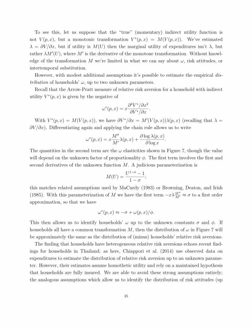
To see this, let us suppose that the “true” (momentary) indirect utility function isnot V (p, x), but a monotonic transformation V ∗(p, x) = M(V (p, x)). We’ve estimatedλ = ∂V/∂x, but if utility is M(U) then the marginal utility of expenditures isn’t λ, butrather λM ′(U), where M ′ is the derivative of the monotone transformation. Without knowl-edge of the transformation M we’re limited in what we can say about ω, risk attitudes, orintertemporal substitution.

However, with modest additional assumptions it’s possible to estimate the empirical dis-tribution of households’ ω, up to two unknown parameters.

Recall that the Arrow-Pratt measure of relative risk aversion for a household with indirectutility V ∗(p, x) is given by the negative of

ω∗(p, x) = x∂2V ∗/∂x2

∂V ∗/∂x.

With V ∗(p, x) = M(V (p, x)), we have ∂V ∗/∂x = M ′(V (p, x))λ(p, x) (recalling that λ =∂V/∂x). Differentiating again and applying the chain rule allows us to write

ω∗(p, x) = xM ′′

M ′ λ(p, x) + ∂ log λ(p, x)∂ log x .

The quantities in the second term are the ω elasticities shown in Figure 7, though the valuewill depend on the unknown factor of proportionality φ. The first term involves the first andsecond derivatives of the unknown function M . A judicious parameterization is

M(U) = U1−σ − 11− σ ;

this matches related assumptions used by MaCurdy (1983) or Browning, Deaton, and Irish(1985). With this parameterization of M we have the first term −xλM ′′

M ′≈ σ to a first order

approximation, so that we have

ω∗(p, x) ≈ −σ + ω(p, x)/φ.

This then allows us to identify households’ ω up to the unknown constants σ and φ. Ifhouseholds all have a common transformation M , then the distribution of ω in Figure 7 willbe approximately the same as the distribution of (minus) households’ relative risk aversions.

The finding that households have heterogeneous relative risk aversions echoes recent find-ings for households in Thailand; as here, Chiappori et al. (2014) use observed data onexpenditures to estimate the distribution of relative risk aversion up to an unknown parame-ter. However, their estimates assume homothetic utility and rely on a maintained hypothesisthat households are fully insured. We are able to avoid these strong assumptions entirely;the analogous assumptions which allow us to identify the distribution of risk attitudes (up

35

to unknown location and scale parameters) are just the much weaker requirements that elas-ticities are constant (instead of all equal to one, and may vary across goods) and that thehousehold maximizes utility within the period subject to a budget constraint.

7. Conclusion

In this paper we’ve outlined some of the key methodological ingredients needed in a recipeto estimate a simple measure of household welfare. This measure is closely related to thehousehold’s marginal utility of expenditures; it differs only in that it controls for householdcharacteristics and adopts a particular cardinalization of utility.

The methods described are theoretically coherent, in the sense that they’re consistent witha particular utility-derived demand system. Further, our approach lends itself to straight-forward statistical inference and hypothesis testing, and is very parsimonious in its datarequirements.

Our approach involves estimating an incomplete demand system of a new sort whichfeatures a highly flexible relationship between total expenditures and demand. The methodsdescribed here involve using one or more cross-sections of data on household expenditureson different nondurable goods and/or services. The limited data requirements suggest thatthese methods may be useful in constructing programs to inexpensively measure and monitorhouseholds’ welfare over both different environments and across time.

In an application of these methods we use four rounds of data from Uganda. We focuson food expenditures in this dataset, estimating a system of 41 demands. We estimate bothhousehold log λ and Frischian elasticity parameters from this expenditure system, in additionto other demand parameters. A separate analysis allows us to characterize the distributionof households’ relative risk aversions; we find convincing evidence of heterogeneity, thoughthe distribution is not fully identified.

8. References

Ahn, Seung Chan, Young Hoon Lee, and Peter Schmidt. 2001. GMM estimation of lin-ear panel data models with time-varying individual effects. Journal of Econometrics101:219–255.

Almas, Ingvild. 2012. International income inequality: measuring PPP bias by estimatingengel curves for food. American Economic Review 102 (2): 1093–1117.

Almas, Ingvild, Timothy K.M. Beatty, and Thomas Crossley. 2018. Lost in translation:what do engel curves tell us about the cost of living? CESifo Working Paper Series 6886.CESifo Group Munich. https://EconPapers.repec.org/RePEc:ces:ceswps:_6886.

36

https://EconPapers.repec.org/RePEc:ces:ceswps:_6886

Angelucci, Manuela, and Giacomo De Giorgi. 2009. Indirect effects of an aid program: howdo cash transfers affect non-eligibles’ consumption. The American Economic Review 99,no. 1 (March): 486–508.

Arellano, M. 1987. Computing robust standard errors for within-groups estimators. OxfordBulletin of Economics and Statistics 49 (4): 431–34.

Arellano, Manuel, Richard Blundell, and Stephane Bonhomme. 2017. Earnings and consump-tion dynamics: a nonlinear panel data framework. Econometrica 85 (3): 693–734.

Atkin, David, Ben Faber, Thibault Fally, and Marco Gonzalez-Navarro. 2018. A new engelon the gains from trade: theory and evidence within and across countries. Manuscript.

Attanasio, Orazio P, and Valerie Lechene. 2014. Efficient responses to targeted cash transfers.Journal of Political Economy 122 (1): 178–222.

Attanasio, Orazio P, and Luigi Pistaferri. 2016. Consumption inequality. Journal of Eco-nomic Perspectives 30 (2): 3–28.

Attfield, Clifford LF, and Martin J Browning. 1985. A differential demand system, rationalexpectations and the life cycle hypothesis. Econometrica 53 (1): 31–48.

Benson, Todd, Samuel Mugarura, and Kelly Wanda. 2008. Impacts in uganda of rising globalfood prices: the role of diversified staples and limited price transmission. AgriculturalEconomics 39 (s1): 513–524.

Blundell, Richard. 1998. Consumer demand and intertemporal allocations: engel, slutsky,and frisch. Econometric Society Monographs 31:147–168.

Blundell, Richard, Luigi Pistaferri, and Itay Saporta-Eksten. 2016. Consumption inequalityand family labor supply. American Economic Review 106 (2).

Bourguignon, F., M. Browning, and P. A. Chiappori. 2009. Efficient intra-household allo-cations and distribution factors: implications and identification. Review of EconomicStudies 76 (2): 503–528.

Browning, Martin. 1986. The costs of using frisch demand functions that are additive in themarginal utility of expenditure. Economics Letters 21 (3): 205–207.

Browning, Martin, Francois Bourguignon, Pierre-Andre Chiappori, and Valerie Lechene.1994. Income and outcomes: a structural model of intrahousehold allocation. Decem-ber, Journal of Political Economy 102 (6): 1067–1096.

37

Browning, Martin, Thomas F. Crossley, and Joachim Winter. 2014. The measurement ofhousehold consumption expenditures. Annual Review of Economics 6:475–501.

Browning, Martin, Angus Deaton, and Margaret Irish. 1985. A profitable approach to laborsupply and commodity demands over the life cycle. Econometrica 53:503–543.

Brunori, Paolo, Flaviana Palmisano, and Vito Peragine. 2015. Inequality of opportunity dur-ing the great recession in uganda. Working Paper 2015/039. WIDER.

Caron, Justin, Thibault Fally, and James R. Markusen. 2014. International trade puzzles: asolution linking production and preferences. The Quarterly Journal of Economics 129(3). doi:10.1093/qje/qju010.

Chiappori, Pierre-Andre, Krislert Samphantharak, Sam Schulhofer-Wohl, and Robert M.Townsend. 2014. Heterogeneity and risk sharing in village economies. QuantitativeEconomies 5, no. 1 (March): 1–27. http://onlinelibrary.wiley.com/doi/10.3982/QE131/epdf.

Cochrane, John H. 1991. A simple test of consumption insurance. Journal of Political Econ-omy 99:957–976.

Comin, Diego A, Danial Lashkari, and Martı Mestieri. 2015. Structural change with long-run income and price effects. Technical report. National Bureau of Economic Research.http://www.nber.org/papers/w21595.pdf.

Cooper, Russel J, and Keith R McLaren. 1996. A system of demand equations satisfyingeffectively global regularity conditions. The Review of Economics and Statistics: 359–364.

Deaton, Angus. 1992. Household saving in LDCs: credit markets, insurance, and welfare.Scandinavian Journal of Economics 94:253–273.

. 1997. The analysis of household surveys. Baltimore: The John Hopkins UniversityPress.

Deaton, Angus, and Margaret Irish. 1984. Statistical models for zero expenditures in house-hold budgets. Journal of Public Economics 23 (1-2): 59–80.

Deaton, Angus, and John Muellbauer. 1980. An almost ideal demand system. The AmericanEconomic Review 70, no. 3 (June): 312–326.

Development Research Group of the World Bank. Downloaded 2017. PovcalNet: the on-linetool for poverty measurement. http://iresearch.worldbank.org/PovcalNet/.

38

http://dx.doi.org/10.1093/qje/qju010

http://onlinelibrary.wiley.com/doi/10.3982/QE131/epdf

http://onlinelibrary.wiley.com/doi/10.3982/QE131/epdf

http://www.nber.org/papers/w21595.pdf

http://iresearch.worldbank.org/PovcalNet/

Diewert, W. E. 1971. An application of the shephard duality theorem: a generalized leontiefproduction function. Journal of Political Economy 79:461–507.

Engel, Ernst. 1857. Die productions-und consumtionsverhaltnisse des konigreichs sachsen.Zeitschrift des Statistischen Biireaus des Koniglich Sachsischen Ministeriums des In-nern, nos. 8 & 9: 1–54.

Fiedler, John L, Keith Lividini, Odilia I Bermudez, and Marc-Francois Smitz. 2012. House-hold consumption and expenditures surveys (hces): a primer for food and nutrition an-alysts in low-and middle-income countries. Food and Nutrition Bulletin 33 (3 suppl2):S170–S184.

Frisch, Ragnar. 1959. A complete scheme for computing all direct and cross demand elastic-ities in a model with many sectors. Econometrica 27, no. 2 (April): 177–196.

. 1964. Dynamic utility. Econometrica: 418–424.

. 1978. New methods of measuring marginal utility. Porcupine Press.

Golub, G. H., and C. Reinsch. 1970. Singular value decomposition and least squares solutions.Numerische Mathematik 14 (5): 403–420.

Gorman, W. M. 1959. Separable utility and aggregation. Econometrica 27:469–81.

Gorman, W.M. 1976. Essays in economic analysis. Chap. Tricks with utility functions, 211–243. Cambridge University Press. http://users.ox.ac.uk/˜econ0211/writings/gorman.pdf.

Hanoch, Giora. 1975. Production and demand models with direct or indirect implicit addi-tivity. Econometrica 43 (3): 395–419.

Heckman, James J. 1974. Shadow prices, market wages, and labor supply. Econometrica 42(4): 679–694. https://www.jstor.org/stable/pdf/1913937.pdf.

. 1976. A life-cycle model of earnings, learning, and consumption. Journal of politicaleconomy: S9–S44. https://www.jstor.org/stable/pdf/1831101.pdf.

Heckman, James J., and Thomas E. MaCurdy. 1980. A life cycle model of female laboursupply. The Review of Economic Studies: 47–74.

Horowitz, Joel L. 2003. Bootstrap methods for markov processes. Econometrica 71 (4): 1049–1082.

Houthakker, Hendrik S. 1960. Additive preferences. Econometrica: 244–257. https://www.jstor.org/stable/pdf/1907719.pdf.

39

http://users.ox.ac.uk/~econ0211/writings/gorman.pdf

http://users.ox.ac.uk/~econ0211/writings/gorman.pdf

https://www.jstor.org/stable/pdf/1913937.pdf




Intersecretariat Working Group on Price Statistics. 2004. Consumer price index manual:theory and practice. Technical report. https : / / www . ilo . org / public / english /bureau/stat/download/cpi/cpi_manual_en.pdf.

Karaivanov, Alexander, and Robert M. Townsend. 2014. Dynamic financial constraints: dis-tinguishing mechanism design from exogenously incomplete regimes. Econometrica 82(3): 887–959.

Kinnan, Cynthia. 2017. Distinguishing barriers to insurance in thai villages. UnpublishedMs.

Laczo, Sarolta. 2015. Risk sharing with limited commitment and preference heterogeneity:structural estimation and testing. Journal of the European Economic Association 13 (2):265–292.

Lewbel, Arthur. 1991. The rank of demand systems: theory and nonparametric estimation.Econometrica 59 (3): 711–730.

. 2003. A rational rank four demand system. Journal of Applied Econometrics 18 (2):127–135. http://www.jstor.org/stable/30035200.

Lewbel, Arthur, and Krishna Pendakur. 2009. Tricks with hicks: the easi demand system.The American Economic Review 99, no. 3 (June): 827–863.

Lise, Jeremy. 2012. On-the-job search and precautionary savings. Review of Economic Studies80 (3): 1086–1113.

Lise, Jeremy, and Ken Yamada. 2017. Household sharing and commitment: evidence frompanel data on individual expenditures and time use. Manuscript.

Little, Roderick, and Donald Rubin. 2002. Statistical analysis with missing data. 2nd. WileySeries in Probability and Statistics. John Wiley & Sons.

Low, Hamish, Costas Meghir, and Luigi Pistaferri. 2010. Wage risk and employment riskover the life cycle. American Economic Review 100 (4): 1432–67.

Mace, Barbara J. 1991. Full insurance in the presence of aggregate uncertainty. Journal ofPolitical Economy 99:928–956. http://www.jstor.org/stable/2937653.

MaCurdy, Thomas E. 1981. An empirical model of labor supply in a a life-cycle setting.Journal of Political Economy 89 (61): 1059–1085.

40

https://www.ilo.org/public/english/bureau/stat/download/cpi/cpi_manual_en.pdf

https://www.ilo.org/public/english/bureau/stat/download/cpi/cpi_manual_en.pdf

http://www.jstor.org/stable/30035200

http://www.jstor.org/stable/2937653

. 1983. A simple scheme for estimating an intertemporal model of labor supply andconsumption in the presence of taxes and uncertainty. International Economic Review24 (2): 265–289.

Mazzocco, Maurizio, and Shiv Saini. 2011. Testing efficient risk sharing with heterogeneousrisk preferences. American Economic Review 102 (1): 428–468.

Meredith, William. 1993. Measurement invariance, factor analysis and factorial invariance.Psychometrika 58 (4): 525–543.

Muellbauer, John. 1976. Community preferences and the representative consmer. Economet-rica 44 (5): 979–999.

Pelleg, Dan, Andrew W Moore, et al. 2000. x-means: extending k-means with efficient es-timation of the number of clusters. In Proceedings of the 17th international conferenceon machine learning, 1:727–734.

Ravallion, Martin, Shaohua Chen, and Prem Sangraula. 2009. Dollar a day revisited. TheWorld Bank Economic Review 23 (2): 163–184.

Townsend, Robert M. 1994. Risk and insurance in village India. Econometrica 62 (3): 539–591.

Vella, Francis. 1998. Estimating models with sample selection bias: a survey. The Journal ofHuman Resources 33:127–169.

Wedel, Michel, and Wagner A Kamakura. 2001. Factor analysis with (mixed) observed andlatent variables in the exponential family. Psychometrika 66 (4): 515–530.

Wooldridge, Jeffrey M. 2002. Econometric analysis of cross section and panel data. Cam-bridge, MA: MIT Press.

Young, Alwyn. 2012. The african growth miracle. Journal of Political Economy 120 (4):696–739.

41

Appendix A. For Online Publication: Issues with Missing Data

We consider two issues related to the possibility that certain item expenditures may bezero or missing for some households in our dataset. The first is a practical issue, having todo with the calculation of the singular value decomposition (SVD) of a matrix when someof the elements of that matrix are missing. The resolution of this problem involves relyingjust on observed data. This is clearly okay if the data is “missing at random” (Little andRubin 2002), but if there’s selection on unobservables then the matter is less clear. Thus,our second issue involves obtaining conditions under which selection doesn’t compromise ourSVD calculation.

A.1. A method for computing the singular value decomposition of random matri-ces with missing elements. Consider a random matrix X having a continuous distributionwith support over some subset of Rn×m and a second random matrix M of the same dimen-sion with elements either 1 or 0. Assume without loss of generality that n ≤ m, and thatthe matrix X is “low rank” in the sense that its rank is strictly less than n. We observe onlya matrix A = X⊗M, where ⊗ is the Hadamard product. Any zero element of A is said tobe “missing;” we assume that both the row and column sums of M are greater than zero.

We wish to construct a matrix X close to X in the Frobenius norm. If we assume that therank of X is some known number r then we have the compact singular value decompositionof the matrix X = U∗Σ∗V∗>, with U∗ n× r, Σ∗ r × r and diagonal, and V∗ m× r.

Our strategy involves first using the m columns of A to estimate the n× r matrix U∗Σ∗.We construct a matrix

P = mAA> � (MM>),

where � is the Hadamard (element-by-element) division operator. P can be interpreted asthe matrix product AA> scaled to ignore zero elements; note that it’s positive semi-definiteby construction. Then the square root of the eigenvalues of P is an estimator for the diagonalmatrix Σ∗, while the corresponding eigenvectors U estimate U∗.

With UΣ in hand we proceed row by row to construct an estimate of V∗: suppose a is acolumn vector from the matrix A, and that A has the compact singular value decompositionUΣV>. The vector a can be partitioned into two parts y and x, while a matrix UΣx can beconstructed by selecting just the rows of UΣ corresponding to the x elements of the vectora. Then the row of V∗ corresponding to a can be estimated by

v = (UΣx)+x,

where the + operator here indicates the Penrose-Moore pseudo-inverse. Iterating over all mcolumns of A then yields the desired matrix X.

42

A.2. Effects of non-random selection. Let (X,M) be corresponding columns of the ran-dom matrices X and M, each an n-dimensional random variable, where X has realizationsx, and M observable realizations m. If X and M are independent we say that the data is“missing at random” and the methods describe above deliver what we want, but otherwisethere may be a selection problem. We want to establish conditions on the joint distribu-tion F (X,M) which ensure that E(UΣ) = U∗Σ∗, provided the columns of X and M areuncorrelated across households.

To this end, we modestly extend an idea due to Meredith (1993) (Theorem 5). Thisidea in turn can be thought of as extending the usual result from the program evaluationliterature that selection on observables doesn’t compromise consistent estimation in theprogram evaluation literature. Instead of assuming that selection depends only on a set ofobservable variables, we allow selection to depend on a set of latent variables. (This alsogeneralizes the idea from fixed effects estimation in unbalanced panels that selection isn’t aproblem if the probability of a household being missing in a given period can be “explained”by a fixed effect.)

In particular, let W be a p-dimensional latent variable with realizations w that underliesX; and let L be an q-dimensional random variable with realizations l that underlies M .

A collection of functions si(l) comprise a selection rule that gives the marginal probabilitythat mi = 1 for an individual with attributes l, i = 1, . . . , n. We adopt the followingassumptions:

Assumption 1. (1) The conditional distribution of X given w is non-degenerate, andfirst and second moments exist;

(2) W and L are not independent; and(3) The joint probability distribution of M is assumed to be conditionally independent

across i, so we have

s(m|L) =n∏i=1

si(L)mi(1− si(L))1−mi .

The first assumption is standard. The second is necessary for knowledge of w to tellsus something about the probability of selection. The third could perhaps be relaxed, butallowing conditional dependence in selection would considerably complicate estimation.

Now, let Es(g(X)|w, l) denote the conditional expectation and Vars(g(X)|w, l) the con-ditional covariance matrix of g(X) conditional on w given the selection rule s(m|l) for anyLebesgue-measurable function g. Otherwise expectations and covariances E(g(X)|w, l) andVar(g(X)|w, l) correspond to the population distribution F (x,w, l) without any selection.

43

Proposition 2. Given Assumption 1, if E(X|w, l) = E(X|w) and Var(X|w, l) = Var(X|w)for all (w, l) then Es(X|w, l) = E(X|w) and Vars(X|w, l) = Var(X|w) for all w, all selectionfunctions s, and all l such that si(l) > 0 for some i = 1, . . . , n.

Proof. Let F (x,w, l,m) be the joint distribution of (x,w, l,m) in the population; then theselected joint distribution is given by the Lebesgue integral

Fs(x,w, l) =∫s(m|l)dF (x,w, l)/

∫s(m|l)dF (l)

for all (x⊗m,w, l) such that si(l) > 0 for some i = 1, . . . , n, and then Fs(x|w, l) = F (x|w, l)over the same set; thus Es(g(X)|w, l) = E(g(X)|w, l) = E(g(X)|w). The first part of theproposition is then established by taking g(X) = X, while the second is established takingg(X) = g(X|w) = E(XX>|w)− E(X|w)E(X|w)> for any w. �

The key to the result is that the factors which determine selection directly affect X only viatheir interaction with the latent variables W ; this is related to but weaker than a conditionsometimes called “missing at random conditional on X” (Wedel and Kamakura 2001).

A special case which satisfies the conditions of Proposition 2 occurs when the selectionrule doesn’t depend on L at all, so that we have s(m|L) = s(m|L′) for all (L,L′). In thiscase data are “missing at random”, in the lexicon of Little and Rubin (2002), and we areable to obtain unbiased estimates of (U∗,Σ∗,V∗). In the more general case in which theselection rule varies with L but the conditions of the proposition are satisfied we can expectto obtain unbiased estimates only of (U∗,Σ∗), as the sample of households for which weobserve expenditures may be systematically different from the population.

A.3. A simple test for selection bias. Our case is related to the case in which there’sattrition in a panel of households, but in which the factors that cause attrition can becaptured by fixed effects. In our case suppose that we’re using only a single cross-section,with a large number of households N and a smaller fixed number of goods n; now the fact thatexpenditures on some goods are zero or missing is just like observations for some householdsbeing missing in the unbalanced panel case. The idea for fixed effects panel estimation isthat the selection process depends on fixed household characteristics. Our latent variablesaren’t household fixed effects, but instead latent interactions which capture variation inprices (ait) and household resources (log λjt), but these are also exactly the features we mightbe concerned would lead to selection problems were we estimating demands for a singlegood, as in Deaton and Irish (1984). If, after conditioning on these, expenditures are zero ormissing simply because of the timing of stocking decisions or some other random censoringprocess then we can expect our linear model with interactive latent variables ait and βi log λjtto deliver consistent results, much as in the case of Ahn, Lee, and Schmidt (2001).

44

Here we describe a simple test of the central conditions required in Proposition 2. Supposethat we have X = WA+ UX , L = WB + UL, and M = LC + UM . Then we have

[X,M] = [WA,LC] + [UX ,UL]

= W[A,BC] + [UX ,ULC + UM ].

Under the null hypothesis that E(X|W,L) = E(X|W ), a singular value decomposition of[X,M] allows us to estimate both W and A. On the other hand, if the hypothesis doesn’thold and W is not orthogonal to ULC + UM then the SVD of this augmented matrix willestimate quantities which depend on ULC + UM .

In the application of this paper the matrix X is obtained from the residuals of (8), de-livering a matrix which is orthogonal to household characteristics and good-time effects.Thus, we similarly filter the dummy variables M by regressing these on the same right-handside, and using estimated residuals from this regression. A maintained assumption of ourapplication is that the rank of the matrix W is one; thus the test proposed here becomes aquestion of whether the decomposition of the augmented matrix yields significantly differentestimates of the rank one UΣ and rank one V what we obtain when we simply decomposeX.

Appendix B. For Online Publication: Food items across rounds andaggregation

Food codes and items are fairly consistently recorded across rounds, but not perfectlyso; further, some are clearly sensibly treated as substitutes (e.g., different size bunches ofmatoke). Other food items are treated separately in some rounds (e.g., “Watermelon” in 2010and 2011) but assigned to an aggregate (e.g., “Other Fruits”) in other rounds, necessitatingthe use of the coarser aggregate to achieve consistency across rounds. Table B.1 gives aprecise accounting of all codes and aggregation. We supply a “Preferred Label” columnand an “Aggregate Label.” The “preferred” label eliminates minor differences in spelling orword usage across rounds (e.g., “Matoke” versus “matooke”). The “Aggregate Label” neednot be unique; expenditures for all items with the same “Aggregate Label” will be summedtogether, yielding what we call a “minimally-aggregated” set of data of food expenditures.This minimal aggregation confines itself to combining expenditures on different food itemswhich seem to obviously be very close substitutes. Sometimes these differences are just inunits: we aggregate “clusters” and “heaps” of Matoke, for example. Othertimes the form ofthe good is somewhat different: fresh and dried cassava are aggregated, for example.

45

Table B.1: Labels for various food items in differentrounds, with “Preferred” and “Aggregate” labels.

Code Preferred Label Aggregate Label

100 Matoke (??) Matoke101 Matoke (bunch) Matoke102 Matoke (cluster) Matoke103 Matoke (heap) Matoke104 Matoke (other) Matoke105 Sweet Potatoes (fresh) Sweet Potatoes106 Sweet Potatoes (dry) Sweet Potatoes107 Cassava (fresh) Cassava108 Cassava (dry/flour) Cassava109 Irish Potatoes Irish Potatoes110 Rice Rice111 Maize (grains) Maize112 Maize (cobs) Maize113 Maize (flour) Maize114 Bread Bread115 Millet Millet116 Sorghum Sorghum117 Beef Beef118 Pork Pork119 Goat Meat Goat Meat120 Other Meat Other Meat121 Chicken Chicken122 Fresh Fish Fresh Fish123 Dry/Smoked fish Dry/Smoked fish124 Eggs Eggs125 Fresh Milk Fresh Milk126 Infant Formula Infant Formula127 Cooking oil Cooking oil128 Ghee Ghee129 Margarine, Butter, etc Margarine, Butter, etc130 Passion Fruits Passion Fruits




131 Sweet Bananas Sweet Bananas132 Mangoes Mangoes133 Oranges Oranges134 Other Fruits Other Fruits135 Onions Onions136 Tomatoes Tomatoes137 Cabbages Cabbages138 Dodo Dodo139 Other vegetables Other Vegetables140 Beans (fresh) Beans141 Beans (dry) Beans142 Ground nuts (in shell) Ground nuts143 Ground nuts (shelled) Ground nuts144 Ground nuts (pounded) Ground nuts145 Peas Peas146 Sim sim Sim sim147 Sugar Sugar148 Coffee Coffee149 Tea Tea150 Salt Salt151 Soda Soda152 Beer Beer153 Other Alcoholic drinks Other Alcoholic drinks154 Other drinks Other drinks155 Cigarettes Cigarettes156 Other Tobacco Other Tobacco157 Restaurant (food) Restaurant (food)158 Restaurant (soda) Soda159 Restaurant (beer) Beer160 Other juice Other juice161 Other foods Other foods162 Peas (dry) Peas163 Ground nut (paste) Ground nuts




164 Green pepper Other Vegetables165 Pumpkins Other Vegetables166 Avocado Other Fruits167 Carrots Other Vegetables168 Eggplant Other Vegetables169 Watermelon Other Fruits170 Pineapple Other Fruits171 Pawpaw Other Fruits

The aggregation in Table B.1 results in total of 49 different items. Most of these arestraightforward types of food, such as peas, mangoes, ground nuts, maize, or sugar. Foodconsumed in restaurants is a category of its own, however, and may be thought of an aggre-gate bundle of food and services. Alcoholic beverages account for two additional categories,“beer” and “other alcoholic drinks.” And then finally there are two non-food categoriesincluded, “cigarettes” and “other tobacco.” Altogether there are five categories which areexplicitly undifferentiated aggregates: “other fruits”, “other vegetables”, “other alchoholicdrinks”, “other drinks”, and “other tobacco.” Other categories may be implicitly aggregated:for example, “ground nut” includes nuts shelled, unshelled, and made into paste. Finally,even after aggregation some of these categories contain very few positive observations in atleast some years; dropping these yields a total of 41 categories.12

B.1. Aggregate and Mean Shares. Aggregate and mean shares for 41 “aggregated”goods.

Aggregate Aggregate Mean MeanGoods 2005 2011 2005 2011

Matoke 0.113 0.114 0.097 0.099Maize 0.079 0.084 0.092 0.091Cassava 0.077 0.092 0.090 0.105Restaurant 0.074 0.073 0.061 0.070Sweet potato 0.070 0.063 0.078 0.075

Continued on next page12. Excluded goods include beer, infant formula, butter & margarine, ghee, ground nuts, pork, other juice,

other drinks, and other meat.48

Continued from previous pageGoods 2005 2011 2005 2011

Beans 0.066 0.074 0.080 0.090Beef 0.058 0.058 0.044 0.046Sugar 0.055 0.044 0.051 0.042Fresh milk 0.041 0.040 0.033 0.034Rice 0.027 0.027 0.022 0.021Fresh fish 0.024 0.022 0.022 0.020Ground nut 0.022 0.024 0.023 0.024Cooking oil 0.021 0.022 0.022 0.022Dried fish 0.020 0.022 0.022 0.021Chicken 0.019 0.026 0.014 0.019Tomatoes 0.019 0.017 0.020 0.017Other Alcohol 0.018 0.016 0.021 0.020Soda 0.016 0.012 0.012 0.008Bread 0.015 0.015 0.010 0.010Other foods 0.015 0.003 0.021 0.003Millet 0.015 0.014 0.016 0.015Other Fruit 0.012 0.019 0.010 0.017Goat meat 0.012 0.015 0.010 0.010Irish potato 0.012 0.012 0.010 0.011Other Veg. 0.011 0.016 0.018 0.020Sorghum 0.009 0.012 0.017 0.018Cigarettes 0.009 0.004 0.009 0.004Dodo 0.008 0.007 0.010 0.010Onions 0.008 0.010 0.009 0.011Passion fruit 0.007 0.003 0.005 0.002Mangos 0.006 0.004 0.007 0.004Sweet Banana 0.006 0.005 0.004 0.003Salt 0.006 0.005 0.008 0.007Eggs 0.006 0.005 0.004 0.004Cabbages 0.005 0.006 0.005 0.007Tea 0.005 0.003 0.005 0.004Peas 0.005 0.005 0.006 0.006Sim sim 0.004 0.004 0.007 0.006


Continued from previous pageGoods 2005 2011 2005 2011

Oranges 0.002 0.002 0.002 0.002Other Tobacco 0.002 0.001 0.004 0.002Coffee 0.001 0.001 0.001 0.000

Appendix C. For Online Publication: Estimating the rank of the demandsystem

Using the fact that our estimates are normally distributed, we can evaluate the likelihoodthat the rank of the system is k ≤ n by solving the k-means problem

Ck = minb∈Rk

[mink|βi − bk|]>i V−1[mink|βi − bk|]i,

where V is the estimated covariance matrix of our estimates of β. Note that under thenull hypothesis that the rank of the matrix k then the statistic Ck is distributed χ2

n−k. Wecompute the corresponding likelihood Lk. Using the Bayesian Information Criterion (BIC)

BICk = k log n− 2 logLk

gives in our case an estimate of rank four for the demand system. Figure 9 presents theresult of these calculations; one can see that the minimum is achieved at k = 4, withb = (0.18, 0.36, 0.47, 0.62).

Figure 9. Using the BIC criterion to estimate the rank of the demand system.50

University of California, Berkeley

51

Household Welfare from Disaggregate Demands

Documents

Transcript of Household Welfare from Disaggregate Demands