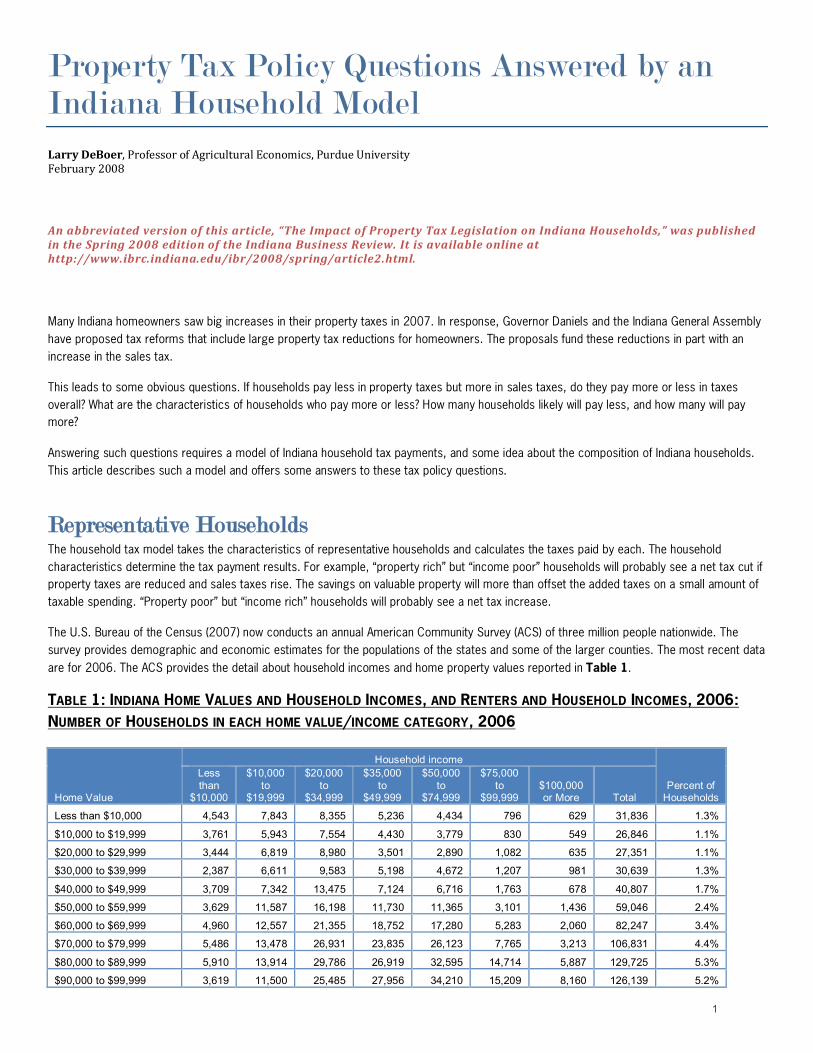
Property Tax Policy Questions Answered by an Indiana Household Model Larry DeBoer, Professor of Agricultural Economics, Purdue University February 2008 

An abbreviated version of this article, “The Impact of Property Tax Legislation on Indiana Households,” was published in the Spring 2008 edition of the Indiana Business Review. It is available online at  H 

http://www.ibrc.indiana.edu/ibr/2008/spring/article2.html H. 

Many Indiana homeowners saw big increases in their property taxes in 2007. In response, Governor Daniels and the Indiana General Assembly have proposed tax reforms that include large property tax reductions for homeowners. The proposals fund these reductions in part with an increase in the sales tax.

This leads to some obvious questions. If households pay less in property taxes but more in sales taxes, do they pay more or less in taxes overall? What are the characteristics of households who pay more or less? How many households likely will pay less, and how many will pay more?

Answering such questions requires a model of Indiana household tax payments, and some idea about the composition of Indiana households. This article describes such a model and offers some answers to these tax policy questions.

0BRepresentative Households The household tax model takes the characteristics of representative households and calculates the taxes paid by each. The household characteristics determine the tax payment results. For example, “property rich” but “income poor” households will probably see a net tax cut if property taxes are reduced and sales taxes rise. The savings on valuable property will more than offset the added taxes on a small amount of taxable spending. “Property poor” but “income rich” households will probably see a net tax increase.

The U.S. Bureau of the Census (2007) now conducts an annual American Community Survey (ACS) of three million people nationwide. The survey provides demographic and economic estimates for the populations of the states and some of the larger counties. The most recent data are for 2006. The ACS provides the detail about household incomes and home property values reported in Table 1.

UTABLE 1: INDIANA HOME VALUES AND HOUSEHOLD INCOMES, AND RENTERS AND HOUSEHOLD INCOMES, 2006: NUMBER OF HOUSEHOLDS IN EACH HOME VALUE/INCOME CATEGORY, 2006 

Home Value 

Household income 

Percent of Households 

Less than 

$10,000 

$10,000 to 

$19,999 

$20,000 to 

$34,999 

$35,000 to 

$49,999 

$50,000 to 

$74,999 

$75,000 to 

$99,999 $100,000 or More  Total 

Less than $10,000  4,543  7,843  8,355  5,236  4,434  796  629  31,836  1.3% 

$10,000 to $19,999  3,761  5,943  7,554  4,430  3,779  830  549  26,846  1.1% 

$20,000 to $29,999  3,444  6,819  8,980  3,501  2,890  1,082  635  27,351  1.1% 

$30,000 to $39,999  2,387  6,611  9,583  5,198  4,672  1,207  981  30,639  1.3% 

$40,000 to $49,999  3,709  7,342  13,475  7,124  6,716  1,763  678  40,807  1.7% 

$50,000 to $59,999  3,629  11,587  16,198  11,730  11,365  3,101  1,436  59,046  2.4% 

$60,000 to $69,999  4,960  12,557  21,355  18,752  17,280  5,283  2,060  82,247  3.4% 

$70,000 to $79,999  5,486  13,478  26,931  23,835  26,123  7,765  3,213  106,831  4.4% 

$80,000 to $89,999  5,910  13,914  29,786  26,919  32,595  14,714  5,887  129,725  5.3% 

$90,000 to $99,999  3,619  11,500  25,485  27,956  34,210  15,209  8,160  126,139  5.2%

1

Home Value 

Household income 

Percent of Households 

Less than 

$10,000 

$10,000 to 

$19,999 

$20,000 to 

$34,999 

$35,000 to 

$49,999 

$50,000 to 

$74,999 

$75,000 to 

$99,999 $100,000 or More  Total 

$100,000 to $199,999  18,066  34,528  98,702  123,496  226,258  157,693  126,772  785,515  32.3% 

$200,000 to $249,999  2,204  3,622  7,939  13,332  26,615  30,723  47,672  132,107  5.4% 

$250,000 to $499,999  1,938  3,357  7,578  11,622  21,931  23,566  73,230  143,222  5.9% 

$500,000 or More  549  818  1,683  1,968  3,711  2,781  22,507  34,017  1.4% 

Total Homeowners  64,205  139,919  283,604  285,099  422,579  266,513  294,409  1,756,328  72.1% 

Total Renters  128,114  144,160  174,859  106,209  84,017  25,373  16,214  678,946  27.9% 

All Households  192,319  284,079  458,463  391,308  506,596  291,886  310,623  2,435,274  100.0% 

Percent of Households  7.9%  11.7%  18.8%  16.1%  20.8%  12.0%  12.8%  100.0% Source: U.S. Census Bureau, American Community Survey

The table shows the numbers of households in seven income categories and fifteen home value categories, plus renters. Homeowners are 72 percent of the 2.4 million Indiana households; renters are 28 percent. Almost a third of households own homes valued between $100,000 and $200,000. The median home value is $120,700. Median income for Indiana households is $45,394. The median for homeowners is $55,634, for renters, $24,922.

These marvelous new data are just what is needed for determining representative households. Indiana is now a market value state, so home values provide the starting point for calculating property tax payments. Household income is the starting point for calculating county, state and federal income taxes.

That leaves sales and excise taxes, which are based on spending on taxable goods and (some) services. The U.S. Bureau of Labor Statistics (2008) conducts an annual Consumer Expenditure Survey, which can be combined with the ACS data to measure spending. The expenditure survey shows average annual spending on 73 categories of goods and services, from alcoholic beverages to women’s clothing. Data are not available by state, so national figures must be used.

Income is the most important determinant of spending. Higher income households spend more. Household size is also important. Households with more people spend more. Since the average Indiana household has 2.6 people, all the households in the model are assumed to have three: two adults and a child.F

1 F The spending data for three-person households are matched to the income data from the ACS to estimate how

much each household spends on each category.F

2 F

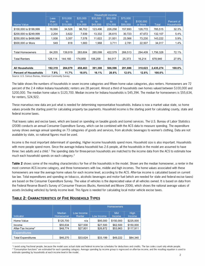
Table 2 shows some of the resulting characteristics for five of the households in the model. Shown are the median homeowner, a renter in the most common ACS income category, and three homeowners with low, middle and high incomes. The home values associated with these homeowners are near the average home values for each income level, according to the ACS. After-tax income is calculated based on current tax law. Total expenditures and spending on tobacco, alcoholic beverages and motor fuel (which are needed for state and federal excise taxes) are based on the Consumer Expenditure Survey. The value of vehicles is the depreciated value of all vehicles owned. It is based on data from the Federal Reserve Board’s Survey of Consumer Finances (Bucks, Kennickell and Moore 2006), which shows the national average values of assets (including vehicles) by family income level. This figure is needed for calculating local motor vehicle excise taxes.

UTABLE 2: CHARACTERISTICS OF FIVE HOUSEHOLD TYPES 

Indicator Median 

Homeowner Low Income 

Renter 

Homeowners 

Low Income Mid 

Income High 

Income 

Home Value  $120,700  n/a  $95,000  $150,000  $225,000 Income  $55,634  $27,500  $27,500  $62,500  $150,000 After­Tax Income*  $48,774  $27,801  $26,872  $53,963  $117,911 

Expenditures Total Expenditures  $46,270  $33,624  $33,199  $49,222  $84,340 

1 I avoid using fractional people, because the model uses actual state and federal income tax schedules for deductions and credits. The tax codes count only whole people. 2 “Consumption functions” are estimated for each spending category. Average spending by income group is regressed on after-tax income, and the resulting equation is used to estimate spending by households at each income level in the model.

2

Indicator Median 

Homeowner Low Income 

Renter 

Homeowners 

Low Income Mid 

Income High 

Income Percent of After­Tax Income  95%  121%  124%  91%  72% 

Spending on: Tobacco  $993  $1,015  $1,016  $988  $921 

Alcoholic Beverages  $683  $459  $449  $738  $1,420 

Motor Fuel  $2,242  $1,855  $1,838  $2,338  $3,518 

Vehicles Value of Vehicles  $14,982  $8,328  $8,328  $16,385  $26,682 

* Under current tax law

The accuracy of the tax analysis depends on the accuracy of the household characteristics. Two curiosities stand out in Table 2. First, the low-income renter household has after-tax income larger than pre-tax income. This happens because this household is eligible for the federal earned income credit (EIC), which supports the incomes of low-income working people. The low-income homeowner also receives the EIC, but must pay property taxes, so after-tax income is slightly less than pre-tax income.

Second, expenditures by the two low-income households exceed after-tax income. This implies that the households must be drawing on savings or going into debt. How, one wonders, do low-income households save out of their small incomes, and how are they managing to borrow?

The Consumer Expenditure Survey does report total spending higher than after-tax income for a large number of households. All of the households with incomes less than $40,000 spend more than their after-tax incomes, on average. One explanation is that some households with lower incomes have experienced a temporary reduction in their incomes—unemployment or business losses, for example—and have savings accumulated from their previous higher incomes. There is some evidence for this at the lowest household income level in the survey. Households with incomes under $5,000 spend more than those with incomes of $5,000 to $15,000. Perhaps previous higher spending levels are being supported with savings, in anticipation that the current lower incomes are truly temporary.

The Federal Reserve’s Consumer Finance Survey provides further evidence. Of families with a median income of $26,000, 44 percent save. Of those same families, 70 percent owe some kind of debt, including 40 percent who owe on installment loans and 43 percent who carry credit card balances.

It seems possible, at least, that lower income households do spend more than their after-tax incomes, financed from savings and debt. This contributes to a pattern that plays a role in tax policy results: spending is a higher percentage of lower income household income than of upper income household income. Apparently, upper income households save a lot; lower income households save little, draw upon past savings, or take on debt.

1BTax Calculations The data on the property, income and spending of representative households are used to calculate tax payments for the various taxes. Included are property taxes, general sales taxes, state and county income taxes, state excise taxes on tobacco, alcoholic beverages and motor fuel, local excise taxes on motor vehicles, federal income taxes, Social Security taxes, and federal excise taxes on tobacco, alcoholic beverages and motor fuel.

Here are brief descriptions of the calculation of each tax.

Property Tax. Assessments are assumed to be accurate, so gross assessed values are set equal to home values. F

3 F Deductions are subtracted,

and then the gross tax bill is calculated using the state average property tax rate, available from the Legislative Services Agency’s (2007) handbook. Property tax replacement credits and homestead credits are subtracted, again based on state average rates. The “circuit breaker” credit is then applied.

3 The 2005 statewide equalization study of Indiana assessments (Indiana Fiscal Policy Institute, 2005) found that 91 percent of counties had median home assessments within 10 percent of selling price. On average, homes are assessed near their market values. Far fewer counties met the standard on dispersion, however, meaning that there are large variations around the average.

3

Sales Tax. Indiana taxes goods except most food with the sales tax. The tax also covers services such as utilities and product rentals. Each expenditure category from the Consumer Expenditure Survey is identified as taxable, not taxable, or partially taxable. Partially taxable spending is assumed to be half taxable, half not. The sum of taxable spending is multiplied by t/(1+t), where “t” is the tax rate. This is done because average expenditures include sales taxes—the Survey does not split out the part of the price that is tax.F

4 F For the current 6 percent sales tax,

this formula produces 5.66 percent. This percentage times taxable sales gives the sales tax payment on each expenditure category, and the sum is the total sales tax payment.

State and County Income Taxes. The model replicates parts of the state income tax form. Adjusted gross income equals the household’s total income. Indiana deductions and exemptions are subtracted. These include the renter’s deduction, the property tax deduction (both with $2,500 upper limits), the $1,000 personal exemption and the $1,500 additional dependent child exemption. The result is Indiana taxable income. This is multiplied by the state’s flat rate of 3.4 percent, and an assumed county rate of 1 percent.F

5 F The Indiana earned income credit

of 6 percent of the Federal EIC is then subtracted. A negative number means that part of the credit has been refunded.

Federal Income Tax. As one might expect, modeling the federal income tax presents the greatest challenge. The federal tax is important for Indiana state and local tax policy because of the deductibility of the local property and motor vehicle excise tax, and either the state and local income or state sales taxes. Changes in state and local taxes cause changes in the federal tax payment.

Federal adjusted gross income is assumed to be the household’s total income. Exemptions and deductions are subtracted, including the personal exemption, and, for itemizers, the local property, local motor vehicle excise, and income or sales tax deductions, the mortgage interest deduction, and the charitable contributions deduction. If the household lowers its tax bill by using the standard deduction, it is assumed to do so. The result is taxable income. The graduated tax rates are applied in six tax brackets. The additional child tax credit is subtracted. The federal earned income credit is calculated, and subtracted. The result is the federal income tax payment. A negative number indicates a refundable EIC.

Social Security Tax. The federal Social Security payroll tax is calculated at 6.2 percent of income up to $97,500. The Medicare payroll tax is 1.45 percent of total income..

Excise Taxes. Excise taxes present a difficulty because they are based on unit sales, not a percentage of price. The Indiana cigarette tax, for example, is currently 99.5 cents per pack, while the Consumer Expenditure data show only total tobacco spending. Estimated prices per pack for cigarettes, per gallon for alcoholic beverages, and per gallon for gasoline were acquired. Spending divided by these prices gives the units purchased. The excise tax rate times the number of units shows the taxes paid. This method is used for both state and federal excise taxes on tobacco, alcoholic beverages and motor fuel.

The Indiana local motor vehicle excise tax presents a greater difficulty. The tax is applied with an elaborate rate schedule based on purchase price and vehicle age. The Consumer Expenditure Survey shows the average number of vehicles owned, but not their value or age.

Knowing something of the history of this tax provides a solution. The motor vehicle excise tax replaced the property tax on vehicles in 1971. The property tax was calculated at the depreciated value of the vehicle times each jurisdiction’s flat rate. The excise tax rate schedule mimics this calculation at a statewide rate. The decreasing tax by age represents depreciation, and the tax on new vehicles is near 1.3 percent for most vehicle values. The tax can be approximated as 1.3 percent of the depreciated value of the household’s vehicles.

But what’s the depreciated value of the household’s vehicles? The Federal Reserve’s Consumer Finance Survey again comes to the rescue, by providing the estimated value of family vehicles by family income level. These vehicle values are associated with income levels, and multiplied by 1.3 percent to estimate the motor vehicle excise taxes paid. F

6

2BTesting the Basic Results Do the tax payments implied by all these calculations make sense? One test is to add up the tax payments for households and compare them to total tax collections in Indiana. Tax calculations are made for 60 households based on the income and home value categories from the ACS in Table 1. The tax payments by each household are then multiplied by the number of households in each category, and the result compared to the state totals.

4 Total expenditures (E) are the sum of the list price (P) and sales tax, which is the sales tax rate times the list price (tP). E = (1+t)P, so P = E/(1+t), and the sales tax paid is tP = E[ t/(1+t)]. 5 The median county income tax rate is greater than 1 percent, but the average rate is less than 1 percent, primarily because Lake County is without an income tax. The 1 percent rate in the model splits the difference. 6 As with spending categories, vehicle values are regressed on incomes, and the resulting equation used to estimate vehicle values for each income level in the model.

4

The model performs best for the income taxes. The state and county income tax total from the model is within 3 percent of the actual collections in 2006. The Federal Internal Revenue Service (U.S. Department of the Treasury, 2008) reported that about $15.7 billion in federal income taxes were collected in Indiana in 2005 (the most recent year available). The model produces an estimate of $9.8 billion. However, the model does not include any households with incomes greater than $200,000. According to the IRS there were 46,000 such households in Indiana, who paid about $5.6 billion in federal tax. Not including these households, the model’s result is within 3 percent of actual collections.

The model’s households pay $2.9 billion in sales taxes, only 55 percent of the state total in 2006. This is expected. Some sales tax is paid on business to business sales, which would not show up (directly) as household tax payments. Estimates of the share of Indiana sales taxes paid by businesses and households vary with the method used. In an earlier paper I estimated the Figure at 23 percent using Indiana revenue data by industry (DeBoer, 2007). The household model total still falls well short of tax collections from households using this figure.

Raymond Ring (1999) used a method similar to this to estimate the household and business shares of sales taxes for all the states. He calculated tax payments from the Consumer Expenditure Survey, summed them for households in each state, then subtracted this figure from each state’s total collections to estimate the share paid by businesses. Using data for Indiana for 1989, Ring found that 65 percent of sales taxes were paid by households, 35 percent by business.F

7 F The national average was 59 percent by households, 41 percent by business. The

result from the household model is near this national average figure. So, results similar to those here have been found before. It seems possible, though, that the sales tax payments estimated for households are an underestimate of actual amounts.

The model shows $3.3 billion in homestead property taxes, while Indiana local governments collected $2.9 billion from homesteads in 2006, an overestimate of 14 percent. In Table 1, the category that includes the Indiana median home value of $120,700 is particularly wide, $100,000 to $199,999. The model assigns homeowners in that category the midpoint value of $150,000. If the median value is used instead, the model’s total homestead property tax revenue is within 1 percent of the actual value.

The household results make sense for state and federal income taxes and property taxes, and fall short of sales taxes in a way that has been seen before. Results for excise taxes are less acceptable. Adjustments must be made.

Tobacco taxes from the household model sum to only 41 percent of the amount actually collected.F

8 F The Consumer Expenditure Survey

appears to substantially underestimate household spending on tobacco. This is confirmed by independent data. The U.S. Department of Agriculture puts U.S. average cigarette consumption at 1,654 per person (U.S. Bureau of Census, 2008, table 986). Adjusting for household size and price per pack, this is $909 per household. The Survey estimate for the average household nationally is $327. Perhaps households under-report their smoking purchases. Tobacco spending is scaled upward by a factor of 2.5, the number required to bring the model’s total tobacco revenue to the state total.

Similar (though smaller) adjustments are made for alcoholic beverage and motor fuel spending, which are also underestimated by the Survey. The model overestimates motor vehicle excise tax revenue by 27 percent. The vehicle values are scaled downward to bring the revenue estimate in line. The expenditure amounts in Table 2 reflect these scaling adjustments.

3BTax Payments by Representative Households Table 3 reports the tax payments estimated for five representative households. These households must be selected with care, because some results depend on which households are selected. First is the median homeowner, with the median home value and the median income for homeowners. Second is a renter with an income of $27,500. This is near the median income for renters. The remaining households are homeowners with successively increasing incomes. The home values were selected based on the average home value of all homeowners in each income category, according to the ACS.

The median homeowner pays $5,423 in Indiana state and local taxes, 9.7 percent of income. It pays $7,809 in Federal Taxes, 14.0 percent of income. In total, it pays taxes of $13,232, 23.8 percent of income.

7 Ring’s published figure for the household share is 54 percent, close to what was found here. However, he overestimated Indiana’s total sales tax revenue, perhaps using a Bureau of Census estimate for 1989. Census estimates always overstated Indiana general sales taxes, apparently counting the old corporate gross income tax as a sales tax. With the denominator in his calculation too large, Ring came up with an individual share that was too small. Using his estimate of individual sales with the Indiana Department of Revenue sales tax revenue data yields a household share of 65 percent. 8 The calculation is made assuming a cigarette tax rate of 55.5 cents per pack, the rate in use in 2006.

5

UTABLE 3: TAX PAYMENT ESTIMATES FOR FIVE HOUSEHOLD TYPES 

Indicator  Median Homeowner  Low Income Renter 

Homeowners Low 

Income Mid 

Income High 

Income 

Income  $55,634  $27,500  $27,500  $62,500  $150,000 

Home Value  $120,700  Renter  $95,000  $150,000  $225,000 

State and Local Taxes 

Property  $1,326  n/a  $857  $1,860  $3,227 

Sales  $1,200  $918  $927  $1,265  $2,065 

County/State Income  $2,192  $828  $900  $2,470  $6,292 

Tobacco  $262  $268  $268  $261  $243 

Alcoholic Beverage  $16  $11  $11  $18  $34 

Motor Fuel  $233  $192  $191  $242  $365 

Motor Vehicle Excise  $195  $108  $108  $213  $347 

Total Indiana Taxes  $5,423  $2,326  $3,262  $6,329  $12,573 

Percent of Income  9.70%  8.50%  11.90%  10.10%  8.40% 

Federal Taxes 

Federal Income  $3,149  ­$1,237  ­$1,237  $3,994  $22,223 

Social Security  $4,256  $2,104  $2,104  $4,781  $8,220 

Federal Tobacco  $90  $92  $92  $89  $83 

Federal Alcoholic Beverage  $77  $52  $51  $84  $161 

Federal Motor Fuel  $238  $197  $195  $248  $373 

Total Federal Taxes  $7,809  $1,207  $1,204  $9,196  $31,060 

Percent of Income  14.00%  4.40%  4.40%  14.70%  20.70% 

Total Taxes  $13,232  $3,533  $4,466  $15,525  $43,633 

Percent of Income  23.80%  12.80%  16.20%  24.80%  29.10% 

Source: Author, using U.S. Census Bureau and Bureau of Labor Statistics data

Table 4 shows the individual taxes as shares of income. These results are useful in measuring “progressivity” and “regressivity.” Progressivity means that higher income households pay a higher percentage of their incomes to a tax than do lower income households. Regressivity means that higher income households pay a lower percentage of their incomes to a tax than do lower income households.

The property tax appears to be regressive. Upper income households pay less as a percentage of income. This is because home values do not rise proportionally as incomes rise. The lower income homeowner owns a home worth three-and-a-half times its income. The upper income homeowner owns a home worth only one-and-a-half times its income. This is the pattern that exists in Indiana, according to the American Community Survey results. Select a lower value home for the lower income household, and a higher value home for the higher income household, however, and the property tax will appear progressive.

The property tax is less regressive than it could be because the existing homestead deduction is a fixed $45,000 up to 50 percent of assessed value. This is a much larger percentage of low-valued homes than high-valued homes, so the percentage reduction in taxes on low- valued homes is greater.

The property tax will appear more regressive if we count the property tax that renters pay as part of their rents. Renters have much lower incomes than homeowners, so counting even a part of the property tax their landlords pay will produce a high percentage of income.

UTABLE 4: TAX PAYMENT ESTIMATES FOR FIVE HOUSEHOLDS AS A PERCENT OF INCOME 

Median Homeowner  Low Income Renter 

Homeowners Low 

Income Mid 

Income High 

Income 

Income  $55,634  $27,500  $27,500  $62,500  $150,000 

Home Value  $120,700  Renter  $95,000  $150,000  $225,000

6

Median Homeowner  Low Income Renter 

Homeowners Low 

Income Mid 

Income High 

Income 

State and Local Taxes 

Property  2.4%  n/a  3.1%  3.0%  2.2% 

Sales  2.2%  3.3%  3.4%  2.0%  1.4% 

County/State Income  3.9%  3.0%  3.3%  4.0%  4.2% 

Tobacco  0.5%  1.0%  1.0%  0.4%  0.2% 

Alcoholic Beverage  0.0%  0.0%  0.0%  0.0%  0.0% 

Motor Fuel  0.4%  0.7%  0.7%  0.4%  0.2% 

Motor Vehicle Excise  0.4%  0.4%  0.4%  0.3%  0.2% 

Total Indiana Taxes  9.7%  8.5%  11.9%  10.1%  8.4% 

Federal Taxes 

Federal Income  5.7%  ­4.5%  ­4.5%  6.4%  14.8% 

Social Security  7.7%  7.7%  7.7%  7.7%  5.5% 

Federal Tobacco  0.2%  0.3%  0.3%  0.1%  0.1% 

Federal Alcoholic Beverage  0.1%  0.2%  0.2%  0.1%  0.1% 

Federal Motor Fuel  0.4%  0.7%  0.7%  0.4%  0.2% 

Total Federal Taxes  14.0%  4.4%  4.4%  14.7%  20.7% 

Total Taxes  23.8%  12.8%  16.2%  24.8%  29.1% 

Source: Author, using U.S. Census Bureau and Bureau of Labor Statistics data

The sales tax is a regressive tax. The low income homeowner in Table 4 pays 3.4 percent of its income in sales taxes, while the upper income homeowner pays only 1.4 percent. As can be seen in Table 2, this is because upper income households save a large share of their incomes, so it is not touched by the sales tax.F

9

The state and county income taxes have flat rates, yet they are progressive. This is because of the fixed personal exemptions, which exempt a larger share of lower income households’ income.

Federal income taxes are steeply progressive (compared to any other existing tax, at least), with higher income households paying substantially higher shares of income. The negative number for the lowest income household results from the federal earned income credit. The Social Security tax is regressive at the highest income level because of the $97,500 cap on taxable income.

All of the excise taxes are regressive. Like the sales tax, this results from the fact that upper income households save more and spend less as a share of income.

The results in Tables 3 and 4 partially mask the importance of the state tobacco tax. Tobacco expenditures in the model are the average of spending by smokers and non-smokers. According to the Center for Disease Control, 27.3 percent of Indiana residents over age 18 smoke (U.S. Bureau of the Census, 2008, table 193). If tobacco taxes paid by non-smokers are zero, tobacco taxes paid by smokers must average nearly four times the figures in Table 3. The median homeowner’s tobacco tax would be almost $1,000.

Indiana taxes in total are regressive across the three homeowner households chosen here. The lower income homeowner pays 11.9 percent of its income to Indiana taxes; the middle income homeowner 10.1 percent, and the upper income homeowner 8.4 percent. The regressivity of the property, sales and excise taxes more than offset the progressivity of the state and county income taxes. The lower income renter pays less than the lower income homeowner, 8.5 percent, because no property taxes are counted, and because the renter’s deduction is more valuable to the renter than the property tax deduction is to the homeowner. Again, the renter household’s percentage would be higher if it was assumed to pay some of its landlord’s property taxes.

9 Of course, eventually savings are spent, and subject to sales taxes. This spending may not take place for many years, however, and may even pass to other households through inheritance before it is spent.

7

4BA Property Tax Cut with a Sales Tax Hike When Indiana policymakers reduce the property tax, they tend to raise the state sales tax and local income taxes. The tax reforms of 1973 increased the sales tax from 2 percent to 4 percent to fund across-the-board reductions in property taxes. The reforms also authorized the first local income tax, with the revenue designated for added property tax relief.

In 2002, Indiana provided an extra billion dollars in property tax relief to lessen the effect of the first market value reassessment. The main funding source was a one point increase in the sales tax, from 5 percent to 6 percent. And in 2007 the legislature responded to big property tax increases for homeowners by authorizing additional local income taxes for property tax relief.

This year, 2008, the Governor has proposed and the General Assembly is considering a 1 percent increase in the sales tax, from 6 percent to 7 percent, to reduce property taxes for homeowners. The property tax reductions would result from a state takeover of the school general fund, school bus operating fund and the county welfare funds. In addition, the proposal would impose a cap on property tax bills equal to one percent of gross assessed value (before deductions) for homeowners, 2 percent for owners of rental housing, and 3 percent for business property. The House of Representatives also considered increases in the state’s earned income credit and the renter’s deduction on the state income tax.

A decrease in the property tax and an increase in the sales tax mean that some taxpayers will pay less, and some will pay more. A household tax model can sort out who is who.

No doubt the General Assembly has added new wrinkles to the bill that the Governor proposed and the House passed since this article was written. The analysis here starts with the following policy proposals, which were in HB1001 as introduced.

• Removing the school general fund, school bus operating fund and county welfare funds from the property tax.

• Adding a new homestead deduction equal to 35 percent of assessed value remaining after the existing $45,000 deduction. According to the Legislative Services Agency, the property tax cut and new homestead deduction will reduce homeowner tax bills by 31 percent by 2010.

• Raising the sales tax rate from 6 percent to 7 percent. This will provide almost $1 billion in extra revenue.

• Eliminating the existing property tax replacement credits and homestead credits. This revenue (about $2 billion) plus the added sales tax revenue is expected to cover the state takeover of the three property tax funds.

In the household model, the state average property tax rate is reduced from $2.86 to $1.97 per $100 assessed value so that the median homeowner sees the expected 31 percent property tax reduction. The property tax replacement credits and homestead credits are eliminated. An additional 35 percent homestead deduction is added. The sales tax rate is increased to 7 percent.

Table 5 shows the results, as dollar and percent changes from the tax payments under the existing system (see Table 3). The median homeowner sees a $145 reduction in the total local, state and federal tax bill. Property taxes fall $415. This results from the decline in the household’s taxable assessed value, due to the added 35 percent deduction. This deduction provides about three-quarters of the median homeowner’s property tax cut. The drop in the tax rate contributes, but it is largely offset by the elimination of the PTRC and homestead tax credits.

UTABLE 5: EFFECT OF HB1001 (AS INTRODUCED) ON REPRESENTATIVE HOUSEHOLD TAX PAYMENTS 

Median Homeowner  Low Income Renter 

Homeowners Low 

Income Mid 

Income High 

Income 

Income  $55,634  $27,500  $27,500  $62,500  $150,000 

Home Value  $120,700  Renter  $95,000  $150,000  $225,000 

Dollar Changes 

Taxable Assessed Value  ­$26,495  $0  ­$17,500  ­$36,750  ­$63,000 

Taxable Sales  $74  $0  $58  $102  $159 

Taxable Income  $415  $0  $276  $574  $254 

Type of Tax

8

Median Homeowner  Low Income Renter 

Homeowners Low 

Income Mid 

Income High 

Income 

Property  ­$415  $0  ­$276  ­$574  ­$981 

Sales  $192  $143  $148  $204  $332 

State/County Income  $18  $0  $12  $25  $11 

Federal Income  $60  $0  $0  $82  $243 

All Other  $1  $0  $1  $1  $1 

Total Tax Payment  ­$145  $143  ­$115  ­$262  ­$394 

Percent Changes 

Taxable Assessed Value  ­36.4%  n/a  ­37.20%  ­36.0%  ­35.6% 

Taxable Sales  0.3%  0.0%  0.4%  0.5%  0.4% 

Taxable Income  0.8%  0.0%  1.2%  1.0%  0.2% 

Type of Tax 

Property  ­31.3%  n/a  ­32.2%  ­30.9%  ­30.4% 

Sales  16.0%  15.6%  16.0%  16.1%  16.1% 

State/County Income  0.8%  0.0%  1.3%  1.0%  0.2% 

Federal Income  1.9%  0.0%  0.0%  2.1%  1.1% 

All Other  0.0%  0.0%  0.0%  0.0%  0.0% 

Total Tax Payment  ­1.1%  4.0%  ­2.6%  ­1.7%  ­0.9% 

Source: Author, using U.S. Census Bureau and Bureau of Labor Statistics data

Other taxes increase. The median homeowner pays an added $192 in sales taxes, a 16 percent increase, caused by the sales tax rate hike. The household is an itemizer on its federal income taxes. The drop in property tax payments reduces deductions, increases taxable income, and so increases the federal income tax bill, by $60. The state and county income tax bills rise by $18 for the same reason. Other taxes rise by a dollar, because a tax cut raises after-tax income, which increases spending on items subject to excise taxes.

The tax cuts are larger for upper income homeowners than for lower income homeowners in dollar terms, but smaller in percentage terms. The lower percentage change occurs because the lower income household does not see a federal income tax increase. This household is eligible for the federal earned income credit, and receives the same refund before and after the state policy change. The middle and upper income homeowners have smaller property tax deductions, which raise their taxable income. This is more costly to the upper income homeowner because it is in a higher federal tax bracket.

Renters do not benefit directly from the property tax cut.F

10 F They pay the added one percent sales tax. The representative low income renter in

Table 5 sees a $143 increase in total tax payments.

With the information from the ACS in Table 1, on the numbers of households in many income and home value categories, it is possible to estimate how many households would see tax increases and tax cuts under these policy changes. Table 6 shows a grid of 60 households based on the ACS categories in Table 1. The figures are the dollar changes in total local, state and federal taxes.

UTABLE 6: TAX CHANGES IN DOLLARS FOR 60 REPRESENTATIVE HOUSEHOLDS* 

Household Income 

$15,000  $27,500  $42,500  $62,500  $87,500  $150,000 

Hom

e Value 

Renter  $123  $143  $165  $197  $235  $319 

$15,000  $84  $103  $126  $164  $203  $294 

$40,000  $19  $39  $62  $109  $149  $246 

$60,000  ­$32  ­$12  $10  $66  $105  $208 

$75,000  ­$70  ­$51  ­$28  $33  $72  $179 

$85,000  ­$96  ­$76  ­$54  $11  $51  $159 

$95,000  ­$135  ­$115  ­$93  ­$22  $18  $130 

10 They may benefit from their landlords’ property tax cuts, as discussed in a later section.9

Household Income 

$15,000  $27,500  $42,500  $62,500  $87,500  $150,000 

$150,000  ­$417  ­$398  ­$294  ­$262  ­$222  ­$81 

$225,000  ­$834  ­$814  ­$648  ­$616  ­$577  ­$394 

$375,000  ­$2,061  ­$2,041  ­$1,691  ­$1,659  ­$1,620  ­$1,314 

*HB 1001 as Introduced. Notes: Households are families of three, two adults under age 65, and one child. Property, PTRC and homestead rates set at state averages. Taxes include property, sales, state and local income, excise; Federal income, social security, and excise.

The cells shaded in gray are those with tax increases or decreases of less than $50. These taxpayers see their property tax cuts approximately offset by sales tax and federal income tax hikes. The cells form a rough diagonal, northwest to southeast.

The biggest tax cuts appear in the southwest part of the grid. These are “property rich income poor” households. They receive bigger tax cuts because they own more valuable houses. Those with lower incomes pay little in extra sales taxes. The biggest tax increases appear in the northeast part of the grid. These are “property poor income rich” households. They receive smaller property tax cuts because they own lower valued homes, and pay more in extra sales taxes because of their relatively high incomes. Across the top row are renters—the ultimate “property poor” households. They all see tax hikes.

The numbers of households with tax hikes and tax cuts, and the number with little change, can be estimated by matching tax model results in Table 6 with the numbers of households in each cell in Table 1. The results show that these policy changes reduce the taxes of about 53 percent of Indiana households by $50 or more. About 11 percent of households see little change in their tax bills, and the remaining 36 percent see tax increases of $50 more.

Of course, homeowners are the targets of the tax relief, while total households include renters. Among homeowners only, about 73 percent see tax cuts of $50 or more, 16 percent see little change, and 11 percent see tax increases of $50 or more. Among renters, 100 percent see tax increases.

5BPolicies to Offset Sales Tax Increases In January 2008, the House of Representatives amended HB1001 to include an increase in the Indiana earned income credit, and an increase in the income tax deduction for renters. Both policies serve to offset the sales tax increases for lower income renters. In the model, the Indiana earned income credit is increased from 6 percent to 9 percent of the federal EIC, and the cap on the renter’s income tax deduction is increased from $2,500 to $5,000.

The representative low income renter receives an income tax reduction of $147 under these two policies. This offsets the sales tax increase (which is $145 in this scenario, because the income tax cut leads to more spending and an additional $2 in sales taxes), leaving a net tax cut of $2.

The federal EIC of this household is $1,237, so a 3 percent increase in the state’s credit raises it $37, from $74 to $111. The household model shows this renter paying more than $5,000 in annual rent, so the household takes the full renter’s deduction. The added $2,500, times the state plus county tax rate of 4.4 percent, means an income tax reduction of $110. The effects of these two policies sum to the $147 income tax cut that this household receives.

The American Community Survey shows that almost three-quarters of Indiana renters with incomes less than $35,000 pay more than $5,000 in annual rent. The quarter of renters who pay less would receive a smaller income tax cut from the renter’s deduction. However, households with lower incomes receive higher earned income credits. A three-person household with one child and an income of $15,000 would see an added $86 from the higher Indiana credit.

The model implies that these two policies work to offset the sales tax increase experienced by low-income renters. The Legislative Services Agency estimates that these policies will reduce income tax revenues by $85 million. Would this imply that some of the added sales tax would have to be diverted to cover these income tax breaks, resulting in smaller property tax cuts? If so, tax reductions for higher income homeowners would be smaller.

10

6BCircuit Breaker Credits HB1001 includes a cap on homeowner tax bills equal to one percent of the gross assessed value of the home. Under existing policies, the median homeowner pays property taxes at 1.1 percent of gross assessed value. The rate cut and especially the added 35 percent deduction reduce this to less than one percent. The median homeowner does not qualify for this credit at the state average tax rate. This homeowner pays $910 in property taxes after the rate cut and added deduction, which is 0.75 percent of the $120,700 gross assessed value of the home.

None of the representative homeowner households qualify for the credit. The upper income homeowners with homes valued at $225,000 just miss the credit. This household has a 1 percent cap at $2,250, and pays property tax of $2,246. In the model, only the homeowners with homes valued at $375,000 qualify for a credit. This homeowner pays $3,750 in property taxes, at the one percent circuit breaker cap. The credit amount is $417, meaning that without the circuit breaker the homeowner would have paid $4,167, 1.1 percent of gross assessed value.

The reason that this highest value homeowner receives the credit while lower value homeowners do not is the fixed $45,000 homestead deduction. The tax as a share of assessed value is higher for high valued homeowners.

The household model implies that at state average tax rates, the minimum assessed value required to receive a circuit breaker credit is about $227,000. The ACS data in Table 1 imply that perhaps 14 percent of homeowners have home values that high or higher. For the median homeowner to receive a circuit breaker credit, the tax rate must be at least $2.60 per $100 assessed value. Adjusted for the 31 percent rate reduction, about 7 percent of Indiana taxing districts have rates this high. Many of these are city districts of Delaware, Lake, Madison, Marion, St. Joseph and Vigo counties. The Legislative Services Agency (2008b) estimates that these counties will see about three-quarters of the statewide revenue losses from the circuit breaker credits.

Owners of higher valued homes, and homes in higher tax jurisdictions, are more likely to be eligible for the circuit breaker credit.

7BEconomic Incidence The analysis so far measures statutory incidence. It assumes that those who remit a tax bear its burden. The 2 percent cap on the property taxes of rental housing is expected to reduce landlords’ taxes by 18 percent. If landlords pass some of this tax cut to their tenants in lower rents, renters will receive some of the benefits of property tax relief.

Hardly anyone but economists thinks that this could happen. If it does, here’s the reason. Lower property taxes make owning rental property more profitable. When something is more profitable, people do more of it. New rental apartments will be built, and more housing will be converted to rentals. Somehow, landlords must attract tenants to all these new apartments. They fill the vacancies by reducing rents. The property tax cut causes a rental building boom, which eventually reduces rents (or, at least, reduces their rate of increase). Renters then benefit from the property tax cut.F

11 F

Property tax changes for landlords may be partially passed forward in rent changes for tenants, both increases and decreases. Evidence varies, of course, but one careful study by Carroll and Yinger (1994) found that each one dollar change in landlord property taxes changes rents by 15 cents.

Suppose this is true. Legislative Services (2008a) estimates that property taxes on rental housing will decline $243 million by 2010. If 15 percent of this cut is passed on in lower rents, rents will fall by $36 million. According to the ACS, the gross rent paid by all Indiana renters is $425 million per month, or about $5.1 billion per year. The property tax cut, then, would reduce rents by about 0.7 percent.

The representative renter in Tables 2 through 5 pays $6,615 per year in rent. The property tax cut, partially passed on in lower rents, would save the representative renter 0.7 percent, or about $47 a year. This would reduce the renter’s tax increase in Table 5 by about one-third, from $143 to $96.

All renters continue to see tax increases from a sales tax hike that funds a property tax cut, even if their landlords share in some of the tax relief. If landlords do pass some of the tax cut to their tenants in lower rents, though, under the above assumptions, renter tax increases are cut by about a third.

11 This result would be partially negated if renters flocked to the new lower rent units, increasing the demand and keeping rents higher. The result depends on landlords being more responsive to more profitable rental opportunities than renters are to lower rents.

11

8BConclusion This is an analysis of a moving target. The Governor’s original proposal has been amended and will be amended some more. Still, Indiana’s history suggests that major property tax relief is provided by increasing the sales tax, and that part of the proposal may survive. That presents a tradeoff for taxpayers: lower property taxes for higher sales taxes.

The median homeowner household pays 9.7 percent of its pre-tax income to Indiana state and local taxes. A representative low-income renter pays 8.5 percent. Indiana’s overall state and local tax system appears to be regressive. Lower income taxpayers pay a higher share of their incomes to Indiana taxes than do higher income taxpayers. Regressive sales, excise and property taxes more than offset the progressive state and county income taxes. The federal income tax is progressive enough to make the whole federal, state and local tax burden progressive.

HB1001 as introduced increases the sales tax by 1 percent, reduces property tax rates by about 31 percent, and offers an additional 35 percent homestead deduction. It also imposes circuit breaker caps on property taxes, at 1 percent of gross assessed value for homeowners.

The household model described here estimates that 53 percent of households and 73 percent of homeowners would see overall tax cuts of $50 or more under these policy changes. The property tax savings more than offset the added sales tax payments and the loss of property tax deductions from the federal, state and county income taxes. Lower income homeowners get bigger percentage tax cuts. The lowest income households continue to receive the federal earned income credit, while households in the highest federal tax brackets find the loss of property tax deductions more costly.

At state average tax rates, homes must be valued at $227,000 or more to be eligible for the 1 percent circuit breaker credit. The median homeowner would be eligible only in jurisdictions with particularly high tax rates. Most circuit breaker credits—and most revenue losses to local governments—will occur through tax caps on higher valued homes in higher tax jurisdictions.

Renters do not receive property tax cuts, but do pay added sales taxes. All the renters in the household model see tax increases. The House amended HB1001 to include an added Indiana earned income credit, and a higher renter’s deduction for the state and county income taxes. These policies would succeed in offsetting the sales tax increases for lower income renters. The lost income tax revenue would have to be recouped.

Some economic evidence implies that tax cuts to landlords lead to somewhat lower rents for tenants. Assumptions based on this evidence imply that renters would see rent reductions equal to about one-third of their sales tax increases.

12

9BSources Bucks, B.K., Kennickell, A.B., and Moore, K.B. (2006) “Recent Changes in U.S. Family Finances: Evidence from the 2001 and 2004 Survey of Consumer Finances,” Federal Reserve Bulletin 92 (March 22), pp. A1-A38. [http://www.federalreserve.gov/pubs/bulletin/2006/financesurvey.pdf]

Carroll, R.J. and Yinger, J. (1994) “Is the property tax a benefit tax? The case of rental housing,” National Tax Journal 47, pp. 295–316.

DeBoer, Larry (2007). “The Shares of Indiana Taxes Paid by Businesses and Individuals:

An Update for 2006.” [http://www.agecon.purdue.edu/crd/Localgov/Topics/Materials/BsnsTaxShares_2006_1007.pdf]

Indiana Fiscal Policy Institute (2005). Statewide Property Tax Equalization Study Policy Report. (October). [http://www.indianafiscal.org/study.html]

Indiana Legislative Services Agency (2007). Handbook of Taxes, Revenues and Appropriations, Fiscal Year 2007. [http://www.in.gov/legislative/publications/handbook.html]

Indiana Legislative Services Agency (2008a). “Estimated Impact on Net Property Tax, HB1001 (2008) as Introduced.” (January 14).

Indiana Legislative Services Agency (2008b). “Potential Circuit Breaker Tax Credits, HB1001 (Introduced).” (January 14).

Ring, R.J. (1999) “Producers’ share and consumers’ share of the general sales tax.” National Tax Journal 52, pp. 79-90.

U.S. Bureau of Labor Statististics. (2008) Consumer Expenditure Survey. [http://stats.bls.gov/cex/home.htm]

U.S. Bureau of the Census. (2007) Quick Guide to the 2006 American Community Survey Products in American FactFinder. [http://factfinder.census.gov/home/saff/aff_acs2006_quickguide.pdf]

U.S. Bureau of the Census (2008). The 2008 Statistical Abstract. Washington, D.C.: Bureau of Census. [http://www.census.gov/compendia/statab/2008edition.html]

U.S. Department of the Treasury, Internal Revenue Service (2008). Statistics of Income, 2005. [http://www.irs.gov/taxstats/article/0,,id=171535,00.html]

13