Policy Research Working Paper 6016

Household Coping and Response to Government Stimulus in an Economic Crisis

Evidence from Thailand

Shahidur R. KhandkerGayatri B. KoolwalJonathan HaughtonSomchai Jitsuchon

The World BankDevelopment Research GroupAgriculture and Rural Development TeamMarch 2012

WPS6016P

ublic

Dis

clos

ure

Aut

horiz

edP

ublic

Dis

clos

ure

Aut

horiz

edP

ublic

Dis

clos

ure

Aut

horiz

edP

ublic

Dis

clos

ure

Aut

horiz

edP

ublic

Dis

clos

ure

Aut

horiz

edP

ublic

Dis

clos

ure

Aut

horiz

edP

ublic

Dis

clos

ure

Aut

horiz

edP

ublic

Dis

clos

ure

Aut

horiz

ed

Produced by the Research Support Team

Abstract

The Policy Research Working Paper Series disseminates the findings of work in progress to encourage the exchange of ideas about development issues. An objective of the series is to get the findings out quickly, even if the presentations are less than fully polished. The papers carry the names of the authors and should be cited accordingly. The findings, interpretations, and conclusions expressed in this paper are entirely those of the authors. They do not necessarily represent the views of the International Bank for Reconstruction and Development/World Bank and its affiliated organizations, or those of the Executive Directors of the World Bank or the governments they represent.

Policy Research Working Paper 6016

The crash of global financial markets in 2008 caused a ripple effect on economic demand and growth worldwide. Export-oriented economies were hit particularly hard, and many governments stepped in quickly with broad-ranging stimulus programs to lessen the effects on households of rising unemployment and falling income. To better understand the role that stimulus policy might play in softening the effects of these shocks, this paper examines recent nationally-representative data from Thailand, an export-dependent economy where a large-scale stimulus program was introduced in 2009. Using monthly data spanning 2006–2010, the paper uses sub-province-level community panel data to examine the effects of major components of the

This paper is a product of the Agriculture and Rural Development Team, Development Research Group. It is part of a larger effort by the World Bank to provide open access to its research and make a contribution to development policy discussions around the world. Policy Research Working Papers are also posted on the Web at http://econ.worldbank.org. The author may be contacted at skhandker@worldbank.org.

stimulus on household consumption, income, borrowing, and debt repaid. To address simultaneity of changes in government spending and household outcomes, the analysis estimates a dynamic panel regression, instrumenting the stimulus effect with second-order lagged outcome variables, and estimating the model using the Generalized Method of Moments. The results suggest that household participation in these programs helped smooth consumption. This increase in monthly consumption was not supported from household receipts from the government stimulus, but more likely through a reallocation of consumption and savings that included greater debt repayment. The paper typically finds stronger effects in urban compared with rural areas.

We would like to thank Will Martin and James Seward for valuable feedback and comments, and Sanonoi Buracharoen of the National Statistics Office for help with understanding the data.

Household Coping and Response to Government

Stimulus in an Economic Crisis: Evidence from Thailand

Shahidur R. Khandker World Bank, Washington DC skhandker@worldbank.org

Gayatri B. Koolwal

World Bank, Washington DC gkoolwal@worldbank.org

Jonathan Haughton Suffolk University, Boston

jonathan.haughton@suffolk.edu

Somchai Jitsuchon

Thailand Development Research Institute sj.tdri@gmail.com

March, 2012

JEL Codes: E21, H12, I38 Keywords: Economic Crisis, Fiscal Stimulus, Consumption Smoothing, Thailand

2

1. Introduction The worldwide economic shock that occurred around 2008, following the near-collapse of the U.S.

financial system, was the worst economic crisis since the Great Depression of the 1930s. US GDP

fell by 4.1 percent in the year to the second quarter of 2009, and by October 2009 the unemployment

rate reached 10.1 percent, the highest level in over half a century (Economic Report of the President

2010). This crisis affected most countries in the world as global networks of finance and trade

caused ripple effects on economic demand and growth worldwide. The crisis in the US financial

sector affected the real sector mainly through a credit crunch that led to a reduction of imports in

industrialized countries, which in turn led to a slump in export demand in countries such as China

and Thailand. In China, GDP growth fell from 13 percent to 6.8 percent during the last quarter of

2008. This had also a global effect on poverty: writing as the crisis began to hit, Chen and Ravallion

(2009) estimated that 53 million more people worldwide would be living below the $1.25-a-day

poverty line in 2009 than would have been the case in the absence of the global economic slowdown

of 2008-2009.

The World Bank‘s response has been to call for the establishment of a Vulnerability Fund,

which would channel funding into helping countries set up safety-net programs, build infrastructure,

support small and medium-sized enterprises, and bolster microcredit. Poor countries with some

financial leeway introduced measures such as these and more, but many had limited ―fiscal space‖ to

expand spending, and often lacked the capacity to respond effectively (Cord et al. 2009). Some

governments responded through broad-based fiscal stimulus programs to help cushion households

and businesses, but owing to the recent nature of the crisis, few studies have been conducted thus far

on how households have coped with the crisis and responded to these initiatives.

Export-oriented economies were hit particularly hard by this shock, as foreign and domestic

demand slumped and the global credit crunch limited access to trade finance. Thailand is a case in

point, with exports making up about 70 percent of GDP. Like China, Thailand was affected by the

US recession. GDP fell by 4.2 percent in the last quarter of 2008, and by a further 0.4 percent in the

3

first quarter of 2009 (Bank of Thailand 2011), with exports falling about 45% in the last half of 2008.

Domestic demand could not pick up the export shortfall because of rising food and fuel prices that

suppressed consumption. The Thai government responded by boosting its spending and making

credit cheaper. In particular, it increased spending to boost wage and salary payments to the lowest-

paid public sector employees, raised payments to pensioners, subsidized utilities for the poor, capped

some food prices, lowered interest rates, provided credit guarantees, and spent on temporary job

creation. The question of interest to us is whether the government measures were effective in helping

households weather the storm of the crisis.

There is a large literature on how households cope in times of economic shocks and crisis.

Within the developing-country literature, many studies have examined the varying impacts of

aggregate shocks (that affect entire communities) compared to idiosyncratic shocks (such as illness or

loss of employment that affects a specific household) (Paxson, 1993; Townsend, 1995; Storesletten

et. al. 2001). Households can cope with sudden risks through a number of mechanisms, including

drawing on savings, reducing consumption, relying on transfers/remittances, and seeking alternative

sources of credit and employment through help from the government and other sources (Besley,

1995; Dercon and Krishnan, 2000; Mukherjee and Nayyar, 2011). However, coping strategies also

depend on the nature of the shock - Alderman (1996), for example, uses a household panel data set

from rural Pakistan that contains detailed income and credit data, and finds that households have

more difficulty in smoothing consumption after successive shocks than with a single shock, thereby

capturing the limitations of self-insurance.

A number of recent papers (focused mostly on industrialized-country contexts) have

examined the role of government spending in mitigating shocks, particularly in the context of the

2008 financial crisis. One confounding issue is that the public anticipates that the government will

step in to solve a crisis, and this expectation affects how they respond to government policy. The

government‘s ability to commit to a policy response affects these expectations as well (Ennis and

Keister, 2010). Endogenous spending dynamics can also center around the government‘s own

4

decisionmaking – a study by Corsetti et. al. (2011) using data from the U.S. detects significant

spending reversals (falling below trend levels) that follow periods of stimulus in the country‘s

economic history. These spending reversals, likely motivated by an effort to stabilize the country‘s

debt, also affect public expectations profoundly through subsequent cycles. Understanding how

exactly government stimulus plays out into different economic sectors, however, hinges on reliable

estimates of the multiplier effects of government spending, which can vary considerably across

models (Auerbach et. al. 2010).

There have been few studies that examine the effects of the 2008 crisis on households in

low- and middle-income countries.1 In the case of East Asia, the most-recent relevant studies have

typically looked at the 1997 financial crisis in which the external environment was much more

favorable and it was possible to stimulate the crisis-hit economies through sharp increases in net

exports. The distributional impacts of that crisis are particularly interesting. Bresciani et al. (2002),

for example, studied the impact of the Asian financial crisis of 1997-98 on farm households in

Thailand and Indonesia; they found that cross-country effects on similar household demographic

groups can vary considerably - poor farmers were hard hit in Thailand, but not in Indonesia, and that

in both countries farmers specializing in export crops benefited from the currency devaluation

associated with that crisis. Friedman and Levinsohn (2002) also find, as in the case of Thailand, that

following the crisis in Indonesia, the urban poor were hit the hardest compared to the rural poor,

who being able to produce food were able to absorb some of the effects of rapid inflation.

Although the broad issue we are addressing – household responses to shocks and the role

that policy might play in softening the effects of these shocks – is of universal importance, our study

focuses on just one country, Thailand. This choice is driven not only by its exposure to the 2008

crisis as a heavily export-oriented economy, but also largely by data availability. In this paper, we

examine recent quantitative evidence on the household response to the crisis from Thailand using

1 Much of the literature on the 2008 crisis is descriptive, including, for example, a recent study from September 2009 by the Economic and Social Commission for Asia and the Pacific on the ―Impact of the Economic Crisis on Poverty and Inclusive Development: Policy Responses and Options‖ (UNESC 2009).

5

household-level data spanning 2006-2010 (that also forms a community-level panel) to examine how

well households have been able to smooth consumption amid income fluctuations in the crisis, and

also respond to a specific set of fiscal and credit initiatives supported by the government. Data for

the Thai Socio-Economic Surveys (SES) are collected on an on-going basis; every month a sample is

collected that is large enough to allow one to track the evolution of measures such as income or

consumption spending with a considerable degree of precision at the national level.

To address simultaneity of changes in government spending and per capita expenditure, we

estimate a dynamic panel regression with the community-level data, instrumenting the stimulus effect

with second-order lagged outcome variables, and estimating the model via Generalized Method of

Moments (GMM) (Arellano and Bond, 1991, Jalan and Ravallion 2002, 1998).

2. Thai Macroeconomic Experience in Recent Years

In what follows we briefly summarize the recent macroeconomic experience of Thailand, in order to

demonstrate that the country faced a significant economic shock in 2008/2009. As mentioned

earlier, between the third and fourth quarters of 2008, Thai GDP fell by 4.2%, and it declined by a

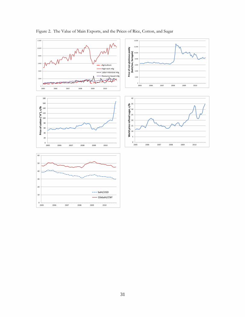
further 0.4% in the first quarter of 2009, as Figure 1 shows. The drop can be attributed to both

external and local factors. Domestically, political instability, including an opposition blockade of the

two main international airports and a change in government in late 2008, deterred tourists and

investors. Globally, the world financial crisis contributed too, as Thai exports of high-tech

manufactures fell sharply in the latter half of 2008 (see Figure 2), and consumers (including potential

tourists) restrained their spending. Thailand was also buffeted by a rapid rise in the price of energy

imports in 2008-09, but was a net beneficiary from the increase in the price of rice experienced in

2008 (and which was partly, but not completely, reversed in 2009), as Figure 2 also shows.

Some of the effects were dramatic. The number of tourist arrivals fell from 1.5 million in

February 2008 to 1.1 million in February 2009. The unemployment rate in the export sector rose

from 2% in the last quarter of 2008 to 9% in the first quarter of 2009. And the total number of

6

unemployed increased from 490,000 in July 2008 to 880,000 by January 2009; even after allowing for

seasonal variation, this represents a substantial rise, as the right-hand panel in Figure 1 shows.

Changes in world prices of important commodities such as rice, cotton, sugar, and energy

(including energy-intensive goods such as fertilizer) were transmitted very quickly to domestic prices.

The average prices of exports and imports both fell sharply after mid-2008, recovering equally

quickly in 2009, representing a major mechanism by which the world recession was transmitted to

Thailand.

In the light of such changes, it is perhaps surprising that the value of the baht has changed

so little since 2007 (see Figure 3). The stability of the real exchange rate meant that changes in the

world prices of important commodities such as rice, cotton, sugar, and energy (including energy-

intensive goods such as fertilizer) were transmitted to domestic prices.

3. Government Measures to Cope with Economic Shocks

The government responded robustly to the shocks with two rounds of stimulus packages – boosting

wage and salary payments to the lowest-paid public employees, raising payments to pensioners,

subsidizing utilities for the poor, capping some food prices, lowering interest rates, providing credit

guarantees, and spending on temporary jobs. Between the first and second quarters of 2009,

government spending rose by 5.6%, and may have prompted the 3.8% rise in consumption spending

that occurred then, even while GDP continued to fall (by 0.2%). By July 2009 the number of

unemployed had fallen to 480,000.

More specifically, the government responded with a range of fiscal and monetary initiatives

to raise consumption and ease the flow of credit to households:2

2 Off-balance sheet support was also provided through Specialized Financial Institutions (SFIs), when commercial banks drew back their lending. Although this channel of financing is not accounted for in the national accounts or public debt figures, to the extent that it took the place of standard bank lending, there may be little or no net effect to pick up.

7

Fiscal measures

(1) In 2008 the government launched a three-pronged program ranging from tax benefits to

individuals and businesses, improving access to credit for the poor in rural and urban areas, as well as

reducing inflationary pressures on the poor through energy and transport subsidies.

(2) These programs were extended after 2008, and in 2009 the government issued two additional

major stimulus measures (called ―SP1‖ and ―SP2‖) to help ward off growing fears of recession.

Between the first and second quarters of 2009 government spending actually rose by 5.6%.

(3) SP1, launched in March 2009, included a series of welfare measures to improve the situation of

the poor, including a tax program to benefit small enterprises and support employment, handouts to

poor households and subsidies for housing, education, fuel, water, and transport; additional funding

was provided for rural health programs and the universal health plan, and buying back farmlands that

had been auctioned off. The overall budget outlay of SP1 was quite large (116.7 billion baht,

equivalent to 5.3% of quarterly GDP in the second quarter of 2009) but, as discussed below, since

these programs were spread widely across the population, each program under SPI involved a

relatively small transfer to a given household (on average 5 percent of monthly household

expenditure).

(4) In mid-2009 SP2 was introduced, which focused primarily on a major increase in funding for

infrastructure, and working with banks to make access to credit easier for businesses and individuals.

Monetary measures

To help support borrowing, the government relaxed its monetary policy throughout the period,

cutting its policy interest rate progressively from 3.5 percent in early 2008 to 1.25 percent by the end

of 2009.

8

4. Data

In this paper, we focus on the effects of some major components of SP1 on household

consumption, income and debt, because this was the first major targeted response to the crisis. Our

main interest is in understanding how households responded to these anti-recessionary policies, in

anticipation of, as well as after, the policies were introduced and implemented. These questions are

particularly relevant in the current economic climate, where the trade-offs of a large-scale

government stimulus in a sudden crisis (and hence rising government deficits) are still being debated.

Examining these trends is difficult without intra-year data on fluctuations in household consumption

and income, to match with the timing of fiscal and monetary policy interventions.

In the case of Thailand, however, relatively detailed nationally-representative data are

available on a monthly basis through the Socioeconomic Survey (SES) conducted by the National

Statistics Organization (NSO). This survey, which covers about 4,000 households each month, has

extensive information on household consumption, sources of income and employment, household

participation in government programs, household debt, as well as household perceptions of their

economic status. In what follows we present a discussion of findings from the SES rounds before

and after the financial crisis, month by month from January 2006-December 2010. The purpose here

is to illustrate the potential impacts of the crisis and its aftermath in Thailand. While the rounds of

the SES do not form a household panel, each round/month surveyed the same rural/urban areas

within Changwats across the five major regions in the country. There were a total of 157 of these

communities, 79 urban and 78 rural. Within each community, there were about 90 primary sampling

units (PSUs: villages/neighborhoods), and 10-15 households were interviewed within each PSU. We

use this synthetic panel of communities to examine the effects of SP1 after 2009; unfortunately we

do not have panel data at the household level.

9

Measuring participation in the stimulus programs

Specifically, we focus on the three components of SP1 that had the greatest share of their budget

disbursed by mid-2009 (Jitsuchon and Patanarangsun 2009). These programs also have the

important advantage that they can be matched with the SES data to determine which households

were targeted. The three programs we examine are as follows:

(1) The extension of free public education to 15 years in the 2009 school year, providing students

with uniforms, textbooks, and exercise books free-of-charge, as well as subsidizing other school

costs. We assume the benefits flow to households with children 18 years of age and younger. The

total budgeted allocation was 19 million baht, of which 82 percent was disbursed between March and

May 2009.

(2) The distribution of 500 baht allowances for a period of six months to senior citizens of 60 years

or older who do not receive support from other government institutions, and who register at local

administration offices. Unlike previous schemes, participants were not selected based on their degree

of poverty. The total budgeted allocation was 9 million baht, of which 67 percent was disbursed by

May 2009.

(3) The provision of one-time 2000-baht subsidies (Saving the Nation checks) to workers who were

contributing to the Social Security Fund, state enterprise employees, and civil servants (including

tambon and village heads), who were earning less than 15,000 baht per month. The handouts were

paid in cashier's checks to be used to purchase goods at local stores, later cashed by businesses at

designated banks. The total budget was 19 million baht, of which 93 percent was disbursed by May

2009.

10

Some schooling subsidies and elderly assistance were in effect prior to March 2009, but SP1

vastly increased the scope and targeting of such programs. We used the detailed data in the SES on

household socioeconomic characteristics as well as participation in other government programs to

determine whether households in the SES were eligible to participate in these SP1 programs based

on the eligibility criteria described above. Because SP1 was introduced in March 2009, we interact

the eligibility status for each program with a post-March 2009 dummy.

Table 1 provides summary statistics on household participation across different government

programs over 2006-2010 (stimulus and non-stimulus programs), including the share of households

that were targeted for the three stimulus programs under SP1 above. Participation in most

government programs was fairly flat throughout 2006-2010, except for social assistance for the

elderly, which rose in both urban and rural areas after 2008. This is likely highly correlated with the

component of SP1 focused on elderly assistance. Among the stimulus programs, roughly 80 percent

of households in urban and rural areas were targeted across any one of the three programs in 2009.

Free education had the largest share of targeted households (45 percent in urban and 60 percent in

rural areas). Elderly assistance targeted about 30 percent of urban households and 39 percent of

rural households. Transfers to workers contributing to Social Security was more lopsided, with about

15 percent of rural households eligible compared to 30 percent in urban areas.

As mentioned earlier, while SP1 was a large program, individual transfer programs spread

out over a large targeted population led to interventions that were relatively small as a percentage of

increases in capital expenditure. Using each program‘s budget outlay/structure of transfers, we

calculated that the free education and elderly assistance programs constituted about 2-3% of

households‘ monthly per capita expenditure, and a one-time 10% increase in consumption from the

Saving the Nation‘s Checks program. For this reason, and also since households could participate in

11

multiple components of the stimulus, we aggregate the three programs into a single binary

participation variable for the analysis.3

Because our participation variable is imputed based on eligibility criteria rather than

measured directly – the SES did not ask about participation in these programs – the effects we

measure in the analysis are more of an intent to treat rather than an actual impact of participation.

We are therefore examining the potential effect of the stimulus as if everyone who was eligible also

received benefits under the program.4 Aggregate statistics do show, however, that most eligible

households participated in the stimulus.

Within some rounds, the SES data also collected information on households‘ perceptions of

the economy. In the first six months of 2008 and 2009, for example, households were asked in the

SES whether they believed the economy was in a worse situation compared to a year ago. Figures 4

and 5 show that just prior to the onset of the financial crisis in late 2008, urban and rural households

across the board believed that the economy was worsening compared to the same point in 2007. By

June 2008, less than 15 percent of rural and urban households both felt that the economy was doing

better compared to 2007, a drop from about 25 percent in January of 2008. Rising oil and

commodity prices helped fuel these sentiments, as indicated by Table 2, which shows that in 2008

price control was among the most important concern for households. By 2009, a greater share of

households (about 35 percent) felt that the economy was doing better compared to in 2008, although

this share slipped somewhat and flattened by mid-2009.

In this context, we can examine the coping strategies households adopt in a crisis. Table 2

presents summary data on how households expected to cope during a crisis, and shows that during

the first half 2008 they were overwhelmingly inclined to reduce spending and limit their borrowing if

3 As reflected in Table 1, households might also be participating in similar programs (with similar eligibility criteria) as SP1 prior to March 2009. In the analysis, therefore, we tested for whether the effect of the stimulus was any different if we also controlled for whether the household matched any of the eligibility criteria across all years (as a proxy for whether they would be participating in any similar programs at any other point of time). We found that the effect of the stimulus was unchanged. 4 This is a common problem with many impact evaluations, where even if a household is targeted they may not participate (or the extent of participation may vary among program households).

12

economic conditions suddenly worsened. Figure 5 shows that while these tendencies did not vary on

a month-to-month basis in early 2008/2009, there are some substantial differences across types of

households (urban/rural, and quantiles of per capita expenditure). Households at the highest end of

the distribution, for example, were less likely to say they would limit spending and borrowing

compared to poorer households, and would be more likely to tap into existing savings during a crisis.

The SES also asked whether households would be ready to seek part-time work in a crisis; there are

limited differences across quantiles, but rural households appear more likely to engage in part-time

work. Generally, Figure 5 does not show big differences in these patterns between 2008 and 2009.

How do these perceptions translate into actual decision-making on household consumption,

income and debt over the period? Table 3 presents summary statistics by year on key outcomes of

particular interest (although income-related variables are not available for 2008 and 2010, when the

SES just collected data on consumption expenditures); the numbers have been deflated by the

monthly and regional (rural/urban) consumer price index of 2006. It shows that there is not much

variation, except for a small year-to-year real increase, in the yearly aggregates of consumption and

income over time. The changes only vary slightly after the crisis of 2008. Of course, there are sharp

differences in these outcomes between rural and urban areas: even after controlling for regional price

indices, household per capita expenditure in rural Thailand in 2010 accounts for some 56 percent of

household per capita expenditure in urban Thailand. The difference in income is even more striking:

An average household in rural areas made only 47 percent as much income, on a per capita basis, as

an urban household in 2009, even after adjusting for price differences.

Table 3 shows some substantial changes, however, in components of per capita expenditure

that were particularly sensitive to the price fluctuations between 2008 and 2009. Spending on fuel for

transport, for example, jumped with oil prices in 2008 and fell back in 2009 only to increase again by

2010. Electricity expenditures increased gradually over the period. Expenditures on public

transport, however, declined over the period, accelerated to some degree after late 2008/2009 by the

public transport subsidies under the stimulus.

13

As for household debt, there are some indications that households were more averse to

taking on debt during the crisis period. The share of households with outstanding loans declined

only very slightly over the period, but the share of households repaying debt rose in 2009 over 2008

levels, particularly in urban areas. Figure 6 shows a general increase in debt repayment during 2009-

early 2010 before falling back in late 2010.

Because of Thailand‘s dependence on its export market for employment and income for

many households in both urban and rural areas, it is likely that a lot of households might have lost

jobs even if temporarily during the crisis. Households‘ income and expenditures therefore depend

on their job stability during the crisis. Table 3 shows trends in the share of households with at least

one unemployed person aged 15 or above over the period. For urban areas in particular, the crisis

that unfolded in late 2008 seems to have generated a short jump in unemployment rates among

households in early 2009. In rural areas, however, there is no change in unemployment over the

period.

Figures 7a and 7b also examine monthly trends in per capita expenditure by different

eligibility groups under the SP1 programs we examine. The graphs reveal some additional patterns

not captured by the year-to-year aggregate trends in Table 3. For households with young children

and elderly, per capita expenditure was either flat or declined until early 2008, fell again in mid to late

2008, and then picked up after 2009 (Figure 7a). Monthly variations in income and consumption for

households across quantiles of per capita expenditure also reveal some interesting trends. We find

that clearly for poorer households, particularly in rural areas, per capita expenditure frequently

outpaces income, and they experience greater income volatility (as measured by the difference

between last month‘s and current income) from month to month. Consumption overall has

remained relatively flat for most households within each percentile over the period; in rural areas, the

bottom 25th percentile saw an increase from around 2000 baht in 2006 to around 2500 baht by the

end of 2010 – a modest rise in monetary terms, but a jump of a fifth over a period of four years.

14

5. Analytical Framework

Changes in monthly income, expenditure, debt, and unemployment across months and years in a

given economy reflect the influence of both government and private sectors. In an open economy

such as Thailand, other countries also play a role through various ways. Therefore, even if the GDP

crunch in early 2009 due to sliding export demand was rapid but short-lived, it is expected that

changes in income, expenditure and other outcomes at the household level between the periods

before and after the crisis are likely to be influenced by the economic crisis. The quick recovery of

GDP demonstrates the resilience of the Thai economy to manage and weather the crisis. What has

happened to the welfare of the citizens of Thailand, especially among the poor and those more

vulnerable to fluctuations in exports dependent on the outside markets? As we can see in Figures 7a

and 7b, some households were hit more than others, with the strongest effects being in the urban

areas. This is because coping abilities differ across households and across regions because not all

segments of the economy are vulnerable to economic crisis linked to the outside economy.

The government stimulus (call it G) is measured here by the extent of support received by

households under the main SP1 programs. We expect that simply by raising the extent of support,

the government stimulus can affect household expenditure (c) both directly and indirectly through

average monthly income (I), and its monthly share (s), which is measured as income in the month of

the interview divided by average income over the previous year, and picks up the effects of

seasonality or other shocks. This relationship is represented in the following equation (1):

. .I s

dc dc dc dc dI dc ds

dG dG dG dI dG ds dG

(1)

There are 4 components of changes likely to take place as a consequence of government stimulus:

The first term measures changes in per capita expenditure due to a government stimulus, for a given

level of average monthly income. The second term measures the changes in expenditure with a

government stimulus, given the distribution of recent monthly share of a household‘s income. The

15

third term is the changes in per capita expenditure due to induced changes in average monthly

income, while the fourth term measures the effect due to induced changes in monthly share of

income. We argue that a government stimulus affects both monthly share as well as monthly income

and thus is expected to help smooth income and consumption during the crisis and its aftermath. It

is not that households did not receive any such support before the crisis, but as Figure 8 shows, the

extent of program coverage and its volume (in particular welfare programs) were increased following

the crisis due to fiscal measures adopted as part of the government stimulus programs.

Estimating (1) to distinguish the role of government stimulus is problematic for a number of

reasons. Because of lack of a proper counterfactual, we do not know what would have happened to

expenditure had there been no crisis and consequently no government interventions adopted,

especially to counter the negative consequences of the crisis. In this case, what we can infer is

possible effects of government stimulus by estimating and comparing the effects of crisis and

government programs on the changes in household outcomes (such as per capita expenditure and

income) before and after the crisis of 2008.

Yet the effects of global economic crisis measured in this way may not be an accurate picture

unless we control for the unobserved inherent ability of households and communities to cope with

any shock that is independent of the observed coping mechanisms adopted by households,

communities, and governments following a crisis. Hence, what we observe in the descriptive and

trend analysis is an outcome of the interactions of all observed and unobserved forces. How to

disentangle them in terms of the relative strengths of government responses versus household coping

strategies is an empirical challenge. What we follow here is a three-step procedure to discern the role

of household and government forces in averting the negative consequences of such a global crisis

affecting the Thai economy.

The first step involves a structural model of income-consumption smoothing where monthly

variations in per capita expenditure are explained by, among other factors, average monthly income

and its monthly volatility (the ratio of last month‘s income, which was recorded in the SES, to

16

average monthly income).5 We argue that income volatility as observed in the monthly data over

time is caused in part by income shocks driven by many factors including global economic crisis. If

households manage to smooth consumption even after the crisis, it is possible either because

households could withstand consumption and income shocks without government help, or managed

to cope with income shocks due to the crisis with help from the government through its stimulus

programs. Consequently, the second step involves estimating a reduced-form model where changes

in monthly income and consumption are explained by household participation in government

stimulus programs.

The second step estimates the total effects of government stimulus programs (i.e., dc/dG in

equation 1), the combined effects of all 4 components as laid out in equation (1). In order to

understand the extent of the effects of government stimulus independent of households‘ own ability

measured by income and its monthly variability, the third step, therefore, involves estimating the

changes in per capita consumption in terms of monthly variations in average household income and

its monthly share, conditioned by household participation in government programs. The third step

essentially helps estimate the relative roles of household and government in weathering the crisis in

terms of monthly fluctuations in income and consumption.

But the main challenge remains, i.e., how to control for the unobserved common time

invariant and time varying heterogeneity that affects household income, expenditure, and access to

government stimulus programs simultaneously. Note that unobserved heterogeneity can be

household-, community- and season-specific. This requires a complicated econometric estimating

strategy to estimate the net effects of government stimulus on household ability to withstand the

crisis unfolded after 2008 in Thailand.

5 This measure of income volatility or seasonality was also used by Paxson (1993).

17

6. Model and Estimation Strategy

Model

The first step involves examining the effects on per capita expenditure from average monthly per

capita income, and the share of actual monthly income to average monthly income (as a measure of

volatility in monthly income). Determining the effects of income volatility on average per capita

consumption is a first step in understanding how policies may have a role in helping households cope

with sudden economic shocks. Specifically, following Khandker (2012), we examine trends in

average household per capita expenditure and other outcomes using the panel of communities in the

SES data,

c jm 1s jm 2I jm x jm jm (2)

Here

c jm is average per capita consumption expenditure across households living in community j at a

specific month m. As a measure of income volatility, s represents last month‘s income divided by

average monthly income I. We also consider a vector of community characteristics

x ,6 and

is a

vector of unobserved characteristics affecting outcomes.

Note that measures the role of time-varying observed household and community

characteristics in consumption. On the other hand, 1 measures the effect of monthly share of

average monthly income, while 2 measures the effect of changes in average monthly income.

If 01 , monthly income variability is not an issue, and monthly consumption is determined by

average monthly income. This is the case of perfect consumption smoothing (within a year) where

households are able to smooth consumption despite any shocks in monthly income.

6 The SES surveys do not have community modules. So these characteristics are basically averages of household level variables such as household head‘s age and age squared, gender, religion, marital status, years of schooling as well as whether any household member 18 years or older had a chronic illness or disability; household age/gender composition and whether the house was made of solid construction (bricks/cement).

18

However, if

1 0 , there is incomplete consumption smoothing, meaning that seasonal

consumption tracks seasonal income. If there is a lack of consumption smoothing, we have

either

1 2, or

1 2. If 1 2 , then household consumption is more sensitive to average income

than to seasonal income; in this case, a fraction of seasonal income may be saved for managing

consumption smoothing if consumption exceeds income in a given season, implying some degree of

consumption smoothing even if imperfect (Deaton, 1997). Conversely, if 1 2 , then household

consumption is more sensitive to seasonality of income than to average income; in this case,

households may not save any fraction of seasonal income to manage consumption smoothing, even

if seasonal income exceeds seasonal consumption in a particular season.

However, both income and expenditure are jointly determined by a set of government policy

variables in addition to household and community characteristics. Therefore, the second step

involves examining the effects of household participation in fiscal stimulus schemes on per capita

expenditure and income. This is to test whether government spending, examined in this paper as the

share of households participating in a government stimulus (G), would allow better smoothing of

income and consumption:

c jm 1G jm x jm jm (3a)

s jm 2G jm x jm jm (3b)

I jm 3G jm x jm jm (3c)

Here measures the effect of participation in the stimulus on income and consumption. As

noted in equation (1), equations (3a-3c) measure the effects of government interventions on

household welfare: it can help the long- or short-run income-earning potential of households,

thereby smoothing income and consumption, or it can increase or change the composition of

household consumption directly. Other than relying on government support, households may have

19

their own strategies to smooth income and consumption, which may be observed and captured

through the effects of socioeconomic variables x.

However, we are also interested in explaining how much variation in monthly consumption,

for example, is attributable to household income (independent of government programs) as well as

the net effect of household participation in government stimulus. As a third step, therefore we

estimate equation (4) below after including participation in the stimulus G directly in equation (2),

given its independent effects as follows.

c jm 1s jm 2I jm G jm x jm jm (4)

Estimation strategy

The most difficult issue in estimating the models laid out in equations (2)-(4) is the joint dependence

of income and consumption on x as well as the endogeneity of household participation in

government programs. In other words, the effects of income and participation in government

programs on consumption cannot be isolated unless an appropriate identification strategy is

followed. The estimation of independent effects of policy intervention is thus a question of

appropriate identification followed in estimation.

In order to understand why identification is an issue and how one can resolve this issue, let

us assume that the error term (

jm ) has the following implicit structure:

jm j m jm (5)

Here j represents common community heterogeneity, m represents unobserved common

month heterogeneity and jm is an independent error uncorrelated with any regressors. Thus,

estimation of equations (2)-(4) will not yield unbiased estimates because of the underlying error

structures given by (5). According to equation (5), the share of households participating in

20

government stimulus programs as well as monthly average income and its volatility plus consumption

are all influenced by unobserved community heterogeneity.

At the same time, when we relate monthly consumption to monthly income and its volatility

plus some non-income factors, we invariably introduce a common month effect, which affects a

household‘s monthly income, consumption and participation. That is, consumption may be

completely independent of monthly variations in income and government policies, and still co-vary

with monthly income, simply because of a common month effect (Khandker, 2012). For example,

there is a common monthly but unobserved factor, such as preference of households for certain

foods in a specific month – the New Year, for instance – in which case we would get an effect simply

because of this common month factor, even though it has nothing to do with monthly variations in

income or prices, or participation in government program.

Note that introducing a monthly dummy in the above equations (2)-(4) does not resolve the

problem of a common-month effect, because this monthly dummy does not control for the

unobserved, location-specific common time effect ( ). Correcting this sort of bias requires monthly

household panel data (i.e., repeated observations across months for each household unit), which we

do not have. But we have monthly data across households over years across communities. For

example, we have community panel data at the sub-Changwat or sub-province level (which as

mentioned earlier is the lowest common sampling unit that can help create the panel across months).

Using the community-level panel, we could apply a panel fixed-effects regression, and to control for

monthly unobserved bias, we can include month*community interaction variables along with a time

trend to control for both j and m .

However, a panel fixed-effects model may not suffice to account for time-varying

unobserved factors that influence how households respond to stimulus and its associated impacts in

the local economy. To account for time-varying unobserved heterogeneity, our approach in this

paper is to estimate a dynamic panel model (Arellano and Bond 1991; Jalan and Ravallion, 1998,

2002) using the multiple waves of monthly data. As described below, we also account for a range of

21

lagged community characteristics and national prices as additional instruments that would affect

access to the stimulus, as well as household outcomes.

Going back to equation (4) as an example, average community per capita expenditure

c jm

(as well as other outcomes) depend on the lagged outcome,

c jm1, the community‘s current and

lagged characteristics jmx and , 1j mx , and government stimulus

G jm :

1 1 2 1 1jm jm jm jm jm jm jmc c x x G u (5)

We assume that the error term includes a community-specific unobserved effect

jm (which may

also include unobserved geographic effects) correlated with the regressors, as well as an i.i.d. random

component

u jm , which is orthogonal to the regressors and serially uncorrelated.

If

jm j (that is, the unobserved effect is fixed over time), taking deviations from

means in equation (5) removes the unobserved effect and yields the following differenced equation:

(c jm c j ) (c jm1 c j )1(x jm x j )2(x jm1 x j )(G jm G j ) (u jm u j ) (6)

However, heterogeneity stemming from the unobserved community-specific effect

may not be

constant over the period

( jm j ) . Changes in other conditions over time (e.g., market

conditions), for example, may alter the effects of household and geographic characteristics on

outcomes from year to year.

On introducing dynamics and both time-invariant and time-varying unobserved effects, the

model we estimate from equation (6) is a modified autoregressive distributed lag of order 1 or

AD(1,1) model. But the OLS estimator of an autoregressive fixed-effects model is not consistent for

a typical panel where the number of periods is small and the asymptotics are driven by the number of

cross-sections going to infinity (Hsiao 1986). The inconsistency arises because of the potential

correlation between the lagged endogenous variables and the residuals in the transformed model.

Thus, instead of standard difference-in-difference techniques, we use a dynamic lagged dependent-

variable approach, proposed by Arellano and Bond (1991), to estimate equation (6).

22

With serially uncorrelated error terms,

u jm , GMM methods are the most efficient in the class

of instrumental variable estimators to estimate the parameters in equation (6). In estimating equation

(2),

c jm1 or higher lagged levels are valid instrumental variables for time-varying unobserved

characteristics that affect outcomes (Jalan and Ravallion 1998, 2002). Our instrument set also

includes second and higher-order levels of community characteristics

x jm reflecting prices and

household access to infrastructure and characteristics of land and labor markets.7 These include, for

example, the lagged proportions of households in agriculture, or that are self-employed, renting or

owning their property, and the average rent per bedroom in the community, as well as the share of

households with internet connections, and who use gas or electricity for cooking. As Thailand‘s

economy is highly integrated with global markets, we also include the world prices of key

commodities as instruments that could affect only income or government stimulus programs but not

directly the consumption pattern of households. We also argue that changes in the interest rates

(repurchase rate) set by the government reflects changes in the stance of monetary policy, which can

have an effect on both income and government spending such as stimulus programs. In the

estimations, income and program participation are instrumented by using lagged monetary policy

decisions (one month lag) on the repurchase rate, as well as lagged world commodity prices (6 month

lag) that are likely to affect imports and exports of Thailand‘s economy. Specifically, the world

commodity prices we used were for copper, rubber, maize, and sugar.

7. Discussion of the Results

Test of consumption smoothing model

Our starting point is to test whether households managed to smooth income and consumption in

Thailand over the study period. Table 4 presents the GMM estimates of the effects of monthly

income volatility, as well as log average per capita monthly income, on household per capita

7 Jalan and Ravallion (1998) also use lagged levels of the dependent and explanatory variables to instrument for

potentially endogenous regressors, as well as initial (first-round) geographic factors.

23

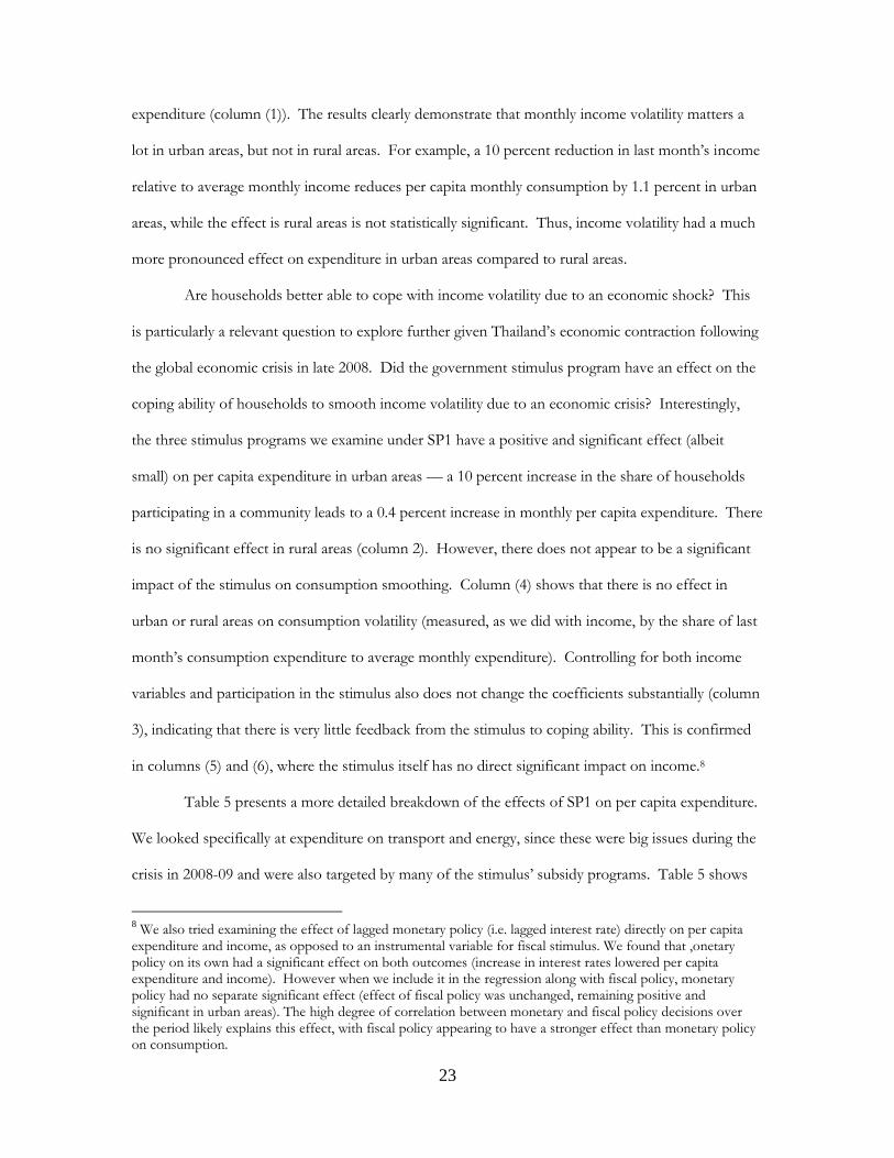
expenditure (column (1)). The results clearly demonstrate that monthly income volatility matters a

lot in urban areas, but not in rural areas. For example, a 10 percent reduction in last month‘s income

relative to average monthly income reduces per capita monthly consumption by 1.1 percent in urban

areas, while the effect is rural areas is not statistically significant. Thus, income volatility had a much

more pronounced effect on expenditure in urban areas compared to rural areas.

Are households better able to cope with income volatility due to an economic shock? This

is particularly a relevant question to explore further given Thailand‘s economic contraction following

the global economic crisis in late 2008. Did the government stimulus program have an effect on the

coping ability of households to smooth income volatility due to an economic crisis? Interestingly,

the three stimulus programs we examine under SP1 have a positive and significant effect (albeit

small) on per capita expenditure in urban areas — a 10 percent increase in the share of households

participating in a community leads to a 0.4 percent increase in monthly per capita expenditure. There

is no significant effect in rural areas (column 2). However, there does not appear to be a significant

impact of the stimulus on consumption smoothing. Column (4) shows that there is no effect in

urban or rural areas on consumption volatility (measured, as we did with income, by the share of last

month‘s consumption expenditure to average monthly expenditure). Controlling for both income

variables and participation in the stimulus also does not change the coefficients substantially (column

3), indicating that there is very little feedback from the stimulus to coping ability. This is confirmed

in columns (5) and (6), where the stimulus itself has no direct significant impact on income.8

Table 5 presents a more detailed breakdown of the effects of SP1 on per capita expenditure.

We looked specifically at expenditure on transport and energy, since these were big issues during the

crisis in 2008-09 and were also targeted by many of the stimulus‘ subsidy programs. Table 5 shows

8 We also tried examining the effect of lagged monetary policy (i.e. lagged interest rate) directly on per capita expenditure and income, as opposed to an instrumental variable for fiscal stimulus. We found that ,onetary policy on its own had a significant effect on both outcomes (increase in interest rates lowered per capita expenditure and income). However when we include it in the regression along with fiscal policy, monetary policy had no separate significant effect (effect of fiscal policy was unchanged, remaining positive and significant in urban areas). The high degree of correlation between monetary and fiscal policy decisions over the period likely explains this effect, with fiscal policy appearing to have a stronger effect than monetary policy on consumption.

24

that expenditure on petrol for transport declined substantially in both urban and rural areas at the

time of the stimulus – perhaps demand for travel fell, or prices came down – and expenditure on

public transportation also declined (although the effects for this outcome were not significant), likely

as a result of government subsidies that made some bus routes free to users. However, expenditures

on electricity rose (again more so in urban than rural areas), indicating that households may have

been re-allocating their expenditures across different areas in response to the stimulus. Per capita

expenditure on water also rose in urban areas. We revisit this issue of reallocating components of

expenditure below, in our discussion of household coping with the crisis.

Throughout the analysis, we present two sets of tests for our dynamic panel results. The

first is the Arellano-Bond test for autocorrelation, which has a null hypothesis of no autocorrelation

and is applied to the differenced residuals. The test for AR(1) in first differences usually rejects the

null hypothesis, which is expected since

u jm u jm u jm1 and

u jm1 u jm1 u jm2 both have

u jm1. The test for AR(2) in first differences is more important, because it will detect higher-order

autocorrelation, namely between

u jm u jm u jm1 and

u jm2 u jm2 u jm3 . The GMM

system estimator, which is consistent if there is no second-order serial correlation in residuals. We

reject second-order autocorrelation for all regressions. The second set of tests is the Sargan and

Hansen overidentification tests (the null being that the instrument set is exogenous). In all of the

regressions, we do not reject the null hypothesis that the instruments are exogenous. The Sargan test

is typically used with unclustered standard errors, whereas the Hansen test is used when standard

errors are robust or clustered. In all the regressions, we cluster standard errors at the community

level.

The role of government stimulus in household coping

The government stimulus has not directly affected average income and its monthly volatility, but yet

has a positive effect on per capita expenditure (at least in urban areas). That is, the 3rd and 4th terms

of equation (1) are essentially zero, while the 1st and 2nd term are significant both for rural and urban

25

areas. So even if raising income or its monthly share is not the most direct route, there must be other

routes through which SP1 might have helped Thai households smooth their consumption by

reducing monthly variations in per capita income. In order to test other possible routes other than

income through which government programs help, we also examine at the coping strategies

households adopt during an economic crisis other than participation in a government welfare or

transfer program. As described earlier, the NSO in Thailand collected information about the

strategies households adopted during an economic crisis in its 2008, 2009 and 2010 SES surveys.

The household responses are categorized in two ways: What would they do in an economic crisis,

and what do they expect the government to do during the crisis? The responses are presented in

Table 2. We find that the most frequent coping strategy households say they would adopt during an

economic crisis was reducing household spending (more than 85 percent of Thai households report

they would reduce spending during a crisis). Households might also adopt some other strategies: 9

percent of households say they would tap into savings, and 8 percent report that they would seek

part-time employment if hit by a crisis. Interestingly, when borrowing is a way to meet the gap

between expected income and consumption, about half of Thai people do not like to be in debt

when a crisis hits. On the other hand, households are found to repay debt at a higher percentage

rate: For example, in urban Thailand, some 41 percent repaid debt in 2008 and 46 percent in 2009,

and 44 percent in 2010 (Table 3). The loan repayment rate is higher in rural areas than urban areas.

We therefore examine the effects of the stimulus on savings, borrowing, and debt repayment

by households in the community as possible coping strategies. Did households draw down on their

savings, or change their borrowing patterns to raise or maintain consumption? Table 6 presents the

results, again in a dynamic panel framework estimated by GMM. We find a negative but not

significant effect of the stimulus on savings in urban areas, as well as a negative effect on borrowing.

We also find that participation in the government stimulus helps increase the probability of debt

repayment with the effect being a little more pronounced in urban than rural areas Our analysis

26

therefore suggests that households were using the stimulus money to repay their existing debts, in a

direct reallocation of how household funds were being spent.

If the effect on savings is not significant, however, what can explain the significant rise in

consumption in urban areas? One possibility is that households experienced greater confidence in

the economy as a result of the government stimulus program, and increased their spending as a

result. Table 7 examines, in a fixed-effects panel framework, the monthly effects on the share of

households in the community that felt the economy was improving (based on the data available in

the SES, described in Figure 4). Although data on household perceptions are only available for the

first six months in 2008 and 2009, we find a significant pattern of lower confidence in urban areas by

mid-2008, with a rise in confidence by early 2009. We see a similar pattern in rural areas, although

the effects post-2008 are stronger in urban localities. The data, despite their limitations in coverage

across years, therefore seem to indicate that higher consumption may have stemmed from greater

confidence in the economy.

8. Lessons Learned: What Matters Most

The crash of global financial markets in 2008 caused a ripple effect on economic demand and growth

worldwide. Export-oriented economies were hit particularly hard by this financial crisis-induced

demand shock, and governments stepped in quickly with broad-ranging stimulus programs to lessen

the negative effects on households from rising unemployment and borrowing costs. To better

understand the role that stimulus policy might play in softening the effects of these shocks, we have

examined the nationally-representative data from Thailand, an export-dependent economy where a

large-scale stimulus program was introduced in 2009. Using monthly data spanning 2006-2010, we

use a dynamic lagged dependent model to examine the potential role of government stimulus on

household consumption, income, borrowing or debt repaid. To address simultaneity of changes in

government spending and household outcomes, we construct a community-level synthetic panel and

27

estimate a dynamic panel regression, instrumenting the stimulus effect with second-order lagged

outcome variables, and estimating the model using the Generalized Method of Moments (GMM).

Our results suggest that household participation in these programs helped smooth

consumption directly through higher consumption. But interestingly, this increase in higher monthly

consumption was not supported from household receipts from government stimulus, but the income

savings that were otherwise used to repay household existing debt. We typically find stronger effects

on consumption in urban compared to rural areas. We find a negative but not significant effect on

savings in urban areas, which may be another channel through which consumption expenditures

increase. Households also seem to have experienced greater confidence in the economy from the

stimulus spending, raising expenditures as well.

The Thai government had established an extensive welfare network after the 1997/98

financial crisis caused by currency shock. Such an extensive network was still present during the

2008/2009 crisis, through which the Thai stimulus program was partially implemented. These

schemes helped households to receive government support during an economic crisis. We found

that household participation in these programs helped not only consumption smoothing directly

through higher consumption.

The economic crisis in 2008 that hit Thailand was not so much through financial

institutions, unlike the case of the United States and other developed countries. Rather, the crisis

manifested itself through job and income cuts due to a sharp drop in export demand, as well as

domestic political uncertainty. In this situation, the stimulus in terms of both monetary and fiscal

measures that effectively reached the affected households through these safety net measures helped

urban households to cope with the fallout of this worldwide crisis. What matters here are that the

fiscal measures be appropriately designed and implemented. Thailand managed to avert the most

negative consequences of this crisis in part because of its reliance on the national level safety net

programs.

28

Bibliography

Alderman, Harold (1996). ―Saving and Economic Shocks in Rural Pakistan.‖ Journal of Development Economics, 51(2): 343-365. Arellano M., and S. Bond. 1991. ―Some Tests of Specification for Panel Data: Monte Carlo Evidence and an Application to Employment Equation.‖ Review of Economic Studies 58(2): 277–98. Auerbach, Alan, William G. Gale, and Benjamin H. Harris (2010). ―Activist Fiscal Policy.‖ Journal of Economic Perspectives 24(4): 141-164. Bank of Thailand (2011). http://www.bot.or.th/English/Statistics/Pages/index1.aspx [Accessed January 10, 2012.] Besley, Tim (1995). ―Nonmarket Institutions for Credit and Risk-Sharing in Low-Income Countries.‖ Journal of Economic Perspectives 9(3): 115-127. Bresciani, Fabrizio, Gershon Feder, Daniel O. Gilligan, Hanan G. Jacoby, Tongroj Onchan, and Jaime Quizon (2002). ―Weathering the Storm: The Impact of the East Asian Crisis on Farm Households in Indonesia and Thailand.‖ World Bank Research Observer 17(1): 1-20. Corsetti, Giancarlo, Andre Meier, and Gernot J. Muller (2011). ―Fiscal Stimulus with Spending Reversals.‖ Forthcoming, Review of Economics and Statistics. Dercon, Stefan, and Pramila Krishnan (2000). ―Vulnerability, Seasonality and Poverty in Rural Ethiopia.‖ Journal of Development Studies 36(6): 25-51. Economic Report of the President (2010). http://www.gpo.gov/fdsys/browse/collection.action?collectionCode=ERP [Accessed January 10, 2012.] Ennis, Huberto M., and Todd Keister (2010). ―Banking Panics and Policy Responses.‖ Journal of Monetary Economics 57: 404-419. Ferreira, Francisco H., Anna Fruttero, Phillippe Leite, and Leonardo Lucchetti (2011). ―Rising Food Prices and Household Welfare: Evidence from Brazil in 2008.‖ Working Paper, The World Bank. Friedman, Jed and James Levinsohn (2002). ―The Distributional Impacts of Indonesia‘s Financial Crisis on Household Welfare: A ‗Rapid Response‘ Methodology.‖ World Bank Economic Review 16(3): 397-423. Hsiao, C. 1986. Analysis of Panel Data. New York: Cambridge University Press. Jalan, J., and M. Ravallion. 1998. ―Are There Dynamic Gains from a Poor-area Development Program?‖ Journal of Public Economics 67(1): 65–85. ———. 2002. ―Geographic Poverty Traps: A Micro-Model of Consumption Growth in Rural China.‖ Journal of Applied Econometrics 17(4): 329–46. Khandker, Shahidur R., 2012. ―Seasonality of income and poverty in Bangladesh,‖ Journal of Development Economics, 97(2):244-256,

29

Mukherjee, Santanu and Shivani Nayyar (2011). ―Monitoring Household Coping During Shocks: Evidence from the Philippines and Kenya.‖ Working Paper, United Nations Development Programme, New York. Paxson, Christina (1993). ―Consumption and Income Seasonality in Thailand.‖ The Journal of Political Economy, 101(1): 39-72. Storesletten, Kjetil, Chris I. Telmer, and Amir Yaron (2001). ―How Important Are Idiosyncratic Shocks? Evidence from Labor Supply.‖ American Economic Review Papers and Proceedings, 413-417. Townsend, Robert (1995). ―Consumption Insurance: An Evaluation of Risk-Bearing systems in Low Income Economies.‖ Journal of Economic Perspectives, 9(3): 83-102. United Nations Economic and Social Commission for Asia and the Pacific (2009). ―Impact of the Economic Crisis on Poverty and Inclusive Development: Policy Responses and Options.‖ Working Paper, UNESC, New York.

30

Figure 1. Recent growth in GDP and consumer spending; and unemployment performance

-6.0

-4.0

-2.0

0.0

2.0

4.0

6.0

8.0

10.0

2005 2006 2007 2008 2009 2010

% c

han

ge f

rom

qu

arte

r to

qu

arte

r,

no

min

alPrivate consumption spending

GDP

0

1

1

2

2

3

3

4

2005 2006 2007 2008 2009 2010

Un

em

plo

yme

nt

rate

31

Figure 2. The Value of Main Exports, and the Prices of Rice, Cotton, and Sugar

0

2,000

4,000

6,000

8,000

10,000

12,000

2005 2006 2007 2008 2009 2010

Agriculture

High-tech mfg

Labor-intensive mfg

Resource-based mfg

0

2,000

4,000

6,000

8,000

10,000

12,000

14,000

2005 2006 2007 2008 2009 2010

Pri

ce o

f n

on

-glu

tin

ou

s p

add

y (b

aht/

ton

, far

mga

te)

0

20

40

60

80

100

120

140

160

180

2005 2006 2007 2008 2009 2010

Pri

ce o

f co

tto

n (

"A")

, c/l

b

0

5

10

15

20

25

30

35

40

2005 2006 2007 2008 2009 2010

Wo

rld

pri

ce r

efin

ed

su

gar,

c/l

b

0

10

20

30

40

50

60

2005 2006 2007 2008 2009 2010

baht/USD

10xbaht/CNY

32

Figure 3. Thailand: Exchange Rates

70

75

80

85

90

95

100

105

110

115

120

2005 2006 2007 2008 2009 2010

Re

al E

ffe

ctiv

e E

xch

ange

Rat

e

(lo

we

r=d

eva

luat

ion

)

80

85

90

95

100

105

110

115

120

2005 2006 2007 2008 2009 2010

Export price

Import price

33

Figure 4. Share of HH feeling that the economy has done better

compared to last year, SES 2008 and 2009 (January-June)

Share of HH thinking economy is doing better

compared to last year

0.1

0.2

0.3

0.4

0.5

2008-1

2008-2

2008-3

2008-4

2008-5

2008-6

2009-1

2009-2

2009-3

2009-4

2009-5

2009-6

Rural Urban

34

Figure 5. Coping strategies in a crisis, by percentiles of HH per capita expenditure

SES 2008 and 2009 (January-June)

Share of rural HH that would reduce spending in a crisis

0.75

0.8

0.85

0.9

0.95

2008-1

2008-2

2008-3

2008-4

2008-5

2008-6

2009-1

2009-2

2009-3

2009-4

2009-5

2009-6

Bottom 25th 25th-50th 50th-75th Top 25th

Share of urban HH that would reduce spending in a

0.75

0.8

0.85

0.9

0.95

2008-1

2008-2

2008-3

2008-4

2008-5

2008-6

2009-1

2009-2

2009-3

2009-4

2009-5

2009-6

Bottom 25th 25th-50th 50th-75th Top 25th

Urban Rural

Share of rural HH that would reduce debt in a

0.3

0.4

0.5

0.6

0.7

2008-1

2008-2

2008-3

2008-4

2008-5

2008-6

2009-1

2009-2

2009-3

2009-4

2009-5

2009-6

Bottom 25th 25th-50th 50th-75th Top 25th

Share of urban HH that would reduce debt in a

0.3

0.4

0.5

0.6

0.7

2008-1

2008-2

2008-3

2008-4

2008-5

2008-6

2009-1

2009-2

2009-3

2009-4

2009-5

2009-6

Bottom 25th 25th-50th 50th-75th Top 25thShare of urban HH that would tap into savings in a

0

0.05

0.1

0.15

2008-1

2008-2

2008-3

2008-4

2008-5

2008-6

2009-1

2009-2

2009-3

2009-4

2009-5

2009-6

Bottom 25th 25th-50th 50th-75th Top 25th

Share of urban HH that would seek part time work in a

0

0.05

0.1

0.15

2008-1

2008-2

2008-3

2008-4

2008-5

2008-6

2009-1

2009-2

2009-3

2009-4

2009-5

2009-6

Bottom 25th 25th-50th 50th-75th Top 25th

Share of rural HH that would seek part time work in a

0

0.05

0.1

0.15

2008-1

2008-2

2008-3

2008-4

2008-5

2008-6

2009-1

2009-2

2009-3

2009-4

2009-5

2009-6

Bottom 25th 25th-50th 50th-75th Top 25th

Share of rural HH that would tap into savings in a crisis

0

0.05

0.1

0.15

2008-1

2008-2

2008-3

2008-4

2008-5

2008-6

2009-1

2009-2

2009-3

2009-4

2009-5

2009-6

Bottom 25th 25th-50th 50th-75th Top 25th

35

Figure 6. Trends in debt repayment, SES 2008-2010

HH has repaid debt in the last 12 months (Y=1 N=0)

0.4

0.45

0.5

0.55

0.6

0.65

2008-5

2008-7

2008-9

2008-1

1

2009-1

2009-3

2009-5

2009-7

2009-9

2009-1

1

2010-1

2010-3

2010-5

2010-7

2010-9

2010-1

2

Urban RuralPoly. (Rural)

36

Figure 7a. Trends in monthly per capita consumption, by eligibility for stimulus

Thailand SES 2006-2010

Per capita expenditure,

rural HH with children aged 14 and below

2500

3000

3500

2006-1

2006-7

2007-1

2007-7

2008-1

2008-7

2009-1

2009-7

2010-1

2010-7

Per capita expenditure,

urban HH with children aged 14 and below

3500

4000

4500

5000

2006-1

2006-7

2007-1

2007-7

2008-1

2008-7

2009-1

2009-7

2010-1

2010-7

Per capita expenditure,

urban HH with at least one elderly member (aged 51+)

4500

5000

5500

6000

2006-1

2006-7

2007-1

2007-7

2008-1

2008-7

2009-1

2009-7

2010-1

2010-7

Per capita expenditure,

rural HH with at least one elderly member (aged 51+)

2500

3000

3500

4000

2006-1

2006-7

2007-1

2007-7

2008-1

2008-7

2009-1

2009-7

2010-1

2010-7

37

Figure 7b. Trends in monthly per capita consumption, by eligibility for stimulus

Thailand SES 2006-2010

Urban areas, bottom 25th percentile

3500

4000

4500

5000

5500

6000

6500

2006-1

2006-7

2007-1

2007-7

2008-1

2008-7

2009-1

2009-7

2010-1

2010-7

HH per capita income last month

HH avg monthly per capita income

HH per capita consumption

Urban areas, 25th-50th percentile

4000

5000

6000

7000

8000

2006-1

2006-7

2007-1

2007-7

2008-1

2008-7

2009-1

2009-7

2010-1

2010-7

HH per capita income last month

HH avg monthly per capita income

HH per capita consumption

Urban areas, 50th-75th percentile

4000

5000

6000

7000

8000

9000

10000

11000

2006-1

2006-7

2007-1

2007-7

2008-1

2008-7

2009-1

2009-7

2010-1

2010-7

HH per capita income last month

HH avg monthly per capita income

HH per capita consumption

Urban areas, top 25th percentile

7000

9000

11000

13000

15000

17000

19000

21000

2006-1

2006-7

2007-1

2007-7

2008-1

2008-7

2009-1

2009-7

2010-1

2010-7

HH per capita income last month

HH avg monthly per capita income

HH per capita consumption

Rural areas, bottom 25th percentile

1500

2000

2500

3000

3500

Rural areas, 25th-50th percentile

2000

3000

4000

5000

Rural areas, 50th-75th percentile

2500

3000

3500

4000

4500

5000

Rural areas, top 25th percentile

4000

5000

6000

7000

8000

2006-1

2006-7

2007-1

2007-7

2008-1

2008-7

2009-1

2009-7

2010-1

2010-7

HH per capita income last monthHH avg monthly per capita incomeHH per capita consumptionTrend, incomeTrend, consumption

38

Table 1. Summary statistics on participation in government programs SES Round

2006 2007 2008 2009 2010

Urban Participation in government programs

Any government welfare program 0.21 0.22 0.22 0.21 0.21

[0.41] [0.41] [0.41] [0.41] [0.41]

Social pension for the poor elderly 0.032 0.053 0.069 0.143 0.23

[0.18] [0.22] [0.25] [0.35] [0.42]

Social assistance for the disabled 0.01 0.01 0.02 0.01 0.02

[0.07] [0.085] [0.108] [0.115] [0.14]

Free school lunch/supplementary food 0.15 0.16 0.16 0.17 0.17

[0.36] [0.36] [0.36] [0.37] [0.38]

Government scholarship 0.02 0.01 0.012 0.010 0.007

[0.13] [0.11] [0.11] [0.096] [0.082]

Other government funds to assist farmers 0.003 0.002 0.001 0.002 0.006

[0.053] [0.043] [0.028] [0.041] [0.08] Borrowing

Village Fund 0.104 0.092 0.081 0.089 0.090

[0.305] [0.29] [0.27] [0.29] [0.29]

People Bank 0.011 0.005 0.003 0.003 0.002

[0.10] [0.069] [0.056] [0.054] [0.043]

Government loan for education/other loan 0.026 0.019 0.019 0.020 0.017

[0.16] [0.14] [0.14] [0.14] [0.13] SPI Stimulus (March 2009)

(A) Free public education - - - 0.46 0.45 - - - [0.50] [0.50]

(B) Elderly assistance - - - 0.32 0.31

- - - [047] [0.46]

(C) Saving the Nation’s Checks - - - 0.32 0.29

- - - [0.46] [0.45]

Combined stimulus ((A), (B) or (C)) - - - 0.79 0.76

- - - [0.09] [0.08]

Number of households 27,939 26,494 27,851 27,048 27,297

Rural Participation in government programs

(A) Government/state enterprise’s welfare 0.12 0.12 0.12 0.12 0.11

[0.32] [0.32] [0.32] [0.32] [0.32]

(B) Social pension for the poor elderly 0.09 0.13 0.16 0.26 0.35

[0.28] [0.34] [0.37] [0.44] [0.48]

(C) Social assistance for the disabled 0.01 0.02 0.03 0.03 0.04

[0.11] [0.13] [0.17] [0.17] [0.20]

(D) Free school lunch/supplementary food 0.30 0.33 0.34 0.34 0.34

[0.46] [0.47] [0.47] [0.47] [0.48]

(E) Government scholarship 0.03 0.02 0.02 0.02 0.01

[0.16] [0.14] [0.14] [0.13] [0.11]

(F) Other government funds to assist farmers 0.01 0.01 0.01 0.02 0.04

[0.11] [0.10] [0.10] [0.12] [0.20] Borrowing

(A) Village Fund 0.43 0.42 0.37 0.39 0.39

[0.50] [0.49] [0.48] [0.49] [0.49]

(B) People Bank 0.01 0.01 0.01 0.01 0.004

[0.12] [0.08] [0.08] [0.07] [0.06]

(C) Government loan for education/other loan 0.056 0.043 0.034 0.030 0.028

[0.23] [0.21] [0.18] [0.17] [0.16] SPI Stimulus (March 2009)

(A) Free public education - - - 0.61 0.60 - - - [0.49] [0.49]

(B) Elderly assistance - - - 0.39 0.40

- - - [0.49] [0.50]

(C) Saving the Nation’s Checks - - - 0.16 0.14

- - - [0.36] [0.35]

Combined stimulus ((A), (B) or (C)) - - - 0.84 0.83

- - - [0.09] [0.08]

Number of households 16,979 16,561 17,118 16,796 16,976 Notes: Means are weighted. Standard deviations in brackets.

39

Table 2. Perceptions of the economy and strategies for coping in an economic

downturn, SES 2008 and 2010

Urban

Rural

2008

(Jan-June)

2009

(Jan-June)

2010

(all

months)

2008

(January-

June)

2009

(January-

June)

2010

(all

months)

(A) Most important issues that the government

needs to address (share of HH reporting):

Reduce income tax rate 0.12 0.11 0.10 0.04 0.03 0.02

[0.33] [0.32] [0.29] [0.20] [0.18] [0.15]

Assistance in finding jobs 0.17 0.20 0.13 0.18 0.17 0.12 [0.37] [0.40] [0.34] [0.38] [0.37] [0.32]

Oil price control 0.77 0.63 0.40 0.72 0.56 0.35 [0.42] [0.48] [0.49] [0.45] [0.50] [0.48]

Price control of goods & services 0.90 0.88 0.47

0.83 0.80 0.41 [0.31] [0.32] [0.50] [0.37] [0.40] [0.49]

Set agricultural price ceiling 0.11 0.12 0.08

0.40 0.44 0.32 [0.31] [0.33] [0.27] [0.49] [0.50] [0.47]

Provide marketplace for agr. and local products 0.05 0.07 0.04

0.15 0.20 0.12 [0.22] [0.25] [0.21] [0.36] [0.40] [0.33]

Support technology for agr. activities 0.01 0.01 0.01

0.02 0.03 0.02 [0.11] [0.12] [0.11] [0.15] [0.16] [0.15]

Assistance on skills improvement for local labor 0.04 0.06 0.06

0.07 0.08 0.06 [0.20] [0.24] [0.24] [0.26] [0.27] [0.24]

Reduce loan interest rates 0.11 0.12 0.13 0.08 0.09 0.09

[0.31] [0.33] [0.34] [0.27] [0.28] [0.29]

(B) What would you do in an economic crisis?

(share of HH reporting)

Reduce household spending 0.86 0.84 0.87 0.84

[0.35] [0.37] [0.33] [0.36]

Not being in debt 0.49 0.51 0.50 0.50

[0.50] [0.50] [0.50] [0.50]

Tap into savings 0.08 0.08 0.09 0.08

[0.28] [0.27] [0.29] [0.27]

Find a part-time job 0.05 0.03 0.08 0.06

[0.21] [0.18] [0.27] [0.24]

Not go out as often 0.18 0.18 0.10 0.10

[0.38] [0.38] [0.30] [0.30]

Use alternative energy 0.08 0.06 0.05 0.04

[0.27] [0.24] [0.23] [0.19]

Number of HH responding 13,995 13,645 27,297 8,517 8.393 16,976

Notes:

(1) Means are weighted. Standard deviations in brackets. Questions in (B) were not asked in 2010.

(2) Multiple answers were allowed in the responses to (A) and (B).

40

Table 3. Summary statistics on household outcomes

Urban

Rural

2006 2007 2008 2009 2010 2006 2007 2008 2009 2010

Total expenditure, income and

unemployment

Mean HH per capita monthly expenditure

6,248.9 6,076.2 6,470.4 6,443.4 6,493.5 3,299.1 3,623.3 3,376.1 3,494.5 3,623.3 [5,565.1] [5,782.7] [5,983.8] [5,670.0] [5,562.3] [3,415.8] [3,299.3] [3,940.7] [3,713.2] [3,299.3]

Share of last month’s income/

avg monthly income 1.03 1.03 - 1.02 - 1.02 - - 0.99 -

[0.52] [0.52] - [0.55] - [1.04] - - [0.89] -

Mean HH avg. per capita

monthly income 8,049.3 8,319.1 - 8,349.7 - 3,510.5 3,608.3 - 3,950.8 -

[16,521.3] [15,171.5] - [13,101.9] - [7,306.4] [6,675.6] - [5,742.7] -

Share of HH with at least one

unemployed member aged 15+ 0.084 0.079 0.076 0.083 0.072 0.072 0.068 0.068 0.065 0.068 [0.28] [0.27] [0.27] [0.28] [0.26] [0.26] [0.25] [0.25] [0.25] [0.25]

Components of monthly

expenditure on fuel and other resources

Fuel for transport 396.1 386.5 466.2 404.0 463.1 229.2 226.5 279.7 242.8 290.9

[667.9] [622.0] [718.7] [609.3] [699.0] [384.5] [365.0] [433.0] [348.4] [451.7]

Public transportation 157.4 157.2 148.2 132.4 122.4 43.4 44.1 40.0 42.6 34.3

[318.3] [307.7] [300.9] [274.9] [281.3] [152.1] [140.0] [131.4] [163.4] [139.0]

Electricity 206.7 210.6 215.6 222.8 237.8 85.5 90.2 92.0 93.8 103.2

[235.6] [212.7] [226.1] [233.3] [254.4] [93.4] [94.1] [112.2] [99.4] [107.8]

Other HH fuel (kerosene, etc.) 26.7 23.2 23.3 22.9 23.1 35.4 33.3 34.2 34.7 35.5

[46.3] [41.9] [45.0] [45.0] [45.1] [46.4] [45.4] [46.7] [48.2] [51.2]

Water 65.1 66.4 63.6 64.8 67.5 23.9 25.0 24.4 24.8 27.2

[51.6] [61.0] [50.7] [54.0] [55.0] [30.0] [31.0] [29.2] [34.9] [28.9]

Savings, debt and transfers

Mean HH per capita savings 1800.4 2242.9 - 1906.3 - 211.5 322.4 - 456.3 -

[14,961.3] [13,809.5] - [11,282.1] - [6602.1] [5850.1] - [5063.5] -

Share of HH with outstanding loans/debt

0.51 0.51 - 0.49 - 0.70 0.69 - 0.66 -

[0.50] [0.50] - [0.50] - [0.46] [0.46] - [0.47] -

Share of HH that have repaid

debt in last year - - 0.41 0.46 0.44 - - 0.60 0.62 0.60 - - [0.49] [0.50] [0.50] - - [0.49] [0.49] [0.49]

Number of households 27,939 26,494 27,851 27,048 27,297 16,979 16,976 17,118 16,796 16,976 Notes:

(1) Means are weighted. Standard deviations in brackets.

(2) Income questions were not asked in the 2008 and 2010 surveys. The debt repayment question was asked only from 2008 onwards. In the 2008 survey, debt repayment was available only for households surveyed from May-December.

(3) Per capita expenditure and income are adjusted by a monthly regional CPI to account for inflation.

41

Table 4. GMM results,

Test of consumption smoothing model and effects of SP1

Average monthly log per capita

expenditure

Share of last

month’s/avg

monthly

consumption

Average

monthly log

per capita

income

Share of last

month’s/

avg monthly

income

(1) (2) (3) (4) (5) (6)

Urban

Share of last month’s income/ avg monthly income

0.109** 0.109** [2.26] [2.45]

Log avg. monthly income 0.375*** 0.371***

[6.39] [6.77]

Stimulus: participation in any of the three SP1 programs from Table 1

0.044** 0.041* 0.010 0.014 0.047 [2.08] [1.95] [0.58] [0.36] [0.77]

Tests AR(1) (T-stat) -6.87 -7.33 -7.01 -7.22 -6.21 -2.92

AR(2) (T-stat) 1.10 0.11 1.28 -0.38 1.11 0.50

Sargan overidentification (p-value) 0.554 0.814 0.519 0.157 0.704 0.772 Hansen overidentification (p-value) 0.999 0.999 0.999 0.999 0.999 0.998

Observations 2499 3883 2499 3883 2499 2499 Number of sub-provinces 79 79 79 79 79 79

Rural Share of last month’s income/

avg monthly income

0.002 0.007

[0.22] [0.62]

Log avg. monthly income 0.355*** 0.374***

[6.10] [7.03]

Stimulus: participation in any of the

three SP1 programs from Table 1

0.032 0.028 0.008 -0.030 0.135

[1.60] [1.39] [0.48] [-0.59] [0.88]

Tests

AR(1) (T-stat) -7.02 -6.50 -7.14 -5.74 -6.65 -2.21

AR(2) (T-stat) 0.58 1.37 0.34 1.36 0.52 0.75 Sargan overidentification (p-value) 0.879 0.887 0.670 0.896 0.517 0.997

Hansen overidentification (p-value) 0.999 0.800 0.999 0.819 0.999 0.999

Observations 2540 3836 2464 3836 2464 2466

Number of sub-provinces 78 78 78 78 78 78

Notes:

(1) Robust t-statistics in brackets, adjusted for clustering at the community (sub-district) level. Fixed effects are also at the sub-

district level. *** p<0.01, ** p<0.05, * p<0.1 (2) We controlled for a year*month time trend, as well as region*month effects.

(3) Income was only recorded in the 2006, 2007 and 2009 waves.

(4) The Hansen test for overidentification did not reject exogeneity of the instruments for all regressions (p-value close to 1). (5) Regressions also control for a range of socioeconomic variables, including average socioeconomic characteristics of households

in the sub-province (of the HH head: age and age squared, gender, religion, marital status, years of schooling; whether any HH

member 18 years or older had a chronic illness or disability; household age/gender composition; whether the house was made of solid construction (bricks/cement)).

(5) Additional instruments in the GMM model include lagged sub-province characteristics (two-month lag) on the share of

households in agriculture; share of households that are self-employed; share of renters; share of households owning land; average rent per bedroom; share of households with access to the internet; and share of households using gas or electricity for cooking. We

also included some national price variables, including lagged monetary policy decisions (one month lag) on the repurchase rate, as

well as lagged world commodity prices (6 month lag) that are likely to affect imports and exports of Thailand’s economy. These included the world prices of copper, rubber, corn, and sugar.

42

Table 5. GMM results,

effects of SP1 across per capita expenditure on transport and household

fuel/water

Log per capita

exp. on fuel for

transport

Log per capita

exp. on public

transport

Log per capita

exp. on electricity

for HH use

Log per capita

exp. on other

fuel for HH use

Log per capita

exp. on water for

HH use

(1) (2) (3) (4) (5)

Urban

Stimulus: participation in any of the three SP1 programs from Table 1

-0.154*** -0.409 0.098*** 0.258 0.081** [-4.89] [-0.54] [3.14] [1.49] [1.96]

Tests AR(1) (T-stat) -6.25 -5.83 -6.57 -4.57 -2.71

AR(2) (T-stat) 0.15 0.40 -0.13 0.07 1.07

Sargan overidentification (p-value) 0.997 0.628 0.485 0.999 0.760 Hansen overidentification (p-value) 0.906 0.975 0.962 0.999 0.999

Observations 3883 3883 3883 3883 3883 Number of sub-provinces 79 79 79 79 79

Rural

Stimulus: participation in any of the

three SP1 programs from Table 1

-0.091* -0.582 0.043* -0.091 -0.065

[-1.76] [-0.88] [1.76] [-0.69] [-1.00]

Tests

AR(1) (T-stat) -5.14 -6.07 -6.52 -4.16 -3.43 AR(2) (T-stat) -0.54 0.71 1.16 -0.34 0.69

Sargan overidentification (p-value) 0.922 0.257 0.188 0.890 0.908

Hansen overidentification (p-value) 0.991 0.691 0.801 0.996 0.994

Observations 3836 3836 3836 3836 3836

Number of sub-provinces 78 78 78 78 78

Notes:

(1) Robust t-statistics in brackets, adjusted for clustering at the community (sub-district) level. Fixed effects are also at the sub-district level. *** p<0.01, ** p<0.05, * p<0.1

(2) We controlled for a year*month time trend, as well as region*month effects.

(3) Regressions also control for a range of socioeconomic variables, including average socioeconomic characteristics of households in the sub-province (of the HH head: age and age squared, gender, religion, marital status, years of schooling; whether any HH member

18 years or older had a chronic illness or disability; household age/gender composition; whether the house was made of solid

construction (bricks/cement)). (4) The Hansen test for overidentification did not reject exogeneity of the instruments for all regressions (p-value close to 1).

(5) Additional instruments in the GMM model include lagged sub-province characteristics (two-month lag) on the share of households

in agriculture; share of households that are self-employed; share of renters; share of households owning land; average rent per bedroom; share of households with access to the internet; and share of households using gas or electricity for cooking. We also

included some national price variables, including lagged monetary policy decisions (one month lag) on the repurchase rate, as well as

lagged world commodity prices (6 month lag) that are likely to affect imports and exports of Thailand’s economy. These included the world prices of copper, rubber, corn, and sugar.

43

Table 6. GMM results,

effects of SP1 across per capita expenditure on savings and debt

Log per capita

monthly

savings

Log per

capita

borrowing

Share of HH

that repaid

debt last year

(1) (2) (3)

Urban

Stimulus: participation in any of the three

SP1 programs from Table 1

-0.087 -0.187 0.067**

[-0.44] [-0.75] [3.51]

Tests

AR(1) (T-stat) -5.47 -3.56 -6.48

AR(2) (T-stat) 0.53 -0.42 0.30

Sargan overidentification (p-value) 0.757 0.942 0.447

Hansen overidentification (p-value) 0.999 0.949 0.999

Observations 1805 2478 1840

Number of sub-provinces 79 79 76

Rural

Stimulus: participation in any of the three SP1 programs from Table 1

0.128 -0.381 0.045** [0.46] [-1.45] [2.46]

Tests AR(1) (T-stat) -4.74 -2.80 -6.33

AR(2) (T-stat) -0.42 -0.02 0.78

Sargan overidentification (p-value) 0.516 0.947 0.818 Hansen overidentification (p-value) 0.999 0.980 0.656

Observations 908 2460 1820 Number of sub-provinces 75 78 75

Notes: (1) Robust t-statistics in brackets, adjusted for clustering at the community (sub-district) level.

Fixed effects are also at the sub-district level. *** p<0.01, ** p<0.05, * p<0.1

(2) We controlled for a year*month time trend, as well as region*month effects. (3) Savings and borrowing questions were only recorded in the 2006, 2007 and 2009 waves.

Repayment of debt was only asked in the 2008, 2009 and 2010 waves.

(4) The Hansen test for overidentification did not reject exogeneity of the instruments for all regressions (p-value close to 1).

(5) Regressions also control for a range of socioeconomic variables, average socioeconomic

characteristics of households in the sub-province (of the HH head: age and age squared, gender, religion, marital status, years of schooling; whether any HH member 18 years or older

had a chronic illness or disability; household age/gender composition; whether the house was

made of solid construction (bricks/cement)). (5) Additional instruments in the GMM model include lagged sub-province characteristics

(two-month lag) on the share of households in agriculture; share of households that are self-

employed; share of renters; share of households owning land; average rent per bedroom; share of households with access to the internet; and share of households using gas or electricity for

cooking. We also included some national price variables, including lagged monetary policy

decisions (one month lag) on the repurchase rate, as well as lagged world commodity prices (6 month lag) that are likely to affect imports and exports of Thailand’s economy. These included

the world prices of copper, rubber, corn, and sugar.

44

Table 7. Monthly effects on share of households who thought the economy was

doing better compared to last year, 2008 and 2009

Panel fixed-effects estimation

Rural areas Urban areas

(1) (2)

Month effects

January 2008 - -

[-] [-]

February 2008 0.06** 0.05*

[2.10] [1.94]

March 2008 0.02 -0.01

[0.81] [-0.59]

April 2008 -0.05* -0.11***

[-1.80] [-4.58]

May 2008 -0.11*** -0.12***

[-3.98] [-4.59]

June 2008 -0.17*** -0.17***

[-5.96] [-6.93]

January 2009 0.08*** 0.10***

[2.90] [4.58]

February 2009 0.063** 0.11***

[2.19] [4.56]

March 2009 0.043 0.060**

[1.50] [2.46]

April 2009 -0.024 -0.018

[-0.83] [-0.73]

May 2009 0.021 0.004

[0.72] [0.17]

Observations 906 924

Number of sub-provinces 75 78

R-squared 0.18 0.25

Notes:

(1) Robust t-statistics in brackets, adjusted for clustering at the community (sub-province) level. Fixed effects are also at the sub-district

level. *** p<0.01, ** p<0.05, * p<0.1

(2) Data on perceptions of the economy were only collected for the first 6 months of 2008 and 2009. Observations were also limited for June 2009.

(3) Regressions also control for region effects and a range of

socioeconomic variables, average socioeconomic characteristics of households in the sub-province (of the HH head: age and age squared,

gender, religion, marital status, years of schooling; whether any HH

member 18 years or older had a chronic illness or disability; household age/gender composition; whether the house was made of solid

construction (bricks/cement)).