Overview Cross-Country Data U.S. Data Model Policy Experiments Conclusion

House Prices, Credit Growth, and Excess Volatility:Implications for Monetary and Macroprudential Policy

Paolo Gelain1 Kevin J. Lansing2 Caterina Mendicino3

Reserve Requirements and Other MacroprudentialPolicies: Experiences in Emerging Economies

October 8-9, 2012

1Norges Bank and CIMS (University of Surrey)2Federal Reserve Bank of San Francisco and Norges Bank3Banco de Portugal

Overview Cross-Country Data U.S. Data Model Policy Experiments Conclusion

All opinions expressed are personal and do not necessarily re�ectthe views of either the Norges Bank, or The Federel ReserveSystem or the Bank of Portugal.

Overview Cross-Country Data U.S. Data Model Policy Experiments Conclusion

What are the lessons of the �nancial crisis for policy?

Could policymakers have done more to prevent the buildup of�nancial imbalances, particularly in the household sector?

Should central banks take deliberate steps to prevent orde�ate suspected bubbles? If so, what policy instrumentsshould be used to do so?

Standard macro-modeling approach: House price boomsdriven by preference shocks. Financial crises caused by�capital quality� shocks. All agents are fully-rational.

This Paper: DSGE model of housing with excess volatility.Subset of agents employ moving-average forecast rules.Policy experiments:

Interest-rate response to house price growth or credit growth.Tightening of lending standards (lower LTV).Weight on wage income in borrowing constraint. (best).

Overview Cross-Country Data U.S. Data Model Policy Experiments Conclusion

What are the lessons of the �nancial crisis for policy?

Could policymakers have done more to prevent the buildup of�nancial imbalances, particularly in the household sector?

Should central banks take deliberate steps to prevent orde�ate suspected bubbles? If so, what policy instrumentsshould be used to do so?

Standard macro-modeling approach: House price boomsdriven by preference shocks. Financial crises caused by�capital quality� shocks. All agents are fully-rational.

This Paper: DSGE model of housing with excess volatility.Subset of agents employ moving-average forecast rules.Policy experiments:

Interest-rate response to house price growth or credit growth.Tightening of lending standards (lower LTV).Weight on wage income in borrowing constraint. (best).

Overview Cross-Country Data U.S. Data Model Policy Experiments Conclusion

What are the lessons of the �nancial crisis for policy?

Could policymakers have done more to prevent the buildup of�nancial imbalances, particularly in the household sector?

Should central banks take deliberate steps to prevent orde�ate suspected bubbles? If so, what policy instrumentsshould be used to do so?

Standard macro-modeling approach: House price boomsdriven by preference shocks. Financial crises caused by�capital quality� shocks. All agents are fully-rational.

This Paper: DSGE model of housing with excess volatility.Subset of agents employ moving-average forecast rules.Policy experiments:

Interest-rate response to house price growth or credit growth.Tightening of lending standards (lower LTV).Weight on wage income in borrowing constraint. (best).

Overview Cross-Country Data U.S. Data Model Policy Experiments Conclusion

What are the lessons of the �nancial crisis for policy?

Could policymakers have done more to prevent the buildup of�nancial imbalances, particularly in the household sector?

Should central banks take deliberate steps to prevent orde�ate suspected bubbles? If so, what policy instrumentsshould be used to do so?

Standard macro-modeling approach: House price boomsdriven by preference shocks. Financial crises caused by�capital quality� shocks. All agents are fully-rational.

This Paper: DSGE model of housing with excess volatility.Subset of agents employ moving-average forecast rules.Policy experiments:

Interest-rate response to house price growth or credit growth.Tightening of lending standards (lower LTV).Weight on wage income in borrowing constraint. (best).

Overview Cross-Country Data U.S. Data Model Policy Experiments Conclusion

Related literature (partial list)

Interest rate response to asset prices or credit in RE modelsDupor (2005)Gilchrist and Saito (2008)Christiano, Ilut, Motto and Rostagno (2010)Airaudo, Cardani, and Lansing (2012)

Macroprudential policy toolsGalati and Moessner (2011), BIS Working Paper 337�Macroprudential policy: A literature review.�Bank of England (2011), Discussion Paper �Instruments ofmacroprudential policy.�

Countercyclical LTV rules in RE modelsKannan, et al. (2009), Angelini, et al. (2010),Christensen and Meh (2011), Lambertini, et al. (2011).

Countercylical tax on debt in RE ModelBianchi and Mendoza (2010).

Overview Cross-Country Data U.S. Data Model Policy Experiments Conclusion

Related literature (partial list)

Interest rate response to asset prices or credit in RE modelsDupor (2005)Gilchrist and Saito (2008)Christiano, Ilut, Motto and Rostagno (2010)Airaudo, Cardani, and Lansing (2012)

Macroprudential policy toolsGalati and Moessner (2011), BIS Working Paper 337�Macroprudential policy: A literature review.�Bank of England (2011), Discussion Paper �Instruments ofmacroprudential policy.�

Countercyclical LTV rules in RE modelsKannan, et al. (2009), Angelini, et al. (2010),Christensen and Meh (2011), Lambertini, et al. (2011).

Countercylical tax on debt in RE ModelBianchi and Mendoza (2010).

Overview Cross-Country Data U.S. Data Model Policy Experiments Conclusion

Related literature (partial list)

Interest rate response to asset prices or credit in RE modelsDupor (2005)Gilchrist and Saito (2008)Christiano, Ilut, Motto and Rostagno (2010)Airaudo, Cardani, and Lansing (2012)

Macroprudential policy toolsGalati and Moessner (2011), BIS Working Paper 337�Macroprudential policy: A literature review.�Bank of England (2011), Discussion Paper �Instruments ofmacroprudential policy.�

Countercyclical LTV rules in RE modelsKannan, et al. (2009), Angelini, et al. (2010),Christensen and Meh (2011), Lambertini, et al. (2011).

Countercylical tax on debt in RE ModelBianchi and Mendoza (2010).

Overview Cross-Country Data U.S. Data Model Policy Experiments Conclusion

Related literature (partial list)

Interest rate response to asset prices or credit in RE modelsDupor (2005)Gilchrist and Saito (2008)Christiano, Ilut, Motto and Rostagno (2010)Airaudo, Cardani, and Lansing (2012)

Macroprudential policy toolsGalati and Moessner (2011), BIS Working Paper 337�Macroprudential policy: A literature review.�Bank of England (2011), Discussion Paper �Instruments ofmacroprudential policy.�

Countercyclical LTV rules in RE modelsKannan, et al. (2009), Angelini, et al. (2010),Christensen and Meh (2011), Lambertini, et al. (2011).

Countercylical tax on debt in RE ModelBianchi and Mendoza (2010).

Overview Cross-Country Data U.S. Data Model Policy Experiments Conclusion

Household leverage, house prices, and consumptionFrom Glick and Lansing (2010), FRBSF Economic Letter 2010-01.

Overview Cross-Country Data U.S. Data Model Policy Experiments Conclusion

Household leverage, house prices, and consumptionFrom Glick and Lansing (2010), FRBSF Economic Letter 2010-01.

Overview Cross-Country Data U.S. Data Model Policy Experiments Conclusion

U.S. Housing Boom of the mid-2000sNew buyers with access to easy credit helped fuel an excessive run-up in house prices.

1970 1980 1990 2000 2010­0.2

0

0.2

0.4

0.6U.S. real house prices (in logs)

1970 1980 1990 2000 2010

­10

0

10

U.S. real house prices

% d

evia

tion 

from

 tren

d1970 1980 1990 2000 2010

­0.5

0

0.5

1

1.5

2U.S. real household debt per capita (in logs)

1970 1980 1990 2000 2010

­20

0

20

U.S. real household debt per capita

% d

evia

tion 

from

 tren

d

1970 1980 1990 2000 20100

0.2

0.4

0.6

0.8U.S. real GDP per capita (in logs)

1970 1980 1990 2000 2010

­10

­5

0

5

10

U.S. real GDP per capita

% d

evia

tion 

from

 tren

d

Linear trend

Linear trend

Linear trend

Overview Cross-Country Data U.S. Data Model Policy Experiments Conclusion

Housing Market ExpectationsFutures tend to overpredict prices when prices are falling (moving average forecast rule).

Overview Cross-Country Data U.S. Data Model Policy Experiments Conclusion

Survey Expectations about U.S. House PricesSurvey expectations are well-described by moving average of past price changes.

Case and Shiller (2003): Surveys in 2002-3. 90% of surveyrespondents expect house prices to increase over the nextseveral years. Over the next 10 years, respondents expectannual price appreciation in the range of 12 to 16% per year.

Piazzesi and Schneider (2009): �Starting in 2004, more andmore households became optimistic after having watchedhouse prices increase for several years.�

Shiller (2007): Surveys in 2006-7. Places with high recenthouse price growth exhibited high expectations of future priceappreciation, while places with slowing price growth exhibiteddownward shifts in expected appreciation.

Case, Shiller and Thompson (2012): Survey in 2008.Respondents in prior boom areas now mostly expect declinesin future house prices.

Overview Cross-Country Data U.S. Data Model Policy Experiments Conclusion

House Prices and Their Expectations in Four CitiesFrom Case, Shiller, and Thompson (2012), NBER Working Paper 18400.

Overview Cross-Country Data U.S. Data Model Policy Experiments Conclusion

Survey-Based In�ation ExpectationsSurvey forecasts exhibit 1-sided forecast errors, resemble moving-average of past in�ation.

Overview Cross-Country Data U.S. Data Model Policy Experiments Conclusion

Loan-to-Value (LTV) versus Loan-to-Income (LTI) RatiosLTI provided a much earlier warning signal of rising household leverage.

1970 1975 1980 1985 1990 1995 2000 2005 201020

30

40

50

60

70

80

90

100

Household mortgage debt/Household real estate assetsAverage LTV of mortgaged homeownersHousehold mortgage debt/Personal disposable income

Leverage ratios ­ U.S. data

Overview Cross-Country Data U.S. Data Model Policy Experiments Conclusion

�Understanding Household Debt Obligations�Remarks at Credit Union National Association Governmental A¤airs Conference (2004)

�Overall, the household sector seems to be in good shape, andmuch of the apparent increase in the household sector�s debt ratiosover the past decade re�ects factors that do not suggest increasinghousehold �nancial stress.�

Fed Chairman Alan Greenspan, February 23, 2004.

Overview Cross-Country Data U.S. Data Model Policy Experiments Conclusion

�Understanding Household Debt Obligations�Remarks at Credit Union National Association Governmental A¤airs Conference (2004)

�Overall, the household sector seems to be in good shape, andmuch of the apparent increase in the household sector�s debt ratiosover the past decade re�ects factors that do not suggest increasinghousehold �nancial stress.�

Fed Chairman Alan Greenspan, February 23, 2004.

Overview Cross-Country Data U.S. Data Model Policy Experiments Conclusion

Households: Patient-lenders and Impatient-borrowersBasic setup is similar to Iacoviello (2005, AER).

max bE1,t ∞

∑t=0

βt1

�log (c1,t � bc1,t�1) + ν1,h log (h1,t )� ν1,L

L1+ϕL1,t1+ϕL

�,

c1,t + It + qt (h1,t � h1,t�1) + b1,t�1Rt�1πt

= b1,t + wtL1,t + r kt kt�1 + φt .

kt = (1� δ)kt�1 + [1� ψ2

�ItIt�1

� 1�2] It ,

max bE2,t ∞

∑t=0

βt2

�log (c2,t � bc2,t�1) + ν2,h log (h2,t )� ν2,L

L1+ϕL2,t1+ϕL

�,

c2,t + qt (h2,t � h2,t�1) + b2,t�1Rt�1πt

= b2,t + wtL2,t ,

b2,t �γ

Rt

hbE1,t qt+1πt+1i h2,t ,β2 < β1 (Incentive to borrow)

Overview Cross-Country Data U.S. Data Model Policy Experiments Conclusion

Household ExpectationsSubset employ moving-average forecast rules. Remainder employ rational forecast rules.

Ft Xt+1| {z }Current forecast

= Ft�1 Xt| {z }Previous forecast

+ λ (Xt � Ft�1 Xt )| {z }Previous forecast error

, 0 < λ � 1,

= λhXt + (1� λ) Xt�1 + (1� λ)2 Xt�2 + ...

i,

where λ = weight on recent data in moving average.

ct = bEt fct+1g| {z }Expected consumption

�rt (example).

bEt Xt+1 = ωFt Xt+1 + (1�ω)Et Xt+1, 0 � ω � 1where ω = fraction who employ moving-average forecast rule.

ω = 0.3, λ = 0.35 (hybrid expectations).

Overview Cross-Country Data U.S. Data Model Policy Experiments Conclusion

Household ExpectationsSubset employ moving-average forecast rules. Remainder employ rational forecast rules.

Ft Xt+1| {z }Current forecast

= Ft�1 Xt| {z }Previous forecast

+ λ (Xt � Ft�1 Xt )| {z }Previous forecast error

, 0 < λ � 1,

= λhXt + (1� λ) Xt�1 + (1� λ)2 Xt�2 + ...

i,

where λ = weight on recent data in moving average.

ct = bEt fct+1g| {z }Expected consumption

�rt (example).

bEt Xt+1 = ωFt Xt+1 + (1�ω)Et Xt+1, 0 � ω � 1where ω = fraction who employ moving-average forecast rule.

ω = 0.3, λ = 0.35 (hybrid expectations).

Overview Cross-Country Data U.S. Data Model Policy Experiments Conclusion

Household ExpectationsSubset employ moving-average forecast rules. Remainder employ rational forecast rules.

Ft Xt+1| {z }Current forecast

= Ft�1 Xt| {z }Previous forecast

+ λ (Xt � Ft�1 Xt )| {z }Previous forecast error

, 0 < λ � 1,

= λhXt + (1� λ) Xt�1 + (1� λ)2 Xt�2 + ...

i,

where λ = weight on recent data in moving average.

ct = bEt fct+1g| {z }Expected consumption

�rt (example).

bEt Xt+1 = ωFt Xt+1 + (1�ω)Et Xt+1, 0 � ω � 1where ω = fraction who employ moving-average forecast rule.

ω = 0.3, λ = 0.35 (hybrid expectations).

Overview Cross-Country Data U.S. Data Model Policy Experiments Conclusion

Calibration of adaptive expectations parameters

0 0.1 0.2 0.3 0.4 0.5 0.6 0.7 0.8 0.9 10

5

10

15

20

λ, weight on recent data in moving­average forecast rule

Sta

ndar

d de

viat

ion

ω = 0.30

Household debtGDPHouse PriceInf lation

0 0.1 0.2 0.3 0.4 0.5 0.6 0.7 0.8 0.9 1­0.5

0

0.5

1ω = 0.30

Cor

rela

tion

λ, weight on recent data in moving­average forecast rule

Corr. House prices­debtCorr. House prices­GDPCorr. Debt­GDP

Overview Cross-Country Data U.S. Data Model Policy Experiments Conclusion

Hybrid Expectations Model Exhibits Excess VolatilityMoving-average forecast rule embeds a unit root which magni�es volatility.

0 100 200­10

­5

0

5

10House price

% d

evia

tion 

from

 ste

ady 

stat

e

Rational expectations Hybrid expectations

0 100 200­20

­10

0

10

20

30Household debt

0 100 200­4

­2

0

2

4

6Price of capital

0 100 200­4

­2

0

2

4

6Consumption

0 100 200­10

­5

0

5

10Output

% d

evia

tion 

from

 ste

ady 

stat

e

0 100 200­4

­2

0

2

4Inflation

0 100 200­4

­2

0

2

4Policy interest rate

0 100 200

­5

0

5Labor hours

Baseline comparison

Overview Cross-Country Data U.S. Data Model Policy Experiments Conclusion

Monetary Policy and Macroprudential PolicyWhat policy actions are e¤ective in dampening excess volatility in credit, output, etc.?

Interest-rate response to house price growth or credit growth:

Rt = (1+ r)�πt1

�1.5 �yty

�0.125 � qtqt�4

�αq � b2,tb2,t�4

�αb

ςt ,

αq or αb 2 [0, 0.4] , (baseline = 0)

Lower LTV or move towards LTI constraint:

b2,t � γ

Rt

hbE1,t qt+1πt+1i h2,tγ 2 [0.2, 1.0] , (baseline = 0.7)

b2,t � bγRt

8>><>>:m wtL2,t| {z }wage income

+ (1�m)hbE1,t qt+1πt+1i h2,t| {z }

collateral

9>>=>>;m 2 [0, 1] (baseline = 0)

Overview Cross-Country Data U.S. Data Model Policy Experiments Conclusion

Monetary Policy and Macroprudential PolicyWhat policy actions are e¤ective in dampening excess volatility in credit, output, etc.?

Interest-rate response to house price growth or credit growth:

Rt = (1+ r)�πt1

�1.5 �yty

�0.125 � qtqt�4

�αq � b2,tb2,t�4

�αb

ςt ,

αq or αb 2 [0, 0.4] , (baseline = 0)

Lower LTV or move towards LTI constraint:

b2,t � γ

Rt

hbE1,t qt+1πt+1i h2,tγ 2 [0.2, 1.0] , (baseline = 0.7)

b2,t � bγRt

8>><>>:m wtL2,t| {z }wage income

+ (1�m)hbE1,t qt+1πt+1i h2,t| {z }

collateral

9>>=>>;m 2 [0, 1] (baseline = 0)

Overview Cross-Country Data U.S. Data Model Policy Experiments Conclusion

Interest Rate Response to House Price GrowthReduces volatility of household debt but magni�es volatility of output and n�ation.

0 0.2 0.4

1

1.1

1.2

αq

House priceV

olat

ility 

ratio

0 0.2 0.40.85

0.9

0.95

1

αq

Household debt

0 0.2 0.4

1

1.1

1.2

1.3

αq

Price of capital

0 0.2 0.40.98

1

1.02

1.04

αq

Consumption

Vol

atilit

y ra

tio

0 0.2 0.4

1

1.05

1.1

αq

Output

0 0.2 0.41

1.2

1.4

αq

Labor hours

0 0.2 0.4

1

1.2

1.4

1.6

αq

Policy interest rate

Vol

atilit

y ra

tio

0 0.2 0.41

1.5

2

αq

Inflation

0 0.2 0.40.8

1

1.2

1.4

αq

Loss function

Rel

ativ

e lo

ss Los s  func . 1

Los s  func . 2

Sensitivity to interest rate response to house price growth ­ Hybrid expectations

Overview Cross-Country Data U.S. Data Model Policy Experiments Conclusion

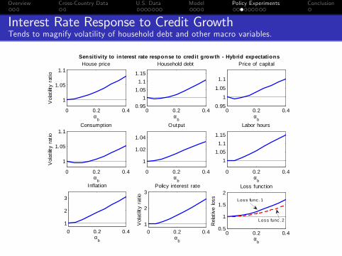
Interest Rate Response to Credit GrowthTends to magnify volatility of household debt and other macro variables.

0 0.2 0.4

1

1.05

1.1

αb

House price

Vol

atilit

y ra

tio

0 0.2 0.40.95

11.05

1.11.15

αb

Household debt

0 0.2 0.40.95

1

1.05

1.1

αb

Price of capital

0 0.2 0.4

1

1.05

1.1

αb

Consumption

Vol

atilit

y ra

tio

0 0.2 0.4

1

1.02

1.04

αb

Output

0 0.2 0.4

11.05

1.11.15

αb

Labor hours

0 0.2 0.41

2

3

αb

Policy interest rate

Vol

atilit

y ra

tio

0 0.2 0.41

2

3

αb

Inflation

0 0.2 0.40.5

1

1.5

2

αb

Loss function

Rel

ativ

e lo

ss

Sensitivity to interest rate response to credit growth ­ Hybrid expectations

Los s  func . 1

Los s  func . 2

Overview Cross-Country Data U.S. Data Model Policy Experiments Conclusion

Monetary policy results depend on expectationsPrevious results obtained from rational expectations models may not be robust.

Interest rate response to credit growth (αb = 0.2)Standard deviations

Houseprice

HHdebt Output In�ation

Rational ExpectationsNot responding 2.08 3.17 2.31 0.81Responding 2.14 2.00 2.34 0.84Volatility Ratio 1.03 0.63 1.01 1.04

Hybrid ExpectationsNot responding 3.62 6.55 3.14 0.90Responding 3.72 6.68 3.18 1.65Volatility Ratio 1.03 1.02 1.01 1.83

Standard deviations expressed as percent deviations from steady state.

Overview Cross-Country Data U.S. Data Model Policy Experiments Conclusion

Tighten Lending Standards: Lower LTVReduces volatility of household debt but magni�es volatility of other macro variables.

0.2 0.4 0.6 0.80.95

1

1.05

1.1

γ

House price

0.2 0.4 0.6 0.80.60.8

11.21.41.6

γ

Household debt

0.2 0.4 0.6 0.80.95

1

1.05

1.1

γ

Price of capital

0.2 0.4 0.6 0.80.99

1

1.01

1.02

1.03

γ

Consumption

0.2 0.4 0.6 0.80.95

1

1.05

γ

Output

0.2 0.4 0.6 0.8

0.98

1

1.02

1.04

γ

Labor hours

0.2 0.4 0.6 0.80.95

1

1.05

γ

Policy interest rate

0.2 0.4 0.6 0.80.98

1

1.02

1.04

γ

Inflation

0.2 0.4 0.6 0.80.5

1

1.5

2

γ

Loss function

Rel

ativ

e lo

ssLos s  func . 1

Los s  func . 2

Sensitivity to LTV ratio ­ Hybrid expectations

Overview Cross-Country Data U.S. Data Model Policy Experiments Conclusion

Generalized constraint maths

b2,t �γ

Rt

hbE1,t qt+1πt+1i h2,t

b2,tRthbE1,t qt+1πt+1i h2,t � γ

b2,t �bγRt

8>><>>:m wtL2,t| {z }wage income

+ (1�m)hbE1,t qt+1πt+1

ih2,t| {z }

collateral

9>>=>>;b2,tRthbE1,t qt+1πt+1

ih2,t| {z }

LTVt

� bγ8<:m wtL2,thbE1,t qt+1πt+1

ih2,t

+ (1�m)

9=;

Overview Cross-Country Data U.S. Data Model Policy Experiments Conclusion

Generalized constraint maths

b2,t �γ

Rt

hbE1,t qt+1πt+1i h2,tb2,tRthbE1,t qt+1πt+1i h2,t � γ

b2,t �bγRt

8>><>>:m wtL2,t| {z }wage income

+ (1�m)hbE1,t qt+1πt+1

ih2,t| {z }

collateral

9>>=>>;b2,tRthbE1,t qt+1πt+1

ih2,t| {z }

LTVt

� bγ8<:m wtL2,thbE1,t qt+1πt+1

ih2,t

+ (1�m)

9=;

Overview Cross-Country Data U.S. Data Model Policy Experiments Conclusion

Generalized constraint maths

b2,t �γ

Rt

hbE1,t qt+1πt+1i h2,tb2,tRthbE1,t qt+1πt+1i h2,t � γ

b2,t �bγRt

8>><>>:m wtL2,t| {z }wage income

+ (1�m)hbE1,t qt+1πt+1

ih2,t| {z }

collateral

9>>=>>;

b2,tRthbE1,t qt+1πt+1

ih2,t| {z }

LTVt

� bγ8<:m wtL2,thbE1,t qt+1πt+1

ih2,t

+ (1�m)

9=;

Overview Cross-Country Data U.S. Data Model Policy Experiments Conclusion

Generalized constraint maths

b2,t �γ

Rt

hbE1,t qt+1πt+1i h2,tb2,tRthbE1,t qt+1πt+1i h2,t � γ

b2,t �bγRt

8>><>>:m wtL2,t| {z }wage income

+ (1�m)hbE1,t qt+1πt+1

ih2,t| {z }

collateral

9>>=>>;b2,tRthbE1,t qt+1πt+1

ih2,t| {z }

LTVt

� bγ8<:m wtL2,thbE1,t qt+1πt+1

ih2,t

+ (1�m)

9=;

Overview Cross-Country Data U.S. Data Model Policy Experiments Conclusion

Volatility Comparison: Wage Income versus Housing ValueWage income is less subject to bubble-induced distortions.

0 50 100 150 200­15

­10

­5

0

5

10

15

20Borrower's wage income

% d

evia

tion 

from

 ste

ady 

stat

e

Rational expectations Hybrid expectations0 50 100 150 200­15

­10

­5

0

5

10

15

20Borrower's housing value

% d

evia

tion 

from

 ste

ady 

stat

e

Volatility comparison: borrower's wage income versus housing value

b2,t �bγRtfm wtL2,t| {z }

wage income

+ (1�m)hbE1,t qt+1πt+1

ih2,t| {z }

collateral

g

Overview Cross-Country Data U.S. Data Model Policy Experiments Conclusion

Endogenous LTV acts like an automatic stabilizerWeight on wage income in borrowing constraint induces countercyclical LTV ratio.

0 50 100­3

­2

­1

0

1

2

3Rational expectations

% d

evia

tion 

from

 ste

ady 

stat

e

LTV House value0 50 100­3

­2

­1

0

1

2

3Hybrid expectations

Endogenous movements in LTV with generalized borrowing constraint

Overview Cross-Country Data U.S. Data Model Policy Experiments Conclusion

Move Towards Loan-to-Income Constraint (Best)Reduces volatility of household debt as well other economic variables.

0 0.5 10.98

1

1.02

1.04

1.06

m

House price

Vol

atilit

y ra

tio

0 0.5 10.4

0.6

0.8

1

m

Household debt

0 0.5 10.98

1

1.02

1.04

m

Price of capital

0 0.5 10.995

1

1.005

m

Consumption

Vol

atilit

y ra

tio

0 0.5 10.99

0.995

1

1.005

m

Output

0 0.5 10.9

0.95

1

m

Labor hours

0 0.5 10.99

1

1.01

1.02

1.03

m

Policy interest rate

Vol

atilit

y ra

tio

0 0.5 10.998

1

1.002

1.004

m

Inflation

0 0.5 1

0.7

0.8

0.9

1

m

Loss function

Rel

ativ

e lo

ss

Los s  func . 2

Los s  func . 1

Sensitivity to weight on wage income in borrowing constraint ­ Hybrid expectations

Overview Cross-Country Data U.S. Data Model Policy Experiments Conclusion

ConclusionNo policy was perfect but some did better than others.

Interest rate response to either house price growth or creditgrowth had the serious drawback of substantially magnifyingthe volatility of in�ation.

A lower LTV ratio mildly raised the volatilities of output,in�ation, and consumption, but reduced the volatility ofhousehold debt� a �nancial stability bene�t.

Best-performing policy: Require lenders to put substantialweight on wage income in the borrowing constraint. Promotesboth economic and �nancial stability (automatic stabilizer).

Best performing policy calls for lending behavior that isbasically the opposite of what U.S. lenders did during housingboom of the mid-2000s. By 2006, 27 percent of all newmortgages were �no-doc�and �low-doc� loans.

Overview Cross-Country Data U.S. Data Model Policy Experiments Conclusion

ConclusionNo policy was perfect but some did better than others.

Interest rate response to either house price growth or creditgrowth had the serious drawback of substantially magnifyingthe volatility of in�ation.

A lower LTV ratio mildly raised the volatilities of output,in�ation, and consumption, but reduced the volatility ofhousehold debt� a �nancial stability bene�t.

Best-performing policy: Require lenders to put substantialweight on wage income in the borrowing constraint. Promotesboth economic and �nancial stability (automatic stabilizer).

Best performing policy calls for lending behavior that isbasically the opposite of what U.S. lenders did during housingboom of the mid-2000s. By 2006, 27 percent of all newmortgages were �no-doc�and �low-doc� loans.

Overview Cross-Country Data U.S. Data Model Policy Experiments Conclusion

ConclusionNo policy was perfect but some did better than others.

Interest rate response to either house price growth or creditgrowth had the serious drawback of substantially magnifyingthe volatility of in�ation.

A lower LTV ratio mildly raised the volatilities of output,in�ation, and consumption, but reduced the volatility ofhousehold debt� a �nancial stability bene�t.

Best-performing policy: Require lenders to put substantialweight on wage income in the borrowing constraint. Promotesboth economic and �nancial stability (automatic stabilizer).

Best performing policy calls for lending behavior that isbasically the opposite of what U.S. lenders did during housingboom of the mid-2000s. By 2006, 27 percent of all newmortgages were �no-doc�and �low-doc� loans.

Overview Cross-Country Data U.S. Data Model Policy Experiments Conclusion

ConclusionNo policy was perfect but some did better than others.

Interest rate response to either house price growth or creditgrowth had the serious drawback of substantially magnifyingthe volatility of in�ation.

A lower LTV ratio mildly raised the volatilities of output,in�ation, and consumption, but reduced the volatility ofhousehold debt� a �nancial stability bene�t.

Best-performing policy: Require lenders to put substantialweight on wage income in the borrowing constraint. Promotesboth economic and �nancial stability (automatic stabilizer).

Best performing policy calls for lending behavior that isbasically the opposite of what U.S. lenders did during housingboom of the mid-2000s. By 2006, 27 percent of all newmortgages were �no-doc�and �low-doc� loans.