Houdini: Fooling Deep Structured Prediction Models

Moustapha CisseFacebook AI Research

moustaphacisse@fb.com

Yossi Adi*Bar-Ilan University, Israel

yossiadidrum@gmail.com

Natalia Neverova*Facebook AI Researchnneverova@fb.com

Joseph KeshetBar-Ilan University, Israeljkeshet@cs.biu.ac.il

Abstract

Generating adversarial examples is a critical step for evaluating and improvingthe robustness of learning machines. So far, most existing methods only workfor classification and are not designed to alter the true performance measure ofthe problem at hand. We introduce a novel flexible approach named Houdini forgenerating adversarial examples specifically tailored for the final performancemeasure of the task considered, be it combinatorial and non-decomposable. Wesuccessfully apply Houdini to a range of applications such as speech recognition,pose estimation and semantic segmentation. In all cases, the attacks based onHoudini achieve higher success rate than those based on the traditional surrogatesused to train the models while using a less perceptible adversarial perturbation.

1 Introduction

Deep learning has redefined the landscape of machine intelligence [22] by enabling several break-throughs in notoriously difficult problems such as image classification [20, 16], speech recognition [2],human pose estimation [35] and machine translation [4]. As the most successful models are perme-ating nearly all the segments of the technology industry from self-driving cars to automated dialogagents, it becomes critical to revisit the evaluation protocol of deep learning models and design newways to assess their reliability beyond the traditional metrics. Evaluating the robustness of neuralnetworks to adversarial examples is one step in that direction [32]. Adversarial examples are syntheticpatterns carefully crafted by adding a peculiar noise to legitimate examples. They are indistinguish-able from the legitimate examples by a human, yet they have demonstrated a strong ability to causecatastrophic failure of state of the art classification systems [12, 25, 21]. The existence of adversarialexamples highlights a potential threat for machine learning systems at large [28] that can limit theiradoption in security sensitive applications. It has triggered an active line of research concerned withunderstanding the phenomenon [10, 11], and making neural networks more robust [29, 7] .

Adversarial examples are crucial for reliably evaluating and improving the robustness of the mod-els [12]. Ideally, they must be generated to alter the task loss unique to the application considereddirectly. For instance, an adversarial example crafted to attack a speech recognition system should bedesigned to maximize the word error rate of the targetted system. The existing methods for generatingadversarial examples exploit the gradient of a given differentiable loss function to guide the search inthe neighborhood of legitimates examples [12, 25]. Unfortunately, the task loss of several structuredprediction problems of interest is a combinatorial non-decomposable quantity that is not amenable togradient-based methods for generating adversarial example. For example, the metric for evaluatinghuman pose estimation is the percentage of correct keypoints (normalized by the head). Automatic

*equal contribution

arX

iv:1

707.

0537

3v1

[st

at.M

L]

17

Jul 2

017

adversarial attackoriginal semantic segmentation framework compromised semantic segmentation framework

Figure 1: We cause the network to generate a minion as segmentation for the adversarially perturbedversion of the original image. Note that the original and the perturbed image are indistinguishable.

speech recognition systems are assessed using their word (or phoneme) error rate. Similarly, thequality of a semantic segmentation is measured by the intersection over union (IOU) between theground truth and the prediction. All these evalutation measures are non-differentiable.

The solutions for this obstacle in supervised learning are of two kinds. The first route is to use aconsistent differentiable surrogate loss function in place of the task loss [5]. That is a surrogate whichis guaranteed to converge to the task loss asymptotically. The second option is to directly optimize thetask loss by using approaches such as Direct Loss Minimization [14]. Both of these strategies havesevere limitations. (1) The use of differentiable surrogates is satisfactory for classification becausethe relationship between such surrogates and the classification accuracy is well established [34]. Thepicture is different for the above-mentioned structured prediction tasks. Indeed, there is no knownconsistency guarantee for the surrogates traditionally used in these problems (e.g. the connectionisttemporal classification loss for speech recognition) and designing a new surrogate is nontrivial andproblem dependent. At best, one can only expect a high positive correlation between the proxy andthe task loss. (2) The direct minimization approaches are more computationally involved becausethey require solving a computationally expensive loss augmented inference for each parameter update.Also, they are notoriously sensitive to the choice of the hyperparameters. Consequently, it is harderto generate adversarial examples for structured prediction problems as it requires significant domainexpertise with little guarantee of success when surrogate does not tightly approximate the task loss.

Results. In this work we introduce Houdini, the first approach for fooling any gradient-basedlearning machine by generating adversarial examples directly tailored for the task loss of interest beit combinatorial or non-differentiable. We show the tight relationship between Houdini and the taskloss of the problem considered. We present the first successful attack on a deep Automatic SpeechRecognition (ASR) system, namely a DeepSpeech-2 based architecture [1], by generating adversarialaudio files not distinguishable from legitimate ones by a human (as validated by an ABX experiment).We also demonstrate the transferability of adversarial examples in speech recognition by foolingGoogle Voice in a black box attack scenario: an adversarial example generated with our model andnot distinguishable from the legitimate one by a human leads to an invalid transcription by the GoogleVoice application (see Figure 9). We also present the first successful untargeted and targetted attackson a deep model for human pose estimation [26]. Similarly, we validate the feasibility of untargetedand targetted attacks on a semantic segmentation system [38] and show that we can make the systemhallucinate an arbitrary segmentation of our choice for a given image. Figure 1 shows an experimentwhere we cause the network to hallucinate a minion. In all cases, our approach generates betterquality adversarial examples than each of the different surrogates (expressly designed for the modelconsidered) without additional computational overhead thanks to the analytical gradient of Houdini.

2 Related Work

Adversarial examples. The empirical study of Szegedy et al. [32] first demonstrated that deepneural networks could achieve high accuracy on previously unseen examples while being vulnerable tosmall adversarial perturbations. This finding has recently aroused keen interest in the community [12,28, 32, 33]. Several studies have subsequently analyzed the phenomenon [10, 31, 11] and variousapproaches have been proposed to improve the robustness of neural networks [29, 7]. More closelyrelated to our work are the different proposals aiming at generating better adversarial examples [12,25]. Given an input (train or test) example (x, y), an adversarial example is a perturbed version ofthe original pattern x = x+ δx where δx is small enough for x to be undistinguishable from x by a

2

human, but causes the network to predict an incorrect target. Given the network gθ (where θ is the setof parameters) and a p-norm, the adversarial example is formally defined as:

x = argmaxx:‖x−x‖p≤ε

`(gθ(x), y

)(1)

where ε represents the strength of the adversary. Assuming the loss function `(·) is differentiable,Shaham et al. [31] propose to take the first order taylor expansion of x 7→ `(gθ(x), y) to compute δxby solving the following simpler problem:

x = argmaxx:‖x−x‖p≤ε

(∇x`(gθ(x), y)

)T(x− x) (2)

When p = ∞, then x = x + εsign(∇x`(gθ(x), y)) which corresponds to the fast gradient signmethod [12]. If instead p = 2, we obtain x = x + ε∇x`(gθ(x), y) where ∇x`(gθ(x), y) is oftennormalized. Optionally, one can perform more iterations of these steps using a smaller norm. Thismore involved strategy has several variants [25]. These methods are concerned with generatingadversarial examples assuming a differentiable loss function `(·). Therefore they are not directlyapplicable to the task losses of interest. However, they can be used in combination with our proposalwhich derives a consistent approximation of the task loss having an analytical gradient.

Task Loss Minimization. Recently, several works have focused on directly minimizing the taskloss. In particular, McAllester et al. [24] presented a theorem stating that a certain perceptron-likelearning rule, involving feature vectors derived from loss-augmented inference, directly correspondsto the gradient of the task loss. While this algorithm performs well in practice, it is extremely sensitiveto the choice of its hyper-parameter and needs two inference operations per training iteration. Doet al. [9] generalized the notion of the ramp loss from binary classification to structured predictionand proposed a tighter bound to the task loss than the structured hinge loss. The update rule ofthe structured ramp loss is similar to the update rule of the direct loss minimization algorithm, andsimilarly it needs two inference operations per training iteration. Keshet et al. [19] generalized thenotion of the binary probit loss to the structured prediction case. The probit loss is a surrogate lossfunction naturally resulted in the PAC-Bayesian generalization theorems. it is defined as follows:

¯probit(gθ(x), y) = Eε∼N (0,I) [`(y, gθ+ε(x))] (3)

where ε ∈ Rd is a d-dimensional isotropic Normal random vector. [18] stated finite sample generaliza-tion bounds for the structured probit loss and showed that it is strongly consistent. Strong consistencyis a critical property of a surrogate since it guarantees the tight relationship to the task loss. Forinstance, an attacker of a given system can expect to deteriorate the task loss if she deteriorates theconsistent surrogate of it. The gradient of the structured probit loss can be approximated by averagingover samples from the unit-variance isotropic normal distribution, where for each sample an inferencewith perturbed parameters is computed. Hundreds to thousands of inference operations are requiredper iteration to gain stability in the gradient computation. Hence the update rule is computationallyprohibitive and limits the applicability of the structured probit loss despite its desirable properties.

We propose a new loss named Houdini. It shares the desirable properties of the structured probit losswhile not suffering from its limitations. Like the structured probit loss and unlike most surrogatesused in structured prediction (e.g. structured hinge loss for SVMs), it is tightly related to the task loss.Therefore it allows to reliably generate adversarial examples for a given task loss of interest. Unlikethe structured probit loss and like the smooth surrogates, it has an analytical gradient hence requireonly a single inference in its update rule. The next section presents the details of our proposal.

3 Houdini

Let us consider a neural network gθ parameterized by θ and the task loss of a given problem `(·).We assume `(y, y) = 0 for any target y. The score output by the network for an example (x, y) isgθ(x, y) and the network’s decoder predicts the highest scoring target:

y = yθ(x) = argmaxy∈Y

gθ(x, y). (4)

Using the terminology of section 2, finding an adversarial example fooling the model gθ with respectto the task loss `(·) for a chosen p-norm and noise parameter ε boils down to solving:

x = argmaxx:‖x−x‖p≤ε

`(yθ(x), y

)(5)

3

The task loss is often a combinatorial quantity which is hard to optimize, hence it is replaced with adifferentiable surrogate loss, denoted ¯(yθ(x), y). Different algorithms use different surrogate lossfunctions: structural SVM uses the structured hinge loss, Conditional random fields use the log loss,etc. We propose a surrogate named Houdini and defined as follows for a given example (x, y):

¯H(θ, x, y) = Pγ∼N (0,1)

[gθ(x, y)− gθ(x, y) < γ

]· `(y, y) (6)

In words, Houdini is a product of two terms. The first term is a stochastic margin, that is theprobability that the difference between the score of the actual target gθ(x, y) and that of the predictedtarget gθ(x, y) is smaller than γ ∼ N (0, 1). It reflects the confidence of the model in its predictions.The second term is the task loss, which given two targets is independent of the model and correspondsto what we are ultimately interested in maximizing. Houdini is a lower bound of the task loss. Indeeddenoting δg(y, y) = gθ(x, y)− gθ(x, y) as the difference between the scores assigned by the networkto the ground truth and the prediction, we have Pγ∼N (0,1)(δg(y, y) < γ) is smaller than 1. Hencewhen this probability goes to 1, or equivalently when the score assigned by the network to the targety grows without a bound, Houdini converges to the task loss. This is a unique property not enjoyedby most surrogates used in the applications of interest in our work. It ensures that Houdini is a goodproxy of the task loss for generating adversarial examples.

We can now use Houdini in place of the task loss `(·) in the problem 5. Following 2, we resort to afirst order approximation which requires the gradient of Houdini with respect to the input x. Thelatter is obtained following the chain rule:

∇x[¯H(θ, x, y)

]=∂ ¯H(θ, x, y)

∂gθ(x, y)

∂gθ(x, y)

∂x(7)

To compute the RHS of the above quantity, we only need to compute the derivative of Houdiniwith respect to its input (the output of the network). The rest is obtained by backpropagation. Thederivative of the loss with respect to the network’s output is:

∇g[Pγ∼N (0,1)

[gθ(x, y)− gθ(x, y) < γ

]`(y, y)

]= ∇g

[1√2π

∫ ∞δg(y,y)

e−v2/2dv `(y, y)

](8)

Therefore, expanding the right hand side and denoting C = 1/√

2π we have:

∇g[¯H(y, y)

]=

−C · e−|δg(y,y)|2/2`(y, y), g = gθ(x, y)

C · e−|δg(y,y)|2/2`(y, y), g = gθ(x, y)

0, otherwise(9)

Equation 9 provides a simple analytical formula for computing the gradient of Houdini with respectto its input, hence an efficient way to obtain the gradient with respect to the input of the network xby backpropagation. The gradient can be used in combination with any gradient-based adversarialexample generation procedure [12, 25] in two ways, depending on the form of attack considered.For an untargeted attack, we want to change the prediction of the network without preference onthe final prediction. In that case, any alternative target y can be used (e.g. the second highest scoreras the target). For a targetted attack, we set the y to be the desired final prediction. Also note that,when the score of the predicted target is very close to that of the ground truth (or desired target),that is when δg(y, y) is small as we expect from the trained network we want to fool, we havee−|δg(y,y)|

2/2 ' 1. In the next sections, we show the effectiveness of the proposed attack scheme onhuman pose estimation, semantic segmentation and automatic speech recognition systems.

4 Human Pose Estimation

We evaluate the effectiveness of Houdini loss in the context of adversarial attacks on neural modelsfor human pose estimation. Compromising performance of such systems can be desirable formanipulating surveillance cameras, altering the analysis of crime scenes, disrupting human-robotinteraction or fooling biometrical authentication systems based on gate recognition. The poseestimation task is formulated as follows: given a single RGB image of a person, determine correct 2Dpositions of several pre-defined key points which typically correspond to skeletal joints. In practice,

4

(a) (b) (c)

Figure 2: Convergence dynamics for pose estimation attacks: (a) perturbation perceptibility vs nb.iterations, (b) PCKh0.5 vs nb. iterations, (c) proportion of re-positioned joints vs perceptibility.

Method SSIM Perceptibility

@PCKh=50 @PCKhlim @PCKh=50 @PCKhlim

untargeted: MSE loss 0.9986 0.9954 0.0048 0.0093untargeted: Houdini loss 0.9990 0.9987 0.0037 0.0048

targetted: MSE loss 0.9984 0.9959 0.0050 0.0089targetted: Houdini loss 0.9982 0.9965 0.0049 0.0079

Table 1: Human pose estimation: comparison of empirical performance for adversarial attacks and adversarialpose re-targeting. PCKh=50 corresponds to 50% correctly detected keypoints and PCKhlim denotes the valueupon convergence or after 300 iterations). (SSIM: the higher the better, perceptibility: the lower the better.)

the performance of such frameworks is measured by the percentage of correctly detected keypoints(PCKh), i.e. keypoints whose predicted locations are within a certain distance from the correspondingtarget positions: [3]:

PCKhα =

∑Ni=1 1(‖yi − yi‖ < αh)

N, (10)

where y and y are the predicted and the desired positions of a given joint respectively, h is the headsize of the person (known at test time), α is a threshold (set to 0.5), and N is the number of annotatedkeypoints. Pose estimations is a good example of a problem where we observe a discrepancy betweenthe training objective and the final evaluation measure. Instead of directly minimizing the percentageof correctly detected keypoints, state-of-the-art methods rely upon a dense prediction of heat maps,i.e. estimation of probabilities of every pixel corresponding to each of keypoint locations. Thesemodels can be trained with binary cross entropy [6], softmax [15] or MSE losses [26] applied to everypixel in the output space, separately for each plane corresponding to every key point. In our firstexperiment, we attack a state-of-the-art model for single person pose estimation based on Hourglassnetworks [26] and aim to minimize the value of PCKh0.5 metric given the minimal perturbation. Forthis task we choose y as:

y = argmaxy:‖p−p‖>αh

gθ(x, y) (11)

where p is the pixel coordinate on the heatmap corresponding to the argmax value of vector y. Weperform the optimization iteratively till convergence with an update rule ε · ∇x

‖∇x‖ where ∇x aregradients with respect to the input and ε = 0.1. Empirical comparison with a similar attack basedon minimizing the training loss (MSE in this case) is given in the top part of Table 1. We performthe evaluations on the validation subset of MPII dataset [3] consisting of 3000 images and definedas in [26]. We evaluate the perceived degree of perturbation where perceptibility is expressed as( 1n

∑(x′i − xi)2)1/2, where x and x′ are original and distorted images, and n is the number of pixels

[32]. In addition, we report the structural similarity index (SSIM) [36] which is known to correlatewell with the visual perception of image structure by a human. As shown in Table 1, adversarialexamples generated with Houdini are more similar to the legitimate examples than the ones generatedwith the training proxy (MSE). For untargeted attacks optimized to convergence, the perturbationgenerated with Houdini is up to 50% less perceptible than the one obtained with MSE.

We measured the number of iterations required to completely compromise the pose estimation system(PCKh = 0) depending on the loss function used. The convergence dynamics illustrated in Fig. 1

5

PCKh0.5 : 81.25 ! 0.00, iter 55, distortion 0.0063, SSIM = 0.9983

PCKh0.5 : 81.25 ! 0.00, iter 55, distortion 0.0063, SSIM = 0.9983

PCKh0.5 : 100.00 ! 0.00, iter 64, distortion 0.0057, SSIM = 0.9981

initial prediction adversarial prediction perturbed noise

initial prediction

initial prediction

adversarial prediction

adversarial prediction

perturbed

perturbed

noise

noise

source image

source image

source image

(a) initial prediction (b) adversarial prediction (c) source image (d) perturbed image (e) noise

Figure 3: Example of disrupted pose estimation due to an adversarial attack exploiting Houdini loss: after 55iterations, PCKh0.5 dropped from 81.25 to 0.00 (final perturbation perceptibility is 0.0063).

PCKh0.5 = 87.5SSIM = 0.9802

distortion 0.2112iter 1000

PCKh0.5 = 87.5SSIM = 0.9824distortion 0.211

iter 1000

PCKh0.5 = 100.0SSIM = 0.9922distortion 0.145

iter 435

PCKh0.5 = 100.0SSIM = 0.9906distortion 0.016

iter 574

perceptibility0.145

perceptibility0.016

perceptibility0.211

perceptibility0.210

Figure 4: Examples of successful targetted attacks on a pose estimation system. Despite the importantdifference between the images selected, it is possible to make the network predict the wrong pose byadding an imperceptible perturbation.

show that employing Houdini makes it possible to completely compromise network performancegiven the target metric after several iterations (100). When using the training surrogate (MSE) forgenerating adversarial examples, we could not achieve a similar success level on the attacks evenafter 300 iterations of the optimization process. This observation underlines the importance of theloss function used to generate adversarial examples in structured prediction problems. We show anexample in Figure 3. Interestingly, the predicted poses for the corrupted images still make an overallplausible impression, while failing the formal evaluation entirely. Indeed, the mistakes made by thecompromised network appear natural and are typical for pose estimation frameworks: imprecision inlocalization, confusion between right and left limbs, combining joints from several people, etc.

In the second experiment, we perform a targetted attack in the form of pose transfer, i.e. we forcethe network to hallucinate an arbitrary pose (with success defined, as before, given the target metricPCKh0.5). The experimental setup is as follows: for a given pair of images (i, j) we force the networkto output the ground truth pose of the picture i when the input is image j and vice versa. This task ismore challenging and depends on the similarity between the original and target poses. Surprisingly,targetted attacks are is still feasible even when the two ground truth poses are very different. Figure 4shows an example where the model predicts the pose of a human body in horizontal position for anadversarially perturbed image depicting a standing person (and vice versa). A similar experimentwith two persons in standing and sitting positions respectively is also shown in figure 4.

5 Semantic segmentation

Semantic segmentation uses another customized metric to evaluate performance, namely themean Intersection over Union (mIoU) measure defined as averaging over classes the IoU =TP/(TP + FP + FN), where TP, FP and FN stand for true positive, false positive and false neg-ative respectively, taken separately for each class. Compared to per-pixel accuracy, which appears tobe overoptimistic on highly unbalanced datasets, and per-class accuracy, which under-penalizes falsealarms for non-background classes, this metric favors accurate object localization with tighter masks

6

Method SSIM Perceptibility

@mIoU/2 @mIoUlim @mIoU/2 @mIoUlim

untargeted: NLL loss 0.9989 0.9950 0.0037 0.0117untargeted: Houdini loss 0.9995 0.9959 0.0026 0.0095

targetted: NLL loss 0.9972 0.9935 0.0074 0.0389targetted: Houdini loss 0.9975 0.9937 0.0054 0.0392

Table 2: Semantic segmentation: comparison of empirical performance for targetted and untargetedadversarial attacks on segmentation systems. mIoU/2 denotes 50% performance drop according tothe target metric and mIoUlim corresponds to convergence or termination after 300 iterations. SSIM:the higher, the better, perceptibility: the lower, the better. Houdini based attacks are less perceptible.

target source

source image initial prediction

perturbed image

noiseadversarial prediction

source image initial prediction adversarial prediction perturbed noise

adversarial prediction perturbed noise

Figure 5: Targetted attack on a semantic segmentation system: switching target segmentation betweentwo images from Cityscapes dataset [8]. The last two columns are respectively zoomed-in parts ofthe perturbed image and the adversarial perturbation added to the original one.

(in instance segmentation) or bounding boxes (in detection). The models are trained with a per-pixelsoftmax or multi-class cross entropy losses depending on the task formulation, i.e. optimized formean per-pixel or per-class accuracy instead of mIoU. Primary targets of adversarial attacks inthis group of applications are self-driving cars and robots. Xie et al. [37] have previously exploredadversarial attacks in the context of semantic segmentation. However, they exploited the same proxyused for training the network. We perform a series of experiments similar to the ones described inSec. 4. That is, we show targetted and untargeted attacks on a semantic segmentation model. Weuse a pre-trained Dilation10 model for semantic segmentation [38] and evaluate the success of theattacks on the validation subset of Cityscapes dataset [8]. In the first experiment, we directly alterthe target mIoU metric for a given test image in both targetted and untargeted attacks. As shown inTable 2, Houdini allows fooling the model at least as well as the training proxy (NLL) while using aless perceptible. Indeed, Houdini based adversarial perturbations generated to alter the performanceof the model by 50% are about 30% less noticeable than the noise created with NLL.

The second set of experiments consists of targetted attacks. That is, altering the input image to obtainan arbitrary target segmentation map as the network response. In Figure 5, we show an instanceof such attack in a segmentation transfer setting, i.e. the target segmentation is the ground truthsegmentation of a different image. It is clear that this type of attack is still feasible with a smalladversarial perturbation (even when after zooming in the picture). Figure 1 depicts a more challengingscenario where the target segmentation is an arbitrary map (e.g. a minion). Again, we can make thenetwork hallucinate the segmentation of our choice by adding a barely noticeable perturbation.

6 Speech Recognition

We evaluate the effectiveness of Houdini concerning adversarial attacks on an Automatic SpeechRecognition (ASR) system. Traditionally, ASR systems are composed of different components,(e.g. acoustic model, language model, pronunciation model, etc.) where each component is trainedseparately. Recently, ASR research is focused on deep learning based end-to-end models. These typeof models get as input a speech segment and output a transcript with no additional post-processing. In

7

ε = 0.3 ε = 0.2 ε = 0.1 ε = 0.05

WER CER WER CER WER CER WER CER

CTC 68 9.3 51 6.9 29.8 4 20 2.5Houdini 96.1 12 85.4 9.2 66.5 6.5 46.5 4.5

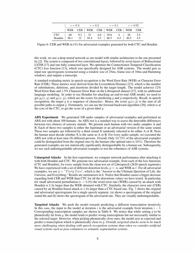
Figure 6: CER and WER in (%) for adversarial examples generated by both CTC and Houdini.

this work, we use a deep neural network as our model with similar architecture to the one presentedby [2]. The system is composed of two convolutional layers, followed by seven layers of BidirectionalLSTM [17] and one fully connected layer. We optimize the Connectionist Temporal Classification(CTC) loss function [13], which was specifically designed for ASR systems. The model gets asinput raw spectrograms (extracted using a window size of 25ms, frame-size of 10ms and Hammingwindow), and outputs a transcript.

A standard evaluating metric in speech recognition is the Word Error Rate (WER) or Character ErrorRate (CER). These metrics were derived from the Levenshtein Distance [23], which is the numberof substitutions, deletions, and insertions divided by the target length. The model achieves 12%Word Error Rate and 1.5% Character Error Rate on the Librispeech dataset [27], with no additionallanguage modeling. In order to use Houdini for attacking an end-to-end ASR model, we need toget gθ(x, y) and gθ(x, y), which are the scores for predicting y and y respectively. Recall, in speechrecognition, the target y is a sequence of characters. Hence, the score gθ(x, y) is the sum of allpossible paths to output y. Fortunately, we can use the forward-backward algorithm [30], which is atthe core of the CTC, to get the score of a given label y.

ABX Experiment We generated 100 audio samples of adversarial examples and performed anABX test with about 100 humans. An ABX test is a standard way to assess the detectable differencesbetween two choices of sensory stimuli. We present each human with two audio samples A andB. Each of these two samples is either the legitimate or an adversarial version of the same sound.These two samples are followed by a third sound X randomly selected to be either A or B. Next,the human must decide whether X is the same as A or B. For every audio sample, we executed theABX test with at least nine (9) different persons. Overall, Only 53.73% of the adversarial examplescould be distinguished from the original ones by the humans (the optimal ratio is 50%). Therefore thegenerated examples are not statistically significantly distinguishable by a human ear. Subsequently,we use such indistinguishable adversarial examples to test the robustness of ASR systems.

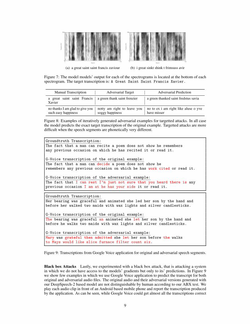
Untargeted Attacks In the first experiment, we compare network performance after attacking itwith both Houdini and CTC. We generate two adversarial example, from each of the loss functions(CTC and Houdini), for every sample from the clean test set of Librispeech (2620 speech segments).We have experienced with a set of different distortion levels, p =∞ and WER as `. For all adversarialexamples, we use y = ”Forty Two”, which is the "Answer to the Ultimate Question of Life, theUniverse, and Everything." Results are summarizes in 6. Notice that Houdini causes a bigger decreaseregarding both CER and WER than CTC for all the distortions values we have tested. In particular,for small adversarial perturbation (ε = 0.05) the word error rate (WER) caused by an attack withHoudini is 2.3x larger than the WER obtained with CTC. Similarly, the character error rate (CER)caused by an Houdini-based attack is 1.8x larger than a CTC-based one. Fig. 7 shows the originaland adversarial spectrograms for a single speech segment. (a) shows a spectrogram of the originalsound file and (b) shows the spectrogram of the adversarial one. They are visually undistinguishable.

Targetted Attacks We push the model towards predicting a different transcription iteratively.In this case, the input to the model at iteration i is the adversarial example from iteration i − 1.Corresponding transcription samples are shown in Table 8. We notice that while setting y to bephonetically far from y, the model tends to predict wrong transcriptions but not necessarily similar tothe selected target. However, when picking phonetically close ones, the model acts as expected andpredict a transcription which is phonetically close to y. Overall, targetted attacks seem to be muchmore challenging when dealing with speech recognition systems than when we consider artificialvisual systems such as pose estimators or semantic segmentation systems.

8

Time (s)0 3.23

0

5000

Freq

uenc

y (H

z)

(a) a great saint saint francis zaviour

Time (s)0 3.23

0

5000

Freq

uenc

y (H

z)

(b) i great sinkt shink t frimsuss avir

Figure 7: The model models’ output for each of the spectrograms is located at the bottom of eachspectrogram. The target transcription is: A Great Saint Saint Francis Xavier.

Manual Transcription Adversarial Target Adversarial Prediction

a great saint saint FrancisXavier

a green thank saint frenzier a green thanked saint fredstus savia

no thanks I am glad to give yousuch easy happiness

notty am right to leave yousoggy happiness

no to ex i am right like aluse o yvehave misser

Figure 8: Examples of iteratively generated adversarial examples for targetted attacks. In all casethe model predicts the exact target transcription of the original example. Targetted attacks are moredifficult when the speech segments are phonetically very different.

Groundtruth Transcription:The fact that a man can recite a poem does not show he remembersany previous occasion on which he has recited it or read it.

G-Voice transcription of the original example:The fact that a man can decide a poem does not show heremembers any previous occasion on which he has work cited or read it.

G-Voice transcription of the adversarial example:The fact that I can rest I’m just not sure that you heard there is anyprevious occasion I am at he has your side it or read it.

Groundtruth Transcription:Her bearing was graceful and animated she led her son by the hand andbefore her walked two maids with wax lights and silver candlesticks.

G-Voice transcription of the original example:The bearing was graceful an animated she let her son by the hand andbefore he walks two maids with wax lights and silver candlesticks.

G-Voice transcription of the adversarial example:Mary was grateful then admitted she let her son before the walksto Mays would like slice furnace filter count six.

Figure 9: Transcriptions from Google Voice application for original and adversarial speech segments.

Black box Attacks Lastly, we experimented with a black box attack, that is attacking a systemin which we do not have access to the models’ gradients but only to its’ predictions. In Figure 9we show few examples in which we use Google Voice application to predict the transcript for bothoriginal and adversarial audio files. The original audio and their adversarial versions generated withour DeepSpeech-2 based model are not distinguishable by human according to our ABX test. Weplay each audio clip in front of an Android based mobile phone and report the transcription producedby the application. As can be seen, while Google Voice could get almost all the transcriptions correct

9

for legitimate examples, it largely fails to produce good transcriptions for the adversarial examples.As with images, adversarial examples for speech recognition also transfer between models.

7 Conclusion

We have introduced a novel approach to generate adversarial examples tailored for the performancemeasure unique to the task of interest. We have applied Houdini to challenging structured predictionproblems such as pose estimation, semantic segmentation and speech recognition. In each case,Houdini allows fooling state of the art learning systems with imperceptible perturbation, henceextending the use of adversarial examples beyond the task of image classification. What the eyes seeand the ears hear, the mind believes. (Harry Houdini)

8 Acknowledgments

The authors thank Alexandre Lebrun, Pauline Luc and Camille Couprie for valuable help with codeand experiments. We also thank Antoine Bordes, Laurens van der Maaten, Nicolas Usunier, ChristianWolf, Herve Jegou, Yann Ollivier, Neil Zeghidour and Lior Wolf for their insightful comments on theearly draft of this paper.

References[1] D. Amodei, R. Anubhai, E. Battenberg, C. Case, J. Casper, B. Catanzaro, J. Chen,

M. Chrzanowski, A. Coates, G. Diamos, et al. Deep speech 2: End-to-end speech recog-nition in english and mandarin. arXiv preprint arXiv:1512.02595, 2015.

[2] D. Amodei, R. Anubhai, E. Battenberg, C. Case, J. Casper, B. Catanzaro, J. Chen,M. Chrzanowski, A. Coates, G. Diamos, et al. Deep speech 2: End-to-end speech recog-nition in english and mandarin. In International Conference on Machine Learning, pages173–182, 2016.

[3] M. Andriluka, L. Pishchulin, P. Gehler, and B. Schiele. 2d human pose estimation: Newbenchmark and state of the art analysis. CVPR, 2014.

[4] D. Bahdanau, K. Cho, and Y. Bengio. Neural machine translation by jointly learning to alignand translate. arXiv preprint arXiv:1409.0473, 2014.

[5] P. L. Bartlett, M. I. Jordan, and J. D. McAuliffe. Convexity, classification, and risk bounds.Journal of the American Statistical Association, 101(473):138–156, 2006.

[6] A. Bulat and G. Tzimiropoulos. Human pose estimation via convolutional part heatmapregression. ECCV, 2016.

[7] M. Cisse, P. Bojanowski, E. Grave, Y. Dauphin, and N. Usunier. Parseval networks: Improvingrobustness to adversarial examples. arXiv preprint arXiv:1704.08847, 2017.

[8] M. Cords, M. Omran, S. Ramos, T. Rehfeld, M. Enzweiler, R. Benenson, U. Franke, S. Roth,and B. Schiele. The cityscapes dataset for semantic urban scene understanding. CVPR, 2016.

[9] C. Do, Q. Le, C.-H. Teo, O. Chapelle, and A. Smola. Tighter bounds for structured estimation.In Advances in Neural Information Processing Systems (NIPS) 22, 2008.

[10] A. Fawzi, O. Fawzi, and P. Frossard. Analysis of classifiers’ robustness to adversarial perturba-tions. arXiv preprint arXiv:1502.02590, 2015.

[11] A. Fawzi, S.-M. Moosavi-Dezfooli, and P. Frossard. Robustness of classifiers: from adversarialto random noise. In Advances in Neural Information Processing Systems, pages 1624–1632,2016.

[12] I. J. Goodfellow, J. Shlens, and C. Szegedy. Explaining and harnessing adversarial examples. InProc. ICLR, 2015.

10

[13] A. Graves, S. Fernández, F. Gomez, and J. Schmidhuber. Connectionist temporal classification:labelling unsegmented sequence data with recurrent neural networks. In Proceedings of the23rd international conference on Machine learning, pages 369–376. ACM, 2006.

[14] T. Hazan, J. Keshet, and D. A. McAllester. Direct loss minimization for structured prediction.In Advances in Neural Information Processing Systems, pages 1594–1602, 2010.

[15] K. He, G. Gkioxari, P. Dollar, and R. Girshick. Mask r-cnn. arXiv preprint arXiv:1703.06870,2016.

[16] K. He, X. Zhang, S. Ren, and J. Sun. Deep residual learning for image recognition. InProceedings of the IEEE Conference on Computer Vision and Pattern Recognition, pages770–778, 2016.

[17] S. Hochreiter and J. Schmidhuber. Long short-term memory. Neural computation, 9(8):1735–1780, 1997.

[18] J. Keshet and D. A. McAllester. Generalization bounds and consistency for latent structuralprobit and ramp loss. In Advances in Neural Information Processing Systems, pages 2205–2212,2011.

[19] J. Keshet, D. McAllester, and T. Hazan. Pac-bayesian approach for minimization of phonemeerror rate. In Acoustics, Speech and Signal Processing (ICASSP), 2011 IEEE InternationalConference on, pages 2224–2227. IEEE, 2011.

[20] A. Krizhevsky, I. Sutskever, and G. E. Hinton. Imagenet classification with deep convolutionalneural networks. In Advances in neural information processing systems, pages 1097–1105,2012.

[21] A. Kurakin, I. Goodfellow, and S. Bengio. Adversarial examples in the physical world. arXivpreprint arXiv:1607.02533, 2016.

[22] Y. LeCun, Y. Bengio, and G. Hinton. Deep learning. Nature, 521(7553):436–444, 2015.

[23] V. I. Levenshtein. Binary codes capable of correcting deletions, insertions, and reversals. InSoviet physics doklady, volume 10, pages 707–710, 1966.

[24] D. McAllester, T. Hazan, and J. Keshet. Direct loss minimization for structured prediction. InAdvances in Neural Information Processing Systems (NIPS) 24, 2010.

[25] S.-M. Moosavi-Dezfooli, A. Fawzi, and P. Frossard. Deepfool: a simple and accurate method tofool deep neural networks. arXiv preprint arXiv:1511.04599, 2015.

[26] A. Newell, K. Yang, and J. Deng. Stacked hourglass networks for human pose estimation.ECCV, 2016.

[27] V. Panayotov, G. Chen, D. Povey, and S. Khudanpur. Librispeech: an asr corpus based onpublic domain audio books. In Acoustics, Speech and Signal Processing (ICASSP), 2015 IEEEInternational Conference on, pages 5206–5210. IEEE, 2015.

[28] N. Papernot, P. McDaniel, I. Goodfellow, S. Jha, Z. Berkay Celik, and A. Swami. Practicalblack-box attacks against deep learning systems using adversarial examples. arXiv preprintarXiv:1602.02697, 2016.

[29] N. Papernot, P. McDaniel, X. Wu, S. Jha, and A. Swami. Distillation as a defense to adversarialperturbations against deep neural networks. In Security and Privacy (SP), 2016 IEEE Symposiumon, pages 582–597. IEEE, 2016.

[30] L. R. Rabiner. A tutorial on hidden markov models and selected applications in speechrecognition. Proceedings of the IEEE, 77(2):257–286, 1989.

[31] U. Shaham, Y. Yamada, and S. Negahban. Understanding adversarial training: Increasing localstability of neural nets through robust optimization. arXiv preprint arXiv:1511.05432, 2015.

11

[32] C. Szegedy, W. Zaremba, I. Sutskever, J. Bruna, D. Erhan, I. Goodfellow, and R. Fergus.Intriguing properties of neural networks. In Proc. ICLR, 2014.

[33] P. Tabacof and E. Valle. Exploring the space of adversarial images. arXiv preprintarXiv:1510.05328, 2015.

[34] A. Tewari and P. L. Bartlett. On the consistency of multiclass classification methods. Journal ofMachine Learning Research, 8(May):1007–1025, 2007.

[35] A. Toshev and C. Szegedy. Deeppose: Human pose estimation via deep neural networks.In Proceedings of the IEEE Conference on Computer Vision and Pattern Recognition, pages1653–1660, 2014.

[36] Z. Wang, A. C. Bovik, H. R. Sheikh, and E. P. Simoncelli. Image quality assessment: fromerror visibility to structural similarity. IEEE Transactions on Image Processing, 13(4):600–612,2004.

[37] C. Xie, J. Wang, Z. Zhang, Y. Zhou, L. Xie, and A. L. Yuille. Adversarial examples for semanticsegmentation and object detection. CoRR, abs/1703.08603, 2017.

[38] F. Yu and V. Koltun. Multi-scale aggregation by dilated convolutions. ICLR, 2016.

12