Horizonal and multirateral well prod. - MODEL MAT..pdf
79
-
Upload
rafael-j-moreno-r -
Category
Documents
-
view
222 -
download
0
Transcript of Horizonal and multirateral well prod. - MODEL MAT..pdf

A Mathematical Model of Horizontal WellsProductivity and Well Testing Analysis
Jing Lu
Thesis submitted to the Faculty of theVirginia Polytechnic Institute and State University
in partial ful�llment of the requirements for the degree of
MASTER OF SCIENCEIN
MATHEMATICS
APPROVED:
Tao Lin
Robert Rogers Shu-Ming Sun
August, 1998Blacksburg, Virginia
Keywords: Horizontal Well, Productivity, Well TestingCopyright 1998, Jing Lu

A Mathematical Model of Horizontal WellsProductivity and Well Testing Analysis
Jing Lu
Department of Mathematics
ABSTRACT
This thesis presents new productivity and well testing formulae of horizontal wells.Taking a horizontal well as a uniform line source, this thesis �nds velocity poten-tial formula and the productivity formulae for a horizontal well in an ellipsoid ofrevolution drainage volume by solving analytically the involved three-dimensionalpartial di�erential equations. These formulae can account for the advantages ofhorizontal wells, and they are more accurate than other formulae which are basedon two-dimensional hypotheses. This thesis also presents new well testing formulaeof horizontal wells in a single porosity system and a double porosity system. Com-pared with the formulae published in the literatures, our formulae, which do not usethe sum of in�nite series, are more reasonable and easy to be used in well testinganalysis.
ACKNOWLEDGEMENTS
I can not use my words to express my deep gratitude to my advisor, Dr. Tao Lin. Whateversuccess I have gotten is due to his support and guidance and encouragement. His knowledge,dedication to research and ideas have been invaluable throughout the last two years and thisresearch project was supported in part by the NSF under grant DMS-9704621.
Expressions of sincere appreciations and gratitude go to Prof. Tao Lu who is the director ofCenter for Mathematical Sciences, Institute of Computer Application, Chengdu Branch, AcademiaSinica, for drawing my attention to these problems.
I would like to thank Dr. Robert Rogers and Dr. Shu-Ming Sun for kindly serving on mycommittee and for having critically read this manuscript and supplied helpful comments and cor-rections. For valuable lessons and practices I have learned in mathematics, I am greatly indebtedto Professors Martin Day, Robert Wheeler, Layne Watson, Michael Renardy, and Jim Thomson,etc.
It was a pleasure and a valuable professional experience to associate with all the members ofDepartment of Mathematics. I thank all of them for their corporations, friendship and kindnesswhich made my stay at Virginia Tech. meaningful and enjoyable.
Deepest appreciations are extended to my mother for her love and many sacri�ces she pouredto give me the opportunity to pursue higher education.
iii

Contents
1 Introduction and Literature Review 1
2 Basic Equations 6
3 Velocity Potential Analysis 15
3.1 Equipotential Surfaces of Horizontal Wells : : : : : : : : : : : : : : : : : : : : : : : 163.2 Average Velocity Potential of Horizontal Wells : : : : : : : : : : : : : : : : : : : : : 20
4 Productivity Formulae 22
4.1 Formulae for Wells at Midheight of Formation : : : : : : : : : : : : : : : : : : : : : : 224.2 Well Eccentricity Problem : : : : : : : : : : : : : : : : : : : : : : : : : : : : : : : : 26
4.2.1 Point Convergence Pressure Distribution Formulae : : : : : : : : : : : : : : 284.2.2 Dimensionless Pressure Formulae of Horizontal Wells : : : : : : : : : : : : : : 304.2.3 Productivity Formulae for Eccentricity Wells : : : : : : : : : : : : : : : : : : 35
4.3 Comparisons of Productivity Formulae : : : : : : : : : : : : : : : : : : : : : : : : : : 38
5 Well Testing Formulae for Single Porosity Reservoir 43
5.1 Point Convergence Pressure Distribution Formula : : : : : : : : : : : : : : : : : : : 435.2 Dimensionless Pressure Formulae in In�nite Reservoirs : : : : : : : : : : : : : : : : : 455.3 Dimensionless Pressure Formulae in Reservoirs of Finite Height : : : : : : : : : : : 46
5.3.1 Reservoirs with Impermeable Boundary Conditions : : : : : : : : : : : : : : : 465.3.2 Reservoirs with Bottom Water or Gas Cap : : : : : : : : : : : : : : : : : : : 52
6 Well Testing Formulae for Double Porosity Reservoir 55
6.1 Warren-Root Model : : : : : : : : : : : : : : : : : : : : : : : : : : : : : : : : : : : : 556.2 Laplace Transform Images of Point Convergence Pressure : : : : : : : : : : : : : : : 566.3 Well Testing Formulae for Wells in Finite Height Reservoirs : : : : : : : : : : : : : : 61
A Conclusions 63
B Nomenclature 64
iv
List of Figures
2.1 Element of Surface in Volume. : : : : : : : : : : : : : : : : : : : : : : : : : : : : : : 72.2 Viscous Flow at P in Volume. : : : : : : : : : : : : : : : : : : : : : : : : : : : : : : : 92.3 Element of Surface in Volume. : : : : : : : : : : : : : : : : : : : : : : : : : : : : : : 102.4 Flow Geometries. : : : : : : : : : : : : : : : : : : : : : : : : : : : : : : : : : : : : : : 13
3.1 Horizontal Well Model. : : : : : : : : : : : : : : : : : : : : : : : : : : : : : : : : : : : 153.2 The Analyses of the Velocity Potential. : : : : : : : : : : : : : : : : : : : : : : : : : : 173.3 The Shape of the Equipotential Surfaces. : : : : : : : : : : : : : : : : : : : : : : : : 183.4 Schematics of Vertical and Horizontal Well Drainage Volume. : : : : : : : : : : : : : 19
4.1 Original Reservoir System with x/z Anisotropy and Horizontal Well. : : : : : : : : : 244.2 Transformed Isotropic Reservoir System with Elliptic Wellbore. : : : : : : : : : : : 244.3 Axis Dimensions for Transformed Wellbore. : : : : : : : : : : : : : : : : : : : : : : 254.4 Division of 3D Horizontal Well Problem into Two 2D Problems. : : : : : : : : : : : 38
6.1 Warren and Root's Sketch of a Naturally Fractured Reservoir. : : : : : : : : : : : : 56
v

List of Tables
3.1 The ratioes of velocity potential of endpoint and midpoint. : : : : : : : : : : : : : : 213.2 The comparisons of the two methods of calculating average velocity potential. : : : : 21
4.1 Dimensionless pressure of endpoint under di�erent boundary conditions. : : : : : : 354.2 The comparisons of methods to compute the productivity of a horizontal well. : : : 42
5.1 The convergence rate of the integration of K0(z). : : : : : : : : : : : : : : : : : : : : 50
vi

Chapter 1
Introduction and Literature Review
A worldwide interest exists today in drilling horizontal wells to increase productivity. Theproduction section of the horizontal well must be parallel to horizontal line. Because of its large ow area, a horizontal well may be several times more productive than a vertical one draining thesame volume. Recent interest in horizontal wells has been accelerating because of improved drillingand completion technology. This has led to increased e�ciency and economics in oil recovery.Increases in oil production rate and improvement in ultimate recovery has given horizontal wellsthe edge over vertical wells in many marginal reservoirs. However, it is more expensive to drill ahorizontal well than a vertical one. Therefore, to determine the economical feasibility of drilling ahorizontal well, the engineers need reliable methods to estimate its expected productivity.
The advantages of horizontal wells can be classi�ed under the following topics: (1)Increasedproductivity or injectivity; (2) Improved sweep e�ciency; (3) Reduced coning or viscous �ngering;(4) Increased drainage area. The reduction in gas or water coning may actually be considered animprovement in vertical sweep e�ciency or a result of increased productivity. The advantage ofhorizontal wells when intersecting undrained areas is obvious, but di�cult to predict. Some of thedisadvantages of horizontal wells compared to vertical wells are: (1) Higher cost; (2) More di�cultto log, stimulate and selectively perforate; (3) Limited recompletion alternatives for high gas orwater rates; (4) Vertical permeability barriers limit vertical sweep e�ciency.
In petroleum engineering, well productivity means well ow rate { the output of a well during aunit time length under a steady pressure drop. Well productivity formula is the formula to computethe productivity with the known well parameters and formation parameters such as well length,wellbore radius, formation thickness, reservoir uid viscosity, formation permeability, etc. Welltesting is a technique to evaluate the reservoir and well parameters according to the mathematicalanalyses of transient pressure behavior { the pressure drop or pressure buildup measured at thewellbore. Well testing formula is the formula to describe the relationship between the time andwellbore pressure drop or pressure buildup. In this thesis, we will introduce a three dimensional(3D) model of horizontal wells, and will derive the productivity formulae and pressure drop welltesting formulae that are based on the 3D model.
Productivity of a horizontal well can be greater than that of vertical wells for several reasons.First, horizontal wells can be open to much greater portion of the reservoir than vertical wells.Horizontal wells can be drilled perpendicular to oriented natural fractures, and therefore, intersectwith more fractures. Also, it may be possible to induce multiple hydraulic fractures in a horizontalwell. The main bene�t of improved productivity obviously is higher oil production rate, which mustbe su�cient to justify the cost of drilling a horizontal well. If the main purpose for a horizontal
1

CHAPTER 1. INTRODUCTION AND LITERATURE REVIEW 2
well is to increase oil production rate, and well ow rate will not be limited by tubing or surfacefacilities, then productivity formula can be used to estimate the well length needed to obtain thedesired oil rate. Another bene�t of increased productivity is reduced the drawdown for the samewithdrawal rates, possibly resulting in reduced water and /or gas production. If surface facilities arelimited by gas or water handling capacity, this may mean that overall �eld oil production rate canbe increased. In condensate systems, increased productivity can result in reduced liquid dropoutnear the well.
There are several potential problems that may limit the productivity increase. Skin damagemay be di�cult to remove from horizontal wells. Also, an e�ective low vertical permeability due toshales, etc., may mean that horizontal well length must be very long to obtain su�cient productivityimprovement. Real sweep e�ciency can be better in horizontal wells compared to vertical wells forfavorable well orientations in pattern oods. As horizontal well length approaches a value equal tothe distance between injectors and producers, areal sweep e�ciency theoretically will approach 100percent. The vertical sweep e�ciency will depend on where the horizontal well is completed in thevertical section. The e�ciency could be greater or less than that of vertical wells. For example,if vertical barriers are present, vertical sweep e�ciency could be very poor. Sweep e�ciency isbest evaluated by numerical simulation. For oil production from a reservoir with a gas cap and/oraquifer, horizontal well sweep e�ciency can be better than that of vertical wells because the gas orwater crest due to horizontal wells is larger than the cone due to vertical wells.
Very long horizontal wells may even allow the reservoir to produce below the critical coning rate.Horizontal wells can be completed farther away from the gas - oil contact, delaying breakthroughof gas and water. However, it may be di�cult to produce oil located above the horizontal wellfor water - oil systems and similarly for oil below the well in gas - oil systems. For systems withboth gas - oil and water - oil contacts, optimum horizontal well placement between the contacts isimportant. Optimum placement depends on the strength of the aquifer or gas cap, phase densities,viscosity, relative permeability and the ability to handle gas or water. Reservoir simulation is thebest way to study optimum placement of the horizontal well in such systems.
In general, horizontal wells are believed to perform better than their vertical counterparts in thinreservoirs, naturally fractured reservoirs ( double-porosity and discretely fractured ), reservoir withwater - and gas - coning problems, and reservoirs with favorable vertical permeability anisotropy.Thus, horizontal wells should be useful in cases of thin-layered reservoirs, heavy oil, and reservoirswith gas - or water - coning problems.
A convenient model to represent the pressure behavior in a horizontal well drainhole is onassumes no pressure drop in its interior during uid ow. This means that pressure is uniformalong the wellbore face, and the well is said to have in�nite conductivity. In practice, it is notfeasible to evaluate the wellbore pressure directly from the in�nite conductivity model solution,this kind of solution is then approximated with either an equivalent pressure-point or pressure-averaging technique.
The main goal of this thesis is to develop necessary mathematical analyses for the horizontalwell, it includes the following objectives:(1) Derive potential formula and show that horizontal wells do not have in�nite conductivity bytaking a horizontal well as a uniform line source in three dimensional space;(2) Derive productivity formulae and pressure drop well testing formulae of horizontal wells byusing equivalent pressure point technique and pressure averaging technique.

CHAPTER 1. INTRODUCTION AND LITERATURE REVIEW 3
For both vertical and horizontal wells, steady-state and unsteady-state pressure-transient test-ings are useful tools for evaluating in-situ reservoir and wellbore parameters that describe theproduction characteristics of a well. The use of transient well testing for determining reservoirparameters and productivity of horizontal wells has become common because of the upsurge inhorizontal drilling. During the last decade, analytic solutions have been presented for the pressurebehavior of horizontal wells.
There have been several attempts to describe and estimate horizontal well productivity and/orinjectivity indexes, sweep e�ciency, and several models have been used for this purpose ([26, 32,47, 48, 72, 78]). Following the tradition of vertical well productivity models, analogous well andreservoir geometries have been considered. A widely used approximation for the well drainageis, conveniently, a parallelepiped model with no- ow or constant-pressure boundaries at the top orbottom, and either no- ow or in�nite-acting boundaries at the sides. One of the earliest models wasintroduced �rst by J.P. Borisov ([15]) in 1964, which assumed a constant pressure drainage ellipsewhose dimensions depend on the well length. Later, in 1984, using Borisov's equation, F.M. Gigerreported reservoir engineering aspects of horizontal drilling, developed a concept of replacementratio, FR, which indicates the number of vertical wells required to produce at the same rate asthat of a single horizontal well ([43, 44, 45]). The repalcement-ratio calculation assumes an equaldrawdown for the horizontal and vertical wells. In addition, Giger studied fracturing of a horizontalwell and provided a graphical solution to calculate reduction of water coning using horizontal wells([46]). In 1987, L.H. Reiss reported a productivity-index equation for horizontal wells ([88]). In1988, S.D. Joshi ([60]) presented an equation to calculate the productivity of horizontal wells anda derivation of that equation using potential { uid theory. That equation may also be used toaccount for reservoir anisotropy. To simplify the mathematical solution, Joshi reduced the three-dimensional drainage problem into two two-dimensional problems. In 1989, D.K. Babu reduceda complex equation to an easy-to-use equation for calculating productivity of horizontal wells,requiring that the drainage volume be approximately box-shaped, and all the boundaries of thedrainage volume be sealed ([6, 7]). In 1991, C.Q. Liu reported a two - dimensional theoreticalequation to calculate oil production from a horizontal well, however the report does not includethe derivation of the equation ([73]). In 1993, Z.F. Fan used conjugate transform method, got theproductivity formula of a horizontal well in a reservoir with bottom water drive, his formula maybe used to account for well eccentricity ( i.e., horizontal well location other than midheight of areservoir ) ([39]).
Determination of transient pressure behavior for horizontal wells has aroused considerable in-terest over the past 10 years. Transient pressure analysis of horizontal well is considerably morecomplicated than it is for vertical wells because of the potential occurrence of several transient owperiods in contrast to the occurrence of essentially one ow period for vertical well. An extensiveliterature survey on horizontal wells can be found. Interpretation of well tests from horizontalwells is much more di�cult than interpretation of those from vertical wells because of a consider-able wellbore storage e�ect, the 3D nature of the ow geometry and lack of radial symmetry, andstrong correlations between certain parameters. Analytical solutions for the pressure behavior ofuniform- ux, as well as, in�nite-conductivity horizontal wells have been discussed in the literatures[1, 33, 35, 50, 51, 69, 70, 71, 91], etc.
In general, the techniques explaining the pressure-transient response in horizontal wells can begrouped into two categories:(1) solutions to the pressure-transient response of horizontal drainholebased on the use of source and Green's functions and (2) solutions based on the use of integral

CHAPTER 1. INTRODUCTION AND LITERATURE REVIEW 4
( Laplace and Fourier ) transforms ([16, 23, 66, 67, 68]). Most work dealing with the horizontalwell pressure transient problem uses the instantaneous Green's function technique developed byA.C. Gringarten and H.J. Ramey to solve the 3D isotropic di�usivity equation ([23, 53, 54]). P.A.Goode and R.K. Thambynayagam used �nite Fourier transforms to solve the anisotropic problemfor the line-source case ([50]), they presented a solution for an in�nite-conductivity horizontal welllocated in a semi-in�nite, homogeneous and anisotropic reservoir of uniform thickness and width.E. Ozkan compared the performances of horizontal wells and fully-penetrating vertical fractures([81, 82, 83, 84]). For the horizontal wellbore, both in�nite-conductivity and uniform- ux boundaryconditions were used. F. Daviau also analysed the pressure behavior of horizontal wells, consideringboth in�nite-conductivity and uniform- ux inner boundary conditions ([31]). They noted thatthe in�nite-conductivity approximation related more closely to the real case than uniform- uxapproximation. M.D. Clonts considerd the pressure response of a uniform- ux horizontal drainholein an anisotropic reservoir of �nite thickness, but in�nite horizontal extension ([27]). They identi�edtwo possible transient ow regimes. F.J. Kuchuk extended the previous works ([31, 50, 81]) onpressure transient bevavior of horizontal wells to include the e�ects of gas cap and/or aquifer([70]). They computed the pressure response at the well by averaging the pressure along the lengthof the well, rather than using an equivalent pressure point.
A.S. Odeh and D.K. Babu noted that in�nite or semi-in�nite extension assumption of thereservoir in the horizontal plane, used by previous authors, could lead to the occurrence or non-occurrence of some of the transient ow regimes. Therefore, they assumed the reservoir to becompletely sealed in all three directions, identi�ed four possible transient ow regimes for a hori-zontal well in a closed, box-shaped reservoir ([8]). R. Agullers and R.A. Beier studied the transientpressure behavior of horizontal wells in anisotropic naturally fractured reservoirs ([3, 12]). R.M.Butler, R.A. Hamm studied the gravity drainage to horizontal wells and the e�ect of gravity onthe movement of water-oil interface for bottom water driving upwards to a horizontal well physi-cally and theoretically ([18, 19, 20, 21, 56, 63]). F.M. Giger, P. Papatzacos, R. Suprunowicz, W.S.Huang and S.D. Joshi et al. studied the cone breakthrough, water ooding, thermal oil recoveryproblems for horizontal wells ([42, 46, 57, 62, 85, 95, 96, 97]). R.A. Novy pointed out that frictionallosses create a pressure drop within a horizontal wellbore, thus friction can thus reduce productiv-ity ([80]). Numerical simulation is a powerful tool for comparing the productivity of vertical andhorizontal wells since it can account for heterogeneities, multi-phase ow and a variety of boundaryconditions. The accuracy of numerical simulation often depends on numerous factors such as gridsize, time-step size, solution methods and accuracy of the input data. In fact, reservoir descriptioncan be considered a limiting factor in accurately predicting future performance ([47, 48]). Theliteratures survey on horizontal wells numerical simulation can be found in [5, 9, 98].
A generalized semi-analytical productivity model, accounting for any well and reservoir con-�guration, has been constructed and presented recently. The model allows for the production orinjection prediction of any well and reservoir con�gurations in both isotropic and anisotropic me-dia. A concern in modern reservoir management is the potential desirability of multiple horizontallaterals, frequently emanating from the same vertical well. Using the analytical solution of M.D.Clonts ([27]), D. Malekzadeh and D. Tiab have presented type curves and appropriate equationsto be used in determining transmissivity and storativity from horizontal well interference test data([58, 75]). T. Zhu discussed both multi-well as well as single well interference test analyses ofhorizontal well data, with the objective of obtaining estimates of the transmissivity and storativityand detection and location of reservoir boundaries ([105]). D. Malekzadeh ([76]) has presented a

CHAPTER 1. INTRODUCTION AND LITERATURE REVIEW 5
solution for interference testing between horizontal and vertical wells, and has explained how thissolution deviates from the exponential-integral solution. T. Zhu and D. Tiab ([104]) have presentedanalytical solutions for Multi-Point-Interference testing in a single horizontal well located in an in-�nite reservoir with a linear discontinuity, and transient pressure data are measured at one or moreperforated horizontal sections, while uids is produced at alternate sections. A. Retnanto studiedthe performance of multiple horizontal well laterals in low - to medium - permeability reservoirs([90]).
Formation damage can be described as any phenomenon induced by the drilling, completion orstimulation process or by regular operations resulting in a permanent reduction in the proinjectivityof a water or gas injection well. Invasive formation damage can occur by the introduction of:(a) Foreign potentially incompatible uids into the formation; (b) Natural or arti�cial solids; (c)Extraneous immiscible phases; (d) Physical mechanical damage. A few detailed discussions ofmechanisms of formation damage in horizontal wells have been presented in the literatures [10, 13,41, 89, 99, 103]. Formation damage tends to be more signi�cant in horizontal vs. vertical wells fora number of reasons, some of these being: (1) Longer uid exposure time to the formation duringdrilling and greater potential depth of invasion in situations where sustained uid and solids lossesto the formation are apparent; (2) The majority of horizontal wells remain as open hole or slottedliner completions, therefore, shallow damage, which would normally be perforated through in atypical vertical completion, may remain as an impermeable or low permeability barrier to oil or gas ow; (3) Drawdowns applied in many horizontal wells result in selective cleanup of a small portionof the total exposed available ow area, causing the majority of the production from a relativelysmall fraction of the exposed wellbore face; (4) Selective stimulation in wells where slotted linersare in place is ine�cient. Extensive stimulation of any horizontal section is generally di�cult andexpensive in comparison to a vertical well, and hence many stimulation programs are ine�ectivedue to cost and/or time limitations.
Most procedures which result in the contact of the formation by foreign uids or solids havea potential of permeability impairment. The most common of these would include: (a) Drilling;(b) Completion procedures; (c) Workover/kill procedures; (d) Stimulation procedures; (e) Injectionprocedures. The ow e�ciency of horizontal wells was derived by G. Renard assuming steady-state ow of an incompressible uid in a homogeneous, anisotropic medium ([89, 103]). T.P.Frick presented conceptual and mathematical descriptions of the damage along and normal toa horizontal well ([41]). D. Tiab pointed out that during the production, some sections of thehorizontal well which have severe damage will not contribute to the production ([99]). The wideuse of horizontal wells has required that the standard procedure for matrix acidzing be adapted tothe new environment. Two major factors must be considered when designing an acid treatmentfor a horizontal well: the area exposed to the formation is large, and the horizontal and verticalpermeabilities must be taken into account ([37, 38, 77]). Althougth productivity of horizontal wellscould be two to �ve times higher than productivity of vertical wells, fracturing a horizontal wellmay further enhance its productivity, especially when formation permeability is low. Presence ofshale streaks or low vertical permeability that impedes uid ow in the vertical direction couldmake fracturing a horizontal well a necessity ([93]).
Chapter 2
Basic Equations
This chapter will serve as an intruction to the basic equations in reservoir engineering.The theory on the ow of reservoir uid is based on the general principles of single-phase uid
owing through porous media.The driving forces for the ow of reservoir uid are reservoir uid potential gradients, temper-
ature gradients, electrical gradients and chemical gradients. Under reservoir formation conditions,the net force Ef acting on a unit mass of reservoir uid can be given by ([14])
Ef = �r�f �rT �rE �rC; (2.1)
where,�f = reservoir uid potential,T = temperature of the reservoir uid,E = electrical potential of the reservoir uid,C = chemical potential of the reservoir uid.
In this thesis, when we refer to the dimension of a physics parameter, L stands for length, itsinternational unit is metre (m); T stands for time, its international unit is second (s); M standsfor mass, its international unit is kilogram (kg).
The reservoir uid potential gradient is the main driving force for reservoir uid. At a certainpoint the reservoir uid potential { �f , i.e., the mechanical energy per unit mass of reservoir uid,and the corresponding total head hT , i.e., the mechanical energy per unit weight, for reservoir uidwhose density is a function of pressure only, is given by M.K. Hubbert as ([24, 29, 30])
�h = ghT =
pZp0
dP
�(P )+ (g=gc)d; (2.2)
where,�h = Hubbert's potential of reservoir uid [L2T�2],hT = total head of reservoir uid [L],g = acceleration due to gravity [LT�2],gc = dimensionless number of g at sea level,� = density of reservoir uid [ML�3],P = pressure of reservoir uid [ML�1T�2].
6

CHAPTER 2. BASIC EQUATIONS 7
R
P ds
Figure 2.1: Element of Surface in Volume.
To derive an expression for potential of a uid at a point, M.K. Hubbert de�ned it as theamount of mechanical energy to transform a unit mass from some reference level to an arbitrarylevel, d.
Equation (2.2) is Hubbert's potential which is valid for both compressible and incompressible uids. For either case, the gradient of the potential is ([5, 28, 98])
r�h =1
�rP + (g=gc)rd: (2.3)
Some authors de�ne another potential function, �, where � = ��h and r� = �r�h in whichequation (2.3) becomes ([98])
r� = rP + �(g=gc)rd = rP + rd; (2.4)
where, = �(g=gc), pressure per unit distance [ML�2T�2], is also called speci�c gravity,� = potential of reservoir uid [ML�1T�2],P = pressure of reservoir uid [ML�1T�2].
We have the below relationship� = P + d: (2.5)
The net driving force for reservoir uid that results from the reservoir uid potential gradientonly, can thus be expressed as
Ef = �r�f : (2.6)
The direction of this force Ef is perpendicular to the equipotential surfaces of the reservoir uid. The uid will be driven in the direction of Ef , i.e., in the direction of decreasing potential.
The three-dimensional ow of reservoir uid through the subsurface can be described by acombination of Darcy's equation for reservoir uid with a continuity equation ( or mass balanceequation ) and equations of state for the reservoir uid and the porous medium ([24, 28, 30]).

CHAPTER 2. BASIC EQUATIONS 8
We all know that Gauss' theorem ( also called the Divergence Theorem ) relates an integralover a volume, R, to an integral de�ned on its surface, S, namely,Z
Rdiv~vd� =
ZS~v � d~� =
ZS~v � ~nds;
where ~v is a velocity vector in R, d� is a di�erential element of volume in R, d� is a directed elementof surface = ~nds, and ~n is an outward drawn unit vector normal to the scalar surface element, dsas depicted in Figure 2.1.
If we consider the uid ux ~q = �~v at a point P , thenZRdiv(�~v)d� =
ZS�~v � ~nds: (2.7)
Now since �~v � ~nds = j�~vjj~ndsj cos � = �dsj~vj cos � where � is the angle between vectors ~n and~v, then �~v � ~nds physically represents the component of the uid ux escaping from R through theelement of surface ds in the direction of the outward drawn normal. Consequently, the integral ofthis quantity over the entire surface of R, i.e., the right-hand side of equation (2.7) represents therate of decrease of mass from R. This can also be expressed asZ
R�@(��)
@td�;
where � is porosity.Therefore it follows that Z
S�~v � ~nds = �
ZR
@(��)
@td�; (2.8)
or combining (2.7) and (2.8) ZRdiv(�~v)d� = �
ZR
@(��)
@td�: (2.9)
Since R is an arbitrary volume, it follows that the arguments of the integrals in equation (2.9)are identical, i.e.,
div(�~v) = �@(��)@t
: (2.10)
Equation (2.10) is known as the continuity equation. It simply is an expression of the law ofconservation of mass at a point P in R. If a source or a sink is a present at the point P , then weadd a mass rate term, ~q say, to the continuity equation ([28, 64, 92]),
r � (�~v)� ~q = �@(��)@t
: (2.11)
The choice of sign on the additive term is purely arbitrary. We adopt the convention that theminus sign represents a source and the plus sign a sink.
Therefore the mathematical form of the mass balance in porous media is given by the continuityequation which may be written using the tensional notation as equation (2.10) or (2.11).
To arrive at the basic equations that describe reservoir ow, we make use of the continuityequation (2.11), an expression for the super�cial ow velocity in a porous medium ( Darcy's Law ),a mathematical expression for ow potential, and appropriate equations of state. In so doing, wetake an Eulerian point of view; i.e., we focus our attention on �xed points of space within the �eld

CHAPTER 2. BASIC EQUATIONS 9
P
z
v
S o l i d
Figure 2.2: Viscous Flow at P in Volume.
of ow, in contradistinction to the Lagrangian method, where the coordinates of a moving particleare represented as functions of time.
We furthermore invoke the basic assumptions enumerated below:(1) Flow is laminar and viscous;(2) Flow is isothermal;(3) Electrokinetic e�ects are negligible;(4) Di�usion e�ects are negligible;(5) Flow is irrotational.
In keeping with assumption (4), we con�ne our attention to immiscible uids throughout thisthesis, and we also restrict ourselves to a single-phase ow.
The geometric complexity of the pores, however, does not permit formulation of the boundaryconditions for the ow through a porous medium. Thus, a di�erent approach must be taken. Darcydiscovered a simple relationship between the velocity vector and pressure gradient for a single phaseviscous ow.
A basic law for uid mechanics is Newton's Law for viscous uids. Consider a uid owingalong a solid interface as shown in Figure 2.2 with velocity, ~v. Newton's Law states
dF = �(dv
dz)surface
where � = viscosity and dF is the di�erential of the viscous force. Since ow in the reservoir is verytortuous, (dv=dz)surface is very di�cult to evaluate and estimations must be used. If we neglectinertial e�ects, then v is proportional to the ux divided by the bulk external area, A, of the porouselement under consideration, i.e., v is directly proportional to q/A, similarly, dv/dz is also directlyproportional to q/A.
Moreover, if we could integrate over the porous surface, the result would be proportional to thebulk volume, AL, of the porous element. ( L is length of the bulk. ) This leads to the conclusionthat the total viscous force F�, is given by
F� = ��q
AAL;
CHAPTER 2. BASIC EQUATIONS 10
dsP
v
n
dz
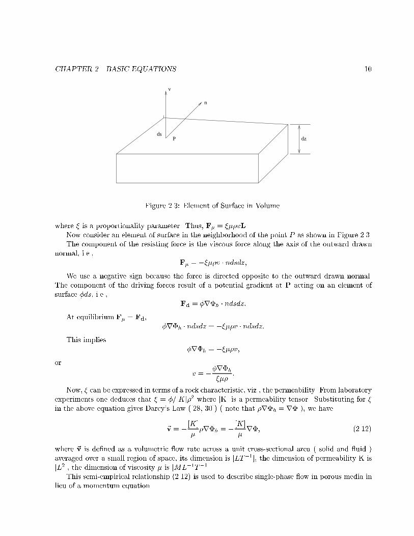
Figure 2.3: Element of Surface in Volume.
where � is a proportionality parameter. Thus, F� = ���vL.Now consider an element of surface in the neighborhood of the point P as shown in Figure 2.3.The component of the resisting force is the viscous force along the axis of the outward drawn
normal, i.e.,F� = ����v � ndsdz;
We use a negative sign because the force is directed opposite to the outward drawn normal.The component of the driving forces result of a potential gradient at P acting on an element ofsurface �ds, i.e.,
Fd = �r�h � ndsdz:At equilibrium F� = Fd,
�r�h � ndsdz = ����v � ndsdz:This implies
�r�h = ����v;or
v = ��r�h
���:
Now, � can be expressed in terms of a rock characteristic, viz., the permeability. From laboratoryexperiments one deduces that � = �=[K]�2 where [K] is a permeability tensor. Substituting for �in the above equation gives Darcy's Law ([28, 30]) ( note that �r�h = r� ), we have
~v = � [K]
��r�h = � [K]
�r�; (2.12)
where ~v is de�ned as a volumetric ow rate across a unit cross-sectional area ( solid and uid )averaged over a small region of space, its dimension is [LT�1], the dimension of permeability K is[L2], the dimension of viscosity � is [ML�1T�1].
This semi-empirical relationship (2.12) is used to describe single-phase ow in porous media inlieu of a momentum equation.
CHAPTER 2. BASIC EQUATIONS 11
Combining equations (2.4) and (2.12), and suppose the coordinate in the vertical downwarddirection is z, then we can write
�� ggcrz = � rz:
In reservoir engineering, we often de�ne the velocity potential as follows ([24, 92]):
�v =K
�� =
K
�(P + z) (2.13)
and the dimension of velocity potential �v is [L2T�1].
By equations of state, we mean relationship that relate density to pressure at a point. Reser-voir uids are considered compressible and, at constant reservoir temperature, we can de�ne anisothermal compressibility of uid as a positive term Cf as follows ([5, 34, 74])
Cf = � 1
V
@V
@P=
1
�
@�
@P: (2.14)
where V denotes original volume and P is pressure. Gas compressibility is signi�cantly greaterthan those of liquid hydrocarbons, which in turn are greater than those of reservoir waters. Thesubscript terminology for the compressibilities of gas, oil and water is Cg; Co; Cw. Reservoir porevolume may change with change in uid pressure, resulting in an increased fraction of overburdenbeing taken by reservoir rock grains. If the variation of pore volume with pressure is the rockcompressibility CR, we have
CR =1
�
@�
@P: (2.15)
Liquid hydrocarbons are often assumed to exhibit constant compressibility. Equation (2.14)can be integrated to yield
� = �0 exp[Cf (P � P0)]; (2.16)
where the zero subscripts refer to a datum level, �0 is the density at the reference pressure P0.If the reservoir liquid is a slightly compressible, then by Taylor's expansion,
� = �0f1 + Cf (P � P0) + C2f (P � P0)
2=2! + � � �g:
If we neglect terms of power two and higher, we get
� = �0[1 + Cf (P � P0)]: (2.17)
Similarly, we have� = �0[1 +CR(P � P0)];
where �o is the porosity at the reference pressure P0.If the uid is a gas, we employ the gas law PV = nZRT = mZ=(MRT ) where m is mass, M is
the molecular weight, T is temperature, and Z is gas deviation factor, and PM = Z�RT ([4, 55]).Since ( [5, 55])
Cf =1
�
@�
@P=
1
P� 1
Z
dZ
dP;
then@�
@P=
M
RT
@
@P(P
Z):
CHAPTER 2. BASIC EQUATIONS 12
Consequently,
Cf =Z
P
@
@P(P
Z);
for a nonideal gas. For an ideal gas Z = 1, so Cf = 1=P .In reservoir engineering, we often de�ne the total compressibility coe�cient as follows ([5, 34,
74]):Ct = �0Cf + CR (2.18)
The dimension of Cf ; CR and Ct is [M�1LT 2].
In summary, we may write equation of state as
� = �(P ): (2.19)
We now have the following relationships: continuity equation (2.11), ow potential equation(2.2), Darcy's law (2.12) and equation of state (2.19). We emphasize that each of these equationsare prescribed at some point in pore space. By combining them in an appropriate manner, one canarrive at the ow equations for single-phase uids in a porous system. Their subsequent integrationover space provides a dynamic picture of global phenomena i.e., at all points in space. ( Here weuse the term \integration" rather loosely, including obtaining a solution or approximate solutionin some sense.) Another important point is that equations (2.11), (2.2), (2.12) and (2.19) are validin any coordinate system. Consequently, for a given reservoir, we need only specify the coordinatesystem, the number of dimensions ( i.e., 1D, 2D, or 3D ), and the type of uid present to arriveat a speci�c ow expression.
When the entire pore space is occupied by a single phase compressible ow, after combiningequations (2.10), (2.12) and (2.2), we have
r � f [K]�
�(rP + rd)g = @(��)
@t: (2.20)
If Cf =1�@�@P , this implies that �rP = (1=Cf )r�, so equation (2.20) can be written
r � f [K]
�Cf(rP + � Cfrd)g = �
@�
@t; (2.21)
for a system with constant porosity. In Cartesian coordinates, we have ([98])
@
@x
Kx
�Cf
@�
@x
!+
@
@y
Ky
�Cf
@�
@y
!+
@
@z
"Kz
�Cf(@�
@z+ � Cf )
#= �
@�
@t: (2.22)
If again, the medium is homogeneous and isotropic and � is constant, we get ([28, 30, 94])
r2� =1
�
@�
@t; � =
K
��Cf(2.23)
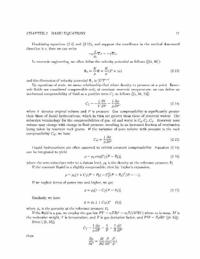
neglecting gravity e�ects. This is known as Fourier's equation or the di�usivity equation. If the uid is slightly compressible, then one can employ (2.17) to obtain an equation identical to (2.23)where � is replaced by P . In equation (2.23), the constant � is frequently called the di�usivitycoe�cient. We have assumed constant rock properties (K;�), constant viscosity (�), negligiblegravitational e�ects and ignored the square of the pressure gradient, and there holds ([92])

CHAPTER 2. BASIC EQUATIONS 13
PLAN
ELEVATION
a) LINEAR RADIAL SPHERICALb) c)
Figure 2.4: Flow Geometries.
r2P =1
�
@P
@t; � =
K
��Cf: (2.24)
Note that in addition to the assumptions already made, the validity of (2.23) and (2.24) arelimited to isotropic media, horizontal formation and the uid ow obeying the Darcy's law.
We know that thermodynamic behavior of gases can be described by the equation of state ([55]),
� =PM
ZRT:
Insertion above equation into (2.20) and subsequent simpli�cations results in the ow equationfor ideal gases ([55])
r2P 2 =1
�
@P 2
@t; � =
K
��Cf: (2.25)
The ow equations, (2.23),(2.24),(2.25) can be written in terms of rectangular ( Cartesian ),cylindrical and spherical coordinates. Since ow is normally dominant in one direction only, asuitable choice of the coordinate system may lead to a substantial mathematical simpli�cation.
A well is considered to produce from a symmetrical drainage area of a uniform pay thickness.Furthermore, a well is open to ow over the entire pay thickness so that the ow lines convergetowards a pressure sink, the wellbore itself ( see Figure 2.4 ). Such a ow model is called theradial-cylindrical or simply the radial ow model and equation (2.24) is then reduced to ([94])
@P
@t=
K
��Cf
1
r
@
@r
�r@P
@r
�: (2.26)
Partial well completion and/or a very thick formation may be better described by using thespherical geometry ([30]). The uid is assumed to ow towards the wellbore which is approximatedby a central point. The radial form of (2.24) in spherical coordinates becomes
@P
@t=
K
��Cf
1
r2@
@r
�r@P
@r
�: (2.27)
Fluid ow in fractured wells of in�nitely large conductivity or in long narrow channels can oftenbe characterized by linear ow in a horizontal plane. In terms of the rectangular coordinates, the

CHAPTER 2. BASIC EQUATIONS 14
one - dimensional form of the ow equation is
@P
@t=
K
��Cf
@2P
@x2: (2.28)
Two di�erent physical conditions may arise at the wellbore during well testing:a) Constant production rate:
qsf =�AK�B
�@P
@r
�rw
; (2.29)
where A = 2�rwh in the case of a radial system, whereas A = 4�r2s is used in a spherical system.Note that qsf refers to the ow rate at the sandface level.
b) Constant bottomhole pressure:
P = Pwf ; r = rw; (2.30)
where Pwf is a constant pressure at the wellbore against which the well produces.The speci�cation of the pressure behavior at the external boundary depends on the type of
reservoir considered.a) Volumetric reservoir: This is a closed system characterized by no uid ow across the outer
boundary. Referring to equation (2.29), the zero ow rate ( velocity ) is expressed in terms ofpressure gradient as �
@P
@r
�re
= 0: (2.31)
b) Reservoir associated with a gas cap or bottom water is featured by constant pressure at theexternal boundaries. In this case the pressure distribution does not change with time and the truesteady-state condition is reached; that is,
P = Pi; r = re: (2.32)
c) In�nitely large reservoir: This is a mathematical concept which is very useful during theinitial stages of well testing when the pressure disturbance does not travel far enough to reach thereservoir boundary.
limr!1
P = Pi: (2.33)
In all situations considered, it is assumed that initially the reservoir pressure is uniform
P = Pi; t = 0: (2.34)
Chapter 3
Velocity Potential Analysis
In this chapter, we will introduce a mathematical and physical model of horizontal wells, thenwe will use it to derive the velocity potential formula and calculate the average velocity potentialof horizontal wells by the pressure-averaging technique and equivalent pressure-point technique.
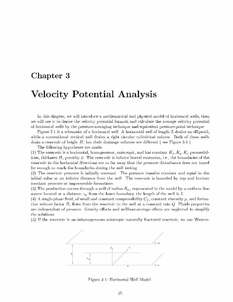
Figure 3.1 is a schematic of a horizontal well. A horizontal well of length L drains an ellipsoid,while a conventional vertical well drains a right circular cylindrical volume. Both of these wellsdrain a reservoir of height H, but their drainage volumes are di�erent ( see Figure 3.4 ).
The following hypotheses are made:(1) The reservoir is a horizontal, homogeneous, anistropic, and has constant Kx;Ky;Kz permeabil-ities, thickness H, porosity �. The reservoir is in�nite lateral extension, i.e., the boundaries of thereservoir in the horizontal directions are so far away that the pressure disturbance does not travelfar enough to reach the boundaries during the well testing.(2) The reservoir pressure is initially constant. The pressure remains constant and equal to theinitial value at an in�nite distance from the well. The reservoir is bounded by top and bottomconstant pressure or impermeable formations.(3) The production occurs through a well of radius Rw, represented in the model by a uniform linesource located at a distance zw from the lower boundary, the length of the well is L.(4) A single-phase uid, of small and constant compressibility Cf , constant viscosity �, and forma-tion volume factor B, ows from the reservoir to the well at a constant rate Q. Fluids propertiesare independent of pressure. Gravity e�ects and wellbore-storage e�ects are neglected to simplifythe solutions.(5) If the reservoir is an inhomogeneous anistropic naturally fractured reservoir, we use Warren-
H
Z
Z Y
X
w
Z = H
Z = 0
Figure 3.1: Horizontal Well Model.
15
CHAPTER 3. VELOCITY POTENTIAL ANALYSIS 16
Root Model, uid movement toward the wellbore occurs only in fractures ([49, 87]).
3.1 Equipotential Surfaces of Horizontal Wells
In this section, we will derive the velocity potential formula of a point in 3D space and equipo-tential surfaces of horizontal wells.
To calculate oil production from a horizontal well mathematically, the three-dimensional (3D)Laplace equation needs to be solved �rst. If constant pressure at the drainage boundary and atthe wellbore is assumed, the solution would give a pressure distribution within a reservoir. Oncethe pressure distribution is known, oil production rates can be calculated by Darcy's law, ( seeequation (2.12), [28, 30])
!v= �K
�r�:
In steady state, we have the continuity equation : ( see equation (2.10), [30] )
div(!v ) = 0;
then
div(�K�r�) = 0:
If we use the velocity potential �v, ( see equation (2.13) ) , therefore in order to derive thereasonable and reliable productivity formulae, we must solve 3D Laplace equation: ( see equation(2.24), [2] )
r2�v = 0: (3.1)
Suppose a mathematical pointM in the 3D space, and an in�nite large percolation �eld aroundM , then the percolation velocity of a sphere surface is ([4, 28])
!v=
q
A=
q
4�r2;
the dimension of q is [L3T�1], and A is cross-sectional ow area.According to Darcy's law ([4, 64]),
!v=
d�v
dr;
thus we obtain the velocity potential of point M in 3D space is
�v = � q
4�r+ constant:
We consider the uniform - ux, �nite - conductivity model, take the horizontal well as a uniformline source in 3D space, the total productivity is Q, thus Q=L is unit length productivity, thedimension of Q is [L3T�1], at every point along the well, the well ow rate is the same.
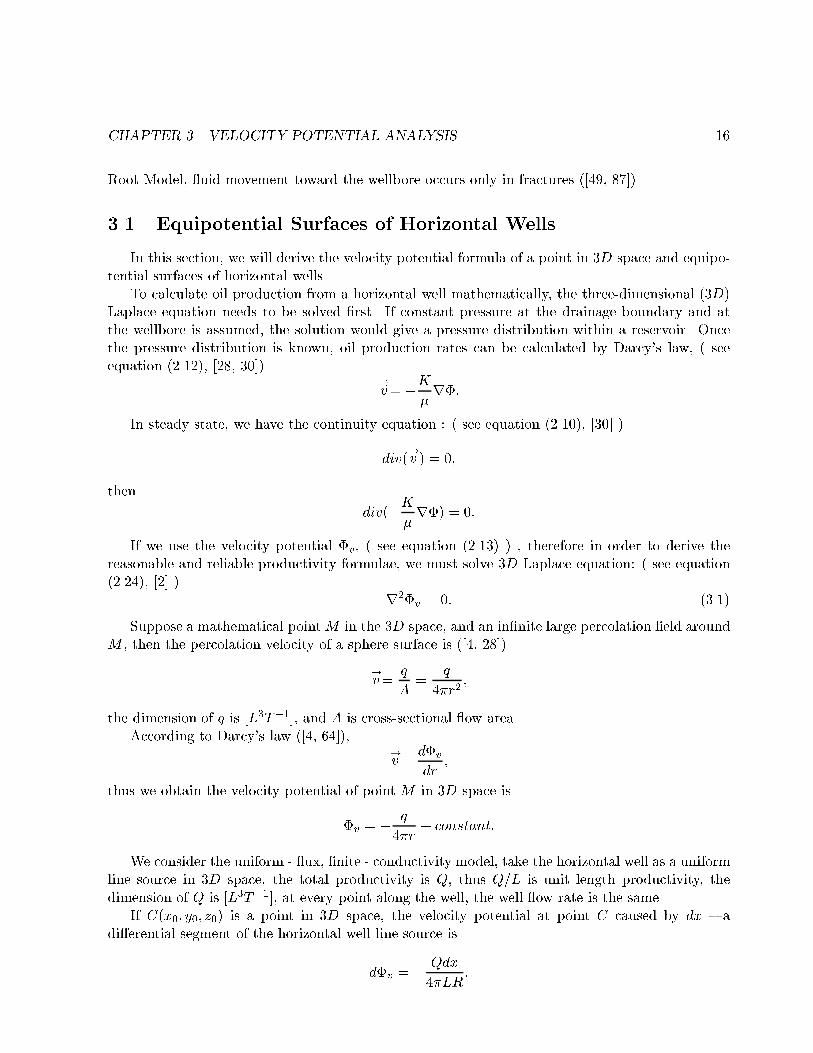
If C(x0; y0; z0) is a point in 3D space, the velocity potential at point C caused by dx { adi�erential segment of the horizontal well line source is
d�v = � Qdx
4�LR;

CHAPTER 3. VELOCITY POTENTIAL ANALYSIS 17
C
D OA B
Figure 3.2: The Analyses of the Velocity Potential.
andR =
q(x� x0)2 + y20 + z20 =
q(x� x0)2 + r20; (3.2)
where r20 = y20 + z20 .If we let c = L
2 , then the velocity potential caused by the whole line source is
�v = � Q
4�L
Z c
�c
dx
R: (3.3)
Figure 3.2 shows the analyses of the velocity potential. Point O(0; 0; 0) is the midpoint ofsegment AB. Point D(x0; 0; 0) is the projection of point C in segment AB. Let eR be the radiusof triangle ABC's circumscribed circle, considering A(�c; 0; 0), B(c; 0; 0), and let the three sides oftriangle ABC be ea;eb; ec, we can show that ([40])
AC = eb = 2 eR sinB; BC = ea = 2 eR sinA; AB = ec = 2 eR sinC;
OA = OB = c; CD =qy20 + z20 = r0;
and according to the Sine Law of Triangle, we have ([40])
AD = OA�OD = c� jx0j = eb cosA = 2 eR sinB cosA;
BD = OA+OD = c+ jx0j = ea cosA = 2 eR sinA cosB;
therefore Z c
�c
dx
R=
Z c
�c
dxq(x� x0)2 + r20
= ln
"c� x0 + eb
�(c+ x0) + ea#
= ln[2 eR sinB(1 + cosA)
2 eR sinA(1� cosB)]
= � ln(tanA
2tan
B
2);

CHAPTER 3. VELOCITY POTENTIAL ANALYSIS 18
Z
Y
X
Figure 3.3: The Shape of the Equipotential Surfaces.
so, we have
�v =Q
4�Lln(tan
A
2tan
B
2): (3.4)
In the triangle, let s be half perimeter, r be the radius of inscribed circle, and let a = 12(ea+ eb),
according to the Half Angle Law of Triangle ([106]), we have
s =1
2(ea+ eb+ ec); r =
s(s� ea)(s� eb)(s� ec)
s;
tanA
2=
r
s� ea; tanB
2=
r
s� eb ;tan
A
2tan
B
2=
r2
(s� ea)(s� eb) = (s� ec)s
=a� c
a+ c:
Therefore we have
�v =Q
4�Lln(
a� c
a+ c): (3.5)
According to the de�nition of ellipsoid of revolution ([40]), if the sum of segment AC andAB's length is 2a, point C is on the ellipsoid of revolution whose focuses are point A and B, anda = 1
2(ea+ eb) is semimajor axis. So we can come to the conclusion:The equipotential surfaces of a horizontal well uniform line source in 3D space are a family of
ellipsoids of revolution whose focuses are the two endpoints of the horizontal well.Figure 3.3 shows the shape of the equipotential surfaces.

CHAPTER 3. VELOCITY POTENTIAL ANALYSIS 19
HR e
L
HR e
Figure 3.4: Schematics of Vertical and Horizontal Well Drainage Volume.

CHAPTER 3. VELOCITY POTENTIAL ANALYSIS 20
3.2 Average Velocity Potential of Horizontal Wells
In this section, we will derive the average velocity potential formulae of horizontal wells by thepressure-averaging technique and equivalent pressure-point technique.
Arbitrary point (x; y; z) in 3D space is on an ellipsoid of revolution equipotential surface, andits semimajor axis is
a(x; y; z) =1
2[q(x� c)2 + y2 + z2 +
q(x+ c)2 + y2 + z2]: (3.6)
Judging by the above formula, the potential of a point on the horizontal well line source isdependent on the location of the point, because each point is on its own ellipsoid of revolutionequipotential surface. However, we can derive the average velocity potential f�v of a horizontalwell.
f�v =1
2c
Z c
�c
Q
4�Lln
�aw(x)� c
aw(x) + c
�dx; (3.7)
where
aw(x) =1
2[q(x+ c)2 +R2
w +q(x� c)2 +R2
w]: (3.8)
To compute the average velocity potential of the whole horizontal well, we may use the averagesemimajor axis of the ellipsoid of revolution equipotential surfaces.
Because L� Rw, thus
1
2
qL2 +R2
w � L=2 +R2w=(4L); ln(L+
qL2 +R2
w) � ln(2L);
consequently,
faw =1
2c
Z c
�caw(x)dx � L=2 +R2
w=(4L) +R2w
2Lln(2L=Rw): (3.9)
As a result, the average velocity potential of the horizontal wellbore g�w is
g�w � Q
4�Lln[
R2w
2L2ln(2L=Rw)]: (3.10)
The velocity potential of the two endpoints and midpoint are dependent on the semimajor axesof the ellipsoids of revolution equipotential surfaces which they are on. So, we have
2L� Rw +R2w=(2L); Rw � R2
w=(2L);
aEw =1
2(qL2 +R2
w +Rw) � L=2 +Rw=2 +R2w=(4L);
aMw =q(L=2)2 +R2
w � L=2 +R2w=L:
Thus, the velocity potential of the endpoints and midpoint are
�Ew �
Q
4�Lln[Rw=(2L)]; (3.11)

CHAPTER 3. VELOCITY POTENTIAL ANALYSIS 21
�Mw � Q
4�Lln(R2
w=L2): (3.12)
According to Simpsons Integral Approximation Rule ([40, 52]), the average velocity potentialof the horizontal well can be approximately represented as follows
g�w � 1
6(2�E
w + 4�Mw ) =
Q
4�L[5
3ln(Rw=L)� 1
3ln 2]: (3.13)
Let I be the ratio of endpoint and midpoint's velocity potential, then
I =�Ew
�Mw
=1
2[1 + 1= log2(L=Rw)] � 1
2; (3.14)
when L!1, I ! 12 :
Let J be the ratio of eqaution (3.13) and equation (3.10), then
J =[53 ln(Rw=L)� 1
3 ln 2]
ln[ R2w
2L2 ln(2L=Rw)]: (3.15)
Table 3.1: The ratioes of velocity potential of endpoint and midpoint.
Rw 0.1m 0.1m 0.1m 0.1m 0.1m
L 200m 300m 400m 500m 600m
I 0.545 0.543 0.542 0.541 0.539
According to Table 3.1, we can see that the endpoint's velocity potential is approximately equalto 54 percent the midpoint's velocity potential. This conclusion tells us:
If we take a horizontal well as a uniform line source in 3D space, the well is not an in�niteconductivity fracture, the in�nite conductivity model is not exact for horizontal wells.
Table 3.2: The comparisons of the two methods of calculating average velocity potential.
Rw 0.1m 0.1m 0.1m 0.1m 0.1m
L 200m 300m 400m 500m 600m
J 0.935 0.933 0.931 0.930 0.929
According to Table 3.2, we can see that these two methods perform similarly, the di�erencebetween them is small.
Chapter 4
Productivity Formulae
In petroleum engineering, in order to determine the economic feasibility of drilling a horizontalwell, the engineers need reliable methods to estimate its expected productivity { well ow rate.
In this chapter, we will derive the productivity formulae of horizontal wells in three-dimensionalspace for steady state ow. We will show that any two-dimensional (2D) methods are not suitablefor three-dimensional (3D) percolation problems unless we assume the horizontal well's length isin�nite. The formulae based on 2D model can not satisfactorily re ect characteristics of horizontalwells.
In a reservoir, there may be several wells working together at the same time. However, a speci�cwell exploits a de�nite volume of reservoir uid, and this volume is called the drainage volume ofthat well.
Let �Pw be the pressure drawdown between the boundary of drainage volume and wellbore,then we have
�Pw = Pe � Pw = Pi � Pw;
the pressure on the external boundary Pe is assumed to be the initial pressure Pi.
4.1 Formulae for Wells at Midheight of Formation
We �rst consider the case in which the horizontal well is at the midheight of the formation.According to our previous equipotential surface conclusion, in order to simplify the boundary
problem, we suppose the external boundary of drainage volume is also on an ellipsoid of revolutionequipotential surface, so we may assume further that:
The drainage volume of a horizontal well is an ellipsoid of revolution whose focuses are the twoendpoints, and minor axis is the formation thickness H, the horizontal well is at the midhight ofthe formation ( see Figure 3.4 ).
Thus, the semimajor axis of the drainage volume is
ae =q(L=2)2 + (H=2)2 =
1
2
pL2 +H2: (4.1)
According to equation (3.5), the velocity potential of the external boundary is
�e =Q
4�Lln
"pL2 +H2 � LpL2 +H2 + L
#: (4.2)
22

CHAPTER 4. PRODUCTIVITY FORMULAE 23
Let
E =
pL2 +H2 � LpL2 +H2 + L
;
then, combining equations (2.13), (3.10) and (4.2), the productivity formula of a horizontal well inan ellipsoid of revolution drainage volume is
Qw =4�KL�Pw=(�B)
ln[ 2EL2
R2w ln(2L=Rw)
]: (4.3)
In the above formula, B is formation volume factor. Formation volume factors have been giventhe general standard designation of B and are used to de�ne the ratio between a volume of uidat reservoir conditions of temperature and pressure and its volume at standard condition : 600Fand 1 atmosphere. The factors are therefore dimensionless but are commonly quoted in terms ofreservoir volume per standard volume. Thus, in this thesis, Qw means well ow rate at standardcondition.
When x! 0;p1 + x � 1 + x=2, thus if L� H, thenp
L2 +H2 + L � 2L;pL2 +H2 � L = L(
q1 +H2=L2)� L � H2=2L;
thus equation (4.3) becomes
Qw =4�KL�Pw=(�B)
ln[ H2
2R2w ln(2L=Rw) ]
: (4.4)
The above formulae (4.3), (4.4) are only suitable for isotropic reservoirs { the formation's verticalpermeability is equal to its horizontal permeability. In fact, in many reservoirs with anisotropicpermeabilities, formation's vertical permeability is smaller than horizontal permeability. To derivethe productivity formula of horizontal wells in anisotropic reservoirs, we assume that Kh = Kx =Ky; Kv = Kz. Then equation (2.22) can be reduced to
Kh@2P
@x2+Kh
@2P
@y2+Kv
@2P
@z2= 0: (4.5)
We let
ex = ( 4
sKv
Kh)x; ey = ( 4
sKv
Kh)y; ez = ( 4
sKh
Kv)z:
Thus, equation (4.5) becomes
pKvKh(
@2P
@ex2 +@2P
@ey2 +@2P
@ez2 ) = 0; (4.6)
and K;L;H become
fK =pKvKh; eL = ( 4
sKv
Kh)L; eH = ( 4
sKh
Kv)H:

CHAPTER 4. PRODUCTIVITY FORMULAE 24
X
Z
x
Kz
K
R w
Figure 4.1: Original Reservoir System with x/z Anisotropy and Horizontal Well.
K
x
z
K, X
,
Z,
,
Figure 4.2: Transformed Isotropic Reservoir System with Elliptic Wellbore.
CHAPTER 4. PRODUCTIVITY FORMULAE 25
b ( semi minor axis )
axis )a (semi major
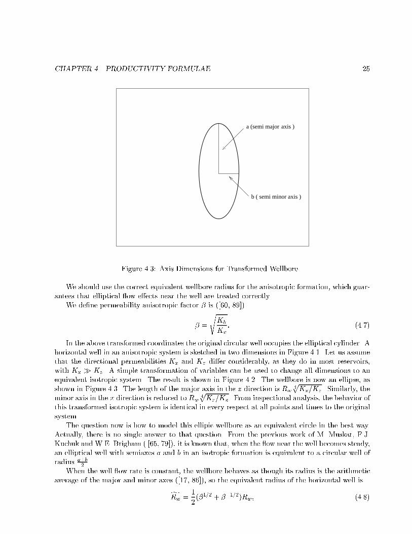
Figure 4.3: Axis Dimensions for Transformed Wellbore.
We should use the correct equivalent wellbore radius for the anisotropic formation, which guar-antees that elliptical ow e�ects near the well are treated correctly.
We de�ne permeability anisotropic factor � is ([60, 89])
� =
sKh
Kv: (4.7)
In the above transformed coordinates the original circular well occupies the elliptical cylinder. Ahorizontal well in an anisotropic system is sketched in two dimensions in Figure 4.1. Let us assumethat the directional permeabilities Kx and Kz di�er considerably, as they do in most reservoirs,with Kx � Kz. A simple transformation of variables can be used to change all dimensions to anequivalent isotropic system. The result is shown in Figure 4.2. The wellbore is now an ellipse, asshown in Figure 4.3. The length of the major axis in the z direction is Rw
4pKx=Kz . Similarly, the
minor axis in the x direction is reduced to Rw4pKz=Kx. From inspectional analysis, the behavior of
this transformed isotropic system is identical in every respect at all points and times to the originalsystem.
The question now is how to model this ellipic wellbore as an equivalent circle in the best way.Actually, there is no single answer to that question. From the previous work of M. Muskat, F.J.Kuchuk and W.E. Brigham ( [65, 79]), it is known that, when the ow near the well becomes steady,an elliptical well with semiaxes a and b in an isotropic formation is equivalent to a circular well ofradius a+b
2 .When the well ow rate is constant, the wellbore behaves as though its radius is the arithmetic
average of the major and minor axes ([17, 86]), so the equivalent radius of the horizontal well is
gRw =1
2(�1=2 + ��1=2)Rw; (4.8)
CHAPTER 4. PRODUCTIVITY FORMULAE 26
where � is permeability anisotropic factor, when � = 1;gRw = Rw.Thus ex; ey; ez; eL; eH are changed to
ex = ��1=2x; ey = ��1=2y; ez = �1=2z: (4.9)
eL = ��1=2L; eH = �1=2H: (4.10)
We de�ne
F = ln[4L
(� + 1)Rw]; (4.11)
G = ln[
pKvL2 +KhH2 �pKvLpKvL2 +KhH2 +
pKvL
]: (4.12)
and we apply F;G and equation (4.8) to equation (4.3), then we obtain the productivity formulaof a horizontal well in an anisotropic permeability reservoir
Qw =4� 4pK3v
4pKhL�Pw=(�B)
(ln 12 + 2F +G� lnF )
: (4.13)
It has been pointed out that, during production, the vertical permeability is more importantthan the horizontal permeability for horizontal wells. But the productivity formulae in [6, 7, 39,44, 60] can not account for this viewpoint. Our formula (4.13) demonstrates it, because in formula(4.13), the exponent of Kv is 3=4 while the exponent of Kh is 1=4.
Our physical system consisted of a horizontal well producing at a uniform and constant rate froman anisotropic, box-shaped drainage volume. We used the well-known line sink/source solution forthe well. Thus, according to our analysis, in the immediate vicinity of the wellbore, i.e., at R = Rw,the ow is characterized by two main features: (1) the ux into the wellbore is uniform; (2) thepressure along the well varies, i.e., the well can not be an isopotential, we may use a representativeaverage wellbore pressure.
In an anisotropic formation, the isopotential lines are ellipses, the circular wellbore can nothave uniform pressure along the perimeter. It is also clear that, because of friction losses and otherfactors, the pressure is not constant along the well ([7]).
Our formulae (4.3), (4.4) and (4.13) are suitable for the horizontal wells at the midhight of aformation.
4.2 Well Eccentricity Problem
In this section, we apply the three dimensional model to study the well eccentricity problem inwhich a horizontal well's location is not at the midheight of a reservoir.
Taking a horizontal well as a uniform line source in 3D space, the coordinates of the two endsare : (�L=2; 0; zw) and (L=2; 0; zw). Point convergence intensity is the ow rate through a pointin 3D space. If the point convergence intensity of point (x0; y0; z0) which is in in�nite space isq, in order to obtain its steady state pressure, we have to obtain the basic solution of the partialdi�erential equation below ([36]), and the point (x0; y0; z0) becomes (x0; 0; zw) ( see Figure 3.1 ).
Kx@2P
@x2+Ky
@2P
@y2+Kz
@2P
@z2

CHAPTER 4. PRODUCTIVITY FORMULAE 27
= �qB�(x� x0)�(y)�(z � zw); (4.14)
where �(x � x0), �(y), �(z � zw) are Dirac functions ([106]). The dimension of the above Diracfunctions such as �(z� zw) is [L
�1], the dimension of q is [L3T�1], and the dimension of both sidesof equation (4.14) is [ML�1T�2]. The total productivity of the horizontal well is Qw, its dimensionis also [L3T�1].
Transformation of a mathematical model into dimensionless form is a common engineering prac-tice. In treating pressure transient problems, the introduction of dimensionless groups reduces thenumber of variables and parameters which can signi�cantly simplify the mathematical statement.
Let
xD =x
L(
�K
Kx)1=2; yD =
y
L(
�K
Ky)1=2; zD =
z
L(
�K
Kz)1=2: (4.15)
We de�ne e�ective permeability
�K= (KxKyKz)
1=3: (4.16)
Generally, there holds Kx = Ky 6= Kz, so we let
Kh = Kx = Ky; Kv = Kz: (4.17)
Consequently, we have
LD = (
�K
Kx)1=2; HD =
H
L(
�K
Kz)1=2; zwD =
zwL(
�K
Kz)1=2: (4.18)
Note that the permeability anisotropic factor � is
� =
sKh
Kv=
sKx
Kz: (4.19)
As we stated before, because of dimensionless transformation, the circular wellbore becomesellipse, the dimensionless equivalent radius of the well is the arithmetic mean of semimajor axisand semiminor axis of the ellipse, i.e. ([17, 86]),
RwD � (�1=2 + ��1=2)Rw=(2L); (4.20)
when � = 1; RwD = Rw=L.According to equation (4.15), there hold
@P
@x=
@P
@xD
@xD@x
= (1
L)(
�K
Kx)1=2
@P
@xD;
@2P
@x2= (
1
L2)(
�K
Kx)@2P
@xD2 :
Similar formulae can be derived for other derivatives, so
Kx@2P
@x2+Ky
@2P
@y2+Kz
@2P
@z2= (
�K
L2)(@2P
@xD2 +
@2P
@yD2 +
@2P
@zD2 ):

CHAPTER 4. PRODUCTIVITY FORMULAE 28
Note that �(cx) = �(x)=c, c is a positive constant ([106]), then
�(xD � x0D) = �
24 (x� x0)
L(
�K
Kx)1=2
35 = (Kx
�K
)1=2L�(x� x0);
and
�qB�(x� x0)�(y)�(z � zw) = (�qB
L3)
24 (�K)3=2
(KxKyKz)1=2
35 �(xD � x0D)�(yD)�(zD � zwD):
According to equation (4.16), there holds24 (�K)3=2
(KxKyKz)1=2
35 = 1:
If we de�ne
PD =
�K L(Pi � P )
�qB; (4.21)
then equation (4.14) becomes
@2PD
@xD2 +
@2PD
@yD2 +
@2PD
@zD2 = ��(xD � x0D)�(yD)�(zD � zwD): (4.22)
We must point out that if the point convergence intensity of point (x0; y0; z0) is q, then thetotal productivity of the horizontal well is
Qw = qLD: (4.23)
4.2.1 Point Convergence Pressure Distribution Formulae
In this subsection, we will derive the point convergence pressure distribution formulae, i.e.,dimensionless pressure formulae of the points in 3D space.
We �rst consider the drainage domain is between the in�nite parallel planes z = H and z = 0with the impermeable boundary condition at z = H, constant boundary condition at z = 0 ( e.g.the horizontal well is in the reservoir with bottom water ), thus
PDjzD=0 = 0;@PD@ND
jzD=HD= 0; (4.24)
where @PD@ND
is the exterior normal derivative of dimensionless pressure.Considering the simultaneous equations of (4.22) and (4.24), let the normalized orthogonal
solution systems be gn(zD), then we have
gn(zD) =q2=HD sin[
(2n� 1)�zD2HD
]; (n = 1; 2; 3; :::); (4.25)
CHAPTER 4. PRODUCTIVITY FORMULAE 29
because gn(zD) satisfy the boundary conditions (4.24), andZ HD
0gigjdzD = 0; (i 6= j); (4.26)
Z HD
0[gn]
2dzD = 1; (n = 1; 2; 3; :::): (4.27)
Therefore, according to the properties of Dirac function and the normalized orthogonal solutionsystems of the partial di�erential equation basic solution, there holds ([100, 101, 102])
�(zD � zwD) =1Xn=1
gn(zwD)gn(zD); (4.28)
i.e.,
�(zD � zwD) =1Xn=1
(2
HD) sin[(2n� 1)�zD)=(2HD)] sin[(2n� 1)�zwD)=(2HD)]: (4.29)
Let
PD =1Xn=1
Un(xD; yD) sin[(2n� 1)�zD
2HD]; (4.30)
and we de�ne the two dimensional Laplace operator as follows:
�Un =@2Un
@xD2 +
@2Un
@yD2 : (4.31)
Apply equations (4.31) and (4.30) to equation (4.22), then Un is the basic solution of thefollowing equation ([100, 101, 102])
�Un(xD; yD)� [(2n� 1)�=(2HD)]2Un(xD; yD)
= (2
HD)�(xD � x0D)�(yD) sin[(2n� 1)�zwD=(2HD)]: (4.32)
Using integration transformation method, we have
Un(xD; yD) = (2
HD) sin[(2n� 1)�zwD=(2HD)]f( 1
2�)K0[(2n� 1)�RD=(2HD)]g
= (1
�HD) sin[(2n� 1)�zwD)=(2HD)]K0[(2n� 1)�RD=(2HD)]; (4.33)
whereRD =
q(xD � x0D)2 + y2D: (4.34)
Combining equations (4.30) and (4.33), if the boundary conditions are (4.24), the dimensionlesspressure of the point (x0D,0,zwD) is
PD =1Xn=1
(1
�HD) sin[
(2n� 1)�zD2HD
] sin[(2n� 1)�zwD
2HD]K0[(2n� 1)�RD=(2HD)]: (4.35)
CHAPTER 4. PRODUCTIVITY FORMULAE 30
In the (4.33) and (4.35), K0(x) is modi�ed Bessel function of second kind and order zero ([106]).If the drainage domain is between the in�nite parallel planes z = H and z = 0 such that the
boundary condition is impermeable at z = 0 , but constant at z = H ( e.g the horizontal well is inthe reservoir with gas cap ), then
PDjzD=HD= 0;
@PD@ND
jzD=0 = 0: (4.36)
Similarly, if the boundary conditions are (4.36), the dimensionless pressure of the point (x0D,0,zwD)is
PD =1Xn=1
(1
�HD) cos[
(2n� 1)�zD2HD
] cos[(2n� 1)�zwD
2HD]K0[(2n� 1)�RD=(2HD)]: (4.37)
If the drainage domain is between the in�nite parallel planes z = H and z = 0 with the boundaryconditions at z = H and z = 0 are both constant ( e.g the horizontal well is in the reservoir withbottom water and gas cap ), then
PDjzD=0 = 0; PDjzD=HD= 0: (4.38)
Considering the simultaneous equations of (4.22) and (4.38), letting the normalized orthogonalsolution systems be fn(zD), then we have
fn(zD) =q2=HD sin[
n�zDHD
]; (n = 1; 2; 3; :::); (4.39)
because fn(zD) satisfy the boundary conditions (4.38), andZ HD
0fifjdzD = 0; (i 6= j); (4.40)
Z HD
0[fn]
2dzD = 1; (n = 1; 2; 3; :::): (4.41)
Hence, if the boundary conditions are (4.38), the dimensionless pressure of the point (x0D,0,zwD)is
PD =1Xn=1
(1
�HD) sin[
n�zDHD
] sin[n�zwDHD
]K0[n�RD=HD]: (4.42)
Formulae (4.35), (4.37), (4.42) are the point convergence pressure distribution formulae, i.e.,dimensionless pressure formulae of the points in 3D space.
4.2.2 Dimensionless Pressure Formulae of Horizontal Wells
In this subsection, we will derive the dimensionless pressure formulae of the endpoint andmidpoint of horizontal wells under di�erent boundary conditions.
Because the horizontal well line uniform source is located between �L=2 � x0 � L=2, i.e.,�LD=2 � x0D � LD=2, according to the Superposition Principle of Potential, the dimensionlesspressure of the endpoints and midpoint can be computed by the integration method, and theaverage dimensionless pressure of the whole horizontal well can be computed by the SimpsonsIntegral Approximation Rule.

CHAPTER 4. PRODUCTIVITY FORMULAE 31
From (4.34), we have
RwD =q(xwD � x0D)2 + y2wD � jxwD � x0Dj: (4.43)
If the boundary conditions are (4.24), in the equation (4.35), let zwD + RwD take the place ofzD, and let x0D be the element of integration, along the well length LD, integrate equation (4.35),we can obtain the dimensionless pressure of the horizontal well at xwD is
PwD =
LD=2Z�LD=2
PDdx0D; (4.44)
i.e.,
PwD = (1
�HD)f1Xn=1
sin[(2n� 1)�(zwD +RwD)
2HD] sin[
(2n� 1)�zwD2HD
]Ang; (4.45)
where ( note that eqauation (4.43) )
An =
Z LD=2
�LD=2K0[(2n� 1)�RwD=(2HD)]dx0D
�Z LD=2
�LD=2K0[jxwD � x0Dj(2n� 1)�=(2HD)]dx0D
=
Z 0
�LD=2K0[jxwD � x0Dj(2n� 1)�=(2HD)]dx0D
+
Z LD=2
0K0[jxwD � x0Dj(2n� 1)�=(2HD)]dx0D:
If we letv = jxwD � x0Dj(2n� 1)�=(2HD);
then
An � 2HD
(2n� 1)�
8>><>>:(2n�1)�(LD
2�xwD)=(2HD)Z0
K0(v)dv +
(2n�1)�(LD2
+xwD)=(2HD)Z0
K0(v)dv
9>>=>>; : (4.46)
If our observation point is the endpoint of horizontal well, i.e., xwD = LD=2 or xwD = �LD=2,then
AEn =
2HD
(2n� 1)�
(2n�1)�LD=(2HD)Z0
K0(v)dv
=2HD
(2n� 1)�fZ 10
K0(v)dv �Z 1(2n�1)�LD=(2HD)
K0(v)dvg:
Simplify the above formula, and note that ([52, 106])Z 10
K0(v)dv = �=2; (4.47)

CHAPTER 4. PRODUCTIVITY FORMULAE 32
we have
AEn =
2HD
(2n� 1)�(�
2)� �n; (4.48)
where
�n =2HD
(2n� 1)�
Z 1(2n�1)�LD=(2HD)
K0(v)dv: (4.49)
If we letu = (2n� 1)�LD=(2HD); (4.50)
then equation (4.49) becomes
�n =LDu
Z 1u
K0(v)dv: (4.51)
By the de�nitions of LD;HD ( see equation (4.18) ), u is a positive number which is greaterthan 1, and we de�ne
F (u) =
Z 1u
K0(v)dv: (4.52)
When v !1, according to the asymptotic expansion formula of K0(v), there holds ([40, 52])
K0(v) �r
�
2ve�v; (4.53)
and note that when v � 1, we have e�vpv� e�v, thus
F (u) �Z 1u
r�
2ve�vdv
�r�
2
Z 1u
e�vdv
=
r�
2e�u:
Because
�n =LDuF (u);
therefore
�n � LDu
r�
2e�u =
p2HD
(2n� 1)p�exp[�(2n� 1)�LD=(2HD)]: (4.54)
Note that equation (4.45) should include the in�nite sum of �n with respect to n. Now weestimate the summation, since there holds equation (4.54) and
sin[(2n� 1)�(zwD +RwD)
2HD] sin[
(2n� 1)�zwD2HD
] � 1;
thus we let
E =
����� 1
�HD
1Xn=1
fsin[(2n� 1)�(zwD +RwD)
2HD] sin[
(2n� 1)�zwD2HD
]�ng����� ;

CHAPTER 4. PRODUCTIVITY FORMULAE 33
then
E �p2
�3=2
1Xn=1
���� 1
(2n� 1)exp[�(2n� 1)�LD=(2HD)]
����=
p2
�3=2
1Xn=1
(�2n�1
2n� 1)
=
p2
2�3=2ln(
1 + �
1� �);
where� = exp[��LD=(2HD)] < 1;
and we have used the below formula ([40, 52])
ln(1 + �
1� �) = 2[� + �3=3 + �5=5 + :::+ �2n+1=(2n+ 1) + :::]; (j�j < 1):
By the de�nitions of �; LD;HD and note the fact that L� H, we come to the conclusion that� is a positive number and � ! 0, we have
ln(1 + �
1� �) � 2�;
thus
E �p2
2�3=2ln(
1 + �
1� �) �
p2��3=2�: (4.55)
Therefore, the global error is controlled by a very small positive number, when n increases, theerror does not increase, it is reasonable to neglect �n in equations (4.45) and (4.48), and we cansimplify (4.48) as follows
AEn � HD=(2n� 1): (4.56)
If our observation point is the midpoint of horizontal well, i.e., xwD = 0, by a similar method,we have
AMn =
4HD
(2n� 1)�
(2n�1)�LD=(2HD)Z0
K0(u)du � 2HD=(2n� 1): (4.57)
When x 6= 0, there hold ([40, 52])
1Xn=1
cos(nx)=n = � ln[2 sin(x=2)]; (4.58)
1Xn=1
cos[(2n� 1)x]=(2n � 1) =1
2ln[cot(x=2)]; (4.59)
sin(x) sin(y) =1
2[cos(x� y)� cos(x+ y)]; (4.60)

CHAPTER 4. PRODUCTIVITY FORMULAE 34
cos(x) cos(y) =1
2[cos(x+ y) + cos(x� y)]: (4.61)
and note thatRwD � 0; 2zwD +RwD � 2zwD: (4.62)
Combining equations (4.45), (4.56), (4.59), (4.60), and (4.62), if the boundary conditions are(4.24), the dimensionless pressure of the endpoints of the horizontal well is
PEwD = (
1
�)f1Xn=1
1
2n� 1sin[
(2n� 1)�(zwD +RwD)
2HD] sin[
(2n� 1)�zwD2HD
]g; (4.63)
PEwD = (
1
4�)fln[cot(�RwD
4HD)]� ln[cot(
�(2zwD +RwD)
4HD)]g; (4.64)
PEwD = (
1
4�)fln[cot(�RwD
4HD)]� ln[cot(
�zwD2HD
)]g: (4.65)
Similarly, if the boundary conditions are (4.24), the dimensionless pressure of the midpoint ofthe horizontal well is
PMwD = (
2
�)f1Xn=1
1
2n� 1sin[
(2n� 1)�(zwD +RwD)
2HD] sin[
(2n� 1)�zwD2HD
]g; (4.66)
PMwD = (
1
2�)fln[cot(�RwD
4HD)]� ln[cot(
�(2zwD +RwD)
4HD)]g; (4.67)
PMwD = (
1
2�)fln[cot(�RwD
4HD)]� ln[cot(
�zwD2HD
)]g: (4.68)
In the same manner, if the boundary conditions are (4.36), the dimensionless pressure of theendpoints and the midpoint of the horizontal well are given by the two formulae below, respectively:
PEwD = (
1
4�)fln[cot(�RwD
4HD)] + ln[cot(
�zwD2HD
)]g; (4.69)
PMwD = (
1
2�)fln[cot(�RwD
4HD)] + ln[cot(
�zwD2HD
)]g: (4.70)
If the boundary conditions are (4.38), the dimensionless pressure of the endpoints and themidpoint of the horizontal well are given by the two formulae below, respectively:
PEwD = (
1
4�) lnf sin(�zwD=HD)
sin[�RwD=(2HD)]g; (4.71)
PMwD = (
1
2�) lnf sin(�zwD=HD)
sin[�RwD=(2HD)]g: (4.72)
In summary, we have Table 4.1.Observe the above dimensionless pressures of the endpoint and the midpoint, we may come to
the following conclusion which is similar to what stated in Chapter 3.

CHAPTER 4. PRODUCTIVITY FORMULAE 35
Table 4.1: Dimensionless pressure of endpoint under di�erent boundary conditions.
Boundary Conditions PEwD
PDjzD=0 = 0; @PD@ND
jzD=HD= 0 ( 1
4� )fln[cot(�RwD4HD)]� ln[cot(�zwD2HD
)]gPDjzD=HD
= 0 ; @PD@ND
jzD=0 = 0 ( 14� )fln[cot(�RwD4HD
)] + ln[cot(�zwD2HD)]g
PDjzD=0 = 0 ; PDjzD=HD= 0 ( 1
4� ) lnf sin(�zwD=HD)sin[�RwD=(2HD)]g
Within the given error tolerance, the dimensionless pressure of midpoint of the horizontal wellis about twice as large as the dimensionless pressure of endpoints, i.e. ( see equation (3.14) ),
PMwD � 2PE
wD: (4.73)
According to Simpsons Integral Approximation Rule, the average dimensionless pressure of thehorizontal well uniform line source is
PAwD �
1
6(2PE
wD + 4PMwD) �
5
3PEwD: (4.74)
Therefore, in a certain sense of approximate representation, the average dimensionless pressureof the whole horizontal well is 5=3 of the dimensionless pressure of endpoints.
4.2.3 Productivity Formulae for Eccentricity Wells
In this subsection, we will derive productivity formulae for eccentricity wells.By the de�nition of dimensionless pressure ( see equation (4.21) ), consider the constant bound-
ary condition, Pe = Pi, thusPe � PE
w = �PEw ; (4.75)
�PEw means the pressure drop is measured at the endpoint of the horizontal well, and �PA
w meansthe average pressure drop of the horizontal well, we have
�PAw � 5
3�PE
w : (4.76)
Combining equations (4.21) and (4.64), note that � ln[cot(x)] = ln[tan(x)]; when x ! 0,tan(x)! x, and RwD � 0, we have
PEwD =
�K L�PE
w
�qB
= (1
4�)fln[cot(�RwD
4HD)]� ln[cot(
�(2zwD +RwD)
4HD)]g
� (1
4�)fln[tan(�zwD
2HD)]� ln[tan(
�RwD
4HD)]g
� (1
4�)fln[tan(�zwD
2HD)]� ln(
�RwD
4HD)g;
CHAPTER 4. PRODUCTIVITY FORMULAE 36
i.e.,
PEwD � (
1
4�)fln[tan(�zwD
2HD)] + ln(
4HD
�RwD)g: (4.77)
In the same manner, we have
PMwD � (
1
2�)fln[tan(�zwD
2HD)] + ln(
4HD
�RwD)g: (4.78)
Combining equations (4.18), (4.21), (4.77) and (4.78), we have
q =4�
�K L�PE
w =(�B)
ln[4HD=(�RwD)] + ln[tan(�zwD2HD)]:
According to equations (4.17), (4.18) and (4.23), the total productivity of the horizontal well is
Qw =4�pKhKvL�P
Ew =(�B)
ln[4HD=(�RwD)] + ln[tan(�zwD2HD)]: (4.79)
In the same manner, we have
Qw =2�pKhKvL�P
Mw =(�B)
ln[4HD=(�RwD)] + ln[tan(�zwD2HD)]; (4.80)
and �PMw means the pressure drop is measured at the midpoint of the horizontal well.
The total productivity Qw is the summation of every point productivity along the well, Qw isalso the whole well productivity under the steady average pressure drop �PA
w , and note equation(4.76), there holds
Qw =4�pKhKvL�P
Ew =(�B)
ln[4HD=(�RwD)] + ln[tan(�zwD2HD)]
=��pKhKvL�P
Aw =(�B)
ln[4HD=(�RwD)] + ln[tan(�zwD2HD)]
=��pKhKvL(
53�P
Ew )=(�B)
ln[4HD=(�RwD)] + ln[tan(�zwD2HD)]:
So, � = 2:4, and we have
Qw =�l�
pKhKvL�P
lw=(�B)
ln[4HD=(�RwD)] + ln[tan(�zwD2HD)]; (4.81)
where �l is a parameter, i.e.,
�l =
8><>:4; if l = E;2; if l =M ;2:4; if l = A:
(4.82)
Equation (4.81) is our horizontal well productivity formula in bottom water reservoir whoseupper boundary is impermeable and bottom boundary pressure is constant.

CHAPTER 4. PRODUCTIVITY FORMULAE 37
Similarly, if the horizontal well is in gas cap reservoir whose bottom boundary is impermeableand upper boundary pressure is constant, then
Qw =�l�
pKhKvL�P
lw=(�B)
ln[4HD=(�RwD)] + ln[cot(�zwD2HD)]: (4.83)
According to equations (4.71) and (4.72), on the analogy of the above derivation of equations, ifthe top and the bottom boundaries are at constant pressure ( the reservoir has gas cap and bottomwater ), then the horizontal well productivity formula is
Qw =�l�
pKhKvL�P
lw=(�B)
lnf sin(�zwD=HD)sin[�RwD=(2HD)]g
; (4.84)
�l has the same meaning as in equation (4.82).When Kx = Ky = Kz, ( or Kh = Kv ), the formulae (4.81), (4.83) and (4.84) reduce to the
formulae below, respectively:
Qw =�l�KL�P l
w=(�B)
ln[4H=(�Rw)] + ln[tan(�zw2H )]; (4.85)
for the wells in the reservoir with bottom water whose upper boundary is impermeable and bottomboundary pressure is constant;
Qw =�l�KL�P l
w=(�B)
ln[4H=(�Rw)] + ln[cot(�zw2H )]; (4.86)
for the wells in the reservoir with gas cap whose bottom boundary is impermeable and upperboundary pressure is constant;
Qw =�l�KL�P l
w=(�B)
lnf sin(�zw=H)sin[�Rw=(2H)]g
; (4.87)
for the wells in the reservoir with gas cap and bottom water, i.e., upper boundary pressure andbottom boundary pressure are constant.
Formulae (4.85), (4.86) and (4.87) are productivity formulae for eccentricity horizontal wells.We must point out the value of �l varies with the point where the pressure is measured. When
the pressure measuring point is the midpoint, �l = 2; when the pressure measuring point is theendpoint, �l = 4; at other points, �l will be a di�erent value, if we apply the average presssuredrop, �l = 2:4.
And we must point that when the horizontal well is at the midheight of the pay formation, i.e.,zw = H=2, we have
tan(�zw2H
) = cot(�zw2H
) = sin(�zw=H) = 1;
soln[tan(
�zw2H
)] = ln[cot(�zw2H
)] = ln[sin(�zw=H)] = 0;
therefore the denominators of the right sides of formulae (4.85), (4.86) and (4.87) reach theirminimum values, i.e., Qw reaches maximum value. So, we have proved that in the steady state and
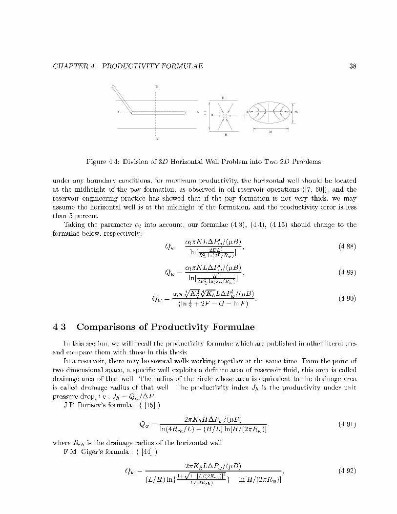
CHAPTER 4. PRODUCTIVITY FORMULAE 38
B
B
A AH
B
B
2b
2a
A A
Figure 4.4: Division of 3D Horizontal Well Problem into Two 2D Problems.
under any boundary conditions, for maximum productivity, the horizontal well should be locatedat the midheight of the pay formation, as observed in oil reservoir operations ([7, 60]), and thereservoir engineering practice has showed that if the pay formation is not very thick, we mayassume the horizontal well is at the midhight of the formation, and the productivity error is lessthan 5 percent.
Taking the parameter �l into account, our formulae (4.3), (4.4), (4.13) should change to theformulae below, respectively:
Qw =�l�KL�P l
w=(�B)
ln[ 2EL2
R2w ln(2L=Rw) ]
; (4.88)
Qw =�l�KL�P l
w=(�B)
ln[ H2
2R2w ln(2L=Rw) ]
; (4.89)
Qw =�l�
4pK3v
4pKhL�P
lw=(�B)
(ln 12 + 2F +G� lnF )
: (4.90)
4.3 Comparisons of Productivity Formulae
In this section, we will recall the productivity formulae which are published in other literaturesand compare them with those in this thesis.
In a reservoir, there may be several wells working together at the same time. From the point oftwo dimensional space, a speci�c well exploits a de�nite area of reservoir uid, this area is calleddrainage area of that well. The radius of the circle whose area is equivalent to the drainage areais called drainage radius of that well. The productivity index Jh is the productivity under unitpressure drop, i.e., Jh = Qw=�P .
J.P. Borisov's formula : ( [15] )
Qw =2�KhH�Pw=(�B)
ln(4Reh=L) + (H=L) ln[H=(2�Rw)]; (4.91)
where Reh is the drainage radius of the horizontal well.F.M. Giger's formula : ( [44] )
Qw =2�KhL�Pw=(�B)
(L=H) lnf1+p
1�[L=(2Reh)]2L=(2Reh)
g+ ln[H=(2�Rw)]; (4.92)
CHAPTER 4. PRODUCTIVITY FORMULAE 39
where Reh is the drainage radius of the horizontal well.S.D. Joshi's formula : ( [60], see Figure 4.4 )
Qw =2�KhH�Pw=(�B)
ln[2a+p4a2�L2
L ] + �HL ln[�H=(2Rw)]
; (4.93)
where a is semimajor axis of the drainage ellipse,
a = (L=2)[0:5 +q0:25 + (2Reh=L)4]
0:5;
and Reh is drainage radius of the horizontal well.G. Renard's formula : ( [89] )
Qw =2�KhH�Pw=(�B)
cosh�1(X) + �HL ln[H=(2�R0
w)]; (4.94)
where X = 2a=L, a is the same as we state in (4.93), cosh�1(x) is the inverse hyperbolic cosinefunction, and
R0
w = [(1 + �)=(2�)]Rw ;
when � = 1; R0
w = Rw.C.Q. Liu's formula : ( [73] )
Qw =2�KL�Pw=(�B)
ln[4H=(�Rw)] + lnf sin[�zw=(2H)]sin[�(H�zw)=(2H)]g
: (4.95)
Z.F. Fan's formula : ( [39] )
Qw =2�pKhKvL�Pw=(�B)
ln[4�H=(�Rw)] + ln[tan(�zw2H )]: (4.96)
In fact, when � = 1, formula (4.95) becomes formula (4.96), because
sin[�(H � zw)=(2H)] = cos[�zw=(2H)]:
And it is interesting to �nd that when � = 1, �l = 2, our formula (4.85) becomes formula (4.95)and formula (4.96). Thus we have obtained formulae (4.95) and (4.96) from a di�erent approach.
In [61], there is an example for us to calculate a horizontal well productivity index with di�erentmethods. The drainage area of the horizontal well is 325 �103m2, the length of the well is 305 m,the wellbore's radius is 0.11 m, the crude oil's formation volume factor B is 1.34, the thickness ofthe pay formation is 50 m, the formation's e�ective permeability is 74 �10�3�m2, the viscosity is0.62 mPa:s. The well is at the midhight of the pay formation.
If we use International Units, and take the constants such as 2�, 4�, 2:4� and dimensional unitconversions into consideration, we apply the above formulae to compute the productivity index {Jh of this well.
In the following calculations, we let
� = 1; �l = 2:4;K = Kh = Kv = 74� 10�3�m2:

CHAPTER 4. PRODUCTIVITY FORMULAE 40
(1) The method of Borisov : ( see formula (4.91) )
Reh =q325� 103=3:14 = 321:64m;
Jh =0:543KhH=(�B)
ln(4Reh=L) + (H=L) ln[H=(2�Rw)]
=(0:543 � 74� 50)=(0:62 � 1:34)
ln[(4� 321:64)=305] + (50=305) ln[50=(2 � 3:14 � 0:11)]
= 1129m3=(day:MPa):
(2) The method of Giger : ( see formula (4.92) )
Jh =0:543KhL=(�B)
(L=H) lnf1+p
1�[L=(2Reh)]2L=(2Reh)
g+ ln[H=(2�Rw)]
=(0:543 � 74� 305)=(0:62 � 1:34)
(305=50) ln[(1 +p1� [305=(2 � 321:64)]2=(305=(2 � 321:64))] + ln[50=(2 � 3:14� 0:11)]
= 1163m3=(day:MPa):
(3) The method of Joshi : ( see formula (4.93) )
a = (L=2)[0:5 +q0:25 + (2Reh=L)4]
0:5
= (305=2)[0:5 +q0:25 + (2� 321:64=305)4 ]0:5
= 340:19m;
Jh =0:543KhH=(�B)
ln[2a+p4a2�L2
L ] + �HL ln[�H=(2Rw)]
=(0:543 � 74� 50)=(0:62 � 1:34)
ln[2�340:19+
p4�(340:19)2�3052305 ] + ( 50
305 ) ln[50=(2 � 0:11)]
= 1038m3=(day:MPa):
(4) The method of Renard : ( see formula (4.94) )
X = 2a=L = 2� 340:19=305 = 2:23;
Jh =0:543KhH=(�B)
cosh�1(X) + �HL ln[H=(2�R0
w)]
=(0:543 � 74� 50)=(0:62 � 1:34)
cosh�1(2:23) + ( 50305 )� ln[50=(2 � 3:14 � 0:11)]
= 1129m3=(day:MPa):

CHAPTER 4. PRODUCTIVITY FORMULAE 41
(5) The method of Liu and Fan : ( see formulae (4.95), (4.96) )
Jh =0:543KL=(�B)
ln[4�H=(�Rw)] + ln[tan(�zw2H )]
=(0:543 � 74� 305)=(0:62 � 1:34)
ln[4� 50=(3:14 � 0:11)] + ln[tan(3:14�252�50 )]
= 2318m3=(day:MPa):
(6) Formula (4.3):
E =
p3052 + 502 � 50p3052 + 502 + 50
= 0:7214;
Jh =1:086KL=(�B)
ln[ 2EL2
R2w ln(2L=Rw)
]
=(1:086 � 74� 305)=(0:62 � 1:34)
ln[ 2�0:7214�30520:112 ln(2�305=0:11) ]
= 2097m3=(day:MPa):
(7) Formula (4.85):
Jh =0:652KL=(�B)
ln[4�H=(�Rw)] + ln[tan(�zw2H )]
=(0:652 � 74� 305)=(0:62 � 1:34)
ln[4� 50=(3:14 � 0:11)] + ln[tan(3:14�252�50 )]
= 2782m3=(day:MPa):
According to the above calculations, we may �nd that the results calculated by 2D formulae(4.91), (4.92), (4.93), (4.94) are smaller than the results calculated by our 3D formulae (4.3), (4.85).
There is a horizontal well in Liu-Hua Reservoir, South China Sea. The well and reservoir'sparameters are as follows ([39]):
The length of the horizontal well is 600 m; the drainage radius is 500 m; the wellbore's radius is0.1098 m; the formation's horizontal permeability is 569 �10�3�m2; and the vertical permeability is280 �10�3�m2; the formation's e�ective thickness is 63 m; the crude oil's formation volume factorB is 1.031; the viscosity is 65 mPa:s; the distance between the horizontal well and the bottomboundary is 56.86 m; when the producing pressure drawdown is 4.57 MPa, the actual productivityis 1288 m3=day; when the producing pressure drawdown is 5.90 MPa, the actual productivity is1516 m3=day. The pressure is the wellhead pressure, it means the pressure measuring point is theendpoint. The horizontal well has additional pressure drop because of formation damage.
Now, we use the above formulae to calculate the productivity of this horizonta well and compareit with the actual productivity data. Because some formulae such as (4.91), (4.92), (4.95) cannot account for anisotropic permeability reservoir, we may use the e�ective permeability of theformation if applicable.
K =pKhKv =
p569 � 280 = 0:399 (�m2);
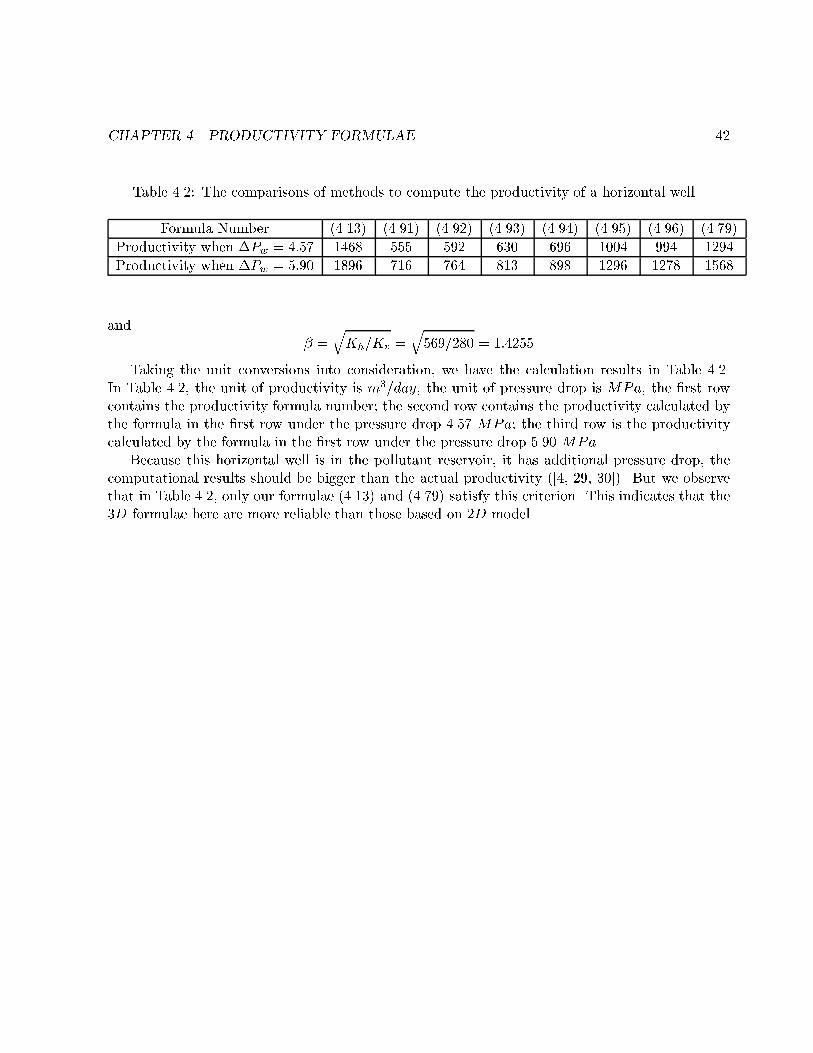
CHAPTER 4. PRODUCTIVITY FORMULAE 42
Table 4.2: The comparisons of methods to compute the productivity of a horizontal well.
Formula Number (4.13) (4.91) (4.92) (4.93) (4.94) (4.95) (4.96) (4.79)
Productivity when �Pw = 4:57 1468 555 592 630 696 1004 994 1294
Productivity when �Pw = 5:90 1896 716 764 813 898 1296 1278 1568
and� =
qKh=Kv =
q569=280 = 1:4255
Taking the unit conversions into consideration, we have the calculation results in Table 4.2.In Table 4.2, the unit of productivity is m3=day, the unit of pressure drop is MPa, the �rst rowcontains the productivity formula number; the second row contains the productivity calculated bythe formula in the �rst row under the pressure drop 4.57 MPa; the third row is the productivitycalculated by the formula in the �rst row under the pressure drop 5.90 MPa.
Because this horizontal well is in the pollutant reservoir, it has additional pressure drop, thecomputational results should be bigger than the actual productivity ([4, 29, 30]). But we observethat in Table 4.2, only our formulae (4.13) and (4.79) satisfy this criterion. This indicates that the3D formulae here are more reliable than those based on 2D model.

Chapter 5
Well Testing Formulae for Single
Porosity Reservoir
The purpose of this chapter is to derive the pressure drop well testing formulae of horizontal wellsin single porosity reservoirs. Taking a horizontal well as a uniform line source in 3D space, we derivethe point convergence pressure distribution formulae. Then according to the superposition principle([2, 59]), we apply quadrature theorem to derive the uniform line source pressure distributionformulae.
5.1 Point Convergence Pressure Distribution Formula
In this section, we will derive the dimensionless pressure formula of a point in a single porosityreservoir.
According to mass conservation and Darcy's law ([29, 30]), if the point convergence intensityof point (x0; y0; z0) in in�nite space is q, we have to solve the equation below to derive the pointconvergence pressure distribution formulae.
Kx@2P
@x2+Ky
@2P
@y2+Kz
@2P
@z2
= ��Ct@P
@t+ �qB�(x� x0)�(y � y0)�(z � z0); (5.1)
where Ct is total compressibility coe�cient ( see equation (2.18) ), and the dimension of both sidesof equation (5.1) is [ML�1T�2].
The initial condition and outer boundary condition are
Pt=0 = Pi; P (x; y; z) = Pi; (x; y !1): (5.2)
We de�nexD = 2x=L; LD = 2; (5.3)
yD = 2y(
sKx
Kz)=L; zD = 2z(
sKx
Ky)=L; (5.4)
tD =4Kxt
��CtL2; PD = 4�L
qKyKz(Pi � P )=(�qB); (5.5)
43
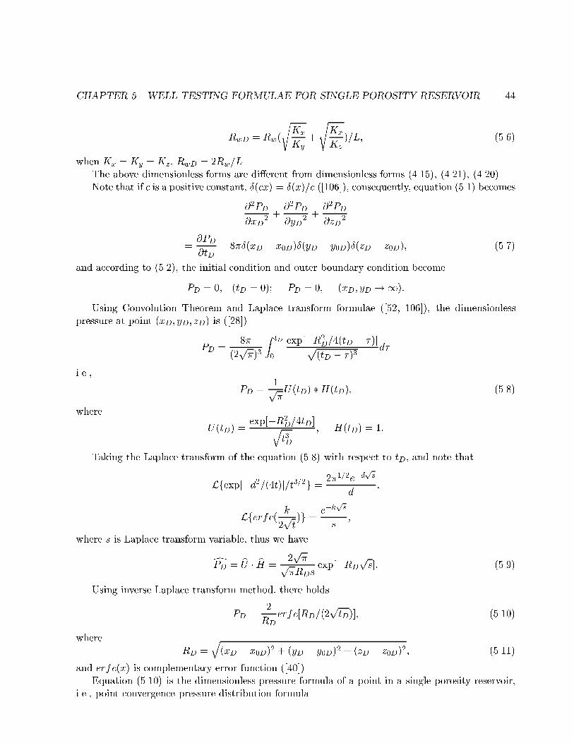
CHAPTER 5. WELL TESTING FORMULAE FOR SINGLE POROSITY RESERVOIR 44
RwD = Rw(
sKx
Ky+
sKx
Kz)=L; (5.6)
when Kx = Ky = Kz, RwD = 2Rw=L.The above dimensionless forms are di�erent from dimensionless forms (4.15), (4.21), (4.20).Note that if c is a positive constant, �(cx) = �(x)=c ([106]), consequently, equation (5.1) becomes
@2PD
@xD2 +
@2PD
@yD2 +
@2PD
@zD2
=@PD@tD
� 8��(xD � x0D)�(yD � y0D)�(zD � z0D); (5.7)
and according to (5.2), the initial condition and outer boundary condition become
PD = 0; (tD = 0); PD = 0; (xD; yD !1):
Using Convolution Theorem and Laplace transform formulae ([52, 106]), the dimensionlesspressure at point (xD; yD; zD) is ([28])
PD =8�
(2p�)3
Z tD
0
exp[�R2D=4(tD � �)]p(tD � �)3
d�
i.e.,
PD =1p�U(tD) �H(tD); (5.8)
where
U(tD) =exp[�R2
D=4tD]qt3D
; H(tD) = 1:
Taking the Laplace transform of the equation (5.8) with respect to tD, and note that
Lfexp[�d2=(4t)]=t3=2g = 2�1=2e�dps
d;
Lferfc( k
2pt)g = e�k
ps
s;
where s is Laplace transform variable, thus we have
dPD = bU � bH =2p�p
�RDsexp[�RD
ps]: (5.9)
Using inverse Laplace transform method, there holds
PD =2
RDerfc[RD=(2
ptD)]; (5.10)
whereRD =
q(xD � x0D)2 + (yD � y0D)2 + (zD � z0D)2; (5.11)
and erfc(x) is complementary error function ([40]).Equation (5.10) is the dimensionless pressure formula of a point in a single porosity reservoir,
i.e., point convergence pressure distribution formula.
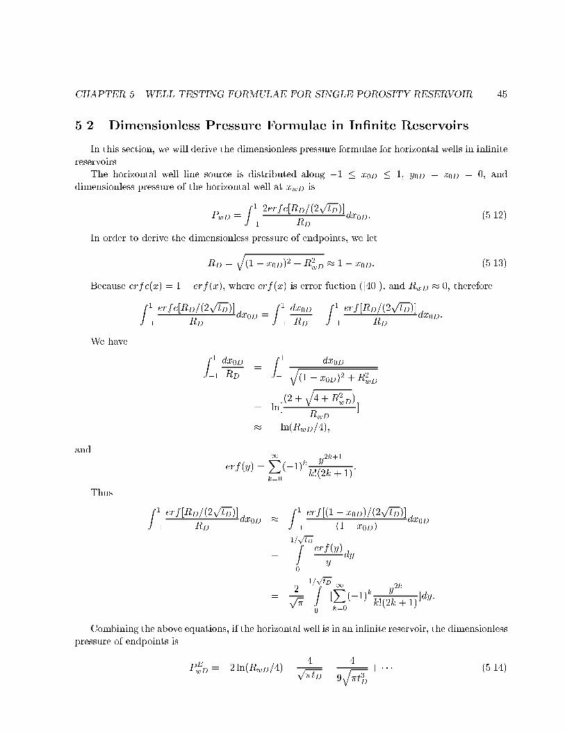
CHAPTER 5. WELL TESTING FORMULAE FOR SINGLE POROSITY RESERVOIR 45
5.2 Dimensionless Pressure Formulae in In�nite Reservoirs
In this section, we will derive the dimensionless pressure formulae for horizontal wells in in�nitereservoirs.
The horizontal well line source is distributed along �1 � x0D � 1, y0D = z0D = 0, anddimensionless pressure of the horizontal well at xwD is
PwD =
Z 1
�1
2erfc[RD=(2ptD)]
RDdx0D: (5.12)
In order to derive the dimensionless pressure of endpoints, we let
RD =q(1� x0D)2 +R2
wD � 1� x0D: (5.13)
Because erfc(x) = 1� erf(x), where erf(x) is error fuction ([40]), and RwD � 0, thereforeZ 1
�1
erfc[RD=(2ptD)]
RDdx0D =
Z 1
�1
dx0DRD
�Z 1
�1
erf [RD=(2ptD)]
RDdx0D:
We have Z 1
�1
dx0DRD
=
Z 1
�1
dx0Dq(1� x0D)2 +R2
wD
= ln[(2 +
q4 +R2
wD)
RwD]
� � ln(RwD=4);
and
erf(y) =1Xk=0
(�1)k y2k+1
k!(2k + 1):
Thus Z 1
�1
erf [RD=(2ptD)]
RDdx0D �
Z 1
�1
erf [(1� x0D)=(2ptD)]
(1� x0D)dx0D
=
1=ptDZ
0
erf(y)
ydy
=2p�
1=ptDZ
0
[1Xk=0
(�1)k y2k
k!(2k + 1)]dy:
Combining the above equations, if the horizontal well is in an in�nite reservoir, the dimensionlesspressure of endpoints is
PEwD = �2 ln(RwD=4) � 4p
�tD+
4
9q�t3D
+ � � � (5.14)

CHAPTER 5. WELL TESTING FORMULAE FOR SINGLE POROSITY RESERVOIR 46
In order to derive the dimensionless pressure of midpoint, we let
RD =qx20D +R2
wD � x0D: (5.15)
Thus Z 1
�1
erf [RD=(2ptD)]
RDdx0D �
Z 1
�1
erf [x0D=(2ptD)]
x0Ddx0D
=
1=(2ptD)Z
�1=(2ptD)
erf(z)
zdz
=2p�
1=(2ptD)Z
0
[21Xk=0
(�1)k z2k
k!(2k + 1)]dz:
Then for the horizontal well in an in�nite reservoir, the dimensionless pressure of midpoint is
PMwD = �2 ln(RwD=4) � 4p
�tD+
1
9q�t3D
+ � � � (5.16)
Formulae (5.14) and (5.16) show that if time is su�ciently long, the pressure of wellbore tendsto become steady. This conclusion is consistent with well testing practice ([4, 8, 30, 91]).
Formulae (5.14) and (5.16) are the dimensionless pressure formulae for horizontal wells in in�nitereservoirs.
5.3 Dimensionless Pressure Formulae in Reservoirs of Finite Height
In this section, we will derive the the well testing formulae in single porosity reservoirs of �niteheight, i.e., dimensionless Pressure formulae for horizontal wells.
As Figure 3.1 shows, if the horizontal well is in a reservoir of height H, and the lateral, longi-tudinal lengths of the reservoir are in�nite, i.e., the boundaries of the reservoir in the horizontaldirections are so far away that the pressure disturbance does not travel far enough to reach theboundaries during the well testing. The well is parallel to the the top and bottom boundaries. Thetwo endpoints of the horizontal well are (�L=2; 0; zw); (L=2; 0; zw), and 0 < zw < H. DimensionlessHD; zwD are de�ned as follows:
HD = 2H(
sKx
Ky)=L; zwD = 2zw(
sKx
Kz)=L: (5.17)
5.3.1 Reservoirs with Impermeable Boundary Conditions
In this subsection, we will derive the well testing formulae for horizontal wells in �nite heightreservoirs with impermeable boundary conditions.
If the horizontal well is in the reservoir with impermeable boundary conditions at z = 0 andz = H, we apply the method of images, and according to Prolongation Theorem ([24, 100, 101, 102]),the dimensionless pressure of point (x0D; 0; zwD) is ([83, 84])
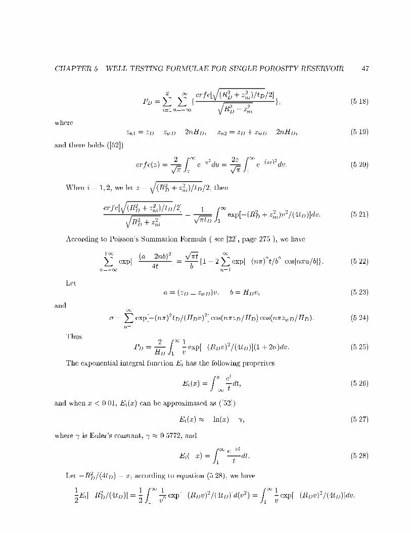
CHAPTER 5. WELL TESTING FORMULAE FOR SINGLE POROSITY RESERVOIR 47
PD =2X
i=1
+1Xn=�1
ferfc[
q(R2
D + z2ni)=tD=2]qR2D + z2ni
g; (5.18)
wherezn1 = zD � zwD � 2nHD; zn2 = zD + zwD � 2nHD; (5.19)
and there holds ([52])
erfc(z) =2p�
Z 1z
e�u2
du =2zp�
Z 11
e�(zv)2
dv: (5.20)
When i = 1; 2, we let z =q(R2
D + z2ni)=tD=2; then
erfc[q(R2
D + z2ni)=tD=2]qR2D + z2ni
=1p�tD
Z 11
exp[�(R2D + z2ni)v
2=(4tD)]dv: (5.21)
According to Poisson's Summation Formula ( see [22], page 275 ), we have
+1Xn=�1
exp[�(a� 2nb)2
4t] =
p�t
bf1 + 2
1Xn=1
exp[�(n�)2t=b2] cos[n�a=b]g: (5.22)
Leta = (zD � zwD)v; b = HDv; (5.23)
and
� =1Xn=1
exp[�(n�)2tD=(HDv)2] cos(n�zD=HD) cos(n�zwD=HD): (5.24)
Thus
PD =2
HD
Z 11
1
vexp[�(RDv)
2=(4tD)](1 + 2�)dv: (5.25)
The exponential integral function Ei has the following properites
Ei(x) =
Z x
�1
et
tdt; (5.26)
and when x < 0.01, Ei(x) can be approximated as ([52])
Ei(x) � � ln(x)� ; (5.27)
where is Euler's constant, � 0.5772, and
�Ei(�x) =Z 11
e�xt
tdt: (5.28)
Let �R2D=(4tD) = x, according to equation (5.28), we have
�1
2Ei[�R2
D=(4tD)] =1
2
Z 11
1
v2exp[�(RDv)
2=(4tD)]d(v2) =
Z 11
1
vexp[�(RDv)
2=(4tD)]dv:

CHAPTER 5. WELL TESTING FORMULAE FOR SINGLE POROSITY RESERVOIR 48
We de�ne
I0 =
Z 11
1
vexp[�(RDv)
2=(4tD)]dv = �1
2Ei[�R2
D=(4tD)]: (5.29)
Because there holds ([52])
K0(x) =1
2
Z 10
exp(�� � x2
4�)d�
�; (5.30)
if we let x = n�RD=HD, � =(RDv)
2
4tD, then d�=� = 2dv=v, according to equation (5.30), there holds
K0(n�RD=HD) =
Z 10
1
vexp[�(RDv)
2
4tD� (n�)2tD
(HDv)2]dv:
Now we de�ne In1 and In2 as follows:
In1 =
Z 10
1
vexp[�(RDv)
2
4tD� (n�)2tD
(HDv)2]dv = K0(n�RD=HD); (5.31)
In2 =
Z 1
0
1
vexp[�(RDv)
2
4tD� (n�)2tD
(HDv)2]dv: (5.32)
Therefore, when n � 1; we de�ne In and we have below relation
In =
Z 11
1
vexp[�(RDv)
2
4tD� (n�)2tD
(HDv)2]dv = In1 � In2: (5.33)
If we let v = 1=u, u2 = w, then du=u = dw=(2w), and In2 can be expressed as
In2 =
Z 1
0
1
vexp[�(RDv)
2
4tD� (n�)2tD
(HDv)2]dv
=
Z 11
1
uexp[� R2
D
4tDu2� (n�u)2tD
H2D
]du
�Z 11
1
uexp[�(n�u)2tD
H2D
]du
=1
2
Z 11
1
wexp[�(n�)2tDw
H2D
]dw
�Z 11
exp[�(n�)2tDw
H2D
]dw
=H2D
(n�)2tDexp[�(n�)2tD
H2D
]:
And we have 1Xn=1
In2 � (H2D
�2tD) exp[��
2tDH2D
]=f1 � exp[�3�2tDH2D
]g:
In order to derive the dimensionless pressure of endpoints, we let
RD =q(1� x0D)2 +R2
wD � 1� x0D;

CHAPTER 5. WELL TESTING FORMULAE FOR SINGLE POROSITY RESERVOIR 49
and we should integrate equation (5.18) or (5.25) with respect to x0D from �1 to 1, according toequation (5.25), we have
PEwD =
2
HDfJ0 + 2
1Xn=1
(Jn1 � Jn2)[cos(n�zD=HD) cos(n�zwD=HD)]g; (5.34)
where
J0 =
Z 1
�1I0dx0D; Jn1 =
Z 1
�1In1dx0D; Jn2 =
Z 1
�1In2dx0D;
and we havezD + zwD � 2zwD; zD � zwD = RwD: (5.35)
So
J0 =
Z 1
�1I0dx0D
=1
2
Z 1
�1Ei[�R2
D=(4tD)]dx0D
� �1
2
Z 1
�1Ei[�(1� x0D)
2=(4tD)]dx0D
= �1
2
Z 2
0Ei[�y2=(4tD)]dy
= �Ei(�1=tD) + 2ptD
1ptDZ
0
exp(�x2)dx;
therefore
J0 = �Ei(�1=tD) +p�tDerf(
1ptD
): (5.36)
In order to obtain the equation (5.36), we have used transformation parameters and integrationby parts method ([59]).
When time is su�ciently long ( tD is large enough ), because there hold formula (5.27) and thefollowing formula ([52])
limtD!1
p�tDerf(1=
ptD) = 2;
so that equation (5.36) reduces to
J0 � �Ei(�1=tD) + 2 � 2� + ln tD � 1:4228 + ln tD:
When time is su�ciently short ( tD is small enough ), we have
�Ei(�1=tD) � 0; erf(1ptD
) � 1;
so that equation (5.36) becomesJ0 �
p�tD:

CHAPTER 5. WELL TESTING FORMULAE FOR SINGLE POROSITY RESERVOIR 50
Table 5.1: The convergence rate of the integration of K0(z).
x = 1 x = 2 x = 3 x = 4 x = 5 x = 6
y = �0:328 y = �0:097 y = �0:031 y = �0:010 y = �0:003 y = �0:001
If we let
y =
xZ0
K0(z)dz � �=2;
then we have Table 5.1.Consequently, we have
Jn1 =
Z 1
�1In1dx0D
=
Z 1
�1K0(n�RD=HD)dx0D
�Z 1
�1K0[n�(1� x0D)=HD]dx0D
=HD
n�
2n�=HDZ0
K0(z)dz:
Note that 2n�=HD � 1, according to Table 5.1 and the formula (4.47), we have
2n�=HDZ0
K0(z)dz � �=2;
thusJn1 � HD=2n; (5.37)
and
Jn2 =
Z 1
�1In2dx0D � 0:
Note that relationships (5.35) and formula (4.61), then
cos(n�zD=HD) cos(n�zwD=HD)
=1
2fcos(n�RwD=HD) + cos[n�(zD + zwD)=HD]g;
and there holds formula (4.58), thus we de�ne
T =1Xn=1
(Jn1 � Jn2) cos(n�zD=HD) cos(n�zwD=HD); (5.38)

CHAPTER 5. WELL TESTING FORMULAE FOR SINGLE POROSITY RESERVOIR 51
and1Xn=1
(Jn1 � Jn2) cos(n�zD=HD) cos(n�zwD=HD)
� HD
2
1Xn=1
1
ncos(n�zD=HD) cos(n�zwD=HD)
= �HD
4lnf4 sin[�(zD � zwD)=(2HD)] sin[�(zD + zwD)=(2HD)]g
� �HD
4lnf4 sin[�RwD=(2HD)] sin(�zwD=HD)g;
so
T � �HD
4lnf4 sin[�RwD=(2HD)] sin(�zwD=HD)g: (5.39)
Combining equations (5.34), (5.36), (5.38) and (5.39), if the horizontal boundary conditions atz = 0 and H are both impermeable, the dimensionless pressure of the endpoints is
PEwD =
2
HD(J0 + 2T ):
Simplify the above equation, we have
PEwD =
2
HD[�Ei(�1=tD) +
p�tDerf(
1ptD
)]� lnf4 sin[�RwD=(2HD)] sin(�zwD=HD)g: (5.40)
When time is su�ciently long, equation (5.40) becomes
PEwD �
2
HD(1:4228 + ln tD)� lnf4 sin[�RwD=(2HD)] sin(�zwD=HD)g: (5.41)
When time is su�ciently short, equation (5.40) becomes
PEwD �
2
HD(p�tD)� lnf4 sin[�RwD=(2HD)] sin(�zwD=HD)g: (5.42)
In order to �nd the dimensionless pressure of midpoint, we let
RD =qx20D +R2
wD � x0D;
and let
L0 =
Z 1
�1I0dx0D
=1
2
Z 1
�1Ei[�R2
D=(4tD)]dx0D
� �1
2
Z 1
�1Ei[�x20D=(4tD)]dx0D
= �Ei[�1=(4tD)] + 4ptD
1
2ptDZ
0
exp(�x2)dx
= �Ei[�1=(4tD)] + 4ptD[
p�
2erf(
1
2ptD
)];

CHAPTER 5. WELL TESTING FORMULAE FOR SINGLE POROSITY RESERVOIR 52
i.e.,
L0 = �Ei[�1=(4tD)] + 2p�tDerf(
1
2ptD
); (5.43)
and we let
Ln1 =
Z 1
�1In1dx0D
=
Z 1
�1K0(n�RD=HD)dx0D
�Z 1
�1K0[n�x0D=HD]dx0D
=HD
n�
n�=HDZ�n�=HD
K0(z)dz
� 2HD
n�(�=2)
= HD=n:
By the analogy of the above arguments, if the horizontal boundary conditions at z = 0 and Hare both impermeable, the dimensionless pressure of the midpoint is
PMwD =
2
HD[�Ei(�1=4tD)+2
p�tDerf(
1
2ptD
)]�2 lnf4 sin[�RwD=(2HD)] sin(�zwD=HD)g: (5.44)
When time is su�ciently long, equation (5.44) becomes
PMwD �
2
HD(2:8091 + ln tD)� 2 lnf4 sin[�RwD=(2HD)] sin(�zwD=HD)g: (5.45)
When time is su�ciently short, equation (5.44) becomes
PMwD �
4
HD(p�tD)� 2 lnf4 sin[�RwD=(2HD)] sin(�zwD=HD)g: (5.46)
Formulae (5.40), (5.41), (5.42), (5.44), (5.45), and (5.46) are dimensionless pressure formulae,i.e., the well testing formulae for horizontal wells in �nite height reservoirs with impermeableboundary conditions.
5.3.2 Reservoirs with Bottom Water or Gas Cap
In this subsection, we will derive the well testing formulae for horizontal wells in �nite heightreservoirs with bottom water or gas cap.
If the horizontal well is in the reservoir with constant boundary conditions at z = 0 and H (the reservoir with bottom water and gas cap ), the pressure of the horizontal wellbore tends tobecome steady when time is su�ciently long ([50, 69, 71]). In such case, the dimensionless pressureat point (x0D; 0; zwD) is
PD =1
HD[1Xn=1
K0(n�RD=HD) sin(n�zD=HD) sin(n�zwD=HD)]: (5.47)

CHAPTER 5. WELL TESTING FORMULAE FOR SINGLE POROSITY RESERVOIR 53
Thus, the steady dimensionless pressure of the endpoints is
PEwD �
1
HDf1Xn=1
sin(n�zD=HD) sin(n�zwD=HD)
Z 1
�1K0[n�(1� x0D)=HD]dx0Dg
� 1
4
1Xn=1
1
nfcos[n�(zD � zwD)=HD]� cos[n�(zD + zwD)=HD]g
� 1
4fln[2 sin(�zwD=HD)]� ln[2 sin(�RwD=(2HD))]g;
so
PEwD �
1
4lnf sin(�zwD=HD)
sin[�RwD=(2HD)]g: (5.48)
According to the de�nitions of dimensionless pressure PD in (4.21) and (5.5), formula (5.48) isequivalent to formula (4.71).
If the boundary condition at z = 0 is impermeable while the boundary condition at z = H isconstant ( the reservoir with gas cap ), the pressure of the horizontal wellbore tends to becomesteady when time is su�ciently long ([50, 69, 71]). In such case, the dimensionless pressure at point(x0D; 0; zwD) is
PD =1
HDf1Xn=1
K0[(2n�1)�RD=(2HD)] cos[(2n�1)�zD=(2HD)] cos[(2n�1)�zwD=(2HD)]g: (5.49)
We de�ne
W =
Z 1
�1K0[(2n� 1)�(1� x0D)=(2HD)]dx0D;
then
W =2HD
(2n� 1)�
Z (2n�1)�=HD
0K0(z)dz
� 2HD
(2n� 1)�(�=2)
= HD=(2n� 1):
Thus, according to formula (4.59), the steady dimensionless pressure of the endpoints is
PEwD � 1
HDf1Xn=1
cos[(2n� 1)�zD=(2HD)] cos[(2n� 1)�zwD=(2HD)]Wg
� 1
2
1Xn=1
1
2n� 1fcos[(2n� 1)�(zD + zwD)=(2HD)] + cos[(2n� 1)�(zD � zwD)=(2HD)]g
� 1
4fln[cot(�zwD=(2HD))] + ln[cot(�RwD=(4HD))]g;
then we have
PEwD �
1
4fln[cot(�RwD=(4HD))] + ln[cot(�zwD=(2HD))]g: (5.50)
CHAPTER 5. WELL TESTING FORMULAE FOR SINGLE POROSITY RESERVOIR 54
Similarly, if the boundary condition at z = H is impermeable while the boundary conditionat z = 0 is constant, ( the reservoir with bottom water ), the dimensionless pressure at point(x0D; 0; zwD) is
PD =1
HDf1Xn=1
K0[(2n�1)�RD=(2HD)] sin[(2n�1)�zD=(2HD)] sin[(2n�1)�zwD=(2HD)]g; (5.51)
thus the steady dimensionless pressure at the endpoints is
PEwD �
1
4fln[cot(�RwD=(4HD))]� ln[cot(�zwD=(2HD))]g: (5.52)
Considering that the de�nition of PD in (4.21) is di�erent from the de�nition of PD in (5.5),thus we may conclude that (5.47) is equivalent to (4.42), (5.49) is equivalent to (4.37), (5.50) isequivalent to (4.69), (5.52) is equivalent to (4.65).
In summary, if the horizontal well is in the reservoir with bottom water or gas cap, the pressureof the wellbore will become steady when time is su�ciently long. The well will produce oil at aconstant rate.

Chapter 6
Well Testing Formulae for Double
Porosity Reservoir
In this chapter, we �rst recall the Warren-Root Model. Then we will use it to �nd the Laplacetransform image of dimensionless pressure of the wellbore. We will also derive the pressure dropwell testing formulae of horizontal wells in �nite height double porosity reservoir.
6.1 Warren-Root Model
If the reservoir is an inhomogeneous, anistropic naturally fractured reservoir { double porosityreservoir, we use Warren-Root Model: Reservoir uid movement toward the wellbore occurs onlyin fractures ([49, 87]). In 1960, Barenblatt et al. published a pioneering work on the subject ofwell testing in naturally fractured reservoirs. Many fractured reservoirs are characterized by aninterconnected fracture network dividing the matrix rock into separate blocks. Such a system maybe modelled by two overlapping continuous media, one for the medium of fractures and one forthe medium of blocks. The fracture network has a high permeability and low storage capacity. Inthe medium of blocks the conditions are reserved. If the permeability contrast ( fracture to matrixpermeability ratio ) is large, then the ow through the blocks may be disregarded and the double- porosity model may be applied. Warren and Root presented a model based on the mathematicalconcept of superposition of two media: A porous rock with a highly developed system of �ssurescan be represented as the superposition of two porous media with pores of di�erent sizes. Theporous media are coupled to each other by the fact that there is a liquid exchange between the two.At each point in space, we can consider two pressures and two velocities of the liquid: P1 and V1for the liquid in the �ssures and P2 and V2 for that in the blocks. The interaction of these mediacan be expressed by the relation:
q = ��(P2 � P1);
where � is a characteristic of the �ssured medium { interporosity ow shape factor, � is density.Warren and Root based their results on the fact that in the most general case both primary
and secondary porosity is present in the reservoir: An independent system of secondary porosity issuperimposed on the primary or intergranular system. The obvious idealization of an intermediateporous medium is a complex of discrete volumetric elements with primary porosity which areanisotropically coupled by secondary voids.
The sketch of the heterogeneous porous media is shown in Figure 6.1.
55
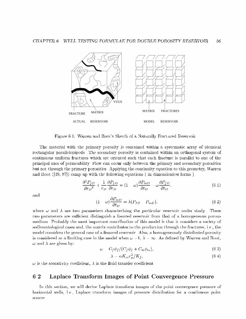
CHAPTER 6. WELL TESTING FORMULAE FOR DOUBLE POROSITY RESERVOIR 56
MATRIXFRACTURE
VUGS
ACTUAL RESERVOIR
MATRIX FRACTURES
MODEL RESERVOIR
Figure 6.1: Warren and Root's Sketch of a Naturally Fractured Reservoir.
The material with the primary porosity is contained within a systematic array of identicalrectangular parallelepipeds. The secondary porosity is contained within an orthogonal system ofcontinuous uniform fractures which are oriented such that each fracture is parallel to one of theprincipal axes of permeability. Flow can occur only between the primary and secondary porositiesbut not through the primary porosities. Applying the continuity equation to this geometry, Warrenand Root ([49, 87]) camp up with the following equations ( in dimensionless forms )
@2PfD
@rD2 +
1
rD
@PfD@rD
= (1� !)@PmD
@tD+ !
@PfD@tD
; (6.1)
and
(1� !)@PmD
@tD= �(PfD � PmD); (6.2)
where ! and � are two parameters characterizing the particular reservoir under study. Thesetwo parameters are su�cient distinguish a �ssured reservoir from that of a homogeneous porousmedium. Probably the most important contribution of this model is that it considers a variety ofsedimentological cases and, the matrix contributes to the production through the fractures, i.e., themodel considers the general case of a �ssured reservoir. Also, a homogeneously distributed porosityis considered as a limiting case in the model when ! =1, � =1. As de�ned by Warren and Root,! and � are given by:
! = Cf�f=(Cf�f + Cm�m); (6.3)
� = �Kmr2w=Kf ; (6.4)
! is the storativity coe�cient, � is the uid transfer coe�cient.
6.2 Laplace Transform Images of Point Convergence Pressure
In this section, we will derive Laplace transform images of the point convergence pressure ofhorizontal wells, i.e., Laplace transform images of pressure distribution for a continuous pointsource.

CHAPTER 6. WELL TESTING FORMULAE FOR DOUBLE POROSITY RESERVOIR 57
According to the mass conservation and Darcy's laws, if the point convergence intensity at point(x0; y0; z0) is q, taking Warren-Root Model into account, we have to solve the equations below toget the point convergence pressure distribution formulae.
�mCm@Pm@t
+�
�Km(Pm � Pf ) = 0; (6.5)
�fCf@Pf@t
� Kfx
�
@2Pf
@x2� Kfy
�
@2Pf
@y2� Kfz
�
@2Pf
@z2
=�
�Km(Pm � Pf )� �qB�(x� x0)�(y � y0)�(z � z0); (6.6)
andPt=0 = Pi; P (x; y; z) = Pi; (x; y !1):
LetxD = 2x=L; yD = 2y
qKfx=Kfy=L; (6.7)
zD = 2zqKfx=Kfz=L; LD = 2; (6.8)
tD =4Kfxt
(�Cf + �Cm)�L2; PD = 4�L
qKfyKfz(Pi � P )=(�qB): (6.9)
Then we have
(1� !)@PmD
@tD+ �(PmD � PfD) = 0; (6.10)
!@PfD@tD
� @2PfD
@xD2 � @2PfD
@yD2 � @2PfD
@zD2
= �(PmD � PfD) + 8��(xD � x0D)�(yD � y0D)�(zD � z0D); (6.11)
where! = Cf�f=(Cf�f + Cm�m); � = �KmL
2=(4Kfx); (6.12)
and ! is the storativity coe�cient, � is the uid transfer coe�cient, � is interporosity ow shapefactor, its dimension is [L�2] ([49, 87]).
And we point that in this chapter, the f subscripts refer to fracture medium, m subscripts referto matrix porous medium.
Taking the Laplace transform of the above equations with respect to tD, we obtain
@2 dPfD@xD
2 +@2 dPfD@yD
2 +@2 dPfD@zD
2 = sf(s)dPfD + 8��(xD � x0D)�(yD � y0D)�(zD � z0D); (6.13)
wheref(s) = [s!(1� !) + �]=[s(1� !) + �]; (6.14)
and s is Laplace transform variable. The elementary solution of equation (6.13) is ([40, 101])
dPfD =2 exp[�psf(s)RD]
sRD; (6.15)
CHAPTER 6. WELL TESTING FORMULAE FOR DOUBLE POROSITY RESERVOIR 58
withRD =
q(xD � x0D)2 + (yD � y0D)2 + (zD � z0D)2; (6.16)
RwD = Rw(
sKfx
Kfy+
sKfx
Kfz)=L: (6.17)
As Figure 3.1 shows, the horizontal well is in a reservoir of heightH, and the lateral, longitudinallengths of the reservoir are in�nite, i.e., the boundaries of the reservoir in the horizontal directionsare so far away that the pressure disturbance does not travel far enough to reach the boundariesduring the well testing. The well is parallel to the the top and bottom boundaries. The twoendpoints of the horizontal well are (�L=2; 0; zw); (L=2; 0; zw), and 0 < zw < H.
The Laplace transform image of the dimensionless pressure of the horizontal well is ([11, 25, 36])
bPfwD =2
s
Z 1
�1
exp[�puRD]
RDdx0D; (6.18)
whereu = sf(s): (6.19)
Application of the method of images, the Laplace transform image of dimensionless pressure ofthe wellbore is ([11, 24, 25, 84])
bPfwD =
Z 1
�1F (s; x0D)dx0D: (6.20)
and if the boundary conditions at z = 0 and H are both impermeable, by the method of imagesand the point-source solution given by equation (6.15), we have
F (s; x0D) =1
s
+1Xn=�1
fexp[�
qu(R2
D + z2n1)]qR2D + z2n1
+exp[�
qu(R2
D + z2n2)]qR2D + z2n2
g; (6.21)
and zn1; zn2 has the same meanings in (5.19),
zn1 = zD � zwD � 2nHD; zn2 = zD + zwD � 2nHD;
and dimensionless HD; zwD are de�ned as follows
HD = 2H(
sKx
Ky)=L; zwD = 2zw(
sKx
Kz)=L: (6.22)
When ! ! 1, � ! 1, the double porosity reservoir would become to the single porosityreservoir ([49, 87]), and
f(s) = 1; u = s: (6.23)
Recall the well known Laplace transform formula ([106]),
Lferfc( k
2pt)g = e�k
ps
s; (6.24)

CHAPTER 6. WELL TESTING FORMULAE FOR DOUBLE POROSITY RESERVOIR 59
where s is Laplace transform variable, k is a constant. If we let
k =qR2D � z2n1;
then combining equations (6.21), (6.23) and (6.24), leads to the formula (5.18).We may use formula (5.22) to similify equation (6.21). Recall the following Laplace transform
formulae ([106])
Lfexp[�d2=(4t)]=(�1=2t3=2)g = 2e�dps
d; (6.25)
Lfexp[�d2=(4t)]=(bt)g = 2K0(dps)
b; (6.26)
Lfexp[�d2=(4t)� ct]=tg = 2K0(dps+ c); (6.27)
where b; c and d are constants, s is Laplace transform variable.Let
d =qj2 + (a� 2nb)2; (6.28)
in formula (6.25), and letc = (n�=b)2; (6.29)
in formula (6.27). Multiplying both sides of equation (5.22) by exp[�j2=(4t)]=(�1=2t3=2), taking theLaplace transform of the resulting expression with respect to tD, and applying equations (6.25),(6.26), (6.27), (6.28), (6.29), we obtain the summation formula
+1Xn=�1
exp[�ps(j2 + (a� 2nb)2)]pj2 + (a� 2nb)2
=1
b[K0(j
ps) + 2
1Xn=1
K0(jqs+ (n�=b)2) cos(n�a=b)]: (6.30)
If we use the summation formula given by (6.30), let u take the place of s, and let
j = RD; a = zD � zwD; b = HD; (6.31)
then use formula (4.61), we have
cos[n�(zD + zwD)=HD] + cos[n�(zD � zwD)=HD] = 2 cos(n�zD=HD) cos(n�zwD=HD): (6.32)
According to (6.30), (6.31) and (6.32), the pressure distribution for a continuous point sourcelocated at (x0D; 0; zwD) in a laterally in�nite reservoir bounded by two impermeable planes, givenby equation (6.21), can be written as:
F (s; x0D) =2
sHD[K0(RD
pu) + 2
1Xn=1
K0(RD�1) cos(n�zD=HD) cos(n�zwD=HD)]; (6.33)
where�1 =
qu+ (n�=HD)2:
Similarly, if the boundary conditions at z = 0 and H are both at constant pressure, then thepressure distribution for a continuous point source solution corresponding is given by
F (s; x0D) =1
s
+1Xn=�1
fexp[�
qu(R2
D + z2n1)]qR2D + z2n1
�exp[�
qu(R2
D + z2n2)]qR2D + z2n2
g; (6.34)

CHAPTER 6. WELL TESTING FORMULAE FOR DOUBLE POROSITY RESERVOIR 60
which, with formula (6.30), can be transformed to
F (s; x0D) =1
sHD[1Xn=1
K0(RD�2) sin(n�zD=HD) sin(n�zwD=HD)]; (6.35)
with�2 =
qu+ (n�=HD)2:
If the boundary condition at z = 0 is impermeable while the boundary condition at z =H is at constant pressure, then the pressure distribution for a continuous point source solutioncorresponding is given by
F (s; x0D) =1
s
+1Xn=�1
(�1)nfexp[�
qu(R2
D + z2n1)]qR2D + z2n1
+exp[�
qu(R2
D + z2n2)]qR2D + z2n2
g: (6.36)
If we note that ([84])+1X
n=�1(�1)n exp[�a(x� 2ny)2
4t]
=+1X
n=�1f2 exp[�a(x� 2n(2y))2
4t]� exp[�a(x� 2ny)2
4t]g; (6.37)
then, with the aid of formula (6.30), we can recast equation (6.36) in the form
F (s; x0D) =1
sHDf1Xn=1
K0(RD�3) cos[(2n� 1)�zD=(2HD)] cos[(2n� 1)�zwD=(2HD)]g; (6.38)
where�3 =
qu+ [(2n� 1)�=(2HD)]2:
If the boundary condition at z = H is impermeable while the boundary condition at z =0 is at constant pressure, then the pressure distribution for a continuous point source solutioncorresponding is given by
F (s; x0D) =1
sHDf1Xn=1
K0(RD�4) sin[(2n� 1)�zD=(2HD)] sin[(2n� 1)�zwD=(2HD)]g; (6.39)
where�4 =
qu+ [(2n� 1)�=(2HD)]2:
As we have stated before, when ! ! 1, �!1, the double porosity reservoir model becomes toa single porosity reservoir model with f(s) = 1; u = s. By the inverse Laplace transform method,we can reduce (6.35) to (5.47), reduce (6.38) to (5.49), reduce (6.39) to (5.51).
Therefore, we have obtained formulae (5.47), (5.49) and (5.51) from a di�erent approach.According to formulae (6.35), (6.38) and (6.39), we come to the conclusion that when time is
su�ciently long, the pressure of the wellbore tends to become steady. Therefore, formulae (5.48),(5.50) and (5.52) are also suitable for the horizontal wells which are in the double-porosity reservoir.
CHAPTER 6. WELL TESTING FORMULAE FOR DOUBLE POROSITY RESERVOIR 61
6.3 Well Testing Formulae for Wells in Finite Height Reservoirs
In this section, we will derive the well testing formulae for horizontal wells in �nite heightreservoirs with impermeable boundaries.
If the boundary conditions at z = 0 and H are both impermeable, according to formula (6.33),the Laplace transform image of the dimensionless pressure of the wellbore is
bPfwD =2
sHD
Z 1
�1[K0(RD
pu) + 2
1Xn=1
K0(RD�1) cos(n�zD=HD) cos(n�zwD=HD)]dx0D; (6.40)
where�1 =
qu+ (n�=HD)2:
When x! 0, there holds ([106])
K0(x) � ln(2=x) � ;
where is Euler's constant, � 0.5772, thus
1
s
Z 1
�1K0(RD
pu)dx0D � 1
s[
Z 1
�1ln(
2
RDpu)dx0D � 2 ]:
In order to �nd the dimensionless pressure of endpoints, we let
RD =q(1� x0D)2 +R2
wD � 1� x0D;
and
cJ0(s) =1
s
Z 1
�1K0[(1� x0D)
pu]dx0D
� 1
s(1:4228 � lnu)
=1:4228
s� ln s
s� ln f(s)
s
=1:4228
s� ln s
s+
ln[s(1� !) + �]
s� ln[s(1� !)! + �]
s:
Therefore, by the inverse Laplace transform, we have
J0(tD) � 1:4228 + ln tD +Ei[�tD�
!(1� !)]�Ei[
�tD�1� !
]: (6.41)
When u! 0, i.e., time is very long, and n � 1, we have
�1 =qu+ (n�=HD)2 � n�=HD;
then when n � 1, we de�ne
cJn(s) =1
s
Z 1
�1K0(RD�1)dx0D
CHAPTER 6. WELL TESTING FORMULAE FOR DOUBLE POROSITY RESERVOIR 62
� 1
s
Z 1
�1K0[n�(1� x0D)=HD]dx0D
=1
s
Z 2
0K0(n�y=HD)dy
=HD
n�s
2n�=HDZ0
K0(z)dz
� HD=(2ns):
Therefore, when n � 1, there holds
Jn(tD) � HD=(2n): (6.42)
Similar to equations (5.38), (5.39), we have
1Xn=1
Jn cos(n�zD=HD) cos(n�zwD=HD)
� �HD
4lnf4 sin[�RwD=(2HD)] sin(�zwD=HD)g:
Therefore, if horizontal boundary conditions at z = 0 and H are both impermeable, and time issu�ciently long, the endpoints' dimensionless pressure of the horizontal well in a double-porosityreservoir is
PEfwD =
2
HDf1:4228 + ln tD +Ei[
�tD�!(1� !)
]�Ei[�tD�1� !
]g
� lnf4 sin[�RwD=(2HD)] sin(�zwD=HD)g: (6.43)
In order to �nd the dimensionless pressure of midpoint, we let
RD =qx20D +R2
wD � x0D:
Similarly, if the horizontal boundary conditions at z = 0 and H are both impermeable, and timeis su�ciently long, the midpoint's dimensionless pressure of the horizontal well in a double-porosityreservoir is
PMfwD =
2
HDf2:8091 + ln tD +Ei[
�tD�!(1� !)
]�Ei[�tD�1� !
]g
�2 lnf4 sin[�RwD=(2HD)] sin(�zwD=HD)g: (6.44)
Formulae (6.43) and (6.44) are dimensionless pressure well testing formulae for horizontal wellsin �nite height reservoirs with impermeable boundaries.
Again, when ! ! 1, � ! 1, the double porosity reservoir model becomes a single porosityreservoir model, and formula (6.43) reduces to formula (5.41), formula (6.44) reduces to formula(5.45).

Appendix A
Conclusions
Now, we may come to the following conclusions:(1) The productivity formulae based on 2D model can not satisfactorily characterize horizontal
wells. In order to get the reasonable and reliable productivity formulae, we must use 3D model;(2) If taking a horizontal well as a uniform line source in 3D space, the equipotential surfaces
are a family of ellipsoids of revolution which focuses are the two endpoints of the well, and the wellhas not in�nite conductivity;
(3) Our well testing formulae of horizontal wells are concise and explicit, they have higherprecision than the formulae in the literatures.
63

Appendix B
Nomenclature
(English)A = drainage areaB = formation volume factorCf = uid compressibilityCR = rock compressibilityCt = total compressibilityEi(x) = exponential integral functionerf(x) = error functionerfc(x) = complementary error functionH = reservoir e�ective thicknessK = absolute permeabilityK0(x) = modi�ed Bessel function of second kind and order zeroL = well lengthP = pressureQ = well productivity, well ow rateRw = wellbore radiusRe = drainage radiuss = Laplace transform variablet = timeV = drainage volumex; y; z = lateral,longitudinal,vertical coordinate.
(Greek)� = interporosity shape factor� = permeability anisotropic factor�(t) = Dirac function.� = uid transfer coe�cient,fraction.� = uid viscosity� = density� = uid potential� = porosity,fraction! = storativity coe�cient,fraction.
64

APPENDIX B. NOMENCLATURE 65
Superscriptsb= Laplace transforme= e�ectiveA = averageE = endpointM = midpoint
SubscriptsD = dimensionlesse = externalf = fractureh = horizontali = initialm = matrixv = verticalw = wellx; y; z = coordinate indicators
Bibliography
[1] M. Abbaszadeh. Pressure - transient behavior in a reservoir with a �nite - conductivity fault.SPE Formation Evaluation, 10(1):26{32, March 1995.
[2] R.P. Agnew. Di�erential Equations. Mcgraw - Hill Book Company, New York, 1960.
[3] R. Agullera. Transient pressure analysis of horizontal wells in anisotropic of horizontal wellsin anisotropic naturally fractured reservoirs. SPE Formation Evaluation, 6(1):95{100, March1991.
[4] J.S. Archer. Petroleum Engineering Principles and Practice. Graham and Trotman Publish-ers, London, 1986.
[5] K. Aziz. Petroleum Reservoir Simulation. Applied Science Publishers, London, 1979.
[6] D.K. Babu. Flow capabilities of horizontal wells. Journal of Petroleum Technology, 41(9):914{915, Sept. 1989.
[7] D.K. Babu. Productivity of a horizontal well. SPE Reservoir Engineering, 4(4):417{421, Nov.1989.
[8] D.K. Babu. Transient ow behaviour of horizontal wells: Pressure drawdown and buildupanalysis. SPE Formation Evaluation, 5(1):7{15, March 1990.
[9] D.K. Babu. The relation between wellblock and wellbore pressure in numerical simulation ofhorizontal wells. SPE Reservoir Engineering, 6(3):324{328, Aug. 1991.
[10] T. Beatty. Minimizing formation damage in horizontal wells: Laboratory and �eld casestudies. Journal of Canadian Petroleum Technology, 34(6):57{63, June 1995.
[11] P. Bedrikovetsky. Mathematical Theory of Oil and Recovery, volume 4 of Petroleum Engi-
neering and Development Studies. Kluwer Academic Publishers, Dordrecht, The Netherlands,1993.
[12] R.A. Beier. Pressure-transient model for a vertically fractured well in a fractal reservoir. SPEFormation Evaluation, 9(2):122{128, June 1994.
[13] D.B. Bennion. Fluid design to minimize invasive damage in horizontal wells. Journal of
Canadian Petroleum Technology, 35(9):45{52, Nov. 1996.
[14] E. Bobok. Fluid Mechanics for Petroleum Engineers, volume 32 of Developments in PetroleumScience. Elsevier Scienti�c Publishing Company, Amsterdam , the Netherlands, 1993.
66

BIBLIOGRAPHY 67
[15] J.P. Borisov. Oil Production Using Horizontal and Multiple Deviation Wells. the R and DTranslation Company, Bartlesville, Oklahoma, 1984.
[16] M.J. Bourgeois. Well { test { model recognition with laplace space. SPE Formation Evalua-
tion, 8(1):17{25, March 1993.
[17] W.E. Brigham. Discussion of productivity of a horizontal well. SPE Reservoir Engineering,5(2):224{225, May 1990.
[18] R.M. Butler. Gravity drainage to horizontal wells. Journal of Canadian Petroleum Technol-
ogy, 31(4):31{37, Apr. 1992.
[19] R.M. Butler. The productivity and optimum pattern shape for horizontal wells arranged instaggered rectangular arrays. Journal of Canadian Petroleum Technology, 31(6):41{46, June1992.
[20] R.M. Butler. Recovery of heavy and conventional oils from pressure-depleted reservoirs usinghorizontal wells. Journal of Canadian Petroleum Technology, 33(10):27{33, Dec. 1994.
[21] R.M. Butler. E�ect of gravity on movement of water-oil interface for bottom water drivingupwards to a horizontal well. Journal of Canadian Petroleum Technology, 35(7):47{56, Sept.1996.
[22] H.S. Carslaw. Conduction of Heat in Solids. Oxford University Press, Oxford, 1986.
[23] H.Y. Chen. An application of the product { solution principle for instantaneous source andgreen's functions. SPE Formation Evaluation, 6(2):161{168, June 1991.
[24] W.C. Chin. Modern Reservoir Flow and Well Transient Analysis. Gulf Publishing Company,Houston, 1993.
[25] W.C. Chin. Wave Propagation in Petroleum Engineering. Gulf Publishing Company, Hous-ton, 1994.
[26] E.L. Claridge. Sweep e�ciency comparisons of horizontal and vertical wells. Journal of
Canadian Petroleum Technology, 30(4):52{57, Aug. 1991.
[27] M.D. Clonts. Spe 15116: Pressure transient analysis for wells with horizontal drainholes. InCalifornia Regional Meeting of the SPE of AIME,Oakland, CA, April,, 1986.
[28] R.E. Collins. Flow of Fluids Through Porous Media. Reinhold Publishing Corporation, NewYork, 1961.
[29] L.P. Dake. Fundamentals of Reservoir Engineering, volume 8 of Developments in Petroleum
Science. Elsevier Scienti�c Publishing Company, Amsterdam , the Netherlands, 1978.
[30] L.P. Dake. The Practice of Reservoir Engineering, volume 36 of Developments in Petroleum
Science. Elsevier Scienti�c Publishing Company, Amsterdam , the Netherlands, 1994.
[31] F. Daviau. Pressure analysis of horizontal wells. SPE Formation Evaluation, 3(4):716{724,Dec. 1988.

BIBLIOGRAPHY 68
[32] J.K. Dietrich. Predicting horizontal well productivity. Journal of Canadian Petroleum Tech-
nology, 35(6):42{48, June 1996.
[33] B.J. Dikken. Pressure drop in horizontal wells and its e�ect on production performance.Journal of Petroleum Technology, 42(11):1426{1433, Nov. 1990.
[34] A.J. Dikkers. Geology in Petroleum Production, volume 20 of Developments in Petroleum
Science. Elsevier Scienti�c Publishing Company, Amsterdam , the Netherlands, 1985.
[35] K.F. Du. Analysis of transient pressure response of horizontal wells in bounded reservoirs.SPE Formation Evaluation, 9(1):32{38, March 1994.
[36] G.F.D. Du�. Di�erential Equations of Applied Mathematics. John Wiley and Sons Company,New York, 1966.
[37] M.J. Economides. Comprehensive simulation of horizontal well performance. SPE Formation
Evaluation, 6(4):418{426, Dec. 1991.
[38] M.J. Economides. Optimization of horizontal well matrix treatments. SPE Production and
Facilities, 9(2):93{99, May 1994.
[39] Z.F. Fan. The productivity formula of horizontal wells with bottom water drive. Journal ofPetroleum Exploration and Development, 20(1):71{75, March 1993.
[40] M. Fogiel. Handbook of Mathematical, Scienti�c, and Engineering. Research and EducationAssociation, New Jersey, 1994.
[41] T.P. Frick. Horizontal well damage characterization and removal. SPE Production Engineer-
ing, 8(1):15{22, Feb. 1993.
[42] C.M.F. Galas. Predictions of horizontal well performance in a mature water ood, weyburnunit, southeastern saskatchewan. Journal of Canadian Petroleum Technology, 33(3):28{35,Nov. 1994.
[43] F.M. Giger. Spe 13024: Reservoir engineering aspects of horizontal drilling. In 1984 SPE
Annual technical conference and exhibition, Houston, Sept,, 1984.
[44] F.M. Giger. Spe 13710: Horizontal wells production technique in heterogeneous reservoirs.In 1985 SPE Middle East Oil Technical Conference and Exhibition, Bahrain, March.,, 1985.
[45] F.M. Giger. Spe 15430: Some practical formulas to predict horizontal well behavior. In the
1986 SPE Annual Technical Conference and Exhibition, New Orleans, Oct.,, 1986.
[46] F.M. Giger. Analytic two-dimensional models of water cresting before breakthrough forhorizontal wells. SPE Reservoir Engineering, 4(4):409{416, Nov. 1989.
[47] J.R. Gilman. Evaluating horizontal vs. vertical well performance. World Oil, 213(4):67{72,Apr. 1992.
[48] J.R. Gilman. Evaluating horizontal vs. vertical well performance. World Oil, 213(6):55{60,June 1992.

BIBLIOGRAPHY 69
[49] T.D.V. Golf-Racht. Fundamentals of Fractured Reservoir Engineering, volume 12 of Devel-opments in Petroleum Science. Elsevier Scienti�c Publishing Company, Amsterdam , theNetherlands, 1982.
[50] P.A. Goode. Pressure drawdown and buildup analysis of horizontal wells in anisotropic media.SPE Formation Evaluation, 2(4):683{697, Dec. 1987.
[51] P.A. Goode. In ow performance of horizontal wells. SPE Formation Evaluation, 6(3):319{323, Aug. 1991.
[52] I.S. Gradshteyn. Table of Integrals, Series, and Products. Academic Press Inc., San Diego,�fth edition, 1994.
[53] A.C. Gringarten. The use of source and green's functions in solving unsteady - ow problemsin reservoirs. Society of Petroleum Engineers Journal, pages 285{296, Oct. 1973.
[54] A.C. Gringarten. An approximate in�nite conductivity solution for a partially penetratingline - source well. Society of Petroleum Engineers Journal, pages 140{148, April 1975.
[55] J. Hagoort. Fundamentals of Gas Reservoir Engineering, volume 23 of Developments in
Petroleum Science. Elsevier Scienti�c Publishing Company, Amsterdam , the Netherlands,1988.
[56] R.A. Hamm. Enhanced steam-assisted gravity drainage: A new horizontal well recoveryprocess for peace river, canada. Journal of Canadian Petroleum Technology, 34(4):33{40,April 1995.
[57] W.S. Huang. Water ooding in a tight sandstone reservoir with horizontal injector and pro-ducer at new hope shallow unit, texas. Journal of Canadian Petroleum Technology, 35(2):40{46, Feb. 1996.
[58] M.B. Issaka. Interpretation of estimated horizontal well lengths from interference test data.Journal of Canadian Petroleum Technology, 36(6):39{47, June 1997.
[59] L.M. Jones. An Introduction to Mathematical Methods of Physics. The Benjamin/CummingsPublishing Company, Menlo Park, California, 1979.
[60] S.D. Joshi. Augmentation of well productivity with slant and horizontal wells. Journal of
Petroleum Technology, 40(6):729{739, June 1988.
[61] S.D. Joshi. Horizontal Well Technology. Penn Well Publishing Company, Tulsa, 1991.
[62] S.D. Joshi. Thermal oil recovery with horizontal wells. Journal of Petroleum Technology,43(11):1302{1304, Nov. 1991.
[63] K.E. Kisman. A new combustion process utilizing horizontal wells and gravity drainage.Journal of Canadian Petroleum Technology, 33(3):39{45, March 1994.
[64] L.F. Koederitz. Introduction to Petroleum Reservoir Analysis, volume 6 of Contributions inPetroleum Geology and Engineering. Elsevier Scienti�c Publishing Company, Amsterdam ,the Netherlands, 1989.
BIBLIOGRAPHY 70
[65] F.J. Kuchuk. Transient ow in elliptical systems. Society of Petroleum Engineers Journal,pages 401{410, Dec. 1979.
[66] F.J. Kuchuk. Applications of convolution and deconvolution to transient well tests. SPE
Formation Evaluation, 5(4):375{384, Dec. 1990.
[67] F.J. Kuchuk. Deconvolution of wellbore pressure and ow rate. SPE Formation Evaluation,5(1):53{59, March 1990.
[68] F.J. Kuchuk. Gladfelter deconvolution. SPE Formation Evaluation, 5(3):285{292, Sept. 1990.
[69] F.J. Kuchuk. Pressure-transient analysis for horizontal wells. Journal of Petroleum Technol-
ogy, 42(8):974{979, Aug. 1990.
[70] F.J. Kuchuk. Pressure transient behavior of horizontal wells with and without gas cap oraquifer. SPE Formation Evaluation, 6(1):86{94, March 1991.
[71] F.J. Kuchuk. Well testing and interpretation for horizontal wells. Journal of Petroleum
Technology, 47(1):36{41, Jan. 1995.
[72] G.J. Lichtenberger. Data acquisition and interpretation of horizontal well pressure transienttests. Journal of Petroleum Technology, 46(2):129{132, Feb. 1994.
[73] C.Q. Liu. The in ow formula of horizontal wells. Journal of Petroleum Drilling and Produc-
tion Technology, 2(1):23{24, Jan. 1991.
[74] K. Magara. Compaction and Fluid Migration { Practical Petroleum Geology, volume 9 ofDevelopments in Petroleum Science. Elsevier Scienti�c Publishing Company, Amsterdam ,the Netherlands, 1978.
[75] D. Malekzadeh. Spe 22733: Interference testing of horizontal wells. In The annual technical
meeting of the SPE of AIME, Dallas, TX,Oct.,, 1991.
[76] D. Malekzadeh. Cim 92-19: Deviation of horizontal interference testing from the exponentialintegral solution. In The annual technical Conference of the Petroleum Society, Calgary,AB,
June,, 1992.
[77] E.P. Motta. Selective matrix acidizing of horizontal wells. Journal of Canadian Petroleum
Technology, 36(5):43{52, May 1997.
[78] H. Mukherjee. A parametric comparison of horizontal and vertical well performance. SPE
Formation Evaluation, 6(2):209{216, June 1991.
[79] M. Muskat. The Flow of Homogeneous Fluids Through Porous Media. McGraw - Hill BookCompany, New York, 1937.
[80] R.A. Novy. Pressure drops in horizontal wells: when can they be ignored ? SPE Reservoir
Engineering, 10(1):29{35, Feb. 1995.
[81] E. Ozkan. Horizontal well pressure analysis. SPE Formation Evaluation, 4(4):567{575, Dec.1989.
BIBLIOGRAPHY 71
[82] E. Ozkan. Performance of horizontal wells subject to bottomwater drive. SPE Reservoir
Engineering, 5(3):375{383, Aug. 1990.
[83] E. Ozkan. New solutions for well test analysis problems: Part 1 { analytical considerations.SPE Formation Evaluation, 6(3):359{368, Sept. 1991.
[84] E. Ozkan. New solutions for well test analysis problems: Part 2 { computational considera-tions and applications. SPE Formation Evaluation, 6(3):369{378, Sept. 1991.
[85] P. Papatzacos. Cone breakthrough time for horizontal wells. SPE Reservoir Engineering,6(3):311{318, Aug. 1991.
[86] D.W. Peaceman. Futher discussion of productivity of a horizontal well. SPE Reservoir
Engineering, 5(3):437{438, August 1990.
[87] G. D. Prat.Well Test Analysis for Fractured Reservoir Evaluation, volume 27 of Developmentsin Petroleum Science. Elsevier Scienti�c Publishing Company, Amsterdam , the Netherlands,1990.
[88] L.H. Reiss. Production from horizontal wells after 5 years. Journal of Petroleum Technology,39(11):1411{1416, Nov. 1987.
[89] G. Renard. Formation damage e�ects on horizontal well ow e�ciency. Journal of PetroleumTechnology, 43(7):786{789, July 1991.
[90] A. Retnanto. Performance of multiple horizontal well laterals in low - to medium - perme-ability reservoirs. SPE Reservoir Engineering, 11(2):73{77, May 1996.
[91] A.J. Rosa. A mathematical model for pressure evaluation in an in�nity { conductivity hori-zontal well. SPE Formation Evaluation, 4(4):559{566, Dec. 1989.
[92] V.I. Selyakov. Percolation Models for Transport in Porous Media. Kluwer Academic Pub-lishers, Dordrecht, 1996.
[93] M.Y. Soliman. Fracturing aspects of horizontal wells. Journal of Petroleum Technology,42(8):966{993, Aug. 1990.
[94] J.F. Stanislav. Pressure Transient Analysis. Prentice Hall, Englewood Cli�s, New Jersey,1990.
[95] R. Suprunowicz. The choise of pattern size and shape for regular arrays of horizontal wells.Journal of Canadian Petroleum Technology, 31(1):39{44, Jan. 1992.
[96] R. Suprunowicz. Vertical con�ned water drive to horizontal well { part 1: Water and oil ofequal densities. Journal of Canadian Petroleum Technology, 31(1):32{38, Jan. 1992.
[97] R. Suprunowicz. The e�ect of vertical fractures upon the performance of horizontal wellswhen coning can occur. Journal of Canadian Petroleum Technology, 35(5):45{54, May 1996.
[98] G.W. Thomas. Principles of Hydrocarbon Reservoir Simulation. International Human Re-sources Development Corporation, Boston, second edition, 1982.

BIBLIOGRAPHY 72
[99] D. Tiab. New technique for the calculation of mechanical skin damage of horizontal wellscaused by the drilling uids. SPE Formation Evaluation, 9(1):15{21, March 1994.
[100] A.N. Tikhonov. Equations of Mathematical Physics. Pergamon Press Company, New York,1963.
[101] P.R. Wallace. Mathematical Analysis of Physical Problems. Dover Publications Company,New York, 1984.
[102] H.F. Weinberger. A First Course in Partial Di�erential Equations. Blaisdell PublishingCompany, New York, 1965.
[103] J. Yan. Evaluation of formation damage caused by drilling and completion uids in horizontalwells. Journal of Canadian Petroleum Technology, 36(5):36{42, May 1997.
[104] T. Zhu. Spe 22734: M-p-i testing in a single horizontal well. In the Annual Technical Meeting
of the SPE of AIME, Dallas, TX, Oct.,, 1991.
[105] T. Zhu. Multipoint interference test in a single horizontal well. SPE Formation Evaluation,9(4):272{278, Dec. 1994.
[106] D. Zwillinger. Standard Mathematical Tables and Formulae. CRC Press, New York, 1996.

Vita of Jing Lu
Jing Lu was born in Chengdu, China on May 8, 1969. He graduated from Chengdu No. 7 highschool in 1987. He received the B.S. degree in geology at Southwest Petroleum Institute in 1991and got the Master degree in petroleum engineering at Chengdu Institute of Technology in 1994.He worked in the Institute under Huachuan Petroleum, Natural Gas Exploration and DevelopmentCompany from 1994 to 1995. He worked as a research assistant in the Institute of Math Sciences,Chengdu Branch, Academia Sinica from 1995 to 1996. He came to America in August, 1996 andstudied in the Mathematics Department of Virginia Polytechnic Institute and State University. Heis a member of Americian Mathematics Society and �;M;� Mathematics Society.
73